��������

����� ������������������

Edward NeumanDepartment of Mathematics

Southern Illinois University at Carbondaleedneuman@siu.edu

The purpose of this tutorial is to present basics of MATLAB. We do not assume any priorknowledge of this package. This tutorial is intended for users running a professional version ofMATLAB 5.3, Release 11 under Windows 95. Topics discussed in this tutorial include theCommand Window, numbers and arithmetic operations, saving and reloading a work, usinghelp, MATLAB demos, interrupting a running program, long command lines, and MATLABresources on the Internet.

� �������� ��� ���

You can start MATLAB by double clicking on the MATLAB icon that should be on the desktopof your computer. This brings up the window called the Command Window. This windowallows a user to enter simple commands. To clear the Command Window type clc and next pressthe Enter or Return key. To perform a simple computations type a command and next press theEnter or Return key. For instance,

s = 1 + 2

s = 3

fun = sin(pi/4)

fun = 0.7071

In the second example the trigonometric function sine and the constant � are used. In MATLABthey are named sin and pi, respectively.

Note that the results of these computations are saved in variables whose names are chosen by theuser. If they will be needed during your current MATLAB session, then you can obtain theirvalues typing their names and pressing the Enter or Return key. For instance,

2

s

s = 3

Variable name begins with a letter, followed by letters, numbers or underscores. MATLABrecognizes only the first 31 characters of a variable name.

To change a format of numbers displayed in the Command Window you can use one of theseveral formats that are available in MATLAB. The default format is called short (four digitsafter the decimal point.) In order to display more digits click on File, select Preferences…, andnext select a format you wish to use. They are listed below the Numeric Format. Next click onApply and OK and close the current window. You can also select a new format from within theCommand Window. For instance, the following command

format long

changes a current format to the format long. To display more digits of the variable fun type

fun

fun = 0.70710678118655

To change a current format to the default one type

format short

fun

fun = 0.7071

To close MATLAB type exit in the Command Window and next press Enter or Return key. Asecond way to close your current MATLAB session is to select File in the MATLAB's toolbarand next click on Exit MATLAB option. All unsaved information residing in the MATLABWorkspace will be lost.

�� �������� ������������ ������ �� ������

There are three kinds of numbers used in MATLAB:

• integers• real numbers• complex numbers

Integers are enterd without the decimal point

3

xi = 10

xi = 10

However, the following number

xr = 10.01

xr = 10.0100

is saved as the real number. It is not our intention to discuss here machine representation ofnumbers. This topic is usually included in the numerical analysis courses.Variables realmin and realmax denote the smallest and the largest positive real numbers inMATLAB. For instance,

realmin

ans = 2.2251e-308

Complex numbers in MATLAB are represented in rectangular form. The imaginary unit 1− isdenoted either by i or j

i

ans = 0 + 1.0000i

In addition to classes of numbers mentioned above, MATLAB has three variables representingthe nonnumbers:

• -Inf• Inf• NaN

The –Inf and Inf are the IEEE representations for the negative and positive infinity, respectively.Infinity is generated by overflow or by the operation of dividing by zero. The NaN stands for thenot-a-number and is obtained as a result of the mathematically undefined operations such as0.0/0.0 or ∞−∞ .

List of basic arithmetic operations in MATLAB include six operations

4

Operation Symboladdition +

subtraction -multiplication *

division / or \exponentiation ^

MATLAB has two division operators / - the right division and \ - the left division. They do notproduce the same results

rd = 47/3

rd = 15.6667

ld = 47\3

ld = 0.0638

�! ��"� �� �������� �#������$

All variables used in the current MATLAB session are saved in the Workspace. You can viewthe content of the Workspace by clicking on File in the toolbar and next selecting ShowWorkspace from the pull-down menu. You can also check contents of the Workspace typingwhos in the Command Window. For instance,

whos

Name Size Bytes Class

ans 1x1 16 double array (complex) fun 1x1 8 double array ld 1x1 8 double array rd 1x1 8 double array s 1x1 8 double array xi 1x1 8 double array xr 1x1 8 double array

Grand total is 7 elements using 64 bytes

shows all variables used in current session. You can also use command who to generate a list ofvariables used in current session

who

5

Your variables are:

ans ld s xrfun rd xi

To save your current workspace select Save Workspace as… from the File menu. Chose a namefor your file, e.g. filename.mat and next click on Save. Remember that the file you just createdmust be located in MATLAB's search path. Another way of saving your workspace is to typesave filename in the Command Window. The following command save filename s saves onlythe variable s.

Another way to save your workspace is to type the command diary filename in the CommandWindow. All commands and variables created from now will be saved in your file. The followingcommand: diary off will close the file and save it as the text file. You can open this file in a texteditor, by double clicking on the name of your file, and modify its contents if you wish to do so.

To load contents of the file named filename into MATLAB's workspace type load filename inthe Command Window.

More advanced computations often require execution of several lines of computer code. Ratherthan typing those commands in the Command Window you should create a file. Each time youwill need to repeat computations just invoke your file. Another advantage of using files is theease to modify its contents. To learn more about files, see [1], pp. 67-75 and also Section 2.2 ofTutorial 2.

�% &��

One of the nice features of MATLAB is its help system. To learn more about a function you areto use, say rref , type in the Command Window

help svd

SVD Singular value decomposition. [U,S,V] = SVD(X) produces a diagonal matrix S, of the same dimension as X and with nonnegative diagonal elements in decreasing order, and unitary matrices U and V so that X = U*S*V'. S = SVD(X) returns a vector containing the singular values. [U,S,V] = SVD(X,0) produces the "economy size" decomposition. If X is m-by-n with m > n, then only the first n columns of U are computed and S is n-by-n.

See also SVDS, GSVD.

Overloaded methods help sym/svd.m

If you do not remember the exact name of a function you want to learn more about use commandlookfor followed by the incomplete name of a function in the Command Window. In thefollowing example we use a "word" sv

6

lookfor sv

ISVMS True for the VMS version of MATLAB.HSV2RGB Convert hue-saturation-value colors to red-green-blue.RGB2HSV Convert red-green-blue colors to hue-saturation-value.GSVD Generalized Singular Value Decomposition.SVD Singular value decomposition.SVDS Find a few singular values and vectors.HSV Hue-saturation-value color map.JET Variant of HSV.CSVREAD Read a comma separated value file.CSVWRITE Write a comma separated value file.ISVARNAME Check for a valid variable name.RANDSVD Random matrix with pre-assigned singular values.Trusvibs.m: % Example: trusvibsSVD Symbolic singular value decomposition.RANDSVD Random matrix with pre-assigned singular values.

The helpwin command, invoked without arguments, opens a new window on the screen. To findan information you need double click on the name of the subdirectory and next double click on afunction to see the help text for that function. You can go directly to the help text of your functioninvoking helpwin command followed by an argument. For instance, executing the followingcommand

helpwin zeros

ZEROS Zeros array. ZEROS(N) is an N-by-N matrix of zeros. ZEROS(M,N) or ZEROS([M,N]) is an M-by-N matrix of zeros. ZEROS(M,N,P,...) or ZEROS([M N P ...]) is an M-by-N-by-P-by-... array of zeros. ZEROS(SIZE(A)) is the same size as A and all zeros.

See also ONES.

generates an information about MATLAB's function zeros.

MATLAB also provides the browser-based help. In order to access these help files click on Helpand next select Help Desk (HTML) . This will launch your Web browser. To access aninformation you need click on a highlighted link or type a name of a function in the text box. Inorder for the Help Desk to work properly on your computer the appropriate help files, in theHTML or PDF format, must be installed on your computer. You should be aware that these filesrequire a significant amount of the disk space.

�' (����

To learn more about MATLAB capabilities you can execute the demo command in theCommand Window or click on Help and next select Examples and Demos from the pull-downmenu. Some of the MATLAB demos use both the Command and the Figure windows.

7

To learn about matrices in MATLAB open the demo window using one of the methods describedabove. In the left pane select Matrices and in the right pane select Basic matrix operations thenclick on Run Basic matrix … . Click on the Start >> button to begin the show.

If you are familiar with functions of a complex variable I recommend another demo. SelectVisualization and next 3-D Plots of complex functions. You can generate graphs of simplepower functions by selecting an appropriate button in the current window.

�) * ����� �� ���� � � ������

To interrupt a running program press simultaneously the Ctrl-c keys. Sometimes you have torepeat pressing these keys a couple of times to halt execution of your program. This is not arecommended way to exit a program, however, in certain circumstances it is a necessity. Forinstance, a poorly written computer code can put MATLAB in the infinite loop and this would bethe only option you will have left.

�+ �� ������ ��� ��

To enter a statement that is too long to be typed in one line, use three periods, … , followed byEnter or Return. For instance,

x = sin(1) - sin(2) + sin(3) - sin(4) + sin(5) -... sin(6) + sin(7) - sin(8) + sin(9) - sin(10)

x = 0.7744

You can suppress output to the screen by adding a semicolon after the statement

u = 2 + 3;

�, ���������������� ���* ��� ��

If your computer has an access to the Internet you can learn more about MATLAB and alsodownload user supplied files posted in the public domain. We provide below some pointers toinformation related to MATLAB.

• The MathWorks Web site: http://www.mathworks.com/

The MathWorks, the makers of MATLAB, maintains an important Web site. Here you canfind information about new products, MATLAB related books, user supplied files and muchmore.

• The MATLAB newsgroup: news://saluki-news.siu.edu/comp.soft-sys.matlab/

If you have an access to the Internet News, you can read messages posted in this newsgroup.Also, you can post your own messages. The link shown above would work only for thosewho have access to the news server in Southern Illinois University at Carbondale.

8

• http://dir.yahoo.com/science/mathematics/software/matlab/

A useful source of information about MATLAB and good starting point to other Web sites.

• http://www.cse.uiuc.edu/cse301/matlab.html

Thus Web site, maintained by the University of Illinois at Champaign-Urbana, providesseveral links to MATLAB resources on the Internet.

• The Mastering Matlab Web site: http://www.eece.maine.edu/mm

Recommended link for those who are familiar with the book Mastering Matlab 5.A Comprehensive Tutorial and Reference, by D. Hanselman and B. Littlefield (see [2].)

9

-�.��� ���

[1] Getting Started with MATLAB, Version 5, The MathWorks, Inc., 1996.

[2] D. Hanselman and B. Littlefield, Mastering MATLAB 5. A Comprehensive Tutorial and Reference, Prentice Hall, Upper Saddle River, NJ, 1998.

[3] K. Sigmon, MATLAB Primer, Fifth edition, CRC Press, Boca Raton, 1998.

[4] Using MATLAB, Version 5, The MathWorks, Inc., 1996.

��������

������ �����������

Edward NeumanDepartment of Mathematics

Southern Illinois University at Carbondaleedneuman@siu.edu

This tutorial is intended for those who want to learn basics of MATLAB programming language.Even with a limited knowledge of this language a beginning programmer can write his/her owncomputer code for solving problems that are complex enough to be solved by other means.Numerous examples included in this text should help a reader to learn quickly basic programmingtools of this language. Topics discussed include the m-files, inline functions, control flow,relational and logical operators, strings, cell arrays, rounding numbers to integers and MATLABgraphics.

�� ��� ������

Files that contain a computer code are called the m-files. There are two kinds of m-files: the scriptfiles and the function files. Script files do not take the input arguments or return the outputarguments. The function files may take input arguments or return output arguments.

To make the m-file click on File next select New and click on M-File from the pull-down menu.You will be presented with the MATLAB Editor/Debugger screen. Here you will type yourcode, can make changes, etc. Once you are done with typing, click on File, in the MATLABEditor/Debugger screen and select Save As… . Chose a name for your file, e.g., firstgraph.mand click on Save. Make sure that your file is saved in the directory that is in MATLAB's searchpath.

If you have at least two files with duplicated names, then the one that occurs first in MATLAB'ssearch path will be executed.

To open the m-file from within the Command Window type edit firstgraph and then pressEnter or Return key.

Here is an example of a small script file

% Script file firstgraph.

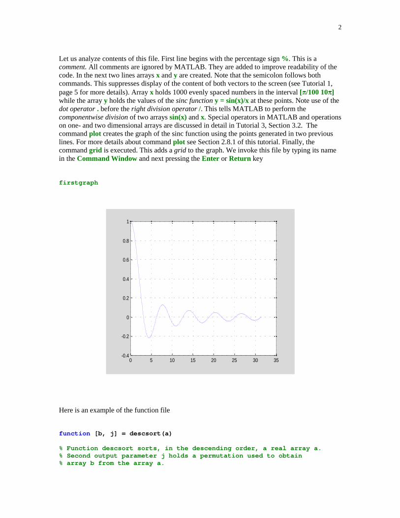
x = pi/100:pi/100:10*pi;y = sin(x)./x;plot(x,y)grid

2

Let us analyze contents of this file. First line begins with the percentage sign % . This is acomment. All comments are ignored by MATLAB. They are added to improve readability of thecode. In the next two lines arrays x and y are created. Note that the semicolon follows bothcommands. This suppresses display of the content of both vectors to the screen (see Tutorial 1,page 5 for more details). Array x holds 1000 evenly spaced numbers in the interval [��/100 10��]while the array y holds the values of the sinc function y = sin(x)/x at these points. Note use of thedot operator . before the right division operator /. This tells MATLAB to perform thecomponentwise division of two arrays sin(x) and x. Special operators in MATLAB and operationson one- and two dimensional arrays are discussed in detail in Tutorial 3, Section 3.2. Thecommand plot creates the graph of the sinc function using the points generated in two previouslines. For more details about command plot see Section 2.8.1 of this tutorial. Finally, thecommand grid is executed. This adds a grid to the graph. We invoke this file by typing its namein the Command Window and next pressing the Enter or Return key

firstgraph

0 5 10 15 20 25 30 35-0.4

-0.2

0

0.2

0.4

0.6

0.8

1

Here is an example of the function file

function [b, j] = descsort(a)

% Function descsort sorts, in the descending order, a real array a.% Second output parameter j holds a permutation used to obtain% array b from the array a.

3

[b ,j] = sort(-a);b = -b;

This function takes one input argument, the array of real numbers, and returns a sorted arraytogether with a permutation used to obtain array b from the array a. MATLAB built-in functionsort is used here. Recall that this function sort numbers in the ascending order. A simple trickused here allows us to sort an array of numbers in the descending order.

To demonstrate functionality of the function under discussion let

a = [pi –10 35 0.15];

[b, j] = descsort(a)

b = 35.0000 3.1416 0.1500 -10.0000j = 3 1 4 2

You can execute function descsort without output arguments. In this case an information about apermutation used will be lost

descsort(a)

ans = 35.0000 3.1416 0.1500 -10.0000

Since no output argument was used in the call to function descorder a sorted array a is assignedto the default variable ans.

� ���������������������������� ���

Sometimes it is handy to define a function that will be used during the current MATLAB sessiononly. MATLAB has a command inline used to define the so-called inline functions in theCommand Window.

Let

f = inline('sqrt(x.^2+y.^2)','x','y')

f = Inline function: f(x,y) = sqrt(x.^2+y.^2)

You can evaluate this function in a usual way

f(3,4)

ans = 5

4

Note that this function also works with arrays. Let

A = [1 2;3 4]

A = 1 2 3 4

and

B = ones(2)

B = 1 1 1 1

Then

C = f(A, B)

C = 1.4142 2.2361 3.1623 4.1231

For the later use let us mention briefly a concept of the string in MATLAB. The character stringis a text surrounded by single quotes. For instance,

str = 'programming in MATLAB is fun'

str =programming in MATLAB is fun

is an example of the string. Strings are discussed in Section 2.5 of this tutorial.

In the previous section you have learned how to create the function files. Some functions take asthe input argument a name of another function, which is specified as a string. In order to executefunction specified by string you should use the command feval as shown below

feval('functname', input parameters of function functname)

Consider the problem of computing the least common multiple of two integers. MATLAB has abuilt-in function lcm that computes the number in question. Recall that the least commonmultiple and the greatest common divisor (gcd) satisfy the following equation

ab = lcm(a, b)gcd(a, b)

MATLAB has its own function, named gcd, for computing the greatest common divisor.

5

To illustrate the use of the command feval let us take a closer look at the code in the m-filemylcm

function c = mylcm(a, b)

% The least common multiple c of two integers a and b.

if feval( 'isint' ,a) & feval( 'isint' ,b) c = a.*b./gcd(a,b);else error( 'Input arguments must be integral numbers' )end

Command feval is used twice in line two (I do do not count the comment lines and the blanklines). It checks whether or not both input arguments are integers. The logical and operator &used here is discussed in Section 2.4. If this condition is satisfied, then the least common multipleis computed using the formula mentioned earlier, otherwise the error message is generated. Noteuse of the command error, which takes as the argument a string. The conditional if - else - endused here is discussed in Section 2.4 of this tutorial. Function that is executed twice in the body ofthe function mylcm is named isint

function k = isint(x);

% Check whether or not x is an integer number.% If it is, function isint returns 1 otherwise it returns 0.

if abs(x - round(x)) < realmin k = 1;else k = 0;end

New functions used here are the absolute value function (abs) and the round function (round).The former is the classical math function while the latter takes a number and rounds it to theclosest integer. Other functions used to round real numbers to integers are discussed in Section2.7. Finally, realmin is the smallest positive real number on your computer

format long

realmin

ans = 2.225073858507201e-308

format short

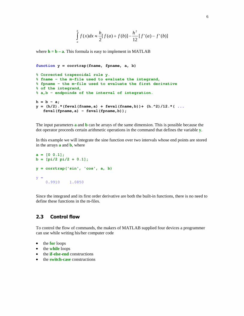
The Trapezoidal Rule with the correction term is often used to numerical integration of functionsthat are differentiable on the interval of integration

6

)](')('[12

)]()([2

)(2

bfafh

bfafh

dxxfb

a

�����

where h = b – a. This formula is easy to implement in MATLAB

function y = corrtrap(fname, fpname, a, b)

% Corrected trapezoidal rule y.% fname - the m-file used to evaluate the integrand,% fpname - the m-file used to evaluate the first derivative% of the integrand,% a,b - endpoinds of the interval of integration.

h = b - a;y = (h/2).*(feval(fname,a) + feval(fname,b))+ (h.^2)/12.*( ... feval(fpname,a) - feval(fpname,b));

The input parameters a and b can be arrays of the same dimension. This is possible because thedot operator proceeds certain arithmetic operations in the command that defines the variable y.

In this example we will integrate the sine function over two intervals whose end points are storedin the arrays a and b, where

a = [0 0.1];b = [pi/2 pi/2 + 0.1];

y = corrtrap('sin', 'cos', a, b)

y = 0.9910 1.0850

Since the integrand and its first order derivative are both the built-in functions, there is no need todefine these functions in the m-files.

�� ����������

To control the flow of commands, the makers of MATLAB supplied four devices a programmercan use while writing his/her computer code

� the for loops� the while loops� the if -else-end constructions� the switch-case constructions

7

����� ������� �� ��� �����

Syntax of the for loop is shown below

for k = arraycommands

end

The commands between the for and end statements are executed for all values stored in thearray .

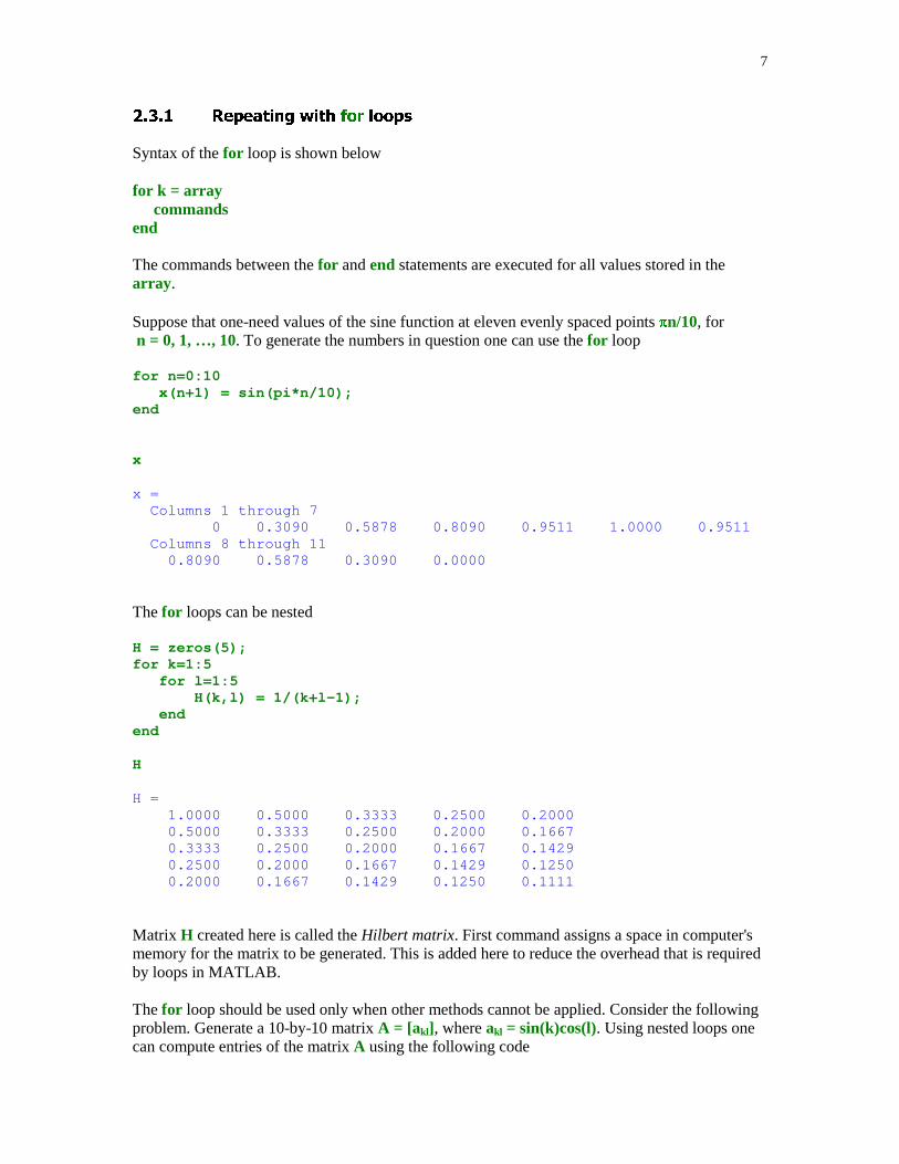
Suppose that one-need values of the sine function at eleven evenly spaced points ��n/10, for n = 0, 1, …, 10. To generate the numbers in question one can use the for loop

for n=0:10 x(n+1) = sin(pi*n/10);end

x

x = Columns 1 through 7 0 0.3090 0.5878 0.8090 0.9511 1.0000 0.9511 Columns 8 through 11 0.8090 0.5878 0.3090 0.0000

The for loops can be nested

H = zeros(5); for k=1:5 for l=1:5 H(k,l) = 1/(k+l-1); endend

H

H = 1.0000 0.5000 0.3333 0.2500 0.2000 0.5000 0.3333 0.2500 0.2000 0.1667 0.3333 0.2500 0.2000 0.1667 0.1429 0.2500 0.2000 0.1667 0.1429 0.1250 0.2000 0.1667 0.1429 0.1250 0.1111

Matrix H created here is called the Hilbert matrix. First command assigns a space in computer'smemory for the matrix to be generated. This is added here to reduce the overhead that is requiredby loops in MATLAB.

The for loop should be used only when other methods cannot be applied. Consider the followingproblem. Generate a 10-by-10 matrix A = [akl], where akl = sin(k)cos(l). Using nested loops onecan compute entries of the matrix A using the following code

8

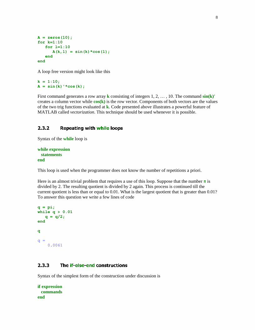
A = zeros(10);for k=1:10 for l=1:10 A(k,l) = sin(k)*cos(l); endend

A loop free version might look like this

k = 1:10;A = sin(k)'*cos(k);

First command generates a row array k consisting of integers 1, 2, … , 10. The command sin(k)'creates a column vector while cos(k) is the row vector. Components of both vectors are the valuesof the two trig functions evaluated at k. Code presented above illustrates a powerful feature ofMATLAB called vectorization. This technique should be used whenever it is possible.

����� ������� �� ���� �����

Syntax of the while loop is

while expression statementsend

This loop is used when the programmer does not know the number of repetitions a priori.

Here is an almost trivial problem that requires a use of this loop. Suppose that the number �� isdivided by 2. The resulting quotient is divided by 2 again. This process is continued till thecurrent quotient is less than or equal to 0.01. What is the largest quotient that is greater than 0.01?To answer this question we write a few lines of code

q = pi;while q > 0.01 q = q/2;end

q

q = 0.0061

����� ��� ���������� ����������

Syntax of the simplest form of the construction under discussion is

if expression commandsend

9

This construction is used if there is one alternative only. Two alternatives require the construction

if expression commands (evaluated if expression is true)else commands (evaluated if expression is false)end

Construction of this form is used in functions mylcm and isint (see Section 2.3).

If there are several alternatives one should use the following construction

if expression1 commands (evaluated if expression 1 is true)elseif expression 2 commands (evaluated if expression 2 is true)elseif …...else commands (executed if all previous expressions evaluate to false)end

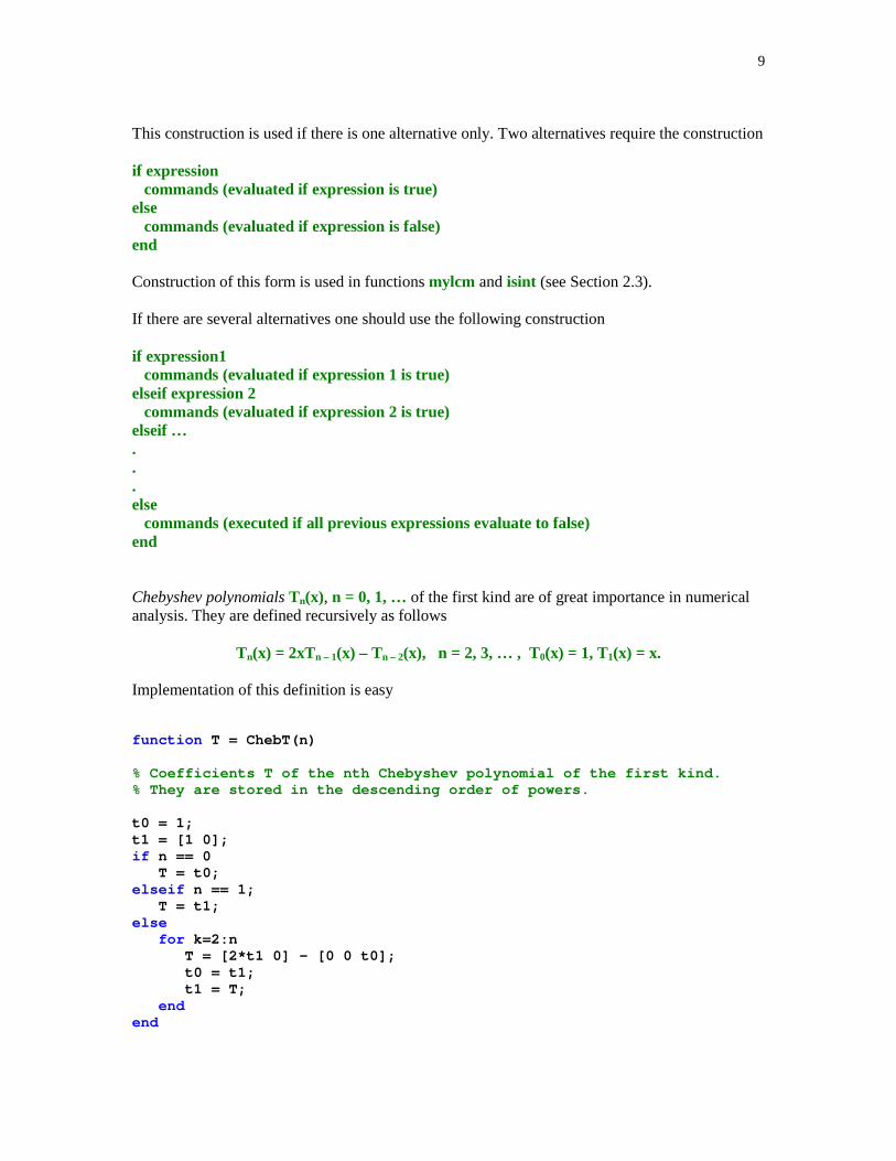
Chebyshev polynomials Tn(x), n = 0, 1, … of the first kind are of great importance in numericalanalysis. They are defined recursively as follows

Tn(x) = 2xTn – 1(x) – Tn – 2(x), n = 2, 3, … , T0(x) = 1, T1(x) = x.

Implementation of this definition is easy

function T = ChebT(n)

% Coefficients T of the nth Chebyshev polynomial of the first kind.% They are stored in the descending order of powers.

t0 = 1;t1 = [1 0];if n == 0 T = t0;elseif n == 1; T = t1;else for k=2:n T = [2*t1 0] - [0 0 t0]; t0 = t1; t1 = T; endend

10

Coefficients of the cubic Chebyshev polynomial of the first kind are

coeff = ChebT(3)

coeff = 4 0 -3 0

Thus T3(x) = 4x3 – 3x.

����� ��� ��������� ���������

Syntax of the switch-case construction is

switch expression (scalar or string) case value1 (executes if expression evaluates to value1) commands case value2 (executes if expression evaluates to value2) commands... otherwise statementsend

Switch compares the input expression to each case value. Once the match is found it executes theassociated commands.

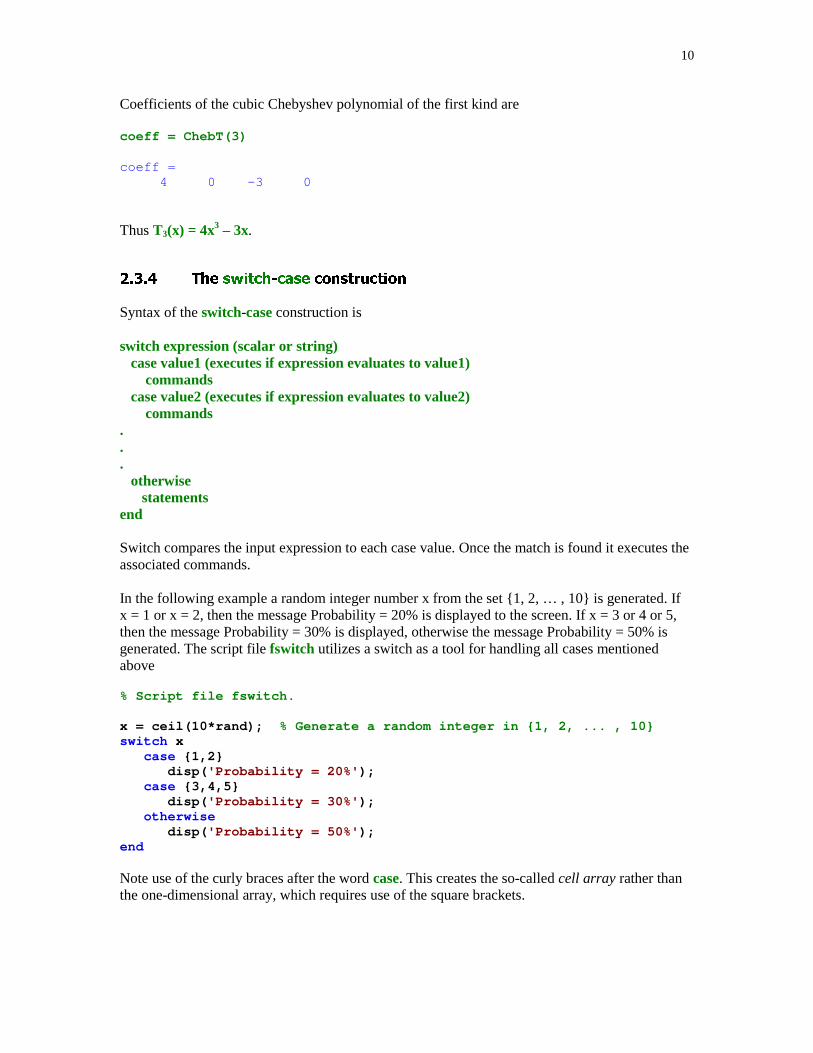
In the following example a random integer number x from the set {1, 2, … , 10} is generated. Ifx = 1 or x = 2, then the message Probability = 20% is displayed to the screen. If x = 3 or 4 or 5,then the message Probability = 30% is displayed, otherwise the message Probability = 50% isgenerated. The script file fswitch utilizes a switch as a tool for handling all cases mentionedabove

% Script file fswitch.

x = ceil(10*rand); % Generate a random integer in {1, 2, ... , 10}switch x case {1,2} disp( 'Probability = 20%' ); case {3,4,5} disp( 'Probability = 30%' ); otherwise disp( 'Probability = 50%' );end

Note use of the curly braces after the word case. This creates the so-called cell array rather thanthe one-dimensional array, which requires use of the square brackets.

11

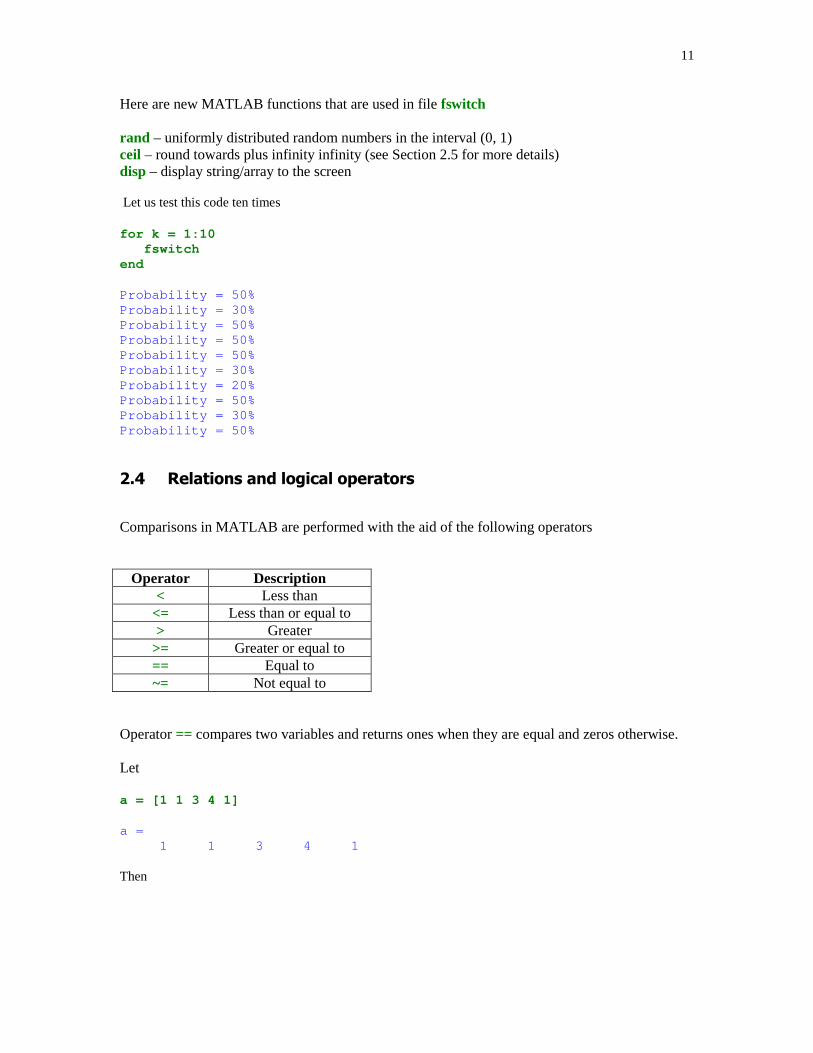
Here are new MATLAB functions that are used in file fswitch

rand – uniformly distributed random numbers in the interval (0, 1)ceil – round towards plus infinity infinity (see Section 2.5 for more details)disp – display string/array to the screen

Let us test this code ten times

for k = 1:10 fswitchend

Probability = 50%Probability = 30%Probability = 50%Probability = 50%Probability = 50%Probability = 30%Probability = 20%Probability = 50%Probability = 30%Probability = 50%

�! "�������������������#�������

Comparisons in MATLAB are performed with the aid of the following operators

Operator Description< Less than

<= Less than or equal to> Greater

>= Greater or equal to== Equal to~= Not equal to

Operator == compares two variables and returns ones when they are equal and zeros otherwise.

Let

a = [1 1 3 4 1]

a = 1 1 3 4 1

Then

12

ind = (a == 1)

ind = 1 1 0 0 1

You can extract all entries in the array a that are equal to 1 using

b = a(ind)

b = 1 1 1

This is an example of so-called logical addressing in MATLAB. You can obtain the same resultusing function find

ind = find(a == 1)

ind = 1 2 5

Variable ind now holds indices of those entries that satisfy the imposed condition. To extract allones from the array a use

b = a(ind)

b = 1 1 1

There are three logical operators available in MATLAB

Logical operator Description| And

& Or~ Not

Suppose that one wants to select all entries x that satisfy the inequalities x �� 1 or x < -0.2 where

x = randn(1,7)

x = -0.4326 -1.6656 0.1253 0.2877 -1.1465 1.1909 1.1892

is the array of normally distributed random numbers. We can solve easily this problem usingoperators discussed in this section

ind = (x >= 1) | (x < -0.2)

ind = 1 1 0 0 1 1 1

y = x(ind)

13

y = -0.4326 -1.6656 -1.1465 1.1909 1.1892

Solve the last problem without using the logical addressing.

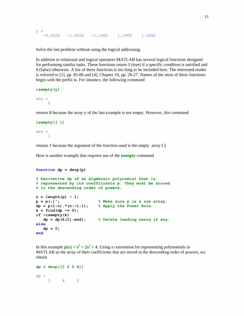
In addition to relational and logical operators MATLAB has several logical functions designedfor performing similar tasks. These functions return 1 (true) if a specific condition is satisfied and0 (false) otherwise. A list of these functions is too long to be included here. The interested readeris referred to [1], pp. 85-86 and [4], Chapter 10, pp. 26-27. Names of the most of these functionsbegin with the prefix is. For instance, the following command

isempty(y)

ans = 0

returns 0 because the array y of the last example is not empty. However, this command

isempty([ ])

ans = 1

returns 1 because the argument of the function used is the empty array [ ] .

Here is another example that requires use of the isempty command

function dp = derp(p)

% Derivative dp of an algebraic polynomial that is% represented by its coefficients p. They must be stored% in the descending order of powers.

n = length(p) - 1;p = p(:)'; % Make sure p is a row array.dp = p(1:n).*(n:-1:1); % Apply the Power Rule.k = find(dp ~= 0);if ~isempty(k) dp = dp(k(1):end); % Delete leading zeros if any.else dp = 0;end

In this example p(x) = x3 + 2x2 + 4. Using a convention for representing polynomials inMATLAB as the array of their coefficients that are stored in the descending order of powers, weobtain

dp = derp([1 2 0 4])

dp = 3 4 0

14

�$ %������

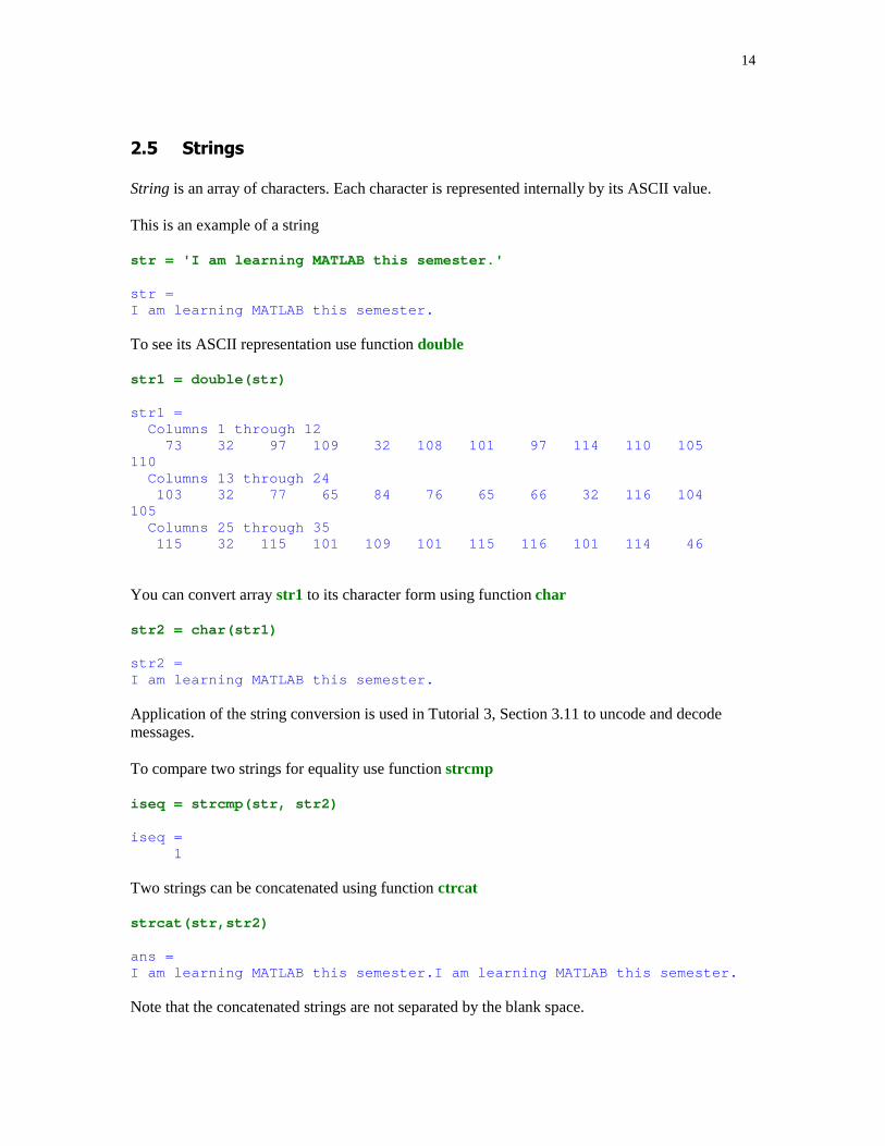
String is an array of characters. Each character is represented internally by its ASCII value.

This is an example of a string

str = 'I am learning MATLAB this semester.'

str =I am learning MATLAB this semester.

To see its ASCII representation use function double

str1 = double(str)

str1 = Columns 1 through 12 73 32 97 109 32 108 101 97 114 110 105110 Columns 13 through 24 103 32 77 65 84 76 65 66 32 116 104105 Columns 25 through 35 115 32 115 101 109 101 115 116 101 114 46

You can convert array str1 to its character form using function char

str2 = char(str1)

str2 =I am learning MATLAB this semester.

Application of the string conversion is used in Tutorial 3, Section 3.11 to uncode and decodemessages.

To compare two strings for equality use function strcmp

iseq = strcmp(str, str2)

iseq = 1

Two strings can be concatenated using function ctrcat

strcat(str,str2)

ans =I am learning MATLAB this semester.I am learning MATLAB this semester.

Note that the concatenated strings are not separated by the blank space.

15

You can create two-dimensional array of strings. To this aim the cell array rather than the two-dimensional array must be used. This is due to the fact that numeric array must have the samenumber of columns in each row.

This is an example of the cell array

carr = {'first name'; 'last name'; 'hometown'}

carr = 'first name' 'last name' 'hometown'

Note use of the curly braces instead of the square brackets. Cell arrays are discussed in detail inthe next section of this tutorial.

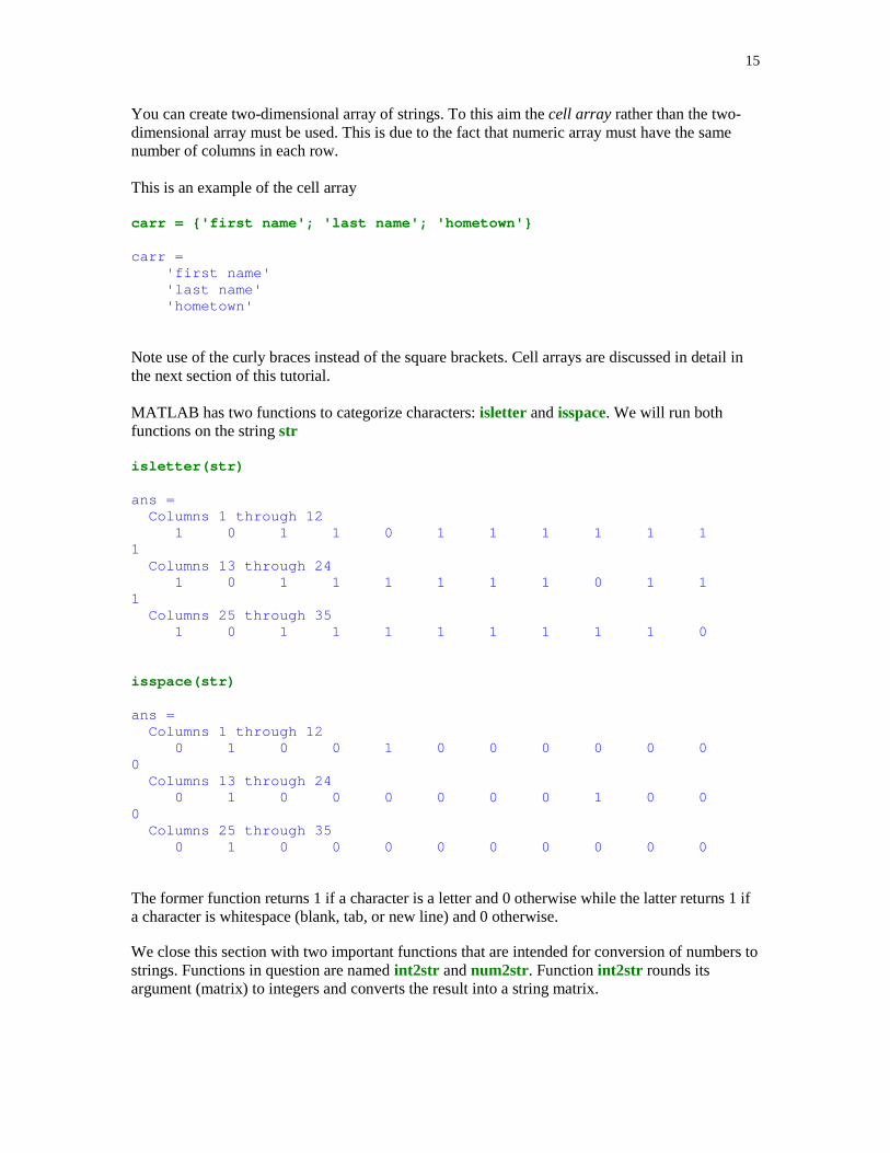
MATLAB has two functions to categorize characters: isletter and isspace. We will run bothfunctions on the string str

isletter(str)

ans = Columns 1 through 12 1 0 1 1 0 1 1 1 1 1 11 Columns 13 through 24 1 0 1 1 1 1 1 1 0 1 11 Columns 25 through 35 1 0 1 1 1 1 1 1 1 1 0

isspace(str)

ans = Columns 1 through 12 0 1 0 0 1 0 0 0 0 0 00 Columns 13 through 24 0 1 0 0 0 0 0 0 1 0 00 Columns 25 through 35 0 1 0 0 0 0 0 0 0 0 0

The former function returns 1 if a character is a letter and 0 otherwise while the latter returns 1 ifa character is whitespace (blank, tab, or new line) and 0 otherwise.

We close this section with two important functions that are intended for conversion of numbers tostrings. Functions in question are named int2str and num2str. Function int2str rounds itsargument (matrix) to integers and converts the result into a string matrix.

16

Let

A = randn(3)

A = -0.4326 0.2877 1.1892 -1.6656 -1.1465 -0.0376 0.1253 1.1909 0.3273

Then

B = int2str(A)

B = 0 0 1-2 -1 0 0 1 0

Function num2str takes an array and converts it to the array string. Running this function on thematrix A defined earlier, we obtain

C = num2str(A)

C =-0.43256 0.28768 1.1892 -1.6656 -1.1465 -0.037633 0.12533 1.1909 0.32729

Function under discussion takes a second optional argument - a number of decimal digits. Thisfeature allows a user to display digits that are far to the right of the decimal point. Using matrix Aagain, we get

D = num2str(A, 18)

D =-0.43256481152822068 0.28767642035854885 1.1891642016521031 -1.665584378238097 -1.1464713506814637 -0.037633276593317645 0.12533230647483068 1.1909154656429988 0.32729236140865414

For comparison, changing format to long, we obtain

format long

A

A = -0.43256481152822 0.28767642035855 1.18916420165210 -1.66558437823810 -1.14647135068146 -0.03763327659332 0.12533230647483 1.19091546564300 0.32729236140865

format short

17

Function num2str his is often used for labeling plots with the title , xlabel, ylabel, and textcommands.

�& ��������'�

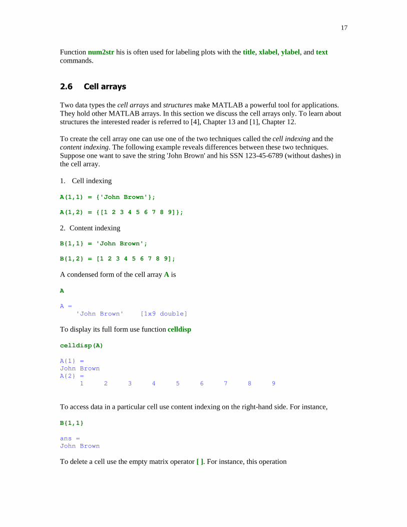
Two data types the cell arrays and structures make MATLAB a powerful tool for applications.They hold other MATLAB arrays. In this section we discuss the cell arrays only. To learn aboutstructures the interested reader is referred to [4], Chapter 13 and [1], Chapter 12.

To create the cell array one can use one of the two techniques called the cell indexing and thecontent indexing. The following example reveals differences between these two techniques.Suppose one want to save the string 'John Brown' and his SSN 123-45-6789 (without dashes) inthe cell array.

1. Cell indexing

A(1,1) = {'John Brown'};

A(1,2) = {[1 2 3 4 5 6 7 8 9]};

2. Content indexing

B{1,1} = 'John Brown';

B{1,2} = [1 2 3 4 5 6 7 8 9];

A condensed form of the cell array A is

A

A = 'John Brown' [1x9 double]

To display its full form use function celldisp

celldisp(A)

A{1} =John BrownA{2} = 1 2 3 4 5 6 7 8 9

To access data in a particular cell use content indexing on the right-hand side. For instance,

B{1,1}

ans =John Brown

To delete a cell use the empty matrix operator [ ] . For instance, this operation

18

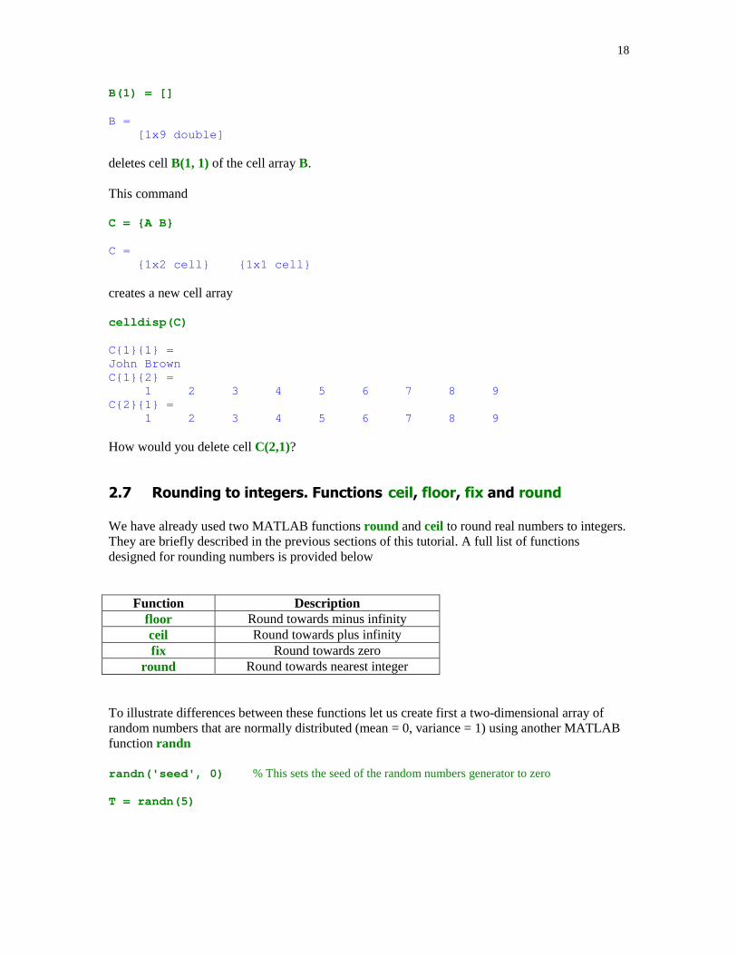
B(1) = []

B = [1x9 double]

deletes cell B(1, 1) of the cell array B.

This command

C = {A B}

C = {1x2 cell} {1x1 cell}

creates a new cell array

celldisp(C)

C{1}{1} =John BrownC{1}{2} = 1 2 3 4 5 6 7 8 9C{2}{1} = 1 2 3 4 5 6 7 8 9

How would you delete cell C(2,1)?

�( "������������������)������������*�����*��+��������

We have already used two MATLAB functions round and ceil to round real numbers to integers.They are briefly described in the previous sections of this tutorial. A full list of functionsdesigned for rounding numbers is provided below

Function Descriptionfloor Round towards minus infinityceil Round towards plus infinityfix Round towards zero

round Round towards nearest integer

To illustrate differences between these functions let us create first a two-dimensional array ofrandom numbers that are normally distributed (mean = 0, variance = 1) using another MATLABfunction randn

randn('seed', 0) % This sets the seed of the random numbers generator to zero

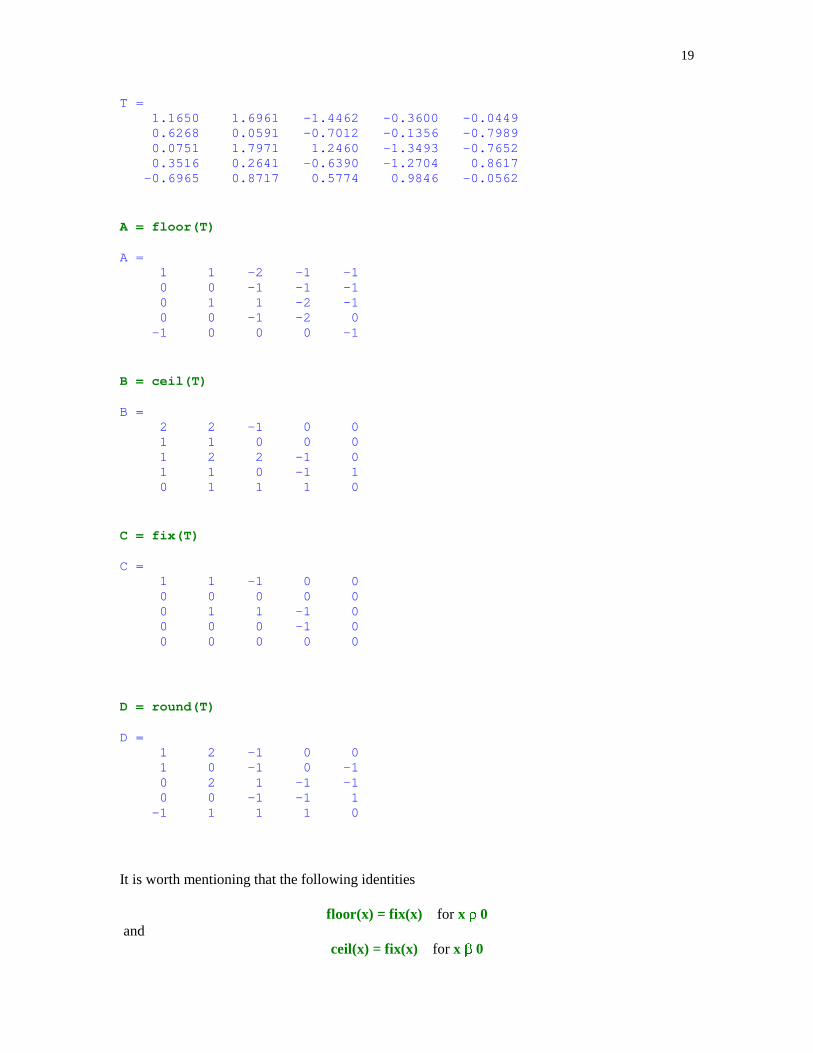
T = randn(5)

19

T = 1.1650 1.6961 -1.4462 -0.3600 -0.0449 0.6268 0.0591 -0.7012 -0.1356 -0.7989 0.0751 1.7971 1.2460 -1.3493 -0.7652 0.3516 0.2641 -0.6390 -1.2704 0.8617 -0.6965 0.8717 0.5774 0.9846 -0.0562

A = floor(T)

A = 1 1 -2 -1 -1 0 0 -1 -1 -1 0 1 1 -2 -1 0 0 -1 -2 0 -1 0 0 0 -1

B = ceil(T)

B = 2 2 -1 0 0 1 1 0 0 0 1 2 2 -1 0 1 1 0 -1 1 0 1 1 1 0

C = fix(T)

C = 1 1 -1 0 0 0 0 0 0 0 0 1 1 -1 0 0 0 0 -1 0 0 0 0 0 0

D = round(T)

D = 1 2 -1 0 0 1 0 -1 0 -1 0 2 1 -1 -1 0 0 -1 -1 1 -1 1 1 1 0

It is worth mentioning that the following identities

floor(x) = fix(x) for x �� 0 and

ceil(x) = fix(x) for x �� 0

20

hold true.

In the following m-file functions floor and ceil are used to obtain a certain representation of anonnegative real number

function [m, r] = rep4(x)

% Given a nonnegative number x, function rep4 computes an integer m% and a real number r, where 0.25 <= r < 1, such that x = (4^m)*r.

if x == 0 m = 0; r = 0; returnendu = log10(x)/log10(4);if u < 0 m = floor(u)else m = ceil(u);endr = x/4^m;

Command return causes a return to the invoking function or to the keyboard. Function log10 isthe decimal logarithm.

[m, r] = rep4(pi)

m = 1r = 0.7854

We check this result

format long

(4^m)*r

ans = 3.14159265358979

format short

�, ���������#����

MATLAB has several high-level graphical routines. They allow a user to create various graphicalobjects including two- and three-dimensional graphs, graphical user interfaces (GUIs), movies, tomention the most important ones. For the comprehensive presentation of the MATLAB graphicsthe interested reader is referred to [2].

21

Before we begin discussion of graphical tools that are available in MATLAB I recommend thatyou will run a couple of demos that come with MATLAB. In the Command Window click onHelp and next select Examples and Demos. ChoseVisualization, and next select 2-D Plots. Youwill be presented with several buttons. Select Line and examine the m-file below the graph. Itshould give you some idea about computer code needed for creating a simple graph. It isrecommended that you examine carefully contents of all m-files that generate the graphs in thisdemo.

����� ��� �������

Basic function used to create 2-D graphs is the plot function. This function takes a variablenumber of input arguments. For the full definition of this function type help plot in theCommand Window.

In this example the graph of the rational function 21

)(x

xxf

�� , -2 � x � 2, will be plotted

using a variable number of points on the graph of f(x)

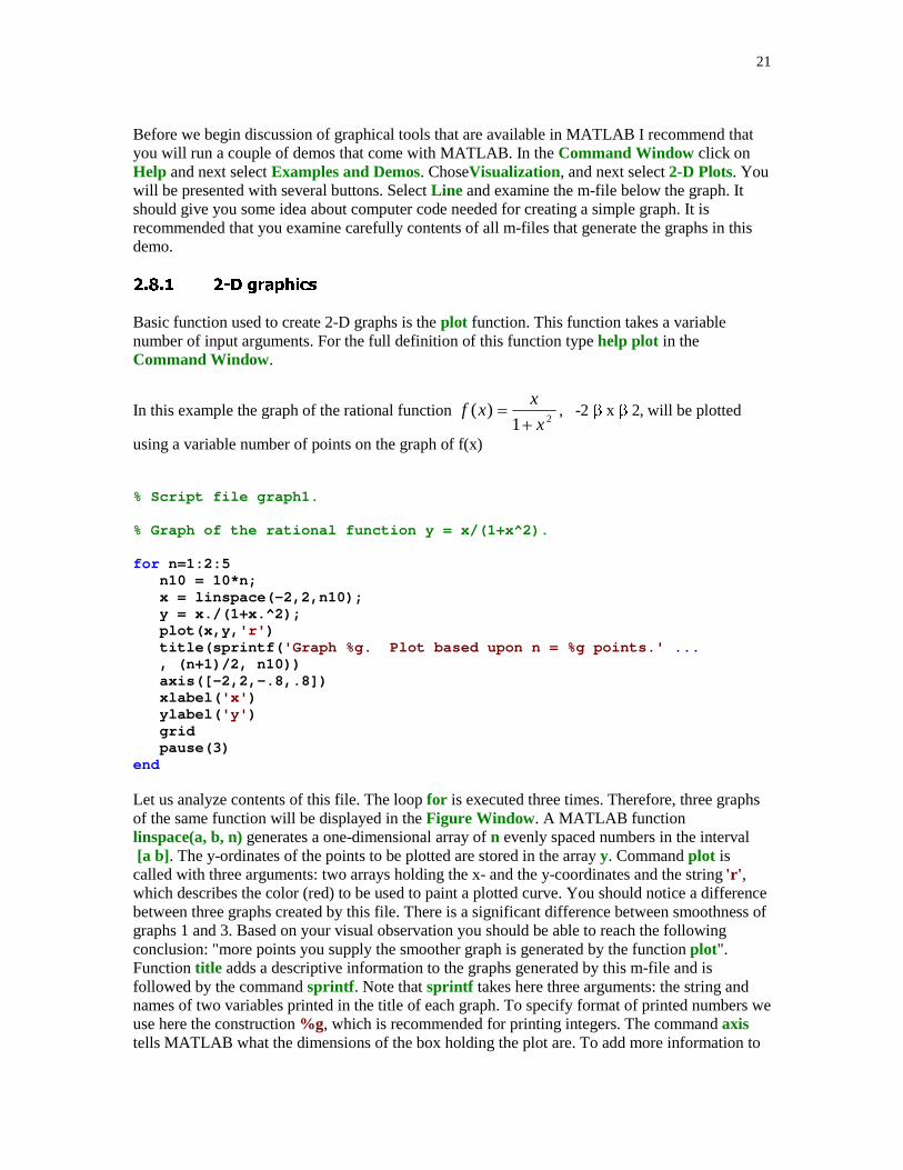
% Script file graph1.

% Graph of the rational function y = x/(1+x^2).

for n=1:2:5 n10 = 10*n; x = linspace(-2,2,n10); y = x./(1+x.^2); plot(x,y, 'r' ) title(sprintf( 'Graph %g. Plot based upon n = %g points.' ... , (n+1)/2, n10)) axis([-2,2,-.8,.8]) xlabel( 'x' ) ylabel( 'y' ) grid pause(3)end

Let us analyze contents of this file. The loop for is executed three times. Therefore, three graphsof the same function will be displayed in the Figure Window. A MATLAB functionlinspace(a, b, n) generates a one-dimensional array of n evenly spaced numbers in the interval [a b]. The y-ordinates of the points to be plotted are stored in the array y. Command plot iscalled with three arguments: two arrays holding the x- and the y-coordinates and the string 'r' ,which describes the color (red) to be used to paint a plotted curve. You should notice a differencebetween three graphs created by this file. There is a significant difference between smoothness ofgraphs 1 and 3. Based on your visual observation you should be able to reach the followingconclusion: "more points you supply the smoother graph is generated by the function plot".Function title adds a descriptive information to the graphs generated by this m-file and isfollowed by the command sprintf . Note that sprintf takes here three arguments: the string andnames of two variables printed in the title of each graph. To specify format of printed numbers weuse here the construction %g, which is recommended for printing integers. The command axistells MATLAB what the dimensions of the box holding the plot are. To add more information to

22

the graphs created here, we label the x- and the y-axes using commands xlabel and the ylabel,respectively. Each of these commands takes a string as the input argument. Function grid addsthe grid lines to the graph. The last command used before the closing end is the pause command.The command pause(n) holds on the current graph for n seconds before continuing, where n canalso be a fraction. If pause is called without the input argument, then the computer waits to userresponse. For instance, pressing the Enter key will resume execution of a program.

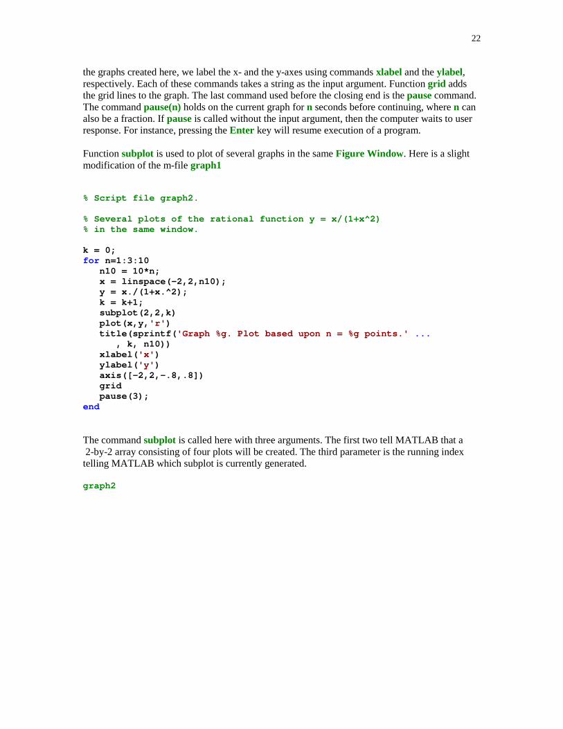
Function subplot is used to plot of several graphs in the same Figure Window. Here is a slightmodification of the m-file graph1

% Script file graph2.

% Several plots of the rational function y = x/(1+x^2)% in the same window.

k = 0;for n=1:3:10 n10 = 10*n; x = linspace(-2,2,n10); y = x./(1+x.^2); k = k+1; subplot(2,2,k) plot(x,y, 'r' ) title(sprintf( 'Graph %g. Plot based upon n = %g points.' ... , k, n10)) xlabel( 'x' ) ylabel( 'y' ) axis([-2,2,-.8,.8]) grid pause(3);end

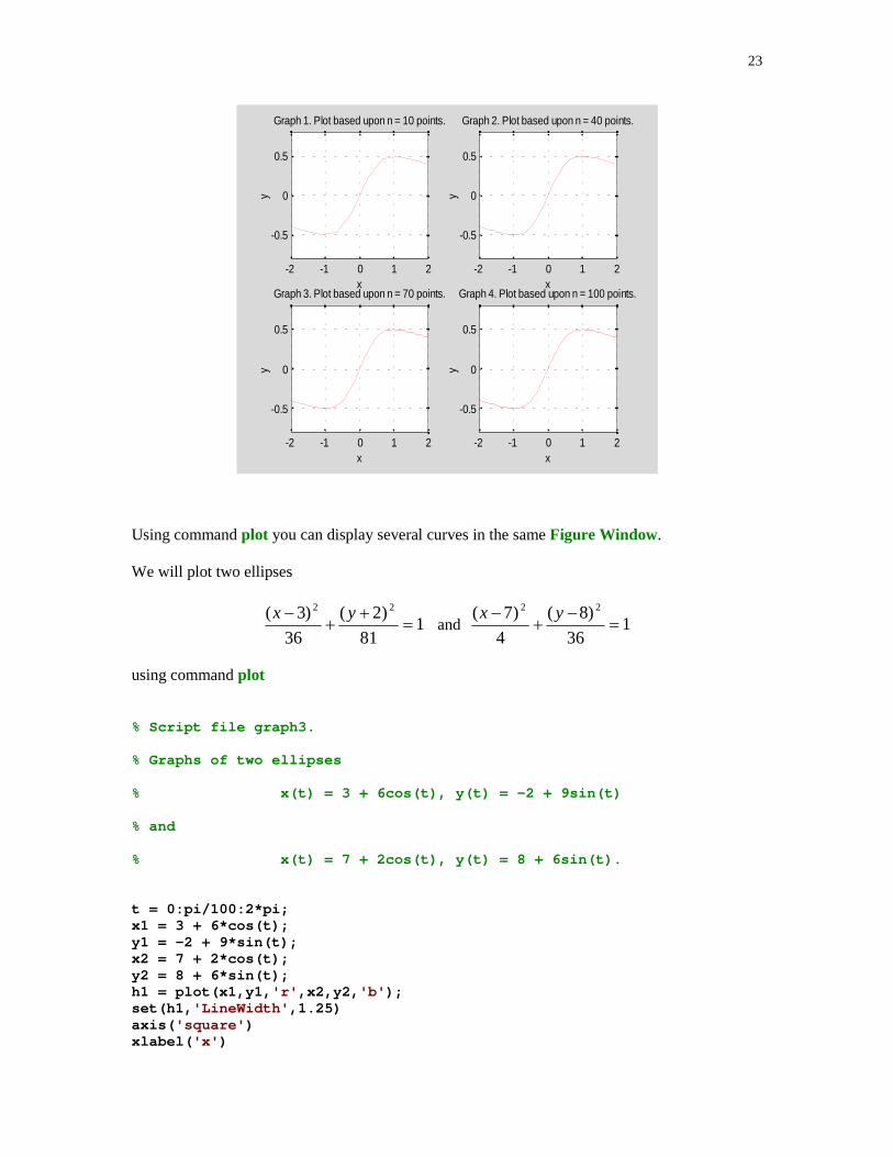
The command subplot is called here with three arguments. The first two tell MATLAB that a 2-by-2 array consisting of four plots will be created. The third parameter is the running indextelling MATLAB which subplot is currently generated.

graph2

23

-2 -1 0 1 2

-0.5

0

0.5

Graph 1. Plot based upon n = 10 points.

x

y-2 -1 0 1 2

-0.5

0

0.5

Graph 2. Plot based upon n = 40 points.

x

y-2 -1 0 1 2

-0.5

0

0.5

Graph 3. Plot based upon n = 70 points.

x

y

-2 -1 0 1 2

-0.5

0

0.5

Graph 4. Plot based upon n = 100 points.

xy

Using command plot you can display several curves in the same Figure Window.

We will plot two ellipses

181

)2(

36

)3( 22

��

�� yx

and 136

)8(

4

)7( 22

��

�� yx

using command plot

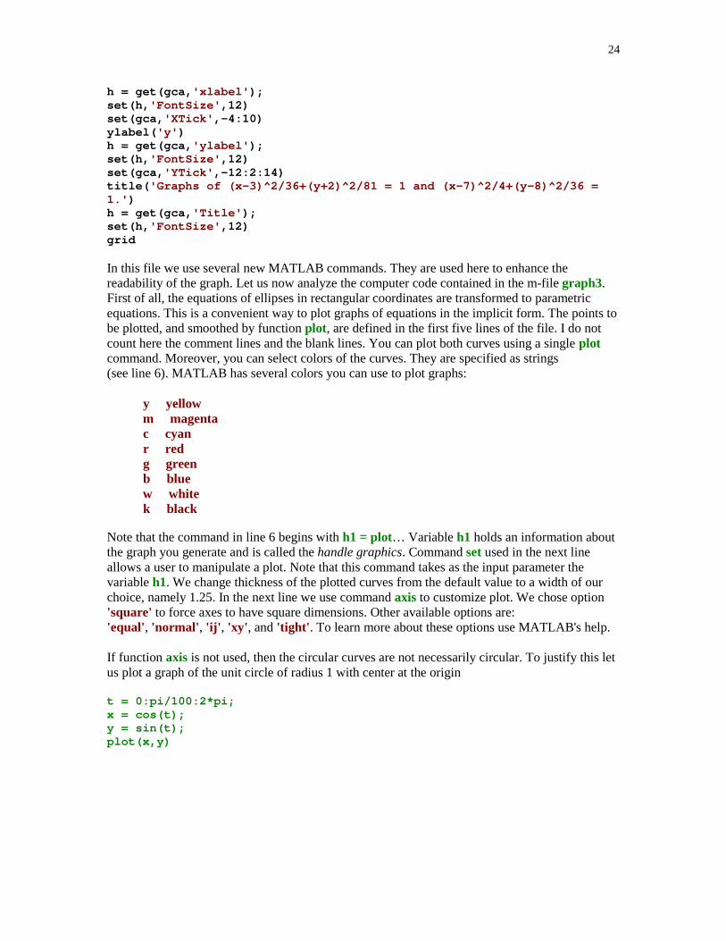
% Script file graph3.

% Graphs of two ellipses

% x(t) = 3 + 6cos(t), y(t) = -2 + 9sin(t)

% and

% x(t) = 7 + 2cos(t), y(t) = 8 + 6sin(t).

t = 0:pi/100:2*pi;x1 = 3 + 6*cos(t);y1 = -2 + 9*sin(t);x2 = 7 + 2*cos(t);y2 = 8 + 6*sin(t);h1 = plot(x1,y1, 'r' ,x2,y2, 'b' );set(h1, 'LineWidth' ,1.25)axis( 'square' )xlabel( 'x' )

24

h = get(gca, 'xlabel' );set(h, 'FontSize' ,12)set(gca, 'XTick' ,-4:10)ylabel( 'y' )h = get(gca, 'ylabel' );set(h, 'FontSize' ,12)set(gca, 'YTick' ,-12:2:14)title( 'Graphs of (x-3)^2/36+(y+2)^2/81 = 1 and (x-7)^2/4+(y-8)^2/36 =1.' )h = get(gca, 'Title' );set(h, 'FontSize' ,12)grid

In this file we use several new MATLAB commands. They are used here to enhance thereadability of the graph. Let us now analyze the computer code contained in the m-file graph3.First of all, the equations of ellipses in rectangular coordinates are transformed to parametricequations. This is a convenient way to plot graphs of equations in the implicit form. The points tobe plotted, and smoothed by function plot, are defined in the first five lines of the file. I do notcount here the comment lines and the blank lines. You can plot both curves using a single plotcommand. Moreover, you can select colors of the curves. They are specified as strings(see line 6). MATLAB has several colors you can use to plot graphs:

y yellow m magenta c cyan r red g green b blue w white k black

Note that the command in line 6 begins with h1 = plot… Variable h1 holds an information aboutthe graph you generate and is called the handle graphics. Command set used in the next lineallows a user to manipulate a plot. Note that this command takes as the input parameter thevariable h1. We change thickness of the plotted curves from the default value to a width of ourchoice, namely 1.25. In the next line we use command axis to customize plot. We chose option'square' to force axes to have square dimensions. Other available options are:'equal', 'normal' , 'ij' , 'xy' , and 'tight' . To learn more about these options use MATLAB's help.

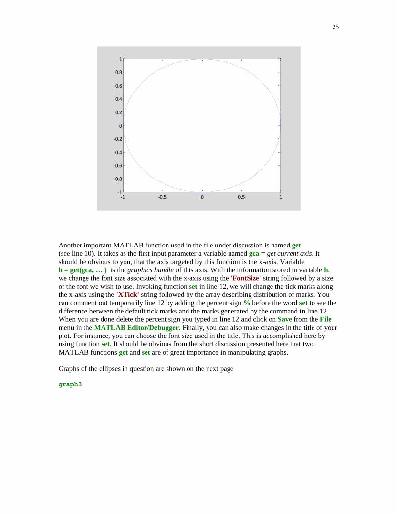
If function axis is not used, then the circular curves are not necessarily circular. To justify this letus plot a graph of the unit circle of radius 1 with center at the origin

t = 0:pi/100:2*pi;x = cos(t);y = sin(t);plot(x,y)

25

-1 -0.5 0 0.5 1-1

-0.8

-0.6

-0.4

-0.2

0

0.2

0.4

0.6

0.8

1

Another important MATLAB function used in the file under discussion is named get(see line 10). It takes as the first input parameter a variable named gca = get current axis. Itshould be obvious to you, that the axis targeted by this function is the x-axis. Variableh = get(gca, … ) is the graphics handle of this axis. With the information stored in variable h,we change the font size associated with the x-axis using the 'FontSize' string followed by a sizeof the font we wish to use. Invoking function set in line 12, we will change the tick marks alongthe x-axis using the 'XTick' string followed by the array describing distribution of marks. Youcan comment out temporarily line 12 by adding the percent sign % before the word set to see thedifference between the default tick marks and the marks generated by the command in line 12.When you are done delete the percent sign you typed in line 12 and click on Save from the Filemenu in the MATLAB Editor/Debugger . Finally, you can also make changes in the title of yourplot. For instance, you can choose the font size used in the title. This is accomplished here byusing function set. It should be obvious from the short discussion presented here that twoMATLAB functions get and set are of great importance in manipulating graphs.

Graphs of the ellipses in question are shown on the next page

graph3

26

-4 -3 -2 -1 0 1 2 3 4 5 6 7 8 9 10

-12

-10

-8

-6

-4

-2

0

2

4

6

8

10

12

14

x

y

Graphs of (x-3)2/36+(y+2)2/81 = 1 and (x-7)2/4+(y-8)2/36 = 1.

MATLAB has several functions designed for plotting specialized 2-D graphs. A partial list ofthese functions is included here fill , polar, bar, barh, pie, hist, compass, errorbar , stem, andfeather.

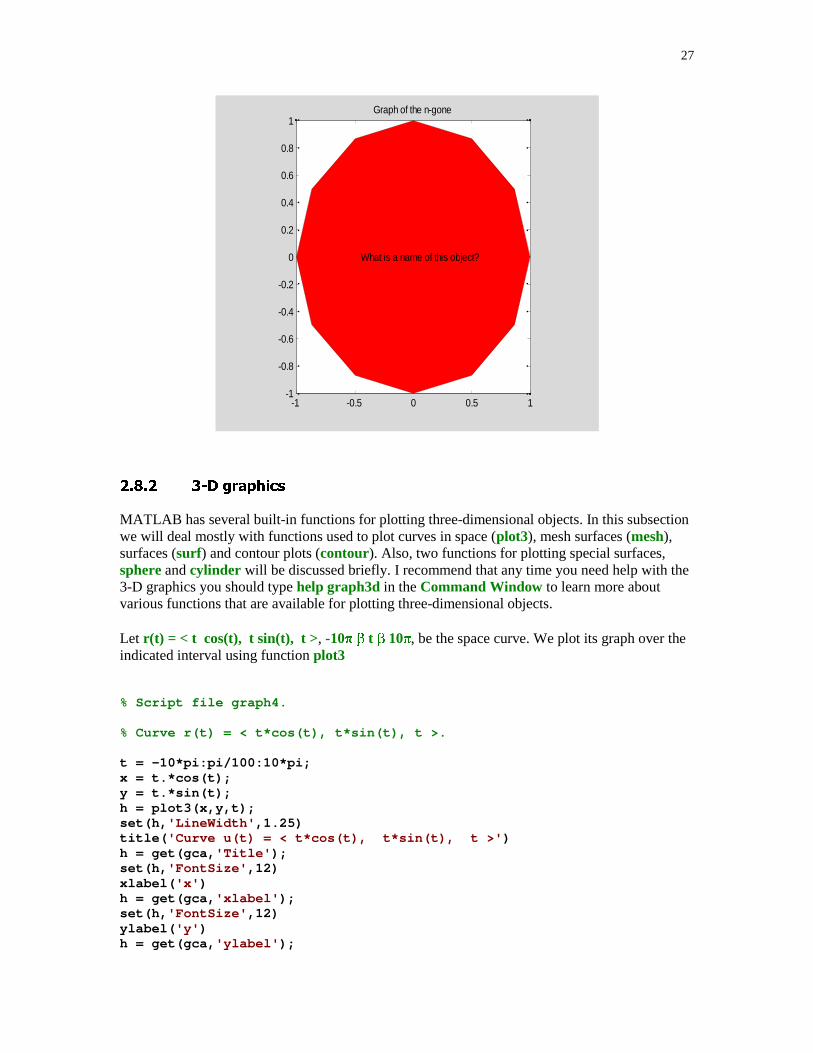
In this example function fill is used to create a well-known object

n = -6:6;x = sin(n*pi/6);y = cos(n*pi/6);fill(x, y, 'r')axis('square')title('Graph of the n-gone')text(-0.45,0,'What is a name of this object?')

Function in question takes three input parameters - two arrays, named here x and y. They hold thex- and y-coordinates of vertices of the polygon to be filled. Third parameter is the user-selectedcolor to be used to paint the object. A new command that appears in this short code is the textcommand. It is used to annotate a text. First two input parameters specify text location. Thirdinput parameter is a text, which will be added to the plot.

Graph of the filled object that is generated by this code is displayed below

27

-1 -0.5 0 0.5 1-1

-0.8

-0.6

-0.4

-0.2

0

0.2

0.4

0.6

0.8

1Graph of the n-gone

What is a name of this object?

����� ��� �������

MATLAB has several built-in functions for plotting three-dimensional objects. In this subsectionwe will deal mostly with functions used to plot curves in space (plot3), mesh surfaces (mesh),surfaces (surf) and contour plots (contour). Also, two functions for plotting special surfaces,sphere and cylinder will be discussed briefly. I recommend that any time you need help with the3-D graphics you should type help graph3d in the Command Window to learn more aboutvarious functions that are available for plotting three-dimensional objects.

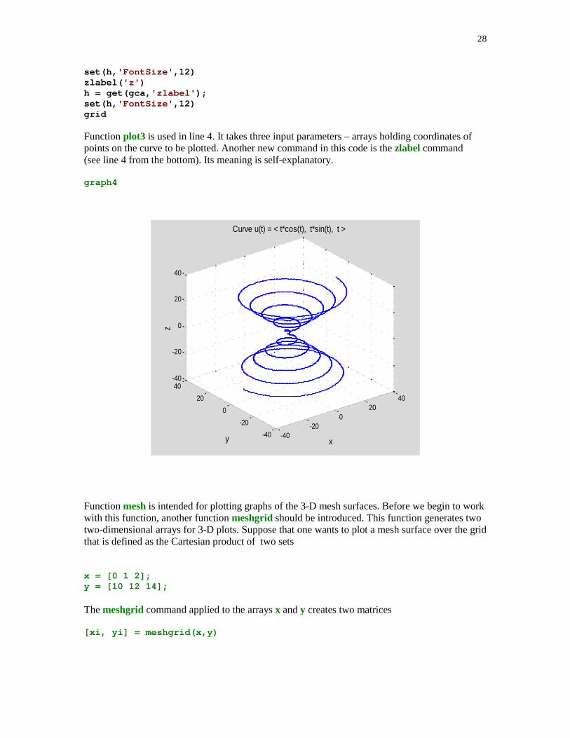
Let r(t) = < t cos(t), t sin(t), t >, -10�� �� t �� 10��, be the space curve. We plot its graph over theindicated interval using function plot3

% Script file graph4.

% Curve r(t) = < t*cos(t), t*sin(t), t >.

t = -10*pi:pi/100:10*pi;x = t.*cos(t);y = t.*sin(t);h = plot3(x,y,t);set(h, 'LineWidth' ,1.25)title( 'Curve u(t) = < t*cos(t), t*sin(t), t >' )h = get(gca, 'Title' );set(h, 'FontSize' ,12)xlabel( 'x' )h = get(gca, 'xlabel' );set(h, 'FontSize' ,12)ylabel( 'y' )h = get(gca, 'ylabel' );

28

set(h, 'FontSize' ,12)zlabel( 'z' )h = get(gca, 'zlabel' );set(h, 'FontSize' ,12)grid

Function plot3 is used in line 4. It takes three input parameters – arrays holding coordinates ofpoints on the curve to be plotted. Another new command in this code is the zlabel command(see line 4 from the bottom). Its meaning is self-explanatory.

graph4

-40-20

020

40

-40

-20

0

20

40-40

-20

0

20

40

x

Curve u(t) = < t*cos(t), t*sin(t), t >

y

z

Function mesh is intended for plotting graphs of the 3-D mesh surfaces. Before we begin to workwith this function, another function meshgrid should be introduced. This function generates twotwo-dimensional arrays for 3-D plots. Suppose that one wants to plot a mesh surface over the gridthat is defined as the Cartesian product of two sets

x = [0 1 2];y = [10 12 14];

The meshgrid command applied to the arrays x and y creates two matrices

[xi, yi] = meshgrid(x,y)

29

xi = 0 1 2 0 1 2 0 1 2yi = 10 10 10 12 12 12 14 14 14

Note that the matrix xi contains replicated rows of the array x while yi contains replicatedcolumns of y. The z-values of a function to be plotted are computed from arrays xi and yi.

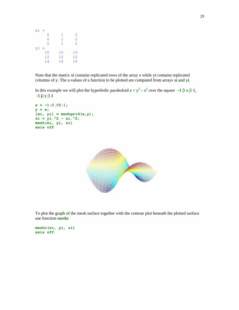
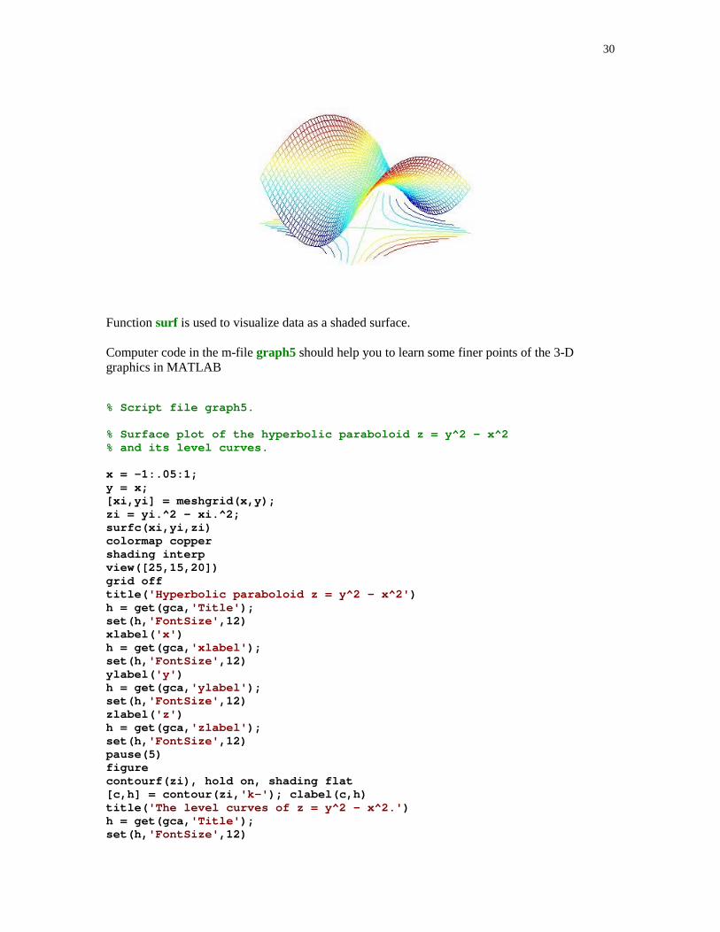
In this example we will plot the hyperbolic paraboloid z = y2 – x2 over the square –1 �� x �� 1, -1 �� y �� 1

x = -1:0.05:1;y = x;[xi, yi] = meshgrid(x,y);zi = yi.^2 – xi.^2;mesh(xi, yi, zi)axis off

To plot the graph of the mesh surface together with the contour plot beneath the plotted surfaceuse function meshc

meshc(xi, yi, zi)axis off

30

Function surf is used to visualize data as a shaded surface.

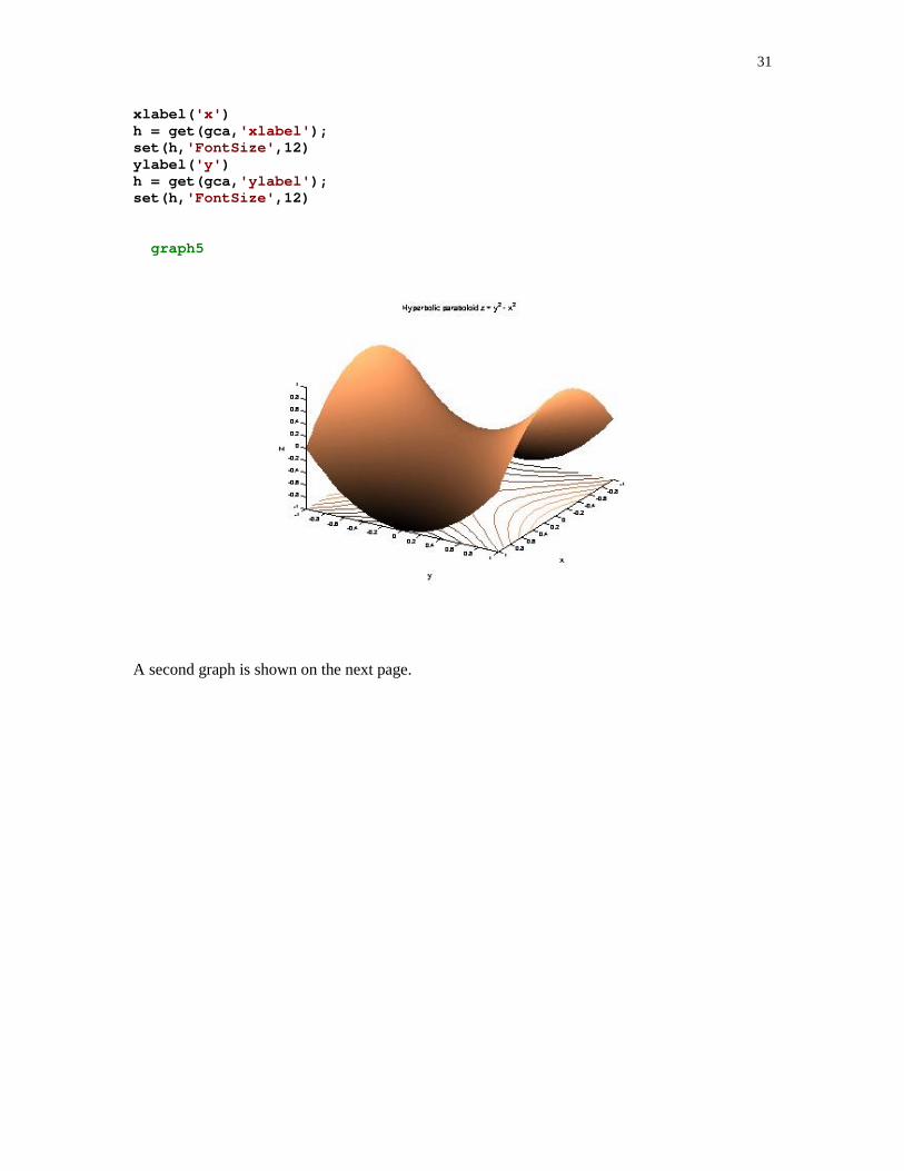
Computer code in the m-file graph5 should help you to learn some finer points of the 3-Dgraphics in MATLAB

% Script file graph5.

% Surface plot of the hyperbolic paraboloid z = y^2 - x^2% and its level curves.

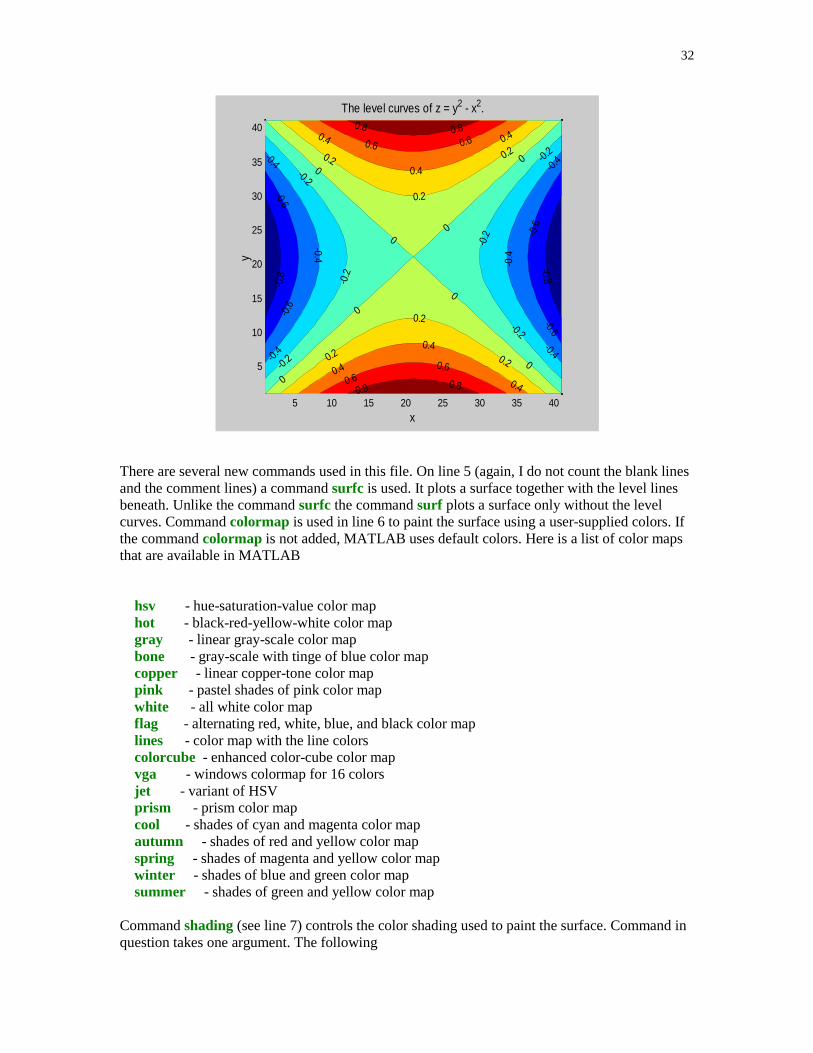
x = -1:.05:1;y = x;[xi,yi] = meshgrid(x,y);zi = yi.^2 - xi.^2;surfc(xi,yi,zi)colormap coppershading interpview([25,15,20])grid offtitle( 'Hyperbolic paraboloid z = y^2 – x^2' )h = get(gca, 'Title' );set(h, 'FontSize' ,12)xlabel( 'x' )h = get(gca, 'xlabel' );set(h, 'FontSize' ,12)ylabel( 'y' )h = get(gca, 'ylabel' );set(h, 'FontSize' ,12)zlabel( 'z' )h = get(gca, 'zlabel' );set(h, 'FontSize' ,12)pause(5)figurecontourf(zi), hold on, shading flat[c,h] = contour(zi, 'k-' ); clabel(c,h)title( 'The level curves of z = y^2 - x^2.' )h = get(gca, 'Title' );set(h, 'FontSize' ,12)

31

xlabel( 'x' )h = get(gca, 'xlabel' );set(h, 'FontSize' ,12)ylabel( 'y' )h = get(gca, 'ylabel' );set(h, 'FontSize' ,12)

graph5

A second graph is shown on the next page.

32

5 10 15 20 25 30 35 40

5

10

15

20

25

30

35

40

x

y

The level curves of z = y2 - x2.

-0.8

-0.8

-0.6

-0.6

-0.6

-0.6

-0.4

-0.4

-0.4

-0.4

-0.4

-0.4

-0.2

-0.2

-0.2

-0.2

-0.2

-0.2

0

0

0

0

0

0

0

0

0.2

0.2

0.2

0.2

0.2

0.2

0.4

0.4

0.4

0.4

0.4

0.4

0.6 0.6

0.60.6

0.8 0.8

0.8 0.8

There are several new commands used in this file. On line 5 (again, I do not count the blank linesand the comment lines) a command surfc is used. It plots a surface together with the level linesbeneath. Unlike the command surfc the command surf plots a surface only without the levelcurves. Command colormap is used in line 6 to paint the surface using a user-supplied colors. Ifthe command colormap is not added, MATLAB uses default colors. Here is a list of color mapsthat are available in MATLAB

hsv - hue-saturation-value color map hot - black-red-yellow-white color map gray - linear gray-scale color map bone - gray-scale with tinge of blue color map copper - linear copper-tone color map pink - pastel shades of pink color map white - all white color map flag - alternating red, white, blue, and black color map lines - color map with the line colors colorcube - enhanced color-cube color map vga - windows colormap for 16 colors jet - variant of HSV prism - prism color map cool - shades of cyan and magenta color map autumn - shades of red and yellow color map spring - shades of magenta and yellow color map winter - shades of blue and green color map summer - shades of green and yellow color map

Command shading (see line 7) controls the color shading used to paint the surface. Command inquestion takes one argument. The following

33

shading flat sets the shading of the current graph to flatshading interp sets the shading to interpolatedshading faceted sets the shading to faceted, which is the default.

are the shading options that are available in MATLAB.

Command view (see line 8) is the 3-D graph viewpoint specification. It takes a three-dimensionalvector, which sets the view angle in Cartesian coordinates.

We will now focus attention on commands on lines 23 through 25. Command figure promptsMATLAB to create a new Figure Window in which the level lines will be plotted. In order toenhance the graph, we use command contourf instead of contour. The former plots filled contourlines while the latter doesn't. On the same line we use command hold on to hold the current plotand all axis properties so that subsequent graphing commands add to the existing graph. Firstcommand on line 25 returns matrix c and graphics handle h that are used as the input parametersfor the function clabel, which adds height labels to the current contour plot.

Due to the space limitation we cannot address here other issues that are of interest forprogrammers dealing with the 3-D graphics in MATLAB. To learn more on this subject theinterested reader is referred to [1-3] and [5].

����� ������

In addition to static graphs discussed so far one can put a sequence of graphs in motion. In otherwords, you can make a movie using MATLAB graphics tools. To learn how to create a movie, letus analyze the m-file firstmovie

% Script file firstmovie.

% Graphs of y = sin(kx) over the interval [0, pi],% where k = 1, 2, 3, 4, 5.

m = moviein(5);x = 0:pi/100:pi;for i=1:5 h1_line = plot(x,sin(i*x)); set(h1_line, 'LineWidth' ,1.5, 'Color' , 'm' ) grid title( 'Sine functions sin(kx), k = 1, 2, 3, 4, 5' ) h = get(gca, 'Title' ); set(h, 'FontSize' ,12) xlabel( 'x' ) k = num2str(i); if i > 1 s = strcat( 'sin(' ,k, 'x)' ); else s = 'sin(x)' ; end ylabel(s) h = get(gca, 'ylabel' ); set(h, 'FontSize' ,12) m(:,i) = getframe; pause(2)

34

endmovie(m)

I suggest that you will play this movie first. To this aim type firstmovie in the CommandWindow and press the Enter or Return key. You should notice that five frames are displayedand at the end of the "show" frames are played again at a different speed.

There are very few new commands one has to learn in order to animate graphics in MATLAB.We will use the m-file firstmovie as a starting point to our discussion. Command moviein, online 1, with an integral parameter, tells MATLAB that a movie consisting of five frames iscreated in the body of this file. Consecutive frames are generated inside the loop for . Almost allof the commands used there should be familiar to you. The only new one inside the loop isgetframe command. Each frame of the movie is stored in the column of the matrix m. With thisremark a role of this command should be clear. The last command in this file is movie(m). Thistells MATLAB to play the movie just created and saved in columns of the matrix m.

Warning. File firstmovie cannot be used with the Student Edition of MATLAB, version 4.2.This is due to the matrix size limitation in this edition of MATLAB. Future release of the StudentEdition of MATLAB, version 5.3 will allow large size matrices. According to MathWorks, Inc.,the makers of MATLAB, this product will be released in September 1999.

����� �������� ������ ��� � �����

MATLAB has some functions for generating special surfaces. We will be concerned mostly withtwo functions- sphere and cylinder.

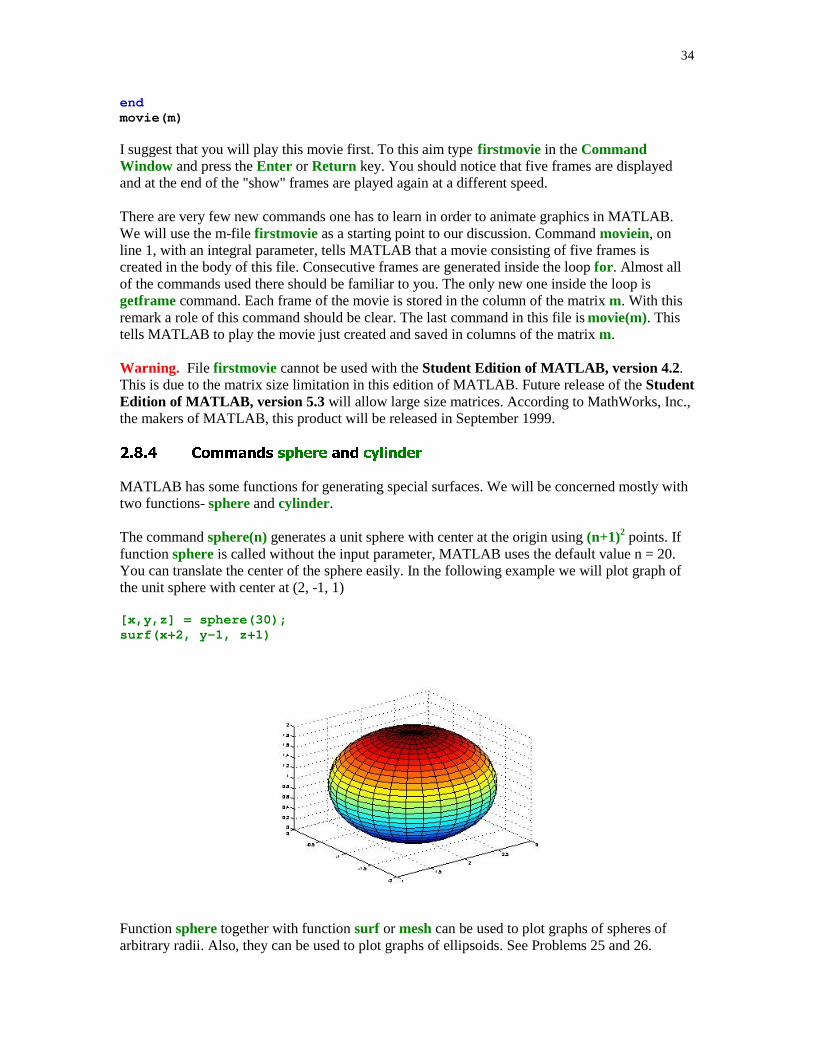
The command sphere(n) generates a unit sphere with center at the origin using (n+1)2 points. Iffunction sphere is called without the input parameter, MATLAB uses the default value n = 20.You can translate the center of the sphere easily. In the following example we will plot graph ofthe unit sphere with center at (2, -1, 1)

[x,y,z] = sphere(30);surf(x+2, y-1, z+1)

Function sphere together with function surf or mesh can be used to plot graphs of spheres ofarbitrary radii. Also, they can be used to plot graphs of ellipsoids. See Problems 25 and 26.

35

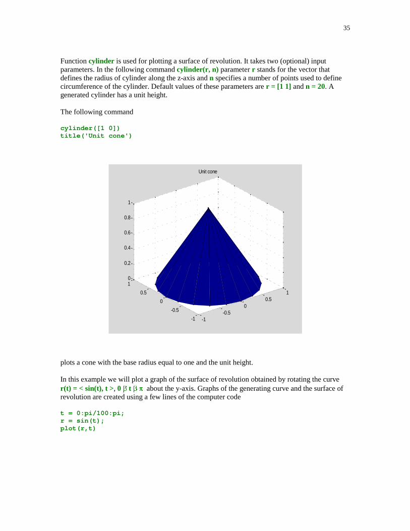
Function cylinder is used for plotting a surface of revolution. It takes two (optional) inputparameters. In the following command cylinder(r, n) parameter r stands for the vector thatdefines the radius of cylinder along the z-axis and n specifies a number of points used to definecircumference of the cylinder. Default values of these parameters are r = [1 1] and n = 20. Agenerated cylinder has a unit height.

The following command

cylinder([1 0])title('Unit cone')

-1-0.5

00.5

1

-1

-0.5

0

0.5

10

0.2

0.4

0.6

0.8

1

Unit cone

plots a cone with the base radius equal to one and the unit height.

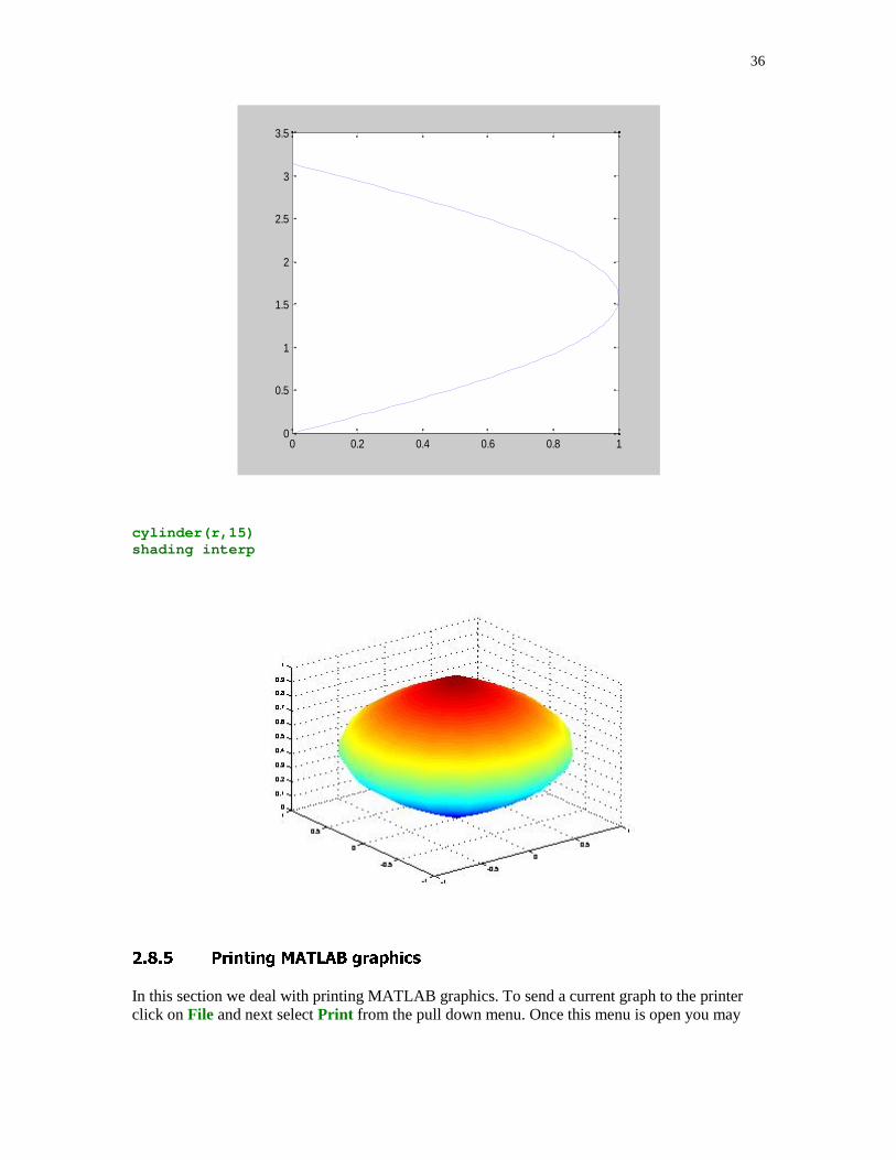
In this example we will plot a graph of the surface of revolution obtained by rotating the curver(t) = < sin(t), t >, 0 �� t �� �� about the y-axis. Graphs of the generating curve and the surface ofrevolution are created using a few lines of the computer code

t = 0:pi/100:pi;r = sin(t);plot(r,t)

36

0 0.2 0.4 0.6 0.8 10

0.5

1

1.5

2

2.5

3

3.5

cylinder(r,15)shading interp

����! "���� #��$�% �������

In this section we deal with printing MATLAB graphics. To send a current graph to the printerclick on File and next select Print from the pull down menu. Once this menu is open you may

37

wish to preview a graph to be printed be selecting the option PrintPreview… first. You can alsosend your graph to the printer using the print command as shown below

x = 0:0.01:1;plot(x, x.^2)print

You can print your graphics to an m- file using built-in device drivers. A fairly incomplete list ofthese drivers is included here:

-depsc Level 1 color Encapsulated PostScript-deps2 Level 2 black and white Encapsulated PostScript-depsc2 Level 2 color Encapsulated PostScript

For a complete list of available device drivers see [5], Chapter 7, pp. 8-9.

Suppose that one wants to print a current graph to the m-file Figure1 using level 2 colorEncapsulated PostScript. This can be accomplished by executing the following command

print –depsc2 Figure1

You can put this command either inside your m-file or execute it from within the CommandWindow.

38

"���������

[1] D. Hanselman and B. Littlefield, Mastering MATLAB 5. A Comprehensive Tutorial and Reference, Prentice Hall, Upper Saddle River, NJ, 1998.

[2] P. Marchand, Graphics and GUIs with MATLAB, Second edition, CRC Press, Boca Raton, 1999.

[3] K. Sigmon, MATLAB Primer, Fifth edition, CRC Press, Boca Raton, 1998.

[4] Using MATLAB, Version 5, The MathWorks, Inc., 1996.

[5] Using MATLAB Graphics, Version 5, The MathWorks, Inc., 1996.

39

���-�� �

In Problems 1- 4 you cannot use loops for or while.

1. Write MATLAB function sigma = ascsum(x) that takes a one-dimensional array x of realnumbers and computes their sum sigma in the ascending order of magnitudes.Hint: You may wish to use MATLAB functions sort, sum, and abs.

2. In this exercise you are to write MATLAB function d = dsc(c) that takes a one-dimensional array of numbers c and returns an array d consisting of all numbers in the array c with all neighboring duplicated numbers being removed. For instance, if c = [1 2 2 2 3 1], then d = [1 2 3 1].

3. Write MATLAB function p = fact(n) that takes a nonnegative integer n and returns value ofthe factorial function n! = 1*2* … *n. Add an error message to your code that will beexecuted when the input parameter is a negative number.

4. Write MATLAB function [in, fr] = infr(x) that takes an array x of real numbers and returnsarrays in and fr holding the integral and fractional parts, respectively, of all numbers in thearray x.

5. Given an array b and a positive integer m create an array d whose entries are those in the array b each replicated m-times. Write MATLAB function d = repel(b, m) that generates array d as described in this problem.

6. In this exercise you are to write MATLAB function d = rep(b, m) that has morefunctionality than the function repel of Problem 5. It takes an array of numbers b and thearray m of positive integers and returns an array d whose each entry is taken from the array band is duplicated according to the corresponding value in the array m. For instance, ifb = [ 1 2] and m = [2 3], then d = [1 1 2 2 2].

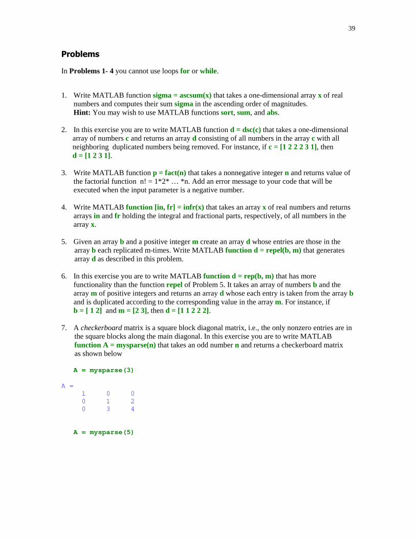
7. A checkerboard matrix is a square block diagonal matrix, i.e., the only nonzero entries are in the square blocks along the main diagonal. In this exercise you are to write MATLAB function A = mysparse(n) that takes an odd number n and returns a checkerboard matrix as shown below

A = mysparse(3)

A = 1 0 0 0 1 2 0 3 4

A = mysparse(5)

40

A = 1 0 0 0 0 0 1 2 0 0 0 3 4 0 0 0 0 0 2 3 0 0 0 4 5

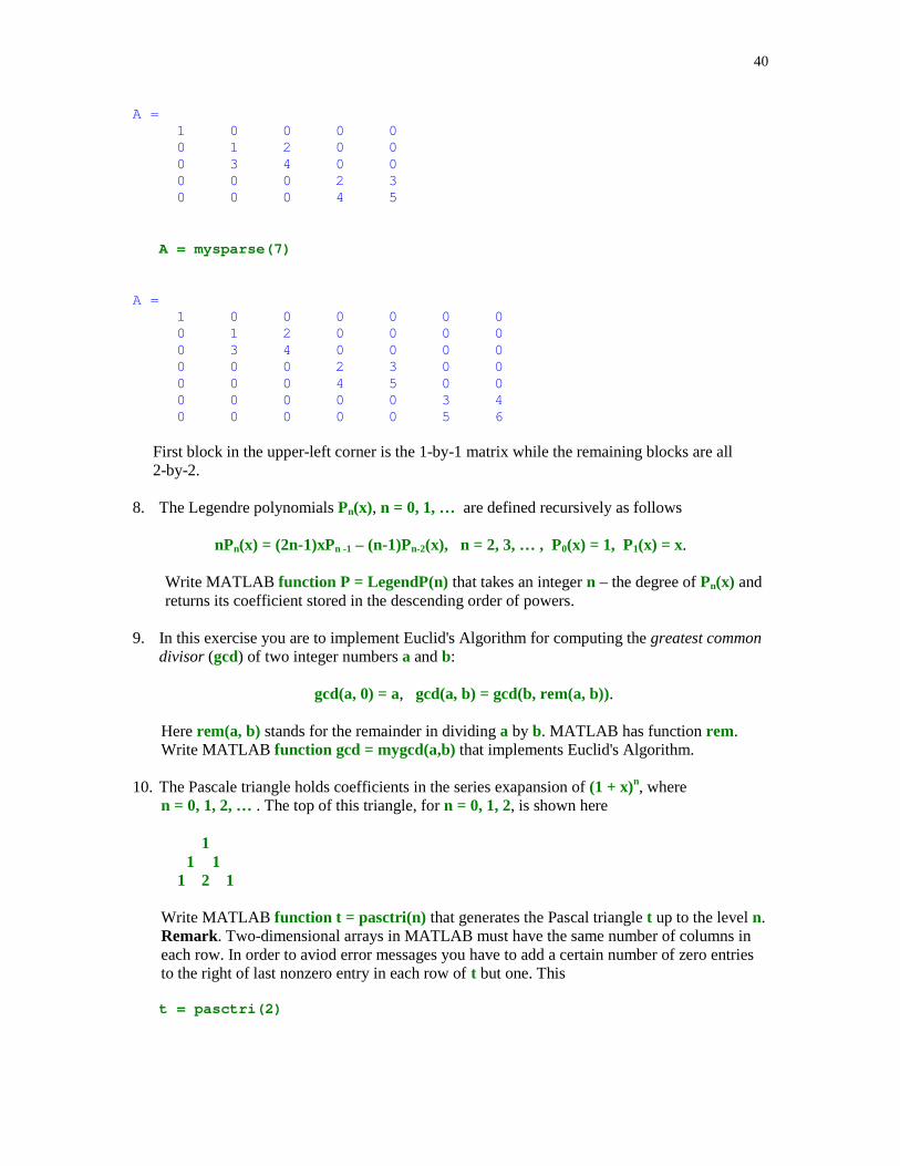
A = mysparse(7)

A = 1 0 0 0 0 0 0 0 1 2 0 0 0 0 0 3 4 0 0 0 0 0 0 0 2 3 0 0 0 0 0 4 5 0 0 0 0 0 0 0 3 4 0 0 0 0 0 5 6

First block in the upper-left corner is the 1-by-1 matrix while the remaining blocks are all 2-by-2.

8. The Legendre polynomials Pn(x), n = 0, 1, … are defined recursively as follows

nPn(x) = (2n-1)xPn -1 – (n-1)Pn-2(x), n = 2, 3, … , P0(x) = 1, P1(x) = x.

Write MATLAB function P = LegendP(n) that takes an integer n – the degree of Pn(x) and returns its coefficient stored in the descending order of powers.

9. In this exercise you are to implement Euclid's Algorithm for computing the greatest commondivisor (gcd) of two integer numbers a and b:

gcd(a, 0) = a, gcd(a, b) = gcd(b, rem(a, b)).

Here rem(a, b) stands for the remainder in dividing a by b. MATLAB has function rem. Write MATLAB function gcd = mygcd(a,b) that implements Euclid's Algorithm.

10. The Pascale triangle holds coefficients in the series exapansion of (1 + x)n, where n = 0, 1, 2, … . The top of this triangle, for n = 0, 1, 2, is shown here

11 1

1 2 1

Write MATLAB function t = pasctri(n) that generates the Pascal triangle t up to the level n. Remark. Two-dimensional arrays in MATLAB must have the same number of columns in each row. In order to aviod error messages you have to add a certain number of zero entries to the right of last nonzero entry in each row of t but one. This

t = pasctri(2)

41

t = 1 0 0 1 1 0

1 2 1

is an example of the array t for n = 2.

11. This is a continuation of Problem 10. Write MATLAB function t = binexp(n) thatcomputes an array t with row k+1 holding coefficients in the series expansion of (1-x)^k ,k = 0, 1, ... , n, in the ascending order of powers. You may wish to make a call from withinyour function to the function pasctri of Problem 10. Your output sholud look like this (case n = 3)

t = binexp(3)

t = 1 0 0 0 1 -1 0 0 1 -2 1 0 1 -3 3 -1

12. MATLAB come with the built-in function mean for computing the unweighted arithmeticmean of real numbers. Let x = {x1, x2, … , xn} be an array of n real numbers. Then

��

�n

knx

nxmean

1

1)(

In some problems that arise in mathematical statistics one has to compute the weightedarithmetic mean of numbers in the array x. The latter, abbreviated here as wam, is defined asfollows

�

�

�

��n

kk

n

kkk

w

xw

wxwam

1

1),(

Here w = {w1, w2, … , wn} is the array of weights associated with variables x. The weightsare all nonnegative with w1 + w2 + … + wn > 0.

In this exercise you are to write MATLAB function y = wam(x, w) that takes the arrays of variables and weights and returns the weighted arithmetic mean as defined above. Add three error messages to terminate prematurely execution of this file in the case when:

� arrays x and w are of different lengths� at least one number in the array w is negative� sum of all weights is equal to zero.

42

13. Let w = {w1, w2, … , wn} be an array of positive numbers. The weighted geometric mean,abbreviated as wgm, of the nonnegative variables x = {x1, x2, … , xn} is defined as follows

nwn

ww xxxwxwgm ...),( 21

21�

Here we assume that the weights w sum up to one. Write MATLAB function y = wgm(x, w) that takes arrays x and w and returns the weighted geometric mean y of x with weights stored in the array w. Add three error messages to terminate prematurely execution of this file in the case when:

� arrays x and w are of different lengths� at least one variable in the array x is negative� at least one weight in the array w is less than or equal to zero

Also, normalize the weights w, if necessary, so that they will sum up to one.

14. Write MATLAB function [nonz, mns] = matstat(A) that takes as the input argument a real matrix A and returns all nonzero entries of A in the column vector nonz. Second output parameter mns holds values of the unweighted arithmetic means of all columns of A.

15. Solving triangles requires a bit of knowledge of trigonometry. In this exercise you are to write MATLAB function [a, B, C] = sas(b, A, c) that is intended for solving triangles given two sides b and c and the angle A between these sides. Your function should determine remaining two angels and the third side of the triangle to be solved. All angles should be expressed in the degree measure.

16. Write MATLAB function [A, B, C] = sss(a, b, c) that takes three positive numbers a, b, and c. If they are sides of a triangle, then your function should return its angles A, B, and C, in the degree measure, otherwise an error message should be displayed to the screen.

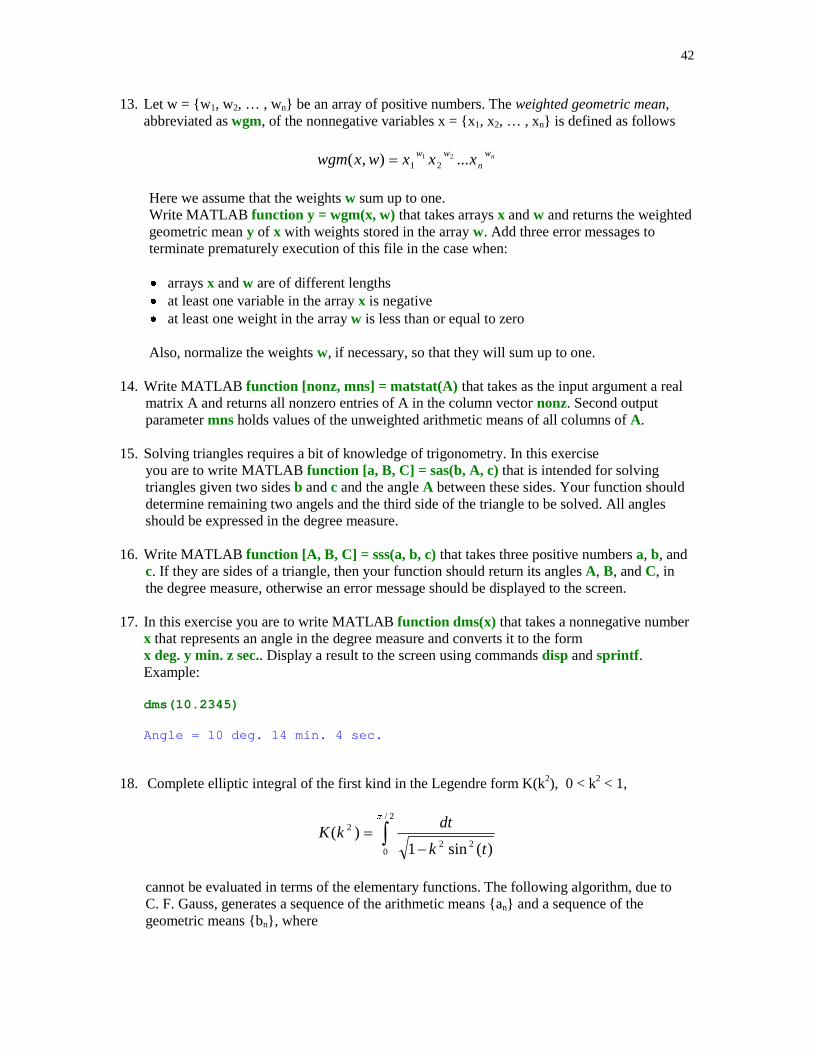
17. In this exercise you are to write MATLAB function dms(x) that takes a nonnegative numberx that represents an angle in the degree measure and converts it to the formx deg. y min. z sec.. Display a result to the screen using commands disp and sprintf .Example:

dms(10.2345)

Angle = 10 deg. 14 min. 4 sec.

18. Complete elliptic integral of the first kind in the Legendre form K(k2), 0 < k2 < 1,

��

�2/

022

2

)(sin1)(

�

tk

dtkK

cannot be evaluated in terms of the elementary functions. The following algorithm, due to C. F. Gauss, generates a sequence of the arithmetic means {an} and a sequence of the geometric means {bn}, where

43

a0 = 1, b0 = 21 k�

an = (an-1 + bn-1)/2, bn = 11 �� nn ba n = 1, 2, … .

It is known that both sequences have a common limit g and that an � bn, for all n. Moreover,

K(k2) = g2

�

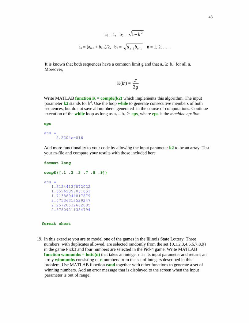
Write MATLAB function K = compK(k2) which implements this algorithm. The input parameter k2 stands for k2. Use the loop while to generate consecutive members of both sequences, but do not save all numbers generated in the course of computations. Continue execution of the while loop as long as an – bn � eps, where eps is the machine epsilon

eps

ans = 2.2204e-016

Add more functionality to your code by allowing the input parameter k2 to be an array. Testyour m-file and compare your results with those included here

format long

compK([.1 .2 .3 .7 .8 .9])

ans = 1.61244134872022 1.65962359861053 1.71388944817879 2.07536313529247 2.25720532682085 2.57809211334794

format short

19. In this exercise you are to model one of the games in the Illinois State Lottery. Threenumbers, with duplicates allowed, are selected randomly from the set {0,1,2,3,4,5,6,7,8,9}in the game Pick3 and four numbers are selected in the Pick4 game. Write MATLAB

function winnumbs = lotto(n) that takes an integer n as its input parameter and returns an array winnumbs consisting of n numbers from the set of integers described in this problem. Use MATLAB function rand together with other functions to generate a set of winning numbers. Add an error message that is displayed to the screen when the input parameter is out of range.

44

20. Write MATLAB function t = isodd(A) that takes an array A of nonzero integers and returns1 if all entries in the array A are odd numbers and 0 otherwise. You may wish to useMATLAB function rem in your file.

21. Given two one-dimensional arrays a and b, not necessarily of the same length. Write MATLAB function c = interleave(a, b) which takes arrays a and b and returns an array c obtained by interleaving entries in the input arrays. For instance, if a = [1, 3, 5, 7] and b = [-2, –4], then c = [1, –2, 3, –4, 5, 7]. Your program should work for empty arrays too. You cannot use loops for or while.

22. Write a script file Problem22 to plot, in the same window, graphs of two parabolas y = x2

and x = y2, where –1 �� x �� 1. Label the axes, add a title to your graph and use command grid . To improve readability of the graphs plotted add a legend. MATLAB has a command legend. To learn more about this command type help legend in the Command Window and press Enter or Return key.

23. Write MATLAB function eqtri(a, b) that plots the graph of the equilateral triangle with twovertices at (a,a) and (b,a). Third vertex lies above the line segment that connects points (a, a)and (b, a). Use function fill to paint the triangle using a color of your choice.

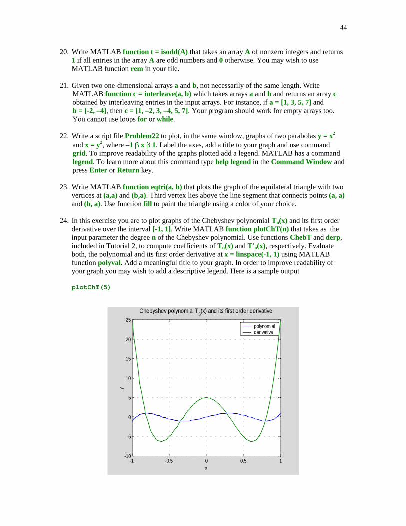
24. In this exercise you are to plot graphs of the Chebyshev polynomial Tn(x) and its first orderderivative over the interval [-1, 1]. Write MATLAB function plotChT(n) that takes as theinput parameter the degree n of the Chebyshev polynomial. Use functions ChebT and derp,included in Tutorial 2, to compute coefficients of Tn(x) and T' n(x), respectively. Evaluateboth, the polynomial and its first order derivative at x = linspace(-1, 1) using MATLABfunction polyval. Add a meaningful title to your graph. In order to improve readability ofyour graph you may wish to add a descriptive legend. Here is a sample output

plotChT(5)

-1 -0.5 0 0.5 1-10

-5

0

5

10

15

20

25

Chebyshev polynomial T5(x) and its first order derivative

x

y

polynomialderivative

45

25. Use function sphere to plot the graph of a sphere of radius r with center at (a, b, c). Use MATLAB function axis with an option 'equal'. Add a title to your graph and save your computer code as the MATLAB function sph(r, a, b, c).

26. Write MATLAB function ellipsoid(x0, y0, z0, a, b, c) that takes coordinates (x0, y0, z0) of the center of the ellipsoid with semiaxes (a, b, c) and plots its graph. Use MATLAB functions sphere and surf. Add a meaningful title to your graph and use function axis('equal').

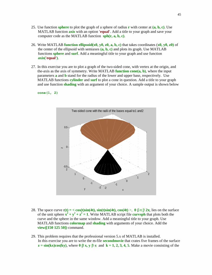
27. In this exercise you are to plot a graph of the two-sided cone, with vertex at the origin, andthe-axis as the axis of symmetry. Write MATLAB function cone(a, b), where the inputparameters a and b stand for the radius of the lower and upper base, respectively. UseMATLAB functions cylinder and surf to plot a cone in question. Add a title to your graphand use function shading with an argument of your choice. A sample output is shown below

cone(1, 2)

-2-1

01

2

-2

-1

0

1

2-0.5

0

0.5

x

Two-sided cone with the radii of the bases equal to1 and2

y

z

28. The space curve r(t) = < cos(t)sin(4t), sin(t)sin(4t), cos(4t) >, 0 �� t �� 2��, lies on the surfaceof the unit sphere x2 + y2 + z2 = 1. Write MATLAB script file curvsph that plots both thecurve and the sphere in the same window. Add a meaningful title to your graph. UseMATLAB functions colormap and shading with arguments of your choice. Add theview([150 125 50]) command.

29. This problem requires that the professional version 5.x of MATLAB is installed. In this exercise you are to write the m-file secondmovie that crates five frames of the surface z = sin(kx)cos(ky), where 0 �� x, y �� �� and k = 1, 2, 3, 4, 5. Make a movie consisting of the

46

frames you generated in your file. Use MATLAB functions colormap and shading with arguments of your choice. Add a title, which might look like this Graphs of z = sin(kx)*cos(ky), 0 <= x, y <= ��, k =1, 2, 3, 4, 5. Greek letters can be printed in the title of a graph using TeX convention, i.e., the following \pi is used to print the Greek letter �. Similarly, the string \alpha will be printed as �.

��������

��� �������� �� ����������

�������

Edward NeumanDepartment of Mathematics

Southern Illinois University at Carbondaleedneuman@siu.edu

One of the nice features of MATLAB is its ease of computations with vectors and matrices. Inthis tutorial the following topics are discussed: vectors and matrices in MATLAB, solvingsystems of linear equations, the inverse of a matrix, determinants, vectors in n-dimensionalEuclidean space, linear transformations, real vector spaces and the matrix eigenvalue problem.Applications of linear algebra to the curve fitting, message coding and computer graphics are alsoincluded.

�� ������������������ ��������� ���� ������ ��������

For the reader's convenience we include lists of special characters and MATLAB functions thatare used in this tutorial.

Special characters; Semicolon operator' Conjugated transpose.' Transpose* Times. Dot operator^ Power operator[ ] Emty vector operator: Colon operator= Assignment

== Equality\ Backslash or left division/ Right division

i, j Imaginary unit~ Logical not

~= Logical not equal& Logical and| Logical or

{ } Cell

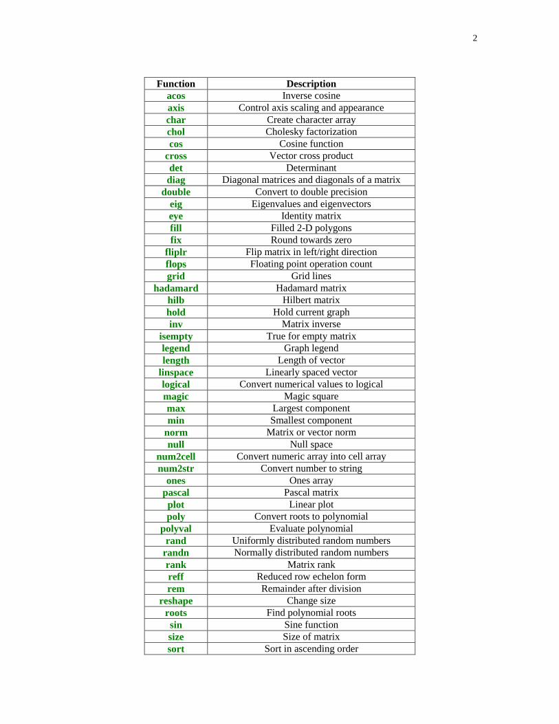
2

Function Descriptionacos Inverse cosineaxis Control axis scaling and appearancechar Create character arraychol Cholesky factorizationcos Cosine function

cross Vector cross productdet Determinantdiag Diagonal matrices and diagonals of a matrix

double Convert to double precisioneig Eigenvalues and eigenvectorseye Identity matrixfill Filled 2-D polygonsfix Round towards zero

fliplr Flip matrix in left/right directionflops Floating point operation countgrid Grid lines

hadamard Hadamard matrixhilb Hilbert matrixhold Hold current graphinv Matrix inverse

isempty True for empty matrixlegend Graph legendlength Length of vector

linspace Linearly spaced vectorlogical Convert numerical values to logicalmagic Magic squaremax Largest componentmin Smallest component

norm Matrix or vector normnull Null space

num2cell Convert numeric array into cell arraynum2str Convert number to string

ones Ones arraypascal Pascal matrixplot Linear plotpoly Convert roots to polynomial

polyval Evaluate polynomialrand Uniformly distributed random numbers

randn Normally distributed random numbersrank Matrix rankreff Reduced row echelon formrem Remainder after division

reshape Change sizeroots Find polynomial rootssin Sine functionsize Size of matrixsort Sort in ascending order

3

subs Symbolic substitutionsym Construct symbolic bumbers and variablestic Start a stopwatch timer

title Graph titletoc Read the stopwatch timer

toeplitz Tioeplitz matrixtril Extract lower triangular parttriu Extract upper triangular part

vander Vandermonde matrixvarargin Variable length input argument list

zeros Zeros array

���������� ���������� ������

The purpose of this section is to demonstrate how to create and transform vectors and matrices inMATLAB.

This command creates a row vector

a = [1 2 3]

a = 1 2 3

Column vectors are inputted in a similar way, however, semicolons must separate the componentsof a vector

b = [1;2;3]

b = 1 2 3

The quote operator ' is used to create the conjugate transpose of a vector (matrix) while the dot-quote operator .' creates the transpose vector (matrix). To illustrate this let us form a complexvector a + i*b' and next apply these operations to the resulting vector to obtain

(a+i*b')'

ans = 1.0000 - 1.0000i 2.0000 - 2.0000i 3.0000 - 3.0000i

while

4

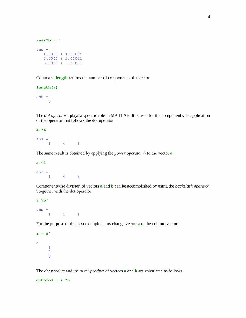
(a+i*b').'

ans = 1.0000 + 1.0000i 2.0000 + 2.0000i 3.0000 + 3.0000i

Command length returns the number of components of a vector

length(a)

ans = 3

The dot operator. plays a specific role in MATLAB. It is used for the componentwise applicationof the operator that follows the dot operator

a.*a

ans = 1 4 9

The same result is obtained by applying the power operator ^ to the vector a

a.^2

ans = 1 4 9

Componentwise division of vectors a and b can be accomplished by using the backslash operator\ together with the dot operator .

a.\b'

ans = 1 1 1

For the purpose of the next example let us change vector a to the column vector

a = a'

a = 1 2 3

The dot product and the outer product of vectors a and b are calculated as follows

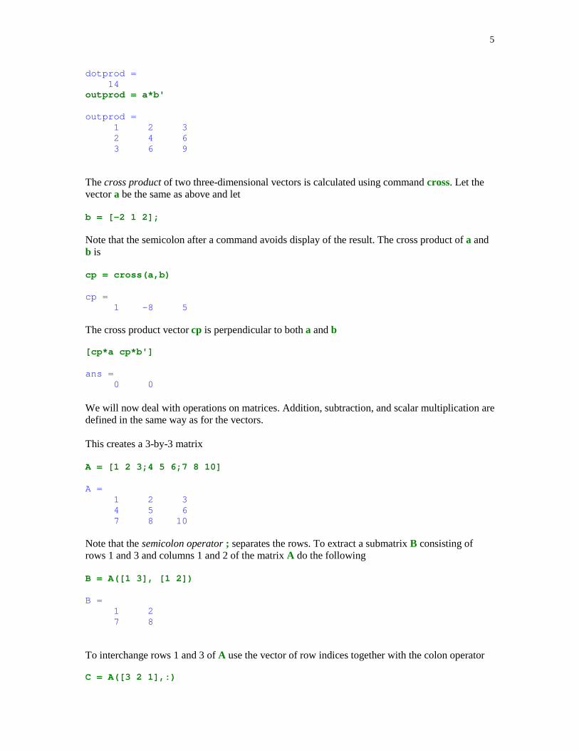
dotprod = a'*b

5

dotprod = 14 outprod = a*b'

outprod = 1 2 3 2 4 6 3 6 9

The cross product of two three-dimensional vectors is calculated using command cross. Let thevector a be the same as above and let

b = [-2 1 2];

Note that the semicolon after a command avoids display of the result. The cross product of a andb is

cp = cross(a,b)

cp = 1 -8 5

The cross product vector cp is perpendicular to both a and b

[cp*a cp*b']

ans = 0 0

We will now deal with operations on matrices. Addition, subtraction, and scalar multiplication aredefined in the same way as for the vectors.

This creates a 3-by-3 matrix

A = [1 2 3;4 5 6;7 8 10]

A = 1 2 3 4 5 6 7 8 10

Note that the semicolon operator ; separates the rows. To extract a submatrix B consisting ofrows 1 and 3 and columns 1 and 2 of the matrix A do the following

B = A([1 3], [1 2])

B = 1 2 7 8

To interchange rows 1 and 3 of A use the vector of row indices together with the colon operator

C = A([3 2 1],:)

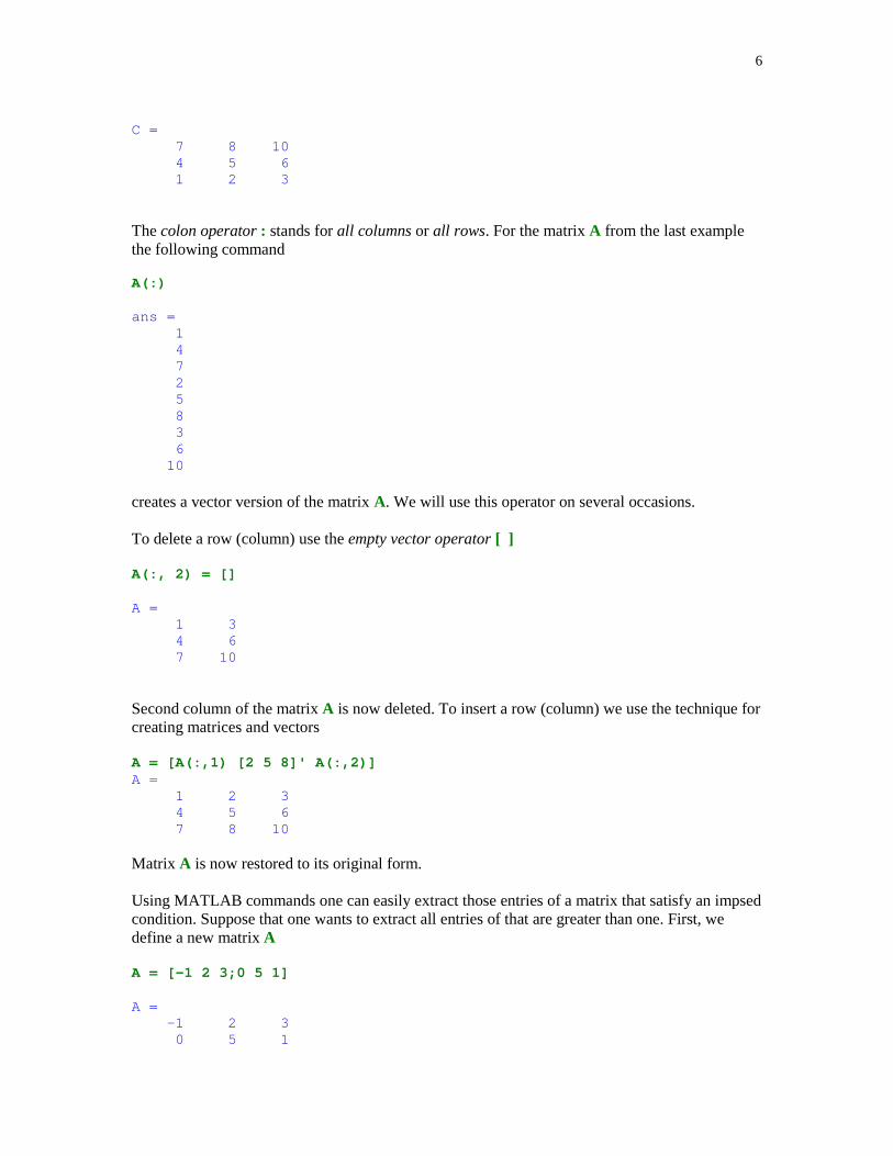
6

C = 7 8 10 4 5 6 1 2 3

The colon operator : stands for all columns or all rows. For the matrix A from the last examplethe following command

A(:)

ans = 1 4 7 2 5 8 3 6 10

creates a vector version of the matrix A. We will use this operator on several occasions.

To delete a row (column) use the empty vector operator [ ]

A(:, 2) = []

A = 1 3 4 6 7 10

Second column of the matrix A is now deleted. To insert a row (column) we use the technique forcreating matrices and vectors

A = [A(:,1) [2 5 8]' A(:,2)]A = 1 2 3 4 5 6 7 8 10

Matrix A is now restored to its original form.

Using MATLAB commands one can easily extract those entries of a matrix that satisfy an impsedcondition. Suppose that one wants to extract all entries of that are greater than one. First, wedefine a new matrix A

A = [-1 2 3;0 5 1]

A = -1 2 3 0 5 1

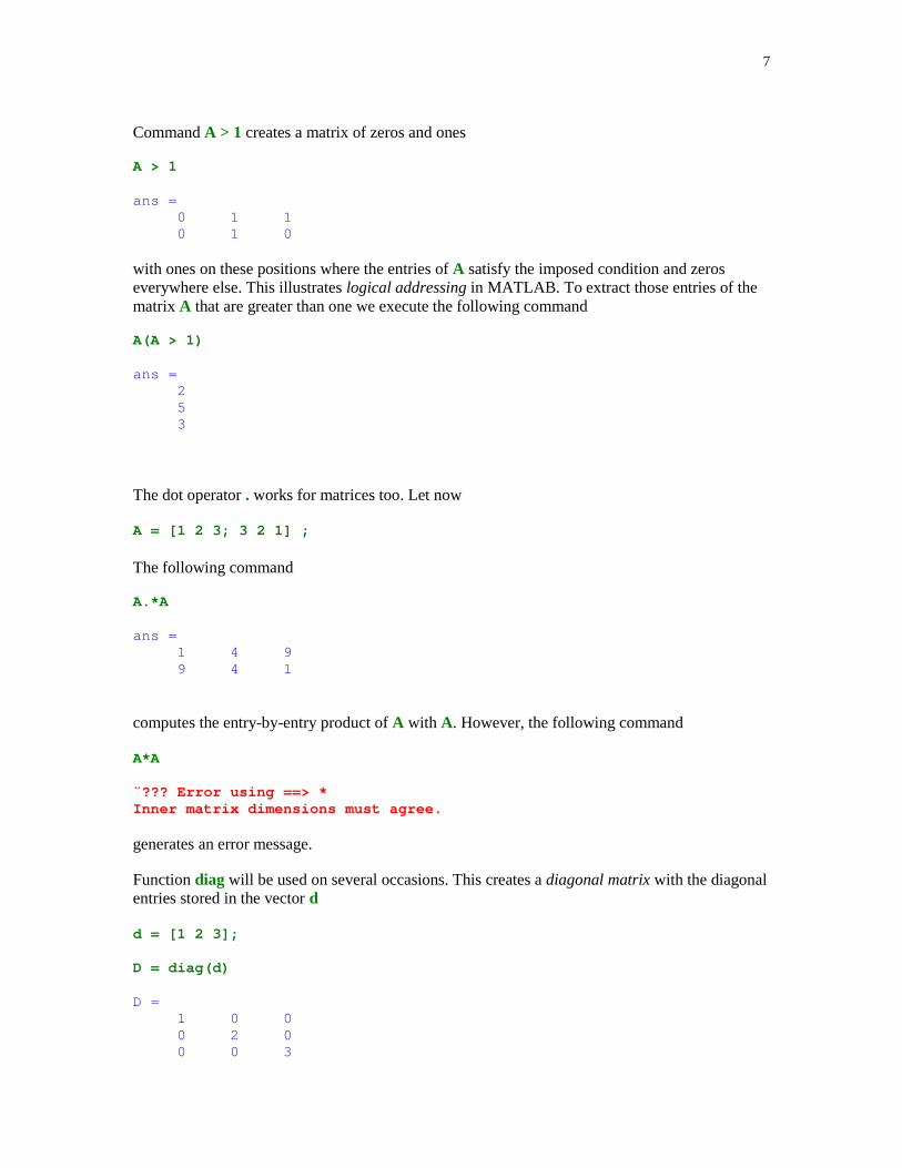
7

Command A > 1 creates a matrix of zeros and ones

A > 1

ans = 0 1 1 0 1 0

with ones on these positions where the entries of A satisfy the imposed condition and zeroseverywhere else. This illustrates logical addressing in MATLAB. To extract those entries of thematrix A that are greater than one we execute the following command

A(A > 1)

ans = 2 5 3

The dot operator . works for matrices too. Let now

A = [1 2 3; 3 2 1] ;

The following command

A.*A

ans = 1 4 9 9 4 1

computes the entry-by-entry product of A with A. However, the following command

A*A

¨??? Error using ==> *Inner matrix dimensions must agree.

generates an error message.

Function diag will be used on several occasions. This creates a diagonal matrix with the diagonalentries stored in the vector d

d = [1 2 3];

D = diag(d)

D = 1 0 0 0 2 0 0 0 3

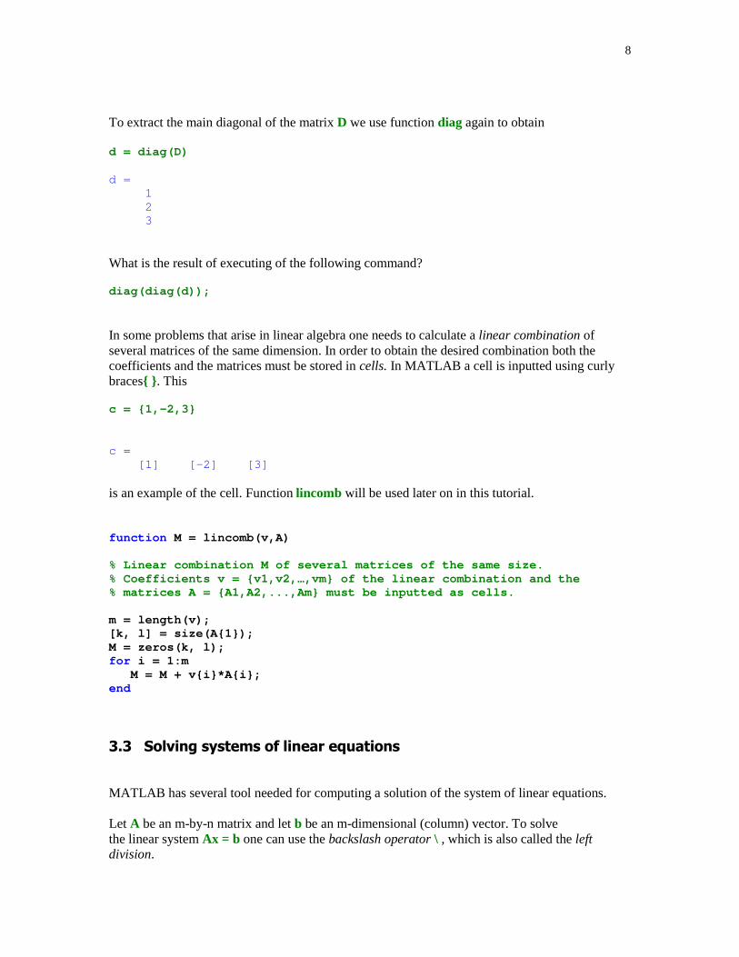
8

To extract the main diagonal of the matrix D we use function diag again to obtain

d = diag(D)

d = 1 2 3

What is the result of executing of the following command?

diag(diag(d));

In some problems that arise in linear algebra one needs to calculate a linear combination ofseveral matrices of the same dimension. In order to obtain the desired combination both thecoefficients and the matrices must be stored in cells. In MATLAB a cell is inputted using curlybraces{ } . This

c = {1,-2,3}

c = [1] [-2] [3]

is an example of the cell. Function lincomb will be used later on in this tutorial.

function M = lincomb(v,A)

% Linear combination M of several matrices of the same size.% Coefficients v = {v1,v2,…,vm} of the linear combination and the% matrices A = {A1,A2,...,Am} must be inputted as cells.

m = length(v);[k, l] = size(A{1});M = zeros(k, l);for i = 1:m M = M + v{i}*A{i};end

���� � ��!��������� ����"����� �

MATLAB has several tool needed for computing a solution of the system of linear equations.

Let A be an m-by-n matrix and let b be an m-dimensional (column) vector. To solvethe linear system Ax = b one can use the backslash operator \ , which is also called the leftdivision.

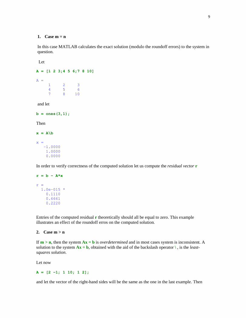
9

1. Case m = n

In this case MATLAB calculates the exact solution (modulo the roundoff errors) to the system inquestion.

Let

A = [1 2 3;4 5 6;7 8 10]

A = 1 2 3 4 5 6 7 8 10

and let

b = ones(3,1);

Then

x = A\b

x = -1.0000 1.0000 0.0000

In order to verify correctness of the computed solution let us compute the residual vector r

r = b - A*x

r = 1.0e-015 * 0.1110 0.6661 0.2220

Entries of the computed residual r theoretically should all be equal to zero. This exampleillustrates an effect of the roundoff erros on the computed solution.

2. Case m > n

If m > n, then the system Ax = b is overdetermined and in most cases system is inconsistent. Asolution to the system Ax = b, obtained with the aid of the backslash operator \ , is the least-squares solution.

Let now

A = [2 –1; 1 10; 1 2];

and let the vector of the right-hand sides will be the same as the one in the last example. Then

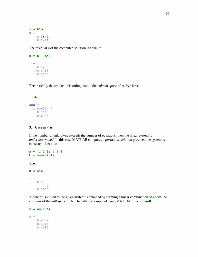
10

x = A\bx = 0.5849 0.0491

The residual r of the computed solution is equal to

r = b - A*x

r = -0.1208 -0.0755 0.3170

Theoretically the residual r is orthogonal to the column space of A. We have

r'*A

ans = 1.0e-014 * 0.1110 0.6994

3. Case m < n

If the number of unknowns exceeds the number of equations, then the linear system isunderdetermined. In this case MATLAB computes a particular solution provided the system isconsistent. Let now

A = [1 2 3; 4 5 6];b = ones(2,1);

Then

x = A\b

x = -0.5000 0 0.5000

A general solution to the given system is obtained by forming a linear combination of x with thecolumns of the null space of A. The latter is computed using MATLAB function null

z = null(A)

z = 0.4082 -0.8165 0.4082

11

Suppose that one wants to compute a solution being a linear combination of x and z, withcoefficients 1 and –1. Using function lincomb we obtainw = lincomb({1,-1},{x,z})

w = -0.9082 0.8165 0.0918

The residual r is calculated in a usual way

r = b - A*w

r = 1.0e-015 * -0.4441 0.1110

�#$� ���� ����� �������������� �

The built-in function rref allows a user to solve several problems of linear algebra. In this sectionwe shall employ this function to compute a solution to the system of linear equations and also tofind the rank of a matrix. Other applications are discussed in the subsequent sections of thistutorial.

Function rref takes a matrix and returns the reduced row echelon form of its argument. Syntax ofthe rref command is

B = rref(A) or [B, pivot] = rref(A)

The second output parameter pivot holds the indices of the pivot columns.

Let

A = magic(3); b = ones(3,1);

A solution x to the linear system Ax = b is obtained in two steps. First the augmented matrix ofthe system is transformed to the reduced echelon form and next its last column is extracted

[x, pivot] = rref([A b])

x = 1.0000 0 0 0.0667 0 1.0000 0 0.0667 0 0 1.0000 0.0667pivot = 1 2 3

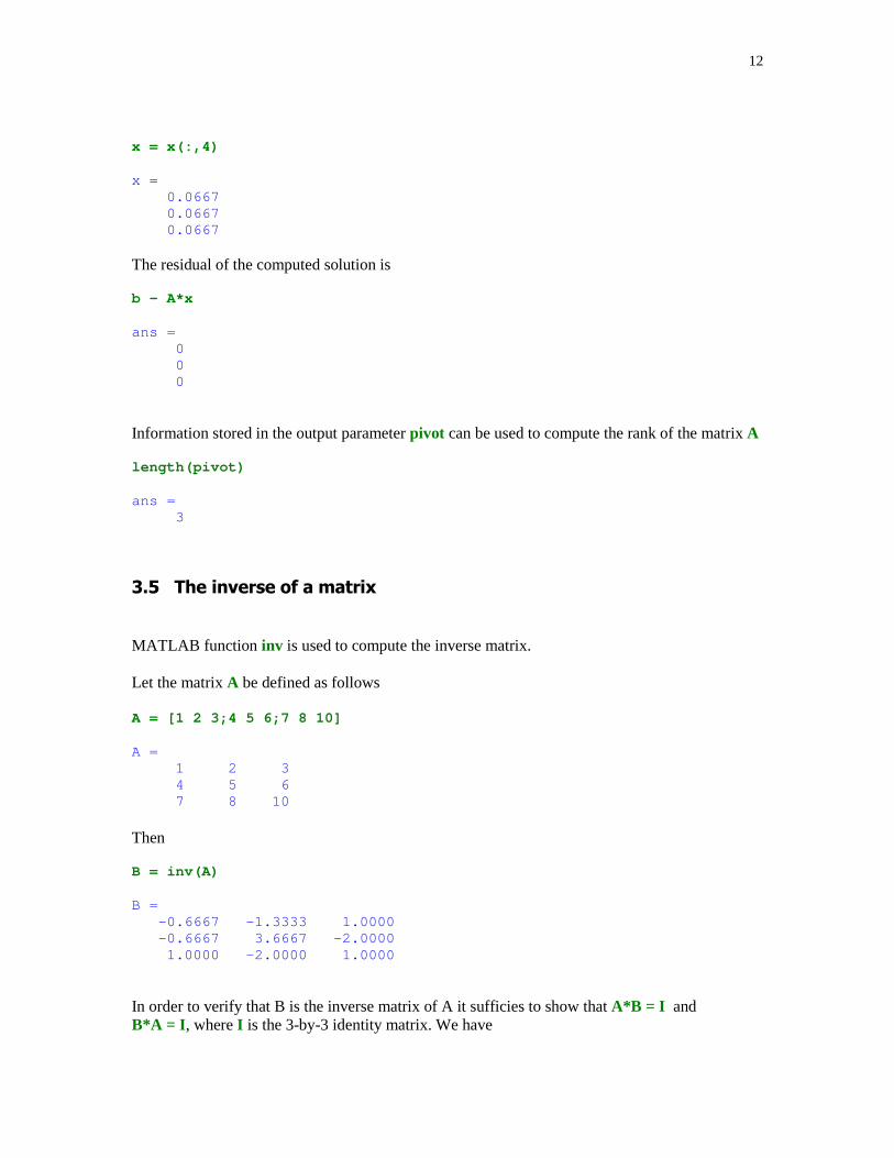
12

x = x(:,4)

x = 0.0667 0.0667 0.0667

The residual of the computed solution is

b - A*x

ans = 0 0 0

Information stored in the output parameter pivot can be used to compute the rank of the matrix A

length(pivot)

ans = 3

�%���� ������������&

MATLAB function inv is used to compute the inverse matrix.

Let the matrix A be defined as follows

A = [1 2 3;4 5 6;7 8 10]

A = 1 2 3 4 5 6 7 8 10

Then

B = inv(A)

B = -0.6667 -1.3333 1.0000 -0.6667 3.6667 -2.0000 1.0000 -2.0000 1.0000

In order to verify that B is the inverse matrix of A it sufficies to show that A*B = I andB*A = I , where I is the 3-by-3 identity matrix. We have

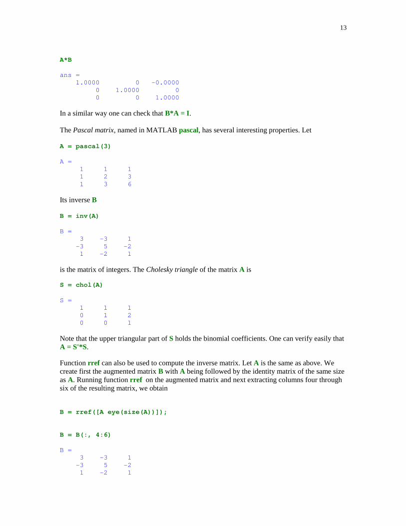
13

A*B

ans = 1.0000 0 -0.0000 0 1.0000 0 0 0 1.0000

In a similar way one can check that B*A = I .

The Pascal matrix, named in MATLAB pascal, has several interesting properties. Let

A = pascal(3)

A = 1 1 1 1 2 3 1 3 6

Its inverse B

B = inv(A)

B = 3 -3 1 -3 5 -2 1 -2 1

is the matrix of integers. The Cholesky triangle of the matrix A is

S = chol(A)

S = 1 1 1 0 1 2 0 0 1

Note that the upper triangular part of S holds the binomial coefficients. One can verify easily thatA = S'*S.

Function rref can also be used to compute the inverse matrix. Let A is the same as above. Wecreate first the augmented matrix B with A being followed by the identity matrix of the same sizeas A. Running function rref on the augmented matrix and next extracting columns four throughsix of the resulting matrix, we obtain

B = rref([A eye(size(A))]);

B = B(:, 4:6)

B = 3 -3 1 -3 5 -2 1 -2 1

14

To verify this result, we compute first the product A *B

A*B

ans = 1 0 0 0 1 0 0 0 1

and next B*A

B*A

ans = 1 0 0 0 1 0 0 0 1

This shows that B is indeed the inverse matrix of A.

�' (������ � ��

In some applications of linear algebra knowledge of the determinant of a matrix is required.MATLAB built-in function det is designed for computing determinants.

Let

A = magic(3);

Determinant of A is equal to

det(A)

ans = -360

One of the classical methods for computing determinants utilizes a cofactor expansion. For moredetails, see e.g., [2], pp. 103-114.

Function ckl = cofact(A, k, l) computes the cofactor ckl of the akl entry of the matrix A

function ckl = cofact(A,k,l)

% Cofactor ckl of the a_kl entry of the matrix A.

[m,n] = size(A);if m ~= n error( 'Matrix must be square' )

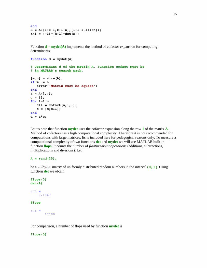
15

endB = A([1:k-1,k+1:n],[1:l-1,l+1:n]);ckl = (-1)^(k+l)*det(B);

Function d = mydet(A) implements the method of cofactor expansion for computingdeterminants

function d = mydet(A)

% Determinant d of the matrix A. Function cofact must be% in MATLAB's search path.

[m,n] = size(A);if m ~= n error( 'Matrix must be square' )enda = A(1,:);c = [];for l=1:n c1l = cofact(A,1,l); c = [c;c1l];endd = a*c;

Let us note that function mydet uses the cofactor expansion along the row 1 of the matrix A.Method of cofactors has a high computational complexity. Therefore it is not recommended forcomputations with large matrices. Its is included here for pedagogical reasons only. To measure acomputational complexity of two functions det and mydet we will use MATLAB built-infunction flops. It counts the number of floating-point operations (additions, subtractions,multiplications and divisions). Let

A = rand(25);

be a 25-by-25 matrix of uniformly distributed random numbers in the interval ( 0, 1 ). Usingfunction det we obtain

flops(0) det(A)

ans = -0.1867

flops

ans = 10100

For comparison, a number of flops used by function mydet is

flops(0)

16

mydet(A)

ans = -0.1867

flops

ans = 223350

The adjoint matrix adj(A) of the matrix A is also of interest in linear algebra (see, e.g., [2],p.108).

function B = adj(A)

% Adjoint matrix B of the square matrix A.

[m,n] = size(A);if m ~= n error( 'Matrix must be square' )endB = [];for k = 1:n for l=1:n B = [B;cofact(A,k,l)]; endendB = reshape(B,n,n);

The adjoint matrix and the inverse matrix satisfy the equation

A-1 = adj(A)/det(A)

(see [2], p.110 ). Due to the high computational complexity this formula is not recommended forcomputing the inverse matrix.

�) �������� ��

The 2-norm (Euclidean norm) of a vector is computed in MATLAB using function norm.

Let

a = -2:2

a = -2 -1 0 1 2

The 2-norm of a is equal to

twon = norm(a)

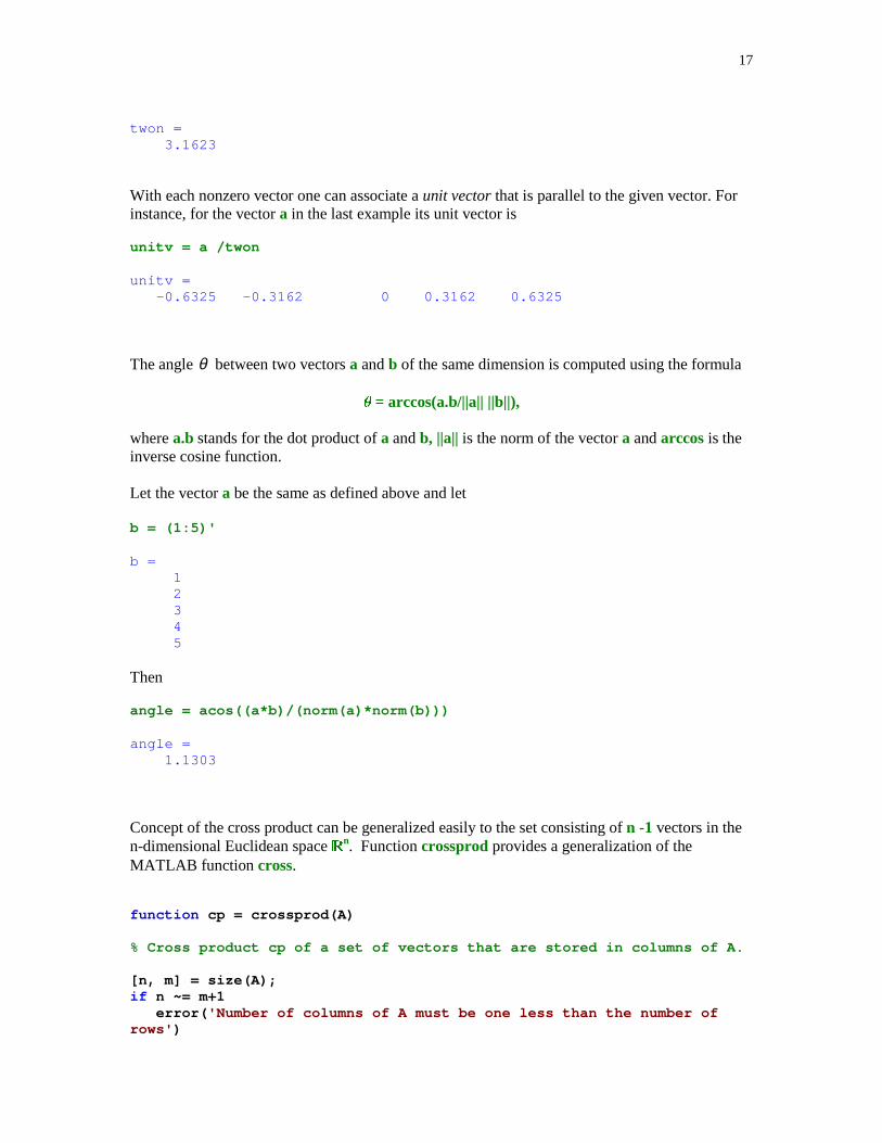
17

twon = 3.1623

With each nonzero vector one can associate a unit vector that is parallel to the given vector. Forinstance, for the vector a in the last example its unit vector is

unitv = a /twon

unitv = -0.6325 -0.3162 0 0.3162 0.6325

The angle θ between two vectors a and b of the same dimension is computed using the formula

� = arccos(a.b/||a|| ||b||),

where a.b stands for the dot product of a and b, ||a|| is the norm of the vector a and arccos is theinverse cosine function.

Let the vector a be the same as defined above and let

b = (1:5)'

b = 1 2 3 4 5

Then

angle = acos((a*b)/(norm(a)*norm(b)))

angle = 1.1303

Concept of the cross product can be generalized easily to the set consisting of n -1 vectors in then-dimensional Euclidean space �

n. Function crossprod provides a generalization of theMATLAB function cross.

function cp = crossprod(A)

% Cross product cp of a set of vectors that are stored in columns of A.

[n, m] = size(A);if n ~= m+1 error( 'Number of columns of A must be one less than the number ofrows' )

18

endif rank(A) < min(m,n) cp = zeros(n,1);else C = [ones(n,1) A]'; cp = zeros(n,1); for j=1:n cp(j) = cofact(C,1,j); endend

Let

A = [1 -2 3; 4 5 6; 7 8 9; 1 0 1]

A = 1 -2 3 4 5 6 7 8 9 1 0 1

The cross product of column vectors of A is

cp = crossprod(A)

cp = -6 20 -14 24

Vector cp is orthogonal to the column space of the matrix A. One can easily verify this bycomputing the vector-matrix product

cp'*A

ans = 0 0 0

�* �� ������ ��������� �����������

Let L: �n � �m be a linear transformation. It is well known that any linear transformation inquestion is represented by an m-by-n matrix A, i.e., L(x) = Ax holds true for any x � �n.Matrices of some linear transformations including those of reflections and rotations are discussedin detail in Tutorial 4, Section 4.3.

With each matrix one can associate four subspaces called the four fundamental subspaces. Thesubspaces in question are called the column space, the nullspace, the row space, and the left

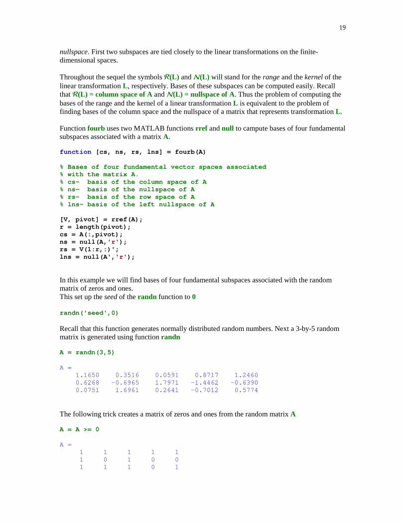
19

nullspace. First two subspaces are tied closely to the linear transformations on the finite-dimensional spaces.

Throughout the sequel the symbols �(L) and �(L) will stand for the range and the kernel of thelinear transformation L , respectively. Bases of these subspaces can be computed easily. Recallthat �(L) = column space of A and �(L) = nullspace of A. Thus the problem of computing thebases of the range and the kernel of a linear transformation L is equivalent to the problem offinding bases of the column space and the nullspace of a matrix that represents transformation L .

Function fourb uses two MATLAB functions rref and null to campute bases of four fundamentalsubspaces associated with a matrix A.

function [cs, ns, rs, lns] = fourb(A)

% Bases of four fundamental vector spaces associated% with the matrix A.% cs- basis of the column space of A% ns- basis of the nullspace of A% rs- basis of the row space of A% lns- basis of the left nullspace of A

[V, pivot] = rref(A);r = length(pivot);cs = A(:,pivot);ns = null(A, 'r' );rs = V(1:r,:)';lns = null(A', 'r' );

In this example we will find bases of four fundamental subspaces associated with the randommatrix of zeros and ones.This set up the seed of the randn function to 0

randn('seed',0)

Recall that this function generates normally distributed random numbers. Next a 3-by-5 randommatrix is generated using function randn

A = randn(3,5)

A = 1.1650 0.3516 0.0591 0.8717 1.2460 0.6268 -0.6965 1.7971 -1.4462 -0.6390 0.0751 1.6961 0.2641 -0.7012 0.5774

The following trick creates a matrix of zeros and ones from the random matrix A

A = A >= 0

A = 1 1 1 1 1 1 0 1 0 0 1 1 1 0 1

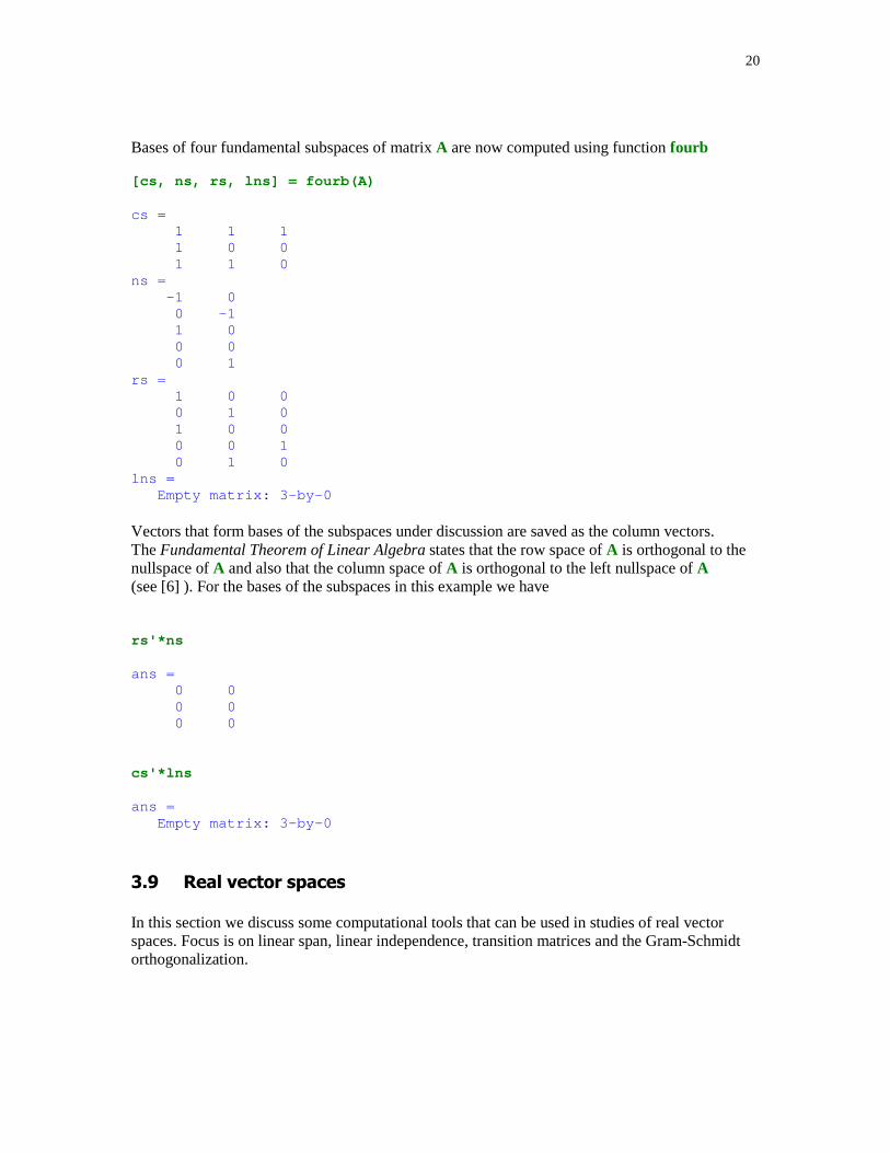
20

Bases of four fundamental subspaces of matrix A are now computed using function fourb

[cs, ns, rs, lns] = fourb(A)

cs = 1 1 1 1 0 0 1 1 0ns = -1 0 0 -1 1 0 0 0 0 1rs = 1 0 0 0 1 0 1 0 0 0 0 1 0 1 0lns = Empty matrix: 3-by-0

Vectors that form bases of the subspaces under discussion are saved as the column vectors.The Fundamental Theorem of Linear Algebra states that the row space of A is orthogonal to thenullspace of A and also that the column space of A is orthogonal to the left nullspace of A(see [6] ). For the bases of the subspaces in this example we have

rs'*ns

ans = 0 0 0 0 0 0

cs'*lns

ans = Empty matrix: 3-by-0

�+ ,��� �����������

In this section we discuss some computational tools that can be used in studies of real vectorspaces. Focus is on linear span, linear independence, transition matrices and the Gram-Schmidtorthogonalization.

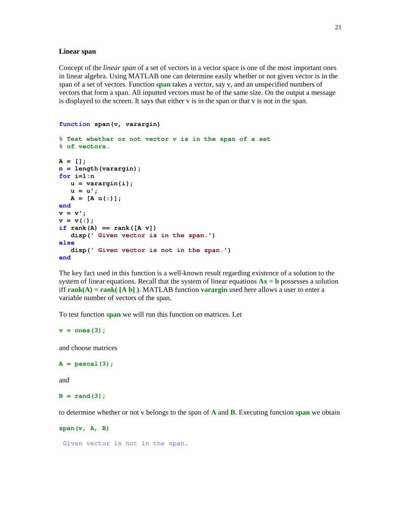
21

Linear span

Concept of the linear span of a set of vectors in a vector space is one of the most important onesin linear algebra. Using MATLAB one can determine easily whether or not given vector is in thespan of a set of vectors. Function span takes a vector, say v, and an unspecified numbers ofvectors that form a span. All inputted vectors must be of the same size. On the output a messageis displayed to the screen. It says that either v is in the span or that v is not in the span.

function span(v, varargin)

% Test whether or not vector v is in the span of a set% of vectors.

A = [];n = length(varargin);for i=1:n u = varargin{i}; u = u'; A = [A u(:)];endv = v';v = v(:);if rank(A) == rank([A v]) disp( ' Given vector is in the span.' )else disp( ' Given vector is not in the span.' )end

The key fact used in this function is a well-known result regarding existence of a solution to thesystem of linear equations. Recall that the system of linear equations Ax = b possesses a solutioniff rank(A) = rank( [A b] ) . MATLAB function varargin used here allows a user to enter avariable number of vectors of the span.

To test function span we will run this function on matrices. Let

v = ones(3);

and choose matrices

A = pascal(3);

and

B = rand(3);

to determine whether or not v belongs to the span of A and B. Executing function span we obtain

span(v, A, B)

Given vector is not in the span.

22

Linear independence

Suppose that one wants to check whether or not a given set of vectors is linearly independent.Utilizing some ideas used in function span one can write his/her function that will take anuspecified number of vectors and return a message regarding linear independence/dependence ofthe given set of vectors. We leave this task to the reader (see Problem 32).

Transition matrix

Problem of finding the transition matrix from one vector space to another vector space is interestin linear algebra. We assume that the ordered bases of these spaces are stored in columns ofmatrices T and S, respectively. Function transmat implements a well-known method for findingthe transition matrix.

function V = transmat(T, S)

% Transition matrix V from a vector space having the ordered% basis T to another vector space having the ordered basis S.% Bases of the vector spaces are stored in columns of the% matrices T and S.

[m, n] = size(T);[p, q] = size(S); if (m ~= p) | (n ~= q) error( 'Matrices must be of the same dimension' ) endV = rref([S T]);V = V(:,(m + 1):(m + n));

Let

T = [1 2;3 4]; S = [0 1;1 0];

be the ordered bases of two vector spaces. The transition matrix V form a vector space having theordered basis T to a vector space whose ordered basis is stored in columns of the matrix S is

V = transmat(T, S)

V = 3 4 1 2

We will use the transition matrix V to compute a coordinate vector in the basis S. Let

[x] T =

1

1

be the coordinate vector in the basis T. Then the coordinate vector [x] S, is

xs = V*[1;1]

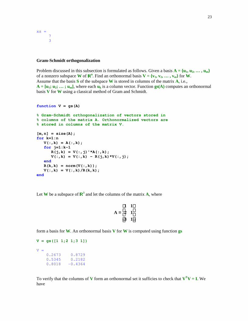
23

xs = 7 3

Gram-Schmidt orthogonalization

Problem discussed in this subsection is formulated as follows. Given a basis A = {u1, u2, … , um}of a nonzero subspace W of �n. Find an orthonormal basis V = {v1, v2, … , vm} for W.Assume that the basis S of the subspace W is stored in columns of the matrix A, i.e.,A = [u1; u2; … ; um], where each uk is a column vector. Function gs(A) computes an orthonormalbasis V for W using a classical method of Gram and Schmidt.

function V = gs(A)

% Gram-Schmidt orthogonalization of vectors stored in% columns of the matrix A. Orthonormalized vectors are% stored in columns of the matrix V.

[m,n] = size(A);for k=1:n V(:,k) = A(:,k); for j=1:k-1 R(j,k) = V(:,j)'*A(:,k); V(:,k) = V(:,k) - R(j,k)*V(:,j); end R(k,k) = norm(V(:,k)); V(:,k) = V(:,k)/R(k,k);end

Let W be a subspace of �3 and let the columns of the matrix A, where

=

13

12

11

A

form a basis for W. An orthonormal basis V for W is computed using function gs

V = gs([1 1;2 1;3 1])

V = 0.2673 0.8729 0.5345 0.2182 0.8018 -0.4364

To verify that the columns of V form an orthonormal set it sufficies to check that VTV = I . Wehave

24

V'*V

ans = 1.0000 0.0000 0.0000 1.0000

We will now use matrix V to compute the coordinate vector [v] V, where

v = [1 0 1];

We have

v*V

ans = 1.0690 0.4364

��-��������&���� �����������

MATLAB function eig is designed for computing the eigenvalues and the eigenvectors of thematrix A. Its syntax is shown below

[V, D] = eig(A)

The eigenvalues of A are stored as the diagonal entries of the diagonal matrix D and theassociated eigenvectors are stored in columns of the matrix V.

Let

A = pascal(3);

Then

[V, D] = eig(A)

V = 0.5438 -0.8165 0.1938 -0.7812 -0.4082 0.4722 0.3065 0.4082 0.8599D = 0.1270 0 0 0 1.0000 0 0 0 7.8730

Clearly, matrix A is diagonalizable. The eigenvalue-eigenvector decomposition A = VDV -1of Ais calculated as follows

V*D/V

25

ans = 1.0000 1.0000 1.0000 1.0000 2.0000 3.0000 1.0000 3.0000 6.0000

Note the use of the right division operator / instead of using the inverse matrix function inv. Thisis motivated by the fact that computation of the inverse matrix takes longer than the execution ofthe right division operation.

The characteristic polynomial of a matrix is obtained by invoking the function poly.Let

A = magic(3) ;

be the magic square. In this example the vector chpol holds the coefficients of the characteristicpolynomial of the matrix A. Recall that a polynomial is represented in MATLAB by itscoefficients that are ordered by descending powers

chpol = poly(A)

chpol = 1.0000 -15.0000 -24.0000 360.0000

The eigenvalues of A can be computed using function roots

eigenvals = roots(chpol)

eigenvals = 15.0000 4.8990 -4.8990

This method, however, is not recommended for numerical computing the eigenvalues of a matrix.There are several reasons for which this approach is not used in numerical linear algebra. Aninterested reader is referred to Tutorial 4.

The Caley-Hamilton Theorem states that each matrix satisfies its characteristic equation, i.e.,chpol(A) = 0, where the last zero stands for the matrix of zeros of the appropriate dimension. Weuse function lincomb to verify this result

Q = lincomb(num2cell(chpol) , {A^3, A^2, A, eye(size(A))})

Q = 1.0e-012 * -0.5684 -0.5542 -0.4832 -0.5258 -0.6253 -0.4547 -0.5116 -0.4547 -0.6821

26

������������� ����� ����������

List of applications of methods of linear algebra is long and impressive. Areas that relay heavilyon the methods of linear algebra include the data fitting, mathematical statistics, linearprogramming, computer graphics, cryptography, and economics, to mention the most importantones. Applications discussed in this section include the data fitting, coding messages, andcomputer graphics.

���� �������

In many problems that arise in science and engineering one wants to fit a discrete set of points inthe plane by a smooth curve or function. A typical choice of a smoothing function is a polynomialof a certain degree. If the smoothing criterion requires minimization of the 2-norm, then one hasto solve the least-squares approximation problem. Function fit takes three arguments, the degreeof the approximating polynomial, and two vectors holding the x- and the y- coordinates of pointsto be approximated. On the output, the coefficients of the least-squares polynomials are returned.Also, its graph and the plot of the data points are generated.

function c = fit(n, t, y)

% The least-squares approximating polynomial of degree n (n>=0).% Coordinates of points to be fitted are stored in the column vectors% t and y. Coefficients of the approximating polynomial are stored in% the vector c. Graphs of the data points and the least-squares% approximating polynomial are also generated.

if ( n >= length(t)) error( 'Degree is too big' )endv = fliplr(vander(t));v = v(:,1:(n+1));c = v\y;c = fliplr(c');x = linspace(min(t),max(t));w = polyval(c, x);plot(t,y, 'ro' ,x,w);title(sprintf( 'The least-squares polynomial of degree n = %2.0f' ,n))legend( 'data points' , 'fitting polynomial' )

To demonstrate functionality of this code we generate first a set of points in the plane. Our goal isto fit ten evenly spaced points with the y-ordinates being the values of the function y = sin(2t) atthese points

t = linspace(0, pi/2, 10); t = t';

y = sin(2*t);

We will fit the data by a polynomial of degree at most three

c = fit(3, t, y)

c = -0.0000 -1.6156 2.5377 -0.0234

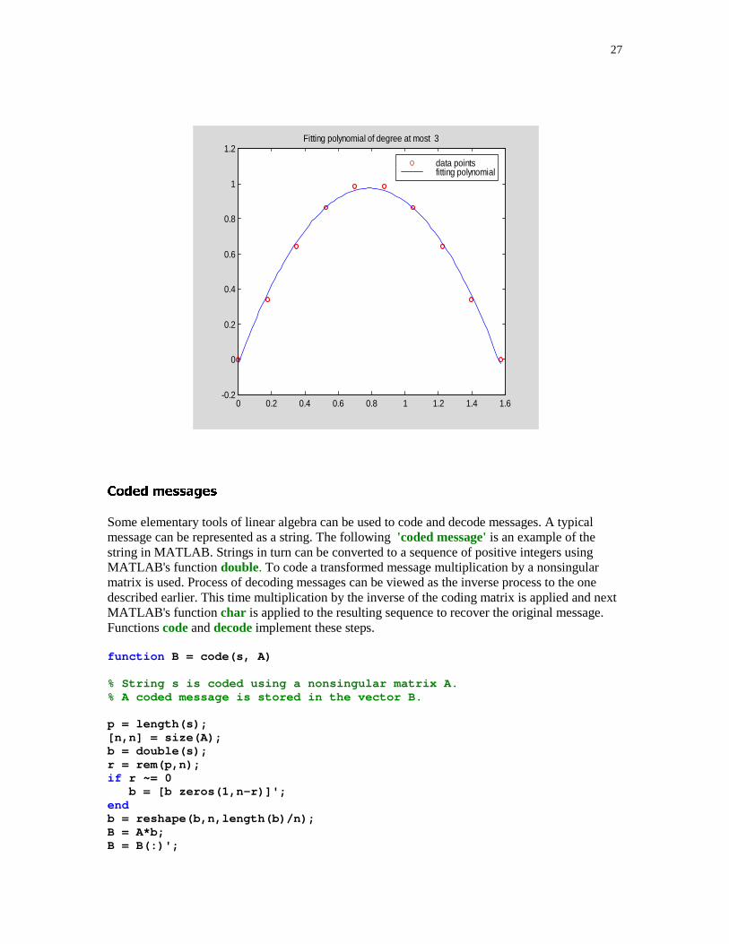
27

0 0.2 0.4 0.6 0.8 1 1.2 1.4 1.6-0.2

0

0.2

0.4

0.6

0.8

1

1.2Fitting polynomial of degree at most 3

data pointsfitting polynomial

��� �������

Some elementary tools of linear algebra can be used to code and decode messages. A typicalmessage can be represented as a string. The following 'coded message' is an example of thestring in MATLAB. Strings in turn can be converted to a sequence of positive integers usingMATLAB's function double. To code a transformed message multiplication by a nonsingularmatrix is used. Process of decoding messages can be viewed as the inverse process to the onedescribed earlier. This time multiplication by the inverse of the coding matrix is applied and nextMATLAB's function char is applied to the resulting sequence to recover the original message.Functions code and decode implement these steps.

function B = code(s, A)

% String s is coded using a nonsingular matrix A.% A coded message is stored in the vector B.

p = length(s);[n,n] = size(A);b = double(s);r = rem(p,n);if r ~= 0 b = [b zeros(1,n-r)]';endb = reshape(b,n,length(b)/n);B = A*b;B = B(:)';

28

function s = dcode(B, A)

% Coded message, stored in the vector B, is% decoded with the aid of the nonsingular matrix A% and is stored in the string s.

[n,n]= size(A);p = length(B);B = reshape(B,n,p/n);d = A\B;s = char(d(:)');

A message to be coded is

s = 'Linear algebra is fun';

As a coding matrix we use the Pascal matrix

A = pascal(4);

This codes the message s

B = code(s,A)

B = Columns 1 through 6 392 1020 2061 3616 340809 Columns 7 through 12 1601 2813 410 1009 20033490 Columns 13 through 18 348 824 1647 2922 366953 Columns 19 through 24 1993 3603 110 110 110110

To decode this message we have to work with the same coding matrix A

dcode(B,A)

ans =Linear algebra is fun

����� ��������

Linear algebra provides many tools that are of interest for computer programmers especially forthose who deal with the computer graphics. Once the graphical object is created one has totransform it to another object. Certain plane and/or space transformations are linear. Thereforethey can be realized as the matrix-vector multiplication. For instance, the reflections, translations,

29

rotations all belong to this class of transformations. A computer code provided below deals withthe plane rotations in the counterclockwise direction. Function rot2d takes a planar objectrepresented by two vectors x and y and returns its image. The angle of rotation is supplied in thedegree measure.

function [xt, yt] = rot2d(t, x, y)

% Rotation of a two-dimensional object that is represented by two% vectors x and y. The angle of rotation t is in the degree measure.% Transformed vectors x and y are saved in xt and yt, respectively.

t1 = t*pi/180;r = [cos(t1) -sin(t1);sin(t1) cos(t1)];x = [x x(1)];y = [y y(1)];hold ongrid onaxis equalfill(x, y, 'b' )z = r*[x;y];xt = z(1,:);yt = z(2,:);fill(xt, yt, 'r' );title(sprintf( 'Plane rotation through the angle of %3.2f degrees' ,t))hold off

Vectors x and y

x = [1 2 3 2]; y = [3 1 2 4];

are the vertices of the parallelogram. We will test function rot2d on these vectors using as theangle of rotation t = 75.

[xt, yt] = rot2d(75, x, y)

xt = -2.6390 -0.4483 -1.1554 -3.3461 -2.6390yt = 1.7424 2.1907 3.4154 2.9671 1.7424

30

-3 -2 -1 0 1 2 30

0.5

1

1.5

2

2.5

3

3.5

4

4.5

5Plane rotation through the angle of 75.00 degrees

The right object is the original parallelogram while the left one is its image.

31

,����� ���

[1] B.D. Hahn, Essential MATLAB for Scientists and Engineers, John Wiley & Sons, New York, NY, 1997.

[2] D.R. Hill and D.E. Zitarelli, Linear Algebra Labs with MATLAB, Second edition, Prentice Hall, Upper Saddle River, NJ, 1996.

[3] B. Kolman, Introductory Linear Algebra with Applications, Sixth edition, Prentice Hall, Upper Saddle River, NJ, 1997.

[4] R.E. Larson and B.H. Edwards, Elementary Linear Algebra, Third edition, D.C. Heath and Company, Lexington, MA, 1996.

[5] S.J. Leon, Linear Algebra with Applications, Fifth edition, Prentice Hall, Upper Saddle River, NJ, 1998.

[6] G. Strang, Linear Algebra and Its Applications, Second edition, Academic Press, Orlando, FL, 1980.

32

.�������

In Problems 1 – 12 you cannot use loops for and/or while.Problems 40 - 42 involve symbolic computations. In order to do these problems you have to usethe Symbolic Math Toolbox.

1. Create a ten-dimensional row vector whose all components are equal 2. You cannot enternumber 2 more than once.

2. Given a row vector a = [1 2 3 4 5]. Create a column vector b that has the same components asthe vector a but they must bestored in the reversed order.

3. MATLAB built-in function sort(a) sorts components of the vector a in the ascending order.Use function sort to sort components of the vector a in the descending order.

4. To find the largest (smallest) entry of a vector you can use function max (min). Suppose thatthese functions are not available. How would you calculate

(a) the largest entry of a vector ?(b) the smallest entry of a vector?

5. Suppose that one wants to create a vector a of ones and zeros whose length is equal to 2n ( n = 1, 2, … ). For instance, when n = 3, then a = [1 0 1 0 1 0]. Given value of n create a vector a with the desired property.

6. Let a be a vector of integers.

(a) Create a vector b whose all components are the even entries of the vector a.(b) Repeat part (a) where now b consists of all odd entries of the vector a.

Hint: Function logical is often used to logical tests. Another useful function you mayconsider to use is rem(x, y) - the remainder after division of x by y.

7. Given two nonempty row vectors a and b and two vectors ind1and ind2 with length(a) =length(ind1) and length(b) = length(ind2). Components of ind1 and ind2 are positiveintegers. Create a vector c whose components are those of vectors a and b. Their indices aredetermined by vectors ind1 and ind2, respectively.

8. Using function rand, generate a vector of random integers that are uniformly distributed inthe interval (2, 10). In order to insure that the resulting vector is not empty begin with avector that has a sufficient number of components.Hint: Function fix might be helpful. Type help fix in the Command Window to learn moreabout this function.

9. Let A be a square matrix. Create a matrix B whose entries are the same as those of A exceptthe entries along the main diagonal. The main diagonal of the matrix B should consist entierlyof ones.

33

10. Let A be a square matrix. Create a tridiagonal matrix T whose subdiagonal, main diagonal,and the superdiagonal are taken from the matrix A.Hint: You may wish to use MATLAB functions triu and tril . These functions take a secondoptional argument. To learn more about these functions use MATLAB's help.

11. In this exercise you are to test a square matrix A for symmetry. Write MATLAB function s = issymm(A) that takes a matrix A and returns a number s. If A is symmetric, then s = 1, otherwise s = 0.

12. Let A be an m-by-n and let B be an n-by-p matrices. Computing the product C = ABrequires mnp multiplications. If either A or B has a special structure, then the number ofmultiplications can be reduced drastically. Let A be a full matrix of dimension m-by-n and letB be an upper triangular matrix of dimension n-by-n whose all nonzero entries are equal toone. The product AB can be calculated without using a single multiplicationa. Write analgorithm for computing the matrix product C = A*B that does not require multiplications.Test your code with the following matrices A = pascal(3) and B = triu(ones(3)).

13. Given square invertible matrices A and B and the column vector b. Assume that the matricesA and B and the vector b have the same number of rows. Suppose that one wants to solve alinear system of equations ABx = b. Without computing the matrix-matrix product A*B , finda solution x to to this system using the backslash operator \.

14. Find all solutions to the linear system Ax = b, where the matrix A consists of rows onethrough three of the 5-by-5 magic square

A = magic(5);

A = A(1:3,: )

A = 17 24 1 8 15 23 5 7 14 16

4 6 13 20 22

and b = ones(3; 1).

15. Determine whether or not the system of linear equations Ax = b, where

A = ones(3, 2); b = [1; 2; 3];

possesses an exact solution x.

16. The purpose of this exercise is to demonstrate that for some matrices the computed solutionto Ax = b can be poor. Define

A = hilb(50); b = rand(50,1);

Find the 2-norm of the residual r = A*x – b . How would you explain a fact that the computed norm is essentially bigger than zero?

34

17. In this exercise you are to compare computational complexity of two methods for finding asolution to the linear system Ax = b where A is a square matrix. First method utilizes thebackslash operator \ while the second method requires a use of the function rref . UseMATLAB function flops to compare both methods for various linear systems of your choice.Which of these methods require, in general, a smaller number of flops?

18. Repeat an experiment described in Problem 17 using as a measure of efficiency a time needed to compute the solution vector. MATLAB has a pair of functions tic and toc that can be used in this experiment. This illustrates use of the above mentioned functions tic; x = A\b; toc. Using linear systems of your choice compare both methods for speed. Which method is a faster one? Experiment with linear systems having at least ten equations.

19. Let A be a real matrix. Use MATLAB function rref to extract all

(a) columns of A that are linearly independent(b) rows of A that are linearly independent

20. In this exercise you are to use MATLAB function rref to compute the rank of the followingmatrices:

(a) A = magic(3)(b) A = magic(4)(c) A = magic(5)(d) A = magic(6)

Based on the results of your computations what hypotheses would you formulate about the rank(magic(n)), when n is odd, when n is even?

21. Use MATLAB to demonstrate that det(A + B) � det(A) + det(B) for matrices of your choice.

22. Let A = hilb(5). Hilbert matrix is often used to test computer algorithms for reliability. In thisexercise you will use MATLAB function num2str that converts numbers to strings, to seethat contrary to the well-known theorem of Linear Algebra the computed determinantdet(A*A') is not necessarily the same as det(A)*det(A'). You can notice a difference incomputed quantities by executing the following commands: num2str(det(A*A'), 16) andnum2str(det(A)*det(A'), 16).

23. The inverse matrix of a symmetric nonsingular matrix is a symmetric matrix. Check thisproperty using function inv and a symmetric nonsingular matrix of your choice.

24. The following matrix

A = ones(5) + eye(5)

A = 2 1 1 1 1 1 2 1 1 1 1 1 2 1 1 1 1 1 2 1 1 1 1 1 2

35

is a special case of the Pei matrix. Normalize columns of the matrix A so that all columns of the resulting matrix, say B, have the Euclidean norm (2-norm) equal to one.

25. Find the angles between consecutive columns of the matrix B of Problem 24.

26. Find the cross product vector cp that is perpendicular to columns one through four of the Peimatrix of Problem 24.

27. Let L be a linear transformation from �5 to �5 that is represented by the Pei matrix ofProblem 24. Use MATLAB to determine the range and the kernel of this transformation.

28. Let �n denote a space of algebraic polynomials of degree at most n. Transformation Lfrom �n to �3 is defined as follows

=

∫

0

)0(p

dt)t(p

)p(L

1

0

(a) Show that L is a linear transformation.(b) Find a matrix that represents transformation L with respect to the ordered basis {t n, tn –1, … 1}.(c) Use MATLAB to compute bases of the range and the kernel of L . Perform your

experiment for the following values of n = 2, 3, 4.

29. Transformation L from �n to �n –1 is defined as follows L(p) = p'(t) . Symbol �n, isintroduced in Problem 28. Answer questions (a) through (c) of Problem 28 for thetransformation L of this problem.

30. Given vectors a = [1; 2; 3] and b = [-3; 0; 2]. Determine whether or not vector c = [4; 1;1] isin the span of vectors a and b.

31. Determine whether or not the Toeplitz matrix

A = toeplitz( [1 0 1 1 1] )

A = 1 0 1 1 1 0 1 0 1 1 1 0 1 0 1 1 1 0 1 0 1 1 1 0 1

is in the span of matrices B = ones(5) and C = magic(5).

36

32. Write MATLAB function linind(varargin) that takes an arbitrary number of vectors(matrices) of the same dimension and determines whether or not the inputted vectors(matrices) are linearly independent. You may wish to reuse some lines of code that arecontained in the function span presented in Section 3.9 of this tutorial.

33. Use function linind of Problem 32 to show that the columns of the matrix A of Problem31 are linearly independent.

34. Let [a]A = ones(5,1) be the coordinate vector with respect to the basis A – columns of thematrix A of Problem 31. Find the coordinate vector [a]P , where P is the basis of the vectorspace spanned by the columns of the matrix pascal(5).

35. Let A be a real symmetric matrix. Use the well-known fact from linear algebra to determinethe interval containing all the eigenvalues of A. Write MATLAB function

[a, b] = interval(A) that takes a symmetric matrix A and returns the endpoints a and b of the interval that contains all the eigenvalues of A.

36. Without solving the matrix eigenvalue problem find the sum and the product of alleigenvalues of the following matrices:

(a) P = pascal(30)(b) M= magic(40)(c) H = hilb(50)(d) H = hadamard(64)

37. Find a matrix B that is similar to A = magic(3).

38. In this exercise you are to compute a power of the diagonalizable matrix A. Let A = pascal(5). Use the eigenvalue decomposition of A to calculate the ninth power of A. You cannot apply the power operator ^ to the matrix A.

39. Let A be a square matrix. A matrix B is said to be the square root of A if B^2 = A.In MATLAB the square root of a matrix can be found using the power operator ^ . In thisexercise you are to use the eigenvalue-eigenvector decomposition of a matrix find the squareroot of A = [3 3;-2 -2].

40. Declare a variable k to be a symbolic variable typing syms k in the Command Window.Find a value of k for which the following symbolic matrix

A = sym( [1 k^2 2; 1 k -1; 2 –1 0] ) is not invertible.

41. Let the matrix A be the same as in Problem 40.

(a) Without solving the matrix eigenvalue problem, determine a value of k for which all theeigenvalues of A are real.

(b) Let v be a number you found in part (a). Convert the symbolic matrix A to a numericmatrix B using the substitution command subs, i.e., B = subs(A, k, v).

(c) Determine whether or not the matrix B is diagonalizable. If so, find a diagonal matrix Dthat is similar to B.

37

(d) If matrix B is diagonalizable use the results of part (c) to compute all the eigenvectors ofthe matrix B. Do not use MATLAB's function eig.

42. Given a symbolic matrix A = sym( [1 0 k; 2 2 0; 3 3 3]).

(a) Find a nonzero value of k for which all the eigenvalues of A are real.(b) For what value of k two eigenvalues of A are complex and the remaining one is real?

��������

��� �������� ����� ���

�����������

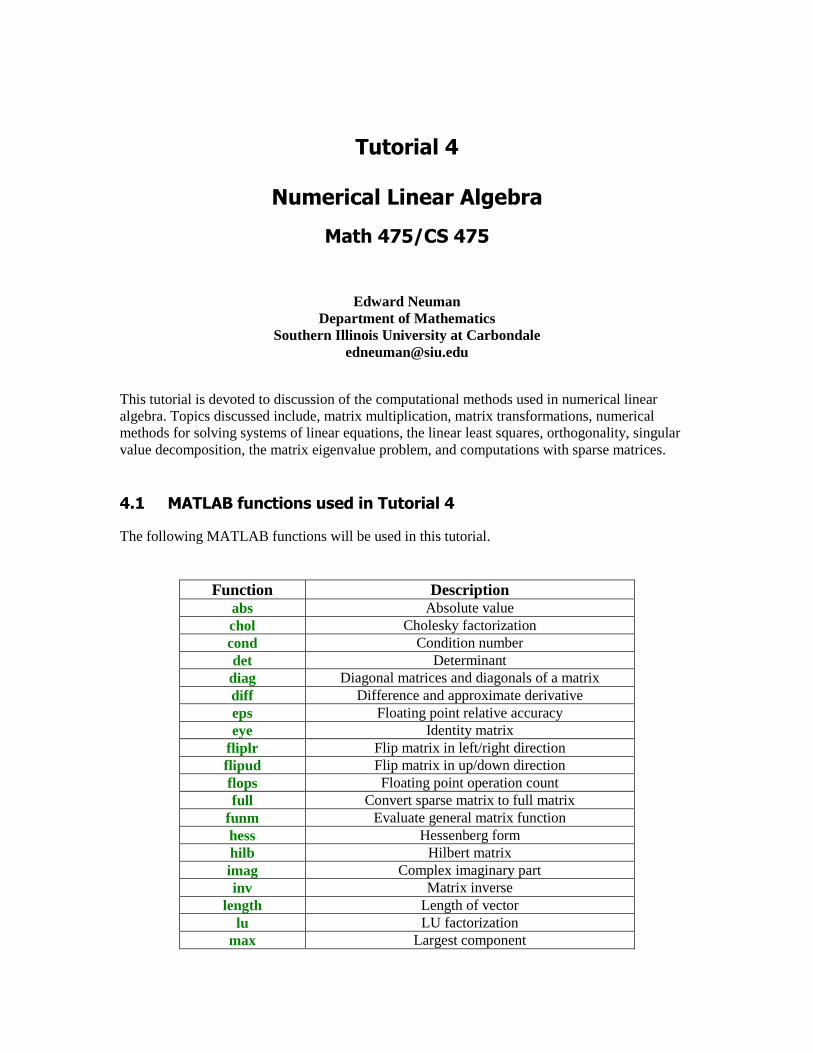
Edward NeumanDepartment of Mathematics

Southern Illinois University at Carbondaleedneuman@siu.edu

This tutorial is devoted to discussion of the computational methods used in numerical linearalgebra. Topics discussed include, matrix multiplication, matrix transformations, numericalmethods for solving systems of linear equations, the linear least squares, orthogonality, singularvalue decomposition, the matrix eigenvalue problem, and computations with sparse matrices.

�� ����������������� ����������

The following MATLAB functions will be used in this tutorial.

Function Descriptionabs Absolute valuechol Cholesky factorizationcond Condition numberdet Determinantdiag Diagonal matrices and diagonals of a matrixdiff Difference and approximate derivativeeps Floating point relative accuracyeye Identity matrix

fliplr Flip matrix in left/right directionflipud Flip matrix in up/down directionflops Floating point operation countfull Convert sparse matrix to full matrix

funm Evaluate general matrix functionhess Hessenberg formhilb Hilbert matriximag Complex imaginary partinv Matrix inverse

length Length of vectorlu LU factorization

max Largest component

2

min Smallest componentnorm Matrix or vector normones Ones array

pascal Pascal matrixpinv Pseudoinverseqr Orthogonal-triangular decomposition

rand Uniformly distributed random numbersrandn Normally distributed random numbersrank Matrix rankreal Complex real part

repmat Replicate and tile an arrayschur Schur decompositionsign Signum functionsize Size of matrixsqrt Square rootsum Sum of elementssvd Singular value decompositiontic Start a stopwatch timertoc Read the stopwach timer

trace Sum of diagonal entriestril Extract lower triangular parttriu Extract upper triangular part

zeros Zeros array

�! �� �����"#�����"$�� ���

Computation of the product of two or more matrices is one of the basic operations in thenumerical linear algebra. Number of flops needed for computing a product of two matrices A andB can be decreased drastically if a special structure of matrices A and B is utilized properly. Forinstance, if both A and B are upper (lower) triangular, then the product of A and B is an upper(lower) triangular matrix.

function C = prod2t(A, B)

% Product C = A*B of two upper triangular matrices A and B.

[m,n] = size(A);[u,v] = size(B);if (m ~= n) | (u ~= v) error( 'Matrices must be square' )endif n ~= u error( 'Inner dimensions must agree' )endC = zeros(n); for i=1:n for j=i:n C(i,j) = A(i,i:j)*B(i:j,j); endend

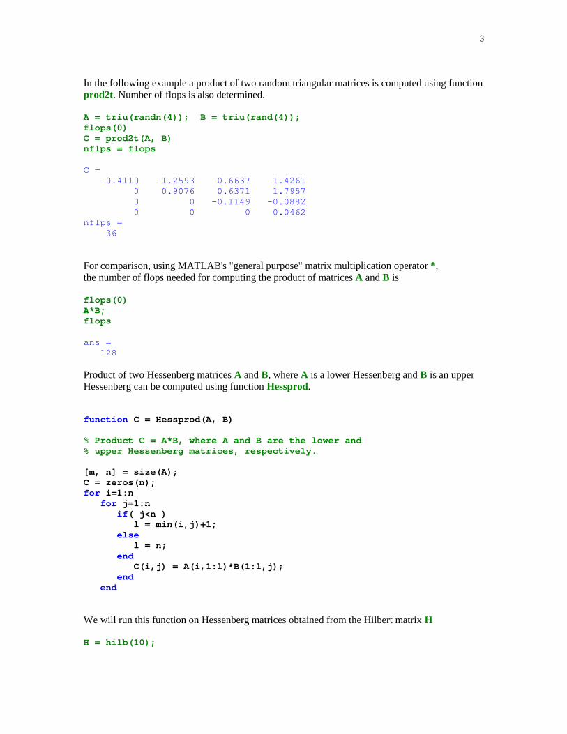
3

In the following example a product of two random triangular matrices is computed using functionprod2t. Number of flops is also determined.

A = triu(randn(4)); B = triu(rand(4));flops(0)C = prod2t(A, B)nflps = flops

C = -0.4110 -1.2593 -0.6637 -1.4261 0 0.9076 0.6371 1.7957 0 0 -0.1149 -0.0882 0 0 0 0.0462nflps = 36

For comparison, using MATLAB's "general purpose" matrix multiplication operator * ,the number of flops needed for computing the product of matrices A and B is

flops(0)A*B;flops

ans = 128

Product of two Hessenberg matrices A and B, where A is a lower Hessenberg and B is an upperHessenberg can be computed using function Hessprod.

function C = Hessprod(A, B)

% Product C = A*B, where A and B are the lower and% upper Hessenberg matrices, respectively.

[m, n] = size(A);C = zeros(n);for i=1:n for j=1:n if ( j<n ) l = min(i,j)+1; else l = n; end C(i,j) = A(i,1:l)*B(1:l,j); end end

We will run this function on Hessenberg matrices obtained from the Hilbert matrix H

H = hilb(10);

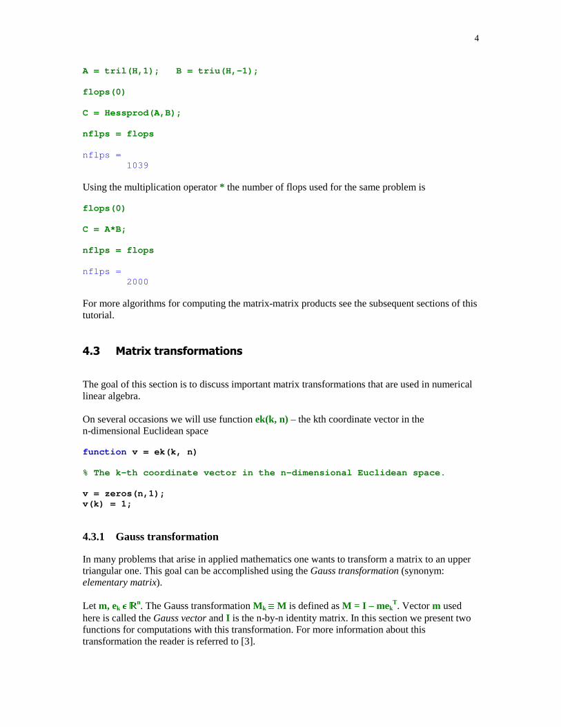
4

A = tril(H,1); B = triu(H,-1);

flops(0)

C = Hessprod(A,B);

nflps = flops

nflps = 1039

Using the multiplication operator * the number of flops used for the same problem is

flops(0)

C = A*B;

nflps = flops

nflps = 2000

For more algorithms for computing the matrix-matrix products see the subsequent sections of thistutorial.

�% �����"���������������

The goal of this section is to discuss important matrix transformations that are used in numericallinear algebra.

On several occasions we will use function ek(k, n) – the kth coordinate vector in then-dimensional Euclidean space

function v = ek(k, n)

% The k-th coordinate vector in the n-dimensional Euclidean space.

v = zeros(n,1);v(k) = 1;

4.3.1 Gauss transformation

In many problems that arise in applied mathematics one wants to transform a matrix to an uppertriangular one. This goal can be accomplished using the Gauss transformation (synonym:elementary matrix).

Let m, ek � �n. The Gauss transformation Mk � M is defined as M = I – mek

T. Vector m usedhere is called the Gauss vector and I is the n-by-n identity matrix. In this section we present twofunctions for computations with this transformation. For more information about thistransformation the reader is referred to [3].

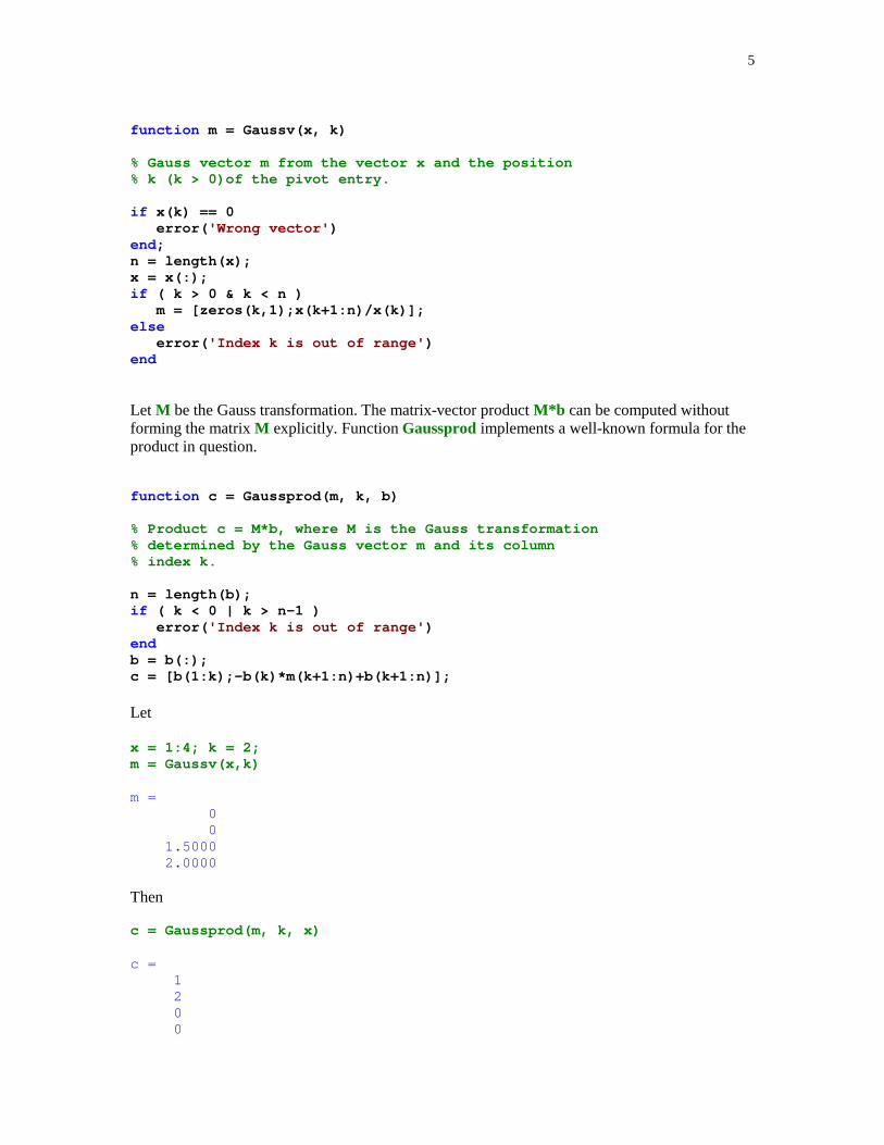
5

function m = Gaussv(x, k)

% Gauss vector m from the vector x and the position% k (k > 0)of the pivot entry.

if x(k) == 0 error( 'Wrong vector' )end ;n = length(x);x = x(:);if ( k > 0 & k < n ) m = [zeros(k,1);x(k+1:n)/x(k)];else error( 'Index k is out of range' )end

Let M be the Gauss transformation. The matrix-vector product M*b can be computed withoutforming the matrix M explicitly. Function Gaussprod implements a well-known formula for theproduct in question.

function c = Gaussprod(m, k, b)

% Product c = M*b, where M is the Gauss transformation% determined by the Gauss vector m and its column% index k.

n = length(b);if ( k < 0 | k > n-1 ) error( 'Index k is out of range' )endb = b(:);c = [b(1:k);-b(k)*m(k+1:n)+b(k+1:n)];

Let

x = 1:4; k = 2;m = Gaussv(x,k)

m = 0 0 1.5000 2.0000

Then

c = Gaussprod(m, k, x)

c = 1 2 0 0

6

4.3.2 Householder transformation

The Householder transformation H, where H = I – 2uuT, also called the Householder reflector, isa frequently used tool in many problems of numerical linear algebra. Here u stands for the realunit vector. In this section we give several functions for computations with this matrix.

function u = Housv(x)

% Householder reflection unit vector u from the vector x.

m = max(abs(x));u = x/m;if u(1) == 0 su = 1;else su = sign(u(1));endu(1) = u(1)+su*norm(u);u = u/norm(u);u = u(:);

Let

x = [1 2 3 4]';

Then

u = Housv(x)

u = 0.7690 0.2374 0.3561 0.4749

The Householder reflector H is computed as follows

H = eye(length(x))-2*u*u'

H = -0.1826 -0.3651 -0.5477 -0.7303 -0.3651 0.8873 -0.1691 -0.2255 -0.5477 -0.1691 0.7463 -0.3382 -0.7303 -0.2255 -0.3382 0.5490

An efficient method of computing the matrix-vector or matrix-matrix products with Householdermatrices utilizes a special form of this matrix.

7

function P = Houspre(u, A)

% Product P = H*A, where H is the Householder reflector% determined by the vector u and A is a matrix.

[n, p] = size(A);m = length(u);if m ~= n error( 'Dimensions of u and A must agree' )endv = u/norm(u);v = v(:);P = [];for j=1:p aj = A(:,j); P = [P aj-2*v*(v'*aj)];end

Let

A = pascal(4);

and let

u = Housv(A(:,1))

u = 0.8660 0.2887 0.2887 0.2887

Then

P = Houspre(u, A)

P = -2.0000 -5.0000 -10.0000 -17.5000 -0.0000 -0.0000 -0.6667 -2.1667 -0.0000 1.0000 2.3333 3.8333 -0.0000 2.0000 6.3333 13.8333

In some problems that arise in numerical linear algebra one has to compute a product of severalHouseholder transformations. Let the Householder transformations are represented by theirnormalized reflection vectors stored in columns of the matrix V. The product in question, denotedby Q, is defined as

Q = V(:, 1)*V(:, 2)* … *V(:, n)

where n stands for the number of columns of the matrix V.

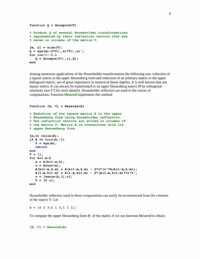
8

function Q = Housprod(V)

% Product Q of several Householder transformations% represented by their reflection vectors that are% saved in columns of the matrix V.

[m, n] = size(V);Q = eye(m)-2*V(:,n)*V(:,n)';for i=n-1:-1:1 Q = Houspre(V(:,i),Q);end

Among numerous applications of the Householder transformation the following one: reduction ofa square matrix to the upper Hessenberg form and reduction of an arbitrary matrix to the upperbidiagonal matrix, are of great importance in numerical linear algebra. It is well known that anysquare matrix A can always be transformed to an upper Hessenberg matrix H by orthogonalsimilarity (see [7] for more details). Householder reflectors are used in the course ofcomputations. Function Hessred implements this method

function [A, V] = Hessred(A)

% Reduction of the square matrix A to the upper% Hessenberg form using Householder reflectors.% The reflection vectors are stored in columns of% the matrix V. Matrix A is overwritten with its% upper Hessenberg form.

[m,n] =size(A);if A == triu(A,-1) V = eye(m); returnendV = [];for k=1:m-2 x = A(k+1:m,k); v = Housv(x); A(k+1:m,k:m) = A(k+1:m,k:m) - 2*v*(v'*A(k+1:m,k:m)); A(1:m,k+1:m) = A(1:m,k+1:m) - 2*(A(1:m,k+1:m)*v)*v'; v = [zeros(k,1);v]; V = [V v];end

Householder reflectors used in these computations can easily be reconstructed from the columnsof the matrix V. Let

A = [0 2 3;2 1 2;1 1 1];

To compute the upper Hessenberg form H of the matrix A we run function Hessred to obtain

[H, V] = Hessred(A)

9

H = 0 -3.1305 1.7889 -2.2361 2.2000 -1.4000 0 -0.4000 -0.2000V = 0 0.9732 0.2298

The only Householder reflector P used in the course of computations is shown below

P = eye(3)-2*V*V'

P = 1.0000 0 0 0 -0.8944 -0.4472 0 -0.4472 0.8944

To verify correctness of these results it suffices to show that P*H*P = A . We have

P*H*P

ans = 0 2.0000 3.0000 2.0000 1.0000 2.0000 1.0000 1.0000 1.0000

Another application of the Householder transformation is to transform a matrix to an upperbidiagonal form. This reduction is required in some algorithms for computing the singular valuedecomposition (SVD) of a matrix. Function upbid works with square matrices only

function [A, V, U] = upbid(A)

% Bidiagonalization of the square matrix A using the% Golub- Kahan method. The reflection vectors of the% left Householder matrices are saved in columns of% the matrix V, while the reflection vectors of the% right Householder reflections are saved in columns% of the matrix U. Matrix A is overwritten with its% upper bidiagonal form.

[m, n] = size(A);if m ~= n error( 'Matrix must be square' )endif tril(triu(A),1) == A V = eye(n-1); U = eye(n-2);endV = [];U = [];

10

for k=1:n-1 x = A(k:n,k); v = Housv(x); l = k:n; A(l,l) = A(l,l) - 2*v*(v'*A(l,l)); v = [zeros(k-1,1);v]; V = [V v]; if k < n-1 x = A(k,k+1:n)'; u = Housv(x); p = 1:n; q = k+1:n; A(p,q) = A(p,q) - 2*(A(p,q)*u)*u'; u = [zeros(k,1);u]; U = [U u]; endend

Let (see [1], Example 10.9.2, p.579)

A = [1 2 3;3 4 5;6 7 8];

Then

[B, V, U] = upbid(A)

B = -6.7823 12.7620 -0.0000 0.0000 1.9741 -0.4830 0.0000 0.0000 -0.0000V = 0.7574 0 0.2920 -0.7248 0.5840 0.6889U = 0 -0.9075 -0.4201

Let the matrices V and U be the same as in the last example and let

Q = Housprod(V); P = Housprod(U);

Then

Q'*A*P

ans = -6.7823 12.7620 -0.0000 0.0000 1.9741 -0.4830 0.0000 -0.0000 0.0000

which is the same as the bidiagonal form obtained earlier.

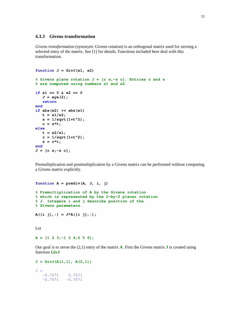
11

4.3.3 Givens transformation

Givens transformation (synonym: Givens rotation) is an orthogonal matrix used for zeroing aselected entry of the matrix. See [1] for details. Functions included here deal with thistransformation.

function J = GivJ(x1, x2)

% Givens plane rotation J = [c s;-s c]. Entries c and s% are computed using numbers x1 and x2.

if x1 == 0 & x2 == 0 J = eye(2); returnendif abs(x2) >= abs(x1) t = x1/x2; s = 1/sqrt(1+t^2); c = s*t;else t = x2/x1; c = 1/sqrt(1+t^2); s = c*t;endJ = [c s;-s c];

Premultiplication and postmultiplication by a Givens matrix can be performed without computinga Givens matrix explicitly.

function A = preGiv(A, J, i, j)

% Premultiplication of A by the Givens rotation% which is represented by the 2-by-2 planar rotation% J. Integers i and j describe position of the% Givens parameters.

A([i j],:) = J*A([i j],:);

Let

A = [1 2 3;-1 3 4;2 5 6];

Our goal is to zeroe the (2,1) entry of the matrix A. First the Givens matrix J is created usingfunction GivJ

J = GivJ(A(1,1), A(2,1))

J = -0.7071 0.7071 -0.7071 -0.7071

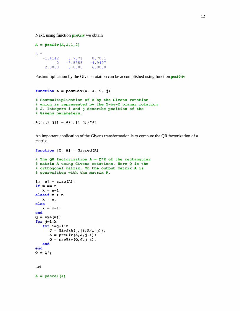
12

Next, using function preGiv we obtain

A = preGiv(A,J,1,2)

A = -1.4142 0.7071 0.7071 0 -3.5355 -4.9497 2.0000 5.0000 6.0000

Postmultiplication by the Givens rotation can be accomplished using function postGiv

function A = postGiv(A, J, i, j)

% Postmultiplication of A by the Givens rotation% which is represented by the 2-by-2 planar rotation% J. Integers i and j describe position of the% Givens parameters.

A(:,[i j]) = A(:,[i j])*J;

An important application of the Givens transformation is to compute the QR factorization of amatrix.

function [Q, A] = Givred(A)

% The QR factorization A = Q*R of the rectangular% matrix A using Givens rotations. Here Q is the% orthogonal matrix. On the output matrix A is% overwritten with the matrix R.

[m, n] = size(A);if m == n k = n-1;elseif m > n k = n;else k = m-1;endQ = eye(m);for j=1:k for i=j+1:m J = GivJ(A(j,j),A(i,j)); A = preGiv(A,J,j,i); Q = preGiv(Q,J,j,i); endendQ = Q';

Let

A = pascal(4)

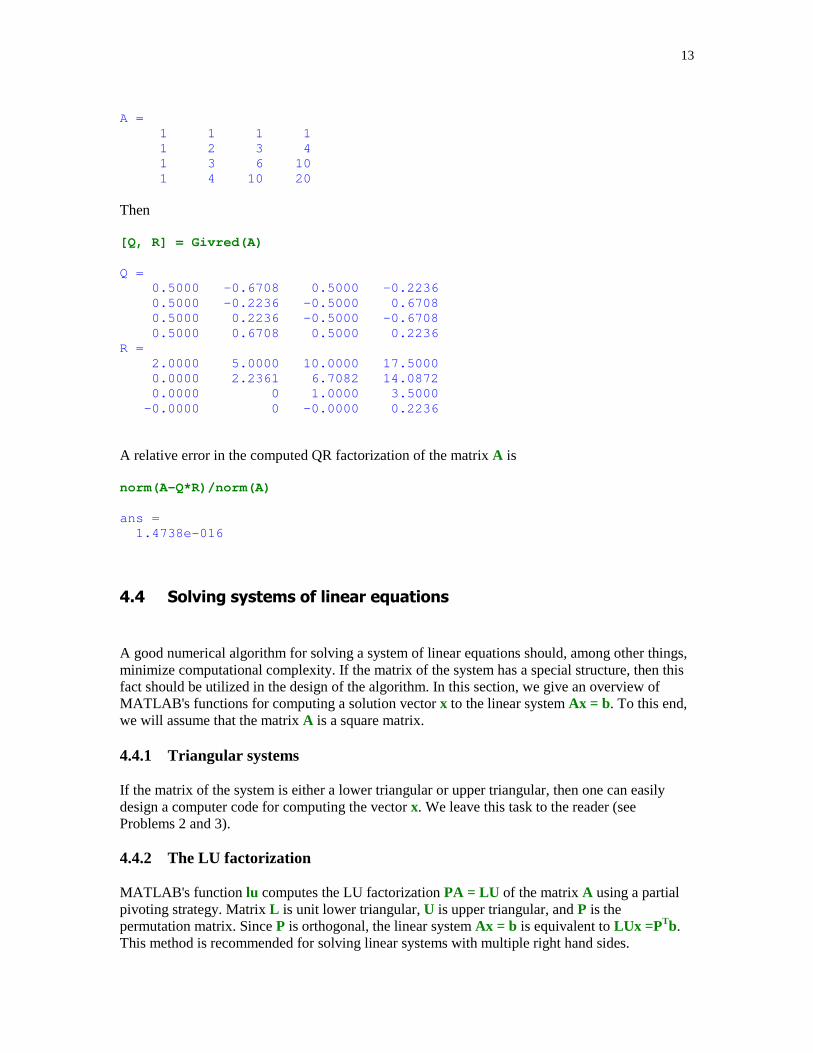
13

A = 1 1 1 1 1 2 3 4 1 3 6 10 1 4 10 20

Then

[Q, R] = Givred(A)

Q = 0.5000 -0.6708 0.5000 -0.2236 0.5000 -0.2236 -0.5000 0.6708 0.5000 0.2236 -0.5000 -0.6708 0.5000 0.6708 0.5000 0.2236R = 2.0000 5.0000 10.0000 17.5000 0.0000 2.2361 6.7082 14.0872 0.0000 0 1.0000 3.5000 -0.0000 0 -0.0000 0.2236

A relative error in the computed QR factorization of the matrix A is

norm(A-Q*R)/norm(A)

ans = 1.4738e-016

� ���&����'�� ������� �� (�������

A good numerical algorithm for solving a system of linear equations should, among other things,minimize computational complexity. If the matrix of the system has a special structure, then thisfact should be utilized in the design of the algorithm. In this section, we give an overview ofMATLAB's functions for computing a solution vector x to the linear system Ax = b. To this end,we will assume that the matrix A is a square matrix.

4.4.1 Triangular systems

If the matrix of the system is either a lower triangular or upper triangular, then one can easilydesign a computer code for computing the vector x. We leave this task to the reader (seeProblems 2 and 3).

4.4.2 The LU factorization

MATLAB's function lu computes the LU factorization PA = LU of the matrix A using a partialpivoting strategy. Matrix L is unit lower triangular, U is upper triangular, and P is thepermutation matrix. Since P is orthogonal, the linear system Ax = b is equivalent to LUx =PTb.This method is recommended for solving linear systems with multiple right hand sides.

14

Let

A = hilb(5); b = [1 2 3 4 5]';

The following commands are used to compute the LU decomposition of A, the solution vector x,and the upper bound on the relative error in the computed solution

[L, U, P] = lu(A);

x = U\(L\(P'*b))

x = 1.0e+004 * 0.0125 -0.2880 1.4490 -2.4640 1.3230

rl_err = cond(A)*norm(b-A*x)/norm(b)

rl_err = 4.3837e-008

Number of decimal digits of accuracy in the computed solution x is defined as the negativedecimal logarithm of the relative error (see e.g., [6]). Vector x of the last example has

dda = -log10(rl_err)

dda = 7.3582

about seven decimal digits of accuracy.

4.4.3 Cholesky factorization

For linear systems with symmetric positive definite matrices the recommended method is basedon the Cholesky factorization A = HTH of the matrix A. Here H is the upper triangular matrixwith positive diagonal entries. MATLAB's function chol calculates the matrix H from A orgenerates an error message if A is not positive definite. Once the matrix H is computed, thesolution x to Ax = b can be found using the trick used in 4.4.2.

���� � ����(��� ����������� �����������)�����

In some problems of applied mathematics one seeks a solution to the overdetermined linearsystem Ax = b. In general, such a system is inconsistent. The least squares solution to this systemis a vector x that minimizes the Euclidean norm of the residual r = b – Ax. Vector x alwaysexists, however it is not necessarily unique. For more details, see e.g., [7], p. 81. In this sectionwe discuss methods for computing the least squares solution.

15

4.5.1 Using MATLAB built-in functions

MATLAB's backslash operator \ can be used to find the least squares solution x = A\b. For therank deficient systems a warning message is generated during the course of computations.A second MATLAB's function that can be used for computing the least squares solution is thepinv command. The solution is computed using the following command x = pinv(A)*b . Herepinv stands for the pseudoinverse matrix. This method however, requires more flops than thebackslash method does. For more information about the pseudoinverses, see Section 4.7 of thistutorial.

4.5.2 Normal equations

This classical method, which is due to C.F. Gauss, finds a vector x that satisfies the normalequations ATAx = ATb. The method under discussion is adequate when the condition number ofA is small.

function [x, dist] = lsqne(A, b)

% The least-squares solution x to the overdetermined% linear system Ax = b. Matrix A must be of full column% rank.

% Input:% A- matrix of the system% b- the right-hand sides% Output:% x- the least-squares solution% dist- Euclidean norm of the residual b - Ax

[m, n] = size(A);if (m <= n) error( 'System is not overdetermined' )endif (rank(A) < n) error( 'Matrix must be of full rank' )endH = chol(A'*A);x = H\(H'\(A'*b));r = b - A*x;dist = norm(r);

Throughout the sequel the following matrix A and the vector b will be used to test variousmethods for solving the least squares problem

format long

A = [.5 .501;.5 .5011;0 0;0 0]; b = [1;-1;1;-1];

Using the method of normal equations we obtain

[x,dist] = lsqne(A,b)

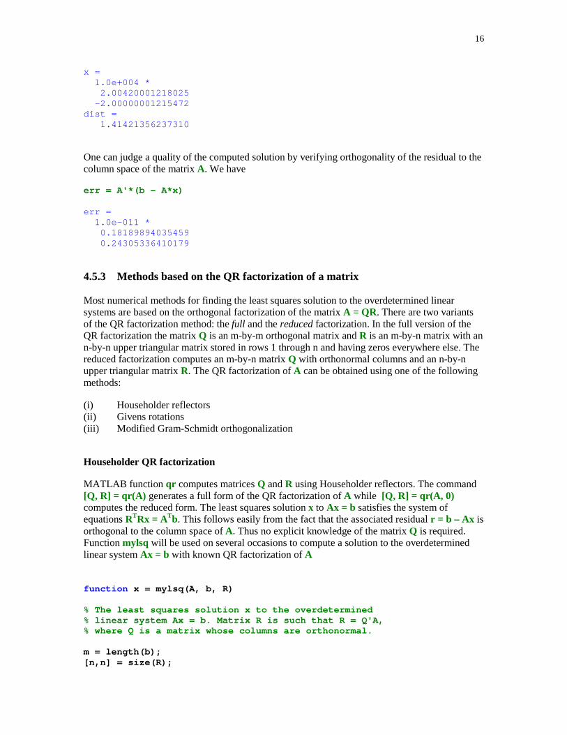
16

x = 1.0e+004 * 2.00420001218025 -2.00000001215472dist = 1.41421356237310

One can judge a quality of the computed solution by verifying orthogonality of the residual to thecolumn space of the matrix A. We have

err = A'*(b - A*x)

err = 1.0e-011 * 0.18189894035459 0.24305336410179

4.5.3 Methods based on the QR factorization of a matrix

Most numerical methods for finding the least squares solution to the overdetermined linearsystems are based on the orthogonal factorization of the matrix A = QR. There are two variantsof the QR factorization method: the full and the reduced factorization. In the full version of theQR factorization the matrix Q is an m-by-m orthogonal matrix and R is an m-by-n matrix with ann-by-n upper triangular matrix stored in rows 1 through n and having zeros everywhere else. Thereduced factorization computes an m-by-n matrix Q with orthonormal columns and an n-by-nupper triangular matrix R. The QR factorization of A can be obtained using one of the followingmethods:

(i) Householder reflectors(ii) Givens rotations(iii) Modified Gram-Schmidt orthogonalization

Householder QR factorization

MATLAB function qr computes matrices Q and R using Householder reflectors. The command[Q, R] = qr(A) generates a full form of the QR factorization of A while [Q, R] = qr(A, 0)computes the reduced form. The least squares solution x to Ax = b satisfies the system ofequations RTRx = ATb. This follows easily from the fact that the associated residual r = b – Ax isorthogonal to the column space of A. Thus no explicit knowledge of the matrix Q is required.Function mylsq will be used on several occasions to compute a solution to the overdeterminedlinear system Ax = b with known QR factorization of A

function x = mylsq(A, b, R)

% The least squares solution x to the overdetermined% linear system Ax = b. Matrix R is such that R = Q'A,% where Q is a matrix whose columns are orthonormal.

m = length(b);[n,n] = size(R);

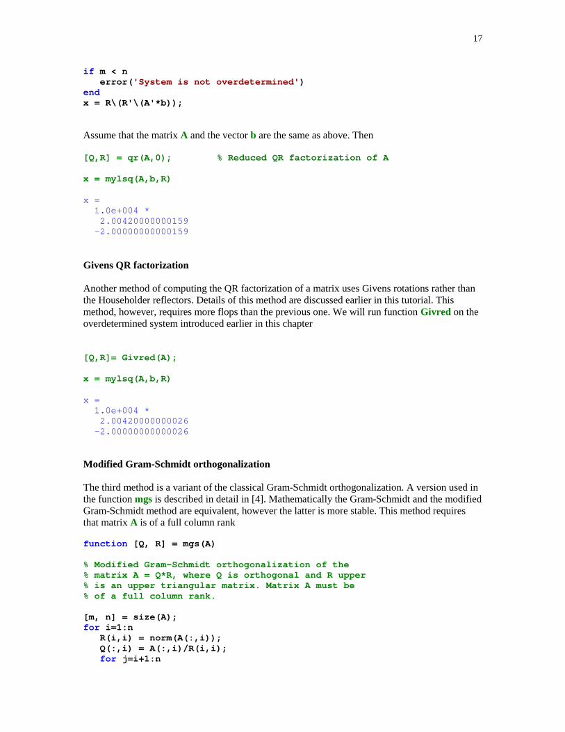
17

if m < n error( 'System is not overdetermined' )endx = R\(R'\(A'*b));

Assume that the matrix A and the vector b are the same as above. Then

[Q,R] = qr(A,0); % Reduced QR factorization of A

x = mylsq(A,b,R)

x = 1.0e+004 * 2.00420000000159 -2.00000000000159

Givens QR factorization

Another method of computing the QR factorization of a matrix uses Givens rotations rather thanthe Householder reflectors. Details of this method are discussed earlier in this tutorial. Thismethod, however, requires more flops than the previous one. We will run function Givred on theoverdetermined system introduced earlier in this chapter

[Q,R]= Givred(A);

x = mylsq(A,b,R)

x = 1.0e+004 * 2.00420000000026 -2.00000000000026

Modified Gram-Schmidt orthogonalization

The third method is a variant of the classical Gram-Schmidt orthogonalization. A version used inthe function mgs is described in detail in [4]. Mathematically the Gram-Schmidt and the modifiedGram-Schmidt method are equivalent, however the latter is more stable. This method requiresthat matrix A is of a full column rank

function [Q, R] = mgs(A)

% Modified Gram-Schmidt orthogonalization of the% matrix A = Q*R, where Q is orthogonal and R upper% is an upper triangular matrix. Matrix A must be% of a full column rank.

[m, n] = size(A);for i=1:n R(i,i) = norm(A(:,i)); Q(:,i) = A(:,i)/R(i,i); for j=i+1:n

18

R(i,j) = Q(:,i)'*A(:,j); A(:,j) = A(:,j) - R(i,j)*Q(:,i); endend

Running function mgs on our test system we obtain

[Q,R] = mgs(A);

x = mylsq(A,b,R)

x = 1.0e+004 * 2.00420000000022 -2.00000000000022

This small size overdetermined linear system was tested using three different functions forcomputing the QR factorization of the matrix A. In all cases the least squares solution was foundusing function mylsq. The flop count and the check of orthogonality of Q are contained in thefollowing table. As a measure of closeness of the computed Q to its exact value is determined byerrorQ = norm(Q'*Q – eye(k)), where k = 2 for the reduced form and k = 4 for the full form ofthe QR factorization

Function Flop count errorQqr(, 0) 138 2.6803e-016Givred 488 2.2204e-016

mgs 98 2.2206e-012

For comparison the number of flops used by the backslash operator was equal to 122 while thepinv command found a solution using 236 flops.

Another method for computing the least squares solution finds first the QR factorization of theaugmented matrix [A b] i.e., QR = [A b] using one of the methods discussed above. The leastsquares solution x is then found solving a linear system Ux = Qb, where U is an n-by- n principalsubmatrix of R and Qb is the n+1st column of the matrix R. See e.g., [7] for more details.Function mylsqf implements this method

function x = mylsqf(A, b, f, p)

% The least squares solution x to the overdetermined% linear system Ax = b using the QR factorization.% The input parameter f is the string holding the% name of a function used to obtain the QR factorization.% Fourth input parameter p is optional and should be% set up to 0 if the reduced form of the qr function% is used to obtain the QR factorization.

[m, n] = size(A);if m <= n

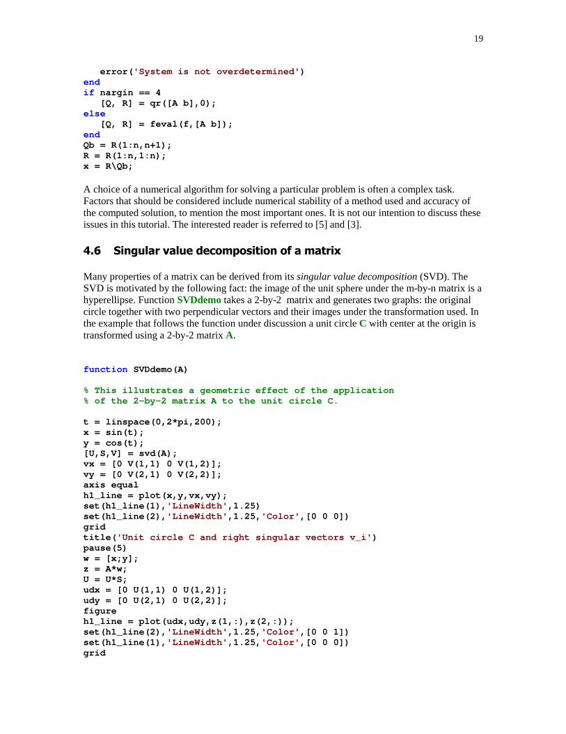
19

error( 'System is not overdetermined' )endif nargin == 4 [Q, R] = qr([A b],0);else [Q, R] = feval(f,[A b]);endQb = R(1:n,n+1);R = R(1:n,1:n);x = R\Qb;

A choice of a numerical algorithm for solving a particular problem is often a complex task.Factors that should be considered include numerical stability of a method used and accuracy ofthe computed solution, to mention the most important ones. It is not our intention to discuss theseissues in this tutorial. The interested reader is referred to [5] and [3].

�*��������&��� ���$���������������"

Many properties of a matrix can be derived from its singular value decomposition (SVD). TheSVD is motivated by the following fact: the image of the unit sphere under the m-by-n matrix is ahyperellipse. Function SVDdemo takes a 2-by-2 matrix and generates two graphs: the originalcircle together with two perpendicular vectors and their images under the transformation used. Inthe example that follows the function under discussion a unit circle C with center at the origin istransformed using a 2-by-2 matrix A.

function SVDdemo(A)

% This illustrates a geometric effect of the application% of the 2-by-2 matrix A to the unit circle C.

t = linspace(0,2*pi,200);x = sin(t);y = cos(t);[U,S,V] = svd(A);vx = [0 V(1,1) 0 V(1,2)];vy = [0 V(2,1) 0 V(2,2)];axis equalh1_line = plot(x,y,vx,vy);set(h1_line(1), 'LineWidth' ,1.25)set(h1_line(2), 'LineWidth' ,1.25, 'Color' ,[0 0 0])gridtitle( 'Unit circle C and right singular vectors v_i' )pause(5)w = [x;y];z = A*w;U = U*S;udx = [0 U(1,1) 0 U(1,2)];udy = [0 U(2,1) 0 U(2,2)];figureh1_line = plot(udx,udy,z(1,:),z(2,:));set(h1_line(2), 'LineWidth' ,1.25, 'Color' ,[0 0 1])set(h1_line(1), 'LineWidth' ,1.25, 'Color' ,[0 0 0])grid

20

title( 'Image A*C of C and vectors \sigma_iu_i' )

Define a matrix

A = [1 2;3 4];

Then

SVDdemo(A)

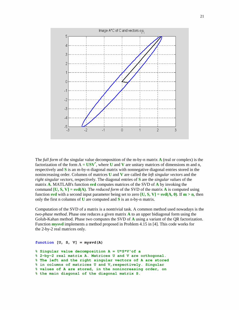
21

The full form of the singular value decomposition of the m-by-n matrix A (real or complex) is thefactorization of the form A = USV*, where U and V are unitary matrices of dimensions m and n,respectively and S is an m-by-n diagonal matrix with nonnegative diagonal entries stored in thenonincreasing order. Columns of matrices U and V are called the left singular vectors and theright singular vectors, respectively. The diagonal entries of S are the singular values of thematrix A. MATLAB's function svd computes matrices of the SVD of A by invoking thecommand [U, S, V] = svd(A). The reduced form of the SVD of the matrix A is computed usingfunction svd with a second input parameter being set to zero [U, S, V] = svd(A, 0). If m > n, thenonly the first n columns of U are computed and S is an n-by-n matrix.

Computation of the SVD of a matrix is a nontrivial task. A common method used nowadays is thetwo-phase method. Phase one reduces a given matrix A to an upper bidiagonal form using theGolub-Kahan method. Phase two computes the SVD of A using a variant of the QR factorization.Function mysvd implements a method proposed in Problem 4.15 in [4]. This code works forthe 2-by-2 real matrices only.

function [U, S, V] = mysvd(A)

% Singular value decomposition A = U*S*V'of a% 2-by-2 real matrix A. Matrices U and V are orthogonal.% The left and the right singular vectors of A are stored% in columns of matrices U and V,respectively. Singular% values of A are stored, in the nonincreasing order, on% the main diagonal of the diagonal matrix S.

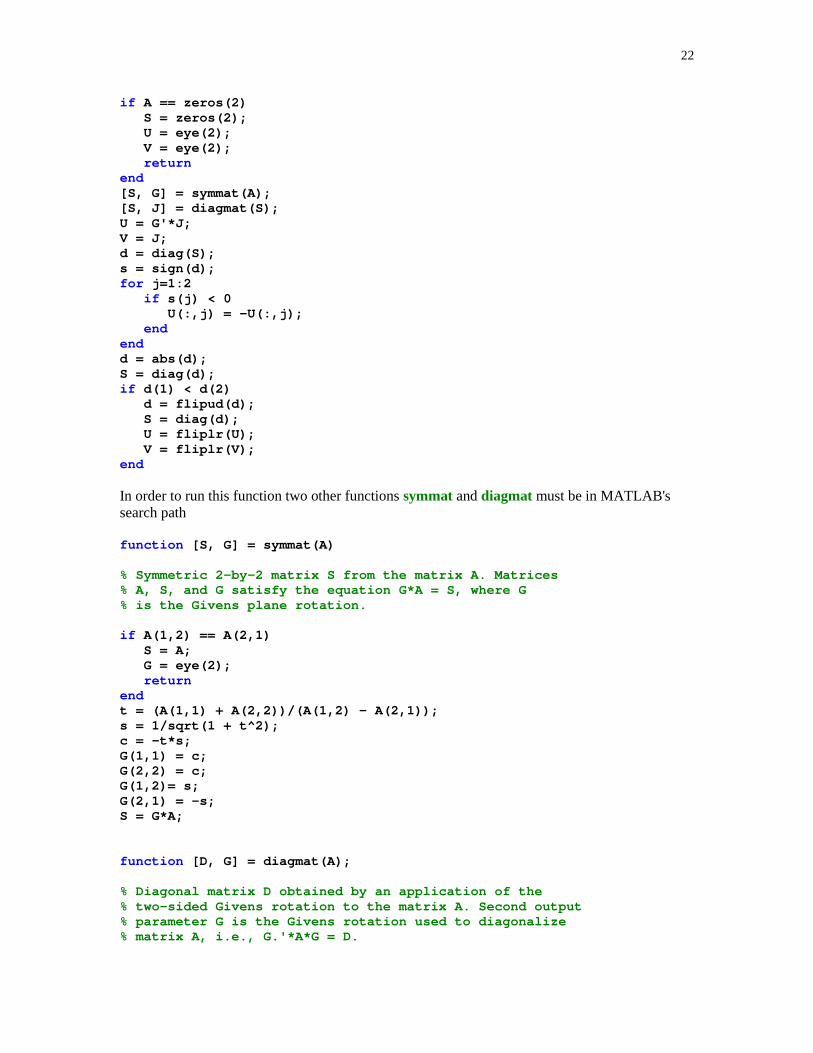
22

if A == zeros(2) S = zeros(2); U = eye(2); V = eye(2); returnend[S, G] = symmat(A);[S, J] = diagmat(S);U = G'*J;V = J;d = diag(S);s = sign(d);for j=1:2 if s(j) < 0 U(:,j) = -U(:,j); endendd = abs(d);S = diag(d);if d(1) < d(2) d = flipud(d); S = diag(d); U = fliplr(U); V = fliplr(V);end

In order to run this function two other functions symmat and diagmat must be in MATLAB'ssearch path

function [S, G] = symmat(A)

% Symmetric 2-by-2 matrix S from the matrix A. Matrices% A, S, and G satisfy the equation G*A = S, where G% is the Givens plane rotation.

if A(1,2) == A(2,1) S = A; G = eye(2); returnendt = (A(1,1) + A(2,2))/(A(1,2) - A(2,1));s = 1/sqrt(1 + t^2);c = -t*s;G(1,1) = c;G(2,2) = c;G(1,2)= s;G(2,1) = -s;S = G*A;

function [D, G] = diagmat(A);

% Diagonal matrix D obtained by an application of the% two-sided Givens rotation to the matrix A. Second output% parameter G is the Givens rotation used to diagonalize% matrix A, i.e., G.'*A*G = D.

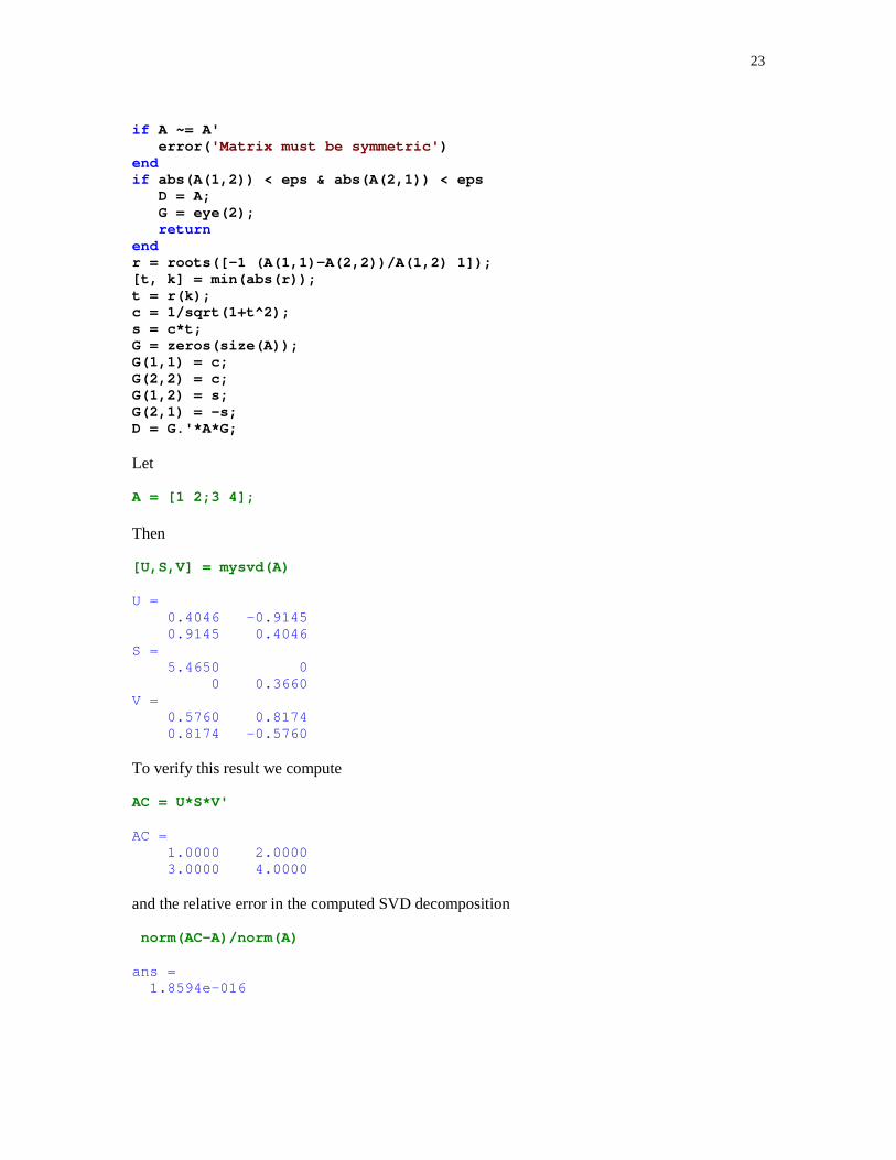
23

if A ~= A' error( 'Matrix must be symmetric' )endif abs(A(1,2)) < eps & abs(A(2,1)) < eps D = A; G = eye(2); returnendr = roots([-1 (A(1,1)-A(2,2))/A(1,2) 1]);[t, k] = min(abs(r));t = r(k);c = 1/sqrt(1+t^2);s = c*t;G = zeros(size(A));G(1,1) = c;G(2,2) = c;G(1,2) = s;G(2,1) = -s;D = G.'*A*G;

Let

A = [1 2;3 4];

Then

[U,S,V] = mysvd(A)

U = 0.4046 -0.9145 0.9145 0.4046S = 5.4650 0 0 0.3660V = 0.5760 0.8174 0.8174 -0.5760

To verify this result we compute

AC = U*S*V'

AC = 1.0000 2.0000 3.0000 4.0000

and the relative error in the computed SVD decomposition

norm(AC-A)/norm(A)

ans = 1.8594e-016

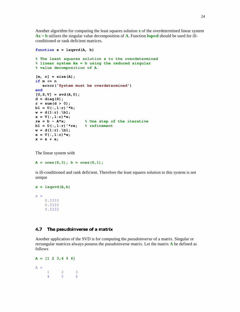
24

Another algorithm for computing the least squares solution x of the overdetermined linear systemAx = b utilizes the singular value decomposition of A. Function lsqsvd should be used for ill-conditioned or rank deficient matrices.

function x = lsqsvd(A, b)

% The least squares solution x to the overdetermined% linear system Ax = b using the reduced singular% value decomposition of A.

[m, n] = size(A);if m <= n error( 'System must be overdetermined' )end[U,S,V] = svd(A,0);d = diag(S);r = sum(d > 0);b1 = U(:,1:r)'*b;w = d(1:r).\b1;x = V(:,1:r)*w;re = b - A*x; % One step of the iterativeb1 = U(:,1:r)'*re; % refinementw = d(1:r).\b1;e = V(:,1:r)*w;x = x + e;

The linear system with

A = ones(6,3); b = ones(6,1);

is ill-conditioned and rank deficient. Therefore the least squares solution to this system is notunique

x = lsqsvd(A,b)

x = 0.3333 0.3333 0.3333

��� ��� ���� ����� �� � ���� �

Another application of the SVD is for computing the pseudoinverse of a matrix. Singular orrectangular matrices always possess the pseudoinverse matrix. Let the matrix A be defined asfollows

A = [1 2 3;4 5 6]

A = 1 2 3 4 5 6

25

Its pseudoinverse is

B = pinv(A)

B = -0.9444 0.4444 -0.1111 0.1111 0.7222 -0.2222

The pseudoinverse B of the matrix A satisfy the Penrose conditions

ABA = A, BAB = B, (AB)T = AB, (BA)T = BA

We will verify the first condition only

norm(A*B*A-A)

ans = 3.6621e-015

and leave it to the reader to verify the remaining ones.

�+�� �����" �� �&��� $���� �

The matrix eigenvalue problem, briefly discussed in Tutorial 3, is one of the central problems inthe numerical linear algebra. It is formulated as follows.

Given a square matrix A = [aij ], 1� i, j � n, find a nonzero vector x � �n and a number � thatsatisfy the equation Ax = �x. Number � is called the eigenvalue of the matrix A and x is theassociated right eigenvector of A.

In this section we will show how to localize the eigenvalues of a matrix using celebratedGershgorin's Theorem. Also, we will present MATLAB's code for computing the dominanteigenvalue and the associated eigenvector of a matrix. The QR iteration for computing alleigenvalues of the symmetric matrices is also discussed.

Gershgorin Theorem states that each eigenvalue � of the matrix A satisfies at least one of thefollowing inequalities |� - akk| � rk, where r k is the sum of all off-diagonal entries in row k of thematrix |A| (see, e.g., [1], pp.400-403 for more details). Function Gershg computes the centers andthe radii of the Gershgorin circles of the matrix A and plots all Gershgorin circles. Theeigenvalues of the matrix A are also displayed.

function [C] = Gershg(A)

% Gershgorin's circles C of the matrix A.

d = diag(A);cx = real(d);cy = imag(d);B = A - diag(d);

26

[m, n] = size(A);r = sum(abs(B'));C = [cx cy r(:)];t = 0:pi/100:2*pi;c = cos(t);s = sin(t);[v,d] = eig(A);d = diag(d);u1 = real(d);v1 = imag(d);hold ongrid onaxis equalxlabel( 'Re' )ylabel( 'Im' )h1_line = plot(u1,v1, 'or' );set(h1_line, 'LineWidth' ,1.5)for i=1:nx = zeros(1,length(t));y = zeros(1,length(t)); x = cx(i) + r(i)*c; y = cy(i) + r(i)*s; h2_line = plot(x,y); set(h2_line, 'LineWidth' ,1.2)endhold offtitle( 'Gershgorin circles and the eigenvalues of a' )

To illustrate functionality of this function we define a matrix A, where

A = [1 2 3;3 4 9;1 1 1];

Then

C = Gershg(A)

C = 1 0 5 4 0 12 1 0 2

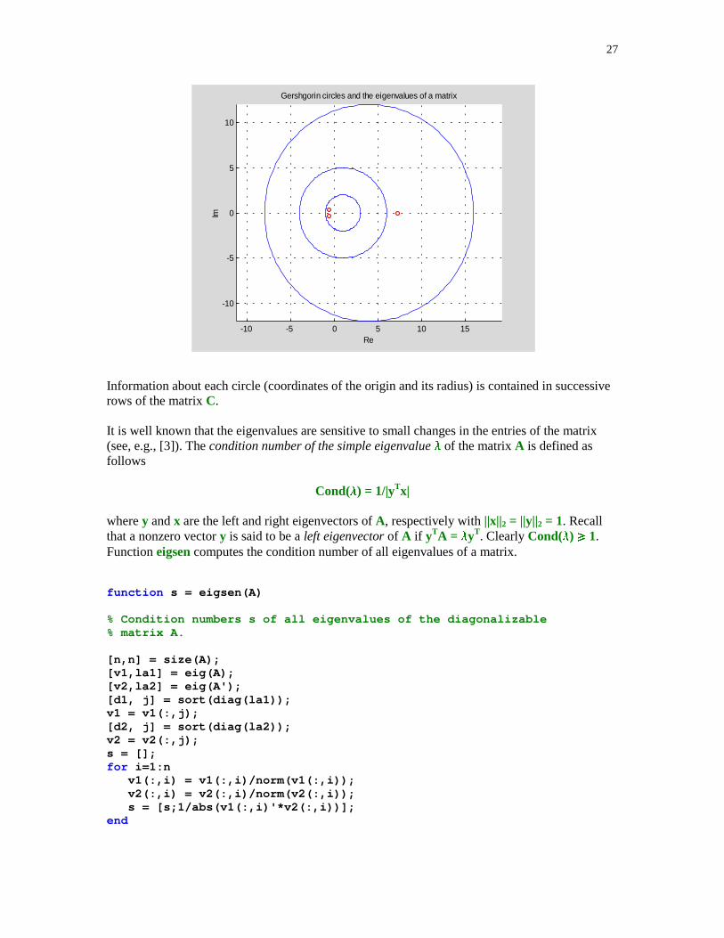
27

-10 -5 0 5 10 15

-10

-5

0

5

10

Re

Im

Gershgorin circles and the eigenvalues of a matrix

Information about each circle (coordinates of the origin and its radius) is contained in successiverows of the matrix C.

It is well known that the eigenvalues are sensitive to small changes in the entries of the matrix(see, e.g., [3]). The condition number of the simple eigenvalue � of the matrix A is defined asfollows

Cond(�) = 1/|yTx|

where y and x are the left and right eigenvectors of A, respectively with ||x||2 = ||y||2 = 1. Recallthat a nonzero vector y is said to be a left eigenvector of A if yTA = �yT. Clearly Cond(�) � 1.Function eigsen computes the condition number of all eigenvalues of a matrix.

function s = eigsen(A)

% Condition numbers s of all eigenvalues of the diagonalizable% matrix A.

[n,n] = size(A);[v1,la1] = eig(A);[v2,la2] = eig(A');[d1, j] = sort(diag(la1));v1 = v1(:,j);[d2, j] = sort(diag(la2));v2 = v2(:,j);s = [];for i=1:n v1(:,i) = v1(:,i)/norm(v1(:,i)); v2(:,i) = v2(:,i)/norm(v2(:,i)); s = [s;1/abs(v1(:,i)'*v2(:,i))];end

28

In this example we will illustrate sensitivity of the eigenvalues of the celebrated Wilkinson'smatrix W. Its is an upper bidiagonal 20-by-20 matrix with diagonal entries 20, 19, … , 1. Thesuperdiagonal entries are all equal to 20. We create this matrix using some MATLAB functionsthat are discussed in Section 4.9.

W = spdiags([(20:-1:1)', 20*ones(20,1)],[0 1], 20,20);

format long

s = eigsen(full(W))

s = 1.0e+012 * 0.00008448192546 0.00145503286853 0.01206523295175 0.06389158525507 0.24182386727359 0.69411856608888 1.56521713930244 2.83519277292867 4.18391920177580 5.07256664475500 5.07256664475500 4.18391920177580 2.83519277292867 1.56521713930244 0.69411856608888 0.24182386727359 0.06389158525507 0.01206523295175 0.00145503286853 0.00008448192546

Clearly all eigenvalues of the Wilkinson's matrix are sensitive.

Let us perturb the w20,1 entry of W

W(20,1)=1e-5;

and next compute the eigenvalues of the perturbed matrix

eig(full(W))

ans = -1.00978219090288 -0.39041284468158 + 2.37019976472684i -0.39041284468158 - 2.37019976472684i 1.32106082150033 + 4.60070993953446i 1.32106082150033 - 4.60070993953446i 3.88187526711025 + 6.43013503466255i 3.88187526711025 - 6.43013503466255i 7.03697639135041 + 7.62654906220393i

29

7.03697639135041 - 7.62654906220393i 10.49999999999714 + 8.04218886506797i 10.49999999999714 - 8.04218886506797i 13.96302360864989 + 7.62654906220876i 13.96302360864989 - 7.62654906220876i 17.11812473289285 + 6.43013503466238i 17.11812473289285 - 6.43013503466238i 19.67893917849915 + 4.60070993953305i 19.67893917849915 - 4.60070993953305i 21.39041284468168 + 2.37019976472726i 21.39041284468168 - 2.37019976472726i 22.00978219090265

Note a dramatic change in the eigenvalues.

In some problems only selected eigenvalues and associated eigenvectors are needed. Let theeigenvalues {�k } be rearranged so that |�1| > |�2| � … � |�n|. The dominant eigenvalue �1 and/orthe associated eigenvector can be found using one of the following methods: power iteration,inverse iteration, and Rayleigh quotient iteration. Functions powerit and Rqi implement the firstand the third method, respectively.

function [la, v] = powerit(A, v)

% Power iteration with the Rayleigh quotient.% Vector v is the initial estimate of the eigenvector of% the matrix A. Computed eigenvalue la and the associated% eigenvector v satisfy the inequality% norm(A*v - la*v,1) < tol,% where tol = length(v)*norm(A,1)*eps.

if norm(v) ~= 1 v = v/norm(v);endla = v'*A*v;tol = length(v)*norm(A,1)*eps;while norm(A*v - la*v,1) >= tol w = A*v; v = w/norm(w); la = v'*A*v;end

function [la, v] = Rqi(A, v, iter)

% The Rayleigh quotient iteration.% Vector v is an approximation of the eigenvector associated with the% dominant eigenvalue la of the matrix A. Iterative process is% terminated either if norm(A*v - la*v,1) < norm(A,1)*length(v)*eps% or if the number of performed iterations reaches the allowed number% of iterations iter.

if norm(v) > 1 v = v/norm(v);endla = v'*A*v;tol = norm(A,1)*length(v)*eps;for k=1:iter

30

if norm(A*v - la*v,1) < tol return else w = (A - la*eye(size(A)))\v; v = w/norm(w); la = v'*A*v; endend

Let ( [7], p.208, Example 27.1)

A = [2 1 1;1 3 1;1 1 4]; v = ones(3,1);

Then

format long

flops(0)

[la, v] = powerit(A, v)

la = 5.21431974337753v = 0.39711254978701 0.52065736843959 0.75578934068378

flops

ans = 3731

Using function Rqi, for computing the dominant eigenpair of the matrix A, we obtain

flops(0)

[la, v] = Rqi(A,ones(3,1),5)

la = 5.21431974337754v = 0.39711254978701 0.52065736843959 0.75578934068378

flops

ans = 512

31

Once the dominant eigenvalue (eigenpair) is computed one can find another eigenvalue oreigenpair by applying a process called deflation. For details the reader is referred to [4],pp. 127-128.

function [l2, v2, B] = defl(A, v1)

% Deflated matrix B from the matrix A with a known eigenvector v1 of A.% The eigenpair (l2, v2) of the matrix A is computed.% Functions Housv, Houspre, Housmvp and Rqi are used% in the body of the function defl.

n = length(v1);v1 = Housv(v1);C = Houspre(v1,A);B = [];for i=1:n B = [B Housmvp(v1,C(i,:))];endl1 = B(1,1);b = B(1,2:n);B = B(2:n,2:n);[l2, y] = Rqi(B, ones(n-1,1),10);if l1 ~= l2 a = b*y/(l2-l1); v2 = Housmvp(v1,[a;y]);else v2 = v1;end

Let A be an 5-by-5 Pei matrix, i.e.,

A = ones(5)+diag(ones(5,1))

A = 2 1 1 1 1 1 2 1 1 1 1 1 2 1 1 1 1 1 2 1 1 1 1 1 2

Its dominant eigenvalue is �1 = 6 and all the remaining eigenvalues are equal to one. To computethe dominant eigenpair of A we use function Rqi

[l1,v1] = Rqi(A,rand(5,1),10)

l1 = 6.00000000000000v1 = 0.44721359549996 0.44721359549996 0.44721359549996 0.44721359549996 0.44721359549996

and next apply function defl to compute another eigenpair of A

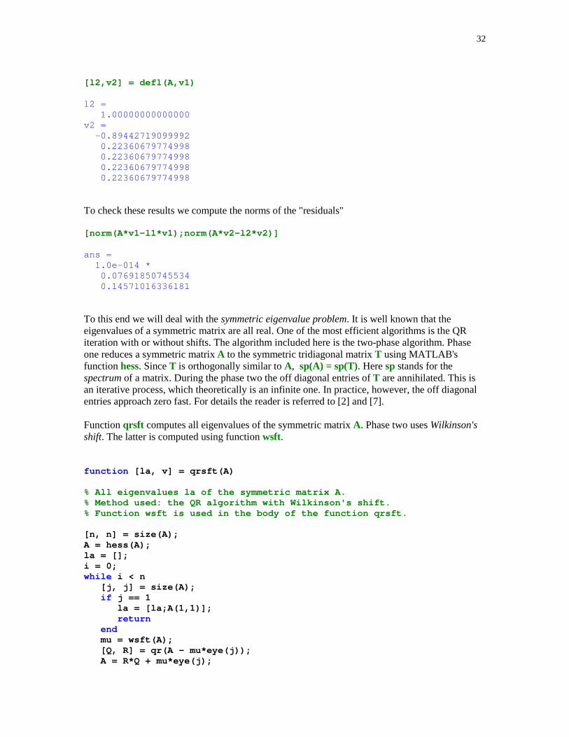
32

[l2,v2] = defl(A,v1)

l2 = 1.00000000000000v2 = -0.89442719099992 0.22360679774998 0.22360679774998 0.22360679774998 0.22360679774998

To check these results we compute the norms of the "residuals"

[norm(A*v1-l1*v1);norm(A*v2-l2*v2)]

ans = 1.0e-014 * 0.07691850745534 0.14571016336181

To this end we will deal with the symmetric eigenvalue problem. It is well known that theeigenvalues of a symmetric matrix are all real. One of the most efficient algorithms is the QRiteration with or without shifts. The algorithm included here is the two-phase algorithm. Phaseone reduces a symmetric matrix A to the symmetric tridiagonal matrix T using MATLAB'sfunction hess. Since T is orthogonally similar to A, sp(A) = sp(T). Here sp stands for thespectrum of a matrix. During the phase two the off diagonal entries of T are annihilated. This isan iterative process, which theoretically is an infinite one. In practice, however, the off diagonalentries approach zero fast. For details the reader is referred to [2] and [7].

Function qrsft computes all eigenvalues of the symmetric matrix A. Phase two uses Wilkinson'sshift. The latter is computed using function wsft.

function [la, v] = qrsft(A)

% All eigenvalues la of the symmetric matrix A.% Method used: the QR algorithm with Wilkinson's shift.% Function wsft is used in the body of the function qrsft.

[n, n] = size(A);A = hess(A);la = [];i = 0;while i < n [j, j] = size(A); if j == 1 la = [la;A(1,1)]; return end mu = wsft(A); [Q, R] = qr(A - mu*eye(j)); A = R*Q + mu*eye(j);

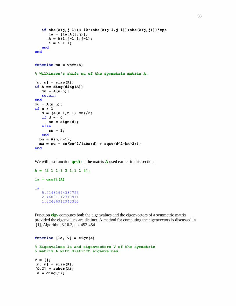
33

if abs(A(j,j-1))< 10*(abs(A(j-1,j-1))+abs(A(j,j)))*eps la = [la;A(j,j)]; A = A(1:j-1,1:j-1); i = i + 1; endend

function mu = wsft(A)

% Wilkinson's shift mu of the symmetric matrix A.

[n, n] = size(A);if A == diag(diag(A)) mu = A(n,n); returnendmu = A(n,n);if n > 1 d = (A(n-1,n-1)-mu)/2; if d ~= 0 sn = sign(d); else sn = 1; end bn = A(n,n-1); mu = mu - sn*bn^2/(abs(d) + sqrt(d^2+bn^2));end

We will test function qrsft on the matrix A used earlier in this section

A = [2 1 1;1 3 1;1 1 4];

la = qrsft(A)

la = 5.21431974337753 2.46081112718911 1.32486912943335

Function eigv computes both the eigenvalues and the eigenvectors of a symmetric matrixprovided the eigenvalues are distinct. A method for computing the eigenvectors is discussed in [1], Algorithm 8.10.2, pp. 452-454

function [la, V] = eigv(A)

% Eigenvalues la and eigenvectors V of the symmetric% matrix A with distinct eigenvalues.

V = [];[n, n] = size(A);[Q,T] = schur(A);la = diag(T);

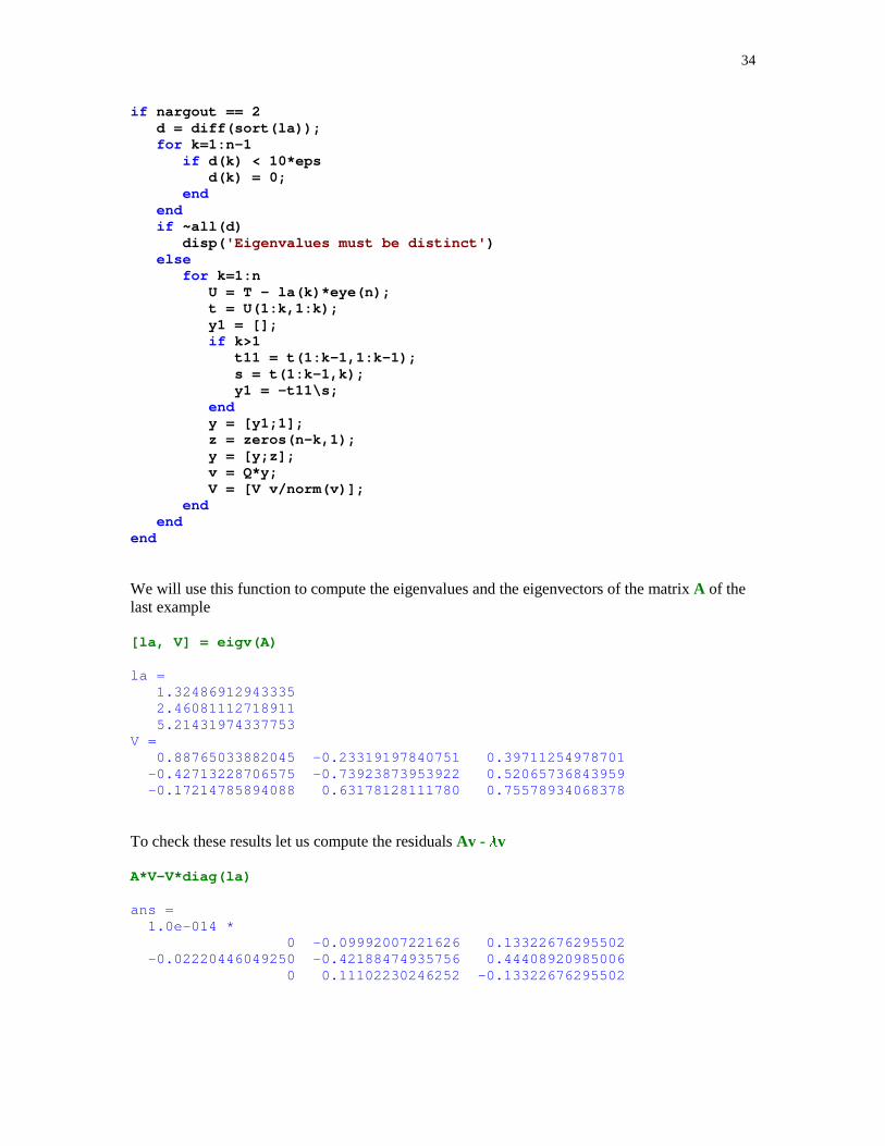
34

if nargout == 2 d = diff(sort(la)); for k=1:n-1 if d(k) < 10*eps d(k) = 0; end end if ~all(d) disp( 'Eigenvalues must be distinct' ) else for k=1:n U = T - la(k)*eye(n); t = U(1:k,1:k); y1 = []; if k>1 t11 = t(1:k-1,1:k-1); s = t(1:k-1,k); y1 = -t11\s; end y = [y1;1]; z = zeros(n-k,1); y = [y;z]; v = Q*y; V = [V v/norm(v)]; end endend

We will use this function to compute the eigenvalues and the eigenvectors of the matrix A of thelast example

[la, V] = eigv(A)

la = 1.32486912943335 2.46081112718911 5.21431974337753V = 0.88765033882045 -0.23319197840751 0.39711254978701 -0.42713228706575 -0.73923873953922 0.52065736843959 -0.17214785894088 0.63178128111780 0.75578934068378

To check these results let us compute the residuals Av - �v

A*V-V*diag(la)

ans = 1.0e-014 * 0 -0.09992007221626 0.13322676295502 -0.02220446049250 -0.42188474935756 0.44408920985006 0 0.11102230246252 -0.13322676295502

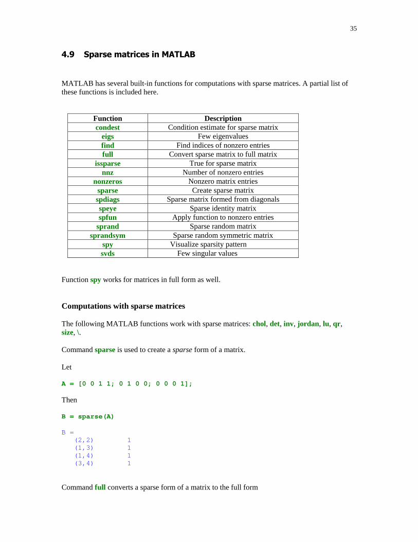
35

�,�$��� ������ ���������

MATLAB has several built-in functions for computations with sparse matrices. A partial list ofthese functions is included here.

Function Descriptioncondest Condition estimate for sparse matrix

eigs Few eigenvaluesfind Find indices of nonzero entriesfull Convert sparse matrix to full matrix

issparse True for sparse matrixnnz Number of nonzero entries

nonzeros Nonzero matrix entriessparse Create sparse matrixspdiags Sparse matrix formed from diagonalsspeye Sparse identity matrixspfun Apply function to nonzero entries

sprand Sparse random matrixsprandsym Sparse random symmetric matrix

spy Visualize sparsity patternsvds Few singular values

Function spy works for matrices in full form as well.

Computations with sparse matrices

The following MATLAB functions work with sparse matrices: chol, det, inv, jordan , lu, qr ,size, \.

Command sparse is used to create a sparse form of a matrix.

Let

A = [0 0 1 1; 0 1 0 0; 0 0 0 1];

Then

B = sparse(A)

B = (2,2) 1 (1,3) 1 (1,4) 1 (3,4) 1

Command full converts a sparse form of a matrix to the full form

36

C = full(B)

C = 0 0 1 1 0 1 0 0 0 0 0 1

Command sparse has the following syntax

sparse(k,l,s,m,n)

where k and l are arrays of row and column indices, respectively, s ia an array of nonzeronumbers whose indices are specified in k and l, and m and n are the row and column dimensions,respectively.

Let

S = sparse([1 3 5 2], [2 1 3 4], [1 2 3 4], 5, 5)

S = (3,1) 2 (1,2) 1 (5,3) 3 (2,4) 4

F = full(S)

F = 0 1 0 0 0 0 0 0 4 0 2 0 0 0 0 0 0 0 0 0 0 0 3 0 0

To create a sparse matrix with several diagonals parallel to the main diagonal one can use thecommand spdiags. Its syntax is shown below

spdiags(B, d, m, n)

The resulting matrix is an m-by-n sparse matrix. Its diagonals are the columns of the matrix B.Location of the diagonals are described in the vector d.

Function mytrid creates a sparse form of the tridiagonal matrix with constant entries along thediagonals.

function T = mytrid(a,b,c,n)

% The n-by-n tridiagonal matrix T with constant entries% along diagonals. All entries on the subdiagonal, main% diagonal,and the superdiagonal are equal a, b, and c,% respectively.

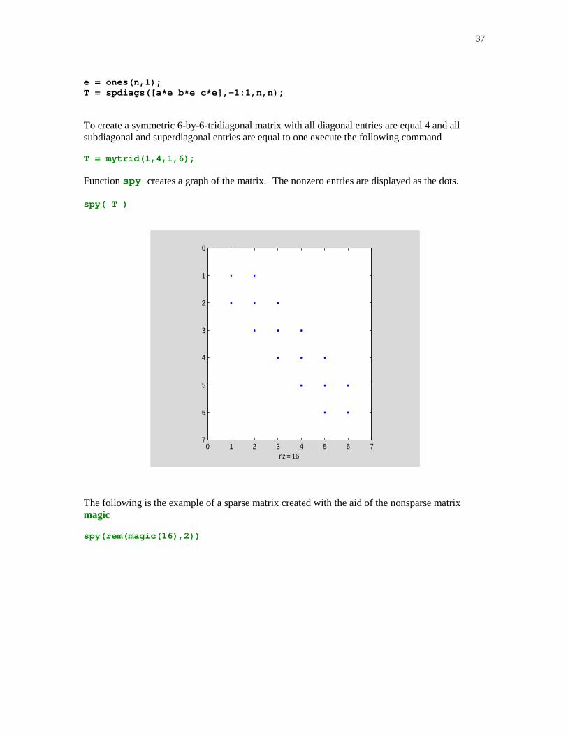
37

e = ones(n,1);T = spdiags([a*e b*e c*e],-1:1,n,n);

To create a symmetric 6-by-6-tridiagonal matrix with all diagonal entries are equal 4 and allsubdiagonal and superdiagonal entries are equal to one execute the following command

T = mytrid(1,4,1,6);

Function spy creates a graph of the matrix. The nonzero entries are displayed as the dots.

spy( T )

0 1 2 3 4 5 6 7

0

1

2

3

4

5

6

7

nz = 16

The following is the example of a sparse matrix created with the aid of the nonsparse matrixmagic

spy(rem(magic(16),2))

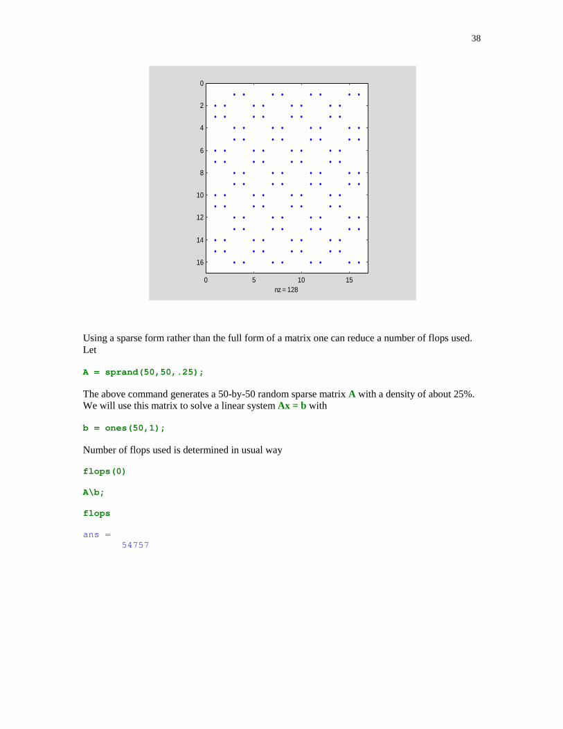
38

0 5 10 15

0

2

4

6

8

10

12

14

16

nz = 128

Using a sparse form rather than the full form of a matrix one can reduce a number of flops used.Let

A = sprand(50,50,.25);

The above command generates a 50-by-50 random sparse matrix A with a density of about 25%.We will use this matrix to solve a linear system Ax = b with

b = ones(50,1);

Number of flops used is determined in usual way

flops(0)

A\b;

flops

ans = 54757

39

Using the full form of A the number of flops needed to solve the same linear system is

flops(0)

full(A)\b;

flops

ans = 72014

40

- � � �� �

[1] B.N. Datta, Numerical Linear Algebra and Applications, Brooks/Cole Publishing Company, Pacific Grove, CA, 1995.

[2] J.W. Demmel, Applied Numerical Linear Algebra, SIAM, Philadelphia, PA, 1997.

[3] G.H. Golub and Ch.F. Van Loan, Matrix Computations, Second edition, Johns Hopkins University Press, Baltimore, MD, 1989.

[4] M.T. Heath, Scientific Computing: An Introductory Survey, McGraw-Hill, Boston, MA, 1997.

[5] N.J. Higham, Accuracy and Stability of Numerical Algorithms, SIAM, Philadelphia, PA, 1996.

[6] R.D. Skeel and J.B. Keiper, Elementary Numerical Computing with Mathematica, McGraw-Hill, New York, NY, 1993.

[7] L.N. Trefethen and D. Bau III, Numerical Linear Algebra, SIAM, Philadelphia, PA, 1997.

41

.���� ��

1. Let A by an n-by-n matrix and let v be an n-dimensional vector. Which of thefollowing methods is faster?

(i) (v*v')*A(ii) v*(v'*A)

2. Suppose that L � �n x n is lower triangular and b � �n. Write MATLAB function x = ltri(L, b)that computes a solution x to the linear system Lx = b.

3. Repeat Problem 2 with L being replaced by the upper triangular matrix U. Name your function utri(U, b) .

4. Let A � �n x n be a triangular matrix. Write a function dettri(A) that computes the determinant of the matrix A.

5. Write MATLAB function MA = Gausspre(A, m, k) that overwrites matrix A � �n x p withthe product MA , where M � �n x n is the Gauss transformation which is determined by theGauss vector m and its column index k.Hint : You may wish to use the following formula MA = A – m(ek

TA).

6. A system of linear equations Ax = b, where A is a square matrix, can be solved applyingsuccessively Gauss transformations to the augmented matrix [A, b] . A solution x then can befound using back substitution, i.e., solving a linear system with an upper triangular matrix.Using functions Gausspre of Problem 5, Gaussv described in Section 4.3, and utri ofProblem 3, write a function x = sol(A, b) which computes a solution x to the linear system

Ax = b.

7. Add a few lines of code to the function sol of Problem 6 to compute the determinant of thematrix A. The header of your function might look like this function [x, d] = sol(A, b). Thesecond output parameter d stands for the determinant of A.

8. The purpose of this problem is to test function sol of Problem 6.

(i) Construct at least one matrix A for which function sol fails to compute a solution.Explain why it happened.

(ii) Construct at least one matrix A for which the computed solution x is poor. Forcomparison of a solution you found using function sol with an acceptable solutionyou may wish to use MATLAB's backslash operator \. Compute the relative error inx. Compare numbers of flops used by function sol and MATLAB's command \.Which of these methods is faster in general?

9. Given a square matrix A. Write MATLAB function [L, U] = mylu(A) that computes the LU decomposition of A using partial pivoting.

42

10. Change your working format to format long e and run function mylu of Problem 11on thefollowing matrices

(i) A = [eps 1; 1 1](ii) A = [1 1; eps 1](iii) A = hilb(10)(iv) A = rand(10)

In each case compute the error �A - LU�F.

11. Let A be a tridiagonal matrix that is either diagonally dominant or positive definite. Write MATLAB's function [L, U] = trilu(a, b, c) that computes the LU factorization of A. Here a, b, and c stand for the subdiagonal, main diagonal, and superdiagonal of A, respectively.

12. The following function computes the Cholesky factor L of the symmetric positive definite matrix A. Matrix L is lower triangular and satisfies the equation A = LL T.

function L = mychol(A)

% Cholesky factor L of the matrix A; A = L*L'.

[n, n] = size(A);for j=1:n

for k=1:j-1 A(j:n,j) = A(j:n,j) - A(j:n,k)*A(j,k); end A(j,j) = sqrt(A(j,j)); A(j+1:n,j) = A(j+1:n,j)/A(j,j);

endL = tril(A);

Add a few lines of code that generates the error messages when A is neither

• symmetric nor• positive definite

Test the modified function mychol on the following matrices

(i) A = [1 2 3; 2 1 4; 3 4 1](ii) A = rand(5)

13. Prove that any 2-by-2 Householder reflector is of the form H = [cos � sin �; sin � -cos �]. What is the Householder reflection vector u of H?

14. Find the eigenvalues and the associated eigenvectors of the matrix H of Problem 13.

15. Write MATLAB function [Q, R] = myqr(A) that computes a full QR factorizationA = QR of A � �m x n with m � n using Householder reflectors. The output matrix Q is an m-by-m orthogonal matrix and R is an m-by-n upper triangular with zero entries in rows n+1through m.

43

Hint : You may wish to use function Housprod in the body of the function myqr .16. Let A be an n-by-3 random matrix generated by the MATLAB function rand. In this exercise you are to plot the error �A - QR�F versus n for n = 3, 5, … , 25. To

compute the QR factorization of A use the function myqr of Problem 15. Plot the graph of thecomputed errors using MATLAB's function semilogy instead of the function plot. Repeat thisexperiment several times. Does the error increase as n does?

17. Write MATLAB function V = Vandm(t, n) that generates Vandermonde's matrix V used in the polynomial least-squares fit. The degree of the approximating polynomial is n while the x-coordinates of the points to be fitted are stored in the vector t.

18. In this exercise you are to compute coefficients of the least squares polynomials using fourmethods, namely the normal equations, the QR factorization, modified Gram-Schmidtorthogonalization and the singular value decomposition.

Write MATLAB function C = lspol(t, y, n) that computes coefficients of the approximating polynomials. They should be saved in columns of the matrix C � �(n+1) x 4. Here n stands for the degree of the polynomial, t and y are the vectors holding the x- and the y-coordinates of the points to be approximated, respectively. Test your function using t = linspace(1.4, 1.8), y = sin(tan(t)) – tan(sin(t)), n = 2, 4, 8. Use format long to display the output to the screen. Hint : To create the Vandermonde matrix needed in the body of the function lspol you may wish to use function Vandm of Problem 17.

19. Modify function lspol of Problem 18 adding a second output parameter err so thatthe header of the modified function should look like thisfunction [C, err] = lspol(t, y, n). Parameter err is the least squares error in the computedsolution c to the overdetermined linear system Vc � y. Run the modified function on the dataof Problem 18. Which of the methods used seems to produce the least reliable numericalresults? Justify your answer.

20. Write MATLAB function [r, c] = nrceig(A) that computes the number of real andcomplex eigenvalues of the real matrix A. You cannot use MATLAB function eig. Runfunction nrceig on several random matrices generated by the functions rand and randn.Hint: You may wish to use the following MATLAB functions schur, diag, find . Note thatthe diag function takes a second optional argument.

21. Assume that an eigenvalue of a matrix is sensitive if its condition number is greater than 103. Construct an n-by-n matrix (5 � n � 10) whose all eigenvalues are real and sensitive.

22. Write MATLAB function A = pent(a, b, c, d, e, n) that creates the full form of then-by-n pentadiagonal matrix A with constant entries a along the second subdiagonal, constantentries b along the subdiagonal, etc.

23. Let A = pent(1, 26, 66, 26, 1, n) be an n-by-n symmetric pentadiagonal matrix generated by function pent of Problem 22. Find the eigenvalue decomposition

A = Q�QT of A for various values of n. Repeat this experiment using random numbers in theband of the matrix A. Based on your observations, what conjecture can be formulated aboutthe eigenvectors of A?

24. Write MATLAB function [la, x] = smeig(A, v) that computes the smallest

44

(in magnitude) eigenvalue of the nonsingular matrix A and the associated eigenvector x. The input parameter v is an estimate of the eigenvector of A that is associated with the largest (in magnitude) eigenvalue of A.

25. In this exercise you are to experiment with the eigenvalues and eigenvectors of thepartitioned matrices. Begin with a square matrix A with known eigenvalues andeigenvectors. Next construct a matrix B using MATLAB's built-in function repmatto define the matrix B as B = repmat(A, 2, 2). Solve the matrix eigenvalueproblem for the matrix B and compare the eigenvalues and eigenvectors of matricesA and B. You may wish to continue in this manner using larger values for the secondand third parameters in the function repmat. Based on the results of your experiment,what conjecture about the eigenvalues and eigenvectors of B can be formulated?

��������

��� �����������������������

�����������

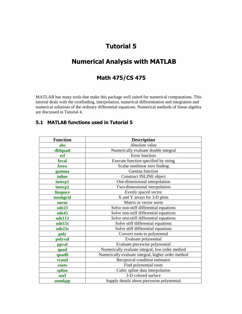
MATLAB has many tools that make this package well suited for numerical computations. Thistutorial deals with the rootfinding, interpolation, numerical differentiation and integration andnumerical solutions of the ordinary differential equations. Numerical methods of linear algebraare discussed in Tutorial 4.

�� ����������������� ����������

Function Descriptionabs Absolute value

dblquad Numerically evaluate double integralerf Error function

feval Execute function specified by stringfzero Scalar nonlinear zero finding

gamma Gamma functioninline Construct INLINE object

interp1 One-dimensional interpolationinterp2 Two-dimensional interpolationlinspace Evenly spaced vector

meshgrid X and Y arrays for 3-D plotsnorm Matrix or vector normode23 Solve non-stiff differential equationsode45 Solve non-stiff differential equationsode113 Solve non-stiff differential equationsode15s Solve stiff differential equationsode23s Solve stiff differential equationspoly Convert roots to polynomial

polyval Evaluate polynomialppval Evaluate piecewise polynomialquad Numerically evaluate integral, low order methodquad8 Numerically evaluate integral, higher order methodrcond Reciprocal condition estimatorroots Find polynomial rootsspline Cubic spline data interpolationsurf 3-D colored surface

unmkpp Supply details about piecewise polynomial

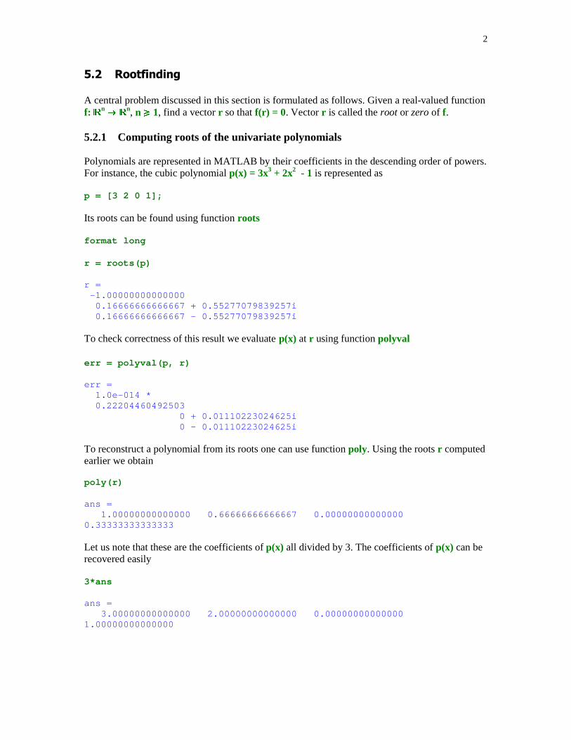
2

�!"������ ��#

A central problem discussed in this section is formulated as follows. Given a real-valued functionf: �n � �n, n � 1, find a vector r so that f(r) = 0. Vector r is called the root or zero of f.

5.2.1 Computing roots of the univariate polynomials

Polynomials are represented in MATLAB by their coefficients in the descending order of powers.For instance, the cubic polynomial p(x) = 3x3 + 2x2 - 1 is represented as

p = [3 2 0 1];

Its roots can be found using function roots

format long

r = roots(p)

r = -1.00000000000000 0.16666666666667 + 0.55277079839257i 0.16666666666667 - 0.55277079839257i

To check correctness of this result we evaluate p(x) at r using function polyval

err = polyval(p, r)

err = 1.0e-014 * 0.22204460492503 0 + 0.01110223024625i 0 - 0.01110223024625i

To reconstruct a polynomial from its roots one can use function poly. Using the roots r computedearlier we obtain

poly(r)

ans = 1.00000000000000 0.66666666666667 0.000000000000000.33333333333333

Let us note that these are the coefficients of p(x) all divided by 3. The coefficients of p(x) can berecovered easily

3*ans

ans = 3.00000000000000 2.00000000000000 0.000000000000001.00000000000000

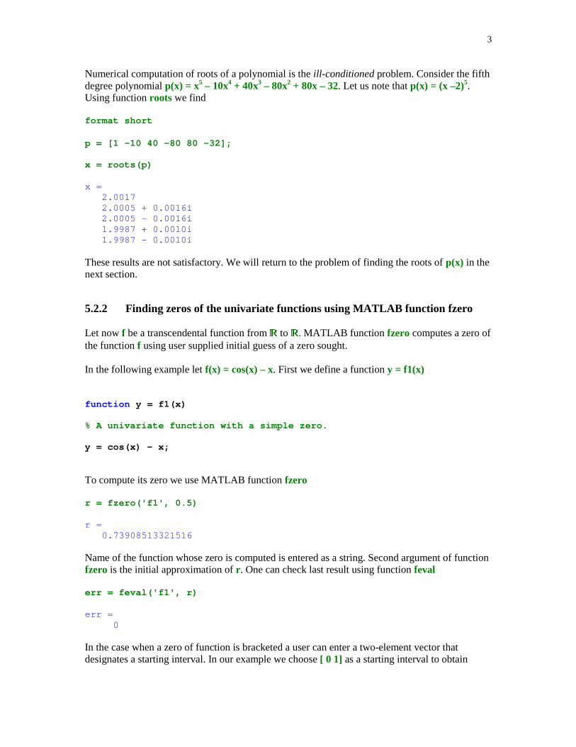
3

Numerical computation of roots of a polynomial is the ill-conditioned problem. Consider the fifthdegree polynomial p(x) = x5 – 10x4 + 40x3 – 80x2 + 80x – 32. Let us note that p(x) = (x –2)5.Using function roots we find

format short

p = [1 –10 40 –80 80 –32];

x = roots(p)

x = 2.0017 2.0005 + 0.0016i 2.0005 - 0.0016i 1.9987 + 0.0010i 1.9987 - 0.0010i

These results are not satisfactory. We will return to the problem of finding the roots of p(x) in thenext section.

5.2.2 Finding zeros of the univariate functions using MATLAB function fzero

Let now f be a transcendental function from � to �. MATLAB function fzero computes a zero ofthe function f using user supplied initial guess of a zero sought.

In the following example let f(x) = cos(x) – x. First we define a function y = f1(x)

function y = f1(x)

% A univariate function with a simple zero.

y = cos(x) - x;

To compute its zero we use MATLAB function fzero

r = fzero('f1', 0.5)

r = 0.73908513321516

Name of the function whose zero is computed is entered as a string. Second argument of functionfzero is the initial approximation of r . One can check last result using function feval

err = feval('f1', r)

err = 0

In the case when a zero of function is bracketed a user can enter a two-element vector thatdesignates a starting interval. In our example we choose [ 0 1] as a starting interval to obtain

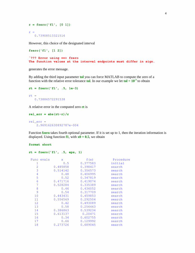
4

r = fzero('f1', [0 1])

r = 0.73908513321516

However, this choice of the designated interval

fzero('f1', [1 2])

¨??? Error using ==> fzeroThe function values at the interval endpoints must differ in sign.

generates the error message.

By adding the third input parameter tol you can force MATLAB to compute the zero of afunction with the relative error tolerance tol. In our example we let tol = 10-3 to obtain

rt = fzero('f1', .5, 1e-3)

rt = 0.73886572291538

A relative error in the computed zero rt is

rel_err = abs(rt-r)/r

rel_err = 2.969162630892787e-004

Function fzero takes fourth optional parameter. If it is set up to 1, then the iteration information isdisplayed. Using function f1, with x0 = 0.5, we obtain

format short

rt = fzero('f1', .5, eps, 1)

Func evals x f(x) Procedure 1 0.5 0.377583 initial 2 0.485858 0.398417 search 3 0.514142 0.356573 search 4 0.48 0.406995 search 5 0.52 0.347819 search 6 0.471716 0.419074 search 7 0.528284 0.335389 search 8 0.46 0.436052 search 9 0.54 0.317709 search 10 0.443431 0.459853 search 11 0.556569 0.292504 search 12 0.42 0.493089 search 13 0.58 0.256463 search 14 0.386863 0.539234 search 15 0.613137 0.20471 search 16 0.34 0.602755 search 17 0.66 0.129992 search 18 0.273726 0.689045 search

5

19 0.726274 0.0213797 search 20 0.18 0.803844 search 21 0.82 -0.137779 search

Looking for a zero in the interval [0.18, 0.82]

22 0.726355 0.0212455 interpolation 23 0.738866 0.00036719 interpolation 24 0.739085 -6.04288e-008 interpolation 25 0.739085 2.92788e-012 interpolation 26 0.739085 0 interpolationrt = 0.7391

We have already seen that MATLAB function roots had faild to produce satisfactory resultswhen computing roots of the polynomial p(x) = (x – 2)5. This time we will use function fzero tofind a multiple root of p(x). We define a new function named f2

function y = f2(x)

y = (x - 2)^5;

and next change format to

format long

Running function fzero we obtain

rt = fzero('f2', 1.5)

rt = 2.00000000000000

This time the result is as expected.

Finally, we will apply function fzero to compute the multiple root of p(x) using an expandedform of the polynomial p(x)

function y = f3(x)

y = x^5 - 10*x^4 + 40*x^3 -80*x^2 + 80*x - 32;

rt = fzero('f3', 1.5)

rt = 1.99845515925755

Again, the computed approximation of the root of p(x) has a few correct digits only.

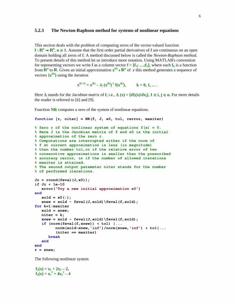
6

5.2.3 The Newton-Raphson method for systems of nonlinear equations

This section deals with the problem of computing zeros of the vector-valued functionf : �n � �n, n � 1. Assume that the first order partial derivatives of f are continuous on an opendomain holding all zeros of f. A method discussed below is called the Newton-Raphson method.To present details of this method let us introduce more notation. Using MATLAB's conventionfor representing vectors we write f as a column vector f = [f 1; …;f n], where each fk is a functionfrom �n to �. Given an initial approximation x(0) � �n of r this method generates a sequence ofvectors {x(k)} using the iteration

x(k+1) = x(k) – Jf (x(k))-1 f(x(k)), k = 0, 1, … .

Here Jf stands for the Jacobian matrix of f, i.e., Jf (x) = [�f i(x)/�xj], 1 � i, j � n. For more detailsthe reader is referred to [6] and [9].

Function NR computes a zero of the system of nonlinear equations.

function [r, niter] = NR(f, J, x0, tol, rerror, maxiter)

% Zero r of the nonlinear system of equations f(x) = 0.% Here J is the Jacobian matrix of f and x0 is the initial% approximation of the zero r.% Computations are interrupted either if the norm of% f at current approximation is less (in magnitude)% than the number tol,or if the relative error of two% consecutive approximations is smaller than the prescribed% accuracy rerror, or if the number of allowed iterations% maxiter is attained.% The second output parameter niter stands for the number% of performed iterations.

Jc = rcond(feval(J,x0));if Jc < 1e-10 error( 'Try a new initial approximation x0' )end xold = x0(:); xnew = xold - feval(J,xold)\feval(f,xold);for k=1:maxiter xold = xnew; niter = k; xnew = xold - feval(J,xold)\feval(f,xold); if (norm(feval(f,xnew)) < tol) | ... norm(xold-xnew, 'inf' )/norm(xnew, 'inf' ) < tol| ... (niter == maxiter) break endendr = xnew;

The following nonlinear system

f1(x) = x1 + 2x2 – 2, f2(x) = x1

2 + 4x22 – 4

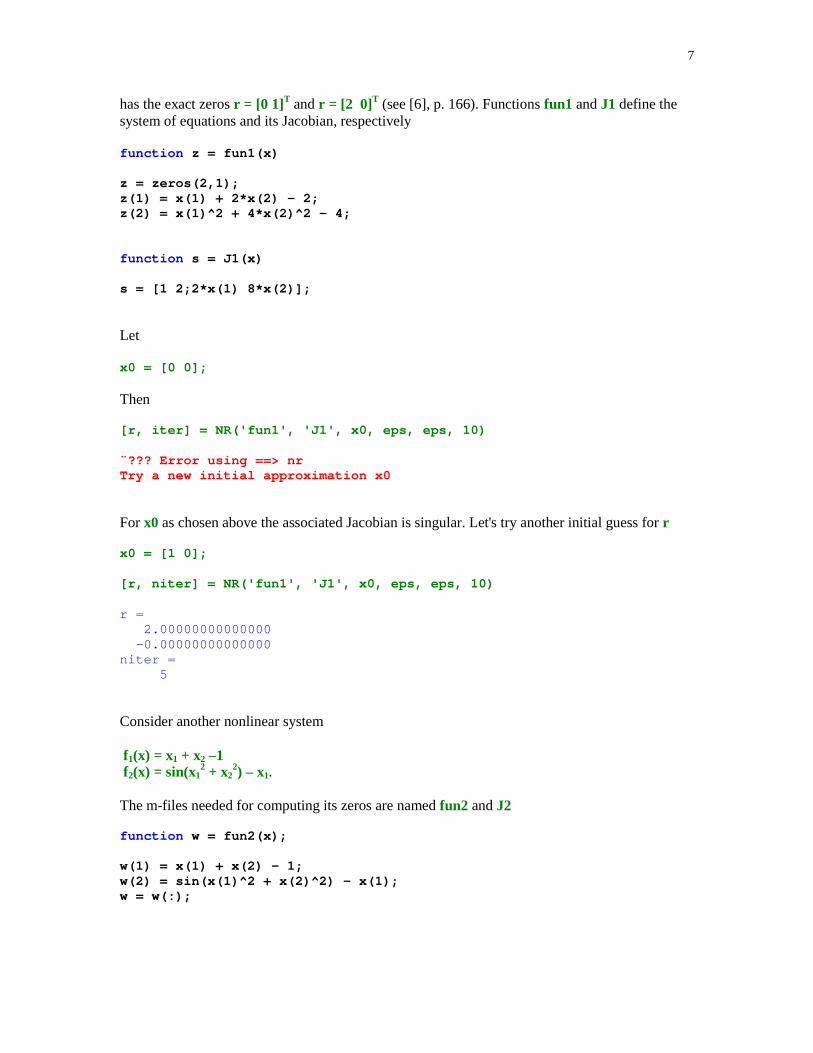
7

has the exact zeros r = [0 1]T and r = [2 0]T (see [6], p. 166). Functions fun1 and J1 define thesystem of equations and its Jacobian, respectively

function z = fun1(x)

z = zeros(2,1);z(1) = x(1) + 2*x(2) - 2;z(2) = x(1)^2 + 4*x(2)^2 - 4;

function s = J1(x)

s = [1 2;2*x(1) 8*x(2)];

Let

x0 = [0 0];

Then

[r, iter] = NR('fun1', 'J1', x0, eps, eps, 10)

¨??? Error using ==> nrTry a new initial approximation x0

For x0 as chosen above the associated Jacobian is singular. Let's try another initial guess for r

x0 = [1 0];

[r, niter] = NR('fun1', 'J1', x0, eps, eps, 10)

r = 2.00000000000000 -0.00000000000000niter = 5

Consider another nonlinear system

f1(x) = x1 + x2 –1 f2(x) = sin(x1

2 + x22) – x1.

The m-files needed for computing its zeros are named fun2 and J2

function w = fun2(x);

w(1) = x(1) + x(2) - 1;w(2) = sin(x(1)^2 + x(2)^2) - x(1);w = w(:);

8

function s = J2(x)

s = [1 1; 2*x(1)*cos(x(1)^2 + x(2)^2)-1 2*x(2)*cos(x(1)^2 + x(2)^2)];

With the initial guess

x0 = [0 1];

the zero r is found to be

[r, niter] = NR('fun2', 'J2', x0, eps, eps, 10)

r = 0.48011911689839 0.51988088310161niter = 5

while the initial guess

x0 = [1 1];

[r, iter] = NR('fun2', 'J2', x0, eps, eps, 10)

r = -0.85359545600207 1.85359545600207iter = 10

gives another solution. The value of function fun2 at the computed zero r is

feval('fun2', r)

ans = 1.0e-015 * 0 -0.11102230246252

Implementation of other classical methods for computing the zeros of scalar equations, includingthe fixed-point iteration, the secant method and the Schroder method are left to the reader (seeProblems 3, 6, and 12 at the end of this tutorial).

�$%� &�� �������'�� �(�������

Interpolation of functions is one of the classical problems in numerical analysis. A onedimensional interpolation problem is formulated as follows.

Given set of n+1 points �xk , yk�, 0 � k � n, with x0 < x1 < … < xn, find a function f(x) whosegraph interpolates the data points, i.e., f(xk) = yk, for k = 0, 1, …, n.

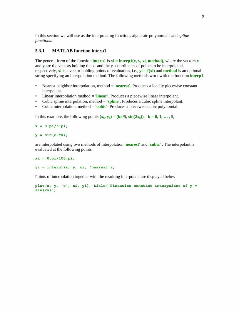
9

In this section we will use as the interpolating functions algebraic polynomials and splinefunctions.

5.3.1 MATLAB function interp1

The general form of the function interp1 is yi = interp1(x, y, xi, method), where the vectors xand y are the vectors holding the x- and the y- coordinates of points to be interpolated,respectively, xi is a vector holding points of evaluation, i.e., yi = f(xi) and method is an optionalstring specifying an interpolation method. The following methods work with the function interp1

• Nearest neighbor interpolation, method = 'nearest'. Produces a locally piecewise constantinterpolant.

• Linear interpolation method = 'linear' . Produces a piecewise linear interpolant.• Cubic spline interpolation, method = 'spline'. Produces a cubic spline interpolant.• Cubic interpolation, method = 'cubic' . Produces a piecewise cubic polynomial.

In this example, the following points (xk, yk) = (k�/5, sin(2xk)), k = 0, 1, … , 5,

x = 0:pi/5:pi;

y = sin(2.*x);

are interpolated using two methods of interpolation 'nearest' and 'cubic' . The interpolant isevaluated at the following points

xi = 0:pi/100:pi;

yi = interp1(x, y, xi, 'nearest');

Points of interpolation together with the resulting interpolant are displayed below

plot(x, y, 'o', xi, yi), title('Piecewise constant interpolant of y =sin(2x)')

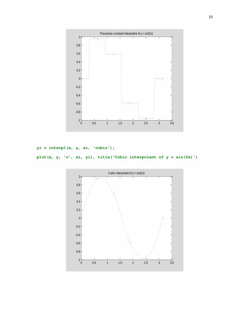
10

0 0.5 1 1.5 2 2.5 3 3.5-1

-0.8

-0.6

-0.4

-0.2

0

0.2

0.4

0.6

0.8

1Piecewise constant interpolant of y = sin(2x)

yi = interp1(x, y, xi, 'cubic');

plot(x, y, 'o', xi, yi), title('Cubic interpolant of y = sin(2x)')

0 0.5 1 1.5 2 2.5 3 3.5-1

-0.8

-0.6

-0.4

-0.2

0

0.2

0.4

0.6

0.8

1Cubic interpolant of y = sin(2x)

11

5.3.2 Interpolation by algebraic polynomials

Assume now that the interpolating function is an algebraic polynomial pn(x) of degree at most n,where n = number of points of interpolation – 1. It is well known that the interpolatingpolynomial pn always exists and is unique (see e.g., [6], [9]). To determine the polynomialinterpolant one can use either the Vandermonde's method or Lagrange form or Newton's form orAitken's method. We shall describe briefly the Newton's method.

We begin writing p(x) as

(5.3.1) pn(x) = a0 + a1(x – x0) + a2(x – x0)(x – x1) + … + an(x – x0)(x – x1) … (x – xn-1)

Coefficients a0, a1, … , an are called the divided differences and they can be computedrecursively. Representation (5.3.1) of pn(x) is called the Newton's form of the interpolatingpolynomial. The k-th order divided difference based on points x0, … xk, denoted by [x0, … , xk],is defined recursively as

[xm] = ym if k = 0

[x0, … , xk] = ([x1, … , xk] – [x0, … , xk-1])/(xk – x0) if k > 0.

Coefficients {ak} in representation (5.3.1) and the divided differences are related in the followingway

ak = [x0, … , xk].

Function Newtonpol evaluates an interpolating polynomial at the user supplied points.

function [yi, a] = Newtonpol(x, y, xi)

% Values yi of the interpolating polynomial at the points xi.% Coordinates of the points of interpolation are stored in% vectors x and y. Horner's method is used to evaluate% a polynomial. Second output parameter a holds coeeficients% of the interpolating polynomial in Newton's form.

a = divdiff(x, y);n = length(a);val = a(n)*ones(length(xi));for m = n-1:-1:1 val = (xi - x(m)).*val + a(m);endyi = val(:);

function a = divdiff(x, y)

% Divided differences based on points stored in arrays x and y.

n = length(x);for k=1:n-1

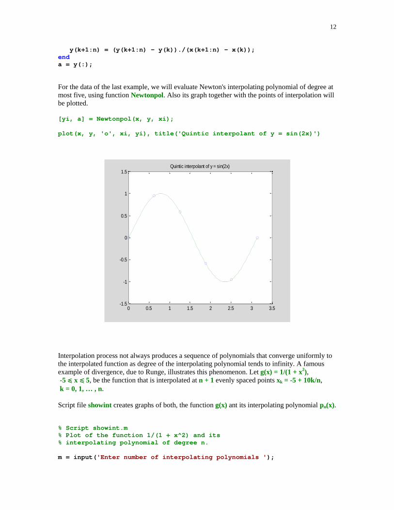
12

y(k+1:n) = (y(k+1:n) - y(k))./(x(k+1:n) - x(k));enda = y(:);

For the data of the last example, we will evaluate Newton's interpolating polynomial of degree atmost five, using function Newtonpol. Also its graph together with the points of interpolation willbe plotted.

[yi, a] = Newtonpol(x, y, xi);

plot(x, y, 'o', xi, yi), title('Quintic interpolant of y = sin(2x)')

0 0.5 1 1.5 2 2.5 3 3.5-1.5

-1

-0.5

0

0.5

1

1.5Quintic interpolant of y = sin(2x)

Interpolation process not always produces a sequence of polynomials that converge uniformly tothe interpolated function as degree of the interpolating polynomial tends to infinity. A famousexample of divergence, due to Runge, illustrates this phenomenon. Let g(x) = 1/(1 + x2), -5 � x � 5, be the function that is interpolated at n + 1 evenly spaced points xk = -5 + 10k/n, k = 0, 1, … , n.

Script file showint creates graphs of both, the function g(x) ant its interpolating polynomial pn(x).

% Script showint.m% Plot of the function 1/(1 + x^2) and its% interpolating polynomial of degree n.

m = input( 'Enter number of interpolating polynomials ' );

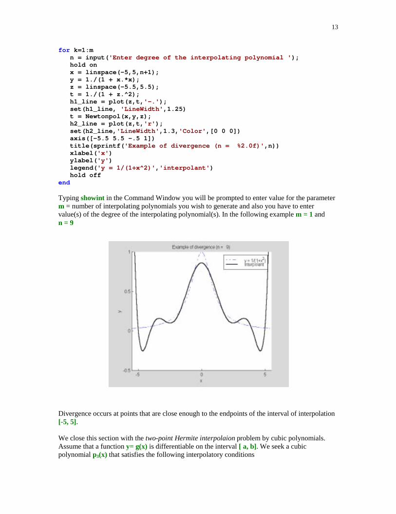
13

for k=1:m n = input( 'Enter degree of the interpolating polynomial ' ); hold on x = linspace(-5,5,n+1); y = 1./(1 + x.*x);

z = linspace(-5.5,5.5); t = 1./(1 + z.^2); h1_line = plot(z,t, '-.' ); set(h1_line, 'LineWidth' ,1.25) t = Newtonpol(x,y,z); h2_line = plot(z,t, 'r' ); set(h2_line, 'LineWidth' ,1.3, 'Color' ,[0 0 0]) axis([-5.5 5.5 -.5 1]) title(sprintf( 'Example of divergence (n = %2.0f)' ,n)) xlabel( 'x' ) ylabel( 'y' ) legend( 'y = 1/(1+x^2)' , 'interpolant' ) hold offend

Typing showint in the Command Window you will be prompted to enter value for the parameterm = number of interpolating polynomials you wish to generate and also you have to entervalue(s) of the degree of the interpolating polynomial(s). In the following example m = 1 andn = 9

Divergence occurs at points that are close enough to the endpoints of the interval of interpolation[-5, 5].

We close this section with the two-point Hermite interpolaion problem by cubic polynomials.Assume that a function y= g(x) is differentiable on the interval [ a, b]. We seek a cubicpolynomial p3(x) that satisfies the following interpolatory conditions

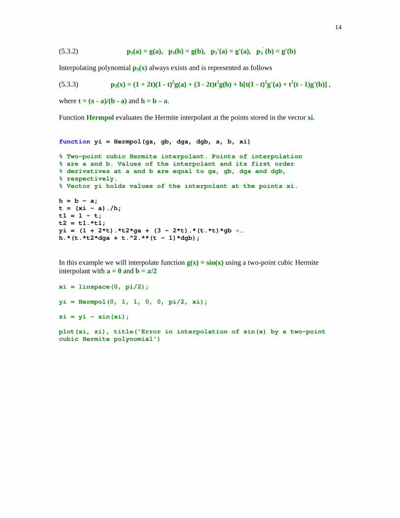
14

(5.3.2) p3(a) = g(a), p3(b) = g(b), p3'(a) = g'(a), p3' (b) = g'(b)

Interpolating polynomial p3(x) always exists and is represented as follows

(5.3.3) p3(x) = (1 + 2t)(1 - t)2g(a) + (3 - 2t)t2g(b) + h[t(1 - t)2g'(a) + t2(t - 1)g'(b)] ,

where t = (x - a)/(b - a) and h = b – a.

Function Hermpol evaluates the Hermite interpolant at the points stored in the vector xi.

function yi = Hermpol(ga, gb, dga, dgb, a, b, xi)

% Two-point cubic Hermite interpolant. Points of interpolation% are a and b. Values of the interpolant and its first order% derivatives at a and b are equal to ga, gb, dga and dgb,% respectively.% Vector yi holds values of the interpolant at the points xi.

h = b – a;t = (xi - a)./h;t1 = 1 - t;t2 = t1.*t1;yi = (1 + 2*t).*t2*ga + (3 - 2*t).*(t.*t)*gb +…h.*(t.*t2*dga + t.^2.**(t - 1)*dgb);

In this example we will interpolate function g(x) = sin(x) using a two-point cubic Hermiteinterpolant with a = 0 and b = �/2

xi = linspace(0, pi/2);

yi = Hermpol(0, 1, 1, 0, 0, pi/2, xi);

zi = yi – sin(xi);

plot(xi, zi), title('Error in interpolation of sin(x) by a two-pointcubic Hermite polynomial')

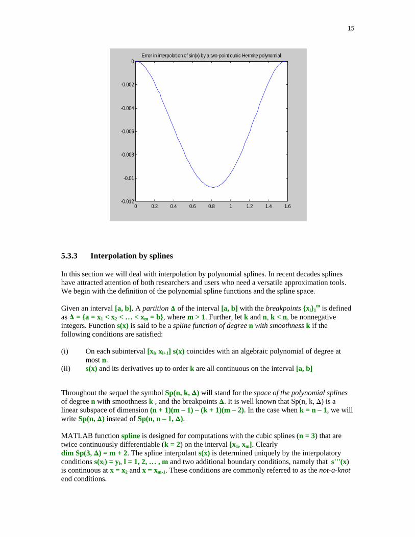
15

0 0.2 0.4 0.6 0.8 1 1.2 1.4 1.6-0.012

-0.01

-0.008

-0.006

-0.004

-0.002

0Error in interpolation of sin(x) by a two-point cubic Hermite polynomial

5.3.3 Interpolation by splines

In this section we will deal with interpolation by polynomial splines. In recent decades splineshave attracted attention of both researchers and users who need a versatile approximation tools.We begin with the definition of the polynomial spline functions and the spline space.

Given an interval [a, b]. A partition � of the interval [a, b] with the breakpoints {xl}1m is defined

as � = {a = x1 < x2 < … < xm = b}, where m > 1. Further, let k and n, k < n, be nonnegativeintegers. Function s(x) is said to be a spline function of degree n with smoothness k if thefollowing conditions are satisfied:

(i) On each subinterval [xl, xl+1] s(x) coincides with an algebraic polynomial of degree atmost n.

(ii) s(x) and its derivatives up to order k are all continuous on the interval [a, b]

Throughout the sequel the symbol Sp(n, k, �) will stand for the space of the polynomial splinesof degree n with smoothness k , and the breakpoints �. It is well known that Sp(n, k, �) is alinear subspace of dimension (n + 1)(m – 1) – (k + 1)(m – 2). In the case when k = n – 1, we willwrite Sp(n, �) instead of Sp(n, n – 1, �).

MATLAB function spline is designed for computations with the cubic splines (n = 3) that aretwice continuously differentiable (k = 2) on the interval [x1, xm]. Clearlydim Sp(3, �) = m + 2. The spline interpolant s(x) is determined uniquely by the interpolatoryconditions s(xl) = yl, l = 1, 2, … , m and two additional boundary conditions, namely that s'''(x )is continuous at x = x2 and x = xm-1. These conditions are commonly referred to as the not-a-knotend conditions.

16

MATLAB's command yi = spline(x, y, xi) evaluates cubic spline s(x) at points stored in the arrayxi. Vectors x and y hold coordinates of the points to be interpolated. To obtain the piecewisepolynomial representation of the spline interpolant one can execute the commandpp = spline(x, y). Command zi = ppval(pp, xi) evaluates the piecewise polynomial form of thespline interpolant. Points of evaluation are stored in the array xi. If a spline interpolant has to beevaluated for several vectors xi, then the use of function ppval is strongly recommended.

In this example we will interpolate Runge's function g(x) = 1/(1 + x2) on the interval [0, 5] usingsix evenly spaced breakpoints

x = 0:5;

y = 1./(1 + x.^2);

xi = linspace(0, 5);

yi = spline(x, y, xi);

plot(x, y, 'o', xi, yi), title('Cubic spline interpolant')

0 1 2 3 4 50

0.1

0.2

0.3

0.4

0.5

0.6

0.7

0.8

0.9

1Cubic spline interpolant

The maximum error on the set xi in approximating Runge's function by the cubic spline we foundis

17

err = norm(abs(yi-1./(1+xi.^2)),'inf')

err = 0.0859

Detailed information about the piecewise polynomial representation of the spline interpolant canbe obtained running function spline with two input parameters x and y

pp = spline(x, y);

and next executing command unmkpp

[brpts, coeffs, npol, ncoeff] = unmkpp(pp)

brpts = 0 1 2 3 4 5coeffs = 0.0074 0.0777 -0.5852 1.0000 0.0074 0.1000 -0.4074 0.5000 -0.0371 0.1223 -0.1852 0.2000 -0.0002 0.0110 -0.0519 0.1000 -0.0002 0.0104 -0.0306 0.0588npol = 5ncoeff = 4

The output parameters brpts, coeffs, npol, and ncoeff represent the breakpoints of the splineinterpolant, coefficients of s(x) on successive subintervals, number of polynomial pieces thatconstitute spline function and number of coefficients that represent each polynomial piece,respectively. On the subinterval [xl, xl+1] the spline interpolant is represented as

s(x) = cl1(x – xl)3 + cl2(x – xl)

2 + cl3(x – xl) + cl4

where [cl1 cl2 cl3 cl4] is the lth row of the matrix coeffs. This form is called the piecewisepolynomial form (pp–form) of the spline function.

Differentiation of the spline function s(x) can be accomplished running function splder. In orderfor this function to work properly another function pold (see Problem 19) must be in MATLAB'ssearch path.

function p = splder(k, pp, x)

% Piecewise polynomial representation of the derivative% of order k (0 <= k <= 3) of a cubic spline function in the% pp form with the breakpoints stored in the vector x.

m = pp(3);lx4 = length(x) + 4;n = pp(lx4);c = pp(1 + lx4:length(pp))';c = reshape(c, m, n);b = pold(c, k);b = b(:)';

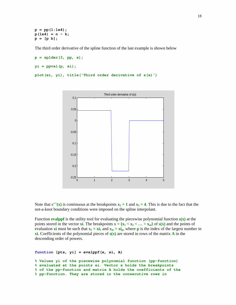
18

p = pp(1:lx4);p(lx4) = n - k;p = [p b];

The third order derivative of the spline function of the last example is shown below

p = splder(3, pp, x);

yi = ppval(p, xi);

plot(xi, yi), title('Third order derivative of s(x)')

0 1 2 3 4 5-0.25

-0.2

-0.15

-0.1

-0.05

0

0.05

0.1Third order derivative of s(x)

Note that s'''(x) is continuous at the breakpoints x2 = 1 and x5 = 4. This is due to the fact that thenot-a-knot boundary conditions were imposed on the spline interpolant.

Function evalppf is the utility tool for evaluating the piecewise polynomial function s(x) at thepoints stored in the vector xi. The breakpoints x = {x1 < x2 < … < xm} of s(x) and the points ofevaluation xi must be such that x1 = xi1 and xm = xip, where p is the index of the largest number inxi. Coefficients of the polynomial pieces of s(x) are stored in rows of the matrix A in thedescending order of powers.

function [pts, yi] = evalppf(x, xi, A)

% Values yi of the piecewise polynomial function (pp-function)% evaluated at the points xi. Vector x holds the breakpoints% of the pp-function and matrix A holds the coefficients of the% pp-function. They are stored in the consecutive rows in

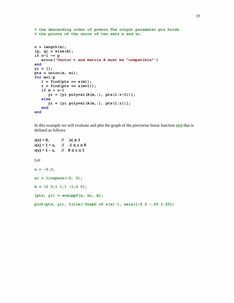
19

% the descending order of powers.The output parameter pts holds% the points of the union of two sets x and xi.

n = length(x);[p, q] = size(A);if n-1 ~= p error( 'Vector t and matrix A must be "compatible"' )endyi = [];pts = union(x, xi);for m=1:p l = find(pts == x(m)); r = find(pts == x(m+1)); if m < n-1 yi = [yi polyval(A(m,:), pts(l:r-1))]; else yi = [yi polyval(A(m,:), pts(l:r))]; endend

In this example we will evaluate and plot the graph of the piecewise linear function s(x) that isdefined as follows

s(x) = 0, if |x| � 1s(x) = 1 + x, if -1 � x � 0s(x) = 1 – x, if 0 � x � 1

Let

x = -2:2;

xi = linspace(-2, 2);

A = [0 0;1 1;1 –1;0 0];

[pts, yi] = evalppf(x, xi, A);

plot(pts, yi), title('Graph of s(x)'), axis([-2 2 -.25 1.25])

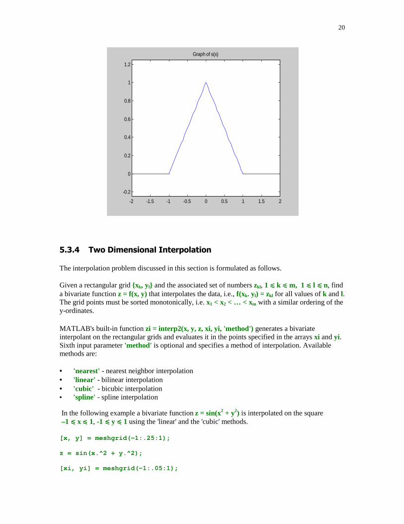
20

-2 -1.5 -1 -0.5 0 0.5 1 1.5 2

-0.2

0

0.2

0.4

0.6

0.8

1

1.2

Graph of s(x)

�$�����&�� �������'�� �(�������

The interpolation problem discussed in this section is formulated as follows.

Given a rectangular grid {xk, yl} and the associated set of numbers zkl, 1 � k � m, 1 � l � n, finda bivariate function z = f(x, y) that interpolates the data, i.e., f(xk. yl) = zkl for all values of k and l.The grid points must be sorted monotonically, i.e. x1 < x2 < … < xm with a similar ordering of they-ordinates.

MATLAB's built-in function zi = interp2(x, y, z, xi, yi, 'method') generates a bivariateinterpolant on the rectangular grids and evaluates it in the points specified in the arrays xi and yi.Sixth input parameter 'method' is optional and specifies a method of interpolation. Availablemethods are:

• 'nearest' - nearest neighbor interpolation• 'linear' - bilinear interpolation• 'cubic' - bicubic interpolation• 'spline' - spline interpolation

In the following example a bivariate function z = sin(x2 + y2) is interpolated on the square–1 � x � 1, -1 � y � 1 using the 'linear' and the 'cubic' methods.

[x, y] = meshgrid(-1:.25:1);

z = sin(x.^2 + y.^2);

[xi, yi] = meshgrid(-1:.05:1);

21

zi = interp2(x, y, z, xi, yi, 'linear');

surf(xi, yi, zi), title('Bilinear interpolant to sin(x^2 + y^2)')

The bicubic interpolant is obtained in a similar fashion

zi = interp2(x, y, z, xi, yi, 'cubic');

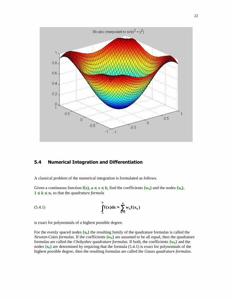
22

�� ��� �����'�� #�������� &��� � ��������

A classical problem of the numerical integration is formulated as follows.

Given a continuous function f(x), a � x � b, find the coefficients {wk} and the nodes {xk},1 � k � n, so that the quadrature formula

(5.4.1) )x(fwdx)x(f k

n

1kk

b

a

∑∫=

≈

is exact for polynomials of a highest possible degree.

For the evenly spaced nodes {xk} the resulting family of the quadrature formulas is called theNewton-Cotes formulas. If the coefficients {wk} are assumed to be all equal, then the quadratureformulas are called the Chebyshev quadrature formulas. If both, the coefficients {wk} and thenodes {xk} are determined by requiring that the formula (5.4.1) is exact for polynomials of thehighest possible degree, then the resulting formulas are called the Gauss quadrature formulas.

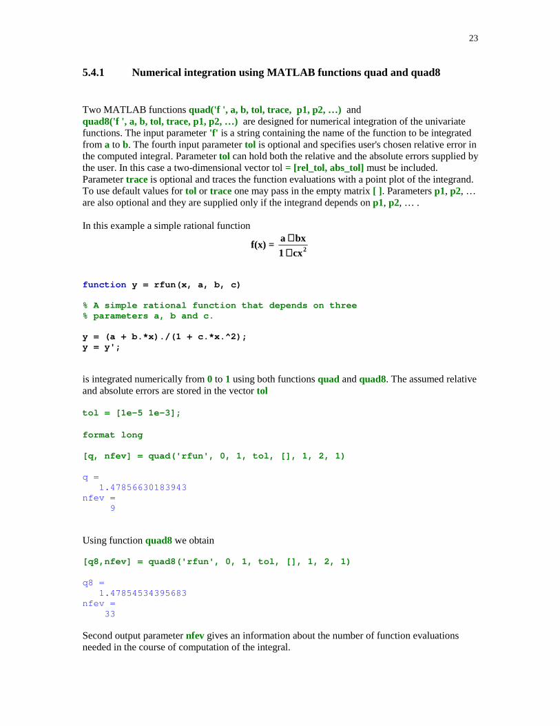
23

5.4.1 Numerical integration using MATLAB functions quad and quad8

Two MATLAB functions quad('f ', a, b, tol, trace, p1, p2, …) andquad8('f ', a, b, tol, trace, p1, p2, …) are designed for numerical integration of the univariatefunctions. The input parameter 'f' is a string containing the name of the function to be integratedfrom a to b. The fourth input parameter tol is optional and specifies user's chosen relative error inthe computed integral. Parameter tol can hold both the relative and the absolute errors supplied bythe user. In this case a two-dimensional vector tol = [rel_tol, abs_tol] must be included.Parameter trace is optional and traces the function evaluations with a point plot of the integrand.To use default values for tol or trace one may pass in the empty matrix [ ] . Parameters p1, p2, …are also optional and they are supplied only if the integrand depends on p1, p2, … .

In this example a simple rational function

f(x) = 2cx1

bxa

++

function y = rfun(x, a, b, c)

% A simple rational function that depends on three% parameters a, b and c.

y = (a + b.*x)./(1 + c.*x.^2);y = y';

is integrated numerically from 0 to 1 using both functions quad and quad8. The assumed relativeand absolute errors are stored in the vector tol

tol = [1e-5 1e-3];

format long

[q, nfev] = quad('rfun', 0, 1, tol, [], 1, 2, 1)

q = 1.47856630183943nfev = 9

Using function quad8 we obtain

[q8,nfev] = quad8('rfun', 0, 1, tol, [], 1, 2, 1)

q8 = 1.47854534395683nfev = 33

Second output parameter nfev gives an information about the number of function evaluationsneeded in the course of computation of the integral.

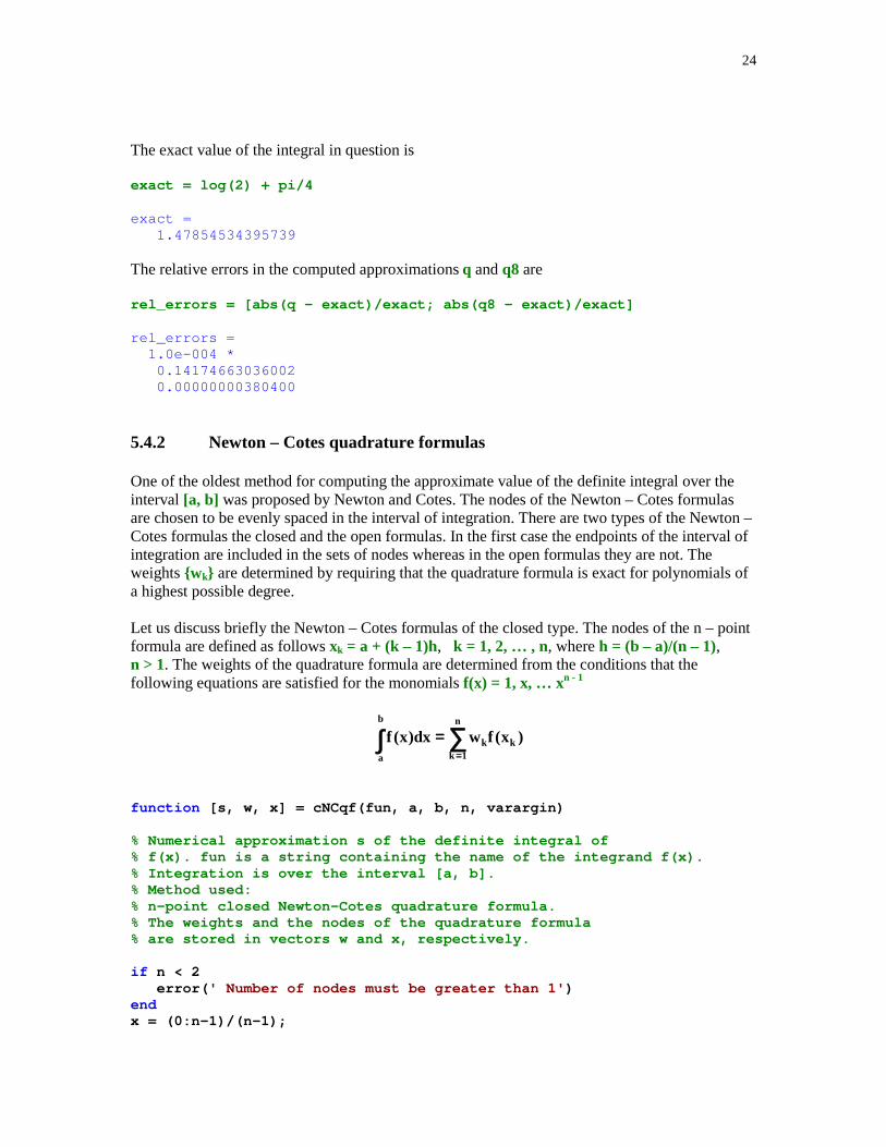
24

The exact value of the integral in question is

exact = log(2) + pi/4

exact = 1.47854534395739

The relative errors in the computed approximations q and q8 are

rel_errors = [abs(q – exact)/exact; abs(q8 – exact)/exact]

rel_errors = 1.0e-004 * 0.14174663036002 0.00000000380400

5.4.2 Newton – Cotes quadrature formulas

One of the oldest method for computing the approximate value of the definite integral over theinterval [a, b] was proposed by Newton and Cotes. The nodes of the Newton – Cotes formulasare chosen to be evenly spaced in the interval of integration. There are two types of the Newton –Cotes formulas the closed and the open formulas. In the first case the endpoints of the interval ofintegration are included in the sets of nodes whereas in the open formulas they are not. Theweights {wk} are determined by requiring that the quadrature formula is exact for polynomials ofa highest possible degree.

Let us discuss briefly the Newton – Cotes formulas of the closed type. The nodes of the n – pointformula are defined as follows xk = a + (k – 1)h, k = 1, 2, … , n, where h = (b – a)/(n – 1),n > 1. The weights of the quadrature formula are determined from the conditions that thefollowing equations are satisfied for the monomials f(x) = 1, x, … xn - 1

)x(fwdx)x(f k

b

a

n

1kk∫ ∑

=

=

function [s, w, x] = cNCqf(fun, a, b, n, varargin)

% Numerical approximation s of the definite integral of% f(x). fun is a string containing the name of the integrand f(x).% Integration is over the interval [a, b].% Method used:% n-point closed Newton-Cotes quadrature formula.% The weights and the nodes of the quadrature formula% are stored in vectors w and x, respectively.

if n < 2 error( ' Number of nodes must be greater than 1' )endx = (0:n-1)/(n-1);

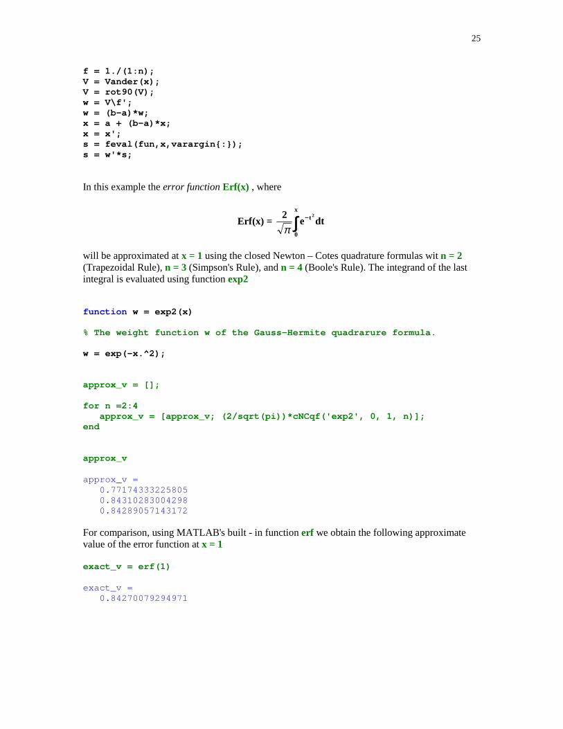
25

f = 1./(1:n);V = Vander(x);V = rot90(V);w = V\f';w = (b-a)*w;x = a + (b-a)*x;x = x';s = feval(fun,x,varargin{:});s = w'*s;

In this example the error function Erf(x) , where

Erf(x) = dte2

x

0

t 2

∫ −

π

will be approximated at x = 1 using the closed Newton – Cotes quadrature formulas wit n = 2(Trapezoidal Rule), n = 3 (Simpson's Rule), and n = 4 (Boole's Rule). The integrand of the lastintegral is evaluated using function exp2

function w = exp2(x)

% The weight function w of the Gauss-Hermite quadrarure formula.

w = exp(-x.^2);

approx_v = [];

for n =2:4 approx_v = [approx_v; (2/sqrt(pi))*cNCqf('exp2', 0, 1, n)];end

approx_v

approx_v = 0.77174333225805 0.84310283004298 0.84289057143172

For comparison, using MATLAB's built - in function erf we obtain the following approximatevalue of the error function at x = 1

exact_v = erf(1)

exact_v = 0.84270079294971

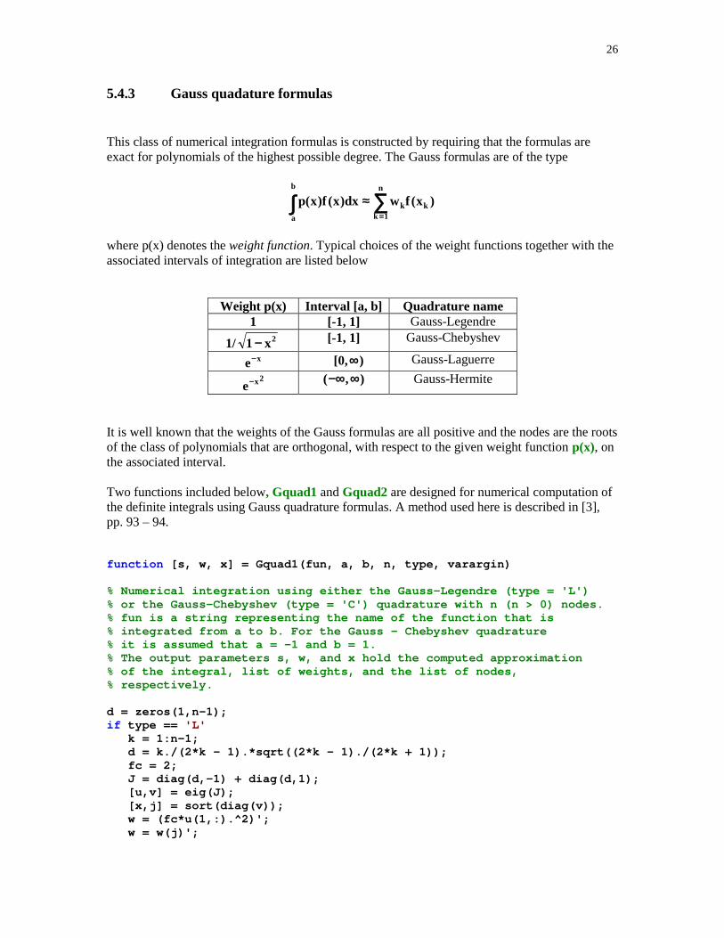
26

5.4.3 Gauss quadature formulas

This class of numerical integration formulas is constructed by requiring that the formulas areexact for polynomials of the highest possible degree. The Gauss formulas are of the type

)x(fwdx)x(f)x(p k

b

a

n

1kk∫ ∑

=

≈

where p(x) denotes the weight function. Typical choices of the weight functions together with theassociated intervals of integration are listed below

Weight p(x) Interval [a, b] Quadrature name1 [-1, 1] Gauss-Legendre

1/ 2x1− [-1, 1] Gauss-Chebyshev

xe− ),0[ ∞ Gauss-Laguerre2xe− ),( ∞−∞ Gauss-Hermite

It is well known that the weights of the Gauss formulas are all positive and the nodes are the rootsof the class of polynomials that are orthogonal, with respect to the given weight function p(x), onthe associated interval.

Two functions included below, Gquad1 and Gquad2 are designed for numerical computation ofthe definite integrals using Gauss quadrature formulas. A method used here is described in [3],pp. 93 – 94.

function [s, w, x] = Gquad1(fun, a, b, n, type, varargin)

% Numerical integration using either the Gauss-Legendre (type = 'L')% or the Gauss-Chebyshev (type = 'C') quadrature with n (n > 0) nodes.% fun is a string representing the name of the function that is% integrated from a to b. For the Gauss - Chebyshev quadrature% it is assumed that a = -1 and b = 1.% The output parameters s, w, and x hold the computed approximation% of the integral, list of weights, and the list of nodes,% respectively.

d = zeros(1,n-1);if type == 'L' k = 1:n-1; d = k./(2*k - 1).*sqrt((2*k - 1)./(2*k + 1)); fc = 2; J = diag(d,-1) + diag(d,1); [u,v] = eig(J); [x,j] = sort(diag(v)); w = (fc*u(1,:).^2)'; w = w(j)';

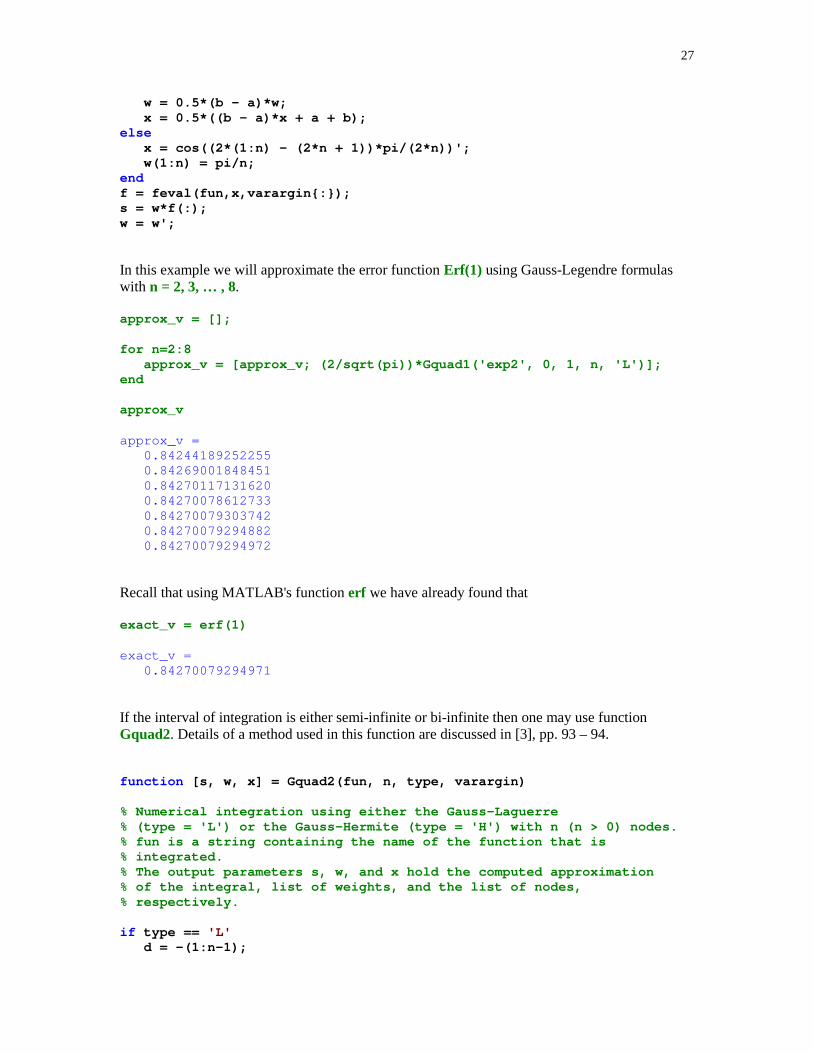
27

w = 0.5*(b - a)*w; x = 0.5*((b - a)*x + a + b);else x = cos((2*(1:n) - (2*n + 1))*pi/(2*n))'; w(1:n) = pi/n;endf = feval(fun,x,varargin{:});s = w*f(:);w = w';

In this example we will approximate the error function Erf(1) using Gauss-Legendre formulaswith n = 2, 3, … , 8.

approx_v = [];

for n=2:8 approx_v = [approx_v; (2/sqrt(pi))*Gquad1('exp2', 0, 1, n, 'L')];end

approx_v

approx_v = 0.84244189252255 0.84269001848451 0.84270117131620 0.84270078612733 0.84270079303742 0.84270079294882 0.84270079294972

Recall that using MATLAB's function erf we have already found that

exact_v = erf(1)

exact_v = 0.84270079294971

If the interval of integration is either semi-infinite or bi-infinite then one may use functionGquad2. Details of a method used in this function are discussed in [3], pp. 93 – 94.

function [s, w, x] = Gquad2(fun, n, type, varargin)

% Numerical integration using either the Gauss-Laguerre% (type = 'L') or the Gauss-Hermite (type = 'H') with n (n > 0) nodes.% fun is a string containing the name of the function that is% integrated.% The output parameters s, w, and x hold the computed approximation% of the integral, list of weights, and the list of nodes,% respectively.

if type == 'L' d = -(1:n-1);

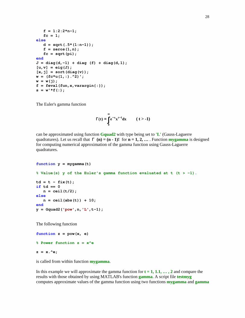
28

f = 1:2:2*n-1; fc = 1;else d = sqrt(.5*(1:n-1)); f = zeros(1,n); fc = sqrt(pi);endJ = diag(d,-1) + diag (f) + diag(d,1);[u,v] = eig(J);[x,j] = sort(diag(v));w = (fc*u(1,:).^2)';w = w(j);f = feval(fun,x,varargin{:});s = w'*f(:);

The Euler's gamma function

dxxe)t( 1t

0

x −∞

−∫=Γ ( t > -1)

can be approximated using function Gquad2 with type being set to 'L' (Gauss-Laguerrequadratures). Let us recall that Γ (n) = (n - 1)! for n = 1, 2, … . Function mygamma is designedfor computing numerical approximation of the gamma function using Gauss-Laguerrequadratures.

function y = mygamma(t)

% Value(s) y of the Euler's gamma function evaluated at t (t > -1).

td = t - fix(t);if td == 0 n = ceil(t/2);else n = ceil(abs(t)) + 10;endy = Gquad2( 'pow' ,n, 'L' ,t-1);

The following function

function z = pow(x, e)

% Power function z = x^e

z = x.^e;

is called from within function mygamma.

In this example we will approximate the gamma function for t = 1, 1.1, … , 2 and compare theresults with those obtained by using MATLAB's function gamma. A script file testmygcomputes approximate values of the gamma function using two functions mygamma and gamma

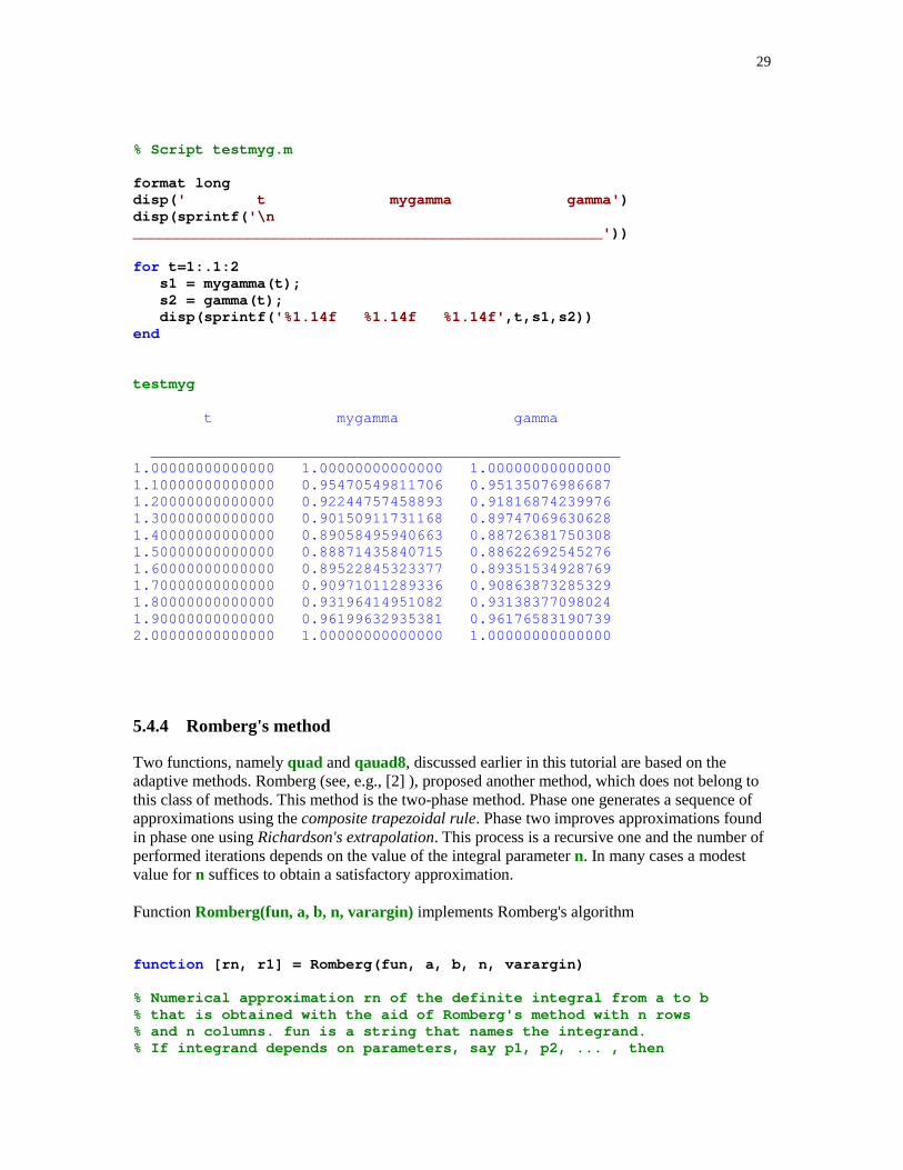
29

% Script testmyg.m

format longdisp( ' t mygamma gamma' )disp(sprintf( '\n_____________________________________________________' ))

for t=1:.1:2 s1 = mygamma(t); s2 = gamma(t); disp(sprintf( '%1.14f %1.14f %1.14f' ,t,s1,s2))end

testmyg

t mygamma gamma

_____________________________________________________1.00000000000000 1.00000000000000 1.000000000000001.10000000000000 0.95470549811706 0.951350769866871.20000000000000 0.92244757458893 0.918168742399761.30000000000000 0.90150911731168 0.897470696306281.40000000000000 0.89058495940663 0.887263817503081.50000000000000 0.88871435840715 0.886226925452761.60000000000000 0.89522845323377 0.893515349287691.70000000000000 0.90971011289336 0.908638732853291.80000000000000 0.93196414951082 0.931383770980241.90000000000000 0.96199632935381 0.961765831907392.00000000000000 1.00000000000000 1.00000000000000

5.4.4 Romberg's method

Two functions, namely quad and qauad8, discussed earlier in this tutorial are based on theadaptive methods. Romberg (see, e.g., [2] ), proposed another method, which does not belong tothis class of methods. This method is the two-phase method. Phase one generates a sequence ofapproximations using the composite trapezoidal rule. Phase two improves approximations foundin phase one using Richardson's extrapolation. This process is a recursive one and the number ofperformed iterations depends on the value of the integral parameter n. In many cases a modestvalue for n suffices to obtain a satisfactory approximation.

Function Romberg(fun, a, b, n, varargin) implements Romberg's algorithm

function [rn, r1] = Romberg(fun, a, b, n, varargin)

% Numerical approximation rn of the definite integral from a to b% that is obtained with the aid of Romberg's method with n rows% and n columns. fun is a string that names the integrand.% If integrand depends on parameters, say p1, p2, ... , then

30

% they should be supplied just after the parameter n.% Second output parameter r1 holds approximate values of the% computed integral obtained with the aid of the composite% trapezoidal rule using 1, 2, ... ,n subintervals.

h = b - a;d = 1;r = zeros(n,1);r(1) = .5*h*sum(feval(fun,[a b],varargin{:}));for i=2:n h = .5*h; d = 2*d; t = a + h*(1:2:d); s = feval(fun, t, varargin{:}); r(i) = .5*r(i-1) + h*sum(s);endr1 = r;d = 4;for j=2:n s = zeros(n-j+1,1); s = r(j:n) + diff(r(j-1:n))/(d - 1); r(j:n) = s; d = 4*d;endrn = r(n);

We will test function Romberg integrating the rational function introduced earlier in this tutorial(see the m-file rfun ). The interval of integration is [a, b] = [0, 1], n= 10, and the values of theparameters a, b, and c are set to 1, 2, and 1, respectively.

[rn, r1] = Romberg('rfun', 0 , 1, 10, 1, 2, 1)

rn = 1.47854534395739r1 = 1.25000000000000 1.42500000000000 1.46544117647059 1.47528502049722 1.47773122353730 1.47834187356141 1.47849448008531 1.47853262822223 1.47854216503816 1.47854454922849

The absolute and relative errors in rn are

[abs(exact - rn); abs(rn - exact)/exact]

ans = 0

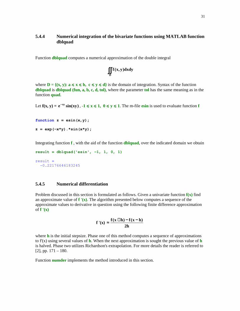
31

5.4.4 Numerical integration of the bivariate functions using MATLAB functiondblquad

Function dblquad computes a numerical approximation of the double integral

∫∫D

dxdy)y,x(f

where D = {(x, y): a � x � b, c � y � d} is the domain of integration. Syntax of the functiondblquad is dblquad (fun, a, b, c, d, tol), where the parameter tol has the same meaning as in thefunction quad.

Let f(x, y) = )xysin(e xy− , -1 � x � 1, 0 � y � 1. The m-file esin is used to evaluate function f

function z = esin(x,y);

z = exp(-x*y).*sin(x*y);

Integrating function f , with the aid of the function dblquad, over the indicated domain we obtain

result = dblquad('esin', -1, 1, 0, 1)

result = -0.22176646183245

5.4.5 Numerical differentiation

Problem discussed in this section is formulated as follows. Given a univariate function f(x) findan approximate value of f '(x) . The algorithm presented below computes a sequence of theapproximate values to derivative in question using the following finite difference approximationof f '(x)

f '(x) h2

)hx(f)hx(f −−+≈

where h is the initial stepsize. Phase one of this method computes a sequence of approximationsto f'(x) using several values of h. When the next approximation is sought the previous value of his halved. Phase two utilizes Richardson's extrapolation. For more details the reader is referred to[2], pp. 171 – 180.

Function numder implements the method introduced in this section.

32

function der = numder(fun, x, h, n, varargin)

% Approximation der of the first order derivative, at the point x,% of a function named by the string fun. Parameters h and n% are user supplied values of the initial stepsize and the number% of performed iterations in the Richardson extrapolation.% For fuctions that depend on parameters their values must follow% the parameter n.

d = [];for i=1:n s = (feval(fun,x+h,varargin{:})-feval(fun,x-h,varargin{:}))/(2*h); d = [d;s]; h = .5*h;endl = 4;for j=2:n s = zeros(n-j+1,1); s = d(j:n) + diff(d(j-1:n))/(l - 1); d(j:n) = s; l = 4*l;endder = d(n);

In this example numerical approximations of the first order derivative of the function2xe)x(f −= are computed using function numder and they are compared against the exact values

of f '(x) at x = 0.1, 0.2, … , 1.0. The values of the input parameters h and n are 0.01 and 10,respectively.

function testnder(h, n)

% Test file for the function numder. The initial stepsize is h and% the number of iterations is n. Function to be tested is% f(x) = exp(-x^2).

format longdisp( ' x numder exact' )disp(sprintf( '\n_____________________________________________________' ))

for x=.1:.1:1 s1 = numder( 'exp2' , x, h, n); s2 = derexp2(x); disp(sprintf( '%1.14f %1.14f %1.14f' ,x,s1,s2))end

function y = derexp2(x)

% First order derivative of f(x) = exp(-x^2).

y = -2*x.*exp(-x.^2);

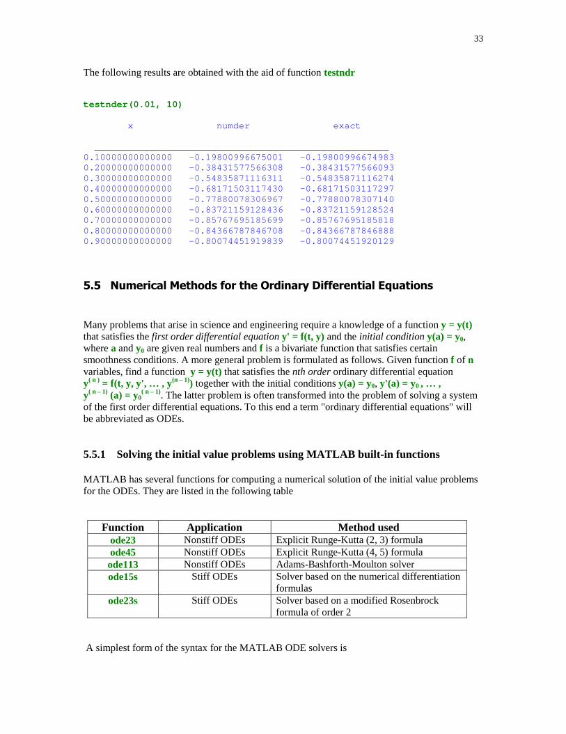
33

The following results are obtained with the aid of function testndr

testnder(0.01, 10)

x numder exact

_____________________________________________________0.10000000000000 -0.19800996675001 -0.198009966749830.20000000000000 -0.38431577566308 -0.384315775660930.30000000000000 -0.54835871116311 -0.548358711162740.40000000000000 -0.68171503117430 -0.681715031172970.50000000000000 -0.77880078306967 -0.778800783071400.60000000000000 -0.83721159128436 -0.837211591285240.70000000000000 -0.85767695185699 -0.857676951858180.80000000000000 -0.84366787846708 -0.843667878468880.90000000000000 -0.80074451919839 -0.80074451920129

���� ������ ��� ������ %� �����&��� � �����)*�������

Many problems that arise in science and engineering require a knowledge of a function y = y(t)that satisfies the first order differential equation y' = f(t, y) and the initial condition y(a) = y0,where a and y0 are given real numbers and f is a bivariate function that satisfies certainsmoothness conditions. A more general problem is formulated as follows. Given function f of nvariables, find a function y = y(t) that satisfies the nth order ordinary differential equationy( n ) = f(t, y, y', … , y(n – 1)) together with the initial conditions y(a) = y0, y'(a) = y0

', … ,y( n – 1) (a) = y0

( n – 1). The latter problem is often transformed into the problem of solving a systemof the first order differential equations. To this end a term "ordinary differential equations" willbe abbreviated as ODEs.

5.5.1 Solving the initial value problems using MATLAB built-in functions

MATLAB has several functions for computing a numerical solution of the initial value problemsfor the ODEs. They are listed in the following table

Function Application Method usedode23 Nonstiff ODEs Explicit Runge-Kutta (2, 3) formulaode45 Nonstiff ODEs Explicit Runge-Kutta (4, 5) formulaode113 Nonstiff ODEs Adams-Bashforth-Moulton solverode15s Stiff ODEs Solver based on the numerical differentiation

formulasode23s Stiff ODEs Solver based on a modified Rosenbrock

formula of order 2

A simplest form of the syntax for the MATLAB ODE solvers is

34

[t, y] = solver(fun, tspan, y0], where fun is a string containing name of the ODE m-file thatdescribes the differential equation, tspan is the interval of integration, and y0 is the vectorholding the initial value(s). If tspan has more than two elements, then solver returns computedvalues of y at these points. The output parameters t and y are the vectors holding the points ofevaluation and the computed values of y at these points.

In the following example we will seek a numerical solution y at t = 0, .25, .5, .75, 1 to thefollowing initial value problem y' = -2ty2, with the initial condition y(0) = 1. We will use both theode23 and the ode45 solvers. The exact solution to this problem is y(t) = 1/(1 + t2) (see, e.g., [6],p.289). The ODE m-file needed in these computations is named eq1

function dy = eq1(t,y)

% The m-file for the ODE y' = -2ty^2.

dy = -2*t.*y(1).^2;

format long

tspan = [0 .25 .5 .75 1]; y0 = 1;

[t1 y1] = ode23('eq1', tspan, y0);[t2 y2] = ode45('eq1', tspan, y0);

To compare obtained results let us create a three-column table holding the points of evaluationand the y-values obtained with the aid of the ode23 and the ode45 solvers

[t1 y1 y2]

ans = 0 1.00000000000000 1.00000000000000 0.25000000000000 0.94118221525751 0.94117646765650 0.50000000000000 0.80002280597122 0.79999999678380 0.75000000000000 0.64001788410487 0.63999998775736 1.00000000000000 0.49999658522366 0.50000000471194

Next example deals with the system of the first order ODEs

y1'(t) = y1(t) – 4y2(t), y2'(t) = -y1(t) + y2(t), y1(0) = 1; y2(0) = 0.

Instead of writing the ODE m – file for this system, we will use MATLAB inline function

dy = inline('[1 –4;-1 1]*y', 't', 'y')

dy = Inline function: dy(t,y) = [1 –4;-1 1]*y

35

The inline functions are created in the Command Window. Interval over wich numerical solution iscomputed and the initial values are stored in the vectors tspan and y0, respectively

tspan = [0 1]; y0 = [1 0];

Numerical solution to this system is obtained using the ode23 function

[t,y] = ode23(dy, tspan, y0);

Graphs of y1(t) (solid line) and y2(t) (dashed line) are shown below

plot(t,y(:,1),t,y(:,2),'--'), legend('y1','y2'), xlabel('t'),ylabel('y(t)'), title('Numerical solutions y_1(t) and y_2(t)')

0 0.2 0.4 0.6 0.8 1-6

-4

-2

0

2

4

6

8

10

12

t

y(t)

Numerical solutions y1(t) and y2(t)

y1y2

The exact solution (y1(t), y2(t)) to this system is

y1, y2

y1 =1/2*exp(-t)+1/2*exp(3*t)y2 =-1/4*exp(3*t)+1/4*exp(-t)

Functions y1 and y2 were found using command dsolve which is available in the Symbolic MathToolbox.

Last example in this section deals with the stiff ODE. Consider

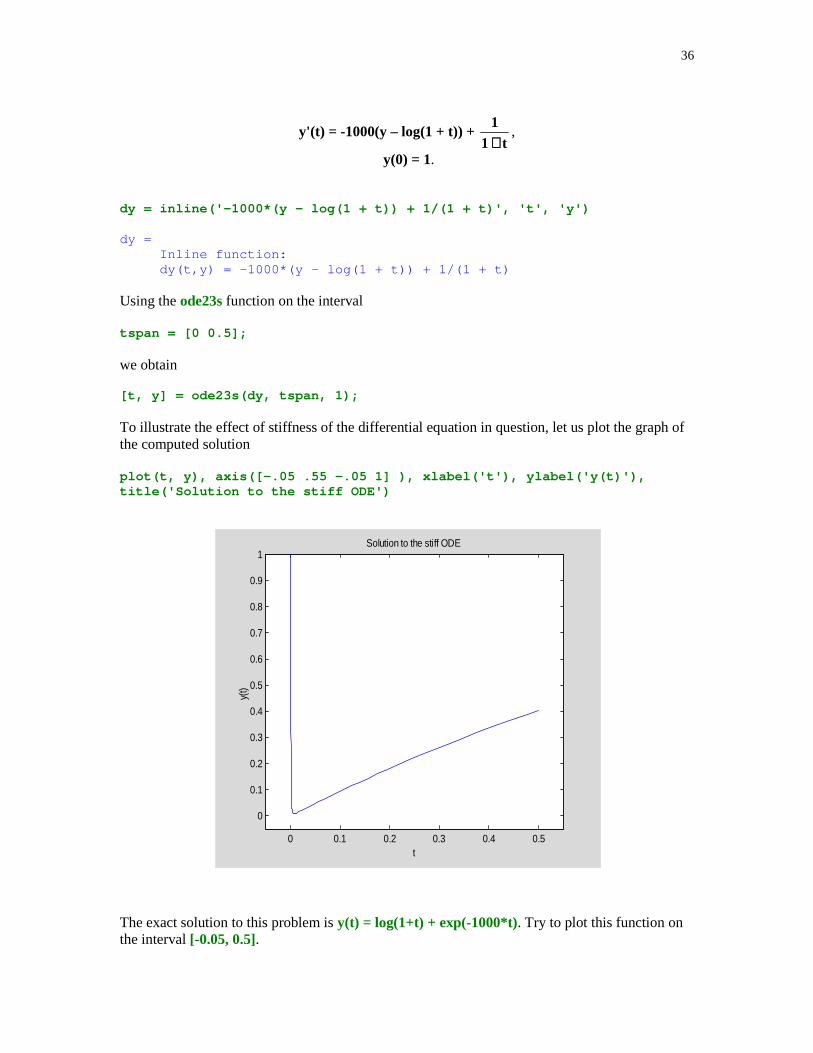
36

y'(t) = -1000(y – log(1 + t)) + t1

1+

,

y(0) = 1.

dy = inline('-1000*(y – log(1 + t)) + 1/(1 + t)', 't', 'y')

dy = Inline function: dy(t,y) = -1000*(y – log(1 + t)) + 1/(1 + t)

Using the ode23s function on the interval

tspan = [0 0.5];

we obtain

[t, y] = ode23s(dy, tspan, 1);

To illustrate the effect of stiffness of the differential equation in question, let us plot the graph ofthe computed solution

plot(t, y), axis([-.05 .55 -.05 1] ), xlabel('t'), ylabel('y(t)'),title('Solution to the stiff ODE')

0 0.1 0.2 0.3 0.4 0.5

0

0.1

0.2

0.3

0.4

0.5

0.6

0.7

0.8

0.9

1

t

y(t)

Solution to the stiff ODE

The exact solution to this problem is y(t) = log(1+t) + exp(-1000*t). Try to plot this function onthe interval [-0.05, 0.5].

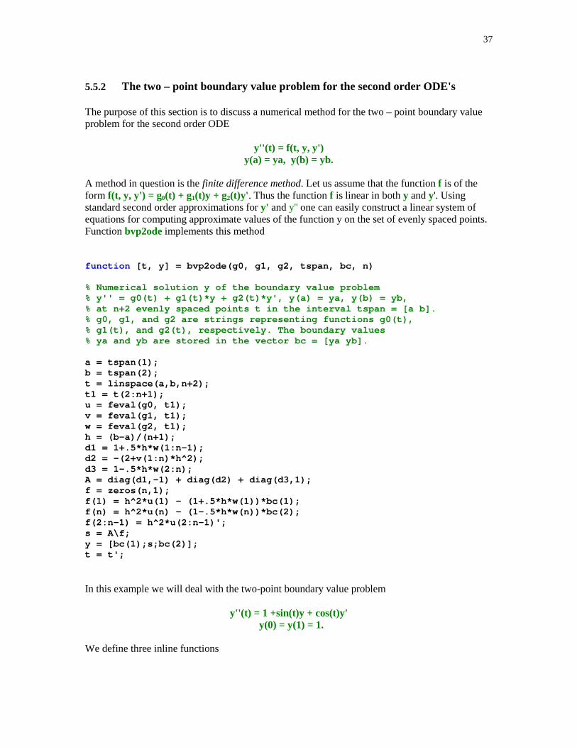
37

5.5.2 The two – point boundary value problem for the second order ODE's

The purpose of this section is to discuss a numerical method for the two – point boundary valueproblem for the second order ODE

y''(t) = f(t, y, y')y(a) = ya, y(b) = yb.

A method in question is the finite difference method. Let us assume that the function f is of theform f(t, y, y') = g0(t) + g1(t)y + g2(t)y' . Thus the function f is linear in both y and y'. Usingstandard second order approximations for y' and y'' one can easily construct a linear system ofequations for computing approximate values of the function y on the set of evenly spaced points.Function bvp2ode implements this method

function [t, y] = bvp2ode(g0, g1, g2, tspan, bc, n)

% Numerical solution y of the boundary value problem% y'' = g0(t) + g1(t)*y + g2(t)*y', y(a) = ya, y(b) = yb,% at n+2 evenly spaced points t in the interval tspan = [a b].% g0, g1, and g2 are strings representing functions g0(t),% g1(t), and g2(t), respectively. The boundary values% ya and yb are stored in the vector bc = [ya yb].

a = tspan(1);b = tspan(2);t = linspace(a,b,n+2);t1 = t(2:n+1);u = feval(g0, t1);v = feval(g1, t1);w = feval(g2, t1);h = (b-a)/(n+1);d1 = 1+.5*h*w(1:n-1);d2 = -(2+v(1:n)*h^2);d3 = 1-.5*h*w(2:n);A = diag(d1,-1) + diag(d2) + diag(d3,1);f = zeros(n,1);f(1) = h^2*u(1) - (1+.5*h*w(1))*bc(1);f(n) = h^2*u(n) - (1-.5*h*w(n))*bc(2);f(2:n-1) = h^2*u(2:n-1)';s = A\f;y = [bc(1);s;bc(2)];t = t';

In this example we will deal with the two-point boundary value problem

y''(t) = 1 +sin(t)y + cos(t)y' y(0) = y(1) = 1.

We define three inline functions

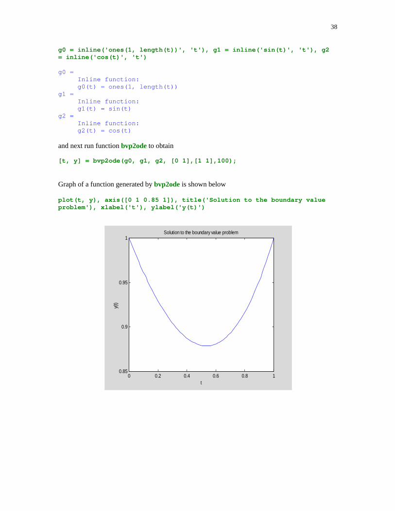
38

g0 = inline('ones(1, length(t))', 't'), g1 = inline('sin(t)', 't'), g2= inline('cos(t)', 't')

g0 = Inline function: g0(t) = ones(1, length(t))g1 = Inline function: g1(t) = sin(t)g2 = Inline function: g2(t) = cos(t)

and next run function bvp2ode to obtain

[t, y] = bvp2ode(g0, g1, g2, [0 1],[1 1],100);

Graph of a function generated by bvp2ode is shown below

plot(t, y), axis([0 1 0.85 1]), title('Solution to the boundary valueproblem'), xlabel('t'), ylabel('y(t)')

0 0.2 0.4 0.6 0.8 10.85

0.9

0.95

1Solution to the boundary value problem

t

y(t)

39

" � � �� �

[1] B.C. Carlson, Special Functions of Applied Mathematics, Academic Press, New York, 1977.

[2] W. Cheney and D. Kincaid, Numerical Mathematics and Computing, Fourth edition, Brooks/Cole Publishing Company, Pacific Grove, 1999.

[3] P.J. Davis and P. Rabinowitz, Methods of Numerical Integration, Academic Press, New York, 1975.

[4] L.V. Fausett, Applied Numerical Analysis Using MATLAB, Prentice Hall, Upper Saddle River, NJ, 1999.

[4] D. Hanselman and B. Littlefield, Mastering MATLAB 5. A Comprehensive Tutorial and Reference, Prentice Hall, Upper Saddle River, NJ, 1998.

[6] M.T. Heath, Scientific Computing: An Introductory Survey, McGraw-Hill, Boston, MA, 1997.

[7] N.J. Higham, Accuracy and Stability of Numerical Algorithms, SIAM, Philadelphia, PA, 1996.

[8] G. Lindfield and J. Penny, Numerical Methods Using MATLAB, Ellis Horwood, New York, 1995.

[9] J.H. Mathews and K.D. Fink, Numerical Methods Using MATLAB, Third edition, Prentice Hall, Upper Saddle River, NJ, 1999.

[10] MATLAB, The Language of Technical Computing. Using MATLAB, Version 5, The MathWorks, Inc., 1997.

[11] J.C. Polking, Ordinary Differential Equations using MATLAB, Prentice Hall, Upper Saddle River, NJ, 1995.

[12] Ch.F. Van Loan, Introduction to Scientific Computing. A Matrix-Vector Approach Using MATLAB, Prentice Hall, Upper Saddle River, NJ, 1997.

[13] H.B. Wilson and L.H. Turcotte, Advanced Mathematics and Mechanics Applications Using MATLAB, Second edition, CRC Press, Boca Raton, 1997.

40

+��,� ��

1. Give an example of a polynomial of degree n � 3 with real roots only for which functionroots fails to compute a correct type of its roots.

2. All roots of the polynomial p(x) = a0 + a1x + … + an-1xn-1 + xn , with real coefficients

ak ( k = 0, 1, … n - 1), are the eigenvalues of the companion matrix

A =

−−−− −1n210 a...aaa

.....

0...100

00...10

Write MATLAB function r = polroots(a) that takes a one-dimensional array a of the coefficients of the polynomial p(x) in the descending order of powers and returns its roots in the array r . Organize your work as follows:

(i) Create a matrix A. You may wish to use MATLAB's built-in function diag to avoidusing loops. Function diag takes a second argument that can be used to put asuperdiagonal in the desired position.

(ii) Use MATLAB's function eig to compute all eigenvalues of the companion matrix A.See Tutorial 4 for more details about the matrix eigenvalue problem.

3. Write MATLAB function [r, niter] = fpiter(g, x0, maxiter) that computes a zero r of x = g(x) using the fixed-point iteration xn + 1 = g(xn), n = 0, 1, … with a given initial approximation x0 of r . The input parameter maxiter is the maximum number of allowed iterations while the output parameter niter stands for the number of iterations performed. Use an appropriate stopping criterion to interrupt computations when current approximation satisfies the exit condition of your choice.

4. In this exercise you are to test function fpiter of Problem 3. Recall that a convergent sequence {x(k)}, with the limit r , has the order of convergence � if

|x(k+1) – r| � C|x(k) – r|�, for some C > 0.

If � = 1, then C < 1.

(i) Construct at least one equation of the form x = g(x), with at least one real zero, forwhich function fpiter computes a sequence of approximations {xn} that convergesto the zero of your function. Print out consecutive approximations of the zero r anddetermine the order of convergence.

(ii) Repeat previous part where this time a sequence of approximations generated bythe function fpiter does not converge to the zero r . Explain why a computedsequence diverges.

41

5. Derive Newton's iteration for a problem of computing the reciprocal of a nonzero number a.

(i) Does your iteration always converge for any value of the initial guess x0?(ii) Write MATLAB function r = recp(a, x0) that computes the reciprocal of a using

Newton's method with the initial guess x0.(iii) Run function recp for the following following values of (a, x0) : (2, 0.3) and (10, 0.15) and print out consecutive approximations generated by the function recp and determine the order of convergence.

6. In this exercise you are to write MATLAB function [r, niter] = Sch(f, derf, x0, m, tol) to compute a multiple root r of the function f(x). Recall that r is a root of multiplicity m of f(x) if f(x) = (x – r)mg(x), for some function g(x). Schroder (see [8]) has proposed the following iterative scheme for computing a multiple root r of f(x)

xk+1 = xk – mf(xk)/f '(xk), k = 0, 1, … .

When m = 1, this method becomes the Newton – Raphson method. The input parameters: f is the function with a multiple root r , derf is the first derivative of f, x0 is the initial guess, m stands for the multiplicity of r and tol is the assumed tolerance for the computed root. The output parameters: r is the computed root and niter is the number of performed iterations.

7. In this exercise you are to test function Sch of Problem 6.

(i) Use function f2 defined in Section 5.2 and write function derf2 to compute the firstorder derivative of a function in file f2.

(ii) Use unexpanded form for the derivative. Run function Sch with m = 5 then repeatthis experiment letting m = 1. In each case choose x0 = 0. Compare number ofiterations performed in each case.

(iii) Repeat the above experiment using function f3. You will need a function derf3 toevaluate the first derivative in the expanded form.

8. Let p(x) be a cubic polynomial with three distinct real roots r k , k = 1, 2, 3. Suppose that the exact values of r 1 and r 2 are available. To compute the root r 3 one wants to use function Sch of Problem 6 with m = 1 and x0 = (r1 + r2)/2. How many iterations are needed to compute r 3?

9. Based on your observations made during the numerical experiments performed whensolving Problem 8 prove that only one step of the Newton-Raphson method is needed tocompute the third root of p(x).

10. Given a system of nonlinear equations

x2/16 + y2/4 = 1x2 – y2 = 1

Use function NR to compute all the zeros of this system. Compare your results with the exactvalues x = 2 and y = 3. Evaluate function f at the computed zeros and print your resultsusing format long.

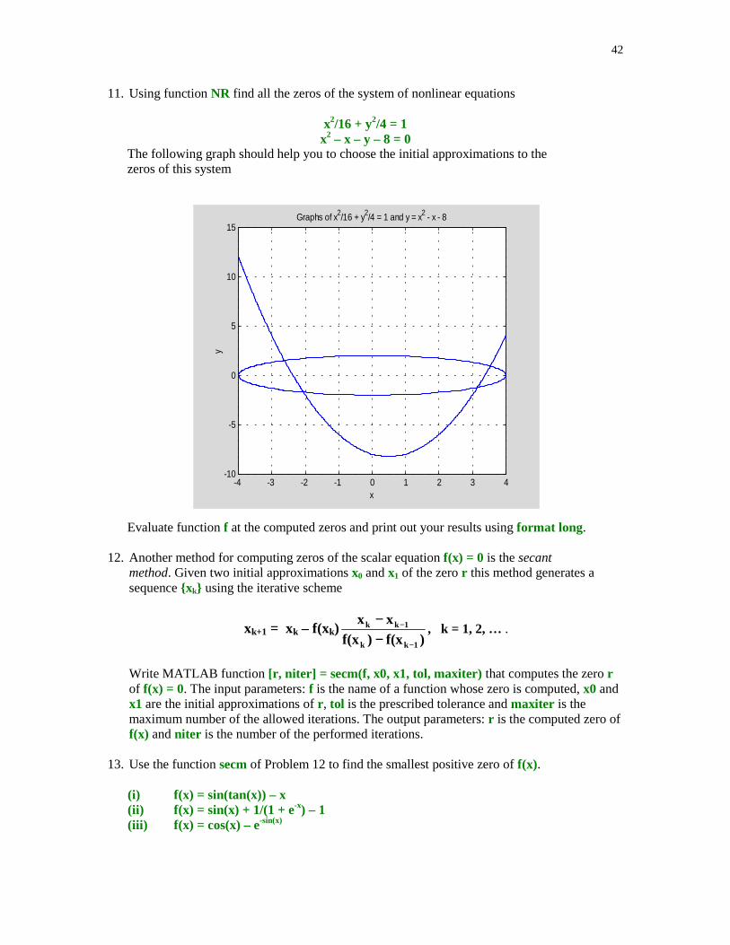
42

11. Using function NR find all the zeros of the system of nonlinear equations

x2/16 + y2/4 = 1x2 – x – y – 8 = 0

The following graph should help you to choose the initial approximations to the zeros of this system

-4 -3 -2 -1 0 1 2 3 4-10

-5

0

5

10

15

x

yGraphs of x2/16 + y2/4 = 1 and y = x2 - x - 8

Evaluate function f at the computed zeros and print out your results using format long.

12. Another method for computing zeros of the scalar equation f(x) = 0 is the secantmethod. Given two initial approximations x0 and x1 of the zero r this method generates asequence {xk} using the iterative scheme

xk+1 = xk – f(xk))f(x)f(x

xx

1kk

1kk

−

−

−−

, k = 1, 2, … .

Write MATLAB function [r, niter] = secm(f, x0, x1, tol, maxiter) that computes the zero rof f(x) = 0. The input parameters: f is the name of a function whose zero is computed, x0 andx1 are the initial approximations of r , tol is the prescribed tolerance and maxiter is themaximum number of the allowed iterations. The output parameters: r is the computed zero off(x) and niter is the number of the performed iterations.

13. Use the function secm of Problem 12 to find the smallest positive zero of f(x).

(i) f(x) = sin(tan(x)) – x(ii) f(x) = sin(x) + 1/(1 + e-x) – 1(iii) f(x) = cos(x) – e-sin(x)

43

Evaluate each function f at the computed zero and print out results using format long.

14. Another form of the interpolating polynomial is due to Lagrange and uses as the basis function the so–called fundamental polynomials Lk(x), 0 � k � n. The kth fundamental polynomial Lk is defined as follows: Lk(xk) = 1, Lk(xm) = 0 for k � m, and deg(Lk) � n. Write MATLAB function yi = fundpol(k, x, xi) which evaluates the kth Lagrange fundamental polynomial at points stored in the array xi.

15. The Lagrange form of the interpolating polynomial pn(x) of degree at most n whichinterpolates the data (xk , yk), 0 � k � n, is

pn(x) = y0L0(x) + y1L1(x) + … + ynLn(x)

Write MATLAB function yi = Lagrpol(x, y, xi) that evaluates polynomial pn at points storedin the array xi. You may wish to use function fundpol of Problem 14.

16. In this exercise you are to interpolate function g(x), a � x � b, using functions Newtonpol(see Section 5.3) and Lagrpol (see Problem 15). Arrays x, y, and xi are defined as follows

xk = a + k(b - a)/10, yk = g(xk), k = 0, 1, … , 10, and xi = linspace(a, b). Run both functions using the following functions g(x) and the associated intervals [a, b]

(i) g(x) = sin(4�x), [a, b] = [0, 1]

(ii) g(x) = J0(x), [a, b] = [2, 3],

where J0 stands for the Bessel function of the first kind of order zero. In MATLAB Besselfunction J0(x) can be evaluated using command besselj(0, x).In each case find the values yi of the interpolating polynomial at xi and compute the error

maximum err = norm(abs(yi - g(xi)), 'inf ') . Compare efficiency of two methods used to interpolate function g(x). Which method is more efficient? Explain why.

17. Continuation of Problem 16. Using MATLAB's function interp1, with options 'cubic' and'spline', interpolate both functions g(x) of Problem 16 and answer the same questions asstated in this problem. Among four method if interpolation you have used to interpolatefunctions g(x) which method is the the best one as long as

(i) efficiency is considered?

(ii) accuracy is considered?

18. The Lebesgue function �(x) of the interpolating operator is defined as follows

�(x) = |Lo(x)| + |L1(x)| + … +|Ln(x)|,

where Lk stands for the kth fundamental polynomial introduced in Problem 14. This function was investigated in depth by numerous researchers. It's global maximum over the interval of interpolation provides a useful information about the error of interpolation. In this exercise you are to graph function �(x) for various sets of the interpolating abscissa {xk}. We will assume that the points of interpolation are symmetric with respect to the origin, i.e., -xk = xn - k, for k = 0, 1, … , n. Without loss of generality, we may also assume

44

that -x0 = xn = 1. Plot the graph of the Lebesgue function �(x) for the following choices of the points xk

(i) xk = -1 +2k/n, k = 0, 1, … , n

(ii) xk = -cos(k�/n), k = 0, 1, … , n

In each case put n = 1, 2, 3 and estimate the global maximum of �(x). Which set of the interpolating abscissa provides a smaller value of Max{�(x) : x0 � x � xn}?

19. MATLAB's function polyder computes the first order derivative of an algebraic polynomialthat is represented by its coefficients in the descending order of powers. In this exercise youare to write MATLAB function B = pold(A, k) that computes the kth order derivative ofseveral polynomials of the same degree whose coefficients are stored in the consecutive rowsof the matrix A. This utility function is useful in manipulations with splines that arerepresented as the piecewise polynomial functions.Hint : You may wish to use function polyder.

20. The Hermite cubic spline interpolant s(x) with the breakpoints � = {xx < x2 < … < xm} is amember of Sp(3, 1, �) that is uniquely determined by the interpolatory conditions

(i) s(xl) = yl, l = 1, 2, … , m (ii) s'(xl) = pl, l = 1, 2, … , m

On the subinterval [xl , xl+1] , l = 1, 2, … , m – 1, s(x) is represented as follows

s(x) = (1 + 2t)(1 – t)2yl + (3 – 2t)t2yl+1 + hl[t(1 – t)2pl + t2(t – 1)pl+1],

where t = (x – xl)/(xl+1 – xl) and hl = xl+1 – xl. Prove that the Hermite cubic spline interpolant s(x) is convex on the interval [x1, xm] if and only if the following inequalities

3

p2p

h

ss

3

pp2 1ll

l

l1l1ll +++ +≤

−≤

+

are satisfied for all l = 1, 2, … , m - 1.

21. Write MATLAB function [pts, yi] = Hermspl(x, y, p) that computes coefficients of theHermite cubic spline interpolant s(x) described in Problem 20 and evaluates spline interpolantat points stored in the array xi. Parameters x, y, and p stand for the breakpoints, values ofs(x), and values of s'(x) at the breakpoints of s(x), respectively. The output parameter yi is thearray of values of s(x) at points stored in the array pts which is defined as the union of thearrays linspace(x(k), x(k+1)), k = 1, 2, … , n – 1, where n = length(x).

Hint: You may wish to use function Hermpol discussed in Section 5.3.

22. The nodes {xk} of the Newton – Cotes formulas of the open type are defined as follows xk = a + (k – 1/2)h, k = 1, 2, … , n – 1, where h = (b – a)/(n – 1). Write MATLAB function [s, w, x] = oNCqf(fun, a, b, n, varargin) that computes an approximate value s of

45

the integral of the function that is represented by the string fun. Interval of integration is [a, b] and the method used is the n-point open formula whose weights and nodes are are stored in the arrays w and x, respectively.

23. The Fresnel integral

f(x) = dt)2ti

exp(x

0

2

∫ π

is of interest in several areas of applied mathematics. Write MATLAB function [fr1, fr2] =Fresnel(x, tol, n) which takes a real array x, a two dimensional vector tol holding the relativeand absolute tolerance for the error of the computed integral (see MATLAB help file for thefunction quad8), and a positive integer n used in the function Romberg and returns numericalapproximations fr1 and fr2 of the Fresnel integral using each of the following methods

(i) quad8 with tolerance tol = [1e-8 1e-8](ii) Romberg with n = 10

Compute Fresnel integrals for the following values of x = 0: 0.1:1.To compare the

approximations fr1 and fr2 calculate the number of decimal places of accuracy dpa = –log10(norm(fr1 – fr2, 'inf ')). For what choices of the input parameters tol and n the

number dpa is greater than or equal to 13? The last inequality must be satisfied for all valuesx as defined earlier.

24. Let us assume that the real-valued function f(x) has a convergent integral

∫∞

0

dx)x(f .

Explain how would you compute an approximate value of this integral using function Gquad2 developed earlier in this chapter? Extend your idea to convergent integrals of the form

∫∞

∞−

.dx)x(f

25. The following integral is discussed in [3], p. 317

J = ∫− ++

1

124 9.0xx

dx.

To compute an approximate value of the integral J use

(i) MATLAB functions quad and quad8 with tolerance tol = [1e-8 1e-8](ii) functions Romberg and Gquad1 with n = 8.

Print out numerical results using format long. Which method should be recommended fornumerical integration of the integral J? Justify your answer.

46

26. The arc length s of the ellipse

1b

y

a

x2

2

2

2

=+

from (a, 0) to (x, y) in quadrant one is equal to

s = b dttsink10

22∫ −θ

where k2 = 1 – (a/b)2 , a ≤ b, and ).b/yarcsin()a/xarccos( ==θ In this exercise you are to write MATLAB function [sR, sq8] = arcell(a, b, x, n, tol) that takes as the input parameters the semiaxes a and b and the x – coordinate of the point on the ellipse in quadrant one and returns an approximate value of the arc of ellipse from (a, 0) to (x, y) using functions Romberg, described in this chapter, and the MATLAB function quad8. The fourth input parameter n will be used by the function Romberg. The fifth input parameter tol is optional and it holds the user supplied tolerances for the relative and absolute errors in the computed approximation sq8. If tol is not supplied, the default values for tolerances should be assigned. For more details about using this parameter, type help quad8 in the Command Window. Your program should also work for ellipses whose semiaxes are not restricted to those in the definition of the parameter k2. Test your function for the following values of the input parameters

(i) a = 1, b = 2, x = 1: -0.1: 0, n = 10, tol = [ ] (ii) a = 2, b = 1, x = 2: -0.2: 0, n = 10, tol = [ ] (iii) a = 2, b = 1, x = 0: -0.2: -2, n = 10, tol = [ ]

Note that the terminal points (x, y) of the third ellipse lie in quadrant two.

27. Many of the most important special functions can be represented as the Dirichlet average Fof a continuous function f (see [1] )

F(b1, b2 ; a, b) = ,dt]b)t1(ta[f)t1(t)b,b(B

1 1b1

0

1b

21

21 −+− −−∫

where B(b1, b2), (b1, b2 > 0) stands for the beta function. Of special interest are the Dirichlet averages of elementary functions f(t) = t -c and f(t) = et. Former gives raise to the hypergeometric functions such as a celebrated Gauss hypergeometric function 2F1 while the latter is used to represent the confluent hypergeometric functions. In this exercise you are to implement a method for approximating the Dirichlet integral defined above using f(t) = t -c. Write MATLAB function y = dav(c, b1, b2, a, b) which computes a numerical approximation of the Dirichlet average of f. Use a method of your choice to integrate numerically the Dirichlet integral. MATLAB has a function named beta designed for evaluating the beta function. Test your function for the following values of the parameter c:

c = 0 (exact value of the Dirichlet average F is equal to 1)

47

c = b1 + b2 (exact value of the Dirichlet average is equal to 1/(ab1 b

b2).

28. Gauss hypergeometric function 2F1(a, b; c; x) is defined by the infinite power series asfollows

2F1(a, b; c; x) = n

0n

x!n)n,c(

)n,b)(n,a(∑∞

=

, |x| ≤ 1,

where (a, n) = a(a + 1) … (a + n – 1) is the Appel symbol. Gauss hypergeometric function can be represented as the Dirichlet average of the power function f(t) = t -a

2F1(a, b; c; x) = F(b, c – b; 1 – x, 1) (c > b > 0, |x| < 1).

Many of the important elementary functions are special cases of this function. For instance for |x| < 1, the following formulas

arcsin x = 2F1(0.5, 0.5; 1.5; x2)ln(1 + x) = x2F1(1, 1; 1.5; x2)

arctanh x = x2F1(0.5, 1; 1.5; x2)

hold true. In this exercise you are to use function dav of Problem 27 to evaluate three functions listed above for x = -0.9 : 0.1 : 0.9. Compare obtained approximate values with those obtained by using MATLAB functions asin, log, and atanh.

29 Let a and b be positive numbers. In this exercise you will deal with the four formulas forcomputing the mean value of a and b. Among the well – known means the arithmetic mean

A(a, b) = (a + b)/2 and the geometric mean G(a, b) = ab are the most frequently usedones. Two less known means are the logarithmic mean L and the identric mean I

L(a, b) = blnaln

ba−−

I(a, b) = e-1(aa/bb)1/(a – b)

The logarithmic and identric means are of interest in some problems that arise in economics, electrostatics, to mention a few areas only. All four means described in this problem can be represented as the Dirichlet averages of some elementary functions. For the means under discussion their b – parameters are both equal to one. Let M(a, b) stand for any of these means. Then

M(a, b) = f -1( F(1, 1; a, b) )

where f -1 stands for the inverse function of f and F is the Dirichlet average of f. In this exercise you will deal with the means described earlier in this problem.

48

(i) Prove that the arithmetic, geometric, logarithmic and identric means can berepresented as the inverse function of the Dirichlet average of the followingfunctions f(t) = t , f(t) = t -2, f(t) = t -1 and f(t) = ln t , respectively.

(ii) The logarithmic mean can also be represented as

.dtba)b,a(L t11

0

t −∫=

Establish this formula.(iii) Use the integral representations you found in the previous part together with the

midpoint and the trapezoidal quadrature formulas (with the error terms) to establishthe following inequalities: G ≤ L ≤ A and G ≤ I ≤ A. For the sake of brevity thearguments a and b are omitted in these inequalities.

30. A second order approximation of the second derivative of the function f(x) is

f ''(x) = )h(Oh

)hx(f)x(f2)hx(f 22 +−+−+

.

Write MATLAB function der2 = numder2(fun, x, h, n, varargin) that computes an approximate value of the second order derivative of a function named by the string fun at the point x. Parameters h and n are user-supplied values of the initial step size and the number of performed iterations in the Richardson extrapolation. For functions that depend on parameters their values must follow the parameter n. Test your function for f(x) = tan x with x = �/4 and h = 0.01. Experiment with different values for n and compare your results with the exact value f ''( �/4) = 4.

31. Consider the following initial – value problem

y1'''(t) = - y 1(t)y1''(t), y 1(0) = 1, y1'(0) = -1, y1''(0) = 1.

(i) Replace the differential equation by the system of three differential equations oforder one.

(ii) Write a MATLAB function dy = order3(t, y) that evaluates the right – hand sides ofthe equations you found in the previous part.

(iii) Write a script file Problem31 to solve the resulting initial – value problem usingMATLAB solver ode45 on the interval [0 1].

(iv) Plot in the same window graphs of function y1(t) together with its derivatives up toorder two. Add a legend to your graph that clearly describes curves you are plotting.

32. In this exercise you are to deal with the following initial – value problem

x '(t) = -x(t) – y(t), y '(t) = -20x(t) – 2y(t), x(0) = 2, y(0) = 0.

(i) Determine whether or not this system is stiff.(ii) If it is, use an appropriate MATLAB solver to find a numerical solution on the

interval [0 1].(iii) Plot the graphs of functions x(t) and y(t) in the same window.

49

33. The Lotka – Volterra equations describe populations of two species

y1'(t) = y1(t) – y1(t)y2(t), y2'(t) = -15y2(t) + y1(t)y2(t).

Write MATLAB function LV(y10, y20, tspan) that takes the initial values y10 = y1(0) and y20 = y2(0) and plots graphs of the numerical solutions y1 and y2 over the interval tspan.

34. Numerical evaluation of a definite integral

∫b

a

dt)t(f

can be accomplished by solving the ODE y'(t) = f(t) with the initial condition y(a) = 0. Then the integral in question is equal to y(b). Write MATLAB function yb = integral(a, b, fun) which implements this method. The input parameter fun is the string holding the name of the integrand f(t) and a and b are the limits of integration. To find a numerical solution of the ODE use the MATLAB solver ode45. Test your function on integrals of your choice.

35. Given the two – point boundary value problem

y'' = -t + t 2 + et – ty + ty' , y(0) = 1, y(1) = 1 + e.

(i) Use function bvp2ode included in this tutorial to find the approximate values of thefunction y for the following values of n = 8, 18.

(ii) Plot, in the same window, graphs of functions you found in the previous part of theproblem. Also, plot the graph of function y(t) = t + et which is the exact solution tothe boundary value problem in question.

36. Another method for solving the two – point boundary value problem is the collocationmethod. Let

y'' = f(t, y, y') , y(a) = ya, y(b) = yb.

This method computes a polynomial p(t) that approximates a solution y(t) using thefollowing conditions

p(a) = ya, p(b) = yb, p'' (tk) = f(tk, p(tk), p'(t k))

where k = 2, 3, … , n – 1 and a = t1 < t2 < … < tn = b are the collocation points that areevenly spaced in the given interval.In this exercise function f is assumed to be of the form f(t, y, y') = g0(t) + g1(t)y + g2(t)y' .

(i) Set up a system of linear equations that follows from the collocation conditions.(ii) Write MATLAB function p = colloc(g0, g1, g2, a, b, ya, yb, n) which computes

coefficients p of the approximating polynomial. They should be stored in the array pin the descending order of powers. Note that the approximating polynomial is ofdegree n – 1 or less.

37. Test the function colloc of Problem 36 using the two – point boundary value problem ofProblem 35 and plot the graph of the approximating polynomial.

50

��������

��� �����������������������

�������������

Edward NeumanDepartment of Mathematics

Southern Illinois University at Carbondaleedneuman@siu.edu

This tutorial is devoted to the discussion of computational tools that are of interest in linearprogramming (LP). MATLAB powerful tools for computations with vectors and matrices makethis package well suited for solving typical problems of linear programming. Topics discussed inthis tutorial include the basic feasible solutions, extreme points and extreme directions of theconstraint set, geometric solution of the linear programming problem, the Two-Phase Method, theDual Simplex Algorithm, addition of a constraint and Gomory's cutting plane algorithm.

�� �������������� � !����������

Function Descriptionabs Absolute valueall True if all elements of a vector are nonzeroany True if any element of a vector is nonzeroaxis Control axis scaling and appearance

break Terminate execution of for or while loopclc Clear Command Window

convhull Convex hulldiff Difference and approximate derivativedisp Display arrayeps Floating point relative accuracyeye Identity matrixfind Find indices of nonzero of nonzero elements

FontSize Size of a fontgca Get handle to current axisget Get object propertiesgrid Grid lineshold Hold current graphinf Infinity

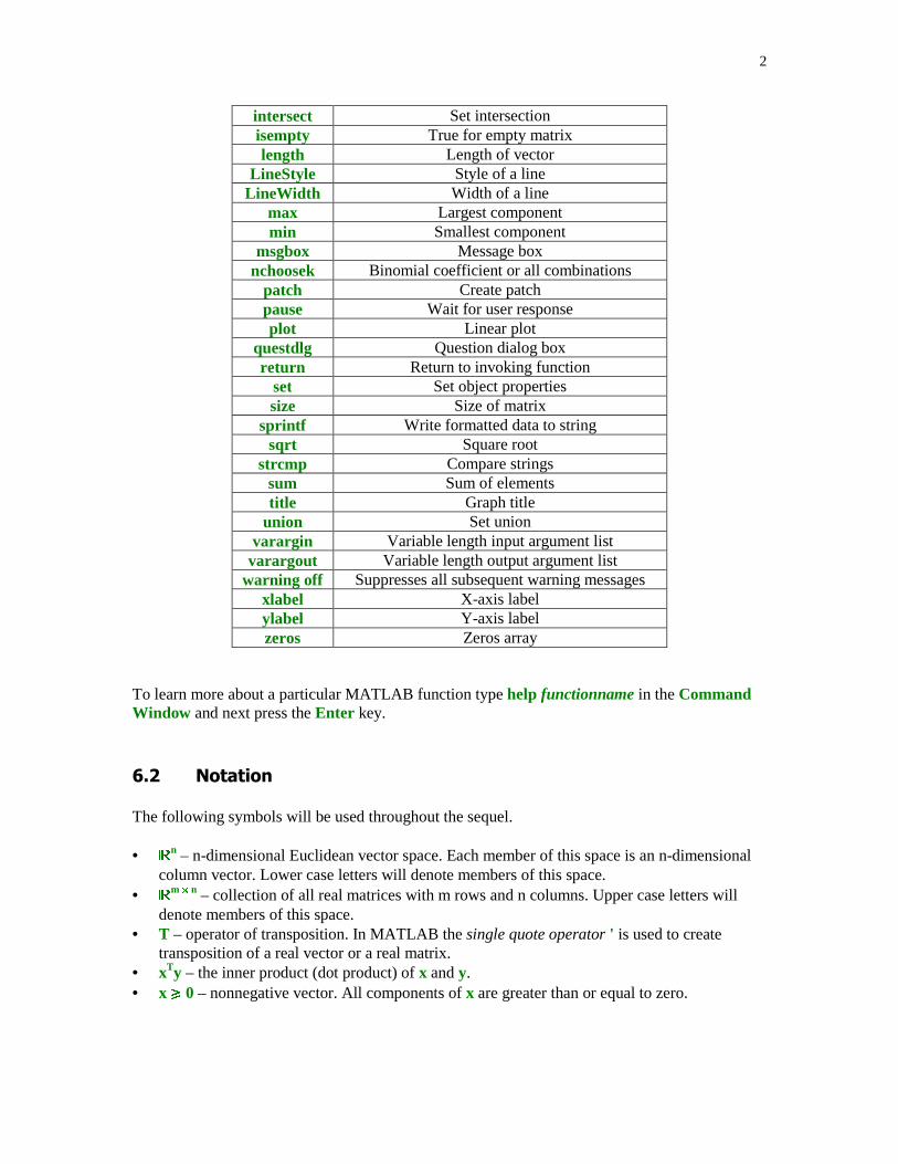
2

intersect Set intersectionisempty True for empty matrixlength Length of vector

LineStyle Style of a lineLineWidth Width of a line

max Largest componentmin Smallest component

msgbox Message boxnchoosek Binomial coefficient or all combinations

patch Create patchpause Wait for user responseplot Linear plot

questdlg Question dialog boxreturn Return to invoking function

set Set object propertiessize Size of matrix

sprintf Write formatted data to stringsqrt Square root

strcmp Compare stringssum Sum of elementstitle Graph title

union Set unionvarargin Variable length input argument listvarargout Variable length output argument list

warning off Suppresses all subsequent warning messagesxlabel X-axis labelylabel Y-axis labelzeros Zeros array

To learn more about a particular MATLAB function type help functionname in the CommandWindow and next press the Enter key.

�� "�������

The following symbols will be used throughout the sequel.

• �n – n-dimensional Euclidean vector space. Each member of this space is an n-dimensional

column vector. Lower case letters will denote members of this space.• �

m � n – collection of all real matrices with m rows and n columns. Upper case letters willdenote members of this space.

• T – operator of transposition. In MATLAB the single quote operator ' is used to createtransposition of a real vector or a real matrix.

• xTy – the inner product (dot product) of x and y.• x � 0 – nonnegative vector. All components of x are greater than or equal to zero.

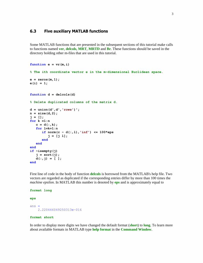
3

�# $�% ��&�����'��������������

Some MATLAB functions that are presented in the subsequent sections of this tutorial make callsto functions named ver, delcols, MRT , MRTD and Br . These functions should be saved in thedirectory holding other m-files that are used in this tutorial.

function e = vr(m,i)

% The ith coordinate vector e in the m-dimensional Euclidean space.

e = zeros(m,1);e(i) = 1;

function d = delcols(d)

% Delete duplicated columns of the matrix d.

d = union(d',d', 'rows' )';n = size(d,2);j = [];for k =1:n c = d(:,k); for l=k+1:n if norm(c - d(:,l), 'inf' ) <= 100*eps j = [j l]; end endendif ~isempty(j) j = sort(j); d(:,j) = [ ];end

First line of code in the body of function delcols is borrowed from the MATLAB's help file. Twovectors are regarded as duplicated if the corresponding entries differ by more than 100 times themachine epsilon. In MATLAB this number is denoted by eps and is approximately equal to

format long

eps

ans = 2.220446049250313e-016

format short

In order to display more digits we have changed the default format (short) to long. To learn moreabout available formats in MATLAB type help format in the Command Window.

4

function [row, mi] = MRT(a, b)

% The Minimum Ratio Test (MRT) performed on vectors a and b.% Output parameters:% row – index of the pivot row% mi – value of the smallest ratio.

m = length(a);c = 1:m;a = a(:);b = b(:);l = c(b > 0);[mi, row] = min(a(l)./b(l));row = l(row);

function col = MRTD(a, b)

% The Maximum Ratio Test performed on vectors a and b.% This function is called from within the function dsimplex.% Output parameter:% col - index of the pivot column.

m = length(a);c = 1:m;a = a(:);b = b(:);l = c(b < 0);[mi, col] = max(a(l)./b(l));col = l(col);

function [m, j] = Br(d)

% Implementation of the Bland's rule applied to the array d.% This function is called from within the following functions:% simplex2p, dsimplex, addconstr, simplex and cpa.% Output parameters:% m - first negative number in the array d% j - index of the entry m.

ind = find(d < 0);if ~isempty(ind) j = ind(1); m = d(j);else m = []; j = [];end

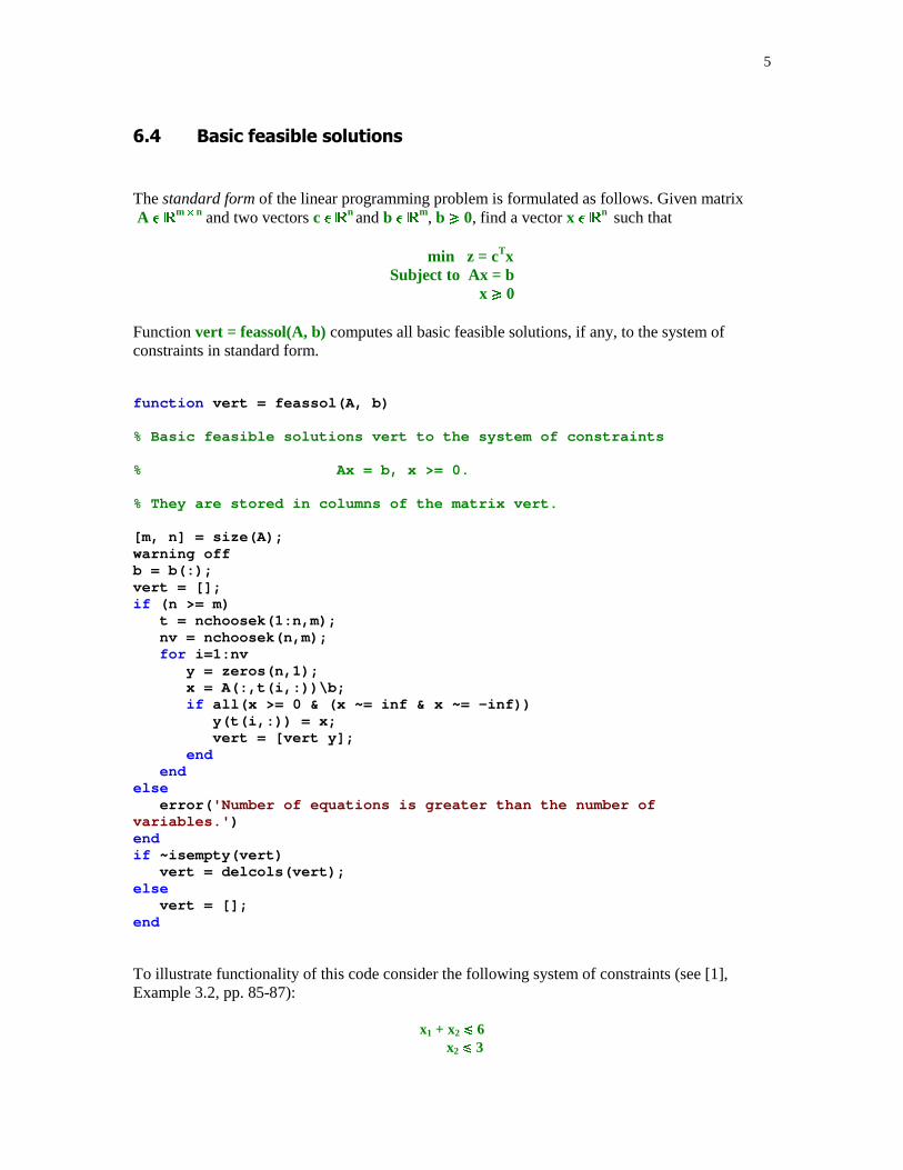
5

�� �� ��� � �(� �������

The standard form of the linear programming problem is formulated as follows. Given matrix A � �m � n and two vectors c � �n and b � �m, b � 0, find a vector x � �n such that

min z = cTxSubject to Ax = b x � 0

Function vert = feassol(A, b) computes all basic feasible solutions, if any, to the system ofconstraints in standard form.

function vert = feassol(A, b)

% Basic feasible solutions vert to the system of constraints

% Ax = b, x >= 0.

% They are stored in columns of the matrix vert.

[m, n] = size(A);warning offb = b(:);vert = [];if (n >= m) t = nchoosek(1:n,m); nv = nchoosek(n,m); for i=1:nv y = zeros(n,1); x = A(:,t(i,:))\b; if all(x >= 0 & (x ~= inf & x ~= -inf)) y(t(i,:)) = x; vert = [vert y]; end endelse error( 'Number of equations is greater than the number ofvariables.' )endif ~isempty(vert) vert = delcols(vert);else vert = [];end

To illustrate functionality of this code consider the following system of constraints (see [1],Example 3.2, pp. 85-87):

x1 + x2 � 6 x2 � 3

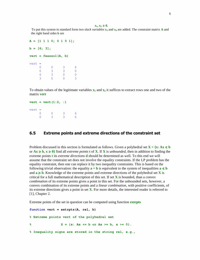
6

x1, x2 � 0.To put this system in standard form two slack variables x3 and x4 are added. The constraint matrix A and

the right hand sides b are

A = [1 1 1 0; 0 1 0 1];

b = [6; 3];

vert = feassol(A, b)

vert = 0 0 3 6 0 3 3 0 6 3 0 0 3 0 0 3

To obtain values of the legitimate variables x1 and x2 it suffices to extract rows one and two of thematrix vert

vert = vert(1:2, :)

vert = 0 0 3 6 0 3 3 0

�) *&�� � +���� ��! &�� � !�� ����� ���� ��� ������ �

Problem discussed in this section is formulated as follows. Given a polyhedral set X = {x: Ax � bor Ax � b, x � 0} find all extreme points t of X. If X is unbounded, then in addition to finding theextreme points t its extreme directions d should be determined as well. To this end we willassume that the constraint set does not involve the equality constraints. If the LP problem has theequality constraint, then one can replace it by two inequality constraints. This is based on thefollowing trivial observation: the equality a = b is equivalent to the system of inequalities a � band a � b. Knowledge of the extreme points and extreme directions of the polyhedral set X iscritical for a full mathematical description of this set. If set X is bounded, than a convexcombination of its extreme points gives a point in this set. For the unbounded sets, however, aconvex combination of its extreme points and a linear combination, with positive coefficients, ofits extreme directions gives a point in set X. For more details, the interested reader is referred to[1], Chapter 2.

Extreme points of the set in question can be computed using function extrpts

function vert = extrpts(A, rel, b)

% Extreme points vert of the polyhedral set

% X = {x: Ax <= b or Ax >= b, x >= 0}.

% Inequality signs are stored in the string rel, e.g.,

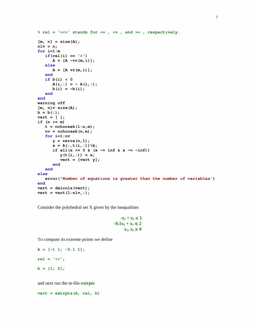
7

% rel = '<<>' stands for <= , <= , and >= , respectively.

[m, n] = size(A);nlv = n;for i=1:m if (rel(i) == '>' ) A = [A -vr(m,i)]; else A = [A vr(m,i)]; end if b(i) < 0 A(i,:) = - A(i,:); b(i) = -b(i); endendwarning off[m, n]= size(A);b = b(:);vert = [ ];if (n >= m) t = nchoosek(1:n,m); nv = nchoosek(n,m); for i=1:nv y = zeros(n,1); x = A(:,t(i,:))\b; if all(x >= 0 & (x ~= inf & x ~= -inf)) y(t(i,:)) = x; vert = [vert y]; end endelse error( 'Number of equations is greater than the number of variables' )endvert = delcols(vert);vert = vert(1:nlv,:);

Consider the polyhedral set X given by the inequalities

-x1 + x2 � 1-0.1x1 + x2 � 2 x1, x2 � 0

To compute its extreme points we define

A = [-1 1; -0.1 1];

rel = '<<';

b = [1; 2];

and next run the m-file extrpts

vert = extrpts(A, rel, b)

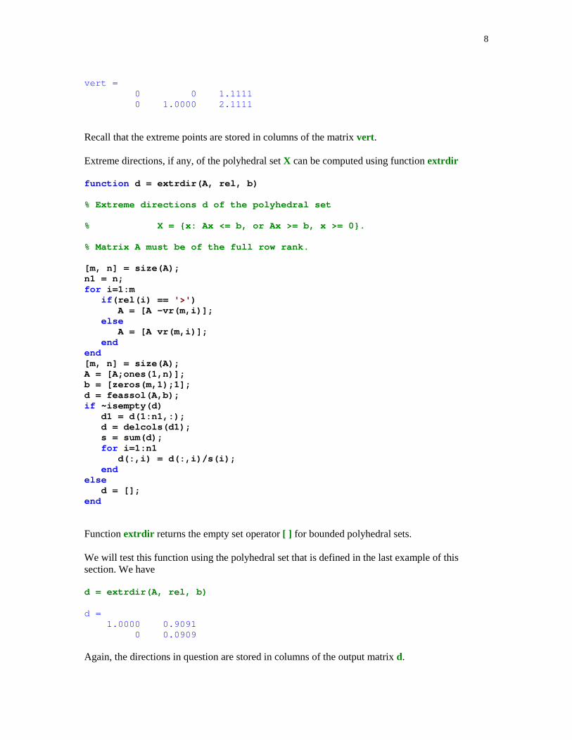
8

vert = 0 0 1.1111 0 1.0000 2.1111

Recall that the extreme points are stored in columns of the matrix vert.

Extreme directions, if any, of the polyhedral set X can be computed using function extrdir

function d = extrdir(A, rel, b)

% Extreme directions d of the polyhedral set

% X = {x: Ax <= b, or Ax >= b, x >= 0}.

% Matrix A must be of the full row rank.

[m, n] = size(A);n1 = n;for i=1:m if (rel(i) == '>' ) A = [A -vr(m,i)]; else A = [A vr(m,i)]; endend[m, n] = size(A);A = [A;ones(1,n)];b = [zeros(m,1);1];d = feassol(A,b);if ~isempty(d) d1 = d(1:n1,:); d = delcols(d1); s = sum(d); for i=1:n1 d(:,i) = d(:,i)/s(i); endelse d = [];end

Function extrdir returns the empty set operator [ ] for bounded polyhedral sets.

We will test this function using the polyhedral set that is defined in the last example of thissection. We have

d = extrdir(A, rel, b)

d = 1.0000 0.9091 0 0.0909

Again, the directions in question are stored in columns of the output matrix d.

9

� ���%����� ��+��(� �� �� �������'

A solution to the LP problem with two legitimate variables x1 and x2 can be found geometricallyin three steps. First, the feasible region described by the constraint system Ax � b or Ax � b with x � 0 is drawn. Next, a direction of the level line z = c1x1 + c2x2 is determined. Finally movingthe level line one can find easily vertex (extreme point) of the feasible region where the minimumor maximum value of z is attained or conclude that the objective function is unbounded. For moredetails see, e.g., [3], Chapter 2 and [1], Chapter 1.

Function drawfr implements two initial steps of this method

function drawfr(c, A, rel, b)

% Graphs of the feasible region and the line level% of the LP problem with two legitimate variables%% min (max)z = c*x% Subject to Ax <= b (or Ax >= b),% x >= 0

clc[m, n] = size(A);if n ~= 2 str = 'Number of the legitimate variables must be equal to 2' ; msgbox(str, 'Error Window' , 'error' ) returnendvert = extrpts(A,b,rel);if isempty(vert) disp(sprintf( '\n Empty feasible region' )) returnendvert = vert(1:2,:);vert = delcols(vert);d = extrdir(A,b,rel);if ~isempty(d) msgbox( 'Unbounded feasible region' , 'Warning Window' , 'warn' ) disp(sprintf( '\n Extreme direction(s) of the constraint set' )) d disp(sprintf( '\n Extreme points of the constraint set' )) vert returnendt1 = vert(1,:);t2 = vert(2,:);z = convhull(t1,t2);hold onpatch(t1(z),t2(z), 'r' )h = .25;mit1 = min(t1)-h;mat1 = max(t1)+h;mit2 = min(t2)-h;

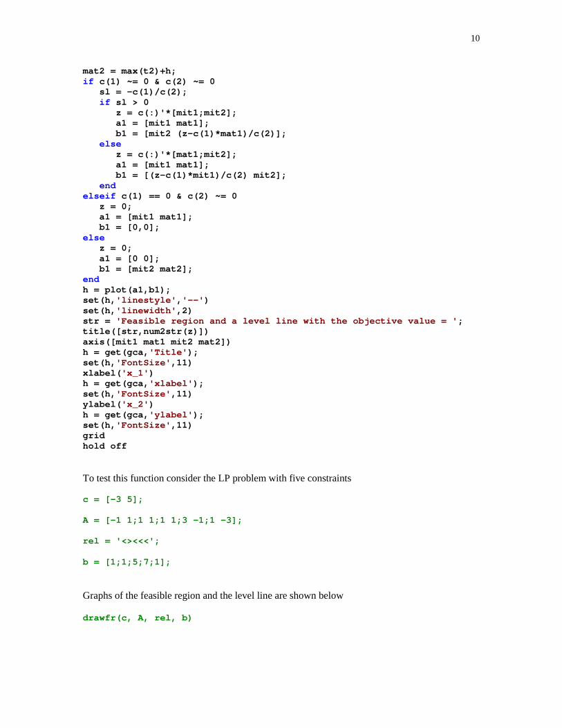
10

mat2 = max(t2)+h;if c(1) ~= 0 & c(2) ~= 0 sl = -c(1)/c(2); if sl > 0 z = c(:)'*[mit1;mit2]; a1 = [mit1 mat1]; b1 = [mit2 (z-c(1)*mat1)/c(2)]; else z = c(:)'*[mat1;mit2]; a1 = [mit1 mat1]; b1 = [(z-c(1)*mit1)/c(2) mit2]; endelseif c(1) == 0 & c(2) ~= 0 z = 0; a1 = [mit1 mat1]; b1 = [0,0];else z = 0; a1 = [0 0]; b1 = [mit2 mat2];endh = plot(a1,b1);set(h, 'linestyle' , '--' )set(h, 'linewidth' ,2)str = 'Feasible region and a level line with the objective value = ' ;title([str,num2str(z)])axis([mit1 mat1 mit2 mat2])h = get(gca, 'Title' );set(h, 'FontSize' ,11)xlabel( 'x_1' )h = get(gca, 'xlabel' );set(h, 'FontSize' ,11)ylabel( 'x_2' )h = get(gca, 'ylabel' );set(h, 'FontSize' ,11)gridhold off

To test this function consider the LP problem with five constraints

c = [-3 5];

A = [-1 1;1 1;1 1;3 –1;1 –3];

rel = '<><<<';

b = [1;1;5;7;1];

Graphs of the feasible region and the level line are shown below

drawfr(c, A, rel, b)

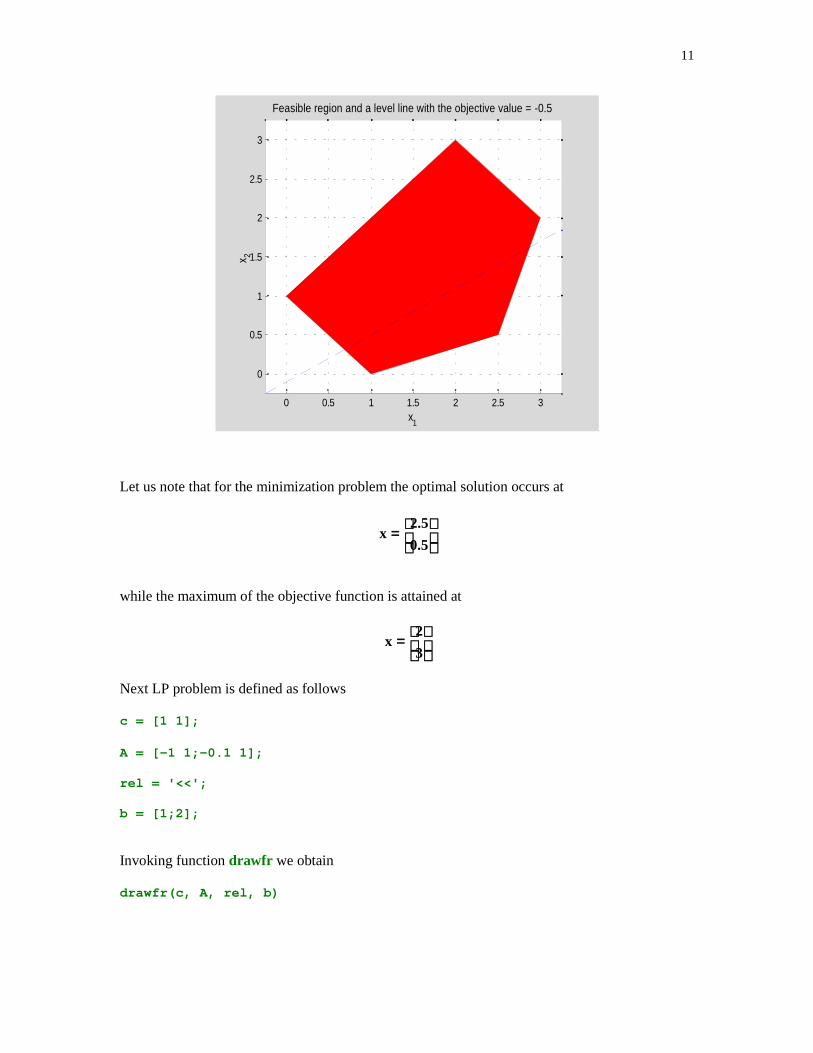
11

0 0.5 1 1.5 2 2.5 3

0

0.5

1

1.5

2

2.5

3

Feasible region and a level line with the objective value = -0.5

x1

x 2

Let us note that for the minimization problem the optimal solution occurs at

=

5.0

5.2x

while the maximum of the objective function is attained at

=3

2x

Next LP problem is defined as follows

c = [1 1];

A = [-1 1;-0.1 1];

rel = '<<';

b = [1;2];

Invoking function drawfr we obtain

drawfr(c, A, rel, b)

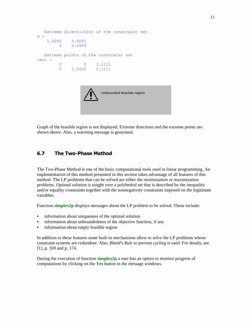
12

Extreme direction(s) of the constraint setd = 1.0000 0.9091 0 0.0909

Extreme points of the constraint setvert = 0 0 1.1111 0 1.0000 2.1111

Unbounded feasible region

Graph of the feasible region is not displayed. Extreme directions and the extreme points areshown above. Also, a warrning message is generated.

�� �� ���,��� � ���!

The Two-Phase Method is one of the basic computational tools used in linear programming. Animplementation of this method presented in this section takes advantage of all features of thismethod. The LP problems that can be solved are either the minimization or maximizationproblems. Optimal solution is sought over a polyhedral set that is described by the inequalityand/or equality constraints together with the nonnegativity constraints imposed on the legitimatevariables.

Function simplex2p displays messages about the LP problem to be solved. These include:

• information about uniqueness of the optimal solution• information about unboundedness of the objective function, if any• information about empty feasible region

In addition to these features some built-in mechanisms allow to solve the LP problems whoseconstraint systems are redundant. Also, Bland's Rule to prevent cycling is used. For details, see[1], p. 169 and p. 174.

During the execution of function simplex2p a user has an option to monitor progress ofcomputations by clicking on the Yes button in the message windows.

13

function simplex2p(type, c, A, rel, b)

% The Two-Phase Method for solving the LP problem

% min(or max) z = c*x% Subject to Ax rel b% x >= 0

% The input parameter type holds information about type of the LP% problem to be solved. For the minimization problem type = 'min' and% for the maximization problem type = 'max'.% The input parameter rel is a string holding the relation signs.% For instance, if rel = '<=>', then the constraint system consists% of one inequality <=, one equation, and one inequality >=.

clcif (type == 'min' ) mm = 0;else mm = 1; c = -c;endb = b(:);c = c(:)';[m, n] = size(A);n1 = n;les = 0;neq = 0;red = 0;if length(c) < n c = [c zeros(1,n-length(c))];endfor i=1:m if (rel(i) == '<' ) A = [A vr(m,i)]; les = les + 1; elseif (rel(i) == '>' ) A = [A -vr(m,i)]; else neq = neq + 1; endendncol = length(A);if les == m c = [c zeros(1,ncol-length(c))]; A = [A;c]; A = [A [b;0]]; [subs, A, z, p1] = loop(A, n1+1:ncol, mm, 1, 1); disp( ' End of Phase 1' ) disp( ' *********************************' )else A = [A eye(m) b]; if m > 1 w = -sum(A(1:m,1:ncol)); else w = -A(1,1:ncol); end

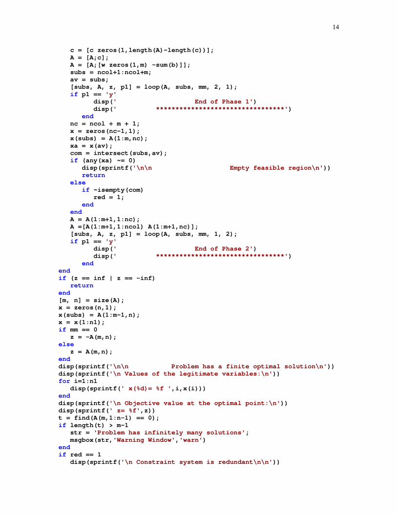
14

c = [c zeros(1,length(A)-length(c))]; A = [A;c]; A = [A;[w zeros(1,m) -sum(b)]]; subs = ncol+1:ncol+m; av = subs; [subs, A, z, p1] = loop(A, subs, mm, 2, 1); if p1 == 'y' disp( ' End of Phase 1' ) disp( ' *********************************' ) end nc = ncol + m + 1; x = zeros(nc-1,1); x(subs) = A(1:m,nc); xa = x(av); com = intersect(subs,av); if (any(xa) ~= 0) disp(sprintf( '\n\n Empty feasible region\n' )) return else if ~isempty(com) red = 1; end end A = A(1:m+1,1:nc); A =[A(1:m+1,1:ncol) A(1:m+1,nc)]; [subs, A, z, p1] = loop(A, subs, mm, 1, 2); if p1 == 'y' disp( ' End of Phase 2' ) disp( ' *********************************' ) endendif (z == inf | z == -inf) returnend[m, n] = size(A);x = zeros(n,1);x(subs) = A(1:m-1,n);x = x(1:n1);if mm == 0 z = -A(m,n);else z = A(m,n);enddisp(sprintf( '\n\n Problem has a finite optimal solution\n' ))disp(sprintf( '\n Values of the legitimate variables:\n' ))for i=1:n1 disp(sprintf( ' x(%d)= %f ' ,i,x(i)))enddisp(sprintf( '\n Objective value at the optimal point:\n' ))disp(sprintf( ' z= %f' ,z))t = find(A(m,1:n-1) == 0);if length(t) > m-1 str = 'Problem has infinitely many solutions' ; msgbox(str, 'Warning Window' , 'warn' )endif red == 1 disp(sprintf( '\n Constraint system is redundant\n\n' ))

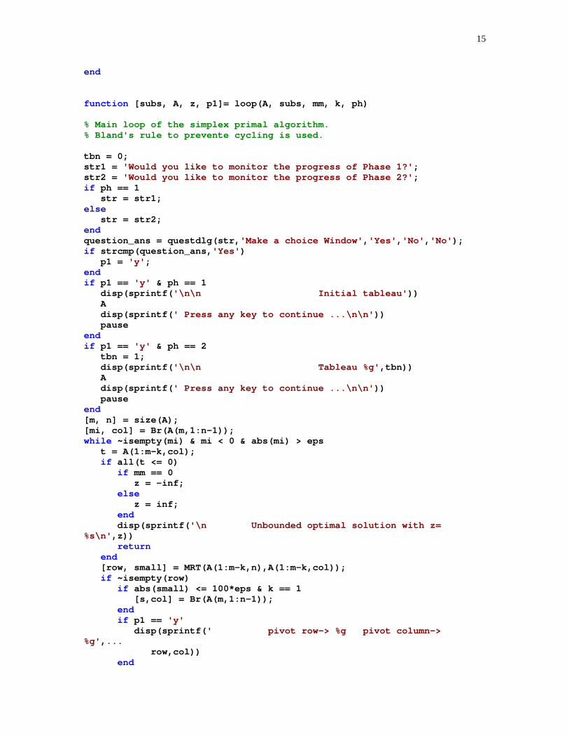
15

end

function [subs, A, z, p1]= loop(A, subs, mm, k, ph)

% Main loop of the simplex primal algorithm.% Bland's rule to prevente cycling is used.

tbn = 0;str1 = 'Would you like to monitor the progress of Phase 1?' ;str2 = 'Would you like to monitor the progress of Phase 2?' ;if ph == 1 str = str1;else str = str2;endquestion_ans = questdlg(str, 'Make a choice Window' , 'Yes' , 'No' , 'No' );if strcmp(question_ans, 'Yes' ) p1 = 'y' ;endif p1 == 'y' & ph == 1 disp(sprintf( '\n\n Initial tableau' )) A disp(sprintf( ' Press any key to continue ...\n\n' )) pauseendif p1 == 'y' & ph == 2 tbn = 1; disp(sprintf( '\n\n Tableau %g' ,tbn)) A disp(sprintf( ' Press any key to continue ...\n\n' )) pauseend[m, n] = size(A);[mi, col] = Br(A(m,1:n-1));while ~isempty(mi) & mi < 0 & abs(mi) > eps t = A(1:m-k,col); if all(t <= 0) if mm == 0 z = -inf; else z = inf; end disp(sprintf( '\n Unbounded optimal solution with z=%s\n' ,z)) return end [row, small] = MRT(A(1:m-k,n),A(1:m-k,col)); if ~isempty(row) if abs(small) <= 100*eps & k == 1 [s,col] = Br(A(m,1:n-1)); end if p1 == 'y' disp(sprintf( ' pivot row-> %g pivot column->%g' , ... row,col)) end

16

A(row,:)= A(row,:)/A(row,col); subs(row) = col; for i = 1:m if i ~= row A(i,:)= A(i,:)-A(i,col)*A(row,:); end end [mi, col] = Br(A(m,1:n-1)); end tbn = tbn + 1; if p1 == 'y' disp(sprintf( '\n\n Tableau %g' ,tbn)) A disp(sprintf( ' Press any key to continue ...\n\n' )) pause endendz = A(m,n);

MATLAB subfunction loop is included in the m-file simplex2p. It implements the main loop ofthe simplex algorithm. Organization of the tableaux generated by function simplex2p is the sameas the one presented in [3].

We will now test this function on five LP problems.

Let

type = 'min';

c = [-3 4];

A = [1 1;2 3];

rel = '<>';

b = [4; 18];

One can easily check, either by drawing the graph of the constraint set or running functiondrawfr on these data, that this problem has an empty feasible region.

simplex2p(type, c, A, rel, b)

Initial tableau

A =

1 1 1 0 1 0 4 2 3 0 -1 0 1 18 -3 4 0 0 0 0 0 -3 -4 -1 1 0 0 -22

Press any key to continue ...

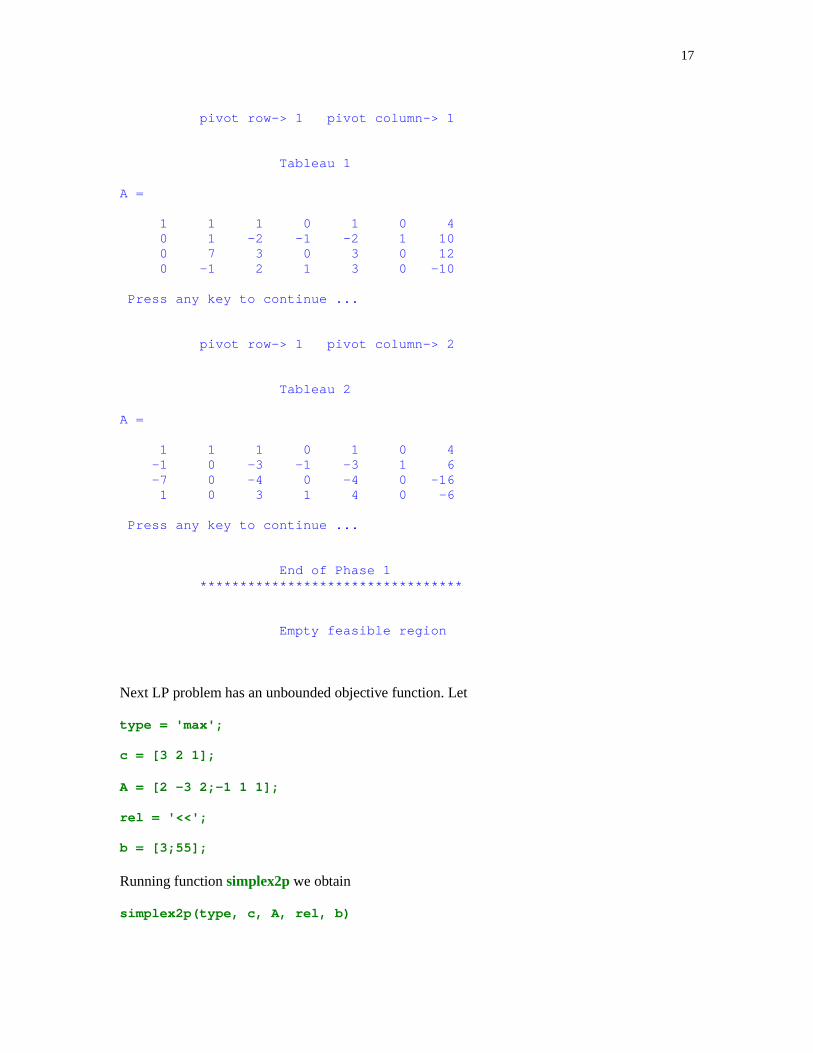
17

pivot row-> 1 pivot column-> 1

Tableau 1

A =

1 1 1 0 1 0 4 0 1 -2 -1 -2 1 10 0 7 3 0 3 0 12 0 -1 2 1 3 0 -10

Press any key to continue ...

pivot row-> 1 pivot column-> 2

Tableau 2

A =

1 1 1 0 1 0 4 -1 0 -3 -1 -3 1 6 -7 0 -4 0 -4 0 -16 1 0 3 1 4 0 -6

Press any key to continue ...

End of Phase 1 *********************************

Empty feasible region

Next LP problem has an unbounded objective function. Let

type = 'max';

c = [3 2 1];

A = [2 –3 2;-1 1 1];

rel = '<<';

b = [3;55];

Running function simplex2p we obtain

simplex2p(type, c, A, rel, b)

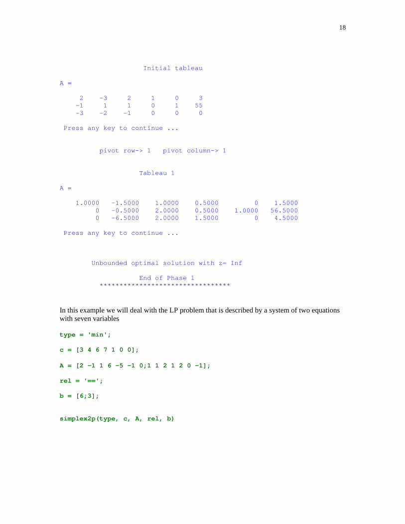
18

Initial tableau

A =

2 -3 2 1 0 3 -1 1 1 0 1 55 -3 -2 -1 0 0 0

Press any key to continue ...

pivot row-> 1 pivot column-> 1

Tableau 1

A =

1.0000 -1.5000 1.0000 0.5000 0 1.5000 0 -0.5000 2.0000 0.5000 1.0000 56.5000 0 -6.5000 2.0000 1.5000 0 4.5000

Press any key to continue ...

Unbounded optimal solution with z= Inf

End of Phase 1 *********************************

In this example we will deal with the LP problem that is described by a system of two equationswith seven variables

type = 'min';

c = [3 4 6 7 1 0 0];

A = [2 –1 1 6 –5 –1 0;1 1 2 1 2 0 –1];

rel = '==';

b = [6;3];

simplex2p(type, c, A, rel, b)

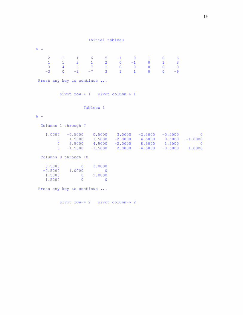
19

Initial tableau

A =

2 -1 1 6 -5 -1 0 1 0 6 1 1 2 1 2 0 -1 0 1 3 3 4 6 7 1 0 0 0 0 0 -3 0 -3 -7 3 1 1 0 0 -9

Press any key to continue ...

pivot row-> 1 pivot column-> 1

Tableau 1

A =

Columns 1 through 7

1.0000 -0.5000 0.5000 3.0000 -2.5000 -0.5000 0 0 1.5000 1.5000 -2.0000 4.5000 0.5000 -1.0000 0 5.5000 4.5000 -2.0000 8.5000 1.5000 0 0 -1.5000 -1.5000 2.0000 -4.5000 -0.5000 1.0000

Columns 8 through 10

0.5000 0 3.0000 -0.5000 1.0000 0 -1.5000 0 -9.0000 1.5000 0 0

Press any key to continue ...

pivot row-> 2 pivot column-> 2

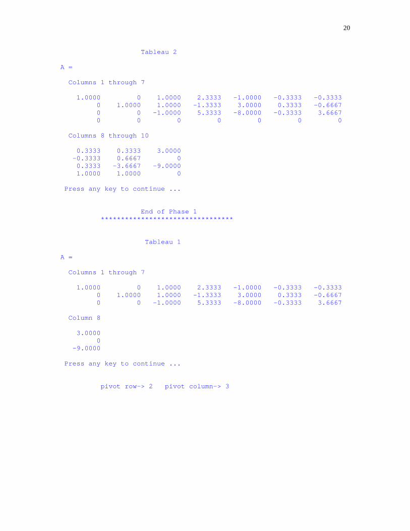
20

Tableau 2

A =

Columns 1 through 7

1.0000 0 1.0000 2.3333 -1.0000 -0.3333 -0.3333 0 1.0000 1.0000 -1.3333 3.0000 0.3333 -0.6667 0 0 -1.0000 5.3333 -8.0000 -0.3333 3.6667 0 0 0 0 0 0 0

Columns 8 through 10

0.3333 0.3333 3.0000 -0.3333 0.6667 0 0.3333 -3.6667 -9.0000 1.0000 1.0000 0

Press any key to continue ...

End of Phase 1 *********************************

Tableau 1

A =

Columns 1 through 7

1.0000 0 1.0000 2.3333 -1.0000 -0.3333 -0.3333 0 1.0000 1.0000 -1.3333 3.0000 0.3333 -0.6667 0 0 -1.0000 5.3333 -8.0000 -0.3333 3.6667

Column 8

3.0000 0 -9.0000

Press any key to continue ...

pivot row-> 2 pivot column-> 3

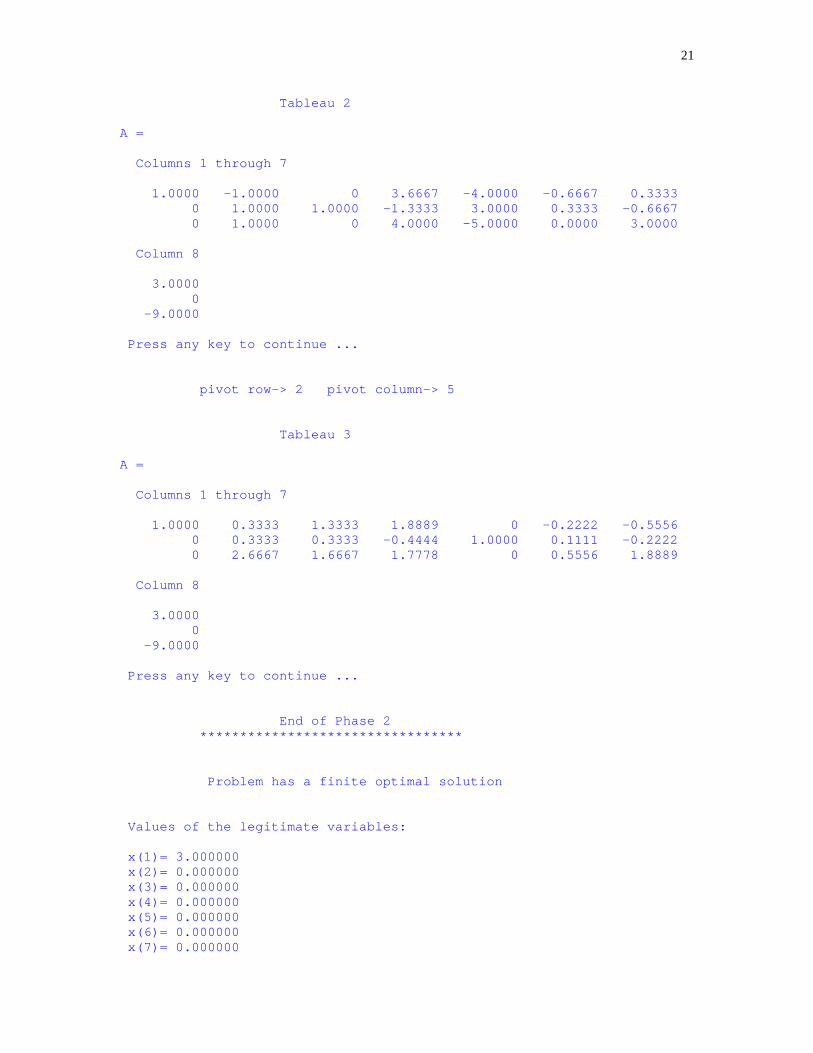
21

Tableau 2

A =

Columns 1 through 7

1.0000 -1.0000 0 3.6667 -4.0000 -0.6667 0.3333 0 1.0000 1.0000 -1.3333 3.0000 0.3333 -0.6667 0 1.0000 0 4.0000 -5.0000 0.0000 3.0000

Column 8

3.0000 0 -9.0000

Press any key to continue ...

pivot row-> 2 pivot column-> 5

Tableau 3

A =

Columns 1 through 7

1.0000 0.3333 1.3333 1.8889 0 -0.2222 -0.5556 0 0.3333 0.3333 -0.4444 1.0000 0.1111 -0.2222 0 2.6667 1.6667 1.7778 0 0.5556 1.8889

Column 8

3.0000 0 -9.0000

Press any key to continue ...

End of Phase 2 *********************************

Problem has a finite optimal solution

Values of the legitimate variables:

x(1)= 3.000000 x(2)= 0.000000 x(3)= 0.000000 x(4)= 0.000000 x(5)= 0.000000 x(6)= 0.000000 x(7)= 0.000000

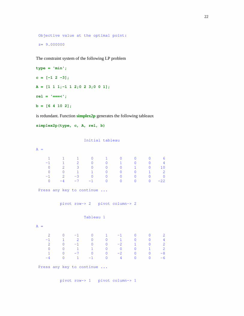
22

Objective value at the optimal point:

z= 9.000000

The constraint system of the following LP problem

type = 'min';

c = [-1 2 –3];

A = [1 1 1;-1 1 2;0 2 3;0 0 1];

rel = '===<';

b = [6 4 10 2];

is redundant. Function simplex2p generates the following tableaux

simplex2p(type, c, A, rel, b)

Initial tableau

A =

1 1 1 0 1 0 0 0 6 -1 1 2 0 0 1 0 0 4 0 2 3 0 0 0 1 0 10 0 0 1 1 0 0 0 1 2 -1 2 -3 0 0 0 0 0 0 0 -4 -7 -1 0 0 0 0 -22

Press any key to continue ...

pivot row-> 2 pivot column-> 2

Tableau 1

A =

2 0 -1 0 1 -1 0 0 2 -1 1 2 0 0 1 0 0 4 2 0 -1 0 0 -2 1 0 2 0 0 1 1 0 0 0 1 2 1 0 -7 0 0 -2 0 0 -8 -4 0 1 -1 0 4 0 0 -6

Press any key to continue ...

pivot row-> 1 pivot column-> 1

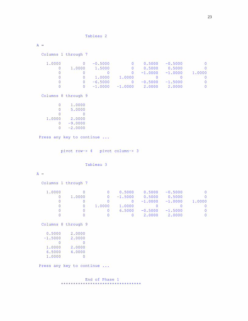
23

Tableau 2

A =

Columns 1 through 7

1.0000 0 -0.5000 0 0.5000 -0.5000 0 0 1.0000 1.5000 0 0.5000 0.5000 0 0 0 0 0 -1.0000 -1.0000 1.0000 0 0 1.0000 1.0000 0 0 0 0 0 -6.5000 0 -0.5000 -1.5000 0 0 0 -1.0000 -1.0000 2.0000 2.0000 0

Columns 8 through 9

0 1.0000 0 5.0000 0 0 1.0000 2.0000 0 -9.0000 0 -2.0000

Press any key to continue ...

pivot row-> 4 pivot column-> 3

Tableau 3

A =

Columns 1 through 7

1.0000 0 0 0.5000 0.5000 -0.5000 0 0 1.0000 0 -1.5000 0.5000 0.5000 0 0 0 0 0 -1.0000 -1.0000 1.0000 0 0 1.0000 1.0000 0 0 0 0 0 0 6.5000 -0.5000 -1.5000 0 0 0 0 0 2.0000 2.0000 0

Columns 8 through 9

0.5000 2.0000 -1.5000 2.0000 0 0 1.0000 2.0000 6.5000 4.0000 1.0000 0

Press any key to continue ...

End of Phase 1 *********************************

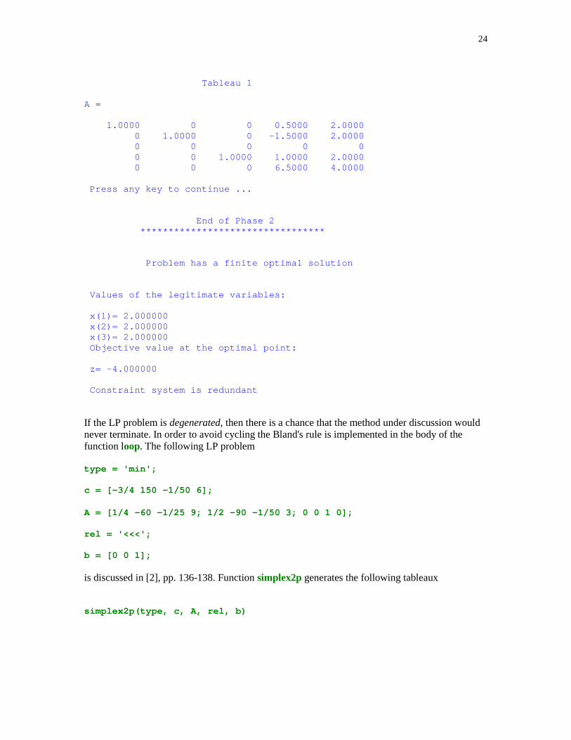
24

Tableau 1

A =

1.0000 0 0 0.5000 2.0000 0 1.0000 0 -1.5000 2.0000 0 0 0 0 0 0 0 1.0000 1.0000 2.0000 0 0 0 6.5000 4.0000

Press any key to continue ...

End of Phase 2 *********************************

Problem has a finite optimal solution

Values of the legitimate variables:

x(1)= 2.000000 x(2)= 2.000000 x(3)= 2.000000 Objective value at the optimal point:

z= -4.000000

Constraint system is redundant

If the LP problem is degenerated, then there is a chance that the method under discussion wouldnever terminate. In order to avoid cycling the Bland's rule is implemented in the body of thefunction loop. The following LP problem

type = 'min';

c = [-3/4 150 –1/50 6];

A = [1/4 –60 –1/25 9; 1/2 -90 –1/50 3; 0 0 1 0];

rel = '<<<';

b = [0 0 1];

is discussed in [2], pp. 136-138. Function simplex2p generates the following tableaux

simplex2p(type, c, A, rel, b)

25

Initial tableau

A =

Columns 1 through 7

0.2500 -60.0000 -0.0400 9.0000 1.0000 0 0 0.5000 -90.0000 -0.0200 3.0000 0 1.0000 0 0 0 1.0000 0 0 0 1.0000 -0.7500 150.0000 -0.0200 6.0000 0 0 0

Column 8

0 0 1.0000 0

Press any key to continue ...

pivot row-> 1 pivot column-> 1

Tableau 1

A =

Columns 1 through 7

1.0000 -240.0000 -0.1600 36.0000 4.0000 0 0 0 30.0000 0.0600 -15.0000 -2.0000 1.0000 0 0 0 1.0000 0 0 0 1.0000 0 -30.0000 -0.1400 33.0000 3.0000 0 0

Column 8

0 0 1.0000 0

Press any key to continue ...

pivot row-> 2 pivot column-> 2

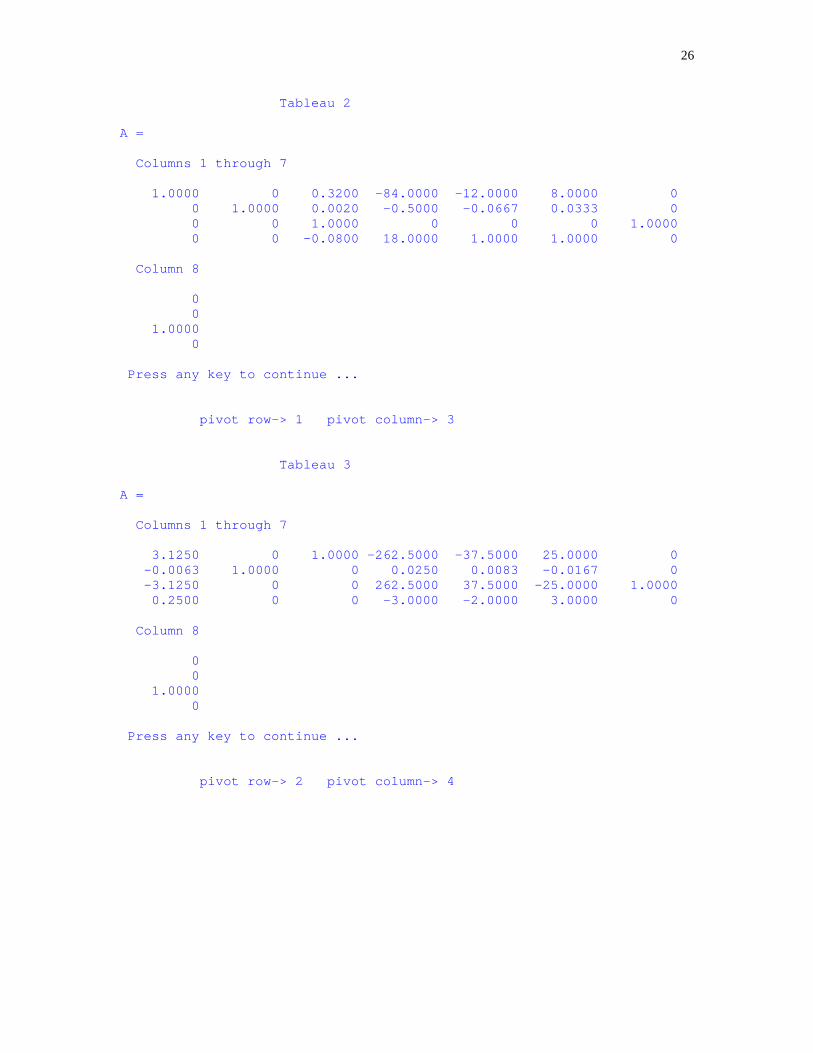
26

Tableau 2

A =

Columns 1 through 7

1.0000 0 0.3200 -84.0000 -12.0000 8.0000 0 0 1.0000 0.0020 -0.5000 -0.0667 0.0333 0 0 0 1.0000 0 0 0 1.0000 0 0 -0.0800 18.0000 1.0000 1.0000 0

Column 8

0 0 1.0000 0

Press any key to continue ...

pivot row-> 1 pivot column-> 3

Tableau 3

A =

Columns 1 through 7

3.1250 0 1.0000 -262.5000 -37.5000 25.0000 0 -0.0063 1.0000 0 0.0250 0.0083 -0.0167 0 -3.1250 0 0 262.5000 37.5000 -25.0000 1.0000 0.2500 0 0 -3.0000 -2.0000 3.0000 0

Column 8

0 0 1.0000 0

Press any key to continue ...

pivot row-> 2 pivot column-> 4

27

Tableau 4

A =

1.0e+004 *

Columns 1 through 7

-0.0062 1.0500 0.0001 0 0.0050 -0.0150 0 -0.0000 0.0040 0 0.0001 0.0000 -0.0001 0 0.0062 -1.0500 0 0 -0.0050 0.0150 0.0001 -0.0000 0.0120 0 0 -0.0001 0.0001 0

Column 8

0 0 0.0001 0

Press any key to continue ...

pivot row-> 3 pivot column-> 1

Tableau 5

A =

Columns 1 through 7

0 0 1.0000 0 0 0 1.0000 0 -2.0000 0 1.0000 0.1333 -0.0667 0.0040 1.0000 -168.0000 0 0 -0.8000 2.4000 0.0160 0 36.0000 0 0 -1.4000 2.2000 0.0080

Column 8

1.0000 0.0040 0.0160 0.0080

Press any key to continue ...

pivot row-> 2 pivot column-> 5

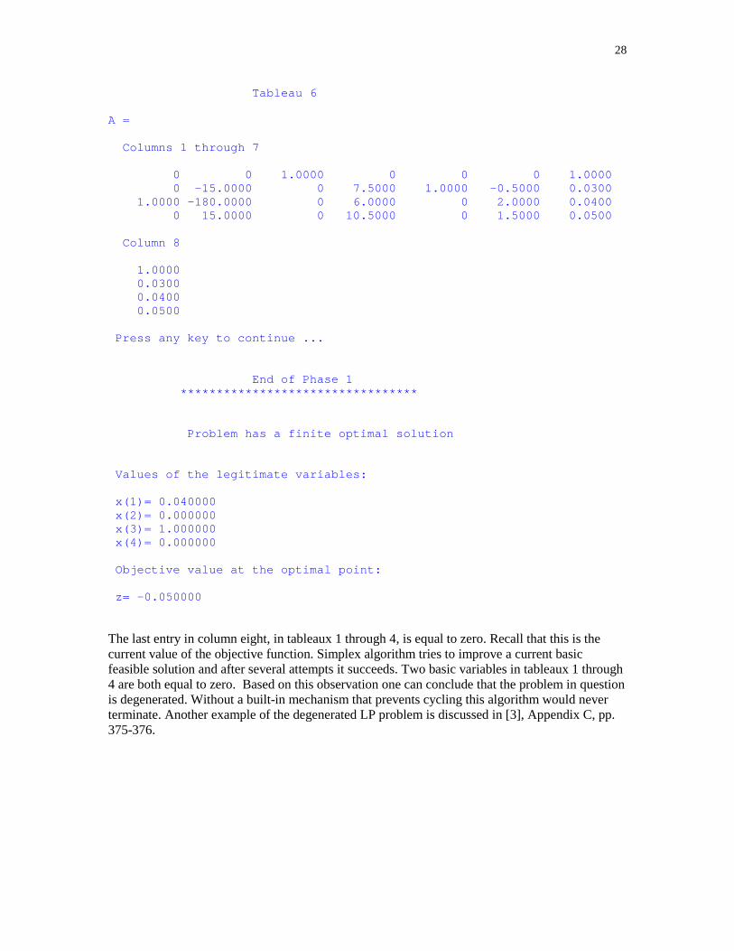
28

Tableau 6

A =

Columns 1 through 7

0 0 1.0000 0 0 0 1.0000 0 -15.0000 0 7.5000 1.0000 -0.5000 0.0300 1.0000 -180.0000 0 6.0000 0 2.0000 0.0400 0 15.0000 0 10.5000 0 1.5000 0.0500

Column 8

1.0000 0.0300 0.0400 0.0500

Press any key to continue ...

End of Phase 1 *********************************

Problem has a finite optimal solution

Values of the legitimate variables:

x(1)= 0.040000 x(2)= 0.000000 x(3)= 1.000000 x(4)= 0.000000

Objective value at the optimal point:

z= -0.050000

The last entry in column eight, in tableaux 1 through 4, is equal to zero. Recall that this is thecurrent value of the objective function. Simplex algorithm tries to improve a current basicfeasible solution and after several attempts it succeeds. Two basic variables in tableaux 1 through4 are both equal to zero. Based on this observation one can conclude that the problem in questionis degenerated. Without a built-in mechanism that prevents cycling this algorithm would neverterminate. Another example of the degenerated LP problem is discussed in [3], Appendix C, pp.375-376.

29

�- �� .������+� &���������

Another method that is of great importance in linear programming is called the Dual SimplexAlgorithm. The optimization problem that can be solved with the aid of this method is formulatedas follows

min(max) z = cTxSubject to Ax � b x � 0

Components of the vector b are not required to satisfy the nonnegativity constraints. The DualSimplex Algorithm has numerous applications to other problems of linear programming. It isused, for instance, in some implementations of the Gomory's cutting plane algorithm for solvingthe integer programming problems.

Function dsimplex computes an optimal solution to the optimization problem that is definedabove. One of the nice features of this method is its ability to detect the case of the empty feasibleregion. Function under discussion takes four input parameters types, c, A and b. Their meaning isdescribed in Section 6.7 of this tutorial.

function varargout = dsimplex(type, c, A, b)

% The Dual Simplex Algorithm for solving the LP problem

% min (max) z = c*x% Subject to Ax >= b% x >= 0%

if type == 'min' mm = 0;else mm = 1; c = -c;endstr = 'Would you like to monitor the progress of computations?' ;A = -A;b = -b(:);c = c(:)';[m, n] = size(A);A = [A eye(m) b];A = [A;[c zeros(1,m+1)]];question_ans = questdlg(str, 'Make a choice Window' , 'Yes' , 'No' , 'No' );if strcmp(question_ans, 'Yes' ) p1 = 'y' ;else p1 = 'n' ;endif p1 == 'y' disp(sprintf( '\n\n Initial tableau' )) A

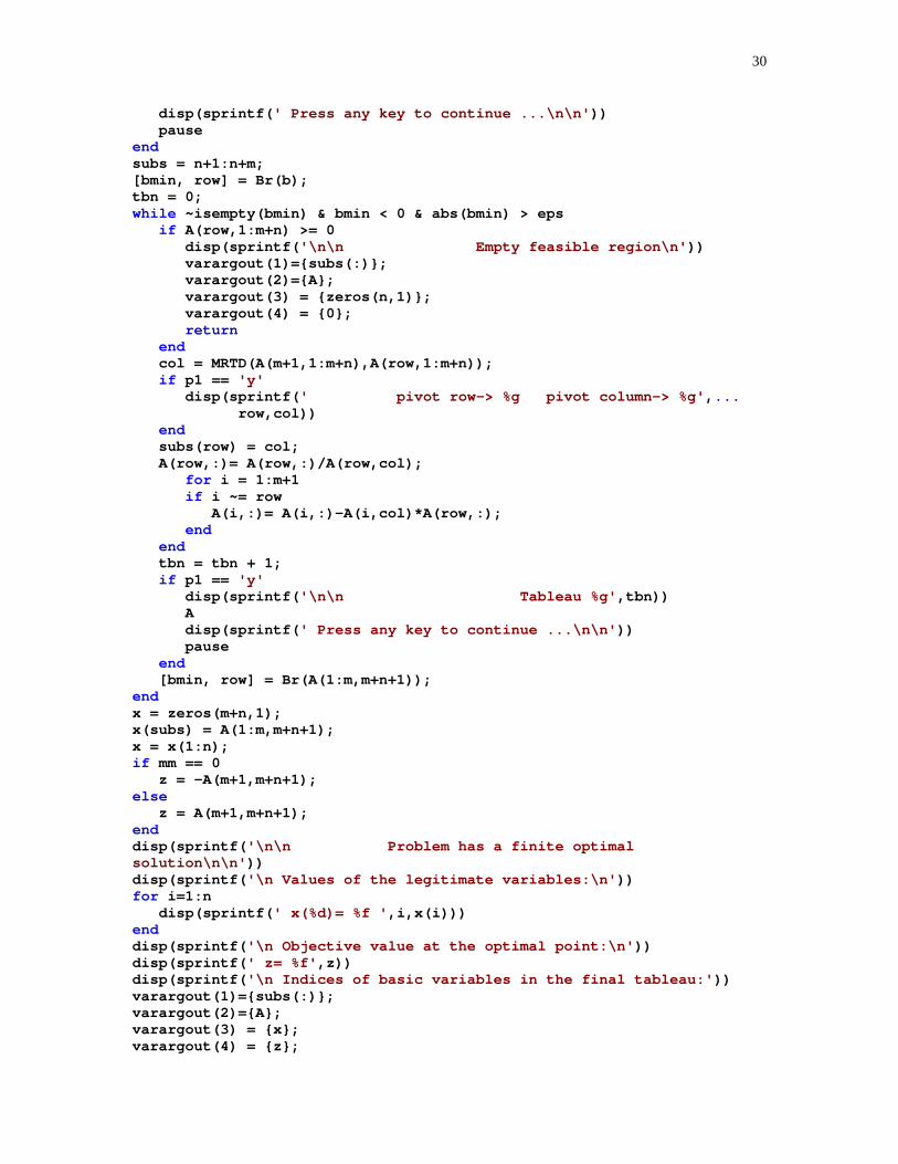
30

disp(sprintf( ' Press any key to continue ...\n\n' )) pauseendsubs = n+1:n+m;[bmin, row] = Br(b);tbn = 0;while ~isempty(bmin) & bmin < 0 & abs(bmin) > eps if A(row,1:m+n) >= 0 disp(sprintf( '\n\n Empty feasible region\n' )) varargout(1)={subs(:)}; varargout(2)={A}; varargout(3) = {zeros(n,1)}; varargout(4) = {0}; return end col = MRTD(A(m+1,1:m+n),A(row,1:m+n)); if p1 == 'y' disp(sprintf( ' pivot row-> %g pivot column-> %g' , ... row,col)) end subs(row) = col; A(row,:)= A(row,:)/A(row,col); for i = 1:m+1 if i ~= row A(i,:)= A(i,:)-A(i,col)*A(row,:); end end tbn = tbn + 1; if p1 == 'y' disp(sprintf( '\n\n Tableau %g' ,tbn)) A disp(sprintf( ' Press any key to continue ...\n\n' )) pause end [bmin, row] = Br(A(1:m,m+n+1));endx = zeros(m+n,1);x(subs) = A(1:m,m+n+1);x = x(1:n);if mm == 0 z = -A(m+1,m+n+1);else z = A(m+1,m+n+1);enddisp(sprintf( '\n\n Problem has a finite optimalsolution\n\n' ))disp(sprintf( '\n Values of the legitimate variables:\n' ))for i=1:n disp(sprintf( ' x(%d)= %f ' ,i,x(i)))enddisp(sprintf( '\n Objective value at the optimal point:\n' ))disp(sprintf( ' z= %f' ,z))disp(sprintf( '\n Indices of basic variables in the final tableau:' ))varargout(1)={subs(:)};varargout(2)={A};varargout(3) = {x};varargout(4) = {z};

31

Function dsimplex allows a variable number of the output parameters. Indices of the basicvariables in the final tableau are always displayed. The final tableau also can be saved in avariable. For instance, execution of the following command [subs, B] = dsimplex(type, c, A, b)will return, among other things, indices of basic variables stored in the variable subs and the finaltableau stored in the variable B.

Let

type = 'min';

c = [-2 3 4];

A = [-1 –1 –1;2 2 2];

b = [-1;4];

One can easily check that the constraint system defines an empty set. Running function dsimplex,we obtain

subs = dsimplex(type, c, A, b)

Initial tableau

A =

1 1 1 1 0 1 -2 -2 -2 0 1 -4 -2 3 4 0 0 0

Press any key to continue ...

pivot row-> 2 pivot column-> 1

Tableau 1

A =

0 0 0 1.0000 0.5000 -1.0000 1.0000 1.0000 1.0000 0 -0.5000 2.0000 0 5.0000 6.0000 0 -1.0000 4.0000

Press any key to continue ...

Empty feasible region

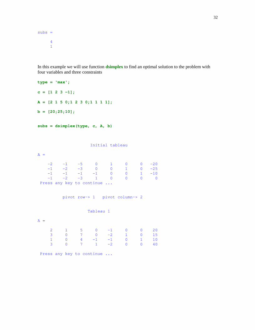
32

subs =

4 1

In this example we will use function dsimplex to find an optimal solution to the problem withfour variables and three constraints

type = 'max';

c = [1 2 3 –1];

A = [2 1 5 0;1 2 3 0;1 1 1 1];

b = [20;25;10];

subs = dsimplex(type, c, A, b)

Initial tableau

A =

-2 -1 -5 0 1 0 0 -20 -1 -2 -3 0 0 1 0 -25 -1 -1 -1 -1 0 0 1 -10 -1 -2 -3 1 0 0 0 0 Press any key to continue ...

pivot row-> 1 pivot column-> 2

Tableau 1

A =

2 1 5 0 -1 0 0 20 3 0 7 0 -2 1 0 15 1 0 4 -1 -1 0 1 10 3 0 7 1 -2 0 0 40

Press any key to continue ...

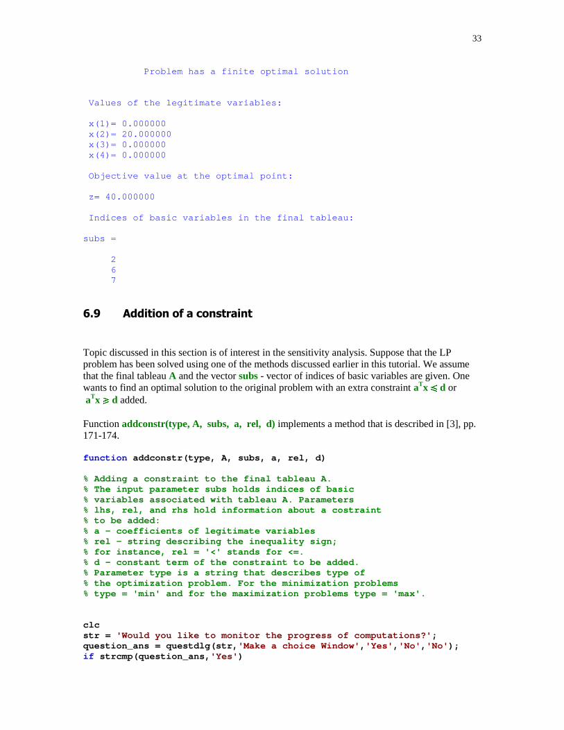
33

Problem has a finite optimal solution

Values of the legitimate variables:

x(1)= 0.000000 x(2)= 20.000000 x(3)= 0.000000 x(4)= 0.000000

Objective value at the optimal point:

z= 40.000000

Indices of basic variables in the final tableau:

subs =

2 6 7

�/ �!!����������� ������

Topic discussed in this section is of interest in the sensitivity analysis. Suppose that the LPproblem has been solved using one of the methods discussed earlier in this tutorial. We assumethat the final tableau A and the vector subs - vector of indices of basic variables are given. Onewants to find an optimal solution to the original problem with an extra constraint aTx � d or aTx � d added.

Function addconstr(type, A, subs, a, rel, d) implements a method that is described in [3], pp.171-174.

function addconstr(type, A, subs, a, rel, d)

% Adding a constraint to the final tableau A.% The input parameter subs holds indices of basic% variables associated with tableau A. Parameters% lhs, rel, and rhs hold information about a costraint% to be added:% a - coefficients of legitimate variables% rel - string describing the inequality sign;% for instance, rel = '<' stands for <=.% d - constant term of the constraint to be added.% Parameter type is a string that describes type of% the optimization problem. For the minimization problems% type = 'min' and for the maximization problems type = 'max'.

clcstr = 'Would you like to monitor the progress of computations?' ;question_ans = questdlg(str, 'Make a choice Window' , 'Yes' , 'No' , 'No' );if strcmp(question_ans, 'Yes' )

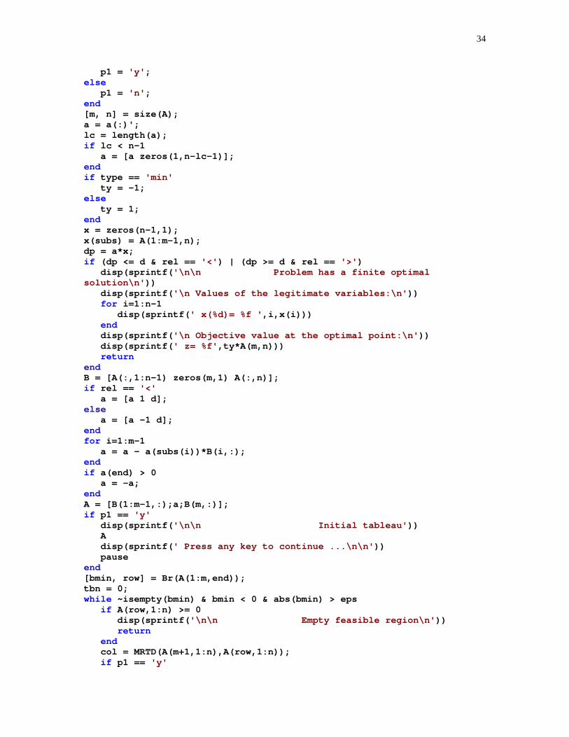
34

p1 = 'y' ;else p1 = 'n' ;end[m, n] = size(A);a = a(:)';lc = length(a);if lc < n-1 a = [a zeros(1,n-lc-1)];endif type == 'min' ty = -1;else ty = 1;endx = zeros(n-1,1);x(subs) = A(1:m-1,n);dp = a*x;if (dp <= d & rel == '<' ) | (dp >= d & rel == '>' ) disp(sprintf( '\n\n Problem has a finite optimalsolution\n' )) disp(sprintf( '\n Values of the legitimate variables:\n' )) for i=1:n-1 disp(sprintf( ' x(%d)= %f ' ,i,x(i))) end disp(sprintf( '\n Objective value at the optimal point:\n' )) disp(sprintf( ' z= %f' ,ty*A(m,n))) returnendB = [A(:,1:n-1) zeros(m,1) A(:,n)];if rel == '<' a = [a 1 d];else a = [a -1 d];endfor i=1:m-1 a = a - a(subs(i))*B(i,:);endif a(end) > 0 a = -a;endA = [B(1:m-1,:);a;B(m,:)];if p1 == 'y' disp(sprintf( '\n\n Initial tableau' )) A disp(sprintf( ' Press any key to continue ...\n\n' )) pauseend[bmin, row] = Br(A(1:m,end));tbn = 0;while ~isempty(bmin) & bmin < 0 & abs(bmin) > eps if A(row,1:n) >= 0 disp(sprintf( '\n\n Empty feasible region\n' )) return end col = MRTD(A(m+1,1:n),A(row,1:n)); if p1 == 'y'

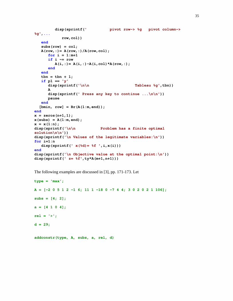
35

disp(sprintf( ' pivot row-> %g pivot column->%g' , ... row,col)) end subs(row) = col; A(row,:)= A(row,:)/A(row,col); for i = 1:m+1 if i ~= row A(i,:)= A(i,:)-A(i,col)*A(row,:); end end tbn = tbn + 1; if p1 == 'y' disp(sprintf( '\n\n Tableau %g' ,tbn)) A disp(sprintf( ' Press any key to continue ...\n\n' )) pause end [bmin, row] = Br(A(1:m,end));endx = zeros(n+1,1);x(subs) = A(1:m,end);x = x(1:n);disp(sprintf( '\n\n Problem has a finite optimalsolution\n\n' ))disp(sprintf( '\n Values of the legitimate variables:\n' ))for i=1:n disp(sprintf( ' x(%d)= %f ' ,i,x(i)))enddisp(sprintf( '\n Objective value at the optimal point:\n' ))disp(sprintf( ' z= %f' ,ty*A(m+1,n+1)))

The following examples are discussed in [3], pp. 171-173. Let

type = 'max';

A = [-2 0 5 1 2 –1 6; 11 1 –18 0 –7 4 4; 3 0 2 0 2 1 106];

subs = [4; 2];

a = [4 1 0 4];

rel = '>';

d = 29;

addconstr(type, A, subs, a, rel, d)

36

Initial tableau

A =

-2 0 5 1 2 -1 0 6 11 1 -18 0 -7 4 0 4 -1 0 2 0 1 0 1 -1 3 0 2 0 2 1 0 106

Press any key to continue ...

pivot row-> 3 pivot column-> 1

Tableau 1

A =

0 0 1 1 0 -1 -2 8 0 1 4 0 4 4 11 -7 1 0 -2 0 -1 0 -1 1 0 0 8 0 5 1 3 103

Press any key to continue ...

Empty feasible region

Changing the additional constraint to 3x1 + x2 + 3x4 � 20, we obtain

a = [3 1 0 3];

rel = '<';

d = 20;

addconstr(type, A, subs, a, rel, d)

Initial tableauA = -2 0 5 1 2 -1 0 6 11 1 -18 0 -7 4 0 4 -2 0 3 0 1 -1 1 -2 3 0 2 0 2 1 0 106 Press any key to continue ...

pivot row-> 3 pivot column-> 6

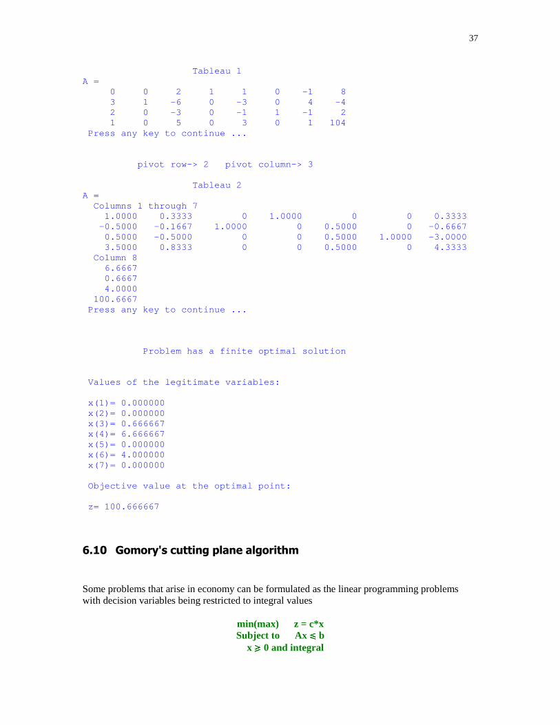
37

Tableau 1A = 0 0 2 1 1 0 -1 8 3 1 -6 0 -3 0 4 -4 2 0 -3 0 -1 1 -1 2 1 0 5 0 3 0 1 104 Press any key to continue ...

pivot row-> 2 pivot column-> 3

Tableau 2A = Columns 1 through 7 1.0000 0.3333 0 1.0000 0 0 0.3333 -0.5000 -0.1667 1.0000 0 0.5000 0 -0.6667 0.5000 -0.5000 0 0 0.5000 1.0000 -3.0000 3.5000 0.8333 0 0 0.5000 0 4.3333 Column 8 6.6667 0.6667 4.0000 100.6667 Press any key to continue ...

Problem has a finite optimal solution

Values of the legitimate variables:

x(1)= 0.000000 x(2)= 0.000000 x(3)= 0.666667 x(4)= 6.666667 x(5)= 0.000000 x(6)= 4.000000 x(7)= 0.000000

Objective value at the optimal point:

z= 100.666667

��0 1����'2 �������+��� ���������

Some problems that arise in economy can be formulated as the linear programming problemswith decision variables being restricted to integral values

min(max) z = c*xSubject to Ax � b x � 0 and integral

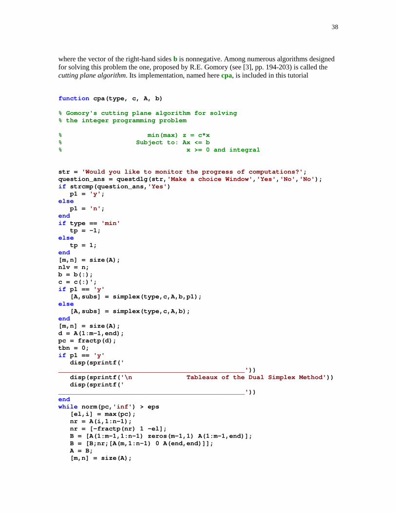
38

where the vector of the right-hand sides b is nonnegative. Among numerous algorithms designedfor solving this problem the one, proposed by R.E. Gomory (see [3], pp. 194-203) is called thecutting plane algorithm. Its implementation, named here cpa, is included in this tutorial

function cpa(type, c, A, b)

% Gomory's cutting plane algorithm for solving% the integer programming problem

% min(max) z = c*x% Subject to: Ax <= b% x >= 0 and integral

str = 'Would you like to monitor the progress of computations?' ;question_ans = questdlg(str, 'Make a choice Window' , 'Yes' , 'No' , 'No' );if strcmp(question_ans, 'Yes' ) p1 = 'y' ;else p1 = 'n' ;endif type == 'min' tp = -1;else tp = 1;end[m,n] = size(A);nlv = n;b = b(:);c = c(:)';if p1 == 'y' [A,subs] = simplex(type,c,A,b,p1);else [A,subs] = simplex(type,c,A,b);end[m,n] = size(A);d = A(1:m-1,end);pc = fractp(d);tbn = 0;if p1 == 'y' disp(sprintf( '________________________________________________' )) disp(sprintf( '\n Tableaux of the Dual Simplex Method' )) disp(sprintf( '________________________________________________' ))endwhile norm(pc, 'inf' ) > eps [el,i] = max(pc); nr = A(i,1:n-1); nr = [-fractp(nr) 1 -el]; B = [A(1:m-1,1:n-1) zeros(m-1,1) A(1:m-1,end)]; B = [B;nr;[A(m,1:n-1) 0 A(end,end)]]; A = B; [m,n] = size(A);

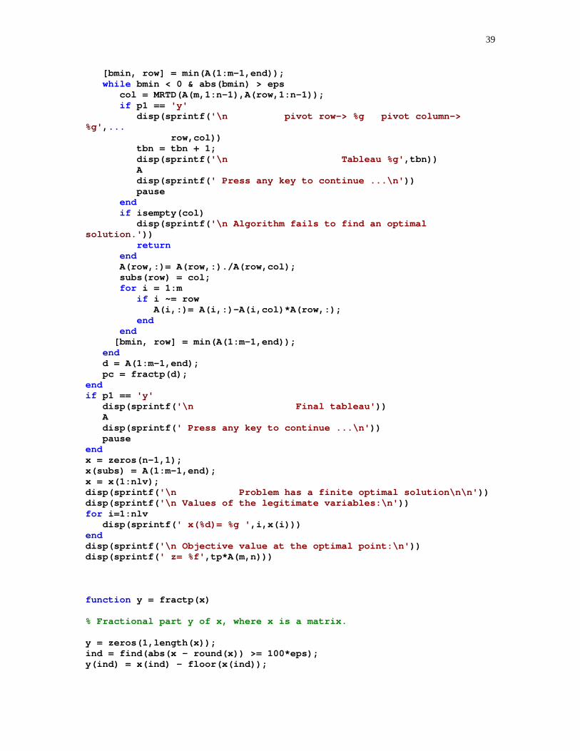
39

[bmin, row] = min(A(1:m-1,end)); while bmin < 0 & abs(bmin) > eps col = MRTD(A(m,1:n-1),A(row,1:n-1)); if p1 == 'y' disp(sprintf( '\n pivot row-> %g pivot column->%g' , ... row,col)) tbn = tbn + 1; disp(sprintf( '\n Tableau %g' ,tbn)) A disp(sprintf( ' Press any key to continue ...\n' )) pause end if isempty(col) disp(sprintf( '\n Algorithm fails to find an optimalsolution.' )) return end A(row,:)= A(row,:)./A(row,col); subs(row) = col; for i = 1:m if i ~= row A(i,:)= A(i,:)-A(i,col)*A(row,:); end end [bmin, row] = min(A(1:m-1,end)); end d = A(1:m-1,end); pc = fractp(d);endif p1 == 'y' disp(sprintf( '\n Final tableau' )) A disp(sprintf( ' Press any key to continue ...\n' )) pauseendx = zeros(n-1,1);x(subs) = A(1:m-1,end);x = x(1:nlv);disp(sprintf( '\n Problem has a finite optimal solution\n\n' ))disp(sprintf( '\n Values of the legitimate variables:\n' ))for i=1:nlv disp(sprintf( ' x(%d)= %g ' ,i,x(i)))enddisp(sprintf( '\n Objective value at the optimal point:\n' ))disp(sprintf( ' z= %f' ,tp*A(m,n)))

function y = fractp(x)

% Fractional part y of x, where x is a matrix.

y = zeros(1,length(x));ind = find(abs(x - round(x)) >= 100*eps);y(ind) = x(ind) - floor(x(ind));

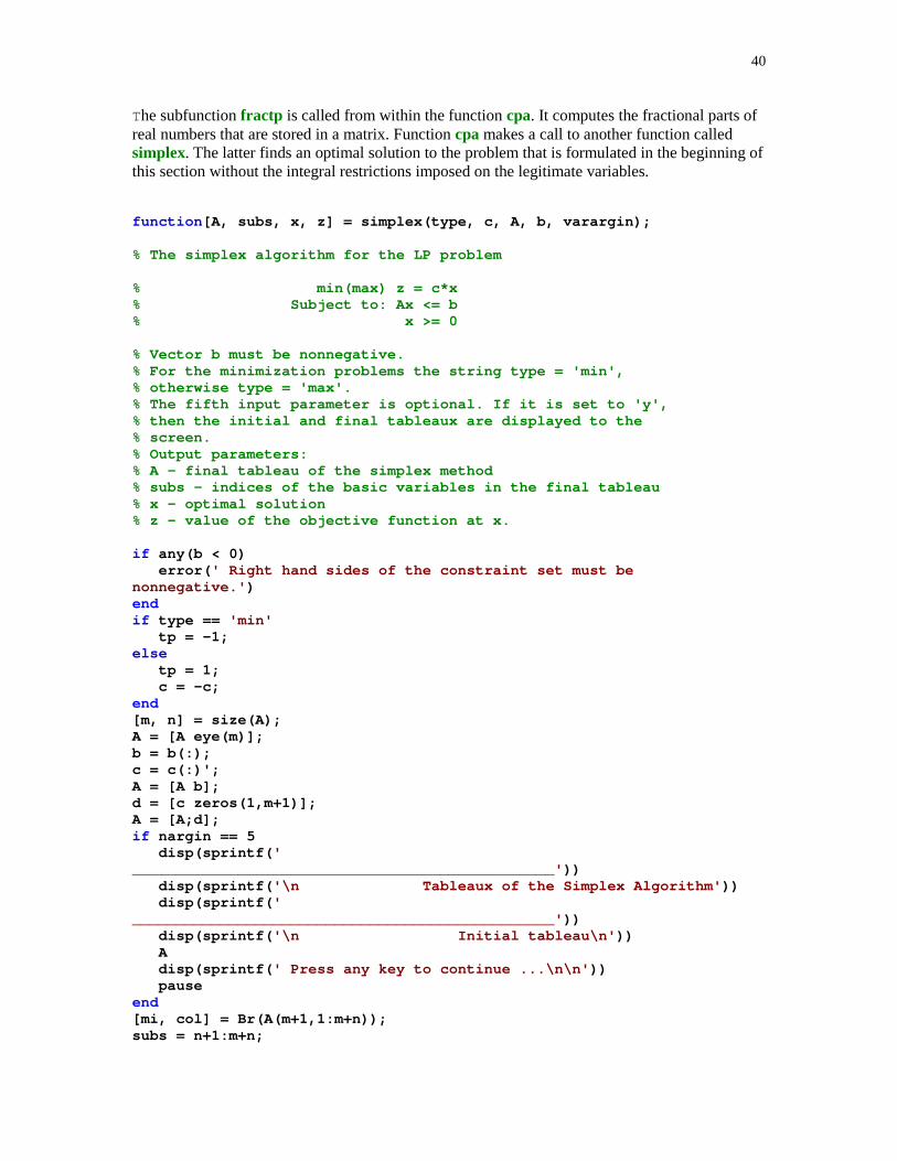
40

The subfunction fractp is called from within the function cpa. It computes the fractional parts ofreal numbers that are stored in a matrix. Function cpa makes a call to another function calledsimplex. The latter finds an optimal solution to the problem that is formulated in the beginning ofthis section without the integral restrictions imposed on the legitimate variables.

function [A, subs, x, z] = simplex(type, c, A, b, varargin);

% The simplex algorithm for the LP problem

% min(max) z = c*x% Subject to: Ax <= b% x >= 0

% Vector b must be nonnegative.% For the minimization problems the string type = 'min',% otherwise type = 'max'.% The fifth input parameter is optional. If it is set to 'y',% then the initial and final tableaux are displayed to the% screen.% Output parameters:% A - final tableau of the simplex method% subs - indices of the basic variables in the final tableau% x - optimal solution% z - value of the objective function at x.

if any(b < 0) error( ' Right hand sides of the constraint set must benonnegative.' )endif type == 'min' tp = -1;else tp = 1; c = -c;end[m, n] = size(A);A = [A eye(m)];b = b(:);c = c(:)';A = [A b];d = [c zeros(1,m+1)];A = [A;d];if nargin == 5 disp(sprintf( '________________________________________________' )) disp(sprintf( '\n Tableaux of the Simplex Algorithm' )) disp(sprintf( '________________________________________________' )) disp(sprintf( '\n Initial tableau\n' )) A disp(sprintf( ' Press any key to continue ...\n\n' )) pauseend[mi, col] = Br(A(m+1,1:m+n));subs = n+1:m+n;

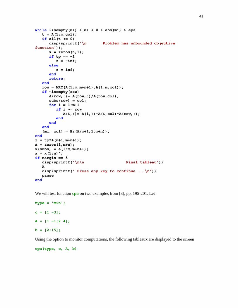
41

while ~isempty(mi) & mi < 0 & abs(mi) > eps t = A(1:m,col); if all(t <= 0) disp(sprintf( '\n Problem has unbounded objectivefunction' )); x = zeros(n,1); if tp == -1 z = -inf; else z = inf; end return ; end row = MRT(A(1:m,m+n+1),A(1:m,col)); if ~isempty(row) A(row,:)= A(row,:)/A(row,col); subs(row) = col; for i = 1:m+1 if i ~= row A(i,:)= A(i,:)-A(i,col)*A(row,:); end end end [mi, col] = Br(A(m+1,1:m+n));endz = tp*A(m+1,m+n+1);x = zeros(1,m+n);x(subs) = A(1:m,m+n+1);x = x(1:n)';if nargin == 5 disp(sprintf( '\n\n Final tableau' )) A disp(sprintf( ' Press any key to continue ...\n' )) pauseend

We will test function cpa on two examples from [3], pp. 195-201. Let

type = 'min';

c = [1 –3];

A = [1 –1;2 4];

b = [2;15];

Using the option to monitor computations, the following tableaux are displayed to the screen

cpa(type, c, A, b)

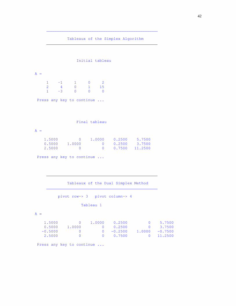
42

________________________________________________

Tableaux of the Simplex Algorithm ________________________________________________

Initial tableau

A =

1 -1 1 0 2 2 4 0 1 15 1 -3 0 0 0

Press any key to continue ...

Final tableau

A =

1.5000 0 1.0000 0.2500 5.7500 0.5000 1.0000 0 0.2500 3.7500 2.5000 0 0 0.7500 11.2500

Press any key to continue ...

________________________________________________

Tableaux of the Dual Simplex Method ________________________________________________

pivot row-> 3 pivot column-> 4

Tableau 1

A =

1.5000 0 1.0000 0.2500 0 5.7500 0.5000 1.0000 0 0.2500 0 3.7500 -0.5000 0 0 -0.2500 1.0000 -0.7500 2.5000 0 0 0.7500 0 11.2500

Press any key to continue ...

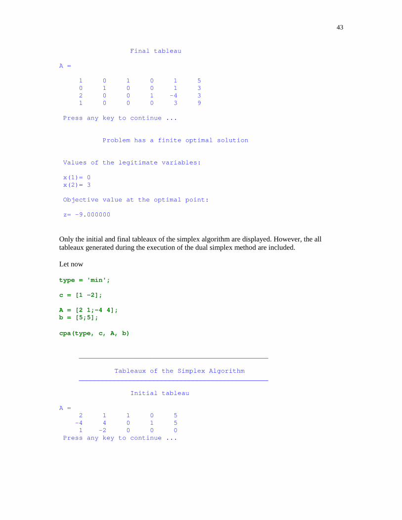
43

Final tableau

A =

1 0 1 0 1 5 0 1 0 0 1 3 2 0 0 1 -4 3 1 0 0 0 3 9

Press any key to continue ...

Problem has a finite optimal solution

Values of the legitimate variables:

x(1)= 0 x(2)= 3

Objective value at the optimal point:

z= -9.000000

Only the initial and final tableaux of the simplex algorithm are displayed. However, the alltableaux generated during the execution of the dual simplex method are included.

Let now

type = 'min';

c = [1 –2];

A = [2 1;-4 4]; b = [5;5];

cpa(type, c, A, b)

________________________________________________

Tableaux of the Simplex Algorithm ________________________________________________

Initial tableau

A = 2 1 1 0 5 -4 4 0 1 5 1 -2 0 0 0 Press any key to continue ...

44

Final tableauA = 1.0000 0 0.3333 -0.0833 1.2500 0 1.0000 0.3333 0.1667 2.5000 0 0 0.3333 0.4167 3.7500 Press any key to continue ...

________________________________________________

Tableaux of the Dual Simplex Method ________________________________________________

pivot row-> 3 pivot column-> 3

Tableau 1A = 1.0000 0 0.3333 -0.0833 0 1.2500 0 1.0000 0.3333 0.1667 0 2.5000 0 0 -0.3333 -0.1667 1.0000 -0.5000 0 0 0.3333 0.4167 0 3.7500 Press any key to continue ...

pivot row-> 4 pivot column-> 4

Tableau 2A = 1.0000 0 0 -0.2500 1.0000 0 0.7500 0 1.0000 0 0 1.0000 0 2.0000 0 0 1.0000 0.5000 -3.0000 0 1.5000 0 0 0 -0.7500 0 1.0000 -0.7500 0 0 0 0.2500 1.0000 0 3.2500 Press any key to continue ...

Final tableauA = 1.0000 0 0 0 1.0000 -0.3333 1.0000 0 1.0000 0 0 1.0000 0 2.0000 0 0 1.0000 0 -3.0000 0.6667 1.0000 0 0 0 1.0000 0 -1.3333 1.0000 0 0 0 0 1.0000 0.3333 3.0000 Press any key to continue ...

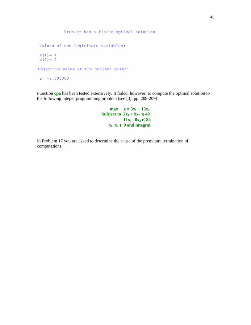
45

Problem has a finite optimal solution

Values of the legitimate variables:

x(1)= 1 x(2)= 2

Objective value at the optimal point:

z= -3.000000

Function cpa has been tested extensively. It failed, however, to compute the optimal solution tothe following integer programming problem (see [3], pp. 208-209)

max z = 3x1 + 13x2

Subject to 2x1 + 9x2 � 40 11x1 –8x2 � 82 x1, x2 � 0 and integral

In Problem 17 you are asked to determine the cause of the premature termination ofcomputations.

46

3 � � ��

[1] M.S. Bazaraa, J.J. Jarvis, and H.D. Sherali, Linear Programming and Network Flows, Second edition, John Wiley & Sons, New York, 1990.

[2] S.G. Nash and A. Sofer, Linear and Nonlinear Programming, The McGraw-Hill Companies, Inc., New York, 1996.

[3] P.R. Thie, An Introduction to Linear Programming and Game Theory, Second edition, John Wiley & Sons, New York, 1988.

47

���(� �

1. Solve the following LP problems geometrically.

(i) min z = -3x1 + 9x2

Subject to -x1 + x2 � 1 x1 + x2 � 1 x1 + x2 � 5 3x1 –x2 � 7 x1 – 3x2 � 1 x1, x2 � 0

Let the objective function and the constraint set be the same as in Part (i). Find the optimal solution to the maximization problem.

(ii) max z = x1 + x2

Subject to x1 + x2 � 2 x1 � 1 x1 + x2 � 1 -x1 + x2 � 1.5 x1, x2 � 0

2. Given the constraint set X = {(x1, x2, x3)T � �3 : 0 � x1 � x2 � x3}.

(i) Write these constraints in the following form Ax � b, x � 0.(ii) Find the extreme points and the extreme directions, if any, of X.(iii) Based on the numerical evidence from Part (ii) of this problem, formulate a hypothesis

about the extreme points and the extreme directions of the more general constraint setX = {(x1, x2, … xn)

T � �n : 0 � x1 � x2 � … � xn}.

3. Give an example of the constraint set with at least three constraints and three variables thathave empty feasible region.

4. Consider the system of constraints in the standard form Ax = b, x � 0 and b � 0, where A is an m-by-n matrix with n � m. Number of all basic feasible solutions to this system is not

bigger than )!(!

!

mnm

n

−. Construct a constraint system with two equations (m = 2) and four

variables (n = 4) that has

(i) no basic feasible solutions(ii) exactly one basic feasible solution(iii) exactly three distinct basic feasible solutions

Hint: You may wish to perform numerical experiments using function feassol discussed inSection 6.4 of this tutorial.

48

5. Let X denote the constraint set that is described in Problem 1(i). Its graph is shown on page

10 of this tutorial. Express point

=

2

2P as a convex combination of its extreme points. Is

this representation unique?Hint: Compute the extreme points P1, P2, … , Pn of X using function extrpts. Next form asystem of linear equations

�1P1 + �2P2 + … + �nPn = P �1 + �2 + … + �n = 1

where all the �'s are nonnegative. Function feassol can be used to find all nonnegative solutions to this system.

6. Repeat Problem 5 with

=2

3P and

=3

3P .

7. The feasible region described by the inequalities of Problem 1(i) is bounded. An optimalsolution to the minimization (maximization) problem can be found by evaluating theobjective function at the extreme points of the feasible region and next finding the smallest(largest) value of the objective function. MATLAB has two functions min and max forcomputing the smallest and largest numbers in a set. The following command [z, ind] = min(t) finds the smallest number in the set t together with the index ind of theelement sought. In this exercise you are to find an optimal solution and the correspondingobjective value of the Problem 1(i).Remark. This method for solving the LP problems is not recommended in practice becauseof its high computational complexity. It is included here for pedagogical reasons only.

8. The following LP problem

min (max) = c1x1 + c2x2 + … + cnxn

Subject to x1 + x2 + … + xn = 1 x1, x2, … , xn � 0

can be solved without using advanced computational methods that are discussed in the Linear Programming class. Write MATLAB function [x, z] = oneconstr(type, c) which takes two input parameters type, where type = 'min' for the minimization problem and type = 'max' for the maximization problem and c – vector of the cost coefficients and returns the optimal solution x and the associated objective value z.

9. The following linear programming problem

min (max) z = c*x Subject to Ax � b x unrestricted

with b � 0 can be solved using function simplex (see Section 6.10). A trick is to use asubstitution x = x' – x'' , where x' , x'' � 0. Write MATLAB function [x, z, A] = simplexu(type, c, A, b) which computes an optimal solution to the LP problemthat is formulated above. The input and the output parameters have the same meaning asthose in function simplex. Test your function on the following problem

49

min z = 2x1 – x2

Subject to x1 + x2 � 2 -x1 + x2 � 1 x1 –2x2 � 2 x1, x2 unrestricted

Also, find an optimal solution to the maximization problem using the same objective functionand the same constraint set. Drop the first inequality in the constraint set and solve themaximization problem for the same objective function.

10. In this exercise you are to write MATLAB function x = nnsol(A, b) which computes anonnegative solution x, if any, to the system of linear equations Ax = b. A trick that canbe used is to add a single artificial variable to each equation and next apply a technique ofPhase 1 of the Dual Simplex Algorithm with the objective function being equal to the sumof all artificial variables. See [3], Section 3.6 for more details. Recall that function feassol,discussed earlier in this tutorial, computes all nonnegative solutions to the constraint systemthat is in the standard form. A method used in this function is quite expensive and therefore isnot recommended for computations with large systems.

11. Write MATLAB function Y = rotright(X, k) that takes a matrix X and a nonnegative integerk and returns a matrix Y whose columns are obtained from columns of the matrix X bycycling them k positions to the right, i.e., if X = [ x1, x2, … , xn], then

Y = [xk+1, …, xn, x1, … , xk], where xl stands for the lth column of X. Function rotright may be used by MATLAB functions you are to write in Problems 12 and 13.

12. The following problem is of interest in interpolation by shape preserving spline functions.Given nonnegative numbers b1, b2, … , bn. Find the nonnegative numbers p1, p2, … ,pn+1 thatsatisfy a system of linear inequalities

2pl + pl+1 � bl � pl + 2pl+1 , l = 1, 2, … , n.

This problem can be converted easily to the problem of finding a basic feasible solution of aconstraint set in standard form Ap = d, p � 0.

(i) What is the structure of the constraint matrix A?(ii) How would you compute the column vector d?(iii) Write MATLAB function p = slopec(b) which computes a nonnegative vector p that

satisfies the system of inequalities in this problem. You may wish to make calls from within your function to the function nnsol of Problem 10.

(iv) Test your function for the following vectors b = [1; 2] and b = [2; 1].

13. Another problem that arose in interpolation theory has the same constraint set as the one inProblem 12 with additional conditions imposed on the legitimate variables

p1 � p2 � … � pn+1. Answer the questions (i) and (ii) of Problem 12 and write MATLAB function p = slopei(b) which computes a solution to the associated LP problem. Also, test your function using vectors b = [1; 2; 3] and b = [3; 2; 1].

50

14. Some LP problems can be solved using different methods that are discussed in this tutorial. Achoice of a right method is often based on the criterion of its computational complexity.MATLAB allows a user to count a number of flops (the floating point operations +, -, * , /)needed by a particular algorithm. To obtain an information about a number of flops used typethe following commands:

flops(0) functionname flops

First command sets up the counter to zero. Next a function is executed and finally a number of flops used is displayed in the Command Window. Suppose that one wants to find an optimal solution to the following LP problem

max (min) z = c*x Subject to Ax � b x � 0

(b � 0). Function simplex, included in Section 6.10, can be used to compute an optimalsolution of this problem. Another option is to use function simplex2p (see Section 6.7). Thirdmethod that would be used is the Dual Simplex Algorithm discussed in Section 6.8. Comparecomputational complexity of these three methods solving the LP problems of your choice.You may begin your experiment using the LP problem in Example 1 (see [3], page 104).

15. Time of execution of a function is also considered as a decisive factor in choosing a computational method for solving a particular problem. MATLAB has a pair of functions named tic and toc used to measure a time of computations. To use these functions issue the following commands: tic, functionname; toc. Compare time of execution of three functions simplex, simplex2p, and dsimplex solving the LP problems of your choice. During the execution of functions simplex2p and dsimplex you will be asked whether or not you wish to monitor the progress of computations. In both instances click on the No button.

16. Consider the following LP problem with bounded variables

min (max) z = cTx Subject to Ax � b 0 � x � u

where u is a given positive vector and b � 0. Special methods for solving this problem arediscussed in [1] and [2]. For the LP problems with a small number of constraints one can addthe upper bound constraints x � u to the original constraint set and next solve the newproblem using the simplex method. In this exercise you are to write MATLAB function[x, z, B] = simplub(type, c, A, b, u) which computes an optimal solution x to the problemunder discussion. Other output parameters include the objective value z at the optimalsolution and the final tableau B that is generated by the simplex method. You may wish touse the function simplex included in Section 6.10. Test your function on the LP problems ofyour choice.

51

17. Use function simplex2p to solve the optimization problem discussed in [3], Appendix C, pp. 375 - 376. Explain why this problem is degenerated. Display all the intermediate tableaux generated by the function simplex2p.

18. Run function cpa on the LP problem that is discussed in [3], Example 3, pp. 208-209 (seealso pages 44 - 45 of this tutorial). Analyze the intermediate tableaux generated by thisfunction. Explain why function cpa terminates computations without finding an optimalsolution.