detecting and measuring fine roots in minirhizotron images

Machine Vision and Applications manuscript No.(will be inserted by the editor)

Detecting and Measuring Fine Roots in Minirhizotron Images

Using Matched Filtering and Local Entropy Thresholding

Guang Zeng1, Stanley T. Birchfield1 and Christina E. Wells2

1 Department of Electrical and Computer Engineering, Clemson University

2 Department of Horticulture, Clemson University

e-mail: {gzeng, stb, cewells}@clemson.edu

Corresponding author:Stanley T. Birchfield

207-A Riggs HallClemson UniversityClemson, SC [email protected]

Phone: 864-656-5912Fax: 864-656-5910

2 G. Zeng and S. T. Birchfield and C. E. Wells

Abstract An approach to automate the extraction and measurement of roots in minirhizotron

images is presented. Two-dimensional matched filtering is followed by local entropy thresholding to

produce binarized images from which roots are detected. After applying a root classifier to discriminate

fine roots from unwanted background objects, a root labeling method is implemented to identify each

root in the image. Once a root is detected, its length and diameter are measured using Dijkstra’s

algorithm for obtaining the central curve and the Kimura-Kikuchi-Yamasaki method for measuring

the length of the digitized path. Experimental results from a collection of peach (Prunus persica) root

images demonstrate the effectiveness of the approach.

Key words root detection, minirhizotron images, matched filtering, thresholding, AdaBoost, Free-

man algorithm

1 Introduction

While most familiar plant parts such as leaves and stems are located aboveground, fine roots (< 1-2

mm in diameter), located belowground, play an equally important role in plant function. Fine roots

absorb water and nutrients and synthesize numerous metabolites [30]. Fine roots are also relatively

short-lived, often dying within a few weeks of their production, and their turnover is responsible

for large fluxes of carbon and nitrogen in terrestrial ecosystems [33,21]. Unfortunately, the difficulty

inherent in observing roots belowground has limited our understanding of their behavior. A better

understanding of fine root population dynamics is urgently needed in order to predict ecosystem

responses to global change [25].

Fine roots are embedded in a non-transparent medium (i.e. the soil) from which they are not

easily separated. Traditionally, they have been studied by removing soil core samples from the ground,

washing roots from the soil, and measuring the resulting root length [7]. This approach is not only

labor-intensive but also potentially destructive to the plant. Furthermore, soil core sampling only

provides information on the amount of root material present on a given date; it provides no information

on the rate at which this material is produced and lost.

Detecting and Measuring Fine Roots in Minirhizotron Images 3

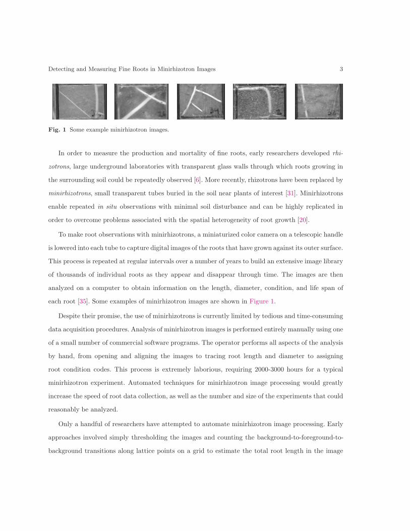
Fig. 1 Some example minirhizotron images.

In order to measure the production and mortality of fine roots, early researchers developed rhi-

zotrons, large underground laboratories with transparent glass walls through which roots growing in

the surrounding soil could be repeatedly observed [6]. More recently, rhizotrons have been replaced by

minirhizotrons, small transparent tubes buried in the soil near plants of interest [31]. Minirhizotrons

enable repeated in situ observations with minimal soil disturbance and can be highly replicated in

order to overcome problems associated with the spatial heterogeneity of root growth [20].

To make root observations with minirhizotrons, a miniaturized color camera on a telescopic handle

is lowered into each tube to capture digital images of the roots that have grown against its outer surface.

This process is repeated at regular intervals over a number of years to build an extensive image library

of thousands of individual roots as they appear and disappear through time. The images are then

analyzed on a computer to obtain information on the length, diameter, condition, and life span of

each root [35]. Some examples of minirhizotron images are shown in Figure 1.

Despite their promise, the use of minirhizotrons is currently limited by tedious and time-consuming

data acquisition procedures. Analysis of minirhizotron images is performed entirely manually using one

of a small number of commercial software programs. The operator performs all aspects of the analysis

by hand, from opening and aligning the images to tracing root length and diameter to assigning

root condition codes. This process is extremely laborious, requiring 2000-3000 hours for a typical

minirhizotron experiment. Automated techniques for minirhizotron image processing would greatly

increase the speed of root data collection, as well as the number and size of the experiments that could

reasonably be analyzed.

Only a handful of researchers have attempted to automate minirhizotron image processing. Early

approaches involved simply thresholding the images and counting the background-to-foreground-to-

background transitions along lattice points on a grid to estimate the total root length in the image


[3,34]. Slightly better results were achieved by applying a morphological thinning operation to the

thresholded result [23]. Nater et al. [24] explored the use of an artificial neural network to detect root

pixels but were unable to achieve satisfactory performance on non-training images. More recently,

Vamerali et al. [32] used exponential contrast stretching, global thresholding, and skeletonization to

measure the total root length. Similarly, Andren et al. [2] extracted skeletons from globally thresholded

images and counted the total number of pixels to estimate total root length. The recent work of Erz

and Posch [15] was aimed at detecting seed points in roots (but not the roots themselves) to assist

more sophisticated search algorithms.

None of these methods have been widely adopted by researchers in the field. One significant

drawback to previous methods is that they generate estimates of total root length only, rather than

identifying and measuring the length of individual roots in each image. Researchers require data on

the length and lifespan of individual roots in order to accurately estimate fine root turnover using

demographic statistical techniques [35].

In this paper, we present an automatic system to detect and measure individual young roots in

minirhizotron images. To our knowledge, this is the first attempt to go beyond merely classifying

pixels as root or background and instead to actually detect an individual root by classifying a group

of contiguous pixels as belonging to the same root. As with previous authors, we focus on young

roots because they are generally brighter than the surrounding soil, making them easier to detect [32].

Our algorithm identifies and measures bright young roots in each image. Future work will involve the

tracking roots over time utilizing temporal consistency to overcome the ambiguities that arise as roots

become dark. Ultimately, we hope to automate all aspects of minirhizotron image analysis that are

currently performed by hand.

The algorithm presented here involves a series of processing steps. After initial preprocessing to

enhance contrast between the young root and the background, matched filters at several orientations

and two scales are applied to the image, utilizing assumptions about root color and shape. The

resulting images are then separately thresholded using an automated technique known as local entropy

thresholding. A robust root classifier is applied to discriminate roots from unwanted background objects

in thresholded binary images, and a root labeling step used to identify individual roots. The root length


is measured by applying Dijkstra’s algorithm to the skeleton to remove undesired branches and by

applying the Kimura-Kikuchi-Yamasaki [22] algorithm to estimate the length of the central curve. The

root diameter is estimated by a robust average of the length of the line segments that are perpendicular

to this curve and extend to the root/background transition. Experimental results from a collection of

200 peach (Prunus persica) root test images show accurate detection and measurement.

2 Detecting Roots

Our approach to detecting roots involves four steps which are described in the following subsections:

matched filtering, thresholding, discriminating, and labeling. To enhance the contrast between the

root and the background, an initial preprocessing step is applied that involves extracting only the

green component from the original red-green-blue color image and linearly stretching the resulting

gray levels.

2.1 Matched Filtering

Because roots generally have low curvature and their two edges run parallel to one another, a root

can be represented by piecewise linear segments of constant width. Moreover, because young roots

generally appear brighter than the surrounding soil (see Figure 2), the gray level profile of the cross

section of each segment can be approximated by a scaled Gaussian curve offset by a constant:

f(x, y) = A

(1 + ke−

d2

2σ2

), (1)

where d is the perpendicular distance between the point (x, y) and the central axis of the root, σ

defines the spread of the intensity profile, A is the gray level intensity of the local background, and k

is the measure of reflectance of the plant root relative to its neighborhood.

Due to similarities between roots and blood vessels, the two-dimensional matched filter kernel

developed by Chaudhuri et al. [9] for blood vessels is adopted here for detecting roots. (Similar

approaches have been adopted by various researchers for detecting roads, canals, hedges, and runways


5 10 15 200

50

100

150

200

250

Data Point

Gra

y S

cale

Inte

nsity

Fig. 2 A minirhizotron image of two roots, along with its preprocessed version. To the right is a plot ofthe intensity profiles of the root cross sections in the preprocessed image along the line shown. (Dash line forthe oblique root on the left and solid line for the vertical root on the right) Note that this is a particularlyclean image with little clutter, so the preprocessing alone goes a long way toward separating the root fromthe background.

in aerial images [28,5,14,19,4].) We convolve the image with a family of scaled Gaussian kernels at

different orientations and scales:

Kθ,σ(x, y) =

⎧⎪⎨⎪⎩

e−y2

θ2σ2 if |xθ|≤ L

2 ,

0 otherwise(2)

where xθ = x cos θ + y sin θ and yθ = −x sin θ + y cos θ are the coordinates along and across the

segment, respectively, and L is the length of the segment for which the root is assumed to have a fixed

orientation.

If the background is viewed as pixels having constant intensity with zero mean additive Gaussian

white noise, its ideal response to the matched filter should be zero. Therefore, the convolution kernel

is modified by subtracting its mean value:

K ′θ,σ(x, y) = Kθ,σ(x, y) − µθ,σ, (3)

where µθ,σ is the mean of the values in the kernel Kθ,σ. For computational efficiency, the coefficients in

the kernel are multiplied by 100 and rounded to the nearest integer. To reduce the effect of background

noise where no root segments are present, the mean value of the resulting kernel is forced to be slightly

negative. Comparing Equations (1), (2), and (3), we see that A = −µθ,σ and k = 100/A.

We apply the matched filter at 12 different orientations, spaced 15 degrees apart, and at two

different scales (σ = 2 and σ = 4 pixels). Based on experimentation, we set L = 11 and the size of

each kernel to 81× 81 pixels, with pixels beyond the length L set to zero. A sample kernel is shown in


Fig. 3 The 81 × 81 matched filter at 180 degrees, with L = 11 and σ = 2.

75o 90o 105o 135o 150o

Fig. 4 Five matched filter kernels (top), along with the output matched filter response (MFR) images at fivedifferent angles for full size (middle) and half size (bottom). The half size images have been scaled for display.

Figure 3. For computational efficiency, the larger sigma is achieved by downsampling the image by a

factor of two in each direction and applying the same set of kernels to the downsampled image. Shown

in Figure 4 are the results of applying five of the matched filter kernels (at every other orientation)

to the preprocessed image of Figure 2. Notice that as the angle increases, the response to the vertical

root on the right becomes stronger, while the response to the oblique root on the left becomes weaker.


2.2 Local Entropy Thresholding

In order to properly segment the roots from the background, we threshold the matched filter response

(MFR) images. The threshold for each image is determined using a technique known as local entropy

thresholding (LET) [27], which applies Shannon’s classic notion of entropy [12] to the image co-

occurrence matrix.

Let tij be the (i, j)th element of the co-occurrence matrix, i.e., tij is the number of pixels in the

image with graylevel i whose immediate neighbor to the right or below has graylevel j. Thus, tij is

defined as:

tij =M∑l=1

N∑k=1

δ(l, k), (4)

where

δ(l, k) =

⎧⎪⎪⎪⎪⎪⎨⎪⎪⎪⎪⎪⎩

1, if f(l, k) = i and

⎧⎪⎪⎨⎪⎪⎩

f(l, k + 1) = j

or

f(l + 1, k) = j

0, otherwise,

(5)

and where M and N are the image dimensions.

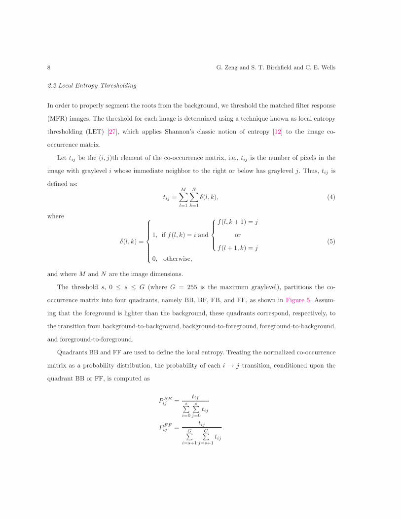
The threshold s, 0 ≤ s ≤ G (where G = 255 is the maximum graylevel), partitions the co-

occurrence matrix into four quadrants, namely BB, BF, FB, and FF, as shown in Figure 5. Assum-

ing that the foreground is lighter than the background, these quadrants correspond, respectively, to

the transition from background-to-background, background-to-foreground, foreground-to-background,

and foreground-to-foreground.

Quadrants BB and FF are used to define the local entropy. Treating the normalized co-occurrence

matrix as a probability distribution, the probability of each i → j transition, conditioned upon the

quadrant BB or FF, is computed as

PBBij =

tijs∑

i=0

s∑j=0

tij

PFFij =

tijG∑

i=s+1

G∑j=s+1

tij

.


Fig. 5 Quadrants of the co-occurrence matrix.

The local entropy method uses the spatial correlation in the image as the criterion for selecting the

optimal threshold by attempting to distribute the transition probabilities within each quadrant. The

threshold is chosen to maximize the sum of the background-to-background entropy and the foreground-

to-foreground entropy:

HT (s) = HBB(s) + HFF (s), (6)

where

HBB(s) = −12

s∑i=0

s∑j=0

PBBij logPBB

ij

HFF (s) = −12

G∑i=s+1

G∑j=s+1

PFFij logPFF

ij

are the entropies of the two quadrants. Local entropy thresholding can be thought of as a simple form

of texture segmentation in which there are exactly two objects separated by their graylevels. The

results of applying LET to the matched filter response (MFR) images are shown in Figure 6.

Because it takes spatial information into account, local entropy thresholding (LET) is superior

to common thresholding techniques such as Otsu’s method [26] that operate only on the graylevel

histogram of the image. Figure 7 compares LET with Otsu’s method using two synthetic images

sharing identical histograms. Ignoring all spatial information, Otsu’s method incorrectly computes

the same threshold in both cases, whereas LET is able to correctly segment both images by taking


75o 90o 105o 135o 150o

Fig. 6 The result of LET thresholding on the matched filter response (MFR) images of Figure 4.

0 50 100 150 200 2500

2000

4000

6000

8000

10000

Gray Level

Nu

mb

er o

f o

ccu

ran

ces

TLET

TOtsu

0 50 100 150 200 2500

2000

4000

6000

8000

10000

Gray Level

Nu

mb

er o

f o

ccu

ran

ces

TOtsu

= TLET

Image Histogram Otsu’s output LET output

Fig. 7 A comparison of Otsu’s method and local entropy thresholding (LET) on two synthetic images sharingthe same graylevel histogram. The former incorrectly computes the same threshold value in both cases, whilethe latter successfully computes the correct thresholds.

into account the spatial relationships of the pixels. The advantage of using LET versus Otsu’s is clearly

seen on several real images in Figure 8. Even when the histogram is unimodal, LET is able to compute

a threshold that successfully retains the roots and attenuates the distracting background pixels.

Traditionally, matched filter responses are combined (e.g., using a pixelwise maximum operator)

before thresholding [8]. The drawback of this approach, however, is that it loses important informa-

tion about the directionality of the responses. As shown in Figure 9, thresholding the combined image

results in shape distortion because bright background noise close to the main root segment is misclas-


0 50 100 150 200 250 3000

0.5

1

1.5

2

2.5

3

3.5

4

4.5

5x 10

4

0 50 100 150 200 250 3000

1

2

3

4

5

6

7

8

9x 10

4

0 50 100 150 200 250 3000

1

2

3

4

5

6

7

8x 10

4

0 50 100 150 200 250 3000

1

2

3

4

5

6

7

8x 10

4

MFR image Histogram Otsu’s output LET output

Fig. 8 A comparison of Otsu’s method and local entropy thresholding (LET) on matched filter response(MFR) images. The top two rows are from one image filtered at two different orientations (105o and 45o,respectively), while the bottom two rows are from a different image filtered at two different orientations (150o

and 45o). LET is more successful at retaining the roots and attenuating the background pixels.

sified. We choose instead to threshold each of the MFR images separately, followed by combining the

24 outputs and extracting the root using the technique described in the next section.

2.3 Discriminating Roots

As shown in Figure 6, the matched filters detect not only bright young roots but also some bright

extraneous objects such as light soil particles, water droplets, or spots caused by uneven diffusion of

light through the minirhizotron wall. After discarding regions detected in the 24 images (12 orientations

and 2 scales) by LET that are smaller than 0.5% of the image, a strong classifier is applied to the


Fig. 9 Five different minirhizotron images (top), the result of thresholding the combined MFR image (middle),and the result of combining the 24 separately thresholded MFR images (bottom). Our approach reduces theshape distortion that results from combining all the orientations before thresholding.

remaining regions to discriminate the actual roots from the extraneous objects. For each region, five

measures are computed: (1) the percentage of pixels in the region with an intensity value greater than

0.8G; (2) the percentage of intensity edges in the region; (3) the eccentricity of the region; (4) the

symmetry of the region around its central curve as measured by the percentage of pixels along the

curve whose corresponding boundary pixels are equidistant; and (5) the percentage of pixels along the

curve whose boundary pixels share parallel tangents.

The AdaBoost algorithm [17] is used to combine these five measures into a strong classifier:

H(x) = sign

(5∑

n=1

αnhn(x)

), (7)

where αn is the coefficients found by AdaBoost to weight the classifier hn according to its importance:

αn =12

(ln

1 − εn

εn

). (8)

The error εn is given by

εn = Pri∼Dn [hn(xi) �= yi] =∑

i:hn(xi) �=yi

Dn(i), (9)


where the output yi ∈ {−1, +1} is the ground truth for the training set, and Dn(i) is the weight

assigned to the ith training example on round n. More details about the root discriminator can be

found in [36].

2.4 Labeling Roots

After the root classifier discriminates roots from the bright background objects in the binary images,

the classified components are compared with each other. Any pair of components that overlap by at

least p% and whose orientations differ by no more than a certain amount (θmax) are combined into one

component. Among the remaining components, the challenge is then to determine which components

belong to the same root, and which components belong to separate roots.

The problem is illustrated in Figure 10. In this figure are shown two images in which the matched

filter responses occur at multiple orientations, yielding components that overlap in the image. To

determine whether the components are part of the same root or whether they indicate separate roots,

we compare the two individual components, which we call R1 and R2, along with the combined

component obtained by logically ORing the two individual components, which we call R12. For each

of the components R1, R2, and R12, we find its extreme points vertically, called endpoints. If both of

the endpoints of R1 are more than a distance dmax to both of the endpoints of R2, then R1 and R2 are

labeled as separate roots. On the other hand, if one endpoint of R1 is separated by one endpoint of

R2 by less than dmax while the remaining endpoints are separated by less than dmax to the endpoints

of R12, then R1 and R2 are combined into a single root. The results are shown in the figure.

An additional challenge occurs when a root is partially covered by soil, in which case the algorithm

detects two disjointed components for the same root. To overcome this problem, we compare the

orientations of the components. If the orientations of the components differ by no more than θmax,

and if the orientation of the line connecting the centroids of the two components is less than θmax from

the orientations of the components, then the separate components are considered to be portions of

the same root. The results of all the processing steps described in this section are shown in Figure 11

for five example images, using p = 60, θmax = 5 degrees, and dmax = 30 pixels.


(a) (b) (c) (d) (e)

Fig. 10 (a) Two images that yield overlapping matched filter responses in multiple directions. (b) and (c)The separate MFR components with the central axis overlaid. (d) The logical OR of the components with thecentral axis overlaid. (e) The final result, in which the crossing roots are detected as separate roots, while thebending root is detected as one.

Fig. 11 Five images with the detected roots. The thin black lines in the first two columns indicate separateroots found by the algorithm. In the last column the two regions are detected as belonging to the same root(this is not shown in the figure), while in the other images disjoint regions belong to different roots.

3 Measuring Roots

Once a root has been detected, it is necessary to measure its length and diameter. First, the morpho-

logical operation of thinning is applied to the binary root image to yield the skeleton, also known as a

skeleton tree [10]. Any irregularity in the shape of the root will cause additional branches in the tree.

To remove these undesirable artifacts, we apply Dijkstra’s algorithm [11] to compute the minimum-

length path between any two points on the skeleton. The two points whose minimum-length path is

maximum are selected, along with the path, to yield the central curve of the root. Figure 12 shows

the skeleton and the resulting central curve for five different images.

The central curve is stored as a sequence of nodes (pixels) 〈C0, C1, . . . CNc〉, where Nc is the number

of nodes. The Euclidean distance along the discretized curve (i.e., the sum of the Euclidean distances


Fig. 12 For five different images, the skeleton tree (top) and the central curve computed by applyingDijkstra’s algorithm to the skeleton (bottom).

between consecutive nodes) is given by

L =√

2Nd + No, (10)

where Nd is the number of consecutive node pairs (Ci, Ci+1) which are diagonally connected and

No is the number of consecutive node pairs which are adjacent either horizontally or vertically. This

equation is also known as the Freeman formula [16]. An alternate approach is to rearrange the node

pairs (see Figure 13) and use the Pythagorean theorem to estimate the root length as the hypotenuse

of the right triangle:

L = (N2d + (No + Nd)2)1/2. (11)

While the Freeman formula generally overestimates the length of a curve [18], the Pythagorean theorem

usually underestimates it [23,13].

Insight into the problem is obtained by noticing that the previous two equations can be written

as special cases of the more general formula:

L =[Nd

2 + (Nd + cNo)2]1/2

+ (1 − c)No, (12)

where c = 0 for the Freeman formula and c = 1 for the Pythagorean theorem. Kimura, Kikuchi, and

Yamasaki [22] proposed a compromise between the overestimation and underestimation by setting c


Freeman Pythagorean Kimura14.5

15

15.5

16

Mea

sure

d le

ng

th

True length

Freeman Pythagorean Kimura14.5

15

15.5

16

Mea

sure

d le

ng

th

True length

One-line axis Two-line axis

Fig. 13 A comparison of the three methods for root length measurement. Top: A simple root with a straightline central curve (left), and a slightly more complicated with two line segments (right). Each gray pixel ison the curve, an open circle indicates a diagonally connection between a pair of pixels, and a closed circleindicating an adjacent connection. The total number and type of connections are the same in both roots.Middle: The rearranged curves by grouping similar circles (the number of circles of each type remains thesame). In both roots the length is estimated as AD+DB (Freeman), AB (Pythagorean), or AE+EB (Kimura).The true length is AB (left) and AF+FB (right). Bottom: A plot of the results. Freeman always overestimates,Pythagorean works perfectly for the linear curve but underestimates the more complex curve, and Kimuraachieves a reasonable compromise.


0 1 2 3 4 5 60

10

20

30

40

50

60

70

80

90

100

Number of roots

Num

ber

of im

ages

60

31

2

19

2 1

85

Fig. 14 The number of images in the test set containing a certain number of roots. 85 images contained noroot, while 115 contained one or more roots.

to the average between the two techniques: c = 12 . For brevity we refer to this approach as Kimura’s

method. See Figure 13 for a graphical illustration and comparison of the three techniques.

Estimating the diameter of the root is rather straightforward. Ten equally-spaced points are found

along the central curve, and the diameter is measured at each of these points using the Euclidean

distance from the curve to the root edge along the line perpendicular to the curve. A robust average

is obtained by discarding the maximum and minimum diameters and computing the mean of the

remaining values.

4 Experimental Results

Our algorithm was developed and tested using a database of 250 minirhizotron images (640×480) from

4-year-old peach trees (Prunus persica) growing in an experimental orchard near Clemson University.

Of the 250 images, 100 contained no roots, while the rest contained one or more young roots of different

size, shape, background composition, and brightness. The image backgrounds contained a wide variety

of bright non-root objects including light soil particles and water droplets. We randomly selected 50

images for algorithm development and used the remaining 200 images as the test set. The number of

roots in the test set images is shown in Figure 14.

The final results of the algorithm on selected images from the test set are shown in Figure 15. The

algorithm is able to detect and measure a variety of roots of different shapes, sizes, and orientations,


with a detection rate of 92%, a false positive rate of 5% (one root per twenty images), and an average

measurement error of 4.1% and 6.8% for length and diameter, respectively. Multiple non-overlapping

roots (as in #5, #9, and #36) cause no problem for the algorithm, while the more difficult scenario of

overlapping roots is also handled correctly (#10 and #12). One important challenge for root imagery

is the occlusion of the roots by the soil which makes it difficult to detect the root as a single region (as

in #36 and #37). By comparing the orientations of the segments, the algorithm is able to correctly

connect the disjointed regions. The occluding soil in some cases creates noise in the shape of the

detected root (#15 and #72), and yet the resulting length and diameter accuracy are still acceptable.

Some examples of partial or complete failure are shown in Figure 16. One common problem is the

partial occlusion of the root by soil which leads to a low contrast in the image between the root and

the background. In such a case the root may not be detected at all (false negative detection) or its

length may be underestimated. Another problem is caused by bright objects in the background that

look like roots, leading to false positive detections. A third problem occurs due to the handwritten

markings on the minirhizotron tube itself which occasionally occlude the roots. More sophisticated

processing, such as hysteresis thresholding, optical character recognition, or context analysis might be

able to reduce the effects of such problems.

To further examine the benefits of local entropy thresholding (LET), we replaced LET with Otsu’s

method and ran the resulting algorithm against 50 images randomly selected from the image database.

These images contained 64 roots in 35 images, while 15 images contained no roots. Both methods

achieved a true positive rate of 96%, but Otsu’s method caused more shape distortion than LET, as

can be seen in Figure 17. In addition, Otsu’s method caused a 20% false positive error, while LET

exhibited no such error.

An additional problem, perhaps unique to this image set, is the presence of parallel black and white

stripes along the edges of the images. These lines result from orientation grooves marked directly

onto the minirhizotron tubes themselves, and can easily be misidentified as roots. Our strategy is

to detect the black stripes by inverting the graylevels of the image and then applying the matched

filter at orientations of 90 and 180 degrees to the downsampled half size image, followed by local

entropy thresholding. If a black stripe is detected, then the white stripe is assumed to be located in a


#5 #9 #10 #12 #15

#36 #37 #64 #72 #108

Fig. 15 The results of the algorithm on some images from the test database. From top to bottom: Originalimage; labeled roots; central curve and diameters estimated by the algorithm overlaid on the image (Thedashed black lines join regions that are detected as a single root by the algorithm); and ground truth. Thenumber below each image identifies it in the database.


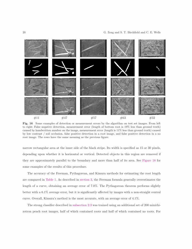
#11 #47 #57 #63 #32

Fig. 16 Some examples of detection or measurement errors by the algorithm on test set images. From leftto right: False negative detection, measurement error (length of bottom root is 19% less than ground truth)caused by handwritten number on the image, measurement error (length is 11% less than ground truth) causedby low contrast / soil occlusion, false positive detection in a root image, and false positive detection in a noroot image. The rows have the same meaning as the previous figure.

narrow rectangular area at the inner side of the black stripe. Its width is specified as 15 or 30 pixels,

depending upon whether it is horizontal or vertical. Detected objects in this region are removed if

they are approximately parallel to the boundary and more than half of its area. See Figure 18 for

some examples of the results of this procedure.

The accuracy of the Freeman, Pythagorean, and Kimura methods for estimating the root length

are compared in Table 1. As described in section 3, the Freeman formula generally overestimates the

length of a curve, obtaining an average error of 7.0%. The Pythagorean theorem performs slightly

better with a 6.1% average error, but it is significantly affected by images with a non-straight central

curve. Overall, Kimura’s method is the most accurate, with an average error of 4.1%.

The strong classifier described in subsection 2.3 was trained using an additional set of 200 minirhi-

zotron peach root images, half of which contained roots and half of which contained no roots. For


#48 #66 #77 #23 #71

Fig. 17 Some examples of errors using Otsu’s method. Top: Original image; Middle: Results using ouralgorithm; Bottom: Results when LET is replaced by Otsu’s method. Otsu’s causes more length measurementerror (#48, #66), shape distortion (#77), and false positive error (#23, #71). In #48, LET yields 5% errorin length while Otsu’s yields 39% error; in #66, the errors are 2% and 18%, respectively.

#5 #27 #31 #69 #79

Fig. 18 Results of our method to remove the white stripes on some example images of the database. Top:Original image; Middle: Detected roots and false positives from white stripes; Bottom: Remaining rootsafter white stripes have been removed using the procedure described.


Method Measurement error (%)

Average Min Max

Freeman formula 7.1 0.5 15.3

Pythagorean theorem 6.0 0.5 21.5

Kimura’s method 4.1 0.1 19.1

Table 1 Length measurement errors using the three different methods.

each of the five methods, an optimal threshold was determined by constructing its receiver operating

characteristic (ROC) curve and then estimating its accuracy by calculating the distance deer of its

corresponding EER point to the ideal point (0,1) on the ROC curve. The inverse of of this distance

indicates the accuracy of the classifier [29]. As shown in Table 2, the eccentricity method performs

the best, followed by approximate line symmetry and boundary parallelism. The strong classifier is

trained by adding the weak classifiers incrementally using the Adaboost algorithm to determine the

weights of the data and the coefficients of the weak classifiers. The final coefficients are shown in the

right column of the table. From these data we conclude that the shape-based methods are much more

discriminative than the intensity-based methods. Further details can be found in [36].

Classifier 1/deer αn

Eccentricity 7.07 1.10

Approximate Line Symmetry 5.05 0.56

Parallel Boundary 4.71 0.78

Interior Intensity Edges 2.62 0.16

Histogram Distribution 2.00 0.00

Table 2 The individual performance 1/deer of each weak classifier, along with its coefficient αn determinedby Adaboost. In both columns, higher values indicate increased reliability and importance.

5 Conclusion

Automated image analysis will enable researchers to make effective use of the overwhelming amount

of data available from minirhizotron root observation systems. In this paper we have described a novel

technique for automatically detecting and measuring bright young roots in a minirhizotron image.


To our knowledge this is the first attempt to detect individual roots, as opposed to estimating the

aggregate lengths of all roots in the image. The approach combines matched filtering and local entropy

thresholding, minimizing the resulting shape distortion by processing each matched filtered image

separately. A robust root classifier discriminates roots from bright background objects, and a root

labeling method prevents misclassification of overlapped roots or separate root segments. Dijkstra’s

algorithm is used to extract the central curve of the root, which is then measured using the Kimura-

Kikuchi-Yamasaki algorithm.

One direction for future work is to improve the efficiency of the algorithm and incorporate it into

an application, such as our Rootfly tool [1], thus enabling plant scientists to immediately benefit from

this research. Another direction is to improve the accuracy of the detection and measurement by

developing more sophisticated algorithms that use hysteresis thresholding, occlusion analysis, or more

top-down processing. Finally, we are exploring algorithms for tracking the location of a root over time

as it grows darker in color and blends into the surrounding soil. Ultimately, we hope to automate all

aspects of minirhizotron image analysis that are currently performed by hand.

Acknowledgments

This work was partially supported by NSF grant DBI-0455221.

References

1. S. Birchfield and C. E. Wells. Rootfly: Software for Minirhizotron Image Analysis,

http://www.ces.clemson.edu/∼stb/rootfly/.

2. O. Andren, H. Elmquist, and A. C. Hansson. Recording, processing and analysis of grass root images

from a rhizotron. Plant and Soil, 185(2):259–264, 1996.

3. J. P. Baldwin, P. B. Tinker, and F. H. C. Marriott. The measurement and distribution of onion roots in

the field and the laboratory. Journal of Applied Ecology, 8:543–554, 1971.

4. A. Barsia and C. Heipkeb. Artificial neural networks for the detection of road junctions in aerial images.

In Proceedings of the International Society for Photogrammetry and Remote Sensing (ISPRS) Workshop

on Photogrammetric Image Analysis, volume XXXIV, Sept. 2003.


5. M. Barzohar and D. B. Cooper. Automatic finding of main roads in aerial images by using geometric-

stochastic models and estimation. IEEE Transactions on Pattern Analysis and Machine Intelligence,

18(7):707–721, July 1996.

6. W. Boehm. Methods of Studying Root Systems. Springer-Verlag, New York, 1979.

7. M. M. Caldwell and R. A. Virginia. Root systems. In R. Pearcy, J. Ehleringer, H. Mooney, and P. Rundel,

editors, Plant Physiological Ecology. Chapman and Hall, New York, 1989.

8. T. Chanwimaluang and G. Fan. An efficient blood vessel detection algorithm for retinal images using

local entropy thresholding. In Proceedings of the IEEE International Symposium on Circuits and Systems,

volume 5, pages 21–24, 2003.

9. S. Chaudhuri, S. Chatterjee, N. Katz, M. Nelson, and M. Goldbaum. Detection of blood vessels in retinal

images using two-dimensional matched filters. IEEE Transactions on Medical Imaging, 8(3):263–269, 1989.

10. D. Chen, B. Li, Z. Liang, M. Wan, A. Kaufman, and M. Wax. A tree-branch searching, multiresolution

approach to skeletonization for virtual endoscopy. In Proceedings of the International Society for Optical

Engineering, volume 3979, pages 726–734, 2000.

11. T. H. Cormen, C. E. Leiserson, and R. L. Rivest. Introduction to Algorithms. McGraw–Hill, New York,

1990.

12. T. M. Cover and J. A. Thomas. Elements of Information Theory. Wiley, New York, 1991.

13. L. Dorst and A. W. M. Smeulders. Length estimators for digitized contours. Computer Vision, Graphics,

and Image Processing, 40:311–333, 1987.

14. R. Duda and P. Hart. Pattern Classification and Scene Analysis. John Wiley and Sons, 1973.

15. G. Erz and S. Posch. A region based seed detection for root detection in minirhizotron images. In

Proceeding of 25th DAGM Symposium, volume 2781, pages 482–489, 2003.

16. H. Freeman. Boundary encoding and processing. In Picture Processing and Psychopictorics, pages 241–

266. Academic Press, New York, 1970.

17. Y. Freund and R. E. Schapire. A short introduction to boosting. Journal of Japanese Society for Artificial

Intelligence, 14(5):771–780, 1999.

18. C. A. Glasbey and G. W. Horgan. Image Analysis for the Biological Sciences. Wiley, Chichester, 1995.

19. J. Han and L. Guo. An algorithm for automatic detection of runways in aerial images. Machine Graphics

and Vision International Journal, 10(4):503–518, Sept. 2001.

20. R. L. Hendrick and K. S. Pregitzer. Spatial variation in tree root distribution and growth associated with

minirhizotrons. Plant and Soil, 143(2):283–288, 1992.


21. J. D. Joslin and G. S. Henderson. Organic matter and nutrients associated with fine root turnover in a

white oak stand. Forest Science, 33:330–346, 1987.

22. K. Kimura, S. Kikuchi, and S. Yamasaki. Accurate root length measurement by image analysis. Plant

and Soil, 216(1):117–127, 1999.

23. R. J. Lebowitz. Digital image analysis measurement of root length and diameter. Environmental and

Experimental Botany, 28:267–273, 1988.

24. E. A. Nater, K. D. Nater, and J. M. Baker. Application of artificial neural system algorithms to image

analysis of roots in soil. Geoderma, 53(3):237–253, 1992.

25. R. J. Norby and R. B. Jackson. Root dynamics and global change: seeking an ecosystem perspective. New

Phytologist, 147:3–12, 2000.

26. N. Otsu. A threshold selection method from gray level histograms. IEEE Transactions on Systems, Man,

and Cybernetics, 9(1):62–66, 1979.

27. N. R. Pal and S. K. Pal. Entropic thresholding. Signal Processing, 16:97–108, 1989.

28. M. Petrou. Optimal convolution filters and an algorithm for the detection of wide linear features. IEE

Proceedings I, Vision, Signal and Image Processing, 140(5):331–339, Oct. 1993.

29. J. Swets. Measuring the accuracy of diagnostic systems. Science, 240:1285–1293, 1988.

30. L. Taiz and E. Zeiger. Plant Physiology. Sinauer, Sunderland, 3rd edition, 2002.

31. D. R. Upchurch and J. T. Ritchie. Root observations using a video recording system in mini-rhizotrons.

Agronomy Journal, 75(6):1009–1015, 1983.

32. T. Vamerali, A. Ganis, S. Bona, and G. Mosca. An approach to minirhizotron root image analysis. Plant

and Soil, 217(1):183–193, 1999.

33. K. A. Vogt, C. C. Grier, and D. J. Vogt. Production, turnover and nutritional dynamics of above- and

belowground detritus of world forests. Advances in Ecological Research, 15:303–307, 1986.

34. W. B. Voorhees, V. A. Carlson, and E. A. Hallauert. Root length measurement with a computer-controlled

digital scanning micro-densitometer. Agronomy Journal, 72:847–851, 1980.

35. C. E. Wells and D. M. Eissenstat. Marked differences in survivorship among apple roots of different

diameters. Ecology, 82:882–892, 2001.

36. G. Zeng, C. E. Wells, and S. T. Birchfield. Automatic discrimination of fine roots in minirhizotron images.

Plant and Soil, 2006. Under review.

detecting and measuring fine roots in minirhizotron images

Documents