detecting anomalous structures by convolutional sparse...
TRANSCRIPT

Detecting Anomalous Structuresby Convolutional Sparse Models
Diego Carrera, Giacomo BoracchiDipartimento di Elettronica,Informazione e BioingegeriaPolitecnico di Milano, Italy
{giacomo.boracchi, diego.carrera}@polimi.it
Alessandro FoiDepartment of Signal Processing
Tampere University of TechnologyTampere, Finland
Brendt WohlbergTheoretical Division
Los Alamos National LaboratoryLos Alamos, NM, USA
Abstract—We address the problem of detecting anomalies inimages, specifically that of detecting regions characterized bystructures that do not conform those of normal images. In theproposed approach we exploit convolutional sparse models tolearn a dictionary of filters from a training set of normal images.These filters capture the structure of normal images and areleveraged to quantitatively assess whether regions of a test imageare normal or anomalous. Each test image is at first encodedwith respect to the learned dictionary, yielding sparse coefficientmaps, and then analyzed by computing indicator vectors thatassess the conformance of local image regions with the learnedfilters. Anomalies are then detected by identifying outliers in theseindicators.
Our experiments demonstrate that a convolutional sparsemodel provides better anomaly-detection performance than anequivalent method based on standard patch-based sparsity. Mostimportantly, our results highlight that monitoring the local groupsparsity, namely the spread of nonzero coefficients across differentmaps, is essential for detecting anomalous regions.
Keywords—Anomaly Detection, Convolutional Sparse Models,Deconvolutional Networks.
I. INTRODUCTION
We address the problem of detecting anomalous regions inimages, i.e. regions having a structure that does not conformto a reference set of normal images [1]. Often, anomalousstructures indicate a change or an evolution of the data-generating process that has to be promptly detected to react ac-cordingly. Consider, for instance, an industrial scenario wherethe production of fibers is monitored by a scanning electronmicroscope (SEM). In normal conditions, namely when themachinery operates properly, images should depict filamentsand structures similar to those in Figure 1(a). Anomalousstructures, such as those highlighted in Figure 1(b), mightindicate a malfunction or defects in the raw materials used,and have to be automatically detected to activate suitablecountermeasures.
Detecting anomalies in images is a challenging problem.First of all because, often, no training data for the anomalousregions are provided and it is not feasible to forecast allthe possible anomalies that might appear. Second, anomaliesin images might cover arbitrarily shaped regions, which canbe very small. Third, anomalies might affect only the localstructures, while leaving macroscopic features such as theaverage pixel-intensity in the region untouched.
Our approach is based on convolutional sparse models,which in [2] were shown to effectively learn mid-level featuresof images. In convolutional sparse representations, the inputimage is approximated as the sum of M convolutions betweena small filter dm and a sparse coefficient map xm, i.e. a spatialmap having few non-zero coefficients. A convolutional sparsemodel is a synthesis representation [3], where the image isencoded with respect to a dictionary of filters, yielding sparsecoefficient maps. The decoding consists in adding all the out-puts of the convolution between the filters and correspondingcoefficient maps.
Structures from normal images are modeled by learning adictionary of M filters {dm} from a training set of normalimages. Learned filters represent the local structure of trainingimages, as shown in Figure 2(a). Each test image is encodedwith respect to the learned filters, computing the coefficientmaps that indicate which filters are activated (i.e. have nonzerocoefficients) in each local region of the image. In normalregions we expect the convolutional sparse model to describethe image well, yielding sparse coefficient maps and a goodapproximation. This is illustrated in Figure 2(b), where thegreen patch in the left half belongs to a normal region and hasonly few filters activated: the corresponding coefficient mapsare sparse. In contrast, in regions characterized by anomalousstructures, we expect coefficient maps to be less sparse or toless accurately approximate the image. The red patch insidethe right (anomalous) half of Figure 2(b) shows coefficientmaps that are not sparse.
We detect anomalies by analyzing a test image and the cor-responding coefficient maps in a patch-wise manner. Patches,i.e. small regions having a predefined shape, are thus thecore objects of our analysis. For each patch we compute alow-dimensional indicator vector that quantitatively assessesthe goodness-of-fit of the convolutional model, namely theextent to which the patch is consistent with normal ones.Indicators are then used to determine whether a given patch isnormal or anomalous. Given the above considerations, the moststraightforward indicator for a patch would be a vector stackingthe reconstruction error and the sparsity of the coefficient mapsover each patch.
However, in our experiments we show that the sparsity ofthe coefficient maps is too loose a criterion for discriminatinganomalous regions, and that it is convenient to consider alsothe spread of nonzero coefficients across different maps. Inparticular we observed that, while normal regions can be

(a) (b)
Fig. 1: Examples of SEM images depicting a nanofibrous material produced by an electrospinning process: Fig. (a) does notcontain anomalies, and is characterized by specific structures also at local-level. Fig. (b) highlights anomalies that are clearlyvisible among the thin fibers.
typically approximated by few filters, the representation ofanomalous ones often involves many filters. Therefore, weinclude in the indicator vector a term measuring the a localgroup-sparsity of the coefficient maps, and show that this isinformation is effective at discriminating anomalous regions.
Summarizing, the contribution of the paper is two-fold.First, we develop a novel approach for detecting anomalies bymeans of convolutional sparse models describing the structuresof normal images. Second, we show that the local group spar-sity of the coefficient maps is a relevant prior for discriminatinganomalous regions.
The remainder of the paper is organized as follows:Section II provides an overview of related works, whileSection III formulates the anomaly-detection problem. Theproposed approach is outlined in Section IV while detailsabout convolutional sparse representations and the indicatorvectors are provided in Sections IV-A and IV-B, respectively.Experiments are presented and discussed in Section V.
II. RELATED WORKS
Anomaly detection [4], refers to the general problem ofdetecting unexpected patterns both in supervised scenarios(where training samples are labeled as normal, or either normaland anomalous) and in unsupervised scenarios (where trainingsamples are provided without labels). Anomaly detection isalso referred to as novelty detection [1], [5], [6], in particularwhen anomalies are intended as patterns that do not conform toa training set of normal data. In the machine learning literature,novelty detection is formulated as a one-class classificationproblem [7]. In this paper, we shall refer to the patternsbeing detected as anomalies, despite the novelty detectioncontext. An overview of novelty-detection methods for imagesis reported in [1].
Convolutional sparse models were originally introducedin [2] to build architectures of multiple encoder layers, theso-called deconvolutional networks. These networks have beenshown to outperform architectures relying on standard patch-based sparsity when learning mid-level features for objectrecognition. More sophisticated architectures involving both
decoder and encoder layers showed to be effective in visualrecognition tasks, such as supervised pedestrian detection [8]and unsupervised learning of object parts [9]. Deconvolutionalnetworks are strictly related to the well-known convolutionalnetworks [10], which in contrast are analysis representations,where the image is subject to multiple layers where it isdirectly convolved against filters. Convolutional sparse modelshave not previously been used for the anomaly-detectionproblem, such as that considered in this work. For simplicity,we presently develop and describe a single-layer architecture,although more layers may also be used.
Convolutional sparse models can be seen as extensionsof patch-based sparse models [11], the former providing arepresentation of the entire image while the latter indepen-dently represent each image patch. Patch-based sparse modelshave been recently used for anomaly detection purposes [12],where an unconstrained optimization problem is solved toobtain the sparse representation of each patch in a test image.Then, the reconstruction error and the sparsity of the computedrepresentation are jointly monitored to detect the anomalousstructures. In [13] anomalies are detected by means of aspecific sparse-coding procedure, which isolates anomalies asdata that do not admit a sparse representation with respect toa learned dictionary. Sparse representations have been usedfor detecting unusual events in video sequences [14], [15] bymonitoring the functional minimized during the sparse codingstage. The detection of structural changes – a problem closelyrelated to anomaly detection – was addressed in [16], wheresparse representations were used to sequentially monitor astream of signals.
Convolutional sparse models offer two main advantagescompared to patch-based ones: first of all, they directly supportthe use of multiscale dictionaries [18], whereas this is notstraightforward for standard patch-based sparse representa-tions. Second, the size of the patch that has to be analyzedin the anomaly detection can be arbitrarily increased at anegligible computational overhead when convolutional sparsemodels are exploited. In contrast, this requires additionaltraining and also increases the computational burden [22] inthe case of patch-based sparsity.

Learned Filters Training Image Test ImageF
eature m
aps anom
alous patch
a) b)
Feature
maps
normal patch
Fig. 2: (a) Learned dictionary (8 filters are of size 8 × 8 and 8 are of size 16 × 16) reports the prominent local structures ofthe training image. (b) A test image used in our experiments: the left half represents the normal region (filters were learnedfrom the other half of the same texture image), while the right half represents the anomalous region. The ideal anomaly detectorshould mark all pixels within the right half as anomalous, and all pixels within the left half as normal. The coefficient mapscorresponding to the two highlighted regions (red and green squares) have approximately the same `1 norms. However, theright-most figures show that there is a substantially different spread of nonzero elements across coefficient maps. Thus, in thisexample the local group sparsity of the coefficient maps is more informative than sparsity for discriminating anomalous regions.Feature maps have been rescaled for better visualization.
III. PROBLEM FORMULATION
Let us denote by s : X → R+ a grayscale image, whereX ⊂ Z2 is the regular pixel grid representing the image domainhaving size N1 ×N2. Our goal is to detect those regions in atest image s where the structures do not conform to those ofa reference training set of normal images T.
To this purpose, we analyze the image locally, and for-mulate the detection problem in terms of image patches. Inparticular, we denote
sc := Πcs = {s(c+ u), u ∈ U}, ∀c ∈ X (1)
the patch centered at a specific pixel c ∈ X , where U is aneighborhood of the origin defining the patch shape, and Πc
denotes the linear operator extracting the patch centered atpixel c. We consider U a square neighborhood of
√P ×
√P
pixels (indicating by P the cardinality of U), even thoughpatches sc can be defined over arbitrary shapes.
We assume that patches in anomaly-free images are drawnfrom a stationary, stochastic process PN and we refer tothese as normal patches. In contrast, anomalous patches aregenerated by a different process PA, which yields unusualstructures that do not conform to those generated by PN .
The training set T is used to learn a suitable modelspecifically for approximating normal images. Instead, notraining samples of anomalous images are provided, thus itis not possible to learn a model approximating anomalousregions. In this sense, PA remains completely unknown.
Anomalous structures are detected at the patch level: eachpatch sc is tested to determine whether it does or does notconform to the model learned to approximate images generatedby PN . This will result in a map locating anomalous regionsin a test image.
IV. METHOD
We treat the low and high-frequency components of imagesseparately; we perform a preprocessing to express s as
s = sl + sh, (2)
where sl and sh denote the low-frequency and high-frequencycomponents of s, respectively. Typically, sl is first computedby low-pass filtering s and then sh = s− sl.
In particular, we compute the convolutional sparse repre-sentation of sh with respect to a dictionary of filters learnedto describe the high-frequency components of normal images.Restricting the convolutional sparse representation to the high-frequency components allows the use of few small filters inthe dictionary. For each patch sc we compute a vector gh(c)that simultaneously assesses the accuracy and the sparsity ofthe convolutional representation around c. The low-frequencycontent of s is instead monitored by computing the samplemoments of sl(·) over patches, yielding vectors gl(·). Then,for each patch, we define the indicator vector g(c) as theconcatenation of gh(c) and gl(c). Anomalies are detected aspatches yielding outliers in these indicator vectors.
Let us briefly summarize the proposed solution, presentingthe high-level scheme in Algorithms 1 and 2; details aboutconvolutional sparse representations and indicators are thenprovided in Section IV-A and IV-B, respectively.
Training: Anomalies are detected by learning a modeldescribing normal patches from the training set T. In particular,we learn a dictionary of filters {dm} yielding convolutionalsparse representation for high-frequency components of normalimages (Algorithm 1, line 1 and Section IV-A1). The indicatorvectors are then computed from all the normal patches, asdescribed in Section IV-B, and a suitable confidence region

Rγ that encompasses most of these indicators is defined(Algorithm 1, lines 2 and 3).
Testing: During operation, each test image s is prepro-cessed to separate the high frequency content sh from the lowfrequency content sl (Algorithm 2, line 1). The convolutionalsparse representation of sh with respect to the dictionary {dm}is obtained by the sparse coding procedure described in Sec-tion IV-A2 (Algorithm 1, line 2). Then, for each pixel c, gh(c)is computed by analyzing the convolutional representation ofsh in the vicinity of c, and gl(c) is computed by analyzingsl in the vicinity of c (Algorithm 1, lines 4 and 5). Theindicator vector g(c) is then obtained by stacking gh(c) andgl(c), namely g(c) = [gh(c),gl(c)]
′. Any indicator g(c) thatfalls outside a confidence region Rγ estimated from normalimages is considered an outlier and the corresponding patchanomalous (Section IV-B3, Algorithm 1, line 7).
Input: training set of normal images T:1. Learn filters {dm} solving (4)2. Compute gh(·) (9) and gl(·) (10) for all the normal
patches, define g as in (11)3. Define Rγ in (12) setting the threshold γ > 0
Algorithm 1: Training the anomaly detector using convolu-tional sparse models.
Input: test image s:1. Preprocess the image s = sl + sh2. Compute the coefficient maps {xm} solving (7)3. foreach pixel c of s do4. Compute gh(c) as (9)5. Compute gl(c) as (10)6. Define g(c) = [gl(c),gl(c)]
′ as (11)7. if g(c) /∈ Rγ then8. c belongs to an anomalous region
else9. c belongs to a normal region
endend
Algorithm 2: Detecting anomalous regions using convolu-tional sparse models.
A. Convolutional Sparse Representations
Convolutional sparse representations [2] express the high-frequency content of an image s ∈ RN1×N2 as the sum of Mconvolutions between filters dm and coefficient maps xm, i.e.
sh ≈M∑m=1
dm ∗ xm , (3)
where ∗ denotes the two dimensional convolution, and thecoefficient maps xm ∈ RN1×N2 have the same size of theimage s. Filters {dm}1 might have different sizes, but aretypically much smaller than the image.
Coefficient maps are assumed to be sparse, namely onlyfew elements of each xm are nonzero, thus ‖xm‖0 (the numberof nonzero elements) is small. Sparsity regularizes the modeland prevents trivial solutions of (3).
1For notational simplicity we omit m ∈ {1, . . . ,M} from the collectionof filters and coefficient maps.
1) Dictionary learning: To detect anomalous regions weneed a collection of filters {dm} that specifically approximatethe local structures of normal images. These filters representthe dictionary of the convolutional sparse model, and canbe learned from a normal image s provided for training.Dictionary learning is formulated as the following optimizationproblem
arg min{dm},{xm}
1
2
∥∥∥∥∥M∑m=1
dm ∗ xm − sh
∥∥∥∥∥2
2
+ λ
M∑m=1
‖xm‖1 ,
subject to ‖dm‖2 = 1, m ∈ {1, . . . ,M} ,
(4)
where {dm} and {xm} denote the collections of M filters andcoefficient maps, respectively. To simplify the notation, (4)presents dictionary learning on a single training image s,however, extending (4) to multiple training images is straight-forward [11].
The first term in (4) denotes the reconstruction error, i.e.the squared `2 norm of the residuals, namely∥∥∥∥∥∑
m
dm ∗ xm − sh
∥∥∥∥∥2
2
=∑c∈X
(∑m
(dm ∗ xm)(c)− sh(c)
)2
,
(5)while the `1 norm of the coefficient maps is defined as∑
m
‖xm‖1 =∑m
∑c∈X|xm(c)|. (6)
In practice, the penalization term in (4) promotes the sparsityof the solution [17], namely the number of nonzero coefficientsin the feature maps. Thus, the `1 norm is often used asreplacement of `0 norm to make (4) computationally tractable.The constraint ‖dm‖2 = 1 is necessary to resolve the scalingambiguity between dm and xm (i.e. xm can be made arbitrarilysmall if the corresponding dm is made correspondingly large).We solve the dictionary learning problem using an efficientalgorithm [18] that operates in Fourier domain. Learned filterstypically report the prominent local structures of trainingimages, as shown in Figure 2(a).
We observe that filters {dm} learned in (4) may havedifferent sizes [18], which is a useful feature for dealing withimage structures at different scales. Figure 2(a) provides anexample where 8 filters of size 8 × 8 and 8 filters of size16× 16 were simultaneously learned from a training image.
2) Sparse Coding: The computation of coefficient maps{xm} of an input image sh with respect to a dictionary {dm}is referred to as sparse coding, and consists in solving thefollowing optimization problem [2]:
arg min{xm}
1
2
∥∥∥∥∥∑m
dm ∗ xm − sh
∥∥∥∥∥2
2
+ λ∑m
‖xm‖1 , (7)
where filters {dm} were previously learned from (4).
The sparse coding problem (7) can be solved via theAlternating Direction Method of Multipliers (ADMM) algo-rithm [19], exploiting an efficient formulation [11] in theFourier domain. The dictionary-learning problem is typicallysolved by alternating the solution of (4) with respect to thecoefficient maps {xm} when filters are fixed (sparse coding)and then with respect to the filters {dm} when coefficient mapsare fixed.

B. Indicators
To determine whether each patch sc is normal or anoma-lous we compute an indicator vector g(c) that quantitativelyassesses the extent to which sc is consistent and with normalpatches. Indicators g(c) are computed from the decompositionof s in (2) to assess the extent to which the dictionary {dm}matches the structures of sh around c (Section IV-B1), as wellas the similarity between low frequency content of Πcsl andnormal patches (Section IV-B2).
1) High-Frequency Components: In anomalous regions fil-ters are less likely to match the local structures of sh, thusit is reasonable to expect the sparse coding (7) to be lesssuccessful, and that either the coefficient maps would be lesssparse or that (3) would yield a poorer approximation. Thisimplies that we should monitor the reconstruction error (5) andthe sparsity of coefficient maps (6), locally, around c. However,we observed that monitoring the sparsity term (6) is too loosea criterion for discriminating anomalous regions.
To improve the detection performance, we take into con-sideration also the distribution of nonzero elements acrossdifferent coefficient maps. This choice was motivated by theempirical observation that often, within normal regions –where filters are well matched with image structures – only fewcoefficient maps are simultaneously active; in contrast, withinregions where filters and image structures do not match, morefilters are typically active. Figure 2(b) compares two coefficientmaps within normal and anomalous regions, and shows that inthe latter case more filters are active. For this reason, we alsoinclude a term in g(h) to monitor the local group sparsity ofthe coefficient maps, namely:∑
m
‖Πcxm‖2 =
M∑m=1
√∑u∈U
(xm(c+ u))2. (8)
The indicator based on the high frequency components ofthe image is defined as
gh(c) =
‖Πc (sh −∑m dm ∗ xm)‖2
2∑m ‖Πcxm‖1∑m ‖Πcxm‖2
, (9)
where first and second components represent the reconstructionerror of sc and the sparsity of the coefficient maps in thevicinity of c, respectively: these directly refer to the termsin (7), thus inherently indicate how successful the sparsecoding was. The third element in (11) represents the groupsparsity, and indicates the spread of nonzero elements acrossdifferent coefficient maps in the vicinity of pixel c.
2) Low-Frequency Components: Anomalies affecting thelow frequency components of s are in principle easy to detectas these affect, for instance, the average value of each patch.We analyze the first two sample moments over patches Πcsl,extracted from sl. More precisely, for each pixel c of sl wedefine
gl(c) =
[µcσ2c
], (10)
where µc =∑u∈U sl(u+ c)/P denotes the sample mean and
σ2c =
∑u∈U (sl(u + c) − µc)2/(P − 1) the sample variance
computed over the patch of sl centered in c.
Both gh and gl can be stacked in a single vector to bejointly analyzed when testing patches, namely
g(c) =
[gl(c)gh(c)
]. (11)
This is the indicator we use to determine whether a patchis anomalous or not, analyzing both the high and the lowfrequency content in the vicinity of pixel c.
3) Detecting Anomalous Patches: We treat indicators asrandom vectors and detect as anomalous all the patches yield-ing indicators that can be considered outliers. Therefore, webuild a confidence region Rγ around the mean vector [20] fornormal patches, namely:
Rγ =
{φ ∈ R2 :
√(φ− g)TΣ−1(φ− g) ≤ γ
}, (12)
where g and Σ denote the sample mean and sample covariancematrix of indicators extracted from normal images in T, andγ > 0 is a suitably chosen threshold. Rγ represents an high-density regions for indicators extracted from normal patches,since the multivariate Chebyshev’s inequality ensures that, fora normal patch sc, holds
Pr({g(sc) /∈ Rγ}) ≤2
γ2, (13)
where Pr({g(sc) /∈ Rγ}) denotes the probability for a normalpatch sc to lie outside the confidence region (false-positive de-tection). Therefore, outliers can be simply detected as vectorsfalling outside a confidence region Rγ , i.e.√
(g(c)− µ)TΣ−1(g(c)− µ) > γ, (14)
and any patch sc yielding an indicator g(c) satisfying (14) isconsidered anomalous.
V. EXPERIMENTS
We design two experiments to assess the anomaly-detectionperformance of convolutional sparse representations and, inparticular, the advantages of monitoring the local group spar-sity of the coefficient maps. In the first experiment we detectanomalies by monitoring both the low and high frequencycomponents of an input image, while in the second experimentwe exclusively analyze the high-frequency components. Thelatter experiment is to assess the performance of detectorsbased exclusively on sparse models.
Considered Algorithms: We compare the following fouralgorithms built on the framework of Algorithm 1 and 2:
• Convolutional Group: a convolutional sparse modelis used to approximate sh. Anomalies are detected byanalyzing the indicator g in (11) which includes alsothe local group sparsity of the coefficient maps (8).The indicator has five dimensions.
• Convolutional: the same dictionary of filters for theConvolutional Group solution is used to approximatesh, however, the local group sparsity term of thecoefficient maps (8) is not considered in g. Thus, theindicator has four dimensions.

Fig. 3: Ten of the textures selected from Brodatz dataset(textures 20, 27, 36, 54, 66, 83, 87, 103, 109, 111). Forvisualization purposes, we show only 240 × 240 regionscropped from the original images, which have size 640× 640.
• Patch-based: a standard sparse model [21] ratherthan a convolutional sparse model is used to describepatches extracted from sh, as in [12]. The indicatorincludes the reconstruction error and the sparsity ofthe representation. To enable a fair comparison againstconvolutional sparse models, the indicator includes thesample mean over each patch from sh and sl, as wellas the sample variance over each patch from sl. Theindicator has five dimensions.
• Sample Moments: no model is used to approximatethe image and we compute the sample mean andvariance over patches from sl and sh. The indicatorhas four dimensions.
In the second experiment, where only the high-frequencycontent of images is processed, the same algorithms areused. In particular, the Convolutional Group computes three-dimensional indicator (gh), the Convolutional computes a two-dimensional indicator (only the first two components of gh areused), the Patch-based operates only on sh computing a three-dimensional indicator and the Sample Moments also operateson sh computing a two-dimensional indicator.
We learned dictionaries of 16 filters (8 filters of size 8× 8and 8 of size 16 × 16), solving (4) with λ = 0.1. The samevalue λ was used also in the sparse coding (7). The dictionariesin the patch-based approach are 1.5 times redundant, andlearned by [22]. In all the considered algorithms, indicatorsare computed from 15× 15 patches.
Preprocessing: We perform a low-pass filtering of eachtest image s to extract the low frequency components. Moreprecisely, sl corresponds to the solution of the followingoptimization problem
arg minsl
1
2‖sl − s‖22 +
α
2‖∇sl‖22 , (15)
where ∇sl denotes the image gradient, α > 0 regulates theamount of high frequency components in sl (in our tests α =10). The problem (15) can be solved as a linear system andadmits a closed-form solution.
Dataset: To test the considered algorithms we have se-lected 25 textures from the Brodatz dataset [23] having astructure that can be properly captured by 15× 15 filters and
Fig. 4: Example of anomaly-detection performance for theConvolutional Group algorithm. Any detection (red pixels) onthe left half represents a false positive, while any detection onthe right half a true positive. The ideal anomaly detector wouldhere detect all the points in the left half and none on the righthalf. Patches across the vertical boundary are not consideredin the anomaly detection to avoid artifacts. As shown in thehighlighted regions, most of false positives in this example aredue to structure that do not conform to the normal image inFigure 2(a).
patches (10 of the selected textures are shown in Figure 3).A dataset of test images has been prepared by splitting eachtexture image in two halves: the left half was exclusively usedfor training, the right half for testing. The right halves of the25 textures are pair-wise combined, creating 600 test imagesby horizontally concatenating two different right halves. Anexample of test image is reported in Figure 2(b). We considerthe left half of each test image as normal and the right halfas anomalous, therefore we perform anomaly detection usingthe model learned from the texture on the left half. Note that,since anomalies are detected in a patch-wise manner, havinganomalies covering half test image does not ease the anomalydetection task with respect to having localized anomalies likethose in Figure 1(a).
Figures of Merit: The anomaly detection performance areassessed by the following figures of merit:
• FPR, false positive rate, i.e. the percentage of normalpatches detected as anomalous.
• TPR, true positive rate, i.e. the percentage of correctlydetected patches.
Figure 4 provides an example of false positives and truepositives over a test image (the left half being normal, theright half anomalous).
Both FPR and TPR depend on the specific value of γ usedwhen defining Rγ . To enable a fair comparison among theconsidered algorithms we consider a wide range of values forγ and plot the receiver operating characteristic (ROC) curvefor each method. In practice, each point of a ROC curvecorresponds to the pair (FPR, TPR) achieved for a specificvalue of γ. When computing FPR and TPR, we excludepatches overlapping the vertical boundary between differenttextures.
0 0.2 0.4 0.6 0.8 10
0.2
0.4
0.6
0.8
1
FPR
TPR
ROC curves from s = sh + sl
Convolutional GroupConvolutionalPatch-basedSample Moments
(a) The Area Under the Curve values are: Convolutional Group: 0.9520;Convolutional: 0.9317; Patch-Based: 0.9422; Sample Moments: 0.9048
0 0.2 0.4 0.6 0.8 10
0.2
0.4
0.6
0.8
1
FPR
TPR
ROC curves from sh
Convolutional GroupConvolutionalPatch-basedSample Moments
(b) The Area Under the Curve values are: Convolutional Group: 0.9198;Convolutional: 0.8578; Patch-Based: 0.8836; Sample Moments: 0.7706
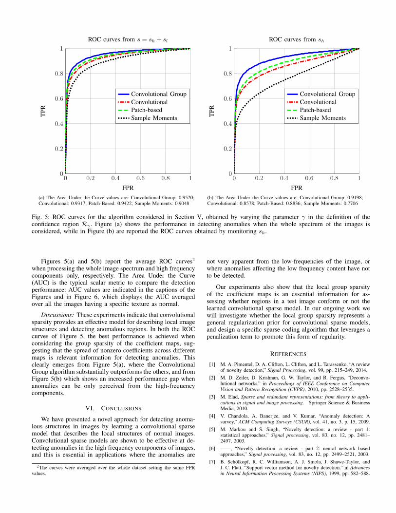
Fig. 5: ROC curves for the algorithm considered in Section V, obtained by varying the parameter γ in the definition of theconfidence region Rγ . Figure (a) shows the performance in detecting anomalies when the whole spectrum of the images isconsidered, while in Figure (b) are reported the ROC curves obtained by monitoring sh.
Figures 5(a) and 5(b) report the average ROC curves2
when processing the whole image spectrum and high frequencycomponents only, respectively. The Area Under the Curve(AUC) is the typical scalar metric to compare the detectionperformance: AUC values are indicated in the captions of theFigures and in Figure 6, which displays the AUC averagedover all the images having a specific texture as normal.
Discussions: These experiments indicate that convolutionalsparsity provides an effective model for describing local imagestructures and detecting anomalous regions. In both the ROCcurves of Figure 5, the best performance is achieved whenconsidering the group sparsity of the coefficient maps, sug-gesting that the spread of nonzero coefficients across differentmaps is relevant information for detecting anomalies. Thisclearly emerges from Figure 5(a), where the ConvolutionalGroup algorithm substantially outperforms the others, and fromFigure 5(b) which shows an increased performance gap whenanomalies can be only perceived from the high-frequencycomponents.
VI. CONCLUSIONS
We have presented a novel approach for detecting anoma-lous structures in images by learning a convolutional sparsemodel that describes the local structures of normal images.Convolutional sparse models are shown to be effective at de-tecting anomalies in the high frequency components of images,and this is essential in applications where the anomalies are
2The curves were averaged over the whole dataset setting the same FPRvalues.
not very apparent from the low-frequencies of the image, orwhere anomalies affecting the low frequency content have notto be detected.
Our experiments also show that the local group sparsityof the coefficient maps is an essential information for as-sessing whether regions in a test image conform or not thelearned convolutional sparse model. In our ongoing work wewill investigate whether the local group sparsity represents ageneral regularization prior for convolutional sparse models,and design a specific sparse-coding algorithm that leverages apenalization term to promote this form of regularity.
REFERENCES
[1] M. A. Pimentel, D. A. Clifton, L. Clifton, and L. Tarassenko, “A reviewof novelty detection,” Signal Processing, vol. 99, pp. 215–249, 2014.
[2] M. D. Zeiler, D. Krishnan, G. W. Taylor, and R. Fergus, “Deconvo-lutional networks,” in Proceedings of IEEE Conference on ComputerVision and Pattern Recognition (CVPR), 2010, pp. 2528–2535.
[3] M. Elad, Sparse and redundant representations: from theory to appli-cations in signal and image processing. Springer Science & BusinessMedia, 2010.
[4] V. Chandola, A. Banerjee, and V. Kumar, “Anomaly detection: Asurvey,” ACM Computing Surveys (CSUR), vol. 41, no. 3, p. 15, 2009.
[5] M. Markou and S. Singh, “Novelty detection: a review - part 1:statistical approaches,” Signal processing, vol. 83, no. 12, pp. 2481–2497, 2003.
[6] ——, “Novelty detection: a review - part 2: neural network basedapproaches,” Signal processing, vol. 83, no. 12, pp. 2499–2521, 2003.
[7] B. Scholkopf, R. C. Williamson, A. J. Smola, J. Shawe-Taylor, andJ. C. Platt, “Support vector method for novelty detection.” in Advancesin Neural Information Processing Systems (NIPS), 1999, pp. 582–588.

36 87 27 78 76 51 65 56 54 55 105 66 74 111 34 49 24 68 20 103 15 109 83 52 37
0.5
0.6
0.7
0.8
0.9
Texture
AU
C
Convolutional GroupConvolutionalPatch-basedSample Moments
Fig. 6: For each texture it is shown the AUC value averaged over the test images where such texture is considered normal.Convolutional Group achieves the best performance in almost all cases, and in some cases it substantially outperforms otheralgorithms.
[8] K. Kavukcuoglu, P. Sermanet, Y.-L. Boureau, K. Gregor, M. Mathieu,and Y. L. Cun, “Learning convolutional feature hierarchies for visualrecognition,” in Advances in Neural Information Processing Systems(NIPS), 2010, pp. 1090–1098.
[9] H. Lee, R. Grosse, R. Ranganath, and A. Y. Ng, “Convolutionaldeep belief networks for scalable unsupervised learning of hierarchicalrepresentations,” in Proceedings of Annual International Conference onMachine Learning (ICML), 2009, pp. 609–616.
[10] Y. LeCun, L. Bottou, Y. Bengio, and P. Haffner, “Gradient-basedlearning applied to document recognition,” Proceedings of the IEEE,vol. 86, no. 11, pp. 2278–2324, 1998.
[11] B. Wohlberg, “Efficient convolutional sparse coding,” in Proceedingsof IEEE International Conference on Acoustics, Speech and SignalProcessing (ICASSP), 2014, pp. 7173–7177.
[12] G. Boracchi, D. Carrera, and B. Wohlberg, “Novelty detection in imagesby sparse representations,” in Proceedings of IEEE Symposium onIntelligent Embedded Systems (IES), 2014, pp. 47–54.
[13] A. Adler, M. Elad, Y. Hel-Or, and E. Rivlin, “Sparse coding withanomaly detection,” in Proceedings of IEEE International Workshopon Machine Learning for Signal Processing (MLSP), 2013, pp. 1–6.
[14] B. Zhao, L. Fei-Fei, and E. P. Xing, “Online detection of unusualevents in videos via dynamic sparse coding,” in Proceedings of IEEEConference on Computer Vision and Pattern Recognition (CVPR), 2011,pp. 3313–3320.
[15] Y. Cong, J. Yuan, and J. Liu, “Sparse reconstruction cost for abnormalevent detection,” in Proceedings of IEEE Conference on ComputerVision and Pattern Recognition (CVPR), 2011, pp. 3449–3456.
[16] C. Alippi, G. Boracchi, and B. Wohlberg, “Change detection in streamsof signals with sparse representations,” in Proceedings of IEEE In-ternational Conference on Acoustics, Speech and Signal Processing(ICASSP), 2014, pp. 5252–5256.
[17] R. Tibshirani, “Regression shrinkage and selection via the lasso,”Journal of the Royal Statistical Society. Series B (Methodological),vol. 58, pp. 267–288, 1996.
[18] B. Wohlberg, “Efficient algorithms for convolutional sparse representa-tions,” Manuscript currently under review, 2015.
[19] S. Boyd, N. Parikh, E. Chu, B. Peleato, and J. Eckstein, “Distributedoptimization and statistical learning via the alternating direction methodof multipliers,” Foundations and Trends R© in Machine Learning, vol. 3,no. 1, pp. 1–122, 2011.
[20] R. Johnson and D. Wichern, Applied multivariate statistical analysis.Prentice Hall, 2002.
[21] A. M. Bruckstein, D. L. Donoho, and M. Elad, “From sparse solutions
of systems of equations to sparse modeling of signals and images,”SIAM review, vol. 51, no. 1, pp. 34–81, 2009.
[22] J. Mairal, F. Bach, J. Ponce, and G. Sapiro, “Online dictionary learningfor sparse coding,” in Proceedings of the Annual International Confer-ence on Machine Learning (ICML), 2009, pp. 689–696.
[23] P. Brodatz, Textures: A Photographic Album for Artists and Designers.Peter Smith Publisher, Incorporated, 1981.