Detecting Design Intent in Approximate CAD Models

Using Symmetry

Ming Lia,b, Frank C. Langbeina, Ralph R. Martina

aSchool of Computer Science, Cardiff University, Cardiff, UKbState Key Lab of CAD & CG, Zhejiang University, Hangzhou, P. R. China

Abstract

Finding design intent embodied as high-level geometric relations between aCAD model’s sub-parts facilitates various tasks such as model editing andanalysis. This is especially important for boundary-representation modelsarising from, e.g., reverse engineering or CAD data transfer. These lackexplicit information about design intent, and often the intended geometricrelations are only approximately present. The novel solution to this problempresented is based on detecting approximate local incomplete symmetries,in a hierarchical decomposition of the model into simpler, more symmetricsub-parts. Design intent is detected as congruencies, symmetries and sym-metric arrangements of the leaf-parts in this decomposition. All elementary3D symmetry types and common symmetric arrangements are considered.They may be present only locally in subsets of the leaf-parts, and may alsobe incomplete, i.e. not all elements required for a symmetry need be present.Adaptive tolerance intervals are detected automatically for matching inter-point distances, enabling efficient, robust and consistent detection of approx-imate symmetries. Doing so avoids finding many spurious relations, reliablyresolves ambiguities between relations, and reduces inconsistencies. Experi-ments show that detected relations reveal significant design intent.

Key words: Design intent, approximate symmetry, feature recognition,beautification, reverse engineering, CAD data transfer.

Email addresses: eMing.Li@gmail.com (Ming Li),F.C.Langbein@cs.cardiff.ac.uk (Frank C. Langbein),Ralph.Martin@cs.cardiff.ac.uk (Ralph R. Martin)

Preprint submitted to Computer-Aided Design May 22, 2009

1. Introduction

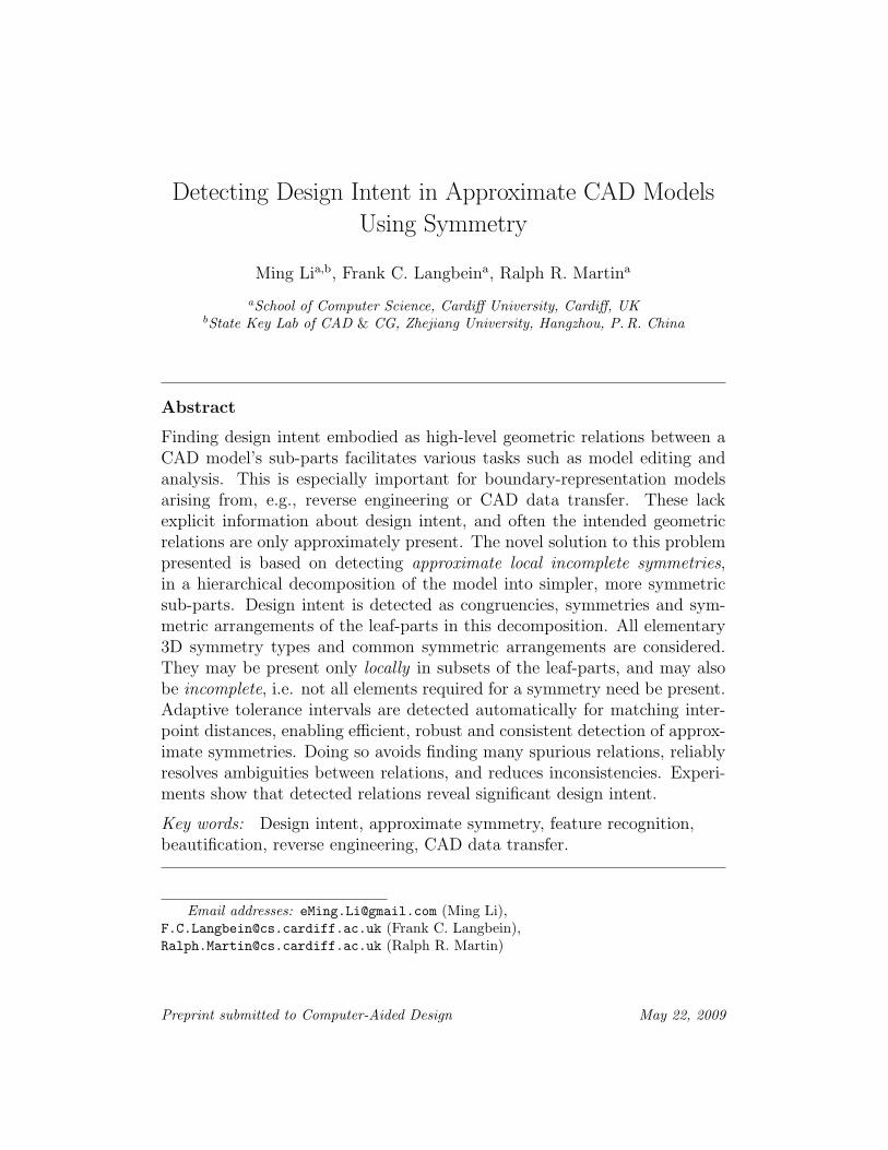
Design intent concerning the shape of a CAD model can be expressedvia geometric properties of, and relations between, its vertices, edges, facesand sub-parts. As shape is often essential to function, such relations mustbe enforced on the model to fulfil its purpose. Many intentional geometricrelations form geometric regularities. However, information about a model’sdesign intent is not always explicitly available. E.g., reverse engineering [42]captures the shape of a model but does not explicitly detect intended reg-ularities. Such models are approximate due to measurement errors, andapproximation and numerical errors occurring during reconstruction. Sim-ilarly, models constructed from inexact user input, e.g. sketches [26, 43],are also approximate, and lack explicit design intent. Exchanging modelsbetween different CAD systems [32] may break intended, exact regularitiesdue to incompatible tolerance systems and representations; design intent isoften not explicitly transferred. Detecting design intent in such approximatemodels can reveal high-level information that is necessary for the model’sfunction or purpose. Such information may be used to constrain and guideediting operations. It may also allow us to improve an approximate modelby enforcing intended regularities. It may enable faster analysis and morecompact representation, if the model has symmetric sub-parts. It may alsoallow models to be more meaningfully indexed for shape search, etc. Thus,this paper considers algorithmic detection of geometric design intent in ap-proximate boundary-representation (B-rep) models of engineering objects,such as the one in Fig. 1.

Symmetry is a key concept in design. Engineering objects often ex-hibit symmetries for functional, aesthetic, and manufacturing reasons [2, 40].Many regularities can be represented via symmetries [19]. A symmetry isan isometry that maps a set exactly onto itself. However, symmetry maybe present approximately—the set is almost invariant under an isometry, lo-cally—only part of the set is invariant, incompletely—not all elements build-ing a symmetry are present, and compatibly—multiple subsets share the samesymmetry. We thus later define a precise concept of approximate incompletesymmetry which includes exact and global symmetries as special cases, gen-eralising the ideas in [29]. For brevity, henceforth, we refer to approximatesymmetry or congruency as symmetry or congruency, unless stated otherwise.An alternative approach [21] considers asymmetries in a model to describedesign intent as a sequence of symmetry breaking operations.

2

Figure 1: An example of an approximate CAD model: Monster

Complex models often exhibit far too many alternative plausible approx-imate regularities for exhaustive methods to be able to determine which reg-ularities represent the original design intent of the whole model [20]. Asa simple example, consider a rectangular block with many prisms attachedto its faces. Analysing the whole model without finding the prisms createsmany candidate angles and distances forming plausible regularities betweenthe model’s planes. By first identifying the individual prisms as sub-parts, wecan detect their approximate prismatic symmetries, and separately determinesymmetric arrangements of the prisms on the block. Analysing sub-parts ofthe model separately increases the speed of regularity detection and providesmore reliable results. Hence, our design intent detection algorithm performsmodel decomposition before detecting regularities in the resulting sub-parts.

The decomposition phase builds a regularity feature tree (RFT) forminga hierarchy of regularity features : simple, closed volumes which in combi-nation describe the original shape. The regularity features at the leaves ofthe RFT describe the complete shape of the object; the tree indicates howto build the complete model from the leaf-parts. Unlike a CSG tree, theRFT does not contain standard primitives, nor does it give a Boolean de-composition [22]. Instead, the emphasis is on the fact that the leaf-partsare simpler and more symmetric than other parts in the tree, and not on

3

Figure 2: Overview of algorithmic steps for detecting design intent of the Monster modelin Fig. 1

how the object was or might have been constructed. The second phase ofthe algorithm seeks regularities within the model in terms of congruencies,incomplete symmetries and symmetric arrangements of these leaf-parts. Itfirst detects congruencies to partition the leaf-parts into congruence sets, eachcontaining one or more congruent leaf-parts. Next, for each congruence set,it seeks subsets forming incomplete symmetries and incomplete symmetricarrangements. Compatible symmetries shared by leaf-parts, and symmetricarrangements, are further combined before we output all detected regular-ities as transformations matching sub-parts of the model. The process isillustrated in Fig. 2 for the model in Fig. 1. Fig. 2(a) shows the computedRFT, Fig. 2(b) shows the congruent leaf-parts found, and the detected sym-metries are given in Figs. 2(c)–(e). The output may, e.g., be used to describea model by geometric constraints [36], or be processed by regularity selectiontechniques [20, 45].

As the models are approximate, the method has to consider tolerancescarefully. We compute suitable (tolerance) validity intervals directly fromdistances present in the model to ensure that model entities match unam-biguously (i.e. in a one-to-one manner) at any tolerance in the interval.During decomposition, each different validity interval yields a different, well-

4

defined RFT. We let the user select a suitable RFT, which is often straight-forward as appropriate tolerances are often known. Regularity detection isthen restricted to that particular validity interval. For a particular decom-position, regularities may also exist at different tolerance levels. To avoidmissing any important regularities, we seek all of these. We ensure that theregularities are unambiguously present to avoid inconsistencies between regu-larities and to reduce the number of spurious regularities found. Regularitiesare detected in a certain sequence for efficiency, and to ensure that rela-tions between regularities are preserved (e.g. congruent sub-parts must havethe same symmetries). Tolerance information is used to ensure that theseinter-regularity relations are preserved at the tolerance intervals at which theregularities are present.

Throughout this paper, we assume that the input model is a manifold 3Dsolid represented by a valid, watertight B-rep data structure, and is boundedby planar, spherical, cylindrical, conical and toroidal surfaces, which coversa wide range of mechanical components [30]. The only reason for this restric-tion is the difficulty of extending the geometry of free-form surfaces involvedin the RFT construction; see Section 6. We assume that blends have beenidentified and suppressed using existing blend-removal methods [35, 46] (orhave not been added during a reverse engineering process).

This paper uses our previous results on constructing RFTs [22] and de-tecting incomplete symmetries of discrete point sets [24, 23]. Here we combineand extend these results to efficiently and robustly detect design intent inB-rep models for a wide range of symmetry-based regularities. We extendour earlier work to include all elementary symmetry types in 3D (mirror,inversion, translation, rotation, rotation-mirror, glide, screw), not just rota-tions and rotation-mirrors, with a single, consistent algorithm. We also givefurther previously unpublished details of our incomplete symmetry detectionalgorithm, and explain how to adapt it to detecting symmetries of B-repmodels (not just point sets).

Detecting symmetries in a B-rep model is achieved by using characteristicpoints. They are the model’s vertices and some other special points whichcharacterise curved edges and faces (e.g. a circular arc is uniquely determinedby its two end points and the arc’s mid-point). These, together with topo-logical and face type information, uniquely characterise the model [10, 29].Hence, although a wireframe model is insufficient to define a volumetric ob-ject uniquely, only regularities of the solid model are detected via consistentmappings between characteristic point sets; see Section 3.2.

5

In summary, this paper presents a novel solution to efficiently detect geo-metric design intent as geometric regularities of and between model sub-partsusing symmetry. It can handle approximate models robustly, yielding well-defined, unambiguous regularities and providing a higher-level descriptionfor downstream processing. Detecting local symmetries using the RFT, in-stead of working directly on the model as a whole, avoids considering manyspurious, almost certainly unintentional geometric relations. It greatly re-duces the computation time required and leads to a better understandingof regularities of the model. Moreover, we consider all possible elementarysymmetry types with a single method based on inter-point distances. Theresults do not depend on arbitrary user-chosen tolerances, but most toler-ances are inferred automatically from the model. This improves robustnessand reliability, as well as efficiency. As some approximate models have mul-tiple consistent interpretations in terms of regularities at different toleranceranges, the user must make a simple choice of a suitable tolerance intervalwhich gives the desired interpretation. Our experiments show that we canefficiently detect regularities which describe significant design intent.

The rest of the paper is organised as follows. Section 2 discusses relatedprevious work and Section 3 gives our definition of incomplete symmetry fordiscrete point sets and B-rep models. Section 4 outlines our design intentdetection algorithm. Details follow in Section 5 on a clustering algorithm tohandle tolerance ranges, Section 6 outlines the RFT construction, and Sec-tions 7 to 11 discuss in detail the stages of our regularity detection approach.Section 12 presents experimental results, and Section 13 concludes the paper.

2. Related Work

We now overview relevant work on representing and detecting geometricdesign intent, and on symmetry detection.

2.1. Design Intent

Previous consideration of design intent has been based on geometric con-straints, features and construction history. Efforts have been made to usethese (including symmetries) to extend the STEP ISO standard for designintent description [32, 18]. Such approaches mostly focus on exact geometricrelations and representation, while our approach is aimed at approximatemodels and design intent detection.

6

Geometric constraints annotate relations between geometric entities [14,12]. However, they usually describe design intent at a low level, prescrib-ing many simple relations and parameters, instead of higher-level relationssuch as a symmetric arrangement of identical complex sub-parts. Solvingconstraint systems provided by a user is the main topic considered, ratherthan detecting constraints. Our algorithm finds high-level relations usingsymmetries, from which low-level constraints can be derived if required.

Feature recognition is often aimed at determining machining operationsneeded to manufacture a model [11, 13, 37]. Recording a complete modelconstruction history, e.g. [7], views design as akin to writing a program toconstruct the model. However, such histories contain artificial constructionsteps as well as the intended regularities. Furthermore, histories are notunique—many can produce the same final object. Bidarra [4] has, however,proposed a semantic feature modelling method in which such design recordingis independent of the model design history. Sitharam et al [36] present ageometric constraint solver which can handle features. In our view theirsis the most promising approach for representing design intent; their systemmay well be suited for downstream processing of the output of our algorithm.Leyton [21] views design as a sequence of symmetry breaking operationsyielding a generative history. As with construction histories, however, thegenerative history of most complex models is ambiguous. In contrast, we areonly concerned with detecting regularities and not inferring a history. Heutilises symmetry and symmetry breaks, but for the representation of designintent, not its detection.

Reverse engineering solid models from measured data, using prescribedfeatures or geometric constraints, has also been considered [3, 27, 41], butfew authors discuss how to extract these from point data [17]. However,detecting candidate geometric constraints after reverse engineering modelshas been previously examined [10, 19, 20, 29]. This approach can handle fairlysimple approximate models, but suffers from ambiguities and inconsistenciesbetween regularities in more complex models. Our approach resolves thisissue for complex models by first decomposing them; it also detects moregeneral incomplete symmetries and symmetric arrangements of sub-parts.Beautification of 3D polyhedral models reconstructed from 2D sketches wasalso considered recently [45].

7

2.2. Symmetry DetectionPrevious work on symmetry detection has mainly considered rotation and

mirror symmetries, with different approaches used for different symmetrytypes. Here, we consider all seven elementary 3D symmetry types using auniform approach.

Exact symmetries can be found in O(n log n) time: see [24] and the refer-ences therein. However, differing definitions of (global) approximate symme-try cause its detection to be NP-hard [15] or to take O(n8) time [1]. Our ap-proach extends the global approximate symmetry detection algorithm in [29],which takes only O(n3.5 log4 n) time.

Little work exists on detecting approximately symmetric subsets of data.Robins [33] considers subsets of points regularly arranged along a line. Whilefor global approximate symmetries a single tolerance applies, for subset sym-metries, a tolerance only applies to a particular subset: different subsets mayhave different tolerances. This complicates the automatic detection of tol-erances. Another approach to finding subset symmetries in solid models ispresented by Tate and Jared [39]. It is based on matching every pair of edgeloops and finding the isometries that relate them. The isometries are thengrouped according to similarity. Their implementation only finds axes of ro-tation and mirror planes. The approach may be used to detect approximatesymmetries by ‘relaxing’ matching tolerance conditions, but this means theresulting notion of approximate symmetry is ambiguous and does not eas-ily enable automated tolerance detection. We aim to detect what is presentunambiguously in the data without predetermined tolerances. Limiting thesearch to edge loops, mainly due to efficiency reasons, is also too restrictivefor finding all symmetries. Instead we employ a volumetric decomposition ofthe model for efficiency reasons and to detect predominantly intended sym-metries. [24] describes an approach for detecting point subsets which formapproximate, complete rotation or rotation-mirror symmetries. We extendthis work here to all incomplete symmetries of sub-parts.

We seek discrete point symmetries to find symmetries of B-rep models asexplained later, but we use quite different point sets compared to symmetryapproaches used in image processing, e.g. [38], and mesh processing, e.g. [31].Generally, the aim there is to detect one or a few dominant approximatesymmetries by partial matching of images or meshes described by dense pointdata, under user-selected tolerances. In contrast, we wish to generate allunambiguous subset symmetries in a carefully chosen characteristic point setderived from the B-rep model, sufficient to uniquely characterise its geometry

8

P2

P1

P3

P4

P5

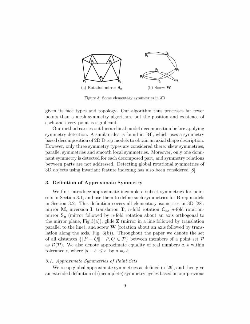
(a) Rotation-mirror Sn (b) Screw W

Figure 3: Some elementary symmetries in 3D

given its face types and topology. Our algorithm thus processes far fewerpoints than a mesh symmetry algorithm, but the position and existence ofeach and every point is significant.

Our method carries out hierarchical model decomposition before applyingsymmetry detection. A similar idea is found in [34], which uses a symmetrybased decomposition of 2D B-rep models to obtain an axial shape description.However, only three symmetry types are considered there: skew symmetries,parallel symmetries and smooth local symmetries. Moreover, only one domi-nant symmetry is detected for each decomposed part, and symmetry relationsbetween parts are not addressed. Detecting global rotational symmetries of3D objects using invariant feature indexing has also been considered [8].

3. Definition of Approximate Symmetry

We first introduce approximate incomplete subset symmetries for pointsets in Section 3.1, and use them to define such symmetries for B-rep modelsin Section 3.2. This definition covers all elementary isometries in 3D [28]:mirror M, inversion I, translation T, n-fold rotation Cn, n-fold rotation-mirror Sn (mirror followed by n-fold rotation about an axis orthogonal tothe mirror plane, Fig 3(a)), glide Z (mirror in a line followed by translationparallel to the line), and screw W (rotation about an axis followed by trans-lation along the axis, Fig. 3(b)). Throughout the paper we denote the setof all distances {‖P − Q‖ : P,Q ∈ P} between members of a point set Pas D(P). We also denote approximate equality of real numbers a, b withintolerance ε, where |a− b| ≤ ε, by a =ε b.

3.1. Approximate Symmetries of Point Sets

We recap global approximate symmetries as defined in [29], and then givean extended definition of (incomplete) symmetry cycles based on our previous

9

work [24]. Merging such cycles leads to incomplete symmetries [23]. Thesedefinitions cover symmetries in a wide mathematical sense: approximate,subset, incomplete, compatible symmetries, and include all the seven typesof elementary symmetries. Further details on these definitions are givenin [24, 23].

Approximate symmetry of a point set is defined in terms of a permuta-tion of the points which maps distances between the points approximatelyonto each other. This definition allows an algorithm to be devised basedon expanding local matches without backtracking, enabling us to keep theefficiency of the approach used in [29].

Specifically, let µ : P1 → P2 be a bijection between two point sets P1,P2, and let ε ≥ 0 be a tolerance. We say DEC(P1,P2, µ, ε) is satisfied if‖P − Q‖ =ε ‖µ(P ) − µ(Q)‖ for all P,Q ∈ P1, and if =ε is an equivalencerelation on D(P1) ∪ D(P2) (see below; this idea was introduced in [29] todefine global approximate symmetry). We define two point sets P1, P2 tobe approximately congruent at tolerance ε if, for at least one of all possiblebijections µ : P1 → P2, DEC(P1,P2, µ, ε) is satisfied. We say that a point setP has an approximate symmetry (µ, ε) for bijection µ : P → P and toleranceε if DEC(P ,P , µ, ε) is satisfied.

Assuming that some ε can be found for which a set of points exhibitsan approximate symmetry, in general, a tolerance validity interval EP =[Emin(P), Emax(P)) around ε exists at which P is approximately symmetric.For tolerances ε smaller than some minimal tolerance Emin(P), some dis-tances in the same distance class would no longer be considered equal, andso the approximate symmetry would not exist. Conversely, for tolerances εgreater than some maximal tolerance Emax(P), the points would no longermap onto each other in a one-to-one fashion, as more than one point wouldbe considered to be at the ‘same’ (approximate) position. The validity in-terval plays a key role in our previous work on detecting (incomplete) pointsymmetries [24, 23], and will also be used throughout this paper.

A complete symmetry consists of cycles : orbits arising by repeatedlyapplying the symmetry mapping to a single point. We define incompletecycles as subsets of a point set P comprising consecutive points from a fullcycle; otherwise, multiple and ambiguous symmetries may appear, e.g. a six-fold rotational cycle can be seen as incomplete twelve-fold cycle by allowinggaps. Further conditions are necessary to uniquely define an incompletecycle: (C1) its points must potentially belong to some symmetric set ofpoints, (C2) its points must be sufficiently far apart from other points in P

10

to avoid ambiguity, and (C3) it should contain as many points as possiblefrom P while still satisfying (C1) and (C2). Formally, let C = (P1, . . . , Pc)be a sequence of c ≥ 2 points from point set P , which induces a bijectionµ mapping Pk to Pk+1 for k = 1, . . . , c − 1. We say that C is a (maximalapproximate) incomplete cycle at tolerance ε ≥ 0 if

(C1) DEC(C, C, µ, ε) is satisfied (Pc maps to P1 in a complete cycle, and tono point otherwise—for simplicity we skip over the fact that µ is notdefined on the last point of an incomplete cycle);

(C2) no point in P \ C can replace a point in C while (C1) still holds underthe same µ; and

(C3) no single point in P \ C can be added to C for any tolerance ε whilestill satisfying (C1) and (C2).

Incomplete symmetries arise by merging compatible cycles under similarconditions to ensure unambiguity as detailed in [23]. A point subset S ⊂ Phas an (approximate) incomplete symmetry (µ, ε) of symmetry type t if

(I1) S is the union of a set of non-intersecting cycles of type t, each havingat least N(t) points to determine a symmetry of a given type t: 2 pointsfor M, I, C2; 3 for T, C3; 4 for Cn≥4, Z and a regular tetrahedron; 5for Sn, W.

(I2) DEC(S,S, µ∗, ε) is satisfied, where µ∗ is the concatenation of the indi-vidual µs of the cycles from (I1); and

(I3) no cycle C∗ of type t in P \ S exists such that (I2) is true for C∗ ∪ C attolerance less than ε for any cycle C of S.

3.2. Approximate Symmetries of B-rep Models

The above ideas can be used to detect congruencies, incomplete sym-metries and symmetric arrangements of sub-parts of a B-rep model, usingcharacteristic points of a B-rep model [10, 29]; see Section 1.

For sub-parts to be congruent or symmetric, any mappings have to satisfythe consistency condition that entities are matched to others of the samegeometric type, e.g. circular arcs to circular arcs. Let µ : S1 → S2 be abijection between the characteristic point sets S1, S2 of two sub-parts S1,S2. We say µ is consistent if whenever a subset S∗ ⊂ S1 defines an entity

11

P2

P3

P4

1 µ1µ4

µ 3µ2

3S

S24

S1

S

P

Q1

Q4

Q 3

Q 2

(a) Type I

4PP2

P1

S3

S4

3P

S2

Q2

Q4

1SQ1

Q3

(b) Type II

Figure 4: Two types of symmetric arrangement of sub-parts

of S1, µ(S∗) are corresponding characteristic points of an entity of the sametype. Two sub-parts thus are approximately congruent if their characteristicpoint sets are congruent at tolerance ε under a consistent bijection µ. Asub-part is approximately symmetric at tolerance ε if its characteristic pointsare symmetric under a consistent bijection µ.

A symmetric arrangement of congruent sub-parts forms a pattern givenby a symmetry group. Even if the relations between them are limited to threeindependent translations in 3D, 230 space groups exist [9]. However, most ofthe cases are not of interest to mechanical engineering, and we only considertwo particularly important types: I and II in Fig. 4. Type I is formed by sub-parts which exhibit global symmetry. Thus, their characteristic points forman (incomplete) symmetry, each cycle of which consists of one point fromeach model at a specific location, called location cycles. E.g., in Fig. 4(a),objects S1, S2, S3, S4 have such an arrangement: cycles (P1, P2, P3, P4) and(Q1, Q2, Q3, Q4) are two of its location cycles forming a symmetry. Alterna-tively, placing a sub-part at symmetric locations while keeping its orientationunchanged gives Type II. In this way, the location cycles are not compati-ble, but are related by a translation. E.g., in Fig. 4(b), models S1, S2, S3, S4

have such an arrangement: cycle (Q1, Q2, Q3, Q4) is a translation of cycle(P1, P2, P3, P4) by Q1 − P1.

Thus, a set of congruent sub-parts S1, . . . , Ss with characteristic point setsS1, . . . ,Ss has a symmetric arrangement at tolerance ε if consistent bijectionsµk : S1 → Sk, k = 2, . . . , s exist such that for all P1 ∈ S1 with location cycleC(P1) = (P1, µ2(P1), . . . , µs(P1)), and, for Type I or Type II respectively,

I: all location cycles C(P1), P1 ∈ S1 form an incomplete symmetry attolerance ε; or

12

II: for any other point Q1 ∈ S1, translating cycle C(P1) by vector Q1 − P1

gives cycle C(Q1) at tolerance ε.

4. Main Design Intent Detection Algorithm

Given an approximate B-rep model as input, our algorithm finds con-gruencies, incomplete symmetries and symmetric arrangements of sub-parts,with corresponding tolerance levels, which describe the model’s geometricdesign intent. Here we describe the top-level algorithm (Algorithm 1). Ittakes as input a B-rep model M . It outputs a hierarchy of congruence sets atdifferent tolerance levels with associated symmetries and symmetric arrange-ments. In general, different regularities may be detected for each congruenceset in the hierarchy. We must detect all regularities at all tolerance levels soas not to miss any intended regularities—a problem noted in [16] with thesymmetry detection approach of Zabrodsky et al [44]. We do not consider theproblem of choosing between alternative, mutually inconsistent regularities(which share entities) here.

As sub-parts are congruent at different tolerance levels, the congruencesets form a tree or forest rather than a simple partition of the sub-parts.Each congruency is described by a set C of sub-parts, a set of pairwisemappings ΓC giving the congruency matchings, and a validity interval ECfor the congruence set. For each C, incomplete symmetries are detected assymmetries of the congruent shape: S[C] gives its symmetries as mappings µmatching the faces of the congruent shape of C within a validity interval. Thecongruencies and the symmetries indicate how the elements of a congruenceset match and are hence necessary to find symmetric arrangements A[C] ofC: we store symmetric arrangements in terms of the mappings between theinvolved sub-parts, and a validity interval.

Initially the algorithm decomposes the model into a regularity featuretree (Line 01), as explained in Section 6. Congruencies between leaf-partsare then found (Lines 02–03). All sets of congruent leaf-parts (Lines 04–13) are next analysed for incomplete symmetries (Line 09) and symmetricarrangements of Type I and II (Lines 10–13). Finally compatible symmetriesare merged (Line 14). We now explain these steps further.

We first construct an RFT T for M , hierarchically decomposing it intosimpler sub-parts (Line 01). More than one possible RFT may exist, eachwith a different validity interval; we discuss later how one is selected. Avalidity interval ET is also reported which indicates the range of tolerances

13

Algorithm (C,R)←DesignIntent(M)Input: M : B-rep modelOutput: C: congruency hierarchy

R: symmetries and symmetric arrangements

01 (T,ET )← RFT(M)02 L ← leaf nodes(T )03 C = {(Ck,ΓCk

, ECk)} ← Congruencies(L, ET )

04 S ← empty, A← empty05 Q ← roots(C)06 while not empty(Q)07 (C,ΓC , EC)← pop(Q)08 Q ← append(Q,children(C))09 S[C]← BRepSymmetries(C,ΓC , EC)10 if S[C] 6= S[parent(C)]11 I ← IncompleteCycles(Centroids(C), EC)12 G ← FilterGlobalSymmetries(S[C], C)13 A[C]← TypeI(C,ΓC , EC ,G, I) ∪ TypeII(C,ΓC , EC ,G, I)14 R ← MergeCompatibleCycles(A ∪ S,ET )

Algorithm 1: Main design intent detection algorithm

for which this tree is valid. Subsequent regularity detection is limited to thisrange. The set L of leaf-parts of this tree is extracted (Line 02) for regularitydetection.

Congruencies are detected first (Line 03) as these facilitate other reg-ularity detection: all members of a congruence set must exhibit the sameincomplete symmetries; symmetrically arranged leaf-parts must be congru-ent. Congruencies are detected as a hierarchy of congruent leaf-part sets Ckat different tolerance levels. For each such congruence set, the bijections ΓCk

indicate how the leaf-parts are matched, and the tolerance validity intervalECk

is also computed. Congruence detection is detailed in Section 7. Thecongruence set hierarchy is examined top-down for incomplete symmetries Sand symmetric arrangements A using a FIFO queueQ (Lines 04–08): all con-gruencies at different tolerance levels in the hierarchy have to be consideredas they may exhibit different regularities.

Detecting incomplete symmetries of a congruence set is achieved by firstdetecting the incomplete symmetries of an exemplar leaf-part in the set andthen retaining those shared by all leaf-parts in the set (Line 09). The in-

14

complete symmetries of the example leaf-part may have been detected pre-viously when examining the parent congruence set. Hence, for efficiency,these symmetries are cached. Details of the symmetry detection algorithmare described in Section 8.

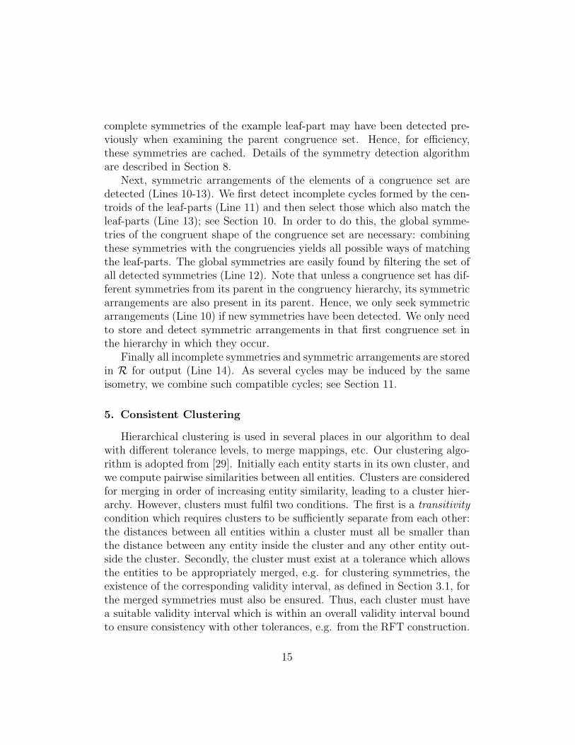
Next, symmetric arrangements of the elements of a congruence set aredetected (Lines 10-13). We first detect incomplete cycles formed by the cen-troids of the leaf-parts (Line 11) and then select those which also match theleaf-parts (Line 13); see Section 10. In order to do this, the global symme-tries of the congruent shape of the congruence set are necessary: combiningthese symmetries with the congruencies yields all possible ways of matchingthe leaf-parts. The global symmetries are easily found by filtering the set ofall detected symmetries (Line 12). Note that unless a congruence set has dif-ferent symmetries from its parent in the congruency hierarchy, its symmetricarrangements are also present in its parent. Hence, we only seek symmetricarrangements (Line 10) if new symmetries have been detected. We only needto store and detect symmetric arrangements in that first congruence set inthe hierarchy in which they occur.

Finally all incomplete symmetries and symmetric arrangements are storedin R for output (Line 14). As several cycles may be induced by the sameisometry, we combine such compatible cycles; see Section 11.

5. Consistent Clustering

Hierarchical clustering is used in several places in our algorithm to dealwith different tolerance levels, to merge mappings, etc. Our clustering algo-rithm is adopted from [29]. Initially each entity starts in its own cluster, andwe compute pairwise similarities between all entities. Clusters are consideredfor merging in order of increasing entity similarity, leading to a cluster hier-archy. However, clusters must fulfil two conditions. The first is a transitivitycondition which requires clusters to be sufficiently separate from each other:the distances between all entities within a cluster must all be smaller thanthe distance between any entity inside the cluster and any other entity out-side the cluster. Secondly, the cluster must exist at a tolerance which allowsthe entities to be appropriately merged, e.g. for clustering symmetries, theexistence of the corresponding validity interval, as defined in Section 3.1, forthe merged symmetries must also be ensured. Thus, each cluster must havea suitable validity interval which is within an overall validity interval boundto ensure consistency with other tolerances, e.g. from the RFT construction.

15

Algorithm H ← ConsistentClustering(Q,E∗)Input: Q = {(Ik, EIk)}: entities Ik with validity intervals EIk

E∗: validity interval boundOutput: H: consistent cluster hierarchy

01 D = {(l, k)} ← sort(Similarity(Q))02 H ← empty03 for each (Ik, EIk) ∈ Q04 C ← {(Ik, EIk)}, v[C]← 1, e[C]← 0, E[C]← EIk05 H ← add root(H, C)06 if not empty(E[C] ∩ E∗), Flag(C)07 for each (l, k) ∈ D // in increasing order of similarity08 if Il, Ik are in the same cluster C of H09 e[C]← e[C] + 110 else Il, Ik are in distinct clusters C1, C2 of H11 C ← Merge(C1, C2,H)12 v[C]← v[C1] + v[C2], e[C]← e[C1] + e[C2] + 113 E[C]← ValidityInterval(C1, C2)14 if Complete(v[C], e[C]) and not empty(E[C] ∩ E∗)15 Flag(C)

Algorithm 2: Consistent hierarchical clustering algorithm

If we construct a graph with nodes representing the entities to be merged,we can detect transitive clusters as complete sub-graphs, i.e. sub-graphs ofv vertices having e edges with acceptable similarities where e = v(v + 1)/2.

The clustering algorithm in Algorithm 2 takes as input a set of distinctentities {Ik} with corresponding tolerance intervals EIk , plus an overall tol-erance range E∗. It outputs a consistent cluster hierarchy. Each distinct pairof entities (l, k) from {Ik} is stored in a list D sorted by increasing order ofentity similarity (Line 01). The similarity measure depends on the type ofentities being clustered; details are given later. For each entity Ik, a clusterC is created with v[C] = 1 vertices, e[C] = 0 edges, and a validity intervalE[C] = EIk ; this is added to the cluster hierarchy H (Lines 03–06). We onlywish to keep clusters fulfilling the two consistency conditions, so we flag suchclusters. The initially created clusters are consistent if the intersection ofthe clusters’ validity interval E[C] with the tolerance range bound E∗ is notempty (Line 06).

In increasing order of similarity, clusters corresponding to the pairs from

16

D are merged: an edge is inserted into the graph of entities (Lines 07–15).During this process, the cluster hierarchy H is updated, and complete com-ponents of the graph are detected by tracking the number of edges e[C] andnodes v[C] in each cluster C. Firstly, the clusters linked by the current en-tity pair (l, k) from D are merged. If the current pair links nodes insidethe same cluster, we increase the edge count for the cluster (Lines 08–09).Otherwise, we merge the two distinct clusters and create new vertex andedge counts accordingly (Lines 10–13). We next check whether the result-ing cluster is consistent. Clusters which are complete and fulfil the validitycondition within the overall tolerance range E∗ are flagged (Lines 14–15).The earlier merging of two clusters (Line 11) only preserves sub-clusters ifthese are flagged. Clusters are ignored if they do not fulfil the validity con-dition and hence are not a valid merged entity, or if they violate the overalltolerance bound.

Line 13 involves computation of the validity interval EC = [Emin(C), Emax(C))for a set of entities C = C1∪C2 to decide if it is valid. Assuming C comprisesthe entities I1, . . . , Ic with given minimal and maximal tolerances for each Ik,we set Emin(C) = max1≤l 6=k≤c(Emin(Il ∪ Ik)), Emax(C) = min1≤k≤c(Emax(Il ∪Ik)).

This clustering method takes O(n2 log n) time for n entities to be clus-tered: n2 pairs have to be sorted and all n(n − 1)/2 pairs must be merged,taking O(log n) time for each pair [29].

6. Regularity Feature Tree Construction

Next we outline the RFT construction used to initially hierarchically de-compose the input model (Line 01, Algorithm 1). Our algorithm is detailedin [22], so here we give a brief overview and concentrate on the associatedtolerance levels in the context of our design intent detection algorithm.

Many regularities can be expressed in terms of symmetries [19]. OurRFT construction is based on recovering symmetries that were broken duringconstruction of the (ideal, rather than approximate) original model by usingmodelling operations on geometric primitives. The regularity feature is usedto represent the newly generated sub-parts for this purpose. While thismeans that some regularity features may become more symmetric, othersmay just represent the symmetry break in the model, i.e. some part whichreduces the model’s symmetry. They hence are not a class of pre-definedsimple geometric primitives, but are determined by the model’s geometry.

17

The RFT is used here to record the hierarchal process of producing theseregularity features. For example, the RFT for the Monster model in Fig. 1is displayed in Fig. 2, and the RFT for the Angle in Fig. 11 is displayed inFig. 10.

Specifically, our approach groups model entities into sub-parts, i.e. regu-larity features, with the aid of newly constructed edges, faces and sub-partsderived from the initial geometry. No Boolean operations are involved. Byanalysing the model’s faces, missing edges are constructed which give riseto new faces, and consequently new sub-parts when combined with existinggeometry. These sub-parts have to be combined with each other to buildthe model. By recursively decomposing the arising sub-parts, the model isdecomposed hierarchically giving the RFT. For details see [22]. Sub-partsin this hierarchy increasingly become simpler and more symmetric until nofurther decomposition can be found. When combined, the leaf-parts of theRFT describe the whole model.

As the input model is approximate, RFT construction requires carefulmatching and intersection of edges and faces. Handling of the tolerancesnecessary for design intent detection was not addressed in [22]. We do so hererobustly by clustering model faces which share the same underlying surfacewithin tolerance—different edges between face pairs which share the sameunderlying surface must belong to the same underlying curve. Where twosurfaces intersect in multiple intersection curves, we consider each in turn,and allocate edges to each intersection curve based on its minimum distance.To decide which underlying surfaces are approximately the same we use ourConsistentClustering algorithm. The input entities Ik are the faces Fkof the input model. We set no predefined tolerance bound (E∗ = [0,∞))and set EIk = [0, d∗), where d∗ is the minimal distance between any twocharacteristic points of Fk (we need these points to be distinctly identifiable).The symmetric Hausdorff distance between two faces is a good measure ofwhether they share the same underlying surface, and we use it to computethe minimal tolerances and similarity measure.

As the face clusters form a hierarchy, different RFTs may be constructedat different tolerance levels. Instead of expensively examining all resultingRFTs for regularities, we let the user interactively choose a tolerance level byselecting suitable clusters and with them an RFT T . This results in a mini-mum distance tolerance Emin(T ) required to match the faces in the clustersand a maximum distance tolerance Emax(T ) at which the selected clusterswould need to be merged with other clusters higher up in the hierarchy. The

18

validity interval ET = [Emin(T ), Emax(T )) is then used to determine whichregularities are found by the rest of the design intent algorithm.

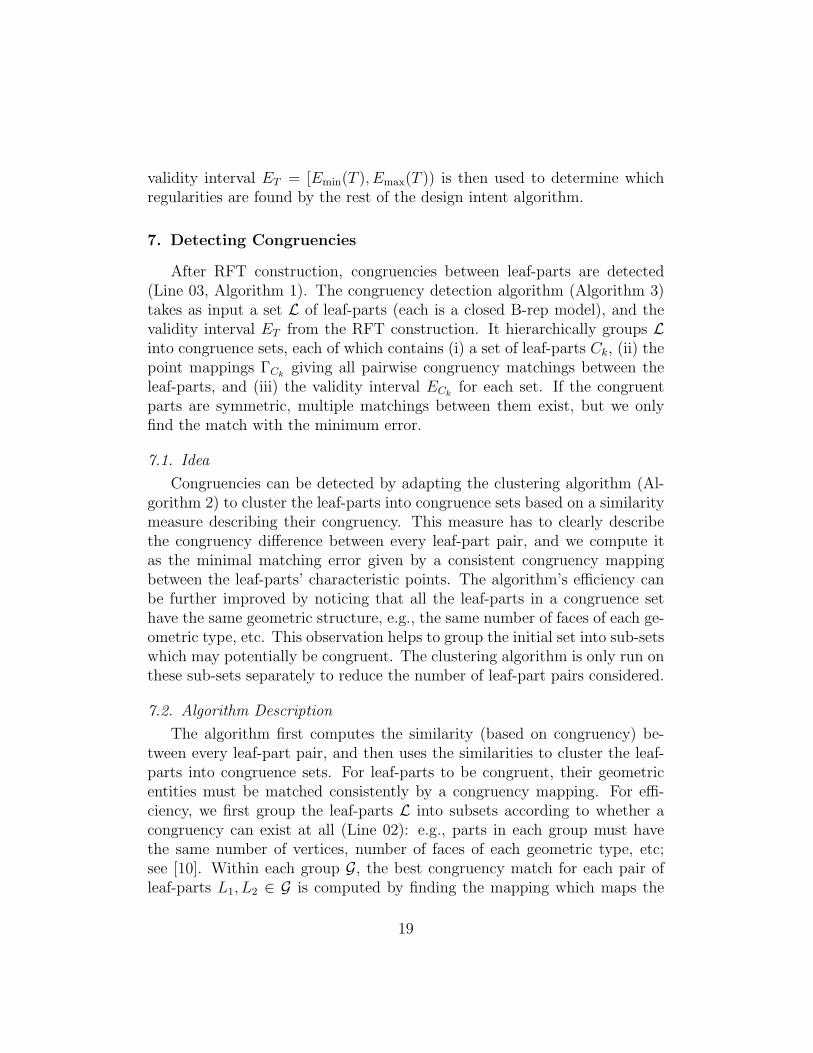
7. Detecting Congruencies

After RFT construction, congruencies between leaf-parts are detected(Line 03, Algorithm 1). The congruency detection algorithm (Algorithm 3)takes as input a set L of leaf-parts (each is a closed B-rep model), and thevalidity interval ET from the RFT construction. It hierarchically groups Linto congruence sets, each of which contains (i) a set of leaf-parts Ck, (ii) thepoint mappings ΓCk

giving all pairwise congruency matchings between theleaf-parts, and (iii) the validity interval ECk

for each set. If the congruentparts are symmetric, multiple matchings between them exist, but we onlyfind the match with the minimum error.

7.1. Idea

Congruencies can be detected by adapting the clustering algorithm (Al-gorithm 2) to cluster the leaf-parts into congruence sets based on a similaritymeasure describing their congruency. This measure has to clearly describethe congruency difference between every leaf-part pair, and we compute itas the minimal matching error given by a consistent congruency mappingbetween the leaf-parts’ characteristic points. The algorithm’s efficiency canbe further improved by noticing that all the leaf-parts in a congruence sethave the same geometric structure, e.g., the same number of faces of each ge-ometric type, etc. This observation helps to group the initial set into sub-setswhich may potentially be congruent. The clustering algorithm is only run onthese sub-sets separately to reduce the number of leaf-part pairs considered.

7.2. Algorithm Description

The algorithm first computes the similarity (based on congruency) be-tween every leaf-part pair, and then uses the similarities to cluster the leaf-parts into congruence sets. For leaf-parts to be congruent, their geometricentities must be matched consistently by a congruency mapping. For effi-ciency, we first group the leaf-parts L into subsets according to whether acongruency can exist at all (Line 02): e.g., parts in each group must havethe same number of vertices, number of faces of each geometric type, etc;see [10]. Within each group G, the best congruency match for each pair ofleaf-parts L1, L2 ∈ G is computed by finding the mapping which maps the

19

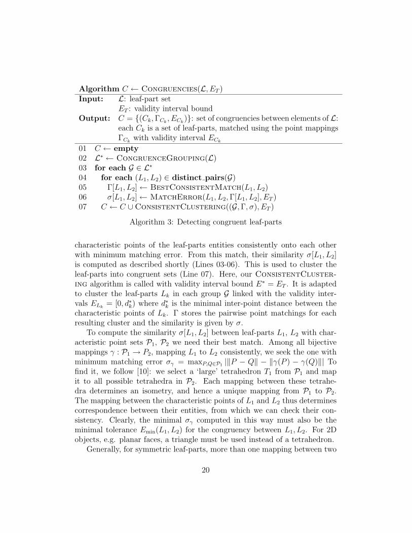
Algorithm C ← Congruencies(L, ET )Input: L: leaf-part set

ET : validity interval boundOutput: C = {(Ck,ΓCk

, ECk)}: set of congruencies between elements of L:

each Ck is a set of leaf-parts, matched using the point mappingsΓCk

with validity interval ECk

01 C ← empty02 L∗ ← CongruenceGrouping(L)03 for each G ∈ L∗04 for each (L1, L2) ∈ distinct pairs(G)05 Γ[L1, L2]← BestConsistentMatch(L1, L2)06 σ[L1, L2]← MatchError(L1, L2,Γ[L1, L2], ET )07 C ← C ∪ConsistentClustering((G,Γ, σ), ET )

Algorithm 3: Detecting congruent leaf-parts

characteristic points of the leaf-parts entities consistently onto each otherwith minimum matching error. From this match, their similarity σ[L1, L2]is computed as described shortly (Lines 03-06). This is used to cluster theleaf-parts into congruent sets (Line 07). Here, our ConsistentCluster-ing algorithm is called with validity interval bound E∗ = ET . It is adaptedto cluster the leaf-parts Lk in each group G linked with the validity inter-vals ELk

= [0, d∗k) where d∗k is the minimal inter-point distance between thecharacteristic points of Lk. Γ stores the pairwise point matchings for eachresulting cluster and the similarity is given by σ.

To compute the similarity σ[L1, L2] between leaf-parts L1, L2 with char-acteristic point sets P1, P2 we need their best match. Among all bijectivemappings γ : P1 → P2, mapping L1 to L2 consistently, we seek the one withminimum matching error σγ = maxP,Q∈P1 |‖P − Q‖ − ‖γ(P ) − γ(Q)‖| Tofind it, we follow [10]: we select a ‘large’ tetrahedron T1 from P1 and mapit to all possible tetrahedra in P2. Each mapping between these tetrahe-dra determines an isometry, and hence a unique mapping from P1 to P2.The mapping between the characteristic points of L1 and L2 thus determinescorrespondence between their entities, from which we can check their con-sistency. Clearly, the minimal σγ computed in this way must also be theminimal tolerance Emin(L1, L2) for the congruency between L1, L2. For 2Dobjects, e.g. planar faces, a triangle must be used instead of a tetrahedron.

Generally, for symmetric leaf-parts, more than one mapping between two

20

congruent leaf-parts exists. We do not need to consider these here, as suchsymmetries are detected as incomplete symmetries later (Section 8), and arethen considered for symmetric arrangements (Section 10).

Given L leaf-parts with at most p characteristic points per leaf-part, theCongruencies algorithm is expected to take O(L2p2.5 log4 p) time: L(L −1)/2 distinct leaf-part pairs are checked for congruency, each requiring thesame time as global symmetry detection: O(p2.5 log4 p) [29].

8. Detecting Incomplete B-Rep Symmetries

We now discuss the detection of common incomplete symmetries of a setof congruent leaf-parts (Line 09, Algorithm 1). This algorithm is called oncefor each congruence set in the congruency hierarchy.

8.1. Idea

We first describe the idea behind Algorithm 4. As the output incompleteB-rep symmetries have to be present in all the leaf-parts in a congruence setC, an efficient strategy is applied: we first detect symmetries of an exemplarleaf-part, and then verify which of these are also present in all the otherleaf-parts in the set. Detecting symmetries within an exemplar leaf-part isvery similar to the overall design intent detection algorithm (Algorithm 1)with the main difference that we are processing faces instead of leaf-parts;it is further described in Section 8.3. The verification process is efficientlyachieved using the point mapping between the leaf-parts in the congruenceset. This mapping prescribes how the exemplars points must be mappedonto the other leaf-parts. Therefore, they can be used to transfer the sym-metry mappings from the exemplar part to the other parts. The transferredsymmetry is only valid if there is a non-empty validity interval for it.

For example, suppose in Fig. 5 that L1, . . . , L3 are congruent leaf-partsgiven by mappings γk : L1 → Lk which map O1 to Ok, P1 to Pk, Q1 toQk and R1 to Rk for k = 2, 3, and L1 is the picked exemplar model. Letσ = (O1, P1, Q1, R1) denote a cycle of L1 that builds a four-fold rotationalsymmetry of L1 at a proper validity interval. To verify that the rotationalsymmetry σ is also shared by other leaf-parts Lk, k = 2, 3 in the congruenceset, we only need to check that each point set γk(σ(L1)) (i.e. the characteristicpoints) also builds a valid four-fold rotational cycle of Lk at a proper validityinterval, and all these intervals together share a common range with that ofL1.

21

Figure 5: Finding common incomplete symmetries of a set of congruent leaf-parts

Algorithm I ←BRepSymmetries(C,ΓC , EC)Input: C: set of congruent leaf-parts

ΓC : pairwise congruency matchings for CEC : validity interval for congruencies of C

Output: I = {(Fk, µFk, EFk

)}: incomplete symmetries of C

01 (L∗, I∗)← FindCachedSymmetry(C)02 if empty(I∗)03 L∗ ← first element(C)04 I∗ = {(Fk, µFk

, EFk)} ←FaceSymmetries(L∗, EC)

05 L∗ ← SymmetryCache(L∗, I∗)06 for each (Fk, µFk

, EFk) ∈ I∗

07 E∗ ← EFk

08 for each L ∈ C09 E∗ ← E∗∩ ValidityInterval(L,L∗, µFk

,ΓC)10 if not empty(E∗), I ←append(I, (Fk, µFk

, E∗))

Algorithm 4: Detecting incomplete symmetries of a congruence set

8.2. Algorithm Description

Our algorithm (Algorithm 4) takes as input a congruence set given by C,ΓC , EC , and outputs the incomplete symmetries shared by all leaf-parts inC. Each incomplete symmetry is represented by a set of faces Fk, a bijectionµFk

indicating how these faces are matched, and a corresponding validityinterval EFk

.The algorithm first detects the incomplete symmetries of an exemplar

leaf-part L∗ selected from the congruence set. Any part may be chosen as theexemplar, as we are only interested in symmetries shown by all leaf-parts inthe set. For efficiency, to avoid re-finding the symmetries of exemplars whileprocessing the congruency hierarchy, we cache all symmetries of exemplars.Lines 01–05 detect incomplete symmetries in the exemplar, while Lines 06–10find which of these are also present in all other leaf-parts in the set.

22

To find incomplete symmetries we first check whether the current congru-ence set contains a leaf-part with previously cached symmetries (Line 01).If so, we use this leaf-part L∗ and its symmetries I∗ to check the other leaf-parts. Otherwise, we arbitrarily select the first leaf-part in the congruenceset as L∗, find its symmetries I∗ as explained below, and cache these withthe leaf-part (Lines 02-05).

We only keep those symmetries of the exemplar L∗ verifiably present inall other leaf-parts (Lines 07–10), to within tolerance. Given the congruencymappings from ΓC , we can convert the symmetry mapping µ for the exem-plar to a potential symmetry mapping µL of any other leaf-part L ∈ C; wecompute its validity interval EµL

as described in Section 9. If the intersectionof all the validity intervals involved is not empty, a validity interval exists atwhich the exemplar’s symmetry is present in all leaf-parts.

8.3. Detecting Incomplete Leaf-part Symmetries

We now describe the algorithm for finding incomplete leaf-part symme-tries (Line 04, Algorithm 4). Our definition of incomplete symmetries of B-rep models (Section 3.2) requires detection of incomplete symmetries formedby a part’s faces. This is the same problem as finding Type I symmetricarrangements of a leaf-part’s faces. Hence, our face symmetry algorithm(Algorithm 5) finds such arrangements of faces. It is very similar to theoverall design intent detection algorithm (Algorithm 1) with the differencethat we are processing faces instead of leaf-parts, and only output Type Isymmetric arrangements.

We first find a hierarchy of congruent faces (Line 01). To detect con-gruent faces the Congruencies algorithm in Algorithm 3 is used, excepttriangles replace tetrahedra for planar faces, when the plane containing thefaces is considered to determine the complete mapping in 3D. As in the maindesign intent detection algorithm, we then process the congruency hierar-chy top-down using a FIFO queue Q to detect the global symmetries S[C]and Type I symmetric arrangements A[C] for each cluster C of congruentfaces (Line 02–08). We only need global symmetries of faces, instead of in-complete symmetries, in this case, so we use a global symmetry detectionalgorithm [29] (Line 05). We then look for Type I symmetric arrangements ifthe symmetries of the current cluster are not the same as those of its parentcluster (Lines 06–08). Firstly, incomplete cycles of the centroids of the facesin the cluster are found (Line 07, Section 9) and then these cycles are used to

23

Algorithm A←FaceSymmetries(L,E)Input: L: leaf-part B-rep model

E: validity interval boundOutput: A = {(Fk, µFk

, EFk)}: face symmetries of L given by a set of faces

Fk with the symmetry mapping µFkand its validity interval EFk

01 C ← Congruencies(Faces(L), E)02 S ← empty, A← empty, Q ← roots(C)03 while not empty(Q)04 (C,ΓC , EC)← pop(Q), Q ← append(Q,children(C))05 S[C]← GlobalFaceSymmetries(C,ΓC , EC)06 if S[C] 6= S[parent(C)]07 I ← IncompleteCycles(Centroids(C), EC)08 A[C]← TypeI(C,ΓC , EC , S[C], I)09 A← MergeCompatibleCycles(A)

Algorithm 5: Detecting incomplete symmetries of faces in a leaf-part

find Type I symmetric arrangements (Section 10). The symmetric arrange-ments are represented as face cycles {(Fk, µFk

, EFk)} formed by the faces

Fk of L. Finally, these are merged into compatible symmetry transforma-tions (Line 09, Section 11). Merging has to be done here in order to identifyglobal symmetries as preparation for detecting symmetric arrangements ofleaf-parts.

9. Detecting Incomplete Symmetry Cycles

We now describe the detection of incomplete symmetry cycles in point setsusing the ideas from Section 3; this is needed by the symmetry and symmetricarrangement detection algorithms. The algorithm is a core element of outdesign intent detection approach, and essentially decides which regularitieswe can detect. An overview was originally reported in [23]; here we give thecomplete algorithm with previously unpublished details.

9.1. Idea

The underlying idea is to expand an (approximate) isosceles triangle pointby point to build up a symmetry cycle. A similar process was proposed byBrass [5] for detecting exact, complete, rotational symmetries by mergingisosceles triangles. We previously extended it to approximate, complete,

24

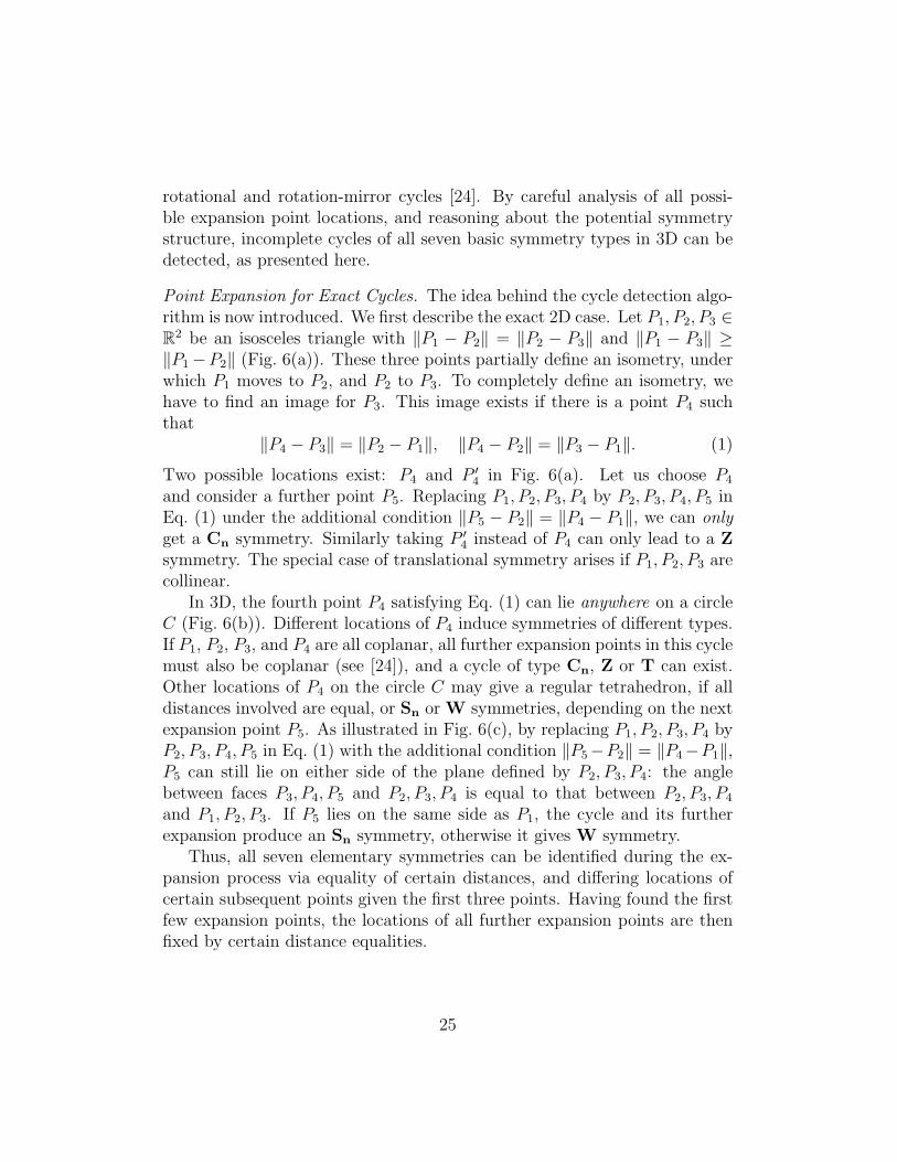
rotational and rotation-mirror cycles [24]. By careful analysis of all possi-ble expansion point locations, and reasoning about the potential symmetrystructure, incomplete cycles of all seven basic symmetry types in 3D can bedetected, as presented here.

Point Expansion for Exact Cycles. The idea behind the cycle detection algo-rithm is now introduced. We first describe the exact 2D case. Let P1, P2, P3 ∈R2 be an isosceles triangle with ‖P1 − P2‖ = ‖P2 − P3‖ and ‖P1 − P3‖ ≥‖P1−P2‖ (Fig. 6(a)). These three points partially define an isometry, underwhich P1 moves to P2, and P2 to P3. To completely define an isometry, wehave to find an image for P3. This image exists if there is a point P4 suchthat

‖P4 − P3‖ = ‖P2 − P1‖, ‖P4 − P2‖ = ‖P3 − P1‖. (1)

Two possible locations exist: P4 and P ′4 in Fig. 6(a). Let us choose P4

and consider a further point P5. Replacing P1, P2, P3, P4 by P2, P3, P4, P5 inEq. (1) under the additional condition ‖P5 − P2‖ = ‖P4 − P1‖, we can onlyget a Cn symmetry. Similarly taking P ′4 instead of P4 can only lead to a Zsymmetry. The special case of translational symmetry arises if P1, P2, P3 arecollinear.

In 3D, the fourth point P4 satisfying Eq. (1) can lie anywhere on a circleC (Fig. 6(b)). Different locations of P4 induce symmetries of different types.If P1, P2, P3, and P4 are all coplanar, all further expansion points in this cyclemust also be coplanar (see [24]), and a cycle of type Cn, Z or T can exist.Other locations of P4 on the circle C may give a regular tetrahedron, if alldistances involved are equal, or Sn or W symmetries, depending on the nextexpansion point P5. As illustrated in Fig. 6(c), by replacing P1, P2, P3, P4 byP2, P3, P4, P5 in Eq. (1) with the additional condition ‖P5−P2‖ = ‖P4−P1‖,P5 can still lie on either side of the plane defined by P2, P3, P4: the anglebetween faces P3, P4, P5 and P2, P3, P4 is equal to that between P2, P3, P4

and P1, P2, P3. If P5 lies on the same side as P1, the cycle and its furtherexpansion produce an Sn symmetry, otherwise it gives W symmetry.

Thus, all seven elementary symmetries can be identified during the ex-pansion process via equality of certain distances, and differing locations ofcertain subsequent points given the first three points. Having found the firstfew expansion points, the locations of all further expansion points are thenfixed by certain distance equalities.

25

P

P’

P’5

P

P1

2P3P

5

4

4

(a) Expansion fromthree points in 2D

C

P4

P3

P4

P1 P4

P2

(b) Expansion fromthree points in 3D

ßß

P1

2P

P P53P’

5

4Pß

(c) Expansion from fourpoints in 3D

Figure 6: Different expansion points of cycles yield different symmetry types

Extension to Approximate Cycles. Unfortunately, the exact expansion pro-cess cannot be applied directly to the approximate case, due to the difficultyof choosing a tolerance to determine equality of distances, and possible ac-cumulation of errors as a cycle is built up. To avoid these problems, weadd further constraints when determining each successive expansion point.We require approximate equality of all point-pair distances that should beequal in the exact case, such that this approximate equality forms an equiv-alence relation on all these distances (Section 3.1). E.g., to determine theexpansion point P5 from the seed set (P1, P2, P3, P4) in Fig. 6(a), we require‖P5−P4‖ =ε ‖Pk+1−Pk‖, k = 1, 2, 3, ‖P5−P3‖ =ε ‖Pl+2−Pl‖, l = 1, 2 and‖P5 − P2‖ =ε ‖P4 − P1‖. This determines the elements of each equivalenceclass Gr(C), 1 ≤ r ≤ R of distances, for a seed set C = {P1, . . . , Pc} of cpoints. From the definition of minimal and maximal tolerances (Section 3.1)we get

Emin(C) = max1≤r≤R(Drmax(C)−Dr

min(C)),Emax(C) = min1≤r≤R−1(D

r+1min (C)−Dr

max(C)), (2)

where Drmin(C) is the minimum and Dr

max(C) the maximum distance in classGr(C). Combining Eq. (2) with the existence of the validity interval (seeSection 3.1) yields a condition on the next expansion point P of C: Emin(C ∪{P}) < Emax(C ∪ {P}).

The main issue for the computation of Emin(C ∪ {P}), Emax(C ∪ {P}) isto determine which class Gr(C ∪ {P}) the distances Lk = ‖P − Pc−k+1‖, k =1, . . . , c belong to. A method for doing this is given in [24] for Cn and Sn

symmetries. Cycles for W,T,Z symmetries can be handled as special cases:we must have Lk ∈ Gk, as all involve translation.

More than one acceptable candidate expansion point may exist in theinput point set, so we must consider all possibilities. We choose the one

26

minimising Emin(C ∪ {P}) to avoid adding any point that would violate thecycle separation condition (C2) (Section 3.1). If the exact case allows morethan one location for the next expansion point (for different symmetry typesas explained above), we must consider every possibility separately. Thus, allpotential fourth expansion points, and the best fifth expansion point for eachlocation in 3D have to be considered.

9.2. Algorithm Description

Based on the ideas described above, the algorithm on detecting incom-plete cycles in a point set is devised in Algorithm 6, and now further ex-plained. This algorithm takes as input a set of distinct 3D points P and avalidity interval bound E∗. We assume no two input points have the sameposition. It outputs all cycles (Ck, ECk) where Ck are the ordered points ofthe cycle, with validity interval ECk . Their symmetry types are determinedlater when merging the cycles into symmetries (Section 11).

To find the set I of all cycles in P , every distinct point triple C in Pis considered for cycle generation (Line 02). A FIFO queue Q (Line 03) isused to store all expansions of the current triple with their validity intervals,so as to consider all possible expansion points. For each triple C of pointsP1, P2, P3, we first compute its validity interval EC (Line 04). Assumingwithout loss of generality that ‖P1 − P3‖ is the largest distance, the validityinterval is the intersection of the overall validity interval bound E∗ and theinterval [0, |‖P2 − P1‖ − ‖P3 − P2‖|) given by the distance matching error.If C satisfies the validity condition and also does not appear consecutivelyin a previously detected cycle, checked by calling Contained (Line 05),it is added to Q for further expansion (Line 06). For the initial triple thevalidity condition is simply that the intersection of its validity interval EC andthe validity interval bound E∗ is not empty. Contained can be efficientlyimplemented by an O(|P|3) Boolean lookup table representing all triples ofpoints as |P| is typically small. As cycles are found, entries corresponding toall consecutive triples in a cycle are set to true.

Each cycle C with validity interval EC in Q is expanded one point ata time (Lines 07–29). We first collect in M all valid potential expansionpoints P ∗ (Line 09), i.e. all points P which can be added to C such thatthe validity interval of the expanded cycle is not empty: Emin(C ∪ {P}) <Emax(C ∪ {P}). If no such point exists, we have found an incomplete cycleC, which is appended to the output and processed no further (Lines 10–12).Otherwise, depending on the number of points in C, alternative locations for

27

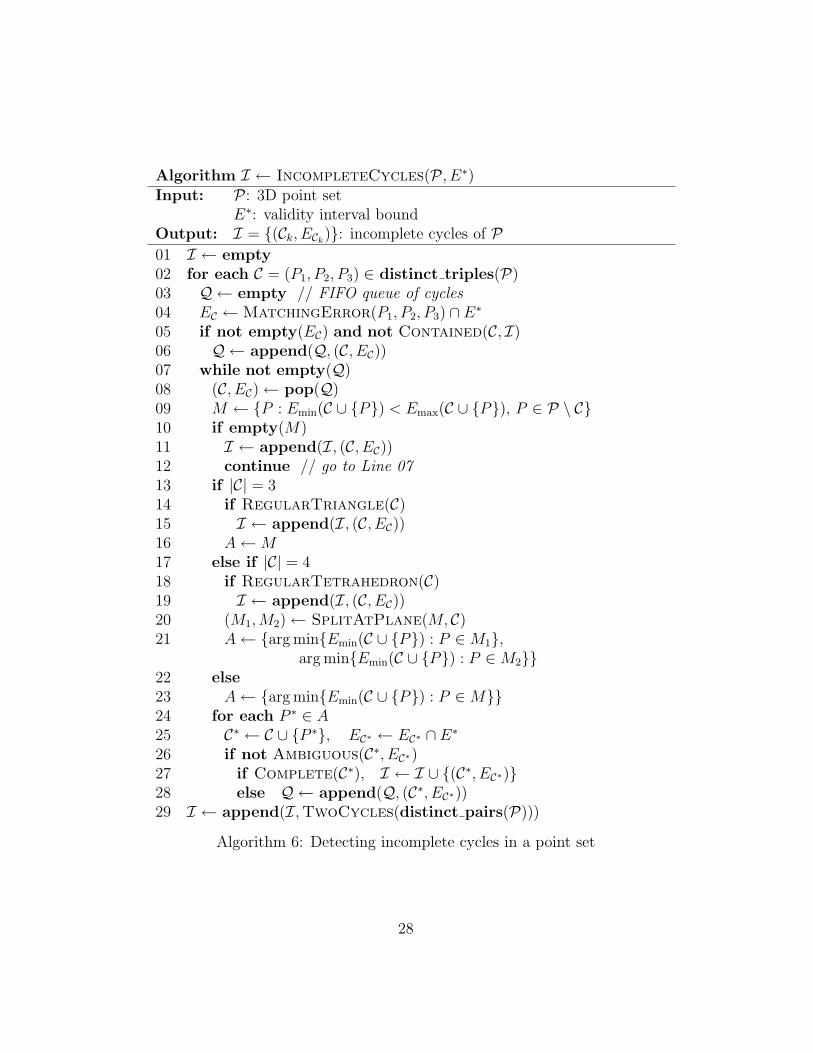
Algorithm I ← IncompleteCycles(P , E∗)Input: P : 3D point set

E∗: validity interval boundOutput: I = {(Ck, ECk)}: incomplete cycles of P01 I ← empty02 for each C = (P1, P2, P3) ∈ distinct triples(P)03 Q ← empty // FIFO queue of cycles04 EC ←MatchingError(P1, P2, P3) ∩ E∗05 if not empty(EC) and not Contained(C, I)06 Q ← append(Q, (C, EC))07 while not empty(Q)08 (C, EC)← pop(Q)09 M ← {P : Emin(C ∪ {P}) < Emax(C ∪ {P}), P ∈ P \ C}10 if empty(M)11 I ← append(I, (C, EC))12 continue // go to Line 0713 if |C| = 314 if RegularTriangle(C)15 I ← append(I, (C, EC))16 A←M17 else if |C| = 418 if RegularTetrahedron(C)19 I ← append(I, (C, EC))20 (M1,M2)← SplitAtPlane(M, C)21 A← {arg min{Emin(C ∪ {P}) : P ∈M1},

arg min{Emin(C ∪ {P}) : P ∈M2}}22 else23 A← {arg min{Emin(C ∪ {P}) : P ∈M}}24 for each P ∗ ∈ A25 C∗ ← C ∪ {P ∗}, EC∗ ← EC∗ ∩ E∗26 if not Ambiguous(C∗, EC∗)27 if Complete(C∗), I ← I ∪ {(C∗, EC∗)}28 else Q ← append(Q, (C∗, EC∗))29 I ← append(I,TwoCycles(distinct pairs(P)))

Algorithm 6: Detecting incomplete cycles in a point set

28

expansion points are considered to find all possible expanded cycles from C(Lines 13–23). In each case we determine the actual expansion points for Cfrom the list M of potential expansion points, and store them in a list A toconstruct the expanded cycles later. If |C| = 3 (Lines 14–16), we first checkfor the special case where C is a regular triangle and if found, append it toI as it is a complete symmetry cycle. To test whether three points forma regular triangle the incomplete cycle conditions (C1) to (C3) are verifieddirectly based on the point distances. Independently, all points in M areadded to A as in the |C| = 3 case all potential expansion points give anexpanded cycle. If |C| = 4 (Lines 17–21), points in M are put into twosubsets M1, M2 according to which side of the plane P2, P3, P4 they lie in.The point minimising Emin(C∪{P}) for each of these two sets is chosen as anexpansion point and added to A (Line 21). Also for |C| = 4 there is a specialcase giving a complete symmetry: the points may form a regular tetrahedron(Lines 18–19). As for the regular triangle, the incomplete cycle conditionscan be verified directly via the distances. For all other cases (Lines 22–23),i.e. |C| ≥ 5, a unique expansion point minimising the matching error isselected.

Next, each expansion point P ∗ in A is used in turn for expanding C(Lines 24–28). If the cycle is complete, and unambiguous, i.e. fulfils condition(C3) (Section 3.1), it is added to the output. Otherwise, only if the new cycleis unambiguous, it is added to the queue of cycles being considered further.A cycle C with c points describes a complete cycle if ‖Pc−P1‖ =ε ‖Pl−Pl+1‖for 1 ≤ l ≤ c − 1. An efficient method to verify unambiguity of a completecycle, which can also be applied to incomplete cycles, is given in [24].

Lastly, each input point pair forms a trivial cycle, corresponding to amirror, an inversion and a C2 symmetry, so we add them all (Line 29).These pairs are considered later when detecting symmetry types and mergingcompatible cycles. The validity interval for each pair is simply [0, d), whered is the distance between the point pair.

This algorithm takes O(Cn4) time, where C is the maximal number ofelements in a cycle, and n is the number of points in P : all triples of pointsare taken as initial seeds, and then each remaining point is considered as anexpansion point in an iterative expansion process.

29

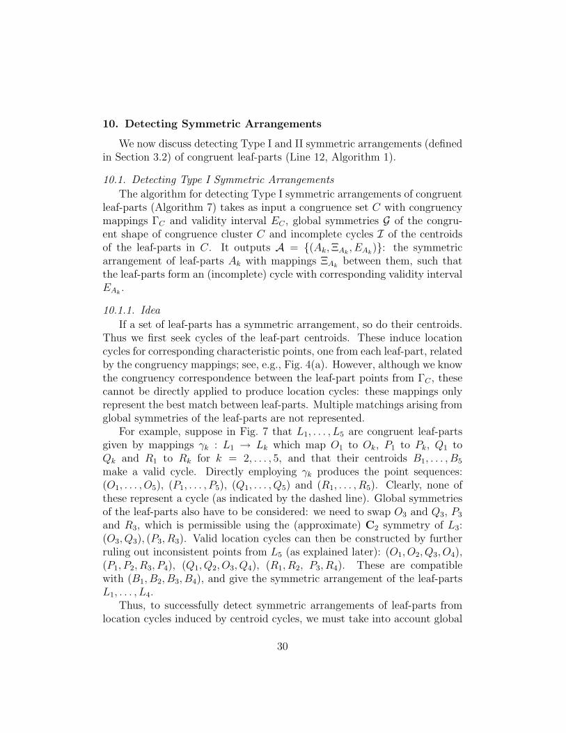
10. Detecting Symmetric Arrangements

We now discuss detecting Type I and II symmetric arrangements (definedin Section 3.2) of congruent leaf-parts (Line 12, Algorithm 1).

10.1. Detecting Type I Symmetric Arrangements

The algorithm for detecting Type I symmetric arrangements of congruentleaf-parts (Algorithm 7) takes as input a congruence set C with congruencymappings ΓC and validity interval EC , global symmetries G of the congru-ent shape of congruence cluster C and incomplete cycles I of the centroidsof the leaf-parts in C. It outputs A = {(Ak,ΞAk

, EAk)}: the symmetric

arrangement of leaf-parts Ak with mappings ΞAkbetween them, such that

the leaf-parts form an (incomplete) cycle with corresponding validity intervalEAk

.

10.1.1. Idea

If a set of leaf-parts has a symmetric arrangement, so do their centroids.Thus we first seek cycles of the leaf-part centroids. These induce locationcycles for corresponding characteristic points, one from each leaf-part, relatedby the congruency mappings; see, e.g., Fig. 4(a). However, although we knowthe congruency correspondence between the leaf-part points from ΓC , thesecannot be directly applied to produce location cycles: these mappings onlyrepresent the best match between leaf-parts. Multiple matchings arising fromglobal symmetries of the leaf-parts are not represented.

For example, suppose in Fig. 7 that L1, . . . , L5 are congruent leaf-partsgiven by mappings γk : L1 → Lk which map O1 to Ok, P1 to Pk, Q1 toQk and R1 to Rk for k = 2, . . . , 5, and that their centroids B1, . . . , B5

make a valid cycle. Directly employing γk produces the point sequences:(O1, . . . , O5), (P1, . . . , P5), (Q1, . . . , Q5) and (R1, . . . , R5). Clearly, none ofthese represent a cycle (as indicated by the dashed line). Global symmetriesof the leaf-parts also have to be considered: we need to swap O3 and Q3, P3

and R3, which is permissible using the (approximate) C2 symmetry of L3:(O3, Q3), (P3, R3). Valid location cycles can then be constructed by furtherruling out inconsistent points from L5 (as explained later): (O1, O2, Q3, O4),(P1, P2, R3, P4), (Q1, Q2, O3, Q4), (R1, R2, P3, R4). These are compatiblewith (B1, B2, B3, B4), and give the symmetric arrangement of the leaf-partsL1, . . . , L4.

Thus, to successfully detect symmetric arrangements of leaf-parts fromlocation cycles induced by centroid cycles, we must take into account global

30

B1

R11O

P1

B2 B 5

1 L3

L4 5

P3

P4

Q

4

3

R3 O3

O4 R4

Q1 QB3 B4

L2 L

5OP

5

Q5R5

O2

P2 Q2

R2

L

Figure 7: Detecting symmetric arrangement of congruent leaf-parts must consider locationcycles as well as its centroid arrangements

symmetries of leaf-parts. Specifically, given a generic point P 1l ∈ L1, we

must consider putting it in correspondence with all points of leaf-part Lkwhich come from γk(g(P 1

l )) for all global symmetries g ∈ G. We also add theidentity to G, as clearly γk(P

11 ) has to be considered. Then, if a compatible

set of location cycles exists, we have a Type I symmetric arrangement of theinvolved leaf-parts.

Furthermore, we must consider cases in which only a subset of all leaf-parts involved in a centroid cycle is symmetrically arranged, as for some onlythe centroids and not the actual leaf-parts may be symmetrically arranged.E.g., in Fig. 6, only L1, . . . , L4 form a symmetric arrangement with L5 be-ing ruled out. This means we seek sub-cycles of the centroid cycle whichyield symmetric arrangements of a leaf-part subset, which can be verifiedby the compatibility of their location cycles. We need not consider leaf-partsubsets that correspond to points of the centroid cycle with fixed index dif-ferences: such sub-cycles are actually also detected as another incompletecentroid cycle in I, as the incomplete cycle detection algorithm also findscycles completely contained in another cycle. Potential symmetric arrange-ments formed by the corresponding leaf-parts are detected when consideringthese cycles instead.

10.1.2. Algorithm Description

Using these ideas, we get the algorithm in Algorithm 7 for detecting TypeI symmetric arrangements. It is carefully designed to avoid combinatorialexplosion of cases when considering symmetric leaf-parts, and to detect leaf-parts that may have symmetric arrangements corresponding to sub-cycles of acentroid cycle. We consider each centroid cycle (B, EB) ∈ I in turn (Line 01).First the points of the leaf-parts involved in B are extracted as P k

l : the l-thpoints of the k-th leaf-part in cycle B such that P k

l is mapped onto P jl by

the congruency mapping in ΓC for leaf-part j (Line 02); see Fig. 8. Then we

31

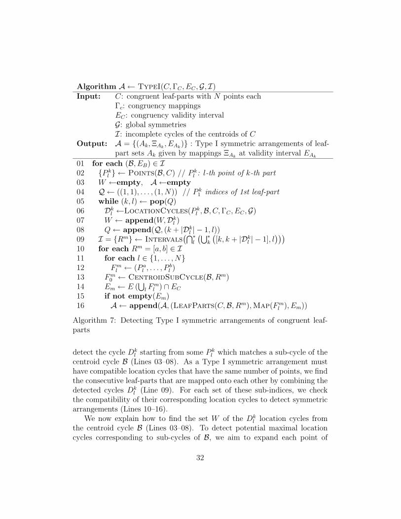
Algorithm A ← TypeI(C,ΓC , EC ,G, I)Input: C: congruent leaf-parts with N points each

Γc: congruency mappingsEC : congruency validity intervalG: global symmetriesI: incomplete cycles of the centroids of C

Output: A = {(Ak,ΞAk, EAk

)} : Type I symmetric arrangements of leaf-part sets Ak given by mappings ΞAk

at validity interval EAk

01 for each (B, EB) ∈ I02 {P k

l } ← Points(B, C) // P kl : l-th point of k-th part

03 W ←empty, A ←empty04 Q ← ((1, 1), . . . , (1, N)) // P k

1 indices of 1st leaf-part05 while (k, l)← pop(Q)06 Dkl ←LocationCycles(P k

l ,B, C,ΓC , EC ,G)07 W ← append(W,Dkl )08 Q← append(Q, (k + |Dkl | − 1, l))09 I = {Rm} ← Intervals

(⋂∗l

(⋃∗k

([k, k + |Dkl | − 1], l

)))10 for each Rm = [a, b] ∈ I11 for each l ∈ {1, . . . , N}12 Fm

l ← (P al , . . . , P

bl )

13 Fm0 ← CentroidSubCycle(B, Rm)

14 Em ← E (⋃l F

ml ) ∩ EC

15 if not empty(Em)16 A ← append(A, (LeafParts(C,B, Rm),Map(Fm

l ), Em))

Algorithm 7: Detecting Type I symmetric arrangements of congruent leaf-parts

detect the cycle Dkl starting from some P k

l which matches a sub-cycle of thecentroid cycle B (Lines 03–08). As a Type I symmetric arrangement musthave compatible location cycles that have the same number of points, we findthe consecutive leaf-parts that are mapped onto each other by combining thedetected cycles Dk

l (Line 09). For each set of these sub-indices, we checkthe compatibility of their corresponding location cycles to detect symmetricarrangements (Lines 10–16).

We now explain how to find the set W of the Dkl location cycles from

the centroid cycle B (Lines 03–08). To detect potential maximal locationcycles corresponding to sub-cycles of B, we aim to expand each point of

32

the leaf-parts to a location cycle without checking sub-cycles of already de-tected cycles. A queue Q is used to store the points for expansion. It isinitialised with the indices of the characteristic points P 1

1 , . . . , P1l of the first

leaf-part L1 in B (Line 04). A maximal location cycle Dkl for each pointP kl in Q is found (Line 06) using a LocationCycles algorithm which is

similar to IncompleteCycles (Algorithm 6). However, it involves fewercomputations as the point sequence is already known from B. Hence, fora starting point P k

l , the r-th point only comes from γk+r−1(g(P 1l )) for all

global symmetries g ∈ G. Thus, only a few characteristic points from leaf-part Lk+r−1 have to be considered for expansion, based on the centroid cycleand the leaf-part’s global symmetries: Lines 02, 09 of Algorithm 6 must bemodified for LocationCycles. Specifically, in Line 02, we only consider(P1, P2, P3) = (P k

l , γk+1(g(P 1l ))), γk+2(g(P 1

l )), and in Line 09, we replace P\Cby {γk+r−1(g(P 1

l ))} for the r-th expansion point. Unlike IncompleteCy-cles, only one cycle can be found in this expansion step for each P k

l byfurther requiring their consistency with B. The detected cycle Dkl is storedin W (Line 07). If there is a point at which the detected location cycle cannotbe expanded further (i.e. Dkl is a sub-cycle not expanded to the end of theB cycle), this point may be a starting point for another location cycle, so itsindex is added to Q for further processing (Line 08).

We find the location cycles by expanding characteristic points of the leaf-parts in sequence of the centroid cycle, to find sub-cycles of consecutiveindices. Note that the Dk

l cycles are essentially intervals [k, k + |Dkl | − 1] of

leaf-part indices k in B for each leaf-part point index l. Each location cyclemust have the same number of points for a symmetric arrangement, so wefind the common maximal consecutive index intervals Rm of the leaf-partindices k for different locations l in the location cycles Dk

l (Line 09). See alsoFig. 8: the centroid cycle induces an order on the leaf-parts Lk, associatedwith their characteristic points P k

l . Location cycles, indicated in the figureby solid lines between the P k

l , describe the matching between the P kl induced

by centroid cycle. In order for the leaf-pars La, . . . , La+c (for some leaf-part-index a and integer c) to form a symmetric arrangement, there has to be alocation cycle for each characteristic point P k

a of the first leaf-part that spansup to at least leaf-part La+c. In Fig. 8, only the leaf-parts La to La+c withcharacteristic points inside the dashed box form a symmetric arrangement.Such leaf-part index intervals Rm can be found by taking the intersectionof the union of the location cycle intervals. However, note that only onelocation cycle Dk

l per starting point index l may be used to find a single Rm

33

leaf part index k

locatio

n in

dex l

P11

1

1

lP

P4

klP

L1 Lk

arrangementsymmetric

L La a+c

Figure 8: Finding symmetric arrangements by intersecting location cycles

interval, otherwise incompatible location cycles would be combined by theunion operation. Hence, in Line 09 the intersection of the union of the Dk

l

intervals only intersects intervals with different l indices (Fig. 8).For each such leaf-part index interval Rm = [a, b] (Line 10) we then find

the corresponding location cycles Fml for characteristic points with index l

from leaf-parts a, . . . , b (Lines 11–12). We also add the centroid sub-cyclecorresponding to Rm (Line 13) to check the compatibility of the cycles Fm

l

and the corresponding centroid sub-cycle, over all characteristic point indicesl, by computing their validity interval (Line 14). If the validity interval isnot empty, a symmetric arrangement of the corresponding leaf-part set exists,which, with associated tolerance and point mappings from the cycles Fml , isoutput in A (Line 16).

This algorithm takes O(LN2) time for each cycle B ∈ I, where L is thenumber of leaf-parts and N is the number of characteristic points per leaf-part. We detect all potential location cycles {Dkl } (Lines 05–08). Duringexpansion, in the worst case, each point of the leaf-parts in B has to be con-sidered (there are at most LN). For each such point we have |G| possibilities,where |G| is the number of global symmetries of the congruence set. Thuswe have LN |G|, and as |G| ≤ max(2N, 120) [28], the time taken is O(LN2).

10.2. Detecting Type II Symmetric Arrangements

Determining symmetric arrangements of Type II is performed in a similarway to detecting those of Type I. The difference is that the location cyclesand B are compatible for Type I while they are linked by a translation forType II. This requires different computations for the validity intervals of thelocation cycles in Line 14, Algorithm 7. Determining location cycle relations

34

for Type II is equivalent to requiring corresponding inter-point distances ofdifferent location cycles to be in the same distance equivalence class: e.g., inFig. 4(b), ‖Pk−P(k+1) mod 4‖, ‖Qk−Q(k+1) mod 4‖, k = 1, 2, 3, 4, should all bein the same distance classes.

Validity intervals for Type II are computed as follows. Let {Fml } be the

compatible location cycles detected by the algorithm in Algorithm 7. As inEq. (2), let Hm

l be the distance classes for Fml , and let Dm

min,l = min(Hml ),

Dmmax,l = max(Hm

l ) be the minimum and maximum distances for each cycle.For Type II, for the same index m (giving a set of compatible location cycles),the distances in Hm

l for different location cycles (i.e. different l) lie in thesame distance class. Hence, for the union Fm = ∪lFm

l of compatible cycles,we have Dm

min(Fm) = maxl(Dmmin,l) and Dm

max(Fm) = minl(Dmmax,l) as the

largest smallest and the smallest largest distance. From these, using Eq. (2),we can then find the validity interval [Emin(Fm), Emax(Fm)).

11. Merging Compatible Cycles

The symmetry and symmetric arrangement detection algorithms considersymmetry cycles only. The last step of the DesignIntent algorithm (Al-gorithm 1) merges compatible cycles which can be represented by a singleisometry. To do so, we first must detect the possible symmetry types foreach cycle (it may have more than one symmetry type as it is approximateand may be incomplete). In the second step we cluster cycles of the samesymmetry type to find the incomplete symmetries.

Two-cycles are trivially assigned to the groups for mirror, inversion andC2 symmetry. Limited space precludes an exhaustive list of all other cases,and we just outline the basic ideas. Instead of trying to find the optimalisometry for a cycle [6], we determine symmetry types by considering therelative locations of the centres of the circles formed by each consecutivetriple of points in C. In 2D, for Cn these centres lie on the same side ofall edges joining consecutive points, whereas they lie alternately on oppositesides for successive triples for Z. If they do not consistently fit either pattern,we assign Cn and Z as possible symmetry types. For a given symmetry type,e.g. Cn, determining the valid values of n for an incomplete cycle is doneby first computing the least squares fitting circle to C, and then computingthe angles between successive points. Each angle is divided by 2π and thenearest integer above and below are included in a list. The overall minimumand maximum values in the list give the permissible range for n. If n is

35

larger than a user-specified maximal rotation order believed to be present inthe object, we also select translational symmetry. For a complete cycle withCn symmetry, n is uniquely determined. Allowing the same points to havemore than one possible symmetry type is necessary, as it is important notto rule out any possible symmetry type too soon, losing information. Cycleclustering helps to rule out inappropriate symmetries.

Incomplete symmetries are found by clustering cycles, sharing the samesymmetry type, induced by the same isometry at a compatible tolerancelevel. This is done using the consistent clustering algorithm (Algorithm 2)where now the Ik are cycles with associated validity intervals and E∗ isthe overall bound from RFT selection. Within the algorithm, we need tocompute Emin(C1 ∪ C2) for two cycles C1, C2. Let C1 = {P1, . . . , P|c1|}, C2 ={Q1, . . . , Q|c2|} be two cycles of the same symmetry type and let C = C1 ∪C2. Taking a concrete case, suppose that the symmetry type is Cn in 2Dand both cycles have the same orientation; other symmetry types can behandled similarly. By definition, Emin(C) is the minimal tolerance such that‖P − Q‖ =ε ‖µ(P ) − µ(Q)‖ for all P,Q in C. This is already satisfied forP,Q ∈ C1 at Emin(C1) and P,Q ∈ C2 at Emin(C2). We consider all pairs P,Qwhere P ∈ C1 and Q ∈ C2, and then allocate distances between such pairsto distance equivalence classes as in Section 9. We then find the maximaldifference between two such distances in each class, and finally take themaximum e∗ of these differences over all classes. Consequently, Emin(C) =max(e∗, Emin(C1), Emin(C2)). Emax(C) is computed similarly.

12. Experiments

We have tested our algorithm on various B-rep models. Approximatemodels were generated from them by perturbing each face (see below). Reg-ularities detected by our algorithm in these approximate models were com-pared with regularities present in the exact model indicated by a human.We ran our algorithm on a 3.4GHz Pentium 4 processor with 1GB RAM.RFT construction and congruence detection were implemented in C++ us-ing OpenCASCADE; other parts were implemented in Matlab.

To generate an approximate model from a given model, we perturbedthe unit normal direction of each planar face and the axis direction of eachcylinder by adding a random vector in [−L,L]3, and then translating it bya random vector in [−sL, sL]3, where L indicates the noise level (by defaultset to 0.1) and s is the area of the face or the radius of the cylinder. Radii

36

Model V F L TT TC TR RD RS

Angle-Bracket: Fig. 9 124 67 27 0.73s 0.04s 3.55s 66 13Monster: Fig. 1 438 198 60 81.62s 17.98s 28.34s 64 5ANC: Fig. 15(a) 236 124 46 13.34s 0.35s 6.82 31 7

Table 1: Results for example models; V : number of vertices; F : number of faces; L:number of detected leaf-parts; TD: RFT decomposition time; TC : congruence detectiontime; TR: regularity detection time; RD: number of detected regularities; RS : number ofspurious regularities.

of cylinders were also perturbed by a random value in [−sL, sL]. The re-sulting perturbed faces were intersected to produce new approximate edgesand vertices based on the original model’s topology. We refer to such modelsin the section simply as approximate models at noise level L = 0.1; othernoise levels were also considered as described below. Perturbing models likethis gives us exact control of the level of noise present and with that enablecomparison with other results. As our algorithms work on relatively highlevel CAD models and not measured point clouds, using real scanner datais less important. Also note that typically in real noise levels are lower thanthose considered here.

E.g., for the Monster in Fig. 1, where minimal and maximal distancesbetween points of the original model were 7 and 385 units respectively, themaximum distance between an original and perturbed vertex was 2 unitsusing this method.

Our algorithm outputs design intent as a congruency hierarchy with as-sociated symmetries and symmetric arrangements at each level, at varioustolerance levels: certain output regularities may be complete subsets of otherregularities. It is hard to display such structures, and often in our experimen-tal results the intended regularities are described by the top-level regularities.Hence, we only show top-level regularities here. Output and timing resultsare summarised in Table 1 for each model.

12.1. Angle-Bracket Example

We first consider the Angle-Bracket model in Fig. 9. The exact model hasa dominant mirror symmetry which is broken on the left side (see the close-up in Fig. 9(b)): the 10 cylindrical holes come in two groups of 5 identicalcylinders. Cylinders in one group are blended while the others are not, andthe blended cylinders have larger radii than the unblended ones. Moreover,

37

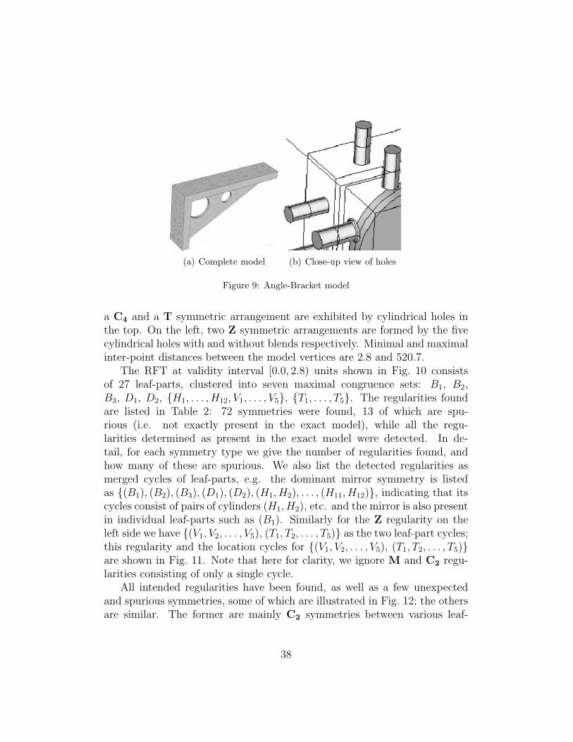
(a) Complete model (b) Close-up view of holes

Figure 9: Angle-Bracket model

a C4 and a T symmetric arrangement are exhibited by cylindrical holes inthe top. On the left, two Z symmetric arrangements are formed by the fivecylindrical holes with and without blends respectively. Minimal and maximalinter-point distances between the model vertices are 2.8 and 520.7.

The RFT at validity interval [0.0, 2.8) units shown in Fig. 10 consistsof 27 leaf-parts, clustered into seven maximal congruence sets: B1, B2,B3, D1, D2, {H1, . . . , H12, V1, . . . , V5}, {T1, . . . , T5}. The regularities foundare listed in Table 2: 72 symmetries were found, 13 of which are spu-rious (i.e. not exactly present in the exact model), while all the regu-larities determined as present in the exact model were detected. In de-tail, for each symmetry type we give the number of regularities found, andhow many of these are spurious. We also list the detected regularities asmerged cycles of leaf-parts, e.g. the dominant mirror symmetry is listedas {(B1), (B2), (B3), (D1), (D2), (H1, H2), . . . , (H11, H12)}, indicating that itscycles consist of pairs of cylinders (H1, H2), etc. and the mirror is also presentin individual leaf-parts such as (B1). Similarly for the Z regularity on theleft side we have {(V1, V2, . . . , V5), (T1, T2, . . . , T5)} as the two leaf-part cycles;this regularity and the location cycles for {(V1, V2, . . . , V5), (T1, T2, . . . , T5)}are shown in Fig. 11. Note that here for clarity, we ignore M and C2 regu-larities consisting of only a single cycle.

All intended regularities have been found, as well as a few unexpectedand spurious symmetries, some of which are illustrated in Fig. 12; the othersare similar. The former are mainly C2 symmetries between various leaf-

38

1

H

H2H4

12H1

7H

H6 H8H10

11H9H

V2

V5

V4

V3

V1 T1

T2

T3T4

H3H5

T5

2

D1

D

B2

B 3

B 1

Figure 10: RFT decomposition of the Angle Bracket model in Fig. 9

parts H1, . . . , H12 and V1, . . . , V5. Such symmetries may be present in theexact model, but their presence may well be unintentional. The spurioussymmetries are generally Cn,n > 2 symmetries (see the last three examplesin the second row of Fig. 12). These clearly do not form an exact symmetryin the exact model and are inconsistent with the translational arrangement.They are detected because when considered as incomplete symmetries, theyare within a valid tolerance.

To test the algorithm’s robustness to increasing noise levels, we also testedit with the Angle-Bracket model with noise levels of 0.0, 0.1, . . . , 0.3 units.The number of detected symmetries may increase or decrease as the noiseincreases. However, only on reaching 0.3 units of noise were certain intendedsymmetries not found; the particular symmetries lost varied on repeatingthe experiment. However, this is quite a high noise level, and we assertthat our algorithm is thus robust in presence of moderate noise, as hoped.In particular, expected symmetries are found at the levels of noise beyond

39

V1

V2

V3

V4

V5

T1

T2

T3

T4

T5

1v

V

VT

T V4 T532T1

5T432 V

Figure 11: Z regularity and location cycles for {(V1, V2, . . . , V5), (T1, T2, . . . , T5)} detectedin the Angle Bracket after RFT construction

V2

V4V3

V5

V1

H1H2

H 7

H 8

H12

H11

Figure 12: Unexpected and spurious symmetries in the Angle Bracket model. Each blackpoint represents one cylinder in H1, . . . ,H12 or V1, . . . , V5

those which might be expected in CAD data exchange and reverse engineeringapplications (less than 0.1 units).

From this example one disadvantage of our algorithm becomes apparent:as the cylinders at the left side do not all have the same radius and some haveblends, their regular translational arrangement is not detected. Even if thedecomposition method could identify and remove the blends, the cylinderswould still have different radii and hence not be part of the same congruenceset for symmetric arrangement detection. Strictly, we do not look for suchregularities, but it is likely to be important for this model to detect this. Itwould require a change in the model decomposition approach, but also moreimportantly our notion of symmetric arrangements would have to be gener-alised to non-congruent shapes. One could consider all point combinations

40

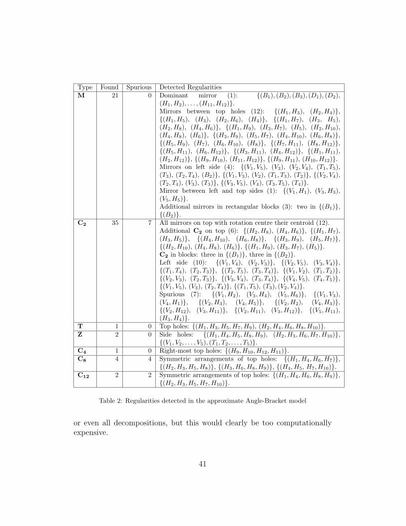
Type Found Spurious Detected RegularitiesM 21 0 Dominant mirror (1): {(B1), (B2), (B3), (D1), (D2),

(H1, H2), . . . , (H11, H12)}.Mirrors between top holes (12): {(H1, H3), (H2, H4)},{(H1, H5), (H3), (H2, H6), (H4)}, {(H1, H7), (H3, H5),(H2, H8), (H4, H6)}, {(H1, H9), (H3, H7), (H5), (H2, H10),(H4, H8), (H6)}, {(H3, H9), (H5, H7), (H4, H10), (H6, H8)},{(H5, H9), (H7), (H6, H10), (H8)}, {(H7, H11), (H8, H12)},{(H5, H11), (H6, H12)}, {(H3, H11), (H4, H12)}, {(H1, H11),(H2, H12)}, {(H9, H10), (H11, H12)}, {(H9, H11), (H10, H12)}.Mirrors on left side (4): {(V1, V5), (V3), (V2, V4), (T1, T5),(T3), (T2, T4), (B2)}, {(V1, V3), (V2), (T1, T3), (T2)}, {(V2, V4),(T2, T4), (V3), (T3)}, {(V3, V5), (V4), (T3, T5), (T4)}.Mirror between left and top sides (1): {(V1, H1), (V3, H3),(V5, H5)}.Additional mirrors in rectangular blocks (3): two in {(B1)},{(B2)}.

C2 35 7 All mirrors on top with rotation centre their centroid (12).Additional C2 on top (6): {(H2, H8), (H4, H6)}, {(H1, H7),(H3, H5)}, {(H4, H10), (H6, H8)}, {(H3, H9), (H5, H7)},{(H2, H10), (H4, H8), (H6)}, {(H1, H9), (H3, H7), (H5)}.C2 in blocks: three in {(B1)}, three in {(B2)}.Left side (10): {(V1, V4), (V2, V3)}, {(V2, V5), (V3, V4)},{(T1, T4), (T2, T3)}, {(T2, T5), (T3, T4)}, {(V1, V2), (T1, T2)},{(V2, V3), (T2, T3)}, {(V3, V4), (T3, T4)}, {(V4, V5), (T4, T5)},{(V1, V5), (V3), (T2, T4)}, {(T1, T5), (T3), (V2, V4)}.Spurious (7): {(V1, H2), (V3, H4), (V5, H6)}, {(V1, V3),(V4, H1)}, {(V2, H3), (V4, H5)}, {(V2, H2), (V4, H3)},{(V2, H12), (V3, H11)}, {(V2, H11), (V3, H12)}, {(V5, H11),(H3, H4)}.

T 1 0 Top holes: {(H1, H3, H5, H7, H9), (H2, H4, H6, H8, H10)}.Z 2 0 Side holes: {(H1, H4, H5, H8, H9), (H2, H3, H6, H7, H10)},

{(V1, V2, . . . , V5), (T1, T2, . . . , T5)}.C4 1 0 Right-most top holes: {(H9, H10, H12, H11)}.C8 4 4 Symmetric arrangements of top holes: {(H1, H4, H6, H7)},

{(H2, H3, H5, H8)}, {(H3, H6, H8, H9)}, {(H4, H5, H7, H10)}.C12 2 2 Symmetric arrangements of top holes: {(H1, H4, H6, H8, H9)},

{(H2, H3, H5, H7, H10)}.

Table 2: Regularities detected in the approximate Angle-Bracket model

or even all decompositions, but this would clearly be too computationallyexpensive.

41

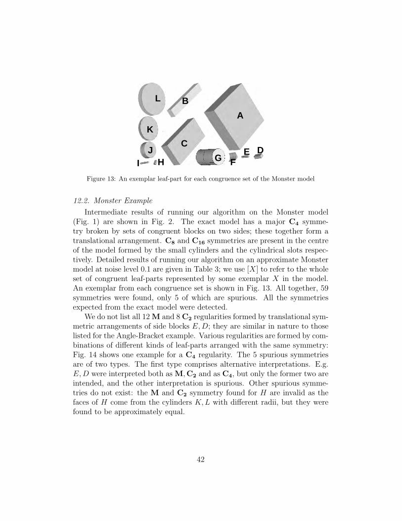
L

K

JI H

C

B

A

G FE D

Figure 13: An exemplar leaf-part for each congruence set of the Monster model

12.2. Monster Example

Intermediate results of running our algorithm on the Monster model(Fig. 1) are shown in Fig. 2. The exact model has a major C4 symme-try broken by sets of congruent blocks on two sides; these together form atranslational arrangement. C8 and C16 symmetries are present in the centreof the model formed by the small cylinders and the cylindrical slots respec-tively. Detailed results of running our algorithm on an approximate Monstermodel at noise level 0.1 are given in Table 3; we use [X] to refer to the wholeset of congruent leaf-parts represented by some exemplar X in the model.An exemplar from each congruence set is shown in Fig. 13. All together, 59symmetries were found, only 5 of which are spurious. All the symmetriesexpected from the exact model were detected.

We do not list all 12 M and 8 C2 regularities formed by translational sym-metric arrangements of side blocks E,D; they are similar in nature to thoselisted for the Angle-Bracket example. Various regularities are formed by com-binations of different kinds of leaf-parts arranged with the same symmetry:Fig. 14 shows one example for a C4 regularity. The 5 spurious symmetriesare of two types. The first type comprises alternative interpretations. E.g.E,D were interpreted both as M,C2 and as C4, but only the former two areintended, and the other interpretation is spurious. Other spurious symme-tries do not exist: the M and C2 symmetry found for H are invalid as thefaces of H come from the cylinders K,L with different radii, but they werefound to be approximately equal.

42

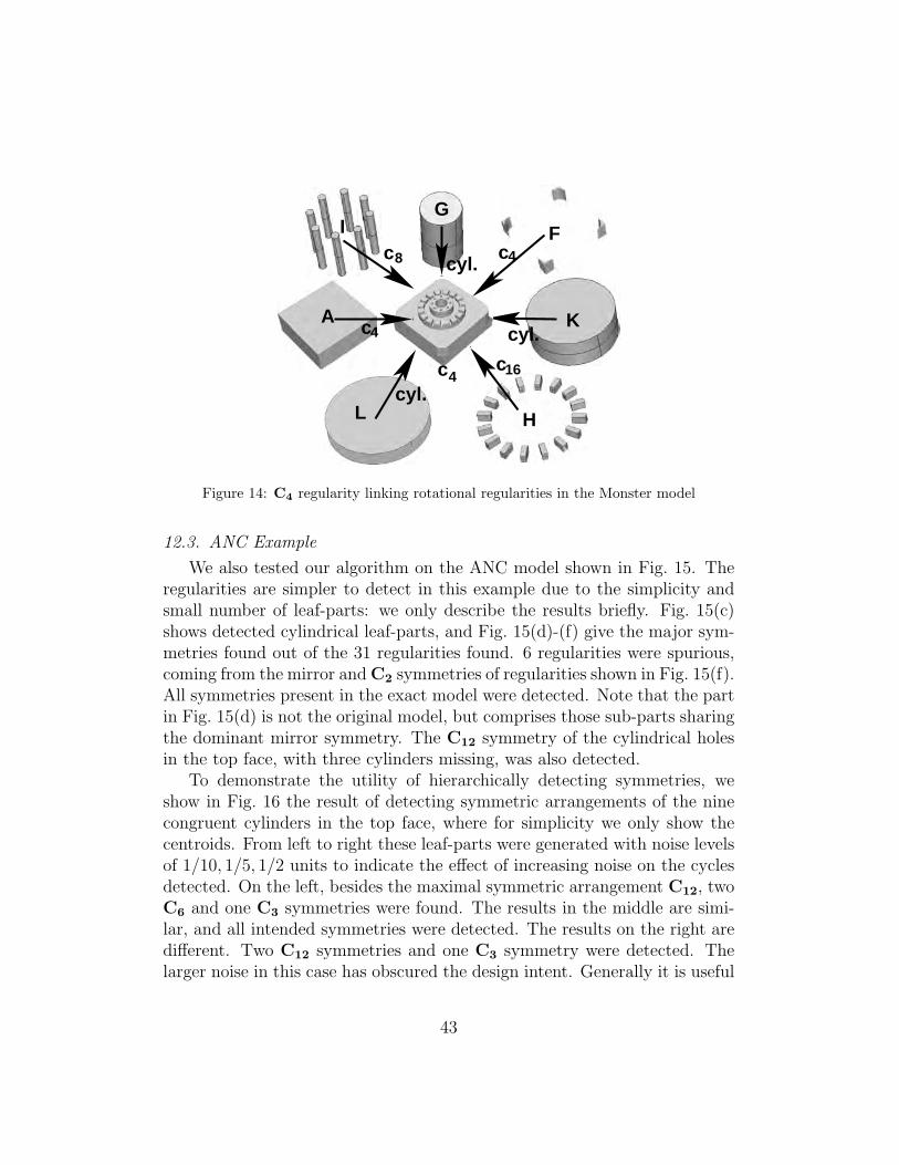
c4

8c

c4

L

A

I

cyl.

c16

H

Kcyl.

c4F

G

cyl.

Figure 14: C4 regularity linking rotational regularities in the Monster model

12.3. ANC Example

We also tested our algorithm on the ANC model shown in Fig. 15. Theregularities are simpler to detect in this example due to the simplicity andsmall number of leaf-parts: we only describe the results briefly. Fig. 15(c)shows detected cylindrical leaf-parts, and Fig. 15(d)-(f) give the major sym-metries found out of the 31 regularities found. 6 regularities were spurious,coming from the mirror and C2 symmetries of regularities shown in Fig. 15(f).All symmetries present in the exact model were detected. Note that the partin Fig. 15(d) is not the original model, but comprises those sub-parts sharingthe dominant mirror symmetry. The C12 symmetry of the cylindrical holesin the top face, with three cylinders missing, was also detected.

To demonstrate the utility of hierarchically detecting symmetries, weshow in Fig. 16 the result of detecting symmetric arrangements of the ninecongruent cylinders in the top face, where for simplicity we only show thecentroids. From left to right these leaf-parts were generated with noise levelsof 1/10, 1/5, 1/2 units to indicate the effect of increasing noise on the cyclesdetected. On the left, besides the maximal symmetric arrangement C12, twoC6 and one C3 symmetries were found. The results in the middle are simi-lar, and all intended symmetries were detected. The results on the right aredifferent. Two C12 symmetries and one C3 symmetry were detected. Thelarger noise in this case has obscured the design intent. Generally it is useful

43

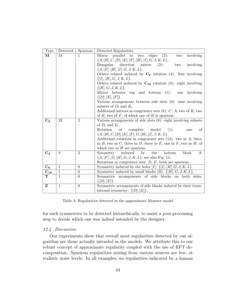
Type Detected Spurious Detected RegularitiesM 34 1 Mirror parallel to two edges (2): two involving

{A, [B], C, [D], [E], [F ], [H], [I], G, J, K, L}.Biangular direction mirror (2): two involving{A, [F ], [H], [I], G, J, K, L}.Others related induced by C8 rotation (4): four involving{[I], [H], G, J, K, L}.Others related induced by C16 rotation (8): eight involving{[H], G, J, K, L}.Mirror between top and bottom (1): one involving{[D], [E], [F ]}.Various arrangements between side slots (9): nine involvingsubsets of Dl and El.Additional mirrors in congruence sets (8): C, A, two of H, twoof B, two of F , of which one of H is spurious.

C2 23 2 Various arrangements of side slots (8): eight involving subsetsof Dl and El.Rotation of complete model (1): one of{A, [B], C, [D], [E], [F ], G, [H], [I], J,K, L}.Additional rotations in congruence sets (14): two in A, threein B, two in C, three in D, three in E, one in F , two in H, ofwhich two in H are spurious.

C4 3 2 Symmetry induced by the bottom block A:{A, [F ], [I], [H], G, J, K, L}; see also Fig. 14.Rotations in congruence sets: D, E, both are spurious.

C8 1 0 Symmetry induced by the holes [I]: {[I], [H], G, J, K, L}.C16 1 0 Symmetry induced by small blocks [H]: {[H], G, J, K, L}.T 1 0 Symmetric arrangements of side blocks on both sides:

{[D], [E]}.Z 1 0 Symmetric arrangements of side blocks induced by their trans-

lational symmetry: {[D], [E]}.

Table 3: Regularities detected in the approximate Monster model

for such symmetries to be detected hierarchically, to assist a post-processingstep to decide which one was indeed intended by the designer.

12.4. Discussion

Our experiments show that overall most regularities detected by our al-gorithm are those actually intended in the models. We attribute this to ourrobust concept of approximate regularity coupled with the use of RFT de-composition. Spurious regularities arising from various sources are few, atrealistic noise levels. In all examples, no regularities indicated by a human

44

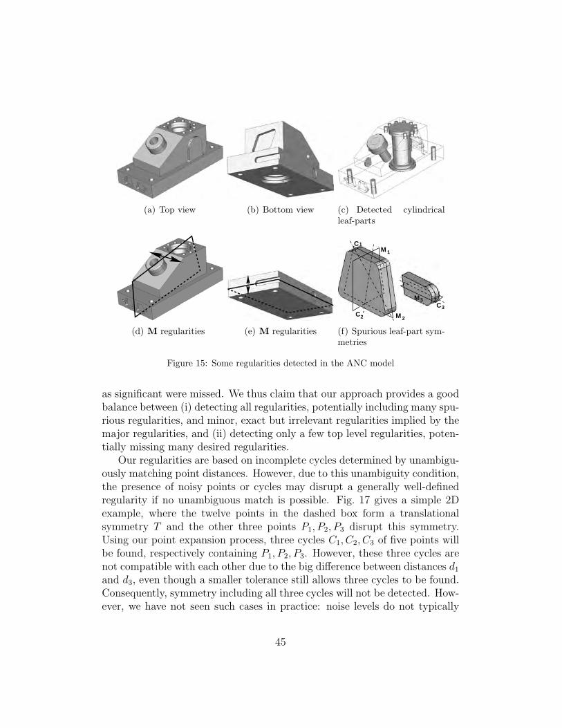
(a) Top view (b) Bottom view (c) Detected cylindricalleaf-parts

(d) M regularities (e) M regularities

1

M 2C2

1CM

MC3

3

(f) Spurious leaf-part sym-metries

Figure 15: Some regularities detected in the ANC model

as significant were missed. We thus claim that our approach provides a goodbalance between (i) detecting all regularities, potentially including many spu-rious regularities, and minor, exact but irrelevant regularities implied by themajor regularities, and (ii) detecting only a few top level regularities, poten-tially missing many desired regularities.

Our regularities are based on incomplete cycles determined by unambigu-ously matching point distances. However, due to this unambiguity condition,the presence of noisy points or cycles may disrupt a generally well-definedregularity if no unambiguous match is possible. Fig. 17 gives a simple 2Dexample, where the twelve points in the dashed box form a translationalsymmetry T and the other three points P1, P2, P3 disrupt this symmetry.Using our point expansion process, three cycles C1, C2, C3 of five points willbe found, respectively containing P1, P2, P3. However, these three cycles arenot compatible with each other due to the big difference between distances d1

and d3, even though a smaller tolerance still allows three cycles to be found.Consequently, symmetry including all three cycles will not be detected. How-ever, we have not seen such cases in practice: noise levels do not typically

45

noise: r/5 noise: rnoise: r/10

Figure 16: Incomplete symmetry hierarchies detected at different noise levels

C1

C2

C3

PP

P1dT

1

2

3d3

Figure 17: Potential symmetry may be missed by cycle merging

vary significantly over a single model.Some spurious regularities are also caused by the fact that we seek incom-

plete cycles. An incomplete cycle is less reliable than a complete cycle dueto the missing positions (and with them the inter-point distances) and itssymmetry type is not always uniquely determined. Our symmetry definitionactually limits the incomplete cases to be considered such that the overallnumber of incomplete cycles remains small, but includes those common inengineering objects.

A significant aspect of our algorithm is that using RFT decompositionallows regularity detection to work without checking all possible relationsbetween all model entities. An algorithm considering and comparing all pos-sible pieces of the object would certainly find considerably more spuriousregularities (e.g. [19]). However, such decomposition already interprets themodel in a certain way which might prevent the algorithm from finding cer-tain regularities, if the decomposition is inappropriate. E.g., consider thefour leaf-parts L1 to L4 created by the crossed slots of the model in Fig. 18.L4 is not congruent to L1, . . . , L3 which means an incomplete C4 symmetrycontaining three leaf-parts is found instead of four. A different decompositionwould be more suitable in this case. Unfortunately, for every model there is inprinciple an infinite number of possible decompositions. The particular RFT

46

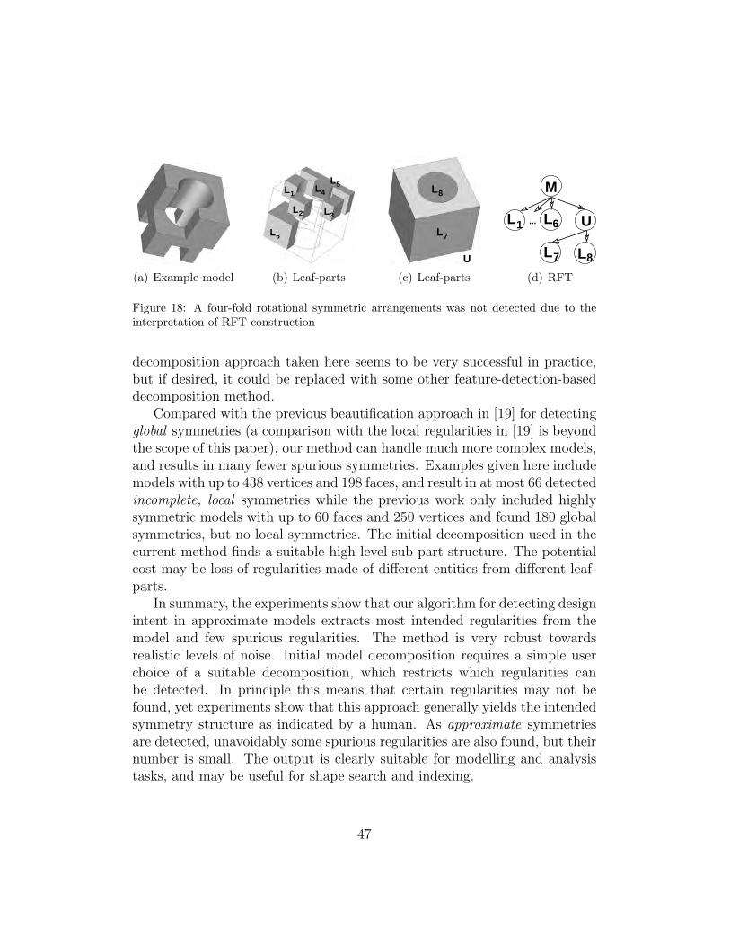
(a) Example model

L2 L3

L4L1

L5

L6

(b) Leaf-parts

U

L7

L8

(c) Leaf-parts

L1 L6 U

L7 L8

M

...

(d) RFT

Figure 18: A four-fold rotational symmetric arrangements was not detected due to theinterpretation of RFT construction

decomposition approach taken here seems to be very successful in practice,but if desired, it could be replaced with some other feature-detection-baseddecomposition method.

Compared with the previous beautification approach in [19] for detectingglobal symmetries (a comparison with the local regularities in [19] is beyondthe scope of this paper), our method can handle much more complex models,and results in many fewer spurious symmetries. Examples given here includemodels with up to 438 vertices and 198 faces, and result in at most 66 detectedincomplete, local symmetries while the previous work only included highlysymmetric models with up to 60 faces and 250 vertices and found 180 globalsymmetries, but no local symmetries. The initial decomposition used in thecurrent method finds a suitable high-level sub-part structure. The potentialcost may be loss of regularities made of different entities from different leaf-parts.

In summary, the experiments show that our algorithm for detecting designintent in approximate models extracts most intended regularities from themodel and few spurious regularities. The method is very robust towardsrealistic levels of noise. Initial model decomposition requires a simple userchoice of a suitable decomposition, which restricts which regularities canbe detected. In principle this means that certain regularities may not befound, yet experiments show that this approach generally yields the intendedsymmetry structure as indicated by a human. As approximate symmetriesare detected, unavoidably some spurious regularities are also found, but theirnumber is small. The output is clearly suitable for modelling and analysistasks, and may be useful for shape search and indexing.

47

13. Conclusions

This paper gives a novel solution to detecting design intent of approx-imate B-rep models using symmetry. It considers symmetries in a widemathematical sense, including all the seven elementary types, which maybe present approximately, locally, incompletely or compatibly. To achievethis goal, models are first hierarchically decomposed into simpler, more sym-metric sub-parts. Design intent is then detected as congruencies, symmetriesand symmetric arrangements of the leaf-parts in this decomposition. Doingso avoids finding many spurious regularities, reliably resolves ambiguities be-tween regularities, and reduces inconsistencies. Yet the decomposition alsolimits what can be found in terms of which model types can be processed andhow these are decomposed into simpler sub-parts. The detection algorithmsare based on a single principle using distances between points for adaptivetolerance interval selection, and hence produce consistent, well-defined ap-proximate regularities. The strict conditions may mean that certain regu-larities are not detected even if we have not observed this in general undertypical noise levels. Experiments show that detected relations reveal signifi-cant design intent.

Despite such good results there is scope for future work to increase therange of regularities detected and the types of models that can be handled.We consider the following as particularly interesting directions:

(1) Our current methods are limited to CAD models bounded by planar,spherical, cylindrical, conical and toroidal surfaces and do not consider moregeneral curved geometries. Extending our approach is currently hamperedby the difficulty of extending the geometry of free-form surfaces required forconstructing RFTs of more general models. Work on identifying DP-featureson free-form solids [25] may help to extend this.

(2) Symmetry detection has attracted researchers from various fields, andmuch good work has been proposed, covering different topics, e.g. [8, 29,39, 31]. However, this work is focused on the detection of “single” pointsymmetry, e.g. reflection, rotation or translation. This paper steps fur-ther considering their combinations as glide symmetry or rotation-reflectionsymmetry. More work is required to detect more general notions of symme-try, and symmetry groups formed by combining symmetry transformations,e.g. wallpaper groups and tetrahedral symmetry. Detecting such regularitieswould simplify the output regularities by representing them in terms of com-bined transformations instead of elementary symmetries. This could lead to

48

more efficient detection, and also help to better represent a model’s intendedstructure.

(3) The design intent detection work covered in this paper as well as otherprevious work, e.g. [41, 19], aims to detect potential geometric regularitiesin the rebuilt approximate model for downstream processing. However, re-producing the original model for CAD/CAM systems and rebuilding a likelyconstruction history should also be considered.

Acknowledgements

This work was supported by EPSRC UK Grant GR/S69085/01. Theexample models used in this paper were obtained from the National DesignRepository, http://www.designrepository.org/.

References

[1] H. Alt, K. Mehlhorn, H. Wagener, E. Welzl. Congruence, similarity andsymmetries of geometric objects. Disc. Comp. Geometry, 3(3):237–256,1988.

[2] K. Barratt. Logic and Design in Art, Science and Mathematics, HerbertPress, London, 1989.

[3] P. Benko, G. Kos, T. Varady, L. Andor, R. Martin. Constraint fitting inreverse engineering. Computer-Aided Geometric Design, 19 (3):173–205,2002.

[4] R. Bidarra, W. Bronsvoort. Semantic feature modelling. Computer-Aided Design, 32 (3):201–225, 2000.

[5] P. Brass. On finding maximum-cardinality symmetric subsets. Comp.Geometry, 24(1):19–25, 2003.

[6] D. Eggert, A. Lorusso, R. Fisher. Estimating 3-D rigid body transfor-mations: a comparison of four major algorithm. Machine Vision andApp., 9(5–6):272–290, 1997.

[7] C. Feng, A. Kusiak. Constraint-based design of parts. Computer-AidedDesign, 27(5):343–352, 1995.

49

[8] P. Flynn. 3-D object recognition with symmetric models: symmetryextraction and encoding. IEEE Trans. Pattern Analysis and MachineIntelligence, 16(8):814–818, 1994.

[9] J. Gallian. Contemporary abstract algebra, D.C. Heath and Company,Lexington, Mass, 1986.

[10] C. Gao, F. Langbein, A. Marshall, R. Martin. Approximate congruencedetection of model features for reverse engineering. In: Proc. Int. Conf.Shape Modeling and Applications, pp. 69–77, 2003.

[11] S. Gao, J. Shah. Automatic recognition of interacting machining fea-tures based on minimal condition subgraph. Computer-Aided Design,30(9):727-739, 1998.

[12] X. Gao, Q. Lin, G. Zhang. A C-tree decomposition algorithm for 2D and3D geometric constraint solving. Computer-Aided Design, 38 (1):1–13,2006.

[13] J. Han, M. Pratt, W. Regli. Manufacturing feature recognition fromsolid models: a status report. IEEE Trans. Robotics and Automation,6(6):782-796, 2000.

[14] C. Hoffman, A. Lomonosov, M. Sitharam. Decomposition plans for ge-ometric constraint problems, part II: new algorithms. J. Symb. Comp.,31(4):409–427, 2001.

[15] S. Iwanowski. Testing approximate symmetry in the plane is NP-hard.Theo. Comp. Sc., 80:227–262, 1991.

[16] K. Kanatani. Comments on ‘symmetry as a continuous feature’. IEEETrans. Pattern Analysis and Machine Intelligence, 19(2):246–247, 1997.

[17] Y. Ke, S. Fan, W. Zhu, A. Li, F. Liu, X. Shi. Feature-based reversemodeling strategies. Computer-Aided Design, 38(5):485–506, 2006.

[18] J. Kim, M. Pratt, R. Iyer, R. Sriram. Standardized data exchange ofCAD models with design intent. Computer-Aided Design, 40(7):760–777, 2008.

[19] F. Langbein. Beautification of reverse engineered geometric models,Ph.D. thesis, Cardiff University, UK, 2003.

50

[20] F. Langbein, A. Marshall, R. Martin. Choosing consistent constraints forbeautification of reverse engineered geometric models. Computer-AidedDesign, 36(3):261–278, 2004.

[21] M. Leyton. A generative theory of shape, LNCS 2145, Springer, 2001.

[22] M. Li, F. Langbein, R. Martin. Constructing regularity feature treesfor solid models. In: Proc. Geometric Modeling and Processing, LNCS,Springer, pp. 267–286, 2006.

[23] M. Li, F. Langbein, R. Martin. Detecting approximate incomplete sym-metries in discrete point sets. In: Proc. ACM Symp. Solid and PhysicalModeling, pp. 335-340, 2007.

[24] M. Li, F. Langbein, R. Martin. Detecting approximate symmetries ofdiscrete point subsets. Computer-Aided Design, 40 (1):76–93, 2008.

[25] T. Lim, H. Medellin, C. Torres-Sanchez, J. Corney, J. Ritchie, J. Davies.Edge-based identification of DP-features on free-form solids. IEEETrans. Pattern Analysis and Machine Intelligence, 27(6):851–860, 2005.

[26] S. Liu, S. Hu, Y. Chen, J. Sun. Reconstruction of curved solids fromengineering drawings. Computer-Aided Design, 33(14):1059–1072, 2001.

[27] Y. Liu, H. Pottmann, W. Wang. Constrained 3D shape reconstructionusing a combination of surface fitting and registration. Computer-AidedDesign, 38(6):572–583, 2006.

[28] E. Lockwood, R. Macmillan. Geometric Symmetry, Cambridge Univer-sity Press, 1978.

[29] B. Mills, F. Langbein, A. Marshall, R. Martin. Approximate symmetrydetection for reverse engineering. In: Proc. 6th ACM Symp. Solid andPhysical Modeling, pp. 241–248, 2001.

[30] B. Mills, F. Langbein, A. Marshall, R. Martin. Estimate of frequencies ofgeometric regularities for use in reverse engineering of simple mechanicalcomponents. Tech. report GVG 2001-1, Dept. Computer Science, CardiffUniversity, 2001.

[31] N. Mitra, L. Guibas, M. Pauly. Partial and approximate symmetry de-tection for 3D geometry. ACM Trans. Graph., 25(3):560–568, 2006.

51

[32] M. Pratt, B. Anderson, T. Ranger. Towards the standardized exchangeof parameterized feature-based CAD models. Computer-Aided Design,37(12):1251-1265, 2005.

[33] G. Robins, B. Robinson, B. Sethi. On detecting spatial regularity innoisy images. Inf. Proc. Letters, 69:189–195, 1999.

[34] H. Rom, G. Medioni. Hierarchical decomposition and axial shape de-scription. IEEE Trans. Pattern Analysis and Machine Intelligence,15(10):973–981, 1993.

[35] V. Sashikumar, S. Milind, R. Rahul. Removal of blends from boundaryrepresentation models. In: Proc. 7th ACM Symp. Solid Modeling andAppl., pp. 83–94, 2002.

[36] M. Sitharam, J. Oung, Y. Zhou, A. Arbree. Geometric constraints withinfeature hierarchies. Computer-Aided Design, 38(1):22–38, 2006.

[37] P. Stefano, F. Bianconi, L. Angelo. An approach for feature semanticsrecognition in geometric models. Computer-Aided Design, 36(10):993–1009, 2004.

[38] C. Sun, J. Sherrah. 3D symmetry detection using the extended Gaus-sian image. IEEE Trans. Pattern Analysis and Machine Intelligence,19(2):164–168, 1997.

[39] S. Tate, G. Jared. Recognising symmetry in solid models. Computer-Aided Design, 35(7):673–692, 2003.

[40] D. Thompson. On growth and form, Cambridge University Press, 1917.

[41] W. Thompson, J. Owen, H. Germain, S. Stark, T. Henderson. Feature-based reverse engineering of mechanical parts, IEEE Trans. Roboticsand Automation, 15(1):57–66, 1999.

[42] T. Varady, R. Martin, J. Cox. Reverse engineering of geometric models—an introduction. Computer-Aided Design, 29(4):255–268, 1997.

[43] P. Varley, R. Martin, H. Suzuki. Frontal geometry from sketches of en-gineering objects: is line labelling necessary. Computer-Aided Design,37(12):1285–1307, 2005.

52

[44] H. Zabrodsky, S. Pelog, D. Avnir. Symmetry as a continuous feature.IEEE Trans. Pattern Analysis and Machine Intelligence, 17(12):1154–1166, 1995.

[45] H. Zou, Y. Lee. Constraint-based beautification and dimensioning of3D polyhedral models reconstructed from 2D sketches. Computer-AidedDesign, 39(11):1025–1036, 2007.

[46] H. Zhu, C. Menq. B-rep model simplification by automatic fillet/roundsuppressing for efficient automatic feature recognition. Computer-AidedDesign, 34(2):109–123, 2002.

53

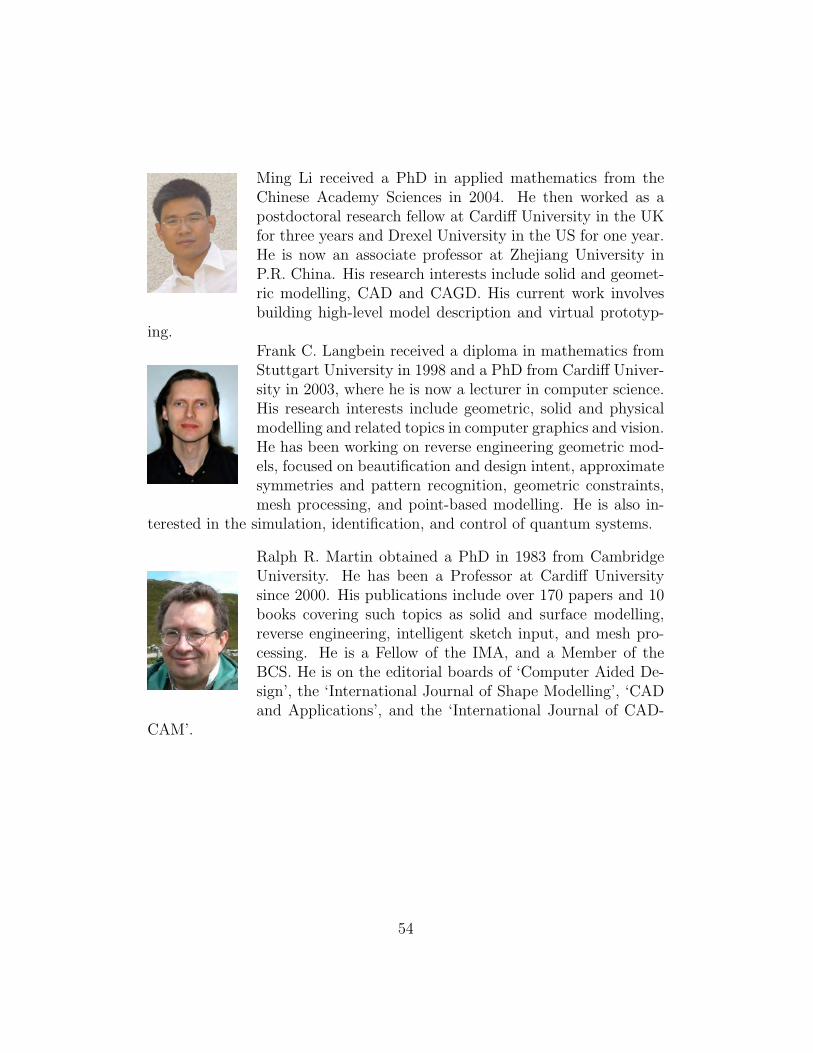
Ming Li received a PhD in applied mathematics from theChinese Academy Sciences in 2004. He then worked as apostdoctoral research fellow at Cardiff University in the UKfor three years and Drexel University in the US for one year.He is now an associate professor at Zhejiang University inP.R. China. His research interests include solid and geomet-ric modelling, CAD and CAGD. His current work involvesbuilding high-level model description and virtual prototyp-

ing.Frank C. Langbein received a diploma in mathematics fromStuttgart University in 1998 and a PhD from Cardiff Univer-sity in 2003, where he is now a lecturer in computer science.His research interests include geometric, solid and physicalmodelling and related topics in computer graphics and vision.He has been working on reverse engineering geometric mod-els, focused on beautification and design intent, approximatesymmetries and pattern recognition, geometric constraints,mesh processing, and point-based modelling. He is also in-

terested in the simulation, identification, and control of quantum systems.

Ralph R. Martin obtained a PhD in 1983 from CambridgeUniversity. He has been a Professor at Cardiff Universitysince 2000. His publications include over 170 papers and 10books covering such topics as solid and surface modelling,reverse engineering, intelligent sketch input, and mesh pro-cessing. He is a Fellow of the IMA, and a Member of theBCS. He is on the editorial boards of ‘Computer Aided De-sign’, the ‘International Journal of Shape Modelling’, ‘CADand Applications’, and the ‘International Journal of CAD-

CAM’.

54