detection and characterization of actuator attacks using
TRANSCRIPT

Marquette Universitye-Publications@Marquette
Master's Theses (2009 -) Dissertations, Theses, and Professional Projects
Detection and Characterization of Actuator AttacksUsing Kalman Filter EstimationYuqin WengMarquette University
Recommended CitationWeng, Yuqin, "Detection and Characterization of Actuator Attacks Using Kalman Filter Estimation" (2019). Master's Theses (2009 -).514.https://epublications.marquette.edu/theses_open/514

DETECTION AND CHARACTERIZATION OF ACTUATOR
ATTACKS USING KALMAN FILTER ESTIMATION
by
YUQIN (OLIVER) WENG, B.S.
A Thesis Submitted to the Faculty of the Graduate School,
Marquette University,
in Partial Fulfillment of the Requirements for
the Degree of Master of Science (Electrical and Computer Engineering).
Milwaukee, Wisconsin
December 2018

ABSTRACT
Yuqin Weng
In this thesis, two discrete-time control systems subject to noise, are modeled,
analyzed and estimated. These systems are then subjected to attack by false signals such
as constant and ramp signals. In order to find out how and when the control systems are
being attacked by the false signals, several detection algorithms are applied to the
systems. This work focuses on actuator attack detection.
To detect the presence of false actuator signals, a bank of Kalman filters is set up
which uses adaptive estimation and conditional probability density functions for detecting
the false signals. The individual Kalman filters are each tuned to satisfy a control system:
one of which is the original system and the other of which is the system with a false
signal. The use of the bank of Kalman filters to detect actuator attacks is tested in 4 cases;
first-order system attacked by a constant or ramp signal and then a second-order system
subject to the same types of attack signals.
This work shows the bank of Kalman filters can successfully detect the intrusion
of false signals for actuator attack by using several different detection algorithms.
Simulations show that the false signal is found and detected in all cases.

i
ACKNOWLEDGEMENTS
Yuqin Weng
It is a great honor for me to have Dr. Edwin Yaz and Dr. Susan Schneider as my
advisers. I feel so grateful for their help and support in my master academic years. I
would not have become who I am now without their dedication.
I would like to thank my parents, Zhongcheng Weng and Suqin Wang, for their
love, support and encouragement in all the years. There is nothing can be compared with
their care and love.
Apart from my advisers, it is my fortune to have Dr. Jennifer Bonniwell on my
committee who gave her precious MATLAB knowledge and suggestions about my thesis
to me. I also want to say “thank you” to all my friends in the research team: Alia Strandt,
John Burroughs, Jiayi Su and Abdulelah Alshareef. I wish everyone in the team achieves
what they want in their career.
In the end, I wish I can have a distinguished career either in industry or continuing
as a PhD student and live a happy life with all my friends and family.

ii
TABLE OF CONTENTS
ACKNOWLEDGEMENTS ................................................................................................. i
LIST OF FIGURES ........................................................................................................... iv
1. INTRODUCTION ...................................................................................................... 1
1.1 General Background ............................................................................................. 1
1.2 Problem Statement ............................................................................................... 3
1.3 Review of Previous Work .................................................................................... 3
1.3.1 Review of Estimation Theory ....................................................................... 3
1.3.2 Literature Review.......................................................................................... 5
1.4 Summary of Main Contributions ......................................................................... 9
1.5 Thesis Organization............................................................................................ 10
2. ACTUATOR INTRUSION DETECTION USING ESTIMATION THEORY: A
REVIEW ........................................................................................................................... 11
2.1 Introduction ........................................................................................................ 11
2.2 Kalman Filter and Its Applications .................................................................... 11
2.2.1 Kalman Filter Equation Derivation ............................................................. 12
2.2.2 Kalman Filter Update Algorithm ................................................................ 16
2.2.3 Kalman Filter Applications ......................................................................... 18
2.3 Adaptive Estimation ........................................................................................... 19
2.3.1 Introduction to Adaptive Estimation ........................................................... 19
2.3.2 Bank of Kalman Filters Algorithm ............................................................. 19
2.3.3 Bank of Kalman Filters Application ........................................................... 24
3. MODELS OF ACTUATOR ATTACKS IN CONTROL SYSTEM ........................ 26
3.1 Introduction to Actuator Attacks in Control System .......................................... 26
3.2 First-Order System Attack Scenario .................................................................. 28
3.2.1 Model of First-Order System Attacked by Constant Signal ....................... 28
3.2.2 Model of First-Order System Attacked by Ramp Signal ............................ 34
3.3 Second Order System attack scenario ................................................................ 39
3.3.1 Model of Second Order System Attacked by Constant Signal ................... 39
3.3.2 Model of Second Order System Attacked by Ramp Signal ........................ 45

iii
4. Actuator Intrusion Detection Discussion .................................................................. 49
4.1 Design of Bank of Kalman Filters...................................................................... 49
4.2 Detection Discussion on Bank of Kalman Filters .............................................. 51
4.2.1 Detection of False Signals using Probability Calculation........................... 51
4.2.2 Detection of False Signals using Innovation Sequence .............................. 55
4.2.3 Detection of False Signals using Bank of Kalman Filters Estimation ........ 59
4.3 Noise Effect on Bank of Kalman Filters ............................................................ 64
4.3.1 Correlation Between Noise and Convergence Time ................................... 65
4.4 Intrusion Detection by Using Sample Mean Values .......................................... 71
4.4.1 Intrusion Detection by Using Sample Mean Values with Known State ..... 71
4.4.2 Intrusion Detection by Using Sample Mean Values with Unknown State . 75
5. Conclusion and Future work ..................................................................................... 78
5.1 Summary ............................................................................................................ 78
5.2 Conclusion .......................................................................................................... 78
5.3 Future Work ....................................................................................................... 79
REFERENCES ................................................................................................................. 81
APPENDIX A: MATLAB CODES .................................................................................. 81
A1. MATLAB Code for Intrusion Detection by Using a Bank of Kalman Filter for
First-order System Attacked by Constant Signal .......................................................... 84
A2. MATLAB Code for Intrusion Detection by Using a Bank of Kalman Filter for
First-order System Attacked by Ramp Signal .............................................................. 87
A3. MATLAB Code for Intrusion Detection by Using a Bank of Kalman Filter for
Second-order System Attacked by Constant Signal ..................................................... 90
A4. MATLAB Code for Intrusion Detection by Using a Bank of Kalman Filter for
Second-order System Attacked by Ramp Signal .......................................................... 93
A5. MATLAB Code for Intrusion Detection by Using Sample Mean Method ............ 96
iv
LIST OF FIGURES
Figure 1.1 Bank of Estimators [10]..................................................................................... 7
Figure 2.1: Figure of Kalman filter algorithm [9] [25]. .................................................... 17
Figure 2.2: Block diagram of adaptive estimation technique based on banks of ............. 21
Figure 2.3:Block diagram of adaptive estimation technique for determining the true
control system. .................................................................................................................. 22
Figure 3.1: Block diagram of a general negative feedback control system with attack
signals. .............................................................................................................................. 26
Figure 3.2: Original state value in time of first-order system ........................................... 30
Figure 3.3: Original output value in time of first-order system ........................................ 31
Figure 3.4: Compromised state value in time of first-order system in the constant signal
attack scenario ................................................................................................................... 33
Figure 3.5: Compromised output value in time of first-order system in the constant signal
attack scenario ................................................................................................................... 34
Figure 3.6: Ramp signal in time with starting value at (1 ,1) and slope equals to 1 ......... 35
Figure 3.7: Compromised state value in time of first-order system in ramp signal attack
scenario ............................................................................................................................. 37
Figure 3.8: Compromised output value in time of first-order system in ramp signal attack
scenario ............................................................................................................................. 38
Figure 3.9: Original states value in time of second-order system in the constant signal
attack scenario ................................................................................................................... 41
Figure 3.10: Original output value in time of second-order system in the constant signal
attack scenario ................................................................................................................... 42
Figure 3.11: Compromised states value in time of second-order system in the constant
signal attack scenario ........................................................................................................ 44
Figure 3.12: Compromised output value in time of second-order system in the constant
signal attack scenario ........................................................................................................ 45

v
Figure 3.13: Compromised states value in time of second-order system in ramp signal
attack scenario ................................................................................................................... 47
Figure 3.14: Compromised output value in time of second-order system in ramp signal
attack scenario ................................................................................................................... 48
Figure 4.1: Design of a bank of Kalman filters for actuator intrusion detection .............. 50
Figure 4.2: Posterior probabilities of the false signal intrusion hypotheses used in the
bank of Kalman filters in which the first-order control system is attacked by the constant
signal ................................................................................................................................. 52
Figure 4.3: Posterior probabilities of the false signal intrusion hypotheses used in the
bank of Kalman filters in which the first-order control system is attacked by the ramp
signal ................................................................................................................................. 53
Figure 4.4: Posterior probabilities of the false signal intrusion hypotheses used in the
bank of Kalman filters in which the second-order control system is attacked by the
constant signal ................................................................................................................... 54
Figure 4.5: Posterior probabilities of the false signal intrusion hypotheses used in the
bank of Kalman filters in which the second-order control system is attacked by the ramp
signal ................................................................................................................................. 55
Figure 4.6: Innovation sequence of the first-order system attacked by the constant signal
........................................................................................................................................... 56
Figure 4.7: Innovation sequence of the first-order system attacked by the ramp signal .. 57
Figure 4.8: Innovation sequence of the second-order system attacked by the constant
signal ................................................................................................................................. 58
Figure 4.9: Innovation sequence of the second-order system attacked by the ramp signal
........................................................................................................................................... 59
Figure 4.10: First-order system estimated state value when the system is attacked by
constant signal at time 25 .................................................................................................. 60
Figure 4.11: First-order system estimated state value when the system is attacked by ramp
signal at time 25 ................................................................................................................ 61
Figure 4.12: Second-order system estimated states value when the system is attacked by
constant signal at time 25 .................................................................................................. 62
Figure 4.13: Second-order system estimated states value when the system is attacked by
constant signal at time 25 with longer iterations .............................................................. 63
vi
Figure 4.14: Second-order system estimated states value when the system is attacked by
the ramp signal at time 25 ................................................................................................. 64
Figure 4.15: Explanation of convergence1 and convergence 2 ........................................ 65
Figure 4.16: Convergence time on the first-order system attacked by the constant signal
........................................................................................................................................... 67
Figure 4.17: Correlation plot between noise covariance and convergence time for the
first- order system attacked by constant signal using the Pearson correlation coefficient 69
Figure 4.18: Correlation plot between noise covariance and convergence time for the
first- order system attacked by constant signal using the Spearman correlation coefficient
........................................................................................................................................... 70
Figure 4.19: System state mean value in time when the system is not attacked by the false
signal ................................................................................................................................. 73
Figure 4.20: System state mean value in time when the system is attacked by the constant
signal with known state ..................................................................................................... 74
Figure 4.21: System state mean value in time when the system is attacked by the constant
signal with known state at time index k=15 ..................................................................... 75
Figure 4.22: System state mean value in time when the system is attacked by the constant
signal with unknown state ................................................................................................. 76

1
1. INTRODUCTION
1.1 General Background
The motivation of this thesis work is to protect control systems from being
attacked by false actuator signals. Actuators are components in a machine or a system
that play a key role in moving a mechanism or controlling a system. An actuator usually
needs a control signal and a power supply, so it can convert the control signal into a real
action. Basically, an actuator acts as a bridge between the control system and the real
world. Actuators are commonly used in everyday life, such as using a motor in an
electro-pump system, starting an engine of a car and controlling a valve for a water
system.
There are several categories of actuators which can be roughly divided into three
types from the perspective of how they are powered: by electric signal, hydraulic fluid or
pneumatic pressure. These three diverse types of actuators are typically used in different
situations as well; power grid systems use electricity to control the actuator, water
treatment systems tend to have its actuator powered by fluid, while a turbine system may
power the actuator by pressure.
As mentioned, actuators are key components in control systems; a malicious
attacker can modify transmission data sent between actuator components and disrupt the
system's operations and cause irreversible damage to the control system and people who

2
depend on the control system [1]. As the security of such actuators in the control systems
has been studied and researched for years, different bad results will show up when
control systems such as oil refineries, water distribution networks, gas networks and
power grid system are corrupted [2]. If any of these control systems is attacked, the
consequences are unthinkable; thus, the safety of the control system is critically
important.
Let’s take a modern power system for an example; a false data injection attack on
a power system would lead to both physical and economic impacts to the control system
[3]. An example of economic attacks is, an attack on the electricity market to gain
financial profit. A successful delayed attack resulting in line overloading undetected by
the control center can lead to physical damage to the power system [3]. A damage of
economic and physical attacks is not negligible for the control systems. In [4], the authors
discuss how the attacks affect other parts of modern power system: state estimation,
automatic generation control, energy market and voltage control. For state estimation,
attackers can intelligently modify the sensor and actuator data at the meter level and then
start an intrusion at the communication layer. In this case, it is very difficult for engineers
to detect and protect the system quickly. Therefore, security detection for actuator and
sensor intrusion is the first and most crucial step for protecting the control system.

3
1.2 Problem Statement
Unauthorized access or hacking is an issue among either control systems or
computer network systems. Malfunction caused by the introduction of false information
sometimes can be fatal to control systems; such an invasion can easily go unnoticed.
Estimation theory is used to analyze the systems for attack detection as well as
protection. Analyzing the state and output of the control system is an effective way to
detect false information or intrusions. When the state of the system is unknown,
estimation techniques, such as Kalman filter or a bank of Kalman filters can be used to
determine when and how the systems are corrupted, so that there may be enough time for
engineers to protect and recover the systems once intrusion happens. Shutting down all
the equipment immediately after the intrusion of false signals is one, and often the best,
way to protect the control system.
1.3 Review of Previous Work
1.3.1 Review of Estimation Theory
Estimation theory is a branch of statistics and signal processing that deals with
estimating and observing the values of unknown parameters based on the measured
empirical data [5] [6] [7]. Finding values for unknown data or states by using an
estimator together with available measurements is commonly called the process of
estimation. Three definitions are usually discussed in estimation theory: smoothing,
filtering and prediction. Smoothing uses available measurement data to estimate

4
historical unknown parameters, filtering uses the measurements to estimate the present
value of unknown parameters and prediction uses available measurement data to estimate
the future value of unknown parameters [5].
There are a lot of fields in which estimation theory is used, for example,
telecommunication, signal processing and adaptive control. There are also various
estimators and estimation methods, such as Kalman filters, Extended Kalman filters, a
Bank of Kalman filters, maximum likelihood estimators, Bayes Estimators, Wiener
Filters, Maximum a posteriori (MAP) Particle Filter and Markov Chain Monte Carlo
(MCMC) [7]. Table 1.1 provides examples of estimation theory used in various fields.

5
Table 1.1: Applications of estimation theory [5][7].
Applications Examples
Control Systems Estimation of the position of a cart in a cart-
pendulum system and stabilizing the system by
using estimators.
Sonar Estimation of the delay of the received signal
from each sensor in the presence of noise
Communications Estimation of the carrier frequency of a signal
for demodulation to the baseband in the presence
of degradation noise.
Signal Processing Estimation of the parameters of the speech
model in the presence of speech variability and
environmental noise.
Biomedical Estimation of the heart rate of a fetus in the
presence of environmental noise.
Image Processing Estimation of the position and orientation of an
object from a camera image in the presence of
lighting and background noise.
Radar Communications Estimation of the delay in the received pulse
echo in the presence of noise.
Orbit determination Estimation of the trajectory of objects such as
moons, planets and aircraft.
As mentioned in the section above, this paper will mainly use a Kalman filter and
a bank of Kalman filters designed for actuator intrusion detection. The filter and how to
apply its algorithms to estimate states will be discussed in the next chapter.
1.3.2 Literature Review
Actuator and sensor security is a widespread problem [2, 8, 9]. The authors in [8]
focus on a decoding algorithm so that the states of the system can be recovered correctly;
at the end of their paper, the performance of the decoder on numerical examples is
demonstrated as well to show the states are recovered from the simulation. In [2], a

6
control gain 𝐾𝑐 is designed for state-feedback which can increase the resilience of the
system when attacked. Then the authors try to find if there exists a control law that drives
the state of the system to the origin even if some of the actuator and sensors are attacked,
in other words, the authors attempt to stabilize the system despite attacks on some of the
actuators and sensors. Simulations of the attack are shown at the end of the paper. A
recent study shows that by using a proper control variable, the system can be recovered to
the original state from attack [9]; in this paper, the authors have used different control
variables and the control variables have different positive impact on the system which
brings the system to the original state after attack. The authors also state that the control
system could quickly go back to the normal operation mode if proper optimal control
laws are applied.
R.N. Clark was the first person to discuss a bank of Kalman filters used for
instrument failure detection (IFD) in 1978 [10]. An example diagram of the system used
in [10] is shown in Figure1.1. In the abstract of [10], Clark stated, “Observer designs, and
detection logic are found for which 14 separate instrument faults are detected without
false alarms. The scheme is shown to be robust with respect to variations in two
significant physical parameters.”

7
Figure 1.1 Bank of Estimators [10]
Clark used a Boat-Instrument-Autopilot Model to illustrate the idea. The logic for fault
detection used the subtraction between the real output and estimated output compared
with a threshold. The alarm sounds if the subtraction exceeds the threshold. In the
conclusion section, Clark presented that the robustness of the attack detection can only
tolerate with 10-percent variations in two important physical parameters [10]. However,
Clark chose a system without random disturbance and the estimators used are Luenberger
observers. Once noise was added to the system, the bank of Luenberger observers is
replaced by a bank of Kalman filters since the Kalman filter does a better job dealing

8
with the random disturbance than a Luenberger observer. Clark also had some later work
involving bank of estimators using a bank of Kalman filters.
In a recent study [11], the authors tried to apply a bank of Kalman filters for fault
detection to a wind turbine generator system. Subtraction between the real output and
estimated output are also used to decide if the system is attacked by the comparison to a
threshold. At the end of the paper, the authors stated there are no miss detections in all
their experiments.
Another paper addresses false data injection attacks (FDIAs) [12]. The authors of
this paper use a tool, X2- detector, which is a proven-effective exploratory method used
with Kalman Filter for detecting false signals. The authors applied this technique to
detect attacks such as denial-of-service (DoS) attacks and then calculate the subtraction
of the real and estimated output value in time and call it the residual matrix. After finding
out the covariance matrix of the residual matrix; the authors compute the product of
residual matrix and its covariance matrix and compare this result with a precomputed
threshold to identify a failure or an attack [12]. However, the X2- detector does not
perform well on detecting failure for the system attacked by FDIAs. Thus, the authors
also analyzed the Euclidean distance method for detecting the failure in which the control
system is attacked by FDIAs. Although this paper has only implemented the methods on
sensors, X2- detector and Euclidean distance method can also be utilized for actuator
failure detection.

9
In 2016, M. S. Ayas and S. M. Djouadi found interesting results for actuator
attacks in cyber-physical systems [13]. M. S. Ayas and S. M. Djouadi have different
experiments on both sensor and actuator attacks and they concluded that there will be
some undetectable attack signals that compromise cyber-physical systems without being
noticed by engineers. More importantly, system output responses obtained without attack
are nearly the same for system output responses under undetectable attack. This proves
that undetectable attack signals have successfully gone into the system without notice. In
addition, the authors state that the actuator signal attack is optimal in the sense of
minimal energy attack signal[13], which means the actuator attack is more likely to
happen in a control system.
References [14]-[18] use similar methods to calculate residuals of real and
estimated output value for each state and compare the residuals to a threshold value to
check if the system is corrupted like discussed before. The difference is that the authors
used different systems to investigate the problem. For examples, [14] used a power grid
system to investigate fault detection, [16] chose an electro-pump system and [17]
implemented their method on a wastewater treatment process by using an extended
Kalman filter.
1.4 Summary of Main Contributions
This thesis proposes to investigate actuator attacks in control systems. Several
control systems are modeled, analyzed and subsequently attacked by false actuator
10
signals. There are two different cases, first and second order systems are both studied in
this paper.
To characterize the attack and detection process, the effect of different process
and measurement noise covariances are investigated in the study. Lastly, a method to
check the system state mean is also presented as an extension for actuator intrusion
detection.
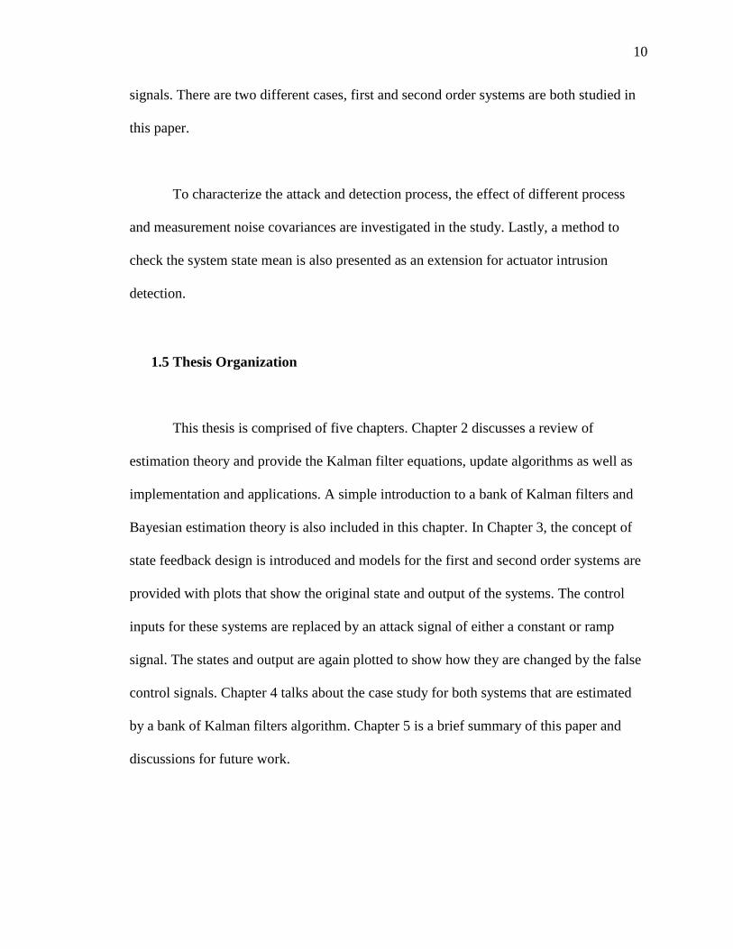
1.5 Thesis Organization
This thesis is comprised of five chapters. Chapter 2 discusses a review of
estimation theory and provide the Kalman filter equations, update algorithms as well as
implementation and applications. A simple introduction to a bank of Kalman filters and
Bayesian estimation theory is also included in this chapter. In Chapter 3, the concept of
state feedback design is introduced and models for the first and second order systems are
provided with plots that show the original state and output of the systems. The control
inputs for these systems are replaced by an attack signal of either a constant or ramp
signal. The states and output are again plotted to show how they are changed by the false
control signals. Chapter 4 talks about the case study for both systems that are estimated
by a bank of Kalman filters algorithm. Chapter 5 is a brief summary of this paper and
discussions for future work.

11
2. ACTUATOR INTRUSION DETECTION USING ESTIMATION THEORY:
A REVIEW
2.1 Introduction
As stated in Chapter 1, estimation theory is a branch of statistics. Kalman filters
and other estimators are commonly used in estimation theory. The Kalman Filter is
named after R.E. Kalman. In 1960, R.E. Kalman first used his filter to obtain reliable
performance for the discrete time linear filtering problem [19]. The Kalman filter has
now become one of the main estimation tools in statistics and estimation theory.
The Kalman filter estimates the value of unknown states by using past
measurement data. The Kalman filter can also be applied to estimate the outputs of
systems [9]. Other estimators like the Luenberger observer, can be used to estimate states
of systems as well; the Luenberger observer has an estimate of the state and output based
on the given system and uses it to determine output error [20]. More studies of
differences between Kalman filter and other observers can be found in [21], where the
authors summarize the strengths and weaknesses of different estimators.
2.2 Kalman Filter and Its Applications
In this section, the Kalman filter equations and algorithm are presented.
Furthermore, the applications of Kalman filter and its derivatives are listed in detail.

12
2.2.1 Kalman Filter Equation Derivation
The Kalman filter equations are derived by starting with a simple stochastic
discrete-time state space model:
𝑥𝑘+1 = 𝐴𝑥𝑘 + 𝐵𝑢𝑘 + 𝐹𝑣𝑘 (2.1)
𝑦𝑘 = 𝐶𝑥𝑘 + 𝐷𝑢𝑘 + 𝐺𝑤𝑘 (2.2)
Eq. 2.1 is the state evolution equation and (2.2) is the measurement equation. In
these equations, index 𝑘, is the sample and takes on value 0, 1, 2… , 𝐴, 𝐵, 𝐶, 𝐷, 𝐹, 𝐺 are
time-invarient system matrices of appropriate dimenstions, 𝑥𝑘 ∈ 𝑅𝑛 is the state vector,
𝑢𝑘 ∈ 𝑅𝑙 is the control input vector, 𝑣𝑘 ∈ 𝑅𝑝 is the process noise vector, 𝑦𝑘 ∈ 𝑅𝑚 is the
output vector, and 𝑤𝑘 ∈ 𝑅𝑞 is the process noise vector. The state has an initial value
𝑥0. The covariance of the process noise 𝑣𝑘, is 𝑉, and the covariance of the measurement
noise 𝑤𝑘, is 𝑊. The cross-covariance of 𝑣𝑘, and 𝑤𝑘, is 𝑆, leading to
Covariance ([𝑥0𝑣𝑘
𝑤𝑘
]) = [𝑃0 0 00 𝑉 𝑆0 𝑆𝑇 𝑊
] (2.3)

13
where 𝑃0, is the first term of the error covariance. The error covariance 𝑃𝑘, will be
discussed later. If 𝑣𝑘, and 𝑤𝑘, are not correlated, the cross-covariance term 𝑆 will be the
zero matrix.
The next step is to define an error term 𝑒𝑘+1, between the true state value 𝑥𝑘+1,
and the estimated state value �̂�𝑘+1,
𝑒𝑘+1 = 𝑥𝑘+1 − �̂�𝑘+1 (2.4)
The goal of a Kalman filter is to minimize the error covariance 𝑃𝑘+1 , which is
dependent on
𝑃𝑘+1 = 𝐸{(𝑒𝑘+1)(𝑒𝑘+1)𝑇} (2.5)
At each time 𝑘, we will have the value of estimated state �̂�𝑘, the value of system input
𝑢𝑘, and the value of system output 𝑦𝑘, [9] [22]. By using these three values, the estimate
is calculated by
�̂�𝑘+1 = 𝐴�̂�𝑘 + 𝐵𝑢𝑘 + 𝐾𝑘(𝑦𝑘 − �̂�𝑘) (2.6)

14
in which �̂�𝑘, and 𝐾𝑘 represent the estimated system output and Kalman gain. The
estimated, �̂�𝑘, is given by
�̂�𝑘 = 𝐶�̂�𝑘 + 𝐷𝑢𝑘 (2.7)
To find the Kalman gain 𝐾𝑘, the error covariance of the Kalman filter given by (2.5)
needs to be found,
The error at time (𝑘 + 1) needs to be calculated in order to calculate the error
covariance term 𝑃𝑘+1. By substituting (2.1), (2.2), (2.6), (2.7) into (2.4), 𝑒𝑘+1, is given
by (2.8),
𝑒𝑘+1 = (𝐴 − 𝐾𝑘𝐶)𝑒𝑘 + 𝐹𝑣𝑘 − 𝐾𝑘𝐺𝑤𝑘 (2.8)
Substituting (2.8) into (2.5) yields:
𝑃𝑘+1 = 𝐴𝑃𝑘𝐴𝑇 − 𝐴𝑃𝑘𝐶𝑇𝐾𝑘𝑇 − 𝐾𝑘𝐶𝑃𝑘𝐴𝑇 + 𝐾𝑘𝐶𝑃𝑘𝐶𝑇𝐾𝑘
𝑇 + 𝐹𝑉𝑘𝐹𝑇
− 𝐾𝑘𝐺𝑆𝑇𝐹𝑇 − 𝐹𝑆𝐺𝑇𝐾𝑘𝑇 + 𝐾𝑘𝐺𝑊𝐺𝑇𝐾𝑘
𝑇 (2.9)
Since the error covariance matrix 𝑃𝑘+1, is a symmetric matrix, one property of this matrix
is that minimizing the error covariance matrix is equivalent to minimizing the trace of
itself, 𝑇𝑟{𝑃𝑘+1} [9] [23]. By taking the partial derivative of of 𝑇𝑟{𝑃𝑘+1} with the respect
to 𝐾𝑘, and setting it equal to zero, the equation for the Kalman gain 𝐾𝑘, is obtained,

15
𝐾𝑘 = (𝐴𝑃𝑘𝐶𝑇 + 𝐹𝑆𝐺𝑇)(𝐶𝑃𝑘𝐶𝑇 + 𝐺𝑊𝑘𝐺𝑇)−1 (2.10)
Knowing the value of the Kalman gain 𝐾𝑘, at each time 𝑘, so the error covariance
equation given in (2.9) can be simplified as
𝑃𝑘+1 = 𝐴𝑃𝑘𝐴𝑇 + 𝐹𝑉𝑘𝐹𝑇 − (𝐴𝑃𝑘𝐶𝑇 + 𝐹𝑆𝐺𝑇)(𝐶𝑃𝑘𝐶𝑇 + 𝐺𝑊𝑘𝐺𝑇)−1
(𝐶𝑃𝑘𝐴𝑇 + 𝐺𝑆𝑇𝐹𝑇) (2.11)
As mentioned before, if the process noise 𝑣𝑘, and the measurement noise 𝑤𝑘, are not
correlated, the cross-covariance term 𝑆, will be zero. Commonly in control systems 𝑣𝑘,
and 𝑤𝑘, are zero mean. Thus, the Kalman gain and the error covariance can be further
simplified,
𝐾𝑘 = 𝐴𝑃𝑘𝐶𝑇 (𝐶𝑃𝑘𝐶𝑇 + 𝐺𝑊𝑘𝐺𝑇)−1 (2.12)
𝑃𝑘+1 = 𝐴𝑃𝑘𝐴𝑇 + 𝐹𝑉𝑘𝐹𝑇 − 𝐴𝑃𝑘𝐶𝑇 (𝐶𝑃𝑘𝐶𝑇 + 𝐺𝑊𝑘𝐺𝑇)−1(𝐶𝑃𝑘𝐴𝑇) (2.13)
By substituting (2.7) into (2.6), the state update equation is given by (2.14),
�̂�𝑘+1 = 𝐴�̂�𝑘 + 𝐵𝑢𝑘 + 𝐾𝑘(𝑦𝑘 − [𝐶�̂�𝑘 + 𝐷𝑢𝑘]) (2.14)

16
The reason why the state update equation is organized in this way is that (2.12), (2.13)
and (2.14) represent a recursive process to update the state estimation based on the past
measurement [9]. For each time, the error covariance is minimized by the Kalman gain so
that the error between the true state value and the estimated state value will also be
decreased. This is how the Kalman filter works for estimating state variables.
2.2.2 Kalman Filter Update Algorithm
Updating a Kalman filter is a two-steps update process, a state prediction and a
measurement update. The Kalman filter update process can be understood as a feedback
control, the Kalman filter estimates the unknown state and then obtains feedback in the
form of output measurements with some noise [24]. Thus, it is can be concluded that the
state update step is to project the current state and error covariance to obtain a new
estimate for the next time step, and the measurement update is to correct or update the
new state using the new measured value by a weighted average [9] [24].
Figure 2.1 shows the update algorithm of the Kalman filter, the Kalman gain is
calculated in ① at k = 0. With the measurement data and the Kalman gain, we can
update the state estimate in ②. Then state estimate is used in ③ for updating the error
covariance. Finally, the error covariance is used to calculate the Kalman gain again at the
next time step k = 1. The process then continues.

17
①Calculate Kalman gain
𝐾𝑘 = 𝐴𝑃𝑘𝐶𝑇 (𝐶𝑃𝑘𝐶𝑇
+ 𝐺𝑊𝑘𝐺𝑇)−1
Update state estimate
�̂�𝑘+1 = 𝐴�̂�𝑘 + 𝐵𝑢𝑘 + 𝐾𝑘(𝑦𝑘
− [𝐶�̂�𝑘 + 𝐷𝑢𝑘])
③Update the error covariance
𝑃𝑘+1 = 𝐴𝑃𝑘𝐴𝑇 + 𝐹𝑉𝑘𝐹𝑇
− 𝐴𝑃𝑘𝐶𝑇 (𝐶𝑃𝑘𝐶𝑇
+ 𝐺𝑊𝑘𝐺𝑇)−1(𝐶𝑃𝑘𝐴𝑇)
Measureme
nt data, 𝒚𝒌
Initialize the state
estimate and
error covariance
�̂�0,𝑃0
Figure 2.1: Figure of Kalman filter algorithm [9] [25].
②

18
2.2.3 Kalman Filter Applications
As mentioned above, since R.E. Kalman developed the Kalman filter, the Kalman
filter has been used in many different applications. As a minimum-variance estimation
for dynamic systems, the Kalman filter has attracted much attention with the increasing
demands of target tracking, navigating or imagine processing and so on. The Kalman
filter has been used in various algorithms that were proposed for deriving optimal state
estimation in the last thirty years [26]. Table 2.1 shows some of the typical applications
of Kalman filter and its variations
Table 2.1: Applications of Kalman filter and its variations.
Applications Examples
Control Systems Estimating the states of control systems.
Tracking and navigation Filtering out the noise for better performance of
tracking and navigation.
Economics Parameter estimation of linear and non-linear
econometric models [9].
Signal Processing The noise of the signal will be filtered, and the
signal will be estimated as well.
Image Processing The noise and disturbance in a photo is filtered
out.
Forecasting Estimating the parameters of the forecasting
model using the measured data [9].

19
2.3 Adaptive Estimation
2.3.1 Introduction to Adaptive Estimation
Adaptive estimation is used for estimating unknown parameters or unknown
states. One way to do adaptive estimation is by using a set of Kalman filters and parallel
processing technique. In this work, the concept of a bank of Kalman filters is used to
estimate and detect the faults in control systems and estimate the system states.
In 1974, researchers studied how parallel identification works, assuming the
unknown parameters or state vector 𝑅, is discrete or quantized to a finite number of
values { 𝑅1, 𝑅2, … , 𝑅𝑖, … , 𝑅𝑛}, with known or assumed priori probability for each 𝑅𝑖 .
The conditional estimator includes a bank of n Kalman filters where the 𝑖th Kalman filter
is the posteriori probability of 𝑅𝑖 , which is updated recursively using the noisy signal
measurements and the state of 𝑖th Kalman filter [22]. For this research work, assuming
that attackers would compromise the input of the control system, the state vector 𝜃
represented by control input 𝑈. Potential false information that attackers insert into the
control system can be expressed as 𝑈1 , 𝑈2,…, 𝑈𝑖 , … , 𝑈𝑛, each of the inputs is used to
design one of the Kalman filters in the bank.
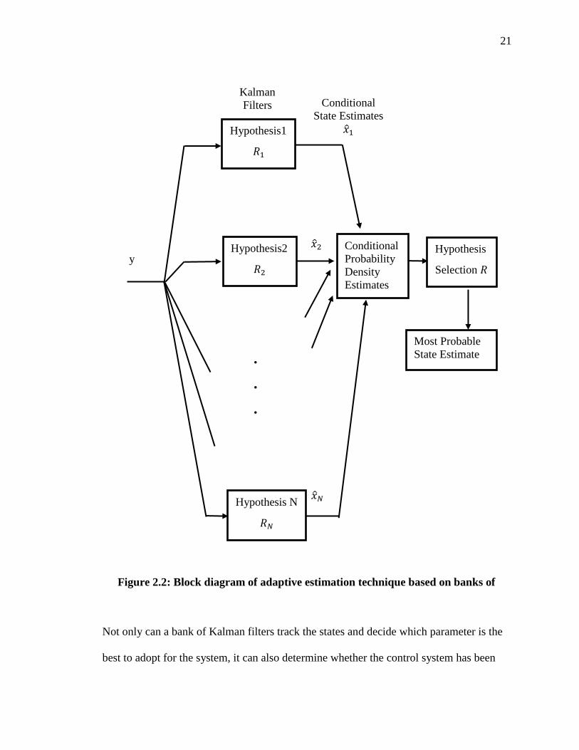
2.3.2 Bank of Kalman Filters Algorithm
Figure 2.2 depicts the flow of data through a bank of Kalman filters to find an
unknown parameter: a set of possible values or hypotheses for the unknown parameter is
calculated as 𝑅 = { 𝑅1, 𝑅2, … , 𝑅𝑖, … , 𝑅𝑛} in which 𝑅𝑖, is one of the hypotheses. A

20
Kalman filter is designed for each possible parameter value or hypothesis. The
conditional probability of each one of the Kalman filters in the bank will be calculated
according to the current measurements [27]. The filter that shows highest probability
among all conditional probabilities identifies the most likely parameter value or
hypothesis.
21
Not only can a bank of Kalman filters track the states and decide which parameter is the
best to adopt for the system, it can also determine whether the control system has been
Figure 2.2: Block diagram of adaptive estimation technique based on banks of
Hypothesis1
𝑅1
.
.
.
y
Kalman
Filters
Conditional
Probability
Density
Estimates
Hypothesis
Selection 𝑅
Most Probable
State Estimate
Conditional
State Estimates
�̂�1
�̂�2
�̂�𝑁 Hypothesis N
𝑅𝑁
Hypothesis2
𝑅2
22
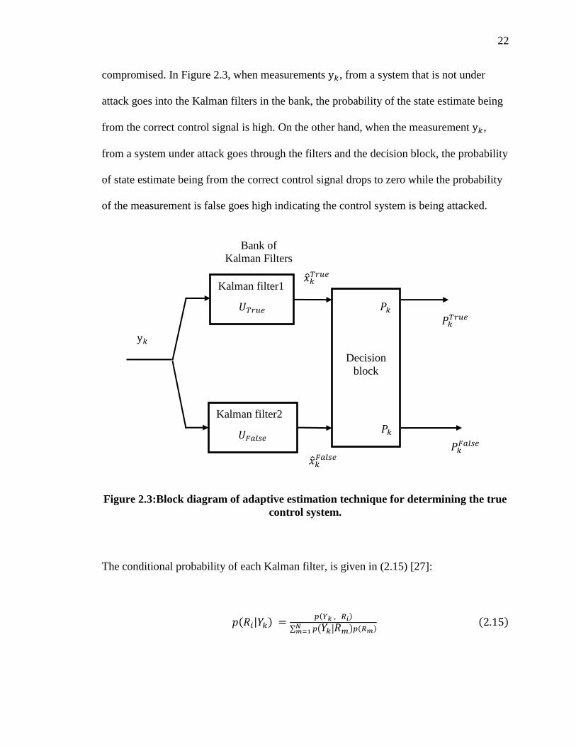
compromised. In Figure 2.3, when measurements y𝑘, from a system that is not under
attack goes into the Kalman filters in the bank, the probability of the state estimate being
from the correct control signal is high. On the other hand, when the measurement y𝑘,
from a system under attack goes through the filters and the decision block, the probability
of state estimate being from the correct control signal drops to zero while the probability
of the measurement is false goes high indicating the control system is being attacked.
Figure 2.3:Block diagram of adaptive estimation technique for determining the true
control system.
The conditional probability of each Kalman filter, is given in (2.15) [27]:
𝑝(𝑅𝑖|𝑌𝑘) =𝑝(𝑌𝑘 , 𝑅𝑖)
∑ 𝑝(𝑌𝑘|𝑅𝑚)𝑁𝑚=1 𝑝(𝑅𝑚)
(2.15)
Bank of
Kalman Filters
Kalman filter1
𝑈𝑇𝑟𝑢𝑒
y𝑘
Decision
block
Kalman filter2
𝑈𝐹𝑎𝑙𝑠𝑒
�̂�𝑘𝑇𝑟𝑢𝑒
�̂�𝑘𝐹𝑎𝑙𝑠𝑒
𝑃𝑘
𝑃𝑘
𝑃𝑘𝑇𝑟𝑢𝑒
𝑃𝑘𝐹𝑎𝑙𝑠𝑒
23
where 𝑝() represents a probability density function. Eq. 2.15 can also be expanded and
to become (2.16) [27]:
𝑝(𝑅𝑖|𝑌𝑘) =𝑝(𝑦𝑘|𝑌𝑘−1, 𝑅𝑖)𝑝(𝑅𝑖|𝑌𝑘−1)
∑ 𝑝(𝑦𝑘|𝑌𝑘−1, 𝑅𝑚)𝑁𝑚=1 𝑝(𝑅𝑚|𝑌𝑘−1)
(2.16)
In (2.16), 𝑌𝑘−1, denotes all the measurements in the sequence up to and including time,
𝑘 − 1 and 𝑦𝑘, represents the measurement at each time 𝑘, finally 𝑅𝑖, means one of the
possible values of the control inputs (the original and false signals) that will be used in
the Kalman filters in the bank. Since there are only two situations in this work: the true
and false control input, (2.16) can be rewritten as:
𝑝(𝑅𝑖|𝑌𝑘) =𝑝(𝑦𝑘|𝑌𝑘−1, 𝑅𝑖)𝑝(𝑅𝑖|𝑌𝑘−1)
𝑝(𝑦𝑘|𝑌𝑘−1,𝑅1)𝑝(𝑅1|𝑌𝑘−1)+𝑝(𝑦𝑘|𝑌𝑘−1,𝑅2)𝑝(𝑅2|𝑌𝑘−1)(2.17)
Convergence occurs when the posterior probability of the filter corresponding to the
hypothesis closest to the current control input of the system approaches one.
To calculate 𝑝(𝑦𝑘|𝑌𝑘−1, 𝑅𝑖) , all the measurement and process noises are
assumed to be Gaussian, which means they have Gaussian conditional probabilities.
Thus, 𝑝(𝑦𝑘|𝑌𝑘−1, 𝑅𝑖) becomes (2.18) [27]:
𝑝(𝑦𝑘|𝑌𝑘−1, 𝑅𝑖) = (2𝜋)−𝑛 2⁄ |Ω𝑘|𝑅𝑖
−1 |1 2⁄
∗ 𝑒𝑥𝑝 (−1
2�̃�𝑘|𝑅𝑖
𝑇 Ω𝑘|𝑅𝑖
−1 �̃�𝑘|𝑅𝑖) (2.18)

24
Here 𝑛, represents the dimension of the control system, and �̃�𝑘|𝑅𝑖, in (2.18) is called
innovation sequence and is defined as:
�̃�𝑘|𝑅𝑖= 𝑦𝑘 − �̂�𝑘|𝑘−1,𝑅𝑖
(2.19)
The innovation covariance of the Kalman filter is Ω𝑘|𝑅𝑖, and is calculated by
Ω𝑘|𝑅𝑖= 𝐶𝑃𝑘|𝑅𝑖
𝐶𝑇 + 𝐺𝑊𝐺𝑇 (2.20)
The conditional probability of the original and the attacked scenarios of the control
system can be calculated according to the equations above.
2.3.3 Bank of Kalman Filters Application
A bank of Kalman filters is usually used in adaptive estimation and parallel
identifications. Engineers use this technique to identify the authenticity of the parameters
or if the control system is compromised. Table 2.2 shows several applications of a bank
of Kalman filters.

25
Table 2.2: Applications of Bank of Kalman filters.
Applications Examples
Parameter Identification Testing several unknown parameters to have the
closest one in a real system.
Sensor Intrusion
Detection
Detecting control system is being compromised
or not by testing control system states.
Actuator Intrusion
Detection
Detecting control system is being compromised
or not by testing control system inputs.
26
3. MODELS OF ACTUATOR ATTACKS IN CONTROL SYSTEM
In this chapter, two discrete-time systems to be used for simulations are designed.
In addition, two distinct types of false signals are created to act as actuator signals. The
performance of each system being attacked by each false signal is shown. To build a
discrete- time state space model with feedback and input for discussing actuator attack, a
control input 𝑢𝑘, needs to be developed therefore, a control variable 𝐾𝑐 is to be
calculated as well. It is common to refer the state-variable controller (full-state control
law plus the observer) as a compensator [28], the concept of a compensator and how the
control variable 𝐾𝑐 is found will be mentioned in the next section.
3.1 Introduction to Actuator Attacks in Control System
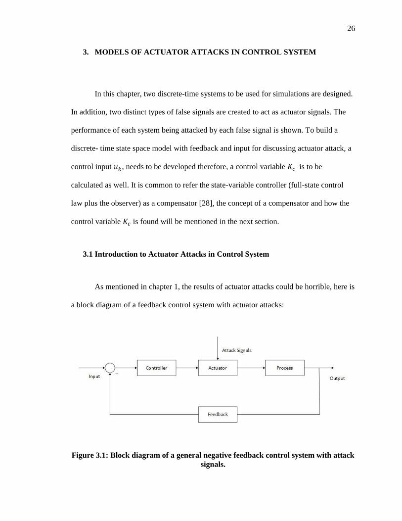
As mentioned in chapter 1, the results of actuator attacks could be horrible, here is
a block diagram of a feedback control system with actuator attacks:
Figure 3.1: Block diagram of a general negative feedback control system with attack
signals.
27
For this work, when designing a feedback control, the pole-placement technique may be
used. Thus, controllability and observability of the control system must be verified before
pole placement can be implemented [28]. After knowing the poles we want to place, the
control gain 𝐾𝑐, can be calculated, so that, 𝑢𝑘 = −𝐾𝑐 𝑥𝑘. The goal of the attackers is to
replace the control input 𝑢𝑘, with a false signal and then the control system is
compromised by the false information.
It is assumed that the state and the output of the control system are available in
this chapter. Both the original and attacked state and output values are obtained by
calculation. By considering the false signal ℎ𝑘 as a state as well when the system is
attacked, the dimension of the discrete-time state space model of the attacked system is
increased by adding one new state.
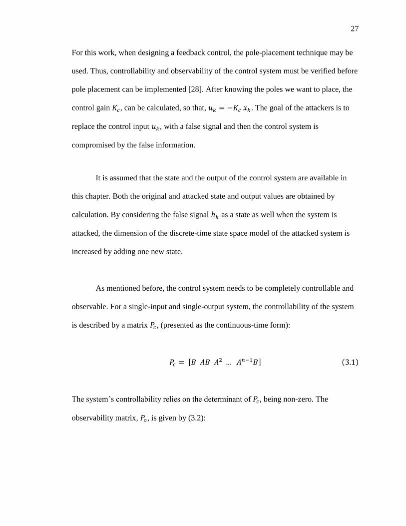
As mentioned before, the control system needs to be completely controllable and
observable. For a single-input and single-output system, the controllability of the system
is described by a matrix 𝑃𝑐, (presented as the continuous-time form):
𝑃𝑐 = [𝐵 𝐴𝐵 𝐴2 … 𝐴𝑛−1𝐵] (3.1)
The system’s controllability relies on the determinant of 𝑃𝑐, being non-zero. The
observability matrix, 𝑃𝑜, is given by (3.2):
28
𝑃𝑜 = [
𝐶𝐶𝐴
⋮𝐶𝐴𝑛−1
] (3.2)
The control system is observable when the determinant of the observability matrix 𝑃𝑜, is
not zero.
3.2 First-Order System Attack Scenario
In this section attack scenarios on a first order system are presented, the state and
the output of the first order system will first be shown and the difference between the
original and attacked systems will be presented as well.
3.2.1 Model of First-Order System Attacked by Constant Signal
Starting with a first-order system attacked by a constant actuator signal which is
represented by ℎ𝑘. The dynamics of the first-order system are: 𝐴 = 0.9, 𝐵 =1, 𝐶= 1, 𝐷= 1,
𝐹 = 1, 𝐺 = 1, 𝑉 = 0.01, 𝑊 = 0.05. By substituting these values into (2.1) and (2.2):
𝑥𝑘+1 = 0.9𝑥𝑘 + 𝑢𝑘 + 𝑣𝑘 (3.3)
𝑦𝑘 = 𝑥𝑘 + 𝑢𝑘 + 𝑤𝑘 (3.4)
Checking the controlibility and observability for the system:

29
𝑃𝑐 = [𝐵] = [1]
𝑃𝑜 = [𝐶] = [1]
Since the determinants are not zero, the first-order system is both controllable and
observable. To reduce response time, the eigenvalue needs to be placed close to the
origin. In this work, the eigenvalue will be placed at 0.4. Using the appropriate control
gain to place the pole, (3.3) becomes:
𝑥𝑘+1 = 0.4𝑥𝑘 + 𝑣𝑘 (3.5)
Figures 3.2 and 3.3 show the first-order system state and output value:

30
Figure 3.2: Original state value in time of first-order system

31
Figure 3.3: Original output value in time of first-order system
The two figures above show that when the control system is not attacked the original
state and output value fluctuate around zero with some noise as expected.
For the control system compromised by a false signal, ℎ𝑘, (ℎ𝑘=2) is used to
represent the false signal. When the actuator in the control system is compromised,
control input, 𝑢𝑘, is replaced by false signal, ℎ𝑘. Once the control system is attacked, the
state and output equations of the first-order system become:
𝑥𝑘+1 = 𝐴𝑥𝑘 + 𝐵ℎ𝑘 + 𝐹𝑣𝑘 (3.6)

32
𝑦𝑘 = 𝐶𝑥𝑘 + 𝐷ℎ𝑘 + 𝐺𝑤𝑘 (3.7)
Now the state is augmented with the false signal ℎ𝑘, yielding
[𝑥𝑘+1
ℎ𝑘] = [
𝐴 𝐵0 𝐼
] [𝑥𝑘
ℎ𝑘] + [
𝐹0
] 𝑣𝑘 (3.8)
𝑦𝑘 = [𝐶 𝐷] [𝑥𝑘
ℎ𝑘] + 𝐺𝑤𝑘 (3.9)
Eq. 3.8 and (3.9) can also be written as
𝓍𝑘+1 = 𝒜𝑋𝑘 + ℱ𝑣𝑘 (3.10)
𝓎𝑘 = 𝒞𝑋𝑘 + 𝐺𝑤𝑘 (3.11)
There is a “switch point” which refers to the time at which the control system is attacked.
In this work, the switch point is set to 25. From this time, the system model of the
attacked system is:
[𝑥𝑘+1
ℎ𝑘] = [
0.9 10 1
] [𝑥𝑘
ℎ𝑘] + [
10
] 𝑣𝑘 (3.12)
𝑦𝑘 = [1 1] [𝑥𝑘
ℎ𝑘] + 𝑤𝑘 (3.13)
33
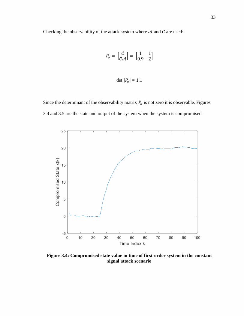
Checking the observability of the attack system where 𝒜 and 𝒞 are used:
𝑃𝑜 = [𝒞
𝒞𝒜] = [
1 10.9 2
]
det |𝑃𝑜| = 1.1
Since the determinant of the observability matrix 𝑃𝑜 is not zero it is observable. Figures
3.4 and 3.5 are the state and output of the system when the system is compromised.
Figure 3.4: Compromised state value in time of first-order system in the constant
signal attack scenario
34
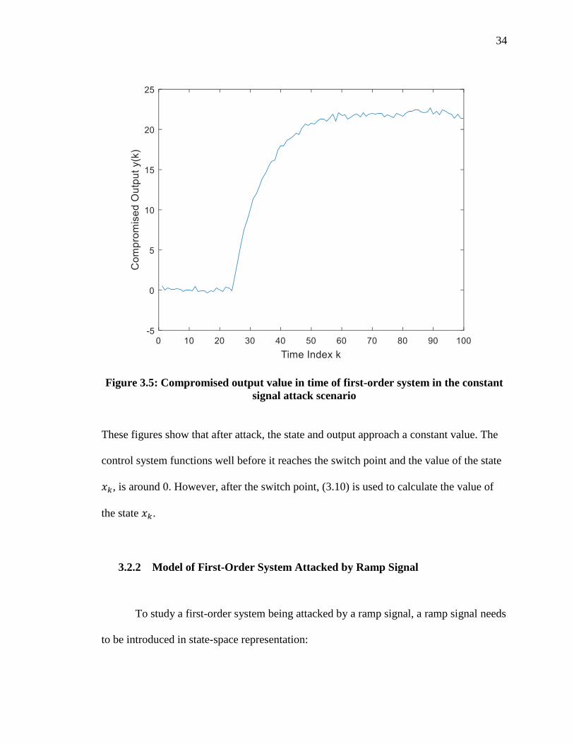
Figure 3.5: Compromised output value in time of first-order system in the constant
signal attack scenario
These figures show that after attack, the state and output approach a constant value. The
control system functions well before it reaches the switch point and the value of the state
𝑥𝑘, is around 0. However, after the switch point, (3.10) is used to calculate the value of
the state 𝑥𝑘.
3.2.2 Model of First-Order System Attacked by Ramp Signal
To study a first-order system being attacked by a ramp signal, a ramp signal needs
to be introduced in state-space representation:
35
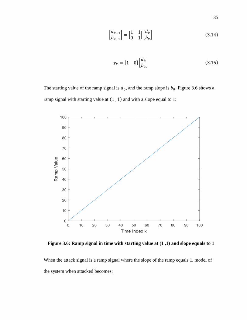
[𝑑𝑘+1
𝑏𝑘+1] = [
1 10 1
] [𝑑𝑘
𝑏𝑘] (3.14)
𝑦𝑘 = [1 0] [𝑑𝑘
𝑏𝑘] (3.15)
The starting value of the ramp signal is 𝑑0, and the ramp slope is 𝑏0. Figure 3.6 shows a
ramp signal with starting value at (1 , 1) and with a slope equal to 1:
Figure 3.6: Ramp signal in time with starting value at (1 ,1) and slope equals to 1
When the attack signal is a ramp signal where the slope of the ramp equals 1, model of
the system when attacked becomes:

36
[
𝑥𝑘+1
𝑑𝑘+1
𝑏𝑘+1
] = [𝐴 𝐵 00 1 10 0 1
] [
𝑥𝑘
𝑑𝑘
𝑏𝑘
] + [𝐹00
] 𝑣𝑘 (3.16)
𝑦𝑘 = [𝐶 1 0] [
𝑥𝑘
𝑑𝑘
𝑏𝑘
] + 𝐺𝑤𝑘 (3.17)
Using the same system parameters as before where 𝐴 = 0.9, 𝐵 =1, 𝐶= 1, 𝐷= 1, 𝐹 =
1, 𝐺 = 1, 𝑉 = 0.01, 𝑊 = 0.05. The equations for the attacked systems become:
[
𝑥𝑘+1
𝑑𝑘+1
𝑏𝑘+1
] = [0.9 1 00 1 10 0 1
] [
𝑥𝑘
𝑑𝑘+1
𝑏𝑘+1
] + [100
] 𝑣𝑘 (3.18)
𝑦𝑘 = [1 1 0] [
𝑥𝑘
𝑑𝑘
𝑏𝑘
] + 𝑤𝑘 (3.19)
Checking the observability for the attack model:
𝑃𝑜 = [𝒞
𝒞𝒜𝒞𝒜2
] = [1 1 0
0.9 2 10.81 2.9 3
]
det |𝑃𝑜| = 1.21
The determinant of the observability matrix 𝑃𝑜 is not zero which means it is observable.

37
Figure 3.7 and 3.8 show the state and output for the first-order system when the
actuator signal has been replaced by a ramp signal that starts at time index, 𝑘 =25.
Figure 3.7: Compromised state value in time of first-order system in ramp signal
attack scenario
38
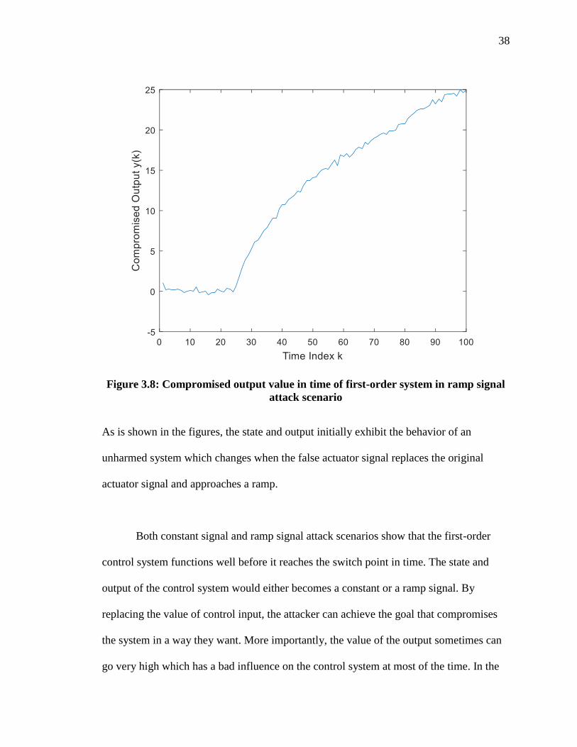
Figure 3.8: Compromised output value in time of first-order system in ramp signal
attack scenario
As is shown in the figures, the state and output initially exhibit the behavior of an
unharmed system which changes when the false actuator signal replaces the original
actuator signal and approaches a ramp.
Both constant signal and ramp signal attack scenarios show that the first-order
control system functions well before it reaches the switch point in time. The state and
output of the control system would either becomes a constant or a ramp signal. By
replacing the value of control input, the attacker can achieve the goal that compromises
the system in a way they want. More importantly, the value of the output sometimes can
go very high which has a bad influence on the control system at most of the time. In the

39
next section, original and attacked second-order system models are developed and
investigated.
3.3 Second Order System attack scenario
3.3.1 Model of Second Order System Attacked by Constant Signal
Assuming the second-order system is 𝐴 = [0 0.8
−0.8 −0.8], 𝐵 = [
10
], 𝐶= [1 0], 𝐷=
1, 𝐹 = [1 00 1
],𝐺 = 1, 𝑉 =0.1, 𝑊 = 0.5. Since there are two states in the second-order
system, two different process noises will be created as 𝑣𝑘1, and 𝑣𝑘2, for two states, but
both noise covariances are still 0.1. The numerical form of the second-order system is:
[𝑥(1)𝑘+1
𝑥(2)𝑘+1] = [
0 0.8−0.8 −0.8
] [𝑥(1)𝑘
𝑥(2)𝑘] + [
10
] 𝑢𝑘 + [1 00 1
] 𝑣𝑘 (3.20)
𝑦𝑘 = [1 0] [𝑥(1)𝑘
𝑥(2)𝑘] + 𝑢𝑘 + 𝑤𝑘 (3.21)
Checking the controllability and observability for the second-order system:
𝑃𝑐 = [𝐵 𝐴𝐵 ] = [1 00 −0.8
]
det |𝑃𝑐| = −0.8

40
𝑃𝑜 = [𝐶
𝐶𝐴] = [
1 00 0.8
]
det |𝑃𝑜| = 0.8
The determinants of matrices 𝑃𝑐, and 𝑃𝑜, are not zero so the control system it is
controllable and observable. Placing the poles of this second-order system at [0.4 −0.4]
to reduce response time, (3.20) becomes:
[𝑥(1)𝑘+1
𝑥(2)𝑘+1] = [
0.8 0.6−0.8 −0.8
] [𝑥(1)𝑘
𝑥(2)𝑘] + [
1 00 1
] 𝑣𝑘 (3.22)
The states and the output of the system are showen in Fgures 3.9 and 3.10:

41
Figure 3.9: Original states value in time of second-order system in the constant
signal attack scenario

42
Figure 3.10: Original output value in time of second-order system in the constant
signal attack scenario
Using ℎ𝑘 equals 8 and when the second order system is attacked by a constant signal, the
attack model of the second-order system becomes:
[
𝑥(1)𝑘+1
𝑥(2)𝑘+1
ℎ𝑘
] = [𝑎11 𝑎11 𝑏11
𝑎21 𝑎22 𝑏21
0 0 1
] [
𝑥(1)𝑘+1
𝑥(2)𝑘+1
ℎ𝑘
] + [𝑓11 𝑓12
𝑓21 𝑓22
0 0
] [𝑣𝑘1
𝑣𝑘2] (3.23)
𝑦𝑘 = [𝑐11 𝑐12 𝐷] [
𝑥(1)𝑘+1
𝑥(2)𝑘+1
ℎ𝑘
] + 𝐺𝑤𝑘 (3.24)

43
where 𝑎𝑖𝑗 are the elements of 𝐴, 𝑏𝑖𝑗 are the elements of 𝐵, 𝑐𝑖𝑗 are the elements of 𝐶 and
𝑓𝑖𝑗 are the elements of 𝐹. Recall that we have a second-order as 𝐴 = [0 0.8
−0.8 −0.8], 𝐵 =
[10
], 𝐶= [1 0], 𝐷= 1, 𝐹 = [1 00 1
],𝐺 = 1, 𝑉 =0.1, 𝑊 = 0.5 Substituting the system
values into the equations above:
[
𝑥(1)𝑘+1
𝑥(2)𝑘+1
ℎ𝑘
] = [0 0.8 1
−0.8 −0.8 00 0 1
] [
𝑥(1)𝑘+1
𝑥(2)𝑘+1
ℎ𝑘
] + [1 00 10 0
] [𝑣𝑘1
𝑣𝑘2] (3.25)
𝑦𝑘 = [1 0 1] [
𝑥(1)𝑘+1
𝑥(2)𝑘+1
ℎ𝑘
] + 𝑤𝑘 (3.26)
Checking the observability for the attack model:
𝑃𝑜 = [𝒞
𝒞𝒜𝒞𝒜2
] = [1 0 10 0.8 2
−0.64 −0.64 2]
det |𝑃𝑜| = 3.392
The determinant of the observability matrix 𝑃𝑜 is not zero so it is observable. Figure 3.11
and 3.12 show what the states and output become when the system is compromised at 25:

44
Figure 3.11: Compromised states value in time of second-order system in the
constant signal attack scenario
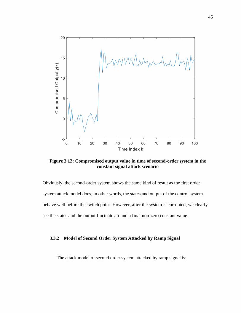
45
Figure 3.12: Compromised output value in time of second-order system in the
constant signal attack scenario
Obviously, the second-order system shows the same kind of result as the first order
system attack model does, in other words, the states and output of the control system
behave well before the switch point. However, after the system is corrupted, we clearly
see the states and the output fluctuate around a final non-zero constant value.
3.3.2 Model of Second Order System Attacked by Ramp Signal
The attack model of second order system attacked by ramp signal is:

46
[
𝑥(1)𝑘+1
𝑥(2)𝑘+1
𝑑𝑘+1
𝑏𝑘+1
] = [
𝑎11 𝑎12
𝑎21 𝑎22
𝑏11 0𝑏21 0
0 00 0
1 10 1
] [
𝑥(1)𝑘+1
𝑥(2)𝑘+1
𝑑𝑘+1
𝑏𝑘+1
] + [
𝑓11 𝑓12
𝑓21
00
𝑓22
00
] [𝑣𝑘1
𝑣𝑘2] (3.27)
𝑦𝑘 = [𝑐11 𝑐21 1 0] [
𝑥(1)𝑘+1
𝑥(2)𝑘+1
𝑑𝑘+1
𝑏𝑘+1
] + 𝐺𝑤𝑘 (3.28)
where 𝑎𝑖𝑗, 𝑏𝑖𝑗, 𝑐𝑖𝑗 and 𝑓𝑖𝑗 are the same elements stated before. Recall that for a second-
order system 𝐴 = [0 0.8
−0.8 −0.8], 𝐵 = [
10
], 𝐶= [1 0], 𝐷= 0, 𝐹 = [1 00 1
],𝐺 = 1, 𝑉 =0.1,
𝑊 = 0.5. Thus:
[
𝑥(1)𝑘+1
𝑥(2)𝑘+1
𝑑𝑘+1
𝑏𝑘+1
] = [
0 0.8−0.8 −0.8
1 00 0
0 00 0
1 10 1
] [
𝑥(1)𝑘+1
𝑥(2)𝑘+1
𝑑𝑘+1
𝑏𝑘+1
] + [
1 0000
100
] [𝑣𝑘1
𝑣𝑘2] (3.29)
𝑦𝑘 = [1 0 1 0] [
𝑥(1)𝑘+1
𝑥(2)𝑘+1
𝑑𝑘+1
𝑏𝑘+1
] + 𝑤𝑘 (3.30)
Checking the observability for the attack model:
𝑃𝑜 = [
𝒞𝒞𝒜
𝒞𝒜2
𝒞𝒜3
] = [
1 00 0.8
1 02 1
−0.64 −0.640.512 0
2 31.36 5
]
47
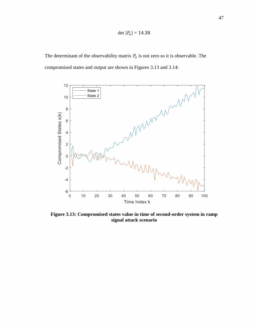
det |𝑃𝑜| = 14.38
The determinant of the observability matrix 𝑃𝑜 is not zero so it is observable. The
compromised states and output are shown in Figures 3.13 and 3.14:
Figure 3.13: Compromised states value in time of second-order system in ramp
signal attack scenario

48
Figure 3.14: Compromised output value in time of second-order system in ramp
signal attack scenario
Similar to the first-order system, after switch point, the states and output of the system
continue as a ramp signal which once again satisfies our goal.
All four situations show that once the control system is corrupted by the false
information, the states and output of the system would go as the attackers set up. In
chapter 4, the states and output values cannot be obtained directly from the system will be
discussed, a bank of Kalman filters is used to estimate the system and decide if the
system is attacked or not by three main aspects.
49
4. Actuator Intrusion Detection Discussion
In this chapter the primary results of this work, the ability of a bank of Kalman
filters to detect of the actuator intrusions of the control system, are presented by using the
system dynamics and attack signals described in chapter three. First, how to design a
bank of Kalman filters for detecting the false signals is presented in this work, then the
detection of false signals using probability calculation is shown, the detection of false
signals using innovation sequence and the detection of false signals using bank of
Kalman filters estimation are discussed as well. By studying of the relationship between
the process and measurement noise covariances, some suggestions are made for
shortening the convergence times. There is an additional method to detect the false
signal, called the sampled mean value method, it will be presented at the end of this
chapter.
4.1 Design of Bank of Kalman Filters
The figure below shows how a bank of Kalman filters is designed specifically for
actuator intrusion in this work. The unknown parameter needs to be estimated is the false
actuator signal, �̂�1𝑘, and �̂�2𝑘, are the corresponding state estimates at time index 𝑘, for
each Kalman filter in the bank, �̂�𝑘, is the combined state estimate at time index 𝑘.
Probability 𝑝1𝑘, and 𝑝2𝑘, are the corresponding conditional probability estimates at time
index 𝑘, for each state estimate.
50
Figure 4.1: Design of a bank of Kalman filters for actuator intrusion detection
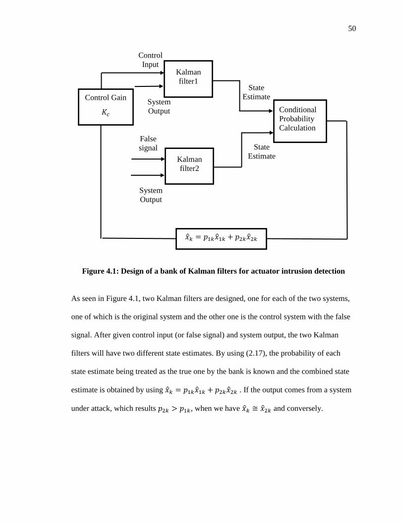
As seen in Figure 4.1, two Kalman filters are designed, one for each of the two systems,
one of which is the original system and the other one is the control system with the false
signal. After given control input (or false signal) and system output, the two Kalman
filters will have two different state estimates. By using (2.17), the probability of each
state estimate being treated as the true one by the bank is known and the combined state
estimate is obtained by using �̂�𝑘 = 𝑝1𝑘�̂�1𝑘 + 𝑝2𝑘�̂�2𝑘 . If the output comes from a system
under attack, which results 𝑝2𝑘 > 𝑝1𝑘, when we have �̂�𝑘 ≅ �̂�2𝑘 and conversely.
System
Output
𝑦
�̂�𝑘 = 𝑝1𝑘�̂�1𝑘 + 𝑝2𝑘�̂�2𝑘
Control Gain
𝐾𝑐
State
Estimate
�̂�
State
Estimate
�̂�
False
signal
ℎ
System
Output
𝑦
Control
Input
𝑢
Conditional
Probability
Calculation
Kalman
filter1
Kalman
filter2

51
4.2 Detection Discussion on Bank of Kalman Filters
4.2.1 Detection of False Signals using Probability Calculation
As was discussed in chapter 2 for calculating the probability of original and
attacked system, both the conditional probability of the two Kalman filters in a bank
should sum to one. The probability of the Kalman filter estimating the original system
with true control input goes to one which means that the control system is not
compromised by the false information. But after the false signal is injected, the
probability of the Kalman filter estimating the attacked system would go to one and the
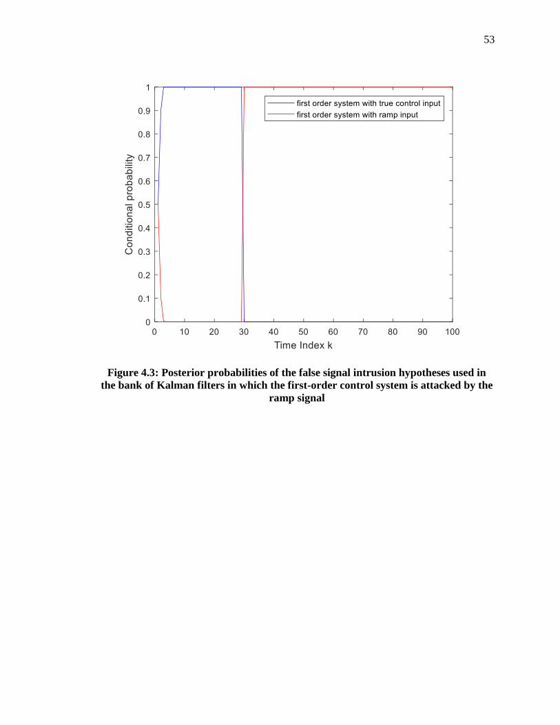
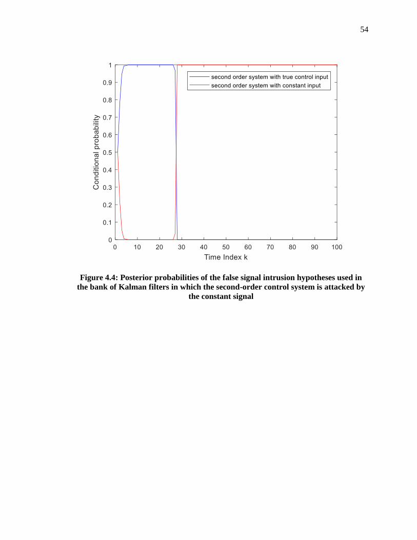
probability of the other Kalman filter goes to zero. Figures 4.2 through 4.5 each show the
detection of attack using probability detection. The blue line represents the control
system without intruded by the false information and the red line means the original
system is being attacked by the false signal. As expected, blue line first goes to 1 before
time 25 but the red line quickly goes up to 1 after switch point, which tells the engineers
that the control system is being attacked.

52
Figure 4.2: Posterior probabilities of the false signal intrusion hypotheses used in
the bank of Kalman filters in which the first-order control system is attacked by the
constant signal
53
Figure 4.3: Posterior probabilities of the false signal intrusion hypotheses used in
the bank of Kalman filters in which the first-order control system is attacked by the
ramp signal
54
Figure 4.4: Posterior probabilities of the false signal intrusion hypotheses used in
the bank of Kalman filters in which the second-order control system is attacked by
the constant signal

55
Figure 4.5: Posterior probabilities of the false signal intrusion hypotheses used in
the bank of Kalman filters in which the second-order control system is attacked by
the ramp signal
There is always some delay at the switch point, especially in the situation the second-
order system attacked by ramp signal. It is interesting to find out if there are any
relationships for the noise covariances and the convergence times. This topic is
investigated in section 4.3.
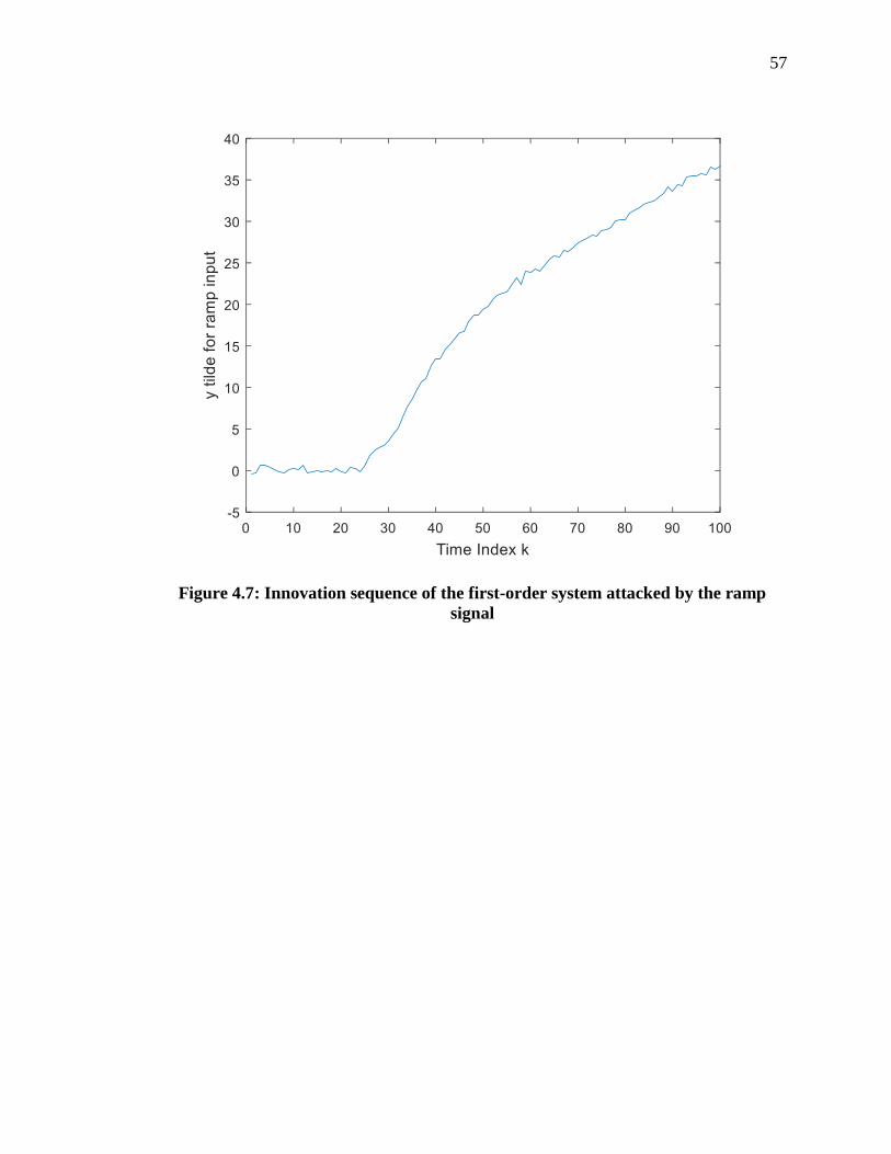
4.2.2 Detection of False Signals using Innovation Sequence
Using the subtraction between the estimation value and the true value of the
system output to decide whether the system is attacked by the false information is also an

56
excellent choice. This difference is used when calculating the innovation sequence in
(2.19). The innovation sequence should be zero when the control system is not attacked
since the estimation value of the output is close to the real value of the output. Once the
control system is intruded by the false information, the true value of the control system
will change instantly, and the innovation sequence is then no longer close to zero. Figures
4.6, 4.7, 4.8 and 4.9 show that the innovation sequence of the first and second order
system attacked by constant and ramp signal at time index 25, we can see clearly how
innovation sequence deviates from zero to another value after time index 25:
Figure 4.6: Innovation sequence of the first-order system attacked by the constant
signal
57
Figure 4.7: Innovation sequence of the first-order system attacked by the ramp
signal

58
Figure 4.8: Innovation sequence of the second-order system attacked by the constant
signal

59
Figure 4.9: Innovation sequence of the second-order system attacked by the ramp
signal
All the figures above show that before the switch point, the innovation sequence
fluctuates at around 0 with some noise but changes to a constant signal away from 0 or a
ramp signal after being intruded, demonstrating the control system is successfully
intruded by the false signal.
4.2.3 Detection of False Signals using Bank of Kalman Filters Estimation
In addition to using the probability calculation and innovation sequence to detect
the actuator intrusion, the combined state estimate �̂� = 𝑝1�̂�1 + 𝑝2�̂�2 produced by bank of
Kalman filters can be used for intrusion detections as well. The next two figures are the

60
estimated state value of the first-order system which is compromised by constant and
ramp signals at time index 25:
Figure 4.10: First-order system estimated state value when the system is attacked by
constant signal at time 25
61
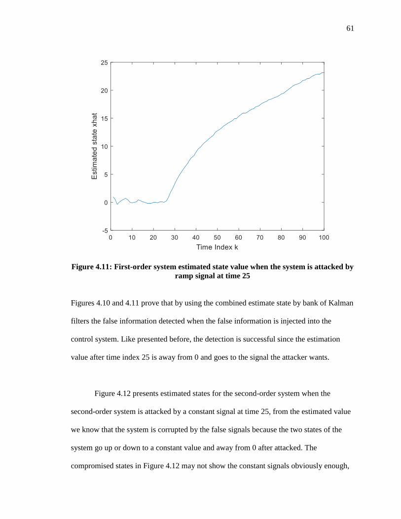
Figure 4.11: First-order system estimated state value when the system is attacked by
ramp signal at time 25
Figures 4.10 and 4.11 prove that by using the combined estimate state by bank of Kalman
filters the false information detected when the false information is injected into the
control system. Like presented before, the detection is successful since the estimation
value after time index 25 is away from 0 and goes to the signal the attacker wants.
Figure 4.12 presents estimated states for the second-order system when the
second-order system is attacked by a constant signal at time 25, from the estimated value
we know that the system is corrupted by the false signals because the two states of the
system go up or down to a constant value and away from 0 after attacked. The
compromised states in Figure 4.12 may not show the constant signals obviously enough,

62
however, when increasing the total iterations to a larger number we can see the attacked
states eventually go up or down to a constant value which once again proves that bank of
Kalman filters detect the intrusion successfully.
Figure 4.12: Second-order system estimated states value when the system is attacked
by constant signal at time 25

63
Figure 4.13: Second-order system estimated states value when the system is attacked
by constant signal at time 25 with longer iterations
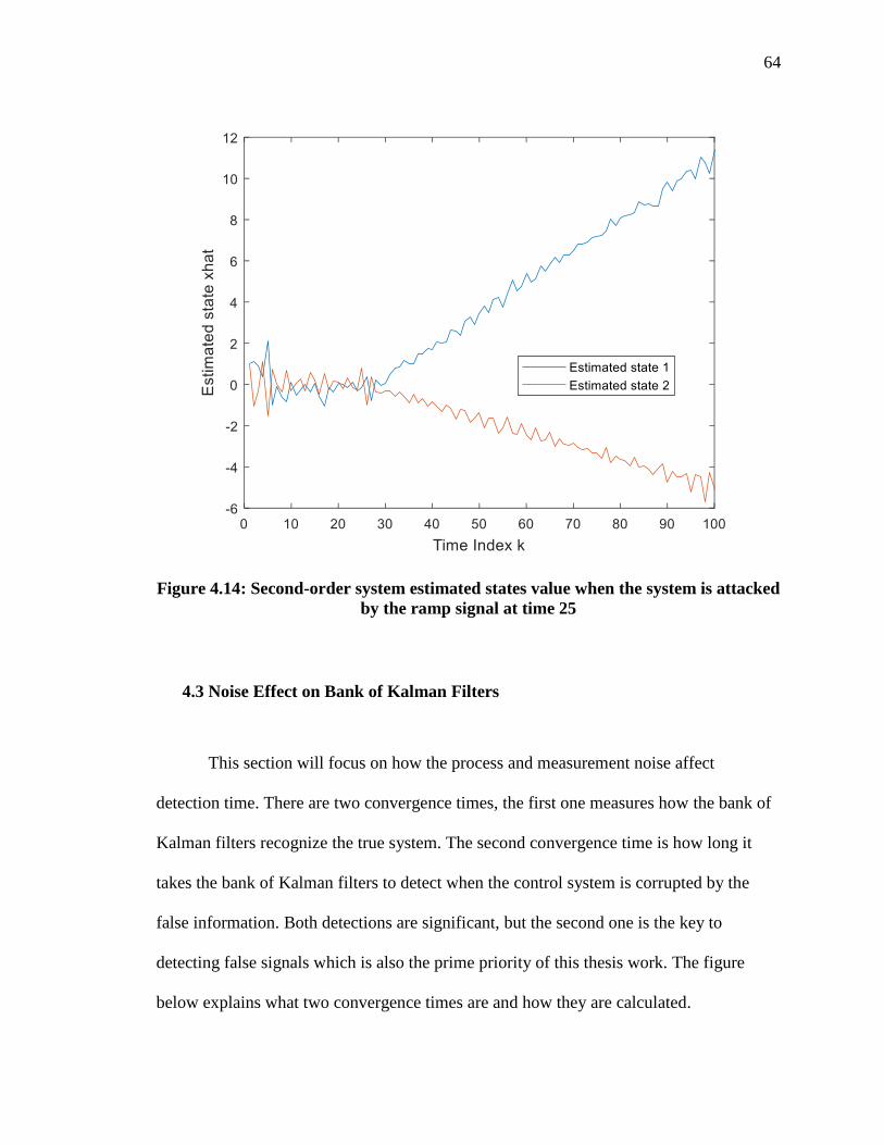
Figure 4.14 presents the bank of Kalman filter estimation of second-order system being
attacked by a ramp signal. The compromised states either go up or go down to a ramp
signal provide an evidence that the bank of Kalman filter estimation also can be used to
detect attacks.
64
Figure 4.14: Second-order system estimated states value when the system is attacked
by the ramp signal at time 25
4.3 Noise Effect on Bank of Kalman Filters
This section will focus on how the process and measurement noise affect
detection time. There are two convergence times, the first one measures how the bank of
Kalman filters recognize the true system. The second convergence time is how long it
takes the bank of Kalman filters to detect when the control system is corrupted by the
false information. Both detections are significant, but the second one is the key to
detecting false signals which is also the prime priority of this thesis work. The figure
below explains what two convergence times are and how they are calculated.

65
Figure 4.15: Explanation of convergence1 and convergence 2
The figure above shows that how both convergence times are defined: setting up a
threshold at 0.99, when the time blue line in the probability figure which stands for the
true system exceeds the threshold, this time period is called convergence 1 and when the
time red line which stands for the attacked system exceeds the threshold, it is then called
convergence 2.
4.3.1 Correlation Between Noise and Convergence Time
In order to find out the potential relationship between convergence time and the
noise covariance, simulations between convergence times and the noise covariances are
investigated.
Conv1
Conv2
Probability
Time Index k
0.5
1

66
This thesis will use the first-order system which attacked by a constant signal
discussed before for demonstrating the correlations and use several different noise
covariance to do the simulations. Table 4.1 shows the covariance values chosen:
Table 4.1: Noise covariance values chosen for convergence analysis for first order
system attacked by the constant signal
𝑉 W
0.01 0.01
0.02 0.02
0.05 0.05
0.1 0.1
0.2 0.2
0.5 0.5
Selecting 𝑉, and 𝑊, for 6 values: 0.01, 0.02, 0.05, 0.1, 0.2 and 0.5, thus there are 36
combinations of simulations to discuss. By testing each one of the simulations 200 times,
there is an average value for each case. The algorithm for probability calculation works
well for each time of the simulation with the noise covariances. This proves that the
algorithm is robust for detecting false information with a decent noise covariance.
After running simulations, there are 36 data points of each convergence time.
Figure 4.16 shows the result of simulations; this figure shows some simple relationship
between the noise covariances and the convergence times.

67
Figure 4.16: Convergence time on the first-order system attacked by the constant signal
4.524.985
5.245.2655.4355.86
4.9955.1355.3255.45.5756.01
5.3055.325.4255.5755.645
6.22
5.4855.4955.5155.725.695
6.215
5.75.785.855.8756.0756.2556.166.236.26.196.2656.365
3.783.834.07
4.4354.905
5.765
3.9154.0354.325
4.725.11
5.965
4.3654.4354.785
55.435
6.315
5.14.9055.1055.375
5.76
6.6
5.4755.585.6855.95
6.28
7.0257.1057.167.37.3457.675
8.12
0
1
2
3
4
5
6
7
8
9W
=0.0
1
W=0
.02
W=0
.05
W=0
.1
W=0
.2
W=0
.5
W=0
.01
W=0
.02
W=0
.05
W=0
.1
W=0
.2
W=0
.5
W=0
.01
W=0
.02
W=0
.05
W=0
.1
W=0
.2
W=0
.5
W=0
.01
W=0
.02
W=0
.05
W=0
.1
W=0
.2
W=0
.5
W=0
.01
W=0
.02
W=0
.05
W=0
.1
W=0
.2
W=0
.5
W=0
.01
W=0
.02
W=0
.05
W=0
.1
W=0
.2
W=0
.5
V=0.01 V=0.02 V=0.05 V=0.1 V=0.2 V=0.5
Tim
eConvergence time discussion on first order system attacked by constant signal
convergence1 convergence2 Linear (convergence1) Linear (convergence2)

68
In this table, the x axis is the value of the noise covariances we choose, the y axis is the
value for time, the blue dots are the values for convergence 1 and the red dots are the
values for convergence 2. The blue line and the red line show that the trend of both
convergence times in the sequence of both noise covariances from small to large values.
For an example, when 𝑉 =0.05, and 𝑊=0.5, convergence 1 equals to 6.22, convergence
2 equals to 6.315.
From the tendency of the convergence time in the table, a simple conclusion is
obvious: both the noise covariance 𝑉, and 𝑊, has a positive relation with the
convergence time. But for validating this conclusion about the correlations between the
noise covariances and the convergence times, the correlation plot between the noise
covariances and the convergence times is needed. There are two correlation coefficients
used in this work, the Pearson and the Spearman correlation coefficients. The Pearson
correlation evaluates the linear relationship between two continuous variables and the
Spearman correlation evaluates the monotonic relationship between two continuous or
ordinal variables [29].

69
Figure 4.17: Correlation plot between noise covariance and convergence time for the
first- order system attacked by constant signal using the Pearson correlation
coefficient

70
Figure 4.18: Correlation plot between noise covariance and convergence time for the
first- order system attacked by constant signal using the Spearman correlation
coefficient
Since the correlation plots are symmetric, only the cells on either the upper or
lower part of the plot need to be considered. Each cell in the figures is the scatter plot of
corresponding element on the x and y axis, the plot diagonal is the histogram of the
element itself. The correlations between 𝑉, W and the convergence times are shown in the
red circled parts of Figures 4.17 and 4.18. The red numbers in each cell are the
correlation values of the elements the x, and y, axes; the larger the number is, the more
correlated the elements are. Both plots suggest that the convergence times have a positive
relationship with the noise covariance 𝑉, W. In addition, the convergence times are more
related to process noise 𝑉 than measurement noise W in a positive way. This means the

71
intrusion detection will be affected more by the value of process noise than the value of
measurement noise. Although the noise covariance of a control system generally cannot
be changed while operating the system, this simulation result of the relationship tells the
engineers if the Kalman filter is to distinguish the true system and detect the false system
in as short in time as possible, a small noise covariance is helpful.
In conclusion: both correlation plots show that the relationship between the noise
covariances and the convergence times is a positive relation.
4.4 Intrusion Detection by Using Sample Mean Values
4.4.1 Intrusion Detection by Using Sample Mean Values with Known State
Apart from the methods used above, there is one more method used for detecting
the false information in the control system; that is comparing the state sample mean value
for the original and attacked systems. This work will continue to use a first-order system
attacked by a constant signal as an example to illustrate this method. It is assumed that
the state of the system is available, and by setting the initial sample mean value of the
state to one, the difference between unharmed and harmed states is shown in the
simulation. The models used are (2.1) and (3.2):
𝑥𝑘+1 = 𝐴𝑥𝑘 + 𝐵𝑢𝑘 + 𝐹𝑣𝑘 (2.1)
72
𝑥𝑘+1 = 𝐴𝑥𝑘 + 𝐵ℎ𝑘 + 𝐹𝑣𝑘 (3.2)
in which ℎ𝑘, is a constant signal that replaces the control input 𝑢𝑘 = −𝐾𝑐𝑥. The state 𝑥𝑘,
is:
�̅�𝑘 = (𝐴 + 𝐵𝐾𝑐)𝑘�̅�0 (4.1)
Eq (3.2), can also be written as:
𝑥𝑘 = 𝐴𝑘𝑥0 + ∑ 𝐴𝑘−𝑖−1𝑘−1𝑖=0 (𝐵ℎ + 𝑣𝑖) (4.2)
Thus, the mean value of the attacked system state is
�̅�𝑘 = 𝐴𝑘�̅�0 + ∑ 𝐴𝑘−𝑖−1
𝑘−1
𝑖=0
𝐵ℎ (4.3)
The summation in (4.3) can be simplified to (𝐴𝑘 − 𝐼)(𝐴 − 𝐼)−1, therefore (4.3) becomes:
�̅�𝑘 = 𝐴𝑘�̅�0 + (𝐴𝑘 − 𝐼)(𝐴 − 𝐼)−1 𝐵ℎ (4.4)
From (4.1) and (4.4), the mean value of the system state for both original and attacked
systems are obtained. If the simulations of the two equations are different, it can prove
that the sample mean value of the original and attacked system are not the same. It also

73
means the sample mean value of the system state will change once the system is attacked
by a false signal. So this method is another that can be used for detecting whether the
control system is attacked or not.
Figure 4.19: System state mean value in time when the system is not attacked by the
false signal

74
Figure 4.20: System state mean value in time when the system is attacked by the
constant signal with known state
In Figure 4.19, the state mean value for the original system goes to zero. On the other
hand, the mean value of the state for the system attacked with a constant actuator signal
converges on a finite non-zero value.
Figure 4.21 is an example of the control system is being attack by a constant
signal at time index k=15:

75
Figure 4.21: System state mean value in time when the system is attacked by the
constant signal with known state at time index k=15
Figure 4.21 shows similar result of what we investigate in chapter 4, the sample mean
value of the state goes to zero before time index k=15 and after this point, it goes to a
non-zero constant value.
4.4.2 Intrusion Detection by Using Sample Mean Values with Unknown State
When the state of the system is unknown, a Kalman filter can be used to estimate
the state, recall (2.6):
�̂�𝑘+1 = 𝐴�̂�𝑘 + 𝐵𝑢𝑘 + 𝐾𝑘(𝑦𝑘 − [𝐶�̂�𝑘 + 𝐷𝑢𝑘]) (2.6)

76
With the help of (2.6), the estimated value of state of the control system is known and
there will not be a large deviation when comparing the estimated state value to the
sample mean value of the state. It can be seen from Figure 4.22 that the estimated state
value is very close to the sample mean value of the state. However, once the estimated
state value deviates too much from sample mean value of the state, it can be considered
as hacked. By setting up a threshold for the deviation, when the deviation exceeds the
threshold, the system is then under attack. The result for the system without knowledge of
the state is very similar to what is found by using the combined state estimate in a bank of
Kalman filters.
Figure 4.22: System state mean value in time when the system is attacked by the
constant signal with unknown state

77
Thus, checking the mean value of the state for the control system is also a good
method for detecting whether the system is attacked or not with or without knowledge of
the state.

78
5. Conclusion and Future work
5.1 Summary
In this thesis, the use of a bank of Kalman filter to detect an attack on a control
system by the injection of false actuator signals is investigated. To document this
investigation, an overview of the effects of “hacking” on control systems to motivate this
work is presented. The design process for Kalman filter and a bank of Kalman filters is
summarized in chapter 2. In chapter 3, the first and second order system models used in
this work together with the constant and ramp false actuator signals are discussed. By
simulating the systems, states and outputs for both the unharmed and attacked situations
are obtained. In chapter 4, intrusion detection using the probability calculation, the
innovation sequence, and the bank of Kalman filters estimation as well as sample mean
method are presented.
5.2 Conclusion
The algorithm for detecting the false information in the control system works as
expected. First and second order system are studied and intruded with constant and ramp
signals. The algorithm of using a bank of Kalman filters to detect the false information is
very robust.

79
In chapter 4, the positive relationship between the noise covariances and both
convergence times are discussed and shown. The analysis shows that the convergence
times are more related to process noise 𝑉, than measurement noise W, in a positive way.
Finally, another method for detecting the false information is shown as well.
Checking the sample mean value of the system state for the system is most suitable for
the situations that we can easily calculate the mean value of the system state, since in this
way engineers do not need a bank of Kalman filter to detect the false signal.
5.3 Future Work
First, a model could be applied to this detection technique of an actual physical or
electrical system. Since this work only used a mathematical model for the state space
equation, engineers can design a real-life state space model which is observable to test it
and this detection method is only used for a first and second order system, it can be
expanded actual physical systems.
Second, the false signal used in this thesis are the constant and ramp signal,
control system engineers can test this detection algorithm with some other false
information such as sin wave or exponential signal.
The relationship between the noise covariance and convergence time can be
investigated further, the concepts of needed shorten the delay time of detecting the false
signal can be informed by simulations.

80
Last but not least, the last method, which is comparing the sample mean value of
the original and attacked state in the control system can be applied to a real-life system as
well. When the state of the control system is known, this method would be more efficient
compared to a bank of Kalman filter detection.

81
REFERENCES
[1] C. H. Xie and G. H. Yang, “Secure estimation for cyber-physical systems under
adversarial actuator attacks,” in IET Control Theory & Applications, vol. 11, no.
17, pp. 2939-2946, Nov 24, 2017.
[2] H. Fawzi, P. Tabuada and S. Diggavi, “Security for control systems under sensor
and actuator attacks,” 2012 IEEE 51st IEEE Conference on Decision and Control
(CDC), Maui, HI, 2012, pp. 3412-3417.
[3] G. Liang, J. Zhao, F. Luo, S. R. Weller and Z. Y. Dong, “A Review of False Data
Injection Attacks Against Modern Power Systems,” in IEEE Transactions on
Smart Grid, vol. 8, no. 4, pp. 1630-1638, July 2017.
[4] K. Chatterjee, V. Padmini and S. A. Khaparde, “Review of cyber-attacks on power
system operations,” 2017 IEEE Region 10 Symposium (TENSYMP), Cochin,
2017, pp. 1-6.
[5] T.Roberto (2005, August 30), “Estimation Theory for Engineers,” Available:
http://www.ee.uwa.edu.au/~roberto/teach/Estimation_Theory.pdf.
[6] W.Greg, B.Gary (2001), “An Introduction to the Kalman Filter,” University of
North Carolina, Chapel Hill, NC. Available: http://www.cs.unc.edu/~welch
[September 21, 2012].
[7] K. Sothivelr, “Analysis of Sensor Signals and Quantification of Analytes Based on
Estimation Theory,” M.S thesis, Marquette University, 2014.
[8] H. Fawzi, P. Tabuada and S. Diggavi, “Secure state-estimation for dynamical
systems under active adversaries,” 2011 49th Annual Allerton Conference on
Communication, Control, and Computing (Allerton), Monticello, IL, 2011, pp.
337-344.
[9] A. Rosich, H. Voos, Y. Li and M. Darouach, “A model predictive approach for
cyber-attack detection and mitigation in control systems,” 52nd IEEE Conference
on Decision and Control, Firenze, 2013, pp. 6621-6626.
[10] R. N. Clark, “Instrument Fault Detection,” in IEEE Transactions on Aerospace
and Electronic Systems, vol. AES-14, no. 3, May 1978, pp. 456-465.
[11] D. H. Trinh and H. Chafouk, “Fault detection and isolation using Kalman filter
bank for a wind turbine generator,” 2011 19th Mediterranean Conference on
Control & Automation (MED), Corfu, 2011, pp. 144-149.
82
[12] K. Manandhar, Xiaojun Cao, Fei Hu and Y. Liu, “Combating False Data
Injection Attacks in Smart Grid using Kalman Filter,” 2014 International
Conference on Computing, Networking and Communications (ICNC), Honolulu,
HI, 2014, pp. 16-20.
[13] M. S. Ayas and S. M. Djouadi, “Undetectable sensor and actuator attacks for
observer based controlled Cyber-Physical Systems,” 2016 IEEE Symposium
Series on Computational Intelligence (SSCI), Athens, 2016, pp. 1-7.
[14] G. Rigatos, D. Serpanos and N. Zervos, “Detection of Attacks Against Power Grid
Sensors Using Kalman Filter and Statistical Decision Making,” in IEEE Sensors
Journal, vol. 17, no. 23, Dec.1, 1 2017, pp. 7641-7648.
[15] W. Xue, Y. q. Guo and X. d. Zhang, “A Bank of Kalman Filters and a Robust
Kalman Filter Applied in Fault Diagnosis of Aircraft Engine
Sensor/Actuator,” Second International Conference on Innovative Computing,
Informatio and Control (ICICIC 2007), Kumamoto, 2007, pp. 10-10.
[16] M. Rezaee, N. Sadeghzadeh-Nokhodberiz and J. Poshtan, “Kalman filter based
sensor fault detection and identification in an electro-pump system,” 2017 5th
International Conference on Control, Instrumentation, and Automation (ICCIA),
Shiraz, 2017, pp. 12-17.
[17] M. Miron, L. Frangu and S. Caraman, “Actuator fault detection using extended
Kalman filter for a wastewater treatment process,” 2017 21st International
Conference on System Theory, Control and Computing (ICSTCC), Sinaia, 2017,
pp. 583-588.
[18] N. Tudoroiu and M. Zaheeruddin, “Fault detection and diagnosis of valve
actuators in HVAC systems,” Proceedings of 2005 IEEE Conference on Control
Applications, 2005. CCA 2005, Toronto, Ont, 2005, pp. 1281-1286.
[19] Kalman, R. E., “A New Approach to Linear Filtering and Prediction Problems”
Transactions of the ASME - Journal of Basic Engineering, vol. 82, pp. 35-45,
1960.
[20] Jennifer L. Riffer. “Time-Optimal Control of Discrete-Time Systems with Known
Waveform Disturbances,” 2009, M.S thesis, Marquette University.
[21] F.Taha, Ahmad, Qi, Junjian, Wng, Jianhui and Panchal, Jitesh. “Dynamic State
Estimation under Cyber Attacks: A Comparative Study of Kalman Filters and
Observers”, Cornell University Library, 2015.
[22] Peter K.S. Tam and John B. Moore, “Adaptive Estimation Using Parallel
Processing Techniques,” Computers & Electrical Engineering Volume 2, Issues
2–3, June 1975, Great Britain, Pages 203-214.

83
[23] E. Yaz, EECE 6340, Class Lecture, Topic: “Kalman Filter,” Faculty of Electrical
and Computer Engineering, Marquette University, Milwaukee, WI, Spring 2018.
[24] W.Greg and B.Gary , “An Introduction to the Kalman Filter,” Department of
Computer Science, University of North Carolina, Chapel Hill, NC, July 2006.
[25] Roberto Sabatini, Subramanian Ramasamy, Alessandro Gardiand and Leopoldo
Rodriguez Salazar, “Low-cost Sensors Data Fusion for Small Size Unmanned
Aerial Vehicles Navigation and Guidance,” 2013 International Journal of
Unmanned Systems Engineering, Vol. 1, No. 3, 16-47, 2013.
[26] Q. Li, R. Li, K. Ji and W. Dai, “Kalman Filter and Its Application,” 2015 8th
International Conference on Intelligent Networks and Intelligent Systems
(ICINIS), Tianjin, 2015, pp. 74-77.
[27] A. R. Strandt, A. P. Strandt, S. C. Schneider and E. E. Yaz, “Stator Resistance
Estimation Using Adaptive Estimation via a Bank of Kalman Filters,” 2018
Annual American Control Conference (ACC), Milwaukee, WI, 2018, pp. 1078-
1083.
[28] R. Dorf and R. Bishop, “Modern control systems,” 12th ed. chapter 11.
[29] “A comparison of the Pearson and Spearman correlation methods - Minitab
Express,” Support.minitab.com, 2018. [Online]. Available:
https://support.minitab.com/en-us/minitab-express/1/help-and-how-to/modeling-
statistics/regression/supporting-topics/basics/a-comparison-of-the-pearson-and-
spearman-correlation-methods/.

84
APPENDIX A: MATLAB CODES
A1. MATLAB Code for Intrusion Detection by Using a Bank of Kalman Filter
for First-order System Attacked by Constant Signal
%Cleaning clear all close all clc;
% count=0; % counter=200 ; % store=NaN(counter,2); % mean_store=NaN(1,2); % for j=1:counter
%Set time index tstop=100; t=1:tstop; %Load the noise for the system load('Vk.mat') load('Wk.mat') %Define noise covariances V=0.01;W=0.05;
%Original First-order System matrices A=0.9;B=1;C=1;D=1;F=1;G=1; %Define the size of state and output of the original system x=NaN(2,tstop); y=NaN(1,tstop);
%Initialize state for the original system x(1,1)=1; %Define new pole for the original system pole=0.4; %Calculate control gain Kc=-place(A,B,pole);
%Attacked First-order System matrices A2=[A,B;0 1];C2=[C 1];F2=[F;0]; %Define switch point SwitchPoint=25; %Define constant signal value h=2; %Initialize state before and on switch point for the attacked system x(2,1:SwitchPoint-1)=0; x(2,SwitchPoint)=h;
%A bank of Kalman filter settings %Define the size of error covariance, Kalman gain and estimated state
of the attacked system p=NaN(1,tstop);

85
Kk=NaN(1,tstop); xhat1=NaN(1,tstop); %Initialize error covariance and estimated state for the original
system p(1)=50; xhat1(1)=1;
%Define the size of error covariance, Kalman gain and estimated state
of the attacked system p2=NaN(2,2,tstop); Kk2=NaN(2,tstop); xhat2=NaN(2,tstop); %Initialize error covariance and estimated state for the attacked
system p2(:,:,1)=50*eye(2); xhat2(:,1)=[1;0];
%Define the size of combined estimated state xhat=NaN(1,tstop); %Define the size of control input U=NaN(1,tstop); %Initialize conbined estimated state xhat(1)=0.5*xhat1(1)+0.5*xhat2(1,1); %Initialize control input U(1)=Kc*xhat(1); %Initialize and define the size of conditional probability pThetaY1=[0.5 NaN(1,length(t)-1)]; pThetaY2=[0.5 NaN(1,length(t)-1)]; %Define the size of innovation sequence y_tilde(1:2,1:length(t)) = NaN; %Initialize innovation sequence y_tilde(:,1)=0;
%A bank of Kalman filter simulation in time for k=1:tstop if k<SwitchPoint %Original system before switch point x(1,k+1)=A*x(1,k)+B*U(k)+Vk(k); y(k)=C*x(1,k)+D*U(k)+G*Wk(k); else %Attacked system after switch point x(:,k+1)=A2*x(:,k)+F2*Vk(k); y(k)=C2*x(:,k) +G*Wk(k); end %Error covariance update equation of the original system p(k+1)=A*p(k)*A'-(A*p(k)*C'*C*p(k)*A')/(C*p(k)*C'+W)+F*V*F'; %Kalman gain update equation of the original system Kk(k)=(A*p(k)*C')/(C*p(k)*C'+G*W*G'); %Estimated state update equation of the original system xhat1(k+1)=A*xhat1(k)+B*U(k)+Kk(k)*(y(k)-C*xhat1(k));
%Error covariance update equation of the attacked system p2(:,:,k+1)=A2*p2(:,:,k)*A2'-
(A2*p2(:,:,k)*C2'*C2*p2(:,:,k)*A2')/...
(C2*p2(:,:,k)*C2'+W)+F2*V*F2'; %Kalman gain update equation of the attacked system Kk2(:,k)=(A2*p2(:,:,k)*C2')/(C2*p2(:,:,k)*C2'+G*W*G');

86
%Estimated state update equation of the attacked system xhat2(:,k+1)=A2*xhat2(:,k)+Kk2(:,k)*(y(k)-C2*xhat2(:,k)); %Innovation squence update equation y_tilde(:,k)=[y(k);y(k)]-[C*xhat1(k);C2*xhat2(:,k)]; %Innovation covariance of the original system y_covar_tilde1=C*p(k)*C'+G*W*G'; %Innovation covariance of the attacked system y_covar_tilde2=C2*p2(:,:,k)*C2'+G*W*G'; %Liklihood function of the original system pYTheta1=(2*pi)^(-1/2)*sqrt(1/det(y_covar_tilde1))... *exp(-0.5*y_tilde(1,k)'*eye/y_covar_tilde1*y_tilde(1,k)); %Liklihood function of the attacked system pYTheta2=(2*pi)^(-2/2)*sqrt(1/det(y_covar_tilde2))... *exp(-0.5*y_tilde(2,k)'*eye/y_covar_tilde2*y_tilde(2,k)); %Calculate condination probability den=pYTheta1*pThetaY1(k)+pYTheta2*pThetaY2(k); pThetaY1(k+1)=pYTheta1*pThetaY1(k)/den; pThetaY2(k+1)=pYTheta2*pThetaY2(k)/den; %Combined estimated state xhat(k+1)=pThetaY1(k)*xhat1(k)+pThetaY2(k)*xhat2(1,k); %Feedback control for calculating control input U(k+1)=Kc*xhat(k+1); end
%Plot combined Estimated state plot(t,xhat(1:end-1)); ylabel('Estimated state xhat') xlabel('Time Index k') %Plot innovation sequence figure plot(t,y_tilde(1,:)) ylabel('y tilde for constant input') xlabel('Time Index k') %Plot conditional probability figure plot(t,pThetaY1(1:end-1),'b',t,pThetaY2(1:end-1),'r') legend('first order system with true control input','first order system
with constant input') ylabel('Conditional probability') xlabel('Time Index k') %Set a threshold thresh = 0.99; %Define convergence time one and two convergenceIndex = [find(pThetaY1 > thresh,1);find(pThetaY2 >
thresh,1);]; %Display convergence time one and two disp('Convergence time:') t(convergenceIndex)

87
A2. MATLAB Code for Intrusion Detection by Using a Bank of Kalman Filter
for First-order System Attacked by Ramp Signal
%Cleaning clear all close all clc;
%Set time index tstop=100; t=1:tstop; %Load the noise for the system load('Vk.mat') load('Wk.mat') %Define noise covariances V=0.01;W=0.05;
%Original first-order System matrices A=0.9;B=1;C=1;D=1;F=1;G=1; %Define the size of state and output of the original system x=NaN(3,tstop); y=NaN(1,tstop); %Initialize state for the original system x(1,1)=1; %Define new pole for the original system pole=0.4; %Calculate control gain Kc=-place(A,B,pole);
%Attacked first-order System matrices hA=[1,1;0 1]; A2=[A, B, zeros(1,1); zeros(2,1),hA]; C2=[C,1,0];F2=[F;0;0]; %Define switch point SwitchPoint=25; %Initialize state before and on switch point for the attacked system x(2:end,1:SwitchPoint-1)=0; x(2:end,SwitchPoint)=[1;0.02];
%A bank of Kalman filter settings %Define the size of error covariance, Kalman gain and estimated state
of the attacked system p=NaN(1,tstop); Kk=NaN(1,tstop); xhat1 = NaN(1,tstop); %Initialize error covariance and estimated state for the original
system p(1)=50; xhat1(1)=1;
%Define the size of error covariance, Kalman gain and estimated state
of the attacked system p2=NaN(3,3,tstop);

88
Kk2=NaN(3,tstop); xhat2= NaN(3,tstop); %Initialize error covariance and estimated state for the attacked
system p2(:,:,1)=50*eye(3); xhat2(:,1)=[1;0;0];
%Define the size of combined estimated state xhat=NaN(1,tstop); %Define the size of control input U=NaN(1,tstop); %Initialize conbined estimated state xhat(1)= 0.5 * xhat1(1) + 0.5 * xhat2(1,1); %Initialize control input U(1)=Kc*xhat(1); %Initialize and define the size of conditional probability pThetaY1=[0.5 NaN(1,length(t)-1)]; pThetaY2=[0.5 NaN(1,length(t)-1)]; %Define the size of innovation sequence y_tilde(1:2,1:length(t))=NaN; %Initialize innovation sequence y_tilde(:,1)=0;
%A bank of Kalman filter simulation in time for k=1:tstop if k<SwitchPoint %Original system before switch point x(1,k+1)=A*x(1,k)+B*U(k)+Vk(k); y(k)=C*x(1,k)+D*U(k)+G*Wk(k); else %Attacked system after switch point x(:,k+1)=A2*x(:,k) + F2*Vk(k); y(k)=C2*x(:,k) + G*Wk(k);
end %Error covariance update equation of the original system p(k+1)=A*p(k)*A'-(A*p(k)*C'*C*p(k)*A')/(C*p(k)*C'+W)+F*V*F'; %Kalman gain update equation of the original system Kk(k)=(A*p(k)*C')/(C*p(k)*C'+G*W*G'); %Estimated state update equation of the original system xhat1(k+1)=A*xhat1(k)+B*U(k)+Kk(k)*(y(k)-C*xhat1(k)); %Error covariance update equation of the attacked system
p2(:,:,k+1)=A2*p2(:,:,k)*A2'(A2*p2(:,:,k)*C2'*C2*p2(:,:,k)*A2')/...
(C2*p2(:,:,k)*C2'+W)+F2*V*F2';
%Kalman gain update equation of the attacked system Kk2(:,k)=(A2*p2(:,:,k)*C2')/(C2*p2(:,:,k)*C2'+G*W*G'); %Estimated state update equation of the attacked system xhat2(:,k+1)=A2*xhat2(:,k)+Kk2(:,k)*(y(k)-C2*xhat2(:,k)); %Innovation squence update equation y_tilde(:,k)=[y(k);y(k)]-[C*xhat1(k);C2*xhat2(:,k)]; %Innovation covariance of the original system y_covar_tilde1=C*p(k)*C'+G*W*G'; %Innovation covariance of the attacked system y_covar_tilde2=C2*p2(:,:,k)*C2'+G*W*G'; %Liklihood function of the original system pYTheta1=(2*pi)^(-1/2)*sqrt(1/det(y_covar_tilde1))...

89
*exp(-0.5*y_tilde(1,k)'*eye/y_covar_tilde1*y_tilde(1,k)); %Liklihood function of the attacked system pYTheta2=(2*pi)^(-3/2)*sqrt(1/det(y_covar_tilde2))... *exp(-0.5*y_tilde(2,k)'*eye/y_covar_tilde2*y_tilde(2,k)); %Calculate condination probability den=pYTheta1*pThetaY1(k)+pYTheta2*pThetaY2(k); pThetaY1(k+1)=pYTheta1*pThetaY1(k)/den; pThetaY2(k+1)=pYTheta2*pThetaY2(k)/den; %Combined estimated state xhat(k+1)=pThetaY1(k)*xhat1(k)+pThetaY2(k)*xhat2(1,k); %Feedback control for calculating control input U(k+1)=Kc*xhat(k+1); end
%Plot combined Estimated state plot(t,xhat(1:end-1)); ylabel('Estimated state xhat') xlabel('Time Index k') %Plot innovation sequence figure plot(t,y_tilde(1,:)) ylabel('y tilde for ramp input') xlabel('Time Index k') %Plot conditional probability figure plot(t,pThetaY1(1:end-1),'b',t,pThetaY2(1:end-1),'r') legend('first order system with true control input','first order system
with ramp input') ylabel('Conditional probability') xlabel('Time Index k') %Set a threshold thresh = 0.99; %Define convergence time one and two convergenceIndex = [find(pThetaY1 > thresh,1);find(pThetaY2 >
thresh,1);]; %Display convergence time one and two disp('Convergence time:') t(convergenceIndex)

90
A3. MATLAB Code for Intrusion Detection by Using a Bank of Kalman Filter
for Second-order System Attacked by Constant Signal
%Cleaning clear all close all clc;
%Set time index tstop=100; t=1:tstop; %Load the noise for the system load('Vk1.mat') load('Vk2.mat') load('Wk.mat') %Define noise covariances V=0.1;W=0.5;
%Original second-order System matrices A=[0,0.8;-0.8,-0.8];B=[1;0];C=[1,0];D=1;F=eye(2);G=1; %Define the size of state and output of the original system x=NaN(3,tstop); y=NaN(1,tstop); %Initialize state for the original system x(1:2,1)=[1,1]; %Define new pole for the original system pole=[0.4,-0.4]; %Calculate control gain Kc=-place(A,B,pole);
%Attacked second-order System matrices A2=[A, B;0,0,1];C2=[C,1];F2=[F;zeros(1,2)]; %Define switch point SwitchPoint=25; %Define constant signal value h=8; %Initialize state before and on switch point for the attacked system x(3,1:SwitchPoint-1)=0; x(3,SwitchPoint)=h;
%A bank of Kalman filter settings %Define the size of estimated state, error covariance and Kalman gain
of the original system xhat1 = NaN(2,tstop); p=NaN(2,2,tstop); Kk=NaN(2,tstop); %Initialize error covariance and estimated state for the original
system p(:,:,1)=eye(2)*50; xhat1(:,1)=[1;1];
%Define the size of error covariance, Kalman gain and estimated state
of the attacked system p2=NaN(3,3,tstop);

91
Kk2=NaN(3,tstop); xhat2= NaN(3,tstop); %Initialize error covariance and estimated state for the attacked
system p2(:,:,1)=50*eye(3); xhat2(:,1)=[1;1;0];
%Define the size of combined estimated state xhat=NaN(2,tstop); %Define the size of control input U=NaN(1,tstop); %Initialize conbined estimated state xhat(:,1)=0.5*xhat1(:,1)+0.5*xhat2(1:2,1); %Initialize control input U(1)=Kc*xhat(:,1); %Initialize and define the size of conditional probability pThetaY1 = [0.5 NaN(1,length(t)-1)]; pThetaY2 = [0.5 NaN(1,length(t)-1)]; %Define the size of innovation sequence y_tilde(1:2,1:length(t)) = NaN; %Initialize innovation sequence y_tilde(:,1)=0;
%A bank of Kalman filter simulation in time for k=1:tstop if k<SwitchPoint %Original system before switch point x(1:2,k+1)=A*x(1:2,k)+B*U(k)+F*[Vk1(:,k);Vk2(:,k)]; y(k)=C*x(1:2,k)+D*U(k)+G*Wk(k); else %Attacked system after switch point x(:,k+1)=A2*x(:,k)+F2*[Vk1(:,k);Vk2(:,k)]; y(k)=C2*x(:,k)+G*Wk(k); end %Error covariance update equation of the original system
p(:,:,k+1)=A*p(:,:,k)*A'-(A*p(:,:,k)*C'*C*p(:,:,k)*A')/...
(C*p(:,:,k)*C'+W)+F*[V,0;0,V]*F'; %Kalman gain update equation of the original system Kk(:,k)=(A*p(:,:,k)*C')/(C*p(:,:,k)*C'+G*W*G'); %Estimated state update equation of the original system xhat1(:,k+1)=A*xhat1(:,k)+B*U(k)+Kk(:,k)*(y(k)-C*xhat1(:,k)); %Error covariance update equation of the attacked system
p2(:,:,k+1)=A2*p2(:,:,k)*A2'(A2*p2(:,:,k)*C2'*C2*p2(:,:,k)*A2')/...
(C2*p2(:,:,k)*C2'+W)+F2*[V,0;0,V]*F2'; %Kalman gain update equation of the attacked system Kk2(:,k)=(A2*p2(:,:,k)*C2')/(C2*p2(:,:,k)*C2'+G*W*G'); %Estimated state update equation of the attacked system xhat2(:,k+1)=A2*xhat2(:,k)+Kk2(:,k)*(y(k)-C2*xhat2(:,k)); %Innovation squence update equation y_tilde(:,k)= [y(k);y(k)]-[C*xhat1(:,k);C2*xhat2(:,k)]; %Innovation covariance of the original system y_covar_tilde1=C*p(:,:,k)*C'+G*W*G'; %Innovation covariance of the attacked system y_covar_tilde2=C2*p2(:,:,k)*C2'+G*W*G'; %Liklihood function of the original system pYTheta1= (2*pi)^(-2/2)*sqrt(1/det(y_covar_tilde1))...

92
*exp(-0.5*y_tilde(1,k)'*eye/y_covar_tilde1*y_tilde(1,k)); %Liklihood function of the attacked system pYTheta2= (2*pi)^(-3/2)*sqrt(1/det(y_covar_tilde2))... *exp(-0.5*y_tilde(2,k)'*eye/y_covar_tilde2*y_tilde(2,k)); %Calculate condination probability den = pYTheta1*pThetaY1(k) + pYTheta2*pThetaY2(k); pThetaY1(k+1) = pYTheta1*pThetaY1(k)/den; pThetaY2(k+1) = pYTheta2*pThetaY2(k)/den; %Combined estimated state xhat(:,k+1) = pThetaY1(k)*xhat1(:,k)+pThetaY2(k)*xhat2(1:2,k); %Feedback control for calculating control input U(k+1)=Kc*xhat(:,k+1);
end
%Plot combined Estimated state plot(t,xhat(:,1:end-1)); ylabel('Estimated state xhat') xlabel('Time Index k') legend('Estimated state 1 ','Estimated state 2','location','best') %Plot innovation sequence figure plot(t,y_tilde(1,:)) ylabel('y tilde for constant input') xlabel('Time Index k') %Plot conditional probability figure plot(t,pThetaY1(1:end-1),'b',t,pThetaY2(1:end-1),'r') legend('second order system with true control input','second order
system with constant input') ylabel('Conditional probability') xlabel('Time Index k') %Set a threshold thresh = 0.99; %Define convergence time one and two convergenceIndex = [find(pThetaY1 > thresh,1);find(pThetaY2 >
thresh,1);]; %Display convergence time one and two disp('Convergence time:') t(convergenceIndex)
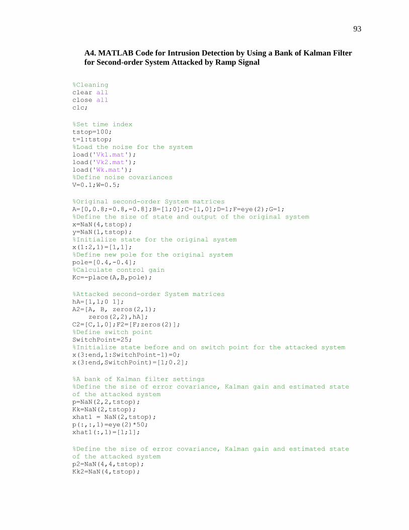
93
A4. MATLAB Code for Intrusion Detection by Using a Bank of Kalman Filter
for Second-order System Attacked by Ramp Signal
%Cleaning clear all close all clc;
%Set time index tstop=100; t=1:tstop; %Load the noise for the system load('Vk1.mat'); load('Vk2.mat'); load('Wk.mat'); %Define noise covariances V=0.1;W=0.5;
%Original second-order System matrices A=[0,0.8;-0.8,-0.8];B=[1;0];C=[1,0];D=1;F=eye(2);G=1; %Define the size of state and output of the original system x=NaN(4,tstop); y=NaN(1,tstop); %Initialize state for the original system x(1:2,1)=[1,1]; %Define new pole for the original system pole=[0.4,-0.4]; %Calculate control gain Kc=-place(A,B,pole);
%Attacked second-order System matrices hA=[1,1;0 1]; A2=[A, B, zeros(2,1); zeros(2,2),hA]; C2=[C,1,0];F2=[F;zeros(2)]; %Define switch point SwitchPoint=25; %Initialize state before and on switch point for the attacked system x(3:end,1:SwitchPoint-1)=0; x(3:end,SwitchPoint)=[1;0.2];
%A bank of Kalman filter settings %Define the size of error covariance, Kalman gain and estimated state
of the attacked system p=NaN(2,2,tstop); Kk=NaN(2,tstop); xhat1 = NaN(2,tstop); p(:,:,1)=eye(2)*50; xhat1(:,1)=[1;1];
%Define the size of error covariance, Kalman gain and estimated state
of the attacked system p2=NaN(4,4,tstop); Kk2=NaN(4,tstop);

94
xhat2= NaN(4,tstop); %Initialize error covariance and estimated state for the attacked
system p2(:,:,1)=50*eye(4); xhat2(:,1)=[1;1;0;0];
%Define the size of combined estimated state xhat=NaN(2,tstop); %Define the size of control input U=NaN(1,tstop); %Initialize conbined estimated state xhat(:,1)=0.5*xhat1(:,1)+0.5*xhat2(1:2,1); %Initialize control input U(1)=Kc*xhat(:,1); %Initialize and define the size of conditional probability pThetaY1=[0.5 NaN(1,length(t)-1)]; pThetaY2=[0.5 NaN(1,length(t)-1)]; %Define the size of innovation sequence y_tilde(1:2,1:length(t))=NaN; %Initialize innovation sequence y_tilde(:,1)=0;
%A bank of Kalman filter simulation in time for k=1:tstop if k<SwitchPoint %Original system before switch point x(1:2,k+1)=A*x(1:2,k)+B*U(k)+F*[Vk1(:,k);Vk2(:,k)]; y(k)=C*x(1:2,k)+D*U(k)+G*Wk(k); else %Attacked system after switch point x(:,k+1)=A2*x(:,k) + F2*[Vk1(:,k);Vk2(:,k)]; y(k)=C2*x(:,k) + G*Wk(k); end %Error covariance update equation of the original system
p(:,:,k+1)=A*p(:,:,k)*A'-(A*p(:,:,k)*C'*C*p(:,:,k)*A')/...
(C*p(:,:,k)*C'+W)+F*[V,0;0,V]*F'; %Kalman gain update equation of the original system Kk(:,k)=(A*p(:,:,k)*C')/(C*p(:,:,k)*C'+G*W*G'); %Estimated state update equation of the original system xhat1(:,k+1)=A*xhat1(:,k)+B*U(k)+Kk(:,k)*(y(k)-C*xhat1(:,k)); %Error covariance update equation of the attacked system
p2(:,:,k+1)=A2*p2(:,:,k)*A2'(A2*p2(:,:,k)*C2'*C2*p2(:,:,k)*A2')/...
(C2*p2(:,:,k)*C2'+W)+F2*[V,0;0,V]*F2'; %Kalman gain update equation of the attacked system Kk2(:,k)=(A2*p2(:,:,k)*C2')/(C2*p2(:,:,k)*C2'+G*W*G'); %Estimated state update equation of the attacked system xhat2(:,k+1)=A2*xhat2(:,k)+zeros(4,1)+Kk2(:,k)*(y(k)- ...
C2*xhat2(:,k)); %Innovation squence update equation y_tilde(:,k)= [y(k);y(k)]-[C*xhat1(:,k);C2*xhat2(:,k)]; %Innovation covariance of the original system y_covar_tilde1=C*p(:,:,k)*C'+G*W*G'; %Innovation covariance of the attacked system y_covar_tilde2=C2*p2(:,:,k)*C2'+G*W*G'; %Liklihood function of the original system pYTheta1= (2*pi)^(-2/2)*sqrt(1/det(y_covar_tilde1))...

95
*exp(-0.5*y_tilde(1,k)'*eye/y_covar_tilde1*y_tilde(1,k)); %Liklihood function of the attacked system pYTheta2= (2*pi)^(-4/2)*sqrt(1/det(y_covar_tilde2))... *exp(-0.5*y_tilde(2,k)'*eye/y_covar_tilde2*y_tilde(2,k)); %Calculate condination probability den = pYTheta1*pThetaY1(k) + pYTheta2*pThetaY2(k); pThetaY1(k+1) = pYTheta1*pThetaY1(k)/den; pThetaY2(k+1) = pYTheta2*pThetaY2(k)/den; %Combined estimated state xhat(:,k+1) = pThetaY1(k)*xhat1(:,k)+pThetaY2(k)*xhat2(1:2,k); %Feedback control for calculating control input U(k+1)=Kc*xhat(:,k+1); end
%Estimated states plot(t,xhat(:,1:end-1)); ylabel('Estimated state xhat') xlabel('Time Index k') legend('Estimated state 1 ','Estimated state 2','location','best') %Plot innovation sequence figure plot(t,y_tilde(1,:)) ylabel('y tilde for ramp input') xlabel('Time Index k') %Plot conditional probability figure plot(t,pThetaY1(1:end-1),'b',t,pThetaY2(1:end-1),'r') legend('second order system with true control input','second order
system with ramp signal') ylabel('Conditional probability') xlabel('Time Index k') %Set a threshold thresh = 0.99; %Define convergence time one and two convergenceIndex = [find(pThetaY1 > thresh,1);find(pThetaY2 >
thresh,1);]; %Display convergence time one and two disp('Convergence time:') t(convergenceIndex)

96
A5. MATLAB Code for Intrusion Detection by Using Sample Mean Method
%Cleaning clear all close all clc;
%Set time index tstop=100; t=1:tstop; %Load the noise for the system load('Vk.mat') load('Wk.mat') %Define noise covariances V=0.01;W=0.05;
%Original First-order System matrices h=2;A=0.9;B=1;C=1;D=1;F=1;G=1; %Define the size of sample mean value of state x_mean=NaN(1,tstop); %Initialize sample mean value of state x_mean(1)=1; %Define switch point switchpoint=15; %Define new pole for the original system pole=0.4; %Calculate control gain Kc=-place(A,B,pole);
%Sample mean value of state simulation in time for k=1:tstop if k<switchpoint; %Original system before switch point x_mean(k+1)=(A+B*Kc)^k*x_mean(1); else %Attacked system before switch point x_mean(k)=(A^k)*x_mean(1)+((A^k)-1)*((A-1)^-1)*B*h; end end
%Plot sample mean value of the state figure plot(t,x_mean) xlabel('Time Index k') ylabel('Sample Mean Value of State')