detection of bodies in maritime rescue operations using
TRANSCRIPT

Detection of bodies in maritime rescue operations usingUnmanned Aerial Vehicles with multispectral cameras
Antonio-Javier Gallego1, Antonio Pertusa1, Pablo Gil1, and Robert B. Fisher2
1Computer Science Research Institute, University of Alicante, San Vicente del Raspeig, 03690, Spain,[email protected], [email protected], [email protected]
2School of Informatics, University of Edinburgh, Edinburgh, EH8 9AB, UK, [email protected]
AbstractIn this work, we use Unmanned Aerial Vehicles (UAVs) equipped with multispectral
cameras to search for bodies in maritime rescue operations. A series of flights wereperformed in open water scenarios in the northwest of Spain, using a certified aquaticrescue dummy in dangerous areas and real people when the weather conditions allowed it.The multispectral images were aligned and used to train a Convolutional Neural Networkfor body detection. An exhaustive evaluation was performed in order to assess the bestcombination of spectral channels for this task. Three approaches based on a MobileNettopology were evaluated, using 1) the full image, 2) a sliding window, and 3) a preciselocalization method. The first method classifies an input image as containing a bodyor not, the second uses a sliding window to yield a class for each sub-image, and thethird uses transposed convolutions returning a binary output in which the body pixels aremarked. In all cases, the MobileNet architecture was modified by adding custom layers andpreprocessing the input to align the multispectral camera channels. Evaluation shows thatthe proposed methods yield reliable results, obtaining the best classification performancewhen combining Green, Red Edge and Near IR channels. We conclude that the preciselocalization approach is the most suitable method, obtaining a similar accuracy as thesliding window but achieving a spatial localization close to 1m. The presented systemis about to be implemented for real maritime rescue operations carried out by BabcockMission Critical Services Spain.
1 Introduction
The number of migrant deaths in the Mediterranean sea reached 3,116 in 2017 (Missing Mi-
grants, 2018). A quick response to localize bodies after shipwrecks is crucial to save lives,
and both Unmanned Aerial Vehicles (UAVs) and Remotely Piloted Aircraft (RPAs) offer an
important advantage when compared to satellite monitoring for this task, as they are able to
monitor specific areas by means of trajectory planning in real time. This is a relevant feature
in emergencies (Voyles and Choset, 2017; Erdelj et al., 2017; Zheng et al., 2017), control tasks
of people on a border area (Minaeian et al., 2016), and disasters of all kinds, like assisting
avalanche search and rescue operations (Bejiga et al., 2017; Silvagni et al., 2017), monitor-
ing after earthquakes (Lei et al., 2017), rescue in wilderness (Goodrich et al., 2009), and sea
robot-assisted inspection (Lindemuth et al., 2011), among others.
1

In this work, we propose a method to search for and rescue people in marine environments
using a remotely piloted UAV equipped with a multispectral camera, a visible spectrum camera,
and a Global Navigation Satellite System (GNSS) based on Global Positioning System (GPS).
Our approach focuses on the detection of people in the sea (i.e. drowned, shipwrecked, or
overboard persons) in emergencies where the response time is critical to avoid hypothermia or
drowning.
Both UAV features and onboard perception systems can be very heterogeneous depending
on the particular remote sensing application where they are used, as described by (Merino et al.,
2006; Pajares, 2015). In the literature, multispectral cameras (i.e. RGB, IR, thermal, LiDAR,
etc.) are used individually or combined for the detection and classification of different targets in
situations such as disaster monitoring or search and rescue. In addition, GNSS and an Inertial
Measurement Unit (IMU) are usually employed for autonomous geo-spatial positioning.
Recently, (Lopez-Fuentes et al., 2017) investigated sensors, methods and techniques based
on computer vision, focusing on emergency situations which present a risk to a person (i.e. fire
and flood) or caused by other humans (i.e. accidents). In this line, (Merino et al., 2012) and
(Giitsidis et al., 2015) proposed a perception system for forest fire monitoring using an UAV
equipped with visible and infrared sensors. Later, (Yuan et al., 2017) were able to detect forest
fires without thermal cameras, only using both color and motion features from color cameras.
In search and rescue missions, UAVs and RPAs are mainly used to classify scenes and rec-
ognize objects. (Sun et al., 2016) presented a hardware and software architecture for an UAV
platform that accomplished a successful target detection with accurate location. A good strat-
egy is to use both semisupervised and supervised machine learning approaches for aerial image
classification and object detection, improving the accuracy compared to traditional approaches
based on hand-crafted feature extraction. These methods have been widely used to classify
aerial imagery (i.e. bareland, farmland, greenland, etc.) as in (Hu et al., 2015; Yang et al.,
2015), to detect land vehicles (Sommer et al., 2017) or ships (Zou and Shi, 2016; Lin et al.,
2017; Gallego et al., 2018), also including humans as marine objects (Leira et al., 2015).
In particular, emergency situations often require that UAVs combine visible and infrared or
thermal cameras, which are used to detect vehicles but also people in urban environments as
shown in (Portmann et al., 2014; Blondel et al., 2014; Teutsch et al., 2014; Aguilar et al., 2017)
and in indoors (Andriluka et al., 2010). More specifically, UAVs and multispectral cameras are
usually used for search and rescue tasks of lying bodies outdoors (Rudol and Doherty, 2008)
where detection and localization are performed to train rescue routines in gravel roads, asphalt
and grass. Missing and lost people (standing and lying) can also be searched for by emergency
2

services in natural environments such as uncovered terrain and forest (Niedzielski et al., 2017a;
Niedzielski et al., 2017b), and in desert and chaparral (Coulter et al., 2012).
However, there are few research works addressing people detection in the sea. In real marine
environments, the detection of bodies from aerial images is a challenge because the weather and
sea conditions as well as the visibility of the body are very variable. The UAV flight altitude
determines the size of the body to be detected. Both camera orientation and UAV motion
also have an influence on the appearance of the body due to the observation perspective. In
addition, if the person is alive the body may be moving, and this also modifies its appearance.
However, if the person is unconscious, the movement of both waves and the UAV may also
cause drastic changes of observation. Additionally, weather (sunny or cloudy) and illumination
(day or night) influence the image brightness. Therefore, the wavelength reflected by the sea
surface or floating objects such as the clothes of a person could change. (Westall et al., 2008)
analyzed some techniques to improve detection performance in different sea states. Also, it is
important to note that the temperature of a person in these conditions quickly decreases, which
presents an additional difficulty.
All these circumstances increase the difficulty to achieve a successful body detection out-
doors and even more so in marine environments due to the movement of waves. For this reason,
we present a method for the detection of bodies in search operations from UAV-acquired data
that is based on deep learning strategies as an alternative to traditional techniques which are
very dependent on hand-crafted features extracted from the images.
There are some previous works addressing people detection on land or in indoor environ-
ments with traditional machine learning methods such as (Andriluka et al., 2010). For exam-
ple, (Amanatiadis et al., 2017) used Chevyshev image moments and thresholding techniques,
(Niedzielski et al., 2017b) employed color information and a k-means method, (Avola et al.,
2017) implemented an RGB-LBP descriptor, (Blondel et al., 2014) and (Rudol and Doherty,
2008) combined local visual features such as HOG to be used as input of a cascaded HAAR clas-
sifier, or combined with an SVM by (Portmann et al., 2014), SURF and FLANN by (Symington
et al., 2010) and local image texture was used by (Coulter et al., 2012).
However, there are very few approaches for the detection of human bodies in the sea.
(Mendonca et al., 2016) describes research on shipwreck survivor detection using color features
and saliency maps such as (Laroze et al., 2016), which introduces a method for shellfish gatherer
detection based on Histogram of Gradients (HoG) and Support Vector Machines (SVM).
Another research was proposed by (Leira et al., 2015) who extracted gradients and Hu
moments for the detection. (Ren et al., 2012) used saliency maps, (Westall et al., 2007) applied
3
mathematical morphology and more recently, (Mendonca et al., 2016) used color conspicuity
maps and saliency maps.
Unlike previous methods for the detection of people in the sea which use hand-crafted
features, our proposal is based on deep learning techniques. In this work, we use Convolutional
Neural Networks (CNN) to address this task. An introduction and review of deep learning
methods was done by (LeCun et al., 2015). We perform the evaluation using a UAV equipped
with a visible spectrum and a multispectral camera, align the gathered images and use them to
train alternative CNN architectures in order to detect and localize bodies in the sea. For this,
the MobileNet architecture from (Howard et al., 2017) was modified by adding custom layers.
Results show that our approach obtains an excellent performance for this task, achieving an
F1 around 89% with a localization precision lower than 1m. In the case of a positive detection
of the system, the UAV will descend so that a human operator can verify the target. As the
vehicle might get much closer, if there is a body it will be clearly visible from a lower altitude
and some help (such as a life vest) can be precisely dropped from the UAV while the rescue
team arrives.
The rest of the paper is organized as follows: Sec. 2 describes the flight missions carried
out to get the training data. Sec. 3 details the settings of the acquisition systems and the
methodology used to perform the alignment of the multispectral channels. Sec. 4 describes
the proposed approach based on Convolutional Neural Networks, Sec. 5 reports the evaluation
results, and finally, conclusions and future work are addressed in Sec. 6.
2 Search missions
2.1 Unmanned Aerial System description
To evaluate our visual detection system for marine search and rescue tasks from UAVs, we
performed several search simulacra missions using a GeoAerial F900c drone flying over the sea.
The visual system is composed of two different cameras: the MicaSense RedEdge multispectral
camera and the Sony ILCE-6000 visual spectrum camera. The GeoAerial F900c was operated
by Babcock Mission Critical Services (MCS) Spain which has the licenses to fly on Spanish
coasts and the qualified pilots. Therefore, our UAV is remotely piloted. It is really a RPA even
though we usually use UAV to refer to it because it is the more commonly used term although
it is not completely autonomous.
The GeoAerial F900c drone (see Figure 1a) is manufactured by GeoAerial, with weight
2.5Kg (up to 5.6Kg depending on configuration), dimension 0.9m, and payload 1.16Kg. It can
4

(a) (b)
Figure 1: (a) GeoAerial F900c drone and (b) aquatic rescue dummy manufactured by Maxpre-ven.
fly in poor weather and withstand harsh conditions, from strong winds (vibration-free images
up to 10 m/s) to high temperatures (-10◦C up to 50◦C), humidity (max 90% r.H.), and other
factors that would ground “fair-weather friend” drones. This drone can fly for 40 minutes
and obtain georeferenced images, allowing planning of the flight route. Besides, this drone
has maximum service ceiling above sea level of 4000m. (although 120m. is the maximum legal
altitude for drones in Spain) and maximum speed of 18m/s. (cruising speed of 5m/s.). Babcock
MCS Spain uses this drone for collaborative tasks in emergency support as well as support for
manned aircraft in marine environments and forest areas.
(a) (b)
Figure 2: (a) MicaSense RedEye Multispectral camera and (b) its spectral response. The fivevertical colored bands are those that are recorded.
The UAV uses two cameras. Table 1 shows a summary of the technical specifications of
the cameras used. The RedEdgeTM camera by MicaSense Inc. (see Figure 2a) simultaneously
captures five discrete spectral bands: three optical color filters – Blue (BLU), Green (GRE),
and Red (RED) – and two more optical filters for the non-visible light spectrum – Red Edge
5

(REG) and Near IR (NIR).
The Sony ILCE-6000 camera has a HD CMOS sensor to obtain RGB images in the visible
spectrum. This second camera was added with the intention of comparing the results obtained
with a sensor that records all the visible spectrum colors with a single CMOS. Therefore, to
make a fair comparison between both sensors, we adjust the acquisition conditions of both
cameras, that is, the altitude of flights and the resolution of the images.
Table 1: MicaSense RedEdge and Sony ILCE-6000 cameras specifications.
Type of camera: MicaSense RedEdge Sony ILCE-6000
Lenses: 5 1Spectral Bands: BLU, GRE, RED, REG, NIR RGBFocal length (mm): 5.5 20.0Sensor size (mm): 4.8×3.6 23.5×15.6Images resolution (px): 1280×960 1500×1000Spectral range (nm): 465–860 400–700
The collected data includes samples with real people and with a realistic manikin used for
the dangerous areas (rocks, waves, etc.). This manikin (see Figure 1b) is an aquatic rescue
dummy manufactured by Maxpreven that simulates both the posture and the correct anatomic
weight distribution of a human body in the water. It was designed in collaboration with the
Royal National Lifeboat Institution (RNLI) of the UK and the British Navy, for training in
search and rescue operations.
2.2 Data obtained from emergency simulacra
Several search simulacra of human bodies were carried out in the open water scenarios in the
northwest of Spain. In particular, we made flights in the Galician estuaries located in the
Atlantic Ocean using both a dummy and a real person as models of a possible shipwrecked
person. The flights were made on different days and times in order to obtain real samples with
varied lighting and weather conditions. On each flight, the clothing of both dummy and person
were changed to simulate real situations. Table 2 shows a summary of the flights, the number
of images captured, as well as statistical data about the relative size of the bodies with respect
to the image size.
The main advantage of multispectral cameras is that they allow us to analyze each spectral
band separately, each of which provides different information. These characteristics can also
be helpful for our task.
Figure 3 shows two examples of multispectral images acquired on the flights described in
Table 2. Both examples show the five spectral bands of the camera separately, zooming in on
6

Table 2: Description of the collected data from our UAV.
Type of camera: MicaSense RedEdge Sony ILCE-6000
Nb. of flights: 4 4Nb. of body samples: 2150 2219Nb. of water samples: 2045 1959Total nb. of samples: 4195 4178Avg. body size (px): 18×18 ±4×5 17×16 ±4×3Relative body size (%): 0.03 0.02Altitude [min, avg, max] (m): [35, 65, 143] [32, 58, 127]
the area where the body appears. In the first row, the last two bands (i.e. Red Edge and Near
IR) present a higher contrast between the water and the body. However, in the second example
(where the body appears centered within the image), it is observed how the first three channels
(Blue, Green and Red optical filters) also offer a high contrast with respect to the waves.
Blue Green Red Red Edge Near IR
Figure 3: Two samples (5 spectral bands) acquired by the MicaSense RedEdge camera mountedon the drone.
Figure 4 shows several examples of images from the visual spectrum camera mounted on the
drone. They represent different wave and lighting conditions, as well as different clothes of the
person in the example of the first row, where body is marked with a bounding box. Sometimes,
the body appears over rocks and waves and at other times appears partially covered by waves
(last image of first row). In search missions, the camera outputs are usually images without
bodies as is shown in the second row of the Figure. Only rocks, waves and ships as well as
obstacles in the view field such as birds (last images) or clouds can be observed from the zenithal
view.
In order to test and validate our field experiments, we have created our own ground truth
with the help of expert operators on maritime rescue. To do so, all the images described in
Table 2 were manually labeled, marking the bounding box of the area where the body was
7

Positivesamples
Negativesamples
Figure 4: Samples acquired by Sony ILCE-6000 camera mounted on the drone.
located. This way, we can train the proposed method to find the body position, and we can
also test and evaluate the accuracy of the detection obtained with our approach.
3 Acquisition systems settings
3.1 Camera setting
As explained in the previous section, to perform a fair comparison between both cameras we
tried to equate the image acquisition conditions, that is, the altitude of flights and the image
formation parameters in both cameras. For this task, it is necessary to calculate the Ground
Sampling Distance (GSD). It determines the equivalence between the pixels of both cameras
and the Euclidean dimensions on the ground. The bigger the value of GSD, the lower the
image spatial resolution and consequently less visible the body is in the sea. We calculate this
transformation using equations 1 and 2 shown below, and the specifications of the cameras
from Tab. 1.
Pixel width (mm) =Sensor width (mm)
Image width (px)· Altitude (mm)
Focal length (mm)(1)
Pixel height (mm) =Sensor height (mm)
Image height (px)· Altitude (mm)
Focal length (mm)(2)
As can be seen in the previous equations, these dimensions depend on the flight altitude,
therefore in high altitudes a larger surface will be covered but the size in pixels of the bodies
will be reduced. Tab. 3 shows a comparison of the real dimension of the pixels of each camera
for the altitudes 25m, 75m and 150m. In addition, it compares the total surface visualized (in
8

m2), the body size (with an approximate shoulder dimension of 0.5m), and the recommended
flight speed according to the altitude in order to guarantee a 75% of image overlapping (at this
speed, each image only visualizes a 25% of new contents).
Table 3: Analysis of the swath size monitored from drone.MicaSense RedEdge Sony ILCE-6000
Altitude (m) Altitude (m)25 75 150 25 75 150
Pixel width×height (m): .02×.02 .05×.05 .10×.10 .02×.02 .06×.06 .12×.12Covered area (m2): 357 3213 12853 573 5155 20621Body width×height (px): 29×29 10×10 5×5 26×26 9×9 4×4Velocity (m/s): 4.09 12.27 24.55 4.88 14.63 29.25
Several considerations were taken into account when planning the altitude of the flights and
the image acquisition conditions in the search and rescue missions with our drone. The Sony
camera has a much larger CMOS sensor, but this can be compensated for by increasing its
focal distance in order to get an equivalent field of vision (FoV) to the MicaSense camera. In
order to equate the number of pixels occupied by the bodies in the images, the resolution of
the camera can be adjusted to an equivalent one.
Using the previous equations, we can calculate the equivalent parameters between both
cameras. Given that the focal length and the RedEdge camera resolution cannot be modified,
we decided to calculate the focal length and equivalent resolution for the Sony camera (which
for an average flight altitude of 65m we obtain a focal length of 23mm and a dimension of
1723×1144px), eventually selecting the closest parameters to the equivalent ones according to
the camera configuration (see Tab. 1).
3.2 Multispectral channels alignment
The MicaSense RedEdge camera captures five discrete spectral bands using lenses that are in
different locations (see Fig. 2a). The images of each band are taken from multiple perspectives
and consequently, all images must be aligned afterwards. This way, each pixel from each band is
sampled at the common image plane. The first column of Fig. 5 shows an example of channels
BLU, GRE, and RED. As can be seen, the overlapping image on a common plane is misaligned
due to the lens distortion and the differing positions and viewing angles of each lens. In order
to correct this effect it is necessary to apply a projective transformation process.
In order to perform this alignment, we evaluated two approaches: Modified Projective
Transformation (MPT) by (Jhan et al., 2016) and Enhanced Correlation Coefficient (ECC)
from (Evangelidis and Psarakis, 2008). MPT is based on the projective transformation rela-
tionships among the images of the channels. The projective transformations are computed as
9

Unaligned MPT ECC
Figure 5: Example of the alignment process for the channels BLU, GRE, and RED. The firstcolumn shows the original images without alignment. The second and third column shows theresults of the alignment process using the methods MPT and ECC, respectively.
homographies among the images using the camera calibration parameters and perspective dif-
ference. ECC is an iterative rectification algorithm based on maximizing the correlation among
the images using a similarity measure for estimating the parameters of the motion caused from
different channels.
As can be seen in the second and third column of Fig. 5, the alignment obtained using these
two approaches is similar and reliable. However, when analyzing the MPT result at the pixel
level, some minor mistakes are made in the alignment. This is due to the uncertainties in the
computation of the camera internal parameters obtained from a calibration process. In addition,
in the initial experiments, we compared the results of classifying images aligned using these
two methods, and we got a slightly higher performance (F1 measure for classification increased
a 0.4% on average with the methodology described in Sec. 4) using the ECC algorithm. For
this reason, we finally have chosen the ECC method for the remaining experiments.
10

4 Method
4.1 System architecture
We use the multispectral data gathered in the flight missions to train a Convolutional Neural
Network for detecting images containing a body. These networks show an excellent performance
when dealing with images as they are able to learn representations for the target tasks. In
particular, we chose a MobileNet architecture from (Howard et al., 2017) due to its efficiency
and performance, as rescue operations require real-time processing and the drone equipment
must be energy-efficient. Alternative CNN topologies (SqueezeNet by (Iandola et al., 2016)
and Xception by (Chollet, 2016) were also evaluated for this task in Sec. 5 to compare their
performance and computational cost.
Multispectral image
Blue, Green, Red, Red
Edge, NearIR
Alignment CNN (modified last
layers)
Method 1: Classification (body/not body)
Methods 2,3: Body localization
Figure 6: Scheme of the proposed method. The acquired multispectral images are aligned andfed to a CNN which is trained to classify the input image between body or not body in thecase of the method 1 (full-image), and perform precise localization to obtain body localization(slide window and precise localization methods).
Fig. 6 shows the scheme of the proposed method. First, the gathered multispectral channels
are aligned using the ECC method described previously. When the input is an image captured
by the Sony ILCE-6000 camera, this alignment is not necessary. Then, the aligned image is
used to feed a CNN using three classification approaches:
• Method 1 : Full-image classification. This method yields a single prediction (body/not
body) for the input image. The target image is scaled to match the size of the CNN input
layer.
• Method 2 : Sliding window classification. This method consists of using a sliding win-
dow across the original image, yielding a prediction for each sub-image. This technique
increments the precision in the localization, but with an additional computational cost.
• Method 3 : Precise localization. This approach uses transposed convolutional layers to
yield an accurate localization of the body. This approach returns a binary output in
which the pixels where a body appears are set to 1, and the rest is 0. In other words, we
apply a function f : I(w×h) → [0, 1](w′×h′), where given an input image I of size w× h, the
11

Table 4: Description of the additional layers.Categorical classification Localization
Global Average Pooling Global Average PoolingFully-connected (1x1024) Conv Transpose(512, kernel=3×3, strides=2)ReLU activation Add (previous layer, “conv pw 11” layer)Dropout=0.2 Conv Transpose (512, kernel=3×3, strides=5)Fully-connected (1x2) Batch NormalizationSoftMax Activation ReLU
Conv (1, kernel=3×3, strides=1)
network returns as output a matrix of dimensions w′× h′ with the positions of the found
bodies set to 1.
For all the initial experiments, we use as the CNN base the MobileNet 224x224 architecture
(also called MobileNet 100%), with width multiplier 1. This architecture can be seen in Tab.1
from (Howard et al., 2017). In addition, Xception (Chollet, 2016) and SqueezeNet (Iandola
et al., 2016) topologies were also evaluated in Sec. 5.6.
To adapt the CNN architectures to each of these methods, it was necessary to modify their
last layers, replacing the last fully-connected part of the original networks by the custom layers
that can be seen in Table 4. We added a global spatial average pooling layer that allowed us
to resize the output dimensionality to the desired size in order to join these layers with the
different output sizes of each network.
In addition, for the categorical classification (methods 1 and 2), a fully connected layer was
added with dropout and ReLU activation, and finally a SoftMax layer to classify between the
two possible classes. For the precise localization network (method 3), transposed convolutions
(Dumoulin and Visin, 2016) layers were added to increase the spatial resolution of the output.
In addition, a residual layer was added with the penultimate convolutional layer of the network
(called “conv pw 11 ” in the MobileNet network definition) to increase the precision of the
output results.
The three proposed methods are evaluated in Sec. 5. Depending on the method choice we
can get a higher performance or increase the computational efficiency.
The last stage of the proposed approach is the location of the actual latitude and longitude
coordinates given the previous detection. The GeoAerial F900c drone uses a GNSS made by 3D-
Robotics UBLOX Neo-7. Therefore, the full images acquired by both cameras, the MicaSense
Redge multiespectral and the Sony ILCE-6000 visual spectrum, are georeferenced. For this
reason, once the proposed method classifies the input image as an “image with a body” then
we obtain the UAV position from GPS. Additionally, the sliding windows technique allows us
12

to determine the body precise localization within the image in pixel coordinates. Later, we use
the GSD, which defines the pixel size for each of the two cameras, to limit the search radius
measured in meters taking as reference the body localization within the image and the global
location obtained by GPS.
4.2 Training stage
The number of images used in the experimentation (Table 2) may seem small for training
a supervised classifier, but it is important to note that there are only two classes (images
representing sea scenes with and without body) and in addition the input images are large so
they can be split into smaller regions, or processed using the sliding window technique. As
an example, if we processed the multispectral images using a window of 224×224px (without
overlapping), we would obtain 30 windows per image, and 157,050 windows for all the images.
The optimization of the network weights was carried out by means of stochastic gradient
descent (Bottou, 2010), using a mini-batch size of 32, and considering the adaptive learning
rate proposed by (Kingma and Ba, 2014). This training was performed for a maximum of 200
epochs, with an early stop if the network did not improve during 10 epochs.
As stated in the background section, deep neural networks are excellent as regards repre-
sentation learning. This feature makes them suitable for transfer learning, which consists of
applying a model trained for a particular task to a different problem (Azizpour et al., 2016).
The advantages of this technique are that the training process converges faster and a large
network model can be trained with little data and still obtain good results. In the proposed
architecture, we initialize the network with the pre-trained weights from the ILSVRC dataset
(a 1,000 classes subset from ImageNet (Russakovsky et al., 2015), a generic purpose database
for object detection), and then we fine-tune these weights using the samples from our flight
sequences. We compare the results using transfer learning to those obtained with full training
in Sec. 5.
In all the experiments, we used an n-fold cross validation (with n = 4), which yields a better
Monte-Carlo estimation than when solely performing the tests in a single random partition
(Kohavi, 1995). We use the data of each flight sequence only in one partition, therefore using
for each fold 3 flight missions for training (75% of the samples) and the rest for the evaluation
(25%). The classifier was trained and evaluated n times using these sets, after which the average
results and the standard deviation σ were reported.
13

4.3 Data augmentation
It must be considered that the processing of an image using a sliding window generates a highly
unbalanced dataset, as for the images of the class Water all the samples are tagged as water,
but for the class Body only 1 sample is extracted (in the best case, 4 samples if the body is
in the intersection of several windows), and the rest of the extracted windows would be added
to the class Water. Therefore, the number of sea samples without body is greater than the
number of sea samples with a body when the sliding windows technique is applied.
In order to alleviate this issue, we apply data augmentation (Krizhevsky et al., 2012; Chat-
field et al., 2014) to balance the number of samples of the body class during the training stage.
To this end, we focus a window around the area of interest (where the body appears) and
extract samples by moving the window around it performing random transformations, includ-
ing flips, rotations, translations and scale (see Table 5). Figure 7 shows an example of the
data augmentation process, in which an original image and the transformations made to obtain
random window samples are shown.
Table 5: Transformations applied for data augmentation.Transformation Range
Flips Horizontal, Vertical, H+VRotation [-90◦, +90◦]Translation [-window/2, +window/2]Scale [-1.5, 2.5]
5 Experiments
This section shows the detection results obtained with the 8 flight missions described in Sec.
2. First, evaluation metrics are detailed in Sec. 5.1. The classification results at the full image
level are shown in Sec. 5.2, followed by the results of applying the sliding window technique
in Sec. 5.3. The precision of the detection is also evaluated with respect to the location (Sec.
5.4) and the altitude (Sec. 5.5). Finally, the overall evaluation results are reported in Sec. 5.6.
5.1 Evaluation metrics
Three evaluation metrics widely used for this kind of task were chosen to evaluate the perfor-
mance of the proposed method: Precision, Recall, and Fβ, which can be defined as:
14

Figure 7: Data augmentation process showing the different random transformations. The leftimage shows a crop of the original image on which several windows have been extracted applyingrandom transformations to the position of the window around the position of the body. Theimages on the right show some examples of the obtained results (marking the position of thebody with a bounding box). As can be seen, a variety of samples are generated when applyingthis process.
Precision =TP
TP + FP(3)
Recall =TP
TP + FN(4)
Fβ = (1 + β2) · Precision · Recall
(β2 · Precision) + Recall(5)
where TP (True Positives) denotes the number of correctly detected targets, FN (False Nega-
tives) the number of non-detected or missed targets, and FP (False Positives or false alarms)
the number of incorrectly detected targets.
Fβ allows us to adjust its parameter β to indicate the weight of each of its components, that
is, to give more importance to precision or recall. The value most commonly used is β = 1,
giving this equation as F1 (also F-score or F-measure). However, for this problem we will also
use β = 2, which weights recall higher than precision by placing more emphasis on FN. In this
case it is more important not to miss any target than to give more FP.
5.2 Full image classification results
In this first experiment, we evaluated the method 1 which classifies the full image (its resolution
is shown in Table 1 and the number of samples in Table 2). For this, the input of the network
15

is a image scaled at 224×224px, and the output is a binary classification (body/not body).
Tab. 6 shows the obtained results when using the visible spectrum camera (Sony ILCE-6000)
and the multispectral camera (Micasense RedEye). In addition, for the multispectral camera we
compared the obtained result when using the information of each of the five channels separately,
and also using the different channels with and without alignment, evaluating all the possible
combinations of 3 channels, and finally using the 5 channels simultaneously. These results were
obtained training the CNN from scratch, i.e., without using any pre-trained weights to initialize
the network. For each experiment, we show the average of the 4 folds as well as the standard
deviation.
As can be seen in Tab. 6, the F1 = 68% when using the visible spectrum camera (ICLE-
6000) is worse than those using the multispectral device (MicaSense RedEye), except for the
NIR channel alone. In addition, the standard deviation of the ICLE-6000 is higher, meaning
that the reliability when using these source images is lower.
When analyzing the performance of the individual channels using the MicaSense camera,
the best results are obtained with the RED channel, followed by GRE, REG, NIR and BLU,
respectively as can be seen in Tab. 6 (“Separated” row). These results are consistent, as the
RED channel can be used for imaging man-made objects in water up to 30 feet deep, soil, and
vegetation, and GRE is used for imaging vegetation and deep water structures, up to 90 feet
in clear water.
The results when the channels are merged without any alignment (Tab. 6, “Unaligned”
row) show that their combination generally increases the performance. The best F1 and F2
in this case are obtained with the GRE-REG-NIR combination. Looking at the evaluation of
individual channels, the best results are obtained with RED but this channel does not appear
in the best combination. This may happen because the frequency response of RED and REG
channels are very close (see Fig. 2(b)), therefore they generate similar outputs. Consistently,
the second best result is obtained with the combination GRE-RED-NIR. The classification
using the 5 spectral bands obtains an intermediate result (70.39%), but it is 5.83% worse than
the best result without alignment (76.22%).
When we compare the unaligned results with those obtained after the alignment process
(Tab. 6, “Aligned” row), we can see that the average F1 improves by 3.14 %, increasing up to
7.63 % for the combination BLU-RED-REG. In this case, the best result is obtained with the
combination GRE-REG-NIR (marked in bold). The second best result is obtained when the 5
channels are combined, improving significantly with respect to the unaligned result, probably
because having more bands causes that the generated noise from the input images be higher.
16

However, this result is still 2.17 % (F1) lower than the best one. The standard deviation
obtained is very high, but this is due to the variability of the missions (in some of them there
are rocks, ships, etc.), as each mission is stored in a separate fold.
Table 6: Classification results using different channel combinations.Channels
Camera BLU
GRE
RED
REG
NIR
Precision Recall F1 F2
ILCE-6000 ## 68 ±16.23 67.55 ±17.48 67.77 ±16.56 67.64 ±16.62
Mic
ase
nse
Red
Eye
Sep
ara
ted #### 66.05 ±15.05 68.83 ±14.78 66.80 ±14.94 67.80 ±14.6
# ### 73.95 ±7.59 70.01 ±7.40 71.89 ±7.22 70.74 ±7.28## ## 76.72 ±10.65 74.16 ±11.13 75.39 ±10.78 74.64 ±10.97### # 70.23 ±12.39 70.60 ±11.11 70.40 ±11.73 70.51 ±11.35#### 67.10 ±12.31 66.42 ±8.40 66.70 ±10.28 66.52 ±9.13
Un
align
ed
## 70.63 ±5.19 69.63 ±4.09 70.13 ±4.57 69.83 ±4.26 # # 72.06 ±3.75 69.62 ±3.9 70.82 ±3.8 70.09 ±3.86 ## 71.77 ±7.75 71.56 ±8.36 71.66 ±8.05 71.60 ±8.23 # # 66.89 ±5.93 66.46 ±4.64 66.67 ±5.21 66.54 ±4.85 # # 72.95 ±4.33 69.98 ±1.89 71.43 ±2.99 70.55 ±2.29 ## 71.73 ±6.05 67.54 ±1.6 69.57 ±3.67 68.34 ±2.38# # 70.67 ±12.31 68.27 ±10.07 69.45 ±10.8 68.74 ±10.27# # 72.78 ±7.01 71.36 ±8.06 72.07 ±7.38 71.64 ±7.76# # 77.02 ±6.13 75.44 ±5.62 76.22 ±5.47 75.75 ±5.47## 69.36 ±5.84 67.55 ±4.31 68.45 ±4.84 67.91 ±4.46 70.51 ±15.44 70.31 ±13.53 70.39 ±14.47 70.34 ±13.9
Align
ed
## 75.24 ±7.06 72.46 ±8.12 73.82 ±7.45 72.99 ±7.83 # # 75.13 ±10.8 72.77 ±10.77 73.93 ±10.64 73.23 ±10.69 ## 75.64 ±6.99 71.98 ±6.57 73.77 ±6.59 72.69 ±6.54 # # 76.14 ±2.53 72.55 ±2.4 74.30 ±1.57 73.24 ±1.92 # # 72.50 ±9.85 70.97 ±6.64 71.73 ±8.25 71.27 ±7.28 ## 72.58 ±12.96 71.07 ±11.7 71.82 ±12.23 71.37 ±11.89# # 73.42 ±9.6 71.97 ±8.69 72.69 ±8.99 72.25 ±8.77# # 75.64 ±7.55 72.71 ±4.83 74.14 ±5.97 73.28 ±5.22# # 77.92 ±9.72 76.74 ±9.47 77.33 ±9.48 76.97 ±9.46## 75.87 ±19.81 72.88 ±11.42 74.34 ±16.13 73.45 ±13.46 75.86 ±6.54 74.53 ±7.41 75.15 ±6.79 74.77 ±7.12
Table 7 shows the results when training the network using the pre-trained weights from the
ILSVRC object classification dataset. For this experiment, we analyzed the results obtained
with the aligned images and only for the combinations of three channels (the classification using
the five channels simultaneously is excluded as the pre-trained weights are only available for
color images from visible spectrum). The multispectral channels are mapped to the network
inputs in the same order as the visible spectrum (BGR). After the fine-tuning it is expected
that the network will adapt its weights to the new channels, and this has been experimentally
proved. As can be seen in the evaluation, the initialization improves consistently all the results
(on average, the performance increases by 4.67%). In addition, the three best results are
17

obtained with the same combination of colors as in the previous case, obtaining again the
highest F1 with the channels GRE-REG-NIR.
Table 7: Classification results using different channel combinations with pre-trained weights.Channels
Camera BLU
GRE
RED
REG
NIR
Precision Recall F1 F2
ILCE-6000 ## 76.9 ±15.53 76.86 ±15.68 76.88 ±15.56 76.87 ±15.01
Mic
ase
nse
Red
Eye
Align
ed
## 77.93 ±8.25 73.59 ±10.83 75.64 ±9.46 74.38 ±10.27 # # 78.06 ±8.76 74.42 ±11.34 76.16 ±10.05 75.09 ±10.83 ## 81.00 ±9.84 76.98 ±13.16 78.90 ±11.58 77.73 ±12.54 # # 83.38 ±6.01 77.34 ±9.66 80.20 ±7.86 78.45 ±8.95 # # 80.97 ±9.69 75.68 ±13.28 78.19 ±11.55 76.65 ±12.60 ## 79.03 ±13.36 75.76 ±14.12 77.33 ±13.66 76.37 ±13.92# # 79.42 ±11.15 75.41 ±13.17 77.33 ±12.12 76.16 ±12.75# # 81.95 ±7.14 77.06 ±10.27 79.40 ±8.76 77.97 ±9.68# # 84.31 ±8.25 79.11 ±11.44 81.59 ±9.89 80.08 ±10.83## 82.43 ±8.04 77.46 ±11.40 79.82 ±9.72 78.38 ±10.73
This approximation gets a high precision for classification, but it is still necessary to perform
precise localization as the network output for an image is only body/not body for a region of
2414m2 (at the average flight altitude of 65m considering the features of the multispectral
camera). For this reason, the next step is evaluating the result when dividing the input image
into smaller regions.
5.3 Sliding window results
In this approach (method 2), we use the same network as in the previous stage but, instead
of scaling the image, we keep its original size and process it using a sliding window of a size
224×224px. This way, we obtain 30 samples per image for the multispectral camera and 35
for the visual spectrum camera. However, it must be considered that this process generates a
highly unbalanced dataset, and therefore the obtained result must be evaluated using the data
augmentation process described in the section 4.3.
Tab. 8 shows the results obtained using the sliding window approach pre-trained with the
ILSVRC weights. As can be seen, all results increase significantly using this method, on average
7.32% and a maximum of 9.22% for the combination GRE-RED-REG. The results follow the
same tendency that could be seen in the previous experiments, and the highest F1 and F2 are
still obtained using the GRE-REG-NIR combination. We can also observe that the standard
deviations decrease significantly, showing a higher reliability when using this method. The
performance increase is because this technique allows us to process the image using its original
resolution (without scaling), and therefore the network has more information to perform the
18

classification as input images have a higher resolution.
Table 8: Results using a sliding window. Precision, Recall, F1 and F2 metrics are shown.Channels
Camera BLU
GRE
RED
REG
NIR
Precision Recall F1 F2
ILCE-6000 ## 81.13 ±10.47 81.39 ±10.85 81.26 ±10.15 81.34 ±10.97
Mic
ase
nse
Red
Eye
Align
ed
## 86.67 ±8.08 78.02 ±6.31 82.12 ±7.11 79.61 ±6.61 # # 87.77 ±6.28 81.02 ±7.13 84.26 ±6.49 82.28 ±6.74 ## 92.66 ±6.55 83.86 ±6.25 88.04 ±6.33 85.48 ±6.21 # # 88.95 ±4.03 80.56 ±5.02 84.55 ±4.47 82.11 ±4.8 # # 88.34 ±6.52 82.88 ±6.56 85.52 ±6.54 83.92 ±7.15 ## 87.66 ±6.46 82.67 ±5.35 85.09 ±6.09 83.62 ±6.24# # 89.67 ±6.67 83.65 ±4.5 86.55 ±5.54 84.79 ±4.91# # 90.93 ±6.02 84.28 ±6.26 87.48 ±6.16 85.53 ±6.19# # 92.85 ±5.02 85.8 ±6.06 89.18 ±5.40 87.12 ±5.98## 91.77 ±6.67 84.3 ±4.46 87.88 ±5.14 85.7 ±4.62
This approach also improves the localization performance, as it uses much smaller regions
than with the previous method. Particularly, for the 224×224 evaluated window, using the
multispectral camera and an average flight altitude of 65m, we obtain a localization precision
of 98m2.
However, although this approach is more accurate than the initial method it is also slower,
as evaluating an image requires 30 executions in the case of the multispectral camera. The
computational cost is analyzed in more detail in Sec. 5.6, Tab. 10.
5.4 Precise localization results
For the evaluation of this third approach (method 3) which aims to get a precise localization,
we adopt the same metrics from the previous sections but using two strategies:
• We analyze if the network correctly found the presence of a body in the full image without
taking into account its position. This allows us to compare the result of this third approach
with the previous ones. For this, we assign a TP when the network correctly predicts the
presence of a body anywhere in the image, a FP when it wrongly indicates that there is
a body in the image, and FN when the network wrongly obtains that the image does not
contain a body.
• We also evaluate the precision of the localization when a body was found (i.e., only for
positive detections). For this, we calculate the Euclidean distance between the predicted
position (the body centroid) and the real localization and we show the MAE (Mean
Absolute Error) measured in meters according the the flight altitude when the image was
captured.
19

Table 9 shows the results obtained in this experiment for each camera. Results are ob-
tained applying the proposed method to the full image or using a sliding window. Using this
approach, the highest F1 is obtained using the multispectral camera (only the best combination
of channels, GRE-REG-NIR, was evaluated) and using a sliding window. As can be seen, this
method decreases the precision but increases the recall, obtaining F1 values a bit smaller than
the former sliding window method, but increasing the F2.
Table 9: Results using the precise localization method with the two cameras. Precision, Recall,F1, F2 and MAE (in meters) are reported using the full image and a sliding window.
Camera Type Precision Recall F1 F2 MAE(m)
ILCE-6000Full image 72.12 ±12.05 77.08 ±12.52 74.52 ±12.15 76.03 ±12.22 3.43 ±0.87Window 80.01 ±9.69 82.17 ±9.88 81.08 ±9.78 81.73 ±9.8 1.67 ±0.54
M. RedEyeFull image 83.57 ±7.83 80.98 ±8.23 82.25 ±8.06 81.49 ±8.04 2.91 ±0.72Window 91.15 ±4.85 86.95 ±5.91 89.00 ±5.31 87.76 ±5.45 0.67 ±0.24
As can be seen in Table 9, this approach obtains similar results to the former methods, but
it considerably increases the precision of the localization, as the position of the bodies that
were found is obtained with an error of 0.67m using multispectral data with a sliding window.
5.5 Accuracy according to flight altitude
In this section, we analyze the performance over the flight altitude in which the images are
acquired. For this, we evaluated the three previous approaches but calculating the average
results according to the altitude where the images were captured. The results are performed
using as input the best combination of channels, as in the previous experiment.
70
75
80
85
90
95
30 40 50 60 70 80 90 100 110 120 130 140
F 1
Altitude (m)
Full imageSliding window
Precise localization
Figure 8: Evaluation of the F1 obtained according to the altitude of flight. The horizontal axisrepresents the altitude (in meters) and the vertical axis the average F1 (in percentage) obtainedfor each approach.
20
Figure 8 shows the results of this experiment. As can be seen, the performance of the
three methods is dependent on the flight altitude and, as expected, the F1 decreases when the
altitude increases. The method using sliding windows suffers a lower degradation (the difference
between the maximum and minimum F1 is 3.57%). The precise localization method presents a
similar tendency (decreasing by 4.16%). The method 1 (full image) is the most influenced by
the altitude.
Therefore, it would be recommended to perform low altitude flights to get the best results,
although analyzing an equivalent search area would take more time than flying at high altitudes.
For example, to explore a 1000×1000 m region, the drone would need 95 minutes at an altitude
of 35m, while the same area could be covered in 27 minutes at an altitude of 65m.
5.6 Overall evaluation
Finally, in this section we compare the MobileNet network results obtained in the previous
experiments with two state-of-the-art CNNs: SqueezeNet, which is smaller than MobileNet as
it is intended to be embedded in FPGA chips or mobile devices, and Xception, a much larger
architecture with 36 convolutional layers which outperforms the Inception (Szegedy et al., 2015)
results using the same number of parameters.
Table 10 shows the results of this comparison, which are also obtained using the best
combination of channels (GRE-REG-NIR). In addition to the obtained F1, we also compared
the runtime (in FPS, frames per seconds) of each of these networks. The times in this table
include the alignment time from the ECC algorithm, which is 0.15 seconds per image on average.
These runtimes were obtained using a Intel(R) Core(TM) i7-6700 CPU @ 3.40GHz with 16 GB
DDR4 RAM and a Nvidia GeForce GTX 1070 GPU.
In this problem there are three possible variables to be optimized: The classification pre-
cision, the localization precision, and the response time. The obtained FPS for classifying an
image is almost the same for the three networks, given that the classification time of an image
is very low and almost all the computational resources are used for the alignment. However,
in the other two approaches which process the image using a sliding window, the classification
time worsens, being considerably higher with the Xception network.
The best classification results are obtained using the sliding window with an Xception
network, although it only improves the MobileNet results by 0.42% and is considerably slower.
The SqueezeNet network obtains on average an F1 which is 5% worse, while it is only a bit
faster than MobileNet.
Using the precise localization method (method 3), the classification results are slightly worse
21
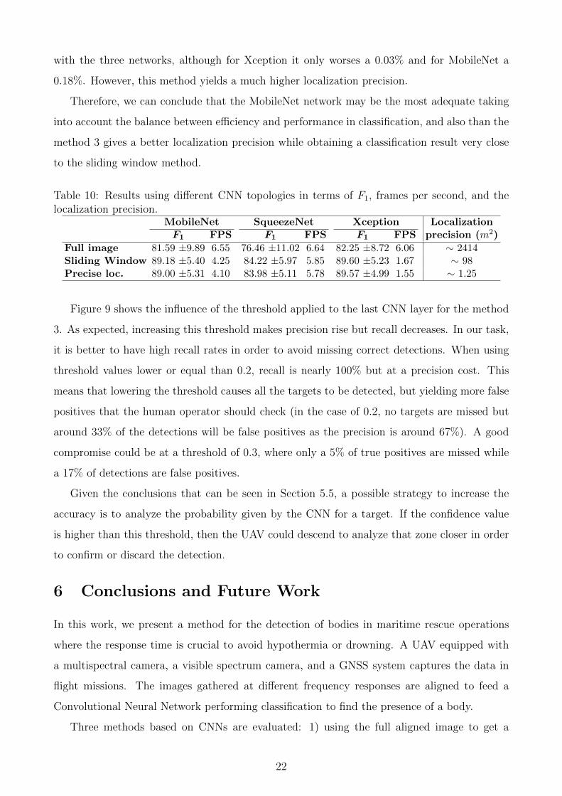
with the three networks, although for Xception it only worses a 0.03% and for MobileNet a
0.18%. However, this method yields a much higher localization precision.
Therefore, we can conclude that the MobileNet network may be the most adequate taking
into account the balance between efficiency and performance in classification, and also than the
method 3 gives a better localization precision while obtaining a classification result very close
to the sliding window method.
Table 10: Results using different CNN topologies in terms of F1, frames per second, and thelocalization precision.
MobileNet SqueezeNet Xception LocalizationF1 FPS F1 FPS F1 FPS precision (m2)
Full image 81.59 ±9.89 6.55 76.46 ±11.02 6.64 82.25 ±8.72 6.06 ∼ 2414Sliding Window 89.18 ±5.40 4.25 84.22 ±5.97 5.85 89.60 ±5.23 1.67 ∼ 98Precise loc. 89.00 ±5.31 4.10 83.98 ±5.11 5.78 89.57 ±4.99 1.55 ∼ 1.25
Figure 9 shows the influence of the threshold applied to the last CNN layer for the method
3. As expected, increasing this threshold makes precision rise but recall decreases. In our task,
it is better to have high recall rates in order to avoid missing correct detections. When using
threshold values lower or equal than 0.2, recall is nearly 100% but at a precision cost. This
means that lowering the threshold causes all the targets to be detected, but yielding more false
positives that the human operator should check (in the case of 0.2, no targets are missed but
around 33% of the detections will be false positives as the precision is around 67%). A good
compromise could be at a threshold of 0.3, where only a 5% of true positives are missed while
a 17% of detections are false positives.
Given the conclusions that can be seen in Section 5.5, a possible strategy to increase the
accuracy is to analyze the probability given by the CNN for a target. If the confidence value
is higher than this threshold, then the UAV could descend to analyze that zone closer in order
to confirm or discard the detection.
6 Conclusions and Future Work
In this work, we present a method for the detection of bodies in maritime rescue operations
where the response time is crucial to avoid hypothermia or drowning. A UAV equipped with
a multispectral camera, a visible spectrum camera, and a GNSS system captures the data in
flight missions. The images gathered at different frequency responses are aligned to feed a
Convolutional Neural Network performing classification to find the presence of a body.
Three methods based on CNNs are evaluated: 1) using the full aligned image to get a
22

40
50
60
70
80
90
100
0 0.2 0.4 0.6 0.8 1Threshold
PrecisionRecall
F1
Figure 9: Impact on the results of the threshold value applied at the network output.
single prediction, 2) using sliding windows to get several predictions per image and a more
accurate localization, and 3) using a precise localization technique which includes transposed
convolutions to increase the detection accuracy. These methods required some changes to the
initial MobileNet topology evaluated, replacing the last fully-connected layers with a series of
new layers both for the categorical classification and the localization approaches.
Different combinations of spectral channels were evaluated for classification, as well as the
three strategies considered. The results show that the best classification performance (F1 =
89%) was obtained when combining the GRE-REG-NIR channels and using sliding windows.
The precise localization approach obtains a similar accuracy but with a localization precision
close to 1m.
In addition, evaluation experiments were performed in terms of flight altitude. Different
CNN topologies (Xception and SqueezeNet) were also tested in terms of F1 and FPS results.
The most evident future work is to use the proposed method in real maritime rescue missions,
which are expected to be carried out by Babcock MSC Spain within the context of the Civil
UAVs Initiative program in order to offer new technological solutions based on UAVs to improve
public services.
We are planning to use this system in real cooperative missions with ground personal for
searching in greater areas using an unmanned rotorcraft which weighs 25kg, has a payload of
10Kg and a flying range of 3 hours. The data gathered from these real missions could also
be added to retrain the CNNs using more images to increase their performance. Besides, our
vision system will be improved in the future with new cameras having different spectral ranges
and with an embedded GPU mounted on the UAV.
23

Acknowledgments
This work was performed in collaboration with Babcock MCS Spain and funded by the Galicia
Region Government through the Civil UAVs Initiative program, the Spanish Government’s Min-
istry of Economy, Industry and Competitiveness through the RTC-2014-1863-8 and INAER4-
14Y (IDI-20141234) projects, and the grant number 730897 under the HPC-EUROPA3 project
supported by Horizon 2020.
References
Aguilar, W. G., Luna, M. A., Moya, J. F., Abad, V., Parra, H., and Ruiz, H. (2017). Pedestrian
detection for uavs using cascade classifiers with meanshift. In IEEE 11th International
Conference on Semantic Computing (ICSC), pages 509–514.
Amanatiadis, A., Bampis, L., Karakasis, E. G., Gasteratos, A., and Sirakoulis, G. (2017). Real-
time surveillance detection system for medium-altitude long-endurance unmanned aerial
vehicles. Concurrency and Computation: Practice and Experience.
Andriluka, M., Schnitzspan, P., Meyer, J., Kohlbrecher, S., Petersen, K., von Stryk, O., Roth,
S., and Schiele, B. (2010). Vision based victim detection from unmanned aerial vehicles.
In IEEE/RSJ International Conference on Intelligent Robots and Systems (IROS), pages
1740–1747.
Avola, D., Foresti, G. L., Martinel, N., Micheloni, C., Pannone, D., and Piciarelli, C. (2017).
Aerial video surveillance system for small-scale uav environment monitoring. In 14th IEEE
International Conference on Advanced Video and Signal Based Surveillance (AVSS), pages
1–6.
Azizpour, H., Razavian, A. S., and Sullivan, J. (2016). Factors of Transferability for a Generic
ConvNet Representation. IEEE Trans. on Pattern Analysis and Machine Intelligence,
38:1790–1802.
Bejiga, M. B., Zeggada, A., Nouffidj, A., and Melgani, F. (2017). A convolutional neural
network approach for assisting avalanche search and rescue operations with uav imagery.
Remote Sensing, 9(2):100:1–22.
Blondel, P., Potelle, A., Pegard, C., and Lozano, R. (2014). Fast and viewpoint robust human
24

detection for sar operations. In IEEE International Symposium on Safety, Security, and
Rescue Robotics (SSRR), pages 1–6.
Bottou, L. (2010). Large-scale machine learning with stochastic gradient descent. In Proceedings
of COMPSTAT’2010, pages 177–186. Springer.
Chatfield, K., Simonyan, K., Vedaldi, A., and Zisserman, A. (2014). Return of the Devil in
the Details: Delving Deep into Convolutional Nets. In British Machine Vision Conference
(BMVC), pages 1–11.
Chollet, F. (2016). Xception: Deep learning with depthwise separable convolutions. CoRR,
abs/1610.02357.
Coulter, L., Stow, D., Tsai, Y. H., Chavis, C., Lippitt, C., Fraley, G., and McCreight, R. (2012).
Automated detection of people and vehicles in natural environments using high temporal
resolution airborne remote sensing. In ASPRS 2012 annual conference, pages 19–23.
Dumoulin, V. and Visin, F. (2016). A guide to convolution arithmetic for deep learning. arXiv
preprint arXiv:1603.07285.
Erdelj, M., Natalizio, E., Chowdhury, K. R., and Akyildiz, I. F. (2017). Help from the sky:
Leveraging uavs for disaster management. IEEE Pervasive Computing, 16(1):24–32.
Evangelidis, G. D. and Psarakis, E. Z. (2008). Parametric image alignment using enhanced
correlation coefficient maximization. IEEE Transactions on Pattern Analysis and Machine
Intelligence, 30(10):1858–1865.
Gallego, A.-J., Pertusa, A., and Gil, P. (2018). Automatic ship classification from optical aerial
images with convolutional neural networks. Remote Sensing, 10(4):511:1–20.
Giitsidis, T., Karakasis, E. G., Gasteratos, A., and Sirakoulis, G. C. (2015). Human and fire
detection from high altitude uav images. In 23rd Euromicro International Conference on
Parallel, Distributed, and Network-Based Processing, pages 309–315.
Goodrich, M. A., Morse, B. S., Engh, C., Cooper, J. L., and Adams, J. A. (2009). Towards
using unmanned aerial vehicles (uavs) in wilderness search and rescue: Lessons from field
trials. Interaction Studies, 10(3):453–478.
Howard, A. G., Zhu, M., Chen, B., Kalenichenko, D., Wang, W., Weyand, T., Andreetto,
M., and Adam, H. (2017). Mobilenets: Efficient convolutional neural networks for mobile
vision applications. arXiv preprint arXiv:1704.04861.
25

Hu, F., Xia, G.-S., Hu, J., and Zhang, L. (2015). Transferring deep convolutional neural
networks for the scene classification of high-resolution remote sensing imagery. Remote
Sensing, 7(11):14680–14707.
Iandola, F. N., Han, S., Moskewicz, M. W., Ashraf, K., Dally, W. J., and Keutzer, K. (2016).
Squeezenet: Alexnet-level accuracy with 50x fewer parameters and¡ 0.5 mb model size.
arXiv preprint arXiv:1602.07360.
Jhan, J.-P., Rau, J.-Y., and Huang, C.-Y. (2016). Band-to-band registration and ortho-
rectification of multilens/multispectral imagery: A case study of minimca-12 acquired by
a fixed-wing uas. ISPRS Journal of Photogrammetry and Remote Sensing, 114:66 – 77.
Kingma, D. P. and Ba, J. (2014). Adam: A Method for Stochastic Optimization. ArXiv
e-prints.
Kohavi, R. (1995). A study of cross-validation and bootstrap for accuracy estimation and
model selection. In 14th International joint conference on Artificial intelligence (IJCAI),
volume 2, pages 1137–1143, San Francisco, CA, USA. Morgan Kaufmann Publishers Inc.
Krizhevsky, A., Sutskever, I., and Hinton, G. E. (2012). Imagenet classification with deep
convolutional neural networks. In Proceedings of the 25th International Conference on
Neural Information Processing Systems (NIPS), volume 1, pages 1097–1105, USA. Curran
Associates Inc.
Laroze, M., Courtrai, L., and Lefevre, S. (2016). Human detection from aerial imagery for
automatic counting of shellfish gatherers. In Proceedings of the 11th Joint Conference on
Computer Vision, Imaging and Computer Graphics Theory and Applications (VISAPP-
VISIGRAPP), volume 4, pages 664–671. INSTICC, SciTePress.
LeCun, Y., Bengio, Y., and Hinton, G. (2015). Deep learning. Nature, 521:436 EP –.
Lei, T., Zhang, Y., Wang, X., Fu, J., Li, L., Pang, Z., Zhang, X., and Kan, G. (2017). The
application of unmanned aerial vehicle remote sensing for monitoring secondary geological
disasters after earthquakes. In Ninth International Conference on Digital Image Processing,
volume 10420. SPIE digital library.
Leira, F. S., Johansen, T. A., and Fossen, T. I. (2015). Automatic detection, classification and
tracking of objects in the ocean surface from uavs using a thermal camera. In Proceedings
of IEEE Aerospace Conference, pages 1–10.
26

Lin, H., Shi, Z., and Zou, Z. (2017). Fully convolutional network with task partitioning for
inshore ship detection in optical remote sensing images. IEEE Geoscience and Remote
Sensing Letters, 14(10):1665–1669.
Lindemuth, M., Murphy, R., Steimle, E., Armitage, W., Dreger, K., Elliot, T., Hall, M.,
Kalyadin, D., Kramer, J., Palankar, M., Pratt, K., and Griffin, C. (2011). Sea robot-
assisted inspection. IEEE Robotics Automation Magazine, 18(2):96–107.
Lopez-Fuentes, L., van de Weijer, J., Gonzalez-Hidalgo, M., Skinnemoen, H., and Bagdanov,
A. D. (2017). Review on computer vision techniques in emergency situations. Multimedia
Tools and Applications.
Mendonca, R., Marques, M. M., Marques, F., Lourenco, A., Pinto, E., Santana, P., Coito, F.,
Lobo, V., and Barata, J. (2016). A cooperative multi-robot team for the surveillance of
shipwreck survivors at sea. In Proceedings of OCEANS 2016 MTS/IEEE Monterey, pages
1–6.
Merino, L., Caballero, F., Martinez-de Dios, J. R., Maza, I., and Ollero, A. (2012). An un-
manned aircraft system for automatic forest fire monitoring and measurement. Journal of
Intelligent and Robotic Systems, 65(1):533–548.
Merino, L., Caballero, F., Martınez-de Dios, J., Ferruz, J., and Ollero, A. (2006). A cooperative
perception system for multiple uavs: Application to automatic detection of forest fires.
Journal of Field Robotics, 23(3-4):165–184.
Minaeian, S., Liu, J., and Son, Y. J. (2016). Vision-based target detection and localization via a
team of cooperative uav and ugvs. IEEE Transactions on Systems, Man, and Cybernetics:
Systems, 46(7):1005–1016.
Missing Migrants (2018). https://missingmigrants.iom.int. Accessed: 2018-03-11.
Niedzielski, T., Jurecka, M., Mizinski, B., Remisz, J., Slopek, J., Spallek, W., Witek-Kasprzak,
M., Kasprzak, L., and Swierczynska Chlasciak, M. (2017a). A real-time field experiment
on search and rescue operations assisted by unmanned aerial vehicles. Journal of Field
Robotics, pages n/a–n/a.
Niedzielski, T., Jurecka, M., Stec, M., Wieczorek, M., and Mizinski, B. (2017b). The nested
k-means method: A new approach for detecting lost persons in aerial images acquired by
unmanned aerial vehicles. Journal of Field Robotics, 34(8):1395–1406.
27

Pajares, G. (2015). Overview and current status of remote sensing applications based on
unmanned aerial vehicles (uavs). Photogrammetric Engineering and Remote Sensing,
81(4):281–329.
Portmann, J., Lynen, S., Chli, M., and Siegwart, R. (2014). People detection and tracking from
aerial thermal views. In 2014 IEEE International Conference on Robotics and Automation
(ICRA), pages 1794–1800.
Ren, L., Shi, C., and Ran, X. (2012). Target detection of maritime search and rescue: Saliency
accumulation method. In 9th International Conference on Fuzzy Systems and Knowledge
Discovery (FSKD), pages 1972–1976.
Rudol, P. and Doherty, P. (2008). Human body detection and geolocalization for uav search
and rescue missions using color and thermal imagery. In Proceedings of IEEE Aerospace
Conference, pages 1–8.
Russakovsky, O., Deng, J., Su, H., Krause, J., Satheesh, S., Ma, S., Huang, Z., Karpathy,
A., Khosla, A., Bernstein, M., Berg, A. C., and Fei-Fei, L. (2015). ImageNet Large Scale
Visual Recognition Challenge. International Journal of Computer Vision, 115(3):211–252.
Silvagni, M., Tonoli, A., Zenerino, E., and Chiaberge, M. (2017). Multipurpose uav for search
and rescue operations in mountain avalanche events. Geomatics, Natural Hazards and Risk,
8(1):18–33.
Sommer, L. W., Schuchert, T., and Beyerer, J. (2017). Deep learning based multi-category
object detection in aerial images. In Proceedings of Automatic Target Recognition XXVII,
volume 10202. SPIE Digital Library.
Sun, J., Li, B., Jiang, Y., and Wen, C.-y. (2016). A camera-based target detection and posi-
tioning uav system for search and rescue (sar) purposes. Sensors, 16(11):1778:1–24.
Symington, A., Waharte, S., Julier, S., and Trigoni, N. (2010). Probabilistic target detection
by camera-equipped uavs. In IEEE International Conference on Robotics and Automation
(ICRA), pages 4076–4081.
Szegedy, C., Liu, W., Jia, Y., Sermanet, P., Reed, S., Anguelov, D., Erhan, D., Vanhoucke,
V., and Rabinovich, A. (2015). Going deeper with convolutions. In Computer Vision and
Pattern Recognition (CVPR).
28

Teutsch, M., Mueller, T., Huber, M., and Beyerer, J. (2014). Low resolution person detection
with a moving thermal infrared camera by hot spot classification. In 2014 IEEE Conference
on Computer Vision and Pattern Recognition Workshops, pages 209–216.
Voyles, R. and Choset, H. (2017). Editorial: Search and rescue robots. Journal of Field
Robotics, 25(1-2):1–2.
Westall, P., Carnie, R. J., O’Shea, P. J., Hrabar, S., and Walker, R. A. (2007). Vision-
based uav maritime search and rescue using point target detection. In Twelfth Australian
International Aerospace Congress, Twelfth Australian Aeronautical Conference(AIAC12).
Westall, P., Ford, J. J., O’Shea, P., and Hrabar, S. (2008). Evaluation of maritime vision tech-
niques for aerial search of humans in maritime environments. In Digital Image Computing:
Techniques and Applications (DICTA), pages 176–183.
Yang, W., Yin, X., and Xia, G. S. (2015). Learning high-level features for satellite image
classification with limited labeled samples. IEEE Transactions on Geoscience and Remote
Sensing, 53(8):4472–4482.
Yuan, C., Liu, Z., and Zhang, Y. (2017). Aerial images-based forest fire detection for fire-
fighting using optical remote sensing techniques and unmanned aerial vehicles. Journal of
Intelligent & Robotic Systems, 88(2):635–654.
Zheng, L., Hu, J., and Xu, S. (2017). Marine search and rescue of uav in long-distance security
modeling simulation. Polish Maritime Research, 24(s3):192–199.
Zou, Z. and Shi, Z. (2016). Ship detection in spaceborne optical image with svd networks.
IEEE Transactions on Geoscience and Remote Sensing, 54(10):5832–5845.
29