detection of cracks and corrosion for automated...

Detection of Cracks and Corrosion for Automated Vessels Visual Inspection

Francisco Bonnin Pascual

[email protected]

Abstract

Despite the efforts on reducing maritime accidents, they still occur and, from time to time, have catastrophic conse-quences both in personal, environmental and financial terms. Structural failure is the major cause of ships wreckagesand, as such, Vessel Classification Societies impose extensive inspection schemes for assessing the structural integrityof vessels.

The external and internal parts of the hull can be affected by different kinds of defects typical of steel surfaces andstructures, such as cracks and corrosion. Nowadays, to detect these defects, visual hull inspections are carried out at agreat cost. The goal of the EU-funded FP7 MINOAS project is to develop a fleet of robots for automating as much aspossible the aforementioned inspection and maintenance operations.

Within this general context, the work presented constitutes a first attempt towards the remote visual inspection anddocumentation of hull surfaces. In this regard, the two main defective situations, cracks and corrosion, are expectedto be autonomously or semi-autonomously detected by means of computer vision techniques.

In this work, several algorithms are presented for visual detection of the above mentioned two kinds of defects. Onthe one hand, a crack detector is described, which is based on a percolation process that exploits the morphologicalproperties of cracks in steel surfaces: dark, narrow and elongated sets of connected pixels.

On the other hand, two different approaches for corrosion detection are introduced and compared. While the firstone takes profit from the distribution of color in corroded areas, the second one has been built around a weak classifiercascade scheme, separating the spatial and colour analysis in two different steps. As an final contribution, the crackdetector is combined with the corrosion detector in order to guide the crack location and improve its performance. Theobtained detectors have shown promising rates of detection as well as close to real-time performance.

Key words: Vessel inspection, Crack detection, Percolation, Corrosion detection, Classification

1

Contents

1 Introduction 2

2 State of the art 3

3 Percolation-based Crack Detector (PCD) 43.1 Description of the algorithm . . . . . . . 43.2 Performance of PCD . . . . . . . . . . . 6

4 Colour-based Corrosion Detector (CCD) 74.1 Description of the algorithm . . . . . . . 74.2 Performance of CCD . . . . . . . . . . . 10

5 Weak-classifier Colour-based Corrosion Detec-tor (WCCD) 115.1 Description of the algorithm . . . . . . . 115.2 Performance of WCCD . . . . . . . . . . 14

6 Guided Percolation-based Crack Detector(GPCD) 196.1 Description of the algorithm . . . . . . . 196.2 Performance of GPCD . . . . . . . . . . 22

7 Conclusions 22

1. Introduction

Vessels constitute one of the most cost effective formsof transporting bulk goods around the world. However,despite the efforts on reducing maritime accidents, theystill occur and, from time to time, have catastrophic con-sequences both in personal, environmental and financialterms. Structural failure is the major cause of ships wreck-ages and, as such, Classification Societies (also known asShipping Registers, Flag States, etc.) impose extensiveinspection schemes for assessing the structural integrityof vessels.

An important part of the vessel maintenance has to dowith the visual inspection of the external and internal partsof the vessel hull. They can be affected by different kindsof defects typical of steel surfaces and structures, such ascracks and corrosion. These two kinds of defects are indi-cators of the state of the metallic surface and, as such,an early detection prevents the structure from bucklingand/or fracturing.

Nowadays, to perform a complete hull inspection, thevessel has to be emptied and situated in a dockyard, wheretypically temporary staging, lifts, movable platforms, etc.need to be installed to allow the workers for close-up in-spection (and repair if needed) of all the different metal-lic surfaces and structures. Taking into account the hugedimensions of some vessels, this process can mean thevisual assessment of more than 600,000 m2 of steel. Be-sides, the surveys are on many occasions performed inhazardous environments for which the access is usuallydifficult, while the operational conditions turn out to besometimes extreme for human operation. For large ton-nage vessels, such as Ultra Large Crude Carriers (ULCC),total expenses can be as high as one million euros.

Corrosion and the presence of cracks are clear indica-tors of the state of the hull metallic structures, and, thus,are of great interest for the surveyor (see Figure 1). Onthe one hand, cracks generally develop at intersections ofstructural items or discontinuities due to stress concen-tration, although they also may be related to material orwelding defects. If the crack remains undetected and un-repaired, it can grow to a size where it can cause suddenfracture. Therefore, care is needed to visually discoverfissure occurrences in areas prone to high stress concen-tration.

On the other hand, different kinds of corrosion mayarise: general corrosion, that appears as non-protectivefriable rust which can occur uniformly on uncoated sur-faces; pitting, a localized process that is normally initi-ated due to local breakdown of coating and that derives,through corrosive attack, in deep and relatively small di-ameter pits that can in turn lead to hull penetration inisolated random places; grooving, again a localized pro-cess, but this time characterized by linear shaped corro-sion which occurs at structural intersections where wa-ter collects and flows; and weld metal corrosion, whichaffects the weld deposits, mostly due to galvanic actionwith the base metal, and are likelier in manual welds thanin machine welds.

To determine the state of a corroded structure it is com-mon to estimate the corrosion level as percentage of af-fected area. Traditional methods quantify corrosion byvisual comparison of the area under study with dot pat-terned charts (see Figure 1[bottom right]).

The goal of the EU-funded FP7 MINOAS project is todevelop a fleet of robots for automating as much as possi-

2

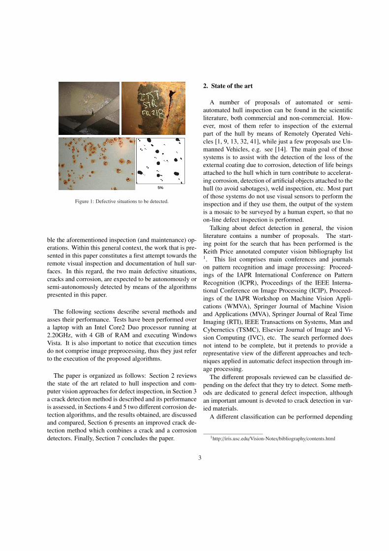
Figure 1: Defective situations to be detected.

ble the aforementioned inspection (and maintenance) op-erations. Within this general context, the work that is pre-sented in this paper constitutes a first attempt towards theremote visual inspection and documentation of hull sur-faces. In this regard, the two main defective situations,cracks and corrosion, are expected to be autonomously orsemi-autonomously detected by means of the algorithmspresented in this paper.

The following sections describe several methods andasses their performance. Tests have been performed overa laptop with an Intel Core2 Duo processor running at2.20GHz, with 4 GB of RAM and executing WindowsVista. It is also important to notice that execution timesdo not comprise image preprocessing, thus they just referto the execution of the proposed algorithms.

The paper is organized as follows: Section 2 reviewsthe state of the art related to hull inspection and com-puter vision approaches for defect inspection, in Section 3a crack detection method is described and its performanceis assessed, in Sections 4 and 5 two different corrosion de-tection algorithms, and the results obtained, are discussedand compared, Section 6 presents an improved crack de-tection method which combines a crack and a corrosiondetectors. Finally, Section 7 concludes the paper.

2. State of the art

A number of proposals of automated or semi-automated hull inspection can be found in the scientificliterature, both commercial and non-commercial. How-ever, most of them refer to inspection of the externalpart of the hull by means of Remotely Operated Vehi-cles [1, 9, 13, 32, 41], while just a few proposals use Un-manned Vehicles, e.g. see [14]. The main goal of thosesystems is to assist with the detection of the loss of theexternal coating due to corrosion, detection of life beingsattached to the hull which in turn contribute to accelerat-ing corrosion, detection of artificial objects attached to thehull (to avoid sabotages), weld inspection, etc. Most partof those systems do not use visual sensors to perform theinspection and if they use them, the output of the systemis a mosaic to be surveyed by a human expert, so that noon-line defect inspection is performed.

Talking about defect detection in general, the visionliterature contains a number of proposals. The start-ing point for the search that has been performed is theKeith Price annotated computer vision bibliography list1. This list comprises main conferences and journalson pattern recognition and image processing: Proceed-ings of the IAPR International Conference on PatternRecognition (ICPR), Proceedings of the IEEE Interna-tional Conference on Image Processing (ICIP), Proceed-ings of the IAPR Workshop on Machine Vision Appli-cations (WMVA), Springer Journal of Machine Visionand Applications (MVA), Springer Journal of Real TimeImaging (RTI), IEEE Transactions on Systems, Man andCybernetics (TSMC), Elsevier Journal of Image and Vi-sion Computing (IVC), etc. The search performed doesnot intend to be complete, but it pretends to provide arepresentative view of the different approaches and tech-niques applied in automatic defect inspection through im-age processing.

The different proposals reviewed can be classified de-pending on the defect that they try to detect. Some meth-ods are dedicated to general defect inspection, althoughan important amount is devoted to crack detection in var-ied materials.

A different classification can be performed depending

1http://iris.usc.edu/Vision-Notes/bibliography/contents.html

3

on the technique applied for the detection. Some meth-ods make use of general image processing techniques se-lected and combined to detect a specific kind of defect in aspecific material, while others rely on a previous learningstage using techniques such powerful as Neural Networks,Support Vector Machines, Genetic Algorithms, etc. Ta-ble 1 shows the proposals reviewed classified accordingto this last criterion.

Some of these methods have been used as starting pointto develop the solutions that are presented, described andassessed in the next sections.

3. Percolation-based Crack Detector

3.1. Description of the algorithm

This section presents a crack detector based on a per-colation model, similarly to the algorithm by Yamaguchiand Hashimoto described in [47]. This latter method was,however, devised for detecting cracks in concrete, whatmakes the authors assume a geometrical structure thatdoes not match exactly the shape of cracks that are formedin steel. Besides our method, which will be referred asPCD from now on, has been speeded up so that the algo-rithm can run as close as possible to real-time onboard arobotic platform.

For a start, a percolation model derives into a region-growing procedure which starts from a seed element andpropagates in accordance with a set of rules. In our case,the rules are defined to identify dark, narrow and elon-gated sets of connected pixels, which are then labelled ascracks.

Once a seed has been located, the percolation processstarts as a two-step procedure: during the first step, thepercolation is applied inside a window of N × N pix-els until the window boundary is reached; in the secondstep, if the elongation of the grown region is above εN ,a second percolation is performed until either the bound-ary of a window of M × M pixels (M > N) is reachedor the propagation cannot proceed because the gray levelof all the pixels next to the current boundary are above athreshold T (see below). Finally, all the pixels within thegrown region are classified as crack pixels if the elonga-tion is larger than εM . Elongation is calculated by means

of Equation 1:

ε =

√√√√√√√1 −

µxx + µyy −√

4µ2xy + (µ2

xx − µ2yy)

µxx + µyy +√

4µ2xy + (µ2

xx − µ2yy)

, (1)

where µxx, µyy and µxy are the normalized second centralmoments of the region [18].

Within the N × N or M ×M pixel window, the percola-tion proceeds in accordance to the next propagation rules:

(1) all the 8-neighbours of the percolated area are de-fined as candidates and

(2) each candidate p is visited and included in the per-colated area only if its gray level value I(p) is lowerthan the threshold T , which has been initialized tothe seed pixel gray level value.

At the end of the percolation process, the mean grayscale level of the set of pixels is checked to determine if itis dark enough to be considered as a crack. Otherwise, theset of pixels is rejected and nothing is marked as a crackin the current percolation.

For reducing the execution time of PCD, seed pointsare defined only at edges that have not yet been classifiedas crack pixels and whose gray level is below γs. Fur-thermore, not all the edges are considered for starting thepercolation, but only those at image places over a regulargrid where the gap between points is ∆ pixels. To ensurethat the relevant edges are always considered, a dilationstep follows the edge detection, where dilation thicknessis in accordance with ∆.

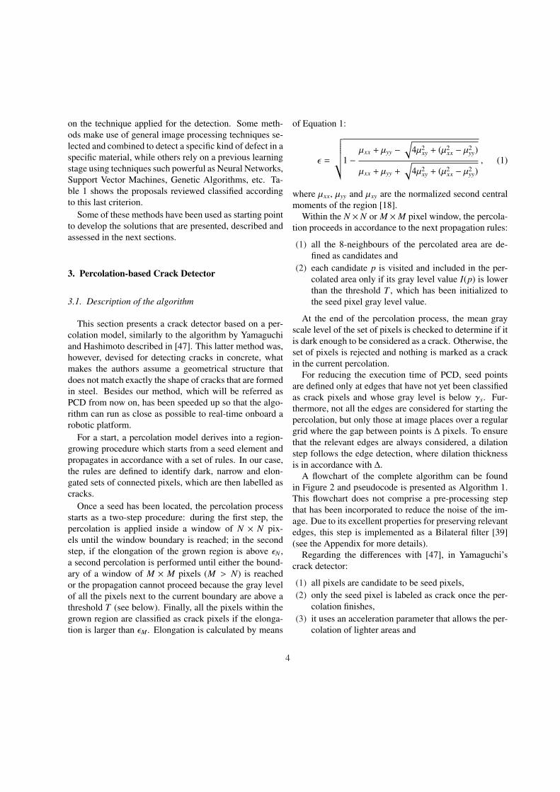
A flowchart of the complete algorithm can be foundin Figure 2 and pseudocode is presented as Algorithm 1.This flowchart does not comprise a pre-processing stepthat has been incorporated to reduce the noise of the im-age. Due to its excellent properties for preserving relevantedges, this step is implemented as a Bilateral filter [39](see the Appendix for more details).

Regarding the differences with [47], in Yamaguchi’scrack detector:

(1) all pixels are candidate to be seed pixels,(2) only the seed pixel is labeled as crack once the per-

colation finishes,(3) it uses an acceleration parameter that allows the per-

colation of lighter areas and

4

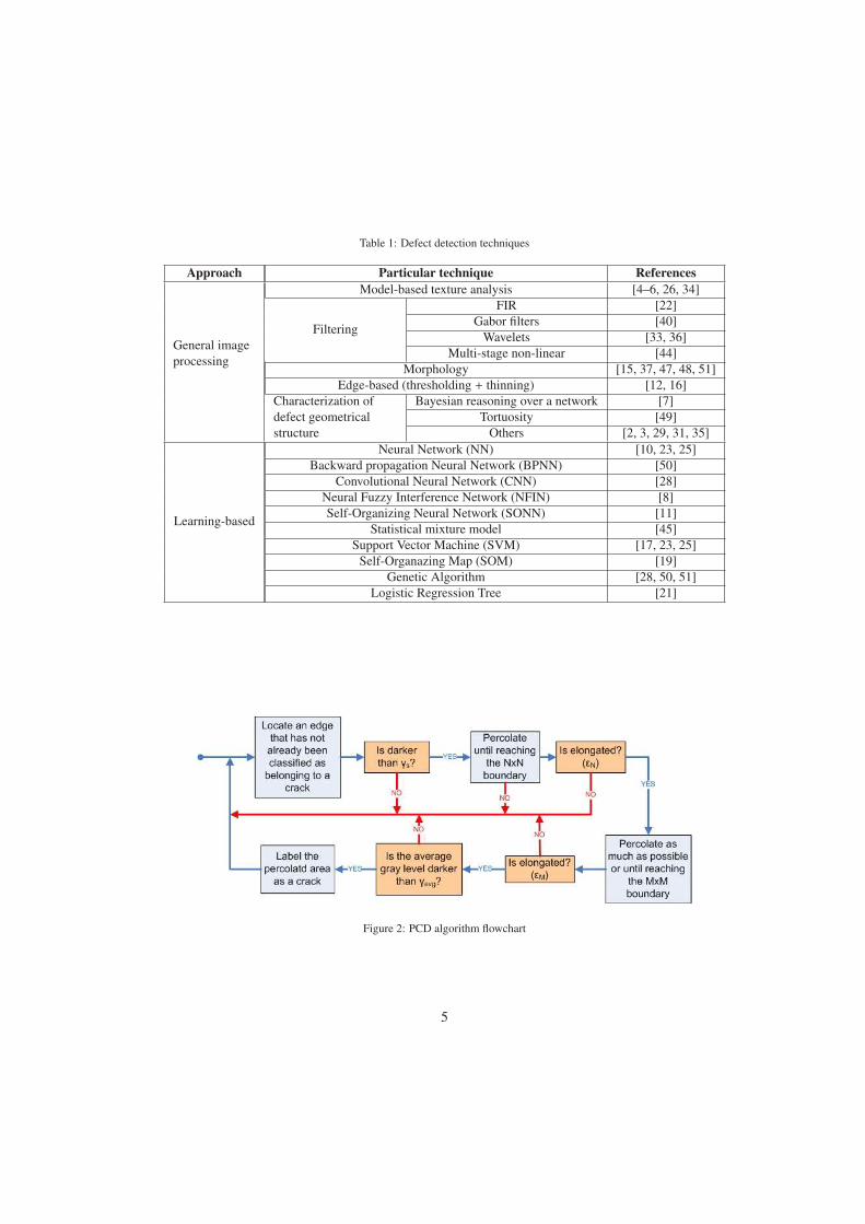
Table 1: Defect detection techniques

Approach Particular technique References

General imageprocessing

Model-based texture analysis [4–6, 26, 34]

Filtering

FIR [22]Gabor filters [40]

Wavelets [33, 36]Multi-stage non-linear [44]

Morphology [15, 37, 47, 48, 51]Edge-based (thresholding + thinning) [12, 16]

Characterization ofdefect geometricalstructure

Bayesian reasoning over a network [7]Tortuosity [49]

Others [2, 3, 29, 31, 35]

Learning-based

Neural Network (NN) [10, 23, 25]Backward propagation Neural Network (BPNN) [50]

Convolutional Neural Network (CNN) [28]Neural Fuzzy Interference Network (NFIN) [8]Self-Organizing Neural Network (SONN) [11]

Statistical mixture model [45]Support Vector Machine (SVM) [17, 23, 25]

Self-Organazing Map (SOM) [19]Genetic Algorithm [28, 50, 51]

Logistic Regression Tree [21]

Figure 2: PCD algorithm flowchart

5

(4) it is not required that the average gray level of thepercolated region is below a certain threshold.

As a result of these differences, PCD has become fasterthan Yamaguchi’s for crack detection in metal surfaces.

3.2. Performance of PCD

The performance of PCD algorithm depends on the par-ticular setting of the percolation parameters as well as onthe size of the gap left between percolations. As a gen-eral rule during the selection of the final parameter val-ues, false negatives have been penalized more than falsepositives. The elapsed time during the entire process hasbeen considered an important factor as well, in the senseof trying to reduce it as much as possible.

Regarding specific parameters, εN and εM , related withthe expected elongation of cracks, and the gray levelthresholds γs and γavg, have all been tuned so as to re-duce as much as possible the number of false positivesover all the test images, while the value for N and M, re-lated with the size of the percolation boundaries, has beendetermined using the mean value of Pratt’s FOM mea-sure [30] calculated for all the test images.

Once all the parameters have been configured, thedetector performance has been assessed with regard toground truth by means of the false positive and false neg-ative rates, respectively FP / (FP+TN) and FN / (FN+TP).After analyzing 2244960 pixels from 15 different images,the global rates result to be 2.31% for false positives and55.60% for false negatives. The false positive rate is notnull because of some dark narrow areas, e.g. shadows,that sometimes are classified as cracks. The high valueobtained for the false negative rate is due to the differentintensity levels that can be found inside a specific crack:i.e. the percolation process tends to tag only the darkestareas inside the crack, not the lightest ones. Thus, therecan be a number of pixels initially labelled as belongingto a crack in the ground truth which finally are not markedby the algorithm.

In order to avoid the effect of ground truth subjectivityover the false negative rate, we decided to make use of an-other set of performance figures not so much affected bythe reduced number of image pixels potentially involvedin a crack. In this regard, performance has also been an-alyzed from the point of view of the false negative andfalse positive percentages, respectively FP / #pixels and

Algorithm 1 Percolation-based Crack Detector (PCD)Require: Bilateral-filtered gray-scale image I is avail-

able. No pixel is labelled as a crack1: Compute the edge map for I using Sobel operator2: for all pixels p = I(u, v) such u = bu/∆c∆ and v =

bv/∆c∆ do3: P = Ø {Currently percolated area}4: if p is darker than γs and p is an edge and p is

not labelled as a crack then {new seed definition}5: P = P ∪ {p }6: T = gray level of p7: while P does not reach N ×N boundary do {first

percolation process}8: for all neighbours q of P do9: if q is darker than T then

10: P = P ∪ {q}11: end if12: end for13: if any non-percolated neighbour is darker than

T then {force percolation}14: d = darkest neighbour of P15: P = P ∪ {d}16: end if17: end while18: while P does not reach M × M bound-

ary and there are neighbours to visit andElongation (P) > εN do {second percolation pro-cess}

19: for all neighbours q of P do20: if q is darker than T then21: P = P ∪ {q}22: end if23: end for24: end while25: if Elongation (P) > εM then26: if the average gray level of P is darker than

γavg then27: Label all the pixels from P as a crack28: end if29: end if30: end if31: end for

6

FN / #pixels. Observe that these performance figures arenot affected by the percentage of pixels labelled as corro-sion since the number of missclassifications are both di-vided by the same amount of cases (i.e. pixels).

The global percentages result to be 2.29% for false pos-itives and 0.47% for false negatives. Percentages for someof the images are additionally shown in Table 3. As canbe observed in Table 3(a), false positive percentages arenot null and its value is quite similar to the false posi-tive rate since most of pixels in the images are not fromcracks. False negative percentages, as can be seen in Ta-ble 3(b), are neither null due to the non-percolation of thelightest pixels of cracks, but its value does not increaseso much as the false negative rate since the percentage iscalculated taking into account all the pixels of the image,not only crack pixels.

Furthermore, if entire cracks are considered as entitiesand it is assumed that the labelling of a single pixel withina crack is useful, then the corresponding percentage FNcracks / #cracks turns out to be zero since all the cracksare always detected (see Table 3(c)). In this regard, it isimportant to remember that this algorithm is intended tobe used to facilitate the visual inspection of vessel imagescarried out by a supervisor and, thus, informing about theexistence of a crack in an image area is considered worthenough even if the crack is not completely marked.

Table 4 shows crack detection running times for someof the test images, together with their sizes. As can beseen, the elapsed time does not increase with the numberof pixels since it depends more on the number and size ofcracks, and edges in general, that are detected.

Some images and the corresponding output are shownin Figure 3. It can be observed that all the cracks thatcan be detected by means of visual inspection are detectedby PCD as well. The values assigned to the algorithmparameters are provided through Table 2.

4. Colour-based Corrosion Detector


The corrosion detection approach has been built arounda supervised classification scheme. The classifier makesuse of a codeword dictionary computed during a previ-ous learning stage. Each codeword consists of stackedhistograms for the red, green and blue colour channels

Table 2: Values taken by the PCD parameters

N 41M 41εM 0.3εN 0.3γs 0.5γavg 0.4∆ 5

of image patches containing different kinds of rust. Thisstructure gives the name to the algorithm which is calledColor-based corrosion detector, CCD from now on.

To reduce the dimensionality and the sensitivity tonoise, intensity values are downsampled from 256 to 32levels, and, thus, a codeword consists of 96 components.As can be observed in Figure 4, this codeword does notpreserve the spatial arrangement of intensity levels nor therelationship between colour channels for the same pixel.

Samples from different kinds of corrosion have beengathered for training, and 30 different images containingcorroded metallic surfaces have been used for this pur-pose. In order to make the dictionary more compact,codewords have been clustered, independently for everykind of rust considered, by means of the well-known K-means algorithm [38]. The size of the dictionary for everytype of corrosion, i.e. the number of models, is thereforegiven by the number of clusters selected during the clus-tering process.

Once the dictionary has been built, the corrosion de-tector proceeds scanning the image and classifying everyimage patch as affected by corrosion or not. To this end,the current patch codeword is built and compared with themodels of the dictionary by means of the Bhattacharyyadistance D = − log(1 − B), with B given by Equation 2:

B =∑

xεX

√pc(x)pm(x) , (2)

where X refers to the histograms domain and pc and pm

are histograms from, respectively, the codeword and themodel.

A patch is labelled as corroded as soon as a model isfound in the dictionary such that D < τD. Therefore, theapproach does not intend to determine which is the closest

7

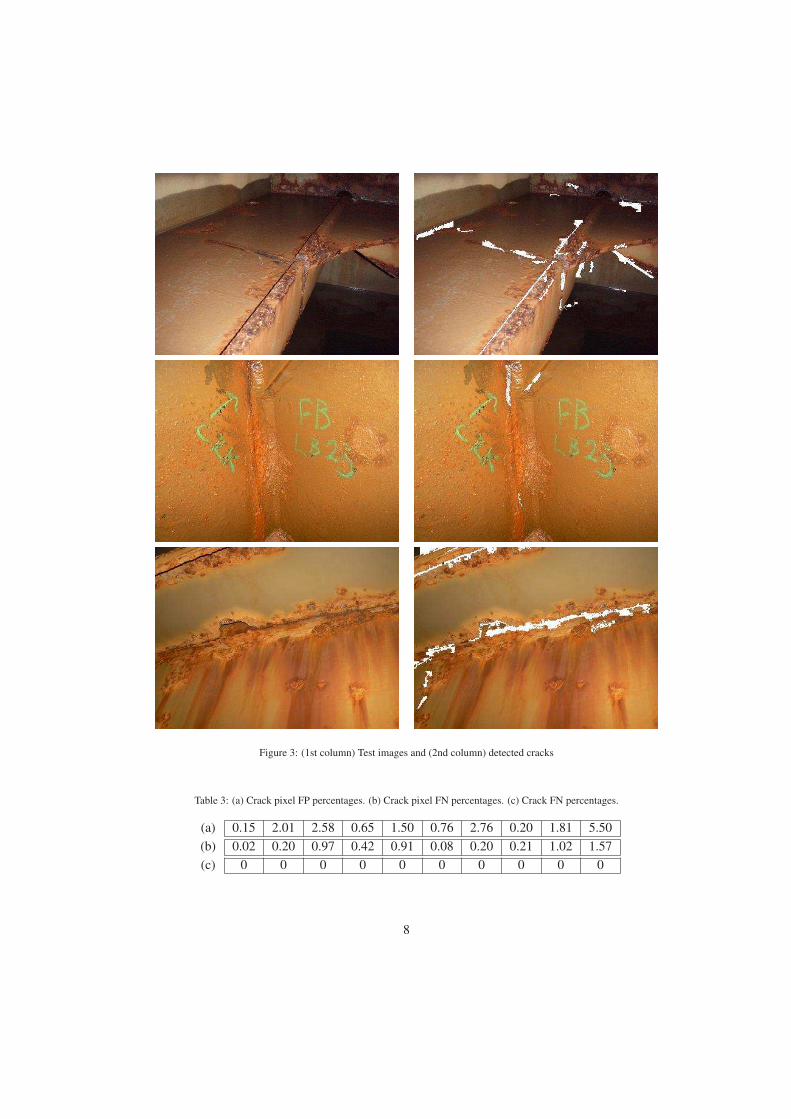
Figure 3: (1st column) Test images and (2nd column) detected cracks

Table 3: (a) Crack pixel FP percentages. (b) Crack pixel FN percentages. (c) Crack FN percentages.

(a) 0.15 2.01 2.58 0.65 1.50 0.76 2.76 0.20 1.81 5.50(b) 0.02 0.20 0.97 0.42 0.91 0.08 0.20 0.21 1.02 1.57(c) 0 0 0 0 0 0 0 0 0 0

8

Table 4: Crack inspection elapsed time for different image sizes

Pixels 120000 120000 144000 144000 158880 162720 172800 172800 177120Time (ms) 139 438 189 67 816 661 353 117 130

Figure 4: Codeword consisting of red, green and blue stacked histograms

model, but whether the patch is close enough to any modelof corrosion. As a consequence, an important reduction inthe computation time is obtained.

An additional stage has been introduced before thiscolour-based classification process in order to improve theclassification and reduce the number of codewords to becompared with the dictionary.

This stage is based on the premise that a corroded areapresents a rough texture. Roughness is then measured asthe energy of the symmetric gray-level co-occurrence ma-trix (GLCM), calculated for downsampled intensity val-ues between 0 and 31, for a given direction α and distanced [38]. The energy is obtained by means of Equation 3:

E =

31∑

i=0

31∑

j=0

p(i, j)2 , (3)

where p(i, j) is the probability of the occurrence of graylevels i and j at distance d and orientations α or α + π.Patches with an energy lower than a given threshold τE ,i.e. exhibit a rough texture, are finally candidates to bemore deeply inspected.

The flowchart for the complete algorithm is shown inFigure 5 and its pseudocode can be found as Algorithm 3.The pseudocode for codewords dictionary generation canbe found as Algorithm 2.

Algorithm 2 Codewords dictionary generation (CCD)Require: Ground truth images have been generated and

different kinds of corrosion have been distinguished1: for all different kinds of corrosion do2: for all images I with this kind of corrosion do3: for all patches Π of I do4: if Π is labelled as corrosion in the ground

truth image then {generate codeword}5: Compute red histogram6: Compute green histogram7: Compute blue histogram8: Stack the three histograms together9: Save codeword

10: end if11: end for12: end for13: Cluster codewords to K models using K-means14: end for15: Save models dictionary

9

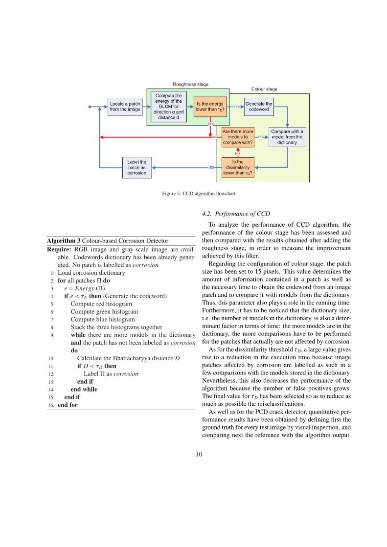
Figure 5: CCD algorithm flowchart

Algorithm 3 Colour-based Corrosion DetectorRequire: RGB image and gray-scale image are avail-

able. Codewords dictionary has been already gener-ated. No patch is labelled as corrosion

1: Load corrosion dictionary2: for all patches Π do3: e = Energy (Π)4: if e < τE then {Generate the codeword}5: Compute red histogram6: Compute green histogram7: Compute blue histogram8: Stack the three histograms together9: while there are more models in the dictionary

and the patch has not been labeled as corrosiondo

10: Calculate the Bhattacharyya distance D11: if D < τD then12: Label Π as corrosion13: end if14: end while15: end if16: end for

4.2. Performance of CCD

To analyze the performance of CCD algorithm, theperformance of the colour stage has been assessed andthen compared with the results obtained after adding theroughness stage, in order to measure the improvementachieved by this filter.

Regarding the configuration of colour stage, the patchsize has been set to 15 pixels. This value determines theamount of information contained in a patch as well asthe necessary time to obtain the codeword from an imagepatch and to compare it with models from the dictionary.Thus, this parameter also plays a role in the running time.Furthermore, it has to be noticed that the dictionary size,i.e. the number of models in the dictionary, is also a deter-minant factor in terms of time: the more models are in thedictionary, the more comparisons have to be performedfor the patches that actually are not affected by corrosion.

As for the dissimilarity threshold τD, a large value givesrise to a reduction in the execution time because imagepatches affected by corrosion are labelled as such in afew comparisons with the models stored in the dictionary.Nevertheless, this also decreases the performance of thealgorithm because the number of false positives grows.The final value for τD has been selected so as to reduce asmuch as possible the misclassifications.

As well as for the PCD crack detector, quantitative per-formance results have been obtained by defining first theground truth for every test image by visual inspection, andcomparing next the reference with the algorithm output.

10

Since the corrosion detector output is in terms of imagepatches instead of image pixels, the ground truth has alsobeen transformed to the patch domain. Since the groundtruth patches labelling admits a number of possibilities,the following strategies have been considered:

label a ground truth patch as corroded if thenumber of pixels labelled as corrosion in theground truth are

1. at least 1,2. at least 25% the patch size,3. at least 50% the patch size,4. at least 75% the patch size, or5. all the pixels of the patch.

False positive (FP / (FP+T N)) and false negative rates(FN / (FN + T P)) for different strategies have been cal-culated and are shown in Figure 6. These misclassifica-tion rates come from the analysis of 7384 patches from11 different images. As happened with the crack detec-tor, the values obtained for the false negative rate are veryhigh due to the miss detection of some patches labelledas corrosion in the ground truth images. For this reason,misclassification percentages have been used instead ofthe aforementioned rates, since these indicators are notaffected by the percentage of the image that is corroded.False positive (FP / #patches) and false negative percent-ages (FN / #patches) are also shown in Figure 6.

After observing the obtained misclassification percent-ages, the roughness filter was incorporated, its parameterswere tuned and its effect on the global algorithm perfor-mance was evaluated.

To configure the parameters of the roughness stagesome considerations have been taken into account. Thevalue for the energy threshold τE affects the algorithmperformance in terms of computation time as well as re-ducing the number of false positives, since all patcheswith a high energy level are discarded and only those witha low value become input for the color checking step. Sev-eral experiments have been performed considering differ-ent values for d and α when calculating the GLCM and,consequently, its energy level. However, no significantdifferences have been observed among the output values,and so the parameter values have been set to d = 5 (pixels)and α = 0 (horizontal direction).

Figure 7 shows rust detection outputs for the same in-

Table 5: Used values for CCD parameters

τE 0.05τD 0.07

put image using different energy thresholds. As can beobserved, τE can be tuned to decrease false positives andjust allow the detection of the most significant corrodedareas, while decreasing the computation time.

Once the roughness stage was configured, the perfor-mance of the CCD algorithm was assessed. Figure 8shows the false positive and false negative percentagesobtained after executing the algorithm using the same in-put images used for colour stage. As can be observed,the incorporation of the roughness filter has dramaticallyreduced the false positive percentage, while the effecton the false negative percentage has not been so impor-tant. Comparing the different patch labelling strategies,the number of incorrect classifications in any case is re-duced: below 10% for the false positives and around 18%for the false negatives. Besides, the number of false posi-tives grows very slightly with regard to the percentage ofpixels that are required to be corroded for the patch to beconsidered as corroded, what indicates that the number offalse alarms is low and independent of how the patcheshave been labelled. Regarding the number of false nega-tives, patches really affected by corrosion are always de-tected and only uncertain cases are left unidentified.

Similarly to what happened with the PCD, the process-ing time for the corrosion classifier depends on the per-centage of image area that is corroded or that presents alow energy level. Some results can be found in this regardin Table 6.

Figure 10 shows detection results for some images. Inthose cases, the algorithm was configured to detect onlythe image areas most significantly affected by corrosion,assigning to the parameters the values shown in Table 5.

5. Weak-classifier Colour-based Corrosion Detector


This section presents a second corrosion detection al-gorithm. As well as CCD, the new classifier has been

11

1 pixel 25% 50% 75% 100%0

20

40

60

80

100False positive rate

1 pixel 25% 50% 75% 100%0

20

40

60

80

100False negative rate

1 pixel 25% 50% 75% 100%0

20

40

60

80

100False positive percentage

1 pixel 25% 50% 75% 100%0

20

40

60

80

100False negative percentage

Figure 6: Misclassification rates and percentages for different ground truth patch labelling strategies to asses the color stage performance of CCD

Table 6: Corrosion inspection elapsed time for different image sizes (CCD)

Pixels 120000 120000 144000 154560 162720 172320 172800 172800 177120Time (ms) 49 47 151 74 61 117 41 277 33

12

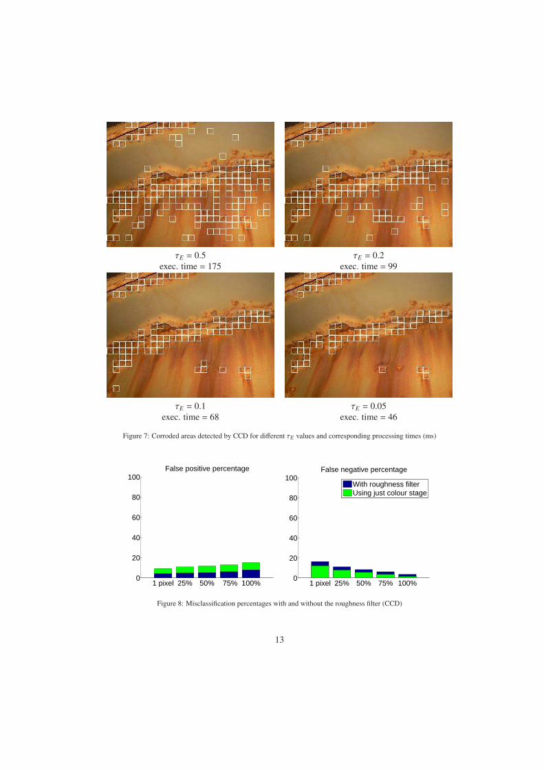
τE = 0.5 τE = 0.2exec. time = 175 exec. time = 99

τE = 0.1 τE = 0.05exec. time = 68 exec. time = 46

Figure 7: Corroded areas detected by CCD for different τE values and corresponding processing times (ms)

1 pixel 25% 50% 75% 100%0

20

40

60

80


1 pixel 25% 50% 75% 100%0

20

40

60

80


With roughness filterUsing just colour stage

Figure 8: Misclassification percentages with and without the roughness filter (CCD)

13

built around a cascade scheme, although the two stages ofthe new corrosion detector can be considered as two weakclassifiers. Thus, it will be called Weak-classifier Colour-based Corrosion Detector, WCCD from now on. The ideais to chain different fast classifiers with poor performancein order to obtain a global classifier attaining a much bet-ter global performance. To this end, each weak classifiertakes profit from different features of the items to classify,reducing the number of false positive detections at eachstage. For a good global performance, the classifiers mustpresent a false negative percentage close to zero.

The first stage of the cascade is the roughness stage ex-plained in section 4 for CCD. Remember that this stagereturns the image patches which present a rough texture,i.e. have an energy lower than a given threshold τE .

The second stage operates over the pixels of the patchesthat have passed the roughness stage. Unlike the first, thisstage makes use of the colour information that can be ob-served from corroded areas. More precisely, the classifierworks over the Hue-Saturation-Value (HSV) space afterthe realization that HSV-values that can be observed incorroded areas are confined in a bounded subspace of theHS plane. Although the V component has been observedneither significant nor necessary to describe the color ofcorrosion, it is used to prevent the well-known instabili-ties in the computation of hue and saturation when color isclose to white or black. In that case, the pixel is classifiedas non-corroded.

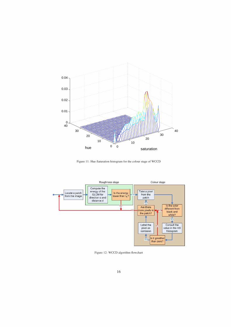
A training step is performed prior to the application ofthis second stage of the corrosion classifier. In this case,training consists of building a bi-dimensional histogramof HS values for image pixels known to be affected bycorrosion in the training image set. The resulting his-togram is subsequently filtered by zeroing entries whosevalue is below 10% the highest peak. By way of example,Figure 11 shows an HS histogram downsampled between0 and 31, calculated using 9 different images with corro-sion.

The classifier proceeds as follows for every 3-tuple(h, s, v):

(1) pixels close to black, v < mV , or white, v > MV∧s <mS , are labeled as non-corroded, and

(2) for the remaining pixels, the HS histogram is con-sulted and the pixel is labelled as corroded ifHS (h, s) > 0,

Figure 9: Venn diagram for corrosion definition

for given thresholds mV , MV and mS .Figure 9 shows a Venn diagram that depicts the corro-

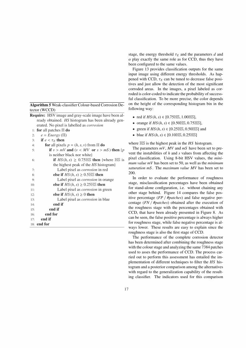
sion definition used by WCCD. Notice that the stages ofthe cascade cannot be swapped since they do not workwith the same kind of entities: while the second stageworks at the pixel level, the first stage operates over15 × 15 -pixel image patches since it depends on tex-ture, which necessarily involves a pixel neighborhood.Figure 12 shows the flow diagram of WCCD. The pseu-docodes for the dictionary corrosion color generation andWCCD corrosion detection algorithm can be found as Al-gorithms 4 and 5.

Algorithm 4 Corrosion color dictionary generation(WCCD)Require: Ground truth images have been generated

1: for all images C do2: for all pixels p do3: if p is labelled as corrosion in the ground truth

image then4: Insert that pixel in HS histogram5: end if6: end for7: end for8: for all bins b of the histogram do9: if b is lower than 0.1 × max(HS) then

10: b = 011: end if12: end for13: Save the histogram

5.2. Performance of WCCDThe performance of WCCD depends on the perfor-

mance of its different stages. Regarding the roughness

14

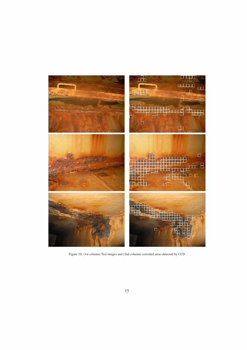
Figure 10: (1st column) Test images and (2nd column) corroded areas detected by CCD

15

010

2030

40

0

10

20

30

400

0.01

0.02

0.03

0.04

saturationhue

Figure 11: Hue-Saturation histogram for the colour stage of WCCD

Figure 12: WCCD algorithm flowchart

16

Algorithm 5 Weak-classifier Colour-based Corrosion De-tector (WCCD)Require: HSV image and gray-scale image have been al-

ready obtained. HS histogram has been already gen-erated. No pixel is labelled as corrosion

1: for all patches Π do2: e = Energy (Π)3: if e < τE then4: for all pixels p = (h, s, v) from Π do5: if v > mV and (v < MV or s > mS ) then {p

is neither black nor white}6: if HS (h, s) ≥ 0.75HS then {where HS is

the highest peak of the HS histogram}7: Label pixel as corrosion in red8: else if HS (h, s) ≥ 0.5HS then9: Label pixel as corrosion in orange

10: else if HS (h, s) ≥ 0.25HS then11: Label pixel as corrosion in green12: else if HS (h, s) ≥ 0 then13: Label pixel as corrosion in blue14: end if15: end if16: end for17: end if18: end for

stage, the energy threshold τE and the parameters d andα play exactly the same role as for CCD, thus they havebeen configured to the same values.

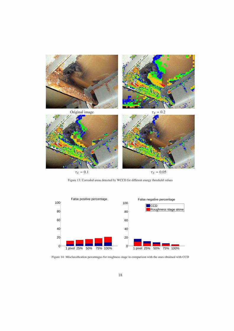
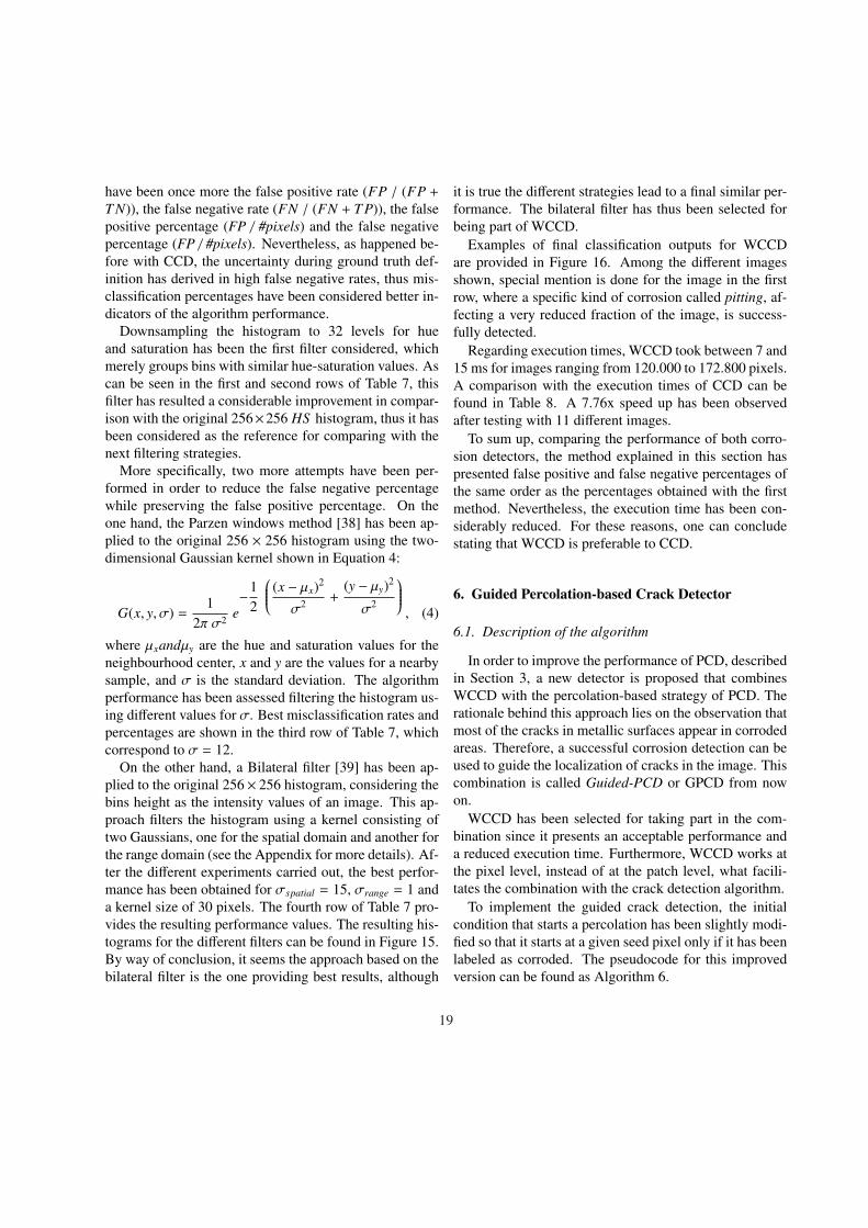
Figure 13 provides classification outputs for the sameinput image using different energy thresholds. As hap-pened with CCD, τE can be tuned to decrease false posi-tives and just allow the detection of the most significantcorroded areas. In the images, a pixel labeled as cor-roded is color-coded to indicate the probability of success-ful classification. To be more precise, the color dependson the height of the corresponding histogram bin in thefollowing way:

• red if HS (h, s) ∈ [0.75HS, 1.00HS],• orange if HS (h, s) ∈ [0.50HS, 0.75HS],• green if HS (h, s) ∈ [0.25HS, 0.50HS] and• blue if HS (h, s) ∈ [0.10HS, 0.25HS]

where HS is the highest peak in the HS histogram.The parameters mV , MV and mS have been set to pre-

vent the instabilities of h and s values from affecting thepixel classification. Using 8-bit HSV values, the mini-mum value mV has been set to 50, as well as the minimumsaturation mS . The maximum value MV has been set to200.

In order to evaluate the performance of roughnessstage, misclassification percentages have been obtainedfor stand-alone configuration, i.e. without chaining anyother stage behind. Figure 14 compares the false pos-itive percentage (FP / #patches) and false negative per-centage (FN / #patches) obtained after the execution ofthe roughness stage with the percentages obtained withCCD, that have been already presented in Figure 8. Ascan be seen, the false positive percentage is always higherfor roughness stage, while false negative percentage is al-ways lower. These results are easy to explain since theroughness stage is also the first stage of CCD.

The performance of the complete corrosion detectorhas been determined after combining the roughness stagewith the colour stage and analyzing the same 7384 patchesused to asses the performance of CCD. The process car-ried out to perform this assessment has entailed the im-plementation of different techniques to filter the HS his-togram and a posterior comparison among the alternativeswith regard to the generalization capability of the result-ing classifier. The indicators used for this comparison

17

Original image τE = 0.2

τE = 0.1 τE = 0.05

Figure 13: Corroded areas detected by WCCD for different energy threshold values

1 pixel 25% 50% 75% 100%0

20

40

60

80


1 pixel 25% 50% 75% 100%0

20

40

60

80


CCDRoughness stage alone

Figure 14: Misclassification percentages for roughness stage in comparison with the ones obtained with CCD

18

have been once more the false positive rate (FP / (FP +

T N)), the false negative rate (FN / (FN + T P)), the falsepositive percentage (FP / #pixels) and the false negativepercentage (FP / #pixels). Nevertheless, as happened be-fore with CCD, the uncertainty during ground truth def-inition has derived in high false negative rates, thus mis-classification percentages have been considered better in-dicators of the algorithm performance.

Downsampling the histogram to 32 levels for hueand saturation has been the first filter considered, whichmerely groups bins with similar hue-saturation values. Ascan be seen in the first and second rows of Table 7, thisfilter has resulted a considerable improvement in compar-ison with the original 256×256 HS histogram, thus it hasbeen considered as the reference for comparing with thenext filtering strategies.

More specifically, two more attempts have been per-formed in order to reduce the false negative percentagewhile preserving the false positive percentage. On theone hand, the Parzen windows method [38] has been ap-plied to the original 256 × 256 histogram using the two-dimensional Gaussian kernel shown in Equation 4:

G(x, y, σ) =1

2π σ2 e−1

2

(x − µx)2

σ2 +(y − µy)2

σ2

, (4)

where µxandµy are the hue and saturation values for theneighbourhood center, x and y are the values for a nearbysample, and σ is the standard deviation. The algorithmperformance has been assessed filtering the histogram us-ing different values for σ. Best misclassification rates andpercentages are shown in the third row of Table 7, whichcorrespond to σ = 12.

On the other hand, a Bilateral filter [39] has been ap-plied to the original 256× 256 histogram, considering thebins height as the intensity values of an image. This ap-proach filters the histogram using a kernel consisting oftwo Gaussians, one for the spatial domain and another forthe range domain (see the Appendix for more details). Af-ter the different experiments carried out, the best perfor-mance has been obtained for σspatial = 15, σrange = 1 anda kernel size of 30 pixels. The fourth row of Table 7 pro-vides the resulting performance values. The resulting his-tograms for the different filters can be found in Figure 15.By way of conclusion, it seems the approach based on thebilateral filter is the one providing best results, although

it is true the different strategies lead to a final similar per-formance. The bilateral filter has thus been selected forbeing part of WCCD.

Examples of final classification outputs for WCCDare provided in Figure 16. Among the different imagesshown, special mention is done for the image in the firstrow, where a specific kind of corrosion called pitting, af-fecting a very reduced fraction of the image, is success-fully detected.

Regarding execution times, WCCD took between 7 and15 ms for images ranging from 120.000 to 172.800 pixels.A comparison with the execution times of CCD can befound in Table 8. A 7.76x speed up has been observedafter testing with 11 different images.

To sum up, comparing the performance of both corro-sion detectors, the method explained in this section haspresented false positive and false negative percentages ofthe same order as the percentages obtained with the firstmethod. Nevertheless, the execution time has been con-siderably reduced. For these reasons, one can concludestating that WCCD is preferable to CCD.

6. Guided Percolation-based Crack Detector


In order to improve the performance of PCD, describedin Section 3, a new detector is proposed that combinesWCCD with the percolation-based strategy of PCD. Therationale behind this approach lies on the observation thatmost of the cracks in metallic surfaces appear in corrodedareas. Therefore, a successful corrosion detection can beused to guide the localization of cracks in the image. Thiscombination is called Guided-PCD or GPCD from nowon.

WCCD has been selected for taking part in the com-bination since it presents an acceptable performance anda reduced execution time. Furthermore, WCCD works atthe pixel level, instead of at the patch level, what facili-tates the combination with the crack detection algorithm.

To implement the guided crack detection, the initialcondition that starts a percolation has been slightly modi-fied so that it starts at a given seed pixel only if it has beenlabeled as corroded. The pseudocode for this improvedversion can be found as Algorithm 6.

19

Table 7: Misclassification measures for different HS histograms (WCCD)

FP rate FN rate FP percentage FN percentageOriginal (256 bins) 0.94 91.22 0.80 13.56

Downsampled to 32 bins 11.50 41.02 9.78 6.10Using Parzen-window 10.85 40.31 9.23 5.99Using Bilateral filter 11.51 39.45 9.80 5.86

Using 256 bins Downsampled to 32 bins

010

2030

40

0

10

20

30

400

0.01

0.02

0.03

0.04

saturationhue

Using Parzen windows density estimation Filtered using Bilateral filter

Figure 15: HS histograms resulting from the different filtering strategies (WCCD)

20

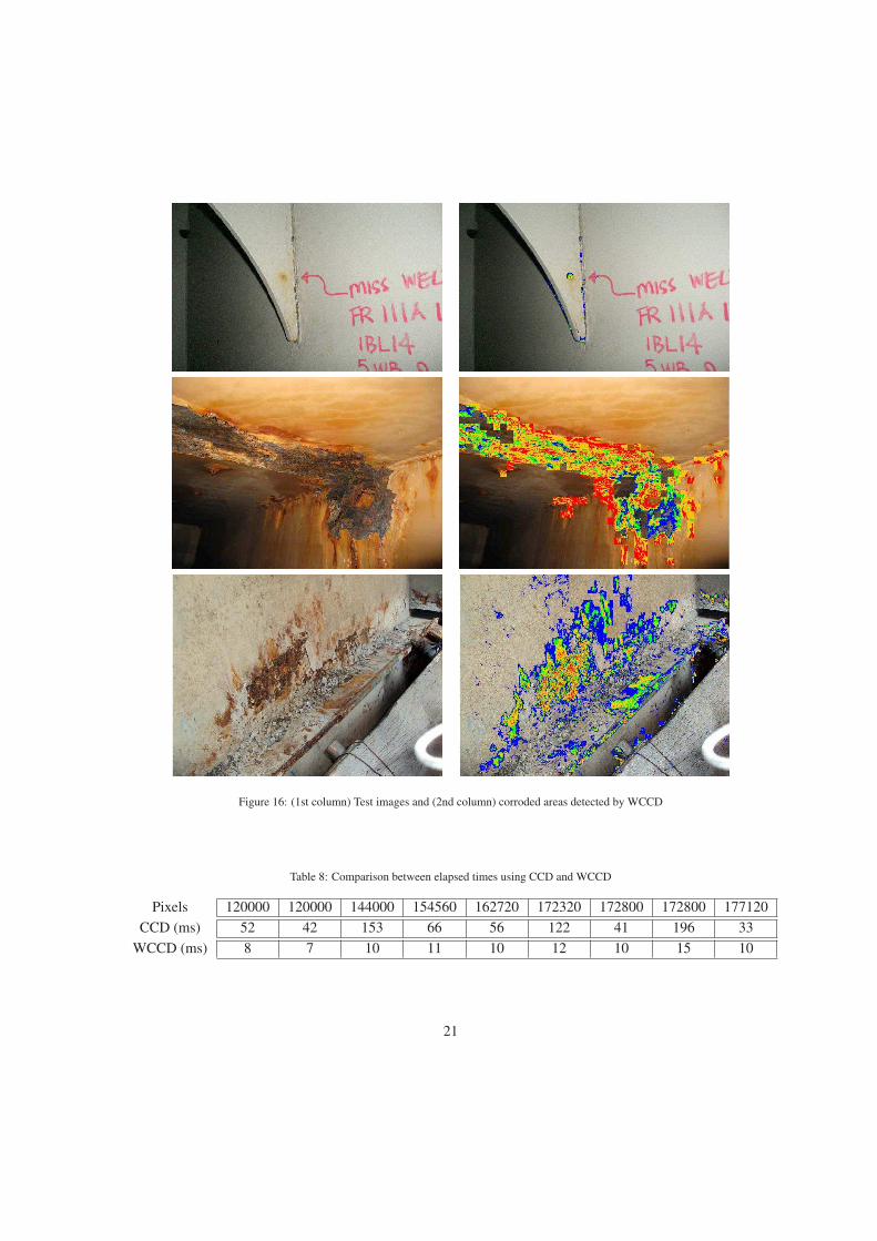
Figure 16: (1st column) Test images and (2nd column) corroded areas detected by WCCD

Table 8: Comparison between elapsed times using CCD and WCCD

Pixels 120000 120000 144000 154560 162720 172320 172800 172800 177120CCD (ms) 52 42 153 66 56 122 41 196 33

WCCD (ms) 8 7 10 11 10 12 10 15 10

21

Algorithm 6 Guided Percolation-based Crack Detector(GPCD)Require: Bilateral-filtered gray-scale image I is avail-

able. No pixel is labelled as a crack1: Call to WCCD (Algorithm 5)2: Compute the edge map from I using Sobel operator3: for all pixels p = I(u, v) such u = bu/∆c∆ and v =

bv/∆c∆ do4: if p is darker than γs and p is an edge and p is not

labelled as a crack and p is labelled as corrodedthen {new seed definition}

5: Proceed as in Algorithm 1, lines 4-296: end if7: end for

6.2. Performance of GPCD

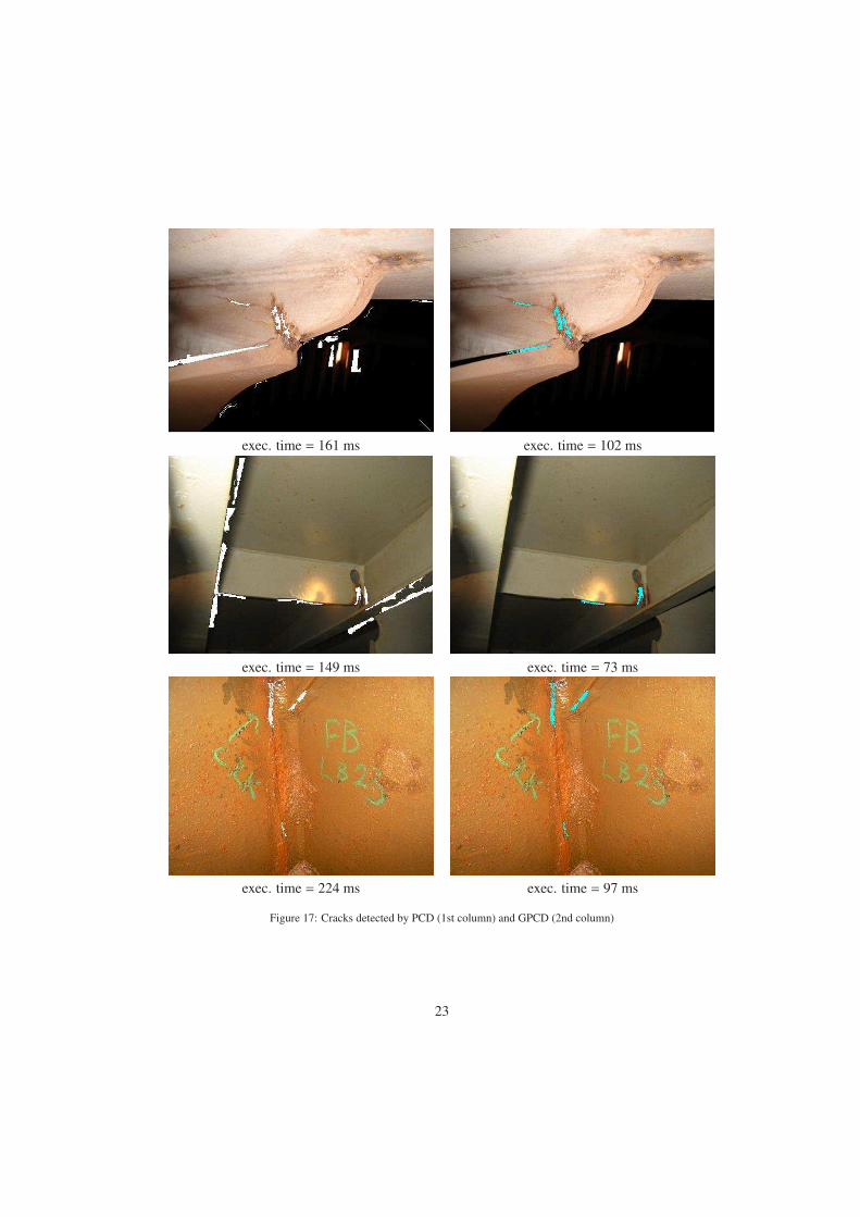
Figure 17 provides some classification outputs for theunguided and guided versions of the crack detector. Ascan be observed, the computation time falls below 50%for GPCD with regard to PCD. In fact, after testing over15 different images, a 3.13x speed up has been observedwhen using the guided version. Some values in this re-gard are shown in Table 9. Moreover, it is also worthobserving that the time reported for guided detection doesinclude the execution of the WCCD corrosion detector.The improvement in terms of time is thus even higher.

A second and very important enhancement that is ob-tained by means of the guidance is the reduction of thefalse positive detection rate, and consequently the im-provement of the classifier reliability. The values for thefalse positive and false negative percentages are 0.72%and 0.57%, respectively. Comparing with the percent-ages obtained without guidance, 2.29% and 0.47%, theimprovement is obvious.

As happened with all other detectors presented inthis report, the uncertainty defining ground truth imagescauses a high false negative rate (67.20%), while falsepositive rate is similar to the false positive percentage(0.73%).

As can be seen in Figure 17, both PCD and GPCD de-tect all the cracks from the images but the unguided ver-sion also marks other elongated, narrow and dark zones,e.g. shadows. GPCD, however, prevents the percolationof some of these false positives since corrosion has not

been detected there. Tables 2 and 5 indicates the param-eter values used to obtain the results shown in Figure 17for, respectively, PCD/GPCD and WCCD.

7. Conclusions

Several defect detection algorithms for support in ves-sel hull inspection have been presented in this report. Onthe one hand, a crack detection method based on a perco-lation idea, PCD, has been introduced and its performancehas been observed in the sense of being able to detect allthe cracks in the test images. Nevertheless, shadows andother crack-like collections of pixels were misclassified,increasing the false positive percentage.

On the other hand, two different corrosion detectionalgorithms have been introduced. The first one, CCD,is based on a supervised classification method that takesprofit from the distribution of color in corroded areas, andhas been significantly improved with the addition of a pre-vious decision stage based on a texture roughness crite-rion. The second corrosion detection algorithm, WCCD,has been built around a weak classifiers approach, separat-ing the spatial and colour analysis in two different stages.Both algorithms (CCD and WCCD) have presented goodperformance, with similar misclassification percentages,but WCCD performs the detection more than seven timesbefore than CCD.

As an additional contribution, WCCD has been usedto improve the performance of PCD. The results obtainedprove that the guided approach, GPCD, reduces more thanthree times the computation time with regard to the un-guided version, while the number of false positive de-tections is also reduced, and the classifier reliability in-creased.

Better results are expected for all the algorithms pro-posed by controlling the imaging process. If the poseand distance of the camera respect to the inspected sur-face could be controlled, the crack detection algorithmsparameters could be tuned for cracks of a specific size, aswell as the patch size could be adjusted for improving thecorrosion detection algorithms performance.

As for future work, WCCD is planned to be enhancedby means of an Adaptative Boosting (AdaBoost) [38]scheme to chain different weak classifiers in a moregrounded way. Before each stage, this method computes aweighting distribution to give emphasis to the incorrectly

22

exec. time = 161 ms exec. time = 102 ms



Figure 17: Cracks detected by PCD (1st column) and GPCD (2nd column)

23

Table 9: Comparison between elapsed times using PCD and GPCD

Pixels 120000 120000 144000 144000 157440 158880 162720 172800 177120PCD (ms) 140 412 190 68 182 795 656 342 111

GPCD (ms) 63 182 47 33 50 37 104 159 58

classified samples of previous stages. This strategy is suc-cessfully used by the Viola-Jones classifier [24, 42, 43]which is able to robustly detect complex structures, e.g.faces, in real-time.

Another research line to be investigated is around theconcept of saliency [20]. Considering corrosion andcracks as anomalies over metallic surfaces, saliency mapsturn out to be relevant tools to improve their detection.Furthermore, some other works, e.g. see [27, 46], givesother ways to work with corrosion that could be usefulfor that research.

Acknowledgements

This work is partially supported by FP7 project SCP8-GA-2009-233715 (MINOAS).

The author is thankful to Lloyd’s Register of Shipping(London, UK) and to RINA s.p.a. (Genova, Italy) for pro-viding the test images used in this study, and speciallygrateful to his tutor Alberto Ortiz, for his help and guid-ance.

Appendix: The Bilateral filter

The Bilateral filter is a simple filter that is very usedin image processing for noise reduction while preservingthe edges that appear in the image. It consists in a com-bination of two Gaussian filters. One works in the spatialdomain, thus takes into account the distance between apixel and its neighbours; the other one works in the rangedomain since it takes into account the difference betweenthe value (e.g. intensity) of a pixel and the values of itsneighbours.

Ib fp =

1

Wb fp

∑

qεS

Gσs (‖ p − q ‖)Gσr (| Ip − Iq |)Iq

where

Wb fp =

∑

qεS

Gσs (‖ p − q ‖)Gσr (| Ip − Iq |)

Gσ(x) = e−x2

2σ2

and S is set of pixels involved in the convolution.

References

[1] T. S. Akinfiev, M. A. Armada, and R. Fernandez.Nondestructive testing of the state of a ships hullwith an underwater robot. Russian Journal of Non-destructive Testing, 44(9):626–633, 2008.

[2] T. Amano. Correlation based image defect detec-tion. In Proceedings of the IAPR InternationalConference on Pattern Recognition, pages 163–166,2006.

[3] S. Avril, A. Vautrin, and Y. Surrel. Grid method:Application to the characterization of cracks. Ex-perimental Mechanics, 44(1):37–43, 2004.

[4] A. Baykuta, A. Atalay, A. Ercil, and M. Guler. Real-time defect inspection of textured surfaces. Real-Time Imaging, 6(1):17–27, 2000.

[5] C. Boukouvalas, J. Kittler, R. Marik, M. Mirmehdi,and M. Petrou. Ceramic tile inspection for colourand structural defects. Technical Report CS-EXT-1995-052, 1995. Also: Proceedings of AMPT95,pp. 390-399, 1995.

[6] A. Branca, F. P. Lovergine, G. Attolico, and A. Dis-tante. Defect detection on leather by oriented singu-larities. Computer Analysis of Images and Patterns,pages 223–230, 1997.

24

[7] N. Bryson, R. Dixon, J. Hunter, and C. Taylor. Con-textual classification of cracks. Image and VisionComputing, 12(3):149–154, 1994.

[8] C.-P. Hsu C.-L. Chang, H.-H. Chang. An intelligentdefect inspection technique for color filter. In Pro-ceedings of the IEEE International Conference onMechatronics, pages 933–936, 2005.

[9] A. Carvalho, L. Sagrilo, I. Silva, J. Rebello, andR. Carneval. On the reliability of an automatedultrasonic system for hull inspection in ship-basedoil production units. Applied Ocean Research,25(5):235–241, 2003.

[10] H. Castilho, J. Pinto, and A. Limas. An automateddefect detection based on optimized thresholding. InProceedings of the International Conference on Im-age Analysis and Recognition, volume 4142 of Lec-ture Notes in Computer Science, pages II:790–801,2006.

[11] C.-Y. Chang, J.-W. Chang, and M. D. Jeng. Anunsupervised self-organizing neural network for au-tomatic semiconductor wafer defect inspection. InProceedings of the IEEE International Conferenceon Robotics and Automation, pages 3000– 3005,2005.

[12] S. Cho, K. Hisatomi, and S. Hashimoto. Cracksand displacement feature extraction of the concreteblock surface. In Proceedings of the IAPR Work-shop on Machine Vision Applications, pages 246–249, 1998.

[13] A. Cormack. Ship hull inspections using AquaMap.Seventh International Symposium on Technologyand the Mine Problem, 2006.

[14] R. Damus, S. Desset, J. Morash, V. Polidoro,F. Hover, and C. Chryssostomidis. A new paradigmfor ship hull inspection using a holonomic hover-capable auv. Informatics in Control, Automation andRobotics I, pages 195–200, 2006.

[15] Y. Fucheng, Z. Lifan, and Z. Yongbin. The researchof printing’s image defect inspection based on ma-chine vision. In Proceedings of the IEEE Interna-tional Conference on Mechatronics and Automation,pages 2404–2408, 2009.

[16] Y. Fujita, Y. Mitani, and Y. Hamamoto. A methodfor crack detection on a concrete structure. In Pro-ceedings of the IAPR International Conference onPattern Recognition, pages III: 901–904, 2006.

[17] J. Hongbin, Y. Murphey, S. Jinajun, and C. Tzyy-Shuh. An intelligent real-time vision system for sur-face defect detection. In Proceedings of the IAPRInternational Conference on Pattern Recognition,pages III:239–242, 2004.

[18] B.K.P. Horn. Robot Vision. MIT Press, 1986.

[19] J. Iivarinen and A. Visa. An adaptive texture andshape based defect classification. In Proceedingsof the IAPR International Conference on PatternRecognition, pages I:117–122, 1998.

[20] Laurent Itti, Christof Koch, and Ernst Niebur. Amodel of saliency-based visual attention for rapidscene analysis. IEEE Transactions on Pattern Anal-ysis and Machine Intelligence, 20:1254–1259, 1998.

[21] B. C. Jiang, C. C. Wang, and P. L. Chen. Logis-tic regression tree applied to classify pcb golden fin-ger defects. The International Journal of AdvancedManufacturing Technology, 24(7-8):496–502, 2004.

[22] A. Kumar and G. Pang. Defect detection in tex-tured materials using optimized filters. IEEE Trans-actions on Systems, Man and Cybernetics Part B,32(5):553–570, 2002.

[23] A. Kumar and H. Shen. Texture inspection for de-fects using neural networks and support vector ma-chines. In Proceedings of the IEEE InternationalConference on Image Processing, pages III:353–356, 2002.

[24] R. Lienhart and J. Maydt. An extended set of haar-like features for rapid object detection. In Proceed-ings of IEEE International Conference on ImageProcessing, pages I: 900–903, 2002.

[25] L. Liu and G. Meng. Crack detection in supportedbeams based on neural network and support vectormachine. In Advances in Neural Networks, volume3498 of Lecture Notes in Computer Science, pages597–602, 2005.

25

[26] C.-J. Lu and D.-M. Tsai. Automated defects inspec-tion for lcd using singular value decomposition. In-ternal Journal of Advanced Manufacturing Technol-ogy, 25(1-2):53–61, 2005.

[27] D. Martin, D. M. Guinea, M. C. Garca-Alegre,E.Villanueva, and D. Guinea. Multi-modal defectdetection of residual oxide scale on a cold stain-less steel strip. Machine Vision and Applications,21(5):653 – 666, 2010.

[28] R. Oullette, M. Browne, and K. Hirasawa. Ge-netic algorithm optimization of a convolutional neu-ral network for autonomous crack detection. InProceedings of the IEEE Congress on EvolutionaryComputation, pages I:516 – 521, 2004.

[29] P. Perner. A knowledge-based image-inspection sys-tem for automatic defect recognition, classification,and process diagnosis. Machine Vision and Applica-tions, 7(3):135–147, 1994.

[30] W. Pratt. Digital Image Processing. John Wiley andSons, 2nd edition, 1991.

[31] M. A. Rodrigues and Y. Liu. A novel 3d-2d com-puter vision algorithm for automatic inspection offilter components. In Proceedings of the interna-tional conference on Industrial and engineering ap-plications of artificial intelligence and expert sys-tems, pages 560–569, 1999.

[32] S.Negahdaripour and P. Firoozfam. An rov stere-ovision system for ship hull inspection. Interna-tional Journal of Oceanic Engineering, 31(3):551–564, 2006.

[33] J. Sobral. Optimised filters for texture defect detec-tion. In Proceedings of the IEEE International Con-ference on Image Processing, pages III:565–568,2005.

[34] K. Song, M. Petrou, and J. Kittler. Texture crack de-tection. Machine Vision and Applications, 8(1):63–76, 1995.

[35] S. Sorncharean and S. Phiphobmongkol. Crack de-tection on asphalt surface image using enhanced gridcell analysis. In Proceedings of IEEE International

Symposium on Electronic Design, Test & Applica-tions, pages 49–54, 2008.

[36] P. Subirats, J. Dumoulin, V. Legeay, and D. Barba.Automation of pavement surface crack detection us-ing the continuous wavelet transform. In Proceed-ings of the IEEE International Conference on ImageProcessing, pages 3037–3040, 2006.

[37] N. Tanaka and K. Uematsu. A crack detectionmethod in road surface images using morphology.In Proceedings of the IAPR Workshop on MachineVision Applications, pages 154–157, 1998.

[38] S. Theodoridis and K. Koutroumbas. Pattern Recog-nition, 3rd Edition. Academic Press, 2006.

[39] C. Tomasi and R. Manduchi. Bilateral filteringfor gray and color images. In Proceedings of theIEEE International Conference on Computer Vision,pages 839 – 846, 1998.

[40] D.-M. Tsai and S.-K. Wu. Automated surface in-spection using gabor filters. Internal Journal of Ad-vanced Manufacturing Technology, 16(7):474–482,2000.

[41] J. Vaganay, M. Elkins, S. Willcox, F. Hover,R. Damus, S. Desset, J. Morash, and V.Pollidoro.Ship hull inspection by hull-relative navigation andcontrol. In Proceedings of MTS/IEEE Oceans, pagesI: 761–766, 2005.

[42] P. Viola and M. Jones. Robust real-time object de-tection. In Proceedings of International Workshopon Statistical and Computational Theories of Vision- Modeling, Learning, Computing and Sampling,2001.

[43] P. Viola and M. Jones. Robust real-time face de-tection. International Journal of Computer Vision,57(2):137–154, 2004.

[44] P. Woods and P. Allen. A cue generator for crackdetection. Image and Vision Computing, 7(4):268–273, 1989.

[45] X. Xie and M. Mirmehdi. Localising surface defectsin random colour textures using multiscale texem

26

analysis in image eigenchannels. In Proceedings ofthe IEEE International Conference on Image Pro-cessing, pages III: 1124–1127, 2005.

[46] S. Xu and Y. Weng. A new approach to estimatefractal dimensions of corrosion images. PatternRecogn. Lett., 27(16):1942–1947, 2006.

[47] T. Yamaguchi and S. Hashimoto. Fast crack detec-tion method for large-size concrete surface imagesusing percolation-based image processing. MachineVision and Applications, 21(5):797–809, 2010.

[48] M. Yoshioka and S. Omatu. Defect detectionmethod using rotational morphology. Artificial Lifeand Robotics, 14(1):20–23, 2009.

[49] T. Zhang and G. Nagy. Surface tortuosity and itsapplication to analyzing cracks in concrete. In Pro-ceedings of the IAPR International Conference onPattern Recognition, pages 851–854, 2004.

[50] X. Zhang, R. Liang, Y. Ding, J. Chen, D. Duan, andG. Zong. The system of copper strips surface de-fects inspection based on intelligent fusion. In Pro-ceedings of the IEEE International Conference onAutomation and Logistics, pages 476–480, 2008.

[51] H. Zheng, L. Kongb, and S. Nahavandia. Automaticinspection of metallic surface defects using geneticalgorithms. Journal of Materials Processing Tech-nology, 125-126:427–433, 2002.

27

detection of cracks and corrosion for automated...

Documents