detection of multiple low-energy impact damage in composites plates ... · detection of multiple...

Detection of Multiple Low-Energy Impact Damage in Composites Plates Using Lamb Wave Technique

Pedro André Viegas Ochôa de Carvalho

Dissertação para obtenção do Grau de Mestre em

Engenharia Aeroespacial

Júri Presidente: Prof. Fernando José Parracho Lau

Orientador: Prof. Virgínia Isabel Infante

Vogal: Prof. Rosa Marat-Mendes

Outubro 2011

The suppression of uncomfortable ideas may be common in

religion and politics, but it is not the path to knowledge; it

has no place in the endeavor of science.

Carl Sagan in “Cosmos”

v

Abstract

The increasing demand for more efficient aircraft has boosted the development of lightweight

structures. However, due to lack of ability to predict damage evolution in composites, the certification

requirements imposed by the airworthiness authorities are still conservative representing an obstacle to energy

efficiency. Hence, along with the research for new composite materials, there has been an active investigation

into more accurate, efficient and cost-effective Non-Destructive Testing (NDT) techniques. These technologies

allow in-service structural health monitoring, better quality control during production and easier evaluation of

structural integrity during maintenance. As a result, it is possible to increase reliability and maintainability, and

to reduce the utilisation costs. Ultimately, NDT techniques help to move towards more damage tolerant

composite structures.

This work concerns the assessment of the suitability of the Lamb wave method, in particular of the two

zero-order Lamb modes (A0 and S0), to detect multiple barely-visible impact damage in composite material. Four

plates were produced with carbon-epoxy cured pre-preg, using a representative stacking sequence. Three

specimens were subjected to multiple impact damage at three different low-energy levels, and one was left as an

undamaged reference sample. Ultrasonic Lamb wave modes were selectively generated by surface-bonded

piezoceramic wafer transducers in two tuned configurations. A signal identification algorithm in the time-scale

domain based on the Akaike Information Criterion (AIC) was used to determine the group velocity of the Lamb

modes.

The effectiveness of the Lamb wave method was successfully verified on all damage scenarios, since

the 5 and 10 J damages were undoubtedly detected by the S0 mode configuration. The results were validated by

digital Shearography, ultrasonic C-scan, and optical microscope observations, revealing strong consistency. For

the material tested, the detection threshold of the three NDT methods was found to be between 3 and 5 J.

Keywords: Composite materials, Non-Destructive Testing (NDT), Lamb wave, multiple barely-visible impact

damage, piezoceramic transducers.

vii

Resumo

A crescente busca por aeronaves mais eficientes tem promovido o desenvolvimento de estruturas ultra-

leves. Porém, devido à imprevisibilidade da evolução de dano em materiais compósitos, os requisitos de

certificação impostos pelas autoridades de segurança aérea são ainda conservadores, o que acaba por representar

um obstáculo à eficiência energética. Assim, a par de estudos sobre novos materiais compósitos, tem havido uma

forte actividade de investigação em técnicas de inspecção não destrutivas (NDT) mais precisas, eficientes e

rentáveis. Estas tecnologias permitem a monitorização da saúde das estruturas em plena operação, melhor

controlo de qualidade na fase de produção e uma avaliação mais fácil da integridade estrutural. Como resultado,

a fiabilidade e a capacidade de manutenção aumentam, e os custos de utilização diminuem. Em última análise, as

técnicas NDT permitem o desenvolvimento de estruturas em material compósito com maior tolerância ao dano.

Este estudo aborda a capacidade do método das ondas de Lamb, e em particular dos dois modos

fundamentais (A0 e S0), para detectar dano de múltiplos impactos de baixa energia, em material compósito.

Quatro placas foram produzidas em tecido de fibra de carbono pré-impregnada, usando um empilhamento

representativo de uma aplicação aeronáutica. Três desses provetes foram danificados através de impactos

múltiplos, com três níveis de energia diferentes, e outro foi usado como amostra de referência não danificada. As

ondas de Lamb ultra-sónicas foram geradas através de transdutores peizoeléctricos finos, dispostos em duas

configurações optimizadas para a excitação selectiva de cada um dos referidos modos. A determinação da

velocidade de grupo dos modos de onda de Lamb foi efectuada por um algoritmo de identificação de sinais no

domínio de tempo, baseado no Critério de Informação de Akaike (AIC).

A eficácia do método das ondas de Lamb foi comprovada com sucesso para todos os casos, tendo sido

possível detectar claramente os danos de 5 e 10 J com a configuração para o modo S0. Os resultados foram

validados através de shearografia digital, C-scan e observações microscópicas, revelando uma forte coerência

entre todas as técnicas. Para o material testado, o limiar de detecção encontrado para os três métodos NDT foi

entre 3 e 5 J de energia de impacto.

Palavras-chave: Materiais compósitos, técnicas NDT, ondas de Lamb, dano de múltiplos impactos de baixa

energia, transdutores piezoeléctricos.

ix

Acknowledgements

First of all, I would like to express my gratitude to Dr. Roger Groves, head of the OptoNDT Laboratory,

who accepted me as his guest researcher, even though he knew about the difficulties that would lie ahead. The

successful web conferencing arranged by him greatly helped me to keep on schedule. He believed in my project,

providing me all the necessary means to carry out the investigation, and was always available to discuss

problems and new ideas. He encouraged my decisions, but never hesitated to see things critically, so that the best

results would always be achieved.

I would also like to thank my supervisor in IST, Professor Virgínia Infante, for her proactive guidance

throughout the thesis, especially regarding the possibility of submitting a conference paper. She was always

patient and played an important role in the review of the work by inviting Professor José Miguel Silva to be co-

advisor of the thesis, to whom I also thank.

I am very grateful to students Eduardo Corso Krutul, for performing the digital Shearography tests,

Mathieux Gauthier, for his precious help in manufacturing the composite specimens, Freddy Moriniere, for

helping me in the application of impact damage, and Nick Miesen and Mariana Melo Mota, for teaching me the

procedure for the Lamb wave method. For all the pleasant and cheerful coffee breaks I thank all the students

from the Fish tank room.

Special thanks go to all the technicians in the Aerospace Structures and Materials Laboratory, and to

Mr. Karel Heller, who allowed me to use the equipment in the Applied Geophysics and Petrophysics Laboratory.

This project would not have been possible without my Portuguese friends Guilherme Trigo, Hugo

Lopes, Nuno Santos, Pedro Simplício and Tiago Milhano, who provided me shelter in the last months of my stay

in The Netherlands. We had the honour and pleasure of sharing amazing moments, and overcoming the daily

obstacles together. To all the other international students thank you for making the sun shine in Marcushof.

A special thank to my friends in Portugal and France, whose memory is always with me.

Finally, I am deeply grateful to my family, especially my parents and my sister, who have opened my

eyes to the importance of being an active part of this world. Even from afar, they showed their love and

affection, supporting me through this transitional journey.

Lisbon, Instituto Superior Técnico Pedro André Viegas Ochôa de Carvalho

September 28th, 2011

xi

Contents

Abstract .................................................................................................................................................. v

Resumo ................................................................................................................................................. vii

Acknowledgements ............................................................................................................................... ix

List of figures ...................................................................................................................................... xiii

List of tables ....................................................................................................................................... xvii

List of acronyms ................................................................................................................................. xix

List of symbols .................................................................................................................................... xxi

1 Introduction ........................................................................................................................................ 1

1.1 Motivation ..................................................................................................................................... 1

1.2 Overview ....................................................................................................................................... 2

2 Composite materials: theory and applications ................................................................................ 3

2.1 Composite structures in aircraft industry ...................................................................................... 3

2.2 Theoretical models for composite laminates ................................................................................. 5

2.2.1 Classical Laminated Plate Theory (CLPT) ............................................................................. 6

2.3 Damage Mechanisms in Composite Materials ............................................................................ 13

2.3.1 Fatigue damage ..................................................................................................................... 13

2.3.2 Low-Velocity Impact Damage ............................................................................................. 14

3 Non-Destructive Testing (NDT) techniques ................................................................................... 17

3.1 Lamb wave method ..................................................................................................................... 19

3.1.1 Physics of Lamb waves ........................................................................................................ 19

3.1.2 Generation and acquisition of Lamb waves ......................................................................... 24

3.1.3 Lamb wave response optimization ....................................................................................... 26

3.1.4 Digital signal processing ...................................................................................................... 29

3.1.5 Algorithm for damage detection ........................................................................................... 30

3.2 Digital Shearography ................................................................................................................... 32

3.2.1 Fundamentals of digital Shearography ................................................................................. 32

3.2.2 Image processing .................................................................................................................. 37

3.3 Ultrasonic C-scan ........................................................................................................................ 38

4 Experimental procedure .................................................................................................................. 41

4.1 Phase 1 – Preliminary approach .................................................................................................. 41

xii

4.1.1 Manufacturing of composite samples ................................................................................... 41

4.1.2 Lamb wave tests ................................................................................................................... 43

4.2 Phase 2 – Study of NDT methods ............................................................................................... 47

4.2.1 Sample manufacturing .......................................................................................................... 47

4.2.2 Quality control ...................................................................................................................... 47

4.2.3 Application of multiple low-velocity impact damage .......................................................... 48

4.2.4 Ultrasonic C-scan tests ......................................................................................................... 50

4.2.5 Digital Shearography tests .................................................................................................... 50

4.2.6 Lamb wave tests ................................................................................................................... 51

4.2.7 Optical microscope observations .......................................................................................... 55

5 Results and discussion ...................................................................................................................... 57

5.1 Lamb wave method ..................................................................................................................... 57

5.2 Digital Shearography ................................................................................................................... 67

5.3 Ultrasonic C-scan ........................................................................................................................ 78

5.4 Optical microscope ...................................................................................................................... 82

6 Conclusions and recommendations................................................................................................. 85

6.1 Conclusions ................................................................................................................................. 85

6.2 Recommendations for future developments ................................................................................ 86

References ............................................................................................................................................ 89

A MATLAB® codes ............................................................................................................................ 97

A.1 Calculation of the laminate properties ........................................................................................ 97

A.2 Determination of the Lamb wave dispersion curves .................................................................. 98

B AIC-picker LabVIEW® code ....................................................................................................... 103

C Clamping device drawings ............................................................................................................ 105

xiii

List of figures

Figure 1.1 – The concept of structure cost effectiveness ……………………………………………………. 2

Figure 2.1 – Boeing aircraft wing skin, manufactures with Cytec prepreg. [6]…..............…………............. 4

Figure 2.2 – Composite fraction of the structural weight for Boeing 787. [14]…………..............…............. 5

Figure 2.3 – Stacking of plies with different fibre orientations to form a laminate. [16]…............................. 6

Figure 2.4 – Unidirectional lamina, with the x1-axis parallel to the fibres. [16]……..............……................ 8

Figure 2.5 – The relation between local and global coordinate systems for an unidirectional lamina. [16].... 9

Figure 2.6 – Matrix crack and debonding of composite lamina under off-axis cyclic loading. [19]............... 14

Figure 2.7 – Typical trapezoidal distribution of low-velocity impact damage in composites laminates. [20] 15

Figure 3.1 – Propagation of guided waves. [55]……...............................................………………................ 19

Figure 3.2 – Geometry for the wave propagation problem………………………………………….............. 20

Figure 3.3 – Lamb wave particle motion: (a) symmetric motion, (b) anti-symmetric motion. [56]................ 20

Figure 3.4 – Simulated displacements field for the (a) S0 Lamb mode, and (b) A0 Lamb mode. [56]............ 21

Figure 3.5 – Phase velocity dispersion curves for an isotropic material with cl = 7199.55 m/s, ct = 3367.60

m/s, and a thickness of 2.24 mm ………………………………………………………….............................. 22

Figure 3.6 – Group velocity dispersion curves for an isotropic material with cl = 7199.55 m/s, ct = 3367.60

m/s, and a thickness of 2.24 mm....................................................................................................................... 23

Figure 3.7 – Dispersion phenomenon at three different locations of a structure. [56]……............................. 23

Figure 3.8 – Electric field and polarization in a piezoelectric plate. [56]………..............………….............. 25

Figure 3.9 – Possible actuator/sensor configurations for the Lamb wave method: a) pitch-catch, b) pulse-

echo. [54]………………………………………….............…………………………………......................... 26

Figure 3.10 – Wavelength tuning effect. [55]……………………………………...............………................ 26

Figure 3.11 – Improvement of the Lamb mode selection by using rectangular PZT wafer transducers…...... 27

Figure 3.12 – Improvement of the Lamb wave mode selection by using circular PZT wafer transducers…. 27

Figure 3.13 - Time and frequency domain contents for pure sinusoidal bursts with a) 1 cycle, and b) 5

cycles…............................................................................................................................................................ 28

Figure 3.14 - Time and frequency domain contents for sinusoidal tone-bursts, with by a) 1 cycle and

modified by an amplitude increase, and b) with 5 cycles modified by a Hanning function windowing

process….......................................................................................................................................................... 29

Figure 3.15 – Typical Lamb wave response from a composite plate excited with a PZT wafer transducer... 31

Figure 3.16 – Generation of two sheared images using the modified Michelson interferometer. [64]............ 32

Figure 3.17 – Difference in the laser light path between two object points, in the undeformed and

deformed states. [64]…….............…………………………………………………………………............... 33

Figure 3.18 – Typical fringe pattern of a shearogram. [64]……………………………...............…............... 34

xiv

Figure 3.19 – Shearography setup. [64]............................................................................................................ 35

Figure 3.20 – Through-thickness C-scan technique. [33]…………………………..............………............... 39

Figure 3.21 – Pulse-echo C-scan technique. [33]…………………………….............……………................ 39

Figure 4.1 - Steps of the manufacturing process: a) automatic cutting of the prepreg material, b) curing

process in the autoclave, c) cured laminated plate, and d) four 110 x 110 x 3.36 mm3 specimens…………. 42

Figure 4.2 – Phase velocity dispersion curves for Laminate 1……………………………………................. 43

Figure 4.3 – Group velocity dispersion curves for Laminate 1……………………………………................ 44

Figure 4.4 – Experimental setup for test sessions 1, 2 and 3: a) position of the actuator and sensors on the

specimen, b) detail of the adhesion of the sensors, and c) overall view of the experimental installation….... 45

Figure 4.5 – Panametrics V103 PZT actuator and the two HF-1.2 PZT sensors……………………............. 46

Figure 4.6 – C-scan system: a) overall view of the setup b) detail of the ultrasonic probes and the

alignment of the water jets…………………………………………………………………………................ 47

Figure 4.7 – Tools for the application of impact damage: a) impact tower, b) original clamping device, and

c) new clamping device…………………………………………………………………................................ 48

Figure 4.8 – Impact pattern…………………………………………………………………………............... 49

Figure 4.9 – Application of BVID on the plates: a) steel impactor with a hemispherical heat, b) installation

of the specimen between the bolted aluminium frames…………………………………................................ 50

Figure 4.10 – Digital Shearography setup…………………………………………………………................ 51

Figure 4.11 – Detailed view of the electric circuit for the a) A0 configuration, and for the b) S0

configuration (upper surface)………………………………………………………………………............... 53

Figure 4.12 - Distances between actuator and sensor, and between two sensors…………………................. 53

Figure 4.13 – Three levels of detail: a) setup for Lamb wave measurements in Phase 2, b) the two actuator

configurations and the two PZT sensors, and c) installation of one of the PZT sensors….............................. 54

Figure 4.14 – Excitation signal for the damaged specimens: 1 cycle-sinusoidal tone-burst at 500 kHz (the

real amplitude was 10 times higher)………………………………………………………............................. 55

Figure 5.1 – AIC-picker program window....................................................................................................... 58

Figure 5.2 –Response of healthy sample for the A0 configuration, at 500 kHz, extracted a) from channel 1,

and b) from channel 2……………………………………………………………………............................... 59

Figure 5.3 - Response of healthy sample for the S0 configuration, at 500 kHz, extracted a) from channel 1,

and b) from channel 2……………………………………………………………………............................... 59

Figure 5.4 – Comparison between experimental and theoretical dispersion curves………………................ 60

Figure 5.5 - Signals from channel 1, for the A0 configuration at 500 kHz, for impact energies of a) 3 J, b)

5 J, and c) 10 J…………………………………………………………………………….............................. 61

Figure 5.6 – Signals from channel 2, for the A0 configuration at 500 kHz, for impact energies of a) 3 J, b)

5 J, and c) 10 J…………………………………………………………………………….............................. 62

Figure 5.7 - Signals from channel 1, for the S0 configuration at 500 kHz, for impact energies of a) 3 J, b) 5

J, and c) 10 J………………………………………………………………………………............................. 62

Figure 5.8 - Signals from channel 2, for the S0 configuration at 500 kHz, for impact energies of a) 3 J, b) 5

J, and c) 10 J………………………………………………………………………………............................. 63

xv

Figure 5.9 – Lag and attenuation coefficients for a) A0 configuration, channel 2, b) S0 configuration,

channel 1, and c) S0 configuration, channel 2………………………………………...................................... 64

Figure 5.10 - Shearograms for the undamaged specimen, for 5 seconds of heating, with a) x-shear, and b)

y-shear…………………………………………………………………………………................................... 68

Figure 5.11 - Shearograms for the 3 J specimens, with x shear, loaded for a) 5s b) 10s, and c) 15 s.............. 69

Figure 5.12 - Shearograms for the 3 J specimens, with y shear, loaded for a) 5s b) 10s, and c) 15 s.............. 70

Figure 5.13 - Shearograms for the 5 J specimens, with x shear, loaded for a) 5s b) 10s, and c) 15 s.............. 71

Figure 5.14 - Shearograms for the 5 J specimens, with y shear, loaded for a) 5s b) 10s, and c) 15 s.............. 72

Figure 5.15 - Shearograms for the 10 J specimens, with x shear, loaded for a) 5s b) 10s, and c)

15s…………………............………………………………………………………………………................. 73

Figure 5.16 - Shearograms for the 10 J specimens, with y shear, loaded for a) 5s b) 10s, and c)

15s…………………………………................................................................................................................. 74

Figure 5.17 – Attenuation map of the healthy sample……………………………………………….............. 79

Figure 5.18 – Attenuation maps of the damaged specimens: a) 3 J, b) 5 J, and c) 10 J……………............... 80

Figure 5.19 – Microscopic observations of the surface of the damaged specimen: a) 3 J impact, b) 5 J

impact, and c) 10 J impact……………………………………........................................................................ 83

Figure 5.20 – Details of the 45 cracks of the 10 J impact: a) crack tip, b) middle of the crack……............... 84

Figure B.1 – LabVIEW code used for AIC-picker…………………………………………………............... 103

xvii

List of tables

Table 4.1 - Properties of the M30SC/DT 120 UD prepreg. [65]………………….......................................... 41

Table 4.2 –Mechanical properties of Laminate 1…………………………………………............................. 42

Table 4.3 – Approximate acoustic properties of Laminate 1………………………………………................ 43

Table 4.4 – Properties of the Physik Instrument PZT wafer actuators. [67]…....……................…................ 52

Table 4.5 – Properties of Physical Acoustics Pico HF-1.2 PZT sensors. [68]………................……............. 52

Table 4.6 – Values of the distances indicated in figure 4.11, for each specimen…………………................. 53

Table 4.7 – Size of the moving-average filter as a function of the resolution enhancement. [69]…………... 56

Table 5.1 – Shearography results: damage areas of the ten impact points for the 5 J specimen, with 5 s

heating………………………………………………………………………………………........................... 75

Table 5.2 - Shearography results: damage areas of the ten impact points for the 5 J specimen, with 10 s

heating…………………………………………………………………………………………....................... 75


heating…………………………………………………………………………………………....................... 76


heating………………………………………………………………………………………........................... 76


heating……………………………………………………………………………………............................... 77

Table 5.6 – Shearography results: damage areas of the ten impact points for the 10 J specimen, with 15 s

heating……………………………………………………………………………………............................... 77

Table 5.7 – C-scan results: Damage areas of the ten impact points for the 5 and 10 J specimens................... 81

Table 5.8 – Damage areas of the circular impact spots observed by optical microscope…………................ 82

xix

List of acronyms

AIC Akaike Information Criterion

AE Acoustic Emission

BVID Barely-Visible Impact Damage

CFRP Carbon-Fiber Reinforced Plastic

CLPT Classical Laminated Plate Theory

ESL Equivalent Single-Layer

ESPI Electronic Speckle Pattern Interferometry

FBG Fibre Bragg Grating

GFRP Glass-Fibre Reinforced Plastic

MDF Medium-Density Fibreboard

NDT Non-Destructive Testing

NDE Non-Destructive Evaluation

NDI Non-Destructive Inspection

NRUS Nonlinear Resonance Ultrasound

NWMS Nonlinear Wave Modulation Spectroscopy

PZT Lead zirconate titanate piezoelectric ceramic material

RTM Resin Transfer Moulding

SEHIT Second Harmonic Imaging Technique

SHM Structural Health Monitoring

SPSI Speckle Pattern Shearing Interferometry

TOF Time-of-Flight

xxi

List of symbols

Greek symbols

γ Modulation of the amplitude interference of an interferogram

δw Infinitesiamal out-of-plane deformation of the loaded object in a Shearography test

Δ Distribution of the phase change in a shearogram

ε Mechanical strain tensor

ε(0) Membrane contribution of the strain tensor

ε(1) Flexural contribution of the strain tensor

ζ Non-dimensional parameter used to describe Lamb wave propagation in isotropic material

θ Fibre orientation angle, or laser light phase angle

θxz Angle of illumination in the xz-plane

λ Wavelength, or Lamé’s first constant

µ Lamé’s second constant

ν Poisson’s ratio

ξ Non-dimensional parameter used to describe Lamb wave propagation in isotropic material

ρ Material density

σ Mechanical stress tensor

φ Phase increment applied in the phase-shifting Shearography

ϕ Relative phase distribution in an interferogram

ω Angular frequency of a sinusoidal wave

Roman symbols

A1, A2, ... Higher-order anti-symmetric Lamb wave modes

Ad, Ad Amplitudes of the damaged and undamaged Lamb wave response

Ai,j Extensional stiffness matrix of a laminate

A0 Zero-order anti-symmetric Lamb wave mode

[A] Extensional stiffness matrix of a laminate

Bi,j Bending-extensional coupling stiffness matrix of a laminate

[B] Bending-extensional coupling stiffness matrix of a laminate

cg Group velocity

cl Longitudinal wave velocity

cp Phase velocity

ct Transverse wave velocity

C Material stiffness tensor, or Shearography sensitivity coefficient relative to the out-of-plane

strain, or position of the CCD camera

xxii

[C] Material stiffness tensor

CV Coefficient of variation

d Half thickness of a plate

Non-dimensional parameter used to describe Lamb wave propagation in isotropic material

dx, dy Shear amounts applied in the x and y directs, respectively

dL1, dL2 Light path changes due to loading of the object

[d] Piezoelectric strain coefficients

Di,j Bending stiffness matrix of a laminate

[D] Bending stiffness matrix of a laminate

{D} Electric displacement

[e] Dielectric permittivity

E Young’s modulus, or impact energy

Epg Gravitational potential energy

{E} Electric field

f Frequency of a sinusoidal wave

g Gravitational acceleration

g(i,j) Gray values of the pixels in a shearogram

G Shear modulus

h Thickness of the a laminate, or drop height of the impactor

H Hanning function

ie Inter-element distance

I Intensity distribution of an interferogram

I0 Mean value of the intensity distribution of an interferogram

I1, I2, I3, I4 Intensities used to calculate the relative phase distribution of an interferogram

Is Intensity distribution in a shearogram

k Wavenumber

ks Shearography sensitivity vector

k(i,j) Phase map filtering coefficients for the gray values of the pixels in a shearogram

L Transformation matrix for the symmetry planes of a lamina

m Impactor mass

M Mirror of the interferometer, or size of the moving-average filter

{M} Resultant moment on a laminate

N Number of plies in a laminate, or length of a time series, or number of cycles in a sinusoidal

burst

{N} Resultant forces on a laminate

P Electric polarization in a PZT wafer transducer

P1, P2 Generic points on the object surface

R Acquired signal in the time-domain

Rc Distance from the object to the CCD camera

xxiii

Rs Distance from the laser to the object

[R] Inverse transformation matrix from global laminate to local lamina coordinate system

s Amplitude-modulated sinusoidal tone-burst

S Material compliance tensor, or position of the laser source

S0 Zero-order symmetric Lamb wave mode

S1, S2, ... Higher-order symmetric Lamb wave modes

SH0 Zero-order shear-horizontal wave mode

t Time

[T] Direct transformation matrix from local lamina to global laminate coordinate system

vd, vu Group velocities of the damaged and undamaged Lamb wave response

V Volume fraction in the material, or voltage, or the gray value

(x1, x2, x3) Local lamina coordinate system

(x, y, z) Global laminate coordinate system, or position of the object in the Shearography setup

(xc, yc, zc) Position of the camera in the Shearography setup

(xs, ys, zs) Position of the laser light source in the Shearography setup

Superscripts

* Quantity relative to the deformed state of the object

T Transpose operation

(k) Kth lamina in the laminate stacking sequence

Subscripts

1, 2, 3 Quantity relative to the principal directions

1, 2, 3, 4, 5, 6 Quantity relative to the principal directions in the single-subscript notation

f Quantity for the fibre material

m Quantity relative to the local lamina coordinate system, or quantity for the matrix material, or

mean value

p Quantity relative to the global laminate coordinate system

w Quantity relative to the wave

x, y, z Quantity relative to the global directions

1

Chapter 1

Introduction

1.1 Motivation

There is a growing concern in the aircraft industry to increase the ratio of the structure effectiveness to

the acquisition and utilization costs, which is called structure cost-effectiveness [1]. Assuming the acquisition

costs depicted in figure 1.1 are fixed, one of the major steps towards the reduction of utilization costs and the

increase of structure effectiveness has been the widespread use of composite materials. Their excellent strength-

to-weight ratio maximizes the structure capability. Their corrosion and fatigue resistance increases the time to

failure, increasing reliability and reducing maintenance costs. Furthermore, their low density allows lower fuel

consumption, and therefore lower operation costs.

However, contrary to metallic materials, one of the most serious issues related to the use of composites

in airframes is their brittle behaviour in the presence of barely-visible impact damage (BVID), which may lead to

unexpected failure under fatigue loading [2]. Therefore, the Non-Destructive Testing (NDT) techniques, that

have already proven to be able to enhance safety, integrity and durability of aircraft structures over the last fifty

years, combined with the recently developed measuring and computational technologies, assume a central role in

the implementation of Structural Health Monitoring (SHM) systems. These systems continuously evaluate the

state of the structure, allowing the real-time identification of BVID, and the estimation of the remaining service

life according to the type of performance of the aircraft. If the damage severity is below a previously established

value, then the component is kept operating. Therefore, an effective SHM system minimizes the ground time for

inspections, increases the availability, and allows a reduction of the total maintenance cost by more than 30% for

an aircraft fleet [3]. The NDT methods for an SHM system should be capable of reliably detecting the damage-

induced changes in local and global properties, which are encoded in the dynamic response of the structure.

Among them the Lamb wave method has been reported as “one of the most encouraging tools for quantitative

identification of damage in composite structures” [4].

2

Figure 1.1 – The concept of structure cost effectiveness

The main goal of this study was to assess the suitability of the Lamb wave method, in particular of the

fundamental Lamb modes, to detect three different levels of multiple BVID on carbon-epoxy composite plates,

and, if possible, to improve its diagnosis capabilities. Digital Shearography with thermal loading and ultrasonic

C-scan were used to substantiate the results from the Lamb wave tests. The comparison between these two

additional NDT methods is expected to yield important conclusions about their sensitivity to BVID, and

contribute to an improvement of the quality control capability, which is also a means to increase structure

reliability.

1.2 Overview

This thesis is divided in six chapters. After the introduction, Chapter 2 contains all the theoretical and

practical aspects related to composite materials that are relevant for this study. It includes some examples of

composite structures in the aircraft industry, the Classical Laminated Plate Theory, a simple mathematical model

used to estimate the mechanical properties of composite plates which are crucial to simulate the Lamb wave

propagation, and the mechanisms of low-velocity impact damage and their relationship with fatigue damage. In

Chapter 3, the fundamentals of the three NDT methods are thoroughly reviewed. The experimental procedures

for the two phases of non-destructive tests are described in Chapter 4. The experimental results are presented and

discussed in Chapter 5. Finally, Chapter 6 summarizes the main conclusions and gives recommendations for

future developments.

This thesis was a joint project between Instituto Superior Técnico, Technical University of Lisbon, and

the Faculty of Aerospace Engineering, Delft University of Technology. The experimental part was performed in

the OptoNDT Laboratory, in the Faculty of Aerospace Engineering of TU Delft, and in the Applied Geophysics

and Petrophysics Laboratory, in the Faculty of Civil Engineering and Geosciences of TU Delft.

Structure cost effectiveness

Structure effectiveness

Capability

Structure efficiency

Availability

Reliability

Maintainability

Acquisition costs

Development Production

Labour

Materials

Equipment

Building

Introduction

Utilization costs

Maintenance

Operation

Ecological

3

Chapter 2

Composite materials: theory and applications

2.1 Composite structures in aircraft industry

From the boron/epoxy skins of the empennage of the Grumman F-14 and the McDonnell Douglas F-15

U.S. fighters [5], up to the modern pre-impregnated carbon-epoxy wing skins and fuselages of the Boeing 787

[6], composite materials have evolved tremendously. In a historical perspective, Jones [7] refers that one of the

first applications in military aviation was a boron-epoxy doubler glued on the F-111 wing-pivot fitting, in order

to prevent further fatigue cracking in that area. In a different approach, the Vought experimental speedbrake and

the Vought S-3A spoiler were entirely designed with graphite-epoxy composites. Later, the McDonnell Douglas

F-18A and the McDonnell AV-8B Harrier had their vertical fin, wings and horizontal tail surfaces also made of

graphite-epoxy composite material [7]. For modern fighters like Lockheed Martin F-22 both Jones [7] and Deo

et al. [5] refer that their composite fraction of the structural weight “seems to be levelling off at 30%”. In civil

aviation, the first applications were on the carbon-epoxy vertical surface of both the Airbus A300/A310 and

Lockheed L-1011. In 2001, Deo et al. [5] stated that composite usage for transport aircraft was around 20%. For

helicopter manufacturers, Megson [8] talks about significant service life extensions and efficient aerodynamic

profile introduction in rotor blades due to the use of carbon fibre reinforced plastics (CFRP’s).

From the examples mentioned above, it should be noted that CFRP’s are the most widely used advanced

composite materials in the aircraft industry. Their properties enable them to achieve great structural

performance. According to Megson [8], “CFRP has a modulus of the order of three times that of glass fibre-

reinforced plastic (GFRP), one and a half times that of a Kevlar composite, and twice that of aluminium alloy.

Its strength is three times that of aluminium alloy, approximately the same as that of GFRP, and slightly less

than that of Kevlar composites”. Hence, the good ability to withstand applied stresses without failure, the

excellent resistance to deformation, along with the low density and relative low cost make CFRP the best choice

for top performance aerospace structural applications.

However, their brittle nature poses some problems when it comes to withstand impulsive loads.

Therefore much research has been done regarding different CFRP solutions. Smeltzer et al. [9] have done a

numerical characterization of a wing-box made of composite sandwich panels, whose facings were manufactured

in T800/3900-2 carbon/epoxy unidirectional pre-impregnated composite (prepreg). In 1997 Masters [10]

4

reported a series of tests to evaluate the fracture toughness of AS4/3501-6 carbon/epoxy fabric designed by

McDonnel Douglas for the skin of a composite subsonic aircraft wing. Two years later Johnson, Kempe and

Simon [11] designed a composite wing access cover to sustain impact loads. They used Fiberite AS4/APC2

carbon/poletheretherketone unidirectional prepreg to manufacture an elliptical shell which was then subjected to

impact. Another approach was taken by Byers and Stoecklin [12] in the preliminary design of composite wing

panels. In their methodological study they set NarmcoT300/5208 carbon/epoxy unidirectional prepreg as the

default material. More recently, De Boer (from the National Aerospace Laboratory of The Netherlands) [13]

helped design and manufacture a composite wing-box for a small aircraft, establishing a series of procedures for

a more cost effective use of automated fibre placement. In this study, De Boer refers Hexcel AS4/8552

carbon/epoxy unidirectional prepreg as the material chosen for the wing skins, which was also used for the

Airbus 380 tail cone. In a review of composite materials and structures used in transport and military aviation,

Deo et al., [5] refer to Hexcel IM7, Hexcel 8552 and Fiberite 977-3 toughened epoxy systems as the most used at

the time of publication.

Through the years there have been improvements in the manufacturing processes, enabling more

accurate, faster fibre positioning and greater final quality in a more cost effective way, as well as progress in

materials science, which reveals new findings and possibilities. Thanks to these developments, material

properties and shapes can now be optimized and tailored according to the operational requirements of the

structure, as shown in figure 2.1.

Figure 2.1 – Boeing aircraft wing skin, manufactures with Cytec prepreg [6]

After decades of research, Stewart [6] reports a clear tendency of the aircraft industry to increase the

number of high performance structural components made of carbon prepreg material, as a deliberate attempt to

reach the level of 50% of composite fraction. An example of that is the Boeing 787 Dreamliner airframe depicted

in figure 2.2. Currently carbon prepreg is used for primary and secondary structures (fuselage, wing-box, wing

panels, tail cone, spoilers, ailerons, elevators, rudder, stabilizers and flaps), interiors, engine cowls, thrust

reversers, nacelles and brakes, as shown in the official websites of Hexcel Corporation, Cytec Industries,

Advanced Composites Group, Gurit AG, Toray Industries and TenCate Advanced Composites, the leading

5

carbon prepreg suppliers for the aerospace industry. This growing tendency was confirmed in 2008, when

“Hexcel was awarded a contract worth about US$4 billion through 2025 to supply primary structure prepreg

for the Airbus A350 XWB aircraft” [6], proving that aircraft industry is finally considering composite materials

as widespread trustworthy solutions for primary structural applications.

Figure 2.2 – Composite fraction of the structural weight for Boeing 787 [14]

2.2 Theoretical models for composite laminates

Composites are formed by combining two or more materials such that they have better engineering

properties than the conventional materials. There are always new mixing possibilities, turning the choice of a

fibre/resin group for a structural application into an optimization problem. To some extent, the composite

properties can be tailored according to the product operational requirements, almost as if the composite material

itself is a structure to be designed. Therefore, it is crucial to understand its mechanical behaviour.

Yet, the physics of composite materials is not simple and there are several theories that can be used,

depending on the level of accuracy required. Some authors have devoted their study to mathematical models

which describe the mechanical behaviour of composites, namely Jones [7], Springer and Kollár [15], and Reddy

[16]. The last author presents the following systematic classification of structural theories:

1 – Equivalent Single-Layer (ESL) theories (2D)

a) Classical Laminated Plate Theory

b) Shear Deformation Plate Theory

2 – Three-Dimensional Elastic theory (3D)

6

a) Traditional 3D elasticity formulations

b) Layerwise theories

3 – Multiple Model methods (2D and 3D)

According to Reddy [16], to estimate the properties of composite plates in an expeditious way, “the

ESL models often provide a sufficiently accurate description of global response for thin to moderately thick

laminates”. Thereby, the simplest ESL theory, the Classical Laminated Plate Theory (CLPT), is described in this

section.

2.2.1 Classical Laminated Plate Theory (CLPT)

A laminate is an aggregate of a finite number N of layers bonded together to achieve a specific

thickness. Each layer is called lamina (or ply) and it is formed by composite material where the fibres may have

a specific orientation, as shown in figure 2.3. The sequence of different fibre orientations within the laminate is

termed lamination scheme, stacking sequence, or lay-up sequence [16], and it determines the overall properties

of the laminate. This grants the engineer some flexibility to tailor the stiffness and strength of the laminate in

order to meet the structural requirements.

Figure 2.3 – Stacking of plies with different fibre orientations to form a laminate [16]

7

In the context of this work it is assumed that, for constant temperature, the material recovers its initial

shape after all loads are removed, showing linear elastic behaviour. Furthermore, it is also assumed that each ply

is a continuous medium [16]. Thus, in these conditions, it is valid to describe the constitutive model for an

individual lamina by the Generalized Hook’s law (2.1), where the stress tensor, �, is a linear function of the

strain tensor, �, and C is a 4th order stiffness tensor with 34 = 81 material parameters.

� � �� (2.1)

Let (x1, x2, x3) be the local material coordinate system for each lamina. If pure moments are not applied,

then the conservation of angular momentum implies that the stress tensor is symmetric. Taking into account that

the strain tensor is symmetric by definition, it follows that the stiffness tensor must also be symmetric, with 6 + 5

+ 4 + 3 + 2 + 1 = 21 independent material parameters [16]. Thereby, equation (2.1) can be re-written as equation

(2.3), using the single-subscript notation [16] in (2.2).

�� (2.2)

��

��

��

��

��

��

��

��(2.3)

The C tensor can be further simplified if it is assumed that all the fibres within each lamina have the

same orientation (unidirectional lamina), and that the material symmetry planes are parallel and transverse to the

fibre direction. In this case each ply behaves as an orthotropic material and only 9 independent material

parameters are necessary to define the constitutive model in equation (2.5), after sequentially applying the

transformation matrices defined in (2.4) to the C tensor.

�� !" � # $ % %% $ %% % &$' �� !" � #&$ % %% $ %% % $ ' �� !" � # $ % %% &$ %% % $ ' (2.4)

��

�� %%%

��%%%

��%%%

%%%� %%

%%%%��%

%%%%%��

��(2.5)

It is important to define the inverse relation ([S] = [C]-1) for orthotropic material (2.6), since the

compliance coefficients in (2.7) are defined directly in terms of engineering constants, therefore allowing the

correct determination of the stiffness coefficients in the C tensor.

8

��

�� (��(��(��%%%

(��(��(��%%%

(��(��(��%%%

%%%( %%

%%%%(��%

%%%%%(��

��(2.6)

(�� $)� (�� & *��)� (�� & *��)�(�� $)� (�� & *��)� (�� $)�( � $+�� (�� $+�� (�� $+��

(2.7)

In the case of orthotropic material, the x1-axis is parallel to the fibres, the x2-axis is perpendicular to the

fibres in the lamina plane, and the x3-axis is perpendicular to the lamina plane, as depicted in figure 2.4.

Figure 2.4 – Unidirectional lamina, with the x1-axis parallel to the fibres [16]

As previously mentioned, a laminate is composed of several plies, usually with different orientations

with respect to each other. Thus, it is necessary to establish another coordinate system in order to define the

constitutive lamina model with respect to the whole laminate. Let (x, y, z) be the global problem coordinate

system, such that the z-axis is parallel to the x3-axis, and the x1x2-plane is parallel to the xy-plane, as displayed in

figure 2.5. If the angle � from the x-axis to the x1-axis is positive counter-clockwise when seen from above, then

the direct and inverse coordinate transformations are defined by equations (2.8) and (2.9), where the

transformation matrix is orthogonal ([L]-1 = [L]T).

,-�-�-�. � # /01 2& 134 2%134 2/01 2%

%%$' 5-678 � 9�: 5-678 (2.8)

5-678 � #/01 2134 2%& 134 2/01 2%

%%$' ,-�-�-�. � 9�:; ,-�-�-�. (2.9)

9

Having defined [L], it is possible to relate the stress components for each layer in both coordinate

systems by equations (2.10) and (2.11), where the subscripts m and p denote the local and the global coordinate

systems respectively.

9�:< � #�== �=> �=?�=> �>> �>?�=? �>? �?? ' 9�:@ � #�� ' (2.10)

9�:@ � 9�:9�:<9�:;9�:< � 9�:;9�:@9�: (2.11)

According to Reddy [16], after performing the matrix operations, the direct and inverse transformations

can be re-written as equations (2.12) and (2.13), respectively.

��==�>>�??�>?�=?�=>��

��

/01� 2134� 2%%%134 2 /01 2

134� 2/01� 2%%%& 134 2 /01 2

%%$%%%

%%%/01 2& 134 2%

%%%134 2/01 2%

& 134 �2134 �2%%%/01� 2 & 134� 2��

�� AA B�C< � 9D:B�C@

(2.12)

��

��

/01� 2134� 2%%%&134 2 /01 2

134� 2/01� 2%%%134 2 /01 2

%%$%%%

%%%/01 2134 2%

%%%&134 2/01 2%

134 �2&134 �2%%%/01� 2 & 134� 2��==�>>�??�>?�=?�=>��

�� AA B�C@ � 9E:B�C<

(2.13)

Figure 2.5 – The relation between local and global coordinate systems for an unidirectional lamina [16]

If the same coordinate system transformation [L] is applied to the strain tensors, equations (2.14) and

(2.15) are obtained.

10

B�C< � 9E:;B�C@ (2.14)

B�C@ � 9D:;B�C< (2.15)

The stiffness coefficients tensor C can finally be transformed from the local material coordinate system

to the global problem coordinate system by combining expressions (2.1), (2.12) and (2.15) into equation (2.16).

B�C< � 9D:B�C@ � 9D:9�:@B�C@ � 9D:9�:@9D:;B�C< FF 9�:< � 9D:9�:@9D:; � 9��: (2.16)

So far, the general constitutive relations for an individual lamina have been presented. The next step is

to take into account the interaction of all the plies through the CLPT in order to describe the behaviour of the

laminate.

The basic premise is that a plate can be treated as a thin body as long as its thickness is small compared

to the in-plane dimensions. As stated by Reddy [16], in CLPT “it is assumed that the Kirchhoff hypothesis

holds”, which implies that the transverse normal strain �zz is zero, as well as the transverse shear strains �xz and

�yz. In other words, in the CLPT the laminate is considered to be under a plane strain state. Consequently, the

transverse shear stresses �xz and �yz must also be zero. Since �zz = 0, the transverse normal stress �zz, although not

null, is automatically excluded from the equations of motion, leading to “a case of both plane strain and plane

stress.” [16] Therefore, the constitutive model for the kth orthotropic lamina with respect to the local material

coordinate system in (2.5) can be simplified into equation (2.17).

,��. G! � #�� %�� %% % �� ' G! ,��.

G!(2.17)

After applying the simplified coordinate transformation in expression (2.18), the stress-strain relation

for the kth orthotropic lamina with respect to the global problem coordinate system can be written as in equation

(2.19).

9DH: � # /01� 2134� 2/01 2 134 2134� 2/01� 2& /01 2 134 2

&� /01 2 134 2� /01 2 134 2/01� 2 & 134� 2' (2.18)

,�==�>>�=>. G! � I�� J

G! ,�==�>>K=>. G!

(2.19)

In order to define the lamina stiffness coefficients it is necessary to introduce the expressions in (2.7)

into the equality [C] = [S]-1 and compare the entries of [C] with the entries of [S]-1, resulting in the relations

(2.20).

11

�� )�$ & *��*�� *��)�$ & *��*�� )�$ & *��*�� +��

(2.20)

The above parameters are functions of 4 independent engineering constants that may be determined

through a theoretical approach. If it is assumed that fibres and matrix are perfectly bonded, that fibres are

uniformly distributed throughout the lamina, that the matrix is free of defects, and that the applied loads are

either parallel or perpendicular to the fibres [16], then the rule of mixtures based on the fibre and matrix

properties can be used to establish the micromechanical model shown in equations (2.21)

)� � )LML N )@M@)� � )L)@)LM@ N )@ML *�� *LML N *@M@*�� *�� )�)�+�� +L+@+LM@ N +@ML +L � )L�O$ N *LP +@ � )@� $ N *@!

Ef – Young’s modulus of the fibre

Em – Young’s modulus of the matrix

�f – Poisson’s ratio of the fibre

�m – Poisson’s ratio of the matrix

Vf – fibre volume fraction

Vm – matrix volume fraction

(2.21)

The last step is to account for the N layers in the composite plate. Let the xy-plane be coincident with

the laminate mid-plane. Then by applying the Principle of Virtual Work and solving for the resultant forces, {N},

and moments, {M}, Reddy [16] shows it is possible to write the laminate constitutive model if the contribution

of the plies is integrated along the entire thickness h, according to equations (2.22) and (2.23).

QR==R>>R=>S � T U ,�==�>>�=>. �7 � TU I�� J G! V�== W! N 7�== �!�>> W! N 7�>> �!K=> W! N 7K=> �!X �7 F?YZ[

?Y\

G]�?YZ[

?Y\

G]�

F QR==R>>R=>S � #^��^��^��^��^��^��

^��^��^��' V�== W!�>> W!K=> W!X N #_��_��_��

_��_��_��_��_��_��' V

�== �!�>> �!K=> �!X(2.22)

12

Q =̀=>̀>`=>S � TU ,�==�>>�=>. 7�7 � T U I�� J G! V�== W! N 7�== �!�>> W! N 7�>> �!K=> W! N 7K=> �!X 7�7 F?YZ[

?Y\

G]�?YZ[

?Y\

G]�

F Q`==>̀>=̀>S � #_��_��_��_��_��_��

_��_��_��' V�== W!�>> W!K=> W!X N #a��a��a��

a��a��a��a��a��a��' V

�== �!�>> �!K=> �!X(2.23)

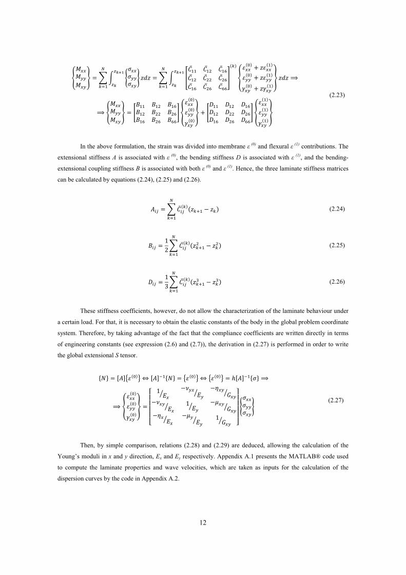
In the above formulation, the strain was divided into membrane � (0) and flexural � (1) contributions. The

extensional stiffness A is associated with � (0), the bending stiffness D is associated with � (1), and the bending-

extensional coupling stiffness B is associated with both � (0) and � (1). Hence, the three laminate stiffness matrices

can be calculated by equations (2.24), (2.25) and (2.26).

^bc � T��bc G! 7Gd� & 7G!\G]� (2.24)

_bc � $�T��bc G! 7Gd�� & 7G�!\G]� (2.25)

abc � $eT��bc G! 7Gd�� & 7G�!\G]� (2.26)

These stiffness coefficients, however, do not allow the characterization of the laminate behaviour under

a certain load. For that, it is necessary to obtain the elastic constants of the body in the global problem coordinate

system. Therefore, by taking advantage of the fact that the compliance coefficients are written directly in terms

of engineering constants (see expression (2.6) and (2.7)), the derivation in (2.27) is performed in order to write

the global extensional S tensor.

BRC � 9^:f� W!g A 9^:h�BRC � f� W!g A f� W!g � i9^:h�B�C FF V�== W!�>> W!K=> W!X �

��

$ )=j&*=> )=j&k= )=j&*>= )>j$ )>j&l> )>j

&k=> +=>j&l=> +=>j$ +=>j �� ,�==�>>�=>. (2.27)

Then, by simple comparison, relations (2.28) and (2.29) are deduced, allowing the calculation of the

Young’s moduli in x and y direction, Ex and Ey respectively. Appendix A.1 presents the MATLAB® code used

to compute the laminate properties and wave velocities, which are taken as inputs for the calculation of the

dispersion curves by the code in Appendix A.2.

13

i9^:�m�h� � $)= A )= � $i9^:�m�h� (2.28)

i9^:�m�h� � $)> A )> � $i9^:�m�h� (2.29)

A composite plate is inherently an anisotropic body, since the material properties are direction-

dependent. However, it is possible to design a stacking sequence with many angle changes such that Ex and Ey

are sufficiently close. In this case, the laminate can be treated as quasi-isotropic.

2.3 Damage Mechanisms in Composite Materials

Depending on the material properties, some laminates may be more resistant to certain kinds of damage

than others. Nevertheless, there are specific damage features that are common to all laminated composite plates,

whose occurrence depends on the load type.

2.3.1 Fatigue damage

Fatigue can be defined as a “degradation of mechanical properties leading to failure of a material or a

component under cyclic loading.” [17] This is a short definition of fatigue damage from the book Mechanical

Behavior of Materials, written by Meyers and Chawla. Although it is generally correct, fatigue behaviour in

composite materials is not a straightforward occurrence, where global damage accumulation takes place and

several damage mechanisms may occur simultaneously. According to Rouchon [18] most of the “references

addressing fatigue of composite materials and structures (...) are providing material data rather than a rational

explanation of the physical phenomena which are involved”. Unlike metals, the damage mechanisms vary

according to the internal architecture of the composite material, and they include matrix cracking, debonding

between fibres and matrix, delamination and fibre failure.

Most structural applications use angle-plied laminates with combinations of 0, 45 and 90 degree

laminae loaded along the 0 degree direction. For this type of laminated composite materials there is a

characteristic damage sequence, as explained by Talreja [19].

The strength of the fibres is much higher than that of the matrix, implying that a lamina is much

stronger along the fibres. Therefore, under cyclic loading, the matrix in the 90 degree plies experiences cyclic

strain and it starts to crack. Then those cracks grow and reach the interface, leading to debonding of the fibres

from the surrounding matrix, as depicted in figure 2.6.

14

Figure 2.6 – Matrix crack and debonding of composite lamina under off-axis cyclic loading [19]

In laminates the loads are mainly carried by the fibres along their specific direction in each ply. Hence,

when the component is loaded there is a mismatch in load paths at the ply interface, inducing interlaminar stress.

The debonding cracks in the 90 degree plies act as stress raisers and, as they reach the ply interfaces, they

magnify the interlaminar stress, leading to delaminations of the 45 degree plies. At this stage the matrix is no

longer performing its load transferring function, causing the overstressing of the intact 0 degree plies and

consequent failure.

Composite materials are known to be less prone to fatigue damage than metals [8]. However, due to

their brittleness, composites “can only absorb energy in elastic deformation and through damage mechanisms.”

[20]

2.3.2 Low-Velocity Impact Damage

The occurrence of low-velocity impacts during production, maintenance or operation may cause

internal defects, reducing structural integrity and therefore increasing the risk of unexpected fatigue failure [20,

21, 22].

This major concern has led many authors to study low-velocity impact damage (or barely-visible impact

damage, BVID) in composite aerospace structures. In a research to assess the equivalence between low-velocity

impact and static loading, Elber [23] was able to identify matrix damage concentrated along the directions of

high interlaminar peel stress, while fibre damage was most severe near the plate bottom surface where the strains

were highest. In 1997, Wiggenraad and Ubels [22] investigated the influence of stacking sequence in the position

of major impact-induced delaminations within the laminate. They understood that, to minimize the harmful

effects of delaminations, “the number of ply angle changes should be limited”. In a different approach,

Hosseinzadeh et al. [21] studied the different behaviours of GFRP and CFRP when subjected to the same drop

weigh impacts. They reported that, for a specific impact energy level, it is possible to enlarge the damage

diameter up to 2-3 times by increasing the impact mass. One year later, Mitrevski et al. [24] drew important

conclusions regarding the effect of impactor shape and bi-axial preload on the impact response of thin GFRP

laminates. Also testing glass reinforced laminates, Rilo and Ferreira [25] confirmed the similarities between

15

static loading and low-velocity impacts, and observed that, although quasi-isotropic plates endure higher loads

than cross-ply plates, they show more severe damage.

In their review article, Richardson and Wisheart [20] gathered the knowledge about BVID in

composites in a systematic way. They describe matrix cracking and debonding between fibres and matrix as the

first types of damages induced by low-velocity impact. Matrix cracks can have two different causes, depending

on their location in the laminate. Some occur in the upper and middle layers as a result of the high transverse

shear stresses induced by the impactor edges, and are inclined approximately at 45 degree, as shown in figure 2.7

– shear cracks. Others take place on the bottom layer, due to the high tensile bending stresses induced by the

flexural deformation of the plates, and are characteristically vertical - bending cracks.

After a certain energy threshold is reached, delaminations take place. These are cracks that run “in the

resin-rich area between plies of different fibre orientation” [20], which are caused by the bending stiffness

mismatch between adjacent plies with different fibre orientations. All the described features constitute the typical

trapezoidal damage distribution depicted on figure 2.7, although it is “practically imperceptible in thin

laminates” [25].

Figure 2.7 – Typical trapezoidal distribution of low-velocity impact damage in composites laminates [20]

However, the two types of low-velocity impact damage do not occur separately. Instead, there is a

strong interaction between them. Richardson and Wisheart reported that “it has been observed that delamination

only occurs in the presence of a matrix crack.” [20] When the matrix cracks reach the ply interfaces, they induce

very high out-of-plane normal stresses. So, due to the combination of those normal stresses with the interlaminar

shear stresses (due to fibre orientation mismatch) delaminations are initiated and forced to propagate between

layers.

Research has shown it is not possible to study isolated damage phenomena in composite structures,

because there is strong interaction between them. Furthermore, in actual operation, it is more likely that multiple

low-velocity impacts occur due to runway debris or hailstones [26], than one single impact. This raises the issue

of more serious interaction when damage sites are in close proximity. Nevertheless, only a few authors have

16

addressed multiple low-velocity impact damage. Paul et al. [27] tested graphite/epoxy specimens with two 30

mm diameter damage sites, one diameter apart. After concluding that there was little interaction between damage

sites, they developed a simple repair methodology for multiple impact damaged structures. From a different

perspective, Malekzadeh et al. [26] programmed a higher-order dynamic algorithm to analyse the low-velocity

impact response of composite sandwich panels. It proved to be a promising tool to further understand the

multiple BVID. Also in a computational approach, Galea et al. [28] used a 3D finite element model to study the

interaction effects in multiple impact damaged laminates subjected to uniaxial and bi-axial loading, as a function

of damage spacing. They analysed two 27.5 mm diameter (D) delaminations underneath 9.5 mm diameter holes,

in different configurations where the separation distance was measured between hole centres. They found that,

for the uniaxial loading case and a damage spacing of a/D = 1.25, the side-by-side configuration induced a

reduction of 30% in the predicted compressive load required for delamination growth (compared to the single

damage case). Recently, Appleby-Thomas et al. [29] studied the effect of multiple ice projectile impacts on

woven and unidirectional CFRP square plates. By testing cumulative impact energies, they were able to visually

establish six different damage severity categories, “ranging from no apparent damage surface damage (type 1)

to penetration accompanied by complete lay-up disruption (type 6).”

Needless to say that the contradictions between the conclusions of Paul [27] and Galea [28], and the

large number of possible untested combinations, prove that further research is needed in this field in order to

increase safety and reliability of composite aerospace structures.

17

Chapter 3

Non-Destructive Testing (NDT) techniques

When evaluating a physical quantity, the human observer cannot detect every variation from the outside

of the specimen and the measurements may present considerable error. However, an intrusive or destructive

inspection would permanently modify the shape of the sample, preventing it from performing its function.

Therefore, Non-Destructive Testing (NDT)1 techniques (or methods) were developed in order to preserve the

original component being inspected, to save both time and money, and ultimately to improve the accuracy of the

measurements [30].

The NDT basic principle is simple. When a material in its original state is subjected to a specific

stimulus it presents a characteristic response, which is taken as the reference. However, if the captured response

differs from that reference, then it means that some new internal feature interfered with the input signal. So, the

evaluation of that change reveals the discontinuity inside the medium.

According to Cartz [30] and Mix [31] NDT technology is divided into methods, based on the physical

principles used. The most common are acoustic emissions, ultrasonics, magnetic flux, electromagnetic induction,

X-rays, laser, thermal properties, fluorescent liquid penetrant, and visual inspection. Due to their particular

natures, some methods are more adequate for some applications than others.

Nowadays, NDT is employed in several industrial activities, namely automotive, aeronautics,

construction, medicine, among others. In the aerospace business, NDT techniques are applied to research,

manufacturing and quality control, aircraft maintenance, and structural health monitoring (SHM) [32]. Although

there are some differences in the requirements for each kind of application, generally they are all used to

evaluate material properties, defects and anomalies, and to assess the capability of a structure to perform a

certain function/task.

One of the first NDT technologies to be successfully applied around 1955/56 was the ultrasonic C-scan

[30]. Over the years, several improvements were implemented and today it is “the primary inspection method for

composite materials” [33]. In 1992, Galea and Saunders [34] developed an in-situ C-scanning system to monitor

damage growth in composite specimens during fatigue tests, without removing the coupons from the loading

machine. In a manufacturing perspective, Kas and Kaynak [35] used C-scan to evaluate microvoids inside

1 Other common terms are Non-Destructive Inspection (NDI) and Non-Destructive Evaluation (NDE).

18

composite plates produced by resin transfer moulding (RTM). More recently, Hasiotis et al. [36] detected

artificial defects in laminates with ultrasonic C-scan.

Since the 1990’s, many developments have been achieved in modern NDT techniques for composite

materials evaluation by trying to understand which technology is more suitable for each application. In 2009,

Polimeno and Meo [37] successfully identified BVID on carbon fibre composite plates, using two NDT

techniques based on the monitoring of the nonlinear elastic response of the damaged material: single-mode

nonlinear resonance ultrasound (NRUS) and nonlinear wave modulation spectroscopy (NWMS). The results

were then compared with C-scan measurements. Later on, Polimeno et al. [38] investigated BVID using a

second harmonic imaging technique (SEHIT), also based on the nonlinear elastic response of the damaged

material “when the sample is periodically excited at one of its resonance frequencies” [38]. The results

accurately identified and quantified the damage, and were validated by pulse thermography and thermosonics. In

order to assess the SHM capabilities, Takeda et al. [39] applied fibre Bragg grating (FBG) sensors to a

composite wing panel during durability tests which consisted of drop-weight impact and two periodic fatigue

tests. The measurements were compared with results from acoustic emission (AE), C-scan and pulsed heating

thermography. Recently, Garnier et al. [40] evaluated the efficiency of ultrasonic testing, infra-red thermography

and speckle shearing interferometry in the detection of BVID on three different composite specimens

manufactured by the aeronautical industry. At the end, they established the limitations and advantages of each

technique regarding accuracy of the results, feasibility and time spent for the experimental protocol.

According to Hung [41], digital Shearography has been receiving considerable industrial acceptance as

a laser-based NDT method for full-field inspection of composite structures. Therefore, some researchers have

explored its advantages and limitations, using several different approaches. Amaro et al. [42] compared the

performance of electronic speckle pattern interferometry (ESPI), ultrasonic C-scan and Shearography in the

detection of BVID in composite laminates. In a similar perspective, Ruzek et al. [43] assessed impact damage in

carbon sandwich panels from an all-composite aircraft wing using Shearography and ultrasonic C-scan. He

reported that, for the tested application, Shearography was the most suitable method. Steinchen [44] focused on

the advantages of using a small and mobile measuring device in conjunction with image processing software,

turning Shearography into an NDT method with online, full-field and non-contact capabilities that can be easily

employed in field/factory environments.

One NDT approach that “is widely acknowledged as one of the most encouraging tools for quantitative

identification of damage in composite structures” [4] is the Lamb wave method. In a quality and process control

perspective, Habeger et al. [45] studied the propagation of ultrasonic plate waves in order to evaluate their

capability in measuring paper strength. Also in a production monitoring orientation, Miesen et al. [46]

demonstrated it is possible to detect flaws in one sheet of unidirectional CFRP prepreg by capturing Lamb waves

with conventional piezoelectric sensors. To better understand the physical phenomena, Percival and Birt [47]

developed and validated a one-dimensional finite element model in order to solve the equations for the

propagation of Lamb waves in anisotropic laminates. Using the fundamental symmetric Lamb mode, Birt [48]

successfully evaluated delamination and impact damage in carbon-fibre laminates. Later, Grondel et al. [49]

developed a SHM system using Lamb waves and acoustic emissions to detect impact and debonding damages in

a composite wingbox. The extraction of signal characteristics can be hindered by the complexity of Lamb wave

propagation phenomena. Therefore, to make the identification process easier, Kessler et al. [50], Grondel et al.

19

[51], Su and Ye [52], Diamanti et al. [53], and Giurgiutiu and Santoni-Bottai [54] have designed several

different systems of multi-element piezoceramic transducers for optimal and selective generation of damage-

sensitive Lamb modes, enabling a more accurate damage detection in composite plates.

The current work focuses on improving the diagnostic capabilities of the Lamb wave method, namely in

the detection and severity quantification of multiple BVID. By using digital Shearography and ultrasonic C-scan

as additional NDT techniques, it is possible to validate the Lamb wave measurements and to establish relevant

conclusions regarding the application of the referred methods. Therefore, in this chapter a complete description

of the physical principles for each NDT method is provided.

3.1 Lamb wave method

3.1.1 Physics of Lamb waves

Mechanical bulk waves can induce particle motion either parallel to the direction of wave propagation

(longitudinal mode), or perpendicular to the direction of wave propagation (transverse or shear mode). So, when

longitudinal and shear waves reach an edge of a thin-wall structure, they are reflected and mode conversion

occurs. If the propagation distance is long enough, this confinement process is enhanced and mode superposition

is allowed, resulting in guided waves [55], as depicted in figure 3.1.

Figure 3.1 – Propagation of guided waves [55]

The number of free surfaces determines the type of guided waves in a plate. With one free surface,

guided waves behave as Rayleigh. With two free surfaces, guided waves travel as Shear-Horizontal (SH) and as

Lamb waves. Rayleigh waves occur close to the free surface, with strong attenuation along the depth, having

their polarization in a plane perpendicular to that surface. Both SH waves and Lamb waves are three-

dimensional, having wave-fronts parallel to the z-axis in figure 3.2 and occurring across the entire thickness.

20

Figure 3.2 – Geometry for the wave propagation problem

However, they have different natures. The particle motion induced by SH waves “is polarized parallel

to the plate surface and perpendicular to the direction of wave propagation” [56]. On the other hand, Lamb

waves generate particle displacements simultaneously along the x-axis and the y-axis, which correspond to

Pressure waves (P waves) and Shear-Vertical waves (SV waves), respectively. The effect of multiple reflections

on both free surfaces combined with interference phenomena creates a “pattern of standing waves in the y-

direction behaving like travelling waves in the x-direction” [56]. Therefore, it is this feature that gives Lamb

waves the ability to travel long distances, making them a very promising solution for SHM and NDT

applications.

First studied by Horace Lamb in 1917 [4], the Lamb wave equations have multiple solutions which

correspond to multiple modes occurring at the same time (multi-mode nature). Lamb wave modes are of two

types, symmetric (S0, S1, S2, ...) and anti-symmetric (A0, A1, A2, ...), depending on the particle motion across the

plate thickness, as depicted in figure 3.3.

Figure 3.3 – Lamb wave particle motion: (a) symmetric motion, (b) anti-symmetric motion [56]

For the fundamental Lamb modes, the total symmetric displacement field is quasi-axial (figure 3.4a)

and it is sensitive to defects anywhere in the thickness, whereas the anti-symmetric displacement field is quasi-

flexural (figure 3.4b) and more sensitive to surface cracks [4, 56].

21

Figure 3.4 – Simulated displacements field for the (a) S0 Lamb mode, and (b) A0 Lamb mode [56]

For isotropic materials, where the properties are not direction-dependent, the S and A Lamb wave modes

are described by equations (3.1) and (3.2), respectively [50].

no4O��p$ & q�Pno4O��pr� & q�P N sq�p$ & q�pr� & q� �q� & $!� � % (3.1)

no4O��p$ & q�Pno4O��pr� & q�P N �q� & $!�sq�p$ & q�pr� & q� � % (3.2)

In the definition of the non-dimensional parameters (3.3), cl and ct are the longitudinal and transverse

wave velocities, respectively, cp is the phase velocity, � is the angular frequency, and d is the half-thickness of

the plate. The velocities cl and ct depend on the density, �, and on the Lamé’s constants, µ and �, which are

written in terms of material properties, such as the Young’s modulus, E, and the Poisson’s ratio, �, as shown in

expressions (3.4) and (3.5).

r� � tu�tv� q� � tu�t<� �� w�tu (3.3)

tu� � lx tv� � y N �l!x (3.4)

l � )� $ N *! y � )* $ & �*! $ N *! (3.5)

22

The wave relations (3.6) for the frequency, f, the wave number, k, the wavelength, �w, and the phase

velocity, cp, enable the solving of the mathematical system.

w � �z{ | � �zy} t< � y}{ (3.6)

After combining equations (3.3) – (3.6), determining the material properties and setting the thickness,

equations (3.1) and (3.2) can be numerically solved for and the phase velocity can be calculated as function of

the frequency (see figure 3.5). This algorithm was programmed in MATLAB® for the S0 and A0 modes, and can

be found in Appendix A.2.

By looking at figure 3.5, two important characteristics can be observed. First, for small frequency

values only the zero-order Lamb modes, S0 and A0, occur. As the frequency increases, the number of Lamb wave

modes that can simultaneously exist also increases. Second, it is clear that the phase velocity varies with

frequency. Lamb waves are then said to possess a dispersive nature.

Figure 3.5 – Phase velocity dispersion curves for an isotropic material with cl = 7199.55 m/s, ct = 3367.60 m/s, and a thickness of 2.24 mm

23

Figure 3.6 – Group velocity dispersion curves for an isotropic material with cl = 7199.55 m/s, ct = 3367.60 m/s, and a thickness of 2.24 mm

To better understand dispersion it is necessary to go into a more detailed explanation of the

phenomenon. By definition, phase velocity is the velocity for each individual frequency within a sinusoidal wave

[57]. However, if a signal has more than one frequency component, then each one propagates with a different

velocity. The multiple slightly different frequencies are alternately in and out of phase, inducing a beat pattern,

which is characterized by wave packets along the signal. Each wave packet propagates with a group velocity, cg,

different from the phase velocity, as defined in equation (3.7). As a result, the initial waveform changes as it

spreads out through the material, as depicted in figure 3.7.

t~ � t< & y} �t<�y} A t~ � t< N | �t<�| A t~ � t<$ & {t< �t<�{ (3.7)

Figure 3.7 – Dispersion phenomenon at three different locations of a structure [56]

24

Lamb waves are inherently beat patterns, because they result from a process of multiple constructive

and destructive interferences across the plate thickness. And each wave packet corresponds to a Lamb mode.

Therefore, they have a highly dispersive nature. Consequently the graph in figure 3.5 is called dispersion curve,

and it is the fundamental way to describe the Lamb wave propagation in a solid medium. The dispersive curve

can also be drawn in terms of group velocity, as in figure 3.6. The multimode and dispersive natures of Lamb

waves make their propagation a complex phenomenon.

However, Lamb wave propagation in composite materials is even more complicated. Their anisotropic

layered structure makes stiffness higher in the fibre direction. Thus, the maximum phase velocity occurs when

the wave propagates parallel to the fibres, and the minimum occurs when the wave propagates perpendicular to

the fibres [54]. Moreover, the larger number of interfaces within the material induces more reflections, making

the wave pattern more difficult to analyse. Therefore, Lamb wave propagation in anisotropic materials cannot be

analytically described by the solutions in equations (3.1) and (3.2). Its study strongly relies on the use of

predictive models. Currently, there are several approaches to calculate the dispersion curves for composite

materials, namely the Effective Elastic Constants method [45, 47], the Transfer Matrix method and the Global

Matrix method [54, 56]. Nevertheless, if the laminate is quasi-isotropic, it is acceptable to use equations (3.1)

and (3.2) to describe Lamb wave propagation [50, 58].

3.1.2 Generation and acquisition of Lamb waves

Nowadays, the state of the art in active Lamb wave generation and acquisition includes ultrasonic

probes, laser-based ultrasonics, laser interferometers, fibre Bragg grating sensors and piezoelectric transducers

[4]. Among these, piezoelectric wafer transducers have proven to be particularly suitable for in-situ NDT and

SHM, due to their negligible mass, easy integration, wide frequency response, low power consumption and low

cost [4].

The most common piezoelectric ceramics are made of lead zirconate titanate, whose chemical formula

is Pb(ZrxTi1-x)O3 (with x between 0 and 1), resulting in the acronym PZT. This dielectric material has a

polycrystalline structure with permanent polarization and piezoelectric properties. When a mechanical stress is

applied, the material changes its polarization, generating an electric field (direct piezoelectric or sensing effect).

On the other hand, when an electric field is applied, the lattice polarization is changed and a mechanical

deformation is induced (converse piezoelectric or actuation effect). These phenomena allow PZT to be used as

an actuator and sensor [56].

,a�a�a�. � I % % % % �� %% % % �� % %�� % % %J��

�� N #�� % %% �� %% % ��' ,)�)�)�. (3.8)

25

��

�� (��(��(��%%%

(��(��(��%%%

(��(��(��%%%

%%%( %%

%%%%(��%

%%%%%(��

�� N��%%%%��%

%%%��%%

��%%% �� ,)�)�)�. (3.9)

{D} – electric displacement

[d] – piezoelectric strain coefficients

{�} – mechanical stress

[e] – dielectric permittivity

{E} – electric field

{�} – mechanical strain

[S] – compliance coefficients as defined in equation (2.7)

According to the actuation effect described in equation (3.9), the application of an electric field, E3,

parallel to the direction of polarization induces an expansion �3 = d33E3 along the x3-axis and contractions �1 = �2= -d31E3 along x1 and x2 axis, respectively [56], as depicted in figure 3.8. The sensing effect can be described by

equation (3.8) in a similar but inverse way.

Figure 3.8 – Electric field and polarization in a piezoelectric plate [56]

For the Lamb wave method there are two possible actuator/sensor configurations, as shown in figure

3.9. In the pitch-catch technique (figure 3.9a) the acquired signals are waves transmitted through the inspected

area. In the pulse-echo technique (figure 3.9b), the acquired signals are waves reflected from interfaces within

the material.

26

Figure 3.9 – Possible actuator/sensor configurations for the Lamb wave method: a) pitch-catch, b) pulse-echo [54]

3.1.3 Lamb wave response optimization

When a PZT wafer is bonded to a structure as an actuator, the coupling between the piezoelectric

material and the specimen enables the transmission of vibrations. The simultaneous strains generated through the

converse effect induce shear stresses, which excite multiple Lamb wave modes. This unavoidable fact poses a

problem, because it is not possible to produce a pure Lamb wave mode, and therefore the interpretation of the

waveform is more difficult.

However, this drawback can be minimized by adapting some transducer parameters. According to

Giurgiutiu [56, 59] Giurgiutiu and Santoni-Bottai [54], and Matt [55] the amplitude of the Lamb mode response

achieves a maximum if the dimension along the direction of propagation (length L in figure 3.10) is an odd

multiple of the half wavelength �w/2. If L is an even multiple of the half wavelength, then the Lamb mode

response reaches a minimum. This is called the wavelength tuning effect [55], which allows the Lamb wave

response to be dominated by a certain mode. These conclusions are entirely valid when the PZT functions as a

sensor, because it has to do with geometric and structural resonance phenomena within the piezoelectric

material.

Figure 3.10 – Wavelength tuning effect [55]

The selective generation of Lamb wave modes can be further improved by using a multi-element

approach. By mounting a pair of rectangular PZT transducers side by side, as in figure 3.11, it is possible to

enhance the amplitude of a specific mode if the inter-element distance, ie, is set as a multiple of the wavelength

[51]. This approach implies previous knowledge of the phase velocity in order to calculate the wavelength, and

therefore the inter-element distance.

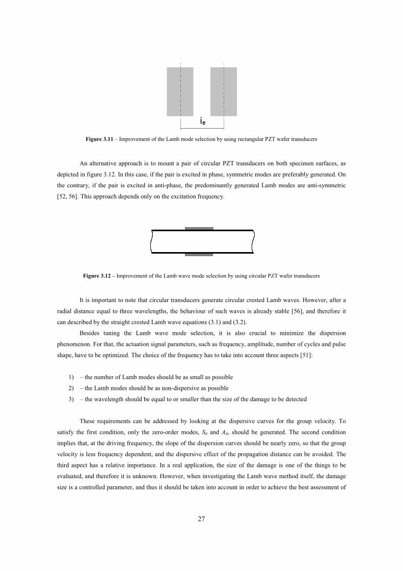
27

Figure 3.11 – Improvement of the Lamb mode selection by using rectangular PZT wafer transducers

An alternative approach is to mount a pair of circular PZT transducers on both specimen surfaces, as

depicted in figure 3.12. In this case, if the pair is excited in phase, symmetric modes are preferably generated. On

the contrary, if the pair is excited in anti-phase, the predominantly generated Lamb modes are anti-symmetric

[52, 56]. This approach depends only on the excitation frequency.

Figure 3.12 – Improvement of the Lamb wave mode selection by using circular PZT wafer transducers

It is important to note that circular transducers generate circular crested Lamb waves. However, after a

radial distance equal to three wavelengths, the behaviour of such waves is already stable [56], and therefore it

can described by the straight crested Lamb wave equations (3.1) and (3.2).

Besides tuning the Lamb wave mode selection, it is also crucial to minimize the dispersion

phenomenon. For that, the actuation signal parameters, such as frequency, amplitude, number of cycles and pulse

shape, have to be optimized. The choice of the frequency has to take into account three aspects [51]:

1) – the number of Lamb modes should be as small as possible

2) – the Lamb modes should be as non-dispersive as possible

3) – the wavelength should be equal to or smaller than the size of the damage to be detected

These requirements can be addressed by looking at the dispersive curves for the group velocity. To

satisfy the first condition, only the zero-order modes, S0 and A0, should be generated. The second condition

implies that, at the driving frequency, the slope of the dispersion curves should be nearly zero, so that the group

velocity is less frequency dependent, and the dispersive effect of the propagation distance can be avoided. The

third aspect has a relative importance. In a real application, the size of the damage is one of the things to be

evaluated, and therefore it is unknown. However, when investigating the Lamb wave method itself, the damage

size is a controlled parameter, and thus it should be taken into account in order to achieve the best assessment of

28

the NDT technique. Either way, it is true that the smaller the wavelength, the higher the sensitivity of the Lamb

mode.

The signal amplitude is directly related to the magnitude of the Lamb wave strain. Therefore, higher

amplitude induces a higher signal-to-noise ratio, yielding a clearer signal. The voltage amplification should be

limited, because, at a certain point, the signal drift begins to deteriorate the resolution of the acquisition system

[50].

The number of cycles is one of the most important parameters, because it has direct influence on the

frequency content of the signal. Figure 3.13 presents the time-domain representations of a one-cycle sinusoidal

burst at 500 kHz and a five-cycle sinusoidal burst at 500 kHz, as well as their frequency-domain representations

calculated through the Fast Fourier Transform (FFT). The comparison between figures 3.13a and 3.13b clearly

demonstrates that the larger the number of cycles, the narrower the bandwidth, and therefore the less dispersive

is the Lamb wave propagation.

Figure 3.13 - Time and frequency domain contents for pure sinusoidal bursts with a) 1 cycle, and b) 5 cycles

The bandwidth can be further reduced if a Hanning function, H(t), is used to window the original

sinusoid, producing an N-cycle amplitude-modulated tone-burst at central frequency f, s(t), as defined in

equations (3.10) and (3.11). In figure 3.14b, where a five-cycle windowed sinusoidal tone-burst at 500 kHz is

represented in both time and frequency domains, it is clear that, although the windowing process reduces the

energy content of the signal, it eliminates the side frequencies almost completely.

� �! � $� �$ & /01 ��z{�R �� (3.10)

� �! � � �! 134 �z{�! (3.11)

29

Then, it is advantageous to use a higher number of cycles, because it reduces dispersion and increases

the energy dedicated to the desired frequency, implying a clearer and stronger Lamb wave response [50]. This

way, the group velocity calculation is more accurate, increasing the sensitivity and reliability of the damage

detection system.

Figure 3.14 - Time and frequency domain contents for sinusoidal tone-bursts, with by a) 1 cycle and modified by an amplitude increase, and b) with 5 cycles modified by a Hanning function windowing process

However, in a short specimen, a burst with more cycles induces a more complicated reflection pattern,

which makes the Lamb wave response more difficult to interpret [4, 50]. Hence, an alternative solution can be to

increase the signal amplitude, while keeping a smaller number of cycles. Figure 3.14a shows the time and

frequency contents of the one-cycle sinusoidal burst from figure 3.13a amplified five times. It is possible to

observe that, instead of changing the frequency content of the excitation pulse, this operation increases the

energy dedicated to the desired frequency, enhancing the Lamb wave strain. Nevertheless, these principles

should always be confirmed by experimental testing.

As for the pulse shape, it has been proven [50, 51, 52, 53] that sinusoidal waveforms are able to excite

Lamb wave modes more efficiently, especially if used as windowed tone-bursts.

3.1.4 Digital signal processing

The raw signals acquired by the sensors are unavoidably influenced by environmental noise. Hence,

before any kind of analysis, it is crucial to filter the signals, so that results are not contaminated by undesired

information. Nowadays there are several denoising methods, from simple low-pass and high-pass filters to

30

elaborate wavelet filter-banks. Nevertheless, filtering operations should be performed carefully, in order to

prevent the loss of data.

According to Vasilescu [60], noise is the result of the combination of several random physical

phenomena which are coupled with the data acquisition system. In that sense, each point of the captured signal is

just as noisy as its neighbour. Thus, a simple and reliable denoising method is the moving-average filter, which

is optimal for “reducing random noise while retaining sharp step response” [61] of time domain encoded

signals. The filtered output signal, y, is produced by equally averaging a set of M points from the input signal, x,

as described in equation (3.12).

6b � $̀ T -bdc�h�c]W (3.12)

The application of the moving-average filter allows a noise reduction equal to the square-root of the

number of points in the average.

3.1.5 Algorithm for damage detection

The presence of BVID originates more discontinuities within the composite material and reduces its

stiffness. So, when Lamb waves propagate through a damaged area, there are more reflections and transmission

of mechanical energy is less efficient [50], when compared to the healthy material. This physical evidence of the

presence of damage is encoded as variations of signal parameters. Thus, it is necessary to translate those

evidences into measurable features.

When a wave reaches a discontinuity, part of the energy is reflected, another part is transmitted and

some is absorbed by the interface itself. If the wave energy is constant and if it is assumed that the portion

absorbed by the interface is also constant, then an increase in the reflected part necessarily implies a decrease in

the transmitted part. This means the amplitude of the transmitted wave is lower or, in other words, it means that

there is attenuation of the transmitted wave, when compared with the initial case. Thus, an increase in the

number of discontinuities, i.e. the presence of damage, can be translated into a stronger signal attenuation, which

is directly evaluated by measuring and comparing the amplitude of the healthy and damaged responses.

The stiffness of a material measures its resistance to elastic deformation [62]. If a higher tensile load is

necessary to obtain the same deformation, it means the constitutive blocks are more closely bonded and therefore

stiffness is higher. Thus, in a material with higher stiffness the bonds between constitutive blocks can transmit

energy more efficiently, yielding a higher wave group velocity. On the contrary, if a stiffness reduction is

induced (e.g. by damage), the group velocity will become lower. Experimentally, the group velocity is calculated

by dividing the propagation distance by the travelling time (Time-of-Flight, TOF) of the wave packet. So, the

presence of damage can be translated into a lower group velocity, which can be evaluated by detecting the

change in TOF.

For the pitch-catch technique, the assessment of damage severity can be done by quantifying the

changes in group velocity and signal attenuation for the excited Lamb modes. As mentioned above, signal

attenuation can be quantified by directly measuring the amplitude of a specific peak within the desired wave

31

packet. However, the determination of the TOF of a Lamb wave group is not always a straightforward task. If

the desired Lamb mode is the fastest, then it is the first group arriving at the sensor. Inside the green circle shown

in figure 3.15, it is possible to manually identify a time interval where the onset of the wave packet can surely be

found. On the other hand, if the desired Lamb mode is not the fastest, then it arrives later at the sensor and the

corresponding wave group occurs in the middle of the signal. In this case, even if the packet has higher

amplitude than the neighbourhood (see red circle in figure 3.1.5), it is much more difficult to manually pick the

onset time of the group, because there is not a clear separation from the rest of the signal. Therefore, a criterion

has to be established in order to make the detection of the TOF of a Lamb mode a reliable and automatic

operation.

Figure 3.15 – Typical Lamb wave response from a composite plate excited with a PZT wafer transducer

The onset time is usually defined as the point where the amplitude first clearly differs from the noise.

Based on this concept, the Akaike Information Criterion (AIC) has been established, according to which a signal

is divided into two segments modelled as autoregressive processes, the data and the noise [63]. The AIC-picker

can determine the onset time by inspecting a pre-selected region of the signal (window) that contains the actual

starting point. Thus, the AIC function is defined in equation (3.13), where Rw denotes the portion of the signal

within the window, tw ranges through all the samples of Rw, and Tw is the last sample of Rw. The variances,

var(Rw(a,b)), are calculated from sample a to sample b according to equation (3.14), where N is the length of the

time series and Rm is the mean value of the entire signal R. When the AIC function reaches its global minimum

within the pre-selected interval, the two autoregressive segments are clearly separated, indicating the onset point.

The onset time for the desired group is then set equal to the TOF of the corresponding Lamb wave mode.

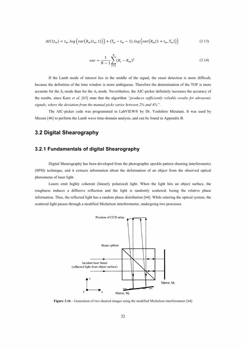
32

^�� }! � �}� �� OE} �}m $!P� N D} & �} & $!� �� OE} $ N �}m D}!P� (3.13)

�� $R & $T Eb & E@!�\b]� (3.14)

If the Lamb mode of interest lies in the middle of the signal, the onset detection is more difficult,

because the definition of the time window is more ambiguous. Therefore the determination of the TOF is more

accurate for the S0 mode than for the A0 mode. Nevertheless, the AIC-picker definitely increases the accuracy of

the results, since Kurz et al. [63] state that the algorithm “produces sufficiently reliable results for ultrasonic

signals, where the deviation from the manual picks varies between 2% and 4%”.

The AIC-picker code was programmed in LabVIEW® by Dr. Yoshihiro Mizutani. It was used by

Miesen [46] to perform the Lamb wave time-domain analysis, and can be found in Appendix B.

3.2 Digital Shearography

3.2.1 Fundamentals of digital Shearography

Digital Shearography has been developed from the photographic speckle pattern shearing interferometry

(SPSI) technique, and it extracts information about the deformation of an object from the observed optical

phenomena of laser light.

Lasers emit highly coherent (linearly polarized) light. When the light hits an object surface, the

roughness induces a diffusive reflection and the light is randomly scattered, losing the relative phase

information. Thus, the reflected light has a random phase distribution [64]. While entering the optical system, the

scattered light passes through a modified Michelson interferometer, undergoing two processes.

Figure 3.16 – Generation of two sheared images using the modified Michelson interferometer [64]

33

As depicted in figure 3.16, each incident ray is first divided into two beams, one going straight to mirror

M1, other to mirror M2. The reflected beams are recombined at the beam splitter, forming an image which is

captured by a charge-coupled-device (CCD) camera. Because one of the mirrors is tilted at a small angle about

the x or y axis, a second wave front is generated, creating two laterally sheared images. It is possible to induce

shear along the x or y direction by tilting one of the mirrors about the y or x axis, respectively.

Due to the image shearing process, rays from neighbouring object points (P1 and P2) are superimposed.

So, because each one of those rays has different phase values (θ1 and θ2), spatial interference occurs and an

interferometric speckle pattern is created [64]. This pattern is called interferogram, and it is formed by small

bright and dark grains, whose size depends on the viewing aperture. The intensity, I, of the interferogram is

defined in equation (3.15), and it depends on the terms I0, γ and ϕ, which denote the mean value of the intensity,

the modulation of the interference term, and the phase difference, respectively.

� = 2��(1 + � cos �) (3.15)

A single interferogram has a random phase distribution and no information about the object can be

extracted. However, when loading is applied, the object is deformed, and the surface points occupy new

positions, as shown in figure 3.17. So, the distances between the laser, the surface points and the CCD camera

are altered according to equations (3.16) and (3.17).

�� = ��∗ + ��∗� � − (�� + �� ) (3.16)

�� = ��∗ + ��∗� � − (�� + �� ) (3.17)

Figure 3.17 – Difference in the laser light path between two object points, in the undeformed and deformed states [64]

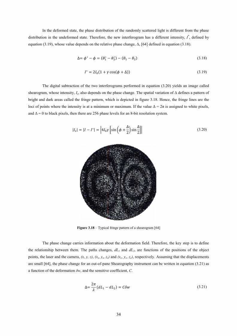
34

In the deformed state, the phase distribution of the randomly scattered light is different from the phase

distribution in the undeformed state. Therefore, the new interferogram has a different intensity, I*, defined by

equation (3.19), whose value depends on the relative phase change, Δ, [64] defined in equation (3.18).

∆= �∗ − � = (��∗ − ��∗) − (�� − ��) (3.18)

�∗ = 2��(1 + � cos(� + Δ)) (3.19)

The digital subtraction of the two interferograms performed in equation (3.20) yields an image called

shearogram, whose intensity, Is, also depends on the phase change. The spatial variation of Δ defines a pattern of

bright and dark areas called the fringe pattern, which is depicted in figure 3.18. Hence, the fringe lines are the

loci of points where the intensity is at a minimum or maximum. If the value Δ = 2π is assigned to white pixels,

and Δ = 0 to black pixels, then there are 256 phase levels for an 8-bit resolution system.

|��| = |� − �∗| = �4�� sin �� + Δ2� sin Δ2�� (3.20)

Figure 3.18 – Typical fringe pattern of a shearogram [64]

The phase change carries information about the deformation field. Therefore, the key step is to define

the relationship between them. The paths changes, dL1 and dL2, are functions of the positions of the object

points, the laser and the camera, (x, y, z), (xs, ys, zs) and (xc, yc, zc), respectively. Assuming that the displacements

are small [64], the phase change for an out-of-pane Shearography instrument can be written in equation (3.21) as

a function of the deformation δw, and the sensitive coefficient, C.

∆= 2�� (�� − ��) = �� (3.21)

35

� = 2�� − �� + � − �� (3.22)

�� = !�� + "�� + ��

� = ! � + " � + � � (3.23)

Then, considering that the object is small compared with the distances to the laser and camera, and that

the applied shear, dx or dy, is small, the phase change for each shearing case can be defined as a function of the

out-of-plane components of the strain tensor, as in equations (3.24).

∆#= �� $�$! � �!

∆%= �� $�$" � �" (3.24)

The Shearography setup can be summarized in figure 3.19, where the sensitivity vector, ks, includes the

sensitivity coefficient, C. Then, it is possible to write the phase change in the vector form [64], transforming

equations (3.24) into equations (3.25).

Figure 3.19 – Shearography setup [64]

∆#= �$�$! &�'⃗,� �!

∆%= �$�$" &�'⃗,� �" (3.25)

Replacing the vector components by the angular relations, and setting the illumination direction in the

xz-plane, equations (3.25) are simplified into equations (3.26).

∆#= 2�� -(1 + cos �#,) $�$! . �!

∆%= 2�� -(1 + cos �#,) $�$" . �"

(3.26)

36

An out-of-pane Shearography instrument has the illumination direction normal to the object surface, θxz

= 0, yielding equations (3.27) for the phase change.

∆#= 4�� $�$! �!

∆%= 4�� $�$" �" (3.27)

The presence of fringes depicted in a shearogram can be interpreted as strain concentration areas [64].

Any discontinuity within the material changes the strain concentration field around it. So, the evaluation of the Δ

distribution in a shearogram allows the quantification of the changes in strain concentration, enabling the

damage detection. The damage size that can be identified depends on the sensitivity, which can be enhanced by

increasing the shear amount. Furthermore, the fact that rigid-body motion does not produce strain makes

Shearography insensitive to vibrations and therefore a suitable NDT method for industrial applications.

Evaluation of a shearogram requires the determination of Δ. Thus, it is first necessary to calculate the

phase distributions ϕ and ϕ*. This is a problem with three unknowns (I0, γ and ϕ), which needs at least three

equations to be solved. One possible way to increase the number of equations is by capturing several different

interferograms for each deformation state. To do that, it is necessary to shift the interfering light waves, by using

the modified Michelson interferometer. A piezoelectric-induced linear movement of mirror M1 by a known

amount, dL, modifies the optical path by an amount of 2dL [64]. The change of the optical path induces the

known phase increment, φ, defined in equation (3.28).

/ = 2�� 2�� (3.28)

Therefore, it is possible to sequentially generate interferograms with different phase distributions by

moving mirror M1 several times. For example, if four sequential movements of M1 are used, then four

interferograms, I1 to I4, are generated, each with a phase increment of π/2, as in equations (3.29).

�� = 2��[1 + � cos(�)] �� = 2�� 01 + � cos 3� + �256 �7 = 2��[1 + � cos(� + �)]

�8 = 2�� 1 + � cos �� + 3�2 ��

(3.29)

Then by solving the mathematical system, the phase distribution, ϕ, can be calculated using equation

(3.30).

� = :;<>:? ��8 − �� − �7� (3.30)

37

The phase distribution in the new deformation state, ϕ*, can be calculated using the same phase-shifting

technique described above. After that, the phase change over a 2π range, Δ, can finally be calculated according

to equation (3.31).

Δ = @�∗ − � , CD; �∗ ≥ ��∗ − � + 2�, CD; �∗ < �G (3.31)

3.2.2 Image processing

3.2.2.1 Phase map filtering

As with any NDT technique, there is noise in Shearography measurements. Hence, the phase map has to

be filtered before being evaluated. A common approach is to use a modified mean value filtering operation [64]

as described below.

In a simple mean value filter, the examined pixel is surrounded by an n x n window. The gray values,

g(i, j), inside the window are multiplied by n x n coefficients, k(i, j). The summation of all the products, k(i, j).

g(i, j), is then divided by the sum of all coefficients k(i, j), S, yielding the mean gray value, Vm, for the examined

pixel, as written in equation (3.32). It should be noted that n must be an odd number greater than or equal to 3.

Because this algorithm does not allow the pixels at the edge of the image to be examined, they are initialized as

zero.

HI = 1 J J &(K, L)M(K, L)N

OP�

N

QP� (3.32)

This filtering operation smooths the image by removing the small gray peaks. However, if the window

is too large, the smoothing effect becomes too strong and relevant gray values may be erased. To increase the

accuracy of the filter, a smaller window can be used. Nevertheless, there will always be loss of information. So,

to mitigate this phenomenon, a modified approach can be applied, by transforming the gray values into a sine

and cosine functions. This way, the sharp peaks do not appear, and therefore they cannot be eliminated. The

mean value filter can then be applied. In the end, an exact, smooth phase map can be obtained by reconstructing

the filtered sine and cosine.

3.2.2.2 Demodulation

When the phase change, Δ, is calculated by equation (3.31), 2π phase jumps may be introduced. Thus,

in order to obtain a continuous phase map, it is necessary to suppress those discontinuities through a

demodulation process.

One of the existing path-dependent demodulation techniques is the pixel queue algorithm [64]. The

starting pixel is fixed and four neighbouring pixels are listed in a counter-clockwise spiral, following the cardinal

directions [N, W, S, E]. For the central point, the phase value is analysed. If it is greater than +π, or –π, it has to

38

be corrected. The next point to be executed is taken from the pixel queue, and the loop is repeated until all the

points in the list have been examined. This process is performed until there are no more valid pixels in the image

to be analysed. In the end, the unwrapped phase change distribution is a function of the gray level of each pixel,

g(i, j), and the integer part of the fringe order, n, as described by equation (3.33).

Δ = 2� R? + M(K, L)255 T (3.33)

It should be noted that the unwrapping process strongly depends on the correct identification of the

phase jumps. Therefore, the pixels must not be affected by noise, which implies that the demodulation can only

be applied after filtering the shearogram.

3.3 Ultrasonic C-scan

Ultrasonic C-scan is an NDT method that uses ultrasounds to generate an “overall view of the planar

extent of damage” [33]. High frequency sound waves are generated by a piezoelectric transducer that converts an

“oscillating applied voltage into a mechanical vibration in the MHz frequency range” [33]. Those waves are

then transmitted into the specimen using a coupling medium (generally water), in order to maximize the

ultrasonic energy transmission. When propagating through the sample, ultrasonic waves reach interfaces

between two regions. If they have different acoustic impedances, reflection and scattering of the waves takes

place, inducing energy variations on the reflected and transmitted signals.

There are two possible approaches for C-scanning. The through-thickness technique depicted in figure

3.20 measures the signal attenuation after propagation through the entire thickness, “at each particular location

on the specimen.” [35] The energy loss is a function of the amount of reflection and scattering phenomena that

occur when the ultrasonic waves encounter discontinuities. Thus, when the signal attenuation is higher than the

value for the surrounding material, it means those non-uniformities are damage sites. This information is then

displayed as colour dB map of the inspected surface.

The pulse-echo technique involves the detection of the ultrasonic signal reflected from interfaces within

the material. As shown by figure 3.21, a specimen in its pristine condition has a typical reflection pattern. The

first reflection is from the front surface, immediately followed by the reflection from the back surface. However,

if there are echoes between the reflections from both surfaces, it means damage is present inside the plate. The

distribution of the reflection energy is displayed as colour dB map of the inspected surface. This technique has

the advantage of enabling the extraction of information about the through-thickness position of the defects,

because different echoes are detected at different instants. Thus, by knowing the average sound velocity inside

the material for the reference sample, the depth at which the damage occurs can be computed. It should be noted

that this technique can only be applied to plates with a thickness lower than ten times the signal wavelength.

According to Fahr and Kandeil [33], the C-scan technology can easily detect voids, porosity and

delaminations along entire plane surfaces normal to the propagation direction of the signal. However, the same

authors state that “detecting fibre fracture and matrix cracking is very difficult when using conventional

ultrasonic C-scan” [33], because these kind of defects usually occurs in planes that are not perpendicular to

39

ultrasonic beam direction. Despite its limitations, “the ultrasonic C-scan is one of the main techniques used for

the quality control of composite materials during fabrication and assembly.” [34]

Figure 3.20 – Through-thickness C-scan technique [33]

Figure 3.21 – Pulse-echo C-scan technique [33]

41

Chapter 4

Experimental procedure

This chapter is divided into two parts. Phase 1 describes the preliminary approach, where all the

methodology was learnt and improvements for the Lamb wave tests were identified. In Phase 2, the improved

procedure for the Lamb wave method is described, as well as the Shearography and C-scan tests. All the

experimental activity in this chapter is described in chronological order.

4.1 Phase 1 – Preliminary approach

4.1.1 Manufacturing of composite samples

The material selected for this project was the M30SC/120DT carbon/epoxy uni-directional (UD)

prepreg, supplied by Delta-Tech S. p. a. The prepreg properties are presented in table 4.1. The 7-ply arrangement

[+45/-45/0/90/0/-45/+45], based on a McDonnel Douglas design [10], was adopted as a representative stacking

sequence for an aircraft structure.

Table 4.1 - Properties of the M30SC/DT 120 UD prepreg [65]E11 (GPa) 155

E22 (GPa) 7.8

G12 (GPa) 5.5

�12 (-) 0.27

Fibre fraction (%) 66

Thickness (mm) 0.16

Density (kg/m3) 1760

For the preliminary approach it was decided to use a lay-up sequence composed of three 7-ply blocks,

[+45/-45/0/90/0/-45/+45]3, in order to produce a laminated plate (Laminate 1) with 250 x 250 x 3.36 mm3.

The prepreg layers were cut using the automatic GERBER machine DC2 2500, operated by the

CutWorks software (figure 4.1a). The quick dry industrial solvent PFQD/1L-GB/DE was applied to clean the

two plates of the aluminium mould, followed by seven coats of mould releasing agent Marbocote 227. After

carefully stacking the prepreg plies on the lower part of the mould, the vacuum bag was prepared (figure 4.1b).

42

First, plastic foil was placed on top of the upper plate of the mould. Then, the foil was covered by white breather

blanket and the vacuum valve was positioned on top of it. A new foil coat was placed on top of everything and

the mould was sealed with two-sided-high-temperature gluing tape. Finally, the laminate was cured in the

autoclave, at a pressure of 6 bar, heating up at a constant rate of +2ºC/min from room temperature to 120ºC,

maintaining that temperature for 90 minutes, and cooling down to 60ºC at a constant rate of -4ºC/min, according

to the material supplier recommendations. The cured composite plate (figure 4.1c) was then cut at 0.5 mm/s into

four 110 x 110 x 3.36 mm3 specimens (figure 4.1d), using the Struers 1312 Unitom machine.

a) b)

c) d) Figure 4.1 - Steps of the manufacturing process: a) automatic cutting of the prepreg material, b) curing process in the

autoclave, c) cured laminated plate, and d) four 110 x 110 x 3.36 mm3 specimens

The mechanical properties of Laminate 1 listed in table 4.2 were calculated according to the CLPT

described in subsection 2.2.1, using the MATLAB® code in Appendix A.1.

Table 4.2 – Mechanical properties of Laminate 1Ex (GPa) 63.514

Ey (GPa) 45.064

�xy (-) 0.2988

�yx (-) 0.4211

43

4.1.2 Lamb wave tests

In this case, no damage was applied to the four specimens because the priority was learning how to use

the equipment for generation and acquisition of Lamb waves, and to visualize key features of Lamb wave

propagation in undamaged composite material.

Although the ratio between Ex and Ey reveals a level of anisotropy of 29%, the laminate was considered

quasi-isotropic and the average of Ex and Ey was taken as the Young’s modulus of the material. With that value,

the velocities of longitudinal and transverse waves (table 4.3) were computed according to expressions (3.4).

Then the Lamb wave dispersion curves in figures 4.2 and 4.3 were calculated using the MATLAB® code in

Appendix A.2.

Table 4.3 – Approximate acoustic properties of Laminate 1cl (m/s) 7199.55

ct (m/s) 3367.60

The assessment of the velocity range for the available frequencies (28, 50 and 108 kHz) showed that

although only the two zero-order Lamb modes exist, only the S0 mode presents a nearly non-dispersive

behaviour, which could make the identification of the A0 mode more difficult . Thus, four laboratory sessions

were scheduled in order to evaluate the feasibility of the Lamb wave method with the available equipment.

Figure 4.2 – Phase velocity dispersion curves for Laminate 1

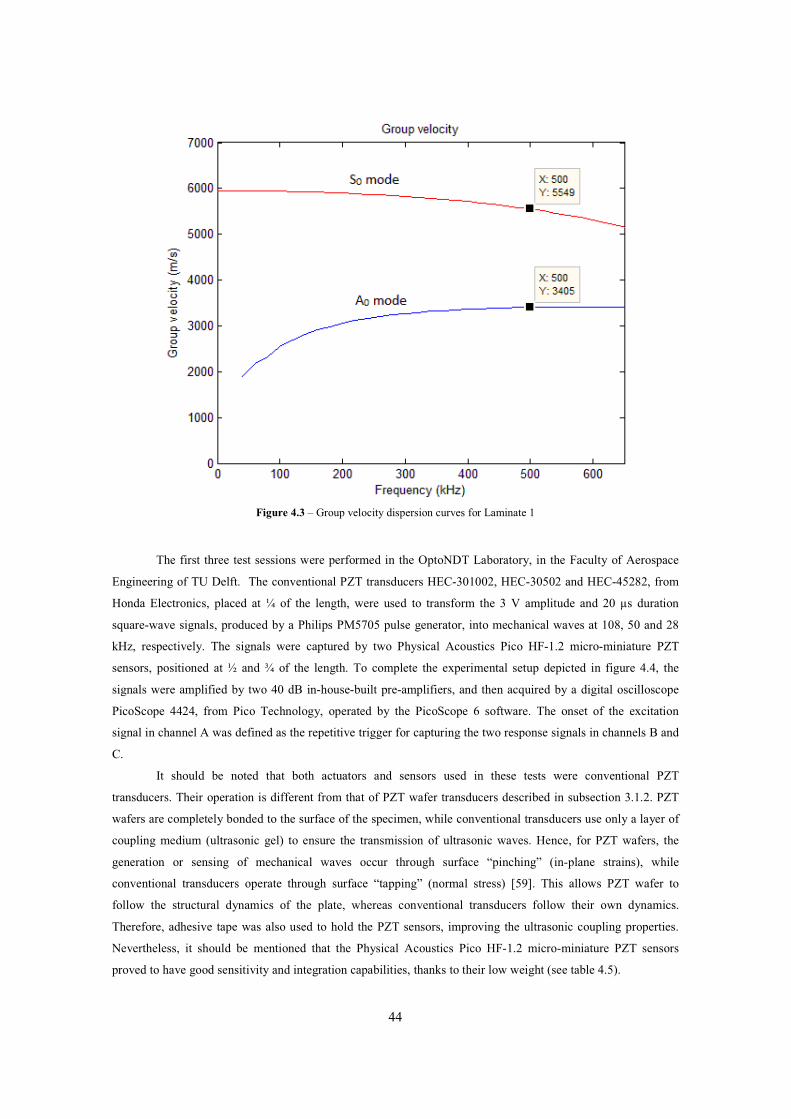
44

Figure 4.3 – Group velocity dispersion curves for Laminate 1

The first three test sessions were performed in the OptoNDT Laboratory, in the Faculty of Aerospace

Engineering of TU Delft. The conventional PZT transducers HEC-301002, HEC-30502 and HEC-45282, from

Honda Electronics, placed at ¼ of the length, were used to transform the 3 V amplitude and 20 µs duration

square-wave signals, produced by a Philips PM5705 pulse generator, into mechanical waves at 108, 50 and 28

kHz, respectively. The signals were captured by two Physical Acoustics Pico HF-1.2 micro-miniature PZT

sensors, positioned at ½ and ¾ of the length. To complete the experimental setup depicted in figure 4.4, the

signals were amplified by two 40 dB in-house-built pre-amplifiers, and then acquired by a digital oscilloscope

PicoScope 4424, from Pico Technology, operated by the PicoScope 6 software. The onset of the excitation

signal in channel A was defined as the repetitive trigger for capturing the two response signals in channels B and

C.

It should be noted that both actuators and sensors used in these tests were conventional PZT

transducers. Their operation is different from that of PZT wafer transducers described in subsection 3.1.2. PZT

wafers are completely bonded to the surface of the specimen, while conventional transducers use only a layer of

coupling medium (ultrasonic gel) to ensure the transmission of ultrasonic waves. Hence, for PZT wafers, the

generation or sensing of mechanical waves occur through surface “pinching” (in-plane strains), while

conventional transducers operate through surface “tapping” (normal stress) [59]. This allows PZT wafer to

follow the structural dynamics of the plate, whereas conventional transducers follow their own dynamics.

Therefore, adhesive tape was also used to hold the PZT sensors, improving the ultrasonic coupling properties.

Nevertheless, it should be mentioned that the Physical Acoustics Pico HF-1.2 micro-miniature PZT sensors

proved to have good sensitivity and integration capabilities, thanks to their low weight (see table 4.5).

45

a) b)

c) Figure 4.4 – Experimental setup for test sessions 1, 2 and 3: a) position of the actuator and sensors on the specimen, b) detail

of the adhesion of the sensors, and c) overall view of the experimental installation

The signal analysis revealed that only the fastest mode, S0, could be identified in the Lamb wave

responses. The slower mode, A0, could not be discerned, due to three main reasons:

1) – there were many reflections from the plate edges superimposed to the A0 Lamb mode response

2) – the tension in the sensor cables induced slight movements which could not be prevented by the

pressure of the adhesive tape, deteriorating the amplitude of the acquired signals, and therefore

influencing the clarity of the response

3) – the excitation waveform (square wave) was not able to efficiently excite the Lamb wave response

The first point strongly suggested that the specimens were probably too small for a clear identification

of the Lamb wave response. The slight movements of the sensors prevented the appropriate transmission of the

Lamb wave response from the specimen to the sensors, indicating that serious improvements regarding the

46

coupling properties would have to be achieved. So, for the fourth laboratory session, it was decided to excite the

A0 at a higher frequency, promoting a less dispersive propagation. Additionally, a sinusoidal tone-burst would be

used as a more efficient excitation waveform, as suggested in subsection 3.1.3.

The fourth test took place in the Applied Geophysics and Petrophysics Laboratory, in the Faculty of

Civil Engineering and Geosciences of TU Delft. A 1-cycle-500 kHz-sinusoidal tone-burst with 400 mVpp

amplitude was produced by an Aglient 33220A arbitrary waveform generator. The electrical signal was then

amplified by a E/N 2100L RF 50dB power amplifier, and transformed into a mechanical wave by a Panametrics

V103 conventional PZT actuator, placed on the specimen at ¼ of the length, as depicted in figure 4.5. The plate

response was captured by the Physical Acoustics Pico HF-1.2 PZT sensors positioned at ½ and ¾ of the length,

amplified by the 40 dB pre-amplifiers, and acquired by a Yokogawa Dl4200 oscilloscope. The excitation signal

was transmitted from the power amplifier to channel A through a Yokogawa 700997 cable that reduces the

amplitude by ten times in order to protect the oscilloscope from overcharges.

Figure 4.5 – Panametrics V103 PZT actuator and the two HF-1.2 PZT sensors

The signal transmission from the plate to the sensors was clearly improved by the use of a different

ultrasonic couplant, the Olympus Sonotech shear gel, which also had adhesive properties. Hence, the

combination of the Sonotech shear gel and a strong adhesive tape would solve the coupling problems. Although

it was possible to acquire a more clear Lamb wave response, still it was impossible to identify the A0 mode due

to the superimposing reflections. This confirmed that the samples were not large enough for an accurate

extraction of the two zero-order Lamb modes.

Therefore, at the end of Phase 1, it was possible to identify two major improvements to be implemented

in Phase 2:

1) – produce four larger composite specimens

2) – use PZT wafer transducers as actuators

By using larger samples the detrimental effect of reflections from the plate edges would be minimized.

Furthermore, it would also allow larger propagation distances, yielding a clearer separation of the Lamb modes,

and therefore a more accurate identification of the TOF of each mode. By using multiple PZT wafer transducers

instead of conventional ones, it would be possible to selectively generate the Lamb wave modes, as described in

subsection 3.1.3.

47

4.2 Phase 2 – Study of NDT methods

4.2.1 Sample manufacturing

The new laminated composite (Laminate 2) was produced with the same M30SC/120DT carbon/epoxy

UD prepreg, using two 7-ply blocks, [+45/-45/0/90/0/-45/+45]2. Two plates of 410 x 410 x 2.24 mm3 were

manufactured by the same procedure described in subsection 4.1.1, and cut into four 400 x 200 x 2.24 mm3

specimens, using a Carat P-3515 cutting machine.

The mechanical and acoustic properties of the new plates were calculated according to the CLPT, using

the MATLAB® code in Appendix A.1. They turned out to be the same as for Laminate 1, whose values are

listed in tables 4.2 and 4.3, yielding the same dispersion curves in figures 4.2 and 4.3. The reason for this lies in

the denominator of expression (2.28). For Laminate 2, the laminate thickness, h, is smaller, but the [A]-11,1 is

higher, yielding the same Young’s modulus.

4.2.2 Quality control

The final quality of the new samples was assessed by performing an ultrasonic C-scan. For that, a Midas

NDT Systems C-scan was used in the through-thickness configuration. The 10 MHz signals were transmitted by

two water jets, as depicted in figure 4.6.

a) b)Figure 4.6 – C-scan system: a) overall view of the setup b) detail of the ultrasonic probes and the alignment of the water jets

This measurement allowed the evaluation of the healthy condition of the specimens, which was crucial

for the choice of the reference undamaged plate. After analyzing the results, it was observed that the dB standard

deviation for the four samples was lower than for the C-scan standard panel. Furthermore, specimen 1 had the

lowest dB standard deviation among all the four plates, meaning it had the lowest signal attenuation, and

therefore less internal defects (better quality). For this reason, specimen 1 was chosen as the reference sample for

the undamaged condition of the material.

48

4.2.3 Application of multiple low-velocity impact damage

The best way to apply controlled impact damage on a plate is through the impact tower depicted in

figure 4.7a. However, the dimensions of the available clamping device (figure 4.7b) are not compatible with the

composite specimens. Hence, it was necessary to design a new clamping device, based on the ASTM D 7136/D

7136M-05 standard [66]. Using the drawings in Appendix C, the clamping device in figure 4.7c was produced,

using medium-density-fibreboard (MDF) wood and aluminium alloy.

b)

a) c) Figure 4.7 – Tools for the application of impact damage: a) impact tower, b) original clamping device, and c) new clamping

device

It was decided to apply ten impact points randomly distributed inside a 6 cm radius circle. So, ten

known random positions were generated by MATLAB®, forming the pattern depicted in figure 4.8. The

multiple BVID was induced to specimens 2, 3 and 4, always using to the same impact pattern. The impactor in

figure 4.9a had a mass equal to 1.2 kg and its hemispherical head had a diameter of 12.7 mm.

In order to test different damage severities, impact energies of 3, 5 and 10 J were applied to specimens

2, 3 and 4, respectively. The energy level of each impact was set by adjusting the height from which the impactor

would be released, according to the definition of gravitational potential energy in equation (4.1). Thus, the 3, 5

and 10 J impact damages were applied by releasing the impactor from 25.5, 42.5 and 85 cm, respectively. It was

not possible to apply an impact energy lower than 3 J, because the impact tower could not release the impactor

from heights lower than 25 cm.

49

)<~ � ��i A i � )<~�� (4.1)

It is important to refer that, every time the location of the impact had to be changed, it was necessary to

unscrew the bolts, move the plate to appropriate position, and screw the bolts again, as shown in figure 4.9b.

Figure 4.8 – Impact pattern

a) b) Figure 4.9 – Application of BVID on the plates: a) steel impactor with a hemispherical heat, b) installation of the specimen

between the bolted aluminium frames

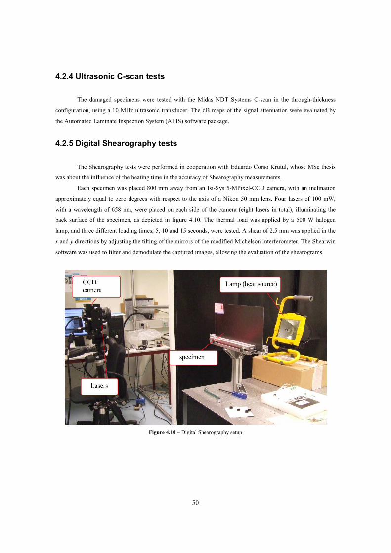
50

4.2.4 Ultrasonic C-scan tests

The damaged specimens were tested with the Midas NDT Systems C-scan in the through-thickness

configuration, using a 10 MHz ultrasonic transducer. The dB maps of the signal attenuation were evaluated by

the Automated Laminate Inspection System (ALIS) software package.

4.2.5 Digital Shearography tests

The Shearography tests were performed in cooperation with Eduardo Corso Krutul, whose MSc thesis

was about the influence of the heating time in the accuracy of Shearography measurements.

Each specimen was placed 800 mm away from an Isi-Sys 5-MPixel-CCD camera, with an inclination

approximately equal to zero degrees with respect to the axis of a Nikon 50 mm lens. Four lasers of 100 mW,

with a wavelength of 658 nm, were placed on each side of the camera (eight lasers in total), illuminating the

back surface of the specimen, as depicted in figure 4.10. The thermal load was applied by a 500 W halogen

lamp, and three different loading times, 5, 10 and 15 seconds, were tested. A shear of 2.5 mm was applied in the

x and y directions by adjusting the tilting of the mirrors of the modified Michelson interferometer. The Shearwin

software was used to filter and demodulate the captured images, allowing the evaluation of the shearograms.

Figure 4.10 – Digital Shearography setup

51

4.2.6 Lamb wave tests

The implementation of PZT wafer transducers required a more detailed analysis of Lamb wave

propagation. As described in subsection 3.1.3, there are several ways of using PZT wafers to tune the Lamb

wave generation. In this case, it was decided to use two circular PZT wafers to predominantly generate the S0

mode, and two rectangular PZT wafers for the selective excitation of the A0 mode (multi-element approach). The

use of two rectangular wafers requires previous knowledge of the phase velocity at the desired excitation

frequency, in order to calculate the wavelength, and then set the inter-element distance, ie (see figure 3.11), equal

to a multiple of the wavelength.

Hence, a more detailed analysis of the dispersion curves was performed, in order to carefully choose the

excitation frequency. To follow the three selection criteria of the excitation frequency, presented in subsection

3.1.3, it was necessary to assess the existence of higher-order Lamb wave modes. Thus, in addition to the

dispersion curves for Laminate 2 in figures 4.2 and 4.3, a more complete version of the dispersion curves was

calculated by the Vallen Dispersion program, version R2001.0806, from Vallen-Systeme GmbH. By inserting

the thickness of the specimens and the velocities of longitudinal and transverse waves in table 4.3, the dispersion

curves depicted in figures 3.5 and 3.6 were obtained. It is relevant to mention that the curves in figures 3.5 and

3.6 agree with those in figures 4.2 and 4.3 for the frequency range 0 – 650 kHz.

An appropriate excitation frequency should be low enough to prevent the existence of higher-order

modes. On the other hand, it should be high enough to enable the detection of BVID. Additionally, the generated

modes should be in a nearly non-dispersive region of the curves (plateau), so that the waveform does not change

significantly along the propagation path. Last but not least, attention should be paid to the constraints imposed

by the available equipment. In that sense, the excitation frequency should be close to the resonance frequencies

of the piezoelectric actuators and sensors (see tables 4.4 and 4.5), in order to avoid non-linear phenomena in the

signals.

Table 4.4 – Properties of the Physik Instrument PZT wafer actuators. [67]Properties Rectangular PZT Circular PZT

Material PIC 151 PIC 255

Dimensions (mm)

Length (L) = 20

Width (W) = 5 Diameter (D) = 10

Thickness (TH) = 1 Thickness (TH) = 1

Resonance frequencies (kHz)

f(L) = 100

f(W) = 400 f(D) = 200

f(TH) = 2000 f(TH) = 2000

Table 4.5 – Properties of Physical Acoustics Pico HF-1.2 PZT sensors [68]

Dimensions (mm) Diameter (D) = 5

Thickness (TH) = 4

Weight (g) 0.1 (7 with cable and connector)

Operating frequency range (kHz) 500 – 1850

Resonance frequency (kHz) 550

52

Therefore, after pondering all the selection criteria, the chosen excitation frequency for damage

detection was 500 kHz. At that frequency, the group velocity curve in figure 3.6 shows that only the S0 and A0

Lamb modes exist, displaying nearly non-dispersive behaviour (plateau regions). According to figure 4.2, for the

A0 mode, the phase velocity at 500 kHz is 2555 m/s, yielding a wavelength of 5.11 mm. Having obtained this

estimate, the inter-element distance, ie, was set equal to 2 x 5.11 = 10.22 mm.

The pair of Physik Instrumente circular PZT wafers for the selective generation of the S0 Lamb wave

mode was named S0 configuration, and the pair of Physik Instrumente rectangular PZT wafers to predominantly

excite the A0 mode was termed A0 configuration. However, there were only seven rectangular transducers, which

posed a setback in the implementation of the A0 configuration for the four specimens. So, an alternative solution

was adopted. A pair of rectangular PZT wafers would be used on the reference healthy sample, because it was

crucial to have a reliable reference signal. Moreover, a pair of rectangular PZT wafers would also be used on the

3 and 5 J impact specimens, because those were the plates damaged with the lowest impact energies, and

therefore the most difficult to evaluate. For the 10 J impact specimen, only one rectangular PZT wafer was used

because that was the plate damaged with the highest impact energy, and thus the less difficult to evaluate.

The PZT wafers were bonded to the surface of the specimens, using silver-loaded-conductive epoxy, as

depicted in figure 4.11a and 4.11b. The actuators in the S0 and A0 configurations were positioned in opposite

ends of the composite plate, according to the distances defined in figure 4.12 and listed in table 4.6.

a) b) Figure 4.11 – Detailed view of the electric circuit for the a) A0 configuration, and for the b) S0 configuration (upper surface)

Table 4.6 – Values of the distances indicated in figure 4.11, for each specimenSpecimen

Distance Reference (cm) 3 J (cm) 5 J (cm) 10 J (cm)

D(A,S)A 4.25 4.2 4.2 4.3

D(A,S)S 4.2 4.2 4.2 4.3

D(S,S) 14 14 14 14

53

Figure 4.12 - Distances between actuator and sensor, and between two sensors

a)

b) c) Figure 4.13 – Three levels of detail: a) setup for Lamb wave measurements in Phase 2, b) the two actuator configurations

and the two PZT sensors, and c) installation of one of the PZT sensors

54

All the Lamb wave measurements of Phase 2 were performed in the Applied Geophysics and

Petrophysics Laboratory, in the Faculty of Civil Engineering and Geosciences of TU Delft. An Aglient 33220A

arbitrary waveform generator was used to produce a 1 cycle-sinusoidal tone-burst with 400 mVpp. The electrical

signal was then amplified by an E/N 2100L RF 50dB power amplifier and transformed into mechanical waves

by the PZT wafer actuators, either in the S0 or in the A0 configuration. The response of the specimen was

captured by two Physical Acoustics Pico HF-1.2 PZT sensors in the pitch-catch configuration, glued by

Olympus Sonotech shear gel and strong adhesive tape. To complete the setup depicted in figure 4.13, the signals

were amplified by the 40 dB pre-amplifiers, and acquired by the PicoScope 4424, which was operated by the

PicoScope 6 software. The excitation signal was transmitted from the power amplifier to channel A through a

Yokogawa 700997 cable that reduces the amplitude by ten times in order to protect the digital oscilloscope from

overcharges. The sensor closest to the active actuation unit was connected to channel B, which was then called

channel 1. The sensor further away from the actuators was connected to channel C, which was then denoted

channel 2. The active actuation unit was changed from S0 configuration to A0 configuration when the desired

dominant mode was changed from S0 to A0.

Figure 4.14 – Excitation signal for the damaged specimens: 1 cycle-sinusoidal tone-burst at 500 kHz (the real amplitude was 10 times higher)

For the undamaged reference sample, Lamb wave measurements were performed with both actuator

configurations, at frequencies ranging from 100 kHz to 2000 kHz, with increments of 100 kHz. For the damaged

specimens, Lamb wave measurements were performed with both actuator configurations, only at a frequency of

500 kHz. There was no National Instruments card available for performing the windowing of a 500 kHz signal,

as suggested in subsection 3.1.3, because it would require a sampling frequency of 10 MHz (20 times the signal

55

frequency). Therefore, in all the tests, only 1 cycle (see figure 4.14) was used in order to make the Lamb wave

response easier to interpret, as justified in subsection 3.1.3.

For each measurement, at each frequency, the PicoScope 4424 acquired 32 waveforms for each channel.

The algorithm described in subsection 3.1.5 was used to compute the Lamb wave group velocity. The TOF

between the actuator and each sensor was extracted through the AIC-picked onset times of the acquired signals,

and then used to divide the corresponding known propagation distance, yielding the group velocity of the desired

Lamb mode. During the measurements, the noise in the acquired signals was reduced by using the PicoScope 6

resolution enhancement tool, which uses the moving-average filter defined in subsection 3.1.4. An effective

resolution of 14 bits was chosen. The difference between that number and the baseline 12-bit vertical resolution

of the PicoScope 4424 was automatically used to set the size, M, of the moving-average filter equal to 16 bits,

according to table 4.7.

Table 4.7 – Size of the moving-average filter as a function of the resolution enhancement [69]Enhancement (bits) Filter size, M (bits)

0.5 2

1.0 4

1.5 8

2.0 16

2.5 32

3.0 64

3.5 128

4.0 256

4.2.7 Optical microscope observations

To finalize Phase 2, the surface of the damaged specimens was observed through an Axiovert 40 MAT

optical microscope, with Carl Zeiss lenses (2.5 and 10 times magnifications), and a 100 W illuminator.

57

Chapter 5

Results and discussion

The results presented in this chapter were obtained exclusively from the tests performed in Phase 2,

which are described in section 4.2.

5.1 Lamb wave method

The Lamb wave tests were conducted according to the setup described in subsection 4.2.6. For each

measurement, the PicoScope 4424 acquired amplitude data of 32 sets of waveforms from the three channels in

the .csv and .mat formats. So, for the sake of statistical relevance, it was decided to analyse sets number 1, 5, 10,

15, 20, 25 and 30 (a total of 7) for each specimen, for each actuator configuration, and for each frequency. The

sampling interval and the starting time of each set were extracted from the .mat file, and the corresponding .csv

file was loaded into the AIC-picker. After selecting the appropriate time window (frames 3 in figure 5.1) for the

desired Lamb mode in each channel, the program was executed and the arrival time (frames 4 in figure 5.1) of

the wave group was computed. In total, for each actuator configuration, 7 sets of waveforms were analysed for

each of twenty frequencies tested on the reference sample, and three sets for the damaged specimens, which

means the extraction and computation process was repeated 2 x [(7 x 20) + (3 x 7)] = 322 times.

58

Figure 5.1 – AIC-picker program window

The successful identification of the desired Lamb mode, and thus the successful damage detection, was

entirely dependent on the correct selection of the time window. Therefore, it was very important to carefully

observe the waveforms. According to theory [47, 52, 56], three wave groups are expected to occur at 500 kHz,

corresponding to the zero-order symmetric Lamb mode (S0), the zero-order shear-horizontal mode (SH0), and the

zero-order anti-symmetric Lamb mode (A0), respectively. Figure 5.2 shows the Lamb wave response of the

reference healthy sample after being excited by the A0 configuration at 500 kHz. For channel 1 (figure 5.2a),

although the clear onset of the signal yields the S0 mode, it is not possible to distinguish three isolated groups. At

about 0.06 ms there is a wave group which has slightly higher amplitude than the surrounding ones, probably

corresponding to the A0 mode, since the A0 actuator configuration was optimized for the predominant generation

of that mode. For channel 2 (figure 5.2b), three groups are undoubtedly observed. The third one, at

approximately 0.07 ms, clearly stands out from the rest, whereas the first one is diminished, confirming the

theoretical results, and proving that the A0 configuration was able to selectively excite the A0 Lamb mode at 500

kHz. It should be noted that a clearer separation of the different modes was achieved, because channel 2 was

further away from the actuation unit. This occurrence demonstrated the dispersion phenomenon in the Lamb

wave propagation

59

Figure 5.2 – Response of healthy sample for the A0 configuration, at 500 kHz, extracted a) from channel 1, and b) from channel 2

Figure 5.3 - Response of healthy sample for the S0 configuration, at 500 kHz, extracted a) from channel 1, and b) from channel 2

60

Contrary to the A0 configuration, the Lamb wave response for the S0 configuration clearly shows a

predominant generation of the S0 mode and a suppression of the A0 mode, as can be seen by the first wave groups

in the signals depicted in figures 5.3a and 5.3b. After the waveform analysis, it is valid to say that the first wave

group is the S0 Lamb mode, and the third corresponds to the A0 mode. Therefore, the S0 mode was investigated in

both channels for the S0 configuration, and the A0 mode was investigated only in channel 2 for the A0

configuration.

Following the algorithm described in subsection 3.1.5, the TOF between the actuation unit and each

PZT sensor was set equal to the arrival time for each channel, and then used to divide the corresponding known

propagation distance, yielding the group velocity of the desired Lamb mode. The statistical analysis was

performed using the mean value, the standard deviation, and the coefficient of variation, CV (the ratio of the

standard deviation to the mean value) [70]. So, the group velocity at each tested frequency was established as the

mean value of the 7 extracted values. This procedure was applied to determine the experimental dispersion

curves. In figure 5.4, the experimental group velocities extracted from channel 2 for both configurations, plotted

as a function of frequency, are compared with the theoretical values.

Figure 5.4 – Comparison between experimental and theoretical dispersion curves

The S0 velocities show good agreement with the theoretical results, whilst the A0 velocities show a

larger deviation from the predicted curve. This is probably related to the nature of each Lamb wave mode. As

referred in subsection 3.1.1, the S0 particle motion is quasi-axial, while A0 has a quasi-flexural displacement

field. Moreover, contrary to isotropic materials, group velocity is direction-dependent in composite plates. Thus,

the S0 mode energy can be more easily propagated than the energy of the A0 mode, because there are fibres in the

61

plane of propagation. The absence of fibres along the flexural displacement field yields an A0 group velocity

lower than in isotropic material. The CV for the velocity measurements varied between 0.07% and 0.38% for the

S0 configuration, and between 0.03% and 0.85% for the A0 configuration.

The damage detection was performed by evaluating the changes in group velocity and amplitude, as

described in subsection 3.1.5. In figures 5.5, 5.6, 5.7 and 5.8 the signals for each damage level are plotted and

compared with the reference signals from channel 1 in the A0 configuration, from channel 2 in the A0

configuration, from channel 1 in the S0 configuration, and from channel 2 in the S0 configuration, respectively. In

a qualitative evaluation, for the A0 configuration, channel 1 shows more or less the same small amplitude

reduction between 0.06 ms and 0.085 ms for all the impact energies. In channel 2, the changes are more obvious

because the identification of the A0 group is clearer. Thus, besides some amplitude reduction in the third group

(A0 mode) for all the damage levels, it is possible to observe a small delay of the A0 mode for 3 and 10 J. For the

S0 configuration, the changes are more obvious. There is a clear amplitude reduction in the first group (S0 mode),

which gets stronger as the damage energy increases. In channel 2, the amplitude reduction for 5 and 10 J is

almost total, may indicate coalescing delaminations. In channel 1, the delay in the onset of the first group for the

5 and 10 J damage clearly reveals a group velocity reduction for the S0 mode.

Hence, the qualitative evaluation demonstrates that the multiple BVID is capable of inducing changes in

the Lamb wave response of the whole composite plate, since variations were captured by sensors ahead and

behind the damaged area

Figure 5.5 - Signals from channel 1, for the A0 configuration at 500 kHz, for impact energies of a) 3 J, b) 5 J, and c) 10 J

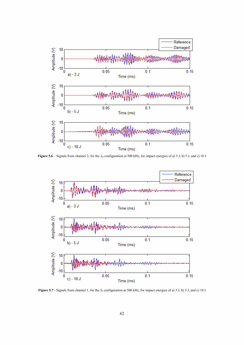
62

Figure 5.6 – Signals from channel 2, for the A0 configuration at 500 kHz, for impact energies of a) 3 J, b) 5 J, and c) 10 J

Figure 5.7 - Signals from channel 1, for the S0 configuration at 500 kHz, for impact energies of a) 3 J, b) 5 J, and c) 10 J

63

Figure 5.8 - Signals from channel 2, for the S0 configuration at 500 kHz, for impact energies of a) 3 J, b) 5 J, and c) 10 J

It is important to mention one experimental occurrence, for the sake of experimental honesty. During

the tests, the excitation signal amplitude was set at 400 mVpp on the waveform generator, yielding a signal with

approximately 300 Vpp after amplification, as depicted in figure 4.14. All the Lamb wave measurements, for both

healthy and damaged specimens, were performed with that amplitude value, and only the frequency was varied

(when necessary). However, unexplainably, for the 5 and 10 J damage levels with the S0 configuration, the

excitation signal amplitude captured was approximately 3 times smaller, exacerbating the amplitude difference

between the pristine and the two damaged states. This occurrence reduces the validity of any conclusions

regarding the amplitude that may be drawn from those two measurements. The conclusions related to the group

velocity are unaffected, since the difference is only in signal amplitude. Thus, in order to make sense out of that

data, it was decided to multiply the signals extracted from those measurements (all three channels) by a factor.

The factor is equal to the ratio between the excitation signal amplitude at the pristine condition, and the

excitation signal amplitude at those two damage levels, yielding a value of 3.0487. This a valid approximation,

as shown by Su and Ye in their paper Selective generation of Lamb wave modes and their propagation

characteristics in defective composite laminates [52]: “For a thin piezoelectric disc of thickness hPZT, the in-

plane strains, �r-PZT and ��-PZT will be generated when an external voltage, V, is applied.”

��h��; � ��h��; � ��)� � ��i��; M (5.1)

The above relation shows it is valid to use the corrected signals to draw conclusions regarding the

amplitude, since the excitation strains transmitted to the laminates were multiples of the applied voltage, which

64

remained in the linear region of the PZT response. Therefore, the dynamic “behaviour” of the signals is totally

unaffected by the multiplication. The responses plotted in figures 5.7b, 5.7c, 5.8b and 5.8c are the “corrected”

signals.

The quantitative evaluation of the changes was done according to the Damage Index approach [3], by

defining the lag coefficient and the attenuation coefficient in equations (5.2) and (5.3). The lag is based on the

ratio between the damaged and undamaged group velocities, vd and vu, respectively. The attenuation uses the

ratio between the damaged and undamaged signal amplitudes, Ad and Au, respectively. Both coefficients are

dimensionless and between 0 and 1. This way, it was possible to relate the reduction in group velocity and

amplitude with damage severity.

�� $ & �� (5.2)

�� $ & ^�^� (5.3)

a) b)

c) Figure 5.9 – Lag and attenuation coefficients for a) A0 configuration, channel 2, b) S0 configuration, channel 1, and c) S0

configuration, channel 2

65

The group velocity and amplitude were determined using the statistical approach, according to which

the values are taken as the average of the 7 values extracted for each impact energy. So, for the A0 configuration

the lag and attenuation coefficients from channel 2 are plotted in figure 5.9a. For the S0 configuration, the

coefficients from channels 1 and 2 are plotted in figures 5.9b and 5.9c, respectively. The amplitudes used for

5.9a, 5.9b and 5.9c were measured in the 4th, 2nd, and 3rd peaks, respectively, of the groups of the desired Lamb

modes, because those were the highest peaks in the corresponding groups of the reference signals.

For the A0 configuration, the 3 and 5 J damages produced very small group velocity variations (3.1%

and 0.3%, respectively), but for 10 J a lag coefficient of about 30.9% was obtained. With the S0 configuration,

the 3 J level was practically not detected in both channels, because the lag coefficient remained approximately

zero. However, for 5 and 10 J, both channels detected clear reductions of S0 group velocity. In channel 1 the lag

coefficient was around 23.7% for both energies, while in channel 2 it was 9.9% and 11.7%.

Contrary to the group-velocity-based-detection, the evaluation of the attenuation coefficient allowed the

detection of the three damage levels with the A0 configuration, yielding 28.9%, 31.1% and 60.6% for 3, 5 and 10

J, respectively. For the S0 configuration, the 3 J impacts remained practically undetected, with 9.5% and 0.5% for

channel 1 and 2, respectively. Only the 5 and 10 J energies were detected, with 54.8% and 87.95% for channel 1

and 2, and 46.5% and 95.6% for channels 1 and 2, respectively. So, although all the damage energies are

detected with A0 configuration, the S0 configuration presents higher attenuation coefficients for 5 and 10 J, and a

clearer difference between levels. It is important to mention that for this quantitative evaluation, only channel 2

was used for the A0 configuration, because it was not possible to unambiguously identify the A0 mode in channel

1.

From the results of the S0 configuration, channel 1 shows more sensitivity to group velocity reductions

than channel 2, which means that the group velocities measured from channel 2 are lower. This fact is related to

the dispersive nature of Lamb waves. The signal captured by channel 2 travels a larger distance from the

actuation unit to the sensor, yielding more changes in the waveform, and therefore a detrimental effect on group

velocity. So, it seems more suitable to evaluate the lag coefficient in channel 1. Following this idea, if it had

been possible to identify the A0 mode in channel 1, group-velocity-based-detection for the A0 configuration

should also be done with that channel, which would probably yield higher lag coefficients. The comparison

between lag and attenuation coefficients shows that the amplitude-based-detection is more sensitive to the

presence of multiple BVID, for both configurations and channels, than the group-velocity-based-detection.

Theoretically, the A0 mode should be more sensitive to the presence of BVID, because its wavelength is

smaller than the S0 wavelength at the same frequency. Yet, the results for the A0 configuration are not as clear as

those for S0 configuration. This discrepancy between theoretical and experimental detection capabilities is most

likely due to the chosen optimization procedure for the generation of the Lamb wave modes. The configuration

for the selective generation of the S0 mode depends only on the correct alignment of the two circular PZT wafers

in opposite surfaces of the plate. On the other hand, the configuration for the predominant excitation of the A0

mode depends on the correct definition of the inter-element distance between rectangular PZT wafers, which

must be a multiple of the wavelength, as described in subsection 3.1.5. Thus, it is necessary to have previous

knowledge of the A0 phase velocity at the desired frequency. In this case, the wavelength was calculated using

the theoretical phase velocity at 500 kHz from the theoretical dispersion curve in figure 4.2. That theoretical

value differs from the actual phase velocity in the composite plate, because that curve is only entirely valid for

66

isotropic material. So, by using the theoretical value to tune the inter-element distance, the two rectangular PZT

wafers were not truly optimized for the predominant excitation of the A0 mode in the composite specimens,

yielding more complex waveforms. Therefore, it was more difficult to distinguish the boundaries of the A0 group

than those of the S0 group, and consequently the results for the A0 configuration are not as accurate as the one for

the S0 configuration.

Furthermore, it is much easier to pick the onset of the S0 mode (first group) than the onset of the A0

mode (third group), which also leads to more inaccuracies in the extraction of the A0 mode.

Thereby, it does not necessarily mean that the S0 Lamb wave mode is more sensitive to multiple BVID

than the A0 mode. It may also indicate that the A0 was not properly generated, nor extracted. Nevertheless, for the

experimental setup used, the S0 configuration proved to be more sensitive to multiple BVID.

Alternatively, the best results for the S0 to BVID may prove that it occurs deeper in the plate thickness,

since the S0 mode is expected to be more sensitive to in-depth damage, while the A0 is expected to be more

sensitive to surface damage, as stated in subsection 3.1.1. This would be a justification for the results obtained

with the A0 configuration.

An interesting fact to discuss is the difference between single and multiple BVID in composites, and the

effect of those differences in the detection results. According to Diamanti et al. [53], a single 8 J impact on a

plate with 2.3 mm of thickness, produced a damage area of approximately 225 mm2, and an amplitude ratio of

about 18%. Grondel et al. [51] were able to detect an almost totally attenuated Lamb wave signal, after inducing

a single 24 J impact on a plate with 4.78 mm of thickness. In this study, the multiple 5 J impacts yielded an

attenuation of 54.8% for channel 1 in the S0 configuration. Therefore, it seems valid to say that multiple BVID

has a more severe effect on the structural integrity of the composite plate than one single impact at slightly

higher energy.

The statistical approach in the Lamb wave measurements was used to take into account the

experimental variability, which was measured by the coefficient of variation, CV. For the measurements in the

damaged specimens, the CV varied between 0.03% and 0.74% for the group velocity, and between 0.31% and

14.86% for the signal amplitude. The experimental variability within the measuring process has several causes:

1) – electronic noise

2) – signal drift and offset

3) – PicoScope inherent errors (DC accuracy is 1% of full scale, vertical resolution is 12 bits, according to

manufacturer [71])

4) – PicoScope filtering error

5) – sensor non-linearities

6) – influence of temperature and humidity on the coupling properties between the sensors and the plates

(within the gel and the adhesive tape)

Additionally and more importantly, there are inaccuracies in the time window selection for the AIC-

picking process, especially for the A0 configuration, posing questions regarding the suitability of the AIC-picker

program to detect the onset time of the group of the A0 Lamb mode. Another source of error that has already

67

been addressed is the (in)efficiency in the selective generation of the A0 Lamb wave mode. Moreover, there are

also errors in measuring the distance between sensors, which induces errors in the calculated group velocity.

The results for the S0 configuration are coherent with the Shearography and C-scan results presented in

sections 5.2 and 5.3, respectively, since the 3 J level was not detected, and the 5 and 10 J damages were clearly

identified, with significant differences between energies.

5.2 Digital Shearography

The Shearography measurements were performed according to the experimental setup described in

subsection 4.2.5. Due to limitations in the laser power and in the field of view of the camera, it was impossible to

examine the whole plate surface. So, it was decided to narrow the measurements to the central part, where the

multiple BVID had been applied. So, the central part of the back surface of the healthy plates was divided in four

portions, and the damaged plates were only divided in two. Those four areas were then examined sequentially to

form a whole image. For all the specimens, shearograms were captured with 2.5 mm of shear in the x and y

directions. For the healthy sample, the loading was applied only during 5 seconds, while for the three damaged

plates three heating times were tested, 5, 10 and 15 seconds. After extracting the images, the Shearwin software

was used to filter and demodulate them, according to the algorithms described in subsection 3.2.2.

The shearograms of the healthy specimen with x-shear and y-shear are shown in figures 5.10a and

5.10b, respectively. The images display the undamaged structure of the plate, where it is possible to clearly

observe the several fibre orientations for approximately half the plate thickness. The x-sheared shearogram in

figure 5.10a appears to be more sensitive to structural details.

The shearograms of the damaged specimens, with x and y shears, and for each heating time, are

presented in figures 5.11 through 5.16. Some results can be readily observed. First, the 3 J impacts were not

detected for any shear or loading time. So, it means the 3 J damage do not alter the out-of-plane strain

distribution. Secondly, the detection of the 5 and 10 J damages proved that those impact energies were able to

produce internal damage (through-thickness damage) on the specimen, since the Shearography measurements

were performed on the back surface. It is interesting to note that features look larger in the shear direction. It is

also important to mention that, because the central area was not divided in an exact way, there are some repeated

features in adjacent shearograms.

In a more detailed analysis of the 5 and 10 J results, the damage was quantitatively evaluated by

visually measuring the approximately circular area of the impact points. The areas of the identified points were

averaged, yielding the mean value of the damage area for each energy level. It is relevant to mention that the

positions of the impact points in the shearograms are mirrored relative to the vertical axis of figure 4.8. The

results are summarized in tables 5.1 through 5.6.

The presence of 5 J damage was not entirely detected. The blue lines in the tables indicate that, with

shear in the x direction, impacts 1 and 3 were not identified by the 5 s loading, and impact 3 was not identified

by the 10 and 15 s loadings. A similar thing happened with y shear, for which points 1, 2 and 3 were not visible

after a 5 s heating, and points 1 and 3 were not visible after a 10s heating. However, for a heating time of 15 s,

the y shear configuration was able to detect all the impact points. Hence, it seems that, for 15 s heating and shear

in the y direction (direction of the 90º fibres), shearograms are more sensitive to changes in the concentration of

68

the out-of-plane strain induced by the applied multiple BVID. This is a curious fact. The comparison between

figures 5.13c and 5.14c, shows that x shear generates shearograms where it is possible to observe the structure

details more clearly, and yet not all impacts can be identified. The existence of undetected damages also suggests

that there are impacts, namely points 1 and 3, which were less severely applied than others.

a) b) Figure 5.10 - Shearograms for the undamaged specimen, for 5 seconds of heating, with a) x-shear, and b) y-shear

For the 5 J damage, the average damage area for x and y shears remained approximately equal to 0.15

cm2 and 0.20 cm2, respectively, as the heating time increased. With x shear, the CV was 30.89%, 35.74%, and

38.37%, for 5, 10, and 15 s heating, respectively. With y shear, the CV was 40.16%, 36.59%, and 40.39%, for 5,

10, and 15 s heating. The average values and the CV were always higher for the y shear, which may have two

interpretations. Higher mean value may indicate that the y shear allows an evaluation of the real damage severity.

On the other hand, higher CV indicates more variability in the measuring process, and thus a less reliable

evaluation.

The 10 J impacts were all detected, with both x and y shears, and for all the heating times. In tables 5.4,

5.5 and 5.6, the yellow lines for points 4 and 5 indicate overlapping damage areas, which may imply coalescence

of internal delaminations. The average damage area increased with loading time. With x shear, the average

damage area was 0.41, 0.50, and 0.66 cm2, for 5, 10, and 15 s heating, respectively. With y shear, the average

damage area was 0.51, 0.74, and 0.75 cm2, for 5, 10, and 15 s heating, respectively. The CV had a similar

evolution. With x shear, the CV was 32.59%, 45.45%, and 28.08%, for 5, 10, and 15 s heating, respectively.

With y shear, the CV was 15.97%, 32.55%, and 23.34%, for 5, 10, and 15 s heating, respectively. So, in this

case, the trend was different from the 5 J case, because, although the average values were higher for the y shear,

the CV was lower for the y shear. Thereby, the evaluated damage severity is closer to reality and the variability

in the measuring process is lower, yielding a more reliable evaluation. Again, this seems to suggest that the y

shear is more sensitive to applied multiple BVID, especially if combined with moderate loading times.

69

a) b)

c) Figure 5.11 - Shearograms for the 3 J specimens, with x shear, loaded for a) 5s b) 10s, and c) 15 s

70

a) b)

c) Figure 5.12 - Shearograms for the 3 J specimens, with y shear, loaded for a) 5s b) 10s, and c) 15 s

71

a) b)


72

a) b)


73

a) b)


74

a) b)


75

Table 5.1 – Shearography results: damage areas of the ten impact points for the 5 J specimen, with 5 s heating 5 J specimen, 5 seconds

x shear y shear

Points Diameter (cm) Area (cm2) Diameter (cm) Area (cm2)

1 0.00 0.00 0.00 0.00

2 0.31 0.08 0.00 0.00

3 0.00 0.00 0.00 0.00

4 0.51 0.21 0.63 0.31

5 0.48 0.18 0.51 0.21

6 0.46 0.16 0.54 0.23

7 0.51 0.21 0.46 0.16

8 0.48 0.18 0.51 0.21

9 0.34 0.09 0.26 0.05

10 0.48 0.18 0.48 0.18

Avg. 0.16 0.19

Std. Dev. 0.05 0.08

CV (%) 30.89 40.16

Table 5.2 - Shearography results: damage areas of the ten impact points for the 5 J specimen, with 10 s heating 5 J specimen, 10 seconds

x shear y shear


1 0.31 0.08 0.00 0.00

2 0.31 0.08 0.29 0.06

3 0.00 0.00 0.00 0.00

4 0.48 0.18 0.57 0.26

5 0.48 0.18 0.57 0.26

6 0.51 0.21 0.60 0.28

7 0.46 0.16 0.54 0.23

8 0.46 0.16 0.54 0.23

9 0.37 0.11 0.40 0.13

10 0.54 0.23 0.60 0.28

Avg. 0.15 0.22

Std. Dev. 0.06 0.08

CV (%) 35.74 36.59

76


x shear y shear


1 0.34 0.09 0.29 0.06

2 0.34 0.09 0.40 0.13

3 0.00 0.00 0.40 0.13

4 0.51 0.21 0.48 0.18

5 0.51 0.21 0.57 0.26

6 0.57 0.26 0.63 0.31

7 0.46 0.16 0.54 0.23

8 0.46 0.16 0.54 0.23

9 0.31 0.08 0.40 0.13

10 0.48 0.18 0.54 0.23

Avg. 0.16 0.19

Std. Dev. 0.06 0.08

CV (%) 38.37 40.39


x shear y shear


1 0.60 0.28 0.74 0.43

2 0.60 0.28 0.74 0.43

3 0.54 0.23 0.83 0.54

4 0.88 0.61 0.71 0.40

5 0.74 0.43 0.91 0.65

6 0.68 0.37 0.83 0.54

7 0.86 0.57 0.83 0.54

8 0.80 0.50 0.88 0.61

9 0.63 0.31 0.83 0.54

10 0.77 0.47 0.77 0.47

Avg. 0.41 0.51

Std. Dev. 0.13 0.08

CV (%) 32.59 15.97

77


x shear y shear


1 0.63 0.31 0.80 0.50

2 0.57 0.26 0.74 0.43

3 0.60 0.28 0.77 0.47

4 1.08 0.92 1.11 0.97

5 0.97 0.74 0.88 0.61

6 0.63 0.31 1.03 0.83

7 0.91 0.65 0.97 0.74

8 0.74 0.43 1.17 1.07

9 0.77 0.47 0.97 0.74

10 0.91 065 1.17 1.07

Avg. 0.50 0.74

Std. Dev. 0.23 0.24

CV (%) 45.45 32.55

Table 5.6 – Shearography results: damage areas of the ten impact points for the 10 J specimen, with 15 s heating 10 J specimen, 15 seconds

x shear y shear


1 0.86 0.57 0.97 0.74

2 0.68 0.37 0.77 0.47

3 0.74 0.43 0.86 0.57

4 0.97 0.74 1.08 0.92

5 0.97 0.74 0.97 0.74

6 1.03 0.83 0.97 0.74

7 1.05 0.87 0.94 0.69

8 1.00 0.78 1.17 1.07

9 0.77 0.47 0.91 0.65

10 1.03 0.83 1.05 0.87

Avg. 0.66 0.75

Std. Dev. 0.19 0.17

CV (%) 28.08 23.34

78

The number of undetected 5 J impact points is larger for shear in the y direction probably because that is

the orientation with the smaller number of fibres, and therefore the direction of lower thermal conductivity in the

composite plate [72]. The thermal load is better distributed along the x direction, inducing clearer changes in the

concentration of the out-of-plane strain. However, the coefficient of thermal expansion across the majority of the

fibres is higher than in the other directions [72]. So, it seems that, at 15 s heating, the load is high enough to

promote the thermal expansion along the y direction, and thus induce visible changes in the out-of-plane strain

concentration.

In a general way, for 15 s of loading it is possible to observe more impact details more clearly, namely

the small 45 degree surface cracks which were observed through the optical microscope (see section 5.4). This is

consistent with theory, because, according to equations (3.27), the phase change increases as the loading

increases. So, clearer changes in the out-of-plane strain concentrations are achieved when a longer heating is

applied, allowing a more reliable evaluation of the damage severity.

The small changes in the Lamb wave response for 3 J, and the clear increase in the lag and attenuation

coefficients for 5 and 10 J in the S0 configuration are in agreement with the Shearography results, for both shear

directions, pointing to the S0 configuration as a more accurate damage detection setup. Yet, the differences in

damage severity between 5 and 10 J are not identified by the Lamb wave method. The fact that the Lamb wave

method captures the dynamic behaviour of the structure allows a more accurate evaluation of the consequences

of damage for structural integrity.

An extensive comparison between the Shearography and C-scan results is made in section 5.3.

When evaluating the measured damage areas it is necessary to pay attention to the spatial resolution of

the shearogram. If a 1 x 1 mm2 surface area is considered, and a shear amount of 2.5 mm is applied (as in the

present study), then the signal in the shearing direction is the average strain of 2.5 areas of 1 x 1 mm2. In the

other direction, the resolution depends on the lens and pixel resolution of the CCD-camera. However, the image

processing described in subsection 3.2.2 induces a resolution loss, which is related to the number of pixels inside

the filter window.

The calculation of the phase change, �, through the phase-shift also introduces errors. They are

generated by the inaccuracies in the piezoelectric-driven movement of the mirrors of the modified Michelson

interferometer, and by the existence of very small denominators when equation (3.30) is used to compute the

phase change.

For the Shearography tests performed in this project, eight lasers were used so that the light intensity

would be enough to generate clear shearograms. This unusual large number of lasers introduced more signal

noise, which may have slightly reduced the accuracy of the measurements.

5.3 Ultrasonic C-scan

The C-scan measurements were performed at 10 MHz, and the data was extracted using the Automated

Laminate Inspection System (ALIS) software package. The colours of the dB attenuation map were selected in

order to enhance the structural details of the plates. The image for the healthy sample is depicted in figure 5.17.

The dB map shows the undamaged fibre structure of the specimen. Although some small manufacturing defects

79

are visible near the lower edge of the plate, the central part is not affected, and, in fact, the standard deviation of

the attenuation distribution in that area was lower than the standard deviation in the C-scan reference sample.

Figure 5.17 – Attenuation map of the healthy sample

The damaged specimens were tested with the same C-scan configuration, and the obtained attenuation

maps are presented in figure 5.18. The colour code for the dB attenuation levels is light blue for nearly -55 dB,

and purple for nearly 108.4 dB. As with Shearography, the 3 J BVID was not detected and it is possible to

observe a clear distinction between the 5 and 10 J impact energies. Furthermore, for each of the detected

energies, there are some impact points more severe than others. In figure 5.18c, the 10 J impacts have a

characteristic purple ring of more severely damaged material around a small blue, less damaged region. This

occurrence was confirmed by the optical microscope observations of the plate surface in section 5.4.

In a quantitative analysis, the evaluation was done by measuring the approximately circular area around

each impact point, similarly to the approach used for Shearography. The C-scan results are summarized in table

5.7. Impact point 3 stands out from the others, because it has the smallest damage area, confirming it is the less

severe of all. That is why it was the most difficult point to identify in Shearography tests. The C-scan mean

values of the measured damage areas for 5 and 10 J, 0.33 cm2 and 1.03 cm2 respectively, are larger than the

corresponding values for all the Shearography tests. Additionally, the C-scan CV values for 5 and 10 J, 42.37%

and 17.44%, respectively, are very similar to the values obtained with Shearography. So, it is possible to

conclude that the C-scan allowed the detection of a more real damage severity, with the same level of reliability

as Shearography.

80

a)

b)

c) Figure 5.18 – Attenuation maps of the damaged specimens: a) 3 J, b) 5 J, and c) 10 J

81

Table 5.7 – C-scan results: Damage areas of the ten impact points for the 5 and 10 J specimens 5 J specimen 10 J specimen


1 0.49 0.19 1.09 0.94

2 0.52 0.21 1.01 0.81

3 0.39 0.12 0.99 0.77

4 0.78 0.48 1.27 1.27

5 0.75 0.45 1.17 1.08

6 0.81 0.51 1.25 1.22

7 0.62 0.31 1.17 1.08

8 0.68 0.36 1.22 1.17

9 0.52 0.21 1.04 0.85

10 0.75 0.45 1.20 1.12

Avg. 0.33 1.03

Std. Dev. 0.14 0.18

CV (%) 42.37 17.44

Nevertheless, the relatively high coefficient of variation for the C-scan and Shearography measurements

denotes the existence of errors in the application of the impact energy. On one hand, there is approximately a 1

cm (0.12 J) inherent error when setting the height to apply a certain level of impact energy, because there is no

real ruler attached to the pulling system of the impact tower. So, naturally, not all the impacts of a certain level

had the same intensity. On the other hand, the application of BVID in multiple points required the specimens to

be moved between the aluminium frames, instead of the whole clamping device with the plates on it, because the

available space underneath the impact tower was limited. So, there were some positions of the plates inside the

clamping device that prevented some bolts to be screwed, allowing small movements of the composite plates

during the impacts. Thus, the energy was not entirely transmitted to the material, and all the impacts occurred

slightly to the left of the ink mark.

The relatively high CV may also indicate that the damage-area-measuring technique is not accurate

enough, since it is based on visual inspection of the acquired images.

The yellow lines in the 10 J column of table 5.7 denote impact points 4, 5 and 6, whose damage areas

are overlapped in figure 5.18c. This overlapping may be caused by the proximity of the small surface cracks, or

by the coalescence of internal delaminations. So when comparing the overlapping of points 4 and 5 in the 10 J

shearograms, with the overlapping of points 4, 5 and 6 in the 10 J C-scan images, attention should be paid to the

difference in the resolutions of the two NDT methods. The water jet of the C-scan system is approximately 6 mm

in diameter. So, if a 1 x 1 mm2 surface area is considered, the water jet captures the combined attenuation of

nearly 19 areas of 1 x 1 mm2 within its diameter. Therefore, contrary to what was previously described for

Shearography, the C-scan resolution is less fine, which may indicate that some features may not be actually

overlapped.

It is important to note that the Shearography results for y shear and 15 s heating are the closest to the C-

scan results, showing good agreement between both NDT methods. Thus, it seems valid to say that, for the used

82

material, lay-up sequence, distance lamp-samples, and powers of the laser and lamp, Shearography is almost as

sensitive as C-scan, when proper loading is applied. The C-scan results confirm that the S0 configuration in the

Lamb wave tests was the most suitable for the detection of multiple BVID.

5.4 Optical microscope

Microscopic observations of the surface of the damaged plates were performed in order to obtain data

merely regarding the surface damage. Only one impact point was observed for each damaged specimen, so no

statistical study could be made. The pictures for the 3, 5 and 10 J samples are shown in figures 5.19a, 5.19b and

5.19c.

In figure 5.19a, it is very difficult to discern the presence of a 3 J impact. Only a slight circular pattern

discloses the barely-visible damage. For the 5 and 10 J specimens a circular border of what seems to be crushed

material surrounds an undamaged region, forming a valley with approximately the shape of the hemispherical

impactor. The areas of the circular valleys are quantified in table 5.8, showing that the indentation area is slightly

larger for the 10 J damage. Interesting details in figures 5.19a and 5.19b are the ink marks, confirming that the

impacts occurred slightly to the left of the intended position.

More importantly, in figures 5.19b and 5.19c, the 5 and 10 J impacts have two small surface cracks

along the 45 degree direction. This specific direction is not a random occurrence. It shows that is the direction of

highest stress concentration during the impact, promoting the rupture of the fibres in the surface layer. The

cracks are longer for the 10 J impact, as they do not fit entirely in the image of figure 5.19c. Two detailed

pictures of the 45 degree cracks from the 10 J impact are presented in figure 5.20. They show that there are

“cliffs” on both sides of the cracks, creating shadow on the outer part.

Table 5.8 – Damage areas of the circular impact spots observed by optical microscopeE (J) Diameter (cm) Area (cm2)

3 - -

5 0.23 0.041

10 0.26 0.054

83

a)

b)

c) Figure 5.19 – Microscopic observations of the surface of the damaged specimen: a) 3 J impact, b) 5 J impact, and c) 10 J

impact

84

a) b) Figure 5.20 – Details of the 45 degree cracks of the 10 J impact: a) crack tip, b) middle of the crack

These small up lifting cracks probably conceal internal delaminations underneath, because they are not

confined to the surface layer. Hence, the growth of the small cracks seems to be the cause for the increase in the

measured damage area from 5 to 10 J in the Shearography and in the C-scan results.

85

Chapter 6

Conclusions and recommendations

6.1 Conclusions

The implementation of Non-Destructive Testing (NDT) technology in the aircraft industry has proven to

be capable of enhancing safety and extending the life-cycle of structures. The increasing needs for life-cycle cost

reduction and lower fuel consumption have promoted the use of composite materials, whose mechanical

behaviour poses new issues regarding the effects of impact damage on residual strength, at an early stage of the

life-cycle of the structure.

Low-velocity (or barely-visible) impact damage (BVID) can be the cause of early fatigue damage, due

to subsurface delaminations and matrix cracks. So, if BVID is detected, it gives a maintenance alert, warning

about the possibility of subsequent fatigue damage at that location. In that sense, the identification of low-

velocity impact damage by an NDT technique does not imply immediate maintenance or replacement of the

component. If the damage size is below a previously established value, then the component is kept operating.

The maximum admissible damage severity is established on a mechanical design basis. The NDT method only

provides a warning (hopefully before that limit is reached), which is crucial for future maintenance inspections.

This way the operational availability is maximized.

Therefore, the main goal of this thesis was to assess the suitability of the Lamb wave method to detect

three different levels of multiple BVID on carbon-epoxy composite plates, and, if possible, improve its diagnosis

capabilities. Digital Shearography with thermal loading, and ultrasonic C-scan were used to substantiate the

results from the Lamb wave tests, and the comparison between these methods yielded important conclusions

about their sensitivity to BVID.

The two fundamental symmetric and anti-symmetric (S0 and A0) Lamb wave modes were tested, using

two different configurations of piezoelectric-wafer actuators for the selective generation of each mode. The

damage detection relied on the identification of changes in the group velocity and amplitude of the modes. The 3

J damage induced little variations, remaining practically undetected, while the 5 and 10 J damages were clearly

detected by both configurations. The amplitude-based approach produced more unambiguous results, as it was

possible to detect an almost totally attenuated signal for the 10 J case. Taking into account the theoretical model,

the piezoelectric transducers, and the signal processing tools used, the S0 configuration proved to be more

sensitive to the presence of multiple BVID. When compared with previous studies [51, 53], the Lamb wave

results showed that the presence of multiple BVID has a more detrimental effect on structural integrity than one

single impact at a slightly higher energy.

86

In the digital Shearography measurements, shear in the x and y direction was combined with three

different heating times, in order to study the effect of the loading time on the detection capabilities of the

shearograms. None of the configurations revealed the 3 J impacts. The 5 J multiple BVID was partially detected

by the x shear, and only with y shear and 15 s heating it was possible to identify all the 5 J damages. The 10 J

impacts were all detected, for both configurations and all the loading times, with the combination of y shear and

15 s heating having the best results.

The ultrasonic C-scan was able to detect the 5 and 10 J damages, and confirmed the higher reliability of

the results from the combination of y shear with 15 s loading. Both the Shearography and the C-scan images

showed some overlapped impact points, probably revealing subsurface delaminations. This suspicion was then

substantiated by microscopic observations of the plate surface, where small 45 degree cracks were identified. So,

it was concluded that, for the tested specimens and experimental setup, Shearography can be as reliable as C-

scan, as long as appropriate loading is applied. At the end, the Lamb wave results for the S0 configuration,

together with the Shearography and C-scan images formed a coherent set of NDT results regarding multiple

BVID.

One of the big issues in the study of NDT is the quest for the detection threshold of each technology.

From this study it was possible to draw some conclusions that show the duality in this matter. The three

techniques seem to coherently point somewhere between 3 J and 5 J as the lowest detectable impact energy.

Nevertheless, it also appears that the detection threshold is not imposed by the measuring technology, but by the

material. The specimens used in this study had a 2.24 mm thickness, and the 5 J impacts were strong enough to

produce detectable damage. However, if a 20 mm thickness plate was impacted at 5 J, probably the induced

damage would not be severe enough to be identified. Therefore, a detection threshold can only be defined with

respect to a property of the material.

6.2 Recommendations for future developments

During this project, the typical challenges in experimental work were encountered. Although there was

autonomy in the decisions, the accomplishment of the experimental work depended on more than one person. In

that sense it was crucial to understand the way of thinking of other students, laboratory technicians, and

professors, in order to benefit from all their help and good advices. It was necessary to have good judgment to

avoid hasty decisions, but also mental agility to be on schedule. Moreover, knowledge about several different

areas was required, from mechanics to electronics, from composite manufacturing to MATLAB® programming,

and new things were learnt every day. The correct management of available time, money and available resources

was crucial for the success of the experimental work. Yet, even in a well managed project there are physical

limitations and the perfect solution is hardly ever achieved. Therefore, it was necessary to extract the largest

amount of useful information from the available data, and to recognize the possible improvements for future

developments.

One of the problems in the Lamb wave method was the proper identification of the zero-order anti-

symmetric mode (A0 mode). Thus, a major advance would be the use of software capable of accurately

calculating the dispersion curves for anisotropic material. One possible choice for the software is the DISPERSE

program, from Imperial College, London. This tool would allow a more precise calculation of the phase velocity

87

at a certain frequency, yielding a better tuning of the A0 configuration with the rectangular PZT wafers. On the

other hand, a better way to improve the A0 Lamb mode selective generation would be by using circular PZT

wafer actuators on opposite plate surfaces, excited in anti-phase, as described in subsection 3.1.3. This solution

would also save money, since the same circular wafers would be used for both the A0 and S0 configurations. To

optimize the acquisition of the Lamb wave response, the sensors should also be circular PZT wafers, instead of

conventional piezoelectric transducers. A better A0 configuration would help to minimize the errors in the

selection of the time-window for the AIC-picking of the onset time of the A0 group. Consequently, the errors in

the computation of the group velocity of the A0 Lamb mode would also be minimized. With the A0 excitation

properly tuned, it would be possible to conduct an unambiguous investigation in order to determine which Lamb

mode is actually the best one to detect BVID.

In order to reduce part of the experimental variability, the application of different impact energies

should be done by changing the impact mass instead of varying the dropping height. This way the changes in

impact energy would be more accurately quantified. It should be noted that an increase in mass has a direct,

more damaging effect upon the plate due to the momentum �� transmitted during the impact, while an

increase in height only increases the momentum p�� i times.

In a damage tolerance approach, it would be interesting to perform fatigue tests with a relevant load

spectrum, to evaluate the residual strength of the plates after the application of multiple BVID. It would be also

interesting to test more impact energies within the range 3 – 15 J, to have a better understanding of the

relationship between the detection parameters of the Lamb wave method and the actual damage severity,

yielding great progress towards the implementation of Structural Health Monitoring systems in aircrafts.

89

References

[1] Beukers, Adriaan (1992), “A new technology for sandwich plates and structures based on the use of

in-situ foamable thermoplastic films”. 37th International SAMPE Symposium and Exhibition,

Anaheim (CA), 9-12 March 1992, Proceedings (A93-15726 04-23), pp. 172-185.

[2] Schijve, Jaap (2004), “Fatigue of Structures and Materials”. Kluwer Academic Publishers,

Dordrecht.

[3] Su, Zhongqing and Ye, Lin (2009), “Identification of Damage Using Lamb Waves: From

Fundamentals to Applications”. Springer

[4] Su, Zhongqing; Ye, Lin and Lu, Ye (2006), “Guided Lamb waves for identification of damage in

composite structures: A review”. Journal of Sound and Vibration, 295, pp.753-780.

[5] Deo, Ravi B.; Starnes, Jr., James H. and Holzwarth, Richard C. (2001), “Low-cost composite

materials and structures for aircraft applications”. RTO AVT Specialists’ Meeting on “Low-cost

composite structures”, Loen (Norway), 7-11 May 2001, RTO-MP-069(II).

[6] Stewart, Richard (2009), “New prepreg materials offer versatility, top performance”. Reinforced

Plastics, June/July, pp. 28-33.

[7] Jones, Robert M. (1999), “Mechanics of Composite Materials” (2nd ed.). Taylor & Francis,

Philadelphia.

[8] Megson, T. H. G. (2007), “Aircraft Structures for Engineering Students”. Butterworth-Heinemann,

Oxford (UK).

[9] Smeltzer, Stanley S.; Lovejoy, Andrew E. and Satyanarayana, Arunkumar (2008), “Numerical

characterisation of a composite bonded wing-box”. 49th AIAA/ASME/ASCE/AHS/ASC Structures,

Structural Dynamics and Materials Conference, Schaumburg, IL (USA), 7-10 April 2008.

[10] Masters, John E. (1997), “Translaminar fracture toughness of a composite wing skin made of

stitched warp-knit fabric”. NASA Contractor Report 201728, NASA Langley Research Center,

Hampton, Virginia (USA).

90

[11] Johnson, A. F.; Kempe, G. and Simon, J. (1999), “Design of composite wing access cover under

impact loads”. Applied Composite Materials, vol. 7, pp. 219-229.

[12] Byers, B. A. and Stoecklin, R. L. (1980), “Preliminary design of graphite composite wing panels for

commercial transport aircraft”. NASA Contractor Report 159150, NASA Langley research Center,

Hampton, Virginia (USA).

[13] Klomp-de Boer, Ronald (2010), “Development of a cost effective composite wing-box for a small

aircraft”. Report NLR-TP-2010-047, NLR Aerospace Vehicle Division, The Netherlands.

[14] Hawk, Jeff (2005), “The Boeing 787 Dreamliner: More Than an Airplane”. AIAA/AAAF Aircraft

Noise and Emissions Reduction Symposium, Monterey, California (USA), 24-26 May 2005

[15] Kollár, László P. and Springer, George S. (2003), “Mechanics of Composite Structures”. Cambridge

University Press, New York.

[16] Reddy, Junuthula N. (2004), “Mechanics of laminated Composite Plates and Shells – Theory and

Analysis”. CRC Press, Boca Raton.

[17] Meyers, Marc André and Chawla, Krishan Kumar (2009), “Mechanical Behavior of Materials”.

Cambridge University Press, New York.

[18] Rouchon, J. (2009), “Fatigue and Damage Tolerance Evaluation of Structures: The Composite

Materials Response”. Report NLR-TP-2009-221, NLR Aerospace Vehicle Division, The

Netherlands.

[19] Talreja, R. (1981), “Fatigue of composite materials: damage mechanisms and fatigue-life diagrams”.

Proceedings of the Royal Society of London, Series A, Mathematical and Physical, vol. 378, no.

1775, pp. 461-475.

[20] Richardson, M. O. W. and Wisheart, M. J. (1996), “Review of low-velocity impact properties of

composite materials”. Composites Part A, vol. 27A, pp. 1123-1131.

[21] Hosseinzadeh, Ramin; Shokireh, Mahmood Mehrdad and Lessard, Larry (2005), “Damage

behaviour of fibre reinforced composite plates subjected to drop weight impacts”. Composites

Science and Technology, vol. 66, pp. 61-68.

[22] Winggenraad, J. F. M. and Ubels, L. C. (1997), “Impact damage and failure mechanisms in structure

relevant composite specimens”. Report NLRTP 97006, NLR, The Netherlands.

91

[23] Elber, Wolf (1983), “Failure mechanics in low-velocity impacts on thin composite plates”. NASA

Technical Paper 2152, NASA Langley Research Center, Hampton, Virginia (USA).

[24] Mitrevski, T.; Marshall, I. H.; Thomson, R. S. and Jones, R. (2006), “Low-velocity impacts on

preloaded GFRP specimens with various impactor shapes”. Composite Structures, vol. 76, pp. 209-

217.

[25] Rilo, Nuno Ferreira and Silva Ferreira, Luís Manuel (2008), “Experimental study of low-velocity

impacts on glass-epoxy laminated composite plates”. International Journal of Mechanics and

Materials in Design, vol. 4, pp. 291-300.

[26] Malekzadeh, K.; Khalili, M. R.; Olsson, R. and Jafari, A. (2006), “Higher-order dynamic response

of composite sandwich panels with flexible core under simultaneous low-velocity impacts of

multiple small masses”. International Journal of Solids and Structures, vol. 43, pp. 6667-6687.

[27] Paul, J. J.; Galea, S. C. and Jones, R. (1994), “Residual strength of composites with multiple impact

damage”. Research Report 13, Aeronautical Research Laboratory, Melbourne, Victoria (Australia).

[28] Galea, S. C; Shah, L. P. and Sanderson, S. (1995), “The effect of multiple damage in composite

structures: a theoretical investigation”. Composite Structures, vol. 32, pp.383-390.

[29] Appleby-Thomas, Gareth J.; Hazell, Paul J. and Dahini, Gussan (2011), “On the response of two

commercially-important CFRP structures to multiple ice impacts”. Composite Structures, vol. 93,

pp. 2619-2627.

[30] Cartz, Louis (1995), “Nondestructive Testing – Radiography, Ultrasonics, Liquid Penetrant,

Magnetic Particle, Eddy Current”. ASM International

[31] Mix, Paul E., (2005), “Introduction to Nondestructive Testing – A Training Guide” (2nd ed.). John

Wiley & Sons, Inc.

[32] Yolken, H. Thomas and Matzkanin, George A. (2009), “Nondestructive evaluation of advanced

fiber reinforced polymer matrix composites – A technology assessment”. NASA Contractor Report

2009-215566, NASA Langley Research Center, Hampton, Virginia (USA).

[33] Fahr, A. and Kandeil, A. Y. (1992), “Ultrasonic C-scan inspection of composite materials”.

Engineering Journal of Qatar University, vol. 5, pp. 201-222.

92

[34] Galea, S. C. and Saunders, D. S. (1992), “In-situ ultrasonic C-scanner”. Technical Report 4,

Aeronautical Research Laboratory, Melbourne, Victoria (Australia).

[35] Kas, Y. Onur and Kaynak, Cevdet (2004), “Ultrasonic (C-scan) and microscopic evaluation of resin

transfer molded epoxy composite plates”. Polymer Testing, vol. 24, pp. 114-120.

[36] Hasiotis, T.; Badogiannis, E. and Tsouvalis, N. G. (2007), “Application of ultrasonic C-scan

techniques for tracing defects in laminated composite materials”. 4th International Conference on

NDT, Chania, Crete (Greece), 11-14 October 2007.

[37] Polimeno, Umberto and Meo, Michele (2009), “Detecting barely visible impact damage on aircraft

composite structures”. Composite Structures, vol. 91, pp. 398-402.

[38] Polimeno, Umberto; Meo, Michele; Almond, Darryl P. and Angioni, Stefano L. (2010), “Detecting

low velocity mpact damage in composite plate using nonlinear acoustic/ultrasound methods”.

Applied Composite Materials, vol.17, pp. 481-488.

[39] Takeda, S.; Aoki, Y.; Ishikawa, T.; Takeda, N. and Kikukawa, H. (2006), “Structural health

monitoring of composite wing structure during durability test”. Composite Structures, vol. 79, pp.

133-139.

[40] Garnier, Christian; Pastor, Marie-Laetitia; Eyma, Florent and Lorrain, Bernard (2010), “The

detection of aeronautical defects in situ on composite structures using Non Destructive Testing”.

Composite Structures, vol.93, pp. 1328-1336.

[41] Hung, Y. Y. (1999), “Applications of digital Shearography for testing of composite structures”.

Composites, Part B: Engineering, vol. 30, pp. 765-773.

[42] Amaro, Ana M.; Santos, J. B. and Cirne, José (2004), “Comparative study of different non-

destructive testing techniques in the characterisation and quantification ofthe damage effects in

carbon-epoxy laminates”. Insight, vol. 46, no. 9, pp. 559-565.

[43] Ruzek, Roman; Lohonka, Radek and Jironc, Josef (2005), “Ultrasonic C-scan and Shearography

NDI techniques evaluation of impact defects identification”. NDT&E International, vol. 39, pp. 132-

142.

[44] Steinchen, Wolfgang; Yang, Lianxiang; Kupfer, Gerhard and Mäckel, Peter (1998), “Non-

destructive testing of aerospace composite materials using digital Shearography”. Proceedings of

Institution of Mechanical Engineers, vol. 212, Part G, pp. 21-30.

93

[45] Habeger, Charles C., Jr.; Mann, Ronald W. and Baum, Gary A. (1979), “Ultrasonic plate waves in

paper”. Ultrasonics, pp. 57-62.

[46] Miesen, Nick; Mizutani, Yoshihiro; Groves, Roger M.; Sinke, Jos and Benedictus, Rinze (2011),

“Lamb wave detection in prepreg composite materials with fibre Bragg grating sensors”. Sensors

and Smart Structures Technologies for Civil, Mechanical, and Aerospace Systems 2011, 7th March

2011, San Diego, California (USA), Proceedings SPIE 7981, 79812J.

[47] Percival, W. J. and Birt, E. Anne. (1997), “A study of Lamb wave propagation in carbon-fibre

composites”. Insight, vol. 39, no. 10, pp. 728-735.

[48] Birt, E. Anne. (1998), “Damage detection in carbon-fibre composites using ultrasonic Lamb waves”.

Insight, vol. 40, no. 5, pp. 335-339.

[49] Grondel, Sébastien; Assaad, Jamal; Delebarre, Christophe and Moulin, Emmanuel. (2004), “Health

monitoring of a composite wingbox structure”. Ultrasonics, vol. 42, pp. 819-824.

[50] Kessler, Seth S.; Spearing, S. Mark and Soutis, Constantinos (2002), “Damage detection in

composite materials using lamb wave methods”. Smart Materials and Structures, vol. 11, pp.269-

278.

[51] Grondel, Sébastien; Paget, Christophe; Delebarre, Christophe and Assaad, Jamal (2002), “Design of

optimal configuration for generating A0 Lamb mode in a composite plate using piezoceramic

transducers”. Journal of the Acoustical Society of America, vol. 112 (1), pp. 84-90.

[52] Su, Zhongqing and Ye, Lin (2004), “Selective generation of Lamb wave modes and their

propagation characteristics in defective composite laminates”. Proceedings of the Institution of

mechanical Engineers, vol. 218, Part L: Journal of Materials design and Applications, pp. 95-110.

[53] Diamanti, K.; Soutis, C. and Hodgkinson, J. M. (2006), “Piezoelectric transducer arrangement for

the inspection of large composite structures”. Composites, Part A: Applied Science and

Manufacturing, vol. 38, pp. 1121-1130.

[54] Giurgiutiu, Victor and Santoni-Bottai, Giola (2011), “Structural health monitoring of composite

structures with piezoelectric-wafer active sensors”. AIAA Journal, vol.49, no. 3, pp. 565-581.

[55] Matt, Howard M. (2006), “Structural Diagnosis of CFRP Composite Aircraft Components by

Ultrasonic Guided Waves and Built-In Piezoelectric Transducers”. PhD Thesis, University of

California, San Diego (USA).

94

[56] Giurgiutiu, Victor (2008), “Structural Health Monitoring with Piezoelectric Wafer Active Sensors”.

Academic Press-Elsevier, San Diego, California (USA).

[57] Elmore, William C. and Heald, Mark A. (1969), “Physics of Waves”. McGraw-Hill.

[58] Mizutani, Yoshihiro and Takemoto, Mikio (1998), “A simplified elastic stiffness estimation of

unidirectional carbon-fiber-reinforced coupon using the in-plane velocity anisotropy of Lamb

waves”. Japanese Journal of Applied Physics, vol. 37, pp. 3110-3115.

[59] Giurgiutiu, Victor (2002), “Lamb wave generation with piezoelectric wafer active sensors for

structural health monitoring”. SPIE’s 10th Annual International Symposium on Smart Structures and

Materials and 8th Annual International Symposium on NDE for Health Monitoring and Diagnosis,

2-6 March 2002, San Diego, California (USA), paper no. 5056-17.

[60] Vasilescu, G. (2005), “Electronic Noise and Interfering Signals – Principles and Applications”.

Springer.

[61] Smith, Steven W. (2003), “Digital Signal Processing – A Practical Guide for Engineers and

Scientists”. Newnes-Elsevier Science.

[62] Leckie, Frederick A. and Dal Bello, Dominic J. (2009), “Strength and Stiffness of Engineering

Systems”. Springer.

[63] Kurz, Jochen H.; Grosse, Christian U. and Reinhardt, Hans-Wolf (2004), “Strategies for reliable

automatic onset time picking of acoustic emissions and of ultrasound signals in concrete”.

Ultrasonics, vol. 43, pp. 538-546.

[64] Steinchen, Wolfgang and Yang, Lianxiang (2003), “Digital Shearography – Theory and Application

of Digital Speckle Pattern Shearing Interferometry”. SPIE, Bellingham, Washington (USA).

[65] Rodi, Riccardo; Campoli, Gianni; Alderliesten, René C. and Benedictus, Rinze (2009),

“Characterization of the crack tip behaviour in fibre metal laminates by means of digital image

correlation”. 50th AIAA/ASME/ASCE/AHS/ASC Structures, Structural Dynamics, and Materials

Conference, vol. 2009-2586.

[66] “Standard Test method for Measuring the Damage Resistance of a Fiber-Reinforced Polymer Matrix

Composite to a Drop-Weight Impact Event”. Designation: D 7136/D 7136M – 05, ASTM

International, 2005.

[67] “Piezo Material Data – Specific parameters of the Standard materials”. Physik Instrumente, 2011.

95

[68] “PICO HF-1.2 Sensor: 600 kHz Frequency, Micro-Miniature Acoustic Emission Sensor”. MISTRAS

Group, Inc, 2010.

[69] “PicoScope 6 user’s Guide”. Pico Technology.

[70] Ott, R. Lyman and Longnecker, Michael (2008), “An Introduction to Statistical Methods and Data

Analysis” (6th ed.). Brooks/Cole, Cengage Learning.

[71] “PicoScope 4000 Series – PC Oscilloscopes User’s Guide”. Pico Technology.

[72] Kelly, Anthony (1989), “Concise Encyclopedia of Composite Materials”. Pergamon Press, Oxford

(England).

[73] Montalvão, Diogo, Maia, Nuno Manuel Mendes and Ribeiro, António Manuel Relógio (2006), “A

review of vibration-based structural health monitoring with special emphasis on composite

materials”. The Shock and Vibration Digest, vol. 38, no. 4, pp. 295-324.

97

Appendix A

MATLAB® codes

A.1 Calculation of the laminate properties

function [E_med,rho_ply,niu_med,lam_t] = laminate % MATERIAL - Toray M30SC-150/DT120-34F prepreg % Fibre properties Ef = 294e9; % fibre tensile modulus - Pa v_f = 0.60; % fibre volume rho_f = 1730; % fibre density - kg/m^3 niu_f = 0.3; % poisson's ratio of carbon fibre Gf = Ef / (2 * (1 + niu_f)); % shear modulus of the fibre - Pa

% Resin properties Em = 7.8e9; % resin compression modulus - Pa v_m = 1 - v_f; % matrix volume rho_m = 1270; % cured resin density - kg/m^3 niu_m = 0.4; % poisson's ratio of cured epoxy resin Gm = Em / (2 * (1 + niu_m)); % shear modulus of the resin - Pa

% Prepreg properties ply_t = 1.6e-4; % cured ply thickness - m %rho_ply = (v_f * rho_f) + (v_m * rho_m); % ply density - kg/m^3 rho_ply = 1760; %property given % LAMINA properties - lamina principal coordinates % E1 = (Ef * v_f) + (Em * v_m); % E2 = (Ef * Em) / ((Ef * v_m) + (Em * v_f)); E1 = 155e9; % property given E2 = 7.8e9; % property given %G12 = (Gf * Gm) / ((Gf * v_m) + (Gm * v_f)); G12 = 5.5e9; % property given % niu_12 = (niu_f * v_f) + (niu_m * v_m); niu_12 = 0.27; % property given niu_21 = niu_12 * (E2 / E1); Q11 = E1 / (1 - (niu_12 * niu_21)); Q12 = (niu_12 * E2) / (1 - (niu_12 * niu_21)); Q22 = E2 / (1 - (niu_12 * niu_21)); Q66 = G12; Q = [Q11 Q12 0;Q12 Q22 0;0 0 Q66]; % LAMINATE lay_up = input('Stacking sequence '); n = length(lay_up); % number of plies

lam_t = n * ply_t;

98

A = zeros(3,3); % Lamninate stiffness matrix in the global coordinate system for i = 1:3 for j = 1:3 for k = 1:n theta = lay_up(k) * (pi / 180); c = cos(theta); s = sin(theta); T = [c^2 s^2 -2*c*s;s^2 c^2 2*c*s;c*s -c*s (c^2)-(s^2)]; Qg = T * Q * T'; A(i,j) = A(i,j) + Qg(i,j) * ply_t; end end end

% Laminate mechanical properties A_inv = inv(A); Ex = (lam_t * A_inv(1,1))^-1 Ey = (lam_t * A_inv(2,2))^-1 thickness_mm = lam_t * 1000 niu_yx = -Ey*(lam_t*A_inv(1,2)) niu_xy = -Ex*(lam_t*A_inv(2,1)) % Averaged material approximated as isotropic E_med = (Ex + Ey) / 2 niu_med = (niu_yx + niu_xy) /2 miu = E_med / (2* (1 + niu_med)); lambda = (E_med * niu_med) / ((1 - (2 * niu_med)) * (1 + niu_med)); % Velocities of transverse and longitudinal waves in the material % considered as isotropic c_t = sqrt(miu / rho_ply) c_l = sqrt((lambda + (2 * miu)) / rho_ply) end

A.2 Determination of the Lamb wave dispersion curves

function solution = plot_modes(type,E,rho,niu,t,f,miu,lambda,ct,cl,csi) % TYPE OF LAMB MODES % Anti-symmetric modes -----> 1 % Symmetric modes ----------> 2

% Zeta range - ranges based on graphs from Grondel,S. et al if type == 1 zeta = 1: 0.05 : 20; else zeta = 0.5 : 0.05: 3; end

for i = 1:length(f) for j = 1:length(zeta) ohm = 2*pi * f(i); d = ((ohm*t) / 2) * sqrt((2 * rho * (1 + niu)) / E); a1 = tan(d * sqrt(1 - zeta(j)^2)); a2 = tan(d * sqrt(csi^2 - zeta(j)^2));

99

a3 = ((2 * zeta(j)^2) - 1)^2; a4 = (4 * zeta(j)^2) * sqrt(1 - zeta(j)^2) *... sqrt(csi^2 - zeta(j)^2); fun_anti(i,j) = (a1 / a2) + (a3 / a4); % function for A modes fun_sym(i,j) = (a1 / a2) + (a4 / a3); % function for S modes tran1(i,j) = log(fun_anti(i,j)); % logarithm for the A modes tran2(i,j) = log(fun_sym(i,j)); % logarithm for the S modes end end

% extraction of the solutions if type == 1 for i = 1:length(f) mina = max(tran1(i,:)); for j = 1:length(zeta) if j > 1 && j < length(zeta) deriv_1 = (tran1(i,j) - tran1(i,j-1)) /... (zeta(j) - zeta(j-1)); deriv_2 = (tran1(i,j+1) - tran1(i,j)) /... (zeta(j+1) - zeta(j)); end if tran1(i,j) < mina && isinf(tran1(i,j)) == 0 &&... (deriv_1 < 0 && deriv_2 > 0) mina=tran1(i,j); solution(i) = zeta(j); end end end else for i = 1:length(f) maxa=min(tran2(i,:)); for j = 1:length(zeta) if tran2(i,j)> maxa && isinf(tran2(i,j)) == 0 maxa=tran2(i,j); solution(i) = zeta(j); end end end endend

function res = mode(zeta,d,csi,type) a = tan(d * sqrt(1 - zeta^2)); b = tan(d * sqrt(csi^2 - zeta^2)); c = ((2 * zeta^2) - 1)^2; d = (4 * zeta^2) * sqrt(1 - zeta^2) * sqrt(csi^2 - zeta^2); if type == 1 res = (a / b) + (c / d); else res = (a / b) + (d / c); endend

clc close allclear all

opt = optimset; opt.Display = 'off';

100

% Laminate properties[E,rho,niu,t] = laminate; % Frequency range - when f=0 there is no wavef = 1 : 20e3 : 1500e3; % Lamé constantsmiu = E / (2 * (1 + niu)); lambda = (E * niu) / ((1 - (2 * niu)) * (1 + niu)); ct = sqrt(miu / rho); cl = sqrt((lambda + (2 * miu)) / rho); csi = sqrt((ct^2) / (cl^2));

% ANTI-SYMMETRIC LAMB MODE% zeta initia guesses for the fsolvetype = 1; zeta_guess = plot_modes(type,E,rho,niu,t,f,miu,lambda,ct,cl,csi); for i = 1:length(f) ohm = 2*pi * f(i); d = ((ohm*t) / 2) * sqrt((2 * rho * (1 + niu)) / E); F = @(zeta)mode(zeta,d,csi,type); zeta = fsolve(F,zeta_guess(i),opt); % phase velocity c_phase_1(i) = ct / zeta; end

for i = 1:length(f)

% c_phase derivative if i ==1 dcp_df(i) = (c_phase_1(i+1) - c_phase_1(i)) / (f(i+1) - f(i)); elseif i == length(f) dcp_df(i) = (c_phase_1(i) - c_phase_1(i-1)) / (f(i) - f(i-1)); else dcp_df(i) = (c_phase_1(i+1) - c_phase_1(i-1)) / (f(i+1) - f(i-1)); end % group velocity c_group_1(i) = c_phase_1(i) / (1 - ((f(i) / c_phase_1(i)) *... dcp_df(i))); end

% SYMMETRIC LAMB MODE% zeta initia guesses for the fsolvetype = 2; zeta_guess = plot_modes(type,E,rho,niu,t,f,miu,lambda,ct,cl,csi); for i = 1:length(f) ohm = 2*pi * f(i); d = ((ohm*t) / 2) * sqrt((2 * rho * (1 + niu)) / E); F = @(zeta)mode(zeta,d,csi,type); zeta = fsolve(F,zeta_guess(i),opt); c_phase_2(i) = ct / zeta; end

for i = 1:length(f)

% c_phase derivative

101

if i ==1 dcp_df(i) = (c_phase_2(i+1) - c_phase_2(i)) / (f(i+1) - f(i)); elseif i == length(f) dcp_df(i) = (c_phase_2(i) - c_phase_2(i-1)) / (f(i) - f(i-1)); else dcp_df(i) = (c_phase_2(i+1) - c_phase_2(i-1)) / (f(i+1) - f(i-1)); end % group velocity c_group_2(i) = c_phase_2(i) / (1 - ((f(i) / c_phase_2(i)) *... dcp_df(i))); end

% phase velocityfigure() plot(f/1000,c_phase_1,'b',f/1000,c_phase_2,'r') axis([0 650 0 7000]) title('Phase velocity') %legend('A_0 mode','S_0 mode')xlabel('Frequency (kHz)') ylabel('Phase velocity (m/s)') % group velocityfigure() plot(f/1000,c_group_1,'b',f/1000,c_group_2,'r') axis([0 650 0 7000]) title('Group velocity') %legend('A_0 mode','S_0 mode')xlabel('Frequency (kHz)') ylabel('Group velocity (m/s)')

103

Appendix B

AIC-picker LabVIEW® code

Figure B.1 – LabVIEW code used for AIC-picker

105

Appendix C

Clamping device drawings

detection of multiple low-energy impact damage in composites plates ... · detection of multiple...

Documents