1

Detection of Sea Surface Artefactsin Airborne Hyperspectral Images

Stephano Pugliese, Instituto Superior Tecnico - University of Lisbon

Abstract—The aim of this work is to detect vessels, oil spillsand other pollutants in an oceanographic environment usingimage processing techniques. Hyperspectral Imaging is a knowneffective tool for automatic target detection, giving a detailedidentification of materials and better estimates of their abundance(avoiding false positives). This technique differs from others byrecording over 200 selected wavelengths of reflected and emittedenergy, making it possible to exploit the spectral signature ofa given material, and distinguish between different types ofmaterials. Furthermore, due to its high spectral and spatialresolution one can clearly identify, for example, shoreline featuresand areas damaged by oil spills. The work presented hereindescribes an attempt to perform ocean aerial surveillance viaHyperspectral Imaging, based on state-of-the-art techniques, suchas unmixing procedure (e.g. endmember extraction), matching ofreferenced spectral signatures with pixels. An intensive study isdone through a different number of papers related to the subject,in order to learn which hyperspectral methods and techniquesare the best. With respect to the datasets used, the PortugueseAir Force and Navy have provided sets of videos with differentkinds of vessels and slicks, that one can see in a real life situation.An overview of the methods and techniques of the state of theart is presented throughout the report. More in depth thereis a discussion about the use of Support Vector Machines inhyperspectral imagery context. Two different approaches aredesigned: image classification with Support Vector Machineson raw hyperspectral data cube and image classification withSupport Vector Machines on abundance maps collected withthe Vertex Component Analysis algorithm (state of the artendmember abundance maps estimation and hyperspectral datadimensionality reduction algorithm). This report documents theevolutive process of finding the best methodologies to face theproblem formulated, the strategy planned and its application toattain the desired results.

Index Terms—Hyperspectral Imaging, Support Vector Ma-chines, Vertex Component Analysis, Dimensionality Reduction,Endmembers abundance maps, image classification

I. INTRODUCTION

EVER since the human race saw the first rainbow inthe sky, and rationally thought about it, certainly and

immediately a wide variety of questions arose. How is pos-sible to see the whole spectrum of visible light? Obviouslythese questions were answered throughout the years, with thecontributions of a great number of scientists and engineers.Image Processing is a field in Computer Vision, where DigitalProcessing techniques help in manipulation of digital imagesusing computers. These techniques are an important and veryuseful tool nowadays to solve a quite big range of problemsin our daily life.

In this work a system to detect vessels was designed,with further applications in oils spills and other pollutants inoceanographic environments. The main goal was to build a

classification system that was able to process hyperspectralimagery and eventually classify with good accuracy. Theproposed solution was based on two different approachesdescribed herein. Hyperspectral imaging is a technique ableto collect useful information of a certain target across allthe electromagnetic spectrum, facilitating the identification ofobjects. Furthermore, a distinctive characteristic of Hyperspec-tral Imaging is that it is possible to acquire a wide numberof bands, with a narrow spacing in the spectrum. It is avaluable tool in various fields of study, such as, in medicine(early detection and treatment of many life-threatening medicalconditions), in agriculture (crops health monitoring) and infood industry (goods and quality assessment of food prod-ucts). Furthermore, this technology is non-contact and non-destructive making it ideal for means of detection.

Various methods and techniques were applied to the col-lected data. First, a robust image alignment was performed,so that image classification was the most accurate possible.Additionally, the endmember extraction of the hyperspectralimagery is a very important aspect to take into account, asthere are some different algorithms for features extractionand dimensionality reduction. Hence the Vertex ComponentAnalysis algorithm proposed by [1] was adopted to performendmember extraction. A hyperspectral image cube can beseen as a set of images layered on top of one another, whereone specific wavelength band is represented by each of thoseimages, and contains the spatial and spectral information ofan object. Through this information it is possible to obtain thesingle characteristic of a given object referred to as SpectralSignature.

As for image classification it is known that in many casesinformation classes that are spectrally similar and thus notseparable when using standard low-dimensional data, can nev-ertheless be separated with a high degree of accuracy in higherdimensional spaces. Although the classification of this type ofdata in higher dimensions could become a real problem forparametric classifiers such as Gaussian Maximum Likelihood.Another aspect to take into account is the large number ofvariables produced alongside the large number of parametersto be estimated from a limited number of training samples. Theusage of non-parametric classifiers is advantageous in terms ofthe insensitivity to the problem’s dimensionality. It is commonsense nowadays that Support Vector Machines are an efficientclassifier and that is why it was used in this work. Regardingdimensionality reduction there are a significant number ofalgorithms from the literature that perform well such as:hyperspectral signal subspace identification by minimum error(HySime) by [2] , second moment linear (SML) by [3]

2

and noise-whitened HarsanyiFarrandChang (NWHFC) by [4].This phenomenon is a process that consists in transforminghyperspectral imagery into a essential form with reduceddimensionality. It is a very powerful way to deal with theproblem arose by the curse of dimensionality as stated by [5].

II. DIMENSION REDUCTION AND FEATURE EXTRACTIONIN HYPERSPECTRAL IMAGERY

Dimension reduction (DR) is a process by which a givenhyperspectral image data is transformed into a reduced di-mensionality form. These kind of methods are very importantin a wide range of different areas. An aspect to note is thatby performing DR irrelevant variance in the data is detectedand eliminated. With respect to feature reduction techniquesthere are two main categories used very frequently in hyper-spectral imagery: feature extraction (FE) and feature selection.Three of the best and most common DR and FE techniquesfor hyperspectral images are Principal Component Analysis(PCA) by [6], the vertex component analysis (VCA) and theindependent components analysis (ICA) by [7], thus the VCAwas the chosen one to deal with this work’s hyperspectraldatasets.

Very briefly, in order to understand how the VCA algorithmworks, one should take into consideration two importantaspects: an endmember is a pure spectral signature for a giveninformation class; the endmembers are vertices of a simplex;the affine transformation of a simples is also a simplex.Summarily the algorithm iteratively projects data (spectralvectors) onto a direction orthogonal to the subspace spannedby the endmembers already determined leading to a newendmember signature that is the extreme of that projection.The algorithm iterates until all endmembers are exhausted, i.e,when all the p endmembers are extracted. Beside the fact thatthe number of endmembers is much smaller than the number ofhyperspectral bands, the abundance maps of the p endmemberscan accurately provide the same spectral information as thehyperspectral raw image with Ns spectral bands.

III. IMAGE ALIGNMENT

Image alignment can be simply described as the processof matching one image called template, with another image.There are several applications for image alignment, such asmotion analysis, tracking objects on video etc. [9] proposedat the time a revolutionary technique that used image intensitygradient information to search for the best match betweentwo images named Lucas-Kanade tracker. Their technique,amongst others, takes advantage of the fact that the images arealready in approximate registration. Furthermore, it can dealwith linear distortions including rotation, scaling and shearing.With this algorithm it was possible to track the boat throughoutthe different frequencies at the same frame (time-instant).Another technique was put into consideration to performthe desired operation: The Scale-Invariant Feature Transform(SIFT) is a very useful technique widely used in ComputerVision. The main idea behind this method is the usage of afeature detector that will extract from a given image a certainnumber of frames or designated regions, in a consistent manner

depending on the variations of the illumination and otherviewing conditions. The feature descriptor will eventuallyassociate the regions with a signature that identifies theirappearance in a very robust and compact fashion. Applyingthis method to the dataset would have helped to perform imagealignment, but unfortunately, after several tests, the techniqueturned out to be unsuccessful with the aforementioned datasetdue to the lack of enough saliences in the scene. Alongsidethe fact that the image scene is mainly composed of regions ofsea and simply a boat, it was very difficult for the algorithmto perform well. Given the difficulty of the process, and sinceimage alignment was not the focus of the thesis, it was decidedthat the most efficient way to do the alignment was to do itmanually. This is described next:

1) Initiate the Control Point Selection Tool in MATLABand start by choosing a set of points in the referenceband that are visible in all the other bands, and markthe corresponding set of points in the other bands.Once again, it is important to note that the alignmentwas performed taking into consideration band 12 asthe central band that is, the alignment was performedwith the pairs band12 and band1, band12 and band2,band12 and band3 · · · until band12 and band24;

2) After a proper choice of the set of points for the firstpair, export the set of points to the workspace. Thepoints are exported in a .mat file containing the valuesof the fixedPoints and the movingPoints of the currentpair. Repeat the process until all pairs are exhausted.

3) Create a cell array that stores each pair4) For each non-reference band i, calculate the geometrical

difference between the marked point coordinates and thereference points with a simple subtraction operation asfollows:∆xpi = fixedPointspi (1, 1)−movingPointspi (1, 1);∆ypi = fixedPointspi (1, 2) − movingPointspi (1, 2),creating two new variables called ∆xpi and ∆ypi , wherep is the point index;

5) After calculating the geometrical difference between thetwo images, one should now perform image translation,that is, add or subtract a certain value line and column-wise so that the pixels move accordingly. This can bedone, for instance, with the MATLAB function imtrans-late. For each image I, from 1 to 25, the respective cor-rection will be done using a 2-dimensional translationvector, that is composed by the two mentioned variablesmaking it possible to translate the image accordingly andeventually change the image matrices’ content position.

After carefully observing the output images of the pre-vious process, it is perceived that some residual translationremained, since the alignment was not as perfect as wanted.That being so, an ultimate technique was implemented thatwould certainly perfect the manual alignment. A method wasdeveloped enabling alignment via images sitting on differentRGB channels as shown below:

1) A white canvas with 3 channels was created in order tocontain the images to be aligned;

2) Using the moving arrows, it was possible to dispose the

3

images in order to align them;3) The resulting figure presented green or red pixels in the

scene as the images were moving to find the best match,as seen in 1 (a);

4) If a good match between two images was found, thefigure should display the pixels in yellow as shown in 1(b)

(a) Images not aligned

(b) Images consistently aligned

Fig. 1. Channels R (RED) and G (GREEN) containing the images to bealigned

The image alignment was accomplished with success andthe hyperspectral data was properly prepared to be used in thecoming applied methods such as the endmember extractionand abundance maps estimation as well as the image pixelclassification via Support Vector Machines.

IV. IMAGE PROCESSING TECHNIQUES

A. VCA - Vertex Component Analysis

The Vertex Component Analysis is the algorithm proposedfor estimating the abundance maps of endmembers and toreduce the dimension of hyperspectral data. Performing theunmixing of hyperspectral data is the decomposition of thepixel spectrum into a linear mixture of the spectra of differentchemical constituents, commonly referred as endmembers

spectral signatures and their corresponding abundance frac-tions [10]. It is important to note that since the number ofendmembers is much lower than the number of spectral bands,these abundance maps can be considered as a compact repre-sentation of spectral information provided by the hyperspectralimage [1] and [11]. To geometrically understand the algorithm,let one assume that a given spectral vector r ∈ RL, where L isthe number of bands, is a linear combination of p signaturesmj , weighted by the respective abundance fraction αj , forj = 1, ..., p. Assuming this linear mixing scenario, it yieldsto:

r = x + n= Mγα+ n (1)

where M ≡ [m1,m2, . . . ,mp] is the mixing matrix, pis the number of endmembers present in the covered area,s ≡ γα (γ is a scaling factor that models the variation of il-lumination due to surface topography), α ≡ [α1, α2, . . . , αp]T

is the abundance vector containing the fractions of eachendmember and n models the additive noise. VCA is a fastmethod that comprehends two different facts:

1) the endmembers are vertices of a simplex2) the affine transformation of a simplex is also a simplexSummarily the algorithm iteratively projects data (spectral

vectors) onto a direction orthogonal to the subspace spannedby the endmembers already determined leading to a newendmember signature that is the extreme of that projection.The algorithm iterates until all endmembers are exhausted, i.e,when all the p endmembers are extracted. Beside the fact thatthe number of endmembers is much smaller than the number ofhyperspectral bands, the abundance maps of the p endmemberscan accurately provide the same spectral information as thehyperspectral raw image with Ns spectral bands. Pseudo-codesof some important procedures and the actual implementationof the VCA algorithm are presented in algorithms

V. SUPPORT VECTOR MACHINE CLASSIFIER APPLICATIONON PROVIDED DATASETS

A large set of classification methods are available in theliterature. All of them are divided into two distinct groups:Supervised Methods (eg. Multilayer perceptrons, Naive Bayesclassifiers, Decision Trees, Maximum Likelihood, Spectral An-gle Mapper and Support Vector Machine) and Non-SupervisedMethods (e.g. K-means clustering algorithm, Expectation-Maximization Algorithm and Principal Component Analysis).Kernel-based methods are proved to be very powerful algo-rithms for hyperspectral image classification thanks to devel-opments conducted by [8]. To perform image classificationsome preceding steps had to be considered. Image alignmentwas very important in this work due to the fact that thecamera used for acquiring the hyperspectral imagery had theability to collect spectral information from a wide range ofdifferent bands, in different time instants, so that the hypercubecould be formed. Given the difficulty of the process, andsince image alignment algorithms from the literature were notas effective as one needed the most efficient way to do thealignment was to do it manually. SVMs are very useful todeal with large input spaces efficiently, since it can produce

4

Algorithm 1: Endmember extraction using the VCA al-gorithm

1 function data (band);Input : Each band, already properly aligned, numbered

from 0 to 24Output: x,Columns, Lines, L,wavlen,Bands, that are

the used arguments in VCA algorithm2 Set the number of columns, lines and bands of the

imagery;3 for i = 0 : 24 do store all bands in an array4 im{i+ 1} = imread(aligned band i);

images{i+ 1} =reshape((imi+ 1)′, 1, total number pixels);

5 r RGB(i+ 1, :) = images{i+ 1}6 end7 Store all created variables;8 function functional algorithm

(x,Columns, Lines, L,wavlen,Bands);Input : Output from function data and user definition of

the number of endmembers pOutput: A:estimated mixing matrix;

index:pixels that were chosen to be the mostpure;

Rp: Data matrix R projected;S: estimated abundance fraction;

All the aforementioned outputs variables are from theactual VCA algorithm designed by [1]

9 Read the number of pixels from the input data;10 Set the desired positive integer number of endmembers in

the scene p;11 Set the desired signal to noise ratio;12 Make sure the input data x is of type double;13 Run the VCA algorithm with inputs: x, p, SNR;14 Using the output variables from VCA, calculate the

estimated abundance fraction using equation 1:S = pinv(A) ∗Rp;

15 Store the estimated abundance fraction in a variable touse afterwards in classification or training;

sparse solutions and work solidly well with noisy samples.There are some aspects regarding the automatic analysis ofhyperspectral data to bare in mind such as the increasingdata dimensionality, atmospheric effects, small ratio betweenthe number of available training samples and the number offeatures and the Hughes phenomenon [12]. The usage of non-parametric classifiers like SVM’s is advantageous in terms ofthe insensitivity to the hyperspectral data’s dimensionality.

A. Datasets Labeling, Training Sets and Test Sets

The first dataset of two consisted in a sequence of images(bands) of a given boat with a resolution of 648 by 1024pixels. One had access to a set of the given frames for 25different bands captured by a Rikola Snapshot HyperspectralCamera. It is important to note that with this camera all pixelsare true image pixels (no interpolation is used i.e. real spectralresponse). It has the capacity to acquire a maximum of 380

Algorithm 2: VCA algorithm

1 function VCA (R, p, SNR);Input : matrix with dimensions L x N (where L is the

number of bands and N the total number ofpixels) R, positive integer number ofendmembers in the scene p

Output: estimated mixing matrix A, pixels that werechosen to be the most pure index, Data matrixR projected

2 SNRth = 15 + 10log10(p)dB;3 if SNR is higher than SNRth then4 project the data onto a subspace of dimension p;5 X := UT

d R;6 Ud is obtained by SVD from RRT /N , where

R ≡ [r1, r2, . . . , rN ];7 [Y ]:,j := [X]:,j/([X]T:,ju) is the projective projection;8 else9 project the data onto a subspace of dimension p− 1;

10 Ud is obtained by PCA;11 end12 Auxiliary matrix A with p× p dimensions, is initialized,

which stores the projection of the estimatedendmembers signatures:A := [eu|0| . . . |0|]; eu = [0, . . . , 0, 1]T ;

13 for i := 1 to p do14 Vector f orthonormal to the space spanned by the

columns of A is randomly generated;15 Data is projected onto f;16 store the endmember signature corresponding to the

maximum between pure pixel a and pure pixel b,assuming that the pure endmembers occupy thevertices of a simplex: a ≤ fT [Y ]:,i ≤ b, fori = 1, . . . , N

17 end18 if SNR is higher than SNRth then19 compute the columns of matrix M that contain the

estimated endmembers signatures in theL-dimensional space: M := Ud[X]:,indice, withdimensions L× p

20 else21 compute the same matrix M but take into account

the mean of R: M := Ud[X]:,indice + r;22 end

different spectral bands, for different time instants. The seconddataset consisted also in a sequence of images in 25 differentbands with a resolution of 648 by 1024 pixels, containing aboat (although different in terms of shape) in another relativeposition in the oceanographic scene. Both datasets are shownin Fig. 2. In order to test the assembled SVM classifier,the second dataset was used. Two information classes weredefined: Class ”sea” assigned as 1, and class ”boat” assignedas −1. A pixel by pixel labeling was performed. To do so,some image processing techniques were employed such asspecifying a polygonal region of interest, in this case pixelsthat represented the boat class, so that it was possible to get

5

the indexes of those pixels and label them accordingly in thedataset provided.

The training data was composed by part of the hyperspectraldata cube, attained after manual image alignment of the data,with 1000 pixels of boat samples and other 1000 samples ofsea pixels, in 25 different features. Also a labeling array wasdesigned with 2000 by 1 dimensions. The Training variablewas set with 26 columns (25 predictors and one label column):2000 x 26. This variable was used in the Classification Learnerapp, a built-in MATLAB application. After some tests andexperiments for different classifiers the Fine Gaussian SupportVector Machine proved to be the best classifier. The testingset is a key factor to evaluate whether a classifier is robust andaccurate.

(a) Band 3 from DATASET #1 (b) Band 3 from DATASET #2

Fig. 2. Dataset #1 used to train the Support Vector Machine, and Dataset #2to test

Test Set: 25 aligned bands with a resolution of 518 by 1007pixels, with a 25 by 521626 dimensional double type array. Inorder to test the classifier, a structure was retrieved from theClassification Learner app, that contained the classifier itself.A simple line of code was enough to get the classificationresults that will be presented in chapter VI. To correctly androbustly analyse the results after performing image classifica-tion via Support Vector Machines, some statistical measureswere collected. There is a brief description of two parametersin special, amongst others: precision or positive predictivevalue, that gives an idea of how relevant are the results andrecall or sensitivity, that measures the proportion of positivesthat are correctly identified as such. In this particular case,for precision, where a ”true positive” is the event where apixel was correctly identified as boat or sea, and the testconfirms it, is the fraction of pixels that the system detectedcorrectly. The values TruePositives (TP), TrueNegatives (TN),FalsePositives (FP) and FalseNegatives (FN) are part of theso called confusion matrix and are very crucial to calculatethe statical measuressuch as: Precision, Recall, Specificity,Fallout, Accuracy, F-Score, Markedness and Informedness.

To better understand the relation between recall and preci-sion on one hand and sensitivity and specificity on the otherhand, it is useful to see the aforementioned matrix. It is moredifficult to get a good precision than a good specificity whilekeeping the sensitivity/recall constant. There is usually a trade-off between sensitivity and specificity (or recall and precision).For instance, in information retrieval, if one cast a wider net,it will detect more relevant documents/positive cases (highersensitivity/recall) but it will also get more false alarms (lowerspecificity and lower precision). Considering all this, whethera classifier is ”good” depends a varied number of factors.

As for the second approach one should take into consid-eration some important phases. Using the designed trainingset some new procedures were held. After getting the mixingmatrix from the output of the VCA algorithm, where thenumber of endmembers was defined as p = 2, one had tocalculate the abundance fractions for the training set used.The abundance fractions are calculated derived from equation2 in the following manner:

Strain = (M)∗ ×Vectrain (2)

where Strain is the training abundance fractions (regardingdataset #1), M∗ is the pseudo inverse of the training mixingmatrix and Vectrain is a portion of the first dataset used fortraining. With respect to the training data, it contained 2000observations. A suitable label array was constructed and a newvariable Training was set with 3 columns (2 predictors and onelabel column containing the two response classes).

Using the first dataset for training and for testing theclassifier was not the initial intent (even though the trainingset used was only a small portion of the entire set) but dueto the lack of different datasets of this type this approach wasessential. Regarding the morphological erosion operation, aproper threshold was determined, that one would later use onthe second dataset after classification. A comprehensive seriesof steps describe the previous explanation:

1) Plug the hyperspectral data cube into VCA to calculatetraining mixing matrix M;

2) Calculate the abundance fractions with:Strain = (M)∗ ×Vectrain

3) Perform the SVM training for the abundance fractions4) With the used dataset for training, test the classifier, and

with the output perform morphological erosion and setup a threshold.

As what occurred in the first approach, training for eachSVM classifiers was performed, and in this case the best optionprovided was the Fine Gaussian SVM classifier.

For the classification procedure one had to use the seconddataset. In this case the entire set was used so that it waspossible to attain a binarized image at the output of theSVM classifier representing the whole image. The first stepwas to get the abundance fractions for Dataset 2, but usingagain equation 2, where M is the training mixing matrixand the V ectest is the second entire Dataset. Using thecalculated abundance fractions, plug it into the SVM classifier.On the output of the classifier, perform some morphologicaloperations (erosion) using the threshold determined for thetraining set.

A comprehensive series of steps are described in the fol-lowing explanation:

PROCESS INPUT: New Test Set , mixing matrix M, SVMclassifier, threshold

1) Get the abundance fraction for the test set:Stest = (Mtraining)∗ ×Vectest

2) Perform classification with test set3) Apply morphological operations (erosion) to the output

of the classifier with the already determined threshold.

6

VI. RESULTS

A. SVM classifier on raw hyperspectral data cube

After performing the Testing phase, the output of theclassifier is analysed. Despite the fact that the second Datasetwas used to test the classifier, results using the first dataset arealso presented in this section (although one might say that theTest Set must never contain any data from the Training Set),so that one can observe and analyse the differences betweenthe outputs of each Test Set. The outputs of both datasets areillustrated in figure 3.

(a) Example of vessel detection in an oceanographic airborne imagery, usingDataset #1 and a Fine Gaussian SVM for the classification stage. This are thedirect outputs in a binary fashion

(b) Example of vessel detection in an oceanographic airborne imagery, usingDataset #2 and a Fine Gaussian SVM for the classification stage. These arethe direct outputs in a binary fashion

Fig. 3. Vessel Detection

As it is possible to observe on both figures, the boat locationis evident in the scene, although there are some pixels, FP,mainly sun reflections and foam trail, that affect the statisticalmeasures. In the first case, considering dataset #1 2272 boatpixels in a total of 2408 were correctly classified (TP), yieldingto a boat classification score of 94.35%. Considering dataset#2 one retrieved 87.2% of the pixels that belong to the boatinformation class (2423 pixels in 2778). The latter values arethe so-called Recall.

B. SVM classifier on abundance maps

After performing the Testing phase, the output of the classi-fier is analysed. Results for both datasets are presented in thissection, so that one can observe and analyse the differencesbetween the outputs of each Test Set. The outputs of bothdatasets are illustrated in figures ?? and 4

(a) Example of vessel detection in an oceanographic airborne imagery, usingDataset #1 and a Fine Gaussian SVM for the classification stage. This are thedirect outputs in a binary fashion

(b) Example of vessel detection in an oceanographic airborne imagery, usingDataset #2 and a Fine Gaussian SVM for the classification stage. These arethe direct outputs in a binary fashion

Fig. 4. Vessel Detection

As it is possible to observe on both figures, the boat locationis also evident in the scene, although there are some pixels,FP, mainly sun reflections and foam trail, that will affect thestatistical measures. In the first case, considering dataset #11992 boat pixels in a total of 2408 were correctly classified(TP), yielding to a boat classification accuracy of 82.72%.Considering dataset #2 one retrieved 79.55% of the pixels thatbelong to the boat information class (2210 pixels in 2778).

VII. STATISTICAL EVALUATION FOR BOTH APPROACHESAFTER SVM AND AFTER MORPHOLOGICAL OPERATIONS

With the results, a quantitative and qualitative analysis forboth classifiers is presented and how these behaved with thedifferent datasets. Starting with the first approach in subsectionVII-A and the second approach in subsection VII-B.

7

A. Approach 1

A SVM Classifier was used to test some hyperspectral datacubes (Dataset #1 and Dataset #2). The statistical measures,already described in subsection V-A, are presented next :Regarding Dataset #1:

• Precision: 0.1221• Recall: 0.9435• Specificity: 0.9685• Fallout: 0.0315• Accuracy: 96.84 %

Regarding Dataset #2:• Precision: 0.0389• Recall: 0.8722• Specificity: 0.8912• Fallout: 0.1088• Accuracy: 89.11 %

Analysing the results, it is clear that the classifier behavedbetter when the test set was composed by Dataset #1, whichis something that one was waiting to happen. Starting withprecision, for the first dataset we have a higher value for thismeasure, thus both values are relatively low. This quantitydenotes the proportion of Predicted Positive cases that arecorrectly Real Positives, so in this case the proportion isnot satisfactory. If Precision, or Confidence are this low,then Recall or Sensitivity must be high, due to their inverserelationship, i.e., as Precision increases, Recall falls and vice-versa. In terms of Specificity or Inverse Recall referred as theproportion of Real Negative cases that are correctly PredictedNegative and also known as the True Negative Rate the valuesare fairly good. This measures how the classifier avoids FP’s,which in this case is significantly accurate and a good resultas the number of false positives is relatively low (16337 FP’sin a total of 521626 pixels for Dataset #1 and 59858 FP’sin a total of 552720 pixels for Dataset #2). As for Falloutor False Positive Rate that measures the proportion of RealNegatives that occur as Predicted Positive in both cases thevalues are relatively low which is good. For this matter, it isimportant to refer the term Reg. This is a standard analysisfor evaluation in Machine Learning context. ROC plots therate Recall against Fallout. Classifiers that are perfect standby the top left hand corner of the ROC space, where the FalsePositive Rate is 0% and the True Positive Rate is 100%. Onthe other hand, a ”bad” classifier will stand in the bottom righthand corner of the ROC space (Fallout is 0% and Recall is100%). A classifier that lies along the positive diagonal, whereboth rates are equal, is a random classifier, since it can predictpositive and negative examples at the same rate. Hence, a goodclassifier would be so as closer as it gets to the point (0, 1).

B. Approach 2

In the same way as the first approach a SVM classifier wasused to test both datasets, although in this approach the dataused was not hyperspectral raw data cubes, as mentioned inV, but the outputs of VCA algorithm and equation 2. Thestatistical measures in this case are: Regarding Dataset #1:

• Precision: 0.0581• Recall: 0.9117• Specificity: 0.9379• Fallout: 0.0621• Accuracy: 93.78 %

Regarding Dataset #2:

• Precision: 0.0455• Recall: 0.7955• Specificity: 0.9157• Fallout: 0.0843• Accuracy: 91.51 %

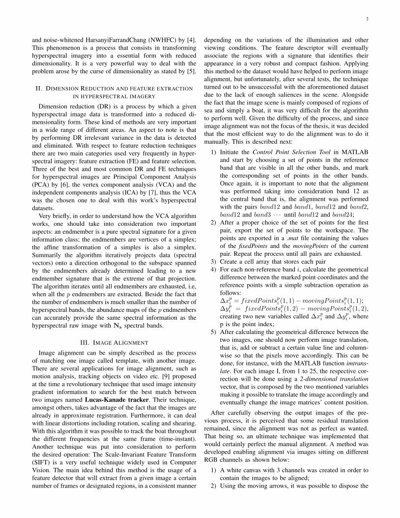
According to the previous information one can observe,once again, that the classifier seem to behave better with thefirst Dataset rather than with the second. With that said, re-garding the first statistical measure, precision, the performanceof both datasets it is rather satisfactory, just like in the firstapproach. Thus, a very reasonable explanation to these lowvalues can be given. With respect to the pixels that lay in theboat, we can see, as illustrated in figure 5, that some pixels aredenoted as false positives although they are in did part of theboat. The misleading assignment is due to the chosen groundtruth. A safety margin in this area was set, that noticeablecontains a great percentage of pixels that here are describedas FP’s. This problem is even more evident with Dataset #1,also in figure 5. Whilst this reason was not mentioned in thefirst approach, it completely addresses also the problem ofprecision values in that case.

Recall values for both cases are reasonable, specially in thefirst dataset, as expected. The true positive rate, the same asrecall, can be viewed as the proportion of Real Positive casesthat are correctly Predicted Positive, which in this context isquite good. As seen before, the inverse of the latter measureis the true negative rate. With this approach both quantitiesrevealed accurate results, as is it is prominent by the number ofTN for both datasets 1 and 2: 487169 and 503563 respectively.Addressing again the ground truth choice problem mentionedabove, as these quantities measure how the classifier avoidsFP’s the values are quite reasonable for the number of FP’sdetected: 32272 FP’s in a total of 521626 pixels for Dataset#1 and 46379 FP’s in a total of 552720 pixels for Dataset #2.The low values for fallout are good in both cases and accurateregarding what one was waiting.

As the classifier in the first approach, this one lies above thediagonal, hence it represents a good classifier. Looking now tothe other measures, in terms of informedness and markednesswe have: Informedness = 0.8482 and Markedness =0.2862. As for Dataset #2: Informedness = 0.7112 andMarkedness = 0.2499. The values in both cases for In-formedness are good, thus again higher for the first Dataset.As for markedness both values are low which is good. As foraccuracy both have high accuracies, and an even more positiveaspect of this results is that both datasets seem to be bestclassified with the second approach, rather than the first. Thiswas exactly one of the objectives of this classification part.It was expected that the second approach would have been

8

(a) Images not aligned

(b) Images consistently aligned

Fig. 5. Zoom on the boat area containing the False Positives of Dataset #1Dataset #2

better to classify data, and the presented results demonstratethat consistently.

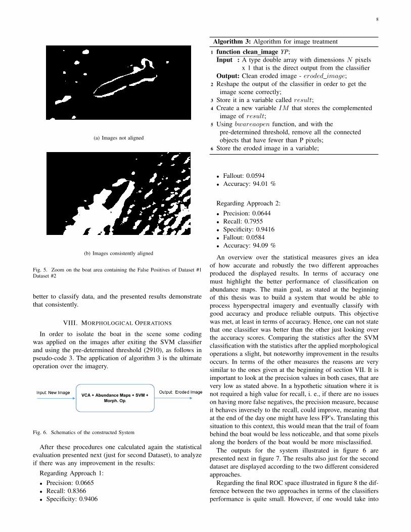
VIII. MORPHOLOGICAL OPERATIONS

In order to isolate the boat in the scene some codingwas applied on the images after exiting the SVM classifierand using the pre-determined threshold (2910), as follows inpseudo-code 3. The application of algorithm 3 is the ultimateoperation over the imagery.

Fig. 6. Schematics of the constructed System

After these procedures one calculated again the statisticalevaluation presented next (just for second Dataset), to analyzeif there was any improvement in the results:

Regarding Approach 1:• Precision: 0.0665• Recall: 0.8366• Specificity: 0.9406

Algorithm 3: Algorithm for image treatment

1 function clean image YP;Input : A type double array with dimensions N pixels

x 1 that is the direct output from the classifierOutput: Clean eroded image - eroded image;

2 Reshape the output of the classifier in order to get theimage scene correctly;

3 Store it in a variable called result;4 Create a new variable IM that stores the complemented

image of result;5 Using bwareaopen function, and with the

pre-determined threshold, remove all the connectedobjects that have fewer than P pixels;

6 Store the eroded image in a variable;

• Fallout: 0.0594• Accuracy: 94.01 %

Regarding Approach 2:• Precision: 0.0644• Recall: 0.7955• Specificity: 0.9416• Fallout: 0.0584• Accuracy: 94.09 %

An overview over the statistical measures gives an ideaof how accurate and robustly the two different approachesproduced the displayed results. In terms of accuracy onemust highlight the better performance of classification onabundance maps. The main goal, as stated at the beginningof this thesis was to build a system that would be able toprocess hyperspectral imagery and eventually classify withgood accuracy and produce reliable outputs. This objectivewas met, at least in terms of accuracy. Hence, one can not statethat one classifier was better than the other just looking overthe accuracy scores. Comparing the statistics after the SVMclassification with the statistics after the applied morphologicaloperations a slight, but noteworthy improvement in the resultsoccurs. In terms of the other measures the reasons are verysimilar to the ones given at the beginning of section VII. It isimportant to look at the precision values in both cases, that arevery low as stated above. In a hypothetic situation where it isnot required a high value for recall, i. e., if there are no issueson having more false negatives, the precision measure, becauseit behaves inversely to the recall, could improve, meaning thatat the end of the day one might have less FP’s. Translating thissituation to this context, this would mean that the trail of foambehind the boat would be less noticeable, and that some pixelsalong the borders of the boat would be more misclassified.

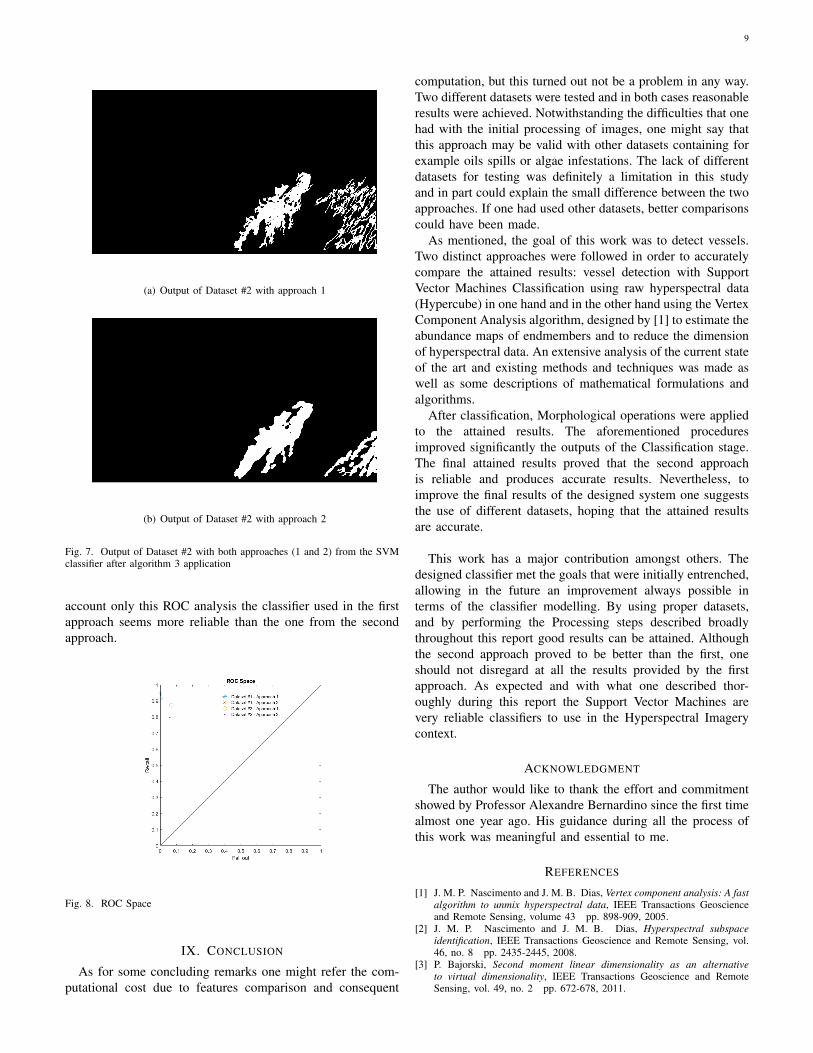
The outputs for the system illustrated in figure 6 arepresented next in figure 7. The results also just for the seconddataset are displayed according to the two different consideredapproaches.

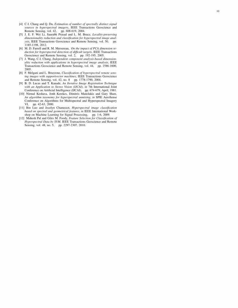
Regarding the final ROC space illustrated in figure 8 the dif-ference between the two approaches in terms of the classifiersperformance is quite small. However, if one would take into

9

(a) Output of Dataset #2 with approach 1

(b) Output of Dataset #2 with approach 2

Fig. 7. Output of Dataset #2 with both approaches (1 and 2) from the SVMclassifier after algorithm 3 application

account only this ROC analysis the classifier used in the firstapproach seems more reliable than the one from the secondapproach.

Fig. 8. ROC Space

IX. CONCLUSION

As for some concluding remarks one might refer the com-putational cost due to features comparison and consequent

computation, but this turned out not be a problem in any way.Two different datasets were tested and in both cases reasonableresults were achieved. Notwithstanding the difficulties that onehad with the initial processing of images, one might say thatthis approach may be valid with other datasets containing forexample oils spills or algae infestations. The lack of differentdatasets for testing was definitely a limitation in this studyand in part could explain the small difference between the twoapproaches. If one had used other datasets, better comparisonscould have been made.

As mentioned, the goal of this work was to detect vessels.Two distinct approaches were followed in order to accuratelycompare the attained results: vessel detection with SupportVector Machines Classification using raw hyperspectral data(Hypercube) in one hand and in the other hand using the VertexComponent Analysis algorithm, designed by [1] to estimate theabundance maps of endmembers and to reduce the dimensionof hyperspectral data. An extensive analysis of the current stateof the art and existing methods and techniques was made aswell as some descriptions of mathematical formulations andalgorithms.

After classification, Morphological operations were appliedto the attained results. The aforementioned proceduresimproved significantly the outputs of the Classification stage.The final attained results proved that the second approachis reliable and produces accurate results. Nevertheless, toimprove the final results of the designed system one suggeststhe use of different datasets, hoping that the attained resultsare accurate.

This work has a major contribution amongst others. Thedesigned classifier met the goals that were initially entrenched,allowing in the future an improvement always possible interms of the classifier modelling. By using proper datasets,and by performing the Processing steps described broadlythroughout this report good results can be attained. Althoughthe second approach proved to be better than the first, oneshould not disregard at all the results provided by the firstapproach. As expected and with what one described thor-oughly during this report the Support Vector Machines arevery reliable classifiers to use in the Hyperspectral Imagerycontext.

ACKNOWLEDGMENT

The author would like to thank the effort and commitmentshowed by Professor Alexandre Bernardino since the first timealmost one year ago. His guidance during all the process ofthis work was meaningful and essential to me.

REFERENCES

[1] J. M. P. Nascimento and J. M. B. Dias, Vertex component analysis: A fastalgorithm to unmix hyperspectral data, IEEE Transactions Geoscienceand Remote Sensing, volume 43 pp. 898-909, 2005.

[2] J. M. P. Nascimento and J. M. B. Dias, Hyperspectral subspaceidentification, IEEE Transactions Geoscience and Remote Sensing, vol.46, no. 8 pp. 2435-2445, 2008.

[3] P. Bajorski, Second moment linear dimensionality as an alternativeto virtual dimensionality, IEEE Transactions Geoscience and RemoteSensing, vol. 49, no. 2 pp. 672-678, 2011.

10

[4] C-I. Chang and Q. Du, Estimation of number of spectrally distinct signalsources in hyperspectral imagery, IEEE Transactions Geoscience andRemote Sensing, vol. 42, pp. 608-619, 2004.

[5] J. E. F. Wei Li, Saurabh Prasad and L. M. Bruce, Locality-preservingdimensionality reduction and classification for hyperspectral image anal-ysis, IEEE Transactions Geoscience and Remote Sensing, vol. 50, pp.1185-1198, 2012.

[6] M. D. Farrell and R. M. Mersereau, On the impact of PCA dimension re-duction for hyperspectral detection of difficult targets, IEEE TransactionsGeoscience and Remote Sensing, vol. 2, pp. 192-195, 2005.

[7] J. Wang, C-I. Chang, Independent component analysis-based dimension-ality reduction with applications in hyperspectral image analysis, IEEETransactions Geoscience and Remote Sensing, vol. 44, pp. 1586-1600,2005.

[8] F. Melgani and L. Bruzzone, Classification of hyperspectral remote sens-ing images with supportvector machines, IEEE Transactions Geoscienceand Remote Sensing, vol. 42, no. 8 pp. 1778-1790, 2004.

[9] B. D. Lucas and T. Kanade, An Iterative Image Registration Techniquewith an Application to Stereo Vision (IJCAI), in 7th International JointConference on Artificial Intelligence (IJCAI), pp. 674-679, April, 1981.

[10] Nirmal Keshava, Jonh Kerekes, Dimitris Manolakis and Gary Shaw,An algorithm taxonomy for hyperspectral unmixing, in SPIE AeroSenseConference on Algorithms for Multispectral and Hyperspectral ImageryVI, pp. 42-63, 2000.

[11] Bin Luo and Jocelyn Chanussot, Hyperspectral image classificationbased on spectral and geometrical features, in IEEE International Work-shop on Machine Learning for Signal Processing, pp. 1-6, 2009.

[12] Mahesh Pal and Giles M. Foody, Feature Selection for Classification ofHyperspectral Data by SVM, IEEE Transactions Geoscience and RemoteSensing, vol. 48, no. 5, pp. 2297-2307, 2010.