detection of voids in prestressed concrete bridges … report . project dtfh61-05-c-00008, task no....
TRANSCRIPT

December 2008David G. PollockKenneth J. DupuisBenjamin LacourKarl R. Olsen
WA-RD 717.1
Office of Research & Library Services
WSDOT Research Report
Detection of Voids in Prestressed Concrete Bridgesusing Thermal Imaging andGround-Penetrating Radar


Research Report
Project DTFH61-05-C-00008, Task No. 8
DETECTION OF VOIDS IN PRESTRESSED CONCRETE BRIDGES USING THERMAL IMAGING AND GROUND-PENETRATING RADAR
by
David G. Pollock, Ph.D., P.E. Associate Professor
Kenneth J. Dupuis
Graduate Research Assistant
Benjamin Lacour Undergraduate Research Assistant
Karl R. Olsen
Graduate Research Assistant
Washington State Transportation Center (TRAC) Washington State University
Department of Civil & Environmental Engineering Pullman, WA 99164-2910
December 2008

1. REPORT NO. 2. GOVERNMENT ACCESSION NO. 3. RECIPIENTS CATALOG NO
WA-RD 717.1
4. TITLE AND SUBTITLE 5. REPORT DATE December 2008 6. PERFORMING ORGANIZATION CODE
Detection of Voids in Prestressed Concrete Bridges Using Thermal Imaging and Ground-Penetrating Radar
7. AUTHOR(S) 8. PERFORMING ORGANIZATION REPORT NO. David G. Pollock, Kenneth J. Dupuis, Benjamin Lacour, and Karl R. Olsen
9. PERFORMING ORGANIZATION NAME AND ADDRESS 10. WORK UNIT NO. 11. CONTRACT OR GRANT NO.
Washington State University Department of Civil and Environmental Engineering PO Box 642910 Pullman, WA 99164-2910
FHWA Project DTFH61-05-C-00008, Task No. 8
12. CO-SPONSORING AGENCY NAME AND ADDRESS 13. TYPE OF REPORT AND PERIOD COVERED Final Report
14. SPONSORING AGENCY CODE Research Office Washington State Department of Transportation PO Box 47372 Olympia, WA 98504-7372 Research Manager: Kim Willoughby 360.705.7978
15. SUPPLEMENTARY NOTES This study was conducted in cooperation with the U.S. Department of Transportation, Federal Highway Administration. 16. ABSTRACT Thermal imaging and ground-penetrating radar was conducted on concrete specimens with simulated air voids. For the thermal imaging inspections, six concrete specimens were constructed during the month of June 2007 to simulate the walls of post-tensioned box girder bridges. The objective was to detect simulated air voids within grouted post-tensioning ducts, thus locating areas where the post-tensioning steel strands are vulnerable to corrosion. The most important deduction taken from these inspections was that PT-ducts and simulated voids were more detectable in the 20 cm (8 in.) thick specimens than in the 30 cm (12 in.) thick specimens. While inspections of the 20 cm (8 in.) thick specimens revealed the majority of their simulated voids, only one thicker specimen inspection (12c) indicated the presence of simulated voids (four voids in two ducts). Also, PT-ducts were much clearer and visible in the thermal images of the thinner specimens. Ground-penetrating radar (GPR) inspection was conducted on fourteen concrete specimens between August and October 2007. Based on the GPR surveys conducted in this study, it is apparent that the detection of post-tensioning strands and simulated voids within grouted ducts embedded in concrete is possible with a 1.5 GHz GPR system. The layout of the top layer of steel reinforcement in each concrete specimen was evident in the GPR images, but the bottom layer of reinforcement was not clearly detected since it was effectively “hidden” beneath the top layer of rebar. Although none of the post-tensioning strands and simulated air voids within the grouted steel ducts was detectable, simulated voids within plastic ducts were generally detectable in GPR images. The high dielectric constant of the steel ducts did not allow the microwaves to transmit through the surface of the duct and reach the simulated voids. However, the general location of the duct, its orientation and its depth in the concrete were accurately determined using GPR. Thus it can be inferred that the void orientation is critical for detection in GPR images. 17. KEY WORDS 18. DISTRIBUTION STATEMENT Bridge inspection, thermal imaging, GPR 19. SECURITY CLASSIF. (of this report) 20. SECURITY CLASSIF. (of this page) 21. NO. OF PAGES 22. PRICE None None
2

DISCLAIMER
The contents of this report reflect the views of the authors, who are responsible for the facts and the accuracy of the data presented herein. The contents do not necessarily reflect the official views or policies of the Washington State Transportation Commission, Department of Transportation, or the Federal Highway Administration. This report does not constitute a standard, specification, or regulation.
3

TABLE OF CONTENTS
Page PART I – Thermal Imaging and Ground-Penetrating Radar Inspection 3 of Concrete Specimens at WSU Part I-A: Specimen Descriptions 3 Part I-B: Thermal Imaging Inspection of Laboratory Specimens 10 Part I-C: Ground-Penetrating Radar (GPR) Inspection of Laboratory Specimens 20 PART II – Field Inspections of Prestressed Concrete Bridges in Washington 29 State Part II-A: Thermal Imaging Inspection of Spokane Street/I-5 Interchange Bridge 29 5/537S in Seattle, WA Part II-B: Thermal Imaging Inspection of Bridge 5/537E-N, Spokane Street/I-5 54 Interchange, in Seattle, WA Part II-C: Thermal Imaging Inspection of Pearl Street Overpass on State Route 16 62 In Tacoma, WA Part II-D: Ground-Penetrating Radar (GPR) Inspection of I-405 Entry/Exit Ramp 70 Bridge Deck in Kirkland, WA. References 73
4

PART I – THERMAL IMAGING AND GROUND-PENETRATING RADAR
INSPECTION OF CONCRETE SPECIMENS AT WSU
Part I-A: Specimen Descriptions
Six concrete specimens were constructed during the month of June 2007 to simulate the
walls of post-tensioned box girder bridges. The objective was to detect simulated air voids
within grouted post-tensioning ducts, thus locating areas where the post-tensioning steel strands
are vulnerable to corrosion. Figure 1 shows a typical specimen and some corresponding
terminology used throughout the project.
Figure 1 – Typical concrete specimen
The concrete used to construct the specimens was a seven-sack mix with 1.9-cm (0.75
in.) angular basaltic rock aggregate and a 28-day compressive strength of 34.5 MPa (5000 psi).
The concrete also had a slump of approximately 13 cm (5 in.). The six specimens were
constructed in four thicknesses: one at 20 cm (8 in.), three at 30 cm (12 in.), one at 41 cm (16
in.), and one at 51 cm (20 in.). The four thinner specimens were inspected using both thermal
imaging and ground penetrating radar (GPR), and had face dimensions of 152 cm by 102 cm (60
in. by 40 in.). The two thicker specimens were inspected using only GPR, and had face
5

dimensions of 102 cm by 102 cm (40 in. by 40 in.). These dimensions were chosen to conform
with older specimens that were previously inspected, and to fit the new thermal imaging test
frame and heater in an efficient manner.
Each specimen contained two or three post-tensioning ducts 10 cm (4 in.) in diameter.
The ducts were spaced at 38 cm (15 in.) on center and made of either galvanized steel or
polypropylene (plastic). The ducts were also numbered Ducts 1-3 for each specimen. The ducts
were 102 cm (40 in.) long, oriented parallel with the 102 cm (40 in.) end of the specimen and
perpendicular to the 152 cm (60 in.) edge. Each duct contained fourteen 7-wire strands sized 1.5
cm (0.6 in.) in diameter (AASHTO M203 Grade 270) and a piece of extruded polystyrene
(Styrofoam) to simulate an air void. A typical duct with post-tensioning steel strands and
simulated air void is shown in Figure 2. The Styrofoam simulated voids were fabricated in three
different sizes (thickness x length): 2.5 cm x 41 cm (1 in. x 16 in.), 1.25 cm x 41 cm (0.5 in. x 16
in.), and 1.3 cm x 20 cm (0.5 in. x 8 in.). One simulated void was attached at the mid-length of
each duct using plastic zip ties fastened through four drilled holes. The ducts were then grouted
with PTX cable grout as post-tensioning strands would be in a typical bridge. To facilitate
placement of the grout, the specimens were placed on edge. The grout was then mixed with
water as directed and poured into each duct after the post-tensioning steel strands were in place.
Each specimen also contained reinforcement in the form of a rebar cage with approximately 2.5
cm (1 in.) of concrete cover at each face. The rebar cage was comprised of #4 Grade 60
reinforcing steel spaced approximately 25 cm (10 in.) on center, as shown in Figure 3.
6

Simulated Void Post-
tensioning strands
Figure 2 – Typical 7-wire strands and simulated void in post-tensioning duct
Figure 3 – Typical specimen formwork with post-tensioning ducts and rebar cage
7

When describing the concrete specimens, the top face must be differentiated from the
bottom face. For all the 30 cm (12 in.), 41 cm (16 in.), and 51 cm (20 in.) thick specimens (both
old and new), the top face is referred to as the face with the least amount of concrete cover to the
ducts. The top face for the older, 20 cm (8 in.) thick specimens was denoted as the face closest
to the simulated voids. The top face in the newer, 20 cm (8 in.) thick specimen was arbitrarily
chosen, but kept constant throughout heating inspections. Figure 4 shows the different simulated
void orientations between the old and new specimens.
Figure 4 – Typical concrete specimen showing various simulated void orientations
A specimen identification scheme was developed to encompass new specimens as well as
previously constructed specimens. The specimen identification scheme reports the specimen
8

thickness (in inches) followed by a letter indicating its position in the construction sequence of
both the new and old specimens. There were eight old specimens, designated 8a-8c, 12a-12c,
16a, and 16b. Unlike the new specimens, not all the post-tensioning ducts in the old specimens
contained simulated voids or the same number of strands. The 7-wire strands in the old
specimens were 1.3 cm (0.5 in.) diameter, and the simulated voids in the old specimens were
thicker and shorter: 5, 10, or 15 cm long (2, 4, or 6 in. long). The old specimens and their
respective attributes are summarized in Table 1, and are further described in Pearson (2003) and
Conner (2004).
Table 1 - Old specimen summary Cover from Top Face
Cover from Bottom Face Simulated Voids
Length Specimen Specimen
Thickness Duct Duct Material
cm in. cm in.
Strands Per Duct No. of
Voids cm in. 1 Steel 5 2 5 2 20 - - - 2 Steel 5 2 5 2 30 - - - 8a 20 cm
(8 in.) 3 Steel 5 2 5 2 30 1 15 6 1 Plastic 5 2 5 2 30 - - - 2 Plastic 5 2 5 2 4 1 15 6 8b 20 cm
(8 in.) 3 Steel 5 2 5 2 4 1 15 6 1 Plastic 2.5 to 7.5 1 to 3 2.5 to 7.5 1 to 3 20 - - - 2 Plastic 2.5 to 7.5 1 to 3 2.5 to 7.5 1 to 3 20 2 5, 10 2, 4 8c 20 cm
(8 in.) 3 Plastic 2.5 to 7.5 1 to 3 2.5 to 7.5 1 to 3 20* - - - 1 Steel 10 4 10 4 30 - - - 2 Steel 7.5 3 12.5 5 20 - - - 12a 30 cm
(12 in.) 3 Steel 5 2 15 6 30 - - - 1 Plastic 10 4 10 4 30 - - - 2 Plastic 7.5 3 12.5 5 20 - - - 12b 30 cm
(12 in.) 3 Steel 10 4 10 4 4 1 15 6 1 Plastic 2.5 to 7.5 1 to 3 12.5 to 17.5 5 to 7 20* - - - 2 Plastic 2.5 to 7.5 1 to 3 12.5 to 17.5 5 to 7 20 2 5, 10 2, 4 12c 30 cm
(12 in.) 3 Plastic 2.5 to 7.5 1 to 3 12.5 to 17.5 5 to 7 30 2 5, 10 2, 4 1 Steel 15 6 15 6 30 - - -
2 Steel 12.5 5 17.5 7 20 - - - 16a 41 cm (16 in.)
3 Steel 10 4 20 8 30 - - - 1 Plastic 15 6 15 6 30 - - - 2 Plastic 12.5 5 17.5 7 20 - - - 16b 41 cm
(16 in.) 3 Steel 15 6 15 6 4 1 15 6
* = corroded tendons
Among the new specimens, there was only one 20 cm (8 in.) thick specimen and it was
identified as 8d. This was the smallest thickness possible to ensure a minimum 5 cm (2 in.) of
9

concrete cover to each face for the 10 cm (4 in.) post-tensioning ducts placed at mid-thickness of
the specimen. Three of the new specimens were each 30 cm (12 in.) thick and differed in the
type of post-tensioning duct, size of simulated air void, and the amount of cover to each duct. 30
cm (12 in.) is a common web thickness for many concrete box girder bridges. These specimens
were identified as 12d, 12e, and 12f. Table 2 summarizes the new specimens. Figure 5
illustrates the four new specimens constructed for both thermal imaging and GPR inspection.
Table 2 - New specimen summary Cover to Top Face
Cover to Bottom Face Simulated Void
(thickness x length) Specimen Specimen Thickness Duct Duct
Material cm (in.) cm (in.)
(cm) (in.) 1 Plastic 5 (2) 5 (2) 2.5 x 40.5 1 x 16 2 Steel 5 (2) 5 (2) 2.5 x 40.5 1 x 16 8d 20 cm
(8 in.) 3 Steel 5 (2) 5 (2) 1.25 x 40.5 0.5 x 16 1 Steel 5 (2) 15 (6) 2.5 x 40.5 1 x 16 2 Steel 10 (4) 10 (4) 2.5 x 40.5 1 x 16 12d 30 cm
(12 in.) 3 Steel 10 (4) 10 (4) 1.25 x 20 0.5 x 8 1 Plastic 5 (2) 15 (6) 1.25 x 40.5 0.5 x 16 2 Steel 10 (4) 10 (4) 1.25 x 40.5 0.5 x 16 12e 30 cm
(12 in.) 3 Steel 5 (2) 15 (6) 1.25 x 40.5 0.5 x 16 1 Plastic 5 (2) 15 (6) 2.5 x 40.5 1 x 16 2 Plastic 10 (4) 10 (4) 2.5 x 40.5 1 x 16 12f 30 cm
(12 in.) 3 Plastic 10 (4) 10 (4) 1.25 x 40.5 0.5 x 16 1 Plastic 5 (2) 25 (10) 2.5 x 40.5 1 x 16 16c 41 cm
(16 in.) 2 Plastic 5 (2) 25 (10) 1.25 x 40.5 0.5 x 16 1 Plastic 5 (2) 36 (14) 2.5 x 40.5 1 x 16 20a 51 cm
(20 in.) 2 Plastic 5 (2) 36 (14) 1.25 x 40.5 0.5 x 16
10

Figure 5 – New specimens for thermal imaging and GPR inspection
The two thickest specimens were constructed solely for GPR inspection. Both had face
dimensions of 102 cm by 102 cm (40 in. by 40 in.) and contained two post-tensioning ducts each.
They were identified as 16c and 20a, indicating thicknesses of 41 cm (16 in.) and 51 cm (20 in.),
respectively. All ducts in these specimens were plastic (since GPR cannot scan through metal)
with 5 cm (2 in.) of cover between each duct and the top face of the specimens. The difference
between ducts occurred in the size of the simulated air voids. One duct in each specimen had a
2.5 cm by 41 cm (1 in. by 16 in.) simulated void, while the other had a 1.3 cm by 41 cm (0.5 in.
by 16 in.) simulated void. The ducts were spaced 30 cm (12 in.) on center, and 36 cm (14 in.)
from either end. Specimen 20a was composed of two layers of concrete. The top 15 cm (6 in.)
of specimen thickness surrounding the ducts was composed of Quick-crete with much smaller
aggregate that was not vibrated. Specimen 20a was evaluated to determine whether “layering”
of concrete affects GPR inspection results. Details of the GPR specimens are shown in Figure 6.
11

Figure 6 – New specimens for GPR inspection
Part I-B: Thermal Imaging Inspection of Laboratory Specimens
Thermal Imaging Test Set-up
A test frame for thermal imaging inspection was fabricated using 3x3 steel hollow
structural sections (HSS). See Figures 7 and 8. To support the concrete specimens, the frame
was composed of four legs connected by horizontal members with welded all-around
connections to provide adequate moment capacity. There were four areas of contact between the
frame and the specimen: two along the entire length of each 102 cm (40 in.) end and two that
were 20 cm (8 in.) in length at the midpoint of each 152 cm edge. Reflective insulation
(Relfectix with an R-value of 14.3, 97% reflectivity, and an allowable contact temperature up to
82 °C or 180 °F) was applied between frame/specimen contact areas and around the edges/ends
of the specimen. The insulation helped reduce edge effects as heat propagated through the
12

specimens. Edge effects for inspection with thermal imaging entail losing heat through the edges
and ends of the specimen. The result was increased heat transfer through the specimen thickness
to the unheated surface (surface for which thermal images were recorded), thus improving
detection of internal features by the thermal imaging camera.
There were two different test set-ups. The first test set-up simulated field inspections
where the heat source is directed at one face of a concrete member while thermal images are
recorded from the opposite face. The second test set-up simulated field conditions in which
access is provided to only one face of a concrete member, so both the heat source and thermal
imaging camera must be directed at the same face. The heater used with each set-up was a heavy
duty metal sheath infrared heater made by Fostoria (Model # CH-1324-3A rated at 13.5 KW, 240
volts, and 33.0 amps).
The first test set-up involved placing the infrared heater underneath the specimen and
heating while thermal images were taken from above. The infrared heater was located 69 cm (27
in.) from the bottom of the specimen, and aluminum-covered plywood sides were installed
around the heater and the test frame to direct most of the radiant heat toward the specimen. The
inside of the test frame was also lined with reflective tape to reduce the amount of heat
conducted through the frame. Each specimen was then inspected with a FLIR (ThermaCAM
P60) thermal imaging camera suspended 4 m (13 ft.) above the unheated face of the specimen.
Figures 7 and 8 show the frame set-up.
13

Figure 7 – Test set-up showing infrared heater and test frame supporting a concrete specimen
Figure 8 – Test set-up showing aluminum-covered plywood sides and insulation on edges/ends of a concrete specimen
14

The second test setup was implemented to allow thermal images to be taken from the
same side as the heated surface. The specimens were placed on the test frame and insulated as
before, but with this setup the infrared heater was suspended above the specimen. A frame made
from steel unistruct was built and the infrared heater was suspended above the specimen using
two lengths of chain. The infrared heater was held between 25 and 30 cm (10 to 12 in.) directly
above the heated surface of the concrete specimen. There were no aluminum-covered plywood
sides directing the radiant heat toward the specimen in this setup. Each specimen was heated for
a period of time, then the heater was removed and thermal images were taken from 4 m (13 ft.)
above the specimen (similar to the first test setup). The second test setup is illustrated in Figure
9.
Figure 9 – Test set-up with heater suspended above a concrete specimen
15

Background
Thermography, or thermal imaging, is a type of nondestructive inspection using infrared
radiation. Thermal imaging cameras are used to detect radiation in the infrared range of the
electromagnetic spectrum (roughly 900 to 14,000 nanometers), or the part of the spectrum we
perceive as heat. Infrared energy is electromagnetic radiation that is not visible because its
wavelength is too long to be detected by the human eye. Unlike visible light, in the infrared
world everything with a temperature above absolute zero emits heat and the higher an object’s
temperature, the greater the radiation emitted. Thermal imaging cameras detect infrared energy
emitted from an object and then convert this energy reading into a display of the material surface
temperature.
With thermal imaging, it is often necessary to obtain a temperature differential or thermal
gradient in an object so that heat will propagate through the material in a known direction. This
is done by introducing some energy (or heat) into the system, which will often cause a variation
in surface temperatures based on the material properties. Thermal imaging can be employed to
detect imperfections that disrupt the heat energy transfer created by the energy source. When
heat is directed through a material, it is conducted at a certain speed based on material thermal
properties. Imperfections are essentially different materials embedded in the system, resulting in
different rates of heat conduction. For example, when steel is embedded in concrete, it will
transmit heat at a faster and more efficient rate than the concrete around it. An air void, on the
other hand, tends to act as an insulator, conducting heat at slower rates than the surrounding
concrete. Table 3 shows heat conduction rates for concrete, steel, air, Styrofoam (extruded
polystyrene), and polypropylene.
16

Table 3 - Thermal conductivity of specimen materials (Conner 2004)
Thermal Conductivity Material
W / (m x ˚C) Lightweight Concrete 0.72 Normal Weight Concrete 2.32 Polypropylene 0.17-0.3 Steel 50 Air 0.025 Polystyrene 0.027
This project involved experimental research concerning thermal imaging of concrete box
girder bridges. Key questions regarding this topic include:
1) What internal defects can and cannot be detected with thermal imaging?
2) What heating applications produce the best inspection results?
3) What concrete thicknesses can be inspected using thermal imaging?
Inspection Procedures
Lab specimens were inspected using three different methods which were similar to the
inspection procedures implemented in field inspections of bridges. The first, called Method 1,
involved placing the specimen on the test frame and heating from underneath while taking
thermal images of the unheated surface from above. In Method 2, the heater was suspended
above the specimen, heated for a period of time, and then removed so that thermal images of the
heated surface could be obtained. The last procedure, Method 3, involved exposing the
specimen to direct sunlight for a relatively long duration of time, and then placing it on the test
stand for thermal imaging of the heated surface. With all three methods, it was important to
obtain a temperature gradient between the two faces of the specimen. The temperature gradient
caused heat energy to propagate through the specimen, which is essential to acquire thermal
images where inherent flaws are detected and seen as surface temperature differences.
17

Conclusions
After considering the results obtained from all ten inspected specimens, a few
conclusions can be drawn. Table 4 provides a summary of what was detected during each
inspection. Inspections were evaluated based on whether rebar, PT-ducts, and/or simulated voids
were detected. If an inspection produced thermal images that revealed these things, then the
appropriate box was marked by an X.
Table 4 - Lab Inspection Summary What was detected?
Specimen Test Method
Inspected Specimen
Face Rebar PT-ducts Simulated voids
Method 3 Top X Method 1 Top X X X 8a Method 1 Bottom X X Method 1 Top X X X Method 1 Top X X X Method 1 Top X X X Method 3 Top X X X Method 1 Bottom X X X
8b
Method 2 Top X Method 3 Top X X X Method 1 Top X X X 8c Method 1 Bottom X X Method 1 Top X X Method 1 Bottom X X 8d Method 2 Top Method 3 Top X Method 1 Top X X 12a Method 2 Top Method 3 Top X 12b Method 1 Top X Method 1 Top X X X 12c Method 2 Top Method 1 Top X X 12d Method 1 Top X X
12e Method 1 Top X X Method 1 Top X X 12f Method 2 Top
Method 1 involved heating one face of a specimen and then taking thermal images from
the opposite face (unheated surface). Method 2 entailed heating a surface and then taking images
18

from that same heated surface. Finally, Method 3 used direct solar radiation as the source of heat
input, where the specimen was placed on the test frame after heating and thermal images were
taken of that same heated surface.
The most important deduction taken from these inspections was that PT-ducts and
simulated voids were more detectable in the 20 cm (8 in.) thick specimens than in the 30 cm (12
in.) thick specimens. While inspections of the 20 cm (8 in.) thick specimens revealed the
majority of their simulated voids, only one thicker specimen inspection (12c) indicated the
presence of simulated voids (four voids in two ducts). Also, PT-ducts were much clearer and
visible in the thermal images of the thinner specimens. The idea that it is harder to detect
specimen characteristics in thicker specimens than in thinner ones is logical. Inspection of the 30
cm (12 in.) thick specimens results in less clear thermal images because, as the heat propagates
through more concrete, it spreads three-dimensionally and the presence of internal hot spots or
cold spots is obscured.
Another conclusion involves the heating methods used. From Table 4, one can see that
Method 1 was the most productive method of the three. This method utilized through heating.
As the heat propagated through the specimen, heat flow rates were either increased or decreased
as embedded materials were encountered. This feature of heat transfer was then recorded by the
thermal camera on the unheated surface as a hot or cool spot relative to the surrounding concrete.
It is known that air and plastic each have a slower rate of heat transfer than concrete, so these
effects showed up as cool areas. Steel, on the other hand, has a faster heat transfer rate, which
yielded warmer areas.
Method 3 resulted in some excellent thermal images as well. The method was used on
three 20 cm (8 in.) thick and two 30 cm (12 in.) thick specimens, but was only successful in two
19

of the thinner ones (although rebar could be detected in all inspections). Images obtained using
this method revealed PT-ducts and simulated voids in Specimens 8b and 8c.
Method 2 was the least effective method of the three. It was added to the inspection
schedule after completing field inspections of bridges on August 6-9 and 13-15, 2007 where it
produced many thermal images showing flaws and near-surface characteristics (delamination,
poorly consolidated concrete, etc.). However, Method 2 was not effective for detecting PT-ducts
and simulated voids in the concrete lab specimens. Out of five different inspections with Method
2, none detected any PT-ducts or simulated voids. Therefore, Method 2 procedures should only
be used to find near-surface irregularities and not characteristics more than 5 cm (2 in.) from the
surface (such as PT-ducts).
Another conclusion from these inspections concerns the simulated voids. Throughout the
inspections, all simulated voids displayed on thermal images were located in the older
specimens. This means that only the simulated voids located between the steel tendons and the
infrared camera were detected. These simulated voids were cut to fit snugly between the PT-
strands and the inner surface of the duct, and to be as wide as the duct would allow. The newer
specimens contained simulated voids that were either 2.5 cm (1 in.) or 1.25 cm (0.5 in.) thick,
and the voids were located adjacent to the steel tendons. The voids in the newer specimens were
not detectable due to the fact that heat could bypass the voids by propagating through the
adjacent tendons. Figure 10 illustrates the orientation of the new vs. old simulated voids with
respect to the direction of heat flow. The new simulated voids were only 2.5 cm (1 in.) or 1.25
cm (0.5 in) thick, whereas the older simulated voids were almost the width of the duct.
20

Figure 10 – Illustration of heat flow through PT-duct and simulated void
The final critical observation from these inspections is that, when the simulated voids
were visible, they were located within plastic PT-ducts. None of the simulated voids in steel
ducts were detected during lab inspections. One theory as to why this happens is that the steel
ducts transfer most of the heat around the simulated void, thus bypassing the location of the
simulated void. A plastic duct conducts heat at a slower rate than steel, so it presents a better
probability of detecting simulated voids during inspection. Additional details regarding thermal
imaging inspection of concrete specimens containing simulated voids in steel and plastic ducts
are reported in Pearson (2003), Musgrove (2006), and Dupuis (2008).
Part I-C: Ground-Penetrating Radar (GPR) Inspection of Laboratory Specimens
Ground-penetrating radar (GPR) inspection was conducted on fourteen concrete
specimens between August and October 2007. Each specimen included unique features as
described in Tables 1 and 2, and a primary feature was the thickness of the specimens. Four
21

different specimen thicknesses were used: 20 cm (8 in.), 30 cm (12 in.), 40 cm (16 in.) and 50 cm
(20 in.). All the specimens in this report were inspected from both faces, meaning that a first
inspection was conducted face up (survey of specimen top face) and a second inspection was
conducted face down (survey of specimen bottom face). See Figure 1.
GPR Test Equipment
The GPR inspection system is composed of four elements: the antenna, the connecting
unit, the signal processing unit with laptop computer, and the survey cart. See Figures 11 and 12.
The system used in this research employed a 1.5 GHz antenna (Model 5100). In order to track
the distance covered during data collection, the antenna was connected to the survey cart and
then to the processing unit. The cart was also used to start the survey process through a trigger
located on the handle. The computer was directly linked to the processing unit and displayed the
data in real time. The term “survey” refers to the process of collecting data with the GPR
antenna.
The software provided with the GPR survey system is called RADAN and can be used in
two different ways. Both procedures were used to obtain images representative of objects
embedded in concrete specimens. The first procedure used is called Linescan and the second is
called SructureScan.
22

Figure 11 – GPR antenna, survey cart, connecting unit, and cables.
Figure 12 – StructureScan processing unit and laptop computer.
23

Linescan Inspection
The Linescan software is basically analogous to an oscilloscope that measures the
amplitudes of the radar waves and displays them on the computer screen in grayscale. The
Linescan module produces real-time images of objects directly beneath the antenna. The antenna
does not send out a continuous stream of microwave energy. Rather it transmits a pulse of
microwave energy and waits for the signal to return. This process is called a “scan”. The
computer uses the wheels of the survey cart to keep track of the distance it has traveled and
typically displays five scans per every inch traveled. Increasing the number of scans per inch
provides better image resolution and allows for the detection of smaller defects, but the antenna
must be moved at a slower rate across the concrete. The antenna continually takes scans of the
concrete while the computer is recording, but the scans are only displayed and recorded as the
survey cart wheels turn. The image produced on the laptop screen only represents what the
antenna passes directly over. The images do not indicate the orientation of any objects it detects,
only that an object is present at that specific point.
When the antenna crosses over a target (rebar, pipe, etc.) the resulting image that appears
on the computer screen is a hyperbola as shown on Figures 13 and 14. This happens because the
antenna radiates the microwave energy in the shape of a wide cone. Therefore, the antenna
detects the target not only when directly over it, but also in several scans before and after that
position. See Figure 13. The summit of the hyperbola is at the location of the target (although
its exact depth will be a function of the dielectric constant of the concrete). When the antenna is
directly over the target, a groove located exactly halfway between the transmitter and receiver on
the antenna housing indicates where the target is located beneath the surface. Figure 14
24

illustrates the antenna directly over a target and the hyperbolic shape as it appears in the
Linescan software.
Figure 13 – Creating a hyperbolic image due to antenna moving over a target (Conner 2004).
Figure 14 – A target shows up as a hyperbola (Conner 2004). The reflection polarity also provides valuable information about what is beneath the
surface of concrete. All Geophysical Survey Systems, Inc. (GSSI) antennas transmit a specific
25

polarity: positive peak first, then a negative peak (possibly followed by a second positive peak).
In the Linescan software, this appears as a white band followed by a black band (and possibly
another white band). Each reflection from a metal object (with a large dielectric constant) is a
copy of the transmitted pulse, so steel object reflections appear with a white band at the top
followed by a black band. However, when the microwaves reflect from an object with a lower
dielectric constant than the concrete, a phase inversion occurs. This means that when the
microwaves reach an object such as styrofoam or air, the reflected signal will start with a
negative (black) peak followed by a positive (white) peak. This is very useful in distinguishing
voids from steel reinforcing bars.
Structurescan Inspection This inspection method involves compiling data from several Linescans conducted
following a grid pattern with parallel and transverse numbered lines. Then the RADAN software
is used to create a three-dimensional image of any objects embedded beneath the concrete
surface. The reflection hyperbolas are plotted as points in three-dimensional space and then
connected to form the shape of each target encountered. The grid is placed over the area under
investigation and secured at each corner with adhesive tape. See Figure 15.
26

Figure 15 – Antenna, survey cart, cables and the grid pattern.
Once the RADAN software has created a three-dimensional image it allows the user to
analyze the results considering the specimen in several slices at specific depths and thicknesses
(defined by the user) and called “depth slices”. The slice thickness can be as small as 0.63 cm
(¼ in.). For example, the user can view what was detected in a 0.63 cm (0.25 in.) slice between
7.5 and 8.13 cm (3.0 and 3.25 in.) beneath the surface of a concrete specimen. Additional
information regarding GPR inspection is provided in Conner (2004) and GSSI (2001).
Conclusions
Based on the GPR surveys conducted in this study, it is apparent that the detection of
post-tensioning strands and simulated voids within grouted ducts embedded in concrete is
possible with a 1.5 GHz GPR system. The layout of the top layer of steel reinforcement in each
27

concrete specimen was evident in the GPR images, but the bottom layer of reinforcement was
not clearly detected since it was effectively “hidden” beneath the top layer of rebar.
Although none of the post-tensioning strands and simulated air voids within the grouted
steel ducts was detectable, simulated voids within plastic ducts were generally detectable in GPR
images. The high dielectric constant of the steel ducts did not allow the microwaves to transmit
through the surface of the duct and reach the simulated voids. However, the general location of
the duct, its orientation and its depth in the concrete were accurately determined using GPR.
Simulated voids in plastic ducts in the older specimens (Specimens 8b, 8c, 12b, 12c, 16b)
were clearly detectable in GPR images of these specimens. However, for the new specimens
with plastic ducts (Specimens 8d, 12e, 12f, 16c, 20a) the simulated voids could not be detected
consistently in GPR images. This is because of the orientation of the simulated voids in the new
specimens. See Figure 16. GPR inspections were conducted on the faces of each concrete
specimen. In the older specimens the voids were either above or below the steel strands in the
ducts and the width of the voids (instead of the thickness) was oriented facing the microwaves.
However, the new specimens had a different orientation of the simulated voids. The void
thickness (smallest dimension) was oriented facing the microwaves and the simulated voids were
located adjacent to the steel tendons, at the same depth in the concrete specimens. Therefore the
reflection from the steel strands was side-by-side with any weaker reflection from the voids, and
tended to “mask” the presence of simulated voids adjacent to the tendons in some of the
specimens. Thus it can be inferred that the void orientation is critical for detection in GPR
images.
28

Old Specimen New Specimen
Simulated voids were located between the steel
strands and face of the specimen, and the void width
was oriented facing the microwaves
Simulated voids were located adjacent to the steel
strands, and the void thickness (smallest dimension) was
oriented facing the microwaves
Figure 16 – Orientations of simulated voids in old and new concrete specimens
Specimen thickness had a predictable effect on GPR image quality. Ducts embedded
deeper in concrete specimens exhibited slightly weaker reflections. Furthermore, the top layer of
steel reinforcement had a slight “masking effect” on the detection of the simulated voids in the
20 cm (8 in.) specimens, in contrast to the thicker specimens, because the simulated voids were
located so close to the reinforcing steel (Conner 2004).
For some of the specimens with steel ducts (8a-8b-8c; 12a-12b-12c; 16a-16b) the GPR
antenna received reflected signals from steel rebar underneath the ducts. This phenomenon can
be explained based on multiple reflections from steel objects in the concrete. The antenna sends a
pulse of microwave energy into the concrete specimen in the shape of a wide cone. Some of the
microwaves are reflected from the bottom layer of rebar to the steel duct which in turn reflects
the microwaves back to the antenna receiver along the same path. This is illustrated in the
diagram in Figure 17. To locate a target the antenna sends a pulse of microwave energy and
29

waits for the signal to return. Since the signal is typically reflected directly from the target itself,
the computer does not take into account the possibility of multiple reflections from two or more
objects as illustrated in Figure 17. Therefore the depths reported in GPR images for the portions
of rebar detected underneath steel ducts actually correspond to the depths of what could be a
virtual piece of steel as represented in light grey in Figure 17. Additional details regarding GPR
inspection of concrete specimens containing simulated voids in plastic ducts are reported in
Conner et al (2006) and Conner (2004).
Figure 17 – Microwave reflections from the rebar grid underneath the duct
30

PART II – FIELD INSPECTIONS OF PRESTRESSED CONCRETE BRIDGES IN
WASHINGTON STATE
Part II-A: Thermal Imaging Inspection of Spokane Street/I-5 Interchange Bridge 5/537S in
Seattle, WA
Location: Spokane Street/I-5 Interchange, Seattle, WA
Dates: August 6 – 9, 2007
Objectives
The objective of this field inspection was to determine whether thermal imaging may be
helpful in locating/assessing near-surface defects on the bottom surface of precast concrete box
girders on the Spokane Street Interchange exit from I-5 in Seattle, WA. Possible problems with
the bridge include poorly consolidated concrete, delamination, air voids, and exposed reinforcing
steel.
Thermal Imaging Inspection
When conducting thermal imaging inspections in the field, it is important to note certain
factors that can affect imaging results. Most of these factors result from environmental
conditions. One such condition involves wind and how it can cool a surface through convection.
Cooling of the surface in question is usually not desirable because thermal images require
temperature differences in order to detect inherent flaws and other characteristics. Temperature
differences are most easily obtained with uniform heat input and constant ambient conditions.
Another factor that affects thermal imaging results is the distance between the infrared
camera and the surface to be inspected. As the distance increases, there is a bigger chance for
atmospheric conditions to reduce the amount of infrared energy that passes between the thermal
camera and the surface in question. One such atmospheric condition is the moisture in the air.
31

Moisture can absorb some of the infrared energy between the camera and surface, so the camera
will detect lower surface temperatures than are actually present.
Other factors affecting thermal images depend on the inspection surface. Surface
properties like emissivity, reflectivity and roughness change both how the camera “sees” a
surface and how that surface absorbs and emits radiant energy. To begin with, the emissivity of
a material is the ratio of radiation emitted by a surface to the radiation emitted by a black body at
the same temperature. A true black body would have an emissivity equal to one, while any real
object would have an emissivity less than one.
Reflectivity, on the other hand, is the fraction of radiation reflected by a surface. In
thermal imaging, highly reflective surfaces tend to reflect radiant energy from other objects
nearby. This can lead to inaccurate surface temperature measurements using an infrared camera.
Also, highly reflective surfaces make it more difficult to absorb thermal energy. With an
infrared heater, or any other heat source for that matter, the rays tend to reflect from the surface
instead of being absorbed. Generally, emissivity is equal to one minus the reflectivity, so
emissivity and reflectivity are inversely proportional.
Surface roughness also affects how radiant energy is absorbed by an object. Surface
roughness is a measurement of the small-scale variations in the height of a physical surface. A
ray will make contact with a surface once, and if it is not absorbed, it is reflected. Rougher
surfaces allow reflected rays to make contact with the surface more often, thus giving the surface
more chances to absorb the energy.
Environmental conditions and surface characteristics (like reflectivity, emissivity and
surface roughness) affect thermal images in one main way. Since they all influence temperature
differences that thermal images require to detect flaws and other attributes, they tend to alter
32

image resolution. If the temperature differences decrease, as is the case with cooling through
wind conduction, greater distance between the surface and thermal camera, or highly reflective
surfaces, then thermal images will not show flaws or embedded materials very clearly. On the
other hand, if undesirable environmental conditions are minimized, the surface roughness is
high, and reflectivity low, the thermal images may show clearly defined embedded objects and
other characteristics.
Generally, thermal imaging inspection must take all these factors into account. It is
important to know wind speeds, ambient temperatures, what materials are involved, and how all
these conditions affect the thermal images and how to interpret them. Any of these factors could
produce thermal images that do not reveal the true conditions within the material.
Inspection Procedure
The inspected bridge was part of the Spokane Street Interchange exit from I-5 in Seattle,
WA, and carried traffic traveling eastward from Spokane Street onto I-5 (northbound). The
bridge is identified as 5/537S by the Washington State Department of Transportation (WSDOT),
and all heating locations are based on a WSDOT drawing of the bridge. Inspection locations
ranged from Pier 9 to Pier 14, and locations were designated by the bridge span in which they
occurred. Bridge spans were named for the lower of the two piers to which they were attached.
For example, heating location #1 took place in Span 11, so it was conducted between Piers 11
and 12. The locations are further described either by distance from a particular edge of the
bridge (denoted by compass direction), or by markers already in place on the inspected surface.
The thermal imaging camera was often used to locate possible heating locations based on
ambient conditions. Images were taken and hot or cold regions in the image were identified as
potential problem areas. Figure 18 shows a thermal image of the bridge under typical ambient
33

conditions from which a heating location might be determined. The arrow points to a location
which should be a solid color inside a rectangle of yellow indicating a uniform temperature
distribution. The yellow areas in the image signify locations of interior webs of the box girder.
However, a closer look at the image reveals a few areas with higher surface temperatures than
the surrounding concrete within the rectangle. This signal of inconsistency may indicate a
problem area.
Possible problem area
Figure 18 – Thermal image and photo of box girder bridge under ambient conditions
Once a heating location was determined, there were two heating options to choose from
(identified as Method 1 and 2 throughout this report). To help place the infrared heater and
thermal imaging camera closer to the bottom surface of the box girder, a lift truck was provided
by WSDOT. Method 1 entailed placing the infrared heater inside the concrete box girder bridge
and applying infrared energy to its floor. This arrangement allowed thermal images to be taken
from the unheated outer surface (i.e., from the exterior surface of the box girder floor)
throughout the entire heating process. Taking images while simultaneously heating the floor of
34

the box girder permits one to observe how internal flaws are revealed in thermal images as heat
propagates through the concrete. It also provides data regarding the length of time it takes the
heat energy to flow through the concrete. Method 1 was used infrequently because it required
access to the inside of the box girder bridge, and there were only a few locations that permitted
access. In order to use inspection Method 1, an access hatch to the box girder was opened and
the infrared heater was hoisted inside. The infrared heater was oriented face down on four
masonry blocks, keeping the top of the heater approximately 61 cm (24 in.) from the surface of
the concrete floor. The blocks were positioned at the corners of the rectangular heater to allow
most of the infrared rays to be directed at the heated surface without interference.
The other type of inspection, Method 2, involved positioning the lift truck underneath the
bottom surface of the box girder bridge and placing the infrared heater on the lift truck platform
facing upward. The lift was then elevated until the top of the infrared heater was approximately
76 to 107 cm (30 to 42 in.) from the heated surface. The range of distances from the infrared
heater to the surface resulted in varied heated surface areas during inspections at various
locations. Figure 19 shows a sample photo and thermal image of the lift platform holding the
infrared heater near the bottom surface of a concrete box girder bridge. After the infrared heater
was in place, it was turned on and heating commenced. Heating times ranged from
approximately one to three hours based on the suspected problem associated with the heated
surface, as well as the inspection timeframe. Following the energy input portion of the
inspection, the infrared heater was removed and thermal images were taken. Images were
acquired at specific time intervals until sequential images showed no substantial change in
temperature patterns. One main feature associated with this inspection setup was that the images
35

were taken of the heated surface. This means that the camera was located on the same side of the
concrete as the heater.
Figure 19 – Typical orientation of lift truck and heater to heated surface (Method 2)
Heating Location # 1
Heating Location # 1 was inspected on August 6th, 2007 using inspection Method 2. The
inspection position was in Span 11 between marker # 1 and marker # 3 (markers were attached to
the surface during prior WSDOT inspections). The surface was heated for a time span of 1:45
(hh:mm). The top of the heater was placed approximately 76 cm (30 in.) from the heated
surface, which was 7.1 m (23.2 ft.) from the ground. This location was chosen because it was an
area that had already been inspected by WSDOT, as indicated by the white chalk in Figure 20.
The objective was to see how the thermal images displayed what was previously discovered.
Figure 20 shows a thermal image and a corresponding photo of the heated surface. The figure
also shows three regions of interest on the heated surface. These regions are clearly shown in
both the photo and the thermal image as locations with thermal anomalies.
36

74.9°F
134.4°F
80
100
120
2
1
1
3
3
2
Marker #3
Marker #3
Figure 20 – Thermal image and photo of Heating Location # 1
The irregularities can be seen more clearly if the thermal image in Figure 20 is enlarged,
as in Figure 21. The points denoted with a white symbol (points 1, 2, and 3 in Figure 21) display
different surface temperatures within fairly close proximity to each other. From the center of the
heated area, point 1 is hottest at 112.2 °F and point 2 is lower at 99.8 °F, as expected (the center
of the heated area should be the hottest, with surface temperatures decreasing farther away from
the center). However, it is evident that point 3 is hotter than point 2, even though it is farther
37

away from the heated center. This shows that there was an irregularity at this location, which
was at approximately the same location as region 1 in Figure 20.
83.3°F
120.2°F
90
100
110
120
1 : 112.22 : 99.8
5 : 111.04 : 101.5 7 : 107.5
6 : 111.9
3 : 105.0
Figure 21 – Thermal image of Heating Location # 1
The green and black colors in Figure 21 also indicate areas where there were noticeable
temperature differences within close proximity. There was roughly a 10 °F difference between
points 4 and 5, which were only a few inches apart. Also, points 6 and 7 show a surface
temperature increase at distances farther away from the heated center, replicating the effect at
points 2 and 3. These irregularities could be a sign of many things. From the photo in Figure 20,
there are some areas with discoloration. As this is reproduced in the thermal images, these may
be locations of poorly consolidated concrete or delamination.
38

Heating Location # 2
Heating Location # 2 was inspected on August 6th, 2007 using inspection Method 2. The
inspection point was in Span 11, between marker # 7 and marker # 9. This location was near the
south edge of the bridge, while Heating Location # 1 was near the north edge. The heating time
was 1:25 (hh:mm). As in the first inspection, the top of the heater was placed approximately 76
cm (30 in.) from the heated surface and the total height to the surface was 7.1 m (23.2 ft.) from
the ground. This location was chosen due to markings that indicated the surface had previously
been inspected by WSDOT.
Figure 22 shows a thermal image of Heating Location # 2. The black mark on the left
side of the image is marker # 9, and marker # 7 would be on the right side if it were within the
viewing range. This image is a very good example of delamination, as indicated by the two
“spots” located to the right of the marker # 9. These two areas look like hot spots because of the
delamination (separated layers within the concrete) that keeps the heat from propagating farther
into the floor of the box girder. The heat propagates at a slower rate due to a layer of air present
at the delamination interface. The air acts as an insulator, keeping more heat within the layer of
concrete nearest the heat source. The delaminations in the thermal image were confirmed by
WSDOT inspectors through tapping the surface with a hammer after the thermal imaging was
completed. Figure 22 also shows three points that demonstrate the temperature differences in the
vicinity of hot spots. The temperature difference between points 1 and 2 is approximately 14 °F
and can be attributed to the delamination occurring between the two points.
39

69.2°F
128.6°F
80
100
120
Marker #9
Figure 22 – Thermal image and enlarged area showing spot temperatures of Heating Location # 2
Heating Location #3
Heating Location # 3 was inspected on August 7th, 2007 using inspection Method 2. The
inspection position was at midspan of Span 10, approximately 3.6 m (12 ft.) north of the south
edge of the bridge. The surface was heated for a time span of 2:00 (hh:mm). The top of the
heater was placed approximately 107 cm (42 in.) from the heated surface, which was 9.9 m (32.5
ft.) above the ground. The initial ambient temperature in the vicinity of the inspection location
was 63.7 °F and average the wind speed was about 5 mph, with gusts up to 12 mph.
Heating Location # 3 did not reveal very many irregularities. A thermal image of this
location is provided in Figure 23, and it only shows one small irregularity denoted by the circle.
Using the thermal imaging software, temperatures at the irregularity and at a location just to the
right of it were 66.3 °F and 68.5 °F, respectively. This is a 2.2 °F difference, which is not very
big considering the temperature range of the image is approximately 28 °F. Due to the relatively
40

small temperature change and the lack of other irregularities around the point, it would probably
not be classified as a point of significance. Heating Location # 3 would therefore be a good
example of a surface with no apparent problems after inspection.
Heating Location # 4
Heating Location # 4 was inspected on August 7th, 2007 using inspection Method 2. The
inspection position was in Span 14, approximately 3.0 m (10 ft.) west of Pier 14 and 1.5 m (5 ft.)
north of the south column of Pier 14. The surface was heated for a time span of 2:48 (hh:mm).
The top of the heater was placed approximately 107 cm (42 in.) from the heated surface, which
was 4.9 m (16 ft.) above the ground. At this location, the initial ambient temperature was 65.7
°F and the average wind speed was about 1.5 mph, with gusts up to 2.8 mph.
Figure 24 shows a thermal image of Heating Location # 4. Many small irregularities
were detected in this image. An example is at points 1 and 2 in the middle of the image. Point 1
is closer to the heated center than point 2, but it is almost 3 °F cooler. Based on more analysis of
the image with the thermal imaging software, most of the other irregularities were found to be
approximately 2 to 3 °F cooler as well. Since the irregularities are not substantially different in
Figure 23 – Thermal image and photo of Heating Location # 3 Point 1
61.8°F
90.5°F90
80
70
41

terms of temperature, one can conclude that they are just surface marks or areas where a small
amount of concrete has spalled off.
92.1°F
113.4°F
95
100
105
110
1 : 103.42 : 106.1
Figure 24 – Thermal image of Heating Location # 4
Heating Location # 5
Heating Location # 5 was inspected on August 8th, 2007 using inspection Method 2. The
inspection position was in Span 14, just west of the expansion joint and 3 m to 4.6 m (10 ft to 15
ft.) east of the north column of Pier 15. The surface was heated for a time span of 2:00 (hh:mm).
The top of the heater was placed approximately 107 cm (42 in.) from the heated surface, which
was 4.6 m (15 ft.) above ground. At this location, the initial ambient temperature was 63.5 °F
and the average wind speed was about 1.7 mph, with gusts up to 2.9 mph.
Figure 25 shows a thermal image of Heating Location # 5. This location was chosen
because of the visible problems on its surface that were apparent from the ground. The thermal
image in Figure 8 is packed with a lot of different types of irregularities, as shown by the great
42

differences in color (indicating different temperatures). Irregularities include spalled concrete,
delamination, exposed steel reinforcement (rebar), and poorly consolidated concrete.
Temperature differences in this image reach approximately 15 °F (like points 1 and 2 shown).
Figure 26 shows both a photo and thermal image of Heating Location # 5. This figure is
helpful because one can see exactly how each area in the photo appears in the thermal image.
An example is the steel reinforcement. It is seen exposed in the photo, and then as a warmer line
in the image, designated by circled area 1 in the figure. Most of the longitudinal rebar can be
traced in a similar manner.
71.5°F
101.7°F
80
90
100
1 : 82.72 : 97.9
Figure 25 – Thermal image of Heating Location # 5
43

71.5°F
101.7°F
80
90
100
2
2
1
1
Figure 26 –Thermal image and photo of Heating Location # 5
44

Circled area 2 in Figure 26 shows an interesting irregularity. The area doesn’t display
anything significant in the photo except a small amount of discoloration, but the thermal image
demonstrates inconsistencies in the material in the form of great temperature differences. The
thermal imaging software showed an approximate 5 °F difference between areas within the
circle. This may be due to delamination, poorly consolidated concrete, or another irregularity,
but there is no way to be certain of the specific cause until further tests are completed (either
“sounding” with a hammer, or chipping out the loose concrete). This does, however, reveal that
there may be a problem at this location. There are also a few other areas in the figure that exhibit
similar temperature anomalies.
Heating Location # 6
Heating Location # 6 was inspected on August 8th, 2007 using inspection Method 2. The
inspection position was at midspan of Span 17, just west of the expansion joint. The surface was
heated for a time span of 2:00 (hh:mm). The top of the heater was placed approximately 107 cm
(42 in.) from the heated surface, which was 5.4 m (17.6 ft.) above the ground. At this location,
the initial ambient temperature was 65.7 °F and the average wind speed was about 5.6 mph, with
gusts up to 8.7 mph.
Figure 27 shows a thermal image of Heating Location # 6. This inspection did not detect
any irregularities. The concrete surface seems to have no flaws. However, the inspection does
show some of the surface texture characteristics. In the center of the thermal image, for
example, is an area where concrete protrudes a very short distance beyond the flat surface. The
surface feature looks like a line with a downward slope. The thermal image also demonstrates
how very small surface defects can be detected.
45

79.0°F
103.8°F
Heating Location # 7
Heating Location # 7 was inspected on August 8th, 2007 using inspection Method 1. The
inspection position was in Span 14, approximately 11 m (36 ft.) west of Pier 14 and 1.5 m (5 ft.)
south of the northern edge of the bridge. The surface was heated for a time span of 3:00
(hh:mm). This location was heated longer than in other inspections because Method 1 was used,
where heating took place from inside the box girder. Through-thickness heating takes longer to
detect flaws in the thermal images because energy must propagate through the whole thickness
of the concrete. The top of the heater was placed approximately 61 cm (24 in.) above the heated
surface inside the box girder, and the box girder was 4.7 m (15.5 ft.) above the ground. At this
location, the initial temperature inside the girder was 69.0 °F and there was no wind.
80
85
90
95
100
Figure 27 – Thermal image of Heating Location # 6
46

Figure 28 shows a thermal image and photo of the unheated surface from Heating
Location # 7. This area was chosen because of discoloration due to leaching on the bottom
surface of the box girder. The leaching may have been caused by water pooling inside the box
girder at this location, and then leaching through. However, the thermal image in Figure 28 does
not show any irregularities. This indicates that there are no delaminations or air voids near the
surface of the concrete.
88.3°F
133.0°F
130
120
110
100
90
Figure 28 – Thermal image and photo of Heating Location # 7
Leaching
47

Heating Location # 8
Heating Location # 8 was inspected on August 9th, 2007 using inspection Method 2. The
inspection position was in Span 11, approximately 6.7 m (22 ft.) east of Pier 12 and at the south
edge of the bridge. The surface was heated for a time span of 1:30 (hh:mm). The top of the
heater was placed approximately 107 cm (42 in.) from the heated surface, which was 7.2 m (23.5
ft.) above the ground. At this location, the initial ambient temperature was 62.0 °F and the
average wind speed was about 0.7 mph, with gusts up to 1.2 mph. With this inspection, the
camera was not located directly underneath the heating location when taking thermal images. It
was actually directed at an angle to the heated surface so that, when the infrared heater was
lowered down for a moment, a thermal image could be obtained. This process was completed
multiple times throughout the heating process in order to assess progressive changes in surface
temperature during the heating process.
Figure 29 shows a photo and thermal image of Heating Location # 8. From the photo,
one can see that the surface had been marked during previous WSDOT inspection. The
markings were somewhat unclear, or at least they did not match up with anything in the thermal
image. The image, however, does show a great deal about the surface. In the middle of the
heated surface area were a few flaws that varied greatly from the areas around them.
Temperature differences ranged from approximately 12 °F to 24 °F between the irregularities
and the surrounding concrete. The left side of the image revealed some flaws as well, but they
were not very clear because heat was not directly applied to that area. The flaws on the left side
of the thermal image do demonstrate, however, that a lot of direct heat is not necessary for flaws
to be detected.
48

62.2°F
138.5°F
80
100
120
Figure 29 – Thermal image and photo of Heating Location # 8
Heating Location # 9
Heating Location # 9 was inspected on August 8th, 2007 using inspection Method 1. The
inspection position was in Span 11, approximately 4.1 m (13.5 ft.) from the west edge of the
southern-most access hatch and just at the south edge of the bridge. The surface was heated for a
time span of 2:10 (hh:mm). This location was inspected like Heating Location # 7, where the
49

infrared heater was placed inside the box girder and images were taken of the unheated surface.
The top of the heater was placed approximately 61 cm (24 in.) above the heated surface inside
the box girder, and the box girder was 7.2 m (23.5 ft.) above the ground. At this location, the
initial temperature inside the girder was 64.5 °F and there was no wind.
Figure 30 shows a thermal image of Heating Location # 9. There is great thermal
variation in this image with temperature differences between 10°F and 25°F in the middle of the
heated area. With Method 1 heating, irregularities like delamination appear as cool regions
because the images were taken of the unheated surface. At delaminations, heat propagates at a
slower rate than through a section of concrete with no irregularities, and thus a cool spot occurs
on the unheated surface of a delaminated region.
The thermal image in Figure 30 was taken near the end of the heating process, at
approximately 1:55 (hh:mm) after heating began. When heat propagates through a material as in
Method 1, thermal images may still be obtained after the heat input has been removed. Even
with no heat source, the heat already within the concrete will still propagate toward regions of
lower temperature. During this inspection, thermal images were taken for two hours following
the removal of the heat source.
Heating Location # 10
Heating Location # 10 was inspected on August 9th, 2007 using inspection Method 2.
The inspection position was in Span 11, just west of the expansion joint and 4.3 m (14 ft.) south
of the north edge of the bridge. The surface was heated for a time span of 1:05 (hh:mm). The
top of the heater was placed approximately 107 cm (42 in.) from the heated surface, which was
7.2 m (23.5 ft.) above the ground. At this location, the initial ambient temperature was 66.9 °F
and the average wind speed was about 0.8 mph, with gusts up to 2.4 mph.
50

62.7°F
102.9°F
70
80
90
100
Figure 30 – Thermal image of Heating Location # 9
Figure 31 shows a thermal image and photo of Heating Location # 10. This image
exhibits a lot of temperature variation. An example exists with points 1 and 2 on the right side of
the image. Point 1 is located on a cool spot at 77.9 °F, while just a few inches above, point 2 is
warmer at 95.9 °F. This is a temperature difference of 18 °F. There are more variations like this
throughout the image, thus irregularities are present. Also, around the edges of the heated area,
small regions of elevated temperature are visible in the thermal image. They show
inconsistencies in the concrete surface. When looking at both the thermal image and the photo, it
appears that temperature variations occur where visual discoloration is present.
51

74.8°F
122.5°F
80
90
100
110
120
1 : 77.92 : 95.9
Figure 31 – Thermal image and photo of Heating Location # 10
Heating Location # 11
Heating Location # 11 was inspected on August 9th, 2007 using inspection Method 2.
The inspection position was in Span 11, approximately 4 m (13 ft.) from the north edge of the
52

bridge and 1.8 m (6 ft.) west of the northern-most access hatch. The surface was heated for a
time span of 0:40 (hh:mm). The top of the heater was placed approximately 107 cm (42 in.)
from the heated surface, which was 7.2 m (23.5 ft.) above the ground. At this location, the initial
ambient temperature was 70.4 °F and the average wind speed was about 0.9 mph, with gusts up
to 2.3 mph. Images obtained during this inspection were taken from the same platform that the
infrared heater rested on. The camera was located approximately 3 m (10 ft.) west of the
infrared heater, so images were taken at an angle to the heated surface.
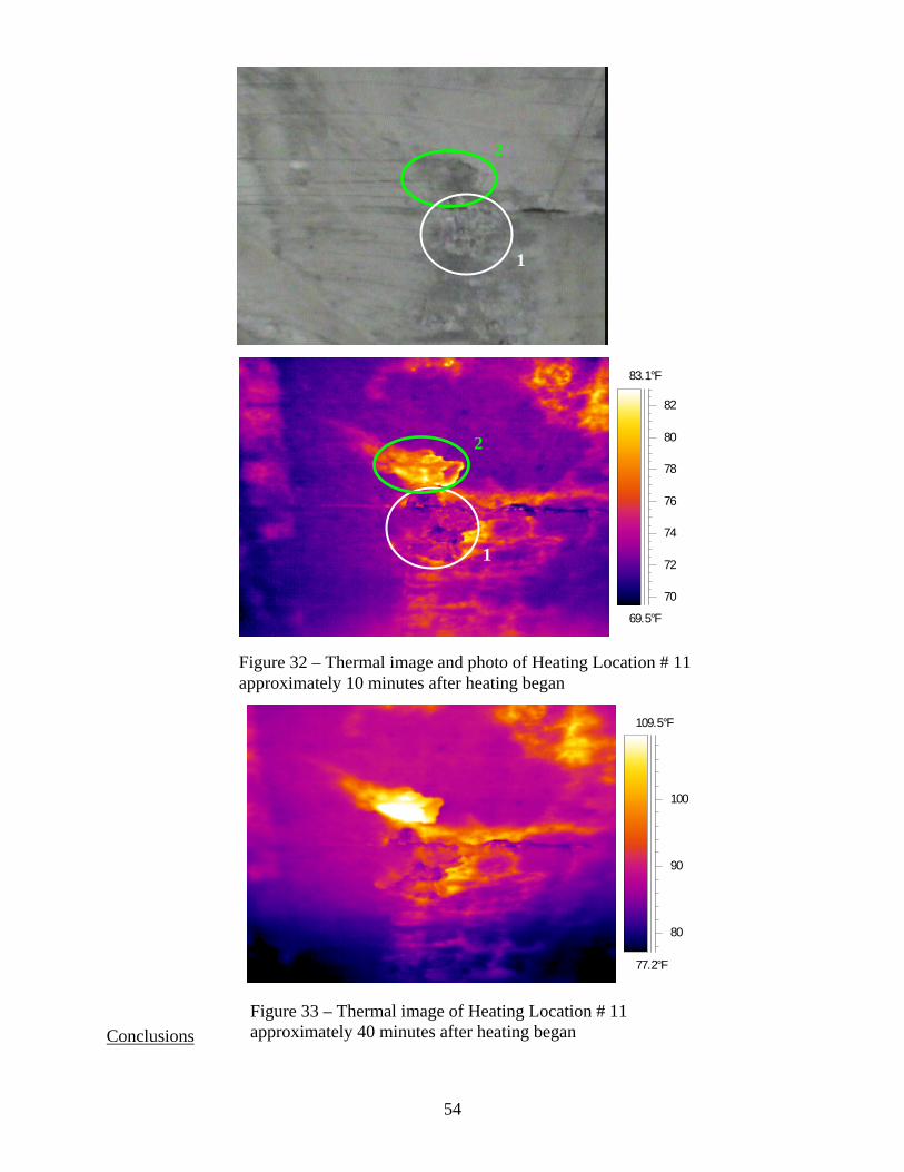
Figure 32 shows a thermal image and photo of Heating Location # 11 that were taken
approximately 10 minutes after heating began. Visible flaws were present on the heated surface
and temperature differences between warm and cool areas were approximately 7 °F. The
thermal image shows that not much heat time is needed to detect surface irregularities and obtain
a significant temperature variation. Figure 32 also shows what looks like spalled concrete
(denoted by circle 1) and an area of delamination (denoted by circle 2).
Figure 33 shows a thermal image of Heating Location # 11 taken approximately 40
minutes after heating commenced. When comparing Figures 32 and 33, it is evident that a lot of
surface detail was lost as the heating time increased. This is likely due to the camera’s automatic
adjustment to a broader temperature range. Broader temperature ranges result in less detailed
images.
53
69.5°F
83.1°F
70
72
74
76
78
80
82
2
1
2
1
Figure 32 – Thermal image and photo of Heating Location # 11 approximately 10 minutes after heating began
77.2°F
109.5°F Conclusions
80
90
100
Figure 33 – Thermal image of Heating Location # 11 approximately 40 minutes after heating began
54

The main conclusion drawn from Field Inspection 1 was that defects in near-surface
locations can be detected using thermal imaging. The numerous heating locations inspected
using both inspection Method 1 and Method 2 show flaws such as delamination, poorly
consolidated concrete, exposed rebar, and air voids. The flaws detected occasionally mimicked
what was seen visually, as with Heating Location # 5 (exposed rebar). However, some of the
flaws detected in thermal images were not detectable from visual inspection alone. Most of the
heating locations were actually chosen based on visual inspections beforehand, or based on
thermal images taken under ambient conditions.
The thermal images indicated temperature differences up to 25 °F between areas that
were usually less than 7.5 to 10 cm (6 to 8 in.) apart. Areas close together like this should have
almost identical temperatures because they receive similar heat intensity. The temperature
differences show up well in the thermal images, especially if a narrow temperature range for the
image can be used (appropriate ranges depend on actual surface temperatures recorded on the
thermal image). Also, as with Heating Location # 11, not much heat time is needed to produce
an image showing near-surface flaws. Figures 32 and 33 show images taken after only 10
minutes and 40 minutes, respectively, and the irregularities are easily discernable from the
concrete around them.
55

Part II-B: Thermal Imaging Inspection of Bridge 5/537E-N, Spokane Street/I-5
Interchange, in Seattle, WA
Location: Spokane Street/I-5 Interchange, Seattle, WA
Dates: August 13 – 14, 2007
Objectives
The objective of this field inspection was to determine whether thermal imaging may be
helpful in assessing discolored regions on the bottom surface of a precast concrete box girder
bridge crossing over the northbound lanes of I-5 near the Spokane Street exit in Seattle, WA.
The bridge is labeled 5/537E-N by WSDOT. This area was designated a possible problem
region based on excessive leaching on the bottom surface of the box girder.
Inspection Procedures
Inspection Method 1 involved placing the heater on four masonry blocks inside the box
girder, heating the floor surface, and taking thermal images of the unheated surface beneath the
box girder throughout the heating process. Inspection Method 2 entailed heating the exterior
bottom surface of the box girder and taking thermal images of that same heated surface after
heating was concluded.
Before any inspections took place, thermal images of the bottom surface of the box girder
under ambient conditions were analyzed to see if problem areas could be identified. Figure 34
shows a thermal image of the bridge under ambient conditions that encompasses most of Span 4.
This thermal image displays the access hatches used during one inspection (Heating Location #
2). However, it does not reveal any specific problem areas. Without thermal identification to
locate problem areas, visual analysis was used, in conjunction with access limitations, to
determine heating locations. The positioning limits were based on access provided by WSDOT
56

lane closures on I-5. Two inspections were conducted, one using Method 1 and the other using
Method 2. The two heating locations were chosen based on what regions presented the most
visible irregularities. It is important to note that inspection of this box girder bridge took place at
night. Setup started around 10:00 pm on August 13th, and the final inspection ended at about
2:00 am on August 14th, for a total inspection time of four hours.
66.2°F
77.0°F
68
70
72
74
76
Figure 34 – Thermal image of Bridge 5/537E-N under ambient conditions
57

Heating Location #1
Heating Location # 1 was inspected on August 13th, 2007 using inspection Method 2.
The inspection position was in Span 4, just west of Pier 3. The surface was heated for a time
span of 0:40 (hh:mm). The top of the heater was placed approximately 107 cm (42 in.) below
the heated surface. This region was chosen due to the extensive leaching on its surface, as
displayed in Figure 35. The leaching shows up as the white area stretching across the photo and
encircled by the orange line.
Figure 35 – Photo of Heating Location # 1 with extensive discoloration due to leaching
Leaching
58

With this inspection, thermal images were taken throughout the heating process. The
camera was placed on the lift platform approximately 3 m (10 ft.) to one side of the heater.
Figure 36 shows two thermal images side by side that were taken approximately four minutes
after heating began. The circled region demonstrates that after a fairly short heat time, surface
characteristics and flaws were visible in thermal images. There were also other visible
irregularities in the middle of the figure.
70.7°F
86.2°F
75
80
85
58.0°F
99.7°F
60
70
80
90
Flaw
Figure 36 – Thermal images of Heating Location # 1, side by side
The thermal images in Figure 36 were taken in order to help locate areas that, with
further heat input, might reveal subsurface flaws. The circled region shows what looks like a
flaw, so the heater was moved so that its center was directly underneath this region, and then
heating commenced again. From here, thermal images were taken every two minutes. Figure 37
shows a typical image progression during heating, or what one would see from the camera
display. Figure 38 shows a single image from the progression.
59

Figure 37 – Thermal image progression at Heating Location # 1
77.4°F
136.1°F
80
100
120
Figure 38 – Thermal image of Heating Location # 1 at middle of time interval
60

Heating Location # 1 was a very important inspection because, after heating was stopped,
the surface was examined with a rock hammer. Tapping confirmed what was seen in the thermal
images. A WSDOT inspector tapped part of the surface that had no apparent flaws (either
visually or thermally) and then tapped at suspected flaw locations. Sound differences were
easily discernable between the two locations, and then the pick end of the hammer was used to
remove surface concrete and excavate the flaw. Delamination and poorly consolidated concrete
(small air voids) were discovered. Figure 39 shows a thermal image of a WSDOT employee
excavating the delaminated concrete at the flaw location shortly after thermal imaging
inspection. This was the first inspection location where flaws discovered thermally were
confirmed using physical means (tapping and excavation).
74.7°F
90.2°F90
85
80
75
Figure 39 – Thermal image of Heating Location # 1: excavating a detected flaw
61

Heating Location # 2
Heating Location # 2 was inspected on August 14th, 2007 using inspection Method 1.
The inspection position was in Span 4 inside the box girder from the south access hatch. The
surface was heated for a time span of 1:15 (hh:mm). The heater was placed inside the box girder
on four masonry blocks, approximately 61 cm (24 in.) from the heated surface. This region was
chosen due to extensive leaching on the exterior surface. Further inspection of the box girder
interior revealed a very moist environment, which suggests that drainage water often
accumulates (most likely in low spots where water cannot drain).
Thermal images from Heating Location # 2 do not reveal anything about the leaching or
the unheated surface. Steel reinforcement inside the concrete is the only thing shown in the
images. Figure 40 is comprised of two thermal images that show the reinforcing steel as cool
lines between warmer regions. There is one hot spot, which is located inside the circled region
in both thermal images.
74.7°F
127.8°F
80
90
100
110
120
Figure 40 – Thermal images of Heating Location # 2
83.3°F
107.4°F
85
90
95
100
105
62

Conclusions
Field Inspection 2, conducted at an I-5 overpass (Bridge 5/537E-N) in Seattle, WA, was
very successful because what was detected with thermal imaging was confirmed by “tapping”
and excavation of the heated surface (at Heating Location # 1). The thermal images (Figures 36
and 38) suggested some sort of flaw (hypothesized as delamination), which was then verified by
a WSDOT employee using a rock hammer to excavate the flaw. These inspections also
confirmed that flaws can be visible in thermal images after only about 10 minutes of heat input
(such as at Heating Location # 1).
63

Part II-C: Thermal Imaging Inspection of Pearl Street Overpass on State Route 16 in
Tacoma, WA
Location: State Route 16, Pearl Street Overpass, Tacoma, WA
Dates: August 14 – 15, 2007
Objectives
The objective of this field inspection was to determine whether thermal imaging may be
helpful in locating embedded tendons and detecting internal voids in the vertical webs of a
precast, post-tensioned (PT) concrete box girder on State Route 16 (crossing over Pearl Street) in
Tacoma, WA. This bridge was inspected because grouting problems had been reported during
construction. The idea was to use thermal imaging to detect any air voids present inside the post-
tensioning ducts. Improperly grouted ducts that contain air voids could lead to corrosion of the
steel tendons if moisture is allowed to accumulate in the system.
Inspection Procedures
The Pearl Street overpass presented a different type of thermal imaging inspection than in
Field Inspections 1 and 2. Investigating post-tensioning ducts located in the bridge web
(interior) and wall (exterior) was the main focus for the Pearl Street overpass. The web and wall
were each 30 cm (12 in.) thick. Therefore longer heat times had to be implemented than in
previous field inspections. Each web or wall had three PT-ducts running longitudinally through
the box girder, and their position varied vertically along the span. Access to only one chamber
inside the box girder was provided. Also, both inspection Method 1 and 2 were used.
64

Heating Location # 1
Heating Location # 1 was inspected on August 14th, 2007 using inspection Method 2.
Figure 41 shows the inspection point of the interior web inside the box girder, which was located
approximately at the midspan of the bridge, 12.2 m (40 ft.) from the edge of the access hatch.
The surface was heated for a total time of 3:00 (hh:mm). This location entailed orienting the
heater horizontally (so that the longer edge of the heater ran longitudinally along the box girder)
on masonry blocks to raise the heater above the floor. The heater was approximately 61 cm (24
in.) from the heated surface and thermal images were obtained both during heating and for one
hour afterward. During heating, the infrared camera was situated to the side of the heater and
angled toward the heated surface.
Figure 41 – Photo of Heating Location # 1
65

Figure 42 shows a thermal image of Heating Location # 1 taken approximately 30 minutes after
heating commenced. This image illustrates the state of the concrete surface and its
characteristics. A few hot and cool spots can be seen, but this image primarily reveals surface
characteristics of the concrete.
83.6°F
165.0°F
100
120
140
160
Figure 42 – Thermal image of Heating Location # 1 (30 minutes after heating began)
The next two thermal images, shown in Figure 43, do not reveal anything regarding
materials embedded in the concrete box girder web. The first image on the left was taken after
2:55 (hh:mm) of heating. The second image on the right was taken after the camera was moved
directly in front of the heated surface, about 0:45 (hh:mm) after heating ended. None of the PT-
ducts are visiblbe in any of the thermal images, which indicates a couple of different things.
First, three hours of heat input may not be enough to provide thermal images showing PT-ducts
embedded in 30 cm (12 in.) thick concrete. Second, it is likely that the inspection setup was not
66

ideal for detecting the ducts. Inspection Method 2 involves taking thermal images from the same
side as the heat input, and specimen inspections conducted in the lab indicated that Method 2
does not yield images showing inner-surface characteristics. Also, due to the confined area
inside the box girder, the camera could not be placed as far from the heated surface as desired.
Thus the camera lens could not capture the entire heated surface area. Unfortunately, since
access to the opposite face of the box girder web was not available, Inspection Method 2 was the
only option available.
91.5°F
180.3°F
100
120
140
160
180
89.9°F
125.1°F
90
100
110
120
Figure 43 –Thermal images of Heating Location # 1: a) after 2:55 (hh:mm) of heating (left) b) 0:45 (hh:mm) after heating stopped (right)
Heating Location # 2
Heating location # 2 was inspected on August 15th, 2007 using inspection Methods 1 and
2. The inspection point was located approximately 3.9 m (12.7 ft.) from the edge of the access
hatch to the center line of the heater. This inspection investigated the outer wall of the box
girder, where the surface was heated for a total heat time of 5:00 (hh:mm). The heater was
oriented vertically (i.e., the longer edge of the heater was vertical). The front of the heater was
positioned parallel to the wall, approximately 35.5 cm (14 in.) from the interior wall surface.
67

The heater was not elevated, so both the box girder wall and floor were heated, as shown in
Figure 44. Thermal images were obtained both during heating and for 40 minutes after heating
ended.
73.0°F
289.9°F
100
150
200
250
Figure 44 – Thermal image of Heating Location # 2 showing heater setup
The inspection setup for this location allowed for two kinds of thermal images to be
obtained. The first kind of image was of the unheated surface, taken from ground level outside
the box girder (Method 1). Due to the large distance from the camera to the surface, images had
less detail and a large viewing window. Figure 45 shows one such image taken about three hours
after heating began. From the image, one can see that the heated surface (wall) was not as warm
as the floor of the box girder. This is due to the fact that the wall is thicker than the floor (12 in.
versus 8 in.), and it takes longer for heat to propagate through thicker concrete. After only three
hours of heat input, there were no PT-ducts or flaws visible in the thermal image. In Figure 45,
circled area 1 shows the floor, while circled area 2 shows the wall of the box girder. Thermal
68

images taken of the unheated surface after five hours of heating did not reveal the PT-ducts in
the box girder wall.
70.6°F
103.8°F
80
90
100
1
2
Figure 45 – Thermal image of Heating Location # 2 taken of the unheated surface
Images of the heated surface were also obtained from inside the box girder after heating
ended. Figure 46 displays one such image where surface characteristics are visible. However, as
with Figures 44 and 45, the image does not show any PT-ducts. The flaws shown are mostly
surface irregularities and small surface voids. Points 1 and 2 in Figure 46 show a temperature
difference of approximately 24 °F in a span of only a few inches.
69

195.4°F
251.4°F
200
210
220
230
240
250
1 : 208.2
2 : 232.3
Figure 46 – Thermal image of Heating Location # 2 taken of the heated surface
Conclusions
Field Inspection 2, conducted on a box girder bridge crossing over Pearl Street in
Tacoma, WA, was a useful inspection in terms of defining thermal imaging limits. Neither
heating location (inside web or outside wall) produced thermal images showing post-tensioning
ducts (the initial goal). Heating Location # 1 suggested that taking images from the heated
surface is not ideal for locating internal concrete attributes or flaws. Also, the web was 30 cm
(12 in.) thick, which presents the test setup with more problems. Thicker concrete provides a
larger heat sink for dissipating the input energy, which makes it difficult to obtain a sufficiently
high temperature gradient from the heated surface to the unheated surface.
Heating Location # 2 used through-heating for five hours, but did not result in any
thermal images showing PT-duct or other internal concrete characteristics. One reason is that the
thermal camera was much farther away from the unheated surface than in any other inspections
(conducted in the field or the lab) due to the height of the bridge above ground. An increased
70

distance also increases the thermal range that the camera reads, therefore making it more difficult
to detect smaller temperature differences on the surface. Also, edge effects may have affected
the results in terms of heat energy dissipation. In the lab, specimen edges and ends were covered
with two layers of insulation to help keep the heat energy within the specimen. In the field,
however, the heat not only propagates through the concrete thickness, but also along the length
and height of the box girder wall. The temperature gradient is reduced, resulting in thermal
images that do not reveal internal conditions of the concrete.
71

Part II-D: Ground-Penetrating Radar (GPR) Inspection of I-405 Entry/Exit Ramp Bridge
Deck in Kirkland, WA.
Location: I-405 Entry/Exit Ramp, Kirkland, WA
Dates: September 28 – 29, 2007
Objectives
The objectives of this field inspection were to demonstrate the effectiveness of ground-
penetrating radar (GPR) inspection for locating transverse tendons and plastic ducts in post-
tensioned bridge decks, and investigate whether internal voids were present in any of the plastic
ducts. This specific bridge deck was inspected because grouting problems had been reported in
four of the ducts during construction in June and July, 2007. Improperly grouted ducts that
contain air voids could lead to corrosion of the steel tendons if moisture is allowed to accumulate
in the system.
Inspection Procedures
The post-tensioned bridge deck consisted of six concrete slabs (Slabs A, B, C, D1, D2,
and E) that were constructed during June-August 2007. Grouting problems had been reported
for four transverse ducts in three of the concrete slabs. The dates of concrete placement for each
of the slabs were: Slab B – July 6, 2007; Slab C – June 28, 2007; Slab D1 – July 31, 2007. The
entry/exit ramp traffic lanes were oriented to accommodate vehicular traffic traveling north/south
on I-405.
GPR inspections were scheduled for September 28-29, 2007, approximately one week
prior to opening the I-405 entry/exit ramp to traffic. Inspections of the east lane (I-405 entry
ramp) were conducted on September 28. Inspections of the west lane (I-405 exit ramp) were
conducted on September 29. GPR Linescan inspections were used to initially locate the tendons
72

and ducts embedded in the concrete deck. Then GPR Structurescan inspections were conducted
at multiple locations for each of the ducts. A summary of GPR inspection locations is provided
in Table 5.
Table 4 – GPR inspection locations for I-405 entry/exit ramp bridge deck
Duct Locations
Traffic Lane Locations
GPR Inspection Locations
East lane Eight (8) locations, beginning at sidewalk curb (east edge of bridge deck) and progressing westward toward median between traffic lanes
Slab B
Ducts 19 and 51
West lane Eight (8) locations, beginning at sidewalk curb (west edge of bridge deck) and progressing eastward toward median between traffic lanes
East lane Nine (9) locations, beginning at east edge of bridge deck and progressing westward toward median between traffic lanes
Slab C
Duct 77 West lane Nine (9) locations, beginning at sidewalk curb (west edge of
bridge deck) and progressing eastward toward median between traffic lanes
Slab D1
Duct 45
East lane Three (3) locations, beginning at east edge of bridge deck and progressing westward toward median between traffic lanes
Results
Since the concrete was relatively “green” (concrete cure time less than three months) at
the time of GPR inspection, tendons and ducts could only be detected to depths of approximately
25 cm (10 in.) in the concrete deck. Furthermore, concrete sidewalks had been recently placed
on top of the deck at the edges of the bridge deck, thus completely obscuring the presence of
tendons and ducts directly beneath the sidewalks. (Note that subsequent GPR inspections of the
regions below sidewalks could be scheduled for a later date, after the concrete has cured and
moisture content has been reduced to an acceptable level for successful GPR inspection.)
As with previous GPR inspections of concrete specimens at WSU (Conner 2004), both
the longitudinal steel rebar and the transverse steel rebar were clearly visible in GPR images of
73

the bridge deck. Steel tendons were also readily detected at all inspection locations, for concrete
depths up to 25 cm (10 in.). The tendons were clearly visible in GPR Structurscan images, as
illustrated in Figure 47. None of the GPR images revealed air voids within the plastic ducts.
Figure 47 – GPR image of steel tendons in Ducts 19 and 51 (Slab B) at a depth of 19.3 cm (7.6 in.) below the surface of the concrete deck.
Conclusions
Steel tendons in plastic ducts embedded in prestressed concrete members were clearly
visible in GPR images at various depths up to 25 cm (10 in.) If concrete is allowed to cure for
six months or more prior to GPR inspection, it may be possible to detect tendons and plastic
ducts at depths of approximately 41 cm (16 in.). Although none of the GPR images from this
bridge inspection revealed air voids in the plastic ducts, laboratory studies indicate that air voids
located between steel tendons and a GPR antenna can be successfully detected.
Acknowledgements Funding for this project was provided by the Federal Highway Administration through contract
number DTFH61-05-C-00008. The prestressing strands and steel ducts were donated by Central
74

Pre-Mix Prestress Company of Spokane, Washington. The plastic ducts were donated by
General Technologies Inc. of Stafford, Texas.
References
Conner, J.M. “Detection of tendons and voids in grouted ducts using ground-penetrating radar,”
Master of Science (M.S.) thesis, Department of Civil & Environmental Engineering, Washington
State University, 2004.
Conner, J.M., Pollock, D.G., and Khaleghi, B. “Detection of simulated voids in grouted ducts
uising ground-penetrating radar,” Proceedings of the Concrete Bridge Conference, Reno, NV,
2006.
Dupuis, K. “Nondestructive testing of concrete box girder bridges using thermal imaging,”
Master of Science (M.S.) thesis, Department of Civil & Environmental Engineering, Washington
State University, 2008.
GSSI, Handbook for Radar Inspection of Concrete, Geophysical Survey Systems, Inc., 2001.
Musgrove, R.R. “Nondestructive detection of post-tensioning tendons and simulated voids in
concrete specimens using thermal imaging,” Master of Science (M.S.) thesis, Department of
Civil & Environmental Engineering, Washington State University, 2006.
Pearson, E.J. “The feasibility of thermal imaging for the location and inspection of post-
tensioning cables in concrete box girder bridges,” Master of Science (M.S.) thesis, Department
of Civil & Environmental Engineering, Washington State University, 2003.
75