detector: a topology-aware monitoring system for data ... · detector: a topology-aware monitoring...
TRANSCRIPT
deTector: a Topology-Aware Monitoring System for Data Center Networks
Yanghua Peng1, Ji Yang2, Chuan Wu1, Chuanxiong Guo3, Chengchen Hu2, Zongpeng Li4
1
1The University of Hong Kong, 2Xi’an Jiaotong University3Microsoft Research, 4University of Calgary
Data Center Network Monitoring
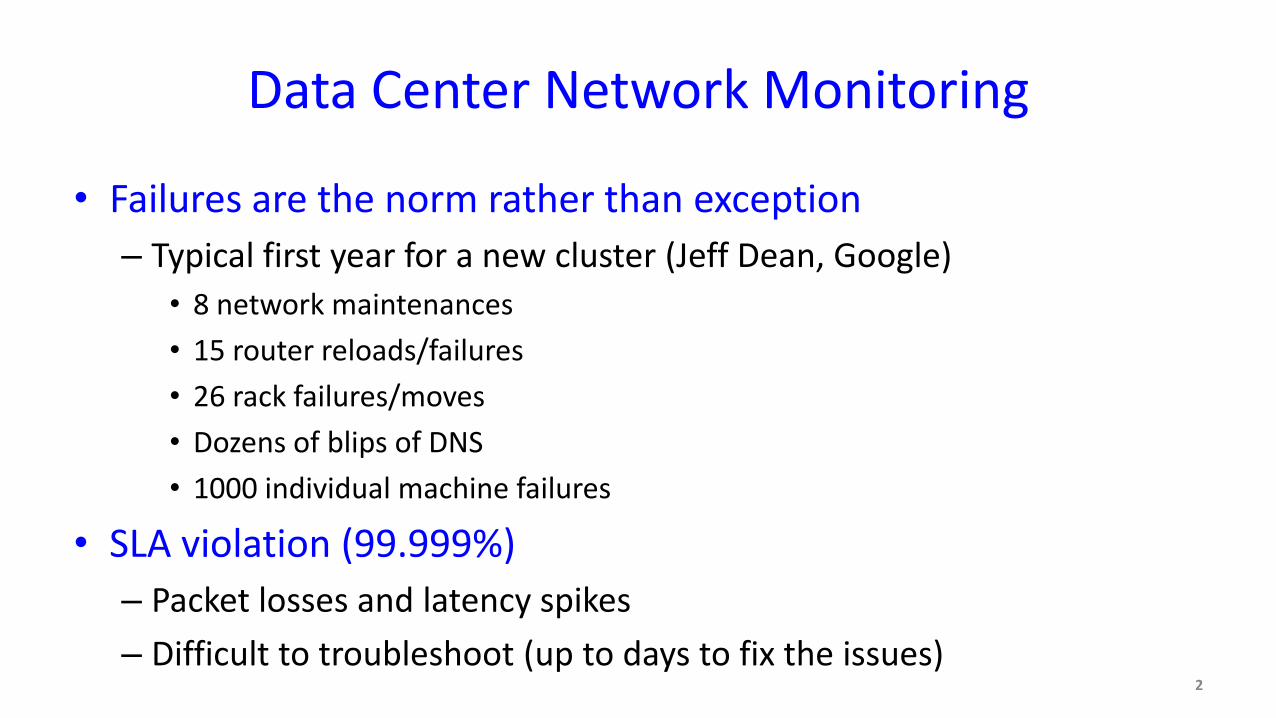
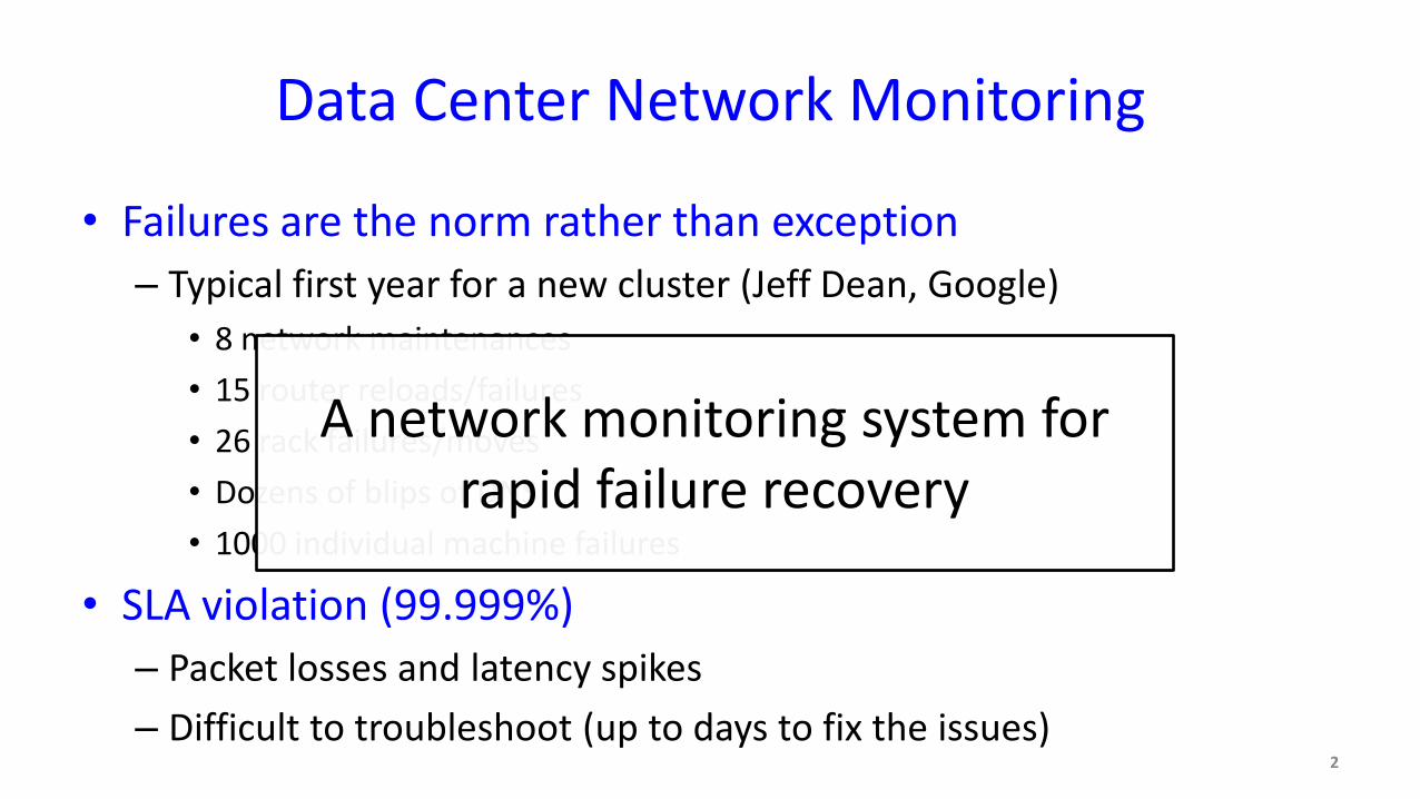
• Failures are the norm rather than exception– Typical first year for a new cluster (Jeff Dean, Google)• 8 network maintenances• 15 router reloads/failures• 26 rack failures/moves• Dozens of blips of DNS• 1000 individual machine failures
• SLA violation (99.999%)– Packet losses and latency spikes– Difficult to troubleshoot (up to days to fix the issues)
2
Data Center Network Monitoring
• Failures are the norm rather than exception– Typical first year for a new cluster (Jeff Dean, Google)• 8 network maintenances• 15 router reloads/failures• 26 rack failures/moves• Dozens of blips of DNS• 1000 individual machine failures
• SLA violation (99.999%)– Packet losses and latency spikes– Difficult to troubleshoot (up to days to fix the issues)
2
A network monitoring system for rapid failure recovery
Challenges
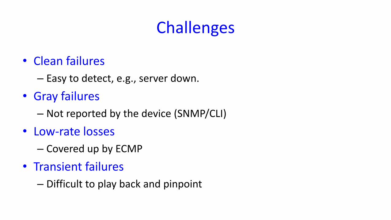
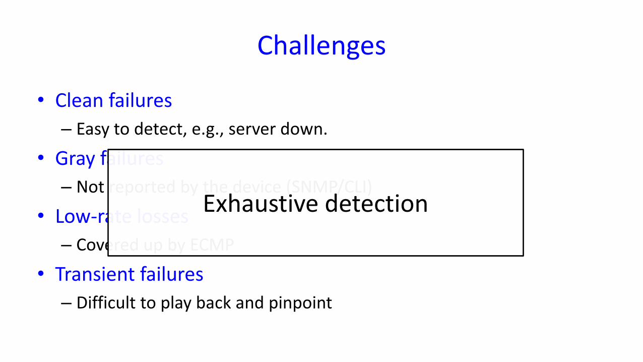
• Clean failures– Easy to detect, e.g., server down.
• Gray failures– Not reported by the device (SNMP/CLI)
• Low-rate losses– Covered up by ECMP
• Transient failures– Difficult to play back and pinpoint
Challenges
• Clean failures– Easy to detect, e.g., server down.
• Gray failures– Not reported by the device (SNMP/CLI)
• Low-rate losses– Covered up by ECMP
• Transient failures– Difficult to play back and pinpoint
Exhaustive detection
Existing Solutions
4
• Existing systems– Passive: CLI/SNMP– Active: Pingmesh, NetNORAD
• Limitations– Fail to detect at least one type of losses– High overhead– Can not pinpoint failures without other tools (e.g., tracert)
Existing Solutions
4
• Existing systems– Passive: CLI/SNMP– Active: Pingmesh, NetNORAD
• Limitations– Fail to detect at least one type of losses– High overhead– Can not pinpoint failures without other tools (e.g., tracert)
Can we design a better network monitoring system by exploiting
network topology?
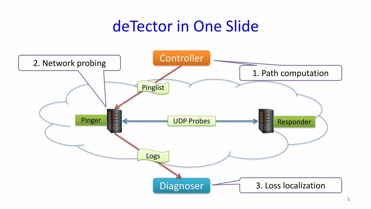
deTector in One Slide
5
Controller
Diagnoser
1. Path computation2. Network probing
3. Loss localization
Pinger
Pinglist
Responder
Logs
UDP Probes

Phase I: Path Computation
6
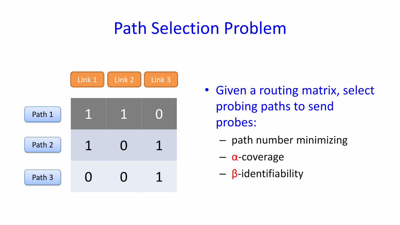
Path Selection Problem
1 1 0
1 0 1
0 0 1
Path 1
Path 2
Path 3
Link 1 Link 2 Link 3• Given a routing matrix, select
probing paths to send probes:– path number minimizing– α-coverage– β-identifiability
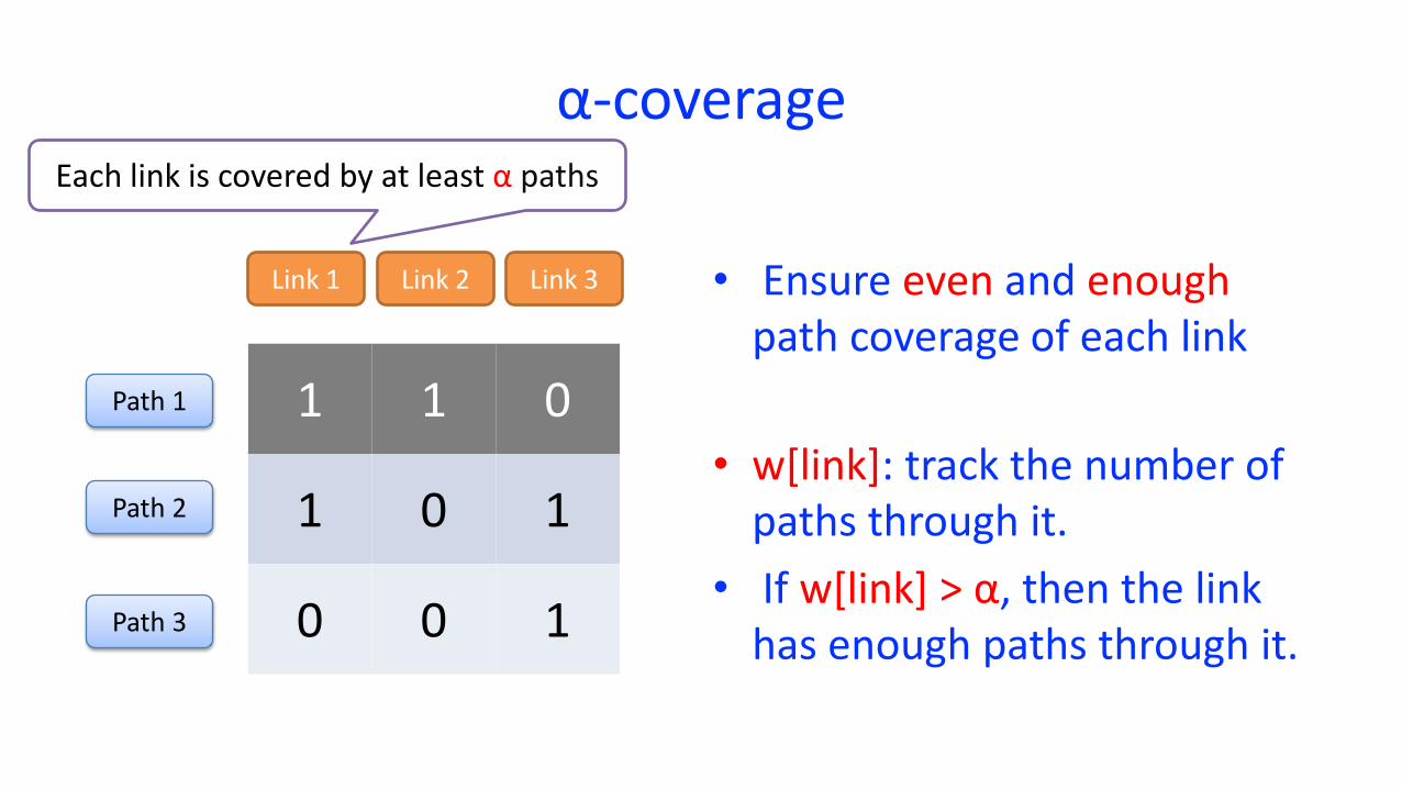
α-coverage
• Ensure even and enoughpath coverage of each link
Each link is covered by at least α paths
• w[link]: track the number of paths through it.
• If w[link] > α, then the link has enough paths through it.
1 1 0
1 0 1
0 0 1
Path 1
Path 2
Path 3
Link 1 Link 2 Link 3
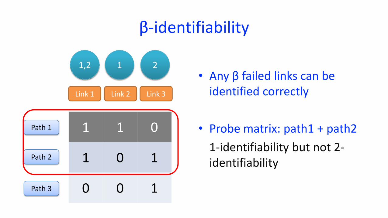
β-identifiability
• Any β failed links can be identified correctly
• Probe matrix: path1 + path2 1-identifiability but not 2-identifiability
1,2 1 2
1 1 0
1 0 1
0 0 1
Path 1
Path 2
Path 3
Link 1 Link 2 Link 3
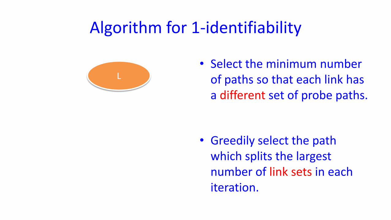
Algorithm for 1-identifiability
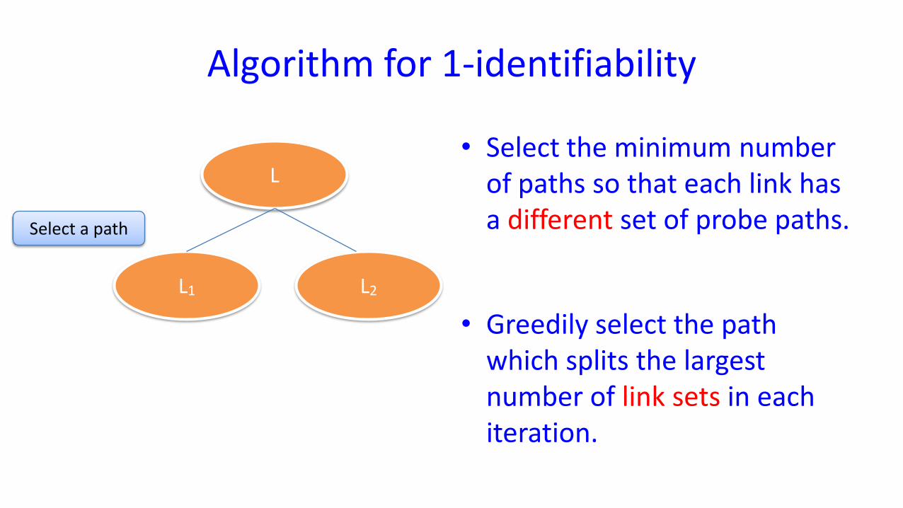
• Select the minimum number of paths so that each link has a different set of probe paths.
• Greedily select the path which splits the largest number of link sets in each iteration.
L
Algorithm for 1-identifiability
• Select the minimum number of paths so that each link has a different set of probe paths.
• Greedily select the path which splits the largest number of link sets in each iteration.
L
L2L1
Select a path
Algorithm for 1-identifiability
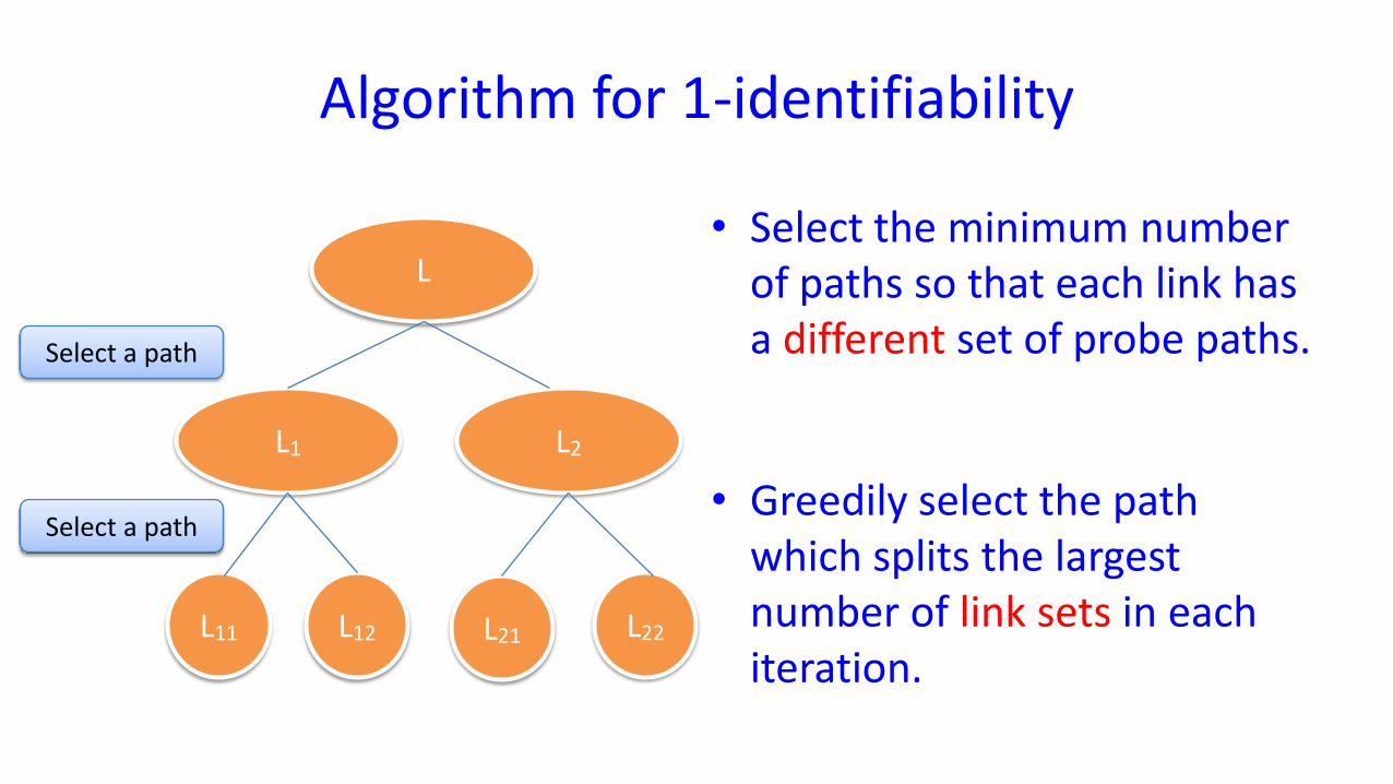
• Select the minimum number of paths so that each link has a different set of probe paths.
• Greedily select the path which splits the largest number of link sets in each iteration.
L
L2L1
L11 L12 L21 L22
Select a path
Select a path
1-identifiability => β-identifiability
1 1 0
1 0 1
0 0 1
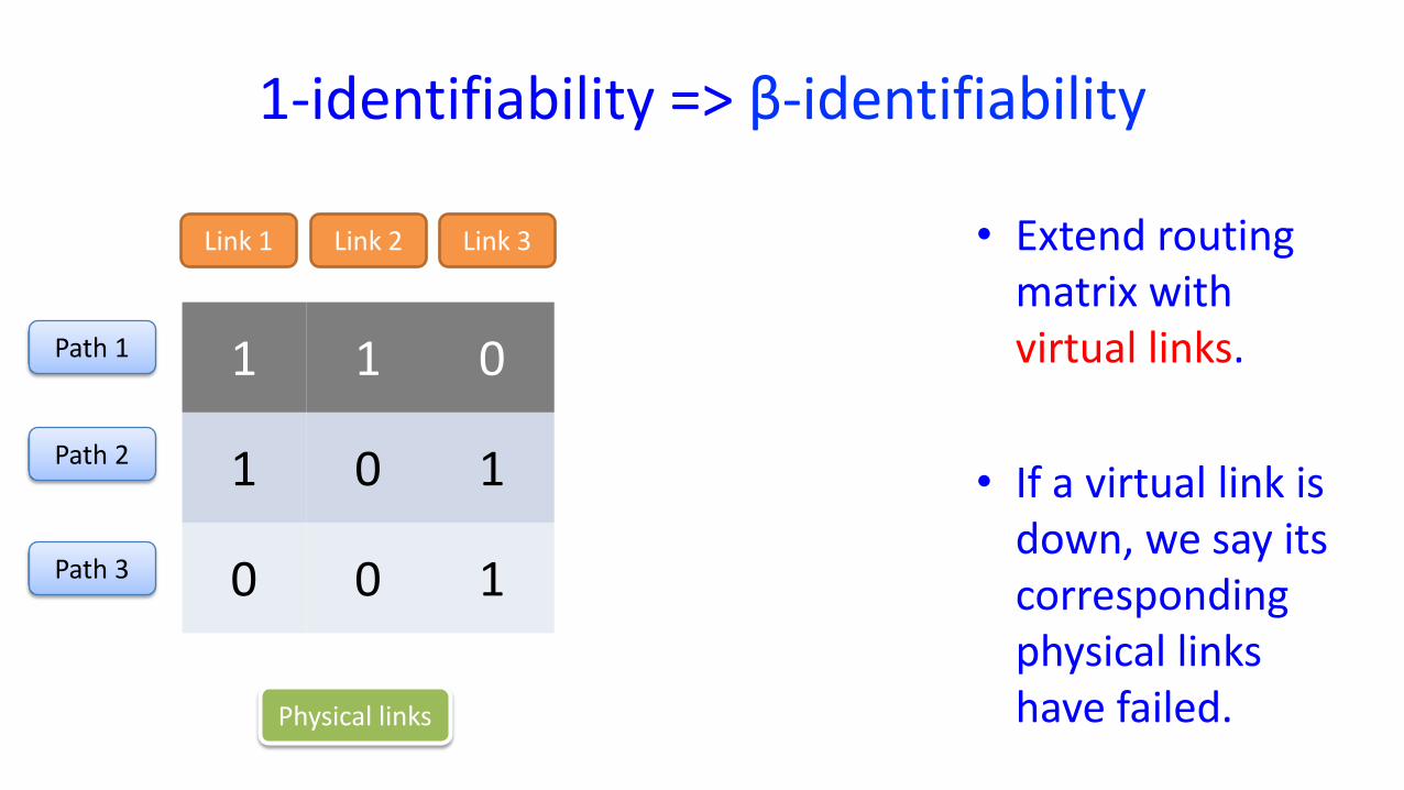
• Extend routing matrix with virtual links.
• If a virtual link is down, we say its corresponding physical links have failed.Physical links
Path 1
Path 2
Path 3
Link 1 Link 2 Link 3
1-identifiability => β-identifiability
1 1 0
1 0 1
0 0 1
1 1 1
1 1 1
0 1 1
Link 12
Link 13
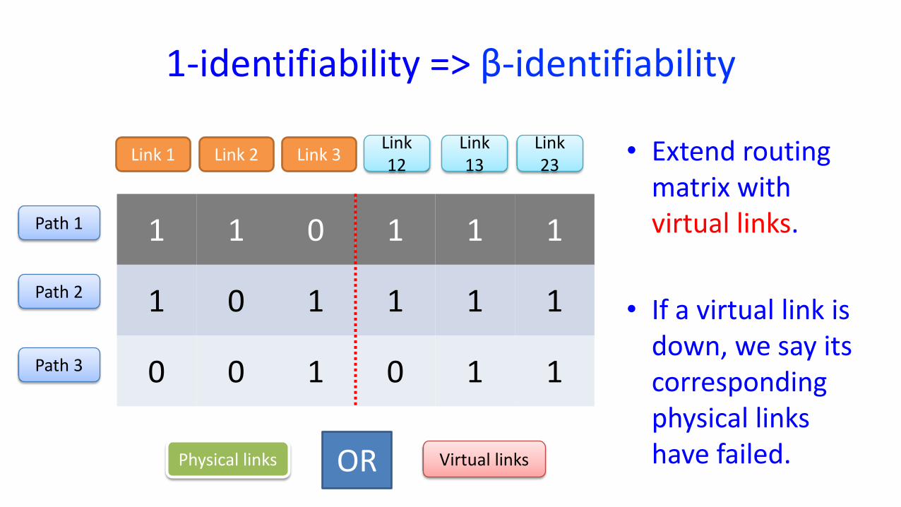
Link 23 • Extend routing
matrix with virtual links.
• If a virtual link is down, we say its corresponding physical links have failed.ORPhysical links Virtual links
Path 1
Path 2
Path 3
Link 1 Link 2 Link 3

Probe Matrix Construction (PMC) Algorithm
• Select a path with minimal score in each iteration• Stop when achieving α-coverage and β-identifiability
• Extend the routing matrix with virtual links• Define a score for each path Quantify
coverage
Quantify identifiability
PMC Algorithm
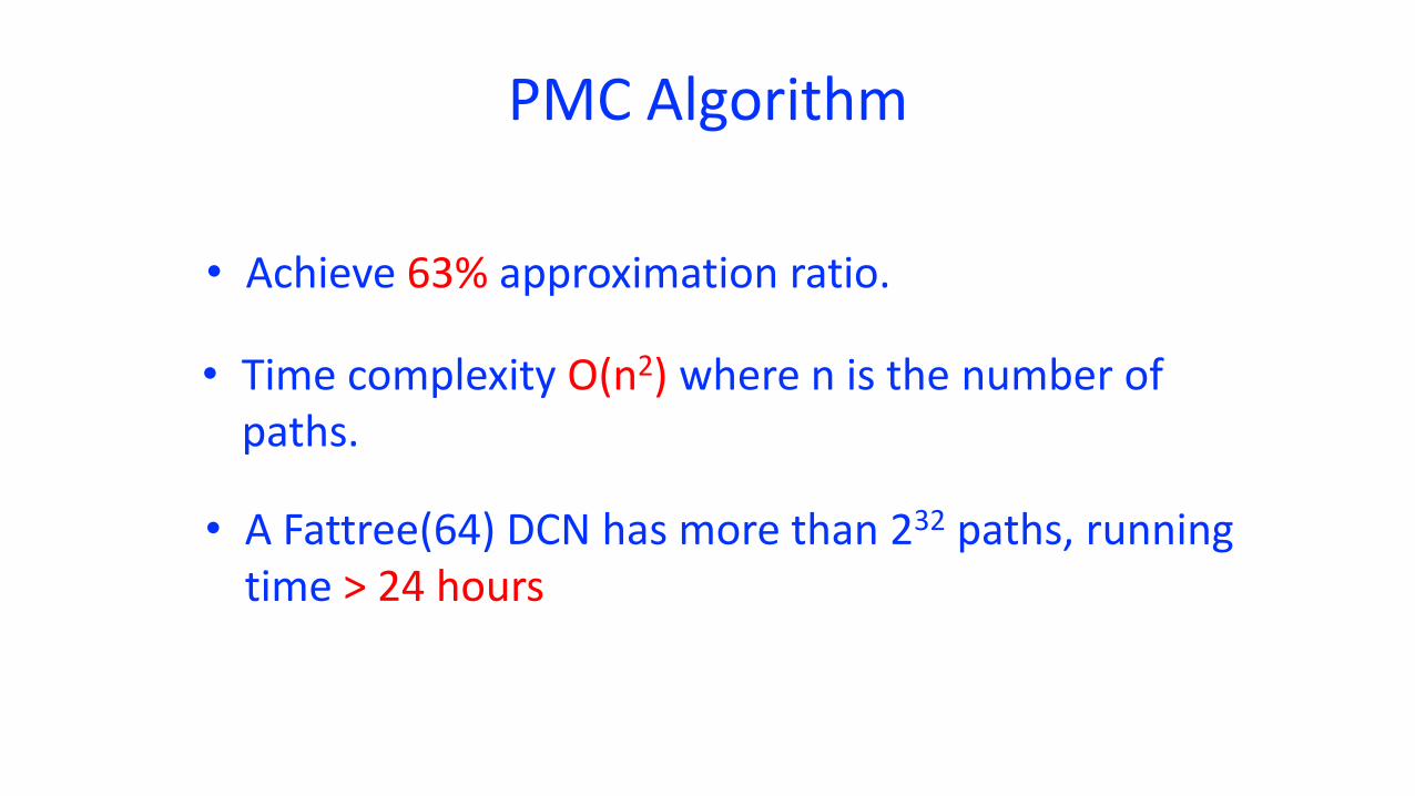
• Achieve 63% approximation ratio.
• Time complexity O(n2) where n is the number of paths.
• A Fattree(64) DCN has more than 232 paths, running time > 24 hours
PMC Algorithm
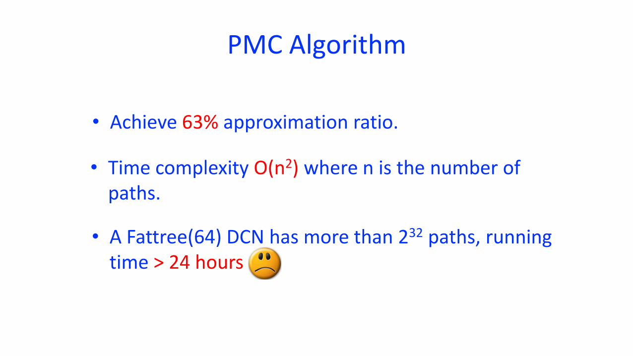
• Achieve 63% approximation ratio.
• Time complexity O(n2) where n is the number of paths.
• A Fattree(64) DCN has more than 232 paths, running time > 24 hours
PMC Algorithm
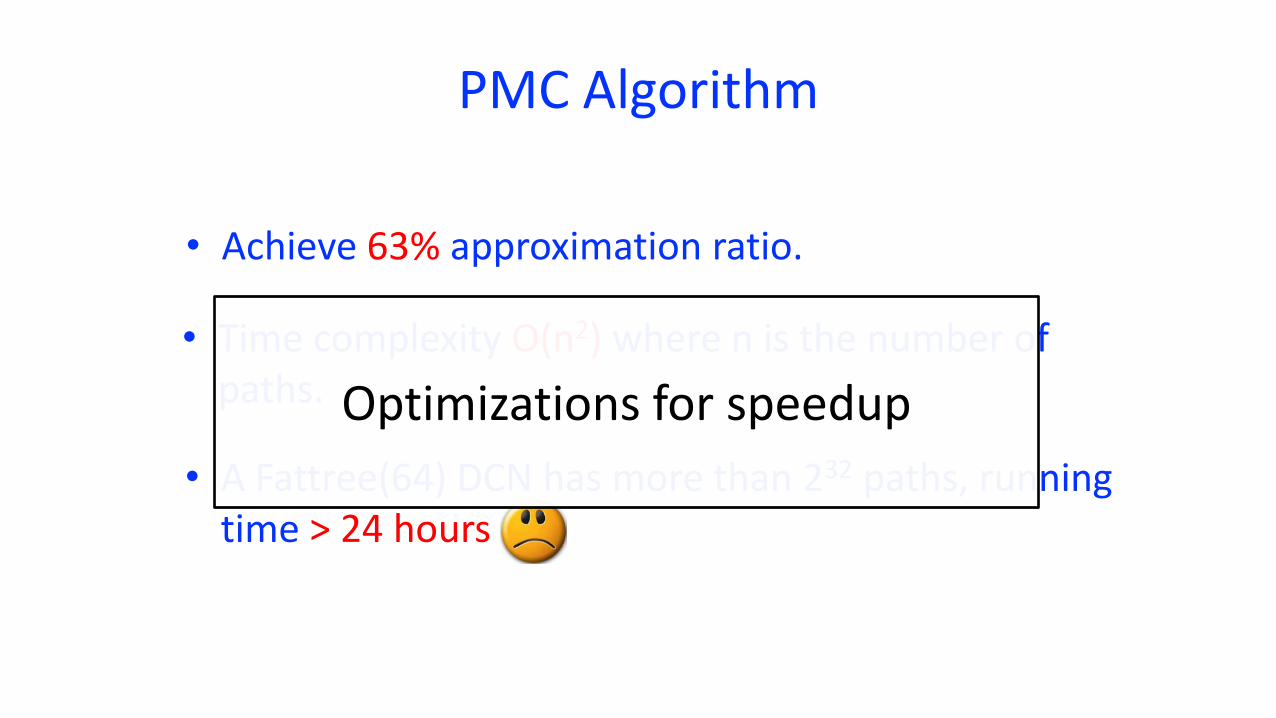
• Achieve 63% approximation ratio.
• Time complexity O(n2) where n is the number of paths.
• A Fattree(64) DCN has more than 232 paths, running time > 24 hours
Optimizations for speedup
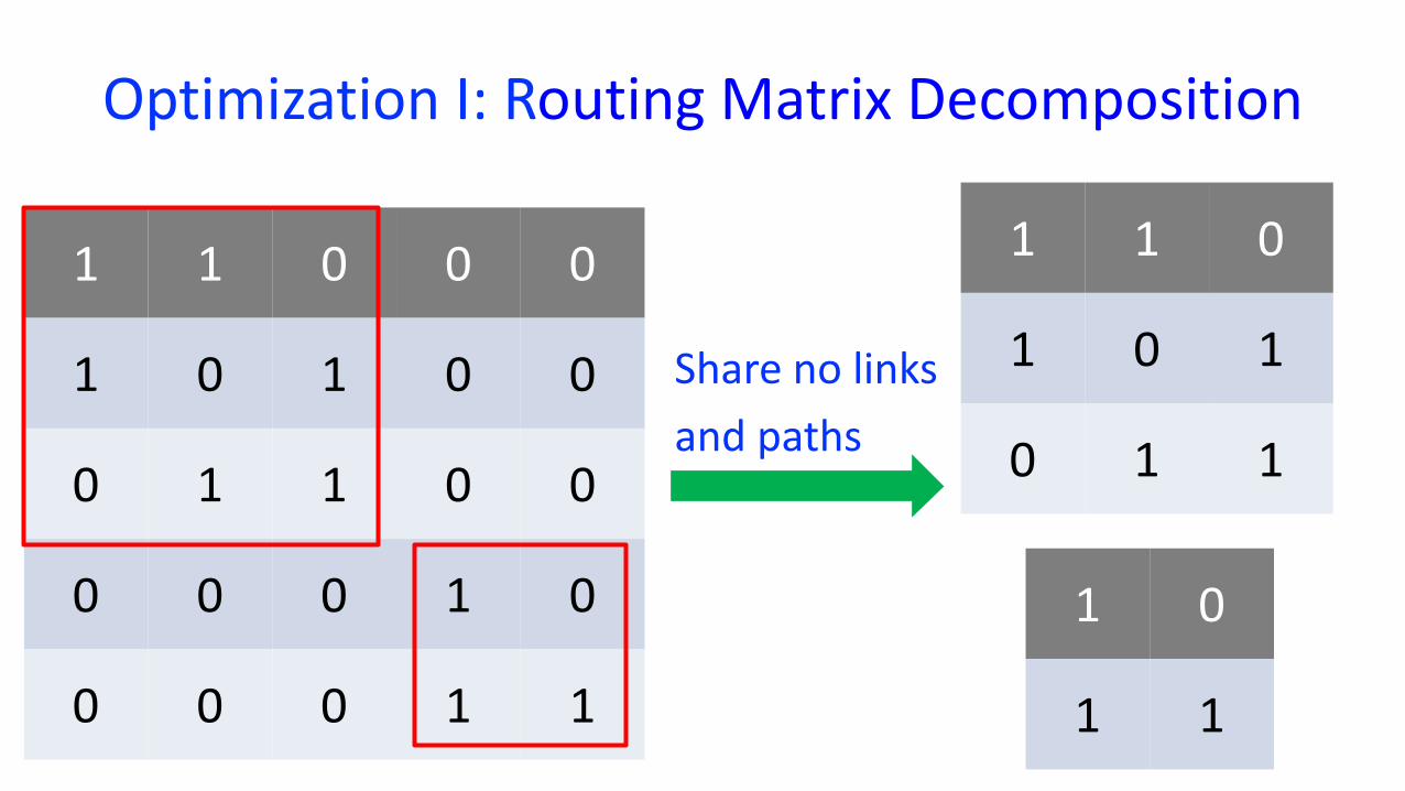
Optimization I: Routing Matrix Decomposition
1 1 0
1 0 1
0 1 1
0 0 0
0 0 0
0 0
0 0
0 0
1 0
1 1
1 1 0
1 0 1
0 1 1
1 0
1 1
Share no links and paths
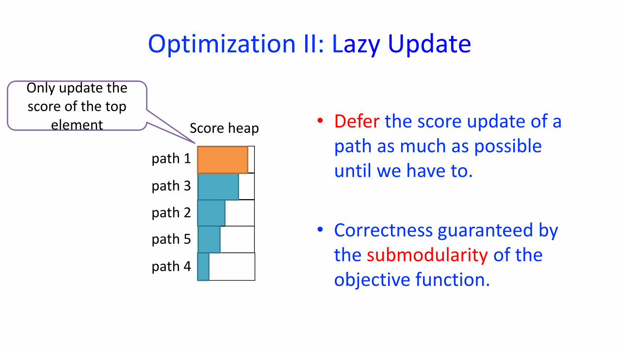
Optimization II: Lazy Update
• Defer the score update of a path as much as possible until we have to.
• Correctness guaranteed by the submodularity of the objective function.
path 1
path 3
Score heap
Only update the score of the top
element
path 2
path 5
path 4
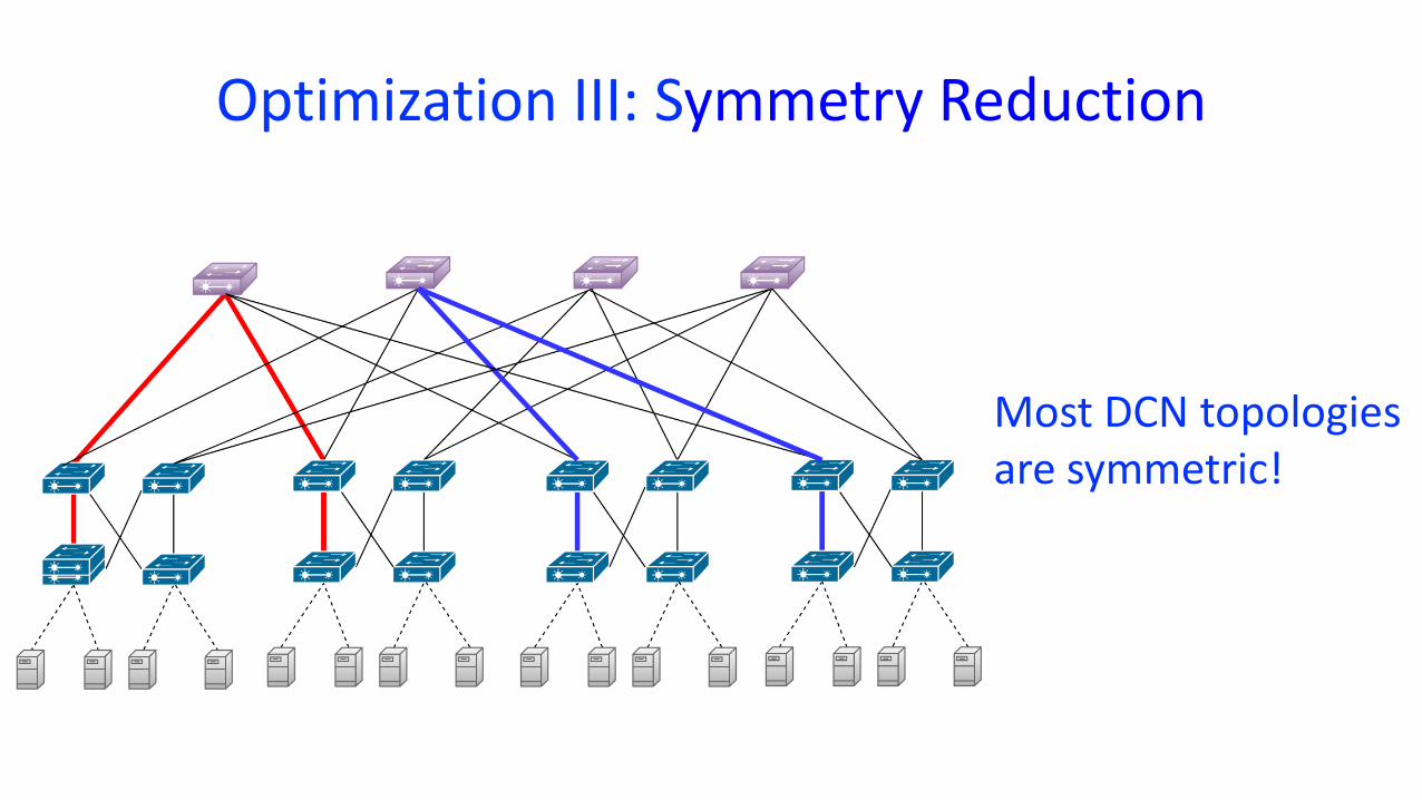
Optimization III: Symmetry Reduction
• Most DCN topologies are symmetric!
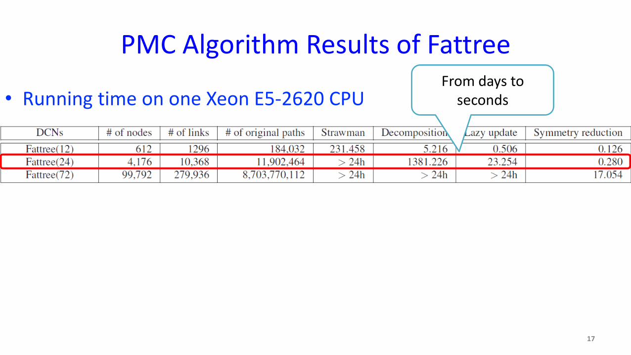
PMC Algorithm Results of Fattree
17
• Running time on one Xeon E5-2620 CPUFrom days to
seconds
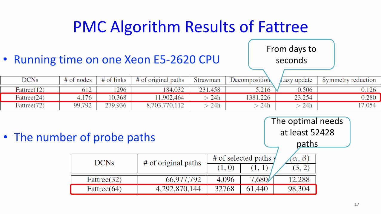
PMC Algorithm Results of Fattree
17
• Running time on one Xeon E5-2620 CPU
• The number of probe pathsThe optimal needs
at least 52428 paths
From days to seconds
Phase II: Network Probing
18
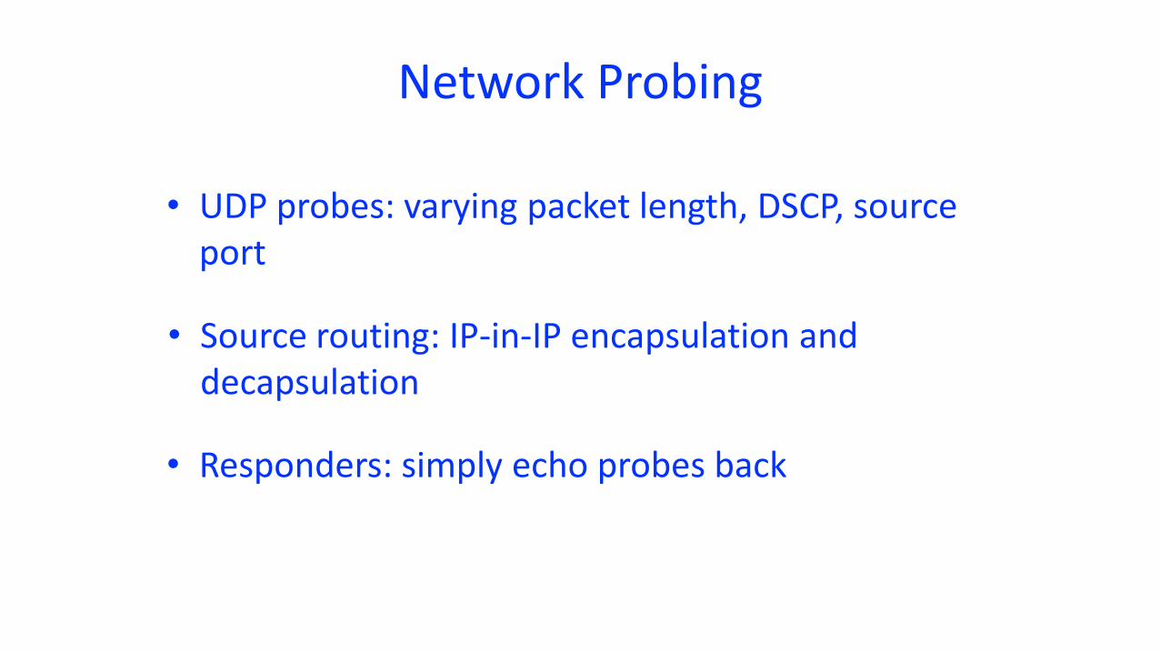
Network Probing
• Source routing: IP-in-IP encapsulation and decapsulation
• UDP probes: varying packet length, DSCP, source port
• Responders: simply echo probes back

Phase III: Loss Localization
20
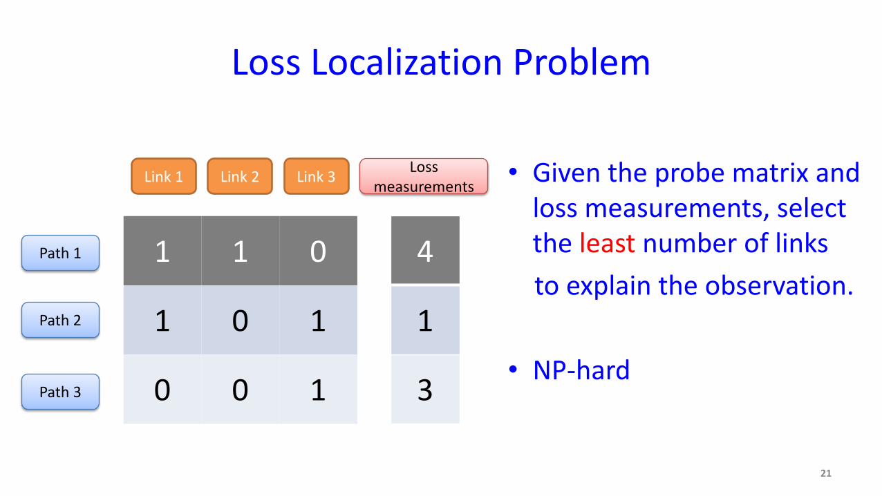
Loss Localization Problem
1 1 0
1 0 1
0 0 1
Path 1
Path 2
Path 3
Link 1 Link 2 Link 3 • Given the probe matrix and loss measurements, select the least number of links to explain the observation.
• NP-hard
Loss measurements
4
1
3
21
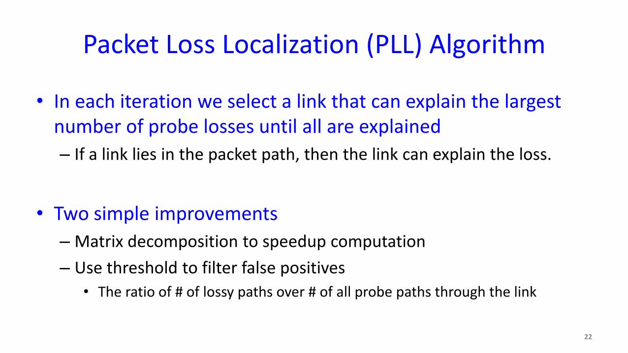
Packet Loss Localization (PLL) Algorithm
• In each iteration we select a link that can explain the largest number of probe losses until all are explained– If a link lies in the packet path, then the link can explain the loss.
• Two simple improvements– Matrix decomposition to speedup computation– Use threshold to filter false positives• The ratio of # of lossy paths over # of all probe paths through the link
22
Experiment
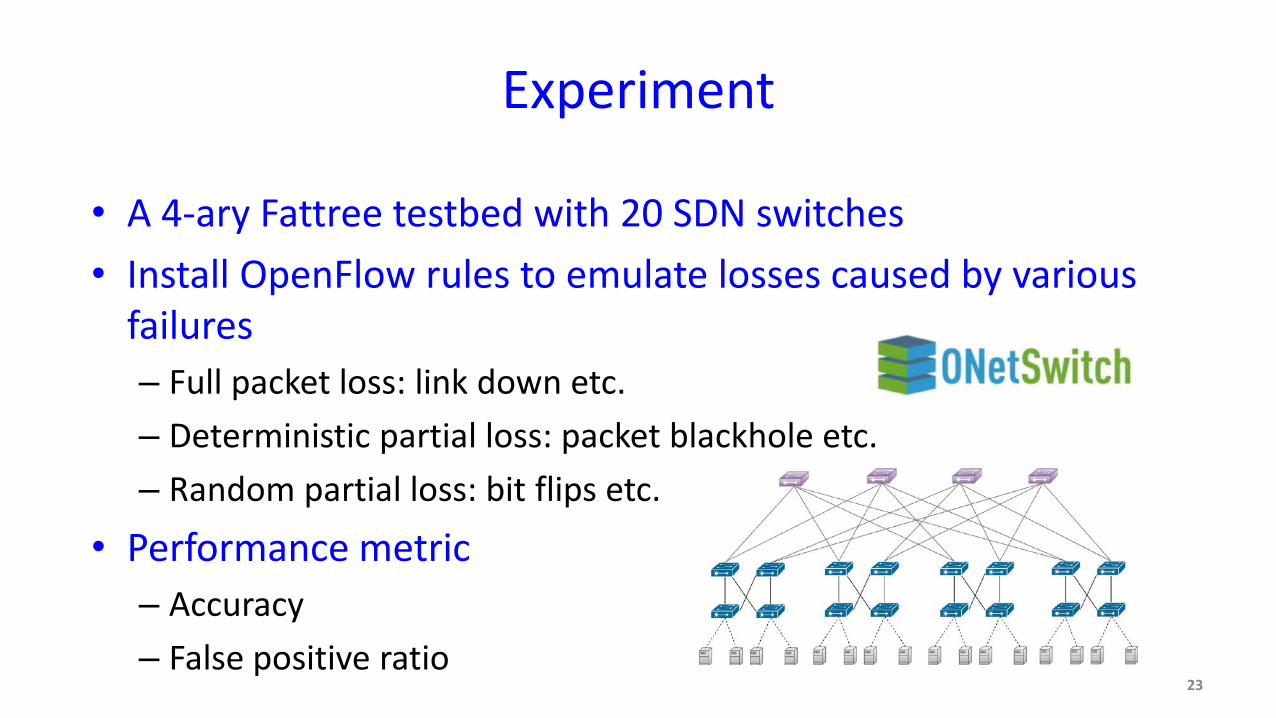
• A 4-ary Fattree testbed with 20 SDN switches• Install OpenFlow rules to emulate losses caused by various
failures– Full packet loss: link down etc.– Deterministic partial loss: packet blackhole etc.– Random partial loss: bit flips etc.
• Performance metric– Accuracy– False positive ratio
23
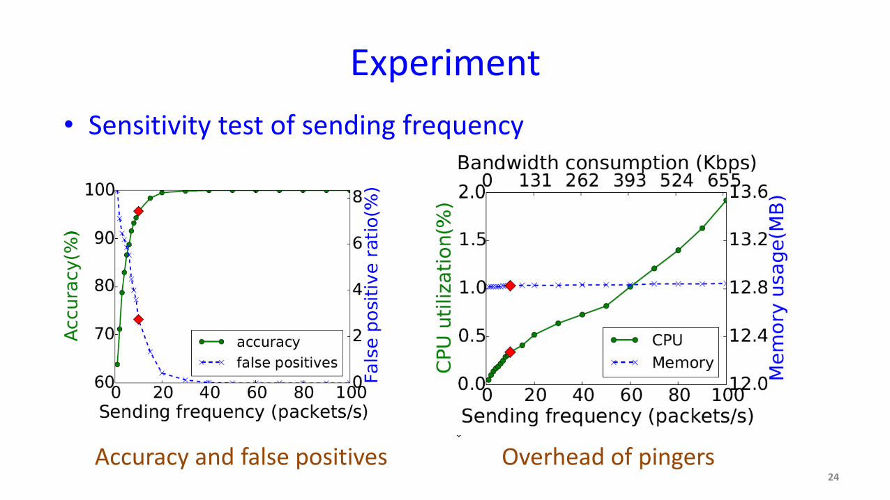
Experiment• Sensitivity test of sending frequency
Overhead of pingersAccuracy and false positives24
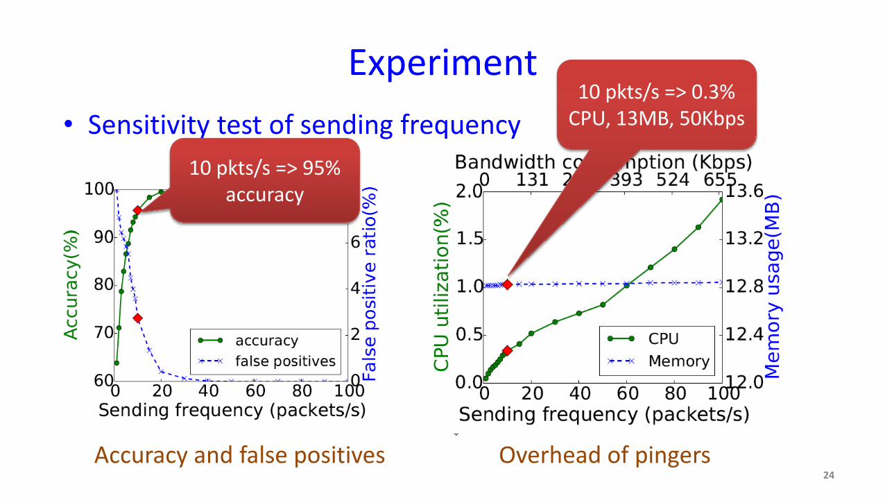
Experiment• Sensitivity test of sending frequency
Overhead of pingersAccuracy and false positives
10 pkts/s => 95% accuracy
10 pkts/s => 0.3% CPU, 13MB, 50Kbps
24
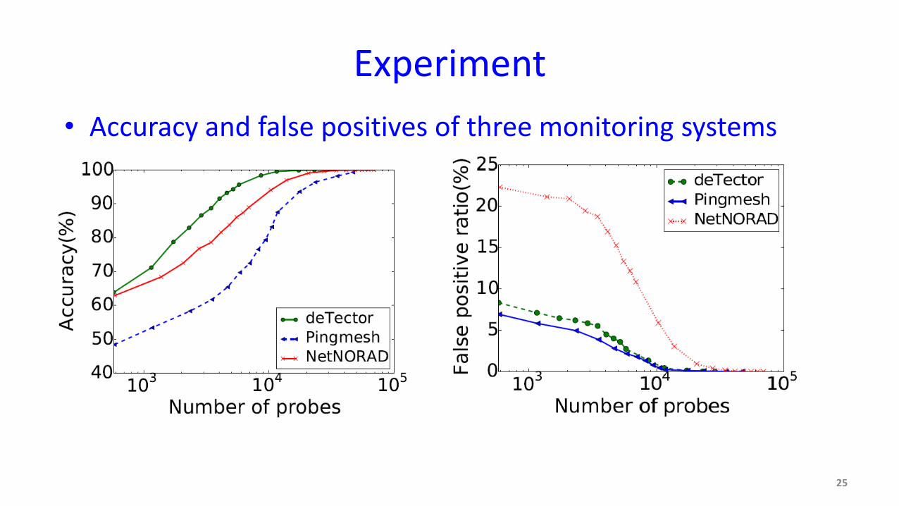
Experiment• Accuracy and false positives of three monitoring systems
25
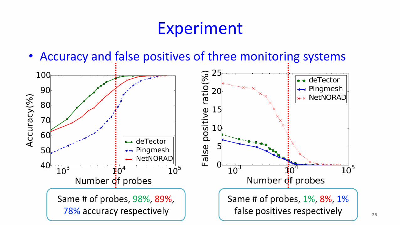
Experiment• Accuracy and false positives of three monitoring systems
Same # of probes, 98%, 89%, 78% accuracy respectively
Same # of probes, 1%, 8%, 1% false positives respectively 25
Simulation• Accuracy in a 18-radix Fattree, with probe matrices of
different levels of α-coverage and β-identifiability
26
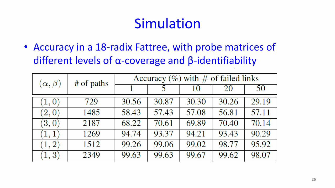
Simulation• Accuracy in a 18-radix Fattree, with probe matrices of
different levels of α-coverage and β-identifiability
26
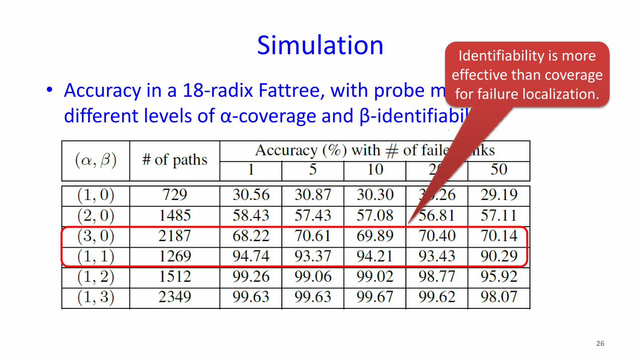
Identifiability is more effective than coverage for failure localization.
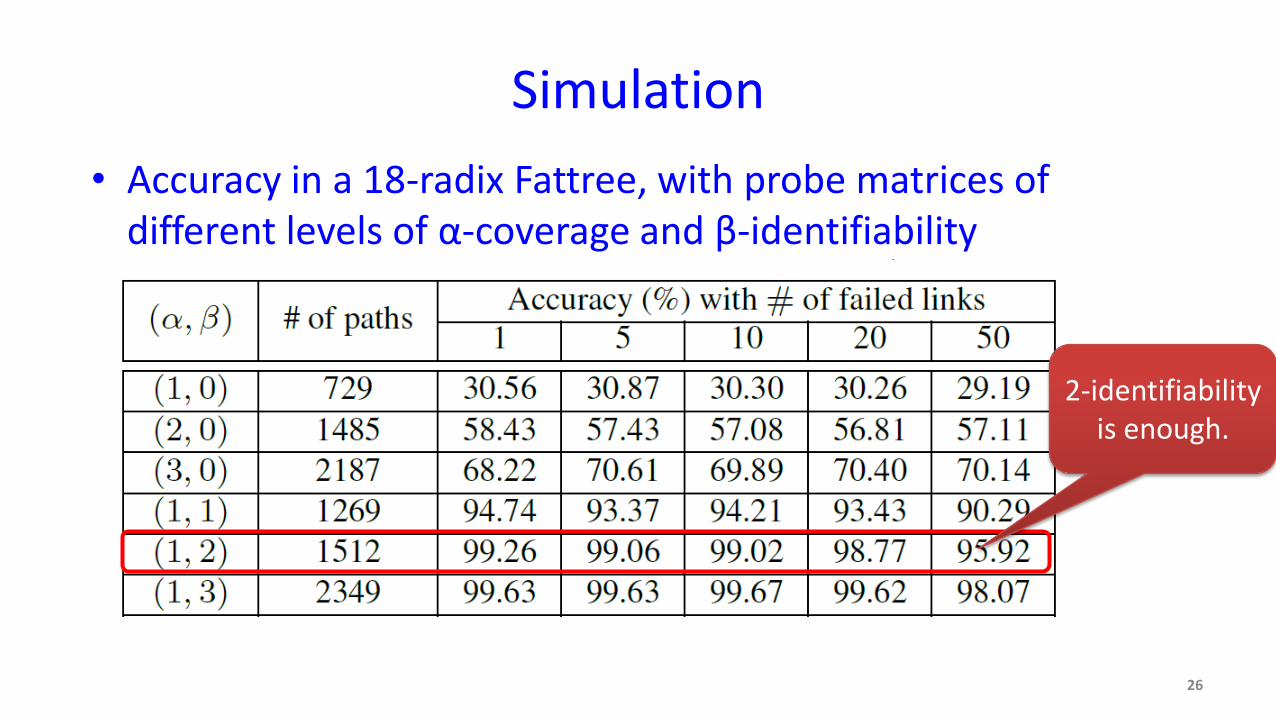
Simulation• Accuracy in a 18-radix Fattree, with probe matrices of
different levels of α-coverage and β-identifiability
26
2-identifiability is enough.
Summary
• The core of deTector is a carefully designed probe matrix, enabling fast and accurate loss detection and localization.
• deTector is practically deployable.• Discussions– Packet entropy: limited destination IP addresses– Loss diagnosis: do not know why packets are dropped– Beyond deTector: apply probe matrix to optimize in-band
techniques
27

Thanks
28