1

Determinants of Child Malnutrition in Tanzania: a Quantile Regression

Approach

Sakiko Shiratori, JICA Research Institute, Shiratori.Sakiko@gmail.com

Selected Paper prepared for presentation at the Agricultural & Applied Economics

Association’s 2014 AAEA Annual Meeting, Minneapolis, MN, July 27-29, 2014.

Copyright 2014 by Sakiko Shiratori. All rights reserved. Readers may make verbatim copies of

this document for non-commercial purposes by any means, provided that this copyright notice

appears on all such copies.

2

Abstract

Reducing child malnutrition is one of the most important development goals. This

study adopts a quantile regression approach to estimate the socioeconomic determinants of

a child’s nutritional status and to explore for whom policy intervention matter the most.

Using the data of children under five in Tanzania, the effects of several variables on child’s

height-for-age z-score (HAZ) and hemoglobin level are examined.

HAZ is influenced by age, sex, preceding birth interval, mother’s height and body-

mass-index (BMI), and wealth, among others. The results from quantile regressions suggest

that the intervention to improve mother’s education, especially higher than primary school,

is effective to reduce the child’s malnutrition at the lower end of distribution. The

interventions to upgrade drinking water or toilet facilities may not be sufficient in raising

malnourished child’s nutritional status.

Hemoglobin level is influenced by age, sex, mother’s hemoglobin level, parental

education, and household size, among others. Conditional distributions make little

difference with regard to hemoglobin level. Since common interventions of deworming or

sleeping under the net are not significant, other interventions such as nutritional ones might

be more effective for reducing anemia.

3

Large effects of mother’s nutritional status on child’s nutritional status imply that

malnutrition is handed down from one generation to another, which could keep children

trapped in the cycle of poverty. It would be effective to carefully integrate applicable

interventions according to the objective and target population in order for wellbeing of

individuals and for the development of the country.

Keywords: Anemia, Child Nutrition, Intervention, Malnutrition, Quantile Regression,

Stunting, Tanzania

4

Introduction

Forty five percent of deaths in children under five (3.1 million children each year)

are linked to malnutrition (WHO 2013). Malnutrition, especially stunting, in early

childhood raises vulnerability to illness and has almost irreversible effects on physical and

cognitive development. It also harms labor productivity and results in less lifetime earnings.

These negative impacts on growth and equality caused by child malnutrition are likely to

keep children trapped in the cycle of poverty. Hence, reducing child malnutrition is one of

the most important goals in developing countries.

In Tanzania, many health indicators such as vaccination have improved; however,

many health challenges still remain (Tanzania NBS and ICF International 2012). Tanzania

is among ten countries worst affected by chronic malnutrition, with 42% of children aged

less than five years are stunted (UNICEF 2013). Though this percentage is slowly declining

from 50% (1991) to 42% (2010), the progress is not sufficient to meet the target in the

Millennium Development Goals. Moreover, anemia remains high with 72% of children

under five years in 2005, which is worse than the world average of 47% in 2004 (World

Bank).

The objective of this study is to estimate the socioeconomic determinants of a

5

child’s nutritional status and to explore for whom policy intervention matter the most. To

tackle the problem of child malnutrition in developing countries, policymakers should

know what intervention is effective to whom in order to adequately target the population at

high risk of undernutrition.

Most of the previous studies focused on finding the determinants at the mean and

only a few paid attentions to the difference at different points of the conditional nutritional

distribution. A quantile regression technique allows us to analyze the relationship between

the dependent and independent variables over the entire distribution of the dependent

variable, not just at the conditional mean.

Using data from Tanzania, this paper explores the effects of individual variables

such as sex, household variables such as parental schooling, and community variables such

as urban/rural on child’s height-for-age and hemoglobin level at different points of their

conditional distributions.

Literature Review

Good nutrition is a prerequisite for the national development of countries and for

the wellbeing of individuals (NBS and ICF Macro 2011). Many studies reported wide range

6

of adverse economic and social consequences of child malnutrition. For example, stunting

is associated with suboptimal brain development, which is likely to have long-lasting

harmful consequences for cognitive ability, school performance and future earnings. This in

turn affects the development potential of nations (UNICEF 2013). Moreover, as Alderman

et al. (2006) suggested, improving the nutritional status of the current generation not only

improves the welfare of the current generation, but also that of future generations as

children born from taller parents are less likely to be malnourished themselves.

Nutritional status of children under age five is an important outcome measure of

children’s health. Especially, 1,000-day period covering pregnancy and the first two years

of the child’s life is considered critical and more and more nutrition intervention programs

aim to reach children during this period (UNICEF 2013).

Proven interventions to reduce in undernutrition include improving women’s

nutrition, especially before, during and after pregnancy; early and exclusive breastfeeding;

timely, safe, appropriate and high-quality complementary food; and appropriate

micronutrient interventions (UNICEF 2013). A combination of income growth and

nutrition interventions is also suggested to adequately tackle this issue (Haddad et al. 2003;

Alderman et al. 2006). Besides, one of the most robust findings is the positive association

7

between mothers’ education and their children’s nutrition (Morales et al. 2004; Francesco

2010). Sahn and Alderman (1997) used data from Mozanbique concluding that mother’s

education and expenditure were substitute factors on child’s HAZ as their effects differ

depending on child’s age.

Aturupane et al. (2011) showed that child weight in Sri Lanka is influenced by birth

order, log expenditure per capita, higher levels of schooling of mother, access to piped

water, and electricity. Their quantile regression showed that expenditure had little effect on

child’s nutritional status at the lower end, though it plays a significant role on average. The

gender discrimination was seen at the lower end, and parental education mattered more at

the upper end.

Data

The 2010 round of the Tanzania Demographic and Health Survey (DHS) is used as

a dataset. The 2010 Tanzania DHS is the eighth in a series of national sample surveys

conducted in Tanzania to measure levels, patterns, and trends in demographic and health

indicators. It also collects several biomarkers such as height and weight (anthropometry),

and hemoglobin level to assess the nutritional status of women and children.

8

The survey collects a two-stage stratified sample of 9,623 households and 10,139

women age 15-49. This study uses the data of 8,023 children under five years old.１

The

average of child’s age is 28 months and male-female ratio is almost 1:1. Average number of

household members and that of children in the household are 7.2 and 2.0, respectively.

About 81% of children are living in rural area.

Nutritional indicators

The nutritional status of a child is usually assessed with three indicators; height-for-

age for chronic nutritional status (“stunting”), weight-for-height for short-term changes in

nutritional status (“wasting”), and weight-for-age which is a composite measure of height-

for-age and weight-for-age (“underweight”).２

A child is considered as moderately stunted

when height-for-age z-score (HAZ) is more than two standard deviations below the

reference, and as severely stunted in case it is below minus three standard deviations.３

Among these three, weight-for-height is one of the nutritional indicators in the

Millennium Development Goals (MDGs).４

However, the WHO recommends stunting as a

reliable measure of overall social deprivation (WHO 1986). In tackling child undernutrition,

there has been a shift from efforts to reduce underweight prevalence to prevention of

9

stunting (UNICEF 2013). In addition, the World Health Assembly adopted a target of

reducing the number of stunted children under the age of five by 40% by 2025 (WHA

2012). Thus, HAZ is examined as a representative nutritional indicator in this study.

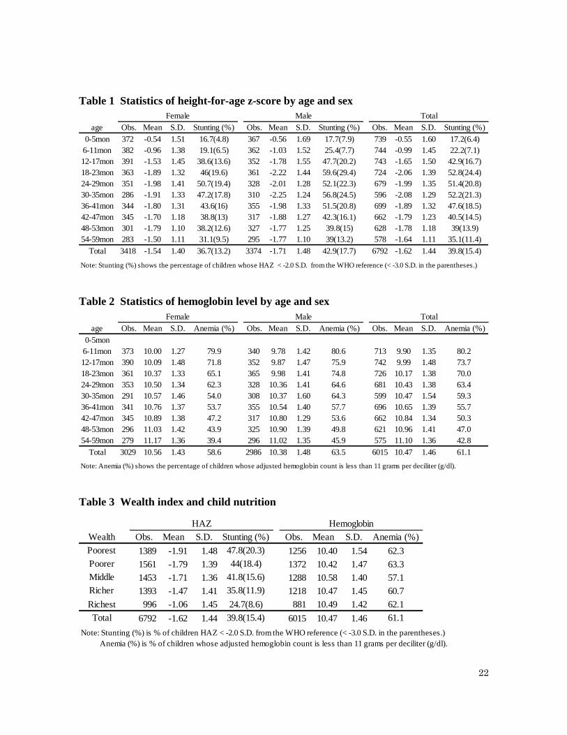
Table 1 reports child’s HAZ by age and sex. About 40% of the children under five

are categorized as “stunting”, and severely stunted children are 15% of the sample.

Analysis of the indicator by age group shows that stunting reaches its peak (53%) in

children age 18-23 months. The risk of stunting seems to increase when the transition from

breastfeeding to solid foods occurs.５

A higher proportion (43%) of male children is stunted

compared with the proportion of female children (37%). Girls perform better than boys in

general, a result in line with the related literature (Svedberg, 1990; Alderman 2006).

In addition to HAZ, the level of hemoglobin is examined in this study. Anemia,

characterized by a low level of hemoglobin in the blood, is a major health problem in

Tanzania, especially among young children and pregnant women. The most common cause

of anemia is nutritional anemia. Anemia also results from sickle cell disease, malaria, or

parasitic infections. A number of interventions have been put in place to address anemia in

children. These include promotion of use of insecticide-treated mosquito nets and

deworming (NBS and ICF International, 2012). In this sample, 50% of children age 6-59

10

months received deworming medication in the six months before the survey and 64% of the

children belong to the household which reported that all children under five slept under the

bed net at the night before the survey.

Table 2 shows the statistics of child’s hemoglobin level and the percentage of

anemic children by age and sex. Since the higher altitude causes a generalized upward shift

of the hemoglobin distributions, an adjustment of the hemoglobin count is made for altitude.

Children less than six months of age are not included because they have higher levels of

hemoglobin at birth and thus may distort the indication of prevalence of anemia (Rutstein

2006). More than 60% of children are suffering from anemia, and notably three-quarters of

children before 18 months old are anemic. The hemoglobin level increases as age increases.

Male children are more likely to be anemic.

The DHS data provide wealth index to measure household’s economic status

instead of their expenditure or income. Wealth represents a more permanent status than

does either income or consumption (Rustein 2004). The wealth index is constructed using

household asset data and principal components analysis.６

Table 3 summarizes the child

nutrition by five wealth levels (quintiles) based on the wealth index. Wealth index is

associated with the percentage of stunting children. Children living in the poorest

11

households are twice as likely (48%) to be stunted as children living in the richest

households (25%). Regarding hemoglobin level, however, the prevalence of anemia varies

little by wealth status.

The mother’s nutrition and health status are also important determinants of child

nutrition and health status. An undernourished mother is more likely to give birth to a

stunted child, perpetuating a vicious cycle of undernutrition and poverty (UNICEF 2013).

The nutritional status of mother is assessed by use of two anthropometric indices—height

and body mass index (BMI), and hemoglobin level. BMI is defined as weight in kilograms

divided by height squared in meters (kg/m2). Short stature and low pre-pregnancy BMI are

risk factors for poor birth outcomes and obstetric complications.

In this sample, the average of mother’s height is 156.3cm with 2.5% of women are

found to fall below 145cm, considered as being at risk. The mean of mother’s BMI is 22.5.

About 10% of mother is underweight (BMI below 18.5), while 20% of mother are

overweight (BMI of 25.0 or above). Forty-three percent of mothers suffer from some

degree of anemia.７

Although anemia is less prevalent among women than among children,

this level of anemia in the population is considered critical from public health perspective

(Tanzania NBS and ICF International 2012).

12

Methods

A quantile regression technique was introduced by Koenker and Bassett (1978). The

central special case is the median regression estimator which minimizes a sum of absolute

residuals. Other conditional quantile functions are estimated by minimizing an

asymmetrically weighted sum of absolute residuals (Koenker and Hallok 2011). This

approach has the advantage of allowing the effect of covariates to differ over the

conditional distribution of the outcome. So, for example, one can allow for the possibility

that income has a different marginal effect on the nutritional status of malnourished and

well-nourished children (O’Donnell et al. 2008). The model in this study is estimated with

bootstrap standard errors (100 repetitions) as the errors may be heteroscedastic.

The explanatory variables used in this study are as follows. As the age of the child

has a strong non-linear impact on his/her nutritional status (Alderman 2006), age-squared

term as well as age are included to capture the effect. Child’s sex is also included as a male

dummy. Birth order number gives the order in which the children were born. Preceding

(succeeding) birth interval is calculated as the difference in months between the current

birth and the previous (following) birth, counting twins as one birth.

13

Mothers’ health and nutritional status namely height, BMI, and hemoglobin are

included. Mother’s and father’s education are categorized into three dummy variables by

educational achievement recodes. The reference group is those who has no education or not

completed primary education. Household size is the total number of household members.

Number of children under five in the household is also included. The deworming dummy

variable means whether the drug for intestinal parasites was given in last six months or not.

Whether all children under five in the household slept under bednet last night is also

included.

Barrier for medical care is a dichotomous variable showing whether the mother has

a problem in getting medical care for herself. This variable was constructed from a series of

questions whether each of the following factors would be a problem in obtaining health

services: getting permission to go, getting money for treatment, and the distance to the

health facility. If they answer “big problem” to either of three questions, they are classified

as having a problem. Though these questions ask the problem in getting medical care not

for children but for her, it shall have an implication for access to medical care.

Safe drinking water and basic sanitation are other Millennium Development Goals

that Tanzania shares with other countries.８

The criteria for improvement follow the

14

WHO/UNICEF Joint Monitoring Program of Water Supply and Sanitation. Safe water

shows whether the major source of drinking water for members of the household is safe or

not.９

A household is classified as having an improved toilet if the toilet is used only by

members of one household (i.e., it is not shared) and if the facility used by the household

separates the waste from human contact (WHO/UNICEF, 2004).１０

Wealth index has five levels, and the base is the middle. Whether the household has

a radio/tv/refridgerator/vehicle is included. Vehicle variable means whether the household

has any of the following; a bicycle, a motorcycle/scooter, or a car/truck. The residence of

the household (1=rural, 0=urban) is also used as an explanatory variable.

Results

The OLS and quantile regression estimates of child HAZ are summarized in Table 4.

The OLS and quantile regression estimates indicate strong age effects, with z-score

declining with age. The negative linear term and positive quadratic term implies that the

curve is at its minimum at

months (in OLS), where b is the coefficient of age

and a is the coefficient of quadratic age. The longer the length of the preceding birth

interval, the less likely it is that the child is stunted. Though the tendency is also seen in the

15

length of succeeding birth interval, its significance is small.

Mother’s height and BMI also have strong significant effects on HAZ, which

indicates that the nutritional status crosses from one generation to another. Mother’s

education has significant effects on HAZ, but only at higher levels of schooling, which is

more than primary completed. This favorable association between maternal schooling and

child nutrition can be attributed to such factors as superior knowledge and practices

concerning childcare, feeding practices, environmental health and household hygiene

(Aturupane et al, 2011). Compared with mother’s education, father’s education does not

seem to be significant.

The HAZ increases as the number of household member increases; however, the

number of children under five in the household has a negative relationship on HAZ. If there

are many children in the household, they are at significantly higher risk of being

undernourished. Feeling a barrier for medical care has a negative effect. Safe drinking

water is not significant. Wealth index has a significant effect for most of the wealth level.

The assets the household has such as radio, tv, refrigerator are not significant but the effect

of having a vehicle is positive. Children in rural area are more likely to be worse off,

though the effect is not significant.

16

The result of OLS and that of quantile regression remarkably differ for some

variables. Boys are more likely to have lower HAZ than girls are. At the lower end of the

distribution, the coefficients on the sex variable are large, significant and negative.

However, they are insignificant at the 0.9 quantile. Aturupane et al. (2011) reported that

intra-household gender discrimination in the allocation of food at lower end was implied,

though their result was in favor of girls.１１

Higher birth-order children have lower HAZ

than lower birth-order children. This is particularly prominent for lower quantile. This is

consistent with evidence from other countries that ‘first born’ children often have a

nutritional advantage compared to children born later (Lewis and Britton 1998).

Improved toilet shows positive effects on HAZ, which coefficient is relatively large.

However, the results from quantile regressions imply that the effect on HAZ may be small

for lower quantile. It could be suggested that the intervention to improve toilets does not

have a high priorities for malnourished children. Compared to the reference group those

mothers have not completed primary school, having a mother who has educational

attainment higher than primary school has larger coefficients and significance at the lower

end of the distribution. The implication here is that the intervention to improve mother’s

education is more effective for the lower end, which differs from the result of Aturupane et

17

al. (2011).

Similarly, the OLS and quantile regression estimates of child hemoglobin level are

summarized in Table 5. It is noteworthy that there is little difference between the result of

OLS and quantile regressions on child’s hemoglobin level. In terms of the intervention to

reduce anemia, their hemoglobin level distribution plays only a minor role.

Age effect is significant, with hemoglobin increasing with age nearly in a linear

fashion. Boys are more likely to have lower hemoglobin level than girls are. Higher birth-

order children seem to have higher hemoglobin level, but the significance is small. The

length of the preceding (and succeeding) birth interval is not strongly significant on

hemoglobin as it is seen on HAZ.

Mother’s hemoglobin level has strong effect on child’s hemoglobin level, which

also back up the concern that the nutritional status crosses from one generation to another.

Regarding parental education, both mother’s and father’s educational attainment have

significant effects, but it does not necessarily mean that the higher the education will be the

better. Compared to child who has parents schooling less than primary, having parents who

completed primary education has positive effect on hemoglobin.

The number of household member has negative effect on child’s hemoglobin level.

18

The number of children under five in the household does not have a significant effect.

Feeling a barrier for medical care seems to have a positive effect, though the reason is not

clear. Safe drinking water is not significant. The effect of wealth is not straightforward

because the relationship between wealth and hemoglobin level does not have a clear pattern

(Table 3). The asset the household has does not have a significant effect. The effect of

urban-rural residence is not significant, either. Though many interventions include

promotion of use of nets and deworming to prevent anemia, net and deworming do not

seem to have significant effects on hemoglobin level in this study.

Conclusions

Reducing child malnutrition is one of the most important goals in developing

countries. This study adopted a quantile regression approach in order to estimate the

socioeconomic determinants of a child’s nutritional status and to explore for whom policy

intervention matter the most. Using data of children under five in Tanzania, this paper

explores the effects of individual variables, household variables, and community variables

on child’s height-for-age and hemoglobin at different points of their conditional

distributions.

19

There are several prominent findings regarding child’s height-for-age. First, the

effect of mother’s educational attainment, especially higher than primary school, is more

significant at the lower end of the distribution. This implies the following things; the

intervention to improve mother’s education is more effective for the lower end, the

schooling should be higher than primary school in order to improve the child’s height-for-

age, and mother’s education seems to be more effective than father’s education.

Second, while the coefficient of sex variable is large, significant and negative at the

lower end of the distribution, it is insignificant at the 0.9 quantile. It implies that the intra-

household gender discrimination is small at the top of the conditional distribution of height-

for-age. We need to take into account that there may be gender discrimination in the

household such as food allocation when the intervention is carried out to the lower ends.

Third, improved toilet has larger effects on child height-for-age at the higher

quantile than at the lower quantile. Safe drinking water has a similar trend, though the

significance is not strong. The implication for policy is that these interventions of water or

sanitation may be insufficient in raising the nutritional status of children in the lower tail.

In regard to hemoglobin level, there is not so much difference at different points of

their conditional distributions. Intrinsically, the relationships between child’s hemoglobin

20

level and mother’s education or wealth are not strong. Distribution is less important for

designing the intervention to reduce children’s anemia.

It is somewhat surprising that the interventions which are believed to have effects

on hemoglobin level, such as the usage of insecticide-treated mosquito nets or deworming

medicine, turn out not to be significant. Anemia is caused by many factors such as malaria,

nutrition, or worm. Other interventions such as nutritional ones than deworming or using

nets might be more effective.

The results also showed strong effect of mother’s nutritional status on child’s

nutritional status. If the mother’s height or BMI is lower, their child is more likely to be

stunted. Likewise, if the mother is anemic, their child is more likely to be anemic.

Malnutrition could be handed down from one generation to other.

There are lots of interventions with proven evidence including improving women’s

nutrition during perinatal period, early and exclusive breastfeeding, food and nutrition. In

addition, there are indirect interventions such as ensuring access to education or updating

infrastructure. It would be effective to carefully integrate these interventions according to

the objective and target population in order for wellbeing of individuals and for the

development of the country.

21

１

Throughout this study, the data are not weighted as relationships are estimated at the individual level. There

are divergent opinions on whether or not sampling weights should be used when estimating relationships so

the use of sampling weights for regression analysis is an analytic decision best made by the researcher (the

DHS program, FAQs).

２ At the other end of the spectrum, weight-for-height can also be used to construct indicators of obesity.

３ The new Child Growth Standards released by the WHO in 2006 is used as a reference.

４ The Millennium Development Goals (MDGs) include eight goals, 21 targets, and 60 indicators. Indicator

“1.8 Prevalence of underweight children under-five years of age” belongs to Target “1.C: Halve, between

1990 and 2015, the proportion of people who suffer from hunger” of “Goal 1: Eradicate extreme poverty and

hunger.” (UN Statistic Division, Official list of MDG indicators)

５ NBS and ICF Macro (2011) recommends several feeding practices such as early initiation of breastfeeding,

exclusive breastfeeding during the first six months of life, continued breastfeeding up to age 2 and beyond,

timely introduction of complementary feeding at age 6 months, frequent feeding of solid/semisolid foods, and

feeding of diverse food groups to children between ages 6 months and 23 months.

６ Asset information is collected in the 2010 TDHS Household Questionnaire and covers information on

household ownership of a number of consumer items, ranging from a television to a bicycle or car, as well as

information on dwelling characteristics, such as source of drinking water, type of sanitation facilities, and

type of materials used in dwelling construction. (NBS and ICF Macro 2011)

７ Women are considered as anemic if they are not pregnant women whose hemoglobin count is less than 12

grams per deciliter (g/dl) or they are pregnant women whose count is less than 11 g/dl.

８ Target 7.C: Halve, by 2015, the proportion of people without sustainable access to safe drinking water and

basic sanitation.

９ In this study, piped into dwelling, piped to yard/plot, public tap/standpipe, neighbor’s tap, protected well in

dwelling, protected well in yard/plot, protected public well, neighbor’s borehole, spring, rainwater are

categorized as an improved source.

１０ Here the toilet is considered to be improved if the toilet type is any of the followings: flush - to piped

sewer system, flush - to septic tank, flush - to pit latrine, pit latrine - ventilated improved pit, or pit latrine -

with slab.

１１ Svedberg (1990) noted that nutritional and health status of females vis-a

、-vis males is favorable in Sub-

Saharan Africa.

22

Table 1 Statistics of height-for-age z-score by age and sex

Table 2 Statistics of hemoglobin level by age and sex

Table 3 Wealth index and child nutrition

age Obs. Mean S.D. Stunting (%) Obs. Mean S.D. Stunting (%) Obs. Mean S.D. Stunting (%)

0-5mon 372 -0.54 1.51 16.7(4.8) 367 -0.56 1.69 17.7(7.9) 739 -0.55 1.60 17.2(6.4)

6-11mon 382 -0.96 1.38 19.1(6.5) 362 -1.03 1.52 25.4(7.7) 744 -0.99 1.45 22.2(7.1)

12-17mon 391 -1.53 1.45 38.6(13.6) 352 -1.78 1.55 47.7(20.2) 743 -1.65 1.50 42.9(16.7)

18-23mon 363 -1.89 1.32 46(19.6) 361 -2.22 1.44 59.6(29.4) 724 -2.06 1.39 52.8(24.4)

24-29mon 351 -1.98 1.41 50.7(19.4) 328 -2.01 1.28 52.1(22.3) 679 -1.99 1.35 51.4(20.8)

30-35mon 286 -1.91 1.33 47.2(17.8) 310 -2.25 1.24 56.8(24.5) 596 -2.08 1.29 52.2(21.3)

36-41mon 344 -1.80 1.31 43.6(16) 355 -1.98 1.33 51.5(20.8) 699 -1.89 1.32 47.6(18.5)

42-47mon 345 -1.70 1.18 38.8(13) 317 -1.88 1.27 42.3(16.1) 662 -1.79 1.23 40.5(14.5)

48-53mon 301 -1.79 1.10 38.2(12.6) 327 -1.77 1.25 39.8(15) 628 -1.78 1.18 39(13.9)

54-59mon 283 -1.50 1.11 31.1(9.5) 295 -1.77 1.10 39(13.2) 578 -1.64 1.11 35.1(11.4)

Total 3418 -1.54 1.40 36.7(13.2) 3374 -1.71 1.48 42.9(17.7) 6792 -1.62 1.44 39.8(15.4)

Female Male Total

Note: Stunting (%) shows the percentage of children whose HAZ < -2.0 S.D. from the WHO reference (< -3.0 S.D. in the parentheses.)

age Obs. Mean S.D. Anemia (%) Obs. Mean S.D. Anemia (%) Obs. Mean S.D. Anemia (%)

0-5mon

6-11mon 373 10.00 1.27 79.9 340 9.78 1.42 80.6 713 9.90 1.35 80.2

12-17mon 390 10.09 1.48 71.8 352 9.87 1.47 75.9 742 9.99 1.48 73.7

18-23mon 361 10.37 1.33 65.1 365 9.98 1.41 74.8 726 10.17 1.38 70.0

24-29mon 353 10.50 1.34 62.3 328 10.36 1.41 64.6 681 10.43 1.38 63.4

30-35mon 291 10.57 1.46 54.0 308 10.37 1.60 64.3 599 10.47 1.54 59.3

36-41mon 341 10.76 1.37 53.7 355 10.54 1.40 57.7 696 10.65 1.39 55.7

42-47mon 345 10.89 1.38 47.2 317 10.80 1.29 53.6 662 10.84 1.34 50.3

48-53mon 296 11.03 1.42 43.9 325 10.90 1.39 49.8 621 10.96 1.41 47.0

54-59mon 279 11.17 1.36 39.4 296 11.02 1.35 45.9 575 11.10 1.36 42.8

Total 3029 10.56 1.43 58.6 2986 10.38 1.48 63.5 6015 10.47 1.46 61.1

Female Male Total

Note: Anemia (%) shows the percentage of children whose adjusted hemoglobin count is less than 11 grams per deciliter (g/dl).

Wealth Obs. Mean S.D. Stunting (%) Obs. Mean S.D. Anemia (%)

Poorest 1389 -1.91 1.48 47.8(20.3) 1256 10.40 1.54 62.3

Poorer 1561 -1.79 1.39 44(18.4) 1372 10.42 1.47 63.3

Middle 1453 -1.71 1.36 41.8(15.6) 1288 10.58 1.40 57.1

Richer 1393 -1.47 1.41 35.8(11.9) 1218 10.47 1.45 60.7

Richest 996 -1.06 1.45 24.7(8.6) 881 10.49 1.42 62.1

Total 6792 -1.62 1.44 39.8(15.4) 6015 10.47 1.46 61.1

HAZ Hemoglobin

Note: Stunting (%) is % of children HAZ < -2.0 S.D. from the WHO reference (< -3.0 S.D. in the parentheses.)

Anemia (%) is % of children whose adjusted hemoglobin count is less than 11 grams per deciliter (g/dl).

23

Table 4 OLS and quantile regressions for child height-for-age z-score

OLS Quantile Regression

0.1 0.25 0.5 0.75 0.9

Coef. Std. Err. Coef. Std. Err. Coef. Std. Err. Coef. Std. Err. Coef. Std. Err. Coef. Std. Err.

Age (months) -0.09 0.00***

-0.07 0.01***

-0.09 0.01***

-0.10 0.00***

-0.11 0.00***

-0.12 0.01***

Quadratic Age (months) 0.00 0.00***

0.00 0.00***

0.00 0.00***

0.00 0.00***

0.00 0.00***

0.00 0.00***

Male -0.17 0.03***

-0.25 0.05***

-0.19 0.04***

-0.17 0.04***

-0.14 0.04***

-0.07 0.06

Birth Order -0.01 0.01*

-0.02 0.01**

-0.02 0.01***

-0.02 0.01***

-0.01 0.01 0.01 0.01

Preceding Birth Interval

(years)

0.02 0.01***

0.03 0.02*

0.03 0.01***

0.02 0.01**

0.02 0.01**

0.01 0.01

Succeeding Birth

Interval

(years)

0.03 0.02*

0.03 0.03 0.02 0.02 0.03 0.02 0.04 0.02**

0.01 0.03

Mother's Height (cm) 0.06 0.00***

0.05 0.00***

0.06 0.00***

0.06 0.00***

0.06 0.00***

0.07 0.00***

Mother's BMI 0.03 0.00***

0.02 0.01***

0.03 0.01***

0.03 0.00***

0.03 0.01***

0.03 0.01***

Mother's Hemoglobin

Level (g/dl, adjusted)

0.01 0.01 0.00 0.02 0.01 0.01 0.01 0.01 0.00 0.01 0.02 0.02

Mother's Education

Complete Primary 0.02 0.04 0.04 0.06 0.02 0.04 -0.03 0.04 -0.01 0.04 -0.02 0.07

Higher than Primary 0.19 0.06***

0.28 0.10***

0.24 0.08***

0.20 0.07***

0.13 0.07*

0.12 0.10

Father's Education

Complete Primary -0.03 0.04 -0.01 0.07 -0.01 0.04 -0.01 0.04 -0.04 0.04 -0.06 0.07

Higher than Primary 0.07 0.05 0.11 0.09 0.12 0.06**

0.05 0.07 0.10 0.07 0.05 0.08

Household Size 0.01 0.01**

0.01 0.01 0.02 0.01**

0.01 0.01*

0.02 0.01**

0.01 0.01

Number of Children <5 -0.06 0.02***

-0.09 0.03***

-0.08 0.03***

-0.06 0.03**

-0.07 0.02***

-0.04 0.03

Deworming -0.10 0.04***

-0.08 0.07 -0.03 0.05 -0.04 0.04 -0.09 0.04**

-0.15 0.07**

All Children<5 Slept

under the Net

-0.02 0.03 0.09 0.07 0.05 0.05 0.02 0.04 -0.01 0.04 -0.10 0.06

Barrier for Medical -0.06 0.03*

-0.08 0.06 -0.05 0.04 -0.03 0.04 -0.05 0.04 -0.11 0.06**

Safe Water 0.06 0.03 -0.01 0.07 0.03 0.05 0.06 0.04 0.06 0.04*

0.03 0.06

Improved Toilet 0.13 0.05**

0.03 0.08 0.10 0.06*

0.13 0.07*

0.14 0.07**

0.15 0.11

Wealth Index

Poorest -0.14 0.05***

-0.21 0.10**

-0.18 0.07**

-0.19 0.06***

-0.15 0.06**

-0.16 0.10

Poorer -0.08 0.05 -0.05 0.08 -0.06 0.06 -0.07 0.05 -0.12 0.05**

-0.17 0.09*

Richer 0.12 0.05**

0.14 0.08*

0.03 0.06 0.10 0.06*

0.11 0.06**

0.13 0.10

Richest 0.28 0.08***

0.14 0.14 0.06 0.12 0.35 0.11***

0.36 0.10***

0.45 0.13***

The Houshold has:

Radio -0.03 0.04 0.10 0.06 0.01 0.04 -0.04 0.04 -0.05 0.04 -0.14 0.06**

TV -0.06 0.08 -0.08 0.14 -0.08 0.12 -0.07 0.11 -0.10 0.09 -0.13 0.16

Refrigerator 0.15 0.10 0.30 0.17*

0.21 0.16 0.16 0.14 0.11 0.13 0.17 0.25

Vehicle 0.10 0.03***

0.07 0.07 0.08 0.05*

0.10 0.04***

0.09 0.04**

0.16 0.06**

Rural -0.05 0.05 -0.04 0.12 -0.06 0.07 0.00 0.06 -0.10 0.07 -0.10 0.09

_cons -9.73 0.45***

-10.73 0.78***

-10.86 0.60***

-10.17 0.53***

-8.75 0.55***

-9.57 0.83***

Observations 6699

R-squared 0.21 0.10 0.10 0.12 0.15 0.16

Note: *, ** and *** for 10%, 5%, and 1% significance levels, respectively.

24

Table 5 OLS and quantile regressions for child hemoglobin level

OLS Quantile Regression

0.1 0.25 0.5 0.75 0.9

Coef. Std. Err. Coef. Std. Err. Coef. Std. Err. Coef. Std. Err. Coef. Std. Err. Coef. Std. Err.

Age (months) 0.03 0.01***

0.03 0.01**

0.03 0.01***

0.04 0.01***

0.04 0.01***

0.03 0.01***

Quadratic Age (months) 0.00 0.00 0.00 0.00 0.00 0.00 0.00 0.00 0.00 0.00*

0.00 0.00

Male -0.20 0.04***

-0.23 0.08***

-0.19 0.05***

-0.24 0.04***

-0.17 0.05***

-0.15 0.05***

Birth Order 0.01 0.01*

0.00 0.02 0.02 0.01*

0.02 0.01*

0.02 0.01**

0.02 0.01*

Preceding Birth Interval

(years)

-0.01 0.01 -0.02 0.02 0.00 0.01 -0.01 0.01 -0.01 0.01 -0.02 0.01

Succeeding Birth Interval

(years)

-0.02 0.02 0.00 0.04 -0.02 0.03 -0.04 0.02 -0.03 0.02 -0.06 0.03**

Mother's Height (cm) 0.00 0.00 0.00 0.01 0.00 0.00 0.01 0.00**

0.00 0.00 0.00 0.00

Mother's BMI 0.00 0.00 0.00 0.01 0.01 0.01 0.00 0.01 0.00 0.01 0.00 0.01

Mother's Hemoglobin

Level (g/dl, adjusted)

0.15 0.01***

0.17 0.03***

0.18 0.02***

0.17 0.01***

0.16 0.01***

0.14 0.02***

Mother's Education

Complete Primary 0.15 0.04***

0.15 0.09*

0.11 0.05**

0.18 0.05***

0.15 0.05***

0.14 0.07**

Higher than Primary -0.02 0.07 -0.07 0.14 0.03 0.09 0.01 0.08 -0.17 0.10 -0.10 0.13

Father's Education

Complete Primary 0.13 0.04***

0.16 0.08**

0.25 0.06***

0.17 0.05***

0.11 0.05**

0.06 0.07

Higher than Primary 0.04 0.06 0.09 0.12 0.11 0.09 0.07 0.07 0.07 0.08 -0.03 0.09

Household Size -0.02 0.01***

-0.02 0.02 -0.03 0.01**

-0.02 0.01**

-0.02 0.01**

-0.02 0.01*

Number of Children <5 -0.01 0.02 -0.09 0.06 0.02 0.03 0.03 0.02 0.00 0.02 0.01 0.03

Deworming 0.03 0.04 -0.02 0.09 0.02 0.05 -0.01 0.05 0.03 0.05 0.06 0.06

All Children<5 Slept

under the Net

-0.04 0.04 -0.05 0.09 -0.08 0.05*

-0.07 0.05 -0.08 0.04*

0.00 0.06

Barrier for Medical Care 0.08 0.04**

0.11 0.08 0.06 0.05 0.06 0.04 0.07 0.04*

0.08 0.06

Safe Water 0.03 0.04 0.00 0.09 0.09 0.05*

0.05 0.05 0.01 0.04 0.06 0.06

Improved Toilet 0.07 0.06 0.31 0.12***

0.14 0.07**

0.03 0.07 -0.04 0.07 0.08 0.11

Wealth Index

Poorest -0.15 0.06**

-0.27 0.11**

-0.20 0.08**

-0.16 0.06**

-0.05 0.06 -0.03 0.10

Poorer -0.10 0.05*

-0.18 0.13 -0.11 0.08 -0.12 0.07*

-0.03 0.06 0.00 0.08

Richer -0.07 0.06 -0.05 0.13 -0.10 0.07 -0.06 0.07 0.01 0.06 0.00 0.08

Richest -0.09 0.09 -0.20 0.25 -0.24 0.14*

-0.10 0.10 0.19 0.11*

0.11 0.13

The Houshold has:

Radio -0.02 0.04 0.07 0.09 0.02 0.06 -0.07 0.05 -0.05 0.04 -0.08 0.07

TV 0.06 0.09 -0.05 0.16 0.03 0.16 0.08 0.11 0.03 0.12 0.10 0.12

Refrigerator 0.17 0.11 0.12 0.21 0.13 0.15 0.22 0.13*

0.20 0.11*

0.06 0.16

Vehicle 0.01 0.04 0.08 0.09 0.03 0.06 -0.04 0.04 -0.07 0.04 -0.02 0.06

Rural 0.03 0.06 0.04 0.14 -0.06 0.10 0.05 0.06 0.09 0.06 0.15 0.08*

_cons 7.32 0.51***

5.92 1.27***

6.33 0.66***

6.50 0.55***

8.11 0.63***

9.57 0.79***

Observations 5975

R-squared 0.13 0.07 0.08 0.08 0.09 0.07

Note: *, ** and *** for 10%, 5%, and 1% significance levels, respectively.

25

References

Alderman, H., H. Hoogeveen, and M. Rossi. 2006. "Reducing Child Malnutrition in

Tanzania. Combined Effects of Income Growth and Program Interventions." Economics

and Human Biology, 4 (1): 1-23.

Aturupane, H., A.B.Deolalikar and D.Gunewardena, 2011. “Determinants of Child Weight

and Height in Sri Lanka: A Quantile Regression Approach”, Health Inequality and

Development, edited by M. McGillivray, I. Dutta and D. Lawson, United Nations

University.

Francesco, Burchi, 2010. “Child nutrition in Mozambique in 2003: The role of mother’s

schooling and nutrition knowledge”, Economics and Human Biology 8 (2010) 331–345.

The DHS program, FAQs, http://www.dhsprogram.com/faq.cfm, accessed on 5/23/2014.

Haddad, L., H. Alderman, S. Appleton, L. Song, Y. Yohannes, 2003. “Reducing child

malnutrition: how far does income growth take us?” World Bank Economic Review, 17,

107–131.

Koenker, R. and G. Bassett, Jr., 1978. “Regression Quantiles”, Econometrica, Vol. 46, No.

1 (Jan., 1978), pp. 33-50.

Koenker, R. and K. F. Hallock. 2001. “Quantile Regression”, Journal of Economic

Perspectives, Volume 15, Number 4, Fall 2001, 143–156.

Lewis, S.A. and J.R. Britton, 1998. “Consistent effects of high socioeconomic status and

low birth order, and the modifying effect of maternal smoking on the risk of allergic disease

during childhood”, Respiratory Medicine, 1998 Oct, 92(10):1237-44.

Morales, R., A.M. Aguilar, A. Calzadilla, 2004. “Geography and culture matter for

malnutrition in Bolivia”, Economics and Human Biology, 2 (3), 373–390.

26

National Bureau of Statistics (NBS) [Tanzania] and ICF Macro. 2011. Tanzania

Demographic and Health Survey 2010, Dar es Salaam, Tanzania: NBS and ICF Macro.

O’Donnell, O., E. v. Doorslaer. A. Wagstaff, and M. Lindelow, 2008. “Analyzing Health

Equity Using Household Survey Data: A Guide to Techniques and Their Implementation”,

WBI Learning Resources Series, World Bank.

Rutstein, S. O. and G. Rojas, 2006. “Guide to DHS Statistics”, Demographic and Health

Surveys, ORC Macro, Calverton, Maryland, September 2006.

Rutstein, S. O. and K. Johnson, 2004. “The DHS Wealth Index”, DHS Comparative

Reports No. 6., Calverton, Maryland: ORC Macro.

Sahn, D. E. and H. Alderman. 1997. "On the Determinants of Nutrition in Mozambique:

The Importance of Age-Specific Effects", World Development, 25 (4): 577-588.

Svedberg, P., 1990. “Undernutrition in Sub-Saharan Africa: is there a gender bias?” The

Journal of Development Studies, 1990 vol 26, issue 3, 469–486.

Tanzania National Bureau of Statistics (NBS) and ICF International. 2012. “2010 Tanzania

Atlas of Maternal Health, Child Health, and Nutrition.” Calverton, Maryland, USA: NBS

and ICF International.

UNICEF, 2013. “Improving Child Nutrition: The achievable imperative for global

progress”, UNICEF.

United Nations Statistics Division, Millennium Development Goals Indicators, the official

United Nations site for the MDG Indicators,

http://mdgs.un.org/unsd/mdg/Host.aspx?Content=Indicators/OfficialList.htm, accessed on

5/14/2014.

World Bank, World Development Indicators in World DataBank,

http://databank.worldbank.org/, accessed on 5/27/2014.

27

WHA, 2012. “Comprehensive implementation plan on maternal, infant and young child

nutrition”, Sixty-fifth World Health Assembly, Geneva, 21–26 May 2012. Available at:

http://apps.who.int/gb/ebwha/pdf_files/WHA65-REC1/A65_REC1-en.pdf, p.12–13,

accessed on 5/15/2014.

WHO, 1986. “Use and interpretation of anthropometric indicators of nutritional status”,

Bulletin of the World Health Organization, Geneva.

WHO, 2013. “Children: reducing mortality”, Fact sheet No. 178, Updated September 2013,

http://www.who.int/mediacentre/factsheets/fs178/en/, Accessed on 5/28/2014.

WHO/UNICEF Joint Monitoring Programme for Water Supply and Sanitation, 2004.

“Meeting the MDG drinking water and sanitation target: a mid-term assessment of

progress.”