determination of dark matter properties at high … · determination of dark matter properties at...
TRANSCRIPT
arX
iv:h
ep-p
h/06
0218
7v4
5 N
ov 2
006
SLAC–PUB–11687LBNL-59634February, 2006hep-ph/0602187
Determination of Dark Matter Propertiesat High-Energy Colliders
Edward A. Baltz1
Kavli Institute for Particle Astrophysics and CosmologyStanford University, Stanford, California 94309 USA
Marco Battaglia2
Department of Physics and Lawrence Berkeley LaboratoryUniversity of California, Berkeley, California 94720 USA
Michael E. Peskin and Tommer Wizansky1
Stanford Linear Accelerator CenterStanford University, Stanford, California 94309 USA
ABSTRACT
If the cosmic dark matter consists of weakly-interacting massive parti-cles, these particles should be produced in reactions at the next generationof high-energy accelerators. Measurements at these accelerators can thenbe used to determine the microscopic properties of the dark matter. Fromthis, we can predict the cosmic density, the annihilation cross sections, andthe cross sections relevant to direct detection. In this paper, we presentstudies in supersymmetry models with neutralino dark matter that givequantitative estimates of the accuracy that can be expected. We show thatthese are well matched to the requirements of anticipated astrophysicalobservations of dark matter. The capabilities of the proposed Interna-tional Linear Collider (ILC) are expected to play a particularly importantrole in this study.
1Work supported by the US Department of Energy, contract DE–AC02–76SF00515.2Work supported by the US Department of Energy, contract DE–AC02–05CH11231.
Contents
1 Introduction 1
2 Preliminaries 4
2.1 Why the WIMP model of dark matter deserves special attention . . . 4
2.2 WIMPs at high-energy colliders . . . . . . . . . . . . . . . . . . . . . 6
2.3 Qualitative determination of WIMP parameters . . . . . . . . . . . . 6
2.4 Quantitative determination of WIMP parameters . . . . . . . . . . . 10
2.5 Astrophysical dark matter measurements: relic density . . . . . . . . 11
2.6 Astrophysical dark matter measurements: direct detection . . . . . . 12
2.7 Astrophysical dark matter measurements: WIMP annihilation . . . . 16
2.8 Summary: steps toward an understanding of WIMP dark matter . . . 20
3 Models of neutralino dark matter 21
3.1 Mechanisms of neutralino annihilation . . . . . . . . . . . . . . . . . 22
3.2 Choice of benchmark models . . . . . . . . . . . . . . . . . . . . . . . 24
3.3 Scanning of parameter space . . . . . . . . . . . . . . . . . . . . . . . 28
3.4 Parameters and constraints . . . . . . . . . . . . . . . . . . . . . . . 29
3.5 Importance sampling . . . . . . . . . . . . . . . . . . . . . . . . . . . 31
4 Benchmark point LCC1 32
4.1 Spectroscopy measurements . . . . . . . . . . . . . . . . . . . . . . . 34
4.2 Relic density . . . . . . . . . . . . . . . . . . . . . . . . . . . . . . . . 37
4.3 Relic density at SPS1a′ . . . . . . . . . . . . . . . . . . . . . . . . . . 38
4.4 Annihilation cross section . . . . . . . . . . . . . . . . . . . . . . . . 41
4.5 Direct detection cross section . . . . . . . . . . . . . . . . . . . . . . 48
4.6 Constraints from relic density and direct detection . . . . . . . . . . . 49
5 Benchmark point LCC2 55
2

5.1 Spectroscopy measurements . . . . . . . . . . . . . . . . . . . . . . . 55
5.2 Relic density . . . . . . . . . . . . . . . . . . . . . . . . . . . . . . . . 57
5.3 Annihilation cross section . . . . . . . . . . . . . . . . . . . . . . . . 59
5.4 Direct detection cross section . . . . . . . . . . . . . . . . . . . . . . 60
5.5 Constraints from relic density and direct detection . . . . . . . . . . . 67
6 Benchmark point LCC3 67
6.1 Spectroscopy measurements . . . . . . . . . . . . . . . . . . . . . . . 68
6.2 Relic density . . . . . . . . . . . . . . . . . . . . . . . . . . . . . . . . 72
6.3 Annihilation cross section . . . . . . . . . . . . . . . . . . . . . . . . 73
6.4 Direct detection cross section . . . . . . . . . . . . . . . . . . . . . . 74
6.5 Constraints from relic density and direct detection . . . . . . . . . . . 77
7 Benchmark point LCC4 81
7.1 Spectroscopy measurements . . . . . . . . . . . . . . . . . . . . . . . 81
7.2 Relic density . . . . . . . . . . . . . . . . . . . . . . . . . . . . . . . . 84
7.3 Annihilation cross section . . . . . . . . . . . . . . . . . . . . . . . . 86
7.4 Direct detection cross section . . . . . . . . . . . . . . . . . . . . . . 87
7.5 Constraints from relic density and direct detection . . . . . . . . . . . 91
8 Neutralino annihilation products 92
8.1 Gamma ray spectra . . . . . . . . . . . . . . . . . . . . . . . . . . . . 92
8.2 Positron spectra . . . . . . . . . . . . . . . . . . . . . . . . . . . . . . 95
9 Recap: Collider determination of WIMP properties 98
9.1 Summary of results: cross sections . . . . . . . . . . . . . . . . . . . . 98
9.2 Summary of result: astrophysics . . . . . . . . . . . . . . . . . . . . . 100
9.3 LHC and astrophysical measurements . . . . . . . . . . . . . . . . . . 103
9.4 ILC at 500 GeV . . . . . . . . . . . . . . . . . . . . . . . . . . . . . . 105
3
9.5 ILC at 1000 GeV . . . . . . . . . . . . . . . . . . . . . . . . . . . . . 106
9.6 Conclusions . . . . . . . . . . . . . . . . . . . . . . . . . . . . . . . . 107
A Markov Chain Monte Carlo 107
A.1 Adaptive Metropolis-Hastings algorithm . . . . . . . . . . . . . . . . 107
A.2 Exploring the distributions . . . . . . . . . . . . . . . . . . . . . . . . 110
A.3 Thinning the chains . . . . . . . . . . . . . . . . . . . . . . . . . . . . 111
A.4 Convergence test . . . . . . . . . . . . . . . . . . . . . . . . . . . . . 111
B Disconnected families of supersymmetry parameters 113
B.1 Benchmark point LCC1 . . . . . . . . . . . . . . . . . . . . . . . . . 114
B.2 Benchmark point LCC2 . . . . . . . . . . . . . . . . . . . . . . . . . 114
B.3 Benchmark points LCC3 and LCC4 . . . . . . . . . . . . . . . . . . . 115
Submitted to Physical Review D
4

1 Introduction
It is now well established that roughly 20% of the energy density of the universeconsists of neutral weakly interacting non-baryonic matter, ‘dark matter’ [1,2,3]. Thepicture of structure formation by the growth of fluctuations in weakly interactingmatter explains the elements of structure in the universe from the fluctuations inthe cosmic microwave background down almost to the scale of galaxies. However,many mysteries remain. From the viewpoint of particle physics, we have no ideawhat dark matter is made of. The possibilities range in mass from axions (mass 10−5
eV) to primordial black holes (mass 10−5M⊙). From the viewpoint of astrophysics,it is still controversial how dark matter is distributed in galaxies and even whetherthe picture of weakly interacting dark matter adequately explains the structure ofgalaxies. Furthermore, a much larger range of masses is allowed, bounded only bythe quantum limit (10−22 eV) for bosons [4] and the discreteness limit (103M⊙) abovewhich galactic globular clusters would be disrupted by the dark matter “particles”[5].
To improve this situation, we need more experimental measurements. Unfortu-nately, precisely because dark matter is weakly interacting and elusive, any single newpiece of data has multiple interpretations. If we improve the upper limit on the directdetection of dark matter, does this mean that the microscopic cross section is smallor that our detector is located in a trough of the galactic dark matter distribution? Ifwe see a signal of dark matter annihilation at the center of the galaxy, does this mea-sure the annihilation cross section, or does it measure the clustering of dark matterassociated with the galaxy’s formation? If we observe a massive weakly-interactingelementary particle in a high-energy physics experiment, can we demonstrate that thisparticle is a constituent of dark matter? For any single question, there are no defi-nite answers. It is only by carrying out a program of experiments that include bothparticle physics and astrophysics measurements and marshalling all of the resultinginformation that we could reach definite conclusions.
It is our belief that the role that particle physics measurements will play in thisprogram has been underestimated in the literature. Much of the particle astrophysicsliterature on dark matter particle detection is written as if we should not expectstrong constraints from particle physics on the microscopic cross sections. This leavesa confusing situation, in which one needs to determine the basic properties of darkmatter in the face of large uncertainties in its galactic distribution, or vice versa.To make matters worse, many of these discussions use models of dark matter withan artificially small number of parameters, precisely to limit the possible modes ofvariation in the microscopic properties of dark matter.
We see good reason to be more optimistic. Among the many possible models of
1
dark matter, we believe that there are strong reasons to concentrate on the particularclass of models in which the dark matter particle is a massive neutral particle witha mass of the order of 100 GeV. We will refer to the particles in this special classof models as WIMPs. We will define the class more precisely in Section 2. In thisclass of models, the WIMP should be discovered in high-energy physics experimentsjust a few years from now at the CERN Large Hadron Collider (LHC). Over the nextten years, the LHC experiments and experiments at the planned International LinearCollider (ILC) will make precision measurements that will constrain the properties ofthe WIMP. This in turn will lead to very precise determinations of the microscopiccross sections that enter the dark matter abundance and detection rates.
In the best situation, these experiments could apply to the study of dark matterthe strategy used in more familiar areas of astrophysics. When we study stars andthe visible components of galaxies and clusters, every measurement is determined bya convolution of microscopic cross sections with astrophysical densities. We go intothe laboratory to measure atomic and nuclear transition rates and then apply thisinformation to learn the species and conditions in the object we are observing. Wemight hope that the LHC and ILC experiments on dark matter would provide thebasic data for this type of analysis of experiments that observe galactic dark matter.
Our main goal in this paper is to demonstrate that this objective can be achieved.To show this, we need to realistically evaluate the power of the LHC and ILC exper-iments to determine the cross sections of direct astrophysical interest. Dark matterparticles are invisible to high-energy physics experiments, and so such determinationsare necessarily indirect. On the other hand, the large number of specific and precisemeasurements that can be expected will allow us to determine the model of whichthe WIMP is a part. We will show that this information indeed constrains the elu-sive WIMP cross sections, and we will estimate the accuracy with which those crosssections can be predicted from the LHC and ILC data.
One might describe the actual calculations in our analysis as merely a simpleexercise in error propagation. This description is correct, except that the exerciseis not simple. The WIMP cross sections have a complicated dependence on theunderlying spectrum parameters, and many of those parameters cannot realisticallybe measured in high-energy physics experiments. We address these problems byusing as our starting point the results of detailed high-energy physics simulations andapplying to these results a statistical method that is robust with respect to incompleteinformation. We believe that the results that we are presenting will be of interestto high-energy physicists who are planning experiments at future accelerators and aswell as to astrophysicists looking into the future of dark matter detection experiments.
Dark matter measurements also have the potential to feed information back toparticle physics. Today, the very existence of dark matter is the strongest piece of
2

evidence for physics beyond the Standard Model. The cosmic density of dark matteris already quite well known. This density has been determined to 6% accuracy by thecosmological data, especially by the WMAP measurement of the cosmic microwavebackground (CMB) [6]. Later in this decade, the Planck satellite should improve thisdetermination to the 0.5% level [7]. If it should become attractive to assume that aWIMP observed at the LHC accounts for all of the dark matter, these measurementscan be used to give precision determinations of some particle physics parameters.Over time, this assumption could be tested with higher-precision high-energy physicsexperiments. In some cases, measurements of direct signals of astrophysical darkmatter could also provide interesting constraints on particle physics. We will givesome illustrations of this interplay between astrophysical and microscopic constraintsin the context of our examples.
Here is an outline of our analysis: In Section 2, we will specify the WIMP class ofdark matter models, and we will review the set of WIMP properties that should bedetermined by microscopic experiments. To perform specific calculations of the abilityof LHC and ILC to determine these cross sections, we will study in detail the case ofsupersymmetry models in which the dark matter particle is the lightest neutralino.In Section 3, we will review the various physical mechanisms that can be responsiblefor setting the dark matter relic density in these models, and we will choose fourbenchmark models for detailed study. We will also explain how we evaluate the modeluncertainty in the predictions from the collider measurements, using an explorationof the parameter space by Markov Chain Monte Carlo techniques. In Sections 4-7,we present the results of our Monte Carlo study for each of the benchmark points.In Section 8, we will present some general observations on the determination of darkmatter annihilation cross sections. Finally, in Section 9, we review the results of ourstudy and present the general conclusions that we draw from them.
Our calculations make heavy use of the ISAJET [8] and DarkSUSY computerprograms [9] to evaluate the neutralino dark matter properties from the underlyingsupersymmetry parameters. We thank the authors for making these useful toolsavailable.
The determination of the cosmic dark matter density from collider data has alsobeen studied recently by Allanach, Belanger, Boudjema, and Pukhov [10] and byNojiri, Polesello, and Tovey [11]. We will compare our strategies and results inSections 3 and 4. A first version of this analysis has been presented in [12]; thiswork supersedes the results presented in that paper.
3
2 Preliminaries
Before beginning our study of specific WIMP models of dark matter, we wouldlike to review some general aspects of dark matter and its observation. In this section,we will define what we mean by the WIMP scenario, give an overview of how WIMPscan be studied at high-energy colliders, and review the set of cross sections neededto analyze WIMP detection. All of the material in this section is review, intended tointroduce the questions that we will answer in the specific model analyses of Section4–7.
2.1 Why the WIMP model of dark matter deserves special attention
Among the particle physics candidates for dark matter, many share a set of com-mon properties. They are heavy, neutral, weakly-interacting particles with interac-tion cross sections nevertheless large enough that they were in thermal equilibriumfor some period in the early universe. It is these particles that we refer to collectivelyas WIMPs.
The assumption of thermal equilibrium allows a precise prediction of the cosmicdensity of the WIMP. We must of course also assume that standard cosmology canbe extrapolated back to this era. Given these assumptions, it is straightforward tointegrate the Boltzmann equation for the WIMP density through the time at whichthe WIMP drops out of equilibrium. The resulting density is the ‘relic density’ of theWIMP. To 10% accuracy, the ratio of this relic density to the closure density is givenby the formula [13]
Ωχh2 =
s0ρc/h2
(45
πg∗
)1/2xf
mPl
1
〈σv〉 (1)
where s0 is the current entropy density of the universe, ρc is the critical density, h isthe (scaled) Hubble constant, g∗ is the number of relativistic degrees of freedom at thetime that the dark matter particle goes out of thermal equilibrium, mPl is the Planckmass, xf ≈ 25, and 〈σv〉 is the thermal average of the dark matter pair annihilationcross section times the relative velocity. Most of these quantities are numbers withlarge exponents. However, combining them and equating the result to ΩN ∼ 0.2 [1],we obtain
〈σv〉 ∼ 0.9 pb (2)
Interpreting this in terms of a mass, using 〈σv〉 = πα2/8m2, we find m ∼ 100 GeV.
This argument gives only the order of magnitude of the dark matter particle mass.Still, it is remarkable that the estimate points to a mass scale where we expect forother reasons to find new physics beyond the Standard Model of particle physics.
4

Our current understanding of the weak interaction is that this arises from a gaugetheory of the group SU(2) × U(1) that is spontaneously broken at the hundred-GeVenergy scale. An astronomer might note this as a remarkable coincidence. A particletheorist would go further. There are many possible, and competing, models of weakinteraction symmetry breaking. In any of these models, it is possible to add a discretesymmetry that makes the lightest newly introduced particle stable. Generically, thisparticle is heavy and neutral and meets the definition of a WIMP that we have givenabove. In many cases, the discrete symmetry in question is actually required forthe consistency of the theory or arises naturally from its geometry. For example, inmodels with supersymmetry, imposing a discrete symmetry called R-parity is the moststraightforward way to eliminate dangerous baryon-number violating interactions.Thus, as particle theorists, we are almost justified in saying that the problem ofelectroweak symmetry breaking predicts the existence of WIMP dark matter. Thisstatement also has a striking experimental implication, which we will discuss in thenext section.
The fact that models of electroweak symmetry breaking predict WIMP dark mat-ter was recognized very early for the important illustrative example of supersymmetry.Dark matter was discussed as a consequence of the theory in some of the earliest pa-pers on supersymmetry phenomenology [14,15,16,17,18]. However, it is important torealize that the logic of this connection is not special to supersymmetry; it is com-pletely general. This has been emphasized recently by the introduction of dark mattercandidates associated with extra-dimensional and little Higgs models of electroweaksymmetry breaking [19,20,21,22,23].
If WIMP dark matter is preferred by theory, it is also preferred by experiment, orat least, by experimenters. Almost every technique that has been discussed for thedetection of dark matter requires that the dark matter is composed of heavy neutralparticles with weak-interaction cross sections. There are a few counterexamples tothis statement; axion dark matter is searched for by a technique special to thatparticle [24], and axion and gravitino warm dark matter are searched for in low-energy gamma rays [25]. But the direct and indirect detection experiments that wewill discuss later in this section, which are considered generic search methods, assumethat the dark matter particle is a WIMP.
The arguments we have given do not rule out additional dark matter particles inother mass regions. It might well be true that WIMPs exist as a consequence of ourmodels of weak interaction symmetry breaking, but that they make up only a smallpart of the dark matter. The only way to find this out is to carry out the experimentsthat define the properties of the WIMPs, predict their relic density and detectioncross sections, and find discrepancies with astrophysical observation. Either way, wemust continue to the steps described in the following sections.
5

2.2 WIMPs at high-energy colliders
There is a further assumption that, when added to the properties of a WIMP justlisted, has dramatic implications. Models of electroweak symmetry breaking typicallycontain new heavy particles with QCD color. These appear as partners of the quarksto provide new physics associated with the generation of the large top quark mass. Insupersymmetry and in many other models, electroweak symmetry breaking arises asa result of radiative corrections due to these particles, enhanced by the large couplingof the Higgs boson to the top quark. Thus, we would like to add to the structureof WIMP models the assumption that there exists a new particle that carries theconserved discrete symmetry and couples to QCD. This particle should have a massof the same order of magnitude as the WIMP, below 1000 GeV.
Any particle with these properties will be pair-produced at the CERN LargeHadron Collider (LHC) with a cross section of tens of pb. The particle will decayto quark or gluon jets and a WIMP that exits a particle physics detector unseen.Thus, any model satisfying these assumptions predicts that the LHC experimentswill observe events with many hadronic jets and an imbalance of measured momen-tum. These ‘missing energy’ events are well-known to be a signature of models ofsupersymmetry. In fact, they should be seen in any model (subject to the assumptionjust given) that contains a WIMP dark matter candidate.
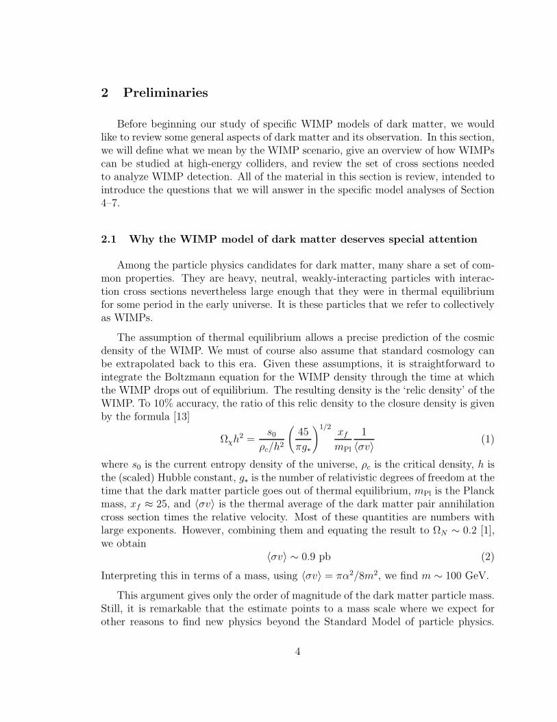
The rate of such missing energy events depends strongly on the mass of the coloredparticle that is produced and only weakly on other properties of the model. So it isreasonable to estimate the discovery potential of the LHC by looking at the predictionsfor the special case of supersymmetry. In Fig. 1, we show the estimates of the ATLAScollaboration for the discovery of missing energy events at various levels of the LHCintegrated luminosity [26]. For the purpose of this discussion, it suffices to follow thecontours of mass for the squarks and gluinos that are the primary colored particlesproduced. According to the figure, if either the squark or the gluino has a mass below1000 GeV, the missing energy events can be discovered with an integrated luminosityof 100 pb−1, about 1% of the LHC first-year design luminosity. Thus, we will knowvery early in the LHC program that the LHC is producing a WIMP candidate. Thiswill open the way to detailed studies of the role of this WIMP in astrophysics.
2.3 Qualitative determination of WIMP parameters
For reasons that we will detail in the next section, it is very important after thediscovery of the WIMP to identify it qualitatively, that is, to single out what theorygives rise to this particle and what its basic interactions are. This next step may turnout to be very difficult at the LHC.
6
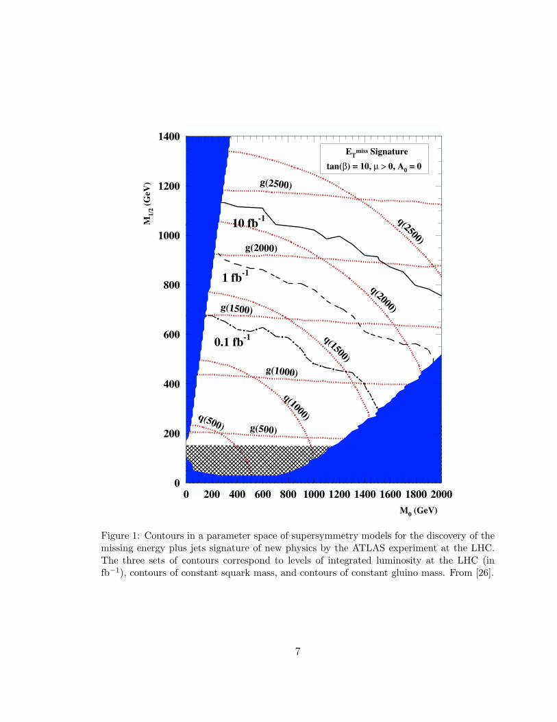
Figure 1: Contours in a parameter space of supersymmetry models for the discovery of themissing energy plus jets signature of new physics by the ATLAS experiment at the LHC.The three sets of contours correspond to levels of integrated luminosity at the LHC (infb−1), contours of constant squark mass, and contours of constant gluino mass. From [26].
7

Figure 2: Four scenarios for decay chains observed at LHC. Each exhibits jets, hard lep-tons, and missing energy. Distinguishing between these cases by detailed study of energydistributions may not be possible with LHC alone.
The reason for this is just the converse of the argument that the characteristicsignature of the WIMP is observed missing momentum. At a proton collider such asthe LHC, reactions that produce heavy particles are initiated by quarks and gluonsinside the proton. We do not know a priori how much of the momentum of theproton each initial particle carries. Since we do not observe the final-state WIMPs,we also cannot learn the energies and momenta of the produced particles from thefinal state. If we cannot find the rest frame of the massive particles, it is very difficultto determine the spins of these particles or to specifically identify their decay modes.
As a concrete illustration of this argument, consider the four models of the decayof a colored primary particle shown in Fig. 2. Examples (a) and (b) are drawnfrom models of supersymmetry in which the WIMP is the supersymmetric partnerof the photon or neutrino. Examples (c) and (d) are drawn from models of extradimensions in which the WIMP is, similarly, a higher-dimensional excitation of aphoton or a neutrino. The observed particles in all four decays are the same; thesubtle differences in their momentum distributions are obscured by the uncertaintyin reconstructing the frame of the primary colored particle. It is possible to make useof more model-dependent features. In the recent papers [27,28,29] specific features ofthe models have been identified that can distinguish the cases of supersymmetry andextra dimensions. Still, it is likely that, from the LHC experiments alone we will be
8

Figure 3: Threshold behavior of pair production cross sections for spin 1/2 (KK muon) andspin 0 (smuon) counterpart to the Standard Model muon. These distributions are easilydistinguished by an e+e− collider.
left with several competing possibilities for the qualitative identity of the WIMP.
Fortunately, another tool is likely to be available to particle physicists. At anelectron-positron collider, the pair production process e+e− → XX is gives an ex-quisite diagnostic of the quantum numbers of a massive particle X . As long as onlythe diagrams with annihilation through γ and Z are relevant, the angular distribu-tion and threshold shape of the reaction are characteristic for each spin, and thenormalization of the cross section directly determines the SU(2) × U(1) quantumnumbers. These tests can be applied to any particles with electric or weak chargewhose pair-production thresholds lie in the range of the collider. In Figure 3, weshow one example of such a test for models (a) and (c) of Fig 2, by plotting thethreshold behavior of the pair-production cross sections for the supersymmetry orextra-dimensional muon partner that appears at the last stage of the decay process.This single measurement would already pin down the spin and quantum numbers ofthe particle and bring us a long way toward the qualitative identification of the model.Particle physicists are now designing an electron-positron collider, the InternationalLinear Collider (ILC), which will reach 500 GeV in the center of mass in its initialstage and will be upgradable in energy to about 1000 GeV.
The discussion of this and the previous section highlights the contrasting strengthsof the LHC and the ILC, and of the technologies of proton and electron colliders. The
9

LHC can more easily reach high energies and offers very large cross sections for specificstates of a model of new physics. The ILC typically reaches fewer states in the newparticle spectrum, but it gives extremely incisive measurements of the properties ofthe particles that are available to it. Also, as we will see, these particles are typicallythe ones on which the dark matter density depends most strongly. Both LHC andILC can make precision measurements, but the measurements at the ILC typicallyhave a more direct interpretation in terms of particle masses and couplings. In ourdiscussion in Section 4–7, we will see many examples in which the greater energyreach of the LHC contrasts with the greater specificity of the measurements from theILC.
2.4 Quantitative determination of WIMP parameters
For the purpose of understanding dark matter, what we actually want from anunderstanding of the WIMP in particle physics is the ability to predict the WIMP’srelic density and detection cross sections. Given that the WIMP is not observable inthe high-energy physics experiments, it is not so obvious how to make these predic-tions, or, even, that the predictions can be made. The only strategy available to usis to understand the underlying particle physics model well enough to fix the interac-tions of the WIMP. To do this, we must determine its couplings and the masses andproperties of the observable particles to which it couples.
As a matter of principle, this is a very difficult undertaking. The one advantagethat we have is that the cross sections of the WIMP that are the most important inastrophysics involve very low energies. The relic density is determined by the WIMPannihilation cross section at temperatures such that T/mχ ∼ 1/25, correspondingto nonrelativistic motion [13]. When we observe the WIMP through its annihilationprocesses, the annihilation energy is very close to threshold. In direct detection ofWIMPs, or in the capture of WIMPs into the earth or the sun, the WIMPs aremoving with a velocity v/c ∼ 10−3. Though we will see some exceptions to this,it is typical that the most important diagrams for computing these cross sectionsinvolve the lightest particles in the model. If we can characterize these particles andmeasure their properties with precision, we can reach the goal of making microscopicpredictions of the WIMP properties.
We do not know a way to give a general proof of this claim, but we can illustrateits validity through studies of models. In Section 3, we will explain in detail how wewill test this claim for supersymmetry models with neutralino dark matter.
10

2.5 Astrophysical dark matter measurements: relic density
In the next three sections, we will review the astrophysical measurements thatwill require cross sections and other particle properties that might be determined byparticle physics measurements. The first of these is the most basic property of darkmatter, its cosmic mass density.
The mass density of dark matter is already known today to impressive accuracy,and this accuracy is expected to improve significantly before the end of the decade.The analysis of fluctuations in the cosmic microwave background (CMB)—in partic-ular, the measurement of the acoustic peaks that reflect oscillations in the plasmathat filled the universe at temperatures just below 1 eV—allow determinations of thedensity of baryonic and non-baryonic matter. The current value of the dark matterdensity, dominated by the data from the WMAP experiment [6], is [1]
Ωχh2 = 0.111 ± 0.006 (3)
This is already a determination to 6% accuracy. In 2007, we expect the launch of thePlanck satellite, which will give an even more precise measurement of the propertiesof the CMB. From this experiment, we can expect an improvement in the accuracyof Ωχh
2 to 0.4% [7].
It will be very difficult for microscopic predictions of the WIMP density to matchthis level of precision. But we will see that, in the specific models that we will consider,it is possible to give a microscopic prediction of the WIMP density to an accuracyof 20% or better. Thus, it will be a quite nontrivial test to compare the microscopicprediction to the density determined from the CMB.
A discrepancy between the microscopic and CMB values could arise for many rea-sons. The WIMP could provide only a portion of the dark matter, with other portionsarising from different types of particles. The WIMP could decay to a lighter and evenmore weakly interacting particle, a ‘superWIMP’ [30]. In this case, experiments onastrophysical WIMP detection should see nothing, but particle physics experimentsmight find evidence for the WIMP instability both from the new particle spectrumand from direct observation of the decay [31,32,33,34]. The density of WIMPs couldbe diluted between the temperature of WIMP decoupling (T ∼ GeV) and the temper-ature of primordial nucleosynthesis by some mechanism of entropy production, due toa phase transition or late particle decay. On the other side, the WIMP density couldmainly be generated out of equilibrium, during reheating to TeV temperatures or fromthe decay of heavy particles to WIMPs. In supersymmetry models, this scenario hasbeen studied in models of anomaly-mediated supersymmetry breaking [35,36]. Thesemodels contain large annihilation cross sections and so predict large astrophysicalsignals of WIMP annihilation.
11

In the study of primordial nucleosynthesis, both late entropy production and non-thermal processes have been considered, along with more exotic effects from newphysics. But, in fact, the predictions of primordial nucleosynthesis are in remarkableagreement with the predictions based on standard cosmology combined with detailedlaboratory measurements of low-energy nuclear cross sections [37]. This gives us con-fidence that our cosmological model is correct back to times of the order of 1 minuteafter the Big Bang. From this experience, we conclude that it is possible also that themeasured and predicted WIMP density might turn out to be in excellent agreement,verifying standard cosmology back to times of 10−9 seconds.
If the CMB and microscopic determinations of the WIMP density within theirindividual accuracies, it will be tempting to impose the more stringent astrophysicalconstraint on the particle physics model. At present, we do not know the particlephysics model, and imposing the constraint (3) does not seem to exclude any qual-itative possibilities, though it does narrow the parameter space if a given model isassumed. After the particle physics model is known, the stringent constraint on thedark matter density from Planck can have more interesting consequences. In Sec-tions 4.6, 5.5, 6.5, and 7.5, we will give specific examples of how a precise value ofthe dark matter density can be combined with LHC data to predict parameters ofthe supersymmetry spectrum that are difficult to measure at the LHC.
2.6 Astrophysical dark matter measurements: direct detection
If the microscopic cross sections measured at colliders agree with the CMB mea-surements of the dark matter density, a crucial uncertainty remains, alluded to in theprevious section. Does the dark matter candidate in addition have a lifetime longerthan the age of the universe, or is the consistency merely a coincidence? A completepicture of dark matter requires that the candidate particle be observed as the majorconstituent of our galaxy. This can be accomplished by direct or indirect detection,discussed in this section and the next.
Direct detection of WIMPs in sensitive low-background experiments involves thecross sections for WIMP scattering from nucleons near threshold. The expressionsfor these cross sections naturally divide into spin-dependent and spin-independentisoscalar and isovector contributions. The spin-independent isoscalar term is en-hanced in WIMP-nucleus cross sections by factors of A2, so we will emphasize theprediction of this contribution. The predictions for direct detection cross sections insupersymmetry models are typically displayed on scatter plots that cover five ordersof magnitude [2]. As we will see, data from the LHC and the ILC can significantlynarrow this range.
The technologies for direct detection of WIMPs and experimental limits have
12

recently been reviewed by Gaitskell[38]. The strongest current limits, from the CDMS[39], CRESST [40], EDELWEISS [41], and ZEPLIN [42] experiments, give an upperbound to the cross section of a 100 GeV WIMP at about σ(χp) < 2 × 10⁻⁷ pb.The DAMA experiment [43] reported the observation of annual modulation in a low-background NaI detector of a size consistent with a WIMP with σ(χp) ∼ 5×10⁻⁶ pb,but unfortunately the experiments listed previously contradict this interpretation [44].For the purposes of this paper, we will choose reference models of WIMP dark matterwith σ(χp) < 10−7 pb.
Later in the paper, we will present analyses in which WIMP direct detection ratesare combined with LHC and ILC results. In these analyses, we will use the predictedcounting rates from the proposed SuperCDMS experiment [45]. This particular ex-periment is chosen simply as a concrete illustration of our methods. Alternativetechnologies, for example, large noble gas detectors [46,47], promise higher countingrates and might well improve on these results.
Predictions for the rate in direct detection experiments rely on the assumptionthat the average density of dark mater in the halo of the galaxy can be used toestimate the flux of dark matter that impinges on a detector on the earth. Thisdensity is uncertain, but, in addition, we do not expect the density of dark matterto be constant over the halo. In models of cold dark matter, the galaxy is assembledfrom smaller clusters of dark matter. The initial situation is inhomogeneous, andthese inhomogeneities are not expected to be smoothed out in the time since thegalaxy was formed.
The local halo density is inferred by fitting to models of the galactic halo. Thesemodels are constrained by a variety of observations, including the rotational speed atthe solar circle and other locations, the total projected mass density (estimated byconsidering the motion of stars perpendicular to the galactic disk), peak to troughvariations in the rotation curve (‘flatness constraint’), and microlensing. Gates, Gyuk,and Turner [48] have collected these constraints and estimated the local halo densityto lie between 4 × 10⁻²⁵ g/cm−3 and 13 × 10−25 g/cm−3. Limits on the density ofMACHO microlensing objects imply that at least 80% of this is cold dark matter.The velocity of the WIMPs would be close to the galactic rotation velocity, 230 ± 20km/sec [49]. The effects of varying the model of the WIMP halo are illustrated in arecent paper of the Torino group that shows this variation in terms of the region ofthe mχ vs. σ plane consistent with the DAMA result [50].
These constraints rely on the assumption that the dark matter has a smoothdistribution in the galactic halo. However, the general conclusion from high resolutionN-body simulations is that the dark matter distribution is highly irregular. Using ahierarchical clustering model of galactic structure, Stiff, Widrow, and Frieman haveargued that the solar neighborhood might be expected to be located within a clump of
13

dark matter with only slightly higher local density but a velocity distribution peakedat a relatively large value [51]. Other authors have argued for larger density variationin the galactic distribution of dark matter. Sikivie and Ipser [52] have proposed thatspherical infall of dark matter on to developing galaxies will tend to accumulate alongsingular surfaces or caustics, leading to very large local fluctuations. An even moreextreme model was recently put forward by Diemand, Moore, and Stadel [53], whoargued that WIMPs are likely to appear in clusters of mass comparable to the massof the earth and densities roughly 103 larger than the average density of the disk. Inaddition to these models that rely on the general features of galaxy formation, thelocal geography of our region of the galaxy might affect the dark matter density. Forexample, Freese, Gondolo and Newberg have proposed that the Sagittarius streamshould add up to 23% to the local dark matter density, with a characteristic annualmodulation [54]. These models illustrate not only that there is a large uncertainty inthe value of the local dark matter flux at the earth but also that the understandingof this value relative to the overall average density of dark matter is an interestingastrophysical question.
If we view these questions as uncertainties, we must say that direct detectionexperiments cannot by themselves put constraints on the microscopic scattering crosssections of WIMPs. On the other hand, if we could obtain the microscopic crosssections from particle physics, the event rate in direct detection experiments woulddirectly measure the local flux of WIMP dark matter. If direct detection experimentsfailed to detect dark matter, it would be even more important to have the microscopiccross section in order to establish strong upper bounds on the local WIMP density.
There is another source of uncertainty in this program that also needs to beaddressed [55]. When the dark matter direct detection cross section is calculatedfrom particle physics models, even if the parameters of these models are assumedto be precisely known, there is an uncertainty in the prediction of the cross sectionthat can be as large as a factor of 4 coming from a poorly understood effect of low-energy QCD. In many WIMP models, including the SUSY models that we will takeas reference points in this study, σ(χp) is dominated by t-channel Higgs exchange.The coupling of the Higgs boson to the proton receives its dominant contributionsfrom two sources, the coupling of the Higgs to gluons through a heavy quark loopand the direct coupling of the Higgs to strange quarks [56]. That means that thiscoupling depends on the parameter
fTs =〈p|msss |p〉〈p|HQCD |p〉 , (4)
that is, the fraction of the mass of the proton that arises from the mass of the non-valence strange quarks in the proton wavefunction. In 1987, Kaplan and Nelson
14

argued that this quantity is larger and more uncertain than previously thought [57],
fTs = 0.36 ± 0.14 (5)
In the intervening twenty years, there has been essentially no progress in improvingour knowledge of this quantity. Several recent papers have highlighted the uncertaintyin fTs as a major uncertainty in WIMP directly detection cross sections [58,59].Indeed, for a heavy SUSY Higgs boson in a model with a large value of the parametertanβ, the Higgs-proton coupling is given quite accurately by
λHpp =mp
250 GeV
[2
27+
25
27fTs
]tan β + · · · (6)
so that σ(χp) is almost proportional to f 2Ts. This can produce an uncertainty in the
direct detection cross section of a factor of 4 or even larger [58].
How could we resolve this problem? We consider it unlikely that an improvementof the data on which the estimate (5) is based will improve the error. However, itshould eventually be possible to compute fTs in lattice gauge theory. Because fTs isa non-valence quantity, this is beyond the current state of the art. For example, thecurrent result from the UKQCD collaboration is fTs = −0.20 ± 0.23 [60]. However,the valence pion nucleon sigma term is already under control; a recent analysis givesσπN = (49 ± 3) MeV [61]. For the non-valence case, the problem seems mainly oneof obtaining computer power to generate high statistics, and this should increasedramatically over the next ten years [62].
For the analyses of this paper, we will ignore uncertainties in the calculation ofdirect detection cross sections that are not associated with variation of the parametersof the new physics model. This means that we will ignore the uncertainty in fTs,corresponding to the assumption that lattice calculations will eventually solve thisproblem. Other sources of theoretical error seem to be under control at the 10%level. We will assume that fTs = 0.14, the default value in the DarkSUSY code [9],so in any event we will underestimate the experimental counting rates.
Parenthetically, we would like to call attention to an aspect of direct detectionexperiments that is very important but is not often emphasized. It is very likely thatdirect detection experiments will see evidence of WIMPs in the same time frame,before the end of the decade, that the LHC observes missing energy events. In thiscase, it will be essential to compare the mass of the WIMP observed in each setting.In supersymmetry models, as we will discuss in Sections 4-7, the kinematics of eventswith squark production and decay can determine the mass of the WIMP to about10% accuracy. We believe that this type of analysis will give the WIMP mass tosimilar accuracy in typical models of the general class discussed in Section 2.2.
15

Direct detection experiments can determine the mass of the WIMP by measuringthe recoil energy ER. This varies with the mass of the WIMP, with a resonance wherethe WIMP mass equals the target mass. Roughly, one expects
〈ER〉 ≈2v2mT
(1 + mT/mχ)2, (7)
where mT is the target mass and v is the WIMP velocity, with corrections dependingon the precise target material and the properties of the detector [63]. Assumingthe standard velocity distribution in smooth halo models, with the 10% uncertaintyquoted above, an experiment with a Xenon or Germanium target that detects 100signal events for a WIMP of mass mχ = 100 GeV can expect to measure the mass ofthis particle to 20–25%. A discrepancy between the value of the WIMP mass observedin direct detection and that found at the LHC could signal a nonstandard velocitydistribution. At a later stage, this could be checked by comparing the detection rate,which is proportional to the flux of WIMPs, to the cross section determined fromhigh-energy collider data.
In Fig. 4, we show a comparison of the determination expected for the WIMPmass from the LHC data and from the analysis of data from the SuperCDMS de-tector [45,64] for one of the supersymmetry models that we introduce in Section 3.2.The contours are based on a sample of 27 events and so are statistically limited. Still,it is clear that a nontrivial comparison of WIMP masses between accelerator andastrophysical experiments will be possible.
More powerful strategies for measuring the WIMP mass from direct detectiondata have been proposed by Primack, Seckel, and Sadoulet [66] and by Bourjaily andKane [67]. However, this would require a sample of direct detection events about 100times larger than those in the illustrative examples we will present here.
Finally, we comment on the possibility that WIMPs measured at colliders makeup only a fraction of the dark matter. In this case, the annihilation cross sectionstend to be larger than the expected 1 pb, and also the direct detection cross sectionstend to be large. In fact, these effects broadly speaking cancel: a WIMP makingup 10% of the cosmic dark matter tends to have cross sections 10 times as large asexpected, thus the direct detection rate is roughly independent of the inferred relicdensity [68].
2.7 Astrophysical dark matter measurements: WIMP annihilation
WIMP annihilation could potentially be observed through gamma ray, positron,antiproton, antideuteron, and neutrino signals. Of these, the observations throughgamma rays is the simplest and most robust. There are already claims that an excess
16

Figure 4: Projected significance contours (1, 2, 3, 4σ) in the plane of WIMP mass versus crosssection for an observation of dark matter by the SuperCDMS experiment (25 kg target, twoyear dataset) [45,65], compared to the determination of these parameters from data fromthe LHC. The projections are done using the model LCC3, to be defined in Section 3.2.
of gamma rays from the galactic center gives evidence for WIMP dark matter [69].We will examine how this study will be aided by collider physics determinations ofthe WIMP annihilation cross section.
The flux of gamma rays observed on earth from WIMP annihilation is given bythe formula
EγdΦγ
dEγdΩ=
1
2(σχχv) · Eγ
σχχ
dσχχ
dEγ
· 1
4πm2χ
·∫
dz ρ2(z) , (8)
where σχχ/2 is the annihilation cross section near threshold, (which typically behavesas 1/v), z is a coordinate along the line of sight, and ρ is the WIMP mass density.The factors of 1/2 are appropriate assuming that the dark matter particles are self-conjugate; we will later apply this equation to the neutralino WIMP in SUSY models.The first three factors come from microscopic physics; the final factor is a questionof astrophysics. The density integral is commonly written
∫dzρ2(z) = r0ρ
20J(Ω) , (9)
where r0 = 8.5 kpc is the distance to the center of the galaxy and ρ0 = 0.3 GeV cm−3
(5.34 × 10⁻²⁵ g/cm3) is a reference value of the local density of dark matter. Thequantity J(Ω) is then dimensionless.
17

It is likely that the microscopic quantities that appear in (8) could be estimated toan accuracy of 20% even in the early stages of the study of WIMPs in particle physicsexperiments. The mass mχ will be determined to better than 10% accuracy from thekinematics of missing energy events at the LHC. We will show in Section 8.1 thatthe second factor in (8), the shape of the gamma-ray spectrum, is almost completelyindependent of the specific annihilation process and can be obtained accurately fromparticle physics simulations. For the first factor, the total annihilation cross section,it is tempting to insert the value (2) from the relic density. This is sometimes, butnot always, a good approximation, depending on the qualitative properties of thesupersymmetry spectrum. We will discuss the systematics of this quantity in Section8.1. In many physics scenarios, all three quantities will be known well enough alreadyfrom the LHC data to quantitatively interpret gamma ray observations.
It is very important that the particle physics factors in (8) can be determined frommicroscopic measurements, because the last factor raises major questions about thestructure of the dark matter halo of the galaxy. Let us first discuss the dark matterprofile at the galactic center. A typical profile of the smoothed dark matter halo iswritten
ρ(r) = ρ0(r/r0)γ
(1 + (r0/a)α
1 + (r/a)α
)(β−γ)/α
, (10)
where α, β, γ are parameters and the scale size a should be about 20 kpc. Navarro,Frenk, and White (NFW) have argued that that numerical simulations of galaxyformation by cold dark matter suggest the profile (α, β, γ) = (1, 3, 1) [70]. In theexplicit examples that we will present in Section 4.4, we will assume the NFW profileas a canonical choice. However, other groups have drawn different conclusions fromthe simulation data. Moore et al. have argued for a much steeper profile at the galacticcenter: (α, β, γ) = (1.5, 3, 1.5) [71]. For this profile, the integral over ρ2(z) formallydiverges at the galactic center [72]. Wechsler and collaborators have argued thatthe halos found in a given simulation can actually have different shapes depending ontheir history, roughly covering the range between the NFW and Moore profiles [73,74].We should note that the simulations that we are discussing include only dark matter,and that the addition of a dissipative component could also alter the profile. Thevariation in (8) near the galactic center for the NFW and Moore profiles, and for anisothermal profile with (α, β, γ) = (2, 2, 0), is shown in Fig. 5. We present both theprofile functions themselves and the value of J(Ω) averaged over a disk of varyingsolid angle centered on the galactic center. The predictions for 〈J(Ω)〉 span six ordersof magnitude between models. Further, these estimates are all smooth profiles, andwe have already seen that the distribution of dark matter might be clumpy. Suchsmall-scale structure would enhance indirect detection rates by the ratio
B =⟨ρ2⟩/ 〈ρ〉2 , (11)
18
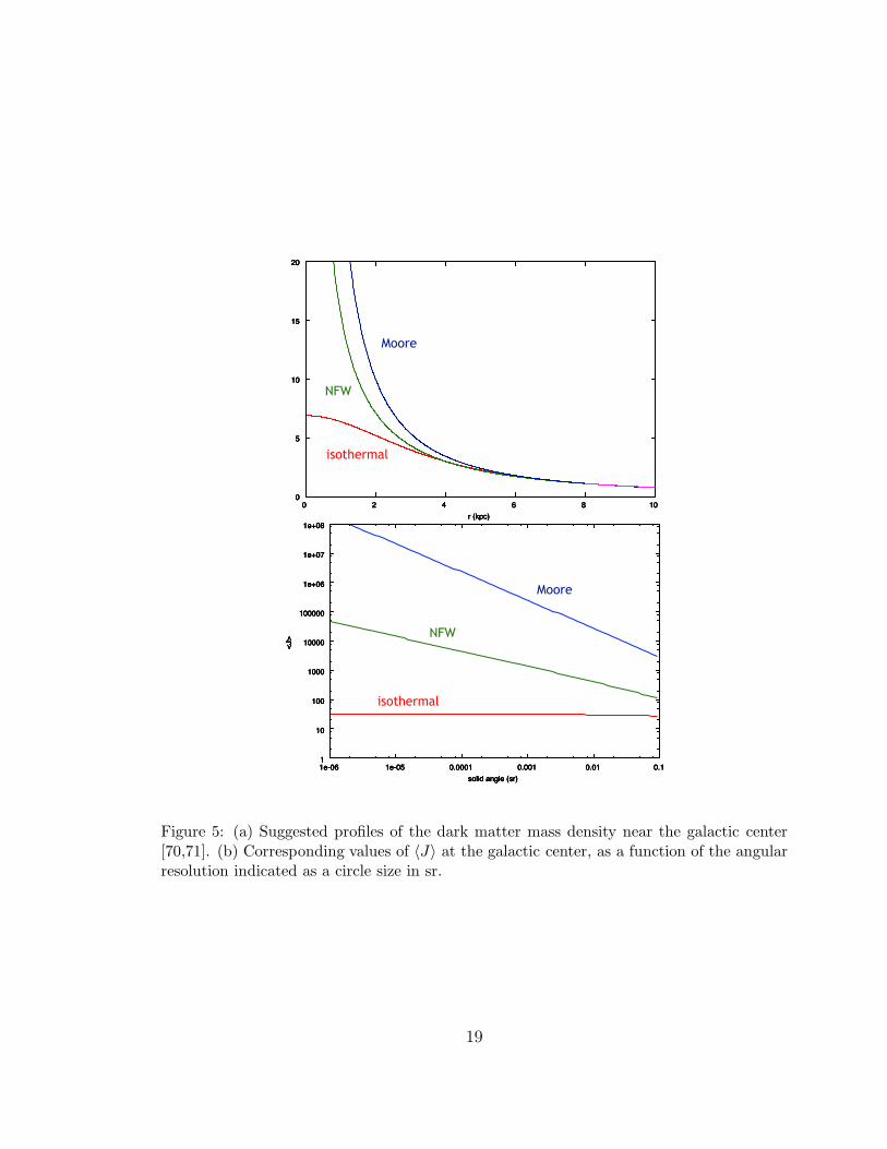
Figure 5: (a) Suggested profiles of the dark matter mass density near the galactic center[70,71]. (b) Corresponding values of 〈J〉 at the galactic center, as a function of the angularresolution indicated as a circle size in sr.
19
sometimes called the ‘boost factor’. The final conclusion from all of these consider-ations is that indirect dark matter detection rates depend on distributions that arehighly uncertain and touch on major questions of astrophysics. It would be inter-esting to extract these distributions from the experiments, or even to obtain upperlimits on them. For this, we need to know the microscopic cross sections from particlephysics.
This conclusion applies also to other possible sources of gamma rays from WIMPannihilation. For gamma rays from the centers of local group and other nearbygalaxies, the considerations are very similar to those for the galactic center [75].Simulations of galaxy formation with cold dark matter predict many more dwarfcompanions of the Milky Way than are actually observed. Probably, many of thesehave been tidally disrupted or absorbed. However, it is likely that some of theseunobserved dwarf galaxy are actually present as pure dark matter halos from whichthe baryonic gas has been blown out [76]. The GLAST telescope, with its π angularcoverage for gamma rays, has the ability to search for these objects. Even upperlimits are interesting, but their interpretation will depend critically on knowledge ofthe microscopic factors in (8).
The expectations for observation of positrons, neutrinos, antiprotons and an-tideuterons from WIMP annihilation depend on more specific details of the physicsmodel. We will discuss the subject of positron signals further in Section 8.2. For theother cases, the analysis of the interplay between collider physics data and indirectdetection signals is more complex and its analysis is beyond the scope of this pa-per. We should note, however, that the four reference models that we will introducein Section 3.2 are consistent with all current constraints from indirect detection ofWIMPs.
2.8 Summary: steps toward an understanding of WIMP dark matter
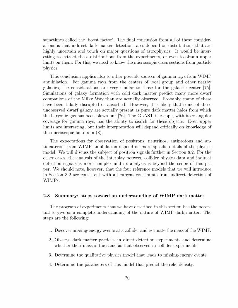
The program of experiments that we have described in this section has the poten-tial to give us a complete understanding of the nature of WIMP dark matter. Thesteps are the following:
1. Discover missing-energy events at a collider and estimate the mass of the WIMP.
2. Observe dark matter particles in direct detection experiments and determinewhether their mass is the same as that observed in collider experiments.
3. Determine the qualitative physics model that leads to missing-energy events
4. Determine the parameters of this model that predict the relic density.
20

5. Determine the parameters of this model that predict the direct and indirectdetection cross sections
6. Measure products of cross sections and densities from astrophysical observationsto reconstruct the density distribution of dark matter.
If dark matter is composed of a single type of WIMP, this program of measurementsshould reveal what this particle is and how it is distributed in the galaxy. If thecomposition of dark matter is more complex, we will only learn that by carryingout this program and finding that it does not sum to a complete picture. Hopefully,further evidence from the microscopic theory will suggest other necessary ingredients.
The main goal of the remainder of this paper is to show that the experimentsforeseen for the LHC and ILC will be able to predict the microscopic dark mattercross sections with sufficient accuracy that we can carry out this program. In thenext section, we will describe our strategy for addressing this question.
3 Models of neutralino dark matter
As we have already noted in Section 2.3, the annihilation and detection crosssections needed to interpret observations of WIMP dark matter cannot be measureddirectly in high-energy physics experiments. To predict these cross sections, we mustinterpret experimental data on the spectra and parameters of the underlying physicsmodel. To do this, we must understand, at a qualitative level, what the correctmodel is. We must then convert measurements of the spectrum of new particles intoconstraints on the underlying model parameters. Some care should be taken in thechoice of the model. If we work in too restrictive a model context, this procedure willartificially restrict the solutions, and we will claim an unjustified small accuracy forour predictions. Thus, to evaluate how accurately collider data will predict the darkmatter cross section, we need to work within a model that, under overall restrictionsfrom spin and quantum number measurements, has a large parameter space andallows a wide variety of physical effects to come into play.
Among models of physics beyond the Standard Model, the only one in which darkmatter properties have been studied over such a large parameter space is supersym-metry [77]. The Minimal Supersymmetric Standard Model (MSSM) introduces a verylarge number of new parameters and allows many physically distinct possibilities forthe mass spectrum of new particles. Thus, our strategy for evaluating the implicationsof collider data for dark matter cross sections will be to study a set of MSSM pa-rameter points which illustrate the variety of physics scenario that this general model
21

Figure 6: Four neutralino annihilation reactions that are important in different regions ofthe MSSM parameter space: (a) annihilation to leptons, (b) annihilation to W+W−, (c)coannihilation with τ , (d) annihilation through the A0 resonance.
can contain. In each case, we will systematically scan the parameter space of theMSSM for models that are consistent with the expected collider measurements. Wehope that the insights obtained from this study will lead us to conclusions of broaderapplicability about the power to high-energy physics measurements to restrict theproperties of dark matter.
3.1 Mechanisms of neutralino annihilation
From here on, then, we restrict our attention to models with supersymmetry inwhich the role of the WIMP χ is taken by the lightest ‘neutralino’—a mixture ofthe superpartners of γ and Z (‘gauginos’) and the superpartners of the neutral Higgsbosons (‘Higgsinos’). Depending on the spectrum and couplings of the superpartners,several different reactions can dominate the process of neutralino pair annihilation.Some of the most important possibilities are illustrated in Fig. 6.
The simplest possibility (Fig. 6(a)) is that neutralinos annihilate to StandardModel fermions by exchanging their scalar superpartners. Sleptons are typicallylighter than squarks, so the dominant reactions are χχ → ℓ+ℓ−. It turns out, however,that this reaction is less important than one might expect over most of the supersym-metry parameter space. Because neutralinos are Majorana particles, they annihilate
22

in the S-wave only in a configuration of total spin 0. However, light fermions are natu-rally produced in a spin-1 configuration, and the spin-0 state is helicity-suppressed bya factor (mℓ/mχ)2. The dominant annihilation is then in the P-wave. Since the relicdensity is determined at a temperature for which the neutralinos are nonrelativistic,the annihilation cross section is suppressed and the prediction for the relic density is,typically, too large. To obtain values for the relic density that agree with the WMAPdetermination, we need light sleptons, with masses below 200 GeV.
Neutralinos can also annihilate to Standard Model vector bosons. A pure U(1)gaugino (‘bino’) cannot annihilate to W+W− or Z0Z0. However, these annihilationchannels open up if the gaugino contains an admixture of SU(2) gaugino (‘wino’) orHiggsino content (Fig. 6(b)). The annihilation cross sections to vector bosons arelarge, so only a relatively small mixing is needed.
The annihilation to third-generation fermions can be enhanced by a resonanceclose to threshold. In particular, if mass of the CP odd Higgs boson A0 is close to2mχ, the resonance produced by this particle can enhance the S-wave amplitude forneutralino annihilation to bb and τ+τ− (Fig. 6(d)).
If other superparticles are close in mass to the neutralino, these particles canhave significant densities when the neutralinos decouple, and their annihilation crosssections can also contribute to the determination of the relic density through a coan-nihilation process. If the sleptons are only slightly heavier than the neutralino, thereactions ℓχ → γℓ and ℓℓ → ℓℓ can proceed in the S-wave and dominate the annihila-tion (Fig. 6(c)). Coannihilation with W+ partners (‘charginos’) and with top squarkscan also be important in some regions of the MSSM parameter space.
A common feature of all four mechanisms is that the annihilation cross sectiondepends strongly both on the masses of the lightest supersymmetric particles andon the mixing angles that relate the original gaugino and Higgsino states to theneutralino mass eigenstates. Both sets of parameters must be fixed in order to obtaina precise prediction for the relic density.
A supersymmetry model that produces a relic density of neutralinos in the rangerequired by the WMAP data should implement one of these mechanisms. To theextent that the operation of the mechanism requires special conditions on the super-symmetry spectrum, the neutralino relic density will depend more sensitively on thespectrum parameters than we might at first have estimated. We will see the effectsof this observation in our model studies.
23
3.2 Choice of benchmark models
We would now like to choose four specific supersymmetry models that illustratethe four mechanisms described in the previous section.
Let us first discuss the parameters of the MSSM. The most general formulation ofthe MSSM has 108 parameters beyond those of the Standard Model. However, manyof these parameters violate CP or induce flavor-changing neutral current processesand are thus tightly constrained. If we include only interactions that conserve CPand flavor, we find the following set of parameters:
• gaugino and Higgsino masses: m1, m2, m3, µ
• slepton masses: m2(Li), m2(ei), i = 1, 2, 3
• squark masses: m2(Qi), m2(ui), m
2(di), i = 1, 2, 3
• Higgs potential terms: mA, tanβ
• A terms: Aτ , Ab, At
a total of 24 new physics parameters.
Most papers on neutralino dark matter adopt additional, ad hoc, assumptions toreduce this parameter list to a smaller set. Most typically, they assume unificationof the various mass terms at the grand unification scale. This assumption, called‘mSUGRA’ or ‘cMSSM’, reduces the parameter set to four, plus a choice of sign: m0,m1/2, A0, tan β, sign(µ). The restricted parameter space of mSUGRA is very inter-esting to illustrate the various possibilities for neutralino dark matter. In particular,this subspace contains examples of all four mechanisms that we have presented in theprevious section [80,81,82].
This makes it very convenient to choose parameter points from the mSUGRAsubspace. In Table 1, we list the four parameter sets that define the supersymmetrymodels that we will study in detail [83]. The spectra for these points, and for themore general supersymmetry parameter points that we will study, are computed withISAJET 7.69 [8]. Results for the relic density and for neutralino detection cross sec-tions are computed with DarkSUSY-4.1 [9]. We have checked that Micromegas 1.3 [84]gives similar results for the relic density.
The four points listed in Table 1 illustrate the four scenarios described in theprevious section. Point LCC1 is identical to the point SPS1a [85] whose colliderphenomenology is studied in some detail in [86]. This point has light sleptons, withneutralino annihilation dominated by roughly equal annihilation cross sections to
24

Point m0 m 1
2
tan β A0 sign mu mt reference Ωχh2
LCC1 100 250 10 −100 + 175 [86] 0.192LCC2 3280 300 10 0 + 175 [87] 0.109LCC3 213 360 40 0 + 175 [88] 0.101LCC4 380 420 53 0 + 178 [90] 0.114SPS1a′ 70 250 10 −300 + 175 [91] 0.115
Table 1: mSUGRA parameter sets for four illustrative models of neutralino dark matter.Masses are given in GeV. The table also lists the value of Ωχh
2. The references given arethe primary references for simulation studies of the accuracy of spectrum measurements atcolliders. The point SPS1a′ has a phenomenology similar to that of LCC1 but gives a morecorrect value of the relic density.
e+e−, µ+µ−, and τ+τ−. The sleptons are not quite light enough; the spectrumachieves a relic density Ωh2 = 0.19, almost doubly the WMAP value. Point LCC2 ischosen as a point with substantial gaugino-Higgsino mixing at which the neutralinoannihilation is dominated by annihilation to W+W−, Z0Z0, and Z0h0. Point LCC3is chosen in the region where coannihilation with the τ plays an important role. PointLCC4 is chosen in a region where the A0 resonance makes an important contributionto the neutralino annihilation cross section.
The four points are intentionally chosen so that the lightest particles of the super-symmetry spectrum can be observed at the ILC at its initial center of mass energy of500 GeV. This is also the most probable region of the parameter space, since in thisregion the dynamics of supersymmetry can generate electroweak symmetry breakingwithout extensive fine-tuning of parameters [92].
It will be important to us to have well-justified estimates for the accuracy withwhich high-energy physics experiments can measure the supersymmetry spectrumparameter at these points. For these reason, we have chosen to analyze points in theMSSM parameter space at which simulations have been carried out to estimate theability of colliders to measure parameters of the supersymmetry spectrum [93]. Forthe point LCC1 or SPS1a, an extensive set of simulation studies for both LHC andILC is described in [86]. These studies assume a luminosity sample of 300 fb−1 andLHC and 500 fb−1 for ILC. They include realistic modeling of particle detection andStandard Model backgrounds. For the other LCC points, similarly detailed studieshave been performed only for the ILC [95]. However, as we will see, the conclusionsof [86] and other LHC studies such as those reported in [96] can be used to estimatethe LHC capabilities at these points. The point LCC2 has been studied for the ILCby Alexander, et al., in [87]. The point LCC3 has been studied by Khotilovich, et al.,in [88,89]. The analysis of this point requires a precision measurement of the τ mass,and the question of how well that can be done has also been studied at related point
25

by Bambade, et al. in [97]. The point LCC4 has been studied in the ILC environmentin [90].
The reader will note that the point LCC1 gives a value of Ωχh2 outside the range
preferred by the current data. We are not troubled by this, except to note that theappropriate figure of merit is the relative accuracy, rather than the absolute accuracy,with which Ωχh
2 can be determined. Other authors, however, have been concernedabout this and have extrapolated the simulation results obtained at LCC1 (SPS1a) toa nearby point SPS1a′ which, because it pushes into the stau coannihilation region,predicts a relic density Ωχh
2 = 0.115 [91]. In this paper, we have done our mainanalysis at the original point in order to cleanly separate examples in which differentphysics determines the relic density. However, Nojiri, Polesello, and Tovey [11] haveperformed a detailed analysis of the LHC prediction of the relic density at SPS1a′,and so, for comparison, we will also present the corresponding results for this pointin our framework.
The four points are chosen within the limited subspace of mSUGRA models. How-ever, when we interpret measurements from the colliders, we will not want to assumethat the true supersymmetry model lives in this subspace. There is no compellingphysics argument for the mSUGRA assumptions. More importantly, the restrictionto a four-parameter model induces correlations between parameters of the supersym-metry spectrum, for example, tanβ, µ, and the top squark mass, that should properlybe considered independent. Some interesting studies have been performed in whichthe capability of the LHC to predict Ωχh
2 has been assessed by scanning over theparameter space of mSUGRA [98,99]. However, we believe that that this restrictionmakes the conclusions excessively optimistic.
Instead, it is our strategy to study the implications of measurements at the LHCand the ILC by comparing to models over the full 24-dimensional parameter space ofthe MSSM described at the beginning of this section. The MSSM is also a restrictedsubspace of the space of all, completely general, supersymmetry models. However, aswe will see, the large number of parameters of the MSSM allows a very wide range ofscenarios to appear, with sufficient independence of parameters that measurementsspecific to the particles involved are needed to constraint the important physical ef-fects. We believe that the exploration of this space is a reasonable way to estimatethe capabilities of colliders to extract model-independent conclusions within the over-all category of supersymmetry models. Many of the dependences of the neutralinorelic density on individual MSSM parameters are displayed in [10], even though theconclusions are stated within the mSUGRA framework. Theoretical errors in the relicdensity calculation, which we do not consider in this paper, are also highlighted there.These errors become relevant when the relic density is determined to the 1% level.The dependence of the relic density on individual MSSM parameters at several of
26
the reference points is also studied in [100]. Nojiri, Polesello and Tovey have recentlyredone the study [98] in the context of the full MSSM [11]. These results can becompared directly to ours, and we will do that in Section 4.3.
We conclude this section with a more technical explanation of our use of theMSSM parameters. First, there is ambiguity in how one would assign values tothe 24 MSSM parameters from the output of ISAJET. We do this as follows: Wefirst run ISAJET with the parameters in Table 1, and we run DarkSUSY at eachpoint using roption=’isasu’ to use the running Yukawa couplings from ISAJET.From this, we extract the various running parameters evaluated at the mass scaleQ = (m(t1)m(t2))
1/2, which ISAJET uses as the mass scale of supersymmetry. Theseinclude the top, bottom and tau masses (MTQ, MBQ, MLQ), the Higgs vacuumexpectation values (VUQ2+VDQ2)1/2, the strong coupling constant GSS(3), and theYukawa couplings GSS(4,5,6). We set the ISAJET parameter NSTEP0 = 10000 toimprove the accuracy of the RG integration, especially in the focus point region.The 24 MSSM parameters listed above are extracted at the SUSY scale, with theexception of mA which we take as the physical mass, tan β which we take as the inputvalue, and m3 which we take as the physical gluino mass. We now run the benchmarkmodel again using a low energy treatment in DarkSUSY. The spectrum is calculatedaccording to the ISAJET function ssmass, from which we extract the neutralino,chargino, sfermion, and Higgs masses and mixings. Then DarkSUSY computes therelic density and other quantities. This is the benchmark point that we use. Thisprocedure defines the benchmark point, yielding the reference spectra and the valuesof Ωχh
2 listed in Table 1.
We note that, because we recompute the spectrum from the low-energy parametersas just defined, our spectrum calculation differs from that of the implementation ofmSUGRA in ISAJET. Thus, we find results for the mass spectrum that differ slightlyfrom those obtained by inserting the original mSUGRA parameters into ISAJET. Forexample, using ISAJET 7.69 directly with the parameters of LCC3 in the Table 1 givesa mass splitting m(τ1)−m(χ0
1) = 12 GeV, while we find a splitting of 10.8 GeV. Thisshift, less than 1% in the τ mass, makes a significant difference in the neutralino relicdensity. However, we calculate the neutralino relic density from the spectrum definedby the low-energy parameters, and that calculation is correct, for that spectrum, tothe percent level.
To describe a point in the more general parameter space of the MSSM, we com-pute the spectrum from ISAJET with ssmass using the new values of the 24 MSSMparameters, taking MTQ, MBQ, MLQ, the Higgs VEV, and the strong coupling con-stant GSS(3) to be fixed at the benchmark value. We take the Yukawa couplingsGSS(4,5,6) scaled by tan β from the benchmark values. For example, for LCC3 wetake GSS(4) to be the benchmark value times ((1 + tan2 β)/(1 + (40)2))1/2. With
27
these choices, we describe the MSSM with low energy parameters in such a way thata point in our parameter space gives a close match to the input mSUGRA model.
3.3 Scanning of parameter space
We have now reduced the prediction of the properties of WIMPs to the followingproblem: Given a parameter space of n coordinates x, and given a set of measurementsmi, each with standard deviation σi, what is the expectation for the prediction foradditional observable quantities Oj that depend on the parameters x? In Bayesianstatistics, the probability distribution of x is given by the likelihood function
dnx L(x) = dnx∏
i
exp
[−(Mi(x) −mi)
2
2σ2i
]. (12)
We have made the assumption of a flat a priori distribution of the values of x, and wehave assumed that the distribution of measurement errors is Gaussian. The predictionfor Oj(x) is then given by the expectation value of this function of x in the measure(12). More generally, we can consider the distribution of the values of Oj(x) inducedby this distribution of the parameters x. In the next few sections, we will use thismethod to present the distributions of the WIMP relic densities and cross sectionsthat follow from the constraints imposed by supersymmetry spectrum measurements.
A simple way to generate the distributions (12) is to choose points x randomlyin the parameter space and assign each one the indicated weight. However, if someof our measurements are very precise, the Gaussian distributions in (12) will bevery steep and important points will be selected only rarely. A much more ef-fective method for sampling points is the Markov Chain Monte Carlo (MCMC)method [101,102,103,104,105]. From an initial starting configuration x0, we gener-ate a sequence of points xI by the following algorithm: Choose a nearby point x′. If L(x′) ≥ L(xI), let xI+1 = x′. If L(x′) < L(xI), set xI+1 either to x′ or to xI , choosingx′ with probability L(x′)/ L(xI). This process satisfies detailed balance and thereforeshould equilibrate to an ensemble of points in which each point appears with therelative weight L(x).
There are many possible ways to choose the distribution of initial conditions,step sizes, and criteria for convergence in the MCMC algorithm. In our use of thisalgorithm, we have chosen a reference point X∗ to be one of the LCC points, wehave set the central values of measurements mi in the likelihood function to be thevalues Mi(X∗) predicted at this point, and we have taken the initial point of the chainto be the reference point: x0 = X∗. In choosing step sizes, we have attempted tomeasure the size of the distribution of points xI and to readjust the step size sothat it is comparable to this size in each dimension. For each reference point, we have
28
generated 25 independent chains, with 160,000 points xI per chain, for a total of 4million points.
We have tested our method by performing MCMC scans in which the step sizehas been preset (to 1 GeV for the masses of color singlet particles and to 10 GeV forthe masses of colored particles), and by performing flat scans of the parameter spacein the vicinity of the reference points. The distributions near the reference pointsare similar in the three methods. The final errors estimated by the MCMC methodare larger, but we are convinced that this is due to the fact that the MCMC scansexplore the parameter space more deeply.
The full details of our MCMC algorithm are presented in Appendix A. It is easyto obtain apparently excellent but incorrect results with MCMC when the chains donot come to equilibrium. In Appendix A, we describe direct tests and cross-checksthat have convinced us that our MCMC chains have correctly converged to the truelikelihood distribution.
3.4 Parameters and constraints
Now that we have described the general idea of MCMC scanning, we would like topresent the explicit manner in which we have applied this algorithm to the scanningof the MSSM parameter space. We need to specify how the variables x with flat apriori distributions are related to the MSSM parameters. If the likelihood function(12) does not constrain a particular parameter, the MCMC chain will run to infinityin that direction. Thus, it is also necessary to constrain the range of the parameters,at least within some broad limits. We will now explain the choices that we have made.
For most of the 24 MSSM parameters, we have taken x to be the logarithm of thecorresponding parameter. Thus, for example, we have taken each MSSM soft massparameter to have the a priori distribution dm/m. The parameters Aτ , Ab, At, andµ, and m1 can take either sign, so a pure logarithmic distribution is inappropriate forthese cases. We have taken instead the formula A = M sinh(x), with M = 50 GeV.This corresponds to an a priori distribution dA/
√A2 + M2. When the results of the
MCMC cluster in a small region, these results are almost independent of the priordistribution. This is true for our scans when the fractional error is less than about30%.
Given a set of MSSM parameters, we have used ISAJET 7.69 to compute thesupersymmetry spectrum and mixing angles, in the manner that we have describedat the end of Section 3.2. The ISAJET computation includes finite one-loop radiativecorrections, assuming the MSSM parameters to be renormalized parameters at thescale Q defined in that discussion. When we have required cross sections for super-symmetric particle production, we have computed these from the ISAJET output
29

parameters using the tree level formulae.
For slepton masses and color-singlet gaugino masses, we have imposed a lowerbound m > 100 GeV; for squark and gluino masses, we have imposed m > 250 GeV,except that m(t) > 150 GeV. These lower limits were almost always irrelevant, sincemeasurements at the LHC and ILC would provide stronger lower bounds. However, wealso needed to provide upper bounds to the parameter space; to do this, we restrictedall mass parameters to be less than 5 TeV in absolute value. We also imposed thefollowing restrictions: For the parameter tanβ: 2 < tan β < 100; for the charginomass: m(χ+
1 ) > 125 GeV, assuming that an excess of trilepton events is not observedat the Tevatron. For the A parameters, we have used
A2t + µ2 < 7.5(m2(t1) + m2(t2)) , (13)
as an approximate criterion to forbid charge- and color-breaking vacuum states [106].We imposed no additional bounds on Ab and Aτ since the top constraint is the moststringent. As we explained in Section 3.2, we set terms in the soft masses and the Aterms that are off-diagonal in flavor equal to zero; this corresponds to the assumptionof ‘minimal flavor violation’. We did not implement the constraint from b → sγ,since the predictions for b → sγ depend on flavor-mixing parameters that we are notincluding in our analysis. In our examples, however, the collider measurements of thesupersymmetry spectrum exclude the region in which a large deviation in b → sγ isexpected in models with minimal flavor violation.
In the results presented in the body of this paper, we further restrict the rangeof µ, m1, and m2 to positive values. It is possible to choose m2 to be positive byconvention, but then m1 and µ can in principle have either sign. It is usually verydifficult to determine these signs from the LHC data. This is a special case of amore general problem, that spectrum constraints from the LHC often allow a numberof interpretations in terms of the underlying supersymmetry parameters, related bydiscrete interchange operations. These ‘discrete ambiguities’ have been highlightedin [107,108]. We will see many examples of such ambiguities in the simulation resultsthat we will present below, and we have studied in detail that our simulations countthe multiple solutions correctly. By studying scans in which m1 and µ can take valuesof either sign, we have concluded that allowing negative signs makes little difference tothe results that we will show for the LHC, and that the ILC can typically distinguishthe solution with positive signs. We will discuss this issue in more detail is AppendixB.
At the LHC, cross sections depend mainly on particle masses and so are usefulonly as cross-checks on the mass determinations. However, the electroweak crosssections at the ILC are often sensitive to mixing angles and provide additional in-formation about the spectrum parameters. We have therefore included in our sets
30

of measurements a number of ILC cross sections. The simulation studies for LCC1,LCC2, and LCC3 include estimates of the error that would be obtained on the totalcross sections for some of the interesting reactions at these points.
The ILC will have polarized electron beams and probably also polarized positronbeams. The cross sections have strong polarization-dependence. With this in mind,we have considered separately the cross sections for two different initial beam con-figurations: left-handed electron beam polarization with right-handed positron beampolarization and right-handed electron beam polarization with left-handed positronbeam polarization, assuming polarizations of 80% for the electron beam and 60% forthe positron beam. (Almost identical results are obtained with 95% electron polariza-tion and zero positron polarization.) For certain processes, especially, e+e− → χ+
1 χ−
1 ,there is additional information in the forward-backward asymmetry. In these cases,we have divided the statistics between forward production (cos θ > 0) and backwardproduction (cos θ < 0) and assigned errors to the two cross sections accordingly.
We have computed cross sections ignoring beamstrahlung and initial state ra-diation, and, for the cases with forward-backward asymmetries, ignoring possibleproblems in determining cos θ from the decay final states. Where the error ∆σ wasnot available from simulation studies, we took the estimated error on the total crosssection for a given polarization setting to be
∆σ/σ = 1/(0.02 × 250 fb−1 × σ)1/2 , (14)
that is, the purely statistical error assuming 2% acceptance and a data sample of 250fb−1 per polarization state. This estimate is typically conservative with respect tothe results of the simulation studies.
3.5 Importance sampling
It is often useful to apply new constraints on a sample set after the calculation iscomplete. This amounts to adding new terms to the likelihood function L. While thepoints in the Markov chain are distributed properly according to the original likelihoodfunction, it is possible to re-weight them so that they are distributed according to anew likelihood function L′. This procedure is called importance sampling. If the twolikelihood functions are very different, the reweighted chains will have poor statistics,so care must be taken. The basic procedure is very simple. Rather than countingeach point in the chain once in computing statistics, count it L′/L times. Points thatare highly unlikely according to L′ are thus counted with a very small weight.
We use importance sampling to apply astrophysical constraints to our datasets.We have considered constraining the relic density to agree with the dark matterdensity as measured from the CMB, and constraining the direction cross section to
31

that corresponding to a direct detection signal and the assumption of a canonicalsmooth halo model.
For the relic density, we take the reweighting factor to be
L′
L = exp
(−(Ωh2 − Ωh2
CMB)2
2σ2
), (15)
with a maximum value of unity. In the examples of the following sections, we haveused a 3% constraint on relic density, corresponding to the design sensitivity ofWMAP. This illustrates the effect of relic density constraints without having tooharsh an effect on the statistical significance of the results.
When we impose constraints from direct detection, we are trying to extract in-formation about the supersymmetry particle masses. For this, we must convert theobserved number of events nev into a cross section. To do that, we must divide bythe effective luminosity assumed in the analysis. In the analyses of the SuperCDMSexperiment described in Section 4.5, the effective integrated luminosities for the fourbenchmark models are LDD = 3.80 zb−1, 3.60 zb−1, 3.12 zb−1, 2.79 zb−1, respectively.It is appropriate to take different values for the four LCC points because the detectionefficiency depends on the mass of the WIMP.
We use this information as follows to compute the new likelihood function: Theexpected number of events is τ = σLDD. We assume that the detection is a Poissonprocess and thus
L′(nev|τ) ∝ e−ττnev . (16)
We use Bayes’ theorem to derive
L′(τ |nev) ∝ e−ττnevP (τ), (17)
where here P (τ) is the prior on τ , which we assume to be constant. The reweightingfactor can thus be taken as
L′
L = enev−τ(
τ
nev
)nev
, (18)
which again has a maximum value of unity.
4 Benchmark point LCC1
In this and the next few sections, we describe the predictions for the properties ofthe neutralino WIMP that would follow from collider measurements for the four LCC
32

Figure 7: Particle spectrum for point LCC1. The lightest neutralino is predominantly bino,the second lightest neutralino and light chargino are predominantly wino, while the heaviesttwo neutralinos and heavy chargino are predominantly Higgsino.
reference points. We will present the qualitative features of the analysis at each pointand display relevant projections of the MCMC data. Our final quantitative resultsfor the predictions of Ωχh
2 and other WIMP properties are collected in Tables 11 and12 in Section 9.
We begin with the point LCC1. The supersymmetry spectrum at this point isshown in Fig. 7. The model contains light sleptons, with masses just above the massof the lightest neutralino. The most important annihilation reactions for determiningthe relic density are those with t-channel slepton exchange. To predict the relicdensity, we will need to make accurate measurements of the masses of the sleptons,including the τ .
Many other effects must be controlled to obtain the cross sections relevant toWIMP detection. The direct detection cross section is dominated by H0 boson ex-change, and the annihilation cross section at zero energy, which enters the rates forgamma ray and positron observations, is dominated by annihilation to bb.
33
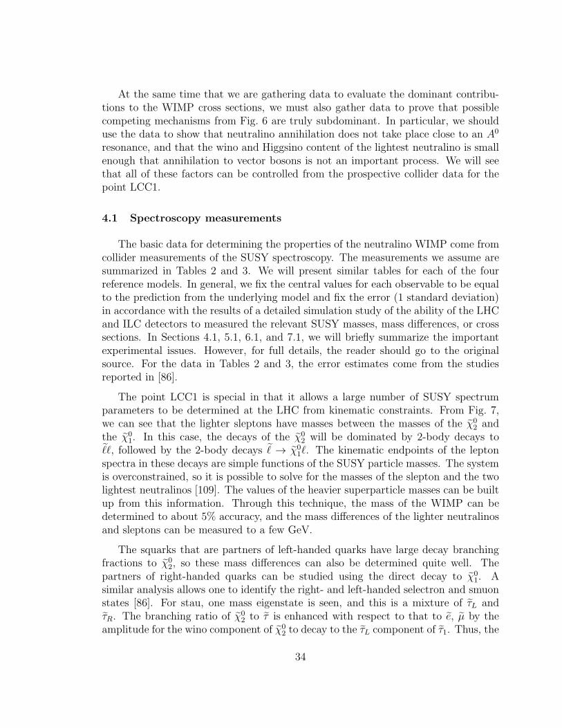
At the same time that we are gathering data to evaluate the dominant contribu-tions to the WIMP cross sections, we must also gather data to prove that possiblecompeting mechanisms from Fig. 6 are truly subdominant. In particular, we shoulduse the data to show that neutralino annihilation does not take place close to an A0
resonance, and that the wino and Higgsino content of the lightest neutralino is smallenough that annihilation to vector bosons is not an important process. We will seethat all of these factors can be controlled from the prospective collider data for thepoint LCC1.
4.1 Spectroscopy measurements
The basic data for determining the properties of the neutralino WIMP come fromcollider measurements of the SUSY spectroscopy. The measurements we assume aresummarized in Tables 2 and 3. We will present similar tables for each of the fourreference models. In general, we fix the central values for each observable to be equalto the prediction from the underlying model and fix the error (1 standard deviation)in accordance with the results of a detailed simulation study of the ability of the LHCand ILC detectors to measured the relevant SUSY masses, mass differences, or crosssections. In Sections 4.1, 5.1, 6.1, and 7.1, we will briefly summarize the importantexperimental issues. However, for full details, the reader should go to the originalsource. For the data in Tables 2 and 3, the error estimates come from the studiesreported in [86].
The point LCC1 is special in that it allows a large number of SUSY spectrumparameters to be determined at the LHC from kinematic constraints. From Fig. 7,we can see that the lighter sleptons have masses between the masses of the χ0
2 andthe χ0
1. In this case, the decays of the χ02 will be dominated by 2-body decays to
ℓℓ, followed by the 2-body decays ℓ → χ01ℓ. The kinematic endpoints of the lepton
spectra in these decays are simple functions of the SUSY particle masses. The systemis overconstrained, so it is possible to solve for the masses of the slepton and the twolightest neutralinos [109]. The values of the heavier superparticle masses can be builtup from this information. Through this technique, the mass of the WIMP can bedetermined to about 5% accuracy, and the mass differences of the lighter neutralinosand sleptons can be measured to a few GeV.
The squarks that are partners of left-handed quarks have large decay branchingfractions to χ0
2, so these mass differences can also be determined quite well. Thepartners of right-handed quarks can be studied using the direct decay to χ0
1. Asimilar analysis allows one to identify the right- and left-handed selectron and smuonstates [86]. For stau, one mass eigenstate is seen, and this is a mixture of τL andτR. The branching ratio of χ0
2 to τ is enhanced with respect to that to e, µ by theamplitude for the wino component of χ0
2 to decay to the τL component of τ1. Thus, the
34

mass/mass splitting LCC1 Value LHC ILC 500 ILC 1000m(χ0
1) 95.5 ± 4.8 0.05m(χ0
2) −m(χ01) 86.1 ± 1.2 0.07
m(χ03) −m(χ0
1) 261.2 ± @a 4.0m(χ0
4) −m(χ01) 280.1 ± 2.2a 2.2
m(χ+1 ) 181.7 ± - 0.55
m(χ+2 ) 374.7 ± - - 3.0
m(eR) 143.1 ± - 0.05m(eR) −m(χ0
1) 47.6 ± 1.0 0.2m(µR) −m(χ0
1) 47.5 ± 1.0 0.2m(τ1) −m(χ0
1) 38.6 ± 5.0 0.3BR(χ0
2 → ee)/BR(χ02 → τ τ) 0.077 ± 0.008
m(eL) −m(χ01) 109.1 ± 1.2 0.2
m(µL) −m(χ01) 109.1 ± 1.2 1.0
m(τ2) −m(χ01) 112.3 ± - 1.1
m(νe) 186.2 ± - 1.2m(h) 113.68 ± 0.25 0.05m(A) 394.4 ± * (> 240) 1.5
m(uR), m(dR) 548. ± 19.0 16.0m(sR), m(cR) 548. ± 19.0 16.0
m(uL), m(dL) 564., 570. ± 17.4 9.8m(sL), m(cL) 570., 564. ± 17.4 9.8
m(b1) 514. ± 7.5 5.7
m(b2) 539. ± 7.9 6.2m(t1) 401. ± (> 270) - 2.0m(g) 611. ± 8.0 6.5
Table 2: Superparticle masses and their estimated errors or lower limits for the parameterpoint LCC1. Lower limits are indicated in parentheses. The ILC columns contain themeasurements added or improved by the ILC at that energy. The symbol ‘-’ denotes thatthe measurement is not yet available. The symbol ‘*’ denotes the formula: mA > 200 GeV,or tan β < 7.0(mA/200.0). The notation ‘@a’ indicates that the mass measurement markedwith a superscript a could equally well be ascribed to this particle. All values are quotedin GeV.
35
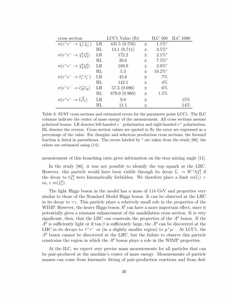
cross section LCC1 Value (fb) ILC 500 ILC 1000σ(e+e− → χ+
1 χ−
1 ) LR 431.5 (0.758) ± 1.1%∗
RL 13.1 (0.711) ± 3.5%∗
σ(e+e− → χ01χ
02) LR 172.2 ± 2.1%∗
RL 20.6 ± 7.5%∗
σ(e+e− → χ02χ
02) LR 189.9 ± 2.0%∗
RL 5.3 ± 10.2%∗
σ(e+e− → τ+1 τ−
1 ) LR 45.6 ± 7%RL 142.1 ± 4%
σ(e+e− → e+Re−
R) LR 57.3 (0.696) ± 6%RL 879.9 (0.960) ± 1.5%
σ(e+e− → t1t1) LR 9.8 ± 15%RL 11.1 ± 14%
Table 3: SUSY cross sections and estimated errors for the parameter point LCC1. The ILCcolumns indicate the center of mass energy of the measurement. All cross sections assumepolarized beams. LR denotes left-handed e− polarization and right-handed e+ polarization;RL denotes the reverse. Cross section values are quoted in fb; the error are expressed as apercentage of the value. For chargino and selectron production cross sections, the forwardfraction is listed in parentheses. The errors labeled by ∗ are taken from the study [86]; theothers are estimated using (14).
measurement of this branching ratio gives information on the stau mixing angle [11].
In the study [86], it was not possible to identify the top squark at the LHC.However, this particle would have been visible through its decay t1 → W+bχ0
1 ifthe decay to tχ0
1 were kinematically forbidden. We therefore place a limit m(t1) >mt + m(χ0
1).
The light Higgs boson in the model has a mass of 114 GeV and properties verysimilar to those of the Standard Model Higgs boson. It can be observed at the LHCin its decay to γγ. This particle plays a relatively small role in the properties of theWIMP. However, the heavy Higgs boson A0 can have a more important effect, since itpotentially gives a resonant enhancement of the annihilation cross section. It is verysignificant, then, that the LHC can constrain the properties of the A0 boson. If theA0 is sufficiently light or if tanβ is sufficiently large, the A0 can be discovered at theLHC in its decays to τ+τ− or (in a slightly smaller region) to µ+µ−. At LCC1, theA0 boson cannot be discovered at the LHC, but the failure to observe this particleconstrains the region in which the A0 boson plays a role in the WIMP properties.
At the ILC, we expect very precise mass measurements for all particles that canbe pair-produced at the machine’s center of mass energy. Measurements of particlemasses can come from kinematic fitting of pair-production reactions and from ded-
36

icated threshold energy scans [86]. In Table 2, mass measurements from kinematicfitting are given as mass differences from the lightest neutralino, and mass measure-ments from threshold determinations are indicated as absolute mass measurements.Because the masses of the light charginos and neutralinos enter the expressions forendpoints of kinematic distributions at the LHC, the determination of squark andgluino masses are improved by the ILC data even though these particles are notobserved directly at the ILC. This effect is reflected in Table 2.
The extension of the ILC to center of mass energies of 1000 GeV allows us toobserve several particles that were not accessible at the first stage of 500 GeV. Theseinclude the top squark and the second chargino. A particularly important additionis that of the H0 and A0 bosons, since the process e+e− → H0A0 becomes kinemat-ically accessible above 900 GeV. We estimate the accuracy of the H0 and A0 massdeterminations from the results of the study [90]. This sharpened knowledge of themasses of A0 and H0 will have an important effect on the determination of several ofthe WIMP properties.
4.2 Relic density
Now we can put the constraints shown in Tables 2 and 3 into the machinerydescribed in Section 3.2 to provide predictions of WIMP dark matter properties. Webegin with the WIMP relic density, as computed from the spectrum using DarkSUSY4.1. To see what the various data sets predict for this quantity, we generate the threelikelihood distributions corresponding to the three sets of constraints in the Tables,including the cross section for the two ILC points. In Fig. 8, we show the projections ofthese three likelihood distributions onto the coordinate representing the relic densityΩχh
2. The LHC data already gives a quantitative prediction for this density, with anaccuracy of about 7%. The data from the 500 GeV ILC sharpens this distributionto 2% accuracy, though the distribution has a long tail toward lower values. Theextension of the ILC to 1000 GeV further sharpens the prediction to about 0.25%accuracy, comparable to the accuracy expected from the Planck CMB measurement.Comparison of two such accurate values of the dark matter relic density would providea striking test of the WIMP model, as we have noted already in Section 2.5.
One might have suspected that the large number of constraints from the LHCwould already produce a very precise value of the relic density. However, it is clearfrom the spread of the LHC predictions in Fig. 8 that some information is missing.The scatter plots in Fig. 9(a,b) show one of the effects that contributes. Though themass differences of the supersymmetry particles are well fixed, the overall scale ofmasses is somewhat uncertain. This translates into the dominant uncertainty in theprediction of the relic density.
37

Figure 8: Relic density measurement for point LCC1. Histograms in this and all followingfigures give the probability distribution dP/dx of the quantity on the x-axis, given the threedifferent sets of accelerator constraints. Where the x axis is plotted logarithmically, theprobability plotted is actually dP/d log10 x. All histograms integrate to unity. Results forthe LHC make use of the assumption that the underlying physics model is supersymmetry.This might not be clear from the LHC data alone.
The tail in the Ωχh2 distribution from the 500 GeV ILC is also a surprise. Its
explanation is given in Fig. 9(c), which shows the correlation between Ωχh2 and the
mass of the A0 boson in this likelihood function. The s-channel process involvingthe A0 boson actually makes a small contribution to the annihilation cross sectionat LCC1, and this must be fixed to determine the cross section to a level below 1%.When we learn the mass of the A0 at the 1000 GeV ILC, this uncertainty in theprediction of Ωχh
2 is removed.
4.3 Relic density at SPS1a′
Nojiri, Polesello, and Tovey (NPT) [11] have also estimated the capability ofthe LHC data to predict the neutralino relic density. Their analysis was done at apoint quite similar, but not identical to, LCC1. By adjusting the parameters of oursimulation, we can make a direct comparison of our results to those of NPT. In thissection, we will describe our analysis of the point considered in [11] and show thatour results are in good agreement. Since NPT used a different method to arrive attheir estimate, this comparison provides a nontrivial check of the two methods.
38
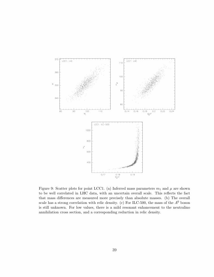
Figure 9: Scatter plots for point LCC1. (a) Inferred mass parameters m1 and µ are shownto be well correlated in LHC data, with an uncertain overall scale. This reflects the factthat mass differences are measured more precisely than absolute masses. (b) The overallscale has a strong correlation with relic density. (c) For ILC-500, the mass of the A0 bosonis still unknown. For low values, there is a mild resonant enhancement to the neutralinoannihilation cross section, and a corresponding reduction in relic density.
39
The value of Ωχh2 at LCC1 is about a factor of 2 too large to be consistent with
the CMB result [1]. It has been suggested that one could remedy this problem bymoving the mass of the τ1 from 134 GeV at LCC1 to 108 GeV, pushing the modelinto the stau coannihilation region. The new point is called SPS1a′ [91]. The shift ofthe τ1 mass adds contributions to the annihilation cross section for supersymmetryand therefore decreases the relic density. The neutralino physics at this point isintermediate between that at LCC1 and LCC3. Because coannihilation is important,the point has increased sensitivity to the value of the τ1 mass, though this sensitivityis not as extreme as we will see in Section 6 in our discussion of LCC3.
According to [91], the table of measurement errors at SPS1a′ should be the sameas that of LCC1 (Tables 2 and 3), even though the expected values are somewhatdifferent. We have therefore carried out MCMC scans for SPS1a′ using the same con-straints as for SPS1a (LCC1), only modifying the reference values of supersymmetrymasses and cross sections. The results of that scan for the relic density are shown inFig. 10.
The analysis of NPT ran as follows: In the stau coannihilation region, the neu-tralino relic density is mainly sensitive to 7 of the 24 MSSM parameters, the fourparameters of the neutralino mass matrix m1, m2, µ, and tan β and the three pa-rameters of the stau mass matrix, which we can represent as the combinations m(τ1),m(τ2), θτ . The LHC data is expected to give relatively precise values for five quan-tities sensitive to these parameters, three neutralino masses, the mass of the τ1, andthe ratio of branching ratios BR(χ0
2 → ee)/BR(χ02 → τ τ1). At the true point, the
gaugino-Higgsino and stau mixing angles are relatively small, so the actual depen-dence of the relic density on the mixing angles (and thus on tan β) is relatively weak.The dependence on m(τ2) is also weak. So it makes sense in this case to solve forthe five parameters m1, m2, µ, m(τ1), and θτ from the measurements, propagate themeasurement errors through to an error on the prediction of Ωχh
2, and then add anestimate of the additional uncertainty from variation of tan β and m(τ2). In solvingfor the five parameters, NPT chose the preferred solution and did not take accountof the possibility of multiple solutions.
The final error on the relic density turned out to be dominated by the uncertaintyin the mass of of the τ1. This is tied to the error in measuring the endpoint of thedilepton mass spectrum in the decay χ0
2 → τ+τ−χ01. For the case of tau leptons, the
endpoint is not a sharp feature and it has not been understood in detail how well thispoint can be measured. For the purpose of their analysis, Polesello and Tovey, whoare two of the experts on such measurements in the ATLAS collaboration, estimatedthat the error would be below 5 GeV and expressed the hope that it could be broughtdown to 1 GeV. This is considerably more aggressive than the uncertainty presentedin [86], which we have assumed in our study.
40

In Fig. 11, we show the histograms of Ωχh2 from the LHC constraints for our
scan with parameters based on [86] and imposing the stronger constraints that theττ endpoint can be measured to 5 GeV or to 1 GeV. From the figure, it is clear thatNPT are correct that this is the dominant source of error. The standard deviationsfor the three histograms correspond to
σ(Ωh2)/Ωh2 = 18.6%, 14.4%, 11.7% (19)
with the last two cases to be compared to the results of NPT,
σ(Ωh2)/Ωh2 = 19.% , 10.5% (20)
Their results correspond to a scan over 5 parameters, while our results scan overthe full set of 24 MSSM parameters. We thus verify that the analysis of NPT doescapture the strongest dependences of Ωh2 on the MSSM parameters, and also thatour method for estimating the uncertainty in Ωχh
2 does agree with a more directmethod in this case where Ωχh
2 is strongly constrained. In Fig. 12, we show thescatter plot of Ωχh
2 vs. m(χ01) from our scan for the case of a 1 GeV measurement
of the ττ endpoint. This is, again, a scan over 24 parameters. It is interesting tocompare this to Fig. 9 of NPT, which gives the result of a 5-parameter scan.
Given the very strong constraints on the spectrum at SPS1a′, the ambiguities inthe solutions play a rather small role. in particular, the constraint on the ratio ofbranching ratios of the χ0
2 almost completely eliminates the solution in which thelighter τ is dominantly τL. Our data contains only a small influence of the region inwhich the A boson provides a resonant enhancement of the neutralino annihilation.Fig. 13 shows a scatter plot Ωχh
2 vs m(A) for the SPS1a′ LHC data sample. We seea small branch leading to low m(A) and low Ωχh
2, representing the effect of an Aboson resonance near the annihilation threshold.
4.4 Annihilation cross section
In Fig. 14, we show the likelihood distribution of the neutralino pair annihilationcross section times velocity σχχv, evaluated at threshold. As we have discussed inSection 2.7, this cross section is needed to interpret astrophysical signals of darkmatter annihilation. We will discuss the determination of this quantity from a moregeneral point of view in Section 8.
At LCC1, the most important neutralino annihilation reactions are P-wave pro-cesses whose cross section vanishes at threshold. The important contributions to thethreshold cross sections then come from annihilation to massive fermion pairs, τ+τ−
and bb, with the latter final state dominating. The most important parameters for
41

Figure 10: Relic density for point SPS1a′. See Fig. 8 for description of histograms. In thiscase, the ILC-1000 provides no improvement in the relic density measurement over ILC-500.
Figure 11: Relic density for point SPS1a′ at LHC. A dominant uncertainty at this point isthe mass of the stau. Results of taking the stau-neutralino mass difference to have an errorof 5 GeV are illustrated in red. Alternatively, results of taking the position of the tau-tauedge to have an error of 5 GeV (purple) and 1 GeV (blue) are also illustrated.
42

Figure 12: Scatter plot for point SPS1a′. Relic density is plotted against neutralino mass,for points where the position of the tau-tau edge is measured to 1 GeV.
Figure 13: Scatter plot for point SPS1a′. The A0 mass is plotted against relic density,illustrating the small allowed region where A0 resonance significantly decreases the relicdensity.
43

χ01χ
01 → bb are the b masses; at LCC1, these masses would be determined at the LHC.
The ILC at 500 GeV determines the neutralino mixing angles, and this makes a smallimprovement in the prediction. The marked improvement from the ILC at 1000 GeVcomes from the determination of the A0 mass. Note that, because of the suppressionof the P-wave channels, this annihilation cross section is about 12 fb, as opposed tothe 0.9 pb predicted by (2).
In Fig. 15, we show the likelihood distribution for the exclusive annihilation crosssections to γγ and γZ0. These cross sections are dominated by squark loops and aredetermined quite well already from LHC data. The cross sections are small, but, atLCC1, these processes might be visible as sharp lines in the gamma ray spectrum.
In Fig. 16, we present two representative calculations that indicate how this infor-mation might be used. We will postulate two situations in which dark matter mightbe detected by gamma rays from annihilation, and we will work through the numbersto see how accurately the absolute dark matter density can be obtained from theseobservations. Because of the intrinsically small annihilation cross sections at LCC1,the final results that we will show in this section will be rather marginal. In latersections, we will present the same calculations for the other three reference points.At points LCC2 and LCC4, the annihilation cross section at threshold is 50 timeslarger, leading to much more optimistic expectations for dark matter detection.
First, we consider the dark matter distribution at the galactic center, assumingthe NFW distribution shown in Fig. 5. We set the boost factor B = 1. Observationin a circle of angular area 1.5×10⁻⁴ sr (angular radius 0.4) gives 〈J(Ω)〉 = 7700. Weuse this value to predict the rate of gamma ray emission from this source. To do this,we use the spectrum of gammas expected for neutralino annihilation at LCC1, scaledto the predicted total annihilation cross section. (We will describe this spectrum inSection 8.1.) We impose a lower energy cutoff of Eγ > 3.1 GeV. Background fromenergetic processes at the galactic center is a major issue in this analysis. We haveadded to the counting rate the gamma ray background in the same energy regionaccording to the parametrization of Bergstrom, Ullio, and Buckley [110]. A five-yearobservation by the GLAST gamma-ray observatory [111], in which the galactic centeris visible 20% of the time, yields an expectation of 5 signal photons over a backgroundof 360 background gamma ray photons. This is a S/
√B less than 1, so we will only
be able to quote upper bounds on 〈J〉 for this model.
We can now work backwards to determine the source strength 〈J(Ω)〉 from theobservation. For the purpose of this exercise, we assign the background rate a 5%systematic uncertainty. In pratice, it will be a challenge to obtain such a good under-standing of the background. Gamma rays come from the galactic center from manysources, and, in particular, from energetic processes associated with the black holeat the center of galaxy. However, gamma rays from π0’s produced in soft hadronic
44

interactions have a soft power-law energy spectrum different from that predicted forneutralino annihilation. In addition, much of the the observed gamma radiationseems to be associated with molecular clouds that ring the galactic center ratherthan having a peak at the center itself. This observation has already been used toimprove the limits on gamma rays from the galactic center from the EGRET observa-tory [112]. However, recent work of the HESS Collaboration, while spatially resolvingmany gamma ray sources from the galactic center, also shows that this center is thesource of a power law spectrum of very high-energy gamma rays, up to 10 TeV inenergy [113]. For the purposes of the analysis in this paper, we assume that it willbe possible to measure these effects and, to the extent allowed by statistics, separatethem from the WIMP annihilation signal. This might well be possible; we will knowbetter in a few years [114].
For the case of LCC1, even this aggressive estimate makes the uncertainty in thebackground the dominant source of error. The likelihood distribution for 〈J(Ω)〉 thatwe obtain from this analysis is shown in Fig. 16(a). In this and later figures forlikelihood distributions of 〈J〉, we assume a prior distribution that is flat in log 〈J〉.For LCC1, we do not obtain a prediction of 〈J(Ω)〉, but we do obtain a strong upperlimit that excludes otherwise viable models predicting large values of J(Ω).
In models in which the galaxy is build up from hierarchical dark matter clustering,one should expect to find localized clumps of dark matter. We choose a typical objectfrom the semi-analytic simulation data of Taylor and Babul [76], a dark matter clumpwith a mass of 106M⊙ and a scale radius of 500 pc, at a distance of 6 kpc, with itsinternal structure described by an NFW profile. Observing in a disk of 1.5× 10⁻⁴ sr,the object has 〈J(Ω)〉 = 2500. We impose a lower energy cutoff of Eγ > 1 GeV andadd extra-galactic background at the level measured by EGRET [115]. Assuminga five-year observation by the GLAST observatory, in which this object would bevisible 20% of the time, we expect 4 signal photons, plus 60 photons from the extra-galactic background. Working backwards from the observations, assuming that theextra-galactic background is well characterized from observations in other regions ofthe sky, we find the likelihood distribution of 〈J(Ω)〉 shown in Fig. 16(b). Given theratio of signal/background, we can only impose an upper limit on 〈J〉, but this stillhas the power to exclude models with very strongly peaked dark matter clumps.
Certainly, the discovery of a localized clump of dark matter in gamma rays wouldbe remarkable in itself. But it would be more remarkable if we could obtain fromparticle physics a calibration of the absolute scale of its dark matter density. Fig. 16(b)shows that this is possible in principle. At the other benchmark points, which givelarger gamma ray fluxes from neutralino annihilation, we will see this idea realizedmore clearly.
45
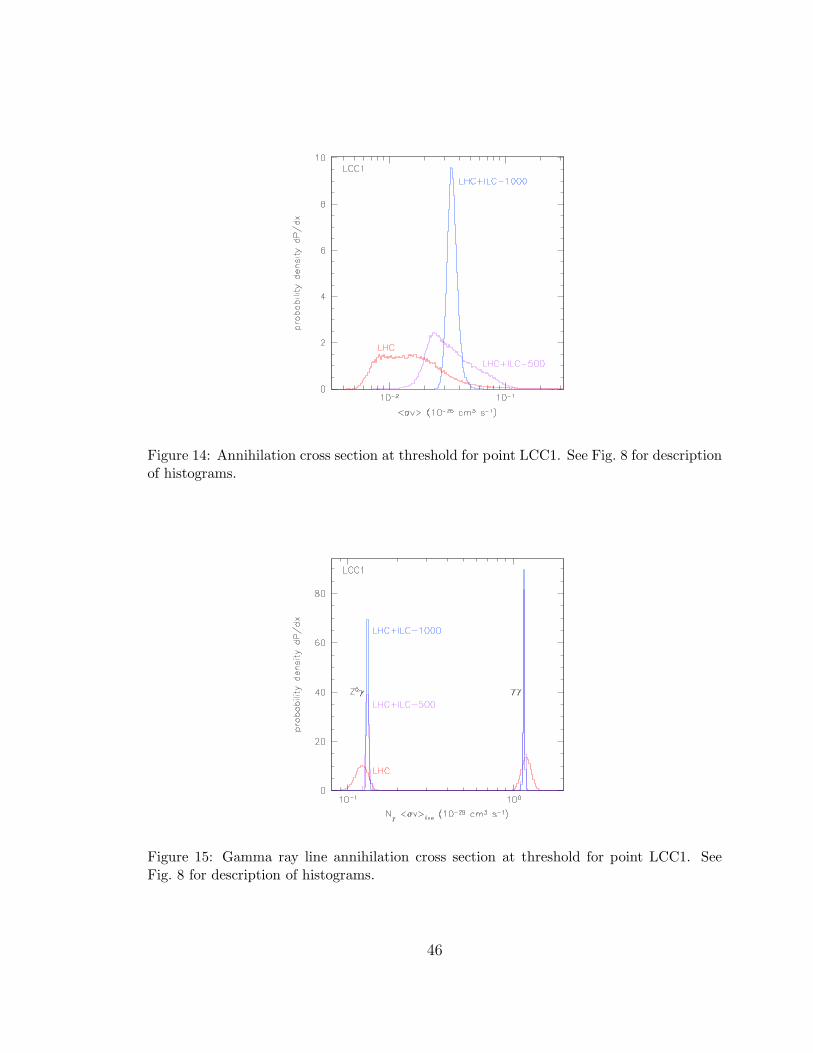
Figure 14: Annihilation cross section at threshold for point LCC1. See Fig. 8 for descriptionof histograms.
Figure 15: Gamma ray line annihilation cross section at threshold for point LCC1. SeeFig. 8 for description of histograms.
46

Figure 16: Halo density profiles for point LCC1: (a) galactic center, (b) dark matter clumpin the galactic halo. Angle-averaged J values as measured by combining a 5-year all-skydataset from GLAST with accelerator measurements are shown. See Fig. 8 for descriptionof histograms.
47

4.5 Direct detection cross section
In Fig. 17, we show the likelihood distributions of the spin-averaged neutralino-proton cross section σχp, evaluated at threshold. We remind the reader that, in ouranalysis in this section and in the corresponding analyses of the other models, we willignore the uncertainty in the evaluation of the σχp resulting from the uncertainty inthe low-energy QCD parameter fTs discussed in Section 2.6. The cross section σχp issufficiently close to the spin-independent isoscalar cross section that it can be usedto interpret signals of direct detection of dark matter in underground detectors. Thecorresponding distributions for the spin-dependent part of the cross section σχn areshown in Fig. 18.
From Fig. 17, it is clear that neither the LHC nor the ILC at 500 GeV can make aparticularly accurate prediction of this cross section. At LCC1, the direct detectioncross section is dominated by the t-channel exchange of the heavy Higgs boson H0.In the MSSM, the mass of the H0 is very close in mass to the A0 unless both are light.Even with the ILC data at 500 GeV, this mass is essentially unconstrained. The sharpedge in the distributions at 10−9 pb reflects the contribution of the light Higgs h0.Fig. 19, which displays the correlation in the LHC likelihood function between theneutralino-proton cross section and the heavy Higgs boson mass, shows clearly thatthis parameter is the essential missing piece of information It also illustrates the factthat above about 1.5 TeV, the cross section is insensitive to the heavy Higgs massas the light Higgs contribution is of a comparable size. The slight improvement fromthe LHC to the 500 GeV ILC reflects the determination of neutralino mixing angles,which enter the neutralino-Higgs vertices. Indeed, when the H0 and A0 particles areobserved and measured at the 1000 GeV ILC, we obtain a prediction of the directdetection cross section to about 20% accuracy.
As in the previous section, it is illuminating to work through an example of thisapplication of this cross section determination to experimental data. At the pointLCC1, dark matter events would not be seen in the CDMS II experiment, but thesignal should be discovered in the next-generation detector SuperCDMS or ‘Super-CDMS 25kg’ [45]. This is a 26.67 kg detector on the model of CDMS, with mostof the mass in Germanium, to be located in the low-background environment of theSudbury mine. Estimates of the detection capabilities of SuperCDMS were com-puted assuming 2.5 years of operation (ending in 2011) with a total exposure of closeto 16,000 kg d. Sensitivity calculations have assumed that the local halo density is0.3 GeV cm−3, the halo circular velocity is 220 km s−1, the halo escape velocity is650 km s−1, and that the velocity distribution is Maxwellian. The capabilities ofheavy-noble-liquid detectors of the same mass and exposure time should be similar.Over the time scale required to realize the ILC at 1000 GeV, we might expect to seea direct detection experiment scaled up to 1 Ton size. This would allow measurement
48

of the annual flux variation and the velocity distribution of directly detected WIMPs.For our analysis, however, we will concentrate on the implication of the total ratemeasurement combined with collider data.
For the parameters that we have just described, the SuperCDMS group estimatesthat they will see 16 signal events, assuming a uniform dark matter distribution inthe disk and the cross section predicted for LCC1, and negligible background [65].Dividing the observed rate by the predicted cross section, we would obtain a directmeasurement of the flux of dark matter impinging on the detector. We should notethat this derived flux is an effective quantity. The detection efficiency for WIMPsdepends on the velocity distribution, and the simulation [65] used the efficiency calcu-lated for the reference halo model described in the previous paragraph. In presentingour results, we will refer to the derived quantity as Φlocal/Φ0, the local flux of WIMPsdivided by the flux in the reference model, assuming the same average detectionefficiency.
In Fig. 20, we show the likelihood distribution for the effective local flux, obtainedby combining the distribution of values of the cross section with the statistical un-certainty of the direct detection measurement. The distribution shown ignores theuncertainty in the direct detection cross section from our poor knowledge of low-energy QCD parameters. But, assuming that these parameters can be determined,we see from the figure that the combination of the data from the ILC at 1000 GeVand count rate from WIMP direct detection would measures the local flux of darkmatter at the Earth to 28% accuracy.
4.6 Constraints from relic density and direct detection
If LCC1 is the correct theory of Nature, it is possible that, by the end of thedecade, the LHC will have observed missing energy events and a convincing signal ofdark matter from annihilation to gamma rays will also have been observed. Values ofthe WIMP mass will have been obtained from the LHC and from the endpoint of thegamma ray spectrum, and these values will have been seen to agree. Undergrounddirect detection experiments in the 25 kg range such as SuperCDMS may also givethe WIMP mass and flux at the Earth. Further, the Planck measurements of theCMB will have provided a very accurate measurement of the cosmic density of darkmatter. Under these circumstances, it would be very tempting to use the Planck andSuperCDMS measurements to constrain the parameters of supersymmetry model.
This analysis would depend on very strong assumptions whose status would stillbe open. It would not be clear that the model leading to missing energy at the LHCwas in fact supersymmetry, or that the neutralino was the lightest supersymmetricparticle. It would also be unclear whether the neutralino made up 100% of the dark
49
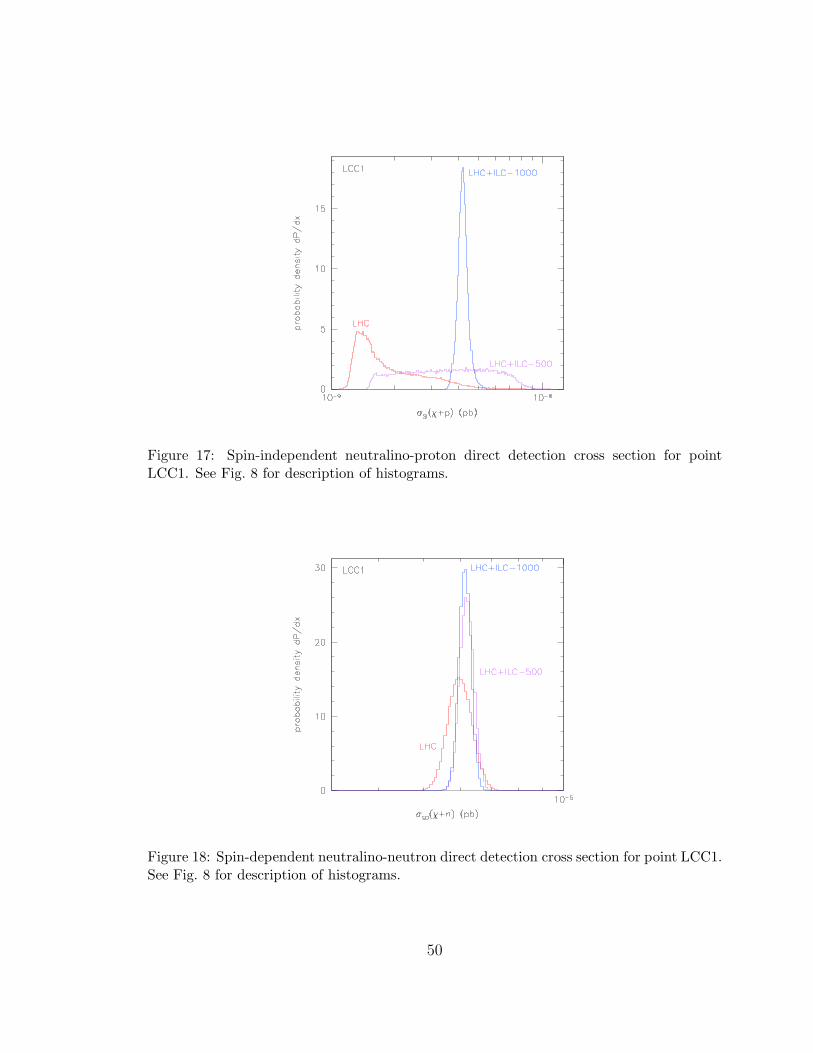
Figure 17: Spin-independent neutralino-proton direct detection cross section for pointLCC1. See Fig. 8 for description of histograms.
Figure 18: Spin-dependent neutralino-neutron direct detection cross section for point LCC1.See Fig. 8 for description of histograms.
50

Figure 19: Scatter plot of the spin-independent direct detection cross section vs. m(A) forpoint LCC1. The strong dependence of the direct detection cross section on the A0 mass isclearly seen.
Figure 20: Effective local WIMP flux Φlocal/Φ0 at the Earth for point LCC1. The resultsassume the SuperCDMS measurement described in the text. See Fig. 8 for description ofhistograms.
51

matter, and whether unknown effects had diluted its abundance. The flux of darkmatter particles at the Earth is also uncertain, and depends on the halo model.Nevertheless, by making these assumptions, we could draw very strong conclusionsthat could later be checked by detailed particle physics measurements.
At this point, LHC data alone provide a prediction of the relic density to 7%accuracy under the assumptions of the standard cosmology. This is already quiteprecise. However, the annihilation and direct detection cross sections would not bewell determined, and information from a direct dectection experiment could be usedto improve our knowledge of the particle physics model. For example, applying aconstraint from the direct detection rate to the annihilation cross section improvesthe determination of this cross section both for the LHC and the ILC-500 data sets.As shown in Fig. 21, the central values of the distributions shift much closer tothe correct value, though, curiously, the variances of the distributions are not muchimproved.
Further into the future, the ILC-500 will predict the relic density at the 1.5%level. It is thus unlikely that CMB or other cosmological measurements of the relicdensity will greatly improve the situation, though if Planck can measure relic densityto 0.5% as advertised, this would be a factor of 3 improvement. The direct detectioncross section measurement is now less skewed, with 45% errors. SuperCDMS wouldgive 16 events, for a 25% error on the WIMP flux times cross section. In a particularhalo model, one might hope to use this measurement, but the advantage would notbe likely to be significant.
Fundamentally, the large uncertainty in the direct detection cross section is dueto the unknown heavy Higgs mass. Applying the direct detection constraint greatlyimproves the shape of the distribution of this quantity at LHC and ILC-500, wherethe heavy Higgs are unobserved, as illustrated in Fig. 22.
The ILC-1000 can predict the relic density at the 0.25% level and the directdetection cross section at the 5% level. This is the unique case under study where theastrophysical measurements have no benefit beyond the crucial consistency checks.
52

Figure 21: Annihilation cross section at threshold for point LCC1. A direct detectionconstraint from 2 years of a 25 kg SuperCDMS is applied. Compared with Fig. 14, it isclear that the direct detection constraint significantly improves the measurement of theannihilation cross section in advance of ILC-1000. See Fig. 8 for description of histograms.
53

Figure 22: LCC1 heavy Higgs mass mA, before and after a direct detection constraint isapplied. The constraint allows a crude measurement of the A0 mass in advance of theILC-1000, which directly produces the A0. See Fig. 8 for description of histograms.
54

5 Benchmark point LCC2
In the next few sections, we will carry out the analysis that we have just describedat LCC1 for the other three reference points. The parameter set LCC1 was speciallychosen by the authors of [86] as a point at which most of particles of the supersym-metry spectrum could be observed at the LHC and then measured precisely at theILC. In more generic scenarios of supersymmetry, the information available to bothcolliders will be more limited.
At LCC2, for example, the squarks and sleptons are made extremely heavy, soheavy that it is unlikely that they could be observed at the LHC. However, the modelstill allows the discovery of supersymmetry at the LHC. The model contains a gluinoat 850 GeV, giving a cross section of about 10 pb for supersymmetry production atthe LHC, and charginos and neutralinos in the range 100–300 GeV. The dominantmode of neutralino annihilation is to W+W− and Z0Z0.
Although we cannot observe the heavy supersymmetric particles, we might hopethat the lighter ones, which we can observe, contain most of the information neededto predict the astrophysical cross sections needed to analyze dark matter detectionexperiments. The main contributions to neutralino annihilation come from diagramsin which neutralinos and charginos are exchanged. The main contribution to thedirect detection cross section comes, in this case, from exchange of the light Higgsboson h0. Both reactions depend strongly on the gaugino-Higgsino mixing angles, andso the measurement of these angles becomes the major issue for the interpretation ofcollider measurements in terms of the underlying spectrum parameters.
5.1 Spectroscopy measurements
As we have already noted, the LHC will give a large sample of supersymmetryevents. Most of these events will involve gluino pair production, followed by gluinodecays to qqχ, where χ is a neutralino or chargino. The subsequent evolution canbe seen from the spectrum of the model, shown in Fig. 23. The mass difference ofthe first and third neutralinos is less than mZ . Thus, both the second and the thirdneutralino will decay to the first neutralino through a virtual Z0 that can be observedas a lepton pair,
χ0i → ℓ+ℓ−χ0
1 , (21)
for i = 2, 3. These processes will allow measurements of the two mass differencesto an accuracy comparable to that with which the χ0
2–χ01 mass difference can be
measured at LCC1. In addition, the gluino mass should be determined to about 10%accuracy from the distribution of missing energy and visible transverse mass, and themass of the lightest neutralino should be determined to about 10% by more detailed
55
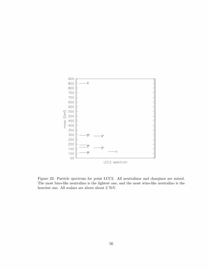
Figure 23: Particle spectrum for point LCC2. All neutralinos and charginos are mixed.The most bino-like neutralino is the lightest one, and the most wino-like neutralino is theheaviest one. All scalars are above about 2 TeV.
56
kinematic fitting of the these events. Unfortunately, it will be more difficult that atLCC1 to find the charginos or the fourth neutralino, so it is likely that these spectrumparameters are the only ones that can be determined from the LHC data.
Measurements at the ILC will map out much more of the chargino and neutralinospectrum [87]. At a center of mass energy of 500 GeV, the ILC will study the lighterstates of this spectrum through e+e− → χ+
1 χ−
1 and e+e− → χ02χ
03. It will also make
a very accurate measurement of the mass of χ+1 by determination of the threshold
for producing this particle. The e+e− production cross sections are sensitive to thegaugino-Higgsino mixing angles and can also be used to constrain the supersymmetryparameters. A second stage of operation at center of mass energies of 1000 GeV canobserve the reactions e+e− → χ0
3χ04 and e+e− → χ+
2 χ−
2 and measure the masses ofthe χ0
4 and χ+2 .
The complete list of spectrum constraints that we expect for this point for theLHC and for each stage of the ILC is given in Tables 4 and 5.
5.2 Relic density
We can now use these constraints on the spectrum as the basis for an explorationof the allowed supersymmetry parameter space. The results of the three Monte Carloscans, projected onto the axis of the predicted WIMP relic density, are shown inFig. 24. The distribution from the LHC constraints is quite broad, with a standarddeviation of about 40% and also a significant secondary peak near Ωχh
2 = 0. Theprediction of Ωχh
2 from the ILC data a 500 GeV has an accuracy of about 14%, andthis improves to about 8% using the data from the ILC at 1000 GeV.
The main difficulty in determining the relic density from the LHC data is that thetwo precision measurements of mass differences do not provide enough informationto fix the gaugino-Higgsino mixing angles. Without an accurate determination ofthe mixing angles, the relatively accurate determination of the WIMP mass has littlepredictive power.
However, it is also true that the LHC data can be interpreted in multiple ways interms of the underlying parameters. This is illustrated by making scatter plots of theMonte Carlo data, as we show in Fig. 25. In Fig. 25(a), we show the scatter plot ofthe data with LHC constraints in the plane of m1 vs. µ. The data clearly shows threesolutions, corresponding to a bino-, wino-, and Higgsino-like lightest neutralino. Thephase space for the latter two solutions is restricted by our constraint that m(χ+
1 )should be greater than 125 GeV. These incorrect solutions are responsible for thepeak in the relic density likelihood function at LHC for very small values.
In Fig. 25(b), we show the correlation between Ωχh2 and m(A) at the 500 GeV
57

mass/mass splitting LCC2 value LHC ILC 500 ILC 1000m(χ0
1) 107.9 ± 10 1.0m(χ0
2) −m(χ01) 58.5 ± 1.0 0.3
m(χ03) −m(χ0
1) 82.3 ± 1.0 0.2m(χ0
4) −m(χ01) 186.3 ± - - 3.0
m(χ+1 ) 159.7 ± - 0.55
m(χ+1 ) −m(χ0
1) 51.8 ± - 0.25m(χ+
2 ) 286.7 ± - - 1.0m(eR) 3277. ± (> 350) (> 480)m(µR) 3277. ± (> 350) (> 480)m(τ1) 3252. ± (> m(χ0
2)) (> 480)m(eL) 3280. ± (> 350) (> 480)m(µL) 3280. ± (> 350) (> 480)m(τ2) 3268. ± (> 480)m(h) 118.68 ± 0.25 0.05m(A) 3242. ± * (> 240) (> 480)
m(uR), m(dR) 3312. ± (> 2000)m(sR), m(cR) 3312. ± (> 1500)
m(uL), m(dL) 3301. ± (> 2000)m(sL), m(cL) 3301. ± (> 1500)
m(b1) 2710. ± (> 1500)
m(b2) 3241. ± (> 1500)m(t1) 1976. ± (> 1500)m(g) 850. ± 85.
Table 4: Superparticle masses and their estimated errors or limits for the parameter pointLCC2. The notation is as in Table 2.
cross section LCC2 value ILC 500 ILC 1000
σ(e+e− → χ+1 χ
−
1 ) LR 1364. (0.479) ± 1%∗
RL 145.6 (0.438) ± 4%∗
σ(e+e− → χ02χ
03) LR 127.6 ± 4%∗
RL 105.8 ± 5%∗
Table 5: SUSY cross sections and estimated errors for the parameter point LCC2. Thenotation is as in Table 3. The errors labeled by ∗ are taken from the study [87].
58
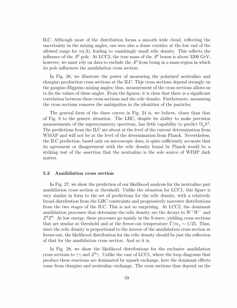
ILC. Although most of the distribution forms a smooth wide cloud, reflecting theuncertainty in the mixing angles, one sees also a dense corridor at the low end of theallowed range for m(A), leading to vanishingly small relic density. This reflects theinfluence of the A0 pole. At LCC2, the true mass of the A0 boson is about 3200 GeV;however, we must rely on data to exclude the A0 from being in a mass region in whichits pole influences the annihilation cross section.
In Fig. 26, we illustrate the power of measuring the polarized neutralino andchargino production cross sections at the ILC. Thje cross sections depend strongly onthe gaugino-Higgsino mixing angles; thus, measurement of the cross sections allows usto fix the values of these angles. From the figures, it is clear that there is a significantcorrelation between these cross sections and the relic density. Furthermore, measuringthe cross sections removes the ambiguities in the identities of the particles.
The general form of the three curves in Fig. 24 is, we believe, closer than thatof Fig. 8 to the generic situation. The LHC, despite its ability to make precisionmeasurements of the supersymmetry spectrum, has little capability to predict Ωχh
2.The predictions from the ILC are about at the level of the current determination fromWMAP and will not be at the level of the determination from Planck. Nevertheless,the ILC prediction, based only on microscopic data, is quite sufficiently accurate thatits agreement or disagreement with the relic density found by Planck would be astriking test of the assertion that the neutralino is the sole source of WIMP darkmatter.
5.3 Annihilation cross section
In Fig. 27, we show the prediction of our likelihood analysis for the neutralino pairannihilation cross section at threshold. Unlike the situation for LCC1, this figure isvery similar in form to the set of predictions for the relic density, with a relativelybroad distribution from the LHC constraints and progressively narrower distributionsfrom the two stages of the ILC. This is not so surprising. At LCC2, the dominantannihilation processes that determine the relic density are the decays to W+W− andZ0Z0. At low energy, these processes go mainly in the S-wave, yielding cross sectionsthat are similar at threshold and at the freeze-out temperature T/mχ ∼ 1/25. Thus,since the relic density is proportional to the inverse of the annihilation cross section atfreeze-out, the likelihood distribution for the relic density should be just the reflectionof that for the annihilation cross section. And so it is.
In Fig. 28, we show the likelihood distributions for the exclusive annihilationcross sections to γγ and Z0γ. Unlike the case of LCC1, where the loop diagrams thatproduce these reactions are dominated by squark exchange, here the dominant effectscome from chargino and neutralino exchange. The cross sections thus depend on the
59
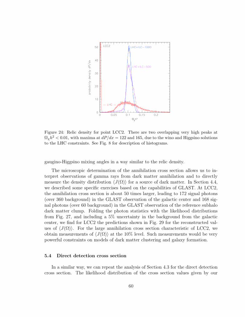
Figure 24: Relic density for point LCC2. There are two overlapping very high peaks atΩχh
2 < 0.01, with maxima at dP/dx = 122 and 165, due to the wino and Higgsino solutionsto the LHC constraints. See Fig. 8 for description of histograms.
gaugino-Higgsino mixing angles in a way similar to the relic density.
The microscopic determination of the annihilation cross section allows us to in-terpret observations of gamma rays from dark matter annihilation and to directlymeasure the density distribution 〈J(Ω)〉 for a source of dark matter. In Section 4.4,we described some specific exercises based on the capabilities of GLAST. At LCC2,the annihilation cross section is about 50 times larger, leading to 172 signal photons(over 360 background) in the GLAST observation of the galactic center and 168 sig-nal photons (over 60 background) in the GLAST observation of the reference subhalodark matter clump. Folding the photon statistics with the likelihood distributionsfrom Fig. 27, and including a 5% uncertainty in the background from the galacticcenter, we find for LCC2 the predictions shown in Fig. 29 for the reconstructed val-ues of 〈J(Ω)〉. For the large annihilation cross section characteristic of LCC2, weobtain measurements of 〈J(Ω)〉 at the 10% level. Such measurements would be verypowerful constraints on models of dark matter clustering and galaxy formation.
5.4 Direct detection cross section
In a similar way, we can repeat the analysis of Section 4.3 for the direct detectioncross section. The likelihood distribution of the cross section values given by our
60

Figure 25: Scatter plots for point LCC2. (a) m1 vs. µ distribution for LHC, illustratingmultiple solutions. Left to right, these are bino (correct), wino, and Higgsino. (b) mA vs.Ωχh
2, showing the influence of resonant annihilation.
61
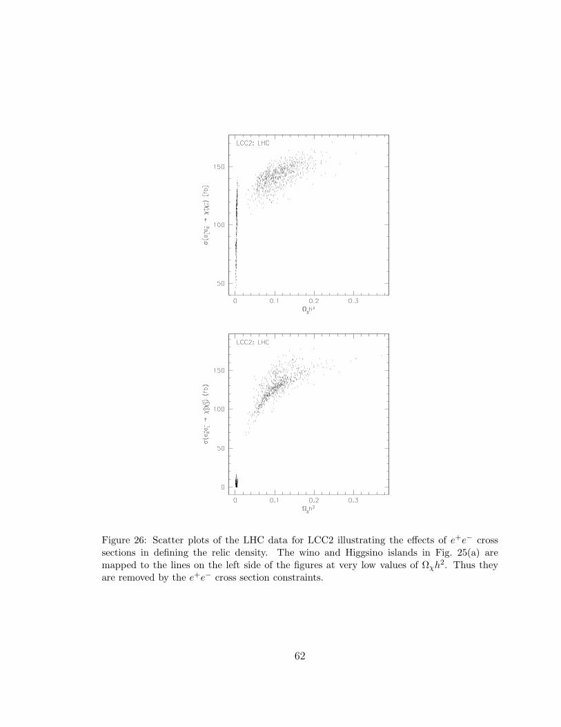
Figure 26: Scatter plots of the LHC data for LCC2 illustrating the effects of e+e− crosssections in defining the relic density. The wino and Higgsino islands in Fig. 25(a) aremapped to the lines on the left side of the figures at very low values of Ωχh
2. Thus theyare removed by the e+e− cross section constraints.
62
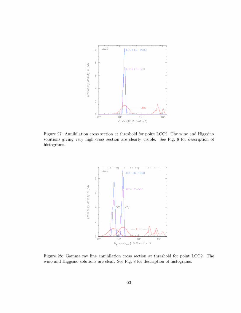
Figure 27: Annihilation cross section at threshold for point LCC2. The wino and Higgsinosolutions giving very high cross section are clearly visible. See Fig. 8 for description ofhistograms.
Figure 28: Gamma ray line annihilation cross section at threshold for point LCC2. Thewino and Higgsino solutions are clear. See Fig. 8 for description of histograms.
63
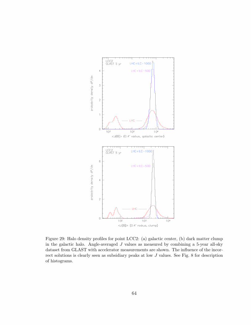
Figure 29: Halo density profiles for point LCC2: (a) galactic center, (b) dark matter clumpin the galactic halo. Angle-averaged J values as measured by combining a 5-year all-skydataset from GLAST with accelerator measurements are shown. The influence of the incor-rect solutions is clearly seen as subsidiary peaks at low J values. See Fig. 8 for descriptionof histograms.
64

Figure 30: Spin-independent neutralino-proton direct detection cross section for pointLCC2. The wino and Higgsino solutions have large cross sections, easily seen. See Fig. 8for description of histograms.
Monte Carlo scans is shown in Fig. 30. At LCC2, the spin-independent neutralino-proton cross section is dominated by t-channel exchange of the light Higgs boson h0.The mass of this particle is expected to be measured well at the LHC in the decayh0 → γγ. So the LHC constraints already give a reasonably precise estimate of thedirect detection cross section, although, as we see from the figure, the ambiguity inthe solution leads to additional peaks at high values of the cross section. The ILCmeasurements sharpen the determination of the mixing angles and also remove thealternative solutions. The corresponding predictions for the spin-dependent part ofthe neutralino-neutron cross section are shown in Fig 31.
As in Section 4.4, we can combine our microscopic knowledge of the detection crosssection with the expected event yield from the SuperCDMS detector to estimate ourability to directly measure the local flux of dark matter at the earth. As before, ouranalysis omits the uncertainty from low-energy QCD parameters. For this case, weexpect a signal of 67 events in SuperCDMS. Folding the statistical uncertainty withthe uncertainty in the cross section, we find the determination of the effective localhalo flux shown in Fig. 32.
65

Figure 31: Spin-dependent neutralino-neutron direct detection cross section for point LCC2.See Fig. 8 for description of histograms.
Figure 32: Effective local WIMP flux at the Earth for point LCC2. The results assumethe SuperCDMS measurement described in the text. The second peak at low effective fluxis due to the high cross section wino and Higgsino solutions. See Fig. 8 for description ofhistograms.
66

5.5 Constraints from relic density and direct detection
LCC2 is a special case in that the identity of the lightest neutralino at LHC isunknown, with discrete possibilities: the bino (correct), wino and Higgsino solutionsdiscussed previously. Both incorrect solutions are confined to regions quite far fromthe central values of both relic density and direct detection cross section. Thus,we find that either the direct detection or relic density constraint completely elim-inates the wino and Higgsino solutions for the lightest neutralino. The eliminationof these islands has very significant effects on the measurements at LHC, includingthe annihilation cross section and branching ratios. In fact, the entire structure ofthe neutralino mass matrix is greatly improved. With either the direct detection orrelic density constraint removing the incorrect islands, the bino and wino fractions ofevery neutralino are measured to better that 15% at the LHC.
Another unique feature of LCC2 is that the annihilation cross section at v = 0is tightly coupled to the relic density. This is because the dominant annihilationchannels are to gauge boson pairs, and coannihilations are unimportant. The gaugeboson channels are not helicity suppressed, thus the annihilation cross section fortypical freeze-out velocities is close to the v = 0 cross section. At the LHC, any relicdensity constraint first removes the incorrect solutions which have very large annihi-lation cross sections, and further constrains the annihilation cross section within thecorrect solution. The 1% constraint provides a 4% measurement of the annihilationcross section. At either stage of the ILC, applying a relic density constraint gives aconstraint on annihilation cross section at the same level of precision. At ILC-1000,both of these are measured at the 8% level, so even here, relic density gives a quitepowerful constraint. This tight correlation is illustrated in Fig. 33.
A third unique feature of LCC2 is that the dominant process in direct detection isthe exchange of the light Higgs boson, because the heavy Higgses are very heavy, at3.2 TeV. Because the lightest neutralino is mixed, the cross section is quite large. Ifthe heavy Higgs were lighter, the cross section would be even larger. Using the directdetection constraint thus places a lower limit of 1 TeV on the mass of the heavy Higgsboson, which is much stronger that any direct lower limit that can be obtained fromLHC or ILC.
6 Benchmark point LCC3
In Sections 6 and 7 we turn to points illustrating special circumstances in which theneutralino relic density depends on accidental relationships among particle masses inthe theory. At LCC1, we would obtain the correct neutralino relic density if sleptons
67

Figure 33: Scatter plot of annihilation cross section against relic density for point LCC2.Given ILC-1000 data, the two quantities are very well correlated.
exchanged in the t-channel were light enough; at LCC2, we would obtain the correctneutralino relic density if the gaugino-Higgsino mixing angles were large enough.These are generic constraints valid in large regions of the MSSM parameter space.At LCC3 and LCC4, we require more specific tuning of particle masses against oneanother.
The essential physics of the neutralino relic density at LCC3 is coannihilation ofthe neutralino with the stau lepton. That is, the dominant annihilation reactions thatdetermine the relic density are τχ0
1 → τγ and τ τ → ττ , both of which can proceedin the S-wave. The relative density of τ particles relative to neutralinos during theannihilation process is [116]
exp
[−m(τ ) −m(χ)
T
]≈ exp
[−25
(m(τ ) −m(χ)
m(χ)
)]. (22)
Thus, this mechanism works only a a narrow region of parameter space, one thatbecomes increasingly constrained as the mass of the neutralino increases.
6.1 Spectroscopy measurements
The supersymmetry spectrum at the point LCC3 is shown in Fig. 34. The pointis one at which the LHC will be able to obtain a reasonably complete overview of
68
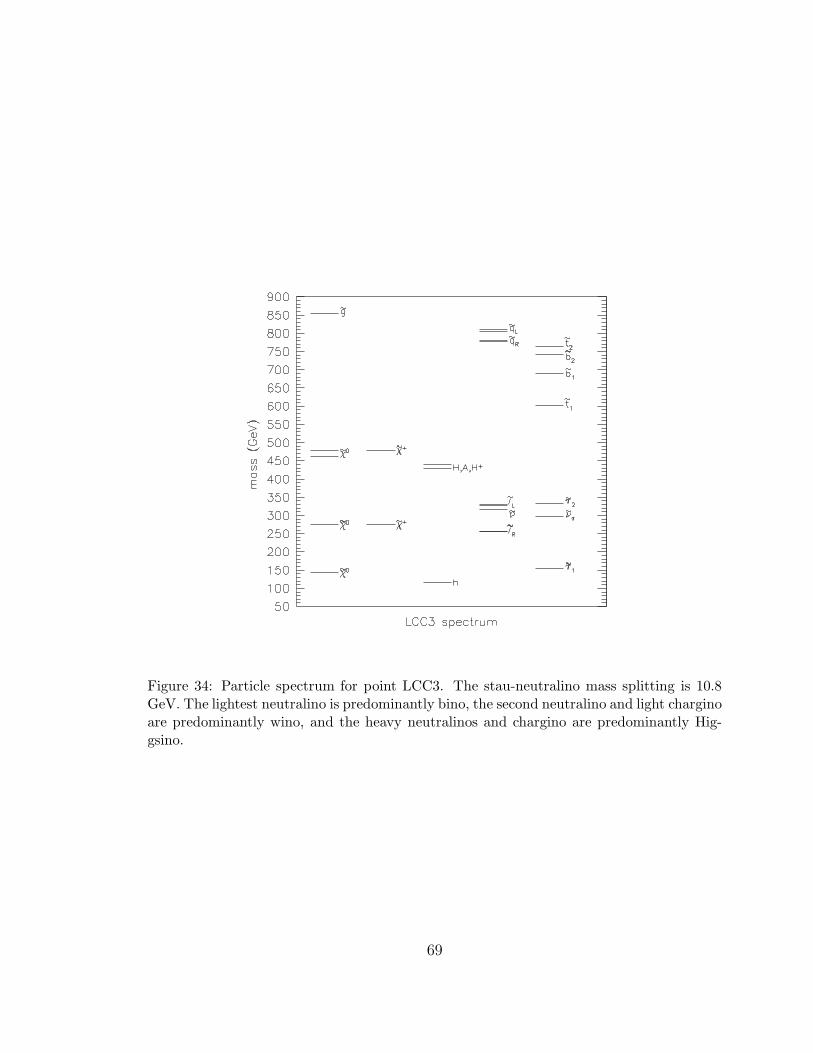
Figure 34: Particle spectrum for point LCC3. The stau-neutralino mass splitting is 10.8GeV. The lightest neutralino is predominantly bino, the second neutralino and light charginoare predominantly wino, and the heavy neutralinos and chargino are predominantly Hig-gsino.
69

the supersymmetry spectrum. The squarks and the gluino have masses of about 800GeV, leading to cross sections of tens of pb for supersymmetry production. Effectsenhanced by the large value of tanβ move the lighter top and bottom squarks downto about 600 GeV. The H0 and A0 bosons can be observed in their decay to τ+τ−.
Unfortunately, we expect that the very precise spectrum measurements that wouldbe available at LCC1 and LCC2 will not be possible here. The dominant decaymode of the χ0
2 is χ02 → τ1τ , with decays also by χ0
2 → h0χ01 (3%) and χ0
2 → Z0χ01
(1%). The right-handed e and µ are lighter than the χ02, so that the decay chains
χ02 → ℓℓ → ℓ+ℓ−χ0
1 are kinematically allowed. However, for the case of eR and µR,the branching fractions of χ0
2 to these channels are only 4× 10⁻⁴, giving too small anevent sample to be useful. The decay chain involving τ1 is difficult to study becausethe mass gap between the τ1 and the χ0
1 is only 10 GeV. This small mass gap is chosenprecisely so that the coannihilation channels will dominate in the computation of therelic density. In the study [117], it is shown that the the soft taus from this decaycan be observed at the LHC and used to estimated the mass gap. What is directlyobserved is the endpoint of the τ+τ− mass spectrum, and this could be measured toan accuracy of ±5 GeV [118]. In our analysis, we have assumed that the mass ofthe χ0
1 can be obtained to 10% accuracy and the mass of the χ02 to 15% accuracy by
general kinematic fitting of supersymmetry events, and that the masses of the eR andµR can be found to 20% accuracy using slepton pair production.
At the ILC, the studies [88,97] have shown that it is possible to observe the staudecay to tau and to measure the mass splitting. The study [88] obtains an error on themass splitting of about 1 GeV from kinematic fitting of the e+e− → τ+τ− events. Thestudy [97] obtains an error of about 0.5 GeV on the stau mass from a scan of the τ+τ−
threshold. This must be combined with a precision measurement of the neutralinomass, which can be obtained from the analysis of the reaction e+e− → χ0
1χ02. The
value of the cross section for e+e− → τ+τ− events measures the stau mixing angle.
However, this is the extent of the information that can be found at this point at the500 GeV ILC. To fix the gaugino-Higgsino mixing angles and tan β, more informationis needed. These additional constraints can be provided by the 1000 GeV ILC, fromtwo sources. First, the remaining states of the chargino and neutralino system canbe discovered and studied in the reactions e+e− → χ0
3χ04 and e+e− → χ+
1 χ−
2 . Second,because the mass of the A0 Higgs boson at LCC3 is 428 GeV, this particle can beobserved in the process e+e− → H0A0. The mass of the A0 can be important forthe detection cross sections, as we have seen, but also the total width of the A0
is interesting as a way to measure tanβ. We have estimated the error on the ΓA
following [90] and used this as a constraint.
The complete list of spectrum constraints that we expect for this point for theLHC and for each stage of the ILC is given in Tables 6 and 7.
70
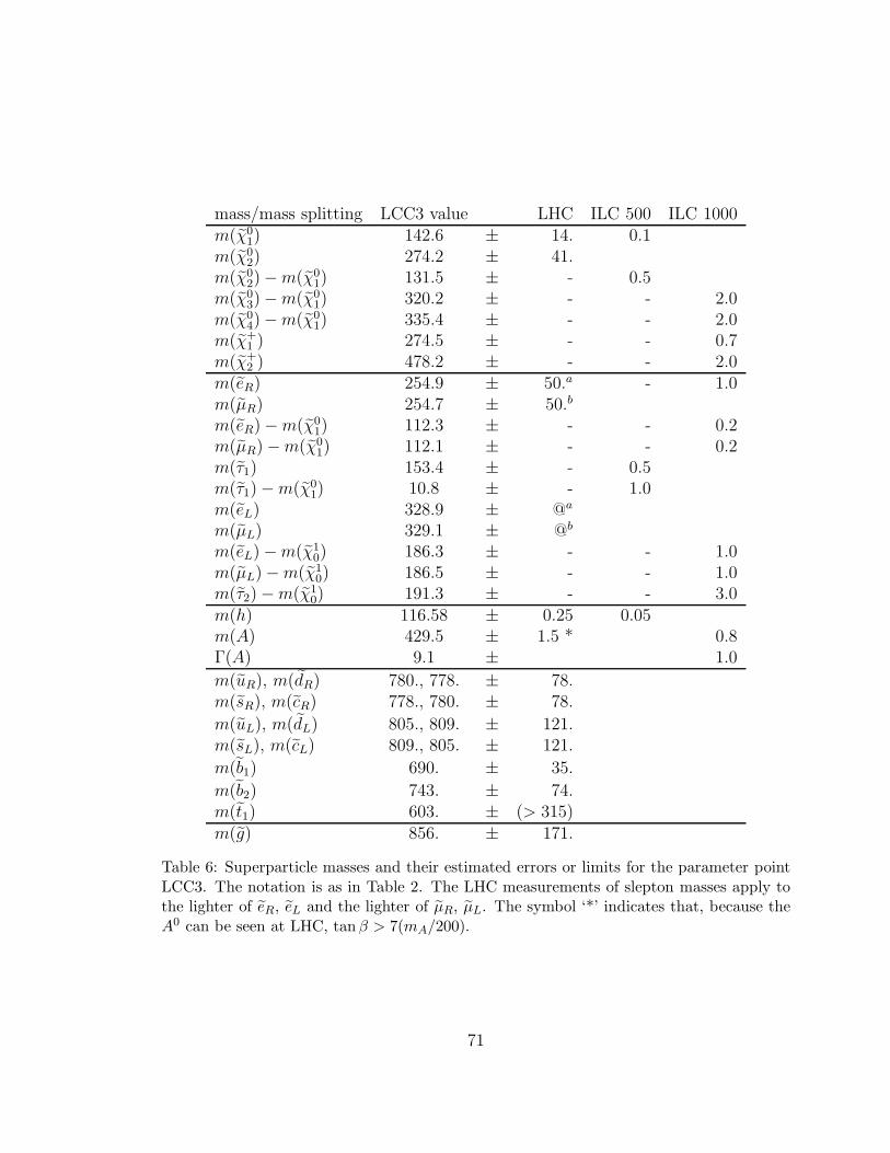
mass/mass splitting LCC3 value LHC ILC 500 ILC 1000m(χ0
1) 142.6 ± 14. 0.1m(χ0
2) 274.2 ± 41.m(χ0
2) −m(χ01) 131.5 ± - 0.5
m(χ03) −m(χ0
1) 320.2 ± - - 2.0m(χ0
4) −m(χ01) 335.4 ± - - 2.0
m(χ+1 ) 274.5 ± - - 0.7
m(χ+2 ) 478.2 ± - - 2.0
m(eR) 254.9 ± 50.a - 1.0m(µR) 254.7 ± 50.b
m(eR) −m(χ01) 112.3 ± - - 0.2
m(µR) −m(χ01) 112.1 ± - - 0.2
m(τ1) 153.4 ± - 0.5m(τ1) −m(χ0
1) 10.8 ± - 1.0m(eL) 328.9 ± @a
m(µL) 329.1 ± @b
m(eL) −m(χ10) 186.3 ± - - 1.0
m(µL) −m(χ10) 186.5 ± - - 1.0
m(τ2) −m(χ10) 191.3 ± - - 3.0
m(h) 116.58 ± 0.25 0.05m(A) 429.5 ± 1.5 * 0.8Γ(A) 9.1 ± 1.0
m(uR), m(dR) 780., 778. ± 78.m(sR), m(cR) 778., 780. ± 78.
m(uL), m(dL) 805., 809. ± 121.m(sL), m(cL) 809., 805. ± 121.
m(b1) 690. ± 35.
m(b2) 743. ± 74.m(t1) 603. ± (> 315)m(g) 856. ± 171.
Table 6: Superparticle masses and their estimated errors or limits for the parameter pointLCC3. The notation is as in Table 2. The LHC measurements of slepton masses apply tothe lighter of eR, eL and the lighter of µR, µL. The symbol ‘*’ indicates that, because theA0 can be seen at LHC, tan β > 7(mA/200).
71

cross section LCC3 value ILC 500 ILC 1000minimal setσ(e+e− → χ0
1χ02) LR 34.4 ± 8%∗
RL 2.1 ± -σ(e+e− → τ+1 τ−1 ) LR 45.6 ± 100%∗
RL 103.4 ± 4%∗
σ(e+e− → χ+1 χ
−
1 ) LR 212.3 (0.808) ± 3%RL 6.3 (0.774) ± -
σ(e+e− → χ02χ
02) LR 88.7 ± 5%
RL 2.5 ± -σ(e+e− → e+R e
−
R) LR 19.5 (0.735) ± 10%RL 350.5 (0.971) ± 3%
Table 7: SUSY cross sections and estimated errors for the parameter point LCC3. Thenotation is as in Table 3. The symbol (-) denotes that the cross section is less than 10 fbor is otherwise not measurable. The errors labeled by ∗ are taken from the study [88,89];the others are estimated using (14).
6.2 Relic density
We can use these constraints on the spectrum as the basis for an explorationof the allowed supersymmetry parameter space. The results from the three MonteCarlo scans, projected onto the axis of the predicted WIMP relic density, are shownin Fig. 35. Because the LHC data is not sensitive to the stau-neutralino mass differ-ence, that set of constraints leads to essentially no information about the relic density,yielding a distribution that stretches well to the right of the region plotted. The infor-mation from the 500 GeV ILC can only check that we are in the stau coannihilationregion, predicting the relic density only within a factor of two. However, when theinformation from the 1000 GeV ILC is added, with strong constraints on the mixingangles and on tanβ, the relic density is predicted to about 18%, an error three timesas large as the current WMAP determination.
Though this is not the main issue for the LHC, the scan data does show quiteclearly the presence of continuous ambiguities in the interpretation of the spectrumdata in terms of underlying parameters. In Fig. 36, we show the correlation of theparameters m1 and µ. The plot shows three regions, two horizontal and one vertical,corresponding to models in which the lightest neutralino is mainly bino, wino, andHiggsino, respectively.
The dependence of the coannihilation cross sections on parameters that are notfixed at the 500 GeV ILC is illustrated by the scatter plot shown in Fig. 37. Thisplot shows the correlation between Ωχh
2, tanβ, and ΓA. The relic density is mainly
72

Figure 35: Relic density measurement for point LCC3. The wino peak at very small relicdensity is clear. See Fig. 8 for description of histograms.
determined by annihilations of the stau. This plot makes clear how the measurementof ΓA, which fixes tan β to about ±2, has such an important effect. At the ILC-1000,there remains a weak correlation between the stau-neutralino mass splitting and relicdensity, illustrated in Fig. 38.
6.3 Annihilation cross section
In Fig. 39, we show the prediction of our likelihood analysis for the neutralinopair annihilation cross section at threshold. The dominant annihilation processescontributing to the relic density at LCC3 are actually coannihilation reactions, andthese are not longer available, because all primordial staus have decayed long ago.So we have a situation similar to that of LCC1, in which a subdominant annihilationreaction for the relic density becomes the most important one for the threshold crosssection. The relevant reaction is the same one that was important at LCC1, χχ → bb,by t-channel b exchange, but also getting a contribution from the A0 s-channel reso-nance. The relative influence of these two contributions is reflected in the sharpeningof the distribution after the A0 is determined at the 1000 GeV ILC. In the LHC distri-bution, we again see a subsidiary peak at high values of the cross section that reflectsthe possibility of solutions in which the lightest neutralino is wino- or Higgsino-like.In Fig. 40, we show the similar evolution for the exclusive annihilation cross sectionsto γγ and γZ.
73
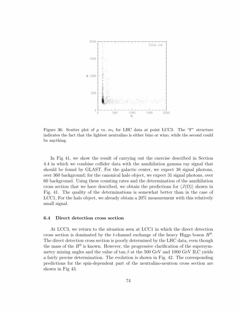
Figure 36: Scatter plot of µ vs. m1 for LHC data at point LCC3. The “F” structureindicates the fact that the lightest neutralino is either bino or wino, while the second couldbe anything.
In Fig 41, we show the result of carrying out the exercise described in Section4.4 in which we combine collider data with the annihilation gamma ray signal thatshould be found by GLAST. For the galactic center, we expect 38 signal photons,over 360 background; for the canonical halo object, we expect 31 signal photons, over60 background. Using these counting rates and the determination of the annihilationcross section that we have described, we obtain the predictions for 〈J(Ω)〉 shown inFig. 41. The quality of the determinations is somewhat better than in the case ofLCC1, For the halo object, we already obtain a 20% measurement with this relativelysmall signal.
6.4 Direct detection cross section
At LCC3, we return to the situation seen at LCC1 in which the direct detectioncross section is dominated by the t-channel exchange of the heavy Higgs boson H0.The direct detection cross section is poorly determined by the LHC data, even thoughthe mass of the H0 is known. However, the progressive clarification of the supersym-metry mixing angles and the value of tan β at the 500 GeV and 1000 GeV ILC yieldsa fairly precise determination. The evolution is shown in Fig. 42. The correspondingpredictions for the spin-dependent part of the neutralino-neutron cross section areshown in Fig 43.
74

Figure 37: Scatter plots of both tan β and ΓA vs. relic density for point LCC3. There is asignificant correlation, which can be resolved at ILC-1000. In fact, the correlation betweentan β and ΓA is quite close.
75

Figure 38: Scatter plot of mτ −mχ0
1
for point LCC3, ILC-1000 sample. A correlation exists,but it is not strong.
Figure 39: Annihilation cross section at threshold for point LCC3. The wino solution givingvery high cross section is clearly visible. See Fig. 8 for description of histograms.
76

Figure 40: Gamma ray line annihilation cross section at threshold for point LCC3. Thewino solution for LHC data at large cross section is clearly seen. See Fig. 8 for descriptionof histograms.
As before, we can combine our determination of the detection cross section withthe expected event yield from the SuperCDMS detector to estimate our ability todirectly measure the local flux of dark matter at the earth. Again, our analysis omitsthe uncertainty from low-energy QCD parameters. For this case, we expect a signalof 27 events in SuperCDMS. This gives the determination of the effective local fluxof neutralinos at the Earth that is shown in Fig. 44.
6.5 Constraints from relic density and direct detection
Point LCC3 illustrates a scenario that in some sense is quite likely. The LHC willmeasure some part of the low energy spectrum of supersymmetric particles, but themechanism for establishing relic density will be completely unknown. In this case,coannihilations with the light stau reduce the relic density by a large amount. LHCdata give no hint of this as the stau is unobserved. Furthermore, only two neutralinosare observed at LHC, and no chargino is observed. Thus, the composition of theneutralinos is almost completely unknown.
Applying a relic density constraint to LHC data is a technical challenge as therange allowed is so large. Applying even the current WMAP constraint of 6% reducesthe effective number of samples by a factor of 40. Nevertheless, we can make a general
77

Figure 41: Halo density profiles for point LCC3: (a) galactic center, (b) dark matter clumpin the galactic halo. Angle-averaged J values as measured by combining a 5-year all-skydataset from GLAST with accelerator measurements are shown. For LHC, the wino peakat low J is clearly visible. See Fig. 8 for description of histograms.
78

Figure 42: Spin-independent neutralino-proton direct detection cross section for pointLCC3. See Fig. 8 for description of histograms.
Figure 43: Spin-dependent neutralino-neutron direct detection cross section for point LCC3.See Fig. 8 for description of histograms.
79

Figure 44: Effective local WIMP flux at the Earth for point LCC3. The results assume theSuperCDMS measurement described in the text. See Fig. 8 for description of histograms.
statement about the composition of the lightest neutralino in that if it has too largea wino or Higgsino fraction, the relic density will be too low. Thus, the relic densityconstraint selects the pure bino solution.
The direct detection cross section is governed by the heavy Higgs boson, seen atthe LHC, and the gaugino-Higgsino mixing of the neutralino. From the cross sectionmeasured by SuperCDMS and the LHC measurement of the H boson mass, it couldimmediately be inferred that the WIMP was a fairly pure gaugino or Higgsino (Zg orZh > 0.94).
The ILC-500 measurements of relic density and direct detection cross section arestill quite poor. We can illustrate an interesting possibility here, that the combinationof relic density and direct detection constraints can be more powerful than eitheralone. In particular, we study the distribution of tan β. As shown in Fig. 45, thedirect detection constraint alone has little effect. Applying the relic density constrainttightens the ILC-500 measurement considerably (and in fact reduces the ILC-1000errors from 5% to 3%). Applying the direct detection constraint does have significantpower if the relic density constraint is also applied, especially in the ILC-500 sample.
The ILC-1000 measures the direct detection cross section to 9%, more accuratelythat it can be determined by SuperCDMS. But the relic density can only be mea-sured to 18%, so there is useful information in a cosmological relic density constraint.
80
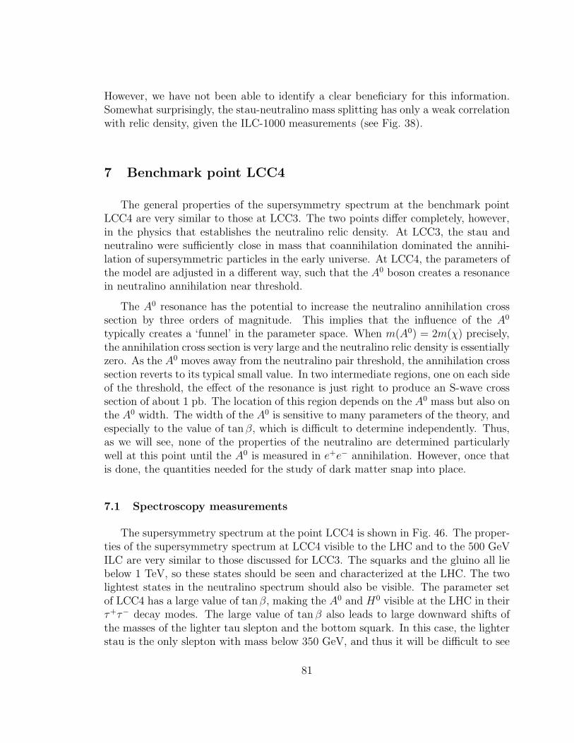
However, we have not been able to identify a clear beneficiary for this information.Somewhat surprisingly, the stau-neutralino mass splitting has only a weak correlationwith relic density, given the ILC-1000 measurements (see Fig. 38).
7 Benchmark point LCC4
The general properties of the supersymmetry spectrum at the benchmark pointLCC4 are very similar to those at LCC3. The two points differ completely, however,in the physics that establishes the neutralino relic density. At LCC3, the stau andneutralino were sufficiently close in mass that coannihilation dominated the annihi-lation of supersymmetric particles in the early universe. At LCC4, the parameters ofthe model are adjusted in a different way, such that the A0 boson creates a resonancein neutralino annihilation near threshold.
The A0 resonance has the potential to increase the neutralino annihilation crosssection by three orders of magnitude. This implies that the influence of the A0
typically creates a ‘funnel’ in the parameter space. When m(A0) = 2m(χ) precisely,the annihilation cross section is very large and the neutralino relic density is essentiallyzero. As the A0 moves away from the neutralino pair threshold, the annihilation crosssection reverts to its typical small value. In two intermediate regions, one on each sideof the threshold, the effect of the resonance is just right to produce an S-wave crosssection of about 1 pb. The location of this region depends on the A0 mass but also onthe A0 width. The width of the A0 is sensitive to many parameters of the theory, andespecially to the value of tanβ, which is difficult to determine independently. Thus,as we will see, none of the properties of the neutralino are determined particularlywell at this point until the A0 is measured in e+e− annihilation. However, once thatis done, the quantities needed for the study of dark matter snap into place.
7.1 Spectroscopy measurements
The supersymmetry spectrum at the point LCC4 is shown in Fig. 46. The proper-ties of the supersymmetry spectrum at LCC4 visible to the LHC and to the 500 GeVILC are very similar to those discussed for LCC3. The squarks and the gluino all liebelow 1 TeV, so these states should be seen and characterized at the LHC. The twolightest states in the neutralino spectrum should also be visible. The parameter setof LCC4 has a large value of tanβ, making the A0 and H0 visible at the LHC in theirτ+τ− decay modes. The large value of tan β also leads to large downward shifts ofthe masses of the lighter tau slepton and the bottom squark. In this case, the lighterstau is the only slepton with mass below 350 GeV, and thus it will be difficult to see
81
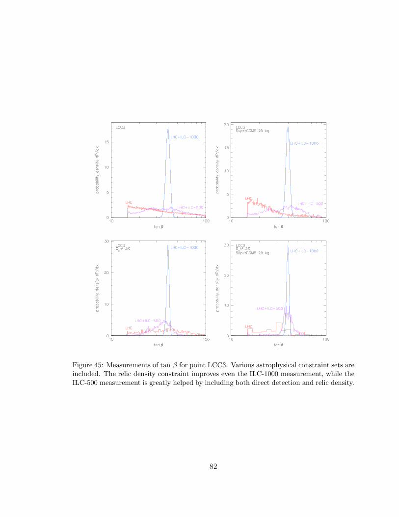
Figure 45: Measurements of tan β for point LCC3. Various astrophysical constraint sets areincluded. The relic density constraint improves even the ILC-1000 measurement, while theILC-500 measurement is greatly helped by including both direct detection and relic density.
82
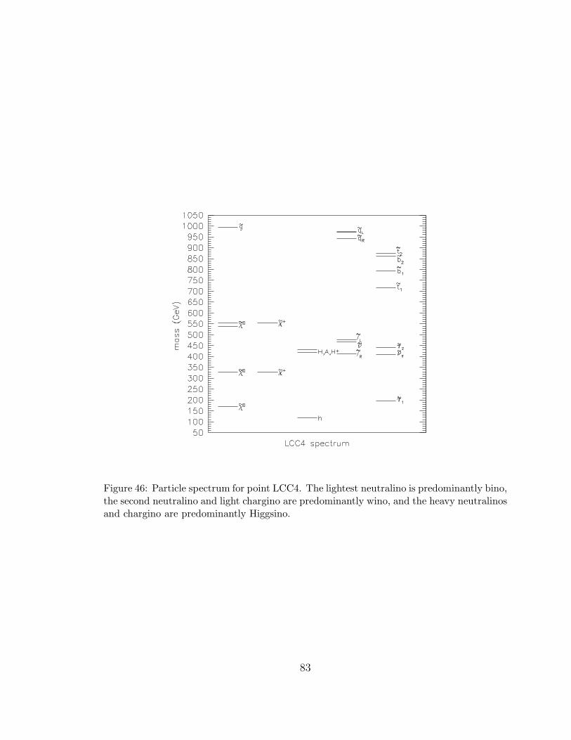
Figure 46: Particle spectrum for point LCC4. The lightest neutralino is predominantly bino,the second neutralino and light chargino are predominantly wino, and the heavy neutralinosand chargino are predominantly Higgsino.
83

any slepton at the LHC. The point LCC4 shares with LCC3 the property that onlythe few lightest supersymmetric states will be visible at the 500 GeV stage of theILC.
At the 1000 GeV ILC, new features of the model can be studied in detail. Theprocess e+e− → H0A0 becomes accessible, leading to striking events with four b jets.The analysis of these events has been studied in [90]. By combining the jets in pairs, itis possible to reconstruct the mass peak of the heavy Higgs bosons. The widths of theH0 and A0 can be measured from this mass distribution. The two peaks substantiallyoverlap, since the widths are about 14 GeV while the mass splitting is about 1 GeV.Since the splitting and the width are controlled by the common MSSM parameterstanβ and m(A0), it is possible to fit for those parameters and improve the accuracyof the A0 width determination.
This is the only place in the paper where we make strong use of the fact thatwe are restricting ourselves to the MSSM rather than working in a still more generalsupersymmetric model. However, in a model with a more general Higgs structure,the masses of the H0 and A0 would typically be distinct, and the two sets of massesand widths could be obtained separately by kinematic fitting of 4-jet events.
The higher energy running of the ILC also makes it possible to observe the gaug-inos χ+
1 and χ03 and to measure their masses. This gives enough information to
determine the parameter µ and thus to fix the gaugino-Higgsino mixing angles.
The complete list of spectrum constraints that we expect for this point for theLHC and for each stage of the ILC is given in Tables 8 and 9.
7.2 Relic density
The evaluation of the relic density at LCC4 from collider data reflects the fact thatthe result depends sensitively on both the mass and width of the A0 boson. At theLHC and the 500 GeV ILC, the qualitative features of the supersymmetry spectrumare known, and the mass of the lightest neutralino and the A0 are both known to someprecision. However, this still leaves almost complete uncertainty as to the predictedvalue of the relic density. It is only when the width of the A0 is measured that theactual picture begins to come into focus. This evolution is shown clearly in Fig. 47.The dependence of relic density on the A0 width is easily seen in the ILC-500 data,illustrated in Fig. 48.
The predicted value of the relic density also depends on the gaugino-Higgsinomixing parameters. The measurement of the mass of the χ0
3, in particular, allows oneto determine the µ parameter. This significantly improves the determination shownin Fig. 47 over scans done without this information. With the full set of collider data,
84

mass/mass splitting LCC4 value LHC ILC 500 ILC 1000m(χ0
1) 169.1 ± 17.0 - 1.4m(χ0
2) 327.1 ± 49.m(χ0
2) −m(χ01) 158.0 ± - - 1.8
m(χ03) −m(χ0
1) 370.6 ± - - 2.0m(χ+
1 ) 327.5 ± - - 0.6m(χ+
1 ) −m(χ01) 158.4 ± - - 2.0
m(χ+2 ) −m(χ+
1 ) 225.8 ± - - 2.0m(eR) −m(χ0
1) 243.2 ± - - 0.5m(µR) −m(χ0
1) 243.0 ± - - 0.5m(τ1) 194.8 ± - 0.9m(τ1) −m(χ0
1) 25.7 ± - 1.0m(h) 117.31 ± 0.25 0.05m(A) 419.3 ± 1.5 * - 0.8Γ(A) 14.8 ± - - 1.2
m(uR), m(dR) 944.,941. ± 94.m(sR), m(cR) 941., 944. ± 97.
m(uL), m(dL) 971., 975. ± 141.m(sL), m(cL) 975., 971. ± 146.
m(b1) 795. ± 40.
m(b2) 862. ± 86.m(t1) 716. ± (> 345)m(g) 993. ± 199.
Table 8: Superparticle masses and their estimated errors or limits for the parameter pointLCC4. The notation is as in Table 6.
cross section LCC4 value ILC 500 ILC 1000minimal setσ(e+e− → τ+1 τ−1 ) LR 21.1 ± 100%
RL 54.2 ± 7%σ(e+e− → χ+
1 χ−
1 ) LR 137.3 (0.786) ± 4%RL 4.0 (0.760) ± -
σ(e+e− → χ01χ
02) LR 43.9 ± 7%
RL 1.8 ± -σ(e+e− → e+R e
−
R) LR 5.1 (0.683) ± -RL 84.7 (0.899) ± 5%
Table 9: SUSY cross sections and estimated errors for the parameter point LCC4. Thenotation is as in Table 3. The symbol (-) denotes that the cross section is less than 10 fbor is otherwise not measurable. The errors are estimated using (14).
85
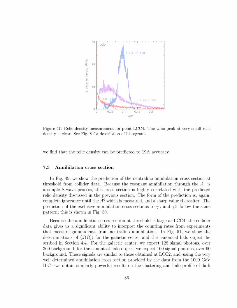
Figure 47: Relic density measurement for point LCC4. The wino peak at very small relicdensity is clear. See Fig. 8 for description of histograms.
we find that the relic density can be predicted to 19% accuracy.
7.3 Annihilation cross section
In Fig. 49, we show the prediction of the neutralino annihilation cross section atthreshold from collider data. Because the resonant annihilation through the A0 isa simple S-wave process, this cross section is highly correlated with the predictedrelic density discussed in the previous section. The form of the prediction is, again,complete ignorance until the A0 width is measured, and a sharp value thereafter. Theprediction of the exclusive annihilation cross sections to γγ and γZ follow the samepattern; this is shown in Fig. 50.
Because the annihilation cross section at threshold is large at LCC4, the colliderdata gives us a significant ability to interpret the counting rates from experimentsthat measure gamma rays from neutralino annihilation. In Fig. 51, we show thedeterminations of 〈J(Ω)〉 for the galactic center and the canonical halo object de-scribed in Section 4.4. For the galactic center, we expect 128 signal photons, over360 background; for the canonical halo object, we expect 100 signal photons, over 60background. These signals are similar to those obtained at LCC2, and–using the verywell determined annihilation cross section provided by the data from the 1000 GeVILC—we obtain similarly powerful results on the clustering and halo profile of dark
86

Figure 48: Scatter plot of the distance from the A0 resonance vs. relic density for pointLCC4. The quantity plotted is actually the distance in widths, with true value 5.5.
matter.
7.4 Direct detection cross section
Again at LCC4, the direct detection cross section is dominated by the exchange ofthe heavy Higgs boson H0. The determination of this cross section from the data atthe three colliders is shown in Fig. 52. The evolution is, if anything, more striking thanthat displayed in the previous two sections. The determination of this cross sectionrelies crucially on the information from the 1000 GeV ILC. The determinations ofthe gaugino-Higgsino mixing angles and tan β are crucial here as elsewhere in fixingthe neutralino-Higgs couplings. The corresponding predictions for the spin-dependentpart of the neutralino-neutron cross section are shown in Fig 53; these show a similarbehavior.
As before, we can combine our determination of the detection cross section withthe expected event yield from the SuperCDMS detector to estimate our ability todirectly measure the local flux of dark matter at the earth. Again, our analysis omitsthe uncertainty from low-energy QCD parameters. The direct detection cross sectionis the same as at LCC3, and again we expect a signal of 27 events in SuperCDMS.This gives the determination of the effective local flux of neutralinos at the Earththat is shown in Fig. 54.
87

Figure 49: Annihilation cross section at threshold for point LCC4. The wino solution givingvery high cross section is clearly visible. See Fig. 8 for description of histograms.
Figure 50: Gamma ray line annihilation cross section at threshold for point LCC4. Again,the wino solution at large cross section is clear. See Fig. 8 for description of histograms.
88

Figure 51: Halo density profiles for point LCC4: (a) galactic center, (b) dark matter clumpin the galactic halo. Angle-averaged J values as measured by combining a 5-year all-skydataset from GLAST with accelerator measurements are shown. See Fig. 8 for descriptionof histograms.
89

Figure 52: Spin-independent neutralino-proton direct detection cross section for pointLCC4. See Fig. 8 for description of histograms.
Figure 53: Spin-dependent neutralino-neutron direct detection cross section for point LCC4.See Fig. 8 for description of histograms.
90
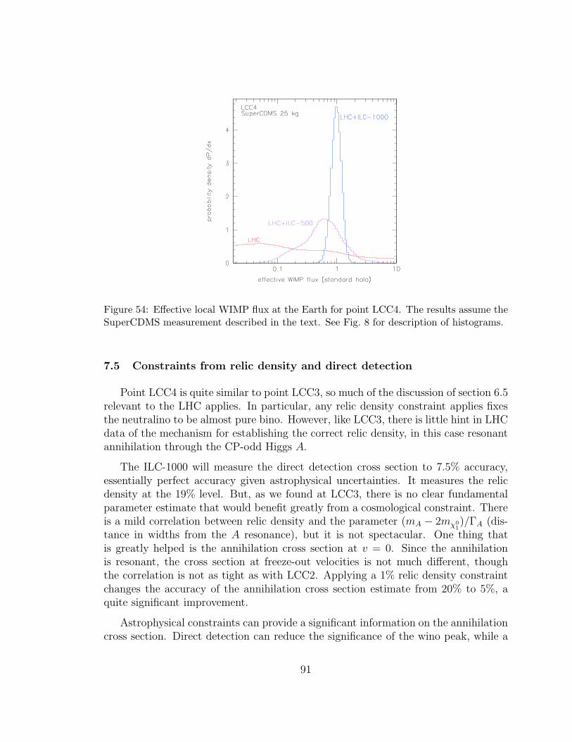
Figure 54: Effective local WIMP flux at the Earth for point LCC4. The results assume theSuperCDMS measurement described in the text. See Fig. 8 for description of histograms.
7.5 Constraints from relic density and direct detection
Point LCC4 is quite similar to point LCC3, so much of the discussion of section 6.5relevant to the LHC applies. In particular, any relic density constraint applies fixesthe neutralino to be almost pure bino. However, like LCC3, there is little hint in LHCdata of the mechanism for establishing the correct relic density, in this case resonantannihilation through the CP-odd Higgs A.
The ILC-1000 will measure the direct detection cross section to 7.5% accuracy,essentially perfect accuracy given astrophysical uncertainties. It measures the relicdensity at the 19% level. But, as we found at LCC3, there is no clear fundamentalparameter estimate that would benefit greatly from a cosmological constraint. Thereis a mild correlation between relic density and the parameter (mA − 2mχ0
1
)/ΓA (dis-tance in widths from the A resonance), but it is not spectacular. One thing thatis greatly helped is the annihilation cross section at v = 0. Since the annihilationis resonant, the cross section at freeze-out velocities is not much different, thoughthe correlation is not as tight as with LCC2. Applying a 1% relic density constraintchanges the accuracy of the annihilation cross section estimate from 20% to 5%, aquite significant improvement.
Astrophysical constraints can provide a significant information on the annihilationcross section. Direct detection can reduce the significance of the wino peak, while a
91

relic density constraint completely removes it. We illustrate this point in Fig. 55.
8 Neutralino annihilation products
In this section, we consider in more detail the computation of indirect signals ofdark matter annihilation from observations of gamma rays and positrons that are pro-duced in neutralino pair annihilation. We leave discussion of neutrinos, antiprotons,and antideuterons to future work.
In the previous few sections, we presented estimates of the neutralino annihila-tion cross section that might be obtained from collider data on the SUSY spectrum.However, as we have remarked in Section 2.7, there is a simpler way to obtain whatwould seem to be an acceptably accurate prediction. We start from a value of theneutralino mass obtained from LHC data. If we assume that the neutralino makes upthe bulk of the dark matter, we can use the cross section (2) derived from the relicdensity as an estimate of the astrophysical annihilation cross section. We assumethat the neutralinos annihilate to hadronic jets, either in direct decays to quarks orthrough decays to W and Z bosons. This gives a roughly universal spectrum of ener-gies for the annihilation products, scaling with the neutralino mass. The argumentsare robust and simple to implement. But are they correct?
8.1 Gamma ray spectra
The argument we have just given works best for the gamma ray spectra from darkmatter annihilation. We have computed the spectrum of gamma rays from neutralinoannihilation for each of our four models using results from the Monte Carlo programPYTHIA [119] (as tabulated in DarkSUSY [9]); this code is expected to give anexcellent description of hadronic final states in the energy region of 100 GeV. InFig. 56, we show the gamma ray spectra computed from the model parameters at thefour LCC points. The four spectra are compared to reference spectra with the shapeof the LCC4 spectrum, scaled horizontally to the correct endpoint at Eγ = m(χ0
1),and normalized so that the peak cross section is proportional to the total annihilationcross section. We have taken the reference shape from LCC4 because, in this case,the dominant annihilation reaction goes to the 2-jet final state bb. We see that theapproximation is an excellent one for all four models.
It is not surprising that the shapes of the spectra are similar for the cases of LCC1,LCC3, and LCC4. In all four cases, the annihilation at threshold is dominated bythe process χχ → bb, with subsequent evolution of the jets into π0’s and the decayof these to gammas. However, it is quite surprising that the spectrum for LCC2,
92

Figure 55: Annihilation cross section at threshold for point LCC4, including various as-trophysical constraints. Direct detection reduces the weight of the wino solution, and relicdensity completely eliminates this possibility.
93

Figure 56: Spectra of gamma rays and positrons from neutralino annihilation at thresholdfor points LCC1-4. Solid curves are gammas, dashed curves are positrons, and dotted curvesshow the gamma spectrum of LCC4, scaled to each endpoint and total cross section. Thescaled LCC4 spectrum is a good match in every case. The positron spectrum for LCC2exhibits a shelf due to direct decays of gauge bosons, e.g. χχ → W+W− → e+νud.
94
which is dominated by the processes χχ → W+W−, Z0Z0, yields the same spectrum.Apparently, the gamma ray spectra from hadronic jets, whatever their origin, do havethe universal form assumed in our argument above.
In addition, the discrepancy in the normalizations is readily understood. The relicdensity of WIMP dark matter is established at a small but nonzero temperature,T/m ∼ 1/25. The cross section relevant to gamma ray detection of WIMP is thatalmost precisely at threshold. In cases in which the dominant modes of annihilationproceed in the S-wave, (2) is a reasonable approximation to the correct cross section.We find for the neutralino annihilation cross section at threshold σv = 0.55 pb forLCC2 and σv = 0.48 pb for LCC4. However, at LCC1, the dominant modes ofannihilation for the purpose of computing the relic density are P-wave annihilationsto ℓ+ℓ−. These cross sections are very small at threshold; the dominant process just atthreshold is the subdominant reaction χχ → bb. At the point LCC3, the relic densityis set by coannihilation processes such as τ−τ− → τ−τ−. In present astrophysicalconditions, all of the τ ’s have decayed away. At both LCC1 and LCC3, bb appearsbecause this is the fermion-antifermion final state with the least amount of helicitysuppression. We find, for the neutralino annihilation cross section at threshold forthese points, σv = 0.012 pb for LCC1 and σv = 0.11 pb for LCC3.
If more incisive probes of WIMP annihilation are available, it might be importantto know what are the fractions of the total annihilation rate that go to the variouspossible final states. In Table 10, we present the branching fractions to the most im-portant final states for the four reference points, and the estimates of these branchingfractions that we obtain from the three sets of collider constraints.
8.2 Positron spectra
We have just shown that the gamma ray spectrum resulting from neutralino an-nihilation is remarkably independent of the model. It is controlled almost entirely bythe total neutralino pair annihilation cross section, and, through this, is often deter-mined if the physics of neutralino annihilation is understood even qualitatively. Forother annihilation products, however, the story can be quite different. In this section,we will discuss the visibility of the positron signal of dark matter annihilation in ourfour models. Similar considerations apply to neutrino signals. However, since in allfour of our models the neutralino mass is below 200 GeV, neutrinos from neutralinoannihilation will be produced at too low an energy to be visible above the thresholdsof cosmic-ray neutrino detectors such as ICE-CUBE.
Unlike gamma rays, which fly directly from the source to a detector on earth,positrons execute a random walk in the galactic magnetic field, losing energy contin-ually along the way. Thus, positrons from WIMP annihilation that are observed at
95

Process LHC ILC-500 ILC-1000LCC1:χχ → bb 0.629 ± 46% 46% 15%
τ+τ− 0.282 ± 79% 71% 43%W+W− 0.046 ± 65% 40% 13%γγ 0.016 ± 54% 42% 10%gg 0.013 ± 52% 41% 11%
LCC2:χχ → W+W− 0.868 ± 11% 11% 1.4%
Z0Z0 0.114 ± 66% 12% 3.7%LCC3:χχ → bb 0.974 ± 70% 36% 1.3%
τ+τ− 0.014 ± 113% 93% 92%LCC4:χχ → bb 0.889 ± 70% 16% 16%
τ+τ− 0.103 ± 90% 50% 52%
Table 10: Branching ratios in neutralino pair annihilation. The last three columns give thefractional error (σ/mean) from the MCMC scans.
the earth must originate inside the galaxy, within a few kpc. The annihilation ratedepends on ρ2(x) averaged over this volume, a quantity closely related to the localhalo density discussed in relation to direct detection, but possibly enhanced by localclumpiness parametrized by the boost factor (11). The energy loss in propagationfavors the highest-energy positrons in the spectrum.
The propagation of positrons through the galaxy has been modeled quantitativelyin [120,121]. We have found it an interesting exercise to fold the positron spectra forour four models with the smearing predicted by the model of [121]. The results areshown in Fig. 57.
The signal from LCC2 is larger than the others, for several reasons. First of all,this point has a full strength total annihilation cross section. In addition, as one cansee from Fig. 56, the positron spectrum at this point has a component with a flatdistribution extending to the kinematic endpoint. This results from the fact thatthe dominant annihilation reactions at LCC2 are to W+W− and Z0Z0, that is, tovector bosons that have direct two-body decays to positrons. The sharp feature atthe extreme right of Fig. 56(b) is transformed into the peak at the high-energy edgeof the LCC2 curve in Fig. 57.
We can compare this spectrum to the recent measurement of the cosmic-raypositron spectrum by the HEAT experiment. The comparison is shown in Fig. 58.
96

Figure 57: Spectrum of positrons for all models after galactic propagation effects are ac-counted for. The “interstellar” spectrum is illustrated. Solar modulation is neglected.Above a few GeV solar modulation effects are negligible.
Figure 58: Positrons observed on earth, as a fraction of electrons, for LCC2. The HEATdata are plotted as well, indicating the possibility of an excess. The positron signal from asmooth halo has been boosted by a factor of 185 in order to fit the data.
97
The HEAT data shows an anomaly at its upper edge, with a cross section that isroughly flat in a region in which the background is expected to be decreasing. Asthe figure shows, we can fit this with the positron spectrum from LCC2. To obtainthe correct normalization, we must enhance the production over that for a smoothdistribution of dark matter with density ρ0 = 0.3 GeV cm−3 by assuming a largeboost factor B = 190.
Is this a correct way to interpret the data? We ourselves are skeptical. Neverthe-less, if we knew from collider measurements that the WIMP mass was 100 GeV andthat we were in a region of the parameter space that favored annihilation throughχχ → W+W−, this fit to the data might be considered compelling evidence forneutralino annihilation and for a significantly clumpy distribution of WIMPs in thegalaxy.
9 Recap: Collider determination of WIMP properties
Our analysis in this paper has presented a series of worked examples that illustratethe interactions we might expect over the coming years between astrophysical darkmatter detection experiments and high-energy physics experiments that will measurethe spectrum of new particles in the hundred-GeV mass range. In this section, wewill assemble the results that we have obtained and give our interpretation of theirimplications.
9.1 Summary of results: cross sections
In Table 11, we summarize the results of our Monte Carlo scans for the mostimportant WIMP parameters that are determined by collider measurements of su-persymmetry spectroscopy: the relic density Ωχh
2, the annihilation cross section atthreshold σv (in pb), and the spin-independent scattering cross section on protonsσ(χp) (in units of 10−8 pb). The results are given for each of the four benchmarkmodels and for each of the three sets of collider measurements discussed in Sections4-7. The results are quoted as a percentage error, defined as the standard devia-tion divided by the mean, computed from the statistical sample generated by ourMonte Carlo process. A large variance indicates a poor determination of the modelparameters and might also indicate the presence of multiple solutions. For the correctinterpretation, one should look at the detailed shapes of the probability distributionsshown in the figures in Sections 4-7. For reference, the mean values of the MonteCarlo samples are listed in the last three columns of the table when these differ by10% or more from the nominal value.
98

LHC ILC-500 ILC-1000 LHC ILC-500 ILC-1000Ωh2 (mean)
LCC1 0.192 7.2% 1.8% 0.24%LCC2 0.109 82.% 14.% 7.6% 0.074LCC3 0.101 167% 50.% 18.% 0.24LCC4 0.114 405% 85.% 19.% 0.26 0.083 0.094
σv (mean)LCC1 0.0121 165.% 54.% 11.% 0.0069LCC2 0.547 143.% 32.% 8.7% 8.47LCC3 0.109 154.% 178.% 10.% 24.2 0.311LCC4 0.475 557.% 228.% 20.% 82.5 1.83 0.57
σ(χp) (mean)LCC1 0.418 44.% 45.% 5.7% 0.20LCC2 1.866 62.% 63.% 22.% 3.57 2.82 2.19LCC3 0.925 184.% 146.% 8.6% 13.2 1.86LCC4 1.046 150.% 190.% 7.5% 23.2 3.59
Table 11: Fractional errors in the determination of the most important microscopic WIMPparameters derived from the MCMC scans: Ωh2, the predicted relic density, σv, the annihi-lation cross section at threshold (in pb), and σ(χp), the spin-independent neutralino-protoncross section (in units of 10−8 pb). The second column lists the values predicted by thebenchmark models. Columns 3–5 give the fractional error (σ/mean) from the MCMC scans.Columns 6-8 give the mean value found from the MCMC data when this deviated by morethan 10% from the nominal value in column 2. As discussed in Appendix A, the quotederrors are accurate to 10% or better, e.g. a 20% error is 20% ± 2%.
We emphasize that all of these cross section determinations are ‘model-indepen-dent’ in the following sense: We assume that it has been shown from collider datathat the model of new physics at the hundred GeV scale is supersymmetry. We thenfit the collider data on new particles to the Minimal Supersymmetric Standard Model,studying the model in complete generality with 24 free parameters. We have shown inmany examples given in Section 4-7 that this parametrization is sufficiently generalto allow all of the possible physical mechanisms that are expected in this generalclass of models to be considered in the fitting procedure. Thus we believe that wehave justified the claim made in Section 3.2 that cross section estimates obtained fromcollider data through an analysis such as ours can be used without undue qualificationto analyze astrophysical measurements.
The table shows that, for all of the quantities listed, carrying out the full programof collider measurements that we have presented results in a clear determination of
99
the microscopic cross sections that can be used to interpret astrophysical dark matterobservations. The precise quality of the determination depends on the specific sce-nario. In scenarios in which the dominant annihilation mechanism is through simpleannihilation to leptons, we find that the accuracy of the prediction of the relic densityis at the level of a fraction of a percent, comparable to the best measurements of thedark matter density from the cosmic microwave background expected in that era. Inscenarios in which special relations among the superparticle masses are necessary forrapid enough annihilation, the quality of the microscopic prediction decreases and wefind an accuracy of about 20%. In all cases, the agreement of the microscopic andastrophysical determinations within the errors would be nontrivial and would pro-vide striking evidence that the particle identified at colliders is indeed the dominantcomponent of astrophysical dark matter.
We believe that the accuracies we have listed are the best ones that can be ob-tained at the current level of our understanding of the experimental capabilities ofthe next-generation colliders. That is, we could not find additional measurementsbeyond the ones we have listed that would significantly improve the accuracies wehave quoted for the neutralino cross sections. We note, though, that, in the linearcollider studies, relatively little effort has gone into analyses aimed at very accuratecross section measurements. We have seen that the ILC cross sections can be veryimportant in fixing the gaugino-Higgsino mixing angles and tan β, parameters thatprovide a major uncertainty in the neutralino properties. If cross sections could bemeasured at the ILC with errors considerably smaller than the estimate (14), theoutput accuracies would improve. To do this, however, it is necessary to confront theStandard Model backgrounds to the observations of supersymmetric particles and tomodel and subtract these backgrounds with very high precision.
We have also shown that the collider data predicts the WIMP annihilation crosssection and the cross section relevant to direct detection at the 20% level or bet-ter in all of the cases that we have considered. This is quite sufficient to use themicroscopically-determined cross sections to provide strong constraints on the distri-bution of the observed WIMPs in the galaxy. For the case of the direct detectioncross section, this conclusion does require that the uncertainty from low-energy QCDmatrix elements, discussed in Section 2.6, can be brought under control.
9.2 Summary of result: astrophysics
In Table 12 we summarize the constraints for the three specific model problemsthat we have considered in this paper, the determination by GLAST of the darkmatter density integral J ∼ ∫
dzρ2 near the galactic center, the determination byGLAST of the value of J for a representative clump of dark matter in the halo ofthe galaxy, and the determination by SuperCDMS of the local flux of dark matter at
100

a location on Earth. The specific parameters assumed for the detectors and sourceswere detailed in Section 4.4 and 4.5. We emphasize that we have chosen these specificexperiments as representative examples meant to illustrate the implications of thecollider measurements for the many dark matter observation experiments that willbe carried out over the next decade.
The results given in the table for determinations of the density integral 〈J〉 reflectseveral factors in addition to the accuracies given in Table 11 with which the mi-croscopic WIMP cross section will be known. They include also the statistics of theobservation, and the error from the expected uncertainty in the background. Thesetwo factors depend in turn on the underlying physics scenario and on the value of therelevant WIMP cross section. If the cross section is small, the statistical error will berelatively large, and the background will be more important relative to the signal.
These contributions are reflected in our results on 〈J〉 from the galactic centerin the following way. The points LCC1 and LCC3 have suppressed annihilationcross sections at threshold. In these cases, the background always dominates, andwe can only set upper limits on the density integral. However, the lower bounds onthe cross sections that we obtain from the collider data allow these upper limits tosignificantly exclude dark matter distributions that are highly peaked at the galacticcenter. For LCC2 and LCC4, the annihilation cross section is at the full strengthexpected from (2), and a robust signal is expected above background. For the LHCdata set, ambiguities arising from multiple solutions still make it difficult to pin downthe value of 〈J〉. We have quoted the error on 〈J〉 obtained when we resolve thisambiguity in favor of the correct solution by removing the subsidiary peaks in thelikelihood distributions for σv at high cross section values. The variances are stillquite large. These ambiguities are resolved by the ILC data, and for those cases wegive the fractional error on 〈J〉 computed from the full scan data. Thus, at LCC2and at LCC4, we find that 〈J〉 is given to 30% accuracy. These accuracies should becompared to the current astrophysical estimates of 〈J〉 at the galactic center, whichrange over many orders of magnitude. A measurement of the 〈J〉 correct to the levelwe have shown, or even an upper limit on 〈J〉 free of astrophysical assumptions, wouldrepresent a major improvement in our knowledge.
For our model dark matter clump in the galactic halo, the situation is somewhatbetter. The background still dominates for LCC1, but not in the other cases. For theLHC data sets, the problem of ambiguities in the solution is still present, and againwe restrict our estimates to MCMC points in the peak corresponding to the correctsolution. But, using the ILC data, we will find quantitative measurements of 〈J〉. AtLCC2, we can achieve a 20% measurement already with the 500 GeV data. At LCC4also, the data from the 1000 GeV stage determines 〈J〉 an accuracy of about 20%.
For the local flux of neutralino dark matter, we find a similar picture. We first
101

LHC ILC-500 ILC-1000 LHC ILC-500 ILC-1000〈J〉(gc) limits (95% CL)
LCC1 7760 < 50,000 < 34,000 < 34,000LCC2 7760 51.% ∗ 25.% 20.%LCC3 7760 < 16900 < 16900 < 11500LCC4 7760 160.% ∗ 122.% 32.%
〈J〉(clump) limits (95% CL)LCC1 2500 < 14500 < 6700 < 5700LCC2 2500 51.% ∗ 21.% 13.%LCC3 2500 152.% ∗ 131.% 81.%LCC4 2500 180.% ∗ 124.% 23.%
Φlocal/Φ0 limits (95% CL)LCC1 1. 54.% 29.% > 0.95LCC2 1. 28.% ∗ 46.% 24.%LCC3 1. 126.% 20.% > 0.016LCC4 1. 115.% 20.% > 0.010
Table 12: Errors or limits for the illustrative astrophysical measurements that we havepresented in Section 4-7. The quantities considered are: 〈J〉gc, the average of the density
integral J ∼∫dzρ2 near the galactic center, 〈J〉clump, the average of J in a small circle
around the center of a typical clump of dark matter in the galactic halo, and Φlocal, theeffective flux of dark matter impinging on a direct detection experiment on earth, normalizedto a standard halo distribution. The output values quoted include the expected experimentalerrors. More details of the assumptions involved in these analyses are given in Sections 4.4and 4.5. The second column lists the assumed astrophysical values. Columns 3–5 give thestandard deviation of ln 〈J〉 from the MCMC scans. Columns 6-8 give 95% upper or lowerconfidence limits based on the MCMC data, as appropriate. Upper limits on J assume〈J〉 > 1 as a prior. For each situation, either an error or a limit is quoted. In the caseslabeled by ∗, the MCMC data includes multiple solutions, and we restrict our calculationto points in the neighborhood of the correct solution. See the text for further discussionof all of these points. As discussed in Appendix A, the quoted errors for the microscopicquantities (annihilation cross section, direct detection cross section) are accurate to 10% orbetter.
102

remind the reader that our estimates ignore uncertainty from the evaluation of low-energy QCD matrix elements. With the assumption that these matrix elements canbe determined, we draw the following conclusions: In all cases except for LCC2, theLHC data set provides only a weak determination of the relevant WIMP cross section.We can at best quote an upper limit on the cross section and thus a lower limit onthe local flux. For the LHC data at LCC2, we have quoted a measurement errorafter removing the peak arising from the incorrect solutions. The data from the 500GeV ILC constrains the direct detection cross sections to some extent, and for theseentries we have quoted the fractional error, which is however large in all cases. Themeasurements at the 1000 GeV ILC finally fix the mass of the heavy Higgs bosons andother spectroscopic parameters involved in the most important contributions to thedirect detection cross section. From this data, the local flux can be determined to 20-30% accuracy for all four benchmark models. Our current knowledge of the galactichalo constrains this flux only to a factor of 2, and even then only if we assume thatthe halo has a smooth distribution both in position and in momentum space. Heretoo, precise microscopic information can have a large impact.
In all three examples, what would be determined would be the density or fluxof that component of dark matter corresponding to the WIMP observed in colliderexperiments. Other possible components of dark matter such as axions or very heavyweakly-interacting particles give negligible signals in direct detection experiments andexperiments on dark matter annihilation. Thus, first of all, the direct and indirectdetection experiments would demonstrate concretely that the WIMP seen in particlephysics is present in the structure of the galaxy. At the next stage, the consistency ofthe overall picture that results from these experiments could give additional insight,beyond what is gained from analysis of the overall relic density, on the broad questionof whether the observed WIMP is the dominant component of dark matter.
9.3 LHC and astrophysical measurements
Up to this point, we have been discussing the comparison to astrophysical dataof the full set of results that we will obtain from the next-generation colliders. Itwill take some time, of course, for the collider data to become available. The LHCexperiments will begin in just another year. The 500 GeV stage of ILC may beginwithin ten years from now. The 1000 GeV stage of the ILC would be an upgradeto the basic facility and would produce data, at the earliest, at the end of the nextdecade. Astrophysical dark matter experiments are also spaced out in time throughthe next decade. It is interesting, then, to look at the implications of colliders interms of this timeline and see what results can be expected at each stage. In this andthe next two sections, we will discuss some aspects of this evolution, emphasizing thethe new information that we will obtain as each collider presents its results.
103

There are many possibilities for what will happen in the future. In the discussionof the next few sections, we will assume that underlying physics model is a supersym-metric model of dark matter similar to those we have analyzed in this paper. Thenwe will be able to discuss the evolution in a very concrete way.
We begin with the situation as it might appear in 2012. In the scenarios dis-cussed in this paper, we will by that time have the discovery of supersymmetry inthe LHC experiments and the first positive results from direct detection experimentsand searches for WIMP annihilation.
At this stage, it should already be possible to compare three observed massesrelevant to dark matter: (1) the mass of the escaping neutral particle produced atthe LHC in missing energy events, (2) the mass of the directly detected dark matterparticle obtained from the recoil energy spectrum, and (3) the mass of the annihilatingdark matter particle, obtained from the endpoint of the gamma ray spectrum. In thebest case, all three masses should be determined to better than 20% accuracy. Theiragreement will provide a nontrivial test that the particle being produced at the LHCis indeed a dominant component of cosmic dark matter.
It will be difficult to learn more about the dark matter particle without additionalassumptions. As we have discussed in Section 2.3, it will be very difficult from theLHC data alone to narrow the possible explanations of missing-energy events and newparticles to a single model. Nevertheless, we might proceed by assuming a particularmodel (for example, supersymmetry or even a restricted model of supersymmetry)and examining its consequences for astrophysics.
In some scenarios (for example, the benchmark points LCC1 and SPS1a′ discussedin Section 4), we would be able to combine the assumption that the new physics issupersymmetry with the detailed spectroscopy measurements available from the LHCto give a quite accurate prediction of the WIMP relic density. In this situation, it istempting to assume that the observed WIMP is the sole component of dark matter,fix the relic density to the value measured from the cosmic microwave background,and make higher-precision predictions for the supersymmetry mass spectrum. Inaddition, because the heavy Higgs bosons typically give the dominant contributionto the spin-independent direct detection cross section, one can assume that the localflux of dark matter is near its nominal value and use the direct detection rate to fixthe heavy Higgs boson mass. In both cases, the later stages of the collider physicsprogram on supersymmetry spectroscopy will test these predictions and thus confirmor refute the astrophysical assumptions.
In most scenarios, however, it is not possible to derive a definite prediction forthe WIMP relic density from the LHC data even if supersymmetry is assumed to bethe underlying theory. The precise point in supersymmetry parameter space might
104

not be determined uniquely from the data, or the data might not select sufficientlyprecisely the special mechanism of neutralino annihilation. We have seen examplesof the first difficulty at LCC2 and of the second at LCC3 and LCC4. In these cases,the LHC would give us only a first tantalizing glimpse of the particle physics originof dark matter, leaving many questions to be resolved by the ILC experiments.
We have also noted a circumstance in which qualitative information from the LHCcan be bootstrapped into quantitative information for astrophysics. The particlephysics cross section needed for the interpretation of gamma ray data must be closeto the value (2) if the observed WIMP is the dominant component of dark matter andif the relic density of WIMPs is set primarily by WIMP annihilation in the S-wavewithout coannihilation. The LHC data could point to a qualitative scenario (onesimilar to LCC2, for example) in which S-wave annihilation would be expected. Wewould then have a quantitative estimate of the annihilation cross section that couldbe used to analyze astrophysical gamma ray spectra.
9.4 ILC at 500 GeV
In all of the scenarios we have discussed, the estimates of the neutralino propertiesfrom the LHC would be dramatically improved when the neutralino and the otherlight particles in its sector are observed in e+e− annihilation.
First of all, the measurements of e+e− annihilation cross sections and angulardistributions will give the spins and Standard Model quantum numbers of the lighteststates in the new particle sector, allowing definite identification of the model that isgiving rise to the stable WIMP. This identification is a prerequisite for any ‘model-independent’ estimation of the WIMP cross sections.
Second, measurements in e+e− annihilation can improve the accuracy on theWIMP mass from 5–10% at the LHC to a fraction of a percent. The value of Ωχh
2
is directly correlated with the WIMP mass in all of our models, so this is crucialinformation for obtaining an accurate prediction of the relic density.
Third, measurements in e+e− annihilation can identify all light partners of theWIMP with electromagnetic or weak charge, including some (e.g., in supersymmetry,the charginos and the staus) that are difficult to study at hadron colliders. Themasses of these particles would also be measured to a fraction of a percent.
Fourth, measurements of production cross sections in e+e− annihilation give directsensitivity to the mixing angles that define the mass eigenstates of the new particles.In supersymmetry, the cross sections for chargino and neutralino pair production fixthe gaugino-Higgsino mixing angles, and the cross section for stau pair productionfix the stau mixing angles. At a linear collider, the cross sections with polarized
105

beams can be measured, and the individual cross sections from left- and right-handedpolarized electrons provide complementary information. We have seen one specialcase (at LCC1) where the measurement of a ratio of branching ratios at the LHCcan substitute some of this information. But the technique of extracting these anglesfrom polarized cross section measurements is general and much more effective.
Finally, the information from spectra and cross sections obtained in e+e− annihi-lation allows one to resolve ambiguities that arise in imposing the constraints fromthe LHC data. Here we refer both to the question of multiple solutions to the variouseigenstate mixing problems and to the question of whether special situations such asa Higgs boson resonance or coannihilation are present. In some cases, as we havediscussed, these predictions can be sharpened by adding constraints from the relicdensity or from direct detection rates.
Looking back at the tables, we see that, in almost all cases, we do not obtainprecise determinations of the basic WIMP cross sections until we have data frome+e− experiments.
In this paper, we have intentionally chosen models in which the lightest states ofthe new particle spectrum can be explored at the ILC at a center of mass energy of500 GeV. This is our expectation, based on the idea that models of WIMPs arisenaturally from models of electroweak symmetry breaking. We will learn very soonfrom the LHC whether this assumption is justified. If the spectrum of new particlesassociated with the WIMP is out of reach of the 500 GeV ILC, we will still need e+e−
data to understand the dark matter problem. We will just have to wait longer toobtain it.
9.5 ILC at 1000 GeV
Although in all of our models the ILC at 500 GeV gives a great improvementin the information available from colliders, we always found an advantage in doingadditional e+e− experiments at higher energy. In all of the models except LCC2,this higher-energy running was particularly important for one specific reason: TheWIMP cross sections are sensitive to the masses and couplings of the heavy Higgsbosons, and we needed accurate values of the Higgs boson masses and the mixingangle tanβ to determine these cross section accurately. The spin-independent directdetection cross section, in particular, is typically dominated by t-channel Higgs bosonexchange. If the heavy Higgs bosons are not seen directly, there is no strong predictionfor this cross section; once these Higgs bosons are seen, there is suddenly a precisedetermination from the collider data.
In supersymmetric models, the heavy Higgs bosons are typically heavier than thelightest superpartners. In this range of parameters, they are pair-produced in the
106
process e+e− → H0A0. In our study, it was important for e+e− experiments to reachthe threshold for this process in order to complete the set of experiments needed topredict the WIMP properties.
9.6 Conclusions
Finally, we return to the larger picture. In this paper, we have shown that theexperimental results from the hadron and e+e− colliders of the next generation canbe used to determine the basic particle physics cross sections of WIMP dark matterparticles. Using this information, we will be able to test whether particles seen athigh-energy accelerators make up cosmic dark matter. If this is so, we can apply thecross sections determined from collider data to astrophysical dark matter experimentsand use them to study in a very general way the distribution of dark matter in thegalaxy.
We expect that the interplay between measurements from high-energy collidersand measurements of dark matter in astrophysics will become a major theme of bothsubjects in their evolution over the next ten to fifteen years. It will lead us to learnmuch more about the structure of the galaxy and of the universe, and also aboutthe underlying structure of the elementary particles and their laws. To carry out thefull program will take persistence and it will require collaboration across the field ofphysics. But if we can see the goal, we can reach it.
A Markov Chain Monte Carlo
In this appendix we detail the Markov Chain Monte Carlo technique used toexplore the D = 24 dimensional parameter space described in this paper. We thendescribe tests of the Markov chains’ convergence.
A.1 Adaptive Metropolis-Hastings algorithm
The Metropolis-Hastings algorithm is simple. Consider a point ~pi in the parameterspace. From this point, a new point ~q is proposed, with probability density P (~q, ~pi).Note that the simple algorithm requires that that the density P be symmetric in itsarguments. If the likelihood of the proposed point is larger than that at the currentpoint, L(~q) ≥ L(~pi), then set ~pi+1 = ~q. If the likelihood at the proposed point is lower,set ~pi+1 = ~q with probability L(~q)/L(~pi), otherwise set ~pi+1 = ~pi. The set of points~pi then converges to the correct target distribution, independent of the proposal
107

density P . The difficulty in implementing this algorithm lies entirely in choosing aproposal P which allows an efficient exploration of the target distribution.
We can use the covariance matrix to construct an efficient proposal. From asample set of N points ~pi, we construct the mean and covariance matrix,
~µ =1
N
N∑
i=1
~pi, (23)
C =1
N
N∑
i=1
(~pi − ~µ) (~pi − ~µ)T . (24)
Note that for C to be a positive definite matrix, N must be at least D+1. This matrixis essentially the variance; it can be thought of as σ
2. If the sample set reasonablycovers the region of high likelihood, then the shape of the region, complete withdegenerate directions, etc., is encoded in C. Is is natural to use a Gaussian proposaldistribution based on the covariance matrix and scaled by an efficiency factor f . Theproposal is ~q = ~pi + ~y, where ~y is distributed as
P (~y) =1
√(2πf 2)D detC
exp
(− 1
2f 2~yTC−1~y
). (25)
This can be implemented by choosing a vector ~x where each element has a Gaussiandistribution with zero mean and unit variance and taking ~y = f
√C ~x. By
√C we
mean any matrix L such that LLT = C. It is convenient to take L to be lowertriangular: this is the Cholesky decomposition of C. It can be shown that for aGaussian target distribution, the most efficient step is f = 2.381/
√D in the limit of
large D. This prefactor is fairly optimal even for D = 1 [102]. Alternatively, we canuse a Cauchy-Lorentz proposal distribution. This has the advantage of occasionallyallowing very long steps, though for a Gaussian target distribution, it is less efficient.The Cauchy-Lorentz distribution in D dimensions is given by
P (~y) =(2/f)D Γ
(D+12
)
√πD+1 detC
(1 +
4
f 2~yTC−1~y
)−(D+1)/2
. (26)
This can be implemented analogously by taking ~x to have a Cauchy-Lorentz distri-bution with a unit full-width at half maximum as follows,
xi =ti
2√i
1 + 4i−1∑
j=1
x2j
1/2
, i ∈ 1 . . .D, (27)
where ti has a t-distribution with i degrees of freedom. As before, ~y = f√C ~x.
108

The Metropolis-Hastings algorithm can be made adaptive, by updating the matrixC. A key consequence of this is that the proposal distribution is no longer symmetric,which must be accounted for. We chose a method that uses N ≥ D+1 Markov chainsin parallel. The covariance matrix used in the proposal is constructed from the currentpoint of each chain. At each step, a chain is chosen at random, and a proposal ismade for that chain. If accepted, the one chain is advanced, and now of course thecovariance matrix changes, C → C′. This means that the probability density toreturn to the previous state is not the same as the probability density to arrive atthe current state from the previous state. If this is not corrected, detailed balance isviolated. As a shorthand, call the two probability densities P (C) and P (C′). Detailedbalance is restored with the following acceptance probability,
P (accept) = min
[1,
P (C′)L(~q)
P (C)L(~pi)
]. (28)
The step ~x′ required to return is different than the step ~x, but both are unit-Gaussiandistributed. For the Gaussian case, it is easy to see that
P (C′)
P (C)=
√detC
detC′exp
[−1
2
(x′2 − x2
)], (29)
=
√detC
detC′exp
[− 1
2f 2~yT(C′−1 −C−1
)~y
]. (30)
We now need to know C′ and its inverse and determinant. Assume that the point ~pjis the one to be updated, ~pj → ~pj + ~y, we find
~µ′ = ~µ +1
N~y, (31)
C′ =1
N
N∑
i=1
[~pi − ~µ +
(δij −
1
N
)~y] [
~pi − ~µ +(δij −
1
N
)~y]T
, (32)
= C +1
N(~pj − ~µ) ~yT +
1
N~y (~pj − ~µ)T +
N − 1
N2~y ~yT . (33)
The covariance matrix has been adjusted by the addition of dyad products, and onlytwo of them (collecting terms in ~yT ). It is possible to invert such a matrix analyticallyif the inverse of the base matrix is known.
C′ = C +∑
i
~ai~bTi , (34)
λij = ~bTi C−1~aj , (35)
C′−1 = C−1 −∑
i,j
(1 + λ)−1ij C−1~ai~b
Tj C
−1, (36)
detC′ = detC det (1 + λ) . (37)
109
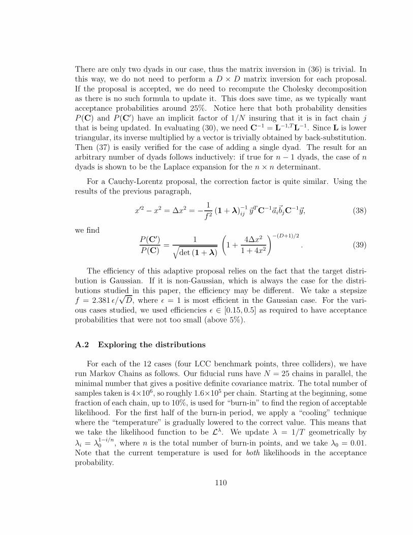
There are only two dyads in our case, thus the matrix inversion in (36) is trivial. Inthis way, we do not need to perform a D × D matrix inversion for each proposal.If the proposal is accepted, we do need to recompute the Cholesky decompositionas there is no such formula to update it. This does save time, as we typically wantacceptance probabilities around 25%. Notice here that both probability densitiesP (C) and P (C′) have an implicit factor of 1/N insuring that it is in fact chain jthat is being updated. In evaluating (30), we need C−1 = L−1,TL−1. Since L is lowertriangular, its inverse multiplied by a vector is trivially obtained by back-substitution.Then (37) is easily verified for the case of adding a single dyad. The result for anarbitrary number of dyads follows inductively: if true for n − 1 dyads, the case of ndyads is shown to be the Laplace expansion for the n× n determinant.
For a Cauchy-Lorentz proposal, the correction factor is quite similar. Using theresults of the previous paragraph,
x′2 − x2 = ∆x2 = − 1
f 2(1 + λ)−1
ij ~yTC−1~ai~bjC−1~y, (38)
we findP (C′)
P (C)=
1√
det (1 + λ)
(1 +
4∆x2
1 + 4x2
)−(D+1)/2
. (39)
The efficiency of this adaptive proposal relies on the fact that the target distri-bution is Gaussian. If it is non-Gaussian, which is always the case for the distri-butions studied in this paper, the efficiency may be different. We take a stepsizef = 2.381 ǫ/
√D, where ǫ = 1 is most efficient in the Gaussian case. For the vari-
ous cases studied, we used efficiencies ǫ ∈ [0.15, 0.5] as required to have acceptanceprobabilities that were not too small (above 5%).
A.2 Exploring the distributions
For each of the 12 cases (four LCC benchmark points, three colliders), we haverun Markov Chains as follows. Our fiducial runs have N = 25 chains in parallel, theminimal number that gives a positive definite covariance matrix. The total number ofsamples taken is 4×10⁶, so roughly 1.6×10⁵ per chain. Starting at the beginning, somefraction of each chain, up to 10%, is used for “burn-in” to find the region of acceptablelikelihood. For the first half of the burn-in period, we apply a “cooling” techniquewhere the “temperature” is gradually lowered to the correct value. This means thatwe take the likelihood function to be Lλ. We update λ = 1/T geometrically by
λi = λ1−i/n0 , where n is the total number of burn-in points, and we take λ0 = 0.01.
Note that the current temperature is used for both likelihoods in the acceptanceprobability.
110
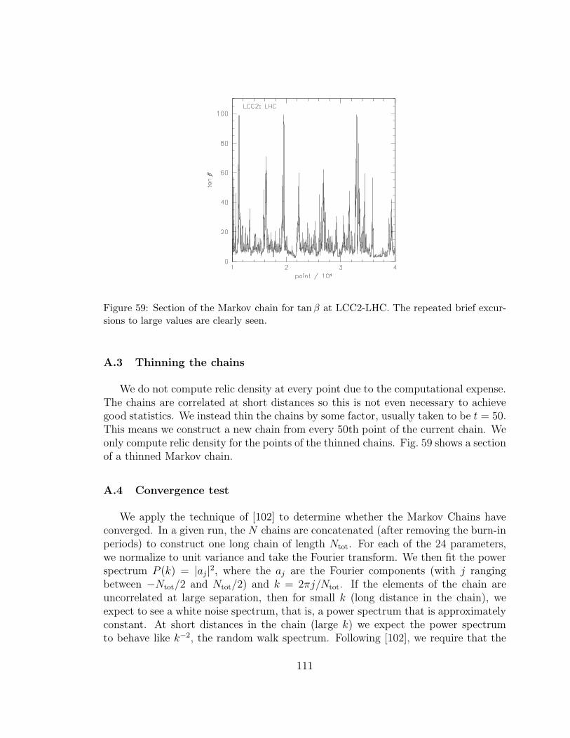
Figure 59: Section of the Markov chain for tan β at LCC2-LHC. The repeated brief excur-sions to large values are clearly seen.
A.3 Thinning the chains
We do not compute relic density at every point due to the computational expense.The chains are correlated at short distances so this is not even necessary to achievegood statistics. We instead thin the chains by some factor, usually taken to be t = 50.This means we construct a new chain from every 50th point of the current chain. Weonly compute relic density for the points of the thinned chains. Fig. 59 shows a sectionof a thinned Markov chain.
A.4 Convergence test
We apply the technique of [102] to determine whether the Markov Chains haveconverged. In a given run, the N chains are concatenated (after removing the burn-inperiods) to construct one long chain of length Ntot. For each of the 24 parameters,we normalize to unit variance and take the Fourier transform. We then fit the powerspectrum P (k) = |aj|2, where the aj are the Fourier components (with j rangingbetween −Ntot/2 and Ntot/2) and k = 2πj/Ntot. If the elements of the chain areuncorrelated at large separation, then for small k (long distance in the chain), weexpect to see a white noise spectrum, that is, a power spectrum that is approximatelyconstant. At short distances in the chain (large k) we expect the power spectrumto behave like k−2, the random walk spectrum. Following [102], we require that the
111
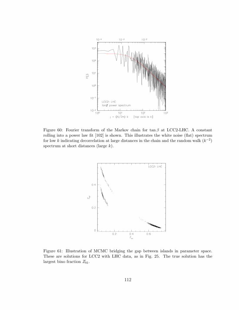
Figure 60: Fourier transform of the Markov chain for tan β at LCC2-LHC. A constantrolling into a power law fit [102] is shown. This illustrates the white noise (flat) spectrumfor low k indicating decorrelation at large distances in the chain and the random walk (k−2)spectrum at short distances (large k).
Figure 61: Illustration of MCMC bridging the gap between islands in parameter space.These are solutions for LCC2 with LHC data, as in Fig. 25. The true solution has thelargest bino fraction Zb1.
112

Figure 62: Illustration of MCMC exploring very different regions of parameter space. Theseregions are actually connected, as shown in Fig. 36, but allow vastly different properties forχ02, as shown here.
break between these two behaviors occurs beyond j = 20. When this is true, the fitto P (0) can be trusted, and r = P (0)/Ntot indicates the fractional error made in thevariance of the parameter. We require r < 0.01, meaning at most 10% errors madein the error of a given parameter, based on the Markov chain.
The power spectrum test can be applied either to the full chain or the thinnedchain. The results are insensitive as long as the scales removed are in the randomwalk regime. For chains of length Ntot, thinning by a factor of t has little effect unlessthe turnover is beyond j = Ntot/t. We typically find j values at turnover of 20− 200,so this is not an issue. An illustration of the power spectrum test is given in Fig. 60.
B Disconnected families of supersymmetry parameters
In this appendix we describe the conditions where multiple discrete regions ofparameter space would be consistent with collider measurements. Such ambiguitiesoccur for all of the benchmark points under study. The simplest alternate solutionsinvolve only changing the signs of µ and m1. This four-fold degeneracy is evidentin every model given only LHC data. Since these signs are relevant to the mixingparameters of the neutralinos and charginos, it is essential to measure the mixed pair
113

production cross sections at the ILC, e.g., e+e− → χ01χ
02. There are more subtle
degeneracies as well, as we discuss in the following sections.
B.1 Benchmark point LCC1
At the LHC, three neutralinos are visible: the lightest (bino) at 95.5 GeV, thenext lightest (wino) at 181.6 GeV, and the heaviest (heavier Higgsino) at 375.6 GeV.No chargino is seen, implying a mass > 125 GeV. Assuming that the identities of theneutralinos are unknown at the LHC, it is possible that the values of the parameters|µ| and m2 are exchanged. This implies that the second and third neutralinos areHiggsinos, and the heaviest is mostly wino. This solution gives an acceptable massspectrum for the LHC errors. In addition, there is the four-fold degeneracy due tothe uncertain signs of µ and m1. There are thus 8 solutions for LHC data. Noticethat we can be confident that the lightest neutralino is mostly bino-like; its mass is95 GeV, and a chargino at this mass would be visible.
The ILC-500 completely resolves the degeneracies of this model. The identitiesof χ0
2 and χ+1 as wino-like are determined by the pair production cross sections, and
the sign ambiguities are completely resolved by the χ01χ
02 production cross section:
changing the signs has a large effect on the (small) bino fraction of χ02.
At this point, the 8 islands are very well separated in parameter space. Forthe LHC, we have shown the results of the correct island only. Including the othersolutions would not make a large difference, as they only affect the subdominant winoand Higgsino admixtures in the lightest neutralino.
B.2 Benchmark point LCC2
The three lightest neutralinos are visible at the LHC, while there is only the usuallimit of 125 GeV on the lightest chargino mass. All of the neutralinos are quitemixed in composition, thus the permutation ambiguities in m1, m2, µ are somewhatambiguous. As shown in Fig. 61, there are essentially three solutions for positive µand m1. When plotted as islands in neutralino composition, the solutions are clearlyseparated. The incorrect solutions have the lightest neutralino being mostly wino-likeor Higgsino-like rather than mostly bino-like. In fact, the wino and Higgsino caseshave two peaks, not well separated, as seen in Fig. 25. There is an additional binosolution as well (not shown), with M2 larger than 1 TeV, but its properties are similarto the proper bino solution, except that the wino fraction is very much smaller.
The ILC-500 removes the degeneracies. The χ02χ
03 cross section identifies the
neutralinos and also their mixing angles, thus the negative µ solution at least is gone.The ILC-1000 allows no incorrect solution.
114

At this point only, the disjoint islands at positive µ and m1 are close together inparameter space. Our LHC results show all islands with the correct signs. During thecooling and burn-in period, Markov chains find an island at random, and remain therefor the remainder of the run. We find that burn-in is slow enough that the numberof chains that finds a solution is proportional to the likelihood of the solution. Wehave verified this with a “stepping stone” technique, where the space between theislands, normally having vanishing likelihood, is assigned a small likelihood. Markovchains can now step away from an island, into this “sea”, and thus travel back andforth between islands. Points in the “sea” can be removed at the end with impor-tance sampling. We have verified the relative weights of the islands with just such asimulation.
B.3 Benchmark points LCC3 and LCC4
Benchmark points LCC3 and LCC4 have similar structure for discrete solutions,thus we discuss them together. Both have the two lightest neutralinos visible atthe LHC. Assuming that none have been missed between the two, the “F” structurein the m1 vs. (m2 or µ) plot appears naturally. This is understood physically asfollows. Given the large mass splitting between the two visible neutralinos, and theassumption that none have been missed, the lightest neutralino is either bino or wino,and the heavier of the two visible neutralinos can be anything. As all neutralinos atthese benchmark points are heavier than 125 GeV, the non-observation of charginosgives no additional information. The “F” structure is repeated for each of the foursign combinations for m1 and µ. In Fig. 62 we illustrate an interesting effect of the“F” structure, in that there are three possible solutions to the composition of thesecond lightest neutralino.
For each of these points, ILC-500 data would collapse the “F” structure somewhat,but the sign ambiguities remain. ILC-1000 is required to remove the last ambiguities,with the neutralino and chargino pair production cross sections.
Unfortunately, the sign ambiguity in µ remains for point LCC4, even taking ILC-1000 data into account. However, since this point has large tan β, its correction to themuon g−2 is large, and has a sign equal to the sign of µ. The BNL measurement [122]rules out the negative µ solution, even with a very conservative constraint allowingthe union of the 3σ regions from the e+e− and τ decay evaluations of the hadronicvacuum polarization [123,124].
For these two points, we have only illustrated the correct signs. The “F” patternsare too far apart in parameter space for easy exploration by single Markov chains.
115
ACKNOWLEDGEMENTS
Our perspective on dark matter has been shaped by discussions with many peopleover the past few years. We are particularly grateful to Genevieve Belanger, AndreasBirkedal, Jonathan Feng, Paolo Gondolo, Konstantin Matchev, and Mark Trodden forsharing their insights. We thank Mihoko Nojiri and Giacomo Polesello for an helpfulcorrespondence. EAB thanks Richard Schnee, Blas Cabrera and Dan Akerib for manyuseful discussions on the capabilities of direct detection experiments, and Larry Waiand Tune Kamae for useful discussions relating to gamma ray detection. MEP thanksJim Alexander, Richard Gray, Bhaskar Dutta, and Teruki Kamon for discussions oftheir ILC simulation results. He is also grateful to Ee Hou Yong and Wu-Yen Chuangfor educating him about neutralino dark matter. The work of MB was supported bythe US Department of Energy under Contract No. DE–AC02-05CH11231 and usedresources of the National Energy Research Scientific Computing Center, supported byContract No. DE-AC03-76SF0098. The work of EAB, MEP, and TW was supportedby the US Department of Energy under Contract No. DE–AC02–76SF00515.
References
[1] O. Lahav and A. Liddle, in S. Eidelman, et al., Review of Particle Properties,Phys. Lett. B592, 1 (2004); http://pdg.lbl.gov/.
[2] G. Jungman, M. Kamionkowski and K. Griest, Phys. Rept. 267, 195 (1996)[arXiv:hep-ph/9506380].
[3] G. Bertone, D. Hooper and J. Silk, Phys. Rept. 405, 279 (2005)[arXiv:hep-ph/0404175].
[4] W. Hu, R. Barkana and A. Gruzinov, Phys. Rev. Lett. 85, 1158 (2000)[arXiv:astro-ph/0003365].
[5] B. Moore, Astrophys. J. 413, L93 (1993) [arXiv:astro-ph/9306004].
[6] D. N. Spergel et al. [WMAP Collaboration], Astrophys. J. Suppl. 148, 175 (2003)[arXiv:astro-ph/0302209].
[7] J. R. Bond, G. Efstathiou and M. Tegmark, Mon. Not. Roy. Astron. Soc. 291,L33 (1997) [arXiv:astro-ph/9702100].
[8] F. E. Paige, S. D. Protopopescu, H. Baer and X. Tata, arXiv:hep-ph/0312045.
116

[9] P. Gondolo, J. Edsjo, P. Ullio, L. Bergstrom, M. Schelke and E. A. Baltz, JCAP0407, 008 (2004) [arXiv:astro-ph/0406204], New Astron. Rev. 49, 149 (2005).
[10] B. C. Allanach, G. Belanger, F. Boudjema and A. Pukhov, JHEP 0412, 020(2004) [arXiv:hep-ph/0410091].
[11] M. M. Nojiri, G. Polesello and D. R. Tovey, arXiv:hep-ph/0512204.
[12] M. Battaglia and M. E. Peskin, arXiv:hep-ph/0509135.
[13] R. J. Scherrer and M. S. Turner, Phys. Rev. D 33, 1585 (1986) [Erratum-ibid.D 34, 3263 (1986)].
[14] H. Pagels and J. R. Primack, Phys. Rev. Lett. 48, 223 (1982).
[15] S. Weinberg, Phys. Rev. Lett. 48, 1303 (1982).
[16] S. Weinberg, Phys. Rev. Lett. 50, 387 (1983).
[17] H. Goldberg, Phys. Rev. Lett. 50, 1419 (1983).
[18] J. R. Ellis, J. S. Hagelin, D. V. Nanopoulos and M. Srednicki, Phys. Lett. B127, 233 (1983); J. R. Ellis, J. S. Hagelin, D. V. Nanopoulos, K. A. Olive andM. Srednicki, Nucl. Phys. B 238, 453 (1984).
[19] H. C. Cheng, J. L. Feng and K. T. Matchev, Phys. Rev. Lett. 89, 211301 (2002)[arXiv:hep-ph/0207125].
[20] G. Servant and T. M. P. Tait, Nucl. Phys. B 650, 391 (2003)[arXiv:hep-ph/0206071].
[21] K. Agashe and G. Servant, Phys. Rev. Lett. 93, 231805 (2004)[arXiv:hep-ph/0403143].
[22] E. Katz, J. y. Lee, A. E. Nelson and D. G. E. Walker, arXiv:hep-ph/0312287.
[23] H. C. Cheng and I. Low, JHEP 0309, 051 (2003) [arXiv:hep-ph/0308199].
[24] S. J. Asztalos et al., Astrophys. J. 571, L27 (2002) [arXiv:astro-ph/0104200];Phys. Rev. D 69, 011101 (2004) [arXiv:astro-ph/0310042].
[25] C. Boehm, D. Hooper, J. Silk, M. Casse and J. Paul, Phys. Rev. Lett. 92, 101301(2004) [arXiv:astro-ph/0309686].
[26] D. R. Tovey, Eur. Phys. J. direct C 4, N4 (2002).
117

[27] M. Battaglia, A. Datta, A. De Roeck, K. Kong and K. T. Matchev, JHEP 0507,033 (2005) [arXiv:hep-ph/0502041]; arXiv:hep-ph/0507284.
[28] A. Datta, K. Kong and K. T. Matchev, Phys. Rev. D 72, 096006 (2005),[Erratum-ibid. D 72, 119901 (2005) [arXiv:hep-ph/0509246].
[29] J. M. Smillie and B. R. Webber, arXiv:hep-ph/0507170.
[30] J. L. Feng, A. Rajaraman and F. Takayama, Phys. Rev. Lett. 91, 011302 (2003)[arXiv:hep-ph/0302215].
[31] J. L. Feng and B. T. Smith, Phys. Rev. D 71, 015004 (2005) [Erratum-ibid. D71, 0109904 (2005)] [arXiv:hep-ph/0409278].
[32] J. L. Feng, A. Rajaraman, B. T. Smith, S. Su and F. Takayama,arXiv:hep-ph/0410178.
[33] K. Hamaguchi, Y. Kuno, T. Nakaya and M. M. Nojiri, Phys. Rev. D 70, 115007(2004) [arXiv:hep-ph/0409248].
[34] A. Brandenburg, L. Covi, K. Hamaguchi, L. Roszkowski and F. D. Steffen, Phys.Lett. B 617, 99 (2005) [arXiv:hep-ph/0501287].
[35] T. Moroi and L. Randall, Nucl. Phys. B 570, 455 (2000) [arXiv:hep-ph/9906527].
[36] R. Kitano and I. Low, Phys. Rev. D 71, 023510 (2005) [arXiv:hep-ph/0411133];R. Kitano and Y. Nomura, Phys. Lett. B 632, 162 (2006)[arXiv:hep-ph/0509221].
[37] K. A. Olive, G. Steigman and T. P. Walker, Phys. Rept. 333, 389 (2000)[arXiv:astro-ph/9905320].
[38] R. J. Gaitskell, Ann. Rev. Nucl. Part. Sci. 54, 315 (2004); see alsohttp://dmtools.berkeley.edu/.
[39] D. S. Akerib et al. [CDMS Collaboration], Phys. Rev. Lett. 96, 011302 (2006)[arXiv:astro-ph/0509259].
[40] G. Angloher et al., Astropart. Phys. 23, 325 (2005) [arXiv:astro-ph/0408006].
[41] V. Sanglard et al. [The EDELWEISS Collaboration], Phys. Rev. D 71, 122002(2005) [arXiv:astro-ph/0503265].
[42] G. J. Alner et al. [UK Dark Matter Collaboration], Astropart. Phys. 23, 444(2005).
118

[43] R. Bernabei et al. [DAMA Collaboration], Phys. Lett. B 480, 23 (2000).
[44] Specific particle physics scenarios that partially resolve the contradiction betweenDAMA and the other experiments listed are reviewed in [38].
[45] R. W. Schnee et al. [The SuperCDMS Collaboration], arXiv:astro-ph/0502435.
[46] E. Aprile [The XENON Collaboration], arXiv:astro-ph/0502279.
[47] N. Ferrari [Warp Collaboration], J. Phys. Conf. Ser. 39, 111 (2006).
[48] E. I. Gates, G. Gyuk and M. S. Turner, Phys. Rev. D 53 (1996)4138 [arXiv:astro-ph/9508071], E. Gates, G. Gyuk and M. S. Turner,arXiv:astro-ph/9704253.
[49] A. K. Drukier, K. Freese and D. N. Spergel, Phys. Rev. D 33, 3495 (1986).
[50] P. Belli, R. Cerulli, N. Fornengo and S. Scopel, Phys. Rev. D 66, 043503 (2002)[arXiv:hep-ph/0203242].
[51] D. Stiff, L. M. Widrow and J. Frieman, Phys. Rev. D 64, 083516 (2001)[arXiv:astro-ph/0106048]; D. Stiff and L. M. Widrow, Phys. Rev. Lett. 90,211301 (2003) [arXiv:astro-ph/0301301].
[52] P. Sikivie and J. R. Ipser, Phys. Lett. B 291, 288 (1992); P. Sikivie, Phys. Lett.B 432, 139 (1998) [arXiv:astro-ph/9705038].
[53] J. Diemand, B. Moore and J. Stadel, Nature 433, 389 (2005)[arXiv:astro-ph/0501589].
[54] K. Freese, P. Gondolo and H. J. Newberg, Phys. Rev. D 71, 043516 (2005)[arXiv:astro-ph/0309279]; K. Freese, P. Gondolo, H. J. Newberg and M. Lewis,Phys. Rev. Lett. 92, 111301 (2004) [arXiv:astro-ph/0310334].
[55] We thank the referee for calling our attention to this important point.
[56] A complete expression for the WIMP-nucleon cross section in SUSY models isgiven in [2].
[57] A. E. Nelson and D. B. Kaplan, Phys. Lett. B 192, 193 (1987); D. B. Kaplanand A. Manohar, Nucl. Phys. B 310, 527 (1988).
[58] A. Bottino, F. Donato, N. Fornengo and S. Scopel, “Size of the neutralinonucleon cross-section in the light of a new Astropart. Phys. 18, 205 (2002)[arXiv:hep-ph/0111229].
119

[59] J. R. Ellis, K. A. Olive, Y. Santoso and V. C. Spanos, Phys. Rev. D 71, 095007(2005) [arXiv:hep-ph/0502001].
[60] C. Michael, C. McNeile and D. Hepburn [UKQCD Collaboration], Nucl. Phys.Proc. Suppl. 106, 293 (2002) [arXiv:hep-lat/0109028].
[61] M. Procura, T. R. Hemmert and W. Weise, Phys. Rev. D 69, 034505 (2004)[arXiv:hep-lat/0309020].
[62] We thank Claude Bernard and Akira Ukawa for discussions of these issues.
[63] J. D. Lewin and P. F. Smith, Astropart. Phys. 6, 87 (1996).
[64] The parameters of the SuperCDMS experiment will be discussed in Section 4.5.
[65] We thank Richard Schnee for providing to us the results of his simulations of thecapabilities of the SuperCDMS detector.
[66] J. R. Primack, D. Seckel and B. Sadoulet, Ann. Rev. Nucl. Part. Sci. 38, 751(1988).
[67] J. L. Bourjaily and G. L. Kane, arXiv:hep-ph/0501262.
[68] G. Duda, G. Gelmini and P. Gondolo, Phys. Lett. B 529, 187 (2002)[arXiv:hep-ph/0102200].
[69] W. de Boer, M. Herold, C. Sander and V. Zhukov, Eur. Phys. J. C 33, S981(2004) [arXiv:hep-ph/0312037]; W. de Boer, C. Sander, V. Zhukov, A. V. Glady-shev and D. I. Kazakov, Phys. Lett. B 636, 13 (2006) [arXiv:hep-ph/0511154];Phys. Rev. Lett. 95, 209001 (2005) [arXiv:astro-ph/0602325].
[70] J. F. Navarro, C. S. Frenk and S. D. M. White, Astrophys. J. 462, 563 (1996)[arXiv:astro-ph/9508025].
[71] B. Moore, F. Governato, T. Quinn, J. Stadel and G. Lake, Astrophys. J. 499,L5 (1998) [arXiv:astro-ph/9709051].
[72] The divergence is logarithmic and thus not very sensitive to the value of a cutoff.In Fig. 5, we put the cutoff at the Schwartzschild radius of the black hole at thecenter of the galaxy.
[73] R. H. Wechsler, J. S. Bullock, J. R. Primack, A. V. Kravtsov and A. Dekel,Astrophys. J. 568, 52 (2002) [arXiv:astro-ph/0108151].
[74] J. R. Primack, arXiv:astro-ph/0312549. We thank Joel Primack for discussionsof the issues reviewed in this paper.
120

[75] E. A. Baltz, C. Briot, P. Salati, R. Taillet and J. Silk, Phys. Rev. D 61, 023514(2000) [arXiv:astro-ph/9909112].
[76] J. E. Taylor and A. Babul, Mon. Not. Roy. Astron. Soc. 348, 811 (2004)[arXiv:astro-ph/0301612].
[77] Recently, the relic density calculation in the Universal Extra Dimension model ofWIMP dark matter [19,20] has been analyzed over a comparably large parameterspace. See [78,79].
[78] K. Kong and K. T. Matchev, JHEP 0601, 038 (2006) [arXiv:hep-ph/0509119].
[79] F. Burnell and G. D. Kribs, Phys. Rev. D 73, 015001 (2006)[arXiv:hep-ph/0509118].
[80] J. R. Ellis, T. Falk, G. Ganis and K. A. Olive, Phys. Rev. D 62, 075010 (2000)[arXiv:hep-ph/0004169]; J. R. Ellis, K. A. Olive, Y. Santoso and V. C. Spanos,Phys. Lett. B 565, 176 (2003) [arXiv:hep-ph/0303043].
[81] J. Edsjo, M. Schelke, P. Ullio and P. Gondolo, JCAP 0304, 001 (2003)[arXiv:hep-ph/0301106].
[82] H. Baer, A. Belyaev, T. Krupovnickas and X. Tata, JHEP 0402, 007 (2004)[arXiv:hep-ph/0311351].
[83] These study points were chosen as a part of a broader study of connections be-tween ILC measurements and cosmology, organized by J. Feng and M. Trodden.The paper is in preparation.
[84] G. Belanger, F. Boudjema, A. Pukhov and A. Semenov, Comput. Phys. Com-mun. 149, 103 (2002) [arXiv:hep-ph/0112278], Comput. Phys. Commun. 174,577 (2006) [arXiv:hep-ph/0405253].
[85] B. C. Allanach et al., in Proc. of the APS/DPF/DPB Summer Study on theFuture of Particle Physics (Snowmass 2001) ed. N. Graf, Eur. Phys. J. C 25,113 (2002) [eConf C010630, P125 (2001)] [arXiv:hep-ph/0202233].
[86] G. Weiglein et al. [LHC/LC Study Group], Phys. Rept. 426, 47 (2006)[arXiv:hep-ph/0410364].
[87] R. Gray et al., arXiv:hep-ex/0507008.
[88] V. Khotilovich, R. Arnowitt, B. Dutta and T. Kamon, Phys. Lett. B 618, 182(2005) [arXiv:hep-ph/0503165].
121

[89] To be precise, [88] studied a set of closely related points with m(τ1) −m(χ01) =
4.7, 9.5, 19.0 GeV, defined with a presciption slightly different from ours for thesupersymmetry spectrum calculation. Our LCC3, which has m(τ1) − m(χ0
1) =10.5 GeV, is sufficiently close to the point 2 defined in [88] to make use of thesimulations done in that study.
[90] M. Battaglia, arXiv:hep-ph/0410123.
[91] J. A. Aguilar-Saavedra et al., Eur. Phys. J. C 46, 43 (2006)[arXiv:hep-ph/0511344].
[92] J. L. Feng, K. T. Matchev and T. Moroi, Phys. Rev. Lett. 84,2322 (2000) [arXiv:hep-ph/9908309], Phys. Rev. D 61, 075005 (2000)[arXiv:hep-ph/9909334].
[93] Additional benchmark points for supersymmetry studies are defined in the pa-pers [94]. Certain of these points are now under study with detailed simulationsby the CMS Collaboration (A. de Roeck, personal communication).
[94] M. Battaglia et al., Eur. Phys. J. C 22, 535 (2001) [arXiv:hep-ph/0106204];M. Battaglia, A. De Roeck, J. R. Ellis, F. Gianotti, K. A. Olive and L. Pape,Eur. Phys. J. C 33, 273 (2004) [arXiv:hep-ph/0306219]; A. De Roeck, J. R. Ellis,F. Gianotti, F. Moortgat, K. A. Olive and L. Pape, arXiv:hep-ph/0508198.
[95] Other studies for the LHC, for example, those reported in [96], choose additionalpoints at much higher values of the superparticle masses. These additional pointstest the ability of the LHC to discover supersymmetry well beyond the regionfavored by natural electroweak symmetry breaking.
[96] ATLAS Collaboration, Detector and Physics Performance Technical Design Re-port, vol. II, CERN/LHCC/99-14 (1999).
[97] P. Bambade, M. Berggren, F. Richard and Z. Zhang, arXiv:hep-ph/0406010.
[98] G. Polesello and D. R. Tovey, JHEP 0405, 071 (2004) [arXiv:hep-ph/0403047].
[99] M. Battaglia, I. Hinchliffe and D. Tovey, J. Phys. G 30, R217 (2004)[arXiv:hep-ph/0406147].
[100] A. Birkedal et al., arXiv:hep-ph/0507214.
[101] W.R. Gilks, S. Richardson, D.J. Spiegelhalter, eds. Markov Chain Monte Carloin Practice. (Chapman and Hall, 1996).
[102] J. Dunkley, M. Bucher, P. G. Ferreira, K. Moodley and C. Skordis, Mon. Not.Roy. Astron. Soc. 356, 925 (2005) [arXiv:astro-ph/0405462].
122
[103] E. A. Baltz and P. Gondolo, JHEP 0410, 052 (2004) [arXiv:hep-ph/0407039].
[104] B. C. Allanach and C. G. Lester, Phys. Rev. D 73, 015013 (2006)[arXiv:hep-ph/0507283].
[105] R. R. de Austri, R. Trotta and L. Roszkowski, arXiv:hep-ph/0602028.
[106] A. Kusenko, P. Langacker and G. Segre, Phys. Rev. D 54, 5824 (1996)[arXiv:hep-ph/9602414].
[107] B. K. Gjelsten, D. J. Miller and P. Osland, arXiv:hep-ph/0507232.
[108] N. Arkani-Hamed, G. L. Kane, J. Thaler and L. T. Wang, JHEP 0608, 070(2006) [arXiv:hep-ph/0512190].
[109] I. Hinchliffe and F. E. Paige, Phys. Rev. D 60, 095002 (1999)[arXiv:hep-ph/9812233].
[110] L. Bergstrom, P. Ullio and J. H. Buckley, Astropart. Phys. 9, 137 (1998)[arXiv:astro-ph/9712318].
[111] N. Gehrels and P. Michelson, Astropart. Phys. 11 (1999) 277.
[112] D. Hooper and B. L. Dingus, Phys. Rev. D 70, 113007 (2004)[arXiv:astro-ph/0210617].
[113] F. Aharonian, et al. (HESS Collaboration), Nature 439, 695 (2006).
[114] We thank Tsuneyoshi Kamae for discussions of these issues.
[115] P. Sreekumar et al. [EGRET Collaboration], Astrophys. J. 494, 523 (1998)[arXiv:astro-ph/9709257].
[116] K. Griest and D. Seckel, Phys. Rev. D 43, 3191 (1991).
[117] R. Arnowitt, B. Dutta, T. Kamon, N. Kolev and D. Toback,arXiv:hep-ph/0603128; R. Arnowitt et al., arXiv:hep-ph/0608193.
[118] The MCMC runs for LCC3 displayed in Section 6 did not include this constrainton the ττ edge position, as Table 6 indicates. After the first paper in [117]appeared, we redid the LHC runs adding this constraint, but found negligibledifference in the results.
[119] T. Sjostrand, L. Lonnblad, S. Mrenna and P. Skands, arXiv:hep-ph/0308153.
[120] I. V. Moskalenko and A. W. Strong, Astrophys. J. 493, 694 (1998)[arXiv:astro-ph/9710124].
123

[121] E. A. Baltz and J. Edsjo, Phys. Rev. D 59, 023511 (1999)[arXiv:astro-ph/9808243].
[122] G. W. Bennett et al. [Muon g-2 Collaboration], Phys. Rev. Lett. 92, 161802(2004) [arXiv:hep-ex/0401008].
[123] M. Davier, S. Eidelman, A. Hocker and Z. Zhang, Eur. Phys. J. C 27, 497(2003) [arXiv:hep-ph/0208177].
[124] M. Davier, S. Eidelman, A. Hocker and Z. Zhang, Eur. Phys. J. C 31, 503(2003) [arXiv:hep-ph/0308213].
124