determination of properties of graded...

Acta mater. 48 (2000) 4293–4306www.elsevier.com/locate/actamat

DETERMINATION OF PROPERTIES OF GRADED MATERIALSBY INVERSE ANALYSIS AND INSTRUMENTED INDENTATION

T. NAKAMURA 1*, T. WANG 1 and S. SAMPATH2

1Department of Mechanical Engineering, State University of New York at Stony Brook, Stony Brook, NY11794, USA and2Department of Materials Science and Engineering, State University of New York at

Stony Brook, Stony Brook, NY 11794, USA

( Received 17 April 2000; received in revised form 6 July 2000; accepted 6 July 2000 )

Abstract—In this paper, a new measurement procedure based on inverse analysis and instrumented micro-indentation is introduced. The inverse analysis is utilized to extract information from indented load–displace-ment data beyond usual parameters such as elastic modulus. For the initial implementation of this procedure,determination of non-linear functionally graded materials (FGMs) parameters is considered. In FGMs, thecompositional profile and the effective mechanical property through the thickness are essential in verifyingthe fabrication process and estimating residual stresses and failure strengths. However, due to spatial variationof their properties, it is often difficult or costly to make direct measurements of these parameters. In orderto alleviate the difficulties associated with testing of FGMs, we propose an effective but simple procedurebased on the inverse analysis which relies solely on instrumented micro-indentation records. More specifically,the Kalman filter technique, which was originally introduced for signal/digital filter processing, is used toestimate FGM through-thickness compositional variation and a rule-of-mixtures parameter that defines effec-tive properties of FGMs. Essentially, the inverse analysis processes the indented displacement record atseveral load magnitudes and attempts to make best estimates of the unknown parameters. Our feasibilitystudy shows promising results when combined data from two differently sized indenters are employed. Theprocedure proposed is also applicable in estimating other physical and mechanical properties of anycoating/layered materials. 2000 Acta Metallurgica Inc. Published by Elsevier Science Ltd. All rightsreserved.

Keywords:Functionally graded materials (FGM); Coating; Mechanical properties (plastic); Inverse analysis

1. INTRODUCTION

Functionally graded materials (FGMs) are spatialcomposites that display discrete or continuously vary-ing compositions over a definable geometrical length.The gradients can be continuous on a microscopiclevel or layers comprised of metals, ceramics andpolymers. In a typical FGM, the volume fractions ofthe constituents are varied gradually over a macro-scale geometrical dimension such as coating thick-ness. Within an FGM, the different phases have dif-ferent functions to suit the needs of the material.FGMs can be fabricated by several techniques includ-ing adhesive bonding, sintering, thermal spray andreactive infiltration [1, 2].

The material gradients induced by the spatial vari-ations of the material properties make FGMs behavedifferently from common homogeneous materials and

* To whom all correspondence should be addressed. Tel.:+1 (631) 632-8312; fax:+1 (631) 632-8544.

E-mail address: [email protected] (T.Nakamura)

1359-6454/00/$20.00 2000 Acta Metallurgica Inc. Published by Elsevier Science Ltd. All rights reserved.PII: S1359-6454(00 )00217-2

traditional composites. Because of this behavior,quantification of material parameters is more difficult.Recently, several methods have been introduced tocharacterize the properties of FGMs. Weissenbeketal. [3] applied a matrix-inclusion model based on theMori–Tanaka method to define the rule of mixturesfor a ceramic/metal system. Sureshet al. [4] andGiannakopoulos and Suresh [5, 6] have developedanalytical and experimental tools to estimate the elas-tic properties of graded materials using instrumentedmicro-indentation. Other efforts on mechanicalcharacterization of FGMs include the thermal residualstresses at the graded interface [7], the process-induced residual stresses [8], the Hertzian-crack sup-pression [9] and the crack-tip field in an elasticmedium with varying Young’s modulus [10]. Manyother works are referenced in [2].

The measurement ofnon-linear or elastic–plasticFGMs is more complex due to additional materialparameters. Unlike elastic FGMs, not only the elasticmodulus but also the flow stress and the plastic strain-hardening modulus, which vary spatially, must beidentified. In order to overcome the complexities

4294 NAKAMURA et al.: INDENTATION OF GRADED MATERIALS

associated with the measurements of non-linearFGMs, we propose a new procedure that requiresminimal effort in estimating the parameters. This pro-cedure is based on the inverse analysis, which maxim-izes the extraction of information available in themicro-indentation data. Here, the Kalman filter theoryis utilized to estimate the FGM’s through-thicknesscompositional profile and the stress–strain transferparameter that defines the effective properties of elas-tic–plastic FGMs. In order to implement the inverseanalysis, the compositional profile is idealized to fol-low the power-law distribution and the effective pro-perty is defined by the rule of mixtures.

2. KALMAN FILTER

The Kalman filter was developed as an optimal,recursive, signal-processing algorithm [11]. Sincethen, due in large part to advances in digital comput-ing, the Kalman filter has been the subject of exten-sive research and application. This inverse procedurehas been applied in signal processing, inertial navi-gation, radar tracking, sensor calibration, manufactur-ing and other aspects [12]. It provides an efficientcomputational solution based on the least-squarestheory. The method is effective in estimatingunknown state variables using measurements thatmay contain substantialerror or noise. Essentially,the algorithm updates the previous estimates throughindirect measurements of the state variables and thecovariance information of both the state and measure-ment variables.

The theory of the Kalman filter is based on the fol-lowing update algorithm

xt = xt21 + Kt[zt2H t(xt21)]. (1)

Here,xt is the state vector containingunknown para-meters, zt is the vector containingexperimentallymeasured variablesand Ht is the vector for themeasurement variables shown as functions of stateparameters. The subscript “t” denotes updatingincrement. It is assumed thatzt contains measurementerror while the exact relation between the state para-meters (e.g., material constants) and the measuredvariables (e.g., displacement record) is given in thefunctionH t. The correction at each increment is madethrough the Kalman gain matrixKt calculated as

Kt = PthTt R21

t , where (2)Pt = Pt212Pt21hT

t (htPt21hTt + Rt)21htPt21.

Here,Pt is the measurement covariance matrix relatedto the range of unknown state parameters at incrementt. Also, Rt is the error covariance matrix which isrelated to the size of the measurement error. Whilethe former matrix is updated every increment accord-

ing to equation (2), the values of the latter matrixmust be prescribed at each increment. The matrixht

contains the gradients ofHt with respect toxt. BothH t and ht functions must be knowna priori.

The Kalman filter has been used in seekingunknown parameters of homogeneous material mod-els [13–15]. Essentially, this inverse analysis post-processes experimentally obtained data and attemptsto best estimate unknown state variables or materialconstants. In our analysis, the Kalman filter techniqueis employed for the determination of elastic–plasticFGM parameters using instrumented indentation. Thefollowing information is required for the procedure:measured indented load–displacement records anddisplacement as a function of load for given materialparameters. In the Kalman filter procedure, it isknown that the convergence characteristics depend onseveral factors including shape of the test specimen,initial estimates of the unknown parameters and themeasurement error, as well as the accuracy ofH t andht functions.

In order to establish an effective procedure basedon the Kalman filter, the following tasks must be per-formed.

1. Representation of the unknown variables in suit-able forms.

2. Selection of appropriate ranges/domain sizes forunknown variables.

3. Creation of reference data source/table for themeasurement variables and their gradients.

4. Choice of total number of filtering increments andtheir magnitudes.

5. Determination of suitable values for the matricesof covariantPt andRt.

The above tasks are carefully examined and discussedin the following sections. Many inverse problems areinitially “ill-posed”, which means that convergence tothe correct solutions is difficult. Therefore, it isrequired to formulate “a priori information” and/orsupply additional information/measurements toimprove the estimates.

3. GEOMETRICAL AND MATERIAL MODELS

3.1. Micro-indentation test

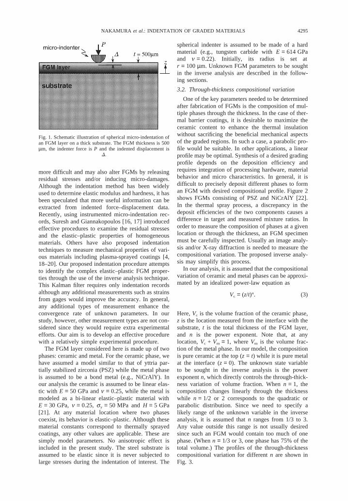
In our effort to establish a useful but robust pro-cedure to determine the properties of FGMs, a thinFGM model placed on top of a thick substrate asshown in Fig. 1 is considered. Although there arevarious methods to measure mechanical responses ofFGMs, including optical techniques and strain gages,an instrumented micro-indentation, whose require-ments for specimen preparation are minimal, ischosen. The instrumented indenter can be used togenerate a continuous indented load–displacementrecord of any sufficiently flat specimen. In otherexperimental procedures, specimen preparation is

4295NAKAMURA et al.: INDENTATION OF GRADED MATERIALS

Fig. 1. Schematic illustration of spherical micro-indentation ofan FGM layer on a thick substrate. The FGM thickness is 500µm, the indenter force isP and the indented displacement is

D.

more difficult and may also alter FGMs by releasingresidual stresses and/or inducing micro-damages.Although the indentation method has been widelyused to determine elastic modulus and hardness, it hasbeen speculated that more useful information can beextracted from indented force–displacement data.Recently, using instrumented micro-indentation rec-ords, Suresh and Giannakopoulos [16, 17] introducedeffective procedures to examine the residual stressesand the elastic–plastic properties of homogeneousmaterials. Others have also proposed indentationtechniques to measure mechanical properties of vari-ous materials including plasma-sprayed coatings [4,18–20]. Our proposed indentation procedure attemptsto identify the complex elastic–plastic FGM proper-ties through the use of the inverse analysis technique.This Kalman filter requires only indentation recordsalthough any additional measurements such as strainsfrom gages would improve the accuracy. In general,any additional types of measurement enhance theconvergence rate of unknown parameters. In ourstudy, however, other measurement types are not con-sidered since they would require extra experimentalefforts. Our aim is to develop an effective procedurewith a relatively simple experimental procedure.

The FGM layer considered here is made up of twophases: ceramic and metal. For the ceramic phase, wehave assumed a model similar to that of yttria par-tially stabilized zirconia (PSZ) while the metal phaseis assumed to be a bond metal (e.g., NiCrAlY). Inour analysis the ceramic is assumed to be linear elas-tic with E = 50 GPa andn = 0.25, while the metal ismodeled as a bi-linear elastic–plastic material withE = 30 GPa,n = 0.25, sy = 50 MPa andH = 5 GPa[21]. At any material location where two phasescoexist, its behavior is elastic–plastic. Although thesematerial constants correspond to thermally sprayedcoatings, any other values are applicable. These aresimply model parameters. No anisotropic effect isincluded in the present study. The steel substrate isassumed to be elastic since it is never subjected tolarge stresses during the indentation of interest. The

spherical indenter is assumed to be made of a hardmaterial (e.g., tungsten carbide withE = 614 GPaand n = 0.22). Initially, its radius is set atr = 100µm. Unknown FGM parameters to be soughtin the inverse analysis are described in the follow-ing sections.

3.2. Through-thickness compositional variation

One of the key parameters needed to be determinedafter fabrication of FGMs is the composition of mul-tiple phases through the thickness. In the case of ther-mal barrier coatings, it is desirable to maximize theceramic content to enhance the thermal insulationwithout sacrificing the beneficial mechanical aspectsof the graded regions. In such a case, a parabolic pro-file would be suitable. In other applications, a linearprofile may be optimal. Synthesis of a desired gradingprofile depends on the deposition efficiency andrequires integration of processing hardware, materialbehavior and micro characteristics. In general, it isdifficult to precisely deposit different phases to forman FGM with desired compositional profile. Figure 2shows FGMs consisting of PSZ and NiCrAlY [22].In the thermal spray process, a discrepancy in thedeposit efficiencies of the two components causes adifference in target and measured mixture ratios. Inorder to measure the composition of phases at a givenlocation or through the thickness, an FGM specimenmust be carefully inspected. Usually an image analy-sis and/or X-ray diffraction is needed to measure thecompositional variation. The proposed inverse analy-sis may simplify this process.

In our analysis, it is assumed that the compositionalvariation of ceramic and metal phases can be approxi-mated by an idealized power-law equation as

Vc = (z/t)n. (3)

Here,Vc is the volume fraction of the ceramic phase,z is the location measured from the interface with thesubstrate,t is the total thickness of the FGM layer,and n is the power exponent. Note that, at anylocation, Vc + Vm = 1, whereVm is the volume frac-tion of the metal phase. In our model, the compositionis pure ceramic at the top (z = t) while it is pure metalat the interface (z = 0). The unknown state variableto be sought in the inverse analysis is the powerexponentn, which directly controls the through-thick-ness variation of volume fraction. Whenn = 1, thecomposition changes linearly through the thicknesswhile n = 1/2 or 2 corresponds to the quadratic orparabolic distribution. Since we need to specify alikely range of the unknown variable in the inverseanalysis, it is assumed thatn ranges from 1/3 to 3.Any value outside this range is not usually desiredsince such an FGM would contain too much of onephase. (Whenn = 1/3 or 3, one phase has 75% of thetotal volume.) The profiles of the through-thicknesscompositional variation for differentn are shown inFig. 3.


Fig. 2. Cross-sectional micrographs and corresponding composition profiles of FGMs containing ceramic (PSZ)and metal (NiCrAlY) phases [22].

Fig. 3. Variations of ceramic volume fraction through-thicknessfor various power-law exponents, ranging from 1/3 to 3. Thesurface of the FGM is atz = t while the interface with the sub-

strate is atz = 0.

3.3. Effective mechanical properties of FGM

Another important variable in FGMs is a parameterthat defines the effective mechanical property of thetwo-phase composite. With a certain mixture of cer-amic and metal phases, the response of the compositeis dependent upon factors such as the concentration,shape and contiguity, and spatial distribution of eachphase. There are two extreme rule-of-mixtures mod-

els to describe the effective mechanical properties ofa composite comprising two elastically isotropic con-stituent phases: the Voigt and Reuss models. TheVoigt model corresponds to the case when the appliedload causes equal strains in the two phases. The over-all composite stress is the sum of stresses carried byeach phase. Therefore, the overall Young’s modulusis the average of the constituents’ moduli weightedby the volume fraction of each phase as

Ef = EcVc + EmVm, (4)

whereE is the Young’s modulus. The subscripts f, cand m denote FGM composite, ceramic and metal,respectively. The Reuss model corresponds to thecase when each phase of the composite carries anequal stress. The overall strain in the composite is thesum of the net strain carried by each phase, and theeffective Young’s modulus is given by

Ef = SVc

Ec+

Vm

EmD21

. (5)

In many composites, the actual effective modulusfalls between the two extreme models shown in equa-tions (4) and (5).

In the current analysis, the so-called “modified rule


of mixtures” described in [2, 7, 23, 24] is adopted. Ifthe composite is treated as isotropic, its uniaxial stressand strain can be decomposed into

sf = Vcsc + Vmsm and ef = Vcec + Vmem, (6)

wheresc, sm and ec, em are the stresses and strainsof the ceramic and metal under uniaxial stress andstrain conditions. The normalized ratio of the stressto strain transfer is then defined by a dimensionlessparameter

q =1Ec

sc2sm

ec2em, (7)

where 0#q#`. Combining equations (6) and (7) andsetting Ef = sf/ef, one may obtain the followingexpression for the effective modulus

Ef =VcEc + VmEmR

Vc + VmR, whereR =

q + 1q + Em/Ec

. (8)

Here, choosing the stress–strain transfer parameterq→0 recovers the Reuss model andq→` refers tothe Voigt model. The above expressions suggest thatthe single parameterq plays a key role in definingthe effective mechanical properties of the composite.In general,q is an empirical parameter that dependson many factors including composition, microstruc-tural arrangement, internal constraints, and others.The exact nature of this dependence, however, is notyet well known. A similar rule can be established forthe effective Poisson’s ratio. However, in our analy-sis, the Poisson’s ratios are assumed to be constantin both phases and not vary throughout the FGM. Themodified rule of mixtures can be extended to elastic–plastic composites [2]. If we consider an elastic cer-amic phase and an elastic–plastic metal phase, theeffective or overall yield stresssyf of the compositemay be expressed as

syf = symSVm +Ec

Em

Vc

RD, (9)

wheresym is the yield stress of the pure metal phase.The effective strain-hardening coefficient of the com-posite can be also expressed withq as

Hf =VcEc + VmHmR9

Vc + VmR9, whereR9 =

q + 1q + Hm/Ec

,

(10)

whereHm is the plastic tangent modulus of the metalphase. If the stress–strain transfer variableq and the

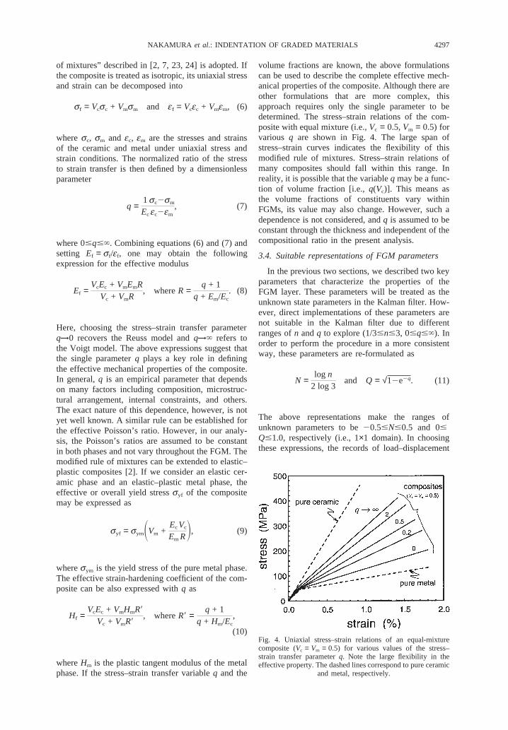
volume fractions are known, the above formulationscan be used to describe the complete effective mech-anical properties of the composite. Although there areother formulations that are more complex, thisapproach requires only the single parameter to bedetermined. The stress–strain relations of the com-posite with equal mixture (i.e.,Vc = 0.5,Vm = 0.5) forvarious q are shown in Fig. 4. The large span ofstress–strain curves indicates the flexibility of thismodified rule of mixtures. Stress–strain relations ofmany composites should fall within this range. Inreality, it is possible that the variableq may be a func-tion of volume fraction [i.e.,q(Vc)]. This means asthe volume fractions of constituents vary withinFGMs, its value may also change. However, such adependence is not considered, andq is assumed to beconstant through the thickness and independent of thecompositional ratio in the present analysis.

3.4. Suitable representations of FGM parameters

In the previous two sections, we described two keyparameters that characterize the properties of theFGM layer. These parameters will be treated as theunknown state parameters in the Kalman filter. How-ever, direct implementations of these parameters arenot suitable in the Kalman filter due to differentranges ofn andq to explore (1/3#n#3, 0#q#`). Inorder to perform the procedure in a more consistentway, these parameters are re-formulated as

N =log n

2 log 3and Q = √12e2q. (11)

The above representations make the ranges ofunknown parameters to be20.5#N#0.5 and 0#Q#1.0, respectively (i.e., 1×1 domain). In choosingthese expressions, the records of load–displacement

Fig. 4. Uniaxial stress–strain relations of an equal-mixturecomposite (Vc = Vm = 0.5) for various values of the stress–strain transfer parameterq. Note the large flexibility in theeffective property. The dashed lines correspond to pure ceramic

and metal, respectively.


for different n and q are closely monitored so thattheir variations are smoother over the domain ofNandQ.

4. INVERSE ANALYSIS PROCEDURE

4.1. Application of Kalman filter in FGM model

Based on the previous sections, the components ofthe state vector or the unknown FGM parameters aredefined asxt = (Qt, Nt)T, where Qt and Nt representthe estimates at timet. In our analysis, we assumethe indenter load to be specified at a time increment(i.e., P = P1, P2, P3, … at t = 1, 2, 3,…) while theindented displacementD is the measured parameter.Alternatively, one may chooseP to be the measuredparameter instead ofD. According to this arrange-ment, the vector containing measured variables inequation (1) can be set aszt = Dmeas

t , where the meas-ured displacement may contain error/noise asDmeas

t = Dt + Derrt . Here,Dt is the exact or known dis-

placement vector at loadPt, and the vectorDerrt con-

tains measurement noise (within an error bound). Fur-thermore, the vectorH t in equation (1) can be shownas Ht = Dt(Qt21, Nt21), where Qt21 and Nt21 corre-spond to most recent estimates of the state para-meters. In equation (2),ht is the displacement gradi-ent with respect toQ and N.

The dimensions of vectors and matrices depend onthe total number ofP–D curves used in the Kalmanfilter. Initially a record from a single indenter is con-sidered. In this case,Dt = (Dt). In a separate analysiswhen we consider two separateP–D records from twoindenters (described in Section 5.2),Dt = (DA

t , DBt )T.

Here the two indenters are denoted as A and B,respectively. The subscriptt indicates the loadincrement/magnitude. Using these relations, equation(1) can be customized for the present procedure as

xt = xt21 + Kt[Dmeast 2Dt(xt21)], (12)

where the Kalman gain matrixKt is computed as

Kt = PtdTt R21

t , where (13)Pt = Pt212Pt21d

Tt (dtPt21d

Tt + Rt)21dtPt21.

Also, the displacement gradient matrixdt can beshown as

dt =∂Dt

∂xt

= 5S∂Dt

∂Q∂Dt

∂ND for one indenter

1∂DA

t

∂Q∂DA

t

∂N

∂DBt

∂Q∂DB

t

∂N2 for two indenters

(14)

In the above equation, the matrixdt is shown for bothone indenter and two indenter cases. Also in equation(13), the two matrices of covariance are chosen as

P0 = S(DQ)2 0

0 (DN)2D and Rt

= 5R2 for one indenter

SR2 0

0 R2D for two indenters(15)

In the initial matrix of measurement covarianceP0,DQ = Qmax2Qmin and DN = Nmax2Nmin (i.e.,DQ = DN = 1 in the present case). WhileP0 is diag-onal, the procedure fillsPt to a matrix during sub-sequent increments. In the error covariance matrixRt,R is generally set close to the estimated maximummeasurement error asR = uDerr

t umax. The suitability ofthis value is examined and discussed in Section 5.3.When the error bound or measurement tolerance(white noise) is assumed to be constant throughoutthe loading,R can be set constant and independent oft as in the present analysis. In many inverse problems,the errors from multiple measurements can be inter-dependent andRt can be a full matrix. The incrementsare carried out fort = 1, 2,…, tmax. The state vectorxt at tmax contains the final estimates ofQ andN fromthe Kalman filter. The above procedure is illustratedby the flow chart shown in Fig. 5. This Kalman filterprocedure is implemented in a computational code.

4.2. Computational model

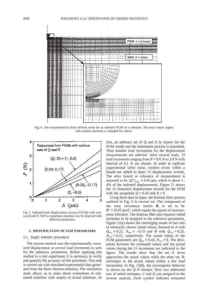
A detailed finite element analysis is carried out toverify the proposed procedure. The micro-indentationon the FGM layer on a thick steel substrate is mod-eled using axisymmetric elements. The mesh shownin Fig. 6 is carefully constructed after several trialcalculations. In order to obtain smoothP–Dresponses, it is essential to have small elements at thecontact area. These elements are needed to accuratelyresolve high stresses and the evolving contact con-dition. Larger elements are used away from the con-tact although the maximum through-thickness lengthof elements within the FGM layer is kept at 10µm.There are 64 element layers through the thickness ofthe FGM. Within each layer, the material propertiesare prescribed according to equations (3) and (8)–(10)for givenn andq, respectively. Although the through-thickness property variation is element by element,the large number of layers should produce a suf-ficiently continuous variation. The element sizes ofthe spherical indenter are also kept small along thecontact surface as shown. In the figure, the radius ofthe indenter isr = 100µm. There is total of about6600 four-noded isoparametric elements in the model.


Fig. 5. Flow chart for the Kalman filter procedure to determineunknown parameters using the indented displacements at sev-

eral load increments.

For the boundary condition, the radial displacementalong the symmetry axis and the vertical displace-ment along the bottom of the substrate are con-strained.

The loading to the FGM is simulated by graduallyincreasing the vertical displacement of nodes on thetop surface of the semi-spherical indenter. Displace-ment-controlled loading is chosen because of itsstable numerical convergence in contact simulations.The equivalent reaction force is reported as the loadP. The indented displacementD is obtained from thevertical displacement of the contact node at thecenter. The difference betweenD and the prescribeddisplacement at the top of the indenter is very smallsince the indenter is much stiffer than the FGM layer.In addition, one may calibrate the displacement toaccount for the compliance of the steel substrate.However, such calibratedD is not used here since itwould not influence the accuracy of the inverse analy-sis. The Kalman filter monitors thechangeof P–D

curves and not the magnitude ofD. In fact, displace-ment with the machine compliance can be also usedas long as its contribution is included in the model.Since the indenter is much stiffer than the FGM layer,the contact radiusr can be approximated asr = √2rD, where r is the radius of indenter. At theminimum load of the Kalman filter used in the analy-sis, the contact area covers 12–17 elements since thesmallest element size is 1.25µm.

4.3. Creation of reference data source

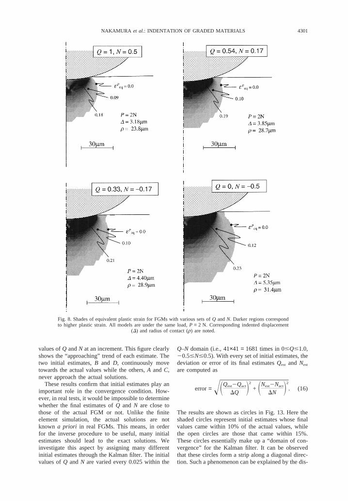
Since the Kalman filter compares the measureddata with known solutions, theP–D relation for givenq andn, or Q andN, must be available. This relationcan be obtained either analytically or numerically. Inour proposed procedure, this information or the refer-ence data source is generated by finite element calcu-lations since no closed-form solution exists for elas-tic–plastic FGMs. By varying the values ofQ andN,stiff to compliant responses can be obtained. Figure7 showsP–D relations of FGMs with four differentsets ofQ and N. In each calculation, the prescribeddisplacement is increased by increments of 0.1µm.Various responses of the FGMs are also illustrated bythe shades of equivalent plastic strain in Fig. 8. Here,shaded areas represent plastic zones and larger plasticstrains are shown by darker shades. All of the modelsare under the same indented load atP = 2 N. Notethe significant differences in the plastic zone sizesunder the same load. The plastic zone of the com-pliant model (Q = 0, N = 20.5) is more than twice aslarge as that of the stiff model (Q = 1, N = 0.5).Regardless of the model, the plastic zone is confinedto a region immediately underneath the indenter.Since the FGM thickness is 500µm, the plastic zonesoccupy small fractions of the thickness.

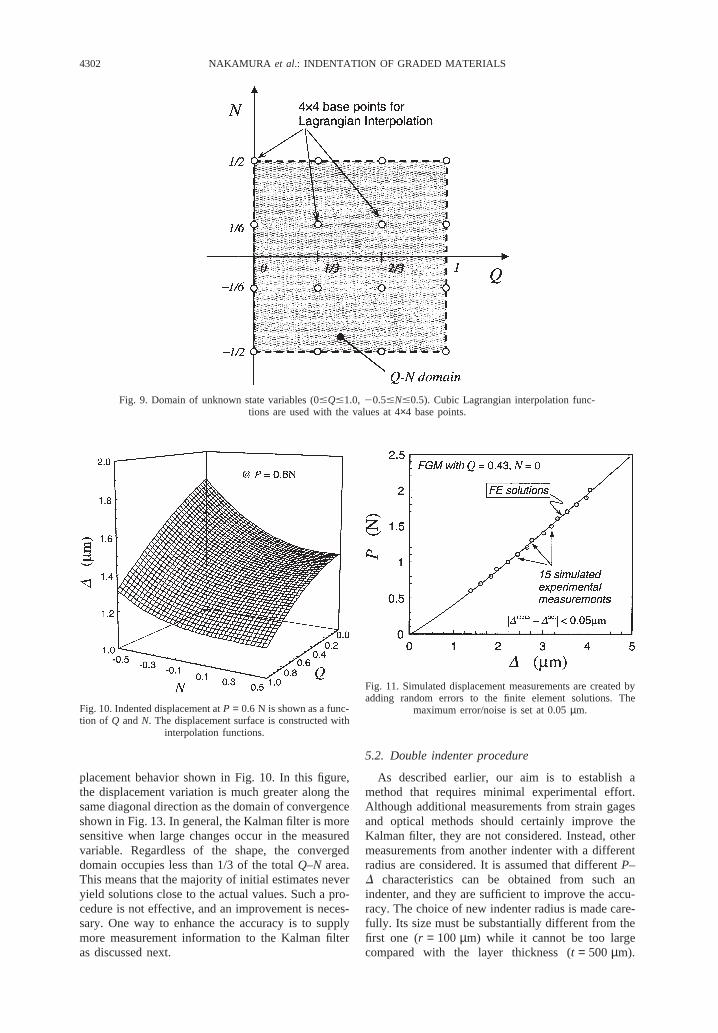
As shown in equations (12) and (13), the Kalmanfilter requiresD and its derivatives with respect toQandN at loadP. These values can be determined bycarrying out many finite element calculations for vari-ous sets ofQ andN. In order to minimize such com-putational effort, we adopt cubic Lagrangian interp-olation functions to calculate the displacement and itsgradients. Sixteen points in theQ–N domain arechosen as the base points whose values are used in thecalculations. These points are uniformly distributed intheQ–N domain as shown in Fig. 9. After 16 separatefinite element calculations are carried out, the dis-placements and their gradients for anyQ andN can beobtained through the cubic Lagrangian interpolationfunctions. Initially bi-quadratic functions at 3×3points were employed. However, the accuracy wasnot sufficient and we tried bi-cubic functions at 4×4points. These higher-order functions enabled interp-olated D to achieve 0.2% accuracy for any combi-nation ofQ andN. The interpolatedD for variousQand N at the load level ofP = 0.6 N is shown inFig. 10.


Fig. 6. The axisymmetrical finite element mesh for an indented FGM on a substrate. The near-contact regionwith smaller elements is enlarged for clarity.

Fig. 7. Indented load–displacement curves of FGMs with vari-ousQ andN. Stiff to compliant responses can be observed with

different parameters.

5. IDENTIFICATION OF FGM PARAMETERS

5.1. Single indenter procedure

The inverse method uses the experimentally meas-ured displacement at several load increments to seekfor the unknown parameters. Before applying thismethod in a real experiment, it is necessary to verifyand quantify the accuracy of this procedure. This taskis carried out with simulated experimental data gener-ated from the finite element solutions. The simulationstudy allows us to make direct evaluations of esti-mated solutions with respect to actual solutions. At

first, an arbitrary set ofQ and N is chosen for theFGM model and the indentation process is simulated.Then suitable load increments for the displacementmeasurements are selected. After several trials, 15load increments ranging fromP = 0.6 N to 2.0 N withinterval of 0.1 N are chosen. In order to replicateexperimental white noise,random errors within abound are added to these 15 displacement records.The error bound or tolerance of measurement isassumed to beuDerr

t umax = 0.05µm, which is about 1–4% of the indented displacements. Figure 11 showsthe 15 simulated displacement records for the FGMwith the propertiesQ = 0.43 andN = 0.

Using these data as input, the Kalman filter processoutlined in Fig. 5 is carried out. The component ofthe error covariance matrixRt is set to beR2 = (0.05µm)2, which equals the square of measure-ment tolerance. The Kalman filter also requires initialestimates to be assigned to the unknown parameters.Figure 12(a) shows the converging trends of two setsof arbitrarily chosen initial values, denoted asA withQinit = 0.25, Ninit = 20.15 and B with Qinit = 0.25,Ninit = 0.25, respectively. The actual values of theFGM parameters areQact = 0.43, Nact = 0. The devi-ations between the estimated values and the actualvalues during the 15 increments are indicated in thefigure. The results show that the setA neverapproaches the actual values while the other set,B,converges to the actual values within a few loadincrements. In Fig. 12(b), the convergence behavioris shown on theQ–N domain. Here two additionalsets of initial estimates,C andD, are assigned in theinverse analysis. Each symbol indicates estimated


Fig. 8. Shades of equivalent plastic strain for FGMs with various sets ofQ andN. Darker regions correspondto higher plastic strain. All models are under the same load,P = 2 N. Corresponding indented displacement

(D) and radius of contact (r) are noted.

values ofQ andN at an increment. This figure clearlyshows the “approaching” trend of each estimate. Thetwo initial estimates,B and D, continuously movetowards the actual values while the others,A and C,never approach the actual solutions.

These results confirm that initial estimates play animportant role in the convergence condition. How-ever, in real tests, it would be impossible to determinewhether the final estimates ofQ and N are close tothose of the actual FGM or not. Unlike the finiteelement simulation, the actual solutions are notknown a priori in real FGMs. This means, in orderfor the inverse procedure to be useful, many initialestimates should lead to the exact solutions. Weinvestigate this aspect by assigning many differentinitial estimates through the Kalman filter. The initialvalues ofQ andN are varied every 0.025 within the

Q–N domain (i.e., 41×41 = 1681 times in 0#Q#1.0,20.5#N#0.5). With every set of initial estimates, thedeviation or error of its final estimatesQest and Nest

are computed as

error= !SQest2Qact

DQ D2

+ SNest2Nact

DN D2

. (16)

The results are shown as circles in Fig. 13. Here theshaded circles represent initial estimates whose finalvalues came within 10% of the actual values, whilethe open circles are those that came within 15%.These circles essentially make up a “domain of con-vergence” for the Kalman filter. It can be observedthat these circles form a strip along a diagonal direc-tion. Such a phenomenon can be explained by the dis-


Fig. 9. Domain of unknown state variables (0#Q#1.0, 20.5#N#0.5). Cubic Lagrangian interpolation func-tions are used with the values at 4×4 base points.

Fig. 10. Indented displacement atP = 0.6 N is shown as a func-tion of Q andN. The displacement surface is constructed with

interpolation functions.

placement behavior shown in Fig. 10. In this figure,the displacement variation is much greater along thesame diagonal direction as the domain of convergenceshown in Fig. 13. In general, the Kalman filter is moresensitive when large changes occur in the measuredvariable. Regardless of the shape, the convergeddomain occupies less than 1/3 of the totalQ–N area.This means that the majority of initial estimates neveryield solutions close to the actual values. Such a pro-cedure is not effective, and an improvement is neces-sary. One way to enhance the accuracy is to supplymore measurement information to the Kalman filteras discussed next.

Fig. 11. Simulated displacement measurements are created byadding random errors to the finite element solutions. The

maximum error/noise is set at 0.05µm.

5.2. Double indenter procedure

As described earlier, our aim is to establish amethod that requires minimal experimental effort.Although additional measurements from strain gagesand optical methods should certainly improve theKalman filter, they are not considered. Instead, othermeasurements from another indenter with a differentradius are considered. It is assumed that differentP–D characteristics can be obtained from such anindenter, and they are sufficient to improve the accu-racy. The choice of new indenter radius is made care-fully. Its size must be substantially different from thefirst one (r = 100µm) while it cannot be too largecompared with the layer thickness (t = 500µm).


Fig. 12. Converging trends of different initial estimates. (a)Two cases shown as a function of load increments. (b) Fourcases shown on theQ–N domain. The diverged cases (A andC) stay away from the actual values (Q = 0.43 andN = 0).

Fig. 13. Shaded circles correspond to initial estimates that achi-eved convergence within 10% of the actual values while opencircles came within 15%. These circles make up the domain

of convergence for the Kalman filter.

After several trials, the new radius is chosen to ber = 500µm. The load increments for this largeindenter are set between 5 and 12 N with 0.5 N inter-vals. At first, as in the smaller indenter, the referencedata are created by carrying out separate finiteelement calculations with 16 sets of differentQ andN. Again the loading to the FGM layer is appliedthrough increasing the displacement of nodes on thetop of the larger indenter. In the next step, actualmeasurements are simulated by adding random errorsto the finite element solutions as shown in Fig. 14.The same measurement tolerance is used. Prior torunning the Kalman filter using both small and largeindenter data, the convergence behavior of the largeindenter alone was inspected. The resulting domainof convergence was very similar to that of the smallindenter shown in Fig. 13. It further confirms that sin-gle indenter results are not sufficient to obtain goodconvergence behavior.

The combined indenter procedure is carried outwith the Kalman filter equations (12)–(15) for the twoindenter case. With the additional measurement data,the dimensions of vectors and matrices increase. Inthe Kalman filter program, the referenceP–D data forboth small and large indenters are supplied initially.After initial estimates ofQ andN are input, the pro-gram processes the two displacements of the firstincrement from the small and large indenters simul-taneously (i.e.,Dmeas at 0.6 N for the small indenterandDmeasat 5 N for the large indenter). These valuesare used to update the estimates ofQ and N. Thisprocess is repeated for 15 increments to obtain thebest estimates in the current procedure. Note that thetotal numbers of load increments for the two indentersmust be identical although the load magnitudes canbe different. The major difference between the singleand double indenter cases is that the Kalman filteruses larger rank tensors to process. This generallyleads to better convergence characteristics.

Fig. 14. Simulated displacement measurements from twoindenters with different radii. The smaller one hasr = 100 µm and the larger one hasr = 500µm. Random errors

of up to 0.05µm are added to the finite element solutions.


As in the single indenter case, its accuracy is evalu-ated by generating a domain of convergence. Theresults are shown in Fig. 15, where a dramaticimprovement can be observed. Almost all of theinitial estimates lead to actual solutions during theKalman filter procedure. Alternatively, one can assignany initial values forQ andN in the Kalman filter toobtain very accurate estimates ofQ andN. This resultsupports the usefulness of the proposed method. Thefeasibility of this method is also examined by choos-ing different Qact and Nact. Their convergencebehaviors are similar to the one in Fig. 15. Whencombined P–D data from the small and largeindenters are used, more than 80% of initial estimateshave achieved convergence to within 10% error ofthe actual solutions.

One of the major strengths of the Kalman filter isits ability to process data containing substantialmeasurement noises or errors. We examined this fea-ture by re-creating simulated measurements withmuch greater random errors as shown in Fig. 16(a).Here, the measurement tolerance or the error boundis set at uDerr

t umax = 0.2 µm in both small and largerindenter results. This magnitude is four times largerthan in the previous cases and the error can be 3–15% of the displacements shown in Fig. 16(a). Usingthese data, the Kalman filter is carried out and theresulting domain of convergence is shown in Fig.16(b). Obviously the accuracy is reduced due to theworsened data quality. However, the domain includ-ing the open circles has nearly maintained its size.More than 80% of the totalQ and N domain is stillcovered by the filled or open circles. These resultsprove the strength of this method even when rela-tively large error/noise is present in the measure-ments.

5.3. Influence of covariant matrices

During the study of this procedure, we have foundthat the values assigned to the error covariant matrix

Fig. 15. Domain of convergence for the combined small andlarge indenter case. The size is significantly enlarged compared

with the single indenter case (Fig. 13).

Fig. 16. (a) Simulated displacement measurements from twoindenters with large random errors (tolerance) of up to 0.20µm. (b) Domain of convergence obtained from the combinedindenter case with large errors. Although the accuracy declines,

the size is still large.

Rt influence the accuracy while initial values assignedto the measurement covariant matrixP0 have a verysmall effect. In all of the results shown previously,the components ofRt in equation (15) have beenassigned asR2 = uDerr

t u2max. However, it appears thatother values may improve the convergence behaviorof the Kalman filter. In order to optimize the Kalmanfilter procedure, different values are assigned to quan-tify the influences ofRt. First, we carried out the pro-cedure with the measurement data shown in Fig. 14.Here the measurement error bound or tolerance is setas uDerr

t umax = 0.05µm. Four separate cases with dif-ferent R in Rt are carried out in the double indenteranalysis. They areR = 0.05, 0.2, 0.5 and 2.0µm, andidentical initial estimates and actual solutions areassigned in all cases. The converging trends of thesecases at each load increment are shown in Fig. 17(a).The normalized error is calculated by equation (14).In general, when largeR is assigned, the convergenceis steady but slow. On the other hand, if smallR is


Fig. 17. Converging trends of the combined indenter case. Eachcurve is for different values in the error covariance matrixRt.The results are shown for the small and large measurementtolerance/error cases. (a)uDmeas2Dactu,0.05µm and (b)

uDmeas2Dactu,0.20µm.

assigned, the convergence may be rapid but alsounstable.

To investigate further the influence ofR, we havecarried out four additional calculations with largermeasurement errors. The simulatedP–D measure-ments with the toleranceuDerr

t umax = 0.20µm, shownin Fig. 16(a), are used. The rate of convergence isshown in Fig. 17(b). With the larger measurementerrors, the convergence of a givenR is different fromthat shown in Fig. 17(a). However, in terms of rela-tive magnitudes, the trends are very similar. A largeR yields slow and steady convergence while a smallR yields fast but unstable convergence. From inspec-tion of both figures, the optimum value appears to beR|10uDerr

t umax. This corresponds toR = 0.5 µm in Fig.17(a) andR = 2 µm in Fig. 17(b). Each curve in therespective figure shows the optimal convergencetrend.

6. SUMMARY

This paper introduces a new procedure based oninverse analysis and instrumented indentation. It hasbeen known that more material information could beextracted from measured load–displacement curves.The present Kalman filter procedure is one of themeans to maximize the usefulness of indentation data.For verification and optimization of the procedure,detailed finite element analyses are carried out todetermine unknown parameters of elastic–plasticFGMs. Using the idealized model, the parameters thatdefine the compositional variations and effectivemechanical properties through the thickness are esti-mated by the inverse analysis. The former parameteris for the assumed power-law compositional distri-bution and the latter parameter sets the stress–straintransfer of modified rule-of-mixtures properties.

As in many inverse analyses, we found that themodel is initially “ill-posed” or “ill-conditioned” (i.e.,not able to achieve good convergence characteristics)with single indenter measurements. This problem isovercome by use of an additional indenter with alarger radius. In addition, it is shown that the Kalmanfilter is well suited for the present non-linear or elas-toplastic problem since it processes overmultiple loadincrements to best estimate the solutions. Althoughsimilar displacements are possible in models with dif-ferent properties at a given load, models with differ-ent q andn should not continue to yield similar dis-placements atvarious loads. Required steps in theproposed procedure are summarized below.

1. Determine the material constants of homogeneousmaterial separately. The ceramic and metal proper-ties can be obtained by indentation proceduresdescribed in [17, 20].

2. Perform preliminary finite element calculations todetermine suitable ranges of load increments fortwo differently sized indenters. The FGM para-meters can be tentatively set atQ = 0.5 andN = 0. Use the finite element solutions to monitorapproximate sizes of plastic zones.

3. Establish reference data from numerically gener-atedP–D records with 16 differentQ andN. Usecubic Lagrangian functions to interpolate the dis-placements and their gradients for each indenter.

4. Carry out instrumented indentation on the FGMlayer using two indenters with different sphericalradii.

5. Assign initial estimates ofQ andN. Set values forP0 (with DQ, DN) and Rt (with R = 10uDerrumax

where uDerrumax is the measurement error/noisebound).

6. Carry out the Kalman filter process for 15increments to obtain the final estimates ofQ andN.

One important question in the inverse analysis ishow to identify the accuracy of the final estimates in


real tests where actual solutions are unknown.Although there is no direct method to judge the accu-racy, we can propose the following procedure. First,carry out the Kalman filter with some initial esti-mates. Instead of terminating at this point, carry outanother Kalman filter procedure. In the secondattempt, the final estimates of the first attempt can beused as the initial estimates. This procedure can berepeated for a few times. If the final estimates aresimilar in all processes, then it is likely that they areclose to the actual solutions. Alternatively, if therepeated procedures produce different final estimates,a different set of initial estimates must be used in theinverse analysis.

Implementation of the procedure for a real FGMspecimen is being prepared currently. Although theproposed procedure is described for elastic–plasticFGMs, a similar procedure can be used to determineother parameters, including thickness, yield stress andanisotropic moduli, of any layers and coatings. Fur-thermore, the number of unknown parameters in theinverse analysis can be also increased. This aspect iscurrently being investigated.

Acknowledgements—The authors acknowledge the NationalScience Foundation for support of this work under award CMS-9800301. T. N. was also supported by the Army ResearchOffice under grant DAAD19-99-1-0318. The helpful dis-cussions with Professor Alan Kushner are also appreciated. Thecomputations were carried out on HP7000/C180 and C360workstations using the finite element code ABAQUS, whichwas made available under academic license from Hibbitt,Karlsson and Sorensen, Inc.

REFERENCES

1. Sampath, S., Herman, H., Shimoda, N. and Saito, T.MRSBull., 1995,20(1), 27.

2. Suresh, S. and Mortensen, A.Fundamentals of Func-tionally Graded Materials, IOC Communications Ltd,London, 1998.

3. Weissenbek, E., Pettermann, H. E. and Suresh, S.Actamater., 1997,45, 3401.

4. Suresh, S., Giannakopoulos, A. E. and Alcala, J.Actamater., 1997,45, 1307.

5. Giannakopoulos, A. E. and Suresh, S.Int. J. Solids Struct.,1997,34, 2357.

6. Giannakopoulos, A. E. and Suresh, S.Int. J. Solids Struct.,1997,34, 2393.

7. Williamson, R. L., Rabin, B. H. and Drake, J. T.J. Appl.Phys., 1993,74, 1310.

8. Kesler, O., Finot, M., Suresh, S. and Sampath, S.ActaMater., 1997,45, 3123.

9. Jitcharoen, J., Padture, N. P., Giannakopoulos, A. E. andSuresh, S.J. Am. Ceram. Soc., 1998,81, 2301.

10. Delale, F. and Erdogan, F.J. Appl. Mech., 1988,55, 317.11. Kalman, R. E.ASME J. Basic Eng., 1960,82D, 35.12. Grewal, M. S. and Andrews, A. P.Kalman Filtering:

Theory and Practice, Prentice-Hall, Inc, New Jersey, 1993.13. Hoshiya, M. and Saito, E.J. Eng. Mech., 1984,110, 1757.14. Ishida, R.Trans. JSME, Part A, 1994,60, 443.15. Aoki, S., Amaya, K., Sahashi, M. and Nakamura, T.Comp.

Mech., 1997,19, 501.16. Suresh, S. and Giannakopoulos, A. E.Acta mater., 1998,

46, 5755.17. Giannakopoulos, A. E. and Suresh, S.Scripta mater., 1999,

40, 1191.18. Jorgensen, O., Giannakopoulos, A. E. and Suresh, S.Int.

J. Solids Struct., 1998,35, 5097.19. Alcala, J., Giannakopoulos, A. E. and Suresh, S.J. Mater.

Res., 1998,13, 1390.20. Alcala, J., Gaudette, F., Suresh, S. and Sampath, S.,J.

Mater. Res., submitted for publication.21. Qian, G., Nakamura, T., Berndt, C. C. and Leigh, S. H.

Acta mater., 1997,45, 1767.22. Sampath, S., Smith, W. C., Jewett, T. J. and Kim, H.

Mater. Sci. Forum, 1999,308, 383.23. Moretensen, A. and Suresh, S.Int. Mater. Rev., 1995,

40, 239.24. Suresh, S. and Mortensen, A.Int. Mater. Rev., 1997,42,

85.

determination of properties of graded...

Documents