determining particle size of polymeric micelles in
TRANSCRIPT

BearWorks BearWorks
MSU Graduate Theses
Spring 2020
Determining Particle Size of Polymeric Micelles in Determining Particle Size of Polymeric Micelles in
Thermothickening Aqueous Solutions Thermothickening Aqueous Solutions
Jessica Diane Bruer Missouri State University Jessica1897livemissouristateedu
As with any intellectual project the content and views expressed in this thesis may be
considered objectionable by some readers However this student-scholarrsquos work has been
judged to have academic value by the studentrsquos thesis committee members trained in the
discipline The content and views expressed in this thesis are those of the student-scholar and
are not endorsed by Missouri State University its Graduate College or its employees
Follow this and additional works at httpsbearworksmissouristateedutheses
Part of the Physical Chemistry Commons and the Polymer Chemistry Commons
Recommended Citation Recommended Citation Bruer Jessica Diane Determining Particle Size of Polymeric Micelles in Thermothickening Aqueous Solutions (2020) MSU Graduate Theses 3472 httpsbearworksmissouristateedutheses3472
This article or document was made available through BearWorks the institutional repository of Missouri State University The work contained in it may be protected by copyright and require permission of the copyright holder for reuse or redistribution For more information please contact BearWorkslibrarymissouristateedu
DETERMINING PARTICLE SIZE OF POLYMERIC MICELLES IN
THERMOTHICKENING AQUEOUS SOLUTIONS
A Masterrsquos Thesis
Presented to
The Graduate College of
Missouri State University
TEMPLATE
In Partial Fulfillment
Of the Requirements for the Degree
Master of Science Chemistry
By
Jessica Diane Bruer
May 2020
ii
Copyright 2020 by Jessica Diane Bruer
iii
DETERMINING PARTICLE SIZE OF POLYMERIC MICELLES IN
THERMOTHICKENING AQUEOUS SOLUTIONS
Chemistry
Missouri State University May 2020
Master of Science
Jessica Bruer
ABSTRACT
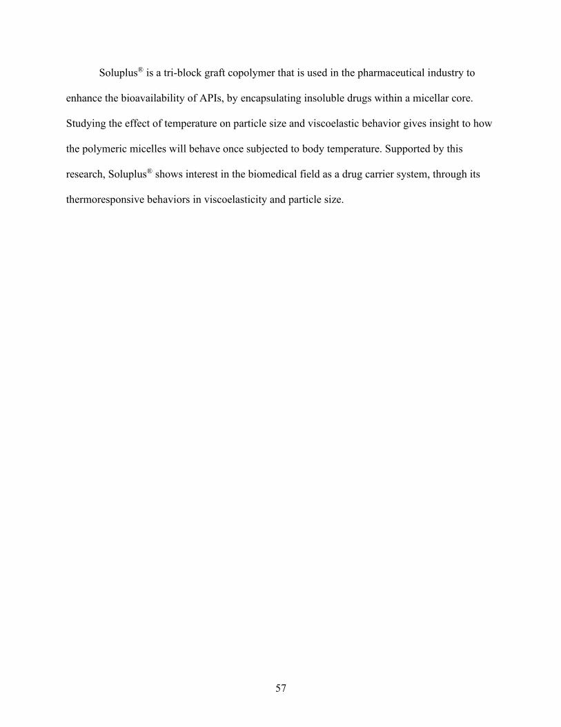
Many active pharmaceutical ingredients (APIs) are poorly soluble and cause inadequate drug
absorption Soluplusreg a polyvinyl caprolactam-polyvinyl acetate-polyethylene glycol graft
copolymer is a commercial excipient (BASF Corp) that enhances the solubility and
bioavailability of many APIs The mechanism of enhancement is related to the ability to form
polymeric micelles in solution These micelles store insoluble APIs in their hydrophobic interior
and transport them to targeted sites in the body An important characteristic of solubility
enhancers is the particle size exhibited in solution before and after loading with APIs This is
most commonly determined by dynamic light scattering (DLS) methods However DLS
measurements involving thermothickening polymer solutions can be complicated by the
temperature dependence of viscosity and refractive index solution properties that directly impact
the size analysis algorithms in DLS In this project the temperature dependence of viscosity for
Soluplusreg solutions were evaluated and used as a correction to particle size measurements by
DLS Solution concentrations ranging 10 to 300 (ww) of Soluplusreg were studied from 50
degC to 400 degC using a cone-and-plate rheometer Refractive index of Soluplusreg solutions were
also studied and used in the correction of particle size It was found that correcting viscosity and
refractive index data drastically affected hydrodynamic effective diameter where viscosity was
more highly weighted The corrected particle size of Soluplusreg solutions was inversely
proportional to concentration with the 01 and 100 solutions showing effective diameters of
6313 plusmn 076 nm and 2498 plusmn 030 nm at 250 degC respectively By properly accounting for these
variables in DLS algorithms particle size of thermoresponsive polymer solutions can be more
accurately characterized
KEYWORDS rheology dynamic light scattering Soluplusreg thermoresponsive block
copolymer active pharmaceutical ingredient viscosity refractive index thermothickening
polymeric micelles
iv
DETERMINING PARTICLE SIZE OF POLYMERIC MICELLES IN
THERMOTHICKENIG AQUEOUS SOLUTIONS
By
Jessica Bruer
A Masterrsquos Thesis
Submitted to the Graduate College
Of Missouri State University
In Partial Fulfillment of the Requirements
For the Degree of Master of Science Chemistry
May 2020
Approved
G Alan Schick PhD Thesis Committee Chair
Gary Meints PhD Committee Member
Ridwan Sakidja PhD Committee Member
Adam Wanekaya PhD Committee Member
Julie Masterson PhD Dean of the Graduate College
In the interest of academic freedom and the principle of free speech approval of this thesis
indicates the format is acceptable and meets the academic criteria for the discipline as
determined by the faculty that constitute the thesis committee The content and views expressed
in this thesis are those of the student-scholar and are not endorsed by Missouri State University
its Graduate College or its employees
v
ACKNOWLEDGEMENTS
I would like to thank those who showed their support during the course of my graduate
studies Specially my family who endlessly support my decisions Without their encouragement
I would not be where I am today A special thank you to my siblings Kyle Bruer and Alyssa
Mansfield for pushing me to be my best in hopes Irsquod be as successful as they are To my future
sister-in-law Jill Davis I greatly appreciated the help and patience with data manipulation I am
upmost grateful for the support of my parents Richard and Theresa Bruer who have taught me
that no ambition is too grand Thank you for always being my cheerleaders and helping me at
any cost
I would also like to thank my research advisor Dr G Alan Schick who has guided me
since my undergraduate years I appreciate his commitment to furthering my education and
introducing me to physical chemistry Additionally I thank my thesis committee for their time
and support Dr Gary Meints Dr Ridwan Sakidja and Dr Adam Wanekaya I am tremendously
grateful for the friends I have made throughout this journey fellow graduate students research
members and faculty who made coming to campus enjoyable and entertaining Specifically
Cody Turner who has been my rock through our entire accelerated masterrsquos journey together
I dedicate this thesis to my mother Theresa Bruer for sparking my interest in science with
participation in the elementary school science fairs
vi
TABLE OF CONTENTS
Chapter 1 Introduction Page 1
11 Poor Solubility in the Pharmaceutical Field Page 1
12 Polymers Page 1
121 Polymer Behavior Page 2
122 Function with Active Pharmaceutical Ingredients Page 3
13 Thermoresponsivity Page 4
14 Soluplusreg Page 7
15 Dynamic Light Scattering Spectroscopy Page 14
151 Effect of Viscosity Page 14
152 Effect of Refractive Index Page 20
16 Objectives Page 21
Chapter 2 Experimental Page 22
21 Overview Page 22
22 Materials Page 22
23 Temperature Dependence of Viscosity Page 23
231 Instrumentation Page 23
232 Methods Page 27
24 Refractive Index Analysis Page 28
241 Instrumentation Page 28
242 Methods Page 29
25 Particle Size Determination by Dynamic Light Scattering Page 30
251 Instrumentation Page 30
252 Methods Page 33
Chapter 3 Results and Discussion Page 35
31 Temperature Dependent Viscoelastic Behavior of Soluplusreg Solutions Page 35
32 Temperature Dependent Refractive Index of Soluplusreg Solutions Page 47
33 Particle Size Analysis of Soluplusreg Solutions Page 48
Chapter 4 Conclusions and Future Directions Page 55
References Page 58
vii
LIST OF TABLES
Table 1 Types and examples of copolymers Page 2
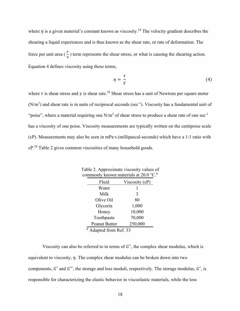
Table 2 Approximate viscosity values of commonly known materials at 200 degC Page 18
Table 3 Cone spindle dimensions and shear rates Page 26
Table 4 Experimental conditions for each samplestandard run on the rheometer Page 28
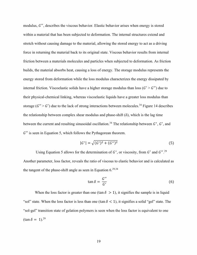
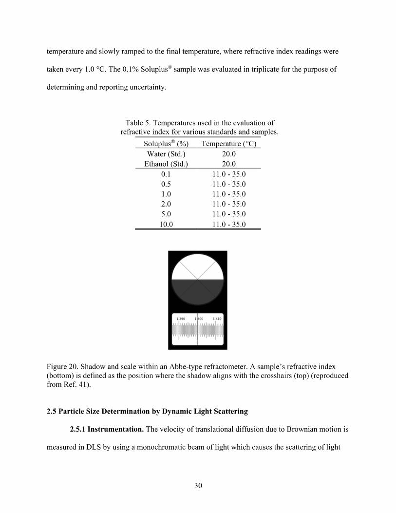
Table 5 Temperatures used in the evaluation of refractive index for various standards
and samples Page 30
Table 6 Standard operating procedures for temperature dependent particle size analysis Page 34
Table 7 Total allowed error for each viscosity standard fluid at 250 degC Page 35
Table 8 Extrema temperatures observed in η-T plots of Soluplusreg solutions Page 39
Table 9 Experimental and literature refractive index values for water and
ethanol at 200 degC Page 47
Table 10 Effective diameters of NIST latex calibration standards at 250 degC Page 49
Table 11 Uncorrected vs corrected effective diameters at 250 degC for Soluplusreg in
aqueous solution Page 52
Table 12 Difference in effective diameter when using uncorrected and corrected
viscosity and refractive index data for a 100 Soluplusreg solution at 200 degC Page 53
Table 13 Effective diameter dependence on refractive index for a 100 Soluplusreg
solution at 200 degC and 5842 cP Page 54
viii
LIST OF FIGURES
Figure 1 Structure of a polymeric micelle with APIs stored in its core Page 4
Figure 2 Temperature vs polymer volume fraction (120601) plots Page 6
Figure 3 Schematic representation of block copolymer phase transitions Page 7
Figure 4 Physical appearance of Soluplusreg Page 8
Figure 5 Structure of Soluplusreg Page 9
Figure 6 Solubilization capacities of various active pharmaceutical ingredients Page 10
Figure 7 Dissolution test for the release of itraconazole with polymeric matrices Page 10
Figure 8 Blood concentration of itraconazole with and without Soluplusreg solution Page 10
Figure 9 Phase diagram for a LCST lt UCST behaving polymer Page 12
Figure 10 Micellization mechanism for solutions of Soluplusreg Page 13
Figure 11 Soluplusreg solution at room temperature cloud point and gel point Page 13
Figure 12 Particle size data for a pigment dispersed in water at two different viscosities Page 15
Figure 13 Two plates model used to describe the physics of viscosity Page 17
Figure 14 Graphical relationship between complex shear modulus 119866lowast storage
moduli 119866prime loss moduli 119866primeprime and the phase-shift angle δ Page 20
Figure 15 Schematics of a cone-and-plate rheometer Page 25
Figure 16 Diagram of the inner workings of the cone and plate Page 25
Figure 17 Top view of spindles CP40 and CP52 Page 26
Figure 18 Set-up used for viscosity data collection on a Brookfield rheometer Page 28
Figure 19 Set-up used for refractive index data collection on an Abbe refractometer Page 29
Figure 20 Shadow and scale within an Abbe-type refractometer Page 30
Figure 21 Schematic representation of the Zetasizer Nano series DLS instrument Page 31
Figure 22 Set-up used for particle size data collection on a NanoBrook Omni Page 33
Figure 23 Brookfield viscosity standard fluids as a function of temperature Page 35
Figure 24 Effect of temperature on viscosity for each aqueous Soluplusreg sample Page 37
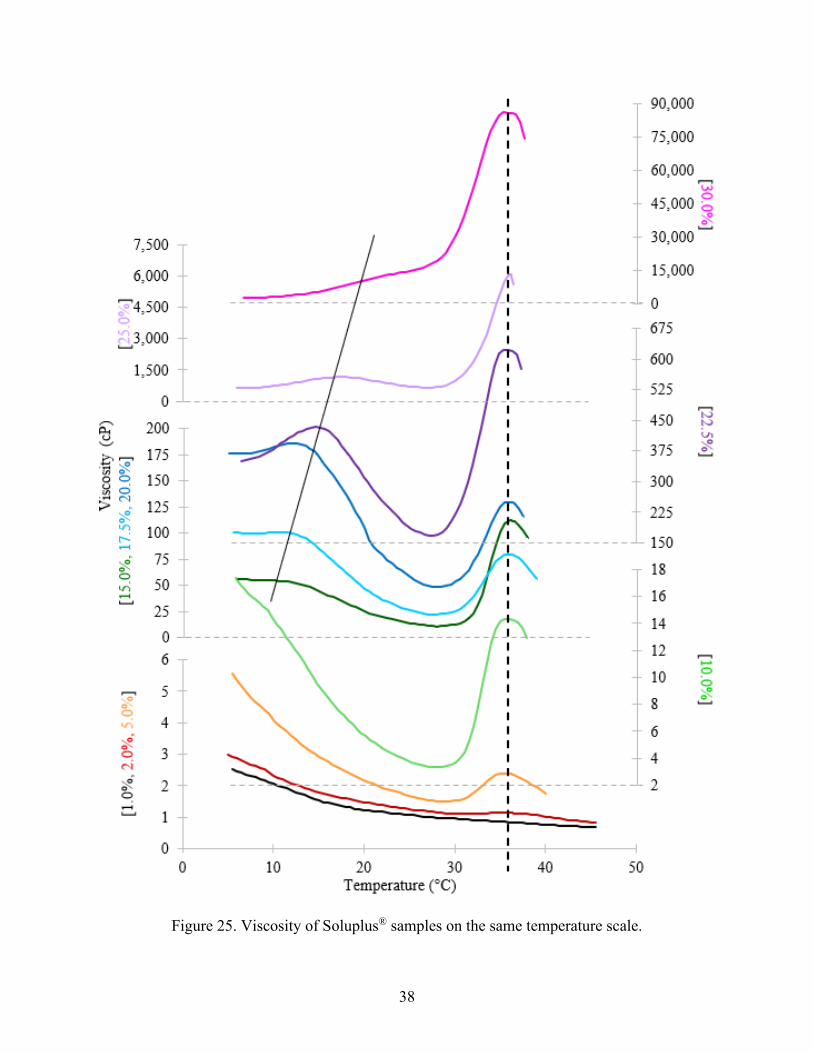
Figure 25 Viscosity of Soluplusreg samples on the same temperature scale Page 38
Figure 26 Temperature dependent functions of 119866prime and 119866primeprime for a gelling material Page 40
Figure 27 Complex viscosity 119866prime and 119866primeprime as a function of temperature for an epoxy Page 40
Figure 28 A gelled 200 Soluplusreg solution on the plate of a cone-and-plate rheometer Page 41
Figure 29 Sol-gel and gel-sol transitions for Soluplusreg samples Page 43
Figure 30 Cloud points for aqueous Soluplusreg solutions as a function of temperature Page 44
Figure 31 Log-linear plot of viscosity vs temperature of aqueous Soluplusreg
solutions at different concentrations Page 45
Figure 32 Full range of experimental data modeled with a Poly55-Bisquare fit Page 45
Figure 33 Short range of experimental data modeled with a Poly54 fit Page 46
Figure 34 Effect of temperature on refractive index for Soluplusreg samples Page 48
Figure 35 Effect of temperature on effective diameter for Soluplusreg solutions using
uncorrected values of viscosity and refractive index Page 50
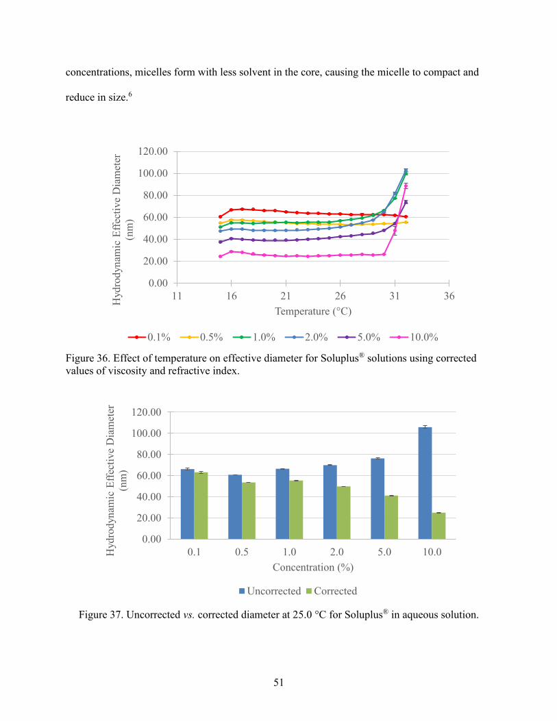
Figure 36 Effect of temperature on effective diameter for Soluplusreg solutions using
corrected values of viscosity and refractive index Page 51
Figure 37 Uncorrected vs corrected diameter at 250 degC for Soluplusreg in solution Page 51
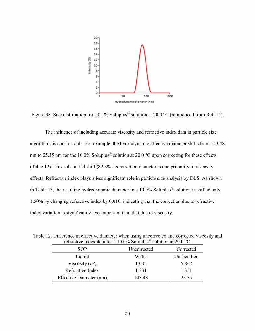
Figure 38 Size distribution for a 01 Soluplusreg solution at 200 degC Page 53
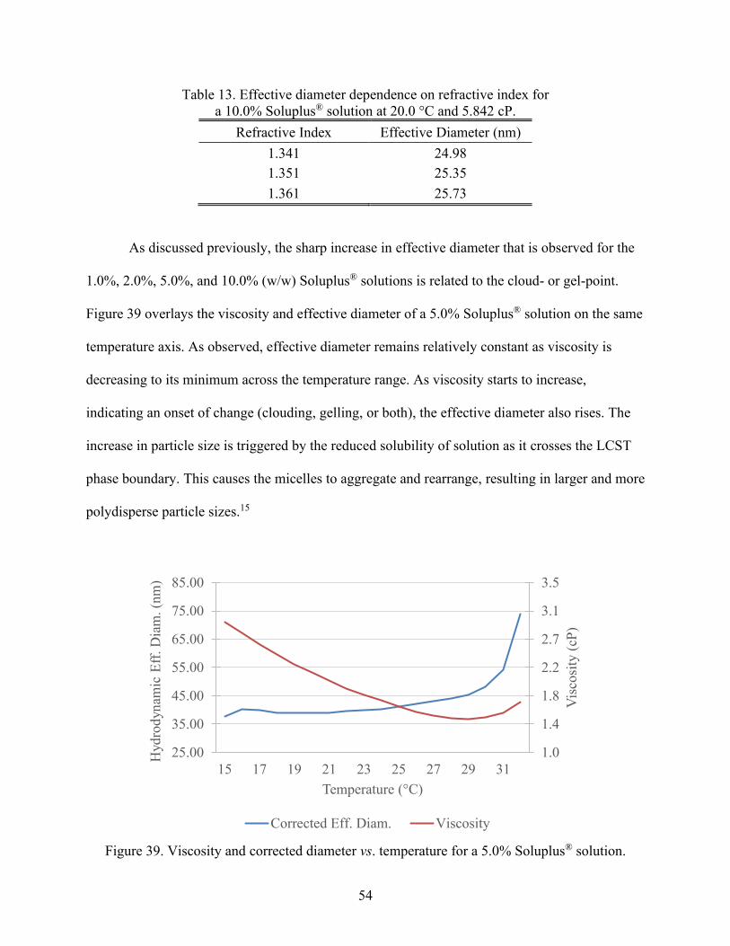
Figure 39 Viscosity and corrected diameter vs temperature for 50 Soluplusreg sample Page 54
1
CHAPTER 1 INTRODUCTION
11 Poor Solubility in the Pharmaceutical Field
In 2011 it was reported that 90 of all compounds in the pharmaceutical drug delivery
system were poorly soluble in water1 This is a significant problem in the pharmaceutical
industry as drugs are ineffective unless they can be solubilized into the bodyrsquos systems rather
than being excreted from the digestive track due to re-crystallization1 It is important that drugs
are delivered to the right area at the right time and at the right concentration but many obstacles
such as poor solubility environmental degradation toxicity and lack of permeability make drug
delivery challenging2 These issues have led to the increasing use of enhanced drug delivery
methods such as polymeric micelles to help drugs reach their molecular target within the body
12 Polymers
Polymers are a type of synthetic macromolecule that consist of repeating structural units
They consist of two main components a backbone and peripheral side chains The repeating
units of a polymer may fall onto either part of a polymerrsquos structure When a polymer has two or
more units of varying composition it is called a copolymer Copolymers can be described as
random- alternating- graft- or block copolymers Random copolymers consist of two or more
monomers that are simultaneously present in one polymerization reactor Alternating copolymers
are comprised of two different monomers on the structural unit In graft copolymers one or more
monomers are grafted onto a homopolymer resulting in a backbone that has perforating side
branches Lastly in block copolymers one monomer is attached to the end group of a previous
2
polymerized chain forming a linear chain with different segments3 Table 1 gives visual
examples of each type of copolymer along with industrial examples
Table 1 Types and examples of copolymersa
a Reproduced from Ref 3
121 Polymer Behavior Polymer properties are identified by the polymerrsquos chemical
structure and molecular weight distribution Structure identities such as repeating unit nature end
group nature and branch composition all effect how a polymer behaves3 Block copolymers
consisting of unlike chains exhibit complicated physical properties such as microphase
separation that is dependent on polymer length composition and concentration4 Microphase
separation is seen in gelation polymers where a self-assembling of polymer networks causes the
polymer to behave as a viscoelastic solid The polymer gel is soft and deformable but can hold
3
its shape making it of interest in drug delivery science5 The gelling of polymers by phase
separation is dependent on many conditions but crucially temperature giving rise to the terms
thermoresponsivity and thermoreversibility as further discussed in Section 13
Polymers that consist of amphiphilic monomers have the tendency to form micelles in
solution Micelles are colloidal dispersions of these amphiphilic units that self-assemble due to
intermolecular forces between the hydrophobic and hydrophilic regions Typical surfactant
micelles are made up of 50 to 200 monomers and have a spherical diameter of three to six
nanometers Polymeric surfactant molecules have spherical diameters that range from 10 to 100
nm6 Factors controlling polymeric micelle size include molecular weight of the amphiphilic
block copolymer aggregation number proportion of hydrophobic to hydrophilic chains and
quantity of solvent trapped inside the micellar core The driving force behind the self-assembling
of polymers into micelles is noted as hydrophobic forces where the water repelling regions of
the polymer aggregate to each other minimizing the contact between the insoluble block and the
solvent and lowering the free energy of system167 The concentration above which micelles are
formed in solution is called the critical micelle concentration (CMC) When at the CMC or
slightly above loosely aggregated micelles are formed containing solvent within their core At
higher concentrations the residual solvent is excluded from the core thereby compacting the
micellar structure In general polymeric micelles have a lower CMC value than traditional
micelles6 Many studies show how polymeric micelles can be used in the biomedical field as
drug carrier systems27-11
122 Function with Active Pharmaceutical Ingredients Polymeric micelles are
capable of encapsulating insoluble active pharmaceutical ingredients (APIs) within their
hydrophobic core (Figure 1)1 Polymeric micelles help to increase the bioavailability of poorly
4
soluble APIs by stabilizing the drug and keeping it dissolved in solution until it is absorbed in the
gastrointestinal track12 Surfactants are also used to increase the bioavailability of APIs through
topical skin application The stratum corneum contains a tough barrier in which poorly soluble
drugs have trouble penetrating Encapsulating an API within a polymeric micelle allows for the
drug to penetrate the skin as the micelle endures a change in structure due to water evaporation10
Local diseases eg infections or inflammations are commonly treated by topical
delivery of the required medicinal drug to the targeted tissue It is important that the drug
remains at the site of application for an extended time to ensure efficacy and interaction with the
disease Such topical drug formulations require knowledge on rheological properties such as
structure and flow to gain insight into their effects on drug diffusion and to ensure ease of
applicationadministration The rheological behavior of polymeric micelles is of increasing
interest to test the performance of surfactants in pharmaceutical systems9
Figure 1 Structure of a polymeric micelle with APIs stored in its core (reproduced from Ref 8)
13 Thermoresponsivity
Materials that respond to external stimuli are referred to as ldquosmart materialsrdquo Polymers
are the most common smart material because they are comparatively cheap and can respond to
5
pH temperature ionic strength electric and magnetic fields and biochemical processes2
Temperature responsive also referred to as thermoresponsive polymers are particularly versatile
in their applications such as tissue engineering sensing gene delivery and drug delivery2 A
thermoresponsive polymerrsquos ability to change abruptly and reversibly between various physical
states over a range of temperatures gives it elevated interest in the biomedical field13
There are two main types of thermoresponsive polymers in aqueous solutions The first
exhibits a lower critical solution temperature (LCST) in which there is a phase separation upon
heating due to the loss of hydration in the system13 This phase separation leaves the polymer
insoluble at temperatures above the phase boundary where the boundary is dependent on
concentration The concentration at which the phase separation occurs at the lowest temperature
is the LCST14 The other type of thermoresponsive polymer exhibits an upper critical solution
temperature (UCST) where there is phase separation upon cooling which is far less common for
aqueous polymer solutions (Figure 2)13 For example a LCST behaving polymer solution that is
below the phase boundary is clear and homogenous whereas above the transition temperature it
appears cloudy2 This behavior occurs due to the loss of entropically unfavorable hydrophobic
segments at the critical temperature13 Considering the Gibbs equation (Equation 1)
∆119866 = ∆119867 minus 119879∆119878 (1)
where 119866 is Gibbs free energy 119867 is enthalpy 119879 is temperature and 119878 is entropy the driving force
behind phase separation is the entropy of water When temperature increases and the polymer is
not in solution the water is less ordered and has a higher entropy (∆119878)2 This decreases the free
energy of the system (∆119866) making it more favorable2 Polymer solutions that have a UCST are
cloudy below the phase boundary but an increase in temperature to above the transition state
renders them clear and homogenous Phase separation of UCST behaving polymer is
6
enthalpically driven because strongly attractive polymer-polymer interactions are broken by
water when the 119879∆119878 term outweighs these enthalpic attractions (∆119867)13
Figure 2 Temperature vs polymer volume fraction (120601) plots used to illustrate polymer solution
phase diagrams for (a) lower critical solution temperature (LCST) behavior and (b) upper critical
solution temperature (UCST) behavior (reproduced from Ref 2)
When LCST and UCST behaving polymers fall within the two-phase region they de-mix
from aqueous solution where the polymer collapses into a globule and forms a precipitate15 The
temperature at which this transition occurs is referred to as the cloud point and can be witnessed
along the phase boundary
Thermoresponsive polymers may also show properties of gelation where polymeric
micelles self-assemble into lattices at a specified temperature At this transition temperature
referred to as a sol-gel point the aqueous solution aggregates and forms a gel By definition from
IUPAC a gel contains covalently bound polymer networks formed from the crosslinking and
physical aggregation of polymer chains16 The sol-gel transition is characterized by a large
increase in viscosity between the micelle and macrolattice states Figure 3 shows the molecular
7
dispersion-to-micelle-to-macrolattice transition at high and low concentrations where low
polymer concentrated solutions donrsquot form macrolattices4
Figure 3 Schematic representation of block copolymer phase transitions at high and low
concentrations (reproduced from Ref 4)
The resulting swollen macrolattice network can also be thermoreversible in which the
regions of local order are thermally reversible16 In simpler terms a thermoreversible polymer
will convert back to its original phase after being subjected to a temperature that causes a phase
change For example a LCST behaving polymer that clouds above the phase boundary will
regain transparency when cooled to temperatures below the boundary This property is important
in characterizing how a micelle loaded with APIs will behave once injected into the body
14 Soluplusreg
Soluplusreg is a polyvinyl caprolactam-polyvinyl acetate-polyethylene glycol graft
copolymer with a respective unit ration of 573013 It was developed by BASF to increase the
bioavailabilty of poorly soluble drugs by making them available in a dissolved state1718 As
supplied Soluplusreg is a granular substance (Figure 4) with an average molar mass of 118000
8
gmol and a mean grain size of 340 microm18 This tri-block amphiphilic copolymer is essentially
miscible in water and forms polymeric micelles with a detectable CMC of 76 mgL at 230 degC18
Figure 5 displays the structure of Soluplusreg and identifies the hydrophilic and hydrophobic
regions that attract to each other to form polymeric micelles Soluplusreg dissolves readily at
colder temperatures and the solutions exhibit an increase in viscosity as concentration increases
Figure 4 Physical appearance of Soluplusreg (reproduced from Ref 17)
BASF has conducted studies on the solubilization capacity of various APIs when using
Soluplusreg and other well-known surfactants19 As seen in Figure 6 Soluplusreg increased the
saturation solubility of several APIs Soluplusreg was also able to compete with and in some cases
outperform other well-known surfactants BASF has also reported dissolution tests showing a
faster release of a poorly soluble API itraconazole in solutions prepared with Soluplusreg as
compared to solutions with other polymeric matrices (Figure 7) As well they performed
bioavailability screenings that showed considerable improvement in the bioavailability of
itraconazole in solutions prepared with Soluplusreg (Figure 8)19 As suggested in Figures 7 and 8
Soluplusreg works as a polymeric matrix to improve the amount of administered API dosage that
9
reaches the bloodstream overall increasing pharmacokinetic parameters such as drug absorption
and distribution20
Figure 5 Structure of Soluplusreg In the diagram the indices l m and n correspond to the number
of units of polyvinyl caprolactam polyvinyl acetate and polyethylene glycol respectively
(adapted from Ref 17)
Soluplusreg is known for its biocompatibility as documented and marked through
toxicological studies presented by BASF Tested according to OECD (Organization for
Economic Cooperation and Development) guidelines there were no elicit ill effects from acute
toxicity irritation or sensitization The surfactant is not yet listed in the FDArsquos Inactive
Ingredients Database indicating that it has not yet been approved for medicinal use within the
US15 However the United States Germany France Japan and other countries are in clinical
trials with Taiwan and Argentina having already approved Soluplusreg for use in healthcare
products1521
10
Figure 6 Solubilization capacities of various active pharmaceutical ingredients with and without
solubilizing excipients (reproduced from Ref 19)
Figure 7 Dissolution test for the release of itraconazole with various polymeric matrices
(reproduced from Ref 19)
Figure 8 Blood concentration of itraconazole with and without Soluplusreg solution (reproduced
from Ref 19)
11
Solutions of Soluplusreg show an increase in viscosity upon warming referred to as
thermothickening which is a property of potential interest in topical drug applications A
thermothickening solution can flow through an applicatorsyringe but then may harden as it
makes its way into the body15 This makes it possible to mix APIs with a polymer in its liquid
room-temperature state but then witness an in-situ gel deposit at the injection site when the
polymer is at body temperature22 The polymers polyvinyl caprolactam and polyethylene glycol
are known to transition from a hydrophilic to amphiphilic state upon warming around 34 degC to
36 degC which results in the self-assembly of micelles and gelation15 Because Soluplusreg is
comprised of these components it is suspected that a similar mechanism occurs upon heating of
aqueous solutions of Soluplusreg15 Soluplusreg also exhibits a gel-sol transition phase as
temperatures continue to rise23 This unusual physical behavior is seen only in doubly
thermoresponsive polymers that exhibit both LCST and UCST behavior Specifically Soluplusreg
is a LCST lt UCST behaving polymer and forms a gel within a designated temperature range
Copolymers that contain OH-functionality eg polyvinyl acetate polyethylene glycol polyvinyl
butyrate and protonated acrylic acid generally show LCST lt UCST behavior rather than UCST
lt LCST13 As seen in Figure 9 the circular temperature-concentration phase diagram describes
how Soluplusreg transitions from a soluble to insoluble phase and then back to a soluble phase as
a function of increasing temperature13
Soluplusreg forms micelles in aqueous media where the hydrophobic regions polyvinyl
acetate and polyvinyl caprolactam are located in the core of the micelle and the hydrated
polyethylene glycol segment is located in the outer region718 The micellization of Soluplusreg in
water is known to be endothermic and is spontaneous at temperatures above the Krafft point
(critical micelle temperature) due to an entropically-driven Gibbs free energy During
12
micellization solvent is released and entropy increases This gain in entropy exceeds the loss of
entropy by self-assembly of the polymeric micelles leaving the system with a positive entropy
change The micellization process occurs in three steps 1) polymeric micelles are formed in
solution at concentrations and temperatures above the CMC and Krafft point 2) the polyethylene
glycol chains dehydrate at temperatures above the Krafft point but below the phase boundary
and 3) there is an onset of physical change as temperature increases (Figure 10)7 This change
could be a cloud point where precipitation from solution at the LCST phase boundary causes
opacity or the change could be gelling due to self-assembly and aggregation of micelles into an
entangled network at a temperature specified as the sol-gel point A thermoresponsive polymer
may exhibit both physicochemical changes clouding and gelling however based on previous
work in our research group these physical onsets do not show any correlation other than their
dependence on increasing temperatures24 The micellization process is dependent on temperature
polymer concentration and medium composition7
Figure 9 Phase diagram for a LCST lt UCST behaving polymer (reproduced from Ref 14)
13
Figure 10 Micellization mechanism for solutions of Soluplusreg (reproduced from Ref 7)
As Soluplusreg solutions below 300 (ww) proceed through the micellization process
they encounter a series of temperature dependent physical behaviors At temperatures below the
LCST phase boundary Soluplusreg solutions appear clear with unrestricted flow At temperatures
above the boundary the solution clouds before a further increase in temperature causes a sol-gel
transition and restricted flow (Figure 11)22 Soluplusreg solutions above 300 (ww) show
restricted flow at room temperature but remain clear24 This indicates that the solutions have not
crossed the LCST phase boundary into the clouding region but have undergone a sol-gel
transition It is suggested that gelling can occur when polymer concentration is substantially
large7
Figure 11 A 300 (ww) Soluplusreg solution at room temperature (left) cloud point (middle)
and gel point (right) Represented as a top view of the cone-and-plate rheometer sample
compartment that was lowered from its housing and subjected to increasing temperatures
14
15 Dynamic Light Scattering Spectroscopy
An important characteristic of solubility enhancers is their particle size in solution before
and after loading with APIs Polymeric micelle particle size is studied through dynamic light
scattering spectroscopy (DLS) This technique also known as photon correlation spectroscopy or
quasi-elastic light scattering measures the translational diffusion of macromolecules in solution
due to Brownian motion25 Brownian motion refers to the random scattering of particles due to
collisions with solvent molecules Larger molecules have a slower Brownian motion while
smaller particles are bombarded further by surrounding solvent molecules and have more rapid
movement26 The Stokes-Einstein equation is used in dynamic light scattering methods to relate
the diffusion coefficient to particle size27 Equation 2 defines the Stokes-Einstein equation
119889(119867) = 119896119879
3120587120578119863 (2)
where 119889(119867) is hydrodynamic diameter 119896 is Boltzmannrsquos constant 119879 is absolute temperature 120578
is viscosity of solvent and 119863 is the velocity of Brownian motion typically defined as the
translational diffusion coefficient26
151 Effect of Viscosity As seen in Equation 2 particle size measurements by DLS are
dependent on temperature and the viscosity of solvent This dependence is seen in calculations
and in how the sample behaves Particles can behave in Newtonian or non-Newtonian manner
Newtonian fluids refer to samples that have the same viscosity at constant temperature and
pressure regardless of the amount of stress and shear strain27 For example a Newtonian fluid
would move twice as fast if it were subjected to twice as much force28 In a non-Newtonian fluid
the particles are suppressed by a larger viscosity of solution therefore restricted from Brownian
motion Viscosities of greater than three centipoise (cP) are generally considered as non-
15
Newtonian Results from DLS measurements can be significantly affected by inaccurate
viscosity values27
As seen in Figure 12 the analysis of a pigment dispersed in water was altered by using
different viscosities The blue graph was analyzed using a viscosity of 10 cP in the sizing
algorithm and the red graph was recomputed using 20 cP A particle size shift from 700 nm to
350 nm shows just how dependent hydrodynamic diameter measurements are on viscosity27
Particle size is also affected by particle concentration ionic strength of medium surface
structure particle shape and the refractive index of solvent2627
Figure 12 Particle size data for a pigment dispersed in water at two different viscosities 10 cP
(blue) and 20 cP (red) (reproduced from Ref 27)
A Further Look into Rheology Rheology is the study of deformation and flow branching
from the physical sciences which study the mechanics of forces deflections and velocities29
Newton was one of the first philosophers to investigate the quantification of a fluidrsquos viscosity
He originally described viscosity as the lack of ldquoslipperinessrdquo between elements of a fluid as they
are forced to move past each other Rheology has advanced throughout the ages from testing
viscosity by dropping heavy spheres through material and recording time differences to using
advanced and accurate instrumentation30 Rheology is observed in everyday life through liquids
16
and solids such as honey gum eraser toothpaste syrup oil rubber and much more These
materials behave simultaneously in a fluid (viscous) and solid (elastic) way giving rise to the
term viscoelasticity Rheology studies the deformation of viscoelastic materials when subjected
to a shear force that causes the material to flow29
Purpose of Studying Flow and Deformation Flow behavior is studied to pre-emptively
design equipment and practice quality control28 Various industries provide great examples of
using these studies in testing their products Ketchup must flow out of the bottle when shaken or
squeezed Household paint is easily stirred but dries on a wall without dripping Pudding seems
solid at rest but is simply spooned from the cup and ointment must effortlessly squeeze from the
tube with moderate pressure2831 The pressure at which a fluid just begins to flow a fundamental
quality control concern is known as the yield stress28 Yield stress measurements can be
routinely performed by using viscometers and rheometers later discussed in Section 231
Flow and deformation are also studied to characterize a material Viscosity is a ldquowindowrdquo
into other properties of a material that may be harder to measure When analyzing a sample for
its viscosity information is also gained regarding temperature shear rate time pressure and
material composition It is important to know how a product will react when subjected to these
other conditions For example motor oils and greases will have a decrease in viscosity when
subjected to higher temperatures28 As well lubricating oils decrease in viscosity at high
temperatures which cause the oils to flow off the metal parts they protects32 Shear rate or the
rate of deformation can also impact a sample causing a material to change in viscosity during
various times in the production process28 Many materials also undergo changes in viscosity
during a chemical process or while subjected to an outside pressure making rheological
measurements dependent on time and pressure Lastly a materials composition can affect
17
viscosity The state of aggregation between the solid particles and liquid phase in emulsions and
dispersions causes viscosity differences due to clumping and packing shape This is seen in
milk which is emulsified fat globules within water28
Viscosity Shear Stress and Shear Rate Rheology describes the elasticity viscosity and
plasticity of materials The interest is specifically on viscosity and the following parameters that
accompany it shear stress and shear rate28 Viscosity is defined as the measure of the internal
friction of a fluid This implies that one layer of fluid passes another layer without a transfer of
matter called laminar flow (Figure 13) A greater amount of friction between the layers
corresponds to a greater amount of force required for the movement28
Figure 13 Two plates model used to describe the physics of viscosity where 119860 is the area of
fluid 1198811 and 1198812 are the velocities at which the fluid is moving 119889119907 is difference in velocities 119889119909
is the distance between the two fluids and 119865 is the force required to cause movement
(reproduced from Ref 28)
As seen in Figure 13 two parallel flat areas of fluid separated by a designated distance
are moving in the same direction at varied speed From this model Newton implied that the force
needed to maintain the difference in speeds was proportional to the difference of speed through
the liquid This velocity gradient ( 119889119907
119889119909 ) is expressed by Equation 3
119865
119860= 120578
119889119907
119889119909 (3)
18
where 120578 is a given materialrsquos constant known as viscosity28 The velocity gradient describes the
shearing a liquid experiences and is thus known as the shear rate or rate of deformation The
force per unit area ( 119865
119860 ) term represents the shear stress or what is causing the shearing action
Equation 4 defines viscosity using these terms
120578 = 120591
120574 (4)
where 120591 is shear stress and 120574 is shear rate28 Shear stress has a unit of Newtons per square meter
(Nm2) and shear rate is in units of reciprocal seconds (sec-1) Viscosity has a fundamental unit of
ldquopoiserdquo where a material requiring one Nm2 of shear stress to produce a shear rate of one sec-1
has a viscosity of one poise Viscosity measurements are typically written on the centipoise scale
(cP) Measurements may also be seen in mPas (millipascal-seconds) which have a 11 ratio with
cP28 Table 2 gives common viscosities of many household goods
Table 2 Approximate viscosity values of
commonly known materials at 200 degCb
Fluid Viscosity (cP)
Water 1
Milk 3
Olive Oil 80
Glycerin 1000
Honey 10000
Toothpaste 70000
Peanut Butter 250000 b Adapted from Ref 33
Viscosity can also be referred to in terms of 119866lowast the complex shear modulus which is
equivalent to viscosity 120578 The complex shear modulus can be broken down into two
components 119866prime and 119866primeprime the storage and loss moduli respectively The storage modulus 119866prime is
responsible for characterizing the elastic behavior in viscoelastic materials while the loss
19
modulus 119866primeprime describes the viscous behavior Elastic behavior arises when energy is stored
within a material that has been subjected to deformation The internal structures extend and
stretch without causing damage to the material allowing the stored energy to act as a driving
force in returning the material back to its original state Viscous behavior results from internal
friction between a materials molecules and particles when subjected to deformation As friction
builds the material absorbs heat causing a loss of energy The storage modulus represents the
energy stored from deformation while the loss modulus characterizes the energy dissipated by
internal friction Viscoelastic solids have a higher storage modulus than loss (119866prime gt 119866primeprime) due to
their physical-chemical linking whereas viscoelastic liquids have a greater loss modulus than
storage (119866primeprime gt 119866prime) due to the lack of strong interactions between molecules34 Figure 14 describes
the relationship between complex shear modulus and phase-shift (δ) which is the lag time
between the current and resulting sinusoidal oscillation34 The relationship between 119866lowast 119866prime and
119866primeprime is seen in Equation 5 which follows the Pythagorean theorem
|119866lowast| = radic(119866prime)2 + (119866primeprime)2 (5)
Using Equation 5 allows for the determination of 119866lowast or viscosity from 119866prime and 119866primeprime29
Another parameter loss factor reveals the ratio of viscous to elastic behavior and is calculated as
the tangent of the phase-shift angle as seen in Equation 62934
tan 120575 = 119866primeprime
119866prime (6)
When the loss factor is greater than one (tan 120575 gt 1) it signifies the sample is in liquid
ldquosolrdquo state When the loss factor is less than one (tan 120575 lt 1) it signifies a solid ldquogelrdquo state The
ldquosol-gelrdquo transition state of gelation polymers is seen when the loss factor is equivalent to one
(tan 120575 = 1)29
20
Figure 14 Graphical relationship between complex shear modulus 119866lowast storage moduli 119866prime loss
moduli 119866primeprime and the phase-shift angle δ (reproduced from Ref 34)
152 Effect of Refractive Index The refractive index of solution medium plays a crucial
role in light scattering Its dependence is seen in the correlation function of a typical DLS
measurement where the intensity of scattered light is transformed into a size distribution by
using various algorithms For most monodisperse particles in Brownian motion the correlation
function (119866) follows an exponential decay as seen in the Equation 7
119866(120591) = 119860[1 + 119861 exp(minus2Γ120591)] (7)
where 120591 is the correlator time delay 119860 and 119861 are the baseline and intercept of the correlation
function respectively and Γ is further defined in Equation 8
Γ = 1198631199022 (8)
where 119863 is the translational diffusion coefficient Refractive index is seen within the definition of
119902 as follows in Equation 9
119902 = (4120587119899
120582) sin (
120579
2) (9)
where 119899 is refractive index 120582 is the wavelength of the laser and 120579 is the scattering angle26
Refractive index becomes increasingly more important in the correlation function when using a
volume distribution display mode that presents the size distribution as a ratio of volume to mass
Using a volume distribution display mode is practical when the size of particles becomes roughly
21
equivalent to the wavelength of the excitation light and is known as Mie theory2526 Specifically
Mie theory compares the size of particles to the wavelength of light by considering particle shape
and difference in refractive index between particles and the medium they are present in while
utilizing a volume distribution display mode25
16 Objectives
This project investigates how the viscosity and refractive index of aqueous Soluplusreg
solutions affects polymeric micelle size as determined by DLS It is hypothesized that if the
temperature dependence of viscosity for aqueous Soluplusreg solutions is rheologically measured
and the relationship between concentration temperature and viscosity is used in DLS
algorithms then DLS particle size measurements will be more reliable in describing the physical
behavior of Soluplusreg
The goals of this project include
1 Analyze the viscoelastic behavior for aqueous Soluplusreg solutions as a function of
temperature and establish a mathematical relationship between concentration temperature and
viscosity
2 Evaluate the refractive index of Soluplusreg solutions as a function of temperature
3 Compare DLS particle size measurements for aqueous solutions of Soluplusreg using
the viscosity and refractive index of water versus the viscosity and refractive index of actual
solution
22
CHAPTER 2 EXPERIMENTAL
21 Overview
Soluplusreg solutions 10 to 300 (ww) were tested on a cone-and-plate rheometer for
their temperature dependence of viscosity The rheometer was set to external mode and
controlled through a software interface A relationship between viscosity concentration and
temperature was created by fitting a polynomial regression to a 3D plot of these variables The
refractive indices of Soluplusreg solutions were analyzed as a function of temperature and used
along with viscosity data to correct inputs within DLS algorithms for particle size analysis on
Soluplusreg solutions ranging 01 to 100
22 Materials
Soluplusreg was provided to Missouri State Universityrsquos Department of Chemistry by
BASF Corporation (Ludwigshafen Germany)35 Aqueous Soluplusreg solutions were made
ranging from 10 to 300 (ww) for analysis by rheometry Using an analytical balance
(Mettler Toledo AL104) and deionized water a 300 (ww) solution of Soluplusreg was made
and then further diluted to other concentrations by weight The targeted weight of solutions was
150 g This process was repeated twice more to have a total of three sets of Soluplusreg solutions
(further labeled as Sets 1 2 and 3) When making aqueous Soluplusreg solutions the solid powder
is added to the water briefly stirred and then refrigerated around 50 degC until dissolved
For analysis by DLS and refractometry Soluplusreg solutions ranging 01 to 100
(ww) were made using an analytical balance (Mettler Toledo AL104) 18 MΩ (Type I) water
(Barnsted Nanopure II with 4 Mod Organic Free cartridge kit) and sterilized equipment Each
23
solution had a targeted final weight of 600 g and was made as described above However in
these cases the solutions were made individually instead of being diluted from a stock solution
Again three sets of Soluplusreg solutions were made and labeled as Sets 1 2 and 3 It is crucial
that sterilized equipment and highly filtered water is used to make the solutions as DLS is very
sensitive to outside contaminants and dust
23 Temperature Dependence of Viscosity
231 Instrumentation Rheology is quantified through use of viscometers and
rheometers As described in Section 151 these instruments are used to measure viscosity shear
stress torque and shear rate Rheometers allow for the measurement of rheological behaviors on
non-Newtonian fluids and for characterization of flow and deformation36 These rheological
behaviors include specific property measurements of viscoelasticity yield stress and stress
relaxation37 Rheometers are distinguished into two categories shear rheometers (sometimes
referred to as rotational rheometers) and extensional rheometers Shear rheometers control shear
stress by applying the independent variable of torque while extensional rheometers control strain
and measure stress as the dependent variable38 There are three types of shear rheometers which
include capillary rotational cylinder and cone-and-plate setups39 This research exclusively uses
a cone-and-plate rheometer to conduct all viscosity analyses Cone-and-plate rheometers
determine absolute viscosity with precise shear rate and stress information available They
require minimal volume of sample and can control temperature through a jacketed sample cup
This geometry is specifically useful in determining rheological behaviors of non-Newtonian
fluids28 However cone-and-plate rheometers are not useful in testing samples that show a three-
dimensional structure such as gels and solids When particles in agglomerate systems become too
24
large there isnrsquot enough free space between the particles in motion causing a greater amount of
friction on the instrumentrsquos surfaces29
The principle of operation behind a rotational rheometer is to drive a spindle through a
calibrated beryllium copper spring into viscous solution within the plate The drag of the sample
is measured by spring deflection and translated into torque and viscosity measurements31 A
greater amount of internal friction requires a greater amount of force needed to move the spring
through layers of fluid28 As seen in Figure 15 the motor pivot shaft spring and spindle are
housed in the upper half of the rheometer A jacketed cup containing the sample is joined to the
upper half of the instrument where the spindle rotates at the intersection of these parts The gap
between the cone and plate is crucial for accurate viscosity measurement It is determined by
locating the ldquohit pointrdquo and then backing off the spindle by one scale division (as designated on
the instrument) The hit point is where the spindle first comes in contact with the plate causing
the torque to change from 00 to 10 or greater31 The cone angle is also of importance as it
keeps constant torque at all distances from the center of rotation40
At a given viscosity the degree of resistance on the spring is proportional to the spindlersquos
size geometry and speed (Figure 16)28 Choosing an optimal match of spindle diameter and
rotational rate is commonly done by trial and error however it is known that viscosity range is
inversely proportional to both of these parameters Therefore samples with a higher viscosity
should be performed with a smaller spindle andor slower speed Measurements are
recommended to be made within a torque range of 100 to 10031
25
Figure 15 Schematics of a cone-and-plate rheometer (reproduced from Ref 31)
Figure 16 Diagram of the inner workings of the cone and plate where ω is the rotational velocity
r is the cone radius and ϴ is the cone angle (adapted from Ref 28)
The rheometer used in this research was a DV-III Ultra programmable rheometer model
RVDV-III from AMETEK Brookfield (Middleboro MA USA) This cone-and-plate rheometer
was provided to Missouri State University Department of Chemistry by Tolmar Inc (Fort
Collins CO USA) Calibration was performed by Brookfield in July 2019 to ensure proper
26
torque readings and drive shaft function Spindles used for measurement included the CP40 and
CP52 (Table 3 Figure 17) allowing for a total viscosity range of 131 cP to 9922000 cP
Table 3 Cone spindle dimensions and shear ratesc
Cone Spindle Angle
(degrees)
Radius
(cm)
Sample
Size (mL)
Shear Rate
(sec-1)
Viscosity Range
(cP)
CP-40 CPA-40Z 08 24 05 75N 131 ndash 327000
CP-52 CPA-52Z 30 12 02 20N 3969 ndash 9922000
c Adapted from Ref 28
N = RPM
Figure 17 Top view of spindles CP40 (left) and CP52 (right)
The rheometer was controlled through Brookfieldrsquos Rheocalc software (Ver 33
Brookfield Engineering Laboratories Inc) which allows for the programming of conditions and
graphical views of viscosity as a function of temperature In order to obtain temperature
measurements through Rheocalc a probe from Brookfield was adjoined to the instrument The
only appropriate attaching probe was the DVP-94Y steel temperature probe that is used in vane
spindle rheometer set ups The cone-and-plate set up required a temperature probe with a flexible
tip so that the measurement could be taken underneath of the metal sample cup To account for
this problem the steel DVP-94Y probe was purchased along with a 100 ohm 4-wire resistance
27
temperature detector (Omega part RTD-3-F3105-36-G) The probes were spliced and
connected so that the DVP-94Y steel probe connected into the rheometer but the flexible end of
the 4-wire resistance temperature detector attached to the sample cup This successfully allowed
for the transmission of temperature from the instrument into the software The temperature of
samples was controlled using a Fisher Scientific Isotemp Refrigerated Circulator (Model 910)
that was connected to the input and output ports of the instrumentrsquos sample cup (see Figure 15)
Calibration standards were purchased from Brookfield to confirm the accuracy and
precision of the instrument Two 100 PAO (polyalphaolefin) oil viscosity standards (3524 cP
and 3439 cP) were tested and showed accuracy according to the specifications defined by
Brookfield These specifications and calibration results can be seen in Section 31
232 Methods Brookfield calibration standards and Soluplusreg samples 10 20 50
100 150 175 200 225 250 and 300 (ww) were evaluated through use of the
Brookfield DV-III Ultra programmable rheometer and the software Rheocalc for their
temperature dependence of viscosity Each samplestandard was evaluated from 50 degC to about
40 degC at a heating rate of 01 degCsec A sample volume of 05 mL was placed into the cup of the
rheometer and probed with the specified spindle and shear rate (Table 4) All programing
parameters were set in Rheocalc and the experimental set-up was as shown in Figure 18 Data
were collected at a rate of one point per second while the total collection time was set to one
hour The resulting data were exported to Microsoft Excel (Ver 2002) for plotting and further
analysis The process was run in triplicate for the purpose of determining and reporting
uncertainties
28
Table 4 Experimental conditions for each samplestandard
run on the rheometer
Soluplusreg () Spindle RPM
3524 cP Std CP40 200
3439 cP Std CP52 100
10 CP40 250
20 CP40 250
50 CP40 250
100 CP40 750
150 CP40 200
175 CP52 250
200 CP52 250
225 CP52 100
250 CP52 150
300 CP52 100
Figure 18 Set-up used for viscosity data collection on a Brookfield rheometer A refrigerated
circulator (1) was connected to the rheometerrsquos sample cup ports (2) for temperature control A
RTD probe (3) attached to the cup was used to measure temperature where a Styrofoam cap (4)
was used to insulate the sample cup The rheometer (5) was externally connected to a laptop (6)
with the software Rheocalc
24 Refractive Index Analysis
241 Instrumentation Refractive index was measured using a 2WAJ monocular Abbe-
type refractometer (Figure 19) that was set up to allow for temperature control over a range of
29
00 degC to 700 degC The instrument has an index range of 13 to 17 with an accuracy of plusmn 00002
Water and ethanol were used as calibration standards (119899 = 13330 and 13611 at 200 degC
respectively) to test the accuracy of the instrument The results of all refractive index
measurements are presented in Section 32
Figure 19 Set-up used for refractive index data collection on an Abbe refractometer
242 Methods Water ethanol and Soluplusreg samples (01 05 10 20 50 and 100)
were evaluated using the 2WAJ Abbe digital refractometer for their refractive index following
the temperatures defined in Table 5 For each sample the refrigerated circulator was first set to
the appropriate temperature then a few drops of sample were placed between the measuring
prisms and lastly the dispersion correction and adjustment knobs were fine-tuned to where the
shadow aligned with the crosshairs giving a refractive index reading (Figure 20) To evaluate the
aqueous Soluplusreg samples from 110 degC to 350 degC the circulator was cooled to the starting
30
temperature and slowly ramped to the final temperature where refractive index readings were
taken every 10 degC The 01 Soluplusreg sample was evaluated in triplicate for the purpose of
determining and reporting uncertainty
Table 5 Temperatures used in the evaluation of
refractive index for various standards and samples
Soluplusreg () Temperature (degC)
Water (Std) 200
Ethanol (Std) 200
01 110 - 350
05 110 - 350
10 110 - 350
20 110 - 350
50 110 - 350
100 110 - 350
Figure 20 Shadow and scale within an Abbe-type refractometer A samplersquos refractive index
(bottom) is defined as the position where the shadow aligns with the crosshairs (top) (reproduced
from Ref 41)
25 Particle Size Determination by Dynamic Light Scattering
251 Instrumentation The velocity of translational diffusion due to Brownian motion is
measured in DLS by using a monochromatic beam of light which causes the scattering of light
31
upon interaction with molecules When the incident light encounters a molecule it is scattered in
all directions based on the size and shape of particle The scattered light will either result in
mutually destructive phases canceling out or in constructive phases producing a detectable
signal25 A digital autocorrelator then correlates intensity fluctuations of scattered light to time
This determines the rate at which intensity fluctuates which is related to the diffusion of
molecules In dynamic light scattering the intensity correlation function is measured and
expressed as hydrodynamic diameter data2526 Figure 21 gives a representative scheme of the
working parts in a DLS instrument
Figure 21 Schematic representation of the Zetasizer Nano series DLS instrument including a
laser (1) sample cell (2) detector (3) attenuator (4) correlator (5) and computer source (6)
(adapted from Ref 26)
32
There are 6 components to a DLS system As labeled in Figure 21 the first component is
a laser (1) that provides a light source to illuminate the sample cell (2) Next a detector (3) is
either placed at 90deg or 173deg to collect the scattered light If too much light is reaching the
detector the attenuator (4) will reduce the intensity of the light source Conversely if not enough
light is being detected the attenuator will allow more light to reach the sample Once the detector
senses the scattered light intensity it sends the data to the correlator (5) which translates the rate
of light intensity fluctuation Finally a computer (6) analyzes the data through software and
derives size information26
There are many advantages to using DLS as a particle size measurement technique These
include having a wide range of sample temperature and concentration parameters and being a
non-invasive low sample volume requirement technique Some limitations to DLS include low
resolution tedious cleaning and filtering procedures time-consuming optimization of
parameters restriction to transparent samples and most importantly for this research the
sensitivity to temperature solvent viscosity and refractive index25
Research was conducted using a Brookhaven (Holtsville NY USA) NanoBrook Omni
particle size and zeta potential analyzer (Figure 22) This instrument utilized dynamic light
scattering techniques with a 40 mW 640 nm red laser and collection angles of 15deg 90deg and 173deg
The measurement range is 03 nm to 10 microm with temperature control from -50 degC to 110 degC
Data collection was accomplished by using Brookhaven Instrumentrsquos Particle Solutions software
(v3606376) which allowed for the programming of experimental conditions and for data
viewingmanipulation
33
NIST (Gaithersburg MD USA) latex calibration standards were used to ensure accurate
performance of the DLS Two standards 40 nm and 300 nm were tested and showed accurate
results according to the manufacturerrsquos specifications (see Section 32)42
Figure 22 Set-up used for particle size data collection on a NanoBrook Omni
252 Methods NIST latex calibration standards and Soluplusreg samples 01 05 10
20 50 and 100 (ww) were evaluated for their hydrodynamic effective diameter The
calibration standards were evaluated at 250 degC and the Soluplusreg samples were evaluated for
their temperature dependence from 150 degC to 320 degC Each sample was analyzed with the
standard operating procedures shown in Table 6 where the average effective diameter of three
120-s measurements is obtained The process was run in triplicate for the purpose of determining
and reporting uncertainties where the average of three 120-s measurements was considered a
single run
Before measurement each sample was filtered using a Sartorius Ministart NML Plus
Syringe Filter with a 07microm glass filter to remove any large aggregates in solution The filter
34
was primed twice with sample solution using the filterings to rinse the cuvette and the sample
was filtered three times A dust rejection algorithm was also used to remove data resulting from
dust and large aggregates in sample The appropriate dust rejection range is selected based off
expected particle size and for multimodal distribution is based off the largest population of
particles in sample43 The samples were first evaluated using the viscosity and refractive index of
water then recomputed to the experimentally determined viscosity and refractive index of
Soluplusreg samples
Table 6 Standard operating procedures for temperature dependent particle size analysis
Parameter Value
Starting Temperature 150 degC
Final Temperature 320 degC
Temperature Increment 10 degC
Set Duration 120 s
Equilibration Time 300 s
Total Measurements 3
Time Between Measurements 00 s
Dust Rejection 50 nm to 250 nm
Fluid Water
Viscosity 0890 cP
Refractive Index 1331
Measurement Angle 90deg
35
CHAPTER 3 RESULTS AND DISCUSSION
31 Temperature Dependent Viscoelastic Behavior of Soluplusreg Solutions
Calibration standards were analyzed by the rheometer to ensure the instrumentrsquos
accuracy The specification on viscosity accuracy is plusmn 10 of full scale range at a specified
spindle and speed The Brookfield viscosity standard fluids are also accurate to plusmn 10 of their
stated value Total allowed error was calculated by summing the deviations from the instrument
and fluid as portrayed by Brookfield (Table 7)31 Figure 23 shows each standard as a function of
temperature and the experimental viscosity values at 250 degC
Table 7 Total allowed error for each viscosity standard fluid at 250 degC
Standard
(cP)
Allowed Error
(cP)
Experimental
Viscosity (cP)
3524 plusmn 1987 35027
3439 plusmn 13269 332883
Figure 23 Brookfield viscosity standard fluids as a function of temperature The solid black
points represent the standardrsquos stated viscosity shown with total allowed error
0
1000
2000
3000
4000
5000
6000
7000
8000
10 15 20 25 30 35 40 45
Vis
cosi
ty (
cP)
Temperature (degC)
36
As shown in Figure 23 at 250 degC the 3524 cP and 3439 cP standards read 35027 cP
and 332883 cP respectively Both values were within their allowed deviance from the stated
value in Table 7 showing accuracy from the rheometer
Each concentration of Soluplusreg samples ranging 10 to 300 (ww) were analyzed
three times (Sets 12 and 3) by the rheometer for their temperature dependence of viscosity (see
Section 232) Plots of Viscosity vs Temperature are shown in Figure 24 For each concentration
a standard deviation was calculated at every 20 degC and plotted on the ldquomost representativerdquo run
(middle of the three traces) Averaging the sets was not plausible due to varying temperature
rates for each run
The most representative run for each concentration is shown in Figure 25 where each
sample is on the same x-axis to better see trends and relationships There is a general trend in
which viscosity decreases to a minimum before rapidly increasing to a maximum As signified by
the solid black tie-line in Figure 25 traces for concentrations above 100 exhibit a slight rise in
viscosity at low temperatures prior to the decrease toward the minimum This rise is
concentration dependent and can be seen shifting to higher temperatures as concentration
increases (1198791198721) Designated by the dashed black line in Figure 25 the steep growth in viscosity
to the maximum is essentially concentration independent and occurs around 360 degC (1198791198722) The
minimum prior to this sharp rise is also essentially concentration independent and occurs around
270 degC (119879119898119894119899) The temperatures corresponding to these features are listed in Table 8
37
0
2000
4000
6000
8000
0 10 20 30 40 50
Vis
cosi
ty (
cP)
Temperature (degC)
Set 1 Set 2 Set 3
0
20000
40000
60000
80000
100000
0 10 20 30 40 50Temperature (degC)
0
50
100
150
200
250
Vis
cosi
ty (
cP)
0
50
100
150
Vis
cosi
ty (
cP)
00
20
40
60
80
Vis
cosi
ty (
cP)
00
10
20
30V
isco
sity
(cP
)
0
200
400
600
800
0
50
100
150
0
5
10
15
20
00
10
20
30
40
Figure 24 Effect of temperature on viscosity for each aqueous Soluplusreg sample
10 20
50 100
225 200
175 150
250 300
38
Figure 25 Viscosity of Soluplusreg samples on the same temperature scale
39
Table 8 Extrema temperatures observed in η-T plots of Soluplusreg solutionsdagger
Concentration
()
1198791198721
(degC) 119879119898119894119899
(degC)
1198791198722
(degC)
10 - - -
20 - 3049 plusmn 043 3498 plusmn 023
50 - 2928 plusmn 041 3570 plusmn 033
100 - 2810 plusmn 007 3586 plusmn 009
150 1054 plusmn 036 2784 plusmn 045 3604 plusmn 017
175 1072 plusmn 026 2796 plusmn 028 3595 plusmn 033
200 1243 plusmn 015 2811 plusmn 003 3587 plusmn 006
225 1475 plusmn 026 2758 plusmn 018 3593 plusmn 013
250 1738 plusmn 018 2699 plusmn 009 3611 plusmn 015
300 2271 plusmn 038 2822 plusmn 077 3618 plusmn 021
dagger Uncertainties were determined by averaging the extrema temperature values from Set 12
and 3 and taking the standard deviation
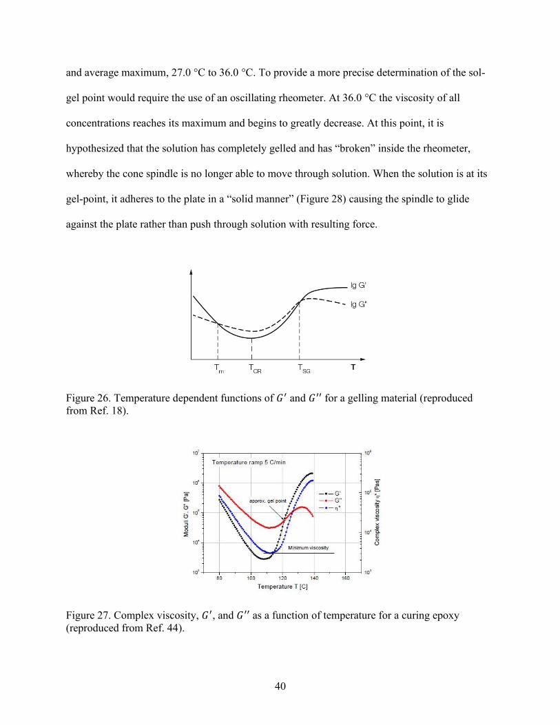
The sol-gel transition of a thermoresponsive polymer is characterized by an increase in
viscosity between the micelle and macrolattice states As seen in the temperature-dependent plots
of viscosity for Soluplusreg solutions the increase in viscosity takes place from 270 degC to 360 degC
This sharp increase in viscosity is also seen in literature (Figures 26 and 27) from plots of
complex shear viscosity versus temperature Figure 26 describes the minimum viscosity as an
onset of chemical reaction where micelles begin to self-assemble and form superstructures
indicating the beginning of gel formation18 Our aqueous Soluplusreg solutions of varying
concentration show this onset of chemical reaction around 270 degC (Figures 24 and 25) As the
gelling process occurs viscosity rapidly increases to a sol-gel point The sol-gel transition is
typically defined as the crossing point between 119866prime and 119866primeprime (Figures 26 and 27)182944 Due to our
use of a cone-and-plate rheometer which is unable to measure 119866prime and 119866primeprime separately precise sol-
gel transitions for our Soluplusreg solutions were indeterminable However as seen in Figure 27
the sol-gel transition occurs within the large increase in viscosity We hypothesize that the
Soluplusreg sol-gel transition is occurring at a temperature that falls between the average minimum
40
and average maximum 270 degC to 360 degC To provide a more precise determination of the sol-
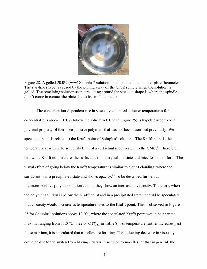
gel point would require the use of an oscillating rheometer At 360 degC the viscosity of all
concentrations reaches its maximum and begins to greatly decrease At this point it is
hypothesized that the solution has completely gelled and has ldquobrokenrdquo inside the rheometer
whereby the cone spindle is no longer able to move through solution When the solution is at its
gel-point it adheres to the plate in a ldquosolid mannerrdquo (Figure 28) causing the spindle to glide
against the plate rather than push through solution with resulting force
Figure 26 Temperature dependent functions of 119866prime and 119866primeprime for a gelling material (reproduced
from Ref 18)
Figure 27 Complex viscosity 119866prime and 119866primeprime as a function of temperature for a curing epoxy
(reproduced from Ref 44)
41
Figure 28 A gelled 200 (ww) Soluplusreg solution on the plate of a cone-and-plate rheometer
The star-like shape is caused by the pulling away of the CP52 spindle when the solution is
gelled The remaining solution seen circulating around the star-like shape is where the spindle
didnrsquot come in contact the plate due to its small diameter
The concentration-dependent rise in viscosity exhibited at lower temperatures for
concentrations above 100 (follow the solid black line in Figure 25) is hypothesized to be a
physical property of thermoresponsive polymers that has not been described previously We
speculate that it is related to the Krafft point of Soluplusreg solutions The Krafft point is the
temperature at which the solubility limit of a surfactant is equivalent to the CMC45 Therefore
below the Krafft temperature the surfactant is in a crystalline state and micelles do not form The
visual effect of going below the Krafft temperature is similar to that of clouding where the
surfactant is in a precipitated state and shows opacity45 To be described further as
thermoresponsive polymer solutions cloud they show an increase in viscosity Therefore when
the polymer solution is below the Krafft point and in a precipitated state it could be speculated
that viscosity would increase as temperature rises to the Krafft point This is observed in Figure
25 for Soluplusreg solutions above 100 where the speculated Krafft point would be near the
maxima ranging from 110 degC to 220 degC (1198791198721 in Table 8) As temperature further increases past
these maxima it is speculated that micelles are forming The following decrease in viscosity
could be due to the switch from having crystals in solution to micelles or that in general the
42
viscosity of Newtonian fluids decreases as temperature increases At concentrations below
100 it is speculated that the polymer fraction wasnrsquot large enough to witness this slight
increase in viscosity or temperatures didnrsquot reach cold enough
Previous work conducted by our research group reported that aqueous Soluplusreg
solutions physically gel at temperatures from 300 degC to 400 degC depending on concentration
where more concentrated solutions gel at lower temperatures (Figure 29)23 This research was
conducted using a 90deg tilt test and observing at which temperatures the samples stopped flowing
The data obtained by a 90deg tilt test roughly matches the rheologically implied temperature range
at which the sol-gel transition occurs 270 degC to 360 degC Differences between these sol-gel
transition temperature ranges could be from the differences in the experimental processes where
rheology is a more precise way of observing viscoelastic behavior Figure 29 also reveals that
aqueous Soluplusreg solutions below 100 (ww) do not exhibit a gel phase at any temperature It
is hypothesized that the polymer solutions are not at high enough concentrations for the micelles
to interact and form macrolattice structures Data acquired from the rheometer is at least
somewhat consistent with this observation as seen in the traces from samples under 100
(ww) where the viscosity behavior exhibits small to negligible features that we attribute to the
gelation process (Figure 25) We speculate that the small features observed in the 20 and 50
samples correspond to a pre-gelation condition that does not lead to a complete gelling as
measured by the 90 deg tilt test
43
Figure 29 Sol-gel and gel-sol transitions for Soluplus samples as a function of temperature
Speculated phase boundaries (solid lines) have been added to emphasize observed trends
(adapted from Ref 23)
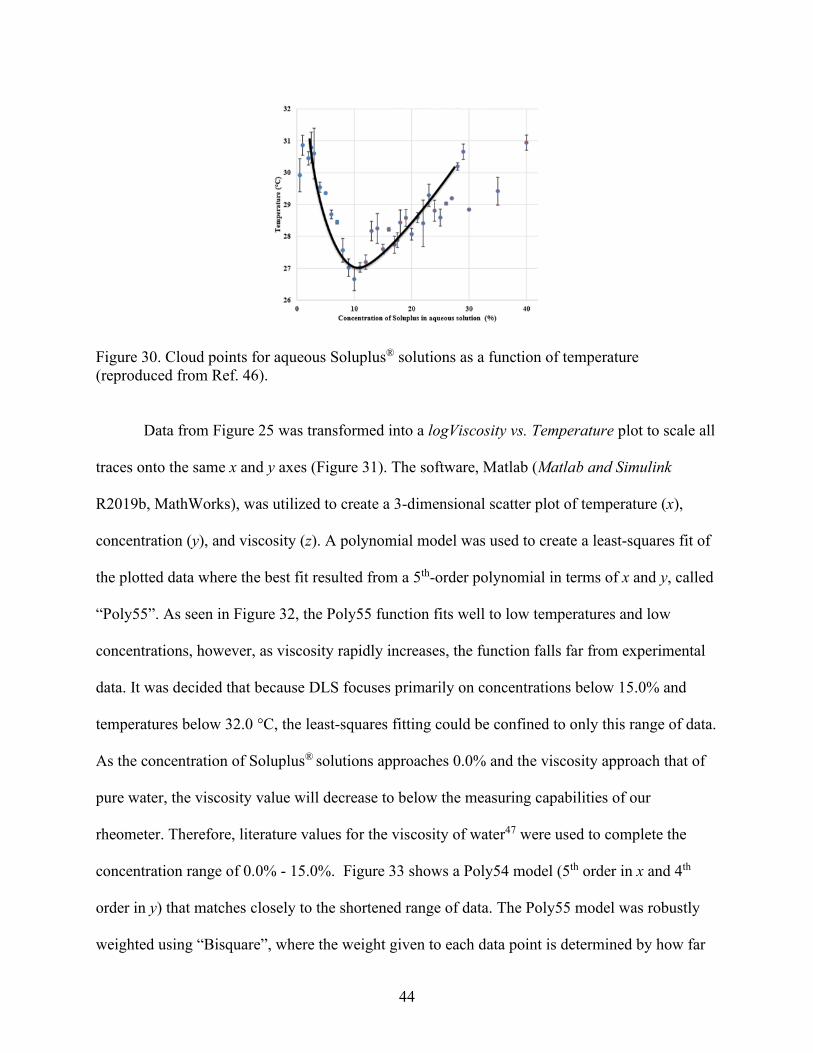
Previous work conducted in our research group also described the cloud-point transitions
of Soluplusreg solutions The cloud point is described as the transition from soluble to insoluble
phases across the LCST phase boundary and has been observed for aqueous Soluplusreg solutions
to be in the range of 270 degC to 310 degC (Figure 30)46 The temperature range of cloud transition
from previous research lies within the sharp increase of viscosity as did the sol-gel transition
Although these two phase transitions clouding and gelling occur at the same temperature range
they are independent of each other Figures 29 and 30 illustrate the differences in gelling and
clouding phase behaviors where the gel point of aqueous Soluplusreg solutions decreases as a
function of increasing concentration but the cloud point increases as a function of increasing
concentration As previously recognized Soluplusreg solutions under 300 first experience a
cloud transition before physically gelling as a function of increasing temperature Therefore it is
hypothesized that for aqueous Soluplusreg solutions below 300 the cloud transition occurs
within the temperature range of the sharp viscosity increase (270 degC to 360 degC) but prior to the
gel point
44
Figure 30 Cloud points for aqueous Soluplusreg solutions as a function of temperature
(reproduced from Ref 46)
Data from Figure 25 was transformed into a logViscosity vs Temperature plot to scale all
traces onto the same x and y axes (Figure 31) The software Matlab (Matlab and Simulink
R2019b MathWorks) was utilized to create a 3-dimensional scatter plot of temperature (x)
concentration (y) and viscosity (z) A polynomial model was used to create a least-squares fit of
the plotted data where the best fit resulted from a 5th-order polynomial in terms of x and y called
ldquoPoly55rdquo As seen in Figure 32 the Poly55 function fits well to low temperatures and low
concentrations however as viscosity rapidly increases the function falls far from experimental
data It was decided that because DLS focuses primarily on concentrations below 150 and
temperatures below 320 degC the least-squares fitting could be confined to only this range of data
As the concentration of Soluplusreg solutions approaches 00 and the viscosity approach that of
pure water the viscosity value will decrease to below the measuring capabilities of our
rheometer Therefore literature values for the viscosity of water47 were used to complete the
concentration range of 00 - 150 Figure 33 shows a Poly54 model (5th order in x and 4th
order in y) that matches closely to the shortened range of data The Poly55 model was robustly
weighted using ldquoBisquarerdquo where the weight given to each data point is determined by how far
45
the point is from the fitted line This allows for the fit to be based on the bulk data minimizing
any outlier effects48 The Poly54 model didnrsquot use robust fitting on top of the polynomial fit
Figure 31 Log-linear plot of viscosity vs temperature of aqueous Soluplusreg solutions at
different concentrations
Figure 32 Full range of experimental data modeled with a Poly55-Bisquare fit
-1
0
1
2
3
4
5
6
0 10 20 30 40 50
Log V
isco
sity
(cP
)
Temperature (degC)
10 20 50 100 150175 200 225 250 300
46
Figure 33 Short range of experimental data modeled with a Poly54 fit
From the Poly54 modeled fit a polynomial function was created so that the viscosity of
Soluplusreg samples could be determined for any temperature ranging 50 degC to 320 degC and
concentration ranging 00 to 150 The full Poly54 fit function is shown below
log(120578) = minus 01652 + 01448(119879) + 0282(120588) minus 002019(1198792) minus 002223(119879)(120588) (10)
minus 004058(1205882) + 0001153(1198793) + 0001691(1198792)(120588) + 000144(119879)(1205882)
+000414(1205883) minus 30211990910minus5(1198794) minus 700811990910minus5(1198793)(120588)
minus 320411990910minus5(1198792)(1205882) minus 798911990910minus5(119879)(1199013) minus 00001442(1205884)
+ 297611990910minus7(1198795) + 104311990910minus6(1198794)(120588) + 506111990910minus7(1198793)(1205882)
minus31911990910minus7(1198792)(1205883) + 334411990910minus6(119879)(1205884)
where 120578 is viscosity 119879 is temperature in Celsius and 120588 is the relative mass concentration (ww)
Equation 10 shows accuracy to experimental viscosity data within a 30 difference around 95
of the time where the other 5 is within a 100 difference (occurring primarily at low
concentrations and low temperatures or high concentrations and high temperatures)
47
32 Temperature Dependent Refractive Index of Soluplusreg Solutions
Because particle size analysis by dynamic light scattering depends on viscosity and
refractive index these parameters were evaluated for on Soluplusreg solutions to ensure accurate
hydrodynamic effective diameter measurement The temperature dependence of viscosity for
Soluplusreg solutions is described in Section 31 and the following gives the refractive index
behavior of aqueous Soluplusreg solutions as a function of temperature
Water and ethanol were evaluated at 200 degC by the 2WAJ Abbe refractometer to check
the instrumentrsquos accuracy The refractometer has a specified accuracy of plusmn 00002 and the
experimental results can be seen in Table 9 compared to literature values The refractive index of
ethanol is within the allowed deviation of its literature value but the value of water lies 00006
away from its literature value Since the effect of refractive index on particle size analysis is
relatively weak (see Section 33) it was concluded that this deviation can be tolerated
Furthermore the NanoBrook Omni instrument considers refractive index to only the thousands
place so the observed deviation is within the natural precision of the correction
Table 9 Experimental and literature refractive index values
for water and ethanol at 200 degC
Refractive Index (119899) at 200 degC
Standard Experimental Literature
Water 13324 13330d
Ethanol 13612 13611e d from Ref 49 e from Ref 50
Each concentration of Soluplusreg solution ranging 01 to 100 (ww) were evaluated
for their refractive index from 110 degC to 350 degC as described in Section 242 These data can be
48
seen in Figure 34 where the 01 trace included representative standard deviations as
determined from repetitive runs As shown in the figure refractive index increases as the
concentration of Soluplusreg increases As well the refractive index decreases slowly as
temperature increases for all concentrations This trend replicates the refractive index behavior of
pure water49
Figure 34 Effect of temperature on refractive index for Soluplusreg samples
33 Particle Size Analysis of Soluplusreg Solutions
Calibration standards were evaluated by the NanoBrook Omni particle size analyzer to
ensure the instrumentrsquos accuracy NIST specifies that their latex calibration standards do not
come with a passfail criterion due to underlying sizing methodology that is customer
dependent51 NIST recommends establishing an in-house criterion to test instrument
performance which has been adopted as plusmn 400 nm in the chemistry department at Missouri
13300
13350
13400
13450
13500
13550
5 10 15 20 25 30 35 40
Ref
ract
ive
Index
Temperature (degC)
01 05 10 20 50 100
49
State University52 The experimental hydrodynamic effective diameters of the 429 nm and 288
nm standards can be seen in Table 10 where it is shown that our measurements pass in-house
criteria displaying good instrument performance The polydispersity index (PDI) is also
included in Table 10 which signifies the relative size-range of particles The PDI can range from
0000 to 1000 where a lower value corresponds to a more monodisperse sample
Table 10 Effective diameters of NIST latex calibration standards at 250 degC
Standard (nm) Experimental
Eff Diam (nm)
Experimental
Polydispersity
429 4592 0106
288 2858 0040
Soluplusreg solutions 01 05 10 20 50 and 100 (ww) were each
evaluated three times (Sets 1 2 and 3) for their hydrodynamic effective diameters as a function
of temperature using the NanoBrook Omni particle size analyzer following the protocol in
Section 252 Figure 35 displays the average hydrodynamic effective diameters along with
uncertainties for each sample as a function of temperature using ldquouncorrectedrdquo viscosity and
refractive index data ldquoUncorrectedrdquo refers to using the pre-programmed viscosity and refractive
index data for a pure water solvent As observed the temperature dependence generally shows
the diameter to decrease with increasing temperature and then sharply rise as the cloud- or gel-
point is reached Additionally the effective diameter appears to be directly proportional to
Soluplusreg concentration in that for any given temperature the largest particle diameter is
obtained for the highest Soluplusreg concentration The sharp rise in the temperature dependence
of the hydrodynamic effective diameter appears to correlate with the solutionrsquos clouding or
gelling point where micelles are aggregating and produce larger particles The 01 and 05
50
Soluplusreg samples donrsquot show this sharp rise in diameter suggesting that there is no onset of
physical change However according to Figure 30 these concentrations do show clouding by
spectroscopy whereas they do not show evidence gelling (Figure 29)
Figure 35 Effect of temperature on effective diameter for Soluplusreg solutions using uncorrected
values of viscosity and refractive index
The traces in Figure 35 were recomputed to correct for the viscosity and refractive index
behavior of Soluplusreg solutions In the following discussion ldquocorrectedrdquo refers to using the
viscosity and refractive index data of Soluplusreg solutions reported in Sections 31 and 32 As
seen in Figure 36 the corrected effective diameters are observed to be inversely proportional to
concentration Figure 37 depicts this trend for one specific temperature (250 degC) by comparing
hydrodynamic diameters obtained from ldquouncorrectedrdquo vs ldquocorrectedrdquo analyses Table 11 gives
the numerical values shown in Figure 37 along with PDI values It is notable that the PDI shows
no dependence on viscosity or refractive index It is reported in literature that the cause for the
decreasing diameter as concentration increases is related to micellar core size At larger
000
10000
20000
30000
40000
50000
60000
70000
11 16 21 26 31 36
Hydro
dyn
amic
Eff
ecti
ve
Dia
met
er
(nm
)
Temperature (degC)
01 05 10 20 50 100
51
concentrations micelles form with less solvent in the core causing the micelle to compact and
reduce in size6
Figure 36 Effect of temperature on effective diameter for Soluplusreg solutions using corrected
values of viscosity and refractive index
Figure 37 Uncorrected vs corrected diameter at 250 degC for Soluplusreg in aqueous solution
000
2000
4000
6000
8000
10000
12000
11 16 21 26 31 36
Hydro
dyn
amic
Eff
ecti
ve
Dia
met
er
(nm
)
Temperature (degC)
01 05 10 20 50 100
000
2000
4000
6000
8000
10000
12000
01 05 10 20 50 100Hydro
dyn
amic
Eff
ecti
ve
Dia
met
er
(nm
)
Concentration ()
Uncorrected Corrected
52
Table 11 Uncorrected vs corrected effective diameters at 250 degC for Soluplusreg in
aqueous solution
Hydrodynamic Effective Diameter (nm)
Concentration
() Uncorrected Corrected Polydispersity
01 6615 plusmn 079 6313 plusmn 076 0030
05 6078 plusmn 008 5359 plusmn 006 0038
10 6648 plusmn 037 5539 plusmn 031 0042
20 6988 plusmn 026 4981 plusmn 019 0059
50 7634 plusmn 054 4114 plusmn 029 0103
100 10585 plusmn 128 2498 plusmn 030 0210
Also depicted in Figure 36 the ldquocorrectedrdquo diameter values remain more consistent
through rises in temperature prior to sharply increasing As well the sharp rise in effective
diameter remains around the same temperature The 01 and 05 Soluplusreg samples were
recomputed using extrapolated viscosities as determined by Equation 10 The Brookfield RVDV-
III Ultra rheometer was unable to test these low concentrated samples because their viscosities
fall below the instrumental limit It is suspected that because theses viscosity values were
extrapolated from outside the experimentally determined range the resulting corrected diameters
may contain an inherently higher level of uncertainty In Figure 36 the 01 and 05 traces
still show no evidence for physical phase change by DLS (ie a sharp increase in diameter at
higher temperatures)
Salah et al report the hydrodynamic diameter of Soluplusreg in a 01 (ww) aqueous
solution at 200 degC to be 6486 plusmn 158 nm (Figure 38)15 The experimentally determined
ldquocorrectedrdquo effective diameter from this thesis for an equivalent sample under the same
conditions is 6576 plusmn 038 nm (Figure 36) consistent with the previously reported value
53
Figure 38 Size distribution for a 01 Soluplusreg solution at 200 degC (reproduced from Ref 15)
The influence of including accurate viscosity and refractive index data in particle size
algorithms is considerable For example the hydrodynamic effective diameter shifts from 14348
nm to 2535 nm for the 100 Soluplusreg solution at 200 degC upon correcting for these effects
(Table 12) This substantial shift (823 decrease) on diameter is due primarily to viscosity
effects Refractive index plays a less significant role in particle size analysis by DLS As shown
in Table 13 the resulting hydrodynamic diameter in a 100 Soluplusreg solution is shifted only
150 by changing refractive index by 0010 indicating that the correction due to refractive
index variation is significantly less important than that due to viscosity
Table 12 Difference in effective diameter when using uncorrected and corrected viscosity and
refractive index data for a 100 Soluplusreg solution at 200 degC
SOP Uncorrected Corrected
Liquid Water Unspecified
Viscosity (cP) 1002 5842
Refractive Index 1331 1351
Effective Diameter (nm) 14348 2535
54
Table 13 Effective diameter dependence on refractive index for
a 100 Soluplusreg solution at 200 degC and 5842 cP
Refractive Index Effective Diameter (nm)
1341 2498
1351 2535
1361 2573
As discussed previously the sharp increase in effective diameter that is observed for the
10 20 50 and 100 (ww) Soluplusreg solutions is related to the cloud- or gel-point
Figure 39 overlays the viscosity and effective diameter of a 50 Soluplusreg solution on the same
temperature axis As observed effective diameter remains relatively constant as viscosity is
decreasing to its minimum across the temperature range As viscosity starts to increase
indicating an onset of change (clouding gelling or both) the effective diameter also rises The
increase in particle size is triggered by the reduced solubility of solution as it crosses the LCST
phase boundary This causes the micelles to aggregate and rearrange resulting in larger and more
polydisperse particle sizes15
Figure 39 Viscosity and corrected diameter vs temperature for a 50 Soluplusreg solution
10
14
18
22
27
31
35
2500
3500
4500
5500
6500
7500
8500
15 17 19 21 23 25 27 29 31
Vis
cosi
ty (
cP)
Hydro
dyn
amic
Eff
D
iam
(n
m)
Temperature (degC)
Corrected Eff Diam Viscosity
55
CHAPTER 4 CONCLUSIONS AND FUTURE DIRECTIONS
The phase behavior of aqueous solutions of Soluplusreg a polyvinyl caprolactam-polyvinyl
acetate-polyethylene glycol graft copolymer were studied throughout this research
Rheologically determining the effect of temperature on viscosity allowed for insight behind the
viscoelastic properties of thermothickening polymer solutions It was observed that as
temperature rises the viscosities of Soluplusreg solutions decrease until reaching a minimum
around 280 degC where viscosity then sharply increases This trend has been observed by other
researchers for gelling polymers where a large increase in viscosity signifies the agglomeration
of polymeric micelles into macrolattices The sharp increase in viscosity for aqueous Soluplusreg
solutions is concentration independent and occurs from 270 degC to 360 degC Within this
temperature range polymeric micelles aggregate into a network and gel but determining a
specific gel-point is unattainable with use of a cone-and-plate rheometer A precise gel-point
could be determined by use of an oscillatory rheometer The temperature at which viscosity
sharply rises is also seen to correlate with cloud point where the solution is in an insoluble phase
and micelles begin to rearrange and agglomerate due to decreased solubility Although gelling
and clouding both occur around the same temperature they show no evidence of true correlation
The cause of swelling in viscosity seen at lower temperatures for concentrations above 100
remains inconclusive however we speculate that this is due to the Krafft point of aqueous
Soluplusreg solutions We hypothesize that the Krafft point temperature where micelles begin to
form is where viscosity begins to increase With further analysis on particle size this behavior
could be better interpolated For example studying the particle size of a 200 (ww) Soluplusreg
solution from 50 degC to 200 degC would show micelle behavior before and after the viscosity
56
increase If the particle size in solution increases as viscosity increases a physical phase behavior
would be witnessed Possibly going from a crystalline to micelle state due to the Krafft point
Particle size algorithms used in DLS analyses are directly dependent on viscosity and
refractive index values of the solutions Therefore it is important to include accurate information
for these parameters In this thesis a relationship between concentration temperature and
viscosity was determined by measuring sets of these variable and fitting the data to a 2-variable
polynomial function From this equation accurate viscosity values could be identified and used
in particle size analysis for Soluplusreg solutions The refractive index of Soluplusreg solutions were
studied and showed close similarity to that of water where refractive index decreases slightly as
a function of increasing temperature The effect of refractive index on hydrodynamic effective
diameter is minimal in DLS However viscosity plays a much more significant role where a
4840 cP increase in viscosity caused effective diameter to decrease 823
The hydrodynamic effective diameter of Soluplusreg particles in aqueous solution as
measured by DLS changed significantly upon application of corrections due to viscosity and
refractive index effect The most significant difference observed after the corrections was in the
relationship between concentration and effective diameter where the uncorrected trend of
particle size increasing with concentration proved to be the opposite trend (particle size
decreases with increasing concentration) after corrections were applied
For a given concentration plots of hydrodynamic effective diameter vs temperature
showed an overall decrease with temperature to a minimum near 270 degC followed by a sharp
rise around 300 degC for all concentrations This rise in diameter appears to correlate with the
solutions phase behaviors clouding and gelling
57
Soluplusreg is a tri-block graft copolymer that is used in the pharmaceutical industry to
enhance the bioavailability of APIs by encapsulating insoluble drugs within a micellar core
Studying the effect of temperature on particle size and viscoelastic behavior gives insight to how
the polymeric micelles will behave once subjected to body temperature Supported by this
research Soluplusreg shows interest in the biomedical field as a drug carrier system through its
thermoresponsive behaviors in viscoelasticity and particle size
58
REFERENCES
1 S Koltzenburg in Solubility Enhancement with BASF Pharma Polymers ed T Reintjes
BASF SE Lampertheim Germany 2011 1 9-26
2 M A Ward and T K Georgiou Polymers 2011 3 1215-1242
3 D W van Krevelen and K te Nijenhuis Properties of Polymers Elsevier Amsterdam
Netherlands 2009
4 S Okabe S Sugihara S Aoshima and M Shibayama Macromolecules 2003 36 4099-
4106
5 Y Tanaka in Rheology ed J D Vicente InTech Rijeck Croatia 2012 2 29-58
6 S S Kulthe Y M Choudhari N N Inamdar and V Mourya Designed Monomers and
Polymers 2012 15 465-521
7 J F Alopaeus E Hagesaether and I Tho Pharmaceuticals 2019 12 1-23
8 R Tanbour A M Martins W G Pitt and G A Husseini Current Pharmaceutical Design
2016 22 1-12
9 G P Andrews and D S Jones Biomacromolecules 2006 7 899-906
10 K Yotsumoto K Ishii M Kokubo and S Yasuoka Int J Pharm 2018 553 132-140
11 A Gandhi A Paul S O Sen and K K Sen Asian J Pharm Sci 2015 10 99-107
12 The Science of Insolubility-BASF httpsthemedicinemakercomdiscovery-
developmentthe-science-of-insolubility (accessed November 2019)
13 Y Zhu R Batchelor A B Lowe and P J Roth Macromolecules 2016 49 672-680
14 R Hoogenboom in Smart Polymers and Their Applications ed M R Aguilar and J S
Roman Woodhead Publishing Sawston Cambridge 2014 2 19
15 I Salah M Abou Shamat and M T Cook J Appl Polym Sci 2019 136 46915
16 The IUPAC Compendium of Chemical Terminology httpsgoldbookiupacorg (accessed
October 2019)
17 Soluplus Technical Information-BASF httpspharmaceuticalbasfcomenDrug-
FormulationSoluplushtml (accessed September 2019)
59
18 D Djuric in Solubility Enhancement with BASF Pharma Polymers ed T Reintjes BASF
SE Lampertheim Germany 2011 5 67-68
19 Soluplusreg-The Solid Solution httpspharmaceuticalbasfcomenDrug-
FormulationSoluplushtml (accessed November 2019)
20 L Di and E H Kerns in Drug-Like Properties Concepts Structure Design and Methods
Academic Press Cambridge Massachusetts 2nd edition 2016 19 267-281
21 Soluplusreg Regulatory Facts Sheet httpswwwpharmaexcipientscomnewssoluplus-is-
approved-in-generics-in-taiwan-and-argentina-and-is-now-filed-in-brazil (accessed
November 2019)
22 G Bonacucina M Cespi G Mencarelli G Giorgioni and G F Palmieri Polymers 2011
3 779-811
23 K Kosinska Non-Thesis Degree Paper Department of Chemistry Missouri State
University 2016
24 C M Reynolds unpublished work 2013
25 J Stetefeld S A McKenna and T R Patel Biophys Rev 2016 8 409-427
26 DLS Technical Note [MRK656-01]-Malvern Instruments httpswarwickacuk
faccross_facsciencecityprogrammesinternalthemesam2bookingparticlesizeintro_to_dl
spdf (accessed November 2019)
27 Technical Note Viscosity Effects-Horiba httpwwwhoribacomfileadminuploads
ScientificDocumentsPSATN140pdf (accessed September 2019)
28 Brookfield Engineering Laboratories Inc More Solutions to Sticky Problems Brookfield
Middleboro MA 2014
29 T G Mezger The Rheology Handbook For users of rotational and oscillatory rheometers
Vincentz Network Hanover Germany 2014
30 D L Blair in Molecular Gels Structure and Dynamics ed R G Weiss Royal Society of
Chemistry London United Kingdom 2018 2 28-32
31 Brookfield Engineering Laboratories Inc Brookfield DV-III Ultra Programmable
Rheometer Operating Instructions Manual No M98-211-B0104 Brookfield Middleboro
MA
32 N Merlet-Lacroix E D Cola and M Cloitre Soft Matter 2010 6 984-993
60
33 Viscosity of Adhesives httpswwwgalindbergsebloggviscosity-of-adhesives (accessed
November 2019)
34 Basics of Rheology-Anton Paar httpswikianton-paarcomus-enbasics-of-
rheologyrheology-and-rheometryrelated-information (accessed November 2019)
35 The provided Soluplusreg expired in May 2017 but there is no evidence of complication due
to expiration
36 Rheometers vs Viscometers-Malvern Panalytical httpswwwmalvernpanalyticalcom
enproductsmeasurement-typeviscosityrheometer-vs-viscometer (accessed October 2019)
37 Rheometers-Malvern Panalytical httpswwwmalvernpanalyticalcom
enproductscategoryrheometers (accessed October 2019)
38 P Fernanda in Structure-Function Analysis of Edible Fats ed A G Marangoni Elsevier
Amsterdam Netherlands 2nd Edition 2018 11 313-385
39 Rheometers-How do they compare httpswwwatascientificcomaurheometers-compare
(accessed October 2019)
40 J W Goodwin and R W Hughes Rheology for Chemists An Introduction Royal Society
of Chemistry London United Kingdom 2008
41 Abbe Refractometer-ChemBuddy httpwwwrefractometerplAbbe-refractometer
(accessed January 2020)
42 The NIST traceable particle size standards expired as of June 2019 but show no evidence of
complication due to expiration
43 NanoBrook Omni Brochure-Brookhaven Instruments httpswwwbrookhaveninstruments
comwp-contentuploads201910NanoBrook-Omnipdf (accessed January 2020)
44 Thermosetting Polymers-Rheological Testing httpswwwazomcom
articleaspxArticleID=12103 (accessed December 2019)
45 Y Nakama in Cosmetic Science and Technology Theoretical Principles and Applications
Elsevier Amsterdam Netherlands 2017 15 231-244
46 R Balzam Masterrsquos Thesis Missouri State University 2016
47 Viscosity of Water httpswikianton-paarcomus-enwater (accessed January 2020)
48 Least-Squares Fitting MathWorksreg httpswwwmathworkscomhelpcurvefitleast-
squares-fittinghtml (accessed January 2020)
61
49 A N Bashkatov and E A Genina Proc of SPIE 2003 5068 393-395
50 US National Library of Medicine-PubChem httpspubchemncbinlmnihgov
compoundEthanol (accessed January 2020)
51 Precision Particles NIST Traceable Size Standards [TDS 623]-Polysciences Inc https
wwwpolysciencescomskinfrontenddefaultpolysciencespdfTDS20623pdf (accessed
February 2020)
52 In-house standard deviation criteria was created by testing fresh sets of the NIST traceable
particle standards on various days with various methods of sample preparation For the 429
nm standard six samples were tested and had an average effective diameter of 4543 plusmn 146
nm The 288 nm standard gave an average effective diameter of 2882 plusmn 217 nm with three
samples tested It was decided that any standard within plusmn 400 nm from the stated true
particle size was acceptable
- Determining Particle Size of Polymeric Micelles in Thermothickening Aqueous Solutions
-
- Recommended Citation
-
- Missouri State University
-
DETERMINING PARTICLE SIZE OF POLYMERIC MICELLES IN
THERMOTHICKENING AQUEOUS SOLUTIONS
A Masterrsquos Thesis
Presented to
The Graduate College of
Missouri State University
TEMPLATE
In Partial Fulfillment
Of the Requirements for the Degree
Master of Science Chemistry
By
Jessica Diane Bruer
May 2020
ii
Copyright 2020 by Jessica Diane Bruer
iii
DETERMINING PARTICLE SIZE OF POLYMERIC MICELLES IN
THERMOTHICKENING AQUEOUS SOLUTIONS
Chemistry
Missouri State University May 2020
Master of Science
Jessica Bruer
ABSTRACT
Many active pharmaceutical ingredients (APIs) are poorly soluble and cause inadequate drug
absorption Soluplusreg a polyvinyl caprolactam-polyvinyl acetate-polyethylene glycol graft
copolymer is a commercial excipient (BASF Corp) that enhances the solubility and
bioavailability of many APIs The mechanism of enhancement is related to the ability to form
polymeric micelles in solution These micelles store insoluble APIs in their hydrophobic interior
and transport them to targeted sites in the body An important characteristic of solubility
enhancers is the particle size exhibited in solution before and after loading with APIs This is
most commonly determined by dynamic light scattering (DLS) methods However DLS
measurements involving thermothickening polymer solutions can be complicated by the
temperature dependence of viscosity and refractive index solution properties that directly impact
the size analysis algorithms in DLS In this project the temperature dependence of viscosity for
Soluplusreg solutions were evaluated and used as a correction to particle size measurements by
DLS Solution concentrations ranging 10 to 300 (ww) of Soluplusreg were studied from 50
degC to 400 degC using a cone-and-plate rheometer Refractive index of Soluplusreg solutions were
also studied and used in the correction of particle size It was found that correcting viscosity and
refractive index data drastically affected hydrodynamic effective diameter where viscosity was
more highly weighted The corrected particle size of Soluplusreg solutions was inversely
proportional to concentration with the 01 and 100 solutions showing effective diameters of
6313 plusmn 076 nm and 2498 plusmn 030 nm at 250 degC respectively By properly accounting for these
variables in DLS algorithms particle size of thermoresponsive polymer solutions can be more
accurately characterized
KEYWORDS rheology dynamic light scattering Soluplusreg thermoresponsive block
copolymer active pharmaceutical ingredient viscosity refractive index thermothickening
polymeric micelles
iv
DETERMINING PARTICLE SIZE OF POLYMERIC MICELLES IN
THERMOTHICKENIG AQUEOUS SOLUTIONS
By
Jessica Bruer
A Masterrsquos Thesis
Submitted to the Graduate College
Of Missouri State University
In Partial Fulfillment of the Requirements
For the Degree of Master of Science Chemistry
May 2020
Approved
G Alan Schick PhD Thesis Committee Chair
Gary Meints PhD Committee Member
Ridwan Sakidja PhD Committee Member
Adam Wanekaya PhD Committee Member
Julie Masterson PhD Dean of the Graduate College
In the interest of academic freedom and the principle of free speech approval of this thesis
indicates the format is acceptable and meets the academic criteria for the discipline as
determined by the faculty that constitute the thesis committee The content and views expressed
in this thesis are those of the student-scholar and are not endorsed by Missouri State University
its Graduate College or its employees
v
ACKNOWLEDGEMENTS
I would like to thank those who showed their support during the course of my graduate
studies Specially my family who endlessly support my decisions Without their encouragement
I would not be where I am today A special thank you to my siblings Kyle Bruer and Alyssa
Mansfield for pushing me to be my best in hopes Irsquod be as successful as they are To my future
sister-in-law Jill Davis I greatly appreciated the help and patience with data manipulation I am
upmost grateful for the support of my parents Richard and Theresa Bruer who have taught me
that no ambition is too grand Thank you for always being my cheerleaders and helping me at
any cost
I would also like to thank my research advisor Dr G Alan Schick who has guided me
since my undergraduate years I appreciate his commitment to furthering my education and
introducing me to physical chemistry Additionally I thank my thesis committee for their time
and support Dr Gary Meints Dr Ridwan Sakidja and Dr Adam Wanekaya I am tremendously
grateful for the friends I have made throughout this journey fellow graduate students research
members and faculty who made coming to campus enjoyable and entertaining Specifically
Cody Turner who has been my rock through our entire accelerated masterrsquos journey together
I dedicate this thesis to my mother Theresa Bruer for sparking my interest in science with
participation in the elementary school science fairs
vi
TABLE OF CONTENTS
Chapter 1 Introduction Page 1
11 Poor Solubility in the Pharmaceutical Field Page 1
12 Polymers Page 1
121 Polymer Behavior Page 2
122 Function with Active Pharmaceutical Ingredients Page 3
13 Thermoresponsivity Page 4
14 Soluplusreg Page 7
15 Dynamic Light Scattering Spectroscopy Page 14
151 Effect of Viscosity Page 14
152 Effect of Refractive Index Page 20
16 Objectives Page 21
Chapter 2 Experimental Page 22
21 Overview Page 22
22 Materials Page 22
23 Temperature Dependence of Viscosity Page 23
231 Instrumentation Page 23
232 Methods Page 27
24 Refractive Index Analysis Page 28
241 Instrumentation Page 28
242 Methods Page 29
25 Particle Size Determination by Dynamic Light Scattering Page 30
251 Instrumentation Page 30
252 Methods Page 33
Chapter 3 Results and Discussion Page 35
31 Temperature Dependent Viscoelastic Behavior of Soluplusreg Solutions Page 35
32 Temperature Dependent Refractive Index of Soluplusreg Solutions Page 47
33 Particle Size Analysis of Soluplusreg Solutions Page 48
Chapter 4 Conclusions and Future Directions Page 55
References Page 58
vii
LIST OF TABLES
Table 1 Types and examples of copolymers Page 2
Table 2 Approximate viscosity values of commonly known materials at 200 degC Page 18
Table 3 Cone spindle dimensions and shear rates Page 26
Table 4 Experimental conditions for each samplestandard run on the rheometer Page 28
Table 5 Temperatures used in the evaluation of refractive index for various standards
and samples Page 30
Table 6 Standard operating procedures for temperature dependent particle size analysis Page 34
Table 7 Total allowed error for each viscosity standard fluid at 250 degC Page 35
Table 8 Extrema temperatures observed in η-T plots of Soluplusreg solutions Page 39
Table 9 Experimental and literature refractive index values for water and
ethanol at 200 degC Page 47
Table 10 Effective diameters of NIST latex calibration standards at 250 degC Page 49
Table 11 Uncorrected vs corrected effective diameters at 250 degC for Soluplusreg in
aqueous solution Page 52
Table 12 Difference in effective diameter when using uncorrected and corrected
viscosity and refractive index data for a 100 Soluplusreg solution at 200 degC Page 53
Table 13 Effective diameter dependence on refractive index for a 100 Soluplusreg
solution at 200 degC and 5842 cP Page 54
viii
LIST OF FIGURES
Figure 1 Structure of a polymeric micelle with APIs stored in its core Page 4
Figure 2 Temperature vs polymer volume fraction (120601) plots Page 6
Figure 3 Schematic representation of block copolymer phase transitions Page 7
Figure 4 Physical appearance of Soluplusreg Page 8
Figure 5 Structure of Soluplusreg Page 9
Figure 6 Solubilization capacities of various active pharmaceutical ingredients Page 10
Figure 7 Dissolution test for the release of itraconazole with polymeric matrices Page 10
Figure 8 Blood concentration of itraconazole with and without Soluplusreg solution Page 10
Figure 9 Phase diagram for a LCST lt UCST behaving polymer Page 12
Figure 10 Micellization mechanism for solutions of Soluplusreg Page 13
Figure 11 Soluplusreg solution at room temperature cloud point and gel point Page 13
Figure 12 Particle size data for a pigment dispersed in water at two different viscosities Page 15
Figure 13 Two plates model used to describe the physics of viscosity Page 17
Figure 14 Graphical relationship between complex shear modulus 119866lowast storage
moduli 119866prime loss moduli 119866primeprime and the phase-shift angle δ Page 20
Figure 15 Schematics of a cone-and-plate rheometer Page 25
Figure 16 Diagram of the inner workings of the cone and plate Page 25
Figure 17 Top view of spindles CP40 and CP52 Page 26
Figure 18 Set-up used for viscosity data collection on a Brookfield rheometer Page 28
Figure 19 Set-up used for refractive index data collection on an Abbe refractometer Page 29
Figure 20 Shadow and scale within an Abbe-type refractometer Page 30
Figure 21 Schematic representation of the Zetasizer Nano series DLS instrument Page 31
Figure 22 Set-up used for particle size data collection on a NanoBrook Omni Page 33
Figure 23 Brookfield viscosity standard fluids as a function of temperature Page 35
Figure 24 Effect of temperature on viscosity for each aqueous Soluplusreg sample Page 37
Figure 25 Viscosity of Soluplusreg samples on the same temperature scale Page 38
Figure 26 Temperature dependent functions of 119866prime and 119866primeprime for a gelling material Page 40
Figure 27 Complex viscosity 119866prime and 119866primeprime as a function of temperature for an epoxy Page 40
Figure 28 A gelled 200 Soluplusreg solution on the plate of a cone-and-plate rheometer Page 41
Figure 29 Sol-gel and gel-sol transitions for Soluplusreg samples Page 43
Figure 30 Cloud points for aqueous Soluplusreg solutions as a function of temperature Page 44
Figure 31 Log-linear plot of viscosity vs temperature of aqueous Soluplusreg
solutions at different concentrations Page 45
Figure 32 Full range of experimental data modeled with a Poly55-Bisquare fit Page 45
Figure 33 Short range of experimental data modeled with a Poly54 fit Page 46
Figure 34 Effect of temperature on refractive index for Soluplusreg samples Page 48
Figure 35 Effect of temperature on effective diameter for Soluplusreg solutions using
uncorrected values of viscosity and refractive index Page 50
Figure 36 Effect of temperature on effective diameter for Soluplusreg solutions using
corrected values of viscosity and refractive index Page 51
Figure 37 Uncorrected vs corrected diameter at 250 degC for Soluplusreg in solution Page 51
Figure 38 Size distribution for a 01 Soluplusreg solution at 200 degC Page 53
Figure 39 Viscosity and corrected diameter vs temperature for 50 Soluplusreg sample Page 54
1
CHAPTER 1 INTRODUCTION
11 Poor Solubility in the Pharmaceutical Field
In 2011 it was reported that 90 of all compounds in the pharmaceutical drug delivery
system were poorly soluble in water1 This is a significant problem in the pharmaceutical
industry as drugs are ineffective unless they can be solubilized into the bodyrsquos systems rather
than being excreted from the digestive track due to re-crystallization1 It is important that drugs
are delivered to the right area at the right time and at the right concentration but many obstacles
such as poor solubility environmental degradation toxicity and lack of permeability make drug
delivery challenging2 These issues have led to the increasing use of enhanced drug delivery
methods such as polymeric micelles to help drugs reach their molecular target within the body
12 Polymers
Polymers are a type of synthetic macromolecule that consist of repeating structural units
They consist of two main components a backbone and peripheral side chains The repeating
units of a polymer may fall onto either part of a polymerrsquos structure When a polymer has two or
more units of varying composition it is called a copolymer Copolymers can be described as
random- alternating- graft- or block copolymers Random copolymers consist of two or more
monomers that are simultaneously present in one polymerization reactor Alternating copolymers
are comprised of two different monomers on the structural unit In graft copolymers one or more
monomers are grafted onto a homopolymer resulting in a backbone that has perforating side
branches Lastly in block copolymers one monomer is attached to the end group of a previous
2
polymerized chain forming a linear chain with different segments3 Table 1 gives visual
examples of each type of copolymer along with industrial examples
Table 1 Types and examples of copolymersa
a Reproduced from Ref 3
121 Polymer Behavior Polymer properties are identified by the polymerrsquos chemical
structure and molecular weight distribution Structure identities such as repeating unit nature end
group nature and branch composition all effect how a polymer behaves3 Block copolymers
consisting of unlike chains exhibit complicated physical properties such as microphase
separation that is dependent on polymer length composition and concentration4 Microphase
separation is seen in gelation polymers where a self-assembling of polymer networks causes the
polymer to behave as a viscoelastic solid The polymer gel is soft and deformable but can hold
3
its shape making it of interest in drug delivery science5 The gelling of polymers by phase
separation is dependent on many conditions but crucially temperature giving rise to the terms
thermoresponsivity and thermoreversibility as further discussed in Section 13
Polymers that consist of amphiphilic monomers have the tendency to form micelles in
solution Micelles are colloidal dispersions of these amphiphilic units that self-assemble due to
intermolecular forces between the hydrophobic and hydrophilic regions Typical surfactant
micelles are made up of 50 to 200 monomers and have a spherical diameter of three to six
nanometers Polymeric surfactant molecules have spherical diameters that range from 10 to 100
nm6 Factors controlling polymeric micelle size include molecular weight of the amphiphilic
block copolymer aggregation number proportion of hydrophobic to hydrophilic chains and
quantity of solvent trapped inside the micellar core The driving force behind the self-assembling
of polymers into micelles is noted as hydrophobic forces where the water repelling regions of
the polymer aggregate to each other minimizing the contact between the insoluble block and the
solvent and lowering the free energy of system167 The concentration above which micelles are
formed in solution is called the critical micelle concentration (CMC) When at the CMC or
slightly above loosely aggregated micelles are formed containing solvent within their core At
higher concentrations the residual solvent is excluded from the core thereby compacting the
micellar structure In general polymeric micelles have a lower CMC value than traditional
micelles6 Many studies show how polymeric micelles can be used in the biomedical field as
drug carrier systems27-11
122 Function with Active Pharmaceutical Ingredients Polymeric micelles are
capable of encapsulating insoluble active pharmaceutical ingredients (APIs) within their
hydrophobic core (Figure 1)1 Polymeric micelles help to increase the bioavailability of poorly
4
soluble APIs by stabilizing the drug and keeping it dissolved in solution until it is absorbed in the
gastrointestinal track12 Surfactants are also used to increase the bioavailability of APIs through
topical skin application The stratum corneum contains a tough barrier in which poorly soluble
drugs have trouble penetrating Encapsulating an API within a polymeric micelle allows for the
drug to penetrate the skin as the micelle endures a change in structure due to water evaporation10
Local diseases eg infections or inflammations are commonly treated by topical
delivery of the required medicinal drug to the targeted tissue It is important that the drug
remains at the site of application for an extended time to ensure efficacy and interaction with the
disease Such topical drug formulations require knowledge on rheological properties such as
structure and flow to gain insight into their effects on drug diffusion and to ensure ease of
applicationadministration The rheological behavior of polymeric micelles is of increasing
interest to test the performance of surfactants in pharmaceutical systems9
Figure 1 Structure of a polymeric micelle with APIs stored in its core (reproduced from Ref 8)
13 Thermoresponsivity
Materials that respond to external stimuli are referred to as ldquosmart materialsrdquo Polymers
are the most common smart material because they are comparatively cheap and can respond to
5
pH temperature ionic strength electric and magnetic fields and biochemical processes2
Temperature responsive also referred to as thermoresponsive polymers are particularly versatile
in their applications such as tissue engineering sensing gene delivery and drug delivery2 A
thermoresponsive polymerrsquos ability to change abruptly and reversibly between various physical
states over a range of temperatures gives it elevated interest in the biomedical field13
There are two main types of thermoresponsive polymers in aqueous solutions The first
exhibits a lower critical solution temperature (LCST) in which there is a phase separation upon
heating due to the loss of hydration in the system13 This phase separation leaves the polymer
insoluble at temperatures above the phase boundary where the boundary is dependent on
concentration The concentration at which the phase separation occurs at the lowest temperature
is the LCST14 The other type of thermoresponsive polymer exhibits an upper critical solution
temperature (UCST) where there is phase separation upon cooling which is far less common for
aqueous polymer solutions (Figure 2)13 For example a LCST behaving polymer solution that is
below the phase boundary is clear and homogenous whereas above the transition temperature it
appears cloudy2 This behavior occurs due to the loss of entropically unfavorable hydrophobic
segments at the critical temperature13 Considering the Gibbs equation (Equation 1)
∆119866 = ∆119867 minus 119879∆119878 (1)
where 119866 is Gibbs free energy 119867 is enthalpy 119879 is temperature and 119878 is entropy the driving force
behind phase separation is the entropy of water When temperature increases and the polymer is
not in solution the water is less ordered and has a higher entropy (∆119878)2 This decreases the free
energy of the system (∆119866) making it more favorable2 Polymer solutions that have a UCST are
cloudy below the phase boundary but an increase in temperature to above the transition state
renders them clear and homogenous Phase separation of UCST behaving polymer is
6
enthalpically driven because strongly attractive polymer-polymer interactions are broken by
water when the 119879∆119878 term outweighs these enthalpic attractions (∆119867)13
Figure 2 Temperature vs polymer volume fraction (120601) plots used to illustrate polymer solution
phase diagrams for (a) lower critical solution temperature (LCST) behavior and (b) upper critical
solution temperature (UCST) behavior (reproduced from Ref 2)
When LCST and UCST behaving polymers fall within the two-phase region they de-mix
from aqueous solution where the polymer collapses into a globule and forms a precipitate15 The
temperature at which this transition occurs is referred to as the cloud point and can be witnessed
along the phase boundary
Thermoresponsive polymers may also show properties of gelation where polymeric
micelles self-assemble into lattices at a specified temperature At this transition temperature
referred to as a sol-gel point the aqueous solution aggregates and forms a gel By definition from
IUPAC a gel contains covalently bound polymer networks formed from the crosslinking and
physical aggregation of polymer chains16 The sol-gel transition is characterized by a large
increase in viscosity between the micelle and macrolattice states Figure 3 shows the molecular
7
dispersion-to-micelle-to-macrolattice transition at high and low concentrations where low
polymer concentrated solutions donrsquot form macrolattices4
Figure 3 Schematic representation of block copolymer phase transitions at high and low
concentrations (reproduced from Ref 4)
The resulting swollen macrolattice network can also be thermoreversible in which the
regions of local order are thermally reversible16 In simpler terms a thermoreversible polymer
will convert back to its original phase after being subjected to a temperature that causes a phase
change For example a LCST behaving polymer that clouds above the phase boundary will
regain transparency when cooled to temperatures below the boundary This property is important
in characterizing how a micelle loaded with APIs will behave once injected into the body
14 Soluplusreg
Soluplusreg is a polyvinyl caprolactam-polyvinyl acetate-polyethylene glycol graft
copolymer with a respective unit ration of 573013 It was developed by BASF to increase the
bioavailabilty of poorly soluble drugs by making them available in a dissolved state1718 As
supplied Soluplusreg is a granular substance (Figure 4) with an average molar mass of 118000
8
gmol and a mean grain size of 340 microm18 This tri-block amphiphilic copolymer is essentially
miscible in water and forms polymeric micelles with a detectable CMC of 76 mgL at 230 degC18
Figure 5 displays the structure of Soluplusreg and identifies the hydrophilic and hydrophobic
regions that attract to each other to form polymeric micelles Soluplusreg dissolves readily at
colder temperatures and the solutions exhibit an increase in viscosity as concentration increases
Figure 4 Physical appearance of Soluplusreg (reproduced from Ref 17)
BASF has conducted studies on the solubilization capacity of various APIs when using
Soluplusreg and other well-known surfactants19 As seen in Figure 6 Soluplusreg increased the
saturation solubility of several APIs Soluplusreg was also able to compete with and in some cases
outperform other well-known surfactants BASF has also reported dissolution tests showing a
faster release of a poorly soluble API itraconazole in solutions prepared with Soluplusreg as
compared to solutions with other polymeric matrices (Figure 7) As well they performed
bioavailability screenings that showed considerable improvement in the bioavailability of
itraconazole in solutions prepared with Soluplusreg (Figure 8)19 As suggested in Figures 7 and 8
Soluplusreg works as a polymeric matrix to improve the amount of administered API dosage that
9
reaches the bloodstream overall increasing pharmacokinetic parameters such as drug absorption
and distribution20
Figure 5 Structure of Soluplusreg In the diagram the indices l m and n correspond to the number
of units of polyvinyl caprolactam polyvinyl acetate and polyethylene glycol respectively
(adapted from Ref 17)
Soluplusreg is known for its biocompatibility as documented and marked through
toxicological studies presented by BASF Tested according to OECD (Organization for
Economic Cooperation and Development) guidelines there were no elicit ill effects from acute
toxicity irritation or sensitization The surfactant is not yet listed in the FDArsquos Inactive
Ingredients Database indicating that it has not yet been approved for medicinal use within the
US15 However the United States Germany France Japan and other countries are in clinical
trials with Taiwan and Argentina having already approved Soluplusreg for use in healthcare
products1521
10
Figure 6 Solubilization capacities of various active pharmaceutical ingredients with and without
solubilizing excipients (reproduced from Ref 19)
Figure 7 Dissolution test for the release of itraconazole with various polymeric matrices
(reproduced from Ref 19)
Figure 8 Blood concentration of itraconazole with and without Soluplusreg solution (reproduced
from Ref 19)
11
Solutions of Soluplusreg show an increase in viscosity upon warming referred to as
thermothickening which is a property of potential interest in topical drug applications A
thermothickening solution can flow through an applicatorsyringe but then may harden as it
makes its way into the body15 This makes it possible to mix APIs with a polymer in its liquid
room-temperature state but then witness an in-situ gel deposit at the injection site when the
polymer is at body temperature22 The polymers polyvinyl caprolactam and polyethylene glycol
are known to transition from a hydrophilic to amphiphilic state upon warming around 34 degC to
36 degC which results in the self-assembly of micelles and gelation15 Because Soluplusreg is
comprised of these components it is suspected that a similar mechanism occurs upon heating of
aqueous solutions of Soluplusreg15 Soluplusreg also exhibits a gel-sol transition phase as
temperatures continue to rise23 This unusual physical behavior is seen only in doubly
thermoresponsive polymers that exhibit both LCST and UCST behavior Specifically Soluplusreg
is a LCST lt UCST behaving polymer and forms a gel within a designated temperature range
Copolymers that contain OH-functionality eg polyvinyl acetate polyethylene glycol polyvinyl
butyrate and protonated acrylic acid generally show LCST lt UCST behavior rather than UCST
lt LCST13 As seen in Figure 9 the circular temperature-concentration phase diagram describes
how Soluplusreg transitions from a soluble to insoluble phase and then back to a soluble phase as
a function of increasing temperature13
Soluplusreg forms micelles in aqueous media where the hydrophobic regions polyvinyl
acetate and polyvinyl caprolactam are located in the core of the micelle and the hydrated
polyethylene glycol segment is located in the outer region718 The micellization of Soluplusreg in
water is known to be endothermic and is spontaneous at temperatures above the Krafft point
(critical micelle temperature) due to an entropically-driven Gibbs free energy During
12
micellization solvent is released and entropy increases This gain in entropy exceeds the loss of
entropy by self-assembly of the polymeric micelles leaving the system with a positive entropy
change The micellization process occurs in three steps 1) polymeric micelles are formed in
solution at concentrations and temperatures above the CMC and Krafft point 2) the polyethylene
glycol chains dehydrate at temperatures above the Krafft point but below the phase boundary
and 3) there is an onset of physical change as temperature increases (Figure 10)7 This change
could be a cloud point where precipitation from solution at the LCST phase boundary causes
opacity or the change could be gelling due to self-assembly and aggregation of micelles into an
entangled network at a temperature specified as the sol-gel point A thermoresponsive polymer
may exhibit both physicochemical changes clouding and gelling however based on previous
work in our research group these physical onsets do not show any correlation other than their
dependence on increasing temperatures24 The micellization process is dependent on temperature
polymer concentration and medium composition7
Figure 9 Phase diagram for a LCST lt UCST behaving polymer (reproduced from Ref 14)
13
Figure 10 Micellization mechanism for solutions of Soluplusreg (reproduced from Ref 7)
As Soluplusreg solutions below 300 (ww) proceed through the micellization process
they encounter a series of temperature dependent physical behaviors At temperatures below the
LCST phase boundary Soluplusreg solutions appear clear with unrestricted flow At temperatures
above the boundary the solution clouds before a further increase in temperature causes a sol-gel
transition and restricted flow (Figure 11)22 Soluplusreg solutions above 300 (ww) show
restricted flow at room temperature but remain clear24 This indicates that the solutions have not
crossed the LCST phase boundary into the clouding region but have undergone a sol-gel
transition It is suggested that gelling can occur when polymer concentration is substantially
large7
Figure 11 A 300 (ww) Soluplusreg solution at room temperature (left) cloud point (middle)
and gel point (right) Represented as a top view of the cone-and-plate rheometer sample
compartment that was lowered from its housing and subjected to increasing temperatures
14
15 Dynamic Light Scattering Spectroscopy
An important characteristic of solubility enhancers is their particle size in solution before
and after loading with APIs Polymeric micelle particle size is studied through dynamic light
scattering spectroscopy (DLS) This technique also known as photon correlation spectroscopy or
quasi-elastic light scattering measures the translational diffusion of macromolecules in solution
due to Brownian motion25 Brownian motion refers to the random scattering of particles due to
collisions with solvent molecules Larger molecules have a slower Brownian motion while
smaller particles are bombarded further by surrounding solvent molecules and have more rapid
movement26 The Stokes-Einstein equation is used in dynamic light scattering methods to relate
the diffusion coefficient to particle size27 Equation 2 defines the Stokes-Einstein equation
119889(119867) = 119896119879
3120587120578119863 (2)
where 119889(119867) is hydrodynamic diameter 119896 is Boltzmannrsquos constant 119879 is absolute temperature 120578
is viscosity of solvent and 119863 is the velocity of Brownian motion typically defined as the
translational diffusion coefficient26
151 Effect of Viscosity As seen in Equation 2 particle size measurements by DLS are
dependent on temperature and the viscosity of solvent This dependence is seen in calculations
and in how the sample behaves Particles can behave in Newtonian or non-Newtonian manner
Newtonian fluids refer to samples that have the same viscosity at constant temperature and
pressure regardless of the amount of stress and shear strain27 For example a Newtonian fluid
would move twice as fast if it were subjected to twice as much force28 In a non-Newtonian fluid
the particles are suppressed by a larger viscosity of solution therefore restricted from Brownian
motion Viscosities of greater than three centipoise (cP) are generally considered as non-
15
Newtonian Results from DLS measurements can be significantly affected by inaccurate
viscosity values27
As seen in Figure 12 the analysis of a pigment dispersed in water was altered by using
different viscosities The blue graph was analyzed using a viscosity of 10 cP in the sizing
algorithm and the red graph was recomputed using 20 cP A particle size shift from 700 nm to
350 nm shows just how dependent hydrodynamic diameter measurements are on viscosity27
Particle size is also affected by particle concentration ionic strength of medium surface
structure particle shape and the refractive index of solvent2627
Figure 12 Particle size data for a pigment dispersed in water at two different viscosities 10 cP
(blue) and 20 cP (red) (reproduced from Ref 27)
A Further Look into Rheology Rheology is the study of deformation and flow branching
from the physical sciences which study the mechanics of forces deflections and velocities29
Newton was one of the first philosophers to investigate the quantification of a fluidrsquos viscosity
He originally described viscosity as the lack of ldquoslipperinessrdquo between elements of a fluid as they
are forced to move past each other Rheology has advanced throughout the ages from testing
viscosity by dropping heavy spheres through material and recording time differences to using
advanced and accurate instrumentation30 Rheology is observed in everyday life through liquids
16
and solids such as honey gum eraser toothpaste syrup oil rubber and much more These
materials behave simultaneously in a fluid (viscous) and solid (elastic) way giving rise to the
term viscoelasticity Rheology studies the deformation of viscoelastic materials when subjected
to a shear force that causes the material to flow29
Purpose of Studying Flow and Deformation Flow behavior is studied to pre-emptively
design equipment and practice quality control28 Various industries provide great examples of
using these studies in testing their products Ketchup must flow out of the bottle when shaken or
squeezed Household paint is easily stirred but dries on a wall without dripping Pudding seems
solid at rest but is simply spooned from the cup and ointment must effortlessly squeeze from the
tube with moderate pressure2831 The pressure at which a fluid just begins to flow a fundamental
quality control concern is known as the yield stress28 Yield stress measurements can be
routinely performed by using viscometers and rheometers later discussed in Section 231
Flow and deformation are also studied to characterize a material Viscosity is a ldquowindowrdquo
into other properties of a material that may be harder to measure When analyzing a sample for
its viscosity information is also gained regarding temperature shear rate time pressure and
material composition It is important to know how a product will react when subjected to these
other conditions For example motor oils and greases will have a decrease in viscosity when
subjected to higher temperatures28 As well lubricating oils decrease in viscosity at high
temperatures which cause the oils to flow off the metal parts they protects32 Shear rate or the
rate of deformation can also impact a sample causing a material to change in viscosity during
various times in the production process28 Many materials also undergo changes in viscosity
during a chemical process or while subjected to an outside pressure making rheological
measurements dependent on time and pressure Lastly a materials composition can affect
17
viscosity The state of aggregation between the solid particles and liquid phase in emulsions and
dispersions causes viscosity differences due to clumping and packing shape This is seen in
milk which is emulsified fat globules within water28
Viscosity Shear Stress and Shear Rate Rheology describes the elasticity viscosity and
plasticity of materials The interest is specifically on viscosity and the following parameters that
accompany it shear stress and shear rate28 Viscosity is defined as the measure of the internal
friction of a fluid This implies that one layer of fluid passes another layer without a transfer of
matter called laminar flow (Figure 13) A greater amount of friction between the layers
corresponds to a greater amount of force required for the movement28
Figure 13 Two plates model used to describe the physics of viscosity where 119860 is the area of
fluid 1198811 and 1198812 are the velocities at which the fluid is moving 119889119907 is difference in velocities 119889119909
is the distance between the two fluids and 119865 is the force required to cause movement
(reproduced from Ref 28)
As seen in Figure 13 two parallel flat areas of fluid separated by a designated distance
are moving in the same direction at varied speed From this model Newton implied that the force
needed to maintain the difference in speeds was proportional to the difference of speed through
the liquid This velocity gradient ( 119889119907
119889119909 ) is expressed by Equation 3
119865
119860= 120578
119889119907
119889119909 (3)
18
where 120578 is a given materialrsquos constant known as viscosity28 The velocity gradient describes the
shearing a liquid experiences and is thus known as the shear rate or rate of deformation The
force per unit area ( 119865
119860 ) term represents the shear stress or what is causing the shearing action
Equation 4 defines viscosity using these terms
120578 = 120591
120574 (4)
where 120591 is shear stress and 120574 is shear rate28 Shear stress has a unit of Newtons per square meter
(Nm2) and shear rate is in units of reciprocal seconds (sec-1) Viscosity has a fundamental unit of
ldquopoiserdquo where a material requiring one Nm2 of shear stress to produce a shear rate of one sec-1
has a viscosity of one poise Viscosity measurements are typically written on the centipoise scale
(cP) Measurements may also be seen in mPas (millipascal-seconds) which have a 11 ratio with
cP28 Table 2 gives common viscosities of many household goods
Table 2 Approximate viscosity values of
commonly known materials at 200 degCb
Fluid Viscosity (cP)
Water 1
Milk 3
Olive Oil 80
Glycerin 1000
Honey 10000
Toothpaste 70000
Peanut Butter 250000 b Adapted from Ref 33
Viscosity can also be referred to in terms of 119866lowast the complex shear modulus which is
equivalent to viscosity 120578 The complex shear modulus can be broken down into two
components 119866prime and 119866primeprime the storage and loss moduli respectively The storage modulus 119866prime is
responsible for characterizing the elastic behavior in viscoelastic materials while the loss
19
modulus 119866primeprime describes the viscous behavior Elastic behavior arises when energy is stored
within a material that has been subjected to deformation The internal structures extend and
stretch without causing damage to the material allowing the stored energy to act as a driving
force in returning the material back to its original state Viscous behavior results from internal
friction between a materials molecules and particles when subjected to deformation As friction
builds the material absorbs heat causing a loss of energy The storage modulus represents the
energy stored from deformation while the loss modulus characterizes the energy dissipated by
internal friction Viscoelastic solids have a higher storage modulus than loss (119866prime gt 119866primeprime) due to
their physical-chemical linking whereas viscoelastic liquids have a greater loss modulus than
storage (119866primeprime gt 119866prime) due to the lack of strong interactions between molecules34 Figure 14 describes
the relationship between complex shear modulus and phase-shift (δ) which is the lag time
between the current and resulting sinusoidal oscillation34 The relationship between 119866lowast 119866prime and
119866primeprime is seen in Equation 5 which follows the Pythagorean theorem
|119866lowast| = radic(119866prime)2 + (119866primeprime)2 (5)
Using Equation 5 allows for the determination of 119866lowast or viscosity from 119866prime and 119866primeprime29
Another parameter loss factor reveals the ratio of viscous to elastic behavior and is calculated as
the tangent of the phase-shift angle as seen in Equation 62934
tan 120575 = 119866primeprime
119866prime (6)
When the loss factor is greater than one (tan 120575 gt 1) it signifies the sample is in liquid
ldquosolrdquo state When the loss factor is less than one (tan 120575 lt 1) it signifies a solid ldquogelrdquo state The
ldquosol-gelrdquo transition state of gelation polymers is seen when the loss factor is equivalent to one
(tan 120575 = 1)29
20
Figure 14 Graphical relationship between complex shear modulus 119866lowast storage moduli 119866prime loss
moduli 119866primeprime and the phase-shift angle δ (reproduced from Ref 34)
152 Effect of Refractive Index The refractive index of solution medium plays a crucial
role in light scattering Its dependence is seen in the correlation function of a typical DLS
measurement where the intensity of scattered light is transformed into a size distribution by
using various algorithms For most monodisperse particles in Brownian motion the correlation
function (119866) follows an exponential decay as seen in the Equation 7
119866(120591) = 119860[1 + 119861 exp(minus2Γ120591)] (7)
where 120591 is the correlator time delay 119860 and 119861 are the baseline and intercept of the correlation
function respectively and Γ is further defined in Equation 8
Γ = 1198631199022 (8)
where 119863 is the translational diffusion coefficient Refractive index is seen within the definition of
119902 as follows in Equation 9
119902 = (4120587119899
120582) sin (
120579
2) (9)
where 119899 is refractive index 120582 is the wavelength of the laser and 120579 is the scattering angle26
Refractive index becomes increasingly more important in the correlation function when using a
volume distribution display mode that presents the size distribution as a ratio of volume to mass
Using a volume distribution display mode is practical when the size of particles becomes roughly
21
equivalent to the wavelength of the excitation light and is known as Mie theory2526 Specifically
Mie theory compares the size of particles to the wavelength of light by considering particle shape
and difference in refractive index between particles and the medium they are present in while
utilizing a volume distribution display mode25
16 Objectives
This project investigates how the viscosity and refractive index of aqueous Soluplusreg
solutions affects polymeric micelle size as determined by DLS It is hypothesized that if the
temperature dependence of viscosity for aqueous Soluplusreg solutions is rheologically measured
and the relationship between concentration temperature and viscosity is used in DLS
algorithms then DLS particle size measurements will be more reliable in describing the physical
behavior of Soluplusreg
The goals of this project include
1 Analyze the viscoelastic behavior for aqueous Soluplusreg solutions as a function of
temperature and establish a mathematical relationship between concentration temperature and
viscosity
2 Evaluate the refractive index of Soluplusreg solutions as a function of temperature
3 Compare DLS particle size measurements for aqueous solutions of Soluplusreg using
the viscosity and refractive index of water versus the viscosity and refractive index of actual
solution
22
CHAPTER 2 EXPERIMENTAL
21 Overview
Soluplusreg solutions 10 to 300 (ww) were tested on a cone-and-plate rheometer for
their temperature dependence of viscosity The rheometer was set to external mode and
controlled through a software interface A relationship between viscosity concentration and
temperature was created by fitting a polynomial regression to a 3D plot of these variables The
refractive indices of Soluplusreg solutions were analyzed as a function of temperature and used
along with viscosity data to correct inputs within DLS algorithms for particle size analysis on
Soluplusreg solutions ranging 01 to 100
22 Materials
Soluplusreg was provided to Missouri State Universityrsquos Department of Chemistry by
BASF Corporation (Ludwigshafen Germany)35 Aqueous Soluplusreg solutions were made
ranging from 10 to 300 (ww) for analysis by rheometry Using an analytical balance
(Mettler Toledo AL104) and deionized water a 300 (ww) solution of Soluplusreg was made
and then further diluted to other concentrations by weight The targeted weight of solutions was
150 g This process was repeated twice more to have a total of three sets of Soluplusreg solutions
(further labeled as Sets 1 2 and 3) When making aqueous Soluplusreg solutions the solid powder
is added to the water briefly stirred and then refrigerated around 50 degC until dissolved
For analysis by DLS and refractometry Soluplusreg solutions ranging 01 to 100
(ww) were made using an analytical balance (Mettler Toledo AL104) 18 MΩ (Type I) water
(Barnsted Nanopure II with 4 Mod Organic Free cartridge kit) and sterilized equipment Each
23
solution had a targeted final weight of 600 g and was made as described above However in
these cases the solutions were made individually instead of being diluted from a stock solution
Again three sets of Soluplusreg solutions were made and labeled as Sets 1 2 and 3 It is crucial
that sterilized equipment and highly filtered water is used to make the solutions as DLS is very
sensitive to outside contaminants and dust
23 Temperature Dependence of Viscosity
231 Instrumentation Rheology is quantified through use of viscometers and
rheometers As described in Section 151 these instruments are used to measure viscosity shear
stress torque and shear rate Rheometers allow for the measurement of rheological behaviors on
non-Newtonian fluids and for characterization of flow and deformation36 These rheological
behaviors include specific property measurements of viscoelasticity yield stress and stress
relaxation37 Rheometers are distinguished into two categories shear rheometers (sometimes
referred to as rotational rheometers) and extensional rheometers Shear rheometers control shear
stress by applying the independent variable of torque while extensional rheometers control strain
and measure stress as the dependent variable38 There are three types of shear rheometers which
include capillary rotational cylinder and cone-and-plate setups39 This research exclusively uses
a cone-and-plate rheometer to conduct all viscosity analyses Cone-and-plate rheometers
determine absolute viscosity with precise shear rate and stress information available They
require minimal volume of sample and can control temperature through a jacketed sample cup
This geometry is specifically useful in determining rheological behaviors of non-Newtonian
fluids28 However cone-and-plate rheometers are not useful in testing samples that show a three-
dimensional structure such as gels and solids When particles in agglomerate systems become too
24
large there isnrsquot enough free space between the particles in motion causing a greater amount of
friction on the instrumentrsquos surfaces29
The principle of operation behind a rotational rheometer is to drive a spindle through a
calibrated beryllium copper spring into viscous solution within the plate The drag of the sample
is measured by spring deflection and translated into torque and viscosity measurements31 A
greater amount of internal friction requires a greater amount of force needed to move the spring
through layers of fluid28 As seen in Figure 15 the motor pivot shaft spring and spindle are
housed in the upper half of the rheometer A jacketed cup containing the sample is joined to the
upper half of the instrument where the spindle rotates at the intersection of these parts The gap
between the cone and plate is crucial for accurate viscosity measurement It is determined by
locating the ldquohit pointrdquo and then backing off the spindle by one scale division (as designated on
the instrument) The hit point is where the spindle first comes in contact with the plate causing
the torque to change from 00 to 10 or greater31 The cone angle is also of importance as it
keeps constant torque at all distances from the center of rotation40
At a given viscosity the degree of resistance on the spring is proportional to the spindlersquos
size geometry and speed (Figure 16)28 Choosing an optimal match of spindle diameter and
rotational rate is commonly done by trial and error however it is known that viscosity range is
inversely proportional to both of these parameters Therefore samples with a higher viscosity
should be performed with a smaller spindle andor slower speed Measurements are
recommended to be made within a torque range of 100 to 10031
25
Figure 15 Schematics of a cone-and-plate rheometer (reproduced from Ref 31)
Figure 16 Diagram of the inner workings of the cone and plate where ω is the rotational velocity
r is the cone radius and ϴ is the cone angle (adapted from Ref 28)
The rheometer used in this research was a DV-III Ultra programmable rheometer model
RVDV-III from AMETEK Brookfield (Middleboro MA USA) This cone-and-plate rheometer
was provided to Missouri State University Department of Chemistry by Tolmar Inc (Fort
Collins CO USA) Calibration was performed by Brookfield in July 2019 to ensure proper
26
torque readings and drive shaft function Spindles used for measurement included the CP40 and
CP52 (Table 3 Figure 17) allowing for a total viscosity range of 131 cP to 9922000 cP
Table 3 Cone spindle dimensions and shear ratesc
Cone Spindle Angle
(degrees)
Radius
(cm)
Sample
Size (mL)
Shear Rate
(sec-1)
Viscosity Range
(cP)
CP-40 CPA-40Z 08 24 05 75N 131 ndash 327000
CP-52 CPA-52Z 30 12 02 20N 3969 ndash 9922000
c Adapted from Ref 28
N = RPM
Figure 17 Top view of spindles CP40 (left) and CP52 (right)
The rheometer was controlled through Brookfieldrsquos Rheocalc software (Ver 33
Brookfield Engineering Laboratories Inc) which allows for the programming of conditions and
graphical views of viscosity as a function of temperature In order to obtain temperature
measurements through Rheocalc a probe from Brookfield was adjoined to the instrument The
only appropriate attaching probe was the DVP-94Y steel temperature probe that is used in vane
spindle rheometer set ups The cone-and-plate set up required a temperature probe with a flexible
tip so that the measurement could be taken underneath of the metal sample cup To account for
this problem the steel DVP-94Y probe was purchased along with a 100 ohm 4-wire resistance
27
temperature detector (Omega part RTD-3-F3105-36-G) The probes were spliced and
connected so that the DVP-94Y steel probe connected into the rheometer but the flexible end of
the 4-wire resistance temperature detector attached to the sample cup This successfully allowed
for the transmission of temperature from the instrument into the software The temperature of
samples was controlled using a Fisher Scientific Isotemp Refrigerated Circulator (Model 910)
that was connected to the input and output ports of the instrumentrsquos sample cup (see Figure 15)
Calibration standards were purchased from Brookfield to confirm the accuracy and
precision of the instrument Two 100 PAO (polyalphaolefin) oil viscosity standards (3524 cP
and 3439 cP) were tested and showed accuracy according to the specifications defined by
Brookfield These specifications and calibration results can be seen in Section 31
232 Methods Brookfield calibration standards and Soluplusreg samples 10 20 50
100 150 175 200 225 250 and 300 (ww) were evaluated through use of the
Brookfield DV-III Ultra programmable rheometer and the software Rheocalc for their
temperature dependence of viscosity Each samplestandard was evaluated from 50 degC to about
40 degC at a heating rate of 01 degCsec A sample volume of 05 mL was placed into the cup of the
rheometer and probed with the specified spindle and shear rate (Table 4) All programing
parameters were set in Rheocalc and the experimental set-up was as shown in Figure 18 Data
were collected at a rate of one point per second while the total collection time was set to one
hour The resulting data were exported to Microsoft Excel (Ver 2002) for plotting and further
analysis The process was run in triplicate for the purpose of determining and reporting
uncertainties
28
Table 4 Experimental conditions for each samplestandard
run on the rheometer
Soluplusreg () Spindle RPM
3524 cP Std CP40 200
3439 cP Std CP52 100
10 CP40 250
20 CP40 250
50 CP40 250
100 CP40 750
150 CP40 200
175 CP52 250
200 CP52 250
225 CP52 100
250 CP52 150
300 CP52 100
Figure 18 Set-up used for viscosity data collection on a Brookfield rheometer A refrigerated
circulator (1) was connected to the rheometerrsquos sample cup ports (2) for temperature control A
RTD probe (3) attached to the cup was used to measure temperature where a Styrofoam cap (4)
was used to insulate the sample cup The rheometer (5) was externally connected to a laptop (6)
with the software Rheocalc
24 Refractive Index Analysis
241 Instrumentation Refractive index was measured using a 2WAJ monocular Abbe-
type refractometer (Figure 19) that was set up to allow for temperature control over a range of
29
00 degC to 700 degC The instrument has an index range of 13 to 17 with an accuracy of plusmn 00002
Water and ethanol were used as calibration standards (119899 = 13330 and 13611 at 200 degC
respectively) to test the accuracy of the instrument The results of all refractive index
measurements are presented in Section 32
Figure 19 Set-up used for refractive index data collection on an Abbe refractometer
242 Methods Water ethanol and Soluplusreg samples (01 05 10 20 50 and 100)
were evaluated using the 2WAJ Abbe digital refractometer for their refractive index following
the temperatures defined in Table 5 For each sample the refrigerated circulator was first set to
the appropriate temperature then a few drops of sample were placed between the measuring
prisms and lastly the dispersion correction and adjustment knobs were fine-tuned to where the
shadow aligned with the crosshairs giving a refractive index reading (Figure 20) To evaluate the
aqueous Soluplusreg samples from 110 degC to 350 degC the circulator was cooled to the starting
30
temperature and slowly ramped to the final temperature where refractive index readings were
taken every 10 degC The 01 Soluplusreg sample was evaluated in triplicate for the purpose of
determining and reporting uncertainty
Table 5 Temperatures used in the evaluation of
refractive index for various standards and samples
Soluplusreg () Temperature (degC)
Water (Std) 200
Ethanol (Std) 200
01 110 - 350
05 110 - 350
10 110 - 350
20 110 - 350
50 110 - 350
100 110 - 350
Figure 20 Shadow and scale within an Abbe-type refractometer A samplersquos refractive index
(bottom) is defined as the position where the shadow aligns with the crosshairs (top) (reproduced
from Ref 41)
25 Particle Size Determination by Dynamic Light Scattering
251 Instrumentation The velocity of translational diffusion due to Brownian motion is
measured in DLS by using a monochromatic beam of light which causes the scattering of light
31
upon interaction with molecules When the incident light encounters a molecule it is scattered in
all directions based on the size and shape of particle The scattered light will either result in
mutually destructive phases canceling out or in constructive phases producing a detectable
signal25 A digital autocorrelator then correlates intensity fluctuations of scattered light to time
This determines the rate at which intensity fluctuates which is related to the diffusion of
molecules In dynamic light scattering the intensity correlation function is measured and
expressed as hydrodynamic diameter data2526 Figure 21 gives a representative scheme of the
working parts in a DLS instrument
Figure 21 Schematic representation of the Zetasizer Nano series DLS instrument including a
laser (1) sample cell (2) detector (3) attenuator (4) correlator (5) and computer source (6)
(adapted from Ref 26)
32
There are 6 components to a DLS system As labeled in Figure 21 the first component is
a laser (1) that provides a light source to illuminate the sample cell (2) Next a detector (3) is
either placed at 90deg or 173deg to collect the scattered light If too much light is reaching the
detector the attenuator (4) will reduce the intensity of the light source Conversely if not enough
light is being detected the attenuator will allow more light to reach the sample Once the detector
senses the scattered light intensity it sends the data to the correlator (5) which translates the rate
of light intensity fluctuation Finally a computer (6) analyzes the data through software and
derives size information26
There are many advantages to using DLS as a particle size measurement technique These
include having a wide range of sample temperature and concentration parameters and being a
non-invasive low sample volume requirement technique Some limitations to DLS include low
resolution tedious cleaning and filtering procedures time-consuming optimization of
parameters restriction to transparent samples and most importantly for this research the
sensitivity to temperature solvent viscosity and refractive index25
Research was conducted using a Brookhaven (Holtsville NY USA) NanoBrook Omni
particle size and zeta potential analyzer (Figure 22) This instrument utilized dynamic light
scattering techniques with a 40 mW 640 nm red laser and collection angles of 15deg 90deg and 173deg
The measurement range is 03 nm to 10 microm with temperature control from -50 degC to 110 degC
Data collection was accomplished by using Brookhaven Instrumentrsquos Particle Solutions software
(v3606376) which allowed for the programming of experimental conditions and for data
viewingmanipulation
33
NIST (Gaithersburg MD USA) latex calibration standards were used to ensure accurate
performance of the DLS Two standards 40 nm and 300 nm were tested and showed accurate
results according to the manufacturerrsquos specifications (see Section 32)42
Figure 22 Set-up used for particle size data collection on a NanoBrook Omni
252 Methods NIST latex calibration standards and Soluplusreg samples 01 05 10
20 50 and 100 (ww) were evaluated for their hydrodynamic effective diameter The
calibration standards were evaluated at 250 degC and the Soluplusreg samples were evaluated for
their temperature dependence from 150 degC to 320 degC Each sample was analyzed with the
standard operating procedures shown in Table 6 where the average effective diameter of three
120-s measurements is obtained The process was run in triplicate for the purpose of determining
and reporting uncertainties where the average of three 120-s measurements was considered a
single run
Before measurement each sample was filtered using a Sartorius Ministart NML Plus
Syringe Filter with a 07microm glass filter to remove any large aggregates in solution The filter
34
was primed twice with sample solution using the filterings to rinse the cuvette and the sample
was filtered three times A dust rejection algorithm was also used to remove data resulting from
dust and large aggregates in sample The appropriate dust rejection range is selected based off
expected particle size and for multimodal distribution is based off the largest population of
particles in sample43 The samples were first evaluated using the viscosity and refractive index of
water then recomputed to the experimentally determined viscosity and refractive index of
Soluplusreg samples
Table 6 Standard operating procedures for temperature dependent particle size analysis
Parameter Value
Starting Temperature 150 degC
Final Temperature 320 degC
Temperature Increment 10 degC
Set Duration 120 s
Equilibration Time 300 s
Total Measurements 3
Time Between Measurements 00 s
Dust Rejection 50 nm to 250 nm
Fluid Water
Viscosity 0890 cP
Refractive Index 1331
Measurement Angle 90deg
35
CHAPTER 3 RESULTS AND DISCUSSION
31 Temperature Dependent Viscoelastic Behavior of Soluplusreg Solutions
Calibration standards were analyzed by the rheometer to ensure the instrumentrsquos
accuracy The specification on viscosity accuracy is plusmn 10 of full scale range at a specified
spindle and speed The Brookfield viscosity standard fluids are also accurate to plusmn 10 of their
stated value Total allowed error was calculated by summing the deviations from the instrument
and fluid as portrayed by Brookfield (Table 7)31 Figure 23 shows each standard as a function of
temperature and the experimental viscosity values at 250 degC
Table 7 Total allowed error for each viscosity standard fluid at 250 degC
Standard
(cP)
Allowed Error
(cP)
Experimental
Viscosity (cP)
3524 plusmn 1987 35027
3439 plusmn 13269 332883
Figure 23 Brookfield viscosity standard fluids as a function of temperature The solid black
points represent the standardrsquos stated viscosity shown with total allowed error
0
1000
2000
3000
4000
5000
6000
7000
8000
10 15 20 25 30 35 40 45
Vis
cosi
ty (
cP)
Temperature (degC)
36
As shown in Figure 23 at 250 degC the 3524 cP and 3439 cP standards read 35027 cP
and 332883 cP respectively Both values were within their allowed deviance from the stated
value in Table 7 showing accuracy from the rheometer
Each concentration of Soluplusreg samples ranging 10 to 300 (ww) were analyzed
three times (Sets 12 and 3) by the rheometer for their temperature dependence of viscosity (see
Section 232) Plots of Viscosity vs Temperature are shown in Figure 24 For each concentration
a standard deviation was calculated at every 20 degC and plotted on the ldquomost representativerdquo run
(middle of the three traces) Averaging the sets was not plausible due to varying temperature
rates for each run
The most representative run for each concentration is shown in Figure 25 where each
sample is on the same x-axis to better see trends and relationships There is a general trend in
which viscosity decreases to a minimum before rapidly increasing to a maximum As signified by
the solid black tie-line in Figure 25 traces for concentrations above 100 exhibit a slight rise in
viscosity at low temperatures prior to the decrease toward the minimum This rise is
concentration dependent and can be seen shifting to higher temperatures as concentration
increases (1198791198721) Designated by the dashed black line in Figure 25 the steep growth in viscosity
to the maximum is essentially concentration independent and occurs around 360 degC (1198791198722) The
minimum prior to this sharp rise is also essentially concentration independent and occurs around
270 degC (119879119898119894119899) The temperatures corresponding to these features are listed in Table 8
37
0
2000
4000
6000
8000
0 10 20 30 40 50
Vis
cosi
ty (
cP)
Temperature (degC)
Set 1 Set 2 Set 3
0
20000
40000
60000
80000
100000
0 10 20 30 40 50Temperature (degC)
0
50
100
150
200
250
Vis
cosi
ty (
cP)
0
50
100
150
Vis
cosi
ty (
cP)
00
20
40
60
80
Vis
cosi
ty (
cP)
00
10
20
30V
isco
sity
(cP
)
0
200
400
600
800
0
50
100
150
0
5
10
15
20
00
10
20
30
40
Figure 24 Effect of temperature on viscosity for each aqueous Soluplusreg sample
10 20
50 100
225 200
175 150
250 300
38
Figure 25 Viscosity of Soluplusreg samples on the same temperature scale
39
Table 8 Extrema temperatures observed in η-T plots of Soluplusreg solutionsdagger
Concentration
()
1198791198721
(degC) 119879119898119894119899
(degC)
1198791198722
(degC)
10 - - -
20 - 3049 plusmn 043 3498 plusmn 023
50 - 2928 plusmn 041 3570 plusmn 033
100 - 2810 plusmn 007 3586 plusmn 009
150 1054 plusmn 036 2784 plusmn 045 3604 plusmn 017
175 1072 plusmn 026 2796 plusmn 028 3595 plusmn 033
200 1243 plusmn 015 2811 plusmn 003 3587 plusmn 006
225 1475 plusmn 026 2758 plusmn 018 3593 plusmn 013
250 1738 plusmn 018 2699 plusmn 009 3611 plusmn 015
300 2271 plusmn 038 2822 plusmn 077 3618 plusmn 021
dagger Uncertainties were determined by averaging the extrema temperature values from Set 12
and 3 and taking the standard deviation
The sol-gel transition of a thermoresponsive polymer is characterized by an increase in
viscosity between the micelle and macrolattice states As seen in the temperature-dependent plots
of viscosity for Soluplusreg solutions the increase in viscosity takes place from 270 degC to 360 degC
This sharp increase in viscosity is also seen in literature (Figures 26 and 27) from plots of
complex shear viscosity versus temperature Figure 26 describes the minimum viscosity as an
onset of chemical reaction where micelles begin to self-assemble and form superstructures
indicating the beginning of gel formation18 Our aqueous Soluplusreg solutions of varying
concentration show this onset of chemical reaction around 270 degC (Figures 24 and 25) As the
gelling process occurs viscosity rapidly increases to a sol-gel point The sol-gel transition is
typically defined as the crossing point between 119866prime and 119866primeprime (Figures 26 and 27)182944 Due to our
use of a cone-and-plate rheometer which is unable to measure 119866prime and 119866primeprime separately precise sol-
gel transitions for our Soluplusreg solutions were indeterminable However as seen in Figure 27
the sol-gel transition occurs within the large increase in viscosity We hypothesize that the
Soluplusreg sol-gel transition is occurring at a temperature that falls between the average minimum
40
and average maximum 270 degC to 360 degC To provide a more precise determination of the sol-
gel point would require the use of an oscillating rheometer At 360 degC the viscosity of all
concentrations reaches its maximum and begins to greatly decrease At this point it is
hypothesized that the solution has completely gelled and has ldquobrokenrdquo inside the rheometer
whereby the cone spindle is no longer able to move through solution When the solution is at its
gel-point it adheres to the plate in a ldquosolid mannerrdquo (Figure 28) causing the spindle to glide
against the plate rather than push through solution with resulting force
Figure 26 Temperature dependent functions of 119866prime and 119866primeprime for a gelling material (reproduced
from Ref 18)
Figure 27 Complex viscosity 119866prime and 119866primeprime as a function of temperature for a curing epoxy
(reproduced from Ref 44)
41
Figure 28 A gelled 200 (ww) Soluplusreg solution on the plate of a cone-and-plate rheometer
The star-like shape is caused by the pulling away of the CP52 spindle when the solution is
gelled The remaining solution seen circulating around the star-like shape is where the spindle
didnrsquot come in contact the plate due to its small diameter
The concentration-dependent rise in viscosity exhibited at lower temperatures for
concentrations above 100 (follow the solid black line in Figure 25) is hypothesized to be a
physical property of thermoresponsive polymers that has not been described previously We
speculate that it is related to the Krafft point of Soluplusreg solutions The Krafft point is the
temperature at which the solubility limit of a surfactant is equivalent to the CMC45 Therefore
below the Krafft temperature the surfactant is in a crystalline state and micelles do not form The
visual effect of going below the Krafft temperature is similar to that of clouding where the
surfactant is in a precipitated state and shows opacity45 To be described further as
thermoresponsive polymer solutions cloud they show an increase in viscosity Therefore when
the polymer solution is below the Krafft point and in a precipitated state it could be speculated
that viscosity would increase as temperature rises to the Krafft point This is observed in Figure
25 for Soluplusreg solutions above 100 where the speculated Krafft point would be near the
maxima ranging from 110 degC to 220 degC (1198791198721 in Table 8) As temperature further increases past
these maxima it is speculated that micelles are forming The following decrease in viscosity
could be due to the switch from having crystals in solution to micelles or that in general the
42
viscosity of Newtonian fluids decreases as temperature increases At concentrations below
100 it is speculated that the polymer fraction wasnrsquot large enough to witness this slight
increase in viscosity or temperatures didnrsquot reach cold enough
Previous work conducted by our research group reported that aqueous Soluplusreg
solutions physically gel at temperatures from 300 degC to 400 degC depending on concentration
where more concentrated solutions gel at lower temperatures (Figure 29)23 This research was
conducted using a 90deg tilt test and observing at which temperatures the samples stopped flowing
The data obtained by a 90deg tilt test roughly matches the rheologically implied temperature range
at which the sol-gel transition occurs 270 degC to 360 degC Differences between these sol-gel
transition temperature ranges could be from the differences in the experimental processes where
rheology is a more precise way of observing viscoelastic behavior Figure 29 also reveals that
aqueous Soluplusreg solutions below 100 (ww) do not exhibit a gel phase at any temperature It
is hypothesized that the polymer solutions are not at high enough concentrations for the micelles
to interact and form macrolattice structures Data acquired from the rheometer is at least
somewhat consistent with this observation as seen in the traces from samples under 100
(ww) where the viscosity behavior exhibits small to negligible features that we attribute to the
gelation process (Figure 25) We speculate that the small features observed in the 20 and 50
samples correspond to a pre-gelation condition that does not lead to a complete gelling as
measured by the 90 deg tilt test
43
Figure 29 Sol-gel and gel-sol transitions for Soluplus samples as a function of temperature
Speculated phase boundaries (solid lines) have been added to emphasize observed trends
(adapted from Ref 23)
Previous work conducted in our research group also described the cloud-point transitions
of Soluplusreg solutions The cloud point is described as the transition from soluble to insoluble
phases across the LCST phase boundary and has been observed for aqueous Soluplusreg solutions
to be in the range of 270 degC to 310 degC (Figure 30)46 The temperature range of cloud transition
from previous research lies within the sharp increase of viscosity as did the sol-gel transition
Although these two phase transitions clouding and gelling occur at the same temperature range
they are independent of each other Figures 29 and 30 illustrate the differences in gelling and
clouding phase behaviors where the gel point of aqueous Soluplusreg solutions decreases as a
function of increasing concentration but the cloud point increases as a function of increasing
concentration As previously recognized Soluplusreg solutions under 300 first experience a
cloud transition before physically gelling as a function of increasing temperature Therefore it is
hypothesized that for aqueous Soluplusreg solutions below 300 the cloud transition occurs
within the temperature range of the sharp viscosity increase (270 degC to 360 degC) but prior to the
gel point
44
Figure 30 Cloud points for aqueous Soluplusreg solutions as a function of temperature
(reproduced from Ref 46)
Data from Figure 25 was transformed into a logViscosity vs Temperature plot to scale all
traces onto the same x and y axes (Figure 31) The software Matlab (Matlab and Simulink
R2019b MathWorks) was utilized to create a 3-dimensional scatter plot of temperature (x)
concentration (y) and viscosity (z) A polynomial model was used to create a least-squares fit of
the plotted data where the best fit resulted from a 5th-order polynomial in terms of x and y called
ldquoPoly55rdquo As seen in Figure 32 the Poly55 function fits well to low temperatures and low
concentrations however as viscosity rapidly increases the function falls far from experimental
data It was decided that because DLS focuses primarily on concentrations below 150 and
temperatures below 320 degC the least-squares fitting could be confined to only this range of data
As the concentration of Soluplusreg solutions approaches 00 and the viscosity approach that of
pure water the viscosity value will decrease to below the measuring capabilities of our
rheometer Therefore literature values for the viscosity of water47 were used to complete the
concentration range of 00 - 150 Figure 33 shows a Poly54 model (5th order in x and 4th
order in y) that matches closely to the shortened range of data The Poly55 model was robustly
weighted using ldquoBisquarerdquo where the weight given to each data point is determined by how far
45
the point is from the fitted line This allows for the fit to be based on the bulk data minimizing
any outlier effects48 The Poly54 model didnrsquot use robust fitting on top of the polynomial fit
Figure 31 Log-linear plot of viscosity vs temperature of aqueous Soluplusreg solutions at
different concentrations
Figure 32 Full range of experimental data modeled with a Poly55-Bisquare fit
-1
0
1
2
3
4
5
6
0 10 20 30 40 50
Log V
isco
sity
(cP
)
Temperature (degC)
10 20 50 100 150175 200 225 250 300
46
Figure 33 Short range of experimental data modeled with a Poly54 fit
From the Poly54 modeled fit a polynomial function was created so that the viscosity of
Soluplusreg samples could be determined for any temperature ranging 50 degC to 320 degC and
concentration ranging 00 to 150 The full Poly54 fit function is shown below
log(120578) = minus 01652 + 01448(119879) + 0282(120588) minus 002019(1198792) minus 002223(119879)(120588) (10)
minus 004058(1205882) + 0001153(1198793) + 0001691(1198792)(120588) + 000144(119879)(1205882)
+000414(1205883) minus 30211990910minus5(1198794) minus 700811990910minus5(1198793)(120588)
minus 320411990910minus5(1198792)(1205882) minus 798911990910minus5(119879)(1199013) minus 00001442(1205884)
+ 297611990910minus7(1198795) + 104311990910minus6(1198794)(120588) + 506111990910minus7(1198793)(1205882)
minus31911990910minus7(1198792)(1205883) + 334411990910minus6(119879)(1205884)
where 120578 is viscosity 119879 is temperature in Celsius and 120588 is the relative mass concentration (ww)
Equation 10 shows accuracy to experimental viscosity data within a 30 difference around 95
of the time where the other 5 is within a 100 difference (occurring primarily at low
concentrations and low temperatures or high concentrations and high temperatures)
47
32 Temperature Dependent Refractive Index of Soluplusreg Solutions
Because particle size analysis by dynamic light scattering depends on viscosity and
refractive index these parameters were evaluated for on Soluplusreg solutions to ensure accurate
hydrodynamic effective diameter measurement The temperature dependence of viscosity for
Soluplusreg solutions is described in Section 31 and the following gives the refractive index
behavior of aqueous Soluplusreg solutions as a function of temperature
Water and ethanol were evaluated at 200 degC by the 2WAJ Abbe refractometer to check
the instrumentrsquos accuracy The refractometer has a specified accuracy of plusmn 00002 and the
experimental results can be seen in Table 9 compared to literature values The refractive index of
ethanol is within the allowed deviation of its literature value but the value of water lies 00006
away from its literature value Since the effect of refractive index on particle size analysis is
relatively weak (see Section 33) it was concluded that this deviation can be tolerated
Furthermore the NanoBrook Omni instrument considers refractive index to only the thousands
place so the observed deviation is within the natural precision of the correction
Table 9 Experimental and literature refractive index values
for water and ethanol at 200 degC
Refractive Index (119899) at 200 degC
Standard Experimental Literature
Water 13324 13330d
Ethanol 13612 13611e d from Ref 49 e from Ref 50
Each concentration of Soluplusreg solution ranging 01 to 100 (ww) were evaluated
for their refractive index from 110 degC to 350 degC as described in Section 242 These data can be
48
seen in Figure 34 where the 01 trace included representative standard deviations as
determined from repetitive runs As shown in the figure refractive index increases as the
concentration of Soluplusreg increases As well the refractive index decreases slowly as
temperature increases for all concentrations This trend replicates the refractive index behavior of
pure water49
Figure 34 Effect of temperature on refractive index for Soluplusreg samples
33 Particle Size Analysis of Soluplusreg Solutions
Calibration standards were evaluated by the NanoBrook Omni particle size analyzer to
ensure the instrumentrsquos accuracy NIST specifies that their latex calibration standards do not
come with a passfail criterion due to underlying sizing methodology that is customer
dependent51 NIST recommends establishing an in-house criterion to test instrument
performance which has been adopted as plusmn 400 nm in the chemistry department at Missouri
13300
13350
13400
13450
13500
13550
5 10 15 20 25 30 35 40
Ref
ract
ive
Index
Temperature (degC)
01 05 10 20 50 100
49
State University52 The experimental hydrodynamic effective diameters of the 429 nm and 288
nm standards can be seen in Table 10 where it is shown that our measurements pass in-house
criteria displaying good instrument performance The polydispersity index (PDI) is also
included in Table 10 which signifies the relative size-range of particles The PDI can range from
0000 to 1000 where a lower value corresponds to a more monodisperse sample
Table 10 Effective diameters of NIST latex calibration standards at 250 degC
Standard (nm) Experimental
Eff Diam (nm)
Experimental
Polydispersity
429 4592 0106
288 2858 0040
Soluplusreg solutions 01 05 10 20 50 and 100 (ww) were each
evaluated three times (Sets 1 2 and 3) for their hydrodynamic effective diameters as a function
of temperature using the NanoBrook Omni particle size analyzer following the protocol in
Section 252 Figure 35 displays the average hydrodynamic effective diameters along with
uncertainties for each sample as a function of temperature using ldquouncorrectedrdquo viscosity and
refractive index data ldquoUncorrectedrdquo refers to using the pre-programmed viscosity and refractive
index data for a pure water solvent As observed the temperature dependence generally shows
the diameter to decrease with increasing temperature and then sharply rise as the cloud- or gel-
point is reached Additionally the effective diameter appears to be directly proportional to
Soluplusreg concentration in that for any given temperature the largest particle diameter is
obtained for the highest Soluplusreg concentration The sharp rise in the temperature dependence
of the hydrodynamic effective diameter appears to correlate with the solutionrsquos clouding or
gelling point where micelles are aggregating and produce larger particles The 01 and 05
50
Soluplusreg samples donrsquot show this sharp rise in diameter suggesting that there is no onset of
physical change However according to Figure 30 these concentrations do show clouding by
spectroscopy whereas they do not show evidence gelling (Figure 29)
Figure 35 Effect of temperature on effective diameter for Soluplusreg solutions using uncorrected
values of viscosity and refractive index
The traces in Figure 35 were recomputed to correct for the viscosity and refractive index
behavior of Soluplusreg solutions In the following discussion ldquocorrectedrdquo refers to using the
viscosity and refractive index data of Soluplusreg solutions reported in Sections 31 and 32 As
seen in Figure 36 the corrected effective diameters are observed to be inversely proportional to
concentration Figure 37 depicts this trend for one specific temperature (250 degC) by comparing
hydrodynamic diameters obtained from ldquouncorrectedrdquo vs ldquocorrectedrdquo analyses Table 11 gives
the numerical values shown in Figure 37 along with PDI values It is notable that the PDI shows
no dependence on viscosity or refractive index It is reported in literature that the cause for the
decreasing diameter as concentration increases is related to micellar core size At larger
000
10000
20000
30000
40000
50000
60000
70000
11 16 21 26 31 36
Hydro
dyn
amic
Eff
ecti
ve
Dia
met
er
(nm
)
Temperature (degC)
01 05 10 20 50 100
51
concentrations micelles form with less solvent in the core causing the micelle to compact and
reduce in size6
Figure 36 Effect of temperature on effective diameter for Soluplusreg solutions using corrected
values of viscosity and refractive index
Figure 37 Uncorrected vs corrected diameter at 250 degC for Soluplusreg in aqueous solution
000
2000
4000
6000
8000
10000
12000
11 16 21 26 31 36
Hydro
dyn
amic
Eff
ecti
ve
Dia
met
er
(nm
)
Temperature (degC)
01 05 10 20 50 100
000
2000
4000
6000
8000
10000
12000
01 05 10 20 50 100Hydro
dyn
amic
Eff
ecti
ve
Dia
met
er
(nm
)
Concentration ()
Uncorrected Corrected
52
Table 11 Uncorrected vs corrected effective diameters at 250 degC for Soluplusreg in
aqueous solution
Hydrodynamic Effective Diameter (nm)
Concentration
() Uncorrected Corrected Polydispersity
01 6615 plusmn 079 6313 plusmn 076 0030
05 6078 plusmn 008 5359 plusmn 006 0038
10 6648 plusmn 037 5539 plusmn 031 0042
20 6988 plusmn 026 4981 plusmn 019 0059
50 7634 plusmn 054 4114 plusmn 029 0103
100 10585 plusmn 128 2498 plusmn 030 0210
Also depicted in Figure 36 the ldquocorrectedrdquo diameter values remain more consistent
through rises in temperature prior to sharply increasing As well the sharp rise in effective
diameter remains around the same temperature The 01 and 05 Soluplusreg samples were
recomputed using extrapolated viscosities as determined by Equation 10 The Brookfield RVDV-
III Ultra rheometer was unable to test these low concentrated samples because their viscosities
fall below the instrumental limit It is suspected that because theses viscosity values were
extrapolated from outside the experimentally determined range the resulting corrected diameters
may contain an inherently higher level of uncertainty In Figure 36 the 01 and 05 traces
still show no evidence for physical phase change by DLS (ie a sharp increase in diameter at
higher temperatures)
Salah et al report the hydrodynamic diameter of Soluplusreg in a 01 (ww) aqueous
solution at 200 degC to be 6486 plusmn 158 nm (Figure 38)15 The experimentally determined
ldquocorrectedrdquo effective diameter from this thesis for an equivalent sample under the same
conditions is 6576 plusmn 038 nm (Figure 36) consistent with the previously reported value
53
Figure 38 Size distribution for a 01 Soluplusreg solution at 200 degC (reproduced from Ref 15)
The influence of including accurate viscosity and refractive index data in particle size
algorithms is considerable For example the hydrodynamic effective diameter shifts from 14348
nm to 2535 nm for the 100 Soluplusreg solution at 200 degC upon correcting for these effects
(Table 12) This substantial shift (823 decrease) on diameter is due primarily to viscosity
effects Refractive index plays a less significant role in particle size analysis by DLS As shown
in Table 13 the resulting hydrodynamic diameter in a 100 Soluplusreg solution is shifted only
150 by changing refractive index by 0010 indicating that the correction due to refractive
index variation is significantly less important than that due to viscosity
Table 12 Difference in effective diameter when using uncorrected and corrected viscosity and
refractive index data for a 100 Soluplusreg solution at 200 degC
SOP Uncorrected Corrected
Liquid Water Unspecified
Viscosity (cP) 1002 5842
Refractive Index 1331 1351
Effective Diameter (nm) 14348 2535
54
Table 13 Effective diameter dependence on refractive index for
a 100 Soluplusreg solution at 200 degC and 5842 cP
Refractive Index Effective Diameter (nm)
1341 2498
1351 2535
1361 2573
As discussed previously the sharp increase in effective diameter that is observed for the
10 20 50 and 100 (ww) Soluplusreg solutions is related to the cloud- or gel-point
Figure 39 overlays the viscosity and effective diameter of a 50 Soluplusreg solution on the same
temperature axis As observed effective diameter remains relatively constant as viscosity is
decreasing to its minimum across the temperature range As viscosity starts to increase
indicating an onset of change (clouding gelling or both) the effective diameter also rises The
increase in particle size is triggered by the reduced solubility of solution as it crosses the LCST
phase boundary This causes the micelles to aggregate and rearrange resulting in larger and more
polydisperse particle sizes15
Figure 39 Viscosity and corrected diameter vs temperature for a 50 Soluplusreg solution
10
14
18
22
27
31
35
2500
3500
4500
5500
6500
7500
8500
15 17 19 21 23 25 27 29 31
Vis
cosi
ty (
cP)
Hydro
dyn
amic
Eff
D
iam
(n
m)
Temperature (degC)
Corrected Eff Diam Viscosity
55
CHAPTER 4 CONCLUSIONS AND FUTURE DIRECTIONS
The phase behavior of aqueous solutions of Soluplusreg a polyvinyl caprolactam-polyvinyl
acetate-polyethylene glycol graft copolymer were studied throughout this research
Rheologically determining the effect of temperature on viscosity allowed for insight behind the
viscoelastic properties of thermothickening polymer solutions It was observed that as
temperature rises the viscosities of Soluplusreg solutions decrease until reaching a minimum
around 280 degC where viscosity then sharply increases This trend has been observed by other
researchers for gelling polymers where a large increase in viscosity signifies the agglomeration
of polymeric micelles into macrolattices The sharp increase in viscosity for aqueous Soluplusreg
solutions is concentration independent and occurs from 270 degC to 360 degC Within this
temperature range polymeric micelles aggregate into a network and gel but determining a
specific gel-point is unattainable with use of a cone-and-plate rheometer A precise gel-point
could be determined by use of an oscillatory rheometer The temperature at which viscosity
sharply rises is also seen to correlate with cloud point where the solution is in an insoluble phase
and micelles begin to rearrange and agglomerate due to decreased solubility Although gelling
and clouding both occur around the same temperature they show no evidence of true correlation
The cause of swelling in viscosity seen at lower temperatures for concentrations above 100
remains inconclusive however we speculate that this is due to the Krafft point of aqueous
Soluplusreg solutions We hypothesize that the Krafft point temperature where micelles begin to
form is where viscosity begins to increase With further analysis on particle size this behavior
could be better interpolated For example studying the particle size of a 200 (ww) Soluplusreg
solution from 50 degC to 200 degC would show micelle behavior before and after the viscosity
56
increase If the particle size in solution increases as viscosity increases a physical phase behavior
would be witnessed Possibly going from a crystalline to micelle state due to the Krafft point
Particle size algorithms used in DLS analyses are directly dependent on viscosity and
refractive index values of the solutions Therefore it is important to include accurate information
for these parameters In this thesis a relationship between concentration temperature and
viscosity was determined by measuring sets of these variable and fitting the data to a 2-variable
polynomial function From this equation accurate viscosity values could be identified and used
in particle size analysis for Soluplusreg solutions The refractive index of Soluplusreg solutions were
studied and showed close similarity to that of water where refractive index decreases slightly as
a function of increasing temperature The effect of refractive index on hydrodynamic effective
diameter is minimal in DLS However viscosity plays a much more significant role where a
4840 cP increase in viscosity caused effective diameter to decrease 823
The hydrodynamic effective diameter of Soluplusreg particles in aqueous solution as
measured by DLS changed significantly upon application of corrections due to viscosity and
refractive index effect The most significant difference observed after the corrections was in the
relationship between concentration and effective diameter where the uncorrected trend of
particle size increasing with concentration proved to be the opposite trend (particle size
decreases with increasing concentration) after corrections were applied
For a given concentration plots of hydrodynamic effective diameter vs temperature
showed an overall decrease with temperature to a minimum near 270 degC followed by a sharp
rise around 300 degC for all concentrations This rise in diameter appears to correlate with the
solutions phase behaviors clouding and gelling
57
Soluplusreg is a tri-block graft copolymer that is used in the pharmaceutical industry to
enhance the bioavailability of APIs by encapsulating insoluble drugs within a micellar core
Studying the effect of temperature on particle size and viscoelastic behavior gives insight to how
the polymeric micelles will behave once subjected to body temperature Supported by this
research Soluplusreg shows interest in the biomedical field as a drug carrier system through its
thermoresponsive behaviors in viscoelasticity and particle size
58
REFERENCES
1 S Koltzenburg in Solubility Enhancement with BASF Pharma Polymers ed T Reintjes
BASF SE Lampertheim Germany 2011 1 9-26
2 M A Ward and T K Georgiou Polymers 2011 3 1215-1242
3 D W van Krevelen and K te Nijenhuis Properties of Polymers Elsevier Amsterdam
Netherlands 2009
4 S Okabe S Sugihara S Aoshima and M Shibayama Macromolecules 2003 36 4099-
4106
5 Y Tanaka in Rheology ed J D Vicente InTech Rijeck Croatia 2012 2 29-58
6 S S Kulthe Y M Choudhari N N Inamdar and V Mourya Designed Monomers and
Polymers 2012 15 465-521
7 J F Alopaeus E Hagesaether and I Tho Pharmaceuticals 2019 12 1-23
8 R Tanbour A M Martins W G Pitt and G A Husseini Current Pharmaceutical Design
2016 22 1-12
9 G P Andrews and D S Jones Biomacromolecules 2006 7 899-906
10 K Yotsumoto K Ishii M Kokubo and S Yasuoka Int J Pharm 2018 553 132-140
11 A Gandhi A Paul S O Sen and K K Sen Asian J Pharm Sci 2015 10 99-107
12 The Science of Insolubility-BASF httpsthemedicinemakercomdiscovery-
developmentthe-science-of-insolubility (accessed November 2019)
13 Y Zhu R Batchelor A B Lowe and P J Roth Macromolecules 2016 49 672-680
14 R Hoogenboom in Smart Polymers and Their Applications ed M R Aguilar and J S
Roman Woodhead Publishing Sawston Cambridge 2014 2 19
15 I Salah M Abou Shamat and M T Cook J Appl Polym Sci 2019 136 46915
16 The IUPAC Compendium of Chemical Terminology httpsgoldbookiupacorg (accessed
October 2019)
17 Soluplus Technical Information-BASF httpspharmaceuticalbasfcomenDrug-
FormulationSoluplushtml (accessed September 2019)
59
18 D Djuric in Solubility Enhancement with BASF Pharma Polymers ed T Reintjes BASF
SE Lampertheim Germany 2011 5 67-68
19 Soluplusreg-The Solid Solution httpspharmaceuticalbasfcomenDrug-
FormulationSoluplushtml (accessed November 2019)
20 L Di and E H Kerns in Drug-Like Properties Concepts Structure Design and Methods
Academic Press Cambridge Massachusetts 2nd edition 2016 19 267-281
21 Soluplusreg Regulatory Facts Sheet httpswwwpharmaexcipientscomnewssoluplus-is-
approved-in-generics-in-taiwan-and-argentina-and-is-now-filed-in-brazil (accessed
November 2019)
22 G Bonacucina M Cespi G Mencarelli G Giorgioni and G F Palmieri Polymers 2011
3 779-811
23 K Kosinska Non-Thesis Degree Paper Department of Chemistry Missouri State
University 2016
24 C M Reynolds unpublished work 2013
25 J Stetefeld S A McKenna and T R Patel Biophys Rev 2016 8 409-427
26 DLS Technical Note [MRK656-01]-Malvern Instruments httpswarwickacuk
faccross_facsciencecityprogrammesinternalthemesam2bookingparticlesizeintro_to_dl
spdf (accessed November 2019)
27 Technical Note Viscosity Effects-Horiba httpwwwhoribacomfileadminuploads
ScientificDocumentsPSATN140pdf (accessed September 2019)
28 Brookfield Engineering Laboratories Inc More Solutions to Sticky Problems Brookfield
Middleboro MA 2014
29 T G Mezger The Rheology Handbook For users of rotational and oscillatory rheometers
Vincentz Network Hanover Germany 2014
30 D L Blair in Molecular Gels Structure and Dynamics ed R G Weiss Royal Society of
Chemistry London United Kingdom 2018 2 28-32
31 Brookfield Engineering Laboratories Inc Brookfield DV-III Ultra Programmable
Rheometer Operating Instructions Manual No M98-211-B0104 Brookfield Middleboro
MA
32 N Merlet-Lacroix E D Cola and M Cloitre Soft Matter 2010 6 984-993
60
33 Viscosity of Adhesives httpswwwgalindbergsebloggviscosity-of-adhesives (accessed
November 2019)
34 Basics of Rheology-Anton Paar httpswikianton-paarcomus-enbasics-of-
rheologyrheology-and-rheometryrelated-information (accessed November 2019)
35 The provided Soluplusreg expired in May 2017 but there is no evidence of complication due
to expiration
36 Rheometers vs Viscometers-Malvern Panalytical httpswwwmalvernpanalyticalcom
enproductsmeasurement-typeviscosityrheometer-vs-viscometer (accessed October 2019)
37 Rheometers-Malvern Panalytical httpswwwmalvernpanalyticalcom
enproductscategoryrheometers (accessed October 2019)
38 P Fernanda in Structure-Function Analysis of Edible Fats ed A G Marangoni Elsevier
Amsterdam Netherlands 2nd Edition 2018 11 313-385
39 Rheometers-How do they compare httpswwwatascientificcomaurheometers-compare
(accessed October 2019)
40 J W Goodwin and R W Hughes Rheology for Chemists An Introduction Royal Society
of Chemistry London United Kingdom 2008
41 Abbe Refractometer-ChemBuddy httpwwwrefractometerplAbbe-refractometer
(accessed January 2020)
42 The NIST traceable particle size standards expired as of June 2019 but show no evidence of
complication due to expiration
43 NanoBrook Omni Brochure-Brookhaven Instruments httpswwwbrookhaveninstruments
comwp-contentuploads201910NanoBrook-Omnipdf (accessed January 2020)
44 Thermosetting Polymers-Rheological Testing httpswwwazomcom
articleaspxArticleID=12103 (accessed December 2019)
45 Y Nakama in Cosmetic Science and Technology Theoretical Principles and Applications
Elsevier Amsterdam Netherlands 2017 15 231-244
46 R Balzam Masterrsquos Thesis Missouri State University 2016
47 Viscosity of Water httpswikianton-paarcomus-enwater (accessed January 2020)
48 Least-Squares Fitting MathWorksreg httpswwwmathworkscomhelpcurvefitleast-
squares-fittinghtml (accessed January 2020)
61
49 A N Bashkatov and E A Genina Proc of SPIE 2003 5068 393-395
50 US National Library of Medicine-PubChem httpspubchemncbinlmnihgov
compoundEthanol (accessed January 2020)
51 Precision Particles NIST Traceable Size Standards [TDS 623]-Polysciences Inc https
wwwpolysciencescomskinfrontenddefaultpolysciencespdfTDS20623pdf (accessed
February 2020)
52 In-house standard deviation criteria was created by testing fresh sets of the NIST traceable
particle standards on various days with various methods of sample preparation For the 429
nm standard six samples were tested and had an average effective diameter of 4543 plusmn 146
nm The 288 nm standard gave an average effective diameter of 2882 plusmn 217 nm with three
samples tested It was decided that any standard within plusmn 400 nm from the stated true
particle size was acceptable
- Determining Particle Size of Polymeric Micelles in Thermothickening Aqueous Solutions
-
- Recommended Citation
-
- Missouri State University
-
1
CHAPTER 1 INTRODUCTION
11 Poor Solubility in the Pharmaceutical Field
In 2011 it was reported that 90 of all compounds in the pharmaceutical drug delivery
system were poorly soluble in water1 This is a significant problem in the pharmaceutical
industry as drugs are ineffective unless they can be solubilized into the bodyrsquos systems rather
than being excreted from the digestive track due to re-crystallization1 It is important that drugs
are delivered to the right area at the right time and at the right concentration but many obstacles
such as poor solubility environmental degradation toxicity and lack of permeability make drug
delivery challenging2 These issues have led to the increasing use of enhanced drug delivery
methods such as polymeric micelles to help drugs reach their molecular target within the body
12 Polymers
Polymers are a type of synthetic macromolecule that consist of repeating structural units
They consist of two main components a backbone and peripheral side chains The repeating
units of a polymer may fall onto either part of a polymerrsquos structure When a polymer has two or
more units of varying composition it is called a copolymer Copolymers can be described as
random- alternating- graft- or block copolymers Random copolymers consist of two or more
monomers that are simultaneously present in one polymerization reactor Alternating copolymers
are comprised of two different monomers on the structural unit In graft copolymers one or more
monomers are grafted onto a homopolymer resulting in a backbone that has perforating side
branches Lastly in block copolymers one monomer is attached to the end group of a previous
2
polymerized chain forming a linear chain with different segments3 Table 1 gives visual
examples of each type of copolymer along with industrial examples
Table 1 Types and examples of copolymersa
a Reproduced from Ref 3
121 Polymer Behavior Polymer properties are identified by the polymerrsquos chemical
structure and molecular weight distribution Structure identities such as repeating unit nature end
group nature and branch composition all effect how a polymer behaves3 Block copolymers
consisting of unlike chains exhibit complicated physical properties such as microphase
separation that is dependent on polymer length composition and concentration4 Microphase
separation is seen in gelation polymers where a self-assembling of polymer networks causes the
polymer to behave as a viscoelastic solid The polymer gel is soft and deformable but can hold
3
its shape making it of interest in drug delivery science5 The gelling of polymers by phase
separation is dependent on many conditions but crucially temperature giving rise to the terms
thermoresponsivity and thermoreversibility as further discussed in Section 13
Polymers that consist of amphiphilic monomers have the tendency to form micelles in
solution Micelles are colloidal dispersions of these amphiphilic units that self-assemble due to
intermolecular forces between the hydrophobic and hydrophilic regions Typical surfactant
micelles are made up of 50 to 200 monomers and have a spherical diameter of three to six
nanometers Polymeric surfactant molecules have spherical diameters that range from 10 to 100
nm6 Factors controlling polymeric micelle size include molecular weight of the amphiphilic
block copolymer aggregation number proportion of hydrophobic to hydrophilic chains and
quantity of solvent trapped inside the micellar core The driving force behind the self-assembling
of polymers into micelles is noted as hydrophobic forces where the water repelling regions of
the polymer aggregate to each other minimizing the contact between the insoluble block and the
solvent and lowering the free energy of system167 The concentration above which micelles are
formed in solution is called the critical micelle concentration (CMC) When at the CMC or
slightly above loosely aggregated micelles are formed containing solvent within their core At
higher concentrations the residual solvent is excluded from the core thereby compacting the
micellar structure In general polymeric micelles have a lower CMC value than traditional
micelles6 Many studies show how polymeric micelles can be used in the biomedical field as
drug carrier systems27-11
122 Function with Active Pharmaceutical Ingredients Polymeric micelles are
capable of encapsulating insoluble active pharmaceutical ingredients (APIs) within their
hydrophobic core (Figure 1)1 Polymeric micelles help to increase the bioavailability of poorly
4
soluble APIs by stabilizing the drug and keeping it dissolved in solution until it is absorbed in the
gastrointestinal track12 Surfactants are also used to increase the bioavailability of APIs through
topical skin application The stratum corneum contains a tough barrier in which poorly soluble
drugs have trouble penetrating Encapsulating an API within a polymeric micelle allows for the
drug to penetrate the skin as the micelle endures a change in structure due to water evaporation10
Local diseases eg infections or inflammations are commonly treated by topical
delivery of the required medicinal drug to the targeted tissue It is important that the drug
remains at the site of application for an extended time to ensure efficacy and interaction with the
disease Such topical drug formulations require knowledge on rheological properties such as
structure and flow to gain insight into their effects on drug diffusion and to ensure ease of
applicationadministration The rheological behavior of polymeric micelles is of increasing
interest to test the performance of surfactants in pharmaceutical systems9
Figure 1 Structure of a polymeric micelle with APIs stored in its core (reproduced from Ref 8)
13 Thermoresponsivity
Materials that respond to external stimuli are referred to as ldquosmart materialsrdquo Polymers
are the most common smart material because they are comparatively cheap and can respond to
5
pH temperature ionic strength electric and magnetic fields and biochemical processes2
Temperature responsive also referred to as thermoresponsive polymers are particularly versatile
in their applications such as tissue engineering sensing gene delivery and drug delivery2 A
thermoresponsive polymerrsquos ability to change abruptly and reversibly between various physical
states over a range of temperatures gives it elevated interest in the biomedical field13
There are two main types of thermoresponsive polymers in aqueous solutions The first
exhibits a lower critical solution temperature (LCST) in which there is a phase separation upon
heating due to the loss of hydration in the system13 This phase separation leaves the polymer
insoluble at temperatures above the phase boundary where the boundary is dependent on
concentration The concentration at which the phase separation occurs at the lowest temperature
is the LCST14 The other type of thermoresponsive polymer exhibits an upper critical solution
temperature (UCST) where there is phase separation upon cooling which is far less common for
aqueous polymer solutions (Figure 2)13 For example a LCST behaving polymer solution that is
below the phase boundary is clear and homogenous whereas above the transition temperature it
appears cloudy2 This behavior occurs due to the loss of entropically unfavorable hydrophobic
segments at the critical temperature13 Considering the Gibbs equation (Equation 1)
∆119866 = ∆119867 minus 119879∆119878 (1)
where 119866 is Gibbs free energy 119867 is enthalpy 119879 is temperature and 119878 is entropy the driving force
behind phase separation is the entropy of water When temperature increases and the polymer is
not in solution the water is less ordered and has a higher entropy (∆119878)2 This decreases the free
energy of the system (∆119866) making it more favorable2 Polymer solutions that have a UCST are
cloudy below the phase boundary but an increase in temperature to above the transition state
renders them clear and homogenous Phase separation of UCST behaving polymer is
6
enthalpically driven because strongly attractive polymer-polymer interactions are broken by
water when the 119879∆119878 term outweighs these enthalpic attractions (∆119867)13
Figure 2 Temperature vs polymer volume fraction (120601) plots used to illustrate polymer solution
phase diagrams for (a) lower critical solution temperature (LCST) behavior and (b) upper critical
solution temperature (UCST) behavior (reproduced from Ref 2)
When LCST and UCST behaving polymers fall within the two-phase region they de-mix
from aqueous solution where the polymer collapses into a globule and forms a precipitate15 The
temperature at which this transition occurs is referred to as the cloud point and can be witnessed
along the phase boundary
Thermoresponsive polymers may also show properties of gelation where polymeric
micelles self-assemble into lattices at a specified temperature At this transition temperature
referred to as a sol-gel point the aqueous solution aggregates and forms a gel By definition from
IUPAC a gel contains covalently bound polymer networks formed from the crosslinking and
physical aggregation of polymer chains16 The sol-gel transition is characterized by a large
increase in viscosity between the micelle and macrolattice states Figure 3 shows the molecular
7
dispersion-to-micelle-to-macrolattice transition at high and low concentrations where low
polymer concentrated solutions donrsquot form macrolattices4
Figure 3 Schematic representation of block copolymer phase transitions at high and low
concentrations (reproduced from Ref 4)
The resulting swollen macrolattice network can also be thermoreversible in which the
regions of local order are thermally reversible16 In simpler terms a thermoreversible polymer
will convert back to its original phase after being subjected to a temperature that causes a phase
change For example a LCST behaving polymer that clouds above the phase boundary will
regain transparency when cooled to temperatures below the boundary This property is important
in characterizing how a micelle loaded with APIs will behave once injected into the body
14 Soluplusreg
Soluplusreg is a polyvinyl caprolactam-polyvinyl acetate-polyethylene glycol graft
copolymer with a respective unit ration of 573013 It was developed by BASF to increase the
bioavailabilty of poorly soluble drugs by making them available in a dissolved state1718 As
supplied Soluplusreg is a granular substance (Figure 4) with an average molar mass of 118000
8
gmol and a mean grain size of 340 microm18 This tri-block amphiphilic copolymer is essentially
miscible in water and forms polymeric micelles with a detectable CMC of 76 mgL at 230 degC18
Figure 5 displays the structure of Soluplusreg and identifies the hydrophilic and hydrophobic
regions that attract to each other to form polymeric micelles Soluplusreg dissolves readily at
colder temperatures and the solutions exhibit an increase in viscosity as concentration increases
Figure 4 Physical appearance of Soluplusreg (reproduced from Ref 17)
BASF has conducted studies on the solubilization capacity of various APIs when using
Soluplusreg and other well-known surfactants19 As seen in Figure 6 Soluplusreg increased the
saturation solubility of several APIs Soluplusreg was also able to compete with and in some cases
outperform other well-known surfactants BASF has also reported dissolution tests showing a
faster release of a poorly soluble API itraconazole in solutions prepared with Soluplusreg as
compared to solutions with other polymeric matrices (Figure 7) As well they performed
bioavailability screenings that showed considerable improvement in the bioavailability of
itraconazole in solutions prepared with Soluplusreg (Figure 8)19 As suggested in Figures 7 and 8
Soluplusreg works as a polymeric matrix to improve the amount of administered API dosage that
9
reaches the bloodstream overall increasing pharmacokinetic parameters such as drug absorption
and distribution20
Figure 5 Structure of Soluplusreg In the diagram the indices l m and n correspond to the number
of units of polyvinyl caprolactam polyvinyl acetate and polyethylene glycol respectively
(adapted from Ref 17)
Soluplusreg is known for its biocompatibility as documented and marked through
toxicological studies presented by BASF Tested according to OECD (Organization for
Economic Cooperation and Development) guidelines there were no elicit ill effects from acute
toxicity irritation or sensitization The surfactant is not yet listed in the FDArsquos Inactive
Ingredients Database indicating that it has not yet been approved for medicinal use within the
US15 However the United States Germany France Japan and other countries are in clinical
trials with Taiwan and Argentina having already approved Soluplusreg for use in healthcare
products1521
10
Figure 6 Solubilization capacities of various active pharmaceutical ingredients with and without
solubilizing excipients (reproduced from Ref 19)
Figure 7 Dissolution test for the release of itraconazole with various polymeric matrices
(reproduced from Ref 19)
Figure 8 Blood concentration of itraconazole with and without Soluplusreg solution (reproduced
from Ref 19)
11
Solutions of Soluplusreg show an increase in viscosity upon warming referred to as
thermothickening which is a property of potential interest in topical drug applications A
thermothickening solution can flow through an applicatorsyringe but then may harden as it
makes its way into the body15 This makes it possible to mix APIs with a polymer in its liquid
room-temperature state but then witness an in-situ gel deposit at the injection site when the
polymer is at body temperature22 The polymers polyvinyl caprolactam and polyethylene glycol
are known to transition from a hydrophilic to amphiphilic state upon warming around 34 degC to
36 degC which results in the self-assembly of micelles and gelation15 Because Soluplusreg is
comprised of these components it is suspected that a similar mechanism occurs upon heating of
aqueous solutions of Soluplusreg15 Soluplusreg also exhibits a gel-sol transition phase as
temperatures continue to rise23 This unusual physical behavior is seen only in doubly
thermoresponsive polymers that exhibit both LCST and UCST behavior Specifically Soluplusreg
is a LCST lt UCST behaving polymer and forms a gel within a designated temperature range
Copolymers that contain OH-functionality eg polyvinyl acetate polyethylene glycol polyvinyl
butyrate and protonated acrylic acid generally show LCST lt UCST behavior rather than UCST
lt LCST13 As seen in Figure 9 the circular temperature-concentration phase diagram describes
how Soluplusreg transitions from a soluble to insoluble phase and then back to a soluble phase as
a function of increasing temperature13
Soluplusreg forms micelles in aqueous media where the hydrophobic regions polyvinyl
acetate and polyvinyl caprolactam are located in the core of the micelle and the hydrated
polyethylene glycol segment is located in the outer region718 The micellization of Soluplusreg in
water is known to be endothermic and is spontaneous at temperatures above the Krafft point
(critical micelle temperature) due to an entropically-driven Gibbs free energy During
12
micellization solvent is released and entropy increases This gain in entropy exceeds the loss of
entropy by self-assembly of the polymeric micelles leaving the system with a positive entropy
change The micellization process occurs in three steps 1) polymeric micelles are formed in
solution at concentrations and temperatures above the CMC and Krafft point 2) the polyethylene
glycol chains dehydrate at temperatures above the Krafft point but below the phase boundary
and 3) there is an onset of physical change as temperature increases (Figure 10)7 This change
could be a cloud point where precipitation from solution at the LCST phase boundary causes
opacity or the change could be gelling due to self-assembly and aggregation of micelles into an
entangled network at a temperature specified as the sol-gel point A thermoresponsive polymer
may exhibit both physicochemical changes clouding and gelling however based on previous
work in our research group these physical onsets do not show any correlation other than their
dependence on increasing temperatures24 The micellization process is dependent on temperature
polymer concentration and medium composition7
Figure 9 Phase diagram for a LCST lt UCST behaving polymer (reproduced from Ref 14)
13
Figure 10 Micellization mechanism for solutions of Soluplusreg (reproduced from Ref 7)
As Soluplusreg solutions below 300 (ww) proceed through the micellization process
they encounter a series of temperature dependent physical behaviors At temperatures below the
LCST phase boundary Soluplusreg solutions appear clear with unrestricted flow At temperatures
above the boundary the solution clouds before a further increase in temperature causes a sol-gel
transition and restricted flow (Figure 11)22 Soluplusreg solutions above 300 (ww) show
restricted flow at room temperature but remain clear24 This indicates that the solutions have not
crossed the LCST phase boundary into the clouding region but have undergone a sol-gel
transition It is suggested that gelling can occur when polymer concentration is substantially
large7
Figure 11 A 300 (ww) Soluplusreg solution at room temperature (left) cloud point (middle)
and gel point (right) Represented as a top view of the cone-and-plate rheometer sample
compartment that was lowered from its housing and subjected to increasing temperatures
14
15 Dynamic Light Scattering Spectroscopy
An important characteristic of solubility enhancers is their particle size in solution before
and after loading with APIs Polymeric micelle particle size is studied through dynamic light
scattering spectroscopy (DLS) This technique also known as photon correlation spectroscopy or
quasi-elastic light scattering measures the translational diffusion of macromolecules in solution
due to Brownian motion25 Brownian motion refers to the random scattering of particles due to
collisions with solvent molecules Larger molecules have a slower Brownian motion while
smaller particles are bombarded further by surrounding solvent molecules and have more rapid
movement26 The Stokes-Einstein equation is used in dynamic light scattering methods to relate
the diffusion coefficient to particle size27 Equation 2 defines the Stokes-Einstein equation
119889(119867) = 119896119879
3120587120578119863 (2)
where 119889(119867) is hydrodynamic diameter 119896 is Boltzmannrsquos constant 119879 is absolute temperature 120578
is viscosity of solvent and 119863 is the velocity of Brownian motion typically defined as the
translational diffusion coefficient26
151 Effect of Viscosity As seen in Equation 2 particle size measurements by DLS are
dependent on temperature and the viscosity of solvent This dependence is seen in calculations
and in how the sample behaves Particles can behave in Newtonian or non-Newtonian manner
Newtonian fluids refer to samples that have the same viscosity at constant temperature and
pressure regardless of the amount of stress and shear strain27 For example a Newtonian fluid
would move twice as fast if it were subjected to twice as much force28 In a non-Newtonian fluid
the particles are suppressed by a larger viscosity of solution therefore restricted from Brownian
motion Viscosities of greater than three centipoise (cP) are generally considered as non-
15
Newtonian Results from DLS measurements can be significantly affected by inaccurate
viscosity values27
As seen in Figure 12 the analysis of a pigment dispersed in water was altered by using
different viscosities The blue graph was analyzed using a viscosity of 10 cP in the sizing
algorithm and the red graph was recomputed using 20 cP A particle size shift from 700 nm to
350 nm shows just how dependent hydrodynamic diameter measurements are on viscosity27
Particle size is also affected by particle concentration ionic strength of medium surface
structure particle shape and the refractive index of solvent2627
Figure 12 Particle size data for a pigment dispersed in water at two different viscosities 10 cP
(blue) and 20 cP (red) (reproduced from Ref 27)
A Further Look into Rheology Rheology is the study of deformation and flow branching
from the physical sciences which study the mechanics of forces deflections and velocities29
Newton was one of the first philosophers to investigate the quantification of a fluidrsquos viscosity
He originally described viscosity as the lack of ldquoslipperinessrdquo between elements of a fluid as they
are forced to move past each other Rheology has advanced throughout the ages from testing
viscosity by dropping heavy spheres through material and recording time differences to using
advanced and accurate instrumentation30 Rheology is observed in everyday life through liquids
16
and solids such as honey gum eraser toothpaste syrup oil rubber and much more These
materials behave simultaneously in a fluid (viscous) and solid (elastic) way giving rise to the
term viscoelasticity Rheology studies the deformation of viscoelastic materials when subjected
to a shear force that causes the material to flow29
Purpose of Studying Flow and Deformation Flow behavior is studied to pre-emptively
design equipment and practice quality control28 Various industries provide great examples of
using these studies in testing their products Ketchup must flow out of the bottle when shaken or
squeezed Household paint is easily stirred but dries on a wall without dripping Pudding seems
solid at rest but is simply spooned from the cup and ointment must effortlessly squeeze from the
tube with moderate pressure2831 The pressure at which a fluid just begins to flow a fundamental
quality control concern is known as the yield stress28 Yield stress measurements can be
routinely performed by using viscometers and rheometers later discussed in Section 231
Flow and deformation are also studied to characterize a material Viscosity is a ldquowindowrdquo
into other properties of a material that may be harder to measure When analyzing a sample for
its viscosity information is also gained regarding temperature shear rate time pressure and
material composition It is important to know how a product will react when subjected to these
other conditions For example motor oils and greases will have a decrease in viscosity when
subjected to higher temperatures28 As well lubricating oils decrease in viscosity at high
temperatures which cause the oils to flow off the metal parts they protects32 Shear rate or the
rate of deformation can also impact a sample causing a material to change in viscosity during
various times in the production process28 Many materials also undergo changes in viscosity
during a chemical process or while subjected to an outside pressure making rheological
measurements dependent on time and pressure Lastly a materials composition can affect
17
viscosity The state of aggregation between the solid particles and liquid phase in emulsions and
dispersions causes viscosity differences due to clumping and packing shape This is seen in
milk which is emulsified fat globules within water28
Viscosity Shear Stress and Shear Rate Rheology describes the elasticity viscosity and
plasticity of materials The interest is specifically on viscosity and the following parameters that
accompany it shear stress and shear rate28 Viscosity is defined as the measure of the internal
friction of a fluid This implies that one layer of fluid passes another layer without a transfer of
matter called laminar flow (Figure 13) A greater amount of friction between the layers
corresponds to a greater amount of force required for the movement28
Figure 13 Two plates model used to describe the physics of viscosity where 119860 is the area of
fluid 1198811 and 1198812 are the velocities at which the fluid is moving 119889119907 is difference in velocities 119889119909
is the distance between the two fluids and 119865 is the force required to cause movement
(reproduced from Ref 28)
As seen in Figure 13 two parallel flat areas of fluid separated by a designated distance
are moving in the same direction at varied speed From this model Newton implied that the force
needed to maintain the difference in speeds was proportional to the difference of speed through
the liquid This velocity gradient ( 119889119907
119889119909 ) is expressed by Equation 3
119865
119860= 120578
119889119907
119889119909 (3)
18
where 120578 is a given materialrsquos constant known as viscosity28 The velocity gradient describes the
shearing a liquid experiences and is thus known as the shear rate or rate of deformation The
force per unit area ( 119865
119860 ) term represents the shear stress or what is causing the shearing action
Equation 4 defines viscosity using these terms
120578 = 120591
120574 (4)
where 120591 is shear stress and 120574 is shear rate28 Shear stress has a unit of Newtons per square meter
(Nm2) and shear rate is in units of reciprocal seconds (sec-1) Viscosity has a fundamental unit of
ldquopoiserdquo where a material requiring one Nm2 of shear stress to produce a shear rate of one sec-1
has a viscosity of one poise Viscosity measurements are typically written on the centipoise scale
(cP) Measurements may also be seen in mPas (millipascal-seconds) which have a 11 ratio with
cP28 Table 2 gives common viscosities of many household goods
Table 2 Approximate viscosity values of
commonly known materials at 200 degCb
Fluid Viscosity (cP)
Water 1
Milk 3
Olive Oil 80
Glycerin 1000
Honey 10000
Toothpaste 70000
Peanut Butter 250000 b Adapted from Ref 33
Viscosity can also be referred to in terms of 119866lowast the complex shear modulus which is
equivalent to viscosity 120578 The complex shear modulus can be broken down into two
components 119866prime and 119866primeprime the storage and loss moduli respectively The storage modulus 119866prime is
responsible for characterizing the elastic behavior in viscoelastic materials while the loss
19
modulus 119866primeprime describes the viscous behavior Elastic behavior arises when energy is stored
within a material that has been subjected to deformation The internal structures extend and
stretch without causing damage to the material allowing the stored energy to act as a driving
force in returning the material back to its original state Viscous behavior results from internal
friction between a materials molecules and particles when subjected to deformation As friction
builds the material absorbs heat causing a loss of energy The storage modulus represents the
energy stored from deformation while the loss modulus characterizes the energy dissipated by
internal friction Viscoelastic solids have a higher storage modulus than loss (119866prime gt 119866primeprime) due to
their physical-chemical linking whereas viscoelastic liquids have a greater loss modulus than
storage (119866primeprime gt 119866prime) due to the lack of strong interactions between molecules34 Figure 14 describes
the relationship between complex shear modulus and phase-shift (δ) which is the lag time
between the current and resulting sinusoidal oscillation34 The relationship between 119866lowast 119866prime and
119866primeprime is seen in Equation 5 which follows the Pythagorean theorem
|119866lowast| = radic(119866prime)2 + (119866primeprime)2 (5)
Using Equation 5 allows for the determination of 119866lowast or viscosity from 119866prime and 119866primeprime29
Another parameter loss factor reveals the ratio of viscous to elastic behavior and is calculated as
the tangent of the phase-shift angle as seen in Equation 62934
tan 120575 = 119866primeprime
119866prime (6)
When the loss factor is greater than one (tan 120575 gt 1) it signifies the sample is in liquid
ldquosolrdquo state When the loss factor is less than one (tan 120575 lt 1) it signifies a solid ldquogelrdquo state The
ldquosol-gelrdquo transition state of gelation polymers is seen when the loss factor is equivalent to one
(tan 120575 = 1)29
20
Figure 14 Graphical relationship between complex shear modulus 119866lowast storage moduli 119866prime loss
moduli 119866primeprime and the phase-shift angle δ (reproduced from Ref 34)
152 Effect of Refractive Index The refractive index of solution medium plays a crucial
role in light scattering Its dependence is seen in the correlation function of a typical DLS
measurement where the intensity of scattered light is transformed into a size distribution by
using various algorithms For most monodisperse particles in Brownian motion the correlation
function (119866) follows an exponential decay as seen in the Equation 7
119866(120591) = 119860[1 + 119861 exp(minus2Γ120591)] (7)
where 120591 is the correlator time delay 119860 and 119861 are the baseline and intercept of the correlation
function respectively and Γ is further defined in Equation 8
Γ = 1198631199022 (8)
where 119863 is the translational diffusion coefficient Refractive index is seen within the definition of
119902 as follows in Equation 9
119902 = (4120587119899
120582) sin (
120579
2) (9)
where 119899 is refractive index 120582 is the wavelength of the laser and 120579 is the scattering angle26
Refractive index becomes increasingly more important in the correlation function when using a
volume distribution display mode that presents the size distribution as a ratio of volume to mass
Using a volume distribution display mode is practical when the size of particles becomes roughly
21
equivalent to the wavelength of the excitation light and is known as Mie theory2526 Specifically
Mie theory compares the size of particles to the wavelength of light by considering particle shape
and difference in refractive index between particles and the medium they are present in while
utilizing a volume distribution display mode25
16 Objectives
This project investigates how the viscosity and refractive index of aqueous Soluplusreg
solutions affects polymeric micelle size as determined by DLS It is hypothesized that if the
temperature dependence of viscosity for aqueous Soluplusreg solutions is rheologically measured
and the relationship between concentration temperature and viscosity is used in DLS
algorithms then DLS particle size measurements will be more reliable in describing the physical
behavior of Soluplusreg
The goals of this project include
1 Analyze the viscoelastic behavior for aqueous Soluplusreg solutions as a function of
temperature and establish a mathematical relationship between concentration temperature and
viscosity
2 Evaluate the refractive index of Soluplusreg solutions as a function of temperature
3 Compare DLS particle size measurements for aqueous solutions of Soluplusreg using
the viscosity and refractive index of water versus the viscosity and refractive index of actual
solution
22
CHAPTER 2 EXPERIMENTAL
21 Overview
Soluplusreg solutions 10 to 300 (ww) were tested on a cone-and-plate rheometer for
their temperature dependence of viscosity The rheometer was set to external mode and
controlled through a software interface A relationship between viscosity concentration and
temperature was created by fitting a polynomial regression to a 3D plot of these variables The
refractive indices of Soluplusreg solutions were analyzed as a function of temperature and used
along with viscosity data to correct inputs within DLS algorithms for particle size analysis on
Soluplusreg solutions ranging 01 to 100
22 Materials
Soluplusreg was provided to Missouri State Universityrsquos Department of Chemistry by
BASF Corporation (Ludwigshafen Germany)35 Aqueous Soluplusreg solutions were made
ranging from 10 to 300 (ww) for analysis by rheometry Using an analytical balance
(Mettler Toledo AL104) and deionized water a 300 (ww) solution of Soluplusreg was made
and then further diluted to other concentrations by weight The targeted weight of solutions was
150 g This process was repeated twice more to have a total of three sets of Soluplusreg solutions
(further labeled as Sets 1 2 and 3) When making aqueous Soluplusreg solutions the solid powder
is added to the water briefly stirred and then refrigerated around 50 degC until dissolved
For analysis by DLS and refractometry Soluplusreg solutions ranging 01 to 100
(ww) were made using an analytical balance (Mettler Toledo AL104) 18 MΩ (Type I) water
(Barnsted Nanopure II with 4 Mod Organic Free cartridge kit) and sterilized equipment Each
23
solution had a targeted final weight of 600 g and was made as described above However in
these cases the solutions were made individually instead of being diluted from a stock solution
Again three sets of Soluplusreg solutions were made and labeled as Sets 1 2 and 3 It is crucial
that sterilized equipment and highly filtered water is used to make the solutions as DLS is very
sensitive to outside contaminants and dust
23 Temperature Dependence of Viscosity
231 Instrumentation Rheology is quantified through use of viscometers and
rheometers As described in Section 151 these instruments are used to measure viscosity shear
stress torque and shear rate Rheometers allow for the measurement of rheological behaviors on
non-Newtonian fluids and for characterization of flow and deformation36 These rheological
behaviors include specific property measurements of viscoelasticity yield stress and stress
relaxation37 Rheometers are distinguished into two categories shear rheometers (sometimes
referred to as rotational rheometers) and extensional rheometers Shear rheometers control shear
stress by applying the independent variable of torque while extensional rheometers control strain
and measure stress as the dependent variable38 There are three types of shear rheometers which
include capillary rotational cylinder and cone-and-plate setups39 This research exclusively uses
a cone-and-plate rheometer to conduct all viscosity analyses Cone-and-plate rheometers
determine absolute viscosity with precise shear rate and stress information available They
require minimal volume of sample and can control temperature through a jacketed sample cup
This geometry is specifically useful in determining rheological behaviors of non-Newtonian
fluids28 However cone-and-plate rheometers are not useful in testing samples that show a three-
dimensional structure such as gels and solids When particles in agglomerate systems become too
24
large there isnrsquot enough free space between the particles in motion causing a greater amount of
friction on the instrumentrsquos surfaces29
The principle of operation behind a rotational rheometer is to drive a spindle through a
calibrated beryllium copper spring into viscous solution within the plate The drag of the sample
is measured by spring deflection and translated into torque and viscosity measurements31 A
greater amount of internal friction requires a greater amount of force needed to move the spring
through layers of fluid28 As seen in Figure 15 the motor pivot shaft spring and spindle are
housed in the upper half of the rheometer A jacketed cup containing the sample is joined to the
upper half of the instrument where the spindle rotates at the intersection of these parts The gap
between the cone and plate is crucial for accurate viscosity measurement It is determined by
locating the ldquohit pointrdquo and then backing off the spindle by one scale division (as designated on
the instrument) The hit point is where the spindle first comes in contact with the plate causing
the torque to change from 00 to 10 or greater31 The cone angle is also of importance as it
keeps constant torque at all distances from the center of rotation40
At a given viscosity the degree of resistance on the spring is proportional to the spindlersquos
size geometry and speed (Figure 16)28 Choosing an optimal match of spindle diameter and
rotational rate is commonly done by trial and error however it is known that viscosity range is
inversely proportional to both of these parameters Therefore samples with a higher viscosity
should be performed with a smaller spindle andor slower speed Measurements are
recommended to be made within a torque range of 100 to 10031
25
Figure 15 Schematics of a cone-and-plate rheometer (reproduced from Ref 31)
Figure 16 Diagram of the inner workings of the cone and plate where ω is the rotational velocity
r is the cone radius and ϴ is the cone angle (adapted from Ref 28)
The rheometer used in this research was a DV-III Ultra programmable rheometer model
RVDV-III from AMETEK Brookfield (Middleboro MA USA) This cone-and-plate rheometer
was provided to Missouri State University Department of Chemistry by Tolmar Inc (Fort
Collins CO USA) Calibration was performed by Brookfield in July 2019 to ensure proper
26
torque readings and drive shaft function Spindles used for measurement included the CP40 and
CP52 (Table 3 Figure 17) allowing for a total viscosity range of 131 cP to 9922000 cP
Table 3 Cone spindle dimensions and shear ratesc
Cone Spindle Angle
(degrees)
Radius
(cm)
Sample
Size (mL)
Shear Rate
(sec-1)
Viscosity Range
(cP)
CP-40 CPA-40Z 08 24 05 75N 131 ndash 327000
CP-52 CPA-52Z 30 12 02 20N 3969 ndash 9922000
c Adapted from Ref 28
N = RPM
Figure 17 Top view of spindles CP40 (left) and CP52 (right)
The rheometer was controlled through Brookfieldrsquos Rheocalc software (Ver 33
Brookfield Engineering Laboratories Inc) which allows for the programming of conditions and
graphical views of viscosity as a function of temperature In order to obtain temperature
measurements through Rheocalc a probe from Brookfield was adjoined to the instrument The
only appropriate attaching probe was the DVP-94Y steel temperature probe that is used in vane
spindle rheometer set ups The cone-and-plate set up required a temperature probe with a flexible
tip so that the measurement could be taken underneath of the metal sample cup To account for
this problem the steel DVP-94Y probe was purchased along with a 100 ohm 4-wire resistance
27
temperature detector (Omega part RTD-3-F3105-36-G) The probes were spliced and
connected so that the DVP-94Y steel probe connected into the rheometer but the flexible end of
the 4-wire resistance temperature detector attached to the sample cup This successfully allowed
for the transmission of temperature from the instrument into the software The temperature of
samples was controlled using a Fisher Scientific Isotemp Refrigerated Circulator (Model 910)
that was connected to the input and output ports of the instrumentrsquos sample cup (see Figure 15)
Calibration standards were purchased from Brookfield to confirm the accuracy and
precision of the instrument Two 100 PAO (polyalphaolefin) oil viscosity standards (3524 cP
and 3439 cP) were tested and showed accuracy according to the specifications defined by
Brookfield These specifications and calibration results can be seen in Section 31
232 Methods Brookfield calibration standards and Soluplusreg samples 10 20 50
100 150 175 200 225 250 and 300 (ww) were evaluated through use of the
Brookfield DV-III Ultra programmable rheometer and the software Rheocalc for their
temperature dependence of viscosity Each samplestandard was evaluated from 50 degC to about
40 degC at a heating rate of 01 degCsec A sample volume of 05 mL was placed into the cup of the
rheometer and probed with the specified spindle and shear rate (Table 4) All programing
parameters were set in Rheocalc and the experimental set-up was as shown in Figure 18 Data
were collected at a rate of one point per second while the total collection time was set to one
hour The resulting data were exported to Microsoft Excel (Ver 2002) for plotting and further
analysis The process was run in triplicate for the purpose of determining and reporting
uncertainties
28
Table 4 Experimental conditions for each samplestandard
run on the rheometer
Soluplusreg () Spindle RPM
3524 cP Std CP40 200
3439 cP Std CP52 100
10 CP40 250
20 CP40 250
50 CP40 250
100 CP40 750
150 CP40 200
175 CP52 250
200 CP52 250
225 CP52 100
250 CP52 150
300 CP52 100
Figure 18 Set-up used for viscosity data collection on a Brookfield rheometer A refrigerated
circulator (1) was connected to the rheometerrsquos sample cup ports (2) for temperature control A
RTD probe (3) attached to the cup was used to measure temperature where a Styrofoam cap (4)
was used to insulate the sample cup The rheometer (5) was externally connected to a laptop (6)
with the software Rheocalc
24 Refractive Index Analysis
241 Instrumentation Refractive index was measured using a 2WAJ monocular Abbe-
type refractometer (Figure 19) that was set up to allow for temperature control over a range of
29
00 degC to 700 degC The instrument has an index range of 13 to 17 with an accuracy of plusmn 00002
Water and ethanol were used as calibration standards (119899 = 13330 and 13611 at 200 degC
respectively) to test the accuracy of the instrument The results of all refractive index
measurements are presented in Section 32
Figure 19 Set-up used for refractive index data collection on an Abbe refractometer
242 Methods Water ethanol and Soluplusreg samples (01 05 10 20 50 and 100)
were evaluated using the 2WAJ Abbe digital refractometer for their refractive index following
the temperatures defined in Table 5 For each sample the refrigerated circulator was first set to
the appropriate temperature then a few drops of sample were placed between the measuring
prisms and lastly the dispersion correction and adjustment knobs were fine-tuned to where the
shadow aligned with the crosshairs giving a refractive index reading (Figure 20) To evaluate the
aqueous Soluplusreg samples from 110 degC to 350 degC the circulator was cooled to the starting
30
temperature and slowly ramped to the final temperature where refractive index readings were
taken every 10 degC The 01 Soluplusreg sample was evaluated in triplicate for the purpose of
determining and reporting uncertainty
Table 5 Temperatures used in the evaluation of
refractive index for various standards and samples
Soluplusreg () Temperature (degC)
Water (Std) 200
Ethanol (Std) 200
01 110 - 350
05 110 - 350
10 110 - 350
20 110 - 350
50 110 - 350
100 110 - 350
Figure 20 Shadow and scale within an Abbe-type refractometer A samplersquos refractive index
(bottom) is defined as the position where the shadow aligns with the crosshairs (top) (reproduced
from Ref 41)
25 Particle Size Determination by Dynamic Light Scattering
251 Instrumentation The velocity of translational diffusion due to Brownian motion is
measured in DLS by using a monochromatic beam of light which causes the scattering of light
31
upon interaction with molecules When the incident light encounters a molecule it is scattered in
all directions based on the size and shape of particle The scattered light will either result in
mutually destructive phases canceling out or in constructive phases producing a detectable
signal25 A digital autocorrelator then correlates intensity fluctuations of scattered light to time
This determines the rate at which intensity fluctuates which is related to the diffusion of
molecules In dynamic light scattering the intensity correlation function is measured and
expressed as hydrodynamic diameter data2526 Figure 21 gives a representative scheme of the
working parts in a DLS instrument
Figure 21 Schematic representation of the Zetasizer Nano series DLS instrument including a
laser (1) sample cell (2) detector (3) attenuator (4) correlator (5) and computer source (6)
(adapted from Ref 26)
32
There are 6 components to a DLS system As labeled in Figure 21 the first component is
a laser (1) that provides a light source to illuminate the sample cell (2) Next a detector (3) is
either placed at 90deg or 173deg to collect the scattered light If too much light is reaching the
detector the attenuator (4) will reduce the intensity of the light source Conversely if not enough
light is being detected the attenuator will allow more light to reach the sample Once the detector
senses the scattered light intensity it sends the data to the correlator (5) which translates the rate
of light intensity fluctuation Finally a computer (6) analyzes the data through software and
derives size information26
There are many advantages to using DLS as a particle size measurement technique These
include having a wide range of sample temperature and concentration parameters and being a
non-invasive low sample volume requirement technique Some limitations to DLS include low
resolution tedious cleaning and filtering procedures time-consuming optimization of
parameters restriction to transparent samples and most importantly for this research the
sensitivity to temperature solvent viscosity and refractive index25
Research was conducted using a Brookhaven (Holtsville NY USA) NanoBrook Omni
particle size and zeta potential analyzer (Figure 22) This instrument utilized dynamic light
scattering techniques with a 40 mW 640 nm red laser and collection angles of 15deg 90deg and 173deg
The measurement range is 03 nm to 10 microm with temperature control from -50 degC to 110 degC
Data collection was accomplished by using Brookhaven Instrumentrsquos Particle Solutions software
(v3606376) which allowed for the programming of experimental conditions and for data
viewingmanipulation
33
NIST (Gaithersburg MD USA) latex calibration standards were used to ensure accurate
performance of the DLS Two standards 40 nm and 300 nm were tested and showed accurate
results according to the manufacturerrsquos specifications (see Section 32)42
Figure 22 Set-up used for particle size data collection on a NanoBrook Omni
252 Methods NIST latex calibration standards and Soluplusreg samples 01 05 10
20 50 and 100 (ww) were evaluated for their hydrodynamic effective diameter The
calibration standards were evaluated at 250 degC and the Soluplusreg samples were evaluated for
their temperature dependence from 150 degC to 320 degC Each sample was analyzed with the
standard operating procedures shown in Table 6 where the average effective diameter of three
120-s measurements is obtained The process was run in triplicate for the purpose of determining
and reporting uncertainties where the average of three 120-s measurements was considered a
single run
Before measurement each sample was filtered using a Sartorius Ministart NML Plus
Syringe Filter with a 07microm glass filter to remove any large aggregates in solution The filter
34
was primed twice with sample solution using the filterings to rinse the cuvette and the sample
was filtered three times A dust rejection algorithm was also used to remove data resulting from
dust and large aggregates in sample The appropriate dust rejection range is selected based off
expected particle size and for multimodal distribution is based off the largest population of
particles in sample43 The samples were first evaluated using the viscosity and refractive index of
water then recomputed to the experimentally determined viscosity and refractive index of
Soluplusreg samples
Table 6 Standard operating procedures for temperature dependent particle size analysis
Parameter Value
Starting Temperature 150 degC
Final Temperature 320 degC
Temperature Increment 10 degC
Set Duration 120 s
Equilibration Time 300 s
Total Measurements 3
Time Between Measurements 00 s
Dust Rejection 50 nm to 250 nm
Fluid Water
Viscosity 0890 cP
Refractive Index 1331
Measurement Angle 90deg
35
CHAPTER 3 RESULTS AND DISCUSSION
31 Temperature Dependent Viscoelastic Behavior of Soluplusreg Solutions
Calibration standards were analyzed by the rheometer to ensure the instrumentrsquos
accuracy The specification on viscosity accuracy is plusmn 10 of full scale range at a specified
spindle and speed The Brookfield viscosity standard fluids are also accurate to plusmn 10 of their
stated value Total allowed error was calculated by summing the deviations from the instrument
and fluid as portrayed by Brookfield (Table 7)31 Figure 23 shows each standard as a function of
temperature and the experimental viscosity values at 250 degC
Table 7 Total allowed error for each viscosity standard fluid at 250 degC
Standard
(cP)
Allowed Error
(cP)
Experimental
Viscosity (cP)
3524 plusmn 1987 35027
3439 plusmn 13269 332883
Figure 23 Brookfield viscosity standard fluids as a function of temperature The solid black
points represent the standardrsquos stated viscosity shown with total allowed error
0
1000
2000
3000
4000
5000
6000
7000
8000
10 15 20 25 30 35 40 45
Vis
cosi
ty (
cP)
Temperature (degC)
36
As shown in Figure 23 at 250 degC the 3524 cP and 3439 cP standards read 35027 cP
and 332883 cP respectively Both values were within their allowed deviance from the stated
value in Table 7 showing accuracy from the rheometer
Each concentration of Soluplusreg samples ranging 10 to 300 (ww) were analyzed
three times (Sets 12 and 3) by the rheometer for their temperature dependence of viscosity (see
Section 232) Plots of Viscosity vs Temperature are shown in Figure 24 For each concentration
a standard deviation was calculated at every 20 degC and plotted on the ldquomost representativerdquo run
(middle of the three traces) Averaging the sets was not plausible due to varying temperature
rates for each run
The most representative run for each concentration is shown in Figure 25 where each
sample is on the same x-axis to better see trends and relationships There is a general trend in
which viscosity decreases to a minimum before rapidly increasing to a maximum As signified by
the solid black tie-line in Figure 25 traces for concentrations above 100 exhibit a slight rise in
viscosity at low temperatures prior to the decrease toward the minimum This rise is
concentration dependent and can be seen shifting to higher temperatures as concentration
increases (1198791198721) Designated by the dashed black line in Figure 25 the steep growth in viscosity
to the maximum is essentially concentration independent and occurs around 360 degC (1198791198722) The
minimum prior to this sharp rise is also essentially concentration independent and occurs around
270 degC (119879119898119894119899) The temperatures corresponding to these features are listed in Table 8
37
0
2000
4000
6000
8000
0 10 20 30 40 50
Vis
cosi
ty (
cP)
Temperature (degC)
Set 1 Set 2 Set 3
0
20000
40000
60000
80000
100000
0 10 20 30 40 50Temperature (degC)
0
50
100
150
200
250
Vis
cosi
ty (
cP)
0
50
100
150
Vis
cosi
ty (
cP)
00
20
40
60
80
Vis
cosi
ty (
cP)
00
10
20
30V
isco
sity
(cP
)
0
200
400
600
800
0
50
100
150
0
5
10
15
20
00
10
20
30
40
Figure 24 Effect of temperature on viscosity for each aqueous Soluplusreg sample
10 20
50 100
225 200
175 150
250 300
38
Figure 25 Viscosity of Soluplusreg samples on the same temperature scale
39
Table 8 Extrema temperatures observed in η-T plots of Soluplusreg solutionsdagger
Concentration
()
1198791198721
(degC) 119879119898119894119899
(degC)
1198791198722
(degC)
10 - - -
20 - 3049 plusmn 043 3498 plusmn 023
50 - 2928 plusmn 041 3570 plusmn 033
100 - 2810 plusmn 007 3586 plusmn 009
150 1054 plusmn 036 2784 plusmn 045 3604 plusmn 017
175 1072 plusmn 026 2796 plusmn 028 3595 plusmn 033
200 1243 plusmn 015 2811 plusmn 003 3587 plusmn 006
225 1475 plusmn 026 2758 plusmn 018 3593 plusmn 013
250 1738 plusmn 018 2699 plusmn 009 3611 plusmn 015
300 2271 plusmn 038 2822 plusmn 077 3618 plusmn 021
dagger Uncertainties were determined by averaging the extrema temperature values from Set 12
and 3 and taking the standard deviation
The sol-gel transition of a thermoresponsive polymer is characterized by an increase in
viscosity between the micelle and macrolattice states As seen in the temperature-dependent plots
of viscosity for Soluplusreg solutions the increase in viscosity takes place from 270 degC to 360 degC
This sharp increase in viscosity is also seen in literature (Figures 26 and 27) from plots of
complex shear viscosity versus temperature Figure 26 describes the minimum viscosity as an
onset of chemical reaction where micelles begin to self-assemble and form superstructures
indicating the beginning of gel formation18 Our aqueous Soluplusreg solutions of varying
concentration show this onset of chemical reaction around 270 degC (Figures 24 and 25) As the
gelling process occurs viscosity rapidly increases to a sol-gel point The sol-gel transition is
typically defined as the crossing point between 119866prime and 119866primeprime (Figures 26 and 27)182944 Due to our
use of a cone-and-plate rheometer which is unable to measure 119866prime and 119866primeprime separately precise sol-
gel transitions for our Soluplusreg solutions were indeterminable However as seen in Figure 27
the sol-gel transition occurs within the large increase in viscosity We hypothesize that the
Soluplusreg sol-gel transition is occurring at a temperature that falls between the average minimum
40
and average maximum 270 degC to 360 degC To provide a more precise determination of the sol-
gel point would require the use of an oscillating rheometer At 360 degC the viscosity of all
concentrations reaches its maximum and begins to greatly decrease At this point it is
hypothesized that the solution has completely gelled and has ldquobrokenrdquo inside the rheometer
whereby the cone spindle is no longer able to move through solution When the solution is at its
gel-point it adheres to the plate in a ldquosolid mannerrdquo (Figure 28) causing the spindle to glide
against the plate rather than push through solution with resulting force
Figure 26 Temperature dependent functions of 119866prime and 119866primeprime for a gelling material (reproduced
from Ref 18)
Figure 27 Complex viscosity 119866prime and 119866primeprime as a function of temperature for a curing epoxy
(reproduced from Ref 44)
41
Figure 28 A gelled 200 (ww) Soluplusreg solution on the plate of a cone-and-plate rheometer
The star-like shape is caused by the pulling away of the CP52 spindle when the solution is
gelled The remaining solution seen circulating around the star-like shape is where the spindle
didnrsquot come in contact the plate due to its small diameter
The concentration-dependent rise in viscosity exhibited at lower temperatures for
concentrations above 100 (follow the solid black line in Figure 25) is hypothesized to be a
physical property of thermoresponsive polymers that has not been described previously We
speculate that it is related to the Krafft point of Soluplusreg solutions The Krafft point is the
temperature at which the solubility limit of a surfactant is equivalent to the CMC45 Therefore
below the Krafft temperature the surfactant is in a crystalline state and micelles do not form The
visual effect of going below the Krafft temperature is similar to that of clouding where the
surfactant is in a precipitated state and shows opacity45 To be described further as
thermoresponsive polymer solutions cloud they show an increase in viscosity Therefore when
the polymer solution is below the Krafft point and in a precipitated state it could be speculated
that viscosity would increase as temperature rises to the Krafft point This is observed in Figure
25 for Soluplusreg solutions above 100 where the speculated Krafft point would be near the
maxima ranging from 110 degC to 220 degC (1198791198721 in Table 8) As temperature further increases past
these maxima it is speculated that micelles are forming The following decrease in viscosity
could be due to the switch from having crystals in solution to micelles or that in general the
42
viscosity of Newtonian fluids decreases as temperature increases At concentrations below
100 it is speculated that the polymer fraction wasnrsquot large enough to witness this slight
increase in viscosity or temperatures didnrsquot reach cold enough
Previous work conducted by our research group reported that aqueous Soluplusreg
solutions physically gel at temperatures from 300 degC to 400 degC depending on concentration
where more concentrated solutions gel at lower temperatures (Figure 29)23 This research was
conducted using a 90deg tilt test and observing at which temperatures the samples stopped flowing
The data obtained by a 90deg tilt test roughly matches the rheologically implied temperature range
at which the sol-gel transition occurs 270 degC to 360 degC Differences between these sol-gel
transition temperature ranges could be from the differences in the experimental processes where
rheology is a more precise way of observing viscoelastic behavior Figure 29 also reveals that
aqueous Soluplusreg solutions below 100 (ww) do not exhibit a gel phase at any temperature It
is hypothesized that the polymer solutions are not at high enough concentrations for the micelles
to interact and form macrolattice structures Data acquired from the rheometer is at least
somewhat consistent with this observation as seen in the traces from samples under 100
(ww) where the viscosity behavior exhibits small to negligible features that we attribute to the
gelation process (Figure 25) We speculate that the small features observed in the 20 and 50
samples correspond to a pre-gelation condition that does not lead to a complete gelling as
measured by the 90 deg tilt test
43
Figure 29 Sol-gel and gel-sol transitions for Soluplus samples as a function of temperature
Speculated phase boundaries (solid lines) have been added to emphasize observed trends
(adapted from Ref 23)
Previous work conducted in our research group also described the cloud-point transitions
of Soluplusreg solutions The cloud point is described as the transition from soluble to insoluble
phases across the LCST phase boundary and has been observed for aqueous Soluplusreg solutions
to be in the range of 270 degC to 310 degC (Figure 30)46 The temperature range of cloud transition
from previous research lies within the sharp increase of viscosity as did the sol-gel transition
Although these two phase transitions clouding and gelling occur at the same temperature range
they are independent of each other Figures 29 and 30 illustrate the differences in gelling and
clouding phase behaviors where the gel point of aqueous Soluplusreg solutions decreases as a
function of increasing concentration but the cloud point increases as a function of increasing
concentration As previously recognized Soluplusreg solutions under 300 first experience a
cloud transition before physically gelling as a function of increasing temperature Therefore it is
hypothesized that for aqueous Soluplusreg solutions below 300 the cloud transition occurs
within the temperature range of the sharp viscosity increase (270 degC to 360 degC) but prior to the
gel point
44
Figure 30 Cloud points for aqueous Soluplusreg solutions as a function of temperature
(reproduced from Ref 46)
Data from Figure 25 was transformed into a logViscosity vs Temperature plot to scale all
traces onto the same x and y axes (Figure 31) The software Matlab (Matlab and Simulink
R2019b MathWorks) was utilized to create a 3-dimensional scatter plot of temperature (x)
concentration (y) and viscosity (z) A polynomial model was used to create a least-squares fit of
the plotted data where the best fit resulted from a 5th-order polynomial in terms of x and y called
ldquoPoly55rdquo As seen in Figure 32 the Poly55 function fits well to low temperatures and low
concentrations however as viscosity rapidly increases the function falls far from experimental
data It was decided that because DLS focuses primarily on concentrations below 150 and
temperatures below 320 degC the least-squares fitting could be confined to only this range of data
As the concentration of Soluplusreg solutions approaches 00 and the viscosity approach that of
pure water the viscosity value will decrease to below the measuring capabilities of our
rheometer Therefore literature values for the viscosity of water47 were used to complete the
concentration range of 00 - 150 Figure 33 shows a Poly54 model (5th order in x and 4th
order in y) that matches closely to the shortened range of data The Poly55 model was robustly
weighted using ldquoBisquarerdquo where the weight given to each data point is determined by how far
45
the point is from the fitted line This allows for the fit to be based on the bulk data minimizing
any outlier effects48 The Poly54 model didnrsquot use robust fitting on top of the polynomial fit
Figure 31 Log-linear plot of viscosity vs temperature of aqueous Soluplusreg solutions at
different concentrations
Figure 32 Full range of experimental data modeled with a Poly55-Bisquare fit
-1
0
1
2
3
4
5
6
0 10 20 30 40 50
Log V
isco
sity
(cP
)
Temperature (degC)
10 20 50 100 150175 200 225 250 300
46
Figure 33 Short range of experimental data modeled with a Poly54 fit
From the Poly54 modeled fit a polynomial function was created so that the viscosity of
Soluplusreg samples could be determined for any temperature ranging 50 degC to 320 degC and
concentration ranging 00 to 150 The full Poly54 fit function is shown below
log(120578) = minus 01652 + 01448(119879) + 0282(120588) minus 002019(1198792) minus 002223(119879)(120588) (10)
minus 004058(1205882) + 0001153(1198793) + 0001691(1198792)(120588) + 000144(119879)(1205882)
+000414(1205883) minus 30211990910minus5(1198794) minus 700811990910minus5(1198793)(120588)
minus 320411990910minus5(1198792)(1205882) minus 798911990910minus5(119879)(1199013) minus 00001442(1205884)
+ 297611990910minus7(1198795) + 104311990910minus6(1198794)(120588) + 506111990910minus7(1198793)(1205882)
minus31911990910minus7(1198792)(1205883) + 334411990910minus6(119879)(1205884)
where 120578 is viscosity 119879 is temperature in Celsius and 120588 is the relative mass concentration (ww)
Equation 10 shows accuracy to experimental viscosity data within a 30 difference around 95
of the time where the other 5 is within a 100 difference (occurring primarily at low
concentrations and low temperatures or high concentrations and high temperatures)
47
32 Temperature Dependent Refractive Index of Soluplusreg Solutions
Because particle size analysis by dynamic light scattering depends on viscosity and
refractive index these parameters were evaluated for on Soluplusreg solutions to ensure accurate
hydrodynamic effective diameter measurement The temperature dependence of viscosity for
Soluplusreg solutions is described in Section 31 and the following gives the refractive index
behavior of aqueous Soluplusreg solutions as a function of temperature
Water and ethanol were evaluated at 200 degC by the 2WAJ Abbe refractometer to check
the instrumentrsquos accuracy The refractometer has a specified accuracy of plusmn 00002 and the
experimental results can be seen in Table 9 compared to literature values The refractive index of
ethanol is within the allowed deviation of its literature value but the value of water lies 00006
away from its literature value Since the effect of refractive index on particle size analysis is
relatively weak (see Section 33) it was concluded that this deviation can be tolerated
Furthermore the NanoBrook Omni instrument considers refractive index to only the thousands
place so the observed deviation is within the natural precision of the correction
Table 9 Experimental and literature refractive index values
for water and ethanol at 200 degC
Refractive Index (119899) at 200 degC
Standard Experimental Literature
Water 13324 13330d
Ethanol 13612 13611e d from Ref 49 e from Ref 50
Each concentration of Soluplusreg solution ranging 01 to 100 (ww) were evaluated
for their refractive index from 110 degC to 350 degC as described in Section 242 These data can be
48
seen in Figure 34 where the 01 trace included representative standard deviations as
determined from repetitive runs As shown in the figure refractive index increases as the
concentration of Soluplusreg increases As well the refractive index decreases slowly as
temperature increases for all concentrations This trend replicates the refractive index behavior of
pure water49
Figure 34 Effect of temperature on refractive index for Soluplusreg samples
33 Particle Size Analysis of Soluplusreg Solutions
Calibration standards were evaluated by the NanoBrook Omni particle size analyzer to
ensure the instrumentrsquos accuracy NIST specifies that their latex calibration standards do not
come with a passfail criterion due to underlying sizing methodology that is customer
dependent51 NIST recommends establishing an in-house criterion to test instrument
performance which has been adopted as plusmn 400 nm in the chemistry department at Missouri
13300
13350
13400
13450
13500
13550
5 10 15 20 25 30 35 40
Ref
ract
ive
Index
Temperature (degC)
01 05 10 20 50 100
49
State University52 The experimental hydrodynamic effective diameters of the 429 nm and 288
nm standards can be seen in Table 10 where it is shown that our measurements pass in-house
criteria displaying good instrument performance The polydispersity index (PDI) is also
included in Table 10 which signifies the relative size-range of particles The PDI can range from
0000 to 1000 where a lower value corresponds to a more monodisperse sample
Table 10 Effective diameters of NIST latex calibration standards at 250 degC
Standard (nm) Experimental
Eff Diam (nm)
Experimental
Polydispersity
429 4592 0106
288 2858 0040
Soluplusreg solutions 01 05 10 20 50 and 100 (ww) were each
evaluated three times (Sets 1 2 and 3) for their hydrodynamic effective diameters as a function
of temperature using the NanoBrook Omni particle size analyzer following the protocol in
Section 252 Figure 35 displays the average hydrodynamic effective diameters along with
uncertainties for each sample as a function of temperature using ldquouncorrectedrdquo viscosity and
refractive index data ldquoUncorrectedrdquo refers to using the pre-programmed viscosity and refractive
index data for a pure water solvent As observed the temperature dependence generally shows
the diameter to decrease with increasing temperature and then sharply rise as the cloud- or gel-
point is reached Additionally the effective diameter appears to be directly proportional to
Soluplusreg concentration in that for any given temperature the largest particle diameter is
obtained for the highest Soluplusreg concentration The sharp rise in the temperature dependence
of the hydrodynamic effective diameter appears to correlate with the solutionrsquos clouding or
gelling point where micelles are aggregating and produce larger particles The 01 and 05
50
Soluplusreg samples donrsquot show this sharp rise in diameter suggesting that there is no onset of
physical change However according to Figure 30 these concentrations do show clouding by
spectroscopy whereas they do not show evidence gelling (Figure 29)
Figure 35 Effect of temperature on effective diameter for Soluplusreg solutions using uncorrected
values of viscosity and refractive index
The traces in Figure 35 were recomputed to correct for the viscosity and refractive index
behavior of Soluplusreg solutions In the following discussion ldquocorrectedrdquo refers to using the
viscosity and refractive index data of Soluplusreg solutions reported in Sections 31 and 32 As
seen in Figure 36 the corrected effective diameters are observed to be inversely proportional to
concentration Figure 37 depicts this trend for one specific temperature (250 degC) by comparing
hydrodynamic diameters obtained from ldquouncorrectedrdquo vs ldquocorrectedrdquo analyses Table 11 gives
the numerical values shown in Figure 37 along with PDI values It is notable that the PDI shows
no dependence on viscosity or refractive index It is reported in literature that the cause for the
decreasing diameter as concentration increases is related to micellar core size At larger
000
10000
20000
30000
40000
50000
60000
70000
11 16 21 26 31 36
Hydro
dyn
amic
Eff
ecti
ve
Dia
met
er
(nm
)
Temperature (degC)
01 05 10 20 50 100
51
concentrations micelles form with less solvent in the core causing the micelle to compact and
reduce in size6
Figure 36 Effect of temperature on effective diameter for Soluplusreg solutions using corrected
values of viscosity and refractive index
Figure 37 Uncorrected vs corrected diameter at 250 degC for Soluplusreg in aqueous solution
000
2000
4000
6000
8000
10000
12000
11 16 21 26 31 36
Hydro
dyn
amic
Eff
ecti
ve
Dia
met
er
(nm
)
Temperature (degC)
01 05 10 20 50 100
000
2000
4000
6000
8000
10000
12000
01 05 10 20 50 100Hydro
dyn
amic
Eff
ecti
ve
Dia
met
er
(nm
)
Concentration ()
Uncorrected Corrected
52
Table 11 Uncorrected vs corrected effective diameters at 250 degC for Soluplusreg in
aqueous solution
Hydrodynamic Effective Diameter (nm)
Concentration
() Uncorrected Corrected Polydispersity
01 6615 plusmn 079 6313 plusmn 076 0030
05 6078 plusmn 008 5359 plusmn 006 0038
10 6648 plusmn 037 5539 plusmn 031 0042
20 6988 plusmn 026 4981 plusmn 019 0059
50 7634 plusmn 054 4114 plusmn 029 0103
100 10585 plusmn 128 2498 plusmn 030 0210
Also depicted in Figure 36 the ldquocorrectedrdquo diameter values remain more consistent
through rises in temperature prior to sharply increasing As well the sharp rise in effective
diameter remains around the same temperature The 01 and 05 Soluplusreg samples were
recomputed using extrapolated viscosities as determined by Equation 10 The Brookfield RVDV-
III Ultra rheometer was unable to test these low concentrated samples because their viscosities
fall below the instrumental limit It is suspected that because theses viscosity values were
extrapolated from outside the experimentally determined range the resulting corrected diameters
may contain an inherently higher level of uncertainty In Figure 36 the 01 and 05 traces
still show no evidence for physical phase change by DLS (ie a sharp increase in diameter at
higher temperatures)
Salah et al report the hydrodynamic diameter of Soluplusreg in a 01 (ww) aqueous
solution at 200 degC to be 6486 plusmn 158 nm (Figure 38)15 The experimentally determined
ldquocorrectedrdquo effective diameter from this thesis for an equivalent sample under the same
conditions is 6576 plusmn 038 nm (Figure 36) consistent with the previously reported value
53
Figure 38 Size distribution for a 01 Soluplusreg solution at 200 degC (reproduced from Ref 15)
The influence of including accurate viscosity and refractive index data in particle size
algorithms is considerable For example the hydrodynamic effective diameter shifts from 14348
nm to 2535 nm for the 100 Soluplusreg solution at 200 degC upon correcting for these effects
(Table 12) This substantial shift (823 decrease) on diameter is due primarily to viscosity
effects Refractive index plays a less significant role in particle size analysis by DLS As shown
in Table 13 the resulting hydrodynamic diameter in a 100 Soluplusreg solution is shifted only
150 by changing refractive index by 0010 indicating that the correction due to refractive
index variation is significantly less important than that due to viscosity
Table 12 Difference in effective diameter when using uncorrected and corrected viscosity and
refractive index data for a 100 Soluplusreg solution at 200 degC
SOP Uncorrected Corrected
Liquid Water Unspecified
Viscosity (cP) 1002 5842
Refractive Index 1331 1351
Effective Diameter (nm) 14348 2535
54
Table 13 Effective diameter dependence on refractive index for
a 100 Soluplusreg solution at 200 degC and 5842 cP
Refractive Index Effective Diameter (nm)
1341 2498
1351 2535
1361 2573
As discussed previously the sharp increase in effective diameter that is observed for the
10 20 50 and 100 (ww) Soluplusreg solutions is related to the cloud- or gel-point
Figure 39 overlays the viscosity and effective diameter of a 50 Soluplusreg solution on the same
temperature axis As observed effective diameter remains relatively constant as viscosity is
decreasing to its minimum across the temperature range As viscosity starts to increase
indicating an onset of change (clouding gelling or both) the effective diameter also rises The
increase in particle size is triggered by the reduced solubility of solution as it crosses the LCST
phase boundary This causes the micelles to aggregate and rearrange resulting in larger and more
polydisperse particle sizes15
Figure 39 Viscosity and corrected diameter vs temperature for a 50 Soluplusreg solution
10
14
18
22
27
31
35
2500
3500
4500
5500
6500
7500
8500
15 17 19 21 23 25 27 29 31
Vis
cosi
ty (
cP)
Hydro
dyn
amic
Eff
D
iam
(n
m)
Temperature (degC)
Corrected Eff Diam Viscosity
55
CHAPTER 4 CONCLUSIONS AND FUTURE DIRECTIONS
The phase behavior of aqueous solutions of Soluplusreg a polyvinyl caprolactam-polyvinyl
acetate-polyethylene glycol graft copolymer were studied throughout this research
Rheologically determining the effect of temperature on viscosity allowed for insight behind the
viscoelastic properties of thermothickening polymer solutions It was observed that as
temperature rises the viscosities of Soluplusreg solutions decrease until reaching a minimum
around 280 degC where viscosity then sharply increases This trend has been observed by other
researchers for gelling polymers where a large increase in viscosity signifies the agglomeration
of polymeric micelles into macrolattices The sharp increase in viscosity for aqueous Soluplusreg
solutions is concentration independent and occurs from 270 degC to 360 degC Within this
temperature range polymeric micelles aggregate into a network and gel but determining a
specific gel-point is unattainable with use of a cone-and-plate rheometer A precise gel-point
could be determined by use of an oscillatory rheometer The temperature at which viscosity
sharply rises is also seen to correlate with cloud point where the solution is in an insoluble phase
and micelles begin to rearrange and agglomerate due to decreased solubility Although gelling
and clouding both occur around the same temperature they show no evidence of true correlation
The cause of swelling in viscosity seen at lower temperatures for concentrations above 100
remains inconclusive however we speculate that this is due to the Krafft point of aqueous
Soluplusreg solutions We hypothesize that the Krafft point temperature where micelles begin to
form is where viscosity begins to increase With further analysis on particle size this behavior
could be better interpolated For example studying the particle size of a 200 (ww) Soluplusreg
solution from 50 degC to 200 degC would show micelle behavior before and after the viscosity
56
increase If the particle size in solution increases as viscosity increases a physical phase behavior
would be witnessed Possibly going from a crystalline to micelle state due to the Krafft point
Particle size algorithms used in DLS analyses are directly dependent on viscosity and
refractive index values of the solutions Therefore it is important to include accurate information
for these parameters In this thesis a relationship between concentration temperature and
viscosity was determined by measuring sets of these variable and fitting the data to a 2-variable
polynomial function From this equation accurate viscosity values could be identified and used
in particle size analysis for Soluplusreg solutions The refractive index of Soluplusreg solutions were
studied and showed close similarity to that of water where refractive index decreases slightly as
a function of increasing temperature The effect of refractive index on hydrodynamic effective
diameter is minimal in DLS However viscosity plays a much more significant role where a
4840 cP increase in viscosity caused effective diameter to decrease 823
The hydrodynamic effective diameter of Soluplusreg particles in aqueous solution as
measured by DLS changed significantly upon application of corrections due to viscosity and
refractive index effect The most significant difference observed after the corrections was in the
relationship between concentration and effective diameter where the uncorrected trend of
particle size increasing with concentration proved to be the opposite trend (particle size
decreases with increasing concentration) after corrections were applied
For a given concentration plots of hydrodynamic effective diameter vs temperature
showed an overall decrease with temperature to a minimum near 270 degC followed by a sharp
rise around 300 degC for all concentrations This rise in diameter appears to correlate with the
solutions phase behaviors clouding and gelling
57
Soluplusreg is a tri-block graft copolymer that is used in the pharmaceutical industry to
enhance the bioavailability of APIs by encapsulating insoluble drugs within a micellar core
Studying the effect of temperature on particle size and viscoelastic behavior gives insight to how
the polymeric micelles will behave once subjected to body temperature Supported by this
research Soluplusreg shows interest in the biomedical field as a drug carrier system through its
thermoresponsive behaviors in viscoelasticity and particle size
58
REFERENCES
1 S Koltzenburg in Solubility Enhancement with BASF Pharma Polymers ed T Reintjes
BASF SE Lampertheim Germany 2011 1 9-26
2 M A Ward and T K Georgiou Polymers 2011 3 1215-1242
3 D W van Krevelen and K te Nijenhuis Properties of Polymers Elsevier Amsterdam
Netherlands 2009
4 S Okabe S Sugihara S Aoshima and M Shibayama Macromolecules 2003 36 4099-
4106
5 Y Tanaka in Rheology ed J D Vicente InTech Rijeck Croatia 2012 2 29-58
6 S S Kulthe Y M Choudhari N N Inamdar and V Mourya Designed Monomers and
Polymers 2012 15 465-521
7 J F Alopaeus E Hagesaether and I Tho Pharmaceuticals 2019 12 1-23
8 R Tanbour A M Martins W G Pitt and G A Husseini Current Pharmaceutical Design
2016 22 1-12
9 G P Andrews and D S Jones Biomacromolecules 2006 7 899-906
10 K Yotsumoto K Ishii M Kokubo and S Yasuoka Int J Pharm 2018 553 132-140
11 A Gandhi A Paul S O Sen and K K Sen Asian J Pharm Sci 2015 10 99-107
12 The Science of Insolubility-BASF httpsthemedicinemakercomdiscovery-
developmentthe-science-of-insolubility (accessed November 2019)
13 Y Zhu R Batchelor A B Lowe and P J Roth Macromolecules 2016 49 672-680
14 R Hoogenboom in Smart Polymers and Their Applications ed M R Aguilar and J S
Roman Woodhead Publishing Sawston Cambridge 2014 2 19
15 I Salah M Abou Shamat and M T Cook J Appl Polym Sci 2019 136 46915
16 The IUPAC Compendium of Chemical Terminology httpsgoldbookiupacorg (accessed
October 2019)
17 Soluplus Technical Information-BASF httpspharmaceuticalbasfcomenDrug-
FormulationSoluplushtml (accessed September 2019)
59
18 D Djuric in Solubility Enhancement with BASF Pharma Polymers ed T Reintjes BASF
SE Lampertheim Germany 2011 5 67-68
19 Soluplusreg-The Solid Solution httpspharmaceuticalbasfcomenDrug-
FormulationSoluplushtml (accessed November 2019)
20 L Di and E H Kerns in Drug-Like Properties Concepts Structure Design and Methods
Academic Press Cambridge Massachusetts 2nd edition 2016 19 267-281
21 Soluplusreg Regulatory Facts Sheet httpswwwpharmaexcipientscomnewssoluplus-is-
approved-in-generics-in-taiwan-and-argentina-and-is-now-filed-in-brazil (accessed
November 2019)
22 G Bonacucina M Cespi G Mencarelli G Giorgioni and G F Palmieri Polymers 2011
3 779-811
23 K Kosinska Non-Thesis Degree Paper Department of Chemistry Missouri State
University 2016
24 C M Reynolds unpublished work 2013
25 J Stetefeld S A McKenna and T R Patel Biophys Rev 2016 8 409-427
26 DLS Technical Note [MRK656-01]-Malvern Instruments httpswarwickacuk
faccross_facsciencecityprogrammesinternalthemesam2bookingparticlesizeintro_to_dl
spdf (accessed November 2019)
27 Technical Note Viscosity Effects-Horiba httpwwwhoribacomfileadminuploads
ScientificDocumentsPSATN140pdf (accessed September 2019)
28 Brookfield Engineering Laboratories Inc More Solutions to Sticky Problems Brookfield
Middleboro MA 2014
29 T G Mezger The Rheology Handbook For users of rotational and oscillatory rheometers
Vincentz Network Hanover Germany 2014
30 D L Blair in Molecular Gels Structure and Dynamics ed R G Weiss Royal Society of
Chemistry London United Kingdom 2018 2 28-32
31 Brookfield Engineering Laboratories Inc Brookfield DV-III Ultra Programmable
Rheometer Operating Instructions Manual No M98-211-B0104 Brookfield Middleboro
MA
32 N Merlet-Lacroix E D Cola and M Cloitre Soft Matter 2010 6 984-993
60
33 Viscosity of Adhesives httpswwwgalindbergsebloggviscosity-of-adhesives (accessed
November 2019)
34 Basics of Rheology-Anton Paar httpswikianton-paarcomus-enbasics-of-
rheologyrheology-and-rheometryrelated-information (accessed November 2019)
35 The provided Soluplusreg expired in May 2017 but there is no evidence of complication due
to expiration
36 Rheometers vs Viscometers-Malvern Panalytical httpswwwmalvernpanalyticalcom
enproductsmeasurement-typeviscosityrheometer-vs-viscometer (accessed October 2019)
37 Rheometers-Malvern Panalytical httpswwwmalvernpanalyticalcom
enproductscategoryrheometers (accessed October 2019)
38 P Fernanda in Structure-Function Analysis of Edible Fats ed A G Marangoni Elsevier
Amsterdam Netherlands 2nd Edition 2018 11 313-385
39 Rheometers-How do they compare httpswwwatascientificcomaurheometers-compare
(accessed October 2019)
40 J W Goodwin and R W Hughes Rheology for Chemists An Introduction Royal Society
of Chemistry London United Kingdom 2008
41 Abbe Refractometer-ChemBuddy httpwwwrefractometerplAbbe-refractometer
(accessed January 2020)
42 The NIST traceable particle size standards expired as of June 2019 but show no evidence of
complication due to expiration
43 NanoBrook Omni Brochure-Brookhaven Instruments httpswwwbrookhaveninstruments
comwp-contentuploads201910NanoBrook-Omnipdf (accessed January 2020)
44 Thermosetting Polymers-Rheological Testing httpswwwazomcom
articleaspxArticleID=12103 (accessed December 2019)
45 Y Nakama in Cosmetic Science and Technology Theoretical Principles and Applications
Elsevier Amsterdam Netherlands 2017 15 231-244
46 R Balzam Masterrsquos Thesis Missouri State University 2016
47 Viscosity of Water httpswikianton-paarcomus-enwater (accessed January 2020)
48 Least-Squares Fitting MathWorksreg httpswwwmathworkscomhelpcurvefitleast-
squares-fittinghtml (accessed January 2020)
61
49 A N Bashkatov and E A Genina Proc of SPIE 2003 5068 393-395
50 US National Library of Medicine-PubChem httpspubchemncbinlmnihgov
compoundEthanol (accessed January 2020)
51 Precision Particles NIST Traceable Size Standards [TDS 623]-Polysciences Inc https
wwwpolysciencescomskinfrontenddefaultpolysciencespdfTDS20623pdf (accessed
February 2020)
52 In-house standard deviation criteria was created by testing fresh sets of the NIST traceable
particle standards on various days with various methods of sample preparation For the 429
nm standard six samples were tested and had an average effective diameter of 4543 plusmn 146
nm The 288 nm standard gave an average effective diameter of 2882 plusmn 217 nm with three
samples tested It was decided that any standard within plusmn 400 nm from the stated true
particle size was acceptable
- Determining Particle Size of Polymeric Micelles in Thermothickening Aqueous Solutions
-
- Recommended Citation
-
- Missouri State University
-
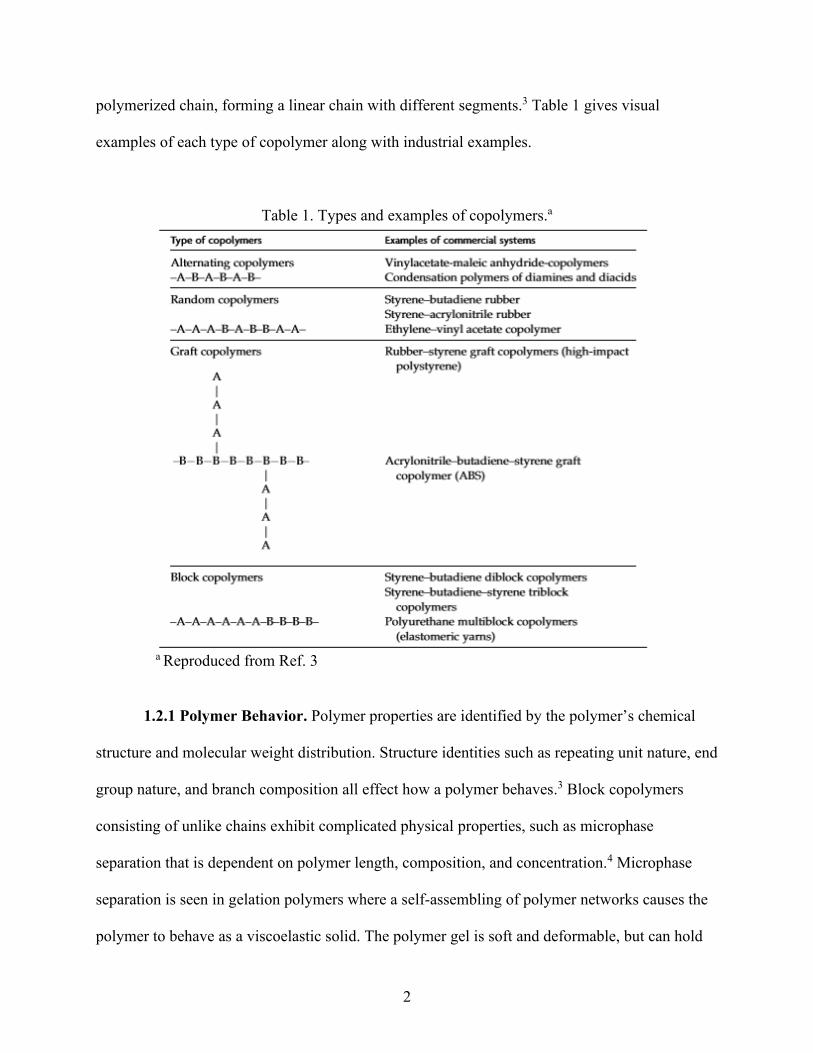
2
polymerized chain forming a linear chain with different segments3 Table 1 gives visual
examples of each type of copolymer along with industrial examples
Table 1 Types and examples of copolymersa
a Reproduced from Ref 3
121 Polymer Behavior Polymer properties are identified by the polymerrsquos chemical
structure and molecular weight distribution Structure identities such as repeating unit nature end
group nature and branch composition all effect how a polymer behaves3 Block copolymers
consisting of unlike chains exhibit complicated physical properties such as microphase
separation that is dependent on polymer length composition and concentration4 Microphase
separation is seen in gelation polymers where a self-assembling of polymer networks causes the
polymer to behave as a viscoelastic solid The polymer gel is soft and deformable but can hold
3
its shape making it of interest in drug delivery science5 The gelling of polymers by phase
separation is dependent on many conditions but crucially temperature giving rise to the terms
thermoresponsivity and thermoreversibility as further discussed in Section 13
Polymers that consist of amphiphilic monomers have the tendency to form micelles in
solution Micelles are colloidal dispersions of these amphiphilic units that self-assemble due to
intermolecular forces between the hydrophobic and hydrophilic regions Typical surfactant
micelles are made up of 50 to 200 monomers and have a spherical diameter of three to six
nanometers Polymeric surfactant molecules have spherical diameters that range from 10 to 100
nm6 Factors controlling polymeric micelle size include molecular weight of the amphiphilic
block copolymer aggregation number proportion of hydrophobic to hydrophilic chains and
quantity of solvent trapped inside the micellar core The driving force behind the self-assembling
of polymers into micelles is noted as hydrophobic forces where the water repelling regions of
the polymer aggregate to each other minimizing the contact between the insoluble block and the
solvent and lowering the free energy of system167 The concentration above which micelles are
formed in solution is called the critical micelle concentration (CMC) When at the CMC or
slightly above loosely aggregated micelles are formed containing solvent within their core At
higher concentrations the residual solvent is excluded from the core thereby compacting the
micellar structure In general polymeric micelles have a lower CMC value than traditional
micelles6 Many studies show how polymeric micelles can be used in the biomedical field as
drug carrier systems27-11
122 Function with Active Pharmaceutical Ingredients Polymeric micelles are
capable of encapsulating insoluble active pharmaceutical ingredients (APIs) within their
hydrophobic core (Figure 1)1 Polymeric micelles help to increase the bioavailability of poorly
4
soluble APIs by stabilizing the drug and keeping it dissolved in solution until it is absorbed in the
gastrointestinal track12 Surfactants are also used to increase the bioavailability of APIs through
topical skin application The stratum corneum contains a tough barrier in which poorly soluble
drugs have trouble penetrating Encapsulating an API within a polymeric micelle allows for the
drug to penetrate the skin as the micelle endures a change in structure due to water evaporation10
Local diseases eg infections or inflammations are commonly treated by topical
delivery of the required medicinal drug to the targeted tissue It is important that the drug
remains at the site of application for an extended time to ensure efficacy and interaction with the
disease Such topical drug formulations require knowledge on rheological properties such as
structure and flow to gain insight into their effects on drug diffusion and to ensure ease of
applicationadministration The rheological behavior of polymeric micelles is of increasing
interest to test the performance of surfactants in pharmaceutical systems9
Figure 1 Structure of a polymeric micelle with APIs stored in its core (reproduced from Ref 8)
13 Thermoresponsivity
Materials that respond to external stimuli are referred to as ldquosmart materialsrdquo Polymers
are the most common smart material because they are comparatively cheap and can respond to
5
pH temperature ionic strength electric and magnetic fields and biochemical processes2
Temperature responsive also referred to as thermoresponsive polymers are particularly versatile
in their applications such as tissue engineering sensing gene delivery and drug delivery2 A
thermoresponsive polymerrsquos ability to change abruptly and reversibly between various physical
states over a range of temperatures gives it elevated interest in the biomedical field13
There are two main types of thermoresponsive polymers in aqueous solutions The first
exhibits a lower critical solution temperature (LCST) in which there is a phase separation upon
heating due to the loss of hydration in the system13 This phase separation leaves the polymer
insoluble at temperatures above the phase boundary where the boundary is dependent on
concentration The concentration at which the phase separation occurs at the lowest temperature
is the LCST14 The other type of thermoresponsive polymer exhibits an upper critical solution
temperature (UCST) where there is phase separation upon cooling which is far less common for
aqueous polymer solutions (Figure 2)13 For example a LCST behaving polymer solution that is
below the phase boundary is clear and homogenous whereas above the transition temperature it
appears cloudy2 This behavior occurs due to the loss of entropically unfavorable hydrophobic
segments at the critical temperature13 Considering the Gibbs equation (Equation 1)
∆119866 = ∆119867 minus 119879∆119878 (1)
where 119866 is Gibbs free energy 119867 is enthalpy 119879 is temperature and 119878 is entropy the driving force
behind phase separation is the entropy of water When temperature increases and the polymer is
not in solution the water is less ordered and has a higher entropy (∆119878)2 This decreases the free
energy of the system (∆119866) making it more favorable2 Polymer solutions that have a UCST are
cloudy below the phase boundary but an increase in temperature to above the transition state
renders them clear and homogenous Phase separation of UCST behaving polymer is
6
enthalpically driven because strongly attractive polymer-polymer interactions are broken by
water when the 119879∆119878 term outweighs these enthalpic attractions (∆119867)13
Figure 2 Temperature vs polymer volume fraction (120601) plots used to illustrate polymer solution
phase diagrams for (a) lower critical solution temperature (LCST) behavior and (b) upper critical
solution temperature (UCST) behavior (reproduced from Ref 2)
When LCST and UCST behaving polymers fall within the two-phase region they de-mix
from aqueous solution where the polymer collapses into a globule and forms a precipitate15 The
temperature at which this transition occurs is referred to as the cloud point and can be witnessed
along the phase boundary
Thermoresponsive polymers may also show properties of gelation where polymeric
micelles self-assemble into lattices at a specified temperature At this transition temperature
referred to as a sol-gel point the aqueous solution aggregates and forms a gel By definition from
IUPAC a gel contains covalently bound polymer networks formed from the crosslinking and
physical aggregation of polymer chains16 The sol-gel transition is characterized by a large
increase in viscosity between the micelle and macrolattice states Figure 3 shows the molecular
7
dispersion-to-micelle-to-macrolattice transition at high and low concentrations where low
polymer concentrated solutions donrsquot form macrolattices4
Figure 3 Schematic representation of block copolymer phase transitions at high and low
concentrations (reproduced from Ref 4)
The resulting swollen macrolattice network can also be thermoreversible in which the
regions of local order are thermally reversible16 In simpler terms a thermoreversible polymer
will convert back to its original phase after being subjected to a temperature that causes a phase
change For example a LCST behaving polymer that clouds above the phase boundary will
regain transparency when cooled to temperatures below the boundary This property is important
in characterizing how a micelle loaded with APIs will behave once injected into the body
14 Soluplusreg
Soluplusreg is a polyvinyl caprolactam-polyvinyl acetate-polyethylene glycol graft
copolymer with a respective unit ration of 573013 It was developed by BASF to increase the
bioavailabilty of poorly soluble drugs by making them available in a dissolved state1718 As
supplied Soluplusreg is a granular substance (Figure 4) with an average molar mass of 118000
8
gmol and a mean grain size of 340 microm18 This tri-block amphiphilic copolymer is essentially
miscible in water and forms polymeric micelles with a detectable CMC of 76 mgL at 230 degC18
Figure 5 displays the structure of Soluplusreg and identifies the hydrophilic and hydrophobic
regions that attract to each other to form polymeric micelles Soluplusreg dissolves readily at
colder temperatures and the solutions exhibit an increase in viscosity as concentration increases
Figure 4 Physical appearance of Soluplusreg (reproduced from Ref 17)
BASF has conducted studies on the solubilization capacity of various APIs when using
Soluplusreg and other well-known surfactants19 As seen in Figure 6 Soluplusreg increased the
saturation solubility of several APIs Soluplusreg was also able to compete with and in some cases
outperform other well-known surfactants BASF has also reported dissolution tests showing a
faster release of a poorly soluble API itraconazole in solutions prepared with Soluplusreg as
compared to solutions with other polymeric matrices (Figure 7) As well they performed
bioavailability screenings that showed considerable improvement in the bioavailability of
itraconazole in solutions prepared with Soluplusreg (Figure 8)19 As suggested in Figures 7 and 8
Soluplusreg works as a polymeric matrix to improve the amount of administered API dosage that
9
reaches the bloodstream overall increasing pharmacokinetic parameters such as drug absorption
and distribution20
Figure 5 Structure of Soluplusreg In the diagram the indices l m and n correspond to the number
of units of polyvinyl caprolactam polyvinyl acetate and polyethylene glycol respectively
(adapted from Ref 17)
Soluplusreg is known for its biocompatibility as documented and marked through
toxicological studies presented by BASF Tested according to OECD (Organization for
Economic Cooperation and Development) guidelines there were no elicit ill effects from acute
toxicity irritation or sensitization The surfactant is not yet listed in the FDArsquos Inactive
Ingredients Database indicating that it has not yet been approved for medicinal use within the
US15 However the United States Germany France Japan and other countries are in clinical
trials with Taiwan and Argentina having already approved Soluplusreg for use in healthcare
products1521
10
Figure 6 Solubilization capacities of various active pharmaceutical ingredients with and without
solubilizing excipients (reproduced from Ref 19)
Figure 7 Dissolution test for the release of itraconazole with various polymeric matrices
(reproduced from Ref 19)
Figure 8 Blood concentration of itraconazole with and without Soluplusreg solution (reproduced
from Ref 19)
11
Solutions of Soluplusreg show an increase in viscosity upon warming referred to as
thermothickening which is a property of potential interest in topical drug applications A
thermothickening solution can flow through an applicatorsyringe but then may harden as it
makes its way into the body15 This makes it possible to mix APIs with a polymer in its liquid
room-temperature state but then witness an in-situ gel deposit at the injection site when the
polymer is at body temperature22 The polymers polyvinyl caprolactam and polyethylene glycol
are known to transition from a hydrophilic to amphiphilic state upon warming around 34 degC to
36 degC which results in the self-assembly of micelles and gelation15 Because Soluplusreg is
comprised of these components it is suspected that a similar mechanism occurs upon heating of
aqueous solutions of Soluplusreg15 Soluplusreg also exhibits a gel-sol transition phase as
temperatures continue to rise23 This unusual physical behavior is seen only in doubly
thermoresponsive polymers that exhibit both LCST and UCST behavior Specifically Soluplusreg
is a LCST lt UCST behaving polymer and forms a gel within a designated temperature range
Copolymers that contain OH-functionality eg polyvinyl acetate polyethylene glycol polyvinyl
butyrate and protonated acrylic acid generally show LCST lt UCST behavior rather than UCST
lt LCST13 As seen in Figure 9 the circular temperature-concentration phase diagram describes
how Soluplusreg transitions from a soluble to insoluble phase and then back to a soluble phase as
a function of increasing temperature13
Soluplusreg forms micelles in aqueous media where the hydrophobic regions polyvinyl
acetate and polyvinyl caprolactam are located in the core of the micelle and the hydrated
polyethylene glycol segment is located in the outer region718 The micellization of Soluplusreg in
water is known to be endothermic and is spontaneous at temperatures above the Krafft point
(critical micelle temperature) due to an entropically-driven Gibbs free energy During
12
micellization solvent is released and entropy increases This gain in entropy exceeds the loss of
entropy by self-assembly of the polymeric micelles leaving the system with a positive entropy
change The micellization process occurs in three steps 1) polymeric micelles are formed in
solution at concentrations and temperatures above the CMC and Krafft point 2) the polyethylene
glycol chains dehydrate at temperatures above the Krafft point but below the phase boundary
and 3) there is an onset of physical change as temperature increases (Figure 10)7 This change
could be a cloud point where precipitation from solution at the LCST phase boundary causes
opacity or the change could be gelling due to self-assembly and aggregation of micelles into an
entangled network at a temperature specified as the sol-gel point A thermoresponsive polymer
may exhibit both physicochemical changes clouding and gelling however based on previous
work in our research group these physical onsets do not show any correlation other than their
dependence on increasing temperatures24 The micellization process is dependent on temperature
polymer concentration and medium composition7
Figure 9 Phase diagram for a LCST lt UCST behaving polymer (reproduced from Ref 14)
13
Figure 10 Micellization mechanism for solutions of Soluplusreg (reproduced from Ref 7)
As Soluplusreg solutions below 300 (ww) proceed through the micellization process
they encounter a series of temperature dependent physical behaviors At temperatures below the
LCST phase boundary Soluplusreg solutions appear clear with unrestricted flow At temperatures
above the boundary the solution clouds before a further increase in temperature causes a sol-gel
transition and restricted flow (Figure 11)22 Soluplusreg solutions above 300 (ww) show
restricted flow at room temperature but remain clear24 This indicates that the solutions have not
crossed the LCST phase boundary into the clouding region but have undergone a sol-gel
transition It is suggested that gelling can occur when polymer concentration is substantially
large7
Figure 11 A 300 (ww) Soluplusreg solution at room temperature (left) cloud point (middle)
and gel point (right) Represented as a top view of the cone-and-plate rheometer sample
compartment that was lowered from its housing and subjected to increasing temperatures
14
15 Dynamic Light Scattering Spectroscopy
An important characteristic of solubility enhancers is their particle size in solution before
and after loading with APIs Polymeric micelle particle size is studied through dynamic light
scattering spectroscopy (DLS) This technique also known as photon correlation spectroscopy or
quasi-elastic light scattering measures the translational diffusion of macromolecules in solution
due to Brownian motion25 Brownian motion refers to the random scattering of particles due to
collisions with solvent molecules Larger molecules have a slower Brownian motion while
smaller particles are bombarded further by surrounding solvent molecules and have more rapid
movement26 The Stokes-Einstein equation is used in dynamic light scattering methods to relate
the diffusion coefficient to particle size27 Equation 2 defines the Stokes-Einstein equation
119889(119867) = 119896119879
3120587120578119863 (2)
where 119889(119867) is hydrodynamic diameter 119896 is Boltzmannrsquos constant 119879 is absolute temperature 120578
is viscosity of solvent and 119863 is the velocity of Brownian motion typically defined as the
translational diffusion coefficient26
151 Effect of Viscosity As seen in Equation 2 particle size measurements by DLS are
dependent on temperature and the viscosity of solvent This dependence is seen in calculations
and in how the sample behaves Particles can behave in Newtonian or non-Newtonian manner
Newtonian fluids refer to samples that have the same viscosity at constant temperature and
pressure regardless of the amount of stress and shear strain27 For example a Newtonian fluid
would move twice as fast if it were subjected to twice as much force28 In a non-Newtonian fluid
the particles are suppressed by a larger viscosity of solution therefore restricted from Brownian
motion Viscosities of greater than three centipoise (cP) are generally considered as non-
15
Newtonian Results from DLS measurements can be significantly affected by inaccurate
viscosity values27
As seen in Figure 12 the analysis of a pigment dispersed in water was altered by using
different viscosities The blue graph was analyzed using a viscosity of 10 cP in the sizing
algorithm and the red graph was recomputed using 20 cP A particle size shift from 700 nm to
350 nm shows just how dependent hydrodynamic diameter measurements are on viscosity27
Particle size is also affected by particle concentration ionic strength of medium surface
structure particle shape and the refractive index of solvent2627
Figure 12 Particle size data for a pigment dispersed in water at two different viscosities 10 cP
(blue) and 20 cP (red) (reproduced from Ref 27)
A Further Look into Rheology Rheology is the study of deformation and flow branching
from the physical sciences which study the mechanics of forces deflections and velocities29
Newton was one of the first philosophers to investigate the quantification of a fluidrsquos viscosity
He originally described viscosity as the lack of ldquoslipperinessrdquo between elements of a fluid as they
are forced to move past each other Rheology has advanced throughout the ages from testing
viscosity by dropping heavy spheres through material and recording time differences to using
advanced and accurate instrumentation30 Rheology is observed in everyday life through liquids
16
and solids such as honey gum eraser toothpaste syrup oil rubber and much more These
materials behave simultaneously in a fluid (viscous) and solid (elastic) way giving rise to the
term viscoelasticity Rheology studies the deformation of viscoelastic materials when subjected
to a shear force that causes the material to flow29
Purpose of Studying Flow and Deformation Flow behavior is studied to pre-emptively
design equipment and practice quality control28 Various industries provide great examples of
using these studies in testing their products Ketchup must flow out of the bottle when shaken or
squeezed Household paint is easily stirred but dries on a wall without dripping Pudding seems
solid at rest but is simply spooned from the cup and ointment must effortlessly squeeze from the
tube with moderate pressure2831 The pressure at which a fluid just begins to flow a fundamental
quality control concern is known as the yield stress28 Yield stress measurements can be
routinely performed by using viscometers and rheometers later discussed in Section 231
Flow and deformation are also studied to characterize a material Viscosity is a ldquowindowrdquo
into other properties of a material that may be harder to measure When analyzing a sample for
its viscosity information is also gained regarding temperature shear rate time pressure and
material composition It is important to know how a product will react when subjected to these
other conditions For example motor oils and greases will have a decrease in viscosity when
subjected to higher temperatures28 As well lubricating oils decrease in viscosity at high
temperatures which cause the oils to flow off the metal parts they protects32 Shear rate or the
rate of deformation can also impact a sample causing a material to change in viscosity during
various times in the production process28 Many materials also undergo changes in viscosity
during a chemical process or while subjected to an outside pressure making rheological
measurements dependent on time and pressure Lastly a materials composition can affect
17
viscosity The state of aggregation between the solid particles and liquid phase in emulsions and
dispersions causes viscosity differences due to clumping and packing shape This is seen in
milk which is emulsified fat globules within water28
Viscosity Shear Stress and Shear Rate Rheology describes the elasticity viscosity and
plasticity of materials The interest is specifically on viscosity and the following parameters that
accompany it shear stress and shear rate28 Viscosity is defined as the measure of the internal
friction of a fluid This implies that one layer of fluid passes another layer without a transfer of
matter called laminar flow (Figure 13) A greater amount of friction between the layers
corresponds to a greater amount of force required for the movement28
Figure 13 Two plates model used to describe the physics of viscosity where 119860 is the area of
fluid 1198811 and 1198812 are the velocities at which the fluid is moving 119889119907 is difference in velocities 119889119909
is the distance between the two fluids and 119865 is the force required to cause movement
(reproduced from Ref 28)
As seen in Figure 13 two parallel flat areas of fluid separated by a designated distance
are moving in the same direction at varied speed From this model Newton implied that the force
needed to maintain the difference in speeds was proportional to the difference of speed through
the liquid This velocity gradient ( 119889119907
119889119909 ) is expressed by Equation 3
119865
119860= 120578
119889119907
119889119909 (3)
18
where 120578 is a given materialrsquos constant known as viscosity28 The velocity gradient describes the
shearing a liquid experiences and is thus known as the shear rate or rate of deformation The
force per unit area ( 119865
119860 ) term represents the shear stress or what is causing the shearing action
Equation 4 defines viscosity using these terms
120578 = 120591
120574 (4)
where 120591 is shear stress and 120574 is shear rate28 Shear stress has a unit of Newtons per square meter
(Nm2) and shear rate is in units of reciprocal seconds (sec-1) Viscosity has a fundamental unit of
ldquopoiserdquo where a material requiring one Nm2 of shear stress to produce a shear rate of one sec-1
has a viscosity of one poise Viscosity measurements are typically written on the centipoise scale
(cP) Measurements may also be seen in mPas (millipascal-seconds) which have a 11 ratio with
cP28 Table 2 gives common viscosities of many household goods
Table 2 Approximate viscosity values of
commonly known materials at 200 degCb
Fluid Viscosity (cP)
Water 1
Milk 3
Olive Oil 80
Glycerin 1000
Honey 10000
Toothpaste 70000
Peanut Butter 250000 b Adapted from Ref 33
Viscosity can also be referred to in terms of 119866lowast the complex shear modulus which is
equivalent to viscosity 120578 The complex shear modulus can be broken down into two
components 119866prime and 119866primeprime the storage and loss moduli respectively The storage modulus 119866prime is
responsible for characterizing the elastic behavior in viscoelastic materials while the loss
19
modulus 119866primeprime describes the viscous behavior Elastic behavior arises when energy is stored
within a material that has been subjected to deformation The internal structures extend and
stretch without causing damage to the material allowing the stored energy to act as a driving
force in returning the material back to its original state Viscous behavior results from internal
friction between a materials molecules and particles when subjected to deformation As friction
builds the material absorbs heat causing a loss of energy The storage modulus represents the
energy stored from deformation while the loss modulus characterizes the energy dissipated by
internal friction Viscoelastic solids have a higher storage modulus than loss (119866prime gt 119866primeprime) due to
their physical-chemical linking whereas viscoelastic liquids have a greater loss modulus than
storage (119866primeprime gt 119866prime) due to the lack of strong interactions between molecules34 Figure 14 describes
the relationship between complex shear modulus and phase-shift (δ) which is the lag time
between the current and resulting sinusoidal oscillation34 The relationship between 119866lowast 119866prime and
119866primeprime is seen in Equation 5 which follows the Pythagorean theorem
|119866lowast| = radic(119866prime)2 + (119866primeprime)2 (5)
Using Equation 5 allows for the determination of 119866lowast or viscosity from 119866prime and 119866primeprime29
Another parameter loss factor reveals the ratio of viscous to elastic behavior and is calculated as
the tangent of the phase-shift angle as seen in Equation 62934
tan 120575 = 119866primeprime
119866prime (6)
When the loss factor is greater than one (tan 120575 gt 1) it signifies the sample is in liquid
ldquosolrdquo state When the loss factor is less than one (tan 120575 lt 1) it signifies a solid ldquogelrdquo state The
ldquosol-gelrdquo transition state of gelation polymers is seen when the loss factor is equivalent to one
(tan 120575 = 1)29
20
Figure 14 Graphical relationship between complex shear modulus 119866lowast storage moduli 119866prime loss
moduli 119866primeprime and the phase-shift angle δ (reproduced from Ref 34)
152 Effect of Refractive Index The refractive index of solution medium plays a crucial
role in light scattering Its dependence is seen in the correlation function of a typical DLS
measurement where the intensity of scattered light is transformed into a size distribution by
using various algorithms For most monodisperse particles in Brownian motion the correlation
function (119866) follows an exponential decay as seen in the Equation 7
119866(120591) = 119860[1 + 119861 exp(minus2Γ120591)] (7)
where 120591 is the correlator time delay 119860 and 119861 are the baseline and intercept of the correlation
function respectively and Γ is further defined in Equation 8
Γ = 1198631199022 (8)
where 119863 is the translational diffusion coefficient Refractive index is seen within the definition of
119902 as follows in Equation 9
119902 = (4120587119899
120582) sin (
120579
2) (9)
where 119899 is refractive index 120582 is the wavelength of the laser and 120579 is the scattering angle26
Refractive index becomes increasingly more important in the correlation function when using a
volume distribution display mode that presents the size distribution as a ratio of volume to mass
Using a volume distribution display mode is practical when the size of particles becomes roughly
21
equivalent to the wavelength of the excitation light and is known as Mie theory2526 Specifically
Mie theory compares the size of particles to the wavelength of light by considering particle shape
and difference in refractive index between particles and the medium they are present in while
utilizing a volume distribution display mode25
16 Objectives
This project investigates how the viscosity and refractive index of aqueous Soluplusreg
solutions affects polymeric micelle size as determined by DLS It is hypothesized that if the
temperature dependence of viscosity for aqueous Soluplusreg solutions is rheologically measured
and the relationship between concentration temperature and viscosity is used in DLS
algorithms then DLS particle size measurements will be more reliable in describing the physical
behavior of Soluplusreg
The goals of this project include
1 Analyze the viscoelastic behavior for aqueous Soluplusreg solutions as a function of
temperature and establish a mathematical relationship between concentration temperature and
viscosity
2 Evaluate the refractive index of Soluplusreg solutions as a function of temperature
3 Compare DLS particle size measurements for aqueous solutions of Soluplusreg using
the viscosity and refractive index of water versus the viscosity and refractive index of actual
solution
22
CHAPTER 2 EXPERIMENTAL
21 Overview
Soluplusreg solutions 10 to 300 (ww) were tested on a cone-and-plate rheometer for
their temperature dependence of viscosity The rheometer was set to external mode and
controlled through a software interface A relationship between viscosity concentration and
temperature was created by fitting a polynomial regression to a 3D plot of these variables The
refractive indices of Soluplusreg solutions were analyzed as a function of temperature and used
along with viscosity data to correct inputs within DLS algorithms for particle size analysis on
Soluplusreg solutions ranging 01 to 100
22 Materials
Soluplusreg was provided to Missouri State Universityrsquos Department of Chemistry by
BASF Corporation (Ludwigshafen Germany)35 Aqueous Soluplusreg solutions were made
ranging from 10 to 300 (ww) for analysis by rheometry Using an analytical balance
(Mettler Toledo AL104) and deionized water a 300 (ww) solution of Soluplusreg was made
and then further diluted to other concentrations by weight The targeted weight of solutions was
150 g This process was repeated twice more to have a total of three sets of Soluplusreg solutions
(further labeled as Sets 1 2 and 3) When making aqueous Soluplusreg solutions the solid powder
is added to the water briefly stirred and then refrigerated around 50 degC until dissolved
For analysis by DLS and refractometry Soluplusreg solutions ranging 01 to 100
(ww) were made using an analytical balance (Mettler Toledo AL104) 18 MΩ (Type I) water
(Barnsted Nanopure II with 4 Mod Organic Free cartridge kit) and sterilized equipment Each
23
solution had a targeted final weight of 600 g and was made as described above However in
these cases the solutions were made individually instead of being diluted from a stock solution
Again three sets of Soluplusreg solutions were made and labeled as Sets 1 2 and 3 It is crucial
that sterilized equipment and highly filtered water is used to make the solutions as DLS is very
sensitive to outside contaminants and dust
23 Temperature Dependence of Viscosity
231 Instrumentation Rheology is quantified through use of viscometers and
rheometers As described in Section 151 these instruments are used to measure viscosity shear
stress torque and shear rate Rheometers allow for the measurement of rheological behaviors on
non-Newtonian fluids and for characterization of flow and deformation36 These rheological
behaviors include specific property measurements of viscoelasticity yield stress and stress
relaxation37 Rheometers are distinguished into two categories shear rheometers (sometimes
referred to as rotational rheometers) and extensional rheometers Shear rheometers control shear
stress by applying the independent variable of torque while extensional rheometers control strain
and measure stress as the dependent variable38 There are three types of shear rheometers which
include capillary rotational cylinder and cone-and-plate setups39 This research exclusively uses
a cone-and-plate rheometer to conduct all viscosity analyses Cone-and-plate rheometers
determine absolute viscosity with precise shear rate and stress information available They
require minimal volume of sample and can control temperature through a jacketed sample cup
This geometry is specifically useful in determining rheological behaviors of non-Newtonian
fluids28 However cone-and-plate rheometers are not useful in testing samples that show a three-
dimensional structure such as gels and solids When particles in agglomerate systems become too
24
large there isnrsquot enough free space between the particles in motion causing a greater amount of
friction on the instrumentrsquos surfaces29
The principle of operation behind a rotational rheometer is to drive a spindle through a
calibrated beryllium copper spring into viscous solution within the plate The drag of the sample
is measured by spring deflection and translated into torque and viscosity measurements31 A
greater amount of internal friction requires a greater amount of force needed to move the spring
through layers of fluid28 As seen in Figure 15 the motor pivot shaft spring and spindle are
housed in the upper half of the rheometer A jacketed cup containing the sample is joined to the
upper half of the instrument where the spindle rotates at the intersection of these parts The gap
between the cone and plate is crucial for accurate viscosity measurement It is determined by
locating the ldquohit pointrdquo and then backing off the spindle by one scale division (as designated on
the instrument) The hit point is where the spindle first comes in contact with the plate causing
the torque to change from 00 to 10 or greater31 The cone angle is also of importance as it
keeps constant torque at all distances from the center of rotation40
At a given viscosity the degree of resistance on the spring is proportional to the spindlersquos
size geometry and speed (Figure 16)28 Choosing an optimal match of spindle diameter and
rotational rate is commonly done by trial and error however it is known that viscosity range is
inversely proportional to both of these parameters Therefore samples with a higher viscosity
should be performed with a smaller spindle andor slower speed Measurements are
recommended to be made within a torque range of 100 to 10031
25
Figure 15 Schematics of a cone-and-plate rheometer (reproduced from Ref 31)
Figure 16 Diagram of the inner workings of the cone and plate where ω is the rotational velocity
r is the cone radius and ϴ is the cone angle (adapted from Ref 28)
The rheometer used in this research was a DV-III Ultra programmable rheometer model
RVDV-III from AMETEK Brookfield (Middleboro MA USA) This cone-and-plate rheometer
was provided to Missouri State University Department of Chemistry by Tolmar Inc (Fort
Collins CO USA) Calibration was performed by Brookfield in July 2019 to ensure proper
26
torque readings and drive shaft function Spindles used for measurement included the CP40 and
CP52 (Table 3 Figure 17) allowing for a total viscosity range of 131 cP to 9922000 cP
Table 3 Cone spindle dimensions and shear ratesc
Cone Spindle Angle
(degrees)
Radius
(cm)
Sample
Size (mL)
Shear Rate
(sec-1)
Viscosity Range
(cP)
CP-40 CPA-40Z 08 24 05 75N 131 ndash 327000
CP-52 CPA-52Z 30 12 02 20N 3969 ndash 9922000
c Adapted from Ref 28
N = RPM
Figure 17 Top view of spindles CP40 (left) and CP52 (right)
The rheometer was controlled through Brookfieldrsquos Rheocalc software (Ver 33
Brookfield Engineering Laboratories Inc) which allows for the programming of conditions and
graphical views of viscosity as a function of temperature In order to obtain temperature
measurements through Rheocalc a probe from Brookfield was adjoined to the instrument The
only appropriate attaching probe was the DVP-94Y steel temperature probe that is used in vane
spindle rheometer set ups The cone-and-plate set up required a temperature probe with a flexible
tip so that the measurement could be taken underneath of the metal sample cup To account for
this problem the steel DVP-94Y probe was purchased along with a 100 ohm 4-wire resistance
27
temperature detector (Omega part RTD-3-F3105-36-G) The probes were spliced and
connected so that the DVP-94Y steel probe connected into the rheometer but the flexible end of
the 4-wire resistance temperature detector attached to the sample cup This successfully allowed
for the transmission of temperature from the instrument into the software The temperature of
samples was controlled using a Fisher Scientific Isotemp Refrigerated Circulator (Model 910)
that was connected to the input and output ports of the instrumentrsquos sample cup (see Figure 15)
Calibration standards were purchased from Brookfield to confirm the accuracy and
precision of the instrument Two 100 PAO (polyalphaolefin) oil viscosity standards (3524 cP
and 3439 cP) were tested and showed accuracy according to the specifications defined by
Brookfield These specifications and calibration results can be seen in Section 31
232 Methods Brookfield calibration standards and Soluplusreg samples 10 20 50
100 150 175 200 225 250 and 300 (ww) were evaluated through use of the
Brookfield DV-III Ultra programmable rheometer and the software Rheocalc for their
temperature dependence of viscosity Each samplestandard was evaluated from 50 degC to about
40 degC at a heating rate of 01 degCsec A sample volume of 05 mL was placed into the cup of the
rheometer and probed with the specified spindle and shear rate (Table 4) All programing
parameters were set in Rheocalc and the experimental set-up was as shown in Figure 18 Data
were collected at a rate of one point per second while the total collection time was set to one
hour The resulting data were exported to Microsoft Excel (Ver 2002) for plotting and further
analysis The process was run in triplicate for the purpose of determining and reporting
uncertainties
28
Table 4 Experimental conditions for each samplestandard
run on the rheometer
Soluplusreg () Spindle RPM
3524 cP Std CP40 200
3439 cP Std CP52 100
10 CP40 250
20 CP40 250
50 CP40 250
100 CP40 750
150 CP40 200
175 CP52 250
200 CP52 250
225 CP52 100
250 CP52 150
300 CP52 100
Figure 18 Set-up used for viscosity data collection on a Brookfield rheometer A refrigerated
circulator (1) was connected to the rheometerrsquos sample cup ports (2) for temperature control A
RTD probe (3) attached to the cup was used to measure temperature where a Styrofoam cap (4)
was used to insulate the sample cup The rheometer (5) was externally connected to a laptop (6)
with the software Rheocalc
24 Refractive Index Analysis
241 Instrumentation Refractive index was measured using a 2WAJ monocular Abbe-
type refractometer (Figure 19) that was set up to allow for temperature control over a range of
29
00 degC to 700 degC The instrument has an index range of 13 to 17 with an accuracy of plusmn 00002
Water and ethanol were used as calibration standards (119899 = 13330 and 13611 at 200 degC
respectively) to test the accuracy of the instrument The results of all refractive index
measurements are presented in Section 32
Figure 19 Set-up used for refractive index data collection on an Abbe refractometer
242 Methods Water ethanol and Soluplusreg samples (01 05 10 20 50 and 100)
were evaluated using the 2WAJ Abbe digital refractometer for their refractive index following
the temperatures defined in Table 5 For each sample the refrigerated circulator was first set to
the appropriate temperature then a few drops of sample were placed between the measuring
prisms and lastly the dispersion correction and adjustment knobs were fine-tuned to where the
shadow aligned with the crosshairs giving a refractive index reading (Figure 20) To evaluate the
aqueous Soluplusreg samples from 110 degC to 350 degC the circulator was cooled to the starting
30
temperature and slowly ramped to the final temperature where refractive index readings were
taken every 10 degC The 01 Soluplusreg sample was evaluated in triplicate for the purpose of
determining and reporting uncertainty
Table 5 Temperatures used in the evaluation of
refractive index for various standards and samples
Soluplusreg () Temperature (degC)
Water (Std) 200
Ethanol (Std) 200
01 110 - 350
05 110 - 350
10 110 - 350
20 110 - 350
50 110 - 350
100 110 - 350
Figure 20 Shadow and scale within an Abbe-type refractometer A samplersquos refractive index
(bottom) is defined as the position where the shadow aligns with the crosshairs (top) (reproduced
from Ref 41)
25 Particle Size Determination by Dynamic Light Scattering
251 Instrumentation The velocity of translational diffusion due to Brownian motion is
measured in DLS by using a monochromatic beam of light which causes the scattering of light
31
upon interaction with molecules When the incident light encounters a molecule it is scattered in
all directions based on the size and shape of particle The scattered light will either result in
mutually destructive phases canceling out or in constructive phases producing a detectable
signal25 A digital autocorrelator then correlates intensity fluctuations of scattered light to time
This determines the rate at which intensity fluctuates which is related to the diffusion of
molecules In dynamic light scattering the intensity correlation function is measured and
expressed as hydrodynamic diameter data2526 Figure 21 gives a representative scheme of the
working parts in a DLS instrument
Figure 21 Schematic representation of the Zetasizer Nano series DLS instrument including a
laser (1) sample cell (2) detector (3) attenuator (4) correlator (5) and computer source (6)
(adapted from Ref 26)
32
There are 6 components to a DLS system As labeled in Figure 21 the first component is
a laser (1) that provides a light source to illuminate the sample cell (2) Next a detector (3) is
either placed at 90deg or 173deg to collect the scattered light If too much light is reaching the
detector the attenuator (4) will reduce the intensity of the light source Conversely if not enough
light is being detected the attenuator will allow more light to reach the sample Once the detector
senses the scattered light intensity it sends the data to the correlator (5) which translates the rate
of light intensity fluctuation Finally a computer (6) analyzes the data through software and
derives size information26
There are many advantages to using DLS as a particle size measurement technique These
include having a wide range of sample temperature and concentration parameters and being a
non-invasive low sample volume requirement technique Some limitations to DLS include low
resolution tedious cleaning and filtering procedures time-consuming optimization of
parameters restriction to transparent samples and most importantly for this research the
sensitivity to temperature solvent viscosity and refractive index25
Research was conducted using a Brookhaven (Holtsville NY USA) NanoBrook Omni
particle size and zeta potential analyzer (Figure 22) This instrument utilized dynamic light
scattering techniques with a 40 mW 640 nm red laser and collection angles of 15deg 90deg and 173deg
The measurement range is 03 nm to 10 microm with temperature control from -50 degC to 110 degC
Data collection was accomplished by using Brookhaven Instrumentrsquos Particle Solutions software
(v3606376) which allowed for the programming of experimental conditions and for data
viewingmanipulation
33
NIST (Gaithersburg MD USA) latex calibration standards were used to ensure accurate
performance of the DLS Two standards 40 nm and 300 nm were tested and showed accurate
results according to the manufacturerrsquos specifications (see Section 32)42
Figure 22 Set-up used for particle size data collection on a NanoBrook Omni
252 Methods NIST latex calibration standards and Soluplusreg samples 01 05 10
20 50 and 100 (ww) were evaluated for their hydrodynamic effective diameter The
calibration standards were evaluated at 250 degC and the Soluplusreg samples were evaluated for
their temperature dependence from 150 degC to 320 degC Each sample was analyzed with the
standard operating procedures shown in Table 6 where the average effective diameter of three
120-s measurements is obtained The process was run in triplicate for the purpose of determining
and reporting uncertainties where the average of three 120-s measurements was considered a
single run
Before measurement each sample was filtered using a Sartorius Ministart NML Plus
Syringe Filter with a 07microm glass filter to remove any large aggregates in solution The filter
34
was primed twice with sample solution using the filterings to rinse the cuvette and the sample
was filtered three times A dust rejection algorithm was also used to remove data resulting from
dust and large aggregates in sample The appropriate dust rejection range is selected based off
expected particle size and for multimodal distribution is based off the largest population of
particles in sample43 The samples were first evaluated using the viscosity and refractive index of
water then recomputed to the experimentally determined viscosity and refractive index of
Soluplusreg samples
Table 6 Standard operating procedures for temperature dependent particle size analysis
Parameter Value
Starting Temperature 150 degC
Final Temperature 320 degC
Temperature Increment 10 degC
Set Duration 120 s
Equilibration Time 300 s
Total Measurements 3
Time Between Measurements 00 s
Dust Rejection 50 nm to 250 nm
Fluid Water
Viscosity 0890 cP
Refractive Index 1331
Measurement Angle 90deg
35
CHAPTER 3 RESULTS AND DISCUSSION
31 Temperature Dependent Viscoelastic Behavior of Soluplusreg Solutions
Calibration standards were analyzed by the rheometer to ensure the instrumentrsquos
accuracy The specification on viscosity accuracy is plusmn 10 of full scale range at a specified
spindle and speed The Brookfield viscosity standard fluids are also accurate to plusmn 10 of their
stated value Total allowed error was calculated by summing the deviations from the instrument
and fluid as portrayed by Brookfield (Table 7)31 Figure 23 shows each standard as a function of
temperature and the experimental viscosity values at 250 degC
Table 7 Total allowed error for each viscosity standard fluid at 250 degC
Standard
(cP)
Allowed Error
(cP)
Experimental
Viscosity (cP)
3524 plusmn 1987 35027
3439 plusmn 13269 332883
Figure 23 Brookfield viscosity standard fluids as a function of temperature The solid black
points represent the standardrsquos stated viscosity shown with total allowed error
0
1000
2000
3000
4000
5000
6000
7000
8000
10 15 20 25 30 35 40 45
Vis
cosi
ty (
cP)
Temperature (degC)
36
As shown in Figure 23 at 250 degC the 3524 cP and 3439 cP standards read 35027 cP
and 332883 cP respectively Both values were within their allowed deviance from the stated
value in Table 7 showing accuracy from the rheometer
Each concentration of Soluplusreg samples ranging 10 to 300 (ww) were analyzed
three times (Sets 12 and 3) by the rheometer for their temperature dependence of viscosity (see
Section 232) Plots of Viscosity vs Temperature are shown in Figure 24 For each concentration
a standard deviation was calculated at every 20 degC and plotted on the ldquomost representativerdquo run
(middle of the three traces) Averaging the sets was not plausible due to varying temperature
rates for each run
The most representative run for each concentration is shown in Figure 25 where each
sample is on the same x-axis to better see trends and relationships There is a general trend in
which viscosity decreases to a minimum before rapidly increasing to a maximum As signified by
the solid black tie-line in Figure 25 traces for concentrations above 100 exhibit a slight rise in
viscosity at low temperatures prior to the decrease toward the minimum This rise is
concentration dependent and can be seen shifting to higher temperatures as concentration
increases (1198791198721) Designated by the dashed black line in Figure 25 the steep growth in viscosity
to the maximum is essentially concentration independent and occurs around 360 degC (1198791198722) The
minimum prior to this sharp rise is also essentially concentration independent and occurs around
270 degC (119879119898119894119899) The temperatures corresponding to these features are listed in Table 8
37
0
2000
4000
6000
8000
0 10 20 30 40 50
Vis
cosi
ty (
cP)
Temperature (degC)
Set 1 Set 2 Set 3
0
20000
40000
60000
80000
100000
0 10 20 30 40 50Temperature (degC)
0
50
100
150
200
250
Vis
cosi
ty (
cP)
0
50
100
150
Vis
cosi
ty (
cP)
00
20
40
60
80
Vis
cosi
ty (
cP)
00
10
20
30V
isco
sity
(cP
)
0
200
400
600
800
0
50
100
150
0
5
10
15
20
00
10
20
30
40
Figure 24 Effect of temperature on viscosity for each aqueous Soluplusreg sample
10 20
50 100
225 200
175 150
250 300
38
Figure 25 Viscosity of Soluplusreg samples on the same temperature scale
39
Table 8 Extrema temperatures observed in η-T plots of Soluplusreg solutionsdagger
Concentration
()
1198791198721
(degC) 119879119898119894119899
(degC)
1198791198722
(degC)
10 - - -
20 - 3049 plusmn 043 3498 plusmn 023
50 - 2928 plusmn 041 3570 plusmn 033
100 - 2810 plusmn 007 3586 plusmn 009
150 1054 plusmn 036 2784 plusmn 045 3604 plusmn 017
175 1072 plusmn 026 2796 plusmn 028 3595 plusmn 033
200 1243 plusmn 015 2811 plusmn 003 3587 plusmn 006
225 1475 plusmn 026 2758 plusmn 018 3593 plusmn 013
250 1738 plusmn 018 2699 plusmn 009 3611 plusmn 015
300 2271 plusmn 038 2822 plusmn 077 3618 plusmn 021
dagger Uncertainties were determined by averaging the extrema temperature values from Set 12
and 3 and taking the standard deviation
The sol-gel transition of a thermoresponsive polymer is characterized by an increase in
viscosity between the micelle and macrolattice states As seen in the temperature-dependent plots
of viscosity for Soluplusreg solutions the increase in viscosity takes place from 270 degC to 360 degC
This sharp increase in viscosity is also seen in literature (Figures 26 and 27) from plots of
complex shear viscosity versus temperature Figure 26 describes the minimum viscosity as an
onset of chemical reaction where micelles begin to self-assemble and form superstructures
indicating the beginning of gel formation18 Our aqueous Soluplusreg solutions of varying
concentration show this onset of chemical reaction around 270 degC (Figures 24 and 25) As the
gelling process occurs viscosity rapidly increases to a sol-gel point The sol-gel transition is
typically defined as the crossing point between 119866prime and 119866primeprime (Figures 26 and 27)182944 Due to our
use of a cone-and-plate rheometer which is unable to measure 119866prime and 119866primeprime separately precise sol-
gel transitions for our Soluplusreg solutions were indeterminable However as seen in Figure 27
the sol-gel transition occurs within the large increase in viscosity We hypothesize that the
Soluplusreg sol-gel transition is occurring at a temperature that falls between the average minimum
40
and average maximum 270 degC to 360 degC To provide a more precise determination of the sol-
gel point would require the use of an oscillating rheometer At 360 degC the viscosity of all
concentrations reaches its maximum and begins to greatly decrease At this point it is
hypothesized that the solution has completely gelled and has ldquobrokenrdquo inside the rheometer
whereby the cone spindle is no longer able to move through solution When the solution is at its
gel-point it adheres to the plate in a ldquosolid mannerrdquo (Figure 28) causing the spindle to glide
against the plate rather than push through solution with resulting force
Figure 26 Temperature dependent functions of 119866prime and 119866primeprime for a gelling material (reproduced
from Ref 18)
Figure 27 Complex viscosity 119866prime and 119866primeprime as a function of temperature for a curing epoxy
(reproduced from Ref 44)
41
Figure 28 A gelled 200 (ww) Soluplusreg solution on the plate of a cone-and-plate rheometer
The star-like shape is caused by the pulling away of the CP52 spindle when the solution is
gelled The remaining solution seen circulating around the star-like shape is where the spindle
didnrsquot come in contact the plate due to its small diameter
The concentration-dependent rise in viscosity exhibited at lower temperatures for
concentrations above 100 (follow the solid black line in Figure 25) is hypothesized to be a
physical property of thermoresponsive polymers that has not been described previously We
speculate that it is related to the Krafft point of Soluplusreg solutions The Krafft point is the
temperature at which the solubility limit of a surfactant is equivalent to the CMC45 Therefore
below the Krafft temperature the surfactant is in a crystalline state and micelles do not form The
visual effect of going below the Krafft temperature is similar to that of clouding where the
surfactant is in a precipitated state and shows opacity45 To be described further as
thermoresponsive polymer solutions cloud they show an increase in viscosity Therefore when
the polymer solution is below the Krafft point and in a precipitated state it could be speculated
that viscosity would increase as temperature rises to the Krafft point This is observed in Figure
25 for Soluplusreg solutions above 100 where the speculated Krafft point would be near the
maxima ranging from 110 degC to 220 degC (1198791198721 in Table 8) As temperature further increases past
these maxima it is speculated that micelles are forming The following decrease in viscosity
could be due to the switch from having crystals in solution to micelles or that in general the
42
viscosity of Newtonian fluids decreases as temperature increases At concentrations below
100 it is speculated that the polymer fraction wasnrsquot large enough to witness this slight
increase in viscosity or temperatures didnrsquot reach cold enough
Previous work conducted by our research group reported that aqueous Soluplusreg
solutions physically gel at temperatures from 300 degC to 400 degC depending on concentration
where more concentrated solutions gel at lower temperatures (Figure 29)23 This research was
conducted using a 90deg tilt test and observing at which temperatures the samples stopped flowing
The data obtained by a 90deg tilt test roughly matches the rheologically implied temperature range
at which the sol-gel transition occurs 270 degC to 360 degC Differences between these sol-gel
transition temperature ranges could be from the differences in the experimental processes where
rheology is a more precise way of observing viscoelastic behavior Figure 29 also reveals that
aqueous Soluplusreg solutions below 100 (ww) do not exhibit a gel phase at any temperature It
is hypothesized that the polymer solutions are not at high enough concentrations for the micelles
to interact and form macrolattice structures Data acquired from the rheometer is at least
somewhat consistent with this observation as seen in the traces from samples under 100
(ww) where the viscosity behavior exhibits small to negligible features that we attribute to the
gelation process (Figure 25) We speculate that the small features observed in the 20 and 50
samples correspond to a pre-gelation condition that does not lead to a complete gelling as
measured by the 90 deg tilt test
43
Figure 29 Sol-gel and gel-sol transitions for Soluplus samples as a function of temperature
Speculated phase boundaries (solid lines) have been added to emphasize observed trends
(adapted from Ref 23)
Previous work conducted in our research group also described the cloud-point transitions
of Soluplusreg solutions The cloud point is described as the transition from soluble to insoluble
phases across the LCST phase boundary and has been observed for aqueous Soluplusreg solutions
to be in the range of 270 degC to 310 degC (Figure 30)46 The temperature range of cloud transition
from previous research lies within the sharp increase of viscosity as did the sol-gel transition
Although these two phase transitions clouding and gelling occur at the same temperature range
they are independent of each other Figures 29 and 30 illustrate the differences in gelling and
clouding phase behaviors where the gel point of aqueous Soluplusreg solutions decreases as a
function of increasing concentration but the cloud point increases as a function of increasing
concentration As previously recognized Soluplusreg solutions under 300 first experience a
cloud transition before physically gelling as a function of increasing temperature Therefore it is
hypothesized that for aqueous Soluplusreg solutions below 300 the cloud transition occurs
within the temperature range of the sharp viscosity increase (270 degC to 360 degC) but prior to the
gel point
44
Figure 30 Cloud points for aqueous Soluplusreg solutions as a function of temperature
(reproduced from Ref 46)
Data from Figure 25 was transformed into a logViscosity vs Temperature plot to scale all
traces onto the same x and y axes (Figure 31) The software Matlab (Matlab and Simulink
R2019b MathWorks) was utilized to create a 3-dimensional scatter plot of temperature (x)
concentration (y) and viscosity (z) A polynomial model was used to create a least-squares fit of
the plotted data where the best fit resulted from a 5th-order polynomial in terms of x and y called
ldquoPoly55rdquo As seen in Figure 32 the Poly55 function fits well to low temperatures and low
concentrations however as viscosity rapidly increases the function falls far from experimental
data It was decided that because DLS focuses primarily on concentrations below 150 and
temperatures below 320 degC the least-squares fitting could be confined to only this range of data
As the concentration of Soluplusreg solutions approaches 00 and the viscosity approach that of
pure water the viscosity value will decrease to below the measuring capabilities of our
rheometer Therefore literature values for the viscosity of water47 were used to complete the
concentration range of 00 - 150 Figure 33 shows a Poly54 model (5th order in x and 4th
order in y) that matches closely to the shortened range of data The Poly55 model was robustly
weighted using ldquoBisquarerdquo where the weight given to each data point is determined by how far
45
the point is from the fitted line This allows for the fit to be based on the bulk data minimizing
any outlier effects48 The Poly54 model didnrsquot use robust fitting on top of the polynomial fit
Figure 31 Log-linear plot of viscosity vs temperature of aqueous Soluplusreg solutions at
different concentrations
Figure 32 Full range of experimental data modeled with a Poly55-Bisquare fit
-1
0
1
2
3
4
5
6
0 10 20 30 40 50
Log V
isco
sity
(cP
)
Temperature (degC)
10 20 50 100 150175 200 225 250 300
46
Figure 33 Short range of experimental data modeled with a Poly54 fit
From the Poly54 modeled fit a polynomial function was created so that the viscosity of
Soluplusreg samples could be determined for any temperature ranging 50 degC to 320 degC and
concentration ranging 00 to 150 The full Poly54 fit function is shown below
log(120578) = minus 01652 + 01448(119879) + 0282(120588) minus 002019(1198792) minus 002223(119879)(120588) (10)
minus 004058(1205882) + 0001153(1198793) + 0001691(1198792)(120588) + 000144(119879)(1205882)
+000414(1205883) minus 30211990910minus5(1198794) minus 700811990910minus5(1198793)(120588)
minus 320411990910minus5(1198792)(1205882) minus 798911990910minus5(119879)(1199013) minus 00001442(1205884)
+ 297611990910minus7(1198795) + 104311990910minus6(1198794)(120588) + 506111990910minus7(1198793)(1205882)
minus31911990910minus7(1198792)(1205883) + 334411990910minus6(119879)(1205884)
where 120578 is viscosity 119879 is temperature in Celsius and 120588 is the relative mass concentration (ww)
Equation 10 shows accuracy to experimental viscosity data within a 30 difference around 95
of the time where the other 5 is within a 100 difference (occurring primarily at low
concentrations and low temperatures or high concentrations and high temperatures)
47
32 Temperature Dependent Refractive Index of Soluplusreg Solutions
Because particle size analysis by dynamic light scattering depends on viscosity and
refractive index these parameters were evaluated for on Soluplusreg solutions to ensure accurate
hydrodynamic effective diameter measurement The temperature dependence of viscosity for
Soluplusreg solutions is described in Section 31 and the following gives the refractive index
behavior of aqueous Soluplusreg solutions as a function of temperature
Water and ethanol were evaluated at 200 degC by the 2WAJ Abbe refractometer to check
the instrumentrsquos accuracy The refractometer has a specified accuracy of plusmn 00002 and the
experimental results can be seen in Table 9 compared to literature values The refractive index of
ethanol is within the allowed deviation of its literature value but the value of water lies 00006
away from its literature value Since the effect of refractive index on particle size analysis is
relatively weak (see Section 33) it was concluded that this deviation can be tolerated
Furthermore the NanoBrook Omni instrument considers refractive index to only the thousands
place so the observed deviation is within the natural precision of the correction
Table 9 Experimental and literature refractive index values
for water and ethanol at 200 degC
Refractive Index (119899) at 200 degC
Standard Experimental Literature
Water 13324 13330d
Ethanol 13612 13611e d from Ref 49 e from Ref 50
Each concentration of Soluplusreg solution ranging 01 to 100 (ww) were evaluated
for their refractive index from 110 degC to 350 degC as described in Section 242 These data can be
48
seen in Figure 34 where the 01 trace included representative standard deviations as
determined from repetitive runs As shown in the figure refractive index increases as the
concentration of Soluplusreg increases As well the refractive index decreases slowly as
temperature increases for all concentrations This trend replicates the refractive index behavior of
pure water49
Figure 34 Effect of temperature on refractive index for Soluplusreg samples
33 Particle Size Analysis of Soluplusreg Solutions
Calibration standards were evaluated by the NanoBrook Omni particle size analyzer to
ensure the instrumentrsquos accuracy NIST specifies that their latex calibration standards do not
come with a passfail criterion due to underlying sizing methodology that is customer
dependent51 NIST recommends establishing an in-house criterion to test instrument
performance which has been adopted as plusmn 400 nm in the chemistry department at Missouri
13300
13350
13400
13450
13500
13550
5 10 15 20 25 30 35 40
Ref
ract
ive
Index
Temperature (degC)
01 05 10 20 50 100
49
State University52 The experimental hydrodynamic effective diameters of the 429 nm and 288
nm standards can be seen in Table 10 where it is shown that our measurements pass in-house
criteria displaying good instrument performance The polydispersity index (PDI) is also
included in Table 10 which signifies the relative size-range of particles The PDI can range from
0000 to 1000 where a lower value corresponds to a more monodisperse sample
Table 10 Effective diameters of NIST latex calibration standards at 250 degC
Standard (nm) Experimental
Eff Diam (nm)
Experimental
Polydispersity
429 4592 0106
288 2858 0040
Soluplusreg solutions 01 05 10 20 50 and 100 (ww) were each
evaluated three times (Sets 1 2 and 3) for their hydrodynamic effective diameters as a function
of temperature using the NanoBrook Omni particle size analyzer following the protocol in
Section 252 Figure 35 displays the average hydrodynamic effective diameters along with
uncertainties for each sample as a function of temperature using ldquouncorrectedrdquo viscosity and
refractive index data ldquoUncorrectedrdquo refers to using the pre-programmed viscosity and refractive
index data for a pure water solvent As observed the temperature dependence generally shows
the diameter to decrease with increasing temperature and then sharply rise as the cloud- or gel-
point is reached Additionally the effective diameter appears to be directly proportional to
Soluplusreg concentration in that for any given temperature the largest particle diameter is
obtained for the highest Soluplusreg concentration The sharp rise in the temperature dependence
of the hydrodynamic effective diameter appears to correlate with the solutionrsquos clouding or
gelling point where micelles are aggregating and produce larger particles The 01 and 05
50
Soluplusreg samples donrsquot show this sharp rise in diameter suggesting that there is no onset of
physical change However according to Figure 30 these concentrations do show clouding by
spectroscopy whereas they do not show evidence gelling (Figure 29)
Figure 35 Effect of temperature on effective diameter for Soluplusreg solutions using uncorrected
values of viscosity and refractive index
The traces in Figure 35 were recomputed to correct for the viscosity and refractive index
behavior of Soluplusreg solutions In the following discussion ldquocorrectedrdquo refers to using the
viscosity and refractive index data of Soluplusreg solutions reported in Sections 31 and 32 As
seen in Figure 36 the corrected effective diameters are observed to be inversely proportional to
concentration Figure 37 depicts this trend for one specific temperature (250 degC) by comparing
hydrodynamic diameters obtained from ldquouncorrectedrdquo vs ldquocorrectedrdquo analyses Table 11 gives
the numerical values shown in Figure 37 along with PDI values It is notable that the PDI shows
no dependence on viscosity or refractive index It is reported in literature that the cause for the
decreasing diameter as concentration increases is related to micellar core size At larger
000
10000
20000
30000
40000
50000
60000
70000
11 16 21 26 31 36
Hydro
dyn
amic
Eff
ecti
ve
Dia
met
er
(nm
)
Temperature (degC)
01 05 10 20 50 100
51
concentrations micelles form with less solvent in the core causing the micelle to compact and
reduce in size6
Figure 36 Effect of temperature on effective diameter for Soluplusreg solutions using corrected
values of viscosity and refractive index
Figure 37 Uncorrected vs corrected diameter at 250 degC for Soluplusreg in aqueous solution
000
2000
4000
6000
8000
10000
12000
11 16 21 26 31 36
Hydro
dyn
amic
Eff
ecti
ve
Dia
met
er
(nm
)
Temperature (degC)
01 05 10 20 50 100
000
2000
4000
6000
8000
10000
12000
01 05 10 20 50 100Hydro
dyn
amic
Eff
ecti
ve
Dia
met
er
(nm
)
Concentration ()
Uncorrected Corrected
52
Table 11 Uncorrected vs corrected effective diameters at 250 degC for Soluplusreg in
aqueous solution
Hydrodynamic Effective Diameter (nm)
Concentration
() Uncorrected Corrected Polydispersity
01 6615 plusmn 079 6313 plusmn 076 0030
05 6078 plusmn 008 5359 plusmn 006 0038
10 6648 plusmn 037 5539 plusmn 031 0042
20 6988 plusmn 026 4981 plusmn 019 0059
50 7634 plusmn 054 4114 plusmn 029 0103
100 10585 plusmn 128 2498 plusmn 030 0210
Also depicted in Figure 36 the ldquocorrectedrdquo diameter values remain more consistent
through rises in temperature prior to sharply increasing As well the sharp rise in effective
diameter remains around the same temperature The 01 and 05 Soluplusreg samples were
recomputed using extrapolated viscosities as determined by Equation 10 The Brookfield RVDV-
III Ultra rheometer was unable to test these low concentrated samples because their viscosities
fall below the instrumental limit It is suspected that because theses viscosity values were
extrapolated from outside the experimentally determined range the resulting corrected diameters
may contain an inherently higher level of uncertainty In Figure 36 the 01 and 05 traces
still show no evidence for physical phase change by DLS (ie a sharp increase in diameter at
higher temperatures)
Salah et al report the hydrodynamic diameter of Soluplusreg in a 01 (ww) aqueous
solution at 200 degC to be 6486 plusmn 158 nm (Figure 38)15 The experimentally determined
ldquocorrectedrdquo effective diameter from this thesis for an equivalent sample under the same
conditions is 6576 plusmn 038 nm (Figure 36) consistent with the previously reported value
53
Figure 38 Size distribution for a 01 Soluplusreg solution at 200 degC (reproduced from Ref 15)
The influence of including accurate viscosity and refractive index data in particle size
algorithms is considerable For example the hydrodynamic effective diameter shifts from 14348
nm to 2535 nm for the 100 Soluplusreg solution at 200 degC upon correcting for these effects
(Table 12) This substantial shift (823 decrease) on diameter is due primarily to viscosity
effects Refractive index plays a less significant role in particle size analysis by DLS As shown
in Table 13 the resulting hydrodynamic diameter in a 100 Soluplusreg solution is shifted only
150 by changing refractive index by 0010 indicating that the correction due to refractive
index variation is significantly less important than that due to viscosity
Table 12 Difference in effective diameter when using uncorrected and corrected viscosity and
refractive index data for a 100 Soluplusreg solution at 200 degC
SOP Uncorrected Corrected
Liquid Water Unspecified
Viscosity (cP) 1002 5842
Refractive Index 1331 1351
Effective Diameter (nm) 14348 2535
54
Table 13 Effective diameter dependence on refractive index for
a 100 Soluplusreg solution at 200 degC and 5842 cP
Refractive Index Effective Diameter (nm)
1341 2498
1351 2535
1361 2573
As discussed previously the sharp increase in effective diameter that is observed for the
10 20 50 and 100 (ww) Soluplusreg solutions is related to the cloud- or gel-point
Figure 39 overlays the viscosity and effective diameter of a 50 Soluplusreg solution on the same
temperature axis As observed effective diameter remains relatively constant as viscosity is
decreasing to its minimum across the temperature range As viscosity starts to increase
indicating an onset of change (clouding gelling or both) the effective diameter also rises The
increase in particle size is triggered by the reduced solubility of solution as it crosses the LCST
phase boundary This causes the micelles to aggregate and rearrange resulting in larger and more
polydisperse particle sizes15
Figure 39 Viscosity and corrected diameter vs temperature for a 50 Soluplusreg solution
10
14
18
22
27
31
35
2500
3500
4500
5500
6500
7500
8500
15 17 19 21 23 25 27 29 31
Vis
cosi
ty (
cP)
Hydro
dyn
amic
Eff
D
iam
(n
m)
Temperature (degC)
Corrected Eff Diam Viscosity
55
CHAPTER 4 CONCLUSIONS AND FUTURE DIRECTIONS
The phase behavior of aqueous solutions of Soluplusreg a polyvinyl caprolactam-polyvinyl
acetate-polyethylene glycol graft copolymer were studied throughout this research
Rheologically determining the effect of temperature on viscosity allowed for insight behind the
viscoelastic properties of thermothickening polymer solutions It was observed that as
temperature rises the viscosities of Soluplusreg solutions decrease until reaching a minimum
around 280 degC where viscosity then sharply increases This trend has been observed by other
researchers for gelling polymers where a large increase in viscosity signifies the agglomeration
of polymeric micelles into macrolattices The sharp increase in viscosity for aqueous Soluplusreg
solutions is concentration independent and occurs from 270 degC to 360 degC Within this
temperature range polymeric micelles aggregate into a network and gel but determining a
specific gel-point is unattainable with use of a cone-and-plate rheometer A precise gel-point
could be determined by use of an oscillatory rheometer The temperature at which viscosity
sharply rises is also seen to correlate with cloud point where the solution is in an insoluble phase
and micelles begin to rearrange and agglomerate due to decreased solubility Although gelling
and clouding both occur around the same temperature they show no evidence of true correlation
The cause of swelling in viscosity seen at lower temperatures for concentrations above 100
remains inconclusive however we speculate that this is due to the Krafft point of aqueous
Soluplusreg solutions We hypothesize that the Krafft point temperature where micelles begin to
form is where viscosity begins to increase With further analysis on particle size this behavior
could be better interpolated For example studying the particle size of a 200 (ww) Soluplusreg
solution from 50 degC to 200 degC would show micelle behavior before and after the viscosity
56
increase If the particle size in solution increases as viscosity increases a physical phase behavior
would be witnessed Possibly going from a crystalline to micelle state due to the Krafft point
Particle size algorithms used in DLS analyses are directly dependent on viscosity and
refractive index values of the solutions Therefore it is important to include accurate information
for these parameters In this thesis a relationship between concentration temperature and
viscosity was determined by measuring sets of these variable and fitting the data to a 2-variable
polynomial function From this equation accurate viscosity values could be identified and used
in particle size analysis for Soluplusreg solutions The refractive index of Soluplusreg solutions were
studied and showed close similarity to that of water where refractive index decreases slightly as
a function of increasing temperature The effect of refractive index on hydrodynamic effective
diameter is minimal in DLS However viscosity plays a much more significant role where a
4840 cP increase in viscosity caused effective diameter to decrease 823
The hydrodynamic effective diameter of Soluplusreg particles in aqueous solution as
measured by DLS changed significantly upon application of corrections due to viscosity and
refractive index effect The most significant difference observed after the corrections was in the
relationship between concentration and effective diameter where the uncorrected trend of
particle size increasing with concentration proved to be the opposite trend (particle size
decreases with increasing concentration) after corrections were applied
For a given concentration plots of hydrodynamic effective diameter vs temperature
showed an overall decrease with temperature to a minimum near 270 degC followed by a sharp
rise around 300 degC for all concentrations This rise in diameter appears to correlate with the
solutions phase behaviors clouding and gelling
57
Soluplusreg is a tri-block graft copolymer that is used in the pharmaceutical industry to
enhance the bioavailability of APIs by encapsulating insoluble drugs within a micellar core
Studying the effect of temperature on particle size and viscoelastic behavior gives insight to how
the polymeric micelles will behave once subjected to body temperature Supported by this
research Soluplusreg shows interest in the biomedical field as a drug carrier system through its
thermoresponsive behaviors in viscoelasticity and particle size
58
REFERENCES
1 S Koltzenburg in Solubility Enhancement with BASF Pharma Polymers ed T Reintjes
BASF SE Lampertheim Germany 2011 1 9-26
2 M A Ward and T K Georgiou Polymers 2011 3 1215-1242
3 D W van Krevelen and K te Nijenhuis Properties of Polymers Elsevier Amsterdam
Netherlands 2009
4 S Okabe S Sugihara S Aoshima and M Shibayama Macromolecules 2003 36 4099-
4106
5 Y Tanaka in Rheology ed J D Vicente InTech Rijeck Croatia 2012 2 29-58
6 S S Kulthe Y M Choudhari N N Inamdar and V Mourya Designed Monomers and
Polymers 2012 15 465-521
7 J F Alopaeus E Hagesaether and I Tho Pharmaceuticals 2019 12 1-23
8 R Tanbour A M Martins W G Pitt and G A Husseini Current Pharmaceutical Design
2016 22 1-12
9 G P Andrews and D S Jones Biomacromolecules 2006 7 899-906
10 K Yotsumoto K Ishii M Kokubo and S Yasuoka Int J Pharm 2018 553 132-140
11 A Gandhi A Paul S O Sen and K K Sen Asian J Pharm Sci 2015 10 99-107
12 The Science of Insolubility-BASF httpsthemedicinemakercomdiscovery-
developmentthe-science-of-insolubility (accessed November 2019)
13 Y Zhu R Batchelor A B Lowe and P J Roth Macromolecules 2016 49 672-680
14 R Hoogenboom in Smart Polymers and Their Applications ed M R Aguilar and J S
Roman Woodhead Publishing Sawston Cambridge 2014 2 19
15 I Salah M Abou Shamat and M T Cook J Appl Polym Sci 2019 136 46915
16 The IUPAC Compendium of Chemical Terminology httpsgoldbookiupacorg (accessed
October 2019)
17 Soluplus Technical Information-BASF httpspharmaceuticalbasfcomenDrug-
FormulationSoluplushtml (accessed September 2019)
59
18 D Djuric in Solubility Enhancement with BASF Pharma Polymers ed T Reintjes BASF
SE Lampertheim Germany 2011 5 67-68
19 Soluplusreg-The Solid Solution httpspharmaceuticalbasfcomenDrug-
FormulationSoluplushtml (accessed November 2019)
20 L Di and E H Kerns in Drug-Like Properties Concepts Structure Design and Methods
Academic Press Cambridge Massachusetts 2nd edition 2016 19 267-281
21 Soluplusreg Regulatory Facts Sheet httpswwwpharmaexcipientscomnewssoluplus-is-
approved-in-generics-in-taiwan-and-argentina-and-is-now-filed-in-brazil (accessed
November 2019)
22 G Bonacucina M Cespi G Mencarelli G Giorgioni and G F Palmieri Polymers 2011
3 779-811
23 K Kosinska Non-Thesis Degree Paper Department of Chemistry Missouri State
University 2016
24 C M Reynolds unpublished work 2013
25 J Stetefeld S A McKenna and T R Patel Biophys Rev 2016 8 409-427
26 DLS Technical Note [MRK656-01]-Malvern Instruments httpswarwickacuk
faccross_facsciencecityprogrammesinternalthemesam2bookingparticlesizeintro_to_dl
spdf (accessed November 2019)
27 Technical Note Viscosity Effects-Horiba httpwwwhoribacomfileadminuploads
ScientificDocumentsPSATN140pdf (accessed September 2019)
28 Brookfield Engineering Laboratories Inc More Solutions to Sticky Problems Brookfield
Middleboro MA 2014
29 T G Mezger The Rheology Handbook For users of rotational and oscillatory rheometers
Vincentz Network Hanover Germany 2014
30 D L Blair in Molecular Gels Structure and Dynamics ed R G Weiss Royal Society of
Chemistry London United Kingdom 2018 2 28-32
31 Brookfield Engineering Laboratories Inc Brookfield DV-III Ultra Programmable
Rheometer Operating Instructions Manual No M98-211-B0104 Brookfield Middleboro
MA
32 N Merlet-Lacroix E D Cola and M Cloitre Soft Matter 2010 6 984-993
60
33 Viscosity of Adhesives httpswwwgalindbergsebloggviscosity-of-adhesives (accessed
November 2019)
34 Basics of Rheology-Anton Paar httpswikianton-paarcomus-enbasics-of-
rheologyrheology-and-rheometryrelated-information (accessed November 2019)
35 The provided Soluplusreg expired in May 2017 but there is no evidence of complication due
to expiration
36 Rheometers vs Viscometers-Malvern Panalytical httpswwwmalvernpanalyticalcom
enproductsmeasurement-typeviscosityrheometer-vs-viscometer (accessed October 2019)
37 Rheometers-Malvern Panalytical httpswwwmalvernpanalyticalcom
enproductscategoryrheometers (accessed October 2019)
38 P Fernanda in Structure-Function Analysis of Edible Fats ed A G Marangoni Elsevier
Amsterdam Netherlands 2nd Edition 2018 11 313-385
39 Rheometers-How do they compare httpswwwatascientificcomaurheometers-compare
(accessed October 2019)
40 J W Goodwin and R W Hughes Rheology for Chemists An Introduction Royal Society
of Chemistry London United Kingdom 2008
41 Abbe Refractometer-ChemBuddy httpwwwrefractometerplAbbe-refractometer
(accessed January 2020)
42 The NIST traceable particle size standards expired as of June 2019 but show no evidence of
complication due to expiration
43 NanoBrook Omni Brochure-Brookhaven Instruments httpswwwbrookhaveninstruments
comwp-contentuploads201910NanoBrook-Omnipdf (accessed January 2020)
44 Thermosetting Polymers-Rheological Testing httpswwwazomcom
articleaspxArticleID=12103 (accessed December 2019)
45 Y Nakama in Cosmetic Science and Technology Theoretical Principles and Applications
Elsevier Amsterdam Netherlands 2017 15 231-244
46 R Balzam Masterrsquos Thesis Missouri State University 2016
47 Viscosity of Water httpswikianton-paarcomus-enwater (accessed January 2020)
48 Least-Squares Fitting MathWorksreg httpswwwmathworkscomhelpcurvefitleast-
squares-fittinghtml (accessed January 2020)
61
49 A N Bashkatov and E A Genina Proc of SPIE 2003 5068 393-395
50 US National Library of Medicine-PubChem httpspubchemncbinlmnihgov
compoundEthanol (accessed January 2020)
51 Precision Particles NIST Traceable Size Standards [TDS 623]-Polysciences Inc https
wwwpolysciencescomskinfrontenddefaultpolysciencespdfTDS20623pdf (accessed
February 2020)
52 In-house standard deviation criteria was created by testing fresh sets of the NIST traceable
particle standards on various days with various methods of sample preparation For the 429
nm standard six samples were tested and had an average effective diameter of 4543 plusmn 146
nm The 288 nm standard gave an average effective diameter of 2882 plusmn 217 nm with three
samples tested It was decided that any standard within plusmn 400 nm from the stated true
particle size was acceptable
- Determining Particle Size of Polymeric Micelles in Thermothickening Aqueous Solutions
-
- Recommended Citation
-
- Missouri State University
-

3
its shape making it of interest in drug delivery science5 The gelling of polymers by phase
separation is dependent on many conditions but crucially temperature giving rise to the terms
thermoresponsivity and thermoreversibility as further discussed in Section 13
Polymers that consist of amphiphilic monomers have the tendency to form micelles in
solution Micelles are colloidal dispersions of these amphiphilic units that self-assemble due to
intermolecular forces between the hydrophobic and hydrophilic regions Typical surfactant
micelles are made up of 50 to 200 monomers and have a spherical diameter of three to six
nanometers Polymeric surfactant molecules have spherical diameters that range from 10 to 100
nm6 Factors controlling polymeric micelle size include molecular weight of the amphiphilic
block copolymer aggregation number proportion of hydrophobic to hydrophilic chains and
quantity of solvent trapped inside the micellar core The driving force behind the self-assembling
of polymers into micelles is noted as hydrophobic forces where the water repelling regions of
the polymer aggregate to each other minimizing the contact between the insoluble block and the
solvent and lowering the free energy of system167 The concentration above which micelles are
formed in solution is called the critical micelle concentration (CMC) When at the CMC or
slightly above loosely aggregated micelles are formed containing solvent within their core At
higher concentrations the residual solvent is excluded from the core thereby compacting the
micellar structure In general polymeric micelles have a lower CMC value than traditional
micelles6 Many studies show how polymeric micelles can be used in the biomedical field as
drug carrier systems27-11
122 Function with Active Pharmaceutical Ingredients Polymeric micelles are
capable of encapsulating insoluble active pharmaceutical ingredients (APIs) within their
hydrophobic core (Figure 1)1 Polymeric micelles help to increase the bioavailability of poorly
4
soluble APIs by stabilizing the drug and keeping it dissolved in solution until it is absorbed in the
gastrointestinal track12 Surfactants are also used to increase the bioavailability of APIs through
topical skin application The stratum corneum contains a tough barrier in which poorly soluble
drugs have trouble penetrating Encapsulating an API within a polymeric micelle allows for the
drug to penetrate the skin as the micelle endures a change in structure due to water evaporation10
Local diseases eg infections or inflammations are commonly treated by topical
delivery of the required medicinal drug to the targeted tissue It is important that the drug
remains at the site of application for an extended time to ensure efficacy and interaction with the
disease Such topical drug formulations require knowledge on rheological properties such as
structure and flow to gain insight into their effects on drug diffusion and to ensure ease of
applicationadministration The rheological behavior of polymeric micelles is of increasing
interest to test the performance of surfactants in pharmaceutical systems9
Figure 1 Structure of a polymeric micelle with APIs stored in its core (reproduced from Ref 8)
13 Thermoresponsivity
Materials that respond to external stimuli are referred to as ldquosmart materialsrdquo Polymers
are the most common smart material because they are comparatively cheap and can respond to
5
pH temperature ionic strength electric and magnetic fields and biochemical processes2
Temperature responsive also referred to as thermoresponsive polymers are particularly versatile
in their applications such as tissue engineering sensing gene delivery and drug delivery2 A
thermoresponsive polymerrsquos ability to change abruptly and reversibly between various physical
states over a range of temperatures gives it elevated interest in the biomedical field13
There are two main types of thermoresponsive polymers in aqueous solutions The first
exhibits a lower critical solution temperature (LCST) in which there is a phase separation upon
heating due to the loss of hydration in the system13 This phase separation leaves the polymer
insoluble at temperatures above the phase boundary where the boundary is dependent on
concentration The concentration at which the phase separation occurs at the lowest temperature
is the LCST14 The other type of thermoresponsive polymer exhibits an upper critical solution
temperature (UCST) where there is phase separation upon cooling which is far less common for
aqueous polymer solutions (Figure 2)13 For example a LCST behaving polymer solution that is
below the phase boundary is clear and homogenous whereas above the transition temperature it
appears cloudy2 This behavior occurs due to the loss of entropically unfavorable hydrophobic
segments at the critical temperature13 Considering the Gibbs equation (Equation 1)
∆119866 = ∆119867 minus 119879∆119878 (1)
where 119866 is Gibbs free energy 119867 is enthalpy 119879 is temperature and 119878 is entropy the driving force
behind phase separation is the entropy of water When temperature increases and the polymer is
not in solution the water is less ordered and has a higher entropy (∆119878)2 This decreases the free
energy of the system (∆119866) making it more favorable2 Polymer solutions that have a UCST are
cloudy below the phase boundary but an increase in temperature to above the transition state
renders them clear and homogenous Phase separation of UCST behaving polymer is
6
enthalpically driven because strongly attractive polymer-polymer interactions are broken by
water when the 119879∆119878 term outweighs these enthalpic attractions (∆119867)13
Figure 2 Temperature vs polymer volume fraction (120601) plots used to illustrate polymer solution
phase diagrams for (a) lower critical solution temperature (LCST) behavior and (b) upper critical
solution temperature (UCST) behavior (reproduced from Ref 2)
When LCST and UCST behaving polymers fall within the two-phase region they de-mix
from aqueous solution where the polymer collapses into a globule and forms a precipitate15 The
temperature at which this transition occurs is referred to as the cloud point and can be witnessed
along the phase boundary
Thermoresponsive polymers may also show properties of gelation where polymeric
micelles self-assemble into lattices at a specified temperature At this transition temperature
referred to as a sol-gel point the aqueous solution aggregates and forms a gel By definition from
IUPAC a gel contains covalently bound polymer networks formed from the crosslinking and
physical aggregation of polymer chains16 The sol-gel transition is characterized by a large
increase in viscosity between the micelle and macrolattice states Figure 3 shows the molecular
7
dispersion-to-micelle-to-macrolattice transition at high and low concentrations where low
polymer concentrated solutions donrsquot form macrolattices4
Figure 3 Schematic representation of block copolymer phase transitions at high and low
concentrations (reproduced from Ref 4)
The resulting swollen macrolattice network can also be thermoreversible in which the
regions of local order are thermally reversible16 In simpler terms a thermoreversible polymer
will convert back to its original phase after being subjected to a temperature that causes a phase
change For example a LCST behaving polymer that clouds above the phase boundary will
regain transparency when cooled to temperatures below the boundary This property is important
in characterizing how a micelle loaded with APIs will behave once injected into the body
14 Soluplusreg
Soluplusreg is a polyvinyl caprolactam-polyvinyl acetate-polyethylene glycol graft
copolymer with a respective unit ration of 573013 It was developed by BASF to increase the
bioavailabilty of poorly soluble drugs by making them available in a dissolved state1718 As
supplied Soluplusreg is a granular substance (Figure 4) with an average molar mass of 118000
8
gmol and a mean grain size of 340 microm18 This tri-block amphiphilic copolymer is essentially
miscible in water and forms polymeric micelles with a detectable CMC of 76 mgL at 230 degC18
Figure 5 displays the structure of Soluplusreg and identifies the hydrophilic and hydrophobic
regions that attract to each other to form polymeric micelles Soluplusreg dissolves readily at
colder temperatures and the solutions exhibit an increase in viscosity as concentration increases
Figure 4 Physical appearance of Soluplusreg (reproduced from Ref 17)
BASF has conducted studies on the solubilization capacity of various APIs when using
Soluplusreg and other well-known surfactants19 As seen in Figure 6 Soluplusreg increased the
saturation solubility of several APIs Soluplusreg was also able to compete with and in some cases
outperform other well-known surfactants BASF has also reported dissolution tests showing a
faster release of a poorly soluble API itraconazole in solutions prepared with Soluplusreg as
compared to solutions with other polymeric matrices (Figure 7) As well they performed
bioavailability screenings that showed considerable improvement in the bioavailability of
itraconazole in solutions prepared with Soluplusreg (Figure 8)19 As suggested in Figures 7 and 8
Soluplusreg works as a polymeric matrix to improve the amount of administered API dosage that
9
reaches the bloodstream overall increasing pharmacokinetic parameters such as drug absorption
and distribution20
Figure 5 Structure of Soluplusreg In the diagram the indices l m and n correspond to the number
of units of polyvinyl caprolactam polyvinyl acetate and polyethylene glycol respectively
(adapted from Ref 17)
Soluplusreg is known for its biocompatibility as documented and marked through
toxicological studies presented by BASF Tested according to OECD (Organization for
Economic Cooperation and Development) guidelines there were no elicit ill effects from acute
toxicity irritation or sensitization The surfactant is not yet listed in the FDArsquos Inactive
Ingredients Database indicating that it has not yet been approved for medicinal use within the
US15 However the United States Germany France Japan and other countries are in clinical
trials with Taiwan and Argentina having already approved Soluplusreg for use in healthcare
products1521
10
Figure 6 Solubilization capacities of various active pharmaceutical ingredients with and without
solubilizing excipients (reproduced from Ref 19)
Figure 7 Dissolution test for the release of itraconazole with various polymeric matrices
(reproduced from Ref 19)
Figure 8 Blood concentration of itraconazole with and without Soluplusreg solution (reproduced
from Ref 19)
11
Solutions of Soluplusreg show an increase in viscosity upon warming referred to as
thermothickening which is a property of potential interest in topical drug applications A
thermothickening solution can flow through an applicatorsyringe but then may harden as it
makes its way into the body15 This makes it possible to mix APIs with a polymer in its liquid
room-temperature state but then witness an in-situ gel deposit at the injection site when the
polymer is at body temperature22 The polymers polyvinyl caprolactam and polyethylene glycol
are known to transition from a hydrophilic to amphiphilic state upon warming around 34 degC to
36 degC which results in the self-assembly of micelles and gelation15 Because Soluplusreg is
comprised of these components it is suspected that a similar mechanism occurs upon heating of
aqueous solutions of Soluplusreg15 Soluplusreg also exhibits a gel-sol transition phase as
temperatures continue to rise23 This unusual physical behavior is seen only in doubly
thermoresponsive polymers that exhibit both LCST and UCST behavior Specifically Soluplusreg
is a LCST lt UCST behaving polymer and forms a gel within a designated temperature range
Copolymers that contain OH-functionality eg polyvinyl acetate polyethylene glycol polyvinyl
butyrate and protonated acrylic acid generally show LCST lt UCST behavior rather than UCST
lt LCST13 As seen in Figure 9 the circular temperature-concentration phase diagram describes
how Soluplusreg transitions from a soluble to insoluble phase and then back to a soluble phase as
a function of increasing temperature13
Soluplusreg forms micelles in aqueous media where the hydrophobic regions polyvinyl
acetate and polyvinyl caprolactam are located in the core of the micelle and the hydrated
polyethylene glycol segment is located in the outer region718 The micellization of Soluplusreg in
water is known to be endothermic and is spontaneous at temperatures above the Krafft point
(critical micelle temperature) due to an entropically-driven Gibbs free energy During
12
micellization solvent is released and entropy increases This gain in entropy exceeds the loss of
entropy by self-assembly of the polymeric micelles leaving the system with a positive entropy
change The micellization process occurs in three steps 1) polymeric micelles are formed in
solution at concentrations and temperatures above the CMC and Krafft point 2) the polyethylene
glycol chains dehydrate at temperatures above the Krafft point but below the phase boundary
and 3) there is an onset of physical change as temperature increases (Figure 10)7 This change
could be a cloud point where precipitation from solution at the LCST phase boundary causes
opacity or the change could be gelling due to self-assembly and aggregation of micelles into an
entangled network at a temperature specified as the sol-gel point A thermoresponsive polymer
may exhibit both physicochemical changes clouding and gelling however based on previous
work in our research group these physical onsets do not show any correlation other than their
dependence on increasing temperatures24 The micellization process is dependent on temperature
polymer concentration and medium composition7
Figure 9 Phase diagram for a LCST lt UCST behaving polymer (reproduced from Ref 14)
13
Figure 10 Micellization mechanism for solutions of Soluplusreg (reproduced from Ref 7)
As Soluplusreg solutions below 300 (ww) proceed through the micellization process
they encounter a series of temperature dependent physical behaviors At temperatures below the
LCST phase boundary Soluplusreg solutions appear clear with unrestricted flow At temperatures
above the boundary the solution clouds before a further increase in temperature causes a sol-gel
transition and restricted flow (Figure 11)22 Soluplusreg solutions above 300 (ww) show
restricted flow at room temperature but remain clear24 This indicates that the solutions have not
crossed the LCST phase boundary into the clouding region but have undergone a sol-gel
transition It is suggested that gelling can occur when polymer concentration is substantially
large7
Figure 11 A 300 (ww) Soluplusreg solution at room temperature (left) cloud point (middle)
and gel point (right) Represented as a top view of the cone-and-plate rheometer sample
compartment that was lowered from its housing and subjected to increasing temperatures
14
15 Dynamic Light Scattering Spectroscopy
An important characteristic of solubility enhancers is their particle size in solution before
and after loading with APIs Polymeric micelle particle size is studied through dynamic light
scattering spectroscopy (DLS) This technique also known as photon correlation spectroscopy or
quasi-elastic light scattering measures the translational diffusion of macromolecules in solution
due to Brownian motion25 Brownian motion refers to the random scattering of particles due to
collisions with solvent molecules Larger molecules have a slower Brownian motion while
smaller particles are bombarded further by surrounding solvent molecules and have more rapid
movement26 The Stokes-Einstein equation is used in dynamic light scattering methods to relate
the diffusion coefficient to particle size27 Equation 2 defines the Stokes-Einstein equation
119889(119867) = 119896119879
3120587120578119863 (2)
where 119889(119867) is hydrodynamic diameter 119896 is Boltzmannrsquos constant 119879 is absolute temperature 120578
is viscosity of solvent and 119863 is the velocity of Brownian motion typically defined as the
translational diffusion coefficient26
151 Effect of Viscosity As seen in Equation 2 particle size measurements by DLS are
dependent on temperature and the viscosity of solvent This dependence is seen in calculations
and in how the sample behaves Particles can behave in Newtonian or non-Newtonian manner
Newtonian fluids refer to samples that have the same viscosity at constant temperature and
pressure regardless of the amount of stress and shear strain27 For example a Newtonian fluid
would move twice as fast if it were subjected to twice as much force28 In a non-Newtonian fluid
the particles are suppressed by a larger viscosity of solution therefore restricted from Brownian
motion Viscosities of greater than three centipoise (cP) are generally considered as non-
15
Newtonian Results from DLS measurements can be significantly affected by inaccurate
viscosity values27
As seen in Figure 12 the analysis of a pigment dispersed in water was altered by using
different viscosities The blue graph was analyzed using a viscosity of 10 cP in the sizing
algorithm and the red graph was recomputed using 20 cP A particle size shift from 700 nm to
350 nm shows just how dependent hydrodynamic diameter measurements are on viscosity27
Particle size is also affected by particle concentration ionic strength of medium surface
structure particle shape and the refractive index of solvent2627
Figure 12 Particle size data for a pigment dispersed in water at two different viscosities 10 cP
(blue) and 20 cP (red) (reproduced from Ref 27)
A Further Look into Rheology Rheology is the study of deformation and flow branching
from the physical sciences which study the mechanics of forces deflections and velocities29
Newton was one of the first philosophers to investigate the quantification of a fluidrsquos viscosity
He originally described viscosity as the lack of ldquoslipperinessrdquo between elements of a fluid as they
are forced to move past each other Rheology has advanced throughout the ages from testing
viscosity by dropping heavy spheres through material and recording time differences to using
advanced and accurate instrumentation30 Rheology is observed in everyday life through liquids
16
and solids such as honey gum eraser toothpaste syrup oil rubber and much more These
materials behave simultaneously in a fluid (viscous) and solid (elastic) way giving rise to the
term viscoelasticity Rheology studies the deformation of viscoelastic materials when subjected
to a shear force that causes the material to flow29
Purpose of Studying Flow and Deformation Flow behavior is studied to pre-emptively
design equipment and practice quality control28 Various industries provide great examples of
using these studies in testing their products Ketchup must flow out of the bottle when shaken or
squeezed Household paint is easily stirred but dries on a wall without dripping Pudding seems
solid at rest but is simply spooned from the cup and ointment must effortlessly squeeze from the
tube with moderate pressure2831 The pressure at which a fluid just begins to flow a fundamental
quality control concern is known as the yield stress28 Yield stress measurements can be
routinely performed by using viscometers and rheometers later discussed in Section 231
Flow and deformation are also studied to characterize a material Viscosity is a ldquowindowrdquo
into other properties of a material that may be harder to measure When analyzing a sample for
its viscosity information is also gained regarding temperature shear rate time pressure and
material composition It is important to know how a product will react when subjected to these
other conditions For example motor oils and greases will have a decrease in viscosity when
subjected to higher temperatures28 As well lubricating oils decrease in viscosity at high
temperatures which cause the oils to flow off the metal parts they protects32 Shear rate or the
rate of deformation can also impact a sample causing a material to change in viscosity during
various times in the production process28 Many materials also undergo changes in viscosity
during a chemical process or while subjected to an outside pressure making rheological
measurements dependent on time and pressure Lastly a materials composition can affect
17
viscosity The state of aggregation between the solid particles and liquid phase in emulsions and
dispersions causes viscosity differences due to clumping and packing shape This is seen in
milk which is emulsified fat globules within water28
Viscosity Shear Stress and Shear Rate Rheology describes the elasticity viscosity and
plasticity of materials The interest is specifically on viscosity and the following parameters that
accompany it shear stress and shear rate28 Viscosity is defined as the measure of the internal
friction of a fluid This implies that one layer of fluid passes another layer without a transfer of
matter called laminar flow (Figure 13) A greater amount of friction between the layers
corresponds to a greater amount of force required for the movement28
Figure 13 Two plates model used to describe the physics of viscosity where 119860 is the area of
fluid 1198811 and 1198812 are the velocities at which the fluid is moving 119889119907 is difference in velocities 119889119909
is the distance between the two fluids and 119865 is the force required to cause movement
(reproduced from Ref 28)
As seen in Figure 13 two parallel flat areas of fluid separated by a designated distance
are moving in the same direction at varied speed From this model Newton implied that the force
needed to maintain the difference in speeds was proportional to the difference of speed through
the liquid This velocity gradient ( 119889119907
119889119909 ) is expressed by Equation 3
119865
119860= 120578
119889119907
119889119909 (3)
18
where 120578 is a given materialrsquos constant known as viscosity28 The velocity gradient describes the
shearing a liquid experiences and is thus known as the shear rate or rate of deformation The
force per unit area ( 119865
119860 ) term represents the shear stress or what is causing the shearing action
Equation 4 defines viscosity using these terms
120578 = 120591
120574 (4)
where 120591 is shear stress and 120574 is shear rate28 Shear stress has a unit of Newtons per square meter
(Nm2) and shear rate is in units of reciprocal seconds (sec-1) Viscosity has a fundamental unit of
ldquopoiserdquo where a material requiring one Nm2 of shear stress to produce a shear rate of one sec-1
has a viscosity of one poise Viscosity measurements are typically written on the centipoise scale
(cP) Measurements may also be seen in mPas (millipascal-seconds) which have a 11 ratio with
cP28 Table 2 gives common viscosities of many household goods
Table 2 Approximate viscosity values of
commonly known materials at 200 degCb
Fluid Viscosity (cP)
Water 1
Milk 3
Olive Oil 80
Glycerin 1000
Honey 10000
Toothpaste 70000
Peanut Butter 250000 b Adapted from Ref 33
Viscosity can also be referred to in terms of 119866lowast the complex shear modulus which is
equivalent to viscosity 120578 The complex shear modulus can be broken down into two
components 119866prime and 119866primeprime the storage and loss moduli respectively The storage modulus 119866prime is
responsible for characterizing the elastic behavior in viscoelastic materials while the loss
19
modulus 119866primeprime describes the viscous behavior Elastic behavior arises when energy is stored
within a material that has been subjected to deformation The internal structures extend and
stretch without causing damage to the material allowing the stored energy to act as a driving
force in returning the material back to its original state Viscous behavior results from internal
friction between a materials molecules and particles when subjected to deformation As friction
builds the material absorbs heat causing a loss of energy The storage modulus represents the
energy stored from deformation while the loss modulus characterizes the energy dissipated by
internal friction Viscoelastic solids have a higher storage modulus than loss (119866prime gt 119866primeprime) due to
their physical-chemical linking whereas viscoelastic liquids have a greater loss modulus than
storage (119866primeprime gt 119866prime) due to the lack of strong interactions between molecules34 Figure 14 describes
the relationship between complex shear modulus and phase-shift (δ) which is the lag time
between the current and resulting sinusoidal oscillation34 The relationship between 119866lowast 119866prime and
119866primeprime is seen in Equation 5 which follows the Pythagorean theorem
|119866lowast| = radic(119866prime)2 + (119866primeprime)2 (5)
Using Equation 5 allows for the determination of 119866lowast or viscosity from 119866prime and 119866primeprime29
Another parameter loss factor reveals the ratio of viscous to elastic behavior and is calculated as
the tangent of the phase-shift angle as seen in Equation 62934
tan 120575 = 119866primeprime
119866prime (6)
When the loss factor is greater than one (tan 120575 gt 1) it signifies the sample is in liquid
ldquosolrdquo state When the loss factor is less than one (tan 120575 lt 1) it signifies a solid ldquogelrdquo state The
ldquosol-gelrdquo transition state of gelation polymers is seen when the loss factor is equivalent to one
(tan 120575 = 1)29
20
Figure 14 Graphical relationship between complex shear modulus 119866lowast storage moduli 119866prime loss
moduli 119866primeprime and the phase-shift angle δ (reproduced from Ref 34)
152 Effect of Refractive Index The refractive index of solution medium plays a crucial
role in light scattering Its dependence is seen in the correlation function of a typical DLS
measurement where the intensity of scattered light is transformed into a size distribution by
using various algorithms For most monodisperse particles in Brownian motion the correlation
function (119866) follows an exponential decay as seen in the Equation 7
119866(120591) = 119860[1 + 119861 exp(minus2Γ120591)] (7)
where 120591 is the correlator time delay 119860 and 119861 are the baseline and intercept of the correlation
function respectively and Γ is further defined in Equation 8
Γ = 1198631199022 (8)
where 119863 is the translational diffusion coefficient Refractive index is seen within the definition of
119902 as follows in Equation 9
119902 = (4120587119899
120582) sin (
120579
2) (9)
where 119899 is refractive index 120582 is the wavelength of the laser and 120579 is the scattering angle26
Refractive index becomes increasingly more important in the correlation function when using a
volume distribution display mode that presents the size distribution as a ratio of volume to mass
Using a volume distribution display mode is practical when the size of particles becomes roughly
21
equivalent to the wavelength of the excitation light and is known as Mie theory2526 Specifically
Mie theory compares the size of particles to the wavelength of light by considering particle shape
and difference in refractive index between particles and the medium they are present in while
utilizing a volume distribution display mode25
16 Objectives
This project investigates how the viscosity and refractive index of aqueous Soluplusreg
solutions affects polymeric micelle size as determined by DLS It is hypothesized that if the
temperature dependence of viscosity for aqueous Soluplusreg solutions is rheologically measured
and the relationship between concentration temperature and viscosity is used in DLS
algorithms then DLS particle size measurements will be more reliable in describing the physical
behavior of Soluplusreg
The goals of this project include
1 Analyze the viscoelastic behavior for aqueous Soluplusreg solutions as a function of
temperature and establish a mathematical relationship between concentration temperature and
viscosity
2 Evaluate the refractive index of Soluplusreg solutions as a function of temperature
3 Compare DLS particle size measurements for aqueous solutions of Soluplusreg using
the viscosity and refractive index of water versus the viscosity and refractive index of actual
solution
22
CHAPTER 2 EXPERIMENTAL
21 Overview
Soluplusreg solutions 10 to 300 (ww) were tested on a cone-and-plate rheometer for
their temperature dependence of viscosity The rheometer was set to external mode and
controlled through a software interface A relationship between viscosity concentration and
temperature was created by fitting a polynomial regression to a 3D plot of these variables The
refractive indices of Soluplusreg solutions were analyzed as a function of temperature and used
along with viscosity data to correct inputs within DLS algorithms for particle size analysis on
Soluplusreg solutions ranging 01 to 100
22 Materials
Soluplusreg was provided to Missouri State Universityrsquos Department of Chemistry by
BASF Corporation (Ludwigshafen Germany)35 Aqueous Soluplusreg solutions were made
ranging from 10 to 300 (ww) for analysis by rheometry Using an analytical balance
(Mettler Toledo AL104) and deionized water a 300 (ww) solution of Soluplusreg was made
and then further diluted to other concentrations by weight The targeted weight of solutions was
150 g This process was repeated twice more to have a total of three sets of Soluplusreg solutions
(further labeled as Sets 1 2 and 3) When making aqueous Soluplusreg solutions the solid powder
is added to the water briefly stirred and then refrigerated around 50 degC until dissolved
For analysis by DLS and refractometry Soluplusreg solutions ranging 01 to 100
(ww) were made using an analytical balance (Mettler Toledo AL104) 18 MΩ (Type I) water
(Barnsted Nanopure II with 4 Mod Organic Free cartridge kit) and sterilized equipment Each
23
solution had a targeted final weight of 600 g and was made as described above However in
these cases the solutions were made individually instead of being diluted from a stock solution
Again three sets of Soluplusreg solutions were made and labeled as Sets 1 2 and 3 It is crucial
that sterilized equipment and highly filtered water is used to make the solutions as DLS is very
sensitive to outside contaminants and dust
23 Temperature Dependence of Viscosity
231 Instrumentation Rheology is quantified through use of viscometers and
rheometers As described in Section 151 these instruments are used to measure viscosity shear
stress torque and shear rate Rheometers allow for the measurement of rheological behaviors on
non-Newtonian fluids and for characterization of flow and deformation36 These rheological
behaviors include specific property measurements of viscoelasticity yield stress and stress
relaxation37 Rheometers are distinguished into two categories shear rheometers (sometimes
referred to as rotational rheometers) and extensional rheometers Shear rheometers control shear
stress by applying the independent variable of torque while extensional rheometers control strain
and measure stress as the dependent variable38 There are three types of shear rheometers which
include capillary rotational cylinder and cone-and-plate setups39 This research exclusively uses
a cone-and-plate rheometer to conduct all viscosity analyses Cone-and-plate rheometers
determine absolute viscosity with precise shear rate and stress information available They
require minimal volume of sample and can control temperature through a jacketed sample cup
This geometry is specifically useful in determining rheological behaviors of non-Newtonian
fluids28 However cone-and-plate rheometers are not useful in testing samples that show a three-
dimensional structure such as gels and solids When particles in agglomerate systems become too
24
large there isnrsquot enough free space between the particles in motion causing a greater amount of
friction on the instrumentrsquos surfaces29
The principle of operation behind a rotational rheometer is to drive a spindle through a
calibrated beryllium copper spring into viscous solution within the plate The drag of the sample
is measured by spring deflection and translated into torque and viscosity measurements31 A
greater amount of internal friction requires a greater amount of force needed to move the spring
through layers of fluid28 As seen in Figure 15 the motor pivot shaft spring and spindle are
housed in the upper half of the rheometer A jacketed cup containing the sample is joined to the
upper half of the instrument where the spindle rotates at the intersection of these parts The gap
between the cone and plate is crucial for accurate viscosity measurement It is determined by
locating the ldquohit pointrdquo and then backing off the spindle by one scale division (as designated on
the instrument) The hit point is where the spindle first comes in contact with the plate causing
the torque to change from 00 to 10 or greater31 The cone angle is also of importance as it
keeps constant torque at all distances from the center of rotation40
At a given viscosity the degree of resistance on the spring is proportional to the spindlersquos
size geometry and speed (Figure 16)28 Choosing an optimal match of spindle diameter and
rotational rate is commonly done by trial and error however it is known that viscosity range is
inversely proportional to both of these parameters Therefore samples with a higher viscosity
should be performed with a smaller spindle andor slower speed Measurements are
recommended to be made within a torque range of 100 to 10031
25
Figure 15 Schematics of a cone-and-plate rheometer (reproduced from Ref 31)
Figure 16 Diagram of the inner workings of the cone and plate where ω is the rotational velocity
r is the cone radius and ϴ is the cone angle (adapted from Ref 28)
The rheometer used in this research was a DV-III Ultra programmable rheometer model
RVDV-III from AMETEK Brookfield (Middleboro MA USA) This cone-and-plate rheometer
was provided to Missouri State University Department of Chemistry by Tolmar Inc (Fort
Collins CO USA) Calibration was performed by Brookfield in July 2019 to ensure proper
26
torque readings and drive shaft function Spindles used for measurement included the CP40 and
CP52 (Table 3 Figure 17) allowing for a total viscosity range of 131 cP to 9922000 cP
Table 3 Cone spindle dimensions and shear ratesc
Cone Spindle Angle
(degrees)
Radius
(cm)
Sample
Size (mL)
Shear Rate
(sec-1)
Viscosity Range
(cP)
CP-40 CPA-40Z 08 24 05 75N 131 ndash 327000
CP-52 CPA-52Z 30 12 02 20N 3969 ndash 9922000
c Adapted from Ref 28
N = RPM
Figure 17 Top view of spindles CP40 (left) and CP52 (right)
The rheometer was controlled through Brookfieldrsquos Rheocalc software (Ver 33
Brookfield Engineering Laboratories Inc) which allows for the programming of conditions and
graphical views of viscosity as a function of temperature In order to obtain temperature
measurements through Rheocalc a probe from Brookfield was adjoined to the instrument The
only appropriate attaching probe was the DVP-94Y steel temperature probe that is used in vane
spindle rheometer set ups The cone-and-plate set up required a temperature probe with a flexible
tip so that the measurement could be taken underneath of the metal sample cup To account for
this problem the steel DVP-94Y probe was purchased along with a 100 ohm 4-wire resistance
27
temperature detector (Omega part RTD-3-F3105-36-G) The probes were spliced and
connected so that the DVP-94Y steel probe connected into the rheometer but the flexible end of
the 4-wire resistance temperature detector attached to the sample cup This successfully allowed
for the transmission of temperature from the instrument into the software The temperature of
samples was controlled using a Fisher Scientific Isotemp Refrigerated Circulator (Model 910)
that was connected to the input and output ports of the instrumentrsquos sample cup (see Figure 15)
Calibration standards were purchased from Brookfield to confirm the accuracy and
precision of the instrument Two 100 PAO (polyalphaolefin) oil viscosity standards (3524 cP
and 3439 cP) were tested and showed accuracy according to the specifications defined by
Brookfield These specifications and calibration results can be seen in Section 31
232 Methods Brookfield calibration standards and Soluplusreg samples 10 20 50
100 150 175 200 225 250 and 300 (ww) were evaluated through use of the
Brookfield DV-III Ultra programmable rheometer and the software Rheocalc for their
temperature dependence of viscosity Each samplestandard was evaluated from 50 degC to about
40 degC at a heating rate of 01 degCsec A sample volume of 05 mL was placed into the cup of the
rheometer and probed with the specified spindle and shear rate (Table 4) All programing
parameters were set in Rheocalc and the experimental set-up was as shown in Figure 18 Data
were collected at a rate of one point per second while the total collection time was set to one
hour The resulting data were exported to Microsoft Excel (Ver 2002) for plotting and further
analysis The process was run in triplicate for the purpose of determining and reporting
uncertainties
28
Table 4 Experimental conditions for each samplestandard
run on the rheometer
Soluplusreg () Spindle RPM
3524 cP Std CP40 200
3439 cP Std CP52 100
10 CP40 250
20 CP40 250
50 CP40 250
100 CP40 750
150 CP40 200
175 CP52 250
200 CP52 250
225 CP52 100
250 CP52 150
300 CP52 100
Figure 18 Set-up used for viscosity data collection on a Brookfield rheometer A refrigerated
circulator (1) was connected to the rheometerrsquos sample cup ports (2) for temperature control A
RTD probe (3) attached to the cup was used to measure temperature where a Styrofoam cap (4)
was used to insulate the sample cup The rheometer (5) was externally connected to a laptop (6)
with the software Rheocalc
24 Refractive Index Analysis
241 Instrumentation Refractive index was measured using a 2WAJ monocular Abbe-
type refractometer (Figure 19) that was set up to allow for temperature control over a range of
29
00 degC to 700 degC The instrument has an index range of 13 to 17 with an accuracy of plusmn 00002
Water and ethanol were used as calibration standards (119899 = 13330 and 13611 at 200 degC
respectively) to test the accuracy of the instrument The results of all refractive index
measurements are presented in Section 32
Figure 19 Set-up used for refractive index data collection on an Abbe refractometer
242 Methods Water ethanol and Soluplusreg samples (01 05 10 20 50 and 100)
were evaluated using the 2WAJ Abbe digital refractometer for their refractive index following
the temperatures defined in Table 5 For each sample the refrigerated circulator was first set to
the appropriate temperature then a few drops of sample were placed between the measuring
prisms and lastly the dispersion correction and adjustment knobs were fine-tuned to where the
shadow aligned with the crosshairs giving a refractive index reading (Figure 20) To evaluate the
aqueous Soluplusreg samples from 110 degC to 350 degC the circulator was cooled to the starting
30
temperature and slowly ramped to the final temperature where refractive index readings were
taken every 10 degC The 01 Soluplusreg sample was evaluated in triplicate for the purpose of
determining and reporting uncertainty
Table 5 Temperatures used in the evaluation of
refractive index for various standards and samples
Soluplusreg () Temperature (degC)
Water (Std) 200
Ethanol (Std) 200
01 110 - 350
05 110 - 350
10 110 - 350
20 110 - 350
50 110 - 350
100 110 - 350
Figure 20 Shadow and scale within an Abbe-type refractometer A samplersquos refractive index
(bottom) is defined as the position where the shadow aligns with the crosshairs (top) (reproduced
from Ref 41)
25 Particle Size Determination by Dynamic Light Scattering
251 Instrumentation The velocity of translational diffusion due to Brownian motion is
measured in DLS by using a monochromatic beam of light which causes the scattering of light
31
upon interaction with molecules When the incident light encounters a molecule it is scattered in
all directions based on the size and shape of particle The scattered light will either result in
mutually destructive phases canceling out or in constructive phases producing a detectable
signal25 A digital autocorrelator then correlates intensity fluctuations of scattered light to time
This determines the rate at which intensity fluctuates which is related to the diffusion of
molecules In dynamic light scattering the intensity correlation function is measured and
expressed as hydrodynamic diameter data2526 Figure 21 gives a representative scheme of the
working parts in a DLS instrument
Figure 21 Schematic representation of the Zetasizer Nano series DLS instrument including a
laser (1) sample cell (2) detector (3) attenuator (4) correlator (5) and computer source (6)
(adapted from Ref 26)
32
There are 6 components to a DLS system As labeled in Figure 21 the first component is
a laser (1) that provides a light source to illuminate the sample cell (2) Next a detector (3) is
either placed at 90deg or 173deg to collect the scattered light If too much light is reaching the
detector the attenuator (4) will reduce the intensity of the light source Conversely if not enough
light is being detected the attenuator will allow more light to reach the sample Once the detector
senses the scattered light intensity it sends the data to the correlator (5) which translates the rate
of light intensity fluctuation Finally a computer (6) analyzes the data through software and
derives size information26
There are many advantages to using DLS as a particle size measurement technique These
include having a wide range of sample temperature and concentration parameters and being a
non-invasive low sample volume requirement technique Some limitations to DLS include low
resolution tedious cleaning and filtering procedures time-consuming optimization of
parameters restriction to transparent samples and most importantly for this research the
sensitivity to temperature solvent viscosity and refractive index25
Research was conducted using a Brookhaven (Holtsville NY USA) NanoBrook Omni
particle size and zeta potential analyzer (Figure 22) This instrument utilized dynamic light
scattering techniques with a 40 mW 640 nm red laser and collection angles of 15deg 90deg and 173deg
The measurement range is 03 nm to 10 microm with temperature control from -50 degC to 110 degC
Data collection was accomplished by using Brookhaven Instrumentrsquos Particle Solutions software
(v3606376) which allowed for the programming of experimental conditions and for data
viewingmanipulation
33
NIST (Gaithersburg MD USA) latex calibration standards were used to ensure accurate
performance of the DLS Two standards 40 nm and 300 nm were tested and showed accurate
results according to the manufacturerrsquos specifications (see Section 32)42
Figure 22 Set-up used for particle size data collection on a NanoBrook Omni
252 Methods NIST latex calibration standards and Soluplusreg samples 01 05 10
20 50 and 100 (ww) were evaluated for their hydrodynamic effective diameter The
calibration standards were evaluated at 250 degC and the Soluplusreg samples were evaluated for
their temperature dependence from 150 degC to 320 degC Each sample was analyzed with the
standard operating procedures shown in Table 6 where the average effective diameter of three
120-s measurements is obtained The process was run in triplicate for the purpose of determining
and reporting uncertainties where the average of three 120-s measurements was considered a
single run
Before measurement each sample was filtered using a Sartorius Ministart NML Plus
Syringe Filter with a 07microm glass filter to remove any large aggregates in solution The filter
34
was primed twice with sample solution using the filterings to rinse the cuvette and the sample
was filtered three times A dust rejection algorithm was also used to remove data resulting from
dust and large aggregates in sample The appropriate dust rejection range is selected based off
expected particle size and for multimodal distribution is based off the largest population of
particles in sample43 The samples were first evaluated using the viscosity and refractive index of
water then recomputed to the experimentally determined viscosity and refractive index of
Soluplusreg samples
Table 6 Standard operating procedures for temperature dependent particle size analysis
Parameter Value
Starting Temperature 150 degC
Final Temperature 320 degC
Temperature Increment 10 degC
Set Duration 120 s
Equilibration Time 300 s
Total Measurements 3
Time Between Measurements 00 s
Dust Rejection 50 nm to 250 nm
Fluid Water
Viscosity 0890 cP
Refractive Index 1331
Measurement Angle 90deg
35
CHAPTER 3 RESULTS AND DISCUSSION
31 Temperature Dependent Viscoelastic Behavior of Soluplusreg Solutions
Calibration standards were analyzed by the rheometer to ensure the instrumentrsquos
accuracy The specification on viscosity accuracy is plusmn 10 of full scale range at a specified
spindle and speed The Brookfield viscosity standard fluids are also accurate to plusmn 10 of their
stated value Total allowed error was calculated by summing the deviations from the instrument
and fluid as portrayed by Brookfield (Table 7)31 Figure 23 shows each standard as a function of
temperature and the experimental viscosity values at 250 degC
Table 7 Total allowed error for each viscosity standard fluid at 250 degC
Standard
(cP)
Allowed Error
(cP)
Experimental
Viscosity (cP)
3524 plusmn 1987 35027
3439 plusmn 13269 332883
Figure 23 Brookfield viscosity standard fluids as a function of temperature The solid black
points represent the standardrsquos stated viscosity shown with total allowed error
0
1000
2000
3000
4000
5000
6000
7000
8000
10 15 20 25 30 35 40 45
Vis
cosi
ty (
cP)
Temperature (degC)
36
As shown in Figure 23 at 250 degC the 3524 cP and 3439 cP standards read 35027 cP
and 332883 cP respectively Both values were within their allowed deviance from the stated
value in Table 7 showing accuracy from the rheometer
Each concentration of Soluplusreg samples ranging 10 to 300 (ww) were analyzed
three times (Sets 12 and 3) by the rheometer for their temperature dependence of viscosity (see
Section 232) Plots of Viscosity vs Temperature are shown in Figure 24 For each concentration
a standard deviation was calculated at every 20 degC and plotted on the ldquomost representativerdquo run
(middle of the three traces) Averaging the sets was not plausible due to varying temperature
rates for each run
The most representative run for each concentration is shown in Figure 25 where each
sample is on the same x-axis to better see trends and relationships There is a general trend in
which viscosity decreases to a minimum before rapidly increasing to a maximum As signified by
the solid black tie-line in Figure 25 traces for concentrations above 100 exhibit a slight rise in
viscosity at low temperatures prior to the decrease toward the minimum This rise is
concentration dependent and can be seen shifting to higher temperatures as concentration
increases (1198791198721) Designated by the dashed black line in Figure 25 the steep growth in viscosity
to the maximum is essentially concentration independent and occurs around 360 degC (1198791198722) The
minimum prior to this sharp rise is also essentially concentration independent and occurs around
270 degC (119879119898119894119899) The temperatures corresponding to these features are listed in Table 8
37
0
2000
4000
6000
8000
0 10 20 30 40 50
Vis
cosi
ty (
cP)
Temperature (degC)
Set 1 Set 2 Set 3
0
20000
40000
60000
80000
100000
0 10 20 30 40 50Temperature (degC)
0
50
100
150
200
250
Vis
cosi
ty (
cP)
0
50
100
150
Vis
cosi
ty (
cP)
00
20
40
60
80
Vis
cosi
ty (
cP)
00
10
20
30V
isco
sity
(cP
)
0
200
400
600
800
0
50
100
150
0
5
10
15
20
00
10
20
30
40
Figure 24 Effect of temperature on viscosity for each aqueous Soluplusreg sample
10 20
50 100
225 200
175 150
250 300
38
Figure 25 Viscosity of Soluplusreg samples on the same temperature scale
39
Table 8 Extrema temperatures observed in η-T plots of Soluplusreg solutionsdagger
Concentration
()
1198791198721
(degC) 119879119898119894119899
(degC)
1198791198722
(degC)
10 - - -
20 - 3049 plusmn 043 3498 plusmn 023
50 - 2928 plusmn 041 3570 plusmn 033
100 - 2810 plusmn 007 3586 plusmn 009
150 1054 plusmn 036 2784 plusmn 045 3604 plusmn 017
175 1072 plusmn 026 2796 plusmn 028 3595 plusmn 033
200 1243 plusmn 015 2811 plusmn 003 3587 plusmn 006
225 1475 plusmn 026 2758 plusmn 018 3593 plusmn 013
250 1738 plusmn 018 2699 plusmn 009 3611 plusmn 015
300 2271 plusmn 038 2822 plusmn 077 3618 plusmn 021
dagger Uncertainties were determined by averaging the extrema temperature values from Set 12
and 3 and taking the standard deviation
The sol-gel transition of a thermoresponsive polymer is characterized by an increase in
viscosity between the micelle and macrolattice states As seen in the temperature-dependent plots
of viscosity for Soluplusreg solutions the increase in viscosity takes place from 270 degC to 360 degC
This sharp increase in viscosity is also seen in literature (Figures 26 and 27) from plots of
complex shear viscosity versus temperature Figure 26 describes the minimum viscosity as an
onset of chemical reaction where micelles begin to self-assemble and form superstructures
indicating the beginning of gel formation18 Our aqueous Soluplusreg solutions of varying
concentration show this onset of chemical reaction around 270 degC (Figures 24 and 25) As the
gelling process occurs viscosity rapidly increases to a sol-gel point The sol-gel transition is
typically defined as the crossing point between 119866prime and 119866primeprime (Figures 26 and 27)182944 Due to our
use of a cone-and-plate rheometer which is unable to measure 119866prime and 119866primeprime separately precise sol-
gel transitions for our Soluplusreg solutions were indeterminable However as seen in Figure 27
the sol-gel transition occurs within the large increase in viscosity We hypothesize that the
Soluplusreg sol-gel transition is occurring at a temperature that falls between the average minimum
40
and average maximum 270 degC to 360 degC To provide a more precise determination of the sol-
gel point would require the use of an oscillating rheometer At 360 degC the viscosity of all
concentrations reaches its maximum and begins to greatly decrease At this point it is
hypothesized that the solution has completely gelled and has ldquobrokenrdquo inside the rheometer
whereby the cone spindle is no longer able to move through solution When the solution is at its
gel-point it adheres to the plate in a ldquosolid mannerrdquo (Figure 28) causing the spindle to glide
against the plate rather than push through solution with resulting force
Figure 26 Temperature dependent functions of 119866prime and 119866primeprime for a gelling material (reproduced
from Ref 18)
Figure 27 Complex viscosity 119866prime and 119866primeprime as a function of temperature for a curing epoxy
(reproduced from Ref 44)
41
Figure 28 A gelled 200 (ww) Soluplusreg solution on the plate of a cone-and-plate rheometer
The star-like shape is caused by the pulling away of the CP52 spindle when the solution is
gelled The remaining solution seen circulating around the star-like shape is where the spindle
didnrsquot come in contact the plate due to its small diameter
The concentration-dependent rise in viscosity exhibited at lower temperatures for
concentrations above 100 (follow the solid black line in Figure 25) is hypothesized to be a
physical property of thermoresponsive polymers that has not been described previously We
speculate that it is related to the Krafft point of Soluplusreg solutions The Krafft point is the
temperature at which the solubility limit of a surfactant is equivalent to the CMC45 Therefore
below the Krafft temperature the surfactant is in a crystalline state and micelles do not form The
visual effect of going below the Krafft temperature is similar to that of clouding where the
surfactant is in a precipitated state and shows opacity45 To be described further as
thermoresponsive polymer solutions cloud they show an increase in viscosity Therefore when
the polymer solution is below the Krafft point and in a precipitated state it could be speculated
that viscosity would increase as temperature rises to the Krafft point This is observed in Figure
25 for Soluplusreg solutions above 100 where the speculated Krafft point would be near the
maxima ranging from 110 degC to 220 degC (1198791198721 in Table 8) As temperature further increases past
these maxima it is speculated that micelles are forming The following decrease in viscosity
could be due to the switch from having crystals in solution to micelles or that in general the
42
viscosity of Newtonian fluids decreases as temperature increases At concentrations below
100 it is speculated that the polymer fraction wasnrsquot large enough to witness this slight
increase in viscosity or temperatures didnrsquot reach cold enough
Previous work conducted by our research group reported that aqueous Soluplusreg
solutions physically gel at temperatures from 300 degC to 400 degC depending on concentration
where more concentrated solutions gel at lower temperatures (Figure 29)23 This research was
conducted using a 90deg tilt test and observing at which temperatures the samples stopped flowing
The data obtained by a 90deg tilt test roughly matches the rheologically implied temperature range
at which the sol-gel transition occurs 270 degC to 360 degC Differences between these sol-gel
transition temperature ranges could be from the differences in the experimental processes where
rheology is a more precise way of observing viscoelastic behavior Figure 29 also reveals that
aqueous Soluplusreg solutions below 100 (ww) do not exhibit a gel phase at any temperature It
is hypothesized that the polymer solutions are not at high enough concentrations for the micelles
to interact and form macrolattice structures Data acquired from the rheometer is at least
somewhat consistent with this observation as seen in the traces from samples under 100
(ww) where the viscosity behavior exhibits small to negligible features that we attribute to the
gelation process (Figure 25) We speculate that the small features observed in the 20 and 50
samples correspond to a pre-gelation condition that does not lead to a complete gelling as
measured by the 90 deg tilt test
43
Figure 29 Sol-gel and gel-sol transitions for Soluplus samples as a function of temperature
Speculated phase boundaries (solid lines) have been added to emphasize observed trends
(adapted from Ref 23)
Previous work conducted in our research group also described the cloud-point transitions
of Soluplusreg solutions The cloud point is described as the transition from soluble to insoluble
phases across the LCST phase boundary and has been observed for aqueous Soluplusreg solutions
to be in the range of 270 degC to 310 degC (Figure 30)46 The temperature range of cloud transition
from previous research lies within the sharp increase of viscosity as did the sol-gel transition
Although these two phase transitions clouding and gelling occur at the same temperature range
they are independent of each other Figures 29 and 30 illustrate the differences in gelling and
clouding phase behaviors where the gel point of aqueous Soluplusreg solutions decreases as a
function of increasing concentration but the cloud point increases as a function of increasing
concentration As previously recognized Soluplusreg solutions under 300 first experience a
cloud transition before physically gelling as a function of increasing temperature Therefore it is
hypothesized that for aqueous Soluplusreg solutions below 300 the cloud transition occurs
within the temperature range of the sharp viscosity increase (270 degC to 360 degC) but prior to the
gel point
44
Figure 30 Cloud points for aqueous Soluplusreg solutions as a function of temperature
(reproduced from Ref 46)
Data from Figure 25 was transformed into a logViscosity vs Temperature plot to scale all
traces onto the same x and y axes (Figure 31) The software Matlab (Matlab and Simulink
R2019b MathWorks) was utilized to create a 3-dimensional scatter plot of temperature (x)
concentration (y) and viscosity (z) A polynomial model was used to create a least-squares fit of
the plotted data where the best fit resulted from a 5th-order polynomial in terms of x and y called
ldquoPoly55rdquo As seen in Figure 32 the Poly55 function fits well to low temperatures and low
concentrations however as viscosity rapidly increases the function falls far from experimental
data It was decided that because DLS focuses primarily on concentrations below 150 and
temperatures below 320 degC the least-squares fitting could be confined to only this range of data
As the concentration of Soluplusreg solutions approaches 00 and the viscosity approach that of
pure water the viscosity value will decrease to below the measuring capabilities of our
rheometer Therefore literature values for the viscosity of water47 were used to complete the
concentration range of 00 - 150 Figure 33 shows a Poly54 model (5th order in x and 4th
order in y) that matches closely to the shortened range of data The Poly55 model was robustly
weighted using ldquoBisquarerdquo where the weight given to each data point is determined by how far
45
the point is from the fitted line This allows for the fit to be based on the bulk data minimizing
any outlier effects48 The Poly54 model didnrsquot use robust fitting on top of the polynomial fit
Figure 31 Log-linear plot of viscosity vs temperature of aqueous Soluplusreg solutions at
different concentrations
Figure 32 Full range of experimental data modeled with a Poly55-Bisquare fit
-1
0
1
2
3
4
5
6
0 10 20 30 40 50
Log V
isco
sity
(cP
)
Temperature (degC)
10 20 50 100 150175 200 225 250 300
46
Figure 33 Short range of experimental data modeled with a Poly54 fit
From the Poly54 modeled fit a polynomial function was created so that the viscosity of
Soluplusreg samples could be determined for any temperature ranging 50 degC to 320 degC and
concentration ranging 00 to 150 The full Poly54 fit function is shown below
log(120578) = minus 01652 + 01448(119879) + 0282(120588) minus 002019(1198792) minus 002223(119879)(120588) (10)
minus 004058(1205882) + 0001153(1198793) + 0001691(1198792)(120588) + 000144(119879)(1205882)
+000414(1205883) minus 30211990910minus5(1198794) minus 700811990910minus5(1198793)(120588)
minus 320411990910minus5(1198792)(1205882) minus 798911990910minus5(119879)(1199013) minus 00001442(1205884)
+ 297611990910minus7(1198795) + 104311990910minus6(1198794)(120588) + 506111990910minus7(1198793)(1205882)
minus31911990910minus7(1198792)(1205883) + 334411990910minus6(119879)(1205884)
where 120578 is viscosity 119879 is temperature in Celsius and 120588 is the relative mass concentration (ww)
Equation 10 shows accuracy to experimental viscosity data within a 30 difference around 95
of the time where the other 5 is within a 100 difference (occurring primarily at low
concentrations and low temperatures or high concentrations and high temperatures)
47
32 Temperature Dependent Refractive Index of Soluplusreg Solutions
Because particle size analysis by dynamic light scattering depends on viscosity and
refractive index these parameters were evaluated for on Soluplusreg solutions to ensure accurate
hydrodynamic effective diameter measurement The temperature dependence of viscosity for
Soluplusreg solutions is described in Section 31 and the following gives the refractive index
behavior of aqueous Soluplusreg solutions as a function of temperature
Water and ethanol were evaluated at 200 degC by the 2WAJ Abbe refractometer to check
the instrumentrsquos accuracy The refractometer has a specified accuracy of plusmn 00002 and the
experimental results can be seen in Table 9 compared to literature values The refractive index of
ethanol is within the allowed deviation of its literature value but the value of water lies 00006
away from its literature value Since the effect of refractive index on particle size analysis is
relatively weak (see Section 33) it was concluded that this deviation can be tolerated
Furthermore the NanoBrook Omni instrument considers refractive index to only the thousands
place so the observed deviation is within the natural precision of the correction
Table 9 Experimental and literature refractive index values
for water and ethanol at 200 degC
Refractive Index (119899) at 200 degC
Standard Experimental Literature
Water 13324 13330d
Ethanol 13612 13611e d from Ref 49 e from Ref 50
Each concentration of Soluplusreg solution ranging 01 to 100 (ww) were evaluated
for their refractive index from 110 degC to 350 degC as described in Section 242 These data can be
48
seen in Figure 34 where the 01 trace included representative standard deviations as
determined from repetitive runs As shown in the figure refractive index increases as the
concentration of Soluplusreg increases As well the refractive index decreases slowly as
temperature increases for all concentrations This trend replicates the refractive index behavior of
pure water49
Figure 34 Effect of temperature on refractive index for Soluplusreg samples
33 Particle Size Analysis of Soluplusreg Solutions
Calibration standards were evaluated by the NanoBrook Omni particle size analyzer to
ensure the instrumentrsquos accuracy NIST specifies that their latex calibration standards do not
come with a passfail criterion due to underlying sizing methodology that is customer
dependent51 NIST recommends establishing an in-house criterion to test instrument
performance which has been adopted as plusmn 400 nm in the chemistry department at Missouri
13300
13350
13400
13450
13500
13550
5 10 15 20 25 30 35 40
Ref
ract
ive
Index
Temperature (degC)
01 05 10 20 50 100
49
State University52 The experimental hydrodynamic effective diameters of the 429 nm and 288
nm standards can be seen in Table 10 where it is shown that our measurements pass in-house
criteria displaying good instrument performance The polydispersity index (PDI) is also
included in Table 10 which signifies the relative size-range of particles The PDI can range from
0000 to 1000 where a lower value corresponds to a more monodisperse sample
Table 10 Effective diameters of NIST latex calibration standards at 250 degC
Standard (nm) Experimental
Eff Diam (nm)
Experimental
Polydispersity
429 4592 0106
288 2858 0040
Soluplusreg solutions 01 05 10 20 50 and 100 (ww) were each
evaluated three times (Sets 1 2 and 3) for their hydrodynamic effective diameters as a function
of temperature using the NanoBrook Omni particle size analyzer following the protocol in
Section 252 Figure 35 displays the average hydrodynamic effective diameters along with
uncertainties for each sample as a function of temperature using ldquouncorrectedrdquo viscosity and
refractive index data ldquoUncorrectedrdquo refers to using the pre-programmed viscosity and refractive
index data for a pure water solvent As observed the temperature dependence generally shows
the diameter to decrease with increasing temperature and then sharply rise as the cloud- or gel-
point is reached Additionally the effective diameter appears to be directly proportional to
Soluplusreg concentration in that for any given temperature the largest particle diameter is
obtained for the highest Soluplusreg concentration The sharp rise in the temperature dependence
of the hydrodynamic effective diameter appears to correlate with the solutionrsquos clouding or
gelling point where micelles are aggregating and produce larger particles The 01 and 05
50
Soluplusreg samples donrsquot show this sharp rise in diameter suggesting that there is no onset of
physical change However according to Figure 30 these concentrations do show clouding by
spectroscopy whereas they do not show evidence gelling (Figure 29)
Figure 35 Effect of temperature on effective diameter for Soluplusreg solutions using uncorrected
values of viscosity and refractive index
The traces in Figure 35 were recomputed to correct for the viscosity and refractive index
behavior of Soluplusreg solutions In the following discussion ldquocorrectedrdquo refers to using the
viscosity and refractive index data of Soluplusreg solutions reported in Sections 31 and 32 As
seen in Figure 36 the corrected effective diameters are observed to be inversely proportional to
concentration Figure 37 depicts this trend for one specific temperature (250 degC) by comparing
hydrodynamic diameters obtained from ldquouncorrectedrdquo vs ldquocorrectedrdquo analyses Table 11 gives
the numerical values shown in Figure 37 along with PDI values It is notable that the PDI shows
no dependence on viscosity or refractive index It is reported in literature that the cause for the
decreasing diameter as concentration increases is related to micellar core size At larger
000
10000
20000
30000
40000
50000
60000
70000
11 16 21 26 31 36
Hydro
dyn
amic
Eff
ecti
ve
Dia
met
er
(nm
)
Temperature (degC)
01 05 10 20 50 100
51
concentrations micelles form with less solvent in the core causing the micelle to compact and
reduce in size6
Figure 36 Effect of temperature on effective diameter for Soluplusreg solutions using corrected
values of viscosity and refractive index
Figure 37 Uncorrected vs corrected diameter at 250 degC for Soluplusreg in aqueous solution
000
2000
4000
6000
8000
10000
12000
11 16 21 26 31 36
Hydro
dyn
amic
Eff
ecti
ve
Dia
met
er
(nm
)
Temperature (degC)
01 05 10 20 50 100
000
2000
4000
6000
8000
10000
12000
01 05 10 20 50 100Hydro
dyn
amic
Eff
ecti
ve
Dia
met
er
(nm
)
Concentration ()
Uncorrected Corrected
52
Table 11 Uncorrected vs corrected effective diameters at 250 degC for Soluplusreg in
aqueous solution
Hydrodynamic Effective Diameter (nm)
Concentration
() Uncorrected Corrected Polydispersity
01 6615 plusmn 079 6313 plusmn 076 0030
05 6078 plusmn 008 5359 plusmn 006 0038
10 6648 plusmn 037 5539 plusmn 031 0042
20 6988 plusmn 026 4981 plusmn 019 0059
50 7634 plusmn 054 4114 plusmn 029 0103
100 10585 plusmn 128 2498 plusmn 030 0210
Also depicted in Figure 36 the ldquocorrectedrdquo diameter values remain more consistent
through rises in temperature prior to sharply increasing As well the sharp rise in effective
diameter remains around the same temperature The 01 and 05 Soluplusreg samples were
recomputed using extrapolated viscosities as determined by Equation 10 The Brookfield RVDV-
III Ultra rheometer was unable to test these low concentrated samples because their viscosities
fall below the instrumental limit It is suspected that because theses viscosity values were
extrapolated from outside the experimentally determined range the resulting corrected diameters
may contain an inherently higher level of uncertainty In Figure 36 the 01 and 05 traces
still show no evidence for physical phase change by DLS (ie a sharp increase in diameter at
higher temperatures)
Salah et al report the hydrodynamic diameter of Soluplusreg in a 01 (ww) aqueous
solution at 200 degC to be 6486 plusmn 158 nm (Figure 38)15 The experimentally determined
ldquocorrectedrdquo effective diameter from this thesis for an equivalent sample under the same
conditions is 6576 plusmn 038 nm (Figure 36) consistent with the previously reported value
53
Figure 38 Size distribution for a 01 Soluplusreg solution at 200 degC (reproduced from Ref 15)
The influence of including accurate viscosity and refractive index data in particle size
algorithms is considerable For example the hydrodynamic effective diameter shifts from 14348
nm to 2535 nm for the 100 Soluplusreg solution at 200 degC upon correcting for these effects
(Table 12) This substantial shift (823 decrease) on diameter is due primarily to viscosity
effects Refractive index plays a less significant role in particle size analysis by DLS As shown
in Table 13 the resulting hydrodynamic diameter in a 100 Soluplusreg solution is shifted only
150 by changing refractive index by 0010 indicating that the correction due to refractive
index variation is significantly less important than that due to viscosity
Table 12 Difference in effective diameter when using uncorrected and corrected viscosity and
refractive index data for a 100 Soluplusreg solution at 200 degC
SOP Uncorrected Corrected
Liquid Water Unspecified
Viscosity (cP) 1002 5842
Refractive Index 1331 1351
Effective Diameter (nm) 14348 2535
54
Table 13 Effective diameter dependence on refractive index for
a 100 Soluplusreg solution at 200 degC and 5842 cP
Refractive Index Effective Diameter (nm)
1341 2498
1351 2535
1361 2573
As discussed previously the sharp increase in effective diameter that is observed for the
10 20 50 and 100 (ww) Soluplusreg solutions is related to the cloud- or gel-point
Figure 39 overlays the viscosity and effective diameter of a 50 Soluplusreg solution on the same
temperature axis As observed effective diameter remains relatively constant as viscosity is
decreasing to its minimum across the temperature range As viscosity starts to increase
indicating an onset of change (clouding gelling or both) the effective diameter also rises The
increase in particle size is triggered by the reduced solubility of solution as it crosses the LCST
phase boundary This causes the micelles to aggregate and rearrange resulting in larger and more
polydisperse particle sizes15
Figure 39 Viscosity and corrected diameter vs temperature for a 50 Soluplusreg solution
10
14
18
22
27
31
35
2500
3500
4500
5500
6500
7500
8500
15 17 19 21 23 25 27 29 31
Vis
cosi
ty (
cP)
Hydro
dyn
amic
Eff
D
iam
(n
m)
Temperature (degC)
Corrected Eff Diam Viscosity
55
CHAPTER 4 CONCLUSIONS AND FUTURE DIRECTIONS
The phase behavior of aqueous solutions of Soluplusreg a polyvinyl caprolactam-polyvinyl
acetate-polyethylene glycol graft copolymer were studied throughout this research
Rheologically determining the effect of temperature on viscosity allowed for insight behind the
viscoelastic properties of thermothickening polymer solutions It was observed that as
temperature rises the viscosities of Soluplusreg solutions decrease until reaching a minimum
around 280 degC where viscosity then sharply increases This trend has been observed by other
researchers for gelling polymers where a large increase in viscosity signifies the agglomeration
of polymeric micelles into macrolattices The sharp increase in viscosity for aqueous Soluplusreg
solutions is concentration independent and occurs from 270 degC to 360 degC Within this
temperature range polymeric micelles aggregate into a network and gel but determining a
specific gel-point is unattainable with use of a cone-and-plate rheometer A precise gel-point
could be determined by use of an oscillatory rheometer The temperature at which viscosity
sharply rises is also seen to correlate with cloud point where the solution is in an insoluble phase
and micelles begin to rearrange and agglomerate due to decreased solubility Although gelling
and clouding both occur around the same temperature they show no evidence of true correlation
The cause of swelling in viscosity seen at lower temperatures for concentrations above 100
remains inconclusive however we speculate that this is due to the Krafft point of aqueous
Soluplusreg solutions We hypothesize that the Krafft point temperature where micelles begin to
form is where viscosity begins to increase With further analysis on particle size this behavior
could be better interpolated For example studying the particle size of a 200 (ww) Soluplusreg
solution from 50 degC to 200 degC would show micelle behavior before and after the viscosity
56
increase If the particle size in solution increases as viscosity increases a physical phase behavior
would be witnessed Possibly going from a crystalline to micelle state due to the Krafft point
Particle size algorithms used in DLS analyses are directly dependent on viscosity and
refractive index values of the solutions Therefore it is important to include accurate information
for these parameters In this thesis a relationship between concentration temperature and
viscosity was determined by measuring sets of these variable and fitting the data to a 2-variable
polynomial function From this equation accurate viscosity values could be identified and used
in particle size analysis for Soluplusreg solutions The refractive index of Soluplusreg solutions were
studied and showed close similarity to that of water where refractive index decreases slightly as
a function of increasing temperature The effect of refractive index on hydrodynamic effective
diameter is minimal in DLS However viscosity plays a much more significant role where a
4840 cP increase in viscosity caused effective diameter to decrease 823
The hydrodynamic effective diameter of Soluplusreg particles in aqueous solution as
measured by DLS changed significantly upon application of corrections due to viscosity and
refractive index effect The most significant difference observed after the corrections was in the
relationship between concentration and effective diameter where the uncorrected trend of
particle size increasing with concentration proved to be the opposite trend (particle size
decreases with increasing concentration) after corrections were applied
For a given concentration plots of hydrodynamic effective diameter vs temperature
showed an overall decrease with temperature to a minimum near 270 degC followed by a sharp
rise around 300 degC for all concentrations This rise in diameter appears to correlate with the
solutions phase behaviors clouding and gelling
57
Soluplusreg is a tri-block graft copolymer that is used in the pharmaceutical industry to
enhance the bioavailability of APIs by encapsulating insoluble drugs within a micellar core
Studying the effect of temperature on particle size and viscoelastic behavior gives insight to how
the polymeric micelles will behave once subjected to body temperature Supported by this
research Soluplusreg shows interest in the biomedical field as a drug carrier system through its
thermoresponsive behaviors in viscoelasticity and particle size
58
REFERENCES
1 S Koltzenburg in Solubility Enhancement with BASF Pharma Polymers ed T Reintjes
BASF SE Lampertheim Germany 2011 1 9-26
2 M A Ward and T K Georgiou Polymers 2011 3 1215-1242
3 D W van Krevelen and K te Nijenhuis Properties of Polymers Elsevier Amsterdam
Netherlands 2009
4 S Okabe S Sugihara S Aoshima and M Shibayama Macromolecules 2003 36 4099-
4106
5 Y Tanaka in Rheology ed J D Vicente InTech Rijeck Croatia 2012 2 29-58
6 S S Kulthe Y M Choudhari N N Inamdar and V Mourya Designed Monomers and
Polymers 2012 15 465-521
7 J F Alopaeus E Hagesaether and I Tho Pharmaceuticals 2019 12 1-23
8 R Tanbour A M Martins W G Pitt and G A Husseini Current Pharmaceutical Design
2016 22 1-12
9 G P Andrews and D S Jones Biomacromolecules 2006 7 899-906
10 K Yotsumoto K Ishii M Kokubo and S Yasuoka Int J Pharm 2018 553 132-140
11 A Gandhi A Paul S O Sen and K K Sen Asian J Pharm Sci 2015 10 99-107
12 The Science of Insolubility-BASF httpsthemedicinemakercomdiscovery-
developmentthe-science-of-insolubility (accessed November 2019)
13 Y Zhu R Batchelor A B Lowe and P J Roth Macromolecules 2016 49 672-680
14 R Hoogenboom in Smart Polymers and Their Applications ed M R Aguilar and J S
Roman Woodhead Publishing Sawston Cambridge 2014 2 19
15 I Salah M Abou Shamat and M T Cook J Appl Polym Sci 2019 136 46915
16 The IUPAC Compendium of Chemical Terminology httpsgoldbookiupacorg (accessed
October 2019)
17 Soluplus Technical Information-BASF httpspharmaceuticalbasfcomenDrug-
FormulationSoluplushtml (accessed September 2019)
59
18 D Djuric in Solubility Enhancement with BASF Pharma Polymers ed T Reintjes BASF
SE Lampertheim Germany 2011 5 67-68
19 Soluplusreg-The Solid Solution httpspharmaceuticalbasfcomenDrug-
FormulationSoluplushtml (accessed November 2019)
20 L Di and E H Kerns in Drug-Like Properties Concepts Structure Design and Methods
Academic Press Cambridge Massachusetts 2nd edition 2016 19 267-281
21 Soluplusreg Regulatory Facts Sheet httpswwwpharmaexcipientscomnewssoluplus-is-
approved-in-generics-in-taiwan-and-argentina-and-is-now-filed-in-brazil (accessed
November 2019)
22 G Bonacucina M Cespi G Mencarelli G Giorgioni and G F Palmieri Polymers 2011
3 779-811
23 K Kosinska Non-Thesis Degree Paper Department of Chemistry Missouri State
University 2016
24 C M Reynolds unpublished work 2013
25 J Stetefeld S A McKenna and T R Patel Biophys Rev 2016 8 409-427
26 DLS Technical Note [MRK656-01]-Malvern Instruments httpswarwickacuk
faccross_facsciencecityprogrammesinternalthemesam2bookingparticlesizeintro_to_dl
spdf (accessed November 2019)
27 Technical Note Viscosity Effects-Horiba httpwwwhoribacomfileadminuploads
ScientificDocumentsPSATN140pdf (accessed September 2019)
28 Brookfield Engineering Laboratories Inc More Solutions to Sticky Problems Brookfield
Middleboro MA 2014
29 T G Mezger The Rheology Handbook For users of rotational and oscillatory rheometers
Vincentz Network Hanover Germany 2014
30 D L Blair in Molecular Gels Structure and Dynamics ed R G Weiss Royal Society of
Chemistry London United Kingdom 2018 2 28-32
31 Brookfield Engineering Laboratories Inc Brookfield DV-III Ultra Programmable
Rheometer Operating Instructions Manual No M98-211-B0104 Brookfield Middleboro
MA
32 N Merlet-Lacroix E D Cola and M Cloitre Soft Matter 2010 6 984-993
60
33 Viscosity of Adhesives httpswwwgalindbergsebloggviscosity-of-adhesives (accessed
November 2019)
34 Basics of Rheology-Anton Paar httpswikianton-paarcomus-enbasics-of-
rheologyrheology-and-rheometryrelated-information (accessed November 2019)
35 The provided Soluplusreg expired in May 2017 but there is no evidence of complication due
to expiration
36 Rheometers vs Viscometers-Malvern Panalytical httpswwwmalvernpanalyticalcom
enproductsmeasurement-typeviscosityrheometer-vs-viscometer (accessed October 2019)
37 Rheometers-Malvern Panalytical httpswwwmalvernpanalyticalcom
enproductscategoryrheometers (accessed October 2019)
38 P Fernanda in Structure-Function Analysis of Edible Fats ed A G Marangoni Elsevier
Amsterdam Netherlands 2nd Edition 2018 11 313-385
39 Rheometers-How do they compare httpswwwatascientificcomaurheometers-compare
(accessed October 2019)
40 J W Goodwin and R W Hughes Rheology for Chemists An Introduction Royal Society
of Chemistry London United Kingdom 2008
41 Abbe Refractometer-ChemBuddy httpwwwrefractometerplAbbe-refractometer
(accessed January 2020)
42 The NIST traceable particle size standards expired as of June 2019 but show no evidence of
complication due to expiration
43 NanoBrook Omni Brochure-Brookhaven Instruments httpswwwbrookhaveninstruments
comwp-contentuploads201910NanoBrook-Omnipdf (accessed January 2020)
44 Thermosetting Polymers-Rheological Testing httpswwwazomcom
articleaspxArticleID=12103 (accessed December 2019)
45 Y Nakama in Cosmetic Science and Technology Theoretical Principles and Applications
Elsevier Amsterdam Netherlands 2017 15 231-244
46 R Balzam Masterrsquos Thesis Missouri State University 2016
47 Viscosity of Water httpswikianton-paarcomus-enwater (accessed January 2020)
48 Least-Squares Fitting MathWorksreg httpswwwmathworkscomhelpcurvefitleast-
squares-fittinghtml (accessed January 2020)
61
49 A N Bashkatov and E A Genina Proc of SPIE 2003 5068 393-395
50 US National Library of Medicine-PubChem httpspubchemncbinlmnihgov
compoundEthanol (accessed January 2020)
51 Precision Particles NIST Traceable Size Standards [TDS 623]-Polysciences Inc https
wwwpolysciencescomskinfrontenddefaultpolysciencespdfTDS20623pdf (accessed
February 2020)
52 In-house standard deviation criteria was created by testing fresh sets of the NIST traceable
particle standards on various days with various methods of sample preparation For the 429
nm standard six samples were tested and had an average effective diameter of 4543 plusmn 146
nm The 288 nm standard gave an average effective diameter of 2882 plusmn 217 nm with three
samples tested It was decided that any standard within plusmn 400 nm from the stated true
particle size was acceptable
- Determining Particle Size of Polymeric Micelles in Thermothickening Aqueous Solutions
-
- Recommended Citation
-
- Missouri State University
-

4
soluble APIs by stabilizing the drug and keeping it dissolved in solution until it is absorbed in the
gastrointestinal track12 Surfactants are also used to increase the bioavailability of APIs through
topical skin application The stratum corneum contains a tough barrier in which poorly soluble
drugs have trouble penetrating Encapsulating an API within a polymeric micelle allows for the
drug to penetrate the skin as the micelle endures a change in structure due to water evaporation10
Local diseases eg infections or inflammations are commonly treated by topical
delivery of the required medicinal drug to the targeted tissue It is important that the drug
remains at the site of application for an extended time to ensure efficacy and interaction with the
disease Such topical drug formulations require knowledge on rheological properties such as
structure and flow to gain insight into their effects on drug diffusion and to ensure ease of
applicationadministration The rheological behavior of polymeric micelles is of increasing
interest to test the performance of surfactants in pharmaceutical systems9
Figure 1 Structure of a polymeric micelle with APIs stored in its core (reproduced from Ref 8)
13 Thermoresponsivity
Materials that respond to external stimuli are referred to as ldquosmart materialsrdquo Polymers
are the most common smart material because they are comparatively cheap and can respond to
5
pH temperature ionic strength electric and magnetic fields and biochemical processes2
Temperature responsive also referred to as thermoresponsive polymers are particularly versatile
in their applications such as tissue engineering sensing gene delivery and drug delivery2 A
thermoresponsive polymerrsquos ability to change abruptly and reversibly between various physical
states over a range of temperatures gives it elevated interest in the biomedical field13
There are two main types of thermoresponsive polymers in aqueous solutions The first
exhibits a lower critical solution temperature (LCST) in which there is a phase separation upon
heating due to the loss of hydration in the system13 This phase separation leaves the polymer
insoluble at temperatures above the phase boundary where the boundary is dependent on
concentration The concentration at which the phase separation occurs at the lowest temperature
is the LCST14 The other type of thermoresponsive polymer exhibits an upper critical solution
temperature (UCST) where there is phase separation upon cooling which is far less common for
aqueous polymer solutions (Figure 2)13 For example a LCST behaving polymer solution that is
below the phase boundary is clear and homogenous whereas above the transition temperature it
appears cloudy2 This behavior occurs due to the loss of entropically unfavorable hydrophobic
segments at the critical temperature13 Considering the Gibbs equation (Equation 1)
∆119866 = ∆119867 minus 119879∆119878 (1)
where 119866 is Gibbs free energy 119867 is enthalpy 119879 is temperature and 119878 is entropy the driving force
behind phase separation is the entropy of water When temperature increases and the polymer is
not in solution the water is less ordered and has a higher entropy (∆119878)2 This decreases the free
energy of the system (∆119866) making it more favorable2 Polymer solutions that have a UCST are
cloudy below the phase boundary but an increase in temperature to above the transition state
renders them clear and homogenous Phase separation of UCST behaving polymer is
6
enthalpically driven because strongly attractive polymer-polymer interactions are broken by
water when the 119879∆119878 term outweighs these enthalpic attractions (∆119867)13
Figure 2 Temperature vs polymer volume fraction (120601) plots used to illustrate polymer solution
phase diagrams for (a) lower critical solution temperature (LCST) behavior and (b) upper critical
solution temperature (UCST) behavior (reproduced from Ref 2)
When LCST and UCST behaving polymers fall within the two-phase region they de-mix
from aqueous solution where the polymer collapses into a globule and forms a precipitate15 The
temperature at which this transition occurs is referred to as the cloud point and can be witnessed
along the phase boundary
Thermoresponsive polymers may also show properties of gelation where polymeric
micelles self-assemble into lattices at a specified temperature At this transition temperature
referred to as a sol-gel point the aqueous solution aggregates and forms a gel By definition from
IUPAC a gel contains covalently bound polymer networks formed from the crosslinking and
physical aggregation of polymer chains16 The sol-gel transition is characterized by a large
increase in viscosity between the micelle and macrolattice states Figure 3 shows the molecular
7
dispersion-to-micelle-to-macrolattice transition at high and low concentrations where low
polymer concentrated solutions donrsquot form macrolattices4
Figure 3 Schematic representation of block copolymer phase transitions at high and low
concentrations (reproduced from Ref 4)
The resulting swollen macrolattice network can also be thermoreversible in which the
regions of local order are thermally reversible16 In simpler terms a thermoreversible polymer
will convert back to its original phase after being subjected to a temperature that causes a phase
change For example a LCST behaving polymer that clouds above the phase boundary will
regain transparency when cooled to temperatures below the boundary This property is important
in characterizing how a micelle loaded with APIs will behave once injected into the body
14 Soluplusreg
Soluplusreg is a polyvinyl caprolactam-polyvinyl acetate-polyethylene glycol graft
copolymer with a respective unit ration of 573013 It was developed by BASF to increase the
bioavailabilty of poorly soluble drugs by making them available in a dissolved state1718 As
supplied Soluplusreg is a granular substance (Figure 4) with an average molar mass of 118000
8
gmol and a mean grain size of 340 microm18 This tri-block amphiphilic copolymer is essentially
miscible in water and forms polymeric micelles with a detectable CMC of 76 mgL at 230 degC18
Figure 5 displays the structure of Soluplusreg and identifies the hydrophilic and hydrophobic
regions that attract to each other to form polymeric micelles Soluplusreg dissolves readily at
colder temperatures and the solutions exhibit an increase in viscosity as concentration increases
Figure 4 Physical appearance of Soluplusreg (reproduced from Ref 17)
BASF has conducted studies on the solubilization capacity of various APIs when using
Soluplusreg and other well-known surfactants19 As seen in Figure 6 Soluplusreg increased the
saturation solubility of several APIs Soluplusreg was also able to compete with and in some cases
outperform other well-known surfactants BASF has also reported dissolution tests showing a
faster release of a poorly soluble API itraconazole in solutions prepared with Soluplusreg as
compared to solutions with other polymeric matrices (Figure 7) As well they performed
bioavailability screenings that showed considerable improvement in the bioavailability of
itraconazole in solutions prepared with Soluplusreg (Figure 8)19 As suggested in Figures 7 and 8
Soluplusreg works as a polymeric matrix to improve the amount of administered API dosage that
9
reaches the bloodstream overall increasing pharmacokinetic parameters such as drug absorption
and distribution20
Figure 5 Structure of Soluplusreg In the diagram the indices l m and n correspond to the number
of units of polyvinyl caprolactam polyvinyl acetate and polyethylene glycol respectively
(adapted from Ref 17)
Soluplusreg is known for its biocompatibility as documented and marked through
toxicological studies presented by BASF Tested according to OECD (Organization for
Economic Cooperation and Development) guidelines there were no elicit ill effects from acute
toxicity irritation or sensitization The surfactant is not yet listed in the FDArsquos Inactive
Ingredients Database indicating that it has not yet been approved for medicinal use within the
US15 However the United States Germany France Japan and other countries are in clinical
trials with Taiwan and Argentina having already approved Soluplusreg for use in healthcare
products1521
10
Figure 6 Solubilization capacities of various active pharmaceutical ingredients with and without
solubilizing excipients (reproduced from Ref 19)
Figure 7 Dissolution test for the release of itraconazole with various polymeric matrices
(reproduced from Ref 19)
Figure 8 Blood concentration of itraconazole with and without Soluplusreg solution (reproduced
from Ref 19)
11
Solutions of Soluplusreg show an increase in viscosity upon warming referred to as
thermothickening which is a property of potential interest in topical drug applications A
thermothickening solution can flow through an applicatorsyringe but then may harden as it
makes its way into the body15 This makes it possible to mix APIs with a polymer in its liquid
room-temperature state but then witness an in-situ gel deposit at the injection site when the
polymer is at body temperature22 The polymers polyvinyl caprolactam and polyethylene glycol
are known to transition from a hydrophilic to amphiphilic state upon warming around 34 degC to
36 degC which results in the self-assembly of micelles and gelation15 Because Soluplusreg is
comprised of these components it is suspected that a similar mechanism occurs upon heating of
aqueous solutions of Soluplusreg15 Soluplusreg also exhibits a gel-sol transition phase as
temperatures continue to rise23 This unusual physical behavior is seen only in doubly
thermoresponsive polymers that exhibit both LCST and UCST behavior Specifically Soluplusreg
is a LCST lt UCST behaving polymer and forms a gel within a designated temperature range
Copolymers that contain OH-functionality eg polyvinyl acetate polyethylene glycol polyvinyl
butyrate and protonated acrylic acid generally show LCST lt UCST behavior rather than UCST
lt LCST13 As seen in Figure 9 the circular temperature-concentration phase diagram describes
how Soluplusreg transitions from a soluble to insoluble phase and then back to a soluble phase as
a function of increasing temperature13
Soluplusreg forms micelles in aqueous media where the hydrophobic regions polyvinyl
acetate and polyvinyl caprolactam are located in the core of the micelle and the hydrated
polyethylene glycol segment is located in the outer region718 The micellization of Soluplusreg in
water is known to be endothermic and is spontaneous at temperatures above the Krafft point
(critical micelle temperature) due to an entropically-driven Gibbs free energy During
12
micellization solvent is released and entropy increases This gain in entropy exceeds the loss of
entropy by self-assembly of the polymeric micelles leaving the system with a positive entropy
change The micellization process occurs in three steps 1) polymeric micelles are formed in
solution at concentrations and temperatures above the CMC and Krafft point 2) the polyethylene
glycol chains dehydrate at temperatures above the Krafft point but below the phase boundary
and 3) there is an onset of physical change as temperature increases (Figure 10)7 This change
could be a cloud point where precipitation from solution at the LCST phase boundary causes
opacity or the change could be gelling due to self-assembly and aggregation of micelles into an
entangled network at a temperature specified as the sol-gel point A thermoresponsive polymer
may exhibit both physicochemical changes clouding and gelling however based on previous
work in our research group these physical onsets do not show any correlation other than their
dependence on increasing temperatures24 The micellization process is dependent on temperature
polymer concentration and medium composition7
Figure 9 Phase diagram for a LCST lt UCST behaving polymer (reproduced from Ref 14)
13
Figure 10 Micellization mechanism for solutions of Soluplusreg (reproduced from Ref 7)
As Soluplusreg solutions below 300 (ww) proceed through the micellization process
they encounter a series of temperature dependent physical behaviors At temperatures below the
LCST phase boundary Soluplusreg solutions appear clear with unrestricted flow At temperatures
above the boundary the solution clouds before a further increase in temperature causes a sol-gel
transition and restricted flow (Figure 11)22 Soluplusreg solutions above 300 (ww) show
restricted flow at room temperature but remain clear24 This indicates that the solutions have not
crossed the LCST phase boundary into the clouding region but have undergone a sol-gel
transition It is suggested that gelling can occur when polymer concentration is substantially
large7
Figure 11 A 300 (ww) Soluplusreg solution at room temperature (left) cloud point (middle)
and gel point (right) Represented as a top view of the cone-and-plate rheometer sample
compartment that was lowered from its housing and subjected to increasing temperatures
14
15 Dynamic Light Scattering Spectroscopy
An important characteristic of solubility enhancers is their particle size in solution before
and after loading with APIs Polymeric micelle particle size is studied through dynamic light
scattering spectroscopy (DLS) This technique also known as photon correlation spectroscopy or
quasi-elastic light scattering measures the translational diffusion of macromolecules in solution
due to Brownian motion25 Brownian motion refers to the random scattering of particles due to
collisions with solvent molecules Larger molecules have a slower Brownian motion while
smaller particles are bombarded further by surrounding solvent molecules and have more rapid
movement26 The Stokes-Einstein equation is used in dynamic light scattering methods to relate
the diffusion coefficient to particle size27 Equation 2 defines the Stokes-Einstein equation
119889(119867) = 119896119879
3120587120578119863 (2)
where 119889(119867) is hydrodynamic diameter 119896 is Boltzmannrsquos constant 119879 is absolute temperature 120578
is viscosity of solvent and 119863 is the velocity of Brownian motion typically defined as the
translational diffusion coefficient26
151 Effect of Viscosity As seen in Equation 2 particle size measurements by DLS are
dependent on temperature and the viscosity of solvent This dependence is seen in calculations
and in how the sample behaves Particles can behave in Newtonian or non-Newtonian manner
Newtonian fluids refer to samples that have the same viscosity at constant temperature and
pressure regardless of the amount of stress and shear strain27 For example a Newtonian fluid
would move twice as fast if it were subjected to twice as much force28 In a non-Newtonian fluid
the particles are suppressed by a larger viscosity of solution therefore restricted from Brownian
motion Viscosities of greater than three centipoise (cP) are generally considered as non-
15
Newtonian Results from DLS measurements can be significantly affected by inaccurate
viscosity values27
As seen in Figure 12 the analysis of a pigment dispersed in water was altered by using
different viscosities The blue graph was analyzed using a viscosity of 10 cP in the sizing
algorithm and the red graph was recomputed using 20 cP A particle size shift from 700 nm to
350 nm shows just how dependent hydrodynamic diameter measurements are on viscosity27
Particle size is also affected by particle concentration ionic strength of medium surface
structure particle shape and the refractive index of solvent2627
Figure 12 Particle size data for a pigment dispersed in water at two different viscosities 10 cP
(blue) and 20 cP (red) (reproduced from Ref 27)
A Further Look into Rheology Rheology is the study of deformation and flow branching
from the physical sciences which study the mechanics of forces deflections and velocities29
Newton was one of the first philosophers to investigate the quantification of a fluidrsquos viscosity
He originally described viscosity as the lack of ldquoslipperinessrdquo between elements of a fluid as they
are forced to move past each other Rheology has advanced throughout the ages from testing
viscosity by dropping heavy spheres through material and recording time differences to using
advanced and accurate instrumentation30 Rheology is observed in everyday life through liquids
16
and solids such as honey gum eraser toothpaste syrup oil rubber and much more These
materials behave simultaneously in a fluid (viscous) and solid (elastic) way giving rise to the
term viscoelasticity Rheology studies the deformation of viscoelastic materials when subjected
to a shear force that causes the material to flow29
Purpose of Studying Flow and Deformation Flow behavior is studied to pre-emptively
design equipment and practice quality control28 Various industries provide great examples of
using these studies in testing their products Ketchup must flow out of the bottle when shaken or
squeezed Household paint is easily stirred but dries on a wall without dripping Pudding seems
solid at rest but is simply spooned from the cup and ointment must effortlessly squeeze from the
tube with moderate pressure2831 The pressure at which a fluid just begins to flow a fundamental
quality control concern is known as the yield stress28 Yield stress measurements can be
routinely performed by using viscometers and rheometers later discussed in Section 231
Flow and deformation are also studied to characterize a material Viscosity is a ldquowindowrdquo
into other properties of a material that may be harder to measure When analyzing a sample for
its viscosity information is also gained regarding temperature shear rate time pressure and
material composition It is important to know how a product will react when subjected to these
other conditions For example motor oils and greases will have a decrease in viscosity when
subjected to higher temperatures28 As well lubricating oils decrease in viscosity at high
temperatures which cause the oils to flow off the metal parts they protects32 Shear rate or the
rate of deformation can also impact a sample causing a material to change in viscosity during
various times in the production process28 Many materials also undergo changes in viscosity
during a chemical process or while subjected to an outside pressure making rheological
measurements dependent on time and pressure Lastly a materials composition can affect
17
viscosity The state of aggregation between the solid particles and liquid phase in emulsions and
dispersions causes viscosity differences due to clumping and packing shape This is seen in
milk which is emulsified fat globules within water28
Viscosity Shear Stress and Shear Rate Rheology describes the elasticity viscosity and
plasticity of materials The interest is specifically on viscosity and the following parameters that
accompany it shear stress and shear rate28 Viscosity is defined as the measure of the internal
friction of a fluid This implies that one layer of fluid passes another layer without a transfer of
matter called laminar flow (Figure 13) A greater amount of friction between the layers
corresponds to a greater amount of force required for the movement28
Figure 13 Two plates model used to describe the physics of viscosity where 119860 is the area of
fluid 1198811 and 1198812 are the velocities at which the fluid is moving 119889119907 is difference in velocities 119889119909
is the distance between the two fluids and 119865 is the force required to cause movement
(reproduced from Ref 28)
As seen in Figure 13 two parallel flat areas of fluid separated by a designated distance
are moving in the same direction at varied speed From this model Newton implied that the force
needed to maintain the difference in speeds was proportional to the difference of speed through
the liquid This velocity gradient ( 119889119907
119889119909 ) is expressed by Equation 3
119865
119860= 120578
119889119907
119889119909 (3)
18
where 120578 is a given materialrsquos constant known as viscosity28 The velocity gradient describes the
shearing a liquid experiences and is thus known as the shear rate or rate of deformation The
force per unit area ( 119865
119860 ) term represents the shear stress or what is causing the shearing action
Equation 4 defines viscosity using these terms
120578 = 120591
120574 (4)
where 120591 is shear stress and 120574 is shear rate28 Shear stress has a unit of Newtons per square meter
(Nm2) and shear rate is in units of reciprocal seconds (sec-1) Viscosity has a fundamental unit of
ldquopoiserdquo where a material requiring one Nm2 of shear stress to produce a shear rate of one sec-1
has a viscosity of one poise Viscosity measurements are typically written on the centipoise scale
(cP) Measurements may also be seen in mPas (millipascal-seconds) which have a 11 ratio with
cP28 Table 2 gives common viscosities of many household goods
Table 2 Approximate viscosity values of
commonly known materials at 200 degCb
Fluid Viscosity (cP)
Water 1
Milk 3
Olive Oil 80
Glycerin 1000
Honey 10000
Toothpaste 70000
Peanut Butter 250000 b Adapted from Ref 33
Viscosity can also be referred to in terms of 119866lowast the complex shear modulus which is
equivalent to viscosity 120578 The complex shear modulus can be broken down into two
components 119866prime and 119866primeprime the storage and loss moduli respectively The storage modulus 119866prime is
responsible for characterizing the elastic behavior in viscoelastic materials while the loss
19
modulus 119866primeprime describes the viscous behavior Elastic behavior arises when energy is stored
within a material that has been subjected to deformation The internal structures extend and
stretch without causing damage to the material allowing the stored energy to act as a driving
force in returning the material back to its original state Viscous behavior results from internal
friction between a materials molecules and particles when subjected to deformation As friction
builds the material absorbs heat causing a loss of energy The storage modulus represents the
energy stored from deformation while the loss modulus characterizes the energy dissipated by
internal friction Viscoelastic solids have a higher storage modulus than loss (119866prime gt 119866primeprime) due to
their physical-chemical linking whereas viscoelastic liquids have a greater loss modulus than
storage (119866primeprime gt 119866prime) due to the lack of strong interactions between molecules34 Figure 14 describes
the relationship between complex shear modulus and phase-shift (δ) which is the lag time
between the current and resulting sinusoidal oscillation34 The relationship between 119866lowast 119866prime and
119866primeprime is seen in Equation 5 which follows the Pythagorean theorem
|119866lowast| = radic(119866prime)2 + (119866primeprime)2 (5)
Using Equation 5 allows for the determination of 119866lowast or viscosity from 119866prime and 119866primeprime29
Another parameter loss factor reveals the ratio of viscous to elastic behavior and is calculated as
the tangent of the phase-shift angle as seen in Equation 62934
tan 120575 = 119866primeprime
119866prime (6)
When the loss factor is greater than one (tan 120575 gt 1) it signifies the sample is in liquid
ldquosolrdquo state When the loss factor is less than one (tan 120575 lt 1) it signifies a solid ldquogelrdquo state The
ldquosol-gelrdquo transition state of gelation polymers is seen when the loss factor is equivalent to one
(tan 120575 = 1)29
20
Figure 14 Graphical relationship between complex shear modulus 119866lowast storage moduli 119866prime loss
moduli 119866primeprime and the phase-shift angle δ (reproduced from Ref 34)
152 Effect of Refractive Index The refractive index of solution medium plays a crucial
role in light scattering Its dependence is seen in the correlation function of a typical DLS
measurement where the intensity of scattered light is transformed into a size distribution by
using various algorithms For most monodisperse particles in Brownian motion the correlation
function (119866) follows an exponential decay as seen in the Equation 7
119866(120591) = 119860[1 + 119861 exp(minus2Γ120591)] (7)
where 120591 is the correlator time delay 119860 and 119861 are the baseline and intercept of the correlation
function respectively and Γ is further defined in Equation 8
Γ = 1198631199022 (8)
where 119863 is the translational diffusion coefficient Refractive index is seen within the definition of
119902 as follows in Equation 9
119902 = (4120587119899
120582) sin (
120579
2) (9)
where 119899 is refractive index 120582 is the wavelength of the laser and 120579 is the scattering angle26
Refractive index becomes increasingly more important in the correlation function when using a
volume distribution display mode that presents the size distribution as a ratio of volume to mass
Using a volume distribution display mode is practical when the size of particles becomes roughly
21
equivalent to the wavelength of the excitation light and is known as Mie theory2526 Specifically
Mie theory compares the size of particles to the wavelength of light by considering particle shape
and difference in refractive index between particles and the medium they are present in while
utilizing a volume distribution display mode25
16 Objectives
This project investigates how the viscosity and refractive index of aqueous Soluplusreg
solutions affects polymeric micelle size as determined by DLS It is hypothesized that if the
temperature dependence of viscosity for aqueous Soluplusreg solutions is rheologically measured
and the relationship between concentration temperature and viscosity is used in DLS
algorithms then DLS particle size measurements will be more reliable in describing the physical
behavior of Soluplusreg
The goals of this project include
1 Analyze the viscoelastic behavior for aqueous Soluplusreg solutions as a function of
temperature and establish a mathematical relationship between concentration temperature and
viscosity
2 Evaluate the refractive index of Soluplusreg solutions as a function of temperature
3 Compare DLS particle size measurements for aqueous solutions of Soluplusreg using
the viscosity and refractive index of water versus the viscosity and refractive index of actual
solution
22
CHAPTER 2 EXPERIMENTAL
21 Overview
Soluplusreg solutions 10 to 300 (ww) were tested on a cone-and-plate rheometer for
their temperature dependence of viscosity The rheometer was set to external mode and
controlled through a software interface A relationship between viscosity concentration and
temperature was created by fitting a polynomial regression to a 3D plot of these variables The
refractive indices of Soluplusreg solutions were analyzed as a function of temperature and used
along with viscosity data to correct inputs within DLS algorithms for particle size analysis on
Soluplusreg solutions ranging 01 to 100
22 Materials
Soluplusreg was provided to Missouri State Universityrsquos Department of Chemistry by
BASF Corporation (Ludwigshafen Germany)35 Aqueous Soluplusreg solutions were made
ranging from 10 to 300 (ww) for analysis by rheometry Using an analytical balance
(Mettler Toledo AL104) and deionized water a 300 (ww) solution of Soluplusreg was made
and then further diluted to other concentrations by weight The targeted weight of solutions was
150 g This process was repeated twice more to have a total of three sets of Soluplusreg solutions
(further labeled as Sets 1 2 and 3) When making aqueous Soluplusreg solutions the solid powder
is added to the water briefly stirred and then refrigerated around 50 degC until dissolved
For analysis by DLS and refractometry Soluplusreg solutions ranging 01 to 100
(ww) were made using an analytical balance (Mettler Toledo AL104) 18 MΩ (Type I) water
(Barnsted Nanopure II with 4 Mod Organic Free cartridge kit) and sterilized equipment Each
23
solution had a targeted final weight of 600 g and was made as described above However in
these cases the solutions were made individually instead of being diluted from a stock solution
Again three sets of Soluplusreg solutions were made and labeled as Sets 1 2 and 3 It is crucial
that sterilized equipment and highly filtered water is used to make the solutions as DLS is very
sensitive to outside contaminants and dust
23 Temperature Dependence of Viscosity
231 Instrumentation Rheology is quantified through use of viscometers and
rheometers As described in Section 151 these instruments are used to measure viscosity shear
stress torque and shear rate Rheometers allow for the measurement of rheological behaviors on
non-Newtonian fluids and for characterization of flow and deformation36 These rheological
behaviors include specific property measurements of viscoelasticity yield stress and stress
relaxation37 Rheometers are distinguished into two categories shear rheometers (sometimes
referred to as rotational rheometers) and extensional rheometers Shear rheometers control shear
stress by applying the independent variable of torque while extensional rheometers control strain
and measure stress as the dependent variable38 There are three types of shear rheometers which
include capillary rotational cylinder and cone-and-plate setups39 This research exclusively uses
a cone-and-plate rheometer to conduct all viscosity analyses Cone-and-plate rheometers
determine absolute viscosity with precise shear rate and stress information available They
require minimal volume of sample and can control temperature through a jacketed sample cup
This geometry is specifically useful in determining rheological behaviors of non-Newtonian
fluids28 However cone-and-plate rheometers are not useful in testing samples that show a three-
dimensional structure such as gels and solids When particles in agglomerate systems become too
24
large there isnrsquot enough free space between the particles in motion causing a greater amount of
friction on the instrumentrsquos surfaces29
The principle of operation behind a rotational rheometer is to drive a spindle through a
calibrated beryllium copper spring into viscous solution within the plate The drag of the sample
is measured by spring deflection and translated into torque and viscosity measurements31 A
greater amount of internal friction requires a greater amount of force needed to move the spring
through layers of fluid28 As seen in Figure 15 the motor pivot shaft spring and spindle are
housed in the upper half of the rheometer A jacketed cup containing the sample is joined to the
upper half of the instrument where the spindle rotates at the intersection of these parts The gap
between the cone and plate is crucial for accurate viscosity measurement It is determined by
locating the ldquohit pointrdquo and then backing off the spindle by one scale division (as designated on
the instrument) The hit point is where the spindle first comes in contact with the plate causing
the torque to change from 00 to 10 or greater31 The cone angle is also of importance as it
keeps constant torque at all distances from the center of rotation40
At a given viscosity the degree of resistance on the spring is proportional to the spindlersquos
size geometry and speed (Figure 16)28 Choosing an optimal match of spindle diameter and
rotational rate is commonly done by trial and error however it is known that viscosity range is
inversely proportional to both of these parameters Therefore samples with a higher viscosity
should be performed with a smaller spindle andor slower speed Measurements are
recommended to be made within a torque range of 100 to 10031
25
Figure 15 Schematics of a cone-and-plate rheometer (reproduced from Ref 31)
Figure 16 Diagram of the inner workings of the cone and plate where ω is the rotational velocity
r is the cone radius and ϴ is the cone angle (adapted from Ref 28)
The rheometer used in this research was a DV-III Ultra programmable rheometer model
RVDV-III from AMETEK Brookfield (Middleboro MA USA) This cone-and-plate rheometer
was provided to Missouri State University Department of Chemistry by Tolmar Inc (Fort
Collins CO USA) Calibration was performed by Brookfield in July 2019 to ensure proper
26
torque readings and drive shaft function Spindles used for measurement included the CP40 and
CP52 (Table 3 Figure 17) allowing for a total viscosity range of 131 cP to 9922000 cP
Table 3 Cone spindle dimensions and shear ratesc
Cone Spindle Angle
(degrees)
Radius
(cm)
Sample
Size (mL)
Shear Rate
(sec-1)
Viscosity Range
(cP)
CP-40 CPA-40Z 08 24 05 75N 131 ndash 327000
CP-52 CPA-52Z 30 12 02 20N 3969 ndash 9922000
c Adapted from Ref 28
N = RPM
Figure 17 Top view of spindles CP40 (left) and CP52 (right)
The rheometer was controlled through Brookfieldrsquos Rheocalc software (Ver 33
Brookfield Engineering Laboratories Inc) which allows for the programming of conditions and
graphical views of viscosity as a function of temperature In order to obtain temperature
measurements through Rheocalc a probe from Brookfield was adjoined to the instrument The
only appropriate attaching probe was the DVP-94Y steel temperature probe that is used in vane
spindle rheometer set ups The cone-and-plate set up required a temperature probe with a flexible
tip so that the measurement could be taken underneath of the metal sample cup To account for
this problem the steel DVP-94Y probe was purchased along with a 100 ohm 4-wire resistance
27
temperature detector (Omega part RTD-3-F3105-36-G) The probes were spliced and
connected so that the DVP-94Y steel probe connected into the rheometer but the flexible end of
the 4-wire resistance temperature detector attached to the sample cup This successfully allowed
for the transmission of temperature from the instrument into the software The temperature of
samples was controlled using a Fisher Scientific Isotemp Refrigerated Circulator (Model 910)
that was connected to the input and output ports of the instrumentrsquos sample cup (see Figure 15)
Calibration standards were purchased from Brookfield to confirm the accuracy and
precision of the instrument Two 100 PAO (polyalphaolefin) oil viscosity standards (3524 cP
and 3439 cP) were tested and showed accuracy according to the specifications defined by
Brookfield These specifications and calibration results can be seen in Section 31
232 Methods Brookfield calibration standards and Soluplusreg samples 10 20 50
100 150 175 200 225 250 and 300 (ww) were evaluated through use of the
Brookfield DV-III Ultra programmable rheometer and the software Rheocalc for their
temperature dependence of viscosity Each samplestandard was evaluated from 50 degC to about
40 degC at a heating rate of 01 degCsec A sample volume of 05 mL was placed into the cup of the
rheometer and probed with the specified spindle and shear rate (Table 4) All programing
parameters were set in Rheocalc and the experimental set-up was as shown in Figure 18 Data
were collected at a rate of one point per second while the total collection time was set to one
hour The resulting data were exported to Microsoft Excel (Ver 2002) for plotting and further
analysis The process was run in triplicate for the purpose of determining and reporting
uncertainties
28
Table 4 Experimental conditions for each samplestandard
run on the rheometer
Soluplusreg () Spindle RPM
3524 cP Std CP40 200
3439 cP Std CP52 100
10 CP40 250
20 CP40 250
50 CP40 250
100 CP40 750
150 CP40 200
175 CP52 250
200 CP52 250
225 CP52 100
250 CP52 150
300 CP52 100
Figure 18 Set-up used for viscosity data collection on a Brookfield rheometer A refrigerated
circulator (1) was connected to the rheometerrsquos sample cup ports (2) for temperature control A
RTD probe (3) attached to the cup was used to measure temperature where a Styrofoam cap (4)
was used to insulate the sample cup The rheometer (5) was externally connected to a laptop (6)
with the software Rheocalc
24 Refractive Index Analysis
241 Instrumentation Refractive index was measured using a 2WAJ monocular Abbe-
type refractometer (Figure 19) that was set up to allow for temperature control over a range of
29
00 degC to 700 degC The instrument has an index range of 13 to 17 with an accuracy of plusmn 00002
Water and ethanol were used as calibration standards (119899 = 13330 and 13611 at 200 degC
respectively) to test the accuracy of the instrument The results of all refractive index
measurements are presented in Section 32
Figure 19 Set-up used for refractive index data collection on an Abbe refractometer
242 Methods Water ethanol and Soluplusreg samples (01 05 10 20 50 and 100)
were evaluated using the 2WAJ Abbe digital refractometer for their refractive index following
the temperatures defined in Table 5 For each sample the refrigerated circulator was first set to
the appropriate temperature then a few drops of sample were placed between the measuring
prisms and lastly the dispersion correction and adjustment knobs were fine-tuned to where the
shadow aligned with the crosshairs giving a refractive index reading (Figure 20) To evaluate the
aqueous Soluplusreg samples from 110 degC to 350 degC the circulator was cooled to the starting
30
temperature and slowly ramped to the final temperature where refractive index readings were
taken every 10 degC The 01 Soluplusreg sample was evaluated in triplicate for the purpose of
determining and reporting uncertainty
Table 5 Temperatures used in the evaluation of
refractive index for various standards and samples
Soluplusreg () Temperature (degC)
Water (Std) 200
Ethanol (Std) 200
01 110 - 350
05 110 - 350
10 110 - 350
20 110 - 350
50 110 - 350
100 110 - 350
Figure 20 Shadow and scale within an Abbe-type refractometer A samplersquos refractive index
(bottom) is defined as the position where the shadow aligns with the crosshairs (top) (reproduced
from Ref 41)
25 Particle Size Determination by Dynamic Light Scattering
251 Instrumentation The velocity of translational diffusion due to Brownian motion is
measured in DLS by using a monochromatic beam of light which causes the scattering of light
31
upon interaction with molecules When the incident light encounters a molecule it is scattered in
all directions based on the size and shape of particle The scattered light will either result in
mutually destructive phases canceling out or in constructive phases producing a detectable
signal25 A digital autocorrelator then correlates intensity fluctuations of scattered light to time
This determines the rate at which intensity fluctuates which is related to the diffusion of
molecules In dynamic light scattering the intensity correlation function is measured and
expressed as hydrodynamic diameter data2526 Figure 21 gives a representative scheme of the
working parts in a DLS instrument
Figure 21 Schematic representation of the Zetasizer Nano series DLS instrument including a
laser (1) sample cell (2) detector (3) attenuator (4) correlator (5) and computer source (6)
(adapted from Ref 26)
32
There are 6 components to a DLS system As labeled in Figure 21 the first component is
a laser (1) that provides a light source to illuminate the sample cell (2) Next a detector (3) is
either placed at 90deg or 173deg to collect the scattered light If too much light is reaching the
detector the attenuator (4) will reduce the intensity of the light source Conversely if not enough
light is being detected the attenuator will allow more light to reach the sample Once the detector
senses the scattered light intensity it sends the data to the correlator (5) which translates the rate
of light intensity fluctuation Finally a computer (6) analyzes the data through software and
derives size information26
There are many advantages to using DLS as a particle size measurement technique These
include having a wide range of sample temperature and concentration parameters and being a
non-invasive low sample volume requirement technique Some limitations to DLS include low
resolution tedious cleaning and filtering procedures time-consuming optimization of
parameters restriction to transparent samples and most importantly for this research the
sensitivity to temperature solvent viscosity and refractive index25
Research was conducted using a Brookhaven (Holtsville NY USA) NanoBrook Omni
particle size and zeta potential analyzer (Figure 22) This instrument utilized dynamic light
scattering techniques with a 40 mW 640 nm red laser and collection angles of 15deg 90deg and 173deg
The measurement range is 03 nm to 10 microm with temperature control from -50 degC to 110 degC
Data collection was accomplished by using Brookhaven Instrumentrsquos Particle Solutions software
(v3606376) which allowed for the programming of experimental conditions and for data
viewingmanipulation
33
NIST (Gaithersburg MD USA) latex calibration standards were used to ensure accurate
performance of the DLS Two standards 40 nm and 300 nm were tested and showed accurate
results according to the manufacturerrsquos specifications (see Section 32)42
Figure 22 Set-up used for particle size data collection on a NanoBrook Omni
252 Methods NIST latex calibration standards and Soluplusreg samples 01 05 10
20 50 and 100 (ww) were evaluated for their hydrodynamic effective diameter The
calibration standards were evaluated at 250 degC and the Soluplusreg samples were evaluated for
their temperature dependence from 150 degC to 320 degC Each sample was analyzed with the
standard operating procedures shown in Table 6 where the average effective diameter of three
120-s measurements is obtained The process was run in triplicate for the purpose of determining
and reporting uncertainties where the average of three 120-s measurements was considered a
single run
Before measurement each sample was filtered using a Sartorius Ministart NML Plus
Syringe Filter with a 07microm glass filter to remove any large aggregates in solution The filter
34
was primed twice with sample solution using the filterings to rinse the cuvette and the sample
was filtered three times A dust rejection algorithm was also used to remove data resulting from
dust and large aggregates in sample The appropriate dust rejection range is selected based off
expected particle size and for multimodal distribution is based off the largest population of
particles in sample43 The samples were first evaluated using the viscosity and refractive index of
water then recomputed to the experimentally determined viscosity and refractive index of
Soluplusreg samples
Table 6 Standard operating procedures for temperature dependent particle size analysis
Parameter Value
Starting Temperature 150 degC
Final Temperature 320 degC
Temperature Increment 10 degC
Set Duration 120 s
Equilibration Time 300 s
Total Measurements 3
Time Between Measurements 00 s
Dust Rejection 50 nm to 250 nm
Fluid Water
Viscosity 0890 cP
Refractive Index 1331
Measurement Angle 90deg
35
CHAPTER 3 RESULTS AND DISCUSSION
31 Temperature Dependent Viscoelastic Behavior of Soluplusreg Solutions
Calibration standards were analyzed by the rheometer to ensure the instrumentrsquos
accuracy The specification on viscosity accuracy is plusmn 10 of full scale range at a specified
spindle and speed The Brookfield viscosity standard fluids are also accurate to plusmn 10 of their
stated value Total allowed error was calculated by summing the deviations from the instrument
and fluid as portrayed by Brookfield (Table 7)31 Figure 23 shows each standard as a function of
temperature and the experimental viscosity values at 250 degC
Table 7 Total allowed error for each viscosity standard fluid at 250 degC
Standard
(cP)
Allowed Error
(cP)
Experimental
Viscosity (cP)
3524 plusmn 1987 35027
3439 plusmn 13269 332883
Figure 23 Brookfield viscosity standard fluids as a function of temperature The solid black
points represent the standardrsquos stated viscosity shown with total allowed error
0
1000
2000
3000
4000
5000
6000
7000
8000
10 15 20 25 30 35 40 45
Vis
cosi
ty (
cP)
Temperature (degC)
36
As shown in Figure 23 at 250 degC the 3524 cP and 3439 cP standards read 35027 cP
and 332883 cP respectively Both values were within their allowed deviance from the stated
value in Table 7 showing accuracy from the rheometer
Each concentration of Soluplusreg samples ranging 10 to 300 (ww) were analyzed
three times (Sets 12 and 3) by the rheometer for their temperature dependence of viscosity (see
Section 232) Plots of Viscosity vs Temperature are shown in Figure 24 For each concentration
a standard deviation was calculated at every 20 degC and plotted on the ldquomost representativerdquo run
(middle of the three traces) Averaging the sets was not plausible due to varying temperature
rates for each run
The most representative run for each concentration is shown in Figure 25 where each
sample is on the same x-axis to better see trends and relationships There is a general trend in
which viscosity decreases to a minimum before rapidly increasing to a maximum As signified by
the solid black tie-line in Figure 25 traces for concentrations above 100 exhibit a slight rise in
viscosity at low temperatures prior to the decrease toward the minimum This rise is
concentration dependent and can be seen shifting to higher temperatures as concentration
increases (1198791198721) Designated by the dashed black line in Figure 25 the steep growth in viscosity
to the maximum is essentially concentration independent and occurs around 360 degC (1198791198722) The
minimum prior to this sharp rise is also essentially concentration independent and occurs around
270 degC (119879119898119894119899) The temperatures corresponding to these features are listed in Table 8
37
0
2000
4000
6000
8000
0 10 20 30 40 50
Vis
cosi
ty (
cP)
Temperature (degC)
Set 1 Set 2 Set 3
0
20000
40000
60000
80000
100000
0 10 20 30 40 50Temperature (degC)
0
50
100
150
200
250
Vis
cosi
ty (
cP)
0
50
100
150
Vis
cosi
ty (
cP)
00
20
40
60
80
Vis
cosi
ty (
cP)
00
10
20
30V
isco
sity
(cP
)
0
200
400
600
800
0
50
100
150
0
5
10
15
20
00
10
20
30
40
Figure 24 Effect of temperature on viscosity for each aqueous Soluplusreg sample
10 20
50 100
225 200
175 150
250 300
38
Figure 25 Viscosity of Soluplusreg samples on the same temperature scale
39
Table 8 Extrema temperatures observed in η-T plots of Soluplusreg solutionsdagger
Concentration
()
1198791198721
(degC) 119879119898119894119899
(degC)
1198791198722
(degC)
10 - - -
20 - 3049 plusmn 043 3498 plusmn 023
50 - 2928 plusmn 041 3570 plusmn 033
100 - 2810 plusmn 007 3586 plusmn 009
150 1054 plusmn 036 2784 plusmn 045 3604 plusmn 017
175 1072 plusmn 026 2796 plusmn 028 3595 plusmn 033
200 1243 plusmn 015 2811 plusmn 003 3587 plusmn 006
225 1475 plusmn 026 2758 plusmn 018 3593 plusmn 013
250 1738 plusmn 018 2699 plusmn 009 3611 plusmn 015
300 2271 plusmn 038 2822 plusmn 077 3618 plusmn 021
dagger Uncertainties were determined by averaging the extrema temperature values from Set 12
and 3 and taking the standard deviation
The sol-gel transition of a thermoresponsive polymer is characterized by an increase in
viscosity between the micelle and macrolattice states As seen in the temperature-dependent plots
of viscosity for Soluplusreg solutions the increase in viscosity takes place from 270 degC to 360 degC
This sharp increase in viscosity is also seen in literature (Figures 26 and 27) from plots of
complex shear viscosity versus temperature Figure 26 describes the minimum viscosity as an
onset of chemical reaction where micelles begin to self-assemble and form superstructures
indicating the beginning of gel formation18 Our aqueous Soluplusreg solutions of varying
concentration show this onset of chemical reaction around 270 degC (Figures 24 and 25) As the
gelling process occurs viscosity rapidly increases to a sol-gel point The sol-gel transition is
typically defined as the crossing point between 119866prime and 119866primeprime (Figures 26 and 27)182944 Due to our
use of a cone-and-plate rheometer which is unable to measure 119866prime and 119866primeprime separately precise sol-
gel transitions for our Soluplusreg solutions were indeterminable However as seen in Figure 27
the sol-gel transition occurs within the large increase in viscosity We hypothesize that the
Soluplusreg sol-gel transition is occurring at a temperature that falls between the average minimum
40
and average maximum 270 degC to 360 degC To provide a more precise determination of the sol-
gel point would require the use of an oscillating rheometer At 360 degC the viscosity of all
concentrations reaches its maximum and begins to greatly decrease At this point it is
hypothesized that the solution has completely gelled and has ldquobrokenrdquo inside the rheometer
whereby the cone spindle is no longer able to move through solution When the solution is at its
gel-point it adheres to the plate in a ldquosolid mannerrdquo (Figure 28) causing the spindle to glide
against the plate rather than push through solution with resulting force
Figure 26 Temperature dependent functions of 119866prime and 119866primeprime for a gelling material (reproduced
from Ref 18)
Figure 27 Complex viscosity 119866prime and 119866primeprime as a function of temperature for a curing epoxy
(reproduced from Ref 44)
41
Figure 28 A gelled 200 (ww) Soluplusreg solution on the plate of a cone-and-plate rheometer
The star-like shape is caused by the pulling away of the CP52 spindle when the solution is
gelled The remaining solution seen circulating around the star-like shape is where the spindle
didnrsquot come in contact the plate due to its small diameter
The concentration-dependent rise in viscosity exhibited at lower temperatures for
concentrations above 100 (follow the solid black line in Figure 25) is hypothesized to be a
physical property of thermoresponsive polymers that has not been described previously We
speculate that it is related to the Krafft point of Soluplusreg solutions The Krafft point is the
temperature at which the solubility limit of a surfactant is equivalent to the CMC45 Therefore
below the Krafft temperature the surfactant is in a crystalline state and micelles do not form The
visual effect of going below the Krafft temperature is similar to that of clouding where the
surfactant is in a precipitated state and shows opacity45 To be described further as
thermoresponsive polymer solutions cloud they show an increase in viscosity Therefore when
the polymer solution is below the Krafft point and in a precipitated state it could be speculated
that viscosity would increase as temperature rises to the Krafft point This is observed in Figure
25 for Soluplusreg solutions above 100 where the speculated Krafft point would be near the
maxima ranging from 110 degC to 220 degC (1198791198721 in Table 8) As temperature further increases past
these maxima it is speculated that micelles are forming The following decrease in viscosity
could be due to the switch from having crystals in solution to micelles or that in general the
42
viscosity of Newtonian fluids decreases as temperature increases At concentrations below
100 it is speculated that the polymer fraction wasnrsquot large enough to witness this slight
increase in viscosity or temperatures didnrsquot reach cold enough
Previous work conducted by our research group reported that aqueous Soluplusreg
solutions physically gel at temperatures from 300 degC to 400 degC depending on concentration
where more concentrated solutions gel at lower temperatures (Figure 29)23 This research was
conducted using a 90deg tilt test and observing at which temperatures the samples stopped flowing
The data obtained by a 90deg tilt test roughly matches the rheologically implied temperature range
at which the sol-gel transition occurs 270 degC to 360 degC Differences between these sol-gel
transition temperature ranges could be from the differences in the experimental processes where
rheology is a more precise way of observing viscoelastic behavior Figure 29 also reveals that
aqueous Soluplusreg solutions below 100 (ww) do not exhibit a gel phase at any temperature It
is hypothesized that the polymer solutions are not at high enough concentrations for the micelles
to interact and form macrolattice structures Data acquired from the rheometer is at least
somewhat consistent with this observation as seen in the traces from samples under 100
(ww) where the viscosity behavior exhibits small to negligible features that we attribute to the
gelation process (Figure 25) We speculate that the small features observed in the 20 and 50
samples correspond to a pre-gelation condition that does not lead to a complete gelling as
measured by the 90 deg tilt test
43
Figure 29 Sol-gel and gel-sol transitions for Soluplus samples as a function of temperature
Speculated phase boundaries (solid lines) have been added to emphasize observed trends
(adapted from Ref 23)
Previous work conducted in our research group also described the cloud-point transitions
of Soluplusreg solutions The cloud point is described as the transition from soluble to insoluble
phases across the LCST phase boundary and has been observed for aqueous Soluplusreg solutions
to be in the range of 270 degC to 310 degC (Figure 30)46 The temperature range of cloud transition
from previous research lies within the sharp increase of viscosity as did the sol-gel transition
Although these two phase transitions clouding and gelling occur at the same temperature range
they are independent of each other Figures 29 and 30 illustrate the differences in gelling and
clouding phase behaviors where the gel point of aqueous Soluplusreg solutions decreases as a
function of increasing concentration but the cloud point increases as a function of increasing
concentration As previously recognized Soluplusreg solutions under 300 first experience a
cloud transition before physically gelling as a function of increasing temperature Therefore it is
hypothesized that for aqueous Soluplusreg solutions below 300 the cloud transition occurs
within the temperature range of the sharp viscosity increase (270 degC to 360 degC) but prior to the
gel point
44
Figure 30 Cloud points for aqueous Soluplusreg solutions as a function of temperature
(reproduced from Ref 46)
Data from Figure 25 was transformed into a logViscosity vs Temperature plot to scale all
traces onto the same x and y axes (Figure 31) The software Matlab (Matlab and Simulink
R2019b MathWorks) was utilized to create a 3-dimensional scatter plot of temperature (x)
concentration (y) and viscosity (z) A polynomial model was used to create a least-squares fit of
the plotted data where the best fit resulted from a 5th-order polynomial in terms of x and y called
ldquoPoly55rdquo As seen in Figure 32 the Poly55 function fits well to low temperatures and low
concentrations however as viscosity rapidly increases the function falls far from experimental
data It was decided that because DLS focuses primarily on concentrations below 150 and
temperatures below 320 degC the least-squares fitting could be confined to only this range of data
As the concentration of Soluplusreg solutions approaches 00 and the viscosity approach that of
pure water the viscosity value will decrease to below the measuring capabilities of our
rheometer Therefore literature values for the viscosity of water47 were used to complete the
concentration range of 00 - 150 Figure 33 shows a Poly54 model (5th order in x and 4th
order in y) that matches closely to the shortened range of data The Poly55 model was robustly
weighted using ldquoBisquarerdquo where the weight given to each data point is determined by how far
45
the point is from the fitted line This allows for the fit to be based on the bulk data minimizing
any outlier effects48 The Poly54 model didnrsquot use robust fitting on top of the polynomial fit
Figure 31 Log-linear plot of viscosity vs temperature of aqueous Soluplusreg solutions at
different concentrations
Figure 32 Full range of experimental data modeled with a Poly55-Bisquare fit
-1
0
1
2
3
4
5
6
0 10 20 30 40 50
Log V
isco
sity
(cP
)
Temperature (degC)
10 20 50 100 150175 200 225 250 300
46
Figure 33 Short range of experimental data modeled with a Poly54 fit
From the Poly54 modeled fit a polynomial function was created so that the viscosity of
Soluplusreg samples could be determined for any temperature ranging 50 degC to 320 degC and
concentration ranging 00 to 150 The full Poly54 fit function is shown below
log(120578) = minus 01652 + 01448(119879) + 0282(120588) minus 002019(1198792) minus 002223(119879)(120588) (10)
minus 004058(1205882) + 0001153(1198793) + 0001691(1198792)(120588) + 000144(119879)(1205882)
+000414(1205883) minus 30211990910minus5(1198794) minus 700811990910minus5(1198793)(120588)
minus 320411990910minus5(1198792)(1205882) minus 798911990910minus5(119879)(1199013) minus 00001442(1205884)
+ 297611990910minus7(1198795) + 104311990910minus6(1198794)(120588) + 506111990910minus7(1198793)(1205882)
minus31911990910minus7(1198792)(1205883) + 334411990910minus6(119879)(1205884)
where 120578 is viscosity 119879 is temperature in Celsius and 120588 is the relative mass concentration (ww)
Equation 10 shows accuracy to experimental viscosity data within a 30 difference around 95
of the time where the other 5 is within a 100 difference (occurring primarily at low
concentrations and low temperatures or high concentrations and high temperatures)
47
32 Temperature Dependent Refractive Index of Soluplusreg Solutions
Because particle size analysis by dynamic light scattering depends on viscosity and
refractive index these parameters were evaluated for on Soluplusreg solutions to ensure accurate
hydrodynamic effective diameter measurement The temperature dependence of viscosity for
Soluplusreg solutions is described in Section 31 and the following gives the refractive index
behavior of aqueous Soluplusreg solutions as a function of temperature
Water and ethanol were evaluated at 200 degC by the 2WAJ Abbe refractometer to check
the instrumentrsquos accuracy The refractometer has a specified accuracy of plusmn 00002 and the
experimental results can be seen in Table 9 compared to literature values The refractive index of
ethanol is within the allowed deviation of its literature value but the value of water lies 00006
away from its literature value Since the effect of refractive index on particle size analysis is
relatively weak (see Section 33) it was concluded that this deviation can be tolerated
Furthermore the NanoBrook Omni instrument considers refractive index to only the thousands
place so the observed deviation is within the natural precision of the correction
Table 9 Experimental and literature refractive index values
for water and ethanol at 200 degC
Refractive Index (119899) at 200 degC
Standard Experimental Literature
Water 13324 13330d
Ethanol 13612 13611e d from Ref 49 e from Ref 50
Each concentration of Soluplusreg solution ranging 01 to 100 (ww) were evaluated
for their refractive index from 110 degC to 350 degC as described in Section 242 These data can be
48
seen in Figure 34 where the 01 trace included representative standard deviations as
determined from repetitive runs As shown in the figure refractive index increases as the
concentration of Soluplusreg increases As well the refractive index decreases slowly as
temperature increases for all concentrations This trend replicates the refractive index behavior of
pure water49
Figure 34 Effect of temperature on refractive index for Soluplusreg samples
33 Particle Size Analysis of Soluplusreg Solutions
Calibration standards were evaluated by the NanoBrook Omni particle size analyzer to
ensure the instrumentrsquos accuracy NIST specifies that their latex calibration standards do not
come with a passfail criterion due to underlying sizing methodology that is customer
dependent51 NIST recommends establishing an in-house criterion to test instrument
performance which has been adopted as plusmn 400 nm in the chemistry department at Missouri
13300
13350
13400
13450
13500
13550
5 10 15 20 25 30 35 40
Ref
ract
ive
Index
Temperature (degC)
01 05 10 20 50 100
49
State University52 The experimental hydrodynamic effective diameters of the 429 nm and 288
nm standards can be seen in Table 10 where it is shown that our measurements pass in-house
criteria displaying good instrument performance The polydispersity index (PDI) is also
included in Table 10 which signifies the relative size-range of particles The PDI can range from
0000 to 1000 where a lower value corresponds to a more monodisperse sample
Table 10 Effective diameters of NIST latex calibration standards at 250 degC
Standard (nm) Experimental
Eff Diam (nm)
Experimental
Polydispersity
429 4592 0106
288 2858 0040
Soluplusreg solutions 01 05 10 20 50 and 100 (ww) were each
evaluated three times (Sets 1 2 and 3) for their hydrodynamic effective diameters as a function
of temperature using the NanoBrook Omni particle size analyzer following the protocol in
Section 252 Figure 35 displays the average hydrodynamic effective diameters along with
uncertainties for each sample as a function of temperature using ldquouncorrectedrdquo viscosity and
refractive index data ldquoUncorrectedrdquo refers to using the pre-programmed viscosity and refractive
index data for a pure water solvent As observed the temperature dependence generally shows
the diameter to decrease with increasing temperature and then sharply rise as the cloud- or gel-
point is reached Additionally the effective diameter appears to be directly proportional to
Soluplusreg concentration in that for any given temperature the largest particle diameter is
obtained for the highest Soluplusreg concentration The sharp rise in the temperature dependence
of the hydrodynamic effective diameter appears to correlate with the solutionrsquos clouding or
gelling point where micelles are aggregating and produce larger particles The 01 and 05
50
Soluplusreg samples donrsquot show this sharp rise in diameter suggesting that there is no onset of
physical change However according to Figure 30 these concentrations do show clouding by
spectroscopy whereas they do not show evidence gelling (Figure 29)
Figure 35 Effect of temperature on effective diameter for Soluplusreg solutions using uncorrected
values of viscosity and refractive index
The traces in Figure 35 were recomputed to correct for the viscosity and refractive index
behavior of Soluplusreg solutions In the following discussion ldquocorrectedrdquo refers to using the
viscosity and refractive index data of Soluplusreg solutions reported in Sections 31 and 32 As
seen in Figure 36 the corrected effective diameters are observed to be inversely proportional to
concentration Figure 37 depicts this trend for one specific temperature (250 degC) by comparing
hydrodynamic diameters obtained from ldquouncorrectedrdquo vs ldquocorrectedrdquo analyses Table 11 gives
the numerical values shown in Figure 37 along with PDI values It is notable that the PDI shows
no dependence on viscosity or refractive index It is reported in literature that the cause for the
decreasing diameter as concentration increases is related to micellar core size At larger
000
10000
20000
30000
40000
50000
60000
70000
11 16 21 26 31 36
Hydro
dyn
amic
Eff
ecti
ve
Dia
met
er
(nm
)
Temperature (degC)
01 05 10 20 50 100
51
concentrations micelles form with less solvent in the core causing the micelle to compact and
reduce in size6
Figure 36 Effect of temperature on effective diameter for Soluplusreg solutions using corrected
values of viscosity and refractive index
Figure 37 Uncorrected vs corrected diameter at 250 degC for Soluplusreg in aqueous solution
000
2000
4000
6000
8000
10000
12000
11 16 21 26 31 36
Hydro
dyn
amic
Eff
ecti
ve
Dia
met
er
(nm
)
Temperature (degC)
01 05 10 20 50 100
000
2000
4000
6000
8000
10000
12000
01 05 10 20 50 100Hydro
dyn
amic
Eff
ecti
ve
Dia
met
er
(nm
)
Concentration ()
Uncorrected Corrected
52
Table 11 Uncorrected vs corrected effective diameters at 250 degC for Soluplusreg in
aqueous solution
Hydrodynamic Effective Diameter (nm)
Concentration
() Uncorrected Corrected Polydispersity
01 6615 plusmn 079 6313 plusmn 076 0030
05 6078 plusmn 008 5359 plusmn 006 0038
10 6648 plusmn 037 5539 plusmn 031 0042
20 6988 plusmn 026 4981 plusmn 019 0059
50 7634 plusmn 054 4114 plusmn 029 0103
100 10585 plusmn 128 2498 plusmn 030 0210
Also depicted in Figure 36 the ldquocorrectedrdquo diameter values remain more consistent
through rises in temperature prior to sharply increasing As well the sharp rise in effective
diameter remains around the same temperature The 01 and 05 Soluplusreg samples were
recomputed using extrapolated viscosities as determined by Equation 10 The Brookfield RVDV-
III Ultra rheometer was unable to test these low concentrated samples because their viscosities
fall below the instrumental limit It is suspected that because theses viscosity values were
extrapolated from outside the experimentally determined range the resulting corrected diameters
may contain an inherently higher level of uncertainty In Figure 36 the 01 and 05 traces
still show no evidence for physical phase change by DLS (ie a sharp increase in diameter at
higher temperatures)
Salah et al report the hydrodynamic diameter of Soluplusreg in a 01 (ww) aqueous
solution at 200 degC to be 6486 plusmn 158 nm (Figure 38)15 The experimentally determined
ldquocorrectedrdquo effective diameter from this thesis for an equivalent sample under the same
conditions is 6576 plusmn 038 nm (Figure 36) consistent with the previously reported value
53
Figure 38 Size distribution for a 01 Soluplusreg solution at 200 degC (reproduced from Ref 15)
The influence of including accurate viscosity and refractive index data in particle size
algorithms is considerable For example the hydrodynamic effective diameter shifts from 14348
nm to 2535 nm for the 100 Soluplusreg solution at 200 degC upon correcting for these effects
(Table 12) This substantial shift (823 decrease) on diameter is due primarily to viscosity
effects Refractive index plays a less significant role in particle size analysis by DLS As shown
in Table 13 the resulting hydrodynamic diameter in a 100 Soluplusreg solution is shifted only
150 by changing refractive index by 0010 indicating that the correction due to refractive
index variation is significantly less important than that due to viscosity
Table 12 Difference in effective diameter when using uncorrected and corrected viscosity and
refractive index data for a 100 Soluplusreg solution at 200 degC
SOP Uncorrected Corrected
Liquid Water Unspecified
Viscosity (cP) 1002 5842
Refractive Index 1331 1351
Effective Diameter (nm) 14348 2535
54
Table 13 Effective diameter dependence on refractive index for
a 100 Soluplusreg solution at 200 degC and 5842 cP
Refractive Index Effective Diameter (nm)
1341 2498
1351 2535
1361 2573
As discussed previously the sharp increase in effective diameter that is observed for the
10 20 50 and 100 (ww) Soluplusreg solutions is related to the cloud- or gel-point
Figure 39 overlays the viscosity and effective diameter of a 50 Soluplusreg solution on the same
temperature axis As observed effective diameter remains relatively constant as viscosity is
decreasing to its minimum across the temperature range As viscosity starts to increase
indicating an onset of change (clouding gelling or both) the effective diameter also rises The
increase in particle size is triggered by the reduced solubility of solution as it crosses the LCST
phase boundary This causes the micelles to aggregate and rearrange resulting in larger and more
polydisperse particle sizes15
Figure 39 Viscosity and corrected diameter vs temperature for a 50 Soluplusreg solution
10
14
18
22
27
31
35
2500
3500
4500
5500
6500
7500
8500
15 17 19 21 23 25 27 29 31
Vis
cosi
ty (
cP)
Hydro
dyn
amic
Eff
D
iam
(n
m)
Temperature (degC)
Corrected Eff Diam Viscosity
55
CHAPTER 4 CONCLUSIONS AND FUTURE DIRECTIONS
The phase behavior of aqueous solutions of Soluplusreg a polyvinyl caprolactam-polyvinyl
acetate-polyethylene glycol graft copolymer were studied throughout this research
Rheologically determining the effect of temperature on viscosity allowed for insight behind the
viscoelastic properties of thermothickening polymer solutions It was observed that as
temperature rises the viscosities of Soluplusreg solutions decrease until reaching a minimum
around 280 degC where viscosity then sharply increases This trend has been observed by other
researchers for gelling polymers where a large increase in viscosity signifies the agglomeration
of polymeric micelles into macrolattices The sharp increase in viscosity for aqueous Soluplusreg
solutions is concentration independent and occurs from 270 degC to 360 degC Within this
temperature range polymeric micelles aggregate into a network and gel but determining a
specific gel-point is unattainable with use of a cone-and-plate rheometer A precise gel-point
could be determined by use of an oscillatory rheometer The temperature at which viscosity
sharply rises is also seen to correlate with cloud point where the solution is in an insoluble phase
and micelles begin to rearrange and agglomerate due to decreased solubility Although gelling
and clouding both occur around the same temperature they show no evidence of true correlation
The cause of swelling in viscosity seen at lower temperatures for concentrations above 100
remains inconclusive however we speculate that this is due to the Krafft point of aqueous
Soluplusreg solutions We hypothesize that the Krafft point temperature where micelles begin to
form is where viscosity begins to increase With further analysis on particle size this behavior
could be better interpolated For example studying the particle size of a 200 (ww) Soluplusreg
solution from 50 degC to 200 degC would show micelle behavior before and after the viscosity
56
increase If the particle size in solution increases as viscosity increases a physical phase behavior
would be witnessed Possibly going from a crystalline to micelle state due to the Krafft point
Particle size algorithms used in DLS analyses are directly dependent on viscosity and
refractive index values of the solutions Therefore it is important to include accurate information
for these parameters In this thesis a relationship between concentration temperature and
viscosity was determined by measuring sets of these variable and fitting the data to a 2-variable
polynomial function From this equation accurate viscosity values could be identified and used
in particle size analysis for Soluplusreg solutions The refractive index of Soluplusreg solutions were
studied and showed close similarity to that of water where refractive index decreases slightly as
a function of increasing temperature The effect of refractive index on hydrodynamic effective
diameter is minimal in DLS However viscosity plays a much more significant role where a
4840 cP increase in viscosity caused effective diameter to decrease 823
The hydrodynamic effective diameter of Soluplusreg particles in aqueous solution as
measured by DLS changed significantly upon application of corrections due to viscosity and
refractive index effect The most significant difference observed after the corrections was in the
relationship between concentration and effective diameter where the uncorrected trend of
particle size increasing with concentration proved to be the opposite trend (particle size
decreases with increasing concentration) after corrections were applied
For a given concentration plots of hydrodynamic effective diameter vs temperature
showed an overall decrease with temperature to a minimum near 270 degC followed by a sharp
rise around 300 degC for all concentrations This rise in diameter appears to correlate with the
solutions phase behaviors clouding and gelling
57
Soluplusreg is a tri-block graft copolymer that is used in the pharmaceutical industry to
enhance the bioavailability of APIs by encapsulating insoluble drugs within a micellar core
Studying the effect of temperature on particle size and viscoelastic behavior gives insight to how
the polymeric micelles will behave once subjected to body temperature Supported by this
research Soluplusreg shows interest in the biomedical field as a drug carrier system through its
thermoresponsive behaviors in viscoelasticity and particle size
58
REFERENCES
1 S Koltzenburg in Solubility Enhancement with BASF Pharma Polymers ed T Reintjes
BASF SE Lampertheim Germany 2011 1 9-26
2 M A Ward and T K Georgiou Polymers 2011 3 1215-1242
3 D W van Krevelen and K te Nijenhuis Properties of Polymers Elsevier Amsterdam
Netherlands 2009
4 S Okabe S Sugihara S Aoshima and M Shibayama Macromolecules 2003 36 4099-
4106
5 Y Tanaka in Rheology ed J D Vicente InTech Rijeck Croatia 2012 2 29-58
6 S S Kulthe Y M Choudhari N N Inamdar and V Mourya Designed Monomers and
Polymers 2012 15 465-521
7 J F Alopaeus E Hagesaether and I Tho Pharmaceuticals 2019 12 1-23
8 R Tanbour A M Martins W G Pitt and G A Husseini Current Pharmaceutical Design
2016 22 1-12
9 G P Andrews and D S Jones Biomacromolecules 2006 7 899-906
10 K Yotsumoto K Ishii M Kokubo and S Yasuoka Int J Pharm 2018 553 132-140
11 A Gandhi A Paul S O Sen and K K Sen Asian J Pharm Sci 2015 10 99-107
12 The Science of Insolubility-BASF httpsthemedicinemakercomdiscovery-
developmentthe-science-of-insolubility (accessed November 2019)
13 Y Zhu R Batchelor A B Lowe and P J Roth Macromolecules 2016 49 672-680
14 R Hoogenboom in Smart Polymers and Their Applications ed M R Aguilar and J S
Roman Woodhead Publishing Sawston Cambridge 2014 2 19
15 I Salah M Abou Shamat and M T Cook J Appl Polym Sci 2019 136 46915
16 The IUPAC Compendium of Chemical Terminology httpsgoldbookiupacorg (accessed
October 2019)
17 Soluplus Technical Information-BASF httpspharmaceuticalbasfcomenDrug-
FormulationSoluplushtml (accessed September 2019)
59
18 D Djuric in Solubility Enhancement with BASF Pharma Polymers ed T Reintjes BASF
SE Lampertheim Germany 2011 5 67-68
19 Soluplusreg-The Solid Solution httpspharmaceuticalbasfcomenDrug-
FormulationSoluplushtml (accessed November 2019)
20 L Di and E H Kerns in Drug-Like Properties Concepts Structure Design and Methods
Academic Press Cambridge Massachusetts 2nd edition 2016 19 267-281
21 Soluplusreg Regulatory Facts Sheet httpswwwpharmaexcipientscomnewssoluplus-is-
approved-in-generics-in-taiwan-and-argentina-and-is-now-filed-in-brazil (accessed
November 2019)
22 G Bonacucina M Cespi G Mencarelli G Giorgioni and G F Palmieri Polymers 2011
3 779-811
23 K Kosinska Non-Thesis Degree Paper Department of Chemistry Missouri State
University 2016
24 C M Reynolds unpublished work 2013
25 J Stetefeld S A McKenna and T R Patel Biophys Rev 2016 8 409-427
26 DLS Technical Note [MRK656-01]-Malvern Instruments httpswarwickacuk
faccross_facsciencecityprogrammesinternalthemesam2bookingparticlesizeintro_to_dl
spdf (accessed November 2019)
27 Technical Note Viscosity Effects-Horiba httpwwwhoribacomfileadminuploads
ScientificDocumentsPSATN140pdf (accessed September 2019)
28 Brookfield Engineering Laboratories Inc More Solutions to Sticky Problems Brookfield
Middleboro MA 2014
29 T G Mezger The Rheology Handbook For users of rotational and oscillatory rheometers
Vincentz Network Hanover Germany 2014
30 D L Blair in Molecular Gels Structure and Dynamics ed R G Weiss Royal Society of
Chemistry London United Kingdom 2018 2 28-32
31 Brookfield Engineering Laboratories Inc Brookfield DV-III Ultra Programmable
Rheometer Operating Instructions Manual No M98-211-B0104 Brookfield Middleboro
MA
32 N Merlet-Lacroix E D Cola and M Cloitre Soft Matter 2010 6 984-993
60
33 Viscosity of Adhesives httpswwwgalindbergsebloggviscosity-of-adhesives (accessed
November 2019)
34 Basics of Rheology-Anton Paar httpswikianton-paarcomus-enbasics-of-
rheologyrheology-and-rheometryrelated-information (accessed November 2019)
35 The provided Soluplusreg expired in May 2017 but there is no evidence of complication due
to expiration
36 Rheometers vs Viscometers-Malvern Panalytical httpswwwmalvernpanalyticalcom
enproductsmeasurement-typeviscosityrheometer-vs-viscometer (accessed October 2019)
37 Rheometers-Malvern Panalytical httpswwwmalvernpanalyticalcom
enproductscategoryrheometers (accessed October 2019)
38 P Fernanda in Structure-Function Analysis of Edible Fats ed A G Marangoni Elsevier
Amsterdam Netherlands 2nd Edition 2018 11 313-385
39 Rheometers-How do they compare httpswwwatascientificcomaurheometers-compare
(accessed October 2019)
40 J W Goodwin and R W Hughes Rheology for Chemists An Introduction Royal Society
of Chemistry London United Kingdom 2008
41 Abbe Refractometer-ChemBuddy httpwwwrefractometerplAbbe-refractometer
(accessed January 2020)
42 The NIST traceable particle size standards expired as of June 2019 but show no evidence of
complication due to expiration
43 NanoBrook Omni Brochure-Brookhaven Instruments httpswwwbrookhaveninstruments
comwp-contentuploads201910NanoBrook-Omnipdf (accessed January 2020)
44 Thermosetting Polymers-Rheological Testing httpswwwazomcom
articleaspxArticleID=12103 (accessed December 2019)
45 Y Nakama in Cosmetic Science and Technology Theoretical Principles and Applications
Elsevier Amsterdam Netherlands 2017 15 231-244
46 R Balzam Masterrsquos Thesis Missouri State University 2016
47 Viscosity of Water httpswikianton-paarcomus-enwater (accessed January 2020)
48 Least-Squares Fitting MathWorksreg httpswwwmathworkscomhelpcurvefitleast-
squares-fittinghtml (accessed January 2020)
61
49 A N Bashkatov and E A Genina Proc of SPIE 2003 5068 393-395
50 US National Library of Medicine-PubChem httpspubchemncbinlmnihgov
compoundEthanol (accessed January 2020)
51 Precision Particles NIST Traceable Size Standards [TDS 623]-Polysciences Inc https
wwwpolysciencescomskinfrontenddefaultpolysciencespdfTDS20623pdf (accessed
February 2020)
52 In-house standard deviation criteria was created by testing fresh sets of the NIST traceable
particle standards on various days with various methods of sample preparation For the 429
nm standard six samples were tested and had an average effective diameter of 4543 plusmn 146
nm The 288 nm standard gave an average effective diameter of 2882 plusmn 217 nm with three
samples tested It was decided that any standard within plusmn 400 nm from the stated true
particle size was acceptable
- Determining Particle Size of Polymeric Micelles in Thermothickening Aqueous Solutions
-
- Recommended Citation
-
- Missouri State University
-

5
pH temperature ionic strength electric and magnetic fields and biochemical processes2
Temperature responsive also referred to as thermoresponsive polymers are particularly versatile
in their applications such as tissue engineering sensing gene delivery and drug delivery2 A
thermoresponsive polymerrsquos ability to change abruptly and reversibly between various physical
states over a range of temperatures gives it elevated interest in the biomedical field13
There are two main types of thermoresponsive polymers in aqueous solutions The first
exhibits a lower critical solution temperature (LCST) in which there is a phase separation upon
heating due to the loss of hydration in the system13 This phase separation leaves the polymer
insoluble at temperatures above the phase boundary where the boundary is dependent on
concentration The concentration at which the phase separation occurs at the lowest temperature
is the LCST14 The other type of thermoresponsive polymer exhibits an upper critical solution
temperature (UCST) where there is phase separation upon cooling which is far less common for
aqueous polymer solutions (Figure 2)13 For example a LCST behaving polymer solution that is
below the phase boundary is clear and homogenous whereas above the transition temperature it
appears cloudy2 This behavior occurs due to the loss of entropically unfavorable hydrophobic
segments at the critical temperature13 Considering the Gibbs equation (Equation 1)
∆119866 = ∆119867 minus 119879∆119878 (1)
where 119866 is Gibbs free energy 119867 is enthalpy 119879 is temperature and 119878 is entropy the driving force
behind phase separation is the entropy of water When temperature increases and the polymer is
not in solution the water is less ordered and has a higher entropy (∆119878)2 This decreases the free
energy of the system (∆119866) making it more favorable2 Polymer solutions that have a UCST are
cloudy below the phase boundary but an increase in temperature to above the transition state
renders them clear and homogenous Phase separation of UCST behaving polymer is
6
enthalpically driven because strongly attractive polymer-polymer interactions are broken by
water when the 119879∆119878 term outweighs these enthalpic attractions (∆119867)13
Figure 2 Temperature vs polymer volume fraction (120601) plots used to illustrate polymer solution
phase diagrams for (a) lower critical solution temperature (LCST) behavior and (b) upper critical
solution temperature (UCST) behavior (reproduced from Ref 2)
When LCST and UCST behaving polymers fall within the two-phase region they de-mix
from aqueous solution where the polymer collapses into a globule and forms a precipitate15 The
temperature at which this transition occurs is referred to as the cloud point and can be witnessed
along the phase boundary
Thermoresponsive polymers may also show properties of gelation where polymeric
micelles self-assemble into lattices at a specified temperature At this transition temperature
referred to as a sol-gel point the aqueous solution aggregates and forms a gel By definition from
IUPAC a gel contains covalently bound polymer networks formed from the crosslinking and
physical aggregation of polymer chains16 The sol-gel transition is characterized by a large
increase in viscosity between the micelle and macrolattice states Figure 3 shows the molecular
7
dispersion-to-micelle-to-macrolattice transition at high and low concentrations where low
polymer concentrated solutions donrsquot form macrolattices4
Figure 3 Schematic representation of block copolymer phase transitions at high and low
concentrations (reproduced from Ref 4)
The resulting swollen macrolattice network can also be thermoreversible in which the
regions of local order are thermally reversible16 In simpler terms a thermoreversible polymer
will convert back to its original phase after being subjected to a temperature that causes a phase
change For example a LCST behaving polymer that clouds above the phase boundary will
regain transparency when cooled to temperatures below the boundary This property is important
in characterizing how a micelle loaded with APIs will behave once injected into the body
14 Soluplusreg
Soluplusreg is a polyvinyl caprolactam-polyvinyl acetate-polyethylene glycol graft
copolymer with a respective unit ration of 573013 It was developed by BASF to increase the
bioavailabilty of poorly soluble drugs by making them available in a dissolved state1718 As
supplied Soluplusreg is a granular substance (Figure 4) with an average molar mass of 118000
8
gmol and a mean grain size of 340 microm18 This tri-block amphiphilic copolymer is essentially
miscible in water and forms polymeric micelles with a detectable CMC of 76 mgL at 230 degC18
Figure 5 displays the structure of Soluplusreg and identifies the hydrophilic and hydrophobic
regions that attract to each other to form polymeric micelles Soluplusreg dissolves readily at
colder temperatures and the solutions exhibit an increase in viscosity as concentration increases
Figure 4 Physical appearance of Soluplusreg (reproduced from Ref 17)
BASF has conducted studies on the solubilization capacity of various APIs when using
Soluplusreg and other well-known surfactants19 As seen in Figure 6 Soluplusreg increased the
saturation solubility of several APIs Soluplusreg was also able to compete with and in some cases
outperform other well-known surfactants BASF has also reported dissolution tests showing a
faster release of a poorly soluble API itraconazole in solutions prepared with Soluplusreg as
compared to solutions with other polymeric matrices (Figure 7) As well they performed
bioavailability screenings that showed considerable improvement in the bioavailability of
itraconazole in solutions prepared with Soluplusreg (Figure 8)19 As suggested in Figures 7 and 8
Soluplusreg works as a polymeric matrix to improve the amount of administered API dosage that
9
reaches the bloodstream overall increasing pharmacokinetic parameters such as drug absorption
and distribution20
Figure 5 Structure of Soluplusreg In the diagram the indices l m and n correspond to the number
of units of polyvinyl caprolactam polyvinyl acetate and polyethylene glycol respectively
(adapted from Ref 17)
Soluplusreg is known for its biocompatibility as documented and marked through
toxicological studies presented by BASF Tested according to OECD (Organization for
Economic Cooperation and Development) guidelines there were no elicit ill effects from acute
toxicity irritation or sensitization The surfactant is not yet listed in the FDArsquos Inactive
Ingredients Database indicating that it has not yet been approved for medicinal use within the
US15 However the United States Germany France Japan and other countries are in clinical
trials with Taiwan and Argentina having already approved Soluplusreg for use in healthcare
products1521
10
Figure 6 Solubilization capacities of various active pharmaceutical ingredients with and without
solubilizing excipients (reproduced from Ref 19)
Figure 7 Dissolution test for the release of itraconazole with various polymeric matrices
(reproduced from Ref 19)
Figure 8 Blood concentration of itraconazole with and without Soluplusreg solution (reproduced
from Ref 19)
11
Solutions of Soluplusreg show an increase in viscosity upon warming referred to as
thermothickening which is a property of potential interest in topical drug applications A
thermothickening solution can flow through an applicatorsyringe but then may harden as it
makes its way into the body15 This makes it possible to mix APIs with a polymer in its liquid
room-temperature state but then witness an in-situ gel deposit at the injection site when the
polymer is at body temperature22 The polymers polyvinyl caprolactam and polyethylene glycol
are known to transition from a hydrophilic to amphiphilic state upon warming around 34 degC to
36 degC which results in the self-assembly of micelles and gelation15 Because Soluplusreg is
comprised of these components it is suspected that a similar mechanism occurs upon heating of
aqueous solutions of Soluplusreg15 Soluplusreg also exhibits a gel-sol transition phase as
temperatures continue to rise23 This unusual physical behavior is seen only in doubly
thermoresponsive polymers that exhibit both LCST and UCST behavior Specifically Soluplusreg
is a LCST lt UCST behaving polymer and forms a gel within a designated temperature range
Copolymers that contain OH-functionality eg polyvinyl acetate polyethylene glycol polyvinyl
butyrate and protonated acrylic acid generally show LCST lt UCST behavior rather than UCST
lt LCST13 As seen in Figure 9 the circular temperature-concentration phase diagram describes
how Soluplusreg transitions from a soluble to insoluble phase and then back to a soluble phase as
a function of increasing temperature13
Soluplusreg forms micelles in aqueous media where the hydrophobic regions polyvinyl
acetate and polyvinyl caprolactam are located in the core of the micelle and the hydrated
polyethylene glycol segment is located in the outer region718 The micellization of Soluplusreg in
water is known to be endothermic and is spontaneous at temperatures above the Krafft point
(critical micelle temperature) due to an entropically-driven Gibbs free energy During
12
micellization solvent is released and entropy increases This gain in entropy exceeds the loss of
entropy by self-assembly of the polymeric micelles leaving the system with a positive entropy
change The micellization process occurs in three steps 1) polymeric micelles are formed in
solution at concentrations and temperatures above the CMC and Krafft point 2) the polyethylene
glycol chains dehydrate at temperatures above the Krafft point but below the phase boundary
and 3) there is an onset of physical change as temperature increases (Figure 10)7 This change
could be a cloud point where precipitation from solution at the LCST phase boundary causes
opacity or the change could be gelling due to self-assembly and aggregation of micelles into an
entangled network at a temperature specified as the sol-gel point A thermoresponsive polymer
may exhibit both physicochemical changes clouding and gelling however based on previous
work in our research group these physical onsets do not show any correlation other than their
dependence on increasing temperatures24 The micellization process is dependent on temperature
polymer concentration and medium composition7
Figure 9 Phase diagram for a LCST lt UCST behaving polymer (reproduced from Ref 14)
13
Figure 10 Micellization mechanism for solutions of Soluplusreg (reproduced from Ref 7)
As Soluplusreg solutions below 300 (ww) proceed through the micellization process
they encounter a series of temperature dependent physical behaviors At temperatures below the
LCST phase boundary Soluplusreg solutions appear clear with unrestricted flow At temperatures
above the boundary the solution clouds before a further increase in temperature causes a sol-gel
transition and restricted flow (Figure 11)22 Soluplusreg solutions above 300 (ww) show
restricted flow at room temperature but remain clear24 This indicates that the solutions have not
crossed the LCST phase boundary into the clouding region but have undergone a sol-gel
transition It is suggested that gelling can occur when polymer concentration is substantially
large7
Figure 11 A 300 (ww) Soluplusreg solution at room temperature (left) cloud point (middle)
and gel point (right) Represented as a top view of the cone-and-plate rheometer sample
compartment that was lowered from its housing and subjected to increasing temperatures
14
15 Dynamic Light Scattering Spectroscopy
An important characteristic of solubility enhancers is their particle size in solution before
and after loading with APIs Polymeric micelle particle size is studied through dynamic light
scattering spectroscopy (DLS) This technique also known as photon correlation spectroscopy or
quasi-elastic light scattering measures the translational diffusion of macromolecules in solution
due to Brownian motion25 Brownian motion refers to the random scattering of particles due to
collisions with solvent molecules Larger molecules have a slower Brownian motion while
smaller particles are bombarded further by surrounding solvent molecules and have more rapid
movement26 The Stokes-Einstein equation is used in dynamic light scattering methods to relate
the diffusion coefficient to particle size27 Equation 2 defines the Stokes-Einstein equation
119889(119867) = 119896119879
3120587120578119863 (2)
where 119889(119867) is hydrodynamic diameter 119896 is Boltzmannrsquos constant 119879 is absolute temperature 120578
is viscosity of solvent and 119863 is the velocity of Brownian motion typically defined as the
translational diffusion coefficient26
151 Effect of Viscosity As seen in Equation 2 particle size measurements by DLS are
dependent on temperature and the viscosity of solvent This dependence is seen in calculations
and in how the sample behaves Particles can behave in Newtonian or non-Newtonian manner
Newtonian fluids refer to samples that have the same viscosity at constant temperature and
pressure regardless of the amount of stress and shear strain27 For example a Newtonian fluid
would move twice as fast if it were subjected to twice as much force28 In a non-Newtonian fluid
the particles are suppressed by a larger viscosity of solution therefore restricted from Brownian
motion Viscosities of greater than three centipoise (cP) are generally considered as non-
15
Newtonian Results from DLS measurements can be significantly affected by inaccurate
viscosity values27
As seen in Figure 12 the analysis of a pigment dispersed in water was altered by using
different viscosities The blue graph was analyzed using a viscosity of 10 cP in the sizing
algorithm and the red graph was recomputed using 20 cP A particle size shift from 700 nm to
350 nm shows just how dependent hydrodynamic diameter measurements are on viscosity27
Particle size is also affected by particle concentration ionic strength of medium surface
structure particle shape and the refractive index of solvent2627
Figure 12 Particle size data for a pigment dispersed in water at two different viscosities 10 cP
(blue) and 20 cP (red) (reproduced from Ref 27)
A Further Look into Rheology Rheology is the study of deformation and flow branching
from the physical sciences which study the mechanics of forces deflections and velocities29
Newton was one of the first philosophers to investigate the quantification of a fluidrsquos viscosity
He originally described viscosity as the lack of ldquoslipperinessrdquo between elements of a fluid as they
are forced to move past each other Rheology has advanced throughout the ages from testing
viscosity by dropping heavy spheres through material and recording time differences to using
advanced and accurate instrumentation30 Rheology is observed in everyday life through liquids
16
and solids such as honey gum eraser toothpaste syrup oil rubber and much more These
materials behave simultaneously in a fluid (viscous) and solid (elastic) way giving rise to the
term viscoelasticity Rheology studies the deformation of viscoelastic materials when subjected
to a shear force that causes the material to flow29
Purpose of Studying Flow and Deformation Flow behavior is studied to pre-emptively
design equipment and practice quality control28 Various industries provide great examples of
using these studies in testing their products Ketchup must flow out of the bottle when shaken or
squeezed Household paint is easily stirred but dries on a wall without dripping Pudding seems
solid at rest but is simply spooned from the cup and ointment must effortlessly squeeze from the
tube with moderate pressure2831 The pressure at which a fluid just begins to flow a fundamental
quality control concern is known as the yield stress28 Yield stress measurements can be
routinely performed by using viscometers and rheometers later discussed in Section 231
Flow and deformation are also studied to characterize a material Viscosity is a ldquowindowrdquo
into other properties of a material that may be harder to measure When analyzing a sample for
its viscosity information is also gained regarding temperature shear rate time pressure and
material composition It is important to know how a product will react when subjected to these
other conditions For example motor oils and greases will have a decrease in viscosity when
subjected to higher temperatures28 As well lubricating oils decrease in viscosity at high
temperatures which cause the oils to flow off the metal parts they protects32 Shear rate or the
rate of deformation can also impact a sample causing a material to change in viscosity during
various times in the production process28 Many materials also undergo changes in viscosity
during a chemical process or while subjected to an outside pressure making rheological
measurements dependent on time and pressure Lastly a materials composition can affect
17
viscosity The state of aggregation between the solid particles and liquid phase in emulsions and
dispersions causes viscosity differences due to clumping and packing shape This is seen in
milk which is emulsified fat globules within water28
Viscosity Shear Stress and Shear Rate Rheology describes the elasticity viscosity and
plasticity of materials The interest is specifically on viscosity and the following parameters that
accompany it shear stress and shear rate28 Viscosity is defined as the measure of the internal
friction of a fluid This implies that one layer of fluid passes another layer without a transfer of
matter called laminar flow (Figure 13) A greater amount of friction between the layers
corresponds to a greater amount of force required for the movement28
Figure 13 Two plates model used to describe the physics of viscosity where 119860 is the area of
fluid 1198811 and 1198812 are the velocities at which the fluid is moving 119889119907 is difference in velocities 119889119909
is the distance between the two fluids and 119865 is the force required to cause movement
(reproduced from Ref 28)
As seen in Figure 13 two parallel flat areas of fluid separated by a designated distance
are moving in the same direction at varied speed From this model Newton implied that the force
needed to maintain the difference in speeds was proportional to the difference of speed through
the liquid This velocity gradient ( 119889119907
119889119909 ) is expressed by Equation 3
119865
119860= 120578
119889119907
119889119909 (3)
18
where 120578 is a given materialrsquos constant known as viscosity28 The velocity gradient describes the
shearing a liquid experiences and is thus known as the shear rate or rate of deformation The
force per unit area ( 119865
119860 ) term represents the shear stress or what is causing the shearing action
Equation 4 defines viscosity using these terms
120578 = 120591
120574 (4)
where 120591 is shear stress and 120574 is shear rate28 Shear stress has a unit of Newtons per square meter
(Nm2) and shear rate is in units of reciprocal seconds (sec-1) Viscosity has a fundamental unit of
ldquopoiserdquo where a material requiring one Nm2 of shear stress to produce a shear rate of one sec-1
has a viscosity of one poise Viscosity measurements are typically written on the centipoise scale
(cP) Measurements may also be seen in mPas (millipascal-seconds) which have a 11 ratio with
cP28 Table 2 gives common viscosities of many household goods
Table 2 Approximate viscosity values of
commonly known materials at 200 degCb
Fluid Viscosity (cP)
Water 1
Milk 3
Olive Oil 80
Glycerin 1000
Honey 10000
Toothpaste 70000
Peanut Butter 250000 b Adapted from Ref 33
Viscosity can also be referred to in terms of 119866lowast the complex shear modulus which is
equivalent to viscosity 120578 The complex shear modulus can be broken down into two
components 119866prime and 119866primeprime the storage and loss moduli respectively The storage modulus 119866prime is
responsible for characterizing the elastic behavior in viscoelastic materials while the loss
19
modulus 119866primeprime describes the viscous behavior Elastic behavior arises when energy is stored
within a material that has been subjected to deformation The internal structures extend and
stretch without causing damage to the material allowing the stored energy to act as a driving
force in returning the material back to its original state Viscous behavior results from internal
friction between a materials molecules and particles when subjected to deformation As friction
builds the material absorbs heat causing a loss of energy The storage modulus represents the
energy stored from deformation while the loss modulus characterizes the energy dissipated by
internal friction Viscoelastic solids have a higher storage modulus than loss (119866prime gt 119866primeprime) due to
their physical-chemical linking whereas viscoelastic liquids have a greater loss modulus than
storage (119866primeprime gt 119866prime) due to the lack of strong interactions between molecules34 Figure 14 describes
the relationship between complex shear modulus and phase-shift (δ) which is the lag time
between the current and resulting sinusoidal oscillation34 The relationship between 119866lowast 119866prime and
119866primeprime is seen in Equation 5 which follows the Pythagorean theorem
|119866lowast| = radic(119866prime)2 + (119866primeprime)2 (5)
Using Equation 5 allows for the determination of 119866lowast or viscosity from 119866prime and 119866primeprime29
Another parameter loss factor reveals the ratio of viscous to elastic behavior and is calculated as
the tangent of the phase-shift angle as seen in Equation 62934
tan 120575 = 119866primeprime
119866prime (6)
When the loss factor is greater than one (tan 120575 gt 1) it signifies the sample is in liquid
ldquosolrdquo state When the loss factor is less than one (tan 120575 lt 1) it signifies a solid ldquogelrdquo state The
ldquosol-gelrdquo transition state of gelation polymers is seen when the loss factor is equivalent to one
(tan 120575 = 1)29
20
Figure 14 Graphical relationship between complex shear modulus 119866lowast storage moduli 119866prime loss
moduli 119866primeprime and the phase-shift angle δ (reproduced from Ref 34)
152 Effect of Refractive Index The refractive index of solution medium plays a crucial
role in light scattering Its dependence is seen in the correlation function of a typical DLS
measurement where the intensity of scattered light is transformed into a size distribution by
using various algorithms For most monodisperse particles in Brownian motion the correlation
function (119866) follows an exponential decay as seen in the Equation 7
119866(120591) = 119860[1 + 119861 exp(minus2Γ120591)] (7)
where 120591 is the correlator time delay 119860 and 119861 are the baseline and intercept of the correlation
function respectively and Γ is further defined in Equation 8
Γ = 1198631199022 (8)
where 119863 is the translational diffusion coefficient Refractive index is seen within the definition of
119902 as follows in Equation 9
119902 = (4120587119899
120582) sin (
120579
2) (9)
where 119899 is refractive index 120582 is the wavelength of the laser and 120579 is the scattering angle26
Refractive index becomes increasingly more important in the correlation function when using a
volume distribution display mode that presents the size distribution as a ratio of volume to mass
Using a volume distribution display mode is practical when the size of particles becomes roughly
21
equivalent to the wavelength of the excitation light and is known as Mie theory2526 Specifically
Mie theory compares the size of particles to the wavelength of light by considering particle shape
and difference in refractive index between particles and the medium they are present in while
utilizing a volume distribution display mode25
16 Objectives
This project investigates how the viscosity and refractive index of aqueous Soluplusreg
solutions affects polymeric micelle size as determined by DLS It is hypothesized that if the
temperature dependence of viscosity for aqueous Soluplusreg solutions is rheologically measured
and the relationship between concentration temperature and viscosity is used in DLS
algorithms then DLS particle size measurements will be more reliable in describing the physical
behavior of Soluplusreg
The goals of this project include
1 Analyze the viscoelastic behavior for aqueous Soluplusreg solutions as a function of
temperature and establish a mathematical relationship between concentration temperature and
viscosity
2 Evaluate the refractive index of Soluplusreg solutions as a function of temperature
3 Compare DLS particle size measurements for aqueous solutions of Soluplusreg using
the viscosity and refractive index of water versus the viscosity and refractive index of actual
solution
22
CHAPTER 2 EXPERIMENTAL
21 Overview
Soluplusreg solutions 10 to 300 (ww) were tested on a cone-and-plate rheometer for
their temperature dependence of viscosity The rheometer was set to external mode and
controlled through a software interface A relationship between viscosity concentration and
temperature was created by fitting a polynomial regression to a 3D plot of these variables The
refractive indices of Soluplusreg solutions were analyzed as a function of temperature and used
along with viscosity data to correct inputs within DLS algorithms for particle size analysis on
Soluplusreg solutions ranging 01 to 100
22 Materials
Soluplusreg was provided to Missouri State Universityrsquos Department of Chemistry by
BASF Corporation (Ludwigshafen Germany)35 Aqueous Soluplusreg solutions were made
ranging from 10 to 300 (ww) for analysis by rheometry Using an analytical balance
(Mettler Toledo AL104) and deionized water a 300 (ww) solution of Soluplusreg was made
and then further diluted to other concentrations by weight The targeted weight of solutions was
150 g This process was repeated twice more to have a total of three sets of Soluplusreg solutions
(further labeled as Sets 1 2 and 3) When making aqueous Soluplusreg solutions the solid powder
is added to the water briefly stirred and then refrigerated around 50 degC until dissolved
For analysis by DLS and refractometry Soluplusreg solutions ranging 01 to 100
(ww) were made using an analytical balance (Mettler Toledo AL104) 18 MΩ (Type I) water
(Barnsted Nanopure II with 4 Mod Organic Free cartridge kit) and sterilized equipment Each
23
solution had a targeted final weight of 600 g and was made as described above However in
these cases the solutions were made individually instead of being diluted from a stock solution
Again three sets of Soluplusreg solutions were made and labeled as Sets 1 2 and 3 It is crucial
that sterilized equipment and highly filtered water is used to make the solutions as DLS is very
sensitive to outside contaminants and dust
23 Temperature Dependence of Viscosity
231 Instrumentation Rheology is quantified through use of viscometers and
rheometers As described in Section 151 these instruments are used to measure viscosity shear
stress torque and shear rate Rheometers allow for the measurement of rheological behaviors on
non-Newtonian fluids and for characterization of flow and deformation36 These rheological
behaviors include specific property measurements of viscoelasticity yield stress and stress
relaxation37 Rheometers are distinguished into two categories shear rheometers (sometimes
referred to as rotational rheometers) and extensional rheometers Shear rheometers control shear
stress by applying the independent variable of torque while extensional rheometers control strain
and measure stress as the dependent variable38 There are three types of shear rheometers which
include capillary rotational cylinder and cone-and-plate setups39 This research exclusively uses
a cone-and-plate rheometer to conduct all viscosity analyses Cone-and-plate rheometers
determine absolute viscosity with precise shear rate and stress information available They
require minimal volume of sample and can control temperature through a jacketed sample cup
This geometry is specifically useful in determining rheological behaviors of non-Newtonian
fluids28 However cone-and-plate rheometers are not useful in testing samples that show a three-
dimensional structure such as gels and solids When particles in agglomerate systems become too
24
large there isnrsquot enough free space between the particles in motion causing a greater amount of
friction on the instrumentrsquos surfaces29
The principle of operation behind a rotational rheometer is to drive a spindle through a
calibrated beryllium copper spring into viscous solution within the plate The drag of the sample
is measured by spring deflection and translated into torque and viscosity measurements31 A
greater amount of internal friction requires a greater amount of force needed to move the spring
through layers of fluid28 As seen in Figure 15 the motor pivot shaft spring and spindle are
housed in the upper half of the rheometer A jacketed cup containing the sample is joined to the
upper half of the instrument where the spindle rotates at the intersection of these parts The gap
between the cone and plate is crucial for accurate viscosity measurement It is determined by
locating the ldquohit pointrdquo and then backing off the spindle by one scale division (as designated on
the instrument) The hit point is where the spindle first comes in contact with the plate causing
the torque to change from 00 to 10 or greater31 The cone angle is also of importance as it
keeps constant torque at all distances from the center of rotation40
At a given viscosity the degree of resistance on the spring is proportional to the spindlersquos
size geometry and speed (Figure 16)28 Choosing an optimal match of spindle diameter and
rotational rate is commonly done by trial and error however it is known that viscosity range is
inversely proportional to both of these parameters Therefore samples with a higher viscosity
should be performed with a smaller spindle andor slower speed Measurements are
recommended to be made within a torque range of 100 to 10031
25
Figure 15 Schematics of a cone-and-plate rheometer (reproduced from Ref 31)
Figure 16 Diagram of the inner workings of the cone and plate where ω is the rotational velocity
r is the cone radius and ϴ is the cone angle (adapted from Ref 28)
The rheometer used in this research was a DV-III Ultra programmable rheometer model
RVDV-III from AMETEK Brookfield (Middleboro MA USA) This cone-and-plate rheometer
was provided to Missouri State University Department of Chemistry by Tolmar Inc (Fort
Collins CO USA) Calibration was performed by Brookfield in July 2019 to ensure proper
26
torque readings and drive shaft function Spindles used for measurement included the CP40 and
CP52 (Table 3 Figure 17) allowing for a total viscosity range of 131 cP to 9922000 cP
Table 3 Cone spindle dimensions and shear ratesc
Cone Spindle Angle
(degrees)
Radius
(cm)
Sample
Size (mL)
Shear Rate
(sec-1)
Viscosity Range
(cP)
CP-40 CPA-40Z 08 24 05 75N 131 ndash 327000
CP-52 CPA-52Z 30 12 02 20N 3969 ndash 9922000
c Adapted from Ref 28
N = RPM
Figure 17 Top view of spindles CP40 (left) and CP52 (right)
The rheometer was controlled through Brookfieldrsquos Rheocalc software (Ver 33
Brookfield Engineering Laboratories Inc) which allows for the programming of conditions and
graphical views of viscosity as a function of temperature In order to obtain temperature
measurements through Rheocalc a probe from Brookfield was adjoined to the instrument The
only appropriate attaching probe was the DVP-94Y steel temperature probe that is used in vane
spindle rheometer set ups The cone-and-plate set up required a temperature probe with a flexible
tip so that the measurement could be taken underneath of the metal sample cup To account for
this problem the steel DVP-94Y probe was purchased along with a 100 ohm 4-wire resistance
27
temperature detector (Omega part RTD-3-F3105-36-G) The probes were spliced and
connected so that the DVP-94Y steel probe connected into the rheometer but the flexible end of
the 4-wire resistance temperature detector attached to the sample cup This successfully allowed
for the transmission of temperature from the instrument into the software The temperature of
samples was controlled using a Fisher Scientific Isotemp Refrigerated Circulator (Model 910)
that was connected to the input and output ports of the instrumentrsquos sample cup (see Figure 15)
Calibration standards were purchased from Brookfield to confirm the accuracy and
precision of the instrument Two 100 PAO (polyalphaolefin) oil viscosity standards (3524 cP
and 3439 cP) were tested and showed accuracy according to the specifications defined by
Brookfield These specifications and calibration results can be seen in Section 31
232 Methods Brookfield calibration standards and Soluplusreg samples 10 20 50
100 150 175 200 225 250 and 300 (ww) were evaluated through use of the
Brookfield DV-III Ultra programmable rheometer and the software Rheocalc for their
temperature dependence of viscosity Each samplestandard was evaluated from 50 degC to about
40 degC at a heating rate of 01 degCsec A sample volume of 05 mL was placed into the cup of the
rheometer and probed with the specified spindle and shear rate (Table 4) All programing
parameters were set in Rheocalc and the experimental set-up was as shown in Figure 18 Data
were collected at a rate of one point per second while the total collection time was set to one
hour The resulting data were exported to Microsoft Excel (Ver 2002) for plotting and further
analysis The process was run in triplicate for the purpose of determining and reporting
uncertainties
28
Table 4 Experimental conditions for each samplestandard
run on the rheometer
Soluplusreg () Spindle RPM
3524 cP Std CP40 200
3439 cP Std CP52 100
10 CP40 250
20 CP40 250
50 CP40 250
100 CP40 750
150 CP40 200
175 CP52 250
200 CP52 250
225 CP52 100
250 CP52 150
300 CP52 100
Figure 18 Set-up used for viscosity data collection on a Brookfield rheometer A refrigerated
circulator (1) was connected to the rheometerrsquos sample cup ports (2) for temperature control A
RTD probe (3) attached to the cup was used to measure temperature where a Styrofoam cap (4)
was used to insulate the sample cup The rheometer (5) was externally connected to a laptop (6)
with the software Rheocalc
24 Refractive Index Analysis
241 Instrumentation Refractive index was measured using a 2WAJ monocular Abbe-
type refractometer (Figure 19) that was set up to allow for temperature control over a range of
29
00 degC to 700 degC The instrument has an index range of 13 to 17 with an accuracy of plusmn 00002
Water and ethanol were used as calibration standards (119899 = 13330 and 13611 at 200 degC
respectively) to test the accuracy of the instrument The results of all refractive index
measurements are presented in Section 32
Figure 19 Set-up used for refractive index data collection on an Abbe refractometer
242 Methods Water ethanol and Soluplusreg samples (01 05 10 20 50 and 100)
were evaluated using the 2WAJ Abbe digital refractometer for their refractive index following
the temperatures defined in Table 5 For each sample the refrigerated circulator was first set to
the appropriate temperature then a few drops of sample were placed between the measuring
prisms and lastly the dispersion correction and adjustment knobs were fine-tuned to where the
shadow aligned with the crosshairs giving a refractive index reading (Figure 20) To evaluate the
aqueous Soluplusreg samples from 110 degC to 350 degC the circulator was cooled to the starting
30
temperature and slowly ramped to the final temperature where refractive index readings were
taken every 10 degC The 01 Soluplusreg sample was evaluated in triplicate for the purpose of
determining and reporting uncertainty
Table 5 Temperatures used in the evaluation of
refractive index for various standards and samples
Soluplusreg () Temperature (degC)
Water (Std) 200
Ethanol (Std) 200
01 110 - 350
05 110 - 350
10 110 - 350
20 110 - 350
50 110 - 350
100 110 - 350
Figure 20 Shadow and scale within an Abbe-type refractometer A samplersquos refractive index
(bottom) is defined as the position where the shadow aligns with the crosshairs (top) (reproduced
from Ref 41)
25 Particle Size Determination by Dynamic Light Scattering
251 Instrumentation The velocity of translational diffusion due to Brownian motion is
measured in DLS by using a monochromatic beam of light which causes the scattering of light
31
upon interaction with molecules When the incident light encounters a molecule it is scattered in
all directions based on the size and shape of particle The scattered light will either result in
mutually destructive phases canceling out or in constructive phases producing a detectable
signal25 A digital autocorrelator then correlates intensity fluctuations of scattered light to time
This determines the rate at which intensity fluctuates which is related to the diffusion of
molecules In dynamic light scattering the intensity correlation function is measured and
expressed as hydrodynamic diameter data2526 Figure 21 gives a representative scheme of the
working parts in a DLS instrument
Figure 21 Schematic representation of the Zetasizer Nano series DLS instrument including a
laser (1) sample cell (2) detector (3) attenuator (4) correlator (5) and computer source (6)
(adapted from Ref 26)
32
There are 6 components to a DLS system As labeled in Figure 21 the first component is
a laser (1) that provides a light source to illuminate the sample cell (2) Next a detector (3) is
either placed at 90deg or 173deg to collect the scattered light If too much light is reaching the
detector the attenuator (4) will reduce the intensity of the light source Conversely if not enough
light is being detected the attenuator will allow more light to reach the sample Once the detector
senses the scattered light intensity it sends the data to the correlator (5) which translates the rate
of light intensity fluctuation Finally a computer (6) analyzes the data through software and
derives size information26
There are many advantages to using DLS as a particle size measurement technique These
include having a wide range of sample temperature and concentration parameters and being a
non-invasive low sample volume requirement technique Some limitations to DLS include low
resolution tedious cleaning and filtering procedures time-consuming optimization of
parameters restriction to transparent samples and most importantly for this research the
sensitivity to temperature solvent viscosity and refractive index25
Research was conducted using a Brookhaven (Holtsville NY USA) NanoBrook Omni
particle size and zeta potential analyzer (Figure 22) This instrument utilized dynamic light
scattering techniques with a 40 mW 640 nm red laser and collection angles of 15deg 90deg and 173deg
The measurement range is 03 nm to 10 microm with temperature control from -50 degC to 110 degC
Data collection was accomplished by using Brookhaven Instrumentrsquos Particle Solutions software
(v3606376) which allowed for the programming of experimental conditions and for data
viewingmanipulation
33
NIST (Gaithersburg MD USA) latex calibration standards were used to ensure accurate
performance of the DLS Two standards 40 nm and 300 nm were tested and showed accurate
results according to the manufacturerrsquos specifications (see Section 32)42
Figure 22 Set-up used for particle size data collection on a NanoBrook Omni
252 Methods NIST latex calibration standards and Soluplusreg samples 01 05 10
20 50 and 100 (ww) were evaluated for their hydrodynamic effective diameter The
calibration standards were evaluated at 250 degC and the Soluplusreg samples were evaluated for
their temperature dependence from 150 degC to 320 degC Each sample was analyzed with the
standard operating procedures shown in Table 6 where the average effective diameter of three
120-s measurements is obtained The process was run in triplicate for the purpose of determining
and reporting uncertainties where the average of three 120-s measurements was considered a
single run
Before measurement each sample was filtered using a Sartorius Ministart NML Plus
Syringe Filter with a 07microm glass filter to remove any large aggregates in solution The filter
34
was primed twice with sample solution using the filterings to rinse the cuvette and the sample
was filtered three times A dust rejection algorithm was also used to remove data resulting from
dust and large aggregates in sample The appropriate dust rejection range is selected based off
expected particle size and for multimodal distribution is based off the largest population of
particles in sample43 The samples were first evaluated using the viscosity and refractive index of
water then recomputed to the experimentally determined viscosity and refractive index of
Soluplusreg samples
Table 6 Standard operating procedures for temperature dependent particle size analysis
Parameter Value
Starting Temperature 150 degC
Final Temperature 320 degC
Temperature Increment 10 degC
Set Duration 120 s
Equilibration Time 300 s
Total Measurements 3
Time Between Measurements 00 s
Dust Rejection 50 nm to 250 nm
Fluid Water
Viscosity 0890 cP
Refractive Index 1331
Measurement Angle 90deg
35
CHAPTER 3 RESULTS AND DISCUSSION
31 Temperature Dependent Viscoelastic Behavior of Soluplusreg Solutions
Calibration standards were analyzed by the rheometer to ensure the instrumentrsquos
accuracy The specification on viscosity accuracy is plusmn 10 of full scale range at a specified
spindle and speed The Brookfield viscosity standard fluids are also accurate to plusmn 10 of their
stated value Total allowed error was calculated by summing the deviations from the instrument
and fluid as portrayed by Brookfield (Table 7)31 Figure 23 shows each standard as a function of
temperature and the experimental viscosity values at 250 degC
Table 7 Total allowed error for each viscosity standard fluid at 250 degC
Standard
(cP)
Allowed Error
(cP)
Experimental
Viscosity (cP)
3524 plusmn 1987 35027
3439 plusmn 13269 332883
Figure 23 Brookfield viscosity standard fluids as a function of temperature The solid black
points represent the standardrsquos stated viscosity shown with total allowed error
0
1000
2000
3000
4000
5000
6000
7000
8000
10 15 20 25 30 35 40 45
Vis
cosi
ty (
cP)
Temperature (degC)
36
As shown in Figure 23 at 250 degC the 3524 cP and 3439 cP standards read 35027 cP
and 332883 cP respectively Both values were within their allowed deviance from the stated
value in Table 7 showing accuracy from the rheometer
Each concentration of Soluplusreg samples ranging 10 to 300 (ww) were analyzed
three times (Sets 12 and 3) by the rheometer for their temperature dependence of viscosity (see
Section 232) Plots of Viscosity vs Temperature are shown in Figure 24 For each concentration
a standard deviation was calculated at every 20 degC and plotted on the ldquomost representativerdquo run
(middle of the three traces) Averaging the sets was not plausible due to varying temperature
rates for each run
The most representative run for each concentration is shown in Figure 25 where each
sample is on the same x-axis to better see trends and relationships There is a general trend in
which viscosity decreases to a minimum before rapidly increasing to a maximum As signified by
the solid black tie-line in Figure 25 traces for concentrations above 100 exhibit a slight rise in
viscosity at low temperatures prior to the decrease toward the minimum This rise is
concentration dependent and can be seen shifting to higher temperatures as concentration
increases (1198791198721) Designated by the dashed black line in Figure 25 the steep growth in viscosity
to the maximum is essentially concentration independent and occurs around 360 degC (1198791198722) The
minimum prior to this sharp rise is also essentially concentration independent and occurs around
270 degC (119879119898119894119899) The temperatures corresponding to these features are listed in Table 8
37
0
2000
4000
6000
8000
0 10 20 30 40 50
Vis
cosi
ty (
cP)
Temperature (degC)
Set 1 Set 2 Set 3
0
20000
40000
60000
80000
100000
0 10 20 30 40 50Temperature (degC)
0
50
100
150
200
250
Vis
cosi
ty (
cP)
0
50
100
150
Vis
cosi
ty (
cP)
00
20
40
60
80
Vis
cosi
ty (
cP)
00
10
20
30V
isco
sity
(cP
)
0
200
400
600
800
0
50
100
150
0
5
10
15
20
00
10
20
30
40
Figure 24 Effect of temperature on viscosity for each aqueous Soluplusreg sample
10 20
50 100
225 200
175 150
250 300
38
Figure 25 Viscosity of Soluplusreg samples on the same temperature scale
39
Table 8 Extrema temperatures observed in η-T plots of Soluplusreg solutionsdagger
Concentration
()
1198791198721
(degC) 119879119898119894119899
(degC)
1198791198722
(degC)
10 - - -
20 - 3049 plusmn 043 3498 plusmn 023
50 - 2928 plusmn 041 3570 plusmn 033
100 - 2810 plusmn 007 3586 plusmn 009
150 1054 plusmn 036 2784 plusmn 045 3604 plusmn 017
175 1072 plusmn 026 2796 plusmn 028 3595 plusmn 033
200 1243 plusmn 015 2811 plusmn 003 3587 plusmn 006
225 1475 plusmn 026 2758 plusmn 018 3593 plusmn 013
250 1738 plusmn 018 2699 plusmn 009 3611 plusmn 015
300 2271 plusmn 038 2822 plusmn 077 3618 plusmn 021
dagger Uncertainties were determined by averaging the extrema temperature values from Set 12
and 3 and taking the standard deviation
The sol-gel transition of a thermoresponsive polymer is characterized by an increase in
viscosity between the micelle and macrolattice states As seen in the temperature-dependent plots
of viscosity for Soluplusreg solutions the increase in viscosity takes place from 270 degC to 360 degC
This sharp increase in viscosity is also seen in literature (Figures 26 and 27) from plots of
complex shear viscosity versus temperature Figure 26 describes the minimum viscosity as an
onset of chemical reaction where micelles begin to self-assemble and form superstructures
indicating the beginning of gel formation18 Our aqueous Soluplusreg solutions of varying
concentration show this onset of chemical reaction around 270 degC (Figures 24 and 25) As the
gelling process occurs viscosity rapidly increases to a sol-gel point The sol-gel transition is
typically defined as the crossing point between 119866prime and 119866primeprime (Figures 26 and 27)182944 Due to our
use of a cone-and-plate rheometer which is unable to measure 119866prime and 119866primeprime separately precise sol-
gel transitions for our Soluplusreg solutions were indeterminable However as seen in Figure 27
the sol-gel transition occurs within the large increase in viscosity We hypothesize that the
Soluplusreg sol-gel transition is occurring at a temperature that falls between the average minimum
40
and average maximum 270 degC to 360 degC To provide a more precise determination of the sol-
gel point would require the use of an oscillating rheometer At 360 degC the viscosity of all
concentrations reaches its maximum and begins to greatly decrease At this point it is
hypothesized that the solution has completely gelled and has ldquobrokenrdquo inside the rheometer
whereby the cone spindle is no longer able to move through solution When the solution is at its
gel-point it adheres to the plate in a ldquosolid mannerrdquo (Figure 28) causing the spindle to glide
against the plate rather than push through solution with resulting force
Figure 26 Temperature dependent functions of 119866prime and 119866primeprime for a gelling material (reproduced
from Ref 18)
Figure 27 Complex viscosity 119866prime and 119866primeprime as a function of temperature for a curing epoxy
(reproduced from Ref 44)
41
Figure 28 A gelled 200 (ww) Soluplusreg solution on the plate of a cone-and-plate rheometer
The star-like shape is caused by the pulling away of the CP52 spindle when the solution is
gelled The remaining solution seen circulating around the star-like shape is where the spindle
didnrsquot come in contact the plate due to its small diameter
The concentration-dependent rise in viscosity exhibited at lower temperatures for
concentrations above 100 (follow the solid black line in Figure 25) is hypothesized to be a
physical property of thermoresponsive polymers that has not been described previously We
speculate that it is related to the Krafft point of Soluplusreg solutions The Krafft point is the
temperature at which the solubility limit of a surfactant is equivalent to the CMC45 Therefore
below the Krafft temperature the surfactant is in a crystalline state and micelles do not form The
visual effect of going below the Krafft temperature is similar to that of clouding where the
surfactant is in a precipitated state and shows opacity45 To be described further as
thermoresponsive polymer solutions cloud they show an increase in viscosity Therefore when
the polymer solution is below the Krafft point and in a precipitated state it could be speculated
that viscosity would increase as temperature rises to the Krafft point This is observed in Figure
25 for Soluplusreg solutions above 100 where the speculated Krafft point would be near the
maxima ranging from 110 degC to 220 degC (1198791198721 in Table 8) As temperature further increases past
these maxima it is speculated that micelles are forming The following decrease in viscosity
could be due to the switch from having crystals in solution to micelles or that in general the
42
viscosity of Newtonian fluids decreases as temperature increases At concentrations below
100 it is speculated that the polymer fraction wasnrsquot large enough to witness this slight
increase in viscosity or temperatures didnrsquot reach cold enough
Previous work conducted by our research group reported that aqueous Soluplusreg
solutions physically gel at temperatures from 300 degC to 400 degC depending on concentration
where more concentrated solutions gel at lower temperatures (Figure 29)23 This research was
conducted using a 90deg tilt test and observing at which temperatures the samples stopped flowing
The data obtained by a 90deg tilt test roughly matches the rheologically implied temperature range
at which the sol-gel transition occurs 270 degC to 360 degC Differences between these sol-gel
transition temperature ranges could be from the differences in the experimental processes where
rheology is a more precise way of observing viscoelastic behavior Figure 29 also reveals that
aqueous Soluplusreg solutions below 100 (ww) do not exhibit a gel phase at any temperature It
is hypothesized that the polymer solutions are not at high enough concentrations for the micelles
to interact and form macrolattice structures Data acquired from the rheometer is at least
somewhat consistent with this observation as seen in the traces from samples under 100
(ww) where the viscosity behavior exhibits small to negligible features that we attribute to the
gelation process (Figure 25) We speculate that the small features observed in the 20 and 50
samples correspond to a pre-gelation condition that does not lead to a complete gelling as
measured by the 90 deg tilt test
43
Figure 29 Sol-gel and gel-sol transitions for Soluplus samples as a function of temperature
Speculated phase boundaries (solid lines) have been added to emphasize observed trends
(adapted from Ref 23)
Previous work conducted in our research group also described the cloud-point transitions
of Soluplusreg solutions The cloud point is described as the transition from soluble to insoluble
phases across the LCST phase boundary and has been observed for aqueous Soluplusreg solutions
to be in the range of 270 degC to 310 degC (Figure 30)46 The temperature range of cloud transition
from previous research lies within the sharp increase of viscosity as did the sol-gel transition
Although these two phase transitions clouding and gelling occur at the same temperature range
they are independent of each other Figures 29 and 30 illustrate the differences in gelling and
clouding phase behaviors where the gel point of aqueous Soluplusreg solutions decreases as a
function of increasing concentration but the cloud point increases as a function of increasing
concentration As previously recognized Soluplusreg solutions under 300 first experience a
cloud transition before physically gelling as a function of increasing temperature Therefore it is
hypothesized that for aqueous Soluplusreg solutions below 300 the cloud transition occurs
within the temperature range of the sharp viscosity increase (270 degC to 360 degC) but prior to the
gel point
44
Figure 30 Cloud points for aqueous Soluplusreg solutions as a function of temperature
(reproduced from Ref 46)
Data from Figure 25 was transformed into a logViscosity vs Temperature plot to scale all
traces onto the same x and y axes (Figure 31) The software Matlab (Matlab and Simulink
R2019b MathWorks) was utilized to create a 3-dimensional scatter plot of temperature (x)
concentration (y) and viscosity (z) A polynomial model was used to create a least-squares fit of
the plotted data where the best fit resulted from a 5th-order polynomial in terms of x and y called
ldquoPoly55rdquo As seen in Figure 32 the Poly55 function fits well to low temperatures and low
concentrations however as viscosity rapidly increases the function falls far from experimental
data It was decided that because DLS focuses primarily on concentrations below 150 and
temperatures below 320 degC the least-squares fitting could be confined to only this range of data
As the concentration of Soluplusreg solutions approaches 00 and the viscosity approach that of
pure water the viscosity value will decrease to below the measuring capabilities of our
rheometer Therefore literature values for the viscosity of water47 were used to complete the
concentration range of 00 - 150 Figure 33 shows a Poly54 model (5th order in x and 4th
order in y) that matches closely to the shortened range of data The Poly55 model was robustly
weighted using ldquoBisquarerdquo where the weight given to each data point is determined by how far
45
the point is from the fitted line This allows for the fit to be based on the bulk data minimizing
any outlier effects48 The Poly54 model didnrsquot use robust fitting on top of the polynomial fit
Figure 31 Log-linear plot of viscosity vs temperature of aqueous Soluplusreg solutions at
different concentrations
Figure 32 Full range of experimental data modeled with a Poly55-Bisquare fit
-1
0
1
2
3
4
5
6
0 10 20 30 40 50
Log V
isco
sity
(cP
)
Temperature (degC)
10 20 50 100 150175 200 225 250 300
46
Figure 33 Short range of experimental data modeled with a Poly54 fit
From the Poly54 modeled fit a polynomial function was created so that the viscosity of
Soluplusreg samples could be determined for any temperature ranging 50 degC to 320 degC and
concentration ranging 00 to 150 The full Poly54 fit function is shown below
log(120578) = minus 01652 + 01448(119879) + 0282(120588) minus 002019(1198792) minus 002223(119879)(120588) (10)
minus 004058(1205882) + 0001153(1198793) + 0001691(1198792)(120588) + 000144(119879)(1205882)
+000414(1205883) minus 30211990910minus5(1198794) minus 700811990910minus5(1198793)(120588)
minus 320411990910minus5(1198792)(1205882) minus 798911990910minus5(119879)(1199013) minus 00001442(1205884)
+ 297611990910minus7(1198795) + 104311990910minus6(1198794)(120588) + 506111990910minus7(1198793)(1205882)
minus31911990910minus7(1198792)(1205883) + 334411990910minus6(119879)(1205884)
where 120578 is viscosity 119879 is temperature in Celsius and 120588 is the relative mass concentration (ww)
Equation 10 shows accuracy to experimental viscosity data within a 30 difference around 95
of the time where the other 5 is within a 100 difference (occurring primarily at low
concentrations and low temperatures or high concentrations and high temperatures)
47
32 Temperature Dependent Refractive Index of Soluplusreg Solutions
Because particle size analysis by dynamic light scattering depends on viscosity and
refractive index these parameters were evaluated for on Soluplusreg solutions to ensure accurate
hydrodynamic effective diameter measurement The temperature dependence of viscosity for
Soluplusreg solutions is described in Section 31 and the following gives the refractive index
behavior of aqueous Soluplusreg solutions as a function of temperature
Water and ethanol were evaluated at 200 degC by the 2WAJ Abbe refractometer to check
the instrumentrsquos accuracy The refractometer has a specified accuracy of plusmn 00002 and the
experimental results can be seen in Table 9 compared to literature values The refractive index of
ethanol is within the allowed deviation of its literature value but the value of water lies 00006
away from its literature value Since the effect of refractive index on particle size analysis is
relatively weak (see Section 33) it was concluded that this deviation can be tolerated
Furthermore the NanoBrook Omni instrument considers refractive index to only the thousands
place so the observed deviation is within the natural precision of the correction
Table 9 Experimental and literature refractive index values
for water and ethanol at 200 degC
Refractive Index (119899) at 200 degC
Standard Experimental Literature
Water 13324 13330d
Ethanol 13612 13611e d from Ref 49 e from Ref 50
Each concentration of Soluplusreg solution ranging 01 to 100 (ww) were evaluated
for their refractive index from 110 degC to 350 degC as described in Section 242 These data can be
48
seen in Figure 34 where the 01 trace included representative standard deviations as
determined from repetitive runs As shown in the figure refractive index increases as the
concentration of Soluplusreg increases As well the refractive index decreases slowly as
temperature increases for all concentrations This trend replicates the refractive index behavior of
pure water49
Figure 34 Effect of temperature on refractive index for Soluplusreg samples
33 Particle Size Analysis of Soluplusreg Solutions
Calibration standards were evaluated by the NanoBrook Omni particle size analyzer to
ensure the instrumentrsquos accuracy NIST specifies that their latex calibration standards do not
come with a passfail criterion due to underlying sizing methodology that is customer
dependent51 NIST recommends establishing an in-house criterion to test instrument
performance which has been adopted as plusmn 400 nm in the chemistry department at Missouri
13300
13350
13400
13450
13500
13550
5 10 15 20 25 30 35 40
Ref
ract
ive
Index
Temperature (degC)
01 05 10 20 50 100
49
State University52 The experimental hydrodynamic effective diameters of the 429 nm and 288
nm standards can be seen in Table 10 where it is shown that our measurements pass in-house
criteria displaying good instrument performance The polydispersity index (PDI) is also
included in Table 10 which signifies the relative size-range of particles The PDI can range from
0000 to 1000 where a lower value corresponds to a more monodisperse sample
Table 10 Effective diameters of NIST latex calibration standards at 250 degC
Standard (nm) Experimental
Eff Diam (nm)
Experimental
Polydispersity
429 4592 0106
288 2858 0040
Soluplusreg solutions 01 05 10 20 50 and 100 (ww) were each
evaluated three times (Sets 1 2 and 3) for their hydrodynamic effective diameters as a function
of temperature using the NanoBrook Omni particle size analyzer following the protocol in
Section 252 Figure 35 displays the average hydrodynamic effective diameters along with
uncertainties for each sample as a function of temperature using ldquouncorrectedrdquo viscosity and
refractive index data ldquoUncorrectedrdquo refers to using the pre-programmed viscosity and refractive
index data for a pure water solvent As observed the temperature dependence generally shows
the diameter to decrease with increasing temperature and then sharply rise as the cloud- or gel-
point is reached Additionally the effective diameter appears to be directly proportional to
Soluplusreg concentration in that for any given temperature the largest particle diameter is
obtained for the highest Soluplusreg concentration The sharp rise in the temperature dependence
of the hydrodynamic effective diameter appears to correlate with the solutionrsquos clouding or
gelling point where micelles are aggregating and produce larger particles The 01 and 05
50
Soluplusreg samples donrsquot show this sharp rise in diameter suggesting that there is no onset of
physical change However according to Figure 30 these concentrations do show clouding by
spectroscopy whereas they do not show evidence gelling (Figure 29)
Figure 35 Effect of temperature on effective diameter for Soluplusreg solutions using uncorrected
values of viscosity and refractive index
The traces in Figure 35 were recomputed to correct for the viscosity and refractive index
behavior of Soluplusreg solutions In the following discussion ldquocorrectedrdquo refers to using the
viscosity and refractive index data of Soluplusreg solutions reported in Sections 31 and 32 As
seen in Figure 36 the corrected effective diameters are observed to be inversely proportional to
concentration Figure 37 depicts this trend for one specific temperature (250 degC) by comparing
hydrodynamic diameters obtained from ldquouncorrectedrdquo vs ldquocorrectedrdquo analyses Table 11 gives
the numerical values shown in Figure 37 along with PDI values It is notable that the PDI shows
no dependence on viscosity or refractive index It is reported in literature that the cause for the
decreasing diameter as concentration increases is related to micellar core size At larger
000
10000
20000
30000
40000
50000
60000
70000
11 16 21 26 31 36
Hydro
dyn
amic
Eff
ecti
ve
Dia
met
er
(nm
)
Temperature (degC)
01 05 10 20 50 100
51
concentrations micelles form with less solvent in the core causing the micelle to compact and
reduce in size6
Figure 36 Effect of temperature on effective diameter for Soluplusreg solutions using corrected
values of viscosity and refractive index
Figure 37 Uncorrected vs corrected diameter at 250 degC for Soluplusreg in aqueous solution
000
2000
4000
6000
8000
10000
12000
11 16 21 26 31 36
Hydro
dyn
amic
Eff
ecti
ve
Dia
met
er
(nm
)
Temperature (degC)
01 05 10 20 50 100
000
2000
4000
6000
8000
10000
12000
01 05 10 20 50 100Hydro
dyn
amic
Eff
ecti
ve
Dia
met
er
(nm
)
Concentration ()
Uncorrected Corrected
52
Table 11 Uncorrected vs corrected effective diameters at 250 degC for Soluplusreg in
aqueous solution
Hydrodynamic Effective Diameter (nm)
Concentration
() Uncorrected Corrected Polydispersity
01 6615 plusmn 079 6313 plusmn 076 0030
05 6078 plusmn 008 5359 plusmn 006 0038
10 6648 plusmn 037 5539 plusmn 031 0042
20 6988 plusmn 026 4981 plusmn 019 0059
50 7634 plusmn 054 4114 plusmn 029 0103
100 10585 plusmn 128 2498 plusmn 030 0210
Also depicted in Figure 36 the ldquocorrectedrdquo diameter values remain more consistent
through rises in temperature prior to sharply increasing As well the sharp rise in effective
diameter remains around the same temperature The 01 and 05 Soluplusreg samples were
recomputed using extrapolated viscosities as determined by Equation 10 The Brookfield RVDV-
III Ultra rheometer was unable to test these low concentrated samples because their viscosities
fall below the instrumental limit It is suspected that because theses viscosity values were
extrapolated from outside the experimentally determined range the resulting corrected diameters
may contain an inherently higher level of uncertainty In Figure 36 the 01 and 05 traces
still show no evidence for physical phase change by DLS (ie a sharp increase in diameter at
higher temperatures)
Salah et al report the hydrodynamic diameter of Soluplusreg in a 01 (ww) aqueous
solution at 200 degC to be 6486 plusmn 158 nm (Figure 38)15 The experimentally determined
ldquocorrectedrdquo effective diameter from this thesis for an equivalent sample under the same
conditions is 6576 plusmn 038 nm (Figure 36) consistent with the previously reported value
53
Figure 38 Size distribution for a 01 Soluplusreg solution at 200 degC (reproduced from Ref 15)
The influence of including accurate viscosity and refractive index data in particle size
algorithms is considerable For example the hydrodynamic effective diameter shifts from 14348
nm to 2535 nm for the 100 Soluplusreg solution at 200 degC upon correcting for these effects
(Table 12) This substantial shift (823 decrease) on diameter is due primarily to viscosity
effects Refractive index plays a less significant role in particle size analysis by DLS As shown
in Table 13 the resulting hydrodynamic diameter in a 100 Soluplusreg solution is shifted only
150 by changing refractive index by 0010 indicating that the correction due to refractive
index variation is significantly less important than that due to viscosity
Table 12 Difference in effective diameter when using uncorrected and corrected viscosity and
refractive index data for a 100 Soluplusreg solution at 200 degC
SOP Uncorrected Corrected
Liquid Water Unspecified
Viscosity (cP) 1002 5842
Refractive Index 1331 1351
Effective Diameter (nm) 14348 2535
54
Table 13 Effective diameter dependence on refractive index for
a 100 Soluplusreg solution at 200 degC and 5842 cP
Refractive Index Effective Diameter (nm)
1341 2498
1351 2535
1361 2573
As discussed previously the sharp increase in effective diameter that is observed for the
10 20 50 and 100 (ww) Soluplusreg solutions is related to the cloud- or gel-point
Figure 39 overlays the viscosity and effective diameter of a 50 Soluplusreg solution on the same
temperature axis As observed effective diameter remains relatively constant as viscosity is
decreasing to its minimum across the temperature range As viscosity starts to increase
indicating an onset of change (clouding gelling or both) the effective diameter also rises The
increase in particle size is triggered by the reduced solubility of solution as it crosses the LCST
phase boundary This causes the micelles to aggregate and rearrange resulting in larger and more
polydisperse particle sizes15
Figure 39 Viscosity and corrected diameter vs temperature for a 50 Soluplusreg solution
10
14
18
22
27
31
35
2500
3500
4500
5500
6500
7500
8500
15 17 19 21 23 25 27 29 31
Vis
cosi
ty (
cP)
Hydro
dyn
amic
Eff
D
iam
(n
m)
Temperature (degC)
Corrected Eff Diam Viscosity
55
CHAPTER 4 CONCLUSIONS AND FUTURE DIRECTIONS
The phase behavior of aqueous solutions of Soluplusreg a polyvinyl caprolactam-polyvinyl
acetate-polyethylene glycol graft copolymer were studied throughout this research
Rheologically determining the effect of temperature on viscosity allowed for insight behind the
viscoelastic properties of thermothickening polymer solutions It was observed that as
temperature rises the viscosities of Soluplusreg solutions decrease until reaching a minimum
around 280 degC where viscosity then sharply increases This trend has been observed by other
researchers for gelling polymers where a large increase in viscosity signifies the agglomeration
of polymeric micelles into macrolattices The sharp increase in viscosity for aqueous Soluplusreg
solutions is concentration independent and occurs from 270 degC to 360 degC Within this
temperature range polymeric micelles aggregate into a network and gel but determining a
specific gel-point is unattainable with use of a cone-and-plate rheometer A precise gel-point
could be determined by use of an oscillatory rheometer The temperature at which viscosity
sharply rises is also seen to correlate with cloud point where the solution is in an insoluble phase
and micelles begin to rearrange and agglomerate due to decreased solubility Although gelling
and clouding both occur around the same temperature they show no evidence of true correlation
The cause of swelling in viscosity seen at lower temperatures for concentrations above 100
remains inconclusive however we speculate that this is due to the Krafft point of aqueous
Soluplusreg solutions We hypothesize that the Krafft point temperature where micelles begin to
form is where viscosity begins to increase With further analysis on particle size this behavior
could be better interpolated For example studying the particle size of a 200 (ww) Soluplusreg
solution from 50 degC to 200 degC would show micelle behavior before and after the viscosity
56
increase If the particle size in solution increases as viscosity increases a physical phase behavior
would be witnessed Possibly going from a crystalline to micelle state due to the Krafft point
Particle size algorithms used in DLS analyses are directly dependent on viscosity and
refractive index values of the solutions Therefore it is important to include accurate information
for these parameters In this thesis a relationship between concentration temperature and
viscosity was determined by measuring sets of these variable and fitting the data to a 2-variable
polynomial function From this equation accurate viscosity values could be identified and used
in particle size analysis for Soluplusreg solutions The refractive index of Soluplusreg solutions were
studied and showed close similarity to that of water where refractive index decreases slightly as
a function of increasing temperature The effect of refractive index on hydrodynamic effective
diameter is minimal in DLS However viscosity plays a much more significant role where a
4840 cP increase in viscosity caused effective diameter to decrease 823
The hydrodynamic effective diameter of Soluplusreg particles in aqueous solution as
measured by DLS changed significantly upon application of corrections due to viscosity and
refractive index effect The most significant difference observed after the corrections was in the
relationship between concentration and effective diameter where the uncorrected trend of
particle size increasing with concentration proved to be the opposite trend (particle size
decreases with increasing concentration) after corrections were applied
For a given concentration plots of hydrodynamic effective diameter vs temperature
showed an overall decrease with temperature to a minimum near 270 degC followed by a sharp
rise around 300 degC for all concentrations This rise in diameter appears to correlate with the
solutions phase behaviors clouding and gelling
57
Soluplusreg is a tri-block graft copolymer that is used in the pharmaceutical industry to
enhance the bioavailability of APIs by encapsulating insoluble drugs within a micellar core
Studying the effect of temperature on particle size and viscoelastic behavior gives insight to how
the polymeric micelles will behave once subjected to body temperature Supported by this
research Soluplusreg shows interest in the biomedical field as a drug carrier system through its
thermoresponsive behaviors in viscoelasticity and particle size
58
REFERENCES
1 S Koltzenburg in Solubility Enhancement with BASF Pharma Polymers ed T Reintjes
BASF SE Lampertheim Germany 2011 1 9-26
2 M A Ward and T K Georgiou Polymers 2011 3 1215-1242
3 D W van Krevelen and K te Nijenhuis Properties of Polymers Elsevier Amsterdam
Netherlands 2009
4 S Okabe S Sugihara S Aoshima and M Shibayama Macromolecules 2003 36 4099-
4106
5 Y Tanaka in Rheology ed J D Vicente InTech Rijeck Croatia 2012 2 29-58
6 S S Kulthe Y M Choudhari N N Inamdar and V Mourya Designed Monomers and
Polymers 2012 15 465-521
7 J F Alopaeus E Hagesaether and I Tho Pharmaceuticals 2019 12 1-23
8 R Tanbour A M Martins W G Pitt and G A Husseini Current Pharmaceutical Design
2016 22 1-12
9 G P Andrews and D S Jones Biomacromolecules 2006 7 899-906
10 K Yotsumoto K Ishii M Kokubo and S Yasuoka Int J Pharm 2018 553 132-140
11 A Gandhi A Paul S O Sen and K K Sen Asian J Pharm Sci 2015 10 99-107
12 The Science of Insolubility-BASF httpsthemedicinemakercomdiscovery-
developmentthe-science-of-insolubility (accessed November 2019)
13 Y Zhu R Batchelor A B Lowe and P J Roth Macromolecules 2016 49 672-680
14 R Hoogenboom in Smart Polymers and Their Applications ed M R Aguilar and J S
Roman Woodhead Publishing Sawston Cambridge 2014 2 19
15 I Salah M Abou Shamat and M T Cook J Appl Polym Sci 2019 136 46915
16 The IUPAC Compendium of Chemical Terminology httpsgoldbookiupacorg (accessed
October 2019)
17 Soluplus Technical Information-BASF httpspharmaceuticalbasfcomenDrug-
FormulationSoluplushtml (accessed September 2019)
59
18 D Djuric in Solubility Enhancement with BASF Pharma Polymers ed T Reintjes BASF
SE Lampertheim Germany 2011 5 67-68
19 Soluplusreg-The Solid Solution httpspharmaceuticalbasfcomenDrug-
FormulationSoluplushtml (accessed November 2019)
20 L Di and E H Kerns in Drug-Like Properties Concepts Structure Design and Methods
Academic Press Cambridge Massachusetts 2nd edition 2016 19 267-281
21 Soluplusreg Regulatory Facts Sheet httpswwwpharmaexcipientscomnewssoluplus-is-
approved-in-generics-in-taiwan-and-argentina-and-is-now-filed-in-brazil (accessed
November 2019)
22 G Bonacucina M Cespi G Mencarelli G Giorgioni and G F Palmieri Polymers 2011
3 779-811
23 K Kosinska Non-Thesis Degree Paper Department of Chemistry Missouri State
University 2016
24 C M Reynolds unpublished work 2013
25 J Stetefeld S A McKenna and T R Patel Biophys Rev 2016 8 409-427
26 DLS Technical Note [MRK656-01]-Malvern Instruments httpswarwickacuk
faccross_facsciencecityprogrammesinternalthemesam2bookingparticlesizeintro_to_dl
spdf (accessed November 2019)
27 Technical Note Viscosity Effects-Horiba httpwwwhoribacomfileadminuploads
ScientificDocumentsPSATN140pdf (accessed September 2019)
28 Brookfield Engineering Laboratories Inc More Solutions to Sticky Problems Brookfield
Middleboro MA 2014
29 T G Mezger The Rheology Handbook For users of rotational and oscillatory rheometers
Vincentz Network Hanover Germany 2014
30 D L Blair in Molecular Gels Structure and Dynamics ed R G Weiss Royal Society of
Chemistry London United Kingdom 2018 2 28-32
31 Brookfield Engineering Laboratories Inc Brookfield DV-III Ultra Programmable
Rheometer Operating Instructions Manual No M98-211-B0104 Brookfield Middleboro
MA
32 N Merlet-Lacroix E D Cola and M Cloitre Soft Matter 2010 6 984-993
60
33 Viscosity of Adhesives httpswwwgalindbergsebloggviscosity-of-adhesives (accessed
November 2019)
34 Basics of Rheology-Anton Paar httpswikianton-paarcomus-enbasics-of-
rheologyrheology-and-rheometryrelated-information (accessed November 2019)
35 The provided Soluplusreg expired in May 2017 but there is no evidence of complication due
to expiration
36 Rheometers vs Viscometers-Malvern Panalytical httpswwwmalvernpanalyticalcom
enproductsmeasurement-typeviscosityrheometer-vs-viscometer (accessed October 2019)
37 Rheometers-Malvern Panalytical httpswwwmalvernpanalyticalcom
enproductscategoryrheometers (accessed October 2019)
38 P Fernanda in Structure-Function Analysis of Edible Fats ed A G Marangoni Elsevier
Amsterdam Netherlands 2nd Edition 2018 11 313-385
39 Rheometers-How do they compare httpswwwatascientificcomaurheometers-compare
(accessed October 2019)
40 J W Goodwin and R W Hughes Rheology for Chemists An Introduction Royal Society
of Chemistry London United Kingdom 2008
41 Abbe Refractometer-ChemBuddy httpwwwrefractometerplAbbe-refractometer
(accessed January 2020)
42 The NIST traceable particle size standards expired as of June 2019 but show no evidence of
complication due to expiration
43 NanoBrook Omni Brochure-Brookhaven Instruments httpswwwbrookhaveninstruments
comwp-contentuploads201910NanoBrook-Omnipdf (accessed January 2020)
44 Thermosetting Polymers-Rheological Testing httpswwwazomcom
articleaspxArticleID=12103 (accessed December 2019)
45 Y Nakama in Cosmetic Science and Technology Theoretical Principles and Applications
Elsevier Amsterdam Netherlands 2017 15 231-244
46 R Balzam Masterrsquos Thesis Missouri State University 2016
47 Viscosity of Water httpswikianton-paarcomus-enwater (accessed January 2020)
48 Least-Squares Fitting MathWorksreg httpswwwmathworkscomhelpcurvefitleast-
squares-fittinghtml (accessed January 2020)
61
49 A N Bashkatov and E A Genina Proc of SPIE 2003 5068 393-395
50 US National Library of Medicine-PubChem httpspubchemncbinlmnihgov
compoundEthanol (accessed January 2020)
51 Precision Particles NIST Traceable Size Standards [TDS 623]-Polysciences Inc https
wwwpolysciencescomskinfrontenddefaultpolysciencespdfTDS20623pdf (accessed
February 2020)
52 In-house standard deviation criteria was created by testing fresh sets of the NIST traceable
particle standards on various days with various methods of sample preparation For the 429
nm standard six samples were tested and had an average effective diameter of 4543 plusmn 146
nm The 288 nm standard gave an average effective diameter of 2882 plusmn 217 nm with three
samples tested It was decided that any standard within plusmn 400 nm from the stated true
particle size was acceptable
- Determining Particle Size of Polymeric Micelles in Thermothickening Aqueous Solutions
-
- Recommended Citation
-
- Missouri State University
-

6
enthalpically driven because strongly attractive polymer-polymer interactions are broken by
water when the 119879∆119878 term outweighs these enthalpic attractions (∆119867)13
Figure 2 Temperature vs polymer volume fraction (120601) plots used to illustrate polymer solution
phase diagrams for (a) lower critical solution temperature (LCST) behavior and (b) upper critical
solution temperature (UCST) behavior (reproduced from Ref 2)
When LCST and UCST behaving polymers fall within the two-phase region they de-mix
from aqueous solution where the polymer collapses into a globule and forms a precipitate15 The
temperature at which this transition occurs is referred to as the cloud point and can be witnessed
along the phase boundary
Thermoresponsive polymers may also show properties of gelation where polymeric
micelles self-assemble into lattices at a specified temperature At this transition temperature
referred to as a sol-gel point the aqueous solution aggregates and forms a gel By definition from
IUPAC a gel contains covalently bound polymer networks formed from the crosslinking and
physical aggregation of polymer chains16 The sol-gel transition is characterized by a large
increase in viscosity between the micelle and macrolattice states Figure 3 shows the molecular
7
dispersion-to-micelle-to-macrolattice transition at high and low concentrations where low
polymer concentrated solutions donrsquot form macrolattices4
Figure 3 Schematic representation of block copolymer phase transitions at high and low
concentrations (reproduced from Ref 4)
The resulting swollen macrolattice network can also be thermoreversible in which the
regions of local order are thermally reversible16 In simpler terms a thermoreversible polymer
will convert back to its original phase after being subjected to a temperature that causes a phase
change For example a LCST behaving polymer that clouds above the phase boundary will
regain transparency when cooled to temperatures below the boundary This property is important
in characterizing how a micelle loaded with APIs will behave once injected into the body
14 Soluplusreg
Soluplusreg is a polyvinyl caprolactam-polyvinyl acetate-polyethylene glycol graft
copolymer with a respective unit ration of 573013 It was developed by BASF to increase the
bioavailabilty of poorly soluble drugs by making them available in a dissolved state1718 As
supplied Soluplusreg is a granular substance (Figure 4) with an average molar mass of 118000
8
gmol and a mean grain size of 340 microm18 This tri-block amphiphilic copolymer is essentially
miscible in water and forms polymeric micelles with a detectable CMC of 76 mgL at 230 degC18
Figure 5 displays the structure of Soluplusreg and identifies the hydrophilic and hydrophobic
regions that attract to each other to form polymeric micelles Soluplusreg dissolves readily at
colder temperatures and the solutions exhibit an increase in viscosity as concentration increases
Figure 4 Physical appearance of Soluplusreg (reproduced from Ref 17)
BASF has conducted studies on the solubilization capacity of various APIs when using
Soluplusreg and other well-known surfactants19 As seen in Figure 6 Soluplusreg increased the
saturation solubility of several APIs Soluplusreg was also able to compete with and in some cases
outperform other well-known surfactants BASF has also reported dissolution tests showing a
faster release of a poorly soluble API itraconazole in solutions prepared with Soluplusreg as
compared to solutions with other polymeric matrices (Figure 7) As well they performed
bioavailability screenings that showed considerable improvement in the bioavailability of
itraconazole in solutions prepared with Soluplusreg (Figure 8)19 As suggested in Figures 7 and 8
Soluplusreg works as a polymeric matrix to improve the amount of administered API dosage that
9
reaches the bloodstream overall increasing pharmacokinetic parameters such as drug absorption
and distribution20
Figure 5 Structure of Soluplusreg In the diagram the indices l m and n correspond to the number
of units of polyvinyl caprolactam polyvinyl acetate and polyethylene glycol respectively
(adapted from Ref 17)
Soluplusreg is known for its biocompatibility as documented and marked through
toxicological studies presented by BASF Tested according to OECD (Organization for
Economic Cooperation and Development) guidelines there were no elicit ill effects from acute
toxicity irritation or sensitization The surfactant is not yet listed in the FDArsquos Inactive
Ingredients Database indicating that it has not yet been approved for medicinal use within the
US15 However the United States Germany France Japan and other countries are in clinical
trials with Taiwan and Argentina having already approved Soluplusreg for use in healthcare
products1521
10
Figure 6 Solubilization capacities of various active pharmaceutical ingredients with and without
solubilizing excipients (reproduced from Ref 19)
Figure 7 Dissolution test for the release of itraconazole with various polymeric matrices
(reproduced from Ref 19)
Figure 8 Blood concentration of itraconazole with and without Soluplusreg solution (reproduced
from Ref 19)
11
Solutions of Soluplusreg show an increase in viscosity upon warming referred to as
thermothickening which is a property of potential interest in topical drug applications A
thermothickening solution can flow through an applicatorsyringe but then may harden as it
makes its way into the body15 This makes it possible to mix APIs with a polymer in its liquid
room-temperature state but then witness an in-situ gel deposit at the injection site when the
polymer is at body temperature22 The polymers polyvinyl caprolactam and polyethylene glycol
are known to transition from a hydrophilic to amphiphilic state upon warming around 34 degC to
36 degC which results in the self-assembly of micelles and gelation15 Because Soluplusreg is
comprised of these components it is suspected that a similar mechanism occurs upon heating of
aqueous solutions of Soluplusreg15 Soluplusreg also exhibits a gel-sol transition phase as
temperatures continue to rise23 This unusual physical behavior is seen only in doubly
thermoresponsive polymers that exhibit both LCST and UCST behavior Specifically Soluplusreg
is a LCST lt UCST behaving polymer and forms a gel within a designated temperature range
Copolymers that contain OH-functionality eg polyvinyl acetate polyethylene glycol polyvinyl
butyrate and protonated acrylic acid generally show LCST lt UCST behavior rather than UCST
lt LCST13 As seen in Figure 9 the circular temperature-concentration phase diagram describes
how Soluplusreg transitions from a soluble to insoluble phase and then back to a soluble phase as
a function of increasing temperature13
Soluplusreg forms micelles in aqueous media where the hydrophobic regions polyvinyl
acetate and polyvinyl caprolactam are located in the core of the micelle and the hydrated
polyethylene glycol segment is located in the outer region718 The micellization of Soluplusreg in
water is known to be endothermic and is spontaneous at temperatures above the Krafft point
(critical micelle temperature) due to an entropically-driven Gibbs free energy During
12
micellization solvent is released and entropy increases This gain in entropy exceeds the loss of
entropy by self-assembly of the polymeric micelles leaving the system with a positive entropy
change The micellization process occurs in three steps 1) polymeric micelles are formed in
solution at concentrations and temperatures above the CMC and Krafft point 2) the polyethylene
glycol chains dehydrate at temperatures above the Krafft point but below the phase boundary
and 3) there is an onset of physical change as temperature increases (Figure 10)7 This change
could be a cloud point where precipitation from solution at the LCST phase boundary causes
opacity or the change could be gelling due to self-assembly and aggregation of micelles into an
entangled network at a temperature specified as the sol-gel point A thermoresponsive polymer
may exhibit both physicochemical changes clouding and gelling however based on previous
work in our research group these physical onsets do not show any correlation other than their
dependence on increasing temperatures24 The micellization process is dependent on temperature
polymer concentration and medium composition7
Figure 9 Phase diagram for a LCST lt UCST behaving polymer (reproduced from Ref 14)
13
Figure 10 Micellization mechanism for solutions of Soluplusreg (reproduced from Ref 7)
As Soluplusreg solutions below 300 (ww) proceed through the micellization process
they encounter a series of temperature dependent physical behaviors At temperatures below the
LCST phase boundary Soluplusreg solutions appear clear with unrestricted flow At temperatures
above the boundary the solution clouds before a further increase in temperature causes a sol-gel
transition and restricted flow (Figure 11)22 Soluplusreg solutions above 300 (ww) show
restricted flow at room temperature but remain clear24 This indicates that the solutions have not
crossed the LCST phase boundary into the clouding region but have undergone a sol-gel
transition It is suggested that gelling can occur when polymer concentration is substantially
large7
Figure 11 A 300 (ww) Soluplusreg solution at room temperature (left) cloud point (middle)
and gel point (right) Represented as a top view of the cone-and-plate rheometer sample
compartment that was lowered from its housing and subjected to increasing temperatures
14
15 Dynamic Light Scattering Spectroscopy
An important characteristic of solubility enhancers is their particle size in solution before
and after loading with APIs Polymeric micelle particle size is studied through dynamic light
scattering spectroscopy (DLS) This technique also known as photon correlation spectroscopy or
quasi-elastic light scattering measures the translational diffusion of macromolecules in solution
due to Brownian motion25 Brownian motion refers to the random scattering of particles due to
collisions with solvent molecules Larger molecules have a slower Brownian motion while
smaller particles are bombarded further by surrounding solvent molecules and have more rapid
movement26 The Stokes-Einstein equation is used in dynamic light scattering methods to relate
the diffusion coefficient to particle size27 Equation 2 defines the Stokes-Einstein equation
119889(119867) = 119896119879
3120587120578119863 (2)
where 119889(119867) is hydrodynamic diameter 119896 is Boltzmannrsquos constant 119879 is absolute temperature 120578
is viscosity of solvent and 119863 is the velocity of Brownian motion typically defined as the
translational diffusion coefficient26
151 Effect of Viscosity As seen in Equation 2 particle size measurements by DLS are
dependent on temperature and the viscosity of solvent This dependence is seen in calculations
and in how the sample behaves Particles can behave in Newtonian or non-Newtonian manner
Newtonian fluids refer to samples that have the same viscosity at constant temperature and
pressure regardless of the amount of stress and shear strain27 For example a Newtonian fluid
would move twice as fast if it were subjected to twice as much force28 In a non-Newtonian fluid
the particles are suppressed by a larger viscosity of solution therefore restricted from Brownian
motion Viscosities of greater than three centipoise (cP) are generally considered as non-
15
Newtonian Results from DLS measurements can be significantly affected by inaccurate
viscosity values27
As seen in Figure 12 the analysis of a pigment dispersed in water was altered by using
different viscosities The blue graph was analyzed using a viscosity of 10 cP in the sizing
algorithm and the red graph was recomputed using 20 cP A particle size shift from 700 nm to
350 nm shows just how dependent hydrodynamic diameter measurements are on viscosity27
Particle size is also affected by particle concentration ionic strength of medium surface
structure particle shape and the refractive index of solvent2627
Figure 12 Particle size data for a pigment dispersed in water at two different viscosities 10 cP
(blue) and 20 cP (red) (reproduced from Ref 27)
A Further Look into Rheology Rheology is the study of deformation and flow branching
from the physical sciences which study the mechanics of forces deflections and velocities29
Newton was one of the first philosophers to investigate the quantification of a fluidrsquos viscosity
He originally described viscosity as the lack of ldquoslipperinessrdquo between elements of a fluid as they
are forced to move past each other Rheology has advanced throughout the ages from testing
viscosity by dropping heavy spheres through material and recording time differences to using
advanced and accurate instrumentation30 Rheology is observed in everyday life through liquids
16
and solids such as honey gum eraser toothpaste syrup oil rubber and much more These
materials behave simultaneously in a fluid (viscous) and solid (elastic) way giving rise to the
term viscoelasticity Rheology studies the deformation of viscoelastic materials when subjected
to a shear force that causes the material to flow29
Purpose of Studying Flow and Deformation Flow behavior is studied to pre-emptively
design equipment and practice quality control28 Various industries provide great examples of
using these studies in testing their products Ketchup must flow out of the bottle when shaken or
squeezed Household paint is easily stirred but dries on a wall without dripping Pudding seems
solid at rest but is simply spooned from the cup and ointment must effortlessly squeeze from the
tube with moderate pressure2831 The pressure at which a fluid just begins to flow a fundamental
quality control concern is known as the yield stress28 Yield stress measurements can be
routinely performed by using viscometers and rheometers later discussed in Section 231
Flow and deformation are also studied to characterize a material Viscosity is a ldquowindowrdquo
into other properties of a material that may be harder to measure When analyzing a sample for
its viscosity information is also gained regarding temperature shear rate time pressure and
material composition It is important to know how a product will react when subjected to these
other conditions For example motor oils and greases will have a decrease in viscosity when
subjected to higher temperatures28 As well lubricating oils decrease in viscosity at high
temperatures which cause the oils to flow off the metal parts they protects32 Shear rate or the
rate of deformation can also impact a sample causing a material to change in viscosity during
various times in the production process28 Many materials also undergo changes in viscosity
during a chemical process or while subjected to an outside pressure making rheological
measurements dependent on time and pressure Lastly a materials composition can affect
17
viscosity The state of aggregation between the solid particles and liquid phase in emulsions and
dispersions causes viscosity differences due to clumping and packing shape This is seen in
milk which is emulsified fat globules within water28
Viscosity Shear Stress and Shear Rate Rheology describes the elasticity viscosity and
plasticity of materials The interest is specifically on viscosity and the following parameters that
accompany it shear stress and shear rate28 Viscosity is defined as the measure of the internal
friction of a fluid This implies that one layer of fluid passes another layer without a transfer of
matter called laminar flow (Figure 13) A greater amount of friction between the layers
corresponds to a greater amount of force required for the movement28
Figure 13 Two plates model used to describe the physics of viscosity where 119860 is the area of
fluid 1198811 and 1198812 are the velocities at which the fluid is moving 119889119907 is difference in velocities 119889119909
is the distance between the two fluids and 119865 is the force required to cause movement
(reproduced from Ref 28)
As seen in Figure 13 two parallel flat areas of fluid separated by a designated distance
are moving in the same direction at varied speed From this model Newton implied that the force
needed to maintain the difference in speeds was proportional to the difference of speed through
the liquid This velocity gradient ( 119889119907
119889119909 ) is expressed by Equation 3
119865
119860= 120578
119889119907
119889119909 (3)
18
where 120578 is a given materialrsquos constant known as viscosity28 The velocity gradient describes the
shearing a liquid experiences and is thus known as the shear rate or rate of deformation The
force per unit area ( 119865
119860 ) term represents the shear stress or what is causing the shearing action
Equation 4 defines viscosity using these terms
120578 = 120591
120574 (4)
where 120591 is shear stress and 120574 is shear rate28 Shear stress has a unit of Newtons per square meter
(Nm2) and shear rate is in units of reciprocal seconds (sec-1) Viscosity has a fundamental unit of
ldquopoiserdquo where a material requiring one Nm2 of shear stress to produce a shear rate of one sec-1
has a viscosity of one poise Viscosity measurements are typically written on the centipoise scale
(cP) Measurements may also be seen in mPas (millipascal-seconds) which have a 11 ratio with
cP28 Table 2 gives common viscosities of many household goods
Table 2 Approximate viscosity values of
commonly known materials at 200 degCb
Fluid Viscosity (cP)
Water 1
Milk 3
Olive Oil 80
Glycerin 1000
Honey 10000
Toothpaste 70000
Peanut Butter 250000 b Adapted from Ref 33
Viscosity can also be referred to in terms of 119866lowast the complex shear modulus which is
equivalent to viscosity 120578 The complex shear modulus can be broken down into two
components 119866prime and 119866primeprime the storage and loss moduli respectively The storage modulus 119866prime is
responsible for characterizing the elastic behavior in viscoelastic materials while the loss
19
modulus 119866primeprime describes the viscous behavior Elastic behavior arises when energy is stored
within a material that has been subjected to deformation The internal structures extend and
stretch without causing damage to the material allowing the stored energy to act as a driving
force in returning the material back to its original state Viscous behavior results from internal
friction between a materials molecules and particles when subjected to deformation As friction
builds the material absorbs heat causing a loss of energy The storage modulus represents the
energy stored from deformation while the loss modulus characterizes the energy dissipated by
internal friction Viscoelastic solids have a higher storage modulus than loss (119866prime gt 119866primeprime) due to
their physical-chemical linking whereas viscoelastic liquids have a greater loss modulus than
storage (119866primeprime gt 119866prime) due to the lack of strong interactions between molecules34 Figure 14 describes
the relationship between complex shear modulus and phase-shift (δ) which is the lag time
between the current and resulting sinusoidal oscillation34 The relationship between 119866lowast 119866prime and
119866primeprime is seen in Equation 5 which follows the Pythagorean theorem
|119866lowast| = radic(119866prime)2 + (119866primeprime)2 (5)
Using Equation 5 allows for the determination of 119866lowast or viscosity from 119866prime and 119866primeprime29
Another parameter loss factor reveals the ratio of viscous to elastic behavior and is calculated as
the tangent of the phase-shift angle as seen in Equation 62934
tan 120575 = 119866primeprime
119866prime (6)
When the loss factor is greater than one (tan 120575 gt 1) it signifies the sample is in liquid
ldquosolrdquo state When the loss factor is less than one (tan 120575 lt 1) it signifies a solid ldquogelrdquo state The
ldquosol-gelrdquo transition state of gelation polymers is seen when the loss factor is equivalent to one
(tan 120575 = 1)29
20
Figure 14 Graphical relationship between complex shear modulus 119866lowast storage moduli 119866prime loss
moduli 119866primeprime and the phase-shift angle δ (reproduced from Ref 34)
152 Effect of Refractive Index The refractive index of solution medium plays a crucial
role in light scattering Its dependence is seen in the correlation function of a typical DLS
measurement where the intensity of scattered light is transformed into a size distribution by
using various algorithms For most monodisperse particles in Brownian motion the correlation
function (119866) follows an exponential decay as seen in the Equation 7
119866(120591) = 119860[1 + 119861 exp(minus2Γ120591)] (7)
where 120591 is the correlator time delay 119860 and 119861 are the baseline and intercept of the correlation
function respectively and Γ is further defined in Equation 8
Γ = 1198631199022 (8)
where 119863 is the translational diffusion coefficient Refractive index is seen within the definition of
119902 as follows in Equation 9
119902 = (4120587119899
120582) sin (
120579
2) (9)
where 119899 is refractive index 120582 is the wavelength of the laser and 120579 is the scattering angle26
Refractive index becomes increasingly more important in the correlation function when using a
volume distribution display mode that presents the size distribution as a ratio of volume to mass
Using a volume distribution display mode is practical when the size of particles becomes roughly
21
equivalent to the wavelength of the excitation light and is known as Mie theory2526 Specifically
Mie theory compares the size of particles to the wavelength of light by considering particle shape
and difference in refractive index between particles and the medium they are present in while
utilizing a volume distribution display mode25
16 Objectives
This project investigates how the viscosity and refractive index of aqueous Soluplusreg
solutions affects polymeric micelle size as determined by DLS It is hypothesized that if the
temperature dependence of viscosity for aqueous Soluplusreg solutions is rheologically measured
and the relationship between concentration temperature and viscosity is used in DLS
algorithms then DLS particle size measurements will be more reliable in describing the physical
behavior of Soluplusreg
The goals of this project include
1 Analyze the viscoelastic behavior for aqueous Soluplusreg solutions as a function of
temperature and establish a mathematical relationship between concentration temperature and
viscosity
2 Evaluate the refractive index of Soluplusreg solutions as a function of temperature
3 Compare DLS particle size measurements for aqueous solutions of Soluplusreg using
the viscosity and refractive index of water versus the viscosity and refractive index of actual
solution
22
CHAPTER 2 EXPERIMENTAL
21 Overview
Soluplusreg solutions 10 to 300 (ww) were tested on a cone-and-plate rheometer for
their temperature dependence of viscosity The rheometer was set to external mode and
controlled through a software interface A relationship between viscosity concentration and
temperature was created by fitting a polynomial regression to a 3D plot of these variables The
refractive indices of Soluplusreg solutions were analyzed as a function of temperature and used
along with viscosity data to correct inputs within DLS algorithms for particle size analysis on
Soluplusreg solutions ranging 01 to 100
22 Materials
Soluplusreg was provided to Missouri State Universityrsquos Department of Chemistry by
BASF Corporation (Ludwigshafen Germany)35 Aqueous Soluplusreg solutions were made
ranging from 10 to 300 (ww) for analysis by rheometry Using an analytical balance
(Mettler Toledo AL104) and deionized water a 300 (ww) solution of Soluplusreg was made
and then further diluted to other concentrations by weight The targeted weight of solutions was
150 g This process was repeated twice more to have a total of three sets of Soluplusreg solutions
(further labeled as Sets 1 2 and 3) When making aqueous Soluplusreg solutions the solid powder
is added to the water briefly stirred and then refrigerated around 50 degC until dissolved
For analysis by DLS and refractometry Soluplusreg solutions ranging 01 to 100
(ww) were made using an analytical balance (Mettler Toledo AL104) 18 MΩ (Type I) water
(Barnsted Nanopure II with 4 Mod Organic Free cartridge kit) and sterilized equipment Each
23
solution had a targeted final weight of 600 g and was made as described above However in
these cases the solutions were made individually instead of being diluted from a stock solution
Again three sets of Soluplusreg solutions were made and labeled as Sets 1 2 and 3 It is crucial
that sterilized equipment and highly filtered water is used to make the solutions as DLS is very
sensitive to outside contaminants and dust
23 Temperature Dependence of Viscosity
231 Instrumentation Rheology is quantified through use of viscometers and
rheometers As described in Section 151 these instruments are used to measure viscosity shear
stress torque and shear rate Rheometers allow for the measurement of rheological behaviors on
non-Newtonian fluids and for characterization of flow and deformation36 These rheological
behaviors include specific property measurements of viscoelasticity yield stress and stress
relaxation37 Rheometers are distinguished into two categories shear rheometers (sometimes
referred to as rotational rheometers) and extensional rheometers Shear rheometers control shear
stress by applying the independent variable of torque while extensional rheometers control strain
and measure stress as the dependent variable38 There are three types of shear rheometers which
include capillary rotational cylinder and cone-and-plate setups39 This research exclusively uses
a cone-and-plate rheometer to conduct all viscosity analyses Cone-and-plate rheometers
determine absolute viscosity with precise shear rate and stress information available They
require minimal volume of sample and can control temperature through a jacketed sample cup
This geometry is specifically useful in determining rheological behaviors of non-Newtonian
fluids28 However cone-and-plate rheometers are not useful in testing samples that show a three-
dimensional structure such as gels and solids When particles in agglomerate systems become too
24
large there isnrsquot enough free space between the particles in motion causing a greater amount of
friction on the instrumentrsquos surfaces29
The principle of operation behind a rotational rheometer is to drive a spindle through a
calibrated beryllium copper spring into viscous solution within the plate The drag of the sample
is measured by spring deflection and translated into torque and viscosity measurements31 A
greater amount of internal friction requires a greater amount of force needed to move the spring
through layers of fluid28 As seen in Figure 15 the motor pivot shaft spring and spindle are
housed in the upper half of the rheometer A jacketed cup containing the sample is joined to the
upper half of the instrument where the spindle rotates at the intersection of these parts The gap
between the cone and plate is crucial for accurate viscosity measurement It is determined by
locating the ldquohit pointrdquo and then backing off the spindle by one scale division (as designated on
the instrument) The hit point is where the spindle first comes in contact with the plate causing
the torque to change from 00 to 10 or greater31 The cone angle is also of importance as it
keeps constant torque at all distances from the center of rotation40
At a given viscosity the degree of resistance on the spring is proportional to the spindlersquos
size geometry and speed (Figure 16)28 Choosing an optimal match of spindle diameter and
rotational rate is commonly done by trial and error however it is known that viscosity range is
inversely proportional to both of these parameters Therefore samples with a higher viscosity
should be performed with a smaller spindle andor slower speed Measurements are
recommended to be made within a torque range of 100 to 10031
25
Figure 15 Schematics of a cone-and-plate rheometer (reproduced from Ref 31)
Figure 16 Diagram of the inner workings of the cone and plate where ω is the rotational velocity
r is the cone radius and ϴ is the cone angle (adapted from Ref 28)
The rheometer used in this research was a DV-III Ultra programmable rheometer model
RVDV-III from AMETEK Brookfield (Middleboro MA USA) This cone-and-plate rheometer
was provided to Missouri State University Department of Chemistry by Tolmar Inc (Fort
Collins CO USA) Calibration was performed by Brookfield in July 2019 to ensure proper
26
torque readings and drive shaft function Spindles used for measurement included the CP40 and
CP52 (Table 3 Figure 17) allowing for a total viscosity range of 131 cP to 9922000 cP
Table 3 Cone spindle dimensions and shear ratesc
Cone Spindle Angle
(degrees)
Radius
(cm)
Sample
Size (mL)
Shear Rate
(sec-1)
Viscosity Range
(cP)
CP-40 CPA-40Z 08 24 05 75N 131 ndash 327000
CP-52 CPA-52Z 30 12 02 20N 3969 ndash 9922000
c Adapted from Ref 28
N = RPM
Figure 17 Top view of spindles CP40 (left) and CP52 (right)
The rheometer was controlled through Brookfieldrsquos Rheocalc software (Ver 33
Brookfield Engineering Laboratories Inc) which allows for the programming of conditions and
graphical views of viscosity as a function of temperature In order to obtain temperature
measurements through Rheocalc a probe from Brookfield was adjoined to the instrument The
only appropriate attaching probe was the DVP-94Y steel temperature probe that is used in vane
spindle rheometer set ups The cone-and-plate set up required a temperature probe with a flexible
tip so that the measurement could be taken underneath of the metal sample cup To account for
this problem the steel DVP-94Y probe was purchased along with a 100 ohm 4-wire resistance
27
temperature detector (Omega part RTD-3-F3105-36-G) The probes were spliced and
connected so that the DVP-94Y steel probe connected into the rheometer but the flexible end of
the 4-wire resistance temperature detector attached to the sample cup This successfully allowed
for the transmission of temperature from the instrument into the software The temperature of
samples was controlled using a Fisher Scientific Isotemp Refrigerated Circulator (Model 910)
that was connected to the input and output ports of the instrumentrsquos sample cup (see Figure 15)
Calibration standards were purchased from Brookfield to confirm the accuracy and
precision of the instrument Two 100 PAO (polyalphaolefin) oil viscosity standards (3524 cP
and 3439 cP) were tested and showed accuracy according to the specifications defined by
Brookfield These specifications and calibration results can be seen in Section 31
232 Methods Brookfield calibration standards and Soluplusreg samples 10 20 50
100 150 175 200 225 250 and 300 (ww) were evaluated through use of the
Brookfield DV-III Ultra programmable rheometer and the software Rheocalc for their
temperature dependence of viscosity Each samplestandard was evaluated from 50 degC to about
40 degC at a heating rate of 01 degCsec A sample volume of 05 mL was placed into the cup of the
rheometer and probed with the specified spindle and shear rate (Table 4) All programing
parameters were set in Rheocalc and the experimental set-up was as shown in Figure 18 Data
were collected at a rate of one point per second while the total collection time was set to one
hour The resulting data were exported to Microsoft Excel (Ver 2002) for plotting and further
analysis The process was run in triplicate for the purpose of determining and reporting
uncertainties
28
Table 4 Experimental conditions for each samplestandard
run on the rheometer
Soluplusreg () Spindle RPM
3524 cP Std CP40 200
3439 cP Std CP52 100
10 CP40 250
20 CP40 250
50 CP40 250
100 CP40 750
150 CP40 200
175 CP52 250
200 CP52 250
225 CP52 100
250 CP52 150
300 CP52 100
Figure 18 Set-up used for viscosity data collection on a Brookfield rheometer A refrigerated
circulator (1) was connected to the rheometerrsquos sample cup ports (2) for temperature control A
RTD probe (3) attached to the cup was used to measure temperature where a Styrofoam cap (4)
was used to insulate the sample cup The rheometer (5) was externally connected to a laptop (6)
with the software Rheocalc
24 Refractive Index Analysis
241 Instrumentation Refractive index was measured using a 2WAJ monocular Abbe-
type refractometer (Figure 19) that was set up to allow for temperature control over a range of
29
00 degC to 700 degC The instrument has an index range of 13 to 17 with an accuracy of plusmn 00002
Water and ethanol were used as calibration standards (119899 = 13330 and 13611 at 200 degC
respectively) to test the accuracy of the instrument The results of all refractive index
measurements are presented in Section 32
Figure 19 Set-up used for refractive index data collection on an Abbe refractometer
242 Methods Water ethanol and Soluplusreg samples (01 05 10 20 50 and 100)
were evaluated using the 2WAJ Abbe digital refractometer for their refractive index following
the temperatures defined in Table 5 For each sample the refrigerated circulator was first set to
the appropriate temperature then a few drops of sample were placed between the measuring
prisms and lastly the dispersion correction and adjustment knobs were fine-tuned to where the
shadow aligned with the crosshairs giving a refractive index reading (Figure 20) To evaluate the
aqueous Soluplusreg samples from 110 degC to 350 degC the circulator was cooled to the starting
30
temperature and slowly ramped to the final temperature where refractive index readings were
taken every 10 degC The 01 Soluplusreg sample was evaluated in triplicate for the purpose of
determining and reporting uncertainty
Table 5 Temperatures used in the evaluation of
refractive index for various standards and samples
Soluplusreg () Temperature (degC)
Water (Std) 200
Ethanol (Std) 200
01 110 - 350
05 110 - 350
10 110 - 350
20 110 - 350
50 110 - 350
100 110 - 350
Figure 20 Shadow and scale within an Abbe-type refractometer A samplersquos refractive index
(bottom) is defined as the position where the shadow aligns with the crosshairs (top) (reproduced
from Ref 41)
25 Particle Size Determination by Dynamic Light Scattering
251 Instrumentation The velocity of translational diffusion due to Brownian motion is
measured in DLS by using a monochromatic beam of light which causes the scattering of light
31
upon interaction with molecules When the incident light encounters a molecule it is scattered in
all directions based on the size and shape of particle The scattered light will either result in
mutually destructive phases canceling out or in constructive phases producing a detectable
signal25 A digital autocorrelator then correlates intensity fluctuations of scattered light to time
This determines the rate at which intensity fluctuates which is related to the diffusion of
molecules In dynamic light scattering the intensity correlation function is measured and
expressed as hydrodynamic diameter data2526 Figure 21 gives a representative scheme of the
working parts in a DLS instrument
Figure 21 Schematic representation of the Zetasizer Nano series DLS instrument including a
laser (1) sample cell (2) detector (3) attenuator (4) correlator (5) and computer source (6)
(adapted from Ref 26)
32
There are 6 components to a DLS system As labeled in Figure 21 the first component is
a laser (1) that provides a light source to illuminate the sample cell (2) Next a detector (3) is
either placed at 90deg or 173deg to collect the scattered light If too much light is reaching the
detector the attenuator (4) will reduce the intensity of the light source Conversely if not enough
light is being detected the attenuator will allow more light to reach the sample Once the detector
senses the scattered light intensity it sends the data to the correlator (5) which translates the rate
of light intensity fluctuation Finally a computer (6) analyzes the data through software and
derives size information26
There are many advantages to using DLS as a particle size measurement technique These
include having a wide range of sample temperature and concentration parameters and being a
non-invasive low sample volume requirement technique Some limitations to DLS include low
resolution tedious cleaning and filtering procedures time-consuming optimization of
parameters restriction to transparent samples and most importantly for this research the
sensitivity to temperature solvent viscosity and refractive index25
Research was conducted using a Brookhaven (Holtsville NY USA) NanoBrook Omni
particle size and zeta potential analyzer (Figure 22) This instrument utilized dynamic light
scattering techniques with a 40 mW 640 nm red laser and collection angles of 15deg 90deg and 173deg
The measurement range is 03 nm to 10 microm with temperature control from -50 degC to 110 degC
Data collection was accomplished by using Brookhaven Instrumentrsquos Particle Solutions software
(v3606376) which allowed for the programming of experimental conditions and for data
viewingmanipulation
33
NIST (Gaithersburg MD USA) latex calibration standards were used to ensure accurate
performance of the DLS Two standards 40 nm and 300 nm were tested and showed accurate
results according to the manufacturerrsquos specifications (see Section 32)42
Figure 22 Set-up used for particle size data collection on a NanoBrook Omni
252 Methods NIST latex calibration standards and Soluplusreg samples 01 05 10
20 50 and 100 (ww) were evaluated for their hydrodynamic effective diameter The
calibration standards were evaluated at 250 degC and the Soluplusreg samples were evaluated for
their temperature dependence from 150 degC to 320 degC Each sample was analyzed with the
standard operating procedures shown in Table 6 where the average effective diameter of three
120-s measurements is obtained The process was run in triplicate for the purpose of determining
and reporting uncertainties where the average of three 120-s measurements was considered a
single run
Before measurement each sample was filtered using a Sartorius Ministart NML Plus
Syringe Filter with a 07microm glass filter to remove any large aggregates in solution The filter
34
was primed twice with sample solution using the filterings to rinse the cuvette and the sample
was filtered three times A dust rejection algorithm was also used to remove data resulting from
dust and large aggregates in sample The appropriate dust rejection range is selected based off
expected particle size and for multimodal distribution is based off the largest population of
particles in sample43 The samples were first evaluated using the viscosity and refractive index of
water then recomputed to the experimentally determined viscosity and refractive index of
Soluplusreg samples
Table 6 Standard operating procedures for temperature dependent particle size analysis
Parameter Value
Starting Temperature 150 degC
Final Temperature 320 degC
Temperature Increment 10 degC
Set Duration 120 s
Equilibration Time 300 s
Total Measurements 3
Time Between Measurements 00 s
Dust Rejection 50 nm to 250 nm
Fluid Water
Viscosity 0890 cP
Refractive Index 1331
Measurement Angle 90deg
35
CHAPTER 3 RESULTS AND DISCUSSION
31 Temperature Dependent Viscoelastic Behavior of Soluplusreg Solutions
Calibration standards were analyzed by the rheometer to ensure the instrumentrsquos
accuracy The specification on viscosity accuracy is plusmn 10 of full scale range at a specified
spindle and speed The Brookfield viscosity standard fluids are also accurate to plusmn 10 of their
stated value Total allowed error was calculated by summing the deviations from the instrument
and fluid as portrayed by Brookfield (Table 7)31 Figure 23 shows each standard as a function of
temperature and the experimental viscosity values at 250 degC
Table 7 Total allowed error for each viscosity standard fluid at 250 degC
Standard
(cP)
Allowed Error
(cP)
Experimental
Viscosity (cP)
3524 plusmn 1987 35027
3439 plusmn 13269 332883
Figure 23 Brookfield viscosity standard fluids as a function of temperature The solid black
points represent the standardrsquos stated viscosity shown with total allowed error
0
1000
2000
3000
4000
5000
6000
7000
8000
10 15 20 25 30 35 40 45
Vis
cosi
ty (
cP)
Temperature (degC)
36
As shown in Figure 23 at 250 degC the 3524 cP and 3439 cP standards read 35027 cP
and 332883 cP respectively Both values were within their allowed deviance from the stated
value in Table 7 showing accuracy from the rheometer
Each concentration of Soluplusreg samples ranging 10 to 300 (ww) were analyzed
three times (Sets 12 and 3) by the rheometer for their temperature dependence of viscosity (see
Section 232) Plots of Viscosity vs Temperature are shown in Figure 24 For each concentration
a standard deviation was calculated at every 20 degC and plotted on the ldquomost representativerdquo run
(middle of the three traces) Averaging the sets was not plausible due to varying temperature
rates for each run
The most representative run for each concentration is shown in Figure 25 where each
sample is on the same x-axis to better see trends and relationships There is a general trend in
which viscosity decreases to a minimum before rapidly increasing to a maximum As signified by
the solid black tie-line in Figure 25 traces for concentrations above 100 exhibit a slight rise in
viscosity at low temperatures prior to the decrease toward the minimum This rise is
concentration dependent and can be seen shifting to higher temperatures as concentration
increases (1198791198721) Designated by the dashed black line in Figure 25 the steep growth in viscosity
to the maximum is essentially concentration independent and occurs around 360 degC (1198791198722) The
minimum prior to this sharp rise is also essentially concentration independent and occurs around
270 degC (119879119898119894119899) The temperatures corresponding to these features are listed in Table 8
37
0
2000
4000
6000
8000
0 10 20 30 40 50
Vis
cosi
ty (
cP)
Temperature (degC)
Set 1 Set 2 Set 3
0
20000
40000
60000
80000
100000
0 10 20 30 40 50Temperature (degC)
0
50
100
150
200
250
Vis
cosi
ty (
cP)
0
50
100
150
Vis
cosi
ty (
cP)
00
20
40
60
80
Vis
cosi
ty (
cP)
00
10
20
30V
isco
sity
(cP
)
0
200
400
600
800
0
50
100
150
0
5
10
15
20
00
10
20
30
40
Figure 24 Effect of temperature on viscosity for each aqueous Soluplusreg sample
10 20
50 100
225 200
175 150
250 300
38
Figure 25 Viscosity of Soluplusreg samples on the same temperature scale
39
Table 8 Extrema temperatures observed in η-T plots of Soluplusreg solutionsdagger
Concentration
()
1198791198721
(degC) 119879119898119894119899
(degC)
1198791198722
(degC)
10 - - -
20 - 3049 plusmn 043 3498 plusmn 023
50 - 2928 plusmn 041 3570 plusmn 033
100 - 2810 plusmn 007 3586 plusmn 009
150 1054 plusmn 036 2784 plusmn 045 3604 plusmn 017
175 1072 plusmn 026 2796 plusmn 028 3595 plusmn 033
200 1243 plusmn 015 2811 plusmn 003 3587 plusmn 006
225 1475 plusmn 026 2758 plusmn 018 3593 plusmn 013
250 1738 plusmn 018 2699 plusmn 009 3611 plusmn 015
300 2271 plusmn 038 2822 plusmn 077 3618 plusmn 021
dagger Uncertainties were determined by averaging the extrema temperature values from Set 12
and 3 and taking the standard deviation
The sol-gel transition of a thermoresponsive polymer is characterized by an increase in
viscosity between the micelle and macrolattice states As seen in the temperature-dependent plots
of viscosity for Soluplusreg solutions the increase in viscosity takes place from 270 degC to 360 degC
This sharp increase in viscosity is also seen in literature (Figures 26 and 27) from plots of
complex shear viscosity versus temperature Figure 26 describes the minimum viscosity as an
onset of chemical reaction where micelles begin to self-assemble and form superstructures
indicating the beginning of gel formation18 Our aqueous Soluplusreg solutions of varying
concentration show this onset of chemical reaction around 270 degC (Figures 24 and 25) As the
gelling process occurs viscosity rapidly increases to a sol-gel point The sol-gel transition is
typically defined as the crossing point between 119866prime and 119866primeprime (Figures 26 and 27)182944 Due to our
use of a cone-and-plate rheometer which is unable to measure 119866prime and 119866primeprime separately precise sol-
gel transitions for our Soluplusreg solutions were indeterminable However as seen in Figure 27
the sol-gel transition occurs within the large increase in viscosity We hypothesize that the
Soluplusreg sol-gel transition is occurring at a temperature that falls between the average minimum
40
and average maximum 270 degC to 360 degC To provide a more precise determination of the sol-
gel point would require the use of an oscillating rheometer At 360 degC the viscosity of all
concentrations reaches its maximum and begins to greatly decrease At this point it is
hypothesized that the solution has completely gelled and has ldquobrokenrdquo inside the rheometer
whereby the cone spindle is no longer able to move through solution When the solution is at its
gel-point it adheres to the plate in a ldquosolid mannerrdquo (Figure 28) causing the spindle to glide
against the plate rather than push through solution with resulting force
Figure 26 Temperature dependent functions of 119866prime and 119866primeprime for a gelling material (reproduced
from Ref 18)
Figure 27 Complex viscosity 119866prime and 119866primeprime as a function of temperature for a curing epoxy
(reproduced from Ref 44)
41
Figure 28 A gelled 200 (ww) Soluplusreg solution on the plate of a cone-and-plate rheometer
The star-like shape is caused by the pulling away of the CP52 spindle when the solution is
gelled The remaining solution seen circulating around the star-like shape is where the spindle
didnrsquot come in contact the plate due to its small diameter
The concentration-dependent rise in viscosity exhibited at lower temperatures for
concentrations above 100 (follow the solid black line in Figure 25) is hypothesized to be a
physical property of thermoresponsive polymers that has not been described previously We
speculate that it is related to the Krafft point of Soluplusreg solutions The Krafft point is the
temperature at which the solubility limit of a surfactant is equivalent to the CMC45 Therefore
below the Krafft temperature the surfactant is in a crystalline state and micelles do not form The
visual effect of going below the Krafft temperature is similar to that of clouding where the
surfactant is in a precipitated state and shows opacity45 To be described further as
thermoresponsive polymer solutions cloud they show an increase in viscosity Therefore when
the polymer solution is below the Krafft point and in a precipitated state it could be speculated
that viscosity would increase as temperature rises to the Krafft point This is observed in Figure
25 for Soluplusreg solutions above 100 where the speculated Krafft point would be near the
maxima ranging from 110 degC to 220 degC (1198791198721 in Table 8) As temperature further increases past
these maxima it is speculated that micelles are forming The following decrease in viscosity
could be due to the switch from having crystals in solution to micelles or that in general the
42
viscosity of Newtonian fluids decreases as temperature increases At concentrations below
100 it is speculated that the polymer fraction wasnrsquot large enough to witness this slight
increase in viscosity or temperatures didnrsquot reach cold enough
Previous work conducted by our research group reported that aqueous Soluplusreg
solutions physically gel at temperatures from 300 degC to 400 degC depending on concentration
where more concentrated solutions gel at lower temperatures (Figure 29)23 This research was
conducted using a 90deg tilt test and observing at which temperatures the samples stopped flowing
The data obtained by a 90deg tilt test roughly matches the rheologically implied temperature range
at which the sol-gel transition occurs 270 degC to 360 degC Differences between these sol-gel
transition temperature ranges could be from the differences in the experimental processes where
rheology is a more precise way of observing viscoelastic behavior Figure 29 also reveals that
aqueous Soluplusreg solutions below 100 (ww) do not exhibit a gel phase at any temperature It
is hypothesized that the polymer solutions are not at high enough concentrations for the micelles
to interact and form macrolattice structures Data acquired from the rheometer is at least
somewhat consistent with this observation as seen in the traces from samples under 100
(ww) where the viscosity behavior exhibits small to negligible features that we attribute to the
gelation process (Figure 25) We speculate that the small features observed in the 20 and 50
samples correspond to a pre-gelation condition that does not lead to a complete gelling as
measured by the 90 deg tilt test
43
Figure 29 Sol-gel and gel-sol transitions for Soluplus samples as a function of temperature
Speculated phase boundaries (solid lines) have been added to emphasize observed trends
(adapted from Ref 23)
Previous work conducted in our research group also described the cloud-point transitions
of Soluplusreg solutions The cloud point is described as the transition from soluble to insoluble
phases across the LCST phase boundary and has been observed for aqueous Soluplusreg solutions
to be in the range of 270 degC to 310 degC (Figure 30)46 The temperature range of cloud transition
from previous research lies within the sharp increase of viscosity as did the sol-gel transition
Although these two phase transitions clouding and gelling occur at the same temperature range
they are independent of each other Figures 29 and 30 illustrate the differences in gelling and
clouding phase behaviors where the gel point of aqueous Soluplusreg solutions decreases as a
function of increasing concentration but the cloud point increases as a function of increasing
concentration As previously recognized Soluplusreg solutions under 300 first experience a
cloud transition before physically gelling as a function of increasing temperature Therefore it is
hypothesized that for aqueous Soluplusreg solutions below 300 the cloud transition occurs
within the temperature range of the sharp viscosity increase (270 degC to 360 degC) but prior to the
gel point
44
Figure 30 Cloud points for aqueous Soluplusreg solutions as a function of temperature
(reproduced from Ref 46)
Data from Figure 25 was transformed into a logViscosity vs Temperature plot to scale all
traces onto the same x and y axes (Figure 31) The software Matlab (Matlab and Simulink
R2019b MathWorks) was utilized to create a 3-dimensional scatter plot of temperature (x)
concentration (y) and viscosity (z) A polynomial model was used to create a least-squares fit of
the plotted data where the best fit resulted from a 5th-order polynomial in terms of x and y called
ldquoPoly55rdquo As seen in Figure 32 the Poly55 function fits well to low temperatures and low
concentrations however as viscosity rapidly increases the function falls far from experimental
data It was decided that because DLS focuses primarily on concentrations below 150 and
temperatures below 320 degC the least-squares fitting could be confined to only this range of data
As the concentration of Soluplusreg solutions approaches 00 and the viscosity approach that of
pure water the viscosity value will decrease to below the measuring capabilities of our
rheometer Therefore literature values for the viscosity of water47 were used to complete the
concentration range of 00 - 150 Figure 33 shows a Poly54 model (5th order in x and 4th
order in y) that matches closely to the shortened range of data The Poly55 model was robustly
weighted using ldquoBisquarerdquo where the weight given to each data point is determined by how far
45
the point is from the fitted line This allows for the fit to be based on the bulk data minimizing
any outlier effects48 The Poly54 model didnrsquot use robust fitting on top of the polynomial fit
Figure 31 Log-linear plot of viscosity vs temperature of aqueous Soluplusreg solutions at
different concentrations
Figure 32 Full range of experimental data modeled with a Poly55-Bisquare fit
-1
0
1
2
3
4
5
6
0 10 20 30 40 50
Log V
isco
sity
(cP
)
Temperature (degC)
10 20 50 100 150175 200 225 250 300
46
Figure 33 Short range of experimental data modeled with a Poly54 fit
From the Poly54 modeled fit a polynomial function was created so that the viscosity of
Soluplusreg samples could be determined for any temperature ranging 50 degC to 320 degC and
concentration ranging 00 to 150 The full Poly54 fit function is shown below
log(120578) = minus 01652 + 01448(119879) + 0282(120588) minus 002019(1198792) minus 002223(119879)(120588) (10)
minus 004058(1205882) + 0001153(1198793) + 0001691(1198792)(120588) + 000144(119879)(1205882)
+000414(1205883) minus 30211990910minus5(1198794) minus 700811990910minus5(1198793)(120588)
minus 320411990910minus5(1198792)(1205882) minus 798911990910minus5(119879)(1199013) minus 00001442(1205884)
+ 297611990910minus7(1198795) + 104311990910minus6(1198794)(120588) + 506111990910minus7(1198793)(1205882)
minus31911990910minus7(1198792)(1205883) + 334411990910minus6(119879)(1205884)
where 120578 is viscosity 119879 is temperature in Celsius and 120588 is the relative mass concentration (ww)
Equation 10 shows accuracy to experimental viscosity data within a 30 difference around 95
of the time where the other 5 is within a 100 difference (occurring primarily at low
concentrations and low temperatures or high concentrations and high temperatures)
47
32 Temperature Dependent Refractive Index of Soluplusreg Solutions
Because particle size analysis by dynamic light scattering depends on viscosity and
refractive index these parameters were evaluated for on Soluplusreg solutions to ensure accurate
hydrodynamic effective diameter measurement The temperature dependence of viscosity for
Soluplusreg solutions is described in Section 31 and the following gives the refractive index
behavior of aqueous Soluplusreg solutions as a function of temperature
Water and ethanol were evaluated at 200 degC by the 2WAJ Abbe refractometer to check
the instrumentrsquos accuracy The refractometer has a specified accuracy of plusmn 00002 and the
experimental results can be seen in Table 9 compared to literature values The refractive index of
ethanol is within the allowed deviation of its literature value but the value of water lies 00006
away from its literature value Since the effect of refractive index on particle size analysis is
relatively weak (see Section 33) it was concluded that this deviation can be tolerated
Furthermore the NanoBrook Omni instrument considers refractive index to only the thousands
place so the observed deviation is within the natural precision of the correction
Table 9 Experimental and literature refractive index values
for water and ethanol at 200 degC
Refractive Index (119899) at 200 degC
Standard Experimental Literature
Water 13324 13330d
Ethanol 13612 13611e d from Ref 49 e from Ref 50
Each concentration of Soluplusreg solution ranging 01 to 100 (ww) were evaluated
for their refractive index from 110 degC to 350 degC as described in Section 242 These data can be
48
seen in Figure 34 where the 01 trace included representative standard deviations as
determined from repetitive runs As shown in the figure refractive index increases as the
concentration of Soluplusreg increases As well the refractive index decreases slowly as
temperature increases for all concentrations This trend replicates the refractive index behavior of
pure water49
Figure 34 Effect of temperature on refractive index for Soluplusreg samples
33 Particle Size Analysis of Soluplusreg Solutions
Calibration standards were evaluated by the NanoBrook Omni particle size analyzer to
ensure the instrumentrsquos accuracy NIST specifies that their latex calibration standards do not
come with a passfail criterion due to underlying sizing methodology that is customer
dependent51 NIST recommends establishing an in-house criterion to test instrument
performance which has been adopted as plusmn 400 nm in the chemistry department at Missouri
13300
13350
13400
13450
13500
13550
5 10 15 20 25 30 35 40
Ref
ract
ive
Index
Temperature (degC)
01 05 10 20 50 100
49
State University52 The experimental hydrodynamic effective diameters of the 429 nm and 288
nm standards can be seen in Table 10 where it is shown that our measurements pass in-house
criteria displaying good instrument performance The polydispersity index (PDI) is also
included in Table 10 which signifies the relative size-range of particles The PDI can range from
0000 to 1000 where a lower value corresponds to a more monodisperse sample
Table 10 Effective diameters of NIST latex calibration standards at 250 degC
Standard (nm) Experimental
Eff Diam (nm)
Experimental
Polydispersity
429 4592 0106
288 2858 0040
Soluplusreg solutions 01 05 10 20 50 and 100 (ww) were each
evaluated three times (Sets 1 2 and 3) for their hydrodynamic effective diameters as a function
of temperature using the NanoBrook Omni particle size analyzer following the protocol in
Section 252 Figure 35 displays the average hydrodynamic effective diameters along with
uncertainties for each sample as a function of temperature using ldquouncorrectedrdquo viscosity and
refractive index data ldquoUncorrectedrdquo refers to using the pre-programmed viscosity and refractive
index data for a pure water solvent As observed the temperature dependence generally shows
the diameter to decrease with increasing temperature and then sharply rise as the cloud- or gel-
point is reached Additionally the effective diameter appears to be directly proportional to
Soluplusreg concentration in that for any given temperature the largest particle diameter is
obtained for the highest Soluplusreg concentration The sharp rise in the temperature dependence
of the hydrodynamic effective diameter appears to correlate with the solutionrsquos clouding or
gelling point where micelles are aggregating and produce larger particles The 01 and 05
50
Soluplusreg samples donrsquot show this sharp rise in diameter suggesting that there is no onset of
physical change However according to Figure 30 these concentrations do show clouding by
spectroscopy whereas they do not show evidence gelling (Figure 29)
Figure 35 Effect of temperature on effective diameter for Soluplusreg solutions using uncorrected
values of viscosity and refractive index
The traces in Figure 35 were recomputed to correct for the viscosity and refractive index
behavior of Soluplusreg solutions In the following discussion ldquocorrectedrdquo refers to using the
viscosity and refractive index data of Soluplusreg solutions reported in Sections 31 and 32 As
seen in Figure 36 the corrected effective diameters are observed to be inversely proportional to
concentration Figure 37 depicts this trend for one specific temperature (250 degC) by comparing
hydrodynamic diameters obtained from ldquouncorrectedrdquo vs ldquocorrectedrdquo analyses Table 11 gives
the numerical values shown in Figure 37 along with PDI values It is notable that the PDI shows
no dependence on viscosity or refractive index It is reported in literature that the cause for the
decreasing diameter as concentration increases is related to micellar core size At larger
000
10000
20000
30000
40000
50000
60000
70000
11 16 21 26 31 36
Hydro
dyn
amic
Eff
ecti
ve
Dia
met
er
(nm
)
Temperature (degC)
01 05 10 20 50 100
51
concentrations micelles form with less solvent in the core causing the micelle to compact and
reduce in size6
Figure 36 Effect of temperature on effective diameter for Soluplusreg solutions using corrected
values of viscosity and refractive index
Figure 37 Uncorrected vs corrected diameter at 250 degC for Soluplusreg in aqueous solution
000
2000
4000
6000
8000
10000
12000
11 16 21 26 31 36
Hydro
dyn
amic
Eff
ecti
ve
Dia
met
er
(nm
)
Temperature (degC)
01 05 10 20 50 100
000
2000
4000
6000
8000
10000
12000
01 05 10 20 50 100Hydro
dyn
amic
Eff
ecti
ve
Dia
met
er
(nm
)
Concentration ()
Uncorrected Corrected
52
Table 11 Uncorrected vs corrected effective diameters at 250 degC for Soluplusreg in
aqueous solution
Hydrodynamic Effective Diameter (nm)
Concentration
() Uncorrected Corrected Polydispersity
01 6615 plusmn 079 6313 plusmn 076 0030
05 6078 plusmn 008 5359 plusmn 006 0038
10 6648 plusmn 037 5539 plusmn 031 0042
20 6988 plusmn 026 4981 plusmn 019 0059
50 7634 plusmn 054 4114 plusmn 029 0103
100 10585 plusmn 128 2498 plusmn 030 0210
Also depicted in Figure 36 the ldquocorrectedrdquo diameter values remain more consistent
through rises in temperature prior to sharply increasing As well the sharp rise in effective
diameter remains around the same temperature The 01 and 05 Soluplusreg samples were
recomputed using extrapolated viscosities as determined by Equation 10 The Brookfield RVDV-
III Ultra rheometer was unable to test these low concentrated samples because their viscosities
fall below the instrumental limit It is suspected that because theses viscosity values were
extrapolated from outside the experimentally determined range the resulting corrected diameters
may contain an inherently higher level of uncertainty In Figure 36 the 01 and 05 traces
still show no evidence for physical phase change by DLS (ie a sharp increase in diameter at
higher temperatures)
Salah et al report the hydrodynamic diameter of Soluplusreg in a 01 (ww) aqueous
solution at 200 degC to be 6486 plusmn 158 nm (Figure 38)15 The experimentally determined
ldquocorrectedrdquo effective diameter from this thesis for an equivalent sample under the same
conditions is 6576 plusmn 038 nm (Figure 36) consistent with the previously reported value
53
Figure 38 Size distribution for a 01 Soluplusreg solution at 200 degC (reproduced from Ref 15)
The influence of including accurate viscosity and refractive index data in particle size
algorithms is considerable For example the hydrodynamic effective diameter shifts from 14348
nm to 2535 nm for the 100 Soluplusreg solution at 200 degC upon correcting for these effects
(Table 12) This substantial shift (823 decrease) on diameter is due primarily to viscosity
effects Refractive index plays a less significant role in particle size analysis by DLS As shown
in Table 13 the resulting hydrodynamic diameter in a 100 Soluplusreg solution is shifted only
150 by changing refractive index by 0010 indicating that the correction due to refractive
index variation is significantly less important than that due to viscosity
Table 12 Difference in effective diameter when using uncorrected and corrected viscosity and
refractive index data for a 100 Soluplusreg solution at 200 degC
SOP Uncorrected Corrected
Liquid Water Unspecified
Viscosity (cP) 1002 5842
Refractive Index 1331 1351
Effective Diameter (nm) 14348 2535
54
Table 13 Effective diameter dependence on refractive index for
a 100 Soluplusreg solution at 200 degC and 5842 cP
Refractive Index Effective Diameter (nm)
1341 2498
1351 2535
1361 2573
As discussed previously the sharp increase in effective diameter that is observed for the
10 20 50 and 100 (ww) Soluplusreg solutions is related to the cloud- or gel-point
Figure 39 overlays the viscosity and effective diameter of a 50 Soluplusreg solution on the same
temperature axis As observed effective diameter remains relatively constant as viscosity is
decreasing to its minimum across the temperature range As viscosity starts to increase
indicating an onset of change (clouding gelling or both) the effective diameter also rises The
increase in particle size is triggered by the reduced solubility of solution as it crosses the LCST
phase boundary This causes the micelles to aggregate and rearrange resulting in larger and more
polydisperse particle sizes15
Figure 39 Viscosity and corrected diameter vs temperature for a 50 Soluplusreg solution
10
14
18
22
27
31
35
2500
3500
4500
5500
6500
7500
8500
15 17 19 21 23 25 27 29 31
Vis
cosi
ty (
cP)
Hydro
dyn
amic
Eff
D
iam
(n
m)
Temperature (degC)
Corrected Eff Diam Viscosity
55
CHAPTER 4 CONCLUSIONS AND FUTURE DIRECTIONS
The phase behavior of aqueous solutions of Soluplusreg a polyvinyl caprolactam-polyvinyl
acetate-polyethylene glycol graft copolymer were studied throughout this research
Rheologically determining the effect of temperature on viscosity allowed for insight behind the
viscoelastic properties of thermothickening polymer solutions It was observed that as
temperature rises the viscosities of Soluplusreg solutions decrease until reaching a minimum
around 280 degC where viscosity then sharply increases This trend has been observed by other
researchers for gelling polymers where a large increase in viscosity signifies the agglomeration
of polymeric micelles into macrolattices The sharp increase in viscosity for aqueous Soluplusreg
solutions is concentration independent and occurs from 270 degC to 360 degC Within this
temperature range polymeric micelles aggregate into a network and gel but determining a
specific gel-point is unattainable with use of a cone-and-plate rheometer A precise gel-point
could be determined by use of an oscillatory rheometer The temperature at which viscosity
sharply rises is also seen to correlate with cloud point where the solution is in an insoluble phase
and micelles begin to rearrange and agglomerate due to decreased solubility Although gelling
and clouding both occur around the same temperature they show no evidence of true correlation
The cause of swelling in viscosity seen at lower temperatures for concentrations above 100
remains inconclusive however we speculate that this is due to the Krafft point of aqueous
Soluplusreg solutions We hypothesize that the Krafft point temperature where micelles begin to
form is where viscosity begins to increase With further analysis on particle size this behavior
could be better interpolated For example studying the particle size of a 200 (ww) Soluplusreg
solution from 50 degC to 200 degC would show micelle behavior before and after the viscosity
56
increase If the particle size in solution increases as viscosity increases a physical phase behavior
would be witnessed Possibly going from a crystalline to micelle state due to the Krafft point
Particle size algorithms used in DLS analyses are directly dependent on viscosity and
refractive index values of the solutions Therefore it is important to include accurate information
for these parameters In this thesis a relationship between concentration temperature and
viscosity was determined by measuring sets of these variable and fitting the data to a 2-variable
polynomial function From this equation accurate viscosity values could be identified and used
in particle size analysis for Soluplusreg solutions The refractive index of Soluplusreg solutions were
studied and showed close similarity to that of water where refractive index decreases slightly as
a function of increasing temperature The effect of refractive index on hydrodynamic effective
diameter is minimal in DLS However viscosity plays a much more significant role where a
4840 cP increase in viscosity caused effective diameter to decrease 823
The hydrodynamic effective diameter of Soluplusreg particles in aqueous solution as
measured by DLS changed significantly upon application of corrections due to viscosity and
refractive index effect The most significant difference observed after the corrections was in the
relationship between concentration and effective diameter where the uncorrected trend of
particle size increasing with concentration proved to be the opposite trend (particle size
decreases with increasing concentration) after corrections were applied
For a given concentration plots of hydrodynamic effective diameter vs temperature
showed an overall decrease with temperature to a minimum near 270 degC followed by a sharp
rise around 300 degC for all concentrations This rise in diameter appears to correlate with the
solutions phase behaviors clouding and gelling
57
Soluplusreg is a tri-block graft copolymer that is used in the pharmaceutical industry to
enhance the bioavailability of APIs by encapsulating insoluble drugs within a micellar core
Studying the effect of temperature on particle size and viscoelastic behavior gives insight to how
the polymeric micelles will behave once subjected to body temperature Supported by this
research Soluplusreg shows interest in the biomedical field as a drug carrier system through its
thermoresponsive behaviors in viscoelasticity and particle size
58
REFERENCES
1 S Koltzenburg in Solubility Enhancement with BASF Pharma Polymers ed T Reintjes
BASF SE Lampertheim Germany 2011 1 9-26
2 M A Ward and T K Georgiou Polymers 2011 3 1215-1242
3 D W van Krevelen and K te Nijenhuis Properties of Polymers Elsevier Amsterdam
Netherlands 2009
4 S Okabe S Sugihara S Aoshima and M Shibayama Macromolecules 2003 36 4099-
4106
5 Y Tanaka in Rheology ed J D Vicente InTech Rijeck Croatia 2012 2 29-58
6 S S Kulthe Y M Choudhari N N Inamdar and V Mourya Designed Monomers and
Polymers 2012 15 465-521
7 J F Alopaeus E Hagesaether and I Tho Pharmaceuticals 2019 12 1-23
8 R Tanbour A M Martins W G Pitt and G A Husseini Current Pharmaceutical Design
2016 22 1-12
9 G P Andrews and D S Jones Biomacromolecules 2006 7 899-906
10 K Yotsumoto K Ishii M Kokubo and S Yasuoka Int J Pharm 2018 553 132-140
11 A Gandhi A Paul S O Sen and K K Sen Asian J Pharm Sci 2015 10 99-107
12 The Science of Insolubility-BASF httpsthemedicinemakercomdiscovery-
developmentthe-science-of-insolubility (accessed November 2019)
13 Y Zhu R Batchelor A B Lowe and P J Roth Macromolecules 2016 49 672-680
14 R Hoogenboom in Smart Polymers and Their Applications ed M R Aguilar and J S
Roman Woodhead Publishing Sawston Cambridge 2014 2 19
15 I Salah M Abou Shamat and M T Cook J Appl Polym Sci 2019 136 46915
16 The IUPAC Compendium of Chemical Terminology httpsgoldbookiupacorg (accessed
October 2019)
17 Soluplus Technical Information-BASF httpspharmaceuticalbasfcomenDrug-
FormulationSoluplushtml (accessed September 2019)
59
18 D Djuric in Solubility Enhancement with BASF Pharma Polymers ed T Reintjes BASF
SE Lampertheim Germany 2011 5 67-68
19 Soluplusreg-The Solid Solution httpspharmaceuticalbasfcomenDrug-
FormulationSoluplushtml (accessed November 2019)
20 L Di and E H Kerns in Drug-Like Properties Concepts Structure Design and Methods
Academic Press Cambridge Massachusetts 2nd edition 2016 19 267-281
21 Soluplusreg Regulatory Facts Sheet httpswwwpharmaexcipientscomnewssoluplus-is-
approved-in-generics-in-taiwan-and-argentina-and-is-now-filed-in-brazil (accessed
November 2019)
22 G Bonacucina M Cespi G Mencarelli G Giorgioni and G F Palmieri Polymers 2011
3 779-811
23 K Kosinska Non-Thesis Degree Paper Department of Chemistry Missouri State
University 2016
24 C M Reynolds unpublished work 2013
25 J Stetefeld S A McKenna and T R Patel Biophys Rev 2016 8 409-427
26 DLS Technical Note [MRK656-01]-Malvern Instruments httpswarwickacuk
faccross_facsciencecityprogrammesinternalthemesam2bookingparticlesizeintro_to_dl
spdf (accessed November 2019)
27 Technical Note Viscosity Effects-Horiba httpwwwhoribacomfileadminuploads
ScientificDocumentsPSATN140pdf (accessed September 2019)
28 Brookfield Engineering Laboratories Inc More Solutions to Sticky Problems Brookfield
Middleboro MA 2014
29 T G Mezger The Rheology Handbook For users of rotational and oscillatory rheometers
Vincentz Network Hanover Germany 2014
30 D L Blair in Molecular Gels Structure and Dynamics ed R G Weiss Royal Society of
Chemistry London United Kingdom 2018 2 28-32
31 Brookfield Engineering Laboratories Inc Brookfield DV-III Ultra Programmable
Rheometer Operating Instructions Manual No M98-211-B0104 Brookfield Middleboro
MA
32 N Merlet-Lacroix E D Cola and M Cloitre Soft Matter 2010 6 984-993
60
33 Viscosity of Adhesives httpswwwgalindbergsebloggviscosity-of-adhesives (accessed
November 2019)
34 Basics of Rheology-Anton Paar httpswikianton-paarcomus-enbasics-of-
rheologyrheology-and-rheometryrelated-information (accessed November 2019)
35 The provided Soluplusreg expired in May 2017 but there is no evidence of complication due
to expiration
36 Rheometers vs Viscometers-Malvern Panalytical httpswwwmalvernpanalyticalcom
enproductsmeasurement-typeviscosityrheometer-vs-viscometer (accessed October 2019)
37 Rheometers-Malvern Panalytical httpswwwmalvernpanalyticalcom
enproductscategoryrheometers (accessed October 2019)
38 P Fernanda in Structure-Function Analysis of Edible Fats ed A G Marangoni Elsevier
Amsterdam Netherlands 2nd Edition 2018 11 313-385
39 Rheometers-How do they compare httpswwwatascientificcomaurheometers-compare
(accessed October 2019)
40 J W Goodwin and R W Hughes Rheology for Chemists An Introduction Royal Society
of Chemistry London United Kingdom 2008
41 Abbe Refractometer-ChemBuddy httpwwwrefractometerplAbbe-refractometer
(accessed January 2020)
42 The NIST traceable particle size standards expired as of June 2019 but show no evidence of
complication due to expiration
43 NanoBrook Omni Brochure-Brookhaven Instruments httpswwwbrookhaveninstruments
comwp-contentuploads201910NanoBrook-Omnipdf (accessed January 2020)
44 Thermosetting Polymers-Rheological Testing httpswwwazomcom
articleaspxArticleID=12103 (accessed December 2019)
45 Y Nakama in Cosmetic Science and Technology Theoretical Principles and Applications
Elsevier Amsterdam Netherlands 2017 15 231-244
46 R Balzam Masterrsquos Thesis Missouri State University 2016
47 Viscosity of Water httpswikianton-paarcomus-enwater (accessed January 2020)
48 Least-Squares Fitting MathWorksreg httpswwwmathworkscomhelpcurvefitleast-
squares-fittinghtml (accessed January 2020)
61
49 A N Bashkatov and E A Genina Proc of SPIE 2003 5068 393-395
50 US National Library of Medicine-PubChem httpspubchemncbinlmnihgov
compoundEthanol (accessed January 2020)
51 Precision Particles NIST Traceable Size Standards [TDS 623]-Polysciences Inc https
wwwpolysciencescomskinfrontenddefaultpolysciencespdfTDS20623pdf (accessed
February 2020)
52 In-house standard deviation criteria was created by testing fresh sets of the NIST traceable
particle standards on various days with various methods of sample preparation For the 429
nm standard six samples were tested and had an average effective diameter of 4543 plusmn 146
nm The 288 nm standard gave an average effective diameter of 2882 plusmn 217 nm with three
samples tested It was decided that any standard within plusmn 400 nm from the stated true
particle size was acceptable
- Determining Particle Size of Polymeric Micelles in Thermothickening Aqueous Solutions
-
- Recommended Citation
-
- Missouri State University
-
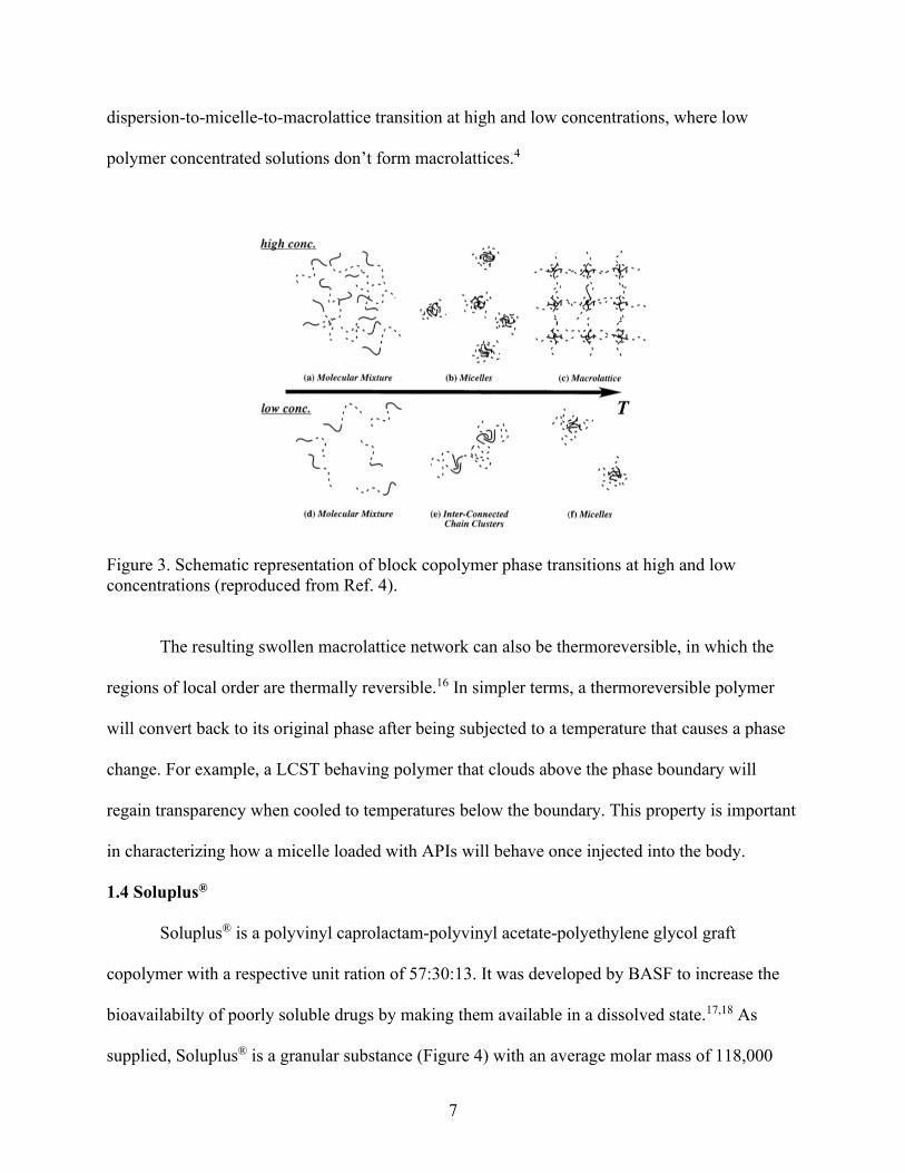
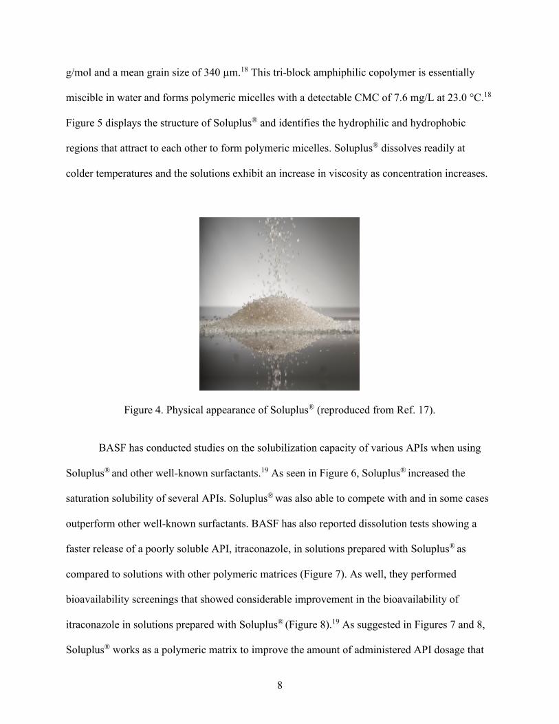
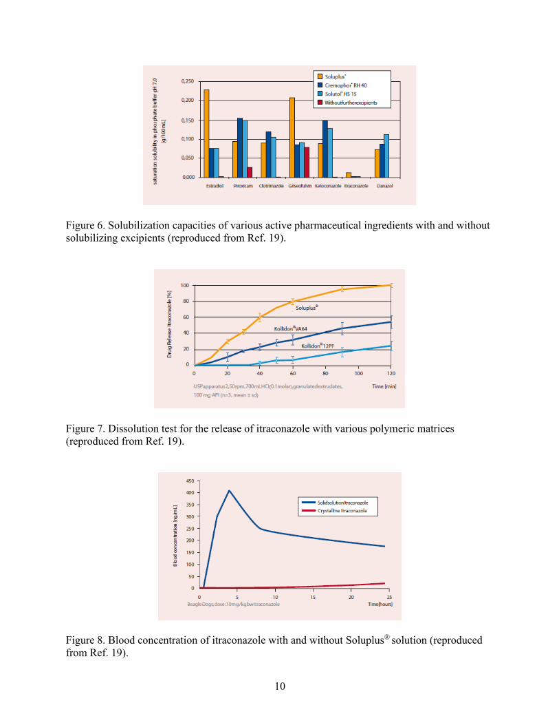
10
Figure 6 Solubilization capacities of various active pharmaceutical ingredients with and without
solubilizing excipients (reproduced from Ref 19)
Figure 7 Dissolution test for the release of itraconazole with various polymeric matrices
(reproduced from Ref 19)
Figure 8 Blood concentration of itraconazole with and without Soluplusreg solution (reproduced
from Ref 19)
11
Solutions of Soluplusreg show an increase in viscosity upon warming referred to as
thermothickening which is a property of potential interest in topical drug applications A
thermothickening solution can flow through an applicatorsyringe but then may harden as it
makes its way into the body15 This makes it possible to mix APIs with a polymer in its liquid
room-temperature state but then witness an in-situ gel deposit at the injection site when the
polymer is at body temperature22 The polymers polyvinyl caprolactam and polyethylene glycol
are known to transition from a hydrophilic to amphiphilic state upon warming around 34 degC to
36 degC which results in the self-assembly of micelles and gelation15 Because Soluplusreg is
comprised of these components it is suspected that a similar mechanism occurs upon heating of
aqueous solutions of Soluplusreg15 Soluplusreg also exhibits a gel-sol transition phase as
temperatures continue to rise23 This unusual physical behavior is seen only in doubly
thermoresponsive polymers that exhibit both LCST and UCST behavior Specifically Soluplusreg
is a LCST lt UCST behaving polymer and forms a gel within a designated temperature range
Copolymers that contain OH-functionality eg polyvinyl acetate polyethylene glycol polyvinyl
butyrate and protonated acrylic acid generally show LCST lt UCST behavior rather than UCST
lt LCST13 As seen in Figure 9 the circular temperature-concentration phase diagram describes
how Soluplusreg transitions from a soluble to insoluble phase and then back to a soluble phase as
a function of increasing temperature13
Soluplusreg forms micelles in aqueous media where the hydrophobic regions polyvinyl
acetate and polyvinyl caprolactam are located in the core of the micelle and the hydrated
polyethylene glycol segment is located in the outer region718 The micellization of Soluplusreg in
water is known to be endothermic and is spontaneous at temperatures above the Krafft point
(critical micelle temperature) due to an entropically-driven Gibbs free energy During
12
micellization solvent is released and entropy increases This gain in entropy exceeds the loss of
entropy by self-assembly of the polymeric micelles leaving the system with a positive entropy
change The micellization process occurs in three steps 1) polymeric micelles are formed in
solution at concentrations and temperatures above the CMC and Krafft point 2) the polyethylene
glycol chains dehydrate at temperatures above the Krafft point but below the phase boundary
and 3) there is an onset of physical change as temperature increases (Figure 10)7 This change
could be a cloud point where precipitation from solution at the LCST phase boundary causes
opacity or the change could be gelling due to self-assembly and aggregation of micelles into an
entangled network at a temperature specified as the sol-gel point A thermoresponsive polymer
may exhibit both physicochemical changes clouding and gelling however based on previous
work in our research group these physical onsets do not show any correlation other than their
dependence on increasing temperatures24 The micellization process is dependent on temperature
polymer concentration and medium composition7
Figure 9 Phase diagram for a LCST lt UCST behaving polymer (reproduced from Ref 14)
13
Figure 10 Micellization mechanism for solutions of Soluplusreg (reproduced from Ref 7)
As Soluplusreg solutions below 300 (ww) proceed through the micellization process
they encounter a series of temperature dependent physical behaviors At temperatures below the
LCST phase boundary Soluplusreg solutions appear clear with unrestricted flow At temperatures
above the boundary the solution clouds before a further increase in temperature causes a sol-gel
transition and restricted flow (Figure 11)22 Soluplusreg solutions above 300 (ww) show
restricted flow at room temperature but remain clear24 This indicates that the solutions have not
crossed the LCST phase boundary into the clouding region but have undergone a sol-gel
transition It is suggested that gelling can occur when polymer concentration is substantially
large7
Figure 11 A 300 (ww) Soluplusreg solution at room temperature (left) cloud point (middle)
and gel point (right) Represented as a top view of the cone-and-plate rheometer sample
compartment that was lowered from its housing and subjected to increasing temperatures
14
15 Dynamic Light Scattering Spectroscopy
An important characteristic of solubility enhancers is their particle size in solution before
and after loading with APIs Polymeric micelle particle size is studied through dynamic light
scattering spectroscopy (DLS) This technique also known as photon correlation spectroscopy or
quasi-elastic light scattering measures the translational diffusion of macromolecules in solution
due to Brownian motion25 Brownian motion refers to the random scattering of particles due to
collisions with solvent molecules Larger molecules have a slower Brownian motion while
smaller particles are bombarded further by surrounding solvent molecules and have more rapid
movement26 The Stokes-Einstein equation is used in dynamic light scattering methods to relate
the diffusion coefficient to particle size27 Equation 2 defines the Stokes-Einstein equation
119889(119867) = 119896119879
3120587120578119863 (2)
where 119889(119867) is hydrodynamic diameter 119896 is Boltzmannrsquos constant 119879 is absolute temperature 120578
is viscosity of solvent and 119863 is the velocity of Brownian motion typically defined as the
translational diffusion coefficient26
151 Effect of Viscosity As seen in Equation 2 particle size measurements by DLS are
dependent on temperature and the viscosity of solvent This dependence is seen in calculations
and in how the sample behaves Particles can behave in Newtonian or non-Newtonian manner
Newtonian fluids refer to samples that have the same viscosity at constant temperature and
pressure regardless of the amount of stress and shear strain27 For example a Newtonian fluid
would move twice as fast if it were subjected to twice as much force28 In a non-Newtonian fluid
the particles are suppressed by a larger viscosity of solution therefore restricted from Brownian
motion Viscosities of greater than three centipoise (cP) are generally considered as non-
15
Newtonian Results from DLS measurements can be significantly affected by inaccurate
viscosity values27
As seen in Figure 12 the analysis of a pigment dispersed in water was altered by using
different viscosities The blue graph was analyzed using a viscosity of 10 cP in the sizing
algorithm and the red graph was recomputed using 20 cP A particle size shift from 700 nm to
350 nm shows just how dependent hydrodynamic diameter measurements are on viscosity27
Particle size is also affected by particle concentration ionic strength of medium surface
structure particle shape and the refractive index of solvent2627
Figure 12 Particle size data for a pigment dispersed in water at two different viscosities 10 cP
(blue) and 20 cP (red) (reproduced from Ref 27)
A Further Look into Rheology Rheology is the study of deformation and flow branching
from the physical sciences which study the mechanics of forces deflections and velocities29
Newton was one of the first philosophers to investigate the quantification of a fluidrsquos viscosity
He originally described viscosity as the lack of ldquoslipperinessrdquo between elements of a fluid as they
are forced to move past each other Rheology has advanced throughout the ages from testing
viscosity by dropping heavy spheres through material and recording time differences to using
advanced and accurate instrumentation30 Rheology is observed in everyday life through liquids
16
and solids such as honey gum eraser toothpaste syrup oil rubber and much more These
materials behave simultaneously in a fluid (viscous) and solid (elastic) way giving rise to the
term viscoelasticity Rheology studies the deformation of viscoelastic materials when subjected
to a shear force that causes the material to flow29
Purpose of Studying Flow and Deformation Flow behavior is studied to pre-emptively
design equipment and practice quality control28 Various industries provide great examples of
using these studies in testing their products Ketchup must flow out of the bottle when shaken or
squeezed Household paint is easily stirred but dries on a wall without dripping Pudding seems
solid at rest but is simply spooned from the cup and ointment must effortlessly squeeze from the
tube with moderate pressure2831 The pressure at which a fluid just begins to flow a fundamental
quality control concern is known as the yield stress28 Yield stress measurements can be
routinely performed by using viscometers and rheometers later discussed in Section 231
Flow and deformation are also studied to characterize a material Viscosity is a ldquowindowrdquo
into other properties of a material that may be harder to measure When analyzing a sample for
its viscosity information is also gained regarding temperature shear rate time pressure and
material composition It is important to know how a product will react when subjected to these
other conditions For example motor oils and greases will have a decrease in viscosity when
subjected to higher temperatures28 As well lubricating oils decrease in viscosity at high
temperatures which cause the oils to flow off the metal parts they protects32 Shear rate or the
rate of deformation can also impact a sample causing a material to change in viscosity during
various times in the production process28 Many materials also undergo changes in viscosity
during a chemical process or while subjected to an outside pressure making rheological
measurements dependent on time and pressure Lastly a materials composition can affect
17
viscosity The state of aggregation between the solid particles and liquid phase in emulsions and
dispersions causes viscosity differences due to clumping and packing shape This is seen in
milk which is emulsified fat globules within water28
Viscosity Shear Stress and Shear Rate Rheology describes the elasticity viscosity and
plasticity of materials The interest is specifically on viscosity and the following parameters that
accompany it shear stress and shear rate28 Viscosity is defined as the measure of the internal
friction of a fluid This implies that one layer of fluid passes another layer without a transfer of
matter called laminar flow (Figure 13) A greater amount of friction between the layers
corresponds to a greater amount of force required for the movement28
Figure 13 Two plates model used to describe the physics of viscosity where 119860 is the area of
fluid 1198811 and 1198812 are the velocities at which the fluid is moving 119889119907 is difference in velocities 119889119909
is the distance between the two fluids and 119865 is the force required to cause movement
(reproduced from Ref 28)
As seen in Figure 13 two parallel flat areas of fluid separated by a designated distance
are moving in the same direction at varied speed From this model Newton implied that the force
needed to maintain the difference in speeds was proportional to the difference of speed through
the liquid This velocity gradient ( 119889119907
119889119909 ) is expressed by Equation 3
119865
119860= 120578
119889119907
119889119909 (3)
18
where 120578 is a given materialrsquos constant known as viscosity28 The velocity gradient describes the
shearing a liquid experiences and is thus known as the shear rate or rate of deformation The
force per unit area ( 119865
119860 ) term represents the shear stress or what is causing the shearing action
Equation 4 defines viscosity using these terms
120578 = 120591
120574 (4)
where 120591 is shear stress and 120574 is shear rate28 Shear stress has a unit of Newtons per square meter
(Nm2) and shear rate is in units of reciprocal seconds (sec-1) Viscosity has a fundamental unit of
ldquopoiserdquo where a material requiring one Nm2 of shear stress to produce a shear rate of one sec-1
has a viscosity of one poise Viscosity measurements are typically written on the centipoise scale
(cP) Measurements may also be seen in mPas (millipascal-seconds) which have a 11 ratio with
cP28 Table 2 gives common viscosities of many household goods
Table 2 Approximate viscosity values of
commonly known materials at 200 degCb
Fluid Viscosity (cP)
Water 1
Milk 3
Olive Oil 80
Glycerin 1000
Honey 10000
Toothpaste 70000
Peanut Butter 250000 b Adapted from Ref 33
Viscosity can also be referred to in terms of 119866lowast the complex shear modulus which is
equivalent to viscosity 120578 The complex shear modulus can be broken down into two
components 119866prime and 119866primeprime the storage and loss moduli respectively The storage modulus 119866prime is
responsible for characterizing the elastic behavior in viscoelastic materials while the loss
19
modulus 119866primeprime describes the viscous behavior Elastic behavior arises when energy is stored
within a material that has been subjected to deformation The internal structures extend and
stretch without causing damage to the material allowing the stored energy to act as a driving
force in returning the material back to its original state Viscous behavior results from internal
friction between a materials molecules and particles when subjected to deformation As friction
builds the material absorbs heat causing a loss of energy The storage modulus represents the
energy stored from deformation while the loss modulus characterizes the energy dissipated by
internal friction Viscoelastic solids have a higher storage modulus than loss (119866prime gt 119866primeprime) due to
their physical-chemical linking whereas viscoelastic liquids have a greater loss modulus than
storage (119866primeprime gt 119866prime) due to the lack of strong interactions between molecules34 Figure 14 describes
the relationship between complex shear modulus and phase-shift (δ) which is the lag time
between the current and resulting sinusoidal oscillation34 The relationship between 119866lowast 119866prime and
119866primeprime is seen in Equation 5 which follows the Pythagorean theorem
|119866lowast| = radic(119866prime)2 + (119866primeprime)2 (5)
Using Equation 5 allows for the determination of 119866lowast or viscosity from 119866prime and 119866primeprime29
Another parameter loss factor reveals the ratio of viscous to elastic behavior and is calculated as
the tangent of the phase-shift angle as seen in Equation 62934
tan 120575 = 119866primeprime
119866prime (6)
When the loss factor is greater than one (tan 120575 gt 1) it signifies the sample is in liquid
ldquosolrdquo state When the loss factor is less than one (tan 120575 lt 1) it signifies a solid ldquogelrdquo state The
ldquosol-gelrdquo transition state of gelation polymers is seen when the loss factor is equivalent to one
(tan 120575 = 1)29
20
Figure 14 Graphical relationship between complex shear modulus 119866lowast storage moduli 119866prime loss
moduli 119866primeprime and the phase-shift angle δ (reproduced from Ref 34)
152 Effect of Refractive Index The refractive index of solution medium plays a crucial
role in light scattering Its dependence is seen in the correlation function of a typical DLS
measurement where the intensity of scattered light is transformed into a size distribution by
using various algorithms For most monodisperse particles in Brownian motion the correlation
function (119866) follows an exponential decay as seen in the Equation 7
119866(120591) = 119860[1 + 119861 exp(minus2Γ120591)] (7)
where 120591 is the correlator time delay 119860 and 119861 are the baseline and intercept of the correlation
function respectively and Γ is further defined in Equation 8
Γ = 1198631199022 (8)
where 119863 is the translational diffusion coefficient Refractive index is seen within the definition of
119902 as follows in Equation 9
119902 = (4120587119899
120582) sin (
120579
2) (9)
where 119899 is refractive index 120582 is the wavelength of the laser and 120579 is the scattering angle26
Refractive index becomes increasingly more important in the correlation function when using a
volume distribution display mode that presents the size distribution as a ratio of volume to mass
Using a volume distribution display mode is practical when the size of particles becomes roughly
21
equivalent to the wavelength of the excitation light and is known as Mie theory2526 Specifically
Mie theory compares the size of particles to the wavelength of light by considering particle shape
and difference in refractive index between particles and the medium they are present in while
utilizing a volume distribution display mode25
16 Objectives
This project investigates how the viscosity and refractive index of aqueous Soluplusreg
solutions affects polymeric micelle size as determined by DLS It is hypothesized that if the
temperature dependence of viscosity for aqueous Soluplusreg solutions is rheologically measured
and the relationship between concentration temperature and viscosity is used in DLS
algorithms then DLS particle size measurements will be more reliable in describing the physical
behavior of Soluplusreg
The goals of this project include
1 Analyze the viscoelastic behavior for aqueous Soluplusreg solutions as a function of
temperature and establish a mathematical relationship between concentration temperature and
viscosity
2 Evaluate the refractive index of Soluplusreg solutions as a function of temperature
3 Compare DLS particle size measurements for aqueous solutions of Soluplusreg using
the viscosity and refractive index of water versus the viscosity and refractive index of actual
solution
22
CHAPTER 2 EXPERIMENTAL
21 Overview
Soluplusreg solutions 10 to 300 (ww) were tested on a cone-and-plate rheometer for
their temperature dependence of viscosity The rheometer was set to external mode and
controlled through a software interface A relationship between viscosity concentration and
temperature was created by fitting a polynomial regression to a 3D plot of these variables The
refractive indices of Soluplusreg solutions were analyzed as a function of temperature and used
along with viscosity data to correct inputs within DLS algorithms for particle size analysis on
Soluplusreg solutions ranging 01 to 100
22 Materials
Soluplusreg was provided to Missouri State Universityrsquos Department of Chemistry by
BASF Corporation (Ludwigshafen Germany)35 Aqueous Soluplusreg solutions were made
ranging from 10 to 300 (ww) for analysis by rheometry Using an analytical balance
(Mettler Toledo AL104) and deionized water a 300 (ww) solution of Soluplusreg was made
and then further diluted to other concentrations by weight The targeted weight of solutions was
150 g This process was repeated twice more to have a total of three sets of Soluplusreg solutions
(further labeled as Sets 1 2 and 3) When making aqueous Soluplusreg solutions the solid powder
is added to the water briefly stirred and then refrigerated around 50 degC until dissolved
For analysis by DLS and refractometry Soluplusreg solutions ranging 01 to 100
(ww) were made using an analytical balance (Mettler Toledo AL104) 18 MΩ (Type I) water
(Barnsted Nanopure II with 4 Mod Organic Free cartridge kit) and sterilized equipment Each
23
solution had a targeted final weight of 600 g and was made as described above However in
these cases the solutions were made individually instead of being diluted from a stock solution
Again three sets of Soluplusreg solutions were made and labeled as Sets 1 2 and 3 It is crucial
that sterilized equipment and highly filtered water is used to make the solutions as DLS is very
sensitive to outside contaminants and dust
23 Temperature Dependence of Viscosity
231 Instrumentation Rheology is quantified through use of viscometers and
rheometers As described in Section 151 these instruments are used to measure viscosity shear
stress torque and shear rate Rheometers allow for the measurement of rheological behaviors on
non-Newtonian fluids and for characterization of flow and deformation36 These rheological
behaviors include specific property measurements of viscoelasticity yield stress and stress
relaxation37 Rheometers are distinguished into two categories shear rheometers (sometimes
referred to as rotational rheometers) and extensional rheometers Shear rheometers control shear
stress by applying the independent variable of torque while extensional rheometers control strain
and measure stress as the dependent variable38 There are three types of shear rheometers which
include capillary rotational cylinder and cone-and-plate setups39 This research exclusively uses
a cone-and-plate rheometer to conduct all viscosity analyses Cone-and-plate rheometers
determine absolute viscosity with precise shear rate and stress information available They
require minimal volume of sample and can control temperature through a jacketed sample cup
This geometry is specifically useful in determining rheological behaviors of non-Newtonian
fluids28 However cone-and-plate rheometers are not useful in testing samples that show a three-
dimensional structure such as gels and solids When particles in agglomerate systems become too
24
large there isnrsquot enough free space between the particles in motion causing a greater amount of
friction on the instrumentrsquos surfaces29
The principle of operation behind a rotational rheometer is to drive a spindle through a
calibrated beryllium copper spring into viscous solution within the plate The drag of the sample
is measured by spring deflection and translated into torque and viscosity measurements31 A
greater amount of internal friction requires a greater amount of force needed to move the spring
through layers of fluid28 As seen in Figure 15 the motor pivot shaft spring and spindle are
housed in the upper half of the rheometer A jacketed cup containing the sample is joined to the
upper half of the instrument where the spindle rotates at the intersection of these parts The gap
between the cone and plate is crucial for accurate viscosity measurement It is determined by
locating the ldquohit pointrdquo and then backing off the spindle by one scale division (as designated on
the instrument) The hit point is where the spindle first comes in contact with the plate causing
the torque to change from 00 to 10 or greater31 The cone angle is also of importance as it
keeps constant torque at all distances from the center of rotation40
At a given viscosity the degree of resistance on the spring is proportional to the spindlersquos
size geometry and speed (Figure 16)28 Choosing an optimal match of spindle diameter and
rotational rate is commonly done by trial and error however it is known that viscosity range is
inversely proportional to both of these parameters Therefore samples with a higher viscosity
should be performed with a smaller spindle andor slower speed Measurements are
recommended to be made within a torque range of 100 to 10031
25
Figure 15 Schematics of a cone-and-plate rheometer (reproduced from Ref 31)
Figure 16 Diagram of the inner workings of the cone and plate where ω is the rotational velocity
r is the cone radius and ϴ is the cone angle (adapted from Ref 28)
The rheometer used in this research was a DV-III Ultra programmable rheometer model
RVDV-III from AMETEK Brookfield (Middleboro MA USA) This cone-and-plate rheometer
was provided to Missouri State University Department of Chemistry by Tolmar Inc (Fort
Collins CO USA) Calibration was performed by Brookfield in July 2019 to ensure proper
26
torque readings and drive shaft function Spindles used for measurement included the CP40 and
CP52 (Table 3 Figure 17) allowing for a total viscosity range of 131 cP to 9922000 cP
Table 3 Cone spindle dimensions and shear ratesc
Cone Spindle Angle
(degrees)
Radius
(cm)
Sample
Size (mL)
Shear Rate
(sec-1)
Viscosity Range
(cP)
CP-40 CPA-40Z 08 24 05 75N 131 ndash 327000
CP-52 CPA-52Z 30 12 02 20N 3969 ndash 9922000
c Adapted from Ref 28
N = RPM
Figure 17 Top view of spindles CP40 (left) and CP52 (right)
The rheometer was controlled through Brookfieldrsquos Rheocalc software (Ver 33
Brookfield Engineering Laboratories Inc) which allows for the programming of conditions and
graphical views of viscosity as a function of temperature In order to obtain temperature
measurements through Rheocalc a probe from Brookfield was adjoined to the instrument The
only appropriate attaching probe was the DVP-94Y steel temperature probe that is used in vane
spindle rheometer set ups The cone-and-plate set up required a temperature probe with a flexible
tip so that the measurement could be taken underneath of the metal sample cup To account for
this problem the steel DVP-94Y probe was purchased along with a 100 ohm 4-wire resistance
27
temperature detector (Omega part RTD-3-F3105-36-G) The probes were spliced and
connected so that the DVP-94Y steel probe connected into the rheometer but the flexible end of
the 4-wire resistance temperature detector attached to the sample cup This successfully allowed
for the transmission of temperature from the instrument into the software The temperature of
samples was controlled using a Fisher Scientific Isotemp Refrigerated Circulator (Model 910)
that was connected to the input and output ports of the instrumentrsquos sample cup (see Figure 15)
Calibration standards were purchased from Brookfield to confirm the accuracy and
precision of the instrument Two 100 PAO (polyalphaolefin) oil viscosity standards (3524 cP
and 3439 cP) were tested and showed accuracy according to the specifications defined by
Brookfield These specifications and calibration results can be seen in Section 31
232 Methods Brookfield calibration standards and Soluplusreg samples 10 20 50
100 150 175 200 225 250 and 300 (ww) were evaluated through use of the
Brookfield DV-III Ultra programmable rheometer and the software Rheocalc for their
temperature dependence of viscosity Each samplestandard was evaluated from 50 degC to about
40 degC at a heating rate of 01 degCsec A sample volume of 05 mL was placed into the cup of the
rheometer and probed with the specified spindle and shear rate (Table 4) All programing
parameters were set in Rheocalc and the experimental set-up was as shown in Figure 18 Data
were collected at a rate of one point per second while the total collection time was set to one
hour The resulting data were exported to Microsoft Excel (Ver 2002) for plotting and further
analysis The process was run in triplicate for the purpose of determining and reporting
uncertainties
28
Table 4 Experimental conditions for each samplestandard
run on the rheometer
Soluplusreg () Spindle RPM
3524 cP Std CP40 200
3439 cP Std CP52 100
10 CP40 250
20 CP40 250
50 CP40 250
100 CP40 750
150 CP40 200
175 CP52 250
200 CP52 250
225 CP52 100
250 CP52 150
300 CP52 100
Figure 18 Set-up used for viscosity data collection on a Brookfield rheometer A refrigerated
circulator (1) was connected to the rheometerrsquos sample cup ports (2) for temperature control A
RTD probe (3) attached to the cup was used to measure temperature where a Styrofoam cap (4)
was used to insulate the sample cup The rheometer (5) was externally connected to a laptop (6)
with the software Rheocalc
24 Refractive Index Analysis
241 Instrumentation Refractive index was measured using a 2WAJ monocular Abbe-
type refractometer (Figure 19) that was set up to allow for temperature control over a range of
29
00 degC to 700 degC The instrument has an index range of 13 to 17 with an accuracy of plusmn 00002
Water and ethanol were used as calibration standards (119899 = 13330 and 13611 at 200 degC
respectively) to test the accuracy of the instrument The results of all refractive index
measurements are presented in Section 32
Figure 19 Set-up used for refractive index data collection on an Abbe refractometer
242 Methods Water ethanol and Soluplusreg samples (01 05 10 20 50 and 100)
were evaluated using the 2WAJ Abbe digital refractometer for their refractive index following
the temperatures defined in Table 5 For each sample the refrigerated circulator was first set to
the appropriate temperature then a few drops of sample were placed between the measuring
prisms and lastly the dispersion correction and adjustment knobs were fine-tuned to where the
shadow aligned with the crosshairs giving a refractive index reading (Figure 20) To evaluate the
aqueous Soluplusreg samples from 110 degC to 350 degC the circulator was cooled to the starting
30
temperature and slowly ramped to the final temperature where refractive index readings were
taken every 10 degC The 01 Soluplusreg sample was evaluated in triplicate for the purpose of
determining and reporting uncertainty
Table 5 Temperatures used in the evaluation of
refractive index for various standards and samples
Soluplusreg () Temperature (degC)
Water (Std) 200
Ethanol (Std) 200
01 110 - 350
05 110 - 350
10 110 - 350
20 110 - 350
50 110 - 350
100 110 - 350
Figure 20 Shadow and scale within an Abbe-type refractometer A samplersquos refractive index
(bottom) is defined as the position where the shadow aligns with the crosshairs (top) (reproduced
from Ref 41)
25 Particle Size Determination by Dynamic Light Scattering
251 Instrumentation The velocity of translational diffusion due to Brownian motion is
measured in DLS by using a monochromatic beam of light which causes the scattering of light
31
upon interaction with molecules When the incident light encounters a molecule it is scattered in
all directions based on the size and shape of particle The scattered light will either result in
mutually destructive phases canceling out or in constructive phases producing a detectable
signal25 A digital autocorrelator then correlates intensity fluctuations of scattered light to time
This determines the rate at which intensity fluctuates which is related to the diffusion of
molecules In dynamic light scattering the intensity correlation function is measured and
expressed as hydrodynamic diameter data2526 Figure 21 gives a representative scheme of the
working parts in a DLS instrument
Figure 21 Schematic representation of the Zetasizer Nano series DLS instrument including a
laser (1) sample cell (2) detector (3) attenuator (4) correlator (5) and computer source (6)
(adapted from Ref 26)
32
There are 6 components to a DLS system As labeled in Figure 21 the first component is
a laser (1) that provides a light source to illuminate the sample cell (2) Next a detector (3) is
either placed at 90deg or 173deg to collect the scattered light If too much light is reaching the
detector the attenuator (4) will reduce the intensity of the light source Conversely if not enough
light is being detected the attenuator will allow more light to reach the sample Once the detector
senses the scattered light intensity it sends the data to the correlator (5) which translates the rate
of light intensity fluctuation Finally a computer (6) analyzes the data through software and
derives size information26
There are many advantages to using DLS as a particle size measurement technique These
include having a wide range of sample temperature and concentration parameters and being a
non-invasive low sample volume requirement technique Some limitations to DLS include low
resolution tedious cleaning and filtering procedures time-consuming optimization of
parameters restriction to transparent samples and most importantly for this research the
sensitivity to temperature solvent viscosity and refractive index25
Research was conducted using a Brookhaven (Holtsville NY USA) NanoBrook Omni
particle size and zeta potential analyzer (Figure 22) This instrument utilized dynamic light
scattering techniques with a 40 mW 640 nm red laser and collection angles of 15deg 90deg and 173deg
The measurement range is 03 nm to 10 microm with temperature control from -50 degC to 110 degC
Data collection was accomplished by using Brookhaven Instrumentrsquos Particle Solutions software
(v3606376) which allowed for the programming of experimental conditions and for data
viewingmanipulation
33
NIST (Gaithersburg MD USA) latex calibration standards were used to ensure accurate
performance of the DLS Two standards 40 nm and 300 nm were tested and showed accurate
results according to the manufacturerrsquos specifications (see Section 32)42
Figure 22 Set-up used for particle size data collection on a NanoBrook Omni
252 Methods NIST latex calibration standards and Soluplusreg samples 01 05 10
20 50 and 100 (ww) were evaluated for their hydrodynamic effective diameter The
calibration standards were evaluated at 250 degC and the Soluplusreg samples were evaluated for
their temperature dependence from 150 degC to 320 degC Each sample was analyzed with the
standard operating procedures shown in Table 6 where the average effective diameter of three
120-s measurements is obtained The process was run in triplicate for the purpose of determining
and reporting uncertainties where the average of three 120-s measurements was considered a
single run
Before measurement each sample was filtered using a Sartorius Ministart NML Plus
Syringe Filter with a 07microm glass filter to remove any large aggregates in solution The filter
34
was primed twice with sample solution using the filterings to rinse the cuvette and the sample
was filtered three times A dust rejection algorithm was also used to remove data resulting from
dust and large aggregates in sample The appropriate dust rejection range is selected based off
expected particle size and for multimodal distribution is based off the largest population of
particles in sample43 The samples were first evaluated using the viscosity and refractive index of
water then recomputed to the experimentally determined viscosity and refractive index of
Soluplusreg samples
Table 6 Standard operating procedures for temperature dependent particle size analysis
Parameter Value
Starting Temperature 150 degC
Final Temperature 320 degC
Temperature Increment 10 degC
Set Duration 120 s
Equilibration Time 300 s
Total Measurements 3
Time Between Measurements 00 s
Dust Rejection 50 nm to 250 nm
Fluid Water
Viscosity 0890 cP
Refractive Index 1331
Measurement Angle 90deg
35
CHAPTER 3 RESULTS AND DISCUSSION
31 Temperature Dependent Viscoelastic Behavior of Soluplusreg Solutions
Calibration standards were analyzed by the rheometer to ensure the instrumentrsquos
accuracy The specification on viscosity accuracy is plusmn 10 of full scale range at a specified
spindle and speed The Brookfield viscosity standard fluids are also accurate to plusmn 10 of their
stated value Total allowed error was calculated by summing the deviations from the instrument
and fluid as portrayed by Brookfield (Table 7)31 Figure 23 shows each standard as a function of
temperature and the experimental viscosity values at 250 degC
Table 7 Total allowed error for each viscosity standard fluid at 250 degC
Standard
(cP)
Allowed Error
(cP)
Experimental
Viscosity (cP)
3524 plusmn 1987 35027
3439 plusmn 13269 332883
Figure 23 Brookfield viscosity standard fluids as a function of temperature The solid black
points represent the standardrsquos stated viscosity shown with total allowed error
0
1000
2000
3000
4000
5000
6000
7000
8000
10 15 20 25 30 35 40 45
Vis
cosi
ty (
cP)
Temperature (degC)
36
As shown in Figure 23 at 250 degC the 3524 cP and 3439 cP standards read 35027 cP
and 332883 cP respectively Both values were within their allowed deviance from the stated
value in Table 7 showing accuracy from the rheometer
Each concentration of Soluplusreg samples ranging 10 to 300 (ww) were analyzed
three times (Sets 12 and 3) by the rheometer for their temperature dependence of viscosity (see
Section 232) Plots of Viscosity vs Temperature are shown in Figure 24 For each concentration
a standard deviation was calculated at every 20 degC and plotted on the ldquomost representativerdquo run
(middle of the three traces) Averaging the sets was not plausible due to varying temperature
rates for each run
The most representative run for each concentration is shown in Figure 25 where each
sample is on the same x-axis to better see trends and relationships There is a general trend in
which viscosity decreases to a minimum before rapidly increasing to a maximum As signified by
the solid black tie-line in Figure 25 traces for concentrations above 100 exhibit a slight rise in
viscosity at low temperatures prior to the decrease toward the minimum This rise is
concentration dependent and can be seen shifting to higher temperatures as concentration
increases (1198791198721) Designated by the dashed black line in Figure 25 the steep growth in viscosity
to the maximum is essentially concentration independent and occurs around 360 degC (1198791198722) The
minimum prior to this sharp rise is also essentially concentration independent and occurs around
270 degC (119879119898119894119899) The temperatures corresponding to these features are listed in Table 8
37
0
2000
4000
6000
8000
0 10 20 30 40 50
Vis
cosi
ty (
cP)
Temperature (degC)
Set 1 Set 2 Set 3
0
20000
40000
60000
80000
100000
0 10 20 30 40 50Temperature (degC)
0
50
100
150
200
250
Vis
cosi
ty (
cP)
0
50
100
150
Vis
cosi
ty (
cP)
00
20
40
60
80
Vis
cosi
ty (
cP)
00
10
20
30V
isco
sity
(cP
)
0
200
400
600
800
0
50
100
150
0
5
10
15
20
00
10
20
30
40
Figure 24 Effect of temperature on viscosity for each aqueous Soluplusreg sample
10 20
50 100
225 200
175 150
250 300
38
Figure 25 Viscosity of Soluplusreg samples on the same temperature scale
39
Table 8 Extrema temperatures observed in η-T plots of Soluplusreg solutionsdagger
Concentration
()
1198791198721
(degC) 119879119898119894119899
(degC)
1198791198722
(degC)
10 - - -
20 - 3049 plusmn 043 3498 plusmn 023
50 - 2928 plusmn 041 3570 plusmn 033
100 - 2810 plusmn 007 3586 plusmn 009
150 1054 plusmn 036 2784 plusmn 045 3604 plusmn 017
175 1072 plusmn 026 2796 plusmn 028 3595 plusmn 033
200 1243 plusmn 015 2811 plusmn 003 3587 plusmn 006
225 1475 plusmn 026 2758 plusmn 018 3593 plusmn 013
250 1738 plusmn 018 2699 plusmn 009 3611 plusmn 015
300 2271 plusmn 038 2822 plusmn 077 3618 plusmn 021
dagger Uncertainties were determined by averaging the extrema temperature values from Set 12
and 3 and taking the standard deviation
The sol-gel transition of a thermoresponsive polymer is characterized by an increase in
viscosity between the micelle and macrolattice states As seen in the temperature-dependent plots
of viscosity for Soluplusreg solutions the increase in viscosity takes place from 270 degC to 360 degC
This sharp increase in viscosity is also seen in literature (Figures 26 and 27) from plots of
complex shear viscosity versus temperature Figure 26 describes the minimum viscosity as an
onset of chemical reaction where micelles begin to self-assemble and form superstructures
indicating the beginning of gel formation18 Our aqueous Soluplusreg solutions of varying
concentration show this onset of chemical reaction around 270 degC (Figures 24 and 25) As the
gelling process occurs viscosity rapidly increases to a sol-gel point The sol-gel transition is
typically defined as the crossing point between 119866prime and 119866primeprime (Figures 26 and 27)182944 Due to our
use of a cone-and-plate rheometer which is unable to measure 119866prime and 119866primeprime separately precise sol-
gel transitions for our Soluplusreg solutions were indeterminable However as seen in Figure 27
the sol-gel transition occurs within the large increase in viscosity We hypothesize that the
Soluplusreg sol-gel transition is occurring at a temperature that falls between the average minimum
40
and average maximum 270 degC to 360 degC To provide a more precise determination of the sol-
gel point would require the use of an oscillating rheometer At 360 degC the viscosity of all
concentrations reaches its maximum and begins to greatly decrease At this point it is
hypothesized that the solution has completely gelled and has ldquobrokenrdquo inside the rheometer
whereby the cone spindle is no longer able to move through solution When the solution is at its
gel-point it adheres to the plate in a ldquosolid mannerrdquo (Figure 28) causing the spindle to glide
against the plate rather than push through solution with resulting force
Figure 26 Temperature dependent functions of 119866prime and 119866primeprime for a gelling material (reproduced
from Ref 18)
Figure 27 Complex viscosity 119866prime and 119866primeprime as a function of temperature for a curing epoxy
(reproduced from Ref 44)
41
Figure 28 A gelled 200 (ww) Soluplusreg solution on the plate of a cone-and-plate rheometer
The star-like shape is caused by the pulling away of the CP52 spindle when the solution is
gelled The remaining solution seen circulating around the star-like shape is where the spindle
didnrsquot come in contact the plate due to its small diameter
The concentration-dependent rise in viscosity exhibited at lower temperatures for
concentrations above 100 (follow the solid black line in Figure 25) is hypothesized to be a
physical property of thermoresponsive polymers that has not been described previously We
speculate that it is related to the Krafft point of Soluplusreg solutions The Krafft point is the
temperature at which the solubility limit of a surfactant is equivalent to the CMC45 Therefore
below the Krafft temperature the surfactant is in a crystalline state and micelles do not form The
visual effect of going below the Krafft temperature is similar to that of clouding where the
surfactant is in a precipitated state and shows opacity45 To be described further as
thermoresponsive polymer solutions cloud they show an increase in viscosity Therefore when
the polymer solution is below the Krafft point and in a precipitated state it could be speculated
that viscosity would increase as temperature rises to the Krafft point This is observed in Figure
25 for Soluplusreg solutions above 100 where the speculated Krafft point would be near the
maxima ranging from 110 degC to 220 degC (1198791198721 in Table 8) As temperature further increases past
these maxima it is speculated that micelles are forming The following decrease in viscosity
could be due to the switch from having crystals in solution to micelles or that in general the
42
viscosity of Newtonian fluids decreases as temperature increases At concentrations below
100 it is speculated that the polymer fraction wasnrsquot large enough to witness this slight
increase in viscosity or temperatures didnrsquot reach cold enough
Previous work conducted by our research group reported that aqueous Soluplusreg
solutions physically gel at temperatures from 300 degC to 400 degC depending on concentration
where more concentrated solutions gel at lower temperatures (Figure 29)23 This research was
conducted using a 90deg tilt test and observing at which temperatures the samples stopped flowing
The data obtained by a 90deg tilt test roughly matches the rheologically implied temperature range
at which the sol-gel transition occurs 270 degC to 360 degC Differences between these sol-gel
transition temperature ranges could be from the differences in the experimental processes where
rheology is a more precise way of observing viscoelastic behavior Figure 29 also reveals that
aqueous Soluplusreg solutions below 100 (ww) do not exhibit a gel phase at any temperature It
is hypothesized that the polymer solutions are not at high enough concentrations for the micelles
to interact and form macrolattice structures Data acquired from the rheometer is at least
somewhat consistent with this observation as seen in the traces from samples under 100
(ww) where the viscosity behavior exhibits small to negligible features that we attribute to the
gelation process (Figure 25) We speculate that the small features observed in the 20 and 50
samples correspond to a pre-gelation condition that does not lead to a complete gelling as
measured by the 90 deg tilt test
43
Figure 29 Sol-gel and gel-sol transitions for Soluplus samples as a function of temperature
Speculated phase boundaries (solid lines) have been added to emphasize observed trends
(adapted from Ref 23)
Previous work conducted in our research group also described the cloud-point transitions
of Soluplusreg solutions The cloud point is described as the transition from soluble to insoluble
phases across the LCST phase boundary and has been observed for aqueous Soluplusreg solutions
to be in the range of 270 degC to 310 degC (Figure 30)46 The temperature range of cloud transition
from previous research lies within the sharp increase of viscosity as did the sol-gel transition
Although these two phase transitions clouding and gelling occur at the same temperature range
they are independent of each other Figures 29 and 30 illustrate the differences in gelling and
clouding phase behaviors where the gel point of aqueous Soluplusreg solutions decreases as a
function of increasing concentration but the cloud point increases as a function of increasing
concentration As previously recognized Soluplusreg solutions under 300 first experience a
cloud transition before physically gelling as a function of increasing temperature Therefore it is
hypothesized that for aqueous Soluplusreg solutions below 300 the cloud transition occurs
within the temperature range of the sharp viscosity increase (270 degC to 360 degC) but prior to the
gel point
44
Figure 30 Cloud points for aqueous Soluplusreg solutions as a function of temperature
(reproduced from Ref 46)
Data from Figure 25 was transformed into a logViscosity vs Temperature plot to scale all
traces onto the same x and y axes (Figure 31) The software Matlab (Matlab and Simulink
R2019b MathWorks) was utilized to create a 3-dimensional scatter plot of temperature (x)
concentration (y) and viscosity (z) A polynomial model was used to create a least-squares fit of
the plotted data where the best fit resulted from a 5th-order polynomial in terms of x and y called
ldquoPoly55rdquo As seen in Figure 32 the Poly55 function fits well to low temperatures and low
concentrations however as viscosity rapidly increases the function falls far from experimental
data It was decided that because DLS focuses primarily on concentrations below 150 and
temperatures below 320 degC the least-squares fitting could be confined to only this range of data
As the concentration of Soluplusreg solutions approaches 00 and the viscosity approach that of
pure water the viscosity value will decrease to below the measuring capabilities of our
rheometer Therefore literature values for the viscosity of water47 were used to complete the
concentration range of 00 - 150 Figure 33 shows a Poly54 model (5th order in x and 4th
order in y) that matches closely to the shortened range of data The Poly55 model was robustly
weighted using ldquoBisquarerdquo where the weight given to each data point is determined by how far
45
the point is from the fitted line This allows for the fit to be based on the bulk data minimizing
any outlier effects48 The Poly54 model didnrsquot use robust fitting on top of the polynomial fit
Figure 31 Log-linear plot of viscosity vs temperature of aqueous Soluplusreg solutions at
different concentrations
Figure 32 Full range of experimental data modeled with a Poly55-Bisquare fit
-1
0
1
2
3
4
5
6
0 10 20 30 40 50
Log V
isco
sity
(cP
)
Temperature (degC)
10 20 50 100 150175 200 225 250 300
46
Figure 33 Short range of experimental data modeled with a Poly54 fit
From the Poly54 modeled fit a polynomial function was created so that the viscosity of
Soluplusreg samples could be determined for any temperature ranging 50 degC to 320 degC and
concentration ranging 00 to 150 The full Poly54 fit function is shown below
log(120578) = minus 01652 + 01448(119879) + 0282(120588) minus 002019(1198792) minus 002223(119879)(120588) (10)
minus 004058(1205882) + 0001153(1198793) + 0001691(1198792)(120588) + 000144(119879)(1205882)
+000414(1205883) minus 30211990910minus5(1198794) minus 700811990910minus5(1198793)(120588)
minus 320411990910minus5(1198792)(1205882) minus 798911990910minus5(119879)(1199013) minus 00001442(1205884)
+ 297611990910minus7(1198795) + 104311990910minus6(1198794)(120588) + 506111990910minus7(1198793)(1205882)
minus31911990910minus7(1198792)(1205883) + 334411990910minus6(119879)(1205884)
where 120578 is viscosity 119879 is temperature in Celsius and 120588 is the relative mass concentration (ww)
Equation 10 shows accuracy to experimental viscosity data within a 30 difference around 95
of the time where the other 5 is within a 100 difference (occurring primarily at low
concentrations and low temperatures or high concentrations and high temperatures)
47
32 Temperature Dependent Refractive Index of Soluplusreg Solutions
Because particle size analysis by dynamic light scattering depends on viscosity and
refractive index these parameters were evaluated for on Soluplusreg solutions to ensure accurate
hydrodynamic effective diameter measurement The temperature dependence of viscosity for
Soluplusreg solutions is described in Section 31 and the following gives the refractive index
behavior of aqueous Soluplusreg solutions as a function of temperature
Water and ethanol were evaluated at 200 degC by the 2WAJ Abbe refractometer to check
the instrumentrsquos accuracy The refractometer has a specified accuracy of plusmn 00002 and the
experimental results can be seen in Table 9 compared to literature values The refractive index of
ethanol is within the allowed deviation of its literature value but the value of water lies 00006
away from its literature value Since the effect of refractive index on particle size analysis is
relatively weak (see Section 33) it was concluded that this deviation can be tolerated
Furthermore the NanoBrook Omni instrument considers refractive index to only the thousands
place so the observed deviation is within the natural precision of the correction
Table 9 Experimental and literature refractive index values
for water and ethanol at 200 degC
Refractive Index (119899) at 200 degC
Standard Experimental Literature
Water 13324 13330d
Ethanol 13612 13611e d from Ref 49 e from Ref 50
Each concentration of Soluplusreg solution ranging 01 to 100 (ww) were evaluated
for their refractive index from 110 degC to 350 degC as described in Section 242 These data can be
48
seen in Figure 34 where the 01 trace included representative standard deviations as
determined from repetitive runs As shown in the figure refractive index increases as the
concentration of Soluplusreg increases As well the refractive index decreases slowly as
temperature increases for all concentrations This trend replicates the refractive index behavior of
pure water49
Figure 34 Effect of temperature on refractive index for Soluplusreg samples
33 Particle Size Analysis of Soluplusreg Solutions
Calibration standards were evaluated by the NanoBrook Omni particle size analyzer to
ensure the instrumentrsquos accuracy NIST specifies that their latex calibration standards do not
come with a passfail criterion due to underlying sizing methodology that is customer
dependent51 NIST recommends establishing an in-house criterion to test instrument
performance which has been adopted as plusmn 400 nm in the chemistry department at Missouri
13300
13350
13400
13450
13500
13550
5 10 15 20 25 30 35 40
Ref
ract
ive
Index
Temperature (degC)
01 05 10 20 50 100
49
State University52 The experimental hydrodynamic effective diameters of the 429 nm and 288
nm standards can be seen in Table 10 where it is shown that our measurements pass in-house
criteria displaying good instrument performance The polydispersity index (PDI) is also
included in Table 10 which signifies the relative size-range of particles The PDI can range from
0000 to 1000 where a lower value corresponds to a more monodisperse sample
Table 10 Effective diameters of NIST latex calibration standards at 250 degC
Standard (nm) Experimental
Eff Diam (nm)
Experimental
Polydispersity
429 4592 0106
288 2858 0040
Soluplusreg solutions 01 05 10 20 50 and 100 (ww) were each
evaluated three times (Sets 1 2 and 3) for their hydrodynamic effective diameters as a function
of temperature using the NanoBrook Omni particle size analyzer following the protocol in
Section 252 Figure 35 displays the average hydrodynamic effective diameters along with
uncertainties for each sample as a function of temperature using ldquouncorrectedrdquo viscosity and
refractive index data ldquoUncorrectedrdquo refers to using the pre-programmed viscosity and refractive
index data for a pure water solvent As observed the temperature dependence generally shows
the diameter to decrease with increasing temperature and then sharply rise as the cloud- or gel-
point is reached Additionally the effective diameter appears to be directly proportional to
Soluplusreg concentration in that for any given temperature the largest particle diameter is
obtained for the highest Soluplusreg concentration The sharp rise in the temperature dependence
of the hydrodynamic effective diameter appears to correlate with the solutionrsquos clouding or
gelling point where micelles are aggregating and produce larger particles The 01 and 05
50
Soluplusreg samples donrsquot show this sharp rise in diameter suggesting that there is no onset of
physical change However according to Figure 30 these concentrations do show clouding by
spectroscopy whereas they do not show evidence gelling (Figure 29)
Figure 35 Effect of temperature on effective diameter for Soluplusreg solutions using uncorrected
values of viscosity and refractive index
The traces in Figure 35 were recomputed to correct for the viscosity and refractive index
behavior of Soluplusreg solutions In the following discussion ldquocorrectedrdquo refers to using the
viscosity and refractive index data of Soluplusreg solutions reported in Sections 31 and 32 As
seen in Figure 36 the corrected effective diameters are observed to be inversely proportional to
concentration Figure 37 depicts this trend for one specific temperature (250 degC) by comparing
hydrodynamic diameters obtained from ldquouncorrectedrdquo vs ldquocorrectedrdquo analyses Table 11 gives
the numerical values shown in Figure 37 along with PDI values It is notable that the PDI shows
no dependence on viscosity or refractive index It is reported in literature that the cause for the
decreasing diameter as concentration increases is related to micellar core size At larger
000
10000
20000
30000
40000
50000
60000
70000
11 16 21 26 31 36
Hydro
dyn
amic
Eff
ecti
ve
Dia
met
er
(nm
)
Temperature (degC)
01 05 10 20 50 100
51
concentrations micelles form with less solvent in the core causing the micelle to compact and
reduce in size6
Figure 36 Effect of temperature on effective diameter for Soluplusreg solutions using corrected
values of viscosity and refractive index
Figure 37 Uncorrected vs corrected diameter at 250 degC for Soluplusreg in aqueous solution
000
2000
4000
6000
8000
10000
12000
11 16 21 26 31 36
Hydro
dyn
amic
Eff
ecti
ve
Dia
met
er
(nm
)
Temperature (degC)
01 05 10 20 50 100
000
2000
4000
6000
8000
10000
12000
01 05 10 20 50 100Hydro
dyn
amic
Eff
ecti
ve
Dia
met
er
(nm
)
Concentration ()
Uncorrected Corrected
52
Table 11 Uncorrected vs corrected effective diameters at 250 degC for Soluplusreg in
aqueous solution
Hydrodynamic Effective Diameter (nm)
Concentration
() Uncorrected Corrected Polydispersity
01 6615 plusmn 079 6313 plusmn 076 0030
05 6078 plusmn 008 5359 plusmn 006 0038
10 6648 plusmn 037 5539 plusmn 031 0042
20 6988 plusmn 026 4981 plusmn 019 0059
50 7634 plusmn 054 4114 plusmn 029 0103
100 10585 plusmn 128 2498 plusmn 030 0210
Also depicted in Figure 36 the ldquocorrectedrdquo diameter values remain more consistent
through rises in temperature prior to sharply increasing As well the sharp rise in effective
diameter remains around the same temperature The 01 and 05 Soluplusreg samples were
recomputed using extrapolated viscosities as determined by Equation 10 The Brookfield RVDV-
III Ultra rheometer was unable to test these low concentrated samples because their viscosities
fall below the instrumental limit It is suspected that because theses viscosity values were
extrapolated from outside the experimentally determined range the resulting corrected diameters
may contain an inherently higher level of uncertainty In Figure 36 the 01 and 05 traces
still show no evidence for physical phase change by DLS (ie a sharp increase in diameter at
higher temperatures)
Salah et al report the hydrodynamic diameter of Soluplusreg in a 01 (ww) aqueous
solution at 200 degC to be 6486 plusmn 158 nm (Figure 38)15 The experimentally determined
ldquocorrectedrdquo effective diameter from this thesis for an equivalent sample under the same
conditions is 6576 plusmn 038 nm (Figure 36) consistent with the previously reported value
53
Figure 38 Size distribution for a 01 Soluplusreg solution at 200 degC (reproduced from Ref 15)
The influence of including accurate viscosity and refractive index data in particle size
algorithms is considerable For example the hydrodynamic effective diameter shifts from 14348
nm to 2535 nm for the 100 Soluplusreg solution at 200 degC upon correcting for these effects
(Table 12) This substantial shift (823 decrease) on diameter is due primarily to viscosity
effects Refractive index plays a less significant role in particle size analysis by DLS As shown
in Table 13 the resulting hydrodynamic diameter in a 100 Soluplusreg solution is shifted only
150 by changing refractive index by 0010 indicating that the correction due to refractive
index variation is significantly less important than that due to viscosity
Table 12 Difference in effective diameter when using uncorrected and corrected viscosity and
refractive index data for a 100 Soluplusreg solution at 200 degC
SOP Uncorrected Corrected
Liquid Water Unspecified
Viscosity (cP) 1002 5842
Refractive Index 1331 1351
Effective Diameter (nm) 14348 2535
54
Table 13 Effective diameter dependence on refractive index for
a 100 Soluplusreg solution at 200 degC and 5842 cP
Refractive Index Effective Diameter (nm)
1341 2498
1351 2535
1361 2573
As discussed previously the sharp increase in effective diameter that is observed for the
10 20 50 and 100 (ww) Soluplusreg solutions is related to the cloud- or gel-point
Figure 39 overlays the viscosity and effective diameter of a 50 Soluplusreg solution on the same
temperature axis As observed effective diameter remains relatively constant as viscosity is
decreasing to its minimum across the temperature range As viscosity starts to increase
indicating an onset of change (clouding gelling or both) the effective diameter also rises The
increase in particle size is triggered by the reduced solubility of solution as it crosses the LCST
phase boundary This causes the micelles to aggregate and rearrange resulting in larger and more
polydisperse particle sizes15
Figure 39 Viscosity and corrected diameter vs temperature for a 50 Soluplusreg solution
10
14
18
22
27
31
35
2500
3500
4500
5500
6500
7500
8500
15 17 19 21 23 25 27 29 31
Vis
cosi
ty (
cP)
Hydro
dyn
amic
Eff
D
iam
(n
m)
Temperature (degC)
Corrected Eff Diam Viscosity
55
CHAPTER 4 CONCLUSIONS AND FUTURE DIRECTIONS
The phase behavior of aqueous solutions of Soluplusreg a polyvinyl caprolactam-polyvinyl
acetate-polyethylene glycol graft copolymer were studied throughout this research
Rheologically determining the effect of temperature on viscosity allowed for insight behind the
viscoelastic properties of thermothickening polymer solutions It was observed that as
temperature rises the viscosities of Soluplusreg solutions decrease until reaching a minimum
around 280 degC where viscosity then sharply increases This trend has been observed by other
researchers for gelling polymers where a large increase in viscosity signifies the agglomeration
of polymeric micelles into macrolattices The sharp increase in viscosity for aqueous Soluplusreg
solutions is concentration independent and occurs from 270 degC to 360 degC Within this
temperature range polymeric micelles aggregate into a network and gel but determining a
specific gel-point is unattainable with use of a cone-and-plate rheometer A precise gel-point
could be determined by use of an oscillatory rheometer The temperature at which viscosity
sharply rises is also seen to correlate with cloud point where the solution is in an insoluble phase
and micelles begin to rearrange and agglomerate due to decreased solubility Although gelling
and clouding both occur around the same temperature they show no evidence of true correlation
The cause of swelling in viscosity seen at lower temperatures for concentrations above 100
remains inconclusive however we speculate that this is due to the Krafft point of aqueous
Soluplusreg solutions We hypothesize that the Krafft point temperature where micelles begin to
form is where viscosity begins to increase With further analysis on particle size this behavior
could be better interpolated For example studying the particle size of a 200 (ww) Soluplusreg
solution from 50 degC to 200 degC would show micelle behavior before and after the viscosity
56
increase If the particle size in solution increases as viscosity increases a physical phase behavior
would be witnessed Possibly going from a crystalline to micelle state due to the Krafft point
Particle size algorithms used in DLS analyses are directly dependent on viscosity and
refractive index values of the solutions Therefore it is important to include accurate information
for these parameters In this thesis a relationship between concentration temperature and
viscosity was determined by measuring sets of these variable and fitting the data to a 2-variable
polynomial function From this equation accurate viscosity values could be identified and used
in particle size analysis for Soluplusreg solutions The refractive index of Soluplusreg solutions were
studied and showed close similarity to that of water where refractive index decreases slightly as
a function of increasing temperature The effect of refractive index on hydrodynamic effective
diameter is minimal in DLS However viscosity plays a much more significant role where a
4840 cP increase in viscosity caused effective diameter to decrease 823
The hydrodynamic effective diameter of Soluplusreg particles in aqueous solution as
measured by DLS changed significantly upon application of corrections due to viscosity and
refractive index effect The most significant difference observed after the corrections was in the
relationship between concentration and effective diameter where the uncorrected trend of
particle size increasing with concentration proved to be the opposite trend (particle size
decreases with increasing concentration) after corrections were applied
For a given concentration plots of hydrodynamic effective diameter vs temperature
showed an overall decrease with temperature to a minimum near 270 degC followed by a sharp
rise around 300 degC for all concentrations This rise in diameter appears to correlate with the
solutions phase behaviors clouding and gelling
57
Soluplusreg is a tri-block graft copolymer that is used in the pharmaceutical industry to
enhance the bioavailability of APIs by encapsulating insoluble drugs within a micellar core
Studying the effect of temperature on particle size and viscoelastic behavior gives insight to how
the polymeric micelles will behave once subjected to body temperature Supported by this
research Soluplusreg shows interest in the biomedical field as a drug carrier system through its
thermoresponsive behaviors in viscoelasticity and particle size
58
REFERENCES
1 S Koltzenburg in Solubility Enhancement with BASF Pharma Polymers ed T Reintjes
BASF SE Lampertheim Germany 2011 1 9-26
2 M A Ward and T K Georgiou Polymers 2011 3 1215-1242
3 D W van Krevelen and K te Nijenhuis Properties of Polymers Elsevier Amsterdam
Netherlands 2009
4 S Okabe S Sugihara S Aoshima and M Shibayama Macromolecules 2003 36 4099-
4106
5 Y Tanaka in Rheology ed J D Vicente InTech Rijeck Croatia 2012 2 29-58
6 S S Kulthe Y M Choudhari N N Inamdar and V Mourya Designed Monomers and
Polymers 2012 15 465-521
7 J F Alopaeus E Hagesaether and I Tho Pharmaceuticals 2019 12 1-23
8 R Tanbour A M Martins W G Pitt and G A Husseini Current Pharmaceutical Design
2016 22 1-12
9 G P Andrews and D S Jones Biomacromolecules 2006 7 899-906
10 K Yotsumoto K Ishii M Kokubo and S Yasuoka Int J Pharm 2018 553 132-140
11 A Gandhi A Paul S O Sen and K K Sen Asian J Pharm Sci 2015 10 99-107
12 The Science of Insolubility-BASF httpsthemedicinemakercomdiscovery-
developmentthe-science-of-insolubility (accessed November 2019)
13 Y Zhu R Batchelor A B Lowe and P J Roth Macromolecules 2016 49 672-680
14 R Hoogenboom in Smart Polymers and Their Applications ed M R Aguilar and J S
Roman Woodhead Publishing Sawston Cambridge 2014 2 19
15 I Salah M Abou Shamat and M T Cook J Appl Polym Sci 2019 136 46915
16 The IUPAC Compendium of Chemical Terminology httpsgoldbookiupacorg (accessed
October 2019)
17 Soluplus Technical Information-BASF httpspharmaceuticalbasfcomenDrug-
FormulationSoluplushtml (accessed September 2019)
59
18 D Djuric in Solubility Enhancement with BASF Pharma Polymers ed T Reintjes BASF
SE Lampertheim Germany 2011 5 67-68
19 Soluplusreg-The Solid Solution httpspharmaceuticalbasfcomenDrug-
FormulationSoluplushtml (accessed November 2019)
20 L Di and E H Kerns in Drug-Like Properties Concepts Structure Design and Methods
Academic Press Cambridge Massachusetts 2nd edition 2016 19 267-281
21 Soluplusreg Regulatory Facts Sheet httpswwwpharmaexcipientscomnewssoluplus-is-
approved-in-generics-in-taiwan-and-argentina-and-is-now-filed-in-brazil (accessed
November 2019)
22 G Bonacucina M Cespi G Mencarelli G Giorgioni and G F Palmieri Polymers 2011
3 779-811
23 K Kosinska Non-Thesis Degree Paper Department of Chemistry Missouri State
University 2016
24 C M Reynolds unpublished work 2013
25 J Stetefeld S A McKenna and T R Patel Biophys Rev 2016 8 409-427
26 DLS Technical Note [MRK656-01]-Malvern Instruments httpswarwickacuk
faccross_facsciencecityprogrammesinternalthemesam2bookingparticlesizeintro_to_dl
spdf (accessed November 2019)
27 Technical Note Viscosity Effects-Horiba httpwwwhoribacomfileadminuploads
ScientificDocumentsPSATN140pdf (accessed September 2019)
28 Brookfield Engineering Laboratories Inc More Solutions to Sticky Problems Brookfield
Middleboro MA 2014
29 T G Mezger The Rheology Handbook For users of rotational and oscillatory rheometers
Vincentz Network Hanover Germany 2014
30 D L Blair in Molecular Gels Structure and Dynamics ed R G Weiss Royal Society of
Chemistry London United Kingdom 2018 2 28-32
31 Brookfield Engineering Laboratories Inc Brookfield DV-III Ultra Programmable
Rheometer Operating Instructions Manual No M98-211-B0104 Brookfield Middleboro
MA
32 N Merlet-Lacroix E D Cola and M Cloitre Soft Matter 2010 6 984-993
60
33 Viscosity of Adhesives httpswwwgalindbergsebloggviscosity-of-adhesives (accessed
November 2019)
34 Basics of Rheology-Anton Paar httpswikianton-paarcomus-enbasics-of-
rheologyrheology-and-rheometryrelated-information (accessed November 2019)
35 The provided Soluplusreg expired in May 2017 but there is no evidence of complication due
to expiration
36 Rheometers vs Viscometers-Malvern Panalytical httpswwwmalvernpanalyticalcom
enproductsmeasurement-typeviscosityrheometer-vs-viscometer (accessed October 2019)
37 Rheometers-Malvern Panalytical httpswwwmalvernpanalyticalcom
enproductscategoryrheometers (accessed October 2019)
38 P Fernanda in Structure-Function Analysis of Edible Fats ed A G Marangoni Elsevier
Amsterdam Netherlands 2nd Edition 2018 11 313-385
39 Rheometers-How do they compare httpswwwatascientificcomaurheometers-compare
(accessed October 2019)
40 J W Goodwin and R W Hughes Rheology for Chemists An Introduction Royal Society
of Chemistry London United Kingdom 2008
41 Abbe Refractometer-ChemBuddy httpwwwrefractometerplAbbe-refractometer
(accessed January 2020)
42 The NIST traceable particle size standards expired as of June 2019 but show no evidence of
complication due to expiration
43 NanoBrook Omni Brochure-Brookhaven Instruments httpswwwbrookhaveninstruments
comwp-contentuploads201910NanoBrook-Omnipdf (accessed January 2020)
44 Thermosetting Polymers-Rheological Testing httpswwwazomcom
articleaspxArticleID=12103 (accessed December 2019)
45 Y Nakama in Cosmetic Science and Technology Theoretical Principles and Applications
Elsevier Amsterdam Netherlands 2017 15 231-244
46 R Balzam Masterrsquos Thesis Missouri State University 2016
47 Viscosity of Water httpswikianton-paarcomus-enwater (accessed January 2020)
48 Least-Squares Fitting MathWorksreg httpswwwmathworkscomhelpcurvefitleast-
squares-fittinghtml (accessed January 2020)
61
49 A N Bashkatov and E A Genina Proc of SPIE 2003 5068 393-395
50 US National Library of Medicine-PubChem httpspubchemncbinlmnihgov
compoundEthanol (accessed January 2020)
51 Precision Particles NIST Traceable Size Standards [TDS 623]-Polysciences Inc https
wwwpolysciencescomskinfrontenddefaultpolysciencespdfTDS20623pdf (accessed
February 2020)
52 In-house standard deviation criteria was created by testing fresh sets of the NIST traceable
particle standards on various days with various methods of sample preparation For the 429
nm standard six samples were tested and had an average effective diameter of 4543 plusmn 146
nm The 288 nm standard gave an average effective diameter of 2882 plusmn 217 nm with three
samples tested It was decided that any standard within plusmn 400 nm from the stated true
particle size was acceptable
- Determining Particle Size of Polymeric Micelles in Thermothickening Aqueous Solutions
-
- Recommended Citation
-
- Missouri State University
-
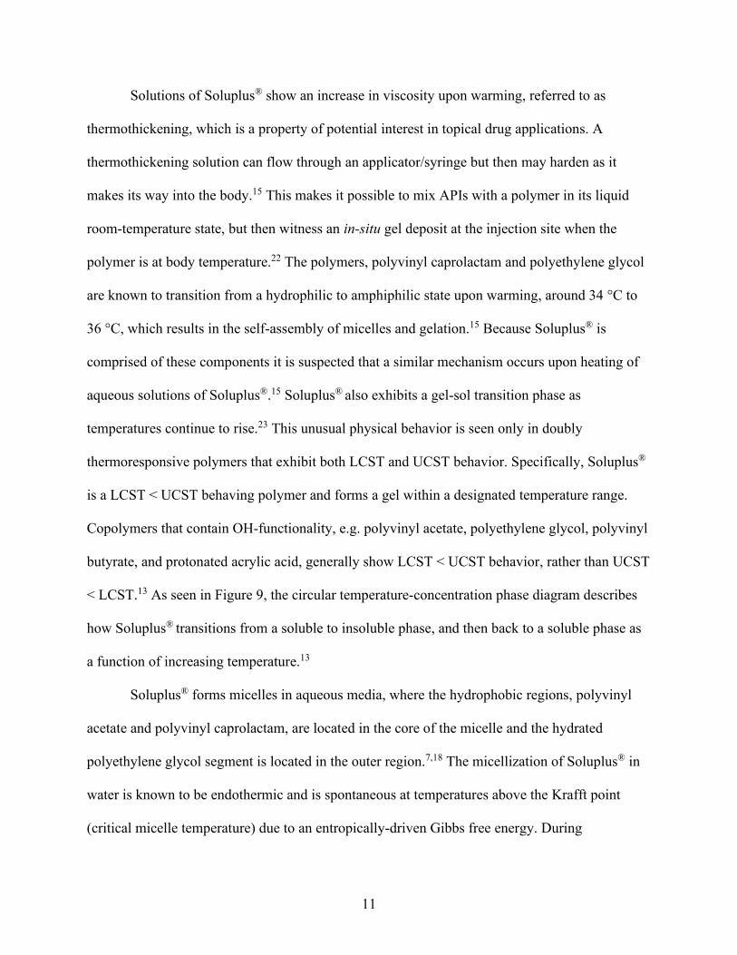
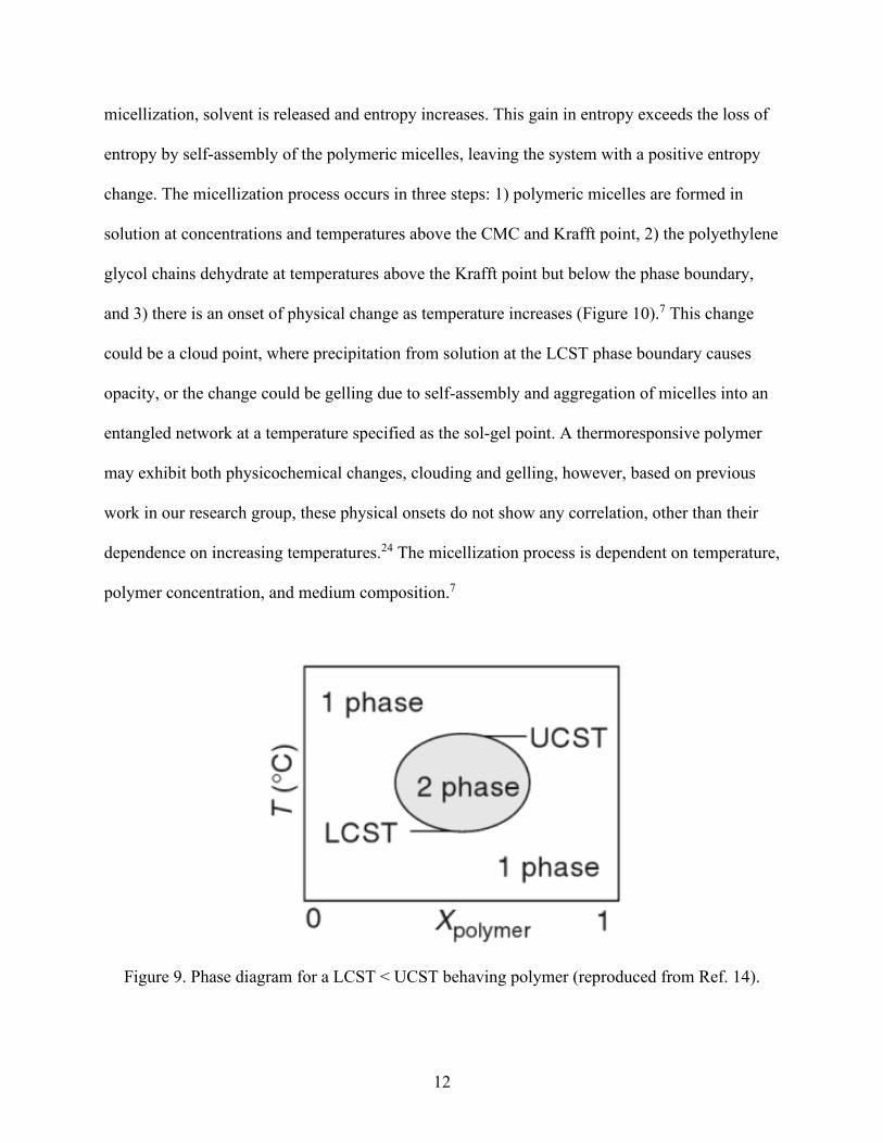