determining the economic effects .)f off-flavor in farm

Determining the economic effects.)f off-flavor in farm-raised catfish

Bulletin 583Alabama Agricultural Experiment Station

r Lowell T. Frobish, Director

March 1987Auburn University

Auburn University, Alabama

CONTENTS

PageINTRODUCTION ............................................. 3

The Catfish Industry........... .................. 4Problem of Off-flavor........... .................. 5Economic Issues of Off-flavor ........................ 5

Impact on Consumers........................... 7Impact on Processors ............................ 7Impact on Producers............. .............. 7

Micro-level Costs............. .............. 7Disequilibrium Costs ......................... 8Revenue Effects ............ ................. 9

METHODOLOGY, DATA, AND STATISTICAL ANALYSIS ........... 12

Modeling Farm Level Demand ...................... 12Data................ ...................... 13Estimating the Model............. ............... 13Demand Elasticities .............................. 16Quasi-pooled Estimates .................................. 18

RESULTS .................................................... 19

Industry-wide Farm Revenue Effects ..................... 19

Distributional Effects .................................... 20

CONCLUSIONS AND IMPLICATIONS ........................... 22

Limitations .................. .................... 24

LITERATURE CITED ................. ........................ 25

FIRST PRINTING 3M, MARCH 1987

Information contained herein is available to all persons,regardless of race, color, sex, or national origin.

DETERMINING THE ECONOMIC EFFECTS

OF OFF-FLAVOR

IN FARM-RAISED CATFISH

SCOTT SINDELAR, HENRY KINNUCAN, AND UPTON HATCH'

INTRODUCTION

THE PRODUCTION of farm-raised catfish is a growing industryin the Southeast, generating additional farm revenues and spurringnew developments and growth in the processing/marketing sector,and providing a new commodity for consumers.

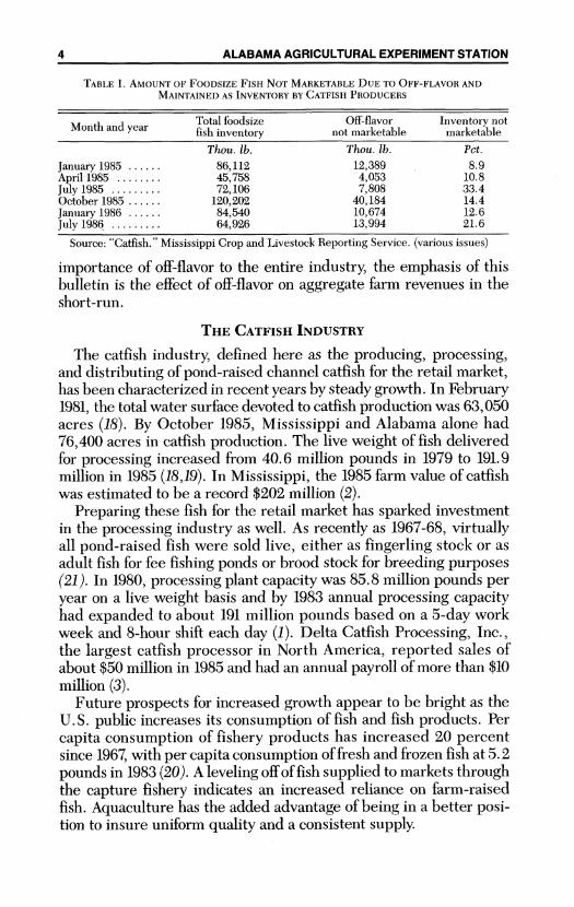
While many of the technical production problems have beensolved for farm raised catfish, a recurrent problem that has caused agreat deal of concern is that of off-flavor. Statistics from Mississippiduring 1985 show that 8.9 to 33.4 percent of the foodsize fish main-tained in inventory by catfish producers could not be marketed on thedesired harvest date due to off-flavor, table 1. This amount variedthroughout the year and was particularly acute from July through No-vember. During July to September of 1983 and 1984, over 50 percentof the catfish ponds evaluated in a study area of western Alabamawere unharvestable at the time of sampling because of off-flavor (9).

Off-flavor affects the producer, processor, and consumer sectors ofthe catfish industry, but the nature of these effects has not been sys-tematically analyzed, discussed, or quantified in an economic sense.It was not the intention of this study to provide a comprehensive ex-amination of the economic impacts of off-flavor, but to look at the ef-fect at one level of the industry, short-run aggregate farm revenues.This bulletin begins with a brief description of the catfish industryand the problem of off-flavor. Next is a general descriptive analysis ofthe economic issues associated with off-flavor, which identifies pos-sible impacts to various sectors and levels of the industry. By identi-fying the economic issues at the various sectors and levels of the cat-fish industry, it is hoped this study will provide a framework foradditional discussion and analysis. While recognizing the economic

'Research Associate and Assistant Professors, respectively, of Agricultural Economics andRural Sociology.

4 ALABAMA AGRICULTURAL EXPERIMENT STATION

TABLE 1. AMOUNT OF FOODSIZE FISH NOT MARKETABLE DUE TO OFF-FLAVOR ANDMAINTAINED AS INVENTORY BY CATFISH PRODUCERS

Month and year Total foodsize Off-flavor Inventory notfish inventory not marketable marketable

Thou. lb. Thou. lb. Pct.

January 1985 ...... 86,112 12,389 8.9April 1985 ........ 45,758 4,053 10.8July 1985 ......... 72,106 7,808 33.4October 1985...... 120,202 40,184 14.4January 1986 ...... 84,540 10,674 12.6July 1986 ......... 64,926 13,994 21.6

Source: "Catfish." Mississippi Crop and Livestock Reporting Service. (various issues)

importance of off-flavor to the entire industry, the emphasis of thisbulletin is the effect of off-flavor on aggregate farm revenues in theshort-run.

THE CATFISH INDUSTRY

The catfish industry, defined here as the producing, processing,and distributing of pond-raised channel catfish for the retail market,has been characterized in recent years by steady growth. In February1981, the total water surface devoted to catfish production was 63,050acres (18). By October 1985, Mississippi and Alabama alone had76,400 acres in catfish production. The live weight of fish deliveredfor processing increased from 40.6 million pounds in 1979 to 191.9million in 1985 (18,19). In Mississippi, the 1985 farm value of catfishwas estimated to be a record $202 million (2).

Preparing these fish for the retail market has sparked investmentin the processing industry as well. As recently as 1967-68, virtuallyall pond-raised fish were sold live, either as fingerling stock or asadult fish for fee fishing ponds or brood stock for breeding purposes(21). In 1980, processing plant capacity was 85.8 million pounds peryear on a live weight basis and by 1983 annual processing capacityhad expanded to about 191 million pounds based on a 5-day workweek and 8-hour shift each day (1). Delta Catfish Processing, Inc.,the largest catfish processor in North America, reported sales ofabout $50 million in 1985 and had an annual payroll of more than $10million (3).

Future prospects for increased growth appear to be bright as theU.S. public increases its consumption of fish and fish products. Percapita consumption of fishery products has increased 20 percentsince 1967, with per capita consumption of fresh and frozen fish at 5.2pounds in 1983 (20). A leveling off of fish supplied to markets throughthe capture fishery indicates an increased reliance on farm-raisedfish. Aquaculture has the added advantage of being in a better posi-tion to insure uniform quality and a consistent supply.

ECONOMIC EFFECTS OF OFF-FLAVOR CATFISH 5

The catfish industry in particular is well positioned to take advan-tage of this situation. The technological problems of production havebeen largely resolved, the enterprise is feasible and profitable withproper management, and consumer acceptance of catfish has grownboth for in-home sales and in added demand from fast food outlets.The entry of Church's, a fast-food type restaurant, in the marketingof catfish products in its retail operations is indicative of this trend.In addition, the poor profitability of row crops, current lower feedprices, and reduced construction costs due to lower energy prices in-dicate increased profits to the fish farmer and may spur new entriesinto production (22). This addition to productive capacity may pro-mote future consumer demand by lowering prices.

PROBLEM OF OFF-FLAVOR

An area that causes concern in the catfish industry is the persistentproblem of off-flavor. Off-flavor occurs when catfish absorb flavorcompounds, produced by pond organisms, that render the fish un-marketable for the period in which the off-flavor exists. Results of anAlabama Agricultural Experiment Station study indicate that thecompound geosmin is the principal cause of most off-flavor in catfishponds during the summer months (11). At present, there are no cost-effective control methods that are satisfactory for most producers. Al-though off-flavor does not permanently damage the product, it doesrepresent an effective supply control that keeps the product in thefarmer's inventory until the fish are marketable. The farmer main-tains the stock until the off-flavor disappears, a matter of months ifkept in the pond or a few days if placed in clean water. Off-flavor isdetected before harvest by taste testers employed by the processor.

The uncertainty surrounding off-flavor, its causes, cures, and test-ing for its presence have created a great deal of concern in the in-dustry. In 1980, the Research Committee of the Catfish Farmers ofAmerica trade organization identified off-flavor as the most seriousproblem the industry faced (11). The concern was due to: (1) the highrate of occurrence, table 1; (2) the damage off-flavor can have on con-sumer confidence; and, (3) the lack of control measures for off-flavor.Alabama producers, responding to a 1984 survey, ranked off-flavor astheir most financially damaging risk (5).

ECONOMIC ISSUES OF OFF-FLAVOR

The catfish industry is a multi-stage system composed of produc-ers, processors, consumers, and other participants (including live-


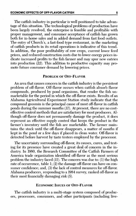
haulers, retailers, and pay-lake operators). Characteristics of the cat-fish market, figure 1, include:

1. A significant amount of the total production available for pro-cessing may be unharvested in any given month or season, table 1.

2. The vast majority of the farm produced supply is sold directly toprocessors, the alternatives being direct sales and live haulers.

3. No close substitutes for catfish exist at the processing level.4. A commodity that is homogenous at the producer level and het-

erogenous at the retail level; this implies that producers are price tak-ers and cannot effectively discriminate in their markets.

Off-flavor is portrayed in figure 1 as a loop in the producing sector.A pond may be available for harvesting, but due to off-flavor, the fishare cycled back into the production process and held in inventory un-til they can be marketed. This supply restriction, imposed by off-fla-vor, has economic impacts at all three stages of the system.

FIG. 1. Simple diagram of the catfish market.

Impact on Consumers

The economic effect of off-flavor on consumers of catfish is largelyin the form of higher prices that result when the amount of the com-modity marketed is less than possible given total production. De-spite the precautions, some off-flavor fish may still reach market.Thus, there is some risk of losing consumers who pay top dollar forgood catfish, but get low quality associated with off-flavor. An effec-tive prevention and control of off-flavor will benefit individual con-sumers by increasing the amount marketed at any given time and byreducing the risk of purchasing an off- flavor product. The aggregateeffect would be increased consumer confidence and acceptability, avital factor for the industry's future growth.

Impact on Processors

The economic problem of the processor is to choose the quantityof catfish under a cost constraint that maximizes profits. At the firmlevel, off-flavor clearly harms processors by keeping input prices upand introducing a degree of uncertainty, particularly in schedulingharvests and anticipating amounts entering the plant. Individualfirms also face a cost in the wage that is paid to the taste testers. Atthe aggregate level, off-flavor reduces the efficiency of the process-ing/marketing sector. An effective prevention or control of off-flavorwill benefit the processing sector through efficiency improvementsthat result from a more dependable supply of on-flavor fish. Harvestschedules and labor assignments at the plant will not be disruptedand orders filled without delay. Input costs may be reduced and in-dividual firms would no longer have to employ the taste testers.

Impact on Producers

Producers were the primary focus of this study. Within this sector,attention was focused on the costs associated with off-flavor. Threelevels of costs due to off-flavor that affect producers have been iden-tified: (1) the micro-level costs to individual producers, (2) the dise-quilibrium in the market caused by reduced marketings, and (3) theshort-run aggregate gross farm revenue effects.

Micro-Level Costs

At the micro, or firm level, there may be direct and indirect coststo individual producers from off-flavor. These are the costs that mostreadily come to mind when people in the industry discuss off-flavor.As described earlier, off-flavor forces the farmer to maintain an in-



ventory of market ready foodsize fish. The direct costs of holding thiscommodity include:

1. The opportunity cost of the delayed income. Since the producercannot harvest and sell the fish when expected, receipt of payment isdelayed.

2. The additional feed costs. The fish held back must be fed. Thecost of this feeding may be somewhat offset by the additional weightgain that occurs in the growing season. The fish, however, may growbeyond the size that processors prefer and larger fish have poorerfeed conversion ratios (10). Outside of the growing season, the ad-ditional feed is merely a maintenance diet.

3. The extra risk of maintaining the inventory. The longer marketready fish are held, the greater the opportunity for disease, pred-ation, or other losses normally encountered in production.

There also may be indirect costs to individual producers. Thefarmer may be bumped from the processor's harvesting schedule,meaning that even if the pond comes back on flavor in a short time,the inventory may have to be maintained until his "turn" comesaround again. In addition, the presence of off-flavor limits the pro-ducer's power to decide when to market his own fish.

Some producers consider these costs high enough that they arewilling to construct holding facilities to purge the fish of off- flavor byplacing them in clean water for several days. For these producers,eliminating the risk and being able to harvest as scheduled mustmore than compensate, at the margin, the weight loss that occursplus the construction and maintenance of these holding facilities.

A technology that effectively prevents or controls off-flavor will, forindividual producers, reduce some of these costs, risks, and uncer-tainties that are connected with off-flavor problems, as well as en-hance their ability to market their product when they choose.

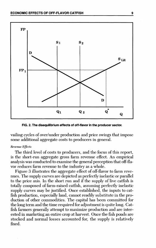
Disequilibrium Costs

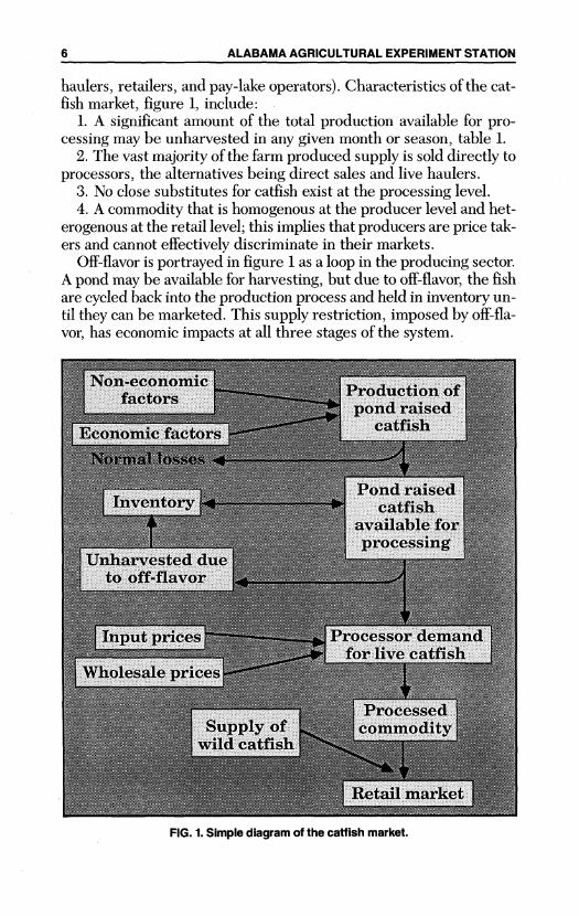
The second level of costs to producers results when the market isin disequilibrium. This is an aggregate cost to producers and is bestdescribed by figure 2. In the graph, S2 represents the short run sup-ply curve of current production, with total quantity Q2, and S1 is theshort run amount marketed, quantity equal to Q1. Q2 - Q1 is theamount withheld from the market due to off-flavor. S(LR) is the longrun supply curve for the industry. Producers respond to price FP, andas they plan the next production cycle, produce out to the intersec-tion of the current price and the long run supply curve, or Q*. Thisresults in overproduction, given the demand, and there will be sub-sequent price drops. This type of disequilibrium results in the pre-


FP

S LR

Q1 Q

FIG. 2. The disequilibrium effects of off-flavor in the producer sector.

vailing cycles of over/under production and price swings that imposesome additional aggregate costs to producers in general.

Revenue Effects

The third level of costs to producers, and the focus of this report,is the short-run aggregate gross farm revenue effect. An empiricalanalysis was conducted to examine the general perception that off-fla-vor reduces farm revenue to the industry as a whole.

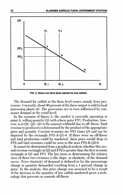
Figure 3 illustrates the aggregate effect of off-flavor to farm reve-nues. The supply curves are depicted as perfectly inelastic or parallelto the price axis. In the short run and if the supply of live catfish istotally composed of farm-raised catfish, assuming perfectly inelasticsupply curves may be justified. Once established, the inputs to cat-fish production, especially land, cannot readily substitute in the pro-duction of other commodities. The capital has been committed forthe long term and the time required for adjustment is quite long. Cat-fish farmers generally attempt to maximize production and are inter-ested in marketing an entire crop at harvest. Once the fish ponds arestocked and normal losses accounted for, the supply is relativelyfixed.

Q2

FP

S1 S 2

D

0 Q1 Q2 Q

FIG. 3. Short-run farm level market for live catfish.

The demand for catfish at the farm level comes mainly from pro-cessors. Currently, about 90 percent of the farm output is sold to localprocessing plants (4). The processors are in turn influenced by con-sumer demand at the retail level.

In the scenario of figure 3, the market is currently operating atpoint A, selling quantity Q1 with a farm price FP1. Production, how-ever, is at Q2. Q2 - Q1 is the amount withheld due to off- flavor. Totalrevenue to producers is determined by the product of the appropriateprice and quantity. Current revenues are FP1 times Q1 and can bedepicted by the rectangle FP1-A-Q1-0. If there were no off-flavorand total production could be marketed, farm price would drop toFP2 and total revenues could be seen in the area FP2-B-Q2-0.

It cannot be determined from a graphical analysis whether this sec-ond revenue rectangle at Q2 and FP2 is greater than the first revenuerectangle at Q1 and FP1. The key issue in determining the relativesizes of these two revenues is the slope, or elasticity, of the demandcurve. Price elasticity of demand is defined to be the percentagechange in quantity demanded resulting from a 1 percent change inprice. In the analysis, this price change was assumed to be a resultof the increase in the quantity of live catfish marketed given a tech-nology that prevents or controls off-flavor.

ALABAMA AGRICULTURAL EXPERIMENT STATION10

If the demand curve in figure 3 is steep enough to be consideredinelastic (if the absolute value of the elasticity is less than 1), increas-ing the amount marketed by effectively preventing or controlling off-flavor and moving from Q1 to Q2 will drive the farm price down sofar that the increased amount sold will not compensate for the pricedrop and aggregate farm revenues will actually decline. In a situationof inelastic demand, then, the presence of off-flavor would serve tokeep farm prices and total farm revenues higher by reducing theamount marketed.

It also should be kept in mind that the quality improvement oc-curring when off-flavor fish are kept off the market may raise the newequilibrium price above that expected. Price (16) and Nguyen and Vo(15) presented this issue in their discussion of discarding low qualityproduce. Basically, the supply shift caused by withholding inferiorproducts from the market is more than compensated for by the risein price due to higher quality. As recognized by the trade association,putting off-flavor fish on the market would damage consumer confi-dence in the product and negatively affect demand.

Many, if not most, agricultural commodities are characterized by ademand that is price inelastic. Government farm programs that at-tempt to raise total farm revenues by controlling supply recognizethis phenomenon. Keeping in mind that we are describing catfishproducers in aggregate and total revenues at the industry level (in-dividual producers obviously will have reduced revenues when pondsare off-flavor), an inelastic farm level demand is plausible for two rea-sons. First, from the processors point of view, there are few substi-tutes for catfish that could be used in their processing plants. Thefewer substitutes available and the more unique the commodity, themore inelastic will be the demand for the commodity. Second, thefarm level demand is related to the demand for catfish at the retaillevel. A commodity that accounts for a small proportion of the con-sumer's budget tends to have less elastic demand curves. Therefore,it is conceivable that the farm level demand for catfish may be inelas-tic and that increasing the amount marketed by solving the problemof off-flavor would reduce total revenues to catfish producers.

This is contrary to the perception that off-flavor reduces total farmrevenues by reducing marketings in the short run. Implicit in thisperception is that the demand faced by catfish producers is price elas-tic. A precise estimate of the demand for catfish at the farm level andthe associated elasticity is necessary for a more accurate assessmentand evaluation of the off-flavor marketing problem. Whether the de-mand is elastic or inelastic is of crucial importance to formulating ap-propriate policy for the industry.


METHODOLOGY, DATA, AND STATISTICAL ANALYSIS

Two previous studies indicate that demand for catfish may, in factbe elastic. A study of Atlanta supermarkets in 1972 estimated a retailprice elasticity at data midpoints of about -2.5 (17). Kinnucan (7) es-timated demand at the wholesale level to be generally elastic, butduring certain seasons of the production year, it may be inelastic.

A model of the farm level demand for live catfish was developed forthis study and estimated using a modified two-stage, least squaresprocedure. Data to estimate the model came from six individual pro-cessing plants. Thus, there were six estimates of the demand elastic-ity. Since the data were from a cross-sectional time series of individ-ual processing plants, a simple procedure to take into account thevariability of the entire data set was used to adjust results from thetwo stage analysis. Adjusted elasticities were calculated from thesecoefficients and weighted by the market shares of the individualplants to estimate an industry-wide, farm level demand elasticity.This weighted average was then used to evaluate potential revenuechanges resulting from off-flavor.

MODELING FARM LEVEL DEMAND

Farm level demand was modeled using a linear function taking theform:

(1) Qt = ao + al FP t + a2SUBP t + a3SPNGt + a4INC t +asMEATt + a6FISHt + Et

where:Qt = the total processed quantity sold in a given month ad-

justed for changes in inventory and per million popu-lation.

FPt = farm price per pound received by producers, liveweight basis.

SUBP t = weighted average of the price received for the two pro-cessed commodities by the five other plants.

SPNGt = spring dummy variable, the months February, March,April.

INC t = personal income in constant terms per million popu-lation.

MEATt = the monthly meat Consumer Price Index (CPI) de-flated by CPI all items.

FISHt = the monthly fish CPI deflated by CPI all items.Et = a random error term.


Farm level demand elasticities were calculated for each plant byusing the coefficient of the farm price obtained from the model andthe mean values of FP and Q from the data set.

DATA

To estimate the model, data from individual processing firms wereused. These data appear in an aggregate form in the USDA's monthlyCatfish Report published by the National Agricultural Statistical Ser-vice. The disaggregated data were made available for this study withthe proviso that individual firms would have their anonymity guar-anteed.

Monthly data from six firms were available, generally covering theperiod January 1980 through December 1983. Data sets were com-plete for three firms, with one firm ceasing to report before the endof the period and two beginning to report after January 1980. The sixplants represented approximately 80 percent of the industry outputover the sample period. The data of interest are the monthly figureson the liveweight amount in pounds delivered for processing, theprice per pound paid to growers, the amount sold as ice pack and theprice received, the amount sold as individually quick frozen and theprice received, and the end of month inventory.

ESTIMATING THE MODEL

The model describes a derived farm level demand as generated bythe processors for live catfish. The disaggregated data provide rathera unique look into the farm level demand in this particular industry,but because of its cross-sectional time series nature it posed some ad-ditional estimation problems. The data were initially evaluated underthis model using an ordinary least squares (OLS) procedure. Thistype of single equation estimation may be appropriate under perfectcompetition, where individual processing firms cannot influence theprice of their inputs, specifically live catfish. In this situation, pro-cessors face a perfectly elastic supply curve for live catfish with thefarm price and quantity determined independently.

A single equation estimation may not be appropriate for the catfishprocessing industry, however. The industry may operate under con-ditions of imperfect competition, with the farm price and quantityjointly determined, indicating that some type of simultaneous equa-tion estimation may be more appropriate (8). Under these conditions,a two-stage, least squares (TSLS) procedure for estimating simulta-neous equations is appropriate.

An additional estimation issue requiring consideration was serialcorrelation in the error terms. This problem became evident when


equation (1) was estimated by the OLS procedure. Serial correlationarises when the disturbance term of one observation is correlatedwith the disturbance term of another observation. It is a commonproblem with time series data of the type used in this analysis. Tocorrect for the problem, a second estimator, an autoregressive max-imum likelihood procedure, was used. In addition, the TSLS esti-mates were obtained using a procedure for estimating simultaneousequations in the presence of serial correlation (6).

In implementing the TSLS procedure, an instrument was con-structed for the endogenous variable, farm price, using additionalpredetermined and exogenous variables that describe the supply in-fluences. These variables were the farm price lagged one period, theprice of soybeans, and a trend variable. The farm price was estimatedin the first stage using these variables plus, following Fair (6), the pre-determined variables from the original equation lagged one period,and a lagged dependent variable.

The first stage, then, is calculated as follows:

(2) FP t = ko + k1 FPt_1 + k2SOYBt + k3 Tt + k4Qt_1 + k5 SUBPt_+ k6SPNGt_1 + klINCt_1 + k8MEATt_1 + k9FISHt_1 + ut

where the as yet undefined variables SOYB and T are the price of soy-beans and trend, respectively.

The predicted farm price from this first stage then acted as the in-strument for FP in the second stage, which used an autoregressivemaximum likelihood procedure to estimate the equation originallyspecified.

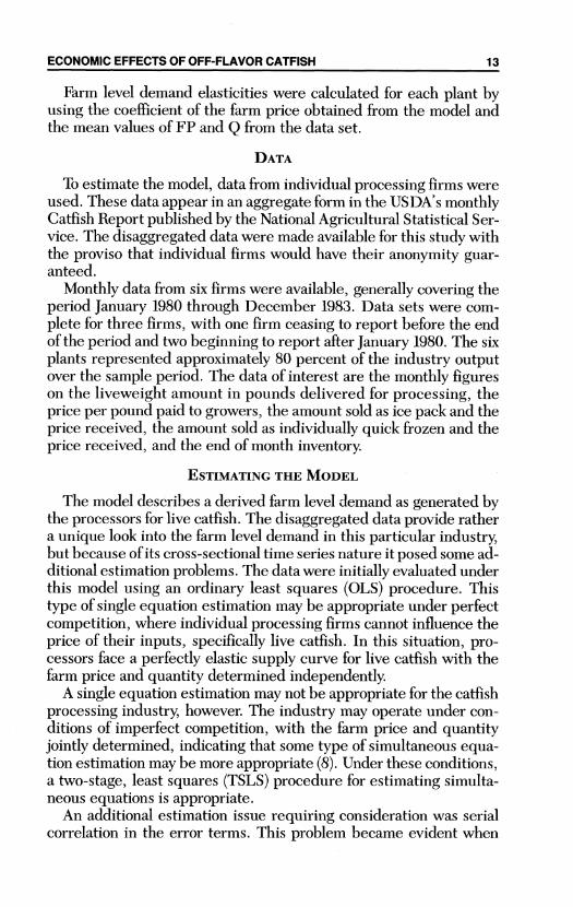
Table 2 presents the results from the three estimation procedures.The R2, a goodness of fit indicator, measures the percentage of thevariation in each plant's purchases that can be explained by the var-iation in the specified variables. The R2's in the OLS estimatesranged from 0.39 for plant F to 0.74 for plant D. The other four plantshad R2 in the 0.51 to 0.63 range. The results from the two stage pro-cedure were the basis for further analysis.

The farm price coefficient was of primary interest in the analysissince it was used to calculate the elasticity. As seen in table 2, thiscoefficient is negative for all firms, as expected, and is significantlydifferent from zero for three firms, B, C, and E. Firm A's farm pricecoefficient has a p-value of between 0.05 and 0.10, providing weakevidence that it is significantly different from zero. Firm A wasunique in that it was on a downward trend throughout the data pe-riod in its liveweight purchases and payments to farmers, and ceasedoperations before the end of 1983. The farm price coefficient cannot


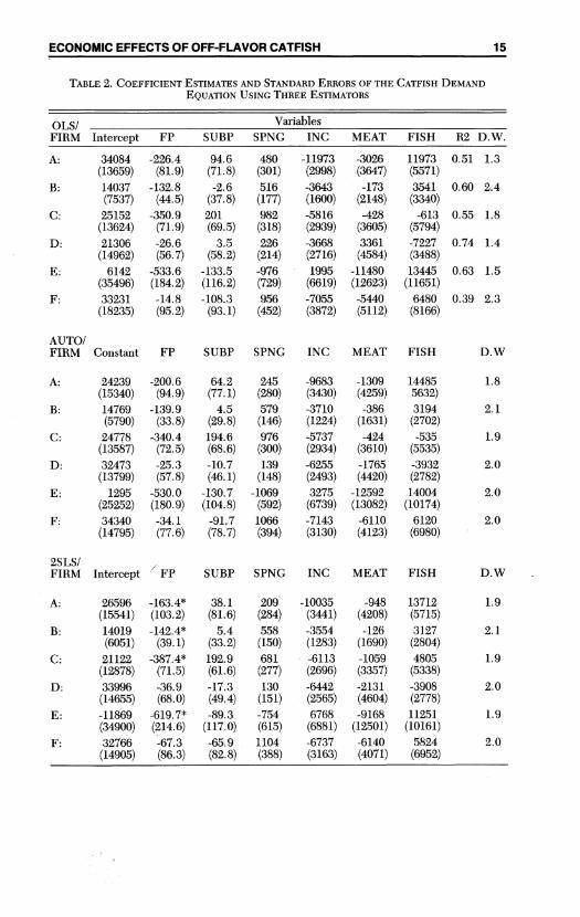
TABLE 2. COEFFICIENT ESTIMATES AND STANDARD ERRORS OF THE CATFISH DEMANDEQUATION USING THREE ESTIMATORS

OLS/ VariablesFIRM Intercept FP SUBP SPNG INC MEAT FISH R2 D.W.

A: 34084 -226.4 94.6 480 -11973 -3026 11973 0.51 1.3(13659) (81.9) (71.8) (301) (2998) (3647) (5571)

B: 14037 -132.8 -2.6 516 -3643 -173 3541 0.60 2.4(7537) (44.5) (37.8) (177) (1600) (2148) (3340)

C: 25152 -350.9 201 982 -5816 -428 -613 0.55 1.8(13624) (71.9) (69.5) (318) (2939) (3605) (5794)

D: 21306 -26.6 3.5 226 -3668 3361 -7227 0.74 1.4(14962) (56.7) (58.2) (214) (2716) (4584) (3488)

E: 6142 -533.6 -133.5 -976 1995 -11480 13445 0.63 1.5(35496) (184.2) (116.2) (729) (6619) (12623) (11651)

F: 33231 -14.8 -108.3 956 -7055 -5440 6480 0.39 2.3(18235) (95.2) (93.1) (452) (3872) (5112) (8166)

AUTO/FIRM Constant FP SUBP SPNG

A: 24239 -200.6 64.2 245(15340) (94.9) (77.1) (280)

B: 14769 -139.9 4.5 579(5790) (33.8) (29.8) (146)

C: 24778 -340.4 194.6 976(13587) (72.5) (68.6) (300)

D: 32473 -25.3 -10.7 139(13799) (57.8) (46.1) (148)

E: 1295 -530.0 -130.7 -1069(25252) (180.9) (104.8) (592)

F: 34340 -34.1 -91.7 1066(14795) (77.6) (78.7) (394)

2SLS/FIRM Intercept FP SUBP SPNG

INC MEAT FISH

-9683 -1309 14485(3430) (4259) 5632)-3710 -386 3194(1224) (1631) (2702)

-5737 -424 -535(2934) (3610) (5535)

-6255 -1765 -3932(2493) (4420) (2782)

3275 -12592 14004(6739) (13082) (10174)-7143 -6110 6120(3130) (4123) (6980)

INC MEAT FISH

A: 26596 -163.4* 38.1 209 -10035 -948 13712(15541) (103.2) (81.6) (284) (3441) (4208) (5715)

B: 14019 -142.4* 5.4 558 -3554 -126 3127(6051) (39.1) (33.2) (150) (1283) (1690) (2804)

C: 21122 -387.4* 192.9 681 -6113 -1059 4805(12878) (71.5) (61.6) (277) (2696) (3357) (5338)

D: 33996 -36.9 -17.3 130 -6442 -2131 -3908(14655) (68.0) (49.4) (151) (2565) (4604) (2778)

E: -11869 -619.7* -89.3 -754 6768 -9168 11251(34900) (214.6) (117.0) (615) (6881) (12501) (10161)

F: 32766 -67.3 -65.9 1104 -6737 -6140 5824(14905) (86.3) (82.8) (388) (3163) (4071) (6952)

D.W

1.8

2.1

1.9

2.0

2.0

2.0

D.W

1.9

2.1

1.9

2.0

1.9

2.0

\~"V'/ \~VV V/ \~-V ~ V/ \VV-/


be considered different from zero for D and F, the smallest and larg-est of the six firms, respectively, in terms of liveweight purchases andpayments to farmers. As the smallest and largest, the behavior ofthese two plants may not be accurately portrayed in the model. Theirpurchase and pricing behavior may be different from the other plants.In addition, plant D, with only 22 observations, may be subject to asmall sample bias. For illustrative purposes, the subsequent analyseswere conducted for all six plants, keeping in mind that plants D andF had statistically insignificant coefficients for the farm price.

A second variable of interest was the income variable. In the mod-ified two-stage least squares results, the coefficient of this variablewas negative and significant in five of the six plants. An interestingimplication of this result is that as incomes rise (all other things beingequal), the amount of catfish purchased decreases. This is consistentwith a perception among some members of the consuming public thatcatfish is typically a commodity purchased by low income consumers.Under this perception and as indicated in the negative coefficient,the consumption of catfish would decrease as family or personal in-come increases. Altering the perception that catfish is a low incomefood commodity may be an area in which the catfish industry can di-rect some of its efforts.

DEMAND ELASTICITIES

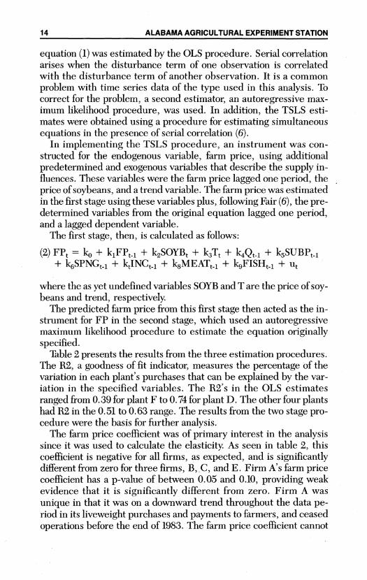
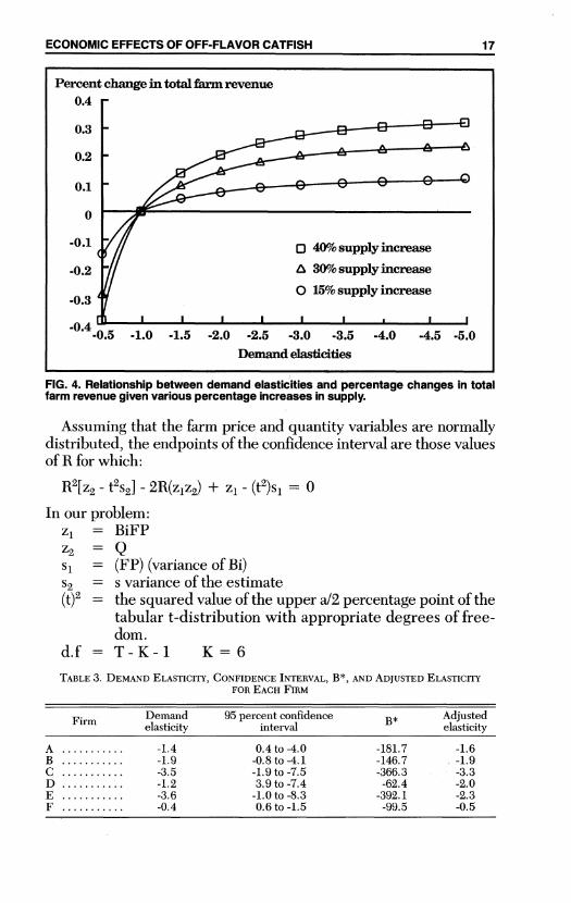
As explained earlier, the demand elasticity is especially importantin the analysis of the farm revenue impacts of off- flavor. As seen infigure 4, a precise estimate of the elasticity is crucial to the analysisof farm revenue changes. The graph shows the percentage change intotal farm revenue associated with some demand elasticity. The mostcrucial changes occur for an elasticity of between -0.5 and -2.0.

The demand elasticity (Ed) was calculated using the formula:

Ed = B x (FP/Q).where B = the coefficient of the farm price from the regressions,

FP = mean farm price, and Q = mean quantity of fish.

Elasticities are all negative, as expected, and with the exception offirm F, all are in the price elastic range, table 3.

Since the equation estimated is assumed to be linear in the origi-nal variables, the estimated elasticity as defined above is partiallyconstructed from a ratio of random variables, farm price, and quan-tity. Considering the importance of this estimate to the analysis, ex-act confidence intervals for these elasticities were constructed usingthe procedure developed by Miller et al. (13), table 3.


ECONOMIC EFF=ECTS OF OFF-FLAVOR CATFISH 1

Percent change in total farm revenue0.4

0.3

0.2

0.1

0 MAI

-0.1 0 40% supply increase

-0.2 A 30%supplyincrease

0 15% supply increase-0.3

-0.4-0.5 -1.0 -1.5 -2.0 -2.5 -3.0 -3.5 -4.0 -4.5 -5.0

Demand elasticities

FIG. 4. Relationship between demand elasticities and percentage changes in totalfarm revenue given various percentage increases in supply.

Assuming that the farm price and quantity variables are normallydistributed, the endpoints of the confidence interval are those valuesof R for which:

R2[ -t 2s2] - 2R(z 1z2 ) + Z1 - (t 2)s 1 = 0In our problem:

z1 = BiFPZ2 = QS1 = (FP) (variance of Bi)S2 = s variance of the estimate

(t)2 = the squared value of the upper a/2 percentage point of thetabular t-distribution with appropriate degrees of free-dom.

d.f =T- K-1 K= 6

TABLE 3. DEMAND ELASTICITY, CONFIDENCE INTERVAL, B*, AND ADJUSTED ELASTICITYFOR EACH FIRM

Fim Demand 95 percent confidence B AdjustedFim elasticity intervalB elasticity

A.............-1.4 0.4 to -4.0 -181.7 -1.6B............. -1.9 -0.8 to -4.1 -146.7 -1.9C............. -3.5 -1.9 to -7.5 -366.3 -3.3D............. -1.2 3.9 to -7.4 -62.4 -2.0E............. -3.6 -1.0Oto -8.3 -392.1 -2.3F............. -0.4 0.6 to -1.5 -99.5 -0.5


Solving the quadratic formula yields the confidence interval aboutthe calculated demand elasticity. All the firms were evaluated at the95 percent confidence level. The plants that showed the highest de-gree of statistical significance in the farm price coefficient had pointestimates of the elasticity well into the elastic range and confidenceintervals that were widely skewed in that direction. Two of theseplants, C and E, accounted for over 40 percent of the industry outputof fish represented by the data. Plant A also had a point estimate thatis elastic, but its confidence interval included the inelastic as well aspositive values, inconsistent with expectations. Plant D, while hav-ing a point estimate that was price elastic, had a confidence intervalso broad as to drastically reduce any meaning to the estimate. PlantF's estimate was price inelastic and its confidence interval is lessskewed to the elastic range than the other plants.

The procedure for calculating exact confidence intervals assumedthat the farm price and quantity are normally distributed randomvariables. This assumption, together with a 95 percent probability,may be too restrictive for the analysis. Nevertheless, these confi-dence intervals indicate that caution must be exercised when inter-preting the calculated price elasticity of demand.

QUASI-POOLED ESTIMATES

As mentioned above, the data are from a cross-sectional time se-ries, so pooling the data and estimating a single equation were alsoexamined. An F-test was constructed using the restricted and un-restricted residual sum of squares from the regressions. The F- testswere highly significant, indicating that pooling could not take place.

Maddala (12, p. 333) suggests an alternative to pooling in whichthe appropriate coefficients are adjusted toward a common mean. Ac-cording to Maddala, "the idea is to bear all the available informationfor the estimation of each regression parameter while at the sametime allowing for potential differences that may exist between the dif-ferent regressions." The procedure is to calculate a B*, an adjustedfarm price coefficient, providing an estimate that is somewhere be-tween pooling all the data and estimating a single equation for all sixplants, and estimating each firm individually. Such a procedurewould be appropriate in this case where some commonalities arelikely among the firms.

B* is calculated using the following formula:

B* - W1Bi + W2B

W1 + W2


where:Bi = estimated coefficient for the ith plantB = the mean of the estimated Bi'sW1 = 1/estimated variance of BiW2 = (N/N-1)(1/t) where:t = (1/N-1)(sum(Bi -B)2) - (1/N)sum(var. Bi)N = number of parameters in the model (= 6)The B*'s for each plant and corresponding elasticities are given in

table 3. Since these adjusted elasticities have incorporated the vari-ability of the entire data set, they will be used in further analysis.These adjusted elasticities, weighted by individual plant marketshares, average -1.8.

RESULTS

The information presented in the preceding section provides themeans to analyze changes in short-run aggregate farm revenue thatmay have occurred in the absence of off-flavor, as if an effective pre-vention or control for off-flavor existed. In this section, both industry-wide and distributional effects are considered.

INDUSTRY-WIDE FARM REVENUE EFFECTS

The weighted demand elasticity of-1.8 is used in the following re-lationship to determine the elasticity of total revenue (Etr) with re-spect to quantity: Etr. = 1 + 1/E

The elasticity of total revenue, defined to be the percentage changein total revenue given a 1 percent change in quantity, is 0.4.

Point estimates of elasticity are generally considered valid only forsmall changes in price. By assuming this 0.4 elasticity for total rev-enue does not change with movement along the demand curve, it isimplicit that the demand elasticity of -1.8 is also constant. For sim-plicity, this was assumed to be the case.

In the analysis, a 15 percent increase in the marketing of live cat-fish under this new technology was assumed. This is approximatelythe yearly average for the percentage of fish held in farmers invento-ries that were unmarketable due to off-flavor as reported in the Mis-sissippi data, and is well below the 50 percent reported during thesummer months in the Alabama survey. It also reflects the uncer-tainties regarding the current status of off-flavor research in terms ofcosts, potential effective controls, and potential adoption.

Using the estimate of the elasticity of total revenues, total revenuescould be increased by 6 percent with a 15 percent increase in quan-tities available for processing. Recognizing that over the data period


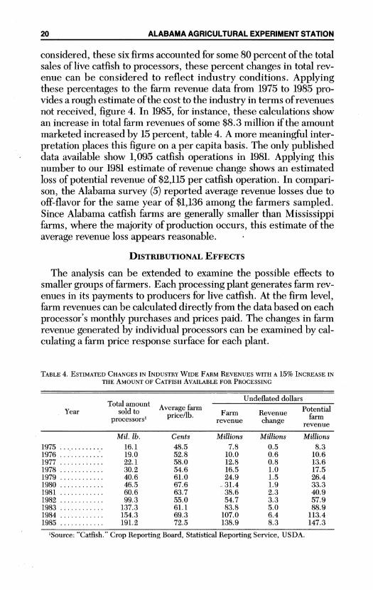
considered, these six firms accounted for some 80 percent of the totalsales of live catfish to processors, these percent changes in total rev-enue can be considered to reflect industry conditions. Applyingthese percentages to the farm revenue data from 1975 to 1985 pro-vides a rough estimate of the cost to the industry in terms of revenuesnot received, figure 4. In 1985, for instance, these calculations showan increase in total farm revenues of some $8.3 million if the amountmarketed increased by 15 percent, table 4. A more meaningful inter-pretation places this figure on a per capita basis. The only publisheddata available show 1,095 catfish operations in 1981. Applying thisnumber to our 1981 estimate of revenue change shows an estimatedloss of potential revenue of $2,115 per catfish operation. In compari-son, the Alabama survey (5) reported average revenue losses due tooff-flavor for the same year of $1,136 among the farmers sampled.Since Alabama catfish farms are generally smaller than Mississippifarms, where the majority of production occurs, this estimate of theaverage revenue loss appears reasonable.

DISTRIBUTIONAL EFFECTS

The analysis can be extended to examine the possible effects tosmaller groups of farmers. Each processing plant generates farm rev-enues in its payments to producers for live catfish. At the firm level,farm revenues can be calculated directly from the data based on eachprocessor's monthly purchases and prices paid. The changes in farmrevenue generated by individual processors can be examined by cal-culating a farm price response surface for each plant.

TABLE 4. ESTIMATED CHANGES IN INDUSTRY WIDE FARM REVENUES WITH A 15% INCREASE INTHE AMOUNT OF CATFISH AVAILABLE FOR PROCESSING

Undeflated dollarsYear Totalamount Average farm PotentialYeaessrsI1 price/lb. Farm Revenue farm

processors revenue change revenue

Mil. lb. Cents Millions Millions Millions1975 ............ 16.1 48.5 7.8 0.5 8.31976 ............ 19.0 52.8 10.0 0.6 10.61977 ............ 22.1 58.0 12.8 0.8 13.61978 ............ 30.2 54.6 16.5 1.0 17.51979 ............ 40.6 61.0 24.9 1.5 26.41980 ............ 46.5 67.6 31.4 1.9 33.31981 ............ 60.6 63.7 38.6 2.3 40.91982 ............ 99.3 55.0 54.7 3.3 57.91983 ............ 137.3 61.1 83.8 5.0 88.91984 ............ 154.3 69.3 107.0 6.4 113.41985 ............ 191.2 72.5 138.9 8.3 147.3

'Source: "Catfish." Crop Reporting Board, Statistical Reporting Service, USDA.


A farm price response surface can be calculated by first estimatinga "collapsed" constant and writing new equations for each plant.These equations are of the form:

Q = a - B*FP"a" is calculated by substituting into the above formula the adjustedfarm price coefficient, B*, and the mean values for farm price andquantity from the data set.

A new farm price can now be determined at any quantity withinthe data range. Again, assuming a 15 percent increase in the quantitymarketed following the development of a technology that effectivelyprevents or controls off-flavor, the effects on farm revenues, or pay-ments by these individual processors, can be evaluated. Percentchanges are derived by comparing the product of this determinedfarm price and quantity with the product of the mean farm price andquantity.

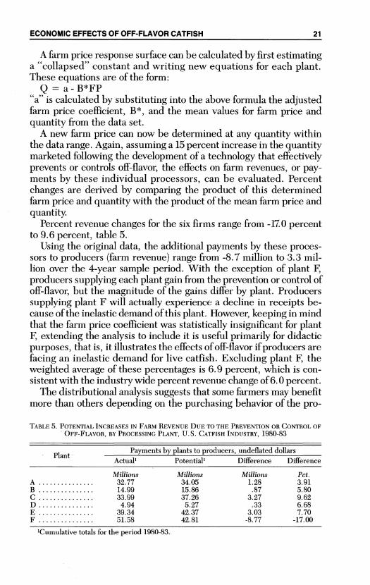
Percent revenue changes for the six firms range from -17.0 percentto 9.6 percent, table 5.

Using the original data, the additional payments by these proces-sors to producers (farm revenue) range from -8.7 million to 3.3 mil-lion over the 4-year sample period. With the exception of plant F,producers supplying each plant gain from the prevention or control ofoff-flavor, but the magnitude of the gains differ by plant. Producerssupplying plant F will actually experience a decline in receipts be-cause of the inelastic demand of this plant. However, keeping in mindthat the farm price coefficient was statistically insignificant for plantF, extending the analysis to include it is useful primarily for didacticpurposes, that is, it illustrates the effects of off-flavor if producers arefacing an inelastic demand for live catfish. Excluding plant F, theweighted average of these percentages is 6.9 percent, which is con-sistent with the industry wide percent revenue change of 6.0 percent.

The distributional analysis suggests that some farmers may benefitmore than others depending on the purchasing behavior of the pro-

TABLE 5. POTENTIAL INCREASES IN FARM REVENUE DUE TO THE PREVENTION OR CONTROL OFOFF-FLAVOR, BY PROCESSING PLANT, U.S. CATFISH INDUSTRY, 1980-83

Payments by plants to producers, undeflated dollarsPlantActual' Potential' Difference Difference

Millions Millions Millions Pct.A ............... 32.77 34.05 1.28 3.91B ............... 14.99 15.86 .87 5.80C ............... 33.99 37.26 3.27 9.62D ............... 4.94 5.27 .33 6.68E ............... 39.34 42.37 3.03 7.70F ............... 51.58 42.81 -8.77 -17.00

'Cumulative totals for the period 1980-83.


cessor with whom they normally do business. For example, in 1981,plant A with 21 percent of the total industry market would have pur-chased catfish from approximately 230 producers. Under the assump-tions of the analysis, each of these producers would have received$1,400 more if the prevention of off-flavor had increased their mar-ketings by 15 percent. The approximately 208 producers selling toplant C, however, would have received an additional $3,400 each.

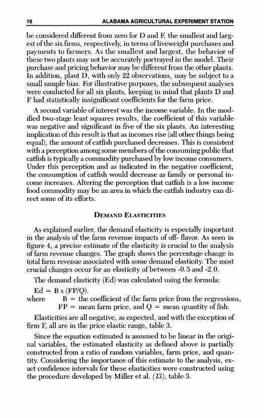
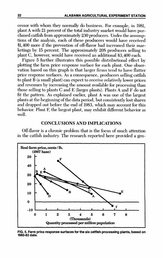
Figure 5 further illustrates this possible distributional effect byplotting the farm price response surface for each plant. One obser-vation based on this graph is that larger firms tend to have flatterprice response surfaces. As a consequence, producers selling catfishto plant B (a small plant) can expect to receive relatively lower pricesand revenues by increasing the amount available for processing thanthose selling to plants C and E (larger plants). Plants A and F do notfit the pattern. As explained earlier, plant A was one of the largestplants at the beginning of the data period, but consistently lost sharesand dropped out before the end of 1983, which may account for thisbehavior. Plant F, the largest plant, may exhibit different behavior aswell.

CONCLUSIONS AND IMPLICATIONS

Off-flavor is a chronic problem that is the focus of much attentionin the catfish industry. The research reported here provided a gen-

Real farm price, cents / Ib.(1967 base)

50

40

30

20

10* E

0

-10 1 I I I ! I I I0 1 2 3 4 5 6 7 8

(Thousands)Quantity processed per million population

FIG. 5. Farm price response surfaces for the six catfish processing plants, based on1980-83 data.


eral outline of the economic issues associated with off-flavor facingthe consumers, processors, and producers of catfish and developedan econometric analysis of off-flavor's effect on short-run farm reve-nues.

The economic effect of off-flavor to consumers of catfish is largelyin the form of higher prices that result when the amount of the com-modity marketed is less than possible given total production. In ad-dition, off-flavor negatively affects consumers' perceptions aboutquality and reduces their confidence when deciding whether to pur-chase catfish. Off-flavor harms processors by keeping prices up andintroducing a degree of uncertainty, particularly in scheduling har-vests and in anticipating the amount of live catfish entering the plant.The economic effect on producers was discussed at three levels. Firstwere the direct costs to individual producers of holding in theirponds a market-sized fish that could not be harvested due to off-fla-vor. Second was the disequilibrium in the market caused by the un-certainty of not knowing the exact level of reduced marketings.Third, and the major focus of this report, was the effect on short-runaggregate farm revenues.

Recognizing the importance of the economic issues outlined, theeconometric analysis developed examined aggregate farm revenuesby modeling farm level demand using data supplied by six processingplants. Calculating the demand elasticity from the econometric re-sults revealed an elastic demand for catfish at the farm level. A de-mand that is price elastic indicates farm revenues will increase whenprice falls due to the greater quantity marketed. This is in contrast tomost agricultural commodities which generally have demands thatare price inelastic. This indicates that preventing or controlling off-flavor will increase the amount marketed and force a lower farmprice, but that the price decrease will be more than compensated bythe greater quantity marketed and total farm revenues will increase.

Using the value of -1.8 as the industry-wide farm level demandelasticity, further analysis calculated potential revenues if a technol-ogy to control or prevent off-flavor existed and allowed marketings toincrease by 15 percent. Keeping in mind the limitations of the anal-ysis, these potential revenues totaled some $8.3 million in 1985, withvalues per catfish operation in 1981 of $2,115. In addition, there maybe distributional effects associated with these enhanced revenues,depending on the processor with whom a producer does business.These results support previous evidence that the catfish industry iscurrently in rather a unique situation for an agricultural commodity,that of having a price elastic demand at the farm level. As a result,


anything that increases the amount marketed, not just preventing off-flavor, will enhance total farm revenue.

An important implication of an elastic demand for catfish regardsthe funding of research to solve the off-flavor problem. An argumentoften presented for funding agricultural research through tax dollarsis that consumers are the primary beneficiaries of such research inthe form of lower food prices. Because solving the off-flavor problemwould raise the farm value of the catfish crop, producers, not con-sumers, may be the primary beneficiaries of a new off-flavor control-ling technology. Thus, producers may wish to consider sharing in thecost of developing the needed technology. These research fundscould be obtained, for example, by increasing the check-off on feedthat currently exists to fund advertising, promotion and new productresearch. The estimates of producer benefits given could serve as abasis for determining the approximate amount of producer revenuesto divert for the funding of research.

LIMITATIONS

The short-run revenue impacts of off-flavor developed in this studyare based on an estimated industry-wide farm level demand elasticityof -1.8 and, moreover, on some general assumptions and additionalrestrictions imposed by the model and analysis. These general as-sumptions include: the quantity of live catfish marketed at any onetime is less than possible because of off-flavor; preventing off-flavorwill increase the quantity marketed in any one period; and that farmlevel demand can be modeled as described and estimated using dis-aggregated data from individual processing plants. The more tech-nical assumptions regarding the estimate were presented in the sec-tion concerning the empirical analysis.

A key assumption used is that off-flavor restricts the amount of livecatfish marketed. One may argue that since off-flavor does not per-manently damage the product, these off-flavor fish are eventually soldand producers, rather than processors, are merely holding an inven-tory. According to the argument, unless these off-flavor fish are heldover from one growing season to the next, off-flavor does not reallyaffect the total amount marketed, only the timing of these market-ings. It is important here to distinguish between quantity producedand available for marketing and actual quantity marketed. At any onetime, the quantity marketed is probably less and certainly no morethan the amount available for that purpose. The assumption in thisstudy, (believed to be the case) is that in any given period, off-flavorreduces the amount actually marketed and preventing or controllingoff-flavor will increase that amount. Whether this will also affect total


production cannot be determined. It is emphasized that this reportfocuses on the short-run effects of off-flavor on total farm revenues,whereas a long-run analysis would consider the nature of the supplyresponse.

LITERATURE CITED

(1) Ammerman, G. 1985. Processing. In Channel Catfish Culture. (C. Tucker,eds.) Elsevier. New York.

(2) Anonymous. 1986. 1985 Was a Great Year for Mississippi's Catfish Farmers.Aquaculture Digest April. 11(4):1.

(3) . 1986. Delta Catfish Processors, Inc. Aquaculture Digest April.11(4):5.

(4) . 1986. PRM Promotes Catfish in July. The Catfish Journal July.1(1):6.

(5) Cacho, 0., H. Kinnucan, and S. Sindelar. 1986. Catfish Farming Risks in Ala-bama. Alabama Agricultural Experiment Station Circular 287.

(6) Fair, R. 1970. The Estimation of Simultaneous Equation Models WithLagged Endogenous Variables and First Order Serially Correlated Errors.Econometrica 38:507-516.

(7) Kinnucan, H. 1986. Demand and Price Relationships for Commercially Pro-cessed Catfish With Industry Growth Projections. Proceedings, Auburn Fish-eries and Aquaculture Symposium. R. O. Smitherman and D. Tave (eds.) Ala-bama Agricultural Experiment Station. (Forthcoming)

(8) and G. Sullivan. 1986. Monopsonistic Food Processing andFarm Prices: The Case of the West Alabama Catfish Industry. Southern Jour-nal of Agricultural Economics 18:15-24.

(9) Lovell, R. T. 1983. Off-flavors in Pond-Cultured Channel Catfish. Water Sci-ence Technology 15:67-73.

(10) . 1984. Effect of Size on Feeding Responses of Catfish in Ponds.Aquaculture Magazine March-April. 10(3):35-36.

(11) and J. Lelana. 1986. Objective Analysis of Fish for Off-flavor.Highlights of Agricultural Research. Alabama Agricultural Experiment Sta-tion. Auburn University 33(1):20.

(12) Maddala, G. 1977. Econometrics. McGraw-Hill, Inc. New York.(13) Miller, A. E., O. Capps, Jr. and G. J. Wells. 1984. Confidence Intervals for

Elasticities and Flexibilities from Linear Equations. American Journal of Ag-ricultural Economics 66:392-396.

(14) Mississippi Crop and Livestock Reporting Service. 1986. Catfish. MississippiDepartment of Agriculture and Commerce. (various issues).

(15) Nguyen, D. and T. Vo. 1985. On Discarding Low Quality Produce. AmericanJournal of Agricultural Economics Aug. 614-18.

(16) Price, D. 1967. Discarding Low Quality Produce With an Elastic Demand.Journal of Farm Economics 57(49):622-632.

(17) Raulerson, R. and W. Trotter. 1973. Demand for Farm-Raised Channel Cat-fish in Supermarkets: Analysis of a Selected Market. USDA Economic Re-search Service. Marketing Research Report No. 993.


26 ALABAMA AGRICULTURAL EXPERIMENTSTATION

(18) USDA. 1982. Aquaculture: Situation and Outlook. Economic Research Ser-vice. AS-3.

(19) . 1986. Catfish. Crop Reporting Board. Statistical Reporting Service(various months).

(20) . 1984. Food Consumption, Prices, and Expenditures, 1963-83. Sta-tistical Bulletin No. 713. Economic Research Service. National EconomicsDivision.

(21) USDI. 1970. A Program of Research for the Catfish Farming Industry. Fishand Wildlife Service. U.S. Bureau of Commercial Fisheries. Ann Arbor,Michigan.

(22) Wilson, W. and G. Sullivan. 1986. Mississippi: Outlook's a Bit Brighter. Eco-nomic Review Federal Reserve Bank of Atlanta. 71(2):77.

.;;: atl L. \p, crimt enl c tatiion SysteiAUBURN UNIVERSITY

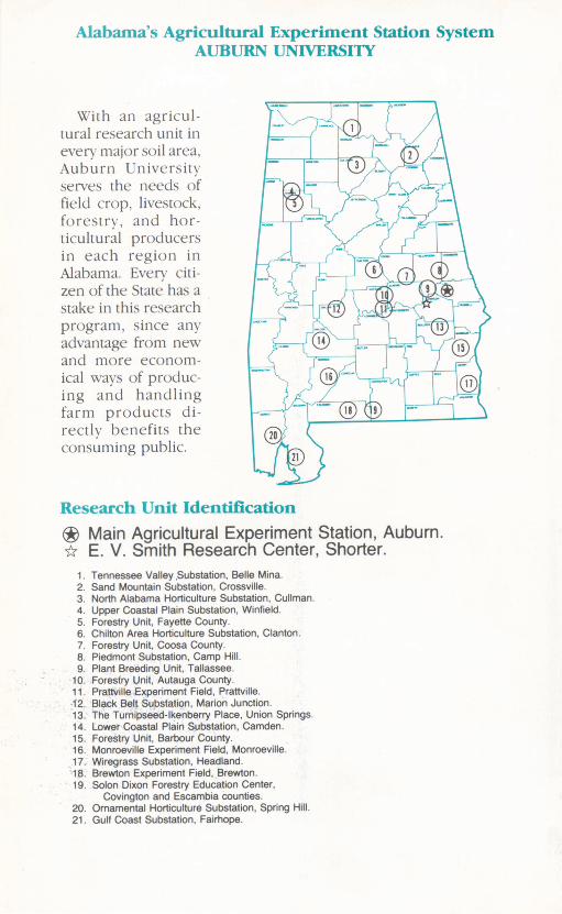
\Wih an agric ul-ttral tear.h it in evert najor soil area.Auburn IUniv ersit x

serves the neecds offfield crop. livestock,forestr y, and hoc - 1ticultural P produtcrsin each region inl 4

Alabama. Fverv c.iti-©Zen of the State has a 1stake in this researc. h ! --program, ince any 13~O '_adv antage from nexx

ital xxavS ot produc-ing aind handlingfarm products di- - ®®irectl\ henetits theconsuming pulblic.

..,.t .irc h i n it kiejiriticatitri

* Main Agricultural Experiment Station, Auburn.a E. V. Smith Research Center, Shorter.

1. Tennessee Valley Substation, Belle Mina.2. Sand Mountain Substation, Crossville3. North Alabama Horticulture Substation, Cullman.4. Upper Coastal Plain Substation, Winfield5. Forestry Unit, Fayette County6 Chilton Area Horticulture Substation, Clanton.7. Forestry Unit, Coosa County.8. Piedmont Substation, Camp Hill.9. Plant Breeding Unit, Tallassee.

10. Forestry Unit, Autauga County11 Prattville Experiment Field, Prattville.12 Black Belt Substation, Marion Junction.13. The Turnipseed-Ikenberry Place, Union Springs.14. Lower Coastal Plain Substation, Camden.15. Forestry Unit, Barbour County.16. Monroeville Experiment Field, Monroeville17. Wiregrass Substation, Headland.18 Brewton Experiment Field, Brewton.19 Solon Dixon Forestry Education Center,

Covington and Escambia counties.20. Ornamental Horticulture Substation, Spring Hill.21. Gulf Coast Substation, Fairhope

determining the economic effects .)f off-flavor in farm

Documents