determining the most efficient type of growth light for an
TRANSCRIPT
Bellarmine University Bellarmine University
ScholarWorks@Bellarmine ScholarWorks@Bellarmine
Undergraduate Theses Undergraduate Works
5-10-2016
Determining the Most Efficient Type of Growth Light for an Determining the Most Efficient Type of Growth Light for an
Aquaponics System using Yellow Lantern Chilies (Capsicum Aquaponics System using Yellow Lantern Chilies (Capsicum
chinense) chinense)
Travis McEachern Bellarmine University, [email protected]
Follow this and additional works at: https://scholarworks.bellarmine.edu/ugrad_theses
Part of the Agribusiness Commons, Agricultural Economics Commons, Bioresource and Agricultural
Engineering Commons, Environmental Design Commons, and the Food Security Commons
Recommended Citation Recommended Citation McEachern, Travis, "Determining the Most Efficient Type of Growth Light for an Aquaponics System using Yellow Lantern Chilies (Capsicum chinense)" (2016). Undergraduate Theses. 9. https://scholarworks.bellarmine.edu/ugrad_theses/9
This Honors Thesis is brought to you for free and open access by the Undergraduate Works at ScholarWorks@Bellarmine. It has been accepted for inclusion in Undergraduate Theses by an authorized administrator of ScholarWorks@Bellarmine. For more information, please contact [email protected], [email protected].
Determining the Most Efficient Type of Growth Light for an
Aquaponics System using Yellow Lantern Chilies (Capsicum chinense)
Travis McEachern
Department of Environmental Studies
Department of Biology Bellarmine University
2
Abstract Aquaponics, a type of urban agriculture, shows potential to produce large amounts of
food with little water and land requirements. Thus, aquaponics could help address the
issue of feeding the growing worldwide population. However, multiple challenges, both
technical and economical, are associated with aquaponics, making large-scale
implementation of these systems difficult – these systems can require tremendous
amounts of energy. This study sought to determine the most efficient types grow lights in
aquaponics systems by comparing the growth rates of yellow lantern chilies (Capsicum
chinense) when grown under four different types of growth lights: light-emitting diode
(LED), metal halide, fluorescent, and induction. The study measured the energy usage of
each light source to determine which type used the least amount of energy, in an effort to
find how to reduce the energy expenses of aquaponics systems, to make the systems more
economically feasible. On average, use of LED and induction growth lights resulted in
the most overall growth and fastest growth rates of pepper plants. These lights are also
known to be relatively energy efficient. Thus, use of LED and induction lamps in
aquaponics systems could result in maximum energy efficiency by increasing plant
production and reducing energy costs. Consequently, implementation of these lights
could make aquaponics more economical for large-scale implementation in the future.
3
Introduction
Stresses of Population Growth
In the last two centuries, the human population has experienced rapid growth. The
current world population is now more than 7 billion people, compared to less than 1
billion only 200 years (Roser 2015). From 1900 to 2000, the human population more than
quadrupled from 1.5 billion people to 6.1 billion (Roser 2015). As overall consumption of
resources has grown alongside the population, an increasing amount of stress has been
placed on the environment in an effort to produce an adequate amount of food and clean
water.
Today, some 70% of available freshwater is used for agricultural irrigation;
furthermore, worldwide, nearly 70% of planted crops never reach the harvest stage due to
environmental factors such as drought, floods, pests, and so on (Despommier 2010).
Presently, about 40% of available land is used for agriculture (Fritsche et al, 2015), an
amount of land comparable to the size of South America (Despommie, 2010). By the year
2050, the global human population is projected to reach 9.6 billion (Goddek 2015). With
traditional farming practices, assuming no increase in their efficiency, approximately
8,500,000km2 of additional cropland would be required to support that amount of people
(Despommier 2010).
Moreover, about 5.7 billion people currently live under conditions of relative water
scarcity, and about 450 million are under severe water stress (Vörösmarty et al. 2000).
Vörösmarty et al. (2000) suggested that much of the world may face substantial
challenges relating to clean water availability and water-related infrastructure in the
future, potentially within the next 25 years. In light of current and projected water
4
shortages and a lack of available farmland to support the growing population
(Despommier 2010), it is appropriate to seek more resource- and water-efficient methods
of food production.
Inefficiencies and Environmental Costs of Traditional Agriculture Developments in agricultural technology have gradually increased food production
for thousands of years. Significant developments in the 18th and 19th centuries in
particular paved the way for the population explosion of the 1900s (Lambert 2013).
However, extensive implementation of conventional agriculture around the world has had
a detrimental effect on soil.
Soil plowing, on which traditional agriculture is largely dependent, releases nutrients
and increases the decomposition rate of organic matter; thus stimulating crop growth in
new fields. However, repeated plowing of fields leads to long-term decreases in water
and nutrient storage capacities of soil (Soil Quality 2011). Plowing also decreases topsoil
depth and organic matter content over time, largely due to increased erosion of exposed
soil. Increased erosion, in addition to losses in nutrient and water content, causes soil
productivity to decline over-time, unless carefully managed (Reganold et al. 1987).
Decreased crop yields due to nutrient losses and increased erosion are often masked
when farmers bring in additional topsoil from other locations and apply fertilizers (Lal
2001). However, application of fertilizers to farmland degrades the environment in other
ways, as evidenced by the Gulf of Mexico “Dead Zone” (Kling 2013; Motsinger 2015).
The “Dead Zone” occurs when fertilizers are carried down he Mississippi River and enter
into the Gulf of Mexico. Once in the gulf, fertilizers induce algal blooms, which
inevitably lead hypoxic conditions as algae die off and consume the oxygen in the water
5
during decomposition. The hypoxia degrades populations of fish and other marine
organisms (Kling 2013; Motsinger 2015).
Additionally, wide-spread application of pesticides is often a characteristic of
conventional agriculture. Pesticides, though they have increased agricultural production,
can have many deleterious consequences for the environment. Damage to farmland,
fisheries and untargeted flora and fauna are a few examples of pesticide-related issues.
Pesticides have also been linked to diseases and increased human mortality in some areas
(Wilson and Tisdell 2001).
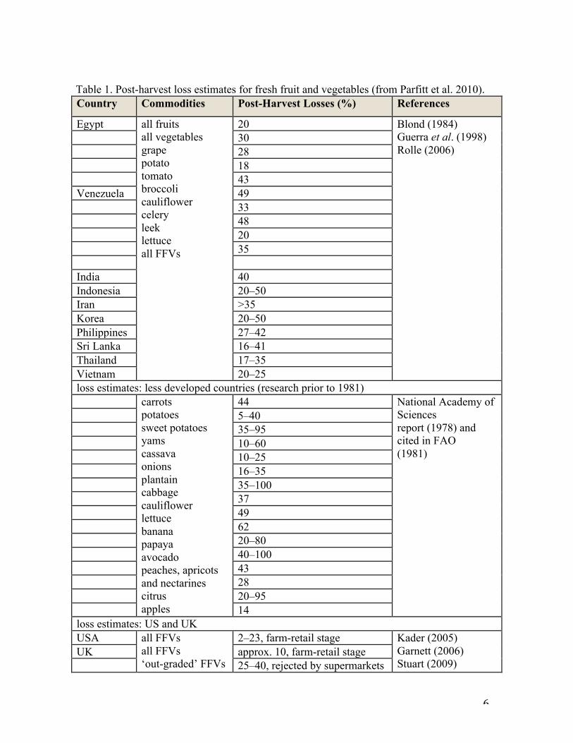
Finally traditional agriculture systems produce a tremendous amount of food waste.
In the United States alone, up to 40% of the food produced does not get eaten (NRDC
2012). Food waste is not an issue in the U.S. alone It is an inefficiency that is common
with traditional agriculture around the world (Table 1). Wasting food means that a
substantial amount of water, soil nutrients and organic matter has been used to no avail.
Food losses occur at various levels of the food production system, including during the
farming process, during harvest and packaging, during processing, and during food
distribution. The difficulty of maintaining crops throughout every step of the production
system is a driving factor for food waste in traditional agricultural systems. Additionally,
the fact that traditional farms are often located far from processors and consumers means
that transportation costs are high: 10% of the total U.S. energy budget is used getting
food to consumers (NRDC 2012).
6
Table 1. Post-harvest loss estimates for fresh fruit and vegetables (from Parfitt et al. 2010). Country Commodities Post-Harvest Losses (%) References
Egypt all fruits all vegetables grape potato tomato broccoli cauliflower celery leek lettuce all FFVs
20 Blond (1984) Guerra et al. (1998) Rolle (2006)
30 28 18 43 Venezuela 49 33 48 20 35 India 40 Indonesia 20–50 Iran >35 Korea 20–50 Philippines 27–42 Sri Lanka 16–41 Thailand 17–35 Vietnam 20–25 loss estimates: less developed countries (research prior to 1981) carrots
potatoes sweet potatoes yams cassava onions plantain cabbage cauliflower lettuce banana papaya avocado peaches, apricots and nectarines citrus apples
44 National Academy of Sciences report (1978) and cited in FAO (1981)
5–40 35–95 10–60 10–25 16–35 35–100 37 49 62 20–80 40–100 43 28 20–95 14 loss estimates: US and UK USA all FFVs
all FFVs ‘out-graded’ FFVs
2–23, farm-retail stage Kader (2005) Garnett (2006) Stuart (2009)
UK approx. 10, farm-retail stage 25–40, rejected by supermarkets
7
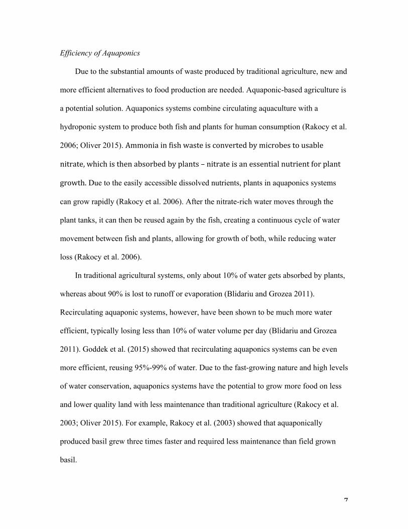
Efficiency of Aquaponics Due to the substantial amounts of waste produced by traditional agriculture, new and
more efficient alternatives to food production are needed. Aquaponic-based agriculture is
a potential solution. Aquaponics systems combine circulating aquaculture with a
hydroponic system to produce both fish and plants for human consumption (Rakocy et al.
2006; Oliver 2015). Ammonia in fish waste is converted by microbes to usable
nitrate, which is then absorbed by plants – nitrate is an essential nutrient for plant
growth. Due to the easily accessible dissolved nutrients, plants in aquaponics systems
can grow rapidly (Rakocy et al. 2006). After the nitrate-rich water moves through the
plant tanks, it can then be reused again by the fish, creating a continuous cycle of water
movement between fish and plants, allowing for growth of both, while reducing water
loss (Rakocy et al. 2006).
In traditional agricultural systems, only about 10% of water gets absorbed by plants,
whereas about 90% is lost to runoff or evaporation (Blidariu and Grozea 2011).
Recirculating aquaponic systems, however, have been shown to be much more water
efficient, typically losing less than 10% of water volume per day (Blidariu and Grozea
2011). Goddek et al. (2015) showed that recirculating aquaponics systems can be even
more efficient, reusing 95%-99% of water. Due to the fast-growing nature and high levels
of water conservation, aquaponics systems have the potential to grow more food on less
and lower quality land with less maintenance than traditional agriculture (Rakocy et al.
2003; Oliver 2015). For example, Rakocy et al. (2003) showed that aquaponically
produced basil grew three times faster and required less maintenance than field grown
basil.
8
Additionally, because aquaponics systems are typically managed indoors, under
controlled conditions, crops and fish can be harvested from these systems year-round.
Since aquaponics systems are not exposed to seasonal changes and harsh weather, they
can be much more annually productive, per unit area, than traditional farmland.
Moreover, because of the ability to produce these systems indoors, aquaponics systems
can be located within cities, where food demand is highest. As a result, wide-spread
application of these systems would mean that food is located much closer to consumers.
Thus, shorter transportation distances between producers and consumers could radically
reduce the above mentioned energy use and food waste produced in conventional
agriculture (NRDC 2012).
Pitfalls of Aquaponics Despite the efficiency and potential of aquaponics, these systems have challenges
that hinder large scale implementation. Aquaponics systems rely on a delicate balance
between three types of organisms: fish, plants and bacteria (which turn fish waste into
usable nutrients). Conditions within the systems must be supportive of all three types of
organisms for the system to function optimally (Goddek et al 2015; Shafeena 2016;
Tyson et al 2011; Somerville et al. 2014). (Water quality conditions ideal for each
organism and for the system as a whole are shown in Tables 2.1 and 2.2.) Therefore,
water quality testing is important in these systems in order to ensure optimal production.
Treatments – such as the additional of bases, micronutrients, or changing fish-feeding
patterns – may also be necessary to keep conditions ideal.
9
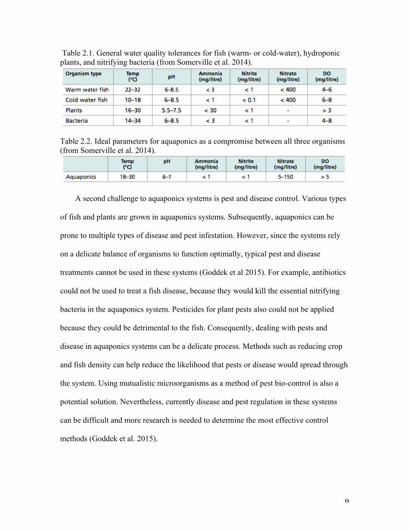
Table 2.1. General water quality tolerances for fish (warm- or cold-water), hydroponic plants, and nitrifying bacteria (from Somerville et al. 2014).
Table 2.2. Ideal parameters for aquaponics as a compromise between all three organisms (from Somerville et al. 2014).
A second challenge to aquaponics systems is pest and disease control. Various types
of fish and plants are grown in aquaponics systems. Subsequently, aquaponics can be
prone to multiple types of disease and pest infestation. However, since the systems rely
on a delicate balance of organisms to function optimally, typical pest and disease
treatments cannot be used in these systems (Goddek et al 2015). For example, antibiotics
could not be used to treat a fish disease, because they would kill the essential nitrifying
bacteria in the aquaponics system. Pesticides for plant pests also could not be applied
because they could be detrimental to the fish. Consequently, dealing with pests and
disease in aquaponics systems can be a delicate process. Methods such as reducing crop
and fish density can help reduce the likelihood that pests or disease would spread through
the system. Using mutualistic microorganisms as a method of pest bio-control is also a
potential solution. Nevertheless, currently disease and pest regulation in these systems
can be difficult and more research is needed to determine the most effective control
methods (Goddek et al. 2015).
10
One final major challenge to aquaponics systems is high-energy costs. In aquaponics
systems, fluctuations in temperature and light availability can harm fish, plants, and
bacteria in the system or cause system productivity to decrease; consequently,
maintaining stable conditions is crucial (Goddek 2015). Sustaining temperature and light
availability, however, can require a lot of energy, making maintenance of the conditions
an expensive proposition.
The Purpose of this Study In order to maximize the potential of aquaponics agricultural systems, it is important
to optimize the efficiency of the systems on an economic basis. If these systems cannot
be made efficient enough to be economically feasible, then they will not be implemented
on a scale large enough to benefit the environment or increase food security. Because one
of the biggest hindrances to aquaponics systems is the cost of energy, discovering the
most efficient type of growth lights could be very beneficial to the long-term
implementation of aquaponics systems. The aim of this experiment was to find what type
of growth light produces the highest plant growth rate with the lowest energy usage.
Different types of lights use varying amounts of energy – whichever light uses the
least energy will be the least expensive to operate. However, for application in
agriculture, it is also important to take into account what growth rates different lights may
produce in the plants. Simply knowing what light uses the least amount of energy is not
enough. To make aquaponics more efficient, it is important to know what types of lights
produce the most plant growth, for the least amount of energy.
In this experiment, yellow lantern chilies (Capsicum chinense) were grown in four
controlled aquaponics systems at Kentucky State University. Each system was divided

11
further into four sections, and each section was grown under a different type of grow
light: induction (IND), metal halide (MH), fluorescent (FL), or light emitting diode
(LED). Induction lights uses an electric or magnetic field to generate power, which is
then transferred into a gas discharge lamp, which emits photons. Metal halide lights
produce light by creating an electric arc in a gaseous metal-halide mixture. Fluorescent
lights run an electric current through mercury vapor, producing ultraviolet light. LED
lights contain a semiconductor. When a sufficient amount of voltage is passed through
the semiconductor, energy is released as photons.
Plants were grown for 55 days under the various light sources. Overall growth,
growth rates and average electricity usage for each type of light were determined. This
study had two purposes: (1) to determine which type of light produces the most plant
growth and (2) to determine which light sources could be used to reduce energy costs,
making operation of aquaponics systems more economically feasible.
Since the different types of lights have different properties and may produce light on
varying spectrums, they may not all influence plant growth the same way. This
experiment seeks to determine what type of light produces the most plant growth with the
least amount of energy. In other words, which light produces the most product for the
least cost? By determining which light produces the most plant growth per unit of energy,
this experiment can help aquaponics users optimize their systems. Such optimization
could make aquaponics more economically feasible, resulting in the implementation of
aquaponics on a larger scale. Large scale implementation of aquaponics could not only
increase food production and food security, but could reduce reliance on traditional
12
agriculture, thus alleviating some of the issues with traditional agriculture, such as
fertilizer and pesticide pollution, soil degradation, and inefficient water use.
Materials and Methods System Design The experimental design consisted of four aquaponic systems, each of which
contained a total of six water tanks: a 110 gallon fish tank, a 55 gallon clarifier tank for
filtering out large solids, a 45 gallon biofilter, two 120 gallon plant tanks, and a small
sump tank.
Water began in the fish tank, where the fish were raised and fed, and thus where fish
waste (the nutrient source for the plants) was produced (Figure 1). From the fish tank,
water flowed into a solid-filtering tank. This tank was divided in half by a plastic barrier,
which reached to the top of the tank but left room for water to pass underneath.
Consequently, water descended to the bottom of the tank before filling the other side and
passing on to the biofilter. The descent of the water provided ample time for large solid
waste to settle out into the bottom of the tank, where it was then be flushed out on a daily
basis using a release valve at the bottom of the tank. Water entered the biofilter (another
water tank filled with plastic netting) at the bottom of the tank and flowed up. While the
water ascended through the biofilter, fine solids collected on the netting, thus reducing
the collection of fine solids on plant roots. If too many fine solids collected on the plant
roots, they would interfere with the plants’ ability to absorb water and nutrients.
Furthermore, the biofilter allowed for the growth of microbes, which breakdown
ammonia-based fish waste, converting it into dissolved nitrate that the plants can use.
After passing through the filtering stages, the nutrient rich water flowed into the plant

13
tanks. The plants were positioned in Styrofoam holders, which allowed the roots hang
suspended in the water, while the rest of the plant was supported above. After passing
through the plant tanks, water flowed in the sump tank, where water was collected and
actively pumped back up into the fish tank to repeat the cycle. The sump pump was the
only active pump in the system; the rest of the tank transitions were gravity-fed.
The systems were further divided into four sections, one section for each type of
growth light (Figure 1). The order of the lights was different in each of the four systems
to prevent any bias that could result from the order in which plants received water. For
example, in system one, section one, two, three, and four could have induction, metal
halide, fluorescent, and LED lights, respectively. The order of lights per section in system
two however would have been metal halide, fluorescent, LED, and induction. Thus the
order of lights in each system varied and each light appeared in each section once. This
was done because plants at the front of the tanks (section one) had access to higher
concentrations of nutrients, while plants towards the tank exit (section four) had access to
fewer nutrients due to continual absorption as water moved through the tank. Alternating
the order of lights in each system reduced the potential that differences in plant growth
were affected by nutrient availability and thus enabled conclusions on plant growth to be
based on the light sources alone.
Each section of the system was separated using black plastic barriers to prevent light
from one section spilling over into adjacent sections and influencing the light absorption
by plants in the other sections. Each section contained five plants. One plant was placed
in each of the four corners of the section, with one plant in the middle,
14
Light intensity readings for each section were taken at the level of the highest leaves
from each section’s tallest plants. These measurements were taken twice per week using a
Photosynthetically Active Radiation (PAR) meter. PAR meters measure the intensity of
light within light spectrum that plants primarily use for photosynthesis. PAR was
measured to make sure that the plants under every light were receiving the same amount
of light, ensuring that some plants would not have advantages over others due to more
light intensity. Light heights were adjusted twice per week in order to maintain a PAR
reading of 200 +/- 5 umol/m2/s over each section.
Water Quality Assessments Water pH was measured twice daily and maintained using additions of potassium
hydroxide (KOH) and calcium hydroxide (CaOH) into the sump tank when the water
became too acidic. Under normal conditions, water in aquaponics systems tends to
become acidic due to the buildup of nitrogen waste. Therefore, the aforementioned bases
were mixed gradually into the sump tank of each system to keep the system’s water
within a pH range of 6.8-7.0. Base additions were added in increments of 15g-30g at a
time, depending on the pH of the water at that time.

15
Figure 1. The diagram shows the layout of each of the four aquaponic systems. The arrows demonstrate the continuous flow of water through the six tanks used in this system. Each tank is represented by a color. Dark blue denotes where the fish were kept and where waste (nutrients) originated. Light blue indicates tanks that were important for water cleaning processes. Green tanks are where plants were grown in float beds in nutrient-rich water. Yellow denotes where used water collected before being actively pumped back into the system. Arrows indicate the direction of water flow between tanks. The yellow arrow denotes water that is actively pumped, whereas black arrows are gravity-fed. The dotted orange lines indicate the location of plastic walls used as light barriers, effectively isolating each section of the fish tank from the other sections, thus allowing a different light source to be used within each section. Plastic barriers also encircled the two fish tanks as a whole, although not shown in the diagram, to reduce the amount of ambient light reaching the plants from outside the system. Furthermore, detailed water analysis tests were conducted twice weekly. Nitrite,
nitrate, total ammonia, iron, and alkalinity measurements were taken during these tests.
Dissolved iron levels were maintained between 1.5-3.0 mg/L. Total ammonia, nitrite and
nitrate levels were monitored in order to visualize the overall health of the systems. Total
ammonia and nitrite levels were not allowed to rise above 1 mg/L, because high levels of
these constituents can cause adverse effects on the fish in the system. If ammonia or
16
nitrite levels became too high, the fish in the given system skipped a feeding or two until
the levels dropped. (Nitrogenous fish waste is the cause for total ammonia and nitrite
buildup.) Contrarily, nitrate is an essential source of nitrogen used by plants. Thus, it was
necessary to keep nitrate levels high (>20mg/L). Consequently, all of the above
measurements were taken regularly in order to find a balanced fish-feeding pattern,
which would allow sufficient amount of nitrate to be produced without excessive buildup
of nitrite.
Other conditions monitored during the experiment included humidity and
temperature within each section. On average, the temperature for each section was
maintained between 28 and 32 degrees Celsius. Slight variations in temperature between
sections were caused due to the various lights being used in each section. Humidity was
more variable than temperature, with measurements usually falling between 40% and
70%. Fans were used above each section to keep humidity levels constant, but levels still
varied between sections.
Measurements Each plant was numbered, and heights were measured in centimeters twice per week
from the base of the plant (where roots started) to the top of the highest leaf. Plant heights
were measured regularly throughout the 55-day experiment, but only final heights were
used for results. The average wet weight of the plants was measured, in grams, before the
study using a representative sample (10%) of the plants and averaging their weights.
Weight for each plant was measured after the study and compared to the average original
weight, as a way of measuring biomass growth during the project. The final weights of
17
plants that were grown under each light were averaged together and used for comparison
against the initial average plant weight.
Each light source was connected to an energy meter, which measured total kilowatt
hours (kWh) used per day. The kWh/day averages were used to calculate overall plant
growth per kWh in g/m2/kWh. This unit allowed for the comparison of total biomass
growth (g) in a given area (m2), per unit of energy (kWh). The amount of energy used by
each light was also used to determine the cost to run each light throughout the study,
using average energy costs for the residential sector of the state of Kentucky (provided by
the U.S. Energy Information Administration).
Calculations The final mean weights and heights of the plants of each section were calculated.
The average biomasses from each light source, pooled across all four systems, were then
compared to determine which light source encouraged the most growth.
Measurements for kWh/day were recorded for each light twice a week. After the
experiment was concluded, the biweekly records were used to calculate the average
kWh/day for each light. The energy meter on one LED light only recorded energy usage
in watts, not kWh, so the following calculation was used to determine the kWh/day usage
of this light:
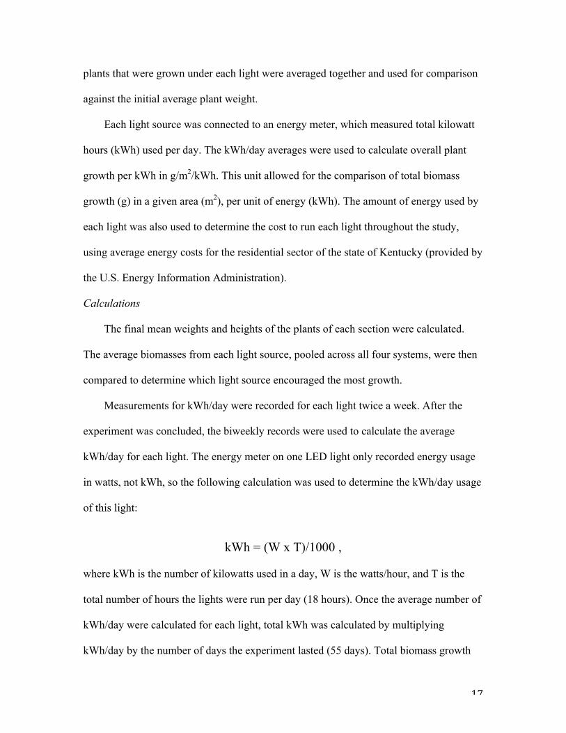
kWh = (W x T)/1000 ,
where kWh is the number of kilowatts used in a day, W is the watts/hour, and T is the
total number of hours the lights were run per day (18 hours). Once the average number of
kWh/day were calculated for each light, total kWh was calculated by multiplying
kWh/day by the number of days the experiment lasted (55 days). Total biomass growth
18
under each light was then calculated by adding the overall biomass of the five plants in
each section and subtracting by 45.5 g (five times 9.1g, the average weight of all plants
initially). This measurement equated to g/m2 because it represents the total net biomass
growth per square meter, the area under each growth light. Finally, g/m2 of each section
was divided by the total kWh of each section to yield the total biomass growth per unit
area per unit of energy (g/m2/kWh) for each light in the four systems. Furthermore, the
above results were averaged for each light source, and used to compare the total energy
use and average g/m2/kWh for each type of light. These results were used to analyze
which light source encouraged the most efficient plant growth.
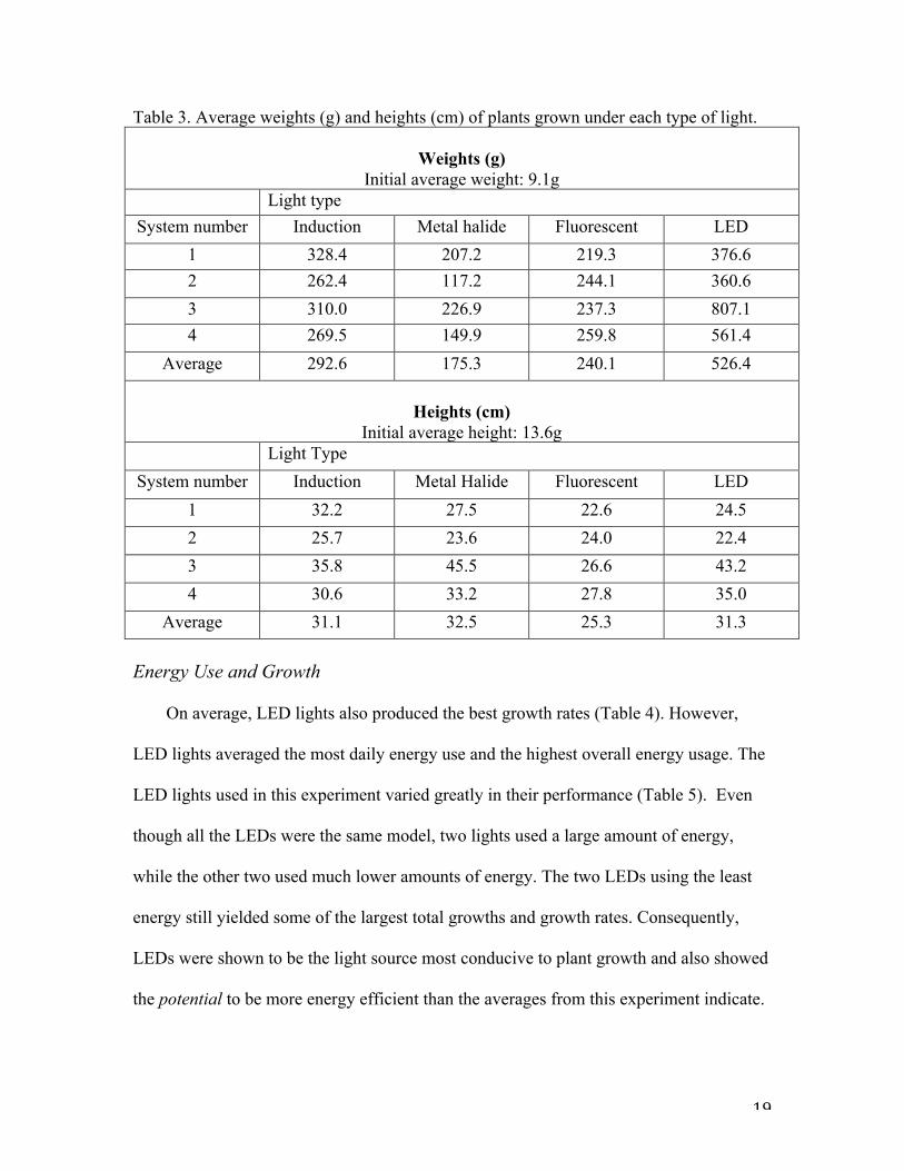
Results Weights and Heights Overall plant growth was expressed in weight and plant height. The average initial
heights and weights of the seedlings were 13.6 cm and 9.1 g, respectively. Plants grown
under LED lights showed the most overall growth (Table 3). LED-grown plants had an
average weight more than two times the weight of metal halide- and fluorescent-grown
plants and outweighed induction grown plants by over 200 g. Furthermore, LED-grown
plants resulted in the second highest average height. Together, the weights and heights
indicate that LED-grown plants were more productive than plants growing under other
types of lights. Metal halide-grown plants, on average, achieved the tallest plant height
but had the lowest average weights. Fluorescent- and induction-grown plants had
relatively similar plant weights; however, fluorescents were substantially shorter than the
plants grown under any of the other light types (Table 3).
19
Table 3. Average weights (g) and heights (cm) of plants grown under each type of light.
Weights (g) Initial average weight: 9.1g
Light type System number Induction Metal halide Fluorescent LED
1 328.4 207.2 219.3 376.6 2 262.4 117.2 244.1 360.6 3 310.0 226.9 237.3 807.1 4 269.5 149.9 259.8 561.4
Average 292.6 175.3 240.1 526.4
Heights (cm) Initial average height: 13.6g
Light Type System number Induction Metal Halide Fluorescent LED
1 32.2 27.5 22.6 24.5 2 25.7 23.6 24.0 22.4 3 35.8 45.5 26.6 43.2 4 30.6 33.2 27.8 35.0
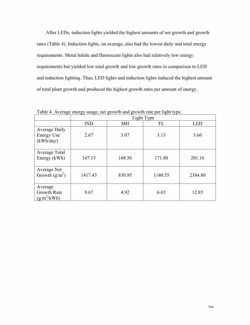
Average 31.1 32.5 25.3 31.3 Energy Use and Growth On average, LED lights also produced the best growth rates (Table 4). However,
LED lights averaged the most daily energy use and the highest overall energy usage. The
LED lights used in this experiment varied greatly in their performance (Table 5). Even
though all the LEDs were the same model, two lights used a large amount of energy,
while the other two used much lower amounts of energy. The two LEDs using the least
energy still yielded some of the largest total growths and growth rates. Consequently,
LEDs were shown to be the light source most conducive to plant growth and also showed
the potential to be more energy efficient than the averages from this experiment indicate.
20
After LEDs, induction lights yielded the highest amounts of net growth and growth
rates (Table 4). Induction lights, on average, also had the lowest daily and total energy
requirements. Metal halide and fluorescent lights also had relatively low energy
requirements but yielded low total growth and low growth rates in comparison to LED
and induction lighting. Thus, LED lights and induction lights induced the highest amount
of total plant growth and produced the highest growth rates per amount of energy.
Table 4. Average energy usage, net growth and growth rate per light type. Light Type IND MH FL LED Average Daily Energy Use (kWh/day)
2.67
3.07
3.13
3.66
Average Total Energy (kWh)
147.13
168.56
171.88
201.16
Average Net Growth (g/m2)
1417.43
830.95
1140.55
2384.80
Average Growth Rate (g/m2/kWh)
9.67
4.92
6.65
12.85
21
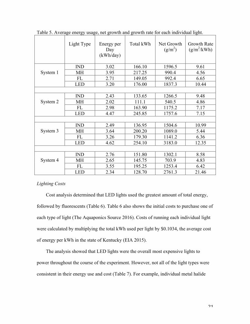
Table 5. Average energy usage, net growth and growth rate for each individual light.
Light Type
Energy per
Day (kWh/day)
Total kWh
Net Growth
(g/m2)
Growth Rate (g/m2/kWh)
System 1
IND 3.02 166.10 1596.5 9.61 MH 3.95 217.25 990.4 4.56 FL 2.71 149.05 992.4 6.65
LED 3.20 176.00 1837.3 10.44
System 2
IND 2.43 133.65 1266.5 9.48 MH 2.02 111.1 540.5 4.86 FL 2.98 163.90 1175.2 7.17
LED 4.47 245.85 1757.6 7.15
System 3
IND 2.49 136.95 1504.6 10.99 MH 3.64 200.20 1089.0 5.44 FL 3.26 179.30 1141.2 6.36
LED 4.62 254.10 3183.0 12.35
System 4
IND 2.76 151.80 1302.1 8.58 MH 2.65 145.75 703.9 4.83 FL 3.55 195.25 1253.4 6.42
LED 2.34 128.70 2761.3 21.46 Lighting Costs Cost analysis determined that LED lights used the greatest amount of total energy,
followed by fluorescents (Table 6). Table 6 also shows the initial costs to purchase one of
each type of light (The Aquaponics Source 2016). Costs of running each individual light
were calculated by multiplying the total kWh used per light by $0.1034, the average cost
of energy per kWh in the state of Kentucky (EIA 2015).
The analysis showed that LED lights were the overall most expensive lights to
power throughout the course of the experiment. However, not all of the light types were
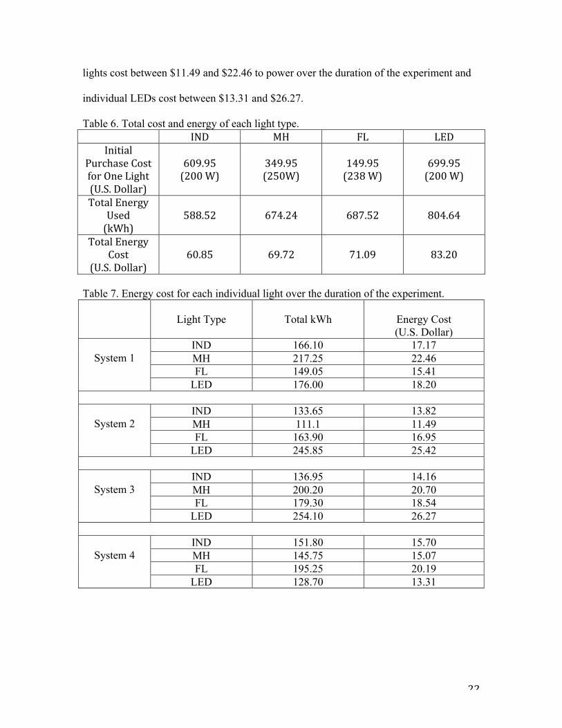
consistent in their energy use and cost (Table 7). For example, individual metal halide
22
lights cost between $11.49 and $22.46 to power over the duration of the experiment and
individual LEDs cost between $13.31 and $26.27.
Table 6. Total cost and energy of each light type. IND MH FL LED
Initial Purchase Cost for One Light (U.S. Dollar)
609.95 (200 W)
349.95 (250W)
149.95 (238 W)
699.95 (200 W)
Total Energy Used (kWh)
588.52
674.24
687.52
804.64
Total Energy Cost
(U.S. Dollar)
60.85
69.72
71.09
83.20
Table 7. Energy cost for each individual light over the duration of the experiment.
Light Type
Total kWh
Energy Cost (U.S. Dollar)
System 1
IND 166.10 17.17 MH 217.25 22.46 FL 149.05 15.41
LED 176.00 18.20
System 2
IND 133.65 13.82 MH 111.1 11.49 FL 163.90 16.95
LED 245.85 25.42
System 3
IND 136.95 14.16 MH 200.20 20.70 FL 179.30 18.54
LED 254.10 26.27
System 4
IND 151.80 15.70 MH 145.75 15.07 FL 195.25 20.19
LED 128.70 13.31
23
Discussion Light Efficiencies and Potentials The results from this experiment suggest that induction and LED lights are among
the most efficient growth lights in aquaponics systems. This analysis is consistent with
the literature (Martineau et al. 2012; Singh et al. 2014). At present, however, due to its
efficiency and lower initial costs, fluorescent lighting may be a more popular light choice
for aquaponics users (Vandre 2011).
LEDs have been shown to be an extremely efficient light source in multiple studies.
Martineau et al (2012), found that Boston Lettuce grown under LED lights were on
average the same size and weight as lettuce grown under High-Pressure Sodium (HPS)
light sources, although LEDs applied only about half the amount of supplemental light as
the HPSs. Their analysis showed no significant differences in the concentrations of most
important pigments between plants grown under the different light sources. In terms of
energy, they found that LED lamps provided an energy savings of at least 33.8%
(Martineau et al. 2012).
LEDs convert up to 50% of energy into usable light, whereas many other light
sources convert only around 30%. The rest of the energy is lost, mostly in the form of
heat (Singh 2014). The high rate of light production per energy use suggests that LEDs
could produce more photosynthetically available light than the other light sources.
Additionally, Singh et al. (2014) found that greenhouse tomato growers can produce the
same yield of tomatoes with 25% of the total energy after switching from other traditional
lighting like HPS, to LEDs. Similar results were reported in other crops, such as
cucumbers and lettuce (Mitchell 2012; Singh et al. 2014).
24
Some LED lamps are also capable of adjusting the spectrum of light they produce.
Since plants absorb certain light more readily than others (i.e., red and blue light is
absorbed more than green, yellow and orange), having lights that can produce particular
light spectrums will be even more efficient in aquaponic systems (Singh et al. 2014).
Fluorescent lights are also capable of being adjusted to produce light spectrums more
suited to plant growth (Vandre 2011).
Cost Analysis Cost determinations from this experiment showed that, of the four types of lights
examined, LED lights are the most expensive initially and had the highest long-term
energy costs. Induction lights, which this study showed to produce the second highest
growth rate, were the second most expensive light for initial purchase; however, they
yielded the lowest energy cost. Metal halide and fluorescent light both had significantly
lower initial costs, but had relatively high energy costs paired with relatively low plant
growth rates.
It is common for consumers to purchase lights based on initial prices (Sumper et al.
2012). However, these results show that the long-term costs of induction lighting could
be much lower than the other sources because induction light costs are much lower than
the other lights and studies have shown that induction lights often last much longer than
other types of lights (Sumper et al. 2012). Metal halide and fluorescents, while they are
cheaper to purchase, must be replaced more often and have higher energy costs.
One issue with a pure cost-analysis with this project, however, is that it does not take
plant growth into account. For industrial aquaponics, it is ideal to reduce energy costs in
order to increase profits. If looking only at the cost to power each light, then it would
25
appear that induction or fluorescent lights would be the best choice of light source
because inductions are cheaper to operate in the long-run, while fluorescents are fairly
inexpensive to operate with the lowest upfront cost. However, it is also important to take
growth rates into account. LEDs, by far, produced the highest growth rates of the four
light sources, followed by induction lighting, which again was far ahead of the other two
(table 4). This is important to remember, because commercial aquaponics users will also
be concerned with production. Since induction and LEDs produce the most plant growth,
they are likely to produce more food in a shorter time frame. As a result, they have the
potential to maximize income and profits of a commercial aquaponics operation, even
with increased energy cost.
LED technology, as mentioned above, has been shown to have great potential to
develop to be more efficient in the future. Some sources project that LEDs, due to their
efficiency and continued technological development will become the primary light
sources in the future lighting market (Sumper et al. 2012). With the extremely high
growth rates they produce, if LED lighting becomes more energy efficient in the future,
as projected, then it will be an ideal choice for aquaponics growers. However, until this
potential is reached, it is likely that induction lighting would be most beneficial to
aquaponics growers, due to the low energy costs and relatively fast growth rates.
Additionally, inductions are less expensive initially than LEDs.
Need for Efficient Agricultural Techniques In the last decades, increases in agricultural land use and productivity have led to a
reduction of undernourished people. The percentage of undernourished people in
developing regions declined from 24% from 1990-1992, to 14% in 2011-2013 (Fritsche

26
et al. 2015). However, the expansion of traditional agriculture has put a lot of pressure on
cropland, causing it to degrade and lose its capacity to support abundant plant life.
Furthermore, as the human population continues to increase, people are rapidly running
out of available arable cropland to farm on to support the growing community
(Despommier 2010). Thus, capacity to produce enough food to support the population is
an area of growing concern.
Large cities currently occupy only 0.5% of global land area, and only 4% of arable
land (Fritsche et al. 2015). Therefore, urban agricultural techniques, like aquaponics,
could have minimal impacts on global land use if they were to become more abundant.
Furthermore, expansion of urban agriculture would reduce the amount of ecological
degradation from excessive use of fertilizers and pesticides, as well as reduce impacts of
crop transport, because aquaponically-grown crops would be raised in close proximity to
cities (Despommier 2010). The efficiency of aquaponics systems means they have
potential to greatly increase local, urban food production and decrease reliance on
traditional agriculture, thus alleviating some of the stress the growing population is
placing on the environment. This is relevant because if increased energy efficiency could
make aquaponics more economically feasible, then the energy efficiency of aquaponics
could help reduce the waste and pollution of traditional agriculture.
Challenges of Commercial Aquaponics Due to its efficient water use, aquaponics has the potential to be an important driver
for the development of integrated urban food production systems, especially in arid
regions (Goddek et al. 2015). However, large-scale aquaponics application faces multiple
technical, as well as economic challenges (Goddek et al. 2015; Vermeulen and Kamstra
27
2013; Fritsche et al. 2015). Vermeulen and Kamstra (2013) found aquaponics to currently
be a “suboptimal” agricultural alternative when compared to other methods, primarily
due to the technological demands and disease management it requires. Securing land and
infrastructure, and in some cases permits, for urban agriculture can also be a strenuous,
expensive process, before the agricultural aspect is even employed (Fritsce et al. 2015).
Moreover, no major markets for aquaponic agriculture are currently in existence,
thus financial reports for aquaponic businesses are scarce and often not open to the public
(Goddek et al. 2015). Aquaponic agriculture as a business, therefore, will likely require
meeting the challenges of finding a niche in the market, establishing supply chains,
educating the public about the significance and potential of aquaponics systems, and
ensuring consumers that aquaponically produced food is healthy and good tasting.
Most relevant to this study, meeting energy demands and costs are a challenge for
large aquaponics systems once implemented. Lights, heat and cooling systems, and
pumps must be constantly managed and maintained in order to produce the optimal
conditions for efficient plant and fish growth (Goddek et al. 2015). Year round, steady
temperature and light maintenance can be costly, especially in temperate regions, which
is why the implications of this study are important.
This study suggest the use of induction and LED lighting in indoor aquaponics
systems to encourage maximum plant growth and a reduction of energy costs. Increased
light efficiency could significantly reduce the long-term energy costs associated with
aquaponics systems, thus making aquaponics operations more economically sustainable
and alleviating one of the challenges facing the implementation of these enterprises.

28
Experimental Error The PAR measurements for LED lights varied greatly – constantly jumping from as
little as 120 umol/m2/s, up to 240 umol/m2/s – even while the meter was being held
steady at the same distance from the light. It is possible that the PAR meter was accurate
and the LEDs fluctuated in light intensity. However, it was assumed during the
experiment that the meter was unable to measure the LEDs accurately. Consequently,
LED lights were always placed 12 cm above the highest plant. (This distance was
determined from the average of the fluctuating PAR readings when the meter was held at
the level of the tallest plant.) Since the PAR readings for LED lights were so variable, the
amount of PAR received by the plants under LEDs could have been more or less than the
PAR plants received from other light sources. It is not understood exactly why the meter
would not correctly measure PAR from LED lights. The meter did, however, measure
steady readings for the other light sources, so all lights other than LEDs were adjusted
accordingly to a level corresponding to 200 +/- 5 umol/m2/s.
Furthermore, approximately halfway through the experiment, aphids were noticed on
some of the plants. Initially only a few aphids were noticed, so steps were taken to
remove the aphids and prevent further infestation using insecticidal soaps. (Care was
taken not to let the soaps drain into the water.) However, despite the control efforts, after
a couple of weeks, aphids began to appear in large numbers in the majority of the
systems. Around this time, the plants also began to show signs of nutrient deficiencies,
such as discoloration and curled leaves. Although conclusions regarding the most
effective types of grow lights for aquaponics systems were drawn from this experiment, it
is possible that the compounded effects of aphids and nutrient issues altered the results.

29
Suggested Additional Studies for Aquaponics Efficiency An additional challenge facing large-scale aquaponic implementation is the control
of pests (Goddek et al. 2015). As aforementioned, this experiment experienced challenges
with aphid infestation. No detailed assessment was conducted regarding aphid damage or
the number of aphids on plants grown under different light sources. However, general
observation seemed to indicate that aphids occurred more on plants growing under LED
lights during this study. Thus, we suggest further behavioral studies be conducted on
aphids and similar plant pests to determine if they show preference to any specific light
sources over others. Such information could help build and understanding and awareness
of potential challenges to aquaponics implementation.
Moreover, due to the inconsistencies in the LED lights observed in this experiment,
further studies in LED lighting are needed to further assess LED lights as the most
efficient light source in aquaponic systems.
Conclusion
This study suggests that induction and LED grow lights are most efficient in
aquaponics systems in terms of their effects on overall plant growth and growth rates.
Both were also found to be relatively energy efficient. Thus, I conclude that these light
sources should be used in the implementation of aquaponic systems in the future to
reduce the economic challenges associated with energy costs and maximize aquaponic
production. Induction lighting may be favorable currently in aquaponic systems due to its
high growth rates and low energy requirements. However, if LED technology can
continue to produce high growth rates and total growth, as seen in this experiment, and
30
develop to use less energy, as has been project in other studies, then LEDs may be the
most cost-efficient light source for aquaponic systems in the future.
I also suggest further study in this area to gather more knowledge about the
efficiency of different light sources in terms of energy use and plant growth. Specifically,
research is needed to determine if LED lighting can consistently produce high rates of
plant growth with lower energy costs. Along with the literature, this study showed the
potential for this, as different LED lights consumed varying amounts of energy – some
used a lot, some very little.
Furthermore, I suggest studies on the relationship between plant pests and
different types of growth lights to determine if plants grown under a specific type of light
are more prone to being infested with pests. In other words, are pests more attractd to a
particular type of light? The knowledge gained from these studies could increase the
efficiency and production of aquaponic systems, thus making them more suitable for
large scale implementation, which could drastically reduce the effects of human
agricultural practices on the environment, as well as increase food production to help
supply a growing population.
31
References Blidariu, F. and Grozea, A. 2011. Increasing the Economical Efficiency and
Sustainability of Indoor Fish Farming by Means of Aquaponics – Review. Animal Science and Biotechnologies. Vol. 44(2).
Despommier, D. 2010. The Vertical Farm. Thomas Dunne’s Books, St, Martin’s Press. Fritsche, U., Laaks, S., Eppler, U. 2015. Urban Food Systems and Global Sustainable
Land Use. International Institute for Sustainability Analysis and Strategy. researchgate.net. Web. 11/19/2015
Goddek, S., Delaide, B., Mankasingh, U., Ragnarsdottir, KV., Jijakli, H., Thorarinsdottir,
R. 2015. Challenges of Sustainable and Commercial Aquaponics. Sustainability. Vol. 7. Pgs 4199-4224
Hambrey Consulting. 2013. Aquaponics research project: The relevance of aquaponics to
the New Zealand aid programme, particularly in the Pacific. Hambrey Consulting Company [cited 2016 April 7]. Available from: http://www.hambreyconsulting.co.uk/Documents/aquaponics%20final%20report.pdf
Kling, C. L. 2013. The Iowa Nutrient Reduction Strategy to Address Gulf of Mexico
Hypoxia. Agricultural Policy Review [cited 2016 April 5]; 2013(1): article 1. Available from: http://lib.dr.iastate.edu/cgi/viewcontent.cgi?article=1027&context=agpolicyreview
Lal, R. 2001. Soil Degradation by erosion. Land Degradation and Development [cited
2016 April 5]; 12(6): 519-539. Available from: http://onlinelibrary.wiley.com/doi/10.1002/ldr.472/abstract
Lambert, T. 2013. A Brief History of Farming [Internet]. localhistories.org. 2013. Web.
4/5/2016. Available from: http://www.localhistories.org/farming.html Martineau, V., Lefsrud, M., Naznin, M.T., Kopsell, D. 2012. Comparison of Light
emitting Diode and High-pressure Sodium Light Treatments for Hydroponics Growth of Boston Lettuce. Horticulture Science. Vol. 47(4). 477-482
Mitchell, CA., Both, A., Bourget, CM., Kuboto, C., Lopez, RG., Morrow, RC., Runkle,
S. 2012. LEDs: The future of greenhouse lighting. Chronica Horticulture. Vol. 55. 6-12.
32
Motsinger, J.C. 2015. Analysis of best management practices implementation on water quality using the Soil and Water Assessment Tool (SWAT). Dissertation – University of Illinois at Urbana-Champaign [cited 2016 April 5]. Available from: https://www.ideals.illinois.edu/handle/2142/78526
Natural Resources Defense Council 2012. Wasted: How America Is Losing Up to 40
Percent of Its Food from Farm to Fork to Landfill. NRDC Issue Paper [cited 2016 April 5]. Available from: https://www.nrdc.org/sites/default/files/wasted-food-IP.pdf
Oliver, L. 2015. Comparison of four artificial lighting technologies for indoor
aquaponic productions of Swisschard (Beta vulgaris) and Kale (Brassica loeracea). Graduate Faculty of Kentucky State University, Masters Thesis.
Parfitt, J., Barthel, M., Macnaughton, S. 2010. Food waste within food supply chain:
quantification and potential for change to 2050. Phil. Trans. R. Soc. B [cited 2016 April 5]; 365: 3065-3081. Available from: http://rstb.royalsocietypublishing.org/content/365/1554/3065.short
Rakocy, J. E., Masser, M. P., Losordo, T. M. 2006. Recirculating aquaculture tank
production systems: aquaponics—integrating fish and plant culture. Southern Regional Aquaculture. Vol. 454: 1-16.
Rakocy, J.E., Shultz, R.C., Baily, D.S., Thoman, E.S. 2003. Aquaponic production of
tilapia and basil: comparing a batch and staggered cropping system. South Pacific Soilless Culture Conference-SPSCC. 648: 63-69.
Reganold, J.P., Elliot, L.F., Unger, Y.L. 1987. Long term effects of organic and
conventional farming on soil erosion. Nature [cited 2016 April 5]; 330: 370-372. Available from: http://eurekamag.com/research/028/646/028646513.php
Roser, M. 2015. World Population Growth. Published online through Our World in
Data. ourworldindata.org. 2015. Web. 11/19/2015 Shafeena, T. 2016. Aquaponics system: Challenges and opportunities. European Journal
of Advances in Engineering and Technology [cited 2016 April 7]; 3(2): 52-55. Available from: http://www.ejaet.com/PDF/3-2/EJAET-3-2-52-55.pdf
Singh, Devesh., B. Chandrajit, M. Meinhardt-Wollweber, and R. Bernhard. 2014. LEDs
for energy efficient greenhouse lighting. Renewable and Sustainable Energy Reviews 49: 139-147.
Soil Quality for Environmental Health 2011. Breaking Land: The Loss of Organic
Matter [Internet]. Natural Resources Conservation Service. soilquality.org. Sept. 9, 2011. Web. 4/5/2016. Available from: http://soilquality.org/history/history_om_loss.html
33
Somerville, C., Cohen, M., Pantanella, E., Stankus, A., Lovatelli, A. 2014. Small-scale
aquaponic food production: Integrated fish and plant farming. Food and Agricultural Organization of the United States. Rome, Italy.
Sumper, A. and Baggini, A. 2012. Electrical Energy Efficiency: Technologies and
Applications, First Edition. Wiley. Available online at: http://site.ebrary.com/lib/bellarmine/reader.action?docID=10542505
The Aquaponic Source [Internet]. 2016. Grow lights and supplies. The Aquaponics
Source: Growing Fish and Plants Together [cited 2016 April 9]. Available from: http://www.theaquaponicsource.com/product-category/build-your-system/grow-lights-and-supplies/
Tyson, R.V., Treadwell, D.D., Simonne, E.H. 2011. Opportunites and challenges to
sustainability in aquaponic systems. HortTechnology [cited 2016 April 7]; 21(1): 6-13. Available from: http://horttech.ashspublications.org/content/21/1/6.full.pdf+html
U.S. Energy Information Administration [Internet]. 2015. Rankings: Average retail price
of electricity to residential sector, December 2015 (cents/kWh). United States Energy Information Administration [cited 2016 April 9]. Available from: http://www.eia.gov/state/rankings/?sid=KY#series/31
Vandre, W. 2011. Fluorescent Lights for Plant Growth. University of Alaska
Cooperative Extension Service. uaf.edu. Web. 11/20/2015 Vermeulen, T. and Kamstra, A. 2013. The Need for Systems Design for Robust
Aquaponics in the Urban Environment. Acta Horticulture. Vol.1004. 71-77 Vörösmarty, C.J., Green, P., Salisbury, J., Lammers, R.B. 2000. Global Water
Resources: Vulnerability from Climate Change and Population Growth. Science. Vol. 289 (5477). Pgs. 284-288.
Wilson, C. and Tisdell, C. 2001. Why farmers continue to use pesticides despite
environmental, health and sustainability costs. Ecological Economics [cited 2016 April 5]; 39(3): 449-462. Available from: http://www.sciencedirect.com/science/article/pii/S0921800901002385
Yamamoto, J. and Brock, A. 2013. A comparison of the effectiveness of aquaponics
gardening to traditional gardening growth method. University of Southern California [cited 2016 April 9]. Available from: http://www.usc.edu/org/quikscience/Projects/2013/HS/Kamehameha-RP.pdf