Determining the Processed Cut Stock Recovery Rate from Stand-ing Dead Beetle-Killed Lodgepole

Pine Timber

Prepared for: The White River Conservation District

Prepared by: Dr. Kurt Mackes, Senior Research Scientist

Colorado State Forest Service and Department of Forest and Rangeland Stewardship

Colorado State University March 14, 2013

Introduction The current mountain pine beetle (MPB, Dendrochtonus ponderosae) has impacted 3.3 million acres of Colorado’s pine for-ests, which is an area approximately the same size as Connecticut. The beetles ini-tially attacked most of the state’s lodgepole pine trees but are spreading into ponderosa and limber pines (CSFS 2013: 8-11). The swath of the epidemic is substantial and so are its related impacts. Costs to re-move beetle-killed trees and to remediate impacted forests are high. Public safety is threatened by blowdowns and increased risk of fire. Recreation and tourism reve-nues are negatively impacted. Wildlife habitat is substantially altered, while water-shed quality is degraded from increased sediment pollution. Perhaps the most significant impact from the mountain pine beetle epidemic is the loss of economic value in the beetle-killed trees. Timber value loss is assessed in terms of stumpage, where stumpage is the raw material from which forest products are derived after felling, skidding, trans-porting, and milling. The economic worth of stumpage is based on its utility after it is cut and removed from the land. Stumpage is considered part of the land prior to being logged or cut. Stumpage losses can be se-vere. Estimates of stumpage losses due to the MPB in Grand County, Colorado, con-servatively approach $1 billion (Mackes et al. 2010). Many reasons exist for the decreased value. Foremost, MPBs introduce a fungus into the wood that causes a bluish discoloration in the sapwood. This blue-stain does not significantly alter the strength and stiffness properties of the wood because it feeds on material inside the cell, not on the cell wall.

However, it does cause consumers to be-lieve the wood is somehow defective as it does look markedly different from clear wood. Additionally, wood moisture content de-creases rapidly as needles fade from green to dull red after the tree is killed. Within a period of months, wood moisture content can drop from 85% or more to 40% (oven-dry basis). Within one year, moisture con-tent can drop below the fiber saturation point (FSP), which is the point where the cell wall material comprising the wood is saturated with water and the cell lumens are void of water. After the wood’s mois-ture content level drops below the FSP (approximately 30% moisture content), the wood begins to shrink and significant checking will start. Generally this will oc-cur one to three years after the tree dies. Rot is not a serious threat to the wood structure provided the tree has not blown over; once on the ground, the rate of decay progresses more rapidly (Lewis and Hart-ley 2006). A number of responses for the MPB epi-demic exist. Forestland owners and manag-ers can attempt to safeguard valued trees by applying preventative chemical sprays or attaching anti-aggregating pheromone packets to the trees. However, sprays and packets can be problematic. They are only highly effective when applied or installed properly. In the case of sprays, rain can cause the topical applications to wash into local waterways, killing waterborne insects and thus imperiling prized fishing streams. Thinning forest stands through active forest management could help but it is time and labor-intensive, expensive and, without producing a product, may not allow public or private managers to recoup all or even some of the cost.

1

Alternatively, one way to reduce the im-pacts of the current MPB epidemic is to develop a sustainable, market-based model for reducing forest stand density using bee-tle-killed trees. By developing a product or products from the removed material, forest management costs may be partially or en-tirely offset. One possible product line that can be pro-duced from beetle-killed lodgepole pine is cut stock. Cut stock is lumber that has been cut into specified length, width and height requirements from a cant or other forms of lumber. MPB-killed lodgepole pine trees could be used to manufacture cut stock. Yet how much defect-free material exists that is suitable for such product, especially given how long the beetle-killed trees have been left standing dead? To answer this question, this project will test two hypotheses: 1: Clear defect free material exists within

the standing-dead lodgepole pine that could be used in the millwork industry.

2: The percentage of defect-free material in a lodgepole pine tree changes based on how long that tree has been stand-ing dead.

To test these hypotheses, the White River Conservation District (WRCD), covering roughly the eastern two-thirds of Rio Blanco County in western Colorado, com-missioned this wood utilization study. Methodology The WRCD first selected trees from the epicenter of the mountain pine beetle epi-demic (see Figure 1). Two sites were cho-

Figure 1: Footprint of the Mountain Pine Beetle Epidemic, 1996-2012

Source: Adapted from CSFS (2013: 9). This map shows part of the mountain pine beetle epidemic footprint in north-central Colorado. The dark red areas are new attacks from 2007-2012 while shades of orange and yellow are attacks from 1996-2006.

sen: the Green Ridge Collection Site (Figure 2) in south-central Jackson County, Colorado, and the Pelton Creek Collection Site located just north of Jackson County in south-central Wyoming (Figure 3). These areas could be considered somewhat cli-matically similar, given the cold weather and similar annual precipitation totals, al-though the Wyoming collection site is comparatively dryer as it receives less pre-cipitation (Prins 2011:2-3). An attempt was made to visually select and harvest 40 trees from these two collections sites according to the following four-category schedule:

2

Figure 2: The Green Ridge Collection Site in South-Central Jackson County, CO

3

Figure 3: The Pelton Creek Collection Site in South-Central Wyoming

4

1. Ten green, healthy trees for control, 2. Ten MPB-killed lodgepole pine trees

that had been standing dead for up to two years,

3. Ten MPB-killed lodgepole pine trees that had been standing dead for be-tween three and five years, and

4. Ten MPB-killed lodgepole pine trees that had been standing dead for six or more years.

Trees were selected for each category based on cues from visual inspection (e.g., bark sloughing, checking, appearance of needles or lack of needles, etc.) in addition to consultation with U.S. Forest Service personnel. Only five green trees were located for the control group because the supply of suit-able green trees was scarce. An additional 31 trees killed by mountain pine beetles that had been standing dead from one year to nine years were identified and harvested. All thirty-six trees were felled over a three-day period in September 2011. They were subsequently delimbed and topped. The tree ends were then painted with green, orange, blue or red paint to signify the esti-mated amount of time passed since mortal-ity. Green paint signified green trees, i.e. those trees that were living and healthy when felled (Category 1). Orange paint (Category 2) marked trees that visually were thought to have been standing dead for up to two years and showed signs of being attacked—most, if not all, needles were brown, pitch tubes evident on trunk, etc. Blue trees (Category 3) were visually thought to have been killed between three and five years prior to felling; symptoms included all brown needles with substantial portions having dropped, pitch tubes were prominent, parts of the bark were falling off, etc. Finally, red paint (Category 4)

meant that the tree was thought to have been killed by MPBs at least six years ago or more with signs including the absence of needles, substantial portions of bark miss-ing, pitch tubes present in significant num-bers on the stem, etc. While these visual cues were not exact, they do provide a rea-sonable, initial framework for close esti-mates. The results of the initial classifica-tion scheme are shown in Table 1. For most trees, the scheme is accurate. To verify theses estimates and categoriza-tion, cross-sections (“cookies”) were taken from the butt-end of each tree and dendro-chronological analyses were completed (see Figure 4 for a sample rough plot). The analysis determined more precisely how old the trees were and, for non-green trees, how many years the tree had been standing dead on the stump by pattern matching against the green trees (see Figure 5). The dendrochronological analyses showed that only a few of the 36 trees were mis-characterized. In addition, some trees ex-hibited growth patterns that did not match the control trees and were excluded from the dating process. As a result, a new clas-sification scheme was developed: 1. Green trees: Healthy trees harvested for

control purposes, 2. Orange trees: Killed within one year of

the harvesting date, 3. Blue trees: Killed within two-to-five

years of the harvesting date, and 4. Red trees: Killed within six-to-ten

years of the harvesting date. Most of the trees remained in their initial category. Tree-length logs were transported to Mor-gan Timber Products in Fort Collins, Colo-rado, for processing. Logs were first seg-

5

mented into 8.5-foot lengths. Log volume, measured in cubic feet, was collected by measuring the large-end and small-end di-ameters and using Smalian’s formula, which assumes logs have a uniform taper:

V = [ ( BA1 + BA2 ) / 2 ] x L Where: V = Log volume BA1 = Basal area of log’s small end BA2 = Basal area of log’s large end

L = Log’s length in feet Log segments were then cut into cants us-ing a Skragg mill; boards were recovered from slabs whenever possible. Cants were then sawn into boards that were 8.5 feet long by one-inch thick and of random widths. The processed cut stock was then transported to the Colorado State Forest Service (CSFS) Foothills Campus in Fort Collins, Colorado, for estimating the per-centage of 1” x 2” cut stock present in the boards. These dimensions were selected

Figure 4: Sample rough dendrochronological plot of microns versus years for Tree #27

The number of microns are on the y-axis and the number of years are on the x-axis. The microns are a measure-ment of annual growth ring thickness i.e., the higher the “spike” on the chart indicates a thicker growth ring and indicates conditions were conducive to tree growth.

6

2006

1993

2002

2006

2011 1993

2002

2006

1993

2002

Figure 5: Comparison of Sample Dendrochronological Plots

As in Figure 4, the y-axis is in microns while the x-axis is in years. Common peak-years and trough-years in the growth pattern are identified in each plot. Color-coding for each plot corresponds to their initial classification.

7

Tree ID No.

Color Code Year Killed

(Determined by Dendrochronology)

No. of Years Tree Spent Standing

Dead

1 Orange 2011 0

2 Red 2003 8

3 Green 2010 1**

4 Red 2004 7

5 Red 2003 8

6 Red 2004 7

7 Blue 2007 4

8 Blue 2008 3

9 Red * *

10 Red * *

11 Orange * *

12 Orange 2010 1

13 Orange 2010 1

14 Red 2004 7

15 Blue 2009 2

16 Blue 2010 1

17 Red 2002 9

18 Orange 2010 1

19 Blue 2009 2

20 Blue * *

21 Blue 2009 2

22 Blue 2011 0

23 Orange * *

24 Orange 2009 2

25 Orange 2010 1

26 Green 2011 0

27 Green 2011 0

28 Green 2011 0

29 Orange 2011 0

30 Orange * *

31 Red 2003 8

32 Green 2011 0

33 Orange 2009 2

34 Orange * *

35 Blue 2009 2

36 Blue 2009 2

Green Ridge or Pelton Creek

Collection Site

PC

GR

PC

GR

GR

GR

PC

PC

GR

GR

PC

PC

PC

GR

PC

PC

GR

PC

PC

PC

PC

PC

PC

PC

PC

PC

PC

PC

PC

PC

GR

PC

PC

PC

PC

PC

Table 1: Initial Color-Coding and Determined Age for the 36 Harvested Trees

* Time of tree’s death could not be determined. ** Tree 3 was living (green) so a value of “0” was used for statistical analysis.

8

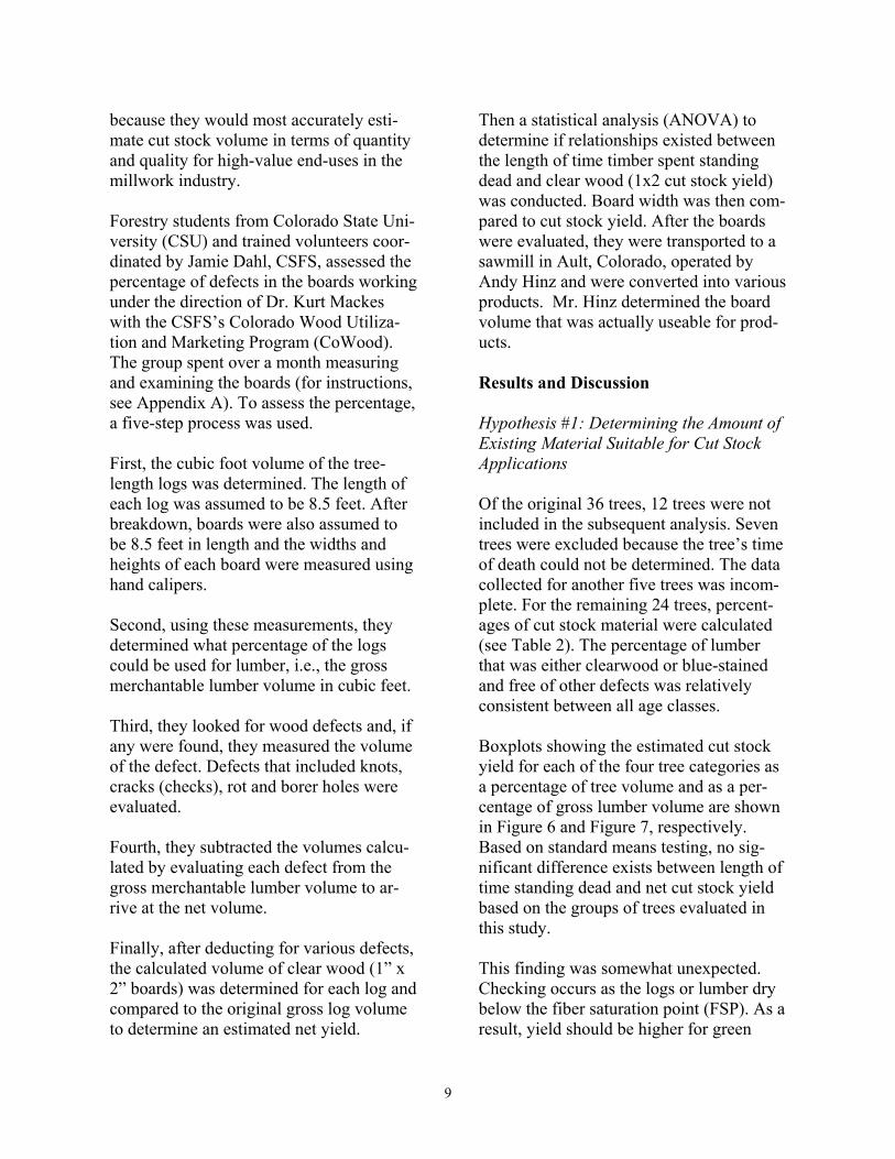
because they would most accurately esti-mate cut stock volume in terms of quantity and quality for high-value end-uses in the millwork industry. Forestry students from Colorado State Uni-versity (CSU) and trained volunteers coor-dinated by Jamie Dahl, CSFS, assessed the percentage of defects in the boards working under the direction of Dr. Kurt Mackes with the CSFS’s Colorado Wood Utiliza-tion and Marketing Program (CoWood). The group spent over a month measuring and examining the boards (for instructions, see Appendix A). To assess the percentage, a five-step process was used. First, the cubic foot volume of the tree-length logs was determined. The length of each log was assumed to be 8.5 feet. After breakdown, boards were also assumed to be 8.5 feet in length and the widths and heights of each board were measured using hand calipers. Second, using these measurements, they determined what percentage of the logs could be used for lumber, i.e., the gross merchantable lumber volume in cubic feet. Third, they looked for wood defects and, if any were found, they measured the volume of the defect. Defects that included knots, cracks (checks), rot and borer holes were evaluated. Fourth, they subtracted the volumes calcu-lated by evaluating each defect from the gross merchantable lumber volume to ar-rive at the net volume. Finally, after deducting for various defects, the calculated volume of clear wood (1” x 2” boards) was determined for each log and compared to the original gross log volume to determine an estimated net yield.

Then a statistical analysis (ANOVA) to determine if relationships existed between the length of time timber spent standing dead and clear wood (1x2 cut stock yield) was conducted. Board width was then com-pared to cut stock yield. After the boards were evaluated, they were transported to a sawmill in Ault, Colorado, operated by Andy Hinz and were converted into various products. Mr. Hinz determined the board volume that was actually useable for prod-ucts. Results and Discussion Hypothesis #1: Determining the Amount of Existing Material Suitable for Cut Stock Applications Of the original 36 trees, 12 trees were not included in the subsequent analysis. Seven trees were excluded because the tree’s time of death could not be determined. The data collected for another five trees was incom-plete. For the remaining 24 trees, percent-ages of cut stock material were calculated (see Table 2). The percentage of lumber that was either clearwood or blue-stained and free of other defects was relatively consistent between all age classes. Boxplots showing the estimated cut stock yield for each of the four tree categories as a percentage of tree volume and as a per-centage of gross lumber volume are shown in Figure 6 and Figure 7, respectively. Based on standard means testing, no sig-nificant difference exists between length of time standing dead and net cut stock yield based on the groups of trees evaluated in this study. This finding was somewhat unexpected. Checking occurs as the logs or lumber dry below the fiber saturation point (FSP). As a result, yield should be higher for green

9

Tree ID# Cubic Foot Volume of the Tree

Cubic Foot Volume of

the Lumber (Gross)

Cubic Foot Volume of

All Lumber Defects

Cubic Foot Volume of

the Lumber (Net)

Percentage of Tree that was Clear-

wood or Blue-Stained

Percentage of Lumber that was

Clearwood or Blue-Stained

Green (Living) Trees (Category 1)

3 25.16 7.91 2.06 5.85 23.2% 74.0%

26 28.04 11.81 2.58 9.23 32.9% 78.1%

27 31.00 10.49 2.89 7.60 24.5% 72.5%

32 21.54 9.35 2.26 7.10 32.9% 75.9%

Sub-Totals 105.74 39.56 9.78 29.78 28.2% 75.3%

Trees Standing Dead from 0 Years to 1 Year (Category 2)

12 53.38 21.57 4.66 16.92 31.7% 78.4%

13 47.77 19.19 3.38 15.82 33.1% 82.4%

16 32.07 12.55 3.57 8.98 28.0% 71.5%

22 35.11 15.65 4.05 11.60 33.0% 74.1%

25 27.43 10.39 5.69 4.70 17.1% 45.2%

29 27.64 11.89 3.07 8.83 31.9% 74.2%

Sub-Totals 223.40 91.25 24.41 66.84 29.9% 73.3%

Trees Standing Dead from 2 Years to 5 Years (Category 3)

7 35.45 12.06 3.12 8.94 25.2% 74.1%

8 19.37 7.77 1.66 6.10 31.5% 78.6%

15 21.82 7.78 2.34 5.44 24.9% 70.0%

21 28.37 10.22 3.15 7.07 24.9% 69.2%

24 25.21 13.92 3.59 9.62 38.1% 69.1%

33 38.13 21.15 4.90 16.26 42.6% 76.9%

35 36.17 13.26 2.93 10.33 28.6% 77.9%

36 24.79 8.70 4.82 3.88 15.7% 44.6%

Sub-Totals 229.31  94.86  26.51  67.64  29.5%  71.3% 

Trees Standing Dead from 6 Years to 10 Years (Category 4)

2 35.60 11.83 2.67 9.16 25.7% 77.4%

4 27.43 11.07 3.27 7.80 28.5% 70.5%

5 32.74 12.22 2.78 9.44 28.8% 77.2%

6 17.45 7.00 1.84 5.16 29.6% 73.7%

17 20.19 7.10 1.97 5.13 25.4% 72.2%

31 24.54  10.33  2.69  7.64  31.1%  74.0% 

Sub-Totals 157.95  59.55  15.22  44.33  28.1%  74.4% 

Table 2: Cut Stock Volume Measurements and Percentages

10

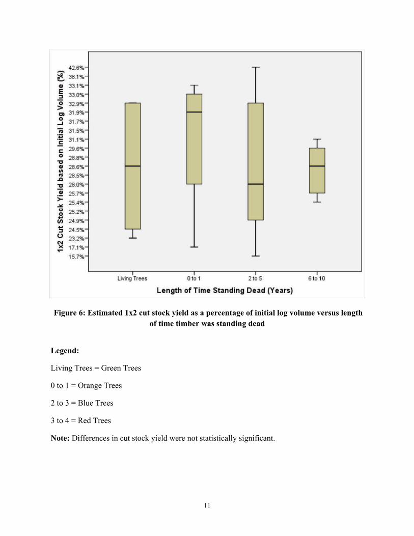
Figure 6: Estimated 1x2 cut stock yield as a percentage of initial log volume versus length of time timber was standing dead

Legend:

Living Trees = Green Trees

0 to 1 = Orange Trees

2 to 3 = Blue Trees

3 to 4 = Red Trees

Note: Differences in cut stock yield were not statistically significant.

11

Figure 7: Estimated 1x2 cut stock yield as a percentage of gross lumber volume versus length of time timber was standing dead

Legend:

Living Trees = Green trees

0 to 1 = Orange trees

2 to 3 = Blue trees

3 to 4 = Red trees

Note: Differences in cut stock yield were not statistically significant.

12

lumber because checking should be mini-mal. One possible explanation is that be-cause of inclement weather it took several months to complete data collection and the green boards could have dried below the FSP during that time. Generally once the wood dries to equilibrium moisture con-tent, the frequency and severity of check-ing should not change significantly. There-fore, no significant differences were ex-pected for wood standing dead longer than one year. The occurrence of rot was low in the lum-ber evaluated, even for trees that had been standing dead for over six years. However, when rot did occur, the impact on clear-wood cut stock yield was dramatic. Tree #36 had heart rot and the net cut stock yield was 44.6%, which is considerably less than the mean 71.3% for its age group. The analysis showed that only a small frac-tion of a tree’s total volume can be proc-essed into cut stock. Initially, about 28% of each tree-length log’s total volume, on av-erage, was suitable for manufacturing into 1” boards. Of this 28%, on average, roughly three-quarters of the total lumber volume was free of defects other than blue-stain or was clearwood suitable for making cut stock. In other words, a little more than 20% of a beetle-killed lodgepole pine tree-length log’s total volume was suitable for processing into 1” x 2” boards or other cut stock applications. While the amount of time that a tree stands dead was not as significant as anticipated, log size proved to be a much more signifi-cant factor. Larger logs yielded a corre-spondingly higher percentage of cut stock. A boxplot showing the cut stock yield as a percentage of gross lumber volume when controlling for log size class is shown in Figure 8. Using standard means testing,

significant differences exist in cut stock yield between log size classes. Generally, as log size class (diameter) increases, cut stock yield increases. This data should be used with caution. Once the material was measured and the data were collected and analyzed, the boards were transported to a small sawmill in Ault, Colorado, where the boards were milled into finished products. The mill re-ported that only about 60% of the suitable material could actually be made into prod-uct, a slight reduction from the measured finding (73%). The unusable 40% consisted of 25% lost due to checking and 15% due to variations in the material thickness. In the original analysis, material thickness variability was not considered to be a defect. Had the ma-terial thickness been more uniform, the percentage of suitable material would have increased to 75%, which is very close to the measured 73%. Conclusion and Future Directions Findings from this study reveal that no sta-tistical difference exists between the per-centage of cut stock yield from green living trees and beetle-killed trees that had been standing dead for up to nine years. The per-centage of a beetle-killed lodgepole pine tree-length log’s cubic volume that was clearwood or blue-stain and suitable for cut stock averaged 28.9%. The average percent of lumber that was suitable for cut stock averaged 73.6%. Finally, tree diameter, not time spent standing dead, is the more sig-nificant factor to consider when maximiz-ing cut stock yield. Caveats exist. The oldest tree in this study had been dead for only nine years and most trees had been standing dead for considera-

13

Figure 8: Estimated 1x2 cut stock yield as a percentage of gross lumber volume versus log class

Legend:

Class 1 = Logs with a small-end diameter between 6” and 9”

Class 2 = Logs with a small-end diameter between 9” and 12”

Class 3 = Logs with a small-end diameter between 12” and 15”

Class 4 = Logs with a minimum small-end diameter of 15”

Note: Cut stock yield was 58.9% for Class 1 logs and 67.2% for Class 2 logs. Cut stock yield was significantly higher for Class 3 and Class 4 logs, being 77.5% and 80.1% respectively. Increasing yield should have increased with log size.

14

bly less time. This study applies to beetle-killed trees with comparatively recent mor-tality that remain standing on the stump. Furthermore, beetle-killed trees typically begin to blow down between three to seven years after mortality. Within 15 years after mortality, about 90% of beetle-killed trees will be on the ground. Because the current mountain pine beetle epidemic has raged for over a decade, the amount of blowdown will increase dramatically in the immediate future. Once on the ground, beetle-killed trees will deteriorate faster. These caveats should convey a sense of urgency. Those who want to use the wood should seek to promote and incentivize the full-value product chain so that more of the tree is usable and do so as quickly as possi-ble. Waste material produced when manu-facturing higher value solid wood products, such as cut stock, could be used to manu-facture other wood products, such as mulch for landscaping or wood pellets for energy. Carl Spaulding, president of the Colorado

Timber Industry Association, notes that “the cheapest wood chip rides on the back of a 2x4,” indicating that wood product producers should strive for 100% utiliza-tion of wood material whenever possible. Statewide policies should follow this ap-proach. Co-locating solid wood product facilities with wood energy product pro-ducers makes some sense. The residue or “waste” material from one operation would become the feedstock for the other. Devel-oping projects that rely on Colorado-produced wood products would further de-crease transportation costs and continued reliance on imported wood products (see Lynch and Mackes 2001). Increasing utilization among beetle-killed trees to reduce forest fuel loads, produce wood products sustainably for market while lessening the taxpayer burden would provide the greatest return on public invest-ment while improving public safety.

15

References Colorado State Forest Service [CSFS]. 2013. 2012 Report on the health of Colorado’s forests.

Available online at http://csfs.colostate.edu/pdfs/137233-ForestReport-12-www.pdf; last accessed 13 March 2013.

Lewis, K.J. and I.D. Hartley. 2006. Rate of deterioration, degrade, and fall of trees killed by mountain pine beetle. BC Journal of Ecosystems and Management 7(2): 11-19.

Lynch, D. and K. Mackes. 2001. Wood use in Colorado at the turn of the twenty-first century. Rocky Mountain Research Station. RMRS-RP-32. Ft. Collins, CO: USDA Forest Service. 23 p.

Mackes, K.H., M. Eckhoff, B. Davis, B. McCarthy, C. Hamma, D. Lynch, and T. Reader. 2010. The impacts of mountain pine beetles on forests in Grand County, Colorado. Fort Collins, CO: Colorado State University.

Prins, C. 2011. Forest products literature review. White Rive Conservation District. Completed September 30.

16

Appendix A: Cut Stock Yield Project Objective Determine the volume of clear 1x2s that can be cut from boards of various width Measuring procedure 1. Measure width and thickness at both ends and at center of board along its length

Measure width to the tenth-inch (0.1)” using engineer’s scale Measure thickness to 1000-inch (0.001”) using hand-held calipers Record measurements on data sheets provided

2. Calculate width deduction

There is a 2” width deduction for boards that contain the pith Record length (inches) that pith extends along board

Ignore end checks that do not extend further than 3 “ More severe checks (cracks) and wane will be assigned a 2” width reduction

Measure the length of checks (cracks) or wane with a tape measure Sum the length of severe checks (cracks) and record in the comment column (for

example, a crack that is 26” long should be recorded as: WD = 26.0”, if the crack extends the full length of the board WD = 102”)

The full width of boards with rot will be deducted for the length of the rot. 3. Calculate the length deduction

Assume the beginning length is 8 feet 6 inches (102”) Assume blue stain is acceptable (do not deduct for blue stain) Locate/mark knots contained in board Determine deduction as follows:

Knots less than 0.5”diameter – 1” deduction Knots 0.5” to 1” diameter – Measure knot and any associated grain distortion,

add 0.5” and round up to next 0.5” (for example, a 0.75” knot would result in a 1.5” deduction, 0.75” + 0.5” = 1.25” which is rounded up to 1.50”)

Knots > 1” diameter – Measure knot and any associated grain distortion), add 0.5” and round up to next inch 0.5” (for example, a 2” knot would result in a 2.5” deduction)

For knot clusters, measure width of cluster using engineer’s scale, round up to next inch + 0.5”

If knot exceeds 2” diameter, double length deduction for knots between 2” and 4” diameter, and triple for knots that are 4” to 6” and so on.

Sum deductions for each board and record on data sheet

17