1

Determining the Radioactivity of A Sample of Cesium-137

Using Special Cases of the Binomial Distribution

Quintin T. Nethercott and M. Evelynn Walton University of Utah

Department of Physics and Astronomy Undergraduate Lab February 26, 2013

The purpose of this experiment was to apply special cases of the Binomial Distribution to a nuclear decay process that would allow for the use of fitting for individual cases. In the case of a large number of measurements with a large number of counts, the Gaussian curve produced a satisfactory fit and the standard deviation of the mean was reduced with each trial to obtain a value for the radioactivity of the sample that was within well-defined constraints. In the case of background radiation, a Poisson distribution was obtained for each trial. This was expected for the random nature of the radiation as well as the low probability of an ionizing particle entering the Geiger tube. Using the parameters defined for each distribution the actual activity of the sample of Cs-137 was found to be (176 +/-8) decays per second and the background radiation in the lab at the South Physics building was less than one decay per second.

I. INTRODUCTION

There are naturally occurring sources of radiation everywhere but types of radiation can vary

depending on the decay chain of a source and whether the radiation is ionizing or non-ionizing. Examples of non-ionizing radiation include microwave, infrared, and radio waves. Ionizing radiation can be dangerous in excessive doses because the radiation is very high frequency/short wavelength and has enough energy to strip electrons and break chemical bonds in living tissue [1]. Although α particles are ionizing, they can not penetrate the skin. This lab restricted the samples to those with β or γ decay. Of the samples available Cs-137 was chosen for its relatively long half-life compared with the purchase date. Isotope Fe-55 Co-60 Cs-137 Ba-133 C-14 Na-22 Tl-204 Emission Type

γ β - β and γ β β β - β

Energy 6 keV 0.3178 MeV

0.512 MeV/0.662 MeV

0.32 MeV 0.049 MeV

0.545 MeV

0.776 MeV

Half-Life 2.7 yrs 5.271 yrs 30.17 yrs 10.74 yrs 5700 yrs 2.6 yrs 3.78 yrs Table 1. Isotopes and their associated emission types, energies, and half-lives [2][3][4].

The activity of the Cs-137 sample was measured using a Geiger detector and the values plotted in

histograms to find a Gaussian fit for the data. When a nucleus in the sample undergoes a disintegration it causes a pulse in the detector that registers in the LabView software. Of course, each measurement is likely to be slightly different but scattered around a mean average. Measurements were taken at 10, 20, 50, 100, 200, 500, 1000, and 15,000 count increments to find the most likely decay rate. The more measurements were taken the smaller the standard deviation became and the more closely the distributions resembled a Gaussian curve. From the mean decay rate the radioactivity of the sample can be verified.

2

A. Theoretical Introduction

To obtain a reliable value for the disintegrations per second the activity was measured many times and the results approached a mean as the readings were increased. Briefly, the possible distributions the readings could resemble and the parameters for each:

Binomial Distribution: in general this distribution is used to model the number of occurrences of one out of two possible outcomes when the probability of obtaining success is known [5]. It is characterized by discrete values of n successes in N trials when the probability of success in one trial is p and q = (1-p):

(1)

The standard deviation is parameterized by the probability such that

(2)

The binomial distribution is symmetric only when p = 0.5. So in that case the distribution will center on the most probable value. Since the probability involved with the decay of the Cs-137 is not known, the Binomial Distribution is likely not the most ideal model to use for the data.

Gaussian (Normal) Distribution: is characterized by continuous values of x measurements centered around the mean. It is a special case of the Binomial distribution when the number of trials, N goes to infinity and the probability of a particular outcome, p goes to 0 and the mean becomes large and finite [5].

(3)

(4)

(5)

When the measurements are plotted in a histogram with the number of times each measurement occurs, the data can be fitted with a normal distribution. When more measurements are taken the standard deviation of the mean will become smaller. The measurements can be confidently characterized as trending toward a particular value [5].

3

(6)

In principle, a very large number of trials would yield almost a point-like mean and the mean could be stated to be within 95% of a very small interval of the width parameter

(7)

The Gaussian is specified by parameters and (the standard deviation and the mean). The histograms obtained in this experiment will attempt to use normal curve fitting.

Poisson Distribution: this distribution is another special case of the Binomial distribution where, like the Gaussian, the number of trials, N, is very large, the probability, p, is very small and the mean is finite and small. The values of n are discrete and the Poisson distribution is parameterized only by the mean.

(8)

(9)

As the mean becomes large the Poisson distribution begins to resemble the Gaussian. The standard deviation is given by:

(10)

In this experiment, the Poisson and the Gaussian will prove most useful in identifying the closest value to the activity in the radioactive sample.

II. EXPERIMENTAL SETUP

The Geiger counter is a device that captures the ionizing radiation from a source. A voltage is run through the tube so that when a β emission occurs it is accelerated in the tube. This acceleration is forceful enough to knock a bound electron from a gas molecule inside the tube from its orbit. The result, in the presence of a sufficiently strong voltage, is a cascade of freed electrons that produce a pulse in the detector [7]. The pulse travels through the counter circuit and has the characteristics shown in Figure 1. The corresponding oscilloscope images are shown in Figure 2.

4

Figure 1. Electronic counter circuit schematics [6].

As shown in Figure 1, the first image is the signal input; the pulse is negative in voltage and about 1

microsecond in duration. The circuit flips the pulse if it exceeds the counter voltage threshold and the resulting pulse displayed on the oscilloscope is the second image in Figure 2. The third image is the square wave needed by the scope trigger to count the pulse. If the signal does not meet the comparator threshold the result is a flat line on the oscilloscope screen. The counter takes intervals of measurement by setting the gate. It was advantageous to gather several hundred counts per interval, so the counter gate was set to 2 seconds on many of the trials in this experiment. In this case a high comparator threshold yielded no signal. This parameter was set at 0.180 V for the experiment and some adjustments in the oscilloscope settings were made to determine the level of “noise” in the signal. 5 and 10 V were not used for this reason.

Once the pulse is counted at the micro-controller [6], the counter shows a tally of the counts on the display and sends the count to the software (in this case LabView) via USB interface as shown in Figure 3. Each count is displayed in a histogram and the data for each set can be plotted in histograms (in this experiment Origin was the data analysis software).

5

Figure 2. Oscillator pulse inputs.

Figure 3. Geiger tube, oscillator and electronics board.

6

III. EXPERIMENTAL PROCEDURE

A. Establishing Operating Point for Geiger-Müller Tube

Figure 4.Response curve for a Geiger-Müller tube [6].

Figure 4 shows the response curve for a Geiger-Müller tube. The operating point for the tube was chosen in the middle of the plateau region. To determine the plateau region for the Geiger-Müller tube used in the experiment the count rate was measured as a function of the power supply voltage. The rate was determined for 600, 599, 594, 590, 588, 585, 575, 565, 555, 550, 541, 534, 529, 500, 480, 470, 450, 430, 420, 410, 407, 402, 397, 392, 390, and 389 Volts. The gate time for most of the voltages is 1 second. However, enough counts the gate time was extended for the last three voltage measurements. The gate time for 392V was 2.5 seconds, 5 seconds for 390V, and 5 seconds for 389V. In order to be 95% confident that the mean of the measurements lies within 10% of the mean accuracy for a Gaussian distribution, the number of times the measurements need to be repeated (N) can be determined by:

√ √

(11)

The average mean for a 1 second gate time was approximately 160 counts. N for this mean would

need to be at least 250 in order to achieve the mentioned accuracy. This level of accuracy was desired for the plateau region and was used for 480-585V. The accuracy of measuring 100 times, for the remaining voltages, was sufficient to determine the location of the knee and general shape of the response curve.A histogram was made at each voltage, and a Gaussian function was fitted to each histogram. The mean and standard deviation of the Gaussian was used to determine the rate and error bars for the associated voltage. These rates were then plotted as a function of voltage to determine the knee and plateau regions for the Geiger-Müller tube.

B. Detection of Radiation from Cs-137 sample

Using an operating voltage of 500V for the Geiger-Müller tube, the count rate for the Cs-137 sample was measured numerous times. A histogram was produced. For a large N and large mean, the data would best be represented by a Gaussian distribution. From a Gaussian fit the mean and standard deviation were taken and compared to those obtained by straight calculation. The reduced Chi-squared and the p-value for the Gaussian model were calculated to determine the accuracy of the model. This count rate was also

7

measured 10, 20, 50, 100, 200, 500, 1000, and 15000 times, with a 2 second gate time. To compare and determine how the accuracy of the Gaussian model was affected by the number of data points the reduced Chi-squared and p-values were calculated.

C. Detection of Background Radiation

To determine the background radiation the count rate was measured in the absence of the source. The count rate was measured 100 times with a 2 second gate time. The resulting histogram can best be described by a Poisson distribution since the mean is small. The mean of the Poisson will then be compared to the mean determined by straight calculation.

D. Binomial Distribution

To obtain data that could be best represented by a Binomial Distribution the counts for background radiation were taken at a gate time of _ sec. so that a mean number of background counts would be about 0.2. Since the mean is small and the number of zeros is large, the data will be better represented by a Binomial Distribution.

( )

(12)

( )

(13)

Equation _ shows that for a mean of 0.2 counts the Poisson probability distribution predicts that

zero counts should be observed 82% of the time. The rate was measured 10 times and the number of zeros observed was recorded. That measurement was then repeated ten times. The mean number of zeros observed will be used to calculate the standard deviation for both a Binomial and Poisson distribution. These will be compared with the standard deviation calculated experimentally.

IV. EXPERIMENTAL RESULTS & DISCUSSION

A. Establishing Operating Point for Geiger-Müller Tube

Figure 5. Histogram of counts at 600V with a Gaussian fit (gate time of 1 sec). Figure 6. Histogram of counts at 599V with a Gaussian fit (gate time of 1 sec)

Freq

uen

cy

Freq

uen

cy

Counts Counts

8

Figure 7. Histogram of counts at 594V with a Gaussian fit (gate time of 1 sec). Figure 8. Histogram of counts at 590V with a Gaussian fit (gate time of 1 sec).

Figure 9. Histogram of counts at 588V with a Gaussian fit (gate time of 1 sec). Figure 10. Histogram of counts at 585V with a Gaussian fit (gate time of 1 sec).

Figure 11. Histogram of counts at 575V with a Gaussian fit (gate time of 1 sec). Figure 12. Histogram of counts at 565V with a Gaussian fit (gate time of 1 sec).

Freq

uen

cy

Freq

uen

cy

Freq

uen

cy

Freq

uen

cy

Freq

uen

cy

Freq

uen

cy

Freq

uen

cy

Counts Counts

Counts Counts

Counts Counts

9

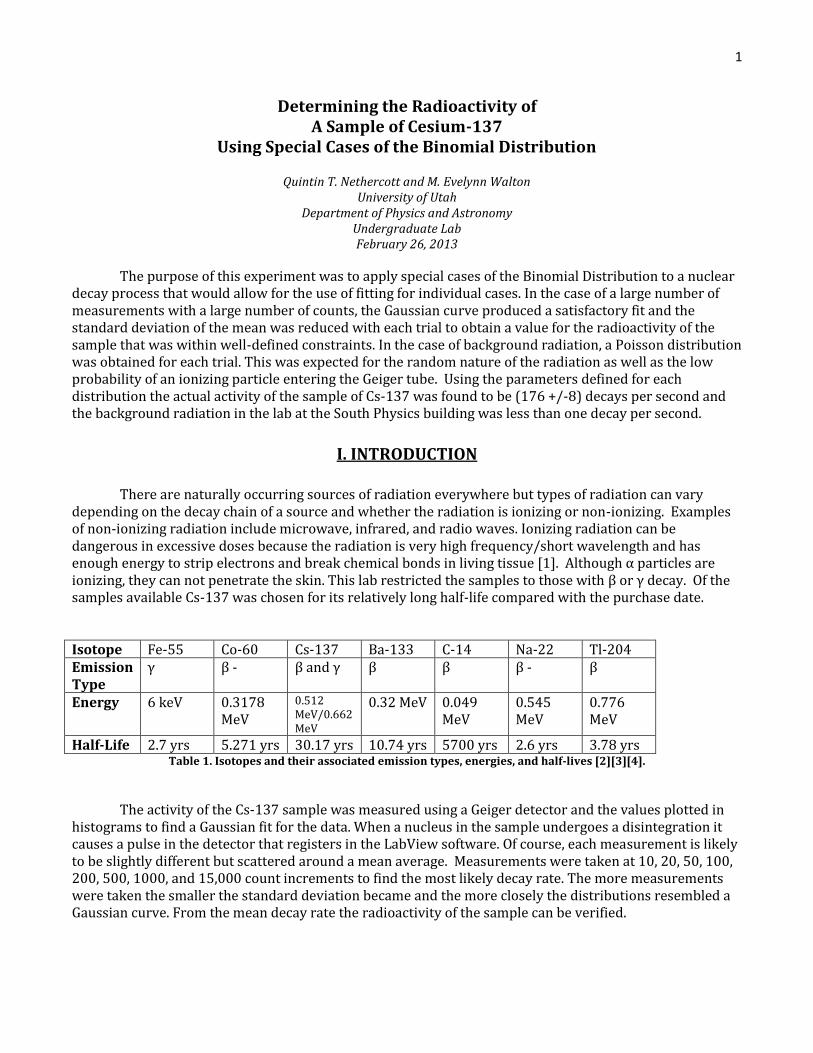
Figure 13. Histogram of counts at 555V with a Gaussian fit (gate time of 1 sec). Figure 14. Histogram of counts at 550V with a Gaussian fit (gate time of 1 sec).

Figure 15. Histogram of counts at 541V with a Gaussian fit (gate time of 1 sec). Figure 16. Histogram of counts at 534V with a Gaussian fit (gate time of 1 sec).

Figure 17. Histogram of counts at 529V with a Gaussian fit (gate time of 1 sec). Figure 18. Histogram of counts at 500V with a Gaussian fit (gate time of 1 sec).

Freq

uen

cy

Freq

uen

cy

Freq

uen

cy

Freq

uen

cy

Freq

uen

cy

Freq

uen

cy

Counts Counts

Counts Counts

Counts Counts

10

Figure 19. Histogram of counts at 480V with a Gaussian fit (gate time of 1 sec). Figure 20. Histogram of counts at 470V with a Gaussian fit (gate time of 1 sec).

Figure 21. Histogram of counts at 450V with a Gaussian fit (gate time of 1 sec). Figure 22. Histogram of counts at 430V with a Gaussian fit (gate time of 1 sec).

Figure 23. Histogram of counts at 420V with a Gaussian fit (gate time of 1 sec). Figure 24. Histogram of counts at 410V with a Gaussian fit (gate time of 1 sec).

Freq

uen

cy

Freq

uen

cy

Freq

uen

cy

Freq

uen

cy

Freq

uen

cy

Freq

uen

cy

Counts Counts

Counts Counts

Counts Counts

11

Figure 25. Histogram of counts at 410V with a Gaussian fit (gate time of 1 sec). Figure 26. Histogram of counts at 407V with a Gaussian fit (gate time of 1 sec).

Figure 27. Histogram of counts at 402V with a Gaussian fit (gate time of 1 sec). Figure 28. Histogram of counts at 397V with a Gaussian fit (gate time of 1 sec).

Figure 29. Histogram of counts at 392V with a Gaussian fit (gate time of 2.5 sec). Figure 30. Histogram of counts at 390V with a Gaussian fit (gate

time of 5 sec).

Freq

uen

cy

Freq

uen

cy

Freq

uen

cy

Freq

uen

cy

Freq

uen

cy

Freq

uen

cy

Counts Counts

Counts Counts

Counts Counts

12

Figure 31. Histogram of counts at 389V with a Gaussian fit (gate time of 5 sec).

N Voltage Mean (Gaussian fit)

St Dev (Gaussian fit)

SDOM (Gaussian fit)

Mean St Dev SDOM

100 600 194.812 13.616 1.3616 194.812 13.616 1.3616 100 599 195.277 12.848 1.2848 195.277 12.848 1.2848 100 594 196.366 13.960 1.3960 196.366 13.960 1.3960 100 590 192.535 13.228 1.3228 192.535 13.228 1.3228 100 588 193.960 12.929 1.2929 193.960 12.929 1.2929 250 585 176.275 12.251 0.7748 176.275 12.251 0.7748 250 575 175.271 12.112 0.7660 175.271 12.112 0.7660 250 565 173.510 12.532 0.7926 173.510 12.532 0.7926 250 555 174.645 13.568 0.8581 174.645 13.568 0.8581 250 550 172.737 12.686 0.8023 172.737 12.686 0.8023 250 541 172.669 12.794 0.8091 172.669 12.794 0.8091 250 534 173.920 12.031 0.7609 173.920 12.031 0.7609 250 529 164.158 8.581 0.7483 172.821 11.832 0.7483 250 500 171.378 10.859 0.6868 171.379 10.859 0.6868 250 480 170.928 11.955 0.7561 170.928 11.955 0.7561 100 470 167.505 10.980 1.0980 167.505 10.980 1.0980 100 450 165.248 10.998 1.0998 165.248 10.998 1.0998 100 430 161.009 10.414 1.0414 161.009 10.414 1.0414 100 420 155.990 11.083 1.1083 155.990 11.083 1.1083 100 410 161.079 12.509 1.2509 161.079 12.509 1.2509 100 410 164.158 8.581 0.8581 164.158 8.581 0.8581 100 407 155.990 9.837 0.9837 155.990 9.837 0.9837 100 402 147.178 9.508 0.9508 147.178 9.508 0.9508 100 397 124.851 6.360 0.6360 124.852 6.360 0.6360 100 392 49.139 6.937 0.6937 49.139 6.937 0.6937 100 390 29.485 5.462 0.5462 29.485 5.462 0.5462 100 389 4.812 2.208 0.2208 4.812 2.208 0.2208

Table2. Comparison between Gaussian fit and straight calculation of mean, standard deviation, and standard deviation of the mean taken from measuring counts at varied voltages.

Figures 5-31 show the histograms and fitted Gaussian functions obtained at 600, 599, 594, 590, 588, 585, 575, 565, 555, 550, 541, 534, 529, 500, 480, 470, 450, 430, 420, 410, 410, 407, 402, 397, 392, 390, and 389 Volts respectively. The mean and standard deviations that were taken from these Gaussian fits are seen in Table 2, and a comparison with the values obtained by straight calculations is shown. Within the accuracy of the calculations, there is no difference in the mean, standard deviation, and standard deviation of the mean for the Gaussian fit and the straight calculations. The count rate was calculated by taken the

Freq

uen

cy

Counts

13

mean and dividing by the gate time. The gate time for each voltage was 1 sec with the exception of 392 V (gate time of 2.5 sec), 390 V (gate time of 5 sec), and 389 V (gate time of 5 sec). The response curve for the Geiger-Müller tube was determined by graphing the count rate as a function of the voltage.

Figure 32.Response curve for Geiger-Müller tube with linear fit in the plateau region.

Figure 33.Residual Plot for linear fit in plateau region of response curve for Geiger-Müller tube.

Figure 32 shows the response curve obtained experimentally. This shows that the knee occurs around 410V and the plateau is can be seen between 430V and 585V. The operating point was chosen at some point far from the knee, on the plateau region. For the remainder of the experiment, an operating voltage of 500V was used. A linear fit was performed in the plateau region between 420V and 585V, giving a value for the slope 0.085+/-0.009 and intercept of 119+/-5. Figure 33 shows the residual plot from the linear fit. Since all of the error bars cross zero the data is a good candidate for a linear fit. The

14

manufacturer’s specification for the slope in the plateau region is “less than 6% per 100V” [6]. The slope of the linear fit gives a change of 8.5 counts per 100V, which is a change of 4.82%, when compared to a rate of 176.27 counts/sec (the rate at 585V), and 5.28% when compared to a rate of 161.01 counts/sec (the rate at 430V). The data representing the plateau region for the Geiger-Müller detector matches very closely to the manufacturer’s specifications.

B. Detection of Radiation from Cs-137

Figure 34. Histogram of counts measured 100 times (2 sec gate time, 500V).

Figure 34 shows the histogram from measuring the count rate 100 times with a gate time of 2 seconds. The data can best be represented by a Gaussian distribution. The mean from the Gaussian fit is 357.5446, the standard deviation 15.0914, and the standard deviation of the mean 1.50914. The mean from straight calculation is 357.5446, the standard deviation 15.0914, and the standard deviation of the mean 1.50914. The values for the Gaussian fit and straight calculation are the same. The reduced Chi-squared for the Gaussian model is 2.9901. The associated p-value is 0.003874. For p-values less than 0.05 the data statistically supports the model. This means that the Gaussian model is acceptable for this data set.

Figure 35. Histogram of counts measured 15000 times (2 sec gate time, 500V). Figure 36. Histogram of counts measured 1000 times (2 sec gate time, 500V).

Counts Counts

Freq

uen

cy

Freq

uen

cy

15

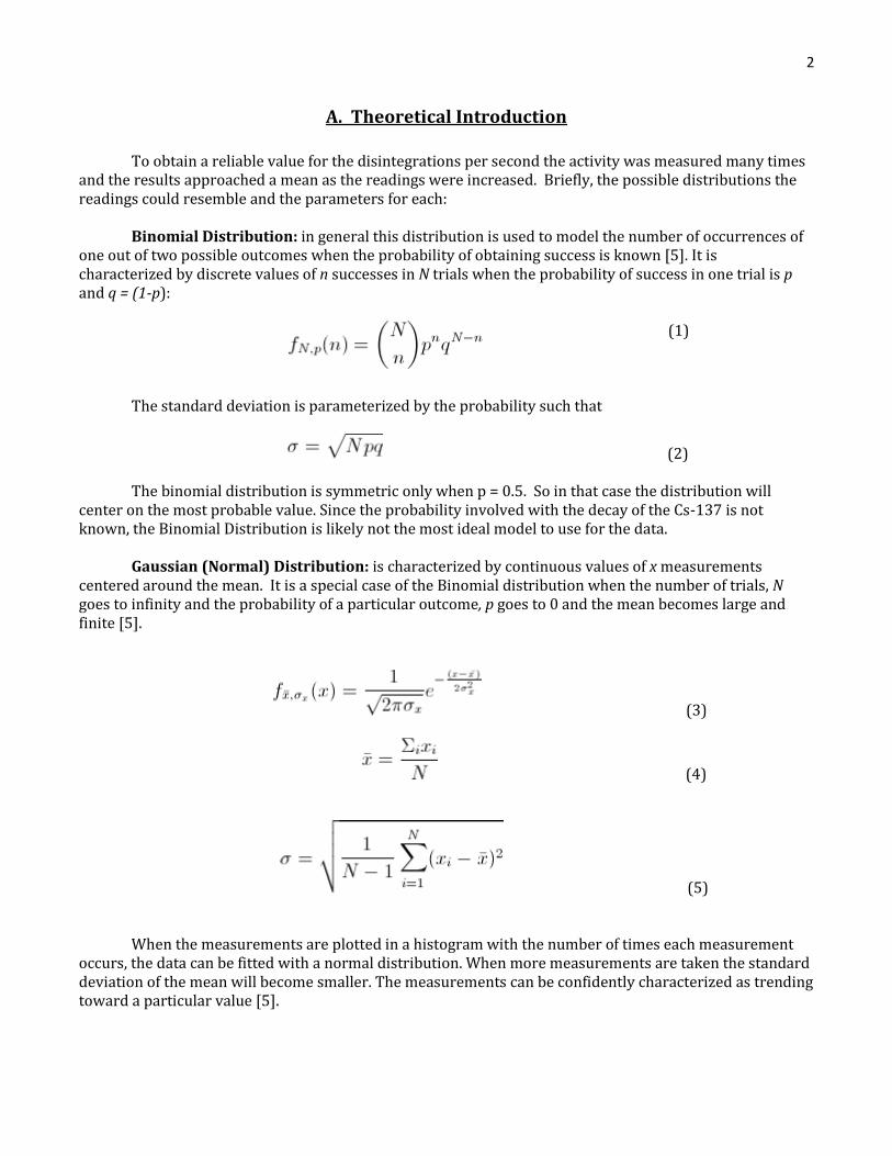
Figure 37_. Histogram of counts measured 500 times (2 sec gate time, 500V). Figure 38. Histogram of counts measured 200 times (2 sec gate time, 500V).

Figure 39. Histogram of counts measured 100 times (2 sec gate time, 500V). Figure40. Histogram of counts measured 50 times (2 sec gate time, 500V).

Figure 41. Histogram of counts measured 20 times (2 sec gate time, 500V). Figure42. Histogram of counts measured 10 times (2 sec gate time, 500V).

Freq

uen

cy

Freq

uen

cy

Counts Counts

Counts Counts

Counts Counts

Freq

uen

cy

Freq

uen

cy

Freq

uen

cy

Freq

uen

cy

16

N Reduced Chi-squared p-value 10 2.284196 0.1307 20 2.534647 0.1114 50 1.459967 0.2233

100 2.412742 0.02474 200 1.702459 0.09224 500 1.912179 0.02062

1,000 0.882811 0.5949 15,000 1.863623 0.000656

Table3. Comparison of reduced chi-squared and p-values for data with an increasing number of measurements.For explanation on calculation of reduced chi-squared and p-value see Appendix B.

Figures 35-42 show the histograms from measuring the count rate for 10, 20, 50, 100, 200, 500, 1000, and 15000, respectively. The mean, standard deviation, and standard deviation of the mean calculated from both the Gaussian fit and straight calculation are compared in Table3. Table 3 also compares the calculated reduced Chi-squared and p-values for each data set. The p-values for N=100 (0.024744), N=500 (0.020619), and N=15000 (0.000656) are below 0.05. Therefore, model is considered statistically significant and can be accepted for those three data sets. The general trend of the p-values is that as N gets large, the p-value gets smaller. This corresponds to what can be seen visually, that the data more closely matches the fit with a larger N. This shows that for larger N, the Gaussian model will be more accurate.

C. Detection of Background Radiation

Figure 43. Histogram of counts for background radiation measured 100 times(gate time 2 sec, 500V).

Figure 43 shows the histogram of background radiation measured 100 times with a gate time of 2 seconds. Since the mean is small the data can best be represented by a Poisson distribution. The mean for the Poisson fit is 0.7921. The mean by straight calculation is 0.7921 counts. The two values are the same.

Freq

uen

cy

Counts

17

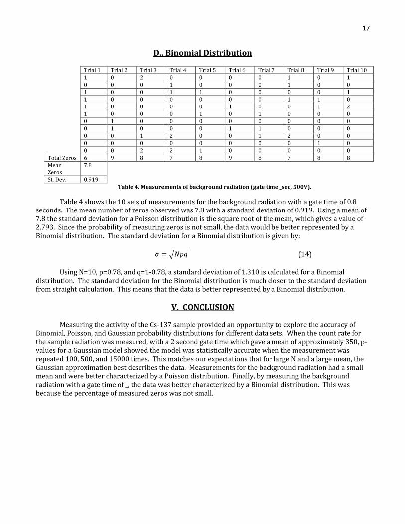
D.. Binomial Distribution

Trial 1 Trial 2 Trial 3 Trial 4 Trial 5 Trial 6 Trial 7 Trial 8 Trial 9 Trial 10 1 0 2 0 0 0 0 1 0 1 0 0 0 1 0 0 0 1 0 0 1 0 0 1 1 0 0 0 0 1 1 0 0 0 0 0 0 1 1 0 1 0 0 0 0 1 0 0 1 2 1 0 0 0 1 0 1 0 0 0 0 1 0 0 0 0 0 0 0 0 0 1 0 0 0 1 1 0 0 0 0 0 1 2 0 0 1 2 0 0 0 0 0 0 0 0 0 0 1 0 0 0 2 2 1 0 0 0 0 0 Total Zeros 6 9 8 7 8 9 8 7 8 8 Mean Zeros

7.8

St. Dev. 0.919 Table 4. Measurements of background radiation (gate time _sec, 500V).

Table 4 shows the 10 sets of measurements for the background radiation with a gate time of 0.8 seconds. The mean number of zeros observed was 7.8 with a standard deviation of 0.919. Using a mean of 7.8 the standard deviation for a Poisson distribution is the square root of the mean, which gives a value of 2.793. Since the probability of measuring zeros is not small, the data would be better represented by a Binomial distribution. The standard deviation for a Binomial distribution is given by:

√ (14)

Using N=10, p=0.78, and q=1-0.78, a standard deviation of 1.310 is calculated for a Binomial

distribution. The standard deviation for the Binomial distribution is much closer to the standard deviation from straight calculation. This means that the data is better represented by a Binomial distribution.

V. CONCLUSION

Measuring the activity of the Cs-137 sample provided an opportunity to explore the accuracy of Binomial, Poisson, and Gaussian probability distributions for different data sets. When the count rate for the sample radiation was measured, with a 2 second gate time which gave a mean of approximately 350, p-values for a Gaussian model showed the model was statistically accurate when the measurement was repeated 100, 500, and 15000 times. This matches our expectations that for large N and a large mean, the Gaussian approximation best describes the data. Measurements for the background radiation had a small mean and were better characterized by a Poisson distribution. Finally, by measuring the background radiation with a gate time of _, the data was better characterized by a Binomial distribution. This was because the percentage of measured zeros was not small.

18

VI. REFERENCES

[1] Environmental Protection Agency, Understanding Radiation, August 7, 2012. http://epa.gov/rpdweb00/understand.

[2] Stanford University, Safety Data Sheets, September 2003. www.stanford.edu

[3] Argonne National Laboratory, Human Health Fact Sheet, August 2005.

www.ead.anl.gov/pub/doc/carbon14.pdf

[4] D. Marasco, Beta Decay Energy, www.foothill.edu/~marasco/4dlabs/4dlab11.html

[5] A.G. Dall’Asén, Undergraduate Lab Lectures (7,8,9), Spring 2013

[6] A.G. Dall’Asén, Geiger-Muller Lab Handout, Spring 2013

[7] Encyclopedia of science, Geiger-Muller counter, http://www.daviddarling.info/encyclopedia/G/Geiger-Muller_counter.html, Feb 26, 2013.

[8] Soper, D. ,Statistics Calculators, p-Value Calculator for a Chi-Square Test, http://www.danielsoper.com/statcalc3/calc.aspx?id=11

VII. ACKNOWLEDGMENTS

We would like to acknowledge the Department of Physics and Astronomy at the University of Utah

for providing the laboratory materials. Also thanks to Dr. A.G. Dall’asen amd Wesley Sanders for assistance

in the laboratory and instruction on error propagation and laboratory methods.

APPENDIX A. Choosing a Bin Width

In order to determine the bin width for the histograms the suggested prescription from the Geiger-Müller Detector and Counting Statistics handout [6] was initially used:

(15)

The value obtained from Equation _, was then rounded to the nearest integer. If this value provided

an acceptable fit to the data it was used, otherwise an integer value that was more pleasing was used. The bin widths that were used for each figure are shown in Table 5.

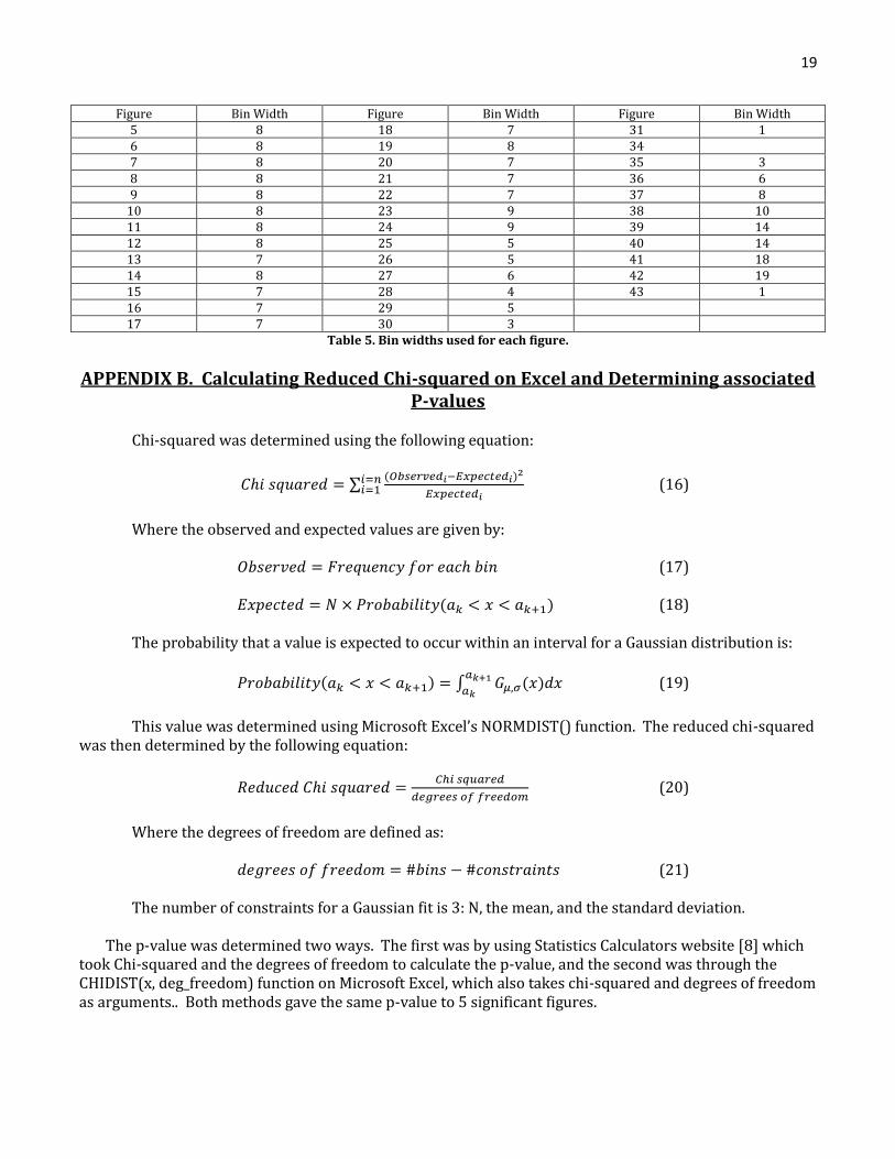
19

Figure Bin Width Figure Bin Width Figure Bin Width 5 8 18 7 31 1 6 8 19 8 34 7 8 20 7 35 3 8 8 21 7 36 6 9 8 22 7 37 8

10 8 23 9 38 10 11 8 24 9 39 14 12 8 25 5 40 14 13 7 26 5 41 18 14 8 27 6 42 19 15 7 28 4 43 1 16 7 29 5 17 7 30 3

Table 5. Bin widths used for each figure.

APPENDIX B. Calculating Reduced Chi-squared on Excel and Determining associated P-values

Chi-squared was determined using the following equation:

∑( )

(16)

Where the observed and expected values are given by:

(17) ( ) (18)

The probability that a value is expected to occur within an interval for a Gaussian distribution is:

( ) ∫ ( )

(19)

This value was determined using Microsoft Excel’s NORMDIST() function. The reduced chi-squared

was then determined by the following equation:

(20)

Where the degrees of freedom are defined as:

(21)

The number of constraints for a Gaussian fit is 3: N, the mean, and the standard deviation.

The p-value was determined two ways. The first was by using Statistics Calculators website [8] which took Chi-squared and the degrees of freedom to calculate the p-value, and the second was through the CHIDIST(x, deg_freedom) function on Microsoft Excel, which also takes chi-squared and degrees of freedom as arguments.. Both methods gave the same p-value to 5 significant figures.