determining the uncertainty associated with integrals … · determining the uncertainty associated...
TRANSCRIPT
Determining the uncertainty associated
with integrals of spectral quantities
EMRP-ENG05-1.3.1
Version 1.0
Emma R. Woolliams Engineering Measurement Division
A report of the EMRP Joint Research
Project
Metrology for Solid State Lighting
www.m4ssl.npl.co.uk
EMRP-ENG05-1.3.1
Version 1.0
- ii -
Title
:
Determining the uncertainty associated with integrals of spectral quantities
Reference : EMRP-ENG05-1.3.1 Version : 1.0 Date : April 2013 Dissemination level : PUBLIC Author(s) : Emma R. Woolliams
National Physical Laboratory
Keywords : Spectral integration, photometry, colorimetry, filter radiometry,
uncertainty, correlation Abstract : This report reviews the mathematical techniques required to
evaluate a spectral integral, including understanding uncertainty associated with the independent variable, wavelength, and the dependent variable, the measured spectral quantity. It also considers correlation in the quantities involved, using both an ‘error model’ and a covariance matrix.
Contact : http://www.m4ssl.npl.co.uk/contact
About the EMRP The European Metrology Research Programme (EMRP) is a metrology-focused European programme of coordinated R&D that facilitates closer integration of national research programmes. The EMRP is jointly supported by the European Commission and the participating countries within the European Association of National Metrology Institutes (EURAMET e.V.). The EMRP will ensure collaboration between National Measurement Institutes, reducing duplication and increasing impact. The overall goal of the EMRP is to accelerate innovation and competitiveness in Europe whilst continuing to provide essential support to underpin the quality of our lives. See http://www.emrponline.eu for more information. About the EMRP JRP “Metrology for Solid State Lighting” In the EMRP Joint Research Project (JRP) “Metrology for Solid State Lighting”, the following partners cooperate to create a European infrastructure for the traceable measurement of solid state lighting: VSL (Coordinator), Aalto, CMI, CSIC, EJPD, INRIM, IPQ, LNE, MKEH, NPL, PTB, SMU, SP, Trescal, CCR, TU Ilmenau and Université Paul Sabatier. See http://www.m4ssl.npl.co.uk/ for more information.
The research leading to these results has received funding from the European Union on the basis of Decision No 912/2009/EC.

EMRP-ENG05-1.3.1
Version 1.0
- iii -
EMRP-ENG05-1.3.1
Version 1.0
- iv -
SUMMARY
Spectral integration provides the link between radiometry and photometry and is an essential tool in optical radiation measurement. Often this integration involves an experimentally determined source spectrum and a defined spectral weighting function, for example the photopic spectral luminous
efficiency function, ( )V λ . Traditionally the ‘integration’ has been performed optically using a detector
(such as a photometer) with a spectral responsivity approximating the spectral weighting curve. It is now common to perform the integration by measuring the source output spectrally, especially with the availability of rapid spectral measurements using hand-held array spectrometers, and calculating the integral numerically.
This report reviews the mathematical techniques required to evaluate such a spectral integral, including understanding uncertainty associated with the independent variable, wavelength, and the dependent variable, the measured spectral quantity. It also considers correlation in the quantities involved, using both an ‘error model’ and a covariance matrix. The concepts of spectral correlation can be quite difficult to understand, and these concepts are therefore discussed first in terms of the effect of correlation on straightforward averages (see Section 6), before considering the effect on spectrally integrated quantities (Sections 7 and 8).
The report has the following sections:
Section 2 provides a reference to the definitions and terminology used in the report.
Section 3 is an introduction to the ideas in the report and describes the types of integrals used in photometry and radiometry.
Section 4 describes how integrated quantities are calculated numerically from measured data.
Section 5 shows how uncertainty analysis relates to spectrally measured quantities.
Section 6 is an introduction to correlation. It uses averages as an example to explain the concepts of correlation.
Sections 7 and 8 then apply those concepts to spectral integrals, using an error model and covariance matrices respectively.
Sections 9 and 10 bring these ideas together to look at the more involved problem of chromaticity calculations.
Appendices deal with some specific requirements – namely determining an integral from the product of two quantities when they are expressed in different wavelength steps, and correcting for bandwidth effects.
EMRP-ENG05-1.3.1
Version 1.0
Contents
1 INTRODUCTION .............................................................................................................................. 1
2 DEFINITIONS ................................................................................................................................... 1
2.1 Types of integrals .......................................................................................................................... 1
2.2 Uncertainty and error..................................................................................................................... 1
2.3 The GUM ....................................................................................................................................... 1
2.4 Random and systematic effects .................................................................................................... 2
2.5 Error model, measurement equation, calculation equation........................................................... 3
2.6 Multiplicative and additive models ................................................................................................. 5
2.7 Type A and Type B evaluations .................................................................................................... 5
2.8 Correct and shorthand phraseology .............................................................................................. 6
3 COMMON SPECTRAL INTEGRALS IN RADIOMETRY AND PHOTOMETRY ............................. 7
3.1 Integrating with a filter (photometer) ............................................................................................. 7
3.2 Spectral measurements ................................................................................................................ 8
3.2.1 Photometric quantities ........................................................................................................ 9
3.2.2 Chromaticity ....................................................................................................................... 9
3.2.3 Ultraviolet output and hazard ............................................................................................. 9
3.2.4 Total radiometric output ..................................................................................................... 9
3.2.5 Filter radiometer measurements ......................................................................................... 9
4 NUMERICAL DETERMINATION OF INTEGRATED QUANTITIES .............................................. 10
4.1 Form of the integrand .................................................................................................................. 10
4.2 Trapezium rule ............................................................................................................................ 10
4.3 Beyond the trapezium rule .......................................................................................................... 12
4.4 Differing measurement intervals ................................................................................................. 12
5 TYPES OF UNCERTAINTIES IN SPECTRAL DATA .................................................................... 13
5.1 Types of uncertainties ................................................................................................................. 13
5.2 Error model with systematic and random terms .......................................................................... 14
5.3 Random effects ........................................................................................................................... 14
5.4 Systematic effects ....................................................................................................................... 14
5.5 Mixed effects ............................................................................................................................... 15
5.6 Wavelength effects ...................................................................................................................... 15
5.7 Bandwidth .................................................................................................................................... 16
5.7.1 Bandwidth correction and defined-product integrals ....................................................... 16
5.7.2 Noise and integrated quantities ........................................................................................ 17
5.8 Stray light .................................................................................................................................... 18
5.9 Dark readings, noise threshold and low signal levels ................................................................. 19
6 COMBINING UNCERTAINTIES ASSOCIATED WITH AVERAGES ............................................ 19
6.1 Purpose of this section of the report ........................................................................................... 19
6.2 Relative and absolute effects ...................................................................................................... 20
6.3 Correlation ................................................................................................................................... 20

EMRP-ENG05-1.3.1
Version 1.0
6.4 Averaging partially correlated data .............................................................................................. 21
6.4.1 Standard uncertainty associated with the mean of a small number of readings ............... 23
6.5 Taking a weighted mean ............................................................................................................. 23
6.5.1 Generalisation .................................................................................................................. 24
6.6 Weighted mean with multiplicative models ................................................................................. 25
6.7 An example – test lamp calibrated against two reference lamps ................................................ 26
7 UNCERTAINTY ASSOCIATED WITH THE INTEGRAL ............................................................... 30
7.1 Assuming only multiplicative systematic effects ......................................................................... 31
7.2 Assuming only multiplicative random effects .............................................................................. 32
7.3 Assuming only wavelength effects .............................................................................................. 34
7.3.1 Systematic spectral offset effects ..................................................................................... 35
7.3.2 Wavelength offset effects ................................................................................................. 35
7.3.3 Random wavelength effects ............................................................................................. 36
7.3.4 Wavelength uncertainties summarised ............................................................................. 37
7.4 Dealing with a combination of effects .......................................................................................... 37
7.4.1 A more complete error model .......................................................................................... 38
7.4.2 Sensitivity coefficients and correlation ............................................................................ 38
7.4.3 Example determination of sensitivity coefficient ............................................................. 39
8 COVARIANCE MATRIX APPROACH ........................................................................................... 39
8.1 When is a covariance matrix needed? ........................................................................................ 39
8.2 How to create a covariance matrix .............................................................................................. 40
8.3 How to use a covariance matrix .................................................................................................. 41
8.3.1 Experimental product integrand ....................................................................................... 41
8.3.2 Defined product integrand ................................................................................................ 42
8.3.3 Simple integrand .............................................................................................................. 42
9 COLOUR MATCHING FUNCTIONS AND TRISTIMULUS VALUES ............................................ 42
9.1 Chromaticity coordinates without matrices.................................................................................. 43
9.2 Chromaticity coordinates with matrices....................................................................................... 45
10 CONCLUSIONS .......................................................................................................................... 46
11 ACKNOWLEDGEMENTS ........................................................................................................... 46
12 REFERENCES ............................................................................................................................ 46
13 APPENDIX 1: DETERMINING AN INTEGRAL FROM A PRODUCT WHERE THE DATA ARE AT DIFFERENT WAVELENGTH STEPS .............................................................................................. 48
14 APPENDIX 2: CORRECTING FOR BANDWIDTH .................................................................... 51
14.1 Step 1: Determine the bandpass function and its moments .................................................... 51
14.2 Step 2: Determine the correction coefficients .......................................................................... 51
14.3 Step 3a: Calculate the correction – derivative approach ......................................................... 51
14.4 Step 3b: Calculate the correction - weighted mean approach ................................................ 52
14.5 Simplification for triangular bandpass functions ...................................................................... 52
14.6 Bandwidth correction and covariance ...................................................................................... 53

EMRP-ENG05-1.3.1
Version 1.0
1
1 INTRODUCTION
This document has been prepared as NPL’s input into Task 1.3 of ENG05:LIGHTING Metrology for Solid State Lighting Annex 1a protocol. The task description is:
Develop mathematical models and methods for combined band-pass and stray-light correction (PTB) and propagation of uncertainty with integrated quantities using spectroradiometers (NPL) (D1.3.1).
This report completes NPL’s input.
Although the application of this work most relevant to that project is the determination of photometric and colorimetric quantities from spectral data taken with an array spectrometer, the examples in this report cover a wider range of applications.
2 DEFINITIONS
This report uses vocabulary from the VIM (International Vocabulary of Metrology, [1] ). In some cases a short-hand version of the correct phraseology is used in order to shorten sentences for ease of reading; in addition some concepts have been introduced in this report that are not formally defined. Technical terms and concepts used in this report are introduced here.
2.1 TYPES OF INTEGRALS
The three types of integrals defined in Section 4.1 use non-standard terms defined for the purposes of this report:
• Simple integrand: A spectral integral of a single experimental quantity
• Defined-product: A spectral integral of the product of an experimental quantity(with associated uncertainties) and a defined quantity (usually provided as a spectral table, with no associated uncertainty)
• Experimental-product: A spectral integral of the product of two experimental quantities (both with associated uncertainties)
2.2 UNCERTAINTY AND ERROR
The terms ‘error’ and ‘uncertainty’ are not synonyms. Each effect that has an influence on the measured spectral values (i.e. each component in the uncertainty budget) has an associated probability distribution
1 describing the set of values that effect could take. The standard uncertainty is
the standard deviation of this probability distribution. When a measurement is made, the value for that particular effect can be regarded as a randomly-selected draw from the associated probability distribution. The mean value of the probability distribution is generally zero; there is, on average (i.e. provided a sufficient number of repeated measured values are obtained) no error in the average measured value due to that effect
2. In practice, each measured value will have an error associated
with this particular effect, which is the difference between the value of the effect for that particular measurement and the mean value of the probability distribution. The (sign and) magnitude of this error is always unknown. If a correction for an effect is made, this error is the residual, post-correction error and it is a draw from the probability distribution with mean zero and a standard deviation equal to the standard uncertainty associated with that correction.
The use of the words ‘error’ and ‘uncertainty’ described here is consistent with paragraph 2.2.4 of the GUM (see Section 4.3).
2.3 THE GUM
The Guide to the Expression of Uncertainty in Measurement, known as ‘the GUM’, provides guidance on how to determine, combine and express uncertainty. It was developed by the JCGM (Joint Committee for Guides in Metrology), combining all the relevant standards organisations and the BIPM (Bureau International des Poids et Mesures). This heritage gives the GUM authority and recognition.
1 For spectral quantities the effect may have the same, or a different probability distribution, at different wavelengths. 2 Note that in the case of random effects it is possible to make multiple draws from the probability distribution, so that the
mean value can be estimated. For systematic effects the probability distribution represents the theoretical distribution of the
values for the effect about the mean ‘most likely’ value. In both cases a correction is usually applied, if necessary, so that the
estimated/theoretical mean value is zero.
EMRP-ENG05-1.3.1
Version 1.0
2
The JCGM continues to develop the GUM and has recently produced a number of supplements. All of these, as well as the ‘VIM’ (International Vocabulary of Metrology) are freely downloadable from the BIPM website
3.
The GUM gives the Law of Propagation of Uncertainty:
( ) ( ) ( )2 1
2 2c
1 1 1
2 , ,
n n n
i i j
i i ji i j i
f f fu y u x u x x
x x x
−
= = = +
∂ ∂ ∂= +
∂ ∂ ∂ ∑ ∑∑ (2.1)
which applies for a measurement model of the form
( )1 2 3, , , , ,iY f X X X X= … … (2.2)
where an estimate i
x of quantity i
X has an associated uncertainty ( )iu x , the squared combined
standard uncertainty (the combined variance) is the sum of two terms (2.1). The first term is the sum
of the squares of the standard uncertainties ( )iu x (the sum of the variances) associated with each
individual effect multiplied by the relevant sensitivity coefficient (the partial derivative). This first term is what is meant by the description ‘adding in quadrature’. The second term deals with the covariance of correlated quantities and is discussed in detail in Section 6.
2.4 RANDOM AND SYSTEMATIC EFFECTS
Correlation will be introduced whenever there is something in common between two measured values that will be combined (for spectral integrals, this means something in common between measured values at different wavelengths; where results are averaged, this means something in common between the measured values that will be averaged). The simplest way to describe this is in terms of random and systematic effects.
Random effects are those that are not common to the multiple measurements being combined. A common example is noise: two measured values may both suffer from noise, but the effect of noise will be different for each of the two measured values (for example, if noise has increased one measured value, this provides no information about whether any other measured value is increased or decreased by that noise, nor by what extent).
Systematic effects are those that are common to all measured values. If one measured value has been increased as a result of a systematic effect, then we can make a reliable prediction regarding whether any other measured value will be increased, and by how much
4. For example each time the
distance is set for an irradiance measurement using a particular lamp, there will be a (small) error in that distance. This will affect equally all measurements of that lamp until the next alignment. If multiple measured values are averaged without realignment, or measured values at different wavelengths are combined in an integral, then the distance error will be common to all those measured values. This is a systematic effect.
Some effects, such as noise, are always random; other effects can be either random or systematic depending on the measurement process. For example, if three measured values of a lamp are combined in an average and the lamp is realigned between each measurement, then alignment/distance is a random effect. If the lamp is not realigned between measurements, then alignment/distance is a systematic effect.
The error in the measured value due to a random effect will change from one measured value to another. In this case the uncertainty associated with the effect may be the same for each measured value (the probability distribution for the effect is the same at each wavelength), but each measured value is independent of each other measured value, as influenced by this effect. The unknown random error at each measured value is an independent draw from the probability distribution, meaning that the error due to the random effect is not only different from, but also independent of, the error at any other wavelength. The standard uncertainty associated with random effects is usually (but
3 http://www.bipm.org/en/publications/guides/gum.html 4 There are some situations where a systematic effect may cause the measured value at one wavelength to increase and the
measured value at another wavelength to decrease – this is described by a wavelength dependent sensitivity coefficient, and
is described in Section 7.4.2

EMRP-ENG05-1.3.1
Version 1.0
3
not always) determined by calculating the standard deviation of repeated measured values (See Section 2.6).
The error in the measured value due to a systematic effect will be the same from one measured value to another. The uncertainty associated with the effect is the same for each measured value and the error is the same draw from the probability distribution for all measured values. The standard uncertainty associated with systematic effects cannot be determined by repeat measurements, unless the effect is intentionally altered between repeats (e.g. by realigning a source multiple times using a series of different ‘extreme but acceptable’ alignments in an experiment to characterise the impact of source alignment.).
2.5 ERROR MODEL, MEASUREMENT EQUATION, CALCULATION EQUATION
In this report, the non-standard terms ‘error model’, ‘measurement equation’ and ‘calculation equation’ are used. These concepts are often all described as ‘measurement equations’ and there can be confusion, particularly when an experimentalist discusses these concepts with a theoretician! To avoid such confusion, these terms are distinguished here.
The measured value that forms the result5 of an experiment is often calculated by combining different
measurands. For example, consider the determination of the luminous intensity of a red traffic signal lamp measured by a lux meter at a distance of 9 m. The traffic signal is mounted on a tripod at one end of a long, blackened room, and the luxmeter on another tripod. The distance between the two is set to be 9 m using a tape measure and they are aligned to be parallel and colinear using a laser alignment system.
The luxmeter displays a nominal value for the illuminance at 9 m, say 20 lx. The luminous intensity,
VI , is given by the illuminance,
VE multiplied by the square of the distance, d . Thus, a suitable
laboratory measurement model is
2
V VI E d= . (2.3)
It may be that Equation (2.3) is sufficient for day-to-day analysis and therefore this is used to calculate the ‘result’ in the laboratory. This is therefore the calculation equation. However, this equation has several hidden assumptions, which may not be explicitly understood until uncertainty analysis is performed. Equation (2.3) assumes that, for example:,
• both the lamp and the luxmeter are normal to the optical axis. An improved measurement
model is 2 cos cos
r VI E d θ φ= , where θ and φ are the angles off-normal for the luxmeter
and lamp respectively. Since normally these angles are nominally zero, the cosine terms have value unity and are therefore not included in the calculation equation.
• the luxmeter matches the ( )V λ curve exactly or the test lamp is sufficiently similar to the
reference lamp which was used to calibrate the luxmeter, such that any mismatch has a negligible impact on the calculated results. A spectral mismatch (colour) correction factor,
ccfC , should be included in the measurement model to account for this, but this is assumed in
the calculation equation to have a value of unity.
• the calibration of the luxmeter is correct and that the reading is equal to the illuminance of the
lamp. It may be appropriate to replace V
E by calVE DC= , where D is the displayed value
6
and calC is the calibration factor. In the calculation equation this calibration factor is assumed
to have a value of unity.
• the instrument is insensitive to temperature, or was used at exactly the same temperature as it was calibrated. It may be appropriate to include in the measurement model a temperature
correction factor T
C with nominal value unity.
5 The VIM defines a measurement result as “set of quantity values being attributed to a measurand together with any other
available relevant information”, and thus the measured value is only one part of the result, the uncertainty being, for
example, another part. 6 Strictly, the “quantity of which the displayed value is a realisation”
EMRP-ENG05-1.3.1
Version 1.0
4
If these quantities are explicitly included in the calculation equation, we obtain the measurement equation
2
ccf calcos cosV T
I Dd C C Cθ φ= . (2.4)
The measurement equation therefore differs from the calculation equation in that it includes terms that do not alter the calculated result
7 (they have a nominal value of zero if additive or one if multiplicative).
The measurement equation is needed for uncertainty analysis because there is assumed to be an uncertainty associated with each quantity in the measurement equation. In other words, there is an
uncertainty associated with the nominal values 0θ φ= = , for example, as there is an uncertainty
associated with the alignment of the detector and source.
In uncertainty analysis for situations where there is no correlation, it is sufficient to determine the measurement equation, either explicitly, by including the additional quantities, or implicitly by including lines in an uncertainty budget table for those quantities that are not needed in the calculation equation. To determine the measurement equation it is helpful to start with the calculation equation and review its derivation (this, for example, will identify terms that have ‘cancelled out’, such as the responsivity of a system used to compare a reference source against a test source). After this it is helpful to consider, term-by-term, each aspect of the measurement facility to see what other hidden assumptions there may be.
When analysing a situation with correlation, it is helpful to introduce a further concept, that of the error model [2] . This is a further extension of the measurement equation to include, explicitly, error terms, and within this to describe clearly which are associated with systematic and which with random effects.
For example, consider the illuminance, calVE DC= , which forms part of the measurement equation
(2.4). The value obtained as the result of a measurement will differ from the true value in two (predominant) ways:
• There will be a random noise on the displayed reading, such that ( )measured tr1
rD D d= × + ,
where the actual displayed reading is equal to the true reading, tr
D , multiplied by an error
term. The term r
d is a random error that has been drawn from the probability distribution with
standard deviation ( )u D . If the measurement were repeated, then r
d would take a different
numerical value, as a different draw from the same probability distribution, described by the same standard deviation (equal to the standard uncertainty).
• There will be a systematic error on the calibration, such that the determined calibration
correction factor, ( )cal,measured cal,true cal1C C s= × + , where cals is the systematic error drawn
from the probability distribution with standard deviation ( )calu C equal to the standard
uncertainty associated with the calibration factor calC . If the measurement is repeated, then
this error does not change. To obtain a different error cals (and hence an independent draw
from that probability distribution), the calibration would need to be repeated.
When these ideas are written explicitly, we obtain an error model, for example of the form
( ) ( ) ( ) ( ) ( ) ( ) ( )2
,measured tr r tr tr tr ccf,tr ccf cal,tr cal ,tr1 1 cos cos 1 1 1V T T
I D d d x C s C s C sθ φθ δ φ δ= × + + + + × + × + × + (2.5)
This error model includes the errors ccf cal
, , , , , ,r T
d x s s sθ φδ δ . By explicitly including these errors, it is
possible to describe which of these are identical and which change when, for example, a
7 In practice, the calibration factor and spectral mismatch correction factors may take values different from unity, and in such
cases these would be included in the calculation equation. The distinction presented here would still hold for other terms and
the example is illustrative only.
EMRP-ENG05-1.3.1
Version 1.0
5
measurement is repeated. This can be done by introducing a numerical subscript, e.g.since the
random error on the displayed reading, r
d will change from measurement to measurement (the
uncertainty associated with this random effect will stay constant but a different error will be ‘drawn’
from the distribution), this can be written ,r id where i represents the measurement sequence number.
A systematic effect, such as the calibration effect, cals will not change from reading to reading and will
not have a subscript i .
Note that in the error model all the uncertainty is now associated with the error terms and these have an associated uncertainty that is equivalent to the uncertainty associated with the corresponding
quantity in the measurement equation. Thus in the error model, the term trD now represents the ‘true
displayed reading’ (i.e. error free) and has no associated uncertainty. The uncertainty associated with
rd , the corresponding error term, is that associated with the impact of noise on the measured
displayed reading, D in the measurement equation, Equation (2.4).
The significance of the error model is that each error term is now modelled as an independent random value, with an expected value of zero and an uncertainty associated with it. There is no correlation between these error terms and analysis can proceed using the simpler version of the law of propagation of uncertainties.
The concept of an error model is further clarified in later sections of this report, particularly in Section 6.
2.6 MULTIPLICATIVE AND ADDITIVE MODELS
Two other non-standard terms are helpful for this report and these are described here.
Multiplicative model is used to describe situations where the measurement equation is of the form 31 2
1 2 3
pp pY X X X= � , i.e. the individual terms are multiplied together (note the exponents can be
positive or negative and take any value, hence this includes ‘division’ and squared terms, for example).
Additive model is used to describe situations where the measurement equation is of the form
1 1 2 2 3 3Y m X m X m X= + + � . Again, the terms 1 2 3, ,m m m can take any value and be positive or
negative, so this includes ‘subtraction’.
In multiplicative models each term can have a different unit. For example in the multiplicative measurement equation, (2.4), the resultant luminous intensity has units candela, the displayed reading has unit lux, the distance has units metre, and the other units are relative terms with no unit.
In contrast, in additive models, each term has the same unit. For example the measured signal V
may be calculated from the light reading lightV and the dark reading, darkV , using the simple
measurement equation light darkV V V= − , and all terms have the units volts.
In general in radiometry, for multiplicative models the uncertainties are expressed as percentages and additive models have uncertainties expressed in the same units as the measured values. So the uncertainty associated with the displayed reading may be expressed as 0.5 % and the uncertainty associated with the light signal may be 0.1 mV. This is further described in Section 6.
2.7 TYPE A AND TYPE B EVALUATIONS
The terms ‘Type A’ and ‘Type B’ are used with uncertainty analysis. This use comes from the GUM, which defines:
• 2.3.2 Type A evaluation (of uncertainty) method of evaluation of uncertainty by the statistical analysis of series of observations
• 2.3.3 Type B evaluation (of uncertainty) method of evaluation of uncertainty by means other than the statistical analysis of series of observations
Type A evaluation uses statistical methods to determine uncertainties. Commonly this means taking repeat measurements and determining the standard deviation of those measurements. From the error

EMRP-ENG05-1.3.1
Version 1.0
6
model we can see that this method can only treat random errors, described in the uncertainty model as uncertainties associated with random effects, for example the uncertainty associated with measurement noise.
Type B evaluation uses 'any other method' to determine the uncertainties. This can include estimates of systematic errors from previous experiments or the metrologist's prior knowledge. It can also include random errors determined 'by any other method'. For example we may model room temperature by a random variable in the interval from 19 °C to 21 °C, the temperature range of the air-conditioning settings.
It is common to assume that ‘Type A’ evaluation is for random effects and ‘Type B’ evaluation is for systematic effects. This is generally, but not always, the case. For example, a ‘Type A’ method may be used to determine the uncertainty associated with alignment: a lamp may be realigned ten times and the standard deviation of those ten measurements used to determine an uncertainty associated with alignment
8. In a later experimental set-up, measurements may be taken at multiple wavelengths
and these combined in a spectral integral. For that integral, alignment is a systematic effect (the lamp is not realigned from wavelength to wavelength) even though the determination of the associated uncertainty was performed using ‘Type A’ methods. Similarly, the uncertainty associated with a random effect may be estimated from prior knowledge, or a measurement certificate, and thus by a ‘Type B’ method.
2.8 CORRECT AND SHORTHAND PHRASEOLOGY
In this report we aim to determine the standard uncertainty associated with the numerical estimate of the integral. Each phrase here has a specific meaning:
• Standard uncertainty represents one standard deviation of the probability distribution for the measurand, here the integral. This distinguishes it from expanded uncertainty, which is calculated from the standard uncertainty, and represents the interval for a particular confidence (often, but not always, the 95 % confidence interval, described for a Gaussian
distribution with the multiplier 2k = ).
• “Associated with” is the correct term to describe the relationship between an estimate of a measurand (quantity measured) and its uncertainty. In general speech it is common to describe the “uncertainty in distance” or, similar phrases. “The standard uncertainty associated with distance” is more correct.
• “the numerical estimate of the integral”. There is no uncertainty associated with the integral per se because it is a mathematical construct. The uncertainty is associated with the numerically calculated value that is an estimate of the true integral, e.g. the experimental value calculated using Equations (4.9) to (4.11) from data with associated uncertainties.
Since “The standard uncertainty associated with the numerical estimate of the integral” is a long phrase, occasionally this will be shorted to “the uncertainty associated with the integral” in order to make sentences more readable, especially where a more difficult concept needs to be described. Please read such phrases with appropriate caution.
Similarly, throughout this report if the terms uncertainty or uncertainties are used without a preceding descriptor, assume that these are ‘standard uncertainties’.
This report is also somewhat cavalier in the approach used for stating uncertainties. Strictly, an
uncertainty is associated with an estimated value of a quantity. For a quantity Q , say, an estimate is
denoted by Q (which may be a measured value or a calculated value of Q ). ( )ˆu Q denotes the
standard uncertainty associated with Q . Rather than stating the formally correct “… where ( )ˆu Q is
the standard uncertainty associated with Q , most of the time this report uses the same symbol, here
Q , for both the quantity and the value of the quantity, and refers simply to the standard uncertainty
( )u Q associated with Q .
8 If this is done, care must be taken to avoid ‘double counting’ any random effect due to, e.g. noise.

EMRP-ENG05-1.3.1
Version 1.0
7
3 COMMON SPECTRAL INTEGRALS IN RADIOMETRY AND PHOTOMETRY
3.1 INTEGRATING WITH A FILTER (PHOTOMETER)
Spectral integration provides the link between radiometry and photometry (and other spectrally integrated quantities). Such spectrally integrated quantities are related to geometrically equivalent
radiometric quantities through definitions that use an integral, for example, illuminance, VE , is related
to spectral irradiance, ( )E λ , through the expression
( ) ( )m dVE K E Vλ λ λ= ∫ (3.1)
where ( )V λ is the photopic relative spectral luminous efficiency function (often referred to as the V-
lambda curve) and mK is the maximum spectral luminous efficacy for photopic vision, 683 lm W-1
.
Traditionally, such integration has usually been performed optically – e.g. using a photometer which
has a spectral responsivity approximating the defined
( )V λ function. This method has many practical
advantages: in particular, a single measurement is required, rather than a complete spectral measurement, and the answer can be read off the device directly. If, instead of using a photometer, a traditional scanning spectrometer was to be used, the measurement would take far longer and the results would require some processing in order to provide the final (photometric) value. More fundamentally, a spectrometer may have insufficient dynamic range and linearity to measure a source correctly; with measurements with a bandwidth of only a few nanometres, the signal for a source that has low output across all or part of the spectrum may be ‘lost in the noise’. With a broadband measurement with a photometer, the integrated spectrum may be sufficient to provide a measureable signal, even when the spectral signal is too small to be measured.
However, a measurement using a photometer also has disadvantages, the most important of which is that of spectral mismatch. In any real photometer, the spectral responsivity will not be identical to the
( )V λ function and in some regions it may be significantly different, especially for the shortest (blue)
wavelengths. This spectral mismatch should be corrected using the spectral mismatch correction factor. The correction factor, F is given by
max
min
max
min
780
caltest380
780
test cal380
( ) ( )( ) ( )
( ) ( ) ( ) ( )
S R dS V d
F
S R d S V d
λ
λ
λ
λ
λ λ λλ λ λ
λ λ λ λ λ λ
=∫∫
∫ ∫ (3.2)
where test ( )S λ is the relative spectral distribution of the test source being measured, cal ( )S λ is the
relative spectral distribution of the source that was used to calibrate the photometer (often a tungsten filament lamp at a correlated colour temperature of 2856 K, which is the CIE Standard Source
representing CIE Standard Illuminant A) and ( )R λ is the spectral responsivity of the photometer,
measured over the full spectral range over which it has significant spectral response, i.e. from minλ to
maxλ . CIE DS023:2011, Characterization of the performance of illuminance meters and luminance
meters, specifies minλ as 360 nm and maxλ as 830 nm with limits on the total response from radiation
at wavelengths outside this range.
Although determining the spectral mismatch does involve some knowledge of the relative spectral distribution of the test source, this generally does not have to be known with as much accuracy as would be needed if the lamp illuminance were calculated from the spectrum. If the test source and the reference source are very similar, and spectrally broad, then this correction factor is very close to unity, even when the photometer has a poor match to the defined spectrum. When there is some difference between the sources, it is often sufficient to use a ‘typical lamp irradiance’ for the specific type of test source, rather than measuring the irradiance of the actual lamp. Thus relatively poor spectral data can be combined with accurate, sensitive, and fast broadband measurements to obtain an accurate result.
EMRP-ENG05-1.3.1
Version 1.0
8
3.2 SPECTRAL MEASUREMENTS
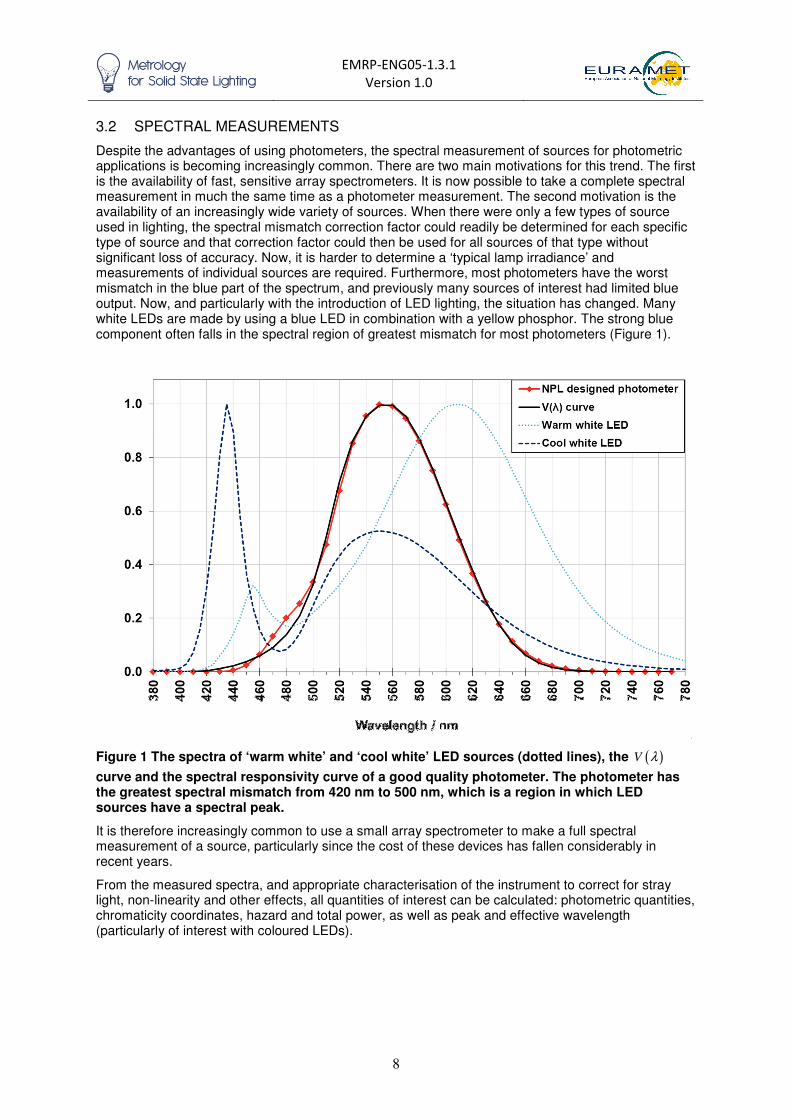
Despite the advantages of using photometers, the spectral measurement of sources for photometric applications is becoming increasingly common. There are two main motivations for this trend. The first is the availability of fast, sensitive array spectrometers. It is now possible to take a complete spectral measurement in much the same time as a photometer measurement. The second motivation is the availability of an increasingly wide variety of sources. When there were only a few types of source used in lighting, the spectral mismatch correction factor could readily be determined for each specific type of source and that correction factor could then be used for all sources of that type without significant loss of accuracy. Now, it is harder to determine a ‘typical lamp irradiance’ and measurements of individual sources are required. Furthermore, most photometers have the worst mismatch in the blue part of the spectrum, and previously many sources of interest had limited blue output. Now, and particularly with the introduction of LED lighting, the situation has changed. Many white LEDs are made by using a blue LED in combination with a yellow phosphor. The strong blue component often falls in the spectral region of greatest mismatch for most photometers (Figure 1).
Figure 1 The spectra of ‘warm white’ and ‘cool white’ LED sources (dotted lines), the ( )V λ
curve and the spectral responsivity curve of a good quality photometer. The photometer has the greatest spectral mismatch from 420 nm to 500 nm, which is a region in which LED sources have a spectral peak.
It is therefore increasingly common to use a small array spectrometer to make a full spectral measurement of a source, particularly since the cost of these devices has fallen considerably in recent years.
From the measured spectra, and appropriate characterisation of the instrument to correct for stray light, non-linearity and other effects, all quantities of interest can be calculated: photometric quantities, chromaticity coordinates, hazard and total power, as well as peak and effective wavelength (particularly of interest with coloured LEDs).

EMRP-ENG05-1.3.1
Version 1.0
9
3.2.1 Photometric quantities
Photometric quantities are all related to their geometrically equivalent radiometric quantities via a
defined spectral luminous efficiency function, such as ( )V λ . Thus illuminance can be calculated from
irradiance according to equation (3.1). Similarly, luminance can be calculated from radiance
( ) ( )m dVL K L Vλ λ λ= ∫ . (3.3)
And total luminous flux can be calculated from spectral total flux (also known as geometrically total spectral radiant flux)
( ) ( )m dV K VΦ Φ λ λ λ= ∫ . (3.4)
Integrals of this form are known in this report as defined-product integrals (see Section 4.1)
3.2.2 Chromaticity
Colour is calculated from the relative spectral emission properties of a source using the CIE colour-
matching functions, ( )x λ , ( )y λ and ( )z λ to calculate the tristimulus values X, Y and Z, e.g.
830 830 830
360 360 360( ) ( )d ( ) ( )d ( ) ( )dX E x Y E y Z E zλ λ λ λ λ λ λ λ λ= = =∫ ∫ ∫ (3.5)
The corresponding chromaticity values are calculated from these quantities by straightforward algebraic expressions. This is discussed in detail in Section 9. These colour integrals are all examples of defined-product integrals (see section 4.1).
3.2.3 Ultraviolet output and hazard
Similar integrals are used in determining the photobiological hazard of sources. For example, the erythemal (skin) hazard is calculated from
( ) ( )sE E s dλ λ λ= ∫ , (3.6)
where (((( ))))E λ is the lamp’s spectral irradiance and ( )s λ is the erythemal action spectrum, which is
defined over the spectral range from 180 nm to 400 nm. Similar functions, with different action spectra, are used to determine other source hazards.
These erythemal integrals are further examples of defined-product integrals (see section 4.1).
3.2.4 Total radiometric output
A more straightforward integral required in radiometry is the total radiometric output at all wavelengths, or over a defined range of wavelengths. This is commonly used where the source is incident on a ‘black’ detector – that is a detector that responds equally to all wavelengths. These are common, for example, in instruments used to measure the Earth’s radiation budget. In calibration of such detectors, it can be necessary to determine the total radiance of a white-light source. To determine this total radiance from a measured spectral radiance, it is necessary to evaluate the integral
( )total d ,L L λ λ= ∫ (3.7)
which is known in this report as a simple-integrand integral (see section 4.1). Another application for a simple-integrand integral is determining the UVA output of the source by integrating the source spectral irradiance over the defined UVA spectral region, with no weighting.
3.2.5 Filter radiometer measurements
Some measurements involve the use of the product of two experimentally determined functions that is then integrated. The most common example of when such a product is used is when a filter
EMRP-ENG05-1.3.1
Version 1.0
10
radiometer is used to determine a scaling factor in order to allow the absolute irradiance or radiance of a source to be calculated from relative spectral data.
If, for example, the filter radiometer’s spectral radiance responsivity is determined experimentally over
its full spectral range of response, giving a function ( ),FRLR λ and the relative spectral radiance of the
source is determined experimentally as ( )sL λ , then the output of the filter radiometer when used to
measure the source will be given by
( ) ( )abs s ,FR dLS L L Rλ λ λ= ∫ . (3.8)
The integral is determined numerically and compared with the experimentally determined signal S to
determine the unknown scaling factor for absolute radiance, absL .
This type of integral is known in this report as an experimental-product integral (Section 4.1).
4 NUMERICAL DETERMINATION OF INTEGRATED QUANTITIES
4.1 FORM OF THE INTEGRAND
In order to develop the mathematics in a generic manner, this report considers three general types of integrand (i.e. three forms for the integral). The different integrands given above can all be written in the form of one of these integrals.
Simple integrand. This is shorthand for an integral of a spectral quantity with no additional weighting: e.g. to determine total output of the UVA component of a source. The integral is of the form
( )max
min
s dI Eλ
λλ λ= ∫ (4.1)
and is a simple integral of the experimentally determined source quantity E(λ) (e.g. irradiance,
radiance, or flux) over a defined wavelength range λmin to λmax (315 nm to 400 nm for UVA).
Defined product. This is shorthand for a product of an experimentally determined quantity and a defined quantity. The integral is of the form
( ) ( )dp dI E Fλ λ λ= ∫ (4.2)
where the integrand is a product of an experimentally determined source quantity ( )E λ (spectral
irradiance, spectral radiance, spectral flux) and a defined quantity ( )F λ (e.g. the ( )V λ function, a
hazard function or the CIE colour-matching functions).
Note that the simple integrand is a special case of the defined product, where the defined term is unity over a particular spectral range.
Experimental product. This is shorthand for the product of two experimentally determined quantities. The integral is of the form
( ) ( )ep dI E Gλ λ λ= ∫ (4.3)
where the integrand is a product of an experimentally determined source quantity ( )E λ (spectral
irradiance, spectral radiance, spectral flux) and an experimentally determined responsivity function
( )G λ .
4.2 TRAPEZIUM RULE
A common method for evaluating integrals is the trapezium (or trapezoidal) rule. The trapezium rule approximates the integral by treating the integrand as varying linearly between adjacent measurement points.
EMRP-ENG05-1.3.1
Version 1.0
11
1λ 2λ 3λ
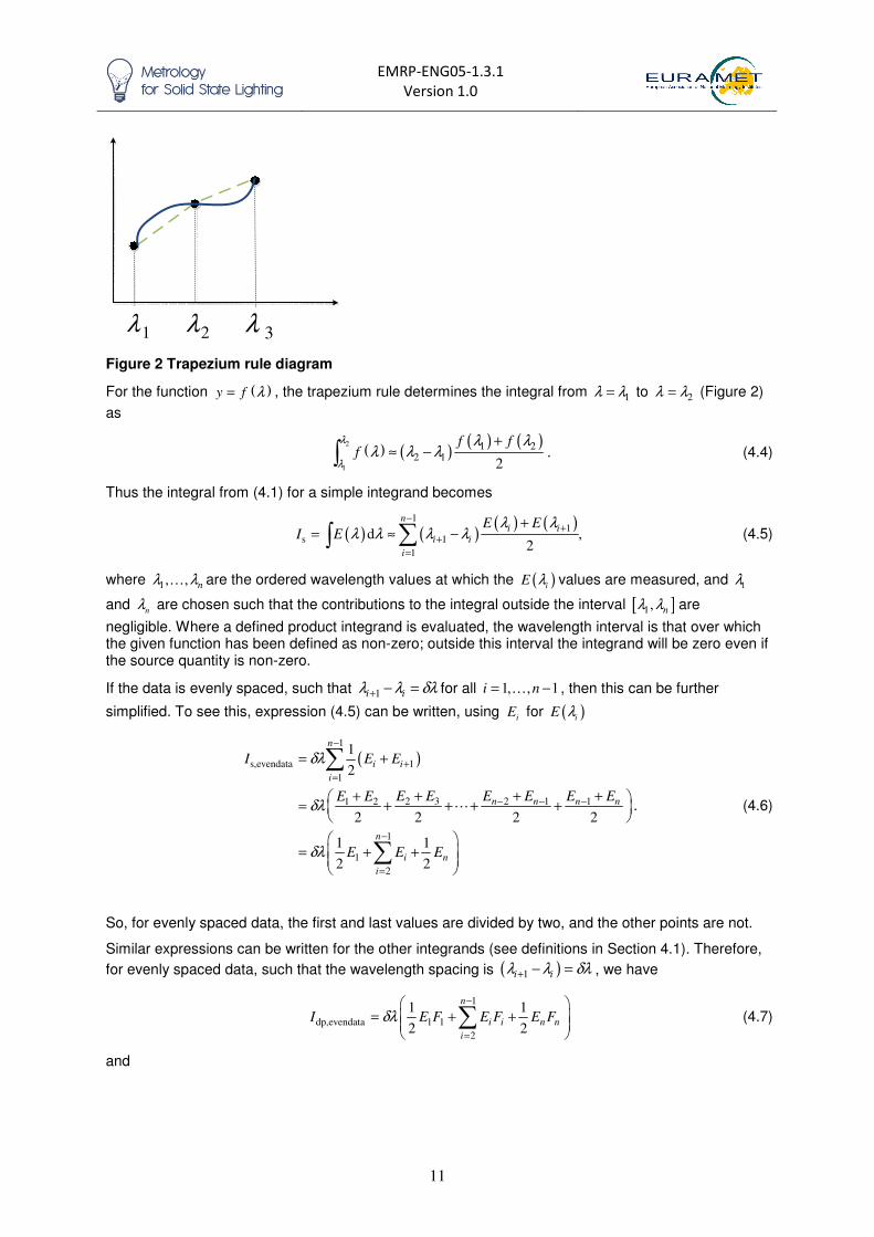
Figure 2 Trapezium rule diagram
For the function ( )y f λ= , the trapezium rule determines the integral from 1λ λ= to 2λ λ= (Figure 2)
as
( ) ( )( ) ( )2
1
1 22 1
2
f ff
λ
λ
λ λλ λ λ
+≈ −∫ . (4.4)
Thus the integral from (4.1) for a simple integrand becomes
( ) ( )( ) ( )1
1s 1
1
d ,2
ni i
i i
i
E EI E
λ λλ λ λ λ
−+
+
=
+= ≈ −∑∫ (4.5)
where 1, , nλ λ… are the ordered wavelength values at which the ( )iE λ values are measured, and 1λ
and
nλ are chosen such that the contributions to the integral outside the interval [ ]1, nλ λ are
negligible. Where a defined product integrand is evaluated, the wavelength interval is that over which the given function has been defined as non-zero; outside this interval the integrand will be zero even if the source quantity is non-zero.
If the data is evenly spaced, such that 1i iλ λ δλ+ − = for all 1, , 1i n= −… , then this can be further
simplified. To see this, expression (4.5) can be written, using i
E for ( )iE λ
( )1
s,evendata 1
1
2 3 2 1 11 2
1
1
2
1
2
2 2 2 2
1 1
2 2
n
i i
i
n n n n
n
i n
i
I E E
E E E E E EE E
E E E
δλ
δλ
δλ
−
+
=
− − −
−
=
= +
+ + ++ = + + + +
= + +
∑
∑
� . (4.6)
So, for evenly spaced data, the first and last values are divided by two, and the other points are not.
Similar expressions can be written for the other integrands (see definitions in Section 4.1). Therefore,
for evenly spaced data, such that the wavelength spacing is , we have
1
dp,evendata 1 1
2
1 1
2 2
n
i i n n
i
I E F E F E Fδλ−
=
= + +
∑ (4.7)
and
( )1i iλ λ δλ+ − =
EMRP-ENG05-1.3.1
Version 1.0
12
1
ep,evendata 1 1
2
1 1.
2 2
n
i i n n
i
I E G E G E Gδλ−
=
= + +
∑ (4.8)
More generally we can write
( )s
1
,
n
i i
i
I E λ=
=∑� (4.9)
( ) ( )dp
1
,
n
i i i
i
I E Fλ λ=
=∑� (4.10)
( ) ( )ep
1
,
n
i i i
i
I E Gλ λ=
=∑� (4.11)
where in all cases i� , which depends on the wavelength spacing either side of iλ , is an appropriate
weighting term. If the data are evenly spaced, such that 1i iλ λ δλ+ − = for all wavelength steps, then,
for the trapezium rule
2 1,
2, , 1.i
i n
i n
δλ
δλ
==
= −�
… (4.12)
giving the equations (4.6) to (4.8). Note that although the first and last points have strictly a different weighting (i.e. half the weighting of the other points), in practice, especially with defined products where the defined function falls to zero at the shortest and longest wavelengths, this can be treated
as an unnecessary complication, and i
δλ=� used throughout.
4.3 BEYOND THE TRAPEZIUM RULE
There are occasions when the trapezium rule is inadequate. As described above, the rule approximates the integrand between successive data points by straight lines. However, real spectra
may have regions of high curvature. If the spectrum of interest is concave (as in Figure 2 between 2λ
and 3λ ) or convex (as in Figure 2 between 1λ and 2λ ), the trapezium rule would give a value of the
integral that is too large or too small, respectively. Since many real spectra have regions of curvature, it is often more appropriate to use other functions to ‘join the dots’. For example, a cubic function could be passed through the two points in question and a neighbouring point on each side.
Cox [3] describes fitting different piecewise polynomials9 to increasing numbers of points in order to
determine the integral with a linear (trapezium), quadratic, cubic, quartic, … function. The paper also describes how to evaluate the associated uncertainty (from random effects only) and suggests that different polynomial orders should be calculated until two successive polynomials agree within the associated uncertainties. These methods are described in detail in the paper, which uses the
formulation similar to that of (4.9), (4.10) and (4.11) (in the paper the symbol iw is used instead of
)i� . For even wavelength spacing, i� always takes the value 1 in the central region, with only the first
few and last few points taking other values (the number of points with a weighting other than 1 increases as the interpolation function increases in order).
4.4 DIFFERING MEASUREMENT INTERVALS
When the integrand is a product (either a defined product or experimental product, as defined in Section 4.1), then it is necessary to have the two functions determined at the same wavelengths in order to use equations (4.10) or (4.11) (i.e. it is necessary that there is a value for both quantities in
the product for each iλ ). If the two functions are at different wavelength values, then one or both must
be interpolated.
In some situations one function may be defined at a subset of the wavelengths of the other function, for example where one function is determined in 10 nm steps and the other in 5 nm steps, with the
9 That is functions composed of polynomial pieces joined end to end

EMRP-ENG05-1.3.1
Version 1.0
13
10 nm steps matching every other 5 nm step measurement. On other occasions the wavelength steps may be completely different. This is particularly common if measurements are made with an array-spectrometer. Array spectrometers rarely make measurements with a uniform wavelength spacing and the measured wavelengths are unlikely to be a whole number of nanometres.
For sources with smooth spectral profiles, measured values are often obtained using a large wavelength step, significantly greater than the bandwidth of the measuring system. For example, the spectral irradiance of a tungsten lamp may be determined with a wavelength interval as large as 20 nm. Here the measured (smoothly-varying) spectral values should be interpolated to match the
wavelengths of the defined function (e.g. the ( )V λ or CIE colour-matching function), or the measured
wavelengths of the filter radiometer for experimental products. This interpolation can be carried out using simple methods such as linear or cubic spline interpolation, or, more accurately, using a physical model (or physico-empirical model), such as the Planck-polynomial model [4, 5] .
For a defined-product of a source with a more complex spectral profile, it is usually advisable to interpolate the defined function to match the wavelengths of measurement, rather than to interpolate the experimentally-determined data to match the defined function. There are two advantages to this. The first is that the source spectrum often has structure on a smaller scale than the defined function, which is smoothly varying; this can lead to errors in interpolation. The second is that because the defined function has no associated uncertainty, interpolating it does not introduce correlation between values at different wavelengths. When experimental data are interpolated, correlation is introduced
and this must be dealt with in the subsequent uncertainty analysis. Functions such as the ( )V λ curve
are defined at a 1 nm interval and it is appropriate [6] where necessary, to interpolate them linearly between these defined wavelength values.
For an experimental-product (the product of two experimental quantities), there are two options. If one curve is known to be significantly smoother than the other, then this smoother curve should be interpolated to match the wavelengths of the other curve. If both curves have significant structure, then both should be interpolated to match the wavelengths of the other. For example if the source is measured at 400 nm, 402 nm, 404 nm, 406 nm, …, and the detector is measured at 401 nm, 403 nm,…, then the source should be interpolated to obtain values at 401 nm, 403 nm, … and the detector should be interpolated to obtain values at 402 nm, 404 nm, …. The integral would then use the products calculated at 401 nm, 402 nm, 403 nm, …. This process is discussed in detail in Appendix 3. Note that, depending on the wavelengths at which the two experimental quantities have been determined, this may lead to data in uneven wavelength steps, as also detailed in Appendix 3.
5 TYPES OF UNCERTAINTIES IN SPECTRAL DATA
5.1 TYPES OF UNCERTAINTIES
Any measurement result will have an associated uncertainty that will come from various physical effects. For example, the results of a measurement of the spectral irradiance of a lamp will be influenced by the effects of instrument noise, lamp alignment, lamp current control, room temperature etc., as well as the instrument calibration. The overall uncertainty associated with the measured value can be calculated by combining the individual uncertainties due to each of these effects. The method for doing this is described in the GUM, see also section 2.3.
When an integral is calculated from spectral data, it is necessary to go beyond a wavelength-by-wavelength uncertainty analysis by taking account of any covariance associated with measured values at different wavelengths, i.e. the correlations associated with the measured value at one wavelength and the measured values at any other wavelengths.
Determining these covariances, and thus the uncertainty associated with a numerical estimate of an integral, requires a distinction to be made between effects that are random, systematic or a mixture of the two. Uncertainties associated with the wavelength setting should also be distinguished from those associated with the measured spectral values (e.g. the irradiance). The rest of this section considers these different effects separately. It also discusses bandwidth, stray light and noise threshold as these have complex effects on the uncertainty associated with an integrated quantity.

EMRP-ENG05-1.3.1
Version 1.0
14
5.2 ERROR MODEL WITH SYSTEMATIC AND RANDOM TERMS
We can describe the irradiance of a lamp at a wavelength i
λ with a simplistic error model10
, for
example saying that the spectral irradiance is described by
( ) ( ) ( ) ( )T 1 1 ,i i iE E S Rλ λ= + + (5.1)
where the measured irradiance ( )iE λ is the true irradiance ( )T iE λ modified by the systematic effect
S , which is the same at all wavelengths and hence has no subscript i and the random effect iR
which varies from wavelength to wavelength.
Both S and iR are unknown. We therefore assume that their expected value is zero, with an
uncertainty given by the uncertainty associated with systematic and random effects, respectively.
5.3 RANDOM EFFECTS
Random effects change from wavelength to wavelength. Even if the uncertainty associated with the effect is the same at each wavelength (because the probability distribution for the effect is the same at each wavelength), the spectral irradiance value at one wavelength, as influenced by this random effect, can be considered to be entirely independent of the spectral irradiance value influenced by the random effect at another wavelength. The standard uncertainty associated with random effects is usually determined by calculating the standard deviation of repeated measured values.
The most common random effect is noise, which can originate electronically or optically. However, there can be other effects that behave randomly in terms of the impact on a measured value at one wavelength and the next. For example, when measured values are obtained sequentially (e.g. with a scanning monochromator), then any quantity that changes over time, such as a random fluctuation in temperature or lamp current, will have a different impact from wavelength to wavelength and thus will be considered a random effect, with no associated correlation from wavelength to wavelength. On the other hand if the spectrum is obtained simultaneously (e.g. with an array spectrometer), then these same effects will create the same error at all wavelengths and are considered systematic effects (with associated correlation from wavelength to wavelength) for e.g. spectral integration
11.
A random effect will either increase or decrease a measured value, and thus contributions at each wavelength to the sum (e.g. that in (4.10)) will behave correspondingly. ‘On average’, when the corresponding uncertainties at each wavelength are comparable, the value of the integral will tend to be closer to the ‘true’ value than it would be if the effects were systematic with wavelength rather than random. The term ‘on average’ is appropriate, as integration can be considered a form of averaging.
5.4 SYSTEMATIC EFFECTS
Systematic effects, for the purposes of evaluating spectral integrals, are effects that do not change between the measured value at one wavelength to the next measured value. For example, usually a lamp is measured at all wavelengths without being realigned (or repositioned) between wavelengths. Thus any error introduced by misalignment is common to the measured values at all wavelengths.
In most cases (i.e. for multiplicative models), systematic effects will scale the measured spectrum. If the lamp is positioned slightly too close to the measuring instrument, for example, then the amplitude of the entire spectrum will be too high by the same proportion at all wavelengths. This means that if a systematic effect provides an uncertainty associated with the measured spectral irradiance of, say 0.2 %, the uncertainty associated with the integral due to this effect will also be 0.2 %.
There are some situations where the systematic effect is more complex because of a wavelength-dependent sensitivity coefficient. The sensitivity coefficient is the scaling factor between the uncertainty associated with a quantity and the uncertainty associated with the measurand. For example, because of the inverse square law, an uncertainty associated with the distance of a point source of 0.1 % (say 1 mm in 1000 mm) causes an uncertainty associated with the lamp irradiance of
10 See sections 2.3-2.6. This is a simplistic multiplicative model. Later sections of this report show how this simple model
can be modified to include additive effects, wavelength dependent sensitivity coefficients and wavelength errors. 11 They may still be random effects when determining the mean of two measurements; see Section 6.
EMRP-ENG05-1.3.1
Version 1.0
15
0.2 %. The sensitivity coefficient for irradiance due to distance, because of the inverse square law, is two. See Section 7.4.1 for a fuller explanation of this concept.
In contrast to distance, which has a constant sensitivity coefficient (of two) at all wavelengths, the sensitivity coefficient associated with the current setting for a tungsten filament lamp varies with wavelength. If the lamp current is set too high, the measured spectral irradiance will be too high at all wavelengths. The effect of the error in the lamp current will be larger in the ultraviolet than in the red spectral region, because the sensitivity coefficient for the relationship between spectral irradiance and lamp current is wavelength-dependent, being higher in the ultraviolet than the red.
5.5 MIXED EFFECTS
Many effects are neither entirely systematic, nor entirely random. For example the lamp current may be set using a reference resistor. Any uncertainty associated with the calibration of that reference resistor will be common for all measured values of lamp irradiance (at all wavelengths) and so relate to a systematic effect. In addition, there may be a time-dependent random effect due to instability of the current control system. If the wavelengths are measured sequentially (e.g. with a scanning monochromator) there will be an additional random effect with wavelength.
Another example of a mixed effect is the uncertainty associated with the irradiance of a reference lamp used to calibrate a test lamp by direct comparison. The uncertainty associated with the irradiance of the reference lamp will be partly due to effects that change from wavelength to wavelength (random effects in its calibration, e.g. noise) and partly due to effects that are common to all wavelengths (systematic effects in its calibration, e.g. misalignment during calibration).
For such mixed effects, it is useful to separate the random and systematic influences as different lines in the uncertainty budget. Thus there will be a line in the uncertainty budget for ‘lamp current systematic effect’ and another line for ‘lamp current random effect’. Sometimes one of these components has significantly less influence than the other, and it is sufficient to describe an effect as ‘mostly systematic’ or ‘mostly random’. Where separation is not possible, it is necessary to use a covariance matrix (Section 8).
5.6 WAVELENGTH EFFECTS
The uncertainties described above are uncertainties associated with the spectral quantities, e.g. irradiance, usually shown on a graph on the vertical axis. In any measuring system there will also be uncertainties associated with wavelength, plotted on the horizontal axis. Consider a test source calibrated against a reference source using a spectrometer or monochromator-based instrument. There are three types of wavelength error:
1. A constant systematic spectral offset that applies to measured values of both sources and at all wavelengths. This offset is due to the particular alignment of the grating and slit and is usually corrected by performing a wavelength scale calibration using an emission line source at a single wavelength. There will be a residual uncertainty associated with that correction and hence an uncertainty in the corrected wavelength scale values.
2. A wavelength offset that is the same for both sources, but which varies with wavelength. This offset is caused by grating ruling errors, or errors in the rotation process for a scanning monochromator. In an array spectrometer this offset can also be due to the alignment of the array and the fact that in general it is flat, while the image field is curved. This offset can also be corrected through wavelength scale calibration, which is typically performed at a few wavelengths across the spectral range of interest (for example using several lines of an Hg emission source). The size of the wavelength scale correction, and the uncertainty associated with it, may be different at each calibration wavelength, and will also vary between the calibration points. The result in terms of the wavelength scale when measuring one source compared with another is an effect that is random from wavelength to wavelength for each source, but systematic from source to source at a particular wavelength.
3. A random effect (scanning monochromators only). There is a residual uncertainty associated with the ability of the system to reposition the grating (turn to the same angle). This residual uncertainty to a random wavelength effect that will vary with wavelength for each particular source, and from source to source at the same wavelength.
EMRP-ENG05-1.3.1
Version 1.0
16
Note that for the first two of these wavelength effects it may be possible to determine an estimate of the offset and apply a correction, for example by measuring a line source as described above (for the wavelength offset, this will involve multiple spectral lines). There will still be a residual uncertainty associated with that correction, an unknown systematic effect. The associated uncertainty can be deduced by comparing the determined correction for the different spectral lines. The uncertainty associated with wavelength due to random effects can be deduced from repeated wavelength scale calibrations.
The sensitivity of the calculated irradiance of the test source to these wavelength effects (and hence the sensitivity of the integrals calculated from that irradiance) depends on the nature of both the test and reference sources. If the spectra for the two sources change slowly with wavelength, then a small wavelength error will not change the measured signal significantly. If the spectra for the two sources change more rapidly with wavelength, but in the same direction, then a small wavelength error will affect both sources in closely the same way (they will both be too high, or both too low) and the ratio (which is what matters for the comparison) will not change much. However a problem arises when one source changes rapidly with wavelength in one direction and the other source changes rapidly in the other direction. In this situation a small wavelength error will increase the signal measured for one source and decrease the signal measured for the other source, and the ratio will be changed significantly. The more rapidly the source spectra change with wavelength, the more significant the consequence.
One example for where one source increases and the other decreases arises when measuring the ‘down slope’ of an LED’s spectral irradiance (the tail on the longer wavelength side) against a tungsten lamp whose irradiance is increasing with wavelength.
The effect of wavelength uncertainty on an integral depends on the type of error and is described in detail in Section 7.3.
5.7 BANDWIDTH
Another important effect in spectral measurements is bandwidth. All spectrally selective instruments will make measurements with a finite bandwidth. The bandpass function is basically triangular for a high quality scanning monochromator. For array spectrometers it is more complex, and often not perfectly symmetrical, but can usually be described by a simple modified Gaussian, with different parameters for the ‘up’ and ‘down’ slopes [7] .
Methods have been developed to correct for bandwidth effects [8, 9] . These corrections are sensitive to noise and measurement step size and will never provide a perfect correction; however good results can be obtained for any relatively smoothly changing source. LED sources have peaks that are broad enough to correct, and narrow enough to benefit from bandwidth correction.
Bandwidth has the effect of broadening spectral features and for such features the signal is effectively measured at the ‘wrong’ wavelength. That process will change the calculated integrals. After correction, the error in the integral will usually be significantly reduced. Section 5.7.2 shows that for spectra with associated random noise, the bandwidth correction introduces artificial pseudo-noise, which makes correction unsuitable for spectral recovery; however, even in this situation, bandwidth correction is appropriate for determining integrals, as the pseudo-noise is removed by integration.
5.7.1 Bandwidth correction and defined-product integrals
The bandwidth correction at � � �� from [9] can be written in the form
( ) ( ) ( ) ( ) ( ) ( )corr 0 0 0 1 0 2 0 3 0 4 0 ,ivE A E A E A E A E A Eλ λ λ λ λ λ′ ′′ ′′′= + + + + +� (5.2)
where 0 1, ,A A … are calculated from the moments of the instrument bandpass function, and the
corrected signal depends on the derivatives of the measured signal. This bandwidth correction process is described in more detail in Section 14.
For most experimentally-realised bandpass functions the multiplicative constants 1 3, ,A A … for the first
and third derivatives, are close to zero and therefore the bandwidth correction depends mostly on the even order derivatives (second, fourth,…) of the measured spectrum. Bandwidth effects are most significant for spectra that have a second derivative that is large in magnitude (i.e. spectra that have high curvature over a bandwidth). Often spectral measurements are performed as a comparison
EMRP-ENG05-1.3.1
Version 1.0
17
between a test source and a reference source. In these situations the effect of bandwidth on the determined test source spectrum depends on how different the second derivatives of the two source spectra are.
If we combine equations (5.2) and (4.10) we obtain12
( )( )
( )( )
dp
dd
d
dd
d
j
j j
j
j j
EI A F
EA F
λλ λ
λ
λλ λ
λ
=
=
∑∫
∑ ∫ (5.3)
which can also be written
( ) ( ) ( ) ( ) ( ) ( )dp 0 1 2d d d .I A E F A E F A E Fλ λ λ λ λ λ λ λ λ′ ′′= + + +∫ ∫ ∫ � (5.4)
Considering just one term of series (5.4) and integrating by parts
( ) ( ) ( ) ( )[ ] ( ) ( )( ) ( 1) ( 1)0
0d d .
j j jE F E F E Fλ λ λ λ λ λ λ λ
∞ ∞− − ′= −∫ ∫ (5.5)
For defined-product functions ( ) ( ) ( )[ ]1
0 0j
E Fλ λ∞
− = since the functions represented by ( )F λ (the
relative spectral luminous efficiency curve, the CIE-colour matching functions, action spectra, …) become zero at the two extremes of the defined wavelength interval. Continuing to integrate by parts yields the expression
( ) ( ) ( ) ( ) ( ) ( ) ( )0 0
d 1 djj j
F E F Eλ λ λ λ λ λ∞ ∞
= −∫ ∫ (5.6)
and therefore, from (5.3),
( ) ( ) ( ) ( )dp 1 d
j j
jI A F Eλ λ λ= −∑ ∫ . (5.7)
Written in full,
( ) ( ) ( ) ( ) ( ) ( )dp 0 1 2d d d .I A F E A F E A F Eλ λ λ λ λ λ λ λ λ′ ′′= − + −∫ ∫ ∫ � (5.8)
Comparing expressions (5.4) and (5.8) it is clear that, apart from the sign change, the only difference is that instead of differentiating the experimentally determined spectral irradiance, the function being differentiated is the defined weighting function.
The above analysis shows that in the case of defined product integrals, the effect of bandwidth (and thus the correction) can be calculated equivalently using derivatives of either the measured values or the weighting function. The weighting functions are defined and tabulated; they do not change from one measurement to the next, nor is there any noise associated with the values. Therefore the bandwidth correction for a particular bandpass function can be applied to the weighting functions and then those used with any experimental spectrum, without further bandpass correction of the measured spectrum.
Venable [10] applied this approach to the common situation of a triangular bandpass function, and measured values with a wavelength interval equal to a bandwidth, to determine appropriate bandwidth corrections for every combination of standard illuminant and colorimetric weighting functions. This is the basis of the tables in the ASTM E-308 standard [11] .
5.7.2 Noise and integrated quantities
Another implication of the analysis in Section 5.7.1 for defined product integrals is that since, after integration, the result of applying the bandwidth correction to the weighting function is exactly
12 In Equation (5.3), the subscript j refers to the term in (5.2). So for 2j = , ( )
( )2
d
d
j
j j
EA A E
λλ
λ′′=
EMRP-ENG05-1.3.1
Version 1.0
18
equivalent to applying the bandwidth correction to the measured values, the effect of noise associated with the measurement is far less significant for integrated quantities than it is for spectrally-resolved
quantities. For example, consider the situation where a photometric quantity dpI is to be determined
from a measured spectrum ( )E λ and the photopic standard observer function, ( )V λ , is adjusted
rather than the measured spectrum13
. The relevant integral is
( ) ( )dp adj dI V Eλ λ λ= ∫ . (5.9)
The value of this integral will be no more sensitive to noise than the value of the integral calculated
from the spectrum without bandwidth correction ( ) ( )dp,meas dI V Eλ λ λ= ∫ and since (from Section
5.7.1) expression (4.10) is identical to ( ) ( )dp corr dI V Eλ λ λ= ∫ , it can be concluded that whether the
weighting function is adjusted for bandwidth, or the measured spectrum is corrected for bandwidth, the measurement noise will never have a larger effect on the integrated value after correction than it has before correction.
This conclusion is somewhat counter-intuitive. The bandpass-corrected spectrum is very sensitive to noise [9] (due to the amplification of measurement noise by the correction algorithm when the true spectrum changes little from one measurement point to the next). It therefore seems surprising that for an integrated quantity, this artificially enhanced noise has no effect. However, this can be understood by recognising that such noise is averaged out in the process of integration.
Gardner [12] looked at the chromaticity calculated for LED sources with an emission width of 25 nm and for central wavelengths of 500 nm, 590 nm and 630 nm measured with a spectrometer with a non-triangular bandpass function of bandwidth approximately 10 nm. He showed that even when the corrected spectrum is noisy, the chromaticity coordinates calculated from the correction were always superior to those calculated from the raw measurements. This result suggests that where the aim is to determine integrated quantities, the correction should always be applied.
5.8 STRAY LIGHT
Stray light is where light of one wavelength is measured as though it were at a different (wrong) wavelength, usually because of scattering mechanisms within
14 the instrument.
One method to correct for stray light is to use a cut-on filter to remove all light below the filter’s cut-on wavelength. Signals measured at the lower wavelengths are entirely due to stray light and can be removed by subtraction, perhaps weighting the subtracted signal by the long wavelength transmission of the cut-on filter. Using a series of bandpass or blocking filters to restrict the range of wavelengths entering the spectrometer allows measurements to be made over a truncated spectral range without the influence of stray radiation at wavelengths outside this range. If a series of such bandpass filters is used, each tailored for a given spectral region, it is possible to make measurements over a broad spectral range whilst still ensuring good stray light performance is achieved [13] .
Stray light can also be characterised and corrected using a monochromatic source. A tuneable laser (or, with care, a narrow bandwidth monochromator) is used to scan sequentially through each wavelength in turn. The response at other wavelengths to this monochromatic light is used to create a stray light correction matrix which can then be used to correct stray light in any measured spectrum [8, 14, 15] .
If uncorrected, stray light can cause very large errors in the spectrum measured by an array spectrometer, even errors greater than 100 % in the blue end of a tungsten lamp spectrum measured using an array spectrometer with significant short wavelength stray light. Such an error will change the value of any integral calculated from that spectrum, and the size of the effect will depend on where in the spectrum the stray light occurs. If corrected, the correction method will introduce mathematical
13 ( )V λ itself does not require any adjustment, but it is adjusted mathematically to a form that can be used with an
uncorrected irradiance spectrum. 14 Here we are referring to internal stray light as opposed to external stray light which is where extraneous light enters the
spectrometer from sources other than the one being measured
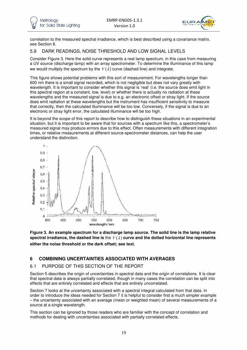
EMRP-ENG05-1.3.1
Version 1.0
19
correlation to the measured spectral irradiance, which is best described using a covariance matrix, see Section 8.
5.9 DARK READINGS, NOISE THRESHOLD AND LOW SIGNAL LEVELS
Consider Figure 3. Here the solid curve represents a real lamp spectrum, in this case from measuring a UV source (discharge lamp) with an array spectrometer. To determine the illuminance of this lamp
we would multiply the spectrum by the ( )V λ curve (dashed line) and integrate.
This figure shows potential problems with this sort of measurement. For wavelengths longer than 600 nm there is a small signal recorded, which is not negligible but does not vary greatly with wavelength. It is important to consider whether this signal is ‘real’ (i.e. the source does emit light in this spectral region at a constant, low, level) or whether there is actually no radiation at these wavelengths and the measured signal is due to e.g. an electronic offset or stray light. If the source does emit radiation at these wavelengths but the instrument has insufficient sensitivity to measure that correctly, then the calculated illuminance will be too low. Conversely, if the signal is due to an electronic or stray light error, the calculated illuminance will be too high.
It is beyond the scope of this report to describe how to distinguish these situations in an experimental situation, but it is important to be aware that for sources with a spectrum like this, a spectrometer’s measured signal may produce errrors due to this effect. Often measurements with different integration times, or relative measurements at different source-spectrometer distances, can help the user understand the distinction.
Figure 3. An example spectrum for a discharge lamp source. The solid line is the lamp relative
spectral irradiance, the dashed line is the curve and the dotted horizontal line represents
either the noise threshold or the dark offset; see text.
6 COMBINING UNCERTAINTIES ASSOCIATED WITH AVERAGES
6.1 PURPOSE OF THIS SECTION OF THE REPORT
Section 5 describes the origin of uncertainties in spectral data and the origin of correlations. It is clear that spectral data is always partially correlated, though in many cases the correlation can be split into effects that are entirely correlated and effects that are entirely uncorrelated.
Section 7 looks at the uncertainty associated with a spectral integral calculated from that data. In order to introduce the ideas needed for Section 7 it is helpful to consider first a much simpler example – the uncertainty associated with an average (mean or weighted mean) of several measurements of a source at a single wavelength.
This section can be ignored by those readers who are familiar with the concept of correlation and methods for dealing with uncertainties associated with partially correlated effects.
( )V λ
EMRP-ENG05-1.3.1
Version 1.0
20
6.2 RELATIVE AND ABSOLUTE EFFECTS
Almost all radiometric and photometric measurements are based on multiplicative measurement models
15. For example the irradiance of a test source is calculated as a ratio of the instrument signal
when measuring a test source and the instrument signal with the reference source (simple division) multiplied by the known reference source irradiance.
For this reason almost all radiometric uncertainties are expressed as relative uncertainties (in per cent) rather than absolute uncertainties (in, say, W m
-2 nm
-1). There are a few occasions when
additive models, or additive terms within models, are used, in particular when subtracting a dark signal, or calculating a distance by combining a measured distance and a measured aperture thickness. Chromaticity values are also calculated from additive expressions using tristimulus values.
The two model types (simple additive and multiplicative) can be considered equivalent if wherever absolute uncertainties (with units) are used in an additive analysis, relative uncertainties (in per cent) are used in a multiplicative analysis. Although relative uncertainties are far more common in radiometry, experience suggests that practitioners more naturally understand additive expressions. Therefore for this section, additive expressions will be used initially.
6.3 CORRELATION
The GUM Law of Propagation of Uncertainty, given above as Equation (2.1), has two terms. Almost all beginner-level texts and courses (and many intermediate level ones) explain the first term in detail and the second term as an advanced additional topic, often ignored entirely. Therefore correlation is often seen as a difficult concept. However, understanding correlation is essential for evaluating spectral integrals, so the ideas are developed in more detail here with the aim of obtaining a more intuitive understanding of what the second term does.
First it is important to understand that uncertainties cannot be correlated. The term ‘uncertainty’ describes the spread of the distribution of possible values that the measured value can take. It is the measured values that have associated correlation and this is due to correlated effects. Two measurements will involve two draws from the probability distribution described by the uncertainty and obtain two estimates (measured values). If the two measured values have (partial) correlation associated with them, then information about one can predict information about the other. Such correlation occurs when both measurements are sensitive to the same (systematic) effect and, for example, if one is too high, the other will be also. Where both measurements are sensitive only to random effects then information about one cannot predict information about the other. If one is too high, the other may be too high or too low and take any value within its own distribution. Systematic effects create correlations associated with the measured values. Random effects do not.
In order to quantify these effects it can be helpful to consider an error model16
. Here we say that the measurement consists of a true value plus an error. For example, the lamp irradiance could be described as
meas true align noiseE E δ δ= + + (6.1)
meaning that the measured irradiance is equal to the true irradiance of the lamp plus an error in the irradiance due to lamp alignment plus an error in the irradiance due to noise. In practice these effects would (generally
17) be multiplicative, but for the purposes of this section we will consider them to be
additive. We will assume that the error term, alignδ , will take a specific value from some probability
distribution (i.e. will be a draw from that distribution). The same applies for noiseδ , but for a different
distribution. Each of these distributions has an expectation value (the mean of the distribution) of zero (being the best estimate of that quantity) and a standard deviation given by the standard uncertainty associated with that estimate.
The true lamp irradiance is the unknown ‘perfect’ result. We assume that irradiance of the lamp does not change and that therefore the true lamp irradiance is a meaningful concept. If there are two consecutive measured values of this lamp irradiance without the lamp being realigned, then there will
15 Term defined in Section 2.6 16 Term defined in Section 2.5 17 Noise may also have a natural additive component from the dark (electronic) noise
EMRP-ENG05-1.3.1
Version 1.0
21
be the same value for for each of those values. The term , on the other hand, will take a
different value for each measured value. Thus the two measured values can be described by
meas,1 true align noise,1
meas,2 true align noise,2
E E
E E
δ δ
δ δ
= + +
= + + (6.2)
Note that the subscripts 1 and 2 relate to the measured values and the noise only since the true lamp irradiance and the alignment error are the same for both values.
In this way the correlation, caused by the alignment, is expressly described in the measurement model. In general correlation will therefore provide a common contribution to the measured values. It is often possible to write those effects explicitly in an error model, which makes it more straightforward to see the effect of that correlation.
6.4 AVERAGING PARTIALLY CORRELATED DATA
Rewriting expression (6.2) in a simpler notation,
1 T 1
2 T 2 .
E E A N
E E A N
= + +
= + + (6.3)
A simple mean of these two is
1 2 1 2T .
2 2
E E N NE E A
+ += = + + (6.4)
The term TE is the true lamp irradiance and as such has no associated uncertainty. There is a
standard uncertainty ( )u A associated with alignment. If the noise level is the same for both measured
values, we can write the associated standard uncertainty as ( ) ( ) ( )1 2u N u N u N= ≡ .
The correlation, which comes from the systematic effect (alignment), is explicitly described in the error model (6.3), as the common effect, A , is included in both. The expression (6.4) has just three terms
with associated uncertainty, 1 2, ,A N N which are uncorrelated with each other. In contrast, 1E and 2E
are correlated because of the common term A.
Therefore with the right-hand side of Expression (6.4), the ‘simple’ version of the law of propagation of uncertainties can be used
18, considering only the first term in (2.1). The combined standard
uncertainty associated with the mean is therefore given by
( ) ( ) ( ) ( )2 2 2
2 2 2 21 2
1 2
.E E E
u E u A u N u NA N N
∂ ∂ ∂= + +
∂ ∂ ∂ (6.5)
The partial derivatives for this simple model (Expression (6.4)) are
1 2
1 11, , .
2 2
E E E
A N N
∂ ∂ ∂= = =
∂ ∂ ∂ (6.6)
Therefore, and taking , we have
( ) ( ) ( )
( ) ( )
22 2 2
22 2
12
2
1.
2
u E u A u N
u A u N
= +
= +
(6.7)
The second term is written in this form to emphasise that what is added in quadrature is the full standard uncertainty associated with the (common) correlated effect (the alignment) and the standard uncertainty associated with the uncorrelated effect (noise), the latter divided by the square root of the
18 Rather than the full expression which would be required for a mean described by ( )1 2 2E E E= + .
alignδ noiseδ
( ) ( ) ( )1 2u N u N u N= ≡
EMRP-ENG05-1.3.1
Version 1.0
22
number of measured values (two in this case). This second term is commonly described as the ‘uncertainty associated with the mean’ or, from older terminology, the ‘standard error of the mean, SEOM’.
If five measurements were averaged, the equivalent to expression (6.7) would be
( ) ( ) ( )
( ) ( )
22 2 2
22 2
15
5
1.
5
u E u A u N
u A u N
= +
= +
(6.8)
Consider now a situation where there are four effects causing an uncertainty associated with the measured value; two of these are random effects (with no associated correlation from one measured value to the next), called here N and P , and two of these are systematic effects (with associated
correlation from one measured value to the next), called A and B . Thus we have instead of (6.3) the expressions
1 T 1 1
2 T 2 2 .
E E A B N P
E E A B N P
= + + + +
= + + + + (6.9)
The mean therefore is written as (cf (6.4))
1 2 1 2 1 2T .
2 2 2
E E N N P PE E A B
+ + += = + + + + (6.10)
Expression (6.10) can be analysed in one of two ways. First treating each term separately, we obtain
the associated standard uncertainty ( )u E using
( ) ( ) ( ) ( ) ( )2 2
2 2 2 2 21 1.
2 2u E u A u B u N u P
= + + +
(6.11)
Defining the terms S A B= + and i i iR N P= + , thus combining the systematic effects and random
effects separately, gives
( ) ( ) ( )
( ) ( ) ( )
2 2 2
2 2 2 .
u S u A u B
u R u N u P
= +
= + (6.12)
Therefore, expression (6.11) becomes
( ) ( ) ( )2
2 2 21.
2u E u S u R
= +
(6.13)
In other words, it is possible to carry out the following steps:
1. The standard uncertainties associated with individual systematic effects are combined in
quadrature to obtain the uncertainty associated with combined systematic effects, ( )u S
2. The standard uncertainties associated with individual random effects are combined in
quadrature to obtain the uncertainty associated with combined random effects, ( )u R
3. Equation (6.13) is used with only these two terms: combined systematic and combined random, to obtain a combined uncertainty associated with the average irradiance.
The standard uncertainty due to systematic effects is unchanged by averaging; the standard uncertainty due to random effects is reduced by the square root of the number of measured values; and then these two uncertainties can in turn be combined in quadrature.
EMRP-ENG05-1.3.1
Version 1.0
23
6.4.1 Standard uncertainty associated with the mean of a small number of readings
In this section we have assumed that although the actual error caused by random effects (e.g. noise) will be different for each measured value, the standard uncertainty associated with the measured value (e.g. lamp irradiance) due to random effects will be the same for each measurement, and we
call this ( )u R . The standard uncertainty associated with random effects will generally be determined
by Type A methods of evaluation, and thus be calculated as the standard deviation ( )s R of the
average of n repeated measured values. It is not appropriate to estimate this quantity from the
standard deviation of a small number of measured values. Preferably at least ten measured values
should be used. If n is small, but at least four, ( )u R should be calculated from19
( ) ( ) ( )[ ] ( )2 21 3 .u R n n s R= − − (6.14)
If a facility is to be used regularly and under normal operation only a small number (say two) measured values are practical, then during a commissioning operational phase, more measured values (ten or more) should be taken in order to determine the standard deviation of the average of
those values, and hence ( )u R as in expression (6.14). If later, during normal operation, two
measured values are averaged, the uncertainty associated with that mean would be calculated from
( ) 2u R , with the standard deviation of the larger sample being divided by the square root of the
number of measured values being averaged for the measurement in question (two) and not of the
number of measured values used to provide ( )u R (at least ten). The result will be more reliable than
it would be from calculating from the standard deviation of the two new measured values20
, because ( )u R is better known.
6.5 TAKING A WEIGHTED MEAN
In some cases, e.g. when the data being averaged has different associated uncertainties, it is appropriate to combine data by taking a weighted mean. The weights may be determined from the uncertainty budget, or from other considerations. For a weighted mean of three measured values, for example, the mean is given by
1 1 2 2 3 3 ,x w x w x w x= + + (6.15)
where the weights sum to unity: 1 2 3 1w w w+ + = .
If we again assume that the different measured values have both random, R , and systematic, S
associated effects, the three measured values can be expressed as
1 t 1
2 t 2
3 t 3
x x S R
x x S R
x x S R
= + +
= + +
= + +
(6.16)
and therefore
( ) ( )1 2 3 t 1 2 3 1 1 2 2 3 3.x w w w x w w w S w R w R w R= + + + + + + + + (6.17)
Since the weights sum to unity,
t 1 1 2 2 3 3.x x S w R w R w R= + + + + (6.18)
The uncertainty associated with this weighted mean is therefore given by
19 In the revised GUM, this expression will replace the Welch-Satterthwaite equation in the existing GUM. It is an indication
of how much the uncertainty associated with a random effect should be increased because of inaccurate knowledge of the
standard deviation. Uncertainties associated with random effects calculated from a small number of readings should be
increased, either individually (as here) or effectively at the end (through the Welch-Satterthwaite). 20 It is common practice to calculate the “SEOM” (a term that comes from standard error of the mean, but actually means
standard uncertainty associated with the mean) from the measured values taken at that time and often this is done by taking
the standard deviation of the average of just two readings. The standard deviation of the average of just two readings is not a
reliable estimate of the uncertainty associated with random effects, and additional information, in the form of a previous,
more extensive set of measurements, can be more reliable.
EMRP-ENG05-1.3.1
Version 1.0
24
( ) ( ) ( ) ( ) ( )2 2 2 2 2 2 2 21 1 2 2 3 3u x u S w u R w u R w u R= + + + . (6.19)
If the purpose of the weighted mean is to combine data taking into account their uncertainties (that is giving a greater weight to data with a lower uncertainty), then the weights will be
( ) ( )2 2
1 1.j
j ii
wu R u R
=
∑ (6.20)
Combining expressions (6.20) and (6.19) gives
( ) ( )
( )
( )
( )
( )
( )
( )
( )
22 231 22 2
2 4 4 41 2 3
2
1,
1
ii
u Ru R u Ru x u S
u R u R u R
u R
= + + +
∑
(6.21)
which reduces to give
( ) ( )
( )
2 2
2
1.
1
ii
u x u S
u R
= + ∑
(6.22)
Again the uncertainty associated with systematic effects is unchanged by averaging, and that associated with random effects is reduced by averaging. Where the uncertainty associated with random effects is the same for each measured value (i.e. the weights are all the same), that uncertainty reduces (for this set of three measured values) as expected to the expression given in Section 6.4,
( ) ( ) ( )2
2 2 21.
3u x u S u R
= +
(6.23)
If we consider three measured values, the first two with an associated standard uncertainty
( ) ( ) ( )1 2u R u R u R= ≡ and the final one with a reduced associated standard uncertainty, say,
( ) ( )3 1.2u R u R= , then we would expect the standard uncertainty ( )u x to be smaller than if we used
only the final (most accurate) measured value, as the other two measured values provide additional information.
Had we only a single measured value with an associated standard uncertainty ( ) ( )3 1.2u R u R= , then
the overall uncertainty would be ( ) ( )( )
( )
22 2
21.2
u Ru x u S= + . Including the other two measured values
gives a combined uncertainty for the weighted mean of
( ) ( )( )( )
( )2 2 2
2
1.
2 1.2u x u S u R= +
+ (6.24)
6.5.1 Generalisation
In general, with an arbitrary number of measured values averaged, a weighted mean is
1
,
n
i i
i
x w x
=
=∑ (6.25)
with the weights summing to one: 1
1
n
i
i
w
=
=∑ . The standard uncertainty ( )u x associated with this
weighted mean is given by
EMRP-ENG05-1.3.1
Version 1.0
25
( ) ( ) ( )2 2 2 2
1
,
n
i i
i
u x u S w u R
=
= +∑ (6.26)
where ( )u S is the combined standard uncertainty from all systematic effects (common to all n
measured values) and ( )iu R is the combined standard uncertainty from all random effects (effects
that change from one measured value to the next) for the i th measured value.
If the weights are defined to take account of the uncertainty associated with random effects, a common form of weighted mean, is
( ) ( )2 2
1 1i
i ii
wu R u R
=
∑ (6.27)
and the standard uncertainty associated with the mean is given by expression (6.22).
6.6 WEIGHTED MEAN WITH MULTIPLICATIVE MODELS
Expression (6.26) gives the uncertainty associated with the weighted mean (6.25) where the error
model for the i
x is given by (6.16). i.e. an additive model21
. In multiplicative models, the standard
uncertainty is best described in a relative sense, i.e. as a percentage of the component effect, rather than as an absolute standard uncertainty (with units the same as those of the measured value). The error model, therefore, uses relative errors, errors that are an (unknown) proportion of the measured value.
With relative errors, the error model22
for 3 measured values is given as
( )( )
( )( )
( )( )
1 t r r1
2 t r r2
3 t r r3
1 1 ,
1 1 ,
1 1 ,
x x S R
x x S R
x x S R
= + +
= + +
= + +
(6.28)
where r
S is the relative error for systematic effects and ri
R is the relative error for random effects. The
weighted mean, calculated as before using expression (6.25), becomes
( )t r r
1
1 1n
i i
i
x x S w R=
= + +
∑ . (6.29)
Since
( )
t r
1r r
t r
rr
1
11
1 ,
1
n
i i
i
i in
ii i
i
x xx w R
S S
x xx S w w
Rw R
=
=
∂ = + = ∂ +
∂= + =
∂+
∑
∑
the combined standard uncertainty ( )u x can be calculated from
( ) ( )( )2 2 2
2r
2 2 1
r 2
r
r
1
.1
1
n
i i
i
n
i i
i
x w u Rx
u x u SS
w R
=
=
= +
+ +
∑
∑ (6.30)
Therefore the relative standard uncertainty associated with the mean x is given by
21 See section 2.6 for an explanation of ‘additive model’ and ‘multiplicative model’ 22 See section 2.5 for a definition of error model

EMRP-ENG05-1.3.1
Version 1.0
26
( ) ( )
( )
( )2 222
rr 1
2
r
r
1
11
n
i i
i
n
i i
i
w u Ru x u S
x Sw R
=
=
= +
+ +
∑
∑. (6.31)
Considering first the more involved second term, we need to understand that the expected value of
riR is zero. That is, that 'on average' we would expect the random error drawn from the probability
distribution to be zero. Therefore, the best estimate of r
1
1
n
i i
i
w R
=
+∑ is unity23
. There is an uncertainty
associated with that assumption, which is the term described on the top line of that fraction. A similar
argument24
gives unity as our best estimate for r
1 S+ . Thus (6.31) reduces to
( )
( ) ( )2
2 2 2
r r
1
,n
i i
i
u xu S w u R
x =
= +
∑ (6.32)
which is the same as (6.26) except that relative uncertainties have replaced absolute uncertainties, as expected for multiplicative models and their counterpart additive models.
6.7 AN EXAMPLE – TEST LAMP CALIBRATED AGAINST TWO REFERENCE LAMPS
Consider the calibration of a test lamp using a photometer by comparison to a reference lamp. For this we will ignore the problem of spectral mismatch by assuming that the test and reference sources have similar spectral profiles and the photometer is a high-quality instrument with a close match to the
( )V λ curve.
The photometer is initially calibrated using the reference lamp. The signal (in this case a current) from the photometer during this calibration is
ref ,ref pht,r ,VI E R= (6.33)
where ,refVE is the illuminance of the reference lamp and pht,rR is the responsivity of the photometer
(during the calibration). When the same instrument is used to measure the test lamp, the signal is
test ,test pht,t .VI E R= (6.34)
From these two expressions, the test lamp illuminance can be calculated using the calculation equation
25:
pht,rtest
,test ,refref pht,t
.V V
RIE E
I R= (6.35)
Assuming the photometer is linear and stable, the final term in this expression can be ignored as it reduces to one. In practice a photometer linearity/stability term is included in the full measurement equation, but not in the calculation equation, as described in Section 2.5. In order to develop a full measurement equation, it can help to review all possible sources of uncertainty.
Consider the situation where the test lamp’s irradiance is calibrated by two different reference lamps sequentially. If the two reference lamps were calibrated by the same National Measurement Institute
23 This is the implicit assumption made when a weighted mean is calculated. 24 The average of any number of repeated measured values does not reduce the magnitude of any systematic error; we still
have no better knowledge than that the best estimate of a systematic effect is zero with an associated uncertainty. If we had
better knowledge, we would apply a correction. One way to consider this aspect is that for a particular measurement
(process) an effect such as lamp alignment may be systematic (e.g. all the measured values being averaged were taken
without realigning the lamp), in general it could be arranged to take multiple measurements with the lamp realigned for each
measurement. In that case, alignment would ‘average to zero’. Even with a single alignment, our best estimate of the
alignment error is zero, but our estimate of zero has an associated uncertainty (the uncertainty associated with lamp
alignment). 25 See section 2.5
EMRP-ENG05-1.3.1
Version 1.0
27
(NMI) and have calibration certificates that have the same recorded uncertainty, then there will be some correlation associated with the two reference lamp irradiances (due to the NMI “Scale” uncertainty). The test lamp illuminance will be calculated as a simple mean of the values obtained from expression (6.35) from each reference lamp in turn.
After listing the sources of uncertainty, it is important to consider whether these effects introduce a correlation between the results of the calibration of the test lamp against the first reference and the results of the calibration of the test lamp against the second reference. Were the effects common for those two calibrations? This information is described in Table 1.
All effects can either be considered entirely correlated for the two measurements, or entirely uncorrelated, or, as with the NMI calibration of the reference lamps, can be split into two parts – one correlated and one not correlated. To simplify, let us consider that there are four types of effect:
• Random effects associated with the test lamp calibration (i.e. with the test and reference lamp measurements with the photometer); e.g. measurement noise, lamp current stability, room temperature effects, etc.
• Systematic effects associated with the test lamp calibration; e.g. spectral mismatch, spatial variation, detector linearity, lamp current setting, etc.
• Embedded random effects in the NMI lamp calibration due to effects that were random at the NMI; they will be different from one reference lamp to the other, etc.
• Embedded systematic effects in the NMI lamp calibration due to effects that were random at the NMI; they will be the same from one reference lamp to the other, etc.

EMRP-ENG05-1.3.1
Version 1.0
28
Table 1 Sources of uncertainty26
associated with a test lamp illuminance calibration using a transfer photometer and two different reference lamps that were calibrated at a single National Measurement Institute (NMI).
Term in the calculation equation
Sources of uncertainty related to this term
Does this effect introduce a correlation between the two test lamp calibrations against different references?
Comments
refI , reference lamp
signal
Lamp alignment
Lamp stability
Noise
Lamp current setting (e.g. resistor accuracy)
Lamp current control
Stray light
No – if lamp realigned27
No
No
Yes – if resistor calibration dominates
No
Partially
Mostly random effects here – the repeatability of the measured signal both with and without realigning
Stray light may be an additive effect
testI , test lamp signal Lamp alignment
Lamp stability
Noise
Lamp current setting (e.g. resistor accuracy)
Lamp current control
Stray light
No – if lamp realigned
No
No
Yes – if resistor calibration dominates
No
Partially
As for reference lamps. The same test lamp is measured on both occasions, but if it is realigned then there will be a change in the values for all these effects due to a different error (a different draw from the same probability distribution)
,refVE , reference lamp
irradiance
NMI Scale uncertainty
NMI random effects uncertainty
Lamp ageing since calibration
Yes
No
No
The distinction between NMI scale uncertainties and NMI random effects uncertainties is important. The calibrated illuminances of the two reference lamps will be partially correlated because they were measured by the same NMI
26 Note that this is not an exhaustive list of all potential source of uncertainty for this measurement process; instead it is a list
of the main effects to show how correlation can be treated in an uncertainty analysis. 27 In practice ‘lamp alignment’ may have a correlated component if the same method is used to align the lamp each time. For
example, the distance measurement may have a systematic effect due to the distance scale uncertainty. This may need to be
split out in the budget as an extra effect (e.g. “alignment random” and “alignment systematic” are two different terms.
EMRP-ENG05-1.3.1
Version 1.0
29
Term in the calculation equation
Sources of uncertainty related to this term
Does this effect introduce a correlation between the two test lamp calibrations against different references?
Comments
pht,r
pht,t
R
R, equivalence of
instrument for test and reference sources
Spectral mismatch
Detector stability
Detector linearity and amplifier gain change
Spatial variation (are sources same size and if not, is diffuser on photometer a good Lambertian?)
Polarisation effects
Yes – if both sources very similar
Maybe – depends if drift or noise is more critical
Yes – if both reference sources very similar and test source different
Yes – if both reference sources very similar and test source different
Probably
All these effects are important, but in this example we will assume they have minimal influence
Environmental effects Room temperature fluctuations and effect on instruments and lamps
Depends on how quickly measurements are made and how room temperature changes
Assume for now that environmental effects are small
Note that embedded random effects are no longer random when the lamp is used as a reference for calibration of the test lamp. They will be different from one reference lamp to another, but the same for all measurements made using a single reference lamp. The calibration certificate effectively ‘fossilises’ random effects. If the NMI’s calibration had noise, for example, this will have affected the result given in the certificate. For multiple measurements with the same reference lamp the uncertainty associated with these embedded random effects does not change. However, if two different reference lamps were used, then the uncertainty associated with these embedded random effects is reduced by averaging, as the error would be different for the two references.
Within any one category, the standard uncertainties associated with estimates of all the different effects can be added in quadrature. Thus the standard uncertainties associated with random effects for the test lamp calibration (measurement noise, lamp current stability, room temperature effects, etc.) can be combined to give a single standard uncertainty associated with random effects. Similarly, all the standard uncertainties associated with systematic effects for the test lamp calibration (spectral mismatch, spatial variation, detector linearity and lamp current setting, etc.) can be combined to give a single standard uncertainty associated with systematic effects.
Following this process we have four uncertainty contributions, each relating to one of the four categories. To describe these four contributions we can write the first calibration (test lamp calibrated with reference lamp 1) as:
,test,1 ,test ,true 1 NMI,1 NMIV VE E R S R S= + + + + (6.36)
and the second calibration, test lamp calibrated with reference lamp 2 as:
,test,2 ,test,true 2 NMI,2 NMI .V VE E R S R S= + + + + (6.37)
When we create a simple mean of two corresponding measured values, the standard uncertainty
( ), testVu E associated with the mean is given by
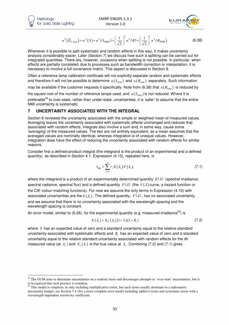
EMRP-ENG05-1.3.1
Version 1.0
30
( ) ( ) ( ) ( ) ( )2 2
2 2 2 2 2,test NMI NMI
1 1.
2 2Vu E u S u S u R u R
= + + +
(6.38)
Whenever it is possible to split systematic and random effects in this way, it makes uncertainty analysis considerably easier. Later (Section 7) we discuss how such a splitting can be carried out for integrated quantities. There are, however, occasions when splitting is not possible. In particular, when effects are partially correlated, due to processes such as bandwidth correction or interpolation, it is necessary to involve a full covariance matrix. This aspect is discussed in Section 8.
Often a reference lamp calibration certificate will not explicitly separate random and systematic effects
and therefore it will not be possible to determine ( )NMIu S and ( )NMI
u R separately. Such information
may be available if the customer requests it specifically. Note from (6.38) that ( )NMIu R is reduced by
the square root of the number of reference lamps used, and ( )NMIu S is not reduced. Where it is
preferable28
to over-state, rather than under-state, uncertainties, it is ‘safer’ to assume that the entire NMI uncertainty is systematic.
7 UNCERTAINTY ASSOCIATED WITH THE INTEGRAL
Section 6 reviewed the uncertainty associated with the simple or weighted mean of measured values. Averaging leaves the uncertainty associated with systematic effects unchanged and reduces that associated with random effects. Integrals also involve a sum and, in some way, cause some 'averaging' of the measured values. The two are not entirely equivalent, as a mean assumes that the averaged values are nominally identical, whereas integration is of unequal values. However, integration does have the effect of reducing the uncertainty associated with random effects for similar reasons.
Consider first a defined-product integral (the integrand is the product of an experimental and a defined quantity), as described in Section 4.1. Expression (4.10), repeated here, is
( ) ( )dp
1
,
n
i i i
i
I E Fλ λ=
=∑ � (7.1)
where the integrand is a product of an experimentally determined quantity ( )E λ (spectral irradiance,
spectral radiance, spectral flux) and a defined quantity ( )F λ (the ( )V λ curve, a hazard function or
the CIE colour-matching functions). For now we assume the only terms in Expression (4.10) with
associated uncertainties are the ( )iE λ . The defined quantity, ( )F λ , has no associated uncertainty
and we assume that there is no uncertainty associated with the wavelength spacing and the wavelength spacing is constant.
An error model, similar to (6.28), for the experimental quantity (e.g. measured irradiance29
) is
( ) ( )( )( )T 1 1i i iE E S Rλ λ= + + (7.2)
where S has an expected value of zero and a standard uncertainty equal to the relative standard
uncertainty associated with systematic effects and iR has an expected value of zero and a standard
uncertainty equal to the relative standard uncertainty associated with random effects for the ith
measured value (at i
λ ) and ( )T iE λ is the true value at iλ . Combining (7.2) and (7.1) gives
28 The GUM aims to determine uncertainties on a realistic basis and discourages attempts to ‘over-state’ uncertainties, but it
is recognised that such practice is common. 29 This model is simplistic in only including multiplicative terms, but such terms usually dominate in a radiometric
uncertainty budget, see Section 7.4.1for a more complete error model including additive terms and systematic terms with a
wavelength dependent sensitivity coefficient.
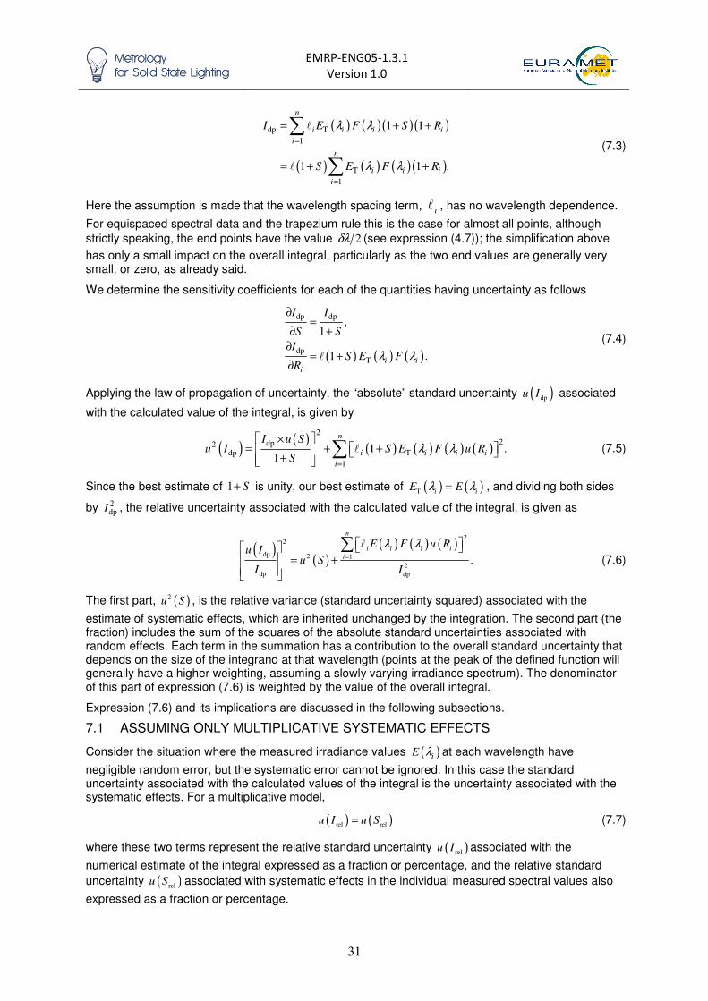
EMRP-ENG05-1.3.1
Version 1.0
31
( ) ( )( )( )
( ) ( ) ( )( )
dp T
1
T
1
1 1
1 1 .
n
i i i i
i
n
i i i
i
I E F S R
S E F R
λ λ
λ λ
=
=
= + +
= + +
∑
∑
�
�
(7.3)
Here the assumption is made that the wavelength spacing term, i� , has no wavelength dependence.
For equispaced spectral data and the trapezium rule this is the case for almost all points, although
strictly speaking, the end points have the value 2δλ (see expression (4.7)); the simplification above
has only a small impact on the overall integral, particularly as the two end values are generally very small, or zero, as already said.
We determine the sensitivity coefficients for each of the quantities having uncertainty as follows
( ) ( ) ( )
dp dp
dp
T
,1
1 .i i
i
I I
S S
IS E F
Rλ λ
∂=
∂ +
∂= +
∂�
(7.4)
Applying the law of propagation of uncertainty, the “absolute” standard uncertainty ( )dpu I associated
with the calculated value of the integral, is given by
( )( )
( ) ( ) ( ) ( )2
2dp2dp T
1
1 .1
n
i i i i
i
I u Su I S E F u R
Sλ λ
=
× = + + +
∑ � (7.5)
Since the best estimate of 1 S+ is unity, our best estimate of ( ) ( )T i iE Eλ λ= , and dividing both sides
by 2dpI , the relative uncertainty associated with the calculated value of the integral, is given as
( )
( )( ) ( ) ( )
22
dp 2 1
2
dp dp
.
n
i i i i
i
E F u Ru I
u SI I
λ λ=
= +
∑ �
(7.6)
The first part, ( )2u S , is the relative variance (standard uncertainty squared) associated with the
estimate of systematic effects, which are inherited unchanged by the integration. The second part (the fraction) includes the sum of the squares of the absolute standard uncertainties associated with random effects. Each term in the summation has a contribution to the overall standard uncertainty that depends on the size of the integrand at that wavelength (points at the peak of the defined function will generally have a higher weighting, assuming a slowly varying irradiance spectrum). The denominator of this part of expression (7.6) is weighted by the value of the overall integral.
Expression (7.6) and its implications are discussed in the following subsections.
7.1 ASSUMING ONLY MULTIPLICATIVE SYSTEMATIC EFFECTS
Consider the situation where the measured irradiance values ( )iE λ at each wavelength have
negligible random error, but the systematic error cannot be ignored. In this case the standard uncertainty associated with the calculated values of the integral is the uncertainty associated with the systematic effects. For a multiplicative model,
( ) ( )rel relu I u S= (7.7)
where these two terms represent the relative standard uncertainty ( )relu I associated with the
numerical estimate of the integral expressed as a fraction or percentage, and the relative standard
uncertainty ( )relu S associated with systematic effects in the individual measured spectral values also
expressed as a fraction or percentage.

EMRP-ENG05-1.3.1
Version 1.0
32
The easiest way to understand expression (7.7) is to consider that the systematic effect scales the entire measured spectral curve. The systematic error for a specific measurement, which is the error drawn from the distribution for the systematic effect, causes the entire spectrum to increase or decrease by the same (relative) proportion. The value of the integral will increase or decrease by this proportion, for example the measured spectrum may be consistently high by a certain percentage (Figure 4) and thus the value of the integral will be high by this same percentage.
Figure 4 Simulated ‘true’ (solid blue line) and ‘measured’ (dotted green line) spectra of an LED with a systematic effect.
7.2 ASSUMING ONLY MULTIPLICATIVE RANDOM EFFECTS
For the defined product integral given above, the standard uncertainty ( )dpu I associated with the
calculated value of the integral, assuming only random effects, is given, from (7.6), by
( )( ) ( ) ( )
2
2 1dp 2
dp
.
n
i i i i
i
E F u R
u II
λ λ=
=
∑ �
(7.8)
The numerator of expression (7.8) is the “absolute” standard uncertainty (i.e. in absolute units, not a fractional value) associated with the value of the integrand at each wavelength, squared and summed. The denominator is the value of the squared integral.
The value of the integral itself is given by (7.1) and therefore expression (7.8) can be written as
( )( ) ( ) ( )
( ) ( )
2
2 1dp 2
1
.
n
i i i i
i
n
i i i
i
E F u R
u I
E F
λ λ
λ λ
=
=
=
∑
∑
�
�
(7.9)
Note the positioning of the parentheses and the square. The numerator is a sum of the squares; the denominator is the square of the sum.
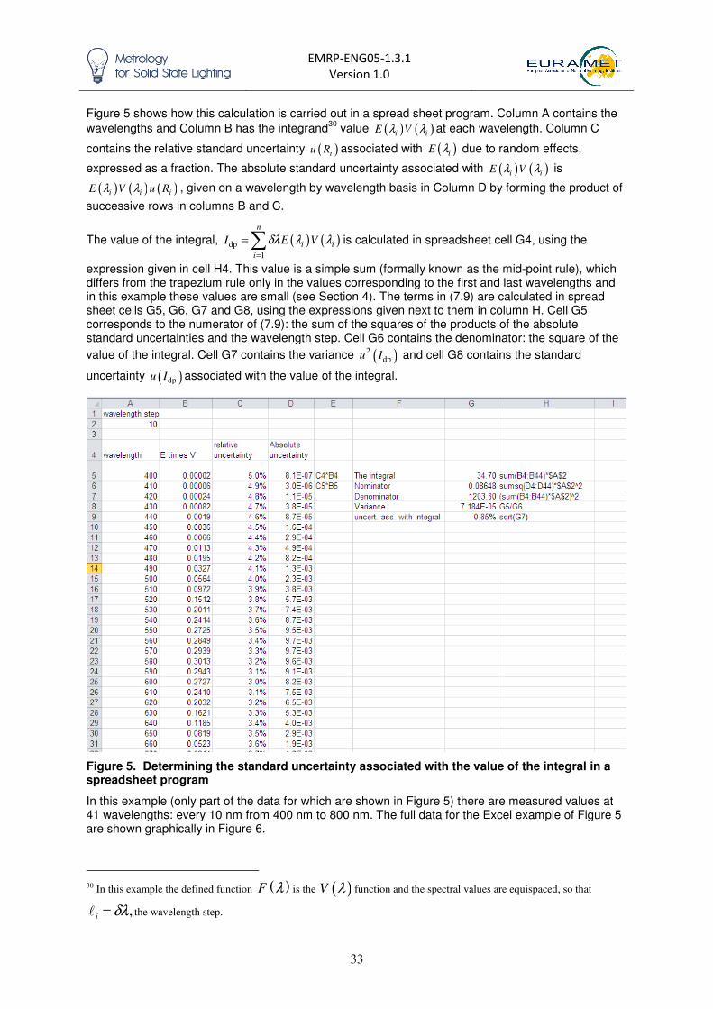
EMRP-ENG05-1.3.1
Version 1.0
33
Figure 5 shows how this calculation is carried out in a spread sheet program. Column A contains the
wavelengths and Column B has the integrand30
value ( ) ( )i iE Vλ λ at each wavelength. Column C
contains the relative standard uncertainty ( )iu R associated with ( )iE λ due to random effects,
expressed as a fraction. The absolute standard uncertainty associated with ( ) ( )i iE Vλ λ is
( ) ( ) ( )i i iE V u Rλ λ , given on a wavelength by wavelength basis in Column D by forming the product of
successive rows in columns B and C.
The value of the integral, ( ) ( )dp
1
n
i i
i
I E Vδλ λ λ=
=∑ is calculated in spreadsheet cell G4, using the
expression given in cell H4. This value is a simple sum (formally known as the mid-point rule), which differs from the trapezium rule only in the values corresponding to the first and last wavelengths and in this example these values are small (see Section 4). The terms in (7.9) are calculated in spread sheet cells G5, G6, G7 and G8, using the expressions given next to them in column H. Cell G5 corresponds to the numerator of (7.9): the sum of the squares of the products of the absolute standard uncertainties and the wavelength step. Cell G6 contains the denominator: the square of the
value of the integral. Cell G7 contains the variance ( )2dpu I and cell G8 contains the standard
uncertainty ( )dpu I associated with the value of the integral.
Figure 5. Determining the standard uncertainty associated with the value of the integral in a spreadsheet program
In this example (only part of the data for which are shown in Figure 5) there are measured values at 41 wavelengths: every 10 nm from 400 nm to 800 nm. The full data for the Excel example of Figure 5 are shown graphically in Figure 6.
30 In this example the defined function ( )F λ is the ( )V λ function and the spectral values are equispaced, so that
,i δλ=� the wavelength step.

EMRP-ENG05-1.3.1
Version 1.0
34
Figure 6 A modelled spectrum of a typical integrand (lamp irradiance multiplied by ( )V λ ), its
associated uncertainty and an example measured spectrum
Although the relative standard uncertainty is smallest at the central wavelengths, the absolute standard uncertainty is larger. The relative uncertainty associated with individual data points ranges from 3 % to 5 % and the uncertainty associated with the integral
31 (Figure 5, cell G9), is 0.85 %. The
simple mean of the uncertainties given is 4.5 %, and dividing this mean by the square root of the number of points (41) used to form the value of the integral, gives 0.70 %. As expected, the process of integration reduces the uncertainty associated with random effects considerably (from 4.5 % to 0.82 %), but not quite as much as if those points had equal weighting (0.70 %).
7.3 ASSUMING ONLY WAVELENGTH EFFECTS
Section 5.6 described uncertainties arising from three types of wavelength effect associated with the measurement of a test source using a reference source and a spectrometer or monochromator-based system:
1. A systematic spectral offset that applies to measurements of both sources and at all wavelengths (uncertainty associated with wavelength correction applied).
2. A wavelength offset that is the same at a particular wavelength for both sources, but that is different for other wavelengths (uncertainty associated with wavelength correction applied).
3. A random effect (scanning monochromators only) in the repeatability of the wavelength scale that is different for each source and for each wavelength.
To understand the sensitivity of the value of the integral to each of these effects, we first need to describe the measuring system with a measurement model. When the test lamp is calibrated using a
reference lamp, the test lamp irradiance ( )testE λ is calculated from (a) the ratio ( ) ( )
test refS Sλ λ of
the signals measured on the instrument with the test and reference lamps and (b) the (known)
reference lamp irradiance ( )refE λ :
( )( )
( )( )test
test refref
.S
E ES
λλ λ
λ= × (7.10)
Combining expression (7.10) with Expression (7.1) for a defined-product integral, with ( ) ( )F Vλ λ= ,
simplified to assume i
δλ=� at all wavelengths, gives
31 The standard uncertainty associated with the numerical estimate of the integral, see Section 2.8.
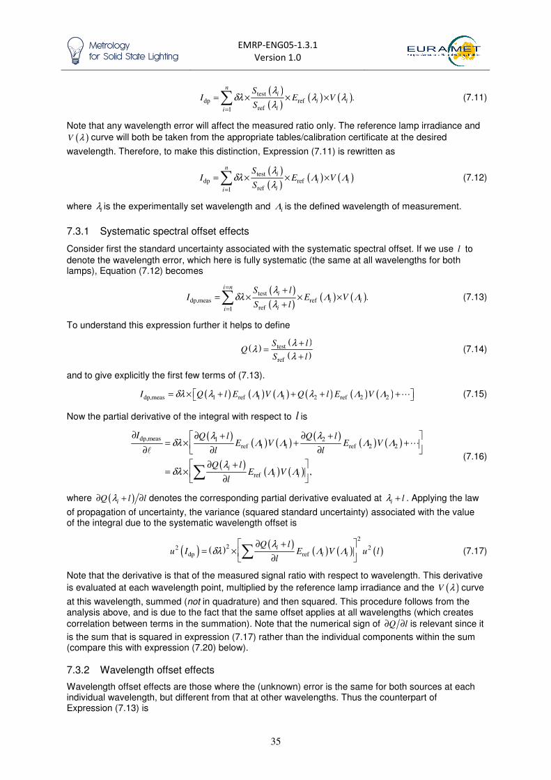
EMRP-ENG05-1.3.1
Version 1.0
35
( )( )
( ) ( )testdp ref
ref1
.
ni
i iii
SI E V
S
λδλ λ λ
λ=
= × × ×∑ (7.11)
Note that any wavelength error will affect the measured ratio only. The reference lamp irradiance and
( )V λ curve will both be taken from the appropriate tables/calibration certificate at the desired
wavelength. Therefore, to make this distinction, Expression (7.11) is rewritten as
( )( )
( ) ( )testdp ref
ref1
ni
i iii
SI E V
S
λδλ Λ Λ
λ=
= × × ×∑ (7.12)
where iλ is the experimentally set wavelength and iΛ is the defined wavelength of measurement.
7.3.1 Systematic spectral offset effects
Consider first the standard uncertainty associated with the systematic spectral offset. If we use l to
denote the wavelength error, which here is fully systematic (the same at all wavelengths for both lamps), Equation (7.12) becomes
( )( )
( ) ( )testdp,meas ref
ref1
.
i ni
i iii
S lI E V
S l
λδλ Λ Λ
λ
=
=
+= × × ×
+∑ (7.13)
To understand this expression further it helps to define
( )( )
( )test
ref
S lQ
S l
λλ
λ
+=
+ (7.14)
and to give explicitly the first few terms of (7.13).
( ) ( ) ( ) ( ) ( ) ( )dp,meas 1 ref 1 1 2 ref 2 2I Q l E V Q l E Vδλ λ Λ Λ λ Λ Λ= × + + + + � (7.15)
Now the partial derivative of the integral with respect to l is
( )( ) ( )
( )( ) ( )
( )( ) ( )
dp,meas 1 2ref 1 1 ref 2 2
ref ,i
i i
I Q l Q lE V E V
l l
Q lE V
l
λ λδλ Λ Λ Λ Λ
λδλ Λ Λ
∂ ∂ + ∂ + = × + +
∂ ∂ ∂
∂ += ×
∂ ∑
��
(7.16)
where ( )iQ l lλ∂ + ∂ denotes the corresponding partial derivative evaluated at i lλ + . Applying the law
of propagation of uncertainty, the variance (squared standard uncertainty) associated with the value of the integral due to the systematic wavelength offset is
( ) ( )( )
( ) ( ) ( )2
22 2dp ref
ii i
Q lu I E V u l
l
λδλ Λ Λ
∂ += ×
∂ ∑ (7.17)
Note that the derivative is that of the measured signal ratio with respect to wavelength. This derivative
is evaluated at each wavelength point, multiplied by the reference lamp irradiance and the ( )V λ curve
at this wavelength, summed (not in quadrature) and then squared. This procedure follows from the analysis above, and is due to the fact that the same offset applies at all wavelengths (which creates
correlation between terms in the summation). Note that the numerical sign of Q l∂ ∂ is relevant since it
is the sum that is squared in expression (7.17) rather than the individual components within the sum (compare this with expression (7.20) below).
7.3.2 Wavelength offset effects
Wavelength offset effects are those where the (unknown) error is the same for both sources at each individual wavelength, but different from that at other wavelengths. Thus the counterpart of Expression (7.13) is

EMRP-ENG05-1.3.1
Version 1.0
36
( )( )
( ) ( )testdp,meas ref
ref1
ni i
i ii ii
S lI E V
S l
λδλ Λ Λ
λ=
+= × × ×
+∑ (7.18)
which can be written as
( ) ( ) ( ) ( ) ( ) ( )dp,meas 1 1 ref 1 1 2 2 ref 2 2 ,I Q l E V Q l E Vδλ λ Λ Λ λ Λ Λ= × + + + + … (7.19)
Because the error changes from wavelength to wavelength, there is no longer a common component
in all terms in the sum. Therefore, again using ( )Q λ to represent the ratio, we determine the variance
associated with the value of the integral from the quadrature sum from
( ) ( )( )
( ) ( ) ( )2
22 2dp ref
1
.
ni i
i i iii
Q lu I E V u l
l
λδλ Λ Λ
=
∂ += ×
∂ ∑ (7.20)
Comparing this expression with Expression (7.17) it is important to note that here we have the sum of squares rather than the square of the sum, a result of the fact that there is no longer the common component creating correlation.
Although the actual error in the wavelength is different at each wavelength, the standard uncertainty
associated with the wavelength offset typically does not change with wavelength, i.e. ( ) ( )iu l u l= .
Thus the squared term within the summation provides a scaling factor for that constant standard uncertainty.
7.3.3 Random wavelength effects
With random effects, not only is there a different error at each wavelength, but also a different error for the two sources; thus
( )( )
( ) ( )test test,
dp,meas refref ref,1
.
ni i
i ii ii
S lI E V
S l
λδλ Λ Λ
λ=
+= × × ×
+∑ (7.21)
Writing out terms as before, but this time not using the ratio function ( )Q λ since it is inapplicable,
( )( )
( ) ( )( )( )
( ) ( )test 1 test,1 test 2 test,2
dp,meas ref 1 1 ref 2 2
ref 1 ref,1 ref 2 ref,2
.S l S l
I E V E VS l S l
λ λδλ Λ Λ Λ Λ
λ λ
+ + = × × × + × × +
+ + … (7.22)
The partial derivative for the integral with respect to the i th wavelength error for the test lamp
measurement is
( ) ( )
( )( )test test,dp ref
test, ref ref, test,
,i ii i
i i i i
S lI E V
l S l l
λδλ Λ Λ
λ
∂ +∂ × ×= ×
∂ + ∂ (7.23)
and that for the integral with respect to the i th wavelength error for the reference lamp measurement
is
( ) ( )( )
( )
( )test test, ref ref,dp
ref 2test, ref,ref ref,
.i i i i
i i
i ii i
S l S lIE V
l lS l
λ λδλ Λ Λ
λ
− + ∂ +∂= × × × ×
∂ ∂+
(7.24)
Assuming that the standard uncertainty associated with random wavelength effects is constant with
wavelength, ( ) ( )iu l u l= , the variance associated with the value of the integral at a particular
wavelength, is
( ) ( ) ( ) ( )( )( ) ( )
2 222 2 test ref
dp testtest ref1
1 1.
i i
n
i i
i i i ii
S Su I u l E V
S l S lλ λ
λ Λ δλλ λ
=
∂ ∂ = × × × × + ×
∂ ∂ ∑ (7.25)
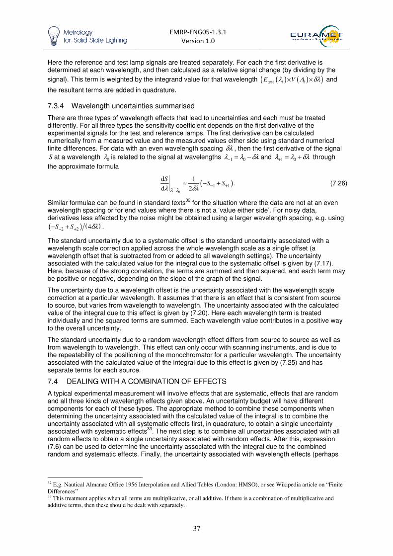
EMRP-ENG05-1.3.1
Version 1.0
37
Here the reference and test lamp signals are treated separately. For each the first derivative is determined at each wavelength, and then calculated as a relative signal change (by dividing by the
signal). This term is weighted by the integrand value for that wavelength ( ) ( )( )test i iE Vλ Λ δλ× × and
the resultant terms are added in quadrature.
7.3.4 Wavelength uncertainties summarised
There are three types of wavelength effects that lead to uncertainties and each must be treated differently. For all three types the sensitivity coefficient depends on the first derivative of the experimental signals for the test and reference lamps. The first derivative can be calculated numerically from a measured value and the measured values either side using standard numerical finite differences. For data with an even wavelength spacing δλ , then the first derivative of the signal
S at a wavelength 0λ is related to the signal at wavelengths 1 0λ λ δλ− = − and 1 0λ λ δλ+ = + through
the approximate formula
( )0
1 1
d 1.
d 2
SS S
λ λλ δλ− +
=
≈ − + (7.26)
Similar formulae can be found in standard texts32
for the situation where the data are not at an even wavelength spacing or for end values where there is not a ‘value either side’. For noisy data, derivatives less affected by the noise might be obtained using a larger wavelength spacing, e.g. using
( ) ( )2 2 4S S δλ− +− + .
The standard uncertainty due to a systematic offset is the standard uncertainty associated with a wavelength scale correction applied across the whole wavelength scale as a single offset (a wavelength offset that is subtracted from or added to all wavelength settings). The uncertainty associated with the calculated value for the integral due to the systematic offset is given by (7.17). Here, because of the strong correlation, the terms are summed and then squared, and each term may be positive or negative, depending on the slope of the graph of the signal.
The uncertainty due to a wavelength offset is the uncertainty associated with the wavelength scale correction at a particular wavelength. It assumes that there is an effect that is consistent from source to source, but varies from wavelength to wavelength. The uncertainty associated with the calculated value of the integral due to this effect is given by (7.20). Here each wavelength term is treated individually and the squared terms are summed. Each wavelength value contributes in a positive way to the overall uncertainty.
The standard uncertainty due to a random wavelength effect differs from source to source as well as from wavelength to wavelength. This effect can only occur with scanning instruments, and is due to the repeatability of the positioning of the monochromator for a particular wavelength. The uncertainty associated with the calculated value of the integral due to this effect is given by (7.25) and has separate terms for each source.
7.4 DEALING WITH A COMBINATION OF EFFECTS
A typical experimental measurement will involve effects that are systematic, effects that are random and all three kinds of wavelength effects given above. An uncertainty budget will have different components for each of these types. The appropriate method to combine these components when determining the uncertainty associated with the calculated value of the integral is to combine the uncertainty associated with all systematic effects first, in quadrature, to obtain a single uncertainty associated with systematic effects
33. The next step is to combine all uncertainties associated with all
random effects to obtain a single uncertainty associated with random effects. After this, expression (7.6) can be used to determine the uncertainty associated with the integral due to the combined random and systematic effects. Finally, the uncertainty associated with wavelength effects (perhaps
32 E.g. Nautical Almanac Office 1956 Interpolation and Allied Tables (London: HMSO), or see Wikipedia article on “Finite
Differences” 33 This treatment applies when all terms are multiplicative, or all additive. If there is a combination of multiplicative and
additive terms, then these should be dealt with separately.
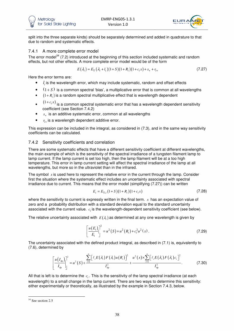
EMRP-ENG05-1.3.1
Version 1.0
38
split into the three separate kinds) should be separately determined and added in quadrature to that due to random and systematic effects.
7.4.1 A more complete error model
The error model34
(7.2) introduced at the beginning of this section included systematic and random effects, but not other effects. A more complete error model would be of the form
( ) ( )( )( )( )T 1 1 1i i i i i iE E l S R c x s rλ λ + += + + + + + + (7.27)
Here the error terms are:
• il is the wavelength error, which may include systematic, random and offset effects
• ( )1 S+ is a common spectral ‘bias’, a multiplicative error that is common at all wavelengths
• ( )1 iR+ is a random spectral multiplicative effect that is wavelength dependent
• ( )1 ic x+
is a common spectral systematic error that has a wavelength dependent sensitivity coefficient (see Section 7.4.2)
• s+ is an additive systematic error, common at all wavelengths
• ir + is a wavelength dependent additive error.
This expression can be included in the integral, as considered in (7.3), and in the same way sensitivity coefficients can be calculated.
7.4.2 Sensitivity coefficients and correlation
There are some systematic effects that have a different sensitivity coefficient at different wavelengths, the main example of which is the sensitivity of the spectral irradiance of a tungsten filament lamp to lamp current. If the lamp current is set too high, then the lamp filament will be at a too high temperature. This error in lamp current setting will affect the spectral irradiance of the lamp at all wavelengths, but more so in the ultraviolet than in the infrared.
The symbol x is used here to represent the relative error in the current through the lamp. Consider
first the situation where the systematic effect includes an uncertainty associated with spectral irradiance due to current. This means that the error model (simplifying (7.27)) can be written
( )( )( )T, 1 1 1i i i iE E S R c x= + + + (7.28)
where the sensitivity to current is expressly written in the final term. x has an expectation value of
zero and a probability distribution with a standard deviation equal to the standard uncertainty
associated with the current value. ic is the wavelength-dependent sensitivity coefficient (see below).
The relative uncertainty associated with ( )iE λ as determined at any one wavelength is given by
( )
( ) ( ) ( )
2
2 2 2 2ii i
i
u Eu S u R c u x
E
= + +
. (7.29)
The uncertainty associated with the defined product integral, as described in (7.1) is, equivalently to (7.6), determined by
( )
( )( ) ( ) ( ) ( ) ( ) ( )
2 222
dp 2 1 1
2 2
dp dp dp
.
n n
i i i i i i i i
i i
E F u R u x E F cu I
u SI I I
λ λ λ λ= =
× = + +
∑ ∑� �
(7.30)
All that is left is to determine the ic . This is the sensitivity of the lamp spectral irradiance (at each
wavelength) to a small change in the lamp current. There are two ways to determine this sensitivity: either experimentally or theoretically, as illustrated by the example in Section 7.4.3, below.
34 See section 2.5

EMRP-ENG05-1.3.1
Version 1.0
39
7.4.3 Example determination of sensitivity coefficient
Consider as an example the determination of the sensitivity of the spectral irradiance of the lamp to a small change in the current supplied to the lamp. The sensitivity coefficient can be determined either experimentally or through theoretical modelling.
An experimental determination would involve measuring the spectral irradiance of the lamp at a few different current settings – one slightly higher than the standard current, one slightly lower and at the standard current itself. Because current has a non-linear effect on spectral irradiance, these deliberate changes to the applied current should be kept small, but they have to be sufficiently large so as to be able to distinguish reliably the change in measured signal. A recommended change would be ten times greater than any natural variability or uncertainty associated with the absolute current setting. For example if the current stability is 1 mA and the current setting uncertainty is 5 mA, then the change made would be 10 times greater than the larger of those numbers, i.e. 50 mA. Thus measured values would be obtained of the spectral irradiance of the lamp with the lamp current set at successively 8.050 A, 8.100 A, 8.150 A for a lamp normally run at 8.100 A (the standard setting for an FEL-type lamp). An assumption would be made that the behaviour over this range is linear and the differences observed for these 50 mA changes would be scaled back to the expected change for a 5 mA current uncertainty, by dividing by ten.
A theoretical determination of the sensitivity coefficient is also possible, by treating the lamp as a radiative hot body, described by a perfect blackbody and a multiplicative polynomial expression accounting for tungsten emissivity and the lamp envelope transmittance [4, 5] . The electrical current change can be related to the electrical power change, which, through the Stefan-Boltzmann law gives the expected temperature change, and thus irradiance change. A full description of this approach is beyond the scope of this report, but the results agree well with experimentally determined changes.
8 COVARIANCE MATRIX APPROACH
8.1 WHEN IS A COVARIANCE MATRIX NEEDED?
When it is possible to split the uncertainty budget into systematic effects and random effects, it is not necessary to use the full form of the law of propagation of uncertainty (Equation (2.1)). In general, as discussed in Section 6.4, the systematic and random effects can separately be explicitly described in an error-model form of the measurement equation, as in Equations (6.3), (6.36) and (7.2). In other words as the correlation is built into the error model, the terms within that error model are entirely uncorrelated with each other.
This approach is often the simplest, particularly when data analysis is carried out using a spreadsheet program. There are, however, occasions when such an analysis is insufficient. Sometimes correlation cannot be described by simply separating random and systematic components. Such separation is inapplicable whenever mathematical correlation has been introduced, for example through interpolation, averaging, smoothing, bandwidth correction and similar processes that combine data from several wavelengths. In these situations a covariance matrix provides the straightforward means to apply the full form of the law of propagation of uncertainty.
The law of propagation of uncertainty (equation (2.1)) is written in matrix form as
( )2y x yu y = C U C� (8.1)
where
1 2
y
n
f f f
x x x
∂ ∂ ∂ = ∂ ∂ ∂
C … (8.2)
is a column vector of sensitivity coefficients. (⊤represents transpose, i.e that vector is written as a
column, rather than as written here, for space reasons, as a row) and xU is the covariance matrix. This
form is given and used in the Supplement 2 to the GUM35
as equation (3) on page 15.
35 Freely downloadable at http://www.bipm.org/en/publications/guides/gum.html
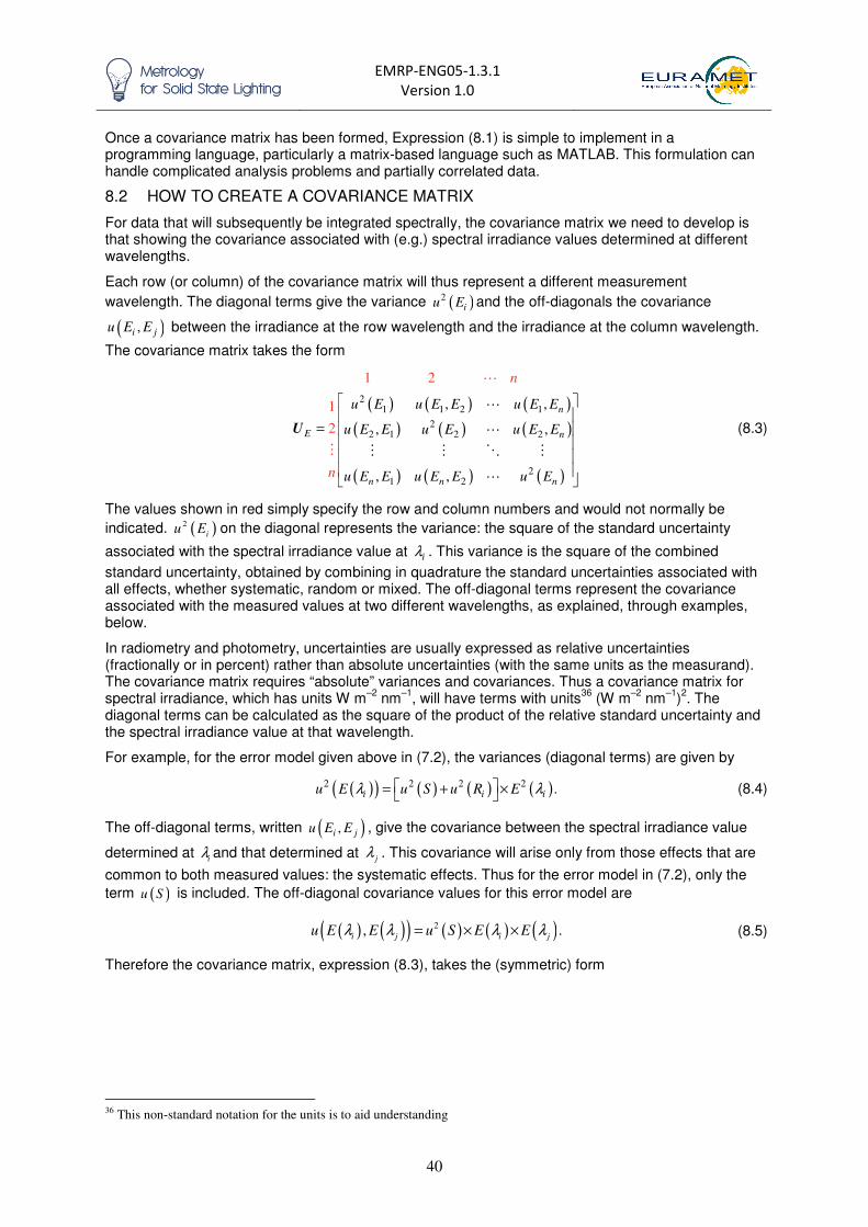
EMRP-ENG05-1.3.1
Version 1.0
40
Once a covariance matrix has been formed, Expression (8.1) is simple to implement in a programming language, particularly a matrix-based language such as MATLAB. This formulation can handle complicated analysis problems and partially correlated data.
8.2 HOW TO CREATE A COVARIANCE MATRIX
For data that will subsequently be integrated spectrally, the covariance matrix we need to develop is that showing the covariance associated with (e.g.) spectral irradiance values determined at different wavelengths.
Each row (or column) of the covariance matrix will thus represent a different measurement
wavelength. The diagonal terms give the variance ( )2iu E and the off-diagonals the covariance
( ),i ju E E between the irradiance at the row wavelength and the irradiance at the column wavelength.
The covariance matrix takes the form
( ) ( ) ( )
( ) ( ) ( )
( ) ( ) ( )
21 1 2 1
22 1 2 2
21 2
, ,
, ,
, ,
1 2
1
2
n
E n
n n n
u E u E E u E E
u E E u E u E E
u E E u E E un E
n
=
U
�
�
� � � �
�
�
�
(8.3)
The values shown in red simply specify the row and column numbers and would not normally be
indicated. ( )2
iu E on the diagonal represents the variance: the square of the standard uncertainty
associated with the spectral irradiance value at iλ . This variance is the square of the combined
standard uncertainty, obtained by combining in quadrature the standard uncertainties associated with all effects, whether systematic, random or mixed. The off-diagonal terms represent the covariance associated with the measured values at two different wavelengths, as explained, through examples, below.
In radiometry and photometry, uncertainties are usually expressed as relative uncertainties (fractionally or in percent) rather than absolute uncertainties (with the same units as the measurand). The covariance matrix requires “absolute” variances and covariances. Thus a covariance matrix for spectral irradiance, which has units W m
–2 nm
–1, will have terms with units
36 (W m
–2 nm
–1)2. The
diagonal terms can be calculated as the square of the product of the relative standard uncertainty and the spectral irradiance value at that wavelength.
For example, for the error model given above in (7.2), the variances (diagonal terms) are given by
( )( ) ( ) ( ) ( )2 2 2 2 .i i iu E u S u R Eλ λ = + × (8.4)
The off-diagonal terms, written ( ),i ju E E , give the covariance between the spectral irradiance value
determined at i
λ and that determined at jλ . This covariance will arise only from those effects that are
common to both measured values: the systematic effects. Thus for the error model in (7.2), only the
term ( )u S is included. The off-diagonal covariance values for this error model are
( ) ( )( ) ( ) ( ) ( )2, .i j i j
u E E u S E Eλ λ λ λ= × × (8.5)
Therefore the covariance matrix, expression (8.3), takes the (symmetric) form
36 This non-standard notation for the units is to aid understanding
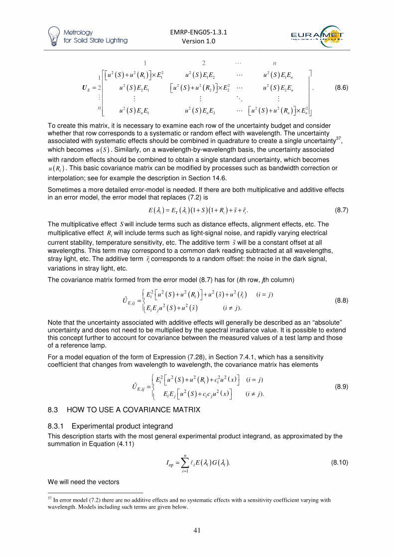
EMRP-ENG05-1.3.1
Version 1.0
41
( ) ( ) ( ) ( )
( ) ( ) ( ) ( )
( ) ( ) ( ) ( )
2 2 2 2 2
1 1 1 2 1
2 2 2 2 2
2 1 2 2 2
2 2 2 2 2
1 2
1 2
1
2 .
n
E n
n n n n
u S u R E u S E E u S E E
u S E E u S u R E u S E E
u S E E u S E E u S u
n
n R E
+ × = + ×
+ ×
U
�
�
�
� � � � �
�
(8.6)
To create this matrix, it is necessary to examine each row of the uncertainty budget and consider whether that row corresponds to a systematic or random effect with wavelength. The uncertainty associated with systematic effects should be combined in quadrature to create a single uncertainty
37,
which becomes ( )u S . Similarly, on a wavelength-by-wavelength basis, the uncertainty associated
with random effects should be combined to obtain a single standard uncertainty, which becomes
( )iu R . This basic covariance matrix can be modified by processes such as bandwidth correction or
interpolation; see for example the description in Section 14.6.
Sometimes a more detailed error-model is needed. If there are both multiplicative and additive effects in an error model, the error model that replaces (7.2) is
( ) ( ) ( )( )T1 1 .
i i i iE E S R s rλ λ= + + + +� � (8.7)
The multiplicative effect S will include terms such as distance effects, alignment effects, etc. The
multiplicative effect iR will include terms such as light-signal noise, and rapidly varying electrical
current stability, temperature sensitivity, etc. The additive term s� will be a constant offset at all
wavelengths. This term may correspond to a common dark reading subtracted at all wavelengths,
stray light, etc. The additive term ir� corresponds to a random offset: the noise in the dark signal,
variations in stray light, etc.
The covariance matrix formed from the error model (8.7) has for (ith row, jth column)
( ) ( ) ( ) ( )
( ) ( )
2 2 2 2 2
,2 2
( )
( ).
i i i
E ij
i j
E u S u R u s u r i jU
E E u S u s i j
+ + + = = + ≠
� ��
� (8.8)
Note that the uncertainty associated with additive effects will generally be described as an “absolute” uncertainty and does not need to be multiplied by the spectral irradiance value. It is possible to extend this concept further to account for covariance between the measured values of a test lamp and those of a reference lamp.
For a model equation of the form of Expression (7.28), in Section 7.4.1, which has a sensitivity coefficient that changes from wavelength to wavelength, the covariance matrix has elements
( ) ( ) ( )
( ) ( )
2 2 2 2 2
,2 2
( )
( ).
i i i
E ij
i j i j
E u S u R c u x i jU
E E u S c c u x i j
+ + = =
+ ≠
� (8.9)
8.3 HOW TO USE A COVARIANCE MATRIX
8.3.1 Experimental product integrand
This description starts with the most general experimental product integrand, as approximated by the summation in Equation (4.11)
( ) ( )ep
1
.
n
i i i
i
I E Gλ λ=
=∑� (8.10)
We will need the vectors
37 In error model (7.2) there are no additive effects and no systematic effects with a sensitivity coefficient varying with
wavelength. Models including such terms are given below.

EMRP-ENG05-1.3.1
Version 1.0
42
[ ]
( ) ( ) ( ) ( )
( ) ( ) ( ) ( )
1 2 1
1 2 1
1 2 1 1 1 2
n n
n n
E E E E
G G G G
δλ
λ λ λ λ
λ λ λ λ
−
−
=
=
=
l
E
G
…
…
…
�
�
�
(8.11)
We will also need the covariance matrices EU and GU that contain the variances and covariances
associated with the iE and the iG respectively, as in (8.6) (or (8.8)).
Applying the matrix form of the law of propagation of uncertainty (8.1) to (8.10) , we immediately38
obtain the variance associated with the numerical estimate of the integral as
( ) ( )2
ep E Gu I = +l GU G EU E l� � �
(8.12)
8.3.2 Defined product integrand
Consider a defined product integral calculated numerically, using Equation (4.10), repeated here:
dp
1
( ) ( )m
i i i
i
I E Fλ λ=
=∑ � (8.13)
The calculated value of this integral is obtained by multiplying the three elements in (8.13) on a wavelength-by-wavelength basis and then summing the resultant terms. In this case the Fi are given exactly and expression (8.12) reduces to
( ) ( )2
dp Eu I = l FU F l� �
(8.14)
8.3.3 Simple integrand
For a simple integrand, the process is similar to that described above. Here, the integrand does not
involve ( )F λ , so the ( )iF λ can be replaced by unity. As a result the standard uncertainty depends
only on the covariance matrix EU and the standard uncertainty associated with the calculated value
of the integral ( )s dI E λ λ= ∫ is given by
( )2
s Eu I = l U l� (8.15)
9 COLOUR MATCHING FUNCTIONS AND TRISTIMULUS VALUES
This report summarises the treatment given in detail in Gardner’s paper [17] . The chromaticity coordinates are derived from the tristimulus values , ,X Y Z formed from defined-product integrals
39
(see Section 4.1) of the CIE colour-matching functions, and the source spectrum (e.g. irradiance):
( ) ( )
( ) ( )
( ) ( )
d
d
d
X x E
Y y E
Z z E
λ λ λ
λ λ λ
λ λ λ
=
=
=
∫∫∫
(9.1)
The uncertainty associated with calculated values of each of these integrals can be determined using the approaches described in this report. However, generally those uncertainties are not the ones that
are needed; rather it is the uncertainties associated with quantities derived from ,X Y and Z , such as
38 This is described on page 64 of the NPL Best Practice Guide 6, 2010 16. M. G. Cox, and P. H. Harris, Best Practice
Guide No.6: Uncertainty and statistical modelling. Software Support for Metrology. http://www.npl.co.uk/ssfm/download/
(2010). 39 Defined-product as the quantities ( ) ( ) ( ), ,x y zλ λ λ are defined by the CIE

EMRP-ENG05-1.3.1
Version 1.0
43
the chromaticity coordinates, that are required. For example, the CIE 1931 ( ),x y coordinates are
calculated by combining these terms:
( )
( )
,
.
x X X Y Z
y Y X Y Z
= + +
= + + (9.2)
Transforms are made to the 1960 uniform colour space40
, by
( )
( )
4 15 3 ,
6 15 3 .
u X X Y Z
v Y X Y Z
= + +
= + + (9.3)
Similarly the CIE 1976 uniform colour space is given by
( )
( )
' 4 15 3
' 9 15 3
u X X Y Z
v Y X Y Z
= + +
= + + (9.4)
The uncertainties associated with ( ),x y , ( ),u v and ( ),u v′ ′ must all be determined taking into account
the fact that , ,X Y Z have associated correlation. This is because the source spectrum ( )E λ is
common to all three chromaticity coordinates.
9.1 CHROMATICITY COORDINATES WITHOUT MATRICES
Gardner [17] simplifies the problem by using a philosophy similar to that presented in other sections of this report – by making the correlation explicit in the measurement model. Where the tristimulus values are calculated from experimental data through numerical integration, expression (9.1) is rewritten as
1
1
1
,
,
.
n
i i i
i
n
i i i
i
n
i i i
i
X E x
Y E y
Z E z
=
=
=
=
=
=
∑
∑
∑
�
�
�
(9.5)
Combining this expression with (9.2) we have
1 1
1 1
,
,
n n
i i i i i i
i i
n n
i i i i i i
i i
x E x E t
y E y E t
= =
= =
=
=
∑ ∑
∑ ∑
� �
� �
(9.6)
where
.i i i it x y z= + + (9.7)
If we use an error model such as that in expression (7.2) ( ) ( )T,1 1
i i iE E S R= + + , then we can write
( ) ( )
( ) ( )
T,
1
T,
1
1 1
1 1
n
i i i i
i
n
i i i i
i
S E R x
x
S E R t
=
=
+ +
=
+ +
∑
∑
�
�
(9.8)
40 Note in this expression u is the standard notation for the chromaticity value and does not represent standard uncertainty.
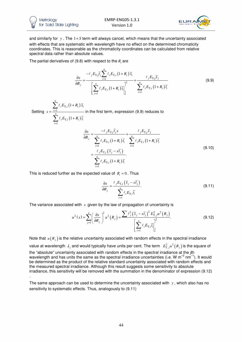
EMRP-ENG05-1.3.1
Version 1.0
44
and similarly for y . The 1 S+ term will always cancel, which means that the uncertainty associated
with effects that are systematic with wavelength have no effect on the determined chromaticity coordinates. This is reasonable as the chromaticity coordinates can be calculated from relative spectral data rather than absolute values.
The partial derivatives of (9.8) with respect to the iR are
( )
( ) ( )
T,j T,T,j1
2
T,T,
11
1
11
n
j j i i i i
j ji
nnj
i i i ii i i i
ii
E t E R xE xx
RE R tE R t
=
==
− +∂
= +∂
++
∑
∑∑
� ��
��
(9.9)
Setting
( )
( )
T,
1
T,
1
1
1
n
i i i i
i
n
i i i i
i
E R x
x
E R t
=
=
+
=
+
∑
∑
�
�
in the first term, expression (9.9) reduces to
( ) ( )
( )
( )
T, T,
T, T,
1 1
T,
T,
1
1 1
.
1
j j j j j j
n nj
i i i i i i i i
i i
j j j j
n
i i i i
i
E t x E xx
RE R t E R t
E x xt
E R t
= =
=
−∂= +
∂+ +
−=
+
∑ ∑
∑
� �
� �
�
�
(9.10)
This is reduced further as the expected value of 0i
R = . Thus
( )T,
T,
1
.j j j j
nj
i i i
i
E x xtx
RE t
=
−∂=
∂∑
�
�
(9.11)
The variance associated with x given by the law of propagation of uncertainty is
( ) ( )( ) ( )
22 2 22T,2 2
21
T,
1
.
nj j j j j
jnjj
i i i
i
x xt E u Rxu x u R
R
E t=
=
−∂ = = ∂
∑∑∑
�
�
(9.12)
Note that ( )ju R is the relative uncertainty associated with random effects in the spectral irradiance
value at wavelength jλ and would typically have units per cent. The term ( )2 2T, j jE u R is the square of
the “absolute” uncertainty associated with random effects in the spectral irradiance at the jth wavelength and has units the same as the spectral irradiance uncertainties (i.e. W m
–2 nm
–1). It would
be determined as the product of the relative standard uncertainty associated with random effects and the measured spectral irradiance. Although this result suggests some sensitivity to absolute irradiance, this sensitivity will be removed with the summation in the denominator of expression (9.12).
The same approach can be used to determine the uncertainty associated with y , which also has no
sensitivity to systematic effects. Thus, analogously to (9.11)

EMRP-ENG05-1.3.1
Version 1.0
45
( )T,
T,
1
.j j j j
nj
i i i
i
E y yty
RE t
=
−∂=
∂∑
�
�
(9.13)
And therefore
( ) ( )( ) ( )
22 2 22T,2 2
21
T,
1
.
nj j j j j
jnjj
i i i
i
y yt E u Ryu y u R
R
E t=
=
−∂ = = ∂
∑∑∑
�
�
(9.14)
A similar analysis can be used to determine the uncertainties associated with ( ),u v or ( ),u v′ ′ . Since
( )
( )
4 15 3
6 15 3
u X X Y Z
v Y X Y Z
= + +
= + + (9.15)
we can define
15 3q X Y Z= + + (9.16)
and hence
( )T,j
T,
1
4.
j j j
nj
i i i
i
E x uqu
RE q
=
−∂=
∂∑
�
�
(9.17)
9.2 CHROMATICITY COORDINATES WITH MATRICES
An analysis made with matrices can be simpler for software implementation. The relevant
uncertainties, as described in Section 9.1, are those associated with random effects, the ( )iu R . By
definition the random effects i
R are uncorrelated, and therefore the n n× covariance matrix, R
U , for
the random effects is a diagonal matrix, with the values ( ) ( )2 2
1, ,
nu R u R… down the main diagonal
and all other values zero. The results of interest are the values ,x y and their associated covariance
matrix. This is defined in matrix form by the 2-element vector [ ],x y=q�
and its associated 2 2×
covariance matrix qU . From the law of propagation of uncertainties (8.1), we can write
q R
=U CU C� (9.18)
where C is the sensitivity matrix
1
1
.n
n
x x
R R
y y
R R
∂ ∂ ∂ ∂ = ∂ ∂ ∂ ∂
C
�
�
(9.19)
Expressions for i
x
R
∂
∂and
i
y
R
∂
∂ are given in (9.11) and (9.13), respectively. Hence C can be calculated
and used in Expression (9.18). The qU so calculated contains the squares ( )2u x and ( )2
u y of the
standard uncertainties associated with x and y , on the diagonal, and the covariance associated with
,x y off the diagonal.

EMRP-ENG05-1.3.1
Version 1.0
46
10 CONCLUSIONS
This report has aimed to be a practical, but simultaneously rigorous, guide for how to determine uncertainty associated with calculated values of integrated quantities. There are two approaches that have been described. The first involves writing an error model that explicitly separates systematic and random effects. This model can then be used in conjunction with averaging (Section 6) and integral analyses (Section 7) such that correlation does not need explicit consideration. The second approach is to develop a covariance matrix to account for correlations and to perform uncertainty analysis using matrices.
In developing the methods to determine uncertainty associated with an integrated quantity calculated from spectral data, this report has also considered uncertainties associated with wavelength effects and bandwidth.
After the references there are two appendices that extend the ideas in this report.
11 ACKNOWLEDGEMENTS
This report is a summary of concepts that have been developed in work over the last 10 years with considerable support from Maurice Cox and Peter Harris of NPL’s mathematics group and many of the ideas in this report are theirs or have been explained to me by them. Our initial work together was summarised in an NPL report [4] and described modelling the spectral irradiance of a lamp using a Planck-polynomial model. It also discussed bandwidth correction for triangular bandpass functions, an approach that was later developed [9] , in collaboration with Réjean Baribeau of NRC, Canada by combining it with the ideas in a paper by Jim Gardner, into a bandwidth correction for non-triangular bandpass functions, the approach given in the Appendix here, which is also the main approach presented in the report being finalised by CIE TC2-60.
The problem of determining the uncertainty associated with integrated spectral quantities in photometry has been extensively investigated by Jim Gardner [17-22] . In addition, and independently, Maurice Cox and Peter Harris worked with me to develop a model for uncertainty propagation for the calibration of the spectral irradiance of a test lamp with respect to a reference lamp. During that work Maurice Cox developed his ideas on determining numerical approximations to an integral and uncertainties associated with those approximations [3] . These ideas were further extended, by Peter Harris and Claire Matthews, in developing the uncertainty budget for the Spectral Radiance and Irradiance Primary Scales (SRIPS) facility of NPL, an uncertainty budget on which we are preparing a full paper for publication.
I thank Teresa Goodman and Maurice Cox for thorough and detailed reviews at all stages of the report preparation, and Tony Bergen for his helpful feedback on an earlier draft.
Emma Woolliams
12 REFERENCES
1. JCGM, JCGM 200:2008 International vocabulary of metrology - basic and general concepts
and associated terms. (2008).
2. A. M. H. van der Veen, and M. G. Cox, Metrologia 40 pp. 42-50 (2003).
3. M. G. Cox, Metrologia 44:5 pp. 365-378 (2007).
4. M. G. Cox, P. M. Harris, P. D. Kenward, and E. R. Woolliams, NPL Report CMSC 27/03:
Spectral Characteristic Modelling. NPL Report CMSC 27/03. (2003).
5. M. Ojanen, P. Kärhä, and E. Ikonen, Applied Optics 49:5 pp. 880-896 (2010).
6. CIE, CIE 18.2:9183 The basis of physical photometry. (1983).
7. Y. Ohno, in 27th Session of the CIE, 2011), pp.
8. S. Nevas, G. Wübbeler, A. Sperling, C. Elster, and A. Teuber, Metrologia 49 pp. S43-S47
(2012).
9. E. R. Woolliams, R. Baribeau, A. Bialek, and M. G. Cox, Metrologia 48 pp. 164-172 (2011).

EMRP-ENG05-1.3.1
Version 1.0
47
10. W. H. Venable, Color Res. Appl. 14:5 pp. 260-267 (1989).
11. ASTM, ASTM E308 - 99: Standard Practice for Computing the Colors of Objects by Using
the CIE System. (1999).
12. J. L. Gardner, Color Res. Appl. 31:5 pp. 374-380 (2006).
13. M. Shaw, and T. Goodman, Applied Optics 47:14 pp. 2637-2647 (2008).
14. S. G. R. Salim, N. P. Fox, W. S. Hartree, E. R. Woolliams, T. Sun, and K. T. V. Grattan,
Applied Optics 50:26 pp. 5130-5138 (2011).
15. Y. Zong, S. B. Brown, B. C. Johnson, K. R. Lykke, and Y. Ohno, Applied Optics 45:6 pp.
1111-1119 (2006).
16. M. G. Cox, and P. H. Harris, Best Practice Guide No.6: Uncertainty and statistical modelling.
Software Support for Metrology. http://www.npl.co.uk/ssfm/download/ (2010).
17. J. L. Gardner, Color Research and Application 25:5 pp. 349-355 (2000).
18. J. L. Gardner, Metrologia 37:5 pp. 381-384 (2000).
19. J. L. Gardner, Metrologia 40:1 pp. S167-S171 (2003).
20. J. L. Gardner, Journal of Research of the National Institute of Standards and Technology
108:1 pp. 69-78 (2003).
21. J. L. Gardner, Metrologia 43:5 pp. 403-408 (2006).
22. J. L. Gardner, and R. B. Frenkel, Metrologia 36:5 pp. 477-480 (1999).
23. Y. Ohno, in AIC Colour 05 - 10th Congress of the International Colour Association, 2005),
pp. 697-700.
24. E. I. Stearns, and R. E. Stearns, Color Res. Appl. 13:4 pp. 257-259 (1988).
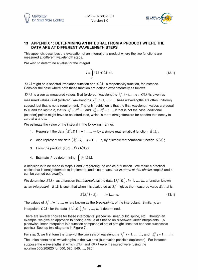
EMRP-ENG05-1.3.1
Version 1.0
48
13 APPENDIX 1: DETERMINING AN INTEGRAL FROM A PRODUCT WHERE THE DATA ARE AT DIFFERENT WAVELENGTH STEPS
This appendix describes the evaluation of an integral of a product where the two functions are measured at different wavelength steps.
We wish to determine a value for the integral
( ) ( )d .
a
b
I E Gλ λ λ= ∫ (13.1)
( )E λ might be a spectral irradiance function and ( )G λ a responsivity function, for instance.
Consider the case where both these function are defined experimentally as follows.
( )E λ is given as measured values Ei at (ordered) wavelengths , 1, ,Ei i mλ = … . ( )G λ is given as
measured values Gj at (ordered) wavelengths , 1, ,Gj j nλ = … . These wavelengths are often uniformly
spaced, but that is not a requirement. The only restriction is that the first wavelength values are equal
to a, and the last to b, that is 1 1E G
aλ λ= = and E Gm n bλ λ= = . If that is not the case, additional
(exterior) points might have to be introduced, which is more straightforward for spectra that decay to zero at a and b.
We estimate the value of the integral in the following manner:
1. Represent the data ( ),Ei iEλ i = 1, …, m, by a simple mathematical function ( )E λ� ;
2. Also represent the data ( ),Fj jGλ j = 1, …, n, by a simple mathematical function ( )G λ� ;
3. Form the product ( ) ( ) ( )Q E Gλ λ λ= �� ;
4. Estimate I by determining ( )d .b
aQ λ λ∫
A decision is to be made in steps 1 and 2 regarding the choice of function. We make a practical choice that is straightforward to implement, and also means that in terms of that choice steps 3 and 4 can be carried out exactly.
We determine ( )E λ� as a function that interpolates the data ( ),Ei iEλ , i = 1, …, m, a function known
as an interpolant. ( )E λ� is such that when it is evaluated at Eiλ it gives the measured value Ei, that is
( ) , 1, , .Ei iE E i mλ = =� … (13.1)
The values of Eiλ , i = 1, …, m, are known as the breakpoints, of the interpolant. Similarly, an
interpolant ( )G λ� for the data ( ),Gj jGλ j = 1, …, n, is determined.
There are several choices for these interpolants: piecewise linear, cubic spline, etc. Through an example, we give an approach to finding a value of � based on piecewise-linear interpolants. (A piecewise-linear interpolant is a function composed of set of straight lines that connect successive points.) See top two diagrams in Figure 7.
For step 3, we first form the union of the two sets of wavelengths Eiλ i = 1, …, m, and G
jλ j = 1, …, n.
The union contains all wavelengths in the two sets (but avoids possible duplicates). For instance
suppose the wavelengths at which ( )E λ and ( )G λ were measured were (using the
notation 500(20)620 for 500, 520, 540, …, 620)

EMRP-ENG05-1.3.1
Version 1.0
49
nm :Eiλ
500(20)620,
nm :Giλ
500(30)620.
Figure 7 −−−− Measured points representing spectra ( )E λ� and ( )G λ� and their piecewise-linear
interpolants and (bottom) the product of these interpolants, which is piecewise quadratic
When merged the two sets of wavelengths (with duplicate entries struck through) give, in nm:
500, 500, 520, 530, 540, 560, 560, 580, 590, 600, 620, 620.
The union of the two sets of wavelengths is thus the p, say, wavelength values (shown as broken vertical lines in Figure 7):
500, 520, 530, 540, 560, 580, 590, 600, 620.
The upper diagram in Figure 7 shows the measured points ( ),Ei iEλ i = 1, …, m, as small circles, and
their piecewise-linear interpolant ( )E λ� , and the middle diagram similarly for the measured
points ( ),Gj jGλ j = 1, …, n, and the interpolant ( )G λ� . The lower diagram in Figure 7 shows the
product ( ) ( ) ( )Q E Gλ λ λ= �� with its breakpoints indicated by broken vertical lines.
That ( )Q λ is piecewise quadratic with these breakpoints can be seen as follows. Since over the first
sub-interval (500 nm, 520 nm), ( )E λ� and ( )G λ� are both linear, their product is quadratic. Over the
second sub-interval (520 nm, 530 nm), ( )E λ� is linear (but different from that previously) and ( )G λ� is
linear (the same as previously). Their product is therefore again a (different) quadratic piece. In a
similar manner, the whole of ( )Q λ is established. Because ( )E λ� and ( )G λ� are continuous, so is
( )Q λ .
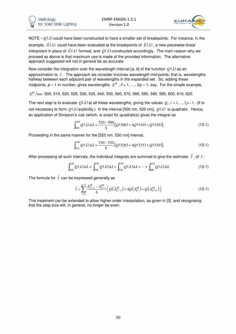
EMRP-ENG05-1.3.1
Version 1.0
50
NOTE – ( )Q λ could have been constructed to have a smaller set of breakpoints. For instance, in the
example, ( )G λ� could have been evaluated at the breakpoints of ( )E λ� , a new piecewise-linear
interpolant in place of ( )G λ� formed, and ( )Q λ constructed accordingly. The main reason why we
proceed as above is that maximum use is made of the provided information. The alternative approach suggested will not in general be as accurate.
Now consider the integration over the wavelength interval [a, b] of the function ( )Q λ as an
approximation to I . The approach we consider involves wavelength mid-points, that is, wavelengths halfway between each adjacent pair of wavelengths in the expanded set. So, adding these
midpoints, p – 1 in number, gives wavelengths allλ� , ℓ = 1, …, 2p – 1, say. For the simple example,
allnm :λ� 500, 510, 520, 525, 530, 535, 540, 550, 560, 570, 580, 585, 590, 595, 600, 610, 620.
The next step is to evaluate ( )Q λ at all these wavelengths, giving the values , 1, , 2 1Q p= −� � … . (It is
not necessary to form ( )Q λ explicitly.) In the interval [500 nm, 520 nm], ( )Q λ is quadratic. Hence,
an application of Simpson’s rule (which, is exact for quadratics) gives the integral as
( ) ( ) ( ) ( )[ ]520
500
520 500d 500 4 510 520 .
6Q Q Q Qλ λ
−= + +∫ (13.1)
Proceeding in the same manner for the [520 nm, 530 nm] interval,
( ) ( ) ( ) ( )[ ]530
520
530 520d 520 4 525 530 .
6Q Q Q Qλ λ
−= + +∫ (13.1)
After processing all such intervals, the individual integrals are summed to give the estimate, I , of I :
( ) ( ) ( ) ( )620 520 530 620
500 500 520 600d d d d .Q Q Q Qλ λ λ λ λ λ λ λ= + + +∫ ∫ ∫ ∫� (13.1)
The formula for I can be expressed generally as
( ) ( ) ( )1 all all
all all all2 1 2 12 1 2 2 1
1
ˆ 4 .6
p
I Q Q Qλ λ
λ λ λ−
+ −− +
=
− = + + ∑ � �� � �
�
(13.1)
This treatment can be extended to allow higher-order interpolation, as given in [3] and recognising that the step-size will, in general, no longer be even.

EMRP-ENG05-1.3.1
Version 1.0
51
14 APPENDIX 2: CORRECTING FOR BANDWIDTH
Reference [9] presents a procedure for correcting a measured spectrum for bandwidth to obtain a corrected spectrum that is, generally, closer to the true spectrum than the measured spectrum. The method builds on previous work [12, 23, 24] . No bandwidth correction algorithm can provide perfect correction, but the recommended method is suitable for many situations.
The bandwidth correction algorithm can deal with non-triangular bandpass functions. A simpler expression applies when the bandpass function is triangular (also given below).
14.1 STEP 1: DETERMINE THE BANDPASS FUNCTION AND ITS MOMENTS
The bandpass function is determined experimentally by one of two methods. In the direct approach, the response of the spectrometer is recorded as a tuneable monochromatic source (e.g. tuneable laser) is tuned to several wavelengths across the bandpass function. In the indirect a non-tuneable monochromatic source (e.g. laser or gaseous emission lamp, such as a mercury lamp) is used and the response of the spectrometer is recorded as its central wavelength is tuned. The direct approach determines the bandpass function, whilst the indirect approach determines the spectral ‘mirror image’ of the bandpass function, known as the line-spread function.
The correction coefficients are determined from the bandpass function, ( ) ,b λ and its moments,
defined as
( )d ,n
nI bλ λ λ= ∫ (14.1)
for 0,1,n = … , where the integral is taken over the support of the bandpass function (the interval of
wavelengths where it is non-zero). The bandpass function should be normalised such that the zeroth moment has the value unity. For a well-calibrated wavelength scale, the wavelengths are corrected so that the first moment is close to zero. The first four moments should be determined.
If the line spread function has been determined rather than the bandpass function (indirect approach), then the moments can be determined directly from the line spread function, but the signs of the odd moments should be reversed (positive to negative and vice versa). The signs of the even moments are unchanged.
14.2 STEP 2: DETERMINE THE CORRECTION COEFFICIENTS
The correction coefficients are calculated from the moments.
0
1 1
222 1
333 1 2 1
2 241 34 2 1 2
4 1
1
2
6
3.
24 3 4 2
A
A I
IA I
IA I I I
I II I I IA I
=
= −
−= +
−= + −
−= + + − +
(14.2)
14.3 STEP 3A: CALCULATE THE CORRECTION – DERIVATIVE APPROACH
There are two ways of determining the bandwidth-corrected signals, the derivative approach (3a, section 14.3) and the weighted mean approach (3b, section 14.4). These are equivalent (and yield identical results) and it is a matter of personal choice which is preferable
41.
41 In practice, the derivative approach is generally easier to implement in a spread sheet and the weighted mean approach is
easier to implement using covariance based uncertainty analysis as it can be more easily described in a matrix
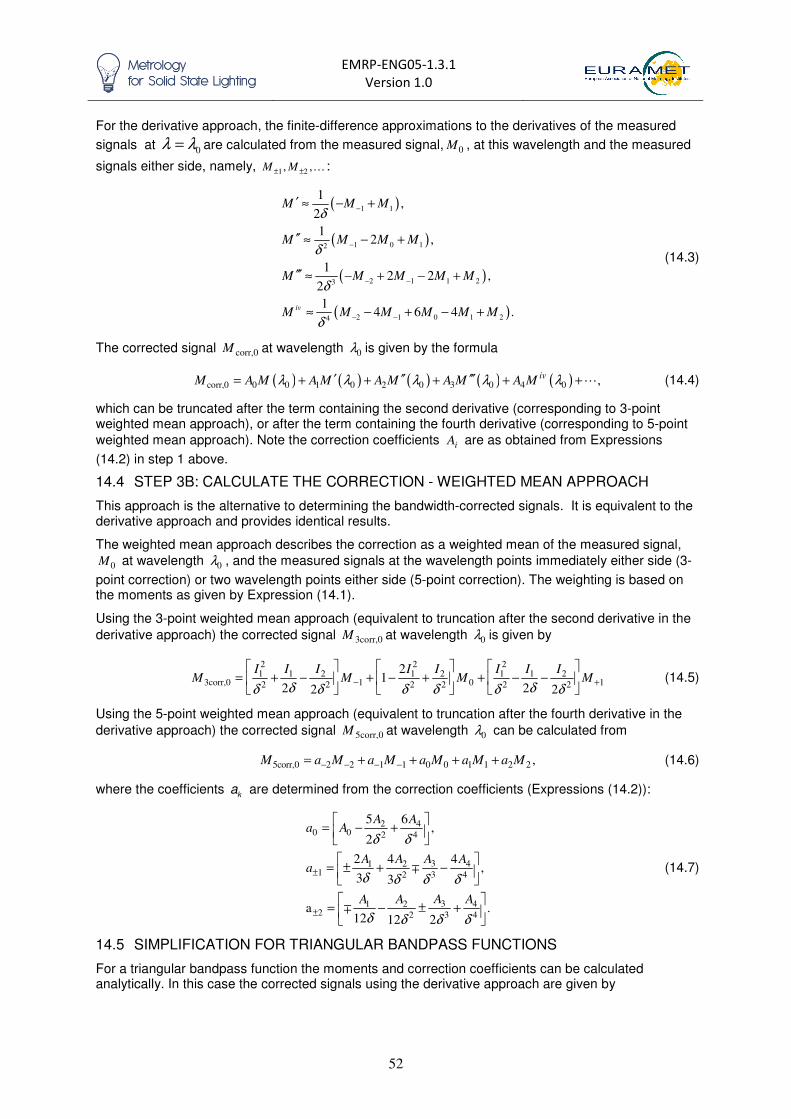
EMRP-ENG05-1.3.1
Version 1.0
52
For the derivative approach, the finite-difference approximations to the derivatives of the measured
signals at 0λ λ= are calculated from the measured signal, 0M , at this wavelength and the measured
signals either side, namely, 1 2, ,M M± ± … :
( )
( )
( )
( )
1 1
1 0 12
2 1 1 23
2 1 0 1 24
1,
2
12 ,
12 2 ,
2
14 6 4 .
iv
M M M
M M M M
M M M M M
M M M M M M
δ
δ
δ
δ
−
−
− −
− −
′ ≈ − +
′′ ≈ − +
′′′ ≈ − + − +
≈ − + − +
(14.3)
The corrected signal corr,0M at wavelength 0λ is given by the formula
( ) ( ) ( ) ( ) ( )corr,0 0 0 1 0 2 0 3 0 4 0 ,iv
M A M A M A M A M A Mλ λ λ λ λ′ ′′ ′′′= + + + + +� (14.4)
which can be truncated after the term containing the second derivative (corresponding to 3-point weighted mean approach), or after the term containing the fourth derivative (corresponding to 5-point
weighted mean approach). Note the correction coefficients iA are as obtained from Expressions
(14.2) in step 1 above.
14.4 STEP 3B: CALCULATE THE CORRECTION - WEIGHTED MEAN APPROACH
This approach is the alternative to determining the bandwidth-corrected signals. It is equivalent to the derivative approach and provides identical results.
The weighted mean approach describes the correction as a weighted mean of the measured signal,
0M at wavelength 0λ , and the measured signals at the wavelength points immediately either side (3-
point correction) or two wavelength points either side (5-point correction). The weighting is based on the moments as given by Expression (14.1).
Using the 3-point weighted mean approach (equivalent to truncation after the second derivative in the
derivative approach) the corrected signal 3corr,0M at wavelength 0λ is given by
2 2 21 1 2 1 2 1 1 2
3corr,0 1 0 12 2 2 2 2 2
21
2 22 2
I I I I I I I IM M M M
δ δδ δ δ δ δ δ− +
= + − + − + + − −
(14.5)
Using the 5-point weighted mean approach (equivalent to truncation after the fourth derivative in the
derivative approach) the corrected signal 5corr,0M at wavelength 0λ can be calculated from
5corr,0 2 2 1 1 0 0 1 1 2 2 ,M a M a M a M a M a M− − − −= + + + + (14.6)
where the coefficients ka are determined from the correction coefficients (Expressions (14.2)):
2 40 0 2 4
31 2 41 2 3 4
31 2 42 2 3 4
5 6,
2
2 4 4,
3 3
a .12 12 2
A Aa A
AA A Aa
AA A A
δ δ
δ δ δ δ
δ δ δ δ
±
±
= − +
= ± + −
= − ± +
∓
∓
(14.7)
14.5 SIMPLIFICATION FOR TRIANGULAR BANDPASS FUNCTIONS
For a triangular bandpass function the moments and correction coefficients can be calculated analytically. In this case the corrected signals using the derivative approach are given by

EMRP-ENG05-1.3.1
Version 1.0
53
2 4
corr_tr,0 0 0 0Triangles:12 240
ivM M M M
∆ ∆′′= − + +� (14.8)
The corrected signals using the 3-point weighted mean approach for a triangular bandpass function can be calculated as
2 2 2
3corr_tr,0 1 0 12 2 2Triangles: 1
12 6 12M M M M
∆ ∆ ∆
δ δ δ− +
= − + + + −
(14.9)
which, when the step size, δ, is equal to the bandwidth, ∆, simplifies further to
( )3corr_tr_eqsp,0 1 0 1 0 1 0 1
1 14 1 1Triangles: 2
12 12 12 12M M M M M M M M− + − +
− −= + + = − − + (14.10)
Note that expression (14.10) is slightly different from the formula given in [24] , but is the more accurate correction built into the bandwidth-corrected tables for colour matching functions [10, 11] . The corrected signals using the 5-point weighted mean approach for a triangular bandpass function when the step size is equal to the bandwidth can also be simplified to
( )5corr_tr_eqsp,0 2 1 0 1 2Triangles: 2 23 222 23 2 180M M M M M M− − + += − + − + (14.11)
14.6 BANDWIDTH CORRECTION AND COVARIANCE
The correction algorithm described above can also be applied using a matrix approach. Consider a correction of the form given in Expression (14.6). In matrix terms this can be created by writing the matrix
11 12 13
21 22 23
2 1 0 1 2
2 1 0 1 2
2 1 0 1
2 1 0
2 1 0 1 2
2 1 0 1 2
1 2 3
1 2 3
m m m
n n n
A A A
A A A
a a a a a
a a a a a
a a a a
a a a
a a a a a
a a a a a
A A A
A A A
− − + +
− − + +
− − +
− −
− − + +
− − + +
=
A
�
�
� � �
(14.12)
Note that for all but the first two rows and the last two rows this matrix has the parameters ia (as
used in (14.6) and defined in (14.7)) listed in the columns corresponding to the measured values iM .
So the third row is used to determine the corrected value at the third wavelength. This corrected value
is obtained as the sum of 2a− times the first measured value, 1a− times the second measured value,
0a times the third measured value (that to be corrected) and so on. The first and last two rows need
modification because there are too few ‘points before’ or ‘points after’.
One suggestion is to use the three-point correction42
for the second and penultimate rows (given by (14.5)); thus
42 This is inconsistent with the five-point formulation given in other rows, but for practical purposes is acceptable.
EMRP-ENG05-1.3.1
Version 1.0
54
21 1 2
21 1 2 2
21 2
22 2 2 2
21 1 2
23 3 2 2
2 2
21
.2 2
m
m
m
I I IA A
I IA A
I I IA A
δδ δ
δ δ
δδ δ
= = + −
= = − +
= = − −
(14.13)
The first and last rows require an asymmetric numerical determination of the derivatives replacing (14.3). Using,
1 0
2 1 0
2
0 1
0 1 2
2
Forward:
2
Backward:
2
M MM
M M MM
M MM
M M MM
δ
δ
δ
δ
+
+ +
−
− −
−′ =
− +′′ =
−′ =
− +′′ =
(14.14)
within Expression (14.4), and truncating at the second derivative term43
, we obtain
1 211 0 2
1 2
12 2
2
13 2
2
1 2
1 2
2 2
1 2
3 0 2
2
2
n
n
n
A AA A
A AA
AA
AA
A AA
A AA A
δ δ
δ δ
δ
δ
δ δ
δ δ
= − +
= −
=
=
−= −
= + +
(14.15)
Once this matrix is formed, bandwidth correction can be performed on a vector of measured irradiance values
44, or better measured signals, using the expression
corr =E AE (14.16)
and the covariance matrix for the spectral values, EU is modified to account for the introduced
covariance from the bandwidth correction process, by
Tcorr .E E=U AU A (14.17)
43 Again, somewhat inconsistently, but in a way that is practically simpler 44 Ideally the correction is done to the measured raw signals (e.g. voltage or photocurrent or ‘digital number’ counts) for both
the reference and the test sources before the calculation of irradiance as reference irradiance multiplied by test signal divided
by reference signal. In this case, replace E in the equations with the reference signal. A full description of this is beyond the
scope of this report.