deterministic scheduling in computer systems: a …archive/pdf/e_mag/vol.31_02_190.pdf ·...
TRANSCRIPT
Journal of the Operations Research Society of Japan
Vol. 31, No. 2, June 1988
DETERMINISTIC SCHEDULING IN COMPUTER SYSTEMS: A SURVEY
Tsuyoshi Kawaguchi Seiki Kyan University of the Ryukyu
(Received May 21, 1987; Revised September 26, 1987)
Abstract The progress of computer architecture has increased the necessity to design efficient scheduling algo-
rithms according to the types of computer systems. We survey recent results of optimization and approximation
algorithms for deterministic models of computer scheduling. We deal with identical, uniform and unrelated parallel
processor systems, and flowshop systems. Optimality criteria considered in this paper are schedule-length and mean
(weighted) flow-time. These are important measures for evaluating schedules in computer systems. Results on
practical algorithms such as list scheduling are emphasized.
1. Introduction
The progress of computer architecture such as multiprocessor systems has
increased the necessity to design efficient scheduling algorithms according to
the types of computer systems. Two basic approaches have been considered for
the evaluation of scheduling algorithms in computer systems. One is deter
ministic approach and the other is stochastic approach. An advantage of
deterministic approach over stochastic one is that job parameter values are
not constrained to fit a prescribed distribution [22].
This paper surveys recent results of optimization and approximation
algorithms for deterministic models of computer scheduling, refered to as
deterministic scheduling problems. We will deal with parallel processor
problems and flowshop problems. Optimality criteria considered in this paper
are schedule-length and mean (weighted) flow-time. We will also emphasize
results of practical algorithms such as list scheduling and highest-level
first strategy, rather than elaborated algorithms. A parallel processor
system corresponds to a multiprocessor computer system which can execute
several jobs simultaneously in parallel. A flowshop system can be interpreted
190
© 1988 The Operations Research Society of Japan
Deterministic Scheduling in Computer Systems 191
as a computer system where all jobs pass through several phases such as input,
execution and output [12]. Moreover schedule-length is a processor utiliza
tion factor, and mean (weighted) flow-time corresponds to the mean (weighted)
response time which is important from the user's viewpoint [6].
In this paper we will treat single processor problems as special cases of
parallel processor problems, but we will r.ot deal with openshop and jobshop
problems which are often used as models of production scheduling rather than
computer scheduling. The reader LS refered to [7, 33, 45, 52, 53] for open
shop problems, jobshop problems and parallel processor problems involving
criteria other than schedule-length and mean (weighted) flow-time. Especially,
we recommend [33] (or [52]) as a comprehensive survey. Moreover [7] gives
detailed descriptions about problems with additoinal resources, and [38]
summarizes recent results of approximation algorithms.
Section 2 introduces the basic concepts and presents a detailed problem
classification. Results on parallel processor scheduling are described in
section 3 for problems with no additional resources, and in section 4 for
problem~ with additional resources. Section 5 deals with flowshop scheduling.
Finally in section 6, we give concluding remarks.
2. Preliminaries
2.1 Basic concepts First we briefly explain the basic ccncepts concerning the theory of the
computational complexity. For formal definitions of these concepts, the
reader is refered to [26].
Let T (n) denote the largest amount of time needed by an algorithm A A
to solve a problem instance of size n. If there exists a constant c such that
TA(n) ~ c f(n) for all values of n ~ 0, we say that the time complexity of the
algorithm is O(f(n». A polynomial time algorithm is one whose time complexity
is O(f(n», where f is some polynomial fur.ction.
There is a large class of problems, called NP-complete problems, which
include classical hard problems such as the traveling salesman problem or the
integer programming problem, etc. The best known algorithms for all NP-com
plete problems have exponential time complexity, and any NP-complete problem
has a polynomial time algorithm if and only if all the others also have poly
nomial time algorithms. Many researchers conjecture that NP-complete problem
has no polynomial time algorithm. As a consequence, the knowledge that a
problem is NP-complete shows inherent intractability of the problem. NP
completeness is defined for decision problems which return "yes" or "no" answer.
Copyright © by ORSJ. Unauthorized reproduction of this article is prohibited.
192 T. Kawaguchi, S. Kiyabu
Further) the notion of NP-hardness is used for showing that a problem is
at least as hard as NP-complete problems. An optimization problem P is NP
hard if the decision problem corresponding to P is NP-complete.
Certain algorithms for NP-hard problems have the following property: they
are polynomial if any upper bounds are imposed on input numbers, for example,
which represent processing times of jobs; and otherwise they are not poly
nomial. Such algorithms are called pseudopolynomial time algorithms. Given
a problem p. let D(P) be the set of all instances of P. Moreover let p'
denote subproblem which lS created by restricting D(P) to the instances. each
of which has the maximum number bounded by a polynomial in its length. If
there exists a polynomial for which P I is NP-hard. the original problem P is
said to be strongly NP-hard or NP-hard in the strong sense.
Next we define a measure for evaluating goodness of approximation algo
rithms. Let P denote a minimization problem and let I be any instance of P.
Then the absolute performance ratio for an algorithm A is given by
R = inf { r ~ 1: R eI) ~ r for all instances of P } A A
where
RA (I) = A(r) /OPT(r) ,
where A(I) is the cost obtained by algorithm A and OPT(I) is the optimum cost.
Moreover the asymptotic performance ratio for algorithm A is given by
RA = inf { r ~ 1: for some K > 0) RA(I) ~ r for any instance I
with OPT(I) ~ K }.
If RA ~ r for some r ~ 1. then RA ~ r. But the converse is not necessarily
true. Unless stated otherwise, the term "performance ratio" means the abso
lut~ performance ratio in this paper.
2.2 Problem classification The scheduling model that we consider has a set of jobs {J
1,· •• )I
n} and
a processor system {P1 ••••• P
m}. Each job is to be executed on no more than
one processor at a time. and each processor can process no more than one job
at a time. Problems involving additional resources are discussed only in
section 4. and so parameters about additional resources are given in section
4. Below we will describe various job and processor characteristics.
2.2.1 Processor environment As stated in the preceding section, this paper deals with two types of
processor systems: parallel processor systems and flowshop systems. In
Copyright © by ORSJ. Unauthorized reproduction of this article is prohibited.
Deterministic Scheduling in Computer Systems 193
a parallel processor system. each job requires the use of exactly one proces
sor, and each job can be performed on each processor. On the other hand,
a flowshop system is a processor system in which each job J. has a chain of m ~
tasks T .. and each task T .. requires execution on processor P .• Further with ~J ~J ]
respect to processing speed, we will distinguish three classes of parallel
processor systems. Let s .. denote the processing speed of a job J. on a ~J ~
processor Pj
• A parallel processor system is said to be uniform if Slj=s2j=
•• • =s . for all processors P., and otherwise the processor system is said to nJ ]
be unrelated. In uniform processors, s .-=sl' (=s2 .= . .. =s .) denotes the speed ] ] ] nJ
of processor P .• ]
Specially, a uniform processor system in which all proces-
sors have the same speed is said to be identical.
The following notation 1.S used for specifying the processor environment.
Let ~ denote the empty symbol.
(1) TP (the type of processors)
TP=~: one processor.
(2)
TP=P: identical processors.
TP=Q: uniform processors.
TP=R: unrelated processors.
TP=F: flowshop.
m (the number of processors)
m=~: m is assumed to be a free parameter.
m=k: m is a constant equal to k (k is a positive
m;;:'k: m is a cons tant greater than or equal to k.
2.2.2 Job characteristics
integer) •
If a job cannot be interrupted once it has begun execution, the job is
said to be nonpreemptive. Otherwise, the job is said to be preemptive.
A partial order < is defined on a given set of jobs, where J. < J. signi~ ]
fies that J. must be completed befure J. can begin. ~ ]
The partial order < is
conveniently represented as a dag (directed acyclic graph) where each node
corresponds to a j ob. Let us denote by "e" the number of edges in >.
Arrival time of a job denotes the time on which the job becomes available
for processing.
Processing time of a job, denoted by ti (or tij
), 1.S defined for each of
three classes of parallel processor systems.
Identical processors: ti is the time needed by a processor to complete Ji
.
Uniform processors: ti is the time needed by the slowest processor to
complete Ji
.
Copyright © by ORSJ. Unauthorized reproduction of this article is prohibited.
194 T. Kawaguchi, S. Kiyabu
Unre lated processors: t .. is the time needed by processor p. to complete ~J ]
J .• ~
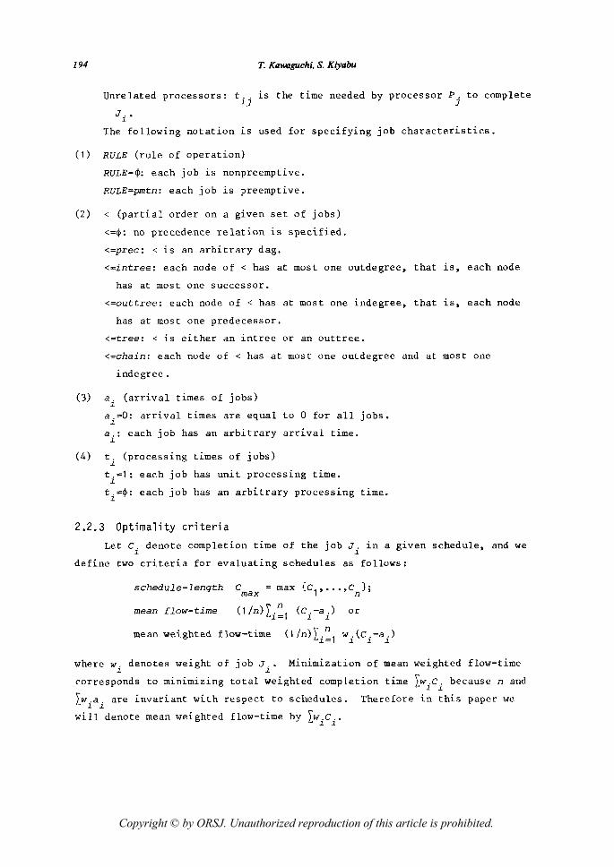
The following notation is used for specifying job characteristics.
(1) RULE (rule of operation)
RULE=~: each job is nonpreemptive.
RULE=pmtn: each job is preemptive.
(2) < (partial order on a given set of jobs)
<=~: no precedence relation ~s specified.
<=prec: < is an arbitrary dag.
(3)
(4)
<=intree: each node of < has at most one outdegree. that is. each node
has at most one successor.
<=outtree: each node of < has at most one indegree, that is, each node
has at most one predecessor.
<=tree: < is either an intree or an outtree.
<=chain: each node of < has at most one outdegree and at most one
indegree.
a. (arrival times of jobs) ~
a.=O: arrival times are equal to 0 for all jobs. ~
ai
: each job has an arbitrary arrival time.
t. (processing times of jobs) ~
ti=1: each job has unit processing time.
ti=~: each job has an arbitrary processing time.
2.2.3 Optimality criteria
Let C. denote completion time of the job J. in a given schedule, and we ~ ~
define two criteria for evaluating schedules as follows:
schedule-length C = max {C1 ••••• C };
max n
mean flow-time (1/n)Li~1 (ci-a i )
mean weighted flow-time (1/n)Li~1
or
w. (C .-a.) ~ ~ ~
where w. denotes weight of job J .• ~ ~
Minimization of mean weighted flow-time
corresponds to minimizing total weighted completion time Lw.c. because nand ~ ~
Lw.a. are invariant with respect to schedules. Therefore in this paper we ~ ~
will denote mean weighted flow-time by Lw.c .. ~ ~
Copyright © by ORSJ. Unauthorized reproduction of this article is prohibited.
Deterministic Scheduling in Computer Systems 195
2.2.4 Three-field notation When we need to distinguish scheduling problems in a short way, we will
use three-field notation defined as follJws [33]:
where
Cl = s y
(TP, m),
(RULE. <. a .• t.). ~ ~
C or LW'C" max ~ ~
3. Parallel Processor Problems With No Additional Resources
This section concerns parallel processor problems with no additional
resources. Both cases of ai=O and arbitrary ai
are considered for each
criterion of C and LW'C" max ~ ~
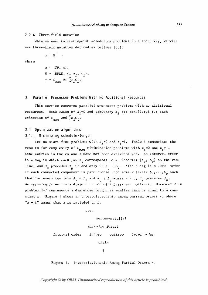
3.1 Optimization algorithms 3.1.1 Minimizing schedule-length
Let us start from problems with a .=0 and t .=1. Table 1 sUllUIlarizes the ~ ~
results for complexity of C minimization problems with a.=O and t.=I. max ~ ~
Some entries in the column < have not been explained yet. An interval order
~s a dag in which each job Jx
corresponds to an interval [a • b ] on the real x x
line. and J precedes J if and only if a > b. Also a dag is a level order X y Y x
if each connected component is partitioned into some k levels L1 •..•• L
k such
that for every two jobs Jx
E Li and Jy
E Lj
where i > j, J x precedes Jy
'
An opposing forest is a disjoint union of intrees and outtrees. Moreover < in
problem 1-7 represents a dag whose heighc is smaller than or equal to a con
SLant h. Figure 1 shows an interrelationship among partial orders <, where
"a + b" means that a is included in b.
prec
series-parallel
opposing forest
interval order intree out tree level order
chain
Figure 1. Interrelationship Among Partial Orders <.
Copyright © by ORSJ. Unauthorized reproduction of this article is prohibited.
196 T. Kawaguchi, S. Kiyabu
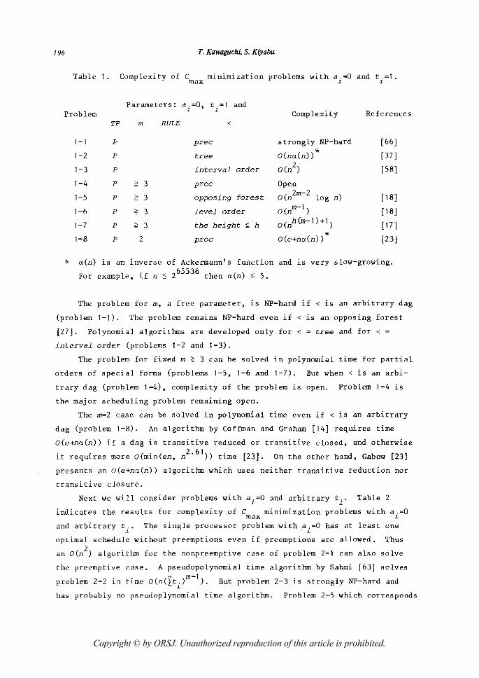
Table 1. Complexity of C minimization problems with a.=O and t.=I. max ~ ~
Parameters: ai=O, t .=1 and Problem ~ Complexity References
TP m RULE <
1-1 P prec strongly NP-hard [66 ]
* 1-2 P tree O(na(n» [37]
1-3 P interval order 2
O(n ) [58]
1-4 P ~ 3 prec Open
1-5 P ~ 3 opposing forest o(n2m- 2 log n) [ 18]
1-6 P ~ 3 level order o(nm- 1 ) [ 18]
1-7 P ~ 3 the height :> h O(nh (m-1) +1) [17 ]
1-8 P 2 prec O(e+na(n) ) * [23]
* a(n) is an inverse of Ackermann's function and is very slow-growing. . 65536 For example, Lf n :> 2 then a(n) :> 5.
The problem for m, a free parameter, is NP-hard if < is an arbitrary dag
(problem 1-1). The problem remains NP-hard even if < is an opposing forest
[27]. Polynomial algorithms are developed only for < = tree and for < = interval order (problems 1-2 and 1-3).
The problem for fixed m ~ 3 can be solved in polynomial time for partial
orders of special forms (problems 1-5, 1-6 and 1-7). But when < is an arbi
trary dag (problem 1-4), complexity of the problem LS open. Problem 1-4 is
the major scheduling problem remaining open.
The m=2 case can be solved in polynomial time even if < is an arbitrary
dag (problem 1-8). An algorithm by Coffman and Graham [14] requires time
O(e+na(n» if a dag is transitive reduced or transitive closed, and otherwise
it requires more O(min(en, n2
•61 » time [23]. On the other hand, Gabow [23]
presents an O(e+na(n» algorithm which uses neither transitive reduction nor
transitive closure.
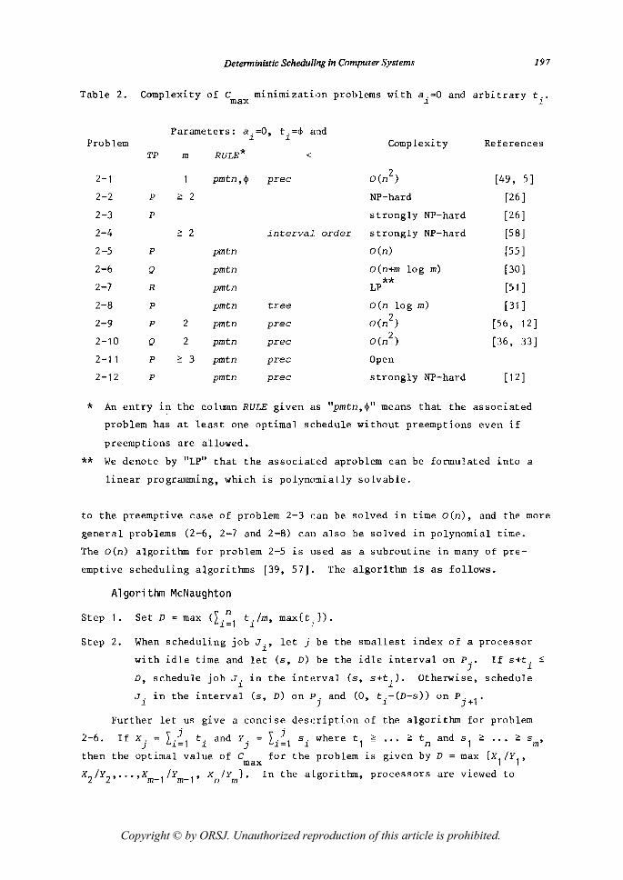
Next we will consider problems with ai=O and arbitrary t i . Table 2
indicates the results for complexity of Cmax minimization problems with ai=O
and arbitrary ti
. The single processor problem with ai=O has at least one
optimal schedule without preemptions even if preemptions are allowed. Thus
an o(n2
) algorithm for the nonpreemptive case of problem 2-1 can also solve
the preemptive case. A pseudopolynomial time algorithm by Sahni [63] solves
problem 2-2 in time O(n(Lt.)m-l). But problem 2-3 is strongly NP-hard and ~
has probably no pseudoplynomial time algorithm. Problem 2-5 which corresponds
Copyright © by ORSJ. Unauthorized reproduction of this article is prohibited.
Deterministic Scheduling in Computer Systems 197
Table 2. Complexity of C minimization problems with a;=O and arbitrary t .. max ~ ~
Problem
2-1
2-2
2-3
2-4
2-5
2-6
2-7
2-8
2-9
2-10
2-11
2-12
TP
P
P
P
Q
R
P
P
Q
P
P
rn
~ 2
~ 2
2
2
~ 3
RULE*
prntn,~
prntn
prntn
prntn
prntn
prntn
prntn
prntn
prntn
<
pree
interval. order
tree
pree
pree
pree
pree
Complexity
o(n2)
NP-hard
strongly NP-hard
strongly NP-hard
O(n)
O(n+rn log rn)
** LP
O(n log rn)
o(n 2)
o(n2)
Open
strongly NP-hard
References
[49, 5]
[26 ]
[26 ]
[58]
[55 ]
[30]
[51 ]
[31 ]
[56, 12]
[36, 33]
[12]
* An entry in the column RULE given as "prntn,~" means that the associated
problem has at least one optimal schedule without preemptions even if
preemptions are allowed.
** We denote by "LP" that the associated aproblem can be formulated into a
linear programming, which is polynmnially solvable.
to the preemptive case of problem 2-3 can be solved in time o(n), and the more
general problems (2-6, 2-7 and 2-8) can also be solved in polynomial time.
The 0 (n) algori thm for problem 2-5 is used as a subroutine in many of pre
emptive scheduling algorithms [39, 57]. The algorithm is as follows.
Algorithm McNaughton
Step 1. Set D = max (Li~1 ti/rn, max{ti }).
Step 2. When scheduling job Ji
, let j be the smallest index of a processor
with idle time and let (5, D) be the idle interval on P .. If s+t. ~ ] ~
D, schedule job Ji
in the interval (5, s+ti
). Otherwise, schedule
J. in the interval (5, D) on P. and (0, t.-(D-S» on P. 1. ~ ] ~ J+
Further let us give a concise description of the algorithm for problem
2-6. If X. = t~1 t. and Y. = t~1 s. where tl ~ ~ t and 51 ~ ... ?: 5 rn' ] ~ ] ~ n then the optimal value of C for the problem is given by D = max {X
l/Y
l,
max X2 /Y2 ,·· • 'Xm- l /Yrn- l , X /Y }. In the algorithm, processors are viewed to
n m
Copyright © by ORSJ. Unauthorized reproduction of this article is prohibited.
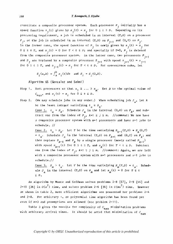
198 T. Kawaguchi, S. Kiyabu
constitute a composite processo.r system. Each pracessor P. initially has a J
speed function s .(t) given by s .(t) = s. for ° J J J
~ t ~ D. Depending on its
processing requirement, a job is scheduled in an interval (T,D) on a processor
P., or the J
job is scheduled in an interval (T,D) an P. 1 and (O,T) on P .. J- J
former case, the speed function of P. is newly given by s .(t) = s. for J J J
In the
° ~ t ~ T, and s .(t) = ° far T < t ~ D; and specially if T=O, P. is deleted J ]
from the camposite processar system. In the latter case, two processars p. 1 r
and P. are replaced by a camposite pracessor P. 1 with speed s. l(t) = s. 1 J r r J-
for ° ~ t ~ T, and s. 1 (t) = s. for T < t ~ D. For convenience sake, let r J
S; (a.b) = fb s. (t)dt and S. = s. (O.D). • a ~ ~ ~
Algorithm GS (Gonzalez and Sahni)
Step 1. Sort pracessors so that sI ~
Cmax ' and si(t) = si far ° ~ ~ s . m
t :;; D.
Set D to the aptimal value of
Step 2. (We may schedule jobs in any order.) When scheduling jab Ja
• let k
be the least integer satisfying ta ~ Sk'
Case 1. ta = Sk' Schedule J a in the interval (O,D) an Pk ' and sub
tract one from the index af P., k+l :;; j ~ m. //camment: We naw have J
a campasite processar system with m-I pracessars and have n-l jabs to.
schedule. / /
Case 2. ta > Sk' Let T be the time satisfying Sk_l(T.D) + Sk(O,T)
= ta' Schedule J a in the interval (T,D) an Pk -1
and (O,T) an Pk ; and
then replace Pk- l and Pk by a single processor (newly called Pk- l )
with speed sk_l(t) for ° ~ t ~ T, and sk(t) far T < t ~ D. Subtract
one from the index af P., k+l ~ j :;; m. //camment: Again, we are left J
with a camposite processar system with m-I pracessars and n-l jobs to.
schedule./ /
Case 3. S > t Let T be the time satisfying S (T,D) = t . Sched-m a m a ule J in the interval (T,D) an P and let s (t) '" ° far T :;; t
a m m ~ D.
An algarithm by Muntz and Caffman salves prablems 2-8 [57], 2-9 [56] and
2-10 [36] in o(n2) time, and salves problem 2-6 [36] in o(mn2
) time. Hawever
as shawn in table 2, mare efficient algarithms are presented far problems 2-6
and 2-8. Far arbitrary <. no. palynomial time algorithm has been faund yet
even if m=3 and preemptians are allawed (see problem 2-11).
Table 3 gives the results far camplexity af C minimizatian prablems max
with arbitrary arrival times. It should be nated that minimization of C max
Copyright © by ORSJ. Unauthorized reproduction of this article is prohibited.
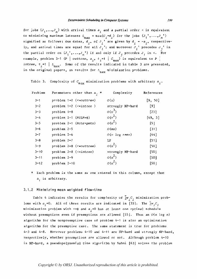
Deterministic Scheduling in Computer Systems 199
for jobs {J 1' . .•• J n} with arrival times ai
and a partial order < is equivalent
to minimizing maximum lateness L = max(C.-d.) for the jobs {J1
' ••••• Jn
'} max ~ ~
signified as follows: due dates. d .• of J.' are given by d. = -a;. respective-~ ~ ~ ~
ly, and arrival times are equal for all ,li'; and moreover Ji
' precedes Jj
' in
the partial order on {J1', •••• J '} if and only if J. precedes J. in <. For
n ] ~
example, problem 3-1 (p I outtree. a .• t .=1 I C ) 1.S equivalent to P ~ 1 max
intree, t.=l I L • ~ max
Some of the results indicated in table 3 are presented.
in the original papers. as results for L minimization problems. max
Table 3. Complexity of C minimization problems with arbitrary a .• max ~
Problem Parameters other than a. "" Complexity References ~
3-1 problem 1-2 «=outtree) O(n) [9, 50]
3-2 problem 1-2 «=intree ) strongly NP-hard [9]
3-3 problem 1-8 o(n3 ) [25 ]
3-4 problem 2-1 (RULE=CP) 2 O(n ) [ 49. 5]
3-5 problem 2-1 (RULE=pmtn) o(n2) [5 ]
3-6 problem 2-5 O(mn) [31 ]
3-7 problem 2-6 O(n log n+mn) [64 ]
3-8 problem 2-7 LP [51 ]
3-9 problem 2-8 «=outtree) 2
O(n ) [50]
3-10 problem 2-8 «=intree) strongly NP-hard [50]
3-11 problem 2-9 o(n2
) [50]
3-12 problem 2-10 o(n2) [50 ]
* Each problem is the same as one entered in this column. except that
a. is arbitrary. ~
3.1.2 Minimizing mean weighted flow-time
Table 4 indicates the results for complexity of l.wiCi
minimization prob
lems with ai=O. All of these results are indicated in [33]. The LWiCi minimization problem with <=CP and ai=O has at least one optimal schedule
without preemptions even if preemptions are allowed [55]. Thus an O(n log n)
algorithm for the nonpreemptive case of problem 4-1 is also an optimization
algorithm for the preemptive case. The same statement is true for problems
4-3 and 4-8. Moreover problems 4-10 and 4-11 are NP-hard and strongly NP-hard,
respectively, whether preemptions are allowed or not. Although problem 4-10
is NP-hard, a pseudopolynomial time algorithm by Sahni [63] solves the problem
Copyright © by ORSJ. Unauthorized reproduction of this article is prohibited.
200 T. Kawaguchi, S. Kiyabu
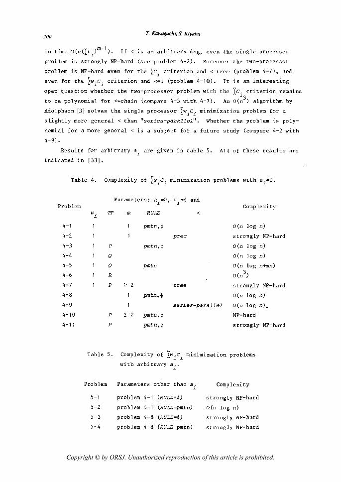
If < is an arbitrary dag, even the single processor
problem is strongly NP-hard (see problem 4-2). Moreover the two-processor
problem is NP-hard even for the Lc. criterion and <=tree (problem 4-7), and ~
even for the LW'C' criterion and <=~ (problem 4-10). It is an interesting ~ ~
open question whether the two-processor problem with the LC' criterion remains ~3
to be polynomial for <=ehain (compare 4-3 with 4-7). An D(n ) algorithm by
Adolphson [3] solves the single processor Lw.c. minimization problem for a ~ ~
slightly more general < than "series-parallel". Whether the problem is poly-
nomial for a more general < is a subject for a future study (compare 4-2 with
4-9) .
Results for arbitrary a. are given in table 5. All of these results are ~
indicated in [33].
Table 4. Complexity of Lw,c. minimization problems with a.=O. ~ ~ ~
Problem
4-1
4-2
4-3
4-4
4-5
4-6
4-7
4-8
4-9
4-10
4-11
Parmneters: ai=O, ti=~ and Complexity
w. TP m RULE < ~
pmtn,~ D(n log n)
pree strongly NP-hard
P pmtn,~ D(n log n)
Q D(n log n)
Q pmtn D(n log n+mn)
R D(n3)
P ,,; 2 tree strongly NP-hard
pmtn,~ D(n log n)
series-parallel D(n log n) ..
P ;;; ') pmtn,~ NP-hard '"
P pmtn,~ strongly NP-hard
Table 5. Complexity of LW'C' minimization problems ~ ~
with arbitrary ai
.
Problem Parameters other than a. Complexity ~
5-1 problem 4-1 (RULE=~) strongly NP-hard
5-2 problem 4-1 (RULE=pmtn) D(n log n)
5-3 problem 4-8 (RULE=~) strongly NP-hard
5-4 problem 4-8 (RULE-pmtn) strongly NP-hard
Copyright © by ORSJ. Unauthorized reproduction of this article is prohibited.
Deterministic Scheduling in Computer Systems
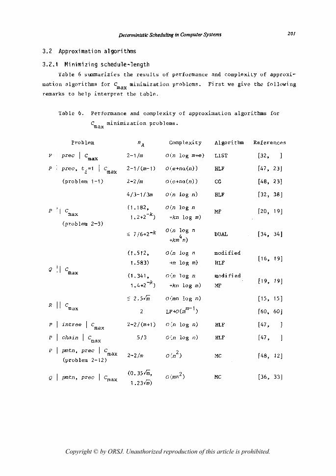
3.2 Approximation algorithms
3.2.1 Minimizing schedule-length
201
Table 6 summarizies the results of performance and complexity of approxi
mation algorithms for C minimization problems. First we give the following max remarks to help interpret the table.
Table 6. Performance and complexity of approximation algorithms for
C minimization problems. max
Problem RA Complexity Algorithm References
p 1 prec 1 C max 2-1/m O(n log m+e) LIST [32,
p 1 prec, t ,=1 1 C 2-1/(m-1) O(e+na(n) ) HLF [47, 23)
~ max
(problem 1-1) 2-2/m o (e+na(n» CG [48, 23)
4/3-1/3m O(n log n) HLF [32, 38)
p 11 Cmax (1.182. O(n log n
MF [20, 19] -k 1.2+2 ) -,kn log m) (problem 2-3)
;;; 7/6+Z-k O(n log n DUAL [34, 34) 4 +km n)
(1.512, O(n log n modified
1.583) log m) HLF [16, 19]
+n Q 11 C
max (1.341, O(n log n modified -k log m)
[19, 19] 1.4+2 ) +kn MF
;;; 2.51iil O(mn log n) [15, 15) R 11 C
Ll'+O(mm-l ) max 2 [60, 60]
p intree 1 C 2-2/(m+1) O(n log n) HLF [47, max
p 1 chain 1 C max 5/3 Ol:n log n) HLF [47,
p 1 pmtn, prec 1 C , 2) max 2-2/m Ol,n MC [ 48, 12]
(problem 2-12)
Q 1 pmtn, prec 1 Cmax (0. 351iil,
1.231iil) o(mn2) MC [36, 33)
Copyright © by ORSJ. Unauthorized reproduction of this article is prohibited.
202 T. Kawaguchi, S. Kiyabu
(1) Each row in the table is associated with an algorithm.
(2) For an algorithm whose performance ratio is not exactly known, we give
upper and lower bounds of the ratio in the column RA' These bounds are best
bounds currently known.
(3) Each complexity indicated ~n the table ~s the minimal one that the authors
know.
(4) Each entry ~n the column on algorithm denotes the name by which the
associated algorithm is called in this paper.
(5) The first entry in references gives the source for the performance of the
associated algorithm, and the second entry indicates the source for complexity
of the algorithm. If the second entry is missing, complexity of the associated
algorithm is obtained by the authors.
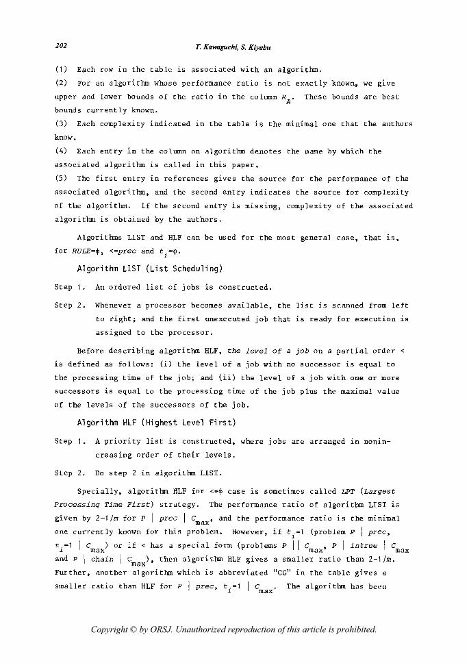
Algorithms LIST and HLF can be used for the most general case, that is,
for RULE=~, <=prec and ti=~'
Algorithm LIST (List Scheduling)
Step 1. An ordered list of jobs is constructed.
Step 2. Whenever a processor becomes available, the list is scanned from left
to right; and the first unexecuted job that is ready for execution is
assigned to the processor.
Before describing algorithm HLF, the level of a job on a partial order <
is defined as follows: (i) the level of a job with no successor is equal to
the processing time of the job; and (ii) the level of a job with one or more
successors is equal to the processing time of the job plus the maximal value
of the levels of the successors of the job.
Algorithm HLF (Highest Level First)
Step 1. A priority list is constructed, where jobs are arranged in nonin
creasing order of their levels.
Step 2. Do step 2 in algorithm LIST.
Specially, algorithm HLF for <=~ case ~s sometimes called LPT (Largest
Processing Time First) strategy. The performance ratio of algorithm LIST is
given by 2-1/m for P I pree le, and the performance ratio is the minimal max one currently known for this problem. However, if t.=1 (problem P I prec,
1.
t.=1 le) or if < has a special form (problems P I le, P I intree I c 1. max max max
and P I chain le), then algorithm HLF gives a smaller ratio than 2-1/m. max Further, another algorithm which is abbreviated "CG" in the table gives a
smaller ratio than HLF for P I prec, t.=1 1.
C max The algorithm has been
Copyright © by ORSJ. Unauthorized reproduction of this article is prohibited.
Deterministic Scheduling in Computer Systems 203
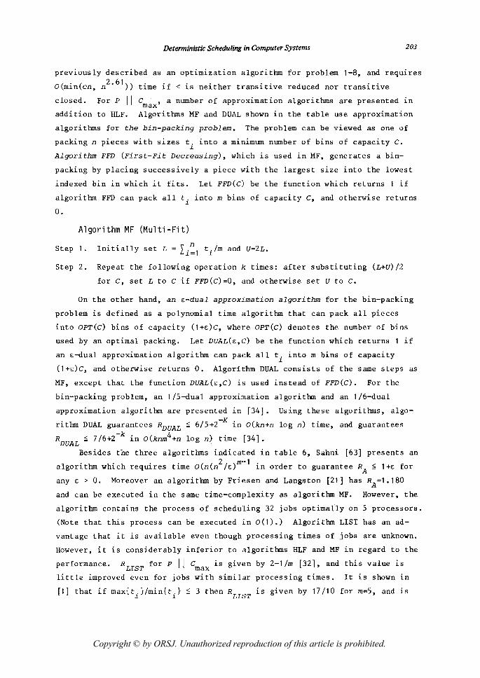
previously described as an optimization algorithm for problem 1-8, and requires
O(min(en, n2
.61 » time if < is neither transitive reduced nor transitive
closed. For P 11 Cmax
' a number of approximation algorithms are presented in
addition to HLF. Algorithms MF and DUAL shown in the table use approximation
algorithms for the bin-packing problem. The problem can be viewed as one of
packing n pieces with sizes t, into a minimum number of bins of capacity C. ~
Algorithm FFD (First-Fit Decreasing), whi.ch is used in MF, generates a bin-
packing by placing successively a piece .rith the largest size into the lowest
indexed bin in which it fits. Let FFD(C) be the function which returns 1 if
algorithm FFD can pack all ti into m bins of capacity C, and otherwise returns
o.
Algorithm MF (Multi-Fit)
Step 1. Initially set L = Li~1 ti/m and U=2L.
Step 2. Repeat the following operation k times: after substituting (L+U) /2
for C, set L to cif FFD (C) =0, and otherwise set U to C.
On the other hand, an s-dual approximation algorithm for the bin-packing
problem is defined as a polynomial time algorithm that can pack all pieces
into OPT(C) bins of capacity (1 +e:)C, where OPT(C) denotes the number of bins
used by an optimal packing. Let DUAL(S,C) be the function which returns 1 if
an s-dual approximation algorithm can paek all ti into m bins of capacity
(1 +s)C, and otherwise returns O. Algorithm DUAL consists of the same steps as
MF, except that the function DUAL(S,C) is used instead of FFD(C). For the
bin-packing problem, an 1/5-dual approximation algorithm and an 1/6-dual
approximation algorithm are presented ~n [34]. Using these algorithms, algo
rithm DUAL guarantees RDUAL ~ 6/5+2-K
in O(kn+n log n) time, and guarantees -k 4
RDUAL
~ 7/6+2 in O(knm +n log n) time [34].
Besides the three algorithms indicated in table 6, Sahni [63] presents an
1 'hm h' h ' , (( 2/ )m--1, d 1 f a gor~t w ~c requ~res t~me 0 n n s ~n or er to guarantee RA ~ +s or
any s > O. Moreover an algorithm by Friesen and Langston [21] has RA
=1.180
and can be executed in the same time-complexity as algorithm MF. However, the
algori thm contains the process of scheduling 32 jobs optimally on 5 processors.
(Note that this process can be executed in 0(1).) Algorithm LIST has an ad
vantage that it is available even though processing times of jobs are unknown.
However, it is considerably inferior to algorithms HLF and MF in regard to the
performance. R for P 11 C is given by 2-1/m [32], and this value is LIST max
little improved even for jobs with similar processing times. It is shown in
[1] that if max{t)/min{tj} ~ 3 then RLI8T
is given by 17/10 for m=5, and is
Copyright © by ORSJ. Unauthorized reproduction of this article is prohibited.
204 T. Kawaguchi, S. Kiyabu
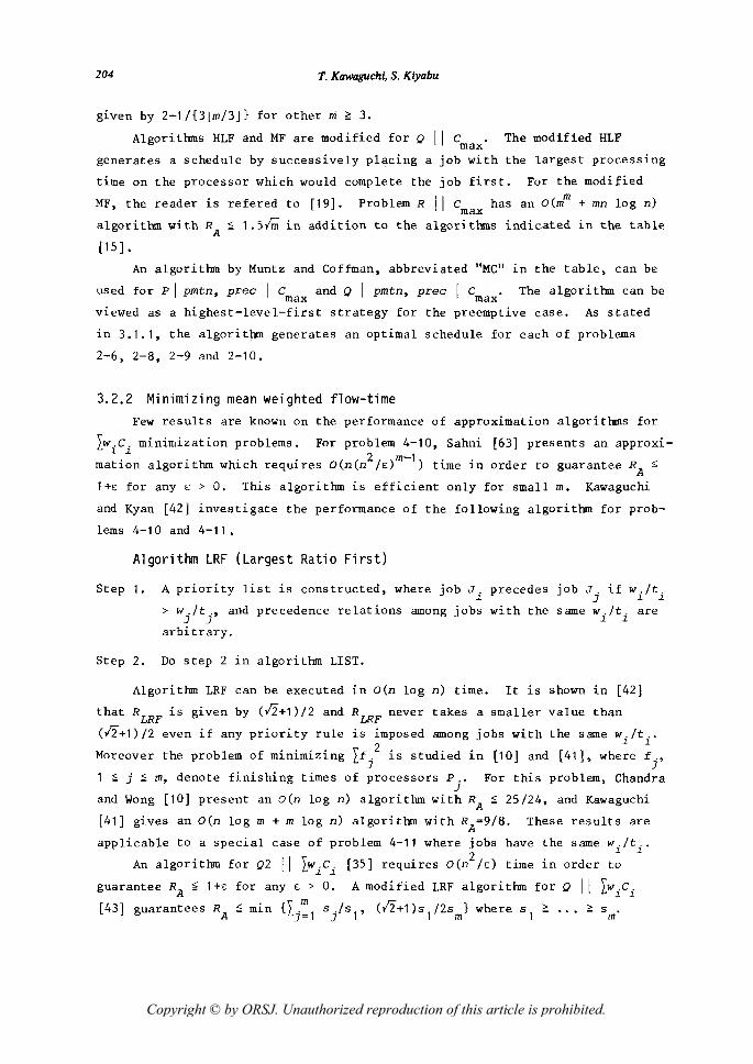
given by 2-1/{3lm/3J} for other ID ~ 3.
Algorithms HLF and MF are modified for Q I I c . The modified HLF max generates a schedule by successively placing a job with the largest processing
time on the processor which would complete the job first. For the modified
MF, the reader is refered to [19]. Problem R I I c has an O(mm + mn log n) max algorithm with RA ~ 1.51m in addition to the algorithms indicated in the table
(15] •
An algorithm by Muntz and Coffman, abbreviated "MC" l.n the table, can be
used for pi pmtn, prec I C and Q I pmtn, prec I C . The algorithm can be max max viewed as a highest-level-first strategy for the preemptive case. As stated
in 3.1.1, the algorithm generates an optimal schedule for each of problems
2-6, 2-8, 2-9 and 2-10.
3.2.2 Minimizing mean weighted flow-time Few results are known on the performance of approximation algorithms for
Lw.c. minimization problems. For problem 4-10, Sahni [63] presents an approxi-~. ~ . . . 2 m-l . .
matl.on algorl.thm whl.ch reqUl.res O(n(n /E) ) tl.me l.n order to guarantee RA ~
l+E for any E > O. This algorithm is efficient only for small m. Kawaguchi
and Kyan [42] investigate the performance of the following algorithm for prob
lems 4-10 and 4-11.
Algorithm LRF (Largest Ratio First)
Step 1. A priority list is constructed, where job J. precedes job J. if w./t. ~ ] ~ ~
> wjltj' and precedence relations among jobs with the same wilti are
arbitrary.
Step 2. Do step 2 l.n algorithm LIST.
Algorithm LRF can be executed in O(n log n) time. It is shown in [42]
that RLRF is given by (12+1)/2 and RLRF never takes a smaller value than
(12+1)/2 even if any priority rule is imposed among jobs with the same wi/ti
.
Moreover the problem of minimizing Lf.2 is studied in (10] and (41], where f., ] ]
1 ~ j ~ m, denote finishing times of processors P .. For this problem, Chandra ]
and Wong [10] present an O(n log n) algorithm with RA ~ 25/24, and Kawaguchi
[41] gives an O(n log m + m log n) algorithm with RA
=9/8. These results are
applicable to a special case of problem 4-11 where jobs have the
AnalgorithmforQ211 Lw,C. [35] requiresO(n2
/E) time in ~ ~
same W ./t .. ~ ~
order to
O. guarantee RA ~ l+E for any E > A modified LRF algorithm for Q I I LW'C' ~ ~
(43] < . {" m guarantees RA = ml.n Lj=l 5/5 1, (12+1)5 1/25 m} where 51 ~ '" ~ Sm'
Copyright © by ORSJ. Unauthorized reproduction of this article is prohibited.
Deterministic Scheduling in Computer Systems 205
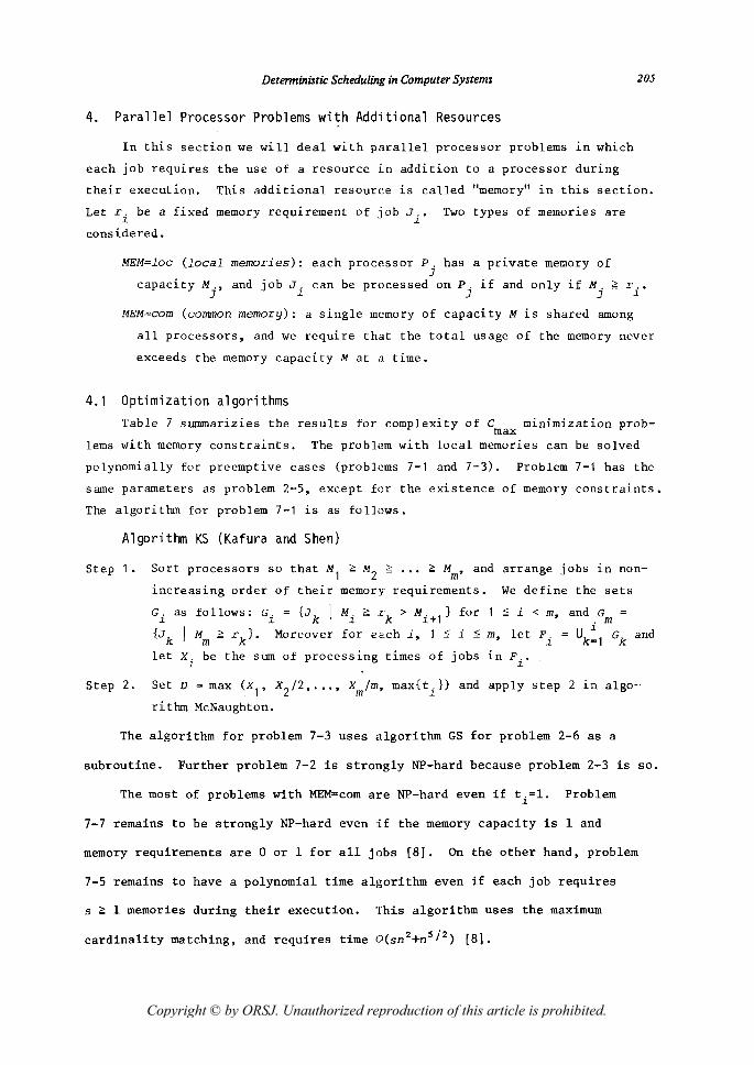
4. Parallel Processor Problems with Additional Resources
In this section we will deal with parallel processor problems in which
each job requires the use of a resource in addition to a processor during
their execution. This additional resouree is called "memory" in this section.
Let ri
be a fixed memory requirement of job Ji
. Two types of memories are
considered.
MEM=loc (local memories): each processor P. has a private memory of ]
capacity M., and job J; can be processed on P. if and only if M. ;;:; L· •• ] ~ ] ] ~
MEM=com (common memory): a single memory of capacity M is shared among
all processors, and we require that the total usage of the memory never
exceeds the memory capacity M at a time.
4.1 Optimization algorithms Table 7 summarizies the results for complexity of C minimization prob-
max lems with memory constraints. The problem with local memories can be solved
polynomially for preemptive cases (problems 7-1 and 7-3). Problem 7-1 has the
same parameters as problem 2-5, except for the existence of memory constraints.
The algorithm for problem 7-1 is as follows.
Algorithm KS (Kafura and Shen)
Step 1. Sort processors so that Ml ;;:; M2 ;;:; ... ;;:; Mm' and arrange jobs in non
increasing order of their memory requirements. We define the sets
~ i < m, and G = .m ~
Moreover for each i, 1 ~ i ~ m, let Fi Uk=l Gk
and
let Xi be the sum of processing times of jobs ~n Fi
.
Step 2. Set D = max (Xl' X2 /2, ... , xm/m, max{ti
}) and apply step 2 in algo-·
rithm McNaughton.
The algorithm for problem 7-3 uses algorithm GS for problem 2-6 as a
subroutine. Further problem 7-2 is strongly NP-hard because problem 2-3 is so.
The most of problems with MEM=com are NP-hard even if ti=l. Problem
7-7 remains to be strongly NP-hard even if the memory capacity is 1 and
memory requirements are 0 or 1 for all jobs [8]. On the other hand, problem
7-5 remains to have a polynomial time algorithm even if each job requires
s <: 1 memories during their execution. This algorithm uses the maximum
cardinality matching, and requires time O(sn 2+n S /2) [8].
Copyright © by ORSJ. Unauthorized reproduction of this article is prohibited.
206 T. Kawaguchi, S. Kiyabu
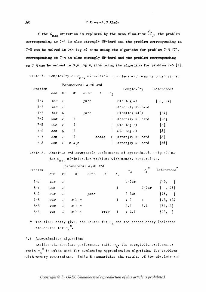
If the Cmax criterion is replaced by the mean flow-time tcl , the problem
corresponding to 7-4 is also strongly NP-hard and the problem corresponding to
7-5 can be solved in O(n log n) time using the algorithm for problem 7-5 [7].
corresponding to 7-4 is also strongly NP-hard and the problem corresponding
to 7-5 can be solved in O(n log n) time using the algorithm for problem 7-5 [7].
Table 7. Complexity of C minimization problems with memory constraints. max
Parameters: ai=O and Problem Complexity References
MEM TP m RULE < ti
7-1 lac P pmtn o (n log m) [39, 54]
7-2 lac P strongly NP-hard
7-3 lac Q pmtn 2 O(nm(log m) ) [54 ]
7-4 corn P 3 strongly NP-hard [26 ]
7-5 corn P 2 O(n log n) [8]
7-6 corn Q 2 O(n log n) [8]
7-7 corn P 2 chain strongly NP-hard [8]
7-8 corn P m ~ n strongly NP-hard [26 ] . Table 8. Absolute and asymptotic performance of approximation algorithms
for C minimization problems with memory constraints. max
Parameters: ai=O and Problem RA RA References
*
MEM TP m RULE < ti
7-2 lac P 2-2/m [39,
8-1 corn P 2-2/m [ , 46]
8-2 corn P pmtn 3-3/m [ 46, ]
7-8 corn P m ~ n ;;; 2 1 [13, 13]
8-3 corn P m f~ n 2.5 5/4 [65, 4]
8-4 cam P m ~ n prec ;;; 2.7 [24, ]
The first entry gives the source for RA and the second entry indicates
the source for RA
oo•
4.2 Approximation algorithms
*
Besides the absolute performance ratio RA' the asymptotic performance
ratio RA
oo is often used for evaluating approximation algorithms for problems
with memory constraints. Table 8 summarizies the results of the absolute and
Copyright © by ORSJ. Unauthorized reproduction of this article is prohibited.
Detenninistic Scheduling in Computer Systems 207
the asymptotic performances of approximation algorithms for Cmax
minimization
problems with memory constraints. Each entry in the columns RA and RA
oo is the
minimum one currently known. The reader should notice that even if a problem
has no entry in the column RA ' an algorithm with the absolute performance 00
ratio RA guarantees RA :;; RA for the problem. The algorithm for problem 8-1
is as follows.
A 1 gorittrn LMF (Larges t Memory Fi rs t)
Step 1. Sort jobs so that r1
;;; ••. ;;; rn" and set t=O.
Step 2. If no processor is idle at time t, set t=t+1 and go to step 3.
Otherwise, scan for the first unexecuted job for which sufficient
units of memory are available at time t. If such job exists, the job
is assigned to an idle processor in the interval (t. t+1); and other
wise set t=t+1.
Step 3. If there are uncompleted jobs, repeat step 2.
The algorithm for problem 8-2 is also the above one. Moreover the ratio
3-3/m is guaranteed for problem 8-2 even if the ordering of jobs is arbitrary
in step 1 of LMF. The algorithm for problem 7-2 is similar to LMF. In this
algorithm, whenever a processor P. becomes available, a job with the largest ]
r. satisfying M. ~ r. ~ ] ~
is assigned to the processor. Fuchs and Kafura [22]
study the C minimization problem in a max
computer consists of dual processors and
parallel computer system where each
a single memory is shared between
these processors. This model can be vie\~ed as a bridge between the extreme
models (problems 7-2 and 8-2) and the more general model where r ;;; 1 processors
share a single memory. A largest-memory·-first strategy for this model guaran
tees the absolute performance ratio (3p-2)/p where p denotes the number of
computers and is equal to half the number of processors. Comparing the results
for 7-2, 8-2 and their model, they conclude that the memory should be shared
among a small number of processors. This is an important suggestion about the
topology of computer system.
Problem 7-8 is known as the bin-packing problem, and an approximation
algorithm for this problem has been described in 3.2.1. This algorithm,
called FFD, gives RFFD
oo=11/9. Note that a bin Bt' t ;;; 1, corresponds to a
time interval (t-1, t). Moreover the following results are known for the
problem [13]:
00
RFF = 17/10 and RMFFLoo = 71/60
where MFFD is a modified FFD algorithm, and FF ~s the same as FFD except that
Copyright © by ORSJ. Unauthorized reproduction of this article is prohibited.
208 T. Kawaguchi, S. Kiyabu
jobs are scheduled in an arbitrary order. Further as shown in the table, the
problem has a polynomial time algorithm with RA
oo=1. However no polynomial
time algorithm that guarantees the absolute performance ratio smaller than 2
is found yet for the problem. On the other hand, even a more primitive algo
rithm than FF guarantees RA ~ 2. In this algorithm, called Next-Fit, a job is
placed in the current bin Bt
if it fits there, and otherwise the job is placed
in the next bin B 1 and t is increased by one. (Remember that FFD (or FF) t+ places a job ~n the lowest indexed bin in which it fits.)
Problem 8-3 is known as the two-dimensional bin-packing problem. A number
of results are reported on the asymptotic performance of algorithms for this
problem, but few results are known on the absolute one. Moreover Garey et al.
[24] presents an algorithm for the problem in which the number of memory is an
arbitrary s ~ 1 and the other parameters are the same as problem 8-4. The
algorithm uses a highest-level-first strategy and guarantees RA ~ 17s/10+1.
The bound for problem 8-4 is obtained by substituting s=l in the above bound.
Very little is known about the performance of approximation algorithms
for Iw.c. minimization problems with memory constraints. ~ ~
5. Flowshop Scheduling
A flowshop consists of m ~ 2 processors {P1, ••• ,Pm} and n ~ 1 jobs {J1
,
••• ,J}. Each job J. has a chain of m tasks T .. , 1 ~ j ~ m. Let t. denote n ~ ~J ~
the processing time of job J; and let t .. be the processing time of task T . .• ~ ~J ~]
Each task T .. requires execution on processor P., and T .. can only be executed ~J ] ~J
after T . . 1 ~s finished. Specially, if T .. has to start at the completion ~,]- ~]
time of T . . l' the resulting flowshop is said to be a no-wait flowshop. ~,J-
Before describing results of flows hop problems, we give the following notes
about the notation used in this section.
(1) Whenever a three field notation alSly ~s used, an information about no
wait constraints is put in the first position of S.
(2) We denote by "ti1=1 (or t i2 =1) " when t11=t21=.·.=tn1 (or t12=t22= ••• =tn2)'
Moreover, the notation "t . . =1" represents that all t .. , 1 ~ i ~ nand 1 ~ j ~] ~J
~ m, are the same.
Copyright © by ORSJ. Unauthorized reproduction of this article is prohibited.
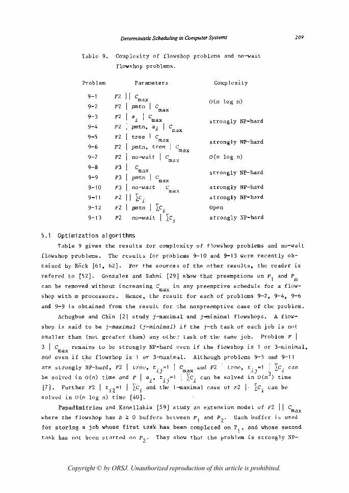
5.1
Deterministic Scheduling in Computer Systems
Table 9. Complexity of flowshop problems and no-wait
flowshop problems.
Problem Parameters Complexity
9-1 F2 11 C max o(n log n)
9-2 F2 I pmtn I C max
9-3 F2 I a. I C ~ max strongly NP-hard
9-4 F2 I pmtn, ai I C max
9-5 F2 I tree I C max strongly NP-hard
9-6 F2 I pmtn, tree I C max
9-7 F2 no-wait C O(n log n) max
9-8 F3 11 C max strongly NP-hard
9-9 F3 I pmtn I C max
9-10 F3 I no-wait I C strongly NP-hard max
9-11 F2 11 Ic. strongly NP-hard ~
9-12 F2 I pmtn I ICi Open
9-13 F2 I no-wait I Ic. strongly NP-hard ~
Optimization algorithms
209
Table 9 gives the results for comp 1 '~xi t y 0 f f lows hop pro b lems and no-wait
flowshop problems. The results for problems 9-10 and 9-13 were recently ob
tained by Rock [61, 62]. For the sources of the other results, the reader is
refered to [52]. Gonzalez and Sahni [29J show that preemptions on PI and Pm
can be removed without increasing Cmax
in any preemptive schedule for a flow
shop with m processors. Hence, the result for each of problems 9-2, 9-4, 9-6
and 9-9 is obtained from the result for che nonpreemptive case of the problem.
Achugbue and Chin [2] study j-maximal and j;ninimal flowshops. A flow
shop is said to be j-maximal (j-minimal) if the j-th task of each job is not
smaller than (not greater than) any other task of the same job. Problem F I 3 I c remains to be strongly NP-hard even if the flowshop is 1 or 3-minimal,
max and even if the flowshop is 1 or 3-maximal. Although problems 9-5 and 9-11
are strongly NP-hard, F2 tree, t .. =1 I C and F2 I tree, t .. =1 I Ic. can ~J max ~J 3 ~
be solved in O(n) time and F I ai' tij=1 I LCi
can be solved in O(n ) time
[7]. Further F2 I t·2
=1 I LC. and the 1·-maximal case of F2 I1 LC. can be ~ ~ ~
solved in O(n log n) time [40].
Papadimitriou and Kanellakis [59] study an extension model of F2 I1 C max where the flowshop has b ;;; 0 buffers bet~veen PI and P
Z. Each buffer is used
for storing a job whose first task has been completed on PI' and whose second
task has not been started on P2
. They show that the problem is strongly NP-
Copyright © by ORSJ. Unauthorized reproduction of this article is prohibited.
21 0 T. Kawaguchi, S. Kiyabu
hard if 1 ~ b < n.
5.2 Approximation algorithms
Problem F 1 no-wait 1 C can be formulated as a traveling salesman max
problem [33]. A number of approximation algorithms are presented for this
problem, and so these algorithms can be applied to F 1 no-wait 1 C max
Further,
approximation algorithms which can be viewed as list scheduling for flowshop
problems are presented for F 11 C and F 11 Lc .. max ~
Algorithm LISTF (List Scheduling for Flowshops)
Step 1. Construct a list in which jobs are arranged in an arbitrary order.
Step 2. Let L., 1 ~ j ~ m, denote m copies of the list obtained in step 1. ]
Whenever a processor P. becomes available, the first job is removed ]
from L. and the j-th task of the job is assigned to the processor. ]
Algorithm SPT (Shortest Processing time First) applies step 2 of the
above algorithm to a list where jobs are arranged in nondecreasing order of
their processing times. The following results are known about the performance
of these algorithms [29]:
RLISTF
RLISTF
m
= n and RSPT
= m
for F 11 Cmax '
for F 11 LC" ~
The performance of algorithm LISTF is not improved for F 11 C even if jobs max
are processed in nonincreasing order of their processing times. Specially for
F2 11 LCi
, the performance of SPT is given by RSPT
= 2S/(S+a) where a denotes
the smallest processing time of tasks and S is the largest one [40]. Chin and
Tsai [11 ] investigate the performance of algorithm LlSTF for j-maximal and
j-minimal flowshop problems, and give the following results:
R LISTF
m-l for the l-minimal case of F 11 C max
(m ;;; 3) ,
R LISTF
~ 1/2+1m for the l-maximal case of F 11 Cmax '
RLISTF 5/3 for the or 3-maximal case of F3 11 C max
Further Kawaguchi and Kyan [44] investigate the performance of an algorithm
for F2 1 t. 1=1 1 LC' and the l-minimal case of F2 11 Lc .. This algorithm is ~ ~ ~
also a list scheduling algorithm and schedules jobs according to nondecreasing
order of t i2 . The perfonnance ratio of this algorithm is given by 5/3 for the
l-minimal case of F2 11 Ici
, and is given by 4/3 for F2 1 til=l 1 LCi
, (As
shown in 5.1, F2 1 t. 2=1 1 LC. and the l-maximal case of F2 11 Lc. can be ~ ~ ~
solved optimally in time O(n log n).)
Copyright © by ORSJ. Unauthorized reproduction of this article is prohibited.
Deterministic Scheduling in Computer Systems 211
Problem F I I C has a polynomial time algorithm which is superior to max LISTF in regard to the performance. This algorithm guarantees RA ::; fm/21 in
O(mn log n) time [29]. However. no polynomial time algorithm with the smaller
performance than R is found yet for the 'C. minimization flowshop problem, SPT /... ~
except for the special cases described above.
An optimization algorithm for F2 I no-wait Cmax
[28] generates a feasi
Cmax
where the flowshop has 1:> ~ 0
This algorithm guarantees RA ::;
ble schedule for an extension model of 1:'2 I I buffers between PI and P 2 (see section 5.1).
(2b+l)/(b+l) in O(n log n) time [59].
6. Conclusion
We have briefly surveyed the recent results of optimization and approxima
tion algorithms for deterministic models of computer scheduling. Many inter
esting models have efficient optimization algorithms, whereas others are
NP-hard. A number of approximation algorithms have been presented for the
latter problems, and analytical results for the performance of approximation
algorithms are obtained mainly for schedule-length minimization problems with
equal arrival times. However at present, many models of computer scheduling
have neither polynomial time optimization algorithms nor approximation algo
rithms with guaranteed performance. Thus it is still important to evaluate
goodness of an approximation algorithm by means of computational experiments,
and such evaluation requires us to find a lower bound on the cost of an optimal
schedule for a given problem instance. (Lower bounds are also used in enumer
ative optimization algorithms such as branch-bound-bound method.) Various
bounding schemes have been reported in recent years although we have not
described these schemes in this survey on account of limited space. These
schemes can be further improved in the future.
Acknowledgement
The authors would like to thank Pr. Y. Nakanishi, Dr. H. Nakano and
Dr. H. Ishii of Osaka university for their valuable suggestions. The first
author was supported by the Grant-in-Aid for Encouragement of Young Scientists
of the Ministry of Education, Science and Culture of Japan under Grant: (A)
61750343 (1986). The second author was also supported by the Grant-in-Aid for
Co-operative Research of the Ministry of Education, Science and Culture of
Japan under Grant: (A) 61302080 (1986).
Copyright © by ORSJ. Unauthorized reproduction of this article is prohibited.
212 T. Kawaguchi, S. K(vabu
References
[1] Achugbue, J. O. and F. Y. Chin: Bounds on Schedules for Independent
Tasks with Similar Execution Times. J. Assoc. Comput. Mach., Vol.28
(1981).81-99.
[2] Achugbue. J. O. and F. Y. Chin: Complexity and Solutions of Some Three
Stage Flow-Shop Scheduling Problems. Math. Oper. Res., Vol.7 (1982),
532-544.
[3] Adolphson. D. L.: Single Machine Job Sequencing with Precedence Con
straints. SIAM J. Comput., Vol.6 (1977), 40-54.
[4] Baker, B. S., D. J. Brown and H. P. Katseff: A 5/4 Algorithm for Two
Dimensional Packing. J. Algorithms, Vol.2 (1981), 348-368.
[5] Baker, K. R., E. L. Lawler, J. K. Lenstra and A. H. G. Rinnooy Kan:
Preemptive Scheduling of a Single Machine to Minimize Maximum Cost Sub
ject to Release Dates and Precedence Constraints. oper. Res., Vol.31
(1983), 381-386.
[6] Blazewicz, J.: Selected Topics in Scheduling Theory. Ann. Discrete.
Math., Vol.31 (1987), 1-59.
[7] Blazewicz, J., W. Cellary, R. Slowinski and J. Weglarz: Scheduling Under
Resource Constraints - Deterministic Model (Ann. Oper. Res.,Vol.7), J. C.
Baltzer AG, 1986.
[8] Blazewicz, J., J. K. Lenstra and A. H. G. Rinnooy Kan: Scheduling Sub
ject to Resource Constraints - Classification and Complexity. Discrete
Appl. Math., vol.5 (1983), 11-24.
[9] Brucker, P., M. R. Garey and D. S. Johnson: Scheduling Equal-Length
Tasks Under Tree-Like Precedence Constraints to Minimize Maximum Late-
ness. Math. Oper. Res., Vo1.2 (1977), 275-284.
[10] Chandra. A. K. and C. K. Wong: Worst-Case Analysis of a Placement Algo
rithmRelated to Storage Allocation. SIAMJ. Comput., Vo1.4 (1975),
249-263.
[11] Chin, F. Y. and L. L. Tsai: OnJ-maximal and J-minimal Flow-Shop Sched
ules. J. Assoc. Comput. Mach., Vol.28 (1981), 462-476.
[12] Coffman, E. G. Jr (cd.): Computer and Job-Shop Scheduling Theory. John
Wiley, 1976.
[13] Coffman, E. G. Jr, M. R. Garey and D. S. Johnson: Approximation Algo
rithms for Bin-Packing - an Updated Survey. In Algorithm Design for
Computer System Design (CISM Courses and Lectures, No.284), Springer
Verlag, 1984, 49-106.
[14] Coffman, E. G. Jr and R. L. Graharn: Optimal Scheduling for Two Processo
Copyright © by ORSJ. Unauthorized reproduction of this article is prohibited.
Deterministic Scheduling in Computer Systems 213
Systems. Acta Informatica, Vol.l (1972), 200-213.
[15] Davis, E. and J. M. Jaffe: Algorithms for Scheduling Tasks on Unrelated
Processors. J. Assoc. Comput. Mach., Vol.28 (1981), 721-736.
[16] Dobson, G.: Scheduling Independent Tasks on Uniform Processors. SIAM J.
Comput., Vol.13 (1984), 705-716.
[17) Dolev, D. and M. K. Warmuth: Scheduling Precedence Graphs of Bounded
Height. J. Algorithms, Vol.5 (1984), 48-59.
[18] Dolev, D. and M. K. Warmuth: Profile Scheduling of Opposing Forests and
Level Orders. SIAMJ. Alg. Disc. Meth., Vo1.6 (1985), 665-687.
[19] Friesen, D. K. and M. A. Langston: Bounds for MULTIFIT Scheduling on
Uniform Processors. SIAM J. Comput., Vol.12 (1983), 60-70.
[20] Friesen, D. K.: Tighter Bounds for the MULTIFIT Processor Scheduling
Algorithm. SIAM J. Comput., Vol.13 (1984), 170-181.
[21] Friesen, D. K. and M. A. Langston: Evaluation of a MULTIFIT-Based Sched
uling Algorithm. J. Algorithms, Vol.7 (1986), 35-59.
[22] Fuchs, K. and D. Kafura: Memory-Constrained Task Scheduling on a Netw'ork
of Dual Processors. J. Assoc. Comput. Mach., Vo1.32 (1985), 102-129.
[23] Gabow, H. N.: An Almost Linear-Algorithm for Two-Processor Scheduling.
J. Assoc. Comput. Mach., Vo1.29 (1982),766-780.
[24] Garey, M. R., R. L. Graham, D. S. Johnson and A. C. C. Yao: Resource
Constrained Scheduling as Generalized Bin Packing. J. Combinatorial
Theory Ser A, Vol. 21 (1976), 257-298.
[25] Garey, M. R. and D. S. Johnson: Two-Processor Scheduling with Start
Times and Deadlines. SIAM J. Comput., Vo1.6 (1977), 416-426.
[26] Garey, M. R. and D. S. Johnson: Computers and Intractability - A Guide
to the Theory of NP-completeness. Freeman, 1979.
[27] Garey, M. R., D. S. Johnson, R. E. Tarjan and M. Yannakakis: Scheduling
Opposing Forests. SIAM J. Alg. Disc. Meth., Vol.4 (1983), 72-93.
[28] Gi lmore , P. C. and R. E. Gomory: Sequencing a One-State Variable Machine
- a Solvable Case of the Traveling Salesman Problem. Oper. Res., Vol.12
(1964) 655-679.
[29] Gonzalez, T. and S. Sahni: Flowshop and Jobshop Schedules - Complexity
and Approximation. Oper. Res., Vo1..26 (1978), 36-52.
[30] Gonzalez, T. and S. Sahni: Preemptive Scheduling of Uniform Processor
Systems. J. Assoc. Comput. Mach., Vo1.25 (1978), 92-101.
[31] Gonzalez, T. and D. B. Johnson: A New Algorithm for Preemptive Schedul
ing of Trees. J. Assoc. Comput. Mach., Vo1.27 (1980), 287-312.
[32] Graham, R. L.: Bounds on Multiprocessing Timing Anomalies. SIAM J. Appl.
Math., vol.17 (1969), 416-429.
Copyright © by ORSJ. Unauthorized reproduction of this article is prohibited.
214 T. Kawaguchi. S. Kiyabu
[33] Graham, R. L., E. L. Lawler, J .. K. Lenstra and A. H. G. Rinnooy Kan:
Optimization and Approximation in Deterministic Sequencing and Schedul
ing - a Survey. Ann. Discrete Math., Vol.5 (1979), 287-326.
[34] Hochbaum, D. S. and D. B. Shmoys: Using Dual Approximation Algorithms
for Scheduling Probelms - Theoretical and Practical Results. Proc. 26th
IEEE Symp. on Foundatoins of Computer Science, 1985, 78-89.
[35] Horowitz, E. and S. Sahni: Exact and Approximate Algorithms for Schedul
ing Nonidentical Processors. J. Assoc. Comput. Mach., Vo1.23 (1976),
317-327.
[36] Horvath. E. C., S. Lam and R. Sethi: A Level Algorithm for Preemptive
Scheduling. J. Assoc. Comput. Mach., Vol.24 (1977), 32-43.
[37] Hu, T. C.: Parallel Sequencing and Assembly Line Problems. Oper. Res.,
Vo1.9 (1961), 841-848.
[38] Ishii, H.: Approximation Algorithms for Scheduling Problems. Comm. Oper.
Res. Soc. Japan, Vol.31 (1986),26-35 (in Japanese).
[39] Kafura, D. G. and V. Y. Shen: Task Scheduling on a Multiprocessor System
with Independent Memories. SIAM J. Comput., Vol.6 (1977), 167-187.
[40] Kawaguchi, T.: On List Scheduling for the Mean Flow-Time Flowshop Prob
lem. Trans. IECE Japan, Vol. J 66-A (1983), 516-523 (in Japanese).
[41] Kawaguchi, T.: A Linear Time Placement Algorithm Related to Storage
Allocation. Trans. lECE Japan, Vol. J 66-A (1983), 1023-1024 (in Japa
nese) .
[42] Kawaguchi, T. and S. Kyan: Worst Case Bound of an LRF Schedule for the
Mean Weighted Flow-Time Problem. SIAM J. Comput., Vol.15 (1986), 1119-
1129.
[43] Kawaguchi, T. and S. Kyan: Recent Topics on Scheduling Algorithms. Proc.
7th Mathematical programming Symposium Japan, 1986, 143-157 (in Japa
nese).
[44] Kawaguchi, T. and S. Kyan: Bounds on Permutation Schedules for the Mean
Finishing Time Flowshop Problem. Paper of Technical Group on Circuit and
System, CAS 86-174, IECE Japan, 1987, 1-8.
[45] Kise, H.: On Recent Topics of the Machine Scheduling Theory. Proc. 2nd
Mathematical Prograrrming Symposium Japan, 1981, 81-92 (in Japanese).
[46] Krause, K. L., V. Y. Shen and H. D. Schwetman: Analysis of Several Task
Scheduling Algorithms for a model of MUltiprogramming Computer Systems.
J. Assoc. Comput. Mach., Vol.22 (1975), 522-550.
[47] Kunde, M.: Nonpreemptive LP-Scheduling on Homogeneous Multiprocessor
Systems. SIAM J. Comput., Vol.l0 (1981), 151-173.
[48] Lam, S. and R. Sethi: Worst Case Analysis of Two Scheduling Algorithms.
Copyright © by ORSJ. Unauthorized reproduction of this article is prohibited.
Deterministic Scheduling in Computer Systems 215
SIAM J. Comput., Vol.6 (1977), 518-536.
[49] Lawler, E. L.: Optimal Sequencing of a Single Machine Subject to Prece
dence Constraints. Management Sci., Vol.19 (1973), 544-546.
[50] Lawler, E. L.: Preemptive Scheduling of Precedence-Constrained Jobs on
Parallel Machines. In Deterministic and Stochastic Scheduling (ed.
M. A. H. Dempster et al.), Reidel, 1982, 101-123.
[51] Lawler, E. L. and J. Labetoulle: On Preemptive Scheduling of Unrelated
Parallel Processors by Linear Programming. J. Assoc. Comput. Mach., Vol.
25 (1978) 612-619.
[52] Lawler, E.L., J. K. Lenstra and A. H. G. Rinnooy Kan: Recent Develop
ments in Deterministic Sequencing and Scheduling - a Survey. In Deter-'
ministic and Stochastic Scheduling (ed. M. A. H. Demps ter et al.),
Reidel, 1982, 35-73.
[53] Lenstra, J. K., A. H. G. Rinnooy Kan and P. Brucker: Complexity of
Machine Scheduling Problems., Ann. Discrete Math., Vol.l (1977), 343-362.
[54] Martel, C.: Preemptive Scheduling to Minimize Maximum Completion Time on
Uniform Processors with Memory Constraints. Oper. Res., Vol.33 (1985),
[55] McNaughton, R.: Scheduling with Deadlines and Loss Functions. Management
Sci., Vo1.6 (1959), 1-12.
[56] Muntz, R. R. and E. G. Coffman, Jr: Optimal Preemptive Scheduling on Two
Processor Systems. IEEE Trans. Computer, Vol.c-18 (1969), 1014-1020.
[57] Muntz, R. R. and E. G. Coffman, Jr: Preemptive Scheduling of Real Time
Tasks on Multiprocessor Systems. J .. Assoc. Comput. Mach., Vol.17 (1970),
324-338.
[58] Papadimitriou, C. H. and M. Yannakakis: Scheduling Interval-Ordered
Tasks. SIAM J. Comput., Vol.8 (1979), 405-409.
[59] Papadimitriou, C. H. and P. C. Kanellakis: Flowshop Scheduling with
Limited Temporary Storage. J. Assoc. Comput. Mach., Vol.27 (1980), 533-
549.
[60] Potts, C. N.: Analysis of a Linear Programming Heuristic for Scheduling
Unrelated Parallel Machines. Discrete Appl. Math., Vol.l0 (1985), 155-
164.
[61] Rock, H.: The Three-Machine No-Wait Flow Shop Is NP-Complete. J. Assoc.
Comput. Mach., Vol.31 (1984),336-345.
[62] Rock, H.: Some new results in flow.shop scheduling. Zeitschrift fUr Opera
tions Research, Vol.28 (1984), pp.1-16.
[63] Sahni, S.: Algorithms for Scheduling Independent Tasks. J. Assoc. Cornput.
Mach., Vol.23 (1976), 116-127.
[64] Sahni, S. and Y. Cho: Scheduling ladependent Tasks with Due Times on a
Copyright © by ORSJ. Unauthorized reproduction of this article is prohibited.
216 T. Kawaguchi, S. Kiyabu
Uniform Processor System. J. Assoc. Comput. Mach., Vol.27 (1980), 550-563~
[65] Sleator, D. K. D. B.: A 2.5 Times Optimal Algorithm for Bin Packing ~n
Two Dimensions. Information processing Lett., Vol.10 (1980),37-40.
[66] Ullman, J. D.: NP-Complete Scheduling Problems. J. Comput. Syst. Sci.,
Vol.10 (1975), 384-393.
Tsuyoshi KAWAGUCHI and Seiki KYAN:
Department of Electronics and
Information Engineering, Faculty of
Engineering, University of the Ryukyus
Nishihara, Okinawa 903-01, Japan
Copyright © by ORSJ. Unauthorized reproduction of this article is prohibited.