developing a convolutional neural network to predict
TRANSCRIPT

Developing a Convolutional Neural Network to Predict
Whether a Brain Tumor is Benign or Malignant
Tariq Shahid
Springhouse Middle School

- Develop a Convolutional Neural Network (CNN) to
Accurately Predict Whether a Tumor is Benign or
Malignant.
Research Objective
Overview
- Every year, around 17,000 people die from brain tumors.
- Many of these deaths could have been prevented if these tumors
had been detected earlier and treated.
- It is very important to detect serious cases of brain cancer before
it is too late.
- The neural network will be able to help hospitals identify which
cases are serious and must be treated immediately.
Overview cont’d
- Currently, the only way to determine malignancy of a tumor is
to do a biopsy.
- These take time and are invasive. Computer vision can solve
this.
- MRIs are better alternatives to surgeries.

Overview contd’
- Why the experiment was chosen
- The experiment was chosen because the experimenter wants
to identify the cancer before it spreads.
- How this project will benefit society
- The experiment will benefit society by providing a free
system to detect cancer before the cancer spreads throughout
the body.
Vocabulary
- Convolutional Neural Network (CNN): A Neural Network
that can be trained on image inputs and then classify new
images. This Neural Network can be programmed using Python.
The researcher used libraries like Keras to program the CNN.
- Library: A plugin that can be imported into Python to assist the
coder in achieving the objective.
- Hidden Layer: A neuron layer of the ‘brain’ of a CNN which
receives weighted inputs and produces an output using an
activation function.
Vocabulary contd’
- Activation Function: A function that determines the input
weights.
- Pooling: A system to decrease the amount of data for a neural
network to process.
- Flattening: Converts the image data from images into pure
numbers for classification.
- Full Connection: Inputs number data through an Artificial
Neural Network.
Vocabulary contd’
- Brain Tumor: A collection, or mass, of abnormal cells that
divide uncontrollably in the brain.
- Benign Tumor: A less serious tumor that does not spread and is
not cancerous.
- Malignant Tumor: A more serious fatal tumor that spreads
throughout the body and is cancerous.
- Mitosis: The division of a cell that results in two new
‘daughter’ cells that are identical to the parent cell.
Variables
- Independent Variables
- Images of brain tumors (benign or malignant).
- Dependent Variables
- The accuracy and prediction of the model.
- Controlled Variables
- The coded neural network, the options for classification.
Materials
- A working laptop that can run Python.
- The dataset for benign and malignant tumors.
- The Keras library in Python.

Procedure
1. Gain access to the dataset containing Pituitary Tumors, Glioma,
and Meningioma. The dataset can be found at
https://figshare.com/articles/brain_tumor_dataset/1512427.
1. In the program GNU Octave, convert all of the images from
.mat files to image files to be processed by the neural network.
1. Use the program Tiny Task to repeat the code: “imshow (uint8
(cjdata.image))” and convert all the images to .tiff file.
Procedure contd’
4. Arrange the images into Pituitary Tumors, Glioma, and
Meningioma. Then put all Pituitary Tumors and Meningioma
under Benign folders and all Glioma images under Malignant
folders.
4. Using TensorFlow, program the Convolutional Neural Network.
Complete all steps including Convolution, ReLU Activation
Function, Pooling, Flattening, Full Connection, Softmax, and
Cross Entropy.

Procedure contd’
6. Train the Neural Network using the data from the dataset given.
6. Record the data from each epoch (for 5 epochs).
6. Save the model.

Scientific Processes: MRI Scans
- An MRI uses magnetic fields to align protons in the body.
- When the magnetic field is turned off, the protons return to their
original spin and give off a radio signal that can be received and
converted into an image.
Scientific Processes: MRI Scans
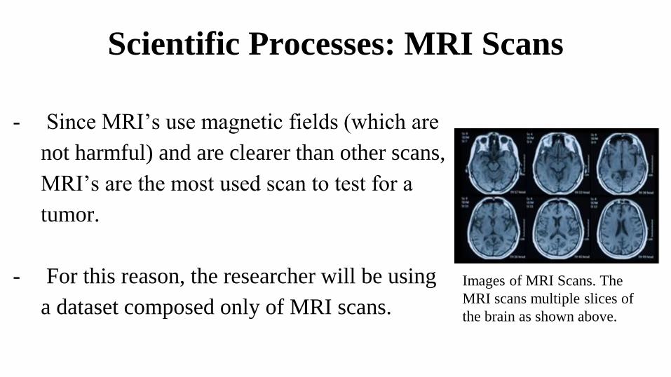
- Since MRI’s use magnetic fields (which are
not harmful) and are clearer than other scans,
MRI’s are the most used scan to test for a
tumor.
- For this reason, the researcher will be using
a dataset composed only of MRI scans.
Images of MRI Scans. The
MRI scans multiple slices of
the brain as shown above.
Scientific Processes: Benign & Malignant
- A tumor can not be definitively classified as benign or malignant
until after a biopsy is done or the growth rate is observed over
time.
- The researcher aims to create a computer model that predicts
whether a tumor is benign or malignant.
- This is especially useful in areas where medical funds are low, and
it is especially expensive to do surgery.
Scientific Processes: Benign & Malignant
- Malignant tumors can be very dangerous as the cancerous cells
multiply and go through mitosis.
- The cancerous cells can damage and spread throughout the entire
body.
- Malignant tumors, even when surgically removed can still resurface,
however benign tumors will not resurface if removed.
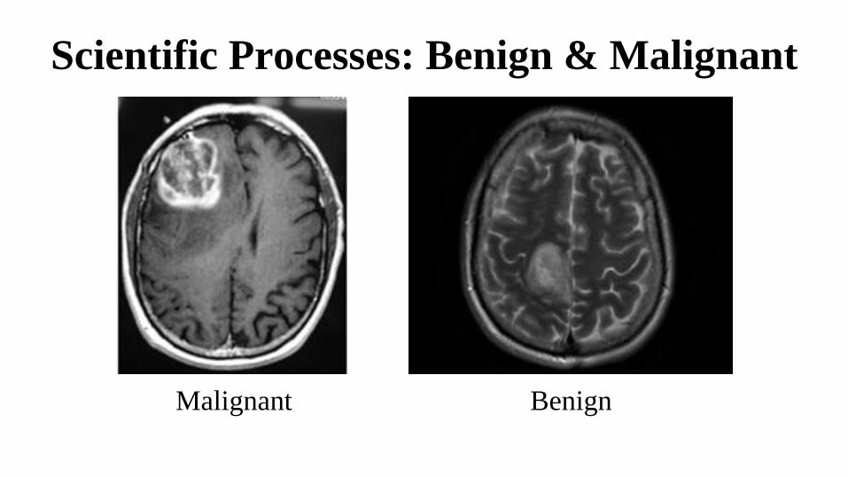
Scientific Processes: Benign & Malignant
Malignant Benign
The Dataset
- All the data used in the experiment was found after extensive
research at
https://figshare.com/articles/brain_tumor_dataset/1512427.
- There were a total of 3064 images of three types of brain tumors:
Pituitary Tumors, Glioma, and Meningioma. These three types of
tumors make up the majority of brain tumors.
- This high value of data allows for the Neural Network to train.

The Dataset Contd’
- Pituitary Tumors: A tumor in the pituitary gland that is
noncancerous (benign) and won’t spread past this area. This can be
treated easily with surgery or minor radiation
Pituitary Tumor

The Dataset Contd’
- Glioma: A tumor that occurs in the brain and spinal cord. This
tumor type is mostly malignant and can be very dangerous.
Glioma

The Dataset Contd’
- Meningioma: A tumor that forms in the brain and spinal cord. This
tumor type is almost always benign and will grow very slowly.
Meningioma
Training the Neural Network
- The dataset used had all files in .mat format.
- The images must be converted to image files (.tiff, .jpg, .png, etc.)
in GNU Octave (an image manipulation program) for the neural
network to recognize the images.
GNU Octave Program
Training the Neural Network
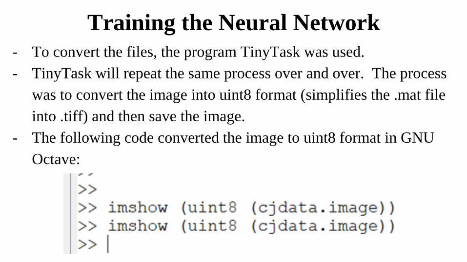
- To convert the files, the program TinyTask was used.
- TinyTask will repeat the same process over and over. The process
was to convert the image into uint8 format (simplifies the .mat file
into .tiff) and then save the image.
- The following code converted the image to uint8 format in GNU
Octave:
Training the Neural Network
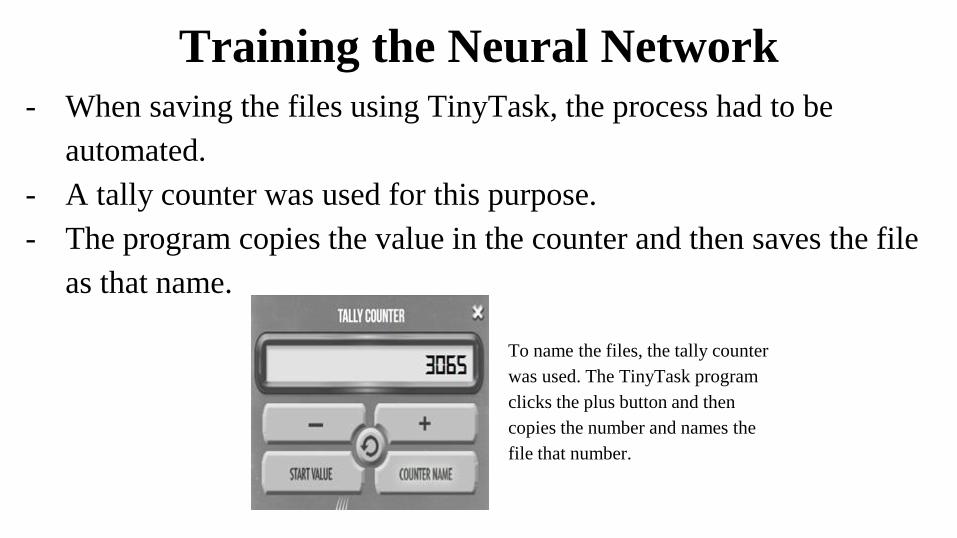
- When saving the files using TinyTask, the process had to be
automated.
- A tally counter was used for this purpose.
- The program copies the value in the counter and then saves the file
as that name.
To name the files, the tally counter
was used. The TinyTask program
clicks the plus button and then
copies the number and names the
file that number.

Training the CNN - Overview
- All of the saved images are sorted into Benign (Pituitary Tumors
and Meningioma) and Malignant (Glioma).
- The Convolutional Neural Network will go through many steps
during the training process as shown below.
Training the CNN - Convolution
- After the images are sorted into Benign and Malignant, the Neural
Network is ready to be programmed. The first step is Convolution.
- In the Convolution step, when an image is inputted, a feature
detector is run through the image.
- A feature detector is a 3x3 square that has randomized numbers
ranging from 0 - 256 assigned to each square.

Training the CNN - Convolution
- As the Neural Network is trained, the feature detector is changed to
recognize specific features that affect the classification of an image.
- For example, a feature detector classifying cats and dogs would be
changed to look for whiskers in order to determine whether the
image is a cat or dog. In this way, many feature detectors are made
to predict the classification of the image.

Training the CNN - Convolution
- The feature detector multiplies the value of the corresponding
squares in the input image and the feature detector.
- The sum of all the products will be inputted into one square of the
Feature Map. After this, the feature detector will move one pixel to
the right and repeat the same process until the entire image has been
processed.
- The Feature Map condenses the data for faster training.

Training the CNN - Convolution
The Feature Detector multiplies the corresponding values and condenses the data.
Training the CNN - ReLU Layer
- Now that the computer has a group of feature maps, (one per feature
detector) the feature maps are run through the rectifier function
(ReLU Function) to decrease linear progression
- The function facilitates easy tumor detection.
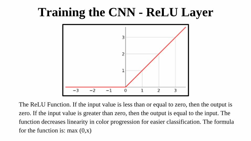
Training the CNN - ReLU Layer
The ReLU Function. If the input value is less than or equal to zero, then the output is
zero. If the input value is greater than zero, then the output is equal to the input. The
function decreases linearity in color progression for easier classification. The formula
for the function is: max (0,x)
Training the CNN - Pooling
- When an image is inputted, the researcher does not want the neural
network to get ‘confused’ by certain occurrences including:
- rotation, squashing, flipping etc.
- For this reason, the researcher uses ‘Max Pooling.’ During this
stage, a 2x2 square is used to check the feature map in the same way
the feature detector did however, moving 2 pixels to the right each
time.
Training the CNN - Pooling
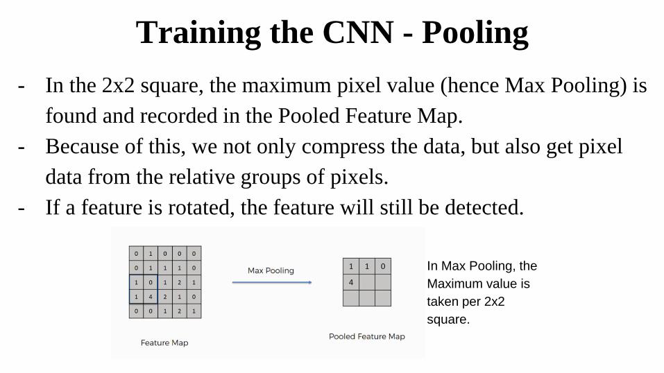
- In the 2x2 square, the maximum pixel value (hence Max Pooling) is
found and recorded in the Pooled Feature Map.
- Because of this, we not only compress the data, but also get pixel
data from the relative groups of pixels.
- If a feature is rotated, the feature will still be detected.
In Max Pooling, the
Maximum value is
taken per 2x2
square.
Training the CNN - Flattening
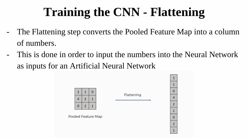
- The Flattening step converts the Pooled Feature Map into a column
of numbers.
- This is done in order to input the numbers into the Neural Network
as inputs for an Artificial Neural Network

Training the CNN - Full Connection
- During the Full Connection step, the inputs of the flattened Pooled
Feature Maps are run through an artificial neural network (ANN).
- In an ANN, the inputs are run through ‘neurons’ and tested to see
the implications on the final classification.
- The ANN determines the weights of the inputs which determine
which inputs affect the output and by how much.
- The weights change over many training sessions.
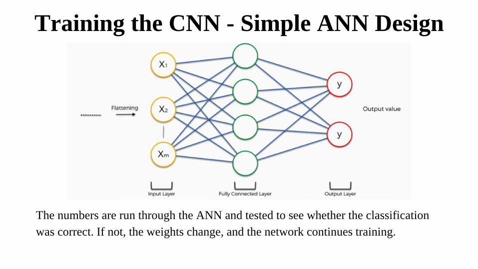
Training the CNN - Simple ANN Design
The numbers are run through the ANN and tested to see whether the classification
was correct. If not, the weights change, and the network continues training.

Training the CNN - Softmax
- When the ANN outputs its probability for an image being classified
into a category, the probability for each image do not add up to
100%.
- The SoftMax Function is used to fit the probabilities such that they
add up to 100%.

CNN Diagram
The above image depicts the steps in a CNN. This particular architecture has 10 outputs while
the researcher’s architecture had 2 outputs, Benign and Malignant.
Running the CNN
- 5 epochs for the CNN to train on.
- One epoch marks when the CNN trains on the entire data once.
- The growth rate slowed significantly at 5 epochs rationalizing the 5
epoch training period.
- The researcher split the data such that 75% was in the training set
and 25% was in the test set.
Running the CNN Contd’
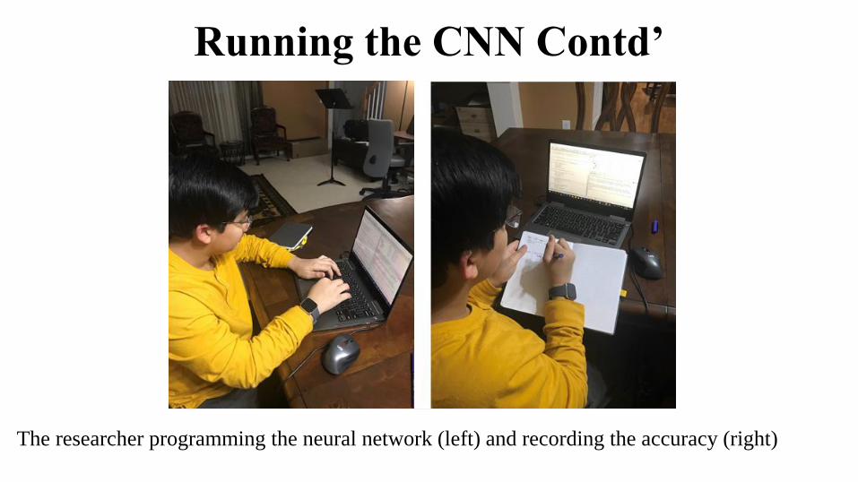
The researcher programming the neural network (left) and recording the accuracy (right)
Running the CNN Contd’
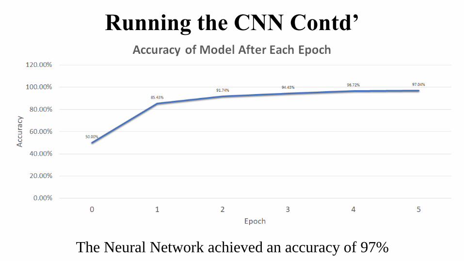
The Neural Network achieved an accuracy of 97%
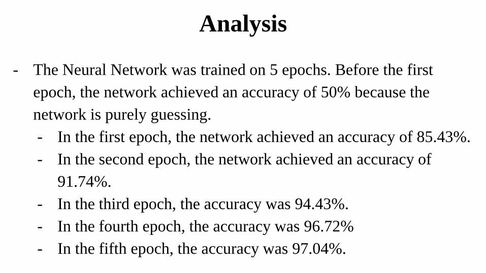
Analysis
- The Neural Network was trained on 5 epochs. Before the first
epoch, the network achieved an accuracy of 50% because the
network is purely guessing.
- In the first epoch, the network achieved an accuracy of 85.43%.
- In the second epoch, the network achieved an accuracy of
91.74%.
- In the third epoch, the accuracy was 94.43%.
- In the fourth epoch, the accuracy was 96.72%
- In the fifth epoch, the accuracy was 97.04%.

Analysis Contd’
- The slowing of the growth rate in percentage shows that the
researcher stopped the number of epochs at the right time.
- If more epochs were to be trained, the neural network would
become less accurate.
- Overall the neural network was a success because it can
successfully classify brain tumors to be benign or malignant.

Conclusions
- Successful creation of Neural Network
- Achieved 97% accuracy
- The dataset used was defined by type of tumor and not malignancy.
Ideally, the dataset would have been classified as benign or
malignant.
- In the future, such a dataset would be used.

Conclusions Contd’
- The model will be useful in hospitals for tumor classification.
- The model will be able to detect tumors and save lives for patients
with brain tumors.
- In the future, the researcher hopes to put the neural network on an
app to allow everyone to access it.
Conclusions Contd’
- The researcher can develop on the project by coding a U-Net Neural
Network.
- The prospective neural network can draw the outline for the tumor
and help doctors identify the tumor region during surgery.
- The dataset used in this experiment came with outlines for tumors
so the same dataset could be used.

Thank You
Any Questions?

Thank You
Any Questions?

Thank You
Any Questions?