developing a simple method to predict ... - accueil | irda · pdf filereport presented to the:...

Report presented to the:

Conseil pour le développement de l‘agriculture

du Québec (CDAQ).

CDAQ Project # 6541

IRDA Project # 300 057

Rapport drafted by :

Carl Boivin, agr., M.Sc. - IRDA

Paul Deschênes, agr., M.Sc. - IRDA

Daniel Bergeron, agr., M.Sc. - MAPAQ

January 2014

Developing a simple method to predict berry harvest volume for a

given day-neutral strawberry production field

Final report

ii

Agriculture and Agri-Food Canada (AAFC) is committed to working with industry

partners. The opinions expressed in the current document are those of the applicant and

are not necessarily shared by the AAFC or CDAQ.

iii

The Research and Development Institute for the Agri-Environment

(IRDA) is a non-profit research corporation created in March 1998 by

four founding members: the Quebec Ministry of Agriculture, Fisheries

and Food (MAPAQ), the Quebec Union of Agricultural Producers

(UPA), the Quebec Ministry of Sustainable Development, Environment,

Wildlife and Parks (MDDEFP) and the Quebec Ministry of Economic

Development, Innovation and Export Trade (MDEIE)

Our mission

IRDA‘s mission is to engage in agri-environmental research,

development and technology transfer activities that foster agricultural

innovation from a sustainable development perspective.

For more information

www.irda.qc.ca

The present report can be cited as follows:

Boivin, C., P. Deschênes and D. Bergeron. 2013. Developing a simple method to predict berry

harvest volume for a given day-neutral strawberry production field. Final report submitted to

CDAQ. IRDA. 51 pages.

http://www.irda.qc.ca/

iv

Project team members :

Applicant and principal

investigator: Carl Boivin, IRDA

Collaborators : Stéphane Nadon, agricultural technician, IRDA

Jérémie Vallée, agronomist, IRDA

Michèle Grenier, statistician, IRDA

Participating farms:

Ferme Onésime Pouliot

Ferme François Gosselin

Daniel and Guy Pouliot

Louis and Gabriel Gosselin

Summer students : Alain Marcoux, Julien Vachon, Nicolas Watters, Paul Harrison,

David Bilodeau, Simon Gagnon, Antoine Lamontagne,

Christopher Lee, Mireille Dubuc, Arianne Blais Gagnon, Hubert

Labissonnière and François Douville.

Readers wishing to comment on this report can contact:

Carl Boivin

Research and Development Institute for the Agri-Environment (IRDA)

2700 Einstein St.

Québec, (Québec) G1P 3W8

e-mail : [email protected]

Internet site : http://www.irda.qc.ca/fr/equipe/carl-boivin/

Acknowledgements :

Funding for this project was in part provided through the Canadian Agricultural Adaptation

Program (CAAP) undes the auspices of Agriculture and Agri-Food Canada. In Quebec, the

portion intended for the agricultural production sector was managed by the Conseil pour le

développement de l'agriculture du Québec (CDAQ).

The authors also wish to recognize financial contributions to this project received from the

Nova Scotia, New Brunswick, Ontario, and British Columbia agricultural adaptation councils.

mailto:[email protected]

http://www.irda.qc.ca/fr/equipe/carl-boivin/

v

Table of Contents

1 INTRODUCTION ...................................................................................................... 1 1.1 Background ........................................................................................................... 1

1.2 General objective .................................................................................................. 2 1.3 Specific objectives ................................................................................................ 2

2 MATERIALS AND METHODS ................................................................................ 3 2.1 Experimental sites, plant material and cropping practices ................................... 3

2.2 Collecting weather data ........................................................................................ 3 2.3 Chemical characterization of the soil ................................................................... 3 2.4 Monitoring soil moisture and salinity ................................................................... 4 2.5 Weekly surveys of strawberry plants and fruit yield assessments ........................ 4

2.6 Strawberry plant dry matter .................................................................................. 5

3 RESULTS AND ANALYSIS ..................................................................................... 6 3.1 Correlations between variables allowing a characterisation of strawberry plant

development ........................................................................................................ 10 3.2 Yield forecasting based on weekly monitoring of strawberry plants ................. 12 3.3 Assessing the accuracy of forecasts .................................................................... 12

3.3.1 Timing of on-site surveys and harvests for fourteen periods spanning the

2013 growing season. .................................................................................. 12

3.3.2 Measured and forecast (Equation 1) yield, 2013 season total. .................... 13 3.3.3 Seasonal totals of measured and forecast yield, Equation 1. ....................... 15 3.3.4 Within-season variation in days from flowering to mature fruit harvest, and

associated yields. ......................................................................................... 17

3.4 Development of a forecasting method applicable to commercial production .... 20 3.4.1 Realigning of harvest periods for use in forecasting yield based on a

period‘s mean number of days from flowering to mature fruit. .................. 21

3.4.2 Forecasting the mean number of fruit harvested for any given period ........ 22 3.4.3 Forecasting cumulative mean fresh weight of mature fruit per plant for a

given period ................................................................................................. 25 3.4.4 Forecast of fruit weight to be harvested ...................................................... 27

3.4.5 Validation of Equations 2 and 3 for the 2013 season .................................. 28 3.4.6 Validation of Equations 2, 3 and 4 for the 2012 season .............................. 30 3.4.7 Proposed forecast method for strawberry cultivar ‗Seascape‘ .................... 33

3.5 Evaluating the potential use of forecasts in scheduling growing season

fertigation. ........................................................................................................... 36

4 CONCLUSIONS....................................................................................................... 37

5 BIBLIOGRAPHY ..................................................................................................... 38

6 DISSEMINATION OF RESULTS ........................................................................... 40

7 APPENDICES .......................................................................................................... 41

vi

List of Figures

Figure 1. Daily rainfall (mm) and daily minimum, maximum and mean air temperature

(Tmin, Tmax, Tavg; °C) - Saint-Laurent site, 2012. .......................................................... 7

Figure 2. Daily rainfall (mm) and daily minimum, maximum and mean air temperature

(Tmin, Tmax, Tavg; °C) - Saint-Jean site, 2012................................................................. 7 Figure 3. Daily rainfall (mm) and daily minimum, maximum and mean air temperature

(Tmin, Tmax, Tavg; °C) - Saint-Laurent site, 2013. .......................................................... 8 Figure 4. Daily rainfall (mm) and daily minimum, maximum and mean air temperature

(Tmin, Tmax, Tavg; °C) - Saint-Jean site, 2013................................................................. 8 Figure 5. Daily potential evapotranspiration (ETp; mm) - Saint-Laurent site, 2012. .......... 9 Figure 6. Daily potential evapotranspiration (ETp; mm) - Saint-Laurent site, 2013. .......... 9 Figure 7. Linear relationship between the number of mature fruit per plant at a given

harvest and the corresponding fresh weight of mature fruit — 2012 Season. ........... 11 Figure 8. Period to period cumulative measured and forecast (Equation 1) yields as a

percent of total yield for the 2013 season - Field 1. .................................................. 14 Figure 9. Period to period cumulative measured and forecast (Equation 1) yields as a

percent of total yield for the 2013 season - Field 2. .................................................. 14 Figure 10. Period to period cumulative measured and forecast (Equation 1) yields as a

percent of total yield for the 2013 season - Field 3. .................................................. 14

Figure 11. Period to period cumulative measured and forecast (Equation 1) yields as a

percent of total yield for the 2013 season - Field 4. .................................................. 14

Figure 12. Percent contribution of individual harvest period yields (measured or forecast

with Eq. 1) to measured 2013 season total yield - Field 1. ........................................ 16 Figure 13. Percent contribution of individual harvest period yields (measured or forecast

with Eq. 1) to measured 2013 season total yield - Field 2. ........................................ 16


with Eq. 1) to measured 2013 season total yield - Field 3. ........................................ 16 Figure 15. Percent contribution of individual harvest period yields (measured or forecast

with Eq. 1) to measured 2013 season total yield - Field 4. ........................................ 16 Figure 16. Length of flowering to mature fruit interval (days) by field and harvest

period - 2013 Season.................................................................................................. 18 Figure 17. Length of flowering to mature fruit interval (days) by field and harvest

period - 2012 Season.................................................................................................. 18 Figure 18. Mean fresh weight of harvested fruit (g) by field and by period - 2013 season.

................................................................................................................................... 19 Figure 19. Mean fresh weight of harvested fruit (g) by field and by period - 2012 season.

................................................................................................................................... 19


with Eqs. 2 and 3) to measured 2013 season total yield - Field 1. ............................ 29


with Eqs. 2 and 3) to measured 2013 season total yield - Field 2. ............................ 29 Figure 22. Percent contribution of individual harvest period yields (measured or forecast

with Eqs. 2 and 3) to measured 2013 season total yield - Field 3. ............................ 29 Figure 23. Percent contribution of individual harvest period yields (measured or forecast

with Eqs. 2 and 3) to measured 2013 season total yield - Field 4. ............................ 29

vii


with Eqs. 2 and 3, or Eqs. 2 and 4) to measured 2012 season total yield - Field 1. .. 32 Figure 25. Percent contribution of individual harvest period yields (measured or forecast

with Eqs. 2 and 3, or Eqs. 2 and 4) to measured 2012 season total yield - Field 2. .. 32


with Eqs. 2 and 3, or Eqs. 2 and 4) to measured 2012 season total yield - Field 3. .. 32 Figure 27. Percent contribution of individual harvest period yields (measured or forecast

with Eqs. 2 and 3, or Eqs. 2 and 4) to measured 2012 season total yield - Field 4. .. 32 Figure 28. Protective netting used. ................................................................................... 41

Figure 29. Coloured ribbon used in identifying specific pedicels. ................................... 42

List of Tables

Table 1.Weekly growing season surveys of strawberry plants. .......................................... 5 Table 2. Timing of on-site surveys and harvests for fourteen periods spanning the 2013

growing season. ......................................................................................................... 12 Table 3. Ex post facto realignment of 2013 harvest periods according to scheduling of

weekly surveys and harvests. ..................................................................................... 21 Table 4. Ex post facto realignment of 2012 harvest periods according to scheduling of

weekly surveys and harvests. ..................................................................................... 21

Table 5. Total number of green fruit inventoried on 60 plants (A), mean per plant (B) and

cumulated mean per plant (C) by period (see Table 4) – Fictitious data. .................. 22

Table 6. Cumulative mean number of green fruit per plant (C) and cumulative mean

number of mature fruit per plant at harvest (D) – Fictitious data. ............................. 24 Table 7. Forecast cumulative mean number of mature fruit per plant at harvest (D) and

forecast cumulative mean weight of mature fruit per plant at harvest (E) - Fictitious

data. ............................................................................................................................ 26 Table 8. Forecast cumulative mean weight of mature fruit per plant at harvest (E) and

forecast mean weight of mature fruit per plant at harvest by period (F) – Fictitious

data. ............................................................................................................................ 27 Table 9. Dates of on-site green fruit inventory periods and associated total yield (f.w.b.)

forecasts according to the number of days from flowering to fruit maturity at any

particular portion of the season. ................................................................................. 33

Table 10. Steps to follow to forecast, from inventories of green fruit on 60 randomly

selected strawberry plants per field, the per hectare fresh weight basis yield of mature

fruit, 21 to 34 days in advance. .................................................................................. 35

viii

List of Equations

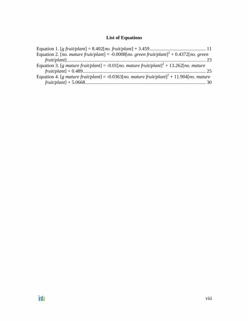
Equation 1. [g fruit/plant] = 8.402[no. fruit/plant] + 3.459 .............................................. 11

Equation 2. [no. mature fruit/plant] = -0.0008[no. green fruit/plant]2 + 0.4372[no. green

fruit/plant] .................................................................................................................. 23 Equation 3. [g mature fruit/plant] = -0.01[no. mature fruit/plant]

2 + 13.262[no. mature

fruit/plant] + 0.489 ..................................................................................................... 25 Equation 4. [g mature fruit/plant] = -0.0363[no. mature fruit/plant]

2 + 11.904[no. mature

fruit/plant] + 5.0668 ................................................................................................... 30

ix

Abstract

While Quebec-grown strawberries are generally afforded a prominent place on food

retailers‘ shelves during the summer season, their marketing presents a number of

challenges. For example, Quebec strawberry producers are under a weekly obligation to

provide food retailers with three weeks notice of anticipated fruit volume. This

requirement arises in part from the lead-time required to prepare store flyers. Moreover, it

represents a key step in the process of setting the retail price. Based largely on past yield

history, the reliability of producer estimates of anticipated yields has often been

inconsistent. To maintain Quebec-grown strawberries‘ market share, steps were taken to

develop a new yield forecasting approach, grounded in field-measurable parameters.

Initiated in the summer of 2011 on two Île d‘Orléans (Quebec) farms‘ commercial day-

neutral strawberry (cv. ‗Seascape‘) production fields, research into this new forecasting

approach was concluded in the fall of 2013.

The first reliable yield forecasts were generated in the summer of 2013. The approach

then employed consisted in a weekly inventory of new green fruit per plant over a given

period of time. Given the difficulty in determining the number of new green fruit per

plant under commercial production conditions, the proposed approach was amended to a

more manageable weekly inventory of green fruit on 60 strawberry plants randomly-

selected within a given field.

Anticipatory harvest scheduling, based on seasonal variability in days from flowering to

fruit maturity, strongly influenced the timing of green fruit inventories. These inventories

potentially allow the number of mature fruit per plant at harvest to be estimated, and

thereby provide a forecasted mean mass of harvestable fruits per plant.

Being an evaluation of the approach‘s potential rather than an example of its

implementation, this study‘s weekly-inventory-based yield forecasts, based on both years

(2012, 2013) of inventory/yield data, were drawn up after the 2013 season. While 2013

forecasts compared favourably with measured yields, those for the 2012 season were less

reliable, unless based solely on 2012 inventories. Forecasts based on two years of data

fared relatively poorly in the difficult task of taking into account differences in weather

conditions from one growing season to another. Using proven count-yield equations to

generate both generous and conservative yield forecasts could help address the variability

brought on by variations in forecast-to-harvest weather conditions.

1

1 INTRODUCTION

1.1 Background

While the United States and Mexico supply the majority of strawberries entering

Quebec‘s major food distribution chains, Quebec-grown fruit are favoured during the

summer season (June-October). However, because Quebec producers are under a weekly

obligation to provide food retailers three weeks‘ notice of anticipated fruit volume,

marketing Quebec strawberries remains difficult. This requirement arises in part from the

lead-time required to prepare store flyers. Moreover, it represents a key step in the

process of setting the retail price. High anticipated yields will exert a downward pressure

on the price per basket (selling unit), while, conversely, lower anticipated yields will

tends to raise the per unit price. While one might expect the laws of supply and demand

to readjust prices in the face of a shift in supply, preset prices for Quebec strawberries

preclude any restoration of the market balance. Therefore, besides their use in marketing,

reliable forecasts might also prove useful in human resources planning and fertigation

regime design.

Unlike single-harvest crops (e.g., corn, soybean) or those which can be stored for

extended periods of time (e.g., cabbage, carrot, apple, potato, etc.), the highly perishable

strawberry is harvested several times a week, at widely varying yields, thereby

significantly complicating their marketing.

Another small fruit produced in Quebec, the raspberry, provides an example of a

production sector quickly losing its market share in food distribution chains. Given the

sector‘s inability to meet large retail chains‘ demands, the Quebec raspberry is gradually

being edged out of supermarket shelves in favour of what are excellent quality imported

raspberries. Highbush blueberries are another example of an imported fruit with a

privileged place on our shelves, though this in part reflects the fact that U-Pick operations

predominate in the marketing of local blueberries.

Estimates of anticipated fruit volumes being at present largely based on past seasons‘

yield history, forecasting anticipated fruit volume from quantitative parameters monitored

in the current season would prove to be a useful and innovative endeavour.

Published strawberry yield-forecasting models, integrate current-day or historical weather

conditions in their calculations, thereby severely limiting the reach of their predictions,

while doing little to address the present issue (Doving and Mage, 2001; Mackenzie and

Chandler, 2009). Another study‘s results lead to a method to forecast when peak

production would occur (Chandler and Mackenzie, 2004). Likewise, models which

integrate regional historic data or means ignore site-specific conditions. Funded by

private enterprises such as Driscoll Strawberry Associates, research in this field has been

undertaken in the United States; however, their results are proprietary and likely not

applicable to the different growing conditions which prevail in Quebec.

2

1.2 General objective

The project sought to enhance the marketing of Quebec strawberries, and thereby the

sector‘s profitability and competitiveness, by developing a reliable method to forecast

weekly-cumulated fruit volume and thereby allow a better coordination of harvests and

sales.

1.3 Specific objectives

Investigate correlations between a number of strawberry plant development

parameters;

Develop yield forecasts based on a weekly characterisation of strawberry plants;

Quantify the accuracy of forecasts;

Propose a method adapted to commercial production;

Evaluate forecasts‘ potential utility in scheduling fertigation applications over the

growing season.

3

2 MATERIALS AND METHODS

2.1 Experimental sites, plant material and cropping practices

Located in the municipalities of Saint-Laurent (46° 52' N, 71° 01' W) and Saint-Jean

(46° 55' N, 70° 54' W) on Île-d‘Orléans (Quebec, Canada), two farms specialized in the

commercial production of day-neutral strawberries each housed two experimental sites.

Each site was located in a different field housing 5 plots of 12 strawberry plants, for a

total of 60 plants per experimental site, and 240 plants across all sites.

Strawberries (cv. ‗Seascape‘) were grown on raised beds covered in black polyethylene

mulch, irrigated through a drip irrigation system. The producer‘s sole responsibility, crop

management included early season blossom removal to encourage plant recovery and

subsequent vigour. The analysis of relationships between production and yield parameters

followed a regression approach.

2.2 Collecting weather data

Rainfall (HOBO model RG3-M rain gauge) was measured on both farms. Set up on the

farm situated in Saint-Laurent, a weather station allowed the monitoring of temperature

and relative humidity (HC-S3, Campbell Scientific), rainfall events (Leaf wetness sensor,

Model 237 Campbell Scientific), solar radiation (LI-200SZ, LI-COR), as well as wind

speed and direction (Wind monitor, Young Model 05103-10). These data (measurements

at 15 sec intervals, averaged over 15 min) were recorded on a datalogger (CR10X,

Campbell Scientific). Potential evapotranspiration (ETp) values were calculated by the

Penman-Monteith method (ASCE, 2005).

2.3 Chemical characterization of the soil

At the end of the production season a single sample of topsoil (0-0.20 m depth) was taken

from each plot. Sifted through a 2 mm mesh, soils samples were then air-dried at 21°C.

Soil water pH was measured at a 1:1 (w/w) soil/water ratio (Conseil des Productions

Végétales du Québec, 1988). Total soil organic matter (SOM) was measured by the

Walkley Black wet oxidation method (Allison, 1965). Phosphorus (P) and micronutrients

were extracted in Mehlich-3 soil extractant (Tran and Simard, 1993) and quantified by

inductively coupled plasma optical emission spectroscopy (ICP-OES). Mineral nitrogen

was extracted by stirring soil in a 2M KCl solution [1:10 (w/w) soil:extractant ratio] for

1 hour. The extract was filtered and analysed by automated colorimetric segmented flow

analysis (Technicon) (Isaac et Johnson, 1976). End-of-season soil soluble salt levels were

estimated by measuring a 1:2 soil:water (w/w) solution‘s conductivity using a

conductivity meter.

4

2.4 Monitoring soil moisture and salinity

Throughout the growing season an array of HORTAU tensiometers (model Tx-80)

continuously monitored selected plots‘ soil water tensions, which were recorded through

HORTAU‘s Irrolis-Light software (ver. 1.9). Certain plots having been found, post-

installation, to lie beyond the chosen tensiometer model‘s wireless range, tension

readings were taken manually during weekly site visits.

Electrical conductivity (dS/m) probes equipped with capacitance sensors (5TE,

DECAGON) were used to monitor evolving soil solution salinity within the volume of

soil under the irrigation system‘s influence, estimated on the basis of the soil‘s apparent

electrical conductivity (ECa). For each farm, five plots — two in one field and three in the

other — were equipped with a 5TE probe, installed 0.30 m below the drip tape. One

probe per field was linked to a datalogger (Em50, DECAGON) which recorded ECa at

15 min intervals throughout the growing season.

2.5 Weekly surveys of strawberry plants and fruit yield assessments

The 1st survey (Table 1), done on a weekly basis from planting through the end of the

2011 growing season, consisted in making an inventory of each strawberry plant‘s leaves

until their number reached nine, as well as the number of flowers, green and mature fruit

by flower cluster (cyme) and then by hierarchy (primary, secondary and tertiary). It

should be noted that the number of ripe fruit was obtained upon their classification. In

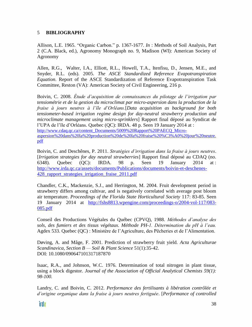
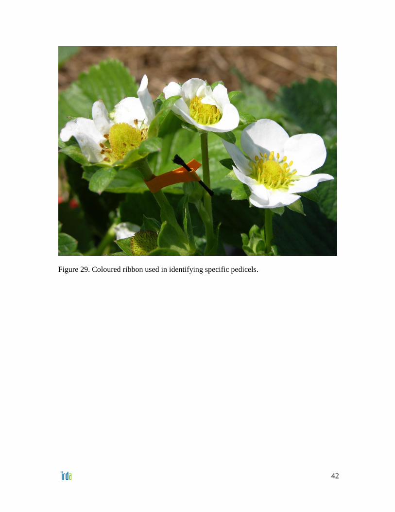
addition, at harvest the number of days from flowering to mature fruit were determined

thanks to the tagging of selected pedicels upon the opening of the flower they supported.

A 2nd

survey, consisting in making an inventory of flowers and green fruit per plot (i.e.,

per 12 strawberry plants), was added to the weekly routine in 2012, while the 1st survey

was simplified to no longer account for flower hierarchy (Table 1). In 2013, there

remained two surveys scheduled per week, but these were identical and only accounted

for per plant cyme and green fruit numbers. Moreover, the number of fruit was assessed

at harvest, while the tagging of pedicels to evaluate the number of days from flowering to

fruit maturity was limited to the 1st survey. In 2013, a 3

rd survey, implemented

concurrently with the 2nd

survey, was added to the weekly routine (Table 1). It consisted

in making an inventory of the total number of green fruit on 60 randomly-chosen

strawberry plants per field. Survey elements are summarized in Table 1.

In 2011, in order to avoid producer-hired pickers from accidentally picking from study

plots, experimental plot harvests were made to coincide with or precede by one day those

set by the producer. In 2012 and 2013, when netting (4.5 cm mesh) was installed to

protect research plots from accidental picking (see Figure 28 in Appendix), harvests

occurred during surveys of strawberry plant characteristics. Harvested fruit were weighed

individually, sorted by weight, and then checked for any defects. Individual marketable

fruit were categorized as ‗saleable‘ ( 6 g) or ‗small‘ (< 6 g), while fruit that were

misshapen or suffered from biotic or abiotic damage were categorized as ‗other.‘

5

Table 1.Weekly growing season surveys of strawberry plants.

Hierarchy

2011 2012 2013

1st 1

st 2

nd 1

st 2

nd 3

rd

Number per strawberry plant

Leaves (max 9) X X

Cyme X X

Flower position on cyme

Primary X

Secondary X

Tertiary X Not considered X

Green fruit X X

Green fruit per cyme

Primary X

Secondary X


Mature fruit X X

Mature fruit per cyme

Primary X

Secondary X


Per strawberry plant — fresh weight

Mature fruit X X

Mature fruit per cyme

Primary X

Secondary X


Per plot bearing 12 strawberry

plants — number

Flowers X

Green fruit X

Days from flowering to mature fruit harvest X X X

Per field – 60 strawberry plants –

number

Green fruit X

2.6 Strawberry plant dry matter

Following the last fruit harvest, strawberry plant dry matter was assessed. Individual

plants were cut off at their base and their remaining green fruit removed. Transported to

the laboratory in plastic bags, individual plants were dried to a constant weight at 105°C,

then weighed. Since a strawberry plant‘s dry matter is strongly correlated with its fruit

yield, this measure can help highlight factors underlying apparent fruit yield outliers and

allow an informed quality control of data.

6

3 RESULTS AND ANALYSIS

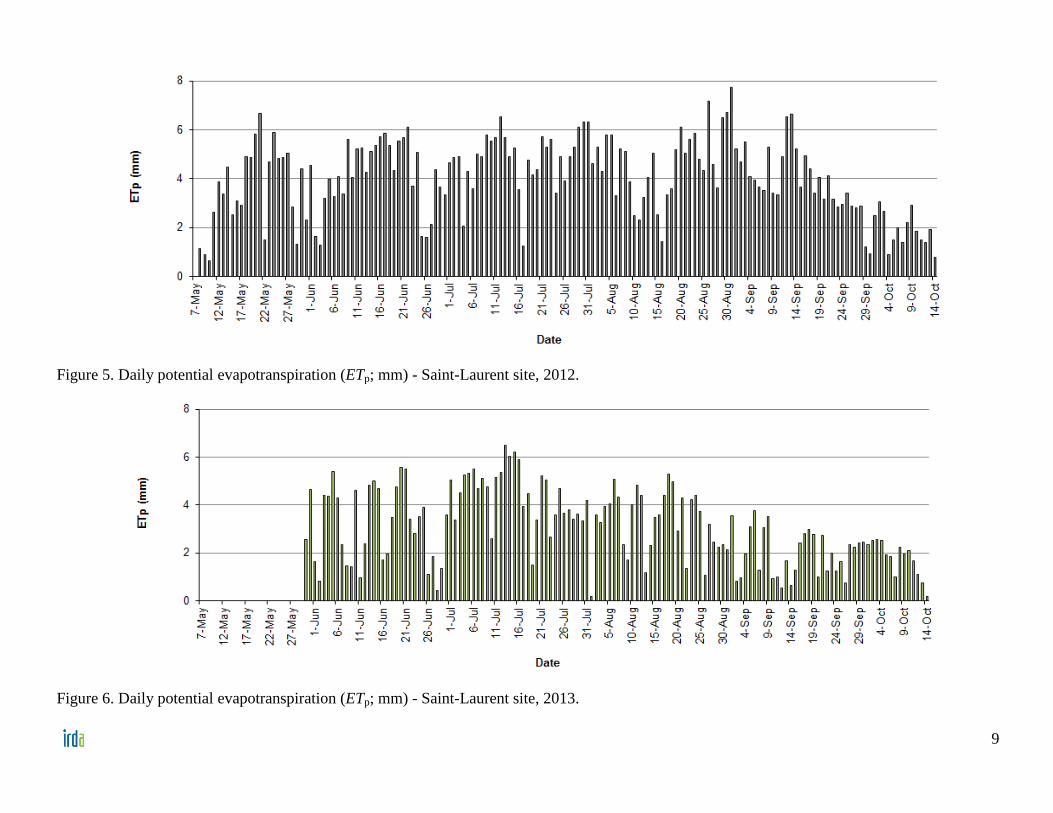
Presented graphically in Figure 1 to Figure 6, total daily rainfall, along with daily

minimum, maximum and mean air temperatures were measured daily at both St. Laurent

and St. Jean sites in 2012 and 2013. Daily potential evapotranspiration (ETp), calculated

on the basis of data from the weather station located on the St-Laurent site, are similarly

presented in Figure 5 and Figure 6). A function of weather conditions, the volume of

water lost through ETp represents the amount of soil water lost through both evaporation

at the soil surface and plant transpiration. When evapotranspirative demand exceeds a

plant‘s soil water uptake capacity, the plant may be subjected to both water and heat

stress.

Upon comparing the two season‘s ETp values at the Saint Laurent site (Figure 5 and

Figure 6), the number of days in 2012 when plants were deemed at risk for water stress

exceeded that in 2013. Indeed, the number of growing season (1 June-1 October) days in

2012 when 2 mm ETp < 4 mm, and particularly when 4 mm ETp < 6 mm, exceeded

the number of equivalent days in 2013. Evapotranspirative demand being therefore

greater in 2012 than 2013, plants were at greater risk of developing developmental

aberrations in 2012 than 2013.

7

Figure 1. Daily rainfall (mm) and daily minimum, maximum and mean air temperature (Tmin, Tmax, Tavg; °C) - Saint-Laurent site, 2012.

Figure 2. Daily rainfall (mm) and daily minimum, maximum and mean air temperature (Tmin, Tmax, Tavg; °C) - Saint-Jean site, 2012.

8

Figure 3. Daily rainfall (mm) and daily minimum, maximum and mean air temperature (Tmin, Tmax, Tavg; °C) - Saint-Laurent site, 2013.

Figure 4. Daily rainfall (mm) and daily minimum, maximum and mean air temperature (Tmin, Tmax, Tavg; °C) - Saint-Jean site, 2013.

9

Figure 5. Daily potential evapotranspiration (ETp; mm) - Saint-Laurent site, 2012.

Figure 6. Daily potential evapotranspiration (ETp; mm) - Saint-Laurent site, 2013.

10

3.1 Correlations between variables allowing a characterisation of strawberry

plant development

The number of new green fruit produced in a given interval of time was identified as the

parameter best suited to accurately forecast yields at future harvests. The strength of the

relationship between these two variables should be excellent considering that each mature

fruit was once green and no mature fruit was culled prior to harvest. At any given time,

correctly establishing the number of new green fruit requires one to subtract from the

present number of green fruit, the number of such fruit present at the last survey or

harvest, along with the number of mature fruit removed at the last harvest. Therefore, in

addition to monitoring the same plants until season‘s end, the fruit harvested from each

plant must also be recorded.

At the end of the 2012 growing season, a linear regression was developed across all 35

harvests — each including up to 240 plant records — between the number of mature fruit

harvested per plant and the corresponding fruit yield per plant on a fresh weight basis

(Figure 7). The strength of this linear relationship was quantified using the coefficient of

determination (0 R2 1) or its square root, the correlation coefficient (-1 R 1). The

R value is positive or negative, respectively, according to whether a direct (slope > 0) or

inverse (slope < 0) relationship exists between the independent variable (e.g., number of

fruit) and the dependent variable (e.g. weight of fruit). The strength of the regression

increases as the absolute value of R (|R|) approaches 1.0 (one). The R value can be

expressed in percentage form, such that the independent variable (e.g., number of fruit)

can be said to explain a certain percentage |R| × 100 of the variation in the dependent

variable. Therefore, the greater the value of |R| the better the independent variable

describes the dependent variable.1 In the present case, the relationship is strong

(R2 = 0.61, R = 78 %), which is all the more noteworthy given that all experimental sites

are included in the regression.

1 For an R2 = 0.6059 (Figure 7) and a direct relationship (slope > 0) between fruit number and fruit weight,

√ √ .

11

Figure 7. Linear relationship between the number of mature fruit per plant at a given

harvest and the corresponding fresh weight of mature fruit — 2012 Season.

The equation linking these parameters,

Equation 1. [g fruit/plant] = 8.402[no. fruit/plant] + 3.459

served to predict yields for 2013 harvests, where the dependent variable was the

forecasted yield of fruits at harvest expressed on a fresh weight basis (f.w.b.), and the

independent variable was the number of new green fruit in existence roughly 21 days

before the harvest of interest. Therefore, assuming no green fruit to be lost before its

eventual maturity and harvest, the number of new green fruit for each of the 60 monitored

plants per field could serve in forecasting the weight of mature fruit at harvest. Based on

planting density, the yield could then be expressed in terms of kg/ha.

To

tal

wei

gh

t m

atu

re

fru

it/p

lan

t (g

)

Total number mature fruit/plant (g)

12

3.2 Yield forecasting based on weekly monitoring of strawberry plants

3.3 Assessing the accuracy of forecasts

The project‘s first season (2011) was dedicated to collecting data which might contribute

to the development of preliminary yield forecasting equations to be validated during the

following growing season (2012); consequently, no yield forecasts were made for 2011.

The equations tested and the method employed proved to be ineffective in yielding

accurate yield forecasts for harvests occurring during the 2012 production season. In

2013, yield forecasts were based on new green fruit per plant and derived using

Equation 1. These results are presented below.

3.3.1 Timing of on-site surveys and harvests for fourteen periods spanning the 2013

growing season.

The growing season of 10 June to 6 September 2013, during which 1st and 2

nd surveys

were undertaken at each of the four fields, was split into 14 periods (Table 2). The

participating farms were provided with field-specific yields forecasts soon after

completion of each period‘s 2nd

survey. These forecasts covered the full range of harvests

from 1 July and 4 October, 2013. For example, data collected in the 1st and 2

nd surveys of

Period 4 (3 July to 9 July, 2013), were employed in forecasting fruit yields (f.w.b.) to be

obtained from 24 July to 30 July.

Table 2. Timing of on-site surveys and harvests for fourteen periods spanning the 2013

growing season.

Period

(2013)

1st and 2

nd surveys

Harvests

Beginning End

Beginning End

1 10 June 18 June 1 July 8 July

2 19 June 25 June 9 July 16 July

3 26 June 2 July 17 July 23 July

4 3 July 9 July 24 July 30 July

5 10 July 14 July 31 July 5 August

6 15 July 21 July 6 August 11 August

7 22 July 26 July 12 August 16 August

8 27 July 1 August 17 August 22 August

9 2 August 7 August 23 August 29 August

10 8 August 12 August 30 August 2 September

11 13 August 19 August 3 September 9 September

12 20 August 26 August 10 September 16 September

13 27 August 2 September 17 September 23 September

14 3 September 6 September 24 September 4 October

13

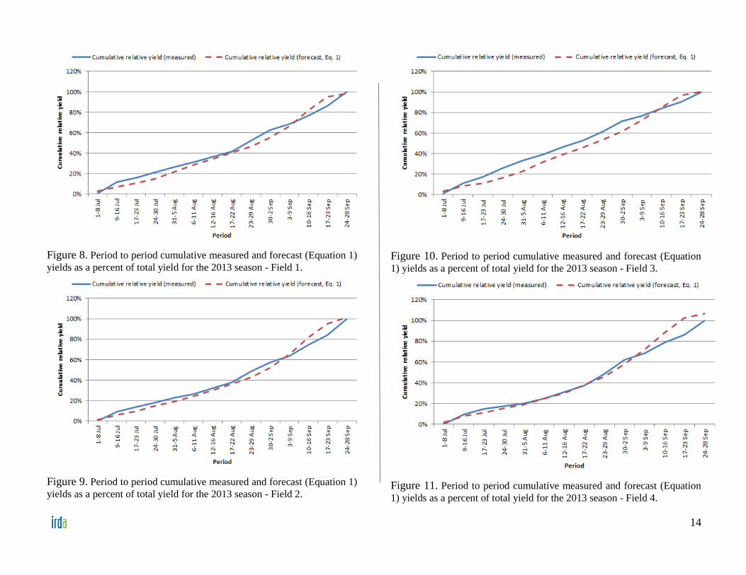
3.3.2 Measured and forecast (Equation 1) yield, 2013 season total.

Yields were recorded and predicted for each of the periods in which mature fruit were

harvested, cumulated from period to period over the season and expressed as a percentage

of the growing season‘s total yield (Figure 8 to Figure 11). The yield presented for any

given period therefore represents the sum of the previous and current period‘s yields, up

to the 14th

period where the cumulated yield corresponds to the total (100%) yield for the

growing season.

Measured and forecast relative yields were compared on a field-by-field basis, in such a

manner that each period‘s cumulative yield corresponded to a specific fraction of the final

period‘s and thus full season‘s cumulative yield. Thus, to evaluate the extent of the

deviation between the forecast and measured yields for each period, these yields are

expressed relative to the full season‘s cumulative yield (100%). For example, in Figure

11 (Field 4), the cumulative measured yield recorded for the last harvest period (24-28

Sept.) represents 100% of the mature fruit harvest over the entire season, whereas the

forecast cumulative yield for the same period is 106% of the measured value. Therefore,

the full-season sum of forecast yields exceeded the full-season sum of measured yields by

6%. Moreover, this manner of presenting yield data highlights how, for Field 4, 62% of

the full season‘s cumulative yield had been harvested by the end of the 10th

period (30

August - 2 September). Similarly, in Fields 1, 3 and 4, roughly half the full season‘s

cumulative yield had been achieved by the end of the 9th

period (23-29 August), whereas

this threshold was reached by the end of the 8th

period in field 2.

With the exception of Field 4 where a 6% difference was noted, cumulative basis

comparisons of total measured yields and associated forecasts for the other fields showed

only very minor differences. However, since forecasts ended 21 days before the final

harvest, the yield potential represented by green fruit never reaching maturity (i.e., green

fruit remaining on the plant when the field production infrastructure is dismantled after

the first frosts) would lead to a disparity in number between forecast and harvested fruit.

Finally, the forecasts prior to the 11th

period (3-9 September) can be seen to slightly

underestimate cumulative yield, while overestimating it slightly thereafter (dotted line).

14

Figure 8. Period to period cumulative measured and forecast (Equation 1)

yields as a percent of total yield for the 2013 season - Field 1.

Figure 9. Period to period cumulative measured and forecast (Equation 1)

yields as a percent of total yield for the 2013 season - Field 2.

Figure 10. Period to period cumulative measured and forecast (Equation

1) yields as a percent of total yield for the 2013 season - Field 3.

Figure 11. Period to period cumulative measured and forecast (Equation

1) yields as a percent of total yield for the 2013 season - Field 4.

15

3.3.3 Seasonal totals of measured and forecast yield, Equation 1.

For each field, measured or forecast yields can be presented (Figure 12 to Figure 15) as

the percent contribution of each individual period to the measured yield cumulated over

the full production season (i.e., summed across all 14 periods). Measured and forecast per

period yields for a given field are both expressed relative to the measured total. Such a

presentation of yields for a given field highlights the relative contribution of a specific

harvest period to seasonal totals.

For example, for the 5th

harvest period (31 July - 5 August) on Field 1 (Figure 12) the

measured yield represents 5% of the measured production season total, while the forecast

yield for the same period represents 7% of the measured production season total. Up to

the 11th period (3-9 September) forecast yields match measured yields fairly closely for

all fields (Figure 12 to Figure 15), which can also be said for the cumulative yields

previously discussed (Figure 8 to Figure 11).

Since, with the exception of Period 2, individual forecast and measured yields for Periods

1-11 are closely matched, the forecasting equation does show some promise. It is after the

11th

period (3-9 September) that a significant difference develops between individual

periods‘ forecast and measured yields. Forecasts are all made 21 days prior to harvest,

regardless of the period in the season. Within-season variation in days from flowering to

mature fruit, a parameter worth exploring in explaining these late season discrepancies, is

discussed in the following section.

16

Figure 12. Percent contribution of individual harvest period yields (measured or

forecast with Eq. 1) to measured 2013 season total yield - Field 1.







17

3.3.4 Within-season variation in days from flowering to mature fruit harvest, and

associated yields.

The number of days from flowering to mature fruit harvest was plotted by field and by

harvest period for the 2013 season (Figure 16). For example, across all fields, the mean

number of days from flowering to mature fruit harvest during the 4th

Period (24-30 July)

was 20. The first thing one notes is that during the first ten periods the number of days

from flowering to fruit maturity varies between 20 and 25, numbers consistent with

effective yield forecasting on 21 days‘ notice. Indeed the number of days match, which

facilitates the process. However, the accuracy of forecasts based on Equation 1 decreases,

when, from the 11th

period onward, the number of days from flowering to fruit maturity

increases (Figure 12 to Figure 15). Altering the linear model (Eq. 1) to account for the

latter portion of the season‘s extended interval between flowering and fruit maturity

could prove useful in correcting the discrepancies observed in this portion of the season.

Plotted for comparative purposes, the length of the flowering to fruit maturity interval for

each field, and each of 2012‘s harvest periods (Figure 17), indicates the variation in

interval length to parallel that in 2013.

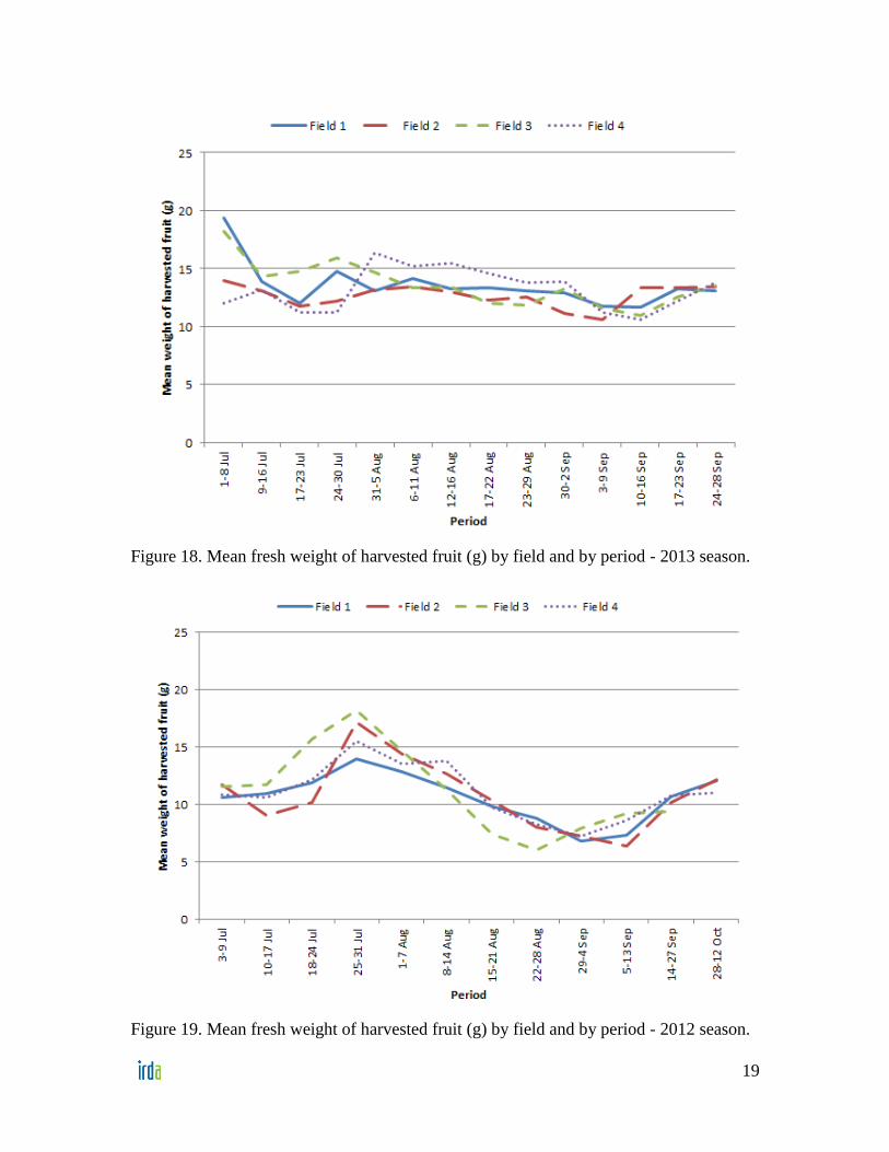
In each of the period in 2013, the mean weight of mature fruit harvested per field,

remained fairly constant throughout the season (Figure 18). This constancy, combined

with the fact that the accuracy of forecasts based on Equation 1 is strongly influenced by

mean fruit weight, proved to be most convenient in the current context. However, the

mean weight of mature fruit harvested in 2012 shows a great deal more variation (Figure

19).

18

Figure 16. Length of flowering to mature fruit interval (days) by field and harvest

period - 2013 Season.

Figure 17. Length of flowering to mature fruit interval (days) by field and harvest

period - 2012 Season.

Flo

we

rin

g to

mat

ure

fru

it in

terv

al (

day

s)

Flo

we

rin

g to

mat

ure

fru

it in

terv

al (

day

s)

19

Figure 18. Mean fresh weight of harvested fruit (g) by field and by period - 2013 season.

Figure 19. Mean fresh weight of harvested fruit (g) by field and by period - 2012 season.

20

3.4 Development of a forecasting method applicable to commercial production

The goal was to devise as easy and accurate a method as possible to forecast the total

weight of mature fruit to be harvested at a later date. Since a method based on monitoring

the number of new green fruit per plant would be difficult to implement under

commercial production conditions, the proposed method will hinge on a weekly

inventory of green fruit on 60 randomly-selected strawberry plants.

To achieve this goal, data gathered in 2013 were reworked under different scenarios and

new equations generated. These new equations and the proposed method are

demonstrated using a set of fictitious values. As shown in Table 3 and Table 4, the

original period dates for 2013 (Table 2) and 2012, respectively, were reassigned

according to the length of the flowering to mature fruit interval (Figure 16 and Figure 17,

respectively), A first step which entailed the forecast of mean numbers of mature fruit per

planting at harvest was followed by a period-weighted forecast of the mean fresh weight

of fruit per plant. Finally, the equations employed in this approach were validated by

forecasting the yields measured in 2012 and 2013 from on-site green fruit inventories.

This demonstration completed, a generalized procedure will be proposed.

21

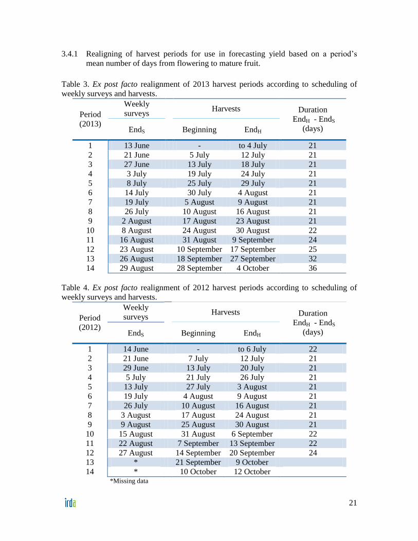
3.4.1 Realigning of harvest periods for use in forecasting yield based on a period‘s

mean number of days from flowering to mature fruit.

Table 3. Ex post facto realignment of 2013 harvest periods according to scheduling of

weekly surveys and harvests.

Period

(2013)

Weekly

surveys

Harvests Duration

EndH - EndS

(days) EndS

Beginning EndH

1 13 June - to 4 July 21

2 21 June 5 July 12 July 21


4 3 July 19 July 24 July 21


6 14 July 30 July 4 August 21

7 19 July 5 August 9 August 21


9 2 August 17 August 23 August 21


11 16 August 31 August 9 September 24

12 23 August 10 September 17 September 25


14 29 August 28 September 4 October 36

Table 4. Ex post facto realignment of 2012 harvest periods according to scheduling of

weekly surveys and harvests.

Period

(2012)

Weekly

surveys

Harvests Duration

EndH - EndS

(days) EndS

Beginning EndH

1 14 June - to 6 July 22




5 13 July 27 July 3 August 21





10 15 August 31 August 6 September 22



13 * 21 September 9 October

14 * 10 October 12 October *Missing data

22

3.4.2 Forecasting the mean number of fruit harvested for any given period

The first step in achieving a meaningful forecast of the mean number of mature fruit per

plant at harvest is to inventory the number of green fruit on plants. To serve as an

example, a fictitious dataset of the number of green fruit inventoried in a particular field

during each of 14 periods‘ 2nd

surveys are presented in column A of Table 5. Since the

initial goal is to forecast the total number of mature fruit per plant at harvest, a single

survey towards the end of the period in question is all that is required. The total number

of green fruit inventoried is then divided by the number of strawberry plants sampled

(column B, Table 5), and cumulated from period to period (column C, Table 5).

For example, for Period 6, 370 green fruit were inventoried during a fictitious survey

occurring around 14 July (column A, Table 5). This number is divided by 60, the number

of plants under consideration, yielding a value of 6.17 fruit per plant (column B). The

value of 19.83 in column C is the sum of the fruits per plant for Periods 1 through 6.

Table 5. Total number of green fruit inventoried on 60 plants (A), mean per plant (B) and

cumulated mean per plant (C) by period (see Table 4) – Fictitious data.

Period

A B C

Measured

Total number of green fruit

On 60 plants Per plant Per plant,

cumulated

1 15 0,25 0,25

2 100 1,67 1,92

3 185 3,08 5,00

4 220 3,67 8,67

5 300 5,00 13,67

6 370 6,17 19,83

7 500 8,33 28,17

8 615 10,25 38,42

9 680 11,33 49,75

10 820 13,67 63,42

11 930 15,50 78,92

12 1000 16,67 95,58

13 1120 18,67 114,25

14 1200 20,00 134,25

23

From any given period, the cumulative mean number of green fruit inventoried per plant

is an excellent indicator of the cumulative mean number of mature fruit obtained 21 to 36

days thereafter. A regression developed between these two parameters was done ex post

facto since the number of red fruit was only known at harvest. For confidentiality

reasons, the values used to generate this relationship are not presented.

Across all fields, for each of the 14 periods, a regression was developed between the

cumulative mean number of green fruit per plant ([no. green fruit/plant], column C, Table

5) and the cumulative mean number of mature fruit per plant at harvest ([no. mature

fruit/plant]), where:

Equation 2. [no. mature fruit/plant] = -0.0008[no. green fruit/plant]2 + 0.4372[no. green

fruit/plant]

This equation will allow one to forecast the mean cumulative number of mature fruit per

plant from the mean cumulative number of green fruit per plant.

24

Using Eq. 2, the cumulative mean number of mature fruit per plant can now be forecast

from the cumulative mean number of green fruit per plant (column C, Table 6). For

example, following the Period 6 inventory of green fruit, the mean number of green fruit

cumulated since the Period 1 inventory is 19.83 per plant. This value was substituted for

[no. green fruit/plant] in Eq. 2, to yield a value of 8.36 for the mean cumulated mature

fruit per plant (column D, Table 6). Consequently, if the cumulative mean number of

green fruit per plant were 19.83, the cumulative mean number of mature fruit per plant at

harvest, some 21 to 36 days later, would be 8.36.

Table 6. Cumulative mean number of green fruit per plant (C) and cumulative mean

number of mature fruit per plant at harvest (D) – Fictitious data.

Period

C

Measured

Cumulative mean no.

green fruit per plant

D

Forecast (Eq. 2)

Cumulative mean no. mature

fruit per plant at harvest

1 0,25 0,11

2 1,92 0,84

3 5,00 2,17

4 8,67 3,73

5 13,67 5,83

6 19,83 8,36

7 28,17 11,68

8 38,42 15,62

9 49,75 19,77

10 63,42 24,51

11 78,92 29,52

12 95,58 34,48

13 114,25 39,51

14 134,25 44,28

25

3.4.3 Forecasting cumulative mean fresh weight of mature fruit per plant for a given

period

The previously discussed period-by-period cumulated mean number of fruit per plant

(see 3.4.2) is an excellent predictor of the cumulative mean fresh weight of mature fruit

per plant to be expected 21 to 36 days after their inventory. Developed ex post facto since

the mean number and weight of mature fruit per plant were only know at harvest, a

quadratic regression equation was developed between the cumulative mean number of

mature fruit per plant and the cumulative mean fresh weight of mature fruit per plant at

harvest, across all periods and fields. For confidentiality reasons, the values used to

generate this relationship are not presented.

Equation 3. [g mature fruit/plant] = -0.01[no. mature fruit/plant]2 + 13.262[no. mature

fruit/plant] + 0.489

26

The mean cumulative weight of mature fruit per plant will therefore now be determined

from the cumulative mean number of mature fruit per plant at harvest (column D, Table

7), using Eq. 3. For example, for Period 6, the cumulative (Periods 1-6) mean number of

mature fruit per plant at harvest, 8.36, replaces [no. mature fruit/plant] in Eq. 3, yielding

a [g mature fruit/plant] value of 110.2 g (column E, Table 7). Therefore, when the

cumulative number of mature fruit per plant is 11.68, the cumulative mean weight of

mature fruit per plant will be 153.6 g, 21 to 36 days later.

Table 7. Forecast cumulative mean number of mature fruit per plant at harvest (D) and

forecast cumulative mean weight of mature fruit per plant at harvest (E) - Fictitious data.

Period

D

Forecast (Eq. 2)

Cumulative mean no.

mature fruit per plant at

harvest

E

Forecast (Eq. 3)

Cumulative mean weight

mature fruit per plant at

harvest

1 0,11 1,5

2 0,84 11,1

3 2,17 28,7

4 3,73 49,4

5 5,83 77,0

6 8,36 110,2

7 11,68 153,6

8 15,62 204,7

9 19,77 258,3

10 24,51 319,1

11 29,52 382,8

12 34,48 445,4

13 39,51 508,4

14 44,28 567,6

27

3.4.4 Forecast of fruit weight to be harvested

To obtain the mean weight of mature fruit per plant at harvest for a given period one need

only subtract the previous period‘s cumulative mean weight of mature fruit per plant from

that of the period of interest. For example, the 33.2 g mean weight of mature fruit per

plant forecast for Period 6 (column F, Table 8) is derived from the subtraction of

Period 5‘s cumulative mean weight of mature fruit per plant (column E, Table 8) from

that of Period 6 (i.e., 110.2 g - 77.0 g = 33.2 g per plant). Finally, as this is a mean weight

per plant, multiplying this value by the planting density or number of plants in the field,

one can obtain the total yield for the field.

Table 8. Forecast cumulative mean weight of mature fruit per plant at harvest (E) and

forecast mean weight of mature fruit per plant at harvest by period (F) – Fictitious data.

Period

E

Forecast

Cumulative mean

weight mature fruit

per plant at harvest

F

Forecast

Mean weight mature

fruit per plant at

harvest by period

1 1,5 1,5

2 11,1 9,6

3 28,7 17,6

4 49,4 20,6

5 77,0 27,6

6 110,2 33,2

7 153,6 43,4

8 204,7 51,1

9 258,3 53,6

10 319,1 60,7

11 382,8 63,8

12 445,4 62,6

13 508,4 63,0

14 567,6 59,2

28

3.4.5 Validation of Equations 2 and 3 for the 2013 season

Field inventories of green fruit were used in validating Eqs. 2 and 3. For each field, single

period measured and forecast yields (f.w.b.) are plotted as each period‘s relative

contribution to measured season yield totals (Figure 20 to Figure 23). This presentation

highlights the temporal evolution in yields and their relative contribution to seasonal

totals over the season, and indicates each period‘s relative contribution to seasonal yield

totals. With the exception of the 2nd

period (5-12 July) wherein relative yields were

significantly underpredicted, overall forecast yields matched measured ones fairly

closely. The accuracy of forecasts for Field 4 were relatively poor compared to the other

fields (Figure 23); indeed, the 2nd

and 9th

Period yield forecasts were significant

underestimates of those measured for these periods, while yield forecasts for the 5th

, 6th

,

11th

and 12th

periods represented significant overestimates.

29


forecast with Eqs. 2 and 3) to measured 2013 season total yield - Field 1.







30

3.4.6 Validation of Equations 2, 3 and 4 for the 2012 season

Before validating Eqs. 2 and 3 with 2012 yield data, a fourth equation was generated. As

with the 2013 season, in 2012 a regression, spanning all fields, was developed between

the cumulative mean number of mature fruit per plant at harvest and the cumulative mean

weight of mature fruit per plant at harvest, which occurred some 21 to 36 days after the

initial inventory of green fruit. For confidentiality reasons, the values used to generate

this relationship are not presented.

Equation 4. [g mature fruit/plant] = -0.0363[no. mature fruit/plant]2 + 11.904[no. mature

fruit/plant] + 5.0668

This analysis was undertaken ex post facto since the mean number and weight of mature

fruit per plant were only known at harvest. Therefore, Eq. 4 allows one to forecast the

cumulative mean weight of mature fruit per plant at harvest from the cumulative mean

number of mature fruit per plant at harvest.

The Figures 24 to 27 shows measured and forecast (Eqs. 2-3 or Eqs. 2-4) yields for

harvests between July 5 and 20 September 2012, those thereafter being eliminated as no

green fruit inventory data were available. Moreover, measured and forecast yields were

again expressed as a proportion of full season yield totals, but where the last harvest was

that of 20 September 2012.

Forecast and measured yields were similar for the first four periods regardless of which

pair of equations was employed. For the 5th

and 6th

periods, forecasts substantially

underestimated yield. For the 8th

period both forecasts overestimated yields, but forecasts

using the 2-4 combination outperformed those using the 2-3 combination.

The mean weight of mature fruit per plant at harvest varied more in 2012 (Figure 19) than

2013 (Figure 18). The first of the two equations used in generating the forecast (Eq. 2)

calculates the mean number of mature fruit per plant at harvest, while the second

(Eq. 3 or 4) derives the total weight of fruit from their number. The second equations —

either Eq. 3 generated from 2013 data, or Eq. 4 generated from 2012 data — generate

slightly different yield values: for the same cumulative mean number of mature fruit per

plant at harvest, Eq. 2 yields a greater cumulative mean weight of mature fruit per plant at

harvest than Eq. 3, particularly when mature fruit number per plant exceeds twenty-five.

Weather and growing conditions are both strong influencing factors, and difficult to

factor into forecasts once these are made. The 2012 season was more conducive to

strawberry plants undergoing water stress than the 2013 season, which was almost ideal

for strawberry production. A difference in yield can be explained by different numbers of

fruit of a common weight, a common mean number of fruit with a different mean weight,

or a combination of both. In the present case, mean fruit weight was the main factor

affecting overall yield. When the mean fruit weight is affected it is recent meteorological

conditions which are the cause, since only weather patterns weeks before flowering could

31

affect flower and thus fruit number. This is supported by the results of a summer

2006/2007 study in which a micro-sprinkler system was used to cool the strawberry

canopy during periods of intense heat (Boivin, 2008).

Further trials must be undertaken before coming to firm conclusions, but at first glance

Eq. 4 (2012) would serve best for a season prone to water stress events, while Eq. 3

(2013) would be best suited to years when strawberry plants were under ideal growing

conditions.

32


forecast with Eqs. 2 and 3, or Eqs. 2 and 4) to measured 2012 season total yield -

Field 1.



Field 2.



Field 3.



Field 4.

33

3.4.7 Proposed forecast method for strawberry cultivar ‗Seascape‘

1. Inventory green fruit as soon as flower removal ends (Table 9). Dates of such

inventories are listed for informational purposes; however, as it varies over the

season, the number of days from flower opening to mature fruit is of greater

importance.

Table 9. Dates of on-site green fruit inventory periods and associated total yield (f.w.b.)

forecasts according to the number of days from flowering to fruit maturity at any

particular portion of the season.

Period

Latest date for inventory

since the previous

inventory

Days from flowering

to fruit maturity based

on observations

Latest date for

harvest since the

last period

1 10 June 21 1 July

2 17 June 21 8 July

3 24 June 21 15 July

4 1 July 21 22 July

5 8 July 21 29 July

6 15 July 21 5 August



9 4 August 21 26 August

10 11 August 22 2 September





15 1 September 36 7 October

16 8 September 36 14 October

34

2. Inventory of the total number of green fruit on 60 strawberry plants randomly chosen

across the production field.

3. Data entry (column A, Table 10), followed by filling in the subsequent columns as

instructed below.

Using the fictitious data in Table 10 :

A. For periods 1, 2 and 3 (column A, Table 10), 15, 100 and 185 green fruit were

inventoried, respectively, per 60 plants;

B. The mean number of green fruit per plant for a given period was obtained by dividing

the total number of fruit inventoried by the number of plants (column B, Table 10);

C. The cumulative mean number of green fruit was obtained by summing the mean

numbers green fruit from the present and previous periods (column C, Table 10);

D. Equation 2 :

[no. mature fruit/plant] = -0.0008 [no. green fruit/plant]

2 + 0.4372 [no. green fruit/plant]

was used to forecast the cumulative number of mature fruit per plant (column D, Table

10), from the value of [no. green fruit] in Column C (Table 10);

E. Equation 3 :

[g mature fruit/plant] = -0.01[no. mature fruit/plant]

2 + 13.262 [no. mature fruit/plant] + 0.489

or

Equation 4 :

[g mature fruit/plant] = -0.0363[no. mature fruit/plant]

2 + 11.904[no. mature fruit/plant] + 5.0668

are used to forecast the cumulative weight of mature fruit per plant at harvest

(column E, Table 10), based on the [no. mature fruit/plant] (column D, Table 10)

F. To obtain the weight of mature fruit per plant at harvest for a given period (Column F,

Table 10) subtract the value from the immediately preceding period, from the value for

a given period in column E (e.g., for Period 3, 28.7 - 11.1 = 17.6);

G. Multiply the value in column F by the per hectare strawberry plant density.

35

Table 10. Steps to follow to forecast, from inventories of green fruit on 60 randomly

selected strawberry plants per field, the per hectare fresh weight basis yield of mature

fruit, 21 to 34 days in advance.

Per

iod

A B C D E F G

Tota

l num

ber

gre

en

fruit

per

60 p

lants

A/6

0

Mea

n n

um

ber

of

gre

en f

ruit

per

pla

nt

Cum

ula

tive

mea

n

num

ber

of

gre

en f

ruit

Eq

uat

ion

2

Fo

reca

st c

um

ula

tive

nu

mb

er o

f m

atu

re f

ruit

per

pla

nt

at h

arv

est

Eq

uat

ion

3 (

20

13)*

Eq

uat

ion

4 (

20

12)

Fore

cast

cum

ula

tive

wei

ght

of

mat

ure

fru

it

per

pla

nt

at h

arves

t (g

)

Fo

reca

st w

eig

ht

of

mat

ure

fru

it p

er p

lan

t at

har

ves

t (g

) b

y p

erio

d

Pla

nti

ng d

ensi

ty/h

a

1 15 0.25 0.25 0.11 *1.5 1.5

2 100 1.67 1.92

(1.67 + 0.25)

0.84 *11.1 9.6

3 185 3.08 5.00

(3.08 + 1.92)

2.17 *28.7 17.6

4

5

…

36

3.5 Evaluating the potential use of forecasts in scheduling growing season

fertigation.

No reference grid for day-neutral strawberry fertilisation by fertigation is presently

available for Québec. The fertigation regime was therefore developed through the

expertise of the producer and his extension agent, and drawn from information in the

literature. Day-neutral strawberry trials run on l‘Île d‘Orléans in 2011 showed no

difference in yield between strawberry plants receiving 50% or 100% of the N delivered

under the producer‘s normal fertigation regime (Landry and Boivin, 2012). Irrigation

management in strawberry production also remain a topic of intensive research. Plant

nutrient use efficiency under fertigation is strongly linked to irrigation efficiency.

Limitations in the soil volume which the drip irrigation system can moisten can lead to

issues of the soil drying out around the drip irrigation tape (Boivin and Deschênes, 2011).

While an approach under which the quantity of nutrients supplied would be adjusted

according to forecasts of strawberry yield (f.w.b.) at harvest would be of some interest;

however, such an approach would only reach its potential when the crop‘s fertilizer and

irrigation needs were determined and adequately addressed. Indeed, variation in fruit yield

is greater from one period to the next than from one growing season to the next.

Moreover, each strawberry taken from the field represents a net export of nitrogen.

Landry and Boivin (2012) found that nitrogen exports from the field attributable to

picking and removal of fruit from the field represented 48% and 43 % of the total nitrogen

taken up by the crop in 2010 and 2011, respectively. Therefore, since the removal of

nitrogen from the field varies from season to season, the nitrogen use efficiency might be

improved if yield forecasts were considered.

37

4 CONCLUSIONS

The on-site green fruit inventories in 2013 allowed the successful formulation of

relatively accurate yield forecasts, which were communicated to producers on a weekly

basis, according to the field in question. Forecasting precision was improved, ex post

facto, by adjustments which took into account the variation in days from flowering to

mature fruit.

The approach‘s accuracy in 2013 was founded, in particular, on an inventory of the

number of new green fruit per plant; however, as such information was difficult to collect

under commercial conditions, an effort was made to develop a simpler approach. The

approach now consists in a simple weekly inventory of the number of green fruit on 60

strawberry plants random-selected in a given field.

These periods of fruit inventory were matched with harvest periods according to the

variation over the season in number of days from flower opening to mature fruit harvest.

Following the inventory of green fruit, their mean numbers per plant can be used to

forecast the eventual number of mature fruit per plant, and, in turn, the mean weight of

mature fruit per plant at harvest.

Done after the compilation of fruit inventories, forecasts for the 2013 season matched

measured values closely. Less accurate than those for 2013, the ex post facto ‗forecasts‘

for the 2012 season, were based on regressions developed from 2013 data. However,

using a regression equation based only on 2012 data was shown to be more accurate in

predicting yields for the 2012 season.

Weather conditions have an impact on strawberry plants‘ productivity. Conditions in 2012

differed significantly from those in 2013: while the latter was ideal for strawberry

production, the former was somewhat drier. Once the forecast is made, the effects of

weather conditions can no longer be integrated into the forecast. Developing a pair of

forecasts, one optimistic and the other conservative, from the regression equations

developed, could help to alleviate any errors in forecasting brought on by unexpected and

unaccounted for weather conditions occurring between forecast and harvest.

Finally, the currently proposed approach would gain by being further confirmed through

additional trials on a greater number of farms; efforts are ongoing to do so.

38

5 BIBLIOGRAPHY

Allison, L.E. 1965. ―Organic Carbon.‖ p. 1367-1677. In : Methods of Soil Analysis, Part

2 (C.A. Black, ed.), Agronomy Monograph no. 9, Madison (WI): American Society of

Agronomy

Allen, R.G., Walter, I.A., Elliott, R.L., Howell, T.A., Itenfisu, D., Jensen, M.E., and

Snyder, R.L. (eds). 2005. The ASCE Standardized Reference Evapotranspiration

Equation. Report of the ASCE Standardization of Reference Evapotranspiration Task

Committee, Reston (VA): American Society of Civil Engineering, 216 p.

Boivin, C. 2008. Étude d’acquisition de connaissances du pilotage de l’irrigation par

tensiométrie et de la gestion du microclimat par micro-aspersion dans la production de la

fraise à jours neutres à l’île d’Orléans.[Data acquisition as background for both

tensiometer-based irrigation regime design for day-neutral strawberry production and

microclimate management using micro-sprinklers] Rapport final déposé au Syndicat de

l‘UPA de l‘île d‘Orléans. Quebec (QC): IRDA. 48 p. Seen 19 January 2014 at : http://www.cdaq.qc.ca/content_Documents/5009%20Rapport%20PAECQ_Micro-

aspersion%20dans%20la%20production%20de%20la%20fraise%20%C3%A0%20jour%20neutre.

pdf

Boivin, C. and Deschênes, P. 2011. Stratégies d’irrigation dans la fraise à jours neutres.

[Irrigation strategies for day neutral strawberries] Rapport final déposé au CDAQ (no.

6348). Quebec (QC): IRDA. 98 p. Seen 19 January 2014 at :

http://www.irda.qc.ca/assets/documents/Publications/documents/boivin-et-deschenes-

428_rapport_strategies_irrigation_fraise_2011.pdf

Chandler, C.K., Mackenzie, S.J., and Herrington, M. 2004. Fruit development period in

strawberry differs among cultivar, and is negatively correlated with average post bloom

air temperature. Proceedings of the Florida State Horticultural Society 117: 83-85. Seen

19 January 2014 at http://fshs8813.wpengine.com/proceedings-o/2004-vol-117/083-

085.pdf

Conseil des Productions Végétales du Québec (CPVQ), 1988. Méthodes d’analyse des

sols, des fumiers et des tissus végétaux. Méthode PH-1. Détermination du pH à l’eau.

Agdex 533. Quebec (QC) : Ministère de l‘Agriculture, des Pêcheries et de l‘Alimentation.

Døving, A. and Måge, F. 2001. Prediction of strawberry fruit yield. Acta Agriculturae

Scandinavica, Section B — Soil & Plant Science 51(1):35-42.

DOI: 10.1080/090647101317187870

Isaac, R.A., and Johnson, W.C. 1976. Determination of total nitrogen in plant tissue,

using a block digestor. Journal of the Association of Official Analytical Chemists 59(1):

98-100.

Landry, C. and Boivin, C. 2012. Performance des fertilisants à libération contrôlée et

d’origine organique dans la fraise à jours neutres fertiguée. [Performance of controlled

http://www.cdaq.qc.ca/content_Documents/5009%20Rapport%20PAECQ_Micro-aspersion%20dans%20la%20production%20de%20la%20fraise%20%C3%A0%20jour%20neutre.pdf



http://www.irda.qc.ca/assets/documents/Publications/documents/boivin-et-deschenes-428_rapport_strategies_irrigation_fraise_2011.pdf

http://www.irda.qc.ca/assets/documents/Publications/documents/boivin-et-deschenes-428_rapport_strategies_irrigation_fraise_2011.pdf

http://fshs8813.wpengine.com/proceedings-o/2004-vol-117/083-085.pdf

http://fshs8813.wpengine.com/proceedings-o/2004-vol-117/083-085.pdf

39

release and organic fertilizers in fertigated day-neutral strawberries] Rapport final

déposé au MAPAQ (no. PSIH10-1-355). Quebec (QC) : IRDA. 53 p. Seen 19 January

2014 at : http://www.irda.qc.ca/assets/documents/Publications/documents/landry-boivin-

479_rapport_elc_fraise_2012.pdf

Mackenzie, S.J. and Chandler, C.K. 2009. A method to predict weekly strawberry fruit

yield from extended season production systems. Agronomy Journal, 101(2): 278-287.

DOI:10.2134/agronj2008.0208

Tran, T. S. and Simard, R. R. 1993. ―Mehlich III-extractable nutrients.‖ p. 43–50, In Soil

sampling and methods of analysis. (M.R. Carter, ed.) London (UK): Lewis Publishers.

http://www.irda.qc.ca/assets/documents/Publications/documents/landry-boivin-479_rapport_elc_fraise_2012.pdf

http://www.irda.qc.ca/assets/documents/Publications/documents/landry-boivin-479_rapport_elc_fraise_2012.pdf

40

6 DISSEMINATION OF RESULTS

IRDA Internet site http://www.irda.qc.ca/fr/equipe/carl-boivin/, since April 2011.

Presentation given at the ―Field Day on Innovations in Small Fruit Production.‖

CRAAQ. Île d‘Orléans, 29 July 2011 o http://www.craaq.qc.ca/UserFiles/File/Communication/Articles_Presse/Nouv_fraiches_Act_ch

amps_2011_10.pdf (Mentioned in APFFQ publication)

o http://www.craaq.qc.ca/Documents/Evenements/EPTF1102/Depliant_EPTF1102.pdf (Field

Day program)

Presentation given at the ―Saint Rémi Horticultural Days.‖ 7 December 2011. o http://www.mapaq.gouv.qc.ca/SiteCollectionDocuments/Regions/Monteregie-

Ouest/Journees_horticoles_2011/7_decembre_2011/Fraise_et_framboises/16h00_Survoldespr

ojetsderecherche_C_Boivin.pdf (PowerPoint presentation) o http://www.mapaq.gouv.qc.ca/SiteCollectionDocuments/Regions/Monteregie-

Ouest/Journees_horticoles_2011/ProgrammeJourneesHorticoles2011.pdf (Horticultural

Day program)

Presentation given at the Provincial Day for Scientific Research. APFFQ. Laval

University, 14 December 2011. o http://www.craaq.qc.ca/UserFiles/File/Communication/Articles_Presse/Nouv_fraiches_Act_ch

amps_2011_10.pdf (Mentioned in APFFQ publication)

Article in newspaper, LaPresse.ca, 3 July 2013 o http://www.lapresse.ca/actualites/national/201307/02/01-4666849-predire-la-production-des-

fraises-pour-mieux-les-vendre.php

Interview on Radio Canada International, 3 July 2013 o http://www.rcinet.ca/fr/2013/07/03/les-fraises-plaisir-dete-pour-le-consommateur-soit-mais-

defi-de-taille-pour-le-producteur-de-fraises-a-jours-neutres/

http://www.irda.qc.ca/fr/equipe/carl-boivin/

http://www.craaq.qc.ca/UserFiles/File/Communication/Articles_Presse/Nouv_fraiches_Act_champs_2011_10.pdf


http://www.craaq.qc.ca/Documents/Evenements/EPTF1102/Depliant_EPTF1102.pdf

http://www.mapaq.gouv.qc.ca/SiteCollectionDocuments/Regions/Monteregie-Ouest/Journees_horticoles_2011/7_decembre_2011/Fraise_et_framboises/16h00_Survoldesprojetsderecherche_C_Boivin.pdf



http://www.mapaq.gouv.qc.ca/SiteCollectionDocuments/Regions/Monteregie-Ouest/Journees_horticoles_2011/ProgrammeJourneesHorticoles2011.pdf

http://www.mapaq.gouv.qc.ca/SiteCollectionDocuments/Regions/Monteregie-Ouest/Journees_horticoles_2011/ProgrammeJourneesHorticoles2011.pdf



http://www.lapresse.ca/actualites/national/201307/02/01-4666849-predire-la-production-des-fraises-pour-mieux-les-vendre.php

http://www.lapresse.ca/actualites/national/201307/02/01-4666849-predire-la-production-des-fraises-pour-mieux-les-vendre.php

http://www.rcinet.ca/fr/2013/07/03/les-fraises-plaisir-dete-pour-le-consommateur-soit-mais-defi-de-taille-pour-le-producteur-de-fraises-a-jours-neutres/

http://www.rcinet.ca/fr/2013/07/03/les-fraises-plaisir-dete-pour-le-consommateur-soit-mais-defi-de-taille-pour-le-producteur-de-fraises-a-jours-neutres/

41

7 APPENDICES

Figure 28. Protective netting used.

42

Figure 29. Coloured ribbon used in identifying specific pedicels.