developing and testing an improved description of
TRANSCRIPT

Developing and Testing an ImprovedDescription of Diffusion For Use inModeling Planetary Atmospheres
Matthew Jackson
Advisor: Dr. Anna DeJongMentor: Dr. Jared Bell
Associated with the National Institute of Aerospace
The objective of this experiment was to create an improved conduction code
for the Global Ionoshpere-Thermosphere Model (GITM) used by NASA. GITM
used an implicit solver to the diffusion equation, which is an unconditionally
stable scheme, but it sacrifices a lot of accuracy, being only first order accu-
rate. The proposed replacement scheme is the Crank-Nicolson scheme, which
is a hybridization of an implicit and explicit solver and has second order ac-
curacy. This hybrid scheme combines the accuracy of the explicit solver, while
theoretically keeping the stability of the implicit solver, which will be explained
in the paper. Another solver for the diffusion equation was found during the
implementation of this project, namely a modified implicit solver. Ultimately,
Dr. Bell and I settled on using the modified implicit solver as it has the same
accuracy as the Crank-Nicolson solver while not being limited by the initial
conditions being passed in.
1

Introduction
Atmospheres are extremely dynamic systems that require a lot of computations to accurately
model. There are a lot of different interactions between molecules with different properties
and densities. One major facet of atmospheric modeling is keeping track of the movement
of energy. As a simplification, there are three big drivers in the movement of energy in an
atmospheric system. These three forms of energy movement are convection, conduction, and
radiation, namely thermal radiation. Convection is the movement of different compositions of
molecules in an atmosphere. It is extremely dynamic which makes it very computationally
expensive to model. Conduction is the collisions of molecules in an atmosphere, which can be
extremely computationally expensive if one were to calculate the transfer of energy between
individual molecules. However, this is not needed since conduction is can be macroscopically
modelled with the diffusion equation. With such a powerful equation, there are a lot of ways
to implement it to varying levels of accuracy. Unfortunately, this accuracy comes at a price
of extra computational expenses. Lastly, thermal radiation is the emission of photons through
the process of black body radiation. All things emit electromagnetic radiation based on an
objects temperature, and planets are no different. Although convection and radiation are very
important processes, this project’s main focus is on the different implementations of calculating
conduction through different methods of implementing the diffusion equation and how these
different methods compare with each other.
To really highlight the differences of the these conduction models, every other atmospheric
condition must be implemented. Given how difficult this would be to do, I will be using the
Global Ionosphere Thermosphere Model, hereby referred to as GITM. GITM is an atmospheric
framework used by the National Aeronautics and Space Administration (NASA). By using
GITM, I am able to change only the conduction code and use the resultant data to numeri-
2

cally show the differences between the current conduction scheme used by GITM and two other
implementations, the Crank Nicolson scheme and the Oscillation Free Second Order Implicit
scheme.
Theory
Diffusion
As stated in the introduction, this line of research mainly focuses on the diffusion equation,
which is given as∂U(~r, t)
∂t= α∇(κ(~r)∇U(~r, t)) (1)
• U is the function of temperature with respect to time and position.
• α contains all the constant factors such as constants intrinsic to the composition of the
atmosphere
• κ contains constants of the atmosphere that are dependent on the distance from the planet
such as density
This equation is currently written in three dimensional coordinates, but for this project, we
will be exploring the diffusion equation is one dimension. This is achieved because the GITM
framework uses parallel processes to run longitude and latitude blocks across multiple nodes in
a cluster of computers. Therefore, conduction, which is modeled by the diffusion equation, is
only run in one dimension on each of these blocks. As such, the diffusion equation is written as
∂U(r, t)
∂t= α
1
r2
∂
∂r(D(r)
∂U(r, t)
∂r) (2)
• As a simplification, D(r) is such that D(r) = κ(r) ∗ r2
3

This equations can further be simplified into two parts, a pseudo-Cartesian diffusion equation
and a spherical correction, which are shown as:
∂U(r, t)
∂t= α
1
r2(D(r)
∂2U(r)
∂r2 +∂D(r)
∂r
∂U(r, t)
∂r) (3)
The following sections focus on the pseudo-Cartesian diffusion equation, and then the spherical
correction will be explored. The reason this is a pseudo-Cartesian method comes from the
inclusion of 1r2
with the Cartesian diffusion equation.
Finite Difference of Diffusion
Although the diffusion equation is fairly simply solved, there is not an analytical solution for an
atmosphere. Because of this, a new method is needed to implement this differential equation.
This new method is finite difference. Finite difference is simply the decomposition of a differ-
ential equation into the difference between values at certain points over the difference between
those points, simply written as:dU(t)
dt=Un+1 − Un
∆t(4)
The notation for this equation is given as:
• n - this is the step in time
• Un corresponds to U(t)
• Un+1 corresponds to U(t+ ∆t)
This decomposition allows for using initial data to calculate future data, depending on the size
of ∆t. However, the greater the size of ∆t, the less accurate the predicted value will be. As
accuracy increases by reducing ∆t, this increases the amount of iterations a processor must run
the computation over again in order to reach a given time frame. As such, a balance between
accuracy and computation time must be found.
4

Fortunately, reducing ∆t is not the only way to improve accuracy. With every finite differ-
ence approximation, there is an associated order of accuracy. This order of accuracy is similar to
the order of accuracy of a Taylor Series, as both are the error associated round off error. For the
finite difference approximation given above, the associated error is first order accurate, which
is written as O(∆r). If a new method with higher accuracy is used, that computation time will
only be increased marginally, by the approximation should have noticeable improvements to
accuracy.
So far, the only finite difference equation explored has been for first order differential equa-
tions. While this is useful for decomposing the diffusion equation, a finite difference approxi-
mation is needed for second order differential equations. This decomposition is given as:
∂2U(r)
∂r2 =Uj+1−Uj
∆r− Uj−Uj−1
∆r
∆r(5)
Simply put, a second order differential equation is the finite difference of a first order differential
equation. Although this equation looks fairly messy, it can easily be rewritten as:
∂2U(r)
∂r2 =Uj+1 − 2Uj + Uj−1
∆r2 (6)
The notation for this equation is given as:
• j - this is the step in space
• U j corresponds to U(r)
• U j−1 corresponds to U(r −∆r)
• U j+1 corresponds to U(r + ∆r)
One thing to note about this decomposition is that it is over ∆r2. This is significant because this
finite difference approximation is second order accurate.
5

With finite difference approximations for first order and second order differential equations,
a finite difference approximation for the pseudo-Cartesian diffusion equation can be created.
One such approximation would be:
Un+1j − Un
j
∆t= α
1
r2Dj(
Unj+1 − 2Un
j + Unj−1
∆r2) (7)
Some things to note with this approximation are
• Un+1j is what is trying to be solved
• temporal differential equation is centered on Uj
• spatial differential equation is centered on Un
This method of approximating the diffusion equation is called an Explicit scheme. This is
because it explicitly uses information of the current time step to calculate the next time step.
As such, it is fairly accurate. However, one major short coming of this scheme is that if ∆t �
∆r2/αDj , the scheme will lose stability. As such, it requires a lot of computation time since ∆t
must be constrained to the constants and the size of the spatial mess. Therefore a new scheme
is needed.
Un+1j − Un
j
∆t= α
1
r2Dj(
Un+1j+1 − 2Un+1
j + Un+1j−1
∆r2) (8)
This approximation is called the Implicit scheme, and it does not have the same short comings
of the explicit scheme. As opposed to the implicit scheme, the spatial differential equation is
centered on Un+1. While this scheme is implying a break in casualty by using future data to
calculate the current data, it is actually a way to set up the math of the system. Ultimately the
system can be written as
Un+1j
m′−Unj
m′= Dj(U
n+1j+1 − 2Un+1
j + Un+1j−1 ) (9)
6
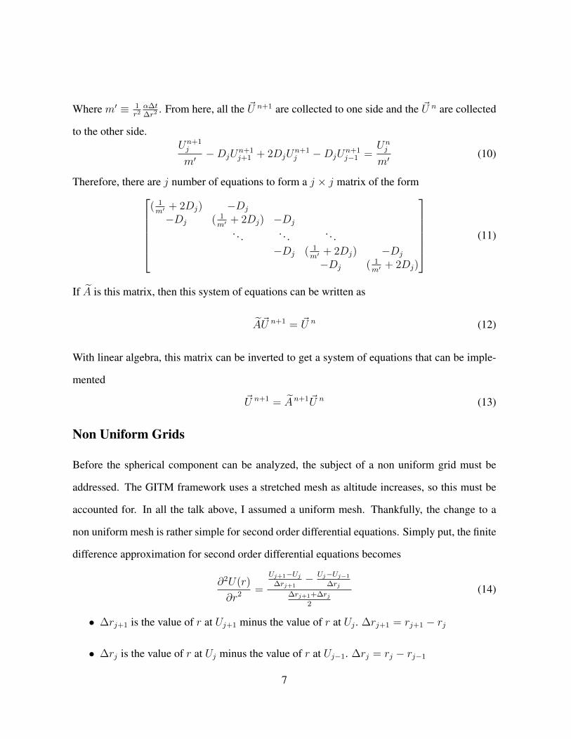
Where m′ ≡ 1r2α∆t∆r2
. From here, all the ~U n+1 are collected to one side and the ~U n are collected
to the other side.Un+1j
m′−DjU
n+1j+1 + 2DjU
n+1j −DjU
n+1j−1 =
Unj
m′(10)
Therefore, there are j number of equations to form a j × j matrix of the form( 1m′
+ 2Dj) −Dj
−Dj ( 1m′
+ 2Dj) −Dj
. . . . . . . . .−Dj ( 1
m′+ 2Dj) −Dj
−Dj ( 1m′
+ 2Dj)
(11)
If A is this matrix, then this system of equations can be written as
A~U n+1 = ~U n (12)
With linear algebra, this matrix can be inverted to get a system of equations that can be imple-
mented
~U n+1 = An+1~U n (13)
Non Uniform Grids
Before the spherical component can be analyzed, the subject of a non uniform grid must be
addressed. The GITM framework uses a stretched mesh as altitude increases, so this must be
accounted for. In all the talk above, I assumed a uniform mesh. Thankfully, the change to a
non uniform mesh is rather simple for second order differential equations. Simply put, the finite
difference approximation for second order differential equations becomes
∂2U(r)
∂r2 =
Uj+1−Uj
∆rj+1− Uj−Uj−1
∆rj∆rj+1+∆rj
2
(14)
• ∆rj+1 is the value of r at Uj+1 minus the value of r at Uj . ∆rj+1 = rj+1 − rj
• ∆rj is the value of r at Uj minus the value of r at Uj−1. ∆rj = rj − rj−1
7

This equation can be simplified to
∂2U(r)
∂r2 =1
12(∆rj+1 + ∆rj)∆rj+1∆rj
(∆rjUj+1 − (∆rj + ∆rj+1)Uj + ∆rj+1Uj−1) (15)
If r′ ≡ ∆rj+1
∆rjthen the equation can be simplified even further to
∂2U(r)
∂r2 =1
12(∆rj+1 + ∆rj)∆rj+1
(Uj+1 − (1 + r′)Uj + r′Uj−1) (16)
With this, the implicit method described above becomes
Un+1j
m−Unj
m=
Dj
12(∆rj+1 + ∆rj)∆rj+1
(Un+1j+1 − (1 + r′)Un+1
j + r′Un+1j−1 ) (17)
This equation still retains the second order accuracy explained in the above subsection, but now
∆rj+1 6= ∆rj . Further more, m′ is no longer used, and instead m is used, which is given as
m ≡ α∆tr2
.
Finite Difference of Spherical Correction
After analyzing the finite difference implementation of the pseudo-Cartesian diffusion equation,
next is the spherical correction terms. Therefore, this section focuses on:
∂D(r)
∂r
∂U(r, t)
∂r(18)
Because these are all first order differential equations, this spherical correction could be approx-
imated asDj+1 −Dj
∆r
Un+1j+1 − Un+1
j
∆r(19)
One major fault of this approximation is that it is first order accurate. This is not ideal since
the second order differential equation from the diffusion equation is second order accurate. It
would be best to retain this accuracy if possible. Thankfully, there is a method to do this for
first order differential equations, with a non uniform mesh. This method is given as:
dU(r)
dr=
∆rj∆rj+1(∆rj + ∆rj+1)
Uj+1 +∆rj+1 −∆rj
∆rj+1∆rjUj −
∆rj+1
∆rj(∆rj + ∆rj+1)Uj−1 (20)
8

Using the notation that r′ ≡ ∆rj+1
∆rj, this equation can be simplified to
dU(r)
dr=
1
∆rjr′(r′ + 1)(Uj+1 − (1− r′2)Uj − r′2Uj−1) (21)
With this approximation of a first order differential equation, the spherical correction can be
approximated as
∂D(r)
∂r
∂U(r, t)
∂r=
1
∆rjr′(r′ + 1)
2
(Dj+1−(1−r′2)Dj−r′2Dj−1)(Uj+1−(1−r′2)Uj−r′2Uj−1)
(22)
This equation can be simplified a little further if dlj ≡ Dj+1− (1− r′2)Dj − r′2Dj−1. This can
be done because ∂D(r)∂r
is constant in time, so all that is needed is a spatial coordinate, denoted
by the subscript j.
With the derivations of the pseudo-Cartesian and spherical correction equations, they can be
combined to form the full implicit method that is used for the rest of this project.
Un+1j
m−Unj
m=
Dj
12(∆rj+1 + ∆rj)∆rj+1
(Un+1j+1 − (1 + r′)Un+1
j + r′Un+1j−1 ) (23)
+dlj
(∆rjr′(r′ + 1))2 (Un+1j+1 − (1− r′2)Un+1
j − r′2Un+1j−1 ) (24)
Methods
With the derivation of different finite difference schemes and a complete implementation of
the implicit method of the diffusion equation, I want to shift into how this derivation will be
applied to the GITM framework and the use of alternative methods to calculate diffusion. Since
conduction is such a big part of energy and particle movement in atmospheres, it is extremely
important to highlight the strengths and weaknesses of the different scheme and talk about their
uses in GITM.
9

Implicit Method in Use
The current method used in the GITM framework is the implicit method explained above. As
stated before, this method has second order accuracy in space, but only first order accuracy in
time, which is not ideal. Below, I will explain two possible replacement schemes.
Crank-Nicolson Method
The Crank Nicolson scheme is an even combination of the Implicit and Explicit methods ex-
plained in the theory section. The reason I wanted to use the Crank-Nicolson scheme was that
it has the unconditional stability of the implicit method while have more of the accuracy of the
implicit method. Further more, this scheme maintains the second order accuracy of the implicit
scheme while having second order accuracy in time because operations are performed on both
the n and n + 1 time steps. Naturally, this would seem to be an improved description of diffu-
sion, however, there is an issue with this scheme when the initial values are very noisy, and it
has to do with the amplification factor for this scheme, which is given as
G =1− q(1− cos(β)
1 + q(1− cos(β)(25)
• q = α∆t∆r2
• β is the Fourier frequency multiplied by ∆r
This amplification factor is simply ratio of the amplitude of Un+1 compared to Un.
Un+1
Un=
1− q(1− cos(β)
1 + q(1− cos(β)(26)
From this, the highest value of G can be 1, which means the system will have reached a steady
state, since Un = Un+1. However, issues arise when G = −1. This means that the Crank-
Nicolson scheme can allow oscillations to exist, which is problematic when q � 1. The main
10

tests Dr. Bell and I did in this experiment were on temperature via conduction, which does
not exhibit the issues described here. However, diffusion is used in many other processes, one
of which is viscosity. Unfortunately, he values of viscosity range so vastly that values where
q � 1 do occur, and the model exhibits oscillatory behavior. For this reason, a newer method
was needed.
Second Order Implicit Method
This newer method came in the form of a paper published by the Department of Mathematics
and Applied Science at George Fox University. In their paper, titled ”Oscillation-free method
for semilinear diffusion equations under noisy initial conditions”[1], they describe an implicit
method that uses a half step and full step to calculate the value of what a full step should be.
This is done with the equation
Un+1W = 2 ∗ Un+ 1
2H − Un+1
F (27)
• Un+1W is the weighed time step being calculated
• Un+ 12
H is the solution to an implicit scheme with only a half time step
• Un+1F is the solution to an implicit scheme with a full time step
Since this method was recently published, Dr. Bell and I decided that it would be pertinent
to first verify that this new method had the second order accuracy in time that was desired of
the new method. There for Dr. Bell and I did a grid convergence on this method plotted against
the first order implicit method used in the original GITM code.
As can be seen in figure 1, the new scheme has second order accuracy. With this condition
satisfied, Dr. Bell and I decided to move to data collection with this new method as well as the
Crank-Nicolson scheme to see if there were any differences between the methods outside of the
oscillatory nature of the Crank-Nicolson.
11

0.01 0.10 1.0010−6
10−5
10−4
10−3
Conduction Grid Covergence Test
0.01 0.10 1.00Ratio of Time Step (no units)
10−6
10−5
10−4
10−3
Erro
r fro
m A
nalyt
ical
Original Model Linear Fit Updated Model Parabolic Fit
Figure 1: The equation being modeled is E = Chp, where E is the error, C is a constant, h isthe step size, and p is the order of accuracy
12

Data From Mars
Figure 2: This is a stacked plot of the three simulations I ran. The first run, Old GITM, uses theImplicit scheme. The second run uses the Second Order Implicit scheme. The third run usesthe Crank-Nicolson scheme.
13
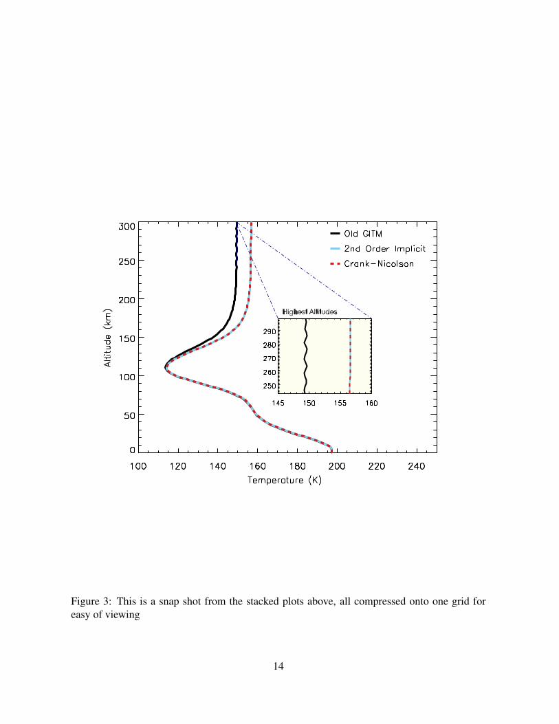
Figure 3: This is a snap shot from the stacked plots above, all compressed onto one grid foreasy of viewing
14

Figure 4: Here is a comparison of densities of the different runs compared to actual data takenfrom MAVEN, the mars orbiter
15
Discussion and Conclusions
From figure 2, it can be seen that there is a fairly significant difference between the original
GITM code and the newer implementations. First, the temperature is higher in the upper at-
mosphere, as can be shown better in figure 3. Second, in figure 2, there is oscillation at the
top of the Old GITM plot that seems to be propagating downward through the lifetime of the
simulation. This was thought to be a quirk of the model itself, but it is actually the result of an
improper implementation of a boundary condition at the top of the model. This boundary con-
dition would switch the signs of the conduction part of the code as it was being calculated, such
that Un+1 = −Un for the top cell of the atmosphere. The removal of this oscillatory nature was
not due to the implementation of a newer scheme, but simply the implementation of a correct
boundary condition.
In figure 3, it can be seen that there is a slight shift of the martian temperature profile at
the top half of the atmosphere. This slight shift can be attributed to the higher accuracy of
the scheme used. The oscillations of the old model have also been highlighted as they were
another large change made to the model. One might notice that there is not model using the
old boundary condition with a newer scheme. The reason for this is simply because the old
boundary condition only created oscillations, but other than that, it did not have an effect on
the temperature profile, so as to eliminate confusion, it was decided that the updated boundary
condition would be used with the updated schemes.
In the last graph, there is a comparison to actual data taken from MAVEN, the martian orbiter
created by NASA. As can be seen, the data better fits the data taken by MAVEN, however, the
change is only 5%. This small of a change is nearly insignificant when looking at how far
off from the actual data the models are. Although, it does not align perfectly with the data, I
want to point out that the data being looked at is density, and not temperature. For this reason,
16

this is not quite an accurate metric of the accuracy of the new model. Further more, the data
used is taken from the planet, which is a 3 dimensional entity, while these simulations are 1
dimensional. Although running a 3 dimensional model will not effect the temperature, it will
effect the density distribution since there will be convection blowing around the gases in Mars’
atmosphere.
Overall, the goal of this project was to increase the accuracy conduction code used in the
GITM framework and to show that there was a measurable difference. By using the Crank-
Nicolson and Second Order Implicit schemes, I showed that the difference between these
schemes and the original implicit scheme is due to the increased accuracy, since these schemes
would not yield the same results when used to simulate the atmosphere of Mars if it wasn’t due
to the increased order of accuracy.
Appendices
In this section, I present the Earth data I took earlier in the life of the project. This data was
left unused in favor of the Mars data due to the lack of evidence of any significant change
between the Crank-Nicolson scheme and the Implicit scheme. This failing is not attributed to
the Crank-Nicolson scheme, but to the atmospheric dynamics of Earth. Conduction is the main
atmospheric process that uses the diffusion equations, so if I wanted to highlight the differences
between schemes that implement the diffusion equation, I would want an atmosphere that has a
large part of its atmospheric dynamics coming from conduction. For this reason, Mars was the
prime candidate of study for this project. With this in mind, there is change between the Crank-
Nicolson scheme and the Implicit scheme at the boundary conditions and with some of the highs
and lows of the atmosphere, but Dr Bell and I felt that we could get better measurements with
Mars.
17

21 22 23 24Dec 21 to 24
0
100
200
300
400
500
600
Alti
tude
(km
)
500
1000
1500
Tem
pera
ture
162.
9817
03.0
8 1000 1100
1200
1300
Tem
pera
ture 1161.03
7%
1200
1400
1600
Tem
pera
ture 1446.47
9%
StartEnd
Figure 5: This is data from an Earth simulation using the original GITM code
18

21 22 23 24Dec 21 to 24
0
100
200
300
400
500
600
Alti
tude
(km
)
500
1000
1500
Tem
pera
ture
162.
9916
51.6
4 1000 1100
1200
1300
Tem
pera
ture 1155.65
7%
1200
1400
1600
Tem
pera
ture 1417.49
9%
StartEnd
Figure 6: This is data from an Earth simulation using the Second Order Implicit scheme
19

21 22 23 24Dec 21 to 24
0
100
200
300
400
500
600
Alti
tude
(km
)
500
1000
1500
Tem
pera
ture
162.
9917
03.2
5 1000 1100
1200
1300
Tem
pera
ture 1161.01
7%
1200
1400
1600
Tem
pera
ture 1446.48
9%
StartEnd
Figure 7: This is data from an Earth simulation using the Crank-Nicolson scheme
20
Bibliography
Harwood, R. Corban; Zhang, Likun; and Manoranjan, V. S., ”Oscillation-free method for semi-
linear diffusion equations under noisy
initial conditions” (2016). Faculty Publications - Department of Mathematics and Applied
Science. Paper 16.
http://digitalcommons.georgefox.edu/math fac/16
21