Developing and Testing Models for

Antibody Kinetics in Surface Plasmon

Resonance Experiments

by

H.A.J Moyse

supervised by

Dr. N. Evans

Thesis

Submitted to the university of Warwick

for the degree of

Master of Science

Abstract

In this thesis three novel models for antibody binding in surface plasmon experi-

ments, that acount for heterogenous binding dynamics, have been created. These have

been structurally analysed, and the best has been tted to data for an experiment on

commercial anti A IgM, and demonstrated to give a dramatically lower RSS than the

existing models.

The structural analysis has demonstrated that meaningful estimates of parameters

can be made even when dealing with clinical samples, where the concentration of analyte

is unknown.

i

Contents

1 Introduction 1

1.1 Existing models . . . . . . . . . . . . . . . . . . . . . . . . . . . . . . . . . . 3

2 methodology 4

2.1 Experimental methods . . . . . . . . . . . . . . . . . . . . . . . . . . . . . . 5

2.2 Extend existing models . . . . . . . . . . . . . . . . . . . . . . . . . . . . . 6

2.2.1 New models . . . . . . . . . . . . . . . . . . . . . . . . . . . . . . . . 8

2.3 Structural Identiability . . . . . . . . . . . . . . . . . . . . . . . . . . . . . 9

2.4 Testing models on monoclonal data . . . . . . . . . . . . . . . . . . . . . . . 12

2.5 Modeling data with multiple binding types . . . . . . . . . . . . . . . . . . . 13

3 Discussion 15

4 Conclusion and Outlook 17

5 Acknowledgements 18

A Appendix 20

A.1 Identiability analysis . . . . . . . . . . . . . . . . . . . . . . . . . . . . . . 20

A.2 Programs . . . . . . . . . . . . . . . . . . . . . . . . . . . . . . . . . . . . . 21

A.2.1 matlab . . . . . . . . . . . . . . . . . . . . . . . . . . . . . . . . . . . 21

A.2.2 Facsimile . . . . . . . . . . . . . . . . . . . . . . . . . . . . . . . . . . 23

ii

Nomenclature

ABO Blood group system

DSAs Donor specic antibodies

HLA Human leukocyte antigen

L Langmuir model

LT Langmuir model with transport equation

ODE Ordinary dierential equation

PDE Partial dierential equation

QSS Langmuir model with a the quasi steady state approximation of the transport equation

RSS Residual sum of squares

SDLN Standard deviation of natural logarithm

SGI Structurally globally identiable

SLI Structurally locally identiable

SU Structurally Unidentiable

SPR Surface plasmon resonance

iii

1 Introduction

One strategy to reduce a patient's risk of transplant rejection would be the use of tailored

immunosuppresant drugs. Before such drugs can be used, a better understanding of the levels

of each type of antibody a transplant can tolerate is needed. This thesis presents the use

of existing mathematical models and new mathematical models to evaluate the dynamics of

antibody binding in surface plasmon resonance (SPR) experiments with commercial anti-A

monoclonal IgM. These ts and models are one of the necessary steps towards identifying and

characterising potential risks in individual patients, and allowing tailored immunosuppresant

drugs[17].

Currently a patient receiving a kidney transplant would undergo crossmatch to test for com-

patibility. Such a test would be failed if donor specic antibodies (DSAs), antibodies that

would attack the transplant, were found in the recipient; either associated with their ABO

blood type or their human leukocyte antigen tissue type(HLA). In such cases pretransplant

antibody removal can be used to allow the operation[8]. However this carries a large immu-

nological risk, with heightened chances of infection dysfunction as well as the existing risk

of rejection. As a result signicant improvements could be made using immunosuppresant

drugs designed for the individual; these would act specically on the antibodies that would

attack the transplant, lowering and maintaining them at safe levels. This would lead to lower

rejection rates, and as a result a greater availability of donor organs and shorter waiting

times for donor organs.

The data analysed in this thesis was taken using SPR experiments conducted with the Pro-

teOn XPR36 platform (manufactured by Bio Rad,See[10] and [19] fora detailed explanation

of this kind of technology). SPR experiments were used rather than the established method

for measuring ABO specic antibody levels, haemaglutenation (HA) because of established

problems with reproducibility[1]. Historically SPR experiments have been used to estimate

the binding coecients of cultured antibodies in [6] and [13].

A number of mathematical models have been developed to describe the dynamics of a reaction

between a ow of one reactant across a sensor surface. The most complex of these involve a

system of partial dierential equations (PDEs) that in include the eects of uid mechanics

1

on the reactants, these models are used to develop appropriate ordinary dierential equations

(ODEs) that can be tted to data. Examples of this include [14] and [4]who consider the

eects of a boundary layer between the well mixed analyte and the ligand where reactions

take place, and use this as a boundary condition for the transport equation; and [5, 20] who

both consider the eects of three dimentional receptor layer that analyte must diuse through

before reacting.The simplest models include a single dierential equation and, assume that

in a short period of time the analyte becomes well mixed, and the rate the rectants bind is

solely dependant on the laws of mass action. However, it has been demonstrated that the

interactions measured are determined not only by the availability of both reactants but the

eects of transport processes[14], as a result the use of these models in parameter tting can

introduce systematic errors [2]. A compromise between the two levels of detail was proposed

by [14], by assuming that the analyte on the boundary layer is in a quasi steady state, a

model may be constructed consisting of only a single dierntial equation in terms bound

concentration. This model was shown to be a good approximation of the physical system

under certain conditions [5] .

The models discussed were designed to deal with experiments where only one binding reaction

is taking place, but antibodies have multiple binding domains, some of which binding and

unbinding at dierant rates [16]. This problem would be exacerbated in clinical conditions

where the analyte may be made up of antibodies of dierant isotypes. As a result, additional

models were developed for this thesis which allow for dierant binding types.

Whilst there may be a number of processes occurring in an SPR experiment, the output

we are given is purely in terms of the concentration of analyte bound to the sensor. It

is necessary to consider the identiability of a new model before tting parameters, and

establish that there are not multiple sets of parameters that would give an identical output.

Even in the case where each parameter of a model is physically meaningful there may not

be enough information in the output to uniquely determine the parameters for a model [9].

Additionally, because the models we are developing need to be useful for clinical data where

the concentration of analyte may be unknown special care has to be taken to ensure that

their parameters can be meaningfully estimated from the output of an experiment where the

analyte concentration would be unknown.

2

Table 1: Parameters, variables and sets

Symbol Meaning Units

C Concentration of analyte at the surface ng/mm3

B Average bound area of the surface ng/mm2

h Quotient of the volume in contact with the surface over the surface area mm?

ka, kd Constants of association and disassociation

KM Transport coecient

R Maximum density of bound analyte

I Inlet concentration of analyte

CT Analyte sample concentration

For non linear systems, such as the models discussed here, there are a number of techniques for

preforming a structural identiability analyses, those based on smooth transitions between

models with identical outputs[15], dierentiable algebra [12, 18], uniqueness of the Taylor

series expansion of the output [7]. The models created in this thesis are such that an equation

relating the output to its derivatives, rather than the state variables of the system, may be

obtained, as a result a method similar to that used in [3] may be applied.

1.1 Existing models

Of the available models in the literature discussed three were selected, and are presented

in this section: one that assumes analyte on the boundary of the receptor is at the same

concentration as that free owing, the Langmuir model (L); one that uses a transport equation

and allows analyte on the boundary to vary, Langmuir with Transport (LT)[14]; one that

doesn't allow the concentration of the analyte on the boundary to vary, but includes the eects

of transport, the Langmuir model with a quasi state approximation of the transport equation

(QSS)[5, 14]. These models are presented using the parameters and variables outlined in 1.

The Langmuir model (L) is dened as:

˙B(t) = kaCT (R−B(t))− kdB(t) (1)

3

it was rst proposed in [11], and forms the basis for the more recent models.

The Langmuir with Transport (LT) model is dened as:

C (t) =−kaC (t) (R−B (t)) + kdB (t) +KM(CT − C (t))

h(2)

B =kaCT (R−B)− kdB (3)

it was rst proposed in [14]. In this paper the transport equation, a dierential equation

governing C(t), the concentration of the analyte at the surface was added to the system, and

was demonstrated to improve ts to simulated data.

The quasi steady state approximation of the Langmuir model(QSS) is

B =kaCT (R−B)− kdB(ka/KM) (R−B) + 1

(4)

it was also rst proposed in [14], but in [5]it was demonstrated to be a good approximation

of a uid dynamics model up to O(Da2)where Da the Damkohler number,the quotient of

reaction velocity to diusion velocity in the boundary layer, is dened as

Da =kaR

kMhd(5)

and hd is a constant that incorporates the eects of the receptor layer. This model may be

derived by setting C = 0 and substituting the solution of eq.2 for C into eq.3.

2 methodology

The method that was used in this project is outlined here:

1. Extend existing models

2. Analyse identiability of extended models

4

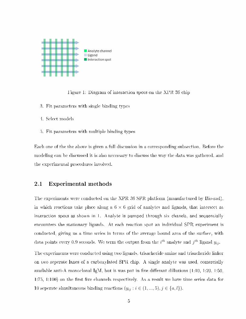
Figure 1: Diagram of interaction spots on the XPR 36 chip

3. Fit parameters with single binding types

4. Select models

5. Fit parameters with multiple binding types

Each one of the the above is given a full discussion in a corresponding subsection. Before the

modeling can be discussed it is also necessary to discuss the way the data was gathered, and

the experimental procedures involved.

2.1 Experimental methods

The experiments were conducted on the XPR 36 SPR platform (manufactured by Bio-rad),

in which reactions take place along a 6 × 6 grid of analytes and ligands, that intersect at

interaction spots as shown in 1. Analyte is pumped through six chanels, and sequentially

encounters the stationary ligands. At each reaction spot an individual SPR experiment is

conducted, giving us a time series in terms of the average bound area of the surface, with

data points every 0.9 seconds. We term the output from the ith analyte and jth ligand yij.

The experiments were conducted using two ligands, trisacheride amine and trisacheride linker

on two seperate lanes of a carboxylated SPR chip. A single analyte was used, comercially

available anti-A monoclonal IgM, but it was put in ve dierant dillutions (1:10, 1:20, 1:50,

1:75, 1:100) on the rst ve channels respectively. As a result we have time series data for

10 seperate simultaneous binding reactions (yij : i ∈ (1, ..., 5), j ∈ a, l).

5

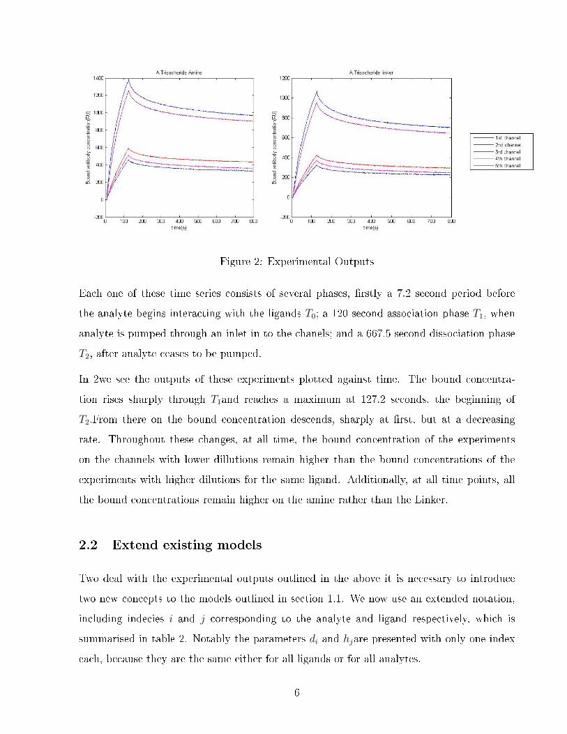
Figure 2: Experimental Outputs

Each one of these time series consists of several phases, rstly a 7.2 second period before

the analyte begins interacting with the ligands T0; a 120 second association phase T1, when

analyte is pumped through an inlet in to the chanels; and a 667.5 second dissociation phase

T2, after analyte ceases to be pumped.

In 2we see the outputs of these experiments plotted against time. The bound concentra-

tion rises sharply through T1and reaches a maximum at 127.2 seconds, the beginning of

T2.From there on the bound concentration descends, sharply at rst, but at a decreasing

rate. Throughout these changes, at all time, the bound concentration of the experiments

on the channels with lower dillutions remain higher than the bound concentrations of the

experiments with higher dilutions for the same ligand. Additionally, at all time points, all

the bound concentrations remain higher on the amine rather than the Linker.

2.2 Extend existing models

Two deal with the experimental outputs outlined in the above it is necessary to introduce

two new concepts to the models outlined in section 1.1. We now use an extended notation,

including indecies i and j corresponding to the analyte and ligand respectively, which is

summarised in table 2. Notably the parameters di and hjare presented with only one index

each, because they are the same either for all ligands or for all analytes.

6

As well as restating these models I shall also be listing the parameters of these models,

corresponding to the number of analytes, ligands and reaction spots and giving the number

of parameters required to deal with the data outlined in section 2.1. This enumeration is

necessary because the numbers of parameters will become important when we analyse their

identiability and t these models.

The Langmuir model is

Bij =

kajdiCT (Rij −Bij)− kdjBij

−kdjBij

t ∈ (T1)

t /∈ (T1)

(6)

and has 24 unknown parameters: two unique to each ligand kaj, kdj; and two Rij, Cij unique

to each interaction spot.

The Langmuir with Transport model (LT) is

Bij =kajCij (Rij −Bij)− kdjBij (7)

hjCij =

−kajCij (Rij −Bij) + kdjBij +KMij(diCT − Cij) t ∈ (T2)

−kajCij (Rij −Bij) + kdjBij − CijKMij t /∈ (T2)

(8)

with 31 unknown parameters: three for each ligand kaj, kdj, and hj; two for each spotRij, kMij,

and one for each analyte channel di.

The Langmuir model with the quasi steady state approximation of the transport equation

(QSS) is

Bij =

kajdiCT (Rij−Bij)−kdjBij

(kaj/kMij)(Rij−Bij)+1t ∈ (T1)

−kdjBij

(kaj/kMij)(Rij−Bij)+1t /∈ (T1)

(9)

with 29 unknown parameters: two for each ligand kaj, kdj, two for each reaction spot Rij, kMij

and one for each analyte Ii.s

7

Table 2: Parameters, variables and sets

Symbol Meaning Units

yij output 10−3 ng/mm3

Cij Concentration of analyte at the surface ng/mm3

Bij Average bound area of the surface ng/mm2

α conversion factor between output and average bound area

hj Quotient of the volume in contact with the surface over the surface area mm?

kaj, kdj Constants of association and dissociation

kMij Transport coecient

Rij Maximum density of bound analyte

Ii Inlet concentration of analyte

CT Analyte sample concentration

di Dilution factor

t1, t2 Start and nish times of the association phase

2.2.1 New models

To deal with the heterogeneous binding established in [16], a new index, k, representing the

type of binding undergone in each reaction, is created. As we have done with the previous

models in this section we shall also number the parameters needed for these models to deal

with the data outlined in section 2.1

We extend the Langmuir without transport for n- binding types (referred to as Ln) :

Bijk =

kajkCij (Rij −∑n

k=1Bijk)− kdjBijk t ∈ (T1)

−kdjBijk t /∈ (T1)

(10)

giving us 10(n+ 1) parameters in total.

We extend the Langmuir with transport for n- binding types (referred to as LTn)

8

Bijk =− kajkCij

(Rij −

n∑k=1

Bijk

)+ kdjBijk (11)

hjCij =

−∑n

k=1 [kajkCij (Rij −∑n

k=1Bijk) + kdjkBijk]− CijkMij t ∈ T1

−∑n

k=1 [kajkCij (Rij −∑n

k=1Bijk) + kdjkBijk] + kmij(diCT − Cij) t ∈ T1(12)

giving us 5(2n+ 6) parameters in total.

We extend the Quasi steady state model for n- binding types (refered to as QSSn)

Bijk =

kajk(KMijdiCT+

∑nk=1 kdjkBijk)(Rij−

∑nk=1 Bijk)∑n

k=1 kajk(Rij−∑n

k=1 Bijk)+kMij− kdjkBijk t ∈ (T1)

kajk(∑n

k=1 kdjkBijk)(Rij−∑n

k=1 Bijk)∑nk=1 kajk(Rij−

∑nk=1 Bijk)+kMij

− kdjkBijk t /∈ (T1)

(13)

for each curve there are 5(2n+ 5) parameters in total

notably there are lots of parameters, so to make tting easier we deal with the cases where

n = 1or 2.

2.3 Structural Identiability

In an SPR experiment we do not necessarily know the values taken by our state variables

(Bij,Cij) at any point in time. We, however, do have an output for each interaction spot on

the chip which is related to our state variables by

yij = αBij (14)

where α is the conversion factor from the units of Bijto the response units of the sensograms

(1 RU= 10−3ng/mm).

As a result it is not immediately apparent whether or not there are more than one parameter

sets that will give us the same evolution of yij during the time of the experiment. Writting

this more formally, it is not apparrent if given a vector of parameters p taken form the set of

all possible vectors of parameters Ω ⊂ R , if yij(p; t)=yij(p; t)→ p = p.

9

Before we can discuss the results that have been obtained for the three models we are dealing

with initially we have to establish some standard denitions relating to identiability.

Denition 1. Two parameter vectors p and p are indistinguishable if they give the same

outputs yij(t; p)=yij(t; p) for ∀t ≥ 0. We write this equivalence relationship with p ∼ p.

Denition 2. A parameter piis locally identiable if there is a neighbourhood, N(p), of the

parameter vector where p ∈ N(p),p ∼ p⇒ pi = pi.

Denition 3. A parameterpiis globally identiable if it is locally identiable for the neigh-

bourhood Ω, that is p ∈ Ω, p ∼ p→ pi = pi.

Denition 4. A parameterpiis unidentiable if there does not exist a neighbourhood where

it is locally identiable.

These terms can be used to make denitions relating to a model as a whole

Denition 5. A systems model is structurally globally identiable (SGI) if all of its parame-

ters are globally identiable.

Denition 6. A systems model is structurally locally identiable (SLI) if all of its parameters

are locally identiable, but not all of its parameters are globally identiable.

Denition 7. A systems model is structurally unidentiable (SU) if one or more of its

parameters are unidentiable.

In this thesis a variation on the approach developed by [3] is used to classify the models LTn,

Ln and QSSn, as SGI, SLI or SU. Firstly the set of derivatives for the dierential equations

dening each model (eq. 10 for Ln, eq.11 and 12 for LTn and eq.13 for QSSn ) is solved to

produce a single equation relating the output yijto a quotient of multinomials in terms of yij

and its time derivatives, i .e

yij(t; p) =M1(yij, yij, ...; p)

M2(yij, yij, ...; p). (15)

For a parameter vector p to be indistinguishable from p these quotients would be equal,

giving:

10

Known CT

Model Globally identiable parameters Locally identiable parameters Unidentiable parameters

Ln Rij, kMij kajk, kdjk -

LTn Rij kdjk kMij, kajk, hij

QSSn Rij, kMij, kMij kajk, kdjk

Table 3: Identiability of parameters for known CT

Unknown CT

Model Globally identiable parameters Locally identiable parameters Unidentiable parameters

Ln Rij, kMij kajk, kdjk, CT

LTn Rij kdjk kMij, kajk,hij, CT

QSSn Rij, kMij, kMij kajk, kdjk CT

Table 4: identiability of parameters for unknown CT

M1(yij, yij, ...; p)M2(yij, yij, ...; p) = M1(yij, yij, ...; p)M2(yij, yij, ...; p). (16)

For this equality to be true the coecient of each product of derivatives must be equal to

a corresponding quotient on the opposite side. As a result we get a new set of equations

relating the elements of p to the elements of p. If this set of equations only has the trivial

solution p = p then the model is SGI, if it has a set of distinct solutions other than the trivial

one it is SLI and it is SU otherwise.

In the appendix (A.1) the maple worksheets that were used to apply this method to LTn, Ln

and QSSn for n = 2. The results obtained are summarised in tables 3and4. In these tables,

the binding constants are never globally identiable because the labelling of one binding type

as k = 1 and the other as k = 2 is arbitrary, so the labels can always be swapped. Additio-

nally, the binding constants are unidentiable in the LTn model for unknown CTmaking it

inappropriate for clinical data.

We make the choice of using only two binding types because of the length of time required

for parameter tting for each model. The methods outlined here could with comparatively

11

little work be extended for n = 3 or a general case.

2.4 Testing models on monoclonal data

A precursor to tting models to clinical data would be tting them to data from experiments

conducted with monoclonal antibodies and demonstrating that they give a dramatically

improved t.

Parameter estimation was preformed in two stages, rst the models L and QSS were t-

ted, secondly a the model that tted the data best was selected and, its extended version

(either Ln, LTn or QSSn) was tted. Notably the LT model was not t, this is because it

would be structurally unidentiable for clinical data, and the parameters obtained would be

meaningless. Fits were conducted using facsimile for windows (MCPA software UK).

Because each parameter represents a physical quantity of an unknown order of magnitude for

each model a large number of starting parameter vectors were created for each model (441

for L and 9261 for QSS1), with each parameter taking every exponent of 10 from 10−4to 102.

These were then read in, and the residual sum of squares for each model with each parameter

vector was calculated. For each model the best 100 starting parameter vectors was then run

1000 times, with facsimile completing an average of 45 simulation runs per model. Of these

best ts the best t for each model was then ran 1000 times more.

In gure3 presents ts to the data of the Langmuir and quasi steady state models. Whilst

they appear similar there is a large dierence in residual sum of squares; whilst the Langmuir

model has an RSS of 1, 578, the quasi steady state model has an RSS of 941. The key

dierences in t that can be seen in g 3 are that the Langmuir model predicts much faster

growth in bound area in the association phase and peaks earlier and lower than the Quasi

steady state model on all ten curves.

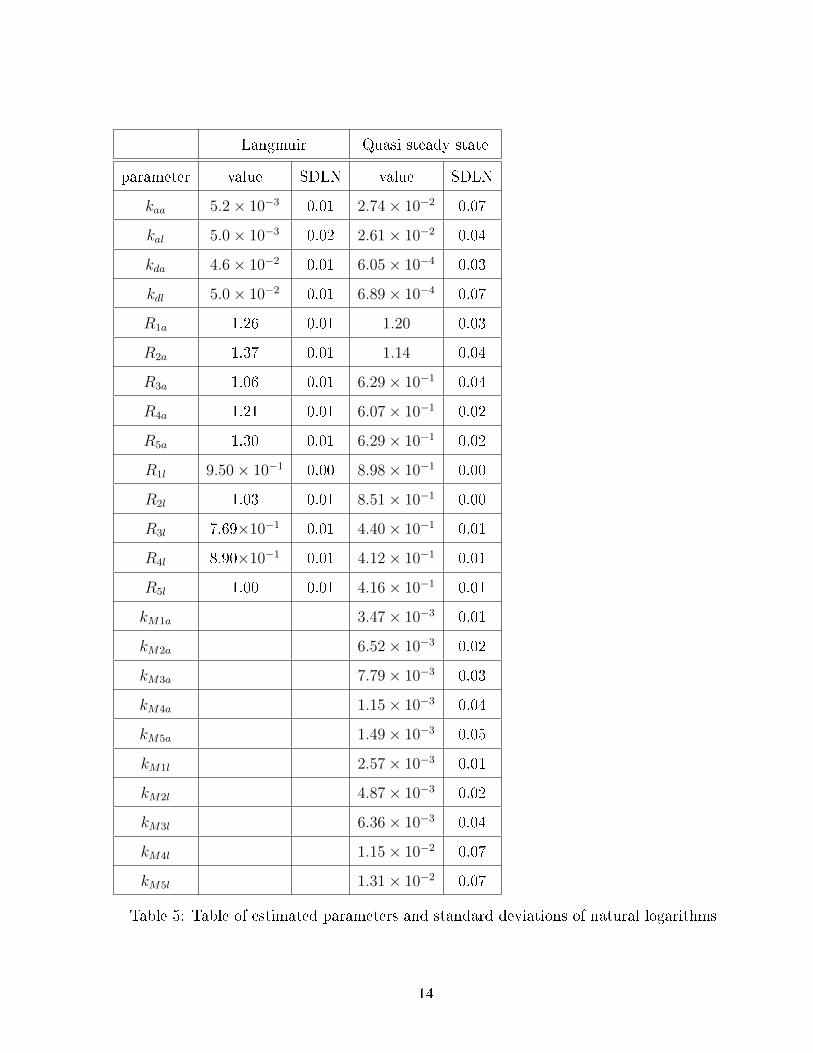
In table 5 we see the parameters from the ts of both models as well as their standard

deviation of natural logarithm (SDLN). All parameters have SDLNs below 0.1 and as a result

are well determined. Interestingly the values of the association constants in the Langmuir

model are an order of magnitude smaller than those from the QSS model, this is likely because

12

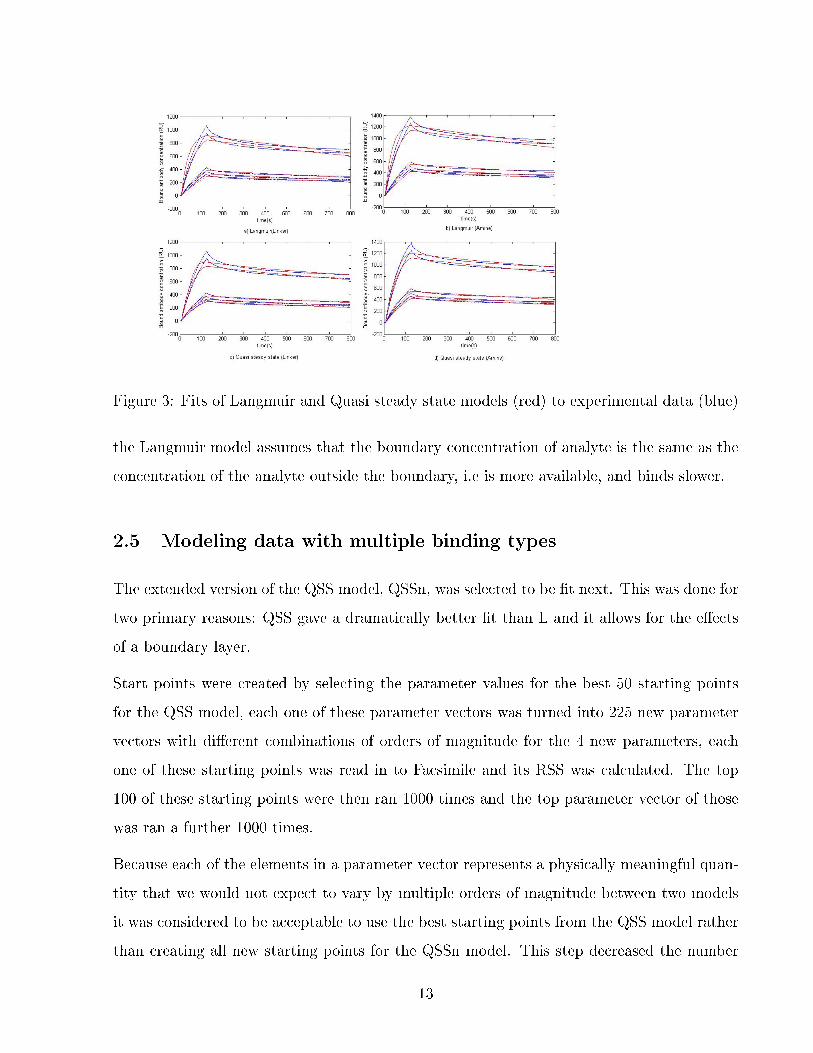
Figure 3: Fits of Langmuir and Quasi steady state models (red) to experimental data (blue)

the Langmuir model assumes that the boundary concentration of analyte is the same as the

concentration of the analyte outside the boundary, i.e is more available, and binds slower.

2.5 Modeling data with multiple binding types

The extended version of the QSS model, QSSn, was selected to be t next. This was done for

two primary reasons: QSS gave a dramatically better t than L and it allows for the eects

of a boundary layer.

Start points were created by selecting the parameter values for the best 50 starting points

for the QSS model, each one of these parameter vectors was turned into 225 new parameter

vectors with dierent combinations of orders of magnitude for the 4 new parameters, each

one of these starting points was read in to Facsimile and its RSS was calculated. The top

100 of these starting points were then ran 1000 times and the top parameter vector of those

was ran a further 1000 times.

Because each of the elements in a parameter vector represents a physically meaningful quan-

tity that we would not expect to vary by multiple orders of magnitude between two models

it was considered to be acceptable to use the best starting points from the QSS model rather

than creating all new starting points for the QSSn model. This step decreased the number

13

Langmuir Quasi steady state

parameter value SDLN value SDLN

kaa 5.2× 10−3 0.01 2.74× 10−2 0.07

kal 5.0× 10−3 0.02 2.61× 10−2 0.04

kda 4.6× 10−2 0.01 6.05× 10−4 0.03

kdl 5.0× 10−2 0.01 6.89× 10−4 0.07

R1a 1.26 0.01 1.20 0.03

R2a 1.37 0.01 1.14 0.04

R3a 1.06 0.01 6.29× 10−1 0.04

R4a 1.21 0.01 6.07× 10−1 0.02

R5a 1.30 0.01 6.29× 10−1 0.02

R1l 9.50× 10−1 0.00 8.98× 10−1 0.00

R2l 1.03 0.01 8.51× 10−1 0.00

R3l 7.69×10−1 0.01 4.40× 10−1 0.01

R4l 8.90×10−1 0.01 4.12× 10−1 0.01

R5l 1.00 0.01 4.16× 10−1 0.01

kM1a 3.47× 10−3 0.01

kM2a 6.52× 10−3 0.02

kM3a 7.79× 10−3 0.03

kM4a 1.15× 10−3 0.04

kM5a 1.49× 10−3 0.05

kM1l 2.57× 10−3 0.01

kM2l 4.87× 10−3 0.02

kM3l 6.36× 10−3 0.04

kM4l 1.15× 10−2 0.07

kM5l 1.31× 10−2 0.07

Table 5: Table of estimated parameters and standard deviations of natural logarithms

14

Figure 4: ts of QSS model outputs (blue) to experimental data (red) with error plots.

of starting points required to cover the possible orders of magnitude the parameters of the

QSSn model by an order of magnitude.

In gure 4 we see ts from the QSSn model, visually it looks much closer to the data than

either of the preceding models, correspondingly it has a signicantly lower residual sum of

squares, 261, less than a third of that of the preceding model. Whilst there is only a small

distance between the model and the data there seem to be some interesting patterns in the

errors. As time increases the model increasingly over predicts the loss of bound analyte, and

the data appears to be reaching an asymptote, suggesting that some of the binding may be

irreversible.

We present the parameters of this model in table 6.

3 Discussion

It has been demonstrated that the QSSn model oers dramatically better ts than either the

L or QSS models. Additionally it remains SLI even if the total sample concentration CT is

unknown. As a result it could be used for clinical data, and in such data could be expected

to preform much better than previously existing models.

15

Quasi steady state model for two binding types

parameter value SDLN

kaa1 3.1× 10−3 0.07

kal1 2.3× 10−2 0.05

kda1 3.23× 10−2 0.03

kdl1 5.01× 10−4 0.07

kaa2 3.30× 10−3 0.03

kal2 2.9× 10−2 0.07

kda2 3.61× 10−4 0.03

kdl2 3.78× 10−2 0.04

R1a2 1.51 0.04

R2a 1.98 0.04

R3a 2.17 0.01

R4a 2.50 0.02

R5a 2.81 0.00

R1l 1.05 0.00

R2l 1.10 0.00

R3l 1.12 0.00

R4l 1.15 0.01

R5l 1.18 0.01

kM1a 9.47× 10−2 0.96

kM2a 3.09× 10−2 0.12

kM3a 2.05× 10−2 0.04

kM4a 3.51× 10−2 0.07

kM5a 3.27× 10−2 0.04

kM1l 1.20× 10−2 0.76

kM2l 1.63× 10−2 0.09

kM3l 1.19× 10−3 0.04

kM4l 1.15× 10−2 0.05

kM5l 1.31× 10−2 0.08

Table 6: Table of estimated parameters and standard deviations of natural logarithms16

The key improvement that the QSSn model oers is that the peaks it predicts are close both

in the time that they occur and in height to those observed in the experiments at the end

of the association phase. This improvement supports the work of [16]. Together that paper

and this thesis give strong grounds to conclude that IgM has heterogeneous binding kinetics.

One criticism of the analysis is that models with varying numbers of parameters were compa-

red, and the ones with least RSS were selected despite having a greater number of parameters.

This could create two potential problems: rstly the dramatic decrease in RSS between mo-

dels could be explained as purely a result of introducing new parameters, rather than the

parameters themselves being physically meaningful; secondly the increase in the number of

parameters makes model tting slower. If a model such as QSSn was adopted for estimating

binding kinetics in a clinical environment each analysis would take dramatically longer than

it would with L.

4 Conclusion and Outlook

In this thesis models have been created, structurally analysed and tted to data. In particular

the QSSn model has been demonstrated to provide a better t to data from a commercial

(IgM) antibody sample than any of the established models discussed, and for two binding

types (n = 2) it has shown to have identiability properties making it appropriate for use on

a clinical samples.

However it also needs to be tted to other commercial antibody types and clinical data

before it could be accepted as the standard model for antibody binding in SPR experiments.

A second hurdle will be extending the identiability analysis for three binding types and

a general case, this is because in clinical experiments there may be an unknown number

of binding types. Additionally if models with increasing numbers of parameters are used,

methods will be needed to estimate the parameters more eciently, and models will have to

be compared using statistical concepts like the Bayesian Information - Criterion or Akaike

information criterion, which will require a detailed assessment of the likelihoods involved,

and the non- normal errors observed.

17

5 Acknowledgements

This project was conducted on funding from the EPSRC, and with the aid of

References

[1] Atsushi Aikawa, Mioko Yamashita, Tomomi Hadano, Takehiro Ohara, Kenji Arai, Ta-

keshi Kawamura, and Akira Hasegawa. Abo incompatible kidney transplantation

immunological aspect-. Exp Clin Transplant, 1(2):112118, Dec 2003.

[2] I. Chaiken, S. Rosé, and R. Karlsson. Analysis of macromolecular interactions using

immobilized ligands. Anal Biochem, 201(2):197210, Mar 1992.

[3] L. Denis-vidal, G. Joly-Blanchard, and C. Noiret. Some eective approaces to check iden-

tiability of uncontrolled nonlinear rational systems. Math. Comput. Simulat., 57:3544,

2001.

[4] D. Edwards, B. Goldstein, and D.S. Cohen. Transport eects on surface volume biolo-

gical reactions. J. Math. Biol., 39:533561, 1999.

[5] D. A. Edwards. The eect of a receptor layer on the measurement of rate constants.

Bull Math Biol, 63(2):301327, Mar 2001.

[6] P. Englebienne. Use of colloidal gold surface plasmon resonance peak shift to infer

anity constants from the interactions between protein antigens and antibodies specic

for single or multiple epitopes. Analyst, 123(7):15991603, Jul 1998.

[7] N.D Evans, Chapman M.J., Chapell M.J., and Godfrey K.R. Identiability of uncon-

trolled nonlinear rational systems. Automatica, 38:17991805, 2002.

[8] Rob Higgins, David Lowe, Mark Hathaway, For Lam, Habib Kashi, Lam Chin Tan, Chris

Imray, Simon Fletcher, Klaus Chen, Nithya Krishnan, Rizwan Hamer, Daniel Zehnder,

and David Briggs. Rises and falls in donor-specic and third-party hla antibody levels

after antibody incompatible transplantation. Transplantation, 87(6):882888, Mar 2009.

18

[9] J.A. Jacquez. compartmental analysis in biology and medicine. Biomedware, ann arbor,

1996.

[10] R. Karlsson, H. Roos, L. Fagerstam, and B. Persson. kinetic and concentration analysis

using bia technology. Methods, 6:99110, 1994.

[11] Irving Langmuir. The constitution and fundamental properties of solids and liquids.

part i. solids. J. Am. Chem. Soc., 38:222195, 1916.

[12] L. Ljung and T. Glad. On global identiability for arbitrary model pa. au, 30:265276,

1994.

[13] C. R. MacKenzie, T. Hirama, S. J. Deng, D. R. Bundle, S. A. Narang, and N. M. Young.

Analysis by surface plasmon resonance of the inuence of valence on the ligand binding

anity and kinetics of an anti-carbohydrate antibody. J Biol Chem, 271(3):15271533,

Jan 1996.

[14] D. G. Myszka, X. He, M. Dembo, T. A. Morton, and B. Goldstein. Extending the range

of rate constants available from biacore: interpreting mass transport-inuenced binding

data. Biophys J, 75(2):583594, Aug 1998.

[15] Pohjanpalo. systrem identiability for arbitrary model parameterizations. automatica,

41:265276, 1978.

[16] Earl Prinsloo, Vaughan Oosthuizen, Maryna Van de Venter, and Ryno J Naudé. Biolo-

gical inferences from igm binding characteristics of recombinant human secretory com-

ponent mutants. Immunol Lett, 122(1):9498, Jan 2009.

[17] D.Lowe F. Lam H. Kashi L.C. Tan C. Imray S. Fetcher D. Zehnder K. Chen N. Krishnan

R. Hamer R. higgins, M. Hathaway and D. Briggs. Blood levels of donor-specic human

leukocyte antigen antibodies after renal transplantation: resolution of rejection in the

prescence of circulating donor- specic antibody. Transplantation, 84:876884, 2007.

[18] M.P. Saccomani, S. Audoly, and D'angio L. parameter identiability of nonlinear sys-

tems: the role of initial conditions. Automatica, 39:619632, 2003.

19

[19] A. Szabo and L. Stolz. Surface plasmon resonance and its use biomolecular interaction

analysis (bia). Curr. Opin. Struct. Biol., 5:699705, 1995.

[20] M.L. Yarmush, D.B. Patankar, and D.M. Yarmush. An analysis of transport resistance

in the operation of biacore; implications for kinetic studies of biospecic interactions.

Mol. Immunol, 33:12031214, 1996.

A Appendix

A.1 Identiability analysis

20

A.2 Programs

A.2.1 matlab

Programs are presented in this order

1. runFACSIM.m

2. startpointsQSS1.m

3. startpointsL1.m

4. compare.m

5. topfew.m

6. startpointsQSS2.m

The program runFACSIM.m allows the user to repeatedly run a single .fac le.

The programs startpointsQSS1.m and startpointsL1.m creates a number of folders containing

dierent .txt les representing parameter values that are read in by a .fac le in the same

folder, they dier in that they create parameter values for use by dierent models. Notably

both of these create these starting parameters based on a number of rules, such as that the

binding coecients of a single reaction are of the same order of magnitude, whilst these may

be false in reality, facsimile is capable of tting parameters extremal quickly and varying

them across orders of magnitude. These both output an index which is to be used with

compare.m or topfew.m

The program compare.m nds the best parameter vectors from a set of les, and runs a

number (ntop) of the best les a number of times (nruns). It also checks for les are missing,

have errors or that haven't been run before, so the user can investigate any issues. This

program outputs an ordered index which lists the folders with the best parameters to the

worst parameters, excluding those that have problems.

The program topfew.m nds uses much of the code as compare.m to nd the best les from

an index. Rather than running the best les, it moves them to a new directory. This allows

21

the user to create a single set of parameter vectors for the QSS model, and copy the best

ones to a new directory where they form the basis for the QSSn model.

The program startpointsQSS2.m creates a number of folders containing dierent .txt les

representing parameter values that are read in by a .fac le in the same folder. It diers

from the other startpoints programs because it needs to have the address of the les created

by topfew.m, it uses the good combinations of parameters from the QSS1 model as the

parameters it shares with that model, and in a new set of les combines these good parameters

with values for the parameters unique to this model.

22

A.2.2 Facsimile

Templates for programs that are edited by matlab and copied into directories where they can

be ran are presented in this order

1. HarryL1.fac

2. HarryQSS1.fac

3. HarryQSS2.fac

These are presented in an abbreviated form, and exclude the data that would be necessary

to run them.

23