developing lqr to control speed motor using...

DEVELOPING LQR TO CONTROL SPEED MOTOR USING MATLAB GUI

SHAMSUL NIZAM BIN MOHD YUSOF @ HAMID

A report submitted in partial fulfillment of the

requirements for the award of the degree of

Bachelor of Electrical (Electronics) Engineering

Faculty of Electrical and Electronics Engineering

Universiti Malaysia Pahang

NOVEMBER 2008

ii

“All the trademark and copyrights use herein are property of their respective owner.

References of information from other sources are quoted accordingly; otherwise the

information presented in this report is solely work of the author.”

Signature : ____________________________

Author : SHAMSUL NIZAM BIN MOHD YUSOF @ HAMID

Date : 10 NOVEMBER 2008

iii

To my beloved parents and my siblings, I’m nothing without them.

iv

ACKNOWLEDGEMENT

During doing this thesis, I found myself around with a lot of great people.

Those people have helped me a lot in doing this research directly or in directly. Their

contribution has helped me in understanding about my project thoroughly.

I would like to say thank to my supervisor, Madam Haszuraidah Binti Ishak for

her support, guide, advices and determination in guiding me to finish my final year

project and this thesis to. I would also like to express my gratitude to my colleagues,

for their intention on helping me in any sort of way.

I, myself are fully in debt with Faculty of Electrical and Electronics (FKEE),

for providing me necessary components, information and funding my project.

Without their helped, this project was deeming to be unfinished.

Last but not least, I would like to say my gratitude toward to my family

member for their support and encouragement. I am grateful to have them all.

v

ABSTRACT This project is mainly upon developing Linear Quadratic Regulator (LQR)

controller and controlling it through software. In the software part, MATLAB GUI is

been implemented to control the whole LQR system. In addition, a servo motor is

attached as a hardware module to show the resultant of the LQR controller. The

ability of the controller on the servo motor is, it is capable to manipulate and control

the rotating speed of the motor. Thus it could also regulate the value from the error

that occurs at output so that the value is stabilized as same as the input. Application

of feedback system is applied in the MATLAB GUI itself before interfacing it with

the servo motor using DAQ Card. The output from the MATLAB is then sent to the

input of the DAQ Card through the Analog pin. A generation of signal from output at

DAQ Card through the Analog pin subsequently enters to the motor driver. Driving

the motor with the signal provided, it will send a feedback signal back to the system

to be compared with the initial input. The whole system built from the simulink

modeling through the software MATLAB.

vi

ABSTRAK

Projek ini boleh dikategorikan ke dalam dua bahagian utama, pengaturcaraan

dan system pengawal servo motor. Untuk system pengawal, “Linear Quadratic

Regulator” dan untuk programnya pula, Matlab GUI digunakan. System pengawal

ini akan diaplikasi ke dalam program Matlab GUI bagi membolehkan pengguna

mengawal dan memanipulasi kelajuan atau putaran servo motor tersebut. System

pengawal yang telah diaplikasi ke dalam program akan disambungkan ke servo

motor menggunakan “serial and parallel port”. Signal keluaran dari Matlab akan

dihantar ke “DAQ Card” melalui pin Analog. Kemudian “feedback” dari servo motor

akan di hantar ke sistem pengawal untuk dibandingkan dengan masukan dan

seterusnya akan diubah sehingga “feedback” tadi akan sama nilainya dengan

masukan.

vii

TABLE OF CONTENTS

CHAPTER TITLE PAGE

DECLARATION ii

DEDICATION iii

ACKNOWLEDGEMENT iv

ABSTRACT v

ABSTRAK vi

TABLE OF CONTENTS vii

LIST OF TABLES xi

LIST OF FIGURES xii

LIST OF ABBREVIATIONS xiv

LIST OF APPENDICES xv

1 INTRODUCTION

1.1 General 1

1.2 Problem Statement 2

1.2.1 Current Controller and Software 2

1.2.2 Problem Solving 3

1.3 Objectives 3

1.4 Scope of Project 4

2 LITERATURE REVIEW

2.1 Linear Quadratic Regulator 5

2.2 Data Acquisition 7

2.3 Servo Motor 10

viii

3 METHODOLOGY

3.1 SOFTWARE 12

3.1.1 Real Time Target Setup 13

3.1.2 Installation and Configuration 15

3.1.2.1 C Compiler 15

3.1.2.2 Installation the Kernel 17

3.1.2.3 Testing the Installation 18

3.1.3 Procedures of Creating Real Time Applications 19

3.1.3.1 Creating a Simulink Model 19

3.1.3.2 Entering Configuration

Parameters for Simulink 26

3.1.3.3 Entering Simulation Parameters

for Real-Time Workshop 28

3.1.3.4 Creating a Real-Time Application 30

3.1.3.5 Running a Real-Time Application 31

3.1.4 Creating Graphical User Interfaces 32

3.1.4.1 GUI Development Environment 33

3.1.4.2 Starting Guide 33

3.1.4.3 The Layout Editor 34

3.1.4.4 Programming a GUI 35

3.1.5 Simulation of the servomotor 36

3.1.6 Graphical User Interface 38

3.2 HARDWARE 42

3.2.1 CLIFTON PRECISION SERVO

MOTOR MODEL JDH-2250-HF-2C-E 42

3.2.2 G340 installation 43

3.2.3 G340 installation 44

3.2.3.1 Encoder hook up 44

3.2.3.2 Power supply hook up 45

3.2.3.3 Testing the encoder 45

3.2.3.4 Control input hook up 46

ix

3.2.3.5 Testing the control inputs 46

3.2.3.6 Motor hook up 46

3.2.4 Advantech PCI-1710HG 47

3.2.5 Common Specifications 47

3.2.6 Pin Assignments 48

3.3 Linear Quadratic Regulator Development 48

3.3.1 The General State-Space Representation 48

3.3.2 Evaluating the State Space equation 51

3.4 Applying Linear Quadratic Regulator 54

4 RESULT AND DISCUSSION

4.1 Simulation result 56

4.1.1 Simulation on the DC motor 56

4.1.2 Simulation on the Clifton

Precision servo motor 58

4.2 Data Analysis 60

4.3 Tuning the value of Q 62

5 CONCLUSION AND RECOMMENDATION

5.1 Introduction 65

5.2 Assessment of design 65

5.3 Strength and Weakness 66

5.4 Suggestion for Future Work 67

5.5 Costing & Commercialization 67

REFERENCES 68

APPENDIX A 69

APPENDIX B 77

xi

LIST OF TABLE

TABLE NO. TITLE PAGE 3.1 Comparison of Matlab GUI with other software

and it’s problem 13

3.2 Parameters of servomotor elements 53

4.1 Data analysis simulink of the system 61

4.2 Simulation results for three different Q 64

xii

LIST OF FIGURES

FIGURE NO. TITLE PAGE 2.1 LQR block diagram 5

2.2 Typical dc servo motor system with either encoder or

resolver feedback 11

3.1 Real Time Windows Target 14

3.2 Simulink Model rtvdp.mdl 18

3.3 Create a new model 20

3.4 Empty Simulink model 20

3.5 Block Parameters of Signal Generator 21

3.6 Block Parameters of Analog Output 23

3.7 Scope Parameters Dialog Box 24

3.8 Scope Properties: axis 1 25

3.9 Completed Simulink Block Diagram 26

3.10 Configuration Parameters – Solver 27

3.11 Configuration Parameters – Hardware Implementation 28

3.12 System Target File Browser 29

3.13 Configuration Parameters – Real-Time Workshop 29

3.14 Connect to target from the Simulation menu 31

3.15 GUIDE Quick start 34

3.16 Layout Editor 35

3.17 M-File Editor 36

3.18 Block diagram for the simulation servo motor 37

3.19 Subsystem for the block diagram above 37

3.20 M-file for the system 38

3.21 Main panel 38

3.22 Supervisor credit 39

3.23 Student credit 39

3.24 Abstract of the project 40

3.25 Manual way to find the K gain 40

xiii

3.26 Simulink model 41

3.27 Find K if different motor constant 41

3.28 Servo Motor 42

3.29 Gecko drive (G340) 43

3.30 G340 block diagram 43

3.31 Advantech PCI-1710HG 47

3.32 Pin Assignment for PCI-1710HG 48

3.33 Graphic representation of state space and state vector 50

3.34 DC motor model system 51

4.1 Result for DC motor 57

4.2 Graph result for K = [0.245006 0.0801054] 57

4.3 Result for Clifton Precision servo motor 58

4.4 Graph result for K = [1.28138 0.90017] 59

4.5 Settling time for simulation DC motor 60

4.6 Rise time for simulation DC motor 61

4.7 Result for Q = 1 62



xiv

LIST OF ABBREVIATIONS

GUI - Graphical User Interface IEEE - Institute of Electrical and Electronics Engineers LQR Linear Quadratic Regulator LQG Linear Quadratic Gaussian

xv

LIST OF APPENDICES

APPENDIX TITLE PAGE

A G340 Installation 69

B Coding Program 77

CHAPTER 1

INTRODUCTION

1.1 GENERAL

This project is based on the controller and the software used to interface the

CLIFTON PRECISION motor. By developing Linear Quadratic Regulator (LQR)

using mathematical equation to get the feedback controller to control the speed of the

servo motor with using Matlab GUI from Mathworks.

Matlab GUI is the one of the software that is using graphical method.

Between the servo motor and Matlab GUI, DAQ Card used to interface the both of

them. From the software, the data transfer first to the DAQ Card. Then the DAQ

Card will convert the data to an electrical signal that acquired by the servo motor.

The drive that drives the servo motor is G340 Servodrive(x10 Step

Multiplier) by Geckodrive that comes in package with the servo motor.

The servo motor is type JDH-2250-HF-2C-E CLIFTON PRECISION that has

the supply voltage -0.5 to 7V interval. The output voltage of the servo motor is -0.5

to Vcc. Choosing this servo motor is because High output power relative to motor

size and weight. It also suitable for the controller that has feedback, not like stepper

motor which is operated open loop.

2

1.2 PROBLEM STATEMENT As research had been done, there are lot of controller that are used. But there

are some features not same as LQR features in others controller.

1.2.1 Current controller and software There are a lot of controllers which can be used to control the speed of the

motor such as Proportional Integral Derivatives (PID) and Fuzzy Logics. For the

software, many companies has developed various software related to engineering in

this day like Matlab, Visual Basic and Labview. However, the problems are:-

i. PID controller

The controller like PID need has percentage of overshoot and take

some time to it’s stabilizing the system. It also has the time settling

that are can reach more than 1 sec. this will affect the effectiveness of

the system.

ii. Software

Software like Labview has problem in term of control system because

we need to download separately from the manufacturer’s website the

control toolkit. Then after that we could use it for the control system.

The toolkit is like the add-ons to the Labview software. For the Visual

Basic, we cannot do the simulation to know the result before we do it

in the real-time.

3

1.2.2 Problem solving i. Linear quadratic regulator is the most effective controller because it

regulates the error to zero and it doesn’t have percentage of overshoot

and time settling. So it can stabilize the system quicker than PID.

ii. Matlab GUI is choose because it is friendly user and don’t use

complex coding to run it. Just drag and drop the function to use it. It

also can simulate the linear system before use in real-time using

Simulink. In Simulink, we need to create the system using block

diagram in Matlab.

1.3 Objectives First objective that has been setup for this project is in developing the

controller that used. Linear Quadratic Regulator need to be develops first before can

proceed to another objective or to the next step for this project. Before can do the

developing, need to study first about this controller because this the first time I want

to use it.

To develop LQR, there is more than one method that can be use. The purpose

is to find the gain value, K. The method is like pole placement, and Algebraic Riccati

equation (ARE). For this project, ARE method used because only need to find the

gain value, K that is need to use to regulate the error that comes from the feedback in

the linear system.

The second objective is to control the speed of the servomotor. We control

the speed of the servomotor with the value of the gain, K that we obtain before. The

gain will be multiplied with the output value to make the error zero and same as the

input. To control the speed of the servomotor, we use Matlab GUI as the user control

4

panel that from there, we can control the speed by change the input as we can say the

speed of the servomotor by just insert the value at the Matlab GUI.

The third one is interfacing the servomotor with the software. To doing that, a

converter that converts data from computer to electrical signal called DAQ Card

(Data Acquisition Card) need to be use.

1.4 Scope

The most important step in this project is obtaining the state space of the

motor that will use for this project first. It is because the gain value, K via Algebraic

Riccati Equation (ARE) can be obtained from state space equation.

After the value of the gain K been obtained, the linear system can be created

and will be simulated. The result is obtained from the simulation of the system, and

the value of the gain can regulate the error or not can be determined. If not, find

another value of K by change the value of the disturbance, Q in the ARE equation.

CHAPTER 2

LITERATURE REVIEW

2.1 Linear Quadratic Regulator (LQR)

Figure 2.1: LQR block diagram

The theory of optimal control is concerned with operating a dynamic system

at minimum cost. The case where the system dynamics are described by a set of

linear differential equations and the cost is described by a quadratic functional is

called the LQ problem. One of the main results in the theory is that the solution is

provided by the linear-quadratic regulator (LQR), a feedback controller whose

equations are given below. The LQR is an important part of the solution to the LQG

problem. Like the LQR problem itself the LQG problem is one of the most

fundamental problems in control theory.

6

In layman's terms this means that the settings of a (regulating) controller

governing either a machine or process (like an airplane or chemical reactor) are

found by using a mathematical algorithm that minimizes a cost function with

weighting factors supplied by a human (engineer). The "cost" (function) is often

defined as a sum of the deviations of key measurements from their desired values. In

effect this algorithm therefore finds those controller settings that minimize the

undesired deviations, like deviations from desired altitude or process temperature.

Often the magnitude of the control action itself is included in this sum as to keep the

energy expended by the control action itself limited.

In effect, the LQR algorithm takes care of the tedious work done by the

control systems engineer in optimizing the controller. However, the engineer still

needs to specify the weighting factors and compare the results with the specified

design goals. Often this means that controller synthesis will still be an iterative

process where the engineer judges the produced "optimal" controllers through

simulation and then adjusts the weighting factors to get a controller more in line with

the specified design goals.

The LQR algorithm is, at its core, just an automated way of finding an

appropriate state-feedback controller. And as such it is not uncommon to find that

control engineers prefer alternative methods like full state feedback (also known as

pole placement) to find a controller over the use of the LQR algorithm. With these

the engineer has a much clearer linkage between adjusted parameters and the

resulting changes in controller behavior. Difficulty in finding the right weighting

factors limits the application of the LQR based controller synthesis. [6]

Linear Quadratic Regulator (LQR) is the most common approach to modern

control design, and one of the controller that are commonly used by users to control

the system besides Proportional Integral Derivatives (PID) because its stability. For a

LTI system:

7

(2.1)

The technique involves choosing a control law u=-ω(x) which stabilizes the origin (i.e., regulates x to zero). The gain K which solves the LQR problem is

K=R−1B

TP* (2.2)

where P* is the unique, positive semidefinite solution to the algebraic Riccati equation (ARE):

ATP + PA – PBR-1BTP + Q = 0 (2.3)

2.2 Data acquisition

Data acquisition is the sampling of the real world to generate data that can be

manipulated by a computer. Sometimes abbreviated DAQ or DAS, data acquisition

typically involves acquisition of signals and waveforms and processing the signals to

obtain desired information. The components of data acquisition systems include

appropriate sensors that convert any measurement parameter to an electrical signal,

which is acquired by data acquisition hardware.

Acquired data are displayed, analyzed, and stored on a computer, either using

vendor supplied software, or custom displays and control can be developed using

various general purpose programming languages. LabVIEW, which offers a

graphical programming environment optimized for data acquisition and MATLAB

provides a programming language but also built-in graphical tools and libraries for

data acquisition and analysis.

Data acquisition begins with the physical phenomenon or physical property

of an object (under investigation) to be measured. This physical property or

phenomenon could be the temperature or temperature change of a room, the intensity

8

or intensity change of a light source, the pressure inside a chamber, the force applied

to an object, or many other things. An effective data acquisition system can measure

all of these different properties or phenomena.

A transducer is a device that converts a physical property or phenomenon into

a corresponding measurable electrical signal, such as voltage, current, change in

resistance or capacitor values, etc. The ability of a data acquisition system to measure

different phenomena depends on the transducers to convert the physical phenomena

into signals measurable by the data acquisition hardware. Transducers are

synonymous with sensors in DAQ systems. There are specific transducers for many

different applications, such as measuring temperature, pressure, or fluid flow. DAQ

also deploy various Signal Conditioning techniques to adequately modify various

different electrical signals into voltage that can then be digitized using ADCs.

Signals may be digital (also called logic signals sometimes) or analog

depending on the transducer used.

Signal conditioning may be necessary if the signal from the transducer is not

suitable for the DAQ hardware to be used. The signal may be amplified or

deamplified, or may require filtering, or a lock-in amplifier is included to perform

demodulation. Various other examples of signal conditioning might be bridge

completion, providing current or voltage excitation to the sensor, isolation,

linearization, etc.

Analog signals tolerate almost no cross talk and so are converted to digital

data, before coming close to a PC or before traveling along long cables. For analog

data to have a high signal to noise ratio, the signal needs to be very high, and sending

+-10 Voltages along a fast signal path with a 50 Ohm termination requires powerful

drivers. With a slightly mismatched or no termination at all, the voltage along the

cable rings multiple time until it is settled in the needed precision. Digital data can

have +-0.5 Volt. The same is true for DACs. Also digital data can be sent over glass

fiber for high voltage isolation or by means of Manchester encoding or similar

9

through RF-couplers, which prevent net hum. Also as of 2007 16bit ADCs cost only

20 $ or €.

DAQ hardware is what usually interfaces between the signal and a PC. It

could be in the form of modules that can be connected to the computer's ports

(parallel, serial, USB, etc...) or cards connected to slots (PCI, ISA) in the mother

board. Usually the space on the back of a PCI card is too small for all the

connections needed, so an external breakout box is required. The cable between this

Box and the PC is expensive due to the many wires and the required shielding and

because it is exotic. DAQ-cards often contain multiple components (multiplexer,

ADC, DAC, TTL-IO, high speed timers, RAM). These are accessible via a bus by a

micro controller, which can run small programs. The controller is more flexible than

a hard wired logic, yet cheaper than a CPU so that it is alright to block it with simple

polling loops. For example: Waiting for a trigger, starting the ADC, looking up the

time, waiting for the ADC to finish, move value to RAM, switch multiplexer, get

TTL input, let DAC proceed with voltage ramp. As 16 bit ADCs and DACs and

OpAmps and sample and holds with equal precision as of 2007 only run at 1 MHz,

even low cost digital controllers like the AVR32 have about 100 clock cycles for

bookkeeping in between. Reconfigurable computing may deliver high speed for

digital signals. Digital signal processors spend a lot of silicon on arithmetic and

allow tight control loops or filters. The fixed connection with the PC allows for

comfortable compilation and debugging. Using an external housing a modular design

with slots in a bus can grow with the needs of the user. High speed binary data needs

special purpose hardware called Time to digital converter and high speed 8 bit ADCs

are called oscilloscope Digital storage oscilloscope, which are typically not

connected to DAQ hardware, but directly to the PC.

Driver software that usually comes with the DAQ hardware or from other

vendors, allows the operating system to recognize the DAQ hardware and programs

to access the signals being read by the DAQ hardware. A good driver offers high and

low level access. So one would start out with the high level solutions offered and

improves down to assembly instructions in time critical or exotic applications.[4]

10

2.3 Servo Motor

A servomechanism or servo is an automatic device which uses error-sensing

feedback to correct the performance of a mechanism. The term correctly applies only

to systems where the feedback or error-correction signals help control mechanical

position or other parameters. For example an automotive power window control is

not a servomechanism, as there is no automatic feedback which controls position—

the operator does this by observation. However, if the operator and the window

motor could be considered together, perhaps they as an entity could be said to

operate via a servomechanism. By contrast the car's cruise control uses closed loop

feedback, which classifies it as a servomechanism.

Servomechanisms may or may not use a servomotor. For example a

household furnace controlled by thermostat is a servomechanism, yet there is no

closed-loop control of a servomotor.

A common type of servo provides position control. Servos are commonly

electrical or partially electronic in nature, using an electric motor as the primary

means of creating mechanical force. Other types of servos use hydraulics,

pneumatics, or magnetic principles. Usually, servos operate on the principle of

negative feedback, where the control input is compared to the actual position of the

mechanical system as measured by some sort of transducer at the output. Any

difference between the actual and wanted values or an "error signal" is amplified and

used to drive the system in the direction necessary to reduce or eliminate the error.

An entire science known as control theory has been developed on this type of system.

Servomechanisms were first used in military fire-control and marine

navigation equipment. Today servomechanisms are used in automatic machine tools,

satellite-tracking antennas, automatic navigation systems on boats and planes, and

antiaircraft-gun control systems. Other examples are fly-by-wire systems in aircraft

which use servos to actuate the aircraft's control surfaces, and radio-controlled

models which use RC servos for the same purpose. Many autofocus cameras also use

11

a servomechanism to accurately move the lens, and thus adjust the focus. A modern

hard disk drive has a magnetic servo system with sub-micrometer positioning

accuracy.

Typical servos give a rotary (angular) output. Linear types are common as

well, using a screw thread or a linear motor to give linear motion.

Another device commonly referred to as a servo is used in automobiles to

amplify the steering or braking force applied by the driver. However, these devices

are not true servos, but rather mechanical amplifiers.

Servo motor is one of the devices that have the applications where precise

positioning and speed required. The big advantage of the servo motor is that servos

are operated "closed loop". This means feedback is required from the motor, that’s

why this system is sensitivity to disturbances and have ability to correct these

disturbances. [7]

Figure 2.2: Typical dc servo motor system with either encoder or resolver feedback.

CHAPTER 3

METHODOLOGY

3.1 SOFTWARE

The MATLAB software is use for this project because it allows one to

perform numerical calculations and visualize the result without need for complicated

and time consuming programming. This software provides an easy way to go directly

from collecting data to deriving informative result. It also accurately solves the

problem, to produce graphics easily and create the code efficiently.

MATLAB software is compatible with the Advantech PCI-1710HG that will

work together in this project. It also supports the entire data acquisition and analysis

process, including interfacing with data acquisition devices and instruments,

analyzing and visualizing the data and producing presentation quality output.

The table shows the different between Matlab GUI and others software that

have the same function and the problem with the GUI. The comparison between

Matlab GUI and others software like Visual Basic, Labview, and C++ can be the

reason why Matlab GUI was selected for this project. In the table also state the

problem with the software and can be a guidance to avoid making mistake while

working with the software. [5]

Table 3.1: Comparison of Matlab GUI with others software and its problem.

Matlab GUI versus others Problems with GUI

Similar to RAD such as C++ builder and VB

Not as flexible

13

Most GUI work across platforms

Cross platform appearance may not be the same

Can perform most functions as traditional GUI through tricks

Often must use tricks and unfriendly techniques

Can link platform dependent code using MEX programs

MEX code GUI eliminates cross platform operation

3.1.1 Real Time Target Setup

Real-Time Windows Target enables to run Simulink and Stateflow model in

real time on desktop or laptop PC for rapid prototyping or hardware-in-the loop

simulation of control system and digital signal processing algorithms. A real-

timeexecution can be created and controlled entirely trough Simulink. Using Real-

time Workshop, C code can be generated, compiled, and started real-time execution

on Windows PC while interfacing to real hardware using PC I/O board. I/O device

drivers are included to support an extensive selection of I/O boards, enabling to

interface to sensor, actuators, and other devices for experimentation, development,

and testing real-time systems. Simulink block diagram can be edited and Real-Time

Workshop can be used to create a new real-time binary file. This integrated

environment would implement any designs quickly without lengthy hand coding and

debugging. Figure shows the required product of Real Time Windows Target.

14

Figure 3.1: Real Time Windows Target

Real-Time Windows Target includes a set of I/O blocks that provide

connections between the physical I/O board and real-time model. Hardware-in-the-

loop simulations can be ran and quickly observed how Simulink model responds to

real-world behavior. I/O signals can be connected using the block library for

operation with numerous I/O boards.

The following types of blocks are included:

• Digital Input blocks : Connect digital input signals to Simulink block

diagram to provide logical inputs.

• Digital Output blocks : Connected logical signals from Simulink block

diagram to control external hardware.

• Analog Input blocks : Enable to use A/D converters that digitize analog

signal for use as input to Simulink block diagram.

• Analog Output blocks : Enable Simulink block diagram to use D/A converters

to output analog signal from Simulink model using I/O board(s).

• Counter Input blocks : Enable to count pulses or measure frequency using

hardware counters on I/O board(s).

• Encoder Input blocks : Enable to include feedback from optical encoders.

REAL TIME WINDOWS TARGET

MATLAB

Command-line interface for the Real-Time Windows Target

SIMULINK

Environment to model physical systems and controllers using block diagrams

REAL-TIME WORKSHOP

Converts Simulink blocks and code from Stateflow Coder into C

15

3.1.2 Installation and Configuration

The Real-Time Windows Target is a self-targeting system where the host and

the targeting computer are the same computer. It can be installed on a PC-compatible

computer running Windows NT 4.0, Windows 2000 or Windows XP.

3.1.2.1 C Compiler The Real-Time Windows Target requires one of following C compilers which

not included in with the Real Time Windows Target:

• Microsoft Visual C/C ++ compiler - - Version 5.0, 6.0 or 7.0

• Watcom C/C ++ compiler - - Version 10.6 and 11.0. During installation of

Watcom C/C ++ compiler, a DOS target is specified in addition to a windows

target to have necessary libraries available for linking.

After installation, the MEX utility is run to select compiler as the default

compiler for building real-time applications.

Real Time Workshop uses the default C compiler to generate executable code

and the MEX utility uses this compiler to create MEX-files.

This procedure is executed in order to select either a Microsoft Visual C/C ++

compiler or a Watcom C/C ++ compiler before build an application. Note, the LCC

compiler is not supported:

1. mex –setup is typed in the MATLAB window

MATLAB will display the following message:

Please choose your compiler for building eternal

interface

16

(MEX) files. Would you like mex to locate installed compilers? ([y] /

n ) :

Then a letter “y” is typed.


Select a compiler:

[1]: WATCOM Compiler in c: \watcaom

[2]: Microsoft compiler in c: \visual

[0]: None

Compiler:

Next, a number is typed. For example, number 2 is typed to select the

Microsoft compiler.


Please verify your choices:

Compiler: Microsoft 5.0

Location: c: \visual

Are these correct? ([y] / n )

Finally, a letter “y” is typed.

MATLAB will reset the default compiler and display the message:

The default option file:

“c:\WINNT\Profiles\username\Application

Data\MathWorks\MATLAB\mexopts.bat” is being updated.

3.1.2.2 Installation the Kernel During installation, all software for the Real-Time Windows Target is copied

onto hard drive. The kernel is not automatically installed. Installing the kernel sets up

the kernel to start running in the background each time when the computer is started.

The kernel can be installed just after the Real-Time Windows Target has been

installed.

The installation of the kernel is necessary before a Real-Time Windows Target can

be executed:

17

1. rtwintgt –install is typed in MATLAB window.


You are going to install the Real-Time Windows Target kernel.

Do you want to proceed? [y] :

2. The kernel installation is continued by typing a letter “y”.

MATLAB will install the kernel and display the following message:

The Real-Time Windows Target kernel has been successfully

installed.

The computer has to be restart if a “restart” message being displayed.

3. The kernel should be checked whether it was correctly installed. Then, rtwho

is typed.

MATLAB would display a message similar to

Real-Time Windows Target version 2.5.0 (C) The MathWorks, Inc.

1994-2003

MATLAB performance = 100.0%

Kernel timeslice period = 1ms

After the kernel being installed, it remains idle, which allows Window to

control the execution of any standard Windows application. Standard Windows

applications include internet browsers, word processors, MATLAB and so on. It is

only during real-time execution of model that the kernel intervenes to ensure that the

model is given priority to use the CPU to execute each model updating at the

prescribed sample intervals. Once the model update at a particular sample interval

completed, the kernel releases the CPU to run any other Windows application that

might need servicing.

3.1.2.3 Testing the Installation The installation can be tested by running the model rtvdp.mdl. This model

does not have any I/O blocks, so that this model can be run regardless of the I/O

18

boards in computer. Running this model would test the installation by executing

Real-Time Workshop, Real-Time Windows Target and Real-Time Windows Target

kernel. After the Real-Time Windows Target kernel being installed, the entire

installation can be tested by building and running a real-time application. The Real-

Time Windows Target includes the model rtvdp.mdl, which already has the correct

Real-Time Workshop options selected for users:

1. rtvdp is typed in MATLAB window.

The Simulink model rtvdp.mdl window will be opened as shown in Figure

3.2

Figure 3.2: Simulink Model rtvdp.mdl

2. From the Tools menu, it should be pointed to Real-Time Workshop, and

then clicked Build Model. The MATLAB window will display the following

messages:

### Starting Real-Time Workshop build for model: rtvdp

### Invoking Target Language Compiler on rtvdp.rtw

. . .

### Compiling rtvdp.c

. . .

### Created Real-Time Windows Target module rtvdp.rwd.

### Successful completion of Real-Time Workshop builds procedure for

model: rtvdp

19

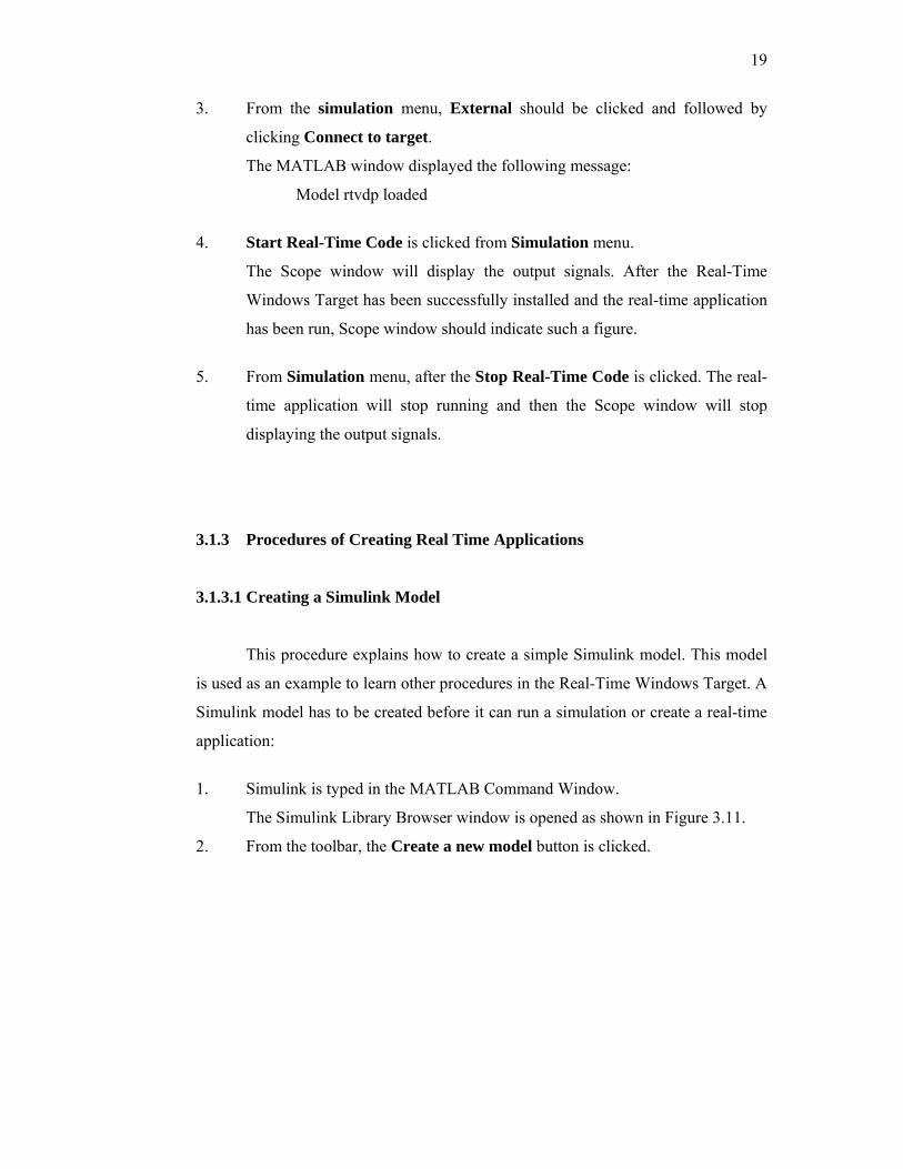
3. From the simulation menu, External should be clicked and followed by

clicking Connect to target.

The MATLAB window displayed the following message:

Model rtvdp loaded

4. Start Real-Time Code is clicked from Simulation menu.

The Scope window will display the output signals. After the Real-Time

Windows Target has been successfully installed and the real-time application

has been run, Scope window should indicate such a figure.

5. From Simulation menu, after the Stop Real-Time Code is clicked. The real-

time application will stop running and then the Scope window will stop

displaying the output signals.

3.1.3 Procedures of Creating Real Time Applications 3.1.3.1 Creating a Simulink Model This procedure explains how to create a simple Simulink model. This model

is used as an example to learn other procedures in the Real-Time Windows Target. A

Simulink model has to be created before it can run a simulation or create a real-time

application:

1. Simulink is typed in the MATLAB Command Window.

The Simulink Library Browser window is opened as shown in Figure 3.11.

2. From the toolbar, the Create a new model button is clicked.

20

Figure 3.3: Create a new model

An empty Simulink window is opened. With the toolbar and status bar

disabled, the window looks like following figure 3.12 (Figure).

Figure 3.4: Empty Simulink model

3. In the Simulink Library Browser window, Simulink is double-clicked and

then Sources is also doubled-clicked. Next, Signal Generator is clicked and

dragged to Simulink window.

Sinks is clicked. Scope is clicked and dragged to the Simulink window. Real-

Time Windows Target is clicked. Analog Output is clicked and dragged to

the Simulink window.

21

4. The Signal Generator output is connected to the scope input by clicking-

and-dragging a line between the blocks. Likewise, the Analog Output input

is connected to the connection between Scope and Signal Generator.

5. The Signal Generator block is double clicked. The Block Parameters dialog

box opened. From the Wave form list, square is selected.

In the Amplitude text box, 0.25 is entered.

In the Frequency text box, 2.5 are entered.

From the Units list, Hertz is selected.

The Block Parameters dialog box is shown in Figure 3.13.

Figure 3.5: Block Parameters of Signal Generator

6. OK is clicked. 7. The analog output block is double clicked.

The Block Parameters dialog box will open.

8. The Install new board button is clicked. From the list, it should be pointed to

manufacturer and then clicked a board name. For example, it should be

pointed to Advantech and then click PCL818.

9. One of the following is selected:

• For an ISA bus board, a base address is entered. This value must

match the base address switches or jumpers set on the physical board.

For example, to enter a base address of 0x300 in the address box, 300

is typed. The base address also could be selected by selecting check

boxes A9 through A3.

22

• For a PCI bus board, the PCI slot is entered or the Auto-detect check

box is selected.

10. The Test button is clicked.

The Real-Time Windows Target tried to connect to the selected board and the

following message would display if successful.

11. On the message box, OK is clicked. 12. The same value as entered in the Fixed step size box from the Configuration

Parameters dialog box is entered in the Sample time box. For example,

0.001 is entered.

13. A channel vector that selected the analog input channels that are using on this

board is entered in the Output channels box. The vector can be any valid

MATLAB vector form. For example, to select analog output channel on

PCL818 board 1 is entered.

14. The input range for the entire analog input channel that has been entered in

the Input channels box is chosen from the Output range list. For example,

with the PCL818 board, 0 to 5V is chosen.

15. From the Block Input signal list, the following options is chosen:

• Volts – Expected a value equal to the analog output range.

• Normalized unipolar – Expected a value between 0 and +1 that is

converted to the full range of the output voltage regardless of the

output voltage range. For example, an analog output range of 0 to +5

volts and -5 to +5 volts would both converted from values between 0

and +1.

• Normalized bipolar – Expected a value between -1 and +1 that is

converted to the full range of output voltage regardless of the output

voltage range.

• Raw – Expected a value of 0 to 2n-1. For example, a 12-bit A/D

converter would expected a value between 0 and 212 -1 (0 to 4095).

The advantage of this method is the expected value is always an

integer with no round off error.

23

16. The initial value is entered for each analog output channel that has been

entered in the Output Channels box. For example, if 1 is entered in the

Output Channels box and the initial value of 0 volts is needed, 0 is entered.

17. The final value is entered for each analog channel that has been entered in

Output Channels box. For example, if 1 is entered in the Output Channels

box and the final value of 0 volts is needed, 0 is entered.

The dialog box would look similar to the Figure 3.14 if Volts is chosen.

Figure 3.6: Block Parameters of Analog Output

18. One of following is executed:

Apply is clicked to apply the changes to the model and the dialog box

is left open.

OK is clicked to apply the changes to the model and the Block

Parameters: Analog Output dialog box will close.

24

19. Parameters dialog box is closed and the parameter values are saved with the

Simulink model.

20. In the Simulink window, the Scope block is double clicked.

A Scope window will open.

21. The Parameters button is clicked.

A Scope parameters dialog box will open.

22. The General tab is clicked. The number of graphs that is needed in one

Scope window is entered in the Number of axes box. For example, 1 is

entered for a single graph. Do not select the floating scope check box. In the

Time range box, upper value the time range is entered. For example, 1

second is entered. From the Tick labels list, bottom axis only is chosen.

From the Sampling list, decimation is chosen and 1 is entered in the text box.

The Scope parameters dialog box would look like such a Figure 3.15 as

shown.

Figure 3.7: Scope Parameters Dialog Box 23. One of following done:


is left open.

OK is clicked to apply the changes to the model and the Scope

parameters dialog box is closed.

25

24. In the Scope window, it should be pointed to the y-axis and then right

clicked.

25. Axes Properties is clicked from the pop-up menu. 26. The Scope properties: axis 1 dialog box is opened. In the Y-min and Y-max

text boxes, the range for the y-axis is entered in the Scope window. For

example, -2 and 2 are entered as shown in the Figure 3.16

Figure 3.8: Scope Properties: axis 1

27. One of the following is done:


is left open.

OK is clicked to apply the changes to the model and the Axes

Parameters dialog box is closed.

The completed Simulink block diagram is shown in Figure 3.17.

developing lqr to control speed motor using...

Documents