development and application of a cellular system simulator...
TRANSCRIPT

Development and Application of a Cellular System Simulator for an Evaluation of Signaling
Performance and Efficiency
Accepting the Challenges of IP-based UMTS Radio Access Network Evolution Scenarios
Dissertation
zur Erlangung des akademischen Grades
Doktor der Naturwissenschaften
Dr. rer. nat.
im Fach Informatik
von
Dipl.-Wirt. Inf. Anja Wiedemann geb. in München
Vorgelegt beim
Institut für Informatik und Wirtschaftsinformatik
der Universität Duisburg-Essen
im Juni 2006
Datum der mündlichen Prüfung: 18. Juni 2007
Gutachter: Prof. Dr.-Ing. Erwin P. Rathgeb (Universität Duisburg-Essen) Prof. Dr. Bruno Müller-Clostermann (Universität Duisburg-Essen)


I
Abstract The tendency in future mobile Radio Access Networks (RANs) consists in an increase of new and Internet Protocol (IP)-based services with strict requirements regarding bandwidth and Quality of Service (QoS) and in a dominance of packet data traffic in future mobile networks. Existing mobile networks (e.g. Universal Mobile Telecommunications System (UMTS) Release 99 (R99)), which are designed assuming a predominance of circuit switched traffic, are not suitable to efficiently carry IP traffic under consideration of the hierarchical and centralistic network structure of existing mobile networks, the coupling of user and control plane and the strict delay requirements in the RAN. Consequently, an architecture evolution of mobile RANs with regard to their network architecture has to take place. Within the cooperation of Lucent Technologies and the University of Duisburg-Essen in the project IPonAir, funded by the German Ministry for Education and Research (Bundesministerium für Bildung und Forschung (BMBF)), and within the work carried out for this thesis, a flexible, efficient and tool-supported approach was developed that allows for an evaluation of future mobile RANs with regard to signaling performance. This approach provides decision support to the designer of future mobile networks in a very early design phase. The evaluation approach comprises a methodology for event-driven simulation of signaling sequences, depicted in the form of Message Sequence Charts (MSCs), as well as a toolkit – both, i.e. the simulation methodology as well as the toolkit, enable an optimization as well as an assessment of future mobile RANs with regard to signaling performance as well as a comparison with the UMTS R99 as a reference architecture. In the thesis on hand, the above mentioned evaluation approach is presented in detail. Moreover, the approach is applied to potential evolution scenarios of mobile RANs. On the one hand these RAN evolution scenarios are optimized with regard to signaling performance. On the other hand the RAN evolution scenarios are compared to the UMTS R99 reference architecture with regard to their signaling performance behavior. Keywords:
UMTS, UTRAN Evolution, Message Sequence Charts, Signaling Performance, Event-driven Simulation


III
Zusammenfassung Der Trend in zukünftigen Mobilfunknetzen besteht in einer Zunahme neuer, Internet Protocol (IP)-basierter Dienste mit strikten Anforderungen an die benötigte Bandbreite und Dienstgüte der Verbindung und infolge dessen einer Dominanz von Paketdatenverkehr in zukünftigen mobilen Netzen. Existierende Mobilfunknetze (z.B. Universal Mobile Telecommunications System (UMTS) Release 99 (R99)), die unter Berücksichtigung einer Dominanz von Sprachdatenverkehr konzipiert wurden, sind im Hinblick auf diesen Trend ungeeignet und zwar aufgrund ihrer hierarchischen und zentralistischen Netzwerkarchitektur, sowie der Kopplung von User und Control Plane und aufgrund ihrer strikten Anforderungen und Sensibilität im Hinblick auf Verzögerungen im Bereich des Funknetzes. Folglich ist eine Evolution der Mobilfunknetze hinsichtlich ihrer Netzwerkarchitektur notwendig. Im Projekt IPonAir des Bundesministeriums für Bildung und Forschung (BMBF) wurde im Rahmen einer Projekt-Kooperation von Lucent Technologies und der Universität Duisburg-Essen, sowie im Rahmen der vorliegenden Dissertation, ein flexibler, effizienter und Werkzeug-unterstützter Ansatz entwickelt, der eine Evaluierung zukünftiger Funknetz-Architekturen im Hinblick auf deren Signalisierungsperformanz ermöglicht und damit eine Entscheidungsunterstützung für den Designer zukünftiger Mobilfunknetz-Architekturen in einer sehr frühen Design-Phase bietet. Der Evaluierungsansatz umfaßt eine Methodik zur ereignisorientierten Simulation von Signalisierungsabläufen, die in Form von Message Sequence Charts (MSCs) abgebildet werden, und einen zugehörigen Werkzeugsatz – beides ermöglicht die Optimierung und Leistungsbewertung zukünftiger Funknetz-Architekturen im Hinblick auf deren Signalisierungsperformanz sowie einen Vergleich mit der UMTS R99 Referenzarchitektur. In der vorliegenden Dissertation wird der oberhalb genannte Evaluierungsansatz detailliert vorgestellt und auf potentielle Mobilfunknetz-Evolutionsszenarien angewendet. Dabei werden die Evolutionsszenarien einerseits hinsichtlich ihrer Signalisierungsperformanz optimiert, und andererseits im Hinblick auf die Signalisierungsperformanz mit der UMTS R99 Referenzarchitektur verglichen. Schlagworte:
UMTS, UTRAN Evolution, Message Sequence Charts, Signalisierungsperformanz, Ereignisorientierte
Simulation


V
Acknowledgements The research activities, on which this thesis is based, were accomplished during my employment in the Computer Networking Technology Group (University of Duisburg-Essen). Moreover, the research work for this thesis had been partly performed during a project cooperation with Lucent Technologies. Therefore, I would like to thank my colleagues Dr. Peter Schefczik, Dr. Michael Söllner and Wilfried Speltacker from Lucent Technologies Bell Labs Europe, Nuremberg, for a good cooperation, when working together within the German funded BMBF project IPonAir. In this context, I also want to include Prof. Dr.-Ing. habil. Andreas Mitschele-Thiel, who formerly also was a colleague working at Lucent Technologies, but in the meantime became the leader of the Integrated Hardware and Software Systems Department at the Technical University of Ilmenau. I appreciated interesting discussions with the colleagues mentioned above that were inspiring for me, when creating new research ideas. Moreover, the longtime professional experience of these colleagues, their colleagueship and humaneness were beneficial for me. Particularly, I would like to express my gratitude to my colleague Dr. Peter Schefczik, who read my thesis and supported me with constructive criticism. It was at the OPNETWORK 2004 conference, when I asked him for this favor, and he promised to do it. Although he had been very busy at work all the time, he did not let me down with it. Finally, I also would like to thank my family on which I could always count. They kept me grounded, and without their support, this thesis would never have come true. Therefore, I dedicate this work to my family. —


IX
Contents
Abstract ............................................................................................................................................. I
Zusammenfassung......................................................................................................................... III
Acknowledgements.........................................................................................................................V
Contents..........................................................................................................................................IX
List of figures................................................................................................................................XIII
List of tables ............................................................................................................................... XVII
List of abbreviations ................................................................................................................... XIX
1 Introduction.............................................................................................................................. 1
1.1 Evolution of mobile wireless communication systems....................................................... 1
1.2 Context of the thesis .......................................................................................................... 3
1.3 Related research activities................................................................................................. 4 1.3.1 Research in the area of UMTS performance evaluation....................................................... 4 1.3.2 Research in the area of RAN evolution ................................................................................ 5
1.4 Outline of the thesis ........................................................................................................... 6
2 Architectures and protocols for 3G and beyond.................................................................. 7
2.1 UMTS protocol model ........................................................................................................ 8 2.1.1 Domain concept ................................................................................................................... 8 2.1.2 Strata concept ...................................................................................................................... 9 2.1.3 High-level overview of the UMTS protocol model............................................................... 10 2.1.4 Protocol model of the Access Stratum ............................................................................... 10
2.1.4.1 Protocol structure of the Uu interface......................................................................................11 2.1.4.2 Protocol structure of the Iu interface .......................................................................................14 2.1.4.3 Protocol structure of the Iub interface .....................................................................................18 2.1.4.4 Protocol structure of the Iur interface ......................................................................................20
2.1.5 Protocol architecture of the Non-Access Stratum............................................................... 21
2.2 UMTS network architecture evolution.............................................................................. 24 2.2.1 Release 99 PLMN infrastructure ........................................................................................ 24 2.2.2 Release 4 PLMN infrastructure .......................................................................................... 25 2.2.3 Release 5 PLMN infrastructure .......................................................................................... 27 2.2.4 Release 6 PLMN infrastructure .......................................................................................... 31
2.3 IP radio access network evolution ................................................................................... 31 2.3.1 Nokia proposal for UTRAN architecture evolution .............................................................. 32 2.3.2 Siemens proposal for UTRAN architecture evolution ......................................................... 33 2.3.3 NEC proposal for UTRAN architecture evolution................................................................ 35 2.3.4 Lucent proposal for UTRAN architecture evolution ............................................................ 36 2.3.5 Alcatel proposal for UTRAN architecture evolution ............................................................ 37 2.3.6 Merged Radio Access Network (MRAN) ............................................................................ 39 2.3.7 Condensed view of company proposals............................................................................. 42
3 Simulation modeling methodology...................................................................................... 45
3.1 Discrete event simulation................................................................................................. 45
3.2 Simulation toolkit OPNET Modeler .................................................................................. 46 3.2.1 OPNET modeling domains and model specification........................................................... 47 3.2.2 Simulation execution, data collection and data analysis..................................................... 54
Contents _______________________________________________________________________________________
X
3.3 Message Sequence Charts (MSCs).................................................................................55 3.3.1 Basic principles of the MSC language................................................................................ 56 3.3.2 Time concept of the MSC language ................................................................................... 59 3.3.3 High-level structural concepts of the MSC language.......................................................... 61 3.3.4 Integration of Data in the MSC language ........................................................................... 64 3.3.5 Principles of object orientation in the MSC language ......................................................... 66
3.4 Message Sequence Chart (MSC)-based simulation methodology ..................................66 3.4.1 Applied modeling concepts of the MSC language.............................................................. 67 3.4.2 Performance extensions of the MSC language .................................................................. 67 3.4.3 Generic node modeling concept......................................................................................... 68 3.4.4 Abstract MSC sequence according to the developed modeling methodology.................... 70 3.4.5 Signaling in the UMTS Control Plane according to standardization ................................... 71 3.4.6 Signaling in the UMTS Control Plane according to the developed modeling
methodology....................................................................................................................... 73 3.4.7 Allocation of FEs to network elements and resources in the UTRAN Control Plane .......... 74 3.4.8 Traffic model....................................................................................................................... 76 3.4.9 Providing scalability............................................................................................................ 80 3.4.10 Assessing the modeling methodology and alternatives...................................................... 82
4 Simulator concept and implementation ..............................................................................85
4.1 Tool chain .........................................................................................................................85 4.1.1 Traffic model parameters ................................................................................................... 86 4.1.2 FE-to-resource configuration.............................................................................................. 90 4.1.3 Technical MSC sequence notation and VBA algorithm...................................................... 93 4.1.4 High-level overview of the OPNET simulator ..................................................................... 98
4.2 Implementation concept ...................................................................................................98 4.2.1 Configurability of FE modules via attributes ....................................................................... 99 4.2.2 Configurability of resource modules via attributes............................................................ 100 4.2.3 Configurability of traffic source modules via attributes ..................................................... 101 4.2.4 Central traffic control manager ......................................................................................... 103 4.2.5 Establishment of coherences between traffic source modules via attributes.................... 106 4.2.6 Configuration of handover, SRNS relocation and paging traffic source modules via
attributes .......................................................................................................................... 107 4.2.7 Adaptation of the implementation for a GUI-based composition of network nodes
from modules.................................................................................................................... 108 4.2.8 Advanced addressing concept for network elements ....................................................... 110 4.2.9 Representation of affiliations between network elements................................................. 113 4.2.10 Routing implementation for the exchange of signaling messages between network
elements........................................................................................................................... 115 4.2.11 Example usage of advanced addressing concept, representation of affiliations
between network elements and external routing concept................................................. 115 4.2.12 Representation of adjacency relationships between network elements for handover
and broadcast signaling ................................................................................................... 117 4.2.13 Packet format of the OPNET simulator ............................................................................ 118 4.2.14 Example usage of adjacency relationships between network elements for handover
signaling ........................................................................................................................... 120
5 Architecture evaluation .......................................................................................................125
5.1 Reference architecture and evolution scenarios ............................................................125 5.1.1 UTRAN reference architecture ......................................................................................... 125
5.1.1.1 Calibration of the UTRAN reference architecture..................................................................125 5.1.1.2 Simulation results of the calibrated reference architecture....................................................126
5.1.2 Merged Radio Access Network (MRAN) .......................................................................... 131 5.1.2.1 ATM-based MRAN ...............................................................................................................131
5.1.2.1.1 ATM-based MRAN architecture dimensioning by optimization......................................................133 5.1.2.1.2 Optimization of Soft Handover signaling performance in the ATM-based MRAN.........................137
5.1.2.2 IP-based MRAN ...................................................................................................................138 5.1.2.2.1 IP-based MRAN architecture dimensioning by optimization..........................................................140 5.1.2.2.2 Optimization of Soft Handover signaling performance in the IP-based MRAN .............................143

Contents __________________________________________________________________________________________
XI
5.1.3 Distributed Radio Access Network (DRAN)...................................................................... 145 5.1.3.1 DRAN architecture dimensioning by optimization..................................................................147
5.1.3.1.1 First allocation approach of FEs to resources in DRAN Control Plane .........................................147 5.1.3.1.2 Second allocation approach of FEs to resources in DRAN Control Plane....................................150 5.1.3.1.3 Optimization of Soft and Hard Handover signaling performance in DRAN ...................................152
5.2 Comparison of signaling performance and efficiency.................................................... 160 5.2.1 Preview on upcoming simulation experiments.................................................................. 160 5.2.2 Variation of the number of users within different traffic mixes .......................................... 161
5.2.2.1 Comparison of ATM-based MRAN signaling performance to the UTRAN reference architecture...........................................................................................................................161
5.2.2.2 Comparison of IP-based MRAN signaling performance to the UTRAN reference architecture...........................................................................................................................165
5.2.2.3 Comparison of DRAN signaling performance to the UTRAN reference architecture..............169 5.2.3 Full meshing of the base stations ..................................................................................... 175
5.2.3.1 Meshed IP-based MRAN ......................................................................................................175 5.2.3.2 Meshed DRAN......................................................................................................................178
5.2.4 Dynamic load impulses..................................................................................................... 180 5.2.5 Variation of the mobility behavior ..................................................................................... 182 5.2.6 Further possibilities of the simulator ................................................................................. 184
6 Conclusion and outlook...................................................................................................... 189
6.1 Summary of the thesis ................................................................................................... 189
6.2 Future steps ................................................................................................................... 192
Bibliography ................................................................................................................................ 197
Index ............................................................................................................................................. 209


XIII
List of figures Fig. 2.1: UMTS architecture [3GPP2002c] ........................................................................................ 7 Fig. 2.2: UTRAN architecture [3GPP2002c] ...................................................................................... 7 Fig. 2.1.1: UMTS domains and reference points [3GPP2000b]............................................................ 8 Fig. 2.1.2: Interrelationship of UMTS domains and strata [3GPP2000b].............................................. 9 Fig. 2.1.3: High-level overview of the UMTS protocol model [3GPP2002c]........................................ 10 Fig. 2.1.4: 3GPP general protocol model of the Access Stratum for UTRAN interfaces
[3GPP2002c]..................................................................................................................... 10 Fig. 2.1.5: Uu interface protocol architecture (following [3GPP2002i]) ............................................... 12 Fig. 2.1.6: Iu interface towards CS domain of CN [3GPP2002h]........................................................ 14 Fig. 2.1.7: Iu interface towards PS domain of CN [3GPP2002h] ........................................................ 14 Fig. 2.1.8: Iub interface protocol structure [3GPP2002d] ................................................................... 18 Fig. 2.1.9: Iur interface protocol structure [3GPP2002b] .................................................................... 20 Fig. 2.1.10: Protocol architecture of the Non-Access Stratum supporting CS and PS mode of
operation within a UE [3GPP2004d].................................................................................. 21 Fig. 2.1.11: Network architecture view on protocol architecture of the Non-Access Stratum (CS /
PS mode of operation) (according to [3GPP2004d]) ......................................................... 23 Fig. 2.2.1: R99 PLMN [3GPP2002g] .................................................................................................. 24 Fig. 2.2.2: Rel-4 PLMN [3GPP2003i] ................................................................................................. 26 Fig. 2.2.3: Rel-5 PLMN (following [3GPP2003p, 3GPP2003x] ........................................................... 28 Fig. 2.2.4: IuCS interface towards CN of IP-based UTRAN (following [3GPP2003x])........................ 29 Fig. 2.2.5: IuPS interface towards CN of IP-based UTRAN (following [3GPP2003x]) ........................ 30 Fig. 2.2.6: Iub interface of IP-based UTRAN (following [3GPP2003x]) .............................................. 30 Fig. 2.2.7: Iur interface of IP-based UTRAN (following [3GPP2003x]) ............................................... 31 Fig. 2.3.1: Nokia architecture proposal on UTRAN evolution (following [3GPP2003e]) ..................... 32 Fig. 2.3.2: Siemens architecture proposal on UTRAN evolution [3GPP2003h].................................. 33 Fig. 2.3.3: NEC architecture proposal on UTRAN evolution [3GPP2003r] ......................................... 35 Fig. 2.3.4: Lucent architecture proposal on UTRAN evolution [BaScSo2003] .................................... 36 Fig. 2.3.5: Decomposition of RNC into functional entities [3GPP2003d] ............................................ 38 Fig. 2.3.6: Conjunction of functional entities and mapping to UTRAN architecture [3GPP2003d]...... 39 Fig. 2.3.7: ATM-based MRAN architecture [MiScWi2005].................................................................. 40 Fig. 2.3.8: IP-based MRAN ................................................................................................................ 40 Fig. 2.3.9: Feature subset for review of UTRAN evolution architecture proposals ............................. 42 Fig. 3.1.1: Ways to study a system (following [LaKe2000])................................................................ 45 Fig. 3.2.1: OPNET Modeler Network Domain..................................................................................... 47 Fig. 3.2.2: OPNET Modeler Network / Node Domain ......................................................................... 48 Fig. 3.2.3: State Executives (OPNET Modeler Process Domain)....................................................... 49 Fig. 3.2.4: Source module (OPNET Modeler Node / Process Domain).............................................. 50 Fig. 3.2.5: Queue + Service module (OPNET Modeler Node / Process Domain) .............................. 51 Fig. 3.2.6: Sink module (OPNET Modeler Node / Process Domain) .................................................. 52 Fig. 3.2.7: Relationship of hierarchical levels in OPNET models [OPN2003]..................................... 53 Fig. 3.3.1: Basic MSC (graphical (a) / textual (b) representation) (following [ITU1999b])................... 56 Fig. 3.3.2: MSC with general order mechanism (based on [ITU1999b])............................................. 57 Fig. 3.3.3: Instance creation (based on [ITU1999b]) .......................................................................... 57 Fig. 3.3.4: Conditions (based on [ITU1999b])..................................................................................... 58 Fig. 3.3.5: Timer stop (a) / expiration (a1) and action (based on [ITU1999b]).................................... 59 Fig. 3.3.6: Observation of time by absolute / relative measurements (a) and time constraints (a1)
(following [ITU1999b]) ....................................................................................................... 60 Fig. 3.3.7: HMSCs with sequence (a), alternative (a1), parallelism (a2) and loop (a3) (based on
[ITU1998]) ......................................................................................................................... 61 Fig. 3.3.8: Inline expressions (alternative, parallelism, loop, exception, option) (based on
[ITU1999b]) ....................................................................................................................... 62 Fig. 3.3.9: MSC references and MSC reference expressions (based on [ITU1999b])........................ 63 Fig. 3.3.10: Coregion without (a) / with (a1) general ordering (based on [ITU1998, ITU1999b]).......... 63 Fig. 3.3.11: MSC data usage (based on [ITU1999b])........................................................................... 65 Fig. 3.3.12: MSC inheritance and virtuality (graphical ((a) / (a1)) and textual ((b) / (b1))
representation) (based on [ITU1999b]) ............................................................................. 66
List of figures __________________________________________________________________________________________
XIV
Fig. 3.4.1: Generic node modeling concept (following [WiScNi2003])................................................ 69 Fig. 3.4.2: Resource model [MiScWi2005] ......................................................................................... 69 Fig. 3.4.3: Short annotated MSC sequence (based on [MiScWi2004]) .............................................. 70 Fig. 3.4.4: RRC Connection Establishment signaling [3GPP2002a] .................................................. 72 Fig. 3.4.5: Refined RRC Connection Establishment signaling sequence [Alt2004]............................ 73 Fig. 3.4.6: Allocation of FEs to resources and network elements in UTRAN Control Plane
(following [MiScWi2005])................................................................................................... 74 Fig. 4.1.1: Survey of the tool chain (following [MiScWi2004]) ............................................................ 85 Fig. 4.1.2: Traffic model parameters for UTRAN service-mix derivation (based on [Spe2002]) ......... 87 Fig. 4.1.3: OPNET environment file derived from GUI-based Excel workbook traffic model
calculation ......................................................................................................................... 89 Fig. 4.1.4: FE / resource configuration sheet within Microsoft Excel (following [Soe2004b]).............. 90 Fig. 4.1.5: OPNET environment file for nodes and FE modules derived from GUI-based Excel
workbook by application of VBA algorithm ........................................................................ 91 Fig. 4.1.6: UTRAN Network Domain model within OPNET Modeler .................................................. 91 Fig. 4.1.7: Node Domain model of Node B within OPNET Modeler ................................................... 92 Fig. 4.1.8: Refined RRC Connection Establishment signaling sequence (as part of MO Voice Call
Establishment signaling SF) annotated in formal MSC sequence notation within Microsoft Excel [Alt2004]................................................................................................... 93
Fig. 4.1.9: RRC Connection Release signaling sequence according to [Alt2004] annotated in formal MSC sequence notation within Microsoft Excel...................................................... 94
Fig. 4.1.10: Excerpt from refined RRC Connection Release signaling sequence with SA according to [Alt2004] ........................................................................................................................ 94
Fig. 4.1.11: Excerpt from OPNET environment file for FE RRC_Connection_Mgm within node UE derived from GUI-based Excel workbook by application of VBA algorithm (RRC Connection Establishment signaling) ................................................................................ 95
Fig. 4.1.12: Excerpt from OPNET environment file for FE RRC_Connection_Mgm within node RNC derived from GUI-based Excel workbook by application of VBA algorithm (RRC Connection Release Signaling) ......................................................................................... 96
Fig. 4.1.13: OPNET environment file for traffic source modules derived from GUI-based Excel workbook by application of VBA algorithm ........................................................................ 97
Fig. 4.1.14: OPNET environment file for sink modules derived from GUI-based Excel workbook by application of VBA algorithm ............................................................................................. 97
Fig. 4.2.1: Attributes of FE module (FE Info Table and FE Supplementary Actions Table) (following [Wie2002b, Wie2002c, WiAt2003]) ................................................................... 99
Fig. 4.2.2: Proto-C code of functions for loading the message processing tables within the FE modules [Wie2005b] ....................................................................................................... 100
Fig. 4.2.3: Attributes of resource module (according to [WiAt2003]) ................................................ 101 Fig. 4.2.4: Attributes of traffic source module and exemplified settings for UTRAN signaling SFs
(cf. [Wie2002c, Wie2004a, Wie2004b])........................................................................... 101 Fig. 4.2.5: Proto-C code snippet for voice call setup scheduling taken from OPNET process
model of the traffic source module [Wie2005b] ............................................................... 102 Fig. 4.2.6: Traffic source interactions (following [Wie2004e])........................................................... 103 Fig. 4.2.7 (a): Sender and receiver traffic source modules of interrupt codes ....................................... 104 Fig. 4.2.7 (b): Interrupt codes, conditions and actions........................................................................... 105 Fig. 4.2.8: Proto-C code snippet for voice call release scheduling within the UE node taken from
OPNET process model of the traffic source module [Wie2005b] .................................... 107 Fig. 4.2.9: Example of a UTRAN network topology.......................................................................... 108 Fig. 4.2.10: Proto-C code of the function for automatical derivation of an IR table [Wie2005b] ......... 109 Fig. 4.2.11: Interconnections of IR module within Node B illustrated in Fig. 4.1.7 and corresponding
IR_Routing_Table ........................................................................................................... 109 Fig. 4.2.12: UTRAN example network topology ................................................................................. 110 Fig. 4.2.13: Simple addressing concept with node identifier .............................................................. 111 Fig. 4.2.14: Advanced addressing concept of [Wie2003] ................................................................... 112 Fig. 4.2.15: UTRAN example network topology for derivation of affiliations....................................... 113 Fig. 4.2.16: Array Topo_Vec_NoID of network topology illustrated in Fig. 4.2.15.......................... 114 Fig. 4.2.17: Tables Topo_Tab_NoID and Topo_Tab_InID of network topology illustrated in
Fig. 4.2.15 ....................................................................................................................... 114 Fig. 4.2.18: External routing table of network element RNC (2,0) ...................................................... 115 Fig. 4.2.19: Proto-C code returning an outstream for packet transmission [Wie2005b] ..................... 116

List of figures __________________________________________________________________________________________
XV
Fig. 4.2.20: Adjacency relationships of node RNC (2,0) derived from network topology illustrated in Fig. 4.2.15 ....................................................................................................................... 117
Fig. 4.2.21: Packet format used within OPNET simulator [Wie2002c, WiAt2003, Wie2004c, Wie2004f, Wie2005a] ...................................................................................................... 118
Fig. 4.2.22: Inter-RNC Hard/Soft Handover scenario ......................................................................... 120 Fig. 4.2.23: Proto-C Code returning a list of UEs [Wie2005b] ............................................................ 122 Fig. 5.1.1.1.1: UTRAN network topology within OPNET Modeler........................................................... 126 Fig. 5.1.1.2.1: Variation of number of users per RNS and E2E signaling performance within UTRAN
reference network architecture (50/50 traffic mix) ........................................................... 129 Fig. 5.1.1.2.2: Resource utilization within UTRAN reference architecture (50/50 traffic mix) ................. 130 Fig. 5.1.2.1.1: Allocation of FEs to network elements in the Control Plane of the ATM-based MRAN
[MiScWi2005] .................................................................................................................. 131 Fig. 5.1.2.1.2: RRC Connection Establishment within the ATM-based MRAN [AlWi2005a]................... 132 Fig. 5.1.2.1.1.1: First allocation approach of FEs to resources in ATM-based MRAN Control Plane........ 133 Fig. 5.1.2.1.1.2: ATM-based MRAN network topology within OPNET Modeler......................................... 134 Fig. 5.1.2.1.2.1: Capacity optimization of the BSC Resource within the MRAN Merged Node B............ 137 Fig. 5.1.2.2.1: Allocation of FEs to network elements in the Control Plane of the IP-based MRAN ....... 139 Fig. 5.1.2.2.2: RRC Connection Establishment within the IP-based MRAN and MPLS / RSVP-TE-
based transport network [AlWi2005b].............................................................................. 139 Fig. 5.1.2.2.1.1: MRAN network topology with IP-based transport network within OPNET Modeler ......... 140 Fig. 5.1.2.2.1.2: Allocation of FEs to resources in MRAN Control Plane by application of an IP-based
transport network............................................................................................................. 141 Fig. 5.1.2.2.2.1: Capacity optimization of the BSC Resource within the Merged Node B ....................... 143 Fig. 5.1.3.1: Allocation of FEs to network elements in DRAN Control Plane....................................... 145 Fig. 5.1.3.2: RRC Connection Establishment in DRAN [AlBa2004]..................................................... 146 Fig. 5.1.3.1.1.1: First allocation approach of FEs to resources in DRAN Control Plane............................ 147 Fig. 5.1.3.1.1.2: DRAN network topology within OPNET Modeler............................................................. 148 Fig. 5.1.3.1.2.1: Second allocation approach of FEs to resources in DRAN Control Plane....................... 150 Fig. 5.1.3.1.3.1: Application of resource parameter configuration according to Table 5.1.3.1.2.1 and
E2E signaling performance results within DRAN (50/50 traffic mix) ................................ 152 Fig. 5.1.3.1.3.2: Utilization of resources located within iNode B and RAN Server (50/50 traffic mix) ........ 153 Fig. 5.1.3.1.3.3: Resource utilization during speed increase of Main Resource within RAN Server
(50/50 traffic mix)............................................................................................................. 153 Fig. 5.1.3.1.3.4: Queueing delays during speed increase of Main Resource within RAN Server (50/50
traffic mix)........................................................................................................................ 154 Fig. 5.1.3.1.3.5: Behavior of E2E signaling SFs during bottleneck resolution of Main Resource within
RAN Server (50/50 traffic mix)......................................................................................... 154 Fig. 5.1.3.1.3.6: Increase of Transport Network Resource capacity within RAN Server and impact
on signaling E2E of SF 17 (Inter-iNode B Soft Handover) and SF 19 (Inter-iNode B Hard Handover) (50/50 traffic mix) .................................................................................. 155
Fig. 5.1.3.1.3.7: Speed increase of Main Resource within iNode B and impact on signaling E2E of SF 17 (Inter-iNode B Soft Handover) and SF 19 (Inter-iNode B Hard Handover) (50/50 traffic mix)........................................................................................................................ 157
Fig. 5.1.3.1.3.8: Reconfigured Iui interface and speed increase of Main Resource within iNode B and impact on signaling E2E of SF 19 (Inter-iNode B Hard Handover) (50/50 traffic mix) ..... 158
Fig. 5.2.2.1.1: Signaling performance comparison of UTRAN and ATM-based MRAN for signaling SF 1 (MO Voice / CS Data Call Establishment) and 9 (MO PDP Context Activation) in the 20/80 traffic mix............................................................................................................... 162
Fig. 5.2.2.1.2 (a): Signaling performance comparison of UTRAN and ATM-based MRAN for signaling SF 15 (Softer Handover) and 17 (Soft Handover) in the 20/80 traffic mix............................. 163
Fig. 5.2.2.1.2 (b): Signaling performance comparison of UTRAN and ATM-based MRAN for signaling SF 19 (Hard Handover) and 20 (SRNS Relocation) in the 20/80 traffic mix.......................... 164
Fig. 5.2.2.2.1: Signaling performance comparison of UTRAN and IP-based MRAN for signaling SF 1 (MO Voice / CS Data Call Establishment) and 9 (MO PDP Context Activation) in the 20/80 traffic mix............................................................................................................... 166
Fig. 5.2.2.2.2 (a): Signaling performance comparison of UTRAN and IP-based MRAN for signaling SF 15 (Softer Handover) and 17 (Soft Handover) in the 20/80 traffic mix.................................. 167
Fig. 5.2.2.2.2 (b): Signaling performance comparison of UTRAN and IP-based MRAN for signaling SF 19 (Hard Handover) and 20 (SRNS Relocation) in the 20/80 traffic mix............................... 168
Fig. 5.2.2.3.1: Signaling performance comparison of UTRAN and DRAN for signaling SF 1 (MO Voice / CS Data Call Establishment) and 9 (MO PDP Context Activation) in the 20/80 traffic mix................................................................................................................................... 170

List of figures __________________________________________________________________________________________
XVI
Fig. 5.2.2.3.2 (a): Signaling performance comparison of UTRAN and DRAN for signaling SF 15 (Softer Handover) and 17 (Soft Handover) in the 20/80 traffic mix ............................................. 171
Fig. 5.2.2.3.2 (b): Signaling performance comparison of UTRAN and DRAN for the signaling SF 19 (Hard Handover) and 20 (SRNS Relocation) in the 20/80 traffic mix ........................................ 172
Fig. 5.2.2.3.3: Signaling performance comparison of UTRAN and DRAN for signaling SF 1 (MO Voice / CS Data Call Establishment) in the 80/20 traffic mix..................................................... 173
Fig. 5.2.2.3.4: Resource utilization in the 20/80 traffic mix..................................................................... 174 Fig. 5.2.2.3.5: Resource utilization in the 80/20 traffic mix..................................................................... 174 Fig. 5.2.3.1.2: Signaling performance comparison of UTRAN and meshed IP-based MRAN for
signaling SF 1 (MO Voice / CS Data Call Establishment) in the 20/80 traffic mix ........... 176 Fig. 5.2.3.1.3: Signaling performance comparison of UTRAN and meshed IP-based MRAN for
signaling SF 17 (Soft Handover) and 20 (SRNS Relocation) in the 20/80 traffic mix ...... 177 Fig. 5.2.3.2.1: Meshed DRAN network topology within OPNET Modeler ............................................... 178 Fig. 5.2.3.2.2: Signaling performance comparison of UTRAN and meshed DRAN for signaling SF 17
(Soft Handover) and 19 (Hard Handover) in the 20/80 traffic mix ................................... 179 Fig. 5.2.4.1: System behavior of UTRAN reference architecture and DRAN ...................................... 181 Fig. 5.2.4.2: System behavior of UTRAN reference architecture and ATM-based MRAN................... 181 Fig. 5.2.4.3: System behavior of UTRAN reference architecture and IP-based MRAN....................... 182 Fig. 5.2.5.1: Mobility variation in the 80/20 traffic mix.......................................................................... 183 Fig. 5.2.5.2: Mobility variation in the 20/80 traffic mix.......................................................................... 184

XVII
List of tables Table 2.1.1: Subset of significant functions of the RRC protocol [3GPP2002i] ..................................... 13 Table 2.1.2: Subset of significant RANAP functions (following [3GPP2003o])...................................... 16 Table 2.1.3: Subset of significant NBAP functions (in accordance with [3GPP2004g])......................... 19 Table 2.1.4: Subset of significant RNSAP functions (according to [3GPP2004f]) ................................. 21 Table 3.1.1: Generic components of discrete event simulation models (following [LaKe2000])............ 46 Table 3.4.1: UTRAN signaling SFs with short explanation.................................................................... 76 Table 3.4.2: Correlation between UTRAN signaling SFs ...................................................................... 78 Table 3.4.3: UTRAN signaling SFs and associations............................................................................ 79 Table 5.1.1.1.1: Resource parameter configuration of UTRAN reference architecture ............................. 125 Table 5.1.1.1.2: Link parameter configuration of UTRAN reference architecture...................................... 126 Table 5.1.1.2.1: Signaling E2E delays at the operating point of the UTRAN reference network
architecture (50/50 traffic mix) ......................................................................................... 127 Table 5.1.1.2.2: Itemization of partial processing delay at the operating point of the UTRAN reference
network architecture (50/50 traffic mix) ........................................................................... 128 Table 5.1.1.2.3: Itemization of partial queueing delay at the operating point of the UTRAN reference
network architecture (50/50 traffic mix) ........................................................................... 128 Table 5.1.1.2.4: Service level definition (operating point of the network, 50/50 traffic mix) ....................... 130 Table 5.1.2.1.1.1: Resource parameter derivation of the ATM-based MRAN from UTRAN......................... 133 Table 5.1.2.1.1.2: Initial resource parameter configuration within ATM-based MRAN ................................. 134 Table 5.1.2.1.1.3: Link parameter configuration within ATM-based MRAN.................................................. 134 Table 5.1.2.1.1.4: Consideration of Handover and SRNS Relocation in UTRAN and MRAN (operation
point of the network, 50/50 traffic mix)............................................................................. 135 Table 5.1.2.1.1.5: Signaling E2E delays at the operating point of the ATM-based MRAN architecture
before optimization (50/50 traffic mix) ............................................................................. 136 Table 5.1.2.1.1.6: Itemization of partial processing delay for Inter-Merged Node B Soft Handover at the
operating point of the ATM-based MRAN architecture before optimization (50/50 traffic mix) ................................................................................................................................. 136
Table 5.1.2.1.1.7: Itemization of partial queueing delay for Inter-Merged Node B Soft Handover at the operating point of the ATM-based MRAN architecture before optimization (50/50 traffic mix) ................................................................................................................................. 136
Table 5.1.2.1.2.1: Optimized resource parameter configuration within the ATM-based MRAN ................... 137 Table 5.1.2.1.2.2: Signaling E2E delays at the operating point of the ATM-based MRAN architecture after
optimization (50/50 traffic mix)......................................................................................... 138 Table 5.1.2.2.1.1: Link parameter configuration within IP-based MRAN...................................................... 140 Table 5.1.2.2.1.2: Resource parameter derivation of the IP-based MRAN from UTRAN............................. 141 Table 5.1.2.2.1.3: Initial resource parameter configuration within IP-based MRAN ..................................... 142 Table 5.1.2.2.1.4: Signaling E2E delays at the operating point of the IP-based MRAN architecture before
optimization (50/50 traffic mix)......................................................................................... 142 Table 5.1.2.2.1.5: Itemization of partial processing delay for Inter-Merged Node B Soft Handover at the
operating point of the IP-based MRAN architecture before optimization (50/50 traffic mix) ................................................................................................................................. 142
Table 5.1.2.2.1.6: Itemization of partial queueing delay for Inter-Merged Node B Soft Handover at the operating point of the IP-based MRAN architecture before optimization (50/50 traffic mix) ................................................................................................................................. 143
Table 5.1.2.2.2.1: Optimized resource parameter configuration within the IP-based MRAN........................ 143 Table 5.1.2.2.2.2: Signaling E2E delays at the operating point of the IP-based MRAN architecture after
optimization (50/50 traffic mix)......................................................................................... 144 Table 5.1.3.1.1.1: DRAN resource parameter configuration according to first allocation approach of FEs
to resources illustrated in Fig. 5.1.3.1.1.1........................................................................ 148 Table 5.1.3.1.1.2: Link parameter configuration of DRAN architecture ........................................................ 148 Table 5.1.3.1.1.3: Signaling E2E delays at the operating point of the DRAN architecture (1st experiment,
50/50 traffic mix).............................................................................................................. 149 Table 5.1.3.1.1.4: Itemization of partial processing delay for performance critical SFs at the operating
point of the DRAN architecture (1st experiment, 50/50 traffic mix)................................... 149 Table 5.1.3.1.1.5: Itemization of partial queueing delay for performance critical SFs at the operating point
of the DRAN architecture (1st experiment, 50/50 traffic mix) ........................................... 150 Table 5.1.3.1.2.1: DRAN resource parameter configuration according to allocation approach of FEs to
resources illustrated in Fig. 5.1.3.1.2.1............................................................................ 151
List of tables __________________________________________________________________________________________
XVIII
Table 5.1.3.1.2.2: Signaling E2E delays of particular SFs at the operating point of the DRAN architecture (2nd experiment, 50/50 traffic mix) ................................................................................... 151
Table 5.1.3.1.2.3: Itemization of partial processing delay at the operating point of the DRAN architecture (2nd experiment, 50/50 traffic mix) ................................................................................... 151
Table 5.1.3.1.2.4: Itemization of partial queueing delay at the operating point of the DRAN architecture (2nd experiment, 50/50 traffic mix) ................................................................................... 151
Table 5.1.3.1.3.1: DRAN resource parameter configuration after resource capacity increase of the Main and Transport Network Resources within the RAN Server ................................... 155
Table 5.1.3.1.3.2: Signaling E2E delays (point of observation: 1,5 million of users per RNS, 50/50 traffic mix) ................................................................................................................................. 155
Table 5.1.3.1.3.3: Itemization of partial processing delay (point of observation: 1,5 million of users per RNS, 50/50 traffic mix) .................................................................................................... 156
Table 5.1.3.1.3.4: Itemization of partial queueing delay (point of observation: 1,5 million of users per RNS, 50/50 traffic mix) .................................................................................................... 156
Table 5.1.3.1.3.5: DRAN resource parameter configuration after resource capacity modification of the Main Resource within the iNode B .............................................................................. 156
Table 5.1.3.1.3.6: Final DRAN resource parameter configuration after optimization ................................... 158 Table 5.1.3.1.3.7: Signaling E2E delays at the operating point of the DRAN architecture after optimization
(50/50 traffic mix) ............................................................................................................ 159 Table 5.2.1.1: Mean number of instantiations per minute for particular signaling SFs ........................... 160 Table 5.2.2.1.1: Assumptions for UTRAN / ATM-based MRAN signaling performance comparison......... 161 Table 5.2.2.2.1: Assumptions for UTRAN / IP-based MRAN signaling performance comparison............. 165 Table 5.2.2.3.1: Assumptions for UTRAN / DRAN signaling performance comparison ............................ 169 Table 5.2.2.3.2: Signaling E2E delays and partial delays of Inter-RNC / -iNode Hard Handover for
UTRAN and DRAN architecture at the operating point of the network (20/80 traffic mix) 173 Table 5.2.3.1.1: Link parameter configuration of meshed IP-based MRAN .............................................. 176 Table 5.2.3.2.1: Link parameter configuration of fully meshed DRAN....................................................... 178 Table 5.2.4.1: Number of voice calls and data connections according to Little’s Law............................ 180 Table 5.2.5.1: Mobility definition............................................................................................................. 182 Table 5.2.6.1: Impact of BHCA increase on instantiation rates of signaling SFs (20/80 traffic mix) ....... 185 Table 5.2.6.2: Service characterization.................................................................................................. 185 Table 5.2.6.3: Impact of BHDSA increase on instantiation rates of signaling SFs with regard to the
Email and FTP service (20/80 traffic mix)........................................................................ 186 Table 5.2.6.4: Experimental setup for a cell size optimization experiment ............................................. 187

XIX
List of abbreviations 1G 1st Generation 2G 2nd Generation 2.5G Generation 2.5 3G 3rd Generation 3GPP 3rd Generation Partnership Project A A Action AAL ATM Adaptation Layer AAL2 AAL Type 2 AAL5 AAL Type 5 Adja_Tab_NoID Local_Adjacence_Table_NodeID Adja_List_SAME_TyID list_of_adjacent_network_elements_with_same_typeID Adja_List_LOWER_TyID list_of_adjacent_network_elements_with_lower_typeID ALCAP Access Link Control Application Part AMPS American Mobile Phone System AMR Adaptive Multi Rate AN Access Network API Application Program Interface ARQ Automatic Repeat Request AS Access Stratum ASCII American Standard Code for Information Interchange ATM Asynchronous Transfer Mode AuC Authentication Centre B BP Basic Procedure BCCH Broadcast Control Channel BGCF Breakout Gateway Control Function BHCA Busy Hour Call Attempt BHDSA Busy Hour Data Session Attempt B-ISDN Broadband-ISDN BMC Broadcast/Multicast Control BSC Base Station Controller BSS Base Station System BSS AN Base Station System Access Network BTS Base Transceiver Station C CAC Call Admission Control CBS Cell Broadcast Service CC Call Control CCCH Common Control Channel CDF Cumulative Distribution Function CDMA Code Division Multiple Access CDMA 2000 Code Division Multiple Access 2000 CDR Call Detail Record CM Connection Management CN Core Network CPCH Common Packet Channel CPU Central Processing Unit CRNC Controlling RNC CRRM Common Radio Resource Management CS Circuit Switched CS Convergence Sublayer CSCF Call Session Control Function CS-MGW Circuit Switched-Media Gateway CSPDN Circuit Switched Packet Data Network CTCH Common Traffic Channel

List of abbreviations __________________________________________________________________________________________
XX
D D-AMPS Digital AMPS DC Dedicated Control (SAP) DCCH Dedicated Control Channel DCH CELL_DCH DCH Dedicated Channel DECT Digital Enhanced Cordless Telecommunications DRNC Drift RNC DRNS Drift RNS DSCH Downlink Shared Channel DRAN Distributed Radio Access Network E E2E End-to-End EFSM Extended Finite State Machine EIR Equipment Identity Register EMA External Model Access email electronic mail eMLPP enhanced Multi-Level Precedence and Pre-emption Service ER External Routing ESD External System Definition esys external system F FACH Forward Access Channel FDD Frequency Division Duplex FE Functional Entity FIFO First-In First-Out FP Frame Protocol FS Feasibility Study FSM Finite State Machine FTP File Transfer Protocol G GC General Control (SAP) GDF General Data File GFC Generic Flow Control GGSN Gateway GPRS Support Node GMM GPRS Mobility Management GMMAS-SAP SAP between GMM protocol and AS GMM coord GMM coordination GMMRABM-SAP SAP between GMM protocol and RABM GMMREG-SAP SAP for registration services with regard to the GMM protocol GMSC Gateway Mobile-services Switching Centre GMMSM-SAP SAP between GMM protocol and SM entity GMMSMS-SAP SAP between GMM protocol and GSMS entity GPRS General Packet Radio Service GSM Global System for Mobile Communication GSMS GPRS Short Message Service GSN GPRS Support Node GTP GPRS Tunnelling Protocol GTP-C GTP Control GTP-U GTP User GUI Graphical User Interface H HDLC High Level Data Link Control HLR Home Location Register HMSC High-Level Message Sequence Chart HN Home Network HSDPA High Speed Downlink Packet Access HSS Home Subscriber Server

List of abbreviations __________________________________________________________________________________________
XXI
I I Initiator ICC Intelligent Carrier Card I-CSCF Interrogating-CSCF ID Identification IETF Internet Engineering Task Force IID independent and identically distributed IMA Internal Model Access IMEI International Mobile Equipment Identities IMS IP Multimedia Subsystem IMS-MGW IMS-Media Gateway Function IMSI International Mobile Subscriber Identity IMT-2000 International Mobile Telecommunications-2000 InID Instance ID iNode B intelligent Node B IP Internet Protocol IPv4 IP Version 4 IPv6 IP Version 6 IR Internal Routing IS Infinite Server ISDN Integrated Service Digital Network ISUP Integrated Services Digital Network User Part ITU-T International Telecommunications Union–Telecommunication
Standardization Sector IT Information Technology Iu Interface between UTRAN and CN Iub Interface between Node B and RNC Iuc Interface between RAN Server and CN IuCS Interface between UTRAN / MRAN and CS CN Domain Iui Context Lucent: Interface between iNode B and RAN Server Iui Context NEC / Siemens: Interface between UPS and RCS IuPS Interface between UTRAN / MRAN and PS CN Domain Iur Interface between two RNCs in UTRAN Iur Context Lucent: Interface between two iNode Bs Iur Context MRAN: Interface between two Merged Node Bs Iur Context Nokia: Interface between two Node B+s Iur Context NEC: Interface either between UPSs or between RCSs Iuu Interface between iNode B and CN K KP Kernel Procedure L L1 Layer 1 L2 Layer 2 L3 Layer 3 LAN Local Area Network LSAP Lower Service Access Point LTE Long Term Evolution M M Message M3UA MTP3 User Adaptation Layer MAC Medium Access Control MDC Macro Diversity Combining ME Mobile Equipment Megaco Media Gateway Control MG Media Gateway MGC Media Gateway Controller MGCF Media Gateway Control Function MIP Mobile IP MM Mobility Management

List of abbreviations __________________________________________________________________________________________
XXII
MMCC-SAP SAP between MM sublayer and CC entity MM coord MM coordination MMS-SAP SAP between MM sublayer and SS entity MMSMS-SAP SAP between MM sublayer and SMS entity MNCC-SAP SAP for CC services with regard to normal and emergency calls
including call related SSS services MNSMS-SAP SAP for SMSS services MNSS-SAP SAP for call independent SSS services MO Mobile Originated MOS MO Session MPLS Multi-Protocol Label Switching MRAN Merged Radio Access Network MRFC Multimedia Resource Function Controller MRFP Multimedia Resource Function Processor MSC Mobile-services Switching Centre MSC Message Sequence Chart MT Mobile Terminated MT Mobile Termination MTP Message Transfer Part MTP1 MTP Level 1 MTP2 MTP Level 2 MTP3 MTP Level 3 MTP3b MTP Level 3 broadband MTS MT Session N NAS Non-Access Stratum NBAP Node B Application Part ni node identifier NMT Nordic Mobile Telephone NNI Network Node Interface NoID Node ID Nt Notification (SAP) O O&M Operation and Maintenance OPNET Optimum Network Performance P P Procedure PCCH Paging Control Channel PCH URA_PCH P-CSCF Proxy-CSCF PD Protocol Discriminator PDCP Packet Data Convergence Protocol PDF Policy Decision Function PDF Probability Density Function PDP Packet Data Protocol PDU Protocol Data Unit PEF Policy Enforcement Function PLMN Public Land Mobile Network PMD Physical Media Dependent PMF Probability Mass Function PMMSMS-SAP SAP between MM sublayer and GSMS entity PPP Point-to-Point Protocol PPPMux PPP Multiplexing PS Packet Switched PSPDN Packet Switched Public Data Network PSTN Public Switched Telephone Network Q QoS Quality of Service
List of abbreviations __________________________________________________________________________________________
XXIII
R [R] [Requirement] R99 Release 99 R&D Research and Development RA Routing Area RADAR Radio Detection and Ranging RAB Radio Access Bearer RABM RAB Manager RABMAS-SAP SAP between RABM entity and AS RABMSM-SAP SAP between RABM entity and SM entity RACH Random Access Channel RAM Random Access Memory RAN Radio Access Network RANAP Radio Access Network Application Part RAT Radio Access Technology RAU RA Update RCS Radio Control Server Rel-4 Release 4 Rel-5 Release 5 Rel-6 Release 6 Rel-7 Release 7 RFC Request for Comment RLC Radio Link Control RNC Radio Network Controller RNG Radio Network Gateway RNS Radio Network Subsystem RNSAP Radio Network Subsystem Application Protocol RR Radio Resource RR-SAP SAP between RR sublayer and MM sublayer RRC Radio Resource Control RSVP-TE Resource Reservation Protocol with Traffic Engineering RTP Real Time Protocol S SA Supplementary Action SAAL Signaling AAL SAP Service Access Point SAR Segmentation and Reassembly SCCP Signaling Connection Control Part S-CSCF Serving-CSCF SCTP Stream Control Transmission Protocol SDL Specification and Description Language SDU Service Data Unit SGSN Serving GPRS Support Node SF System Function SHRiNK Small Scale High-fidelity Reproduction of Network Kinetics SIGTRAN Signaling Transport SIP Session Initiation Protocol SLF Subscription Locator Function SM Session Management SMpSDU Support Mode for predefined SDU size SMREG-SAP SAP for SM services SMS Short Message Service SMSS Short Message Services Support SN Serving Network SRNC Serving RNC SRNS Serving RNS SS Supplementary Services SS7 Signaling System Number Seven SSCF Service Specific Coordination Function SSCOP Service Specific Connection Oriented Protocol SSS Supplementary Services Support

List of abbreviations __________________________________________________________________________________________
XXIV
STD State Transition Diagram STM-1 Synchronous Transport Module level 1 STP Shielded Twisted Pair T T Transaction TACS Total Access Communication System TBS Transport Block Set TC Transmission Convergence TCP Transmission Control Protocol TDD Time Division Duplex TDMA Time Division Multiple Access TD–SCDMA Time Division–Synchronous Code Division Multiple Access TDoc Technical Document TE Terminal Equipment TFCI2 Transport Format Combination Indicator 2 TI Transaction Identifier TN Transit Network TN Transport Network TNL Transport Network Latency Topo_Tab_NoID Global_Topology_Table_NodeID Topo_Tab_InID Global_Topology_Table_InstanceID Topo_Vec_NoID Global_Topology_Vector_NodeID TPU Traffic Processing Unit TR Technical Report TrM Transparent Mode TSG Technical Specification Group TTI Transmission Time Interval TyID Type ID U UE User Equipment UMTS Universal Mobile Telecommunications System UNI User Network Interface UP User Plane UPS User Plane Server URA UTRAN Registration Area URAU URA Update U-RNTI UTRAN Radio Network Temporary Identifier USCH Uplink Shared Channel USIM User Services Identity Module UTP Unshielded Twisted Pair UTRA Universal Terrestrial Radio Access UTRAN Universal Terrestrial Radio Access Network Uu Interface between UE and UTRAN (Air Interface) UuS Uu Stratum UWC Universal Wireless Communications V VBA Visual Basic for Applications VHE Virtual Home Environment VLR Visitor Location Register VoIP Voice over IP W WAN Wide Area Network W-CDMA Wideband-Code Division Multiple Access WG Working Group WI Working Item WLAN Wireless Local Area Network WWW World Wide Web


Introduction __________________________________________________________________________________________
__________________________________________________________________________________________ 1
1 Introduction “It is dangerous to put limits on wireless.” —
This is the opinion expressed by Guglielmo Marconi in 1932 who is characterized as the pioneer of wireless communications. Following [Mar2001], Marconi freed communications from the constraints imposed by fixed wiring and visible distance, because he was the inventor of wireless telegraphy, and the first patent ever granted for a system of wireless telegraphy stands in his name (British patent No. 12039). Marconi also was the first person who applied wireless technology across the Atlantic in 1900, and it was John Ambrose Fleming, an engineer of Marconi’s homonymous company, who invented and patented the oscillation valve in 1904. At this time neither Marconi nor Fleming were aware of the potential of this invention for wireless telephony as it could be applied for the wireless transmission of speech instead of Morse code. However, when reverting to the introductory citation of Marconi, the Nobel prize laureate in Physics of the year 1909, it has to be admitted that the context in which he gave this comment is not fully resolved, but his attitude is evident: Marconi was in favor of the evolution of wireless systems and the evolution of cellular mobile wireless communication systems, as described subsequently, would probably satisfy him. With regard to the succeeding description it has to be mentioned that the focus is on significant steps within the evolution of European mobile wireless communication systems.
1.1 Evolution of mobile wireless communication systems
Following [Mar2001], the technologies invented by Marconi and his company were mainly deployed by the military, the police and within the navy as predecessor technologies of Radio Detection and Ranging (RADAR) systems. In 1918 the German state railway also started experiments in the area of mobile telephony so that in 1926 people traveling in the 1st class were enabled to use the mobile telephony service during the train journey [Inf2005]. Around 1945 radio installations also became available for private users (e.g. for taxi drivers), and from 1952 forth it was possible to call a mobile subscriber from a telephone extension in the fixed network. But these solutions represent isolated systems, which merely covered the area of a single city (i.e. the usage of a mobile terminal by the subscriber was limited to the area of a particular city), so that the necessity arose to establish nationwide mobile radio communication systems. Consequently, in 1958 the first Public Land Mobile Network (PLMN), the A net, was established in Germany. At this time, the A net was the largest PLMN in the world. The A net covered 80% of the German territory, but it remained an exclusive technology for round about 10,500 subscribers, because of the exorbitant costs for the mobile terminals and the services. In 1972 the B net was introduced in Germany, Austria, the Netherlands and Luxembourg as a successor of the A net. The B net supported the automatic switching of incoming and outgoing calls of the mobile station and the process of roaming between the countries mentioned above, provided that the calling party in the fixed network knew about the current location of the mobile subscriber. If the mobile subscriber in the B net had left the coverage area of a particular base station, the connection would have been interrupted, i.e. the B net did not have the handover functionality at its deposal. Although the costs were still significant for subscribers in the B net, the number of subscribers increased to a number of about 270,000. The A net and the B net were fully analog mobile radio networks. The C net, introduced in 1985, was the first partly digital mobile radio network as signaling information was transmitted via digital radio technology as opposed to the transmission of voice that was still analog. Furthermore, the large, cumbersome and heavy devices denoted as “mobile terminals” in the A net and in the B net developed to portable devices in the C net. The C net also provided the handover functionality, and in the C net it was possible to automatically determine the current location of the mobile subscriber. Moreover, in the C net the costs for services and devices decreased, and the number of mobile subscribers further increased to approximately 800,000. Beside the German evolution of mobile communication systems, such systems also evolved in other countries at the time of the emergence of the C net. In 1981 the Nordic countries introduced the Nordic Mobile Telephone (NMT), and in Great Britain the Total Access Communication System (TACS) was established in 1985. Both, the NMT and the TACS system, are also analog systems [Wal2001, Inf2005]. As these mobile radio systems of the first generation (1G), i.e. the C net, the NMT, the TACS system and also other systems beside the European systems (e.g. the American Mobile Phone System (AMPS) which was established in 1983), were developed with

Introduction __________________________________________________________________________________________
__________________________________________________________________________________________ 2
national scope only, the result was a development of incompatible systems. Consequently, specification work on a semi-global or at least regional (e.g. European region) standard for the specification of the 2nd Generation (2G) digital mobile radio communication system was started in the late 1980s. Due to the regional nature of standardization, the concept of globalization did not succeed completely so that there are several 2G systems available on the market [KaAhLa2001, EbVöBe2001] which are the Global System for Mobile Communication (GSM), Code Division Multiple Access (CDMA) one (also known as IS-95) and Digital AMPS (D-AMPS) (also known as IS-136) [GSM2005a]. The standard of the 2G digital mobile radio communication system that was established in Europe in 1991 is GSM. Following [ETSI1993], a GSM PLMN is expected to provide a wide range of both voice and non voice services to its users. These services are compatible with those services offered by fixed networks such as the Public Switched Telephone Network (PSTN), the Integrated Services Digital Network (ISDN), the Circuit Switched Public Data Network (CSPDN) and the Packet Switched Public Data Network (PSPDN) through standardized access to these networks which implies interworking between GSM and these networks [ETSI1994]. Moreover, a GSM PLMN is expected to offer facilities for automatic roaming, locating and updating mobile subscribers [ETSI1993]. With regard to Germany and the GSM standard, the D net was established in 1991 and the E net in 1994. The D net and the E net are based on the GSM standard, but they use different frequency ranges and they are run by different operators [Wal2001, EbVöBe2001]. The continuously increasing number of mobile subscribers reflects the increasing significance of mobile radio networks for communication purposes (e.g. 1st quarter of the year 2005, cf. [Bun2005], D net: round about 54.7 millions of mobile subscribers, E net: around 17.6 millions of subscribers; cf. [GSM2005b], GSM in Europe: round about 559.2 millions of mobile subscribers). In this context, the increasing number of mobile subscribers is also a consequence of the further decreasing costs for mobile services and devices, which themselves experienced a significant technical evolution. At the time when GSM was standardized, speech was the main application executed within digital mobile radio networks, but with the evolution of the Internet in the mid 1990s the application of data transmission on mobile wireless radio networks gained in importance. Although packet data transmission has already been standardized within GSM in terms of offering access to PSPDNs (e.g. Datex-P net), the applied technology, which occupies a complete circuit switched traffic channel on the air interface for the entire call period, leads to a highly inefficient resource utilization in case of bursty traffic, like Internet traffic. Consequently, in case of Internet traffic, packet switched bearer services result in a better utilization of the traffic channels, because a packet channel will only be allocated when it is needed, and it will be released after the transmission of the packets so that multiple users can share one physical channel by means of statistical multiplexing. Therefore, in Generation 2.5 (2.5G) GSM was enhanced by the General Packet Radio Service (GPRS) technology which offers a packet switched bearer service for GSM also at the air interface. The GPRS technology supports access to packet data networks which are either based on the Internet Protocol (IP) (e.g. the global Internet, private/corporate intranets) or X.25 networks. Moreover, users of GPRS benefit from higher data rates (approximately 40-50 kbit/sec in contrast to GSM with 9.6 kbit/sec) and shorter establishment times for data transmission which are less than 1 second within GPRS and about several seconds within GSM. Besides, GPRS supports a more appropriate approach of billing. Billing, offered by circuit switched data services, is based on the duration of the connection. If this billing approach is applied to applications with bursty traffic, the user has to pay for the entire time he is connected. This means that idle periods (i.e. periods when no packets are sent) are included into the billing time. Therefore GPRS introduces a billing approach that is based on the amount of transmitted data [EbVöBe2001]. However, the evolution of the mobile radio communication system went on towards the 3rd Generation (3G). For the specification of 3G systems the International Telecommunications Union–Telecommunication Standardization Sector (ITU-T) defined the concept of the International Mobile Telecommunications-2000 (IMT-2000) family. Following [ITU1999a], the two key features of the IMT-2000 family members are as follows: Firstly, the systems of the IMT-2000 family support users of other family members in a roaming service offer. Secondly, the IMT-2000 family is a federation of systems that provide a consistent set of service offerings to the users as defined within the IMT-2000 Capability Set in [ITU1999a]. Following the Capability Set in [ITU1999a], systems of the IMT-2000 family are expected to show a significant improvement with regard to their capabilities compared to 2G systems. Therefore, systems of the IMT-2000 family are expected to provide higher data rates for both circuit and packet services of at least 144 kbit/sec, which are available everywhere in the environment, and up to 2 Mbit/sec within indoor environments. The IMT-2000 family members are expected to support connectionless as well as connection oriented network services, fixed and variable bit rate traffic and symmetric (i.e. equal bit rates upstream and downstream) as well as asymmetric (i.e. unequal bit rates upstream and downstream) data transmission. A general interoperability of the systems belonging to the IMT-2000 family is expected to support the Virtual Home Environment (VHE) concept that enables the user to have the same

Introduction __________________________________________________________________________________________
__________________________________________________________________________________________ 3
service experience when roaming as when the user is in the home network. Furthermore, interworking of the IMT-2000 family members with ISDN, Broadband-ISDN (B-ISDN), X.25, IP networks (including intranet, IP Version 4 (IPv4) and IP Version 6 (IPv6)) and Public Switched Telephone Networks (PSTNs) is required. When the IMT-2000 Capability Set was set up, several proposals for systems intended to meet these requirements were submitted to the ITU-T by standardization bodies from different continents. Finally, the IMT-2000 family comprises six family members. The first and second family members are Universal Terrestrial Radio Access (UTRA) Frequency Division Duplex (FDD) and UTRA Time Division Duplex (TDD) which are the FDD and TDD components of the European Universal Mobile Telecommunications System (UMTS) standard. Thirdly, there is the Chinese Time Division–Synchronous Code Division Multiple Access (TD-SCDMA) which has already been integrated into UTRA TDD. The fourth member of the IMT-2000 family is the American CDMA 2000 system which is a successor of CDMAone. The fifth family member is the Universal Wireless Communications (UWC)-136 system which is a successor of the IS-36 / D-AMPS system, and the sixth member is the European cordless telephone standard Digital Enhanced Cordless Telecommunications (DECT) for applications with low mobility [Wal2001, WaAlSe2002]. As already mentioned, the focus of the description within this introduction is on the evolution of European cellular mobile wireless communication systems, and with regard to the title of this work, the focus is further narrowed down to the evolution of the UMTS standard in particular. Following the discussion on the further evolution of the UMTS standard within 3rd Generation Partnership Project (3GPP) working groups (cf., for instance, [3GPP2003r, 3GPP2003x, 3GPP2005d, 3GPP2005f]), the assumption becomes evident that the traffic within the evolving UMTS standard will predominantly be packet based, particularly IP-based, as a result of new types of services provided to the users (e.g. IP multimedia consumption). Consequently, and under consideration of ongoing discussions within 3GPP working groups, especially the Long Term Evolution (LTE) working groups, the forthcoming evolution of the UMTS standard is expected to impose serious changes on the network architecture as well as on the protocols applied.
1.2 Context of the thesis
The work performed for this thesis particularly focuses on the evolution of the Radio Access Network (RAN) applied within UMTS, which is the Universal Terrestrial Radio Access Network (UTRAN), and was partly done within the IPonAir project [IPo2005], while cooperating with Lucent Technologies. The IPonAir project was run from 2001 to 2004 and was funded by the German Ministry for Education and Research. In this project many companies and universities were involved and cooperated with each other, one cooperation is the above mentioned one. The IPonAir project basically focuses on issues emerging from wireless Internet usage, such as those issues coming up from the utilization of heterogeneous Radio Access Technologies (RATs) and a wired network infrastructure which coexists with a wireless network infrastructure. In this context, examples for such issues are the development of new infrastructures for RANs that are expected to support heterogeneous RATs, new solutions in the field of wireless routing and radio resource management, new protocols for the wireless Internet, the development of new mechanisms for efficient load balancing and congestion resolution, and there are also security issues. During the cooperation with Lucent Technologies a flexible, efficient and tool supported approach, based on use cases and simulation, was developed for signaling performance evaluation in the RAN. This approach can be applied generically in a very early design phase (i.e. before any equipment is manufactured) to evaluate various future UTRAN architectures with regard to their signaling performance behavior. The parameter set applied during simulation also allows for conclusions with regard to capital investments necessary to set up the new RANs. The above mentioned approach provides decision support for the network designer of future mobile radio networks.
Introduction __________________________________________________________________________________________
__________________________________________________________________________________________ 4
1.3 Related research activities
Studies on performance evaluation of UMTS as well as the subject of RAN evolution are also of interest to other researchers. Therefore, this section firstly reports on issues which are worthwhile to be researched within UMTS performance studies. Secondly, this section provides a survey about related research activities in the area of RAN evolution. Moreover, the report on related research activities is used to delineate the scope of this thesis.
1.3.1 Research in the area of UMTS performance evaluation
Intensive work in the area of UMTS performance evaluation studies is performed with regard to the usage of the Transmission Control Protocol (TCP). The catalyst for these studies is the increasing portion of Internet applications (e.g. browsing the World Wide Web (WWW), sending / receiving electronic mail (email), up- / downloading of files via the File Transfer Protocol (FTP)) in cellular networks. Normally, these Internet applications rely on the protocols IP and TCP. IP is concerned with routing data from a source to a destination host through one or more networks, which are connected by routers, and TCP provides a reliable end-to-end data transfer service. As already mentioned, IP will be part of the evolved UTRAN (cf. section 1.1). Consequently, scientists actively research the integration of TCP into cellular networks. In this context, the researchers are confronted with the challenge to integrate TCP, which is originally designed for wired networks, into a wireless environment with its specific characteristics. As an example for these characteristics, packet losses, caused by errors of the wireless link, can be mentioned. These packet losses might be misinterpreted by TCP which might assume network congestion as the cause of the lost packets and invokes congestion control actions, such as a reduction of the window size. The result of this congestion control measure, which is unnecessarily invoked, is a performance degradation in wireless networks in terms of an end-to-end throughput reduction. With regard to an efficient integration of TCP into wireless networks, on the one hand research is done regarding a performance evaluation of TCP data transfer over the UMTS air interface (cf. [BaVa2002, HeHeKe2002, AlBoIg2004]). On the other hand scientists investigate TCP end-to-end performance in UMTS (cf. [CaCh2001, ChCaEl2003, CoFaLa2005, BoCaGr2005]). In this context, [CoFaLa2005] compares the end-to-end performance of different TCP versions, and [BoCaGr2005] particularly focuses on the end-to-end performance of different congestion control algorithms provided by different TCP versions. [ChCaEl2003] considers the influence of UMTS power control schemes on TCP performance. [CaCh2001] and [VaDeTo2003] investigate end-to-end TCP performance, if TCP is operated over Automatic Repeat Request (ARQ), which is a link-level error detection and correction mechanism. [BaCu2001, LeVi2001, RoScZo2003, LiMoWa2004] investigate the variation of settings of the UMTS Radio Link Control (RLC) protocol, which is regarded as a suitable protocol to support reliable upper layer protocols, such as TCP, and the impacts of these variations on TCP performance. [BeGoMa2002] also focuses on an operation of TCP over the RLC protocol, but introduces an extension on top of RLC for early error notification. Further research is performed with regard to the UMTS transport network which originally is based on Asynchronous Transfer Mode (ATM). The authors of [GaGaÁl2002] developed a tool for a dimensioning of ATM links, for a performance evaluation of different traffic classes with different Quality of Service (QoS) requirements and for an investigation of QoS mechanisms within an ATM-based transport network. The focus of the research work reported in [EnFoLe1999, NaGuHo2000, IsCaBe2000a, IsCaBe2000b and CaToZe2002] is also the ATM-based transport network. Another important area of research is the performance analysis of handovers. As each handover requires network resources to reroute the call to the new base station, it is desirable to minimize the expected number of handovers and thus, to minimize the demand on network resources. [MaPiKy2004] presents a set of intelligent algorithms which use the mobile terminal location information and area awareness in order to assist reasonable handover decisions. These intelligent algorithms are evaluated by simulation (cf. [MaPiKy2002]). In this context, the authors of [MaPiKy2004] dissociate themselves from existing approaches for handover decision which utilize the relative signal strength criterion. The signal strength criterion assumes that a handover to a base station is initiated if the signal strength of this base station is stronger than that of the current base station. If the signal strength criterion is applied, the authors of [MaPiKy2004] bring forward the argument that this criterion may generate an unnecessary handover, when the signal strength of the

Introduction __________________________________________________________________________________________
__________________________________________________________________________________________ 5
current base station is still strong enough. [FoKyKa2001] also reports on research in the area of the development of an intelligent algorithm based on location information provided by the mobile terminal. The research work of [SiScLo2004] is a further approach in this area, but the approach is more sophisticated, as it considers the exchange of location based information between mobile terminals. The handover execution in cellular communication networks is performance critical and may impact QoS negatively (e.g. in terms of data or connection loss), if the handover execution takes too long or the bandwidth available within the target radio cell is not sufficient. The authors of [GuBo2002] conduct research in this area. Therefore, the authors developed particular algorithms based on a pre-establishment of paths within neighboring cells in order to reduce the blocking of calls and dropping of handovers during handover execution. Moreover, further research is performed in the area of Soft Handover (cf. [MiLaGo1999, LuDiSc2000, LeMa2002, FoScWo2003 and ScFoHa2003]). As the mobile terminal in UMTS is in a Soft Handover state most of the time, it is beneficial to investigate an optimization of Soft Handover. On the one hand being in Soft Handover state improves the performance of mobile stations. On the other hand mobile stations in Soft Handover state introduce more interference in the network and occupy more network resources so that there is a trade-off which needs investigation and optimization. Another research issue is in the area of heterogeneous networks, such as an integration of GSM, UMTS and Wireless Local Area Network (WLAN). [BuChHa2003] describes a performance evaluation study of two architectural approaches for an integration of 3G networks and WLAN. The research item of a Common Radio Resource Management (CRRM) in heterogeneous networks is picked up by [PéSaAg2005]. The authors of [PéSaAg2005] developed and evaluated CRRM algorithms which allow to manage the scarce radio resources with multiple Radio Access Technologies (RATs) in an optimum way. Other researchers focus on QoS control in heterogeneous networks in order to maintain strong service guarantees. So, [WaMiMe2004] presents and assesses a QoS framework of an integrated WLAN and 3G network. Moreover, the authors of [SoJiZh2005] focus on resource management and call admission control for QoS support in cellular / WLAN environments. Further research is done in the area of handover optimization in heterogeneous networks (cf. [YlPaMä2001, SaFrAg2003, ZhGuGu2003, McZh2004, MaYuLe2004 and BuKiBa2005]).
1.3.2 Research in the area of RAN evolution
Research work in the area of RAN evolution, emerging from the tendency towards a predominance of IP-based traffic in future mobile RANs, can be categorized as follows: Firstly, there are pure theoretical considerations with regard to conceivable RAN evolution scenarios or with regard to the integration of an IP-based transport network into 3G UMTS. Secondly, there is research work that also analytically assesses particular issues of the proposed RAN evolution scenarios or integration concepts of an IP-based transport network into 3G UMTS. Thirdly, there is ongoing research work that either analytically or by means of simulation assesses issues in the area of the IP-based transport network. With regard to the above mentioned research activities, [VrLaLe2002] theoretically considers the connection of 3G UTRAN network elements to an IP-based transport network on a high level, but without the consideration of a RAN evolution. Within the framework of further research activities, [VeViVr2003] theoretically and analytically analyzes the impacts of the introduction of an IP-based transport network into a 3G UTRAN in more detail. The authors of [VeViVr2003] focus on a suitable QoS framework within the IP backbone, suitable protocol stacks and interworking strategies between the existing and IP-based transport network. Other research activities in the area of RAN evolution merely consist in various proposals for evolved RAN architectures. In this context, the advantages and disadvantages of these proposals are merely theoretically considered (cf. [KeYe2002, Usk2003, VeViSi2002, LiPaHa2002, KiJeCh2003, BeCrJo2004] and related work within standardization working groups as, for instance, [3GPP2003b, 3GPP2003d, 3GPP2003h, 3GPP2003r]). The research work reported in [HaMuLa2003] proposes an evolved architecture that allows for an efficient transport of IP voice packets by providing an interworking unit between traditional wireless networks and Internet telephony networks. The authors show the effectiveness of their approach by analytically comparing the signaling performance with and without application of their interworking unit. Within this analytical signaling performance comparison, the area of examination is limited to Internet telephony signaling call flows. As the results of this analytical signaling performance assessment showed that the

Introduction __________________________________________________________________________________________
__________________________________________________________________________________________ 6
interworking unit is advantageous, the authors of [HaMuLa2003] recommend their approach as a migration step towards all-IP-based future mobile networks. Other related research activities within the framework of RAN evolution focus on the IP-based transport network. In this context, [3GPP2003n] shows an analytical assessment of last mile bandwidth impacts with regard to the RAN evolution proposal provided by Nokia (cf. [3GPP2003b]) compared to 3G UTRAN. With regard to the IP-based transport network, [SaCh2003] investigates the performance of an IP-based transport network in UMTS, and the authors of [KeMaKa2004] contrast the performance of an IPv4- and an IPv6-based transport network. Furthermore, the authors of [ArIePu2003, MaNiVe2002 and BöMiBa2004] perform simulation studies in order to investigate feasible solutions for the provision of a QoS guarantee to users accessing UMTS through a packet switched UTRAN. [ArIePu2003] and [MaNiVe2002] consider a 3G UTRAN, [BöMiBa2004] also considers RAN evolution scenarios. The evaluation approach for RAN evolution scenarios mentioned in section 1.2, which was developed during the IPonAir project cooperation of Lucent Technologies and the University of Duisburg-Essen, is generically applicable to the proposed RAN evolution scenarios within the aforementioned related research work. The approach allows for a comparison of UTRAN signaling performance within 3G UTRAN and RAN evolution proposals of interest. Impacts in terms of delays resulting from the IP-based transport network are also considered within simulation runs. Moreover, the simulation approach allows for a signaling performance optimization of future RAN architectures by processing capacity adjustment. The option for such an optimization is beneficial, as also new usage patterns of mobile communications emerge in terms of IP multimedia consumption via mobile networks or new group communication patterns (e.g. Push-to-X) [Usk2003] which demand for fast signaling. By application of the mentioned simulation approach, the designer of future mobile networks is supported when differentiating between advantageous and unfavorable RAN evolution scenarios in terms of signaling performance. Moreover, the network designer is also enabled to draw conclusions from the simulation parameter set assumed for the processors inside the network elements of the RAN architectures under study. As the applied simulation parameter set allows for a determination of the processing capacity necessary within particular network elements in the RAN as well as for a determination of the overall processing capacity of the investigated RAN architectures, the network designer is enabled to estimate necessary capital expenses for processing capacity of the network elements during the process of network rollout.
1.4 Outline of the thesis
The thesis with its forthcoming five chapters is organized as follows: • Chapter 2 describes the protocol model of the UMTS standard. The evolution of the overall
UMTS network architecture is presented in detail as well as company proposals of emerging UTRAN evolution scenarios, which are also theoretically compared under consideration of a set of features derived.
• Chapter 3 is about simulation, i.e. at first, the method of discrete event simulation is recapitulated shortly. Then the applied simulation environment OPNET Modeler [OPN2005] is presented in terms of its capabilities and methodical modeling approach. As the approach, developed for the evaluation of UTRAN evolution scenarios, is based on use cases in terms of Message Sequence Charts (MSCs), the MSC language and its concepts are also described. The chapter concludes with the presentation of the simulation modeling methodology which was especially developed for the evaluation of the UTRAN evolution scenarios.
• As the approach for the evaluation of UTRAN architecture variants is supported by a tool chain, Chapter 4 focuses on this tool chain and particularly on the implementation of the simulation model, which had to follow particular requirements that result from the universality and the flexibility the evaluation approach is expected to provide.
• Chapter 5 describes the UTRAN architecture evolution scenarios, which are evaluated within this thesis. Moreover, this chapter provides simulation results and conclusions with regard to the signaling efficiency of the evolved UTRAN architectures.
• Chapter 6 summarizes the main outcome of the work performed and provides an outlook towards possible areas of future work.
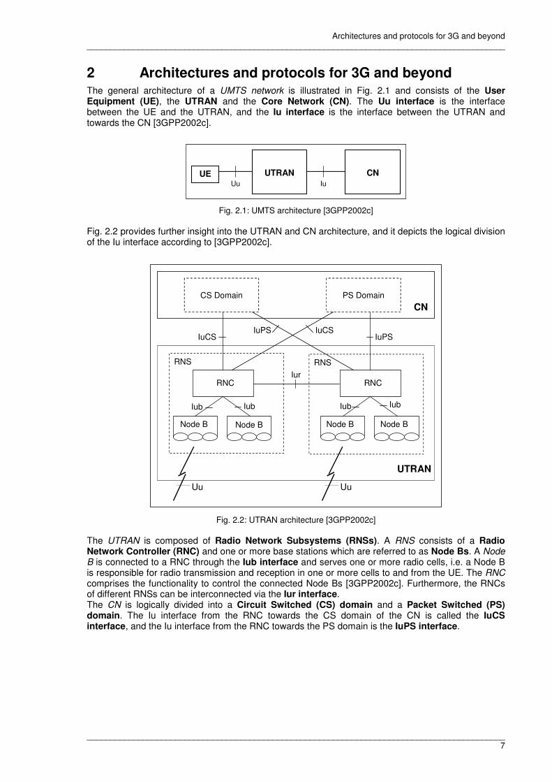
Architectures and protocols for 3G and beyond __________________________________________________________________________________________
__________________________________________________________________________________________ 7
2 Architectures and protocols for 3G and beyond The general architecture of a UMTS network is illustrated in Fig. 2.1 and consists of the User Equipment (UE), the UTRAN and the Core Network (CN). The Uu interface is the interface between the UE and the UTRAN, and the Iu interface is the interface between the UTRAN and towards the CN [3GPP2002c].
UE
UTRAN
CN
Uu Iu
Fig. 2.1: UMTS architecture [3GPP2002c]
Fig. 2.2 provides further insight into the UTRAN and CN architecture, and it depicts the logical division of the Iu interface according to [3GPP2002c].
RNS
RNC
RNS
RNC
Node B Node B Node B Node B
IuCS IuPS
Iur
Iub Iub Iub Iub
Uu
UTRAN
Uu
CN
CS Domain
PS Domain
IuCS IuPS
Fig. 2.2: UTRAN architecture [3GPP2002c]
The UTRAN is composed of Radio Network Subsystems (RNSs). A RNS consists of a Radio Network Controller (RNC) and one or more base stations which are referred to as Node Bs. A Node B is connected to a RNC through the Iub interface and serves one or more radio cells, i.e. a Node B is responsible for radio transmission and reception in one or more cells to and from the UE. The RNC comprises the functionality to control the connected Node Bs [3GPP2002c]. Furthermore, the RNCs of different RNSs can be interconnected via the Iur interface. The CN is logically divided into a Circuit Switched (CS) domain and a Packet Switched (PS) domain. The Iu interface from the RNC towards the CS domain of the CN is called the IuCS interface, and the Iu interface from the RNC towards the PS domain is the IuPS interface.

Architectures and protocols for 3G and beyond __________________________________________________________________________________________
__________________________________________________________________________________________ 8
2.1 UMTS protocol model
Following [3GPP2000b], the general UMTS architecture is modeled, at a high level, from physical and functional viewpoints. The physical aspects are modeled using the domain concept and the functional aspects are modeled using the strata concept. Both concepts are fundamental for the classification of protocols in UMTS.
2.1.1 Domain concept
A domain represents the highest-level group of physical entities. Reference points are defined between the domains [3GPP2000b]. Fig. 2.1.1 shows the basic domains in UMTS.
UE Domain
AN Domain
CN Domain
Infrastructure Domain
Cu
ME Domain
USIM Domain
HN Domain
TN Domain
Uu Iu
[Zu]
[Yu]
SN Domain
Fig. 2.1.1: UMTS domains and reference points [3GPP2000b]
The basic architectural split between the UE and the infrastructure results in the UE Domain and in the Infrastructure Domain. The UE Domain comprises a variety of equipment types referred to as UEs with different levels of functionality. The UE is a device applied by the user to access UMTS network services. The UE Domain is further subdivided into the User Services Identity Module (USIM) Domain and the Mobile Equipment (ME) Domain. The USIM Domain contains data and procedures embedded in a stand-alone smart card for unique and secure identification. The ME Domain performs radio transmission, contains applications and is further subdivided into the Mobile Termination (MT) Domain and Terminal Equipment (TE) Domain. The MT Domain is responsible for radio transmission, and the TE domain contains end-to-end applications. The UE Domain has a radio interface towards the Infrastructure Domain. The Infrastructure Domain consists of the physical nodes which perform the functionality necessary for termination of the radio interface and for support of the telecommunication requirements of the users. Thus, the Infrastructure Domain is a shared resource that provides its services to all authorized users within its coverage area. The Infrastructure Domain is further subdivided into the Access Network (AN) Domain and the CN Domain in order to decouple access related functionality from non-access related functionality. The AN Domain consists of the physical entities which manage the resources of the access network and enable the user to access the CN Domain. The CN Domain consists of the physical entities which provide support for the network features and telecommunication services. The CN domain itself is subdivided into the Serving Network (SN) Domain, the Home Network (HN) Domain and the Transit Network (TN) Domain. The SN Domain is responsible for call routing and the transport of user data from a source to a destination. It is the point of contact inside the CN Domain for the AN Domain, and it interacts with the HN Domain in case of user specific data or services as well as with the TN Domain in case of non-user specific data or services. The HN Domain is responsible for the management of user related subscription information and permanently contains user specific data. The TN Domain is located on the communication path between the SN Domain and the remote party representing the remote end entity which either might be a user or a machine (provided that the remote party is not located inside the same network as the originating UE, because in this case an activation of a TN Domain is unnecessary) [3GPP2000b].

Architectures and protocols for 3G and beyond __________________________________________________________________________________________
__________________________________________________________________________________________ 9
2.1.2 Strata concept
A stratum refers to a grouping of protocols related to one aspect of the services provided by one or several domains [3GPP2000b]. Fig. 2.1.2 clarifies the interrelationship of domains and strata in the UMTS architecture. Dotted lines within Fig. 2.1.2 denote that the protocol used is not specific to UMTS.
USIM
MT - AN
MT/ME AN Domain
SN Domain
HN Domain
AN - SN
Access Stratum
MT - SN
Serving Stratum
USIM - HN
SN - HN
Home Stratum
MT - SN USIM - MT
Transport Stratum
USIM - MT
TE
MT - AN
MT AN
Domain SN
Domain TN
Domain
AN - SN
Access Stratum
TE - MT MT - SN
Serving Stratum
Application Stratum
Application
Transport Stratum
Remote Party
ME Domain
Fig. 2.1.2: Interrelationship of UMTS domains and strata [3GPP2000b] The Access Stratum is part of the Transport Stratum and provides services related to the transmission of data over the radio interface and the management of the radio interface to other parts of the UMTS. Thus, the Access Stratum comprises the protocols between MT and AN Domain as well as the protocols between AN and SN Domain. The Transport Stratum supports the transport of user data and network control signaling from other strata through UMTS. In this context, the Transport Stratum provides mechanisms for error correction and recovery, for the encryption of data over the air interface and in the Infrastructure Domain, mechanisms for the adaptation of data to the supported physical format as well as mechanisms for data conversion to enable efficient usage of the radio interface, if required. The Serving Stratum comprises protocols and functions to route and transmit data generated by the user or by the network from a source to a destination. In this context, source and destination may be within the same or different networks. The Home Stratum contains protocols and functions related to the handling and storage of subscription data and services specific to the HN Domain. The Application Stratum represents the applications provided to the end user and thus, comprises end-to-end protocols and functions which utilize services provided by the Home, Serving and Transport Strata in order to support services and/or value added services [3GPP2000b].
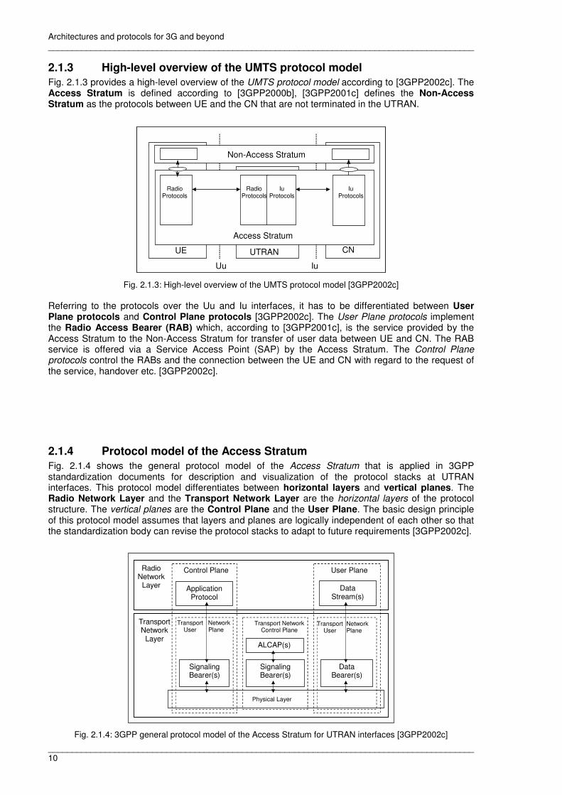
Architectures and protocols for 3G and beyond __________________________________________________________________________________________
__________________________________________________________________________________________ 10
2.1.3 High-level overview of the UMTS protocol model
Fig. 2.1.3 provides a high-level overview of the UMTS protocol model according to [3GPP2002c]. The Access Stratum is defined according to [3GPP2000b], [3GPP2001c] defines the Non-Access Stratum as the protocols between UE and the CN that are not terminated in the UTRAN.
UE CN
Access Stratum
Non-Access Stratum
Uu Iu
Radio Protocols
Radio Protocols
Iu Protocols
Iu Protocols
UTRAN
Fig. 2.1.3: High-level overview of the UMTS protocol model [3GPP2002c]
Referring to the protocols over the Uu and Iu interfaces, it has to be differentiated between User Plane protocols and Control Plane protocols [3GPP2002c]. The User Plane protocols implement the Radio Access Bearer (RAB) which, according to [3GPP2001c], is the service provided by the Access Stratum to the Non-Access Stratum for transfer of user data between UE and CN. The RAB service is offered via a Service Access Point (SAP) by the Access Stratum. The Control Plane protocols control the RABs and the connection between the UE and CN with regard to the request of the service, handover etc. [3GPP2002c].
2.1.4 Protocol model of the Access Stratum
Fig. 2.1.4 shows the general protocol model of the Access Stratum that is applied in 3GPP standardization documents for description and visualization of the protocol stacks at UTRAN interfaces. This protocol model differentiates between horizontal layers and vertical planes. The Radio Network Layer and the Transport Network Layer are the horizontal layers of the protocol structure. The vertical planes are the Control Plane and the User Plane. The basic design principle of this protocol model assumes that layers and planes are logically independent of each other so that the standardization body can revise the protocol stacks to adapt to future requirements [3GPP2002c].
Application Protocol
Data Stream(s)
Data Bearer(s)
ALCAP(s)
Transport Network
Layer
Signaling Bearer(s)
Physical Layer
Signaling Bearer(s)
Transport Network User Plane
Control Plane User Plane
Transport Network Control Plane
Radio Network
Layer
Transport Network User Plane
Fig. 2.1.4: 3GPP general protocol model of the Access Stratum for UTRAN interfaces [3GPP2002c]

Architectures and protocols for 3G and beyond __________________________________________________________________________________________
__________________________________________________________________________________________ 11
Following [3GPP2002c], the Control Plane contains the Application Protocol, which is used for bearer establishment in the Radio Network Layer, and the Signaling Bearer(s) for transportation of the Application Protocol messages. The User Plane comprises the Data Stream(s) and the associated Data Bearer(s) which are the transport bearers for the Data Stream(s). The Transport Network Control Plane acts between the Control Plane and the User Plane and allows the Application Protocol in the Radio Network Control Plane to be completely independent from the technology chosen for the Data Bearer(s) in the User Plane. The Transport Network Control Plane includes on the one hand the Access Link Control Application Part (ALCAP) protocol(s) that is/are necessary for the establishment of the Data Bearer(s) and on the other hand the appropriate Signaling Bearer(s) needed for the ALCAP protocol(s). Furthermore, the Transport Network Control Plane controls the Data Bearer(s) during real time operation, but it is not involved in Signaling Bearer establishment and control for the Application Protocol. If there is no ALCAP signaling transaction, the Transport Network Control Plane is not needed. The Transport Network User Plane consists of the Data Bearer(s) in the User Plane and of the Signaling Bearer(s) in the Control Plane. Subsequently, the protocol structures of the UTRAN interfaces Uu, IuCS, IuPS, Iub and Iur are presented according to the general protocol model for UTRAN interfaces (cf. Fig. 2.1.4). 2.1.4.1 Protocol structure of the Uu interface
Fig. 2.1.5 shows the protocol architecture of the radio interface Uu which is layered into the three protocol layers Physical Layer (Layer 1 (L1)), Data Link Layer (Layer 2 (L2)) and Network Layer (Layer 3 (L3)). Layer 1 is based on the Wideband-Code Division Multiple Access (W-CDMA) technology [3GPP2002i]. The W-CDMA technology allows for a division of the radio resource among the users sending on the same frequency based on unique codes for their transactions so that an unambiguous correlation of a user and the related transaction via the code is possible. The application of the code to the user signal on the one hand enables the scrambling of the user code and on the other hand spreads the signal over the entire bandwidth of the radio connection [KaAhLa2001]. Layer 2 is split into the sublayers Medium Access Control (MAC), Radio Link Control (RLC), Packet Data Convergence Protocol (PDCP) and Broadcast/Multicast Control (BMC). The lowest sublayer of Layer 3, which terminates in the UTRAN, is the Radio Resource Control (RRC). The next sublayer of Layer 3, which is still part of the Access Stratum, does not belong to the radio interface any more, as this sublayer terminates in the CN. The remaining sublayers of Layer 3, following above, already belong to the Non-Access Stratum. MAC and RLC are used in the Control Plane as well as in the User Plane. The RRC protocol only exists in the Control Plane, and PDCP as well as BMC exist in the User Plane only [3GPP2002i].

Architectures and protocols for 3G and beyond __________________________________________________________________________________________
__________________________________________________________________________________________ 12
L3 co
ntro
l
cont
rol
cont
rol
cont
rol
Logical Channels
Transport Channels
Control Plane User Plane
W-CDMA Physical Layer
L2/MAC
L1
RLC
DC Nt GC
L2/RLC
MAC
RLC RLC
RLC
RLC
RLC RLC
RLC
UuS boundary
BMC L2/BMC
control
PDCP PDCP L2/PDCP
DC Nt GC
Radio Bearers
RRC
L3
Non-Access Stratum
Access Stratum
Transport Network
Layer
Radio Network
Layer
L3
Fig. 2.1.5: Uu interface protocol architecture (following [3GPP2002i])
The circles between different layers and sublayers (cf. Fig. 2.1.5) indicate SAPs used for offering services to upper layers/sublayers. The SAP between W-CDMA Physical Layer and MAC provides the transport channels, and the SAPs between MAC and RLC provide the logical channels. The service provided by Layer 2 is the radio bearer, and those radio bearers, which are provided by RLC to RRC, are the signaling radio bearers [3GPP2002i]. Moreover, Fig. 2.1.5 shows control interfaces between RRC and the lower layers and sublayers of the radio interface. These control interfaces provide local inter-layer control services, i.e. they allow the RRC sublayer to control the configuration of the lower layers locally [3GPP2002i]. The Physical Layer offers information transfer services in the form of Transport Channels which are classified into Common Transport Channels and Dedicated Transport Channels to the MAC and higher layers. These physical layer transport services are described by how and with what characteristics data is transferred over the radio interface. Moreover, the Physical Layer maps the Transport Channels onto Physical Channels. The MAC layer provides data transfer services on Logical Channels which specify what kind of information is transferred. These Logical Channels are classified into Control Channels for the transfer of Control Plane information and Traffic Channels for the transfer of User Plane information. Furthermore, the MAC layer maps the Transport Channels provided by the Physical Layer on the Logical Channels [3GPP2002i]. The MAC layer provides an unacknowledged data transfer service without segmentation and reassembly functionality to the upper layers. On request of the RRC protocol, it performs a reallocation of radio resources and also performs measurements on the logical channels with regard to the traffic volume. Based on the measurements reported by the MAC layer, the RRC protocol decides on transport channel switching [3GPP2002i]. The MAC protocol is fully specified in [3GPP2004b]. The RLC protocol (fully specified in [3GPP2004c]) either provides a transparent data transfer service (i.e. a transfer service that does not add supplementary protocol information) or an unacknowledged

Architectures and protocols for 3G and beyond __________________________________________________________________________________________
__________________________________________________________________________________________ 13
or acknowledged data transfer mode to the upper layers. RLC cares for segmentation and reassembly of Protocol Data Units (PDUs), for in-sequence delivery, for error correction by retransmission (in acknowledged data transfer mode), detection of duplicates and flow control [3GPP2002i]. According to [3GPP2002i], the PDCP protocol is responsible for the transfer of user data between the Non-Access Stratum and RLC layer. PDCP cares for header compression and decompression of IP data streams at the transmitting and the receiving entity. The entire specification of PDCP can be found in [3GPP2002k]. The BMC protocol provides a broadcast/multicast transmission service on the radio interface. BMC stores cell broadcast messages received from the RNC for scheduled transmission to upper protocol layers of the Non-Access Stratum inside the UE. Moreover, BMC calculates transmission rates required for Cell Broadcast Service (CBS) and requests appropriate radio resources from the RRC protocol [3GPP2002i, 3GPP2004i]. The RRC protocol is a substantial protocol, the entire specification can be found in [3GPP2004j]. Table 2.1.1 lists a subset of significant functions and explanations of these functions performed by the RRC protocol according to [3GPP2002i].
RRC Protocol Function Short Explanation
Broadcast of information provided by the Non-Access Stratum
The RRC layer performs system information broadcasting from the CN to all UEs. Normally, the system information is repeated on a regular basis. Thereby, the RRC layer performs the scheduling, segmentation and repetition of the system information. Furthermore, information broadcasting from higher protocol layers (above RRC) is supported. The information to be broadcasted may be cell specific or not.
Broadcast of information related to the Access Stratum
This functionality typically supports broadcast of cell-specific information.
Establishment, re-establishment, maintenance and release of an RRC connection between the UE and the UTRAN
The establishment of an RRC connection is initiated by a request from higher protocol layers at the UE side to establish the first signaling connection for the UE. The release of an RRC connection can also be initiated by a request from higher protocol layers or by the RRC layer itself in case of a RRC connection failure. In the event of connection loss the UE requests a re-establishment of the RRC connection.
Establishment, reconfiguration and release of radio bearers
The RRC layer can, if requested from higher protocol layers, perform the establishment, reconfiguration and release of radio bearers in the user plane. Thereby, the radio bearer is the service provided by L2 for transfer of user data between the UE and the UTRAN [3GPP2001b].
Assignment, reconfiguration and release of radio resources for the RRC connection
The RRC layer handles the assignment of radio resources needed for the RRC connection including requirements from both the control and user plane. Furthermore, the RRC layer may reconfigure radio resources during an established RRC connection.
Paging The RRC layer can broadcast paging information from the network to selected UEs.
Control of requested Quality of Service (QoS) The RRC layer ensures that the QoS requirements of the radio bearers can be met by allocation of a sufficient number of radio resources.
UE measurement reporting and control of the reporting
The RRC layer controls the measurements, the UE has to perform on the UMTS air interface and other systems, in terms of what and when to measure and how to report. Furthermore, the RRC layer reports the measurements performed by the UE to the network.
RRC connection mobility functions
The RRC layer performs evaluation, decision and execution related to RRC connection mobility during an already established RRC connection, such as handover, based on, for instance, measurements performed by the UE.
Outer loop power control The RRC layer controls the setting of the target of the closed loop power control.
Control of ciphering The RRC layer provides procedures for switching on and off the ciphering between the UE and the UTRAN.
Initial configuration for CBS The RRC layer performs the initial configuration of the BMC layer.
Allocation of radio resource for CBS The RRC layer allocates radio resources for CBSs based on traffic volume requirements indicated by the BMC layer.
Table 2.1.1: Subset of significant functions of the RRC protocol [3GPP2002i]
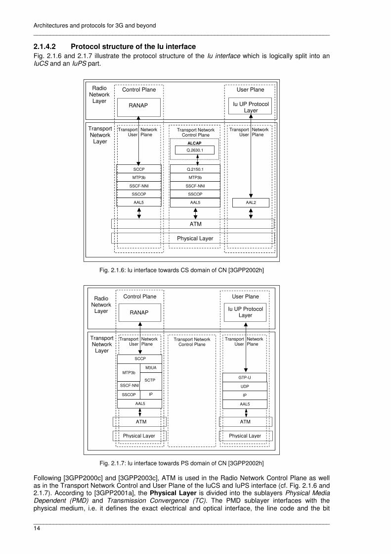
Architectures and protocols for 3G and beyond __________________________________________________________________________________________
__________________________________________________________________________________________ 14
2.1.4.2 Protocol structure of the Iu interface
Fig. 2.1.6 and 2.1.7 illustrate the protocol structure of the Iu interface which is logically split into an IuCS and an IuPS part.
Q.2630.1
RANAP Iu UP Protocol Layer
Transport Network
Layer
Physical Layer
TransportUser
Network Plane
Control Plane User Plane
TransportUser
Network Plane
Transport Network Control Plane
Radio Network
Layer
ATM
SSCOP
AAL2
MTP3b
SCCP
SSCF-NNI
ALCAP
SSCOP
MTP3b
Q.2150.1
SSCF-NNI
AAL5 AAL5
Fig. 2.1.6: Iu interface towards CS domain of CN [3GPP2002h]
RANAP Iu UP Protocol
Layer
Transport Network
Layer
Physical Layer
TransportUser
Network Plane
Control Plane User Plane
TransportUser
Network Plane
Transport Network Control Plane
Radio Network
Layer
ATM
SSCF-NNI
SSCOP
AAL5
IP
SCTP
SCCP
AAL5
SSCF-NNI
IP
UDP
GTP-U
Physical Layer
ATM
MTP3b M3UA
Fig. 2.1.7: Iu interface towards PS domain of CN [3GPP2002h]
Following [3GPP2000c] and [3GPP2003c], ATM is used in the Radio Network Control Plane as well as in the Transport Network Control and User Plane of the IuCS and IuPS interface (cf. Fig. 2.1.6 and 2.1.7). According to [3GPP2001a], the Physical Layer is divided into the sublayers Physical Media Dependent (PMD) and Transmission Convergence (TC). The PMD sublayer interfaces with the physical medium, i.e. it defines the exact electrical and optical interface, the line code and the bit
Architectures and protocols for 3G and beyond __________________________________________________________________________________________
__________________________________________________________________________________________ 15
timing. The PMD transforms the data received from the TC sublayer according to the type of physical medium applied (e.g. fiber optic cable, coaxial cable, Shielded Twisted Pair (STP) or Unshielded Twisted Pair (UTP)) [Cla1996]. The PMD is expected to meet at least one of the standards listed in [3GPP2001a]. On the one hand the TC sublayer is responsible for the adaptation of the cell stream received from the higher layer into a bit stream that can be passed to the lower PMD layer and transferred via the physical medium. On the other hand the TC sublayer cares for the conversion of the bit stream received from the PMD layer into a cell stream so that the cell stream can be passed to the upper layer. Further functions of the TC sublayer are the identification of cell boundaries (cell delineation) and the checksum calculation for error correction purposes. Also, the TC sublayer cares for cell scrambling/descrambling which randomizes the cell payload in order to minimize the chance of continuous non-varying bit patterns that could emulate network status and control signals and might disturb the network [Cla1996]. The ATM Layer is the layer above the Physical Layer and provides the cell switching of the 53 octet ATM cells. Special header fields, defined within the ATM cell format, support the ATM Layer when transmitting the cells. These header fields provide the addresses of virtual channels and paths on which the cells are transmitted. Moreover, these header fields allow for a differentiation between user cells and cells for management purposes (e.g. for testing the network) as well as for a differentiation between cells which shall be discarded in favor of other cells with a lower loss priority. The ATM cell header fields also contain information related to Generic Flow Control (GFC) which is a means of regulating the rate at which cells are submitted to the network by customer end devices, i.e. depending on the GFC mode applied certain types of lower priority traffic may or may not be submitted by the customer end device to the network [Cla1996]. The ATM layer, the Physical Layer and the physical medium are defined as an ATM transport network. Above the ATM Layer there is the ATM Adaptation Layer (AAL) which is responsible for the conversion of the data submitted by the higher layers into a format which is suitable for transfer by an ATM transport network. Furthermore, the AAL provides ATM networks with the capability to transfer different information types by adapting these different information types for carriage across a common ATM transport network. And, moreover, the AAL provides additional functionality required by these communications services and the different protocols of the higher layers. The overall functionality of the AAL is provided by two sublayers which are the Convergence Sublayer (CS) that comprises this additional functionality and the Segmentation and Reassembly (SAR) sublayer that processes the higher layer information into the ATM cell format. The AAL protocols are categorized within the four service classes A, B, C and D with different transmission characteristics. A timing relation between source and destination is required by AAL Type 2 (AAL2) which belongs to service class B, but it is not required by AAL Type 5 (AAL5) (service class C). AAL2 as well as AAL5 are conceived for the transfer of connection-oriented services with variable bit rate. For further information on AAL, the ATM protocol model or ATM in general, [Cla1996] can be taken as reference. Moreover, [RaWa1997] provides a more detailed and sophisticated reference on ATM. The Service Specific Connection Oriented Protocol (SSCOP) is a service specific as well as an ATM specific protocol which generically offers assured or unassured transfer of data. SSCOP extends the unassured transmission service provided by AAL5, and moreover, SSCOP cares for the sequencing of the data units, for flow control as well as error detection and correction. By application of the Service Specific Coordination Function (SSCF), the transmission service provided by SSCOP is adapted to the requirements of higher layer protocols. Therefore, the SSCF is specified differently at the User Network Interface (UNI) and Network Node Interface (NNI). The UNI is the interface between the ATM customer equipment and the ATM network, and the NNI is the interface between ATM specific devices inside the ATM network. AAL5, SSCOP and SSCF are defined as Signaling AAL (SAAL) [Cla1996, RaWa1997]. The protocol Message Transfer Part (MTP) Level 3 (MTP3) broadband (MTP3b) on top of SSCF-NNI is part of B-ISDN. Following [DrHaBe2002], MTP3 usually operates on top of MTP Level 1 (MTP1) and MTP Level 2 (MTP2) which provide a signaling link for reliable transfer of signaling messages between two directly connected signaling points. In the Transport Network Control and User Plane illustrated in Fig. 2.1.6, 2.1.7 and 2.1.9, MTP1 and MTP2 are substituted by the protocols forming the SAAL so that ATM-based reliable transfer is enabled. MTP3 provides functionality related to the routing of signaling messages between signaling points and functions related to signaling network management. This functionality related to signaling network management particularly implies the activation of new signaling links, the maintenance of the signaling service, traffic control in case of congestion and reconfiguration of the signaling network in case of failures. The Signaling Connection Control Part (SCCP) offers enhancements to MTP3b by providing connectionless and connection-oriented network services as well as an address translation function. The basic connectionless service does not provide segmentation and reassembly functionality, flow

Architectures and protocols for 3G and beyond __________________________________________________________________________________________
__________________________________________________________________________________________ 16
control or in-sequence delivery. The sequenced connectionless service is identical to the basic connectionless service, but offers in-sequence delivery. The connection-oriented SCCP services allow for the establishment of a temporary or permanent signaling connection. The basic connection-oriented service provides bidirectional transfer of messages as well as segmentation and reassembly functionality. The flow control connection-oriented service provides flow control, assures in-sequence delivery and cares for appropriate error handling during the sequencing process or handling of message loss. Furthermore, SCCP translates addresses of signaling messages into addresses that can be routed by MTP3b [DrHaBe2002]. Following [3GPP2003c], Q.2630.1 represents the ALCAP which is used in the form of a protocol for the establishment of AAL2 connections towards the CS domain. Q.2150.1 represents the AAL2 MTP3b Signaling Transport Converter which is needed for correspondence of Q.2630.1 and the lower layers of the protocol stack. According to [3GPP2003o], the Radio Access Network Application Part (RANAP), which is used as Application Protocol in the Control Plane of the Radio Network Layer (cf. Fig. 2.1.6 and 2.1.7), provides the signaling service between UTRAN and CN on the Iu interface. RANAP services are divided into three groups. Firstly, there are the general control services which are related to the whole Iu interface instance between RNC and the logical CN domain and utilize connectionless signaling transport provided by the Iu signaling bearer. In case of a connectionless data transfer service, RANAP is notified, when a RANAP message did not reach the intended peer RANAP entity. Secondly, there are the notification services which are related to specified UEs or all UEs in a specified area and also utilize connectionless signaling transport provided by the Iu signaling bearer. Thirdly, there is the group of dedicated control services which are related to one UE. The RANAP functions, which provide these dedicated control services, are associated with an Iu signaling connection that is maintained for the particular UE, and these RANAP functions utilize connection-oriented signaling transport provided by the Iu signaling bearer. In case of connection-oriented data transfer service, the signaling connection provides in-sequence delivery of RANAP messages and a notification for RANAP in the event of a signaling connection failure. Furthermore, each active UE has its own signaling connection. Table 2.1.2 lists a subset of significant functions of the RANAP protocol with a short explanation. The full RANAP protocol specification can be found in [3GPP2003o].
RANAP Protocol Function Short Explanation Overall Radio Access Bearer (RAB) management
This function is responsible for RAB setup, modification and release. The overall RAB management is a function of the CN.
Queueing of RAB setup Requested RABs are placed into a queue, the peer entitiy is notified about the enqueueing.
Request of RAB release The RNC has the ability to request RAB releases. Release of all Iu connection resources
This function is used to explicitly release all resources related to one Iu connection. The Iu release is managed from the CN.
Request of release of all Iu connection resources
The RNC is capable to request the release of all Iu connection resources from the corresponding Iu connection.
Overload control in the Iu interface This function allows for load balancing in the Iu interface. Reset of Iu interface This function is used for resetting an Iu interface. Transport of Non-Access Stratum information
This function cares for the transport of Non-Access Stratum signaling messages between the UE and the CN.
Paging The CN is enabled to page the UE. Location reporting Actual location information can be sent from the RNC to the CN.
Serving RNC Relocation This function enables to change the Serving RNC functionality as well as the related Iu resources (i.e. RAB(s) and signaling connection) from one RNC to another one.
Security mode control in UTRAN This function is used to send the security keys (for ciphering and integrity protection) to the UTRAN and set the operation mode for the security functions.
Report of general error situations This function allows for reporting of general error situations.
Table 2.1.2: Subset of significant RANAP functions (following [3GPP2003o]) The Iu User Plane (UP) protocol in the User Plane of the Radio Network Layer (cf. Fig. 2.1.6 and 2.1.7) is used to transfer user data associated with RABs. In this context, one Iu UP protocol instance is associated with one RAB, and the Iu UP protocol instances are established, relocated and released together with the associated RAB. An objective, the Iu UP protocol is expected to meet, is to remain independent of the logical CN domain and to have limited or no dependency on the Transport Network Layer. This limitation of dependencies enables the evolution of services regardless of the logical CN domain and a migration of services across CN domains. Therefore, the Iu UP protocol is defined with two modes of operation that can be activated on a RAB basis rather than on a CN domain or service basis. The modes of operation determine which set of features is provided for a particular RAB. Firstly, the Transparent Mode (TrM) is applied to RABs that do not require any

Architectures and protocols for 3G and beyond __________________________________________________________________________________________
__________________________________________________________________________________________ 17
particular feature from the Iu UP protocol other than the transfer of user data. Thus, the Iu UP protocol in TrM is an empty layer which transparently relays user data between the Transport Network Layer and the upper layers of the Non-Access Stratum (and vice versa). Secondly, the Support Mode for predefined Service Data Unit (SDU) (SMpSDU) size is intended for RABs which require particular features like, for instance, variable predefined SDU sizes from the Iu UP protocol in addition to the transfer of user data (e.g. the transfer of Adaptive Multi Rate (AMR) speech PDUs would utilize the SMpSDU) [3GPP2002j]. Following [3GPP2000c] and Fig. 2.1.7, the standard allows operators to choose one out of two standardized protocol suites for signaling bearer establishment in the Control Plane of the IuPS interface. The first option is to apply the protocols on left hand side of the Transport Network User Plane protocol stack between AAL5 and SCCP illustrated in Fig. 2.1.7 which are also used at the IuCS interface (i.e. SAAL-NNI and MTP3b, cf. Fig. 2.1.6). The second option is to use the protocols on right hand side of the Transport Network User Plane protocol stack shown in Fig. 2.1.7, such as IP [Pos1981] over ATM (as specified in [GrHe1999] and [LaHa1998]). Furthermore, protocols, that are part of the Signaling Transport (SIGTRAN) standards, are used which are defined by the Internet Engineering Task Force (IETF). These SIGTRAN standards contain a set of protocols which are suitable to transfer signaling messages (e.g. Signaling System Number Seven (SS7) messages) over an IP network [DrHaBe2002]. The protocol stacks illustrated in Fig. 2.1.7 and 2.1.9 utilize the Stream Control Transmission Protocol (SCTP) and the MTP3 User Adaptation Layer (M3UA) protocol which are part of the SIGTRAN standards. SCTP [StXiMo2000] enables transportation of various signaling protocols over IP networks and offers short transmission delay time as well as reliable data delivery [DrHaBe2002]. The M3UA protocol supports the transport of any MTP3-user signaling (e.g. SCCP messages over IP by utilizing the services of SCTP) [SiMoPa2002, DrHaBe2002]. For the data bearer in the Transport Network User Plane of the IuPS interface (cf. Fig. 2.1.7), IP over ATM is used as specified in [GrHe1999] and [LaHa1998]. IPv4 [Pos1981] shall be supported, IPv6 [DeHi1998] support is optional. The User Datagram Protocol (UDP) [Pos1980] is used as path protocol [3GPP2003c]. The GPRS Tunnelling Protocol (GTP), which is fully specified in [3GPP2004a], comprises the GTP Control (GTP-C) protocol and the GTP User (GTP-U) protocol. GTP-U is used in the Transport Network User Plane of the IuPS interface and operates on top of UDP (cf. Fig. 2.1.7). Moreover, GTP-U provides a tunneling mechanism for carrying multi-protocol user data packets, i.e. GTP-U provides packet transmission and reception services between a pair of GTP-U tunnel endpoints as well as in-sequence delivery at the IuPS interface. The tunnel between two GTP-U endpoints at the IuPS interface is established via Control Plane procedures defined in the RANAP protocol [3GPP2004a].

Architectures and protocols for 3G and beyond __________________________________________________________________________________________
__________________________________________________________________________________________ 18
2.1.4.3 Protocol structure of the Iub interface
The Radio Network Layer of the Iub interface protocol architecture (cf. Fig. 2.1.8) contains the protocols related to the operation of the Node B. The Transport Network Layer comprises the protocols necessary for the establishment of physical connections between the Node B and the RNC [3GPP2002d]. Beside the already established protocols in the Transport Network Control and User Plane, the protocol Q.2150.2 is used in the Transport Network Control Plane of the Iub interface (cf. Fig. 2.1.8). Following [Def2005], Q.2150.2 represents the AAL2 Signaling Transport Converter on SSCOP.
NBAP
AAL2
ALCAP Transport Network
Layer
Physical Layer
Radio Network
Layer
Control Plane
Transport Network
Control Plane
DC
H F
P
RA
CH
FP
DS
CH
FP
AAL5
User Plane
SSCF-UNI
SSCOP
AAL5
SSCF-UNI
SSCOP
Q.2630.1
Q.2150.2
FA
CH
FP
PC
H F
P
US
CH
FP
CP
CH
FP
TF
CI2
FP
ATM
Fig. 2.1.8: Iub interface protocol structure [3GPP2002d]
According to [3GPP2002c], the Operation and Maintenance (O&M) of the Node B is divided into the two parts Implementation Specific O&M and Logical O&M. The Implementation Specific O&M depends on the actual implementation of the Node B, i.e. on the one hand it depends on the hardware components of the Node B, and on the other hand it depends on the management of its software components. The Logical O&M denotes the signaling associated with the control of logical resources (i.e. cells, channels), which are owned by the RNC, but physically implemented in the Node B. As the RNC controls these logical resources, an information exchange between Node B and RNC is required. The signaling, which is related to this information exchange, forms a substantial part of the Node B Application Part (NBAP) protocol [3GPP2002c, 3GPP2002d]. In this context, the NBAP protocol requires an assured in-sequence delivery service from the signaling bearer and a notification, if the assured in-sequence delivery service is not available any more. Table 2.1.3 lists a subset of significant functions of the NBAP protocol with a short explanation. The full NBAP protocol specification can be found in [3GPP2004g].

Architectures and protocols for 3G and beyond __________________________________________________________________________________________
__________________________________________________________________________________________ 19
NBAP Protocol Function Short Explanation
Cell configuration management
The Controlling RNC (CRNC) is enabled to manage the cell configuration information in a Node B. Following [3GPP2002c], the CRNC is a role, that a RNC can take over, with regard to a specific set of Node Bs. For any Node B there is only one CRNC that has the overall control of the logical resources of the Node B.
Common transport channel management
The CRNC has the ability to manage the configuration of common transport channels in a Node B.
System information management This function enables the CRNC to manage the scheduling of system information to be broadcasted in a cell.
Resource event management This function allows the Node B to inform the CRNC about the status of the Node B resources.
Configuration alignment
The CRNC as well as the Node B have the possibility to verify and enforce that both nodes have the same information on the configuration of the radio resources (i.e. frequencies, scrambling codes, spreading factors, etc. [3GPP2002c]).
Measurements on common / dedicated resources
The CRNC can initiate measurements on common and/or dedicated resources in the Node B. The results of these measurements are reported by the Node B to the CRNC.
Radio link management
This function enables the CRNC to manage radio links by usage of dedicated resources in the Node B. [3GPP2002c] defines a radio link as a logical association between a single UE and a single UTRAN access point, whereas a UTRAN access point is a conceptual point within the UTRAN, performing radio transmission and reception, and is associated with one specific radio cell.
Radio link supervision This function allows the CRNC to report failures and restorations of a radio link.
Report of general error situations This function allows for the reporting of general error situations.
Table 2.1.3: Subset of significant NBAP functions (in accordance with [3GPP2004g]) Regarding the Frame Protocols (FP) in the User Plane, i.e. Radio Network Layer of the Iub interface protocol structure (cf. Fig. 2.1.8), it has to be distinguished between Common and Dedicated Transport Channel FPs. The Common Transport Channel FPs [3GPP2003u] are responsible for the transfer of Transport Block Sets (TBS) between Node B and Controlling RNC (CRNC). These TBSs define the data exchange between MAC and the Physical Layer, i.e. on a Transport Channel one TBS can be transmitted for every Transmission Time Interval (TTI) [3GPP2003q]. Furthermore, the Common Transport Channel FPs support transport channel synchronization mechanisms as well as node synchronization mechanisms. Node synchronization relates to the estimation and compensation of timing differences among the UTRAN nodes RNC and Node B. The transport channel synchronization mechanism defines synchronization of the frame transport between RNC and Node B by considering radio interface timing [3GPP2002e]. The Dedicated Transport Channel FPs [3GPP2003v] are also responsible for the transfer of TBSs across the Iub interface, and they support transport channel as well as node synchronization mechanisms. Moreover, the Dedicated Transport Channel FPs transport outer loop power control information between the Serving RNC (SRNC) and the Node B, and they are responsible for the transfer of radio interface parameters from the SRNC to the Node B.

Architectures and protocols for 3G and beyond __________________________________________________________________________________________
__________________________________________________________________________________________ 20
2.1.4.4 Protocol structure of the Iur interface
The Transport Network Layer of the Iur interface protocol architecture (cf. Fig. 2.1.9) consists of the protocols necessary for the establishment of physical connections between two RNCs. The Radio Network Layer comprises the protocols related to the interaction of the two RNCs [3GPP2002b].
RNSAP Iur Data Stream(s)
Transport Network
Layer
Physical Layer
Transport User
Network Plane
Control Plane User Plane
Transport User
Network Plane
Transport Network Control Plane
Radio Network
Layer
ATM
SCCP
AAL5
MTP3b M3UA
SSCF-NNI SCTP
SSCOP IP
Q2150.1
AAL5
MTP3b M3UA
SSCF-NNI SCTP
SSCOP IP
AAL2
Q2630.1 ALCAP
Fig. 2.1.9: Iur interface protocol structure [3GPP2002b]
The Radio Network Subsystem Application Part (RNSAP) (fully specified in [3GPP2004f]) is the protocol which is responsible to provide signaling information across the Iur interface [3GPP2002b]. The Iur interface RNSAP procedures are divided into four modules: • Firstly, the RNSAP Basic Mobility Procedures module contains procedures which are used to
handle the mobility within UTRAN. • Secondly, the RNSAP Dedicated Channel (DCH) Procedures module consists of procedures
which are used to handle DCHs, Downlink Shared Channels (DSCHs) and Uplink Shared Channels (USCHs) between two RNSs.
• Thirdly, the RNSAP Common Transport Channel Procedures module includes procedures that are used to control common transport channels (except the DSCH and USCH) over the Iur interface.
• Fourthly, the Global Procedures module contains procedures that are not related to a specific UE and, which in contrast to the above mentioned modules, involve two peer CRNCs [3GPP2004f].
The signaling transport shall provide both connectionless and connection-oriented data transfer service to support RNSAP procedures. When utilizing connectionless data transfer service, RNSAP shall be notified in case a RNSAP message did not attain to the intended peer RNSAP entity. The connection-oriented data transfer service shall provide in-sequence delivery of RNSAP messages and a notification for RNSAP in case of a signaling connection failure. Furthermore, each active UE shall have its own signaling connection. [3GPP2004f] specifies in detail which RNSAP procedures require either connectionless or connection-oriented data transfer service. Table 2.1.4 below lists a subset of significant functions of the RNSAP protocol and a short explanation for each of these functions. But, previous to the table, the terms Serving RNS (SRNS), SRNC, Drift RNS (DRNS) and Drift RNC (DRNC), which are used within the table, are explained according to [3GPP2002c], hereafter. The SRNS is a role, a RNS can take, with regard to a specific connection between a UE and the UTRAN, and there is one SRNS for each UE that has a connection to the UTRAN. The SRNS is in charge of the radio connection between the UE and the UTRAN, and it terminates the Iu for this UE. The SRNC is the RNC of the SRNS. Hence, the DRNS is also a role, a RNS can take over, regarding a specific connection between a UE and the UTRAN, and the DRNC is the RNC of the RNS. The DRNS supports the SRNS with radio resources, when the connection between the UTRAN and the UE needs to use one or more radio cells which are administrated by the corresponding DRNS.
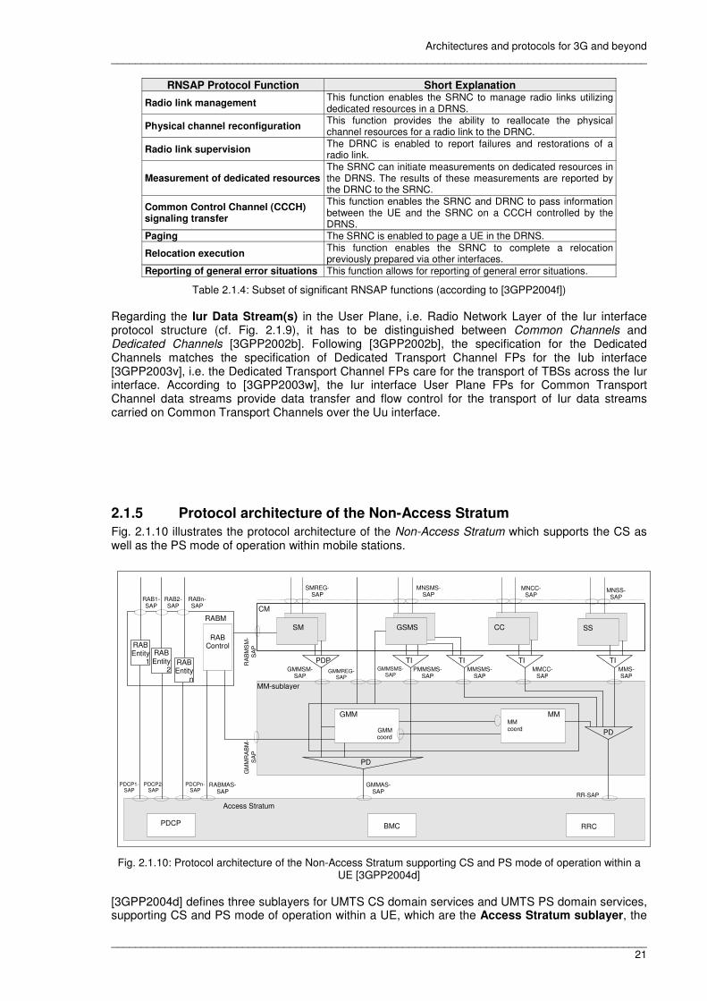
Architectures and protocols for 3G and beyond __________________________________________________________________________________________
__________________________________________________________________________________________ 21
RNSAP Protocol Function Short Explanation
Radio link management This function enables the SRNC to manage radio links utilizing dedicated resources in a DRNS.
Physical channel reconfiguration This function provides the ability to reallocate the physical channel resources for a radio link to the DRNC.
Radio link supervision The DRNC is enabled to report failures and restorations of a radio link.
Measurement of dedicated resources The SRNC can initiate measurements on dedicated resources in the DRNS. The results of these measurements are reported by the DRNC to the SRNC.
Common Control Channel (CCCH) signaling transfer
This function enables the SRNC and DRNC to pass information between the UE and the SRNC on a CCCH controlled by the DRNS.
Paging The SRNC is enabled to page a UE in the DRNS.
Relocation execution This function enables the SRNC to complete a relocation previously prepared via other interfaces.
Reporting of general error situations This function allows for reporting of general error situations.
Table 2.1.4: Subset of significant RNSAP functions (according to [3GPP2004f]) Regarding the Iur Data Stream(s) in the User Plane, i.e. Radio Network Layer of the Iur interface protocol structure (cf. Fig. 2.1.9), it has to be distinguished between Common Channels and Dedicated Channels [3GPP2002b]. Following [3GPP2002b], the specification for the Dedicated Channels matches the specification of Dedicated Transport Channel FPs for the Iub interface [3GPP2003v], i.e. the Dedicated Transport Channel FPs care for the transport of TBSs across the Iur interface. According to [3GPP2003w], the Iur interface User Plane FPs for Common Transport Channel data streams provide data transfer and flow control for the transport of Iur data streams carried on Common Transport Channels over the Uu interface.
2.1.5 Protocol architecture of the Non-Access Stratum
Fig. 2.1.10 illustrates the protocol architecture of the Non-Access Stratum which supports the CS as well as the PS mode of operation within mobile stations.
CM
GMMSM-SAP
MM-sublayer
GMMREG-SAP
PDP TI
PD
SMREG-SAP
RA
BM
SM
-S
AP
RABM
RAB1-SAP
RABn-SAP
RAB2-SAP
GM
MR
AB
M-
SA
P
RABMAS-SAP
GMMAS-SAP
PDCPn-SAP
PDCP2-SAP
PDCP1-SAP
MNSMS-SAP
GMM
PMMSMS-SAP
SM
TI GMMSMS-
SAP
GSMS
MNCC-SAP
PD
MNSS-SAP
TI TI
CC SS
RR-SAP
Access Stratum
RRC PDCP BMC
MMMM coord
GMM
GMMcoord
MMSMS-SAP
MMCC-SAP
MMS-SAP
RAB Control RAB
Entity 1
RAB Entity
2RAB Entity
n
Fig. 2.1.10: Protocol architecture of the Non-Access Stratum supporting CS and PS mode of operation within a UE [3GPP2004d]
[3GPP2004d] defines three sublayers for UMTS CS domain services and UMTS PS domain services, supporting CS and PS mode of operation within a UE, which are the Access Stratum sublayer, the
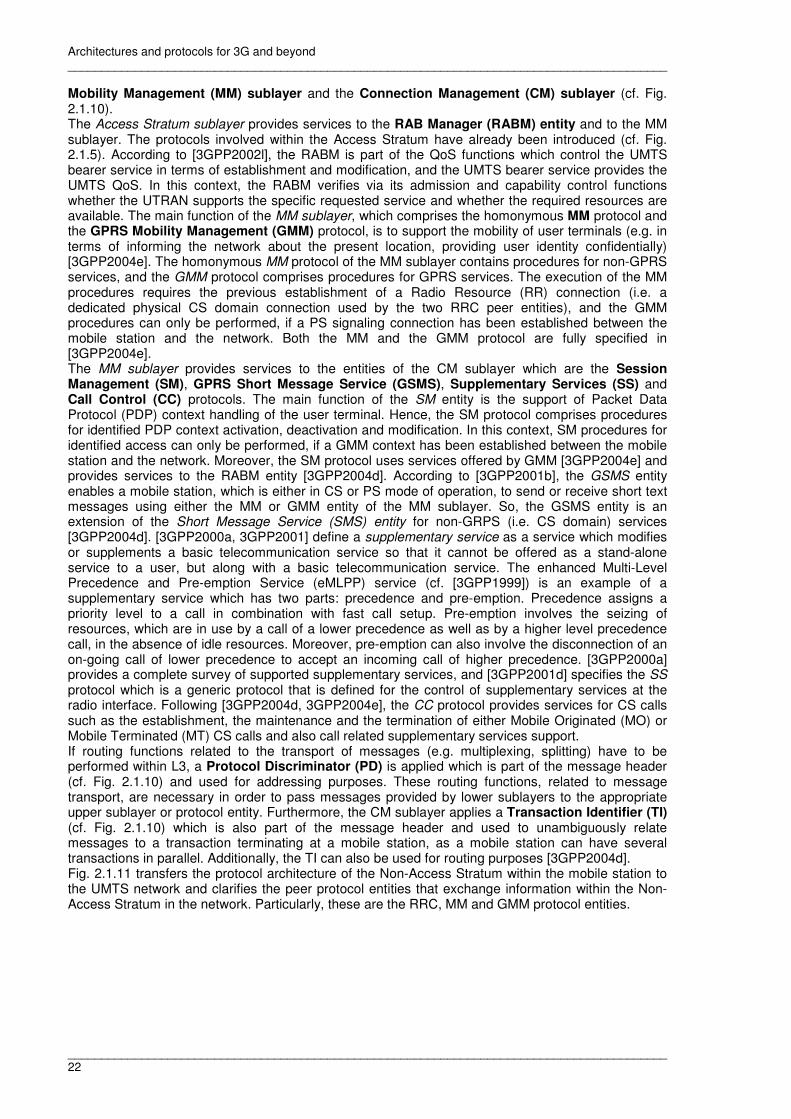
Architectures and protocols for 3G and beyond __________________________________________________________________________________________
__________________________________________________________________________________________ 22
Mobility Management (MM) sublayer and the Connection Management (CM) sublayer (cf. Fig. 2.1.10). The Access Stratum sublayer provides services to the RAB Manager (RABM) entity and to the MM sublayer. The protocols involved within the Access Stratum have already been introduced (cf. Fig. 2.1.5). According to [3GPP2002l], the RABM is part of the QoS functions which control the UMTS bearer service in terms of establishment and modification, and the UMTS bearer service provides the UMTS QoS. In this context, the RABM verifies via its admission and capability control functions whether the UTRAN supports the specific requested service and whether the required resources are available. The main function of the MM sublayer, which comprises the homonymous MM protocol and the GPRS Mobility Management (GMM) protocol, is to support the mobility of user terminals (e.g. in terms of informing the network about the present location, providing user identity confidentially) [3GPP2004e]. The homonymous MM protocol of the MM sublayer contains procedures for non-GPRS services, and the GMM protocol comprises procedures for GPRS services. The execution of the MM procedures requires the previous establishment of a Radio Resource (RR) connection (i.e. a dedicated physical CS domain connection used by the two RRC peer entities), and the GMM procedures can only be performed, if a PS signaling connection has been established between the mobile station and the network. Both the MM and the GMM protocol are fully specified in [3GPP2004e]. The MM sublayer provides services to the entities of the CM sublayer which are the Session Management (SM), GPRS Short Message Service (GSMS), Supplementary Services (SS) and Call Control (CC) protocols. The main function of the SM entity is the support of Packet Data Protocol (PDP) context handling of the user terminal. Hence, the SM protocol comprises procedures for identified PDP context activation, deactivation and modification. In this context, SM procedures for identified access can only be performed, if a GMM context has been established between the mobile station and the network. Moreover, the SM protocol uses services offered by GMM [3GPP2004e] and provides services to the RABM entity [3GPP2004d]. According to [3GPP2001b], the GSMS entity enables a mobile station, which is either in CS or PS mode of operation, to send or receive short text messages using either the MM or GMM entity of the MM sublayer. So, the GSMS entity is an extension of the Short Message Service (SMS) entity for non-GRPS (i.e. CS domain) services [3GPP2004d]. [3GPP2000a, 3GPP2001] define a supplementary service as a service which modifies or supplements a basic telecommunication service so that it cannot be offered as a stand-alone service to a user, but along with a basic telecommunication service. The enhanced Multi-Level Precedence and Pre-emption Service (eMLPP) service (cf. [3GPP1999]) is an example of a supplementary service which has two parts: precedence and pre-emption. Precedence assigns a priority level to a call in combination with fast call setup. Pre-emption involves the seizing of resources, which are in use by a call of a lower precedence as well as by a higher level precedence call, in the absence of idle resources. Moreover, pre-emption can also involve the disconnection of an on-going call of lower precedence to accept an incoming call of higher precedence. [3GPP2000a] provides a complete survey of supported supplementary services, and [3GPP2001d] specifies the SS protocol which is a generic protocol that is defined for the control of supplementary services at the radio interface. Following [3GPP2004d, 3GPP2004e], the CC protocol provides services for CS calls such as the establishment, the maintenance and the termination of either Mobile Originated (MO) or Mobile Terminated (MT) CS calls and also call related supplementary services support. If routing functions related to the transport of messages (e.g. multiplexing, splitting) have to be performed within L3, a Protocol Discriminator (PD) is applied which is part of the message header (cf. Fig. 2.1.10) and used for addressing purposes. These routing functions, related to message transport, are necessary in order to pass messages provided by lower sublayers to the appropriate upper sublayer or protocol entity. Furthermore, the CM sublayer applies a Transaction Identifier (TI) (cf. Fig. 2.1.10) which is also part of the message header and used to unambiguously relate messages to a transaction terminating at a mobile station, as a mobile station can have several transactions in parallel. Additionally, the TI can also be used for routing purposes [3GPP2004d]. Fig. 2.1.11 transfers the protocol architecture of the Non-Access Stratum within the mobile station to the UMTS network and clarifies the peer protocol entities that exchange information within the Non-Access Stratum in the network. Particularly, these are the RRC, MM and GMM protocol entities.

Architectures and protocols for 3G and beyond __________________________________________________________________________________________
__________________________________________________________________________________________ 23
CC SS GSMS
MM sublayer MM sublayer
MM peer-to-peer protocol (MM, GMM)
UE CN
RR sublayer
RR peer-to-peer protocol (RRC)
SM
RR-SAP
CC SS GSMS SM
Uu Iu
RR-SAP
GMMSM-SAP
PMMSMS-SAP
MMCC-SAP
MMS-SAP GMMSM-SAP
PMMSMS-SAP
MMCC-SAP
MMS-SAP
Fig. 2.1.11: Network architecture view on protocol architecture of the Non-Access Stratum (CS / PS mode of operation) (according to [3GPP2004d])

Architectures and protocols for 3G and beyond __________________________________________________________________________________________
__________________________________________________________________________________________ 24
2.2 UMTS network architecture evolution Following [KaAhLa2001], the term evolution, as a high level context, covers the technical evolution of network elements and also extensions to network architecture and services. In this section the focus is on the evolution of the UMTS network architecture in terms of 3GPP releases under consideration of a predominance of IP traffic instead of CS voice traffic in future mobile networks. In this context, there is the need for future mobile networks to be able to handle considerably increased volumes of IP traffic. In order to be able to adapt to these requirements, 3G (3rd Generation) mobile networks have to evolve [3GPP2005c].
2.2.1 Release 99 PLMN infrastructure
Following [3GPP2002g], the PLMN infrastructure in Release 99 (R99) is divided into a CN and an Access Network (AN) infrastructure. The CN is logically divided into a CS domain and a PS domain. A PLMN can either implement one domain (CS or PS) or both domains. The AN is called Base Station System (BSS) for GSM and RNS for UMTS. Figure 2.2.1 illustrates a PLMN according to [3GPP2002g]. Bold lines denote interfaces which support user traffic, and dashed lines represent signaling interfaces.
BSS BSC
RNS
RNC
CN
Node B Node B
A IuPS
Iur
Iub
USIM
ME
MS
Cu
Uu
SGSN
Gs
GGSN
Gn HLR
Gr
Gc
AuC
H
EIR
Gf
Gi PSTN
IuCS Gb
Gp
BTS
Um
RNC
Abis
SIM
SIM-ME i/f or
cell BTS
GMSC
E
G
PSTN
C
D
F
PS CS
MSC
VLR B
VLR
MSC
B
GGSN in Different PLMN
External Data Networks
PSTN
Fig. 2.2.1: R99 PLMN [3GPP2002g]

Architectures and protocols for 3G and beyond __________________________________________________________________________________________
__________________________________________________________________________________________ 25
The CS and PS domain of the CN support user traffic in different ways. The entities of the CS domain allocate and release dedicated network resources for connection establishment and release so that user traffic is transported via a CS type of connection. These entities, which are specific to the CS domain of the CN, are the Mobile-services Switching Centre (MSC), the Gateway MSC (GMSC) and the Visitor Location Register (VLR). They also support the related signaling. The MSC constitutes the interface between the radio system and the fixed networks for CS services. The MSC provides the functionality necessary for handling the CS services and related signaling to and from the mobile stations in a certain area. Moreover, it is responsible for issues related to mobility management of mobile stations, in particular location registration and handover. The GMSC is a MSC which receives a call delivered by a fixed network to the PLMN. The GMSC interrogates the appropriate database and then routes the call to the MSC where the mobile station is located. The VLR is a database that keeps information about mobile stations which roam into a certain MSC area that is controlled by this particular VLR. This information (e.g. identity of the location area where the mobile station is situated, the International Mobile Subscriber Identity (IMSI), the identity of the Serving GPRS Support Node (SGSN) where the mobile station has been registered) is relevant for the handling of calls involving a particular mobile station [3GPP2002g]. The entities of the CN PS domain transport user traffic in the form of packets which are routed independently, and they are also responsible for the related signaling. These entities, specific to the PS domain of the CN, are the Serving GPRS Support Node (SGSN) and the Gateway GPRS Support Node (GGSN). These GPRS Support Nodes (GSNs) constitute the interface between the radio system and the fixed networks for PS services, i.e. they provide the functionality necessary to handle the packet transmission to and from the mobile stations. Both GSNs store subscription information (e.g. the IMSI, PDP addresses) and location information (e.g. SGSN stores GGSN address and vice versa) in order to handle originating and terminating packet data transfer [3GPP2002g]. The SGSN for PS services is comparable to the MSC for CS services, and the GGSN connects the PLMN to external packet data networks. The CS and PS domain of the CN are overlapping, i.e. they also contain some common entities which are the Home Location Register (HLR), Authentication Centre (AuC) and Equipment Identity Register (EIR). The HLR is a database necessary for the management of mobile subscribers. It stores subscription information, location information which allows for charging and routing of calls / packets towards the MSC/SGSN where the mobile station is currently registered and identities of the mobile subscriber (e.g. IMSI, PDP addresses). The AuC stores data for each mobile subscriber which is necessary for the authentication of IMSI and for an enciphered communication over the radio path between the mobile station and the network. Moreover, the AuC transmits this data via the HLR to the VLR, MSC and SGSN which need to authenticate a mobile station. The EIR stores the International Mobile Equipment Identities (IMEI) which is related to the hardware of the mobile device [3GPP2002g]. The Base Station System Access Network (BSS AN) consists of one Base Station Controller (BSC) and one or more Base Transceiver Stations (BTSs). The BSC controls one or more BTS(s), while one BTS serves one radio cell [3GPP2002g]. The technology applied in the BSS, to distribute the radio channel as a shared medium among the users, is the Time Division Multiple Access (TDMA) technology. TDMA allows multiple users to share the same frequency by dividing the frequency into time slots, which are repeated frequently, and assigning these time slots to the users for different operations [KaAhLa2001]. The structure of the RNS AN follows the description within the introductory part of chapter 2 and is according to Fig. 2.2. It can be summarized that R99 is based on the PLMN architecture specified for GSM Phase 2+ within [ETSI2000], but the R99 CN has to provide appropriate interfaces for connecting the CS and PS domains with the newly introduced RNS AN.
2.2.2 Release 4 PLMN infrastructure
According to [3GPP2003i], the PLMN infrastructure of Release 4 (Rel-4) is based on the infrastructure of R99, but envisages architectural changes in the CS domain of the CN which is defined as Bearer Independent CS CN (cf. [3GPP2005f]). In this context, the CS CN enables the support of different transport technologies (e.g. ATM or IP transport) in a bearer-independent way. This means that for ATM and IP transport there is a strict separation between the call control level and the bearer control

Architectures and protocols for 3G and beyond __________________________________________________________________________________________
__________________________________________________________________________________________ 26
level so that the transfer of compressed speech at variable bit rates is enabled through the CS CN [3GPP2005f]. Fig. 2.2.2 visualizes a PLMN according to Rel-4.
BSS RNS
CN
Node B Node B
A IuPS
Iur
Iub
Uu
SGSN Gs
GGSN
Gn HLR
Gr
Gc
AuC
H
EIR
Gf
Gi
IuCS Gb
Gp
BTS
Um
RNC
Abis
cell BTS
GMSC
E
G
Nc
C
D
F
PS CS
MSC Server
VLR B
VLR
MSC Server B
CS-MGW CS-MGW
Mc Nc
Mc
Nb
PSTN
CS-MGW
Nb
RNC BSC
GGSN in Different PLMN
External Data Networks PSTN
Fig. 2.2.2: Rel-4 PLMN [3GPP2003i]
According to Rel-4 [3GPP2003i], the MSC is implemented in two different entities which are the MSC Server and the CS-Media Gateway (CS-MGW). These entities make up the complete functionality of the MSC. The same applies to the GMSC which is a MSC possessing special routing functionality for calls delivered from a fixed network to the PLMN. The MSC Server handles the signaling of MO and MT CS domain calls and comprises the call control and mobility control parts of a MSC. Furthermore, the MSC Server is responsible for connection control of media channels in a CS-MGW. The CS-MGW handles user data and terminates bearer channels from a CS network as well as media streams from a packet network (e.g. Real Time Protocol (RTP) streams in an IP network). Moreover, the CS-MGW supports media conversion, bearer control and payload processing for support of different Iu options for CS services (ATM-based as well as RTP/UDP/IP-based).

Architectures and protocols for 3G and beyond __________________________________________________________________________________________
__________________________________________________________________________________________ 27
2.2.3 Release 5 PLMN infrastructure
Following [3GPP2003p], the PLMN infrastructure of Release 5 (Rel-5) contains architectural changes in the CN. The Rel-5 CN is logically divided into a CS domain, a PS domain and an IP Multimedia Subsystem (IMS). The IMS comprises all CN elements for provision of IP multimedia services (e.g. audio, video, chat, etc.). The IMS uses the PS domain to transport multimedia signaling and bearer traffic. The PS domain maintains the service to the moving terminal and hides the movements of the terminal from the IMS. The session control protocol, used for the delivery of multimedia type services via the PS domain, is the Session Initiation Protocol (SIP) [RoScCa2002]. SIP is used within the IMS as well as within the UE and its contact point inside the IMS [3GPP2004h]. Although there are common network elements between the IMS and the CS domain of the CN, the IMS is independent of the CS domain, i.e. it is not necessary to implement a CS domain in order to support an IMS-based network [3GPP2004h]. Nevertheless, it shall be possible to support voice communications between IMS users and users of CS networks, i.e. the support for interworking between the IMS and CS networks shall be provided [3GPP2002f]. Furthermore, Rel-5 envisages the combination of the entities HLR and AuC in the Home Subscriber Server (HSS). The HSS is the master database for a given user, contains subscription related information and supports the entities of the CN when handling calls and packet sessions [3GPP2003p]. [3GPP2004k] describes a further novelty of Rel-5 which is the intra-domain connection of RAN nodes to multiple CN nodes that allows the connectivity of BSCs and RNCs to multiple MSC Server or SGSNs. Consequently, this intra-domain connectivity feature breaks the strict hierarchy of previous releases which restricts the connection of a RAN to not more than one CN node. The idea of this development is to increase network performance in terms of scalability by distributing the network load and reducing the required signaling caused by the roaming behavior of the user. Fig. 2.2.3 illustrates a PLMN according to Rel-5. As the components of the IMS and their functionality are not essential within the context of this thesis, they are not described in detail in this chapter. The reader, who is interested in detailed information about the IMS, is referred to [RoScCa2002, 3GPP2003r, 3GPP2004i].

Architectures and protocols for 3G and beyond __________________________________________________________________________________________
__________________________________________________________________________________________ 28
BSS RNS
CN
Node B Node B
A IuPS
Iur
Iub
Uu
SGSN Gs
GGSN
Gn
HSS (HLR, AuC)
Gr
Gc
EIR
Gf
Gi
IuCS Gb
Gp
BTS
Um
RNC
Abis
cell BTS
GMSC
E
G
Nc
C
D
F
PS CS
MSC Server
VLR B
VLR
MSC Server B
CS-MGW CS-MGW
Mc Nc
Mc
Nb
PSTN
CS-MGW
Nb
RNC BSC
Go
P-CSCF
I-CSCF / S-CSCF
MGCF MRFC
BGCF SLF
Dx
Cx
Mi
Mj Mr Mg
Mn Mp
Mw
Mb
IMS
MRFP
PSTN Mb Mk Mm Mb
IMS-MGW
IP Transport in UTRAN
GGSN in Different PLMN
External Data Networks
PSTN
IP Multimedia Networks
BGCF
Fig. 2.2.3: Rel-5 PLMN (following [3GPP2003p, 3GPP2003x]
� IP transport in Rel-5 UTRAN
According to [3GPP2003x], UMTS Rel-5 envisages the usage of IP technology for the transport of signaling and user data over the Iu, Iur and Iub interfaces in the UTRAN (cf. Fig. 2.2.3). IPv6
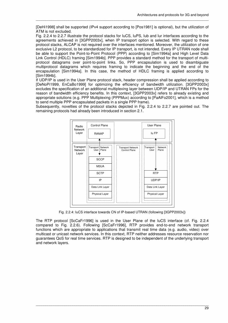
Architectures and protocols for 3G and beyond __________________________________________________________________________________________
__________________________________________________________________________________________ 29
[DeHi1998] shall be supported (IPv4 support according to [Pos1981] is optional), but the utilization of ATM is not excluded. Fig. 2.2.4 to 2.2.7 illustrate the protocol stacks for IuCS, IuPS, Iub and Iur interfaces according to the agreements achieved in [3GPP2003x], when IP transport option is selected. With regard to these protocol stacks, ALCAP is not required over the interfaces mentioned. Moreover, the utilization of one exclusive L2 protocol, to be standardized for IP transport, is not intended. Every IP UTRAN node shall be able to support the Point-to-Point Protocol (PPP) according to [Sim1994a] and High Level Data Link Control (HDLC) framing [Sim1994b]. PPP provides a standard method for the transport of multi-protocol datagrams over point-to-point links. So, PPP encapsulation is used to disambiguate multiprotocol datagrams which requires framing to indicate the beginning and the end of the encapsulation [Sim1994a]. In this case, the method of HDLC framing is applied according to [Sim1994b]. If UDP/IP is used in the User Plane protocol stack, header compression shall be applied according to [DeNoPi1999, EnCaBo1999] for optimizing the efficiency of bandwidth utilization. [3GPP2003x] excludes the specification of an additional multiplexing layer between UDP/IP and UTRAN FPs for the reason of bandwidth efficiency benefits. In this context, [3GPP2003x] refers to already existing and appropriate solutions (e.g. PPP Multiplexing (PPPMux) according to [PaAlFo2001], which is a method to send multiple PPP encapsulated packets in a single PPP frame). Subsequently, novelties of the protocol stacks depicted in Fig. 2.2.4 to 2.2.7 are pointed out. The remaining protocols had already been introduced in section 2.1.
RANAP Iu FP
Transport Network
Layer
TransportUser
Network Plane
Control Plane User Plane
TransportUser
Network Plane
Transport Network Control Plane
Radio Network
Layer
SCTP
IP
Data Link Layer
Physical Layer
UDP/IP
Data Link Layer
Physical Layer
SCCP
M3UA
RTP
Fig. 2.2.4: IuCS interface towards CN of IP-based UTRAN (following [3GPP2003x])
The RTP protocol [ScCaFr1996] is used in the User Plane of the IuCS interface (cf. Fig. 2.2.4 compared to Fig. 2.2.6). Following [ScCaFr1996], RTP provides end-to-end network transport functions which are appropriate to applications that transmit real time data (e.g. audio, video) over multicast or unicast network services. In this context, RTP neither addresses resource reservation nor guarantees QoS for real time services. RTP is designed to be independent of the underlying transport and network layers.

Architectures and protocols for 3G and beyond __________________________________________________________________________________________
__________________________________________________________________________________________ 30
RANAP Iu FP
Transport Network
Layer
TransportUser
Network Plane
Control Plane User Plane
TransportUser
Network Plane
Transport Network Control Plane
Radio Network
Layer
SCTP
IP
Data Link Layer
Physical Layer
UDP/IP
Data Link Layer
Physical Layer
SCCP
M3UA
GTP-U
Fig. 2.2.5: IuPS interface towards CN of IP-based UTRAN (following [3GPP2003x])
In the User Plane of the IuPS interface GTP-U according to [3GPP2004a] (cf. section 2) is used on top of UDP/IP (cf. Fig. 2.2.5 as opposed to Fig. 2.1.7).
NBAP Iub FP
Transport Network
Layer
TransportUser
Network Plane
Control Plane User Plane
TransportUser
Network Plane
Transport Network Control Plane
Radio Network
Layer
SCTP
IP
Data Link Layer
Physical Layer
UDP/IP
Data Link Layer
Physical Layer
Fig. 2.2.6: Iub interface of IP-based UTRAN (following [3GPP2003x])
With regard to the Iub interface the SCTP protocol [StXiMo2000] is supported as signaling bearer for the NBAP application (cf. Fig. 2.2.6 in contrast to Fig. 2.1.8).

Architectures and protocols for 3G and beyond __________________________________________________________________________________________
__________________________________________________________________________________________ 31
RNSAP Iur FP
Transport Network
Layer
TransportUser
Network Plane
Control Plane User Plane
TransportUser
Network Plane
Transport Network Control Plane
Radio Network
Layer
SCTP
IP
Data Link Layer
Physical Layer
UDP/IP
Data Link Layer
Physical Layer
SCCP
M3UA
Fig. 2.2.7: Iur interface of IP-based UTRAN (following [3GPP2003x])
2.2.4 Release 6 PLMN infrastructure
Following [3GPP2005a], a PLMN according to Release 6 (Rel-6) envisages minor architectural changes within the IMS which are not essential in the context of this thesis and thus, neither reported here in detail nor visualized in terms of a figure that depicts a Rel-6 PLMN. Moreover, Rel-6 cares for backwards compatibility with Rel-5 IMS configurations. According to [3GPP2005d], the Rel-6 IMS supports the principle of access independence, i.e. the services of the IMS are offered regardless of the way the IP connection is obtained (e.g. via GPRS, fixed lines, LAN). In this context, the principle of access independence is restricted to access technologies which are either defined by 3GPP or by specific interworking strategies (for example 3GPP system to WLAN interworking as specified for Rel-6, cf. [3GPP2005e]). Furthermore, the Rel-6 IMS supports interworking with existing voice and data networks for fixed (e.g. PSTN, ISDN, Internet, etc.) as well as for mobile users.
2.3 IP radio access network evolution
Under consideration of the first step of UTRAN architecture evolution, which is the introduction of an IP-based transport network in Rel-5, further steps with regard to the evolution of the UTRAN architecture were identified by 3GPP Technical Specification Groups (TSGs). Therefore, requirements for the evolved UTRAN as well as several company proposals for evolved UTRAN architectures were specified and added to the Feasibility Study (FS) reported in [3GPP2003k]. Following [3GPP2003a, 3GPP2003g, 3GPP2003k, 3GPP2003s], 3GPP TSG RAN Working Group (WG) 3 proposes the following requirements the evolved UTRAN architecture is expected to meet: • Changes to the Uu interface shall be avoided so that the evolved architecture is able to connect
to 3GPP early UE (R99). • The impact of the evolved architecture on the CN shall be minimal.

Architectures and protocols for 3G and beyond __________________________________________________________________________________________
__________________________________________________________________________________________ 32
• The evolved architecture shall allow for a different distribution of RAN functionalities to network elements (Node B and RNC in particular).
• Network operators shall be enabled to improve at least one of the following aspects of their network without significantly deteriorating the others: performance, scalability, flexibility and reliability. The result shall be an overall improvement of the UTRAN.
• Performance and reliability for real time as well as non real time services are expected to be similar or better than in the existing architecture.
• Interworking and backward compatibility with the existing architecture shall be envisaged. • Maximum reuse of existing protocols shall be possible. • The usage of equipment made by different vendors shall be enabled by providing open standard
interfaces. • The application of ATM and IP transportation option shall be possible. • An independent optimization of control and User Plane shall be supported. • The usage of specifications other than 3GPP standards (e.g. IETF) shall be possible. • An UTRAN architecture shall be developed that allows for the coexistence of multiple RATs, i.e.
for instance CDMA 2000 and WLAN in addition to W-CDMA. Subsequently, the company proposals for UTRAN architecture evolution submitted by Nokia, Siemens, NEC, Lucent Technologies and Alcatel as well as a further conceivable UTRAN architecture evolution scenario, which was not submitted to the 3GPP standardization discussion, are described in detail.
2.3.1 Nokia proposal for UTRAN architecture evolution
The first proposal for an evolved UTRAN architecture was submitted by Nokia [3GPP2003b] and is illustrated in Fig. 2.3.1.
Iu
Iu Iu Iu Iu Iu
RNG
Node B+
Iur
SGSN
GGSN
Node B+ Node B+ Node B+ Node B+ Node B+
Iur Iur Iur Iur
Iur Iur Iur Iur Iur
Iur RNC
Fig. 2.3.1: Nokia architecture proposal on UTRAN evolution (following [3GPP2003e])
Nokia assumes that most functions of the former RNC are moved to an intelligent Node B which is called Node B+ in this architecture proposal. Particularly, the radio interface protocols are relocated into the Node B+ and thus, located closer to the radio interface. The Iub interface is eliminated, instead, an Iur interface is used between Node B+s to support Control Plane signaling as well as User Plane traffic. An intermediate Radio Network Gateway (RNG) element is introduced as an interworking unit to RANs and CNs of earlier releases. This RNG hides the distributed network architecture (i.e. the bigger number of Node B+s in particular) from the CN and RNC nodes. Furthermore, the RNG acts as a mobility anchor point which implies that the RNG, once selected for a connection, will be retained for the duration of the call. However, Nokia also considers the removal of the RNG element. Node B+s are connected to the RNG via Iu interface, and an additional connection between Node B+s and RNG via Iur interface is necessary for the interworking with RANs from earlier releases in case of drift situations. Nokia assumes enhancements to Iur and Iu interfaces in the
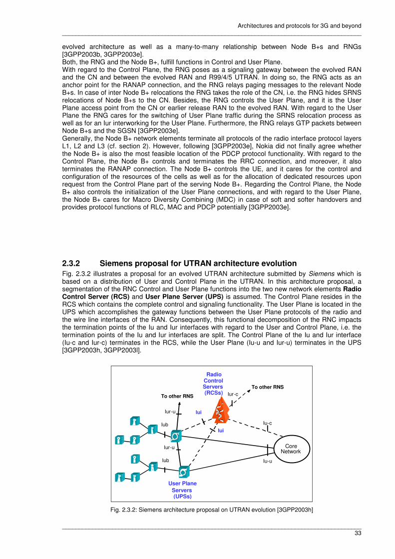
Architectures and protocols for 3G and beyond __________________________________________________________________________________________
__________________________________________________________________________________________ 33
evolved architecture as well as a many-to-many relationship between Node B+s and RNGs [3GPP2003b, 3GPP2003e]. Both, the RNG and the Node B+, fulfill functions in Control and User Plane. With regard to the Control Plane, the RNG poses as a signaling gateway between the evolved RAN and the CN and between the evolved RAN and R99/4/5 UTRAN. In doing so, the RNG acts as an anchor point for the RANAP connection, and the RNG relays paging messages to the relevant Node B+s. In case of inter Node B+ relocations the RNG takes the role of the CN, i.e. the RNG hides SRNS relocations of Node B+s to the CN. Besides, the RNG controls the User Plane, and it is the User Plane access point from the CN or earlier release RAN to the evolved RAN. With regard to the User Plane the RNG cares for the switching of User Plane traffic during the SRNS relocation process as well as for an Iur interworking for the User Plane. Furthermore, the RNG relays GTP packets between Node B+s and the SGSN [3GPP2003e]. Generally, the Node B+ network elements terminate all protocols of the radio interface protocol layers L1, L2 and L3 (cf. section 2). However, following [3GPP2003e], Nokia did not finally agree whether the Node B+ is also the most feasible location of the PDCP protocol functionality. With regard to the Control Plane, the Node B+ controls and terminates the RRC connection, and moreover, it also terminates the RANAP connection. The Node B+ controls the UE, and it cares for the control and configuration of the resources of the cells as well as for the allocation of dedicated resources upon request from the Control Plane part of the serving Node B+. Regarding the Control Plane, the Node B+ also controls the initialization of the User Plane connections, and with regard to the User Plane, the Node B+ cares for Macro Diversity Combining (MDC) in case of soft and softer handovers and provides protocol functions of RLC, MAC and PDCP potentially [3GPP2003e].
2.3.2 Siemens proposal for UTRAN architecture evolution
Fig. 2.3.2 illustrates a proposal for an evolved UTRAN architecture submitted by Siemens which is based on a distribution of User and Control Plane in the UTRAN. In this architecture proposal, a segmentation of the RNC Control and User Plane functions into the two new network elements Radio Control Server (RCS) and User Plane Server (UPS) is assumed. The Control Plane resides in the RCS which contains the complete control and signaling functionality. The User Plane is located in the UPS which accomplishes the gateway functions between the User Plane protocols of the radio and the wire line interfaces of the RAN. Consequently, this functional decomposition of the RNC impacts the termination points of the Iu and Iur interfaces with regard to the User and Control Plane, i.e. the termination points of the Iu and Iur interfaces are split. The Control Plane of the Iu and Iur interface (Iu-c and Iur-c) terminates in the RCS, while the User Plane (Iu-u and Iur-u) terminates in the UPS [3GPP2003h, 3GPP2003l].
User Plane Servers (UPSs)
Radio Control Servers (RCSs)
Iu - c
-
Iui
Iub
Iub
Core Network
Iur - c
Iur - u
Iui Iur - u
To other RNS
To other RNS
Iu u
Fig. 2.3.2: Siemens architecture proposal on UTRAN evolution [3GPP2003h]

Architectures and protocols for 3G and beyond __________________________________________________________________________________________
__________________________________________________________________________________________ 34
According to [3GPP2003l], the functions in Control and User Plane are classified into three types based on their scope which are the UE, the cell and the RNS scope. A RNS, according to the UTRAN evolution scenario depicted in Fig. 2.3.2, consists of one RCS and one or more UPS(s). The UPS fulfills UE and cell related functions, and the RCS achieves functions related to all three scopes. In particular, the RCS has management functionality with regard to the radio resources, mobility, sessions and call control as well as for the User Plane data flow. Furthermore, the RCS cares for the identification and addressing of the UE, for integrity, security and authentication as well as for billing and accounting. The Control Plane related protocols RANAP and RNSAP are terminated in the RCS. Moreover, the RRC protocol is part of the RCS, and the RRC protocol is the only radio interface protocol used by radio signaling. The lower layer radio protocols (L1, MAC and RLC) are commonly used for user traffic and radio signaling. Following [3GPP2003k], the RCS is expected to logically terminate the NBAP protocol. The UPS is responsible for the transfer of user data according to the required QoS. The transport of user data through the UPS is provided by the User Plane protocol stacks which on the one hand comprise the radio interface protocols (L1, MAC, RLC and PDCP) and on the other hand the User Plane protocols towards the CN. According to the mapping decisions of the RCS, the UPS maps radio bearers to logical and transport channel resources and vice versa. Moreover, the UPS cares for the handling of inband signaling data either between the RCS and the UE or between the RCS and adjacent network nodes (e.g. UPS, Node B, CN) [3GPP2003l]. Besides, the UPS processes radio frames and cares for MDC [3GPP2003h]. The BMC radio interface protocol is also located in the UPS [3GPP2003l]. Following [3GPP2003h], UPSs are controlled by RCSs via the new RAN internal Iui interface. The protocols on the Iui interface can be derived from existing 3GPP protocols like NBAP and RRC. Every UPS can be connected to one or more Node B(s) via Iub interface. In this case, the functionalities of the Node B and the Iub interface are unchanged [3GPP2003l]. [3GPP2003h] recommends the collocation of UPSs relatively close to the Node Bs and a centralization of RCSs in pools or clusters. With regard to a physical implementation of the evolved UTRAN evolution scenario presented in Fig. 2.3.2, the Iu, Iur and the new Iui interface are assumed to be mostly based on IP transport, but the evolved architecture is assumed to not explicitly exclude other transport options. The Iub interface is assumed to implement the IP as well as the ATM transport option in order to enable UPSs to connect to already deployed Node Bs which are based on an ATM transportation infrastructure [3GPP2003h]. In case of an ATM-based Iub interface, NBAP messages are carried over UPS to RCS, and in case of an IP-based Iub interface, an optimization by direct routing of NBAP messages to the RCS is enabled [3GPP2003k].

Architectures and protocols for 3G and beyond __________________________________________________________________________________________
__________________________________________________________________________________________ 35
2.3.3 NEC proposal for UTRAN architecture evolution
Fig. 2.3.3 depicts a UTRAN architecture evolution scenario suggested by NEC. This architecture proposal is based on an assumed split on UE and cell level. The proposed architecture also assumes a segmentation of the RNC into the two nodes RCS and UPS. The RCS performs UE control, and the UPS performs cell control and handles User Plane protocols. Furthermore, a separation of Control and User Plane is provided [3GPP2003r].
CP Control Plane UP User Plane
* Location of Iur interface not fully resolved
CN
Iu (UP)
NB
NB
UPS UPS
RCS
NB
RNC
Iu (CP & UP)
RCS Iu (CP)
Iur
Iur * Iub
Iui
Fig. 2.3.3: NEC architecture proposal on UTRAN evolution [3GPP2003r]
A single RCS attends to any given communication process between a UE and the evolved RAN for the complete duration of the communication. UPSs either act as serving or drift UPSs. This drift and serving functionality is almost identical to the equivalent functionality of a RNC [3GPP2003r]. There is a many-to-many relationship between RCSs and UPSs, i.e. a RCS can control many UPSs via the new Iui interface and a UPS may be controlled by many RCSs. [3GPP2003r] recommends the implementation of the Media Gateway Control (Megaco) / ITU-T H.248.1 protocol [GrPaAn2003] on the Iui interface, as the Megaco protocol is specifically defined for architectures with Control and User Plane separation. Following [GrPaAn2003], Megaco is used between elements of a physically decomposed multimedia gateway. In this context, [GrPaAn2003] defines a Media Gateway (MG) as a converter of media, provided in one type of a network into the format required within another type of network. Moreover, [GrPaAn2003] specifies that a Media Gateway Controller (MGC) monitors those parts of the call state that belong to connection control for media channels in a MG. According to [3GPP2003r], the UPS acts as a MG, and the RCS acts as a MGC so that the suitability of Megaco for the Iui interface is justified. For implementation of IP connectivity, Megaco will be used on top of SCTP and in case of ATM connectivity on top of MTP3b. The relationship between UPSs and Node Bs is one-to-many, i.e. a UPS controls and terminates the User Plane for several Node Bs, but a single Node B is controlled by a single UPS and terminates the User Plane for a single UPS. The Node B is connected to the UPS via Iub interface which can be adopted to this architecture proposal [3GPP2003r]. In [3GPP2003r] the location of the Iur interface is not fully resolved. In the proposed architecture the Iur interface is used to handle mobility between UPSs and does not require any modifications. However, the Iur interface might be located either between UPSs or between RCSs. If the Iur interface is located between UPSs, the RCS communicates with the serving UPS, and the serving and drift UPSs communicate with each other via Iur interface. If, in contrast to this, the Iur interface is located between RCSs, the RCS communicates with all UPSs under its control, and the RCS utilizes the Iur interface towards other RCSs for handling of mobility towards UPSs which are not under its control. When controlling the UEs in the cells, there is also the necessity for the RCS to request actions from the UPSs for handling certain UE related activities (e.g. paging, radio bearer setup/modification/release, etc.) which are interconnected with actions on cell level (e.g. sending of paging messages, radio link setup/modification/release, etc.). The RCS terminates the RRC, RANAP and RNSAP protocol, provided that the Iur interface is located between RCS and UPS. The UPS terminates NBAP, RNSAP and ALCAP (in case of ATM transportation deployment) and also all User Plane protocols on transport level (IP, GTP-U, etc.), radio network layer (MAC, RLC, PDCP) and Iu, Iur and Iub interface. Moreover, the UPS is responsible for the handling of User Plane resources [3GPP2003r].

Architectures and protocols for 3G and beyond __________________________________________________________________________________________
__________________________________________________________________________________________ 36
2.3.4 Lucent proposal for UTRAN architecture evolution
The Distributed Radio Access Network (DRAN) [BaScSo2003, 3GPP2003j] is the contribution of Lucent Technologies to the standardization discussion on UTRAN evolution and is illustrated in Fig. 2.3.4. DRAN introduces a functional split between cell related and RAN specific functions and a location of these functions in different network elements. The cell related protocol handling is located in the extended Node B which is called intelligent Node B (iNode B) in this architecture proposal. The RAN specific functions reside in the RAN Server. Furthermore, this proposal also envisages a separation of User and Control Plane so that the Iu interface towards the CN is also split into a control and a User Plane part.
IP Network
Iuc
Iui
Iui
Iuu Iub
Iur
iNode B
iNode B
RAN Server
UE
Uu
UE
Uu
UE
Uu
Iu
Node B
CN (SGSN)
RNC
Fig. 2.3.4: Lucent architecture proposal on UTRAN evolution [BaScSo2003]
In this architecture proposal ATM, as the transport technology in the RAN, is eliminated in favor of an IP-routed network which is not critical in DRAN, because in DRAN the complete time critical radio specific processing from the RNC is relocated into the iNode B and does not require any synchronization with the RAN Server [3GPP2003j]. This means in particular that all radio specific user data handling as well as associated Control Plane functionality, i.e. the cell specific Radio Resource Management (RRM) functionality, is relocated and handled by the iNode B autonomously. In this context, the iNode B comprises the radio interface protocols RRC on the Control Plane and PDCP on the User Plane as well as the lower layer radio protocols (L1, MAC and RLC) which are commonly used for user traffic and radio signaling. The Iub interface becomes node internal to the iNode B and can be optimized independently from standardization. The cell specific RRM functionality within the iNode B is connected via the new Iui interface to the RRM functions within the RAN Server, i.e. although the iNode B is able to manage its radio resources autonomously, they are requested from the RAN Server via Iui interface on demand. The RAN Server has full control on the distributed RAN, it is responsible for the management of bearer services, for paging and for the micro mobility management in the RAN. However, User Plane traffic bypasses the RAN Server, i.e. user traffic is directly routed from the CN to the destination iNode B via the Iuu interface. Nevertheless, the RAN Server is responsible for the management of appropriate transport resources within the RAN as well as for the establishment of necessary radio bearers in the iNode B and Iuu bearers and their coordination. As User Plane traffic does not pass the RAN Server, the RAN Server does not contain any protocol functionality related to the User Plane, but the iNode B which terminates the GTP-U tunnel towards the CN. In consideration of bearer establishment the RAN Server is also responsible for signaling bearer establishment on Iuc towards the CN via RANAP protocol and on the Iui interface towards the iNode B [BaScSo2003, 3GPP2003k]. The iNode Bs are able to perform soft and softer handover via their Iur interface autonomously, interaction with the RAN Server is only necessary in case of hard handovers, which will be handled similar to SRNS relocation [3GPP2003j] concerning the User Plane traffic on the Iuu interface. Consequently, the CN will be involved in the hard handover process which may result in unwanted load within the SGSN. The network operator might be interested to avoid such load situations in the SGSN. Therefore, Lucent recommends an optional GTP-U relay in order to hide hard handover

Architectures and protocols for 3G and beyond __________________________________________________________________________________________
__________________________________________________________________________________________ 37
handling from the CN. The idea of the GTP-U relay is that the existing GTP-U tunnel between SGSN and serving iNode B will be extended to the drift iNode B. Afterwards, the drift iNode B becomes the new serving iNode B, and the former serving iNode B acts as a GTP-U relay. Accordingly, the hard handover is hidden from the CN [3GPP2003t]. DRAN meets the requirements defined by 3GPP. Changes to the Uu interface are avoided so that a 3GPP compliant UE is able to connect to DRAN. There is minimal impact on the Iu interface towards the CN in consequence of the separation of User and Control Plane proposed in this architecture recommendation. This means in particular that the Iu interface is split into a control and a User Plane part. The control part of the Iu interface (Iuc) is terminated at the RAN Server, and the User Plane traffic is directly routed to the iNode B via the User Plane part (Iuu) of the interface (cf. Fig. 2.3.4). Following [3GPP2003j], the separation of User and Control Plane and the fact that user traffic is exclusively processed in the iNode B, enables the integration of different RATs (e.g. WLAN). The interaction between the RAN Server and the access node of the other RAT has to be adopted to the specific control requirements of this RAT (i.e. particularly the Iui interface has to be adopted). As user traffic is carried in IP packets down to the access node, the Iuu interface does not require specific adaptation. With regard to DRAN, the CN will have to handle more network elements, because beside the RAN Servers the iNode Bs will be connected to the CN. In this case, a feasible solution is the aforementioned GTP-U relay. DRAN provides standardized interfaces, but following [3GPP2003k], there is the necessity for standardization of the new Iui interface in order to keep the multi-vendor compatibility. According to [3GPP2003k], an interworking of DRAN and legacy UTRAN is seamlessly possible. The exception to this is the case of soft handover between legacy Node Bs and iNode Bs due to the fact that a legacy Node B does not provide the Iur interface so that a link to the respective RNC might be necessary. Following [BaScSo2003], a possible solution could be that the RNC splits the Iur interface on separate IP tunnels towards the involved Node Bs. DRAN reuses existing protocols [3GPP2003j], but the DRAN network elements can also be configured to support other specifications than 3GPP (e.g. IETF). DRAN allows for a new distribution of RAN functionalities to network elements by transferring all radio-specific user data handling and related Control Plane functionality from the RNC to the iNode B, i.e. a centralized node (RAN Server) is only used in the Control Plane, and User Plane handling is decentralized down to the iNode B. Therefore, DRAN is a step forward towards a flat and decentralized network and towards increased network reliability. Nevertheless, it has to be considered that a RAN Server centralizes the main signaling functionality so that the RAN Server is responsible for large parts of the network and a significant number of iNode Bs. In case of a RAN Server failure the connected UEs can still send/receive data as long as no mobility management with regard to hard handover or call management signaling (e.g. for call establishment / release) is needed. However, compared to a RNC failure in UTRAN which makes large parts of a network completely inaccessible and causes immediate breakups of all ongoing transactions, DRAN provides improved network reliability. DRAN is inherently scalable, i.e. iNode Bs can be added as long as the RAN Server is capable of handling them. It can be assumed that a RAN Server will be able to handle at least a number of iNode Bs which corresponds to the number of Node Bs which can be handled by a Flexent® RNC. Due to the fact that DRAN allows for a logical and physical separation of User and Control Plane, which can be optimized independently, the scalability of the network architecture itself is facilitated so that DRAN can handle an increasing User Plane traffic volume by expanding the IP network and without any extensions to the UMTS nodes.
2.3.5 Alcatel proposal for UTRAN architecture evolution
The architectural proposal for UTRAN evolution submitted by Alcatel on the one hand intends to provide a framework which can be applied for the analysis of existing and evolved UTRAN architectures. On the other hand this proposal aims at the provision of guidelines which can be applied when designing evolved UTRAN architectures [3GPP2003m]. Following [3GPP2003d], the proposal is based on two main principles. Firstly, a split of User and Control Planes is assumed. Secondly, a separation and classification of functions into cell, multi-cell and user scope is

Architectures and protocols for 3G and beyond __________________________________________________________________________________________
__________________________________________________________________________________________ 38
performed. Moreover, the methodology defines functional entities which are allocated to scopes and planes. These functional entities can be grouped heterogeneously. Moreover, the assignment of these bundles to network elements can be varied so that alternative RAN architectures originate which can be evaluated against each other. Fig. 2.3.5 visualizes the application of the developed modeling methodology to the RNC. According to Fig. 2.3.5, user related functional entities implicate that there exists one instance per user. The scope of cell related functional entities is a single cell, and consequently, one instance of such functional entities per cell is assumed. Functional entities having a multi-cell scope are responsible for a certain group of cells and therefore, for a certain geographical area.
Control Plane
User Plane
Multi-Cell RRM
Paging Broadcast Distribution
Multi-cell scope Cell scope
Cell Control
Common Channels
Processing
Mobile Control
User scope
Dedicated Channels
Processing
Fig. 2.3.5: Decomposition of RNC into functional entities [3GPP2003d]
According to [3GPP2003m, VeViSi2002], the functional entities illustrated in Fig. 2.3.5 are described in more detail. The Multi-cell RRM functional entity is responsible for the coordination between different cells in order to optimize RRM. The Paging entity cares for the distribution of paging messages to the appropriate cells, and the Broadcast Distribution functional entity cares for the allocation of CBS messages to the relevant cells. The Cell Control entity comprises those common parts of the RRC protocol which are used for the generation and processing of messages sent on the logical control channels Common Control Channel (CCCH), Paging Control Channel (PCCH) and Broadcast Control Channel (BCCH). Moreover, the Cell Control entity terminates the NBAP protocol. The Common Channels Processing functional entity is responsible for radio processing on common and shared channels and therefore includes RLC and MAC-c/sh protocol layers used for these channels. Furthermore, the Common Channels Processing entity comprises the BMC protocol used for transmission and repetition of CBS messages on the logical traffic channel named Common Traffic Channel (CTCH). The Mobile Control entity cares for the generation and processing of messages exchanged through the logical control channel named Dedicated Control Channel (DCCH) and thus, contains the dedicated parts of the RRC protocol. Moreover, the Mobile Control functional entity is in charge of handover control, macrodiversity control and relocation control and therefore also terminates the RANAP and RNSAP protocols. The Dedicated Channels Processing functional entity carries out functions which are mainly related to radio processing for dedicated channels and hence, comprises the radio layer protocols used for dedicated channels (i.e. PDCP, RLC and MAC-d protocol layer) as well as the macrodiversity combining and splitting unit in case of soft and softer handover. Fig. 2.3.6 illustrates the functional entities of the RNC, their interconnections and a mapping to the UTRAN architecture. [3GPP2003d] explicitly points out that Fig. 2.3.6 does not present a network reference architecture, but a functional architecture, i.e. an identification of the main functional entities was performed which still allows for different groupings of these functional entities in order to reduce the number of external interfaces and the complexity of the architecture.

Architectures and protocols for 3G and beyond __________________________________________________________________________________________
__________________________________________________________________________________________ 39
Control plane
User plane
Core Network Node-B
Multi-Cell Radio Resource Management
Common Channels Processing
Cell Control
Dedicated Channels Processing
Mobile Control
Broadcast Distribution
CRNC/DRNC SRNC
Iub-c
Iub-u Iub-u
Iur-u
Iur-c
Iu-c
Iu-u
Iur-c
Iu-BC
Iu-c
Paging
Fig. 2.3.6: Conjunction of functional entities and mapping to UTRAN architecture [3GPP2003d]
[3GPP2003d] suggests to utilize the functional architecture of the RNC as illustrated in Fig. 2.3.6 as a starting point for the derivation of RAN evolution scenarios. Following [VeViSi2002], SRNC and CRNC/DRNC functions are separated (cf. Fig. 2.3.6), because the cells used by a particular user connection may be controlled by the same RNC, acting as the SRNC, or by a different one. Consequently, the groups of functions may communicate with each other internally within the same RNC or externally via the Iur interface. Moreover, the proposal assumes an IP-based multi-standard RAN, i.e. the Node Bs are capable to support different radio technologies. The basic idea of the architecture proposal is the definition of two main building blocks in terms of a Control Plane platform and a User Plane platform. In a first step both platforms can be implemented in a centralized RAN controller and interconnected via an internal interface. In the framework of further evolution the platforms can be implemented in separate network elements resulting in a distributed architecture where Control and User Plane server are not necessarily colocated and interconnected via an external interface [3GPP2003d]. The resulting RAN consists of more and smaller nodes. Part of the architecture is fully distributed, but part of the architecture is hierarchical. As far as server nodes and server pools are considered with flexible associations between the nodes, the architecture is fully distributed. A hierarchical scope is addressed with regard to the relationship of the Node B and the cell related nodes and between cell and multi-cell related nodes. Between such nodes the interconnectivity is less flexible [VeViSi2002].
2.3.6 Merged Radio Access Network (MRAN)
The Merged RAN (MRAN) evolution scenario assumes that the complete functionality of the Node B and RNC network elements in the UTRAN reference architecture is merged into one single network element. This network element is named Merged Node B so that the MRAN RNS consists of Merged Node Bs. The Merged Node Bs can either be connected to the CN via an ATM-based transport network, or the Merged Node Bs are connected to an IP-based transport network. The MRAN approach is similar to the RAN evolution approach provided by Nokia [3GPP2003b, 3GPP2003k], if the removal of the RNG out of the evolved RAN is considered. The ATM-based (MRAN) [MiScWi2005] is illustrated in Fig. 2.3.7. Within this MRAN evolution scenario, the Merged Node Bs are connected to the CS and PS Domain of the CN via an ATM-based transport network.
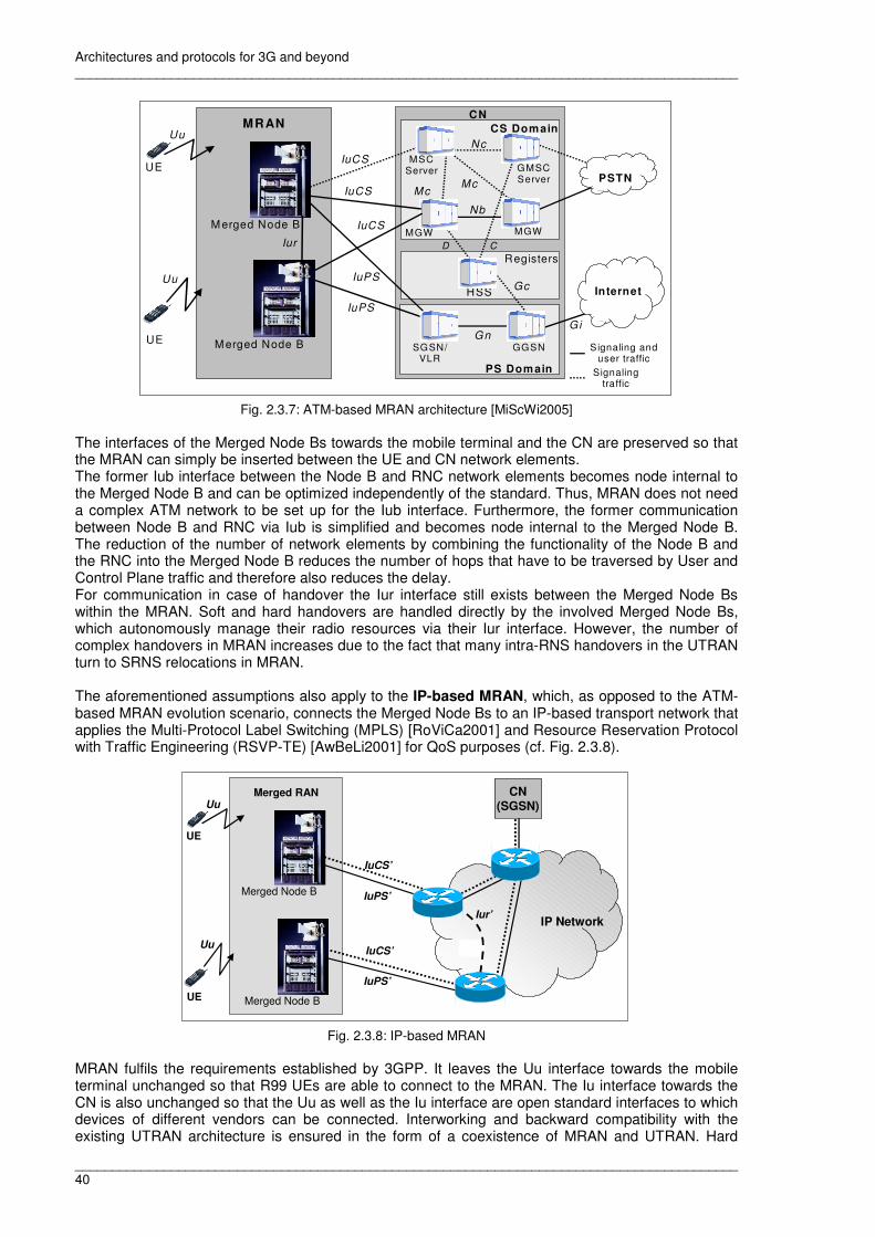
Architectures and protocols for 3G and beyond __________________________________________________________________________________________
__________________________________________________________________________________________ 40
CN
PS Domain
Registers
UE
Uu
Gn
IuCS
Iur
IuPS
CS Domain
IuPS
IuCS
Nc
Gi
MRAN
D C
IuCS
Nb
Mc
Gc
Mc
GMSC Server
HSS
GGSN SGSN/VLR
UE
Uu
Internet
MGW
Merged Node B Signaling and user traffic
Signaling traffic
MSC Server
MGW Merged Node B
PSTN
Fig. 2.3.7: ATM-based MRAN architecture [MiScWi2005]
The interfaces of the Merged Node Bs towards the mobile terminal and the CN are preserved so that the MRAN can simply be inserted between the UE and CN network elements. The former Iub interface between the Node B and RNC network elements becomes node internal to the Merged Node B and can be optimized independently of the standard. Thus, MRAN does not need a complex ATM network to be set up for the Iub interface. Furthermore, the former communication between Node B and RNC via Iub is simplified and becomes node internal to the Merged Node B. The reduction of the number of network elements by combining the functionality of the Node B and the RNC into the Merged Node B reduces the number of hops that have to be traversed by User and Control Plane traffic and therefore also reduces the delay. For communication in case of handover the Iur interface still exists between the Merged Node Bs within the MRAN. Soft and hard handovers are handled directly by the involved Merged Node Bs, which autonomously manage their radio resources via their Iur interface. However, the number of complex handovers in MRAN increases due to the fact that many intra-RNS handovers in the UTRAN turn to SRNS relocations in MRAN. The aforementioned assumptions also apply to the IP-based MRAN, which, as opposed to the ATM-based MRAN evolution scenario, connects the Merged Node Bs to an IP-based transport network that applies the Multi-Protocol Label Switching (MPLS) [RoViCa2001] and Resource Reservation Protocol with Traffic Engineering (RSVP-TE) [AwBeLi2001] for QoS purposes (cf. Fig. 2.3.8).
UE
UE
Uu
IuCS’
IuPS’
IuPS’
Merged RAN
IuCS’
Uu
Merged Node B
Merged Node B
IP Network
CN (SGSN)
Iur’
Fig. 2.3.8: IP-based MRAN
MRAN fulfils the requirements established by 3GPP. It leaves the Uu interface towards the mobile terminal unchanged so that R99 UEs are able to connect to the MRAN. The Iu interface towards the CN is also unchanged so that the Uu as well as the Iu interface are open standard interfaces to which devices of different vendors can be connected. Interworking and backward compatibility with the existing UTRAN architecture is ensured in the form of a coexistence of MRAN and UTRAN. Hard
Architectures and protocols for 3G and beyond __________________________________________________________________________________________
__________________________________________________________________________________________ 41
handovers between both RANs can be performed through cooperation with the CN by redirecting the traffic to the RNC or Merged Node B. In case of soft handover the design of the Iur interface of the Merged Node B is crucial for an interworking of MRAN and legacy UTRAN. If the Iur interface of the Merged Node B allows for a connection to a RNC, then soft handover between MRAN and UTRAN is feasible. Since MRAN can coexist with UTRAN, it can also exist next to other RATs. The fact that handover handling becomes more complex in MRAN (see explanation above: Many intra-RNS handovers in MRAN turn to SRNS relocations which involve the CN and cause extra load there) might be handled similar to the description in [3GPP2003t]. Following [3GPP2003t], the former serving Merged Node B might act as a relay node for the traffic between the CN and the new serving Merged Node B so that a SRNS relocation is not necessary, provided that the Merged Node Bs are connected via an Iur interface. As the Merged Node Bs, MRAN consists of, are designed by combining the RAN functionalities of the UTRAN network elements Node B and RNC, a maximum reuse of existing protocols is assured, but Merged Node Bs can also be configured to support other specifications than 3GPP (e.g. IETF) mainly by changes in software. If appropriate physical interfaces are provided, Merged Node Bs can apply the ATM as well as the IP transport option towards the CN. Depending on the design of the Merged Node B, a separation of the User and Control Plane traffic can be implemented in the device so that an independent optimization of these planes is feasible. Consequently, in this case the Iu interface towards the CN will also be split into a control and a User Plane part. MRAN is a step forward towards a flat and a more flexible network. The coverage of Merged Node Bs can be compared to the coverage of Node Bs in UTRAN, i.e. the number of Merged Node Bs corresponds to the number of Node Bs, as Merged Node Bs substitute the Node Bs in a certain territory. Consequently, reliability is increased as failures in the RAN only have a very local and thus limited impact on the whole system compared to a RNC failure in UTRAN. The architecture is inherently scalable, and impacts resulting from an increasing number of Merged Node Bs managed by the CN are not a crucial point under consideration of the information provided in [Luc2004a, Luc2004b]. According to [Luc2004a], the Flexent® SGSN, taken as an example, is connected to an ATM or IP network, and it is able to serve several Flexent® RNCs which are also connected to the ATM/IP network. Each Flexent® RNC itself is capable to support 250 Node Bs and is expandable to support up to 750 Node Bs [Luc2004b] so that in consequence the Flexent® SGSN is able to handle the load of up to 750 Node Bs (which will be substituted by Merged Node Bs) via an ATM or IP network. The limiting factor for network elements like the SGSN is the number of users or their data throughput and voice traffic [Luc2004a].

Architectures and protocols for 3G and beyond __________________________________________________________________________________________
__________________________________________________________________________________________ 42
2.3.7 Condensed view of company proposals
Fig. 2.3.9 provides a consolidated view of the proposals for an evolved UTRAN in terms of a defined subset of proposed features.
Feature Nokia Siemens NEC Lucent Alcatel MRAN
Focus on IP transport XXXX XXXX XXXX XXXX XXXX XXXX
IP and ATM transport ---- XXXX (X)(X)(X)(X) ---- (X)(X)(X)(X) (X)(X)(X)(X)
Different distribution of functionality XXXX XXXX XXXX XXXX XXXX XXXX
Distributed architecture XXXX XXXX XXXX XXXX (X)(X)(X)(X) XXXX
Evolution of hierarchical one-to-one bindings towards many-to-many bindings XXXX XXXX XXXX XXXX (X)(X)(X)(X) XXXX
Separation of control and user plane ---- XXXX XXXX XXXX XXXX XXXX
Separation of control and user plane in different network elements ---- XXXX XXXX (X)(X)(X)(X) XXXX ----
Differentiation on cell, UE or RAN level ---- ---- XXXX XXXX XXXX ----
RNC as starting point for architecture considerations XXXX XXXX XXXX XXXX XXXX XXXX
Relocation of functions from RNC to Node B XXXX ---- ---- XXXX ---- XXXX
Avoidance of changes to Uu interface XXXX XXXX XXXX XXXX XXXX XXXX
Minimal impact on CN XXXX XXXX XXXX XXXX XXXX XXXX
Scalable architecture XXXX XXXX XXXX XXXX XXXX XXXX
Improvement of reliability XXXX XXXX XXXX XXXX XXXX XXXX
Changes to existing interfaces XXXX XXXX XXXX XXXX XXXX XXXX
New network elements XXXX XXXX XXXX XXXX XXXX XXXX
Additional interfaces ---- XXXX XXXX XXXX XXXX ----
Binding of network nodes to a particular location ---- XXXX ???? ---- (X)(X)(X)(X) ----
Interworking with existing architectures XXXX XXXX XXXX XXXX ???? XXXX
Reuse of existing protocols XXXX XXXX XXXX XXXX XXXX XXXX
Possibility for usage of specifications other than 3GPP standards ???? XXXX XXXX XXXX ???? XXXX
Readiness for multi-radio networks XXXX XXXX XXXX XXXX XXXX XXXX
Legend: X : Architecture proposal implements the feature (X): Architecture proposal only partly considers this feature - : Architecture proposal does not comprise the feature ? : References do not obtain the information whether architecture proposal implements the feature or not Grey parts of the table highlight features which are envisaged by at least four of five company proposals.
Fig. 2.3.9: Feature subset for review of UTRAN evolution architecture proposals Under consideration of Fig. 2.3.9, the development trend of RAN evolution is towards an IP-based transport network and can be characterized in terms of a tendency towards increased reliability. In this context, the presented company proposals focus on the RNC as a starting point for the architecture considerations. The RNC, which is the most vulnerable point in UTRAN, is identified as a single point of failure in [3GPP2003f]. The reason for this is that the R99 RNC is the centralized controlling node for hundreds of Node Bs which in turn can only be connected to one single RNC, i.e. the R99 UTRAN is based on a hierarchical network architecture. Moreover, the R99 RNC comprises the main UTRAN functionalities so that it is of great importance in the network. A RNC failure in the UTRAN impacts large parts of the network which consequently will not be reachable any more [3GPP2003f]. In the RAN evolution proposals the functionality provided by the RNC is distributed differently, and moreover, a distributed instead of a hierarchical network architecture is intended so that failures of network elements only have local and thus limited impact in the network. For the evolution of a hierarchical R99 architecture towards an architecture, which is optimal for delivery of IP-based services, [Usk2003] on the one hand recommends the transformation of one-to-many bindings into many-to-many bindings between the hierarchy levels. On the other hand [Usk2003] advises a decoupling of Control and User Planes which is also envisaged by the architecture evolution proposals presented in this section. The evolved RAN is intended to be more scalable than the R99 UTRAN architecture with regard to the addition of extra network elements (e.g. base stations for better coverage or higher capacity), functionality (e.g. new radio related functionality like High Speed Downlink Packet Access (HSDPA)) or processing capacity in the RAN without drastically impacting the already existing network. If, for instance, in a R99 UTRAN a few Node Bs need to be added to an already existing network, this will most likely require the introduction of a new RNC, because in efficiently used networks the RNC is usually utilized close to its maximum. If in R99 HSDPA is to be introduced, this also requires either a RNC update or a new HSDPA capable RNC, even though the introduction of HSDPA is only intended in small areas like hot spots. Consequently, scalability in R99 UTRAN is a critical point with regard to the aspects mentioned and is subject to improvement in an evolved RAN architecture [3GPP2003f]. Moreover, the evolved architecture is expected to be able to support multiple RATs. Although changes to the Uu interface for backward compatibility with R99 mobile terminals are avoided, changes to existing interfaces as well as an occurrence of new interfaces can be assumed due to the development of new network elements in the RAN. Under consideration of necessary changes to existing interfaces and the protocol design of the new interfaces, a reuse of existing 3GPP protocols is intended. Despite necessary changes the

Architectures and protocols for 3G and beyond __________________________________________________________________________________________
__________________________________________________________________________________________ 43
RAN evolution proposals focus on an interworking with legacy UTRAN and on a minimization of effects caused by the evolved RAN to the CN. As 3GPP requirements on UTRAN evolution demand for similar or better performance within the UTRAN evolution scenarios than in the existing UTRAN architecture, the necessity for a performance evaluation of the evolved UTRAN scenarios emerges. Following [Jai1991], performance evaluation requires a solid understanding of the system to be modeled and a careful selection of an appropriate methodology, the load on the system and the applied tools used within the evaluation.


Simulation modeling methodology __________________________________________________________________________________________
__________________________________________________________________________________________ 45
3 Simulation modeling methodology This chapter introduces a methodology which enables a network designer to assess the performance of general (signaling) network architectures such as the UTRAN evolution scenarios described in section 2.3. Moreover, the chapter presents the fundamentals, the afore mentioned methodology is based on.
3.1 Discrete event simulation
In [LaKe2000] the concept of discrete event simulation described as illustrated in Fig. 3.1.1. In this context, the term system is introduced, and [LaKe2000] defines a system as a facility or process of the real world which is of interest for scientific studies. The intention is to gain insight into the relationship between different components of the system under study or to predict the performance of the system under varying conditions.
System
Actual System Model of the System
Physical Model Mathematical Model
Analytical Solution Simulation
Static Dynamic Deterministic Stochastic Continuous Discrete
Fig. 3.1.1: Ways to study a system (following [LaKe2000])
Under certain conditions the actual system can be studied, provided that the actual system is already existing in reality and that a physical alteration with a subsequent operation of the system is possible, cost-effective and not disruptive to the system itself. If it is not possible to study the actual system, a model of the system has to be built which represents the system and is used in the study as a substitute of the actual system. Nevertheless, the validity of the model has to be taken into account, i.e. it has to be considered, whether the model is an accurate representation of the actual system. A physical construction of the system under study is usually not of interest in operations research and systems analysis. Instead, mathematical models are applied which represent a system in logical and quantitative relationships that can be altered in order to observe the succeeding reaction of the model to the modification and conclude to the reaction of the system under study (provided that the mathematical model is valid). If the mathematical model is a simple model, it may be possible to work with its logical and quantitative relationships to compute an exact analytical solution. Provided that the mathematical model is analytically solvable and computationally efficient, [LaKe2000] recommends to study the model analytically. If the system under study is complex and consequently, the mathematical model is also complex and analytically insolvable, the recommendation of [LaKe2000] is to study the model by means of simulation. The application of simulation means to numerically exercise the model and observe the influence of the inputs of interest on the output measures of performance. [LaKe2000] defines a simulation model as a mathematical model, which is studied by means of simulation and further classifies simulation models (cf. Fig. 3.1.1). A static simulation model is a representation of a system at a particular time or it may be applied to represent a system in which time is irrelevant. In contrast to this a dynamic simulation model represents a system as it evolves when time elapses. A deterministic simulation model does not contain any probabilistic components, and the output is determined when the set of input
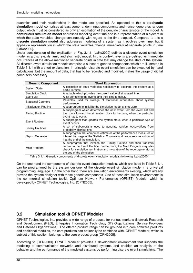
Simulation modeling methodology __________________________________________________________________________________________
__________________________________________________________________________________________ 46
quantities and their relationships in the model are specified. As opposed to this a stochastic simulation model comprises at least some random input components and hence, generates random output which must be considered as only an estimation of the genuine characteristics of the model. A continuous simulation model addresses modeling over time and is a representation of a system in which the state variables change continuously with regard to the time elapsed. Compared to this a discrete simulation model also addresses modeling of a system as it evolves over time, but it applies a representation in which the state variables change immediately at separate points in time [LaKe2000]. Under consideration of the explication of Fig. 3.1.1, [LaKe2000] defines a discrete event simulation model as a discrete, dynamic and stochastic model. In this context, events are defined as immediate occurrences at the above mentioned separate points in time that may change the state of the system. All discrete event simulation models comprise a subset of generic components which are illustrated in Table 3.1.1 with a short explanation. In principle, discrete event simulation can be executed by hand calculations, but the amount of data, that has to be recorded and modified, makes the usage of digital computers necessary.
Generic Component Short Explanation
System State A collection of state variables necessary to describe the system at a particular time.
Simulation Clock A variable which provides the current value of simulated time. Event List A list containing the events and their time to occur.
Statistical Counters Variables used for storage of statistical information about system performance.
Initialization Routine A subprogram to initialize the simulation model at time zero.
Timing Routine A subprogram which determines the next event from the event list and then puts forward the simulation clock to the time, when the particular event has to occur.
Event Routine A subprogram that updates the system state, when a particular type of event occurs.
Library Routines A set of subprograms used to generate random observations from probability distributions.
Report Generator A subprogram that computes estimates of the performance measures of interest by usage of the Statistical Counters and produces a report out of it at the end of the simulation.
Main Program
A subprogram that invokes the Timing Routine and then transfers control to the Event Routine. Furthermore, the Main Program may also check for simulation termination and invocation of the report generator at the end of the simulation.
Table 3.1.1: Generic components of discrete event simulation models (following [LaKe2000]) On the one hand the components of discrete event simulation models, which are listed in Table 3.1.1, can be programmed by the system designer of the discrete event simulation model in a universal programming language. On the other hand there are simulation environments existing, which already provide the system designer with these generic components. One of these simulation environments is the commercial simulation toolkit Optimum Network Performance (OPNET) Modeler which is developed by OPNET Technologies, Inc. [OPN2005].
3.2 Simulation toolkit OPNET Modeler
OPNET Technologies, Inc. provides a wide range of products for various markets (Network Research and Development (R&D), Enterprise Information Technology (IT) Organizations, Service Providers and Defense Organizations). The offered product range can be grouped into core software products and additional modules, the core products can optionally be combined with. OPNET Modeler, which is subject of this section, belongs to the core product group [OPN2005]. According to [OPN2003], OPNET Modeler provides a development environment that supports the modeling of communication networks and distributed systems and enables an analysis of the behavior and the performance of the modeled systems by performing discrete event simulations. The

Simulation modeling methodology __________________________________________________________________________________________
__________________________________________________________________________________________ 47
OPNET Modeler environment comprises tools for model specification, simulation, data collection and data analysis. Consequently, on the one hand the network designer, who applies OPNET Modeler to specify the network model under study, is enabled to build customized models. But on the other hand OPNET Modeler comes along with an extensive Model Library of protocols, technologies and vendor devices (cf. [OPN2005]) which can be utilized or modified and integrated into custom OPNET models. For the purposes of model specification OPNET supports a hierarchical modeling concept which is based on four modeling domains. The OPNET modeling domains are the Network, Node, Process and External System modeling environments which will be described subsequently [OPN2003].
3.2.1 OPNET modeling domains and model specification
The Network Domain defines the topology of a communication network in terms of nodes, links, a geographical context and subnetworks. The nodes are the communicating entities within the communication network. As most nodes require the ability to communicate with other nodes to fulfill their function in a network model, OPNET provides different types of communication link architectures to interconnect nodes for communication purposes. Particularly, these types of link architectures are unidirectional and bidirectional point-to-point links for connection of nodes in pairs, bus links for broadcast communication within an arbitrarily large set of nodes and radio links. The possibility for specification of a geographic context for a network model enables the network designer to choose locations on world or country maps for the specification of WANs or the usage of a dimensioned area for the modeling of LANs. Moreover, the specification of a geographical context for a network model implies an intrinsic notion of distance which allows for an automatic calculation of communication delays between nodes. For the modeling of large networks OPNET enables the reduction of complexity by the utilization of the subnetwork concept that allows to group various combinations of nodes, links and also other subnetworks into subnetworks which themselves form networks that can be connected by communication links [OPN2003]. Fig. 3.2.1 depicts a M/M/1 OPNET model as an example of the Network Domain and, Fig. 3.2.1 (a) depicts the topmost subnetwork which comprises a network model of a M/M/1 system. If the topmost subnetwork is expanded by double click, Fig. 3.2.1 (b) shows that it contains a Source node, a Queue + Service node and a Sink node which are interconnected by a unidirectional point-to-point link. In the M/M/1 system the Source nodes sends packets to the Queue + Service node which enqueues and services the packets and sends them to the Sink node that destroys them.
(a) (b)
Node Link Subnet
Fig. 3.2.1: OPNET Modeler Network Domain
The Node Domain provides for the modeling of the node entities that can be deployed and interconnected in the Network Domain. In the real world the nodes correspond to various types of computing and communicating equipment (e.g. workstations, bridges, routers, UE, Node B, RNC, CN, etc.). In OPNET nodes are composed of modules and connections. Modules represent smaller building blocks inside the nodes, and connections interconnect modules and thus, enable interaction

Simulation modeling methodology __________________________________________________________________________________________
__________________________________________________________________________________________ 48
between modules. The modules of the Node Domain are transmitters, receivers, processors, queues and external systems (esys). Transmitters and receivers enable the attachment of a node to communication links in the Network Domain. Processors, queues and esys are modules which are highly programmable by the network designer who can specify their overall behavior in the Process Domain. A node model can consist of modules of different types. OPNET provides three types of connections between modules. These types of connections are packet streams, statistic wires and logical associations. Packet streams enable the transfer of messages between modules. Statistic wires convey simple numerical signals or control information between modules. Logical associations specify a binding between modules. However, the application of logical associations is only allowed between transmitter and receiver modules to indicate that a particular transmitter and receiver should be used as a pair when attaching the node to a link in the Network Domain [OPN2003]. Fig. 3.2.2 continues the expansion of the OPNET M/M/1 model, i.e. the Source node, the Queue + Service node and the Sink node of the M/M/1 system are expanded so that their node models become visible. The Source node consists of a processor module and a transmitter module. The processor module of the Source node comprises the functionality to generate packets, and the transmitter module is needed for interconnection with the Queue + Service node in the Network Domain (cf. Fig. 3.2.2 (a)). The Queue + Service node consists of a queue module that comprises a First-In First-Out (FIFO) queue for enqueueing of packets and a service unit to service the packets as well as a transmitter module and a receiver module for interconnection with the Source and Sink node in the Network Domain (cf. Fig. 3.2.2 (b)). The Sink node consists of a receiver module for interconnection with the Queue + Service node and a processor module that comprises the functionality to destroy incoming packets (cf. Fig. 3.2.2 (c)).
(a) (b) (c)
Processor Receiver Queue + Service
Unit
Packet stream
Transmitter
Fig. 3.2.2: OPNET Modeler Network / Node Domain The Process Domain provides for the modeling of process models. Processor, queue and esys modules of the Node Domain execute tasks which are referred to as processes. Processes occupy a set of instructions, they maintain state memory and they are specified in the form of process models. A process, that operates in a processor, queue or esys module, is an instance of a particular process model. The process modeling paradigm supports the concept of modeling process groups. A process group consists of multiple processes that execute within the same module. At simulation begin each module has only one single process which is the root process. During simulation progression the root process can create new processes, which can in turn create others, etc. These processes, which are created during simulation run, are referred to as dynamic processes. The creation and the destruction of processes depends on dynamic conditions that are analyzed by the logic of the executing processes. With regard to real world modeling tasks, the process group modeling paradigm provides a natural framework for modeling common systems (e.g. multitasking operating systems, where the root process represents the operating system itself and the dynamically created processes correspond to new tasks; multi-context protocols, where the root process

Simulation modeling methodology __________________________________________________________________________________________
__________________________________________________________________________________________ 49
represents a session manager and each new session that is requested is modeled by the creation of a new process). Processes are designed to respond to interrupts which are events (e.g. message arrival, timer expiration, state changes in other modules, etc.) that are directed at a process and that may require it to perform some action. If some action is taken in response, the process blocks after performing the actions and waits for the next interrupt. Interrupts can be generated by sources external to a process group, by other members of a process group or by a process itself. OPNET process models are specified using the language Proto-C which is specifically designed to support the development of protocols and algorithms. The Proto-C language is based on a combination of State Transition Diagrams (STDs) to represent Finite State Machines (FSMs), a library of high level commands referred to as Kernel Procedures (KPs) and the general features of the C or C++ programming language. The STD defines the states that the process can enter, and for each state it defines the conditions that cause the process to change to another state. The condition, necessary for a state change, and the associated destination state are referred to as transition. OPNET STDs comprise several extensions compared to traditional STD approaches which are State Executives, Transition Conditions and Transition Executives. State Executives enable the network designer to specify actions which are executed whenever a process enters or leaves a particular state. Hence, regarding the State Executives, it has to be differentiated between Enter Executives and Exit Executives (cf. Fig. 3.2.3) as places for the specification of actions within a particular state. Enter Executives are traversed and the actions specified inside are executed when a process enters a particular state. Exit Executives are passed and the actions related to them are performed when a process leaves a state. Transition Conditions enable the network designer to specify statements which pass back Boolean return values when evaluated and determine, under consideration of the return value, whether a transition will be traversed or not. Transition Executives specify actions which are executed whenever a transition is traversed.
Enter Executive
Exit Executive
Fig. 3.2.3: State Executives (OPNET Modeler Process Domain)
The states within the STD can either be forced states that use a green colored state symbol within OPNET Modeler or unforced states which utilize a red colored state symbol. The difference between forced and unforced states is that forced states do not block. As opposed to this, unforced states block immediately in the middle of the state upon executing the code within the Enter Executive. Then unforced states wait for a new interrupt before continuing with the Exit Executive. The Proto-C library of KPs is grouped into packages of related functions (e.g. Distribution Package, Interrupt Package, etc.). These functions are available to the network designer and provide commonly needed actions (e.g. the KP op_dist_exponential (mean) which is part of the Distribution Package returns a random value from an exponential distribution which has a specified mean). Moreover, Proto-C enables the network designer to express actions at various points in the FSM by definition of C or C++ statements. Fig. 3.2.4, 3.2.5 and 3.2.6 show the process models of the Source module, the FIFO Queue + Service module and the Sink module. As transmitter and receiver modules are basic modules, they are not part of the programmable modules, i.e. transmitter and receiver modules cannot be further specified by process models. Instead, they provide a defined functionality to interconnect nodes in the Network Domain which cannot be modified by the network designer.
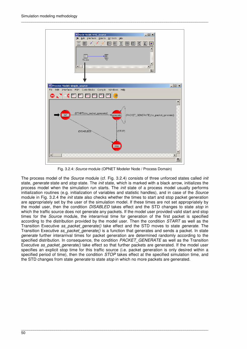
Simulation modeling methodology __________________________________________________________________________________________
__________________________________________________________________________________________ 50
Fig. 3.2.4: Source module (OPNET Modeler Node / Process Domain) The process model of the Source module (cf. Fig. 3.2.4) consists of three unforced states called init state, generate state and stop state. The init state, which is marked with a black arrow, initializes the process model when the simulation run starts. The init state of a process model usually performs initialization routines (e.g. initialization of variables and statistic handles), and in case of the Source module in Fig. 3.2.4 the init state also checks whether the times to start and stop packet generation are appropriately set by the user of the simulation model. If these times are not set appropriately by the model user, then the condition DISABLED takes effect and the STD changes to state stop in which the traffic source does not generate any packets. If the model user provided valid start and stop times for the Source module, the interarrival time for generation of the first packet is specified according to the distribution provided by the model user. Then the condition START as well as the Transition Executive ss_packet_generate() take effect and the STD moves to state generate. The Transition Executive ss_packet_generate() is a function that generates and sends a packet. In state generate further interarrival times for packet generation are determined randomly according to the specified distribution. In consequence, the condition PACKET_GENERATE as well as the Transition Executive ss_packet_generate() take effect so that further packets are generated. If the model user specifies an explicit stop time for this traffic source (i.e. packet generation is only desired within a specified period of time), then the condition STOP takes effect at the specified simulation time, and the STD changes from state generate to state stop in which no more packets are generated.

Simulation modeling methodology __________________________________________________________________________________________
__________________________________________________________________________________________ 51
/* Proto-C code of state arrival */
/* Enter executive */
/* acquire the arriving packet */
/* from packet stream */
pkptr = op_pk_get (op_intrpt_strm ());
/* attempt to enqueue the packet at tail */
/* of subqueue 0 */
if (op_subq_pk_insert (0, pkptr, OPC_QPOS_TAIL) != OPC_QINS_OK) {
/* the inserton failed (due to to a full queue)
/* deallocate, i.e. destroy the packet */
op_pk_destroy (pkptr);
/* set flag indicating failed insertion */
/* (as this flag is used to determine */
/* transition out of this state) */
insert_ok = 0;
}
else {
/* set flag indicating successful insertion */
insert_ok = 1; }
Fig. 3.2.5: Queue + Service module (OPNET Modeler Node / Process Domain) The process model of the FIFO Queue + Service module (cf. Fig. 3.2.5) consists of four forced states (init, arrival, svc_start and svc_comp) and the unforced state idle. If the FIFO Queue + Service module is in state init, that again performs initialization routines, the STD afterwards changes by default to state idle provided that no packet arrives. If a packet arrives when the FIFO Queue + Service module is in state init, then the STD switches to state arrival. The Proto-C code that is executed in state arrival is also illustrated in Fig. 3.2.5 and specifies the action that a packet is either enqueued at the tail of the FIFO queue or destroyed. Although the FIFO Queue + Service module allows to use queues with infinite buffer, the model user can also specify the buffer capacity of the queue either in bits or by the number of packets. If the buffer capacity of the queue is limited and the buffer is filled to capacity with packets, the necessity arises to destroy incoming packets. If the STD is in state arrival, due to a previous packet arrival, the buffer capacity of the FIFO queue allows for insertion of the packet, and the service unit is idle, the STD changes to state svc_start. In case one of these conditions fails (i.e. the packet cannot be inserted into the queue due to a full buffer or the service unit is already busy), the STD returns to state idle. In state svc_start the packet, which is positioned at the head of the FIFO queue, is taken out of the queue for getting serviced, and the service unit is declared busy for the duration of the service time which is calculated according to (1).

Simulation modeling methodology __________________________________________________________________________________________
__________________________________________________________________________________________ 52
]sec[bits/RateService
[bits]LengthPacket]sec[TimeService = (1)
Subsequently, the utilization statistics of the service unit is updated, the process sets a self interrupt for the point of time when service ends, and the STD switches to state idle. If the point of time occurs that the service time is over, the STD moves to state svc_comp; in the meantime the STD can also change to other states (e.g. state arrival, if further packets arrive). In state svc_comp statistical values are written to statistic handles (e.g. sojourn time of a packet in the FIFO queue and service unit system, waiting time in the queue, service time), and the service unit is declared idle. Consequently, the STD can change to state svc_start again, provided that the FIFO queue is not empty. Otherwise, the STD moves to state idle.
Fig. 3.2.6: Sink module (OPNET Modeler Node / Process Domain) The process model of the Sink module (cf. Fig. 3.2.6) consists of the forced state init and the unforced state discard. In the state discard statistical values (e.g. the End-to-End (E2E) delays of incoming packets, the number of packets and bits received) are written to statistic handles that are initialized in state init. After recording the statistics of interest, the packets are destroyed within state discard. The esys module of the External System Domain provides the mechanism that enables an OPNET simulator to communicate with other simulators and allows other simulators to interact with an OPNET simulation. This interaction, which is referred to as cosimulation, means that the two simulators can exchange data while running in parallel. The esys module consists of an External System Definition (ESD) and a process model. The ESD specifies the way the cosimulation has to be built and defines the esys interface that will exchange data with the external code (i.e. accept data from the external code, send data to the external code or both). The process model of the esys module delivers values to esys interfaces or reads values delivered to esys interfaces by the external simulator. Thus, the process model of the esys module serves as the interface between the external code and the rest of the OPNET model [OPN2003].

Simulation modeling methodology __________________________________________________________________________________________
__________________________________________________________________________________________ 53
Fig. 3.2.7 summarizes the OPNET modeling domains and their relationships.
Network
Node
Module
Process
ESD
Fig. 3.2.7: Relationship of hierarchical levels in OPNET models [OPN2003]
The OPNET modeling domains are covered by graphical editors which provide an interface for the network designer to the OPNET Modeler environment and can be used by the network designer to specify the network under study. But OPNET also provides an Application Program Interface (API) which is the External Model Access (EMA). EMA is the technique of accessing an OPNET model externally to the OPNET Modeler program (i.e. without using the graphical editors). The process of accessing an OPNET model externally comprises the creation and the modification of the model as well as the extraction of data from the model. EMA is supported by a library of C and C++ accessible functions that can be used as a programmatic specification and query language [OPN2003]. Communication of data takes place at all levels of the OPNET modeling domain hierarchy. The fundamental structure which provides the most commonly used mechanism for information exchange between the modeling domains is the packet. Packets can be stored by and transferred between objects in each of the modeling domains, and packets are objects which contain formatted information that can change dynamically. With regard to packets it has to be differentiated between formatted, unformatted and value vector packets. Formatted packets have fields that are defined according to a template which is the packet format. A packet field is further specified in terms of a name, a data type (e.g. integer, floating point), a size (assigned in bits) and a default value. Unformatted packets have no fields at creation time, but fields can be added one at a time and can only be referenced by a numeric index, not by name. Value vector packets do not contain user-defined fields, but a sequence of binary numbers representing data passed within cosimulation. The term packet does not restrict the types of applications that can be modeled using OPNET Modeler. Instead, OPNET packets represent information-carrying structures of various types that appear in communication networks and system architectures, like, for instance, packets, messages, frames, cells, datagrams and transactions [OPN2003]. OPNET Modeler supports increased reusability of OPNET models and objects, which represent the entities of the system under study, as it enables the network designer when setting up the simulation model to equip models and objects with attributes (e.g. distribution, packet formats). The values of these attributes can be varied by the user of the simulation model which enables the user to alter the behavior of models and objects in a well-defined manner without the necessity to actually modify the internals of models or objects themselves. The values of these attributes can be specified in advance, i.e. before the start of the simulation run, but the attributes can also be promoted. A promoted attribute moves up to the next level in the model hierarchy, allowing the specification of its value to be performed there. If attributes are promoted to the top of the hierarchy, which is the topmost subnetwork, they become attributes of the simulation. In this case, the values of these attributes can be specified on a Graphical User Interface (GUI) during simulation run or within an environment file which is loaded and evaluated during simulation execution [OPN2003].

Simulation modeling methodology __________________________________________________________________________________________
__________________________________________________________________________________________ 54
3.2.2 Simulation execution, data collection and data analysis
If the model of the network under study is specified within OPNET Modeler, simulations can be executed. On the one hand OPNET provides a graphical simulation tool which enables the network designer to configure and run any number of simulations conveniently via the GUI. On the other hand OPNET simulations, as they are ordinary programs, can also be executed from the command line which enables the network designer to run a significant number of simulations (e.g. for production runs) using a batch file [OPN2003]. Moreover, command line execution speeds up simulations and preserves memory, because the GUI does not have to be maintained (e.g. permanent display of the GUI during simulation run and update of progress bars). OPNET Modeler provides three types of output which are automatically generated by the simulation runs performed. These types of output, which are used by the network designer for an assessment of performance measures and a behavioral analysis of the system under study, are Output Vectors, Output Scalars and Animations. An Output Vector is a collection of pairs of real values which are referred to as entries. These entries are collected during one simulation run. The first value within the entries can be considered as the independent variable and the second as the dependent variable which in OPNET are referred to as the abscissa and ordinate. In the majority of cases the independent variable represents the simulation time which increases monotonically when simulation progresses, but it is also possible to create Output Vectors that have abscissa variables other than time. If the independent variable of the Output Vector represents the simulation time, then the Output Vector represents the value of the dependent variable as it varies over time [OPN2003]. Output Scalars are individual values, i.e. typically scalar statistics are averages, probabilities or peak values which are derived from a collection of measurements. If Output Scalars are taken as individual data points, they are only of limited significance. Therefore, the usual practice is to combine Output Scalars recorded over multiple simulation runs to form a graph which shows how a system variable varies as a function of other system parameters. The dependent as well as the independent system variables of the graph are recorded as Output Scalars. The Output Scalar results generated by multiple simulation runs are kept within a single Output Scalar file. In the Output Scalar file the scalars from each simulation run are kept in groups so that they can be related to each other. If a graph is plotted from the results in the Output Scalar file, then each point of the graph usually corresponds to a single simulation run [OPN2003]. The specification whether statistics are collected as Output Vectors or Output Scalars is performed by the network designer. Moreover, the network designer is enabled to specify custom statistics within process models in addition to the predefined OPNET statistics within OPNET models. Custom statistics can either have local or global scope. If a custom statistic has local scope, then it is maintained separately for each processor or queue that declares it so that local custom statistics are appropriate to record information that only relates to events at a particular location (e.g. the utilization of a Central Processing Unit (CPU) on a particular server). A custom statistic with global scope is shared and contributed to by many entities in the model so that global custom statistics are adequate for recording information that relates to the performance or behavior of the system as a whole (e.g. the E2E delay of all application data transported by a network) [OPN2003]. An Animation is a dynamic graphical representation of selected events that occurred during a simulation which can be depicted within a diagram from the Network, the Node or the Process Domain or simply within an empty window. The provision of animated output of OPNET simulations enables the network designer to visually analyze the behavior of a network model. In this context, OPNET allows for an automatic generation of certain types of predefined animations, but the Animation KP package also enables the network designer to program sophisticated animations which represent simulation events in a customized way. Automatic as well as custom animations can be viewed interactively during simulation run or after the simulation in a replay mode [OPN2003]. OPNET models usually contain a large number of potential statistics and animations of interest. If all statistics and animations were activated by default, large amounts of data would be recorded which on the one hand would occupy large amounts of hard disk memory and on the other hand would slow down simulation execution. Therefore, OPNET provides a mechanism that enables the network designer to explicitly activate particular statistics and animations of interest for collection which will be recorded in appropriate output files. The selected statistics and animations are referred to as probes which indicate whether a particular scalar statistic, vector statistic or form of animation is to be collected [OPN2003]. Finally, OPNET also supports the network designer in the examination phase of the collected simulation results which on the one hand requires a graphical and/or numerical presentation of Output Scalar and Output Vector files and on the other hand demands visualization of recorded animations.
Simulation modeling methodology __________________________________________________________________________________________
__________________________________________________________________________________________ 55
The visualization of recorded animations is provided by a built-in viewer tool within the OPNET Modeler environment that allows for animation visualization either during simulation run or afterwards. But OPNET Modeler also provides a tool for the analysis of Output Vector and Output Scalar files. Individual or multiple Output Vectors can be loaded and displayed as traces which are ordered sets of abscissa and ordinate pairs. In addition, the OPNET built-in data analysis tool provides a number of numerical processing operations that can be applied to traces to generate new data for plotting. With regard to the numerical processing operations, the creation of Probability Mass Functions (PMFs), Probability Density Functions (PDFs), Cumulative Distribution Functions (CDFs), Histograms and Confidence Intervals is supported and moreover, Mathematical Filters can be applied to the traces (e.g. the Mean Filter generates a second statistic out of an input statistic, and the second statistic represents the running mean of the ordinate values of the input statistic beginning with the first entry). In the analysis tool provided by OPNET Modeler, scalar files can be selected and Output Scalars from the same file can be plotted against each other to view the results of multi-simulation parametric studies. These graphs created from Output Vector and Output Scalar files can be preserved and saved as an analysis configuration. Besides, OPNET Modeler allows for an export of Output Vector and Output Scalar data to Microsoft Excel so that the numbers are externally available for customized processing within Microsoft Excel or other data analysis software (e.g. R [RPr2005], etc.).
3.3 Message Sequence Charts (MSCs)
[ITU1999b] defines Message Sequence Chart (MSC) as a trace language for the specification and description of the communication behavior of system components and their environment by means of message exchange. More abstractly, this means that MSC is a language to describe the interaction between a number of independent instances passing messages. The MSC language is applicable to various application domains, and an overview specification of the communication behavior of real time systems, particularly telecommunication switching systems, is an important area of MSC application. MSC can be applied throughout the system engineering process (i.e. in the phase of domain analysis and idea generation, in the requirements capture phase, in the specification phase of test cases and for documentation purposes) as well as for simulation and validation purposes. In this context MSC can be utilized for the specification of standard, exceptional and disallowed cases. Moreover, MSC supports complete specifications (e.g. for documentation purposes) as well as incomplete specifications (e.g. as an outcome of early analysis).

Simulation modeling methodology __________________________________________________________________________________________
__________________________________________________________________________________________ 56
3.3.1 Basic principles of the MSC language
On the one hand MSC can be used as a graphical language which utilizes two-dimensional diagrams to give a survey of the behavior of communicating instances. On the other hand MSC can be applied textually for the exchange between tools and as a base for automated formal analysis. Fig. 3.3.1 illustrates a basic MSC graphically (a) as well as textually (b).
msc basic; inst Instance_1: process message_exchange; inst Instance_2: process message_exchange; gate out message_1 to Instance_1; gate in message_4 from Instance_2;
Instance_1: instance process message_exchange; in message_1 from environment; out message_2 to Instance_2; in message_3 from Instance_2; out message_4 to Instance_2; endinstance; Instance_2: instance process message_exchange; in message_2 from Instance_1; out message_3 to Instance_1; in message_4 from Instance_1; out message_5 to environment; endinstance;
endmsc;
(b)
msc basic
process message_exchange
Instance_1 Instance_2
message_1
message_2
message_5
message_3
(a)
message_4 Output message event
Input message event
Instance kind name
Instance name
Message name
Instance axis Instance end Message to the environment
Message from the environment
process message_exchange
Fig. 3.3.1: Basic MSC (graphical (a) / textual (b) representation) (following [ITU1999b]) One single MSC describes the partial behavior of a system. The MSC shown in Fig. 3.3.1 depicts the message exchange between the interacting instances Instance_1 and Instance_2 (also specified with their instance kind name process message_exchange) and their environment. With regard to the message exchange the sending and the consumption of messages are asynchronous events. Moreover, it is assumed that the environment of a MSC is able to send messages to the MSC, and the environment is able to receive messages from the MSC. Gates represent the interface between the MSC and its environment (cf. Fig. 3.3.1 (b)). A message within a MSC is a relation between an output and an input. The output may be sent by the environment, by an instance or may be a spontaneously found message. The input is either sent to the environment or to an instance or it is lost, i.e. a message which is sent, but not consumed. For each instance, which is included in the MSC, there is an instance axis. Along each instance axis the time elapses from top to bottom. A
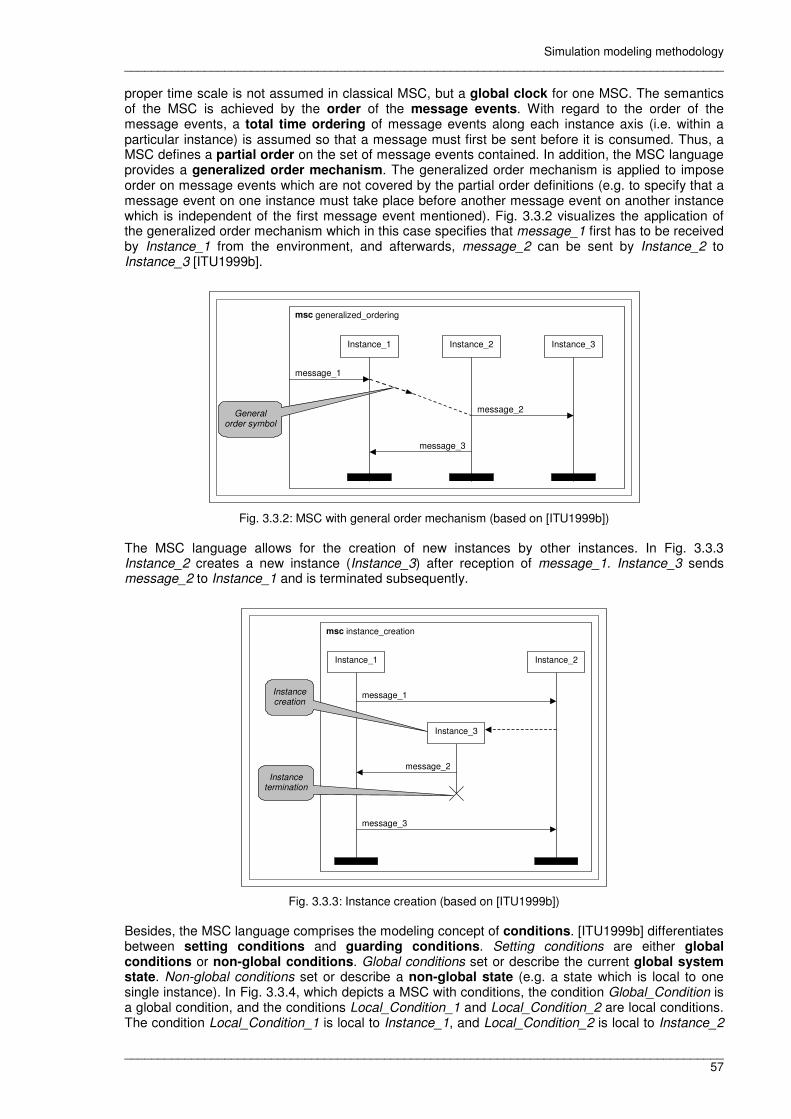
Simulation modeling methodology __________________________________________________________________________________________
__________________________________________________________________________________________ 57
proper time scale is not assumed in classical MSC, but a global clock for one MSC. The semantics of the MSC is achieved by the order of the message events. With regard to the order of the message events, a total time ordering of message events along each instance axis (i.e. within a particular instance) is assumed so that a message must first be sent before it is consumed. Thus, a MSC defines a partial order on the set of message events contained. In addition, the MSC language provides a generalized order mechanism. The generalized order mechanism is applied to impose order on message events which are not covered by the partial order definitions (e.g. to specify that a message event on one instance must take place before another message event on another instance which is independent of the first message event mentioned). Fig. 3.3.2 visualizes the application of the generalized order mechanism which in this case specifies that message_1 first has to be received by Instance_1 from the environment, and afterwards, message_2 can be sent by Instance_2 to Instance_3 [ITU1999b].
msc generalized_ordering
Instance_1 Instance_2
message_1
Instance_3
message_2
message_3
General order symbol
Fig. 3.3.2: MSC with general order mechanism (based on [ITU1999b])
The MSC language allows for the creation of new instances by other instances. In Fig. 3.3.3 Instance_2 creates a new instance (Instance_3) after reception of message_1. Instance_3 sends message_2 to Instance_1 and is terminated subsequently.
msc instance_creation
Instance_1 Instance_2
message_1
Instance_3
message_2
message_3
Instance creation
Instance termination
Fig. 3.3.3: Instance creation (based on [ITU1999b])
Besides, the MSC language comprises the modeling concept of conditions. [ITU1999b] differentiates between setting conditions and guarding conditions. Setting conditions are either global conditions or non-global conditions. Global conditions set or describe the current global system state. Non-global conditions set or describe a non-global state (e.g. a state which is local to one single instance). In Fig. 3.3.4, which depicts a MSC with conditions, the condition Global_Condition is a global condition, and the conditions Local_Condition_1 and Local_Condition_2 are local conditions. The condition Local_Condition_1 is local to Instance_1, and Local_Condition_2 is local to Instance_2
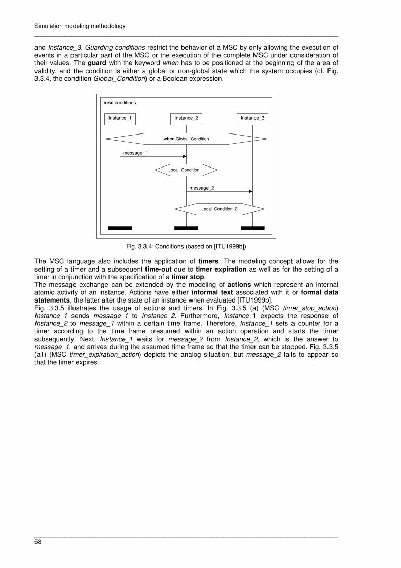
Simulation modeling methodology __________________________________________________________________________________________
__________________________________________________________________________________________ 58
and Instance_3. Guarding conditions restrict the behavior of a MSC by only allowing the execution of events in a particular part of the MSC or the execution of the complete MSC under consideration of their values. The guard with the keyword when has to be positioned at the beginning of the area of validity, and the condition is either a global or non-global state which the system occupies (cf. Fig. 3.3.4, the condition Global_Condition) or a Boolean expression.
msc conditions
Instance_1 Instance_2
message_1
message_2
when Global_Condition
Instance_3
Local_Condition_1
Local_Condition_2
Fig. 3.3.4: Conditions (based on [ITU1999b])
The MSC language also includes the application of timers. The modeling concept allows for the setting of a timer and a subsequent time-out due to timer expiration as well as for the setting of a timer in conjunction with the specification of a timer stop. The message exchange can be extended by the modeling of actions which represent an internal atomic activity of an instance. Actions have either informal text associated with it or formal data statements; the latter alter the state of an instance when evaluated [ITU1999b]. Fig. 3.3.5 illustrates the usage of actions and timers. In Fig. 3.3.5 (a) (MSC timer_stop_action) Instance_1 sends message_1 to Instance_2. Furthermore, Instance_1 expects the response of Instance_2 to message_1 within a certain time frame. Therefore, Instance_1 sets a counter for a timer according to the time frame presumed within an action operation and starts the timer subsequently. Next, Instance_1 waits for message_2 from Instance_2, which is the answer to message_1, and arrives during the assumed time frame so that the timer can be stopped. Fig. 3.3.5 (a1) (MSC timer_expiration_action) depicts the analog situation, but message_2 fails to appear so that the timer expires.

Simulation modeling methodology __________________________________________________________________________________________
__________________________________________________________________________________________ 59
msc timer_expiration_action
Instance_1 Instance_2
message_1
(a1)
set timer_counter
T (timer_counter)
wait
Timer expired
msc timer_stop_action
Instance_1 Instance_2
message_1
message_2
(a)
set timer_counter
T (timer_counter)
wait
Timer started
Timer stopped
Action
Fig. 3.3.5: Timer stop (a) / expiration (a1) and action (based on [ITU1999b])
3.3.2 Time concept of the MSC language
As classical MSC ignores time and simply can be interpreted as a set of traces of message events, a time concept was introduced which revises the MSC modeling methodology for the purpose of modeling real time systems. The time concept envisages the representation of the time progression explicitly in a quantified way. According to the time concept, the traces of message events are amended with an additional event which represents the passage of time so that the time distance between pairs of message events becomes evident. However, the message events themselves do not consume time, and the time progression is equal for all instances within a MSC. MSC distinguishes between relative timing and absolute timing. Relative timing uses pairs of message events, i.e. preceding and subsequent events. In this case, the preceding event enables either directly or indirectly, i.e. via intermediate events, the succeeding event. Absolute timing is applied to specify the occurrence of message events at points in time. Moreover, MSC specifies the concept of time intervals which define constraints on the timing for the occurrence of message events by means of the interval boundaries. Time intervals can be used for relative timing as well as for absolute timing. Furthermore, in case of relative timing, the delay between the enabling and the occurrence of a message event can be measured, and in case of absolute timing, the absolute time of the occurrence of a message event is measurable. Fig. 3.3.6 shows the observation of time in a MSC via absolute and relative measurements and the application of time constraints [ITU1999b].
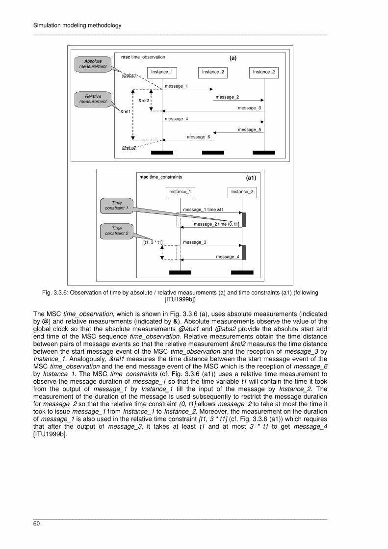
Simulation modeling methodology __________________________________________________________________________________________
__________________________________________________________________________________________ 60
msc time_observation
Instance_1 Instance_2
(a)
@abs1
@abs2
&rel2
&rel1
message_1
message_6
Instance_2
message_2
message_3
message_4
message_5
Absolute measurement
Relative measurement
msc time_constraints
Instance_1 Instance_2
(a1)
[t1, 3 * t1]
message_1 time &t1
message_2 time (0, t1]
message_3
message_4
Time constraint 1
Time constraint 2
Fig. 3.3.6: Observation of time by absolute / relative measurements (a) and time constraints (a1) (following [ITU1999b])
The MSC time_observation, which is shown in Fig. 3.3.6 (a), uses absolute measurements (indicated by @) and relative measurements (indicated by &). Absolute measurements observe the value of the global clock so that the absolute measurements @abs1 and @abs2 provide the absolute start and end time of the MSC sequence time_observation. Relative measurements obtain the time distance between pairs of message events so that the relative measurement &rel2 measures the time distance between the start message event of the MSC time_observation and the reception of message_3 by Instance_1. Analogously, &rel1 measures the time distance between the start message event of the MSC time_observation and the end message event of the MSC which is the reception of message_6 by Instance_1. The MSC time_constraints (cf. Fig. 3.3.6 (a1)) uses a relative time measurement to observe the message duration of message_1 so that the time variable t1 will contain the time it took from the output of message_1 by Instance_1 till the input of the message by Instance_2. The measurement of the duration of the message is used subsequently to restrict the message duration for message_2 so that the relative time constraint (0, t1] allows message_2 to take at most the time it took to issue message_1 from Instance_1 to Instance_2. Moreover, the measurement on the duration of message_1 is also used in the relative time constraint [t1, 3 * t1] (cf. Fig. 3.3.6 (a1)) which requires that after the output of message_3, it takes at least t1 and at most 3 * t1 to get message_4 [ITU1999b].

Simulation modeling methodology __________________________________________________________________________________________
__________________________________________________________________________________________ 61
3.3.3 High-level structural concepts of the MSC language
MSC supports the high-level structural concepts of High-Level MSC (HMSC), inline expressions, MSC references and coregions [ITU1999b]. The HMSC concept supports structured design by facilitating the combination of simple scenarios described by basic MSCs to more complete specifications in the representation of HMSC. A modular design methodology presumed, the reuse of basic MSCs within several HMSC is enabled. HMSC can be modeled as classical MSC as well as the time concept can be applied. Fig. 3.3.7 visualizes the HMSC modeling concept.
MSC_1
MSC_2
MSC_3
msc HMSC_sequence (a)
MSC_1
MSC_2 MSC_3
msc HMSC_alternative (a1)
MSC_1 MSC_2
msc HMSC_parallelism (a2) msc HMSC_loop
MSC_1
loop<1,inf>
(a3)
Fig. 3.3.7: HMSCs with sequence (a), alternative (a1), parallelism (a2) and loop (a3) (based on [ITU1998]) The HMSC illustrated in Fig. 3.3.7 (a) models a sequence of MSCs, i.e. MSC_1 is executed before MSC_2, and MSC_3 is executed after MSC_2. Fig. 3.3.7 (a1) visualizes an alternative construct within a HMSC, i.e. after the execution of MSC_1 either MSC_2 or MSC_3 is executed. In Fig. 3.3.7 (a2) MSC_1 and MSC_2 are executed in parallel. Fig. 3.3.7 (a3) models the repetition of MSC_1 in terms of an infinite loop. By application of inline expressions, message event structures within a MSC can be specified in terms of alternative execution of MSC sections, parallel execution, iterations, exceptional cases and optional regions of a MSC. Inline expressions can be applied with or without the MSC time concept. Fig. 3.3.8 depicts the usage of inline expressions within a MSC.
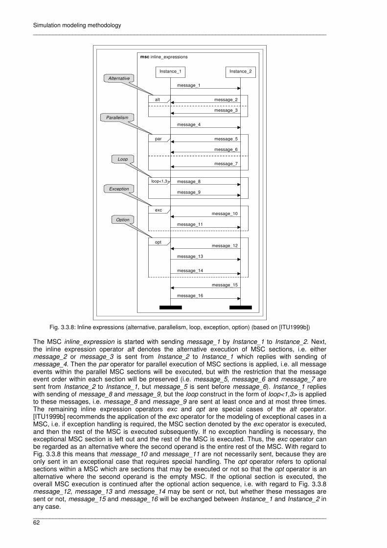
Simulation modeling methodology __________________________________________________________________________________________
__________________________________________________________________________________________ 62
msc inline_expressions
message_1
message_4
Instance_1 Instance_2
Alternative
message_2
message_3
alt
message_5
message_7
par
message_6
loop<1,3> message_8
message_9
Parallelism
Loop
exc message_10
message_11
opt message_12
message_13
message_14
message_15
message_16
Exception
Option
Fig. 3.3.8: Inline expressions (alternative, parallelism, loop, exception, option) (based on [ITU1999b]) The MSC inline_expression is started with sending message_1 by Instance_1 to Instance_2. Next, the inline expression operator alt denotes the alternative execution of MSC sections, i.e. either message_2 or message_3 is sent from Instance_2 to Instance_1 which replies with sending of message_4. Then the par operator for parallel execution of MSC sections is applied, i.e. all message events within the parallel MSC sections will be executed, but with the restriction that the message event order within each section will be preserved (i.e. message_5, message_6 and message_7 are sent from Instance_2 to Instance_1, but message_5 is sent before message_6). Instance_1 replies with sending of message_8 and message_9, but the loop construct in the form of loop<1,3> is applied to these messages, i.e. message_8 and message_9 are sent at least once and at most three times. The remaining inline expression operators exc and opt are special cases of the alt operator. [ITU1999b] recommends the application of the exc operator for the modeling of exceptional cases in a MSC, i.e. if exception handling is required, the MSC section denoted by the exc operator is executed, and then the rest of the MSC is executed subsequently. If no exception handling is necessary, the exceptional MSC section is left out and the rest of the MSC is executed. Thus, the exc operator can be regarded as an alternative where the second operand is the entire rest of the MSC. With regard to Fig. 3.3.8 this means that message_10 and message_11 are not necessarily sent, because they are only sent in an exceptional case that requires special handling. The opt operator refers to optional sections within a MSC which are sections that may be executed or not so that the opt operator is an alternative where the second operand is the empty MSC. If the optional section is executed, the overall MSC execution is continued after the optional action sequence, i.e. with regard to Fig. 3.3.8 message_12, message_13 and message_14 may be sent or not, but whether these messages are sent or not, message_15 and message_16 will be exchanged between Instance_1 and Instance_2 in any case.

Simulation modeling methodology __________________________________________________________________________________________
__________________________________________________________________________________________ 63
MSC references enable to refer to other MSCs from within a MSC, i.e. on the one hand it can be referred to a single MSC, and on the other hand it can be referred to MSC reference expressions which are constructed by application of inline expressions. Besides, the time concept can also be applied to MSC references. Fig. 3.3.9 depicts an example of MSC references and MSC reference expressions.
msc references_and_reference_expressions
Instance_1 Instance_2
MSC_2 alt MSC_3
MSC_1
MSC reference
MSC reference
expression
Fig. 3.3.9: MSC references and MSC reference expressions (based on [ITU1999b])
In the MSC references_and_reference_expressions MSC_1 is referenced. After the execution of MSC_1 either MSC_2 or MSC_3 is executed. The high level structural concept of the coregion allows for an exception to the total time ordering of message events along each instance axis so that message events contained in the coregion are unordered, if no further ordering in the form of the generalized order mechanism is prescribed. Fig. 3.3.10 illustrates a MSC example on the coregion modeling concept with and without application of a general ordering mechanism.
msc coregion
message_1
message_3
message_2
(a)
message_4
Instance_1 Instance_2
Coregion
msc coregion_with_general_ordering
message_3
message_4
(a1)
Coregion with
general ordering
Instance_1 Instance_2
message_1
message_2
Fig. 3.3.10: Coregion without (a) / with (a1) general ordering (based on [ITU1998, ITU1999b])

Simulation modeling methodology __________________________________________________________________________________________
__________________________________________________________________________________________ 64
In the MSC coregion message_1 and message_2 reach Instance_1 in the concurrent region and message_3 and message_4 are sent by Instance_1 in the concurrent region (cf. Fig. 3.3.10 (a)), i.e. the input of message_1 and message_2 as well as the output of message_3 and message_4 is unordered (e.g. message_2 may arrive before message_1, message_3 may be sent before message_4, etc.). In the MSC coregion_with_general_ordering the generalized ordering mechanism is applied which imposes a partial order on the messages within the coregion of Instance_1 (cf. Fig. 3.3.10 (a1)). Therefore, the instance axis of Instance_1 in the coregion area is depicted in column-form (instead of the line-form) for specification of the general ordering mechanism inside the column. The lines have to be interpreted from top to bottom and the arrow direction imposes the message order. With regard to the MSC coregion_with_general_ordering, the general message ordering mechanism implies that message_1 is received before message_2 and message_1 is received before message_4 is sent. Moreover, message_3 is sent before the sending of message_4 and message_3 is sent before message_2 is received. However, message_1 and message_3 are still unordered, i.e. it is not explicitly regulated whether message_1 is received before message_3 is sent or vice versa and the same applies for message_3 and message_4. Consequently, the generalized ordering mechanism applied to the MSC example illustrated in Fig. 3.3.10 only imposes a partial order within the coregion [ITU1998, ITU1999b].
3.3.4 Integration of Data in the MSC language
The MSC language enables the incorporation of data into MSCs (e.g. in the form a message passing, actions or MSC references). With regard to the integration of data, the MSC concept does not define a specific language to implement the incorporation of data, but it specifies interfaces to the MSC data concept so that the choice of the data language (e.g. Specification and Description Language (SDL) [ITU2002], C, C++, Java, etc.) is left to the user of the MSC language. In the MSC language data is either used statically or dynamically. Static variables, referring to static data, are used as formal parameters which are substituted by actual parameters. Dynamic variables, which refer to dynamic data, are variables that can be assigned and reassigned values through actions, message parameters, timer parameters and instance creation via their parameter lists. As dynamic variables are owned by instances, only message events on the owning instance are allowed to modify their values. The mechanism for assigning or modifying the value of a dynamic variable is that of a binding. A binding consists of an expression part and a pattern part that are connected by a bind symbol. If x is a dynamic variable, (2) denotes a binding example [ITU1999b].
1y:x += (2)
Fig. 3.3.11 illustrates the declaration and usage of data within an example. The declaration of data takes place in a MSC document, except static variables which are declared in a MSC head. A MSC document is a collection of MSCs in a defining part and a utility part. The defining part of a MSC document defines the collection of MSC traces, and the utility part contains utility MSCs which are reused by the MSCs of the defining part [ITU1999b].
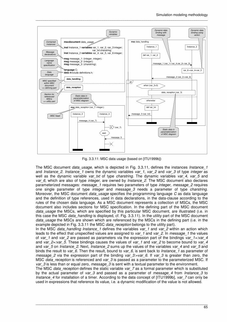
Simulation modeling methodology __________________________________________________________________________________________
__________________________________________________________________________________________ 65
mscdocument data_usage inst Instance_1 variables var_1, var_2, var_3:integer; var_txt:charstring; inst Instance_2 variables var_4, var_5, var_6:integer; msg message_1: (integer, integer); msg message_2: (integer); msg message_3: (charstring); language C; data #include definitions.h;
data_handling
data_reception
msc data_handling
Instance_1 Instance_2
message_1 (var_1=:var_4,var_2=:var_5)
message_2 (var_3:=var_6)
var_6:=var_4+var_5
data_reception (var_3)
when (var_3>0)
alt
otherwise
message_3 (var_txt)
msc data_reception (var_7: integer;)
Instance_3 Instance_4
message_4 (var_7)
message_5
T (var_7)
wait
Contained instances
Dynamic variables
Message declarations
Language name
specification
Data language definitions
Section for referenced
MSCs => utility part
MSC specified within MSC document
=> defining part
Dynamic data binding using
action
Static data in parameterization of MSC diagram
Static data in parameterization of MSC diagram
MSC head
Dynamic data binding with
message
def var_1, var_2
def var_txt
Fig. 3.3.11: MSC data usage (based on [ITU1999b]) The MSC document data_usage, which is depicted in Fig. 3.3.11, defines the instances Instance_1 and Instance_2. Instance_1 owns the dynamic variables var_1, var_2 and var_3 of type integer as well as the dynamic variable var_txt of type charstring. The dynamic variables var_4, var_5 and var_6, which are also of type integer, are owned by Instance_2. The MSC document also declares parameterized messages: message_1 requires two parameters of type integer, message_2 requires one single parameter of type integer and message_3 needs a parameter of type charstring. Moreover, the MSC document data_usage specifies the programming language C as data language and the definition of type references, used in data declarations, in the data-clause according to the rules of the chosen data language. As a MSC document represents a collection of MSCs, the MSC document also includes sections for MSC specification. In the defining part of the MSC document data_usage the MSCs, which are specified by this particular MSC document, are illustrated (i.e. in this case the MSC data_handling is displayed, cf. Fig. 3.3.11). In the utility part of the MSC document data_usage the MSCs are shown which are referenced by the MSCs in the defining part (i.e. in the example depicted in Fig. 3.3.11 the MSC data_reception belongs to the utility part). In the MSC data_handling Instance_1 defines the variables var_1 and var_2 within an action which leads to the effect that unspecified values are assigned to var_1 and var_2. In message_1 the values of var_1 and var_2 are passed as parameters via the expression part of the bindings var_1=:var_4 and var_2=:var_5. These bindings causes the values of var_1 and var_2 to become bound to var_4 and var_5 on Instance_2. Next, Instance_2 sums up the values of the variables var_4 and var_5 and binds the result to var_6. Then the result, bound to var_6, is sent back to Instance_1 as parameter of message_2 via the expression part of the binding var_3:=var_6. If var_3 is greater than zero, the MSC data_reception is referenced and var_3 is passed as a parameter to the parameterized MSC. If var_3 is less than or equal zero, message_3 is sent with a textual parameter to the environment. The MSC data_reception defines the static variable var_7 as a formal parameter which is substituted by the actual parameter of var_3 and passed as a parameter of message_4 from Instance_3 to Instance_4 for installation of a timer. According to the data concept of [ITU1999b], var_7 can only be used in expressions that reference its value, i.e. a dynamic modification of the value is not allowed.

Simulation modeling methodology __________________________________________________________________________________________
__________________________________________________________________________________________ 66
3.3.5 Principles of object orientation in the MSC language
The MSC language also considers principles of object orientation, as it allows for an inheritance mechanism that can be specified within a MSC document. If the inherits-clause is applied within a MSC document, then all instances are inherited and also all MSCs specified in the defining as well as in the utility part. Moreover, the idea of virtuality also enables to redefine inherited MSCs which are marked and therefore, allows for redefinition in case of inheritance [ITU1999b]. Fig. 3.3.12 depicts an example of inheritance and virtuality.
mscdocument basic inst Instance_basic_1; inst Instance_basic_2;
MSC_basic_1
MSC_basic_2 MSC_basic_3
(a)
mscdocument basic; inst Instance_basic_1; inst Instance_basic_2; MSC_basic_1; utilities reference virtual MSC_basic_2, reference MSC_basic_3;
(b)
mscdocument advanced inst Instance_advanced_1 inherits basic; inst Instance_advanced_2 inherits basic; inst Instance_advanced_3 inherits basic;
MSC_advanced_1
MSC_advanced_2
(a1)
mscdocument advanced; inst Instance_advanced_1 inherits basic; inst Instance_advanced_2 inherits basic; inst Instance_advanced_3 inherits basic; MSC_advanced_1; utilities reference MSC_advanced_2;
(b1)
Fig. 3.3.12: MSC inheritance and virtuality (graphical ((a) / (a1)) and textual ((b) / (b1)) representation) (based on
[ITU1999b]) The MSC document advanced which is illustrated in Fig. 3.3.12 (a1) / (b1) inherits all instances (i.e. Instance_basic_1 and Instance_basic_2) from the MSC document basic (cf. Fig. 3.3.12 (a) / (b)). Moreover, the MSC document advanced also inherits the MSCs specified in the defining part (i.e. MSC_basic_1) and in the utility part (i.e. MSC_basic_2 and MSC_basic_3) of the MSC document basic. MSC_basic_2 of MSC document basic is marked with the keyword virtual in the textual representation (cf. Fig. 3.3.12 (b)) so that it can be redefined in the MSC document advanced.
3.4 Message Sequence Chart (MSC)-based simulation methodology
This section introduces the simulation modeling methodology on which the performance evaluation environment for evolved RAN architectures, which was developed during the cooperation with Lucent Technologies in the IPonAir project [IPo2005] and in the context of this thesis, is based. The simulation modeling concept [WiScNi2003, MiScWi2004] focuses on the signaling traffic, i.e. on the control plane, of the network architectures under study. The modeling methodology does not envisage a full functional model based on extended finite state machines (EFSMs) for the signaling protocols, as an EFSM-based modeling approach is not advantageous under consideration of the requirements, which were made on the performance evaluation environment for evolved RAN architectures. In this section the developed modeling methodology will be presented, and the section closes with an assessment of the presented modeling methodology under consideration of the aforementioned requirements and modeling alternatives.

Simulation modeling methodology __________________________________________________________________________________________
__________________________________________________________________________________________ 67
3.4.1 Applied modeling concepts of the MSC language
A basic set of signaling use cases is identified from standards documents [3GPP2002a] to generate the dominant signaling load in the network. Each signaling load use case is modeled in the form of a MSC according to [ITU1999b] and forms one System Function (SF). In this context, only a subset of the MSC language framework provided by [ITU1999b] is utilized for the modeling of the signaling load use cases. The basic MSC modeling concept is assumed with instances that communicate via message exchange and execute predefined actions. The semantics of the MSC is provided by the order of the message events. The time concept is applied, i.e. particularly the possibility for relative measurements of the duration of the signaling use cases and the possibility for the imposition of time constraints to the signaling use cases. Furthermore, the possibility to incorporate data into MSCs is utilized in the form of parameterized messages. The application of parameterized messages enables the enhancement of [ITU1999b] with performance extensions for the specification of the cost of message processing and message transfer. Some MSCs contain parallel message sequences modeled by application of the par operator that is part of the inline expression modeling concept of [ITU1999b]. These parallel message sequences are modeled so that the focus is on one particular branch of those two branches running in parallel. In case of parallel message sequences, the developed modeling concept forces the network designer, who specifies the MSC sequence, to particularly denote the message which terminates the MSC sequence and thus, the focused branch is denoted. The MSCs, describing the signaling use cases in UTRAN, are taken from standards documents [3GPP2002a], but had to be refined [Alt2004] according to the developed modeling concept. As these MSCs generate the dominant signaling load in the network, they are instantiated according to a stochastic process. With regard to the stochastic process, a Poisson process is applied, which is an arrival process that provides interarrival times for the MSC instances in terms of independent and identically distributed (IID) exponential random variables [LaKe2000].
3.4.2 Performance extensions of the MSC language
For the purposes of an enhancement of [ITU1999b] with performance extensions for the specification of the cost of message processing and message transfer, each signaling message is annotated with a parameter tuple (c,l). Following [Mül2003], the annotation of each single signaling message with the factor c, which represents an integer value (i.e. c = 1, 2, …, C), allows to categorize the signaling messages into complexity classes. The categorization of messages within the refined signaling sequences in [Alt2004] assumes three complexity classes (i.e. C = 3). According to the assigned complexity class factor c, signaling message i gets a predefined amount of processing ai (in milliseconds) within a particular resource module j. The higher the complexity class factor c is, the higher is the amount of service the signaling message needs within a certain resource. Each resource module has a speed factor gj assigned which reflects the processing power of the particular resource. (3) denotes the derivation of the service time stij for signaling message i from the processing amount ai and the speed factor gj within resource module j.
j
iij
g
ast = (3)
Although the MSC instantiation takes place in terms of a Poisson process, the distribution of the service time is deterministic, as each single signaling message gets a predefined amount of processing ai according to its complexity class. The parameter l within the tuple (c,l) denotes the packet length in bytes required for the signaling message i and thus, allows to calculate the transmission delay trans_dik on a link k with a specific link speed lsk according to (4).
k
iik
ls
ld_trans = (4)
Simulation modeling methodology __________________________________________________________________________________________
__________________________________________________________________________________________ 68
In order to measure E2E delays of signaling SFs, further parameters are considered, such as the queueing delay, the propagation delay and the latency of the IP-based transport network. The queueing delay qdij, which represents the amount of time a single signaling message i has to spend within a resource module j waiting for service, is obtained as follows: If a signaling message enters a resource module at time t1 and the service is started at time t2, then the queueing delay is the time difference of t2 and t1. (cf. (5)).
ijijij ttqd 12 −= (5)
The propagation delay prop_dik for a single signaling message i on a particular link k is specified under consideration of the link length llk, which reflects the distance between network element a and network element b, and the propagation speed psk of link k (cf. (6)).
k
kik
ps
lld_prop = (6)
In case of UTRAN evolution scenarios, which consider an IP-based transport network, the latency of this transport network is considered in terms of a fixed and constant Transport Network Latency (TNL) delay. This constant TNL delay is added to the signaling E2E delay of a particular signaling SF x (i.e. x = 1, 2, ..., X, and X is the overall number of signaling SFs considered), whenever a signaling message i passes the IP-based transport network. Equation (4), (6) and the aforementioned definition of the TNL delay show that the modeling of the transport network is simplified, as a full protocol model for the transport network (e.g. in terms of a full protocol model of ATM or IP) is not considered. Consequently, effects of the transport network, such as packet losses or resource contention, are not considered either. However, the integration of a detailed protocol model of the transport network is possible and is an issue for future work. Propagation delay and transmission times as well as queueing delays, processing times and the constant delays from the IP-based transport network are included when measuring signaling E2E delays for a particular signaling SF x, which consists of signaling messages i (i.e. i = 1, 2, ..., m).
3.4.3 Generic node modeling concept
The signaling messages, which make up a SF, are exchanged between stateless Functional Entities (FEs). These FEs are architecture sub entities which reside inside the network elements. FEs can be relevant protocol entities or entities that contain a specific network functionality. In case of an exchange of signaling messages between FEs residing in different network elements, the involved FEs have to be of the same type of architecture sub entity. In reality, FEs are physically located on processors, and within the simulation modeling methodology the FEs are allocated to resource modules as illustrated in Fig. 3.4.1 which depicts the generic node modeling concept all network elements (mobile terminals, base stations, etc.) correspond to.

Simulation modeling methodology __________________________________________________________________________________________
__________________________________________________________________________________________ 69
Lower Service Access Points
Resources
External Routing (ER)
FE 1 FE 2 FE 3
Internal Routing (IR)
Traffic Sources
Sink
Fig. 3.4.1: Generic node modeling concept (following [WiScNi2003])
According to the generic node modeling concept each network element consists of (cf. Fig. 3.4.1): • One or more Lower Service Access Points (LSAPs) • External Routing (ER) module
• Internal Routing (IR) module
• One or more FEs • One or more resource modules • Sink module
• Optionally one or more traffic source modules. Network elements which initiate signaling SFs contain traffic sources to model user and network initiated traffic. A LSAP transparently interconnects the elements within the network and might serve as a connection point with regard to lower layers of the transport network, if these are fully modeled and implemented within future working activities. Moreover, the predefined protocol models of ATM and IP, which are provided by the OPNET Modeler simulation environment, could be interconnected to the generic node, illustrated within Fig. 3.4.1, with the help of the LSAP module. The ER and IR modules implement the routing functionality between network elements and within network elements. If a signaling message reaches the ER module, it is checked whether the message is addressed to the local node or not. If it is addressed to the local node, the message is passed to the IR module, otherwise it is sent to the LSAP in direction to the addressed node which means that the message is simply relayed by the ER module. The IR module forwards an incoming message to the addressed FE. FEs logically process incoming messages (e.g. convert them to another message type and provide new addresses) and pass the processed message either to the resource or to the sink module. Messages tagged for transmission to the sink module are analyzed by the sink module which performs statistical measurements in order to provide performance measures (e.g. E2E delays). Resource modules model time consumption and resource contention. The modeling methodology allows for the application of single- and multi-server, but single FIFO queue resource modules (cf. Fig. 3.4.2).
FIFO Queue
[...]
1
N Server
Fig. 3.4.2: Resource model [MiScWi2005]

Simulation modeling methodology __________________________________________________________________________________________
__________________________________________________________________________________________ 70
One or more FEs can be allocated to a single resource (cf. Fig. 3.4.1). The resource module forwards incoming messages to the IR module which determines whether the message is addressed to a FE within the local node or not. If the message is addressed to a FE within the local node, the IR module sends the message to the addressed FE, otherwise the message is passed to the ER module. In this case, the ER module sends the message to the LSAP in direction to the addressed node.
3.4.4 Abstract MSC sequence according to the developed modeling methodology
Fig. 3.4.3 illustrates a short MSC sequence which is annotated according to the modeling concept described within section 3.4.1 and 3.4.2.
Legend: message_name (complexity class (c), message length (l))
req (1, 2)
set (3, 16)
ok (1, 42)
ack (2, 4)
Node 2 Node 1
FE 1 FE 2 FE 1
(b)
init (3, 42)
Optional time
constraint
req (c, l)
ok (c, l)
Node 2
Waiting time in queue for FE 2
Service time of processor of FE 2
& Response Time
(Signaling E2E Delay)
Node 1
Link Propagation + Transmission Delay
FE 2
msc signaling_system_function
message processing
and
c := 3 l := 16
set (c, l)
message processing
and
c := 1 l := 42
message processing
and
c := 2 l := 4
ack (c, l)
(0,t]
FE 1
(a)
FE 1
message processing
and
c := 1 l := 2
init (c := 3, l := 42)
Fig. 3.4.3: Short annotated MSC sequence (based on [MiScWi2004])
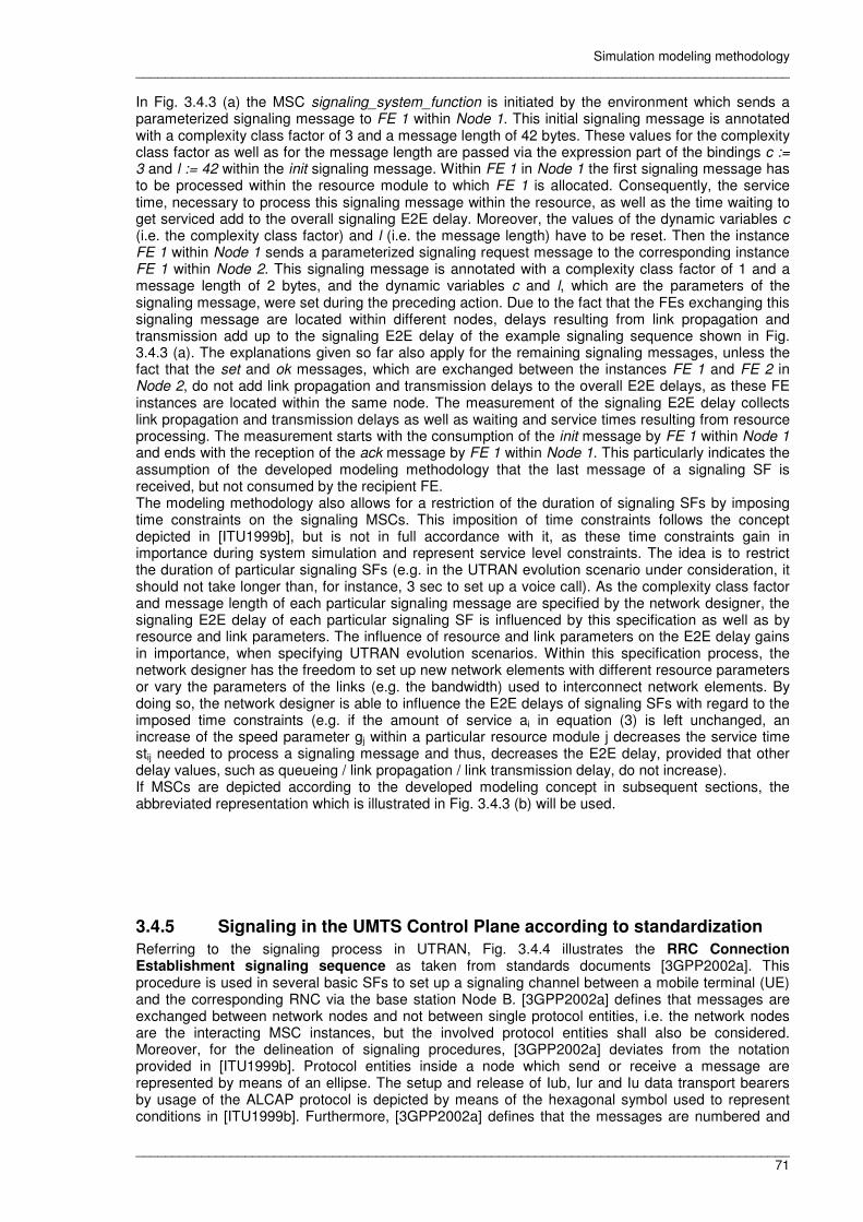
Simulation modeling methodology __________________________________________________________________________________________
__________________________________________________________________________________________ 71
In Fig. 3.4.3 (a) the MSC signaling_system_function is initiated by the environment which sends a parameterized signaling message to FE 1 within Node 1. This initial signaling message is annotated with a complexity class factor of 3 and a message length of 42 bytes. These values for the complexity class factor as well as for the message length are passed via the expression part of the bindings c := 3 and l := 42 within the init signaling message. Within FE 1 in Node 1 the first signaling message has to be processed within the resource module to which FE 1 is allocated. Consequently, the service time, necessary to process this signaling message within the resource, as well as the time waiting to get serviced add to the overall signaling E2E delay. Moreover, the values of the dynamic variables c (i.e. the complexity class factor) and l (i.e. the message length) have to be reset. Then the instance FE 1 within Node 1 sends a parameterized signaling request message to the corresponding instance FE 1 within Node 2. This signaling message is annotated with a complexity class factor of 1 and a message length of 2 bytes, and the dynamic variables c and l, which are the parameters of the signaling message, were set during the preceding action. Due to the fact that the FEs exchanging this signaling message are located within different nodes, delays resulting from link propagation and transmission add up to the signaling E2E delay of the example signaling sequence shown in Fig. 3.4.3 (a). The explanations given so far also apply for the remaining signaling messages, unless the fact that the set and ok messages, which are exchanged between the instances FE 1 and FE 2 in Node 2, do not add link propagation and transmission delays to the overall E2E delays, as these FE instances are located within the same node. The measurement of the signaling E2E delay collects link propagation and transmission delays as well as waiting and service times resulting from resource processing. The measurement starts with the consumption of the init message by FE 1 within Node 1 and ends with the reception of the ack message by FE 1 within Node 1. This particularly indicates the assumption of the developed modeling methodology that the last message of a signaling SF is received, but not consumed by the recipient FE. The modeling methodology also allows for a restriction of the duration of signaling SFs by imposing time constraints on the signaling MSCs. This imposition of time constraints follows the concept depicted in [ITU1999b], but is not in full accordance with it, as these time constraints gain in importance during system simulation and represent service level constraints. The idea is to restrict the duration of particular signaling SFs (e.g. in the UTRAN evolution scenario under consideration, it should not take longer than, for instance, 3 sec to set up a voice call). As the complexity class factor and message length of each particular signaling message are specified by the network designer, the signaling E2E delay of each particular signaling SF is influenced by this specification as well as by resource and link parameters. The influence of resource and link parameters on the E2E delay gains in importance, when specifying UTRAN evolution scenarios. Within this specification process, the network designer has the freedom to set up new network elements with different resource parameters or vary the parameters of the links (e.g. the bandwidth) used to interconnect network elements. By doing so, the network designer is able to influence the E2E delays of signaling SFs with regard to the imposed time constraints (e.g. if the amount of service ai in equation (3) is left unchanged, an increase of the speed parameter gj within a particular resource module j decreases the service time stij needed to process a signaling message and thus, decreases the E2E delay, provided that other delay values, such as queueing / link propagation / link transmission delay, do not increase). If MSCs are depicted according to the developed modeling concept in subsequent sections, the abbreviated representation which is illustrated in Fig. 3.4.3 (b) will be used.
3.4.5 Signaling in the UMTS Control Plane according to standardization
Referring to the signaling process in UTRAN, Fig. 3.4.4 illustrates the RRC Connection Establishment signaling sequence as taken from standards documents [3GPP2002a]. This procedure is used in several basic SFs to set up a signaling channel between a mobile terminal (UE) and the corresponding RNC via the base station Node B. [3GPP2002a] defines that messages are exchanged between network nodes and not between single protocol entities, i.e. the network nodes are the interacting MSC instances, but the involved protocol entities shall also be considered. Moreover, for the delineation of signaling procedures, [3GPP2002a] deviates from the notation provided in [ITU1999b]. Protocol entities inside a node which send or receive a message are represented by means of an ellipse. The setup and release of Iub, Iur and Iu data transport bearers by usage of the ALCAP protocol is depicted by means of the hexagonal symbol used to represent conditions in [ITU1999b]. Furthermore, [3GPP2002a] defines that the messages are numbered and

Simulation modeling methodology __________________________________________________________________________________________
__________________________________________________________________________________________ 72
that the transport channel, used by the MAC protocol, or the logical channel, used by the RLC and RRC protocols, is to be indicated before the message name.
Node B Serving RNS
Serving
RNC
1. CCCH: RRC Connection Request
2. Radio Link Setup Request
DCH-FP
NBAP
RRC RRC
RRC RRC
Allocate RNTI Select L1 and L2
parameters
NBAP
NBAP NBAP
NBAP NBAP
Start RX
3. Radio Link Setup Response
4. ALCAP Iub Data Transport Bearer Setup
DCH-FP
DCH-FP
DCH-FP
5. Downlink Synchronization
6. Uplink Synchronization
Start TX
7. CCCH: RRC Connection Setup
8. Uplink Synchronization
RRC RRC
9. DCCH: RRC Connection Setup Complete
UE
Fig. 3.4.4: RRC Connection Establishment signaling [3GPP2002a]
The RRC Connection Establishment procedure is initiated by the UE which sends a RRC Connection Request message on the CCCH, i.e. in particular on the Random Access Channel (RACH) in uplink direction. The RRC Connection Request message contains information about the reason for the requested RRC connection and the terminal and subscriber identity. The RRC Connection Request message arrives to the RNC over the Iub RACH data port. It depends on the request reason whether the RNC allocates dedicated or common resources to the upcoming transaction. However, based on this decision, the RNC allocates a UTRAN Radio Network Temporary Identifier (U-RNTI) for identification purposes of the UE and further resources to the transaction. As the signaling flow illustrated in Fig. 3.4.4 and [3GPP2002a] indicates, a DCH is to be set up. Therefore, the RNC sends a NBAP Radio Link Setup Request message to the Node B. This message contains transport format description, power control information, cell identifier, frequency, uplink scrambling code (for FDD), time slots and user codes (for TDD). The base station allocates resources, starts physical reception and acknowledges the request message by sending a NBAP Radio Link Setup Response message which contains transport layer addressing information (AAL2 address) for the Iub data transport bearer. The RNC initiates the Iub data transport bearer establishment using the ALCAP protocol and requests to bind the Iub data transport bearer to the DCH. The Node B acknowledges the setup request for the Iub data transport bearer. Next, the Node B and RNC establish synchronism for the Iub and Iur data transport bearer by exchanging the appropriate DCH FP frames. Subsequently, the Node B starts downlink transmission. After Iub communication establishment, the RNC sends the RRC Connection Setup message to the UE on CCCH, i.e. in particular on the Forward Access Channel (FACH) in downlink direction. In this message the RNC informs the UE about the U-RNTI, the transport format, power control, frequency, downlink scrambling code (for FDD), time slots and user codes (for TDD). When the Node B achieves uplink synchronization, it notifies the RNC with the NBAP message Radio Link Restore Indication. The UE confirms the RRC connection establishment notification by sending the message RRC Connection Setup Complete on the DCCH, which contains integrity and ciphering information as well as information about the radio access capability of the UE [3GPP2002a, KaAhLa2001].

Simulation modeling methodology __________________________________________________________________________________________
__________________________________________________________________________________________ 73
3.4.6 Signaling in the UMTS Control Plane according to the developed modeling methodology
In Fig. 3.4.4 the network elements UE, Node B and RNC directly exchange signaling messages which are not annotated. Since the modeling concept defines that annotated signaling messages are exchanged between stateless FEs, the signaling sequences taken from standards documents had to be refined. The refined RRC Connection Establishment signaling procedure is illustrated in Fig. 3.4.5. It still corresponds to the signaling flow shown in Fig. 3.4.4, but the signaling messages in Fig. 3.4.5 are broken down into message flows between functional components the network elements consist of.
(1,30)
(1,30) (1,30)
(1,7)
(1,30) (1,30)
(1,30)
(1,30)
(1,30)
(1,30)
(1,30)
(2,123)
(1,7)
(2,63)
(2,63)
(2,75)
(1,75)
(1,75)
(2,75)
(2,123)
(2,121)
(1,7)
(1,22)
(1,22)
(1,22)
(1,22)
(1,43)
NBAP Iub Uu RRC Conn. Mgm.
UE
ALCAP
Node B
Uu User Mgm.
Bearer Mgm.
RRC Conn. Mgm.
NBAP ALCAP Iub
RNC
Iub
RRC Connection Request
Creation of UE Request
Radio Link Setup Request
Radio Link Setup Response
(2,63) ALCAP Iub: Establish Request
ALCAP Iub: Establish Confirm
RRC Connection Setup
RRC Connection Setup Complete
Radio Access Bearer Mgm.
Bearer Mapping
Unit
(2,121)
(3,121)
(1,121)
(1,121)
(1,121)
(1,121) (1,121)
(1,22)
Fig. 3.4.5: Refined RRC Connection Establishment signaling sequence [Alt2004]

Simulation modeling methodology __________________________________________________________________________________________
__________________________________________________________________________________________ 74
If, for instance, the RRC Connection Establishment signaling sequence, as illustrated in Fig. 3.4.5, is part of a MO Voice Call Setup signaling sequence, the modeling concept of parallel message sequences can be applied: After reception of the last message within the RRC Connection Setup message sequence (marked in grey within the overall RRC Connection Establishment signaling sequence), the RRC Conn. Mgm. FE on the one hand starts the RRC Connection Setup Complete message sequence and on the other hand in parallel can initiate a signaling procedure with the Non-Access Stratum to request services from the CM sublayer.
3.4.7 Allocation of FEs to network elements and resources in the UTRAN Control Plane
Fig. 3.4.6 depicts the allocation of FEs to resources and network elements in the Control Plane of the UTRAN reference architecture. The FEs and their functionality are explained subsequently.
CN RNC Node B UE
Uu Iub Iu
Infinite Server
Resource
RRC Connection
Management
Uu
Infinite
Server
Resource
Iub
Uu
Main
Resource
NBAP
ALCAP
Infinite
Server
Resource
RANAP
ICC_1 Resource
ALCAP_Iub
Iub
ICC_3 Resource
ALCAP_Iu
RANAP
ALCAP_Iur ICC_2 Resource
Bearer Mapping
Unit
BSC Resource NBAP
RNSAP
RRC Connection
Management
Bearer Management
User Management
Mobility Management
Paging Entity
Broadcast / Multicast
Management
Radio Access Bearer
Management
Micro Mobility Management
ALCAP
Fig. 3.4.6: Allocation of FEs to resources and network elements in UTRAN Control Plane (following [MiScWi2005])
The Uu FE models the air interface between the mobile terminal and the base station. The Iub FE models the Iub interface between the base station and the RNC. The RRC Connection Management handles the radio resource connection between the mobile terminal and the RAN and is the termination point for control messages. The Bearer Management FE manages bearers on various interfaces; the Radio Access Bearer Management entity sets up and releases links between the UE and the CN, while the Bearer Mapping Unit coordinates the radio and transport bearers towards the CN. The Mobility Management entity manages the mobility of the users in case of hard handover, while the Micro Mobility Management FE manages soft and softer handover inside the UTRAN. The User Management FE models the users’ data and states, the Broadcast/Multicast Management entity manages broadcast channels and the Paging Entity executes paging co-ordination. The remaining
Simulation modeling methodology __________________________________________________________________________________________
__________________________________________________________________________________________ 75
FEs are protocol units which can be classified as Control Plane protocols of the radio network layer, namely the NBAP [3GPP2004g], ALCAP, RANAP [3GPP2003o] and RNSAP [3GPP2004f] with their specific functionality according to 3GPP standards documents [MiScWi2005]. The resources of the UE and the CN as well as the resource inside the Node B, which keeps the FEs representing the interfaces towards the mobile terminal (Uu) and the RNC (Iub), are modeled as Infinite Server (IS) Resources according to the definition of IS in [Jai1991]. In accordance with [Jai1991], IS are devices that have no queueing so that jobs spend the same amount of time in the device regardless of the number of jobs in the device. In case of the Uu and Iub FE the IS approach is appropriate, because signaling messages transmitted via these interfaces experience fixed delays. The IS approach is also adequate for the resources in the UE and the CN, because the focus, when observing signaling E2E delays, is on the contribution of the resources inside the network elements of the UTRAN to the signaling delays. The remaining FEs in the Node B (NBAP and ALCAP) are mapped to a separate resource which will be modeled in the form of a multi-server resource in accordance with Fig. 3.4.2 and N > 1. The allocation of FEs to resources inside the RNC is performed according to the internal hardware composition of the Lucent RNC. According to [AnByKa2002], the RNC consists of two components which are the BSC and the Traffic Processing Unit (TPU). The BSC is unexceptionally responsible for signaling and control [AnByKa2002]. The TPU provides traffic and signaling processing and is built from Intelligent Carrier Cards (ICC) [McBu2003]. Following [AnByKa2002], ICC are multiprocessor cards that run a real time operating system and terminate the application protocols and network interfaces. Under consideration of the internal hardware composition of the Lucent RNC, all FEs necessary for ALCAP transportation establishment towards the Node B (ALCAP_Iub), towards other RNCs in case of drift handover situations (ALCAP_Iur) and towards the CN (ALCAP_Iu) as well as the RANAP FE and the interface FE towards the Node B (Iub) are allocated to resources that represent ICC. The remaining FEs are mapped to the BSC resource. The BSC resource as well as the ICC resources are modeled as multiple server resources according to Fig. 3.4.2 with N > 1.

Simulation modeling methodology __________________________________________________________________________________________
__________________________________________________________________________________________ 76
3.4.8 Traffic model
The UTRAN signaling SFs, which are identified as the basic set of signaling use cases, are depicted in Table 3.4.1 with a short explanation.
# UTRAN signaling SF Short Explanation
1 MO Voice / CS Data Call Establishment UE initiated call setup 2 MO Voice / CS Data Call Release UE initiated call tear down 3 MT Voice / CS Data Call Establishment UE terminated call setup 4 MT Voice / CS Data Call Release UE terminated call tear down
5 PS Data Transfer Establishment (with follow on: UE PS attaches and automatically gets PDP context, then goes to URA_PCH)
UE changes from state IDLE to the mobility state PMM_CONNECTED in which it can send and receive data and signaling and then goes to RRC state URA_PCH in which no uplink activity is possible, but uplink activity can become possible by changing to RRC state CELL_DCH via SF 7 described below
6 PS Detach (UE initiated)
PS Detach signaling resets the UE to the mobility management state PMM_DETACHED in which no communication between the mobile terminal and SGSN is possible
7 Transition from URA_PCH to CELL_DCH due to Downlink Data Transfer
Transfer of UE from RRC state URA_PCH to CELL_DCH
8 Transition from CELL_DCH to URA_PCH due to RRC inactivity timer expiring
Transfer of UE from RRC state CELL_DCH to URA_PCH state due to the incident that no considerable data has to be transferred
9 MO PDP Context Activation (from PMM_CONNECTED+Cell_DCH)
Activation of a PDP Context for a PS service with certain packet connection characteristics (e.g. QoS class)
10 MO PDP Context Deactivation (from PMM_CONNECTED+Cell_DCH)
Deletion of a PDP Context related to a certain packet connection
11 IMSI Detach Signaling Flow De-registration of the UE when the mobile terminal is switched off
12 Location Updating Signaling Flow Update of the location of the UE in the Visitor Location Register (VLR) with location area accuracy
13 UTRAN Registration Area (URA) Update (URAU) Signaling Flow
UE initiated location update towards the RNC in case of a mobility related URA change
14 Routing Area (RA) Update (RAU) Signaling Flow Location update procedure between UE and CN PS domain in case of a mobility related RA change
15 Intra-RNC Softer Handover Handover between certain sectors of one Node B
16 Intra-RNC Soft Handover Soft handover between Node Bs belonging to the same RNS
17 Inter-RNC Soft Handover Soft handover between Node Bs belonging to different RNSs
18 Intra-RNC Hard Handover Hard handover between Node Bs belonging to the same RNS
19 Inter-RNC Hard Handover Hard handover between Node Bs belonging to different RNSs
20 Serving Radio Network Subsystem (SRNS) Relocation
Transfer of radio resource control from the SRNS to the drift RNS
21 Paging in idle mode Paging procedure and UE in RRC IDLE mode
22 Paging in connected mode Paging procedure and UE in RRC CONNECTED mode
23 Paging unsuccessful Signaling procedure for unsuccessful paging cases
24 Measurement Report UE initiated measurement procedure on radio channel
Table 3.4.1: UTRAN signaling SFs with short explanation The UTRAN signaling use cases, which are described in Table 3.4.1, are instantiated according to calculated interarrival times during simulation run. These interarrival times are calculated within an Excel workbook [Spe2002] before simulation start. The calculation of these interarrival times considers the behavior of a certain number of users, which is specified by the network designer in the Excel workbook in terms of voice call / packet data session related parameters (e.g. Busy Hour Call Attempts (BHCAs) and Busy Hour Data Session Attempts (BHDSAs) per user) and mobility related parameters (e.g. percentage of Inter- and Intra-RNC Hard Handovers), according to empirical values. Section 4.1.1 provides detailed information about the aforementioned parameters and the calculation of the interarrival times. The instantiation of MO and MT voice call setups as well as an activation of a MO PDP context within the radio cell is only possible under consideration of the Call Admission Control (CAC) parameters [Soe2004c]. The applied CAC regulation is based on the assumption that within each radio cell there is a maximum throughput (kbit/sec) available for usage to all users within the cell. With regard to the maximum throughput, the policy is presumed that voice traffic supersedes data traffic. Consequently, a QoS assumption, which is the Data Channel Utilization (%), is necessary for data traffic in such a way that the utilization of the data channels may not exceed a certain level. Furthermore,

Simulation modeling methodology __________________________________________________________________________________________
__________________________________________________________________________________________ 77
assumptions have to be made for the voice and data rates (kbit/sec) available to each single user. The values of the CAC parameters, set by the network designer, are taken into account by the traffic source, which initiates MO Voice / CS Data Call Establishment signaling and is located within the UE node, when deciding about the setup of another call or potential handovers into the particular radio cell according to (7) and packet sessions within the radio cell according to (8) [Soe2004c].
[ ] [ ] [ ][ ]
)% nUtilizatio Channel Data
100kbit/secRateData*Sessions(Packetkbit/secRateVoice*1)Calls(Voicekbit/secusedBandwidth ∗++=
(7)
[ ] [ ] [ ][ ]
)%nUtilizatio Channel Data
100kbit/secRateData*1)Sessions((Packetkbit/secRateVoice*CallsVoicesec/kbitusedBandwidth ∗++=
(8)
As an example for further clarification of the CAC regulation mechanism, the following situation is considered: Let us assume two radio cells, A and B, both with a maximum cell throughput of 1 Mbit/sec. The voice rate is assumed with 12.2 kbit/sec, the data rate is 6.4 kbit/sec, the utilization of the data channels should not exceed 80%, and this applies for both radio cells. Let us further assume that due to user mobility, a handover from radio cell B into radio cell A becomes necessary so that the CAC mechanism has to be considered in radio cell A. The number of voice calls in radio cell A is assumed with 65 at this time, and the number of packet sessions is considered with 25. In radio cell B, 60 voice calls are assumed and 20 packet sessions at this time. Equation (9) shows that the maximum cell throughput of 1 Mbit/sec within radio cell A will be exceeded by the bandwidth requirements of an additional voice call which moves into radio cell A due to handover.
[ ] [ ] [ ][ ]
2.1005)% 80
100seckbit/4.6*25(seckbit/2.12*)165(seckbit/usedBandwidth A =∗++= (9)
Due to the bandwidth in radio cell A, which will be exceeded by an additional voice call, a handover into radio cell A is impossible, and the corresponding voice call will be lost. This particularly means that in radio cell A, the number of voice calls and packet sessions does not change under consideration of the lost voice call (i.e. 65 voice calls, 25 packet sessions). But in radio cell B, the number of number of voice calls changes from 60 to 59 voice calls, and the number of packet sessions is not affected (i.e. 20 packet sessions in radio cell B after the unsuccessful handover). The aforementioned example for further clarification of the CAC regulation mechanism also shows that on the one hand CAC is modeled under consideration of particular parameters assumed within the radio cell and set by the network designer, such as maximum cell throughput, voice and data rate as well as maximum data channel utilization. On the other hand counters, which record the currently active number of voice calls and packet sessions within the radio cells, are considered and updated according to equation (7) and (8). In context with CAC, resource parameters (e.g. available processor resources of the RNC) are not considered so that CAC is modeled disregarding the situation of processor resources within particular network elements. With regard to the signaling SFs depicted in Table 3.4.1, a partly correlated traffic model is applied to generate the signaling traffic within the UTRAN reference architecture and the evolution scenarios. This means that the signaling SFs are not triggered entirely independently. Table 3.4.2 visualizes the correlation of particular signaling SFs.

Simulation modeling methodology __________________________________________________________________________________________
__________________________________________________________________________________________ 78
# UTRAN signaling SF Condition Action,
if condition applies
Action,
if condition does not apply
1 MO Voice / CS Data Call Establishment in radio cell A
bandwidth (kbit/sec), necessary to set up another voice call in radio cell A, does not exceed the maximum throughput (kbit/sec)
available within radio cell A under consideration of CAC and (8)
• Instantiation of signaling SF 1 • Increase of counter for voice
calls in radio cell A
• Connection blockage
2 MO Voice / CS Data Call Release in radio cell A number of active voice calls in radio cell A > 0
• Instantiation of signaling SF 2 • Decrease of counter for voice
calls in radio cell A —
3 MT Voice / CS Data Call Establishment in radio cell A
bandwidth (kbit/sec), necessary to set up another voice call in radio cell A, does not exceed the maximum throughput (kbit/sec)
available within radio cell A under consideration of CAC and (8)
• Instantiation of signaling SF 3 • Increase of counter for voice
calls in radio cell A
• Connection blockage
4 MT Voice / CS Data Call Release in radio cell A number of active voice calls in radio cell A > 0
• Instantiation of signaling SF 4 • Decrease of counter for voice
calls in radio cell A —
9 MO PDP Context Activation (from PMM_CONNECTED+Cell_DCH) in radio cell A
bandwidth (kbit/sec), necessary to set up another packet data connection in radio cell A,
does not exceed the maximum throughput (kbit/sec) available within radio cell A under consideration of CAC and (9)
• Instantiation of signaling SF 9 • Increase of counter for packet
data connections in radio cell A
• Connection blockage
10 MO PDP Context Deactivation (from PMM_CONNECTED+Cell_DCH) in radio cell A
number of active packet data connections in radio cell A > 0 • Instantiation of signaling SF 10 • Decrease of counter for packet
data connections in radio cell A —
16 Intra-RNC Soft Handover from radio cell A into radio cell B
number of active voice calls in radio cell A > 0 and
bandwidth (kbit/sec), necessary to set up another voice call in radio cell B, does not exceed the maximum throughput (kbit/sec)
available within radio cell B under consideration of CAC and (8)
• Instantiation of signaling SF 16 • Increase of counter for voice
calls in radio cell B • Decrease of counter for voice
calls in radio cell A
• Connection dropping (i.e. loss of the connection)
17 Inter-RNC Soft Handover from radio cell A into radio cell C
number of active voice calls in radio cell A > 0 and
bandwidth (kbit/sec), necessary to set up another voice call in radio cell C, does not exceed the maximum throughput (kbit/sec)
available within radio cell C under consideration of CAC and (8)
• Instantiation of signaling SF 17 • Increase of counter for voice
calls in radio cell C • Decrease of counter for voice
calls in radio cell A
• Connection dropping
18 Intra-RNC Hard Handover from radio cell A into radio cell B
number of active voice calls in radio cell A > 0 and
bandwidth (kbit/sec), necessary to set up another voice call in radio cell B, does not exceed the maximum throughput (kbit/sec)
available within radio cell B under consideration of CAC and (8)
• Instantiation of signaling SF 18 • Increase of counter for voice
calls in radio cell B • Decrease of counter for voice
calls in radio cell A
• Connection dropping
19 Inter-RNC Hard Handover from radio cell A into radio cell C
number of active voice calls in radio cell A > 0 and
bandwidth (kbit/sec), necessary to set up another voice call in radio cell C, does not exceed the maximum throughput (kbit/sec)
available within radio cell C under consideration of CAC and (8)
• Instantiation of signaling SF 19 • Increase of counter for voice
calls in radio cell C • Decrease of counter for voice
calls in radio cell A
• Connection dropping
Table 3.4.2: Correlation between UTRAN signaling SFs Table 3.4.2 shows that the number of active (i.e. still ongoing) voice calls and packet data connections as well as the amount of bandwidth, which is still available for a further setup of a voice call or packet data connection within a particular radio cell, impacts the instantiation of the signaling SFs depicted in Table 3.4.2. The instantiation of a MO and MT voice call as well as the instantiation of a packet data connection depends on the evaluation of the CAC policy within the radio cell according to equation (7) and (8). This means, as long as the CAC policy is not violated (i.e. as long as there is bandwidth available within the radio cell), a further MO or MT voice call or a packet connection can be set up, and this also implies an instantiation of the particular signaling SF. Moreover, if the CAC policy according to equation (7) is violated within a particular radio cell, a handover into this particular radio cell is not possible either. MO and MT voice call releases are coupled with the number of active voice calls in the radio cell, i.e. if there are no active voice calls within the radio cell, a MO or MT voice call release cannot be instantiated, and a handover out of this radio cell is not possible either. The same holds true for the MO PDP Context Deactivation signaling SF, i.e. a PDP Context Deactivation instantiation is not possible, if there are not any active packet data connections within the radio cell [AtMüWi2003]. So, Table 3.4.2 on the one hand provides the information that the depicted signaling SFs are instantiated, if the relevant condition is fulfilled. On the other hand Table 3.4.2 also provides information about the consequences, if the relevant condition is not fulfilled. In this case, connection blockage or dropping (i.e. loss of the connection) is recorded so that information about the blocking and dropping probability can be provided. However, in case of connection blockage or dropping, no signaling is instantiated due to the fact that the modeling methodology only considers the carried traffic, but no unsuccessful signaling cases (cf. Table 3.4.1), although an extension of the modeling methodology by unsuccessful signaling cases would be possible in terms of future work. Nevertheless, the user of the presented methodology has to be aware of the effect that resource utilizations and measured signaling E2E delays are incorrectly lower, if the blocking and dropping probability significantly increases, as the signaling load caused by unsuccessful signaling cases is not considered.

Simulation modeling methodology __________________________________________________________________________________________
__________________________________________________________________________________________ 79
Furthermore, the number of active voice calls and packet data connections within a radio cell impacts the interarrival time of other signaling SFs so that the probability of an instantiation of these signaling SFs increases, the higher the number of active voice calls or packet data connections within the radio cell [AtMüWi2003]. Therefore, particular signaling SFs are associated with the number of active voice calls or packet data connections in the radio cell. Table 3.4.3 provides a survey of the UTRAN signaling SFs and their associations.
# UTRAN signaling SF Association with
1 MO Voice / CS Data Call Establishment —
2 MO Voice / CS Data Call Release Active (MO and MT) Voice Calls in Radio Cell
3 MT Voice / CS Data Call Establishment —
4 MT Voice / CS Data Call Release Active (MO and MT) Voice Calls in Radio Cell
5 PS Data Transfer Establishment (with follow on: UE PS attaches and automatically gets PDP context, then goes to URA_PCH)
—
6 PS Detach (UE initiated) Active MO Packet Data Connections in Radio Cell
7 Transition from URA_PCH to CELL_DCH due to Downlink Data Transfer
Active MO Packet Data Connections in Radio Cell
8 Transition from CELL_DCH to URA_PCH due to RRC inactivity timer expiring
Active MO Packet Data Connections in Radio Cell
9 MO PDP Context Activation (from PMM_CONNECTED+Cell_DCH) —
10 MO PDP Context Deactivation (from PMM_CONNECTED+Cell_DCH)
Active MO Packet Data Connections in Radio Cell
11 IMSI Detach Signaling Flow — 12 Location Updating Signaling Flow —
13 UTRAN Registration Area (URA) Update (URAU) Signaling Flow Active MO Packet Data Connections in Radio Cell
14 Routing Area (RA) Update (RAU) Signaling Flow Active MO Packet Data Connections in Radio Cell
15 Intra-RNC Softer Handover Active (MO and MT) Voice Calls in Radio Cell
16 Intra-RNC Soft Handover Active (MO and MT) Voice Calls in Radio Cell
17 Inter-RNC Soft Handover Active (MO and MT) Voice Calls in Radio Cell
18 Intra-RNC Hard Handover Active (MO and MT) Voice Calls in Radio Cell
19 Inter-RNC Hard Handover Active (MO and MT) Voice Calls in Radio Cell
20 Serving Radio Network Subsystem (SRNS) Relocation — 21 Paging in idle mode — 22 Paging in connected mode — 23 Paging unsuccessful — 24 Measurement Report —
Table 3.4.3: UTRAN signaling SFs and associations Furthermore, regarding signaling SF 2 and 4 (MO / MT Voice / CS Data Call Release) as well as with regard to signaling SF 10 (MO PDP Context Deactivation), it is assumed that their interarrival rates are initially associated with the assumed voice call or packet session holding time [AtMüWi2003]. If, for instance, the voice call holding time is assumed with 100 sec for a single voice call and the holding time for packet sessions is considered with 200 sec, then the initial release rate per voice call is 0.01 per sec, and the deactivation rate per packet session is 0.005 per sec initially. During simulation run, these initial rates are adapted with regard to the number of currently active voice calls and packet sessions within a radio cell so that the probability of an instantiation of these signaling SFs increases, the higher the number of active voice calls or packet data connections within the radio cell. Further detailed information with regard to the traffic model and its implementation is provided in chapter 4, particularly within section 4.1.1, 4.2.3, 4.2.4 and 4.2.5.

Simulation modeling methodology __________________________________________________________________________________________
__________________________________________________________________________________________ 80
3.4.9 Providing scalability
Following [PsPaPr2002, PaPrPs2003] and [AtMü2003], the Small Scale High-fidelity Reproduction of Network Kinetics (SHRiNK) modeling technique is applied in order to provide scalability of the RAN architectures. The basic idea of SHRiNK is to impose a sample of the input traffic on an appropriately scaled down version of the system under study and then extrapolate from the performance of the scaled down version to that of the original system. The application of the SHRiNK approach enables an efficient performance simulation of large network systems and high traffic volumes by decreasing the computational requirements of network simulations and the cost of experiments significantly. If a large network topology with high traffic load is modeled and simulated explicitly, the number of simulation events will increase significantly and also the amount of real time as well as the amount of computational resources which are necessary to perform the simulation study. Consequently, the aspect of network scalability is limited, if large topologies are explicitly modeled and simulated. If SHRiNK is applied to a large network topology of interest, it is possible to simply model and simulate a small network topology and impose an appropriately scaled down sample of the input traffic load to this small network topology. Consequently, the number of simulation events is significantly lower so that the amount of real time and computational resources, which are necessary to perform the simulation study, are also lower. However, if SHRiNK is applied and a large network topology is scaled down accordingly, it is necessary to extrapolate the performance values of the scaled down simulation model, gathered during the simulation run, to those performance values of the full simulation model. In [PaPrPs2003], the researchers of the SHRiNK modeling technique apply their approach to a M/M/1 system, but also to large IP networks and web server farms. In this context, the authors evaluate their results analytically as well as by simulation experiments so that the SHRiNK modeling technique is validated by the authors. Subsequently, the SHRiNK modeling technique will be explained by applying SHRiNK to a M/M/1 system. Following [PaPrPs2003], it is assumed that the arrival rate λ and the service rate µ are multiplied with the SHRiNK factor α so that the service unit of the M/M/1 system runs slower, in order to gain the scaled down M/M/1 model. According to the SHRiNK factor α, the following constraint applies: 0 < α < 1. By application of the SHRiNK factor α, the M/M/1 model is slowed down, as service times are extended and arrivals are more infrequent. Following literature on queueing theory (e.g. [LaKe2000]), the utilization ρ of a M/M/1 system is defined according to (10), and the utilization of the scaled down M/M/1 system is according to (11).
µ
λρ = (10)
µα
λαρSHRiNK = (11)
According to queueing theory, the mean number of customers in the M/M/1 system E[N] is according to (12), and moreover, in the equilibrium state of the M/M/1 system Little’s Law can be applied according to (13). The mean sojourn time E[V] is defined according to (14) (cf. [LaKe2000]). The equations (15), (16) and (17) apply to the scaled down version of the M/M/1 system according to the SHRiNK modeling technique.
ρ1
ρE[N]
−= (12)
E[V]λE[N] ∗= (13)
λµ
1E[V]
−= (14)
SHRiNK
SHRiNKSHRiNK
ρ1
ρE[N]
−= (15)
SHRiNKSHRiNK E[V]λαE[N] ∗= (16)

Simulation modeling methodology __________________________________________________________________________________________
__________________________________________________________________________________________ 81
αλαµ
1E[V]SHRiNK
−= (17)
If the equations from queueing theory are mapped to the UTRAN reference architecture, a numerical example can be built which exemplifies the application of the SHRiNK modeling technique on the number of active MO voice calls in the UTRAN reference architecture. Let us assume a network consisting of 180 Node Bs and 1 RNC in the fully scaled UTRAN reference architecture and 2 Node Bs and 1 RNC in the scaled down UTRAN reference architecture. The SHRiNK factor α of the scaled UTRAN is derived according to (18) (cf. [AtMü2003]).
11110.0
2
180
1=
=α
(18)
At the operating point of the network, the arrival rate λ of the MO voice calls is assumed with 58.33 [1/sec] in the 50/50 traffic mix. Furthermore, in this example it is assumed that E[V] represents the holding time of a MO voice call and is assumed to be 100 sec. According to Little’s Law and the equations (13) and (16), E[N], which, in this example, represents the number of active MO voice calls in the network, can be derived (cf. equation (19) and (20)).
583310033.58]N[E UTRANScaleFull =∗= (19)
11118.6410033.5811110.0]N[E UTRANDownScaled =∗∗= (20)
The interpretation of the results provided in equation (19) and (20) is as follows: If the full scale UTRAN reference architecture is modeled and simulated, the number of active MO voice calls in the network equals 5833. If the scaled down version of the UTRAN reference architecture is simulated, the number of active MO voice calls, which is measured during simulation run, is about 64. Therefore, the next task is to extrapolate from the results, which were gathered in the scaled down UTRAN architecture, to the results of the original, full scale UTRAN architecture by an application of the reciprocal value αreciprocal of the SHRiNK factor α to the number of active MO voice calls in the UTRAN reference architecture network (cf. equations (21) and (22)).
9011110.0
11reciprocal ==
α=α (21)
58339011118.64]N[E]N[E reciprocalUTRANDownScalededExtrapolat =∗=α∗= (22)
Thus, equation (22) shows that the scaled down version of the UTRAN reference architecture provides the same number of MO voice calls in the network as the full scale UTRAN architecture, when extrapolated. In this context, i.e. if the SHRiNK modeling technique is applied to the UTRAN reference architecture and the RAN evolution scenarios, the derived SHRiNK factor α also has to be applied to the speed factor g (cf. section 3.4.1) of particular resource modules in order to slow down the resource (cf. [AtMü2003, PaPrPs2003]). With regard to the example network consisting of 180 Node Bs and 1 RNC in the full scale version and 2 Node Bs and 1 RNC in the scaled down version, this means that the SHRiNK factor α has to be applied to the resources inside the RNC and the CN in the scaled down version. Consequently, the RNC and the CN are slowed down and act as if there were 180 Node Bs in the network. [AtMü2003] defines the speed factor gj of a resource module j in a scaled down RAN architecture according to (23).
α∗= jj ggUTRANDownScaled
(23)
Applying equation (23) to the BSC Resource inside the RNC of the UTRAN reference architecture, which, let us assume, has a speed factor value of 11,500 assigned, the speed factor of the BSC Resource is reduced to a value of 127.7778 during simulation according to equation (23), when assuming the SHRiNK factor α according to equation (18).

Simulation modeling methodology __________________________________________________________________________________________
__________________________________________________________________________________________ 82
3.4.10 Assessing the modeling methodology and alternatives
The simulation modeling methodology, presented within section 3.4, is significantly influenced by the requirements, which are made on the performance evaluation environment for evolved RAN architectures (cf. [Soe2001]). A subset of the major requirements, denoted with [R] ([Requirement]), which significantly influenced design decisions with regard to the developed simulation modeling methodology, are presented hereafter.
[R] I. The simulator shall be flexible with regard to
i) the allocation of FEs to network elements and resources.
ii) the relocation of FEs between network elements.
iii) the configuration of resources (e.g. resource capacity) and links (e.g. bandwidth).
iv) modifications of the assumed traffic model and load parameters.
v) an extension by additional signaling load use cases.
vi) a modification of particular signaling use cases.
Constraint: In this context, the simulator shall allow the introduction of modifications
quickly and comfortably in a simple manner, i.e. by changing parameters
and not the implemented code itself, so that a quick performance evaluation
is enabled.
With regard to the requirements [R] I. i) and [R] I. ii), an EFSM-based approach for modeling the FEs is not useful to fulfill these requirements. If the FEs (cf. Fig. 3.4.6), representing protocol or network functionality, are modeled and implemented in full detail with their state machines, then a relocation of these FEs between network elements without code changes, but with simple parameter changes, as required by the constraint of [R] I., will not be feasible, as each network element (e.g. RNC, Node B) consists of interacting FEs. This particularly means that a network element consists of interacting state machines. Consequently, the implementation of those FEs, which interact with a newly allocated or relocated FE, has to be adapted so that an interaction of all FEs within a particular network element is enabled again. Therefore, the generic node modeling concept (cf. section 3.4.3) is favorable in this context. This concept provides the required flexibility, as it is applicable to each type of network element, such as, for instance, RNC or Node B, and considers generic components, i.e. in this case generic FE modules, which are not bound to a particular functionality or type of network element. A generic and sophisticated implementation of these generic node components, which will be presented in section 4.2, enables the allocation of FEs to network elements and resources as well as a relocation of FEs between network elements without any code changes in the implementation.
However, requirement [R] I. iii) can be fulfilled, if the resources and links are modeled as EFSMs or not. Usually, a meaningful implementation will allow the user of this implementation to easily modify parameter settings, such as the capacity of a processor or the bandwidth of a transport link, without any code changes.
If the UTRAN signaling use cases, illustrated in Table 3.4.1, form a traffic model, which is based on EFSMs, the resulting traffic model will be a very complex state machine (cf. [Sch2003a]) which will not be able to flexibly fulfill the requirement [R] I. iv) (i.e. the modification of the assumed traffic model) as well as requirements [R] I. v) and [R] I. vi) (i.e. extension by / modification of particular signaling load use cases) under consideration of the constraint within [R] I. If the traffic model or particular signaling use cases are modified (cf. requirements [R] I. iv) and [R] I. vi)), the complex, EFSM-based state machine also has to be modified, and this modification will necessarily require code changes, as it implies changes of the signaling flows and thus, changes in communication between different states. Moreover, if the complex state machine, which implements the EFSM-based traffic model, has to be extended by additional signaling load use cases (cf. requirement [R] I. v)), then this complex state machine also has to be extended by new states which have to communicate with each other and with the already existing states. The integration of these additional signaling load use cases is definitely not possible without any changes to the EFSM-based traffic model. Moreover, the effort for this integration is assumed to be time-consuming so that an EFSM-based modeling approach is not feasible with regard to the requirements [R] I. iv), [R] I. v) and [R] I. vi) under consideration of the aforementioned constraint. However, the relinquishment of an EFSM-based modeling approach with regard to the traffic model also leads to an information loss in terms of the correlation between signaling use cases (e.g. the release of a voice call within a radio cell is only possible, if there is at least one ongoing voice call within this particular radio cell). Consequently, it is also not meaningful to trigger the signaling use cases within Table 3.4.1, which form the traffic model, entirely independently of

Simulation modeling methodology __________________________________________________________________________________________
__________________________________________________________________________________________ 83
each other. Therefore, the partly correlated traffic model was developed (cf. section 3.4.8) which rebuilds a certain correlation between particular signaling use cases so that the system behavior is modeled more realistically compared to an entirely independent instantiation of the signaling use cases under study.
[R] II. The simulator shall be quickly and easily extendable to other and modified protocol
scenarios in terms of modified input data rather than code changes.
If the FEs (cf. Fig. 3.4.6) are modeled in terms of EFSMs, it will not be possible to fulfill requirement [R] II. The reason is that a detailed modeling of protocols and network functionality in terms of EFSMs is time-consuming and work-intensive, as states and state machines have to be specified and the full protocol and network functionality has to be implemented into the state machines. Modifications of protocol and network functionality will necessarily require code changes within the state machine implementation so that an EFSM-based modeling approach is not feasible in order to fulfill requirement [R] II. The FE, as a component of the generic node (cf. section 3.4.3) and its generic and configurable implementation, enables an easy extension or modification of protocol scenarios by parameter changes and without any changes of the implementation, as FEs are stateless and generic components that represent protocol or network functionality. Nevertheless, the user of the developed modeling methodology has to be aware that state information of protocols and signaling use cases is lost, as FEs are not modeled in terms of EFSMs. Consequently, as an EFSM-based modeling approach is not applied with regard to the protocols and network functionality, the developed simulation modeling methodology and the resulting simulator cannot be used in order to study protocol behavior in full detail.
[R] III. The simulator shall be able to deal with large network configurations, such as 1000
access nodes, and high traffic load, but without negatively impacting the amount of
time, needed in reality, to perform the simulation studies.
The application of the SHRiNK modeling technique (cf. section 3.4.9) makes the fulfillment of requirement [R] III. possible under consideration of the simulation modeling methodology which relinquishes EFSMs. However, if network elements are composed of FEs and resources and modeled as EFSMs within OPNET Modeler, then the SHRiNK modeling technique might also be applicable under consideration of a meaningful implementation concept, such as the concept of dynamic processes (cf. section 3.2.1) so that scalability might also be provided.


Simulator concept and implementation __________________________________________________________________________________________
__________________________________________________________________________________________ 85
4 Simulator concept and implementation This chapter introduces a toolkit that supports the simulation modeling methodology presented in section 3.4 and provides the network designer with measured values gathered during simulation runs for the performance measures of interest on the evolved UTRAN architectures. Based on the received performance values, a classification of the UTRAN evolution scenarios of interest with regard to performance and efficiency is enabled.
4.1 Tool chain
The toolkit that supports the simulation modeling methodology, introduced in section 3.4, is based on the simulation environment OPNET Modeler and on Microsoft Excel and its macro language Visual Basic for Applications (VBA), which are applied in the form of a tool chain as illustrated in Fig. 4.1.1.
Microsoft Excel
Microsoft Excel(GUI-based Excel Workbook)
Graphical MSC Diagrams
OPNET Modeler
INPUT (OPNET Modeler)
Traffic Model: MSC Invocation Rates
Technical MSC Sequence Notation
FE / Resource Configuration
INPUT (Simulation)
1st environment file: MSC Interarrival Times
2nd environment file: MSC Sequences
VBA Algorithm
OUTPUT (Statistics of Performance Measures)
MSCs
E2E Signaling Delays
Partial Signaling Delays (Processing, Queueing,
Transmission, Propagation)
Resources
Utilizations
Partial Signaling Delays (Processing, Queueing) per
MSC and Resource
CS Calls / PS Sessions
Number of - active CS calls / PS sessions - blocked CS calls / PS sessions - successful / unsuccessful
handovers - lost CS calls due to
unsuccessful handover and cell throughput
Simulation
Simulation Model
Node Domain Network Domain Process Domain (Generic Implementation)
Fig. 4.1.1: Survey of the tool chain (following [MiScWi2004])

Simulator concept and implementation __________________________________________________________________________________________
__________________________________________________________________________________________ 86
According to Fig. 4.1.1, a GUI-based Excel workbook [Soe2004b] is used to • calculate the invocation rates for the UTRAN signaling SFs illustrated in Table 3.4.1 according to
the traffic model specified in [Spe2002] and section 3.4.8. The invocation rates are converted into interarrival times which are used to instantiate the signaling SFs within the OPNET simulation model.
• technically specify the UTRAN signaling SFs (cf. Table 3.4.1) so that the specification can be used as input to the VBA algorithm according to [KrTaFr2002] which transforms the technical MSC specification into a format that is importable into the OPNET simulation model.
• specify the mapping of FEs to resources which has to be represented within the Node Domain of the OPNET simulation model accordingly and which is also incorporated within the VBA algorithm.
• generate a graphical representation from the technical specification of the UTRAN signaling SFs for visualization of the MSCs specified.
Particularly, • the interarrival times for instantiation of the signaling SFs and • the technical MSC specification, which is transformed into an OPNET importable format by
application of the VBA algorithm represent the input, which is provided by the GUI-based Excel workbook to the OPNET Modeler simulation environment and used by the simulation engine to instantiate the signaling SFs and execute the signaling sequences (cf. Fig. 4.1.1). Moreover, the mapping definition of FEs to resources in the Node Domain of OPNET Modeler has to be taken out of the GUI-based Excel workbook and has to be adopted to the OPNET node models which built up the network nodes such as, for instance, RNCs or Node Bs. Afterwards, simulation runs of the RAN architectures of interest can be performed within the OPNET Modeler simulation environment which also provides statistics of interest (cf. Fig. 4.1.1): • signaling E2E delays for each of the signaling SFs depicted in Table 3.4.1, • the components of the signaling E2E delays which are the partial signaling delays, • utilizations of resources, • information related to CS calls and PS sessions (e.g. number of active or blocked CS calls or PS
sessions) and radio cell throughput. Within the upcoming subsections of section 4.1, the components of the tool chain, which is illustrated within Fig. 4.1.1, are presented in detail.
4.1.1 Traffic model parameters
The traffic model specified in [Spe2002], that calculates the invocation rates for the UTRAN signaling SFs, considers miscellaneous parameters. The basic subset of traffic model parameters necessary for rate calculation is illustrated within Fig 4.1.2 in terms of an exemplified configuration. With regard to the parameters it has to be differentiated between call / session related parameters and mobility related parameters. These parameters can be varied by the network designer, and thus, the derivation of various service mixes of interest is enabled. The calculated invocation rates apply for a single RNS.

Simulator concept and implementation __________________________________________________________________________________________
__________________________________________________________________________________________ 87
Call / Session Parameters Total Number of Users per RNS 1,000,000
CS Calls (Voice) PS Sessions (Data) Service MO MT MOS DCH PCH MTS
Fraction of Usage [%] 50.0 50.0 Number of Users per Service 500,000 500,000 Further Fragmentation with regard to Fraction of Usage [%] 70.0 30.0 - 80.0 20.0 20.0 Number of Users per Service 350,000 150,000 320,000 400,000 80,000 100,000 Average Data Rate per Session [kbit/sec] 12.2 6.4 BHCA/BHDSA per User [Calls/h] 0.6 0.26 Average Service Time per User [sec] 100.0 200.0
Average Load per User [mErl] = ]1000[sec/6.3
[sec]]/[/ UserperTimeServiceAveragehCallsUserperBHDSABHCA ∗ 16.67 14.44
Mobility Parameters (only applicable to users with active calls)
Soft Handover (5 Soft Handover / BHCA)
Hard Handover (0.1 Hard Handover / BHCA) Service Location Update Softer Handover
Intra RNC Inter RNC Intra RNC Inter RNC Fraction of Usage [%] 100.0 22.2 93.33 6.67 93.33 6.67 BHCA/BHDSA per User [Calls/h] 1.5 20.0 20.0 20.0 1.8 1.8 Average Service Time per User [sec] 3.0 -
Fig. 4.1.2: Traffic model parameters for UTRAN service-mix derivation (based on [Spe2002]) With regard to the exemplified traffic model parameter configuration in Fig. 4.1.2, the number of users within a single RNS is assumed to be 1,000,000. 50% of the calls are CS voice calls, the remaining 50% are PS data sessions. Consequently, the number of voice users as well as the number of data session users is 500,000. With regard to the number of CS voice calls, it is assumed that 70% of these voice calls are MO voice calls, and 30% are MT voice calls so that the number of MO voice call users is 350,000, and the number of MT voice call users is 150,000. The average data rate per voice call session is assumed to be 12.2 kbit/sec, the BHCAs per user are assumed to be 0.6 voice calls/h, the mean voice call holding time is 100.0 sec, and the average load per user can be calculated according to the formula provided in Fig. 4.1.2 and is 16.67 mErl for a single voice call in this example configuration. With regard to the PS data sessions, four types of state scenarios are considered which are referred to as Mobile Originated Session (MOS), CELL_DCH (DCH), URA_PCH (PCH) and Mobile Terminated Session (MTS) (cf. Fig. 4.1.2). In this context, the terms DCH and PCH refer to the protocol state machines of the RRC and GMM protocol. Regarding these protocol state machines in this context, mobile stations with an established RRC signaling connection are in state CELL_DCH of the RRC protocol state machine and are referred to be of type DCH. The CELL_DCH state of the RRC protocol state machine is the state that is reached after establishment of a RRC connection (cf. [3GPP2004j]). The established RRC connection is the requirement for a change of the mobile station from the PMM_IDLE state of the GMM protocol state machine to state PMM_CONNECTED (cf. [3GPP2004e]) in which the mobile terminal is enabled to send and receive signaling and user data. After a certain amount of time, a mobile station changes to state SM_ACTIVE of the SM protocol state machine in which a PDP context is activated (cf. [3GPP2003y]). However, mobile stations of type DCH, having an active PDP context, might change from the RRC state CELL_DCH to the RRC state URA_PCH. This change is a state transition due to explicit signaling for such as reconfiguration of physical channels, transport channels or radio bearers (cf. [3GPP2004j]) and takes place, if a mobile station does not use assigned radio resources within a certain amount of time. In this case, the assigned PDP context remains activated, but the assigned radio resources are lost and have to be provided again when required. This backslide into RRC state URA_PCH refers to the type of state scenario which is referred to as PCH. According to [Spe2002], PS data sessions of type MOS do not consider UEs of type PCH. Consequently, PS data sessions of type MOS are defined to be PS data sessions of type DCH reduced by the number of PS data sessions of type PCH. Fig. 4.1.2 depicts that 80% of the PS data calls are of type DCH, and 20% out of these 80% are of type PCH. This particularly means 400,000 users of type DCH, 80,000 users of type PCH and consequently, 320,000 users of type MOS. 20% of the PS data calls are of type MTS, which corresponds to 100,000 users. Data sessions of type MTS are like data sessions of type MOS, but it is assumed that the mobile stations do not change from state PMM_CONNECTED to state SM_ACTIVE after an unpredictable amount of time, instead the mobile terminals change immediately from state PMM_CONNECTED to state SM_ACTIVE. Moreover, regarding data sessions of type MTS, it is assumed that the MT data session is opened immediately after the operation of paging the mobile station. Consequently, a state change from RRC state CELL_DCH to state URA_PCH is not expected to take place, because of immediate data session opening and usage of assigned radio resources. The average data rate per data session is assumed to be 6.4 kbit/sec, the BHDSAs per user are assumed to be 0.26 data sessions/h, the mean data session holding time is 200.0 sec, and the average load per user is equivalent to 14.44 mErl for a data session in this example configuration.

Simulator concept and implementation __________________________________________________________________________________________
__________________________________________________________________________________________ 88
The mobility parameters illustrated within Fig. 4.1.2 differentiate between Location Update and Handover. Location Updates on the one hand concern users having active calls or sessions (i.e. an active RR connections exists and MM / GMM procedures are running), and on the other hand Location Updates also pertain to users without running GMM / MM procedures and without an active RR connection. Consequently, the fraction of usage is assumed to be 100.0 % with regard to Location Update (i.e. all users considered within the system perform Location Update). Moreover, it is assumed that the BHCA (and BHDSA) per user is assumed to be 1.5 Location Updates/h. A Location Update is presumed to last for 3 sec. In contrast to the Location Updates, Handovers only apply to users having active calls or sessions. With regard to Hard Handover, 0.1 Hard Handovers / BHCA are assumed: 93.33% are Intra-RNC Hard Handovers, and 6.67% are Inter-RNC Hard Handovers. The BHCA (and BHDSA) per user is assumed with 1.8 Hard Handovers/h. Furthermore, 5 Soft Handover / BHCA are presumed: 93.33% are Intra-RNC Soft Handovers, and 6.67% are Inter-RNC Soft Handovers. Moreover, 22.2% of the Intra-RNC Handovers are Softer Handovers. The BHCA (and BHDSA) per user is assumed to be 20.0 Soft / Softer Handovers/h [Spe2002]. Following [Spe2002], the assumed mobility parameters for Location Update and Handover strongly depend on the assumptions for user mobility and the network topology (e.g. the smaller the cell size presumed, the more handovers will have to be performed) so that the values for Location Update and Handover behavior of the users, which are depicted in Fig. 4.1.2, reflect empirical values provided by the network engineers of Lucent Technologies. These values, of course, are considered when calculating interarrival rates for Location Update and Handover signaling SF instantiation. However, this approach for modeling user mobility is an abstract modeling approach, which does not apply any known approaches of mobility modeling such as random walk mobility modeling or Brownian motion. Following [Spe2002], the rate for the MO Voice / CS Data Call Establishment signaling SF is, for instance, calculated according to equation (24).
sec][3600
ServiceperUsersofNumber[calls/h]BHCA[1/sec]Rate
∗= (24)
If equation (24) is applied to the example configuration illustrated in Fig. 4.1.2, the invocation rate for the MO Voice / CS Data Call Establishment signaling SF, taken as an example, is 58.33 [1/sec] and applies for a single RNS. In order to derive an interarrival time for the traffic source within the OPNET simulation model that generates MO Voice / CS Data Call Setups, the number of UEs within a single RNS has to be taken into account. In the modeling methodology applied, a single UE does not represent a single mobile terminal, but it aggregates the overall behavior of all users within one radio cell. Moreover, it is assumed that one single Node B serves one single radio cell and a single RNC manages 180 Node Bs. Consequently, the invocation rate for the MO Voice / CS Data Call Establishment signaling SF derived from the traffic model parameter configuration illustrated in Fig. 4.1.2 has to be divided by 180, and the reciprocal value, which is 3.09 sec, represents the interarrival time that can be passed to the MO Voice / CS Data Call Setup traffic source within the OPNET simulation model. The calculation of invocation rates and interarrival times for the signaling SFs depicted in Table 3.4.1 is automatically performed within the GUI-based Excel workbook. In this context, the parameters in Fig. 4.1.2 and their values, provided by the network designer, are considered as well as the assumptions for a single RNS. The output of this Excel calculation is an environment file for the OPNET Modeler simulation environment like the one illustrated in Fig. 4.1.3 which is derived from the configuration provided in Fig. 4.1.2.
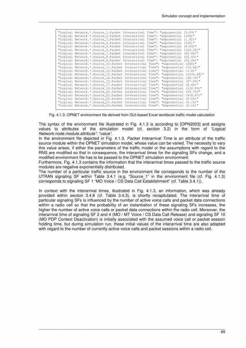
Simulator concept and implementation __________________________________________________________________________________________
__________________________________________________________________________________________ 89
"Logical Network.*.Source_1.Packet Interarrival Time": "exponential (3.09)"
"Logical Network.*.Source_2.Packet Interarrival Time": "exponential (100)"
"Logical Network.*.Source_3.Packet Interarrival Time": "exponential (1.82)"
"Logical Network.*.Source_4.Packet Interarrival Time": "exponential (100)"
"Logical Network.*.Source_5.Packet Interarrival Time": "exponential (6.83)"
"Logical Network.*.Source_6.Packet Interarrival Time": "exponential (104.32)"
"Logical Network.*.Source_7.Packet Interarrival Time": "exponential (52.69)"
"Logical Network.*.Source_8.Packet Interarrival Time": "exponential (52.69)"
"Logical Network.*.Source_9.Packet Interarrival Time": "exponential (12.96)"
"Logical Network.*.Source_10.Packet Interarrival Time": "exponential (200)"
"Logical Network.*.Source_11.Packet Interarrival Time": "exponential (12.96)"
"Logical Network.*.Source_12.Packet Interarrival Time": "exponential (1.0)"
"Logical Network.*.Source_13.Packet Interarrival Time": "exponential (1534.88)"
"Logical Network.*.Source_14.Packet Interarrival Time": "exponential (38.76)"
"Logical Network.*.Source_15.Packet Interarrival Time": "exponential (27.59)"
"Logical Network.*.Source_17.Packet Interarrival Time": "exponential (8.44)"
"Logical Network.*.Source_19.Packet Interarrival Time": "exponential (118.09)"
"Logical Network.*.Source_20.Packet Interarrival Time": "exponential (29.76)"
"Logical Network.*.Source_21.Packet Interarrival Time": "exponential (416.67)"
"Logical Network.*.Source_22.Packet Interarrival Time": "exponential (9.09)"
"Logical Network.*.Source_23.Packet Interarrival Time": "exponential (0.15)" "Logical Network.*.Source_24.Packet Interarrival Time": "exponential (0.15)"
Fig. 4.1.3: OPNET environment file derived from GUI-based Excel workbook traffic model calculation
The syntax of the environment file illustrated in Fig. 4.1.3 is according to [OPN2003] and assigns values to attributes of the simulation model (cf. section 3.2) in the form of “Logical Network.node.module.attribute”: “value”. In the environment file depicted in Fig. 4.1.3, Packet Interarrival Time is an attribute of the traffic source module within the OPNET simulation model, whose value can be varied. The necessity to vary this value arises, if either the parameters of the traffic model or the assumptions with regard to the RNS are modified so that in consequence, the interarrival times for the signaling SFs change, and a modified environment file has to be passed to the OPNET simulation environment. Furthermore, Fig. 4.1.3 contains the information that the interarrival times passed to the traffic source modules are negative exponentially distributed. The number of a particular traffic source in the environment file corresponds to the number of the UTRAN signaling SF within Table 3.4.1 (e.g. “Source_1” in the environment file (cf. Fig. 4.1.3) corresponds to signaling SF 1 “MO Voice / CS Data Call Establishment” (cf. Table 3.4.1)). In context with the interarrival times, illustrated in Fig. 4.1.3, an information, which was already provided within section 3.4.8 (cf. Table 3.4.3), is shortly recapitulated. The interarrival time of particular signaling SFs is influenced by the number of active voice calls and packet data connections within a radio cell so that the probability of an instantiation of these signaling SFs increases, the higher the number of active voice calls or packet data connections within the radio cell. Moreover, the interarrival time of signaling SF 2 and 4 (MO / MT Voice / CS Data Call Release) and signaling SF 10 (MO PDP Context Deactivation) is initially associated with the assumed voice call or packet session holding time, but during simulation run, these initial values of the interarrival time are also adapted with regard to the number of currently active voice calls and packet sessions within a radio cell.
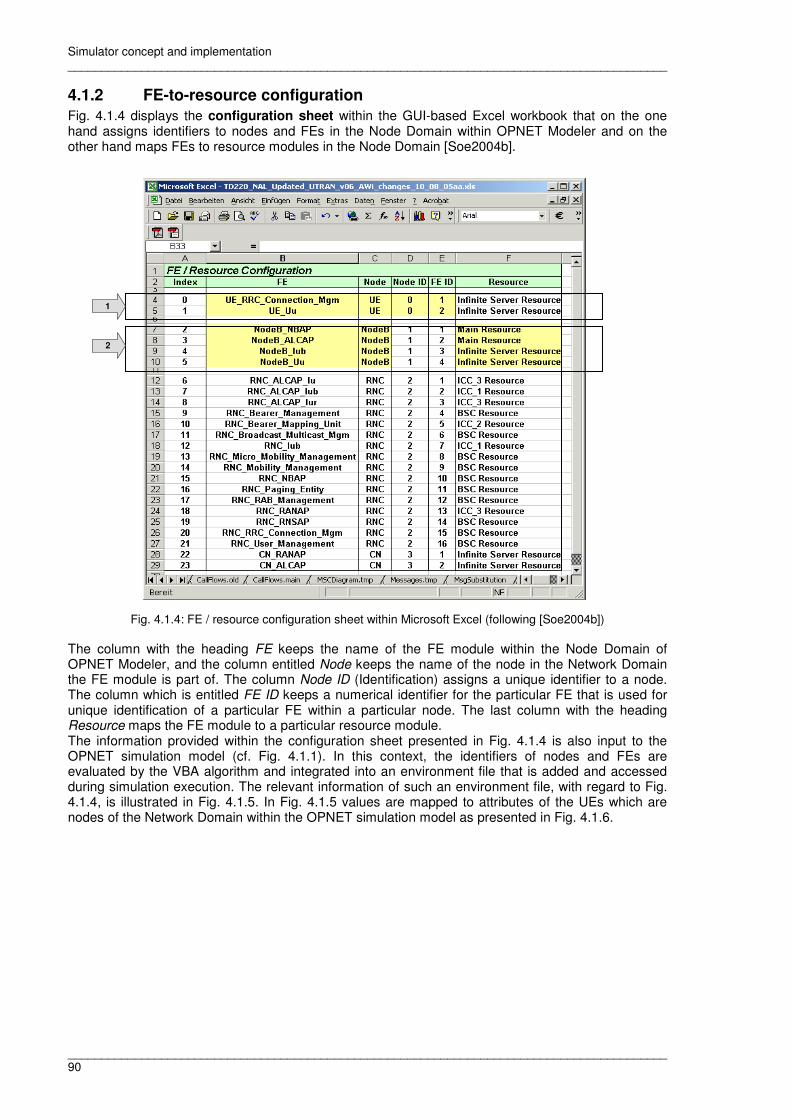
Simulator concept and implementation __________________________________________________________________________________________
__________________________________________________________________________________________ 90
4.1.2 FE-to-resource configuration
Fig. 4.1.4 displays the configuration sheet within the GUI-based Excel workbook that on the one hand assigns identifiers to nodes and FEs in the Node Domain within OPNET Modeler and on the other hand maps FEs to resource modules in the Node Domain [Soe2004b].
1
2
Fig. 4.1.4: FE / resource configuration sheet within Microsoft Excel (following [Soe2004b]) The column with the heading FE keeps the name of the FE module within the Node Domain of OPNET Modeler, and the column entitled Node keeps the name of the node in the Network Domain the FE module is part of. The column Node ID (Identification) assigns a unique identifier to a node. The column which is entitled FE ID keeps a numerical identifier for the particular FE that is used for unique identification of a particular FE within a particular node. The last column with the heading Resource maps the FE module to a particular resource module. The information provided within the configuration sheet presented in Fig. 4.1.4 is also input to the OPNET simulation model (cf. Fig. 4.1.1). In this context, the identifiers of nodes and FEs are evaluated by the VBA algorithm and integrated into an environment file that is added and accessed during simulation execution. The relevant information of such an environment file, with regard to Fig. 4.1.4, is illustrated in Fig. 4.1.5. In Fig. 4.1.5 values are mapped to attributes of the UEs which are nodes of the Network Domain within the OPNET simulation model as presented in Fig. 4.1.6.
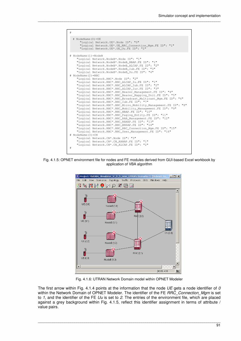
Simulator concept and implementation __________________________________________________________________________________________
__________________________________________________________________________________________ 91
#
# NodeName(1)=NodeB
"Logical Network.NodeB*.Node ID": "1"
"Logical Network.NodeB*.NodeB_NBAP.FE ID": "1"
"Logical Network.NodeB*.NodeB_ALCAP.FE ID": "2"
"Logical Network.NodeB*.NodeB_Iub.FE ID": "3"
"Logical Network.NodeB*.NodeB_Uu.FE ID": "4"
# NodeName(2)=RNC
"Logical Network.RNC*.Node ID": "2"
"Logical Network.RNC*.RNC_ALCAP_Iu.FE ID": "1"
"Logical Network.RNC*.RNC_ALCAP_Iub.FE ID": "2"
"Logical Network.RNC*.RNC_ALCAP_Iur.FE ID": "3"
"Logical Network.RNC*.RNC_Bearer_Management.FE ID": "4"
"Logical Network.RNC*.RNC_Bearer_Mapping_Unit.FE ID": "5"
"Logical Network.RNC*.RNC_Broadcast_Multicast_Mgm.FE ID": "6"
"Logical Network.RNC*.RNC_Iub.FE ID": "7"
"Logical Network.RNC*.RNC_Micro_Mobility_Management.FE ID": "8"
"Logical Network.RNC*.RNC_Mobility_Management.FE ID": "9"
"Logical Network.RNC*.RNC_NBAP.FE ID": "10"
"Logical Network.RNC*.RNC_Paging_Entity.FE ID": "11"
"Logical Network.RNC*.RNC_RAB_Management.FE ID": "12"
"Logical Network.RNC*.RNC_RANAP.FE ID": "13"
"Logical Network.RNC*.RNC_RNSAP.FE ID": "14"
"Logical Network.RNC*.RNC_RRC_Connection_Mgm.FE ID": "15"
"Logical Network.RNC*.RNC_User_Management.FE ID": "16"
# NodeName(3)=CN
"Logical Network.CN*.Node ID": "3"
"Logical Network.CN*.CN_RANAP.FE ID": "1"
"Logical Network.CN*.CN_ALCAP.FE ID": "2" #
# NodeName(0)=UE
"Logical Network.UE*.Node ID": "0"
"Logical Network.UE*.UE_RRC_Connection_Mgm.FE ID": "1" "Logical Network.UE*.UE_Uu.FE ID": "2"
Fig. 4.1.5: OPNET environment file for nodes and FE modules derived from GUI-based Excel workbook by
application of VBA algorithm
Fig. 4.1.6: UTRAN Network Domain model within OPNET Modeler The first arrow within Fig. 4.1.4 points at the information that the node UE gets a node identifier of 0 within the Network Domain of OPNET Modeler. The identifier of the FE RRC_Connection_Mgm is set to 1, and the identifier of the FE Uu is set to 2. The entries of the environment file, which are placed against a grey background within Fig. 4.1.5, reflect this identifier assignment in terms of attribute / value pairs.

Simulator concept and implementation __________________________________________________________________________________________
__________________________________________________________________________________________ 92
The second arrow within Fig. 4.1.4 points at the FE to resource mapping within the Node B which also has to be set up within the Node Domain of the OPNET simulation model. In this context, Fig. 4.1.4 provides the information that the FEs NBAP and ALCAP are mapped to the main resource within the Node B and that the interface FEs Uu and Iub are allocated to an infinite server resource (see also Fig. 3.4.6). The allocation of FEs to resources, as specified in the configuration sheet within the GUI-based Excel workbook (cf. Fig. 4.1.4), is also applied to FE and resource modules in the Node Domain of OPNET Modeler. Fig. 4.1.7 shows the Node Domain of the Node B within OPNET Modeler according to the configuration illustrated in Fig. 4.1.4.
Fig. 4.1.7: Node Domain model of Node B within OPNET Modeler The models of the Node Domain within OPNET Modeler are built according to the generic node modeling concept introduced in section 3.4 (cf. Fig. 4.1.7 and see also Fig. 3.4.1).

Simulator concept and implementation __________________________________________________________________________________________
__________________________________________________________________________________________ 93
4.1.3 Technical MSC sequence notation and VBA algorithm
Fig. 4.1.8 depicts the RRC Connection Establishment signaling sequence (cf. Fig. 3.4.5) which is taken as a signaling example throughout this thesis. Within Fig. 4.1.8, the RRC Connection Establishment signaling sequence is part of the MO Voice / CS Data Call Establishment signaling SF and technically specified within the GUI-based Excel workbook [Alt2004, Soe2004b].
1
2
Fig. 4.1.8: Refined RRC Connection Establishment signaling sequence (as part of MO Voice Call Establishment signaling SF) annotated in formal MSC sequence notation within Microsoft Excel [Alt2004]
The first column within the Excel sheet illustrated in Fig. 4.1.8 contains an identification code for the VBA algorithm. As the VBA algorithm parses the technical MSC sequence notation within the Excel sheet, it analyses each single line and determines the message type in order to reproduce the MSC flow into a format which is importable into OPNET Modeler. An identification code of T (Transaction) indicates the begin of a new signaling SF which is in this case the MO Voice / CS Data Call Establishment signaling SF. The identification code of P (Procedure) indicates the begin of an enclosed and autonomous signaling sequence within a signaling SF which is referred to as a Basic Procedure (BP). In this case, the RRC Connection Establishment signaling sequence is a BP, because it is an autonomous signaling sequence that is used within several signaling SFs. The first message of a BP is denoted with code I (Initiator) and subsequent messages with code M (Message). If a MSC sequence contains parallelism, this is indicated with an identification code of A (Action) and is referred to as Supplementary Action (SA), but the RRC Connection Establishment signaling sequence does not contain parallelism (cf. Fig. 4.1.8) [KrTaFr2002, Soe2004a]. Therefore, the RRC Connection Release signaling sequence is taken as a further example. This signaling sequence is used in several basic SFs (e.g. MO and MT Voice / CS Data Call Release) to release an existing signaling connection between a mobile terminal (UE), a RNC and the CN. Fig. 4.1.9 visualizes the technical specification of the RRC Connection Release signaling sequence according to [Alt2004] within the GUI-based Excel workbook, and Fig. 4.1.10 depicts an excerpt from the RRC Connection Release signaling flow, which contains the SA, in terms of a graphical MSC diagram for further clarification. The arrow, which points at line 233 within Fig. 4.1.9, marks the row that denotes the parallelism within the RRC Connection Release signaling sequence.

Simulator concept and implementation __________________________________________________________________________________________
__________________________________________________________________________________________ 94
Fig. 4.1.9: RRC Connection Release signaling sequence according to [Alt2004] annotated in formal MSC sequence notation within Microsoft Excel
(1,35)
(1,35)
(1,35)
(2,91)
(2,91)
Iub Uu RRC Conn. Mgm.
UE Node B
Uu RRC Conn. Mgm.
RNC
Iub
Iu Release Command
RRC Connection Release
RANAP
CN
RANAP
Iu Release Complete
(1,35)
(1,35)
(1,35)
(1,35)
Supplementary Action of FE RRC Conn. Mgm.
inside the RNC
...
Fig. 4.1.10: Excerpt from refined RRC Connection Release signaling sequence with SA according to [Alt2004] Fig. 4.1.9 and 4.1.10 show that the FE RRC_Connection_Mgm inside the RNC has to perform a SA. Within the RRC Connection Release signaling sequence, the RRC_Connection_Mgm FE receives an Iu Release Command which was initiated by the CN. Consequently, the RRC connection towards the CN has to be released, and this release has to be acknowledged to the CN by instantiation of an Iu Release Complete reply. Additionally, the RRC connection towards the mobile terminal also has to be released so that the RRC_Connection_Mgm FE also has to instantiate a RRC Connection Release signaling via the base station towards the UE, and this means that the RRC_Connection_Mgm FE has to send more than one message. Actually, the RRC_Connection_Mgm FE has to send two messages, and the second message, which initiates the RRC Connection Release signaling towards
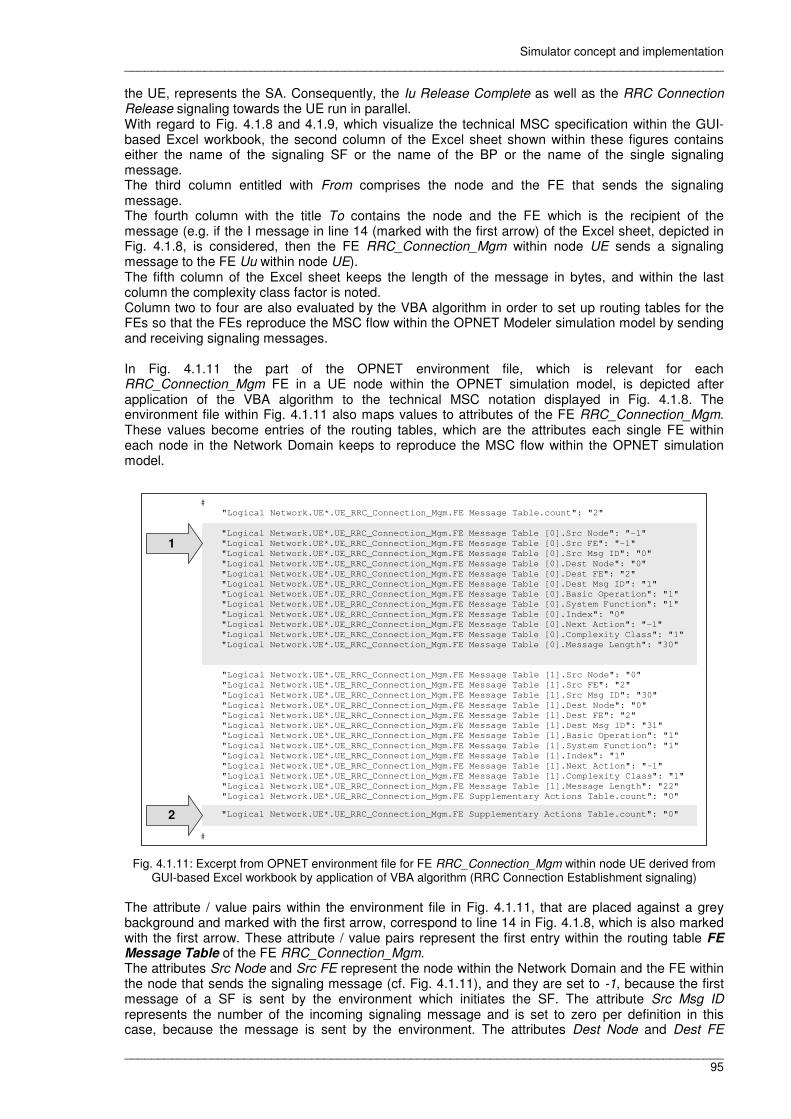
Simulator concept and implementation __________________________________________________________________________________________
__________________________________________________________________________________________ 95
the UE, represents the SA. Consequently, the Iu Release Complete as well as the RRC Connection Release signaling towards the UE run in parallel. With regard to Fig. 4.1.8 and 4.1.9, which visualize the technical MSC specification within the GUI-based Excel workbook, the second column of the Excel sheet shown within these figures contains either the name of the signaling SF or the name of the BP or the name of the single signaling message. The third column entitled with From comprises the node and the FE that sends the signaling message. The fourth column with the title To contains the node and the FE which is the recipient of the message (e.g. if the I message in line 14 (marked with the first arrow) of the Excel sheet, depicted in Fig. 4.1.8, is considered, then the FE RRC_Connection_Mgm within node UE sends a signaling message to the FE Uu within node UE). The fifth column of the Excel sheet keeps the length of the message in bytes, and within the last column the complexity class factor is noted. Column two to four are also evaluated by the VBA algorithm in order to set up routing tables for the FEs so that the FEs reproduce the MSC flow within the OPNET Modeler simulation model by sending and receiving signaling messages. In Fig. 4.1.11 the part of the OPNET environment file, which is relevant for each RRC_Connection_Mgm FE in a UE node within the OPNET simulation model, is depicted after application of the VBA algorithm to the technical MSC notation displayed in Fig. 4.1.8. The environment file within Fig. 4.1.11 also maps values to attributes of the FE RRC_Connection_Mgm. These values become entries of the routing tables, which are the attributes each single FE within each node in the Network Domain keeps to reproduce the MSC flow within the OPNET simulation model.
#
"Logical Network.UE*.UE_RRC_Connection_Mgm.FE Message Table.count": "2"
"Logical Network.UE*.UE_RRC_Connection_Mgm.FE Message Table [1].Src Node": "0"
"Logical Network.UE*.UE_RRC_Connection_Mgm.FE Message Table [1].Src FE": "2"
"Logical Network.UE*.UE_RRC_Connection_Mgm.FE Message Table [1].Src Msg ID": "30"
"Logical Network.UE*.UE_RRC_Connection_Mgm.FE Message Table [1].Dest Node": "0"
"Logical Network.UE*.UE_RRC_Connection_Mgm.FE Message Table [1].Dest FE": "2"
"Logical Network.UE*.UE_RRC_Connection_Mgm.FE Message Table [1].Dest Msg ID": "31"
"Logical Network.UE*.UE_RRC_Connection_Mgm.FE Message Table [1].Basic Operation": "1"
"Logical Network.UE*.UE_RRC_Connection_Mgm.FE Message Table [1].System Function": "1"
"Logical Network.UE*.UE_RRC_Connection_Mgm.FE Message Table [1].Index": "1"
"Logical Network.UE*.UE_RRC_Connection_Mgm.FE Message Table [1].Next Action": "-1"
"Logical Network.UE*.UE_RRC_Connection_Mgm.FE Message Table [1].Complexity Class": "1"
"Logical Network.UE*.UE_RRC_Connection_Mgm.FE Message Table [1].Message Length": "22"
"Logical Network.UE*.UE_RRC_Connection_Mgm.FE Supplementary Actions Table.count": "0"
#
"Logical Network.UE*.UE_RRC_Connection_Mgm.FE Message Table [0].Src Node": "-1"
"Logical Network.UE*.UE_RRC_Connection_Mgm.FE Message Table [0].Src FE": "-1"
"Logical Network.UE*.UE_RRC_Connection_Mgm.FE Message Table [0].Src Msg ID": "0"
"Logical Network.UE*.UE_RRC_Connection_Mgm.FE Message Table [0].Dest Node": "0"
"Logical Network.UE*.UE_RRC_Connection_Mgm.FE Message Table [0].Dest FE": "2"
"Logical Network.UE*.UE_RRC_Connection_Mgm.FE Message Table [0].Dest Msg ID": "1"
"Logical Network.UE*.UE_RRC_Connection_Mgm.FE Message Table [0].Basic Operation": "1"
"Logical Network.UE*.UE_RRC_Connection_Mgm.FE Message Table [0].System Function": "1"
"Logical Network.UE*.UE_RRC_Connection_Mgm.FE Message Table [0].Index": "0"
"Logical Network.UE*.UE_RRC_Connection_Mgm.FE Message Table [0].Next Action": "-1"
"Logical Network.UE*.UE_RRC_Connection_Mgm.FE Message Table [0].Complexity Class": "1"
"Logical Network.UE*.UE_RRC_Connection_Mgm.FE Message Table [0].Message Length": "30"
"Logical Network.UE*.UE_RRC_Connection_Mgm.FE Supplementary Actions Table.count": "0"
1
2
Fig. 4.1.11: Excerpt from OPNET environment file for FE RRC_Connection_Mgm within node UE derived from
GUI-based Excel workbook by application of VBA algorithm (RRC Connection Establishment signaling) The attribute / value pairs within the environment file in Fig. 4.1.11, that are placed against a grey background and marked with the first arrow, correspond to line 14 in Fig. 4.1.8, which is also marked with the first arrow. These attribute / value pairs represent the first entry within the routing table FE Message Table of the FE RRC_Connection_Mgm. The attributes Src Node and Src FE represent the node within the Network Domain and the FE within the node that sends the signaling message (cf. Fig. 4.1.11), and they are set to -1, because the first message of a SF is sent by the environment which initiates the SF. The attribute Src Msg ID represents the number of the incoming signaling message and is set to zero per definition in this case, because the message is sent by the environment. The attributes Dest Node and Dest FE

Simulator concept and implementation __________________________________________________________________________________________
__________________________________________________________________________________________ 96
correspond to the next node within the Node Domain and to the FE within the node that is the recipient of the signaling message which is sent by node UE and FE RRC_Connection_Mgm after consumption of the initial signaling message sent by the environment. The values for the attributes Dest Node and Dest FE are automatically taken by the VBA algorithm from the sheet that keeps the mapping of FEs to resources within the GUI-based Excel workbook and is illustrated in Fig. 4.1.4 (marked with the first arrow). The number of the message that is to be sent to the destination node and FE corresponds to the attribute Dest Msg ID and is increased by 1. The attribute Basic Operation and its value of 1 reveal that the message belongs to the first BP within the signaling SF which is RRC Connection Establishment. Consequently, the attribute System Function and its value of 1 states that the message belongs to the first signaling SF which is MO Voice / CS Data Call Establishment. The value of the attribute Next Action is set to -1, because the FE RRC_Connection_Mgm simply has to process and then forward the initial signaling message to the destination FE. Beyond this activity of message processing and subsequent forwarding, the FE RRC_Connection_Mgm does not have to initiate further message flows which run in parallel to the message flow created by the forwarding of the initial signaling message. According to the technical MSC notation illustrated in Fig. 4.1.8, line 14, the attribute Complexity Class is set to 1 and the attribute Message Length is set to 30 [Wie2002a, FrKrTa2002]. The routing table FE Supplementary Actions Table of the FE RRC_Connection_Mgm (cf. Fig. 4.1.9, the attribute / value pairs placed against a grey background and marked with the second arrow) is empty, because the RRC Connection Establishment signaling sequence does not contain parallelism. Particularly, this means that the routing table FE Supplementary Actions Table has only entries, if a MSC contains parallel sequences [Wie2002a, FrKrTa2002], as in case of RRC Connection Release signaling. Fig. 4.1.12 displays an excerpt of the OPNET environment file, which is relevant for the RRC_Connection_Mgm FE in the RNC within the OPNET simulation model, after application of the VBA algorithm to the technical MSC notation of the RRC Connection Release signaling sequence displayed in Fig. 4.1.9.
#
"Logical Network.RNC*.RNC_RRC_Connection_Mgm.FE Message Table.count": "1"
"Logical Network.RNC*.RNC_RRC_Connection_Mgm.FE Message Table [0].Src Node": "2"
"Logical Network.RNC*.RNC_RRC_Connection_Mgm.FE Message Table [0].Src FE": "13"
"Logical Network.RNC*.RNC_RRC_Connection_Mgm.FE Message Table [0].Src Msg ID": "2"
"Logical Network.RNC*.RNC_RRC_Connection_Mgm.FE Message Table [0].Dest Node": "2"
"Logical Network.RNC*.RNC_RRC_Connection_Mgm.FE Message Table [0].Dest FE": "13"
"Logical Network.RNC*.RNC_RRC_Connection_Mgm.FE Message Table [0].Dest Msg ID": "3"
"Logical Network.RNC*.RNC_RRC_Connection_Mgm.FE Message Table [0].Basic Operation": "1"
"Logical Network.RNC*.RNC_RRC_Connection_Mgm.FE Message Table [0].System Function": "2"
"Logical Network.RNC*.RNC_RRC_Connection_Mgm.FE Message Table [0].Index": "0"
"Logical Network.RNC*.RNC_RRC_Connection_Mgm.FE Message Table [0].Next Action": "0"
"Logical Network.RNC*.RNC_RRC_Connection_Mgm.FE Message Table [0].Complexity Class": "2"
"Logical Network.RNC*.RNC_RRC_Connection_Mgm.FE Message Table [0].Message Length": "91"
"Logical Network.RNC*.RNC_RRC_Connection_Mgm.FE Supplementary Actions Table.count": "1"
"Logical Network.RNC*.RNC_RRC_Connection_Mgm.FE Supplementary Actions Table [0].Dest Node": "2"
"Logical Network.RNC*.RNC_RRC_Connection_Mgm.FE Supplementary Actions Table [0].Dest FE": "7"
"Logical Network.RNC*.RNC_RRC_Connection_Mgm.FE Supplementary Actions Table [0].Dest Msg ID": "5"
"Logical Network.RNC*.RNC_RRC_Connection_Mgm.FE Supplementary Actions Table [0].Basic Operation": "1"
"Logical Network.RNC*.RNC_RRC_Connection_Mgm.FE Supplementary Actions Table [0].System Function": "2"
"Logical Network.RNC*.RNC_RRC_Connection_Mgm.FE Supplementary Actions Table [0].Index": "0"
"Logical Network.RNC*.RNC_RRC_Connection_Mgm.FE Supplementary Actions Table [0].Next Action": "-1"
"Logical Network.RNC*.RNC_RRC_Connection_Mgm.FE Supplementary Actions Table [0].Complexity Class": "1"
"Logical Network.RNC*.RNC_RRC_Connection_Mgm.FE Supplementary Actions Table [0].Message Length": "35" #
"Logical Network.RNC*.RNC_RRC_Connection_Mgm.FE Message Table [0].Next Action": "0" SA
Fig. 4.1.12: Excerpt from OPNET environment file for FE RRC_Connection_Mgm within node RNC derived from GUI-based Excel workbook by application of VBA algorithm (RRC Connection Release Signaling)
Fig. 4.1.12 particularly depicts the SA, which is part of the RRC Connection Release signaling sequence. The arrow, marked with “SA”, points at the line of the environment file, which denotes that the FE RRC_Connection_Mgm has to perform a SA. The value of the attribute Next Action in the FE Message Table of the FE RRC_Connection_Mgm within the node RNC is set to 0 so that the execution of a SA is indicated. Following [Wie2002a, FrKrTa2002], the rule is that the execution of a SA is indicated, whenever the value of the attribute Next Action within the FE Message Table and / or FE Supplementary Actions Table is unequal from -1. As the value of the attribute Next Action in the FE Message Table, which is depicted in Fig. 4.1.12, is set to 0, this implies that the action which is denoted in line 0 of the FE Supplementary Actions Table, i.e. FE Supplementary Actions Table [0], has to be executed. Thus, as a further rule, the entry in the column Next Action within the FE Message Table corresponds to the row index in the Supplementary Actions Table. The column Dest Node and Dest FE in the FE Supplementary Actions Table (cf. Fig. 4.1.12) keep the identifier of the node and of the FE that is the recipient of the SA message. The meaning of the

Simulator concept and implementation __________________________________________________________________________________________
__________________________________________________________________________________________ 97
remaining columns within this table corresponds to the meaning of the homonymous columns within the FE Message Table. If a FE starts more than one parallel message sequence, the entry within the column Next Action in the FE Supplementary Actions Table will again point to the corresponding row within the FE Supplementary Actions Table, but in this case the entry within the column Next Action in the FE Supplementary Actions Table of the RRC_Connection_Mgm FE is set to -1 (cf. Fig. 4.1.12) so that the RRC_Connection_Mgm FE simply performs one SA. In Fig. 4.1.13 and 4.1.14 those parts of the OPNET environment file, which are relevant for traffic source and sink modules within the Node Domain of the OPNET simulation model (cf. Fig. 4.1.7), are depicted after application of the VBA algorithm to the technical MSC notation displayed in Fig. 4.1.8. The traffic source modules generate UTRAN signaling SFs, and the sink modules perform statistical measurements on incoming messages and destroy them subsequently to free memory for the OPNET simulation kernel.
#
# System Function Sources
#
"Logical Network.*.Source_1.Packet Parameters[0].System Function": "1"
"Logical Network.*.Source_1.Packet Parameters[0].Name": "MO Voice / CS Data Call Establishment"
"Logical Network.*.Source_1.Packet Parameters[0].Dest Node ID": "0"
"Logical Network.*.Source_1.Packet Parameters[0].Dest FE ID": "1"
#
Fig. 4.1.13: OPNET environment file for traffic source modules derived from GUI-based Excel workbook by
application of VBA algorithm The traffic source module (cf. Fig. 4.1.13) keeps the number of the SF which is set to 1 and the name of the SF (MO Voice / CS Data Call Establishment). Moreover, the traffic source holds the identifier of the FE that initiates the SF and the identifier of the node the FE belongs to which are the attributes Dest Node ID and Dest FE ID. As SF 1 starts at the FE RRC_Connection_Mgm (cf. Fig. 4.1.8) inside the node UE, the values of the attributes Dest Node ID and Dest FE ID are set to 0 and 1 (under consideration of the configuration depicted in Fig. 4.1.4) [WiAt2003].
#
# System Function Sinks
#
"Logical Network.*.Sink.End of SF[1].SF": "1"
"Logical Network.*.Sink.End of SF[1].Statistics": "MO Voice / CS Data Call Establishment"
"Logical Network.*.Sink.End of SF[1].BP": "1"
"Logical Network.*.Sink.End of SF[1].Src Node ID": "2"
"Logical Network.*.Sink.End of SF[1].Src FE ID": "7"
"Logical Network.*.Sink.End of SF[1].Message ID": "35" #
Fig. 4.1.14: OPNET environment file for sink modules derived from GUI-based Excel workbook by application of
VBA algorithm The sink module (cf. Fig. 4.1.14) keeps the number of the SF which is set to 1 and the name of the SF (MO Voice / CS Data Call Establishment) for the statistics that have to be measured. The sink also holds the number of the BP which is also set to 1, because the RRC Connection Establishment signaling sequence is the only BP within the example illustrated in Fig. 4.1.8. Furthermore, the sink keeps the identifier of the FE, that sent the last message of the SF which is chosen for statistical measurements, the identifier of the node the FE belongs to and the number of the last message (Src Node ID, Src FE ID and Message ID attributes, cf. Fig. 4.1.14). As the last message of SF 1 represents the last message of BP 1 (cf. Fig. 4.1.8, second arrow), the values of the attributes Src Node ID and Src FE ID are set to 2 and 7 (under consideration of the configuration depicted in Fig. 4.1.4), because the last message of the RRC Connection Establishment signaling sequence is sent by the FE Iub which is part of the node RNC. The number of the last message is 35. The sink module needs these values to match incoming packets against the table that keeps the values of those packets which are chosen for statistical measurements [WiAt2003].

Simulator concept and implementation __________________________________________________________________________________________
__________________________________________________________________________________________ 98
4.1.4 High-level overview of the OPNET simulator
If the input for the OPNET simulator is completely provided according to Fig. 4.1.1 and the nodes within the Network Domain are built according to the FE and resource configuration instructions (cf. Fig. 4.1.4 and 4.1.7), simulations can be performed with the OPNET simulator either by usage of the graphical simulation tool provided by OPNET Modeler or from the command line with or without making use of a batch file (cf. section 3.2). The environment files are bound during simulation execution and assign values to unresolved attributes which makes the simulator highly configurable. The OPNET simulator is conceptually based on components which represent the modules of the node domain. These components enable the network designer to set up nodes in the Network Domain within OPNET Modeler under consideration of the generic node modeling concept described in section 3.4 (see also Fig. 3.4.1). Moreover, the network designer is enabled to arbitrarily build network configurations of interest within the Network Domain of OPNET Modeler (cf. Fig. 4.1.6 as an example network configuration). In order to implement this component-based approach, that allows the network designer to set up UTRAN architecture evolution scenarios of interest as described above without caring for implementation details, the simulator implementation within the Process Domain of OPNET Modeler is generic and elaborate. The forthcoming section focuses on concepts of the simulator implementation which enable the component-based approach of the simulator application. The OPNET simulator, its versions and usage is fully specified in the bibliographical section starting with reference [Wie2002c] up to reference [Wie2005b]. Executed simulation runs provide values for the performance measures of interest in the categories of MSCs, resources and regarding the number of active calls and sessions (cf. Fig. 4.1.1). Particularly for the MSCs, the network designer gets E2E signaling delays for the UTRAN signaling SFs specified in Table 3.4.1. Moreover, information about the composition of the E2E signaling delays is provided in the form of partial signaling delays [WiAt2003]. If, for instance, an E2E signaling delay of 5 sec is measured for the MO Voice / CS Data Call Establishment signaling sequence, the network designer can get the information that this E2E delay is composed of 2 sec processing delay within resources, 2.5 sec queueing delay experienced within resources, 0.35 sec transmission delay and 0.15 sec link propagation delay. With regard to the resources, the utilization of the resources is provided. Moreover, partial processing and queueing delays per MSC and resource are available so that the network designer gets explicitly to know how much time a particular signaling SF spent within a particular resource for processing or waiting for service. This information is particularly of interest when dimensioning resources. Moreover, information about the number of active or blocked CS calls and PS sessions, the number of successful / unsuccessful handovers and about the number of lost CS voice calls due to unsuccessful handovers is provided. These statistics are collected within a single radio cell as well as for the complete network.
4.2 Implementation concept
A sophisticated implementation within the Process Domain of OPNET Modeler reduces the interaction of the network designer, interested to set up and evaluate UTRAN architecture evolution scenarios according to the generic node modeling concept presented in section 3.4, to the Node and Network Domain within OPNET Modeler. Particularly, this means that the network designer has a set of modules according to the generic node modeling concept available in the Node Domain which can be used and interconnected by packet streams (cf. section 3.2) to set up nodes within the Network Domain. Subsequently, the network designer is enabled to build network configurations of interest in the Network Domain by interconnecting the nodes via bidirectional communication links (e.g. a Synchronous Transport Module level 1 (STM-1) link between the RNC and CN of 155 Mbit/sec) which are also provided, configured via the OPNET GUI and available for usage. The modules available to the network designer are the ER, IR, FE, traffic source, sink and resource modules in the Node Domain, and each of these modules possesses its particular process model within the Process Domain. LSAPs are constructed from transmitter and receiver modules which are available in the Node Domain of OPNET Modeler, i.e. a transmitter / receiver pair forms a LSAP. With regard to the aforementioned modules in the Node Domain, it has to be considered that various nodes in the Network Domain (e.g. UEs, Node Bs, RNCs, CN and even new network devices of the UTRAN evolution scenarios) have to be built with them. Consequently, the modules have to be highly
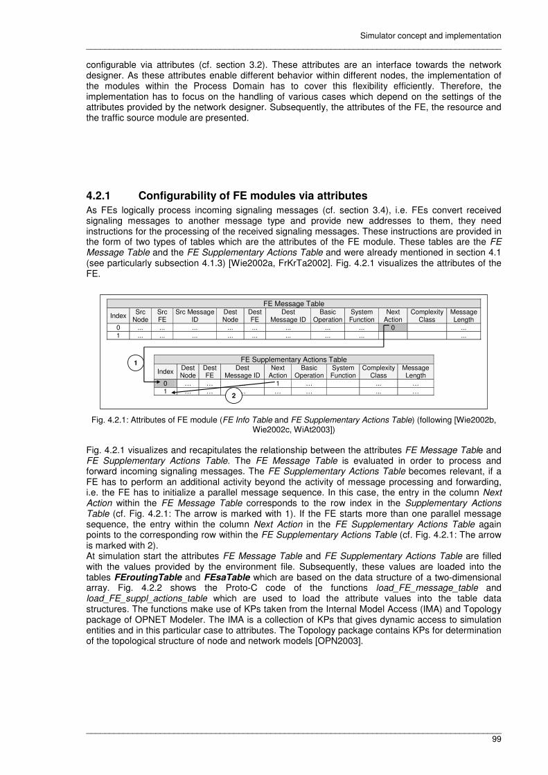
Simulator concept and implementation __________________________________________________________________________________________
__________________________________________________________________________________________ 99
configurable via attributes (cf. section 3.2). These attributes are an interface towards the network designer. As these attributes enable different behavior within different nodes, the implementation of the modules within the Process Domain has to cover this flexibility efficiently. Therefore, the implementation has to focus on the handling of various cases which depend on the settings of the attributes provided by the network designer. Subsequently, the attributes of the FE, the resource and the traffic source module are presented.
4.2.1 Configurability of FE modules via attributes
As FEs logically process incoming signaling messages (cf. section 3.4), i.e. FEs convert received signaling messages to another message type and provide new addresses to them, they need instructions for the processing of the received signaling messages. These instructions are provided in the form of two types of tables which are the attributes of the FE module. These tables are the FE Message Table and the FE Supplementary Actions Table and were already mentioned in section 4.1 (see particularly subsection 4.1.3) [Wie2002a, FrKrTa2002]. Fig. 4.2.1 visualizes the attributes of the FE.
FE Message Table
Index Src
Node Src FE
Src Message ID
Dest Node
Dest FE
Dest Message ID
Basic Operation
System Function
Next Action
Complexity Class
Message Length
0 ... ... ... ... ... ... ... ... 0 ... 1 ... ... ... ... ... ... ... ... ...
FE Supplementary Actions Table
Index Dest Node
Dest FE
Dest Message ID
Next Action
Basic Operation
System Function
Complexity Class
Message Length
0 … … … 1 … ... … 1 … … … … … ... …
1
2
Fig. 4.2.1: Attributes of FE module (FE Info Table and FE Supplementary Actions Table) (following [Wie2002b, Wie2002c, WiAt2003])
Fig. 4.2.1 visualizes and recapitulates the relationship between the attributes FE Message Table and FE Supplementary Actions Table. The FE Message Table is evaluated in order to process and forward incoming signaling messages. The FE Supplementary Actions Table becomes relevant, if a FE has to perform an additional activity beyond the activity of message processing and forwarding, i.e. the FE has to initialize a parallel message sequence. In this case, the entry in the column Next Action within the FE Message Table corresponds to the row index in the Supplementary Actions Table (cf. Fig. 4.2.1: The arrow is marked with 1). If the FE starts more than one parallel message sequence, the entry within the column Next Action in the FE Supplementary Actions Table again points to the corresponding row within the FE Supplementary Actions Table (cf. Fig. 4.2.1: The arrow is marked with 2). At simulation start the attributes FE Message Table and FE Supplementary Actions Table are filled with the values provided by the environment file. Subsequently, these values are loaded into the tables FEroutingTable and FEsaTable which are based on the data structure of a two-dimensional array. Fig. 4.2.2 shows the Proto-C code of the functions load_FE_message_table and load_FE_suppl_actions_table which are used to load the attribute values into the table data structures. The functions make use of KPs taken from the Internal Model Access (IMA) and Topology package of OPNET Modeler. The IMA is a collection of KPs that gives dynamic access to simulation entities and in this particular case to attributes. The Topology package contains KPs for determination of the topological structure of node and network models [OPN2003].

Simulator concept and implementation __________________________________________________________________________________________
__________________________________________________________________________________________ 100
void load_FE_message_table () {
// A. Wiedemann - Comment + Function:
// The function loads the values of the FE Message Table.
// Input parameters: none
// Output parameters: none
int i, j, // Loop variables
number_of_compound_entries; // Variable to keep the number of values in the compound model attribute
FIN (load_FE_message_table ());
// Get number of rows in compound attribute FE Message Table:
number_of_compound_entries = op_topo_child_count (FE_Msg_Table_ID, OPC_OBJMTYPE_ALL);
// Load the values of each row into the two-dimensional table FEroutingTable[MAX_ROW][MAX_COLUMN]:
for (i=0 ; i < number_of_compound_entries ; i++) {
op_ima_obj_attr_get (op_topo_child(FE_Msg_Table_ID, OPC_OBJMTYPE_ALL, i), \
"Src Node", &FEroutingTable[i][0]);
op_ima_obj_attr_get (op_topo_child(FE_Msg_Table_ID, OPC_OBJMTYPE_ALL, i), \
"Src FE", &FEroutingTable[i][1]);
op_ima_obj_attr_get (op_topo_child(FE_Msg_Table_ID, OPC_OBJMTYPE_ALL, i), \
"Src Msg ID", &FEroutingTable[i][2]);
op_ima_obj_attr_get (op_topo_child(FE_Msg_Table_ID, OPC_OBJMTYPE_ALL, i), \
"Dest Node", &FEroutingTable[i][3]);
op_ima_obj_attr_get (op_topo_child(FE_Msg_Table_ID, OPC_OBJMTYPE_ALL, i), \
"Dest FE", &FEroutingTable[i][4]);
op_ima_obj_attr_get (op_topo_child(FE_Msg_Table_ID, OPC_OBJMTYPE_ALL, i), \
"Dest Msg ID", &FEroutingTable[i][5]);
op_ima_obj_attr_get (op_topo_child(FE_Msg_Table_ID, OPC_OBJMTYPE_ALL, i), \
"Basic Operation", &FEroutingTable[i][6]);
op_ima_obj_attr_get (op_topo_child(FE_Msg_Table_ID, OPC_OBJMTYPE_ALL, i), \
"System Function", &FEroutingTable[i][7]);
op_ima_obj_attr_get (op_topo_child(FE_Msg_Table_ID, OPC_OBJMTYPE_ALL, i), \
"Next Action", &FEroutingTable[i][8]);
op_ima_obj_attr_get (op_topo_child(FE_Msg_Table_ID, OPC_OBJMTYPE_ALL, i), \
"Complexity Class", &FEroutingTable[i][9]);
op_ima_obj_attr_get (op_topo_child(FE_Msg_Table_ID, OPC_OBJMTYPE_ALL, i), \
"Message Length", &FEroutingTable[i][10]);
}
FOUT;
}
void load_FE_suppl_actions_table () {
// A. Wiedemann - Comment + Function:
// The function loads the values of the FE Supplementary Actions Table.
// Input parameters: none
// Output parameters: none
int i, j, // Loop variables
number_of_compound_entries; // Variable to keep the number of values in the compound model attribute
FIN (load_FE_suppl_actions_table ());
// Get number of rows in compound attribute FE Supplementary Actions Table:
number_of_compound_entries = op_topo_child_count (FE_Suppl_Actions_Table_ID, OPC_OBJMTYPE_ALL);
// Load the values of each row into the two-dimensional table FEsaTable[MAX_ROW][MAX_COLUMN]:
for (i=0 ; i < number_of_compound_entries ; i++) {
op_ima_obj_attr_get (op_topo_child(FE_Suppl_Actions_Table_ID, OPC_OBJMTYPE_ALL, i), \
"Dest Node", &FEsaTable[i][0]);
op_ima_obj_attr_get (op_topo_child(FE_Suppl_Actions_Table_ID, OPC_OBJMTYPE_ALL, i), \
"Dest FE", &FEsaTable[i][1]);
op_ima_obj_attr_get (op_topo_child(FE_Suppl_Actions_Table_ID, OPC_OBJMTYPE_ALL, i), \
"Dest Msg ID", &FEsaTable[i][2]);
op_ima_obj_attr_get (op_topo_child(FE_Suppl_Actions_Table_ID, OPC_OBJMTYPE_ALL, i), \
"Next Action", &FEsaTable[i][3]);
op_ima_obj_attr_get (op_topo_child(FE_Suppl_Actions_Table_ID, OPC_OBJMTYPE_ALL, i), \
"Basic Operation", &FEsaTable[i][4]);
op_ima_obj_attr_get (op_topo_child(FE_Suppl_Actions_Table_ID, OPC_OBJMTYPE_ALL, i), \
"System Function", &FEsaTable[i][5]);
op_ima_obj_attr_get (op_topo_child(FE_Suppl_Actions_Table_ID, OPC_OBJMTYPE_ALL, i), \
"Complexity Class", &FEsaTable[i][6]);
op_ima_obj_attr_get (op_topo_child(FE_Suppl_Actions_Table_ID, OPC_OBJMTYPE_ALL, i), \
"Message Length", &FEsaTable[i][7]);
}
FOUT; }
Fig. 4.2.2: Proto-C code of functions for loading the message processing tables within the FE modules [Wie2005b]
4.2.2 Configurability of resource modules via attributes
Fig. 4.2.3 depicts the attributes of the resource module which correspond to the resource modeling concept of [Mül2003] (cf. section 3.4). These attributes have to be specified by the network designer either within the OPNET GUI or within an environment file.

Simulator concept and implementation __________________________________________________________________________________________
__________________________________________________________________________________________ 101
Attributes of Resource Module Speed Factor
Complexity Class 1 Complexity Class 2 Amount of Service Table Complexity Class 3
Number of Servers Measurement of Resource Delays
Fig. 4.2.3: Attributes of resource module (according to [WiAt2003]) Following [Mül2003], the attribute Speed Factor of the resource module represents the processing power of the particular resource module. The attribute Amount of Service Table keeps the processing amounts necessary to process signaling messages of three complexity classes. The sub-attributes Complexity Class 1, 2, and 3 of the Amount of Service Table attribute contain the processing amounts in milliseconds (ms). These service amounts are assigned to signaling messages of the particular complexity type, when they enter the service unit of the resource module. The attribute Number of Servers contains the number of service units of the resource module (cf. Fig. 3.4.2). The attribute Measurement of Resource Delays corresponds to the statistical measurement of partial signaling delays during simulation run (cf. section 4.1) and is either enabled or disabled (the latter is the default value). Consequently, the network designer has to enable this measurement attribute, if partial signaling delays are of interest. The reason to handle the measurement of the partial signaling delay like this is that this measurement slows down simulation progression, as measurement values have to be taken whenever a packet enters a resource module so that a convenient solution is provided to execute these measurements when required.
4.2.3 Configurability of traffic source modules via attributes
Fig. 4.2.4 shows the attributes of the generic traffic source module that is used to generate the UTRAN signaling SFs explained in Table 3.4.1.
UTRAN Signaling SFs
MO
Voi
ce /
CS
Dat
a C
all E
stab
lishm
ent
MO
Voi
ce /
CS
Dat
a C
all R
elea
se
MT
Voi
ce /
CS
Dat
a C
all E
stab
lishm
ent
MT
Voi
ce /
CS
Dat
a C
all R
elea
se
PS
Dat
a T
rans
fer
Est
ablis
hmen
t
PS
Det
ach
(UE
initi
ated
)
Tra
nsiti
on fr
om U
RA
_PC
H t
o C
ELL
_DC
H
due
to D
ownl
ink
Dat
a T
rans
fer
Tra
nsiti
on fr
om C
ELL
_DC
H to
UR
A_P
CH
du
e to
RR
C in
activ
ity ti
mer
exp
iring
MO
PD
P C
onte
xt A
ctiv
atio
n
MO
PD
P C
onte
xt D
eact
ivat
ion
IMS
I D
etac
h S
igna
ling
Flo
w
Loca
tion
Upd
atin
g S
igna
ling
Flo
w
UR
A U
pdat
e S
igna
ling
Flo
w
RA
Upd
ate
Sig
nalin
g F
low
Intr
a-R
NC
Sof
ter
Han
dove
r
Intr
a-R
NC
Sof
t Han
dove
r
Inte
r-R
NC
Sof
t Han
dove
r
Intr
a-R
NC
Har
d H
ando
ver
Inte
r-R
NC
Har
d H
ando
ver
SR
NS
Rel
ocat
ion
Pag
ing
in id
le m
ode
Pag
ing
in c
onne
cted
mod
e
Pag
ing
unsu
cces
sful
Mea
sure
men
t Rep
ort
Attributes of Traffic Source Module 1 2 3 4 5 6 7 8 9 10 11 12 13 14 15 16 17 18 19 20 21 22 23 24 Packet Interarrival Time ef Start Time ND Stop Time ND
System Function ef Name ef Dest Node ID ef
Traffic Source Parameters
Dest FE ID ef Voice Call Setup E - E - - - - - - - - - - - - - - - - - - - - - Voice Call Release - E - E - - - - - - - - - - - - - - - - - - - - MO PDP Context Activation - - - - - - - - E - - - - - - - - - - - - - - -
Type of Call
MO PDP Context Deactivation - - - - - - - - - E - - - - - - - - - - - - - - Active Voice Calls - E - E - - - - - - - - - - E E E E E - - - - - Association Active Packet Data Sessions - - - - - E E E - E - - - E - - - - - - - - - - Intra - - - - - - - - - - - - - - - E - E - - - - - - Handover /
SRNS Relocation Drift - - - - - - - - - - - - - - - - E - E E - - - - Broadcast Initiator - - - - - - - - - - - - - - - - - - - - - - E - Broadcast Broadcast - - - - - - - - - - - - - - - - - - - - E E E -
Legend: E Enabled - Disabled ef Value is taken from environment file ND Value can be specified by the network designer
Fig. 4.2.4: Attributes of traffic source module and exemplified settings for UTRAN signaling SFs (cf. [Wie2002c, Wie2004a, Wie2004b])

Simulator concept and implementation __________________________________________________________________________________________
__________________________________________________________________________________________ 102
The Packet Interarrival Time attribute (cf. Fig. 4.2.4) of the particular traffic source module is taken from the environment file (cf. section 4.1, Fig. 4.1.3) which is derived from the traffic model within the GUI-based Excel workbook. The attributes Start Time and Stop Time enable the network designer to specify time values for each particular traffic source, when the traffic source module is expected to start and stop the generation of signaling SF instances. The attribute Traffic Source Parameters and its sub-attributes System Function, Name, Dest Node ID and Dest FE ID have already been introduced in section 4.1 (cf. Fig. 4.1.10). In this context, the configuration sheet depicted in Fig. 4.1.4 is assumed for the derivation of the values for the sub-attributes Dest Node ID and Dest FE ID and the full set of UTRAN signaling SFs is presumed as specified in [Alt2004]. The Type of Call attribute and its sub-attributes Voice Call Setup, Voice Call Release, MO PDP Context Activation and MO PDP Context Deactivation (cf. Fig. 4.2.4) are used to denote a traffic source as either a Voice Call Setup or Release source or as a MO PDP Context Activation or Deactivation traffic source. Consequently, if one of these sub-attributes is set to enabled, the traffic source is set to this particular type. The classification according to the Type of Call attribute is necessary for the scheduling process of voice call setups and releases as well as packet data session setups and releases. Fig. 4.2.5 illustrates a snippet from the Proto-C code of the process model of the generic traffic source which will be used for further explanation of the functionality of the traffic source module.
1 if (setup_voice == 1) { 2 // i.e. if this condition matches, the module is a setup source for voice calls 3 4 // Schedule the interarrival time of the next voice call: 5 next_intarr_time = op_dist_outcome (interarrival_dist_ptr); 6 7 // Make sure that interarrival time is not negative. In that case the interarrival time is negative, it will be set to 0: 8 if (next_intarr_time < 0) { 9 next_intarr_time = 0; 10 } 11 12 if (network_element_typeID == 0) { 13 // i.e. if this condition matches, the generic micro traffic source is part of an UE network element, 14 // because per definition the Type ID of the UE network element is set to zero. 15 // Consequently, an MO Voice Call Setup will be generated. 16 17 // Schedule self interrupt for the generation of the next MO Voice Call Setup: 18 next_pk_evh = op_intrpt_schedule_self (op_sim_time () + next_intarr_time, SSC_GENERATE); 19 } 20 21 if (network_element_typeID != 0) { 22 // i.e. if this condition matches, the generic micro traffic source is part of the CN. 23 // Consequently, an MT Voice Call Setup will be generated. 24 25 // In this case an UE has to be determined randomly to terminate the MT Voice Call Setup: 26 randomly_determined_UE_inst_id = determine_UE_for_MT_call_randomly (lptr_to_list_with_eligible_UEs_for_MT_calls, \ 27 instanceID, \ 28 nodeID, \ 29 network_element_typeID); 30 31 // Get Object ID of the randomly determined UE network element: 32 // Note: 0 is given to the function as the Type ID of the UE network element which is - per definition - always set to zero. 33 randomly_determined_UE_objid = get_objid_of_UE_network_element (randomly_determined_UE_inst_id, 0); 34 35 // Get Object ID of the voice call or packet data setup traffic source within the randomly determined UE network element: 36 // Note: 1 is given to the function to indicate that the number of active voice calls is of interest, 37 // 0 is given to the function to indicate that the number of active packet data connections is NOT of interest. 38 setup_src_objid_in_randomly_determined_UE = get_objid_of_setup_micro_traffic_source (randomly_determined_UE_objid, 1, 0); 39 40 // Schedule remote interrupt at the MO Voice Call Setup traffic source of the randomly determined UE: 41 next_pk_evh = op_intrpt_schedule_remote (op_sim_time () + next_intarr_time, MT_SETUP_RI_GENERATE, \ 42 setup_src_objid_in_randomly_determined_UE); 43 } 44}
Fig. 4.2.5: Proto-C code snippet for voice call setup scheduling taken from OPNET process model of the traffic source module [Wie2005b]
The Proto-C code snippet, illustrated in Fig. 4.2.5, shows the scheduling procedure for MO and MT Voice Call Setups. The condition of the if statement in the first line evaluates the setting of the sub-attribute Voice Call Setup which has a value of 1, if the traffic source module is either a MO Voice Call Setup traffic source or a MT Voice Call Setup source. Then the interarrival time of the next voice call is determined by usage of the KP op_dist_outcome (cf. line 4/5) which generates a floating-point numeric outcome for a random variable that has the distribution specified by the network designer (e.g. negative exponential) [OPN2003]. With regard to the received floating-point numeric outcome, it is checked whether the value is non-negative, otherwise it is set to zero (cf. line 7-10). Next, it is

Simulator concept and implementation __________________________________________________________________________________________
__________________________________________________________________________________________ 103
differentiated between MO and MT Voice Call Setup sources, i.e. in case of a true condition in line 12, the traffic source is of type MO and in case of a true condition in line 21, the traffic source is of type MT. If the traffic source is of type MO Voice Call Setup source, it schedules a self interrupt (cf. line 17/18) which allows the process to schedule its own activity at some future time [OPN2003]. In this particular case, the activity is the generation of an instance of type MO Voice Call Setup signaling SF from the current point in simulation time plus the interarrival time randomly determined before (cf. line 4-10). If the traffic source is of type MT Voice Call Setup source, it first has to randomly determine a UE which is expected to terminate the MT voice call (cf. line 25-29). Next, it has to determine the object Identification (ID) of the simulation object MO Voice Call Setup source within the UE randomly determined (cf. line 31-38). Finally, the MT Voice Call Setup source schedules a remote interrupt for this particular MO Voice Call Setup source within the UE randomly determined (cf. line 40-42) to request the generation of a MT voice call into this particular radio cell. The direction of the MT Voice Call Setup request to the MO Voice Call Setup source within the UE, randomly determined, is necessary, because the MO Voice Call Setup source is the central traffic control manager of the radio cell.
4.2.4 Central traffic control manager
This central traffic control manager inside the radio cell decides about incoming and outgoing voice calls, packet data sessions and handovers according to the CAC regulation described in section 3.4.8 and [Soe2004c]. The values of the CAC regulation mechanism are established as the attributes Maximum Cell Throughput (kbit/sec), Voice Rate / User (kbit/sec), Data Rate / User (kbit/sec) and Maximum Data Channel Utilization (%) of the UE node. The values of the CAC parameters, which are set by the network designer, are taken into account by the MO Voice Call Setup traffic source within the UE node, when deciding about the setup of another voice call or potential handovers into the particular radio cell according to equation (7) and regarding packet sessions into this particular radio cell according to (8) [Soe2004c]. Beyond monitoring the compliance of the CAC regulations, the MO Voice Call Setup source within a particular UE updates the statistics of the number of active / blocked CS calls / PS data sessions, the number of successful / unsuccessful handovers and the number of lost CS voice calls due to unsuccessful handovers within the radio cell and in the network (cf. Fig. 4.1.1). As the MO Voice Call Setup source within the UE node provides the functionality of a central traffic control manager, it has to interact with other traffic source modules. These traffic source modules direct their requests for voice call / packet session setups or releases as well as for handovers into the particular radio cell to the MO Voice Call Setup source, and the MO Voice Call Setup source has to reply to these requests according to the current conditions within the radio cell. Fig. 4.2.6 provides a survey of the traffic source modules, the MO Voice Call Setup source has to interact with, and Fig. 4.2.7 (a) and (b) further clarify resulting request / reply dialogues.
2. MO Voice Call Release
9. MO PDP Context Activation
10. MO PDP Context Deactivation
3. MT Voice Call Setup
4. MT Voice Call Release
16. Intra-RNC Soft Handover
17. Inter-RNC Soft Handover
18. Intra-RNC Hard Handover
19. Inter-RNC Hard Handover
UE RNC CN
1. MO Voice Call Setup
Traffic Control Manager
Fig. 4.2.6: Traffic source interactions (following [Wie2004e])

Simulator concept and implementation __________________________________________________________________________________________
__________________________________________________________________________________________ 104
SF
Tra
ffic
Con
trol
Man
ager
: M
O V
oice
/ C
S D
ata
Cal
l Est
ablis
hmen
t
MO
Voi
ce /
CS
Dat
a C
all R
elea
se
MT
Voi
ce /
CS
Dat
a C
all E
stab
lishm
ent
MT
Voi
ce /
CS
Dat
a C
all R
elea
se
MO
PD
P C
onte
xt A
ctiv
atio
n
MO
PD
P C
onte
xt D
eact
ivat
ion
Intr
a-R
NC
Sof
t Han
dove
r
Inte
r-R
NC
Sof
t Han
dove
r
Intr
a-R
NC
Har
d H
ando
ver
Inte
r-R
NC
Har
d H
ando
ver
Interrupt Code 1 2 3 4 9 10 16 17 18 19 MO_RELEASE_RI_GENERATE R S MT_SETUP_RI_GENERATE R S MT_RELEASE_RI_GENERATE R S MO_PD_SETUP_RI_GENERATE R S MO_PD_RELEASE_RI_GENERATE R S MT_HO_SERVING_RI_REQUEST R S S S S MT_HO_DRIFT_RI_REQUEST R S S S S SERVING_OK S R R R R DRIFT_OK S R R R R DECREASE_VOICE_CALLS_DUE_TO_HO R S S S S INCREASE_VOICE_CALLS_DUE_TO_HO R S S S S NO_SERVING S R R R R NO_DRIFT S R R R R SERVING_LOST_VOICE_CALL R DRIFT_LOST_VOICE_CALL R START_SF S R R R R R R R R R NO_SF S R R R R R R R R R
Legend (Fig. 4.2.7 (a) and (b): # Number S Sender of Interrupt R Receiver of Interrupt
Fig. 4.2.7 (a): Sender and receiver traffic source modules of interrupt codes
The interpretation of Fig. 4.2.7 (a) is as follows: The interrupt code MO_RELEASE_RI_GENERATE, taken as an example, is sent by the MO Voice / CS Data Call Release traffic source to the MO Voice / CS Data Call Establishment source which is the traffic control manager inside the radio cell. The interrupt code MT_HO_DRIFT_RI_REQUEST, taken as a further example, is always sent by one of the handover traffic sources in order to perform a handover into the particular radio cell, and it is received by the traffic control manager source within the radio cell. When the interrupt codes illustrated in Fig. 4.2.7 (a) are received by the process of a particular module, the process performs activities in response which are illustrated in Fig. 4.2.7 (b). The meaning of Fig. 4.2.7 (b) is explained by taking the interrupt codes MO_RELEASE_RI_GENERATE and MT_HO_DRIFT_RI_REQUEST as examples.

Simulator concept and implementation __________________________________________________________________________________________
__________________________________________________________________________________________ 105
Interrupt Code Condition Action
number of active voice calls in radio cell > 0
• Sending of Interrupt Code START_SF • Random determination: MO or MT Voice Call Release • Decrease
- # and throughput of active MO or MT voice calls (according to random determination, see above) in radio cell / network
- # and throughput of active voice calls in radio cell / network - # and throughput of active connections in radio cell / network
MO_RELEASE_RI_GENERATE
number of active voice calls in radio cell = 0 • Sending of Interrupt Code NO_SF
bandwidth used (kbit/sec) <=
maximum cell throughput (kbit/sec)
• Sending of Interrupt Code START_SF • Increase
- # and throughput of active MT voice calls in radio cell / network - # and throughput of active voice calls in radio cell / network - # and throughput of active connections in radio cell / network
MT_SETUP_RI_GENERATE
bandwidth used (kbit/sec) >
maximum cell throughput (kbit/sec)
• Sending of Interrupt Code NO_SF • Increase
- # of blocked MT voice calls in radio cell / network - # of blocked voice calls in radio cell / network - # of blocked active connections in radio cell / network
number of active voice calls in radio cell > 0
• Sending of Interrupt Code START_SF • Random determination: MO or MT Voice Call Release • Decrease
- # and throughput of active MO or MT voice calls (according to random determination, see above) in radio cell / network
- # and throughput of active voice calls in radio cell / network - # and throughput of active connections in radio cell / network
MT_RELEASE_RI_GENERATE
number of active voice calls in radio cell = 0 • Sending of Interrupt Code NO_SF
bandwidth used (kbit/sec) <=
maximum cell throughput (kbit/sec)
• Sending of Interrupt Code START_SF • Increase
- # and throughput of active packet data sessions in radio cell / network - # and throughput of active connections in radio cell / network
MO_PD_SETUP_RI_GENERATE
bandwidth used (kbit/sec) >
maximum cell throughput (kbit/sec)
• Sending of Interrupt Code NO_SF • Increase
- # of blocked packet data sessions in radio cell / network - # of blocked active connections in radio cell / network
number of active packet data sessions
in radio cell > 0
• Sending of Interrupt Code START_SF • Decrease
- # and throughput of active packet data sessions in radio cell / network - # and throughput of active connections in radio cell / network MO_PD_RELEASE_RI_GENERATE
number of active packet data sessions
in radio cell = 0 • Sending of Interrupt Code NO_SF
number of active voice calls in radio cell > 0
• Sending of Interrupt Code SERVING_OK • Random determination: MO or MT Voice Call Handover MT_HO_SERVING_RI_REQUEST
number of active voice calls in radio cell = 0 • Sending of Interrupt Code NO_SERVING
bandwidth used (kbit/sec) <=
maximum cell throughput (kbit/sec) • Sending of Interrupt Code DRIFT_OK
MT_HO_DRIFT_RI_REQUEST bandwidth used (kbit/sec)
> maximum cell throughput (kbit/sec)
• Sending of Interrupt Code NO_DRIFT
SERVING_OK - • Determine drift network element • Sending of Interrupt Code MT_HO_DRIFT_RI_REQUEST
DRIFT_OK -
• Instantiation of Signaling SF • Scheduling of next interarrival time • Sending of Interrupt Code DECREASE_VOICE_CALLS_DUE_TO_HO • Sending of Interrupt Code INCREASE_VOICE_CALLS_DUE_TO_HO
DECREASE_VOICE_CALLS_DUE_TO_HO -
• Decrease - # and throughput of active MO or MT voice calls (according to random
determination, see Interrupt Code MT_HO_SERVING_RI_REQUEST) in radio cell
- # and throughput of active voice calls in radio cell - # and throughput of active connections in radio cell
• Increase - # of outgoing handovers in radio cell
INCREASE_VOICE_CALLS_DUE_TO_HO -
• Increase - # and throughput of active MO or MT voice calls (according to random
determination, see Interrupt Code MT_HO_SERVING_RI_REQUEST) in radio cell
- # and throughput of active voice calls in radio cell - # and throughput of active connections in radio cell
• Decrease - # of incoming handovers in radio cell - # of successful handovers in network
NO_SERVING - • Scheduling of next interarrival time
NO_DRIFT - • Sending of Interrupt Code SERVING_LOST_VOICE_CALL • Sending of Interrupt Code DRIFT_LOST_VOICE_CALL • Scheduling of next interarrival time
SERVING_LOST_VOICE_CALL -
• Decrease - # and throughput of active MO or MT voice calls (according to random
determination, see Interrupt Code MT_HO_SERVING_RI_REQUEST) in radio cell
- # and throughput of active voice calls in radio cell - # and throughput of active connections in radio cell
DRIFT_LOST_VOICE_CALL -
• Decrease - # and throughput of active MO or MT voice calls (according to random
determination, see Interrupt Code MT_HO_SERVING_RI_REQUEST) in network
- # and throughput of active voice calls in network - # and throughput of active connections in network
• Increase - # of lost voice calls in radio cell / network
START_SF - Instantiation of Signaling SF NO_SF - Scheduling of next interarrival time
Fig. 4.2.7 (b): Interrupt codes, conditions and actions

Simulator concept and implementation __________________________________________________________________________________________
__________________________________________________________________________________________ 106
If the MO_RELEASE_RI_GENERATE interrupt code is received by the MO Voice / CS Data Call Establishment traffic control manager (cf. Fig. 4.2.7 (b)), it first checks whether the number of active voice calls within the radio cell is greater than zero. Provided that the number of active voice calls is greater than zero, the traffic control manager source replies to the MO Voice / CS Data Call Release traffic source by sending the interrupt code START_SF which causes the release source to instantiate a release. Next, the traffic control manager determines randomly whether this release will either terminate a MO Call or a MT Call. Afterwards, the traffic control manager updates the statistics within the radio cell and within the network accordingly (i.e. the number and throughput of either MO or MT calls is decreased and the number and throughput of active voice calls and connections in the radio cell and in the network is also decreased, as the statistics differentiate between MO calls, MT calls, voice calls and connections in the radio cell / network). If the traffic control manager receives a MO_RELEASE_RI_GENERATE interrupt code and there are no active voice calls in the radio cell, it replies with the interrupt code NO_SF which causes the release source to schedule a new interarrival time for the next release. When the interrupt code MT_HO_DRIFT_RI_REQUEST has been received by the traffic control manager (cf. Fig. 4.2.7 (b)), it calculates the bandwidth currently used within the radio cell under consideration of (7). If the result of this calculation is less than or equals the value specified by the network designer for the attribute Maximum Cell Throughput (kbit/sec), a handover into this particular radio cell can be performed, and the request is answered with the interrupt code DRIFT_OK. If the bandwidth currently used within the radio cell under consideration of a further incoming call (cf. (7)) is greater than the value of the attribute Maximum Cell Throughput (kbit/sec), then a handover into this particular radio is not possible. Consequently, the interrupt code NO_DRIFT is sent to the inquiring handover traffic source.
4.2.5 Establishment of coherences between traffic source modules via attributes
Following [AtMüWi2003] and under consideration of Fig. 4.2.4, the attribute Association associates a traffic source module either with the number of active voice calls or with the number of active packet data sessions within a single radio cell via its sub-attributes Active Voice Calls or Active Packet Data Sessions. If one of these sub-attributes is set to enabled, the traffic source refines the next interarrival time gained from the call of the KP op_dist_outcome for generation of the next instance of the particular signaling SF according to (26) or (27).
CellRadiotheinCallsVoiceActiveofNumber
[sec]TimearrivalInterNext[sec]TimeterarrivalInNext = (25)
CellRadiotheinSessionsDataPacketActiveofNumber
sec][TimearrivalInterNext[sec]TimeterarrivalInNext = (26)
Fig. 4.2.8 shows another snippet from the Proto-C code of the process model of the generic traffic source that implements the scheduling procedure for MO voice call releases. In line 36 the interarrival time for the scheduling of the next voice call release is performed according to the equation provided in (26). The remaining part of the code is according to the explanations provided for Fig. 4.2.5.

Simulator concept and implementation __________________________________________________________________________________________
__________________________________________________________________________________________ 107
1 if (release_voice == 1) { 2 // i.e. if this condition matches, the module is a release source for voice calls 3 4 // Schedule the interarrival time of the next voice call: 5 next_intarr_time = op_dist_outcome (interarrival_dist_ptr); 6 7 // Make sure that interarrival time is not negative. In that case the interarrival time is negative, it will be set to 0: 8 if (next_intarr_time < 0) { 9 next_intarr_time = 0; 10 } 11 12 // If the SF which has to be triggered is associated with the number of active voice calls, which applies for a release SF 13 if (association_with_number_of_active_voice_calls == OPC_TRUE) { 14 if (network_element_typeID == 0) { 15 // i.e. if this condition matches, the generic micro traffic source is located within an UE network element 16 17 // Get Object ID of the UE network element the MO voice call release source belongs to: 18 // Note: 0 is given to the function as the Type ID of the UE network element which is - per definition - always set to zero. 19 UE_objid = get_objid_of_UE_network_element (instanceID, 0); 20 // Get Object ID of the voice call traffic source within the UE network element: 21 // Note: 1 is given to the function to indicate that the number of active voice calls is of interest, 22 // 0 is given to the function to indicate that the number of active packet data connections is NOT of interest. 23 setup_src_objid_of_UE = get_objid_of_setup_micro_traffic_source (UE_objid, 1, 0); 24 // Get the number of active packet data connections within this particular UE: 25 // Note: 1 is given to the function to indicate that the number of active voice calls is of interest, 26 // 0 is given to the function to indicate that the number of active MT voice calls 27 // (i.e. voice calls coming from the CN to this particular UE) is NOT of interest, 28 // 0 is given to the function to indicate that the number of active packet data connections is NOT of interest. 29 number_of_active_voice_calls_in_particular_UE = \ 30 get_number_of_active_connections_in_particular_UE (setup_src_objid_of_UE, 1, 0, 0); 31 32 if (number_of_active_voice_calls_in_particular_UE > 0) { 33 // i.e. if the number of active voice calls within the particular UE is greater than zero 34 35 // Divide 'next_intarr_time' by the number of active voice calls in the UE: 36 next_intarr_time = next_intarr_time / number_of_active_voice_calls_in_particular_UE; 37 38 // Schedule remote interrupt: 39 next_pk_evh = op_intrpt_schedule_remote (op_sim_time () + next_intarr_time, \ 40 MO_RELEASE_RI_GENERATE, \ 41 setup_src_objid_of_UE); 42 } 43 44 if (number_of_active_voice_calls_in_particular_UE == 0) { 45 // i.e. if the number of active voice calls within the particular UE is zero, 46 47 // Determine the next interarrival time for setting up a self interrupt: 48 determine_next_interarrival_time_in_special_case_and_set_self_interrupt (objid_of_setup_source, -1); 49 } 50 } 51 } 52}
Fig. 4.2.8: Proto-C code snippet for voice call release scheduling within the UE node taken from OPNET process model of the traffic source module [Wie2005b]
4.2.6 Configuration of handover, SRNS relocation and paging traffic source modules via attributes
The attribute Handover / SRNS Relocation (cf. Fig. 4.2.4) is related to traffic sources which initiate handover signaling SFs or SRNS Relocation and contains the sub-attributes Intra and Drift. In case of Intra-RNC Soft and Hard Handover, the sub-attribute Intra has to be set to enabled, and in case of Inter-RNC Soft / Hard Handover as well as in case of SRNS Relocation, the sub-attribute Drift has to be set to enabled [Wie2004c]. The Broadcast attribute is related to traffic sources which initiate paging signaling SFs and comprises the sub-attributes Broadcast and Broadcast Initiator. If the sub-attribute Broadcast is set to enabled, then the broadcast is sent to one of the adjacent network elements in downlink direction which is determined randomly. Under consideration of Fig. 4.2.4, the sub-attribute Broadcast is set to enabled for the signaling SF Paging in idle mode which is instantiated by the CN.

Simulator concept and implementation __________________________________________________________________________________________
__________________________________________________________________________________________ 108
CN (3,0)
RNC (2,0)
RNC (2,1)
Node B (1,2)
Node B (1,1)
Node B (1,0)
UE (0,0)
UE (0,1)
UE (0,2)
Node B (1,5)
Node B (1,4)
Node B (1,3)
UE (0,3)
UE (0,4)
UE (0,5)
Fig. 4.2.9: Example of a UTRAN network topology
Considering the topology illustrated in Fig. 4.2.9, the CN will randomly determine either RNC (2,0) or RNC (2,1) for the broadcast. Supposed, RNC (2,0) is randomly determined by the CN, the paging request will be broadcasted by RNC (2,0) to all nodes that belong to it (i.e. to Node B (1,0), Node (1,1), Node B ( 1,2), UE (0,0), UE (0,1) and UE (0,2)). If, in case of the signaling SF Paging in idle mode, the sub-attribute Broadcast Initiator (instead of the sub-attribute Broadcast) was set to enabled in addition to the enabling of the Broadcast attribute, then the CN would send the broadcast to both RNCs (RNC (2,0) and RNC (2,1)), and all nodes that belong to these RNCs would also receive the broadcast. This behavior reflects the flexibility of the simulator implementation, which can be controlled and adapted to future needs (e.g. if a flooding of the network is desired) by simply enabling or disabling particular attributes.
4.2.7 Adaptation of the implementation for a GUI-based composition of network nodes from modules
With regard to the modules, which are available to the network designer for the construction of nodes in the Network Domain of OPNET Modeler, it has to be considered that these modules, when interconnected by packet streams, have incoming and outgoing packet streams. Indices are automatically assigned to these packet streams by the OPNET GUI, depending on the order the network designer interconnects the modules with packet streams. This implies (cf. Fig. 4.1.9) that the activity in which the network designer first adds a packet stream from the IR module to the NodeB_ALCAP FE module and then adds a second packet stream from the IR module to the NodeB_NBAP FE, is not identical with the activity, to first add a packet stream from the IR module to the NodeB_NBAP FE module and then add a second packet stream from the IR module to the NodeB_ALCAP FE. The reason is that in the first case the values of the indices of the outgoing packet streams from the IR module to the FE modules NodeB_NBAP and NodeB_ALCAP are different from the values of the indices automatically provided by the OPNET GUI in the second case. This behavior of OPNET Modeler basically applies for all modules when interconnected with packet streams. However, the indices of the packet streams have to be provided for delivery of packets between modules and also between nodes. As these indices are significant for packet delivery and at the same time depend on the order of activities the network designer performs to build nodes and interconnect them in the Network Domain and may consequently vary, the indices cannot be hard coded in the implementation. If these indices are hard coded in the implementation, the network designer has to change the implementation, whenever he builds nodes from modules in the Node Domain and interconnects them in the Network Domain. In order to avoid this error-prone kind of interaction, at each simulation start, the implementation within the process domain has to provide the functionality to automatically scan on the one hand the complete network topology in the network domain as well as the complete module topology within each node to derive routing tables keeping the packet stream indices for reliable packet delivery within and between nodes. In this case, the network topology is developed by the ER module, and those parts of the module topology, which are relevant for the respective module within each node, are derived by the module itself.

Simulator concept and implementation __________________________________________________________________________________________
__________________________________________________________________________________________ 109
Fig. 4.2.10 shows the Proto-C code function load_internal_routing_table which is executed in the initialization state of the IR module’s process model. The function automatically derives a routing table within the IR module that provides the indices of the packet streams towards the FEs. Consequently, the network designer is free with regard to the order, when connecting FEs to the IR module. The function makes use of KPs from the IMA and from the Topology package of OPNET Modeler [WiAt2003].
1 void load_internal_routing_table () { 2 // A. Wiedemann - Comment + Function:
3 // This function automatically derives a routing table for the Internal Routing (IR) module
4 // using functions of the Topology package within OPNET. This routing table is written
5 // to the variable Internal_Routing_Table[MAX_FE] which is not a table but an array
6 // which keeps the IDs of the outgoing streams of the IR module within its indices
7 // which comply with the corresponding FE ID.
8 // Input parameters: None
9 // Output parameters: None
10 11 int i, // Loop variable
12 number_of_outstrm_associations, // Variable to keep the number
13 // of outgoing streams of the IR module
14 out_stream_to_fe, // Variable to keep the stream on which
15 // the packet will be sent to the addressed FE
16 fe_id; // Variable to keep the ID of a FE
17
18 Objid out_strm_objid, // Variable to keep the Object ID of outgoing streams of the IR module
19 fe_objid; // Variable to keep the Object ID of FEs which are connected to the IR module
20 21 FIN (load_internal_routing_table ()); 22 23 // Determine the number of outgoing streams of the IR module: 24 number_of_outstrm_associations = op_topo_assoc_count (op_id_self(), OPC_TOPO_ASSOC_OUT, OPC_OBJTYPE_STRM); 25 26 // Derive the IR routing table, therefore check all outgoing streams of IR module: 27 for (i=1 ; i < number_of_outstrm_associations ; i++) { 28 // Get the Object ID of the outgoing packet stream:
29 out_strm_objid = op_topo_assoc (op_id_self(), OPC_TOPO_ASSOC_OUT, OPC_OBJTYPE_STRM, i);
30 31 // Get the particular outstream value (show connectivitiy) of this outgoing packet stream:
32 op_ima_obj_attr_get (out_strm_objid, "src stream", &out_stream_to_fe);
33 34 // Get the Object ID of the FE the outgoing packet stream terminates at:
35 fe_objid = op_topo_assoc (out_strm_objid, OPC_TOPO_ASSOC_OUT, OPC_OBJMTYPE_MODULE, i);
36 37 // Get the ID of the FE the outgoing packet stream terminates at:
38 op_ima_obj_attr_get (fe_objid, "FE ID", &fe_id);
39 40 // Write the ID of the outgoing stream to the IR routing table at the index of the detected FE:
41 IR_Routing_Table [fe_id] = out_stream_to_fe;
42 } 43 44 FOUT; 45}
Fig. 4.2.10: Proto-C code of the function for automatical derivation of an IR table [Wie2005b] First the number of packet streams going out of the IR module is determined (cf. Fig. 4.2.10, line 23/24), and the subsequent activities are performed for each of the packet streams detected (line 26/27). The index of the outgoing packet stream is determined (line 31/32) and the FE ID (line 37/38). Subsequently, the index of the outgoing packet stream is inserted into the array IR_Routing_Table. The index of the array IR_Routing_Table represents the FE ID, while the entries of this array represent the indices of the packet streams going out of the IR module towards the particular FE [WiAt2003]. Fig. 4.2.11 depicts the algorithm by taking the IR module of the Node B (cf. Fig. 4.1.7) as an example.
Interconnections of IR Module derived by ‚Show Connectivity’ instruction
in Node Domain (a)
IR_Routing_Table (b)
FE ID 0
NodeB_NBAP: 1 NodeB_ALCAP: 2 NodeB_Iub: 3 NodeB_Uu: 4 Outstream
Index - 3 2 1 4
Fig. 4.2.11: Interconnections of IR module within Node B illustrated in Fig. 4.1.7 and corresponding IR_Routing_Table

Simulator concept and implementation __________________________________________________________________________________________
__________________________________________________________________________________________ 110
In Fig. 4.2.11 (a) the interconnections of the IR module with other modules are shown as taken from OPNET Modeler. On the outgoing packet stream 0, the IR module is connected to the ER module, and on outstream 1 / 2 / 3 / 4 it is connected to the FEs Iub / ALCAP / NBAP / Uu (marked with a rectangle). Fig. 4.2.11 (b) depicts the corresponding array IR_Routing_Table which keeps the indices of the outgoing packet streams. The interconnection of the IR module with the ER module on the outgoing packet stream 0 is not inserted into the array IR_Routing_Table, because the array exclusively keeps indices of outgoing packet streams towards the FEs.
4.2.8 Advanced addressing concept for network elements
In order to enable the network designer to build arbitrary network topologies in the Network Domain of OPNET Modeler with various numbers of nodes and affiliations, an addressing scheme to uniquely identify senders and recipients of signaling messages is needed. Fig. 4.2.12 visualizes an example of a UTRAN network topology, which might have been built by a network designer.
CN (3,0)
RNC (2,0)
RNC (2,1)
Node B (1,2)
Node B (1,1)
Node B (1,0)
UE (0,0)
UE (0,1)
UE (0,2)
Node B (1,3)
UE (0,3)
Fig. 4.2.12: UTRAN example network topology
Under consideration of the example network topology, which is illustrated in Fig. 4.2.12, the term affiliation means the assignment of UE (0,0) to Node B (1,0) and the assignment of Node B (1,0) to RNC (2,0) as well as, taken as a further example, the allocation of UE (0,2) to Node B (1,2) and the assignment of Node B (1,2) to RNC (2,1). These aforementioned affiliations play a decisive role in case of signaling message exchange. Furthermore, a unique identification of the sender and the receiver of a particular signaling message is an important aspect, when signaling messages are exchanged. Supposed, UE (0,0) and UE (0,1) simply have a node identifier of 0 and both Node Bs also simply have a node identifier of 1, and UE (0,0) initiates the RRC Connection Establishment signaling sequence and characterizes itself as the sender of a particular signaling message by adding nothing else but its node identifier of 0 to this signaling message. Let us further assume that nothing else but the node identifier is used to address the recipient of a signaling message. Fig. 4.2.13 visualizes the assumptions.

Simulator concept and implementation __________________________________________________________________________________________
__________________________________________________________________________________________ 111
CN (3,0)
RNC (2,0)
RNC (2,1)
Node B (1,2)
Node B (1,1)
Node B (1,0)
UE (0,0)
UE (0,1)
UE (0,2)
Node B (1,3)
UE (0,3)
ni = 0
ni = 0
ni = 0
ni = 0
ni = 1
ni = 1
ni = 1
ni = 1
ni = 2
ni = 2
ni = 3
ni: node identifier
RRC Connection Establishment
Signaling inquiry received, which is sent by UE with ni = 0. Reply to UE (0,0) or to UE (0,1)??
ni = 0 for both UEs ����
Address Node B (1,0) or Node B (1,1)??
ni = 1 for both Node Bs ���� Addressing ambiguity!!
Sender: ni=0
Fig. 4.2.13: Simple addressing concept with node identifier
In case that the node identifier is the only identifier of a network element (cf. Fig. 4.2.13), then the RNC can neither unambiguously address the Node B, UE (0,0) is assigned to, because both Node Bs merely have a node identifier of 1, nor the RNC can unambiguously address the UE, as both UEs have a node identifier of 0. Moreover, the RNC cannot even unambiguously identify the UE which initialized RRC Connection Establishment signaling, because both UEs have a node identifier of 0. Consequently, a single node identifier is not sufficient for unique identification and addressing of nodes, if an extended network topology with many node instances is created so that a more advanced addressing concept has to be used. Following [Wie2003], the developed addressing scheme differentiates between a Node ID, a Type ID and an Instance ID to uniquely identify each node in the Network Domain of the OPNET Modeler simulation environment. Fig. 4.2.14 visualizes this advanced addressing concept under consideration of the aforementioned signaling example that was depicted under consideration of a simple addressing concept by usage of a single node identifier according to Fig. 4.2.13.
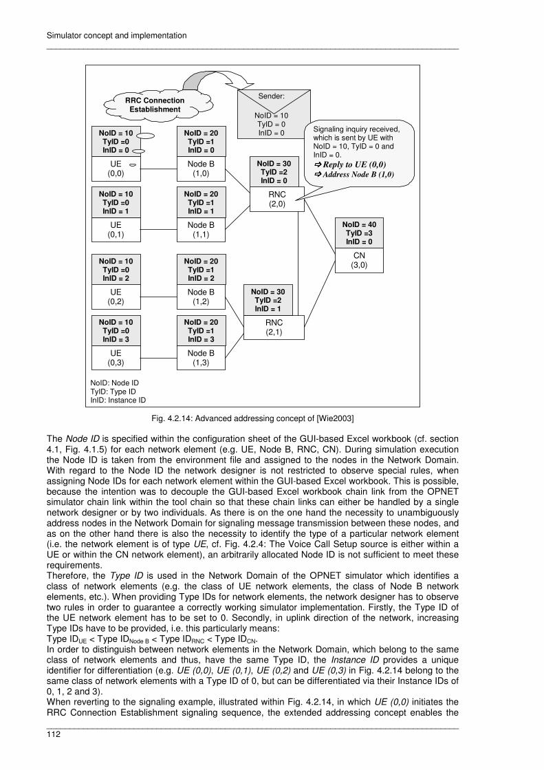
Simulator concept and implementation __________________________________________________________________________________________
__________________________________________________________________________________________ 112
CN (3,0)
RNC (2,0)
RNC (2,1)
Node B (1,2)
Node B (1,1)
Node B (1,0)
UE (0,0)
UE (0,1)
UE (0,2)
Node B (1,3)
UE (0,3)
NoID = 10 TyID =0 InID = 0
RRC Connection Establishment
NoID = 10 TyID =0 InID = 1
NoID = 10 TyID =0 InID = 2
NoID = 10 TyID =0 InID = 3
NoID = 20 TyID =1 InID = 0
NoID = 20 TyID =1 InID = 1
NoID = 20 TyID =1 InID = 2
NoID = 20 TyID =1 InID = 3
NoID = 30 TyID =2 InID = 0
NoID = 30 TyID =2 InID = 1
NoID = 40 TyID =3 InID = 0
Sender:
NoID = 10 TyID = 0 InID = 0 Signaling inquiry received,
which is sent by UE with NoID = 10, TyID = 0 and InID = 0. ���� Reply to UE (0,0) ���� Address Node B (1,0)
NoID: Node ID TyID: Type ID InID: Instance ID
Fig. 4.2.14: Advanced addressing concept of [Wie2003]
The Node ID is specified within the configuration sheet of the GUI-based Excel workbook (cf. section 4.1, Fig. 4.1.5) for each network element (e.g. UE, Node B, RNC, CN). During simulation execution the Node ID is taken from the environment file and assigned to the nodes in the Network Domain. With regard to the Node ID the network designer is not restricted to observe special rules, when assigning Node IDs for each network element within the GUI-based Excel workbook. This is possible, because the intention was to decouple the GUI-based Excel workbook chain link from the OPNET simulator chain link within the tool chain so that these chain links can either be handled by a single network designer or by two individuals. As there is on the one hand the necessity to unambiguously address nodes in the Network Domain for signaling message transmission between these nodes, and as on the other hand there is also the necessity to identify the type of a particular network element (i.e. the network element is of type UE, cf. Fig. 4.2.4: The Voice Call Setup source is either within a UE or within the CN network element), an arbitrarily allocated Node ID is not sufficient to meet these requirements. Therefore, the Type ID is used in the Network Domain of the OPNET simulator which identifies a class of network elements (e.g. the class of UE network elements, the class of Node B network elements, etc.). When providing Type IDs for network elements, the network designer has to observe two rules in order to guarantee a correctly working simulator implementation. Firstly, the Type ID of the UE network element has to be set to 0. Secondly, in uplink direction of the network, increasing Type IDs have to be provided, i.e. this particularly means: Type IDUE < Type IDNode B < Type IDRNC < Type IDCN. In order to distinguish between network elements in the Network Domain, which belong to the same class of network elements and thus, have the same Type ID, the Instance ID provides a unique identifier for differentiation (e.g. UE (0,0), UE (0,1), UE (0,2) and UE (0,3) in Fig. 4.2.14 belong to the same class of network elements with a Type ID of 0, but can be differentiated via their Instance IDs of 0, 1, 2 and 3). When reverting to the signaling example, illustrated within Fig. 4.2.14, in which UE (0,0) initiates the RRC Connection Establishment signaling sequence, the extended addressing concept enables the

Simulator concept and implementation __________________________________________________________________________________________
__________________________________________________________________________________________ 113
RNC to unambiguously identify the UE which sent the signaling message: It is UE (0,0) with a Type ID of 0, a Node ID of 10 and an Instance ID of 0. Moreover, the RNC is also able to unambiguously address the corresponding Node B: It is the Node B with a Type ID of 1, an Instance ID of 0 and a Node ID of 20. The identification of the corresponding Node B, UE (0,0) is assigned to, is derived by an evaluation of the affiliations within the network topology. These affiliations and their representation within the simulator implementation are subject of the next section.
4.2.9 Representation of affiliations between network elements
Moreover, the above mentioned affiliations of the network topology have to be represented for the complete topology within the implementation that has to allow for an automatical derivation of this representation from the network topology arbitrarily built by the network designer in the OPNET GUI. The affiliations within the network topology on the one hand gain in importance in case of handover signaling sequences, i.e. if, for instance, an Inter-RNC Hard Handover has to be performed, the particular RNC, which initiates this handover, has to know about the RNCs which are directly connected to it via Iur interface so that the RNC can choose a handover partner from these. On the other hand knowledge about the affiliations enables a highly generic routing mechanism between nodes in the Network Domain. This knowledge of the affiliations allows a node to address other nodes that are not directly connected to it. However, the routing algorithm automatically determines the next node on the way to the addressed node and sends the packet to the next node, which itself forwards the packet, according to the generic routing algorithm implemented, towards the addressed node. Subsequently, the representation of the affiliations within the OPNET simulator implementation is described in general and under consideration of the network topology illustrated in Fig. 4.2.15 that is taken as an example topology.
CN (3,0)
RNC (2,0)
RNC (2,1)
Node B (1,2)
Node B (1,1)
Node B (1,0)
UE (0,0)
UE (0,1)
UE (0,2)
Node B (1,3)
UE (0,3)
NoID = 10 TyID =0 InID = 0
NoID = 10 TyID =0 InID = 1
NoID = 10 TyID =0 InID = 2
NoID = 10 TyID =0 InID = 3
NoID = 20 TyID =1 InID = 0
NoID = 20 TyID =1 InID = 1
NoID = 20 TyID =1 InID = 2
NoID = 20 TyID =1 InID = 3
NoID = 30 TyID =2 InID = 0
NoID = 30 TyID =2 InID = 1
NoID = 40 TyID =3 InID = 0
Fig. 4.2.15: UTRAN example network topology for derivation of affiliations
At simulation start the affiliations within the network topology are automatically derived by the Proto-C implementation of the ER module of each node from the network topology arbitrarily built by the network designer. The derived affiliations within the network topology are represented in the form of two global tables which are the Global_Topology_Table_NodeID (Topo_Tab_NoID) and the Global_Topology_Table_InstanceID (Topo_Tab_InID), and one global vector data structure
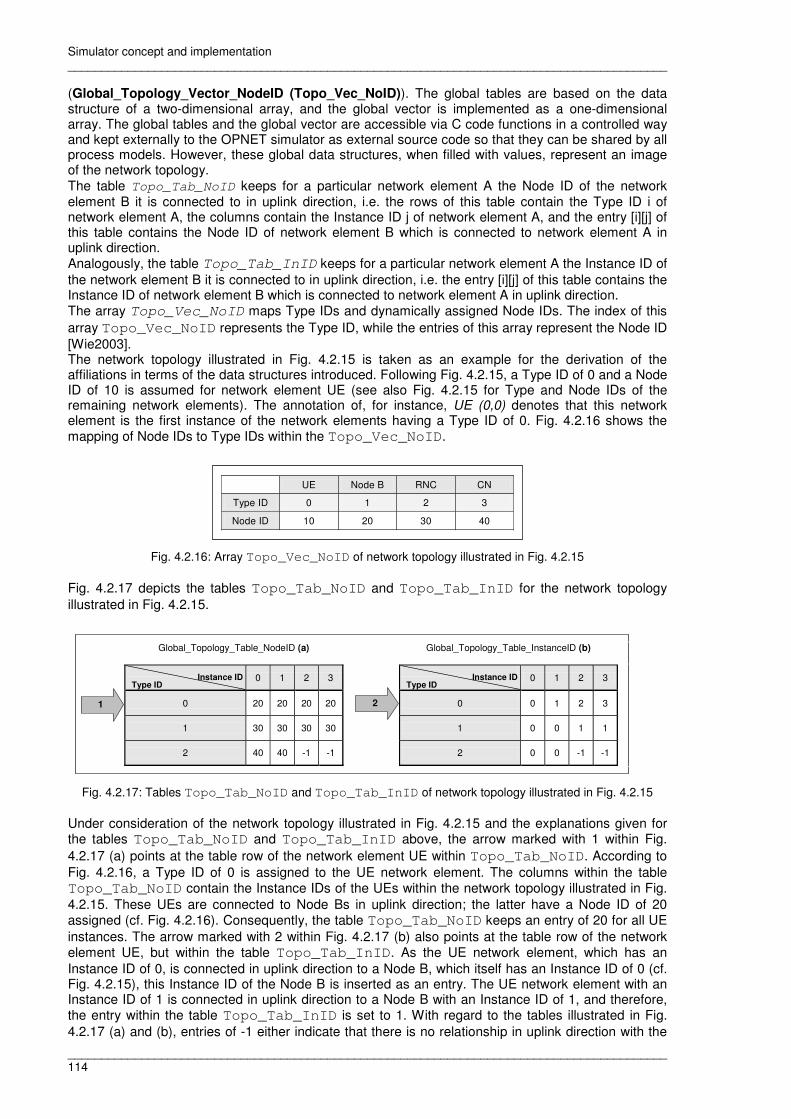
Simulator concept and implementation __________________________________________________________________________________________
__________________________________________________________________________________________ 114
(Global_Topology_Vector_NodeID (Topo_Vec_NoID)). The global tables are based on the data structure of a two-dimensional array, and the global vector is implemented as a one-dimensional array. The global tables and the global vector are accessible via C code functions in a controlled way and kept externally to the OPNET simulator as external source code so that they can be shared by all process models. However, these global data structures, when filled with values, represent an image of the network topology. The table Topo_Tab_NoID keeps for a particular network element A the Node ID of the network element B it is connected to in uplink direction, i.e. the rows of this table contain the Type ID i of network element A, the columns contain the Instance ID j of network element A, and the entry [i][j] of this table contains the Node ID of network element B which is connected to network element A in uplink direction. Analogously, the table Topo_Tab_InID keeps for a particular network element A the Instance ID of the network element B it is connected to in uplink direction, i.e. the entry [i][j] of this table contains the Instance ID of network element B which is connected to network element A in uplink direction. The array Topo_Vec_NoID maps Type IDs and dynamically assigned Node IDs. The index of this array Topo_Vec_NoID represents the Type ID, while the entries of this array represent the Node ID [Wie2003]. The network topology illustrated in Fig. 4.2.15 is taken as an example for the derivation of the affiliations in terms of the data structures introduced. Following Fig. 4.2.15, a Type ID of 0 and a Node ID of 10 is assumed for network element UE (see also Fig. 4.2.15 for Type and Node IDs of the remaining network elements). The annotation of, for instance, UE (0,0) denotes that this network element is the first instance of the network elements having a Type ID of 0. Fig. 4.2.16 shows the mapping of Node IDs to Type IDs within the Topo_Vec_NoID.
UE Node B RNC CN
Type ID 0 1 2 3
Node ID 10 20 30 40
Fig. 4.2.16: Array Topo_Vec_NoID of network topology illustrated in Fig. 4.2.15 Fig. 4.2.17 depicts the tables Topo_Tab_NoID and Topo_Tab_InID for the network topology illustrated in Fig. 4.2.15.
Global_Topology_Table_NodeID (a)
Global_Topology_Table_InstanceID (b)
0 1 2 3
0 20 20 20 20
1 30 30 30 30
2 40 40 -1 -1
0 1 2 3
0 0 1 2 3
1 0 0 1 1
2 0 0 -1 -1
Type ID Instance ID
Type ID Instance ID
2 1
Fig. 4.2.17: Tables Topo_Tab_NoID and Topo_Tab_InID of network topology illustrated in Fig. 4.2.15 Under consideration of the network topology illustrated in Fig. 4.2.15 and the explanations given for the tables Topo_Tab_NoID and Topo_Tab_InID above, the arrow marked with 1 within Fig. 4.2.17 (a) points at the table row of the network element UE within Topo_Tab_NoID. According to Fig. 4.2.16, a Type ID of 0 is assigned to the UE network element. The columns within the table Topo_Tab_NoID contain the Instance IDs of the UEs within the network topology illustrated in Fig. 4.2.15. These UEs are connected to Node Bs in uplink direction; the latter have a Node ID of 20 assigned (cf. Fig. 4.2.16). Consequently, the table Topo_Tab_NoID keeps an entry of 20 for all UE instances. The arrow marked with 2 within Fig. 4.2.17 (b) also points at the table row of the network element UE, but within the table Topo_Tab_InID. As the UE network element, which has an Instance ID of 0, is connected in uplink direction to a Node B, which itself has an Instance ID of 0 (cf. Fig. 4.2.15), this Instance ID of the Node B is inserted as an entry. The UE network element with an Instance ID of 1 is connected in uplink direction to a Node B with an Instance ID of 1, and therefore, the entry within the table Topo_Tab_InID is set to 1. With regard to the tables illustrated in Fig. 4.2.17 (a) and (b), entries of -1 either indicate that there is no relationship in uplink direction with the

Simulator concept and implementation __________________________________________________________________________________________
__________________________________________________________________________________________ 115
particular network element or the particular instance of the network element is not existing. Furthermore, the CN is not included in these tables, because it is not connected to other network elements in uplink direction. Moreover, these tables do not include connections between network elements of the same Type ID (e.g. the connection between RNC (2,0) and RNC (2,1), cf. Fig. 4.2.15). The relevance and efficiency of these data structures (i.e. the global tables and the global vector) will be shown within several examples of usage. But before the first example is presented, another data structure has to be introduced, which is the external routing table within the ER module.
4.2.10 Routing implementation for the exchange of signaling messages between network elements
Beside the affiliations of the network topology, which are derived by the ER module, the ER module also creates an external routing table for the particular node it is part of, i.e. the external routing table is not a global table, but it is local to a particular node. The external routing table is necessary for the exchange of packets between nodes in the Network Domain. The rows of this table represent the Type IDs applied, and the columns represent the Instance IDs, i.e. the external routing table has as many rows as there are Type IDs assigned, and it has as many columns as there are instances of network elements. The entries of the external routing table correspond to the indices of the outgoing communication links, which are automatically assigned by the OPNET GUI, when interconnecting nodes in the Network Domain with communication links. Fig. 4.2.18 depicts the external routing table of the network element RNC (2,0) (cf. network topology illustrated in Fig. 4.2.15) which is directly connected to the network elements Node B (1,0), Node B (1,1), RNC (2,1) and CN (3,0). This direct interconnection of RNC (2,0) with the network elements mentioned is reflected in the external routing table within Fig. 4.2.18. As the indices for the outgoing communication links are automatically assigned by the OPNET GUI so that the particular values that will be assigned cannot be specified in advance, the values of these indices are replaced with a X in Fig. 4.2.18. Entries of -1 in the external routing table indicate that there is either no outstream connection towards this particular network element or the particular instance of the network element is not existing.
0 1 2 3
0 -1 -1 -1 -1
1 X X -1 -1
2 -1 X -1 -1
3 X -1 -1 -1
Type ID Instance ID
Fig. 4.2.18: External routing table of network element RNC (2,0)
4.2.11 Example usage of advanced addressing concept, representation of affiliations between network elements and external routing concept
Subsequently, the relevance of the global tables and global vector, which are derived by the ER module at simulation start, is explained in terms of two typical routing situations that occur during the message flow of a signaling SF. Firstly, within the network topology illustrated in Fig. 4.2.15, node RNC (2,0) has to send a packet to the node CN (3,0). As the RNC is directly connected to the CN, the message forwarding is simply possible by sending the packet on the appropriate outstream which corresponds to entry [3][0] of the external routing table (cf. Fig. 4.2.18).

Simulator concept and implementation __________________________________________________________________________________________
__________________________________________________________________________________________ 116
Secondly, node RNC (2,0) has to send a packet to node UE (0,1) and it is not directly connected to node UE (0,1), but to four other nodes so that the question emerges: Which of these nodes connected to node RNC (2,0) is suitable to relay the packet that has to be sent to UE (0,1)? Now, the global tables and the global vector get involved. The packet that has to be sent keeps the Node ID of the recipient node in the packet field Dest Node ID which is 10 in this case. The knowledge of the Node ID is sufficient to derive further information from the packet and the global tables / vector. Therefore, from the array Topo_Vec_NoID the Type ID of the recipient node is taken which is 0 in this case (cf. Fig. 4.2.15). Under consideration of the Type ID, the Instance ID of the recipient node is taken from the packet which is 1. Next, the Proto-C code depicted in Fig. 4.2.19 is executed which returns the outstream on which the packet can be forwarded.
1 int get_outstream_from_external_routing_table (int dest_node_tID, int dest_node_iID) {
2 // A. Wiedemann - Comment + Function:
3 // This function determines the outstream necessary for external routing purposes in such cases
4 // where packets have to routed to network elements which are not directly adjacent network elements
5 // so that there is no entry in the external routing table and the packet has to be relayed by
6 // other network elements.
7 // Input parameters: int, i.e. the Type ID of the network element the packet is addressed to
8 // int, i.e. the Instance ID of the network element the packet is addressed to
9 // Output parameter: int, i.e. the outstream on which the packet has to be sent
10 by the external routing module in direction to the addressed network element
11
12 int outstream, // Variable to keep the outstream taken out of the
13 // External Routing Table which is returned by the function
14 next_connected_instanceID, // Variable to keep an Instance ID
15 next_connected_nodeID, // Variable to keep a Node ID
16 next_connected_typeID, // Variable to keep a Type ID
17 cp_next_connected_instanceID, // Variable to keep the copy of an Instance ID
18 cp_next_connected_nodeID, // Variable to keep the copy of a Node ID
19 cp_next_connected_typeID; // Variable to keep the copy of a Type ID
20
21 FIN (get_outstream_from_external_routing_table(dest_node_tID, dest_node_iID));
22
23 // Note: The functions used to get the desired information from the global table/vector
24 // is declared within external C Code 'MxRAN_Simulator_V_3_3_external_C'!
25 // The function ‘get_information_from_global_table’ returns a Node Id or an Instance ID,
26 // depending on the pointer that is given to the function, i.e.
27 // If the pointer ‘ptr_to_global_topology_table_instanceID’ is given, an Instance ID is returned, and
28 // if the pointer ‘ptr_to_global_topology_table_nodeID’ is given, a Node ID is returned.
29 // The function ‘get_typeID_from_global_vector_nodeID’ returns a Type ID from the global vector.
30 next_connected_instanceID = get_information_from_global_table (ptr_to_global_topology_table_instanceID, \
31 dest_node_tID, \
32 dest_node_iID);
33 next_connected_nodeID = get_information_from_global_table (ptr_to_global_topology_table_nodeID, \
34 dest_node_tID, \
35 dest_node_iID);
36 next_connected_typeID = get_typeID_from_global_vector_nodeID (ptr_to_global_topology_vector_nodeID, \
37 next_connected_nodeID);
38 while (ER_Routing_Table [next_connected_typeID][next_connected_instanceID] == -1) {
39 // i.e. while the outstream for packet forwarding is not found
40 cp_next_connected_instanceID = get_information_from_global_table (ptr_to_global_topology_table_instanceID, \
41 next_connected_typeID, \
42 next_connected_instanceID);
43 cp_next_connected_nodeID = get_information_from_global_table (ptr_to_global_topology_table_nodeID, \
44 next_connected_typeID, \
45 next_connected_instanceID);
46 cp_next_connected_typeID = get_typeID_from_global_vector_nodeID (ptr_to_global_topology_vector_nodeID, \
47 next_connected_nodeID);
48
49 next_connected_instanceID = cp_next_connected_instanceID;
50 next_connected_nodeID = cp_next_connected_nodeID;
51 next_connected_typeID = cp_next_connected_typeID;
52
53 if ((next_connected_typeID == -1) ||
54 (next_connected_instanceID == -1)) {
55 // i.e. if this condition matches, no adequate routing table entry
56 // can be found within 'ER_Routing_Table',
57 // because the row or column index is -1.
58 // In order to avoid misleading simulation results the simulation is terminated subsequently.
59 // A notification message for the user is provided.
60 // Print the ID of the node and the FE where no suitable routing entry was found:
61 printf("\n\n +++++++++++++++++++++++++++++++++++++++++");
62 printf("\n + An ERROR occured in Node %d, Instance %d. +\n", nodeID, instanceID);
63 printf(" +++++++++++++++++++++++++++++++++++++++++ \n\n");
64 // Print an error message for the user and terminate the simulation run:
65 op_sim_end ( "AWi - Simulation Message:", \
66 "ERROR: No routing entry for packet found in ER Routing Table!", \
67 "Check simulation system, solve problem and retry!", \
68 "The simulation run is terminated subsequently.");
69 }
70 // Get outstream out of the External Routing Table:
71 outstream = ER_Routing_Table [next_connected_typeID][next_connected_instanceID];
72 }
73 // Return outstream:
74 FRET (outstream);
75}
Fig. 4.2.19: Proto-C code returning an outstream for packet transmission [Wie2005b] The function get_outstream_from_external_routing_table, illustrated in Fig. 4.2.19, adopts backtracking functionality. First, the Instance ID (line 30-32), the Node ID (line 33-35) and the Type ID (line 36/37) of the network element A, the recipient node (i.e. UE (0,1) in the example) is directly connected to, is determined: In this case, network element A fits with Node B (1,1), because UE (0,1) is directly connected to Node B (1,1). As the recipient node (i.e. UE (0,1)) is not directly connected to RNC (2,0), the while loop in line 38 is entered, and the Instance ID (line 40-42), the Node ID (line 43-
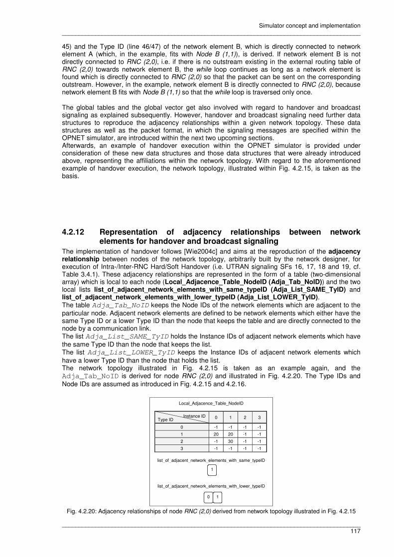
Simulator concept and implementation __________________________________________________________________________________________
__________________________________________________________________________________________ 117
45) and the Type ID (line 46/47) of the network element B, which is directly connected to network element A (which, in the example, fits with Node B (1,1)), is derived. If network element B is not directly connected to RNC (2,0), i.e. if there is no outstream existing in the external routing table of RNC (2,0) towards network element B, the while loop continues as long as a network element is found which is directly connected to RNC (2,0) so that the packet can be sent on the corresponding outstream. However, in the example, network element B is directly connected to RNC (2,0), because network element B fits with Node B (1,1) so that the while loop is traversed only once. The global tables and the global vector get also involved with regard to handover and broadcast signaling as explained subsequently. However, handover and broadcast signaling need further data structures to reproduce the adjacency relationships within a given network topology. These data structures as well as the packet format, in which the signaling messages are specified within the OPNET simulator, are introduced within the next two upcoming sections. Afterwards, an example of handover execution within the OPNET simulator is provided under consideration of these new data structures and those data structures that were already introduced above, representing the affiliations within the network topology. With regard to the aforementioned example of handover execution, the network topology, illustrated within Fig. 4.2.15, is taken as the basis.
4.2.12 Representation of adjacency relationships between network elements for handover and broadcast signaling
The implementation of handover follows [Wie2004c] and aims at the reproduction of the adjacency relationship between nodes of the network topology, arbitrarily built by the network designer, for execution of Intra-/Inter-RNC Hard/Soft Handover (i.e. UTRAN signaling SFs 16, 17, 18 and 19, cf. Table 3.4.1). These adjacency relationships are represented in the form of a table (two-dimensional array) which is local to each node (Local_Adjacence_Table_NodeID (Adja_Tab_NoID)) and the two local lists list_of_adjacent_network_elements_with_same_typeID (Adja_List_SAME_TyID) and list_of_adjacent_network_elements_with_lower_typeID (Adja_List_LOWER_TyID). The table Adja_Tab_NoID keeps the Node IDs of the network elements which are adjacent to the particular node. Adjacent network elements are defined to be network elements which either have the same Type ID or a lower Type ID than the node that keeps the table and are directly connected to the node by a communication link. The list Adja_List_SAME_TyID holds the Instance IDs of adjacent network elements which have the same Type ID than the node that keeps the list. The list Adja_List_LOWER_TyID keeps the Instance IDs of adjacent network elements which have a lower Type ID than the node that holds the list. The network topology illustrated in Fig. 4.2.15 is taken as an example again, and the Adja_Tab_NoID is derived for node RNC (2,0) and illustrated in Fig. 4.2.20. The Type IDs and Node IDs are assumed as introduced in Fig. 4.2.15 and 4.2.16.
Local_Adjacence_Table_NodeID
0 1 2 3
0 -1 -1 -1 -1
1 20 20 -1 -1
2 -1 30 -1 -1
3 -1 -1 -1 -1
list_of_adjacent_network_elements_with_same_typeID
list_of_adjacent_network_elements_with_lower_typeID
Instance ID Type ID
1
0 1
Fig. 4.2.20: Adjacency relationships of node RNC (2,0) derived from network topology illustrated in Fig. 4.2.15
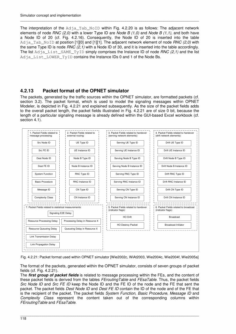
Simulator concept and implementation __________________________________________________________________________________________
__________________________________________________________________________________________ 118
The interpretation of the Adja_Tab_NoID within Fig. 4.2.20 is as follows: The adjacent network elements of node RNC (2,0) with a lower Type ID are Node B (1,0) and Node B (1,1), and both have a Node ID of 20 (cf. Fig. 4.2.16). Consequently, the Node ID of 20 is inserted into the table Adja_Tab_NoID at position [1][0] and [1][1]. The adjacent network element of node RNC (2,0) with the same Type ID is node RNC (2,1) with a Node ID of 30, and it is inserted into the table accordingly. The list Adja_List_SAME_TyID simply comprises the Instance ID of node RNC (2,1) and the list Adja_List_LOWER_TyID contains the Instance IDs 0 and 1 of the Node Bs.
4.2.13 Packet format of the OPNET simulator
The packets, generated by the traffic sources within the OPNET simulator, are formatted packets (cf. section 3.2). The packet format, which is used to model the signaling messages within OPNET Modeler, is depicted in Fig. 4.2.21 and explained subsequently. As the size of the packet fields adds to the overall packet length, the packet fields illustrated in Fig. 4.2.21 are of size 0 bit, because the length of a particular signaling message is already defined within the GUI-based Excel workbook (cf. section 4.1).
1. Packet Fields related to message processing:
Src Node ID
Dest Node ID
Src FE ID
Dest FE ID
System Function
Basic Procedure
Message ID
Complexity Class
2. Packet Fields related to external routing:
3. Packet Fields related to handover (serving network elements):
4. Packet Fields related to handover (drift network elements):
UE Type ID
Node B Type ID
UE Instance ID
Node B Instance ID
RNC Type ID
RNC Instance ID
CN Type ID
CN Instance ID
Serving UE Type ID
Serving Node B Type ID
Serving UE Instance ID
Serving Node B Instance ID
Serving RNC Type ID
Serving RNC Instance ID
Serving CN Type ID
Serving CN Instance ID
Drift UE Type ID
Drift Node B Type ID
Drift UE Instance ID
Drift Node B Instance ID
Drift RNC Type ID
Drift RNC Instance ID
Drift CN Type ID
Drift CN Instance ID
5. Packet Fields related to handover (indicator flags):
HO Drift
HO Destroy Packet
6. Packet Fields related to broadcast (indicator flags):
Broadcast
Broadcast Initiator
7. Packet Fields related to statistical measurements:
Signaling E2E Delay
Resource Queueing Delay
Resource Processing Delay
Link Transmission Delay
Link Propagation Delay
Queueing Delay in Resource X
Processing Delay in Resource X
Fig. 4.2.21: Packet format used within OPNET simulator [Wie2002c, WiAt2003, Wie2004c, Wie2004f, Wie2005a] The format of the packets, generated within the OPNET simulator, consists of seven groups of packet fields (cf. Fig. 4.2.21). The first group of packet fields is related to message processing within the FEs, and the content of these packet fields is derived from the tables FEroutingTable and FEsaTable. Thus, the packet fields Src Node ID and Src FE ID keep the Node ID and the FE ID of the node and the FE that sent the packet. The packet fields Dest Node ID and Dest FE ID contain the ID of the node and of the FE that is the recipient of the packet. The packet fields System Function, Basic Procedure, Message ID and Complexity Class represent the content taken out of the corresponding columns within FEroutingTable and FEsaTable.

Simulator concept and implementation __________________________________________________________________________________________
__________________________________________________________________________________________ 119
The second group of packet fields is related to the external routing operation between nodes in the Network Domain of OPNET Modeler. These packet fields contain the Instance IDs and Type IDs of the UE, Node B, RNC and CN which belong together with regard to a single instance of a particular signaling SF. If, for instance, UE (0,0) initiates an instance of the signaling SF MO Voice / CS Data Call Establishment, then the Type IDs and Instance IDs of UE (0,0), Node B (1,0), RNC (2,0) and CN (3,0) are kept within the second group of packet fields. The reason for this is that these network elements belong together as a result of the network topology established in Fig. 4.2.15 and the instance of the signaling SF under consideration). With regard to the external routing operation, Type ID and Instance ID match the row and column index of the external routing table (cf. Fig. 4.2.18) kept within each node so that the outstream on which the packet (i.e. each particular message of the signaling SF) is sent to the destination node is derived according to the explanation provided in connection with Fig. 4.2.18. The third and fourth group of packet fields are related to handover. These packet fields comprise the Instance and Type IDs of the serving (3rd group) and drift (4th group) network elements. If, for instance and under consideration of the network topology illustrated within Fig. 4.2.15, a user performs Inter-RNC Hard or Soft handover out of radio cell UE (0,1) into radio cell UE (0,2), then UE (0,1), Node B (1,1), RNC (2,0) and CN (3,0) are the serving network elements, and their Type and Instance IDs are kept within the packet fields of the 3rd group. The Type and Instance IDs of UE (0,2), Node B (1,2), RNC (2,1) and CN (3,0) are kept within the packet fields of the 4th group, because RNC (2,1) represents drift RNC and the target radio cell of the handover is UE (0,2). The packet fields of the fifth group are also related to handover, but their entries have the functionality of indicators with regard to external routing. The packet field HO Drift has a default value of -1 and is set to a value ≥ 0 and coevally < 1000 by the FE that processed the message, in case one of the serving network elements is addressed. If one of the drift network elements is addressed, the value of the HO Drift packet field is set to a value ≥ 1000 by the FE that processed the message. The packet field HO Destroy Packet is an indicator, whether the packet has to be destroyed within the ER module. The default value of the packet field HO Destroy Packet is -1, and the packet field value is set to 1 to mark a packet for destruction. The need to destroy a packet, generated by one of the handover signaling SFs (cf. Fig. 4.2.6) or by the SRNS Relocation SF, arises, if handover or SRNS Relocation cannot be performed in the network topology that was set up by the network designer. As an example, a network topology consisting of one single RNC is assumed so that Inter-RNC Hard/Soft Handover as well as SRNS Relocation cannot be performed. In consequence, the packet field HO Destroy Packet of the first packet generated by these sources is set to 1, the packet is destroyed subsequently, and the traffic source is shut down). The packet fields of the sixth group also have the functionality of indicators within the ER module, but they are related to broadcast. The default value of the packet field Broadcast is -1, and it is set to 1 by the traffic source, if the sub-attribute Broadcast of the traffic source is set to enabled. This setting applies for SF 21 and 22 (Paging in idle / connected mode) within Fig. 4.2.4. If a packet with a packet field Broadcast that is set to 1 reaches an ER module, the ER module checks whether the traffic source, that generated the packet, is part of the same node the ER module is part of. If this traffic source is part of the same node the ER module is part of, the packet is not broadcasted to all nodes in downlink direction, because in this case the broadcast is sent to one of the adjacent network elements with lower Type ID which is determined randomly. If the traffic source is not part of the same node the ER module is part of, then the broadcast of the packet is performed. In this case, the packet field Broadcast is set to 0 in order to prevent further broadcast within the recipient nodes. Then the packet is copied and sent to all adjacent network elements with a lower Type ID in downlink direction by usage of the list Adja_List_LOWER_TyID (i.e. the packet is sent to all elements within the list). When reverting to SF 21 and 22 (Paging in idle / connected mode) (cf. Fig. 4.2.4), which are instantiated by the CN and apply this setting, this implies that the CN at first determines one single RNC randomly. Next, this RNC performs the paging broadcast by copying and sending the packet to all Node Bs which are connected to it. The default value of the packet field Broadcast Initiator is -1, and it is set to 1 by the traffic source, if the sub-attribute Broadcast Initiator is set to enabled. This setting applies for SF 23 (Paging unsuccessful) within Fig. 4.2.4. If a packet with a packet field Broadcast Initiator set to 1 reaches an ER module, the packet is broadcasted, i.e. at first the packet fields Broadcast and Broadcast Initiator are set to 0 to prevent further broadcast within the recipient nodes. Then the packet is copied and sent to all adjacent network elements with a lower Type ID in downlink direction by usage of the list Adja_List_LOWER_TyID (i.e. sending of the packet to all list elements). With regard to SF 23 (Paging unsuccessful) (cf. Fig. 4.2.4), which is initiated by a RNC, this means that the RNC performs the paging broadcast by copying and sending the packet to all Node Bs that are connected to it. The seventh group of packet fields are related to the statistical measurement of performance values. The value of the packet field Signaling E2E Delay is updated, whenever a packet traverses a

Simulator concept and implementation __________________________________________________________________________________________
__________________________________________________________________________________________ 120
link or passes a resource module (i.e. in these cases the signaling E2E delay is increased by the time necessary for link propagation, link transmission, waiting for service and the service time itself). The packet fields Resource Processing Delay, Resource Queueing Delay, Link Transmission Delay and Link Propagation Delay keep the homonymous partial delays per signaling SF. The packet fields Processing Delay in Resource X and Queueing Delay in Resource X refer to the partial queueing and processing delays per SF and resource module. The default values of these packet fields are set to 0.0 [Wie2002c, WiAt2003, Wie2004c, Wie2004f, Wie2005a].
4.2.14 Example usage of adjacency relationships between network elements for handover signaling
Fig. 4.2.22 visualizes the scenario which is taken as an example within this section. Within this scenario, a mobile user intends to perform a handover out of radio cell UE (0,1) into radio cell UE (0,2). In this context, Fig. 4.2.22 also provides the communication flow in terms of numbered activities (from activity 0 to activity 11) between the involved network elements. On the one hand this communication flow is necessary in order to determine the network elements which are involved in handover signaling. On the other hand the communication flow is also necessary in order to check particular conditions which have to fulfilled, as otherwise handover signaling cannot be instantiated.
CN (3,0)
RNC (2,1)
Node B (1,2)
UE (0,0)
UE (0,1)
UE (0,2)
Node B (1,3)
UE (0,3)
NoID = 10 TyID =0 InID = 0
NoID = 10 TyID =0 InID = 1
NoID = 10 TyID =0 InID = 2
NoID = 10 TyID =0 InID = 3
NoID = 20 TyID =1 InID = 0
NoID = 20 TyID =1 InID = 1
NoID = 20 TyID =1 InID = 2
NoID = 20 TyID =1 InID = 3
NoID = 30 TyID =2 InID = 0
NoID = 30 TyID =2 InID = 1
NoID = 40 TyID =3 InID = 0
Inter-RNC Hard / Soft Handover
1. MT_HO_SERVING_RI_REQUEST
Node B (1,1)
3. SERVING_OK
Node B (1,0)
2. number of active voice calls in radio
cell (0,1) > 0
0. Perform handover
4. Be drift
RNC
5. Be target radio cell
6. MT_HO_DRIFT_RI_REQUEST
7. CAC policy in radio cell (0,2) not violated
8. DRIFT_OK
9. Instantiate Inter-RNC Hard / Soft Handover
signaling
RNC (2,0)
11. INCREASE_NUMBER_OF_ACTIVE_VOICE_CALLS
10. DECREASE_NUMBER_OF_ACTIVE_VOICE_CALLS
Fig. 4.2.22: Inter-RNC Hard/Soft Handover scenario

Simulator concept and implementation __________________________________________________________________________________________
__________________________________________________________________________________________ 121
In the simulator implementation Intra- and Inter-RNC Hard and Soft Handover are induced by random determination of a UE, i.e. it is assumed that a user is going to perform a handover out of a particular radio cell. Under consideration of Fig. 4.2.22, it is assumed that Inter-RNC Hard or Soft Handover is to be performed, and the corresponding traffic source within the serving RNC (2,0) randomly chooses UE (0,1) (cf. activity 0), i.e. a user is going to perform Inter-RNC Hard or Soft Handover out of radio cell UE (0,1). Next, the interrupt code MT_HO_SERVING_RI_REQUEST (cf. Fig. 4.2.7 (b) and activity 1 within Fig. 4.2.22) is sent by the serving RNC (2,0) to the central traffic control manager source within UE (0,1). Provided that there are active voice calls within the radio cell (Fig. 4.2.22, activity 2), the central traffic control manager randomly determines whether a MO or a MT call will provide the Inter-RNC Hard/Soft Handover, and it replies with the interrupt code SERVING_OK (cf. Fig. 4.2.22, activity 3). As an Inter-RNC Handover implies the participation of a second RNC, i.e. the participation of a second network element from the same class of network elements is required, that acts as a drift RNC, the handover traffic source within the serving RNC (2,0) has to determine a second RNC for handover execution randomly from the list Adja_List_SAME_TyID. Following the network topology illustrated in Fig. 4.2.22, this list contains one single entry (cf. Fig. 4.2.20), which is the RNC (2,1), and this RNC is chosen as drift RNC (see Fig. 4.2.22, activity 4). Thereafter, the handover traffic source within the serving RNC (2,0) has to determine a UE randomly, i.e. a radio cell that is the target of the user, which performs Inter-RNC Hard/Soft Handover out of radio cell (0,1). Now, the global tables and the global vector get involved again. Fig. 4.2.21 illustrates the Proto-C code function determine_eligible_UEs_for_MT_calls which returns a list with UEs to be considered as target radio cells and makes use of the information stored within the global tables and the global vector.

Simulator concept and implementation __________________________________________________________________________________________
__________________________________________________________________________________________ 122
1 List* determine_eligible_UEs_for_MT_calls (int iID, int nID, int tID, \
2 int (* ptr_to_global_table_iID) [MAX_INSTANCES], \
3 int (* ptr_to_global_table_nID) [MAX_INSTANCES], \
4 int * ptr_to_global_vector_nID) {
5 // A. Wiedemann - Comment + Function:
6 // This function sets up a list with UEs which are eligible to terminate calls either from the CN or from an RNC.
7 // It is considered that
8 // - all UEs in the network are eligible to terminate calls from the CN
9 // - only UEs which are connected to Node Bs within the area the particular RNCs covers
10 // are eligible to terminate signaling SFs instantiated by the particular RNC.
11 // Input parameters: int, int, int, i.e. Instance ID, Node ID and Type ID of the calling network element,
12 // int*, int*, int*, i.e. Pointer to the global tables and vector
13 // Output parameter: List *, i.e. a pointer to a list with eligible UEs
14
15 List* ptr_to_list_with_eligible_UEs_for_MT_calls = // Pointer to list with UEs that will be returned
16 op_prg_list_create();
17 int i = 0, // Loop variable
18 highest_instanceID, // Variable to keep the highest Instance ID
19 // provided within the network topology
20 loop_termination = -1, // Variable (used as a Boolean variable)
21 // which is initiated with -1 and
22 // set to 1 under a certain condition to terminate a while loop
23 instanceID_from_global_table, // Variable to keep an Instance ID temporarily
24 nodeID_from_global_table, // Variable to keep a Node ID temporarily
25 typeID_from_global_vector, // Variable to keep a Type ID temporarily
26 evaluation_result; // Variable (used as a Boolean variable)
27 // which will be either -1 or 1 depending
28 // on the evaluation result of the function
29 // 'check_eligibility_of_UE_within_global_table'
30
31 FIN (List* determine_eligible_UEs_for_MT_calls (iID, nID, tID, \
32 (* ptr_to_global_table_iID) [MAX_INSTANCES], \
33 (* ptr_to_global_table_nID) [MAX_INSTANCES], \
34 (* ptr_to_global_vector_nID));
35
36 // Get hightest Instance ID:
37 highest_instanceID = get_highest_instanceID();
38
39 while ((i < highest_instanceID) &&
40 (loop_termination != 1)) {
41 // i.e. execute the following code for all existing UE Instances
42 // Also note: The function used to get the Instance ID ('get_information_from_global_tables') is declared
43 // within external C Code 'MxRAN_Simulator_V_3_external_C'! // This function needs a pointer to the global table,
44 // a Type ID (which is 0 for UEs per convention) and an Instance ID which varies, because all UEs have to be investigated.
45 // Get Instance, Node and Type IDs from global topology tables:
46 // Note: The functions used to get Instance, Node and Type IDs are declared within external C Code
47 // 'MxRAN_Simulator_V_3_external_C'!
48 instanceID_from_global_table = get_information_from_global_table (ptr_to_global_table_iID, 0, i);
49 nodeID_from_global_table = get_information_from_global_table (ptr_to_global_table_nID, 0, i);
50 typeID_from_global_vector = get_typeID_from_global_vector_nodeID (ptr_to_global_vector_nID, nodeID_from_global_table);
51
52 if (instanceID_from_global_table != -1) {
53 // This condition checks if the entry within the global topology table is a valid Instance ID.
54 // The search procedure in order to find an eligible UE to terminate calls will be performed within
55 // the function 'check_eligibility_of_UE_within_global_table' which returns
56 // - '1' in the positive case (i.e. if an eligible UE was found)
57 // - '-1' in the negative case (i.e. if no eligible UE was found).
58 evaluation_result = check_eligibility_of_UE_within_global_table (instanceID_from_global_table, \
59 nodeID_from_global_table, typeID_from_global_vector, \
60 iID, nID, tID, \
61 ptr_to_global_table_iID, ptr_to_global_table_nID, ptr_to_global_vector_nID);
62 if (evaluation_result == 1) {
63 // i.e. if this condition matches, an eligible UE was found and has to be inserted
64 // into the sorted list of eligible UEs.
65 op_prg_list_insert_sorted (ptr_to_list_with_eligible_UEs_for_MT_calls, i, sort_list_with_UEs_eligible_for_MT_calls);
66 }
67 // Increase loop variable 'i':
68 i++;
69 }
70 else {
71 // If this condition matches, there are no more valid Instance IDs within the global topology table
72 // so that the search can be terminated.
73 loop_termination = 1;
74 }
75 }
76 // Return list with eligible UEs:
77 FRET (ptr_to_list_with_eligible_UEs_for_MT_calls);
78 }
Fig. 4.2.23: Proto-C Code returning a list of UEs [Wie2005b] The function determine_eligible_UEs_for_MT_calls is a generic function that returns a list of UEs to be considered to terminate signaling SFs (i.e. signaling SFs which are either initiated by the CN or by a RNC). The node that calls the function (which, in this case, is the serving RNC (2,0)) has to provide an Instance ID, Node ID, Type ID (i.e. in this case the Instance ID, Node ID and Type ID of the drift RNC (2,1) are provided to the function, as the intention is to find a drift UE) as well as its pointers to the global tables and the global vector. The function checks for all UEs in the network topology (line 39-50), starting with an UE Instance ID of 0, whether they are eligible to terminate a signaling SF under consideration of the Instance ID, Node ID and Type ID that were provided to the function (which, in this case, are the Instance ID, Node ID and Type ID of the drift RNC (2,1)). The aforementioned eligibility is verified within the function check_eligibility_of_UE_within_global_table (cf. Fig. 4.2.23: Function call in line 58). This function also utilizes the global tables and the global vector and adopts a backtracking functionality which is comparable to the backtracking functionality provided within function get_outstream_from_external_routing_table (cf. Fig. 4.2.19). The basic idea of the function check_eligibility_of_UE_within_global_table is to check, whether a UE is assigned to the drift RNC, i.e. whether a UE is within the coverage area of the drift RNC, or not. Therefore, the function extracts information (i.e. Instance ID, Node ID, Type ID) from the global tables and vector about network element A, the UE is directly connected to (i.e. in this case network element A will correspond to a

Simulator concept and implementation __________________________________________________________________________________________
__________________________________________________________________________________________ 123
Node B). Moreover, the function check_eligibility_of_UE_within_global_table checks, whether the IDs (i.e. the Instance ID, Node ID and Type ID) of network element A equal the IDs of the drift RNC. If the IDs of network element A equal the IDs of the drift RNC, the UE is eligible, but this is not possible in this particular case, because the UE is not directly connected to a RNC, but to a Node B that corresponds to network element A in this case. Therefore, the algorithm has to continue to gather information form the global tables and vector by determination of the IDs of network element B that is directly connected to network element A, i.e. in this particular case network element A corresponds to a Node B, and network element B will correspond to a RNC. Next, the function check_eligibility_of_UE_within_global_table checks again whether the IDs of network element B equal the IDs of the drift RNC. The IDs of network element B will match the IDs of the drift RNC, if a UE Instance ID of 2 and 3 is given to the function check_eligibility_of_UE_within_global_table. In this case, an evaluation result of 1 is returned to the function determine_eligible_UEs_for_MT_calls. Consequently, these UEs are inserted into the list of UEs which are eligible to terminate this kind of signaling SF (cf. Fig. 4.2.23, line 62-66). Next, the handover traffic source within the serving RNC (2,0) uses the list with eligible UEs that was returned by the function determine_eligible_UEs_for_MT_calls. This list with eligible UEs is used to randomly determine one of these UEs that is the target of the user which performs Inter-RNC Hard/Soft Handover out of radio cell (0,1). As an example, it is assumed that UE (0,2) is randomly chosen (cf. Fig. 4.2.22, activity 5). Subsequently, the interrupt code MT_HO_DRIFT_RI_REQUEST is sent by the serving RNC (2,0) to the central traffic control manager source within UE (0,2) (Fig. 4.2.22, activity 6). Provided that the bandwidth currently used within the radio cell allows for an additional call within this particular radio cell (cf. equation (7)) under consideration of the maximum cell throughput value specified by the network designer (Fig. 4.2.22, activity 7), the central traffic control manager source within UE (0,2) replies with the interrupt code DRIFT_OK (Fig. 4.2.22, activity 8) so that the Inter-RNC Hard/Soft Handover can be instantiated (Fig. 4.2.22, activity 9) (i.e. a user performs Inter-RNC Hard/Soft Handover out of radio cell (0,1) into radio cell (0,2)). The instantiation of a signaling SF means that a packet has to be generated and represents the initialization message of a signaling SF sent by the environment (cf. section 3.4). Within the OPNET simulator, the environment is represented by the traffic source module that generates a particular signaling SF. Consequently, the handover traffic source, which in this particular case is located in the serving RNC (2,0), has to initiate an instance of the handover signaling SF, i.e. a packet according to the packet format specified in Fig. 4.2.21 has to be created, and the packet fields have to be set appropriately. The values of the first group of packet fields are taken from the attribute Traffic Source Parameters of the traffic source module (cf. Fig. 4.2.4). Next, the packet fields of the second, third and fourth group of packet fields have to be set. Under consideration of the Inter-RNC Hard/Soft Handover example, UE (0,1), Node B (1,1), RNC (2,0) and CN (3,0) are the serving network elements, and their Type and Instance IDs are kept within the packet fields of the 3rd group. The reason is that a user intends to perform handover out of the radio cell UE (0,1), and RNC (2,0) instantiates the Inter-RNC Hard/Soft Handover. The Type and Instance IDs of UE (0,2), Node B (1,2), RNC (2,1) and CN (3,0) are kept within the packet fields of the 4th group, because in the example RNC (2,1) was chosen as drift RNC and the target radio cell of the handover is UE (0,2). The determination of these values (i.e. Type IDs and Instance IDs) is also performed by usage of the global tables and vector. The Type and Instance IDs of the serving network elements are initially also kept within the packet fields of the 2nd group, but the content of the packet fields of the 2nd group changes during handover execution. The reason is that the packet fields of the 2nd group are closely related to the packet field HO Drift. As long as the value of the packet field HO Drift is set to a value ≥ 0 and < 1000 by the FE that processed the message, the serving network elements are addressed to receive the packet. This implies that the values of the packet fields within the 2nd group (i.e. the Type and Instance IDs) have to fit with the values of the third group of packet fields (cf. Fig. 4.2.21) so that the packet can be sent to the network by the ER module orderly and reaches the addressed node. If the necessity arises to address the drift network elements (e.g. the RNSAP FE within RNC (2,0) addresses the RNSAP FE within the drift RNC (2,1) in order to request the drift RNC to set up a radio link), the values of the packet fields within the 2nd group have to be exchanged with the values of the packet fields in the fourth group (cf. Fig. 4.2.21). In consequence, the packet is sent to the drift network elements. The indicator of this exchange of packet field values is the value of the packet field HO Drift which is set to a value ≥ 1000 by the FE that processed the message. If the values of the packet fields within the 2nd group are not exchanged with the values of the packet fields in the fourth group in this case, the packet is not sent to the RNSAP FE within the drift RNC (2,1), but again to the RNSAP FE within the serving RNC (2,0) which is actually not intended.
Simulator concept and implementation __________________________________________________________________________________________
__________________________________________________________________________________________ 124
The values of the fifth and sixth group of packet fields are taken from the attributes Association Handover / SRNS Relocation and Broadcast and their sub-attributes of the traffic source module (cf. Fig. 4.2.4). Finally, the values of the packet fields in the seventh group are left to the default settings. Next, the interrupt code DECREASE_VOICE_CALLS_DUE_TO_HO is sent by the serving RNC (2,0) to the central traffic control manager source within UE (0,1) (cf. Fig. 4.2.22, activity 10), as UE (0,1) is the originating radio cell of the handover. Furthermore, the interrupt code INCREASE_VOICE_CALLS_DUE_TO_HO is sent to by the serving RNC to the traffic control manager source within UE (0,2) (Fig. 4.2.22, activity 11), as UE (0,2) is the target radio cell of the handover. Both UEs update the radio cell statistics with regard to the number of active voice calls, throughput, number of incoming / outgoing / successful handovers according to Fig. 4.2.7 (b). The example that was described above considered the Inter-RNC Hard/Soft Handover. The Intra-RNC Hard/Soft Handover proceeds identically with regard to the interrupt codes exchanged. The only difference is that an Intra-RNC Handover implies the participation of a second Node B (instead of a drift RNC). Therefore, the handover traffic source within the serving RNC has to randomly determine a drift Node B for handover execution from the list Adja_List_LOWER_TyID. As the SRNS Relocation signaling SF is not associated with the number of active voice calls (cf. Fig. 4.2.4), there is no interaction with a traffic control manager source in terms of interrupt code exchange. The drift RNC which is necessary in order to take over the functionality of the SRNC, is taken from the list Adja_List_SAME_TyID [Wie2004c].

Architecture evaluation __________________________________________________________________________________________
__________________________________________________________________________________________ 125
5 Architecture evaluation In this chapter an evaluation of two promising UTRAN evolution scenarios, DRAN (cf. section 2.3.4) and MRAN (cf. section 2.3.6), with regard to their signaling performance behavior is performed using the simulation modeling methodology described in section 3.4 and the toolkit presented in chapter 4. Initial results of this study were published in [ScWi2005], the full set of simulation results for this chapter is available in [Wie2006].
5.1 Reference architecture and evolution scenarios
In the first section of this chapter, the UTRAN reference architecture is calibrated for the upcoming simulation studies. Then the evolution scenarios are presented according to the modeling methodology described in section 3.4. Moreover, the process of calibration and optimization of the RAN evolution scenarios for the simulation experiments of interest is described. In this context, the usefulness of the modeling methodology and the developed toolkit for the designer of future mobile networks becomes obvious.
5.1.1 UTRAN reference architecture
This section focuses on the UTRAN reference architecture introduced in section 3.4 (cf. Fig. 3.4.6). This UTRAN reference architecture is calibrated first in order to derive the overall resource capacity which is available for distribution among the resources within the evolution scenarios. 5.1.1.1 Calibration of the UTRAN reference architecture
The reference architecture is calibrated so that the utilization of the Main Resource within the Node B is about 50%, and the utilization of the BSC Resource within the RNC is about 70% at the operating point of the network, which is assumed to be 1 million of users per RNC and 2 millions of users in the network. This calibration applies for the 50/50 traffic mix which assumes that the portion of voice and data traffic is identical and equals 50% each. The remaining call / session and mobility related traffic model parameters for UTRAN service-mix derivation are according to the exemplified configuration illustrated in Fig. 4.1.2. The resource parameters for the UTRAN reference architecture are depicted in Table 5.1.1.1.1. This configuration represents the overall resource capacity that is available for distribution among the resources inside the network elements of the evolution scenarios.
Amount of Service (ms)
# Server Speed Factor
# Server * Speed Factor
# Network Elements in the Network
System Capacity = (# Server * Speed Factor) * # Network Elements in the
Network C = 1 C = 2 C = 3
UE IS Resource 10,000 25 250,000 360 90,000,000 1 1 1 Node B IS Resource 10,000 50 500,000 360 180,000,000 1 1 1 Node B Main Resource 4 10 40 360 14,400 1 2 3 RNC BSC Resource 4 11,500 46,000 2 92,000 1 2 36 RNC ICC_1 Resource 100 672 67,200 2 134,400 1 2 40 RNC ICC_2 Resource 100 672 67,200 2 134,400 1 2 40 RNC ICC_3 Resource 100 672 67,200 2 134,400 1 2 40 CN IS Resource 10,000 100 1,000,000 1 1,000,000 1 1 1 Total System Resource Capacity in the Network Σ = 271,509,600
Table 5.1.1.1.1: Resource parameter configuration of UTRAN reference architecture

Architecture evaluation __________________________________________________________________________________________
__________________________________________________________________________________________ 126
With regard to the network topology it is assumed that one single RNC manages 180 Node Bs. One single Node B serves one radio cell. The network topology, used for calibration of the UTRAN reference architecture within OPNET Modeler, is according to the network topology illustrated in Fig. 5.1.1.1.1 which points out that two RNCs as well as two Node Bs and UEs / radio cells per RNC are modeled explicitly, although 180 Node Bs and UEs / radio cells per RNC are assumed.
Fig. 5.1.1.1.1: UTRAN network topology within OPNET Modeler Reverting to the calibration of the UTRAN reference architecture, the CAC mechanism, which is applied within the radio cell, and its assumptions are described subsequently. With regard to the CAC mechanism it is assumed that the maximum throughput within the radio cell is 1 Mbit/sec. The assumption, with regard to the maximum cell throughput, is based on physical measurements performed with a UTRAN R99 Node B by network engineers of Lucent Technologies. These measurements aimed at the determination of the traffic, such a base station is able to carry, and provided the aforementioned result. The QoS policy of the CAC mechanism, described in section 4.1, is fulfilled, if the utilization of the data channels is less than or equal to 80%. Table 5.1.1.1.2 depicts the parameters assumed for the communication links between the network elements in the Network Domain of OPNET Modeler. The link parameters, which are depicted in Table 5.1.1.1.2, are assumed according to the expected traffic volume and also with regard to the architecture itself, i.e. as, for instance, RNCs are assumed to cover large areas, the distance between two RNCs is assumed to be significantly higher than the distance between a RNC and a Node B, and these assumptions can also be applied to upcoming link parameter configurations of MRAN and DRAN within this chapter. The propagation speed parameters within the link parameter configurations result from the type of media applied between two network elements.
UE �� Node B (Air interface) Node B �� RNC RNC �� RNC RNC �� CN
Link Speed [Mbit/sec] 2 6 6 155 Distance [km] 1 10 50 100
Propagation Speed [meters/sec] Speed of Light (in air): 299,702,547
Speed (in thin coax): 194,865,098
Speed of Light (in glass): 199, 861,638
Speed of Light (in glass): 199, 861,638
Table 5.1.1.1.2: Link parameter configuration of UTRAN reference architecture 5.1.1.2 Simulation results of the calibrated reference architecture
Table 5.1.1.2.1 visualizes the signaling E2E delays at the operating point of the UTRAN reference network architecture within the 50/50 traffic mix for all signaling SFs depicted in Table 3.4.1. These signaling E2E delays are mean delay values, and whenever a signaling E2E delay is numerically or

Architecture evaluation __________________________________________________________________________________________
__________________________________________________________________________________________ 127
graphically presented within chapter 5, mean delay values are considered. Besides, for each of these mean signaling E2E delay values, the 90% level of confidence value is provided which is used to compute the lower and upper bound of the 90% confidence interval for each of the signaling E2E delays. Moreover, Table 5.1.1.2.1 shows the partial delays (cf. section 3.4.4), a particular signaling E2E delay consists of. On the one hand these partial delays result from link propagation and link transmission of the signaling messages. On the other hand these partial delays arise from the time, necessary to process a single signaling message within a resource module as well as from the time, the signaling message has to wait for service within a resource module. These partial delay values are also mean delay values. With regard to the upcoming simulation results, the level of confidence is assumed to be 90% for all experiments in chapter 5 and [Wie2006]. As far as graphs are concerned, the confidence intervals are partly very small so that they are not visible within the figures. Under consideration of the simulation results presented in chapter 5 (except section 5.2.4 which is about transient analysis) and [Wie2006], steady-state performance, i.e. the performance after the system has reached a stable state, is of interest. This also implies for the aforementioned simulation results that the transient state of the performed simulation runs has to be eliminated from the final computation of the mean for a particular performance measure of interest (e.g. the signaling E2E delay). With the exception of section 5.2.4, the provided simulation results within tables and curves represent mean values (e.g. mean E2E signaling delay of a particular SF). In order to provide confidence intervals for the performance measures of interest, 50 independent replications of a single simulation run were performed using a different seed value for each of these runs. All of these independent replications, of course, eliminate the transient state, which equals the initial 30 minutes of a single simulation run. The system simulation time for the simulation experiments presented within this chapter (except section 5.2.4) and [Wie2006] adds up to 10 hours for all experiments performed. The time expenditure, spent for a single simulation run in reality, differs between different experiments: If, for instance, the UTRAN reference architecture, illustrated within Fig. 5.1.1.1.1, is simulated with 100,000 users, the amount of time, necessary to perform a single simulation run of this experiment in reality, is about 30 sec. If the UTRAN reference architecture is simulated with 1,000,000 of users, the amount of time, spent for a single simulation run of this experiment, is about 30 minutes.
Partial Delays [sec]
# UTRAN Signaling SF Signaling E2E
Delay [sec] ± 90%
Confidence Processing Delay [sec]
Queueing Delay [sec]
Link Transmission Delay [sec]
Link Propagation Delay [sec]
1 MO Voice / CS Data Call Establishment 1.71 0.000349 1.6792 0.0223 0.00114 0.00531 2 MO Voice / CS Data Call Release 0.85 0.00038 0.8253 0.0245 0.00064 0.00348 3 MT Voice / CS Data Call Establishment 1.83 0.000198 1.8044 0.0214 0.00127 0.00642 4 MT Voice / CS Data Call Release 0.72 0.000434 0.6962 0.0238 0.00043 0.00293 5 PS Data Transfer Establishment 0.82 0.000264 0.785 0.0301 0.00028 0.00047 6 PS Detach (UE initiated) 1.19 0.000565 1.1492 0.0403 0.00049 0.00168
7 Transition from URA_PCH to CELL_DCH due to Downlink Data Transfer
0.78 0.000202 0.7622 0.0198 0.0003 0.00042
8 Transition from CELL_DCH to URA_PCH due to RRC inactivity timer expiring
0.57 0.000332 0.5526 0.0196 0.00025 0.00031
9 MO PDP Context Activation 0.44 0.000007 0.437 0.0008 0.00036 0.00222 10 MO PDP Context Deactivation 0.63 0.000644 0.6031 0.0214 0.00033 0.00237 11 IMSI Detach Signaling Flow 1.19 0.000472 1.1475 0.0398 0.00039 0.00168 12 Location Updating Signaling Flow 1.63 0.000348 1.581 0.0406 0.0006 0.00390 13 URA Update Signaling Flow 0.20 0.000003 0.2032 0.0001 0.0001 0.00011 14 RA Update Signaling Flow 0.22 0.0000001 0.2174 0.0 0.00016 0.00111 15 Intra-RNC Softer Handover 0.63 0.000319 0.6131 0.0184 0.00052 0.00042 16 Intra-RNC Soft Handover 0.87 0.000274 0.8256 0.0408 0.00048 0.00063 17 Inter-RNC Soft Handover 0.88 0.000104 0.8354 0.0409 0.00052 0.00113 18 Intra-RNC Hard Handover 0.66 0.000708 0.6226 0.041 0.00042 0.00052 19 Inter-RNC Hard Handover 0.67 0.000261 0.6231 0.042 0.00045 0.00102 20 SRNS Relocation 0.47 0.000037 0.4647 0.0013 0.0006 0.00497 21 Paging in idle mode 0.22 0.000002 0.2177 0.0004 0.00012 0.00061 22 Paging in connected mode 0.09 0.000003 0.0933 0.0004 0.00006 0.00056 23 Paging unsuccessful 0.08 0.000005 0.0818 0.0005 0.00002 0.00005 24 Measurement Report 0.08 0.000001 0.0815 0.0 0.00007 0.00005
Table 5.1.1.2.1: Signaling E2E delays at the operating point of the UTRAN reference network architecture (50/50 traffic mix)
Table 5.1.1.2.2 and 5.1.1.2.3 further itemize the partial processing and queueing delays of the overall signaling E2E delay. These two tables particularly show for each single signaling SF which portions of the partial processing and queueing delays are caused by which resource. Table 5.1.1.2.3 also shows that the IS Resources in UTRAN, of course, follow the definition provided in section 3.4.7 and [Jai1991], i.e. within the IS Resources the queueing delay is always zero for all signaling SFs, and this applies for all IS Resources in UTRAN and the considered
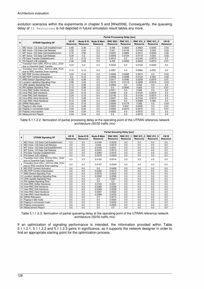
Architecture evaluation __________________________________________________________________________________________
__________________________________________________________________________________________ 128
evolution scenarios within the experiments in chapter 5 and [Wie2006]. Consequently, the queueing delay of IS Resources is not depicted in future simulation result tables any more.
Partial Processing Delay [sec]
# UTRAN Signaling SF UE IS
Resource Node B IS Resource
Node B Main Resource
RNC BSC Resource
RNC ICC_1 Resource
RNC ICC_2 Resource
RNC ICC_3 Resource
CN IS Resource
1 MO Voice / CS Data Call Establishment 0.68 0.48 0.3 0.005 0.0833 0.0863 0.0045 0.04 2 MO Voice / CS Data Call Release 0.32 0.24 0.2 0.001 0.0149 0.0164 0.003 0.03 3 MT Voice / CS Data Call Establishment 0.76 0.56 0.3 0.0023 0.0863 0.0313 0.0045 0.06 4 MT Voice / CS Data Call Release 0.24 0.2 0.2 0.0009 0.0104 0.0119 0.003 0.03 5 PS Data Transfer Establishment 0.2 0.16 0.4 0.0012 0.0 0.0164 0.0074 0.0 6 PS Detach (UE initiated) 0.32 0.28 0.5 0.005 0.0045 0.0223 0.0074 0.01
7 Transition from URA_PCH to CELL_DCH due to Downlink Data Transfer 0.24 0.2 0.3 0.0043 0.0 0.0134 0.0045 0.0
8 Transition from CELL_DCH to URA_PCH due to RRC inactivity timer expiring 0.12 0.12 0.3 0.0007 0.0 0.0089 0.003 0.0
9 MO PDP Context Activation 0.24 0.16 0.0 0.0006 0.0089 0.0074 0.0 0.02 10 MO PDP Context Deactivation 0.2 0.16 0.2 0.0008 0.0089 0.0104 0.003 0.02 11 IMSI Detach Signaling Flow 0.32 0.28 0.5 0.0017 0.0045 0.0238 0.0074 0.01 12 Location Updating Signaling Flow 0.56 0.44 0.5 0.0019 0.0119 0.0298 0.0074 0.03 13 URA Update Signaling Flow 0.12 0.08 0.0 0.0002 0.0 0.003 0.0 0.0 14 RA Update Signaling Flow 0.12 0.08 0.0 0.0 0.0045 0.003 0.0 0.01 15 Intra-RNC Softer Handover 0.24 0.16 0.2 0.0071 0.0 0.006 0.0 0.0 16 Intra-RNC Soft Handover 0.24 0.16 0.4 0.0048 0.0 0.0134 0.0074 0.0 17 Inter-RNC Soft Handover 0.24 0.16 0.4 0.0145 0.0 0.0134 0.0074 0.0 18 Intra-RNC Hard Handover 0.12 0.08 0.4 0.0047 0.0 0.0104 0.0074 0.0 19 Inter-RNC Hard Handover 0.12 0.08 0.4 0.0082 0.0 0.0089 0.006 0.0 20 SRNS Relocation 0.24 0.16 0.0 0.0009 0.0179 0.006 0.0 0.04 21 Paging in idle mode 0.12 0.08 0.0 0.0003 0.003 0.0045 0.0 0.01 22 Paging in connected mode 0.04 0.04 0.0 0.0003 0.0015 0.0015 0.0 0.01 23 Paging unsuccessful 0.04 0.04 0.0 0.0003 0.0 0.0015 0.0 0.0 24 Measurement Report 0.04 0.04 0.0 0.0 0.0 0.0015 0.0 0.0
Table 5.1.1.2.2: Itemization of partial processing delay at the operating point of the UTRAN reference network architecture (50/50 traffic mix)
Partial Queueing Delay [sec]
# UTRAN Signaling SF UE IS
Resource Node B IS Resource
Node B Main Resource
RNC BSC Resource
RNC ICC_1 Resource
RNC ICC_2 Resource
RNC ICC_3 Resource
CN IS Resource
1 MO Voice / CS Data Call Establishment 0.0 0.0 0.0194 0.0029 0.0 0.0 0.0 0.0 2 MO Voice / CS Data Call Release 0.0 0.0 0.023 0.0015 0.0 0.0 0.0 0.0 3 MT Voice / CS Data Call Establishment 0.0 0.0 0.0182 0.0031 0.0 0.0 0.0 0.0 4 MT Voice / CS Data Call Release 0.0 0.0 0.0224 0.0013 0.0 0.0 0.0 0.0 5 PS Data Transfer Establishment 0.0 0.0 0.0285 0.0016 0.0 0.0 0.0 0.0 6 PS Detach (UE initiated) 0.0 0.0 0.0378 0.0025 0.0 0.0 0.0 0.0
7 Transition from URA_PCH to CELL_DCH due to Downlink Data Transfer
0.0 0.0 0.0182 0.0016 0.0 0.0 0.0 0.0
8 Transition from CELL_DCH to URA_PCH due to RRC inactivity timer expiring
0.0 0.0 0.0187 0.0009 0.0 0.0 0.0 0.0
9 MO PDP Context Activation 0.0 0.0 0.0 0.0008 0.0 0.0 0.0 0.0 10 MO PDP Context Deactivation 0.0 0.0 0.0202 0.0012 0.0 0.0 0.0 0.0 11 IMSI Detach Signaling Flow 0.0 0.0 0.0375 0.0023 0.0 0.0 0.0 0.0 12 Location Updating Signaling Flow 0.0 0.0 0.0380 0.0026 0.0 0.0 0.0 0.0 13 URA Update Signaling Flow 0.0 0.0 0.0 0.0001 0.0 0.0 0.0 0.0 14 RA Update Signaling Flow 0.0 0.0 0.0 0.0 0.0 0.0 0.0 0.0 15 Intra-RNC Softer Handover 0.0 0.0 0.0163 0.0021 0.0 0.0 0.0 0.0 16 Intra-RNC Soft Handover 0.0 0.0 0.0382 0.0026 0.0 0.0 0.0 0.0 17 Inter-RNC Soft Handover 0.0 0.0 0.0369 0.0039 0.0 0.0 0.0 0.0 18 Intra-RNC Hard Handover 0.0 0.0 0.0387 0.0023 0.0 0.0 0.0 0.0 19 Inter-RNC Hard Handover 0.0 0.0 0.0388 0.0032 0.0 0.0 0.0 0.0 20 SRNS Relocation 0.0 0.0 0.0 0.0013 0.0 0.0 0.0 0.0 21 Paging in idle mode 0.0 0.0 0.0 0.0004 0.0 0.0 0.0 0.0 22 Paging in connected mode 0.0 0.0 0.0 0.0004 0.0 0.0 0.0 0.0 23 Paging unsuccessful 0.0 0.0 0.0 0.0005 0.0 0.0 0.0 0.0 24 Measurement Report 0.0 0.0 0.0 0.0 0.0 0.0 0.0 0.0
Table 5.1.1.2.3: Itemization of partial queueing delay at the operating point of the UTRAN reference network architecture (50/50 traffic mix)
If an optimization of signaling performance is intended, the information provided within Table 5.1.1.2.1, 5.1.1.2.2 and 5.1.1.2.3 gains in significance, as it supports the network designer in order to find an appropriate starting point for the optimization process.

Architecture evaluation __________________________________________________________________________________________
__________________________________________________________________________________________ 129
� Varying the number of users in the calibrated UTRAN reference architecture
Next, the number of users per RNC is varied from 100,000 users up to 1,5 million of users (i.e. from 200,000 users up to 3 million of users in the network).
Fig. 5.1.1.2.1: Variation of number of users per RNS and E2E signaling performance within UTRAN reference network architecture (50/50 traffic mix)
The E2E signaling performance results, illustrated within Fig. 5.1.1.2.1, show that the UTRAN reference architecture becomes instable within the 50/50 traffic mix, if the number of users per RNS is 1,5 million. In this context, the stability condition for the experiments in chapter 5 is defined according to predefined service levels that are represented by the upper boundaries of E2E signaling delay values which are defined to be acceptable for the signaling SFs under study. Table 5.1.1.2.4 illustrates the assumed service levels for the signaling SFs under study at the operating point of the network, which is 1 million of users, in the 50/50 traffic mix, and these service levels are considered for the UTRAN reference architecture as well as for the RAN evolution scenarios under study within this chapter. As the stability condition is defined under consideration of predefined service levels, a violation of the stability criterion for a particular signaling SF under study is not necessarily based on an instability within the queueing system. In this context, the instability of the queueing system is defined as a situation, in which the number of jobs within one of the queues grows continuously and becomes infinite so that the system is said to be instable, and an infinite buffer system is assumed (cf. [Jai1991]).
0.0
1.0
2.0
3.0
4.0
5.0
6.0
7.0
8.0
9.0
0 200,000 400,000 600,000 800,000 1,000,000 1,200,000 1,400,000 1,600,000
Number of Users in Radio Network Subsystem
E2E
Del
ay [s
ec]
SF 1: MO Voice / CS Data Call Establishment SF 3: MT Voice / CS Data Call Establishment
SF 9: MO PDP Context Activation
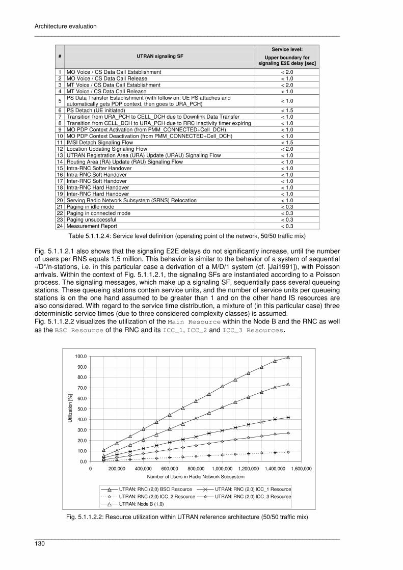
Architecture evaluation __________________________________________________________________________________________
__________________________________________________________________________________________ 130
# UTRAN signaling SF
Service level:
Upper boundary for signaling E2E delay [sec]
1 MO Voice / CS Data Call Establishment < 2.0 2 MO Voice / CS Data Call Release < 1.0 3 MT Voice / CS Data Call Establishment < 2.0 4 MT Voice / CS Data Call Release < 1.0
5 PS Data Transfer Establishment (with follow on: UE PS attaches and automatically gets PDP context, then goes to URA_PCH) < 1.0
6 PS Detach (UE initiated) < 1.5 7 Transition from URA_PCH to CELL_DCH due to Downlink Data Transfer < 1.0 8 Transition from CELL_DCH to URA_PCH due to RRC inactivity timer expiring < 1.0 9 MO PDP Context Activation (from PMM_CONNECTED+Cell_DCH) < 1.0
10 MO PDP Context Deactivation (from PMM_CONNECTED+Cell_DCH) < 1.0 11 IMSI Detach Signaling Flow < 1.5 12 Location Updating Signaling Flow < 2.0 13 UTRAN Registration Area (URA) Update (URAU) Signaling Flow < 1.0 14 Routing Area (RA) Update (RAU) Signaling Flow < 1.0 15 Intra-RNC Softer Handover < 1.0 16 Intra-RNC Soft Handover < 1.0 17 Inter-RNC Soft Handover < 1.0 18 Intra-RNC Hard Handover < 1.0 19 Inter-RNC Hard Handover < 1.0 20 Serving Radio Network Subsystem (SRNS) Relocation < 1.0 21 Paging in idle mode < 0.3 22 Paging in connected mode < 0.3 23 Paging unsuccessful < 0.3 24 Measurement Report < 0.3
Table 5.1.1.2.4: Service level definition (operating point of the network, 50/50 traffic mix) Fig. 5.1.1.2.1 also shows that the signaling E2E delays do not significantly increase, until the number of users per RNS equals 1,5 million. This behavior is similar to the behavior of a system of sequential -/D*/n-stations, i.e. in this particular case a derivation of a M/D/1 system (cf. [Jai1991]), with Poisson arrivals. Within the context of Fig. 5.1.1.2.1, the signaling SFs are instantiated according to a Poisson process. The signaling messages, which make up a signaling SF, sequentially pass several queueing stations. These queueing stations contain service units, and the number of service units per queueing stations is on the one hand assumed to be greater than 1 and on the other hand IS resources are also considered. With regard to the service time distribution, a mixture of (in this particular case) three deterministic service times (due to three considered complexity classes) is assumed. Fig. 5.1.1.2.2 visualizes the utilization of the Main Resource within the Node B and the RNC as well as the BSC Resource of the RNC and its ICC_1, ICC_2 and ICC_3 Resources.
Fig. 5.1.1.2.2: Resource utilization within UTRAN reference architecture (50/50 traffic mix)
0.0
10.0
20.0
30.0
40.0
50.0
60.0
70.0
80.0
90.0
100.0
0 200,000 400,000 600,000 800,000 1,000,000 1,200,000 1,400,000 1,600,000
Number of Users in Radio Network Subsystem
Util
izat
ion
[%]
UTRAN: RNC (2,0) BSC Resource UTRAN: RNC (2,0) ICC_1 Resource
UTRAN: RNC (2,0) ICC_2 Resource UTRAN: RNC (2,0) ICC_3 Resource
UTRAN: Node B (1,0)

Architecture evaluation __________________________________________________________________________________________
__________________________________________________________________________________________ 131
Under consideration of Fig. 5.1.1.2.2, the instability of the UTRAN reference architecture at 1,5 million of users per RNS is caused by the BSC Resource within the RNC that is fully utilized at this point and consequently, turns out as a bottleneck.
5.1.2 Merged Radio Access Network (MRAN)
The MRAN architecture evolution scenario was already introduced and explained in section 2.3.6 (cf. Fig. 2.3.7 and 2.3.8). In the upcoming section, the simulation modeling methodology, which was presented in section 3.4, is applied to the ATM- and IP-based MRAN evolution scenarios, and both architectures are calibrated. 5.1.2.1 ATM-based MRAN
Fig. 5.1.2.1.1 displays the allocation of FEs to the network elements of the MRAN Control Plane. The figure shows that the Merged Node B combines the FEs and thus, the complete functionality, of the Node B and RNC network elements of the UTRAN reference architecture (cf. Fig. 3.4.6 and 5.1.2.1.1). However, some FEs which are relevant in UTRAN are unnecessary in MRAN. These are on the one hand those FEs necessary for communication purposes between the Node B and the RNC (NBAP, Iub) and on the other hand the ALCAP_Iub FE necessary for ATM transportation establishment on the Iub interface. Consequently, those FEs are not functional components of the Merged Node B. An allocation of FEs to resources is not yet provided in the Merged Node B so that the network designer has the freedom to study various resource allocation scenarios via simulation and reach a decision based on the simulation results received. As in UTRAN (cf. section 3.4), the FEs located within the mobile terminal and the CN are mapped to IS Resources.
Infinite Server
Resource
Infinite Server
Resource
CN Merged Node B UE
RRC Connection
Management
Uu Iu
ALCAP_Iu
RANAP
RNSAP
Bearer Management
User Management
Micro Mobility Management
Mobility Management
Paging Entity
Broadcast / Multicast
Management
Radio Access Bearer
Management
Bearer Mapping
Unit
ALCAP Uu Uu
RRC Connection
Management
RANAP
ALCAP_Iur
Fig. 5.1.2.1.1: Allocation of FEs to network elements in the Control Plane of the ATM-based MRAN
[MiScWi2005]

Architecture evaluation __________________________________________________________________________________________
__________________________________________________________________________________________ 132
Fig. 5.1.2.1.2 illustrates the RRC Connection Establishment signaling procedure in the ATM-based MRAN according to the modeling concept introduced in section 3.4. The figure shows that the Merged Node B autonomously handles the radio resource connection as well as the radio resource reservation.
(1,30)
(2,63)
(1,30)
(1,30)
(1,30)
(1,7)
(1,121)
(1,121)
(2,121)
(1,30)
(1,30)
Uu RRC Conn. Mgm.
UE
User Mgm.
Bearer Mgm.
Merged Node B
Uu RRC Conn. Mgm.
Radio Access Bearer Mgm.
Bearer Mapping
Unit
(3,121)
(2,121)
(1,22)
(1,22)
(1,22)
(1,43)
RRC Connection Request
Creation of UE Request
Bearer Establish Request
Bearer Establish Confirm
RRC Connection Setup
RRC Connection Setup Complete
(1,30)
Fig. 5.1.2.1.2: RRC Connection Establishment within the ATM-based MRAN [AlWi2005a]
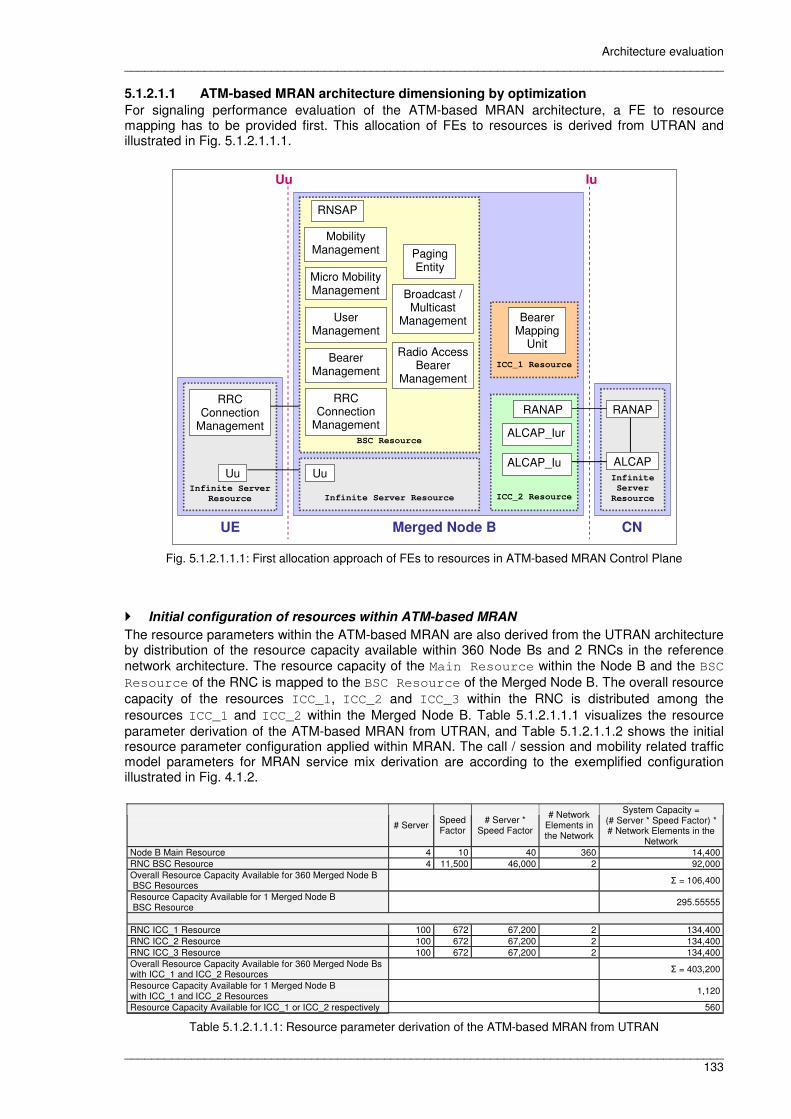
Architecture evaluation __________________________________________________________________________________________
__________________________________________________________________________________________ 133
5.1.2.1.1 ATM-based MRAN architecture dimensioning by optimization
For signaling performance evaluation of the ATM-based MRAN architecture, a FE to resource mapping has to be provided first. This allocation of FEs to resources is derived from UTRAN and illustrated in Fig. 5.1.2.1.1.1.
Infinite
Server
Resource
Infinite Server
Resource
CN Merged Node B UE
RRC Connection
Management
Uu Iu
ALCAP Uu
RANAP
BSC Resource
RNSAP
Bearer Management
User Management
Micro Mobility Management
Mobility Management Paging
Entity
Broadcast / Multicast
Management
Radio Access Bearer
Management
RRC Connection
Management
ICC_1 Resource
Bearer Mapping
Unit
ICC_2 Resource
Infinite Server Resource
Uu ALCAP_Iu
RANAP
ALCAP_Iur
Fig. 5.1.2.1.1.1: First allocation approach of FEs to resources in ATM-based MRAN Control Plane
� Initial configuration of resources within ATM-based MRAN
The resource parameters within the ATM-based MRAN are also derived from the UTRAN architecture by distribution of the resource capacity available within 360 Node Bs and 2 RNCs in the reference network architecture. The resource capacity of the Main Resource within the Node B and the BSC Resource of the RNC is mapped to the BSC Resource of the Merged Node B. The overall resource capacity of the resources ICC_1, ICC_2 and ICC_3 within the RNC is distributed among the resources ICC_1 and ICC_2 within the Merged Node B. Table 5.1.2.1.1.1 visualizes the resource parameter derivation of the ATM-based MRAN from UTRAN, and Table 5.1.2.1.1.2 shows the initial resource parameter configuration applied within MRAN. The call / session and mobility related traffic model parameters for MRAN service mix derivation are according to the exemplified configuration illustrated in Fig. 4.1.2.
# Server Speed Factor
# Server * Speed Factor
# Network Elements in the Network
System Capacity = (# Server * Speed Factor) * # Network Elements in the
Network Node B Main Resource 4 10 40 360 14,400 RNC BSC Resource 4 11,500 46,000 2 92,000 Overall Resource Capacity Available for 360 Merged Node B BSC Resources Σ = 106,400
Resource Capacity Available for 1 Merged Node B BSC Resource 295.55555
RNC ICC_1 Resource 100 672 67,200 2 134,400 RNC ICC_2 Resource 100 672 67,200 2 134,400 RNC ICC_3 Resource 100 672 67,200 2 134,400 Overall Resource Capacity Available for 360 Merged Node Bs with ICC_1 and ICC_2 Resources Σ = 403,200
Resource Capacity Available for 1 Merged Node B with ICC_1 and ICC_2 Resources 1,120
Resource Capacity Available for ICC_1 or ICC_2 respectively 560
Table 5.1.2.1.1.1: Resource parameter derivation of the ATM-based MRAN from UTRAN

Architecture evaluation __________________________________________________________________________________________
__________________________________________________________________________________________ 134
Amount of Service (ms)
# Server Speed Factor
# Server * Speed Factor
# Network Elements in the Network
System Capacity = (# Server * Speed Factor) * # Network Elements in the
Network C = 1 C = 2 C = 3
UE IS Resource 10,000 25 250,000 360 90,000,000 1 1 1 Merged Node B IS Resource 10,000 50 500,000 360 180,000,000 1 1 1 Merged Node B BSC Resource 1 295.55555 295.55555 360 106,400 1 2 36 Merged Node B ICC_1 Resource 1 560 560 360 201,600 1 2 40 Merged Node B ICC_2 Resource 1 560 560 360 201,600 1 2 40 CN IS Resource 10,000 100 1,000,000 1 1,000,000 1 1 1 Total System Resource Capacity in the Network Σ = 271,509,600
Table 5.1.2.1.1.2: Initial resource parameter configuration within ATM-based MRAN With regard to the network topology in the ATM-based MRAN, 360 Merged Node Bs are assumed in the network (i.e. 180 Merged Node Bs per RNS), which are not modeled in full detail according to the SHRiNK modeling technique. Instead, 4 Merged Node Bs are modeled explicitly. One single Merged Node B serves one radio cell. Fig. 5.1.2.1.1.2 shows the network topology assumed for MRAN simulation experiments.
Fig. 5.1.2.1.1.2: ATM-based MRAN network topology within OPNET Modeler The CAC parameters, applied within the radio cell of the ATM-based MRAN, conform to the settings within the UTRAN reference architecture, i.e. it is assumed that the maximum throughput within the radio cell is 1 Mbit/sec, and the QoS policy is achieved, if the utilization of the data channels is less than or equals 80%. Table 5.1.2.1.1.3 shows the communication link configuration that is assumed for the network elements within MRAN in the Network Domain of OPNET Modeler.
UE �� Merged Node B (Air interface) Merged Node B �� Merged Node B Merged Node B �� CN
Link Speed [Mbit/sec] 2 6 6 Distance [km] 1 10 100
Propagation Speed [meters/sec] Speed of Light (in air): 299,702,547
Speed of Light (in glass): 199,861,638
Speed of Light (in glass): 199, 861,638
Table 5.1.2.1.1.3: Link parameter configuration within ATM-based MRAN

Architecture evaluation __________________________________________________________________________________________
__________________________________________________________________________________________ 135
Table 5.1.2.1.1.4 visualizes the interarrival rates for Handover and SRNS Relocation signaling in UTRAN and the derivation of these rates in MRAN. Table 5.1.2.1.1.4 and the corresponding explanations are also applicable to DRAN under consideration of [Bau2003, Sch2003b].
Rate [1/sec]
# Signaling SF UTRAN MRAN
15 Intra-RNC / Merged Node B Softer Handover 16.58 16.58 16 Intra-RNC Soft Handover 74.67 Handover type not applicable 17 Inter-RNC / Merged Node B Soft Handover 5.33 80.0 18 Intra-RNC Hard Handover 7.26 Handover type not applicable 19 Inter-RNC / Merged Node B Hard Handover 0.52 7.78 20 SRNS / Serving Merged Node B Relocation 0.52 2.59
Table 5.1.2.1.1.4: Consideration of Handover and SRNS Relocation in UTRAN and MRAN (operation point of the network, 50/50 traffic mix)
As Merged Node Bs of the ATM- as well as of the IP-based MRAN are able to handle Soft and Hard Handover autonomously and directly via their Iur interface, which (at least) logically interconnects them, the affiliation of these Merged Node Bs with a particular RNS does not play a decisive role any more. As Merged Node Bs also independently manage their own radio resources, an inter-RNS soft and hard handover can be handled in exactly the same way as a soft or hard handover between two Merged Node Bs within the same RNS. Consequently, the interarrival rates for Inter-Merged Node B Soft and Hard Handover are derived from the traffic model in the Excel workbook according to equation (28) and (29) (see also Table 5.1.2.1.1.4 and [Spe2002]).
sec]/[RatealInterarrivsec]/[RatealInterarriv[1/sec] Rate lnterarrivaI UTRANSFUTRANSF MRAN17 SF 11 1716 += (27)
sec]/[RatealInterarrivsec]/[RatealInterarriv[1/sec] Rate lnterarrivaI UTRANSFUTRANSF MRAN19 SF 11 1918 += (28)
With regard to SRNS Relocation in UTRAN, it is assumed that the interarrival rate for SRNS Relocation equals the interarrival rate of Inter-RNC Hard Handover (i.e. each Inter-RNC Hard Handover requires SRNS Relocation signaling). This assumption was provided by the network engineers of Lucent Technologies, and it reflects results that were gathered by the network engineers of Lucent Technologies in the framework of field measurements in existing UMTS networks. The interarrival rate for SRNS Relocation in MRAN and DRAN considers the calculations provided in [Sch2003b], the idea of the GTP-U relay, which enables the hiding of hard handover handling from the CN (cf. section 2.3.4 and [3GPP2003t]), and [Bau2003] so that not each Inter-Merged / iNode B Hard Handover requires SRNS / Serving Merged or iNode B Relocation. Nevertheless, Table 5.1.2.1.1.4 shows that the number of complex handovers, which require SRNS / Serving Merged or iNode B Relocation, increases in MRAN and DRAN compared to the UTRAN reference architecture.

Architecture evaluation __________________________________________________________________________________________
__________________________________________________________________________________________ 136
� Simulation results with initial MRAN resource configuration
Table 5.1.2.1.1.5 shows the signaling E2E delays of the ATM-based MRAN within the 50/50 traffic mix at the operating point of the network before optimization, which is also assumed with 1 million of users per RNS. The resource parameter configuration illustrated in Table 5.1.2.1.1.2 is used for the experiment.
Signaling E2E
Delay [sec] ATM-based MRAN Partial Delays [sec]
# ATM-based MRAN Signaling SF ATM-based
MRAN ± 90%
Confidence Processing Delay [sec]
Queueing Delay [sec]
Link Transmission
Delay [sec]
Link Propagation Delay [sec]
1 MO Voice / CS Data Call Establishment 1.65 0.000467 1.2862 0.3532 0.000256 0.006541 2 MO Voice / CS Data Call Release 0.68 0.000411 0.5001 0.1756 0.000121 0.003019 3 MT Voice / CS Data Call Establishment 1.73 0.00021 1.3249 0.4019 0.000259 0.007549 4 MT Voice / CS Data Call Release 0.54 0.000402 0.388 0.153 0.000033 0.002515 5 PS Data Transfer Establishment 0.41 0.000215 0.294 0.1109 0.000082 0.00001 6 PS Detach (UE initiated) 0.82 0.00061 0.6047 0.2164 0.000153 0.001017
7 Transition from URA_PCH to CELL_DCH due to Downlink Data Transfer
0.6 0.000229 0.474 0.1289 0.000109 0.000013
8 Transition from CELL_DCH to URA_PCH due to RRC inactivity timer expiring
0.24 0.000312 0.1753 0.062 0.000067 0.000007
9 MO PDP Context Activation 0.5 0.000672 0.3744 0.1255 0.000044 0.002015 10 MO PDP Context Deactivation 0.44 0.000642 0.3128 0.1282 0.00004 0.002011 11 IMSI Detach Signaling Flow 0.64 0.000773 0.4829 0.1597 0.000109 0.001017 12 Location Updating Signaling Flow 1.07 0.000227 0.8386 0.2254 0.000155 0.003032 13 URA Update Signaling Flow 0.19 0.000002 0.1668 0.0243 0.000042 0.000007 14 RA Update Signaling Flow 0.18 0.000001 0.1754 0.0026 0.000028 0.001007 15 Intra-Merged Node B Softer Handover 0.62 0.000346 0.4587 0.1603 0.000156 0.000013 16 Intra-Merged Node B Soft Handover – – – – – – 17 Inter-Merged Node B Soft Handover 1.14 0.000162 0.7465 0.3929 0.000211 0.00018 18 Intra-Merged Node B Hard Handover – – – – – – 19 Inter-Merged Node B Hard Handover 0.59 0.000275 0.3395 0.2515 0.00017 0.000174 20 SRNS Relocation 0.62 0.000032 0.4153 0.1953 0.0001 0.004599 21 Paging in idle mode 0.24 0.000004 0.1837 0.052 0.000047 0.000507 22 Paging in connected mode 0.14 0.000003 0.0853 0.0532 0.000005 0.000504 23 Paging unsuccessful 0.13 0.000002 0.0735 0.0612 0.000005 0.000003 24 Measurement Report 0.06 0.000001 0.06 0.0 0.00005 0.000003
Table 5.1.2.1.1.5: Signaling E2E delays at the operating point of the ATM-based MRAN architecture before optimization (50/50 traffic mix)
With regard to Table 5.1.2.1.1.5, the E2E delay of signaling SF 17 (Inter-Merged Node B Soft Handover), which is greater than 1 sec, violates the service level defined for handover signaling within Table 5.1.1.2.4 and might turn out even more critically, if the number of users per RNS is increased. As handovers occur due to user mobility during an ongoing voice call or data session, fast signaling is required so that the user does not perceive the transfer of the active connection from one radio cell into another one. Consequently, an optimization of handover signaling performance is necessary in case of signaling performance values greater than 1 sec. Table 5.1.2.1.1.6 and 5.1.2.1.1.7 illustrate the itemization of the processing and queueing delays for signaling SF 17 (Inter-Merged Node B Soft Handover) within the ATM-based MRAN at the operating point of the network before optimization.
ATM-based MRAN Partial Processing Delay [sec]
# ATM-based MRAN Signaling SF UE IS Resource
Merged Node B IS Resource
Merged Node B BSC Resource
Merged Node B ICC_1 Resource
Merged Node B ICC_2 Resource
CN IS Resource
17 Inter-Merged Node B Soft Handover 0.24 0.08 0.4229 0.0036 0.0 0.0
Table 5.1.2.1.1.6: Itemization of partial processing delay for Inter-Merged Node B Soft Handover at the operating point of the ATM-based MRAN architecture before optimization (50/50 traffic mix)
ATM-based MRAN Partial Queueing Delay [sec]
# ATM-based MRAN Signaling SF Merged Node B BSC Resource
Merged Node B ICC_1 Resource
Merged Node B ICC_2 Resource
17 Inter-Merged Node B Soft Handover 0.3929 0.000005 0.0
Table 5.1.2.1.1.7: Itemization of partial queueing delay for Inter-Merged Node B Soft Handover at the operating point of the ATM-based MRAN architecture before optimization (50/50 traffic mix)
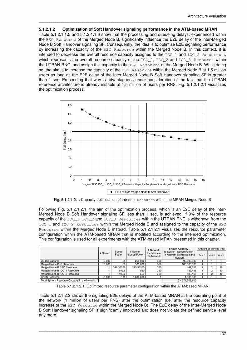
Architecture evaluation __________________________________________________________________________________________
__________________________________________________________________________________________ 137
5.1.2.1.2 Optimization of Soft Handover signaling performance in the ATM-based MRAN
Table 5.1.2.1.1.5 and 5.1.2.1.1.6 show that the processing and queueing delays, experienced within the BSC Resource of the Merged Node B, significantly influence the E2E delay of the Inter-Merged Node B Soft Handover signaling SF. Consequently, the idea is to optimize E2E signaling performance by increasing the capacity of the BSC Resource within the Merged Node B. In this context, it is intended to decrease the overall resource capacity assigned to the ICC_1 and ICC_2 Resources, which represents the overall resource capacity of the ICC_1, ICC_2 and ICC_3 Resource within the UTRAN RNC, and assign this capacity to the BSC Resource of the Merged Node B. While doing so, the aim is to increase the capacity of the BSC Resource within the Merged Node B at 1,5 million users as long as the E2E delay of the Inter-Merged Node B Soft Handover signaling SF is greater than 1 sec. Proceeding that way is advantageous under consideration of the fact that the UTRAN reference architecture is already instable at 1,5 million of users per RNS. Fig. 5.1.2.1.2.1 visualizes the optimization process.
Fig. 5.1.2.1.2.1: Capacity optimization of the BSC Resource within the MRAN Merged Node B Following Fig. 5.1.2.1.2.1, the aim of the optimization process, which is an E2E delay of the Inter-Merged Node B Soft Handover signaling SF less than 1 sec, is achieved, if 9% of the resource capacity of the ICC_1, ICC_2 and ICC_3 Resources within the UTRAN RNC is withdrawn from the ICC_1 and ICC_2 Resources within the Merged Node B and assigned to the capacity of the BSC Resource within the Merged Node B instead. Table 5.1.2.1.2.1 visualizes the resource parameter configuration within the ATM-based MRAN that is modified according to the intended optimization. This configuration is used for all experiments with the ATM-based MRAN presented in this chapter.
Amount of Service (ms)
# Server Speed Factor
# Server * Speed Factor
# Network Elements in the Network
System Capacity = (# Server * Speed Factor) * # Network Elements in the
Network C = 1 C = 2 C = 3
UE IS Resource 10,000 25 250,000 360 90,000,000 1 1 1 Merged Node B IS Resource 10,000 50 500,000 360 180,000,000 1 1 1 Merged Node B BSC Resource 1 396.35556 295.55555 360 142,688 1 2 36 Merged Node B ICC_1 Resource 1 509.6 560 360 183,456 1 2 40 Merged Node B ICC_2 Resource 1 509.6 560 360 183,456 1 2 40 CN IS Resource 10,000 100 1,000,000 1 1,000,000 1 1 1 Total System Resource Capacity in the Network Σ = 271,509,600
Table 5.1.2.1.2.1: Optimized resource parameter configuration within the ATM-based MRAN Table 5.1.2.1.2.2 shows the signaling E2E delays of the ATM-based MRAN at the operating point of the network (1 million of users per RNS) after the optimization (i.e. after the resource capacity increase of the BSC Resource within the Merged Node B). The E2E delay of the Inter-Merged Node B Soft Handover signaling SF is significantly improved and does not violate the defined service level any more.
0
0.2
0.4
0.6
0.8
1
1.2
1.4
1.6
0 1 2 3 4 5 6 7 8 9 10 11 12 13 14 15 16
%age of RNC ICC_1 / ICC_2 / ICC_3 Resource Capacity Supplement to Merged Node BSC Resource
E2E
Del
ay [s
ec]
SF 17: Inter-Merged Node B Soft Handover

Architecture evaluation __________________________________________________________________________________________
__________________________________________________________________________________________ 138
Signaling E2E
Delay [sec] ATM-based MRAN Partial Delays [sec]
# ATM-based MRAN Signaling SF ATM-based
MRAN ± 90%
Confidence Processing Delay [sec]
Queueing Delay [sec]
Link Transmission
Delay [sec]
Link Propagation Delay [sec]
1 MO Voice / CS Data Call Establishment 1.44 0.000462 1.2468 0.1844 0.000256 0.006541 2 MO Voice / CS Data Call Release 0.59 0.000409 0.4943 0.0948 0.000121 0.003019 3 MT Voice / CS Data Call Establishment 1.53 0.000208 1.3125 0.2128 0.000259 0.007549 4 MT Voice / CS Data Call Release 0.47 0.000401 0.3834 0.0819 0.000033 0.002515 5 PS Data Transfer Establishment 0.34 0.000213 0.2866 0.0508 0.000082 0.00001 6 PS Detach (UE initiated) 0.67 0.000609 0.5634 0.1074 0.000153 0.001017
7 Transition from URA_PCH to CELL_DCH due to Downlink Data Transfer 0.5
0.000227 0.4355 0.06 0.000109 0.000013
8 Transition from CELL_DCH to URA_PCH due to RRC inactivity timer expiring 0.2
0.000311 0.1721 0.0289 0.000067 0.000007
9 MO PDP Context Activation 0.44 0.000671 0.3694 0.0677 0.000044 0.002015 10 MO PDP Context Deactivation 0.38 0.000641 0.3089 0.0704 0.00004 0.002011 11 IMSI Detach Signaling Flow 0.55 0.000772 0.4726 0.0759 0.000109 0.001017 12 Location Updating Signaling Flow 0.95 0.000225 0.8275 0.1149 0.000155 0.003032 13 URA Update Signaling Flow 0.18 0.000002 0.165 0.0119 0.000042 0.000007 14 RA Update Signaling Flow 0.18 0.000001 0.1759 0.0035 0.000028 0.001007 15 Intra-Merged Node B Softer Handover 0.5 0.000345 0.4234 0.0789 0.000156 0.000013 16 Intra-Merged Node B Soft Handover – – – – – – 17 Inter-Merged Node B Soft Handover 0.82 0.000161 0.6393 0.1787 0.000211 0.00018 18 Intra-Merged Node B Hard Handover – – – – – – 19 Inter-Merged Node B Hard Handover 0.41 0.000274 0.2951 0.1159 0.00017 0.000174 20 SRNS Relocation 0.52 0.000031 0.4088 0.1034 0.0001 0.004599 21 Paging in idle mode 0.21 0.000004 0.1815 0.0241 0.000047 0.000507 22 Paging in connected mode 0.11 0.000003 0.0821 0.0248 0.000005 0.000504 23 Paging unsuccessful 0.1 0.000002 0.0701 0.0265 0.000005 0.000003 24 Measurement Report 0.06 0.000001 0.06 0.0 0.00005 0.000003
Table 5.1.2.1.2.2: Signaling E2E delays at the operating point of the ATM-based MRAN architecture after optimization (50/50 traffic mix)
The execution of these consecutive simulation experiments points out the support that is provided to the network designer, who is requested to calibrate, optimize and assess RAN evolution scenarios of interest, by application of the developed modeling methodology and tool chain. If the results are not satisfactory, the network designer can modify his assumptions under consideration of the insight he gained out of the performed result analysis. Once, the network designer fixed his assumptions within the tool chain, he is able to perform simulations and analyze the performance values gathered during these simulation runs. Recapitulating, this section provided an allocation of FEs to resources in the Control Plane of the ATM-based MRAN as well as an initial resource capacity derivation from UTRAN to the ATM-based MRAN. Moreover, the usefulness of the partial delay measurement information became obvious during the optimization process of E2E signaling performance. Simulation results, which were achieved with the initial resource parameter configuration, showed poor Soft Handover signaling performance due to substantial processing and queueing delays within the BSC Resource of the Merged Node B. A redistribution of the available UTRAN resource capacity in MRAN, which increases the capacity of the BSC Resource, helped to improve Soft Handover signaling performance to a value less than 1 sec. 5.1.2.2 IP-based MRAN
Fig. 5.1.2.2.1 displays the allocation of FEs to the network elements of the Control Plane in the IP-based MRAN. With regard to the IP-based transport network, the Merged Node B comprises some new FEs, which are in particular the Transport Network (TN) Resource Management, the RSVP-TE and the Iur / Iu RSVP-TE FEs. The TN Resource Management FE reserves physical resources in the transport network. The RSVP-TE FE is a RSVP-TE agent, which runs on the Merged Node B and is necessary for traffic engineering in the transport network. The Iur RSVP-TE FE is responsible for resource allocation on the Iur interface towards another Merged Node B, and the Iu RSVP-TE FE is responsible for resource allocation on the Iu interface. An allocation of FEs to resources is not yet provided in the Merged Node B so that the network designer in this case also has the freedom to study various resource allocation scenarios via

Architecture evaluation __________________________________________________________________________________________
__________________________________________________________________________________________ 139
simulation and reach a decision based on the simulation results received. As in UTRAN (cf. section 3.4), the FEs located within the mobile terminal and the CN are mapped to IS Resources.
Infinite
Server
Resource
Infinite Server
Resource
CN Merged Node B UE
RRC Connection
Management
Uu Iu
Uu
RNSAP
Bearer Management
User Management
Micro Mobility Management
Mobility Management Paging
Entity
Broadcast / Multicast
Management
Radio Access Bearer
Management
RRC Connection
Management
Uu
Iur RSVP-TE
TN Resource Management
RSVP-TE
RANAP
Iu RSVP-TE
RANAP
RSVP-TE
Fig. 5.1.2.2.1: Allocation of FEs to network elements in the Control Plane of the IP-based MRAN
Fig. 5.1.2.2.2 visualizes the RRC Connection Establishment signaling procedure within the IP-based MRAN.
(1,30)
(2,14)
(2,63)
(2,63)
(1,30)
(2,14)
(1,121)
(1,30)
(1,30)
Uu RRC Conn. Mgm.
UE
User Mgm.
Bearer Mgm.
Merged Node B
Uu RRC Conn. Mgm.
TN Resource
Mgm.
(3,121)
(2,121)
(1,22)
(1,22)
(1,22)
(1,43)
RRC Connection Request
Creation of UE Request
TN Resource Request
TN Resource Request ACK
RRC Connection Setup
RRC Connection Setup Complete
(1,30)
Fig. 5.1.2.2.2: RRC Connection Establishment within the IP-based MRAN and MPLS / RSVP-TE-based transport
network [AlWi2005b]

Architecture evaluation __________________________________________________________________________________________
__________________________________________________________________________________________ 140
5.1.2.2.1 IP-based MRAN architecture dimensioning by optimization
In the IP-based MRAN 360 Merged Node Bs are connected to an IP-based network, and 180 Merged Node Bs are assumed per RNS. The SHRiNK modeling technique is applied so that only 4 Merged Node Bs are explicitly modeled in total, although 360 Merged Node Bs are assumed. The IP-based transport network is modeled by the TNL cloud (cf. Fig. 5.1.2.2.1.1). The delay, each single signaling message experiences, when passing the TNL cloud, is assumed with 10 ms.
Fig. 5.1.2.2.1.1: MRAN network topology with IP-based transport network within OPNET Modeler In Table 5.1.2.2.1.1 the assumptions for the links of the IP-based MRAN in the Network Domain within OPNET Modeler are depicted.
UE �� Merged Node B (Air interface)
Merged Node B �� TNL Cloud CN �� TNL Cloud
Link Speed [Mbit/sec] 2 6 155 Distance [km] 1 10 10
Propagation Speed [meters/sec] Speed of Light (in air): 299,702,547
Speed (in thin coax): 194,865,098
Speed of Light (in glass): 199, 861,638
Table 5.1.2.2.1.1: Link parameter configuration within IP-based MRAN

Architecture evaluation __________________________________________________________________________________________
__________________________________________________________________________________________ 141
Fig. 5.1.2.2.1.2 visualizes the allocation of FEs to resources within the Control Plane of the IP-based MRAN.
Infinite Server
Resource
Infinite Server
Resource
CN Merged Node B UE
RRC Connection
Management
Uu Iu
Uu
BSC Resource
RNSAP
Bearer Management
User Management
Micro Mobility Management
Mobility Management Paging
Entity
Broadcast / Multicast
Management
Radio Access Bearer
Management
RRC Connection
Management
ICC_1 Resource
Infinite Server Resource
Uu
Iur RSVP-TE
TN Resource Management
RSVP-TE
RANAP
Iu RSVP-TE
RANAP
RSVP-TE
Fig. 5.1.2.2.1.2: Allocation of FEs to resources in MRAN Control Plane by application of an IP-based transport
network The resource parameters within the IP-based MRAN are also derived from the UTRAN architecture by distribution of the resource capacity available within 360 Node Bs and 2 RNCs in the reference network architecture. In this context, the resource capacity of the Main Resource within the Node B and the BSC Resource of the RNC is mapped to the BSC Resource of the Merged Node B, and the overall resource capacity of the resources ICC_1, ICC_2 and ICC_3 within the RNC is allocated to the ICC_1 Resource within the Merged Node B. Table 5.1.2.2.1.2 visualizes the resource parameter derivation within the IP-based MRAN from UTRAN, and Table 5.1.2.2.1.3 shows the initial resource parameter configuration applied within the IP-based MRAN. The call / session and mobility related traffic model parameters for service mix derivation within the IP-based MRAN are according to the exemplified configuration illustrated in Fig. 4.1.2.
# Server Speed Factor
# Server * Speed Factor
# Network Elements in the Network
System Capacity = (# Server * Speed Factor) * # Network Elements in the
Network Node B Main Resource 4 10 40 360 14,400 RNC BSC Resource 4 11,500 46,000 2 92,000 Overall Resource Capacity Available for 360 Merged Node B BSC Resources Σ = 106,400
Resource Capacity Available for 1 Merged Node B BSC Resource 295.55555
RNC ICC_1 Resource 100 672 67,200 2 134,400 RNC ICC_2 Resource 100 672 67,200 2 134,400 RNC ICC_3 Resource 100 672 67,200 2 134,400 Overall Resource Capacity Available for 360 Merged Node Bs with ICC_1 Resource Σ = 403,200
Resource Capacity Available for 1 Merged Node B with ICC_1 Resource 1,120
Table 5.1.2.2.1.2: Resource parameter derivation of the IP-based MRAN from UTRAN
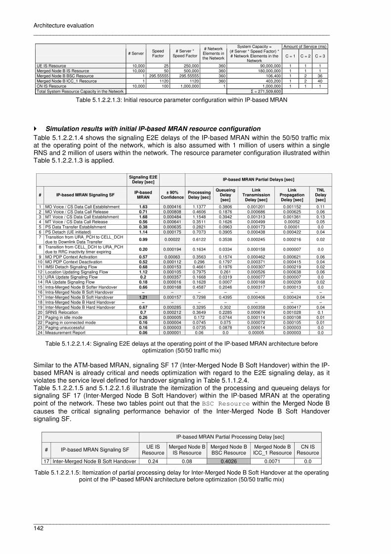
Architecture evaluation __________________________________________________________________________________________
__________________________________________________________________________________________ 142
Amount of Service (ms)
# Server Speed Factor
# Server * Speed Factor
# Network Elements in the Network
System Capacity = (# Server * Speed Factor) * # Network Elements in the
Network C = 1 C = 2 C = 3
UE IS Resource 10,000 25 250,000 360 90,000,000 1 1 1 Merged Node B IS Resource 10,000 50 500,000 360 180,000,000 1 1 1 Merged Node B BSC Resource 1 295.55555 295.55555 360 106,400 1 2 36 Merged Node B ICC_1 Resource 1 1120 1120 360 403,200 1 2 40 CN IS Resource 10,000 100 1,000,000 1 1,000,000 1 1 1 Total System Resource Capacity in the Network Σ = 271,509,600
Table 5.1.2.2.1.3: Initial resource parameter configuration within IP-based MRAN
� Simulation results with initial IP-based MRAN resource configuration
Table 5.1.2.2.1.4 shows the signaling E2E delays of the IP-based MRAN within the 50/50 traffic mix at the operating point of the network, which is also assumed with 1 million of users within a single RNS and 2 million of users within the network. The resource parameter configuration illustrated within Table 5.1.2.2.1.3 is applied.
Signaling E2E Delay [sec]
IP-based MRAN Partial Delays [sec]
# IP-based MRAN Signaling SF IP-based
MRAN ± 90%
Confidence Processing Delay [sec]
Queueing Delay [sec]
Link Transmission
Delay [sec]
Link Propagation Delay [sec]
TNL Delay [sec]
1 MO Voice / CS Data Call Establishment 1.63 0.000416 1.1377 0.3806 0.001201 0.001152 0.11 2 MO Voice / CS Data Call Release 0.71 0.000808 0.4606 0.1876 0.000686 0.000625 0.06 3 MT Voice / CS Data Call Establishment 1.68 0.000484 1.1548 0.3942 0.001313 0.001361 0.13 4 MT Voice / CS Data Call Release 0.56 0.000641 0.3511 0.1626 0.000499 0.00052 0.05 5 PS Data Transfer Establishment 0.38 0.000635 0.2821 0.0963 0.000173 0.00001 0.0 6 PS Detach (UE initiated) 1.14 0.000175 0.7073 0.3905 0.000438 0.000422 0.04 7 Transition from URA_PCH to CELL_DCH
due to Downlink Data Transfer 0.99 0.00022 0.6122 0.3538 0.000245 0.000216 0.02
8 Transition from CELL_DCH to URA_PCH due to RRC inactivity timer expiring
0.20 0.000194 0.1634 0.0334 0.000158 0.000007 0.0
9 MO PDP Context Activation 0.57 0.00063 0.3563 0.1574 0.000462 0.000621 0.06 10 MO PDP Context Deactivation 0.52 0.000112 0.296 0.1797 0.000371 0.000415 0.04 11 IMSI Detach Signaling Flow 0.68 0.000153 0.4661 0.1976 0.000307 0.000219 0.02 12 Location Updating Signaling Flow 1.12 0.000105 0.7975 0.261 0.000526 0.000638 0.06 13 URA Update Signaling Flow 0.2 0.000357 0.1668 0.0319 0.000077 0.000007 0.0 14 RA Update Signaling Flow 0.18 0.000016 0.1628 0.0007 0.000168 0.000209 0.02 15 Intra-Merged Node B Softer Handover 0.66 0.000168 0.4587 0.2046 0.000317 0.000013 0.0 16 Intra-Merged Node B Soft Handover – – – – – – – 17 Inter-Merged Node B Soft Handover 1.21 0.000157 0.7298 0.4395 0.000406 0.000424 0.04 18 Intra-Merged Node B Hard Handover – – – – – – – 19 Inter-Merged Node B Hard Handover 0.67 0.000285 0.3295 0.302 0.000358 0.000417 0.04 20 SRNS Relocation 0.7 0.000212 0.3649 0.2285 0.000674 0.001028 0.1 21 Paging in idle mode 0.26 0.000005 0.172 0.0744 0.000114 0.000108 0.01 22 Paging in connected mode 0.16 0.000004 0.0745 0.075 0.000072 0.000105 0.01 23 Paging unsuccessful 0.16 0.000003 0.0735 0.0878 0.000014 0.000003 0.0 24 Measurement Report 0.06 0.000001 0.06 0.0 0.00005 0.000003 0.0
Table 5.1.2.2.1.4: Signaling E2E delays at the operating point of the IP-based MRAN architecture before optimization (50/50 traffic mix)
Similar to the ATM-based MRAN, signaling SF 17 (Inter-Merged Node B Soft Handover) within the IP-based MRAN is already critical and needs optimization with regard to the E2E signaling delay, as it violates the service level defined for handover signaling in Table 5.1.1.2.4. Table 5.1.2.2.1.5 and 5.1.2.2.1.6 illustrate the itemization of the processing and queueing delays for signaling SF 17 (Inter-Merged Node B Soft Handover) within the IP-based MRAN at the operating point of the network. These two tables point out that the BSC Resource within the Merged Node B causes the critical signaling performance behavior of the Inter-Merged Node B Soft Handover signaling SF.
IP-based MRAN Partial Processing Delay [sec]
# IP-based MRAN Signaling SF UE IS Resource
Merged Node B IS Resource
Merged Node B BSC Resource
Merged Node B ICC_1 Resource
CN IS Resource
17 Inter-Merged Node B Soft Handover 0.24 0.08 0.4026 0.0071 0.0
Table 5.1.2.2.1.5: Itemization of partial processing delay for Inter-Merged Node B Soft Handover at the operating point of the IP-based MRAN architecture before optimization (50/50 traffic mix)

Architecture evaluation __________________________________________________________________________________________
__________________________________________________________________________________________ 143
IP-based MRAN Partial Queueing Delay [sec]
# IP-based MRAN Signaling SF Merged Node B BSC Resource
Merged Node B ICC_1 Resource
17 Inter-Merged Node B Soft Handover 0.4367 0.0029
Table 5.1.2.2.1.6: Itemization of partial queueing delay for Inter-Merged Node B Soft Handover at the operating point of the IP-based MRAN architecture before optimization (50/50 traffic mix)
5.1.2.2.2 Optimization of Soft Handover signaling performance in the IP-based MRAN
In order to improve the E2E signaling performance of the Inter-Merged Node B Soft Handover, the approach that was already applied within the ATM-based MRAN (cf. section 5.1.2.1.2) is again used here. This means that the overall resource capacity assigned to the ICC_1 Resource within the Merged Node B of the IP-based MRAN, which represents the overall resource capacity of the ICC_1, ICC_2 and ICC_3 Resource within the UTRAN RNC, is decreased. Next, the released resource capacity of the ICC_1 Resource is assigned to the BSC Resource of the Merged Node B. The optimization is performed by increasing the capacity of the BSC Resource within the Merged Node B at 1,5 million users as long as the E2E delay of the Inter-Merged Node B Soft Handover signaling SF is greater than 1 sec. Fig. 5.1.2.2.2.1 visualizes the optimization process.
Fig. 5.1.2.2.2.1: Capacity optimization of the BSC Resource within the Merged Node B According to Fig. 5.1.2.2.2.1, the E2E delay of the Inter-Merged Node B Soft Handover signaling SF is less than 1 sec, which meets the overall aim of the optimization process, if 10% of the ICC_1, ICC_2 and ICC_3 Resources within the UTRAN RNC are removed from the ICC_1 Resource within the Merged Node B and assigned to the capacity of the BSC Resource. Table 5.1.2.2.2.1 visualizes the resource parameter configuration within the IP-based MRAN that is modified according to the intended optimization. This configuration is used for all experiments with the IP-based MRAN presented in this chapter.
Amount of Service (ms)
# Server Speed Factor # Server *
Speed Factor
# Network Elements in the Network
System Capacity = (# Server * Speed Factor) * # Network Elements in the
Network C = 1 C = 2 C = 3
UE IS Resource 10,000 25 250,000 360 90,000,000 1 1 1 Merged Node B IS Resource 10,000 50 500,000 360 180,000,000 1 1 1 Merged Node B BSC Resource 1 407.555556 407.555556 360 146,720 1 2 36 Merged Node B ICC_1 Resource 1 1008 1008 360 362,880 1 2 40 CN IS Resource 10,000 100 1,000,000 1 1,000,000 1 1 1 Total System Resource Capacity in the Network Σ = 271,509,600
Table 5.1.2.2.2.1: Optimized resource parameter configuration within the IP-based MRAN
0
0.2
0.4
0.6
0.8
1
1.2
1.4
1.6
0 1 2 3 4 5 6 7 8 9 10 11 12 13 14 15 16%age of RNC ICC_1, ICC_2 and ICC_3 Resource Capacity Supplement to Merged Node B BSC Resource
E2E
Del
ay [s
ec]
SF 17: Inter-Merged Node B Soft Handover

Architecture evaluation __________________________________________________________________________________________
__________________________________________________________________________________________ 144
Table 5.1.2.2.2.2 shows the signaling E2E delays of the IP-based MRAN at the operating point of the network after the optimization. Now, the E2E delay of the Inter-Merged Node B Soft Handover signaling SF is also satisfactory and does not violate the defined service level any more.
Signaling E2E Delay [sec]
IP-based MRAN Partial Delays [sec]
# IP-based MRAN Signaling SF IP-based
MRAN ± 90%
Confidence Processing Delay [sec]
Queueing Delay [sec]
Link Transmission
Delay [sec]
Link Propagation Delay [sec]
TNL Delay [sec]
1 MO Voice / CS Data Call Establishment 1.37 0.000414 1.0935 0.1693 0.001201 0.001152 0.11 2 MO Voice / CS Data Call Release 0.6 0.000806 0.4533 0.0879 0.000686 0.000625 0.06 3 MT Voice / CS Data Call Establishment 1.45 0.000483 1.1396 0.1819 0.001313 0.001361 0.13 4 MT Voice / CS Data Call Release 0.47 0.00064 0.3454 0.0773 0.000499 0.00052 0.05 5 PS Data Transfer Establishment 0.32 0.000634 0.2767 0.0397 0.000173 0.00001 0.0 6 PS Detach (UE initiated) 0.84 0.000173 0.6308 0.1697 0.000438 0.000422 0.04 7 Transition from URA_PCH to CELL_DCH
due to Downlink Data Transfer 0.7 0.00022 0.5336 0.1463 0.000245 0.000216 0.02
8 Transition from CELL_DCH to URA_PCH due to RRC inactivity timer expiring
0.18 0.000193 0.1625 0.0136 0.000158 0.000007 0.0
9 MO PDP Context Activation 0.48 0.000631 0.3498 0.0699 0.000462 0.000621 0.06 10 MO PDP Context Deactivation 0.41 0.000111 0.2882 0.082 0.000371 0.000415 0.04 11 IMSI Detach Signaling Flow 0.56 0.000152 0.4555 0.0824 0.000307 0.000219 0.02 12 Location Updating Signaling Flow 0.96 0.000104 0.7856 0.1134 0.000526 0.000638 0.06 13 URA Update Signaling Flow 0.18 0.000356 0.1649 0.0142 0.000077 0.000007 0.0 14 RA Update Signaling Flow 0.18 0.000014 0.1631 0.0008 0.000168 0.000209 0.02 15 Intra-Merged Node B Softer Handover 0.51 0.000167 0.4206 0.0899 0.000317 0.000013 0.0 16 Intra-Merged Node B Soft Handover – – – – – – – 17 Inter-Merged Node B Soft Handover 0.84 0.000156 0.6199 0.1805 0.000406 0.000424 0.04 18 Intra-Merged Node B Hard Handover – – – – – – – 19 Inter-Merged Node B Hard Handover 0.45 0.000284 0.2857 0.1259 0.000358 0.000417 0.04 20 SRNS Relocation 0.56 0.000211 0.3568 0.0983 0.000674 0.001028 0.1 21 Paging in idle mode 0.21 0.000005 0.1694 0.0284 0.000114 0.000108 0.01 22 Paging in connected mode 0.11 0.000004 0.0709 0.029 0.000072 0.000105 0.01 23 Paging unsuccessful 0.1 0.000003 0.0698 0.0325 0.000014 0.000003 0.0 24 Measurement Report 0.06 0.000001 0.06 0.0 0.00005 0.000003 0.0
Table 5.1.2.2.2.2: Signaling E2E delays at the operating point of the IP-based MRAN architecture after optimization (50/50 traffic mix)
In this section, an initial resource capacity derivation from UTRAN to the IP-based MRAN was performed. Simulation results, which were received with the initial resource parameter configuration, also showed poor Soft Handover signaling performance due to substantial processing and queueing delays experienced within the BSC Resource of the Merged Node B. Similar to the ATM-based MRAN, a redistribution of the available UTRAN resource capacity was performed in this case, which increased the capacity of the BSC Resource and helped to decrease the Soft Handover E2E signaling delay down to a value of less than 1 sec.

Architecture evaluation __________________________________________________________________________________________
__________________________________________________________________________________________ 145
5.1.3 Distributed Radio Access Network (DRAN)
The DRAN architecture evolution scenario was already introduced and explained in section 2.3.4 (cf. Fig. 2.3.4). In this section the simulation modeling methodology, which was presented in section 3.4, is applied to DRAN, and the DRAN architecture is calibrated. Fig. 5.1.3.1 shows the allocation of FEs to the network elements of the DRAN Control Plane. The figure depicts the relocation of functionality closer to the air interface. This particularly concerns the FEs RRC Connection Management, Radio Bearer Management, Broadcast/Multicast Management, Micro Mobility Management and RNSAP which were relocated from the RNC into the iNode B. Furthermore, there are several FEs which were necessary in UTRAN, but are not needed in DRAN any more. These are in particular FEs necessary for the former communication between Node B and RNC (Iub, NBAP) as well as FEs necessary for ATM transportation establishment (ALCAP) and management of radio and transport bearers towards the CN (Bearer Mapping Unit). Regarding the IP-based transport network, DRAN also assumes the provision of QoS in the transport network by application of appropriate IETF protocols for resource allocation and traffic engineering, in particular MPLS [RoViCa2001] and RSVP-TE [AwBeLi2001]. Consequently, new FEs emerge in DRAN with regard to the technology applied in the transport network, which are, similar to the IP-based MRAN, in particular the TN Resource Management, the RSVP-TE and the Iur / Iuc / Iui RSVP-TE FEs. The TN Resource Management FE also reserves physical resources in the transport network. The RSVP-TE FE in this case is a RSVP-TE agent, which runs on the iNode B and is also necessary for traffic engineering in the transport network. The Iur RSVP-TE FE is responsible for resource allocation on the Iur interface, accordingly, the Iuc RSVP-TE and Iui RSVP-TE FEs are responsible for resource allocation on the Iuc and the new Iui interface, which itself is also represented by the new Iui FE. An allocation of FEs to resources is not provided for the iNode B and the RAN Server so that the network designer is enabled to study various resource allocation scenarios by simulation. Based on the simulation results the network designer can decide on a beneficial FE to resource mapping. As in UTRAN (cf. section 3.4), the FEs located within the UE and the CN are mapped to IS Resources.
Infinite
Server
Resource
Infinite Server
Resource
CN RAN Server iNode B UE
RRC Connection
Management
RSVP-TE
Iui Iuc Uu
Uu Iui Uu Iui
TN Resource Management
Iur RSVP-TE
RSVP-TE
TN Resource Management
Iui RSVP-TE
Bearer Management
User Management
Mobility Management
Paging Entity
RNSAP Micro Mobility Management
Broadcast / Multicast
Management
Radio Bearer Management
RANAP
Iuc RSVP-TE
RANAP RRC Connection
Management
Fig. 5.1.3.1: Allocation of FEs to network elements in DRAN Control Plane Fig. 5.1.3.2 displays the RRC Connection Establishment signaling procedure in DRAN according to the modeling concept described in section 3.4. The figure shows that the iNode B autonomously handles the radio resource connection, but it requests the radio resources from the RAN Server.

Architecture evaluation __________________________________________________________________________________________
__________________________________________________________________________________________ 146
(2,123)
(1,75)
(1,75)
(2,63)
(2,63)
(1,121)
(2,14)
(2,121)
(2,75)
(1,30) (1,30)
(1,123)
RRC Conn. Mgm.
(1,123)
Uu RRC Conn. Mgm.
UE iNode B
Uu Iui User Mgm.
Bearer Mgm.
TN Res. Mgm.
RAN Server
Iui
RRC Connection Request
Radio Bearer Mgm.
Creation of UE Request
(2,14)
(1,121)
(1,22)
(1,22)
(2,121)
(2,22)
(1,22)
(1,43)
TN Resource Request
TN Resource Request ACK
Creation of UE Response
RRC Connection Setup
RRC Connection Setup Complete
(1,30)
Fig. 5.1.3.2: RRC Connection Establishment in DRAN [AlBa2004]

Architecture evaluation __________________________________________________________________________________________
__________________________________________________________________________________________ 147
5.1.3.1 DRAN architecture dimensioning by optimization
When intending to evaluate the signaling performance of DRAN, a reasonable allocation of FEs to resources within the iNode B and the RAN Server has to be provided first. Moreover, the resource capacity of the UTRAN reference architecture also has to be reasonably distributed. 5.1.3.1.1 First allocation approach of FEs to resources in DRAN Control Plane
Fig. 5.1.3.1.1.1 illustrates an allocation approach of FEs to resources in the DRAN Control Plane.
Infinite Server
Resource
Infinite Server
Resource
CN RAN Server iNode B UE
RRC Connection
Management
RSVP-TE
Iui Iuc Uu
Infinite Server Resource
Infinite Server
Resource
Uu Iui Uu Iui
Transport Network
Resource
TN Resource Management
Iur RSVP-TE
RSVP-TE
Transport
Network Resource
TN Resource Management
Iui RSVP-TE
Main Resource
Bearer Management
User Management
Mobility Management
Paging Entity
Main Resource
RNSAP Micro Mobility Management
Broadcast / Multicast
Management
RRC Connection
Management
Radio Bearer Management
RANAP
Iuc RSVP-TE
RANAP
Fig. 5.1.3.1.1.1: First allocation approach of FEs to resources in DRAN Control Plane
The basic idea of this approach is to have a separate resource for those FEs which are related to the reservation and management of resources in the transport network. This applies to the RSVP-TE FE, to the Iur RSVP-TE FE and to the TN Resource Management FE within the iNode B as well as to the Iui RSVP-TE FE, to the Iuc RSVP-TE FE and to the TN Resource Management FE within the RAN Server. Moreover, those FEs, which represent interfaces towards other network elements, are allocated to IS resources. This basically applies to the Uu and Iui FE, and the reason to do this is that signaling messages that are transmitted via these interfaces experience fixed delays. The remaining FEs within the iNode B and the RAN Server are allocated to one single resource which is the main resource within these network elements (cf. Fig. 5.1.3.1.1.1).
� Initial configuration of DRAN resources
The DRAN architecture is calibrated for simulation so that the utilization of the Main Resource as well as the utilization of the Transport Network Resource within the iNode B is about 50%. Both, the utilization of the Main Resource as well as the utilization of the Transport Network Resource within the RAN Server is about 70%. This calibration applies for the 50/50 traffic mix and assumes 1 million of users per RAN Server at the operating point of the network. The call / session and mobility related traffic model parameters for DRAN service-mix derivation are according to the exemplified configuration illustrated in Fig. 4.1.2. The resource parameters set within DRAN are depicted in Table 5.1.3.1.1.1.

Architecture evaluation __________________________________________________________________________________________
__________________________________________________________________________________________ 148
Amount of Service (ms)
# Server Speed Factor
# Server * Speed Factor
# Network Elements in the Network
System Capacity = (# Server * Speed Factor) * # Network Elements in the
Network C = 1 C = 2 C = 3
UE IS Resource 10,000 25 250,000.0 360 90,000,000 1 1 1 iNode B IS Resource 10,000 50 500,000.0 360 180,000,000 1 1 1 iNode B Main Resource 4 40.5 162.0 360 58,320 1 2 3 iNode B Transport Network Resource 2 4.9 9.8 360 3,528 1 2 3 RAN Server IS Resource 3709 50.00701 185,476.0 2 370,952 1 1 1 RAN Server Main Resource 4 8,570 34,280.0 2 68,560 1 2 36 RAN Server Transport Network Resource 4 1,030 4,120.0 2 8,240 1 2 36 CN IS Resource 10,000 100 1,000,000.0 1 1,000,000 1 1 1 Total System Resource Capacity in the Network Σ = 271,509,600
Table 5.1.3.1.1.1: DRAN resource parameter configuration according to first allocation approach of FEs to resources illustrated in Fig. 5.1.3.1.1.1
With regard to the network topology it is assumed that one single RAN Server manages 180 iNode Bs, and one single iNode B serves one radio cell. The network topology of DRAN, used within OPNET Modeler, is illustrated in Fig. 5.1.3.1.1.2 which points out that, according to the SHRiNK concept, two RAN Servers as well as two iNode Bs and UEs / radio cells per RAN Server are modeled explicitly, although 180 iNode Bs and UEs / radio cells per RAN Server are assumed. The TNL cloud models the IP-based transport network that applies the MPLS) and RSVP-TE protocol for QoS purposes. The delay, each single signaling message experiences, when passing the TNL cloud, is assumed with 10 ms.
Fig. 5.1.3.1.1.2: DRAN network topology within OPNET Modeler The CAC parameters, applied within the radio cell, conform to the settings within the UTRAN reference architecture, i.e. it is assumed that the maximum throughput within the radio cell is 1 Mbit/sec, and the QoS policy is fulfilled, if the utilization of the data channels is less than or equals 80%. Table 5.1.3.1.1.2 depicts the parameters assumed for the communication links between the DRAN network elements in the Network Domain of OPNET Modeler.
UE �� iNode B (Air interface)
iNode B �� TNL Cloud RAN Server �� TNL Cloud CN �� TNL Cloud
Link Speed [Mbit/sec] 2 6 6 155 Distance [km] 1 10 10 10
Propagation Speed [meters/sec] Speed of Light (in air): 299,702,547
Speed (in thin coax): 194,865,098
Speed (in thin coax): 194,865,098
Speed of Light (in glass): 199, 861,638
Table 5.1.3.1.1.2: Link parameter configuration of DRAN architecture As iNode Bs in DRAN are also able to handle soft and hard handover autonomously and directly via their Iur interface, which (at least) logically interconnects them within the IP-based transport network, the affiliation of these iNode Bs with a particular RNS lost its importance with regard to handover

Architecture evaluation __________________________________________________________________________________________
__________________________________________________________________________________________ 149
handling. As iNode Bs also autonomously manage their own radio resources independently from the RAN Server, inter-RNS soft and hard handover can be handled in exactly the same way as intra-RNS soft and hard handover (cf. [Bau2003]). Therefore, the interarrival rates for Inter-iNode B Soft and Hard Handover are also according to Table 5.1.2.1.1.4 and equation (28) and (29).
� Simulation results within initial DRAN resource configuration
Table 5.1.3.1.1.3 depicts the signaling E2E delays at the operating point of the DRAN architecture (1 million of users per RNS) for the signaling SFs as well as the partial delays.
Signaling E2E
Delay [sec] DRAN Partial Delays [sec]
# DRAN Signaling SF DRAN ± 90%
Confidence Processing Delay [sec]
Queueing Delay [sec]
Link Transmission
Delay [sec]
Link Propagation Delay [sec]
TNL Delay [sec]
1 MO Voice / CS Data Call Establishment 2.04 0.000776 1.7156 0.0733 0.03118 0.00227 0.22 2 MO Voice / CS Data Call Release 1.05 0.000465 0.9 0.0195 0.01707 0.00114 0.11 3 MT Voice / CS Data Call Establishment 2.31 0.000573 1.9505 0.0823 0.03216 0.00249 0.24 4 MT Voice / CS Data Call Release 0.78 0.000372 0.6609 0.0168 0.0137 0.00093 0.09 5 PS Data Transfer Establishment 0.5 0.000272 0.4566 0.0085 0.00291 0.00032 0.03 6 PS Detach (UE initiated) 1.18 0.000436 1.0227 0.0234 0.02287 0.00114 0.11
7 Transition from URA_PCH to CELL_DCH due to Downlink Data Transfer 0.95
0.000857 0.8245 0.0131 0.01501 0.00104 0.1
8 Transition from CELL_DCH to URA_PCH due to RRC inactivity timer expiring 0.32
0.000293 0.2895 0.0053 0.00102 0.00021 0.02
9 MO PDP Context Activation 0.69 0.000649 0.5317 0.0444 0.01 0.00103 0.1 10 MO PDP Context Deactivation 0.62 0.000312 0.5262 0.0142 0.00827 0.00072 0.07 11 IMSI Detach Signaling Flow 0.99 0.000734 0.8814 0.0246 0.00971 0.00073 0.07 12 Location Updating Signaling Flow 1.68 0.000644 1.4808 0.0357 0.01576 0.00156 0.15 13 URA Update Signaling Flow 0.26 0.000056 0.2402 0.0001 0.00244 0.00021 0.02 14 RA Update Signaling Flow 0.87 0.000676 0.7397 0.0129 0.01658 0.00103 0.1 15 Intra-iNode B Softer Handover 0.54 0.000327 0.5175 0.0171 0.00032 0.00001 0.00 16 Intra-iNode B Soft Handover – – – – – – – 17 Inter-iNode B Soft Handover 3.42 0.000212 2.8546 0.4996 0.0004 0.0006 0.06 18 Intra-iNode B Hard Handover – – – – – – – 19 Inter-iNode B Hard Handover 3.72 0.000177 3.0455 0.4351 0.0154 0.0023 0.22 20 SRNS Relocation 1.91 0.000277 1.5354 0.2766 0.0043 0.0009 0.09 21 Paging in idle mode 0.34 0.000006 0.3 0.0057 0.0030 0.0003 0.03 22 Paging in connected mode 0.16 0.000008 0.1352 0.003 0.0017 0.0002 0.02 23 Paging unsuccessful 0.14 0.000007 0.125 0.0029 0.0004 0.0001 0.01 24 Measurement Report 0.13 0.000001 0.12 0.0 0.0016 0.0001 0.01
Table 5.1.3.1.1.3: Signaling E2E delays at the operating point of the DRAN architecture (1st experiment, 50/50 traffic mix)
The results within Table 5.1.3.1.1.3 illustrate that some of the signaling SFs show poor performance values with regard to the E2E delay and violate the defined service levels (cf. Table 5.1.1.2.4), particularly the handover signaling SFs and SRNS Relocation. Consequently, the next step is to analyze the origin of these performance problems. Therefore, it is necessary to further analyze the itemization of the partial processing and queueing delays of the overall signaling E2E delay per particular resource. Table 5.1.3.1.1.4 and 5.1.3.1.1.5 visualizes this itemization.
DRAN Partial Processing Delay [sec]
# DRAN Signaling SF UE IS Resource
iNode B IS Resource
iNode B Main
Resource
iNode B Transport Network
Resource
RAN Server IS Resource
RAN Server Main Resource
RAN Server Transport Network
Resource
CN IS Resource
17 Inter-iNode B Soft Handover 0.24 0.08 0.4938 2.0408 0.0 0.0 0.0 0.0
19 Inter-iNode B Hard Handover 0.24 0.24 0.5432 1.8367 0.14 0.002 0.0136 0.03 20 SRNS Relocation 0.0 0.06 0.1481 1.2245 0.1 0.0008 0.0019 0.0
Table 5.1.3.1.1.4: Itemization of partial processing delay for performance critical SFs at the operating point of the DRAN architecture (1st experiment, 50/50 traffic mix)

Architecture evaluation __________________________________________________________________________________________
__________________________________________________________________________________________ 150
DRAN Partial Queueing Delay [sec]
# DRAN Signaling SF iNode B
Main Resource
iNode B Transport Network
Resource
RAN Server Main
Resource
RAN Server Transport Network
Resource
17 Inter-iNode B Soft Handover 0.0379 0.4617 0.0 0.0
19 Inter-iNode B Hard Handover 0.0394 0.3889 0.0018 0.005 20 SRNS Relocation 0.0196 0.2557 0.0007 0.0007
Table 5.1.3.1.1.5: Itemization of partial queueing delay for performance critical SFs at the operating point of the DRAN architecture (1st experiment, 50/50 traffic mix)
5.1.3.1.2 Second allocation approach of FEs to resources in DRAN Control Plane
The results presented within Table 5.1.3.1.1.4 and 5.1.3.1.1.5 show that the poor performance values are basically caused by the Transport Network Resource within the iNode B. In particular, the overall processing delay, the handover signaling SFs experience in the Transport Network
Resource of the iNode B, is significant in this case. Consequently, the idea is to eliminate this resource and to also allocate the FEs necessary for transport resource reservation and management to the Main Resource of the iNode B as illustrated in Fig. 5.1.3.1.2.1.
Main Resource
Infinite
Server
Resource
Infinite Server
Resource
CN RAN Server iNode B UE
RRC Connection
Management
RSVP-TE
Iui Iuc Uu
Infinite Server Resource
Infinite Server
Resource
Uu Iui Uu Iui
Transport
Network
Resource
TN Resource Management
Iui RSVP-TE
Main Resource
Bearer Management
User Management
Mobility Management
Paging Entity
RANAP
Iuc RSVP-TE
RANAP
RNSAP Micro Mobility Management
Broadcast / Multicast
Management
RRC Connection
Management
Radio Bearer Management
TN Resource Management
Iur RSVP-TE
RSVP-TE
Fig. 5.1.3.1.2.1: Second allocation approach of FEs to resources in DRAN Control Plane
� Initial configuration of DRAN resources
Next, the simulation experiment is repeated under the assumptions of the first experiment. The simulator is calibrated so that the utilization of the Main Resource within the iNode B is about 50%, and the utilization of the Main Resource and Transport Network Resource within the RAN Server is 70%. The resource parameters under consideration of the varied resource allocation within the iNode B are visualized in Table 5.1.3.1.2.1.

Architecture evaluation __________________________________________________________________________________________
__________________________________________________________________________________________ 151
Amount of Service (ms)
# Server Speed Factor
# Server * Speed Factor
# Network Elements in the Network
System Capacity = (# Server * Speed Factor) * # Network Elements in the
Network C = 1 C = 2 C = 3
UE IS Resource 10,000 25 250,000.0 360 90,000,000 1 1 1 iNode B IS Resource 10,000 50 500,000.0 360 180,000,000 1 1 1 iNode B Main Resource 4 42.9 171.6 360 61,776 1 2 3 RAN Server IS Resource 3,707 50.01133 185,392.0 2 370,784 1 1 1 RAN Server Main Resource 4 8,600 34,400.0 2 68,800 1 2 36 RAN Server Transport Network Resource 4 1,030 4,120.0 2 8,240 1 2 36 CN IS Resource 10,000.0 100 1,000,000 1 1,000,000 1 1 1 Total System Resource Capacity in the Network Σ = 271,509,600
Table 5.1.3.1.2.1: DRAN resource parameter configuration according to allocation approach of FEs to resources illustrated in Fig. 5.1.3.1.2.1
� Simulation results with initial configuration of DRAN resources
Table 5.1.3.1.2.2 depicts the signaling E2E delays for Hard / Soft Handover signaling and SRNS Relocation which are received from the second simulation experiment.
Signaling E2E Delay [sec] DRAN Partial Delays [sec]
# DRAN Signaling SF DRAN
(1st Experiment)
DRAN
(2nd Experiment)
± 90% Confidence
(2nd Experiment)
Processing Delay [sec]
Queueing Delay [sec]
Link Transmission Delay [sec]
Link Propagation Delay [sec]
TNL Delay [sec]
17 Inter-iNode B Soft Handover 3.42 1.14 0.000211 1.0193 0.0617 0.0004 0.0006 0.06
19 Inter-iNode B Hard Handover 3.72 1.7 0.000177 1.3881 0.0693 0.0154 0.0023 0.22 20 SRNS Relocation 1.91 0.57 0.000276 0.4425 0.0333 0.0043 0.0009 0.09
Table 5.1.3.1.2.2: Signaling E2E delays of particular SFs at the operating point of the DRAN architecture (2nd experiment, 50/50 traffic mix)
The results within Table 5.1.3.1.2.2 illustrate that it was advantageous to replace the Transport Network Resource within the iNode B and to also allocate these FEs, which were formerly located at the Transport Network Resource, to the Main Resource of the iNode B, because the E2E delays of the handover and SRNS Relocation signaling SFs significantly decreased. Consequently, this resource configuration is regarded to be a promising configuration, although the E2E delays for signaling SF 17 (Inter-iNode B Soft Handover) and SF 19 (Inter-iNode B Hard Handover) are also critically in the 2nd simulation experiment so that further optimization of the resource parameter configuration is necessary. Table 5.1.3.1.2.3 and 5.1.3.1.2.4 show the itemized processing and queueing delays of the second experiment for Inter-iNode B Soft and Hard Handover.
DRAN Partial Processing Delay [sec]
# DRAN Signaling SF UE IS Resource
iNode B IS Resource
iNode B Main Resource
RAN Server IS Resource
RAN Server Main
Resource
RAN Server Transport Network
Resource
CN IS Resource
17 Inter-iNode B Soft Handover 0.24 0.08 0.6993 0.0 0.0 0.0 0.0
19 Inter-iNode B Hard Handover 0.24 0.24 0.7226 0.14 0.002 0.0136 0.03
Table 5.1.3.1.2.3: Itemization of partial processing delay at the operating point of the DRAN architecture (2nd experiment, 50/50 traffic mix)
DRAN Partial Queueing Delay [sec]
# DRAN Signaling SF iNode B Main Resource
RAN Server Main
Resource
RAN Server Transport Network
Resource
17 Inter-iNode B Soft Handover 0.0617 0.0 0.0
19 Inter-iNode B Hard Handover 0.0623 0.0018 0.0053
Table 5.1.3.1.2.4: Itemization of partial queueing delay at the operating point of the DRAN architecture (2nd experiment, 50/50 traffic mix)

Architecture evaluation __________________________________________________________________________________________
__________________________________________________________________________________________ 152
5.1.3.1.3 Optimization of Soft and Hard Handover signaling performance in DRAN
Under consideration of Table 5.1.3.1.2.3 as well as 5.1.3.1.2.4 and the critical performance behavior of SF 17 (Inter-iNode B Soft Handover) and SF 19 (Inter-iNode B Hard Handover), it seems to be promising to take the Main Resource of the iNode B as a starting point for further optimization. However, before parameter changes to the configuration of the Main Resource within the iNode B are performed, the performance behavior of DRAN is investigated in the 50/50 traffic mix, when the number of users within a single RNS is varied from 100,000 up to 1,5 million and the resource parameter configuration according to Table 5.1.3.1.2.1 is applied. Fig. 5.1.3.1.3.1 visualizes the result of this experiment. The reason to proceed like this is the fact that the UTRAN reference architecture is already instable, if there are 1,5 million of users in the RNS, and as a comparison in terms of signaling E2E delays between UTRAN and DRAN is intended, it is not sufficient to simply take a look at the operating point of the network.
Fig. 5.1.3.1.3.1: Application of resource parameter configuration according to Table 5.1.3.1.2.1 and E2E signaling performance results within DRAN (50/50 traffic mix)
The E2E signaling performance results illustrated in Fig. 5.1.3.1.3.1 show that DRAN also becomes instable, if the number of users per RNS is 1,5 million and the resource parameter configuration is according to Table 5.1.3.1.2.1. Consequently, one of the resources within DRAN turns out as a bottleneck at this point and has to be identified next. Fig. 5.1.3.1.3.2 illustrates the utilization of the resources within the iNode B and RAN Server. The curves show congestion of the Main Resource as well as of the Transport Network Resource within the RAN Server which are identified as bottlenecks in this case and need to be resolved.
0.0
5.0
10.0
15.0
20.0
25.0
0 200,000 400,000 600,000 800,000 1,000,000 1,200,000 1,400,000 1,600,000
Number of Users in Radio Network Subsystem
E2E
Del
ay [s
ec]
SF 1: MO Voice / CS Data Call Establishment SF 3: MT Voice / CS Data Call Establishment
SF 9: MO PDP Context Activation

Architecture evaluation __________________________________________________________________________________________
__________________________________________________________________________________________ 153
Fig. 5.1.3.1.3.2: Utilization of resources located within iNode B and RAN Server (50/50 traffic mix)
� Bottleneck resolution in RAN Server resources
Fig. 5.1.3.1.3.3, 5.1.3.1.3.4 and 5.1.3.1.3.5 show the results of the simulation experiments executed for resolution of the bottleneck within the Main Resource of the RAN Server. The curves point out that in order to improve signaling performance, it is not sufficient to increase the capacity of the Main Resource within the RAN Server. The reason is a close correlation between the utilization of the Main Resource and the Transport Network Resource within the RAN Server, i.e. if the capacity of the Main Resource is increased (cf. Fig. 5.1.3.1.3.4), the capacity of the Transport Network Resource also has to be increased which is performed in a further experiment.
Fig. 5.1.3.1.3.3: Resource utilization during speed increase of Main Resource within RAN Server (50/50 traffic mix)
0
10
20
30
40
50
60
70
80
90
100
0 200,000 400,000 600,000 800,000 1,000,000 1,200,000 1,400,000 1,600,000
Number of Users in Radio Network Subsystem
Util
izat
ion
[%]
DRAN: RAN Server (2,0) Main Resource
DRAN: RAN Server (2,0) Transport Network Resource
DRAN: iNode B (1,0) Main Resource
0
20
40
60
80
100
8500 8600 8700 8800 8900 9000 9100 9200 9300 9400 9500 9600
RAN Server Main Resource Speed
Util
izat
ion
[%]
Utilization RAN Server (Transport Network Resource)
Utilization RAN Server (Main Resource)
Utilization iNode B (Main Resource)

Architecture evaluation __________________________________________________________________________________________
__________________________________________________________________________________________ 154
Fig. 5.1.3.1.3.4: Queueing delays during speed increase of Main Resource within RAN Server (50/50 traffic mix)
Fig. 5.1.3.1.3.5: Behavior of E2E signaling SFs during bottleneck resolution of Main Resource within RAN Server (50/50 traffic mix)
The curves illustrated within Fig. 5.1.3.1.3.6 show the improvement of the signaling performance of SF 19 (Inter-iNode B Hard Handover) due to an increase of the Main and Transport Network Resource capacity within the RAN Server.
0
5
10
15
20
25
8500 8600 8700 8800 8900 9000 9100 9200 9300 9400 9500 9600
RAN Server Main Resource Speed
E2E
Del
ay [s
ec]
SF 1: MO Voice / CS Data Call Establishment SF 3: MT Voice / CS Data Call Establishment
SF 9: MO PDP Context Activation SF 15: Intra-iNode B Softer Handover
SF 16: Inter-iNode B Soft Handover SF 17: Inter-iNode B Hard Handover
SF 20: SRNS Relocation
0
0.2
0.4
0.6
0.8
1
1.2
1.4
1.6
1.8
2
8500 8600 8700 8800 8900 9000 9100 9200 9300 9400 9500 9600
RAN Server Main Resource Speed
Que
uein
g D
elay
[sec
]
Queueing Delay RAN Server (Transport Network Resource) Queueing Delay RAN Server (Main Resource)

Architecture evaluation __________________________________________________________________________________________
__________________________________________________________________________________________ 155
Fig. 5.1.3.1.3.6: Increase of Transport Network Resource capacity within RAN Server and impact on signaling E2E of SF 17 (Inter-iNode B Soft Handover) and SF 19 (Inter-iNode B Hard Handover) (50/50 traffic
mix) Under consideration of Fig. 5.1.3.1.3.6 the aim of the optimization, which is an E2E signaling delay less than 1 sec, is neither achieved for SF 17 (Inter-iNode B Soft Handover) nor for SF 19 (Inter-iNode B Hard Handover) by this measure, because the increase of the Main Resource within the RAN Server combined with an increase of the Transport Network Resource capacity only decreases the E2E signaling delays down to a certain saturation point. At this point, delays caused by other resources define the E2E signaling delays of the signaling SFs so that a further increase of the RAN Server resource capacity is not promising. Table 5.1.3.1.3.1 depicts the resource capacity applied within DRAN for the described optimization experiments. For further investigation of the signaling delays and its components, the partial delays are inspected in terms of Table 5.1.3.1.3.2, 5.1.3.1.3.3 and 5.1.3.1.3.4.
Amount of Service (ms)
# Server Speed Factor
# Server * Speed Factor
# Network Elements in the Network
System Capacity = (# Server * Speed Factor) * # Network Elements in the
Network C = 1 C = 2 C = 3
UE IS Resource 10,000 25 250,000.0 360 90,000,000 1 1 1 iNode B IS Resource 10,000 50 500,000.0 360 180,000,000 1 1 1 iNode B Main Resource 4 42.9 172.6 360 61,776 1 2 3 RAN Server IS Resource 3642 50.003295 182,112.0 2 364,224 1 1 1 RAN Server Main Resource 4 9,300 37,200.0 2 74,400 1 2 36 RAN Server Transport Network Resource 4 1,150 4,600.0 2 9,200 1 2 36 CN IS Resource 10,000 100 1,000,000.0 1 1,000,000 1 1 1 Total System Resource Capacity in the Network Σ = 271,509,600
Table 5.1.3.1.3.1: DRAN resource parameter configuration after resource capacity increase of the Main and Transport Network Resources within the RAN Server
Signaling E2E Delay [sec]
DRAN Partial Delays [sec]
# DRAN Signaling SF DRAN ± 90% Confidence
Processing Delay [sec]
Queueing Delay [sec]
Link Transmission Delay [sec]
Link Propagation Delay [sec]
TNL Delay [sec]
17 Inter-iNode B Soft Handover 1.35 0.00021 1.0193 0.2654 0.00042 0.00063 0.06
19 Inter-iNode B Hard Handover 1.93 0.00015 1.3866 0.3096 0.01537 0.00226 0.22
Table 5.1.3.1.3.2: Signaling E2E delays (point of observation: 1,5 million of users per RNS, 50/50 traffic mix)
RAN Server Main Resource Speed = 9300
0.0
5.0
10.0
15.0
20.0
25.0
1010 1030 1050 1070 1090 1110 1130 1150 1170
RAN Server Transport Network Resource Speed
E2E
Del
ay [s
ec]
SF 17: Inter-iNode B Soft Handover SF 19: Inter-iNode B Hard Handover
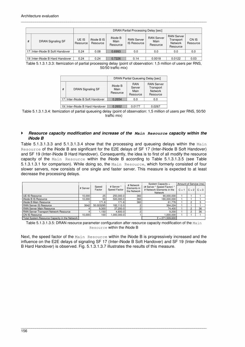
Architecture evaluation __________________________________________________________________________________________
__________________________________________________________________________________________ 156
DRAN Partial Processing Delay [sec]
# DRAN Signaling SF UE IS Resource
iNode B IS Resource
iNode B Main
Resource
RAN Server IS Resource
RAN Server Main
Resource
RAN Server Transport Network
Resource
CN IS Resource
17 Inter-iNode B Soft Handover 0.24 0.08 0.6993 0.0 0.0 0.0 0.0
19 Inter-iNode B Hard Handover 0.24 0.24 0.7226 0.14 0.0018 0.0122 0.03
Table 5.1.3.1.3.3: Itemization of partial processing delay (point of observation: 1,5 million of users per RNS, 50/50 traffic mix)
DRAN Partial Queueing Delay [sec]
# DRAN Signaling SF iNode B
Main Resource
RAN Server Main
Resource
RAN Server Transport Network
Resource
17 Inter-iNode B Soft Handover 0.2654 0.0 0.0
19 Inter-iNode B Hard Handover 0.2652 0.0177 0.0267
Table 5.1.3.1.3.4: Itemization of partial queueing delay (point of observation: 1,5 million of users per RNS, 50/50 traffic mix)
� Resource capacity modification and increase of the Main Resource capacity within the
iNode B
Table 5.1.3.1.3.3 and 5.1.3.1.3.4 show that the processing and queueing delays within the Main Resource of the iNode B are significant for the E2E delays of SF 17 (Inter-iNode B Soft Handover) and SF 19 (Inter-iNode B Hard Handover). Consequently, the idea is to first of all modify the resource capacity of the Main Resource within the iNode B according to Table 5.1.3.1.3.5 (see Table 5.1.3.1.3.1 for comparison). While doing so, the Main Resource, which formerly consisted of four slower servers, now consists of one single and faster server. This measure is expected to at least decrease the processing delays.
Amount of Service (ms)
# Server Speed Factor
# Server * Speed Factor
# Network Elements in the Network
System Capacity = (# Server * Speed Factor) * # Network Elements in the
Network C = 1 C = 2 C = 3
UE IS Resource 10,000 25 250,000.0 360 90,000,000 1 1 1 iNode B IS Resource 10,000 50 500,000.0 360 180,000,000 1 1 1 iNode B Main Resource 1 171.6 171.6 360 61,776 1 2 3 RAN Server IS Resource 3642 50.003295 182,112.0 2 364,224 1 1 1 RAN Server Main Resource 4 9,300 37,200.0 2 74,400 1 2 36 RAN Server Transport Network Resource 4 1,150 4,600.0 2 9,200 1 2 36 CN IS Resource 10,000 100 1,000,000.0 1 1,000,000 1 1 1 Total System Resource Capacity in the Network Σ = 271,509,600
Table 5.1.3.1.3.5: DRAN resource parameter configuration after resource capacity modification of the Main Resource within the iNode B
Next, the speed factor of the Main Resource within the iNode B is progressively increased and the influence on the E2E delays of signaling SF 17 (Inter-iNode B Soft Handover) and SF 19 (Inter-iNode B Hard Handover) is observed. Fig. 5.1.3.1.3.7 illustrates the results of this measure.

Architecture evaluation __________________________________________________________________________________________
__________________________________________________________________________________________ 157
Fig. 5.1.3.1.3.7: Speed increase of Main Resource within iNode B and impact on signaling E2E of SF 17 (Inter-iNode B Soft Handover) and SF 19 (Inter-iNode B Hard Handover) (50/50 traffic mix)
With regard to signaling SF 17 (Inter-iNode B Soft Handover), Fig. 5.1.3.1.3.7 shows that it was sufficient, when intending to have a signaling E2E delay less than 1 sec, to replace the four slower servers of the Main Resource within the iNode B with one faster server. Regarding SF 19 (Inter-iNode B Hard Handover), the speed factor increase of the Main Resource within the iNode B also improves the signaling E2E delay, and a further speed increase of the Main Resource within the iNode B might also be useful, when intending to decrease this delay to a value that is less than 1 sec.
� Resource reconfiguration of the Iui interface
However, a further speed increase of the Main Resource within the iNode B is not performed due to the fact that in consequence, this resource might be oversized at the operating point of the network, which is 1 million of users per RNS. Instead, another attempt is made which is a reconfiguration of the Iui Interface that is represented by the IS Resource of the RAN Server. Following [3GPP2003k], which particularly emphasizes potential drawbacks of new interfaces within the evolving RANs, a reconfiguration of the Iui interface is promising. In this case, the Iui interface is reconfigured so that the processing time for a single signaling message at the Iui interface is decreased from formerly 20 ms down to 1 ms. Provided that the processing time for a single signaling message is 1 ms at the Iui interface, the simulation experiment that increased the speed factor of the Main Resource within the iNode B is repeated. The result with regard to signaling SF 19 (Inter-iNode B Hard Handover) is displayed within Fig. 5.1.3.1.3.8.
0
0.2
0.4
0.6
0.8
1
1.2
1.4
1.6
161.6 181.6 201.6 221.6 241.6 261.6 281.6 301.6 321.6
iNode B Main Resource Speed
E2E
Del
ay [s
ec]
SF 17: Inter-iNode B Soft Handover SF 19: Inter-iNode B Hard Handover

Architecture evaluation __________________________________________________________________________________________
__________________________________________________________________________________________ 158
Fig. 5.1.3.1.3.8: Reconfigured Iui interface and speed increase of Main Resource within iNode B and impact on signaling E2E of SF 19 (Inter-iNode B Hard Handover) (50/50 traffic mix)
According to Fig. 5.1.3.1.3.8, it was advantageous to reconfigure the Iui interface, because with the combination of the reconfigured Iui interface and a speed increase of the Main Resource within the iNode B, the aim of an E2E signaling delay of the Inter-iNode B Hard Handover signaling SF that is less than 1 sec is achieved. Table 5.1.3.1.3.6 illustrates the final resource parameter configuration of DRAN, after completion of the optimization process.
Amount of Service (ms)
# Server Speed Factor
# Server * Speed Factor
# Network Elements in the Network
System Capacity = (# Server * Speed Factor) * # Network Elements in the
Network C = 1 C = 2 C = 3
UE IS Resource 10,000 25 250,000.0 360 90,000,000 1 1 1 iNode B IS Resource 10,000 50 500,000.0 360 180,000,000 1 1 1 iNode B Main Resource 1 271.6 271.6 360 97,776 1 2 3 RAN Server IS Resource 164 1000.68292 164,112.0 2 328,224 1 1 1 RAN Server Main Resource 4 9,300 37,200.0 2 74,400 1 2 36 RAN Server Transport Network Resource 4 1,150 4,600.0 2 9,200 1 2 36 CN IS Resource 10,000 100 1,000,000.0 1 1,000,000 1 1 1 Total System Resource Capacity in the Network Σ = 271,509,600
Table 5.1.3.1.3.6: Final DRAN resource parameter configuration after optimization Table 5.1.3.1.3.7 shows the signaling E2E delays for all SFs at the operating point of the network, if the resource parameter configuration is applied according to Table 5.1.3.1.3.6. None of the E2E signaling delay results in Table 5.1.3.1.3.7 violates the defined service levels of Table 5.1.1.2.4.
0
0.2
0.4
0.6
0.8
1
1.2
1.4
1.6
161.6 181.6 201.6 221.6 241.6 261.6 281.6 301.6 321.6
iNode B Main Resource Speed
E2E
Del
ay [s
ec]
SF 17: Inter-iNode B Hard Handover
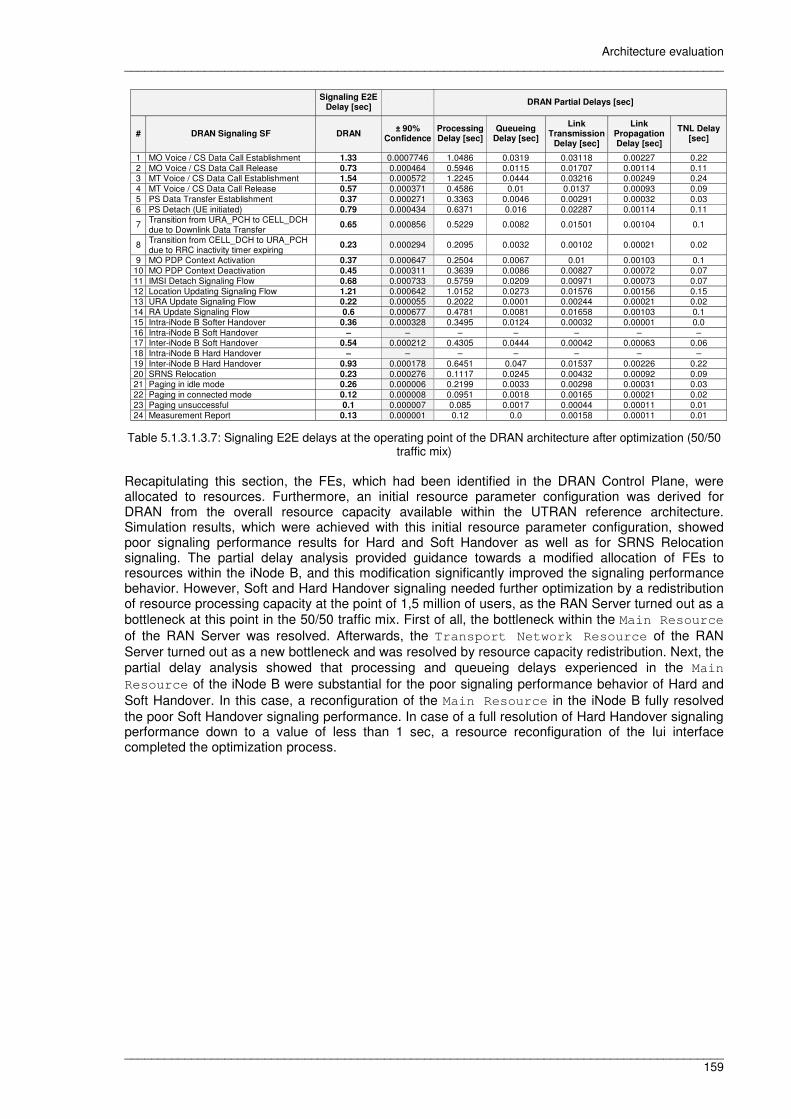
Architecture evaluation __________________________________________________________________________________________
__________________________________________________________________________________________ 159
Signaling E2E
Delay [sec]
DRAN Partial Delays [sec]
# DRAN Signaling SF DRAN ± 90%
Confidence Processing Delay [sec]
Queueing Delay [sec]
Link Transmission
Delay [sec]
Link Propagation Delay [sec]
TNL Delay [sec]
1 MO Voice / CS Data Call Establishment 1.33 0.0007746 1.0486 0.0319 0.03118 0.00227 0.22 2 MO Voice / CS Data Call Release 0.73 0.000464 0.5946 0.0115 0.01707 0.00114 0.11 3 MT Voice / CS Data Call Establishment 1.54 0.000572 1.2245 0.0444 0.03216 0.00249 0.24 4 MT Voice / CS Data Call Release 0.57 0.000371 0.4586 0.01 0.0137 0.00093 0.09 5 PS Data Transfer Establishment 0.37 0.000271 0.3363 0.0046 0.00291 0.00032 0.03 6 PS Detach (UE initiated) 0.79 0.000434 0.6371 0.016 0.02287 0.00114 0.11
7 Transition from URA_PCH to CELL_DCH due to Downlink Data Transfer
0.65 0.000856 0.5229 0.0082 0.01501 0.00104 0.1
8 Transition from CELL_DCH to URA_PCH due to RRC inactivity timer expiring
0.23 0.000294 0.2095 0.0032 0.00102 0.00021 0.02
9 MO PDP Context Activation 0.37 0.000647 0.2504 0.0067 0.01 0.00103 0.1 10 MO PDP Context Deactivation 0.45 0.000311 0.3639 0.0086 0.00827 0.00072 0.07 11 IMSI Detach Signaling Flow 0.68 0.000733 0.5759 0.0209 0.00971 0.00073 0.07 12 Location Updating Signaling Flow 1.21 0.000642 1.0152 0.0273 0.01576 0.00156 0.15 13 URA Update Signaling Flow 0.22 0.000055 0.2022 0.0001 0.00244 0.00021 0.02 14 RA Update Signaling Flow 0.6 0.000677 0.4781 0.0081 0.01658 0.00103 0.1 15 Intra-iNode B Softer Handover 0.36 0.000328 0.3495 0.0124 0.00032 0.00001 0.0 16 Intra-iNode B Soft Handover – – – – – – – 17 Inter-iNode B Soft Handover 0.54 0.000212 0.4305 0.0444 0.00042 0.00063 0.06 18 Intra-iNode B Hard Handover – – – – – – – 19 Inter-iNode B Hard Handover 0.93 0.000178 0.6451 0.047 0.01537 0.00226 0.22 20 SRNS Relocation 0.23 0.000276 0.1117 0.0245 0.00432 0.00092 0.09 21 Paging in idle mode 0.26 0.000006 0.2199 0.0033 0.00298 0.00031 0.03 22 Paging in connected mode 0.12 0.000008 0.0951 0.0018 0.00165 0.00021 0.02 23 Paging unsuccessful 0.1 0.000007 0.085 0.0017 0.00044 0.00011 0.01 24 Measurement Report 0.13 0.000001 0.12 0.0 0.00158 0.00011 0.01
Table 5.1.3.1.3.7: Signaling E2E delays at the operating point of the DRAN architecture after optimization (50/50 traffic mix)
Recapitulating this section, the FEs, which had been identified in the DRAN Control Plane, were allocated to resources. Furthermore, an initial resource parameter configuration was derived for DRAN from the overall resource capacity available within the UTRAN reference architecture. Simulation results, which were achieved with this initial resource parameter configuration, showed poor signaling performance results for Hard and Soft Handover as well as for SRNS Relocation signaling. The partial delay analysis provided guidance towards a modified allocation of FEs to resources within the iNode B, and this modification significantly improved the signaling performance behavior. However, Soft and Hard Handover signaling needed further optimization by a redistribution of resource processing capacity at the point of 1,5 million of users, as the RAN Server turned out as a bottleneck at this point in the 50/50 traffic mix. First of all, the bottleneck within the Main Resource of the RAN Server was resolved. Afterwards, the Transport Network Resource of the RAN Server turned out as a new bottleneck and was resolved by resource capacity redistribution. Next, the partial delay analysis showed that processing and queueing delays experienced in the Main Resource of the iNode B were substantial for the poor signaling performance behavior of Hard and Soft Handover. In this case, a reconfiguration of the Main Resource in the iNode B fully resolved the poor Soft Handover signaling performance. In case of a full resolution of Hard Handover signaling performance down to a value of less than 1 sec, a resource reconfiguration of the Iui interface completed the optimization process.

Architecture evaluation __________________________________________________________________________________________
__________________________________________________________________________________________ 160
5.2 Comparison of signaling performance and efficiency
In this section, the calibrated RAN architectures will be studied within various simulation experiments. In the subsequent section a preview on the upcoming simulation experiments is provided at first.
5.2.1 Preview on upcoming simulation experiments
With regard to the RAN architecture evolution scenarios, the question is whether these scenarios show a comparable, better or worse signaling performance behavior than the UTRAN reference architecture by providing a resource capacity that equals the overall resource capacity within UTRAN in Table 5.1.1.1.1. In the upcoming experiments, the RAN evolution scenarios of interest are studied under varying conditions. Despite the variation of the number of users within a single RNS, the portion of voice and data traffic is varied, i.e. three traffic mixes are simulated which are the • 50/50 traffic mix, i.e. the portion of voice and data traffic equals 50% each • 80/20 traffic mix, i.e. the portion of voice traffic equals 80% and the portion of data traffic is 20% • 20/80 traffic mix, i.e. the portion of voice traffic is 20% and the portion of data traffic equals 80%. As future mobile networks presume higher portions of data traffic than voice traffic (cf. [3GPP2003k]), the focus in this chapter will be on simulation results gathered within the 20/80 traffic mix, when comparing the signaling performance behavior within the RAN evolution scenarios to the UTRAN reference architecture. Table 5.2.1.1 provides a survey with regard to the instantiation of the signaling SFs necessary for MO / MT call setup initiation and MO PDP context activation for PS services. In this table the mean number of instantiations of these signaling SFs per minute is provided for all traffic mixes at the operating point of the network which is with 1 million of users. The given values apply to the UTRAN reference architecture as well as to the RAN evolution scenarios of interest which are studied in this chapter. In this context, it has to be considered that MO signaling SFs refer to a single radio cell. This means that the overall invocation rate of all signaling SFs, originating at a particular UE, is divided by the number of UEs considered per RNS, and the reciprocal value of this ratio provides the interarrival time of the signaling SF. The reason for this operation is the fact that the traffic model for UTRAN service mix derivation provides invocation rates that apply for a single RNS under consideration of a certain number of users within this particular RNS. In this case, 180 UEs / radio cells or base stations are assumed for a single RNS, and two RNSs are assumed in the network topologies under study. Moreover, it has to be considered that the MT signaling SFs consider the overall SHRiNK factor of the network topology under study. This SHRiNK factor is derived under consideration of the assumed number of UEs / radio cells and base stations in the network (i.e. 360) and the number of UEs / radio cells / base stations which are explicitly modeled (i.e. 4), and corresponds to the reciprocal value of this ratio.
Mean Number of Signaling SF Instantiations per Minute
Traffic Mix # Signaling SF 50/50 80/20 20/80 1 MO Voice / CS Data Call Establishment 19 31 7 3 MT Voice / CS Data Call Establishment 16 26 6
9 MO PDP Context Activation(from PMM_CONNECTED+Cell_DCH)
4 1 7
Table 5.2.1.1: Mean number of instantiations per minute for particular signaling SFs
Besides, in this section, the sensitivity of the UTRAN reference architecture and the RAN evolution scenarios towards other parameter variations than the number of users per RNS is of interest. Thus, the behavior of the RANs is studied, if • the latency of the IP-based transport network is varied. • the base stations are fully meshed. • the systems are exposed to sudden load impulses. • the mobility of the users changes.
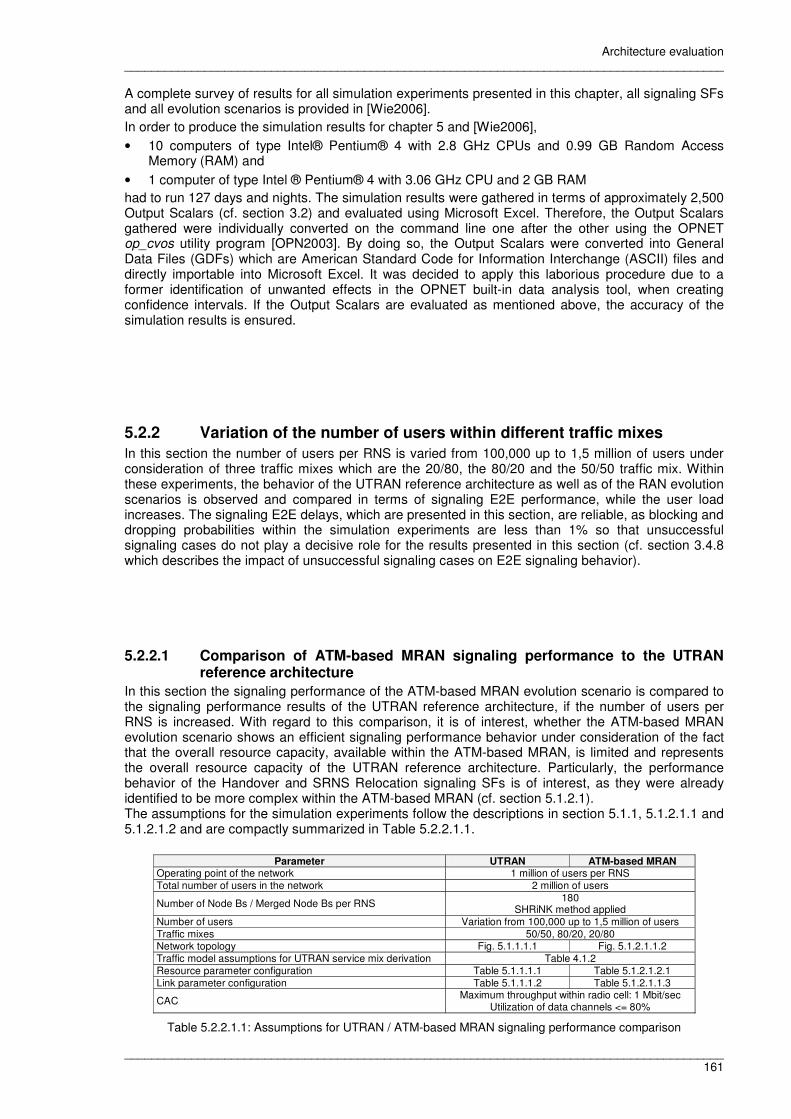
Architecture evaluation __________________________________________________________________________________________
__________________________________________________________________________________________ 161
A complete survey of results for all simulation experiments presented in this chapter, all signaling SFs and all evolution scenarios is provided in [Wie2006]. In order to produce the simulation results for chapter 5 and [Wie2006], • 10 computers of type Intel® Pentium® 4 with 2.8 GHz CPUs and 0.99 GB Random Access
Memory (RAM) and • 1 computer of type Intel ® Pentium® 4 with 3.06 GHz CPU and 2 GB RAM had to run 127 days and nights. The simulation results were gathered in terms of approximately 2,500 Output Scalars (cf. section 3.2) and evaluated using Microsoft Excel. Therefore, the Output Scalars gathered were individually converted on the command line one after the other using the OPNET op_cvos utility program [OPN2003]. By doing so, the Output Scalars were converted into General Data Files (GDFs) which are American Standard Code for Information Interchange (ASCII) files and directly importable into Microsoft Excel. It was decided to apply this laborious procedure due to a former identification of unwanted effects in the OPNET built-in data analysis tool, when creating confidence intervals. If the Output Scalars are evaluated as mentioned above, the accuracy of the simulation results is ensured.
5.2.2 Variation of the number of users within different traffic mixes
In this section the number of users per RNS is varied from 100,000 up to 1,5 million of users under consideration of three traffic mixes which are the 20/80, the 80/20 and the 50/50 traffic mix. Within these experiments, the behavior of the UTRAN reference architecture as well as of the RAN evolution scenarios is observed and compared in terms of signaling E2E performance, while the user load increases. The signaling E2E delays, which are presented in this section, are reliable, as blocking and dropping probabilities within the simulation experiments are less than 1% so that unsuccessful signaling cases do not play a decisive role for the results presented in this section (cf. section 3.4.8 which describes the impact of unsuccessful signaling cases on E2E signaling behavior). 5.2.2.1 Comparison of ATM-based MRAN signaling performance to the UTRAN
reference architecture
In this section the signaling performance of the ATM-based MRAN evolution scenario is compared to the signaling performance results of the UTRAN reference architecture, if the number of users per RNS is increased. With regard to this comparison, it is of interest, whether the ATM-based MRAN evolution scenario shows an efficient signaling performance behavior under consideration of the fact that the overall resource capacity, available within the ATM-based MRAN, is limited and represents the overall resource capacity of the UTRAN reference architecture. Particularly, the performance behavior of the Handover and SRNS Relocation signaling SFs is of interest, as they were already identified to be more complex within the ATM-based MRAN (cf. section 5.1.2.1). The assumptions for the simulation experiments follow the descriptions in section 5.1.1, 5.1.2.1.1 and 5.1.2.1.2 and are compactly summarized in Table 5.2.2.1.1.
Parameter UTRAN ATM-based MRAN Operating point of the network 1 million of users per RNS Total number of users in the network 2 million of users
Number of Node Bs / Merged Node Bs per RNS 180 SHRiNK method applied
Number of users Variation from 100,000 up to 1,5 million of users Traffic mixes 50/50, 80/20, 20/80 Network topology Fig. 5.1.1.1.1 Fig. 5.1.2.1.1.2 Traffic model assumptions for UTRAN service mix derivation Table 4.1.2 Resource parameter configuration Table 5.1.1.1.1 Table 5.1.2.1.2.1 Link parameter configuration Table 5.1.1.1.2 Table 5.1.2.1.1.3
CAC Maximum throughput within radio cell: 1 Mbit/sec Utilization of data channels <= 80%
Table 5.2.2.1.1: Assumptions for UTRAN / ATM-based MRAN signaling performance comparison
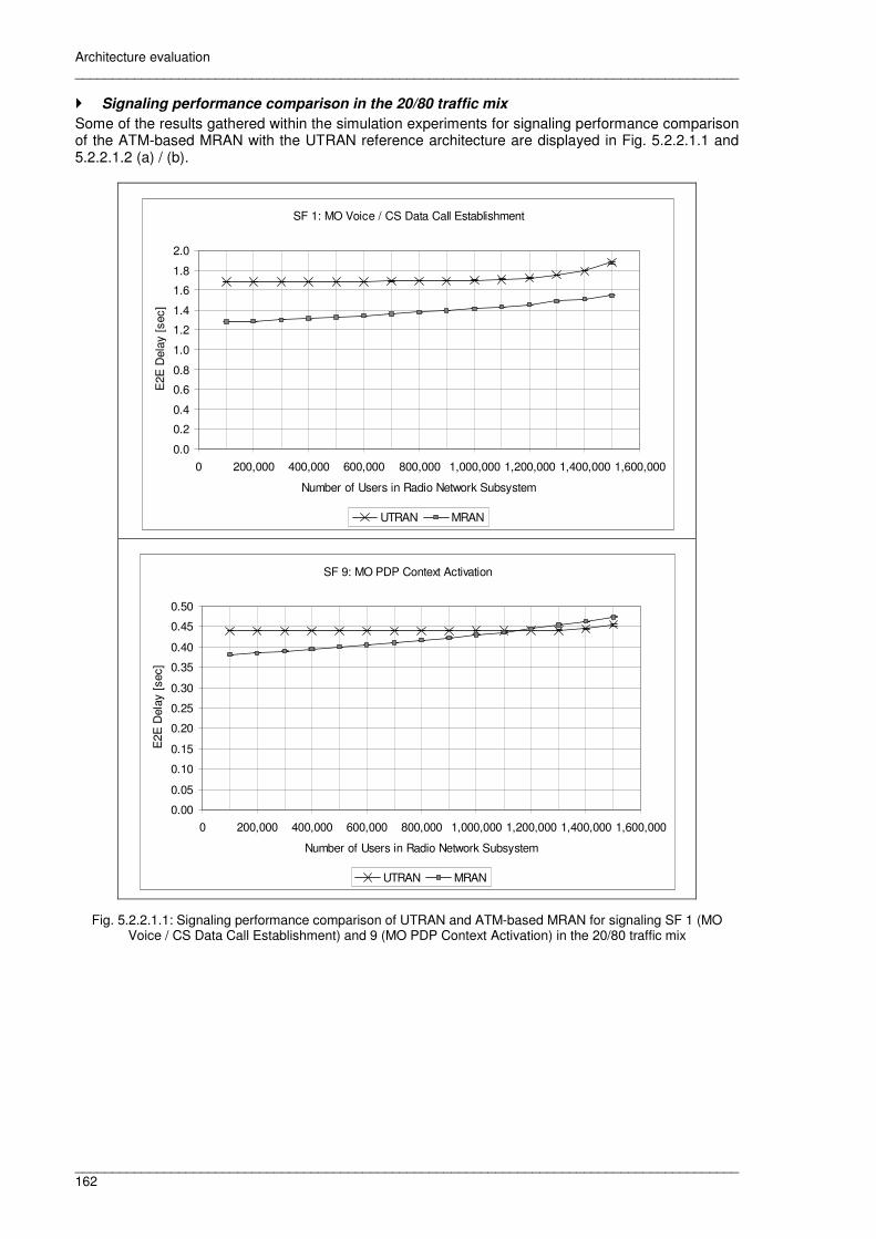
Architecture evaluation __________________________________________________________________________________________
__________________________________________________________________________________________ 162
� Signaling performance comparison in the 20/80 traffic mix
Some of the results gathered within the simulation experiments for signaling performance comparison of the ATM-based MRAN with the UTRAN reference architecture are displayed in Fig. 5.2.2.1.1 and 5.2.2.1.2 (a) / (b).
Fig. 5.2.2.1.1: Signaling performance comparison of UTRAN and ATM-based MRAN for signaling SF 1 (MO Voice / CS Data Call Establishment) and 9 (MO PDP Context Activation) in the 20/80 traffic mix
SF 1: MO Voice / CS Data Call Establishment
0.0
0.2
0.4
0.6
0.8
1.0
1.2
1.4
1.6
1.8
2.0
0 200,000 400,000 600,000 800,000 1,000,000 1,200,000 1,400,000 1,600,000
Number of Users in Radio Network Subsystem
E2E
Del
ay [
sec]
UTRAN MRAN
SF 9: MO PDP Context Activation
0.00
0.05
0.10
0.15
0.20
0.25
0.30
0.35
0.40
0.45
0.50
0 200,000 400,000 600,000 800,000 1,000,000 1,200,000 1,400,000 1,600,000
Number of Users in Radio Network Subsystem
E2E
Del
ay [
sec]
UTRAN MRAN

Architecture evaluation __________________________________________________________________________________________
__________________________________________________________________________________________ 163
Fig. 5.2.2.1.2 (a): Signaling performance comparison of UTRAN and ATM-based MRAN for signaling SF 15 (Softer Handover) and 17 (Soft Handover) in the 20/80 traffic mix
SF 15: Intra-RNC / -Merged Node B Softer Handover
0.0
0.1
0.2
0.3
0.4
0.5
0.6
0.7
0.8
0.9
0 200,000 400,000 600,000 800,000 1,000,000 1,200,000 1,400,000 1,600,000
Number of Users in Radio Network Subsystem
E2E
Del
ay [
sec]
UTRAN MRAN
SF 17: Inter-RNC / -Merged Node B Soft Handover
0.0
0.2
0.4
0.6
0.8
1.0
1.2
1.4
0 200,000 400,000 600,000 800,000 1,000,000 1,200,000 1,400,000 1,600,000
Number of Users in Radio Network Subsystem
E2E
Del
ay [
sec]
UTRAN MRAN
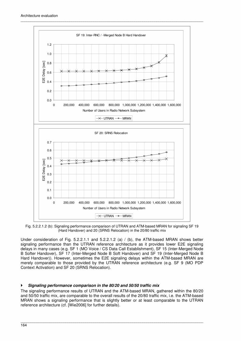
Architecture evaluation __________________________________________________________________________________________
__________________________________________________________________________________________ 164
Fig. 5.2.2.1.2 (b): Signaling performance comparison of UTRAN and ATM-based MRAN for signaling SF 19 (Hard Handover) and 20 (SRNS Relocation) in the 20/80 traffic mix
Under consideration of Fig. 5.2.2.1.1 and 5.2.2.1.2 (a) / (b), the ATM-based MRAN shows better signaling performance than the UTRAN reference architecture as it provides lower E2E signaling delays in many cases (e.g. SF 1 (MO Voice / CS Data Call Establishment), SF 15 (Inter-Merged Node B Softer Handover), SF 17 (Inter-Merged Node B Soft Handover) and SF 19 (Inter-Merged Node B Hard Handover)). However, sometimes the E2E signaling delays within the ATM-based MRAN are merely comparable to those provided by the UTRAN reference architecture (e.g. SF 9 (MO PDP Context Activation) and SF 20 (SRNS Relocation).
� Signaling performance comparison in the 80/20 and 50/50 traffic mix
The signaling performance results of UTRAN and the ATM-based MRAN, gathered within the 80/20 and 50/50 traffic mix, are comparable to the overall results of the 20/80 traffic mix, i.e. the ATM-based MRAN shows a signaling performance that is slightly better or at least comparable to the UTRAN reference architecture (cf. [Wie2006] for further details).
SF 20: SRNS Relocation
0.0
0.1
0.2
0.3
0.4
0.5
0.6
0.7
0 200,000 400,000 600,000 800,000 1,000,000 1,200,000 1,400,000 1,600,000
Number of Users in Radio Network Subsystem
E2E
Del
ay [
sec]
UTRAN MRAN
SF 19: Inter-RNC / -Merged Node B Hard Handover
0.0
0.2
0.4
0.6
0.8
1.0
1.2
0 200,000 400,000 600,000 800,000 1,000,000 1,200,000 1,400,000 1,600,000
Number of Users in Radio Network Subsystem
E2E
Del
ay [
sec]
UTRAN MRAN

Architecture evaluation __________________________________________________________________________________________
__________________________________________________________________________________________ 165
Moreover, in the 50/50 traffic mix the ATM-based MRAN still provides stable E2E delays, if the number of users per RNS equals 1,5 million [Wie2006]. Unlike MRAN, the UTRAN reference architecture is already instable at this point (cf. section 5.1.1.2). As a conclusion of this section, which compared the signaling performance of the ATM-based MRAN and the UTRAN reference architecture for three different traffic mixes and an increasing number of users per RNS, it is realized that the ATM-based MRAN showed an efficient signaling performance behavior. This conclusion also applies to the Handover and SRNS Relocation signaling SFs within the ATM-based MRAN, which were already identified to be more complex. In this context, the resource capacity applied within the UTRAN reference network architecture is also sufficient for the ATM-based MRAN. 5.2.2.2 Comparison of IP-based MRAN signaling performance to the UTRAN
reference architecture
This section presents the comparison of the IP-based MRAN evolution scenario and the UTRAN reference architecture with regard to E2E signaling performance, if the number of users per RNS is increased. In this case, it is of interest, whether an IP-based MRAN evolution scenario will still perform efficiently with regard to signaling performance, when contrasted to the UTRAN reference architecture, under consideration of the fact that the available resource capacity is again the same in both architectures and an IP-based transport network is applied. Particularly, the behavior of the Handover and SRNS Relocation SFs is interesting to be observed, when the transport network is assumed to be IP-based. The assumptions for the intended simulation experiments follow the descriptions in section 5.1.1, 5.1.2.2.1 and 5.1.2.2.2 and are briefly summarized in Table 5.2.2.2.1. With regard to the delay, a single signaling message experiences by passing the TNL cloud within the IP-based MRAN simulation model, the value of this delay is varied, i.e. one experiment assumes a TNL delay of 10 ms and a second experiment assumes a TNL delay of 100 ms. In this context, a delay value of 5 ms to 10 ms can be assumed in urban areas, and a TNL delay of 100 ms might occur in the countryside.
Parameter UTRAN IP-based MRAN Operating point of the network 1 million of users per RNS Total number of users in the network 2 million of users
Number of Node Bs / Merged Node Bs per RNS 180 SHRiNK method applied
Number of users Variation from 100,000 up to 1,5 million of users Traffic mixes 50/50, 80/20, 20/80 Network topology Fig. 5.1.1.1.1 Fig. 5.1.2.2.1.1 Traffic model assumptions for UTRAN service mix derivation Table 4.1.2 Resource parameter configuration Table 5.1.1.1.1 Table 5.1.2.2.2.1 Link parameter configuration Table 5.1.1.1.2 Table 5.1.2.2.1.1
CAC Maximum throughput within radio cell: 1 Mbit/sec Utilization of data channels <= 80%
TNL delay per signaling message – 10 ms 100 ms
Table 5.2.2.2.1: Assumptions for UTRAN / IP-based MRAN signaling performance comparison
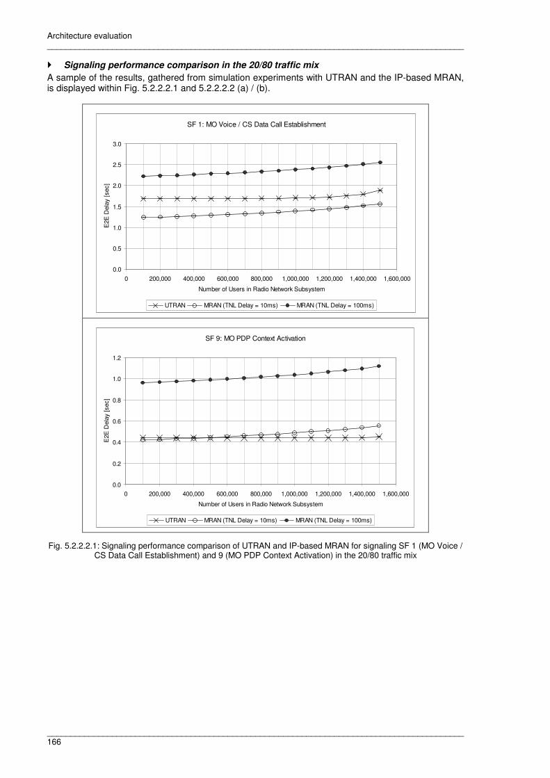
Architecture evaluation __________________________________________________________________________________________
__________________________________________________________________________________________ 166
� Signaling performance comparison in the 20/80 traffic mix
A sample of the results, gathered from simulation experiments with UTRAN and the IP-based MRAN, is displayed within Fig. 5.2.2.2.1 and 5.2.2.2.2 (a) / (b).
Fig. 5.2.2.2.1: Signaling performance comparison of UTRAN and IP-based MRAN for signaling SF 1 (MO Voice / CS Data Call Establishment) and 9 (MO PDP Context Activation) in the 20/80 traffic mix
SF 1: MO Voice / CS Data Call Establishment
0.0
0.5
1.0
1.5
2.0
2.5
3.0
0 200,000 400,000 600,000 800,000 1,000,000 1,200,000 1,400,000 1,600,000
Number of Users in Radio Network Subsystem
E2E
Del
ay [s
ec]
UTRAN MRAN (TNL Delay = 10ms) MRAN (TNL Delay = 100ms)
SF 9: MO PDP Context Activation
0.0
0.2
0.4
0.6
0.8
1.0
1.2
0 200,000 400,000 600,000 800,000 1,000,000 1,200,000 1,400,000 1,600,000
Number of Users in Radio Network Subsystem
E2E
Del
ay [s
ec]
UTRAN MRAN (TNL Delay = 10ms) MRAN (TNL Delay = 100ms)

Architecture evaluation __________________________________________________________________________________________
__________________________________________________________________________________________ 167
Fig. 5.2.2.2.2 (a): Signaling performance comparison of UTRAN and IP-based MRAN for signaling SF 15 (Softer Handover) and 17 (Soft Handover) in the 20/80 traffic mix
SF 15: Intra-RNC / -Merged Node B Softer Handover
0.0
0.1
0.2
0.3
0.4
0.5
0.6
0.7
0.8
0.9
0 200,000 400,000 600,000 800,000 1,000,000 1,200,000 1,400,000 1,600,000
Number of Users in Radio Network Subsystem
E2E
Del
ay [s
ec]
UTRAN MRAN (TNL Delay = 10ms) MRAN (TNL Delay = 100ms)
SF 17: Inter-RNC / -Merged Node B Soft Handover
0.0
0.2
0.4
0.6
0.8
1.0
1.2
1.4
1.6
0 200,000 400,000 600,000 800,000 1,000,000 1,200,000 1,400,000 1,600,000
Number of Users in Radio Network Subsystem
E2E
Del
ay [s
ec]
UTRAN MRAN (TNL Delay = 10ms) MRAN (TNL Delay = 100ms)

Architecture evaluation __________________________________________________________________________________________
__________________________________________________________________________________________ 168
Fig. 5.2.2.2.2 (b): Signaling performance comparison of UTRAN and IP-based MRAN for signaling SF 19 (Hard Handover) and 20 (SRNS Relocation) in the 20/80 traffic mix
With regard to the signaling E2E delays of the SFs illustrated in Fig. 5.2.2.2.1 and 5.2.2.2.2 (a) / (b), the IP-based MRAN evolution scenario provides an E2E signaling performance that is very similar to the ATM-based MRAN scenario. This means that the IP-based MRAN provides a signaling performance which is better or at least comparable to signaling performance provided by the UTRAN reference architecture, and this basically applies for those simulation experiments that assume a TNL delay of 10 ms. If the TNL delay is assumed to be 100 ms, the IP-based MRAN performs significantly worse than the UTRAN reference architecture. This observation also applies to the handover signaling SFs and SRNS Relocation, but SF 15 (Intra-Merged Node B Softer Handover) is exceptional to this (cf. Fig. 5.2.2.2.2 (a)), i.e. the E2E delay of the Intra-Merged Node B Softer Handover is significantly better within the IP-based MRAN than within the UTRAN reference architecture, and this E2E delay is independent of the TNL delay, because it simply involves one single Merged Node B and does not imply communication with a drift Merged Node B.
SF 19: Inter-RNC / -Merged Node B Hard Handover
0.0
0.2
0.4
0.6
0.8
1.0
1.2
0 200,000 400,000 600,000 800,000 1,000,000 1,200,000 1,400,000 1,600,000
Number of Users in Radio Network Subsystem
E2E
Del
ay [s
ec]
UTRAN MRAN (TNL Delay = 10ms) MRAN (TNL Delay = 100ms)
SF 20: SRNS Relocation
0.0
0.2
0.4
0.6
0.8
1.0
1.2
1.4
1.6
1.8
0 200,000 400,000 600,000 800,000 1,000,000 1,200,000 1,400,000 1,600,000
Number of Users in Radio Network Subsystem
E2E
Del
ay [s
ec]
UTRAN MRAN (TNL Delay = 10ms) MRAN (TNL Delay = 100ms)

Architecture evaluation __________________________________________________________________________________________
__________________________________________________________________________________________ 169
� Signaling performance comparison in the 80/20 and 50/50 traffic mix
The results of a signaling performance comparison of the UTRAN reference architecture and the IP-based MRAN within the 80/20 traffic mix are comparable to the results gathered within the 20/80 traffic mix (cf. [Wie2006]). If the 50/50 traffic mix is considered, the IP-based MRAN evolution scenario also provides stable delays and an E2E signaling performance that is comparable to the UTRAN reference architecture, when the TNL delay is assumed to be 10 ms (cf. [Wie2006]). To resume this section, which compared the signaling performance of the IP-based MRAN and the UTRAN reference architecture within three different traffic mixes and an increasing number of users per RNS, the IP-based MRAN also showed an efficient signaling performance behavior, provided that the delay resulting from the IP-based transport network is low. This conclusion also applies to the more complex Handover and SRNS Relocation signaling SFs within the IP-based MRAN. In this context, the resource capacity of the UTRAN reference network architecture also turned out to be sufficient for the IP-based MRAN. 5.2.2.3 Comparison of DRAN signaling performance to the UTRAN reference
architecture
In this section the signaling performance of DRAN is compared to the signaling performance results of the UTRAN reference architecture, if the number of users per RNS is increased. The assumptions for the simulation experiments follow the descriptions in section 5.1.1, 5.1.3.1.1, 5.1.3.1.2 and 5.1.3.1.3 and are shortly summarized in Table 5.2.2.3.1. The value of the TNL delay is also varied, i.e. one experiment assumes a delay of 10 ms (within urban areas) and a second experiment assumes a TNL delay of 100 ms (in the countryside).
Parameter UTRAN DRAN Operating point of the network 1 million of users per RNS Total number of users in the network 2 million of users
Number of Node Bs / Merged Node Bs per RNS 180 SHRiNK method applied
Number of users Variation from 100,000 up to 1,5 million of users Traffic mixes 50/50, 80/20, 20/80 Network topology Fig. 5.1.1.1.1 Fig. 5.1.3.1.1.2 Traffic model assumptions for UTRAN service mix derivation Table 4.1.2 Resource parameter configuration Table 5.1.1.1.1 Table 5.1.3.1.3.6 Link parameter configuration Table 5.1.1.1.2 Table 5.1.3.1.1.2
CAC Maximum throughput within radio cell: 1 Mbit/sec Utilization of data channels <= 80%
TNL delay per signaling message – 10 ms 100 ms
Table 5.2.2.3.1: Assumptions for UTRAN / DRAN signaling performance comparison
� Signaling performance comparison in the 20/80 traffic mix
When comparing the E2E signaling performance in UTRAN and DRAN by variation of the number of users per RNS, it is of interest, whether DRAN shows a comparable, significantly better or worse performance behavior than the UTRAN reference architecture under consideration of the fact that the available resource capacity is the same in both architectures. Particularly, the behavior of the handover signaling SFs is of interest, as these signaling procedures are already assumed to be more complex. Moreover, it is interesting to compare the behavior of DRAN with regard to the different traffic mixes, as DRAN is an evolution scenario that was specifically designed under the assumption of an increasing portion of data traffic [3GPP2003k]. A sample of the results, gathered from simulation experiments with UTRAN and DRAN in the 20/80 traffic mix, is displayed within Fig. 5.2.2.3.1, 5.2.2.3.2 (a) / (b) and 5.2.2.3.3.

Architecture evaluation __________________________________________________________________________________________
__________________________________________________________________________________________ 170
Fig. 5.2.2.3.1: Signaling performance comparison of UTRAN and DRAN for signaling SF 1 (MO Voice / CS Data Call Establishment) and 9 (MO PDP Context Activation) in the 20/80 traffic mix
Fig. 5.2.2.3.1 shows that the DRAN scenario with a TNL delay of 10 ms definitely provides slightly better E2E signaling performance, if the portion of data traffic is the dominating traffic portion within the network. If the TNL delay is assumed with 100 ms, DRAN provides worse signaling performance results than the UTRAN reference architecture. This underlines the optimization issue of the transport network within a distributed and IP-based architecture. However, while the graphs of the E2E signaling delays within UTRAN already show the beginning instability of the network at varying numbers of users, DRAN provides stable delays. Fig 5.2.2.3.2 (a) and (b) provide similar results for the handover signaling SFs as well as for SRNS Relocation.
SF 1: MO Voice / CS Data Call Establishment
0.0
0.5
1.0
1.5
2.0
2.5
3.0
3.5
0 200,000 400,000 600,000 800,000 1,000,000 1,200,000 1,400,000 1,600,000
Number of Users in Radio Network Subsystem
E2E
Del
ay [s
ec]
UTRAN DRAN (TNL Delay = 10ms) DRAN (TNL Delay = 100ms)
SF 9: MO PDP Context Activation
0.0
0.2
0.4
0.6
0.8
1.0
1.2
1.4
0 200,000 400,000 600,000 800,000 1,000,000 1,200,000 1,400,000 1,600,000
Number of Users in Radio Network Subsystem
E2E
Del
ay [s
ec]
UTRAN DRAN (TNL Delay = 10ms) DRAN (TNL Delay = 100ms)

Architecture evaluation __________________________________________________________________________________________
__________________________________________________________________________________________ 171
Fig. 5.2.2.3.2 (a): Signaling performance comparison of UTRAN and DRAN for signaling SF 15 (Softer Handover) and 17 (Soft Handover) in the 20/80 traffic mix
SF 15: Intra-RNC / -iNode B Softer Handover
0.0
0.1
0.2
0.3
0.4
0.5
0.6
0.7
0.8
0.9
0 200,000 400,000 600,000 800,000 1,000,000 1,200,000 1,400,000 1,600,000
Number of Users in Radio Network Subsystem
E2E
Del
ay [s
ec]
UTRAN DRAN (TNL Delay = 10ms) DRAN (TNL Delay = 100ms)
SF 17: Inter-RNC / -iNode B Soft Handover
0.0
0.2
0.4
0.6
0.8
1.0
1.2
1.4
0 200,000 400,000 600,000 800,000 1,000,000 1,200,000 1,400,000 1,600,000
Number of Users in Radio Network Subsystem
E2E
Del
ay [s
ec]
UTRAN DRAN (TNL Delay = 10ms) DRAN (TNL Delay = 100ms)

Architecture evaluation __________________________________________________________________________________________
__________________________________________________________________________________________ 172
Fig. 5.2.2.3.2 (b): Signaling performance comparison of UTRAN and DRAN for the signaling SF 19 (Hard Handover) and 20 (SRNS Relocation) in the 20/80 traffic mix
With regard to the Intra-iNode B Softer Handover (cf. Fig. 5.2.2.3.2 (a)), DRAN definitely provides better signaling performance values than the UTRAN reference architecture, and the same applies for the Inter-iNode B Soft Handover and SRNS Relocation (cf. Fig. 5.2.2.3.2 (a) and (b)) in those experiments, when the TNL delay is set to a value of 10 ms. With regard to the Intra-iNode B Softer Handover, there is no difference between a TNL of 10 ms or 100 ms, because a Softer Handover simply involves one single iNode B so that the TNL cloud does not have to be passed in order to reach a second iNode B. The E2E delay of the Inter-iNode B Hard Handover signaling SF in DRAN is a little bit worse than the signaling delay of the Inter-RNC Hard Handover SF in UTRAN. Table 5.2.2.3.2 shows that this difference is basically caused by the transport network, as processing and queueing delays are very similar for this signaling SF in UTRAN and DRAN. This also raises the question, why the transport network more negatively impacts the Inter-iNode B Hard Handover than the Inter-iNode B Soft Handover signaling SF in DRAN. The answer to this question is that iNode Bs are able to handle Soft Handover signaling autonomously, but need interaction with the RAN Server and also with the CN for
SF 19: Inter-RNC / -iNode B Hard Handover
0.0
0.5
1.0
1.5
2.0
2.5
3.0
3.5
0 200,000 400,000 600,000 800,000 1,000,000 1,200,000 1,400,000 1,600,000
Number of Users in Radio Network Subsystem
E2E
Del
ay [s
ec]
UTRAN DRAN (TNL Delay = 10ms) DRAN (TNL Delay = 100ms)
SF 20: SRNS Relocation
0.0
0.2
0.4
0.6
0.8
1.0
1.2
0 200,000 400,000 600,000 800,000 1,000,000 1,200,000 1,400,000 1,600,000
Number of Users in Radio Network Subsystem
E2E
Del
ay [s
ec]
UTRAN DRAN (TNL Delay = 10ms) DRAN (TNL Delay = 100ms)

Architecture evaluation __________________________________________________________________________________________
__________________________________________________________________________________________ 173
resource reservation purposes and relocation of the termination point for the User Plane in case of Hard Handover which implies additional passages of the transport network.
Partial Delays [sec]
19 Inter-RNC / -iNode B Hard
Handover Signaling E2E
Delay [sec] Processing Delay [sec]
Queueing Delay [sec]
Link Transmission
Delay [sec]
Link Propagation Delay [sec]
TNL Delay [sec]
UTRAN 0.66 0.6231 0.0375 0.00045 0.00102 –
DRAN 0.91 0.6451 0.0412 0.01537 0.00226 0.22
Table 5.2.2.3.2: Signaling E2E delays and partial delays of Inter-RNC / -iNode Hard Handover for UTRAN and DRAN architecture at the operating point of the network (20/80 traffic mix)
� Signaling performance comparison in the 80/20 traffic mix
If the portion of voice traffic significantly exceeds the portion of data traffic in the network, DRAN on the one hand shows a satisfactory signaling performance. But, on the other hand DRAN also shows a beginning tendency towards an instability within the E2E signaling delays (cf. Fig. 5.2.2.3.3 and [Wie2006]). This reflects the conceptual perspective of DRAN as it is not designed for networks in which voice traffic dominates.
Fig. 5.2.2.3.3: Signaling performance comparison of UTRAN and DRAN for signaling SF 1 (MO Voice / CS Data Call Establishment) in the 80/20 traffic mix
Fig. 5.2.2.3.4 and 5.2.2.3.5 visualize the utilization of particular resources within the UTRAN and DRAN network elements, if the 20/80 or 80/20 traffic mix is applied. Fig. 5.2.2.3.5 shows that the Transport Network Resource as well as the Main Resource within the RAN Server are significantly higher utilized in the 80/20 traffic mix than in the 20/80 traffic mix, and consequently, the beginning instability of DRAN is caused.
SF 1: MO Voice / CS Data Call Establishment
0.0
0.5
1.0
1.5
2.0
2.5
3.0
3.5
4.0
0 200,000 400,000 600,000 800,000 1,000,000 1,200,000 1,400,000 1,600,000
Number of Users in Radio Network Subsystem
E2E
Del
ay [
sec]
UTRAN DRAN (TNL Delay = 10ms) DRAN (TNL Delay = 100ms)

Architecture evaluation __________________________________________________________________________________________
__________________________________________________________________________________________ 174
Fig. 5.2.2.3.4: Resource utilization in the 20/80 traffic mix
Fig. 5.2.2.3.5: Resource utilization in the 80/20 traffic mix
� Signaling performance comparison in the 50/50 traffic mix
However, if the portion of voice traffic equals the portion of data traffic in the network (50/50 traffic mix), DRAN shows a behavior that is comparable to its behavior in the 20/80 traffic mix, and, unlike UTRAN, DRAN provides stable E2E signaling delays (cf. [Wie2006]). When recapitulating the results of the signaling performance comparison of DRAN to the UTRAN reference architecture within this section, which assumed an increase of the number of users per RNS, DRAN also behaved efficiently with regard to E2E signaling performance without the need for a
0.0
10.0
20.0
30.0
40.0
50.0
60.0
70.0
80.0
90.0
100.0
0 200,000 400,000 600,000 800,000 1,000,000 1,200,000 1,400,000 1,600,000
Number of Users in Radio Network Subsystem
Util
izat
ion
[%]
UTRAN: RNC (2,0) BSC Resource
DRAN: RAN Server (2,0) Main Resource
DRAN: RAN Server (2,0) Transport Network Resource
UTRAN: Node B (1,0) Main Resource
DRAN: iNode B (1,0) Main Resource
Architecture evaluation __________________________________________________________________________________________
__________________________________________________________________________________________ 175
higher resource capacity than the resource capacity applied within the UTRAN reference architecture. This conclusion holds true as long as the delay resulting from the IP-based transport network is low. With regard to the different traffic mixes that were applied, the conception of DRAN, as an evolution scenario for future mobile networks, in which data traffic is predominating, was confirmed.
5.2.3 Full meshing of the base stations
The simulation results presented in section 5.2.2 showed that the IP-based RAN evolution scenarios, which are the IP-based MRAN and DRAN, provide worse E2E signaling performance in the countryside due to higher transport network latency. Therefore, the idea is to improve handover and SRNS relocation signaling in the countryside by a full meshing of the base stations in the network. The results of this measure with regard to the IP-based MRAN and DRAN evolution scenario are subject of this section. As a full meshing of the base stations is considered, a simplified modeling of a meshing concept is implied. Meshed topologies, which consider an additional base station, i.e. an additional hop, between two base stations are not simulated. Consequently, costs which arise from the full meshing of the base stations in terms of a full cabling between the base stations also have to be considered with regard to the efficiency criterion. As the full meshing of the base stations represents a simplified modeling of the meshing principle, the influence of this measure can be described as follows: A full meshing of the base stations will be advantageous, whenever a direct communication between two base stations is required (e.g. in case of handover signaling or SRNS Relocation), because in this case the TNL cloud, which imposed high delays to the signaling messages in the countryside, does not have to be passed any more. Instead, these signaling messages, which formerly had to pass the TNL cloud, experience delays in the transport network, which are significantly lower, as the base stations directly communicate with each other via a direct communication link. However, whenever signaling into the CN is required, the TNL cloud has to be passed so that in this case the full meshing of the base stations is not advantageous any more. The E2E signaling results, which are presented in this section, are reliable as blocking and dropping probability within the simulation experiments are less than 1% so that unsuccessful signaling cases do not play a decisive role for the results presented in this section. 5.2.3.1 Meshed IP-based MRAN
In this section the fully meshed IP-based MRAN is the objective of investigation. The fully meshed IP-based MRAN assumes that the Merged Node Bs are directly connected with each other via communication links so that a direct communication between the Merged Node Bs is enabled and signaling messages between Merged Node Bs are exchanged without passing the TNL cloud. The assumptions for the experiments with the meshed MRAN are according to Table 5.2.2.2.1. The topology of the meshed MRAN is according to Fig. 5.2.3.1.1, and the assumptions for the link parameter configuration within the Merged Node Bs are provided in Table 5.2.3.1.1.

Architecture evaluation __________________________________________________________________________________________
__________________________________________________________________________________________ 176
Fig. 5.2.3.1.1: Meshed IP-based MRAN
Merged Node B (2,0) �� Merged Node B (2,1) Merged Node B (2,1) �� Merged Node B (2,2) Merged Node B (2,2) �� Merged Node B (2,3)
Merged Node B (2,0) �� Merged Node B (2,2) Merged Node B (2,1) �� Merged Node B (2,3)
Merged Node B (2,0) �� Merged Node B (2,3)
Link Speed [Mbit/sec] 6 6 6 Distance [km] 10 20 30 Propagation Speed [meters/sec] Speed (in thin coax): 194,865,098 Speed (in thin coax): 194,865,098 Speed (in thin coax): 194,865,098
Table 5.2.3.1.1: Link parameter configuration of meshed IP-based MRAN Fig. 5.2.3.1.2 and 5.2.3.1.3 provide simulation results of E2E delays for signaling SF 1 (MO Voice / CS Data Call Establishment) as well as for the handover signaling SFs and SRNS Relocation. These figures visualize that a fully meshed, IP-based MRAN basically impacts the handover signaling SFs (except the Intra-Merged Node B Softer Handover) and SRNS Relocation, as these signaling SF require a direct communication between two base stations. A full meshing does not provide any improvement in case of, for instance, signaling SF 1 (MO Voice / CS Data Call Establishment) (cf. Fig. 5.2.3.1.2), as this signaling SF does not require a direct communication between two base stations, but the signaling SF requires signaling into the CN, and this signaling necessarily has to pass the TNL cloud.
Fig. 5.2.3.1.2: Signaling performance comparison of UTRAN and meshed IP-based MRAN for signaling SF 1 (MO Voice / CS Data Call Establishment) in the 20/80 traffic mix
SF 1: MO Voice / CS Data Call Establishment
0.0
0.5
1.0
1.5
2.0
2.5
3.0
0 200,000 400,000 600,000 800,000 1,000,000 1,200,000 1,400,000 1,600,000
Number of Users in Radio Network Subsystem
E2E
Del
ay [s
ec]
UTRAN MRAN (TNL Delay = 10ms)
MRAN (TNL Delay = 100ms) meshed MRAN (TNL Delay = 10ms)
meshed MRAN (TNL Delay = 100ms)

Architecture evaluation __________________________________________________________________________________________
__________________________________________________________________________________________ 177
Fig. 5.2.3.1.3: Signaling performance comparison of UTRAN and meshed IP-based MRAN for signaling SF 17 (Soft Handover) and 20 (SRNS Relocation) in the 20/80 traffic mix
With regard to SF 17 (Inter-Merged Node B Soft Handover) (cf. Fig. 5.2.3.1.3), the fully meshed IP-based MRAN only provides a small gain with regard to the E2E delay, if the TNL delay is assumed with 10 ms. But, if the TNL delay is assumed with 100 ms, the fully meshed, IP-based MRAN is advantageous as it reduces the E2E delay to a value that corresponds to the delay provided by the fully meshed IP-based MRAN in the 10 ms TNL delay case. Consequently, the fully meshed, IP-based MRAN provides an independency of the delay caused by the TNL cloud in case of Inter-Merged Node B Soft Handover, and this also applies in case of SF 19 (Inter-Merged Node B Hard Handover). The reason for this effect is that the Merged Node Bs are able to handle Inter-Merged Node B Soft and Hard Handover autonomously so that the possibility for a direct communication between these base stations, i.e. without passage of the TNL cloud that provides additional transport network delays, is advantageous in this case. With regard to SF 20 (SRNS Relocation) (cf. Fig. 5.2.3.1.3), the fully meshed, IP-based MRAN does not provide significant improvement with regard to the signaling E2E delay. The reason for this is the necessity for interaction with the CN for inquiry of the relocation, routing area update and resource reservation in the transport network.
SF 17: Inter-RNC / -Merged Node B Soft Handover
0.0
0.2
0.4
0.6
0.8
1.0
1.2
1.4
1.6
0 200,000 400,000 600,000 800,000 1,000,000 1,200,000 1,400,000 1,600,000
Number of Users in Radio Network Subsystem
E2E
Del
ay [s
ec]
UTRAN MRAN (TNL Delay = 100ms)
meshed MRAN (TNL Delay = 10ms) meshed MRAN (TNL Delay = 100ms)
MRAN (TNL Delay = 10ms)
SF 20: SRNS Relocation
0.0
0.2
0.4
0.6
0.8
1.0
1.2
1.4
1.6
1.8
0 200,000 400,000 600,000 800,000 1,000,000 1,200,000 1,400,000 1,600,000
Number of Users in Radio Network Subsystem
E2E
Del
ay [s
ec]
UTRAN MRAN (TNL Delay = 10ms)
MRAN (TNL Delay = 100ms) meshed MRAN (TNL Delay = 10ms)
meshed MRAN (TNL Delay = 100ms)

Architecture evaluation __________________________________________________________________________________________
__________________________________________________________________________________________ 178
Furthermore, a fully meshed, IP-based MRAN does not have any influence on the E2E delay of the Intra-Merged Node B Softer Handover. The explanation to this is that the Inter-Merged Node B Softer Handover simply involves one single Merged Node B so that an exchange of signaling messages with a second Merged Node B (with or without passing the TNL cloud) does not occur. The explanations provided with regard to the Handover and SRNS Relocation signaling SFs in the fully meshed, IP-based MRAN are, of course, also applicable to the 50/50 and 80/20 traffic mix. 5.2.3.2 Meshed DRAN
Similar to the fully meshed IP-based MRAN, the fully meshed DRAN assumes that the iNode Bs are fully meshed so that a direct communication between the iNode Bs is enabled and signaling messages between iNode Bs are exchanged without passing the TNL cloud. This fully meshed DRAN is studied in this section. The assumptions for the experiments with the meshed DRAN are according to Table 5.2.2.3.1. The topology of the meshed DRAN is according to Fig. 5.2.3.2.1, and the assumptions for the link parameter configuration are provided in Table 5.2.3.2.1.
Fig. 5.2.3.2.1: Meshed DRAN network topology within OPNET Modeler
iNode B (1,0) �� iNode B (1,1) iNode B (1,1) �� iNode B (1,2) iNode B (1,2) �� iNode B (1,3)
iNode B (1,0) �� iNode B (1,1) iNode B (1,1) �� iNode B (1,2) iNode B (1,0) �� iNode B (1,3)
Link Speed [Mbit/sec] 6 6 6 Distance [km] 10 20 30
Propagation Speed [meters/sec] Speed (in thin coax): 194,865,098
Speed (in thin coax): 194,865,098
Speed (in thin coax): 194,865,098
Table 5.2.3.2.1: Link parameter configuration of fully meshed DRAN The simulation results of the meshed DRAN also show that a full meshing of the iNode Bs only influences the E2E signaling delays of the Handover (except the Intra-iNode B Softer Handover) and SRNS Relocation signaling SFs (cf. [Wie2006]). The explanation for this effect is the same than for the fully meshed, IP-based MRAN, i.e. a full meshing of iNode Bs can only impact signaling SFs requiring direct communication between iNode Bs. This only applies to the handover signaling SFs (with the exception of Intra-iNode B Softer Handover which simply involves one single iNode B) and SRNS Relocation. Fig. 5.2.3.2.2 visualizes the impact of a fully meshed DRAN architecture in terms of the Soft and Hard Handover signaling SF.

Architecture evaluation __________________________________________________________________________________________
__________________________________________________________________________________________ 179
Fig. 5.2.3.2.2: Signaling performance comparison of UTRAN and meshed DRAN for signaling SF 17 (Soft Handover) and 19 (Hard Handover) in the 20/80 traffic mix
With regard to signaling SF 17 (Inter-iNode Soft Handover) (cf. Fig. 5.2.3.2.2), a fully meshed DRAN provides an E2E delay gain for Inter-iNode B Soft Handover. This delay gain is small, if the TNL delay is assumed with 10 ms and turns out significantly, if the TNL delay is 100 ms. However, the simulation studies showed that the fully meshed DRAN provides equal signaling delays for Inter-iNode B Soft Handover independently of the particular TNL delay that is assumed. The reason for this observation is that the iNode Bs are able to handle Inter-iNode B Soft Handover autonomously so that the possibility for a direct communication between the involved iNode Bs (i.e. without the exchange of signaling messages between the involved base stations via the TNL cloud) is advantageous in this case. With regard to SF 19 (Inter-iNode B Hard Handover), Fig. 5.2.3.2.2 shows that a fully meshed DRAN does not provide significant delay gains, if the TNL delay is low (i.e. assumed with a value of 10 ms). If the TNL delay is set to a value of 100 ms, the full meshing of the iNode Bs provides a certain delay gain as it enables the direct communication of the involved iNode Bs so that those signaling messages, which are directly exchanged between the involved iNode Bs, do not experience any TNL delay. However, in case of the Inter-iNode B Hard Handover within the fully meshed DRAN and an assumed TNL delay of 100 ms, it is not possible to reduce the E2E delay to a value that corresponds to the E2E delay in the 10 ms TNL delay case. The reason is that the iNode Bs are not able to handle an Inter-iNode B Hard Handover autonomously, i.e. the Inter-iNode B Hard Handover needs
SF 19: Inter-RNC / -iNode B Hard Handover
0.0
0.5
1.0
1.5
2.0
2.5
3.0
3.5
0 200,000 400,000 600,000 800,000 1,000,000 1,200,000 1,400,000 1,600,000
Number of Users in Radio Network Subsystem
E2E
Del
ay [s
ec]
UTRAN DRAN (TNL Delay = 10ms)
DRAN (TNL Delay = 100ms) meshed DRAN (TNL Delay = 10ms)
meshed DRAN (TNL Delay = 100ms)
SF 17: Inter-RNC / -iNode B Soft Handover
0.0
0.2
0.4
0.6
0.8
1.0
1.2
1.4
0 200,000 400,000 600,000 800,000 1,000,000 1,200,000 1,400,000 1,600,000
Number of Users in Radio Network Subsystem
E2E
Del
ay [s
ec]
UTRAN meshed DRAN (TNL Delay = 100ms)
DRAN (TNL Delay = 10ms) DRAN (TNL Delay = 100ms)
meshed DRAN (TNL Delay = 10ms)
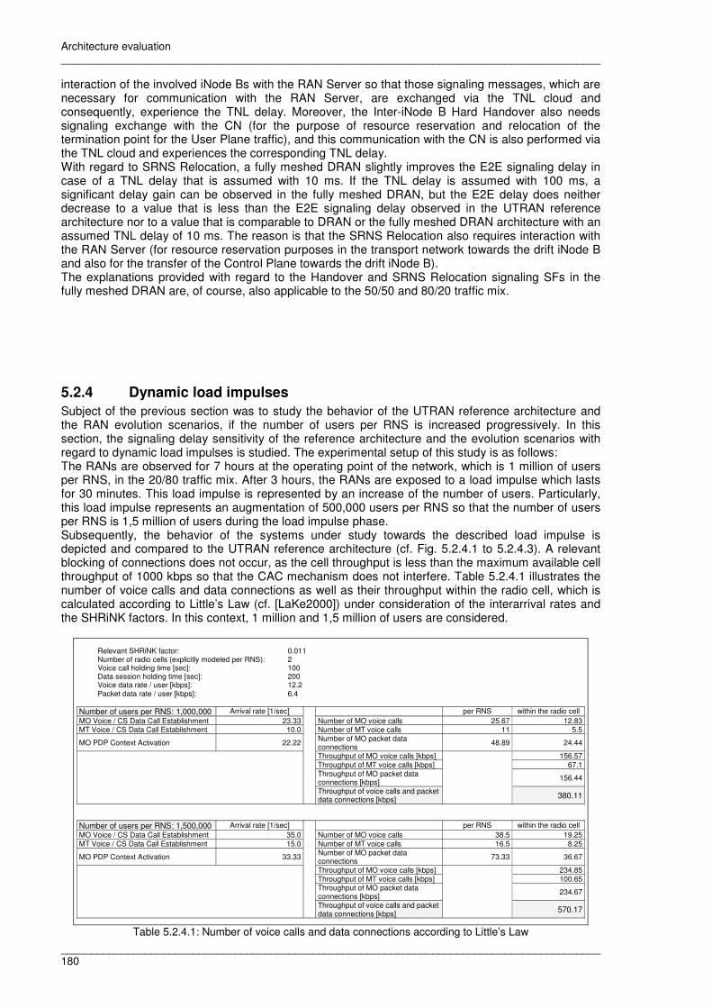
Architecture evaluation __________________________________________________________________________________________
__________________________________________________________________________________________ 180
interaction of the involved iNode Bs with the RAN Server so that those signaling messages, which are necessary for communication with the RAN Server, are exchanged via the TNL cloud and consequently, experience the TNL delay. Moreover, the Inter-iNode B Hard Handover also needs signaling exchange with the CN (for the purpose of resource reservation and relocation of the termination point for the User Plane traffic), and this communication with the CN is also performed via the TNL cloud and experiences the corresponding TNL delay. With regard to SRNS Relocation, a fully meshed DRAN slightly improves the E2E signaling delay in case of a TNL delay that is assumed with 10 ms. If the TNL delay is assumed with 100 ms, a significant delay gain can be observed in the fully meshed DRAN, but the E2E delay does neither decrease to a value that is less than the E2E signaling delay observed in the UTRAN reference architecture nor to a value that is comparable to DRAN or the fully meshed DRAN architecture with an assumed TNL delay of 10 ms. The reason is that the SRNS Relocation also requires interaction with the RAN Server (for resource reservation purposes in the transport network towards the drift iNode B and also for the transfer of the Control Plane towards the drift iNode B). The explanations provided with regard to the Handover and SRNS Relocation signaling SFs in the fully meshed DRAN are, of course, also applicable to the 50/50 and 80/20 traffic mix.
5.2.4 Dynamic load impulses
Subject of the previous section was to study the behavior of the UTRAN reference architecture and the RAN evolution scenarios, if the number of users per RNS is increased progressively. In this section, the signaling delay sensitivity of the reference architecture and the evolution scenarios with regard to dynamic load impulses is studied. The experimental setup of this study is as follows: The RANs are observed for 7 hours at the operating point of the network, which is 1 million of users per RNS, in the 20/80 traffic mix. After 3 hours, the RANs are exposed to a load impulse which lasts for 30 minutes. This load impulse is represented by an increase of the number of users. Particularly, this load impulse represents an augmentation of 500,000 users per RNS so that the number of users per RNS is 1,5 million of users during the load impulse phase. Subsequently, the behavior of the systems under study towards the described load impulse is depicted and compared to the UTRAN reference architecture (cf. Fig. 5.2.4.1 to 5.2.4.3). A relevant blocking of connections does not occur, as the cell throughput is less than the maximum available cell throughput of 1000 kbps so that the CAC mechanism does not interfere. Table 5.2.4.1 illustrates the number of voice calls and data connections as well as their throughput within the radio cell, which is calculated according to Little’s Law (cf. [LaKe2000]) under consideration of the interarrival rates and the SHRiNK factors. In this context, 1 million and 1,5 million of users are considered.
Relevant SHRiNK factor: 0.011 Number of radio cells (explicitly modeled per RNS): 2 Voice call holding time [sec]: 100 Data session holding time [sec]: 200 Voice data rate / user [kbps]: 12.2 Packet data rate / user [kbps]: 6.4
Number of users per RNS: 1,000,000 Arrival rate [1/sec] per RNS within the radio cell MO Voice / CS Data Call Establishment 23.33 Number of MO voice calls 25.67 12.83 MT Voice / CS Data Call Establishment 10.0 Number of MT voice calls 11 5.5
MO PDP Context Activation 22.22 Number of MO packet data connections
48.89 24.44
Throughput of MO voice calls [kbps] 156.57 Throughput of MT voice calls [kbps] 67.1 Throughput of MO packet data connections [kbps]
156.44
Throughput of voice calls and packet data connections [kbps]
380.11
Number of users per RNS: 1,500,000 Arrival rate [1/sec] per RNS within the radio cell MO Voice / CS Data Call Establishment 35.0 Number of MO voice calls 38.5 19.25 MT Voice / CS Data Call Establishment 15.0 Number of MT voice calls 16.5 8.25
MO PDP Context Activation 33.33 Number of MO packet data connections
73.33 36.67
Throughput of MO voice calls [kbps] 234.85 Throughput of MT voice calls [kbps] 100.65 Throughput of MO packet data connections [kbps]
234.67
Throughput of voice calls and packet data connections [kbps]
570.17
Table 5.2.4.1: Number of voice calls and data connections according to Little’s Law

Architecture evaluation __________________________________________________________________________________________
__________________________________________________________________________________________ 181
Fig. 5.2.4.1: System behavior of UTRAN reference architecture and DRAN Fig. 5.2.4.1 shows that the reaction of the UTRAN reference architecture towards the given load impulse is an increase of the signaling E2E delay of approximately 18%. Moreover, the occurrence of delay values, which are greater than 2 sec, can be observed. Delay values greater than 2 sec can be regarded as critical values, when establishing a MO voice call, and thus, are not acceptable, as they violate the service level. The DRAN evolution scenario shows a superior behavior with regard to the given load impulse (cf. Fig. 5.2.4.1), as the increase of the signaling E2E delay is approximately 3%. The delay values remain beneath the acceptable limit of 2 sec so that the service level is not violated. With regard to the low increase of the signaling E2E delay in DRAN, it also has to be considered that the full resource capacity of the UTRAN reference architecture was assigned to DRAN as well as to the other RAN evolution scenarios. The signaling performance result, DRAN provided within this experiment, might serve as an indicator that a resource capacity, which is less than the resource capacity of UTRAN, might also be sufficient for DRAN.
Fig. 5.2.4.2: System behavior of UTRAN reference architecture and ATM-based MRAN
MO Voice / CS Data Call Establishment
1.2
1.4
1.6
1.8
2
2.2
Simulation Time (7 Hours)
E2E
Del
ay [s
ec]
UTRAN
DRAN
MO Voice / CS Data Call Establishment
1
1.2
1.4
1.6
1.8
2
2.2
Simulation Time (7 Hours)
E2E
Del
ay [s
ec]
UTRAN
ATM-based MRAN

Architecture evaluation __________________________________________________________________________________________
__________________________________________________________________________________________ 182
Fig. 5.2.4.3: System behavior of UTRAN reference architecture and IP-based MRAN The ATM-based MRAN as well as the IP-based MRAN evolution scenario indicate a more noticeable reaction to the load impulse than the DRAN architecture. However, in both MRAN scenarios the signaling delay values do not exceed the acceptable limit of 2 sec (cf. Fig. 5.2.4.2 and 5.2.4.3). Summarizing the results, achieved by an imposition of a dynamic load impulse onto the RANs under study, it was observed that the RAN evolution scenarios did not violate the given service level during the load impulse phase as opposed to the UTRAN reference architecture. Moreover, this experiment indicated that a resource capacity, which is less than the resource capacity of UTRAN, might also be sufficient for the DRAN scenario.
5.2.5 Variation of the mobility behavior
In this section the mobility behavior of the users is varied in the 20/80 and in the 80/20 traffic mix at the operating point of the networks under study (1 million of users per RNS). The further assumptions for the architectures under study are according to Table 5.2.2.1.1 (ATM-based MRAN), Table 5.2.2.2.1 (IP-based MRAN) and Table 5.2.2.3.1 (DRAN). The measured signaling E2E delays are reliable, as blocking and dropping probability within the simulation experiments are low so that unsuccessful signaling cases do not play a decisive role for the results presented in this section. The mobility behavior of the users is defined by three parameters, which are the number of Location Updates per hour, the number of Soft Handovers per hour and the number of Hard Handovers per hour. Table 5.2.5.1 visualizes the standard mobility and provides examples for a variation of the standard mobility. In this context, it has to be recapitulated that the modeling concept of the mobility model is an abstract concept (cf. section 4.1.1) based on particular assumptions, such as those assumptions provided in Table 5.2.5.1, which are considered when calculating the interarrival rates [1/sec] for Handover and Location Update signaling.
Mobility definition Mobility value Location Update / h Soft Handover / h Hard Handover / h Standard mobility 1 1.5 20 1.8
Duplicated standard mobility 2 3 40 3.6 Half of the standard mobility 0.5 0.75 10 0.9
Table 5.2.5.1: Mobility definition With regard to the variation of the mobility behavior of the users, it is of interest to look at both, the 80/20 traffic mix as well as the 20/80 traffic mix due to the fact that only services, which continuously
MO Voice / CS Data Call Establishment
1
1.2
1.4
1.6
1.8
2
2.2
Simulation Time (7 Hours)
E2E
Dea
ly [s
ec]
UTRAN
IP-based MRAN

Architecture evaluation __________________________________________________________________________________________
__________________________________________________________________________________________ 183
use dedicated channels, perform Soft and Softer Handover. Therefore, CS voice calls perform Soft and Softer Handover, as they use dedicated channels continuously. But the packet sessions do not perform Soft / Softer Handover, as they do not use dedicated channels continuously. Moreover, these packet sessions do not comprise Voice over IP (VoIP) calls which also would apply dedicated channels continuously. The results of this study are shown within Fig. 5.2.5.1 regarding the 80/20 traffic mix and Fig. 5.2.5.2 that comprises the results for the 20/80 traffic mix. The E2E signaling delay curves illustrated in Fig. 5.2.5.1 and 5.2.5.2 represent the values measured for signaling SF 1 (MO Voice / CS Data Call Establishment), but the course of this curve applies for all signaling SFs depicted in Table 3.4.1.
Fig. 5.2.5.1: Mobility variation in the 80/20 traffic mix Fig. 5.2.5.1 visualizes the variation of the user mobility under consideration of the 80/20 traffic mix. The diagram shows that the signaling E2E delays within the UTRAN reference architecture and also in DRAN become instable. The reason for this instability is an overload situation that occurs slightly earlier with regard to the mobility scale in the BSC Resource within the RNC, but it also occurs in the Main Resource within the RAN Server. On the one hand the increasing number of Location Updates leads to this overload situation, and on the other hand the fact that an increasing number of voice users has legs within two radio cells (i.e. an increasing number of voice users demands resources within two radio cells) due to increasing Soft Handover mobility. Moreover, the fact that the number of voice users, who demand resources within two radio cells, at least doubles, also increases the blocking and the dropping probability in the radio cell, when user mobility increases.
1.0
10.0
100.0
0.0 0.5 1.0 1.5 2.0
Mobility [dimensionless]
E2E
Del
ay [
sec]
and
Blo
ckin
g P
roba
bilit
y [%
] an
d D
ropp
ing
Pro
babi
lity
[%]
and
%ag
e of
Use
rs in
Rad
io C
ell w
ith 2
Leg
s an
d R
esou
rce
Util
izat
ion
[%]
UTRAN DRAN
ATM-based MRAN IP-based MRAN
Blocking Probability (in Radio Cell) Dropping Probability (in Radio Cell)
%age of Users in Radio Cell with 2 Legs RNC BSC Resource
RAN Server Main Resource

Architecture evaluation __________________________________________________________________________________________
__________________________________________________________________________________________ 184
Fig. 5.2.5.2: Mobility variation in the 20/80 traffic mix Fig. 5.2.5.2 shows the variation of user mobility within the 20/80 traffic mix. The result of this experiment is not that obvious than in the 80/20 traffic mix due to the fact that the portion of voice users, who contribute to the increasing user mobility in terms of Softer and Soft Handovers, represents the minor traffic portion with regard to the overall traffic in the network. Consequently, the overload situation within the BSC Resource in the RNC and the Main Resource in the RAN Server occurs later as well as the instability of the signaling E2E delays in UTRAN and DRAN. Furthermore, the fact that the portion of voice users represents the minor traffic portion and thus, the contribution of the voice users to the overall user mobility in terms of Softer / Soft Handover is less than in the 80/20 traffic mix, also results in a lower blocking and dropping probability. Within the 20/80 traffic mix, blocking and dropping occurs for the first time at a later point of the mobility scale compared to the 80/20 traffic mix. As a summary of this section, it can be realized that an increase of the mobility behavior of the users leads to slightly different results depending on the dominating traffic portion in the network due to the assumption that only services, which continuously apply dedicated channels, perform Soft and Softer Handover. However, in any case an increase of the user mobility affects the signaling E2E delays of the UTRAN reference architecture and also of the DRAN evolution scenario at a certain point of the mobility scale. The reason is an overload situation within major resources due to an increasing number of Location Updates and an increasing number of voice users, who demand resources within two radio cells due to increasing Soft Handover mobility. The increasing number of voice users, who request resources within two radio cells, also increases the blocking and the dropping probability in the radio cell.
5.2.6 Further possibilities of the simulator
The developed simulation environment as well as the modeling methodology allow for further studies with regard to RAN performance evaluation which are described in this section. However, initial simulation results provided the information that the aforementioned studies require a refinement of the simulator with regard to the consideration of unsuccessful signaling cases (cf. section 3.4.8 in this context), as significant blocking and loss probabilities play a decisive role with regard to these experiments. Without this refinement, a reliable assessment of E2E signaling performance is not possible so that the aforementioned initial simulation results cannot be published in the framework of
0.0
0.1
1.0
10.0
100.0
1000.0
0.0 0.5 1.0 1.5 2.0 2.5
Mobility [dimensionless]
E2E
Del
ay [s
ec] a
ndB
lock
ing
Pro
babi
lity
[%] a
nd D
ropp
ing
Pro
babi
lity
[%] a
nd%
age
of U
sers
in R
adio
Cel
l with
2 L
egs
UTRAN DRAN
ATM-based MRAN IP-based MRAN
Blocking Probability (in Radio Cell) Dropping Probability (in Radio Cell)
%age of Users in Radio Cell with 2 Legs

Architecture evaluation __________________________________________________________________________________________
__________________________________________________________________________________________ 185
this thesis. Moreover, one of these experiments also needs a further validation of the SHRiNK modeling concept which was introduced in section 3.4.9. A simulation experiment, which is of interest to be performed, is the variation of BHCAs and BHDSAs at the operating point of the networks under study, which is 1 million of users per RNS. As BHCAs and BHDSAs are part of the traffic model parameters (cf. section 4.1.1), they are modified in the framework of the GUI-based Excel workbook. Table 5.2.6.1 shows the influence of a BHCA increase on the instantiation rates [1/sec] of particular signaling SFs under consideration of a voice call holding time which is assumed with 100 sec. The voice call holding time is represented by the interarrival time [sec] of the MO and MT Voice / CS Data Call Release signaling SFs. The holding time for packet data sessions is assumed with 200 sec in this simulation experiment and is represented by the interarrival time [sec] of the MO PDP Context Deactivation signaling SF. As the instantiation rates for MO and MT Voice / CS Data Call Establishment increase, the number of concurrent active users also increases so that the instantiation rates for Handover and SRNS Relocation signaling also increase, as these rates are impacted by the number of concurrent active users. If the instantiation rate of a signaling SF is not impacted by a BHCA increase, the signaling SF is not depicted in Table 5.2.6.1.
BHCA per user [calls/h] = 0.6
BHCA per user [calls/h] = 0.8
BHCA per user [calls/h] = 1.0
# UTRAN signaling SF Rate [1/sec] Rate [1/sec] Rate [1/sec]
1 MO Voice / CS Data Call Establishment 23.33 31.11 38.89 3 MT Voice / CS Data Call Establishment 10.0 13.33 16.67 15 Intra-RNC Softer Handover 15.01 16.29 17.57 16 Intra-RNC Soft Handover 67.61 73.38 79.14 17 Inter-RNC Soft Handover 4.83 5.24 5.65 18 Intra-RNC Hard Handover 6.95 7.47 7.99 19 Inter-RNC Hard Handover 0.5 0.53 0.57 20 Serving Radio Network Subsystem (SRNS) Relocation 0.5 0.53 0.57
Interarrival time [sec] of • MO Voice / CS Data Call Release = 100 sec • MT Voice / CS Data Call Release = 100 sec
Table 5.2.6.1: Impact of BHCA increase on instantiation rates of signaling SFs (20/80 traffic mix) An increase of the BHDSAs can be performed under consideration of different services, such as the Web Browsing service, Email service, FTP service and a Power-User service. With regard to the aforementioned services, it is assumed that a user of a particular service initiates PDP context signaling once; afterwards, packet sessions of the service of interest can be set up. The different services are modeled by a variation of the packet session holding time and the average service data rate in the radio cell. On the one hand the average service data rate impacts the CAC regulation mechanism within the radio cell (cf. section 3.4.8 and equations (7) and (8)). On the other hand this variation is performed in the framework of the traffic model parameters (cf. Table 4.1.2) within the GUI-based Excel workbook so that the instantiation rates of particular signaling SFs are influenced. Table 5.2.6.2 visualizes the characteristics of the assumed services, and Table 5.2.6.3 shows the impact of the Email and FTP services, taken as an example, on the instantiation rates of particular signaling SFs. The interarrival time [sec] of signaling SF 9 (MO PDP Context Deactivation) in Table 5.2.6.3 represents the session holding time of the particular service which is depicted in Table 5.2.6.2.
Service Session holding Time [sec]
Average data rate in radio cell [kbit/sec]
Web Browsing 200 6.4 Email 50 0.64 FTP 400 12.8
Power-User 950 32
Table 5.2.6.2: Service characterization Regarding Table 5.2.6.2 and the Web Browsing service, it is assumed that a user visits and studies several web pages. With regard to the Email service the assumption is that several email messages with or without attachments are sent and/or downloaded, and the FTP service considers the upload

Architecture evaluation __________________________________________________________________________________________
__________________________________________________________________________________________ 186
as well as the download of files. The Power-User service considers business users who connect to their company network from outside (e.g. at home) in order to work.
Email Service BHDSA per user
[calls/h] = 0.6 BHDSA per user
[calls/h] = 0.8 BHDSA per user
[calls/h] = 1.0
# UTRAN signaling SF Rate [1/sec] Rate [1/sec] Rate [1/sec]
5 PS Data Transfer Establishment (with follow on: UE PS attaches and automatically gets PDP context, then goes to URA_PCH)
96.89 125.33 153.78
6 PS Detach (UE initiated) 96.89 125.33 153.78
7 Transition from URA_PCH to CELL_DCH due to Downlink Data Transfer
96.89 125.33 153.78
8 Transition from CELL_DCH to URA_PCH due to RRC inactivity timer expiring
96.89 125.33 153.78
Interarrival time [sec] of • MO PDP Context Deactivation = 50 sec in case of Email service
FTP Service BHDSA per user
[calls/h] = 0.6 BHDSA per user
[calls/h] = 0.8 BHDSA per user
[calls/h] = 1.0
# UTRAN signaling SF Rate [1/sec] Rate [1/sec] Rate [1/sec]
5 PS Data Transfer Establishment (with follow on: UE PS attaches and automatically gets PDP context, then goes to URA_PCH)
96.89 125.33 153.78
6 PS Detach (UE initiated) 96.89 125.33 153.78
7 Transition from URA_PCH to CELL_DCH due to Downlink Data Transfer 96.89 125.33 153.78
8 Transition from CELL_DCH to URA_PCH due to RRC inactivity timer expiring
96.89 125.33 153.78
Interarrival time [sec] of • MO PDP Context Deactivation = 400 sec in case of FTP service
Table 5.2.6.3: Impact of BHDSA increase on instantiation rates of signaling SFs with regard to the Email and FTP service (20/80 traffic mix)
With regard to the different services and their characteristics (cf. Table 5.2.6.2), the E2E signaling performance behavior of particular signaling SFs is not the only interesting aspect. Moreover, the effects of these services on the networks under study in terms of connection blockage and their impact on the voice calls in the network (i.e. in terms of a suppression of voice users in the network) are particularly of interest. The simulation experiment, which considers the variation of the BHDSAs, also implicitly shows that the simulator allows to study the impact on E2E signaling performance, if the holding time of the assumed services is varied. Consequently, the variation of the call and session holding time for voice calls and packet data sessions can also be studied with the developed simulator. If the network designer is interested to study the impact of the call and session holding time on RAN architectures of interest, he simply has to modify the traffic model parameter Average Service Time per User [sec] (cf. Table 4.1.2) within the GUI-based Excel workbook either for voice calls or packet data sessions. Moreover, the network designer has to set the interarrival time [sec] for MO and MT Voice / CS Data Call Release to the corresponding values, if the voice call holding time is to be varied, and the interarrival time [sec] for MO PDP Context Deactivation accordingly, in case of a variation of the packet data session holding time. Besides, the simulator can provide decision support with regard to a particular task, a network operator might be confronted with, i.e. the network operator might have the duty to equip a particular RNS area, i.e. a RNS with a particular size in terms of m2, with radio cells under consideration of a particular, constant number of users per RNS (e.g. 1 million of users per RNS). In this context, the RNS can be equipped with a few large radio cells or with many small radio cells. With regard to this task, the network operator is interested to provide an appropriate service level in terms of acceptable signaling E2E delays as well as acceptable blocking and dropping probabilities so that the network operator is interested to investigate the impact of the radio cell size and find the optimum radio cell size in this context. A study like this is promising, as the following important aspects can already simply be derived from theoretical considerations:
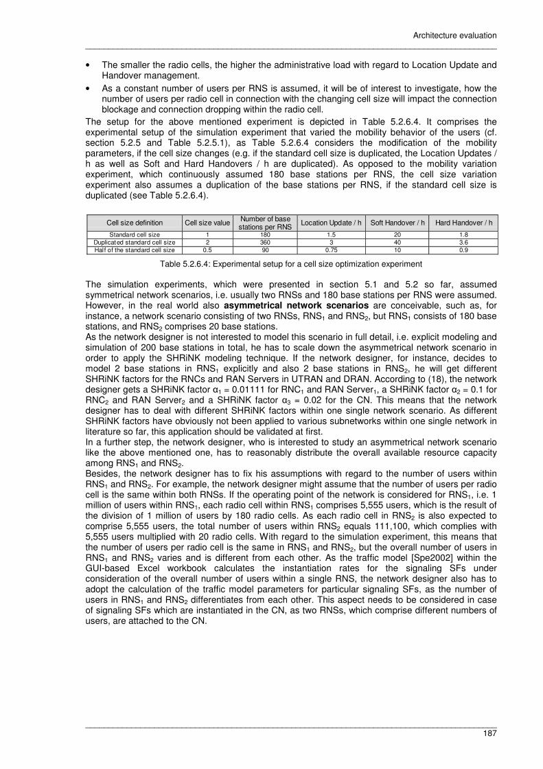
Architecture evaluation __________________________________________________________________________________________
__________________________________________________________________________________________ 187
• The smaller the radio cells, the higher the administrative load with regard to Location Update and Handover management.
• As a constant number of users per RNS is assumed, it will be of interest to investigate, how the number of users per radio cell in connection with the changing cell size will impact the connection blockage and connection dropping within the radio cell.
The setup for the above mentioned experiment is depicted in Table 5.2.6.4. It comprises the experimental setup of the simulation experiment that varied the mobility behavior of the users (cf. section 5.2.5 and Table 5.2.5.1), as Table 5.2.6.4 considers the modification of the mobility parameters, if the cell size changes (e.g. if the standard cell size is duplicated, the Location Updates / h as well as Soft and Hard Handovers / h are duplicated). As opposed to the mobility variation experiment, which continuously assumed 180 base stations per RNS, the cell size variation experiment also assumes a duplication of the base stations per RNS, if the standard cell size is duplicated (see Table 5.2.6.4).
Cell size definition Cell size value Number of base stations per RNS
Location Update / h Soft Handover / h Hard Handover / h
Standard cell size 1 180 1.5 20 1.8 Duplicated standard cell size 2 360 3 40 3.6 Half of the standard cell size 0.5 90 0.75 10 0.9
Table 5.2.6.4: Experimental setup for a cell size optimization experiment The simulation experiments, which were presented in section 5.1 and 5.2 so far, assumed symmetrical network scenarios, i.e. usually two RNSs and 180 base stations per RNS were assumed. However, in the real world also asymmetrical network scenarios are conceivable, such as, for instance, a network scenario consisting of two RNSs, RNS1 and RNS2, but RNS1 consists of 180 base stations, and RNS2 comprises 20 base stations. As the network designer is not interested to model this scenario in full detail, i.e. explicit modeling and simulation of 200 base stations in total, he has to scale down the asymmetrical network scenario in order to apply the SHRiNK modeling technique. If the network designer, for instance, decides to model 2 base stations in RNS1 explicitly and also 2 base stations in RNS2, he will get different SHRiNK factors for the RNCs and RAN Servers in UTRAN and DRAN. According to (18), the network designer gets a SHRiNK factor α1 = 0.01111 for RNC1 and RAN Server1, a SHRiNK factor α2 = 0.1 for RNC2 and RAN Server2 and a SHRiNK factor α3 = 0.02 for the CN. This means that the network designer has to deal with different SHRiNK factors within one single network scenario. As different SHRiNK factors have obviously not been applied to various subnetworks within one single network in literature so far, this application should be validated at first. In a further step, the network designer, who is interested to study an asymmetrical network scenario like the above mentioned one, has to reasonably distribute the overall available resource capacity among RNS1 and RNS2. Besides, the network designer has to fix his assumptions with regard to the number of users within RNS1 and RNS2. For example, the network designer might assume that the number of users per radio cell is the same within both RNSs. If the operating point of the network is considered for RNS1, i.e. 1 million of users within RNS1, each radio cell within RNS1 comprises 5,555 users, which is the result of the division of 1 million of users by 180 radio cells. As each radio cell in RNS2 is also expected to comprise 5,555 users, the total number of users within RNS2 equals 111,100, which complies with 5,555 users multiplied with 20 radio cells. With regard to the simulation experiment, this means that the number of users per radio cell is the same in RNS1 and RNS2, but the overall number of users in RNS1 and RNS2 varies and is different from each other. As the traffic model [Spe2002] within the GUI-based Excel workbook calculates the instantiation rates for the signaling SFs under consideration of the overall number of users within a single RNS, the network designer also has to adopt the calculation of the traffic model parameters for particular signaling SFs, as the number of users in RNS1 and RNS2 differentiates from each other. This aspect needs to be considered in case of signaling SFs which are instantiated in the CN, as two RNSs, which comprise different numbers of users, are attached to the CN.


Conclusion and outlook __________________________________________________________________________________________
__________________________________________________________________________________________ 189
6 Conclusion and outlook The final chapter of this thesis provides a summary of the thesis as well as a summary of the results achieved by application of the developed approach and the simulator that enables the optimization and an evaluation of RAN evolution scenarios with regard to signaling performance in comparison with the UTRAN R99 reference architecture. Moreover, research activities with regard to the developed evaluation approach and regarding the subject of RAN evolution, which are of interest for future research work, are presented.
6.1 Summary of the thesis
The thesis on hand portrayed the evolution of European mobile radio communication systems and in this context, particularly described the evolution of the UMTS architecture with a special focus on the UMTS RAN (cf. section 1, 2.1 and 2.2). In this context, a dominance of new services based on IP technologies is assumed for future mobile networks (e.g. IP multimedia services). Consequently, a predominance of IP-based packet data traffic can be presumed in future mobile networks instead of circuit switched voice traffic which represented the dominating traffic portion within former mobile networks. As future mobile radio networks have to efficiently carry the increasing portion of IP traffic, further evolution has to take place. This issue was already picked up by 3GPP standardization bodies which identified requirements as well as potential solutions for future mobile UMTS RANs assuming a rapid growth of IP data traffic (cf. section 2.3). As 3GPP requirements on the evolution of the UTRAN architecture demand for at least similar or even better performance within the emerging UTRAN evolution scenarios than in the existing R99 UTRAN architecture, the necessity for a performance evaluation of the evolved UTRAN scenarios arose. In the cooperation of Lucent Technologies and the University of Duisburg-Essen within the IPonAir project, funded by the German Ministry for Education and Research, and within the work carried out for this thesis, a flexible, efficient and tool-supported approach for event-driven system simulation was developed that can be used for an evaluation of RAN evolution scenarios with regard to signaling performance in a very early design phase. Therefore, section 3.1 shortly outlines the basic idea of discrete event simulation, and section 3.2 deals with the simulation environment OPNET Modeler which was applied for signaling performance evaluation of the RAN evolution scenarios. In the context of the IPonAir project work, the UTRAN signaling flows (e.g. necessary to establish voice calls or packet data sessions, etc.) are specified in the form of MSCs and apply parts of the MSC specifications defined by ITU-T. Section 3.3 deals with the ITU-T-based MSC specification, and section 3.4 specifically describes the developed MSC-based simulation modeling methodology for UTRAN signaling sequences. The UTRAN signaling flows are annotated within a Microsoft Excel workbook and are converted into a specific format by application of a VBA algorithm. This output is directly importable into the simulation environment OPNET Modeler. Under consideration of the traffic model, which is necessary to calculate the invocation rates of the UTRAN signaling flows during simulation and is also part of the Excel workbook, the imported UTRAN signaling flows represent the system load during discrete event simulation. Section 4.1 specifically describes the tool chain that is based on the simulation toolkit OPNET Modeler, on Microsoft Excel and its macro language VBA and supports the simulation modeling methodology introduced in section 3.4. As the developed simulation approach for evaluation of RAN evolution scenarios regarding signaling performance is expected to be applicable to various RAN evolution scenarios without the necessity to implement a new simulation model for each evolution scenario of interest, the simulation model requires a high-grade and sophisticated simulator implementation. Section 4.2 depicts the fundamental aspects which enable the flexibility and usability of the simulator implementation and make it applicable with regard to the challenging task of an assessment of various RAN evolution scenarios of interest. During the runtime of the IPonAir project, Lucent Technologies contributed to the 3GPP standardization discussion about future mobile UMTS RANs, under consideration of an assumed rapid augmentation of IP data traffic, in terms of a distributed RAN evolution scenario (DRAN) (cf. section 2.3). The idea of DRAN is to relocate functionality (i.e. all radio specific user data handling as well as the cell specific RRM functionality) from the UTRAN RNC into the base station that becomes

Conclusion and outlook __________________________________________________________________________________________
__________________________________________________________________________________________ 190
more complex and is enabled to handle the relocated functionality autonomously in this approach. This idea is promising, because the UTRAN RNC was identified as a single point of failure and as a limiting factor with regard to scalability by 3GPP working groups. Consequently, by relocating functionality from the RNC into the base stations, the DRAN evolution scenario is advantageous with regard to reliability and scalability of the RAN. The remaining functionality of the RNC, which particularly concerns the management of bearer services, paging and micro mobility management in the RAN, remains at the RAN Server network element. Furthermore, the DRAN evolution scenario assumes the attachment of all network elements within the mobile network to an IP-based transport network which cares for an appropriate QoS policy by application of the MPLS and RSVP-TE protocols. As the requirements for RAN evolution scenarios, established by 3GPP working groups, also demand performance values of the evolved RAN scenarios which are comparable or better than the values of the existing, ATM-based UTRAN architecture, the developed simulation approach was applied to the DRAN evolution scenario (cf. section 5) in order to investigate its signaling performance. With regard to the simulation studies performed, it also has to be mentioned that the processing capacity, available within the UTRAN reference architecture, turned out to be also sufficient for the DRAN evolution scenario. Within the simulation experiments, the delay caused by the latency of the transport network was also varied according to values that can be assumed in urban areas and in the countryside. In the countryside, the latency of the transport network for each single signaling message can be assumed to be about 10 times higher than in urban areas. If the delay caused by the transport network is varied, the experiments showed that the transport network latency is an important factor with regard to signaling performance. However, in this context, it also has to be recapitulated that the modeling concept of the IP-based transport network is simplified, as constant values are assumed for the TNL delay which add to the overall signaling E2E delay. The results presented within section 5.2.2.3 show that DRAN provides signaling performance values within urban areas which are comparable to the values provided by the UTRAN reference architecture, and for some of the signaling flows DRAN even provides better signaling performance values. In the countryside, DRAN showed worse signaling performance values than the UTRAN reference architecture, which were caused by the higher transport network latency. However, the performance values, achieved in the countryside, were not entirely unacceptable with the exception of the handover signaling flows. Therefore, the idea was to improve signaling performance in the countryside by fully meshing the base stations within DRAN. In this context, it is also necessary to recapitulate that the modeling concept, which considers a full meshing of the base stations, is simplified, as it does not consider the usage of a base station as an additional hop between two base stations so that a full meshing of the base stations can be avoided in favor of a partly meshing which is advantageous under consideration of the cabling costs. The results, which were achieved under consideration of a full meshing of the base stations and presented within section 5.2.3.2, show that this idea is advantageous in case of those signaling SFs which do not need interaction with the RAN Server or the CN, such as the Soft Handover signaling flow which can be handled by the DRAN base stations autonomously. However, if a signaling use case requires interaction with the RAN Server or CN (e.g. in case of Hard Handover and SRNS Relocation signaling), a fully meshed DRAN does not improve signaling performance in the countryside, as the IP-based transport network has to be passed in this case. In the framework of this thesis, another RAN evolution scenario was also compared to the UTRAN reference architecture. This RAN evolution scenario, MRAN, combines the complete functionality of the RNC and the UTRAN base station within one single network element. The coverage of this network element, which is the Merged Node B, corresponds to the coverage of the UTRAN base station so that a breakdown of a Merged Node B has only local and thus, limited impact on the RAN. Consequently, this approach improves the reliability of the RAN and also the scalability. In the MRAN approach, the Merged Node Bs can either be directly connected to the CN by ATM connections or all network elements within the mobile network are attached to an IP-based transport network that applies MPLS and RSVP-TE for QoS purposes. In order to assess the signaling performance of MRAN (ATM- and IP-based) with regard to the UTRAN reference architecture, the developed simulation approach was also applied to MRAN (cf. section 5). Section 5.2.2.1 and 5.2.2.2 show that the ATM-based MRAN evolution scenario as well as the IP-based MRAN evolution scenario in urban areas provide signaling performance values which are comparable to those values gathered within the UTRAN reference architecture. For some of the signaling flows MRAN even provides better signaling performance values. In this context, the processing capacity, available within the UTRAN reference architecture, was also sufficient for the

Conclusion and outlook __________________________________________________________________________________________
__________________________________________________________________________________________ 191
MRAN evolution scenarios. In the countryside, the IP-based MRAN showed worse signaling performance values than the UTRAN reference architecture, which were caused by the higher transport network latency. Similar to DRAN, the performance values, achieved within the countryside, were not entirely unacceptable with the exception of the handover signaling flows. Therefore, in this case the idea of fully meshing the base stations was also applied to the IP-based MRAN in order to improve the signaling performance in the countryside. Under consideration of the constraint that a full meshing of the base stations represents a simplified modeling concept, the simulation results, presented within section 5.2.3.1, again show that this idea is advantageous in case of those signaling SFs which can be handled by the Merged Node Bs autonomously (i.e. in case of Soft and Hard Handover signaling). Consequently, a full meshing of the base stations within the IP-based MRAN does not improve signaling performance of those signaling use cases in the countryside which need interaction with the CN via the IP-based transport network such as SRNS Relocation signaling. Within the above mentioned simulation experiments for DRAN and MRAN, the number of users per RNS was varied as well as the TNL delay, the traffic mix (i.e. the portion of voice and data traffic, which was imposed to the network, was varied) and the network topology in terms of a full meshing of the base stations. However, in the framework of this thesis, further simulation experiments were performed (cf. section 5.2) in order to investigate the signaling performance behavior of the RAN evolution scenarios DRAN and MRAN and contrast them to the UTRAN reference architecture. In the context of the above mentioned simulation experiments, the RAN evolution scenarios were exposed to dynamic load impulses in terms of an increased number of users per RNS for particular amount of time. Within this experiment, the evolved RANs showed a superior performance behavior compared to the UTRAN reference architecture, as they did not violate the presumed service level (cf. section 5.2.4). In the framework of a further simulation experiment the mobility behavior of the users was varied at the operating point of the networks under study (cf. section 5.2.5). The experiment showed that an increase of the user mobility affects the signaling E2E performance of the UTRAN reference architecture and also of the DRAN evolution scenario, as it causes an overload situation within major resources at a certain point of the mobility scale. The reason for this overload situation is an increasing number of Location Updates and an increasing number of voice users, who demand resources within two radio cells due to increasing Soft Handover mobility. The experiment also provided the information that the increasing number of voice users, who request resources within two radio cells, also increases the blocking and the dropping probability within the radio cell. Apart from the comparison of the signaling performance within the RAN evolution scenarios to the UTRAN reference architecture, the developed simulation methodology and toolkit can also be applied to dimension and optimize RANs as well as particular network elements within the RANs. Section 5.1.2 and 5.1.3 deal with the dimensioning and the optimization of the ATM- and IP-based MRAN architectures as well as the DRAN evolution scenario. These sections show that the steps of optimization and dimensioning of RAN evolution scenarios are important as far as the evolution scenarios are expected to provide a signaling performance which is at least comparable to the reference architecture, but without the necessity to provide them with a higher processing capacity. In the context of dimensioning and optimization of RAN evolution scenarios, on the one hand the network designer is enabled to modify the distribution of processing capacity to particular resources in order to improve signaling performance. On the other hand the network designer is also enabled to improve signaling performance by modifying the distribution of resources to particular network elements as well as the allocation of FEs to resources. Results in terms of statistical measurements, gathered from simulation runs, support the network designer, when taking decisions in this context. Regarding the statistical measurements, the composition of measured signaling delays for single signaling flows as well as the utilizations of particular resources are especially helpful, when taking decisions in terms of dimensioning and optimization. With regard to the composition of measured signaling delays, the simulator implementation provides partial delay information for each single signaling flow so that the network designer knows about the • portion of processing delay resulting from processing time of the signaling messages within
particular resources, • portion of queueing delay experienced by signaling messages, while waiting for service within
particular resources, • portion of link transmission and propagation delay experienced by signaling messages due to the
traversal of communication links.

Conclusion and outlook __________________________________________________________________________________________
__________________________________________________________________________________________ 192
Neither when dimensioning and optimizing RAN architecture evolution scenarios of interest nor when comparing RAN evolution scenarios to the UTRAN reference architecture, there is a need for the network designer to impose changes to the simulator implementation. This is a consequence of the sophisticated simulator implementation that enables a high user-friendliness and flexibility for the network designer. As the developed simulation methodology and the toolkit are applicable to the developed RAN architectures in a very early design phase (i.e. particularly, before any network rollout takes place), the likelihood of choosing and investing capital into an inefficient architecture is considerably reduced.
6.2 Future steps
Some of the working activities, which represent issues for future work, were already pointed out in the context of this thesis and thus, are shortly repeated within a bullet point list subsequently. • Section 3.4.8 pointed out that in case of connection blockage or dropping, no signaling use case
is instantiated due to the fact that the modeling methodology considers the carried traffic, but no unsuccessful signaling cases (cf. Table 3.4.1 and 3.4.2). The effect of this modeling decision is that resource utilizations and measured signaling E2E delays are incorrectly lower, if the blocking and dropping probability significantly increases. The reason for this effect is that the signaling load caused by unsuccessful signaling cases is not considered. Consequently, simulation results, which are achieved under consideration of significant blocking and dropping probabilities, do not represent reliable results of the systems under study. Therefore, an extension of the modeling methodology by unsuccessful signaling cases shall be performed in terms of future work. In this context, the unsuccessful signaling cases simply have to be specified within the GUI-based Excel workbook and integrated into the correlated traffic model (cf. Table 3.4.2) so that they are instantiated, whenever connection blockage or dropping occurs.
• In order to study the signaling performance behavior of the RAN evolution scenarios in further detail, the simulation studies, which were described in section 5.2.6, shall be performed. However, section 5.2.6 also pointed out that these simulation studies require the aforementioned refinement of the simulator with regard to the consideration of unsuccessful signaling cases, as initial simulation results provided the information that blocking and dropping probabilities play a decisive role with regard to these experiments. Moreover, the experiment, which considers asymmetrical network topologies, also needs a further validation of the SHRiNK modeling concept as well as a refinement of the traffic model within the GUI-based Excel workbook which calculates the instantiation rates for the signaling SFs under study.
• As the modeling concept of the overall transport network is a simplified modeling concept (cf. section 3.4.2), a more advanced modeling concept of the overall transport network, which also considers particular effects of the transport network (e.g. packet losses or resource contention), is an issue for future work. In terms of an advanced transport network modeling, the OPNET ATM or IP protocol stack might be applied to the generic node within UTRAN and the RAN evolution scenarios, but it is also possible to attach an own-defined protocol model of the transport network to the generic node.
• As the modeling concept, which considers a full meshing of the RAN base stations, represents a simplified modeling concept, it is also an issue for future work to perform further simulation experiments under consideration of a more realistic meshing concept. This concept might consider a partly meshing of the base stations so that meshed topologies are simulated, which implement the meshing between two base stations A and B by application of an additional base station C, which serves as an additional hop between the two base stations A and B and thus, implements the meshing between A and B.
Regarding further steps in the future, the remaining RAN evolution scenarios, presented within section 2.3, as well as further evolution scenarios, which might emerge due to discussions within 3GPP RAN LTE working groups, can be modeled according to the developed simulation methodology. In this context, the FEs have to be firstly identified and secondly, the identified FEs have to be allocated to network elements and resources within the simulation model in OPNET Modeler. Then the signaling flows have to be specified within Microsoft Excel and converted by application of the VBA algorithm into the format that is importable into OPNET Modeler.
Conclusion and outlook __________________________________________________________________________________________
__________________________________________________________________________________________ 193
Subsequently, the process of dimensioning and optimization has to be applied to the RAN evolution scenarios. Afterwards, the newly set up evolution scenarios can be compared to the UTRAN reference architecture within the framework of simulation experiments like those presented in section 5.2. Moreover, the signaling flows can be modeled for all of the RAN evolution scenarios according to other than 3GPP protocols (e.g. according to IETF protocols like SIP or Mobile IP (MIP)). In this case, the signaling flows also have to be specified within Microsoft Excel under consideration of the new protocols and then converted by usage of the VBA algorithm into the format that is importable into OPNET Modeler. If new FEs emerge by application of other than 3GPP protocols, the new FEs have to be allocated to network elements and resources. Subsequently, the process of dimensioning and optimization might have to be repeated. However, the aforementioned prospective activities (i.e. studying RAN evolution scenarios mentioned in section 2.3, modeling of signaling flows according to other than 3GPP protocols) do not require any changes to the simulator implementation or the tool chain, i.e. the simulation modeling methodology as well as the developed tool chain is seamlessly applicable to these future tasks.


__________________________________________________________________________________________ 197
Bibliography [3GPP1999] 3GPP Technical Specification Group Services and System Aspects: enhanced Multi-Level Precedence and
Pre-emption service (eMLPP) (Release 99), TS 22.067, V. 3.0.1, October 1999. [3GPP2002a] 3GPP Technical Specification Group Services and System Aspects: General on supplementary services
(Release 99), TS 22.004, V. 3.3.0, June 2000. [3GPP2000b] 3GPP Technical Specification Group Services and System Aspects: General UMTS Architecture (Release 99),
TS 23.101, V. 3.1.0, December 2000. [3GPP2000c] 3GPP Technical Specification Group Radio Access Network: UTRAN Iu Interface Signalling Transport
(Release 99), TS 25.412, V. 3.6.0, December 2000. [3GPP2001a] 3GPP Technical Specification Group Radio Access Network: UTRAN Iu Interface Layer 1 (Release 99), TS
25.411, V. 3.5.0, June 2001. [3GPP2001b] 3GPP Technical Specification Group Core Network: Point-to-Point (PP) Short Message Service (SMS) support
on mobile radio interfaces (Release 99), TS 24.011, V. 3.6.0, June 2001. [3GPP2001c] 3GPP Technical Specification Group Services and System Aspects: Vocabulary for 3GPP Specifications
(Release 99), TS 21.905, V. 3.3.0, October 2001. [3GPP2001d] 3GPP Technical Specification Group Core Network: Mobile radio interface layer 3 specification, Supplementary
services specification (Release 99), TS 24.010, V. 3.2.0, December 2001. [3GPP2002a] 3GPP Technical Specification Group Radio Access Network: UTRAN Functions, Examples on Signaling
Procedures (Release 1999), TS 25.931, V. 3.6.0, March 2002. [3GPP2002b] 3GPP Technical Specification Group Radio Access Network: UTRAN Iur Interface: General Aspects and
Principles (Release 99), TS 25.420, V. 3.5.0, March 2003. [3GPP2002c] 3GPP Technical Specification Group Radio Access Network: UTRAN Overall Description (Release 99), TS
25.401, V. 3.10.0, June 2002. [3GPP2002d] 3GPP Technical Specification Group Radio Access Network: UTRAN Iub Interface: General Aspects and
Principles (Release 99), TS 25.430, V. 3.8.0, June 2002. [3GPP2002e] 3GPP Technical Specification Group Radio Access Network: Synchronisation in UTRAN Stage 2 (Release 99),
TS 25.402, V. 3.10.0, June 2002. [3GPP2002f] 3GPP Technical Specification Group Services and System Aspects: Service requirements for the IP Multimedia
Core network Subsystem (Stage 1) (Release 5), TS 22.228, V. 5.6.0, June 2002. [3GPP2002g] 3GPP Technical Specification Group Services and System Aspects: Network architecture (Release 99), TS
23.002, V. 3.6.0, September 2002. [3GPP2002h] 3GPP Technical Specification Group Radio Access Network: UTRAN Iu Interface: General Aspects and
Principles (Release 99), TS 25.410, V. 3.8.0, September 2002. [3GPP2002i] 3GPP Technical Specification Group Radio Access Network: Radio Interface Protocol Architecture (Release
99), TS 25.301, V. 3.11.0, September 2002. [3GPP2002j] 3GPP Technical Specification Group Radio Access Network: UTRAN Iu interface user plane protocols
(Release 99), TS 25.415, V. 3.12.0, September 2002. [3GPP2002k] 3GPP Technical Specification Group Radio Access Network: Packet Data Convergence Protocol (PDCP)
Specification (Release 99), TS 25.323, V. 3.10.0, September 2002. [3GPP2002l] 3GPP Technical Specification Group Services and System Aspects: Quality of Service (QoS) concept and
architecture (Release 99), TS 23.107, V. 3.9.0, September 2002. [3GPP2003a] 3GPP Technical Specification Group Radio Access Network Working Group 3: Requirements for UTRAN
Evolution, TDoc R3-030007, Rel6 Adhoc Meeting, Wokingham, United Kingdom, January 2003. [3GPP2003b] 3GPP Technical Specification Group Radio Access Network Working Group 3: Target Architecture for UTRAN
Evolution, Nokia, TDoc R3-030020, Rel6 Adhoc Meeting, Wokingham, United Kingdom, January 2003. [3GPP2003c] 3GPP Technical Specification Group Radio Access Network: UTRAN Iu interface data transport and transport
signalling (Release 99), TS 25.414, V. 3.13.0, March 2003. [3GPP2003d] 3GPP Technical Specification Group Radio Access Network Working Group 3: Architecture principles for the
evolution of the UTRAN architecture: Split of control and user planes, Alcatel, TDoc R3-030439, Meeting #36, Seoul, Korea, April 2003.

Bibliography __________________________________________________________________________________________
__________________________________________________________________________________________ 198
[3GPP2003e] 3GPP Technical Specification Group Radio Access Network Working Group 3: Further clarifications on the presented evolved architecture, Nokia, TDoc R3-030407, Meeting #35, Seoul, Korea, April 2003.
[3GPP2003f] 3GPP Technical Specification Group Radio Access Network Working Group 3: Analysis of Rel99 Architecture,
Nokia, TDoc R3-030489, Meeting #35, Seoul, Korea, April 2003. [3GPP2003g] 3GPP Technical Specification Group Radio Access Network Working Group 3: Requirements for UTRAN
Evolution, TDoc R3-030638, Meeting #36, Marne la Vallée, France, May 2003. [3GPP2003h] 3GPP Technical Specification Group Radio Access Network Working Group 3: Proposed architecture for
UTRAN evolution, Siemens, TDoc R3-030678, Meeting #36, Marne la Vallée, France, May 2003. [3GPP2003i] 3GPP Technical Specification Group Services and System Aspects: Network architecture (Release 4), TS
23.002, V. 4.8.0, June 2003. [3GPP2003j] 3GPP Technical Specification Group Radio Access Network Working Group 3: Architecture Proposal for
UTRAN evolution Study Item, Lucent Technologies, TDoc R3-031054, Meeting #37, Budapest, Hungary, August 2003.
[3GPP2003k] 3GPP Technical Specification Group Radio Access Network Working Group 3: Feasibility Study on the
Evolution of the UTRAN Architecture (Release 6), TR 25.897 (Draft), V. 0.3.1, August 2003. [3GPP2003l] 3GPP Technical Specification Group Radio Access Network Working Group 3: Proposed function split for
evolved UTRAN, Siemens, TDoc R3-031031, Meeting #37, Budapest, Hungary, August 2003. [3GPP2003o] 3GPP Technical Specification Group Radio Access Network Working Group 3: Architectural principles for the
evolution of the UTRAN architecture: Separation of cell, multi-cell and user related functions, Alcatel, TDoc R3-031048, Meeting #37, Budapest, Hungary, August 2003.
[3GPP2003n] 3GPP Technical Specification Group Radio Access Network Working Group 3: UTRAN Evolutions - Last Mile
impacts for NodeB+, Alcatel, TDoc R3-030965, Meeting #37, Budapest, Hungary, August 2003. [3GPP2003o] 3GPP Technical Specification Group Radio Access Network: UTRAN Iu interface RANAP signalling (Release
99), TS 25.413, V. 3.14.0, September 2003. [3GPP2003p] 3GPP Technical Specification Group Services and System Aspects: Network architecture (Release 5), TS
23.002, V. 5.12.0, September 2003. [3GPP2003q] 3GPP Technical Specification Group Radio Access Network: Services provided by the physical layer (Release
99), TS 25.302, V. 3.16.0, September 2003. [3GPP2003r] 3GPP Technical Specification Group Radio Access Network Working Group 3: UE / Cell split UTRAN evolved
architecture, NEC, TDoc R3-031298, Meeting #38, Sophia-Antipolis, France, October 2003. [3GPP2003s] 3GPP Technical Specification Group Radio Access Network Working Group 3: Additional requirements for the
evolution of UTRAN architecture, LG Electronics Inc., TDoc R3-031422, Meeting #38 Sophia-Antipolis, France, October 2003.
[3GPP2003t] 3GPP Technical Specification Group Radio Access Network: Updates to Evolved Architecture based on
iNodeB and RAN server, Lucent Technologies, TDoc R3-031644, Meeting #39, San Diego, USA, November 2003.
[3GPP2003u] 3GPP Technical Specification Group Radio Access Network: UTRAN Iub Interface User Plane Protocols for
Common Transport Channel Data Streams (Release 99), TS 25.435, V. 3.11.0, December 2003. [3GPP2003v] 3GPP Technical Specification Group Radio Access Network: UTRAN Iub/Iur interface user plane protocol for
DCH data streams (Release 99), TS 25.427, V. 3.11.0, December 2003. [3GPP2003w] 3GPP Technical Specification Group Radio Access Network: UTRAN Iur interface user plane protocols for
Common Transport Channel data streams (Release 99), TS 25.425, V. 3.8.0, December 2003. [3GPP2003x] 3GPP Technical Specification Group Radio Access Network: IP transport in UTRAN (Release 5), TS 25.933, V.
5.4.0, December 2003. [3GPP2003y] 3GPP Technical Specification Group Services and System Aspects: General Packet Radio Service (GPRS)
Service Description (Release 99), TS 23.060, V. 3.16.0, December 2003. [3GPP2004a] 3GPP Technical Specification Group Core Network: General Packet Radio Service (GPRS); GPRS Tunnelling
Protocol (GTP) across the Gn and Gp interface (Release 99), TS 29.060, V. 3.19.0, March 2004. [3GPP2004b] 3GPP Technical Specification Group Radio Access Network: Medium Access Control (MAC) protocol
specification (Release 99), TS 25.321, V. 3.17.0, June 2004. [3GPP2004c] 3GPP Technical Specification Group Radio Access Network: Radio Link Control (RLC) protocol specification
(Release 99), TS 25.322, V. 3.18.0, June 2004. [3GPP2004d] 3GPP Technical Specification Group Core Network: Mobile radio interface signalling layer 3 (Release 99), TS
24.007, V. 3.10.0, June 2004.
Bibliography __________________________________________________________________________________________
__________________________________________________________________________________________ 199
[3GPP2004e] 3GPP Technical Specification Group Core Network: Mobile radio interface layer 3 specification, Core Network Protocols (Release 99), TS 24.008, V. 3.19.0, June 2004.
[3GPP2004f] 3GPP Technical Specification Group Radio Access Network: UTRAN Iur interface (RNSAP) signalling (Release
99), TS 25.423, V. 3.14.2, July 2004. [3GPP2004g] 3GPP Technical Specification Group Radio Access Network: UTRAN Iub interface (NBAP) signalling (Release
99), TS 25.433, V. 3.14.2, September 2004. [3GPP2004h] 3GPP Technical Specification Group Services and System Aspects: IP Multimedia Subsystem (IMS) Stage 2
(Release 5), TS 23.228, V. 5.13.0, December 2004. [3GPP2004i] 3GPP Technical Specification Group Radio Access Network: Broadcast/Multicast Control (BMC) (Release 99),
TS 25.324, V. 3.9.0, December 2004. [3GPP2004j] 3GPP Technical Specification Group Radio Access Network: Radio Resource Control (RRC) protocol
specification (Release 99), TS 25.331, V. 3.21.0, December 2004. [3GPP2004k] 3GPP Technical Specifications Group Services and System Aspects: Intra-domain connection of RAN nodes to
multiple CN nodes (Release 5), TS 23.236, V. 5.3.0, December 2004. [3GPP2005a] 3GPP Technical Specification Group Services and System Aspects: Network architecture (Release 6), TS
23.002, V. 6.7.0, March 2005. [3GPP2005b] 3GPP Technical Specification Group Radio Access Network: Work Plan and Working Procedures - RAN WG3
(Release 6), TR 30.531, V. 0.17.0, March 2005. [3GPP2005c] 3GPP Technical Specification Group Services and System Aspects: All-IP Network (AIPN) feasibility study
(Release 7), TR 22.978, V. 7.0.0, March 2005. [3GPP2005d] 3GPP Technical Specification Group Services and System Aspects: Service requirements for the IP Multimedia
CN Subsystem (Stage 1) (Release 6), TS 22.228, V. 6.8.0, March 2005. [3GPP2005e] 3GPP Technical Specification Group Services and System Aspects: 3GPP system to Wireless Local Area
Network (WLAN) interworking (Release 6), TS 23.234, V. 6.4.0, March 2005. [3GPP2005f] 3GPP Technical Specification Group Core Network: Bearer-independent circuit-switched CN (Stage 2)
(Release 4), TS 23.205, V. 4.8.0, March 2005. [Alt2004] Altan, N.: UTRAN Signaling Message Sequence Charts (MSCs), IPonAir TDoc 220, October 2004. [AlBa2004] Altan, N., Bauer, M.: DRAN Signaling Message Sequence Charts (MSCs), IPonAir TDoc 221, October 2004. [AlBoIg2004] Alexiou, A. G., Bouras, C. J., Igglesis, V. G.: Performance Evaluation of UMTS for Mobile Internet Access, 12th
Annual Meeting of the IEEE International Symposium on Modeling, Analysis and Simulation of Computer and Telecommunication Systems (MASCOTS) 2004, Volendam, The Netherlands, October 2004.
[AlWi2005a] Altan, N., Wiedemann, A.: MRAN Signaling Message Sequence Charts (MSCs), IPonAir TDoc 265, January
2005. [AlWi2005b] Altan, N., Wiedemann, A.: MRAN Signaling Message Sequence Charts (MSCs) for MPLS / RSVP-TE-Based
Transport Network, IPonAir TDoc 268, November 2005. [AnByKa2002] Andrews, M. G., Byers, C. C., Kapauan, P. T., et al.: The SPEED Platform for Programmable Bearer Channel
Processing, Bell Labs Technical Journal, Volume 5, Issue 3, pp. 76-97, August 2002. [ArIePu2003] Araniti, G., Iera, A., Pulitanó, S., et al.: Managing IP Traffic in Radio Access Networks of Next-Generation
Mobile Systems, IEEE Wireless Communications Magazine, pp. 36-43, August 2003. [AtMü2003] Attermeyer, C., Müller-Clostermann, B.: Modelling of Background Traffic – Concepts and Experimental
Evaluation using OPNET Modeler (Part II: MxRAN Simulator Experiments using SHRiNK), IPonAir TDoc 146, June 2003.
[AtMüWi2003] Attermeyer, C., Müller-Clostermann, B., Wiedemann, A.: Proposals for Traffic Model Improvement & UTRAN /
DRAN Comparison, IPonAir TDoc 189, November 2003. [AwBeLi2001] Awduche, D., Berger, L., Li, T., et al.: RSVP-TE: Extensions to RSVP for LSP Tunnels, RFC 3209, December
2001, http://www.ietf.org/rfc/rfc3209.txt?number=3209. [BaCu2001] Baiocchi, A., Cuomo, F.: Efficiency and Fairness Trade-Off for TCP Over UMTS-TDD, IEEE International
Conference on Communications (ICC) 2001, pp. 2110-2114, Helsinki, Finland, June 2001. [Bau2003] Bauer, M.: Handover in Distributed RAN, IPonAir TDoc 176, August 2003. [BaScSo2003] Bauer, M., Schefczik P., Soellner, M., et al.: Evolution of the UTRAN Architecture, 3G Mobile Communication
Technologies (3G) 2003, London, United Kingdom, June 2003.
Bibliography __________________________________________________________________________________________
__________________________________________________________________________________________ 200
[BaVa2002] Baiocchi, A., Vacirca, F.: End-to-End Evaluation of WWW and File Transfer Performance for UMTS-TDD, IEEE Global Communications (GLOBECOM) Conference 2002, pp. 746-750, Taipei, Taiwan, R.O.C., November 2002.
[Bec2004] Becker, H.: IP-based Mobility Management for a Distributed Radio Access Network Architecture, Siemens
Mobile, Presentation, Workshop “Zukunft der Netze” des Fachausschusses 5.2 der Informationstechnischen Gesellschaft (ITG) im Verband der Elektrotechnik, Elektronik und Informationstechnik (VDE), Kaiserslautern, Germany, October 2004.
[BeCrJo2004] Beming, P., Cramby, M., Johansson, N., et al.: Beyond 3G Radio Access Network Reference Architecture, 59th
IEEE Vehicular Technology Conference (VTC) 2004, Milan, Italy, May 2004. [BeGoMa2002] Bestak, R., Godlewski, P., Martins, R.: A TCP Connection Over Uplink UMTS Radio Access Bearer in RLC
Acknowledged Mode, IEEE 55th Vehicular Technology Conference (VTC) 2002, pp. 972-976, Vol. 2, ISBN 0-7803-7484-3, Birmingham, United Kingdom, May 2002.
[BöMiBa2004] Böringer, R., Mitschele-Thiel, A., Bauer, M., et al.: Comparison of MPLS- and IP-based Transport in Future
RANs Under Varying QoS Requirements, 2nd International Working Conference on Performance Modelling and Evaluation of Heterogeneous Networks (HET-NETs) 2004, Ilkley, United Kingdom, July 2004.
[BoCaGr2005] Boggia, G., Camarda, P., Grieco, L. A., et al.: Performance Evaluation of TCP Congestion Control Algorithms
Over UMTS, 11th Ka and Broadband Communications Conference, Rome, Italy, September 2005. [BuChHa2003] Buddhikot, M., Chandranmenon, G., Han, S., et al.: Integration of 802.11 and Third-Generation Wireless Data
Networks, IEEE International Conference on Computer Communications (INFOCOM) 2003, pp. 503-512, San Francisco, California, USA, March/April 2003.
[BuKiBa2005] Burmeister, C., Killat, U., Bachmann, J.: TCP Throughput Optimized Handover Decisions, 11th European
Wireless Conference 2005, Nicosia, Cyprus, April 2005. [Bun2005] Bundesnetzagentur für Elektrizität, Gas, Telekommunikation, Post und Eisenbahnen: Teilnehmerentwicklung
im Mobiltelefondienst nach Netzen pro Quartal (2. Quartal 1992 bis 1. Quartal 2005), http://www.bundesnetzagentur.de/enid/7d2a42bd585afc04b6bbfa3dde03593b,0/Marktbeobachtung/Mobilfunkd
ienste_vw.html#mobiltelefondienst_teilnehmerentwicklung [found: August 22, 2005]. [CaCh2001] Canton, A. F., Chahed, T.: End-to-End Reliability in UMTS: TCP Over ARQ, IEEE Global Communications
(GLOBECOM) Conference 2001, pp. 3473-3477, San Antonio, Texas, USA, November 2001. [CaToZe2002] Canton, A. F., Tohmé, S., Zeghlache, D., et al.: Performance Analysis of ATM/AAL2 in UMTS Radio Access
Network, 13th IEEE International Symposium on Personal, Indoor and Mobile Radio Communications (PIMRC) 2002, Lisbon, Portugal, September 2002.
[ChCaEl2003] Chahed, T., Canton, A. F., Elayoubi, S. E.: End-to-End TCP Performance in W-CDMA / UMTS, IEEE
International Conference on Communications (ICC) 2003, pp. 71-75, Anchorage, Alaska, USA, May 2003. [Cla1996] Clark, M. P.: ATM Networks: Principles and Use, ISBN 0-471-96701-7, Chichester, New York, Brisbane, et al.,
John Wiley & Sons, Ltd, B. G. Teubner Publishers, 1996. [CoFaLa2005] Costamagna, E., Favalli, L, Lanati, M., et al.: An End to End Simulator for Performance Comparison of Different
TCP Schemes Over UTRA Channels, I Information Society Technologies (IST) Mobile & Wireless Communications Summit 2005, Dresden, Germany, June 2005.
[Def2005] Defense Information Systems Agency: Commercial Telecommunication Standards, Q-series ITU-T
Recommendations, Switching and Signalling, http://comm.disa.mil/itu/r_q2000.html#Q.2150 [found: April 25, 2005].
[DeHi1998] Deering, S., Hinden, R.: Internet Protocol, Version 6 (IPv6) Specification, RFC 2460, December 1998,
http://www.ietf.org/rfc/rfc2460.txt?number=2460. [DeNoPi1999] Degermark, M., Nordgren, B., Pink, S.: IP Header Compression, RFC 2507, February 1999,
http://www.ietf.org/rfc/rfc2507.txt?number=2507. [DrHaBe2002] Dreher, R., Harte, L., Beninger, T.: Signaling System 7: Basics, ISBN 1-89397007-8, Tampa, APDG
Publishing/Intertec, 2002. [EbVöBe2001] Eberspächer, J., Vögel, H.-J., Bettstetter, C.: GSM, ISBN 0-471-49903-X, 2nd Edition, Chichester, New York,
Weinheim, et al., John Wiley & Sons, Ltd, 2001. [EnCaBo1999] Engan, M., Casner, S. Bormann, C.: IP Header Compression over PPP, RFC 2509, February 1999,
http://www.ietf.org/rfc/rfc2509.txt?number=2509. [EnFoLe1999] Eneroth, G., Fodor, G., Leijonhufvud, G., et al.: Applying ATM/AAL2 as a Switching Technology in Third-
Generation Mobile Access Networks, IEEE Communications Magazine, pp. 112-122, June 1999. [ETSI1993] European Telecommunications Standards Institute (ETSI): European digital cellular telecommunications
system (Phase 2), General description of a GSM Public Land Mobile Network (PLMN), GSM 01.02, V. 4.0.2, ETR 099, October 1993.

Bibliography __________________________________________________________________________________________
__________________________________________________________________________________________ 201
[ETSI1994] European Telecommunications Standards Institute (ETSI): European digital cellular telecommunications system (Phase 2), General network interworking scenarios, GSM 09.01, V. 4.0.1, ETR 109, February 1994.
[ETSI2000] European Telecommunications Standards Institute (ETSI): Digital cellular telecommunications system (Phase
2+), Network architecture, GSM 03.02 Release 1998, TS 100 522, V. 7.1.0, January 2001. [FaLaMi1997] Faltin, N., Lambert, L., Mitschele-Thiel, A., et al.: An Annotational Extension of Message Sequence Charts to
Support Performance Engineering, 8th SDL Forum, pp. 307-322, Elsevier Science Publishers, ISBN 0-444-82816-8, Evry, France, September 1997.
[FoKyKa2001] Fournogerakis, P., Kyriazakos, S., Karetsos, G.: Enhanced Handover Performance in Cellular Systems based
on Position Location of Mobile Terminals, Information Society Technologies (IST) Mobile & Wireless Communications Summit 2001, Barcelona, Spain, September 2001.
[FoScWo2003] Forkel, I., Schinnenburg, M., Wouters, B.: Performance Evaluation of Soft Handover in a Realistic UMTS
Network, IEEE 57th Vehicular Technology Conference (VTC) 2003, pp. 1979-1983, Vol. 3, ISBN 0-7803-7757-5, Jeju, Korea, April 2003.
[FrKrTa2002] Frangiadakis, N., Kralli D., Tatsi, A., et al.: MO Voice/CS Data Call Establishment Protocol Dialogue
Incorporating “Massive” Message Handling Through FEs’ Internal Structures, IPonAir TDoc 80, April 2002. [GaGaÁl2002] García, A. B., García, E., Álvarez-Campana, M., et al.: A Simulation Tool for Dimensioning and Performance
Evaluation of the UMTS Terrestrial Radio Access Network, Lecture Notes in Computer Science, pp. 49-60, Vol. 2515, ISSN 0302-9743, Springer, Berlin, Heidelberg, 2002.
[GrHe1999] Grossman, D., Heinanen, J.: Multiprotocol Encapsulation over ATM Adaptation Layer 5, RFC 2684, September
1999, http://www.ietf.org/rfc/rfc2684.txt?number=2684. [GrPaAn2003] Groves, C., Pantaleo, M., Anderson, T., et al.: The Megaco/H.248 Gateway Control Protocol, Version 2, April
2003, Internet Draft, http://www.ietf.org/internet-drafts/draft-ietf-megaco-h248v2-04.txt. [GSM2005a] GSM World from the GSM Association, Homepage: http://www.gsmworld.com/index.shtml. [GSM2005b] GSM World from the GSM Association: GSM subscriber statistics, 1
st Quarter 2005,
http://www.gsmworld.com/news/statistics/pdf/gsma_stats_q1_05.pdf [found: August 25, 2005]. [GuBo2002] Gueroui, A., Boumerdassi, A.: A Handover Optimisation Scheme in Cellular Networks, Rapport Scientifique
CEDRIC, 2002. [HaMuLa2003] Haase, O., Murakami, K., LaPorta, T.: Unified Mobility Manager: Enabling Efficient SIP/UMTS Mobile Network
Control, IEEE Wireless Communications Magazine, pp. 66-75, August 2003. [HeHeKe2002] Heier, S., Heindrichs, D., Kemper, A.: Performance Evaluation of Internet Applications Over the UMTS Radio
Interface, IEEE 55th Vehicular Technology Conference (VTC) 2002, pp. 1834-1838, Vol. 4, ISBN 0-7803-7484-3, Birmingham, United Kingdom, May 2002.
[Inf2005] Informationszentrum Mobilfunk: Geschichte des Mobilfunks, http://www.izmf.de/html/de/705.html [found:
August 22, 2005]. [IPo2005] IPonAir Project Homepage: http://www.iponair.de. [IsCaBe2000a] Isnard, O., Calmel, J. M., Beylot, A. L., et al.: Performance Evaluation of AAL2 Protocol in UMTS Terrestrial
Radio Access Network, ITC Specialist Seminar on Mobile Systems and Mobility, pp. 289-300, Lillehammer, Norway, March 2000.
[IsCaBe2000b] Isnard, O., Calmel, J. M., Beylot, A. L., et al.: Handling Traffic Classes at AAL2 / ATM Layer Over the Logical
Interfaces of the UMTS Terrestrial Access Network, 11th IEEE International Symposium on Personal, Indoor and Mobile Radio Communications (PIMRC) 2002, pp. 1464-1468, London, England, September 2002.
[ITU1998] International Telecommunications Union–Telecommunication (ITU-T): Formal description techniques (FDT) –
Message Sequence Chart (MSC), Series Z: Languages and General Software Aspects for Telecommunication Systems, Z.120, Annex B: Formal semantics of Message Sequence Charts, April 1998.
[ITU1999a] International Telecommunications Union–Telecommunication (ITU-T): Framework for IMT-2000 networks,
Series Q: Switching and Signalling, Q.1701, March 1999. [ITU1999b] International Telecommunications Union–Telecommunication (ITU-T): Formal description techniques (FDT) –
Message Sequence Chart (MSC), Series Z: Languages and General Software Aspects for Telecommunication Systems, Z.120, November 1999.
[ITU2002] International Telecommunications Union–Telecommunication (ITU-T): Formal description techniques (FDT) –
Specification and Description Language (SDL), Series Z: Languages and General Software Aspects for Telecommunication Systems, Z.100, August 2002.
[Jai1991] Jain, R.: The Art of Computer Systems Performance Analysis, ISBN 0-471-50336-3, New York, Chichester,
Brisbane, et al., John Wiley & Sons, Ltd, 1991.

Bibliography __________________________________________________________________________________________
__________________________________________________________________________________________ 202
[KaAhLa2001] Kaaranen, H., Athiainen, A., Laitinen, L., et al.: UMTS Networks, ISBN 0471-48654-X, Chichester, New York, Weinheim, et al., John Wiley & Sons, Ltd, 2001.
[KeMaKa2004] Kemper, A., Malkowski, M., Karacan, I.: IPv6 Performance Evaluation on Dedicated Channels in UMTS, 5th
European Wireless Conference, Barcelona, Spain, February 2004. [KeYe2002] Kempf, J., Yegani, P.: OpenRAN: A New Architecture for Mobile Wireless Internet Radio Access Networks,
IEEE Communications Magazine, pp. 118-123, May 2002. [KiJeCh2003] Kim, Y., Jeong, B. J., Chung, J., et al.: Beyond 3G: Vision, Requirements, and Enabling Technologies, IEEE
Communications Magazine, pp. 120-124, March 2003. [KrTaFr2002] Kralli, D., Tatsi, A., Frangiadakis, N., et al.: Analysis of the MSC based System Description and Transformation
to an OPNET Simulator Configuration Description in XML, IPonAir TDoc 112, September 2002. [LaHa1998] Laubach, M., Halpern, J.: Classical IP and ARP over ATM, RFC 2225, April 1998,
http://www.ietf.org/rfc/rfc2225.txt?number=2225. [LaKe2000] Law, A. M., Kelton, W. D.: Simulation Modeling and Analysis, ISBN 0-07-059292-6, Boston, Burr Ridge,
Dubuque, et al., McGraw-Hill, 3rd ed., 2000. [LeMa2002] Leu, A. E., Mark, B. L.: Discrete-time Analysis of Soft Handoff Algorithms for CDMA Cellular Networks, IEEE
International Conference on Communications (ICC) 2002, pp. 3222-3226, New York City, USA, April 2002. [LeVi2001] Lefevre, F., Vivier, G.: Optimizing UMTS Link Layer Parameters for a TCP Connection, 53rd IEEE Vehicular
Technology Conference (VTC) 2001, pp. 2318-2322, Vol. 4, ISBN 0-7803-6728-6, Rhodes, Greece, May 2001. [LiMoWa2004] Li, J., Montuno, D. Y., Wang, J., et al.: Performance Evaluation of the Radio Link Control Protocol in 3G UMTS,
Technical Report, Carleton University / Nortel Networks, Ontario, Canada / Beijing, China, January 2004. [Lin2006] Linktionary: Policy-Based Management, http://www.linktionary.com/p/policy.html. [LiPaHa2002] Lin, Y., Pang, A., Haung, Y., et al.: An All-IP Approach for UMTS Third-Generation Mobile Networks, IEEE
Network Magazine, pp. 8-19, September/October 2002. [LuDiSc2000] Luo, J., Dillinger, M., Schulz, E., et al.: Optimal Timer Settings for the Soft Handover Algorithm in WCDMA,
IEEE 3Gwireless 2000, San Francisco, California, USA, June 2000. [Luc2004a] Lucent Technologies: Flexent
® Serving GPRS Support Node (SGSN) for UMTS, Brochure Number SGSN
07.2004, July 2004, http://www.lucent.com/livelink/09009403800225c7_Brochure_datasheet.pdf [found: March 15, 2005]. [Luc2004b] Lucent Technologies: Flexent
® Radio Network Controller for UMTS/W-CDMA, Brochure Number
EasyServSetup 07.2004, July 2004, http://www.lucent.com/livelink/09009403800167dc_Brochure_datasheet.pdf [found: March 15, 2005]. [Mar2001] MarconiCalling: Digital Archive about Guglielmo Marconi and his Company, 2001,
http://www.marconicalling.com. [MaNiVe2002] Maniatis, S. I., Nikolouzou, E. G., Venieris, I. S.: QoS Issues in the Converged 3G Wireless and Wired
Networks, IEEE Communications Magazine, pp. 44-53, August 2002. [MaPiKy2002] Markopoulos, A., Pissaris, P., Kyriazakos S.: Combining Position Location Information and Network
Performance Data for Simulating Location Aided Handoff, Information Society Technologies (IST) Mobile & Wireless Communications Summit 2002, Thessaloniki, Greece, June 2002.
[MaPiKy2004] Markopoulos, A., Pissaris, P., Kyriazakos, S., et al.: Performance Analysis of Cellular Networks by Simulating
Location Aided Handover Algorithms, 5th European Wireless Conference, Barcelona, Spain, February 2004. [MaYuLe2004] Ma, L., Yu, F., Leung, V., et al.: A New Method to Support UMTS/WLAN Vertical Handover Using SCTP, IEEE
Wireless Communications Magazine, pp. 44-51, August 2004. [McBu2003] McKiou, K. W., Buckley, F. R.: Data-Driven Fault Management Within a Distributed Object-Oriented OAM&P
Framework, Bell Labs Technical Journal, Volume 8, Issue 1, pp. 157-179, July 2003. [McZh2004] McNair, J., Zhu, F.: Vertical Handoffs in Fourth-Generation Multinetwork Environments, IEEE Wireless
Communications Magazine, pp. 8-15, June 2004. [MiLaGo1999] Mihailescu, C., Langrange, X., Godlewski, P.: Soft Handover Analysis in Downlink UMTS WCDMA System,
IEEE Workshop on Mobile Multimedia Communications (MOMUC), San Diego, Florida, USA, November 1999. [MiScWi2004] Mitschele-Thiel, A., Schefczik, P., Wiedemann, A.: Architecture Optimization of 3rd Generation Wireless
Systems based on Use Cases, Applied Telecommunication Symposium (ATS) 2004, Arlington, Virginia, USA, April 2004.
[MiScWi2005] Mitschele-Thiel, A., Schefczik, P., Wiedemann, A.: Comparison of Signaling Performance in the UMTS Radio
Access Network and a Merged Radio Access Network Architecture, IEEE Wireless Communications and Networking Conference (WCNC) 2005, pp. 1767-1772, New Orleans, Louisiana, USA, March 2005.

Bibliography __________________________________________________________________________________________
__________________________________________________________________________________________ 203
[Moh2005] Mohamed, H. K. A.: MINA - A Tool for MSC-Based Performance Analysis and Simulation of Distributed Systems, Doctoral Thesis, University of Duisburg-Essen, Essen, Germany, April 2005.
[Mül2003] Müller-Clostermann, B.: Complexity Classes of Messages and Service Time Calculation, IPonAir TDoc 132,
January 2003. [NaGuHo2000] Nananukul, S., Guo, Y., Holma, M., et al.: Some Issues in Performance and Design of the ATM/AAL2
Transport in the UTRAN, IEEE Wireless Communications and Networking Conference (WCNC) 2000, Chicago, Illinois, USA, September 2000.
[Nec2002] NEC Corporation: Towards the All-IP Mobile Network, Cat. No. BMM009 0208302001VV, 2002 http://www.nec-mobilesolutions.com/infrastructures/download/file/all_ip_catalog.pdf [found: June 9, 2005]. [OlMiRa2003] Olaziregi, N., Micocci, S., Ravasio, G., et al.: Architecture of IP based Network Elements Supporting
Reconfigurable Terminals, Information Society Technologies (IST) Mobile & Wireless Communications Summit 2003, Aveiro, Portugal, June 2003.
[OPN2003] OPNET Technologies, Inc.: OPNET Modeler Product Documentation, Release 10.0, August 2003. [OPN2005] OPNET Technologies, Inc., Homepage: http://www.opnet.com. [PaAlFo2001] Pazhyannur, R., Ali, I., Fox, C.: PPP Multiplexing, RFC 3153, August 2001,
http://www.ietf.org/rfc/rfc3153.txt?number=3153. [PaPrPs2003] Pan R., Prabhakar B., Psounis K., et al.: SHRINK: A Method for Scalable Performance Prediction and Efficient
Network Simulation, IEEE International Conference on Computer Communications (INFOCOM) 2003, pp. 1943-1953, San Francisco, California, USA, March/April 2003.
[PéSaAg2005] Pérez-Romero, J., Sallent, O., Agustí, R.: On Evaluating Beyond 3G Radio Access Networks: Architectures,
Approaches, Tools, 61st IEEE Vehicular Technology Conference (VTC) 2003, Stockholm, Sweden, May/June 2005.
[Pos1980] Postel, J.: User Datagram Protocol, RFC 768, August 1980, http://www.ietf.org/rfc/rfc0768.txt?number=768. [Pos1981] Postel, J.: Internet Protocol, RFC 791, September 1981, http://www.ietf.org/rfc/rfc0791.txt?number=791. [PsPaPr2002] Psounis, K., Pan R., Prabhakar, P., et al.: The Scaling Hypothesis: Simplifying the Prediction of Network
Performance using Scaled-down Simulations, ACM SIGCOMM, HotNets-I, Princeton, New Jersey, USA, October 2002.
[RaWa1997] Rathgeb, E., Wallmeier, E.: ATM – Infrastruktur für die Hochleistungskommunikation, ISBN 3-540-60380-0,
Berlin, Heidelberg, New York, et al., Springer, 1997. [RoScCa2002] Rosenberg, J., Schulzrinne, H., Camarillo, G., et al.: SIP: Session Initiation Protocol, RFC 3261, June 2002,
http://www.ietf.org/rfc/rfc3261.txt?number=3261. [RoScZo2003] Rossi, M., Scaranari, L., Zorzi, M.: On the UMTS RLC Parameters Setting and their Impact on Higher Layers
Performance, 58th IEEE Vehicular Technology Conference (VTC) 2003, Orlando, Florida, USA, October 2003. [RoViCa2001] Rosen, E., Viswanathan, A., Callon, R.: Multiprotocol Label Switching Architecture, RFC 3031, January 2001,
http://www.ietf.org/rfc/rfc3031.txt?number=3031. [RPr2005] The R Project for Statistical Computing, Homepage: http://www.r-project.org/index.html. [SaCh2003] Samhat, A., Chahed, T.: Performance Evaluation of IP in the UMTS Terrestrial Radio Access Network, 18th
International Teletraffic Congress (ITC) 2003, Elsevier Science Publishers, ISBN 0-444-51455-4, Berlin, Germany, August/September 2003.
[SaFrAg2003] Samarasinghe, R., Friderikos, V., Aghvami, A. H.: Analysis of Inter-System Handover: UMTS-FDD & WLAN,
London Communications Symposium (LCS) 2003, London, United Kingdom, September 2003. [Sch2003a] Schefczik, P.: MxRAN Traffic Modeling Issues, IPonAir TDoc 145, June 2003. [Sch2003b] Schefczik, P.: MxRAN DRAN Handover Load Issues, IPonAir TDoc 182, November 2003. [ScCaFr1996] Schulzrinne, H., Casner, S., Frederick, R., et al.: RTP: A Transport Protocol for Real-Time Applications, RFC
1889, January 1996, http://www.ietf.org/rfc/rfc1889.txt?number=1889. [ScFoHa2003] Schinnenburg, M., Forkel, I., Haverkamp, B.: Realization and Optimization of Soft and Softer Handover in
UMTS Networks, European Personal and Mobile Communications Conference (EPMCC) 2003, Glasgow, Scotland, United Kingdom, April 2003.
[ScWi2004] Schefczik, P., Wiedemann, A.: Comparison of UMTS and Beyond Architecture Evolution Scenarios,
Performance Modelling and Evaluation of Heterogeneous Networks (HET-NETs) ’04, Ilkley, United Kingdom, July 2004.
[ScWi2005] Schefczik, P., Wiedemann, A.: A Generic, Flexible and Efficient Approach for Assessing Future Radio Access
Network Evolution Scenarios, IEEE International Conference on Computer Communications (INFOCOM) 2005 (Poster Session), Miami, Florida, USA, March 2005.

Bibliography __________________________________________________________________________________________
__________________________________________________________________________________________ 204
[Sim1994a] Simpson, W.: The Point-to-Point Protocol (PPP), RFC 1661, July 1994, http://www.ietf.org/rfc/rfc1661.txt?number=1661.
[Sim1994b] Simpson, W.: PPP in HDLC-like Framing, RFC 1662, July 1994,
http://www.ietf.org/rfc/rfc1662.txt?number=1662. [SiMoPa2002] Sidebottom, G., Morneault, K., Pastor-Balbas, J.: Signaling System 7 (SS7) Message Transfer Part 3 – User
Adaptation Layer (M3UA), September 2002, ftp://ftp.rfc-editor.org/in-notes/rfc3332.txt. [SiScLo2004] Siebert, M., Schinnenburg, M., Lott, M., et al.: Location Aided Handover Support for Next Generation System
Integration, 5th European Wireless Conference 2004, pp. 195-202, Barcelona, Spain, February 2004. [Soe2001] Soellner, M.: Multistandard RAN simulator requirements specification, IPonAir TDoc 38, December 2001. [Soe2004a] Soellner, M.: Format Specification of the MSC Excel Workbook, IPonAir TDoc 117, January 2004. [Soe2004b] Soellner, M.: Lucent MSC Tools (Version V09a), IPonAir TDoc 191, March 2004. [Soe2004c] Soellner, M.: Call Admission Control Modification in Traffic Model, IPonAir TDoc 261, November 2004. [SoJiZh2005] Song, W., Jiang, H., Zhuang, W., et al.: Resource Management for QoS Support in Cellular/WLAN
Interworking, IEEE Network Magazine, pp. 12-18, September/October 2005. [Spe2002] Speltacker, W.: UTRAN Service-Mix Load Estimation, IPonAir TDoc 86, July 2002. [StXiMo2000] Stewart, R., Xie, Q., Morneault, K., et al.: Stream Control Transmission Protocol, RFC 2960, October 2000,
http://www.ietf.org/rfc/rfc2960.txt?number=2960. [Usk2003] Uskela, S.: Key Concepts for Evolution Toward Beyond 3G Networks, IEEE Wireless Communications
Magazine, pp. 43-48, February 2003. [VaDeTo2003] Vacirca, F., De Vendictis, A., Todini, A., et al.: On the Effects of ARQ Mechanisms on TCP Performance in
Wireless Environments, IEEE Global Communications (GLOBECOM) Conference 2003, San Francisco, California, USA, December 2003.
[VeViSi2002] Venken, K., Vinagre, I. G., Sigle, R., et al.: Enabling Network Redundancy in the Radio Access Network, 3G
Mobile Communication Technologies (3G) 2002, London, United Kingdom, May 2002. [VeViVr2003] Venken, K, Vinagre, I. G., De Vriendt, J.: Analysis of the Evolution to an IP-based UMTS Terrestrial Radio
Access Network, IEEE Wireless Communications Magazine, pp. 46-53, October 2003. [VrLaLe2002] De Vriendt, J., Lainé, P, Lerouge, C., et al.: Mobile Network Evolution: A Revolution on the Move, IEEE
Communications Magazine, pp. 104-111, April 2002. [WaAlSe2002] Walke, B., Althoff, M. P., Seidenberg, P.: UMTS - Ein Kurs, ISBN 3-935340-22-2, 2nd Edition, Weil der Stadt, J.
Schlembach Publishers, 2002. [Wak2003] Wakabayashi, K.: All-IP Network Architecture, Nokia, Presentation, received via 3GPP mailing list, March 2003. [Wal2001] Walke, B.: Mobilfunknetze und ihre Protokolle 1, ISBN 3-519-26430-7, 3rd Edition, Stuttgart, Leipzig,
Wiesbaden, B. G. Teubner Publishers, 2001. [WaMiMe2004] Wang, X. G., Min, G., Mellor, J. E.: Adaptive QoS Control in Cellular and WLAN Interworking Networks,
Performance Modelling and Evaluation of Heterogeneous Networks (HET-NETs) ’04, Ilkley, United Kingdom, July 2004.
[WiScNi2003] Wiedemann, A., Schefczik, P., Nikolaidis, G.: Simulation Methodology for Assessing MxRAN Architecture
Performance, European Simulation Multiconference (ESM) 2003, Nottingham, United Kingdom, June 2003. [Wie2002a] Wiedemann, A.: Proposal for Generic Routing, IPonAir TDoc 79, February 2002. [Wie2002b] Wiedemann, A.: MxRAN Simulator Version 1.0, IPonAir TDoc 90, June 2002. [Wie2002c] Wiedemann, A.: Documentation of MxRAN Simulator Version 1.3, IPonAir TDoc 114, October 2002. [WiAt2003] Wiedemann A., Attermeyer C.: Documentation of MxRAN Simulator Version 2.3, IPonAir TDoc 151, June 2003. [Wie2003] Wiedemann, A.: Documentation of MxRAN Simulator Version 3.0, IPonAir TDoc 173, September 2003. [Wie2004a] Wiedemann, A.: Documentation of MxRAN Simulator Version 3.1, IPonAir TDoc 207, January 2004. [Wie2004b] Wiedemann, A.: Documentation of MxRAN Simulator Version 3.1.1, IPonAir TDoc 214, February 2004. [Wie2004c] Wiedemann, A.: Documentation of MxRAN Simulator Version 3.2, IPonAir TDoc 257, March 2004. [Wie2004d] Wiedemann, A.: Documentation of MxRAN Simulator Version 3.3, IPonAir TDoc 258, March 2004. [Wie2004e] Wiedemann, A.: Documentation of MxRAN Simulator Version 3.3.1.1, IPonAir TDoc 259, March 2004.

Bibliography __________________________________________________________________________________________
__________________________________________________________________________________________ 205
[Wie2004f] Wiedemann, A.: Documentation of MxRAN Simulator Version 3.4, IPonAir TDoc 260, July 2004. [Wie2004g] Wiedemann, A.: Validation of the Traffic Model and CAC Mechanism in MxRAN Simulator Version 3.4.1, July
2004. [Wie2004h] Wiedemann, A.: Validation of Simulation Results for MxRAN Simulator Version 3.4.1, July 2004. [Wie2005a] Wiedemann, A.: Documentation of MxRAN Simulator Version 3.5.2, IPonAir TDoc 266, August 2005. [Wie2005b] Wiedemann, A.: OPNET Simulator for the Evaluation of Signaling Performance in UMTS and Beyond Radio
Access Networks (Version 3.5.2), IPonAir TDoc 267, August 2005. [Wie2006] Wiedemann, A.: Full Set of Simulation Results, IPonAir TDoc 268, March 2006. [YlPaMä2001] Ylianttila, M., Pande, M., Mäkelä, J., et al.: Optimization Scheme for Mobile Users Performing Vertical Handoffs
between 802.11 and GPRS/EDGE Networks, IEEE Global Communications (GLOBECOM) Conference 2001, pp. 3439-3443, San Antonio, Texas, USA, November 2001.
[ZhGuGu2003] Zhang, Q., Guo, C., Guo, Z., et al.: Efficient Mobility Management for Vertical Handoff between WWAN and
WLAN, IEEE Wireless Communications Magazine, pp. 102-108, November 2003.


_______________________________________________________________________________________ 209
Index
A
AAL 15 Type 2 15 Type 5 15
Access Stratum 9, 10 protocol model 10 sublayer 21
active CS voice calls 78, 79, 89, 103, 106, 121, 124 PS data sessions 78, 79, 89, 103, 106
air interface 74 ALCAP 29, 75, 145
protocol(s) 11 Alcatel proposal on UTRAN architecture
evolution 32, 37 amount of processing 67 Amount of Service Table 101 AN 24
Domain 8, 9 analytical solution 45 Application
Protocol 11, 16, 75 Stratum 9
Association 106, 124 ATM 14, 29
Adaptation Layer 15 -based MRAN see MRAN Layer 15 transport 25, 32, 36
network 15 attribute / value pairs 95 AuC 25, 27
B
backward compatibility 32, 40, 42 Basic
Operation 96 Procedure 118
Bearer Independent CS CN 25 BHCA 87, 88 BHDSA 87, 88 blocked
CS voice calls 103 PS data sessions 103
blocking probability 183 BMC 11, 13 bottleneck 131, 152
resolution 153 BSC 25, 75
Resource 75, 81, 125, 130, 131, 133, 137, 141, 142, 143, 183, 184
BSS 24, 25 BTS 25
C
CAC 103, 126, 134, 148, 180 parameters 76, 103
calibration 125, 138
UTRAN 125 call / session parameters 86 CBS 13 CC 22 CCCH 72 cell size 88 central traffic control manager 103 CM sublayer 22 CN 7, 10, 24, 25, 27, 74
Domain 8 coexistence 32, 40 Common Transport Channel 12
FP 19 complexity class 67, 96, 101, 118, 130
factor 67, 71, 95 configuration sheet 90, 112 connectionless 15, 20 connection-oriented 15, 20 continuous simulation model 46 control
channels 12 Control
Plane 32, 36, 74 protocol suite 17 protocols 10, 75
countryside 165, 169, 175 CS (Circuit Switched)
domain 7, 14, 24, 25, 27 -MGW 26 mode of operation 21 services 25 voice call 87
CS (Convergence Sublayer) 15
D
Data Bearer(s) 11 Link Layer (Layer 2) 11 Stream(s) 11, 21
DCH 20, 72 dedicated control services 16 Dedicated Transport Channel 12
FP 19 Dest
FE 95, 96 ID 97, 102, 118
Msg ID 96 Node 95, 96
ID 97, 102, 116, 118 deterministic
service time distribution 67, 130 simulation model 45
discrete event simulation 45, 46 simulation model 46
domain 8 concept 8
downlink 72, 107, 119 DRAN 36, 131, 145
allocation of FEs to resources 147, 150 architecture dimensioning and optimization
147

Index _______________________________________________________________________________________
_______________________________________________________________________________________ 210
Control Plane 145 full meshing
Handover 178, 180 Hard 179 Soft 179 Softer 178
iNode B 178 SRNS Relocation 178, 180
Handover 169, 170, 171, 172 Hard 36, 37, 172 Inter-RAN 37 optimization 152 Soft 36, 171, 172 Softer 36, 171, 172
iNode B 36, 37, 145, 147, 148, 150 interfaces 36, 37, 147
Iui 157, 158 link parameter configuration 148 network
architecture 36 topology in OPNET Modeler 148
RAN Server 36, 37, 145, 147, 148, 150 resource parameter configuration 158 SRNS Relocation 36, 170, 172
dropping probability 183, 184 DSCH 20 dynamic simulation model 45
E
E2E delay see signaling E2E delay EFSM 66, 82, 83 EIR 25 environment file 53, 88, 89, 90, 98, 99, 102,
112 ER module 69, 70, 108, 113, 115 esys interface 52 event 46 Excel 55, 85
F
FACH 72 FE
Info Table 99 Message Table 95, 96, 99 Supplementary Actions Table 96, 99
FEroutingTable 99, 118 FEs 68
ALCAP 75 ALCAP_Iu 75 ALCAP_Iub 75 ALCAP_Iur 75 Bearer Management 74 Bearer Mapping Unit 74, 145 Broadcast/Multicast Management 74, 145 Iu RSVP-TE 138 Iub 74 Iuc RSVP-TE 145, 147 Iui 145, 147 Iui RSVP-TE 145 Iur RSVP-TE 138, 145, 147 Micro Mobility Management 74, 145 Mobility Management 74 NBAP 75 Paging Entity 74 Radio Access Bearer Management 74 Radio Bearer Management 145 RANAP 75
RNSAP 75, 145 RRC Connection Management 74, 145 RSVP-TE 138, 145, 147 TN Resource Management 138, 145, 147 User Management 74 Uu 74
FEsaTable 99, 118 FIFO 69 FP 19
G
GDF 161 general control services 16 generic node modeling concept 68, 69, 92,
98 GFC 15 GGSN 25 GMM 22
protocol state machine 87 GMSC 25, 26 Graphical User Interface see GUI GSMS 22 GTP 17
-C 17 -U 17, 36
relay 36, 135 GUI 53
-based Excel workbook 86, 88, 90, 93
H
Handover 25, 78, 88, 182, 187 Hard 88, 182 Soft 88, 182, 183, 184 Softer 88, 183, 184
HLR 25, 27 HN Domain 8 holding time
CS voice call 81, 87 PS data session 87, 185
Home Stratum 9 horizontal layers 10 HSDPA 42 HSS 27
I
ICC 75 Resource(s) 75, 130, 133, 137, 141, 143
identification code 93 A (Action) 93 BP (Basic Procedure) 93 I (Initiator) 93 M (Message) 93 P (Procedure) 93 SA (Supplementary Action) 93 T (Transaction) 93
IMEI 25 IMS 27 IMSI 25 Infrastructure Domain 8, 9 iNode B 36, 37, 145, 147, 148, 150, 178 instability 129, 131, 137, 152, 165, 170, 173,
183, 184

Index _______________________________________________________________________________________
_______________________________________________________________________________________ 211
Instance ID 111, 112, 114, 115, 116, 117, 119, 122, 123
intelligent Node B 36 interarrival time 67, 79, 86, 88, 89, 102, 106 interface 42
Iu 7, 10, 14 Iub 7, 18, 30, 36, 40 Iuc 36, 37, 145 IuCS 7, 14, 29 Iui (Lucent, DRAN) 36, 145, 157, 158 Iui (NEC) 35 Iui (Siemens) 34 IuPS 7, 14, 30 Iur 7, 20, 31, 36, 40 Iuu 36, 37 Uu 7, 10, 11, 31
interworking 31, 32, 37, 40, 43 unit 32
invocation rate 86, 88, 160 IP
-based multi-standard RAN 39 transport network 31, 39, 40, 42, 68, 140, 141,
148, 160 -based MRAN see MRAN over ATM 17 transport 25, 32 v4 17, 29 v6 17, 28
IR module 69, 70, 108, 109 IS 75
Resource(s) 75, 131, 139, 145, 147, 157 ITU-T H.248.1 35 Iu UP protocol 16
L
level of confidence 127 link
propagation delay 70, 71, 98, 120, 191 transmission delay 70, 71, 98, 120, 191
load impulse 160, 180, 181, 182 Location Update 88, 182, 183, 187 logical channels 12 LSAP 69, 70, 98 Lucent proposal on UTRAN architecture
evolution 32, 36
M
M/D*/n 130 M/D/1 130 M/M/1 47, 80 M3UA 17 MAC 11, 12, 36 Main Resource 92, 125, 130, 133, 141, 147,
150, 151, 152, 153, 155, 156, 157, 158, 173, 183, 184
mapping of FEs to resources 86, 92, 96 of Node IDs to Type IDs 114
mathematical model 45 maximum throughput 76, 126, 134, 148 MDC 33, 34 Megaco 35
Merged Node B 39, 40, 41, 132, 133, 134, 138, 140, 141, 175, 176
meshing of the base stations 160, 175 message length 71, 96 MG 35 MGC 35 MIP 193 MM
protocol 22 sublayer 22
MO CS call 22, 26, 74 mobility 20, 22, 74, 136, 160, 182, 183, 184
management 25, 37 parameters 86, 88, 182, 187
module topology 108 MPLS 40, 145, 148 MRAN 39
ATM-based 39 allocation of FEs to resources 133 Control Plane 131 Handover 161, 163, 164
Hard 164 optimization 137 Soft 163, 164 Softer 163, 164 SRNS Relocation 164
interfaces 40, 41, 131 link parameter configuration 134 Merged Node B 39, 40, 41, 132, 133, 134 network
architecture 40 topology within OPNET Modeler 134
resource parameter configuration 137 derivation 133
SRNS Relocation 40, 41, 161, 164 Handover 40, 41
Inter-RAN 41 Soft 40
IP-based 40 allocation of FEs to resources 141 Control Plane 139 full meshing
Handover 176, 178 Hard 177 Soft 177 Softer 176, 178
Merged Node B 175, 176 SRNS Relocation 176, 177, 178
Handover 165, 167, 168 Hard 168 optimization 143 Soft 167 Softer 167, 168 SRNS Relocation 168
interfaces 40, 145 link parameter configuration 140 Merged Node B 40, 138, 140, 141 network
architecture 40 topology within OPNET Modeler 140
resource parameter configuration 143 derivation 141
SRNS Relocation 165, 168 Merged Node B 39 relay node 41
MSC (Message Sequence Chart) 55, 56, 98 action 58, 59, 67, 71 -based simulation methodology 66 condition 57, 58
guarding condition 57 setting condition 57
data 64, 65, 67 dynamic 64 static 64

Index _______________________________________________________________________________________
_______________________________________________________________________________________ 212
document 64, 65 defining part 64, 65 utility part 64, 65
environment 56, 71 graphical language 56 high-level structural concepts 61
coregion 61, 63 HMSC 61
alternative 61 loop 61 parallelism 61 sequence 61
inline expression 61, 62 alternative 61, 62 exceptional case 61, 62 iteration 61, 62 optional region 61, 62 parallelism 61, 62, 67, 74, 93, 96, 97, 99
MSC reference 61, 63 expression 63
instance 56, 66, 67 axis 56, 63 creation 57
message 56, 67 event 57, 59, 67
generalized order mechanism 57 partial order 57 total time ordering 57
exchange 55, 56, 58, 67 processing 67 transfer 67
object orientation 66 inheritance mechanism 66 virtuality 66
textual language 56 time concept 59, 60, 61, 63, 67
absolute timing 59 measurement 59, 67, 71 relative timing 59 time constraint 59, 67, 71
timer 58, 59 expiration 58 stop 58
MSC (Mobile-services Switching Centre) 25, 26 Server 26, 27
MT CS call 22, 26 Domain 8, 9
MTP1 15 MTP2 15 MTP3b 15, 17 multi-server resource 69, 75
N
NBAP 18, 19, 75 NEC proposal on UTRAN architecture
evolution 32, 35 Network Layer (Layer 3) 11 network topology 88, 108, 111, 113, 117 Next Action 96, 99 NNI 15 node
identifier 91, 110 instance 111
Node B 7, 18, 32, 36, 39, 71, 73, 75, 125, 126
Node B+ 32 Node ID 90, 111, 114, 116, 117, 122 Nokia proposal on UTRAN architecture
evolution 32, 39
Non-Access Stratum 10, 11, 13, 17 protocol architecture 21, 22, 23
notification services 16
O
O&M 18 Implementation Specific O&M 18 Logical O&M 18
operating point of the network 81, 125, 136, 142, 147, 152, 160, 180, 182, 187
OPNET Modeler 46 attribute 53
promoted 53 data analysis 54
configuration 55 viewer tool 55
data collection 54 animation 54 custom statistics 54 output scalar 54, 161 output vector 54 probe 54
EMA 53 GUI 108 IMA package 99, 109 modeling domains 47, 53
esys Domain 47, 52 cosimulation 52 ESD 52
Network Domain 47 geographical context 47 link 47
bus link 47 point-to-point link 47 radio link 47
node 47 subnetwork 47
Node Domain 47, 48 connection 47
logical association 48 packet stream 48 statistic wire 48
module 47 esys 48 processor 48 queue 48 receiver 48 transmitter 48
Process Domain 47, 48, 50, 51 dynamic process 48 FSM 49 interrupt 49 KP 49 process group 48 Proto-C 49 root process 48 STD 49
condition 49 forced state 49 State Executive 49 transition 49 Transition Condition 49 Transition Executive 49 unforced state 49
op_cvos utility program 161 packet 53
field 53, 118, 119 formatted 53 unformatted 53 value vector 53
simulation environment 46 simulation execution 54
command line 54 GUI 53, 54
Topology package 99, 109 OPNET simulator
addressing concept 110, 115
Index _______________________________________________________________________________________
_______________________________________________________________________________________ 213
adjacency relationships 117, 120 adjacent 117
network elements 107, 119 affiliations 110, 113, 115, 117 backtracking functionality 116, 122 blocked
CS voice calls 98 PS data sessions 98
Broadcast 107, 117, 119, 120, 124 Initiator 107, 119
components 98 eligibility 122, 123 external routing
operation 119 table 115, 117, 119
generic routing mechanism 113 Global_Topology_Table_InstanceID XXII, 113,
114 Global_Topology_Table_NodeID 113, 114 Global_Topology_Vector_NodeID 114, 116 Handover 98, 103, 104, 106, 107, 113, 117,
119, 120, 123, 124 Hard 119, 121, 123 Soft 119, 121, 123
indicator 119, 123 indices 115 interrupt code 104, 106, 121, 123, 124
DECREASE_VOICE_CALLS_DUE_TO_HO 124 DRIFT_OK 106, 123 INCREASE_VOICE_CALLS_DUE_TO_HO 124 MO_RELEASE_RI_GENERATE 104, 106 MT_HO_DRIFT_RI_REQUEST 104, 106, 123 MT_HO_SERVING_RI_REQUEST 121 NO_DRIFT 106 NO_SF 106 SERVING_OK 121 START_SF 106
IR_Routing_Table 109 list_of_adjacent_network_elements_with_lower
_typeID XVII, 117, 118, 119, 124 list_of_adjacent_network_elements_with_same
_typeID XVII, 117, 118, 121, 124 Local_Adjacence_Table_NodeID XVII, 117 lost
CS voice calls 98, 103 op_dist_outcome 102, 106 packet
format 118 stream 108, 109
indices 108, 109 Paging 107, 119
in connected mode 119 in idle mode 107, 119 unsuccessful 119
random determination 121 remote interrupt 103 self interrupt 103 SRNS Relocation 107, 119, 124 target radio cell 119, 121, 123, 124
optimization 32, 41, 125, 128, 138, 170
P
Packet Interarrival Time 89, 102 packet length 67, 118 partial delays 120, 191
measurement 138 PD 22 PDCP 11, 13, 36 PDP 22
address 25
context 22, 87, 185 performance
evaluation 43 measure 54, 69, 85, 98 values 85, 119, 138
physical channels 12 Physical Layer (Layer 1) 11 PMD 14, 15 Poisson
arrivals 130 process 67
policy 76 processing
delay 98, 120, 191 time 68, 157, 191
processor 68 propagation delay 68 PS
data session 87 domain 7, 14, 24, 25, 27 mode of operation 21 services 25
Q
Q.2150.1 16 Q.2150.2 18 Q.2630.1 16 QoS 40, 76, 145, 148
policy 126, 134, 148 queueing delay 68, 70, 98, 120, 191
R
RAB 10, 16 RABM 22
entity 22 RACH 72 radio
bearer 12, 36 interface 8, 9, 11 resources 12, 20, 36, 40, 145
Radio Network Layer 10, 11, 16 RAN Server 36, 37, 145, 147, 148, 150 RANAP 16, 17, 75 RAT 32, 37, 41, 42 RCS 33, 35 reliability 32, 37, 41, 42, 190 resource
capacity 125, 133, 141, 147, 160 module 67, 68, 69, 70, 71, 81, 90, 92, 98, 100,
101, 120, 127 RLC 11, 12, 36 RNC 7, 20, 32, 36, 39, 42, 71, 73, 75, 93,
125 CRNC 19 DRNC 20 SRNC 20
RNG 32, 39 RNS 7, 24, 86
area 186 DRNS 20 SRNS 20
RNSAP 20, 21, 75 Basic Mobility Procedures 20

Index _______________________________________________________________________________________
_______________________________________________________________________________________ 214
Common Transport Channel Procedures 20 DCH Procedures 20 Global Procedures 20
routing table 95, 96, 108 RRC 11, 13, 22, 36
Connection Establishment ATM-based MRAN 132 DRAN 145, 146 IP-based MRAN 139 UTRAN 71, 72, 73, 93
Connection Release UTRAN 93, 94, 96
protocol state machine 87 RRM 36 RSVP-TE 40, 145, 148
agent 145 RTP 26, 29
S
SAAL 15 -NNI 17
SAP 10, 12 SAR 15 saturation 155 scalability 27, 32, 37, 42, 190 SCCP 15, 17 scheduling 102, 106 SCTP 17 service
amount 101 classes 15 mix 86 time 67, 70, 71, 80, 120, 130
Serving Stratum 9 SF 67, 68, 95 SGSN 25, 27, 36, 41 SHRiNK 80, 81, 134, 140, 148
factor 80, 81, 160, 180 Siemens proposal on UTRAN architecture
evolution 32, 33 signaling
E2E delay 68, 69, 70, 71, 98, 119 flow 72, 73 message 67, 68, 73, 95, 99, 101 performance 128, 133, 138, 147, 160, 161,
165, 169 radio bearer 12 sequence 67, 71, 73, 93 SF 69, 71, 77, 79, 88, 89, 93, 98, 115
instance 102 traffic 66, 77 use case 67, 76
Signaling Bearer(s) 11
establishment 17, 36 Transport Converter 16
SIGTRAN 17 simulation 45
modeling methodology 68, 85, 125, 138 sink module 69, 97 SIP 27, 193 SM 22
protocol state machine 87 SMpSDU 17 SN Domain 8
speed factor 67, 81, 101 Src
FE 95 ID 97, 118
Msg ID 95 Node 95
ID 97, 118 SS 22 SSCF 15
-NNI 15 SSCOP 15, 18 stateless
FEs 68, 73 static simulation model 45 statistical measurements 69, 97, 101, 119 statistics 54, 97, 98, 103, 106, 124 stochastic simulation model 46 strata concept 8, 9 stratum 9 supplementary service 22 System Function 96, 102, 118
T
TBS 19, 21 TC 14, 15 TDMA 25 TE Domain 8 TI 22 TN Domain 8 TNL
cloud 140, 148, 165, 175, 178 delay 168, 169, 170, 172, 177, 179, 180
TNL delay 68 tool chain 85, 112, 138 toolkit 85, 125 TPU 75 traffic
channels 12 mix 160, 161
20/80 160, 162, 169, 180, 182, 184 50/50 81, 125, 160, 164, 165, 169, 174, 178, 180 80/20 160, 164, 169, 173, 178, 180, 182, 183
model 77, 86, 88, 89, 102, 160 source module 69, 97, 101, 102, 103, 104,
106, 123 transmission delay 67 Transport
Network Control Plane 11 Layer 10, 16 Resource 147, 150, 151, 152, 153, 155, 173 User Plane 11
Stratum 9 transport channels 12 TrM 16 Type ID 111, 112, 114, 115, 116, 117, 119,
122, 123
U
UE 7, 10, 71, 73, 74, 88, 91, 95, 96, 103, 122 Domain 8
UMTS 3 architecture 7, 9

Index _______________________________________________________________________________________
_______________________________________________________________________________________ 215
CS domain services 21 domains 8 network architecture evolution 24 protocol model 8, 10 PS domain services 21 R99 24 Rel-4 25 Rel-5 27 Rel-6 31
UNI 15 uplink 72, 112, 114 UPS 33, 35 urban area 165, 169 U-RNTI 72 USCH 20 User and Control Plane
separation 36, 37, 41 User Plane 10, 32, 36
protocols 10 traffic 36
USIM Domain 8 utilization 80
data channels 76, 126, 134, 148 resource 98, 125, 147, 150, 191
UTRAN 7, 10, 28, 74 allocation of FEs to resources 74 Control Plane 74 evolution 31, 32, 42
scenarios 125 Handover
Hard 74 Soft 74 Softer 74
interfaces 10, 11 link parameter configuration 126 network topology in OPNET Modeler 91 reference architecture 125, 129 resource parameter configuration 125 signaling SFs 76, 78, 79, 86, 97, 101, 102
V
VBA 85 algorithm 86, 90, 93, 95, 96, 97
vertical planes 10 VLR 25
W
W-CDMA 11, 12, 32

