Pappu L. N. MurthyGlenn Research Center, Cleveland, Ohio

Paria Naghipour GhezeljehOhio Aerospace Institute, Brook Park, Ohio

Brett A. BednarcykGlenn Research Center, Cleveland, Ohio

Development and Application of a Tool forOptimizing Composite Matrix ViscoplasticMaterial Parameters

NASA/TM—2018-219745

January 2018

https://ntrs.nasa.gov/search.jsp?R=20180001239 2019-08-30T12:41:40+00:00Z

NASA STI Program . . . in Profi le

Since its founding, NASA has been dedicated to the advancement of aeronautics and space science. The NASA Scientifi c and Technical Information (STI) Program plays a key part in helping NASA maintain this important role.

The NASA STI Program operates under the auspices of the Agency Chief Information Offi cer. It collects, organizes, provides for archiving, and disseminates NASA’s STI. The NASA STI Program provides access to the NASA Technical Report Server—Registered (NTRS Reg) and NASA Technical Report Server—Public (NTRS) thus providing one of the largest collections of aeronautical and space science STI in the world. Results are published in both non-NASA channels and by NASA in the NASA STI Report Series, which includes the following report types: • TECHNICAL PUBLICATION. Reports of

completed research or a major signifi cant phase of research that present the results of NASA programs and include extensive data or theoretical analysis. Includes compilations of signifi cant scientifi c and technical data and information deemed to be of continuing reference value. NASA counter-part of peer-reviewed formal professional papers, but has less stringent limitations on manuscript length and extent of graphic presentations.

• TECHNICAL MEMORANDUM. Scientifi c

and technical fi ndings that are preliminary or of specialized interest, e.g., “quick-release” reports, working papers, and bibliographies that contain minimal annotation. Does not contain extensive analysis.

• CONTRACTOR REPORT. Scientifi c and technical fi ndings by NASA-sponsored contractors and grantees.

• CONFERENCE PUBLICATION. Collected papers from scientifi c and technical conferences, symposia, seminars, or other meetings sponsored or co-sponsored by NASA.

• SPECIAL PUBLICATION. Scientifi c,

technical, or historical information from NASA programs, projects, and missions, often concerned with subjects having substantial public interest.

• TECHNICAL TRANSLATION. English-

language translations of foreign scientifi c and technical material pertinent to NASA’s mission.

For more information about the NASA STI program, see the following:

• Access the NASA STI program home page at http://www.sti.nasa.gov

• E-mail your question to help@sti.nasa.gov • Fax your question to the NASA STI

Information Desk at 757-864-6500

• Telephone the NASA STI Information Desk at 757-864-9658 • Write to:

NASA STI Program Mail Stop 148 NASA Langley Research Center Hampton, VA 23681-2199

Pappu L. N. MurthyGlenn Research Center, Cleveland, Ohio

Paria Naghipour GhezeljehOhio Aerospace Institute, Brook Park, Ohio

Brett A. BednarcykGlenn Research Center, Cleveland, Ohio

Development and Application of a Tool forOptimizing Composite Matrix ViscoplasticMaterial Parameters

NASA/TM—2018-219745

January 2018

National Aeronautics andSpace Administration

Glenn Research CenterCleveland, Ohio 44135

Available from

Trade names and trademarks are used in this report for identifi cation only. Their usage does not constitute an offi cial endorsement, either expressed or implied, by the National Aeronautics and

Space Administration.

Level of Review: This material has been technically reviewed by technical management.

NASA STI ProgramMail Stop 148NASA Langley Research CenterHampton, VA 23681-2199

National Technical Information Service5285 Port Royal RoadSpringfi eld, VA 22161

703-605-6000

This report is available in electronic form at http://www.sti.nasa.gov/ and http://ntrs.nasa.gov/

NASA/TM—2018-219745 1

Development and Application of a Tool for Optimizing Composite Matrix Viscoplastic Material Parameters

Pappu L. N. Murthy

National Aeronautics and Space Administration Glenn Research Center Cleveland, Ohio 44135

Paria Naghipour Ghezeljeh Ohio Aerospace Institute Brook Park, Ohio 44142

Brett A. Bednarcyk

National Aeronautics and Space Administration Glenn Research Center Cleveland, Ohio 44135

Abstract

This document describes a recently developed analysis tool that enhances the resident capabilities of the Micromechanics Analysis Code with the Generalized Method of Cells (MAC/GMC) (Refs. 1 to 3) and its application. MAC/GMC is a composite material and laminate analysis software package developed at NASA Glenn Research Center. The primary focus of the current effort is to provide a graphical user interface (GUI) capability that helps users optimize highly nonlinear viscoplastic constitutive law parameters by fitting experimentally observed/measured stress-strain responses under various thermo-mechanical conditions for braided composites. The tool has been developed utilizing the MATrix LABoratory (MATLAB) (The Mathworks, Inc., Natick, MA) programming language (Ref. 4). Illustrative examples shown are for a specific braided composite system wherein the matrix viscoplastic behavior is represented by a constitutive law described by seven parameters. The tool is general enough to fit any number of experimentally observed stress-strain responses of the material. The number of parameters to be optimized, as well as the importance given to each stress-strain response, are user choice. Three different optimization algorithms are included: (1) Optimization based on gradient method, (2) Genetic algorithm (GA) based optimization and (3) Particle Swarm Optimization (PSO). The user can mix and match the three algorithms. For example, one can start optimization with either 2 or 3 and then use the optimized solution to further fine tune with approach 1. The secondary focus of this paper is to demonstrate the application of this tool to optimize/calibrate parameters for a nonlinear viscoplastic matrix to predict stress-strain curves (for constituent and composite levels) at different rates, temperatures and/or loading conditions utilizing the Generalized Method of Cells. After preliminary validation of the tool through comparison with experimental results, a detailed virtual parametric study is presented wherein the combined effects of temperature and loading rate on the predicted response of a braided composite is investigated.

Introduction

The Micromechanics Analysis Code with Generalized Method of Cells (MAC/GMC) is NASA developed software (Refs. 1 and 2). It can perform a comprehensive composite material and laminate analysis by utilizing the generalized method of cells (GMC) family of micromechanics theories (Ref. 3). These theories provide access to the local stress and strain fields in the composite material that are crucial for assessing damage initiation and progression in composite structures. The software package is built on a user-friendly framework, along with a library of local inelastic, damage, and failure models. Further,

NASA/TM—2018-219745 2

application of simulated thermo-mechanical loading, generation of output results, and selection of repeating unit cell (RUC) architectures to represent the composite material have been automated in MAC/GMC. Finally, classical lamination theory, wherein GMC is used to model the composite material response of each ply, along with a recursive multiscale GMC for woven and braided composites, have been implemented within MAC/GMC. Thus, the full range of GMC composite material capabilities is available for analysis of arbitrary laminated/woven/braided configurations as well. The many features that are available in the code as well as the procedures to actually setup and run a problem are described in the MAC/GMC User’s Manuals (Refs. 1 and 2).

Impact analysis of composites is of interest because it enables the assessment of deformation and damage that might occur during the service life of composite parts. However, high strain rate effects coupled with highly nonlinear viscoplastic deformation of certain matrix materials under thermomechani-cal loading conditions pose some unique challenges. These need to be captured accurately in order to model the response of composite structures under impact loading. Current MAC/GMC code has inbuilt constitutive laws to represent such behavior. The matrix material constitutive behavior is represented with the aid of a multi parameter viscoplastic law, wherein the parameters need to be determined by fitting to carefully selected experimental stress-strain response curves. The task is not trivial because of the complex nonlinear nature of the material constitutive law, requiring a nonlinear regression fitting to determine the parameters.

In order to determine the optimized constitutive law parameters a graphical user interface (GUI) based tool has been developed utilizing the MATLAB programming language. The tool is general enough to fit any number of experimentally observed stress-strain responses of the material that have been generated for a given material with a design of experiments. Furthermore, the parameters to be optimized, as well as the importance given to each stress-strain response curve, are kept as user choices. Thus the user may opt for only a subset of the parameters as design variables, as well as specify different weights to each of the experimentally observed stress-strain response. The parameters are extracted by minimizing the error between the experimentally observed stress-strain response and the corresponding responses predicted by MAC/GMC. For the minimization, three different optimization algorithms are utilized herein: (1) Optimization based on the gradient method, (2) Genetic algorithm (GA) based optimization, and (3) Particle Swarm Optimization (PSO). The user can use these algorithms sequentially, with the optimized results of one serving as the starting point for another. It is generally recommended to use either Genetic or PSO to zero in on plausible parameters followed by a fine tuning of the parameters by using the Gradient based algorithm.

“Virtual Testing,” which provides material properties via simulation, can be valuable in situations where testing would be impractical. MAC/GMC (Refs. 1 and 2), can predict the multiaxial nonlinear data needed as input for the elastoplastic orthotropic material model (LS-DYNA MAT 213) (Ref. 5). The successful utilization of the Parameter Optimization Tool in the development of a virtual testing platform and all the required preliminary constituent-level and composite-level validations are demonstrated herein.

This report is organized as follows. First the optimization algorithms and objective function implemented in the Multiobjective Viscoplastic Parameter Optimization Tool are described. This is followed by an overview of the modified Bodner-Partom viscoplastic material constitutive model (Refs. 6 and 7) to which the tool has been applied. Next, a detailed description of the Multiobjective Viscoplastic Parameter Optimization Tool GUI and its functionality is given. Results are then presented which demonstrate and validate the application of the tool to a neat resin material as well as a triaxially braided composite whose matrix material is this same resin. For both the neat resin and the composite, stress-strain responses are predicted under various rates, temperatures, and loading conditions and then validated through comparison with available experimental results. The validated Multiobjective Viscoplastic Parameter Optimization Tool, coupled with the MAC/GMC software, constitute a virtual material testing platform, which can be used to generate the required sets of stress-strain curves for use in LS-DYNA MAT213 (Ref. 5).

NASA/TM—2018-219745 3

Optimization Algorithms

Three different approaches to find the optimum parameters that minimize the error between target and predicted stress-strain responses with an optimum set of design parameters are available within the tool. These are (1) Gradient Based, (2) Genetic Algorithm, and (3) Particle swarm optimization.

Gradient Based Optimization

Gradient based optimization is the conventional, basic optimization procedure wherein it is assumed that the objective function is differentiable and a derivative of the function with respect to each of the design variables is available either explicitly or via finite difference scheme. The procedure starts with user given feasible starting design set of parameters. A search direction is constructed by using the first derivatives of an objective function with respect to each of the design parameters. MATLAB’s internal function “fmincon” is utilized to perform the gradient based optimization. For further details of the algorithm the user may refer to (Ref. 8).

Genetic Algorithm

Genetic algorithms (GAs) are often considered as part of the Evolutionary Computational (EC) approaches or the evolutionary algorithms (Ref. 9). They are also referred to as global search algorithms. Essentially, evolution acts as type of natural optimization process based on the concepts of competition, reproduction, and mutation. Genetic algorithms are the most popular among ECs and the dominant use has been in optimization. The main difference between the conventional gradient based optimization and GA is that GA works with a starting population of eligible candidates that satisfy our constraints of upper and lower bounds. In contrast, in Gradient based approaches, as discussed above, the process starts with just one eligible candidate solution and attempts to improve it sequentially, while terminating the process when no further improvement is possible. In this context, the improvement means reduction in the error between target and the predicted solutions in the least square sense. The GA typically starts with a population of candidates and then improves this population from generation to generation. This involves four parts. The first part is keeping some of the best candidates as they are. These candidates are known as the elite candidates. Next, among the remaining population, a certain number of candidates (children) are generated by the so called “crossover” between the better candidates (parents). This number is arbitrary. In the present GA implementation, the same number of additional candidates are chosen by introducing Gaussian perturbations to the parents. Thus, for example if the number of children is set to 10, the algorithm creates 10 candidates by cross over and 10 more by introducing the Gaussian perturbations. The remaining population is made by generating fresh candidates, which are mixed with the existing ones and their mutations. Suppose that, for a given generation, the number of elite candidates from the previous generation is six, the number of mutations is 10, and the total population is 100. The 10 Gaussian noise candidates will be generated along with 74 freshly populated candidates. Then the six elite candidates from the total population are identified, and the process repeats. If the GA is successful, the population of solutions will cluster at the global optimum after some number of generations.

Another important difference between the conventional gradient algorithms and GA is that, while in the former, gradients of the objective function are required to perform the search operations, in the latter, the gradients are never required. So, for all cases where the functions are discontinuous or gradients can simply be not obtainable, GAs are perhaps the only possible avenue to perform the search for the optimum. In addition, since the process is not sequential, the algorithm adapts nicely to parallelization of the processes for improved computational performance. Readers interested in more details pertaining to GAs are advised to refer to textbooks such as Reference 9.

NASA/TM—2018-219745 4

Particle Swarm Optimization (PSO)

Particle swarm optimization (PSO) is a population based stochastic optimization technique developed by Eberhart and Kennedy (Ref. 10). It is analogous to the social behavior of bird flocking or fish schooling. PSO shares many similarities with evolutionary computational techniques such as Genetic Algorithms (GA) in the sense that it attempts to solve a problem by having a population of candidate solutions satisfying all the constraints. The candidate solutions are usually termed “particles”. The particles fly through the problem space (design space) by closely following the current best set of particles. At the end of each iteration, based on the individual performance of particles, they are moved according to simple mathematical formulae over the particle’s position and velocity. Each particle’s movement is influenced by its local best known position, but is also guided toward the best known positions in the search space. The best known position is the position of the particle that is closest to the optimum. In the present case, this is the candidate having the least amount of error compared to the target values. Compared to GA, the advantages of PSO are that the actual implementation of the code is quite simple and there are very few parameters to adjust. PSO has been successfully applied in many areas: function optimization, artificial neural network training, fuzzy system control, and other areas where GA can also be applied.

The algorithm that is implemented here is sometimes referred to as accelerated particle swarm optimization and is described in detail in Reference 11. There are two parameters that control the updated candidates, β and ϒ. β affects the fixed part of the correction to the population and varies between 0 and 1. It is the fraction of the location of the best particle (design vector) from the previous generation that is added to (1- β) times the current candidate position to get the fixed part of the current population. This is then augmented with random noise that is equal to α times a random number which is picked from the standard normal distribution (zero mean and a standard deviation 1). α varies from generation to generation and is equal to ϒi where “i” is the iteration number and ϒ is a parameter between 0 and 1. As the iterations (generations) progress, the magnitude of the random noise correction diminishes. This is because, as the generations progress, the particles are tending towards the best possible solution and therefore do not need diversity that was needed initially to better scope the entire design space. Many different versions of PSO exist, and some are extremely fast but might end up in local minima. Conversely, some are slow but have better chance of locking on the global minimum. The one that is implemented in the current code is fairly robust in finding global minima quickly. The default values are set as β = 0.5 and ϒ = 0.75. As β increases, the convergence is faster, and similarly, as ϒ decreases, the convergence is faster. These parameters can be accessed by the user via the “Advanced Options” panel in the optimization tool GUI, as described below.

Objective Function

The objective of the parameter optimization is to minimize the error between the simulated versus target stress-strain responses for all datasets. Let Nds be the number of stress-strain responses. Let Wi be the weight for response dataset number i. Let y0 be the target and y be the simulated responses. We can construct the following objective function, which is based on a combined weighted root mean square error,

 

Nds

iii WErrRMSErr

1

  (1)

where,

 

jN

jjji yyErr

1

20   (2)

NASA/TM—2018-219745 5

Here, yj and y0j are the predicted and the target stress values at strain xj and Nj is the number of target values (i.e., stress-strain points) in the ith response dataset. Erri is the total square error for the ith dataset. RMSErr is the weighted root mean square error for all the datasets combined. The same objective function is used for all the three optimization schemes.

Viscoplastic Material Constitutive Model

The Parameter Optimization Tool has been specialized herein for application to the Bodner-Partom viscoplastic model (Ref. 6), as modified by Goldberg et al. (Ref. 7) to include hydrostatic effects. Note, however, that the tool can be easily modified to handle any viscoplastic constitutive model. The flow rule in the model by Goldberg et al. (Ref. 7) is given by,

 

ijtij

n

e

Iij

J

ZD

2

2

02

ˆ

2

1exp2   (3)

where a dot over a symbol denotes a time-derivative, ij is the Kronecker delta, J2 is the second invariant

of the deviatoric stress tensor, whose components are ij , and,

kkte J 33 2   (4)

The evolution equations for the internal state variables, Z and t, are given by,

Iij

IijeeZZqZ

3

21   (5)

Iij

Iijtt eeq

3

21   (6)

where

  ijIm

Iij

Iije   (7)

and Im is the mean inelastic strain rate. In the above equations, D0, Z1, 1, q, and n are material

parameters, as are the initial values of the state variables Z and t, denoted by Z0 and 0. This viscoplastic constitutive model has been implemented within the MAC/GMC micromechanics

software (Refs. 1 and 2) such that it can simulate the behavior of the matrix material within a unidirectional, laminated, woven, or braided composite (as well as the neat resin matrix itself).

NASA/TM—2018-219745 6

Description of the Multiobjective Viscoplastic Parameter Fitting Tool

The neat PR520 resin stress-strain curves depicted in Figure 1 were used to demonstrate the capabilities of the Parameter Optimization Tool. These room-temperature results, which were generated as part of the experimental program described in Reference 7, were conducted at different strain rates, with three tests representing torsion (pure shear) and two tests representing tension. Because the employed constitutive model does not admit post-yield softening as observed in the torsion results, the three experimental torsion curves were capped at their maximum values and subsequently treated as perfectly plastic. Since these capped experimental curves were provided to the Parameter Optimization Tool, it is the goal of the tool to match these capped curves as closely as possible.

It should also be noted that the Parameter Optimization Tool is designed only to optimize a material’s viscoplastic constitutive model parameters, not its elastic constants. Therefore, the elastic constants must be provided. For the PR520 epoxy resin at room-temperature, the isotropic Young’s modulus is 3.54 GPa and the Poisson’s ratio is 0.38.

To use the Multiobjective Viscoplastic Parameter Fitting Tool, the user must provide (in addition to various settings) the following basic input data:

1. A number of target (usually experimental) stress-strain curves, stored in Microsoft Excel. 2. The same number of MAC/GMC input files that simulate these stress-strain curves utilizing the

Reference 7 constitutive model and the associated output X-Y type stress-strain data. 3. The names of the X-Y plot output files, as specified in the above MAC/GMC input files.

Note that the contents of the target stress-strain curve Microsoft Excel files used herein are given in the Appendices, along with MAC/GMC input files. The tool is a standalone Microsoft Windows program and must be placed in the same folder as the folder that contains all the MAC/GMC input files, and the Excel files containing stress-strain response data. Installation of the full MATLAB program is not necessary, however, the run time libraries must be installed. These can be installed from MATLAB website for free.

Figure 1.—Room-temperature, rate-dependent stress-strain responses for PR520 material used

in a braided composite whose properties are to be used as input for MAT213.

0 0.2 0.4

Strain

0

20

40

60

80

100

Str

ess

MP

a

0 0.2 0.4

Strain

0

20

40

60

80

100

Str

ess

MP

a

0 0.2 0.4

Strain

0

20

40

60

80

100

Str

ess

MP

a

0 0.02 0.04

Strain

0

20

40

60

80

Str

ess

MP

a

0 0.02 0.04

Strain

0

20

40

60

80

Str

ess

MP

a

NASA/TM—2018-219745 7

Figure 2, shows the GUI layout of the Multiobjective Viscoplastic Constitutive Law Parameter Fitting Tool. The figure presents all available windows, buttons, graphic panels, and tables and appears somewhat cluttered. The intention of including this figure is to indicate every possible item that the GUI contains. However, when the program is executed, the actual design of the GUI follows context sensitive windows, tables and buttons in the sense that, depending on the user choice, only the appropriate windows and buttons are shown, and all the other details are suppressed. This keeps a clean and uncluttered look to interface when it is in use. Furthermore, context-sensitive helpful tips for all the user choices are provided to give appropriate hints pertaining to the inputs just by hovering the mouse pointer over the button on box. The next few paragraphs provide a step-by-step introduction to the GUI’s tables, buttons, and boxes that require user interaction.

Figure 2.—Multiobjective Viscoplastic Constitutive Law Parameter Fitting Tool graphical user interface layout.

NASA/TM—2018-219745 8

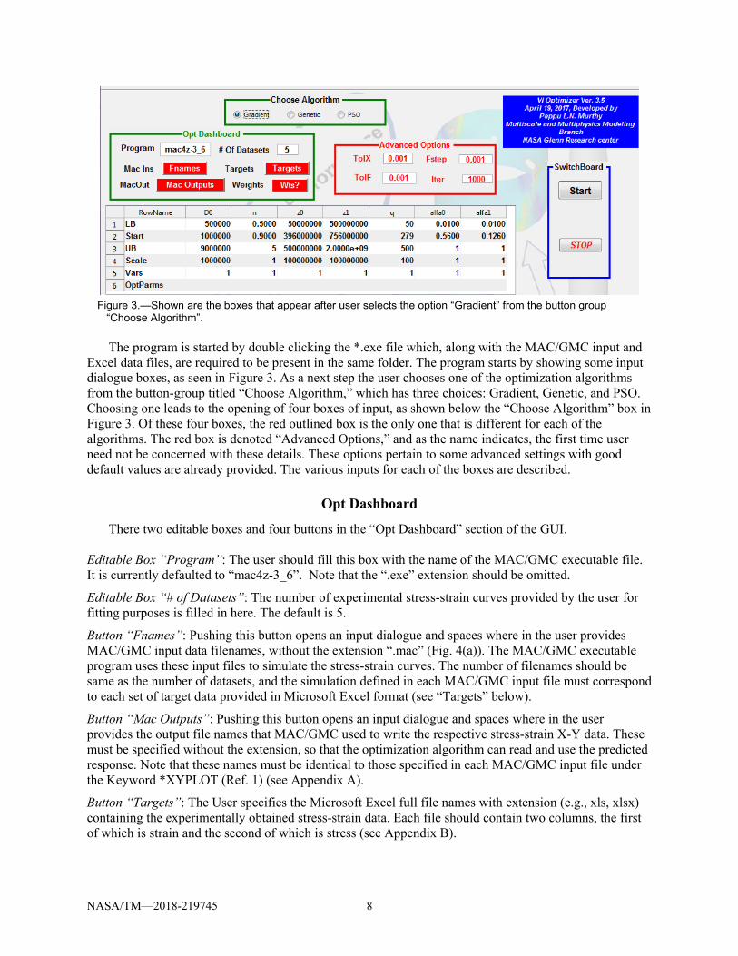
Figure 3.—Shown are the boxes that appear after user selects the option “Gradient” from the button group

“Choose Algorithm”.

The program is started by double clicking the *.exe file which, along with the MAC/GMC input and Excel data files, are required to be present in the same folder. The program starts by showing some input dialogue boxes, as seen in Figure 3. As a next step the user chooses one of the optimization algorithms from the button-group titled “Choose Algorithm,” which has three choices: Gradient, Genetic, and PSO. Choosing one leads to the opening of four boxes of input, as shown below the “Choose Algorithm” box in Figure 3. Of these four boxes, the red outlined box is the only one that is different for each of the algorithms. The red box is denoted “Advanced Options,” and as the name indicates, the first time user need not be concerned with these details. These options pertain to some advanced settings with good default values are already provided. The various inputs for each of the boxes are described.

Opt Dashboard

There two editable boxes and four buttons in the “Opt Dashboard” section of the GUI. Editable Box “Program”: The user should fill this box with the name of the MAC/GMC executable file. It is currently defaulted to “mac4z-3_6”. Note that the “.exe” extension should be omitted.

Editable Box “# of Datasets”: The number of experimental stress-strain curves provided by the user for fitting purposes is filled in here. The default is 5.

Button “Fnames”: Pushing this button opens an input dialogue and spaces where in the user provides MAC/GMC input data filenames, without the extension “.mac” (Fig. 4(a)). The MAC/GMC executable program uses these input files to simulate the stress-strain curves. The number of filenames should be same as the number of datasets, and the simulation defined in each MAC/GMC input file must correspond to each set of target data provided in Microsoft Excel format (see “Targets” below).

Button “Mac Outputs”: Pushing this button opens an input dialogue and spaces where in the user provides the output file names that MAC/GMC used to write the respective stress-strain X-Y data. These must be specified without the extension, so that the optimization algorithm can read and use the predicted response. Note that these names must be identical to those specified in each MAC/GMC input file under the Keyword *XYPLOT (Ref. 1) (see Appendix A).

Button “Targets”: The User specifies the Microsoft Excel full file names with extension (e.g., xls, xlsx) containing the experimentally obtained stress-strain data. Each file should contain two columns, the first of which is strain and the second of which is stress (see Appendix B).

NASA/TM—2018-219745 9

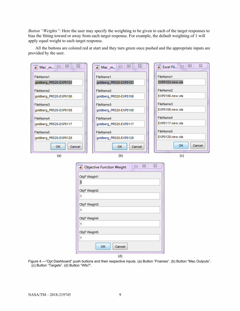
Button “Weights”: Here the user may specify the weighting to be given to each of the target responses to bias the fitting toward or away from each target response. For example, the default weighting of 1 will apply equal weight to each target response.

All the buttons are colored red at start and they turn green once pushed and the appropriate inputs are provided by the user.

(a) (b) (c)

(d)

Figure 4.—“Opt Dashboard” push buttons and their respective inputs. (a) Button “Fnames”. (b) Button “Mac Outputs”. (c) Button “Targets”. (d) Button “Wts?”.

NASA/TM—2018-219745 10

Algorithm Input Details Table

The next set of input details are common to all three algorithm choices. It consists of a table of details related to the seven parameters of the material constitutive law. The seven parameters are D0, Z1, 1, q, n, Z0, and 0 as explained above. The user must provide the lower bound (LB), the upper bound (UB), and starting values for these parameters, as well as scaling values for these parameters. The scaling parameter provides the tool with a sense of the relative magnitudes of each of the parameters. This is important because the parameters typically vary widely in magnitude from each other, and it is recommended that these are scaled in such a manner the resulting scaled parameter values are all of same order of magnitude. Appropriate defaults are provided for all of these and thus the user usually needs only to choose the starting values. Row 5 values (Fig. 3) toggle between 0 and 1 to enable users to turn parameters on (1) or off (0) in the fitting optimization process. If a parameter is turned off (0), it will be kept at its start value and not optimized to improve the fit. In Figure 3, all the values are set to the default value of 1, meaning all seven parameters will be treated as active variables. Once the minimization of the error is accomplished, row 6 is populated with the appropriate optimum values for the parameters.

Advanced Options

The advanced options are intended for fine tuning the optimization algorithms and are specific to each of the three algorithms. The default values should provide a sufficient starting point for most users. Figures 5(a) to (c) show these option panels for each algorithm.

(a)

(b)

(c)

Figure 5.—Advanced options for the three different optimization algorithms that are supported by the tool. (a) Advanced Options for the Gradient based algorithm. (b) Advanced Options for the Genetic algorithm. (c) Advanced Options for the Particle Swarm Optimization.

NASA/TM—2018-219745 11

Advanced Options for the Gradient Option

For the gradient based algorithm there are four advanced options TolX, Fstep, TolF, and Iter, as shown in Figure 5(a). For further details of these the user is advised to check MATLAB help files under the “fmincon” algorithm (Ref. 8). A brief description of these are given below:

1. TolX: Termination tolerance on x, the design vector. 2. Fstep: Step size used to compute the numerical derivatives and is known by the name

“FiniteDifferenceStepSize” by the MATLAB algorithm “fmincon”. 3. TolF: Termination tolerance on the function value. 4. Iter: Number of iterations allowed to terminate the optimization process.

Advanced Options for the Genetic Algorithm

For Genetic Algorithm (GA), the advanced options are shown in Figure 5(b). Each of the four boxes of the inputs are explained below:

1. NPop: The number of candidate solutions that satisfy the upper and lower bounds. Based on this number, the program generates candidates by using a uniform probability distribution between the upper and lower bounds. For example shown a population consisting of 100 has been chosen.

2. NGen: The number of generations the GA is required to perform the search operations, after which the optimization stops. Here we have chosen this number to be 10.

3. NElite: After performing the fitness calculations (that is the square of the error between prediction and target) for each candidate, the top candidates which give rise to the lowest error are considered elite and are preserved for the next generation as they are. The number of elite candidates must be even and is typically 2 or higher. In this example, 2 has been chosen.

4. NMut: This is the number of cross over, or Gaussian noise, candidates to be chosen by the algorithm. In the example shown here, NMut = 10. It should be noted that in the algorithm it is hardcoded to have the Gaussian and cross over candidates to be equal, however, in general they can be different.

Advanced Options for the PSO Algorithm

For the particle swarm optimization algorithm the advanced options are shown in Figure 5(c). Each of these are explained briefly here:

1. Nps: Number of particles constituting the total population. 2. NSteps: Number of steps before the process is terminated. 3. Gamma: Particle swarm algorithm ϒ parameter (see discussion in “Optimization Algorithm”

Section). 4. Beta: Particle swarm algorithm β parameter (see discussion in “Optimization Algorithm”

Section).

SwitchBoard

After completing all the necessary input the user pushes the button “Start” to begin the fitting optimization (on right in Fig. 3). Once the algorithm completes it indicates the CPU time taken to complete the procedure. The red “Stop” button, if pushed at any time aborts the program. Figure 6 shows the switchboard and its contents at the end of successful gradient based algorithm run. As the run completes, the “SwitchBoard” shows a box that indicates the total CPU time taken in seconds (here it is 253.8677 s) and a push button labeled “Results?”. In addition, row 6 of the algorithm input details

NASA/TM—2018-219745 12

Figure 6.—Contents

of Switchboard at the end of a successful Gradient based algorithm run.

table, “Opt Parms”, is populated with optimum parameters that the tool determined by performing the optimization. During the execution at the end of each iteration, the code outputs two figures. The first one shows the progress of each design variable and the computed least square error (objective function value) as a function of iteration number. The second figure shows a comparison of target and predicted stress-strain curves at the end of each iteration. These figures are output only for the Gradient based algorithm and are meant for monitoring the code progress towards an optimum set of design variables. Once the optimum set of design variables is determined, the code depicts a dialogue box showing “all the operations are completed”. At this point the user may push the “Results” button to see how the code performed in matching the target stress-strain response curves with the predictions based on the optimum set of design variables (row 6).

Results and Discussion

In this section, results are presented that first validate the optimized material parameters (and associated viscoplastic model) for neat PR520 epoxy resin. Next, the Parameter Optimization Tool is applied to determine parameters optimized for the in-situ resin response within a multiscale MAC/GMC model of a triaxially braided T700/PR520 carbon/epoxy composite, with the model results and again validated vs. experimental data. The ability to generate virtual stress-strain curve data for the composite, suitable for use in LS-DYNA MAT 213 (Ref. 5), is also demonstrated, followed by presentation of a parametric study wherein the combined effect of temperature and loading rate on the predicted composite response is investigated.

Application to Monolithic Resin Material

As an illustrative example we chose a cascading approach where we first try to get a feasible optimum design vector by using the Genetic Algorithm based optimization followed by a Gradient based optimization to arrive at the best possible solution. Genetic Algorithm based optimization often becomes computationally intensive, however, for those problems with many local minima in which no good starting point can be easily found. In such cases GA can be used to arrive at a good starting point from which a Gradient search method can be used to quickly zero in on the best possible solution. Here we chose a population of 1000, NElite = 10, NGen = 20, and NMut = 80. The algorithm was run overnight for this problem. The total time taken was 13622 s and the results are shown in Figure 7.

NASA/TM—2018-219745 13

Figure 7.—GA based optimization results.

The GA algorithm led to the following optimum set of design parameters:

D0 = 6.803106 s, n = 1.0575, Z0 = 1.9503108 Pa, Z1 = 6.6344108 Pa, q = 96.8116, 0 = 0.2559, 1 = 0.10. The quality of the fit can be seen from the Figure 7 in the “Results” panel. Although, results are close to target response, it is clear a better fit can probably still be pursued. At this point we used the following starting point that is close to the GA design point and chose to optimize with Gradient based approach. The starting point is

D0 = 6.8106 s, n = 1.0575, Z0 = 1.95108 Pa, Z1 = 6.63108 Pa, q = 96.8, 0 = 0.26, 1 = 0.1.

The Gradient based approach is able to improve the solution significantly. The CPU time taken was 253.8677 s. The optimum design parameters are listed below:

D0 = 6.3358106 s, n = 0.9546, Z0 = 1.421108 Pa, Z1 = 7.353108 Pa, q = 92.0838, 0 = 0.01, 1 = 0.01.

NASA/TM—2018-219745 14

The results of Gradient based approach are shown in Figure 8. As discussed in the Introduction, the Multiobjective Viscoplastic Parameter Optimization Tool along

with MAC/GMC form the basis for a “Virtual Testing” platform. Given some experimental data, either on the scale of the constituent materials of a composite or that of a composite material itself, optimized constitutive model parameters for the constituent materials can be determined. Then, other data (e.g., stress-strain responses under other types of loading, at other temperatures, or at other loading rates) can be predicted for either constituents or composites. The predicted virtual data, in combination with available experimental data, can then be used as input for characterization of other models. A perfect example of such a model is the LS-DYNA MAT 213 elastoplastic orthotropic material model (Ref. 5). This constitutive model requires as input 12 stress-strain curves in the form of tabular data for each temperature and each applied strain rate. Some of these curves are difficult to obtain experimentally and the ability to obtain virtual data to fill in gaps in the experimental data can be quite valuable.

Figure 8.—Illustrative example showing the use of Genetic Algorithm followed by a fine tuning with

Gradient approach. The results shown above are by Gradient Based optimization.

NASA/TM—2018-219745 15

Figure 9 compares the predicted nonlinear PR520 resin behavior at varying temperatures, loading rates, and loading scenarios where the previously optimized model parameters have been employed. viscoplastic parameters were determined utilizing the Multiobjective Viscoplastic Parameter Optimization Tool at room temperature to reproduce the reported stress-strain response of PR520 resin (Fig. 8). An example of neat resin elastic and viscoplastic parameters at room temperature, as they appear in the MAC/GMC input file, are provided in Appendix A (Files 1-5). Note that these files provide starting points for the Parameter Optimization Tool, and they are not updated with the output from the parameter optimization. This is why the viscoplastic parameters (specified using “VI=” under the *CONSTITUENTS keyword) in the Appendix A files do not match the output from the optimization tool shown in Figure 8.

Figure 9.—Tensile and torsional (shear) stress-strain responses of Neat resin (PR520) at various rates and temperatures.

Note that the scales are different across the plots.

0

10

20

30

40

50

60

70

80

0.00 0.01 0.02 0.03 0.04 0.05 0.06

Stress (MPa)

Strain

Test

Prediction

0

10

20

30

40

50

60

70

0.00 0.01 0.02 0.03 0.04 0.05 0.06

Stress (MPa)

Strain

0

10

20

30

40

50

60

70

80

0.00 0.01 0.02 0.03 0.04 0.05 0.06

Stress (MPa)

Strain

0

5

10

15

20

25

30

35

40

45

0.00 0.10 0.20 0.30 0.40 0.50

Stress (MPa)

Strain

0

10

20

30

40

50

60

0.00 0.10 0.20 0.30 0.40 0.50

Stress (MPa)

Strain

0

5

10

15

20

25

30

35

40

0.00 0.10 0.20 0.30 0.40 0.50

Stress (MPa)

Strain

Tension, 50 C, ε 3 10 /s

Tension, 50 C, ε 5 10 /s

Torsion, 50 C, ε 1.3 10 /s

Tension, 80 C, ε 5 10 /s

Torsion, 80 C, ε 4 10 /s

Torsion, 80 C, ε 1.3 10 /s

NASA/TM—2018-219745 16

While the viscoplastic parameters remained unchanged from the reported values, elastic modulus was adjusted from 3.5 GPa at 23 C to be 3.2 GPa at 50 C, and 2.5 GPa at 80 C. As it can be seen in Figure 9, the model can predict the stress-strain responses with minimal error in majority of the cases. Details of the plotted experimental results are reported in Reference 7. A higher percentage of error (~16 percent) is observed at higher temperatures (T = 80 C), which might stem from the fact that viscoplastic parameters were left unchanged across different temperatures. This was mainly done to assess the predictive capability of the Multiobjective Viscoplastic Parameter Optimization Tool across various temperature profiles, instead of calibrating the model for every given temperature value, which could also be done.

Application to a Triaxially Braided T700/PR520 Composite

Once the predicted nonlinear PR520 behavior was validated at the various temperatures and rates (Fig. 9), the mechanical response of a T700/PR520 braided composite system was predicted and validated. Figure 10 shows the geometry of the multiscale model of the braided composite simulated using the Multiscale Generalized Method of Cells (MSGMC) capability within MAC/GMC. The procedure and geometry employed follows that presented in References 12 and 13, in which MSGMC was applied to model the elastic response and viscoplastic response, respectively, of triaxially braided composites. A typical architecture of the triaxial braided composite is shown in Figure 10(a) with the indicated repeated unit cell. It is composed of three significant volumes: pure matrix, axial tows, and braided tows. Straight axial fiber tows and braided fiber tows are oriented at an angle θ (braid angle). The architecture being analyzed is assumed to be an idealized homogenized RUC with the transversely isotropic elastic fibers and a viscoplastic resin (Fig. 10(c) and (d)). The present homogenization methodology represents the triaxial braided composite with its constituent materials (fiber and matrix), where the constitutive models are applied. Larger scale stress state and moduli are determined through the GMC homogenization methods (Ref. 3). Further details about microstructural parameters in defining a triaxial braided composite architecture can be found in Reference 12. For the triaxial braided composite analyzed here, resin PR520 properties are calibrated through Multiobjective Viscoplastic Parameter Optimization Tool and the transversely isotropic T700 fiber properties are acquired from Reference 7 (EA = 230 GPa, ET = 15 GPa, A = 0.2, A = 0.2, GA = 15 GPa). The subcell dimensions shown in Figure 10(c) are: h1 = 0.0022, h2 = 0.00251, d = 0.00018, with the length units being arbitrary. The fiber volume fractions shown in Figure 10(c) are: Vf1 = 0.8, Vf2 = 0.7467, Vf3 = 0.3733. As discussed in Reference 12, the fiber volume fractions account for the regions of pure resin that are homogenized into the subcells. These subcell dimensions and fiber volume fractions result in an overall composite fiber volume fraction of 0.56.

Rather than using the previously optimized neat resin material parameters, the ability of the optimization tool to utilize composite level stress-strain data as input was employed to back out in-situ data for the resin in the composite. This is a key capability that enables the tool to function even in cases where neat resin data is unavailable. Two available composite level stress-strain curves were used for this purpose (transverse tension and in-plane shear), along with the gradient based optimization method.

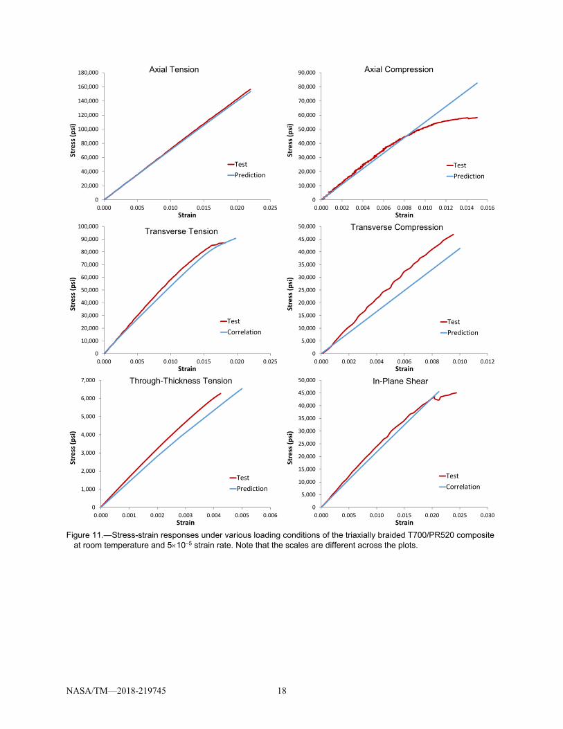
The multiscale model of the T700/PR520 composite was subjected to simulated tensile and shear loading at room-temperature at a strain rate of 510–5 /s and compared to available experimental data in Figure 11. For the two stress-strain curves used to determine the in-situ resin viscoplastic parameters, the simulated response is labeled as “correlation,” whereas, the remaining simulations represent predictions. In cases where there was no available experimental data, the simulations represent virtual test data, and the associated plots in Figure 11 are labeled as such. Examining Figure 11, the stress-strain response of the composite is reproduced with relatively acceptable error (< 20 percent) for all loading cases. The error observed for compression seems to be the highest (~20 percent). This may be due to the complex nature of composite nonlinear deformation under compression, which depends on various interacting

NASA/TM—2018-219745 17

mechanisms other than just matrix viscoplasticity. Therefore, it can still be stated that the model’s predictive capability is fairly good for various loading scenarios at room-temperature. The virtual data reported in Figure 11 (without one-to-one comparison with experiments) seems to fall in a reasonable range, when compared to similar available data in literature (Ref. 14).

(a)

(b)

(c)

(d)

Figure 10.—MAC/GMC multiscale model of a triaxially braided composite (T700/PR520). (a) Triaxial braid pattern with repeating unit cell identified. (b) Top view of the triaxial braid repeating unit cell. (c) MAC/GMC idealization of the triaxial braid repeating unit cell (Ref. 12), with subcell dimensions (h1, h2, d) and fiber volume fractions (Vf1, Vf2, Vf3) denoted. (d) Repeating unit cell used to model the unidirectional composite within each tow.

NASA/TM—2018-219745 18

Figure 11.—Stress-strain responses under various loading conditions of the triaxially braided T700/PR520 composite

at room temperature and 510–5 strain rate. Note that the scales are different across the plots.

0

20,000

40,000

60,000

80,000

100,000

120,000

140,000

160,000

180,000

0.000 0.005 0.010 0.015 0.020 0.025

Stress (psi)

Strain

Test

Prediction

0

10,000

20,000

30,000

40,000

50,000

60,000

70,000

80,000

90,000

0.000 0.002 0.004 0.006 0.008 0.010 0.012 0.014 0.016

Stress (psi)

Strain

Test

Prediction

0

10,000

20,000

30,000

40,000

50,000

60,000

70,000

80,000

90,000

100,000

0.000 0.005 0.010 0.015 0.020 0.025

Stress (psi)

Strain

Test

Correlation

0

5,000

10,000

15,000

20,000

25,000

30,000

35,000

40,000

45,000

50,000

0.000 0.002 0.004 0.006 0.008 0.010 0.012

Stress (psi)

Strain

Test

Prediction

0

1,000

2,000

3,000

4,000

5,000

6,000

7,000

0.000 0.001 0.002 0.003 0.004 0.005 0.006

Stress (psi)

Strain

Test

Prediction

0

5,000

10,000

15,000

20,000

25,000

30,000

35,000

40,000

45,000

50,000

0.000 0.005 0.010 0.015 0.020 0.025 0.030

Stress (psi)

Strain

Test

Correlation

Axial Tension Axial Compression

Transverse Tension Transverse Compression

Through-Thickness Tension In-Plane Shear

NASA/TM—2018-219745 19

Figure 12.—Parametric study showing combined effect of temperature and loading rate on the stress-strain response

of the braided T700/PR520 composite. Note that the scales are different across the plots.

Performing composite parametric studies to evaluate the “virtual testing” predictions over the full range of temperatures and rates for composite systems constitutes the final step for a viable virtual testing platform. After validating the composite response through available tests at room temperature, parametric studies were conducted to examine the influence of rate and temperature variation on the mechanical behavior of the composite system for various loading scenarios. Sample parametric study results are shown in Figure 12, wherein room-temperature/low rate and high-temperature/high rate results are compared. As shown, variation of temperature and rate has a relatively minor effect, except for the 45 off-axis shear loading. Note that the 13 and 23 plane 45 off-axis shear results were nearly identical, so

0

20,000

40,000

60,000

80,000

100,000

120,000

140,000

160,000

0.000 0.005 0.010 0.015 0.020 0.025

Stress (psi)

Strain

0

20,000

40,000

60,000

80,000

100,000

120,000

0.000 0.005 0.010 0.015 0.020 0.025

Stress (psi)

Strain

0

1,000

2,000

3,000

4,000

5,000

6,000

7,000

8,000

0.000 0.001 0.002 0.003 0.004 0.005 0.006

Stress (psi)

Strain

0

5,000

10,000

15,000

20,000

25,000

30,000

35,000

40,000

45,000

50,000

0.000 0.005 0.010 0.015 0.020 0.025

Stress (psi)

Strain

0

2,000

4,000

6,000

8,000

10,000

12,000

14,000

16,000

0.00 0.01 0.02 0.03 0.04 0.05 0.06 0.07

Stress (psi)

Strain

0

10,000

20,000

30,000

40,000

50,000

60,000

70,000

80,000

90,000

0.000 0.005 0.010 0.015 0.020

Stress (psi)

Strain

Axial Tension Transverse Tension

Through-Thickness Compression In-Plane Shear

45 Off-Axis 13 (and 23) plane 45 Off-Axis (in-plane)

NASA/TM—2018-219745 20

only the 13 plane results are shown. Also, although not shown, the rate was increased in various increments (from 0.00005 to 200 /s) and the resulted stress-strain curves were obtained for every case. A noticeable difference in stress-strain response (for the presented loading scenarios) was only observed when the rate reached approximately 100 /s. Therefore, it was not deemed necessary to illustrate redundant stress-strain curves with no distinct difference in this section. Further parametric studies on different composite systems are necessary to obtain a better understanding of rate/temperature influence on a given system.

Conclusion

The Multiobjective Viscoplastic Constitutive Law Parameter Fitting Tool helps in fitting experimentally observed stress-strain responses generated at different temperatures and different strain rates to a seven parameter Bodner-Partom constitutive law. The fit can be performed for a neat matrix material (as done herein) or for the composite-scale response. The software supports any number of stress-strain response curves as well as the importance given to these responses in the form of weights. Furthermore, three different algorithms (gradient based, genetic and particle swarm) provide flexibility to be used sequentially or individually in order to zero in on an optimum set of constitutive law parameters with a reasonable amount of computational resources.

The constitutive law parameters for the modified Bodner-Partom model generated by the tool were utilized within a multiscale micromechanics model in MAC/GMC to predict the response of braided composites that were then compared with experimental stress-strain curves. Two available composite level stress-strain curves (transverse tension and in-plane shear) were used to back-out in-situ data for the resin in the composite. Utilizing these in-situ properties, remaining composite stress-strain curves were predicted successfully with an acceptable margin of error for most of the loading cases. Some higher deviation in compression was observed which might be due to complicated nature of a composite behavior under compression. The tools discussed herein form the basis of a virtual test platform, wherein stress-strain curves that are extremely difficult to obtain experimentally can be predicted using the model. This can be very valuable in minimizing experimental costs and filling in experimental gaps.

NASA/TM—2018-219745 21

Appendix A.—Input Data for MAC/GMC Executable, (see Refs. 1 and 2 for details)

File 1: Goldberg_PR520-EXPO123.mac: (The input deck is meant to output axial tensile stress for an applied rate (1.4 /s) and temperature (23 C). The rate is the strain/time ratio). MAC/GMC - effective properties *CONSTITUENTS NMATS=1 # -- PR520 Resin Pa M=1 CMOD=12 MATID=U MATDB=1 & EL=3.54E9,3.54E9,0.38,0.38,1.28261E9,45.E-6,45.E-6 & VI=1E6,1.07,206977131.37,868911452.11,348.72,0.2548,0.126 *RUC MOD=1 M=1 *MECH LOP=1 NPT=2 TI=0.,0.014 MAG=0.,0.02 MODE=1 *THERM NPT=2 TI=0.,0.014 TEMP=23.,23. *SOLVER METHOD=1 NPT=2 TI=0.,0.014 STP=0.00003 *XYPLOT FREQ=1 MACRO=1 NAME=goldberg_PR520-EXP0128 X=1 Y=7 MICRO=0 *PRINT NPL=6 *END

File 2: Goldberg_PR520-EXPO123.mac: (The input deck is meant to output axial tensile stress for an applied rate (510–5 /s) and temperature (23 C). The rate is the strain/time ratio). MAC/GMC - effective properties *CONSTITUENTS NMATS=1 # -- PR520 Resin Pa M=1 CMOD=12 MATID=U MATDB=1 & EL=3.54E9,3.54E9,0.38,0.38,1.28261E9,45.E-6,45.E-6 & VI=1E6,1.07,206977131.37,868911452.11,348.72,0.2548,0.126 *RUC MOD=1 M=1 *MECH LOP=1 NPT=2 TI=0.,600. MAG=0.,0.032 MODE=1 *THERM NPT=2 TI=0.,600. TEMP=25.,25. *SOLVER METHOD=1 NPT=2 TI=0.,600. STP=1 *XYPLOT FREQ=1 MACRO=1 NAME=goldberg_PR520-EXP0117 X=1 Y=7 MICRO=0 *PRINT NPL=6 *END

NASA/TM—2018-219745 22

File 3: Goldberg_PR520-EXPO123.mac: (The input deck is meant to output out-of-plane shear stress (Torsion) for an applied rate (2.6 /s) and temperature (23 C). The rate is the strain/time ratio).

MAC/GMC - effective properties *CONSTITUENTS NMATS=1 # -- PR520 Resin Pa M=1 CMOD=12 MATID=U MATDB=1 & EL=3.54E9,3.54E9,0.38,0.38,1.28261E9,45.E-6,45.E-6 & VI=1E6,1.07,206977131.37,868911452.11,348.72,0.2548,0.126 *RUC MOD=1 M=1 *MECH LOP=6 NPT=2 TI=0.,0.115 MAG=0.,0.3 MODE=1 *THERM NPT=2 TI=0.,0.115 TEMP=25.,25. *SOLVER METHOD=1 NPT=2 TI=0.,0.115 STP=0.0002 *XYPLOT FREQ=1 MACRO=1 NAME=goldberg_PR520-EXP0108 X=6 Y=12 MICRO=0 *PRINT NPL=6 *END File 4: Goldberg_PR520-EXPO123.mac: (The input deck is meant to output out-of-plane shear stress (Torsion) for an applied rate (1.310–4 /s) and temperature (23 C). The rate is the strain/time ratio).

MAC/GMC - effective properties *CONSTITUENTS NMATS=1 # -- PR520 Resin Pa M=1 CMOD=12 MATID=U MATDB=1 & EL=3.54E9,3.54E9,0.38,0.38,1.28261E9,45.E-6,45.E-6 & VI=1E6,1.07,206977131.37,868911452.11,348.72,0.2548,0.126 *RUC MOD=1 M=1 *MECH LOP=6 NPT=2 TI=0.,3076. MAG=0.,0.4 MODE=1 *THERM NPT=2 TI=0.,3076. TEMP=25.,25. *SOLVER METHOD=1 NPT=2 TI=0.,3076. STP=5 *XYPLOT FREQ=1 MACRO=1 NAME=goldberg_PR520-EXP0106 X=6 Y=12 MICRO=0 *PRINT NPL=6 *END

NASA/TM—2018-219745 23

File 5: Goldberg_PR520-EXPO123.mac: (The input deck is meant to output out-of-plane shear stress (Torsion) for an applied rate (700 /s) and temperature (25 C). The rate is the strain/time ratio). MAC/GMC - effective properties *CONSTITUENTS NMATS=1 # -- PR520 Resin Pa M=1 CMOD=12 MATID=U MATDB=1 & EL=3.54E9,3.54E9,0.38,0.38,1.28261E9,45.E-6,45.E-6 & VI=1E6,1.07,206977131.37,868911452.11,348.72,0.2548,0.126 *RUC MOD=1 M=1 *MECH LOP=6 NPT=2 TI=0.,0.000714 MAG=0.,0.5 MODE=1 *THERM NPT=2 TI=0.,0.000714 TEMP=25.,25. *SOLVER METHOD=1 NPT=2 TI=0.,0.000714 STP=0.000001 *XYPLOT FREQ=1 MACRO=1 NAME=goldberg_PR520-EXP0103 X=6 Y=12 MICRO=0 *PRINT NPL=6 *END File 6: goldberg_triax_test: (The input deck is meant to output transverse axial stress for an applied rate (510–5 /s) and temperature (25 C). The rate is the strain/time ratio). MAC/GMC - effective properties *CONSTITUENTS NMATS=2 # -- T700 fiber - Pa M=1 CMOD=6 MATID=U MATDB=1 & EL=230.E9,15.E9,0.2,0.2,15.E9,-99.E-6,-99.E-6 # -- PR520 Resin Pa M=2 CMOD=12 MATID=U MATDB=1 & EL=3.54E9,3.54E9,0.38,0.38,1.28261E9,45.E-6,45.E-6 & VI=1775518,1.969662,1.51E8,6.33E8,249.05,0.477916,0.1 # Axial tension 3, transverse tension 2, and in-plane shear 4. *MSGMC NA=1 NB=4 NG=1 D=0.00070 H=0.00220,0.00251,0.00220,0.00251 L=0.00272 # -- gamma = 1 SM=-17,-18,-19,-20 *MSMATS NMATS=11 MSM=-17 DIM=3 ARCHID=99 NA=4 NB=1 NG=1 D=0.00018,0.00018,0.00018,0.00018 H=1.00000 L=1.00000 # -- gamma = 1 SM=-23 SM=-21

NASA/TM—2018-219745 24

SM=-21 SM=-22 MSM=-18 DIM=3 ARCHID=99 NA=4 NB=1 NG=1 D=0.00018,0.00018,0.00018,0.00018 H=1.00000 L=1.00000 # -- gamma = 1 SM=-27 SM=-27 SM=-24 SM=-24 MSM=-19 DIM=3 ARCHID=99 NA=4 NB=1 NG=1 D=0.00018,0.00018,0.00018,0.00018 H=1.00000 L=1.00000 # -- gamma = 1 SM=-22 SM=-21 SM=-21 SM=-23 MSM=-20 DIM=3 ARCHID=99 NA=4 NB=1 NG=1 D=0.00018,0.00018,0.00018,0.00018 H=1.00000 L=1.00000 # -- gamma = 1 SM=-25 SM=-25 SM=-26 SM=-26 MSM=-21 DIM=2 ARCHID=1 VF=8.000000e-01 F=1 M=2 D1=0.00000,0.00000,1.00000 D2=0.00000,1.00000,0.00000 D3=-1.00000,0.00000,0.00000 MSM=-22 DIM=2 ARCHID=1 VF=7.466667e-01 F=1 M=2 D1=0.00000,0.86603,0.50000 D2=1.00000,0.00000,0.00000 D3=0.00000,0.50000,-0.86603 MSM=-23 DIM=2 ARCHID=1 VF=7.466667e-01 F=1 M=2 D1=0.00000,-0.86603,0.50000 D2=1.00000,0.00000,0.00000 D3=-0.00000,0.50000,0.86603 MSM=-24 DIM=2 ARCHID=1 VF=0.3733 F=1 M=2 D1=-0.17795,0.85220,0.49202 D2=0.00000,0.50000,-0.86603 D3=0.98404,0.15411,0.08897 MSM=-25 DIM=2 ARCHID=1 VF=0.3733 F=1 M=2 D1=0.17795,0.85220,0.49202 D2=0.00000,0.50000,-0.86603 D3=0.98404,-0.15411,-0.08897 MSM=-26 DIM=2 ARCHID=1 VF=0.3733 F=1 M=2 D1=-0.17795,-0.85220,0.49202 D2=0.00000,0.50000,0.86603 D3=0.98404,-0.15411,0.08897 MSM=-27 DIM=2 ARCHID=1 VF=0.3733 F=1 M=2

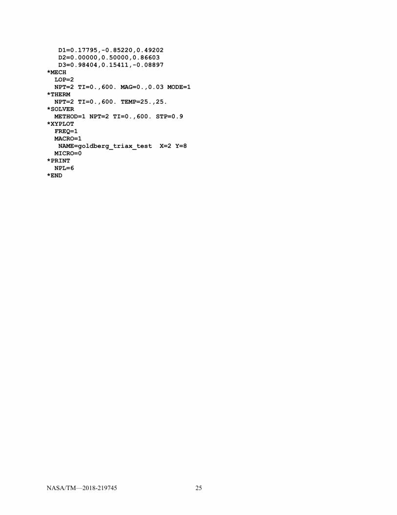
NASA/TM—2018-219745 25

D1=0.17795,-0.85220,0.49202 D2=0.00000,0.50000,0.86603 D3=0.98404,0.15411,-0.08897 *MECH LOP=2 NPT=2 TI=0.,600. MAG=0.,0.03 MODE=1 *THERM NPT=2 TI=0.,600. TEMP=25.,25. *SOLVER METHOD=1 NPT=2 TI=0.,600. STP=0.9 *XYPLOT FREQ=1 MACRO=1 NAME=goldberg_triax_test X=2 Y=8 MICRO=0 *PRINT NPL=6 *END

NASA/TM—2018-219745 27

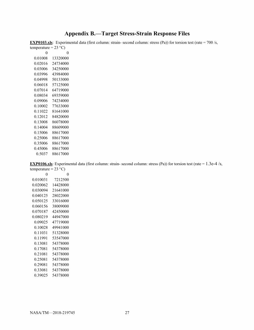
Appendix B.—Target Stress-Strain Response Files

EXP0103.xls: Experimental data (first column: strain- second column: stress (Pa)) for torsion test (rate = 700 /s, temperature = 23 C)

0 0 0.01008 13320000 0.02016 24734000 0.03006 34250000 0.03996 43984000 0.04998 50133000 0.06018 57125000 0.07014 64719000 0.08034 69359000 0.09006 74234000 0.10002 77633000 0.11022 81641000 0.12012 84820000 0.13008 86078000 0.14004 88609000 0.15006 88617000 0.25006 88617000 0.35006 88617000 0.45006 88617000

0.5037 88617000 EXP0106.xls: Experimental data (first column: strain- second column: stress (Pa)) for torsion test (rate = 1.3e-4 /s, temperature = 23 C)

0 0 0.010031 7212500 0.020062 14428000 0.030094 21641000 0.040125 28022000 0.050125 33016000 0.060156 38009000 0.070187 42450000 0.080219 44947000 0.09025 47719000 0.10028 49941000 0.11031 51328000 0.11991 53547000 0.13081 54378000 0.17081 54378000 0.21081 54378000 0.25081 54378000 0.29081 54378000 0.33081 54378000 0.39025 54378000

NASA/TM—2018-219745 28

EXP0108.xls: Experimental data (first column: strain- second column: stress (Pa)) for torsion test (rate = 2.6 /s, temperature = 23 C)

0 0 0.010032 10822000 0.020063 18591000 0.030063 26916000 0.040094 34959000 0.050125 40509000 0.060157 47169000 0.070625 53828000 0.080219 58269000 0.091125 62431000 0.098533 65481000 0.109433 67703000 0.119903 70200000 0.130343 71859000 0.140373 72137000 0.175373 72137000 0.210373 72137000 0.245373 72137000 0.280373 72137000 0.310873 72137000

EXP0117.xls: Experimental data (first column: strain- second column: stress (Pa)) for tension test (rate = 5e-5 /s, temperature = 23 C)

0 0 0.002081 6793700 0.004031 13369000 0.006006 19944000 0.008025 25856000 0.010044 31337000 0.012019 36381000 0.014006 40981000 0.016019 44925000 0.018031 49306000 0.020044 53912000 0.022062 57200000 0.024006 60706000 0.026019 63994000

0.028 65744000 0.03005 68594000

0.032631 70562000

NASA/TM—2018-219745 29

EXP0128.xls: Experimental data (first column: strain- second column: stress (Pa)) for tension test (rate = 1.4 /s, temperature = 23 C)

0 0 0.001013 3650000 0.00205 6443700

0.003019 9025000 0.004031 12250000 0.005006 15900000 0.006044 18262000 0.007019 21269000 0.008025 24281000 0.009069 26856000 0.010044 29006000 0.011013 32012000 0.01205 34594000

0.013094 38031000 0.014006 40181000 0.015044 42756000 0.01585 44694000

NASA/TM—2018-219745 30

References

1. Bednarcyk, B.A, and Arnold, S.M. “MAC/GMC 4.0 User’s Manual—Keywords Manual,” NASA/TM—2002-212077/Vol. 2.

2. Bednarcyk, B.A, and Arnold, S.M. “MAC/GMC 4.0 User’s Manual—Example Problem Manual,” NASA/TM—2002-212077/Vol. 3.

3. Aboudi, J., Arnold, S.M., and Bednarcyk, B.A. (2013) Micromechanics of Composite Materials: A Generalized Multiscale Analysis Approach, Elsevier, Oxford, UK.

4. MATLAB and Statistics Toolbox Release 2016a, The MathWorks, Inc., Natick, Massachusetts, United States.

5. Hoffarth C., Harrington J., Subramaniam R., Goldberg R.K., Carney K., Dubois P., Blackenhorn G. “An Orthotropic 3D Elasto-Plastic Material Model for Composite Materials Subjected to High Velocity Impact Loads”. MECHComp 2014, Stony Brook, NY.

6. Bodner, S.R. (2002) Unified Plasticity for Engineering Application, Kluwer Academic/Plenum Publishers, New York.

7. Goldberg, R.K., Roberts, G.D., and Gilat, A. (2005) “Implementation of an Associative Flow Rule Including Hydrostatic Stress Effects into the High Strain Rate Deformation Analysis of Polymer Matrix Composites,” Journal of Aerospace Engineering, 18, 18–27.

8. The Mathworks, Inc., https://www.mathworks.com/help/optim/ug/fmincon.html 9. James C. Spall, “Introduction to Stochastic Search and Optimization, Estimation, Simulation, and

Control,” John Wiley & Sons, Inc., 2003. 10. J. Kennedy and R. Eberhart, “Particle swarm optimization,” in Neural Networks, IEEE International

Conference on, vol. 4, nov/dec 1995, pp. 1942–1948. 11. Xin-She Yang, Nature-Inspired Metaheuristic Algorithms, Chapter 8 (section 8.3, page 65) of the

second edition (2010). 12. Liu, K.C., Chattopadhyay, A., Bednarcyk, B.A., and Arnold, S.M. (2011) “Efficient Multiscale

Modeling Framework for Triaxially Braided Composites Using Generalized Method of Cells,” ASCE Journal of Aerospace Engineering, 24, 162–169.

13. Liu, K.C. and Chattopadhyay, A. (2011) “Strain Rate Dependent Inelastic Response of Triaxially Braided Fabric Composites via Multiscale Generalized Method of Cells,” 52nd AIAA/ASME/ ASCE/AHS/ASC Structures, Structural Dynamics and Materials Conference, April, Denver, Colorado, AIAA-2011-2176.

14. Gilat, A.; Goldberg, R.K.; and Roberts, G.D.: “Experimental Study of Strain-Rate-Dependent Behavior of Carbon/Epoxy Composite.” Composites Science and Technology, Vol. 62, pp. 1469–1476, 2002.