development and application of the method …€¦ · this work introduces the method of...

DEVELOPMENT AND APPLICATION OF THE METHOD OF DISTRIBUTED

VOLUMETRIC SOURCES TO THE PROBLEM OF UNSTEADY-STATE

FLUID FLOW IN RESERVOIRS

A Dissertation

by

SHAHRAM AMINI

Submitted to the Office of Graduate Studies of Texas A&M University

in partial fulfillment of the requirements for the degree of

DOCTOR OF PHILOSOPHY

December 2007

Major Subject: Petroleum Engineering

ii

DEVELOPMENT AND APPLICATION OF THE METHOD OF DISTRIBUTED

VOLUMETRIC SOURCES TO THE PROBLEM OF UNSTEADY-STATE

FLUID FLOW IN RESERVOIRS

A Dissertation

by

SHAHRAM AMINI

Submitted to the Office of Graduate Studies of Texas A&M University

in partial fulfillment of the requirements for the degree of

DOCTOR OF PHILOSOPHY Approved by:

Co-Chairs of Committee, Peter P. Valkó Thomas A. Blasingame Committee Members, Duane A. McVay Richard Gibson Head of Department, Stephen A. Holditch

December 2007

Major Subject: Petroleum Engineering

iii

ABSTRACT

Development and Application of the Method of Distributed Volumetric Sources to the Problem of

Unsteady-State Fluid Flow in Reservoirs. (December 2007)

Shahram Amini

B.S.; M.S., University of Tehran;

M.S., IFP School (ENSPM)

Co-Chairs of Advisory Committee: Dr. Peter P. Valkó Dr. Thomas A. Blasingame

This work introduces the method of Distributed Volumetric Sources (DVS) to solve the transient and

pseudosteady-state flow of fluids in a rectilinear reservoir with closed boundaries. The development and

validation of the DVS solution for simple well/fracture configurations and its extension to predict the

pressure and productivity behavior of complex well/fracture systems are the primary objectives of this

research.

In its simplest form, the DVS method is based on the calculation of the response for a closed rectilinear

system to an instantaneous change in a rectilinear, uniform volumetric source inside the reservoir.

Integration of this response over the time provides us with the solution to a continuous change (constant-

rate pressure response). Using the traditional material balance equations and the DVS pressure response

of the system, we can calculate the productivity index of the system in both transient and pseudosteady-

state flow periods, which enables us to predict the production behavior over the life of the well/reservoir.

Solutions for more complex situations, such as sources with infinite or finite-conductivity (i.e., a fracture),

are provided using discretization of the source. This work considers the case of a complex system with a

horizontal well intersecting multiple transverse fractures as an example to show the ability (and flexibility)

of the new method. The DVS solution method provides accurate solutions for complex well/fracture

configurations — which will help engineers to design and implement optimum well completions.

The DVS solutions has been validated by comparing to existing analytical solutions (where applicable), as

well as to numerical (simulation) solutions. In all cases the DVS solution was successfully validated — at

least in a practical sense — specifically in terms of the accuracy and precision of the DVS solution. As the

DVS method is approximate (at early times), there are small discrepancies which are of little or no

practical consequence. In terms of computation times, because of its analytic nature, the DVS method is

not always optimal in terms of speed for certain problems, but the DVS approach is similar in computation

speed with commercial reservoir simulation programs.

iv

DEDICATION

To my parents,

Abbas Amini and Farideh Gorji,

and to my sisters,

Shohreh and Shahla

— for their love and support

v

ACKNOWLEDGEMENTS

I would like to thank my co-chairs of advisory committee, Dr. Peter P. Valkó and Dr. Thomas A.

Blasingame for their guidance and support. I would like also to thank Dr. Duane A. McVay and Dr.

Richard Gibson for serving as committee members and for their valuable contributions to this research.

Finally, I appreciate the support and encouragement of all my Iranian friends in the Department of

Petroleum Engineering at Texas A&M University. God bless them all.

vi

TABLE OF CONTENTS

Page

CHAPTER I INTRODUCTION..................................................................................................... 1

1.1 Introduction ...................................................................................................................... 1

1.2 Objectives ......................................................................................................................... 1

1.3 Statement of the Problem.................................................................................................. 2

1.4 Deliverables...................................................................................................................... 3

1.5 Organization of the Dissertation....................................................................................... 4

CHAPTER II DEVELOPMENT OF THE DVS METHOD............................................................ 6

2.1 Literature Review ............................................................................................................. 6

2.2 Development of Uniform-Flux Solution......................................................................... 10

2.3 Solution for Infinite-Conductivity Cases........................................................................ 13

2.4 Solution for Finite-Conductivity Cases .......................................................................... 14

2.5 Productivity Index Calculation ....................................................................................... 20

CHAPTER III VALIDATION OF THE MODEL .......................................................................... 23

3.1 Introduction .................................................................................................................... 23

3.2 Validation with Pressure Models.................................................................................... 23

3.3 Validation with Productivity Index Models.................................................................... 30

CHAPTER IV APPLICATION OF THE NEW TECHNIQUE TO A COMPLEX WELL/FRACTURE CONFIGURATION CASE ................................................... 34

4.1 Introduction .................................................................................................................... 34

4.2 Formulation of the Problem............................................................................................ 34

4.3 Validation Through Simulation ...................................................................................... 35

4.4 Design and Optimization ................................................................................................ 38

4.5 Application to Field Examples ....................................................................................... 48

4.6 Summary......................................................................................................................... 61

CHAPTER V SUMMARY, CONCLUSIONS, AND RECOMMENDATIONS FOR FUTURE WORK .................................................................................................... 62

5.1 Summary......................................................................................................................... 62

5.2 Conclusions .................................................................................................................... 62

5.3 Recommendations for Future Work ............................................................................... 63

vii

Page

NOMENCLATURE .............................................................................................................................. 64

REFERENCES ...................................................................................................................................... 67

APPENDIX A — DEVELOPMENT OF THE SOLUTION................................................................ 69

APPENDIX B — DIMENSIONLESS PRODUCTIVITY INDEX FROM PRESSURE DATA......... 76

APPENDIX C — DETAILED RESULTS OF CALCULATION FOR MAXIMUM

DIMENSIONLESS PRODUCTIVITY INDEX OF THE EXAMPLE CASE,

PROPPANT NUMBER (NPROP) = 0.001 ............................................................... 78

APPENDIX D — DETAILED RESULTS OF CALCULATION FOR MAXIMUM


PROPPANT NUMBER (NPROP) = 0.01 ................................................................. 89

APPENDIX E — DETAILED RESULTS OF CALCULATION FOR MAXIMUM



APPENDIX F — DETAILED RESULTS OF CALCULATION FOR MAXIMUM



APPENDIX G — COMPLETE RESULTS OF FIELD APPLICATION WHELAN GAS FIELD ... 125

APPENDIX H — COMPLETE RESULTS OF FIELD APPLICATION PERCY WHEELER

GAS FIELD........................................................................................................... 129

APPENDIX I— COMPLETE RESULTS OF FIELD APPLICATION APPLEBY NORTH

GAS FIELD........................................................................................................... 133

VITA.................................................................................................................................................... 137

viii

LIST OF FIGURES

FIGURE Page

2.1 Schematic of the Model. ......................................................................................................... 11

2.2 Discretized of the Rectangular Source. ................................................................................... 13

2.3 Example of 1D Flow in the Source. ........................................................................................ 15

2.4 Example of 2D Flow in the Source. ........................................................................................ 15

2.5 Schematic of a Discretized 1D Source. ................................................................................... 16

2.6 Schematic of a Finite Difference Presentation of a Continuous System. ................................ 18

2.7 Example of Discretized 2D Source ........................................................................................ 19

2.8 Graphical Representation of the D Matrix for 2D Flow in Fracture. ...................................... 20

3.1 Comparison of the DVS Results with Line Source and Cylindrical Source Solutions:

Vertical Well in a Bounded Reservoir (In the Box-in-Box Model wz=ze/2, wx = wy

=0.477 ft, and the actual value of ze is irrelevant) ....................................................................24

3.2 Comparison of DVS Results with Yildiz's Model for a Partially-Penetrating Vertical Well

(Box-in- Box Model),(h, hp, and hb are represented by ze, 2wz, and cz- wz respectively) ....... 25

3.3 Comparison of DVS Results with Ozkan's and Gringarten's Solutions for a Horizontal

Well in a Bounded Reservoir, Uniform Flux Solution (In the Box-in-Box Model xeD=

xe/wx , yeD= ye/wx , and LD= ze/wx ) ...........................................................................................26

3.4 Comparison DVS Results with Gringarten, Ramey and Raghavan (1974) Solution for a

Vertically Fractured Well in a Bounded Reservoir; Uniform Flux Solution (xeD= xe/wx in

the Box-in-Box Model) ........................................................................................................... 28

3.5 Comparison of DVS Results with Gringarten, Ramey and Raghavan (1974) Solution for

a Vertically Fractured Well in Bounded Reservoir; Infinite Conductivity Solution. (xeD=

xe/wx in the Box-in-Box Model) ...............................................................................................28

3.6 Comparison of DVS with Cinco-Ley, Samaniego, and Dominguez (1978) Results for

Finite Conductivity Fracture ................................................................................................... 29

3.7 Distribution of the Contribution of Different Segments to Total Production at Various

Times, Finite Conductivity Vertical Fracture of Full Vertical Penetration for Half the

Fracture (CfD =1.6 and Ix = 0.25)............................................................................................. 29

3.8 Dimensionless Productivity Index of a Vertically Fully Penetrated Fracture as a Function

of Fracture Conductivity and Proppant Number (From Economides, Oligney, and Valkó

2002) ....................................................................................................................................... 32

3.9 Dimensionless Productivity Index of the Example Case Using DVS Method........................ 33

4.1 Schematic of the Model's Building Block. .............................................................................. 34

ix

FIGURE Page

4.2 A 3D View of ¼ of the Simulation Model, (Case of 4 Transverse Fractures) .........................36

4.3 Simulation Output, Well Bottomhole Pressure and Average Reservoir Pressure for Cases

of 1 Fracture and 4 Fractures................................................................................................... 37

4.4 Comparison Between Simulation Results and DVS Method's................................................ 37

4.5 Distribution of Dimensionless Productivity Index as a Function of Number of Fractures...... 42

4.6 Fracture Contribution to Flow as a Function of Dimensionless Time and Number of

Fractures (NProp = 1.0, kx = ky = kz =1 md)................................................................................43


Fractures (kx = ky = 1 md, kz =0.1 md). ....................................................................................43


Fractures (kx = ky = 1 md, kz =0.01 md). ..................................................................................44


Fractures (kx = ky = 1 md, kz =0.001 md)..................................................................................44

4.10 Maximum Dimensionless Pseudosteady-State Productivity Index as a Function of

Number of Fractures and Proppant Number (kx = ky = kz =1 md) ........................................... 46


Number of Fractures and Proppant Number (kx = ky = 1 md, kz =0.1 md). ............................. 46


Number of Fractures and Proppant Number (kx = ky = 1 md, kz =0.01 md). ........................... 47


Number of Fractures and Proppant Number (kx = ky = 1 md, kz =0.001 md). ......................... 47

4.14 Gas Production Rate as a Function of Production Time, Number of Fractures, and

Completion Scheme for Whelan Field (80 Acres Spacing, 250,000 lb Proppant) .................. 52


Completion Scheme for Percy Wheeler Field (80 Acres Spacing, 250,000 lb Proppant) ....... 53




Completion Scheme for Appleby North Field (80 Acres Spacing, 250,000 lb Proppant)....... 54


Completion Scheme for Appleby Nprth Field (80 Acres Spacing, 500,000 lb Proppant)....... 54

4.19 Average Reservoir Pressure as a Function of Production Time, Number of Fractures, and


x

FIGURE Page


Completion Scheme for Percy Whelan Field (80 Acres Spacing, 500,000 lb Proppant) ........ 56





4.23 Cumulative Gas Production as a Function of Production Time, Number of Fractures, and












xi

LIST OF TABLES TABLE Page

3.1 Reservoir/Fluid Properties Used for Example Cases of Chen and Asaad (2003)

(Comparison of Different Pseudosteady-State Productivity Index Correlations).................... 30

3.2 Comparison of DVS Results with Various Pseudosteady-State Productivity Index

Correlations. ............................................................................................................................ 31

4.1 Reservoir, Fracture, and Fluid Characteristic Used for Simulation Model and DVS

Calculations............................................................................................................................. 35

4.2 Reservoir and Proppant Characteristics Used for Case Study................................................. 38

4.3 Range of Variation of Design Parameters. .............................................................................. 39

4.4 Table of Mathematically Feasible Fracture Sizes for Example Case. ..................................... 40

4.5 Locus of Maxima for Example as a Function of Number of Fractures and Permeability

Anisotropy (NProp = 1.0). ......................................................................................................... 42

4.6 Reservoir and Fluid Properties for Example Cases. ................................................................ 48

4.7 Initial Gas-in-Place (G) for Example Cases. ........................................................................... 48

4.8 Optimum Fracture Dimensions for Field Cases as a Function of Proppant Used and

Number of Fractures. Fully-Penetrating Horizontal Well Contributes to Flow. ..................... 49

4.9 Results of Field Case Studies, Average Reservoir Pressure, Gas Production Rate, and

Cumulative Gas Production as a Function of the Amount of Proppant, Number of

Fractures, and Completion Schemes for Example Cases. ....................................................... 51

1

CHAPTER I

INTRODUCTION

1.1 Introduction

In this work we present the development and application of a new solution to the problem of unsteady-

state flow of a slightly compressible fluid in a rectilinear reservoir. The method of Distributed Volumetric

Sources (DVS) is developed to solve problems of transient and pseudosteady-state fluid flow. The basic

building block of the method is the calculation of the analytical response of a rectilinear reservoir with

closed outer boundaries to an instantaneous volumetric source, also shaped as a rectilinear body (a

rectilinear geometry is required for the DVS approach). The DVS solution provides the time-derivative of

the pressure response to a continuous source in analytical form (i.e., the derivative of the constant rate

pressure response function). This result is integrated over time to provide the required pressure response.

The results from the new solution are combined with the traditional material balance equations and are

used to predict the production behavior of the system in the form of the dimensionless Productivity Index

(PI) — for transient, transition, and pseudosteady-state flow behavior (flow regimes). This approach can

be used to design optimal completion schemes for a specific well/reservoir configuration.

The new method has been shown to provide a relatively fast and uniformly robust mechanism to generate

pressure transient solutions and well performance predictions whenever complex well/fracture configura-

tions are considered.

1.2 Objectives

The following objectives are proposed for this work:

� To develop the distributed volumetric source (or DVS) method as a solution to the problem of

pressure distributions in closed, rectangular reservoirs for the case of a uniform-flux source.

� To develop and validate a series of solutions for pressure behavior of simple and complex well/

fracture configurations such as:

— Unfractured vertical wells.

— Horizontal wells (uniform-flux and infinite-conductivity).

— Vertically fractured wells (infinite- and finite-conductivity fractures).

� To generate the transient and pseudosteady-state behavior of the productivity index using the DVS

pressure solution and to validate these results with existing models used in production engineering.

_____________________

This dissertation follows the style and format of the SPE Journal.

2

� To demonstrate the applicability of the new solution method in predicting pressure and production

behavior for a complex well/fracture configuration.

—Horizontal well with multiple transverse fractures, where both horizontal section and fractures

contribute to the flow.

� To apply the new method as an optimization tool to obtain the best completion scheme for

development of an example case.

1.3 Statement of the Problem

Most of the solutions for flow problems in porous media have been investigated in a similar manner as the

classical heat transfer problems — and in fact, many common solutions originated from the heat transfer

literature. Along that path, the work of Gringarten and Ramey (1973) is an early application of the

Green's (source) function for the problem of unsteady-state fluid flow in a reservoir. They introduced

Green's functions for a series of source shapes and boundary conditions and they showed that the point

source solution is actually a more general form of the Green's function. Gringarten and Ramey (1973)

used the integration of the response for an instantaneous source solution to obtain the response for a

continuous source solution. In addition, the application of Newman's (1936) principle in expressing a

problem into 3 dimensions as the product of three 1-dimensional solutions is also discussed in their work.

The major disadvantage of this method is the inherent singularity of the solution where the source is

placed. Since the source is assumed to have no volume (point, line, or plane source), the source is

considered to be at infinite pressure at any time and it is not possible to calculate the exact pressure as a

function of time at the point where the source is placed. The solutions provided for finite reservoir cases

yield infinite series, which converge very slowly as we approach the coordinates of the source. This

makes the process of computation inefficient as we approach the source. To address this problem, we

must assume an arbitrary point a certain distance from the source, and compute the solution at that point.

The solution obtained by using this method is only a function of the distance from the source, regardless of

the coordinates, so it may raise questions as to the reliability of the solution for anisotropic systems and/or

complex well completion schemes.

The application of Green's functions was later extended to the case of an unsteady-state pressure

distribution for more complex well completion schemes (Gringarten, Ramey, and Raghavan 1974; Cinco-

Ley, Samaniego, and Dominguez 1978; Cinco-Ley and Meng 1988; Ozkan 1988 ). These solutions do not

suffer the singularity problem (because the line source solution is integrated over the length or area of the

source) but these solutions still require reference points from which to perform calculations. Moreover,

the assumption of the source not having a volume has led us to develop different solutions for each special

case.

3

The DVS method was developed to remove this singularity problem and provide a faster and more reliable

solution to the problems of transient and pseudosteady-state fluid flow in a reservoir with closed

boundaries. In the DVS method, every source, regardless of its size and dimensions, is assumed to contain

a volume. In this case, the initial value of pressure in the source is never infinite. This assumption

provides the opportunity to treat any kind of source in a similar way — in other words, the DVS solution

for a uniform-flux source is unique no matter whether it is a point, a vertical or horizontal well with partial

penetration, or a well with a vertical fracture.

The main concept in this research is to introduce an instantaneous volumetric source inside the reservoir

and then to construct the analytical 3-dimensional response of the system as a product of three 1-

dimensional responses based on Newman's principle. This solution approach will yield the well-testing

(time) derivative of the response to a continuous source, in an analytical form. This result can be

integrated over time to provide the pressure response for a continuous source.

In production engineering application, the productivity of a well is calculated using the pressure response

of the reservoir in its pseudosteady-state period. There are numerous studies for different well completion

schemes — such as horizontal wells and fractured wells — where correlations for the pseudosteady-state

productivity index are provided for specific cases. Most of the models developed for complex well

completion schemes use some type of approximation(s) for the productivity index calculation, and as such,

have some limitations in practice.

The need for an analytical form of the productivity index (i.e., a solution that is valid for all times) is

necessitated by the exploitation of lower quality reservoirs (low- and ultra low-permeability reservoirs to

be exact) where transient flow dominates and pseudosteady-state productivity calculations are less

applicable in prediction of the production behavior of the reservoir. The DVS method seems able to fill

this gap, as it can provide the solution for the productivity index of a general well completion scheme for

transient as well as pseudosteady-state flow.

1.4 Deliverables

The general derivation of the DVS method and its application to productivity index calculation are

presented in Chapter II, Appendix A, and Appendix B. To demonstrate the effectiveness of the DVS

method in the prediction of the pressure and production behavior of different systems, the DVS results

have been compared to the existing (analytical) models for the following cases (Chapter III):

� Unfractured vertical wells

� Horizontal wells (uniform-flux and infinite-conductivity).

� Vertically fractured wells (infinite- and finite-conductivity fractures).

4

Comparisons are also made with well-known models for the productivity index: (Chapter III)

� Horizontal wells

� Vertically-fractured wells

Chapter IV provides the application of the new method in the prediction of the behavior of complex

well/fracture systems. Specifically, the case of a horizontal well with multiple transverse fractures is

studied where both the horizontal well section and fractures contribute to the flow. This case is validated

using a commercial reservoir simulator. The DVS and reservoir simulation results compare well, and we

note for comparison that the DVS computation times are comparable to the reservoir simulation times.

However, the advantage of the DVS method is the "analytic" nature of this method, which means that the

DVS method can be used for design, analysis, modeling, and optimization. While not an objective of this

dissertation, the DVS method may be useful for developing approximate, closed-form solutions for

complex well/fracture systems.

In Chapter IV we provide the results of a study to develop an optimum completion scheme, along with the

correlation plots used to assess the optimal well completion scheme. The detailed calculations for cases

with different proppant number are provided in Appendices C through F. Specifically, the optimum

dimensionless productivity index (based on the constant rate DVS method) is integrated with the material

balance equation to provide reservoir performance predictions for cases producing at constant bottomhole

pressure. The results of three gas field examples are provided in Appendices G through I.

A summary of the research results and the conclusions of this work are discussed in Chapter V.

1.5 Organization of the Dissertation

The outline of the proposed dissertation is as follows:

� Chapter I Introduction � Introduction � Objectives � Statement of the Problem � Deliverables

� Chapter II Development of the DVS Method � Literature Review � Development of Uniform-Flux Solution � Solution for Infinite Conductivity Cases � Solution for Finite-Conductivity Cases � Productivity Index Calculation

� Chapter III Validation of the Model � Comparison with Existing Pressure Models � Comparison with Existing Productivity Index Models

5

� Chapter IV Application of the New Technique to a Complex Well/Fracture Configuration Case � Introduction � Formulation of the Problem � Validation through Simulation � Design and Optimization � Application to Field Examples � Summary

� Chapter V Summary, Conclusions, and Recommendations for Future Work � Summary � Conclusions � Recommendations for future work

� Nomenclature

� References

� Appendices

� Appendix A Detailed Derivation of the DVS Method � Appendix B Derivation of Productivity Index from Pressure Data � Appendix C Detailed Results of Calculation for Maximum Dimensionless Productivity

Index of the Example Case, Proppant Number (Nprop) = 0.001 � Appendix D Detailed Results of Calculation for Maximum Dimensionless Productivity

Index of the Example Case, Proppant Number (Nprop) = 0.01 � Appendix E Detailed Results of Calculation for Maximum Dimensionless Productivity

Index of the Example Case, Proppant Number (Nprop) = 0.1 � Appendix F Detailed Results of Calculation for Maximum Dimensionless Productivity

Index of the Example Case, Proppant Number (Nprop) = 1.0 � Appendix G Complete Results of Field Application Whelan Gas Field � Appendix H Complete Results of Field Application Percy Wheeler Gas Field � Appendix I Complete Results of Field Application Appleby North Gas Field

� Vita

6

CHAPTER II

DEVELOPMENT OF THE DVS METHOD

2.1 Literature Review

As noted earlier, Gringarten and Ramey (1973) provided the first application of the Green's function

approach to the problem of unsteady-state fluid flow in the reservoirs. The general form of the diffusivity

equation is written as:

0),(

),(2 =∂

∂−∇t

tMptMpη (2.1)

For production at a prescribed flowrate and homogeneous boundary conditions (constant pressure, con-

stant rate, or a mix of those conditions), They state that the variation of pressure at each point M(x, y, z)

and time t can be described using a proper Green's function (if available) as follows:

∫ ∫ ∂−∂−−

∂∂−

∫ ∫ −=∆

t

ees

tw

wDww

t

dMdSMn

tMMGMptMMG

Mn

Mp

ddMtMMGMqc

tMp

0

0

)'(})'(

),',(),'(),',(

)'(

),'({

),,(),(1

),(

τττττη

τττφ

(2.2)

Where

∫ −=∆D

tMpdMMMGMptMp ),('),',()0,'(),( τ (2.3)

And assuming a uniform initial pressure (pi), we have:

),(),( τMpptMp i −=∆ (2.4)

In the equations given above, M′ and τ are integration variables; D, Dw, and Se denote reservoir domain,

source domain, and boundaries respectively.

The instantaneous Green's function (i.e., the Green's function corresponding to an instantaneous source of

unit strength) is written for an infinite one-dimensional, linear reservoir with uniform initial pressure and

constant pressure boundaries as follows:

−−=t

ii

ttiiG

ii ηπη 4

)'(exp

2

1),',(

2 (2.5)

Where the source is assumed to located at point i′. Gringarten and Ramey also showed that the proposed

function meets all the properties expected for a Green's function.

7

As the system is infinite, with only a single instantaneous point source, the first integral of the right hand

side of Eq. 2.2 becomes a point and the second integral vanishes. In this case, we can write the following

expression for the pressure variation:

−−==∆t

ii

tctiiG

ctip

iitt ηπηφφ 4

)'(exp

2

1),',(

1),(

2 (2.6)

After developing the response for an infinite one-dimensional system with an instantaneous source,

Gringarten and Ramey discuss the fact that developing a general solution for a continuous source is

possible by integrating the instantaneous source response over time. They also developed solutions for

constant rate or constant pressure boundary conditions for finite reservoir systems using the method of

images. Gringarten and Ramey (1973) also discussed the applicability of Newman's principle and

demonstrated the application of this principle where the solution for a 3-dimensional reservoir system can

be obtained as the product of the solutions for three 1-dimensional reservoir systems. They used this

approach to generate a series of solutions for different cases of boundary conditions and different source

shapes (uniform-flux sources only).

The application of Green's function was later extended by Gringarten, Ramey, and Raghavan (1974) to the

case of an unsteady-state pressure distribution created by a vertical well with an infinite conductivity

vertical fracture. They generated this solution by dividing the fracture into M segments, assuming each

segment as a uniform-flux source. Writing the pressure response as the sum of the variations caused by

each uniform-flux segment (i.e., the superposition principle) yields:

∫

∑ ∫

∑ ∫

−+−−−

−+−−

=−

=

−

−−

= −t

M

m

M

mx

M

xm

ww

m

w

M

m

M

mx

M

xm

wm

ti d

dxt

yxxq

dxt

yxxq

ctyxpp

f

f

f

f

0

1 )1(

22

1 )1(

22

)(4

)(exp)(

)(4

)(exp)(

1),,( τ

τητ

τητ

φ (2.7)

Assuming an infinite conductivity vertical fracture leads to the condition where the pressure must be

constant along the fracture-face (which is in contact with the reservoir). Equating the pressure response

caused by each uniform-flux segment, and imposing the constant rate constraint implies that:

8

=

−=+∆=−∆

∑=

f

M

m

fm

ff

qhM

xq

MjtxM

jptx

M

jp

1

)(2

1,1),,0,2

12(),0,

212

(

(2.8)

Gringarten, Ramey, and Raghavan (1974) provided the solution to the system of equations (which yields

the pressure distribution and the contribution of each segment to the total flow) for two conditions — one

early-time condition where the assumption of uniform-flux fracture is valid, and a late-time condition

where the contributions from each segment (qm) are stabilized (i.e., no longer a function of time).

As an aside, they also provided the solution for a uniform-flux fracture in a finite reservoir with no-flow

boundary. They also showed that the solution to pressure behavior for an infinite-conductivity fracture in

the same closed boundary reservoir can be calculated at the point x= 0.732 xf of the uniform-flux case.

Following this effort, Cinco-Ley, Samaniego, and Dominguez (1978) developed the solution for a well

with a finite-conductivity vertical fracture in an infinite-acting reservoir using the discretized fracture

approach and application of the Green's function for the pressure solution for the reservoir. Equating the

pressure and flow between the reservoir and the fracture leads to a system of equations that can be solved

using the discretization of Eq. 2.8 in both space and time.

Later, Cinco-Ley and Meng (1988) introduced a more general solution for the pressure transient behavior

of a finite-conductivity hydraulic fracture in a dual-porosity medium in the Laplace domain. They used the

application of the source and Green's function in calculation of the fracture pressure (Eq. 2.9) in

combination with a pressure drop function for calculation of pressure losses because of the fluid flow in

the finite-conductivity vertical fracture (Eq. 2.10).

ττ

ττ ddx

t

t

xx

xqtxpDxf

Dxf

D

Dt

fDDxfDfD ')(

)(4

)'(exp

),'(4

1),(

2

0

1

1 −

−−−

∫ ∫=−

(2.9)

]'"),"([)(

),()(0

1

1

dxdxtxqxbk

txptp Dxf

x

fDDDff

DxfDfDDxfwD

D

∫ ∫−

−=− π (2.10)

It should be noted that Eq. 2.10 is derived assuming incompressible flow in the fracture — which was

shown by Cinco-Ley, Samaniego, and Dominguez (1978) to be valid for practical values of production

time.

9

Using the Laplace transform of the Eq. 2.10 and discretization of the integrals in the space, Cinco-Ley and

Meng (1988) developed the following result:

DjDff

fDjfDj

ij

iDj

Dff

Dj

n

i

x

x

DjfDiwD

xsbk

sqx

sqxixx

bk

dxssfxxKssfxxKsqspDi

Di

)()(

8)(

)(])(2)(

[)(

'])()'()()'([)(2

1)(

2

1

2

01

0

1

ππ =∆+∆−+∆+

++−−

∑

∑ ∫−

=

=

+

(2.11)

Combining Eq. 2.11 with the identity for the sum of dimensionless rates to be equal to unity, and writing

this identity in the form of the Laplace transform yields:

∑=

=n

ifDi s

sq1

1)( (2.12)

Combining Eq. 2.11 and Eq. 2.12 leads to a system of (n+1) equations and (n+1) unknowns — which

represents the contribution of flow from each fracture segment to the total flow and the dimensionless

wellbore pressure.

A new form of the point source solution was introduced by Ozkan (1988) where he developed a point

source solution in Laplace domain in order to remove the limitations of the Gringarten and Ramey (1973)

model in considering the wellbore storage and skin effects. Obtaining the solution for a dual-porosity

medium was made possible using this new solution in Laplace domain. The Ozkan’s source function

approach lets the user obtain solutions for a wide variety of complex well and/or fracture configurations,

but this approach is limited to the infinite conductivity and uniform-flux cases.

Yildiz and Bassiouni (1991) developed the transient pressure solution for a partially-penetrating well using

the combination of Laplace transformation and the method of separation of variables. The solution is

expressed in the form of infinite Fourier-Bessel series in the Laplace space.

Azar-Nejad, Tortike, and Farouq-Ali (1996a, 1996b, 1996c) studied the steady-state and transient potential

distribution around sources with a finite length using the point source solution (developed by Muskat), for

the cases of uniform flux and uniform potential (infinite conductivity). They introduced the Discrete Flux

Element (DFE) method similar to the discretization of source used by Gringarten, Ramey, and Raghavan

(1974) and Cinco-Ley, Samaniego, and Dominguez (1978) to model the infinite and finite-conductivity

fractures, respectively. Azar-Nejad, Tortike, and Farouq-Ali (1996a, 1996b, 1996c) applied their model to

predict the productivity index for partially-penetrated vertical wells as well as horizontal wells. The

method was then extended to wells with irregular geometries to evaluate the effect of the well path on

productivity index of such wells.

10

The estimation of the productivity performance for well/fracture systems has been subject of numerous

studies. Some of these studies are reviewed for this work to illustrate the methods used and to provide a

basis for comparing the results from our new DVS method to the results which can be obtained from the

existing models.

Babu and Odeh (1989) developed a general, approximate method for prediction of the productivity of a

horizontal well in a rectilinear reservoir of closed or constant pressure boundary. The Babu-Odeh solution

uses a Fourier series solution for the rate-dependent pressure solution and this result requires several

simplifying assumptions in order to obtain an expression for the pseudosteady-state productivity for a

horizontal well in an anisotropic homogeneous medium. In such cases, the Babu-Odeh solution is very

similar to the results developed for a vertical well. Babu and Odeh (1989) report an estimated error of 3 to

10 percent, depending on the penetration ratio of the well.

Goode and Kuchuk (1991) introduced another solution for productivity of a horizontal well in a reservoir

with no-flow and constant-pressure boundaries. Their solution is expressed in the form of an infinite series

and a simplified solution for a "short" horizontal well was presented in their study.

Chen and Asaad (2005) developed a rigorous solution for estimation of the productivity of horizontal wells

as well as fractured wells for both uniform-flux and uniform-pressure (infinite conductivity). They

presented a rigorous (analytical) solution as well as simplified forms (for estimating the productivity index

for the various wellbore conditions).

Economides, Oligney, and Valkó (2002) present a discussion regarding the optimal design of a hydraulic

fracture treatment job. They present graphs describing how the dimensionless productivity index can

change as a function of fracture conductivity, proppant number, and the penetration ratio — for a system

consisting of a fully-penetrating vertical fracture in a square (closed) reservoir.

Meyer and Jacot (2005) provide a new solution methodology for the estimation of the pseudosteady-state

productivity index based on a formulation which uses a reservoir/fracture "domain resistivity" concept.

This solution is capable of accounting for piece-wise continuous linearly-varying fracture conductivity,

which enables us to consider the effects of skin, proppant tail-ins, over-flushing, and chocked flow.

2.2 Development of Uniform-Flux Solution

The first step of our approach is to develop the pressure response of a rectilinear reservoir with closed

boundaries for an instantaneous withdrawal from the source. The porous media is assumed to be an

anisotropic, homogeneous reservoir (shaped like a box). The "box" is oriented in line with the three

principal directions of the permeability field. The source is assumed to be a smaller rectilinear box with

11

its surfaces parallel to the reservoir boundaries. The "source box" is assumed to have the same properties

as the reservoir. The schematic of the basic DVS system is shown in Fig. 2.1.

Figure 2.1 — Schematic of the Model.

The instantaneous (unit) withdrawal is distributed uniformly in the volume of the source. This assumption

is unique to the DVS model and is the fundamental characteristic of this approach.

As shown in Fig. 2.1, the model is described with the following parameters:

� Reservoir dimensions in the x, y, and z directions respectively ),,( eee zyx .

� Reservoir permeability in principal axes ),,( zyx kkk .

� Coordinates of the center point of the source ),,( zyx ccc .

� The half-lengths of the source in the x, y, and z directions respectively ),,( zyx www .

The pressure response for an instantaneous source at any point ),,( DDD zyx is referred to in dimensionless

form as ),,,;( DDDDD tzyxparsboxp −δ . For this "box-in-box" method. the box-pars variable contains all the

parameters needed to properly describe the reservoir model.

For an anisotropic, homogeneous reservoir with an internal source, the diffusivity equation can be written

as:

t

ptzyxQ

cz

p

y

p

x

p

tzyx ∂

∂=+∂∂+

∂∂+

∂∂

),,,(1

2

2

2

2

2

2

φηηη (2.13)

12

Where the following initial and boundary conditions are used in this work:

Initial Condition (IC): (uniform pressure in the reservoir system)

ipzyxp =)0,,,( (2.14)

Boundary Conditions (BC):

0

0

0

0

0

0

=∂∂=

∂∂

=∂∂=

∂∂

=∂∂=

∂∂

==

==

==

e

e

e

zzz

yyy

xxx

z

p

z

p

y

p

y

p

x

p

x

p

(2.15)

Where

t

ii c

k

φµη = , i = x, y, and z (2.16)

And ),,,( tzyxQ in Eq. 2.13 is the source function — which, for the instantaneous source, is written as:

)]()([

)]()([

)]()()[(8

),,,(

zzzz

yyyy

xxxxzyx

wczHwczH

wcyHwcyH

wcxHwcxHtwww

qBtzyxQ

+−−−−×

+−−−−×

+−−−−= δ

(2.17)

)(tδ and )(xH in Eq. 2.17 represent the Dirac delta function and the Heaviside unit-step function,

respectively. The homogeneity of the diffusivity equation and its boundary conditions dictates that the 3D

pressure derivative solution can be obtained using Newman's principle (a product of three 1D solutions.

),(),(),(),,,( DDDDDDDDDDD tzZtyYtxXtzyxp =δ (2.18)

In Eq. 2.18, the X, Y, and Z terms represent the solutions of 1D problems (in X, Y, and Z) with the source

distributed along a finite section of the "linear" reservoir. The detailed derivation of the DVS solution is

provided in Appendix A. The final form of 1D solution is written as:

−×

∑+−−+−

+=∞

=

Dei

Dn iD

iDiDDiDiDDDD

tL

i

k

kn

inwn

wcinwcintiI

222

1

)(exp

)cos()](sin()([sin(

1),(

π

ππ

ππ

(2.19)

13

To obtain the response of the reservoir for a continuous unit source, distributed uniformly in the small

(source) box, we numerically integrate the pressure derivative solution over time:

ττδ dzyxptzyxpDt

DDDDDDDDuD ∫=0

),,,(),,,( (2.20)

To obtain the wellbore flowing pressure, we can calculate ),,,( DDDDuD tzyxp at the geometric center of

the well. Since the solution is not singular, we do not have to select an arbitrary surface point (as is

ordinarily done with Green's function solutions).

2.3 Solution for Infinite-Conductivity Cases

In the cases where we have an infinite or finite conductivity condition (e.g., horizontal wells and wells

with hydraulic fractures) we must divide the source into n uniform-flux segments as prescribed in

(Gringarten, Ramey, and Raghavan 1974; Cinco-Ley, Samaniego, and Dominguez 1978; Cinco-Ley and

Meng 1988). Fig. 2.2 shows an example of how the source in Fig. 2.1 can be discretized into 9 segments.

Figure 2.2 — Discretization of the Rectangular Source.

For a source with an infinite conductivity, our primary assumption is that of a uniform pressure over the

source. Knowing that the pressure at each segment of the source is defined as the sum of the pressure

drops for the other segments (i.e., the superposition of pressure effects), we can write:

∑=

=n

jjDiDjDi pqp

1, (2.21)

2wx

2wz

14

In Eq. 2.21, qDj represents the source strength of the segment j and pDi,j represents the dimensionless

pressure calculated at the center of segment i as if the source is put in the segment j. Fig. 2.2 presents an

example of how pD1,6 is calculated. The pressure pDi,j can be calculated using the uniform flux solution for

a continuous source as introduced in Section 2.2. The problem can be written in the matrix form as:

[ ] 0bqA =−⋅ (2.22)

We use the notation A to describe these (n × n) matrices containing pDi,j terms as its elements. q is the

vector of source strengths and b is the vector where its elements are all equal to pD,wf (the wellbore flowing

pressure) since all dimensionless pressures are equal because of the infinite conductivity assumption. The

calculation procedure for cases with an infinite conductivity source is as follows:

1. Divide the source into proper number of segments (n)

2. Construct the matrix of pDi,j terms for the series of dimensionless time values as discussed in Section

2.2 and Appendix A. At this stage we should have m matrices of size (n × n) where m represents the

number of time steps at which we would like to calculate the pressure responses.

3. For each time step, calculate the source strength vector as the normalized sum of the columns of the

pseudo-inverse of its corresponding A matrix.

4. Calculate the dimensionless pressure using Eq. 2-21.

In the cases where we use infinite- or finite- conductivity sources, we assume pseudosteady-state flow in

the source — which means that there is no accumulation of mass in the source. This enables us to solve

the A matrix independently for each time step.

2.4 Solution for Finite-Conductivity Cases

For the cases with a finite conductivity source we use the same approach as the infinite conductivity

source case except that we now have to introduce another term to account for the pressure drop between

source segments (because of the finite conductivity of the source term). The matrix notation for this

system is given by:

[ ] 0bqCA =−⋅+ (2.23)

The (i,j)th element of the C matrix describes the pressure drop in the fracture between the center of the i th

source and the wellbore reference point due to the j th inflow. It contains — as a factor — the conductivity

of the well. The vector b contains the unknown pressure drawdown at the wellbore reference point. The

system of equations is augmented with the identity that the sum of strengths should be equal to one. The

calculation procedures are similar to what we presented in Section 2.2.

15

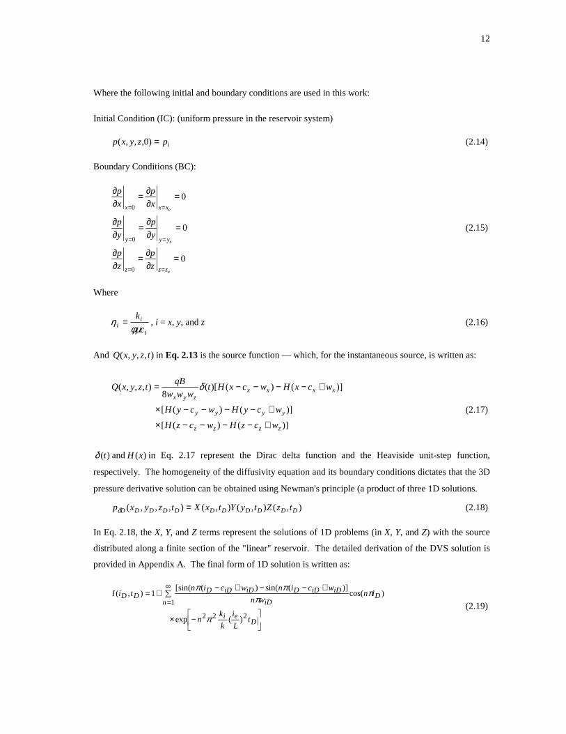
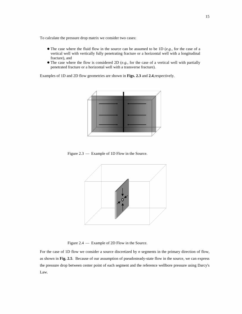
To calculate the pressure drop matrix we consider two cases:

� The case where the fluid flow in the source can be assumed to be 1D (e.g., for the case of a vertical well with vertically fully penetrating fracture or a horizontal well with a longitudinal fracture), and

� The case where the flow is considered 2D (e.g., for the case of a vertical well with partially penetrated fracture or a horizontal well with a transverse fracture).

Examples of 1D and 2D flow geometries are shown in Figs. 2.3 and 2.4,respectively.

Figure 2.3 — Example of 1D Flow in the Source.

Figure 2.4 — Example of 2D Flow in the Source.

For the case of 1D flow we consider a source discretized by n segments in the primary direction of flow,

as shown in Fig. 2.5. Because of our assumption of pseudosteady-state flow in the source, we can express

the pressure drop between center point of each segment and the reference wellbore pressure using Darcy's

Law.

16

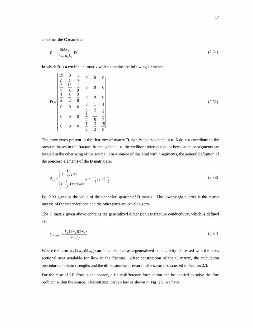
For example, in Fig. 2.5 we have discretized the source into 6 segments, and the wellbore is located in the

middle of the segments 3 and 4.

Figure 2.5 — Schematic of a Discretized 1D Source.

The pressure drop is given as:

∫=−wf

i

x

xfywfi qdx

hkwpp

2

µ (2.24)

Since each segment is assumed to be a uniform-flux source, the rate at each segment is a linear function of

length. Therefore we can integrate over each segment from the center of i th segment to wellbore by

summing over each segment in the path. For the case shown in Fig. 2.5 (for i= 1 to 3), we can write

(numbering from left to right):

++∆=

∆++

+∆++∆=−22

3

8

19

222

22

2

2

8

3

22321321211

1qqq

kww

xx

qqqx

qqx

q

kwwpp

fzyfzywf

µµ (2.25)

++∆=

∆++

+∆+=−28

11

2

3

222

22

8

34

2232132121

2qqq

kww

xx

qqqx

qq

kwwpp

fzyfzywf

µµ (2.26)

++∆=

∆++

=−8

3

22228

344

22321321

3qqq

kww

xx

qqq

kwwpp

fzyfzywf

µµ (2.27)

Eqs. 2.25 to 2.27 can be written in dimensionless form as:

++=−22

3

8

19

4

2321

1,DDD

fzy

fDwfD

qqq

kwnw

kLxpp (2.28)

++=−28

11

2

3

4

2321

2DDD

fzy

fDDwf

qqq

kwnw

kLxpp (2.29)

++=−8

3

224

2321

3DDD

fzy

fDDwf

qqq

kwnw

kLxpp (2.30)

As For this example, for the finite conductivity vertical fracture represented by n = 6 source boxes first we

xf ∆x

2wy

17

construct the C matrix as:

DCfzy

f

kwnw

kLx

4

2= (2.31)

In which D is a coefficient matrix which contains the following elements:

=

8

19

2

3

2

1000

2

3

8

11

2

1000

2

1

2

1

8

3000

0008

3

2

1

2

1

0002

1

8

11

2

3

0002

1

2

3

8

19

D (2.32)

The three zeros present in the first row of matrix D signify that segments 4 to 6 do not contribute to the

pressure losses in the fracture from segment 1 to the wellbore reference point because those segments are

located in the other wing of the source. For a source of this kind with n segments, the general definition of

the non-zero elements of the D matrix are:

21, ,

2 ,1,

Otherwise ,2

1

,8

5

,n

jn

i

i

ijjd ji ==

−

=−= (2.33)

Eq. 2.33 gives us the value of the upper-left quarter of D matrix. The lower-right quarter is the mirror

inverse of the upper-left one and the other parts are equal to zero.

The C matrix given above contains the generalized dimensionless fracture conductivity, which is defined

as:

f

zyfgenfD Lxk

wwkC

)2)(2(, = (2.34)

Where the term )2)(2( zyf wwk can be considered as a generalized conductivity expressed with the cross

sectional area available for flow in the fracture. After construction of the C matrix, the calculation

procedure to obtain strengths and the dimensionless pressure is the same as discussed in Section 2.3.

For the case of 2D flow in the source, a finite-difference formulation can be applied to solve the flux

problem within the source. Discretizing Darcy's law as shown in Fig. 2.6, we have:

18

)]2()2([2

,1,1,,,1,1, jijijijijijizf

ji pppy

xppp

x

ywkq −+

∆∆+−+

∆∆= +−+−µ

(2.35)

Or in dimensionless format, Eq. 2.35 becomes:

)]2()2([2

,1,1,,,1,1, jDijDijDijDijDijDizf

jDi pppy

xppp

x

y

kL

wkq −+

∆∆+−+

∆∆= +−+− (2.36)

i, j+1

i-1, j i, j i+1, j

i, j-1

∆x

∆y

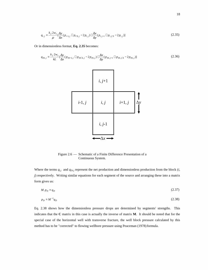
Figure 2.6 — Schematic of a Finite Difference Presentation of a Continuous System.

Where the terms qi,j and qDi,j represent the net production and dimensionless production from the block (i,

j) respectively. Writing similar equations for each segment of the source and arranging these into a matrix

form gives us:

DD qpM =. (2.37)

DD qMp 1−= (2.38)

Eq. 2.38 shows how the dimensionless pressure drops are determined by segments' strengths. This

indicates that the C matrix in this case is actually the inverse of matrix M. It should be noted that for the

special case of the horizontal well with transverse fracture, the well block pressure calculated by this

method has to be "corrected" to flowing wellbore pressure using Peaceman (1978) formula.

19

The dimensionless form of the Peaceman (1978) formula (which relates the wellbore pressure with the

grid pressure) is given by:

]14.0ln[22

1 22

,wfy

ExtraD r

zx

kw

kLp

∆+∆=π

(2.39)

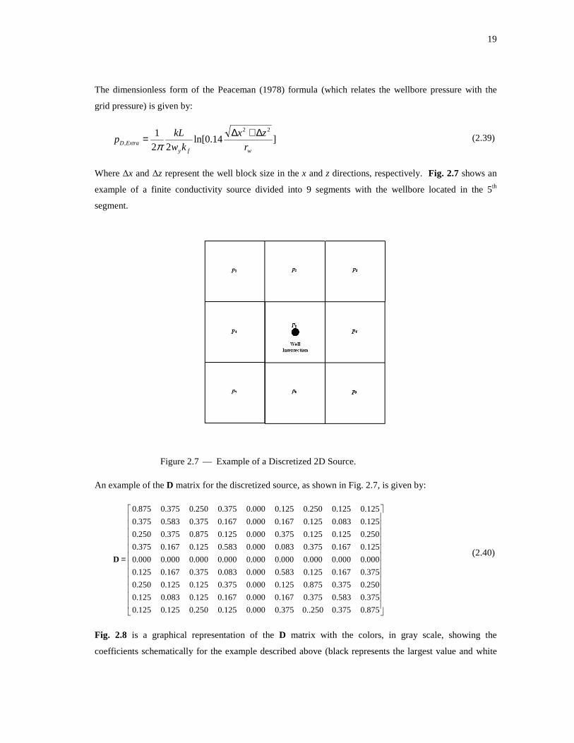
Where ∆x and ∆z represent the well block size in the x and z directions, respectively. Fig. 2.7 shows an

example of a finite conductivity source divided into 9 segments with the wellbore located in the 5th

segment.

Figure 2.7 — Example of a Discretized 2D Source.

An example of the D matrix for the discretized source, as shown in Fig. 2.7, is given by:

=

875.0375.0250..0375.0000.0125.0250.0125.0125.0

375.0583.0375.0167.0000.0167.0125.0083.0125.0

250.0375.0875.0125.0000.0375.0125.0125.0250.0

375.0167.0125.0583.0000.0083.0375.0167.0125.0

000.0000.0000.0000.0000.0000.0000.0000.0000.0

125.0167.0375.0083.0000.0583.0125.0167.0375.0

250.0125.0125.0375.0000.0125.0875.0375.0250.0

125.0083.0125.0167.0000.0167.0375.0583.0375.0

125.0125.0250.0125.0000.0375.0250.0375.0875.0

D (2.40)

Fig. 2.8 is a graphical representation of the D matrix with the colors, in gray scale, showing the

coefficients schematically for the example described above (black represents the largest value and white

20

represents the zero coefficient). We note that all of the elements of the row corresponding to the well

block are equal to zero, which indicates that there is no pressure drop — other than the correction using

Peaceman formula (which relates the wellbore and block pressures).

Figure 2.8 — Graphical Representation of the D Matrix for 2D Flow in Fracture

2.5 Productivity Index Calculation

Apart from the well-test analysis applications, use of the new solution in the prediction of productivity

behavior for a well/fracture system is considered in this work. We cast the results into a transient/pseudo-

steady-state productivity index form and then we compare these results with the well-known productivity

models for different well/fracture systems.

The application of DVS method is not limited to prediction of the pressure behavior of well/fracture

configurations. The pressure data calculated from the DVS method can be used to predict the productivity

index (PI) behavior of the system. The productivity index and in particular, the pseudosteady-state

productivity index of a system is a measure of the capability of the system to produce the fluid from a

reservoir. Comparison of pseudosteady-state productivity indexes of two completion schemes can be used

to establish which completion drains the reservoir most efficiently.

21

The definition of dimensionless productivity index of a system using the dimensionless pressure and time

data as it is discussed by Ramey and Cobb (1971), and the dimensionless productivity index is stated as:

DAtradDD tp

Jπ2

1

, −= (2.41)

The detailed derivation of Eq. 2.41 is presented in Appendix B. We note that although Eq. 2.41 is derived

for the case of a constant production rate, this solution has also been proved to be correct for a system

producing at a constant wellbore pressure condition. To compute the variable-rate performance as a

function of time (constant flowing pressure case), we use the following procedure:

1. Calculate the average reservoir pressure and flowing pressure. Starting from zero time, the average

reservoir pressure is equal to the initial pressure (i.e., uniform pressure initial condition).

2. Assuming the productivity index is constant for the chosen time interval, we can calculate the

corresponding flowrate of the system using Eq. 2.42:

)( , wfiavgii ppJq −= (2.42)

Assuming that the flowrate is constant over a given time interval, we can calculate the incremental

cumulative production over that time interval as the rate multiplied by the time interval. For the

(total) cumulative production profile, we simply add the incremental cumulative production values.

3. The average reservoir pressure for the (i+1)th time interval can then be calculated by subtracting

ip∆ from the pressure of the i th time interval. For the pseudosteady-state flow assumption,

this ip∆ represents the reduction in the average reservoir pressure of the system due to the fluid

withdrawal during the i th time interval, and ip∆ is calculated using the material balance equation as:

t

ii

t

pi Ahc

tBq

Ahc

BNp

φφ∆

=∆

=∆ (2.43)

Steps 1–4 are repeated for each time interval — which yields the calculated flowrate profile as a function

of time. For gas reservoirs, a similar procedure can be followed using the gas material balance equation

for a volumetric dry gas reservoir and the gas inflow performance equation, which are given by:

−=

G

G

z

p

z

p p

i

i 1 (2.44)

)]()([ 1

1424

1wfavgDyx pmpmJhkk

Tq −= (2.45)

22

Where in Eq. 2.45 q represents the gas production rate in MSCF/D and T is reservoir temperature in °R.

Eq. 2.44 is known as the material balance equation for a volumetric gas reservoir and Eq. 2.45 represents

the inflow performance of a gas well. )( pm is the pseudopressure function, which is defined as:

∫=p

pi

dpz

ppm

µ2)( (2.46)

Where µ and z are the gas viscosity and the gas compressibility, respectively. The subscript i represents

the reference pressure of which we integrate the pseudopressure function and it is chosen arbitrarily,

typically the reference pressure is the base pressure or the pressure at standard conditions.

At each time step, assuming the average pressure is constant for that time step, we calculate the product-

ion rate at that time step using the dimensionless productivity index and the calculated pseudopressure

values. Knowing the rate, we can calculate the cumulative gas production and the new average pressure.

This is an iterative process for the gas case since the compressibility factor (z) and gas viscosity (µ) are

functions of pressure, but usually the convergence is quite fast because of the small changes in pressure

incurred at each time step.

23

CHAPTER III

VALIDATION OF THE MODEL

3.1 Introduction

To show the applicability of the new DVS method, results of this method are validated using comparisons

with existing solutions for several simple well configurations (e.g., vertical well with full and partial

penetration, horizontal well, and fractured wells with finite- and infinite-conductivity fractures). In this

effort we not only validate the pressure response, but we also validate the productivity index function

using the existing models. All procedures discussed in Chapter II were programmed in the

MATHEMATICA (Version 5.2, Wolfram Research Inc. 2005) programming/computation language.

3.2 Validation with Pressure Models

Fully Penetrating Vertical Well

For this case we have two well-known representations — the line source and the cylindrical source

solutions. Both solutions can be combined with the method of images (Raghavan 1993) to produce

bounded reservoir responses. Also, it is well-known that the medium-late time solution is not sensitive to

the actual source geometry (i.e., the transition period between which neither the source nor the boundaries

control the pressure response). In Fig. 3.1 we provide a comparison between the results of the line- and

cylinder-source solutions and the DVS method solution. Except at very early times, we note very good

agreement between the DVS solution and the line- and cylinder-source solutions.

To represent the actual well by a box source, we have to define the wx and wy parameters, which are the

widths of the hypothetical source box. Detailed numerical experimentation has revealed that the following

relation provides the best results:

wyx 1.4444rww == (3.1)

We note that in Fig. 3.1, the DVS solution is much closer to the cylindrical source solution than to the line

source solution, suggesting that the DVS is something of an approximation for a cylinder, but not a line.

Partially Penetrated Vertical Well

Using the solution proposed by Yildiz and Bassiouni (1991) for the transient pressure behavior of a

partially penetrated vertical well as our reference for comparison to the DVS solution, we present the

comparison of their solution and the DVS solution in Fig. 3.2. We note differences only in the early

behavior — which are due to source size, the location of the observation point, and (ultimately) the nature

of the flow in the near vicinity of the well.

2

4

10-2

10-1

100

101

102

pD a

nd p

D' F

unct

ions

10-9

10-8

10-7

10-6

10-5

10-4

10-3

10-2

10-1

100

101

102

Dimensionless Time Based on Drainage Area, tDA

xe

ye

Legend :

pD, Cylindrical Source Solution

pD, Line Source Solution

pD, DVS Method

p'D, Cylindrical Source Solution

p'D, Line Source Solution

p'D, DVS Method

Calculation Parameters :

A= 40 Acresrw= 0.33 ftxe= ye= 1320 ft

Well Schematic :

Comparison of DVS Solution for a Fully Penetrated Vertical Well With Line So urce and Cylindrical Solutions

Figure 3.1 — Comparison of the DVS Results With Line Source and Cylindrical Source Solutions: Vertical Well in a Bounded Reservoir (In the Box-in-Box Model wz=ze/2, wx = wy =0.477 ft, and the actual value of ze is irrelevant)

2

5

10-2

10-1

100

101

102

pD a

nd p

' D F

unct

ions

10-1

100

101

102

103

104

105

106

107

108

Dimensionless Time Based on Well Radius, tDrw

h

hb

hp

Legend :

pD, Yildiz & Bassiouni Infinite Acting Solution (SPE 21551) pD, DVS Method, Closed Reservoir p'D, Yildiz & Bassiouni Infinite Acting Solution (SPE 21551) p'D, DVS Method, Closed Reservoir


rw= 0.50 ftkx= ky= 10kz

h= 20 fthp= 10 fthb= 10 ftxe= ye= 2500 ft (Closed System)

Well Schematic :

Comparison of Results From DVS Method and Yildiz's Solution for a Partially Penetrated Vertical Well

Figure 3.2 — Comparison of DVS Results with Yildiz's Model for a Partially-Penetrating Vertical Well (Box-in- Box Model), h, hp, and hb are represented by ze, 2wz, and cz- wz respectively.

26

Differences observed at late times are due to the effect of boundaries imposed on the DVS solution.

Recalling that the Yildiz and Bassiouni (1991) solution is only valid for transient flow, it would be far from

trivial to develop a method-of-images solution for a boundary case using this solution. We recorded the

computation times for each solution computed on a typical desktop computer with Pentium IV processor —

the DVS solution required 1.23 seconds, compared to 436.1 seconds for the Yildiz-Bassiouni solution.

Uniform Flux Horizontal Well

Ozkan (1988) presented a method to compute the performance of a horizontal well and specifically, he

developed a series solution in Laplace domain for a fracture with uniform flux and adjusted the solution to

obtain the performance of a horizontal well. In this work we used the results given in Table 2.6.2 of Ref. 6

for comparison purposes.

10-2

10-1

100

101

102

Dim

ensi

onle

ss P

ress

ure,

p

D

0.0001 0.001 0.01 0.1 1 10


Legend :

pD, Gringarten's Solution pD, Ozkan's Solution pD, DVS Method

xeD= 2

xeD= 10

xeD= 20

CalCulation Parameters :

xeD= yeD

xwD= ywD= zwD= 0.50LD= 10.0

rwD = 2×10-3

Well/Reservoir Schematic :

Comparison of Dimensionless Pressure Results From DVS Method With Gringarten's and Ozkan's Solution

for a Horizontal Well With Uniform Flux

Figure 3.3 — Comparison of DVS Results with Ozkan‘s and Gringarten’s Solutions for a Horizontal Well in a Bounded Reservoir, Uniform Flux Solution (In the Box-in-Box Model xeD= xe/wx , yeD= ye/wx , and LD= ze/wx ).

27

Fig. 3.3 shows the graphical presentation of the solutions by Gringarten, Ramey and Raghavan (1974) and

Ozkan (1988) compared to the DVS for the case of uniform flux horizontal well with various horizontal

penetrations. For the DVS represen-tation of the horizontal well, Eq. 3.1 is used to obtain the wy and wz

widths of the source box. The data given in Ozkan (1988) omits the very early time period of the solution,

so we do not observe any differences between the DVS solution and the reference solutions.

Fully Penetrating Vertical Fracture (Uniform-Flux and Infinite-Conductivity Fracture)

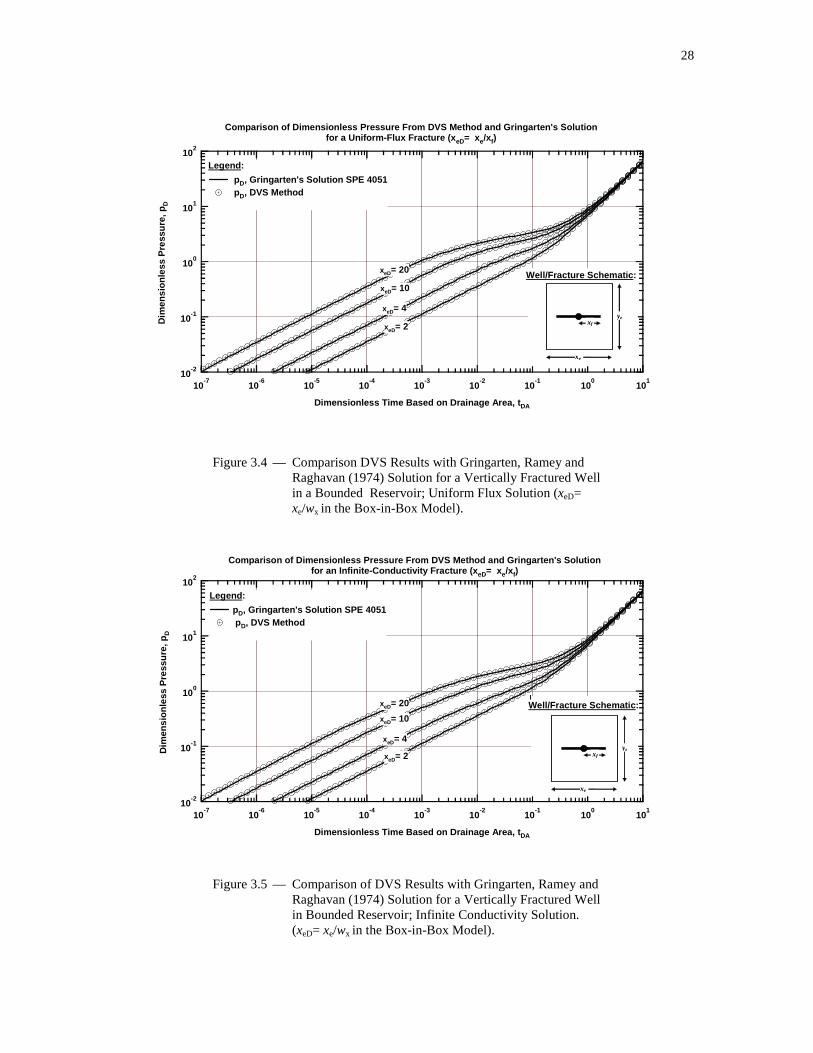
In Figs. 3.4 and 3.5 we present the results of the widely accepted Gringarten, Ramey and Raghavan (1974)

(Green's function) solution for the case of vertical well with a fully-penetrating vertical fracture along with

our DVS results for the uniform flux fracture case (Fig. 3.4) and the infinite conductivity fracture case (Fig.

3.5). The DVS solution results presented in Fig. 3.4 are calculated with a single uniform box source (the wy

width is selected to be "sufficiently small" (10-6ye.) as to not distort the solution). The DVS solution results

presented in Fig. 3.5 were obtained using the uniform-flux solution with the "equivalent observation point"

(0.732 xf) for the infinite conductivity fracture case. For these particular cases, the analytical and DVS

results are indistinguishable.

The computation times for these cases are as follows:

� DVS Method: — Uniform-flux fracture (84.73 seconds). — Infinite conductivity fracture (542 seconds).

� Gringarten Solution: — Uniform-flux fracture (520.1 seconds). — Infinite conductivity fracture (815.1 seconds).

Fully Penetrating Vertical Fracture (Finite-Conductivity Fracture)

As a natural progression, we need to compare our new DVS solution to the case of a vertical well with a

finite-conductivity vertical fracture in an infinite acting reservoir. The reference solution for this case is

given by Cinco-Ley, Samaniego, and Dominguez (1978) — and we also note that we will require a

"discretized" fracture solution for this case due to the finite conductivity of the fracture (i.e., the fracture

has to be treated as a separate "reservoir to account for the non-trivial pressure drop in the fracture). The

comparison of results is presented in Fig. 3.6. For the DVS solution we divided the fracture into 32

segments. From Fig. 3.6 we note a very good comparison of the DVS solution and the results of Cinco-

Ley, Samaniego, and Dominguez (1978) — except at early times where the source of the volume affects

the solution.

In Fig. 3.7 we present the distribution of the computed source strengths along the lateral coordinate in one

fracture wing. For pseudosteady-state (late times), the stabilized strength distribution profiles computed by

the DVS method are somewhat similar to the "U-shaped" distributions shown by Cinco-Ley, Samaniego,

and Dominguez (1978) We believe that this is a relatively minor issue, and that the DVS solution is

validated for this case, except at very early times. For comparison, the DVS solution required a

computational time of 689 seconds and their solution required a computational time of 9632 seconds.

28

10-2

10-1

100

101

102

Dim

ensi

onle

ss P

ress

ure,

p

D

10-7

10-6

10-5

10-4

10-3

10-2

10-1

100

101


xe

ye xf

Legend :

pD, Gringarten's Solution SPE 4051 pD, DVS Method

xeD= 2

xeD= 4

xeD= 20

xeD= 10

Comparison of Dimensionless Pressure From DVS Method and Grin garten's Solutionfor a Uniform-Flux Fracture ( xeD= xe/xf)

Well/Fracture Schematic :

Figure 3.4 — Comparison DVS Results with Gringarten, Ramey and Raghavan (1974) Solution for a Vertically Fractured Well in a Bounded Reservoir; Uniform Flux Solution (xeD= xe/wx in the Box-in-Box Model).

10-2

10-1

100

101

102

Dim

ensi

onle

ss P

ress

ure,

p

D

10-7

10-6

10-5

10-4

10-3

10-2

10-1

100

101


xe

ye xf

Legend :

pD, Gringarten's Solution SPE 4051 pD, DVS Method

xeD= 2

xeD= 4

xeD= 20

xeD= 10Well/Fracture Schematic :

Comparison of Dimensionless Pressure From DVS Method and Gring arten's Solutionfor an Infinite-Conductivity Fracture ( xeD= xe/xf)

Figure 3.5 — Comparison of DVS Results with Gringarten, Ramey and Raghavan (1974) Solution for a Vertically Fractured Well in Bounded Reservoir; Infinite Conductivity Solution. (xeD= xe/wx in the Box-in-Box Model).

29

10-1

100

101

102

Dim

ensi

onle

ss P

ress

ure,

p

D

10-2

10-1

100

101

102

103

104

Dimensionless Time Based on Fracture Half-Length, tDxf

xe

ye xf

Legend :

Cinco-Ley and Samaniego, SPE 6014 DVS Method (C fD = 1.60)

CfD= 0.2 π π π π

CfD= 1.6 CfD= 2 π π π π


Comparison of DVS Solution to Cinco's Solution for a Vertically-Fractured Well with CfD= 1.6)

Figure 3.6 — Comparison of DVS with Cinco-Ley, Samaniego, and Dominguez (1978) Results for Finite Conductivity Fracture.

0.4

0.3

0.2

0.1

0.0

Sou

rce

Str

engt

h (F

ract

ion

of T

otal

Flo

w)

16151413121110987654321

Segment Number

xe

ye xf

Legend :

tDA= 6.4X 10-6

tDA= 6.4X 10-5

tDA= 6.4X 10-4

tDA= 6.4X 10-3

tDA= 6.4X 10-2

tDA= 6.4X 10-1

tDA= 6.4X 100

tDA= 6.4X 101


CfD= 1.6Ix= xf/xe= 0.25


Contribution to FLow of Each Fracture Segments for Different Values of Dimen sionless Time

Figure 3.7 — Distribution of the Contribution of Different Segments to Total Production at Various Times, Finite Conductivity Vertical Fracture of Full Vertical Penetration for Half the Fracture (CfD =1.6 and Ix = 0.25, n = 32).

30

3.3 Validation with Productivity Index Models

The results of our DVS method can be used to calculate the transient as well as the pseudosteady-state

productivity index for a given well/reservoir configuration. The method of calculation for the dimen-

sionless productivity index (JD) is provided in Appendix B. To validate the applicability and reliability of

the results obtained from the DVS method for the case of a horizontal well, we used the work of Chen and

Asaad (2003). They validated their work using the results taken from Babu and Odeh (1989) and from

Goode and Kuchuck (1991) for the case of horizontal well. Chen and Asaad later extended their correlation

to fractured wells. We compare our DVS results for the examples A1, B1, and B2 given by Chen and

Asaad (2003). Table 3.1 provides the reservoir/fluid properties used for the calculation and Table 3.2

present the results of our comparative study.

Table 3.1 — Reservoir/Fluid Properties Used for Example Cases of Chen and Asaad (2003) (Comparison of Different Pseudosteady-State Productivity Index Correlations).

Reservoir/Fluid Properties Unit A1 B1 B2 Drainage Length in x, 2xe ft 2640 2000 4000

Drainage Length in y, 2ye ft 2640 4000 2000

Formation thickness, h ft 45 100 200

Horizontal well length, Lh ft 1475 1000 1000

Well location in x, xw ft 1320 1250 1500

Well location in y, yw ft 1320 3000 1000

Well location in z, zw ft 22.5 50 150

Wellbore radius, rw ft 0.33 0.25 0.25

Formation volume Factor, B RB/STB 1.05 1 1

Fluid viscosity, µ cp 7.5 1 1

Horizontal permeability in x, kx md 350 200 100

Horizontal permeability in y, ky md 350 200 100

Vertical permeability, kz md 70 50 20

From Table 3.2 we can see that for this case (a horizontal well), we have obtained excellent agreement

between the results of different methods (our DVS solution, the Chen and Asaad (2003) solution, and the

Babu and Odeh (1989) solution). This agreement is consistent for both the uniform-flux and infinite-

conductivity horizontal well cases. Further to this effort, we compared our DVS solution with the Chen and

Asaad (2003) solution for the case of a vertically-fractured well (uniform flux and infinite conductivity

cases are considered). We do note that for case B2 the difference between solution results rises to around

10 percent (compared to less than 1 percent difference for all of the other cases). We suspect that the

discrepancy is due to the approximations used in the Chen and Asaad (2003) formulation, which tend to

show higher error in cases where the horizontal penetration of the vertical fracture is relative small.

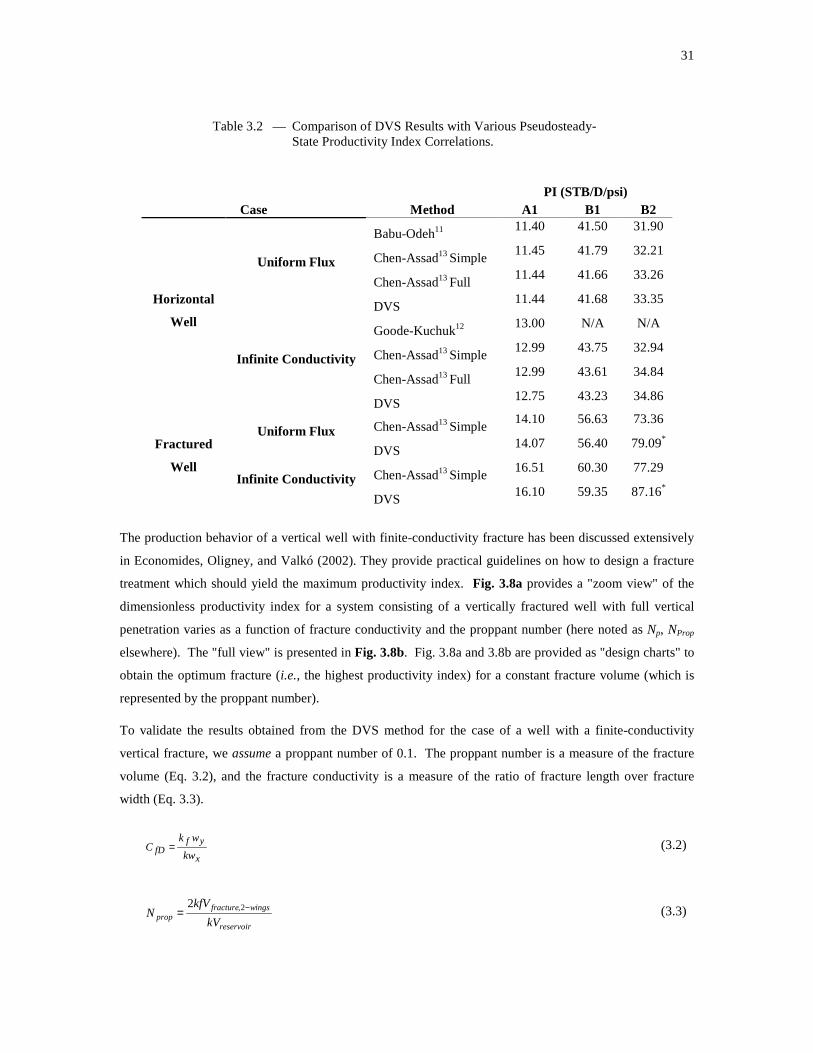
31

Table 3.2 — Comparison of DVS Results with Various Pseudosteady-State Productivity Index Correlations.

PI (STB/D/psi) Case Method A1 B1 B2

Babu-Odeh11 11.40 41.50 31.90

Chen-Assad13 Simple

11.45 41.79 32.21

Chen-Assad13 Full

11.44 41.66 33.26 Uniform Flux

DVS 11.44 41.68 33.35

Goode-Kuchuk12 13.00 N/A N/A

Chen-Assad13 Simple

12.99 43.75 32.94

Chen-Assad13 Full

12.99 43.61 34.84

Horizontal

Well

Infinite Conductivity

DVS 12.75 43.23 34.86

Chen-Assad13 Simple

14.10 56.63 73.36 Uniform Flux

DVS 14.07 56.40 79.09*

Chen-Assad13 Simple

16.51 60.30 77.29

Fractured

Well Infinite Conductivity

DVS 16.10 59.35 87.16*

The production behavior of a vertical well with finite-conductivity fracture has been discussed extensively

in Economides, Oligney, and Valkó (2002). They provide practical guidelines on how to design a fracture

treatment which should yield the maximum productivity index. Fig. 3.8a provides a "zoom view" of the

dimensionless productivity index for a system consisting of a vertically fractured well with full vertical

penetration varies as a function of fracture conductivity and the proppant number (here noted as Np, NProp

elsewhere). The "full view" is presented in Fig. 3.8b. Fig. 3.8a and 3.8b are provided as "design charts" to

obtain the optimum fracture (i.e., the highest productivity index) for a constant fracture volume (which is

represented by the proppant number).

To validate the results obtained from the DVS method for the case of a well with a finite-conductivity

vertical fracture, we assume a proppant number of 0.1. The proppant number is a measure of the fracture

volume (Eq. 3.2), and the fracture conductivity is a measure of the ratio of fracture length over fracture

width (Eq. 3.3).

x

yffD kw

wkC = (3.2)

reservoir

wingsfractureprop kV

kfVN −= 2,2

(3.3)

32

Figure 3.8a — (zoom view) Dimensionless Productivity Index of a

Vertically Fully Penetrated Fracture as a Function of Fracture Conductivity and Proppant Number (From Economides, Oligney, and Valkó 2002).

Figure 3.8b — Dimensionless Productivity Index of a Vertically Fully Penetrated Fracture as a Function of Fracture Conductivity and Proppant Number (From Economides, Oligney, and Valkó 2002).

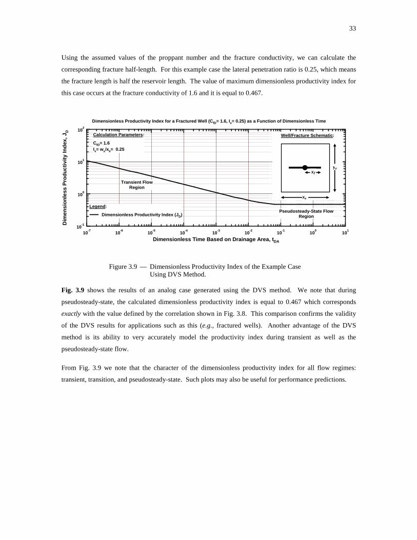
33

Using the assumed values of the proppant number and the fracture conductivity, we can calculate the

corresponding fracture half-length. For this example case the lateral penetration ratio is 0.25, which means

the fracture length is half the reservoir length. The value of maximum dimensionless productivity index for

this case occurs at the fracture conductivity of 1.6 and it is equal to 0.467.

10-1

100

101

102

Dim

ensi

onle

ss P

rodu

ctiv

ity In

dex,

J D

10-7

10-6

10-5

10-4

10-3

10-2

10-1

100

101


xe

ye xf


CfD= 1.6Ix= wx/xe= 0.25


Pseudosteady-State FlowRegion

Transient FlowRegion

Legend :

Dimensionless Productivity Index ( JD)

Dimensionless Productivity Index for a Fractured We ll (CfD= 1.6, Ix= 0.25) as a Function of Dimensionless Time

Figure 3.9 — Dimensionless Productivity Index of the Example Case Using DVS Method.

Fig. 3.9 shows the results of an analog case generated using the DVS method. We note that during

pseudosteady-state, the calculated dimensionless productivity index is equal to 0.467 which corresponds

exactly with the value defined by the correlation shown in Fig. 3.8. This comparison confirms the validity

of the DVS results for applications such as this (e.g., fractured wells). Another advantage of the DVS

method is its ability to very accurately model the productivity index during transient as well as the

pseudosteady-state flow.

From Fig. 3.9 we note that the character of the dimensionless productivity index for all flow regimes:

transient, transition, and pseudosteady-state. Such plots may also be useful for performance predictions.

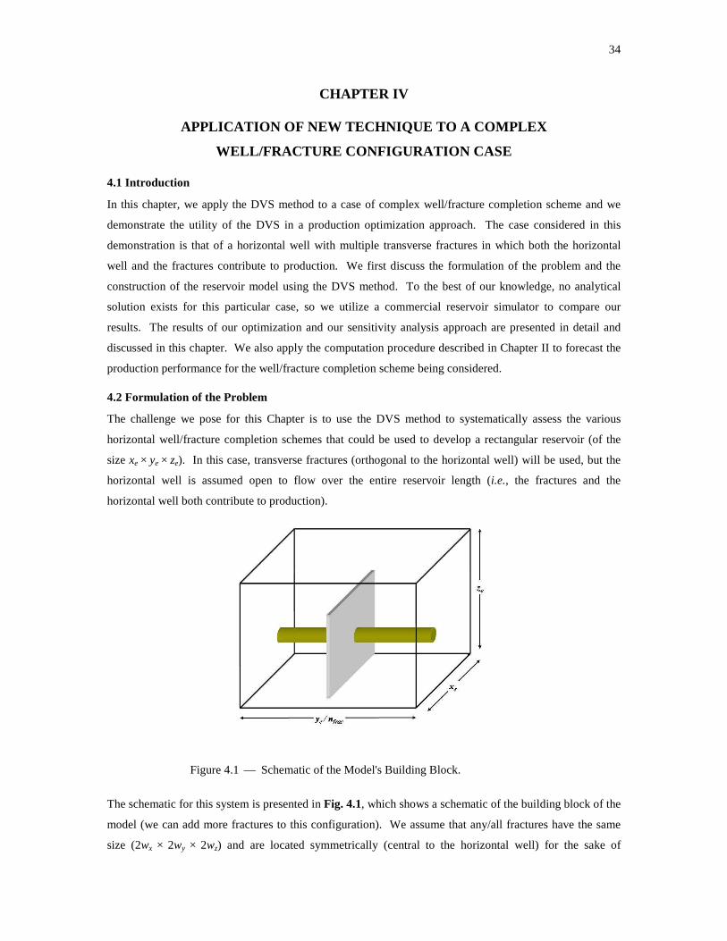
34

CHAPTER IV

APPLICATION OF NEW TECHNIQUE TO A COMPLEX

WELL/FRACTURE CONFIGURATION CASE

4.1 Introduction

In this chapter, we apply the DVS method to a case of complex well/fracture completion scheme and we

demonstrate the utility of the DVS in a production optimization approach. The case considered in this

demonstration is that of a horizontal well with multiple transverse fractures in which both the horizontal

well and the fractures contribute to production. We first discuss the formulation of the problem and the

construction of the reservoir model using the DVS method. To the best of our knowledge, no analytical

solution exists for this particular case, so we utilize a commercial reservoir simulator to compare our

results. The results of our optimization and our sensitivity analysis approach are presented in detail and

discussed in this chapter. We also apply the computation procedure described in Chapter II to forecast the

production performance for the well/fracture completion scheme being considered.

4.2 Formulation of the Problem

The challenge we pose for this Chapter is to use the DVS method to systematically assess the various

horizontal well/fracture completion schemes that could be used to develop a rectangular reservoir (of the

size xe × ye × ze). In this case, transverse fractures (orthogonal to the horizontal well) will be used, but the

horizontal well is assumed open to flow over the entire reservoir length (i.e., the fractures and the

horizontal well both contribute to production).

Figure 4.1 — Schematic of the Model's Building Block.

The schematic for this system is presented in Fig. 4.1, which shows a schematic of the building block of the

model (we can add more fractures to this configuration). We assume that any/all fractures have the same

size (2wx × 2wy × 2wz) and are located symmetrically (central to the horizontal well) for the sake of

35

simplicity. The variable nfrac represents the number of transverse fractures and, in principle could be any

integer from 1 to ∞, but for this study, we limit the number of fractures from 1 to 5. We assume the total

system is composed of nfrac building blocks connected together in the y direction. Lastly we assume the

fractures to be of finite-conductivity and the horizontal well to of infinite-conductivity.

As we discussed in Chapter II, the entire source should be divided into sub-sources for cases of finite-

and/or infinite-conductivity sources. In this case, we divide the individual fractures into (2nx + 1) by (2nz +

1) segments and the horizontal well into 2nh segments. Because the fractures are assumed to be of finite

conductivity, the C matrix is only calculated for the fracture sub-sources. We also incorporate Peaceman's

correction (Peaceman 1978) to account for 2D flow in the fracture.

4.3 Validation Through Simulation

To validate the model, we used the CMG (Version 2005.10, Computer Modeling Group Ltd.) commercial

reservoir simulator to simulate a rectangular reservoir of the size (1320×1320×100 ft), with horizontal

permeability of 1 md and permeability anisotropy (kv/kh) equal to 0.1. The individual fractures are of the

size (1000 × 0.01 × 80 ft) and have permeabilities of 10,000 md. For our validation, we consider the case of

1 fracture and the case of 4 fractures. Lastly, the horizontal well penetrates the entire reservoir width.

Table 4.1 presents the reservoir, fracture, and fluid characteristics used for both the simulation model and

the DVS calculations.

Table 4.1 — Reservoir, Fracture, and Fluid Characteristic Used for

Simulation Model and DVS Calculations.

Reservoir Characteristics:

xe = 1320 ft ye = 1320 ft ze = 100 ft kx = 1 md ky = 1 md kz = 0.1 md φ�= 10 percen t

Fracture Characteristics:

wx = 500 ft wy = 0.01 ft wz = 40 ft kx = 10,000 md

Fluid Characteristics:

µ�= 1.011 cp ct = 1.35 ×10-5 psi-1

well Characteristics:

rw= 0.3 ft Lh = 1320 ft

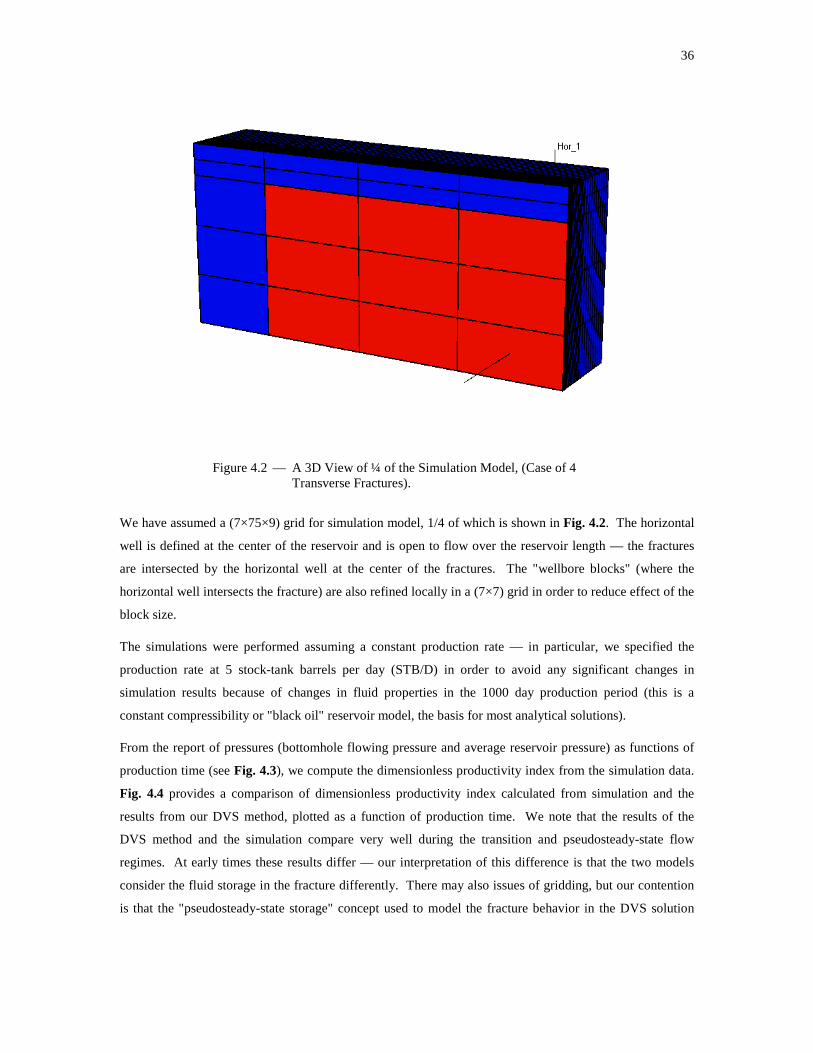
36

Figure 4.2 — A 3D View of ¼ of the Simulation Model, (Case of 4 Transverse Fractures).

We have assumed a (7×75×9) grid for simulation model, 1/4 of which is shown in Fig. 4.2. The horizontal

well is defined at the center of the reservoir and is open to flow over the reservoir length — the fractures

are intersected by the horizontal well at the center of the fractures. The "wellbore blocks" (where the

horizontal well intersects the fracture) are also refined locally in a (7×7) grid in order to reduce effect of the

block size.

The simulations were performed assuming a constant production rate — in particular, we specified the

production rate at 5 stock-tank barrels per day (STB/D) in order to avoid any significant changes in

simulation results because of changes in fluid properties in the 1000 day production period (this is a

constant compressibility or "black oil" reservoir model, the basis for most analytical solutions).

From the report of pressures (bottomhole flowing pressure and average reservoir pressure) as functions of

production time (see Fig. 4.3), we compute the dimensionless productivity index from the simulation data.

Fig. 4.4 provides a comparison of dimensionless productivity index calculated from simulation and the

results from our DVS method, plotted as a function of production time. We note that the results of the

DVS method and the simulation compare very well during the transition and pseudosteady-state flow

regimes. At early times these results differ — our interpretation of this difference is that the two models

consider the fluid storage in the fracture differently. There may also issues of gridding, but our contention

is that the "pseudosteady-state storage" concept used to model the fracture behavior in the DVS solution

37

may not be sufficient to address the early time flux distribution in a finite-conductive vertical fracture (see

Fig. 3.6 for comparison). Regardless, we accept that this issue may be significant for some cases.

Time (day)

Pre

ssur

e: P

RE

S A

vera

ge R

eser

voir

Pre

ssur

e. (p

si)

0 250 500 750 1,0005,850

5,875

5,900

5,925

5,950

5,975

6,000

Well Bottom-hole Pressure Hor_1 4_With_Frac_7X75X9. irfPressure: PRES Average Reservoir Pressure. 4_With_ Frac_7X75X9.irfWell Bottom-hole Pressure Hor_1 1_With_Frac_7X75X9. irfPressure: PRES Average Reservoir Pressure. 1_With_ Frac_7X75X9.irf

Figure 4.3 — Simulation Output, Well Bottomhole Pressure and Average Reservoir Pressure for Cases of 1 Fracture and 4 Fractures.

10-1

10-1

100

100

101

101

Dim

ensi

onle

ss P

rodu

ctiv

ity In

dex

(J D

)

100

100

101

101

102

102

103

103

Production Time (Day)

ye/ nfrac

xe

ze

Comparison Between Simulation and DVS Results( kx= ky= 1 md, kz= 0.1 md, k f= 10000 md )

n frac = 1, N Prop = 0.092

n frac = 4, N Prop = 0.368

Legend :

Simulation Results DVS, nx= nz= nh= 1 DVS, nx= nz= nh= 2


Figure 4.4 — Comparison Between Simulation Results and DVS Method's.

38

The computational "run time" for the numerical simulation case was about 32 seconds, while for this case,

the DVS method required 292 seconds. We believe that if the DVS method were programmed into a more

traditional programming language (other than MATHEMATICA), then the computational times for the

DVS method would improve substantially. We recognize the implication that, for this case, the numerical

simulation model is substantially faster than our DVS method, but we believe that there is a balance of

speed and potential accuracy in the DVS method.

For the DVS method we considered only two cases of grid sizes, nx= nz= nh= 1, and 2. Our investigations

showed that the dimensionless productivity index for pseudosteady-state flow does change as the number

of segments change, but in most cases this change is negligible (less than 0.1 percent when nx, nz, and nh are

equal to 2). We note that the CPU computation times increase quadratically as nx, nz, and nh increase, and

based on this observation we elected to use nx= nz= nh= 2 (which yields 25 blocks for each fracture source

and 4 block for the horizontal section).

4.4 Design and Optimization

The DVS method has been shown to predict the productivity index behavior of complex well/fracture

completion schemes with reasonable (i.e., practical) accuracy. Considering the semi-analytical nature of

the method, we could (and should) use the DVS method as an optimization/screening tool to evaluate

different well design and completion scenarios for reservoir development applications. To illustrate this

premise, we provide a demonstration application of DVS method to optimize production for an example

case.

Table 4.2 — Reservoir and Proppant Characteristics Used for Case

Study.

Reservoir Characteristics:

xe = 1320 ft

ye = 1320 ft

ze = 100 ft

kx = 1 md

ky = 1 md kz = 1, 0.1, 0.01, 0.001 md

Proppant Characteristics:

dp = 0.005 ft

ρp = 2.83

φp = 35 percent kf = 10,000 md

Table 4.2 provides the characteristics of the reservoir and the fracture proppant we will use for our

example case. The challenge we face is how to find the best completion schemes in term of number and

size of fractures. The "best" completion scheme will be defined as that which provides us the maximum

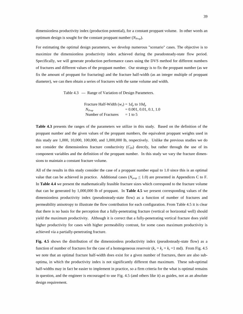
39

dimensionless productivity index (production potential), for a constant proppant volume. In other words an

optimum design is sought for the constant proppant number (NProp).

For estimating the optimal design parameters, we develop numerous "scenario" cases. The objective is to

maximize the dimensionless productivity index achieved during the pseudosteady-state flow period.

Specifically, we will generate production performance cases using the DVS method for different numbers

of fractures and different values of the proppant number. Our strategy is to fix the proppant number (as we

fix the amount of proppant for fracturing) and the fracture half-width (as an integer multiple of proppant

diameter), we can then obtain a series of fractures with the same volume and width.

Table 4.3 — Range of Variation of Design Parameters.

Fracture Half-Width (wx) = 1dp to 10dp

NProp = 0.001, 0.01, 0.1, 1.0

Number of Fractures = 1 to 5

Table 4.3 presents the ranges of the parameters we utilize in this study. Based on the definition of the

proppant number and the given values of the proppant numbers, the equivalent proppant weights used in

this study are 1,000, 10,000, 100,000, and 1,000,000 lb, respectively. Unlike the previous studies we do

not consider the dimensionless fracture conductivity (CfD) directly, but rather through the use of its

component variables and the definition of the proppant number. In this study we vary the fracture dimen-

sions to maintain a constant fracture volume.

All of the results in this study consider the case of a proppant number equal to 1.0 since this is an optimal

value that can be achieved in practice. Additional cases (Nprop < 1.0) are presented in Appendices C to F.

In Table 4.4 we present the mathematically feasible fracture sizes which correspond to the fracture volume

that can be generated by 1,000,000 lb of proppant. In Table 4.5 we present corresponding values of the

dimensionless productivity index (pseudosteady-state flow) as a function of number of fractures and

permeability anisotropy to illustrate the flow contribution for each configuration. From Table 4.5 it is clear

that there is no basis for the perception that a fully-penetrating fracture (vertical or horizontal well) should

yield the maximum productivity. Although it is correct that a fully-penetrating vertical fracture does yield

higher productivity for cases with higher permeability contrast, for some cases maximum productivity is

achieved via a partially-penetrating fracture.

Fig. 4.5 shows the distribution of the dimensionless productivity index (pseudosteady-state flow) as a

function of number of fractures for the case of a homogeneous reservoir (kx = ky = kz =1 md). From Fig. 4.5

we note that an optimal fracture half-width does exist for a given number of fractures, there are also sub-

optima, in which the productivity index is not significantly different than maximum. These sub-optimal

half-widths may in fact be easier to implement in practice, so a firm criteria for the what is optimal remains

in question, and the engineer is encouraged to use Fig. 4.5 (and others like it) as guides, not as an absolute

design requirement.

40

Table 4.4 — Table of Mathematically Feasible Fracture Sizes for Example Case (NProp = 1.0).

nfrac wx wy wz nfrac wx wy wz

1 660.0 0.033 50.0 3 660.0 0.025 22.0

1 622.3 0.035 50.0 3 242.0 0.030 50.0

1 641.1 0.035 48.5 3 451.0 0.030 26.8

1 660.0 0.035 47.1 3 660.0 0.030 18.3

1 544.5 0.040 50.0 3 207.4 0.035 50.0

1 602.3 0.040 45.2 3 433.7 0.035 23.9

1 660.0 0.040 41.3 3 660.0 0.035 15.7

1 484.0 0.045 50.0 3 181.5 0.040 50.0

1 572.0 0.045 42.3 3 420.8 0.040 21.6

1 660.0 0.045 36.7 3 660.0 0.040 13.8

1 435.6 0.050 50.0 3 161.3 0.045 50.0

1 547.8 0.050 39.8 3 410.7 0.045 19.6

1 660.0 0.050 33.0 3 660.0 0.045 12.2

2 660.0 0.017 50.0 3 145.2 0.050 50.0

2 544.5 0.020 50.0 3 402.6 0.050 18.0

2 602.3 0.020 45.2 3 660.0 0.050 11.0

2 660.0 0.020 41.3 4 660.0 0.008 50.0

2 435.6 0.025 50.0 4 544.5 0.010 50.0

2 547.8 0.025 39.8 4 602.3 0.010 45.2

2 660.0 0.025 33.0 4 660.0 0.010 41.3

2 363.0 0.030 50.0 4 363.0 0.015 50.0

2 511.5 0.030 35.5 4 511.5 0.015 35.5

2 660.0 0.030 27.5 4 660.0 0.015 27.5

2 311.1 0.035 50.0 4 272.3 0.020 50.0

2 485.6 0.035 32.0 4 466.1 0.020 29.2

2 660.0 0.035 23.6 4 660.0 0.020 20.6

2 272.3 0.040 50.0 4 217.8 0.025 50.0

2 466.1 0.040 29.2 4 438.9 0.025 24.8

2 660.0 0.040 20.6 4 660.0 0.025 16.5

2 242.0 0.045 50.0 4 181.5 0.030 50.0

2 451.0 0.045 26.8 4 420.8 0.030 21.6

2 660.0 0.045 18.3 4 660.0 0.030 13.8

2 217.8 0.050 50.0 4 155.6 0.035 50.0

2 438.9 0.050 24.8 4 407.8 0.035 19.1

2 660.0 0.050 16.5 4 660.0 0.035 11.8

3 660.0 0.011 50.0 4 136.1 0.040 50.0

3 484.0 0.015 50.0 4 398.1 0.040 17.1

3 572.0 0.015 42.3 4 660.0 0.040 10.3

3 660.0 0.015 36.7 4 121.0 0.045 50.0

3 363.0 0.020 50.0 4 390.5 0.045 15.5

3 511.5 0.020 35.5 4 660.0 0.045 9.2

3 660.0 0.020 27.5 4 108.9 0.050 50.0

3 290.4 0.025 50.0 4 384.5 0.050 14.2

3 475.2 0.025 30.6 4 660.0 0.050 8.3

41

Table 4.4 — Continued.

nfrac wx wy wz

5 660.0 0.007 50.0

5 435.6 0.010 50.0

5 547.8 0.010 39.8

5 660.0 0.010 33.0

5 290.4 0.015 50.0

5 475.2 0.015 30.6

5 660.0 0.015 22.0

5 217.8 0.020 50.0

5 438.9 0.020 24.8

5 660.0 0.020 16.5

5 174.2 0.025 50.0

5 417.1 0.025 20.9

5 660.0 0.025 13.2

5 145.2 0.030 50.0

5 402.6 0.030 18.0

5 660.0 0.030 11.0

5 124.5 0.035 50.0

5 392.2 0.035 15.9

5 660.0 0.035 9.4

5 108.9 0.040 50.0

5 384.5 0.040 14.2

5 660.0 0.040 8.3

5 96.8 0.045 50.0

5 378.4 0.045 12.8

5 660.0 0.045 7.3

5 87.1 0.050 50.0

5 373.6 0.050 11.7

5 660.0 0.050 6.6

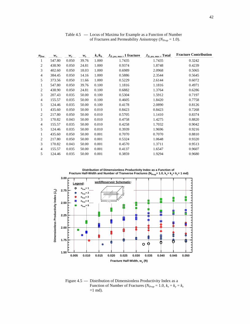
42

Table 4.5 — Locus of Maxima for Example as a Function of Number of Fractures and Permeability Anisotropy (NProp = 1.0).

nfrac wx wy wz kv/kh JD, pss, max , 1 fracture JD, pss, max , Total Fracture Contribution

1 547.80 0.050 39.76 1.000 1.7435 1.7435 0.3242 2 438.90 0.050 24.81 1.000 0.9374 1.8748 0.4239 3 402.60 0.050 18.03 1.000 0.6989 2.0968 0.5065 4 384.45 0.050 14.16 1.000 0.5886 2.3544 0.5645 5 373.56 0.050 11.66 1.000 0.5229 2.6144 0.6072 1 547.80 0.050 39.76 0.100 1.1816 1.1816 0.4971 2 438.90 0.050 24.81 0.100 0.6882 1.3764 0.6286 3 207.43 0.035 50.00 0.100 0.5304 1.5912 0.7197 4 155.57 0.035 50.00 0.100 0.4605 1.8420 0.7758 5 124.46 0.035 50.00 0.100 0.4178 2.0890 0.8126 1 435.60 0.050 50.00 0.010 0.8423 0.8423 0.7268 2 217.80 0.050 50.00 0.010 0.5705 1.1410 0.8374 3 170.82 0.043 50.00 0.010 0.4758 1.4275 0.8820 4 155.57 0.035 50.00 0.010 0.4258 1.7032 0.9042 5 124.46 0.035 50.00 0.010 0.3939 1.9696 0.9216 1 435.60 0.050 50.00 0.001 0.7070 0.7070 0.8810 2 217.80 0.050 50.00 0.001 0.5324 1.0648 0.9320 3 170.82 0.043 50.00 0.001 0.4570 1.3711 0.9513 4 155.57 0.035 50.00 0.001 0.4137 1.6547 0.9607 5 124.46 0.035 50.00 0.001 0.3859 1.9294 0.9680

3.00

2.75

2.50

2.25

2.00

1.75

1.50

Dim

ensi

onle

ss P

rodu

ctiv

ity In

dex

(J D

)

0.0500.0450.0400.0350.0300.0250.0200.0150.0100.005

Fracture Half-Width, wy (ft)

ye/ nfrac

xe

ze

Legend :

nfrac= 1

nfrac= 2

nfrac= 3

nfrac= 4

nfrac= 5

Distribution of Dimensionless Productivity Index as a Function of Fracture Half-Width and Number of Tranverse Fractur es (NProp = 1.0, kx= ky= kz= 1 md)

well/Reservoir Schematic :

Figure 4.5 — Distribution of Dimensionless Productivity Index as a Function of Number of Fractures (NProp = 1.0, kx = ky = kz =1 md).

43

In Figs. 4.6 to 4.9 we present the fracture contributions to flow (as a fraction of total flow) shown as a

function of dimensionless time and the number of fractures for the NProp = 1.0 case, as well as for different

permeability anisotropy ratios (kv/kh).

1.0 1.0

0.9 0.9

0.8 0.8

0.7 0.7

0.6 0.6

0.5 0.5

0.4 0.4

0.3 0.3

0.2 0.2

0.1 0.1

0.0 0.0

Fra

ctur

e C

ontr

ibut

ion

to F

low

(F

ract

ion)

10-10

10-10

10-9

10-9

10-8

10-8

10-7

10-7

10-6

10-6

10-5

10-5

10-4

10-4

10-3

10-3

10-2

10-2

10-1

10-1

100

100

Dimensionless Time Based on Drainage Area ( tDA)

ye/ nfrac

xe

ze

Legend :

Fracture Contribution to Flow

Fracture Contribution as a Function of Dimensionle ss Time and Number of Fractures ( NProp = 1.0, kx= ky= kz= 1 md)

n frac = 1

3

2

4

n frac = 5


Figure 4.6 — Fracture Contribution to Flow as a Function of Dimensionless Time and Number of Fractures (NProp = 1.0, kx = ky = kz =1 md).

1.0 1.0

0.9 0.9

0.8 0.8

0.7 0.7

0.6 0.6

0.5 0.5

0.4 0.4

0.3 0.3

0.2 0.2

0.1 0.1

0.0 0.0

Fra

ctur

e C

ontr

ibut

ion

to F

low

(F

ract

ion)

10-10

10-10

10-9

10-9

10-8

10-8

10-7

10-7

10-6

10-6

10-5

10-5

10-4

10-4

10-3

10-3

10-2

10-2

10-1

10-1

100

100


ye/ nfrac

xe

ze

Legend :


Fracture Contribution as a Function of Dimensionle ss Time and Number of Fractures ( NProp = 1.0,, kx= ky= 1 md, kz= 0.1 md)

n frac = 1

3

2

4

n frac = 5


Figure 4.7 — Fracture Contribution to Flow as a Function of Dimensionless Time and Number of Fractures (NProp = 1.0, kx = ky = 1 md, kz = 0.1 md).

44

For all cases shown in Figs. 4.6 to 4.9 the early-time production is dominated by the horizontal well, the

fracture contribution increases during the transient flow period and then stabilizes during the pseudosteady-

state flow period. We also note that the fracture contribution increases as the permeability anisotropy

increases (which is logical as less fluid would be produced by the horizontal well for such cases).

Obviously, the fracture contribution to flow increases with the number of fractures — each fracture simply

adds to the fracture contribution.

1.0 1.0

0.9 0.9

0.8 0.8

0.7 0.7

0.6 0.6

0.5 0.5

0.4 0.4

0.3 0.3

0.2 0.2

0.1 0.1

0.0 0.0

Fra

ctur

e C

ontr

ibut

ion

to F

low

(F

ract

ion)

10-10

10-10

10-9

10-9

10-8

10-8

10-7

10-7

10-6

10-6

10-5

10-5

10-4

10-4

10-3

10-3

10-2

10-2

10-1

10-1

100

100


ye/ nfrac

xe

ze

Legend :


Fracture Contribution as a Function of Dimensionle ss Time and Number of Fractures ( NProp = 1.0, kx= ky= 1 md, kz= 0.01 md)

n frac = 1

3

2

4n frac = 5



1.0 1.0

0.9 0.9

0.8 0.8

0.7 0.7

0.6 0.6

0.5 0.5

0.4 0.4

0.3 0.3

0.2 0.2

0.1 0.1

0.0 0.0

Fra

ctur

e C

ontr

ibut

ion

to F

low

(F

ract

ion)

10-10

10-10

10-9

10-9

10-8

10-8

10-7

10-7

10-6

10-6

10-5

10-5

10-4

10-4

10-3

10-3

10-2

10-2

10-1

10-1

100

100


ye/ nfrac

xe

ze

Legend :



n frac = 1

3

2

4n frac = 5



45

In Figs. 4.10 to 4.13 we present the behavior of the maximum dimensionless productivity index versus the

number of fractures, for various cases of the proppant number and a specific case of permeability

anisotropy. We note that the dimensionless pseudosteady-state productivity index (JD, pss ,Max) decreases as

the anisotropy ratio increases — this phenomenon is observed for cases. This behavior is more severe for

cases with a lower proppant number. Decreasing productivity as a consequence of increased anisotropy

can be attributed to the fact that the production in the horizontal section decreases as the anisotropy

increases, as discussed by Mukherjee and Economides (1991). If there is sufficient proppant to achieve an

efficient (i.e., high conductivity) fracture, then the lost productivity of the horizontal section would be

compensated for by the increased fracture contribution.

For the specific case of proppant numbers of 1.0 and 0.001, we note a reduction of 59.5 and 26.2 percent in

JD ,pss, Max. For the cases of 1 and 5 fractures (and a proppant number equal to 1.0), we have 87.3 and 83.8

percent loss compared to the same cases for a proppant number equal to 0.001. These cases illustrate the

need (if not the absolute requirement) to maximize proppant volume (and proppant placement) for cases of

high permeability anisotropy.

From Figs. 4.10 to 4.13 we note that JD ,pss, Max increases as the number of fractures increase — and that this

behavior is consistent for every case. We also note that the size of the increase in well productivity

depends directly on the amount of proppant used.

An interesting outcome of this study is that the selection of an optimal well completion is clearly a function

of all of the major variables — proppant number, number of fractures, and permeability anisotropy. In

isolation — for example, the maximizing number of fractures would seem to always be the best choice.

However, the issue of permeability anisotropy, which is obviously fixed by nature in practice, changes the

perception that more fractures is always better (see Fig. 4.8 (kv/kh = 0.01) and Fig. 4.9 (kv/kh = 0.001), where

the profiles essentially flat (i.e., the number of fractures does not significantly influence the JD,pss,Max

function).)

The impact of this "sensitivity study" is that any well/fracture design must be considered in terms of the

objectives (maximize production performance) and the practical limitations of the system (permeability

anisotropy and fracture treatment size). We can design the optimal fracture treatment — there will always

be a clear best case(s), but can we delivery said treatment to the formation? This work provides the means

to design optimal treatments for complex well/fracture configurations, but the engineer must consider any

and all practical limitations of this design for implementation in the field.

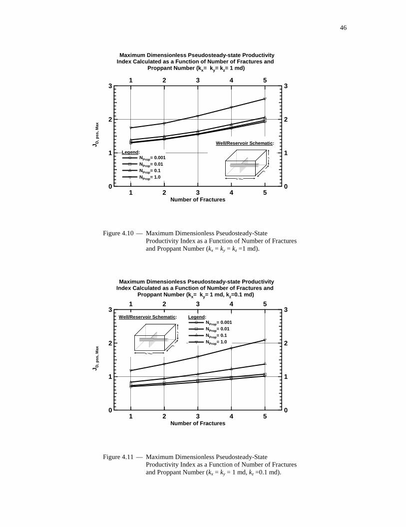
46

3 3

2 2

1 1

0 0

J D, p

ss, M

ax

5

5

4

4

3

3

2

2

1

1

Number of Fractures

ye/ nfrac

xe

ze

Legend : NProp = 0.001 NProp = 0.01 NProp = 0.1 NProp = 1.0

Maximum Dimensionless Pseudosteady-state Productiv ityIndex Calculated as a Function of Number of Fractur es and

Proppant Number ( kx= ky= kz= 1 md)


Figure 4.10 — Maximum Dimensionless Pseudosteady-State Productivity Index as a Function of Number of Fractures and Proppant Number (kx = ky = kz =1 md).

3 3

2 2

1 1

0 0

J D, p

ss, M

ax

5

5

4

4

3

3

2

2

1

1

Number of Fractures

ye/ nfrac

xe

ze



Proppant Number ( kx= ky= 1 md, kz=0.1 md)


Figure 4.11 — Maximum Dimensionless Pseudosteady-State Productivity Index as a Function of Number of Fractures and Proppant Number (kx = ky = 1 md, kz =0.1 md).

47

3 3

2 2

1 1

0 0

J D, p

ss, M

ax

5

5

4

4

3

3

2

2

1

1

Number of Fractures

ye/ nfrac

xe

ze



Proppant Number ( kx= ky= 1 md, kz= 0.01 md)


Figure 4.12 — Maximum Dimensionless Pseudosteady-State Productivity Index as a Function of Number of Fractures and Proppant Number (kx = ky = 1 md, kz = 0.01 md).

.

3 3

2 2

1 1

0 0

J D, p

ss, M

ax

5

5

4

4

3

3

2

2

1

1

Number of Fractures

ye/ nfrac

xe

ze



Proppant Number ( kx= ky= 1 md, kz= 0.001 md)


Figure 4.13 — Maximum Dimensionless Pseudosteady-State Productivity Index as a Function of Number of Fractures and Proppant Number (kx = ky = 1 md, kz =0.001 md).

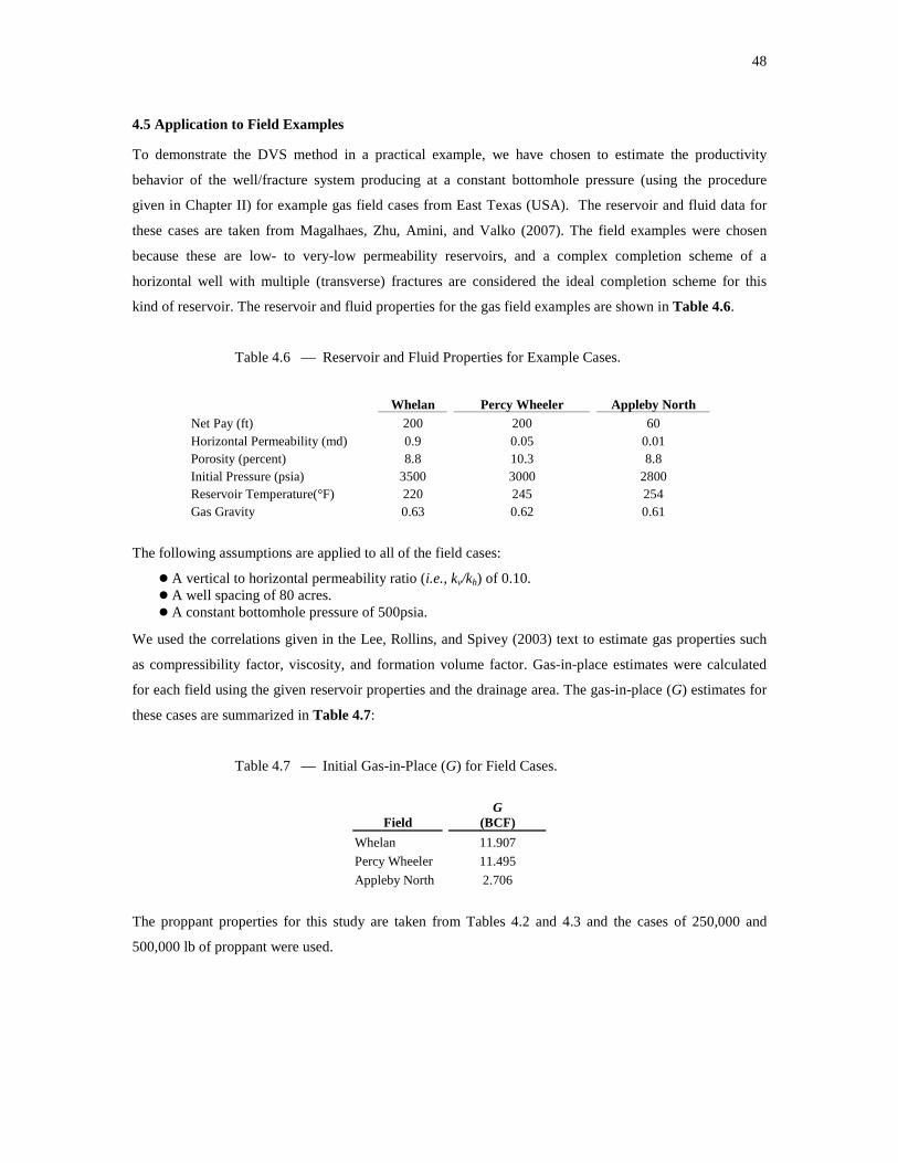
48

4.5 Application to Field Examples

To demonstrate the DVS method in a practical example, we have chosen to estimate the productivity

behavior of the well/fracture system producing at a constant bottomhole pressure (using the procedure

given in Chapter II) for example gas field cases from East Texas (USA). The reservoir and fluid data for

these cases are taken from Magalhaes, Zhu, Amini, and Valko (2007). The field examples were chosen

because these are low- to very-low permeability reservoirs, and a complex completion scheme of a

horizontal well with multiple (transverse) fractures are considered the ideal completion scheme for this

kind of reservoir. The reservoir and fluid properties for the gas field examples are shown in Table 4.6.

Table 4.6 — Reservoir and Fluid Properties for Example Cases.

Whelan Percy Wheeler Appleby North Net Pay (ft) 200 200 60 Horizontal Permeability (md) 0.9 0.05 0.01 Porosity (percent) 8.8 10.3 8.8 Initial Pressure (psia) 3500 3000 2800 Reservoir Temperature(°F) 220 245 254 Gas Gravity 0.63 0.62 0.61

The following assumptions are applied to all of the field cases:

� A vertical to horizontal permeability ratio (i.e., kv/kh) of 0.10. � A well spacing of 80 acres. � A constant bottomhole pressure of 500psia.

We used the correlations given in the Lee, Rollins, and Spivey (2003) text to estimate gas properties such

as compressibility factor, viscosity, and formation volume factor. Gas-in-place estimates were calculated

for each field using the given reservoir properties and the drainage area. The gas-in-place (G) estimates for

these cases are summarized in Table 4.7:

Table 4.7 — Initial Gas-in-Place (G) for Field Cases.

Field G

(BCF)

Whelan 11.907

Percy Wheeler 11.495

Appleby North 2.706

The proppant properties for this study are taken from Tables 4.2 and 4.3 and the cases of 250,000 and

500,000 lb of proppant were used.

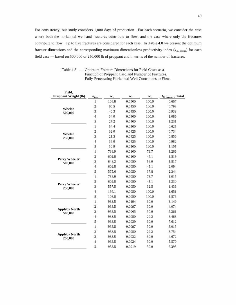
49

For consistency, our study considers 1,000 days of production. For each scenario, we consider the case

where both the horizontal well and fractures contribute to flow, and the case where only the fractures

contribute to flow. Up to five fractures are considered for each case. In Table 4.8 we present the optimum

fracture dimensions and the corresponding maximum dimensionless productivity index (JD, pss,ma) for each

field case — based on 500,000 or 250,000 lb of proppant and in terms of the number of fractures.

Table 4.8 — Optimum Fracture Dimensions for Field Cases as a Function of Proppant Used and Number of Fractures. Fully-Penetrating Horizontal Well Contributes to Flow.

Field, Proppant Weight (lb) nfrac wx wy wz JD, pss,max , Total

1 108.8 0.0500 100.0 0.667

2 60.5 0.0450 100.0 0.793

3 40.3 0.0450 100.0 0.938

4 34.0 0.0400 100.0 1.086

Whelan 500,000

5 27.2 0.0400 100.0 1.231

1 54.4 0.0500 100.0 0.625

2 32.0 0.0425 100.0 0.734

3 21.3 0.0425 100.0 0.856

4 16.0 0.0425 100.0 0.982

Whelan 250,000

5 10.9 0.0500 100.0 1.105

1 738.9 0.0100 73.7 1.266

2 602.8 0.0100 45.1 1.519

3 648.2 0.0050 56.0 1.817

4 602.8 0.0050 45.1 2.094

Percy Wheeler 500,000

5 575.6 0.0050 37.8 2.344

1 738.9 0.0050 73.7 1.015

2 602.8 0.0050 45.1 1.230

3 557.5 0.0050 32.5 1.436

4 136.1 0.0050 100.0 1.651


5 108.8 0.0050 100.0 1.876

1 933.5 0.0194 30.0 3.149

2 933.5 0.0097 30.0 4.074

3 933.5 0.0065 30.0 5.261

4 933.5 0.0050 29.2 6.468

Appleby North 500,000

5 933.5 0.0039 30.0 7.612

1 933.5 0.0097 30.0 3.015

2 933.5 0.0050 29.2 3.754

3 933.5 0.0032 30.0 4.672

4 933.5 0.0024 30.0 5.570

Appleby North 250,000

5 933.5 0.0019 30.0 6.398

50

It can be seen from Table 4.8 that for higher permeability reservoirs, then full penetration in vertical

direction (i.e., wz → h/2) is most likely to yield the optimum productivity index. Similarly, for the lower

permeability reservoirs the tendency changes toward extension in the horizontal direction (i.e., wx → xe/2).

For the case of Wheeler field the optimum results are achieved by fractures with partial penetration in both

directions (except for the cases with 250,000 lb of proppant and 4 and 5 fractures). This observation of

vertical penetration being required in "high" permeability reservoirs is due primarily to the fact that the

given amount of proppant is not sufficient to achieve efficient fractures. For the lowest permeability case

(Appleby North), we observe that the optimum productivity is achieved by fractures which fully penetrate

the reservoir in both directions (vertical and horizontal) — even in this case, where the amount of proppant

is insufficient to yield a fracture with the width of at least a single proppant diameter.

Table 4.9 presents our final results for each field case (in terms of performance at 1000 says of production)

as a function of the amount of proppant and the number of fractures (for the case where the horizontal well

and fractures contribute to flow, and the case where only the fractures contribute to flow). Specifically,

Table 4.9 contains the average reservoir pressure, the gas production rate, and the cumulative gas

production at 1000 days of production. For reference, the complete set of results is provided for each field

in Appendices G through I.

The work presented in the remainder of this section is provided to support the observations thus far, and to

provide a "time-dependent" view of the performance for these cases. As noted above, the details and the

complete suite of results for these examples are given in Appendices G through I.

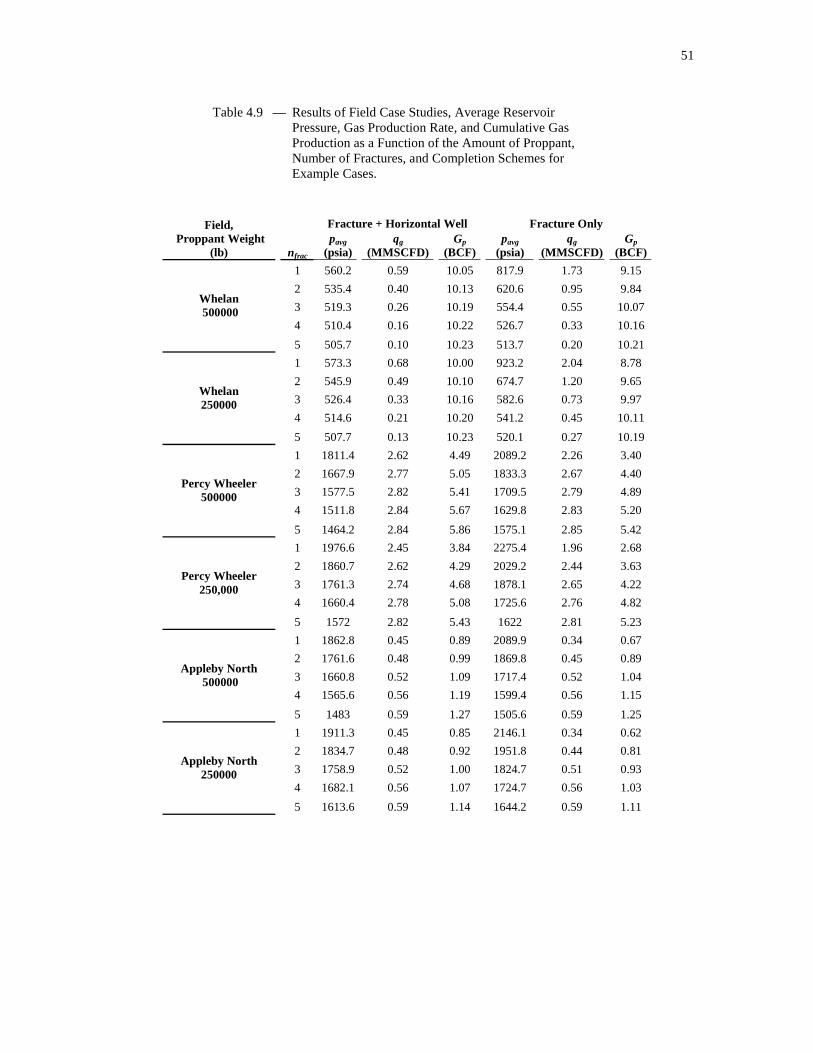
51

Table 4.9 — Results of Field Case Studies, Average Reservoir Pressure, Gas Production Rate, and Cumulative Gas Production as a Function of the Amount of Proppant, Number of Fractures, and Completion Schemes for Example Cases.

Fracture + Horizontal Well Fracture Only Field, Proppant Weight

(lb) nfrac pavg

(psia) qg

(MMSCFD) Gp

(BCF) pavg

(psia) qg

(MMSCFD) Gp

(BCF)

1 560.2 0.59 10.05 817.9 1.73 9.15

2 535.4 0.40 10.13 620.6 0.95 9.84

3 519.3 0.26 10.19 554.4 0.55 10.07

4 510.4 0.16 10.22 526.7 0.33 10.16

Whelan 500000

5 505.7 0.10 10.23 513.7 0.20 10.21

1 573.3 0.68 10.00 923.2 2.04 8.78

2 545.9 0.49 10.10 674.7 1.20 9.65

3 526.4 0.33 10.16 582.6 0.73 9.97

4 514.6 0.21 10.20 541.2 0.45 10.11

Whelan 250000

5 507.7 0.13 10.23 520.1 0.27 10.19

1 1811.4 2.62 4.49 2089.2 2.26 3.40

2 1667.9 2.77 5.05 1833.3 2.67 4.40

3 1577.5 2.82 5.41 1709.5 2.79 4.89

4 1511.8 2.84 5.67 1629.8 2.83 5.20

Percy Wheeler 500000

5 1464.2 2.84 5.86 1575.1 2.85 5.42

1 1976.6 2.45 3.84 2275.4 1.96 2.68

2 1860.7 2.62 4.29 2029.2 2.44 3.63

3 1761.3 2.74 4.68 1878.1 2.65 4.22

4 1660.4 2.78 5.08 1725.6 2.76 4.82


5 1572 2.82 5.43 1622 2.81 5.23

1 1862.8 0.45 0.89 2089.9 0.34 0.67

2 1761.6 0.48 0.99 1869.8 0.45 0.89

3 1660.8 0.52 1.09 1717.4 0.52 1.04

4 1565.6 0.56 1.19 1599.4 0.56 1.15

Appleby North 500000

5 1483 0.59 1.27 1505.6 0.59 1.25

1 1911.3 0.45 0.85 2146.1 0.34 0.62

2 1834.7 0.48 0.92 1951.8 0.44 0.81

3 1758.9 0.52 1.00 1824.7 0.51 0.93

4 1682.1 0.56 1.07 1724.7 0.56 1.03

Appleby North 250000

5 1613.6 0.59 1.14 1644.2 0.59 1.11

52

Fig. 4.14 presents the computed gas production rate as a function of production time for the Whelan field,

where each fracture stimulation consists of 250,000 lbs of proppant. The Whelan field has the highest

permeability of our field cases (0.10 md). In Fig. 4.14 we can distinguish two distinct flow periods — the

first flow period is the transient flow period (which has very little rate decline). The second flow period is

that of pseudosteady-state or boundary-dominated flow, and we note a much steeper rate decline due to the

influence of the reservoir boundaries.

10-1

100

101

102

103

Gas

Pro

duct

ion

Rat

e,

qg (

MM

SC

FD

)

10-2

10-1

100

101

102

103

Production Time (Days)

Gas Production Rate as a Function of Production Tim e and Number of Fractures for Whelan Example

(80 Acres Spacing, Total 250,000 lb of Proppant)

Legend :

Fracture + Horizontal Well Fracture Only

nfrac = 1 2

nfrac = 1 2 3 4

3 45

5

5

11

5 3

Figure 4.14 — Gas Production Rate as a Function of Production Time, Number of Fractures, and Completion Scheme for Whelan Field (80 Acres Spacing, 250,000 lb Proppant).

For other two field cases (Percy Wheeler and Appleby North), the 1,000 day production period is not

sufficient time for the reservoir to produce under boundary-dominated flow conditions, even for the cases

of 500,000 lb of proppant (large, highly conductive fractures). Figs. 4.15 to 4.18 present the gas rate

profiles for the Percy Wheeler and Appleby North fields, respectively for the cases of 250,000 and 500,000

lb of proppant. For production at 1,000 days, we note that the Percy Wheeler field case shows evidence of

the start of the boundary-dominated flow, but for the Appleby North field case we can only observe the

transition into boundary-dominated flow.

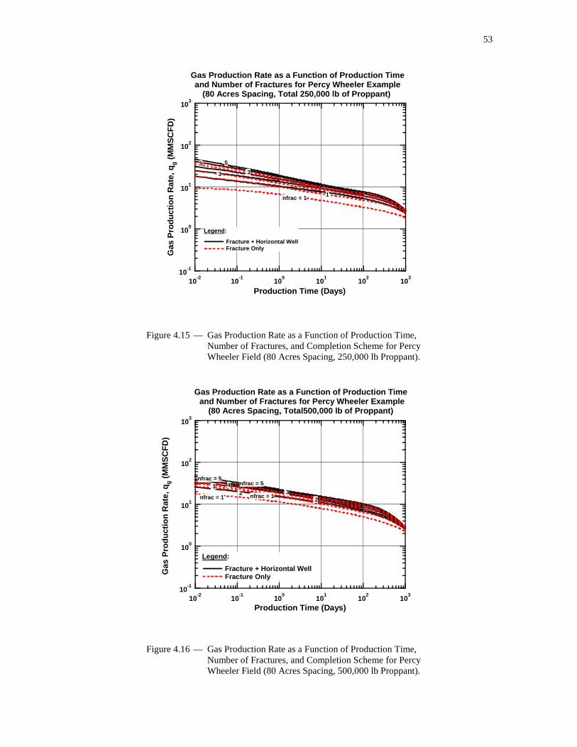
53

10-1

100

101

102

103

Gas

Pro

duct

ion

Rat

e,

qg (

MM

SC

FD

)

10-2

10-1

100

101

102

103


Gas Production Rate as a Function of Production Tim eand Number of Fractures for Percy Wheeler Example


Legend :


55

nfrac = 1 1

3 3

Figure 4.15 — Gas Production Rate as a Function of Production Time, Number of Fractures, and Completion Scheme for Percy Wheeler Field (80 Acres Spacing, 250,000 lb Proppant).

10-1

100

101

102

103

Gas

Pro

duct

ion

Rat

e,

qg

(MM

SC

FD

)

10-2

10-1

100

101

102

103


Gas Production Rate as a Function of Production Tim e and Number of Fractures for Percy Wheeler Example

(80 Acres Spacing, Total500,000 lb of Proppant)

Legend :


nfrac = 5nfrac = 5

nfrac = 1 2nfrac = 1

2 34 3

Figure 4.16 — Gas Production Rate as a Function of Production Time, Number of Fractures, and Completion Scheme for Percy Wheeler Field (80 Acres Spacing, 500,000 lb Proppant).

54

10-1

100

101

102

103

Gas

Pro

duct

ion

Rat

e,

qg (

MM

SC

FD

)

10-2

10-1

100

101

102

103


Gas Production Rate as a Function of Production Tim e and Number of Fractures for Appleby North Example


Legend :


nfrac = 5

nfrac = 5

nfrac = 1

2

nfrac = 1

3 4

Figure 4.17 — Gas Production Rate as a Function of Production Time, Number of Fractures, and Completion Scheme for Appleby North Field (80 Acres Spacing, 250,000 lb Proppant).

10-1

100

101

102

103

Gas

Pro

duct

ion

Rat

e,

qg (

MM

SC

FD

)

10-2

10-1

100

101

102

103


Gas Production Rate as a Function of Production Tim e and Number of Fractures for Appleby North Example


Legend :


nfrac = 5

nfrac = 5

nfrac = 1

2

nfrac = 1

3

4

Figure 4.18 — Gas Production Rate as a Function of Production Time, Number of Fractures, and Completion Scheme for Appleby North Field (80 Acres Spacing, 500,000 lb Proppant).

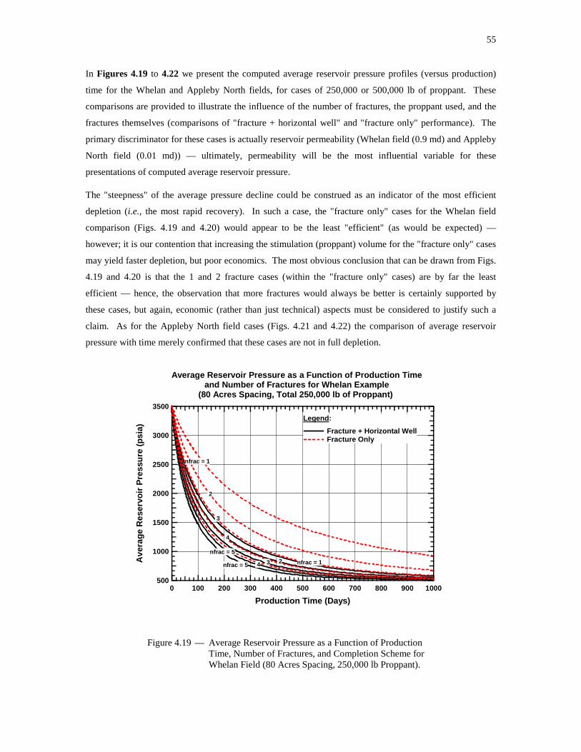
55

In Figures 4.19 to 4.22 we present the computed average reservoir pressure profiles (versus production)

time for the Whelan and Appleby North fields, for cases of 250,000 or 500,000 lb of proppant. These

comparisons are provided to illustrate the influence of the number of fractures, the proppant used, and the

fractures themselves (comparisons of "fracture + horizontal well" and "fracture only" performance). The

primary discriminator for these cases is actually reservoir permeability (Whelan field (0.9 md) and Appleby

North field (0.01 md)) — ultimately, permeability will be the most influential variable for these

presentations of computed average reservoir pressure.

The "steepness" of the average pressure decline could be construed as an indicator of the most efficient

depletion (i.e., the most rapid recovery). In such a case, the "fracture only" cases for the Whelan field

comparison (Figs. 4.19 and 4.20) would appear to be the least "efficient" (as would be expected) —

however; it is our contention that increasing the stimulation (proppant) volume for the "fracture only" cases

may yield faster depletion, but poor economics. The most obvious conclusion that can be drawn from Figs.

4.19 and 4.20 is that the 1 and 2 fracture cases (within the "fracture only" cases) are by far the least

efficient — hence, the observation that more fractures would always be better is certainly supported by

these cases, but again, economic (rather than just technical) aspects must be considered to justify such a

claim. As for the Appleby North field cases (Figs. 4.21 and 4.22) the comparison of average reservoir

pressure with time merely confirmed that these cases are not in full depletion.

3500

3000

2500

2000

1500

1000

500

Ave

rage

Res

ervo

ir P

ress

ure

(psi

a)

10009008007006005004003002001000


Average Reservoir Pressure as a Function of Product ion Timeand Number of Fractures for Whelan Example


Legend :


nfrac = 5

nfrac = 5

nfrac = 1

2

nfrac = 1

2 3

4

3

4

Figure 4.19 — Average Reservoir Pressure as a Function of Production Time, Number of Fractures, and Completion Scheme for Whelan Field (80 Acres Spacing, 250,000 lb Proppant).

56

3500

3000

2500

2000

1500

1000

500

Ave

rage

Res

ervo

ir P

ress

ure

(psi

a)

10009008007006005004003002001000


Average Reservoir Pressure as a Function of Production Timeand Number of Fractures for Whelan Example


Legend :


nfrac = 5

nfrac = 5nfrac = 1

2

nfrac = 1

2 3

4

3

4

Figure 4.20 — Average Reservoir Pressure as a Function of Production Time, Number of Fractures, and Completion Scheme for Percy Whelan Field (80 Acres Spacing, 500,000 lb Proppant).

3000

2500

2000

1500

Ave

rage

Res

ervo

ir P

ress

ure

(psi

a)

10009008007006005004003002001000


Average Reservoir Pressure as a Function of Production Timeand Number of Fractures for Appleby North Example


Legend :

Fracture + Horizontal Well Fracture Only nfrac = 5

nfrac = 5

nfrac = 1

2

nfrac = 1

2

3

4

3

4

Figure 4.21 — Average Reservoir Pressure as a Function of Production Time, Number of Fractures, and Completion Scheme for Appleby North Field (80 Acres Spacing, 250,000 lb Proppant).

57

3000.0

2500.0

2000.0

1500.0

1000.0

Ave

rage

Res

ervo

ir P

ress

ure

(psi

a)

10009008007006005004003002001000


Average Reservoir Pressure as a Function of Production Timeand Number of Fractures for Appleby North Example


Legend :


nfrac = 5

nfrac = 5

nfrac = 1 2

nfrac = 1

2

3

4

3

4

Figure 4.22 — Average Reservoir Pressure as a Function of Production Time, Number of Fractures, and Completion Scheme for Appleby North Field (80 Acres Spacing, 500,000 lb Proppant).

12

11

10

9

8

7

6

5

4

3

2

1

0

Cum

ulat

ive

Gas

Pro

duct

ion,

G

P (

BC

F)

10009008007006005004003002001000


Cumulative Gas Production as a Function of Producti on Timeand Number of Fractures for Whelan Example


Legend :


nfrac = 5nfrac = 5

nfrac = 1

2

nfrac = 1

2

3

4 3

4

Figure 4.23 — Cumulative Gas Production as a Function of Production Time, Number of Fractures, and Completion Scheme for Whelan Field (80 Acres Spacing, 250,000 lb Proppant).

58

In contrast to comparison of the computed average reservoir pressure profiles, comparison of the

cumulative gas production as a function of time will definitively illustrate "efficient" depletion. That is, the

cases with the most rapid depletion (of a fixed resource) will yield the highest return on investment (all

factors being equal). In Figs. 4.23 to 4.28 we present the behavior of the cumulative gas production as a

function of production time for all field cases and differing completions (i.e., proppant volumes and well

structures).

The most straightforward conclusion we can make is that adding new fractures increases the production and

accelerates the production of reserves. We note that the importance of these two issues (production

increases and reserve acceleration) varies as the permeability of the reservoir changes. For low

permeability reservoirs such as the Appleby North field, additional fracture(s) may provide more additional

reserves (but this is actually only likely in very low permeability scenarios (<0.001 md) and in cases of

geological reservoir heterogeneity (poor vertical and lateral continuity of the reservoir)). In a practical

sense, for homogeneous reservoir systems of low to moderate permeability (>0.01 md), we should expect

acceleration of reserves when we deploy well completions such as these.

12

11

10

9

8

7

6

5

4

3

2

1

0

Cum

ulat

ive

Gas

Pro

duct

ion,

G

P (

BC

F)

10009008007006005004003002001000


Cumulative Gas Production as a Functionof Productio n Time and Number of Fractures for Whelan Example


Legend :


nfrac = 5nfrac = 5

nfrac = 1

2

nfrac = 1

2

3

4

3

4

Figure 4.24 — Cumulative Gas Production as a Function of Production Time, Number of Fractures, and Completion Scheme for Whelan Field (80 Acres Spacing, 500,000 lb Proppant).

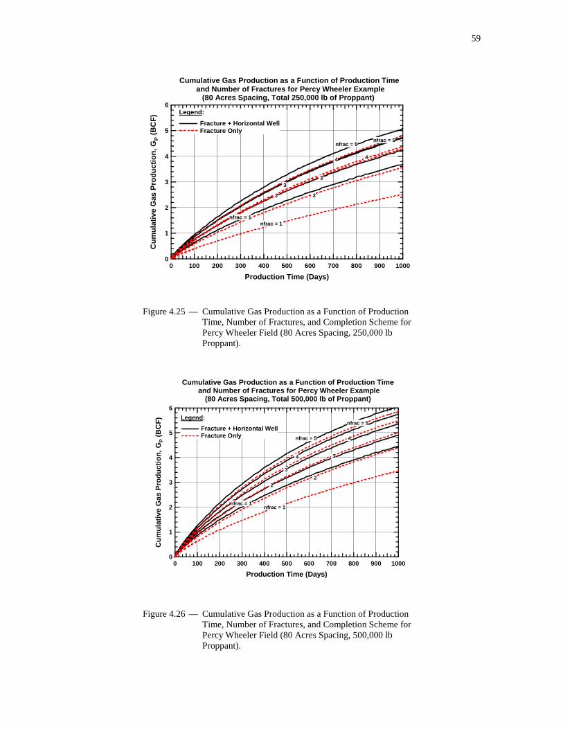
59

6

5

4

3

2

1

0

Cum

ulat

ive

Gas

Pro

duct

ion,

G

P (

BC

F)

10009008007006005004003002001000


Cumulative Gas Production as a Function of Producti on Time and Number of Fractures for Percy Wheeler Example


Legend :


nfrac = 5nfrac = 5

nfrac = 1

2

nfrac = 1

2

3

4

3

4

Figure 4.25 — Cumulative Gas Production as a Function of Production Time, Number of Fractures, and Completion Scheme for Percy Wheeler Field (80 Acres Spacing, 250,000 lb Proppant).

6

5

4

3

2

1

0

Cum

ulat

ive

Gas

Pro

duct

ion,

G

P (

BC

F)

10009008007006005004003002001000




Legend :


nfrac = 5

nfrac = 1

2

nfrac = 1

2

3

4 3

4

Figure 4.26 — Cumulative Gas Production as a Function of Production Time, Number of Fractures, and Completion Scheme for Percy Wheeler Field (80 Acres Spacing, 500,000 lb Proppant).

60

1.2

1.0

0.8

0.6

0.4

0.2

0.0

Cum

ulat

ive

Gas

Pro

duct

ion,

G

P (

BC

F)

10009008007006005004003002001000


Cumulative Gas Production as a Function of Producti on Timeand Number of Fractures for Appleby North Example


Legend :


nfrac = 5

nfrac = 5

nfrac = 1

2

nfrac = 1

2

3

4

3

4

Figure 4.27 — Cumulative Gas Production as a Function of Production Time, Number of Fractures, and Completion Scheme for Appleby North Field (80 Acres Spacing, 250,000 lb Proppant).

1.50

1.25

1.00

0.75

0.50

0.25

0.00

Cum

ulat

ive

Gas

Pro

duct

ion,

G

P (

BC

F)

10009008007006005004003002001000


Cumulative Gas Production as a Functionof Production Time and Number of Fractures for Appleby North Example


Legend :


nfrac = 5

nfrac = 1

2

nfrac = 1

2

3

4

3

4

Figure 4.28 — Cumulative Gas Production as a Function of Production Time, Number of Fractures, and Completion Scheme for Appleby North Field (80 Acres Spacing, 500,000 lb Proppant).

61

It is also a general perception that the advantage of placing additional fractures in the reservoir diminishes

as the number of fractures increases. This perception is based on the fact that since the total drainage area

is limited, individual fractures will begin to drainage volumes, and produce less over time. This is true for

both cases presented in this study — the case where the horizontal well and fractures contribute to flow,

and the case where only the fractures contribute to flow. A practical issue regarding multiple fractures is a

risk of an adverse event as more and more fractures are added — such as accessing water or damage to the

wellbore that limits access to all of the created hydraulic fractures.

For all of the cases we consider, the horizontal well adds more to the production performance than adding

another fracture. We note this observation because some may opt to drain a given reservoir partition with

only vertically fractured wells, while others may employ horizontal wells with multiple transverse

fractures. It is important to recognize that, in a sensitivity study such as this, the contribution of the

horizontal well is always relevant, but as Figs. 4.10 to 4.13 illustrate the influence of reservoir anisotropy is

extremely important, and may minimize or even negate the effects of the horizontal well.

The use of additional proppant is seen to accelerate the recovery of reserves for all the cases studied, but

the level of improvement is dependent on the reservoir permeability and the well/fracture configuration.

We generally note positive effects of using more proppant for a larger number of fractures, as more

proppant should build more efficient fractures. However; if a given set of fractures can effectively deplete

the reservoir, then larger treatments would be unjustifiable in an economic sense.

4.6 Summary

This chapter provides example applications of the DVS method for the prediction of well productivity for

various complex well/fracture configurations. Modeling and validation procedures were demonstrated and

discussed, and example applications to relevant field cases are given. Our results imply that the most

effective well configuration is that of a horizontal well with multiple (transverse) fractures, where as much

as proppant and as many fractures as possible are used. Obviously this is an ideal scenario, and we need to

establish an optimal well completion for each individual case — which would be the most technically

feasible as well as the most economic well completion scheme that yields the highest possible productivity.

The primary objective of this chapter was to demonstrate that the DVS method can be used effectively to

design and optimize a well completion from a technical standpoint. We believe that the DVS method has

been successfully demonstrated and validated for that purpose, and we recognize that such tools must be

used with the relevant economic constraints. Our goal was to provide a tool. We believe that the DVS

method can be used to effectively design and model virtually any well completion that can be envisioned.

62

CHAPTER V

SUMMARY, CONCLUSIONS, AND

RECOMMENDATIONS FOR FUTURE WORK

5.1 Summary

The primary purpose of this work is to develop a new method to predict the transient and pseudosteady-

state pressure and production behavior of a closed, rectangular reservoir. In particular, to develop an

analytical/semi-analytical solution that can be used to model vertical and horizontal wells with or without a

variety of hydraulic fractures. Such a solution can be extended to other cases, but the aforementioned

cases are the focus of this work.

In this work we performed the following tasks as:

� We developed the method of distributed volumetric sources (DVS) as a solution for the problem of

pressure distributions in a closed, rectangular reservoir using a uniform flux source (the simplest case

for such problems).

� Using the DVS solution method, we have successfully developed and validated the solutions for

pressure behavior of simple and complex well/fracture configurations as follows:

— Unfractured vertical wells

— Horizontal well (uniform-flux and infinite-conductivity)

— Hydraulically fractured vertical wells (infinite- and finite-conductivity fractures).

� We have generated the transient and pseudosteady-state productivity index behavior using the pressure

response results (using the DVS method) and we validated these results using reservoir simulation

and/or existing analytical/semi-analytical models from the production engineering literature.

� We demonstrated the applicability of the new solution method in predicting production behavior for a

complex well/fracture configuration — specifically, the case of a horizontal well with multiple trans-

verse fractures, where both the horizontal section and the fractures contribute to production.

� As an application, we applied the DVS method as an optimization/screening tool to obtain the best

completion scheme for the development of a field example case (estimated multiple production

performance cases for a reservoir with wells produced at constant bottomhole pressures for various

completion scenarios).

5.2 Conclusions

We have successfully developed, validated, and demonstrated the DVS method to a practical mechanism

for the generation of consistent transient and pseudosteady-state solutions for complex well/fracture

systems. The DVS method has been shown to provide reliable results with relatively moderate com-

putational effort.

63

As a validation, we utilized the DVS approach to create well/reservoir models for simple cases with well-

known solutions as well as for a complex well/reservoir configuration case that where a reservoir simula-

tion model was used for validation. The advantage of the DVS method is more obvious for cases with

significant complexities — such as permeability anisotropy, partial penetration of the source in any of the

principal directions, and/or additional pressure losses stemming from the particular geometry of the flow

path inside the sources.

For our particular purposes (production forecasting and optimizing the well completion strategy), we

wanted to provide a consistent mechanism to generate the transient and pseudosteady-state productivity

indices. In such applications the DVS method has been shown to be extraordinarily flexible in model

construction and the DVS method is comparable in terms of computation speeds with most analytical

solutions (for simple cases) and the DVS method is competitive with numerical simulation models for

complex reservoir cases.

5.3 Recommendations for Future Work

The future work on this topic should focus on the application of the DVS method for more cases of

complex well/fracture schemes. In this work we demonstrate a single example case of the application of

the DVS method. One of the basic assumptions in development of the DVS solution is the assumption of

the reservoir having closed (no flow) boundaries — future efforts should also consider constant pressure

and/or mixed boundary conditions.

Also, complex well/fracture completion schemes are typically deployed for the development of economi-

cally-marginal gas reservoirs — those in which non-Darcy (i.e., non-laminar) flow effects can considerably

affect the production performance of the system. Incorporation of non-Darcy effects should be considered

in future research efforts.

Perhaps less important from a research standpoint, but certain important from the application standpoint is

the issue of computational efficiency. The DVS method is an analytical/semi-analytical solution approach

(the "semi-analytical" label applies to cases such as finite-conductivity wells or fractures which require

discretization of the source), and as such the solutions are direct — but this fact does not guarantee speed or

efficiency of computations due to the structure and component terms in the DVS solutions. Optimization

of DVS solutions in terms of computational speed may be achieved at a cost in accuracy, but in a research

initiative such as this, we are far more interested in accuracy than speed. As a suggestion, it is likely that

the conversion of the DVS method to a more traditional programming language (all of our work is

performed in Mathematica) will substantially improve computational times.

64

NOMENCLATURE

Variables

A = matrix of source effects

b = drawdown vector

bf = Fracture width, ft

C = matrix of pressure drop effects

CfD = dimensionless fracture conductivity

ct = total compressibility, psi-1

ctrad = conversion factor

cx = position of the center of the source in x direction, ft

cy = position of the center of the source in y direction, ft

cz = position of the center of the source in z direction, ft

Dw = source domain

D = coefficient matrix

dp = proppant diameter, in

f = 1D solution to the flow equation

G = Green's function, initial gas in place, BCF

Gp = Cumulative gas production, BCF

H = Heaviside unit step function

h = Height, ft

JD = dimensionless productivity index

JD,trad = traditional definition of dimensionless productivity index

K0 = Bessel K function of order zero

k = permeability, reference permeability, md

kf = fracture permeability

kx = directional permeability in x direction, md

ky = directional permeability in y direction, md

kz = directional permeability in z direction, md

L = reference length, ft

M = coefficient matrix of material balance equation

m(p) = pseudopressure function ∫p

pref

z

pdp

µ2

Nprop = Proppant number, reservoir

fracturef

kV

Vk2

65

n = number of fracture segments

nh = number segments in horizontal section

nx = number of fracture segments in x direction

nz = number of fracture segments in z direction

p = pressure, psi

PD = Dimensionless pressure vector

pi = initial pressure, psi

pwf = well flowing pressure, psi

wDp = Dimensionless wellbore pressure in Laplace domain

pδD = dimensionless pressure due to instantaneous source

PI = Productivity index, STB/d/psi

puD = dimensionless pressure due to continuous source

q = source strength, production rate

fDq = Dimensionless flow in fracture in Laplace domain

q = source strength vector

rw = wellbore radius

s = Laplace parameter

Se = Boundary surface domain

t = time

t = integrating variable

tD = dimensionless time

tDA = dimensionless time with regard to reference drainage volume

tDA,trad = dimensionless time with regard to fracture half-length

tDxf = traditional dimensionless time with regard to drainage area

U = Product of 3 unit step functions

ut = derivative of function u with respect to time

uxx = second derivative of function u with respect to position

Vfracture = Fracture volume, ft3

Vreservoir = reservoir volume, ft3

wx = source width in x direction, ft

wy = source width in y direction, ft

wz = source width in y direction, ft

xD = dimensionless length in x direction, x/xe

xe = length of the outer box, ft

xf = fracture half length, ft

xl = dimensionless starting position of the source

66

xu = dimensionless ending position of the source

yD = dimensionless width in y direction, y/ye

ye = width of the outer box, ft

z = Gas compressibility

zD = dimensionless height in z direction, z/ze

ze = height of the outer box, ft

Greek Symbols

φ = porosity, fraction

φp = proppant porosity

η = diffusivity, tc

k

φµ

µ = viscosity, cp

ρp = proppant density

Subscript

f = fracture

g = gas

gen = general

max = maximum

67

REFERENCES

1. Azar-Nejad, F., Tortike, W.S., and Farouq Ali. S.M. 1996. Potential Distribution Around the Sources

With Finite Length (Horizontal, Vertical Partially Penetrating Wells and Fractures) Part I: Steady

State Fluid Flow. Paper SPE 35270 presented at the Mid-Continent Gas Symposium, Amarillo,

Texas, 28–30 April.

2. Azar-Nejad, F., Tortike, W.S., and Farouq Ali. S.M. 1996. Potential Distribution Around the Sources

With Finite Length (Horizontal, Vertical Partially Penetrating Wells and Fractures) Part II: Transient

Flow. Paper SPE 35269 presented at the Mid-Continent Gas Symposium, Amarillo, Texas, 28–30

April.

3. Azar-Nejad, F, Tortike, W.S., and Farouq Ali S.M. 1996. Performance of Horizontal Wells With

Irregular Geometry. Paper SPE 36550 presented at the SPE Annual Technical Conference and

Exhibition, Denver, Colorado, 6–9 October.

4. Babu, D.K. and Odeh, A.S. 1989. Productivity of a Horizontal Well. SPERE 4 (4): 417–421. SPE-

18298-PA.

5. Chen, H.Y. and Asaad, N. 2005. Horizontal-Well Productivity Equations With Both Uniform-Flux

and Uniform-Pressure Wellbore Models. Paper SPE 97190 presented at the SPE Annual Technical

Conference and Exhibition, Houston, Texas, 9–12 October.

6. Cinco-Ley, H. and Meng, H.-Z. 1988. Pressure Transient Analysis of Wells With Finite

Conductivity Vertical Fracture in Double Porosity Reservoirs. Paper SPE 18172 presented at the

SPE Annual Technical Conference and Exhibition, Houston, Texas, 2–5 October.

7. Cinco-Ley, H., Samaniego-V. F., and Domínguez, N. 1978. Transient Pressure Behavior of a Well

With a Finite-Conductivity Vertical Fracture. SPEJ 18 (4): 253–264. SPE-6014-PA.

8. Economides, M.J., Oligney, R.E., and Valkó, P.P. 2002. Unified Fracture Design, 23–38. Alvin,

Texas: Orsa Press.

9. Goode, P.A. and Kuchuk, F.J. 1991. Inflow Performance of Horizontal Wells. SPERE 6 (3): 319–

323. SPE-21460-PA.

10. Gringarten, A.C. and Ramey, H.J. Jr. 1973. The Use of Source and Green's Functions in Solving

Unsteady-Flow Problems in Reservoirs. SPEJ 13 (5): 285–296; Trans., AIME, 255. SPE-3818-PA.

11. Gringarten, A.C., Ramey, H.J. Jr., and Raghavan, R. 1974. Unsteady-State Pressure Distribution

Created by a Well With a Single Infinite-Conductivity Vertical Fracture. SPEJ 14 (4): 347–360;

Trans., AIME, 257. SPE-4051-PA.

68

12. Lee, J, Rollins, J. B., and Spivey, J. P. 2003. Pressure Transient Testing. SPE Textbook Series,

Richardson, Texas 9: 313–340

13. Magalhaes, F., Zhu, D., Amini, S., and Valkó, P. P. 2007. Optimization of Fractured Well

Performance of Horizontal Gas Wells. Paper SPE 108779 presented at the International Oil

Conference and Exhibition, Veracruz, Mexico, 27–30 June.

14. Meyer, B.R. and Jacot, R.H. 2005. Pseudosteady-State Analysis of Finite-Conductivity Vertical

Fractures. Paper SPE 95941 presented at the SPE Annual Technical Conference and Exhibition,

Dallas, Texas, 9–12 October.

15. Mukherjee, H., and Economides, M. J. 1991. A Parametric Comparison of Horizontal and Vertical

Well Performance. SPEFE 6 (2): 209–216. SPE-18303-PA.

16. Newman, A.B. 1936. Heating and Cooling Rectangular and Cylindrical Solids. Ind. and Eng. Chem.

28 (5): 545–548.

17. Ozkan, E. 1988. Performance of Horizontal Wells, PhD dissertation, U. of Tulsa, Tulsa, Oklahoma.

18. Peaceman, D.W. 1978. Interpretation of Well-Block Pressures in Numerical Reservoir Simulation.

SPEJ 18 (3): 183–194; Trans., AIME, 265. SPE-6893-PA.

19. Raghavan, R. 1993. Well Test Analysis, Englewood Cliffs, New Jersey, Prentice Hall. 45–68

20. Ramey, H. J. Jr., and Cobb, W. M. 1971. A General Pressure Buildup Theory for a Well in a Closed

Drainage Area. JPT 23 (12): 1493–1505. SPE-3012-PA.

21. Yildiz, T. and Bassiouni, Z. 1991. Transient Pressure Analysis in Partially-Penetrating Wells. Paper

SPE 21551 presented at The International Joint Meeting of the Petroleum Society of CIM and SPE,

Calgary, Alberta, Canada, 10–13 June.

69

APPENDIX A

DEVELOPMENT OF THE SOLUTION

Development of the Model

The model consists of a rectilinear, anisotropic, homogeneous medium with no-flow boundaries with

boundaries parallel to the main permeability axes. The source is defined as a rectilinear box in the

surrounding box with the same properties of the main reservoir medium. Fig. A.1 shows the schematic of

the model.

Figure A.1— Schematic of the Model

For an anisotropic, homogeneous reservoir with internal source, the diffusivity equation can be written as:

t

ptzyxQ

cz

p

y

p

x

p

tzyx ∂

∂=+∂∂+

∂∂+

∂∂

),,,(1

2

2

2

2

2

2

φηηη (A.1)

70

With the following initial and boundary conditions:

I.C.:

ipzyxp =)0,,,( (A.2)

B.C.s:

0

0

0

0

0

0

=∂∂=

∂∂

=∂∂=

∂∂

=∂∂=

∂∂

==

==

==

e

e

e

zzz

yyy

xxx

z

p

z

p

y

p

y

p

x

p

x

p

(A.3)

Where

t

ii c

k

φµη = , i = x, y, and z (A.4)

),,,( tzyxQ in Eq. A.1 is the source function, which for the instantaneous source can be written as:

)]()([

)]()([

)]()()[(8

),,,(

zzzz

yyyy

xxxxzyx

wczHwczH

wcyHwcyH

wcxHwcxHtwww

qBtzyxQ

+−−−−×

+−−−−×

+−−−−= δ

(A.5)

)(tδ represents the Dirac delta function and )(xH represents the Heaviside unit-step function.

To simplify the problem we define dimensionless variables as the followings:

eD

eD

eD

z

zz

y

yy

x

xx

=

=

=

(A.6)

)( ppqB

kLp iD −=

µ (A.7)

tLc

kt

tD 2φµ

= (A.8)

It should be noted that the dimensionless pressure and time defined in Eqs. A.7 and A.8 have different

definitions than the traditional definitions of the dimensionless pressure and time. k and L are reference

permeability and length with the following definitions:

3

1

3

1

)(

)(

eee

zyx

zyxL

kkkk

=

= (A.9)

Introducing the dimensionless variables to Eq. A.1 and its initial and boundary conditions we have:

71

D

D

zDyDxD

DDDD

D

Dez

D

Dey

D

Dex

t

p

www

zyxUt

z

p

L

z

k

k

y

p

L

y

k

k

x

p

L

x

k

k

∂∂=+

∂∂+

∂∂+

∂∂

8

),,()())(())(())((

2

22

2

22

2

22 δ

(A.10)

With

I.C.:

0)0,,,( =DDDD zyxp (A.11)

B.C.s:

0

0

0

10

10

10

=∂∂=

∂∂

=∂∂=

∂∂

=∂∂=

∂∂

==

==

==

DD

DD

DD

zD

D

zD

D

yD

D

yD

D

xD

D

xD

D

z

p

z

p

y

p

y

p

x

p

x

p

(A.12)

),,( DDD zyxU represents the product of three unit step functions in the three coordinate axes as:

)]()()][(

)()][()([),,(

zDzDDzDzDDyDyDD

yDyDDxDxDDxDxDDDDD

wczHwczHwcyH

wcyHwcxHwcxHzyxU

+−−−−+−−

−−+−−−−= (A.13)

e

iiD i

cc = , i = x, y, and z (A.14)

e

iiD i

ww = , i = x, y, and z (A.15)

Solution of the Problem

According to our definition of the instantaneous source function and benefiting from the properties of the

Dirac delta function, we can assume that the source function is only effective at the time (tD= 0) and there is

no continuous effect of source after this time. Based on this assumption we can transfer the source function

from the partial differential equation (Eq. A.10) to the initial condition. The two equations are essentially

equivalent. The new equation with its new initial condition (boundary conditions are still the same as

described in Eq. A.12) can be written as:

D

D

D

Dez

D

Dey

D

Dex

t

p

z

p

L

z

k

k

y

p

L

y

k

k

x

p

L

x

k

k

∂∂=

∂∂+

∂∂+

∂∂

2

22

2

22

2

22 ))(())(())(( (A.16)

I.C.:

zDyDxD

DDDDDDD www

zyxUzyxp

8

),,()0,,,( = (A.17)

This condition describe the system at time (tD= 0), where a unit-strength change is introduced uniformly

over the source volume. This change raises the dimensionless pressure of the source to the value equal to

72

zDyDxD www8

1, whereas the rest of the system is still in its initial pressure. This situation is formulated in

Eq. A.17.

Regarding to the homogeneity of the main PDE and its initial and boundary conditions, we applied the

method of separation of variables to solve the problem. In this method we assume that the solution in 3D

can be described as the product of three 1D solutions in different axes.

),(),(),(),,,( DDDDDDDDDDD tzZtyYtxXtzyxp = (A.18)

Introducing this assumption to Eq. A.16 and A.12 we will have 3 separate simple PDEs as the followings:

0

))((

10

2

22

=∂∂=

∂∂

∂∂=

∂∂

== DD iDiD

DD

ei

i

I

i

I

t

I

i

I

L

i

k

k

, i = x, y, and z, I = X, Y, and Z

(A.19)

Eq. A.19 has a solution in the form of an infinite series as:

))(exp()cos(),( 222

0D

eiD

ninDD t

L

i

k

kninatiI ππ −=∑

∞

=

, i = x, y, and z, I = X, Y, and Z (A.20)

In order to obtain the series coefficients (ain) we have to use the initial condition. It can be seen in Eq. A.17

that the initial condition function is the product of three separate functions of x, y, and z as the following:

zD

zDzDDzDzDD

yD

yDyDDyDyDD

xD

xDxDDxDxDDDDDD

w

wczHwczH

w

wcyHwcyH

w

wcxHwcxHzyxp

2

)]()([

2

)]()([

2

)]()([)0,,,(

+−−−−×

+−−−−×

+−−−−=

(A.21)

This leads us to use the following initial condition for a 1D solution as:

iD

iDiDDiDiDDD

niniDD w

wciHwciHinaatiI

2

)]()([)cos(),(

10

+−−−−=+= ∑∞

=

π (A.22)

Using the orthogonality property of the cosine function the values of ains are calculated as:

≠+−−+−

==

0,)](sin()([sin(

0, 1

nwn

wcinwcin

n

a

iD

iDiDDiDiDD

in

πππ

, i = x, y, and z (A.23)

We can define a new dimensionless time for each direction as:

73

Dei

Di tL

i

k

kt 2)(= , i = x, y, and z (A.24)

The final form of 1D solution can be described as:

)exp(

)cos()](sin()([sin(

1),(

22

1

Di

Dn iD

iDiDDiDiDDDiD

tn

inwn

wcinwcintiI

π

ππ

ππ

−×

+−−+−+= ∑∞

= (A.25)

Apart from the solution in the form of time series, we can describe the solution in 1D as the following

forms:

- Solution in the form of Jacobian Elliptic Theta function:

( ) ξξϑξϑ dti

ti

iitiI Di

Di

iDi

D

DlDuDiD

Du

Dl

++

−−

= ∫ ,2

3,2

32

1),( (A.26)

- Solution in Laplace domain

( )( ) ( )

( ) ( ) ( )]1

[12

1),(

2

222

2

222

2

2

2

2

222

DuD

iii

DlD

iii

iiiiiii

iii

lDuDD

iiHsssiiHssss

sssssssiiss

siI

DDuDlDlDDu

DuDlDlDuDlDu

D

lDuDD

−

−−−

−−+

−+−+

−−=

++++−

(A.27)

In Eqs. A.26 and A.27 iDl and iDu are defined as the following:

e

iiDu

e

iiDl

i

wci

i

wci

+=

−=, i = x, y, and z, I = X, Y, and Z (A.28)

Each of these representations has advantages and disadvantages. For instance, the Laplace transform

solution is in closed form, but needs numerical inversion. The Theta function form needs numerical

integration. The time series form, used in this work, is easy to calculate for moderate and large times, but

converges slowly for short times. A numerically efficient formulation uses an additional "trick":

The infinite sum is replaced by a finite sum

)exp(

)cos()](sin()([sin(

21),(

22

,1

max

Di

D

n

nn iD

iDiDDiDiDDdelDiD

tn

inwn

wcinwcinntiI

del

π

ππ

ππ

−×

+−−+−+= ∑= (A.29)

Where

74

+=

tn

58.5Ceiling1max

(A.30)

and

×+=000,10

Floor21 maxnndel (A.31)

With this modification the 1D solution is calculated with maximum a couple of thousand terms, and the

result is very accurate according to the corroboration done both with multi-precision inversion of the

Laplace transform form and numerical integration of the Theta function form.

And the final solution for dimensionless pressure is:

),(),(),(),,,( DzDDyDDxDDDDDD tzZtyYtxXtzyxp =δ (A.32)

It should be noted that the use of symbol )( Dpδ is to emphasize on the fact that the solution for

dimensionless pressure is derived for the case where we have an instantaneous source. Solution to a

continuous source can be derived by integration of the instantaneous source solution over the time.

'

0

' ).( D

t

DDuD tdtppD

∫= δ (A.33)

Integration of Eq. A.33 is carried out numerically. Starting from a very early time (in this work tD= 10-12),

we assume the value of pressure is equal to the value of pressure derivative. Integration is then taking place

from the starting point over the time.

It should be noted again that the dimensionless pressure and time used for this calculation differs from what

is defined traditionally. The dimensionless time with respect to the drainage area is related to our

dimensionless time through the relation:

DtradtradDA

xxetrad

tct

kL

kkzc

=

=

,

(A.34)

The dimensionless pressure, traditionally used in the petroleum industry is related to our uDp function

according to the relation:

uDtradtraduD pcp π2, = (A.35)

In field units, the pressure drawdown is correlated to dimensionless pressure as:

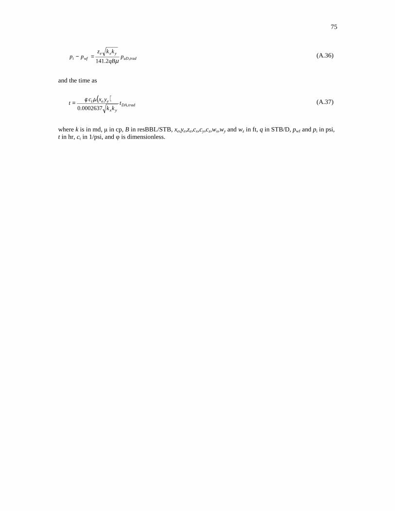
75

traduDyxe

wfi pqB

kkzpp ,2.141 µ

=− (A.36)

and the time as

( )tradDA

yx

eet tkk

yxct ,

0002637.0

µφ= (A.37)

where k is in md, µ in cp, B in resBBL/STB, xe,ye,ze,cx,cy,cz,wx,wy and wz in ft, q in STB/D, pwf and pi in psi, t in hr, ct in 1/psi, and φ is dimensionless.

76

APPENDIX B

DIMENSIONLESS PRODUCTIVITY INDEX FROM PRESSURE DATA

In production engineering, the productivity index is defined as the ability of the reservoir to produce hydrocarbon

per unit pressure drop in the reservoir (volume/time/pressure).

)( wfavg pp

qJ

−= (B.1)

In which

q = Flow Rate

pavg = Average Reservoir Pressure

pwf = Well Flowing Pressure

Introducing the Dimensionless parameters as the followings the expression for the Dimensionless productivity

index would be obtained.

)(2

, ppqB

khp itradD −=

µπ

(B.2)

Jkh

BJD π

µ2

= . (B.3)

With:

Pi = Initial Reservoir Pressure

k = Reservoir Permeability

h = Reservoir Thickness

B = Formation Volume Factor

µ = Fluid Viscosity

Combining Eqs. B.1 through B.3 we have:

tradavgDtradD

D ppJ

,,,

1

−= (B.4)

Assuming a constant compressibility during depletion we can write:

V

p

Vct ∂

∂−= 1 (B.5)

AhV φ= (B.6)

77

cteAhcV

p

t

==∂∂

φ1

(B.7)

tt

p

tiavg Ahc

qBt

Ahc

BN

Ahc

Vppp

φφφ==∆=−=∆ (Constant flow rate production) (B.8)

Using the definition for dimensionless pressure and applying it on Eq. B.8 we have:

DAt

tradavgD tAc

ktp π

φµπ 22,, == (B.9)

Where;

Ac

ktt

tDA φµ

= (Dimensionless time defined based on drainage area) (B.10)

Combination of Eqs. B.9 and B.4 would lead us to an expression correlating the dimensionless productivity index

as a function of dimensionless pressure and dimensionless time (Eq. B.11)

DAtradDD tp

Jπ2

1

, −= (B.11)

Or based on the new dimensionless variables defined in Appendix A

( )DuDtradD tpc

J−

=π2

1 (B.12)

The dimensionless productivity index is time dependent in the transient flow regime and constant in the

pseudo-steady state.

In field units, the productivity index is expressed as

tradDyxe

JB

kkzPI ,2.141 µ

= (B.13)

Where k is in md, µ in cp, B in resBBL/STB, q in STB/D, pwf and pi in psi, t in hr, ct in 1/psi, φ is dimensionless and PI is in (STB/D/psi).

78

APPENDIX C

DETAILED RESULTS OF CALCULATION FOR MAXIMUM


PROPPANT NUMBER (NProp) = 0.001

In this appendix we provide details of calculation results and complete set of graphs describing the

production behavior of example problem in chapter IV when 1,000 lb of proppant (NProp =0.001) is used for

stimulation. All the fracture sizes have been described in ft.

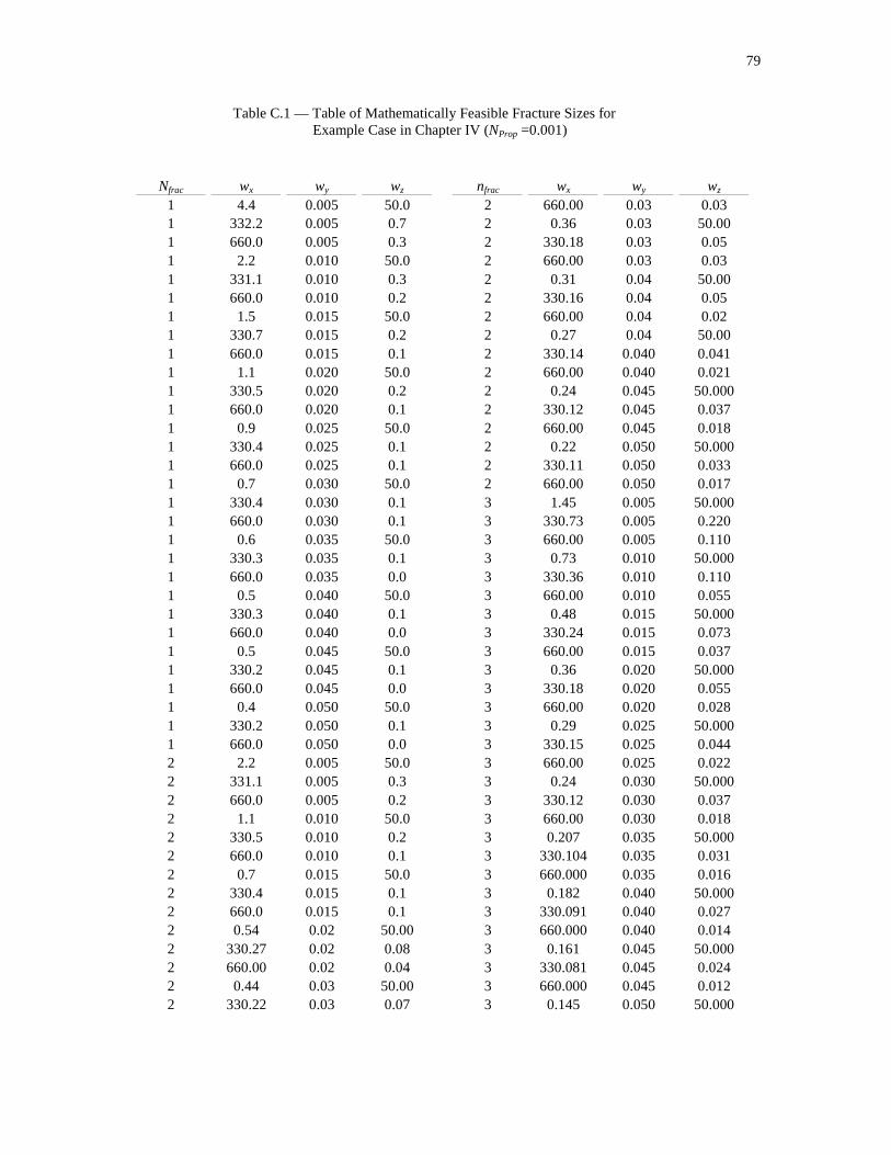
79

Table C.1 — Table of Mathematically Feasible Fracture Sizes for Example Case in Chapter IV (NProp =0.001)

Nfrac wx wy wz nfrac wx wy wz 1 4.4 0.005 50.0 2 660.00 0.03 0.03 1 332.2 0.005 0.7 2 0.36 0.03 50.00 1 660.0 0.005 0.3 2 330.18 0.03 0.05 1 2.2 0.010 50.0 2 660.00 0.03 0.03 1 331.1 0.010 0.3 2 0.31 0.04 50.00 1 660.0 0.010 0.2 2 330.16 0.04 0.05 1 1.5 0.015 50.0 2 660.00 0.04 0.02 1 330.7 0.015 0.2 2 0.27 0.04 50.00 1 660.0 0.015 0.1 2 330.14 0.040 0.041 1 1.1 0.020 50.0 2 660.00 0.040 0.021 1 330.5 0.020 0.2 2 0.24 0.045 50.000 1 660.0 0.020 0.1 2 330.12 0.045 0.037 1 0.9 0.025 50.0 2 660.00 0.045 0.018 1 330.4 0.025 0.1 2 0.22 0.050 50.000 1 660.0 0.025 0.1 2 330.11 0.050 0.033 1 0.7 0.030 50.0 2 660.00 0.050 0.017 1 330.4 0.030 0.1 3 1.45 0.005 50.000 1 660.0 0.030 0.1 3 330.73 0.005 0.220 1 0.6 0.035 50.0 3 660.00 0.005 0.110 1 330.3 0.035 0.1 3 0.73 0.010 50.000 1 660.0 0.035 0.0 3 330.36 0.010 0.110 1 0.5 0.040 50.0 3 660.00 0.010 0.055 1 330.3 0.040 0.1 3 0.48 0.015 50.000 1 660.0 0.040 0.0 3 330.24 0.015 0.073 1 0.5 0.045 50.0 3 660.00 0.015 0.037 1 330.2 0.045 0.1 3 0.36 0.020 50.000 1 660.0 0.045 0.0 3 330.18 0.020 0.055 1 0.4 0.050 50.0 3 660.00 0.020 0.028 1 330.2 0.050 0.1 3 0.29 0.025 50.000 1 660.0 0.050 0.0 3 330.15 0.025 0.044 2 2.2 0.005 50.0 3 660.00 0.025 0.022 2 331.1 0.005 0.3 3 0.24 0.030 50.000 2 660.0 0.005 0.2 3 330.12 0.030 0.037 2 1.1 0.010 50.0 3 660.00 0.030 0.018 2 330.5 0.010 0.2 3 0.207 0.035 50.000 2 660.0 0.010 0.1 3 330.104 0.035 0.031 2 0.7 0.015 50.0 3 660.000 0.035 0.016 2 330.4 0.015 0.1 3 0.182 0.040 50.000 2 660.0 0.015 0.1 3 330.091 0.040 0.027 2 0.54 0.02 50.00 3 660.000 0.040 0.014 2 330.27 0.02 0.08 3 0.161 0.045 50.000 2 660.00 0.02 0.04 3 330.081 0.045 0.024 2 0.44 0.03 50.00 3 660.000 0.045 0.012 2 330.22 0.03 0.07 3 0.145 0.050 50.000

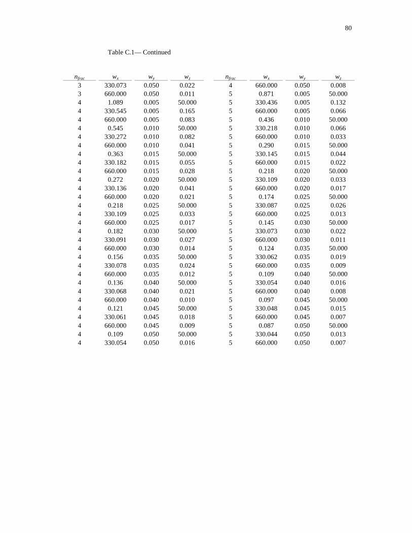
80

Table C.1— Continued

nfrac wx wy wz nfrac wx wy wz 3 330.073 0.050 0.022 4 660.000 0.050 0.008 3 660.000 0.050 0.011 5 0.871 0.005 50.000 4 1.089 0.005 50.000 5 330.436 0.005 0.132 4 330.545 0.005 0.165 5 660.000 0.005 0.066 4 660.000 0.005 0.083 5 0.436 0.010 50.000 4 0.545 0.010 50.000 5 330.218 0.010 0.066 4 330.272 0.010 0.082 5 660.000 0.010 0.033 4 660.000 0.010 0.041 5 0.290 0.015 50.000 4 0.363 0.015 50.000 5 330.145 0.015 0.044 4 330.182 0.015 0.055 5 660.000 0.015 0.022 4 660.000 0.015 0.028 5 0.218 0.020 50.000 4 0.272 0.020 50.000 5 330.109 0.020 0.033 4 330.136 0.020 0.041 5 660.000 0.020 0.017 4 660.000 0.020 0.021 5 0.174 0.025 50.000 4 0.218 0.025 50.000 5 330.087 0.025 0.026 4 330.109 0.025 0.033 5 660.000 0.025 0.013 4 660.000 0.025 0.017 5 0.145 0.030 50.000 4 0.182 0.030 50.000 5 330.073 0.030 0.022 4 330.091 0.030 0.027 5 660.000 0.030 0.011 4 660.000 0.030 0.014 5 0.124 0.035 50.000 4 0.156 0.035 50.000 5 330.062 0.035 0.019 4 330.078 0.035 0.024 5 660.000 0.035 0.009 4 660.000 0.035 0.012 5 0.109 0.040 50.000 4 0.136 0.040 50.000 5 330.054 0.040 0.016 4 330.068 0.040 0.021 5 660.000 0.040 0.008 4 660.000 0.040 0.010 5 0.097 0.045 50.000 4 0.121 0.045 50.000 5 330.048 0.045 0.015 4 330.061 0.045 0.018 5 660.000 0.045 0.007 4 660.000 0.045 0.009 5 0.087 0.050 50.000 4 0.109 0.050 50.000 5 330.044 0.050 0.013 4 330.054 0.050 0.016 5 660.000 0.050 0.007

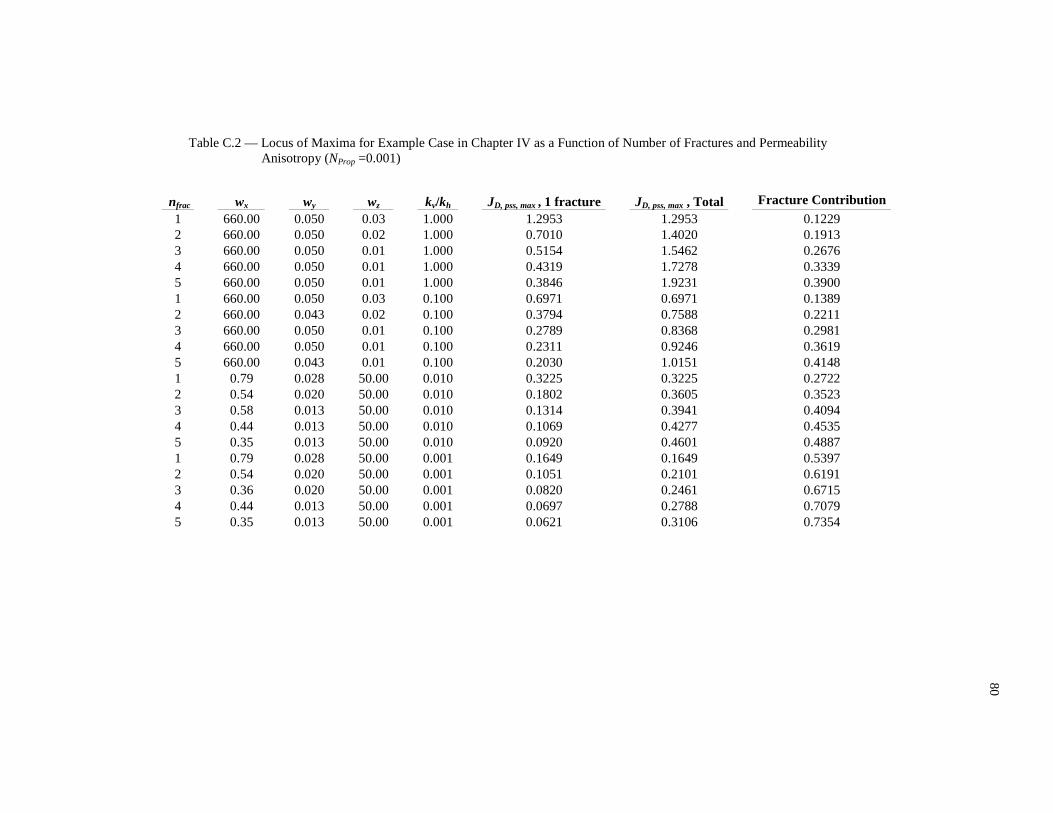
80

Table C.2 — Locus of Maxima for Example Case in Chapter IV as a Function of Number of Fractures and Permeability

Anisotropy (NProp =0.001)

nfrac wx wy wz kv/kh JD, pss, max , 1 fracture JD, pss, max , Total Fracture Contribution 1 660.00 0.050 0.03 1.000 1.2953 1.2953 0.1229 2 660.00 0.050 0.02 1.000 0.7010 1.4020 0.1913 3 660.00 0.050 0.01 1.000 0.5154 1.5462 0.2676 4 660.00 0.050 0.01 1.000 0.4319 1.7278 0.3339 5 660.00 0.050 0.01 1.000 0.3846 1.9231 0.3900 1 660.00 0.050 0.03 0.100 0.6971 0.6971 0.1389 2 660.00 0.043 0.02 0.100 0.3794 0.7588 0.2211 3 660.00 0.050 0.01 0.100 0.2789 0.8368 0.2981 4 660.00 0.050 0.01 0.100 0.2311 0.9246 0.3619 5 660.00 0.043 0.01 0.100 0.2030 1.0151 0.4148 1 0.79 0.028 50.00 0.010 0.3225 0.3225 0.2722 2 0.54 0.020 50.00 0.010 0.1802 0.3605 0.3523 3 0.58 0.013 50.00 0.010 0.1314 0.3941 0.4094 4 0.44 0.013 50.00 0.010 0.1069 0.4277 0.4535 5 0.35 0.013 50.00 0.010 0.0920 0.4601 0.4887 1 0.79 0.028 50.00 0.001 0.1649 0.1649 0.5397 2 0.54 0.020 50.00 0.001 0.1051 0.2101 0.6191 3 0.36 0.020 50.00 0.001 0.0820 0.2461 0.6715 4 0.44 0.013 50.00 0.001 0.0697 0.2788 0.7079 5 0.35 0.013 50.00 0.001 0.0621 0.3106 0.7354

81

10 10

9 9

8 8

7 7

6 6

5 5

4 4

3 3

2 2

1 1

0 0

Dim

ensi

onle

ss P

rodu

ctiv

ity In

dex

(J D

)

10-6

10-6

10-5

10-5

10-4

10-4

10-3

10-3

10-2

10-2

10-1

10-1

100

100


ye/ nfrac

xe

ze

n frac = 1

n frac = 5

Legend :



Dimensionless Productivity Index as a Function of Dimensionless Time and Number of Fractures ( NProp = 0.001, kx= ky= kz= 1 md)


n frac = 1

3

2

4

n frac = 5

3


Figure C.1 — Dimensionless Productivity Index as a Function of Dimensionless Time and Number of Fractures for Example Case (NProp = 0.001, kx = ky = kz = 1 md)

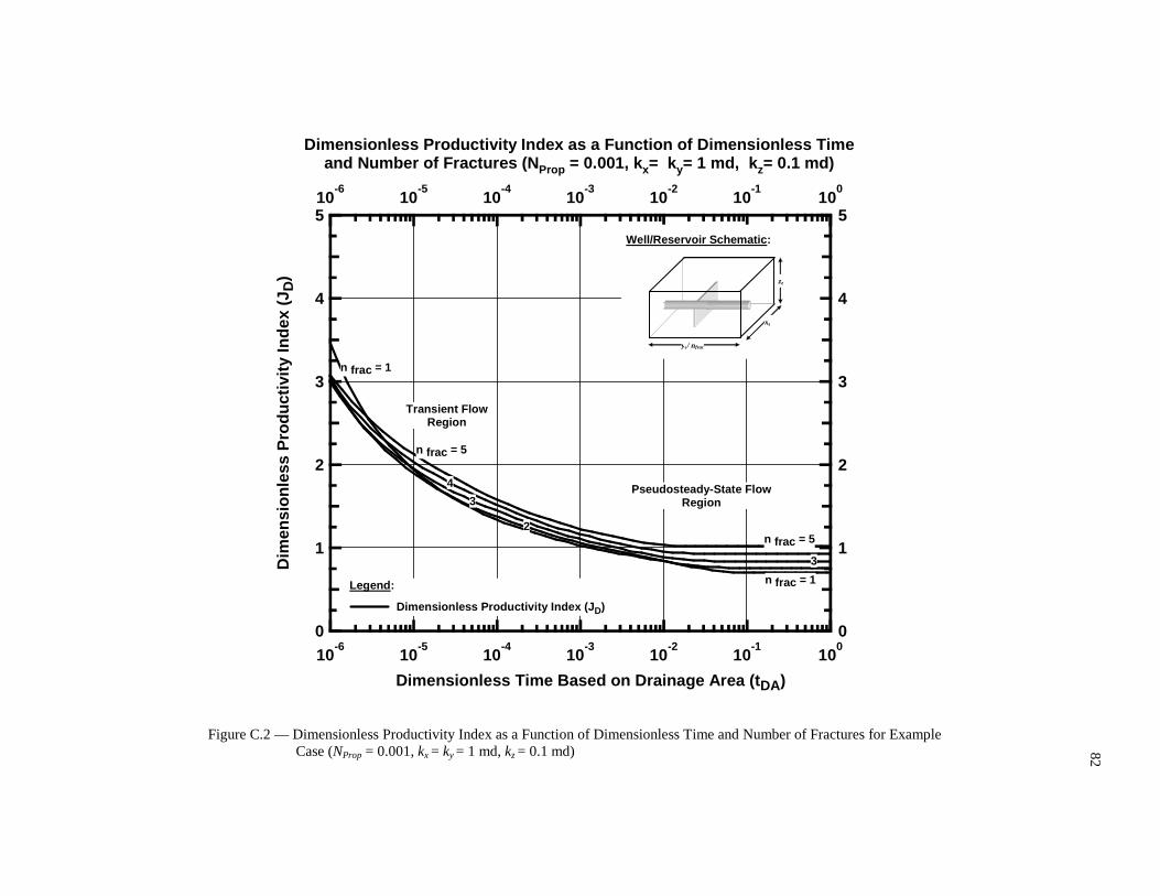
82

5 5

4 4

3 3

2 2

1 1

0 0

Dim

ensi

onle

ss P

rodu

ctiv

ity In

dex

(J D

)

10-6

10-6

10-5

10-5

10-4

10-4

10-3

10-3

10-2

10-2

10-1

10-1

100

100


ye/ nfrac

xe

ze

n frac = 1

n frac = 5

Legend :



Dimensionless Productivity Index as a Function of Dimensionless Time and Number of Fractures ( NProp = 0.001, kx= ky= 1 md, kz= 0.1 md)


n frac = 1

3

2

4

n frac = 5

3


Figure C.2 — Dimensionless Productivity Index as a Function of Dimensionless Time and Number of Fractures for Example Case (NProp = 0.001, kx = ky = 1 md, kz = 0.1 md)

83

5 5

4 4

3 3

2 2

1 1

0 0

Dim

ensi

onle

ss P

rodu

ctiv

ity In

dex

(J D

)

10-6

10-6

10-5

10-5

10-4

10-4

10-3

10-3

10-2

10-2

10-1

10-1

100

100


ye/ nfrac

xe

ze

n frac = 1

n frac = 5

Legend :





n frac = 1

3

2

4

n frac = 53



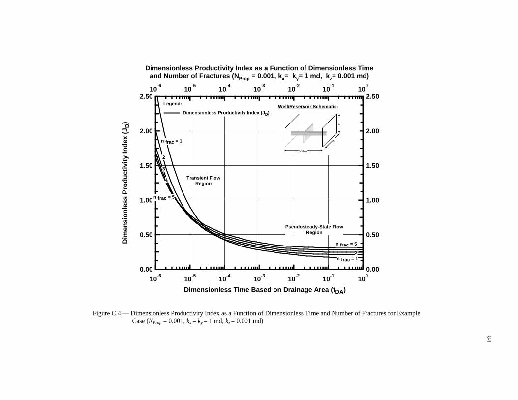
84

2.50 2.50

2.00 2.00

1.50 1.50

1.00 1.00

0.50 0.50

0.00 0.00

Dim

ensi

onle

ss P

rodu

ctiv

ity In

dex

(J D

)

10-6

10-6

10-5

10-5

10-4

10-4

10-3

10-3

10-2

10-2

10-1

10-1

100

100


ye/ nfrac

xe

ze

n frac = 1

n frac = 5

Legend :





n frac = 1

3

2

4

n frac = 5

3



85

1.0 1.0

0.9 0.9

0.8 0.8

0.7 0.7

0.6 0.6

0.5 0.5

0.4 0.4

0.3 0.3

0.2 0.2

0.1 0.1

0.0 0.0

Fra

ctur

e C

ontr

ibut

ion

to F

low

(F

ract

ion)

10-10

10-10

10-9

10-9

10-8

10-8

10-7

10-7

10-6

10-6

10-5

10-5

10-4

10-4

10-3

10-3

10-2

10-2

10-1

10-1

100

100


ye/ nfrac

xe

ze

Legend :



n frac = 1

3

2

4

n frac = 5


Figure C.5 — Fracture Contribution to Flow as a Function of Dimensionless Time and Number of Fractures for Example Case (NProp = 0.001, kx = ky = kz = 1 md)

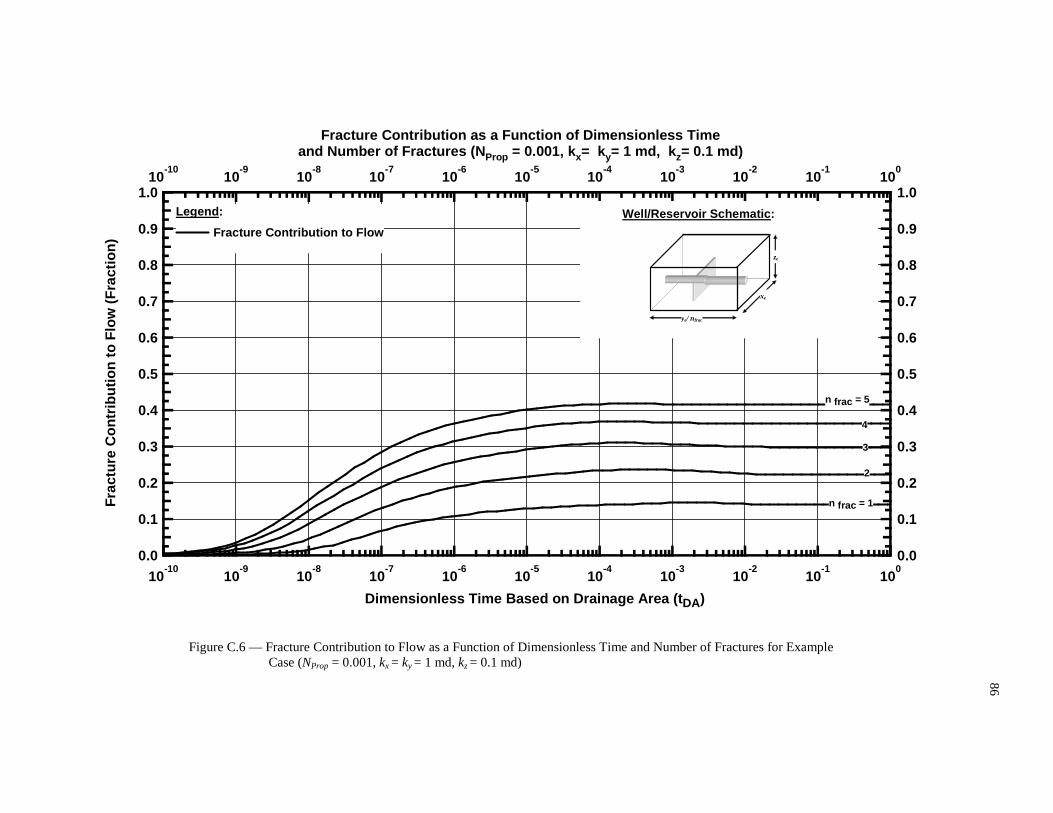
86

1.0 1.0

0.9 0.9

0.8 0.8

0.7 0.7

0.6 0.6

0.5 0.5

0.4 0.4

0.3 0.3

0.2 0.2

0.1 0.1

0.0 0.0

Fra

ctur

e C

ontr

ibut

ion

to F

low

(F

ract

ion)

10-10

10-10

10-9

10-9

10-8

10-8

10-7

10-7

10-6

10-6

10-5

10-5

10-4

10-4

10-3

10-3

10-2

10-2

10-1

10-1

100

100


ye/ nfrac

xe

ze

Legend :



n frac = 1

3

2

4

n frac = 5


Figure C.6 — Fracture Contribution to Flow as a Function of Dimensionless Time and Number of Fractures for Example Case (NProp = 0.001, kx = ky = 1 md, kz = 0.1 md)

87

1.0 1.0

0.9 0.9

0.8 0.8

0.7 0.7

0.6 0.6

0.5 0.5

0.4 0.4

0.3 0.3

0.2 0.2

0.1 0.1

0.0 0.0

Fra

ctur

e C

ontr

ibut

ion

to F

low

(F

ract

ion)

10-10

10-10

10-9

10-9

10-8

10-8

10-7

10-7

10-6

10-6

10-5

10-5

10-4

10-4

10-3

10-3

10-2

10-2

10-1

10-1

100

100


ye/ nfrac

xe

ze

Legend :



n frac = 1

3

2

4n frac = 5



88

1.0 1.0

0.9 0.9

0.8 0.8

0.7 0.7

0.6 0.6

0.5 0.5

0.4 0.4

0.3 0.3

0.2 0.2

0.1 0.1

0.0 0.0

Fra

ctur

e C

ontr

ibut

ion

to F

low

(F

ract

ion)

10-10

10-10

10-9

10-9

10-8

10-8

10-7

10-7

10-6

10-6

10-5

10-5

10-4

10-4

10-3

10-3

10-2

10-2

10-1

10-1

100

100


ye/ nfrac

xe

ze

Legend :



n frac = 1

3

2

4

n frac = 5



89

APPENDIX D







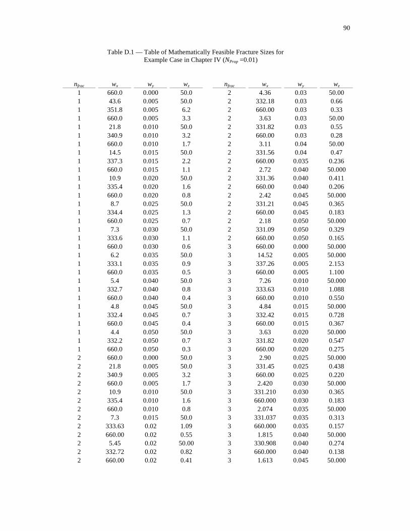
90

Table D.1 — Table of Mathematically Feasible Fracture Sizes for Example Case in Chapter IV (NProp =0.01)

nfrac wx wy wz nfrac wx wy wz 1 660.0 0.000 50.0 2 4.36 0.03 50.00 1 43.6 0.005 50.0 2 332.18 0.03 0.66 1 351.8 0.005 6.2 2 660.00 0.03 0.33 1 660.0 0.005 3.3 2 3.63 0.03 50.00 1 21.8 0.010 50.0 2 331.82 0.03 0.55 1 340.9 0.010 3.2 2 660.00 0.03 0.28 1 660.0 0.010 1.7 2 3.11 0.04 50.00 1 14.5 0.015 50.0 2 331.56 0.04 0.47 1 337.3 0.015 2.2 2 660.00 0.035 0.236 1 660.0 0.015 1.1 2 2.72 0.040 50.000 1 10.9 0.020 50.0 2 331.36 0.040 0.411 1 335.4 0.020 1.6 2 660.00 0.040 0.206 1 660.0 0.020 0.8 2 2.42 0.045 50.000 1 8.7 0.025 50.0 2 331.21 0.045 0.365 1 334.4 0.025 1.3 2 660.00 0.045 0.183 1 660.0 0.025 0.7 2 2.18 0.050 50.000 1 7.3 0.030 50.0 2 331.09 0.050 0.329 1 333.6 0.030 1.1 2 660.00 0.050 0.165 1 660.0 0.030 0.6 3 660.00 0.000 50.000 1 6.2 0.035 50.0 3 14.52 0.005 50.000 1 333.1 0.035 0.9 3 337.26 0.005 2.153 1 660.0 0.035 0.5 3 660.00 0.005 1.100 1 5.4 0.040 50.0 3 7.26 0.010 50.000 1 332.7 0.040 0.8 3 333.63 0.010 1.088 1 660.0 0.040 0.4 3 660.00 0.010 0.550 1 4.8 0.045 50.0 3 4.84 0.015 50.000 1 332.4 0.045 0.7 3 332.42 0.015 0.728 1 660.0 0.045 0.4 3 660.00 0.015 0.367 1 4.4 0.050 50.0 3 3.63 0.020 50.000 1 332.2 0.050 0.7 3 331.82 0.020 0.547 1 660.0 0.050 0.3 3 660.00 0.020 0.275 2 660.0 0.000 50.0 3 2.90 0.025 50.000 2 21.8 0.005 50.0 3 331.45 0.025 0.438 2 340.9 0.005 3.2 3 660.00 0.025 0.220 2 660.0 0.005 1.7 3 2.420 0.030 50.000 2 10.9 0.010 50.0 3 331.210 0.030 0.365 2 335.4 0.010 1.6 3 660.000 0.030 0.183 2 660.0 0.010 0.8 3 2.074 0.035 50.000 2 7.3 0.015 50.0 3 331.037 0.035 0.313 2 333.63 0.02 1.09 3 660.000 0.035 0.157 2 660.00 0.02 0.55 3 1.815 0.040 50.000 2 5.45 0.02 50.00 3 330.908 0.040 0.274 2 332.72 0.02 0.82 3 660.000 0.040 0.138 2 660.00 0.02 0.41 3 1.613 0.045 50.000

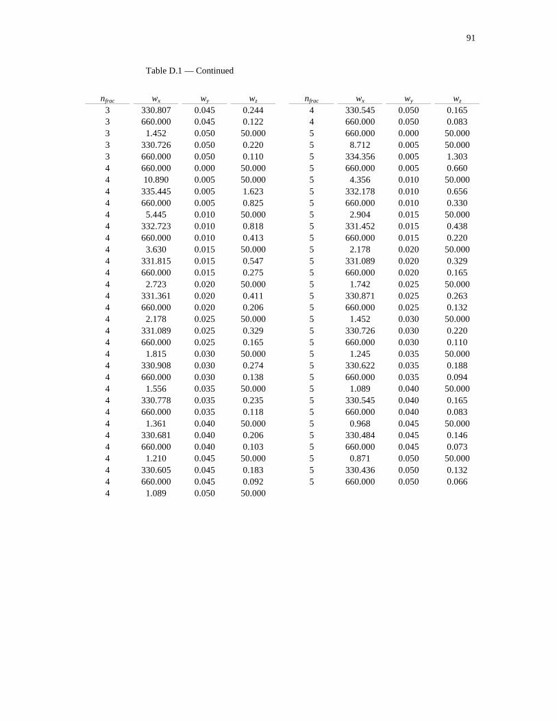
91

Table D.1 — Continued

nfrac wx wy wz nfrac wx wy wz 3 330.807 0.045 0.244 4 330.545 0.050 0.165 3 660.000 0.045 0.122 4 660.000 0.050 0.083 3 1.452 0.050 50.000 5 660.000 0.000 50.000 3 330.726 0.050 0.220 5 8.712 0.005 50.000 3 660.000 0.050 0.110 5 334.356 0.005 1.303 4 660.000 0.000 50.000 5 660.000 0.005 0.660 4 10.890 0.005 50.000 5 4.356 0.010 50.000 4 335.445 0.005 1.623 5 332.178 0.010 0.656 4 660.000 0.005 0.825 5 660.000 0.010 0.330 4 5.445 0.010 50.000 5 2.904 0.015 50.000 4 332.723 0.010 0.818 5 331.452 0.015 0.438 4 660.000 0.010 0.413 5 660.000 0.015 0.220 4 3.630 0.015 50.000 5 2.178 0.020 50.000 4 331.815 0.015 0.547 5 331.089 0.020 0.329 4 660.000 0.015 0.275 5 660.000 0.020 0.165 4 2.723 0.020 50.000 5 1.742 0.025 50.000 4 331.361 0.020 0.411 5 330.871 0.025 0.263 4 660.000 0.020 0.206 5 660.000 0.025 0.132 4 2.178 0.025 50.000 5 1.452 0.030 50.000 4 331.089 0.025 0.329 5 330.726 0.030 0.220 4 660.000 0.025 0.165 5 660.000 0.030 0.110 4 1.815 0.030 50.000 5 1.245 0.035 50.000 4 330.908 0.030 0.274 5 330.622 0.035 0.188 4 660.000 0.030 0.138 5 660.000 0.035 0.094 4 1.556 0.035 50.000 5 1.089 0.040 50.000 4 330.778 0.035 0.235 5 330.545 0.040 0.165 4 660.000 0.035 0.118 5 660.000 0.040 0.083 4 1.361 0.040 50.000 5 0.968 0.045 50.000 4 330.681 0.040 0.206 5 330.484 0.045 0.146 4 660.000 0.040 0.103 5 660.000 0.045 0.073 4 1.210 0.045 50.000 5 0.871 0.050 50.000 4 330.605 0.045 0.183 5 330.436 0.050 0.132 4 660.000 0.045 0.092 5 660.000 0.050 0.066 4 1.089 0.050 50.000

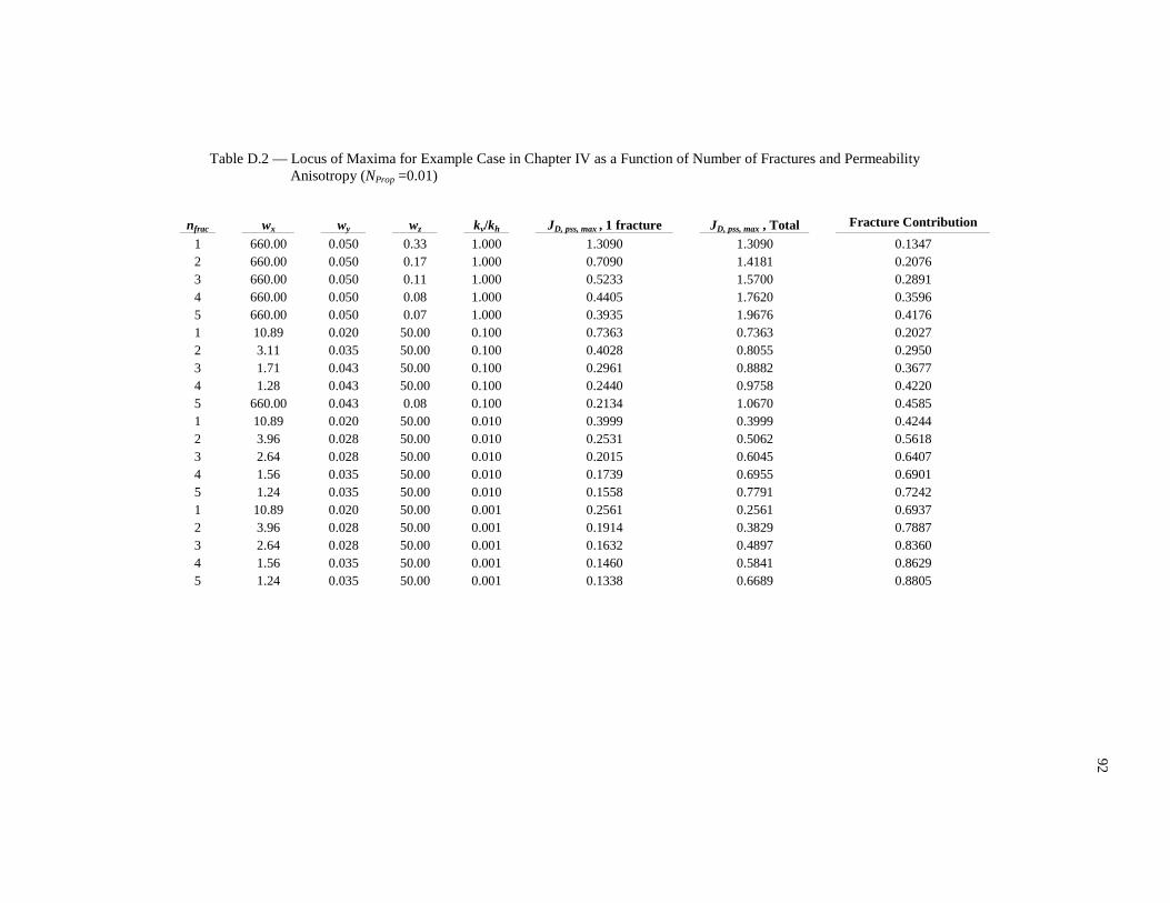
92

Table D.2 — Locus of Maxima for Example Case in Chapter IV as a Function of Number of Fractures and Permeability

Anisotropy (NProp =0.01)


1 660.00 0.050 0.33 1.000 1.3090 1.3090 0.1347 2 660.00 0.050 0.17 1.000 0.7090 1.4181 0.2076 3 660.00 0.050 0.11 1.000 0.5233 1.5700 0.2891 4 660.00 0.050 0.08 1.000 0.4405 1.7620 0.3596 5 660.00 0.050 0.07 1.000 0.3935 1.9676 0.4176 1 10.89 0.020 50.00 0.100 0.7363 0.7363 0.2027 2 3.11 0.035 50.00 0.100 0.4028 0.8055 0.2950 3 1.71 0.043 50.00 0.100 0.2961 0.8882 0.3677 4 1.28 0.043 50.00 0.100 0.2440 0.9758 0.4220 5 660.00 0.043 0.08 0.100 0.2134 1.0670 0.4585 1 10.89 0.020 50.00 0.010 0.3999 0.3999 0.4244 2 3.96 0.028 50.00 0.010 0.2531 0.5062 0.5618 3 2.64 0.028 50.00 0.010 0.2015 0.6045 0.6407 4 1.56 0.035 50.00 0.010 0.1739 0.6955 0.6901 5 1.24 0.035 50.00 0.010 0.1558 0.7791 0.7242 1 10.89 0.020 50.00 0.001 0.2561 0.2561 0.6937 2 3.96 0.028 50.00 0.001 0.1914 0.3829 0.7887 3 2.64 0.028 50.00 0.001 0.1632 0.4897 0.8360 4 1.56 0.035 50.00 0.001 0.1460 0.5841 0.8629 5 1.24 0.035 50.00 0.001 0.1338 0.6689 0.8805

93

10 10

9 9

8 8

7 7

6 6

5 5

4 4

3 3

2 2

1 1

0 0

Dim

ensi

onle

ss P

rodu

ctiv

ity In

dex

(J D

)

10-6

10-6

10-5

10-5

10-4

10-4

10-3

10-3

10-2

10-2

10-1

10-1

100

100


ye/ nfrac

xe

ze

n frac = 1

n frac = 5

Legend :





n frac = 1

3

2

4

n frac = 5

3


Figure D.1 — Dimensionless Productivity Index as a Function of Dimensionless Time and Number of Fractures for Example Case (NProp = 0.01, kx = ky = kz = 1 md)

94

5 5

4 4

3 3

2 2

1 1

0 0

Dim

ensi

onle

ss P

rodu

ctiv

ity In

dex

(J D

)

10-6

10-6

10-5

10-5

10-4

10-4

10-3

10-3

10-2

10-2

10-1

10-1

100

100


ye/ nfrac

xe

ze n frac = 1

n frac = 5

Legend :



Dimensionless Productivity Index as a Function of Dimensionless Time and Number of Fractures ( NProp = 0.01, kx= ky= kz= 0.1 md)


n frac = 1

3

2

4

n frac = 5

3


Figure D.2 — Dimensionless Productivity Index as a Function of Dimensionless Time and Number of Fractures for Example Case (NProp = 0.01, kx = ky = 1 md, kz = 0.1 md)

95

5 5

4 4

3 3

2 2

1 1

0 0

Dim

ensi

onle

ss P

rodu

ctiv

ity In

dex

(J D

)

10-6

10-6

10-5

10-5

10-4

10-4

10-3

10-3

10-2

10-2

10-1

10-1

100

100


ye/ nfrac

xe

ze

n frac = 1

n frac = 5

Legend :





n frac = 1

3

2

4

n frac = 5

3



96

4 4

3 3

2 2

1 1

0 0

Dim

ensi

onle

ss P

rodu

ctiv

ity In

dex

(J D

)

10-6

10-6

10-5

10-5

10-4

10-4

10-3

10-3

10-2

10-2

10-1

10-1

100

100


ye/ nfrac

xe

ze

n frac = 1

n frac = 5

Legend :





n frac = 1

3

2

4

n frac = 5

3



97

1.0 1.0

0.9 0.9

0.8 0.8

0.7 0.7

0.6 0.6

0.5 0.5

0.4 0.4

0.3 0.3

0.2 0.2

0.1 0.1

0.0 0.0

Fra

ctur

e C

ontr

ibut

ion

to F

low

(F

ract

ion)

10-10

10-10

10-9

10-9

10-8

10-8

10-7

10-7

10-6

10-6

10-5

10-5

10-4

10-4

10-3

10-3

10-2

10-2

10-1

10-1

100

100


ye/ nfrac

xe

ze

Legend :



n frac = 1

3

2

4

n frac = 5


Figure D.5 — Fracture Contribution to Flow as a Function of Dimensionless Time and Number of Fractures for Example Case (NProp = 0.01, kx = ky = kz = 1 md)

98

1.0 1.0

0.9 0.9

0.8 0.8

0.7 0.7

0.6 0.6

0.5 0.5

0.4 0.4

0.3 0.3

0.2 0.2

0.1 0.1

0.0 0.0

Fra

ctur

e C

ontr

ibut

ion

to F

low

(F

ract

ion)

10-10

10-10

10-9

10-9

10-8

10-8

10-7

10-7

10-6

10-6

10-5

10-5

10-4

10-4

10-3

10-3

10-2

10-2

10-1

10-1

100

100


ye/ nfrac

xe

ze

Legend :



n frac = 1

3

2

4

n frac = 5


Figure D.6 — Fracture Contribution to Flow as a Function of Dimensionless Time and Number of Fractures for Example Case (NProp = 0.01, kx = ky = 1 md, kz = 0.1 md)

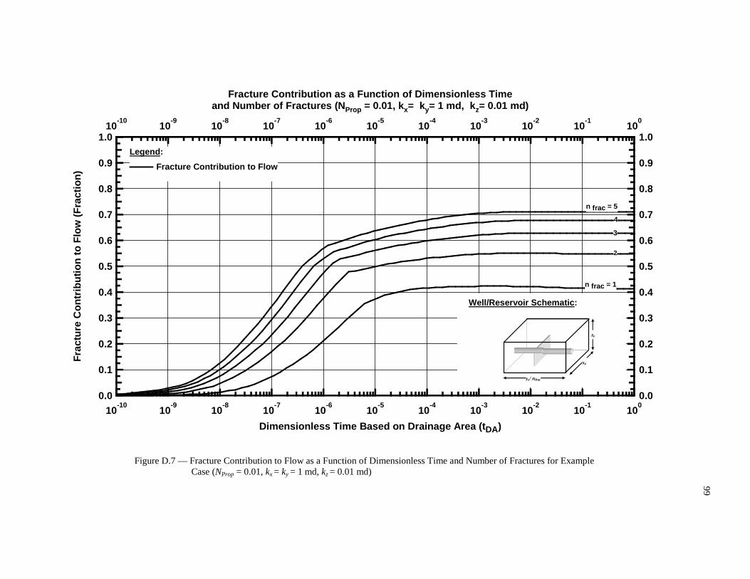
99

1.0 1.0

0.9 0.9

0.8 0.8

0.7 0.7

0.6 0.6

0.5 0.5

0.4 0.4

0.3 0.3

0.2 0.2

0.1 0.1

0.0 0.0

Fra

ctur

e C

ontr

ibut

ion

to F

low

(F

ract

ion)

10-10

10-10

10-9

10-9

10-8

10-8

10-7

10-7

10-6

10-6

10-5

10-5

10-4

10-4

10-3

10-3

10-2

10-2

10-1

10-1

100

100


ye/ nfrac

xe

ze

Legend :



n frac = 1

3

2

4

n frac = 5



10

0

1.0 1.0

0.9 0.9

0.8 0.8

0.7 0.7

0.6 0.6

0.5 0.5

0.4 0.4

0.3 0.3

0.2 0.2

0.1 0.1

0.0 0.0

Fra

ctur

e C

ontr

ibut

ion

to F

low

(F

ract

ion)

10-10

10-10

10-9

10-9

10-8

10-8

10-7

10-7

10-6

10-6

10-5

10-5

10-4

10-4

10-3

10-3

10-2

10-2

10-1

10-1

100

100


ye/ nfrac

xe

ze

Legend :



n frac = 1

3

2

4

n frac = 5



101

APPENDIX E







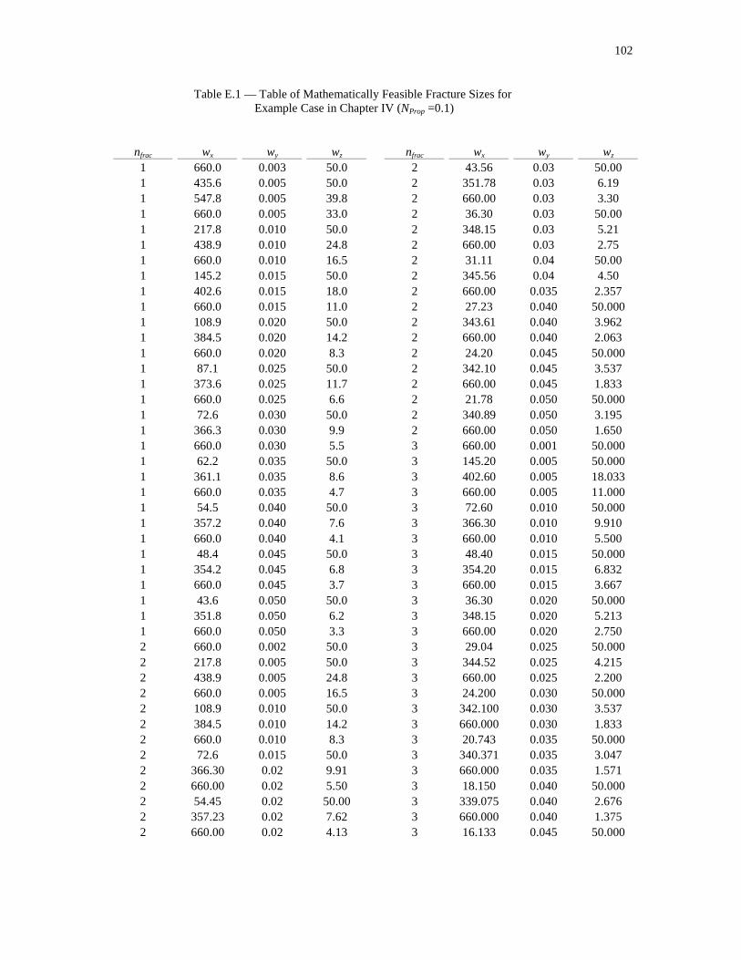
102

Table E.1 — Table of Mathematically Feasible Fracture Sizes for Example Case in Chapter IV (NProp =0.1)

nfrac wx wy wz nfrac wx wy wz 1 660.0 0.003 50.0 2 43.56 0.03 50.00 1 435.6 0.005 50.0 2 351.78 0.03 6.19 1 547.8 0.005 39.8 2 660.00 0.03 3.30 1 660.0 0.005 33.0 2 36.30 0.03 50.00 1 217.8 0.010 50.0 2 348.15 0.03 5.21 1 438.9 0.010 24.8 2 660.00 0.03 2.75 1 660.0 0.010 16.5 2 31.11 0.04 50.00 1 145.2 0.015 50.0 2 345.56 0.04 4.50 1 402.6 0.015 18.0 2 660.00 0.035 2.357 1 660.0 0.015 11.0 2 27.23 0.040 50.000 1 108.9 0.020 50.0 2 343.61 0.040 3.962 1 384.5 0.020 14.2 2 660.00 0.040 2.063 1 660.0 0.020 8.3 2 24.20 0.045 50.000 1 87.1 0.025 50.0 2 342.10 0.045 3.537 1 373.6 0.025 11.7 2 660.00 0.045 1.833 1 660.0 0.025 6.6 2 21.78 0.050 50.000 1 72.6 0.030 50.0 2 340.89 0.050 3.195 1 366.3 0.030 9.9 2 660.00 0.050 1.650 1 660.0 0.030 5.5 3 660.00 0.001 50.000 1 62.2 0.035 50.0 3 145.20 0.005 50.000 1 361.1 0.035 8.6 3 402.60 0.005 18.033 1 660.0 0.035 4.7 3 660.00 0.005 11.000 1 54.5 0.040 50.0 3 72.60 0.010 50.000 1 357.2 0.040 7.6 3 366.30 0.010 9.910 1 660.0 0.040 4.1 3 660.00 0.010 5.500 1 48.4 0.045 50.0 3 48.40 0.015 50.000 1 354.2 0.045 6.8 3 354.20 0.015 6.832 1 660.0 0.045 3.7 3 660.00 0.015 3.667 1 43.6 0.050 50.0 3 36.30 0.020 50.000 1 351.8 0.050 6.2 3 348.15 0.020 5.213 1 660.0 0.050 3.3 3 660.00 0.020 2.750 2 660.0 0.002 50.0 3 29.04 0.025 50.000 2 217.8 0.005 50.0 3 344.52 0.025 4.215 2 438.9 0.005 24.8 3 660.00 0.025 2.200 2 660.0 0.005 16.5 3 24.200 0.030 50.000 2 108.9 0.010 50.0 3 342.100 0.030 3.537 2 384.5 0.010 14.2 3 660.000 0.030 1.833 2 660.0 0.010 8.3 3 20.743 0.035 50.000 2 72.6 0.015 50.0 3 340.371 0.035 3.047 2 366.30 0.02 9.91 3 660.000 0.035 1.571 2 660.00 0.02 5.50 3 18.150 0.040 50.000 2 54.45 0.02 50.00 3 339.075 0.040 2.676 2 357.23 0.02 7.62 3 660.000 0.040 1.375 2 660.00 0.02 4.13 3 16.133 0.045 50.000

103

Table E.1 — Continued

nfrac wx wy wz nfrac wx wy wz 3 338.067 0.045 2.386 4 335.445 0.050 1.623 3 660.000 0.045 1.222 4 660.000 0.050 0.825 3 14.520 0.050 50.000 5 660.000 0.001 50.000 3 337.260 0.050 2.153 5 87.120 0.005 50.000 3 660.000 0.050 1.100 5 373.560 0.005 11.661 4 660.000 0.001 50.000 5 660.000 0.005 6.600 4 108.900 0.005 50.000 5 43.560 0.010 50.000 4 384.450 0.005 14.163 5 351.780 0.010 6.191 4 660.000 0.005 8.250 5 660.000 0.010 3.300 4 54.450 0.010 50.000 5 29.040 0.015 50.000 4 357.225 0.010 7.621 5 344.520 0.015 4.215 4 660.000 0.010 4.125 5 660.000 0.015 2.200 4 36.300 0.015 50.000 5 21.780 0.020 50.000 4 348.150 0.015 5.213 5 340.890 0.020 3.195 4 660.000 0.015 2.750 5 660.000 0.020 1.650 4 27.225 0.020 50.000 5 17.424 0.025 50.000 4 343.613 0.020 3.962 5 338.712 0.025 2.572 4 660.000 0.020 2.063 5 660.000 0.025 1.320 4 21.780 0.025 50.000 5 14.520 0.030 50.000 4 340.890 0.025 3.195 5 337.260 0.030 2.153 4 660.000 0.025 1.650 5 660.000 0.030 1.100 4 18.150 0.030 50.000 5 12.446 0.035 50.000 4 339.075 0.030 2.676 5 336.223 0.035 1.851 4 660.000 0.030 1.375 5 660.000 0.035 0.943 4 15.557 0.035 50.000 5 10.890 0.040 50.000 4 337.779 0.035 2.303 5 335.445 0.040 1.623 4 660.000 0.035 1.179 5 660.000 0.040 0.825 4 13.613 0.040 50.000 5 9.680 0.045 50.000 4 336.806 0.040 2.021 5 334.840 0.045 1.445 4 660.000 0.040 1.031 5 660.000 0.045 0.733 4 12.100 0.045 50.000 5 8.712 0.050 50.000 4 336.050 0.045 1.800 5 334.356 0.050 1.303 4 660.000 0.045 0.917 5 660.000 0.050 0.660 4 10.890 0.050 50.000

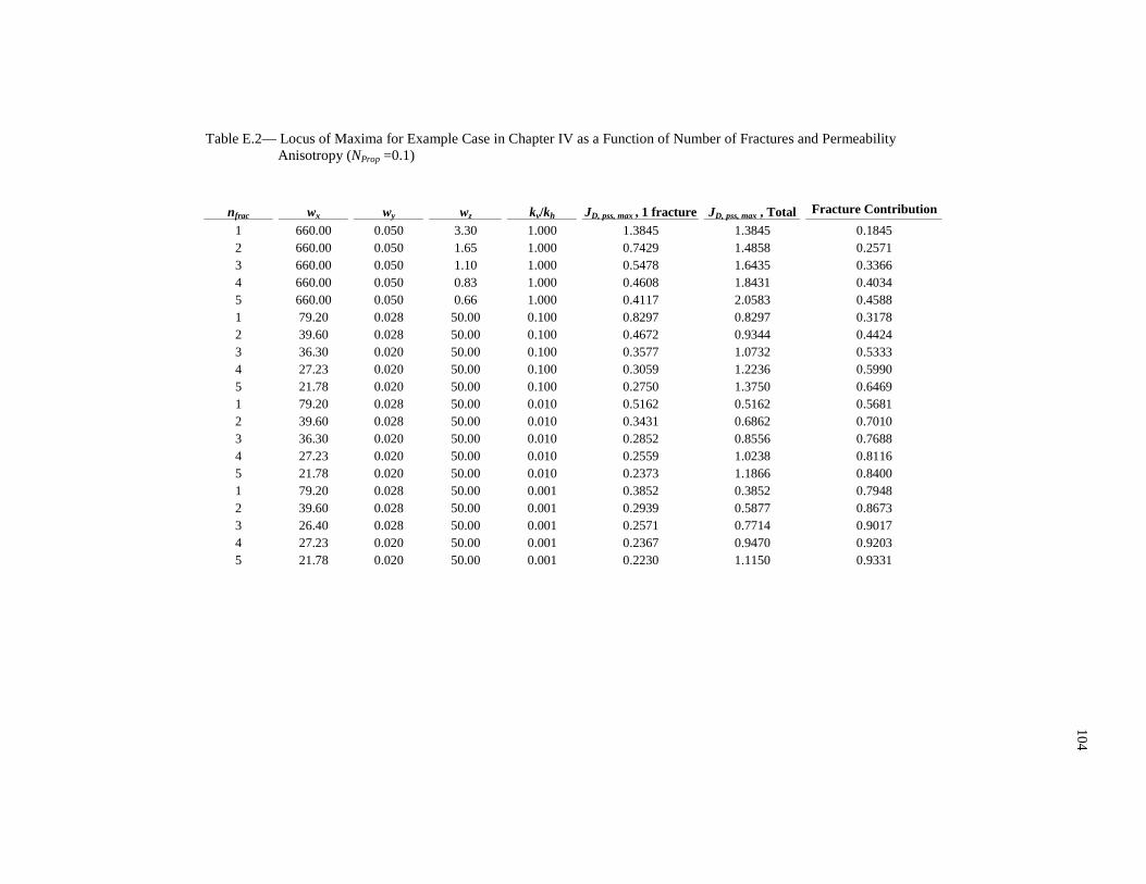
10

4

Table E.2— Locus of Maxima for Example Case in Chapter IV as a Function of Number of Fractures and Permeability Anisotropy (NProp =0.1)


1 660.00 0.050 3.30 1.000 1.3845 1.3845 0.1845 2 660.00 0.050 1.65 1.000 0.7429 1.4858 0.2571 3 660.00 0.050 1.10 1.000 0.5478 1.6435 0.3366 4 660.00 0.050 0.83 1.000 0.4608 1.8431 0.4034 5 660.00 0.050 0.66 1.000 0.4117 2.0583 0.4588 1 79.20 0.028 50.00 0.100 0.8297 0.8297 0.3178 2 39.60 0.028 50.00 0.100 0.4672 0.9344 0.4424 3 36.30 0.020 50.00 0.100 0.3577 1.0732 0.5333 4 27.23 0.020 50.00 0.100 0.3059 1.2236 0.5990 5 21.78 0.020 50.00 0.100 0.2750 1.3750 0.6469 1 79.20 0.028 50.00 0.010 0.5162 0.5162 0.5681 2 39.60 0.028 50.00 0.010 0.3431 0.6862 0.7010 3 36.30 0.020 50.00 0.010 0.2852 0.8556 0.7688 4 27.23 0.020 50.00 0.010 0.2559 1.0238 0.8116 5 21.78 0.020 50.00 0.010 0.2373 1.1866 0.8400 1 79.20 0.028 50.00 0.001 0.3852 0.3852 0.7948 2 39.60 0.028 50.00 0.001 0.2939 0.5877 0.8673 3 26.40 0.028 50.00 0.001 0.2571 0.7714 0.9017 4 27.23 0.020 50.00 0.001 0.2367 0.9470 0.9203 5 21.78 0.020 50.00 0.001 0.2230 1.1150 0.9331

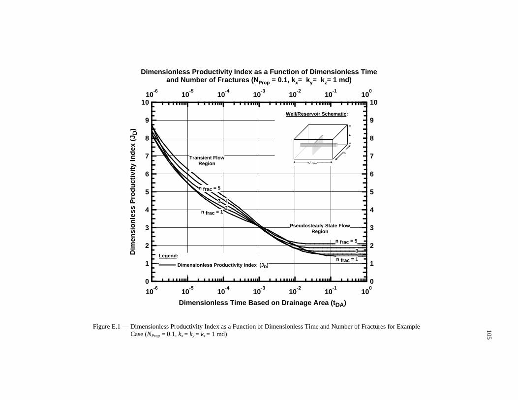
10

5

10 10

9 9

8 8

7 7

6 6

5 5

4 4

3 3

2 2

1 1

0 0

Dim

ensi

onle

ss P

rodu

ctiv

ity In

dex

(J D

)

10-6

10-6

10-5

10-5

10-4

10-4

10-3

10-3

10-2

10-2

10-1

10-1

100

100


ye/ nfrac

xe

ze

n frac = 1

n frac = 5

Legend :





n frac = 1

324

n frac = 5

3


Figure E.1 — Dimensionless Productivity Index as a Function of Dimensionless Time and Number of Fractures for Example Case (NProp = 0.1, kx = ky = kz = 1 md)

10

6

10 10

9 9

8 8

7 7

6 6

5 5

4 4

3 3

2 2

1 1

0 0

Dim

ensi

onle

ss P

rodu

ctiv

ity In

dex

(J D

)

10-6

10-6

10-5

10-5

10-4

10-4

10-3

10-3

10-2

10-2

10-1

10-1

100

100


ye/ nfrac

xe

ze

n frac = 1

n frac = 5

Legend :





n frac = 1

32

4

n frac = 5

3


Figure E.2 — Dimensionless Productivity Index as a Function of Dimensionless Time and Number of Fractures for Example Case (NProp = 0.1, kx = ky = 1 md, kz = 0.1 md)

10

7

10 10

9 9

8 8

7 7

6 6

5 5

4 4

3 3

2 2

1 1

0 0

Dim

ensi

onle

ss P

rodu

ctiv

ity In

dex

(J D

)

10-6

10-6

10-5

10-5

10-4

10-4

10-3

10-3

10-2

10-2

10-1

10-1

100

100


ye/ nfrac

xe

ze

n frac = 1

n frac = 5

Legend :





n frac = 1

3

2

4

n frac = 5

3



10

8

10 10

9 9

8 8

7 7

6 6

5 5

4 4

3 3

2 2

1 1

0 0

Dim

ensi

onle

ss P

rodu

ctiv

ity In

dex

(J D

)

10-6

10-6

10-5

10-5

10-4

10-4

10-3

10-3

10-2

10-2

10-1

10-1

100

100


ye/ nfrac

xe

ze

n frac = 1

n frac = 5

Legend :





n frac = 1

3

2

4

n frac = 5

3



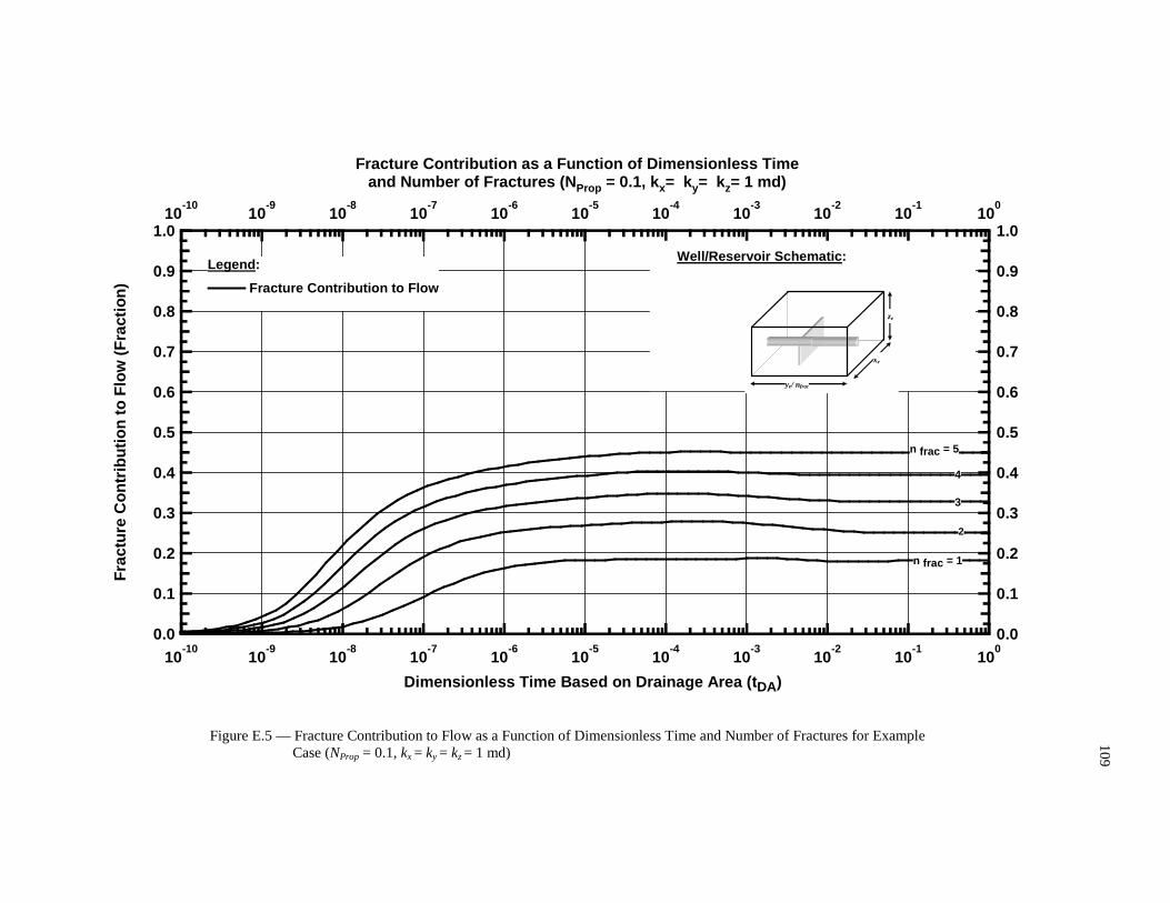
10

9

1.0 1.0

0.9 0.9

0.8 0.8

0.7 0.7

0.6 0.6

0.5 0.5

0.4 0.4

0.3 0.3

0.2 0.2

0.1 0.1

0.0 0.0

Fra

ctur

e C

ontr

ibut

ion

to F

low

(F

ract

ion)

10-10

10-10

10-9

10-9

10-8

10-8

10-7

10-7

10-6

10-6

10-5

10-5

10-4

10-4

10-3

10-3

10-2

10-2

10-1

10-1

100

100


ye/ nfrac

xe

ze

Legend :



n frac = 1

3

2

4

n frac = 5


Figure E.5 — Fracture Contribution to Flow as a Function of Dimensionless Time and Number of Fractures for Example Case (NProp = 0.1, kx = ky = kz = 1 md)

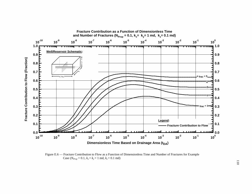
11

0

1.0 1.0

0.9 0.9

0.8 0.8

0.7 0.7

0.6 0.6

0.5 0.5

0.4 0.4

0.3 0.3

0.2 0.2

0.1 0.1

0.0 0.0

Fra

ctur

e C

ontr

ibut

ion

to F

low

(F

ract

ion)

10-10

10-10

10-9

10-9

10-8

10-8

10-7

10-7

10-6

10-6

10-5

10-5

10-4

10-4

10-3

10-3

10-2

10-2

10-1

10-1

100

100


ye/ nfrac

xe

ze

Legend :



n frac = 1

3

2

4

n frac = 5


Figure E.6 — Fracture Contribution to Flow as a Function of Dimensionless Time and Number of Fractures for Example Case (NProp = 0.1, kx = ky = 1 md, kz = 0.1 md)

11

1

1.0 1.0

0.9 0.9

0.8 0.8

0.7 0.7

0.6 0.6

0.5 0.5

0.4 0.4

0.3 0.3

0.2 0.2

0.1 0.1

0.0 0.0

Fra

ctur

e C

ontr

ibut

ion

to F

low

(F

ract

ion)

10-10

10-10

10-9

10-9

10-8

10-8

10-7

10-7

10-6

10-6

10-5

10-5

10-4

10-4

10-3

10-3

10-2

10-2

10-1

10-1

100

100


ye/ nfrac

xe

ze

Legend :



n frac = 1

3

2

4

n frac = 5


Figure E.7 — Fracture Contribution to Flow as a Function of Dimensionless Time and Number of Fractures for Example Case (NProp = 0.1, kx = ky = 1 md, kz = 0.01 md)

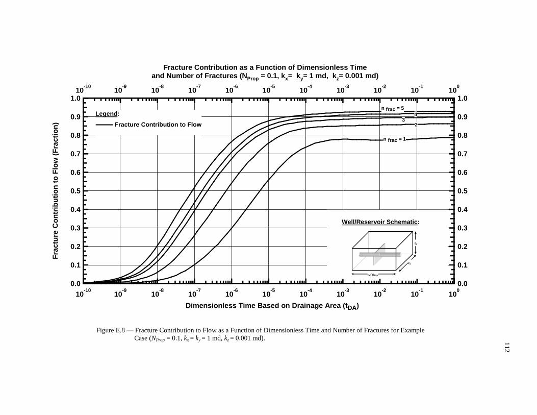
11

2

1.0 1.0

0.9 0.9

0.8 0.8

0.7 0.7

0.6 0.6

0.5 0.5

0.4 0.4

0.3 0.3

0.2 0.2

0.1 0.1

0.0 0.0

Fra

ctur

e C

ontr

ibut

ion

to F

low

(F

ract

ion)

10-10

10-10

10-9

10-9

10-8

10-8

10-7

10-7

10-6

10-6

10-5

10-5

10-4

10-4

10-3

10-3

10-2

10-2

10-1

10-1

100

100


ye/ nfrac

xe

ze

Legend :



n frac = 1

32

4n frac = 5


Figure E.8 — Fracture Contribution to Flow as a Function of Dimensionless Time and Number of Fractures for Example Case (NProp = 0.1, kx = ky = 1 md, kz = 0.001 md).

113

APPENDIX F





production behavior of example problem in chapter IV when 1,000,000 lb of proppant (NProp = 1.0) is used

for stimulation. All the fracture sizes have been described in ft.

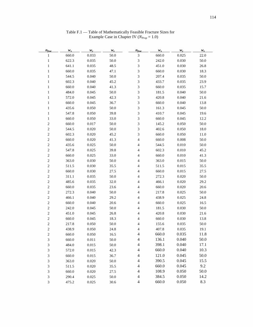
114

Table F.1 — Table of Mathematically Feasible Fracture Sizes for Example Case in Chapter IV (NProp = 1.0)

nfrac wx wy wz nfrac wx wy wz

1 660.0 0.033 50.0 3 660.0 0.025 22.0

1 622.3 0.035 50.0 3 242.0 0.030 50.0

1 641.1 0.035 48.5 3 451.0 0.030 26.8

1 660.0 0.035 47.1 3 660.0 0.030 18.3

1 544.5 0.040 50.0 3 207.4 0.035 50.0

1 602.3 0.040 45.2 3 433.7 0.035 23.9

1 660.0 0.040 41.3 3 660.0 0.035 15.7

1 484.0 0.045 50.0 3 181.5 0.040 50.0

1 572.0 0.045 42.3 3 420.8 0.040 21.6

1 660.0 0.045 36.7 3 660.0 0.040 13.8

1 435.6 0.050 50.0 3 161.3 0.045 50.0

1 547.8 0.050 39.8 3 410.7 0.045 19.6

1 660.0 0.050 33.0 3 660.0 0.045 12.2

2 660.0 0.017 50.0 3 145.2 0.050 50.0

2 544.5 0.020 50.0 3 402.6 0.050 18.0

2 602.3 0.020 45.2 3 660.0 0.050 11.0

2 660.0 0.020 41.3 4 660.0 0.008 50.0

2 435.6 0.025 50.0 4 544.5 0.010 50.0

2 547.8 0.025 39.8 4 602.3 0.010 45.2

2 660.0 0.025 33.0 4 660.0 0.010 41.3

2 363.0 0.030 50.0 4 363.0 0.015 50.0

2 511.5 0.030 35.5 4 511.5 0.015 35.5

2 660.0 0.030 27.5 4 660.0 0.015 27.5

2 311.1 0.035 50.0 4 272.3 0.020 50.0

2 485.6 0.035 32.0 4 466.1 0.020 29.2

2 660.0 0.035 23.6 4 660.0 0.020 20.6

2 272.3 0.040 50.0 4 217.8 0.025 50.0

2 466.1 0.040 29.2 4 438.9 0.025 24.8

2 660.0 0.040 20.6 4 660.0 0.025 16.5

2 242.0 0.045 50.0 4 181.5 0.030 50.0

2 451.0 0.045 26.8 4 420.8 0.030 21.6

2 660.0 0.045 18.3 4 660.0 0.030 13.8

2 217.8 0.050 50.0 4 155.6 0.035 50.0

2 438.9 0.050 24.8 4 407.8 0.035 19.1

2 660.0 0.050 16.5 4 660.0 0.035 11.8 3 660.0 0.011 50.0 4 136.1 0.040 50.0 3 484.0 0.015 50.0 4 398.1 0.040 17.1 3 572.0 0.015 42.3 4 660.0 0.040 10.3 3 660.0 0.015 36.7 4 121.0 0.045 50.0 3 363.0 0.020 50.0 4 390.5 0.045 15.5 3 511.5 0.020 35.5 4 660.0 0.045 9.2 3 660.0 0.020 27.5 4 108.9 0.050 50.0 3 290.4 0.025 50.0 4 384.5 0.050 14.2 3 475.2 0.025 30.6 4 660.0 0.050 8.3

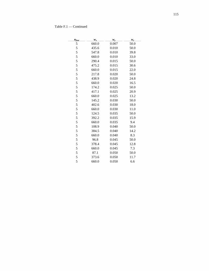
115

Table F.1 — Continued

nfrac wx wy wz 5 660.0 0.007 50.0 5 435.6 0.010 50.0 5 547.8 0.010 39.8 5 660.0 0.010 33.0 5 290.4 0.015 50.0 5 475.2 0.015 30.6 5 660.0 0.015 22.0 5 217.8 0.020 50.0 5 438.9 0.020 24.8 5 660.0 0.020 16.5 5 174.2 0.025 50.0 5 417.1 0.025 20.9 5 660.0 0.025 13.2 5 145.2 0.030 50.0 5 402.6 0.030 18.0 5 660.0 0.030 11.0 5 124.5 0.035 50.0 5 392.2 0.035 15.9 5 660.0 0.035 9.4 5 108.9 0.040 50.0 5 384.5 0.040 14.2 5 660.0 0.040 8.3 5 96.8 0.045 50.0 5 378.4 0.045 12.8 5 660.0 0.045 7.3 5 87.1 0.050 50.0 5 373.6 0.050 11.7 5 660.0 0.050 6.6

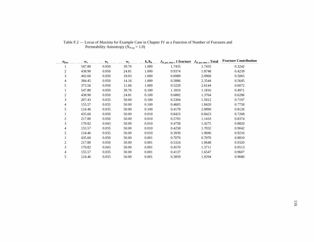
11

6

Table F.2 — Locus of Maxima for Example Case in Chapter IV as a Function of Number of Fractures and Permeability Anisotropy (NProp = 1.0)


1 547.80 0.050 39.76 1.000 1.7435 1.7435 0.3242 2 438.90 0.050 24.81 1.000 0.9374 1.8748 0.4239 3 402.60 0.050 18.03 1.000 0.6989 2.0968 0.5065 4 384.45 0.050 14.16 1.000 0.5886 2.3544 0.5645 5 373.56 0.050 11.66 1.000 0.5229 2.6144 0.6072 1 547.80 0.050 39.76 0.100 1.1816 1.1816 0.4971 2 438.90 0.050 24.81 0.100 0.6882 1.3764 0.6286 3 207.43 0.035 50.00 0.100 0.5304 1.5912 0.7197 4 155.57 0.035 50.00 0.100 0.4605 1.8420 0.7758 5 124.46 0.035 50.00 0.100 0.4178 2.0890 0.8126 1 435.60 0.050 50.00 0.010 0.8423 0.8423 0.7268 2 217.80 0.050 50.00 0.010 0.5705 1.1410 0.8374 3 170.82 0.043 50.00 0.010 0.4758 1.4275 0.8820 4 155.57 0.035 50.00 0.010 0.4258 1.7032 0.9042 5 124.46 0.035 50.00 0.010 0.3939 1.9696 0.9216 1 435.60 0.050 50.00 0.001 0.7070 0.7070 0.8810 2 217.80 0.050 50.00 0.001 0.5324 1.0648 0.9320 3 170.82 0.043 50.00 0.001 0.4570 1.3711 0.9513 4 155.57 0.035 50.00 0.001 0.4137 1.6547 0.9607 5 124.46 0.035 50.00 0.001 0.3859 1.9294 0.9680

11

7

10 10

9 9

8 8

7 7

6 6

5 5

4 4

3 3

2 2

1 1

0 0

Dim

ensi

onle

ss P

rodu

ctiv

ity In

dex

(J D

)

10-6

10-6

10-5

10-5

10-4

10-4

10-3

10-3

10-2

10-2

10-1

10-1

100

100


ye/ nfrac

xe

ze

n frac = 1

n frac = 5

Legend :



Dimensionless Productivity Index as a Function of Dimensionless Time and Number of Fracture ( NProp = 1.0, kx= ky= kz= 1 md)


n frac = 1

3

2

4

n frac = 5

3


Figure F.1 — Dimensionless Productivity Index as a Function of Dimensionless Time and Number of Fractures for Example Case (NProp = 1.0, kx = ky = kz = 1 md)

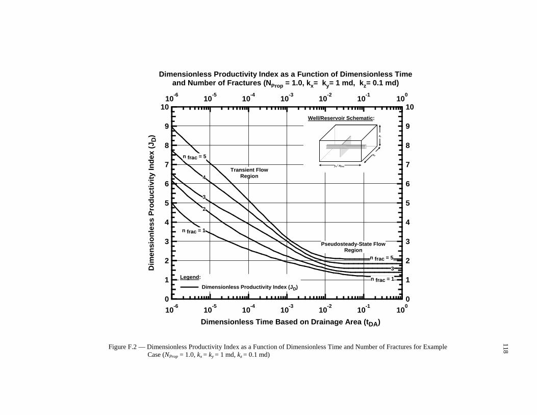
11

8

10 10

9 9

8 8

7 7

6 6

5 5

4 4

3 3

2 2

1 1

0 0

Dim

ensi

onle

ss P

rodu

ctiv

ity In

dex

(J D

)

10-6

10-6

10-5

10-5

10-4

10-4

10-3

10-3

10-2

10-2

10-1

10-1

100

100


ye/ nfrac

xe

ze

n frac = 1

n frac = 5

Legend :





n frac = 1

3

2

4

n frac = 5

3


Figure F.2 — Dimensionless Productivity Index as a Function of Dimensionless Time and Number of Fractures for Example Case (NProp = 1.0, kx = ky = 1 md, kz = 0.1 md)

11

9

10 10

9 9

8 8

7 7

6 6

5 5

4 4

3 3

2 2

1 1

0 0

Dim

ensi

onle

ss P

rodu

ctiv

ity In

dex

(J D

)

10-6

10-6

10-5

10-5

10-4

10-4

10-3

10-3

10-2

10-2

10-1

10-1

100

100


ye/ nfrac

xe

ze

n frac = 1

n frac = 5





n frac = 1

3

2

4

n frac = 5

3 Legend :



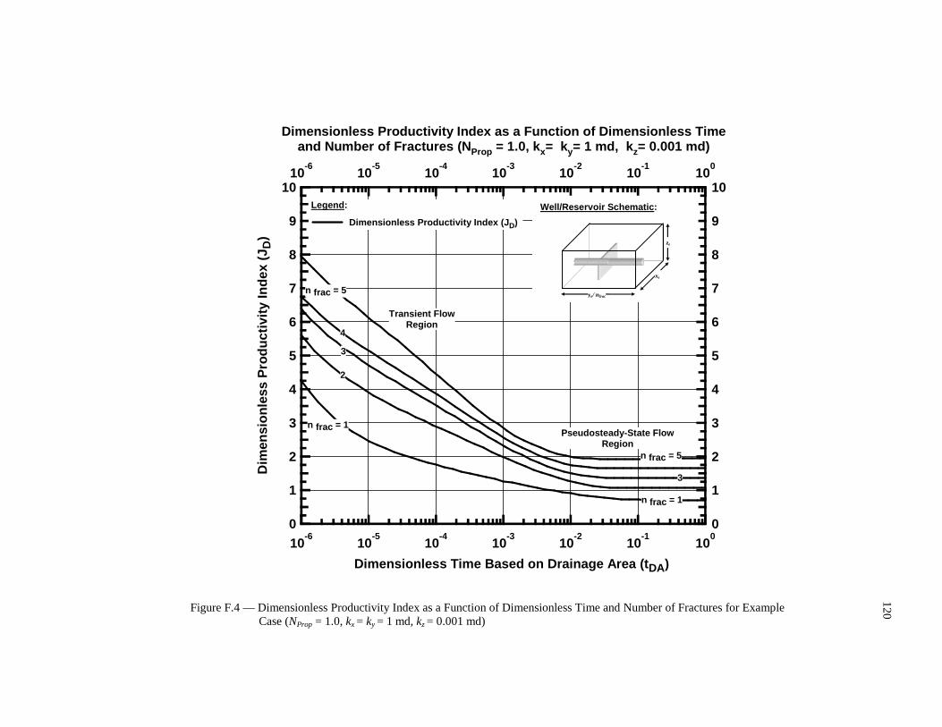
12

0

10 10

9 9

8 8

7 7

6 6

5 5

4 4

3 3

2 2

1 1

0 0

Dim

ensi

onle

ss P

rodu

ctiv

ity In

dex

(J D

)

10-6

10-6

10-5

10-5

10-4

10-4

10-3

10-3

10-2

10-2

10-1

10-1

100

100


ye/ nfrac

xe

ze

n frac = 1

n frac = 5

Legend :





n frac = 1

3

2

4

n frac = 5

3



12

1

1.0 1.0

0.9 0.9

0.8 0.8

0.7 0.7

0.6 0.6

0.5 0.5

0.4 0.4

0.3 0.3

0.2 0.2

0.1 0.1

0.0 0.0

Fra

ctur

e C

ontr

ibut

ion

to F

low

(F

ract

ion)

10-10

10-10

10-9

10-9

10-8

10-8

10-7

10-7

10-6

10-6

10-5

10-5

10-4

10-4

10-3

10-3

10-2

10-2

10-1

10-1

100

100


ye/ nfrac

xe

ze

Legend :


Fracture Contribution as a Function of Dimensionles s Time and Number of Fractures ( NProp = 1.0, kx= ky= kz= 1 md)

n frac = 1

3

2

4

n frac = 5


Figure F.5 — Fracture Contribution to Flow as a Function of Dimensionless Time and Number of Fractures for Example Case (NProp = 1.0, kx = ky = kz = 1 md)

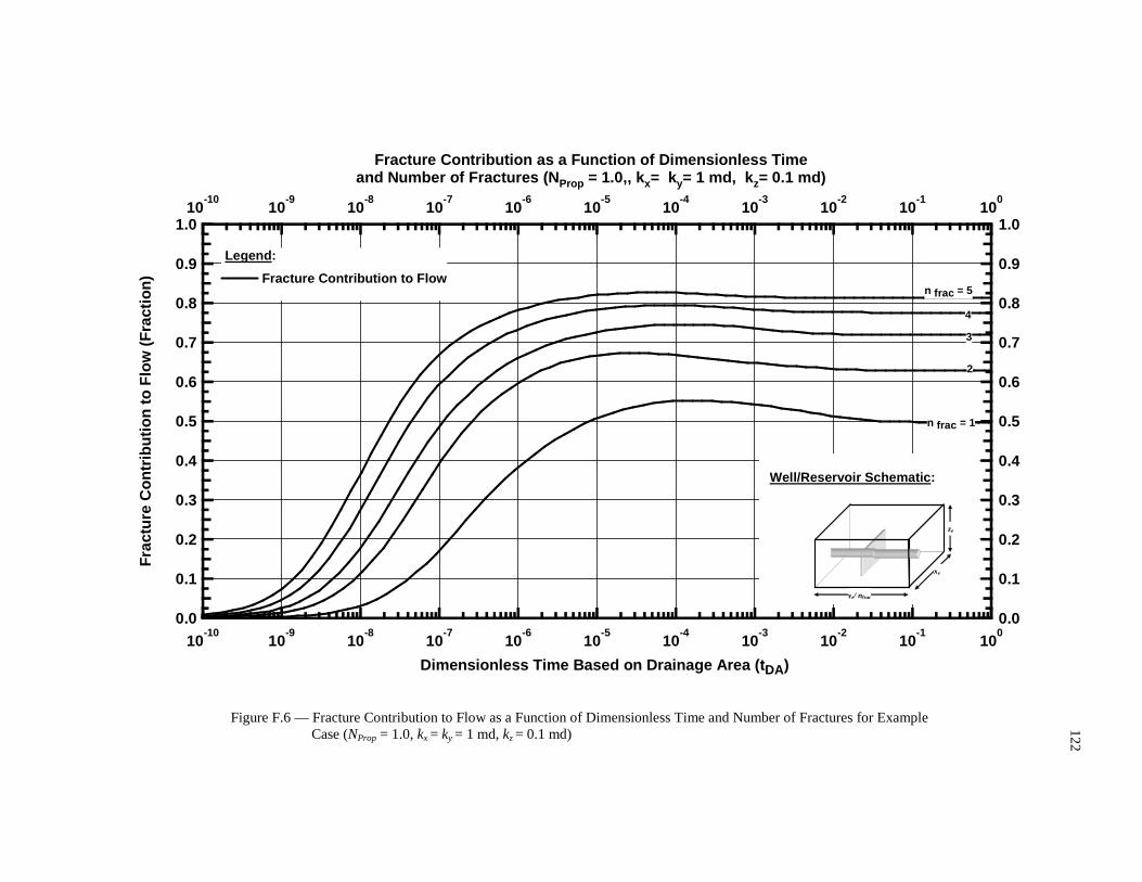
12

2

1.0 1.0

0.9 0.9

0.8 0.8

0.7 0.7

0.6 0.6

0.5 0.5

0.4 0.4

0.3 0.3

0.2 0.2

0.1 0.1

0.0 0.0

Fra

ctur

e C

ontr

ibut

ion

to F

low

(F

ract

ion)

10-10

10-10

10-9

10-9

10-8

10-8

10-7

10-7

10-6

10-6

10-5

10-5

10-4

10-4

10-3

10-3

10-2

10-2

10-1

10-1

100

100


ye/ nfrac

xe

ze

Legend :


Fracture Contribution as a Function of Dimensionle ss Time and Number of Fractures ( NProp = 1.0,, kx= ky= 1 md, kz= 0.1 md)

n frac = 1

3

2

4

n frac = 5


Figure F.6 — Fracture Contribution to Flow as a Function of Dimensionless Time and Number of Fractures for Example Case (NProp = 1.0, kx = ky = 1 md, kz = 0.1 md)

12

3

1.0 1.0

0.9 0.9

0.8 0.8

0.7 0.7

0.6 0.6

0.5 0.5

0.4 0.4

0.3 0.3

0.2 0.2

0.1 0.1

0.0 0.0

Fra

ctur

e C

ontr

ibut

ion

to F

low

(F

ract

ion)

10-10

10-10

10-9

10-9

10-8

10-8

10-7

10-7

10-6

10-6

10-5

10-5

10-4

10-4

10-3

10-3

10-2

10-2

10-1

10-1

100

100


ye/ nfrac

xe

ze

Legend :



n frac = 1

3

2

4n frac = 5



12

4

1.0 1.0

0.9 0.9

0.8 0.8

0.7 0.7

0.6 0.6

0.5 0.5

0.4 0.4

0.3 0.3

0.2 0.2

0.1 0.1

0.0 0.0

Fra

ctur

e C

ontr

ibut

ion

to F

low

(F

ract

ion)

10-10

10-10

10-9

10-9

10-8

10-8

10-7

10-7

10-6

10-6

10-5

10-5

10-4

10-4

10-3

10-3

10-2

10-2

10-1

10-1

100

100


ye/ nfrac

xe

ze

Legend :


Fracture Contribution as a Function of Dimensionles s Time and Number of Fractures ( NProp = 1.0, kx= ky= 1 md, kz= 0.001 md)

n frac = 1

3

2

4n frac = 5



125

APPENDIX G

COMPLETE RESULTS OF FIELD APPLICATION

WHELAN GAS FIELD

The material balance equation for dry gas volumetric reservoirs has been integrated to the results of DVS

calculation to obtain the production performance behavior of Whelan gas field in East Texas, USA. This

Appendix provides figures of the estimation of gas production rate, average reservoir pressure, and

cumulative gas production of this field for an 80-acre spacing, development plan as a function of the

completion scheme— Fracture and horizontal section produce together and production only from

fractures—, number of transverse fractures, and the amount of propant (250,000 and 500,000 lb). Table

G.1 Provides the reservoir and fluid properties used for the calculations

Table G.1 — Reservoir and Fluid Properties for Whelan Field Example

Whelan Net Pay (ft) 200 Hor. Permeability (md) 0.9 Porosity (%) 8.8 Initial Pressure (psia) 3500 Reservoir Temperature(°F) 220 Gas Gravity 0.63 Gas in Place(BCF) 11.907

126

10-1

100

101

102

103

Gas

Pro

duct

ion

Rat

e,

qg

(MM

SC

FD

)

10-2

10-1

100

101

102

103




Legend :


nfrac = 1 2

nfrac = 1 2 3 4

3 45

5

5

11

5 3

Figure G.1 — Gas Production Rate as a Function of Production Time, Number of Fractures, and Completion Scheme for Whelan Field (80 Acres Spacing, 250,000 lb

10-1

100

101

102

103

Gas

Pro

duct

ion

Rat

e,

qg (

MM

SC

FD

)

10-2

10-1

100

101

102

103




Legend :


5

nfrac = 5

nfrac = 1nfrac = 1

2 3

4 3

5

5

nfrac = 1

3

5

Figure G.2 — Gas Production Rate as a Function of Production Time, Number of Fractures, and Completion Scheme for Whelan Field (80 Acres Spacing, 500,000 lb

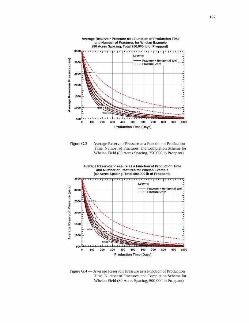
127

3500

3000

2500

2000

1500

1000

500

Ave

rage

Res

ervo

ir P

ress

ure

(psi

a)

10009008007006005004003002001000




Legend :


nfrac = 5

nfrac = 5

nfrac = 1

2

nfrac = 1

2 3

4

3

4

Figure G.3 — Average Reservoir Pressure as a Function of Production Time, Number of Fractures, and Completion Scheme for Whelan Field (80 Acres Spacing, 250,000 lb Proppant)

3500

3000

2500

2000

1500

1000

500

Ave

rage

Res

ervo

ir P

ress

ure

(psi

a)

10009008007006005004003002001000




Legend :


nfrac = 5

nfrac = 5nfrac = 1

2

nfrac = 1

2 3

4

3

4

Figure G.4 — Average Reservoir Pressure as a Function of Production Time, Number of Fractures, and Completion Scheme for Whelan Field (80 Acres Spacing, 500,000 lb Proppant)

128

12

11

10

9

8

7

6

5

4

3

2

1

0

Cum

ulat

ive

Gas

Pro

duct

ion,

G

P (

BC

F)

10009008007006005004003002001000


Cumulative Gas Production as a Function of Producti on Timeand Number of Fractures for Whelan Example


Legend :


nfrac = 5nfrac = 5

nfrac = 1

2

nfrac = 1

2

3

4 3

4

Figure G.5 — Cumulative Gas Production as a Function of Production Time, Number of Fractures, and Completion Scheme for Whelan Field (80 Acres Spacing, 250,000 lb Proppant)

12

11

10

9

8

7

6

5

4

3

2

1

0

Cum

ulat

ive

Gas

Pro

duct

ion,

G

P (

BC

F)

10009008007006005004003002001000


Cumulative Gas Production as a Functionof Productio n Time and Number of Fractures for Whelan Example


Legend :


nfrac = 5nfrac = 5

nfrac = 1

2

nfrac = 1

2

3

4

3

4

Figure G.6 — Cumulative Gas Production as a Function of Production Time, Number of Fractures, and Completion Scheme for Whelan Field (80 Acres Spacing, 500,000 lb Proppant)

129

APPENDIX H


PERCY WHEELER GAS FIELD


calculation to obtain the production performance behavior of Percy Wheeler gas field in East Texas, USA.

This Appendix provides figures of the estimation of gas production rate, average reservoir pressure, and



fractures—, number of transverse fractures, and the amount of propant (250,000 and 500,000 lb). ). Table

H.1 Provides the reservoir and fluid properties used for the calculations

Table H.1 — Reservoir and Fluid Properties for Percy Wheeler Field Example

Percy Wheeler Net Pay (ft) 200 Hor. Permeability (md) 0.05 Porosity (%) 10.3 Initial Pressure (psia) 3000 Reservoir Temperature(°F) 245 Gas Gravity 0.62 Gas in Place(BCF) 11.495

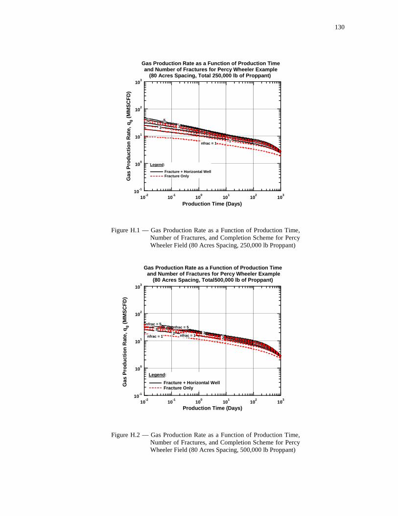
130

10-1

100

101

102

103

Gas

Pro

duct

ion

Rat

e,

qg (

MM

SC

FD

)

10-2

10-1

100

101

102

103


Gas Production Rate as a Function of Production Tim eand Number of Fractures for Percy Wheeler Example


Legend :


55

nfrac = 11

3 3

Figure H.1 — Gas Production Rate as a Function of Production Time, Number of Fractures, and Completion Scheme for Percy Wheeler Field (80 Acres Spacing, 250,000 lb Proppant)

10-1

100

101

102

103

Gas

Pro

duct

ion

Rat

e,

qg (

MM

SC

FD

)

10-2

10-1

100

101

102

103


Gas Production Rate as a Function of Production Tim e and Number of Fractures for Percy Wheeler Example

(80 Acres Spacing, Total500,000 lb of Proppant)

Legend :


nfrac = 5nfrac = 5

nfrac = 1 2nfrac = 1

2 34 3

Figure H.2 — Gas Production Rate as a Function of Production Time, Number of Fractures, and Completion Scheme for Percy Wheeler Field (80 Acres Spacing, 500,000 lb Proppant)

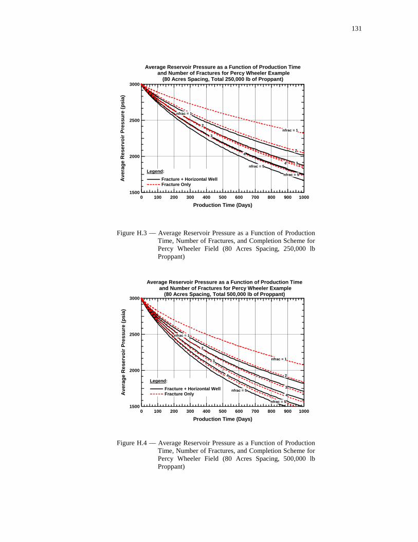
131

3000

2500

2000

1500

Ave

rage

Res

ervo

ir P

ress

ure

(psi

a)

10009008007006005004003002001000


Average Reservoir Pressure as a Function of Product ion Time and Number of Fractures for Percy Wheeler Example


Legend :


nfrac = 5

nfrac = 5

nfrac = 1 2

nfrac = 1

2

3 4

3

4

Figure H.3 — Average Reservoir Pressure as a Function of Production Time, Number of Fractures, and Completion Scheme for Percy Wheeler Field (80 Acres Spacing, 250,000 lb Proppant)

3000

2500

2000

1500

Ave

rage

Res

ervo

ir P

ress

ure

(psi

a)

10009008007006005004003002001000


Average Reservoir Pressure as a Function of Product ion Time and Number of Fractures for Percy Wheeler Example


Legend :


nfrac = 5

nfrac = 5

nfrac = 1

2

nfrac = 1

2

3

4

3

4

Figure H.4 — Average Reservoir Pressure as a Function of Production Time, Number of Fractures, and Completion Scheme for Percy Wheeler Field (80 Acres Spacing, 500,000 lb Proppant)

132

6

5

4

3

2

1

0

Cum

ulat

ive

Gas

Pro

duct

ion,

G

P (

BC

F)

10009008007006005004003002001000




Legend :


nfrac = 5nfrac = 5

nfrac = 1

2

nfrac = 1

2

3

4

3

4

Figure H.5 — Cumulative Gas Production as a Function of Production Time, Number of Fractures, and Completion Scheme for Percy Wheeler Field (80 Acres Spacing, 250,000 lb Proppant)

6

5

4

3

2

1

0

Cum

ulat

ive

Gas

Pro

duct

ion,

G

P (

BC

F)

10009008007006005004003002001000




Legend :


nfrac = 5

nfrac = 1

2

nfrac = 1

2

3

4 3

4

Figure H.6 — Cumulative Gas Production as a Function of Production Time, Number of Fractures, and Completion Scheme for Percy Wheeler Field (80 Acres Spacing, 500,000 lb Proppant)

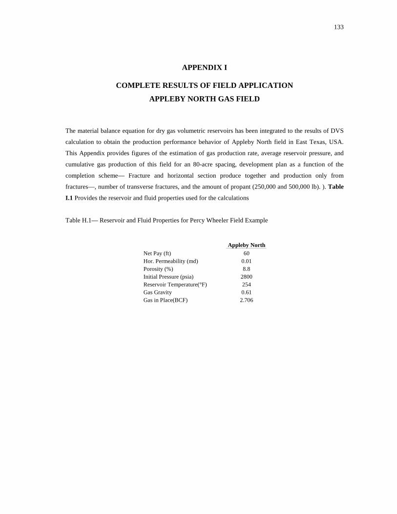
133

APPENDIX I


APPLEBY NORTH GAS FIELD


calculation to obtain the production performance behavior of Appleby North field in East Texas, USA.

This Appendix provides figures of the estimation of gas production rate, average reservoir pressure, and



fractures—, number of transverse fractures, and the amount of propant (250,000 and 500,000 lb). ). Table

I.1 Provides the reservoir and fluid properties used for the calculations

Table H.1— Reservoir and Fluid Properties for Percy Wheeler Field Example

Appleby North Net Pay (ft) 60 Hor. Permeability (md) 0.01 Porosity (%) 8.8 Initial Pressure (psia) 2800 Reservoir Temperature(°F) 254 Gas Gravity 0.61 Gas in Place(BCF) 2.706

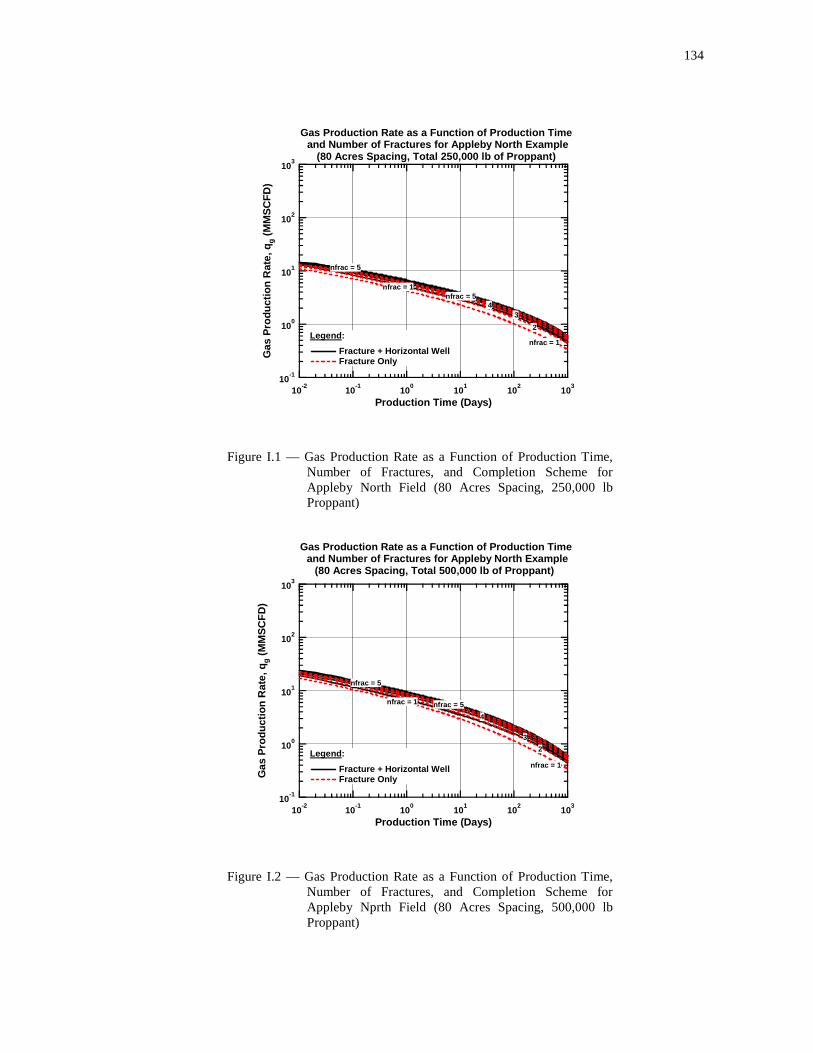
134

10-1

100

101

102

103

Gas

Pro

duct

ion

Rat

e,

qg (

MM

SC

FD

)

10-2

10-1

100

101

102

103


Gas Production Rate as a Function of Production Time and Number of Fractures for Appleby North Example


Legend :


nfrac = 5

nfrac = 5

nfrac = 1

2

nfrac = 1

3 4

Figure I.1 — Gas Production Rate as a Function of Production Time, Number of Fractures, and Completion Scheme for Appleby North Field (80 Acres Spacing, 250,000 lb Proppant)

10-1

100

101

102

103

Gas

Pro

duct

ion

Rat

e,

qg (

MM

SC

FD

)

10-2

10-1

100

101

102

103


Gas Production Rate as a Function of Production Time and Number of Fractures for Appleby North Example


Legend :


nfrac = 5

nfrac = 5

nfrac = 1

2

nfrac = 1

3

4

Figure I.2 — Gas Production Rate as a Function of Production Time, Number of Fractures, and Completion Scheme for Appleby Nprth Field (80 Acres Spacing, 500,000 lb Proppant)

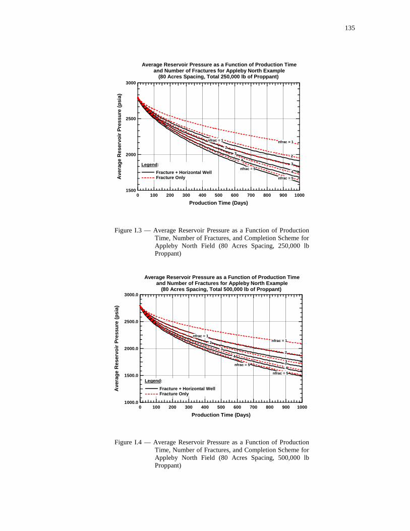
135

3000

2500

2000

1500

Ave

rage

Res

ervo

ir P

ress

ure

(psi

a)

10009008007006005004003002001000


Average Reservoir Pressure as a Function of Product ion Timeand Number of Fractures for Appleby North Example


Legend :


nfrac = 5

nfrac = 1

2

nfrac = 1

2

3

4

3

4

Figure I.3 — Average Reservoir Pressure as a Function of Production Time, Number of Fractures, and Completion Scheme for Appleby North Field (80 Acres Spacing, 250,000 lb Proppant)

3000.0

2500.0

2000.0

1500.0

1000.0

Ave

rage

Res

ervo

ir P

ress

ure

(psi

a)

10009008007006005004003002001000


Average Reservoir Pressure as a Function of Product ion Timeand Number of Fractures for Appleby North Example


Legend :


nfrac = 5

nfrac = 5

nfrac = 1 2

nfrac = 1

2

3

4

3

4

Figure I.4 — Average Reservoir Pressure as a Function of Production Time, Number of Fractures, and Completion Scheme for Appleby North Field (80 Acres Spacing, 500,000 lb Proppant)

136

1.2

1.0

0.8

0.6

0.4

0.2

0.0

Cum

ulat

ive

Gas

Pro

duct

ion,

G

P (

BC

F)

10009008007006005004003002001000


Cumulative Gas Production as a Function of Producti on Timeand Number of Fractures for Appleby North Example


Legend :


nfrac = 5

nfrac = 5

nfrac = 1

2

nfrac = 1

2

3

4

3

4

Figure I.5 — Cumulative Gas Production as a Function of Production Time, Number of Fractures, and Completion Scheme for Appleby North Field (80 Acres Spacing, 250,000 lb Proppant)

1.50

1.25

1.00

0.75

0.50

0.25

0.00

Cum

ulat

ive

Gas

Pro

duct

ion,

G

P (

BC

F)

10009008007006005004003002001000


Cumulative Gas Production as a Functionof Productio n Time and Number of Fractures for Appleby North Example


Legend :


nfrac = 5

nfrac = 1

2

nfrac = 1

2

3

4

3

4

Figure I.6 — Cumulative Gas Production as a Function of Production Time, Number of Fractures, and Completion Scheme for Appleby North Field (80 Acres Spacing, 500,000 lb Proppant)

137

VITA

Name: Shahram Amini

Mailing Address: 31 Ehsan Street

Farahzadi Boulevard

Shahrak E Gharb

Tehran, 14689 83153

IRAN

E-mail Address: [email protected]

Education: Texas A&M University, College Station, Texas, USA

Doctor of Philosophy Degree in Petroleum Engineering

December 2007

IFP School (ENSPM), Rueil-Malmaison, France

Master of Science Degree in Reservoir Geosciences and Engineering

December 2000

University of Tehran, Tehran, Iran

Master of Science Degree in Chemical Engineering

June 1996

University of Tehran, Tehran, Iran

Bachelor of Science Degree in Chemical Engineering

September 1993

Affiliations: Society of Petroleum Engineers

development and application of the method …€¦ · this work introduces the method of...

Documents