development and comparison of image encoders based...
TRANSCRIPT

Escola Tècnica Superior d’Enginyeria de Telecomunicació de Barcelona
Universitat Politècnica de Catalunya
Development and Comparison of Image Encoders Based on Different Compression Techniques
Marc Rosanes Siscart Thesis Advisor: Marta Casar
Barcelona, February 2010

Acknowledgments I would like to thank my family, friends and my new flat-mates that are my second family in Barcelona this year. I would also like to thank Marta Casar, who has supervised this project and has always advised me when I have needed it. Finally I would like to acknowledge Lluís Torres, who has given me the opportunity to do this project.

CONTENTS
ABSTRACT 1- INTRODUCTION________________________________ 1
1.1- Introduction………………………………………. 1 1.2- Motivation…………………………………………. 1
2- IMAGES________________________________________ 2 3- LOSSLESS COMPRESSION________________________4
3.1- Introduction……………………………………….. 4 3.2- Entropy Coding…………………………………… 4 3.2.1- THEORY AND ALGORITHM ▪ 4
3.2.2-RESULTS ▪ 5 3.3- Laplace Pyramid………………………………...... 8 3.3.1- THEORY AND ALGORITHM ▪ 8
3.3.2- RESULTS ▪ 11

4- LOSSY COMPRESSION__________________________ 12
4.1- Introduction…………………………………………12 4.2- Measures of image quality……………………….....12
4.2.1- MEAN SQUARE ERROR ▪ 12 4.2.2- PSNR ▪ 13
4.3- Quantization………………………………………14
4.4- Fractal compression……………………………….15 4.4.1- FRACTAL DEFINITION AND CONCEPTS ▪ 15
4.4.2- FIRST FRACTAL ALGORITHM ▪ 16 4.4.2.1- THEORY AND ALGORITHM ▪ 16
4.4.2.2- RESULTS ▪ 18 4.4.3- SECOND FRACTAL ALGORITHM ▪ 21
4.4.3.1- THEORY AND ALGORITHM ▪ 21 4.4.3.2- RESULTS ▪ 24
4.5- JPEG compression………………………………..28
4.5.1- CORRELATION AND DPCM ▪ 28 4.5.2- DCT: DISCRETE COSINE TRANSFORMATION ▪ 31 4.5.3- QUANTIZATION ▪ 33 4.5.4- ZERO-RUN ▪ 33 4.5.5- JPEG ALGORITHM: THE ENCODER ▪ 34 4.5.6- JPEG ALGORITHM: THE DECODER ▪ 36 4.5.7- RESULTS ▪ 37
5- COMPARATIVE ANALISYS _______________________45 6- CONCLUSION___________________________________52 ANNEX 1: Fractal 1 numerical developments 54 ANNEX 2: Fractal 2 numerical developments 58 ANNEX 3: Encoding time prediction for Fractal 2 61 ANNEX 4: JPEG numerical developments 62 ANNEX 5: Index of algorithms 66 BIBLIOGRAPHY 67 INDEX OF FIGURES 69 INDEX OF TABLES 71

ABSTRACT In this project we present some of the most relevant image compression methods of the digital era. From lossless compression techniques like Laplacian Pyramid, to the current and frequently used lossy JPEG compression techniques, going through techniques that have been very influential in the past, as Fractal compression. The project is organized by chapters describing briefly the algorithms and presenting the results obtained when applied to three different test images. Finally we perform a comparative analysis synthesizing the main results. In this analysis we see the large difference in compression ratios between lossy and lossless compression algorithms. We also compare our developed lossy algorithms, observing that the first Fractal algorithm gives poor PSNR results, while our second Fractal algorithm and the JPEG algorithm give quite better qualities of compression; the latter achieving results comparable to present day JPEG algorithms.

ABSTRACT Este proyecto presenta algunos de los más relevantes métodos de compresión de imagen de la era digital. Desde métodos de compresión sin pérdidas como es la compresión por Pirámide de Laplace, hasta las bases de las actuales y altamente utilizadas técnicas de JPEG, pasando por otras que alcanzaron su punto álgido en el pasado como es el caso de la compresión Fractal. El proyecto está organizado por capítulos que describen brevemente los algoritmos y presentan los resultados obtenidos con ellos, usándolos en la compresión de tres imágenes diferentes. Para acabar presentamos un análisis comparativo de los principales resultados. En este análisis vemos la gran diferencia en las tasas de compresión obtenidas con compresión sin pérdidas i aquellas obtenidas en la compresión con pérdidas. También comparamos entre ellos los algoritmos con pérdidas desarrollados, observando que el primer algoritmo Fractal nos da resultados bastante pobres en términos de PSNR, mientras que el segundo algoritmo fractal y el algoritmo JPEG nos dan resultados mucho mejores; el último de ellos logrando resultados comparables a aquellos obtenidos por los algoritmos JPEG utilizados a hoy en día.

ABSTRACT Ce projet présente quelques unes des méthodes de compression d’images digitales qui ont eu plus d’influence pendant les dernières années. Depuis des méthodes de compression sans pertes comme la Pyramide de Laplace, jusqu’aux actuels et hautement utilisées techniques de compression JPEG, en passant par des techniques qui ont eu leur point algide dans le passé comme est le cas de la compression Fractale. Le projet est organisé par chapitres qui décrivent brièvement les algorithmes développés et présentent les résultats obtenus avec eux, en les utilisant dans la compression de trois images différentes. Vers la fin du projet on donne une analyse comparative des principaux résultats obtenus avec les différentes méthodes. Dans cette analyse on voit la grande différence entre les taux de compression obtenus avec la compression sans pertes et ceux obtenus en utilisant techniques de compression avec des pertes. On compare aussi entre eux les algorithmes avec des pertes développés, en observant que le premier algorithme Fractal développé nous donné des résultats assez pauvres en termes de PSNR, n’étant pas le cas pour le deuxième algorithme Fractal et pour l’algorithme JPEG pour lesquels on obtient des beaucoup mieux résultats; le dernier d’entre eux réussissant des résultats comparables a ceux obtenus avec les algorithmes JPEG utilisées dans l’actualité.
ABSTRACT Aquest projecte presenta alguns dels mètodes més rellevants utilitzats per la compressió d’imatges durant l’era digital. Des de mètodes de compressió sense pèrdues com la compressió per Piràmide de Laplace, fins a mètodes de compressió amb pèrdues com les actuals i altament utilitzades tècniques de JPEG, passant per altres que van tenir el seu punt àlgid en el passat, com és el cas de la compressió Fractal. El projecte ha estat organitzat per capítols que descriuen breument els algoritmes i presenten els resultats obtinguts amb ells utilitzant-los per comprimir tres imatges diferents. Per acabar, donem un anàlisis comparatiu dels principals resultats. En aquest anàlisis veiem la gran diferencia existent entre les taxes de compressió obtingudes amb la compressió sense pèrdues i en aquelles obtingudes utilitzant compressió amb pèrdues. També comparem entre ells els algoritmes amb pèrdues desenvolupats, observant que el primer algoritme Fractal ens dona resultats de PSNR bastant pobres, metres que el segon algoritme Fractal i l’algoritme JPEG ens donen resultats molt millors; l’últim d’ells aconseguint resultats comparables a aquells obtinguts amb els algoritmes JPEG utilitzats avui dia.

INTRODUCTION
1
1- INTRODUCTION
1.1- Introduction With the growth of Networks and the rising amount of information that we live with nowadays, new strategies of information processing are emerging in order to optimize the transmission and the storage of information. The capacity of transmission and storage is growing, but so are the amounts of information with which we are dealing. It is here, where compression becomes necessary. When considering data compression, we find some of the most important applications to the fields of images and video. This is because those files contain high amounts of information; as such, engineers are searching for efficient ways to reduce it. In this project we focus on image compression. The project is subdivided into six chapters: in chapter two we present the images that we will compress with our developed algorithms. In chapters three and four we present the lossless and lossy compression techniques from which our algorithms have been inspired. In chapter five we present a comparative analysis displaying the main results and detailing the advantages and disadvantages of each one of our algorithms. We finish the project in chapter six by presenting the main conclusions. All our developed algorithms have been attached to the project in computer support. In Annex 5 we present its organization in the computer folder named: ‘Compression Algorithms’. Both Lossless and Lossy algorithms have been developed, and they have been organized following the project index. Those algorithms have been implemented using Matlab, and we have named the main functions as Encoder and Decoder for easy execution.
1.2- Motivation With this project I had the objective to deepen my knowledge about such a broad subject as image compression. One of the main goals at the beginning was to learn more about Fractal compression, and fractals in general, as I was attracted to the subject. After that, I thought that it could be interesting to develop a JPEG algorithm, as nowadays it is one of the most widely used compression techniques. My goal was to compare those two lossy compression schemes and other lossless compression techniques in order to get a global vision of the subject. People interested in the subject can get a first idea of the compression achieved when using each one of the compression schemes and reach conclusions based on the comparative analysis. This is a subject that touches a wide spectrum of different strategies with the final objective of compressing images. This is one of the most attractive aspects, because a lot of the concepts used here are found in many other fields, such as signal processing, audio compression and computer vision, to name a few. This has been of vital importance, because being personally involved in a robotics project, I realize the high amount of knowledge that is common between those two disciplines, which has come to benefit my work in this new context.

IMAGES
2
2- IMAGES After a short introduction in chapter 1 we present the images which have been used to test our developed compression algorithms in Figures 2.1 to 2.3. The first is an image of Lenna. It has many features that allow us to check the advantages and the weaknesses of different compression algorithms. We can see that some parts of the image have very good resolution, as is the case of the details in her hat or her hair. Other parts such as the background or the reflection in the mirror are blurry. Lenna is an image with different degrees of contrast and brightness; the illumination comes from different points, and we can see this in the hat and her face. The image contains a nice mixture of details, and for all those reasons, this image is largely used in the world of image compression [1]. Moreover it is beneficial to have a common image to compress in the scientific community in order to test the algorithms. Thanks to Lenna it is easy to evaluate the results and the efficiency of a given algorithm because we have the opportunity to compare the results of this algorithm with the results of other important algorithms that has been used to compress exactly the same image.
Figure 2.1: LENNA image (512x512 pixels)

IMAGES
3
Smaller images have also been used (Figures 2.2 and 2.3). The two main reasons of this choice are that, on one hand, fractal algorithms are very time consuming [2], and big images prolong the encoding process to many days. The other reason is that small images have, in general, higher spatial frequencies, and the relation between the image size and the block size (often, 8x8 pixels) that we will use for our algorithms is smaller. We can say that for such images our resolution will be smaller. Because of that, we can appreciate in a more accurate way the faults of the compression algorithms used. Figure 2.2: PARROT (192X128) Figure 2.3: TOUCAN (216X160) The transformations that an image undergoes in order to be compressed are shown in Figure 2.4 [3]. The first block prepares the image in order to quantize it, later on. In the quantization step we lose information, but it is in this step that we can compress the most; quantization is only present in lossy techniques. After that, we have the entropy coding that allows us to compress without losing additional information. Figure 2.4: Image compression diagram (Extracted from [3]) In the following chapters we will describe in more detail the different steps of the compression process, analyzing our developed algorithms. We will also put these algorithms in relation with the theory and the results.

LOSSLESS COMPRESSION
4
3- LOSSLESS COMPRESSION
3.1- Introduction In this chapter we present the concept of lossless compression, developing algorithms which have been used to compress the images presented in chapter two. This kind of compression is used to store an image with fewer bits while keeping the image without any modification in its pixels [4]. Lossless compression is often used, even in lossy schemes where it is used as the last step in the compression chain to further improve compression without losing additional information [5]. This step is called entropy coding. Different types of entropy coding exist, the two most important being probably, Huffman coding and arithmetic coding [6], both are forms of variable length codewords encoding. The point number two presents a short introduction to entropy coding based on Huffman coding. Other algorithms of lossless compression exist, and here we will develop the Laplace Pyramid method in order to illustrate one of them. It is important to emphasize that lossless compression is indispensable in some applications where high degrees of security and fidelity are required. One example of this is medical imagering, a technology that is evolving rapidly nowadays and where artifacts in images could lead to a mistaken diagnosis. It is for this reason that lossy compression is not used in this discipline.
3.2- Entropy Coding
3.2.1- THEORY AND ALGORITHM
When working with images, it is very useful to know the number of pixels of each color that composes them. This is because when we code an image it is interesting to assign short codewords to the colors that are more present in the image, and longer codewords to the color pixels that are in a lower quantity. Huffman coding consists of this method [7]. Thus, we reduce the amount of information that we have to store, without any loss of image quality. We have to underline that it is not only possible to use entropy coding to code pixel color values, but also symbols representing other features of the image that have variable probabilities of appearing. The histogram allows us to compute the number of pixels of each color contained in an image. Entropy is computed from to the data that furnishes the histogram, that is, the probabilities of the appearance of each symbol in the image. The entropy is a scalar quantity that indicates the smaller length of an average codeword that we could use without getting losses in the image (Formula 3.2.1). If we code an image using a good entropy coding algorithm, and we compute the average codeword length, we will obtain a scalar that will approach, but never pass below the entropy value. Otherwise that would mean that we are losing relevant image information and we would distort the image.
Formula 3.2.1: Entropy

LOSSLESS COMPRESSION
5
3.2.2-RESULTS
In Figures 3.2.2.1 to 3.2.2.4 we display the histograms of our images as well as the histogram of a mathematically generated ‘random’ image in which each pixel color value is randomized. The computed entropies have been displayed near the histograms. Parrot image entropy: 7.7457 bpp
0 50 100 150 200 2500
100
200
300
400
500
600
700
800
Figure 3.2.2.1: Parrot image histogram Toucan image entropy: 7,4795 bpp
0 50 100 150 200 2500
50
100
150
200
250
300
350
400
450
500
Figure 3.2.2.2: Toucan image histogram
COLORS
P I X E L S
COLORS
P I X E L S

LOSSLESS COMPRESSION
6
0 50 100 150 200 25060
80
100
120
140
160
180
200
Lenna image entropy: 7,4295 bpp
0 50 100 150 200 2500
500
1000
1500
2000
2500
3000
Figure 3.2.2.3: Lenna image histogram Randomized image entropy: 7.9937 bpp
Figure 3.2.2.4: Random image histogram
P I X E L S
COLORS
COLORS
P I X E L S

LOSSLESS COMPRESSION
7
Images: Parrot Toucan Lenna Random Compression Ratios (CR)
8/7.75=1.032 8/7.48=1.070 8/7.43=1.077 8/7.99=1.001
Table 3.2.2.1: CR achieved using entropy coding When we interpret the results in Table 3.2.2.1 we see that the typical entropy of an image oscillates around 7.5. If we are working with a good entropy coding algorithm we will find that the average codeword length for an image will approach its entropy, but it will never be greater than 8 bpp for images coded with 256 colors. In the image histograms we appreciate that some images have high concentrations of few colors while others have a more homogenous distribution of colors (e.g. the parrot image and the randomized image). For the last ones the entropy is greater because we have to code every color using almost the same number of bits. On the other hand, for images that have high concentrations of certain colors, we will code the color pixels with higher probability with fewer bits than the other pixels. Doing so we reduce the total number of bits needed to code exactly the same image. We can see that for a totally random image the entropy approaches 8 (CR: 1.001); knowing that we are working with images in 256 colors, 8bpp is the maximum reachable value; thus the result is coherent with the theory. The compression ratio obtained using only entropy coding is quite poor; we observe this fact in the results displayed in Table 3.2.2.1. However, the compression is totally lossless and we can reconstitute the original image, thereby storing less information.
LOSSLESS COMPRESSION
8
3.3- Laplacian Pyramid
3.3.1- THEORY AND ALGORITHM
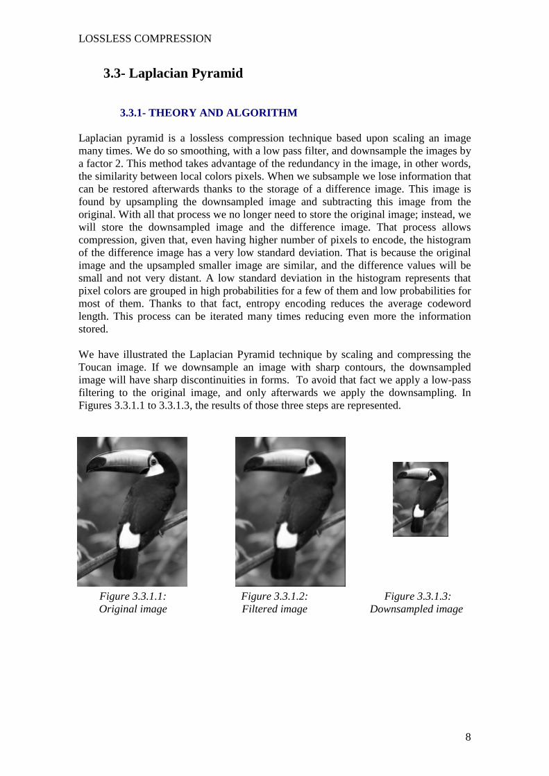
Laplacian pyramid is a lossless compression technique based upon scaling an image many times. We do so smoothing, with a low pass filter, and downsample the images by a factor 2. This method takes advantage of the redundancy in the image, in other words, the similarity between local colors pixels. When we subsample we lose information that can be restored afterwards thanks to the storage of a difference image. This image is found by upsampling the downsampled image and subtracting this image from the original. With all that process we no longer need to store the original image; instead, we will store the downsampled image and the difference image. That process allows compression, given that, even having higher number of pixels to encode, the histogram of the difference image has a very low standard deviation. That is because the original image and the upsampled smaller image are similar, and the difference values will be small and not very distant. A low standard deviation in the histogram represents that pixel colors are grouped in high probabilities for a few of them and low probabilities for most of them. Thanks to that fact, entropy encoding reduces the average codeword length. This process can be iterated many times reducing even more the information stored. We have illustrated the Laplacian Pyramid technique by scaling and compressing the Toucan image. If we downsample an image with sharp contours, the downsampled image will have sharp discontinuities in forms. To avoid that fact we apply a low-pass filtering to the original image, and only afterwards we apply the downsampling. In Figures 3.3.1.1 to 3.3.1.3, the results of those three steps are represented.
Figure 3.3.1.1: Original image
Figure 3.3.1.2: Filtered image
Figure 3.3.1.3: Downsampled image
LOSSLESS COMPRESSION
9
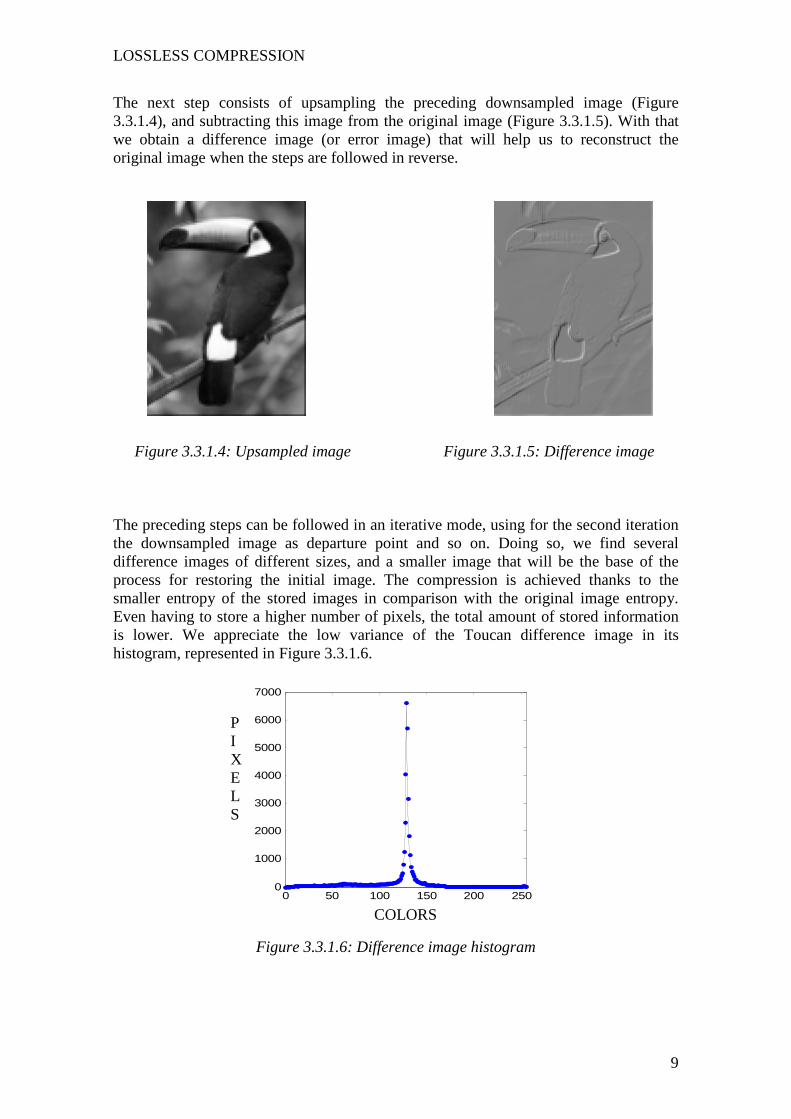
The next step consists of upsampling the preceding downsampled image (Figure 3.3.1.4), and subtracting this image from the original image (Figure 3.3.1.5). With that we obtain a difference image (or error image) that will help us to reconstruct the original image when the steps are followed in reverse.
Figure 3.3.1.4: Upsampled image
Figure 3.3.1.5: Difference image
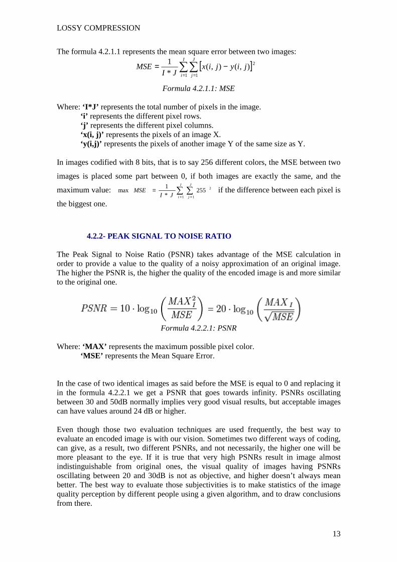
The preceding steps can be followed in an iterative mode, using for the second iteration the downsampled image as departure point and so on. Doing so, we find several difference images of different sizes, and a smaller image that will be the base of the process for restoring the initial image. The compression is achieved thanks to the smaller entropy of the stored images in comparison with the original image entropy. Even having to store a higher number of pixels, the total amount of stored information is lower. We appreciate the low variance of the Toucan difference image in its histogram, represented in Figure 3.3.1.6.
Figure 3.3.1.6: Difference image histogram
0 50 100 150 200 2500
1000
2000
3000
4000
5000
6000
7000
COLORS
P I X E L S

LOSSLESS COMPRESSION
10
In Figure 3.3.1.7 we display a scheme representing the iterative Laplacian pyramid method to obtain the successive ‘difference images’ and the smaller image of the chain. Those are the images which will be used in the decoding.
Figure 3.3.1.7: Laplacian pyramid images
To decode, we only need to take the smaller image that we get after the last iteration, upsample it, and add the corresponding difference image. With the obtained image we repeat the same process. To get back the original image we iterate this process as many times as we have done in the encoding.

LOSSLESS COMPRESSION
11
3.3.2- RESULTS
A) Entropy: bits per pixel
B) Number of pixels
Stored information: A*B
CR
Original image entropy:
7.4795 bpp 34560 258492 1
Coded images 1 iteration
5.4094 bpp 43200 233687 1.11
Coded images 2 iterations:
4.7855 bpp 45360 217071 1.19
Coded images 3 iterations:
4.6402 bpp 45900 212986 1.21
Coded images 6 iterations:
4.5875 bpp 46087 211425 1.22
Coded images 7 iterations:
4.5863 bpp 46091 211388 1.22
Coded images 10 iterations:
4.5854 bpp 46094 211360 1.22
Coded images 12 iterations:
4.5853 bpp 46096 211364 1.22
Table 3.3.2.1: Results from Laplace Pyramid compression Results from applying the Laplacian Pyramid to compress the Toucan image are displayed in Table 3.3.2.1. Entropies of the difference image together with the stored small image have been computed. Multiplying it by the total number of pixels stored we obtain the information stored after coding. To compute the compression ratio we divide this amount by the information needed to store the original image without Laplacian encoding. We observe that the total amount of information stored after applying the Laplacian pyramid together with entropy coding is smaller than the information needed to store the original image. We also see that by incrementing the number of iterations we reduce the overall quantity of information. At the end the entropy tends to a limit, and, as we cannot divide the image size an infinite amount of times, each additional iteration only adds irrelevant one pixel size images. This fact is appreciable when we code this image with 12 iterations. For the Toucan image the maximum compression is achieved with 10 iterations for which we obtain a compression ratio of 1,22. The compression ratio achieved with Laplacian Pyramid is higher than for a simple entropy coding and as it is a lossless method, we can reconstruct the exact original image. The conclusion that we reach is that, finally, we can store an image by only storing a pyramid of difference images with low standard deviation.

LOSSY COMPRESSION
12
4- LOSSY COMPRESSION
4.1- Introduction In contrast with the previous chapter, this part of the project presents lossy compression techniques. Lossy compression is made up of a big group of compression methods, more efficient than lossless techniques in compression terms; this is the reason for which lossy algorithms are used presently in most applications. This kind of compression takes advantage of the incapacity of our vision to sense all the image details. This fact, allows us to store images that, not being exactly equal from the original ones, they are very similar. Storing those similar images allows us to reduce the amount of information used.
In this chapter we will introduce some important concepts that did not exist in the lossless compression world but have relevance when speaking about lossy methods. Those tools will allow us to measure in some way the quality of the resulting images after encoding. Next we present the concept of quantization. Quantization exists almost always in the lossy compression chains. Normally it is in this step when the loss of information takes place and is in this step where the maximum amount of compression is achieved. Entropy coding always closes the compression chain, after quantization.
Afterwards we will develop two important methods of lossy compression. One of them is the fractal compression, a method that had its apogee in the 80’s but, because of some disadvantages such as a high encoding time, it did not have a big impact in the market. The other presented algorithm will be a personal approach of JPEG, a very important compression method used currently in most of image applications. Those image compression algorithms have been implemented in a simple scheme with the two main functions being Coder and Decoder (algorithms annexed in the Matlab computer files).
4.2- Image quality measures
4.2.1- MEAN SQUARE ERROR
The mean square error (MSE) measures the squared differences between the pixels of two different images or image subblocks that have the same size. We compare the pixels located in the same position in both images to evaluate it. Many times, in order to find nice correspondences between the original image and the corresponding encoded image, we search to minimize such mean square error and different algorithms use this concept in its implementation. Using squared differences we are sure that all the quantities are positive, so when we add them we get always a bigger difference. If we worked without squared measures, the pixel differences could cancel each other, resulting in a low MSE and thus, in a bad measure of difference.
LOSSY COMPRESSION
13
[ ]∑∑= =
−=I
i
J
j
jiyjixJI
MSE1 1
2),(),(*
1
∑ ∑= =
=I
i
J
jJIMSE
1 1
2255*
1max
The formula 4.2.1.1 represents the mean square error between two images:
Formula 4.2.1.1: MSE
Where: ‘I*J’ represents the total number of pixels in the image. ‘i’ represents the different pixel rows. ‘j’ represents the different pixel columns. ‘x(i, j)’ represents the pixels of an image X. ‘y(i,j)’ represents the pixels of another image Y of the same size as Y. In images codified with 8 bits, that is to say 256 different colors, the MSE between two
images is placed some part between 0, if both images are exactly the same, and the
maximum value: if the difference between each pixel is
the biggest one.
4.2.2- PEAK SIGNAL TO NOISE RATIO
The Peak Signal to Noise Ratio (PSNR) takes advantage of the MSE calculation in order to provide a value to the quality of a noisy approximation of an original image. The higher the PSNR is, the higher the quality of the encoded image is and more similar to the original one.
Formula 4.2.2.1: PSNR Where: ‘MAX’ represents the maximum possible pixel color. ‘MSE’ represents the Mean Square Error.
In the case of two identical images as said before the MSE is equal to 0 and replacing it in the formula 4.2.2.1 we get a PSNR that goes towards infinity. PSNRs oscillating between 30 and 50dB normally implies very good visual results, but acceptable images can have values around 24 dB or higher. Even though those two evaluation techniques are used frequently, the best way to evaluate an encoded image is with our vision. Sometimes two different ways of coding, can give, as a result, two different PSNRs, and not necessarily, the higher one will be more pleasant to the eye. If it is true that very high PSNRs result in image almost indistinguishable from original ones, the visual quality of images having PSNRs oscillating between 20 and 30dB is not as objective, and higher doesn’t always mean better. The best way to evaluate those subjectivities is to make statistics of the image quality perception by different people using a given algorithm, and to draw conclusions from there.

LOSSY COMPRESSION
14
4.3- Quantization Quantization is one of the most important steps in lossy image compression. To quantize means to give a finite number of values to represent image data. In digital systems the information is always quantized, even without compression, but when using quantizers we reduce the possible set of values. Those values can represent directly the color pixel values or some other features in relation with the image pixels. In the case of scalar quantization [8] or PCM, we reduce the range of possible color values. Another kind of quantization is the vector quantization [9], where the stored values represent groups of pixels in an image. In this case we use a codebook with different blocks which combination and organization can approach an original image. In a vector quantization, rather than store the pixel values, we provide a codebook of ‘vectors’ and we store the vector positions, from the codebook, that works well to restore an image reducing the losses and thus increasing the PSNR as much as possible. The quantization step is normally implemented after some image preprocessing, and it is in this step when we lose information, so after quantizing, the restitution of the original image is no longer possible if before we did not store the differences between the non-quantized and quantized data. On Figure 4.3.1 we show a simple PCM quantization, consisting of coding with fewer bits an image initially coded with 8 bits. The number of grey scale colors is related with the number of bits per pixels by the relation: different grey scale values = 2^bpp (bpp: number of bits per pixel). We observe that beyond a certain number of bits per pixel, we cannot distinguish differences between the original image and the quantized one, because our eye does not have such precision. This threshold varies from one person to another but normally it oscillates between six and seven bits per pixel.
Figure 4.3.1: Scalar quantization images (from 1 to 8bpp)

LOSSY COMPRESSION
15
4.4- Fractal compression
In this section we have implemented two different fractal compression algorithms giving an impression of what fractal compression is about. Both algorithms are based on fractal compression literature and they try to show the most important concepts related with this kind of compression. The first one is a very simplified view and the second one goes more deeply into the iterative fractal approach.
4.4.1- FRACTAL DEFINITION AND CONCEPTS
A fractal is a mathematical object that has resolution at all levels, and which has self similarity at different scales. This self similarity is achieved using affine transformations: rotation, stretching, compression and translation of an input image [10]. In order to find fractal images with a computer we can use the iterated function systems (IFS). Such a system takes an image as input, and applies to that image some affine transformations, until we get an output image. We iterate by using this output image as input and applying to it the same affine transformations. Little by little we approach an image which receives the name of attractor. The attractor doesn’t depend on the input image; it only depends on the affine transformations defined at the beginning. To see more precisely the precedent concepts, in Figure 4.4.1.1 we have implemented an IFS and we have applied it to two different input images. We observe how after some iterations we get the same attractor because, as said before, the attractor only depends on the affine transformations used. Fractal image compression relies on the fact that some parts of an image are similar to other parts. Applying a certain number of affine transformations to the different parts of the image and iterating, the fractal algorithm leads to an image attractor which approaches the original image [11, 12]. Original image 1 iteration 4 iterations 6 iterations Figure 4.4.1.1: IFS applied to two different input images.

LOSSY COMPRESSION
16
1) Division of the image in regions
(e.g: 32*32 pixels)
4)Division of the image in range blocks (e.g:8*8 pixels)
3)Taking one domain block for each region, called reference blocks.
They are the blocks keeping most similarity with the other domain
blocks of the region.
6) Storage of codebook and positions found when searching matches between reference and range blocks.
2) Division of the regions in
domain blocks (e.g:16*16
pixels)
5)For every range block we search the reference block of the codebook that matches the best
4.4.2- FIRST FRACTAL ALGORITHM
4.4.2.1- THEORY AND ALGORITHM
The first of our developed algorithms is based in the paper ‘A simplified fractal image compression algorithm’ [13]. It is an algorithm that takes only a few ideas of fractal compression, but important concepts like the iterations leading to an attractor, are not present here. On the other hand, it shows well how to code an image searching self-similarities within it, which is a very important feature of the fractal procedure. Another well shown method in the algorithm which schema is displayed in Figure 4.4.2.1.1 is the implementation of vector quantization. For this reason we have considered it appropriate to place this chapter after the quantization part (Chapter 4.3) that already showed the principle of scalar quantization, but in which the vector quantization was not illustrated. In this algorithm, which organization is showed in Figure 4.4.2.1.1, we are interested in searching self-similarities within an image and to store the best possible codebook, formed by a pool of blocks similar to many other parts of the image; those blocks are called reference blocks. That will allow us to restitute the image after decoding, organizing the blocks of the stored codebook to form an image approaching the original one. The stored codebook is smaller in size than the entire image, and at the end of the encoding we only need to store it and the positions that will occupy those reference blocks when decoding the image.
Figure 4.4.2.1.1: First fractal algorithm scheme

LOSSY COMPRESSION
17
As we can see in Figures 4.4.2.1.1 and 4.4.2.1.2, the first step in the algorithm is based on a region division of the original image (dark blue blocks). In the second step, we divide all the regions in domain blocks (blue sky blocks). After that we perform a search for each region in order to find the domain block that best describe the region, that is to say, the most similar domain block to the other domain blocks of the region. This search is done looking for the minimum MSE between blocks. Such blocks (orange blocks, one by region) will make up the codebook with which we will reconstitute the image regions in the decoding phase. Now we only need to find where the small blocks forming the reference blocks (yellow blocks) must be placed to match with the different range blocks of the image (green blocks). We do so, by dividing the original image in range blocks, and for each of them, searching the small block from the codebook that best match with it, by means of reducing the MSE. The codebook from each region is formed by the small blocks from the found reference block representing the region. In the decoding we only have to place the different small blocks from the codebook in the positions that we have stored (positions that indicate the best match with the range blocks from the original image). Doing so, we use the self-similarity property, to make up a decoded image thanks to the only translation of a subset of blocks. This technique consists of storing a codebook of blocks (vectors), and the positions that must occupy those blocks at the decoding, is the form of vector quantization.
Figure 4.4.2.1.2: First fractal algorithm diagram
EEnnccooddiinngg
DDeeccooddiinngg
… …
… … . . .
.
.
.
.
.
.
.
.
.

LOSSY COMPRESSION
18
4.4.2.2- RESULTS Hereafter we present the results for two different images: Lenna and Toucan images. First of all we give an introduction to the calculated features and the calculation method. After that we present the most relevant results organized in tables, and two coded images are displayed for better visualization. The numerical developments are presented in Annex 1. Calculated Features: A) Coding elapsed time B) Decoding elapsed time: Time that it takes the coding/decoding algorithm to reach a result using an INTEL processor at 1,80GHz. C) PSNR: Power Signal to Noise Ratio (see Chapter 4.2) D) Compression Ratio (CR): The ratio between the bits used to code the original image and the bits used to store the compressed image is called compression ratio (CR). This ratio is the division of the total amount of bits used to store the original image and the bits used to store the compressed image. To compute it we need to know the total amount of pixels stored in the codebook, the bits that we need to store every pixel of the codebook (codebook entropy), the total amount of stored positions, and the bits that we need to store every position. We have to remember that to decode each region we are restricted to the usage of only a reference block, so it is as if we had a small codebook for every region, corresponding to the reference block of the region. This fact greatly limits the bits that we need to store a position. d1) Codebook size (in bits)= Nº of pixels in codebook* codebook entropy d2) Stored positions for block decoding= Range blocks= Number of regions*Number of small blocks in a region d3) Bits per stored position= Log2 (nº of pixels in a ref block / nºof pixels in a small block) Total Bits Stored (TBS)= d1+d2*d3 bits CR= (TBS) / (Original image size in bits) E) Bits per pixel in decoded image = TBS / nº of pixels

LOSSY COMPRESSION
19
Other important information that has to be stored is the size of the image and three input parameters corresponding to the region size, the reference block size and the range block size. The space on bits occupied by this information is very small compared with the rest of stored data, so it will be neglected in our compression calculations. On the other hand those parameters are indispensable because the coding results depend solely on them. For that reason the results are organized by coding parameters following the notation: Coding parameters: -region size, reference block size, range block size-.
Synthesis of results:
Coding parameters A B PSNR CR BPP 1: -32, 16, 4-
~1.58s ~0.56s 21.21 3.56 2.1
2: -16, 8, 4- ~0.72s ~0.52s 19.79 3.69 2.03 3: -8, 4, 2- ~1.23s ~0.44s 22.56 3.19 2.35 4: -16, 4, 2- ~1.81s ~0.59s 19.22 7.64 0.98
Table 4.4.2.2.1: First Fractal algorithm results synthesis (Toucan)
Coding parameters A B PSNR CR BPP 1: -32, 16, 4- ~7.02s ~2.27s 22.58 3.54 2.1 2: -32, 16, 4- ~2.82s ~2.24s 23.13 3.77 1.97 3: -32, 16, 4- ~9.30s ~3.08s 27.15 3.16 2.35 4: -32, 16, 4- ~12.95s ~4.26s 22.77 7.77 0.95
Table 4.4.2.2.2: First Fractal algorithm results synthesis (Lenna)
Figure 4.4.2.2.1: Decoded Toucan with CP: 8,4,2
Figure 4.4.2.2.2: Decoded Lenna with CP: 8,4,2

LOSSY COMPRESSION
20
From the results displayed in Tables 4.4.2.2.1 and 4.4.2.2.2 we can draw the conclusion that the algorithm used is quite poor in terms of quality/compression. The PSNRs are situated around 19-23 in most of cases, and only with Lenna and the coding parameters in case number 3 we achieve a PSNR of 27. The block effect derived from this coding is highly visible. To get better visual results we could for example apply a low pass filter in order to smooth the block effect. Another thing that we could do is code the difference image between the original one and the decoded one, but in that case the compression ratio would decrease substantially. On the other hand we can see that the algorithm is fast and the image can be coded in a few seconds. The most time consuming part of the algorithm is the research of reference blocks that represents at best the domain blocks from each region, so when we have many domain blocks in a region, the coding time increases. We also observe that the decoding is faster than the coding phase, having times which oscillate between 0.5 and 5 seconds for images going until 512x512 pixels. Another result that we can draw is that in general we obtain better qualities coding a big image than coding a small one. Lenna image is bigger than Toucan image and we obtain higher PSNRs for the same coding parameters; we observe that in images 4.2.2.1 and 4.2.2.2. In fact, for bigger images the block resolution is higher, because we continue using blocks of the same size while the detail dimensions are bigger; so the relation ‘(details size)/(block size)’ is also bigger. The last conclusion is that we obtain very similar compression ratios when we work with the same coding parameters with different images. This is logical because we are using the same algorithm and doing the calculations for two images helps us to verify this fact.

LOSSY COMPRESSION
21
1) Division of the image into 16x16
overlapping blocks
4) Division of the image into non-overlapping
range blocks (8*8 pixels)
3) Apply rotations and mirror symmetries to the subsampled
blocks (domain blocks)
6) Apply contrast ‘s’ and brightness ‘o’ minimizing
the MSE distance between both range and
domain blocks
2) Subsample of the previous
blocks
5) For every range block, we find the domain block that
matches the best, by means of MSE
7) We store the positions, the rotation transformations, the contrasts and the brightness that we have found allowing us to decode the image.
4.4.3- SECOND FRACTAL ALGORITHM
4.4.3.1- THEORY AND ALGORITHM
The second fractal algorithm developed is based on the steps described in the first chapter of the book: Fractal Image Compression, theory and applications [14]. In this algorithm, new based fractal features not seen in the chapter 4.4.2 are implemented. The concept of iterations used to approach more and more the attractor, geometrical transformations as rotations of the codebook blocks [15], and other transformations as contrast and brightness are applied to find the best possible match between the original image and the coded one. With this algorithm we see the real power of the fractal approach, allowing us to reconstitute an entire image without storing any specific codebook and storing only block transformations. When decoding, those transformations are applied iteratively to an arbitrary image, of the same size of the coded one, used as input in the decoder. The organization of the coding algorithm is showed in the Figure 4.4.3.1.1:
Figure 4.4.3.1.1: Second fractal algorithm scheme

LOSSY COMPRESSION
22
In the scheme showed in Figure 4.4.3.1.1 we see the steps followed to accomplish the encoding of the image. The first step of the algorithm consists of dividing the image in overlapping blocks of 16x16 pixel size. Those blocks will be subsampled reducing its size to 8x8 and we will apply all the possible rotations and mirror effects to each block in order to achieve eight different symmetric configurations of a single block. Those blocks will be called domain blocks and they will form our data base from where we will find the image attractor when encoding. The attractor is the image that approaches the original image using its own self similarities. In Figures 4.4.3.1.2 we can see the division in overlapping blocks (left) which are subsampled and transformed afterwards by applying eight different symmetries to each one of them in order to find the domain blocks (right).
Figure 4.4.3.1.2: Domain blocks for one of the overlapping blocks. On the other hand we will divide the image in non-overlapping range blocks of 8x8 pixel size, as described in step four. For each one of the range blocks we will search the domain block that best matches it. We do so by means of finding the minimum MSE between a given range block and the domain blocks. In Figure 4.4.3.1.3 we have made a diagram where we show, for an original image (left), the process of coding. We search the domain blocks that once subsampled and rotated best matches each one of the range blocks (center and right). In the diagram, the white square boundaries represent the distribution of overlapping domain blocks (center) and the non-overlapping range blocks (right).
Figure 4.4.3.1.3: original image (left). Matching block research (right).

LOSSY COMPRESSION
23
−= ∑=
n
iii baMSE
1
2' )(
−
−=
∑ ∑
∑ ∑ ∑
= =
= = =n
i
n
iii
n
i
n
i
n
iiiii
aan
babans
1 1
22
1 1 1
)(
−= ∑ ∑= =
n
i
n
iii asb
no
1 1
1
osaa ii +⋅='
Once we have found the best possible match, we will try to get the domain blocks very close visually to the correspondent range blocks. We do that by applying contrast ‘s’ and brightness ‘o’ transformations to the domain blocks. Those parameters are applied to all the pixels (ai) from a domain block in order to get a new block (ai’) that approaches as much as possible a given range block (Formula 4.4.3.1.1).
Formula 4.4.3.1.1: contrast and brightness block transformation. Contrast and brightness are two scalar quantities optimized to minimize the MSE between domain and range blocks (Formula 4.4.3.1.2). The minimum of MSE occurs when the partial derivatives with respect to ‘s’ and ‘o’ are zero, from that fact we find the Formulas 4.4.2.1.3 [14].
Formula 4.4.3.1.2: contrast and brightness block transformation.
Formula 4.4.3.1.3: contrast and brightness block transformation. The last step is to store all the found parameters, that is to say, the overlapping block position and geometrical transformation (one among eight) that best matches every range block, and the two transformations ‘s’ and ‘o’ that we have to apply to those domain blocks, allowing us to minimize the MSE with every range block. After storing all those features, the image is entirely encoded in the form of a collection of transformations. To decode the image we input an arbitrary image of the same size of the encoded image to the decoder. The other decoder inputs are the outputs of the encoder, that is to say, all the stored positions and transformations. When decoding, those transformations will be applied to the arbitrary decoder image input. In the decoding step we will apply many iterations approaching little by little the attractor that we had found in the encoding step. We could say that, in fractal compression, all the necessary information to decode an image is stored in form of transformations that we apply to a random input image in order to decode the original image.

LOSSY COMPRESSION
24
4.4.3.2- RESULTS In this subchapter we present the numerical results and the images obtained with the Fractal 2 algorithm. The calculation method used to compute the CR and some more images obtained with this compression algorithm, are presented in Annex 2. Working with the parrot image, we observe that we get a low resolution because the image is quite small and the details are big compared with the domain block size. Because of that fact we get quite low values of PSNR (around 23dB) for this image. In Figure 4.4.3.2.1 we have displayed different iterations from the decoding phase, and we see that even taking very different images as decoder input, at the end we get good approximations of the original coded image, the limit always being the attractor; in that case, the parrot attractor.
Figure 4.4.3.2.1: Fractal coded parrot image
1 iteration
8 iterations
Decoder input
2 iterations

LOSSY COMPRESSION
25
In Figure 4.4.3.2.4 we observe the evolution of visual image quality when increasing the number of decoding iterations. In fact, we can get a good approximation of the attractor PSNR (31dB) with only eight iterations. The image series from this figure have been decoded using as input a 512x512 grey image. 1 iteration 2 iterations 3 iteration 5 iterations 8 iterations 15 iterations
Figure 4.4.3.2.2: Fractal compressed Lenna image decoding

LOSSY COMPRESSION
26
In Figure 4.4.3.2.3 we have displayed the Lenna attractor image. The PSNR of the Lenna attractor is around 30dB. We observe that, in general, the PSNR improves for bigger images because with them we have a better detail resolution.
Figure 4.4.3.2.3: Lenna attractor
In Table 4.4.3.2.1 we display the synthesis of the obtained results after coding and decoding every one of the three images using the Fractal algorithm. In it, the results of encoding time (T), power signal to noise ratio (PSNR), compression ratio (CR) and amount of bits per pixel (BPP) are presented. The PSNR results are given for the image attractors. We find it by decoding when using the original image as decoder input image and applying an only iteration. We observe that for big images the CR tends to be a little smaller, because we need more bits to store every one of the domain blocks position. On the other hand the bits used to store the rotations and the color transformations are linearly proportional to the image size. Comparing the achieved CRs results with literature results [14] where they obtain a CR of 16.5 for an image of 256*256 pixels, we observe that for similar image sizes, we obtain similar CRs (CR of 15.44 for Toucan image).
IMAGES T PSNR CR BPP Parrot ~25min 23.71dB 15.99 ~0.48bpp Toucan ~65min 29dB 15.44 ~0.48bpp Lenna ~52h 31.83dB 14.40 ~0.52bpp
Table 4.4.3.2.1: Main results from Fractal compression algorithm

LOSSY COMPRESSION
27
Table 4.4.3.2.2 displays the decoding times and the PSNRs in function of the number of iterations. We observe that after a certain number of iterations, the PSNR approaches a limit and stops to increase. This limit is close to the attractor image PSNR. From those results we can draw the conclusion that this algorithm is capable to achieve acceptable compression ratios and PSNRs, which improves when coding big images because of the better detail resolution. Using this algorithm the block effect is still visible but very reduced, the transitions between one range block to the next one being quite soft. Even so, the encoded images have not a perfect visual quality and it is still very difficult to confound the original image with the compressed one. To improve even more the image quality it would be possible to store the quantized difference image obtained when subtracting the encoded image to the original one.
Table 4.4.3.2.2: Fractal decoding results for different iterations One of the main disadvantages of this Fractal algorithm is the high encoding time needed to find the attractor; not being the case in the decoding step. Coding the parrot image takes 25 minutes, and coding Lenna (512x512 pixels) goes up to 2 days. It is for this reason that it would interesting to have a way to predict the time that a big image takes to be encoded. We present a method to compute such a prediction in Annex 3 and we use it to predict the time of the Lenna encoding time in function of the Parrot encoding time. A possible solution to reduce the encoding time could be to use a MSE threshold when searching good matches between range and domain blocks. Doing so, the research for the current range block would stop when the found MSE would be inferior to the MSE threshold.
Parrot image Toucan image Lenna image
Iterations Decoding time (s)
PSNR (dB)
Decoding time (s)
PSNR (dB) Decoding
time (s)
PSNR (dB)
1 ~0.12 11.42 ~0.19 14.88 ~1.34 15.23 2 ~0.18 13.82 ~0.41 16.9 ~2.32 17.40 3 ~0.25 16.36 ~0.42 19.26 ~3.61 20.04 4 ~0.32 18.83 ~0.47 21.45 ~4.73 22.86 5 ~0.38 20.60 ~0.64 23.35 ~5.72 25.58 6 ~0.45 21.67 ~0.87 24.68 ~6.70 27.78 7 ~0.51 22.25 ~0.93 25.66 ~8.35 29.31 8 ~0.58 22.53 ~1.16 26.29 ~8.52 30.15 15 ~1.15 22.76 ~1.78 27.19 ~15.08 30.80 20 ~1.38 22.76 ~2.56 27.21 ~29.63 30.80

LOSSY COMPRESSION
28
4.5- JPEG Compression
In this section we expose an algorithm developing the main features of a JPEG compression algorithm. We have tried to apply the most relevant aspects of JPEG with a MATLAB algorithm performing the functions of coding and decoding. Nowadays, JPEG is one of the most used techniques for image coding, because this technique gives good compression factors and PSNRs, at the same time that it is a very fast technique compared with fractal coding. JPEG compression is a method that collects many image processing and compression techniques as different as “differential pulse code modulation” (DPCM) or “discrete cosine transform” (DCT). The base of JPEG consists on eliminate the high color frequencies of the image, those that are less evident to our eyes, and keep only the lower frequencies. In the following sections we analyze the different parts which make up JPEG and afterwards we will see how they are organized together in the whole JPEG coder/decoder algorithm.
4.5.1- CORRELATION AND DPCM
DPCM is one of the compression techniques used in JPEG [16]. This method exploits the high color intensity correlation that exists in the same regions of an image, having variations between one pixel and the following one that can be approximated by a linear prediction. This approximation is very imprecise and for that reason, after applying linear prediction to an image, we have to code the difference image too, to be able to restitute the original image. To store the difference image requires few memory when it is entropy coded, because of its low entropy. To decode, we apply the predictor to the initial coefficients to create the predicted image and then adding the difference image we get the decoded original image. A linear predictor consists in some coefficients that applied to some image pixels returns a new pixel that conserves the intensity color evolution trend. A simple linear predictor would be deduced assuming the fact that the difference between a pixel and the precedent one must be equal to the following pixel minus the current one. Doing so we have:
Formula 4.5.1.1 Using the Formula 4.5.1.1 we can deduce a linear approximation of a pixel i having the value of the two precedent pixels. In this case the linear predictor coefficients are 2 and -1.
Pixel(i-1)-Pixel(i-2)=Pixel(i)-Pixel(i-1) => Pixel (i)= 2*Pixel(i-1) - 1*Pixel(i-2)

LOSSY COMPRESSION
29
The information that we have to store in order to apply DPCM is formed by the linear predictor coefficients, some initial pixel values from the original image that we use to apply the linear prediction, and the pixel values of the difference image that we get subtracting the linear predicted image to the original image. The lossy or lossless character of DPCM technique is given by the existence or not of difference image quantization. The linear predictor presented in formula 4.5.1.1 is used for 1 dimension linear prediction, but when working with images we can use information coming from two dimensions. One of the easiest forms to make a prediction is to use an average of the pixels surrounding the pixel for which we want to deduce its value. Knowing that the pixels of a same region have tendency to get similar values, that kind of prediction allow us to reduce the entropy of the difference matrix, and thus, reduce the amount of information to store. The Formula 4.5.1.2 describes the behavior of the presented predictor:
Formula 4.5.1.2
Applying the precedent predictor with the Toucan image we obtain the results presented in Figures 4.5.1.1 to 4.5.1.4.
Figure 4.5.1.1: ‘Initial image’: Pixels used for the prediction
Figure 4.5.1.2: Predicted image
Figure 4.5.1.3: ‘Difference image’ (original-predicted)
Figure 4.5.1.4: Initial+difference
Using such predictor and storing the difference image plus the initial pixels, the Toucan image that normally needs 2.5849*105 bits to be stored, would need 2.1274*105 bits; resulting in a CR of 1.215. In fact the image formed by the initial pixels plus the difference image (that are the stored pixels) has an entropy of 6.16 while the original image has an entropy of 7.4795. Operations: Original image: 216*160*7.4795=2.5849*105 bits Coded image: 216*160*6.16=2.1274*105 bits
0.25*Pixel (i ,j-1) + 0.25*Pixel(i-1, j) + 0.25*Pixel(i-1, j-1) + 0.25*Pixel(i-1, j+1)]= Pixel(i,j) Predictor Coefficients: [0.25, 0.25, 0.25, 0.25]

LOSSY COMPRESSION
30
We have also tried to use a 2D linear predictor with four coefficients but the obtained results, in terms of the stored data entropy, were worse that using an average predictor, so we have used the average one for our JPEG algorithm. Our four coefficient linear predictor had the coefficients: And so, calculating the prediction in three directions of our image (diagonally, by rows and by columns), the predicted pixels responded to the formula 4.5.1.3:
Formula 4.5.1.3 The performed prediction took 4 rows and 4 columns every 10, like first coefficients. Applying such predictor with the Toucan image we obtained the results in Figures 4.5.1.6 to 4.5.1.8. Using such predictor the stored bits for Toucan image had been 2.5849*105; resulting in a CR of 1.012. We have computed this result using the entropy of 7.39 from the stored image (initial pixels + difference image). We can see that we obtain better results with the average predictor, because with a linear predictor the errors increase when we are far from the given initial values. Such error is reduced with an average predictor where the value of the researched pixel is always delimited by the higher and the lower pixel values that we have used to calculate it.
Figure 4.5.1.5: ‘Initial image’: Pixels used for the prediction
Figure 4.4.5.1.6: Predicted image
Figure 4.5.1.7: ‘Difference image’ (original-predicted)
Figure 4.5.1.8: Initial+differentce
a=pixel(i,j-1)*p(1) + pixel(i,j-2)*p(2) + pixel(i,j-3)*p(3) + pixel(i,j-4)*p(4); by columns b=pixel(i-1,j)*p(1) + pixel(i-2,j)*p(2) + pixel(i-3,j)*p(3) + pixel(i-4,j)*p(4); by rows c=pixel(i-1,j-1)*p(1) + pixel(i-2,j-2)*p(2) + pixel(i-3,j-3)*p(3) + pixel(i-4,j-4)*p(4);
=> Predictedpixel=(1/3)*(a+b+c)
Linear predictor coefficients P(i) = [1.2, 0.8, -0.75, -0.25]

LOSSY COMPRESSION
31
4.5.2- DISCRETE COSINE TRANSFORMATION Discrete Cosine Transform, more commonly called DCT, is at the heart of JPEG compression. In fact, this technique allows us to decompose the image information in its intensity color frequencies (Figure 4.5.2.1), keeping only the real part of a Discrete Fourier Transform (DFT) [17]. This decomposition allows us to filter the image in a very simple way. In fact, the DCT tends to concentrate the information in the first coefficients and keeping only few DCT coefficients we can restitute a good approximation of an image losing little information.
Figure 4.5.2.1: Intensity color frequencies
The DCT is defined by the Formula 4.5.2.1 [18], where B is the DCT output of an image A. In this formula, M and N are the dimensions in pixels of the image:
Formula 4.5.2.1: DCT of an image A Formula 4.5.2.2 is used to compute the inverse discrete cosine transform iDCT, which is used to restitute an image from its DCT spectrum.
Formula 4.5.2.2: Inverse DCT of a DCT spectrum B

LOSSY COMPRESSION
32
When working with images, the DCT transformation is applied in two dimensions and normally by small blocks of 8x8 pixels or more. After applying it, we get new blocks of the same size, containing the block frequencies. Lower frequencies are located at top left of the new blocks, while higher frequencies are located at bottom right. In Figure 4.5.2.2 we have displayed the complete DCT of an image. In Figures 4.5.2.4 and 4.5.2.5 we have displayed the DCT spectrums of the Parrot image by 8x8 pixel blocks and by organized DCT coefficients, respectively. The black and white colors from the DCT spectrums represent higher magnitude DCT coefficients when grey color represents lower coefficients. In Figure 4.4.2.3 we observe that, normally, higher magnitude coefficients are placed at the top left corner of the 8x8 pixel blocks. When we organize the block spectrums by its DCT coefficient number it becomes very clear that first coefficients have much more energy that the rest. That means that keeping only the first coefficients, that is to say the lower frequencies, we could restore the original image with few losses. This is the principle of JPEG which stores only the more energetic DCT coefficients and restitutes the image using the iDCT with those stored coefficients.
Figure 4.5.2.2: Detail from Parrot image and its DCT spectrum
Figure 4.5.2.3: Parrot DCT spectrum by 8x8 pixel blocks
Figure 4.5.2.4: Parrot DCT spectrum with the coefficients grouped

LOSSY COMPRESSION
33
4.5.3- QUANTIZATION In JPEG the quantization is performed by 8x8 pixel blocks, and it is not directly applied to the image blocks, but to the block spectrum that we get after DCT image transformation. For the block quantization we can use different 8x8 matrices. One of the most used is the quantization matrix presented in Figure 4.5.3.1:
Figure 4.5.3.1: JPEG quantization matrix
In JPEG, once we have performed the DCT with each 8x8 pixel block, we divide every DCT block coefficient by the corresponding quantization matrix coefficient and we round the resulting values. Doing so, a lot of the DCT quantized coefficients becomes null, and at the same time we reduce the block standard deviation and thus we reduce its entropy. This matrix can also be multiplied by a quality coefficient ‘Q’ which allows tuning the quantization, reaching higher compression but lower quality when it is high, and higher quality but lower compression when it is low.
4.5.4- ZERO-RUN Zero run encoding (ZRE) is a form of run length encoding (RLE) consisting into code a long stream of zero values with a simple symbol representing the number of consecutive zeros. In fact when quantizing the DCT coefficients with JPEG we obtain a high number of zero coefficients and it is often interesting to use zero-run, instead of coding every zero using the same codeword repeated as many times as consecutive zeros we have. Frequently this technique reduces the amount of stored information. Example of zero-run encoding: Stream: 50, 0, 0, 0, 0, 0, 0, 4, 5, 0, 0, 0, 0, 9 The precedent stream would be coded like: 1, 50, 6, 0, 1, 4, 1, 5, 4, 0, 1, 9 Where the italic characters represent the number of zero values coded from the initial stream. We can appreciate the reduction in the number of symbols to be coded, after applying the zero run encoding.
Q=

LOSSY COMPRESSION
34
4.5.5- JPEG ALGORITHM: THE ENCODER In order to develop a JPEG encoder, we have to put together all the concepts previously seen in this subchapter 4.5. First of all, we give a diagram where we can see how the image processing techniques must be organized (Figure 4.5.5.1) [19], and after that we explain how our encoder has been implemented. Following, the organization of our developed JPEG algorithm is presented:
Figure 4.5.5.1: JPEG algorithm scheme As shown in the Figure 4.5.5.1 to encode an image using JPEG first of all we divide the original input image into 8x8 pixel blocks and we apply the DCT to every one of those blocks. Then, we quantize the blocks by dividing every one of the block coefficients by the quantization matrix coefficients multiplied by the quality factor, as described in section 4.5.3.
Input: image 1) We work by blocks of 8 by 8
pixels
4) We organize the coefficients of every
block in vectors, following a diagonal zig-zag configuration
3) We quantize the DCT blocks, using the quantization matrix and the quality factor given as input to
the coder
7) We apply zero-run coding to the AC
coefficients, and we remove the last zero coefficients of each
vector
2) We apply the DCT transform to each block
5) We put together the DC coefficient of each one of the vectors in a
matrix
6) We apply the DPCM compression technique
to the DC matrix coefficients
Outputs: DPCM outputs
8) We store the AC coefficients coded with zero-run or not, depending on the vector. Only coded with ZLC if
it diminishes the number of stored values. Outputs: coded AC vectors

LOSSY COMPRESSION
35
After quantization, we get smaller coefficients presenting a smaller standard deviation between them and a lot of them became null. If we use a high quality factor, the quantization matrix coefficients will be high and after dividing the DCT blocks by this matrix, we will get very low coefficients that, after rounding, will become null in most cases, thus the compression achieved will be higher. The next step consist into organize the gotten coefficients in a vector, following a zigzag ordering [20] that allows us to group the higher coefficients together and leave the null coefficients at the end of the vector (Figure 4.5.5.2).
Figure 4.5.5.2: JPEG coded coefficients organization
After organizing the block coefficients into vectors the algorithm is shared into two main tasks: In one hand we group together all the DC coefficients in a matrix. Those coefficients are the continuous color component of each block (color offset), that are situated in the first component of each DCT block. After grouping, we apply the DPCM compression described in section 4.5.1 to the DC coefficient matrix. In our algorithm we have used the averaging predictor for the DPCM, and we have stored one row and one column each five like a subset of initial coefficients. After that, we have performed the prediction using this coefficient subset and the averaging predictor; subtracting it from the original DC coefficients we got the difference matrix that we will use in the decoding together with the subset of initial coefficients to reconstitute the coefficients DC. On the other hand we work with the AC coefficients to store them using the lower possible amount of bits. First of all, we eliminate the null coefficients at the end of the vectors representing the DCT quantized blocks. The null coefficients can be reconstituted in the decoding phase adding zeros until reaching 64 coefficients per vector. We use the described zero-run technique to diminish the number of coefficients to be coded, when possible. We only have used zero-run with the vectors that becomes shorter when applying it, otherwise we transmit the AC coefficients without ZRE. In short, at the end of the JPEG coding, our outputs are the AC vectors coded with zero-run or not, depending on the vector; the initial DC coefficients allowing us to perform the linear prediction, and a difference matrix allowing us to restitute the DC coefficients. Those three data structures, entropy coded [21], will be passed as input to the JPEG decoder in order to find the decoded image.

LOSSY COMPRESSION
36
1) We take as input the outputs
of the JPEG coding funtion
4) We add zeros to the vectors until reaching
64 coefficients per vector (8x8)
7) Reorganization of the vectors coefficients into
8x8 DCT blocks
2) Reconstitution of the DC components matrix using DPCM
4) Reconstitution of the vectors with the first
component being a DC coefficient and the others being the AC coefficients
3) Decoding of the vectors containing the AC coefficients that
were coded using zero-run coding
8) Dequantizing using the JPEG quantization matrix and the same
quality factor that has been used in the
encoding
3) We apply the iDCT to the obtainded
dequantized blocks, to get the colour pixel
blocks
3) Reorganization of the blocks to get the
decoded image in output
4.5.6- JPEG ALGORITHM: THE DECODER The JPEG decoder follows the same steps of the encoder in reverse order. The scheme showed in Figure 4.5.6.1 represents the organization of the decoder algorithm.
Figure 4.5.6.1: JPEG algorithm decoding scheme In order to decode we have to reconstitute the vectors that will form the DCT decoded blocks. In the first place, we use the DPCM method to reconstitute the DC coefficients thanks to the initial DC coefficients and the difference matrix passed as input argument to the decoder. After doing so and knowing that the encoder used two different codewords to know if a vector was coded using zero-run or not, we decode the AC vectors that had been codified using zero-run, we concatenate each DC coefficient with every one of the AC vectors and we add zeros at the end of the vectors until getting 64 coefficients per vector. With that, we can reconstitute the 8x8 blocks reorganizing the vector coefficients inside the blocks using the zig-zag JPEG configuration.

LOSSY COMPRESSION
37
The next step consists into dequantize the blocks using the same quality factor and matrix quantization as we have used in the encoder, but this time multiplying each term of the 8x8 block, instead of dividing them by the quantization matrix coefficients. The blocks that we obtain when decoding are not exactly the same blocks that we had obtained applying the DCT in the encoding step, because we have lost information in the quantization step. Once we have reconstituted the 8x8 DCT blocks, we apply the iDCT transform to those blocks and we reorganize them in order to get the decoded image. The decoded image quality will depend on the quality factor that we have used to encode and decode the image. With a very low quality factor we will have almost no loses and our PSNR will go towards infinity. On the contrary if the used quality factor is high, the PSNR will be small and the CR will increase because we are storing less coefficients, and the stored ones will own a lower standard deviation, so a lower entropy.
4.5.7- RESULTS
The outputs and results that have been found using our developed JPEG algorithm are organized in tables in this part, with an explanation of the calculations done as well as other important results presented in Annex 4. Images bearing witness to the encoded image quality using different quality factors will be also displayed. Results are given for the three studied images: Parrot image Original image size in bits: (Size in pixels)*(Entropy) = 192*144*7.75=214272bits Results obtained applying the JPEG algorithm for different quality factors:
Table 4.5.7.1: JPEG compression results (Parrot)
Initial DC coefficients
entropy (bps)
Difference DC vector entropy
(bps)
Quality factor
Encoding time (s)
Decoding time(s)
PSNR (dB)
Vector length: 166
Vector length: 266
AC coded coefficients
entropy (bps) with its vector
length
0.0003 ~1.37 ~0.61 51.39 6.62 6.08 6.50 26721 0.001 ~1.07 ~0.60 47.76 6.71 6.13 5.27 23558 0.005 ~1.36 ~0.60 38.84 6.70 6.15 4.13 16128 0.01 ~0.97 ~0.66 35.53 6.66 6.09 3.82 12370 0.05 ~1.37 ~0.59 28.90 5.20 4.16 3.23 5660 0.1 ~0.96 ~0.59 26.02 4.36 3.24 3.35 3560 0.2 ~0.99 ~0.59 22.66 3.37 2.29 2.96 2014 0.4 ~0.96 ~0.58 19.14 2.50 1.48 2.58 992 0.7 ~1.00 ~0.58 16.10 1.91 0.93 1.80 627 1 ~0.97 ~0.65 15.00 1.28 0.56 1.07 505
LOSSY COMPRESSION
38
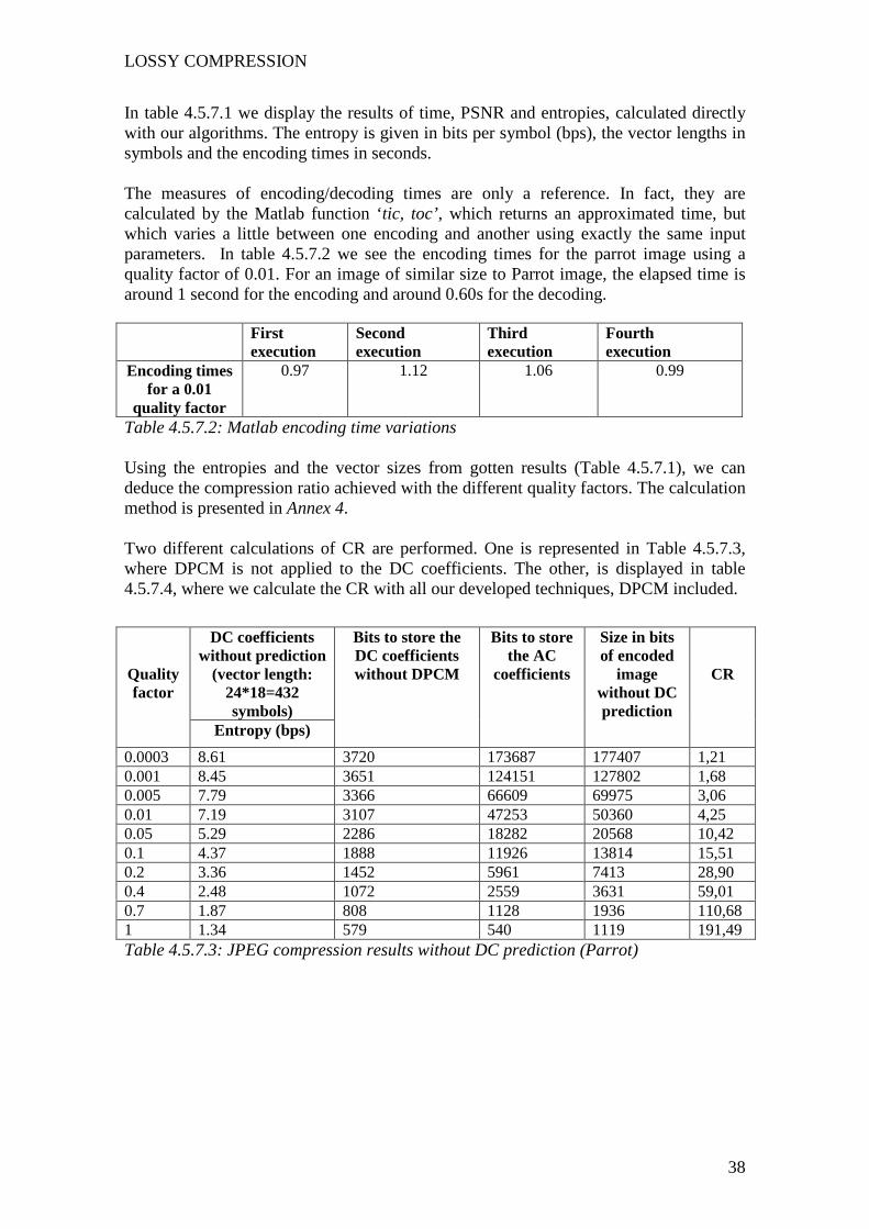
In table 4.5.7.1 we display the results of time, PSNR and entropies, calculated directly with our algorithms. The entropy is given in bits per symbol (bps), the vector lengths in symbols and the encoding times in seconds. The measures of encoding/decoding times are only a reference. In fact, they are calculated by the Matlab function ‘tic, toc’, which returns an approximated time, but which varies a little between one encoding and another using exactly the same input parameters. In table 4.5.7.2 we see the encoding times for the parrot image using a quality factor of 0.01. For an image of similar size to Parrot image, the elapsed time is around 1 second for the encoding and around 0.60s for the decoding.
First execution
Second execution
Third execution
Fourth execution
Encoding times for a 0.01
quality factor
0.97 1.12 1.06 0.99
Table 4.5.7.2: Matlab encoding time variations Using the entropies and the vector sizes from gotten results (Table 4.5.7.1), we can deduce the compression ratio achieved with the different quality factors. The calculation method is presented in Annex 4. Two different calculations of CR are performed. One is represented in Table 4.5.7.3, where DPCM is not applied to the DC coefficients. The other, is displayed in table 4.5.7.4, where we calculate the CR with all our developed techniques, DPCM included.
Table 4.5.7.3: JPEG compression results without DC prediction (Parrot)
DC coefficients without prediction
(vector length: 24*18=432 symbols)
Quality factor
Entropy (bps)
Bits to store the DC coefficients without DPCM
Bits to store the AC
coefficients
Size in bits of encoded
image without DC prediction
CR
0.0003 8.61 3720 173687 177407 1,21 0.001 8.45 3651 124151 127802 1,68 0.005 7.79 3366 66609 69975 3,06 0.01 7.19 3107 47253 50360 4,25 0.05 5.29 2286 18282 20568 10,42 0.1 4.37 1888 11926 13814 15,51 0.2 3.36 1452 5961 7413 28,90 0.4 2.48 1072 2559 3631 59,01 0.7 1.87 808 1128 1936 110,68 1 1.34 579 540 1119 191,49
LOSSY COMPRESSION
39
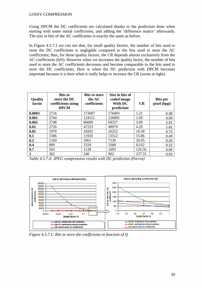
Using DPCM the DC coefficients are calculated thanks to the prediction done when starting with some initial coefficients, and adding the ‘difference matrix’ afterwards. The size in bits of the AC coefficients is exactly the same as before. In Figure 4.5.7.1 we can see that, for small quality factors, the number of bits used to store the DC coefficients is negligible compared to the bits used to store the AC coefficients; thus, for those quality factors, the CR depends almost exclusively from the AC coefficients (left). However when we increases the quality factor, the number of bits used to store the AC coefficients decreases and become comparable to the bits used to store the DC coefficients. Here is when the DC prediction with DPCM becomes important because it is here when it really helps to increase the CR (zoom at right).
Table 4.5.7.4: JPEG compression results with DC prediction (Parrot)
Figure 4.5.7.1: Bits to store the coefficients in function of Q
Quality factor
Bits to store the DC
coefficients using DPCM
Bits to store the AC
coefficients
Size in bits of coded image
With DC prediction
CR
Bits per
pixel (bpp)
0.0003 2716 173687 176403 1.21 6,38 0.001 2744 124151 126895 1.69 4,59 0.005 2748 66609 69357 3.09 2,51 0.01 2726 47253 49979 4.29 1,81 0.05 1970 18282 20252 10.58 0,73 0.1 1586 11926 13512 15.86 0,49 0.2 1169 5961 7130 30.05 0,26 0.4 809 2559 3368 63.62 0,12 0.7 565 1128 1693 126.56 0,06 1 362 540 902 237.55 0,03

LOSSY COMPRESSION
40
bits to store the DC coefficients=f(Q)
0
50
100
150
200
250
0 0,2 0,4 0,6 0,8 1Quality factor: Q
bits
to s
tore
th
e D
C c
oef
fici
ents
CR using DC prediction CR without DC prediction
In Figure 4.5.7.2, we display the compression ratios, using DC coefficient prediction (blue) and not using it (red). We can see that for small quality factors (high PSNR and small compression) our curves takes almost the same values because the bits used to store the DC coefficients are negligible compared with the bits used to store the AC coefficients. However this is not the case for higher quality factors when the AC and DC stored bits begins to be comparable. In Figure 4.5.7.3 we display the PSNR in function of the bits per pixel of the encoded image when using DC prediction. PSNRs between 30 and 40dB give quite good image qualities and for such PSNRs we obtain BPP between 0.73bpp and 2.51bpp.
Figure 4.5.7.2: Compression ratio in function of the quality factor Q.
Figure 4.5.7.3: PSNR in function of bits per pixel (Parrot).

LOSSY COMPRESSION
41
The Figure 4.5.7.4 gives the Parrot image results after coding it with three different quality factors: - With a quality factor Q of 0.01 we can almost not distinguish any difference
between the coded and the original image. This image has a PSNR of 35.53 and is coded with 1.81bpp (left).
- With a quality factor of 0.05 we get a PSNR of 28.90 and we begin to see a blurred
image and some artifacts. This image can be encoded with only 0.73bpp (center). - With a quality factor of 0.4, the JPEG artifacts are very visible and the image is
almost unrecognizable (PSNR of 22.66). The high spatial frequencies are eliminated and we almost only get the offset color for each 8x8 pixel block. Coding using the DCT by blocks and keeping only the DC coefficient return this kind of results with a block effect (right).
Original Image
Q=0.01 PSNR=35.53 dB BPP=1.81 bpp
Q=0.05 PSNR=28.90 dB BPP=0.73 bpp
Q=0.4 PSNR=22.66 dB BPP=0.12 bpp
Figure 4.5.7.4: JPEG coded Parrot image
LOSSY COMPRESSION
42
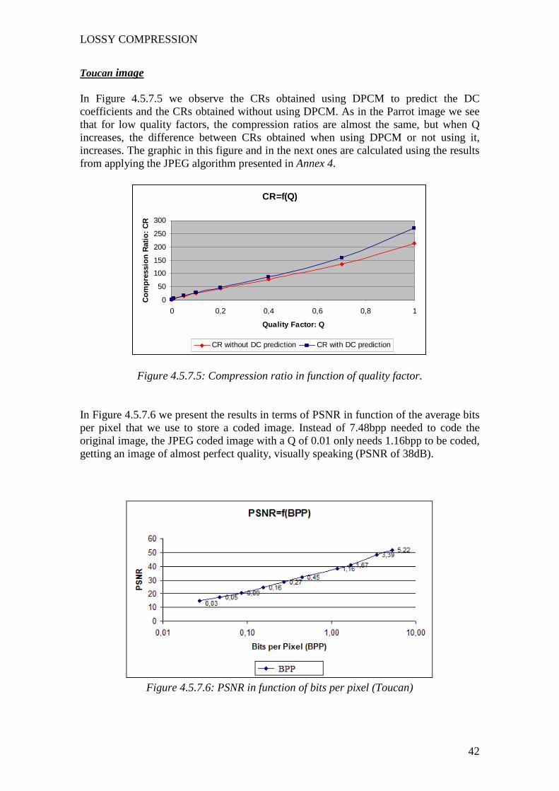
Toucan image In Figure 4.5.7.5 we observe the CRs obtained using DPCM to predict the DC coefficients and the CRs obtained without using DPCM. As in the Parrot image we see that for low quality factors, the compression ratios are almost the same, but when Q increases, the difference between CRs obtained when using DPCM or not using it, increases. The graphic in this figure and in the next ones are calculated using the results from applying the JPEG algorithm presented in Annex 4.
CR=f(Q)
0
50
100
150
200
250
300
0 0,2 0,4 0,6 0,8 1
Quality Factor: Q
Co
mp
ress
ion
Rat
io:
CR
CR without DC prediction CR with DC prediction
Figure 4.5.7.5: Compression ratio in function of quality factor.
In Figure 4.5.7.6 we present the results in terms of PSNR in function of the average bits per pixel that we use to store a coded image. Instead of 7.48bpp needed to code the original image, the JPEG coded image with a Q of 0.01 only needs 1.16bpp to be coded, getting an image of almost perfect quality, visually speaking (PSNR of 38dB).
Figure 4.5.7.6: PSNR in function of bits per pixel (Toucan)
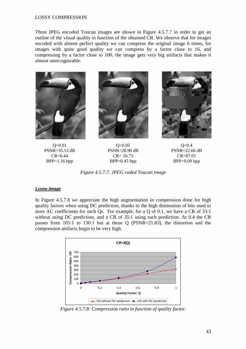
LOSSY COMPRESSION
43
Three JPEG encoded Toucan images are shown in Figure 4.5.7.7 in order to get an outline of the visual quality in function of the obtained CR. We observe that for images encoded with almost perfect quality we can compress the original image 6 times, for images with quite good quality we can compress by a factor close to 16, and compressing by a factor close to 100, the image gets very big artifacts that makes it almost unrecognizable.
Q=0.01 PSNR=35.53 dB
CR=6.44 BPP=1.16 bpp
Q=0.05 PSNR=28.90 dB
CR= 16.73 BPP=0.45 bpp
Q=0.4 PSNR=22.66 dB
CR=87.01 BPP=0.09 bpp
Figure 4.5.7.7: JPEG coded Toucan image
Lenna image In Figure 4.5.7.8 we appreciate the high augmentation in compression done for high quality factors when using DC prediction, thanks to the high diminution of bits used to store AC coefficients for such Qs. For example, for a Q of 0.1, we have a CR of 33:1 without using DC prediction, and a CR of 35:1 using such prediction. At 0.4 the CR passes from 105:1 to 130:1 but at those Q (PSNR=21.83), the distortion and the compression artifacts begin to be very high.
CR=f(Q)
0
100
200
300
400
500
600
700
0 0,2 0,4 0,6 0,8 1
Quality Factor: Q
Co
mp
ress
ion
Rat
io:
CR
CR without DC prediction CR with DC prediction Figure 4.5.7.8: Compression ratio in function of quality factor.

LOSSY COMPRESSION
44
Figure 4.5.7.9 shows the PSNR evolution in function of the number of bits per pixel. We observe that 0.2 bits per pixel are enough in order to obtain PSNRs higher than 30dB, and so, images with quite good quality.
Figure 4.5.7.9: PSNR in function of bits per pixel (Lenna)
In Figure 4.5.7.10 the results for two different encodings are displayed. With a quality factor of 0.01 we can almost no appreciate any difference with the original image, but with a quality factor of 0.05, even if the image still has a good visual quality, the artifacts from JPEG begin to be quite visible.
Q: 0.01
PSNR: 39.78 BPP: 0.98
Q: 0.05 PSNR: 33.30
BPP: 0.35
Figure 4.5.7.10: JPEG coded Lenna image

COMPARATIVE ANALYSIS
45
5- COMPARATIVE ANALYSIS We arrive at the last part of the study and we do so by comparing and analyzing similarities, differences, advantages and disadvantages of the techniques presented in the preceding chapters. With this we will be able to establish which algorithms are more efficient in terms of compression ratio, PSNR, time of encoding/decoding and each feature used to qualify the compression quality. This can be a reference to decide whether an algorithm is a good choice or not for a given application. The first and most important observed difference appears when comparing lossless and lossy compression. In fact, the compression ratios achieved by lossless techniques are much lower than those achieved by lossy techniques as the latter only stores the most relevant information when encoding an image, while the former are able to reconstruct the exact original image after decoding. In Table 5.1 we examine the orders of magnitude of the compression ratios that result when we encode an image with the goal of getting a very good visual quality image output. In fact, when using lossless compression we get PSNRs approaching infinity, because with the stored information we can reconstitute the original image without any difference. With a lossless method however, it would be difficult to obtain compression ratios higher than 1.5. Using JPEG to code the Toucan image with a quality factor of 0.01 we get a PSNR of 35.53dB for which it is difficult to observe any difference between the original image (Figure 5.1) and the coded one (Figure 5.2). With that, we obtain a CR of 6.44 and we could codify the image with only 1.16 bpp instead of 4.59 bpp that we would need to code it using Laplace Pyramid and far from 7.75 bpp that we need to code it using Huffman entropy coding. Using other lossy methods such as uniform scalar quantization, we would code the image with at least 6 bpp (Figure 5.3) to get a high quality output image, but the compression achieved doing so is quite low, being comparable to the CR of lossless compression algorithms. In Figure 5.4 we have coded the Toucan image with 5 bpp and we still observe the different scaled color levels even having a PSNR of 35.68. Here, the subjectivity of the PSNR measure becomes evident, because for lower PSNRs using JPEG coding (with Q=0.01) we get better visual image results than using 5 bits uniform scalar quantization. In the end however, the most important judge of visual quality will always be our eyes.
LOSSLESS LOSSY TOUCAN IMAGE Huffman
Coding Laplace Pyramid
Scalar Quantization
JPEG with Q=0.01
PSNR (dB)
+infinity +infinity 42.70 35.53
CR 1.032 1.22 1.29 6.44 BPP (bpp) 7.75 4.59 6 1.16 Table 5.1: Comparison between Lossless and Lossy compression for high PSNRs.
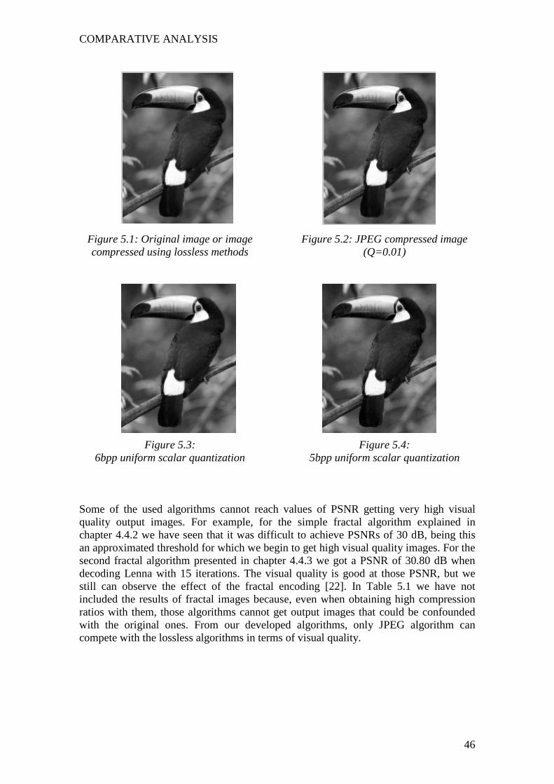
COMPARATIVE ANALYSIS
46
Figure 5.1: Original image or image compressed using lossless methods
Figure 5.2: JPEG compressed image (Q=0.01)
Figure 5.3: 6bpp uniform scalar quantization
Figure 5.4: 5bpp uniform scalar quantization
Some of the used algorithms cannot reach values of PSNR getting very high visual quality output images. For example, for the simple fractal algorithm explained in chapter 4.4.2 we have seen that it was difficult to achieve PSNRs of 30 dB, being this an approximated threshold for which we begin to get high visual quality images. For the second fractal algorithm presented in chapter 4.4.3 we got a PSNR of 30.80 dB when decoding Lenna with 15 iterations. The visual quality is good at those PSNR, but we still can observe the effect of the fractal encoding [22]. In Table 5.1 we have not included the results of fractal images because, even when obtaining high compression ratios with them, those algorithms cannot get output images that could be confounded with the original ones. From our developed algorithms, only JPEG algorithm can compete with the lossless algorithms in terms of visual quality.

COMPARATIVE ANALYSIS
47
If in Table 5.1 the common feature was the high visual quality of the outputted images, in Table 5.2 we compare algorithms having as common denominator they belonging to the group of lossy techniques. In it we compare our developed JPEG and Fractal algorithms. We will refer to the Fractal algorithm described in chapter 4.4.2 as Fractal 1, and the Fractal algorithm in chapter 4.4.3 as Fractal 2. On the displayed results in Tables 5.2, we have worked with -8, 4, 2- coding parameters for Fractal 1, because it is with them that we have obtained the higher values of PSNR for this algorithm and they give us an insight of the algorithm compression capacity. For Fractal 2 we work with 15 iterations, because this value gives us a good equilibrium between a PSNR close to the attractor and a low decoding time. For JPEG we give the results in terms of ranges, using as extremums the quality factors (Q) 0.4 and 0.003. For such Q values we get PSNRs between 20dB and 50dB approximately, that are the values for which we begin to appreciate the shape of the image, until we get a very high visual quality image, respectively. Parrot Fractal 2
(15 iterations) JPEG (Q: from 0.003 to 0.4)
PSNR (dB) 23.71 From 50 down to 19 dB BPP (bpp) 0.48 From 6.38 down to 0.12 CR 15.99 From 1.21 up to 63 Encoding time ~ 25 min ~ 1 s Decoding time ~ 1 s ~ 0.6 s Toucan Fractal 1
(8, 4, 2) Fractal 2 (15 iterations)
JPEG (Q: from 0.003 to 0.4)
PSNR (dB) 22.56 27.19 From 50 down to 20 dB BPP (bpp) 2.35 0.48 From 5.22 down to 0.09 CR 3.19 15.44 From 1.43 up to 87 Encoding time ~ 1.5 s ~ 65 min ~ 1.5 s Decoding time ~ 0.5 s ~ 2 s ~ 1 s Lenna Fractal 1
(8, 4, 2) Fractal 2 (15 iterations)
JPEG (Q: from 0.003 to 0.4)
PSNR (dB) 27.15 30.80 From 53 down to 22 dB BPP (bpp) 2.35 0.45 From 5.09 down to 0.06 CR 3.16 16.40 From 1.46 up to 130 Encoding time ~ 9 s ~52 h ~ 9 s Decoding time ~ 3 s ~ 15 s ~ 5 s Tables 5.2: Comparison between our 3 lossy compression algorithms From Table 5.2 and comparing between both Fractal algorithms, we conclude that Fractal 2 is more efficient than Fractal 1 in terms of relation PSNR/BPP, but it is not in terms of encoding time. In fact the encoding time for Fractal 2 is more than an hour for images of Toucan image size, and more than two days for image with sizes comparable to Lenna image size. In terms of visual quality we also get better results with Fractal 2.
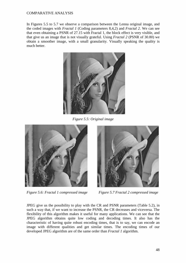
COMPARATIVE ANALYSIS
48
In Figures 5.5 to 5.7 we observe a comparison between the Lenna original image, and the coded images with Fractal 1 (Coding parameters 8,4,2) and Fractal 2. We can see that even obtaining a PSNR of 27.15 with Fractal 1, the block effect is very visible, and that give us an image that is not visually grateful. Using Fractal 2 (PSNR of 30.80) we obtain a smoother image, with a small granularity. Visually speaking the quality is much better.
Figure 5.5: Original image Figure 5.6: Fractal 1 compressed image
Figure 5.7 Fractal 2 compressed image
JPEG give us the possibility to play with the CR and PSNR parameters (Table 5.2), in such a way that, if we want to increase the PSNR, the CR decreases and viceversa. The flexibility of this algorithm makes it useful for many applications. We can see that the JPEG algorithm obtains quite low coding and decoding times. It also has the characteristic of having quite robust encoding times, that is to say, we can encode an image with different qualities and get similar times. The encoding times of our developed JPEG algorithm are of the same order than Fractal 1 algorithm.

COMPARATIVE ANALYSIS
49
In Tables 5.3 to 5.6 we compare Fractal 2 with JPEG. In fact, those two algorithms are those which give us the best results in terms of PSNR. Two different comparisons have been established. First, in Tables 5.3 and 5.4, we have analyzed the compression ratio of both algorithms taking similar PSNRs as starting point. Secondly, in Table 5.5 and 5.6, we compare the quality image outputs of both algorithms in terms of PSNR, when we take similar compression ratios as the common characteristic. Those comparisons become possible thanks to the flexibility of JPEG that allows us to tune the CR in function of the PSNR and viceversa. Contrarily, the compression ratio gotten from Fractal 2 is fixed by a given image. We could diminish the encoding time by using MSE thresholds or diminish the decoding time by decoding with fewer iterations, but the amount of bits used to store the compressed image wouldn’t change. Analyzing the results of Table 5.3 we see that for similar PSNRs (around 27- 28 dB), we obtain much higher CR for JPEG than for Fractal 2. In fact we almost obtain a difference of a factor two between CR’s. TOUCAN IMAGE Fractal 2
(15 iterations) JPEG (Q: 0.1)
PSNR 27.19 28.54 BPP 0.48 0.27 CR 15.44 27.43 Tables 5.3: Comparison by similar PSNRs (Toucan) In Figures 5.8 and 5.9 we observe that even when working with similar PSNRs the artifacts in compressed images using both algorithms are quite different. The JPEG encoded image (Figure 5.9) presents a clear block effect, while Fractal 2 gives us a more homogeneous image, but it has an effect similar to pointillism and the small details are not so clear than in JPEG. That is very visible in the Toucan eye. Figure 5.8: Fractal 2 coded Toucan image
(PSNR=27.19) Figure 5.9: JPEG coded Toucan image
(PSNR=28.54)

COMPARATIVE ANALYSIS
50
In Tables 5.4 we analyze the results from coding Lenna. With similar PSNRs (around 29.5 dB) in Fractal 2 and JPEG, we get, as in the case of Toucan image, CRs much higher for JPEG than for Fractal 2. We also almost get a difference of a factor two between them. The effects of the artifacts in the image for JPEG are exactly the described for Toucan image, but this time, the Fractal 2 coded image has a higher quality and we don’t observe so much the pointillism effect. The details are always clearer in the JPEG coded image, we appreciate it in the plume of her had and in her eyes, but the Fractal coded image is smoother and visually it is more pleasing. LENNA Fractal 2
(7 iterations) JPEG (Q: 0.1)
PSNR 29.31 29.84 BPP 0.45 0.21 CR 16.40 35.56 Tables 5.4: Comparison by similar PSNRs (Lenna)
Figure 5.10: Fractal 2 coded Lenna image (PSNR=29.31)
Figure 5.11: JPEG coded Lenna image (PSNR=29.84)
In Tables 5.5 and 5.6, comparing the PSNRs in function of similar CRs, we observe the advantage of JPEG upon Fractal 2. TOUCAN Fractal 2
(15 iterations) JPEG (Q: 0.05)
CR 15.44 16.73 BPP 0.48 0.45 PSNR 27.19 31.85 Tables 5.5: Comparison by similar compression ratios (Toucan)

COMPARATIVE ANALYSIS
51
When compressing Lenna with both algorithms using a CR around 16, we obtain a resulting PSNR around 30dB when compressing with Fractal 2 and a PSNR around 35dB when compressing with JPEG, that is to say, a difference of 5dB between them (Table 5.6). With this comparison we clearly see that even having a quite important difference between PSNRs, we get a quite similar visual quality (Figures 5.14 and 5.15). We observe that fact above all in Lenna image, where the details and the brightness of the Fractal 2 coded image are not so clear and intense, but the image is smoother than in the JPEG coded image where we appreciate sharper color changes.
Tables 5.6: Comparison by similar compression ratios (Lenna)
Figure 5.12: Fractal 2 coded Toucan image (PSNR=27.19)
Figure 5.13: JPEG coded Toucan image (PSNR=31.85)
Figure 5.14: Fractal 2 coded Lenna (PSNR=30.80)
Figure 5.15: JPEG coded Lenna (PSNR=34.98)
LENNA Fractal 2 (15 iterations)
JPEG (Q: 0.035)
CR 16.40 16.98 BPP 0.45 0.44 PSNR 30.80 34.98

CONCLUSION
52
6- CONCLUSION In this project we have presented an overview of the main techniques that have been used in the digital image compression discipline over the last decades. Algorithms based on the described techniques have been implemented with the purpose of presenting a guide for people interested in the subject. One of the most important points in image compression is the fact that it is very difficult to obtain high compression ratios without lose image information. Thus, with the exception of some specific disciplines where images without losses are required, as in medical imagery, most of the techniques used nowadays are lossy compression techniques. The two primary lossy techniques we have studied were Fractal and JPEG compression. Fractal compression had its apogee in the 1980’s as a compression technique which was capable of quite acceptable PSNRs and compression ratios. As a counterpoint, it is a very time consuming technique; we have seen it with the implementation of our second Fractal algorithm. Currently, Fractal compression techniques have lost favor in place of JPEG compression, a method that gives similar results as Fractal compression, but with much lower coding and decoding compression times. Those times are quite robust and don’t vary as much when coding with higher or lower quality factors. JPEG is a very flexible algorithm that allows us to obtain one or another PSNR as a function of the compression ratio that we want to achieve. Working with this algorithm we have had the opportunity to go into other techniques widely used in the world of image compression. Such is the case of the discrete cosine transform, which is at the heart of JPEG, or other compression techniques as zero-run or DPCM. We have seen that our JPEG algorithm is able to obtain similar PSNRs and CRs of the current algorithms in the market; giving us, for example, the possibility to obtain images with an excellent quality with compression ratios around 10:1. Our developed Fractal algorithms were not as efficient as JPEG, but they gave us a good idea of how Fractal compression uses the self-similarity in images. In the first Fractal algorithm we have seen how to find similarities between different parts of an image and decode it using a very small codebook, but doing so we produced very visually low quality images. In the second studied Fractal algorithm we have seen the large capacity that this technique has to encode images getting quite good visual results and compressing in a very unintuitive way. That is to say, storing only transformations and iterating the decoding process without any need of a stored codebook. The digital era is still very young; clearly, image compression is not yet at the end of its evolution.

ANNEXES
53
ANNEXES

ANNEXES
54
ANNEX 1: FRACTAL 1 NUMERICAL DEVELOPMENTS
In this annex we present the numerical results from compressing Lenna and Toucan images with our developed Fractal 1 algorithm. They are organized by coding parameters following the notation: CP: region size, reference block size, range block size. 1- Coding parameters (CP): 32, 16, 4 Pixels in region: 32*32 Domain/reference block pixels: 16*16 Range block pixels: 4*4 Toucan Image: Original size in bits: 216*160*7.49bpp=258855bits A- Encoding time= 1.58s B- Decoding time= 0.56s C- PSNR=21.21 D- d1) 8960*7.10=63616 bits d2) (5*7)*(8*8)=2240 positions d3) Log2(16*16/(4*4))=4 bpsp TBS: 63616+2240*4=72576 bits CR= 258855/72576=3.56 E- BPP=72576/(216*160)= 2.1bpp
Figure A1.2: Decoded Toucan with CP: 32,16,4
Lenna Image: Original size in bits: 512*512*7.43bpp=1947599bits A- Encoding time=7.02s B- Decoding time2.27s C- PSNR=22.58 D- d1) 7.40*65536=484967 bits d2) (16*16)*(8*8)=16384positions d3) Log2(16*16/(4*4))= 4 bpsp TBS: 484967+16384*4=550503 bits CR= 1947599/550503=3.54 E- BPP=550503/(512*512)= 2.1bpp
Figure A1.2: Decoded Lenna with CP: 32,16,4

ANNEXES
55
2- Coding parameters: 16, 8, 4 Pixels in region: 16*16 Domain blocks/reference blocks pixels: 8*8 Range blocks pixels: 4*4
Toucan Image: A- Encoding time= 0.72s B- Decoding time= 0.52s C- PSNR= 19.79 D- d1) 8960*7.32=65588 bits d2) (14*10)*(4*4)=2240 positions d3) Log2(8*8/(4*4))=2 bpsp
TBS: 63616+2240*4=70068 bits CR= 258855/70068=3.69 E- BPP=70068/(216*160)= 2.03bpp
Figure A1.3: Decoded Toucan with CP: 16,8,4
Lenna Image: A- Encoding time= 2.82s B- Decoding time = 2.24s C- PSNR= 23.13 D- d1) 65536*7.39=484312 bits d2) (32*32)*(4*4)=16384positions d3) Log2(8*8/(4*4))= 2 bpsp TBS: 484312+16384*2=517080 bits CR= 1947599/517080=3.77 E- BPP=517080/(512*512)= 1.97bpp
Figure A1.4: Decoded Lenna with CP: 16,8,4

ANNEXES
56
3- Coding parameters: 8, 4, 2 Pixels in region: 8*8 Domain blocks/reference blocks pixels: 4*4 Range blocks pixels: 2*2 Toucan Image: A- Encoding time= 1.23s B- Decoding time= 0.44s C- PSNR= 22.56 D- d1) 8640*7.40= 63936 bits d2) (27*20)*(4*4)= 8640 positions d3) Log2(4*4/(2*2))= 2 bpsp
TBS: 63936+8640*2=81216 bits CR= 258855/81216=3.19 E- BPP= 81216/(216*160)= 2.35bpp
Figure 4.4.2.2.5:
Decoded Toucan with CP: 8,4,2
Lenna Image: A- Encoding time= 9.30s B- Decoding time= 3.08s C- PSNR= 27.15 D- d1) 65536*7.39=484312 bits d2) (32*32)*(4*4)=16384positions d3) Log2(8*8/(4*4))= 2 bpsp TBS: 484312+16384*2=517080 bits CR= 1947599/517080=3.77 E- BPP= 616039/(512*512)= 2.35bpp
Figure 4.4.2.2.6: Decoded Lenna with CP: 8,4,2
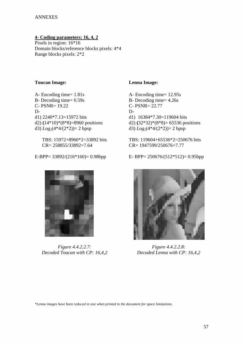
ANNEXES
57
4- Coding parameters: 16, 4, 2 Pixels in region: 16*16 Domain blocks/reference blocks pixels: 4*4 Range blocks pixels: 2*2
Toucan Image: A- Encoding time= 1.81s B- Decoding time= 0.59s C- PSNR= 19.22 D- d1) 2240*7.13=15972 bits d2) (14*10)*(8*8)=8960 positions d3) Log2(4*4/(2*2))= 2 bpsp
TBS: 15972+8960*2=33892 bits CR= 258855/33892=7.64 E-BPP= 33892/(216*160)= 0.98bpp
Figure 4.4.2.2.7:
Decoded Toucan with CP: 16,4,2
Lenna Image: A- Encoding time= 12.95s B- Decoding time= 4.26s C- PSNR= 22.77 D- d1) 16384*7.30=119604 bits d2) (32*32)*(8*8)= 65536 positions d3) Log2(4*4/(2*2))= 2 bpsp TBS: 119604+65536*2=250676 bits CR= 1947599/250676=7.77 E- BPP= 250676/(512*512)= 0.95bpp
Figure 4.4.2.2.8: Decoded Lenna with CP: 16,4,2
*Lenna images have been reduced in size when printed in the document for space limitations.

ANNEXES
58
ANNEX 2: FRACTAL 2 NUMERICAL DEVELOPMENTS
In this annex we present the numerical developments used to compute the compression ratios and the number of bits per pixel achieved with the Fractal 2 algorithm. To calculate the compression ratio, first of all, we have to compute the original size in bits of the processed images: Parrot original image size in bits: (image size) *(entropy)= 128*192*7.7457=190359 Toucan original image size in bits: (image size) *(entropy)= 216*160*7,4795=258492 Lenna original image size in bits: (image size) *(entropy)= 512*512*7,4295=1947599 The size in bits of the compressed image is mostly defined by the positions, the geometrical transformations and the color transformations stored. Following, we calculate the bits used to store those features:
1- Positions: The bits that we have to use in order to store the domain blocks position matching with the range blocks, varies in function of the image size and the result can be found with the formula: Position= [(positions in axe x in bits)+( positions in axe y in bits)]*(nº of range blocks)
Formula 4.4.3.2.1 Where: size of the image in x axe= 2(max positions in axe x in bits) � � positions in axe x= log2 (size of the image in axe x)
size of the image in y axe= 2(positions in axe y in bits) � � positions in axe y= log2 (size of the image in axe y) For every one of the processed images we have: Bits Parrot: [log2 (192)+log2 (128)]*[(192*128)/(8*8)] ~ [8bits+8bits]*[384]=6144 bits Bits Toucan: [log2 (216)+log2 (160)]*[(216*160)/(8*8)] ~ [8bits+8bits]*[540]=8640bits Bits Lenna: [log2 (512)+log2 (512)]*[(5122)/(8*8)] ~ [9bits+9bits]*[4096]=73728 bits
2- Geometrical transformation:
In total, eight different symmetries could be applied to a subsampled block, in order to find the domain blocks, so 3 bits will be enough to store every one of such transformations. Thus, for the totality of range blocks we have:
Bits to store the geometrical transformations=(3 bits/rotation)*(nº of range blocks) Formula 4.4.3.2.2
Bits needed to store the geometrical transformations for Parrot: 3*384=1152 bits Bits needed to store the geometrical transformations for Toucan: 3*540=1620 bits Bits needed to store the geometrical transformations for Lenna: 3*4096=12288 bits
ANNEXES
59
3- Contrast and brightness (color transformations):
Contrast and brightness are two scalars that, from the literature, can be optimally coded using with 5 and 7 bits respectively [3]. We have to apply such transformations for every one of the range blocks:
(5bits+7bits)*(nº of rang blocks)
Formula 4.4.3.2.3 Bits needed to store the color transformations for Parrot: (5+7)*384= 4608 bits Bits needed to store the color transformations for Toucan: (5+7)*540= 6480 bits Bits needed to store the color transformations for Lenna: (5+7)*4096= 49152 bits Other values needed to decode the image such as the size of the image or the size of the range blocks can be neglected because their size in bits is negligible in comparison with the rest of stored data. In total we will have to store for each one of the compressed images: Bits to store to store the encoded Parrot: 6144+1152+4608 = 11904 Bits needed to store the encoded Toucan: 8640+1620+6480= 16740 Bits needed to store the encoded Lenna: 73728+ 12288+49152= 135168
After those intermediate calculations we can proceed to compute the compression ratios (CR) and average number of bits per pixel (BPP): CR for Parrot image: 190359/11904=15.99 CR for Toucan image: 258492/16740=15.44 CR for Lenna image: 1947599/135168=14.40
Nº of bits per pixel for parrot image= 11904/(192*128)=0.4843 bpp Nº of bits per pixel for Toucan image= 16740/(216*160)=0.4844 bpp Nº of bits per pixel for Lenna image= 135168/(512*512)=0.5156 bpp

ANNEXES
60
In Figure 4.4.3.2.2 we present the attractor of the Toucan image, followed by some decoding iterations. The decoded images have been obtained using a 216x160 (Toucan image size) grey image as decoder input, but we could use whatever decoder input image at its place getting almost the same result after some iterations.
Attractor PSNR: 29
1 iteration 2 iterations 3 iterations
5 iteration 8 iterations 15 iterations
Figure 4.4.3.2.2: Fractal compressed Toucan image decoding
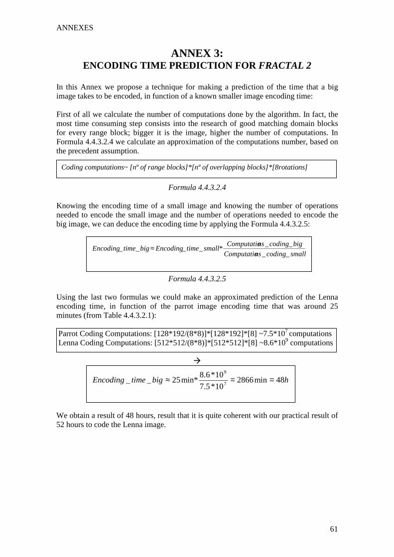
ANNEXES
61
smallcodingnsComputatio
bigcodingnsComputatiosmalltimeEncodingbigtimeEncoding
__
__*____ ≈
ANNEX 3: ENCODING TIME PREDICTION FOR FRACTAL 2
In this Annex we propose a technique for making a prediction of the time that a big image takes to be encoded, in function of a known smaller image encoding time: First of all we calculate the number of computations done by the algorithm. In fact, the most time consuming step consists into the research of good matching domain blocks for every range block; bigger it is the image, higher the number of computations. In Formula 4.4.3.2.4 we calculate an approximation of the computations number, based on the precedent assumption.
Formula 4.4.3.2.4 Knowing the encoding time of a small image and knowing the number of operations needed to encode the small image and the number of operations needed to encode the big image, we can deduce the encoding time by applying the Formula 4.4.3.2.5:
Formula 4.4.3.2.5
Using the last two formulas we could make an approximated prediction of the Lenna encoding time, in function of the parrot image encoding time that was around 25 minutes (from Table 4.4.3.2.1): Parrot Coding Computations: [128*192/(8*8)]*[128*192]*[8] ~7.5*107 computations Lenna Coding Computations: [512*512/(8*8)]*[512*512]*[8] ~8.6*109 computations
�
We obtain a result of 48 hours, result that it is quite coherent with our practical result of 52 hours to code the Lenna image.
Coding computations~ [nº of range blocks]*[nº of overlapping blocks]*[8rotations]
hbigtimeEncoding 48min286610*7.5
10*8.6min*25__
7
9
==≈

ANNEXES
62
ANNEX 4: JPEG NUMERICAL DEVELPMENTS
Hereafter, we present the numerical results obtained from applying the JPEG algorithm to the Toucan and the Lenna images, the calculations done to find the CRs are the following ones: Bits to store DC coefficients=Entropy DC vector *Size DC vector Bits to store AC coefficients=Entropy AC vector * Size AC vector Size in bits of coded image= Bits to store DC coefficients+ Bits to store AC coefficients CR=size in bits of original image/ size in bits of encoded image Using DPCM, the number of bits occupied by the DC coefficients must be calculated in the following way: Initial coefficient bits=Initial coefficients entropy* Initial coefficients vector size Difference coefficient bits=Difference vector entropy* Difference vector size Bits to store DC coefficients= Initial coefficient bits+ Difference coefficient bits Toucan image results: Image size in bits without encoding: Size*Entropy= 216*160*7.48= 258509 bits The results obtained applying our developed JPEG algorithm for different quality factors are shown in Tables 4.5.7.5 to 4.5.7.7. As seen in Table 4.5.7.5, the encoding and decoding times for the Toucan image oscillates between one and two seconds. The obtained PSNRs are very similar to those obtained for the Parrot image when using identical quality factors. Entropies and vector lengths have been used to compute the size in bits of the compressed images, and thus, the CR and the number of bits per pixel of those images.
Table A4.1: JPEG compression results (Toucan)
Initial DC coefficients
entropy (bps)
Difference DC vector entropy
(bps)
Quality factor:
Q
Encoding time (s)
Decoding time(s)
PSNR (dB)
vector length: 204
Vector length: 336
AC coded coefficients
entropy (bps) and vector
length
0.0003 ~1.27 ~0.82 51.54 6.70 6.00 5.42 32641 0.001 ~1.40 ~1.00 48.39 6.58 5.99 4.59 24820 0.005 ~1.51 ~1.34 40.88 6.68 6.63 3.92 13846 0.01 ~1.58 ~1.32 38.07 6.63 5.99 3.76 9788 0.05 ~1.51 ~1.27 31.85 4.87 3.90 3.35 3924 0.1 ~1.38 ~1.23 28.54 3.97 2.95 3.13 2435 0.2 ~1.29 ~0.77 24.66 3.04 1.98 2.79 1475 0.4 ~1.43 ~0.91 20.47 2.12 1.29 2.22 948 0.7 ~1.31 ~0.77 17.40 1.36 0.67 1.57 712 1 ~2.07 ~0.86 15.00 1.18 0.51 0.89 606

ANNEXES
63
Table A4.2: JPEG compression results without DC prediction (Toucan) In Table 4.5.7.7 we observe that the CRs achieved for the Toucan image are higher than the CRs found with the correspondent quality factors for the Parrot image. That is because the Toucan image is bigger than the Parrot image, their details are bigger, and thus the 8x8 pixel blocks of the Toucan image have better detail resolution. Because of that, the frequencies used to encode the Toucan image are lower and we don’t need to use so many AC coefficients to encode the image blocks, getting higher CR results than we got for the Parrot image while getting similar PSNR results.
Table A4.3: JPEG compression results with DC prediction (Toucan)
DC coefficients without prediction
(vector length: 27*20=540 symbols)
Quality factor: Q
Entropy (bps)
Bits to store the DC coefficients without linear
prediction
Bits to store the AC
coefficients
Size in bits of coded image
Without DC prediction
CR
0.0003 8.99 4855 176914 181769 1,42 0.001 8.74 4720 113924 118644 2,18 0.005 7.77 4196 54276 58472 4,42 0.01 7.05 3807 36803 40610 6,37 0.05 4.99 2695 13145 15840 16,32 0.1 4.05 2187 7622 9809 26,35 0.2 3.08 1663 4115 5778 44,74 0.4 2.19 1183 2105 3288 78,62 0.7 1.47 794 1118 1912 135,20 1 1.24 670 539 1209 213,82
Quality
factor: Q
Bits to store the DC coefficients
using linear prediction
Bits to store the AC
coefficients
Size in bits of coded image
with DC prediction
CR
BPP
0.0003 3383 176914 180297 1.43 5.22 0.001 3355 113924 117279 2.20 3.39 0.005 3590 54276 57866 4.47 1.67 0.01 3365 36803 40168 6.44 1.16 0.05 2304 13145 15449 16.73 0.45 0.1 1801 7622 9423 27.43 0.27 0.2 1285 4115 5400 47.87 0.16 0.4 866 2105 2971 87.01 0.09 0.7 503 1118 1621 159.47 0.05 1 412 539 951 271.83 0.03

ANNEXES
64
Lenna image results: Image size in bits without encoding: Size*Entropy= 512*512*7.43=1947730bits Results obtained applying JPEG coding for different quality factors are displayed in Tables 4.5.7.8 to 4.5.7.10. Working with the Lenna image of 512x512 pixels, we observe how the encoding times ascends to almost 10 seconds and the decoding times to almost 6 seconds. We have almost a factor 10 between the times elapsed by an image of 216x160 pixels and the times elapsed by an image of the size of Lenna. In fact, for a bigger image we have much more 8x8 pixel blocks to be coded. Other measures as the PSNRs or the entropy measures are quite close to the results obtained when coding the precedent images, independently of the image size and content.
Table A4.4: JPEG compression results (Lenna)
Table A4.5: JPEG compression results without DC prediction (Lenna)
Initial DC coefficients
entropy (bps)
Difference DC vector entropy
(bps)
Quality factor
Encoding time (s)
Decoding time(s)
PSNR (dB)
Vector length: 1495
Vector length: 2601
AC coded coefficients
entropy (bps) and vector
length
0.0003 ~9.52 ~6.12 52.96 7.64 6.02 5.20 251595 0.001 ~9.47 ~5.75 48.43 7.56 5.92 4.15 201958 0.005 ~9.80 ~5.67 41.97 7.26 5.61 3.70 96823 0.01 ~9.13 ~5.62 39.78 7.27 5.61 3.59 64795 0.05 ~9.07 ~5.53 33.30 5.04 3.36 3.26 22777 0.1 ~9.11 ~5.55 29.84 4.04 2.45 3.04 13937 0.2 ~9.16 ~5.53 25.82 3.08 1.56 2.60 8582 0.4 ~9.12 ~5.51 21.83 2.20 0.86 1.68 5631 0.7 ~9.08 ~5.78 18.51 1.43 0.69 0.69 4490 1 ~9.15 ~5.53 17.09 1.16 0.20 0.26 4219
DC coefficients without prediction
(vector length: 64*64=4096 symbols)
Quality factor
Entropy (bps)
Bits to store the DC coefficients without linear
prediction
Bits to store the AC
coefficients
Size in bits of coded image
without DC prediction
CR
0.0003 11.30 46285 1308294 1354579 1.44 0.001 10.31 42230 838126 880356 2.21 0.005 8.28 33915 358245 392160 4.97 0.01 7.31 29942 232614 262556 7.42 0.05 5.02 20562 74253 94815 20.54 0.1 4.05 16589 42368 58957 33.04 0.2 3.06 12534 22313 34847 55.89 0.4 2.20 9011 9460 18471 105.5 0.7 1.43 5857 3098 8955 217.5 1 1.18 4833 1097 5930 328.5

ANNEXES
65
We also appreciate the augmentation of CRs for Lenna image compared with the precedent coded images. For encodings giving a very good quality we can achieve CR up to 7:1, CR around 20:1 are achieved for encodings resulting in quite good visual quality images.
Table A4.6: JPEG compression results with DC prediction (Lenna)
Quality
factor (Q)
Bits to store the DC coefficients
using linear prediction
Bits to store the AC
coefficients
Size in bits of coded image
AC+ DC with prediction
CR
BPP
0.0003 27080 1308294 1335374 1.46 5,09 0.001 26700 838126 864826 2.25 3,30 0.005 25445 358245 383690 5.08 1,46 0.01 25460 232614 258074 7.55 0,98 0.05 16274 74253 90527 21.52 0,35 0.1 12412 42368 54780 35.56 0,21 0.2 8662 22313 30975 62.88 0,12 0.4 5526 9460 14986 129.97 0,06 0.7 3933 3098 7031 277.02 0,03 1 2254 1097 3351 581.24 0,01

ANNEXES
66
ANNEX 5:
INDEX OF ALGORITHMS The algorithms developed are presented in computer support and have been organized in folders inside a main folder named ‘Compression Algorithms’. Each folder contains the algorithms used in the different chapters of the project. Hereafter the list of folders with the correspondent associated chapters is presented: (1) – IMAGES: ……………………………………………… Chapters 2, 3, 4 and 5 (2)- ENTROPY AND HISTOGRAM……………………….. Chapter 3.2 (3)- LAPLACIAN PYRAMID………………………………. Chapter 3.3 (4)- QUALITY CONTROL –PSNR ……………………….. Chapters 4 and 5 (5)- SCALAR QUANTIZER ………………………………. Chapter 4.3 (6)- FRACTAL IMAGES ………………………………….. Chapter 4.4.1 (7)- FRACTAL 1 COMPRESSION ALGORITHM……….. Chapter 4.4.2 (8)- FRACTAL 2 COMPRESSION ALGORITHM……….. Chapter 4.4.3 (9)- DPCM AND CORRELATION…………………………. Chapter 4.5.1 (10)- DCT ….……………………………………………….....Chapter 4.5.2 (11)- JPEG COMPRESSION ALGORITHM…………………Chapter 4.5

BIBLIOGRAPHY
67
BIBLIOGRAPHY [1] Wikipedia. “Lenna”, (www.wikipedia.org/wiki/jpeg). [2] Zhao, E.; Liu, D. “Fractal image compression methods: a review”, Information Technology and Applications, 2005. ICITA 2005. Third International Conference on. Volume 1, 4-7 July 2005, pp:756 – 759. [3] Torres, Lluís. “Introduction to image and video coding”, Chapter 2, slide 19, (http://gps-tsc.upc.es/GTAV/Torres/Teaching/Teaching-IVC.htm). [4] Oliver Gil, José. “Compresión de imagen y vídeo: fundamentos teóricos y aspectos prácticos”, Universidad Politécnica de Valencia, Departamento de Informática de Sistemas y Computadoras, 2001. [5] John W. Woods. “Multidimensional Signal, Image and Video Processing and Coding”, Ensevier, 2006, pp. 284-287. [6] Howard, P.G.; Vitter, J.S. “Arithmetic coding for data compression” Proceedings of the IEEE, Volume 82, Issue 6, June 1994 pp:857 – 865. [7] Vasudev Bhaskaran. “Image and Video Compression Standards: Algorithms and Architectures”, kluwer Academic Publishers, 1956, pp. 15-34. [8] David Salomon, G. Motta, D. Bryant. “Data Compression: The Complete Reference”, Springer, 2007, pp. 390-406. [9] Pei-Yin Chen. “An efficient prediction algorithm for image vector quantization”, Systems, Man, and Cybernetics, Part B, IEEE Transactions on. Volume 34, Issue 1, Feb. 2004, pp:740 – 746. [10] A. Jacquin. “Image Coding Based On A Fractal Theory of Iterated Contractive Image Transformations”, IEEE Trans. on Image Processing. 1991, vol. 1, pp. 18-30. [11] Barnsley, M.; Sloan, A. D. "A Better Way To Compress Images", BYTE, vol. 13, January 1988, pp. 215-224. [12] Kung, C.M.; Yang, W.S; Ku, C.C.; Wang, C.Y. “Fast Fractal Image Compression Base on Block Property”, Advanced Computer Theory and Engineering, ICACTE '08, International Conference on. 20-22 Dec. 2008, pp:477 – 481. [13] Selim ,A.; Hadhoud, M.M.; Dessouky, M.I.; Abd El-Samie, F.E. “A simplified fractal image compression algorithm”, Menoufia University. [14] Yuval Fisher. “Fractal Image Compression: Theory and Application”, Springer-Verlag, 1995, pp. 10 – 23.

BIBLIOGRAPHY
68
[15] Xiangjian He; Wang, H; Wu, O.; Hintz, T.; Hur, N. “Fractal Image Compression on Spiral Architecture”, Computer Graphics, Imaging and Visualisation, International Conference on. 26-28 July 2006, pp:76 – 83. [16] Majid Rabbani, Paul W. Jones. “Digital Image Compression Techniques”, SPIE, 1991, pp. 73-92. [17] S. G. Hoggar. “Mathematics of Digital Images: Creation, Compression, Restoration, Recognition”, Cambridge University Press, 2006, pp. 560-635.
[18] Jain, Anil K. “Fundamentals of Digital Image Processing”, Englewood Cliffs, NJ, Prentice Hall, 1989, pp. 150-153. [19] Marshall, Dave. “JPEG Compression”. Cardiff School of Computer Science. (http://www.cs.cf.ac.uk/Dave/Multimedia/node234.html). [20] Wikipedia. “JPEG”, (www.wikipedia.org/wiki/jpeg). [21] Kingsbury, Nick. “JPEG Entropy Coding”, Connexions (http://cnx.org/content/m11096/latest/). [22] Jackson, D.J.; Hannah, S.J. “Comparative analysis of image compression techniques”, System Theory, Proceedings SSST '93, Twenty-Fifth Southeastern Symposium on. 7-9 March 1993, pp:513 – 517.

69
INDEX OF FIGURES 2- IMAGES Figure 2.1: LENNA image (512x512 pixels) ▪ 2 Figure 2.2: PARROT (192X128) ▪ 3 Figure 2.3: TOUCAN (216X160) ▪ 3 Figure 2.4: Image compression diagram ▪ 3 3- LOSSLESS COMPRESSION Figure 3.2.2.1: Parrot image histogram ▪ 5 Figure 3.2.2.2: Toucan image histogram ▪ 5 Figure 3.2.2.3: Lenna image histogram ▪ 6 Figure 3.2.2.4: Random Image histogram ▪ 6 Figure 3.3.1.1: Original image ▪ 8 Figure 3.3.1.2: Filtered image ▪ 8 Figure 3.3.1.3: Downsampled image ▪ 8 Figure 3.3.1.4: Upsampled image ▪ 9 Figure 3.3.1.5: Difference image ▪ 9 Figure 3.3.1.6: Difference image histogram ▪ 9 Figure 3.3.1.7: Laplacian pyramid images ▪ 10 4- LOSSY COMPRESSION Figure 4.3.1: Scalar quantization images (from 1 to 8bpp) ▪ 14 Figure 4.4.1.1: IFS applied to two different input images ▪ 15 Figure 4.4.2.1.1: First fractal algorithm scheme ▪ 16 Figure 4.4.2.1.2: First fractal algorithm diagram ▪ 17 Figure 4.4.2.2.1: Decoded Toucan with CP: 8,4,2 ▪ 19 Figure 4.4.2.2.2: Decoded Lenna with CP: 8,4,2 ▪ 19 Figure 4.4.3.1.1: Second fractal algorithm scheme ▪ 21 Figure 4.4.3.1.2: Domain blocks for one of the overlapping blocks ▪ 22 Figure 4.4.3.1.3: Original image (left). Matching block research (right) ▪ 22 Figure 4.4.3.2.1: Fractal coded parrot image ▪ 24 Figure 4.4.3.2.2: Fractal compressed Lenna image decoding ▪ 25 Figure 4.4.3.2.3: Lenna attractor ▪ 26 Figure 4.5.1.1: ‘Initial image’: Pixels used for the prediction ▪ 29 Figure 4.5.1.2: Predicted image ▪ 29 Figure 4.5.1.3: ‘Difference image’ (original-predicted) ▪ 29 Figure 4.5.1.4: Initial +difference ▪ 29 Figure 4.5.1.5: ‘Initial image’: Pixels used for the prediction ▪ 30 Figure 4.4.5.1.6: Predicted image ▪ 30 Figure 4.5.1.7: ‘Difference image’ (original-predicted) ▪ 30 Figure 4.5.1.8: Initial+difference ▪ 30 Figure 4.5.2.1: Intensity color frequencies ▪ 31

70
Figure 4.5.2.2: Detail from Parrot image and its DCT spectrum ▪ 32 Figure 4.5.2.3: Parrot DCT spectrum by 8x8 pixels blocks ▪ 32 Figure 4.5.2.4: Parrot DCT spectrum with the coefficients grouped ▪ 32 Figure 4.5.3.1: JPEG quantization matrix ▪ 33 Figure 4.5.5.1: JPEG algorithm scheme ▪ 34 Figure 4.5.5.2: JPEG coded coefficients organization ▪ 35 Figure 4.5.6.1: JPEG algorithm decoding scheme ▪ 36 Figure 4.5.7.1: Bits to store the coefficients in function of Q ▪ 39 Figure 4.5.7.2: Compression ratio in function of the quality factor Q ▪ 40 Figure 4.5.7.3: PSNR in function of bits per pixel (Parrot) ▪ 40 Figure 4.5.7.4: JPEG coded Parrot image ▪ 41 Figure 4.5.7.5: Compression ratio in function of the quality factor (Toucan) ▪ 42 Figure 4.5.7.6: PSNR in function of bits per pixel (Toucan) ▪ 42 Figure 4.5.7.7: JPEG coded Toucan image ▪ 43 Figure 4.5.7.8: Compression ratio in function of quality factor (Lenna) ▪ 43 Figure 4.5.7.9: PSNR in function of bits per pixel (Lenna) ▪ 44 Figure 4.5.7.10: JPEG coded Lenna image ▪ 44 5- COMPARATIVE ANALISYS Figure 5.1: Original image or image compressed using lossless methods ▪ 46 Figure 5.2: JPEG compressed image (Q=0.01) ▪ 46 Figure 5.3: 6bpp uniform scalar quantization ▪ 46 Figure 5.4: 5bpp uniform scalar quantization ▪ 46 Figure 5.5: Original image ▪ 48 Figure 5.6: Fractal 1 compressed image ▪ 48 Figure 5.7 Fractal 2 compressed image ▪ 48 Figure 5.8: Fractal 2 coded Toucan image (PSNR=27.19) ▪ 49 Figure 5.9: JPEG coded Toucan image (PSNR=28.54) ▪ 49 Figure 5.10: Fractal 2 coded Lenna image (PSNR=29.31) ▪ 50 Figure 5.11: JPEG coded Lenna image (PSNR=29.84) ▪ 50 Figure 5.12: Fractal 2 coded Toucan image (PSNR=27.19) ▪ 51 Figure 5.13: JPEG coded Toucan image (PSNR=31.85) ▪ 51 Figure 5.14: Fractal 2 coded Lenna (PSNR=30.80) ▪ 51 Figure 5.15: JPEG coded Lenna (PSNR=34.98) ▪ 51
ANNEX 1 Figure A1.1: Decoded Toucan with CP: 32,16,4 ▪ 54 Figure A1.2: Decoded Lenna with CP: 32,16,4 ▪ 54 Figure A1.3: Decoded Toucan with CP: 16,8,4 ▪ 55 Figure A1.4: Decoded Lenna with CP: 16,8,4 ▪ 55 Figure A1.5: Decoded Toucan with CP: 8,4,2 ▪ 56 Figure A1.6: Decoded Lenna with CP: 8,4,2 ▪ 56 Figure A1.7: Decoded Toucan with CP: 16,4,2 ▪ 57 Figure A1.8: Decoded Lenna with CP: 16,4,2 ▪ 57
ANNEX 2 Figure A2.1: Fractal compressed Toucan image decoding ▪ 60

71
INDEX OF TABLES 3- LOSSLESS COMPRESSION Table 3.2.2.1: CR achieved using entropy coding ▪ 7 Table 3.3.2.1: Results from Laplace Pyramid compression ▪ 11 4- LOSSY COMPRESSION Table 4.4.2.2.1: First Fractal algorithm results synthesis (Toucan) ▪ 19 Table 4.4.2.2.2: First Fractal algorithm results synthesis (Lenna) ▪ 19 Table 4.4.3.2.1: Main results from Fractal compression algorithm ▪ 26 Table 4.4.3.2.2: Fractal decoding results for different iterations ▪ 27 Table 4.5.7.1: JPEG compression results (Parrot) ▪ 37 Table 4.5.7.2: Matlab encoding time variations ▪ 38 Table 4.5.7.3: JPEG compression results without DC prediction (Parrot) ▪ 38 Table 4.5.7.4: JPEG compression results with DC prediction (Parrot) ▪ 39 5- COMPARATIVE ANALISYS Table 5.1: Comparison between Lossless and Lossy for high PSNRs ▪ 45 Tables 5.2: Comparison between our 3 lossy compression algorithms ▪ 47 Tables 5.3: Comparison by similar PSNRs (Toucan) ▪ 49 Tables 5.4: Comparison by similar PSNRs (Lenna) ▪ 50 Tables 5.5: Comparison by similar compression ratios (Toucan) ▪ 50 Tables 5.6: Comparison by similar compression ratios (Lenna) ▪ 51
ANNEX 4 Table A4.1: JPEG compression results (Toucan) ▪ 62 Table A4.2: JPEG compression results without DC prediction (Toucan) ▪ 63 Table A4.3: JPEG compression results with DC prediction (Toucan) ▪ 63 Table A4.4: JPEG compression results (Lenna) ▪ 64 Table A4.5: JPEG compression results without DC prediction (Lenna) ▪ 64 Table A4.6: JPEG compression results with DC prediction (Lenna) ▪ 65