1

Journal of the Air & Waste Management Association (in press)

DEVELOPMENT AND EVALUATION OF THE PRIME

PLUME RISE AND BUILDING DOWNWASH MODEL

Lloyd L. Schulman

David G. Strimaitis

Joseph S. Scire

Earth Tech, Inc., 196 Baker Avenue, Concord, MA USA 01742

ABSTRACT

A new Gaussian dispersion model, PRIME, has been developed for plume rise and building

downwash. PRIME considers the position of the stack relative to the building, streamline

deflection near the building, and vertical wind speed shear and velocity deficit effects on plume

rise. Within the wake created by a sharp-edged, rectangular building, PRIME explicitly

calculates fields of turbulence intensity, wind speed, and streamline slope, which gradually decay

to ambient values downwind of the building. The plume trajectory within these modified fields is

estimated using a numerical plume rise model. A probability density function and an eddy

diffusivity scheme are used for dispersion in the wake. A cavity module calculates the fraction of

plume mass captured by and recirculated within the near wake. The captured plume is re-emitted

to the far wake as a volume source and added to the uncaptured primary plume contribution to

obtain the far wake concentrations. The modeling procedures currently recommended by the

U.S. Environmental Protection Agency, using SCREEN and the Industrial Source Complex

model (ISC), do not include these features. PRIME also avoids the discontinuities resulting from

the different downwash modules within the current models and the reported over predictions

during light wind speed, stable conditions. PRIME is intended for use in regulatory models.

PRIME was evaluated using data from a power plant measurement program, a tracer field study

for a combustion turbine, and several wind-tunnel studies. PRIME performed as well as, or better

than ISC/SCREEN for nearly all of the comparisons.

2

INTRODUCTION

The entrainment of exhaust gases released by short stacks or rooftop vents into the wakes of

buildings can result in ground-level pollutant concentrations that are significantly larger than

those from gases released at the same height in the absence of the buildings. The concentrations

are dependent upon the complex airflow patterns near the buildings as well as the stack location

and the characteristics of the exhaust gases. The influence of buildings on plume dispersion has

been the subject of many wind-tunnel studies and some field studies, mostly for non-buoyant

plumes from stacks on the roof or in the immediate lee of isolated buildings during neutral,

moderate to high wind speed conditions. A number of mathematical formulas and models have

also been proposed to simulate aerodynamic building downwash. Comprehensive reviews of

many of these studies and models are available in Hosker1 and Meroney2.

Current Environmental Protection Agency (EPA) recommendations for modeling building

downwash are divided into two categories: (1) the SCREEN3 model (U.S. EPA3) is

recommended for receptors in the near-wake (the recirculation cavity downwind of the building),

and (2) the Industrial Source Complex (ISC) model (U.S. EPA4) is recommended for receptors in

the far-wake and beyond. The SCREEN model downwash algorithm uses a wake height

formulation from Hosker1 that, because of insufficient data, did not depend on the ratio of

building width to height. This omission, plus the restriction that either all or none of the plume is

captured by the cavity, was shown by Schulman and Scire5 to lead to unrealistically large

predicted concentrations for many narrow buildings (width and length less than height) and

unrealistically small or zero predicted concentrations for many squat buildings (width and length

greater than height.)

The ISC downwash model was constructed by EPA as a combination of two algorithms. The

first, based on Huber and Snyder6, is applied for stacks taller than 1.5 times the building height.

The second, based on Scire and Schulman7 and Schulman and Hanna8, is applied for shorter

stacks. These downwash algorithms have several important limitations: (1) the location of the

stack relative to the building is not considered (if the stack is determined to be within the general

region of influence of the building, the stack is always treated as though it were at the center of

the lee wall of the building); (2) streamline deflection is not considered (ascent of the mean

streamlines upwind of and over the building and descent in the lee of buildings); (3) effects of

3

in-wake turbulence intensity and wind speed on plume rise are not included; (4) the

concentrations are not linked to any plume material that may have been captured by the near

wake; (5) there are discontinuities at the interface between the two separate downwash

algorithms used in ISC; (6) there are no wind direction effects for squat buildings; (7) large

concentrations predicted during light wind speed, stable conditions are not supported by

observations.

A new model, the Plume Rise Model Enhancements (PRIME) model has been developed to

incorporate the two fundamental features associated with building downwash: enhanced plume

dispersion coefficients due to the turbulent wake, and reduced plume rise caused by a

combination of the descending streamlines in the lee of the building and the increased

entrainment in the wake. The PRIME algorithms (Version 99020) have been integrated into the

ISC model, and can be installed in other analytical, Gaussian-based models.

This paper summarizes some of the data used to develop PRIME, presents the formulation of the

new model, and compares the model predictions with field and wind-tunnel observations.

WIND-TUNNEL AND FIELD DATA

A significant portion of the PRIME development effort was directed towards measuring flow

fields and plume behavior near buildings, which provided valuable data for model development.

(A separate, independent evaluation was conducted after the completion of the model (EPRI 9).)

Fluid modeling simulations were conducted at the EPA Meteorological Wind Tunnel (Snyder10

and Snyder and Lawson11). These simulations provided concentration and flow field

measurements for several generic building and source configurations. Some of the findings from

these studies were presented by Snyder12 and Snyder and Lawson 13. In Snyder12, descent of the

mean streamlines above and downwind of a steam boiler building was noted. The largest ground-

level concentrations were observed for a stack located just downwind of the building. For stacks

located upwind of the building, the plume was released in a region of ascending streamlines and

plume rise was higher than for stacks located downwind of the building. As the stack was moved

farther downwind of the building, the ground level concentrations decreased. Figure 1, taken

from Snyder and Lawson13, illustrates streamline deflection for flow perpendicular to a cubic

building. It was also observed that plumes from shorter stacks released in the region of strong

4

Figure 1. Vertical cross section of wind-tunnel simulation of streamlines near a cubic building.

Vertical and horizontal axes are number of building heights, H. (Adopted from Snyder and

Lawson13).

5

shear and turbulence near the ground resulted in lower rise than that experienced by plumes

released from taller stacks. That rise was initially higher for plumes released just downwind of

the building, where winds speeds were lower than in the absence of the building. Fluid modeling

was also conducted at the Monash University Wind Tunnel (Melbourne and Taylor14).

Simulations were conducted for two full-scale facilities; the Lee Power Plant in North Carolina

and the Sayreville Generating Station in New Jersey. The Sayreville site was also the location of

the project field study. The wind-tunnel simulations were used to confirm and extend the field

results from a combustion turbine plume at the plant.

The field study at the Sayreville Generating Station was conducted from 10 February to 5 March

1994. Four instrumented, 10m towers were deployed and measurements of wind speed and

direction, wind turbulence, temperature, humidity, and short-wave and long-wave radiation were

made (Oncley15). A mobile, 1.06 micron wavelength Mark IX lidar system (Kaiser, et al.16)

collected back scatter data from the particulate plumes released by both a combustion turbine and

a steam boiler with short stacks. These data were processed to obtain one hour average centroid

and variances for the composite plume images. The steam boiler building had a crosswind

dimension about twice its height. The stack was located on the building and rose to a height 40%

higher than the building’s roof. The primary combustion turbine building had a crosswind

dimension of just over half its height, with the exhaust vent flush with its roof.

The steam boiler plume was observed to descend downwind of the boiler house during two high

wind speed events (Scire, Schulman and Strimaitis17). The slope of the descent was greatest on

the day when the wind was oriented nearly 45 degrees to the face of the steam boiler building,

instead of perpendicular to the building. The wind speed and boiler operation were nearly

identical on both days. The plume rise from the combustion turbine was too high above the

turbine roof to be significantly affected by the descending flow induced by nearby structures.

In addition to the wind-tunnel and field data, three-dimensional numerical modeling, using a

finite element turbulence model, was conducted to provide a numerical laboratory for other

building shapes and orientations. Comparisons of the numerical model simulations with the

wind-tunnel observations showed similar velocity vectors, but a larger recirculation zone

(Brzoska, Stock and Lamb18).

6

FORMULATION OF THE PRIME MODEL

The wind-tunnel and field studies made clear that incorporating estimates of wind speed,

streamline deflection, and turbulence intensities in the wake, as well as including the location of

the source relative to the building, were crucial to improving modeling simulations of the

influence of buildings on ground-level concentrations. This is the central approach used in

PRIME; to explicitly treat the trajectory of the plume near the building, and to use the position of

the plume relative to the building to calculate interactions with the building wake. PRIME

calculates fields of turbulence intensity, wind speed, and the slopes of the mean streamlines as a

function of projected building shape. These fields gradually decay to ambient values downwind

of the building. Using a numerical plume rise model, PRIME determines the change in plume

centerline location and the rate of plume dispersion with downwind distance in these fields.

Plume rise incorporates the advection along mean streamlines, and rise of the plume relative to

the streamlines due to buoyancy and momentum. Concentrations are predicted in both near and

far wakes, with the plume mass captured by the near wake treated separately from the uncaptured

primary plume, and re–emitted to the far wake as a volume source. Figure 2 presents a schematic

of the downwash process for two plumes illustrating the importance of stack location.

Cavity and Wake Dimensions

The building cavity is defined as the region bounded above the roof by the separation streamline

originating at the upwind roof edge, and bounded downwind of the building by the reattachment

streamline. The cavity is bounded laterally by the streamlines separating from the corners.

Depending on the building geometry, there can be distinct roof-top and downwind cavities, or a

single recirculation cavity. The cavity downwind of the building is often called the near-wake or

separation bubble. The wake beyond the reattachment streamline is called the far wake. A wake

envelope bounds the recirculation cavities and the far wake. These wake features are unsteady.

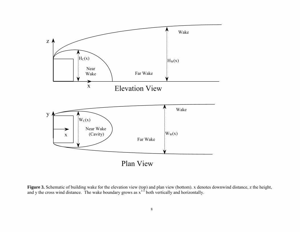
A schematic of the building wake is shown in Figure 3. Simple formulae for height and width of

the cavity envelope (Hc(x), Wc(x)) and the wake boundary (Hw(x), Ww(x)) are defined below.

The structure of the cavity and wake is controlled by the building dimensions, as projected

along-wind and crosswind. These dimensions are the building height (H), the projected building

width across the flow (W), and the projected building length along the flow (L). Following

Wilson19, a length scale for flow and diffusion near a building is defined as,

7

Figure 2. Schematic of building downwash for two identical plumes emitted at different locations. The plume released from the rooftop

stack has a larger rate of growth and more descent than the plume released farther downwind.

Near WakeFar Wake

Streamline

8

Figure 3. Schematic of building wake for the elevation view (top) and plan view (bottom). x denotes downwind distance, z the height,and y the cross wind distance. The wake boundary grows as x1/3 both vertically and horizontally.

NearWake Far Wake

Wake

z

x Elevation View

Near Wake (Cavity)

Far Wake

Wake

x

y

Plan View

WC(x)

WW(x)

HC(x) HW(x)

9

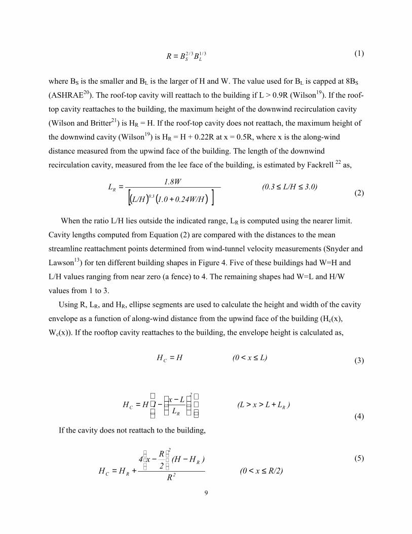
(1)

where BS is the smaller and BL is the larger of H and W. The value used for BL is capped at 8BS

(ASHRAE20). The roof-top cavity will reattach to the building if L > 0.9R (Wilson19). If the roof-

top cavity reattaches to the building, the maximum height of the downwind recirculation cavity

(Wilson and Britter21) is HR = H. If the roof-top cavity does not reattach, the maximum height of

the downwind cavity (Wilson19) is HR = H + 0.22R at x = 0.5R, where x is the along-wind

distance measured from the upwind face of the building. The length of the downwind

recirculation cavity, measured from the lee face of the building, is estimated by Fackrell 22 as,

(2)

When the ratio L/H lies outside the indicated range, LR is computed using the nearer limit.

Cavity lengths computed from Equation (2) are compared with the distances to the mean

streamline reattachment points determined from wind-tunnel velocity measurements (Snyder and

Lawson13) for ten different building shapes in Figure 4. Five of these buildings had W=H and

L/H values ranging from near zero (a fence) to 4. The remaining shapes had W=L and H/W

values from 1 to 3.

Using R, LR, and HR, ellipse segments are used to calculate the height and width of the cavity

envelope as a function of along-wind distance from the upwind face of the building (Hc(x),

Wc(x)). If the rooftop cavity reattaches to the building, the envelope height is calculated as,

(3)

(4)

If the cavity does not reattach to the building,

(5)

L)x(0HHC ≤<=

)LLx(LL

Lx1HH R

2

RC +>>

−−=

R/2)x(0R

)H(H2Rx4

HH 2

R

2

RC ≤<−−

+=

( ) ( )[ ]3.0)L/H(0.3

0.24W/H1.0L/H

1.8WL0.3

R ≤≤+

=

3/13/2LS BBR =

10

Figure 4. Comparison of the lengths of the downwind recirculation cavities for ten different

building shapes as calculated by the PRIME model and observed in the wind tunnel (Snyder and

Lawson13). The lengths were defined as the distance from the lee wall to the point of streamline

reattachment.

11

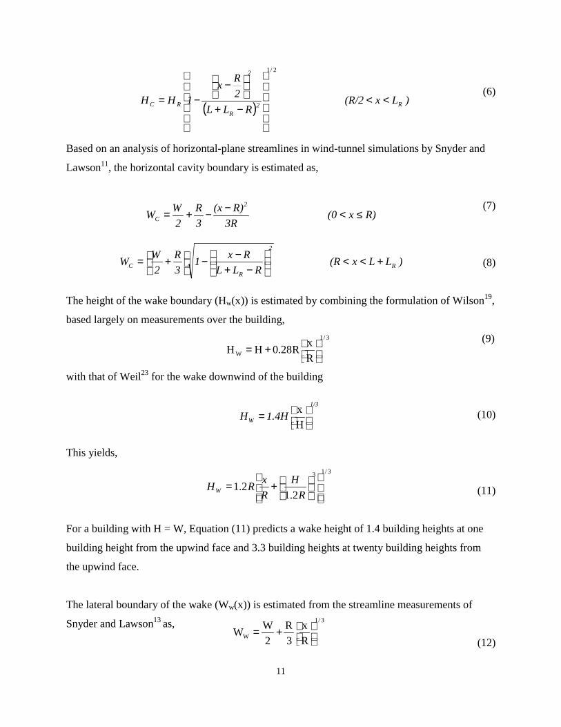
(6)

Based on an analysis of horizontal-plane streamlines in wind-tunnel simulations by Snyder and

Lawson11, the horizontal cavity boundary is estimated as,

(7)

(8)

The height of the wake boundary (Hw(x)) is estimated by combining the formulation of Wilson19,

based largely on measurements over the building,

(9)

with that of Weil23 for the wake downwind of the building

(10)

This yields,

(11)

For a building with H = W, Equation (11) predicts a wake height of 1.4 building heights at one

building height from the upwind face and 3.3 building heights at twenty building heights from

the upwind face.

The lateral boundary of the wake (Ww(x)) is estimated from the streamline measurements of

Snyder and Lawson13 as,

(12)

)LLx(RRLL

Rx13R

2WW R

2

RC +<<

−+

−−

+=

3/1

W RxR28.0HH

+=

1/3

W 1.4HH

=

Hx

3/13

2.12.1

+=

RH

RxRHW

3/1

W Rx

3R

2WW

+=

R)x(03R

R)(x3R

2WW

2

C ≤<−−+=

( ) )Lx(R/2RLL

2Rx

1HH R2R

2

RC <<

−+

−

−=

2/1

12

This formula includes the x1/3 dependence characteristic of three-dimensional far wake growth

and compares very well with the data.

Mean Streamline Slope

The model for the slope of the mean streamlines is based on the location and maximum height

(HR) of the roof-top recirculation cavity, the length of the downwind recirculation cavity (LR)

and the building length scale (R). The wind-tunnel data, in general, show that the slope of the

mean streamlines can be partitioned into five regions. Figure 5 illustrates these five regions for a

cubic building (H=W=L). The modeled streamlines are shown in the upper part of the figure, and

those observed in the wind tunnel (Snyder and Lawson13 ) are in the lower part. The streamline

slope is zero until about a distance R upwind of the building (Region A). The region of ascent

upwind of and over the building (Regions B and C) shows that streamlines attain a maximum

slope near the upwind face, and continue to rise to the point of maximum height of the roof-top

cavity. In Region B, streamlines below about 2H/3 do not rise over the building, but rather

stagnate, or deflect around the sides. A region of streamline descent (Region D) then follows to

the end of the near wake, in which the slope of streamlines follows that of the upper boundary of

the near wake. Beyond, in the far wake (Region E), there is a gradual decrease in the rate of

streamline descent. Also, the absolute magnitude of slope at any x decreases with height above

the building. The shape of the building also affects streamline slope. For example, the descent of

the mean streamlines for a very wide building is not as steep as for a narrow building of the same

height and length. The descent of the mean streamlines for two buildings of the same height and

width is steeper for the building with the shorter length. The magnitude of the descent changes

with wind direction as the projected building width and length change. Also, wind-tunnel

observations of upwind slopes near the ground show that for tall buildings (H > W) only the air

above the upper one-third of the building flows over the building, but for very squat buildings

nearly all the air flows over the buildings.

Using these general observations, empirical relationships for the mean streamline slopes for z@H

were constructed for each region, and a height-dependent decay factor was applied for slopes at

elevations above z = H: (1) a slope of zero is used for all points in Region A; (2) a parabola was

fit to the streamlines below z = H in Regions B, C, and D, yielding slopes that change linearly

13

Figure 5. Comparison of streamlines predicted by the PRIME model with those observed in wind-tunnel simulations of a cubic

building (Snyder and Lawson13). The five regions of streamline deflection (A-E) are noted. The height and distances are scaled by

building height H.

14

0dxdz =

with distance; the fitted streamlines rise 0.22R in both Region B and Region C, and fall 0.22R in

Region D; (3) the streamline slope at the start of Region E decays as x-1; and (4) slopes computed

at z = H decay with z-3 in regions of streamline ascent and z-1 in regions of descent. The value

of 0.22R is the maximum height of the rooftop cavity (Wilson19) and was found to give a good

approximation to the magnitude of the deflection of the streamlines for z ≤ H. Upwind of the

building (Region B), the streamline slope was maintained at zero for when

R@H and for when R > H. The resulting expressions for streamline slope

(dz/dx) at z @ H and the vertical decay factor (Fz) that is applied for z > H are:

Region Streamline SlopeDownwind Distance from the

Windward Face Factor for z>H

A (13)

B (14)

C (15)

D (16)

For crosswind distances outside of the projected width of the building the slopes are linearly

decreased to zero at a crosswind distance of . This cross-stream relaxation is based on

unpublished streamline plots provided by Snyder24.

Streamline slopes predicted at z = H for several points downwind of the buildings were

compared to the streamline slopes presented by Snyder and Lawson13 for ten different building

shapes. This comparison, which showed excellent agreement, was reported in Schulman and

Scire25 and is reproduced as Figure 6. The correlation coefficient from a linear fit to these data is

0.90.

3R

2W +

( )( ) 3.0

2

R

R

Hz

2RLL

x2RHHdxdz

−+

−−=

( )

R

1Rx2HH4

dxdz R

−−−

=

( )( )2

R

RRxHH2

dxdz +−=

( )Rx −<

( )0xR <≤−

( )R5.0x0 <≤

( )RLLxR5.0 +≤≤

1Fz =3

z HzF

−

=

H32z <

)RH2(32z −=

3

z HzF

−

=

1

z HzF

−

=

15

Figure 6. Comparison of the mean streamline slope for ten different building shapes ascalculated by the PRIME model and observed in the wind tunnel (Snyder and Lawson13). Theslopes were determined at building height at 3-4 points downwind of each building.

16

Plume Rise

The PRIME plume rise is computed using a numerical solution of the mass, energy and

momentum conservation laws (Zhang and Ghoniem26). The model allows arbitrary ambient

temperature stratification, arbitrary uni-directional wind shear, and arbitrary initial plume size. It

includes radiative heat losses and can be run in a non-Boussinesq mode. The implementation of

the plume rise model in PRIME allows for streamline ascent/descent effects to be considered, as

well as the enhanced dilution due to building-induced turbulence. A key feature of the model is

its ability to include vertical wind shear effects, which are important for many buoyant releases

from short stacks. Additionally, the wind speed deficit induced by the building is modified as a

function of downwind distance from the building. The deficit also leads to increased plume rise

from short stacks. The temperature profile is not modified from ambient values, which is

conservative during stable conditions.

The governing equations for plume rise are:

(1) Mass (17)

where ? = 0.11 and A = 0.6 (Hoult and Weil 27) are the entrainment parameters corresponding to

the differences of velocity components between the wind and the plume in directions parallel and

normal to the plume centerline, Ua (z) is the ambient horizontal wind speed, which can be an

arbitrary function of height; and

(18)

is the velocity of the plume cross section along its centerline, with two components u and w in

the horizontal and vertical directions, a and aa are the plume density and air density,

respectively, s is the distance along the plume centerline measured from the emission source, r is

the plume radius, and k is the centerline inclination.

(2) Momentum - Along- wind (19)

22sc wuU +=

( )( )dzdUwrr a2 ρρ 2

asc UuUdsd =−

( ) Φ+Φ−= sinUr2cosUUr2rUdsd

aaasca2

sc ρβαρρ

17

(3) Momentum – Vertical

(20)

where g is the gravitational acceleration.

(4) Energy

(21)

where T is the plume temperature, Ta is the ambient temperature, cp is the specific heat of

ambient air and Rp is a variable characterizing the radiation properties with a value of 9.1 x 10-11

kg/(m2K3s).

The effect of increased wake turbulence on entrainment is included by assuming that the mass

entrainment equation (Equation (17)) may be dominated at times by the plume growth due to the

wake turbulence. This is implemented by using the maximum of the two entrainment rates each

step,

(22)

The radial growth rate due to wake turbulence is obtained from the growth rate of the vertical

spreading parameter cz, (whose formulation is discussed in the next section)

(23)

For plume rise downwind of the building, the ambient wind speed profile is modified to reflect

the reduced wind speeds in the wake, so that

(24)

where F(z) is the fraction of the ambient wind speed. Within the cavity, F equals a constant ( Fc),

and above the wake, F = 1. F is a linear function of height between HC and HW,

( )[ ] ( )4a4p

2 TTrRwrTTrU −−

+−=− ρ

cg

dzdTρ

dsd

p

aa

2sc

( ) ( )

=

wakeaa

tentrainmen

2sc

2sc ds

drUr2,rUdsdMaximumrU

dsd ρρρ

(z)F(z)(z) aw UU =

dxdσ

2π

dsdr z

wake

=

( ) ( )ρρρ −= a2

scUdsd grwr 2

18

(25)

FC is calculated by assuming a mean fractional velocity deficit through the full depth of the wake

at the lee wall of the building, FU0/U0, where U0 is a uniform speed upwind of the building. This

constraint with Equation (25) forces Fc to be,

(26)

The value of FU0/U0 was estimated as 0.7 from the wind-tunnel data of Snyder and Lawson11.

The modified wind profile in the wake was allowed to decay from the lee wall to the ambient

profile with an x -2/3 dependence, based on Weil’s23 model of the wake region.

Dispersion Coefficients

Dispersion is based on the approach of Weil23. Enhanced turbulence intensity and velocity deficit

values are calculated within the wake region. These values are a maximum at the lee wall of the

building and decay with the two-thirds power downwind. If the plume is released upwind of the

wake, the plume initially grows at the ambient rate. At the point that the plume centerline

intercepts the wake, a probability density function (p. d. f.) model is used for plume dispersion

over a distance equal to the length of the near wake, and an eddy diffusivity model for plume

growth is used beyond. The key assumption in the p.d.f. approach is that the travel time is short

enough that particles released by the source remember their initial velocity. When the turbulence

intensity within the wake has decayed to the ambient intensity, a virtual source technique is used

to transition to the ISC3 dispersion curves. For an unstable ambient stability, or if the plume is

intercepted by the wake several building heights downwind, the building effects on plume

dispersion may be small and short-lived. This is consistent with the Castro and Robins28 wind-

tunnel simulation of flow around a cube for a fairly rough suburban boundary layer. They found

that the wake decayed completely within about six cube heights downstream. Nearer to the

building or with neutral and stable approach flows the building effects will be larger. The

formulation is presented for vertical dispersion, but is analogous for the horizontal dispersion.

( ) )Hz(HHzHHF1

FF wcccw

cc ≤≤−

−

−+=

( )( )

+−=

cw

00wc

HH0.5

/U∆UH1F

19

Following Weil23 , who estimated constants from the wind-tunnel data of Arya and Gadiyaram29,

turbulence intensity, iz, is calculated within the wake at a distance ([-R) from the lee wall (where

[ is defined such that [ = R at the lee wall) as the quotient of the turbulence velocity in the wake

and the mean wind speed in the wake,

(27)

where the subscript 0 denotes ambient values and cwN denotes the turbulence velocity typical of

neutral flows. At the lee wall, [=R, the turbulence intensity is a maximum,

(28)

At large [/R, the ambient turbulence is recovered

(29)

Recasting Equation (27) using turbulence intensity, and rearranging terms,

(30)

The x-2/3 decay, as used in Weil23 is based on a free wake with uniform approach flow, but gave

the best agreement with wind-tunnel turbulence measurements (Snyder and Lawson13).

Consistent with the plume rise formulation, FU0/U0 was estimated as 0.7 from the wind-tunnel

data. The values of 0.06 for izN and 0.08 for iyN were inferred from the Briggs dispersion

coefficient formula for neutral stability and rural conditions as reported in Gifford30. Ambient

turbulence intensities for iz0 and iy0 were inferred from the Briggs dispersion coefficient formulas

for rural and urban. These values led to good modeled agreement with the observed data

presented later in the paper.

( ) 32

32

00

0wwN0ww

z

R

R7.1

i

−

−

∆−

−+

==ξ

ξσσσσ

UUU

0

000z

1

i7.17.1

UUUU

i zNwN

∆−=

∆−= σ

z00

w0z i

Uσi ==

−

+

−

+=

0

032

0

0

z0

zN

z0z

U∆U

Rξ

U∆U1

i1.7i

1ii

20

Within the p. d. f. growth region spanning a travel distance equal to the length of the near-wake,

the change in the plume spread with distance is proportional to the local turbulence intensity,

. . An eddy diffusivity growth model is used beyond the p.d.f. region, following Weil23,

by assuming

(31)

By matching the growth rate at xd, the distance from the upwind building face to the point of

transition from the p. d. f. to eddy diffusivity growth regime it can be shown that,

(32)

The eddy diffusivity growth rate is followed to the distance at which the turbulence intensity has

decayed to the ambient value, or 15R from the downwind face of the building, whichever

distance is smaller. The cap at 15R is needed for very stable ambient turbulence levels where the

decay distance is unreasonably long. A virtual source distance is used to match the ambient

dispersion coefficients for all further distances. Note that in the ISC downwash model, the

transition to ambient dispersion is always made at 10H or 10W, whichever is less.

Both the horizontal and vertical dispersion coefficients are enhanced within the building wake.

This is supported by Snyder and Lawson11 and the original wind-tunnel data for Huber and

Snyder6. This virtually eliminates the suspiciously large predictions by ISC3 during light wind

speed, stable conditions which are caused by only enhancing the vertical dispersion coefficient

when the stack height is more than 20% higher than the building height.

Near/Far Wake Concentrations

PRIME predicts concentrations in both the near and far wakes. The near wake concentration has

a vertically mixed component resulting from the capture and recirculation of some fraction of the

elevated primary plume by the near wake. From Wilson and Britter21, this concentration is,

(33)

)x(idxd

zz =σ

( ) ( )xHxikUHkσ

U2K

dxdσ

wzwwz

2

===

)(xH(x)H(x)i)(x2σ

dxdσ

dw

wzdz

2

=

BcH

2

yc

N WHU

y21

expQfBC

′

−

=σ

21

where f is the fraction of the plume mass captured by the near wake, Q is the emission rate, W′Bis the width scale through which the plume is mixed, cyc is the horizontal dispersion coefficient

for cavity dispersion, and the constant B is taken as 3 (Wilson and Britter21). W�B is nominally

the building width, but with a maximum value of 3HB and minimum value of HB/3. Wilson and

Britter had suggested 4 HB as the maximum value, but comparisons with Thompson31 wind-

tunnel observations in the near wake led to the adopted values. In addition, for plumes released

upwind of the cavity, W�B is obtained from the plume cy at the lee wall using the equivalent top-

hat distribution. This accounts for initial horizontal plume growth upwind of the cavity. The

value cyc is calculated as W�B/(2_)0.5, which also assumes a top-hat distribution.

The fraction of the plume captured by the near wake is calculated in several steps. Using the

equations for the height and width of the near wake boundary, the fractions of the vertical plume

mass distribution, fZ, and the horizontal plume mass distribution, fY, that are within the

boundary of the near wake, are calculated at many distances along the near wake length. The

fraction captured is then estimated as the maximum of the product fZ fY along the near wake

length. This concept can be seen from Figure 2 for the vertical distribution. The plume

emanating from the rooftop stack is partially intercepted by the near wake boundary. The

fraction that is intercepted changes with downwind distance and can be calculated from:

(34)

where Hp is plume height. Because plumes released within the near wake would always have

100% capture with this procedure, the value of fZ was capped at the fraction below HB at the end

of the near wake to allow plumes with momentum or buoyancy to partially or fully escape

capture. The choice for the fz cap was based upon comparisons of vertical plume profiles with

the wind-tunnel data of Snyder10.

That plume mass captured by the near wake is re-emitted to the far wake as a volume source.

The volume source is modeled as a ground-level point source located at the base of the lee wall.

The growth of the point source at this location is used as a surrogate for the loss of cavity mass

up the wall and through the surface boundary of the cavity as it fluctuates unsteadily. This source

−=

)x(2)x(H)x(H

erf)x(fz

pcz σ

22

is only applied to the far wake using the formula,

(35)

where cy has the initial value cyc at the lee wall and cz has the initial value czc, which is

calculated by matching CN=CF at the lee wall. cyc and czc grow using the same methods as for

the elevated plume.

Also contributing to the far wake is the portion of the primary plume that is not captured by the

near wake. This second source has mass rate (1-f) Q and follows the Gaussian plume formulation

to calculate the concentration Cp,

(36)

The terms for receptors above ground level and for reflection from the top of the mixed layer are

not shown, but these terms are identical to those in the ISC model.

A transition zone between the near and far wakes is used to represent the unsteadiness of the near

wake/far wake interface, and based on observations of the fluctuations of reattachment lengths in

wind tunnels by Hosker1, is taken as the region within 15% of the mean interface location. In the

transition zone, a linear interpolation using a weighting parameter U is made from the near wake,

CN, to far wake, CF, concentrations. CP is added beyond the end of the near wake to calculate the

total concentration.

In summary, for the near and far wake concentrations,

C=Cn (L≤ x ≤ L+0.85 LR) (37)

C=UCN + (1-U)CF (L + 0.85LR ≤ x < L+LR) (38)

yczcs

2

y

F U

y21expfQ

Cσσπ

σ

−

=

( )

szy

2

y

2

z

p

p U

y21exp

H21expQf1

Cσπσ

σσ

−

−−

=

23

C=Cp + UCN +(1-U)CF (L + LR ≤ x ≤ L + 1.15 LR) (39)

C=Cp + CF (x ≥ L + 1.15 LR) (40)

where U decreases linearly from U = 1 at x = L + 0.85LR to U = 0 at x = L + 1.15LR.

COMPARISON WITH OBSERVATIONS

Snyder Wind-Tunnel Data

As reported earlier, a portion of the wind-tunnel data collected for this effort, Snyder10, included

systematic variations of stack to building height ratios, ratios of exhaust speeds to wind speeds,

wind angle, Froude number and stack location for both a generic steam boiler and combustion

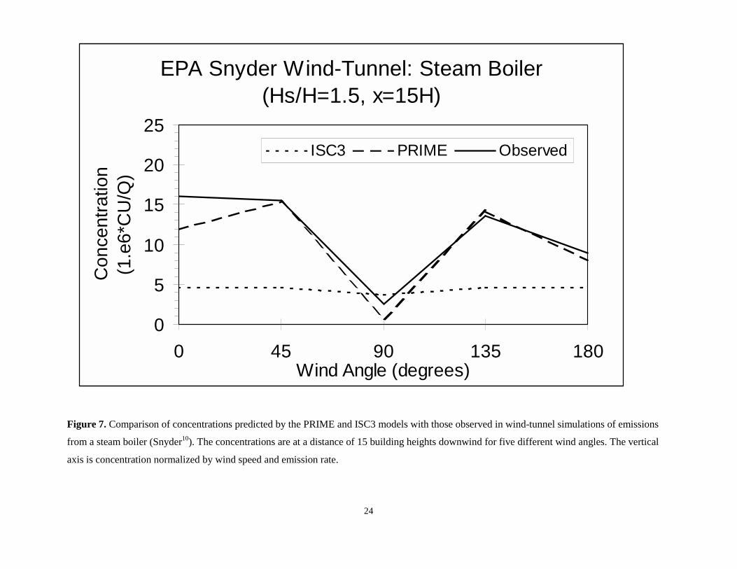
turbine. Figure 7 shows the comparison of PRIME and ISC3 predicted concentrations with

observations at 15 building heights downwind for the steam boiler. The building width is twice

the height and 2.5 times the length. The stack is located in the middle of the wider horizontal

dimension and is 1.5 times the building height. The stack is downwind of the building for a

direction of zero degrees, which is defined as perpendicular to the wider horizontal dimension.

Five different wind angles to the building face were simulated in the tunnel. For all of these

cases, the plume has an exhaust speed to wind speed ratio of 1.5 and a Froude number of 16.

This is a highly buoyant plume with a full-scale equivalent buoyancy flux of 528 m4/s3.

PRIME better matches the concentration trends with wind direction. The lowest concentrations

are both observed and predicted with winds perpendicular to the shorter dimension. For this

direction, the stack is along the side of the building halfway down the length. The wake will have

smaller dimensions for this case. For both the 45 degree and 135 degree cases, the wind is at a 45

degree angle with the larger horizontal dimension, but the stack is upwind of the building for the

135 degree case, resulting in slightly lower concentrations. The concentrations for these cases is

a competition between the plume height, which is higher for the 135 degree case and the plume

dimensions, which are larger for the 45 degree case.

ISC3 not only underestimates the observed concentrations for all cases except for the 90-degree

direction, but also shows almost no variation with wind direction. This is because the projected

24

Figure 7. Comparison of concentrations predicted by the PRIME and ISC3 models with those observed in wind-tunnel simulations of emissions

from a steam boiler (Snyder10). The concentrations are at a distance of 15 building heights downwind for five different wind angles. The vertical

axis is concentration normalized by wind speed and emission rate.

EPA Snyder Wind-Tunnel: Steam Boiler (Hs/H=1.5, x=15H)

0

5

10

15

20

25

0 45 90 135 180Wind Angle (degrees)

Con

cent

ratio

n (1

.e6*

CU

/Q)

ISC3 PRIME Observed

25

width is larger than the building height for all but the 90-degree direction. The vertical dispersion

coefficient in ISC3 only depends on projected width when the building height is larger than the

projected width. Plume trajectory, wind speed and the horizontal dispersion coefficient are

always unchanged with wind direction in ISC3 for this stack height.

Thompson Wind-Tunnel Data

These data31 consist of non-buoyant, zero-momentum releases upwind of and in the near and far

wakes of four different building shapes. Concentrations were measured at ground level on the

centerplane. Figure 8 shows the comparison of PRIME and ISC3 predicted concentrations with

observed concentrations for a source in the downwind cavity of a cubic building. The source is

one building height downwind of the lee wall and half the building height above the ground. The

flow is perpendicular to the building. Because ISC3 is only valid beyond three building heights

downwind, SCREEN3 was used to predict the cavity concentration. In this case the ISC3

predictions are not valid until four building heights from the lee wall, since the building is moved

to the source location in ISC3.

As can be seen in Figure 8, when a passive source is released in the cavity, the concentrations are

not uniform. The peak concentration is observed at the downwind location of the source and

some mass is mixed upwind. PRIME agrees reasonably well with observations in the cavity,

underestimating the peak value by about 25%, but overestimating about half the cavity

concentrations. Beyond the cavity, which extends less than two building heights downwind from

the lee wall, PRIME shows very good agreement with observations.

SCREEN3 underestimated all the cavity concentrations, including the peak value by about 65%.

The ISC3 predictions, which start at four building heights downwind, do as well as PRIME with

the observations.

26

Figure 8. Comparison of concentrations predicted by the PRIME and ISC3 models with those observed in wind-tunnel simulations of a source

located in the downwind recirculation cavity of a cubic building (Thompson31). The vertical axis is non- dimensional concentration and

the horizontal axis is distance from the lee wall in building heights, H.

Thompson Wind-Tunnel: W/H=L/H=1Source (x/H=1, z/H=0.5)

0

1

2

3

4

5

6

0 1 2 3 4 5 6 7 8 9 10 11 12 13 14Distance from Lee Wall (x/H)

Con

cent

ratio

n (n

ondi

m) ISC3

PRIME

Observed

27

Alaska North Slope Field Study

A field study was conducted near Prudhoe Bay (Guenther, Lamb and Allwine32) for a high

buoyancy, high momentum combustion turbine with a stack to building height ratio of 1.15. The

buoyancy flux was 355 m4/s3 and the momentum flux 575 m4/s2. Thirty-eight hours of SF6 tracer

data and onsite meteorological data were collected during very high wind speed conditions (up to

18 m/s) over a 7 day period. Samplers were placed at up to 60 locations, in arcs at distances

from 20 m to 3400 m, so that the largest concentrations could be measured.

Figure 9 shows a quantile-quantile plot of the maximum observed and predicted concentrations

for each of the 38 hours. Hour-by-hour comparisons are often not meaningful because of the

uncertainties in meteorological conditions and model components. For the largest observed

concentrations PRIME shows much better agreement than ISC3. PRIME overestimates the

largest concentration by 31%, while ISC3 overestimates by 296%. Both models overestimate the

smaller observed concentrations, but PRIME overestimates by a smaller margin. For the highest

predicted concentrations, PRIME estimates lower plume heights than ISC3, but also smaller

dispersion coefficients.

Bowline Point Power Plant

One-half year of measured meteorological, emissions and concentration data for a 1200 MW

power plant (Schulman and Hanna8) were used to evaluate ISC3 and PRIME. The plant has two

identical stacks that are 1.33 times the building height of 65.2 m. Only two monitors observed

any significant concentrations. The highest concentrations were observed at a monitor 848 m

from the midpoint of the stacks during hours with high wind speeds. Meteorological data were

measured at a 100 m tower located 250 m from the plant.

Figure 10 shows the ten highest observed and predicted concentrations at the monitor with the

largest observed values, as well as the stability class associated with that hour. These values are

unpaired in time. PRIME is within 3% of each of the top three observed concentrations and

overestimates the tenth highest value by 29%. ISC3 overestimates the highest three observations

by an average of 21% and the tenth highest value by 40%.

28

Figure 9. Ranked comparison of the maximum concentrations (normalized by emission rate)

predicted by PRIME and ISC3 with the highest concentrations observed during each of the 38

hours of a field study on the Alaska North Slope (Guenther, Lamb and Allwine32). The source

was a highly buoyant combustion turbine.

Alaska North Slope: Quantile-Quantile of Hourly Maximum Concentrations

0

5

10

15

20

0 1 2 3 4 5 6Observed (C/Q)

Mod

eled

(C/Q

)

PRIMEISC31:1

29

Figure 10. Comparison of the ten highest hourly concentrations predicted by the PRIME and ISC3 models with those observed at amonitor near the Bowline Point Generating Station. The atmospheric stability class associated with each concentration is noted(1=very unstable, 2=unstable, 3=slightly unstable, 4=neutral, 5=slightly stable and 6=stable).

Top Ten Predicted and Observed Concentrations: Bowline Point Monitor

(Stability Class is Noted)

455154

66

5

6

414444444

4

4444

444

4

4

4

0

100

200

300

400

500

600

700

800

900

0 1 2 3 4 5 6 7 8 9 10 11Rank

Con

cent

ratio

n (u

g/m

3)

ISC3PRIMEObserved

30

PRIME correctly matches the high wind speed, neutral stability conditions (stability class 4) of

the highest observed hours. In fact, four of the highest concentrations predicted by PRIME occur

during the same hours as the ten highest observed values. All of the ten highest observations are

during neutral stability conditions and nine of the ten highest concentrations predicted by PRIME

occur during neutral stability conditions. Only one of the ten highest concentrations predicted by

ISC3 occurs during an hour with one of the ten highest observed concentrations. Seven of the ten

highest are predicted to occur during stable conditions. Much lower concentrations were actually

measured during hours with stable conditions.

CONCLUSIONS

The PRIME model includes several advances in modeling building downwash effects including

enhanced dispersion in the wake, reduced plume rise due to streamline deflection and increased

turbulence, and a continuous treatment of the near and far wakes. All of these effects consider

the location of the plume within the wake. Comparisons of the model with wind-tunnel and field

data have shown improved performance over the current ISC3 model. The PRIME model is

implemented within the ISC3 model code, but can be implemented in other refined or screening

air quality models.

ACKNOWLEDGMENTS

This research was sponsored by EPRI of Palo Alto, CA and participating EPRI members. The

authors are thankful for the support of Dr. Charles Hakkarinen, the EPRI project manager,

Richard Osa of Science and Technology Management, the project administrator, Richard Dunk

of Jersey Central Power and Light for providing the field study facility, Dr. William Snyder of

NOAA, Roger Thompson of EPA, and Dr. William Melbourne of Monash University for

providing wind tunnel data, and Dr. Rex Britter of the University of Cambridge, project

consultant, for his helpful discussions.

31

NOMENCLATURE

a α entrainment parameter parallel to the plume centerlineb β entrainment parameter normal to the plume centerlineb B empirical constant (recirculation factor for near wake concentration)bl BL larger of H and Wbs BS smaller of H and Wcf CF contribution to the far wake concentration from fraction of the plume captured

by the near wake (µg m-3)cn CN near wake concentration from fraction of the plume captured by the near wake

(µg m-3)cp cP specific heat of ambient air (J kg-1 K-1)cp CP contribution to the far wake concentration from portion of the plume not

captured by the near wake (µg m-3)dz dz/dx mean streamline slope

F fraction of the ambient wind speed at height z in wakef f fraction of the plume mass captured by the near wakefc FC constant value of F in the cavityfy fY fraction of the horizontal plume mass captured by the near wakefz FZ vertical decay factor for streamline slope for z>Hfz fZ fraction of the vertical plume mass captured by the near wakeg g acceleration of gravity (m s-2)h H building height (m)hc HC height of the downwind recirculation cavity (m)hp HP plume height (m)hr HR maximum height of the downwind recirculation cavity (m)hw HW height of the wake boundary (m)iz iz vertical turbulence intensityizn izN value of iz typical of neutral flowizo iz0 ambient value of izl L projected building length along the flow (m)l λ linear weighting factor (from 0 to 1) for contributions from CN and CF in the

transition zone between the near and far wakeslr LR distance along the downwind recirculation cavity measured from lee face (m)ph φ angle of plume centerline inclination with the horizontal (rad)q Q emission rate (g s-1)r R building length scale (m)r r plume radius (m)r ρ density of plume (kg m-3)ra ρa density of ambient air (kg m-3)rp RP plume radiation properties with value 9.1x10-11 kg m-2 K3 s if emissivity is taken

as 0.8s s distance along the plume centerline measured from the emission source (m)sw σw standard deviation of the turbulent velocity fluctuations in the vertical (m s-1)

32

swa σw0 ambient value of σw (m s-1)swn σwN value of σw typical of neutral flow (m s-1)sy σy standard deviation of the lateral concentration distribution, referred to as the

horizontal dispersion coefficient (m)syc σyc horizontal dispersion coefficient for the downwind recirculation cavity (m)sz σz standard deviation of vertical concentration distribution, referred to as the

vertical dispersion coefficient (m)szc σzc vertical dispersion coefficient for the downwind recirculation cavity (m)t T plume temperature (K)ta Ta ambient temperature (K)u u along-wind velocity component (m s-1)ua Ua ambient wind speed (m s-1)uh UH ambient wind speed at building height (m s-1)uo U0 uniform wind speed upwind of the building used as part of ratio ∆U0/U0usc USC velocity of the plume along centerline (m s-1)uw Uw wind speed in the wake (m s-1)w W projected building width across the flow (m)w w vertical velocity component (m s-1)wb W′B building width scale through which plume is mixed in the recirculation cavity

(m)wc WC width of the downwind recirculation cavity (m)ww WW width of the wake boundary (m)x x along-wind distance measured from the upwind face of the building (m)x ξ downwind distance defined so that it equals R at the lee wall (m)

33

REFERENCES

1. Hosker, R. P. Jr. In Atmospheric Science and Power Production; D. Randerson, Ed.; DOE/TIC-27601; United States Department of Energy: Washington, DC, 1984; Chapter 7.

2. Meroney, R. N. In Engineering Meteorology; E.J. Plate, Ed.; Elsevier Scientific Publishing Co.:Amsterdam, 1982; pp 481-525.

3. Screening Procedures for Estimating the Air Quality Impact of Stationary Sources - Revised454/R-92-019; U.S. Environmental Protection Agency: Research Triangle Park, NC, 1992.

4. User’s Guide for the Industrial Source Complex (ISC3) Dispersion Models 454/B-95-003b; U.S.Environmental Protection Agency: Research Triangle Park, NC, 1995.

5. Schulman, L.L.; Scire, J.S. J. Air and Waste Management Association 1993, 43, 1122-1127.

6. Huber, A. H.; Snyder, W.H. Atmospheric Environment 1982, 176, 2837-2848.

7. Scire, J. S.; Schulman, L.L. In Second Joint Conference on Applications of Air PollutionMeteorology; American Meteorological Society: Boston, MA, 1980; pp 133-139.

8. Schulman, L.L.; Hanna, S.R. J. Air Pollution Control Association 1986, 36, 258-264.

9. EPRI. Results of the Independent Evaluation of ISCST3 and ISC-PRIME. Report TR-2460026.Palo Alto, CA, 1997.

10. Snyder, W. H. Wind-Tunnel Simulation of Building Downwash from Electric-Power GeneratingStations. Part I: Boundary Layer and Concentration Measurements. U.S. EnvironmentalProtection Agency: Research Triangle Park, NC, 1992.

11. Snyder, W.H., Lawson, R. Wind-Tunnel Simulation of Building Downwash from Electric-PowerGenerating Stations. Part II: Pulsed-Wire Measurements in Vicinity of Steam-Boiler Building.U.S. Environmental Protection Agency: Research Triangle Park, NC, 1993.

12. Snyder, W.H. In NATO Advanced Research Workshop, Recent Advances in the Fluid Mechanicsof Turbulent Jets and Plumes; Viano so Castelo, Portugal, 1993.

13. Snyder, W.H.; Lawson, Jr., R.E. In Eighth Joint Conference on Applications of Air PollutionMeteorology with A&WMA; American Meteorological Society: Boston, MA, 1994; pp 244-250.

14. Melbourne, W. H.; Taylor, T.J. Plume Rise and Downwash Wind Tunnel Studies: CombustionTurbine Unit 4 Sayreville; Draft Final Report; Monash University Department of MechanicalEngineering: Clayton, Victoria, Australia, 1994; TR-235274.

15. Oncley, S. Summary of ASTER Operations During DOWNWASH94, Final Report; NationalCenter for Atmospheric Research: Boulder, CO, 1994.

16. Kaiser, R. D.; Nielsen, N.; Uthe, E. Remote Sensing of Plume Diffusion and Building WakeEffects. Final Report; SRI International: Menlo Park, CA, 1994; SRI Project 50067.

17. Scire, J. S.; Schulman, L.L.; Strimaitis, D.G. In 88th Annual Meeting of the Air and WasteManagement Association; Air and Waste Management Association: Pittsburgh, PA, 1995; Paper95-WP75B.01.

34

18. Brzoska, M. A.; Stock, D.; Lamb, B. In Ninth Joint Conference on Applications of Air PollutionMeteorology with A&WMA; American Meteorological Society: Boston, MA, 1996; pp 322-328.

19. Wilson, D. J. ASHRAE Transactions 1979, 85, 284-295.

20. 1997 ASHRAE Handbook - Fundamentals; American Society of Heating, Refrigerating and Air-Conditioning Engineers: Atlanta, GA, 1997.

21. Wilson, D. J.; Britter, R.E. Atmospheric Environment 1982,16, 2631-2646.

22. Fackrell, J.E. J. Wind Engineering and Industrial Aerodynamics 1984, 16, 97-118.

23. Weil, J. C. In Ninth Joint Conference on Applications of Air Pollution Meteorology withA&WMA; American Meteorological Society: Boston, MA, 1996; pp 333-337.

24. Snyder, W.H., personal communication, 1995

25. Schulman, L.L.; Scire, J.S. In Ninth Joint Conference on Applications of Air PollutionMeteorology with A&WMA; American Meteorological Society: Boston, MA, 1996; pp 307-310.

26. Zhang, X.; Ghoniem, A.F. Atmospheric Environment 1993, 15, 2295-2311.

27. Hoult, D.P.; Weil, J.C., Atmospheric Environment. 1972, 6, 513-531

28. Castro, I. P.; Robins, A.G. J. Fluid Mechanics 1977, 79, 307-335.

29. Arya, S.P.S., Gadiyaram, P.S., Atmospheric Environment 1986, 20, 729-740

30. Gifford, F. A. Nuclear Safety 1976, 17, 68-86.

31. Thompson, R.S. Atmospheric Environment 1993, 15, 2313-2325.

32. Guenther, A.; Lamb, B.; Allwine, E. Atmospheric Environment 1989, 24A, 2329-2347.