development and income distribution in a dual economy: a
TRANSCRIPT

Development and Income Distribution in a DualEconomy: A Dynamic Simulation Model for Zambia
SWP-292World Bank Staff Working Paper No. 292
August 1978
The views and interpretations in this document are those of the authorsand should not be attributed to the World Bank, to its affiliatedorganizations, or to any individual acting in their behalf.
Prepared by: Charles R. BlitzerDevelopment Research CenterDevelopment Planning Division
Copyright © 1978'd Bank E L k }m reet, N.W.
PUB zn, D.C. 20433, U.S.A.HG3881.5.W57W67no.292
Pub
lic D
iscl
osur
e A
utho
rized
Pub
lic D
iscl
osur
e A
utho
rized
Pub
lic D
iscl
osur
e A
utho
rized
Pub
lic D
iscl
osur
e A
utho
rized
Pub
lic D
iscl
osur
e A
utho
rized
Pub
lic D
iscl
osur
e A
utho
rized
Pub
lic D
iscl
osur
e A
utho
rized
Pub
lic D
iscl
osur
e A
utho
rized

DEVELOPMENT AND INCOME DISTRIBUTION IN A DUAL ECONOMY:
A DYNAMIC SIMULATION MODEL FOR ZAMBIA
by
Charles R. Blitzer
Development Research CenterWorld Bank
Washington, D.C.
The specific facts, methods of analysis, and conclusions are thesole responsibility of the author and do not necessarily reflect officialWorld Bank positions. The author is extremely grateful for the assistancehe received from numerous colleagues, particularly from Bela Balassa, CliveBell, John Cleave, Kemal Dervis, Jan Gunning, Per Ljung, Alan Manne, BillMcCleary, T.N. Srinivasan, and Martin Wolf. Computations were carried outby Thomas Cauchois.


The views and interpretations in this document are those of the authorand should not be attributed to the World Bank, to its affiliated organ-izations or to any individual acting in their behalf.
WORLD BANK
Staff Working Paper No. 292
August 1978
DEVELOPMENT AND INCOME DISTRIBUTION IN A DUAL ECONOMY:
A DYNAMIC SIMULATION MODEL FOR ZAMBIA
This paper discusses medium-term development prospects for Zambia. Theanalysis is carried out in terms of a modified dual economy model, suit-ably modified to capture a number of key aspects of the Zambian Economy.Mining is separated from other urban production and the rural sector issub-divided into traditional, emergent, and commercial farming. Simula-tions are carried out on the basis of alternative governmental expenditure,investment, and taxation policies. Special attention is paid to sectoralemployment and income distribution implications. In addition, the modelis used to derive a number of shadow prices which would be used for projectappraisal. These include shadow price of government savings, and a socialdiscount rate.
Prepared by:Charles R. BlitzerDevelopment Research CenterDevelopment Planning Division
Copyright D 1978The World Bank1818 H Street, N.W.Washington, D.C. 20433 U.S.A.
/

I

I. Introduction
Derelopment theorists have long made use of the simplifying
paradigm of the dual economy. With this theory, the key structural
characteristic of developing countries is the dualism in the economy
between a ticaditional, relatively poor, mostly agricultural sector and
a modern, relatively rich, mostly industrial sector. Seen in this
light, policy discussions should focus most strongly on the implications
of the linkages and characteristics of the two sectors. This approach
to economic development has its roots in Ricardo and Marx and has been
repopularized in recent decades by the work by Lewis, Fei and Ranis,
Marglin, Sen, and many others.-/
Although rich in general policy conclusions, specific policy
applications are rare. Numerical economy-wide forecasting and programming
models have emphasized other important constraints (e.g., savings and
foreign exchange limitations, intermediate industrial demands, human capital,
etc.) in comparison to dual economy factors.-/ This tendency is due both
to data rarely being collected with dual economy models in mind, and to
the development of the numerical models out of Keynesian and neo-classical
roots.
Dual economy models have, however, found a real use in the
literature on project evaluation in developing countries. Both the
Little-Mirrlees and UNIDO methods are based on use of shadow prices
implicitly derived from optimization of a dynamic dual economy model.
1/ Lluch 11977] provides a thorough survey of the theoretical implicationsof various strands in this literature.
2/ A notable exception is the study of Japan by Kelley, Williamson andCheetham [1972].

-2-
Unfortunately, in practice partial equilibrium estimates of the parameters
(principally, the shadow prices of labor, capital, and foreign exchange)
are utilized, putting the whole project evaluation procedure in question.
The standard procedure is broken into two distinct exercises -- the first
focusing on the determination of the dynamic parameters determined by dual
economy-like assumptions, and the second using these together with a
description of the economy's static equilibrium to derive the shadow
prices of each good.1 /
Here, we broaden the use of dual economy models by attempting to
construct a numerical application designed explicitly for simultaneous
derivation of long-term macroeconomic forecasts and shadow prices.
Particular attention is paid to the policy implications of alternative
income distribution objectives. It is important to note that the model
is not explicitly maximizing. Rather it simulates the development process
under a number of different assumptions regarding government policy and
exogenous factors.
Zambia is the country for which this dual economy model has been
developed.-/ Through exploitation of its mining resources (mainly copper),
Zambia maintains one of the highest levels of national income per capita
in Africa. Especially since Independence, its industrial and urban
sectors have grown dramatically. On the other hand, the Zambian economy
remains highly dualized, with the majority of the population living in
1/ For recent discussions of these issues see Blitzer, Little, and Squire[1977], Blitzer, Dasgupta, and Stiglitz [1977], Bruno [1976], and Rhee [1978].
2/ For a recent description of the Zambian economy see World Bank [1977].

- 3-
rural areas where income per capita averages less than one third the
level in the modern sectors. Indeed, most of the rural population is
engaged in subsistance farming. Not only is income low in agriculture,
but growth in food production has been sluggish and irregular.
Reduction of income gaps between rural and urban areas and
increased agricultural output are key policy objectives of the Zambian
government. The dynamic model of Zambia (DYZAM) is designed as a tool
planners could use in studying the impact of alternative policy packages.
Although DYZAM is an economy-wide model, the major emphasis throughout
is on income and production in the rural sectors. The other major focus
is on the medium and long-term affects of various public policies. Hence,
short-run adjustment problems are largely neglected.
The model itself is reviewed in general terms in Section II.
A more complete algebraic formulation is contained in the Appendix. In
Section III, several alternative macroeconomic policies are compared in
terms of their implied forecasts. The shadow price and welfare implica-
tions of DYZAM are developed in Section IV
II. Assumptions and the Model Formulation
I1.1 2erneraZ Assumption's
The typical theoretical dual economy model postulated a two-
sector (traditional and modern) economy producing two goods (rural and
urban), having two consuming classes (rural and urban workers), and one
savings class (profit earners or government). This structure clearly

-4-
is too narrow for any real country application.-/ A broader disaggregation
has been adopted for DYZAM to more accurately reflect Zambian reality,
while remaining sufficiently aggregative to be estimable and computable.
In the model, it is assumed that the Zambian economy produces
three goods: a rural good (highly aggregative and largely agricultural);
an urban good (even more highly aggregative); and a mining good (mostly
copper). In order to focus more heavily on production, income levels,
and dualism within agriculture itself, the rural economy is subdivided
into three producing sectors. The first, referred to as "traditional
agriculture", incorporates subsistance farming and small farmers
marketing only a small share of their production. Roughly half the
population is supported by the income generated in traditional agriculture.
The second, referred to as "emergent agriculture", includes small-scale
Zambian farmers who earn most of their income through marketing their
produce. Finally, there is a large-scale commercial agriculture sector.
Although relatively small in terms of employment, this sector produces
about 40% of all marketed agricultural produce. In total then, there
are five producing sectors in the model: traditional agriculture,
emergent agriculture, commercial agriculture, urban, and mining.
To further emphasize income distribution (and to improve the
savings and demand projections), the economy is divided into seven
income classes. The first five correspond to the workers in each sector
(i.e., traditional farmers, emergent farmers, commercial farm workers,
urban workers, mining workers). The other two refer to the high income
elite of the economy who receive portions of the returns to capital, viz.,
1/ Lluch [1977].
-5-
the Zambian bourgeoisie and foreigners.
In DYZAM, open unemployment in the urba-u sectors is endogenously
computed. Except for migration effects, interactions between the unemployed
and the economy is not directly modeled. Hence, there is some ambiguity
about their real income levels and sources. In some sense, they must form
a part of the "informal" sector which does not enter directly into national
income calculations. Given a lack of data, not much could be done. For
calculating shadow prices, however, some assumptions of income level are
required. These are outlined in Section IV.
The next set of assumptions deals with commodity prices. Through-
out, we assume that all three goods are tradeable and that Zambia, by
itself, canrnot change the relative world terms of trade. Thuis, the
economy faces fixed international prices in each year, although these may
change exogenously year-to-year.- With given international prices,
domestic producers' prices are set by tariff levels and domestic consumers'
prices by tariffs and excise taxes.
On the basis of consumer and producer behavior, as well as on
government policy, the model calculates sectoral resource allocations
(of capital and labor), production and income levels, consumption and
investment demands, government revenue and expenditure, and intersectoral
demographic movements for each year. The solution for any given year
determines certain initial conditions for the next and consequently the
model can simulate Zambian development forward in time until its underlying
assumptions are no longer sufficiently valid to produce realistic
1/ While this may be a reasonable assumption for agricultural and urbangoods, it is quite possible that Zambia could affect the world price ofcopper by adjusting its own inventories. Since DYZAM is ill-suited foruse in choosing optimal inventory levels, we assume that the country willcontinue to act as a price taker and sell its output at going prices.Alternative policies could be easily simulated as well. See World Bank [19771.

projections.-/ In the following subsections, we consider each step more
explicitly.
11.2 YearZy Output Levels and Resource AZlocations.
Consider the agricultural sectors first. It is postulated that
all three sectors operate along a similar Cobb-Douglas production function,
relating output to labor and capital inputs.-/ This amounts to assuming
the productivity differentials are largely due to different choices of
technique, which in turn are caused by various market imperfections and
rigidities.
Wages paid to hired labor in commercial farming are exogenously
forecasted on the basis of productivity estimates. We assume that
commercial farmers maximize profits, given fixed producers' prices and
capital stock. This process determines the employment and output levels.
If on balance emergent farmers neither hire labor from outside their
subsector nor seek outside employment,-/ then labor and capital usage are
known and output determined. The labor force in traditional agriculture is
then taken as the residual between the total agricultural labor force and
employment in commercial and emergent agriculture.
Employment and output in the urban sector are calculated in the
same way as with commercial agriculture. The producers' price and the
nominal wage are pre-determined; output is a function of labor and
capital inputs. Given that the capital stock is fixed by past investment
decisions, labor is hired until profits are maximized.
Mining is handled in a somewhat different fashion. First, we assume
1/ Here we report on simulations for a fifteen-year period, 1977-1992.
2/ With this formulation, land is treated implicitly as a surplus resource.This is supported by Ljung's finding that farm size is an almost linearfunction of other factors. In commercial agriculture, acreage is usuallylimited by direct government regulation. See Ljung [1975].
3/ Rural services are treated as part of agricultural production andare thus included.

-7-
that there is little scope for capital-labor substitution in production;
capital, labor, and intermediate input requirements are proportional to
output levels.-' Output levels cannot now be determined by explicit
profit maximization; rather, we suppose that the sector will follow a
long-term growth strategy formulated by government planners. This strategy
can then be one of the policies tested by the model.
While full employment is postulated for the agriculture as a
whole (although mostly at low productivity), DYZAM allows for open
unemployment in urban areas. Unemployment is computed residually as the
difference between the total urban work force and employment in the mining
2/and urban sectors.- Thus, the urban "informal" sector is included
neither in national income nor in employment calculations.
II.3 PersonaZ Income Distribution
It is a comparatively easy task to compute the total gross income
which accrues to each of the five "worker" classes, once output (and
employment) levels are known. Traditional and emergent farmers earn the
full value of their production (i.e., as if they "owned" the capital used
in their production activities). Total income earned by commercial farm,
urban, and mining workers is simply employment times the respective real
wage.
1/ Although these ratios are fixed for any one year, the change overtime, reflecting technical progress and long-term choice of technique.Similarly, technical progress forms are included in the Cobb-Douglasproduction functions used for determining output in the other sectors.
2/ The total urban labor force is fixed during each year, but changesover time in response to population growth and rural-urban migration.This process is reviewed in Section II.7 .

- 8-
Calculation of the distribution of the rest of total value
added is more complicated. Consider the share going to the Zambian
bourgeoisie. They are treated as partial owners of the commercial farming
and urban sectors, and their total gross income is determined by their
share of profits (returns to capital) in each sector. Foreigners have
a 49% interest in mining, as well as considerable investments in
commercial agriculture and the urban sector. Remaining ownership shares
in these three sectors belong to the government directly and indirectly.-/
Net personal income can then be derived by applying the average
corporate tax rates to profits and the relevant income tax rates to all
gross personal incomes. The new incomes of each group can then be
invested, spent for consumption purposes, or (in the case of foreigners)
repatriated abroad.
II.4 Private Expenditure Patterns
The parameters of an extended linear expenditure system have been
estimated for each of the seven income classes.-/ The system is "extended"
in that savings levels are determined as a function of consumers' prices,
as well as income levels. These relationships determine per capita savings
and consumption of agricultural and urban goods within each income class;
1/ Indirect governmental profits are those accruing to para-statals.Here, we aggregate net para-statal income together with direct governmentrevenues although it is entirely allocated (net of taxation) to investmentas described earlier.
2/ These parameters are the marginal budget shares and propensity tosave, and "subsistance" levels of consumption. Those all differ amongthe groups. See Lluch, Powell, and Williams [1977] for descriptions ofthis class of expenditure systems.

- 9_
which are summed to provide projections of total consumption and private
savings. Foreign remittances by non-Zambians are computed as part of their
expenditure system.
Since producers' and consumers' prices can differ, total private
demands can be used to calculate excise tax and net import duty revenue.
II.5 Government Revenue and Expenditure
Net government revenue is composed of its direct and indirect
share of profits, direct taxes (on corporate and personal incomes), and
indirect taxes (on imports and consumption goods). In the experiments
reported here, we assume that the government can borrow from abroad what-
ever it needs to close any gap between its net expenditures and revenues.
Moreover, in our basic forecasts all government expenditures (net invest-
ment, public consumption, and depreciation) are projected exogenously,
thus making the trade gap technically an endogenous variable.
This determination of the level and pattern of public expenditure
is arbitrary and many alternatives, often called "closing rules", are
possible.-/ The key implication of the rule chosen is that copper is
effectively separated from the rest of the economy. That is, for any
given policy choice set, alternative forecasts of the world price of copper
affect only the model's forecasts of net trade deficits -- not growth or
real income. Since this clearly is not always the case, the basic
forecasts of expenditures were carefully chosen so the implied time pattern
1/ See papers by Bruno, Bell, Taylor and Lysy, and Lluch forthcoming inthe JournaZ of DeveZopment Economics.

- 10 -
of net borrowing was consistent with projected export earnings. No
cross-check is imposed that the present value of foreign borrowing be
any particular number. Thus, in our experiments we implicitly assume
that there is room for minor adjustments in level and pattern of foreign
borrowing as compared with the base case whose feasibility is assumed.
I1.6 CapitaZ AccumuZation
So far, we have concentrated on the statics of the model -- income
determination and resource allocation in any given year. To obtain a
solution, we have to determine capital availability in each sector at the
start of each year. Investment allocations, in turn, determine capital
stocks in future years. Therefore, in order to form the dynamic linkages
between any two consecutive years, the model has to allocate public and
private savings into each of the five sectors.
Consider first the allocation of private savings. We assume
that the savings generated in the commercial farming and urban sectors
are re-invested in proportion to the profits generated in each sector.
Similarly, the savings of traditional and emergent farmers are invested
entirely in those sectors.-/
Investment in the mining sector is handled exogenously in
accordance with the production plan discussed above. Since capital
requirements are projected exogenously, and the ownership pattern is
fixed, both foreign and public investment in mining can be pre-determined.
Any foreign profits above this amount are then re-patriated.
1/ In Section 11.7 , we discuss how demographic movements affect theallocation of capital between traditional and emergent farming.

- 11 -
The final and major policy issue is the allocation of the rest
of public savings between the urban and agricultural sectors, and within
agriculture itself. Public policy here is of crucial importance in
determining the sectoral pattern of development and future demographic
shifts and income distribution. The public net investment budget is broken
into three components -- mining, para-statal, and development. Mining has
been discussed previously. The para-statal investment budget is derived
from the profits of public sector ownership of part of the commercial
agriculture and urban sectors and is divided between those sectors in
proportion to profits generated. This budget is endogenously determined.
The development budget is projected exogenously, as are its marginal
shares to the different sectors.
II.7 Migration and Demographic Shifts
As we have seen, the sectoral distribution of the population plays
a key role in determining the level and composition of output and demand,
urban unemployment, etc. In particular, to solve DYZAM during any year,
total urban and total rural labor forces and the number of emergent
farmers must be known. For the initial year these are taken as data;
for all later years, they are determined endogenously on the basis of
demographic and economic behavior.
The two most important population movements which the model
- 12 -
simulates are growth in the ranks of emergent farmers and the steady
migration of labor from agriciulture to the urbani areas. Both phenomena
are explained and projected o}L economic rather tha-ok social Or political
grounds. The rural-urban migration rae rin an-y year- is taken as an
increasing function of the ratio of eaxpected urban to expected rural
income, and of the urban employment rate for that year.
At the same time that some traditional farmers are moving to
cities, others are becoming emergent farmers throug'h adaptation of more
modern techniques, planting a higher proporti:n of marketable crops, and
gradual accumulation of capital and land. The yearly rate of this rural-
rural migration (or, more properly, transformation) is dependent on the
average income level of emergent farmniers (at hilgher expected income,
commercial farming becomes maore attractivel and traditionaal farmers (at
higher income, capital is accumulated more rapidly).
I1.8 Solution Procedure
Given the behavioral, and technical pa-rameters of the model and
initial labor and capital configurationse, DYZAMI can be solved yearly
once government taxation and expenditure policies are snecified. In
each year, the economy is represented by a set of simultaneous equations;
being small, the set is relatively. &asy t solvc Thie solution for any
one year provides the dynamic linkages (such as capital accumulation
and migration flows) which provide the next year's initial conditions.
1/ This formulation is similar to that of Todaro '1969 _I and others. Fora recent Zambian application see Ljung fi975].

- 13 -
III. The Basic Case and General Policy Experiments-/
The Government influences the development process through its
taxation, pricing, and expenditure policies. Domestic relative prices
play a key role since they directly affect profit and investment rates
in the agricultural and urban sectors, the income levels of Zambian
farmers (and thereby rural-urban income distribution), sectoral output
levels, and the demand patterns (and hence the foreign trade pattern).
Since Zambia faces fixed international prices for all three goods,
producers' and consumers' prices are set in each year by the government's
indirect tax choices (tariffs and excise duties). World relative prices
are projected independently and specified before each DYZAM simulation.-/
The major impact of Zambia's indirect taxation structure
(including implied food subsidy rates) comes through the allocative effects
of changing domestic prices, rather than through changes in government
revenue levels. Thus, we suppose that indirect tax rates are chosen with
pricing, rather than revenue, objectives in mind. In the basic case it is
supposed that the government attempts to hold domestic relative prices
(for producers and consumers) of urban and agricultural goods constant.
Since world prices are moving over time, this policy implies adjustments
in the tariff and excise tax structure. This seems to correlate rather
well with recent practice in Zambia, where the government has tried hard
1/ Data sources and parameterization procedures are described in anearlier version of this paper (March 1975). Estimation was largely carriedout as part of a World Bank survey of the Zambian rural sector. Theresults reported here are based on more recent data sources, see WorldBank [1977]. However, it is important to note again that these forecastsare entirely personal and do not represent the World Bank in any way.
2/ Since we are ignoring the impact of general international infla-tion, only relative prices matter and one good must be chosen as anumeraire. In this model, the world price of the urban good is heldconstant while those for mining and agricultural goods vary.
- 14 -
to insulate both farmers and consumers from recent rises in the world
relative price of food.
On the expenditure side, the government must select current and
capital budgets, as well as allocate investable resources among the five
sectors. For the basic case, we suppose that the government succeeds
in holding growth in public consumption to 3.5% per year (below recent
trends), while increasing the rate for the development budget to 3.5%
(above recent experience). Within the development budget, 10% is
allocated to traditional and emergent agriculture, 10% to government
commercial farming, and the remainder to the urban sector.
A number of assumptions are made about the behavior of other
exogenous variables that are beyond (or less subject to) government control.
Among the most important are: (1) that mining output will grow at the
rate of 1 percent p.a. until 1983; combined with the assumption that
ratio of intermediate goods to final product will maintain its trend rate
of increase at about 2.5 percent p.a., this means that value added in
mining will continue to fall; (2) that annual labor productivity and
real wage grow at 3% and 5% in the commercial and urban sectors;
that productivity in emergent agriculture grows at 1.5% per year;
(3) that the world prices for copper, agricultural and urban goods will
behave according to the trends currently projected by the World Bank in
its series for copper, agricultural food and the exports of manufacturers
from developed countries; as compared with the 1972 base, these forecasts
imply an improvement in the relative price of copper, as compared with
manufactured goods, of 3.6 percent by 1980 and 10.8 percent by 1985

- 15 -
and an improvement in the relative price of agricultural goods of 7.2
percent and 12.7 percent by those two years respectively.
III.1 The Basic Case
Results for the basic case are summarized in Tables 1 and 2
Over the period, the projections seem quite optimistic. The average rate
of growth of GNP exceeds 5% , while the economy becomes increasingly
more diversified as value added in mining declines. This process is
stimulated by a rapid growth in real investment rates, which are financed
by increasing public sector shares of profit income. This result, in
turn, hinges on the ability of the government to hold real wage increases
to productivity gains.-/ With the rapid growth in the urban sectors,
it becomes possible to reduce net imports of those goods allowing Zambia
to maintain a low real growth rate for total imports. We take this as
necessarily implied by the projected copper revenues and existing foreign
debt.2/
However, it appears that income distribution is likely to get
worse -- for typical dual economy reasons. Growth is highly concentrated
in the modern sectors where productivity is already high and growing
relative to small scale agriculture. This allows for only modest employ-
ment growth in the urban and commercial farming sectors, while those
employed find themselves with steadily rising real wages. Income levels
1/ Although not reported here, the model has been used to test scenarioswith wage increases outpacing productivity gains. These indicate thatan equilibrium wage policy is extremely important for sustained growth.
2/ For a much more detailed analysis, see World Bank [1977].

- 16 -
Table 1 National Account Projections (Basic Case)
(units : millions of 1972 Kwacha)
average
1977 1982 1987 1992 annualgrowth rate
Value Added (Producer's prices)
Agricultural sectors 287.7 339.0 408.1 500.6 3.7
Commercial 50.9 68.4 92.4 124.7 6.1
Non-commercial 236.8 270.5 315.7 375.9 3.1
Urban sector 814.5 1154.7 1647.9 2360.6 7.3
Mining sector 300.0 287.7 261.6 225.6 -1.9
GNP 1402.2 1781.3 2317.5 3086.8 5.4
Expenditures (Market prices)
Private consumption 733.1 956.0 1266.1 1698.2 5.7
Public consumption 207.7 246.7 293.0 348.0 3.5
Net capital formation 198.7 280.8 386.9 553.1 7.0
Depreciation 299.3 388.7 513.0 689.1 5.7
Net imports 465.0 516.7 538.5 543.3 1.1
Gross domestic expenditure 1473.8 1881.0 2456.7 3281.2 5.5

- 17 -
Table 2 Employment and Income Distribution Projections (Base Case)
(units thousands of persons and 1972 Kwacha)
average
1977 1982 1987 1999 annualgrowth rate
Traditional Agriculture
Labor force 700.1 683.6 670.0 650.8 - .5
Income level 226 225 224 224 -
Emergent Farming
Labor force 179.0 270.3 376.1 498.9 7.1
Income level 327 348 372 400 1.4
Commercial Farming
Employment 53.9 62.5 72.8 84.8 3.1
Wage rate 389 451 523 606 3.0
Urban Sector (Non-mining)
Employment 348.9 426.7 525.2 649.0 4.2
Wage rate 1093 1207 1468 1702 3.0
Unemployment rate (%) 16.3 20.4 21.5 21.5 -

- 18 -
in Zambian agriculture, on the other hand, remain low. Investment is
barely sufficient (even with its public supplement) to allow emergent
farm income to grow at the exogenous productivity rate.
Table 3 illustrates this point by comparing population and
income shares of the principal groups. Of the 19% drop in the relative
size of the traditional farming group, roughly half move into emergent
farming while the rest become part of the urban labor force. Of those,
more than 40% are unable to find modern sector employment. Although
absolute incomes do not fall, the share of total wage and farm income
going to the bottom 40% falls to 11% from approximately 20% in 1977.
III.2 Alternative PubZic Expenditure PoZicies
The government can affect the development process by the propor-
tions of its budget it allocates to recurrent and development expenditures.
In the basic case, a 3.5% annual growth rate in both types of expenditure
was assumed. This rate was chosen in line with the growth projections
and Zambia's capacity to borrow and service debt. To test the impact in
marginal charges in the overall budget, experiments were conducted with
alternative assumptions.
First, consider a case where public consumption is held to a
2.5% real growth rate and the savings transferred to the development
budget. In comparison with the basic case, the increased investment
results in a balanced increase in sectoral growth and private consumption
(Table 4). Unemployment is reduced somewhat with the stimulus given
urban growth (Table 5).

- 19 -
Table 3-: Demographic and Income Distribution Projections (Base Case)
Group 1977 1992
Traditional Farming population share .49 .30
income share .23 .09
Emergent Farming population share .12 .22
income share .08 .12
Commercial Farm Workers population share .04 .04
income share .03 .03
Urban Sector Workers population share .26 .31
income share .53 .64
Mining Sector Workers population share .04 .04
income share .11 .10
Urban Unemployed population share .05 .09
income share-/ .02 .02
1/ Although not included in national income accounts, it is supposedthat the unemployed manage to support themselves at about the same incomelevel as in traditional agriculture. This assumption is also discussedin Section IV.

- 20 -
Table 4 National Account Projections
(increased public investment, reduced public consumption)
(units : millions of 1972 Kwacha)
average
1977 1982 1987 1992 annualgrowth rate
Value Added (Producer's prices)
Agricultural sectors 287.6 339.5 410.8 508.7 3.9
Commercial 50.9 68.8 94.2 130.1 6.5
Non-commercial 236.8 270.7 316.6 378.7 3.2
Urban sector 814.5 1158.2 1668.1 2421.9 7.5
Mining sector 300.0 287.7 261.6 225.5 -1.9
GNP . 1402.1 1785.3 2340.6 3156.1 5.6
Expenditures (Market prices)
Private consumption 733.1 957.8 1276.7 1730.0 5.9
Public consumption 207.7 235.0 265.9 300.8 2.5
Net capital formation 198.7 287.7 406.8 596.0 7.6
Depreciation 299.3 389.6 518.4 705.3 5.9
Net imports 465.0 510.5 522.8 512.7 .7
Gross domestic expenditure 1473.8 1885.2 2481.1 3355.5 5.6

- 21 -
Alternatively, DYZAM can analyze the impact of changing the
sectoral allocation of public investment. Tables 6 and 7 summarize
results for a case in which the allocations to agriculture are increased
by one half, while the share allocated to urban investment is reduced
accordingly. The results are quite striking. Agricultural output grows
much more rapidly while the growth rate in the urban sector is reduced
only .2% , leaving aggregate growth almost unchanged. While agricultural
incomes grow somewhat more rapidly, urban unemployment is worse than in
the base case.
111.3 Alternative Indirect Tax Policies
In the basic case, indirect taxes are continually adjusted, year-
by-year, to maintain constant domestic relative prices for consumers as
well as producers. Since agricultural prices have risen rapidly in
recent years, this policy has implied higher explicit and implicit subsidies
in order to maintain low food prices.- As long as the world relative
price of agricultural products continues to rise (until 1985 in our examples),
more and more potential government revenue will be diverted for subsidies,
at the expense of investments in agriculture and the urban sectors, and
farmers' incomes. On the positive side, the constant price policy does
tend to hold down nominal wages, which in the short-run, at least, is a
stimulus to the urban sector. In addition, there may well be non-quantifi-
able benefits from maintaining relative price stability.
To show the effects of improved agricultural pricing policies,
assume that the government eliminates tariffs and subsidies on agricultural
1/ See World Bank [1975, 1977].

- 22 -
Table 5 Employment and Income Distribution Projections
(increased public investment, reduced public consumption)
(units thousands of persons and 1972 Kwacha)
average
1977 1982 1987 1992 ~~annual1977 1982 1987 1992 growth rate
Traditional Agriculture
Labor force 700.1 683.1 666.5 640.6 - .6
Income level 226 225 226 229 .1
Emergent Farming
Labor force 179.0 270.3 376.2 499.2 7.1
Income level 327 348 373 404 1.4
Commercial Farming
Employment 53.9 62.9 74.3 88.4 3.4
Wage rate 389 451 523 606 3.0
Urban Sector (Non-mining)
Employment 348.9 427.9 531.7 665.9 4.4
Wage rate 1093 1267 1468 1702 3.0
Unemployment rate (%) 16.3 20.2 20.7 20.0 -

- 23 -
Table 6 National Account Projections
(increased (decreased) public investment in agriculture (urban sectors)).
(units : millions of 1972 Kwacha)
average
1977 1982 1987 1992 annual
______________ (%),
Value Added (Producer's prices)
Agricultural sectors 287.6 348.1 431.4 544.5 4.3
Commercial 50.9 74.2 106.4 150.5 7.5
Non-commercial 236.8 273.9 324.9 394.0 3.4
Urban sector 814.5 1139.4 1607.8 2282.2 7.1
Mining sector 300.0 287.7 261.6 1 225.5 -1.9
GNP 1402.1 1775.1 2300.8 3052.2 5.3
Expenditures (Market prices)
Private consumption 733.1 953.8 1260.4 1686.2 5.7
Public consuml4ion 207.7 246.7 293.0 348.0 3.5
Net capital formation 198.7 279.5 383.3 546.2 7.0
Depreciation 299.3 387.8 510.5 683.6 5.7
Net imports 465.0 519.2 545.0 555.9 1.2
Gross domestic expenditure 1473.8 1874.1 2438.3 3244.1 5.4

- 24 -
Table 7-: Employment and Income Distribution Projections
(increased (decreased) public investment in agriculture (urban sectors))
(units thousands of persons and 1972 Kwacha)
average
1977 1982 1987 1992 annual
Traditional Agriculture
Labor force 700.1 680.2 665.3 645.9 - .5
Income level 226 229 232 237 .3
Emergent Farming
Labor force 179.0 270.6 378.0 503.8 7.1
Income level 327 353 381 415 1.6
Commercial Farming
Employment 53.9 67.8 83.9 102.3 4.4
Wage rate 389 451 523 606 3.0
Urban Sector (Non-mining)
Employment 348.9 421.0 512.5 627.4 4.0
Wage rate 1093 1267 1468 1702 3.0
Unemployment rate (%) 16.3 21.1 22.4 22.5 -

- 25 -
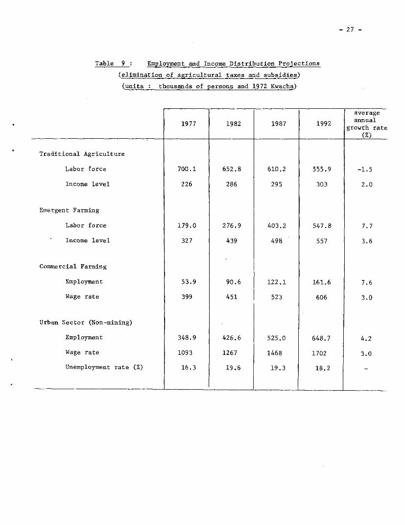
products over a five-year period. This results in 25% and 31% increases
in the producer's and consumer's prices respectively. The results of this
policy experiment are presented in Tables 8 and 9 . In comparing these
projections with those for the basic case, it is immediately obvious that
the entire development pattern is much improved. There is much more rapid
growth in agriculture with no falloff in urban sector growth. Incomes of
Zambian farmers improve most dramatically leading to reduced migration and
unemployment. The root of these changes is not hard to trace. Since under
this policy, agricultural prices are allowed to rise in step with the world
market, Zambian farmers can earn higher income, helping to reduce rural-
urban income inequality and providing even more investable resources for
growth in agricultural production. It is evident from the foregoing that
food pricing policy can be a very powerful instrument for improving the
country's position: improved prices stimulate production and raise the
incomes of the poorest groups; they also reduce food imports and conserve
scarce foreign exchange. Since the government's budgetary position is also
improved dramatically by the reduction in expenditures on subsidies, it
can either reduce its dependence on foreign borrowing or carry out a larger
development program or some combination of the two.
It is important to keep in mind that the real wage, which is
exogenous for the urban sector, is fixed in terms of the urban good. Hence,
when the consumer price of food rises in this experiment, profit rates in
the sector are not reduced, and urban sector growth is virtually identical
with the base case. To the extent that those workers already employed in
the urban sectors can insulate themselves from these food price rises,
profit rates and growth will fall. An experiment was conducted in which

- 26 -
Table 8 National Account Projections
(elimination of agricultural taxes and subsidies)
(units : millions of 1972 Kwacha)
average
1977 1982 1987 1992 growth rate
Value Added (Producer's prices)
Agricultural sectors 287.6 351.8 451.1 598.0 5.0
Commercial 50.9 81.1 123.8 190.0 9.2
Non-commercial 236.8 270.7 327.3 407.9 3.7
Urban sector 814.5 1154.5 1647.2 2359.3 7.3
Mining sector 300.0 287.7 261.6 225.5 -1.9
GNP 1402.1 1794.0 2359.9 3182.8 5.6
Expenditures (Market prices)
Private consumption 733.1 919.7 1228.0 1667.4 5.6
Public consumption 207.7 246.7 293.0 348.0 3.5
Net capital formation 198.7 291.4 410.6 597.9 7.6
Depreciation 299.3 389.8 520.0 708.2 5.9
Net imports 465.0 480.2 487.7 475.3 .2
Gross domestic expenditure 1473.8 1892.8 2500.0 3382.2 5.7
- 27 -
Table 9 Employment and Income Distribution Projections
(elimination of agricultural taxes and subsidies)
(units thousands of persons and 1972 Kwacha)
average
1977 1982 1987 1992 growth rate
________________________________________ ~~~~~~~~(%)
Traditional Agriculture
Labor force 700.1 652.8 610.2 555.9 -1.5
Income level 226 286 295 303 2.0
Emergent Farming
Labor force 179.0 276.9 403,2 547.8 7.7
Income level 327 439 498 557 3.6
Commercial Farming
Employment 53.9 90.6 122.1 161.6 7.6
Wage rate 399 451 523 606 3.0
Urban Sector (Non-mining)
Employment 348.9 426.6 525.0 648.7 4.2
Wage rate 1093 1267 1468 1702 3.0
Unemployment rate (%) 16.3 19.6 19.3 18.2 -

- 28 -
the opposite extreme assumption is made, namely, that the urban real wage
is fixed in terms of food prices. After a few years, this policy completely
shuts down growth in the urban sector, leading to increased unemployment,
reduced farmer average income, and unreasonably high imports. Getting the
prices right does no good if the line is not held on relative wages as well.
IV. Welfare Implications and Shadow Prices-/
So far, we have discussed how DYZAM can be used as a tool for
simulating various growth paths of the Zambian economy. It is now time
to return to the basic welfare issues raised in the Introduction -- namely,
how the model could be utilized for evaluation of alternative public
policies and the derivation of shadow prices for use in appraising
marginal public projects.
We must resort to a social utility metric in order to compare
any two growth paths. Here, an identical isoelastic per capita welfare
function is postulated for each of the seven income classes at each
point in time. Let v denote the elasticity of the marginal utility
of consumption; let p denote the one-year subjective discount rate;
and let T denote the number of years in the planning horizon. Then
the intertemporal interpersonal social welfare function is defined as
follows:
T F 1 -v
t-l (l+p)t s-l s,t 1-v
where ns t is the number of persons having consumption level y t
in year t .-/ For v=O the only objective is that of maximizing
1/ This section draws heavily on the analysis in Blitzer and Manne [1975].
2/ Ideally, we would wish T to approach infinity. In practice, T ischosen sufficiently large so as to have little marginal impact on shadowprices calculated for the first 10 to 15 years. Usually, 30 yearsis a sufficient approximation for our numbers.

- 29 -
discounted aggregate consumption, regardless of income distribution. The
higher the value of v , the more weight is placed on reducing the number
of those in low income groups. The higher the value of p , the more
weight is placed upon short, rather than long, term objectives of the economy.
The consumer classes are defined as follows:
s=l : traditional farmers and dependents;
s=2 : emergent farmers and dependents;
s=3 : commercial farm workers and dependents;
s=4 : urban workers and dependents;
s=5 : mining workers and dependents;
s=6 : Zambian bourgeoisie and dependents;
s=7 : unemployed urban workers and dependents.
Dependency ratios are used to relate the number of workers in each
category to the relevant n .
With the exception of the unemployed urban workers, the model
itself computes the levels of private consumption for each group. To
these must be added the relevant share of public consumption. For this
purpose, we make the simple assumption that all government consumption
is allocated to each "family" in proportion to their relative incomes.l/
2/Thus, y t includes both the value of private and public consumption.-
Using our social welfare function, DYZAM can be used to compare
any two sets of government policies. Once v and p are specified,
it becomes possible to rank those discussed previously. Such a comparison
1/ We use this assumption since there is no readily available data onthe personal distribution of government consumption.
2/ While in terms of the simulation model, the income level of theunemployed is zero, they do manage to survive on the basis of transfersand income earned in an "informal" sector which is not directly modelled.Somewhat arbitrarily, we have set their level of private consumption tobe identical with the 1972 level for traditional farmers.

- 30 -
Table 10 Ranking of Policies for v=2 , p=4%
Policy Tables As % of value Rankin basic case
Basic case 1, 2, 3 100 3
Public consumptiongrowth rate = 2.5% , 4, 5 98 4investment increased
Increased publicinvestment in 6, 7 102 2agriculture
Eliminate agricultural 8, 9 106 1taxes

- 31 -
is shown in Table 10 . For the most part, these confirm the insights
gained from examining the projections themselves. But, in the discussion
of the alternative with reduced public consumption, Section III.2 ,
it would have been difficult to evaluate the policy without a way of
measuring the value of public consumption.
Two additional comments should be made. In the first place, even
though the percentage differences may seem small, their importance should
not be minimized. Indeed given the high subjective role of discounting
and strong preference for income equality (through the choice of v and
p), these differences are actually quite significant. Second, the
policies were also compared for a number of other parameter values.-/
Surprisingly, the overall rankings were stable, although the percentage
differences widened (lowered) when v and p was reduced (raised).
Presumably, the choice of parameters would be more crucial if the compari-
sons were made between much "closer" alternatives.
DYZAM being a simulation rather than a programming model,
government policies (taxes, tariffs, choice of techniques, etc.) are
predetermined and not chosen optimally in any direct sense. The welfare
function serves as a measuring rod for evaluation of small changes, and
does not have the interactive effects upon resource allocations and
income flows that would normally occur with an optimizing framework.-/
Thus, shadow prices can be derived for simulations using any projected
set of government policies.
For example, let us consider the shadow price of public savings
in year t , defined as:
1/ In all, tests were made for v=1,2,3 and p=4%,8%
2/ Moreover, our assumptions about foreign borrowing being the adjustmentmechanism is not strong for very large shifts.

- 32 -
AWI,t AW where
I't AS~~
St is public savings in year t , and the "own" rate of return on
capital is
I,t+l
These are illustrated in the top row of Table 11 . Given that optimal
investment rules have not been selected, there is no reason why (-AI/A1)
should be closely related to the market or the public sector rates of
return on capital. Here the average rate is 12.8% per year, and
is increasing slowly through the period.
The shadow price of public consumption, AC , is defined similarly
and its ratio to AI represents the premium on public investment discussed
frequently in the dual economy, shadow price literature. As can be seen,
this "gap" narrows at about 5% per year. Note that A falls at 7.8%c
which is less than the value derived from the standard formula (T = p + vcIc C
The shadow price of labor is presented in a form that might
be readily adapted to the evaluation of labor intensive projects. The
shadow price of labor refers to a two-way change: a removal of labor
from the pool of urban unemployed (or of rural underemployed, traditional
agriculture) workers and an addition to the pool of wage earners, in the
urban or commercial agriculture sectors. That is, the shadow price of
labor is defined as the change in aggregate utility for each unemployed
worker who becomes employed at the wage specified for each sector.

- 33 -
Table 11 Shadow Price Projections (Base Case ; p 4% , v 2)
aver ageVariable 1977 1982 1987 1992 own rate
of return
Shadow price of 1.0 .576 .318 .163 12.8%public investment
X 1/C
Shadow price of .14 .18 .22 .29 7.8%public consumption
H 1/a
Shadow wage, .57 .43 .24 .04rural sectors
11 1/u
Shadow wage, .78 .79 .75 .68urban sectors
1/ X , T , and T[ are relative to XI ; H and T are expressed as ac a u I a uproportion of W and W u
In computing the shadow wage, no account is taken of any output
which might be produced by the newly employed worker. Rather, the shadow
wage can be interpreted, as in Sen [19721, as the minimum labor productivity

- 34 -
(in terms of utility) which would be required for it to be socially
beneficial to undertake such a labor-intensive "project". So that this
can be more readily seen, the shadow price of labor is normalized in
terms of the shadow price of public investment (the numeraire) relative
to the wage.
Before discussing the numerical results, it is useful to review
the factors influencing them. For the newly employed worker, the effects
are straightforward. His income and utility go up, thereby raising social
welfare. However, the wage paid must be financed out of government revenues.
These revenues have an opportunity cost in terms of foregone public savings,
since in the basic case government consumption is fixed.
The shadow price of agricultural labor (T ) is computed on
the basis of hiring a worker from the traditional sector at a wage of W
This reduces the total labor force in traditional agriculture, reducing
total production. But, since incomes in that sector are equal to average,
rather than marginal, products per capita income of these remaining will
increase somewhat. This has an important impact on the shadow price.
Returning to Table 11 , note that after 1982 the shadow price
of urban labor , IU , steadily falls as a proportion of the urban wage.
Thus, for example, in 1982 it would be socially profitable to undertake
labor-intensive projects if the marginal product of labor were 79% of
the urban wage, while it would be profitable in 1992 even if the marginal
product were only 68% of the wage. For higher values of v or p
and/or lower levels of consumption for unemployed workers, the shadow rate
could become negative. This is the logical counterpart of an employment

- 35 -
maximizing development strategy.
This is seen more clearly in the shadow price projections of
agricultural labor. It decreased steadily as a proportion of Wa ; indeed,
by 1992 it is only 4% of the wage rate in commercial agriculture. This
implies that by then, the positive income distribution effects are relatively
more important than the loss in investment which seems natural given the
worsening distribution of income.
V. Conclusions
A principal purpose of this study has been to test the practi-
cality of numerical dual economy models for deriving medium-term economic
forecasts.
The methodology amounts to formulating a simiplified general
equilibrium (not necessarily neo-classical in any respect) model focusing
attention on rural-urban distinctions. To the extent that the basic
nature of the economy conforms to the paradigm -- that the key feature
of the income distribution problem is low rural and high urban income
levels, and that real incomes are affected by the rural-urban terms of
trade -- these models provide a concise way of deriving the income
distribution implications of a number of macroeconomic policies.
Simplification has definite practical advantages. The model
builder is constrained to focus attention only on the key elements of
that particular economy which determine rural-urban demographic and income
patterns.-/ The models are easy to explain since by construction they
1/ This may not be an advantage if there is no consensus on what the keyelements are.

- 36 -
conform to a rather simple development theory. In comparison with
multi-sector models, dual economy models can be built rapidly utilizing
little more then national income accounts, budget surveys, and plan
documents.
At the macroeconomic level, the simulation model can be utilized
in discussing the implications of alternative scenarios of exogenous
factors and public policy. How far this could go depends on how much
has been included in the specific model. In the example discussed here,
little direct attention is paid to the determinants of foreign exchange
availability and nothing at all about the composition of non-food imports.
On the other hand, the model seems to shed some light on the likely
demographic and income shifts among six groups, which are implied by
changes in public investment and taxation policy.-/
The other potential advantage is in linking the derivation of
shadow prices of factors to specific projections of the development path.
Heretofore, little operational use has been made of shadow prices derived
from economy-wide models..-/ The alternative approaches (Little-Mirrlees,
UNIDO, etc.) all derive factor shadow prices based on dual economy models
in which the dynamic properties are very simplified. These is no check
on the consistency of the dynamic parameters (e.g., relative income growth,
discount rates, savings premium, exchange rate, etc.), with whatever
medium-run forecasts are being prepared. Here, the linkage is explicit.
A number of refinements can easily be made in the basic dual
1/ A modified version of DYZAM formed the background to an operationaldiscussion of various "scenarios" conducted by the World Bank.
2/ For an excellent summary of why this has been so, see Bruno [1975].

- 37 -
economy framework. Additional sectors could be added, including several
producing non-traded goods (handling more than a few endogenous prices
quickly becomes difficult). If the real exchange rate is a key price,
then introducing non-traded goods becomes crucial. The foreign trade side
could be made more explicit through introduction of non-competitive
imports and a description of the capital flows.
It would be more difficult to endogenize either the pattern of
investment or public finance. The model simulations are time recursive
and the difficult questions in public finance or investment choice are
intrinsically dynamic and depend on some dynamic optimization problem
at each starting point.

I

A-1
APPENDIX Algebraic Formulation of DYZAM
In the main text, we discussed in general terms the formulation
of the dynamic simulation model, focusing on the underlying rationale of
the methodology. Here, the specific algebraic equations are presented
with a minimum of additional verbal comment.
For the equations, a standard subscripting pattern is used.
The subscript "t" always refers to the year relative to the base year.
Thus, for 1980, t = 3 . Where the meaning is clear from context, these
time subscripts are dropped. The subscripts "a" and "u" are sometimes
used to refer to the agricultural and urban sectors; e.g., Pa t =
producers' price of agricultural goods in year t . Occasionally, "g"
is used as a subscript denoting government; e.g., K4 g t is government
owned capital in sector 4 in year t .
Table A.1 Sectoral and Income Class Indices
Number Producing sector Income group
1 traditional agriculture Workers in sector 1
2 emergent agriculture . IV 2
3 commercial agriculture i t " 3
4 urban agriculture . II H 4
5 mining , " 5
6 _______________Zambian profit earners
7 Foreigners

A-2
Production Functions
Cobb-Douglas production functions are utilized to relate
inputs of labor and capital to output of agricultural and urban goods.
Thus:
Xi t ='Ai K i t (1 + g i) L i t) , for i=l,...,4 (1)
where X.it I K it, and Li.t refer to output, capital input, and
labor inputs in sector i in year t . Ai is a scaling constant and
gi the rate of growth in labor productivity for sector i . Our
assumptions regarding the agricultural sectors are al = a2 = 3
92 = 93 ; gl 0 ; A3 A2 1
Labor, capital, and intermediate inputs in mining are proportional
ot output levels. Thus:
X5,t al,t K5,t (2)
L5 t a52 , and (3)(g5)
intermediate inputs = a3,t X5,t (4)
Here, al t - a3 t are the coefficients of a Leontief-type production
process, and g5 is the annual rate of increase in the productivity of
mining workers.
Resource AZ?ocation
In the short-run, physical capital is fixed in each sector. Thus,

A-3
the only resource allocation problem within a given year involves labor.
The total supply of labor in the rural and urban sectors also is fixed
in the short-run.
In the urban sector, we assume that competative forces lead
to maximize profits. Thus, labor is hired until the value of its
marginal product equals its fixed nominal wage:
ax4
u UL4 W4*(5
This in turn can be solved for L4 as a function of K4 W4 , and P
Since L5 is determined through equations (2) and (3) the urban
unemployment rate can be computed residually as:
L. - L - Lu 4 5(6
u =L (6)u
where u is the rate of urban unemployment, and
L is the total urban work force.u
Within agriculture, the labor allocation works in a similar
fashion. Commercial farms act as if they maximize their profits, just
like firms in the urban sector. Thus,
ax3
P _pW 3* (7)a 33
L3 can then be solved for as a function of P , W3 , and K3 . Since
we have assumed that emergent farmers neither hire outside labor nor
compete themselves for jobs in commercial agriculture, L2,t is fixed
in each year. Since there is no open unemployment in the rural sector,
L1 is determined residually:
1~~~~~~~~~~~~~~~~~~~~~~~~~~~~~~~~~~~~~~~~~~~~~~~~~~~~~~~~~~~~~~~~~~~~~~~~~~~~~~~~~~~~~~~~~~~~~~~~~~.
A-4
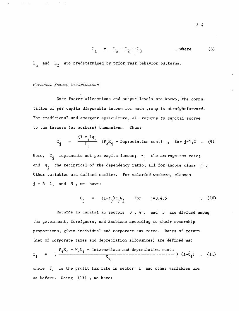
L1 L a L 2 3 , where (8)
L and L2 are predetermined by prior year behavior patterns.
Persona1 Income Distribution
Once factor allocations and output levels are known, the compu-
tation of per capita disposable income for each group is straightforward.
For traditional and emergent agriculture, all returns to capital accrue
to the farmers (or workers) themselves. Thus:
(l-t .)q.C. = L 2 (PaXj - Depreciation cost) , for j=1,2 . (9)
Here, C. represents net per capita income; t. the average tax rate;
and q. the reciprical of the dependency ratio, all for income class j
Other variables are defined earlier. For salaried workers, classes
j = 3, 4, and 5 , we have:
C. (l-t.)qjW. for j=3,4,5 . (10)
Returns to capital in sectors 3 , 4 , and 5 are divided among
the government, foreigners, and Zambians according to their ownership
proportions, given individual and corporate tax rates. Rates of return
(net of corporate taxes and depreciation allowances) are defined as:
PiX. - W L - intermediate and depreciation costs
ri1 = ( i i Ki ) 1(l-ti) , (11)
where ti is the profit tax rate in sector i and other variables are
as before. Using (11) , we have:

A-5
5C = (l-t.) I ri Ki, N , for j=6,7 . (12)
i=3
Here, N. is the number of persons in class j and K. is the capital
stock in sector i owned by income class j
Personal Consumption and Savings
Consumption and savings patterns for each income group are
determined using an extended linear expenditure system. Thus:
C. i PY., + (1-TI.) i [C - P y _ p y ]1~~j 1 i,j j i,j j a a,j u u,j
i=a,u and j=1,...,7 . (13)
In (13) ,Cij is expenditures by a member of class j on consumption
good i ; Yij and i . are minimal and marginal proportions spent
by members of group j on good i ; i. is the marginal propensity to
save for group j ; and P. is the consumers' price of good i
Completing the system, we have:
S. = H. [C. - Pa Ya,j Pu YU ] , where (14)
Sj is net savings by members of group j . Total expenditures on each
good are easily calculated by multiplying the average expenditures in
each income group by the number in that group.-/
1/ For j=7 , foreigners, remittances are subtracted from C beforeusing (13) and (14) . Total remittances are profits, less Investmentin mining, plus a constant share of net income from foreign profits fromother sectors.

A-6
Government Revenue
The government "earns" revenue through: (i) its ownership of
capital assets in sectors 3 , 4 , and 5 : (ii) direct taxes on
personal and profit income; and, (iii) indirect taxes on consumption
and imports. If we aggregate income from the first two sources we have:
government 5 7 intermediatedirect = P. X. I C N - and depreciation . (15)revenue i=l j 1 costs
In other words, all of net national income at producers' prices which does
not end up as personal disposable income accrues to the government.
In order to compute revenue from consumption taxes, we first
compute total consumption of each good in quantity terms, defined as C.
7Ci j-l iC,j Nj / P. , for i=a,u . (16)
j=1
Then for good i , consumption tax revenue is:
revenue from consumption ( i) . (17)tax, good i (P'i Pi) (7
In order to compute revenue from tariffs, we must compute total
private sector imports, which is the difference between total consumption
and investment demands and production; specifically:
revenue from tariff,agriculture good (Pa ) ( - X1 - X2 X3) (18a)
andrevenue from tariff, (P + intermediateurban good u u 4+ S + deliveries + depreciation- X4)
(18b)
A-7
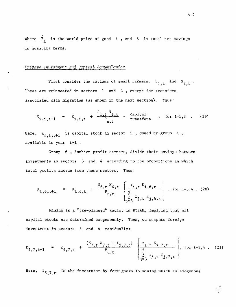
where Pi is the world price of good i , and S is total net savings
in quantity terms.
Private Investment and Capital AccumuZation
First consider the savings of small farmers, S1 t and S2,t
These are reinvested in sectors 1 and 2 , except for transfers
associated with migration (as shown in the next section). Thus:
K - K + ~~~i,tNi't _capital
i,i,t+l i,i,t P tan , for i1,2 . (19)u,t
Here, Ki i. t+l is capital stock in sector i , owned by group i
available in year t+l .
Group 6 , Zambian profit earners, divide their savings between
investments in sectors 3 and 4 according to the proportions in which
total profits accrue from these sectors. Thus:
K i,K+ 6,ti6,t,6,t +1p4for i=3,4 u (20)
Mining is a "pre-planned" sector in DYZAM, implying that all
capital stocks are determined exogenously. Then, we compute foreign
investment in sectors 3 and 4 residually:
S 7,t N7,t I5,7,t I ,t Ki,7;t ]i34Ki,7,t+ Kt i,7 ,t + P 4,, for i=3,4 . (21)
u,tIr K
Here., I 5,, is the investment by foreigners in mining which is exogenous

A-8
and is subtracted from total foreign savings.
Migration and Demographic Changes
Let L be the total urban work force in year t . GrowthU,t
in L depends on the rate of population growth as well as on rural-U
urban migration, MN1 t . Thus:
u,t+l ( u) u,t l,t and (22)
by symmetry, the growth in the total agricultural labor force, La , is:
a,t+l ( a + ga) Lat ml,t ' (23)
where g , g are the natural population growth rates in rural and
urban areas. Rural-urban migration depends upon the ratio of expected
urban income to income in traditional agriculture and the urban
unemployment rate.
r (1 - urban unemployment rate)W4 urban 2Mlt L ( a 1' / 1 ()rate J _ Llt (24)
where ¢1 and f2 are estimated parameters.
The number of workers in emergent farming, sector 2 , depends
also on population growth and the transformation rate of traditional into
emergent farmers, defined as M2,t . Thus:
2,t+l (I + ga) L2,t + M2,t and (25)

A-9
pa 1 ) a x2 t) la1t\M'2, = 01 + 02 ( L ') + 63 (L ) / ( L j ) L| (26)
where 61 ' 62 , and 63 are estimated paramters.
Finally, as part of this transformation process, the traditional
farmers who become "emergent" take with them their capital stock. We
assume that it is always the richer traditional farmers who engage in
this process. Thus:
K1 1tcapital transfers = 64 ( £ ) M2 t (27)
4 Ll,t 2t
where 64 > 1
PubZic Expenditure and Trade BaZance
Government consumption and the development budget (exclusively,
urban goods) are projected exogenously and in the base case grow at
constant real rates. This is allocated to the different sectors in
fixed marginal proportions. Remembering that parastatal profits are
reinvested where earning, we have:
r. K. +6.1 K = K + 1 i,g,t 1 g,t (28)i,g,t+l i,g,t
U,t
where S. is sector i 's share of the development budget anc I is1 ~~~~~~~~~~~~~~~g,t
its fixed level.
Using national income accounting conventions, it can be shown
that for this model,
-2,

A-10
r trade deficit,1 V government 1 - rl world price L orud prics - L remittances j . (29)

REFERENCES
[ 1] Bell, Clive. "A Simple Dualistic Economy in a Comparative StaticsSetting". Paper presented at Workshop on Analysis ofDistributional Issues in Development Planning in Bellagio,Italy, April 22-27, 1977.
[ 2] Blitzer, Charles R. and Alan S. Manne. "Employment, IncomeDistribution, and Shadow Prices in a Dualistic Economy".In T.N. Srinivasan and P.K. Bardhan (editors), Povertyand Income Distribution in India. Statistical PublishingSociety. 1975.
[ 3] Blitzer, Charles R., Ian M.D. Little, and Lyn Squire. "MultiplierEffects and Project Evaluation". DRC mimeograph. October 1977.
[ 4] Blitzer, Charles, Partha Dasgupta, and Joseph Stiglitz. "ProjectEvaluation and the Foreign Exchange Constraint". Forthcomingin Economic Journal. 1978.
[ 5] Bruno, Michael. "Planning Models, Shadow Prices, and ProjectEvaluation". In Blitzer, Clark, Taylor (editors),Economy-Wide Models and Development Planning. OxfordUniversity Press. 1975.
l 6] Bruno, Michael. "The Two-Sector Open Economy and the RealExchange Rate". American Economic Review. September 1976.
[ 7] Bruno, Michael. "Distributional Issues in Development Planning --Some Reflections on the State of the Art". Paper presented atWorkshop on Analysis of Distributional Issues in DevelopmentPlanning in Bellagio, Italy, April 22-27, 1977.
[ 8] Kelly, A.J., J.G. Williamson, and R.J. Cheetham. Economic Dualismin Theory and History. University of Chicago Press. 1972.
t 9] Little, I.M.D. and J.A. Mirrlees. ManuaZ of Industrial ProjectAnaZysis in DeveZoping Countries. Vol. ii. Paris: Develop-ment Centre of the OECD. 1969.
[10] Ljung, Per. "Agricultural Migration in Zambia". World Bankpublication. 1975.
[111 Lluch, Constantino. "Theory of Development in Dual Economies. ASurvey". DRC memeograph. September 1977.
[12] Lluch, Constantino. "A Model of Employment and Income Distribution".Paper presented at Workshop on Analysis of DistributionalIssues in Development Planning in Bellagio, Italy, April 22-27,1977.

[13] Lluch, Constantino, Alan D. Powell, and Ross A. Williams.Patterns in Household Demand and Saving. Oxford UniversityPress. 1977.
[14] Taylor, Lance and Frank Lysy. "Vanishing Short-Run IncomeRedistributions: Keynesian Clues about Model Surprises".Paper presented at Workshop on Analysis of DistributionalIssues in Development Planning, in Bellagio, Italy, April22-27, 1977.
[151 Rhee, Yung W. "Dynamics of Dual Exchange Rate in an OpenDeveloping Economy with Foreign Borrowing". World BankPublication. 1978.
[161 Sen, Amortya K. "Accounting Prices and Control Areas: An Approachto Project Evaluation". Economic Journal. March 1972.
[17] Todaro, Michael P. "A Model of Labor Migration and UrbanUnemployment in Less Developed Countries". American EconomicReview. March 1969.
[18] UNIDO. Guidelines for Project Evaluation. U.N.: New York. 1972.
[19] World Bank. Zambia: Agriculture and RuraZ Survey Sector Report.Washington, D.C. 1975.
[20] World Bank. Zambia: A Basic Economic Report. Washington, D.C.1977.

RECENT PAPPLRS TIlT THIS SERPIS:
No. TITLE OE PAPIER A,ilTHOR
265 India's Population Policy: Ifistory and Future R. Gulhati
266 Radio for Education and Development: P. Spain, D. JamisonCase Studies (Vols. I & II) E. McAnany
267 Food Insecurity: Magnitude and Remedies S. Reutlinger
268 Basic Education and Income Inequality in J. JalladeBrazil: The Long-Term View
269 A Plalning Study of the Fertilizer Sector A. Choksi, A Meerausin Egypt A. Stoutjesdijk
270 Economic Fluctuations and Speed of Urbanization: B. RenaudA Case Study of Korea 1955-1975
271 The Nutritional and Economic Implications of L. Latham, M. LathamAscaris Infection in Kenya S. Basta
272 A System of Monitoring and Evaluation of M. Cernea, B. TeppingAgricultural Projects
273 The Measurement of Poverty Across Space: V. ThomasThe Case of Peru
274 Economic Growth, Foreign Loans and Debt G. FederServicing Capacity of Developing Countries
275 Land Reform in Latin America: Bolivia, Chile, S. Eckstein, G. DonaldMexico, Pe u and Venezuela D. "orton, T. Carrol
(cor.ultants)
276 A Model of Agricultural Prodiuction and Trade R. Norton.in Central America C. Cappi, L. Fletcher,
C. Pomareda, M. Wainer(con.zultants)
277 The Impact of Agricultural Price Policies on M. CGterrieth,Demand and Supply, Incomes and Imports: E. Verrydt, J. WaelbroeckAn Experimental Model for South Asia (con.ultants)
278 Labor Market Segmentation and the Determination D. Y zumdarof Earnings: A case Study M. A med
279 India - Occasional Papers M. A> luwalia, J. WallS. R-utlinger, M. WolfR. O-ssen (consultant)
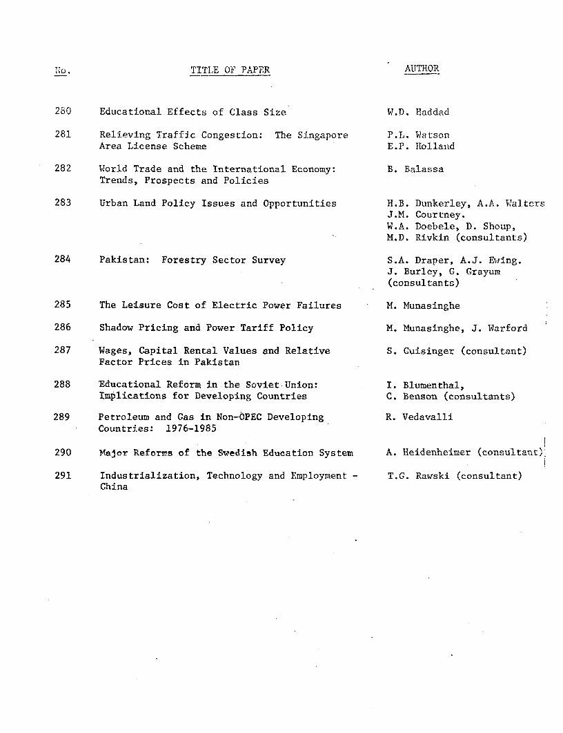
No. TITLE OF PAPER AUTHOR
280 Educational Effects of Class Size W.D. Haddad
281 Relieving Traffic Congestion: The Singapore P.L. WatsonArea License Scheme E.P. Holland
282 World Trade and the International Economy: B. BalassaTrends, Prospects and Policies
283 Urban Land Policy Issues and Opportunities H.B. Dunkerley, A.A. WaltersJ.M. Courtney.W.A. Doebele, D. Shoup,M.D. Rivkin (consultants)
284 Pakistan: Forestry Sector Survey S.A. Draper, A.J. Ewing.J. Burley, G. Grayum(consultants)
285 The Leisure Cost of Electric Power Failures M. Munasinghe
286 Shadow Pricing and Power Tariff Policy M. Munasinghe, J. Warford
287 Wages, Capital Rental Values and Relative S. Guisinger (consultant)Factor Prices in Pakistan
288 Educational Reform in the Soviet Union: I. Blumenthal,Implications for Developing Countries C. Benson (consultants)
289 Petroleum and Gas in Non-OPEC Developing R. VedavalliCountries: 1976-1985
290 Major Reforms of the Swedish Education System A. Heidenheimer (consultant)
291 Industrialization, Technology and Employment - T.G. Rawski (consultant)China

PUB HG3881.5 .W57 W67 no.292Blitzer, Charles R.Development and incomedistribution in a dualeconomy: a dvnamic
PUB HG3881.5 .W57 W67 no.292Blitzer, Charles R.Development and incomedistribution in a dualeconomy: a dynamic