development and study of narrow pressure probes – stethoscope … · development and study of...
TRANSCRIPT

Development and study of narrow pressure probes –
stethoscope applications
André Filipe de Azevedo Mendes Palma
Thesis to obtain the Master of Science Degree in
Mechanical Engineering
Supervisor: Prof. Edgar Caetano Fernandes
Examination Committee
Chairperson: Prof. Viriato Sérgio de Almeida Semião
Supervisor: Prof. Edgar Caetano Fernandes
Members of the Committee: Prof. Fernando José Parracho Lau
November 2014

ii

iii
Abstract
Pressure probes have been widely used in many research and industry fields to achieve real time
efficient pressure fluctuations measurements. This work describes the development of a maintenance
tool-pack of pressure probes to be used to acquire an acoustical signature of flow behaviour inside
and outside the combustion chamber.
Attempting to provide a technological improvement, with a pre-test bench tool, on the assessment of
primary swirl nozzle/fuel nozzle misalignment of CFM56-5 gas turbine engine, a new design is
suggested and a robust mathematical model is derived using the low reduced frequency model that
contemplates viscous-thermal damping due to the development of an inner acoustic boundary layer.
The tool-pack has two different sets of probes, validated experimentally with the same mathematical
model, a static-pressure probe able to detect a wide range of pressure fluctuations, and a stethoscope
configuration probe that differs from the first one by the addition of a pressure sensor. The developed
mathematical model proved to be versatile and indispensable once a non-viscous approach was
implemented and compared.
While developing a static pressure probe important relations were computed that would overcome a
lack of understanding on pre-design procedures. With this work, the importance of providing reliable
acoustic response gained relevance due to the fact that no information regarding pressure sensors is
available.
An analogous primary swirl nozzle/fuel nozzle assembly case study was carried out to assess probe’s
sensitivity on small changes on flow characteristics, and proved to be a promising tool to be included
in the maintenance facilities.
Keywords: Pressure probes, stethoscope probe, acoustics, low reduced frequency model, gas
turbine, combustion chamber.

iv

v
Resumo
As sondas de pressão têm sido extensivamente utilizadas em diversas áreas de pesquisa científica e
na indústria. No entanto, o denominador comum é a recolha eficiente e em tempo real de flutuações
de pressão. Este trabalho descreve o desenvolvimento de um conjunto de sondas que permitirão, em
última instância, adquirir uma assinatura acústica representativa do escoamento que se desenvolve
quer no interior, quer no exterior de uma câmara de combustão.
Dando enfoque à possibilidade de uma significativa melhoria tecnológica através do desenvolvimento
de uma ferramenta de trabalho que possibilite diagnosticar o impacto que o desalinhamento que o
injector de combustível provoca no escoamento no interior do motor CFM 56-5, uma nova
configuração de sonda de pressão é apresentada. Para caracterizar eficientemente a resposta das
sondas de pressão foi desenvolvido um modelo matemático, robusto e versátil, baseado na solução
de frequência reduzida que contempla efeitos termo-viscosos devido ao crescimento de uma camada
limite acústica.
O pacote de sondas apresentado neste trabalho consiste em dois tipos, ambas validadas
experimentalmente pelo mesmo modelo. A primeira trata-se de uma sonda de pressão estática que
apenas mede flutuações de pressão, e a segunda apresenta uma configuração tipo estetoscópio que
difere da primeira através da inclusão de um sensor de pressão. O estudo de sondas de pressão
estática permitiu reforçar o processo de pré-desenvolvimento deste tipo de sondas.
Elaborando um estudo de caso análogo ao que se verificaria num ambiente de manutenção a sonda
mostrou sensibilidade na detecção de pequenas modificações nas características do escoamento.
Palavras-chave: sondas de pressão, sonda-estetoscópio, acústica, modelo de solução de frequência
reduzida, turbina a gás, câmara de combustão.

vi

vii
Acknowledgments
I would like to express my deepest gratitude to Prof. Edgar Fernandes, for all the support, patience
and guidance throughout the entire process of this thesis. His enthusiasm towards teaching and
pedagogic methodology helped me reaching the proposed goals.
I want to thank Prof. Marcus Girão to whom I am deeply grateful for all the help, the discussions about
diverse subjects, patience and kindness. I would also like to thank Jana for the expertise and useful
conversations despite the time-zone. To Prof. Luís Manuel Braga da Costa Campos, for the effective
discussion. To all my colleagues at IN+, Tomás, Diogo, João Cunha, Zé Neves, Zita a sincere thank
you for all the help, laughs and coffee-breaks.
To all my friends who fought with me side by side and were my shelter: Manel, Johnny, Miguel, RR,
Marco, Carlos, Tribuna, Zé, Rúben, João, Henrique, Luís. Thank you.
To Matilde, for all the support, love, patience and care. You would always find time for me.
To my parents, and brother. I love you.

viii

ix
Table of Contents
Abstract .................................................................................................................... iii
Resumo ..................................................................................................................... v
Acknowledgments .................................................................................................. vii
Table of Contents..................................................................................................... ix
List of figures ........................................................................................................... xi
List of Tables .......................................................................................................... xiv
Nomenclature .......................................................................................................... xv
1 Introduction ......................................................................................................... 1
1.1 Pressure Probes ...................................................................................................... 1
1.2 State-of-Art .............................................................................................................. 2
1.3 Motivation and Objectives .....................................................................................10
1.4 Thesis Outline ........................................................................................................ 11
2 Theoretical Considerations .............................................................................. 12
2.1 Introduction ............................................................................................................12
2.2 Basic Equations .....................................................................................................13
2.3 Probe mathematical model and boundary conditions .........................................18
3 Experimental Apparatus ................................................................................... 21
3.1 Acoustic Calibration setup Type A ........................................................................21
3.1.1 Interface and data processing .............................................................................22
3.1.2 Signal Generation ...............................................................................................22
3.1.3 Signal Acquisition ................................................................................................23
3.2 Acoustic Calibration setup Type B ........................................................................25
3.3 Development of a Swirler .......................................................................................27
4 Acoustic Probes - Theoretical and Experimental Results ............................. 28
4.1 Introduction ............................................................................................................28
4.2 Calibration of probes .............................................................................................28
4.3 Development of a SP-Probe ..................................................................................31
4.3.1 Boundary conditions of SP-Probe .......................................................................33
4.3.2 Probe sensitivity ..................................................................................................33
4.3.3 Probe transfer function and standing waves .......................................................35

x
4.3.4 Non-Viscous Model .............................................................................................41
4.3.5 Acoustic Energy Balance in SP-Probe ................................................................46
4.3.6 Parametric Analysis of SP-Probe ........................................................................50
4.4 Development of a Stethoscope probe ..................................................................53
4.4.1 Non-Viscous Analysis .........................................................................................54
4.4.2 Boundary conditions of Stethoscope Probe ........................................................55
4.4.3 Stethoscope probe sensitivity .............................................................................56
4.4.4 Stethoscope standing waves ..............................................................................57
4.5 Collecting data with Stethoscope probe...............................................................59
4.5.1 Experimental rig ..................................................................................................59
4.5.2 Data Acquisition and post-processing data .........................................................60
4.5.3 Results ...............................................................................................................61
5 Conclusion ........................................................................................................ 65
5.1 Concluding remarks ...............................................................................................65
5.2 Future work .............................................................................................................67
6 References ........................................................................................................ 68
Appendix A .............................................................................................................. 71
Appendix B .............................................................................................................. 72
Appendix C .............................................................................................................. 78

xi
List of figures
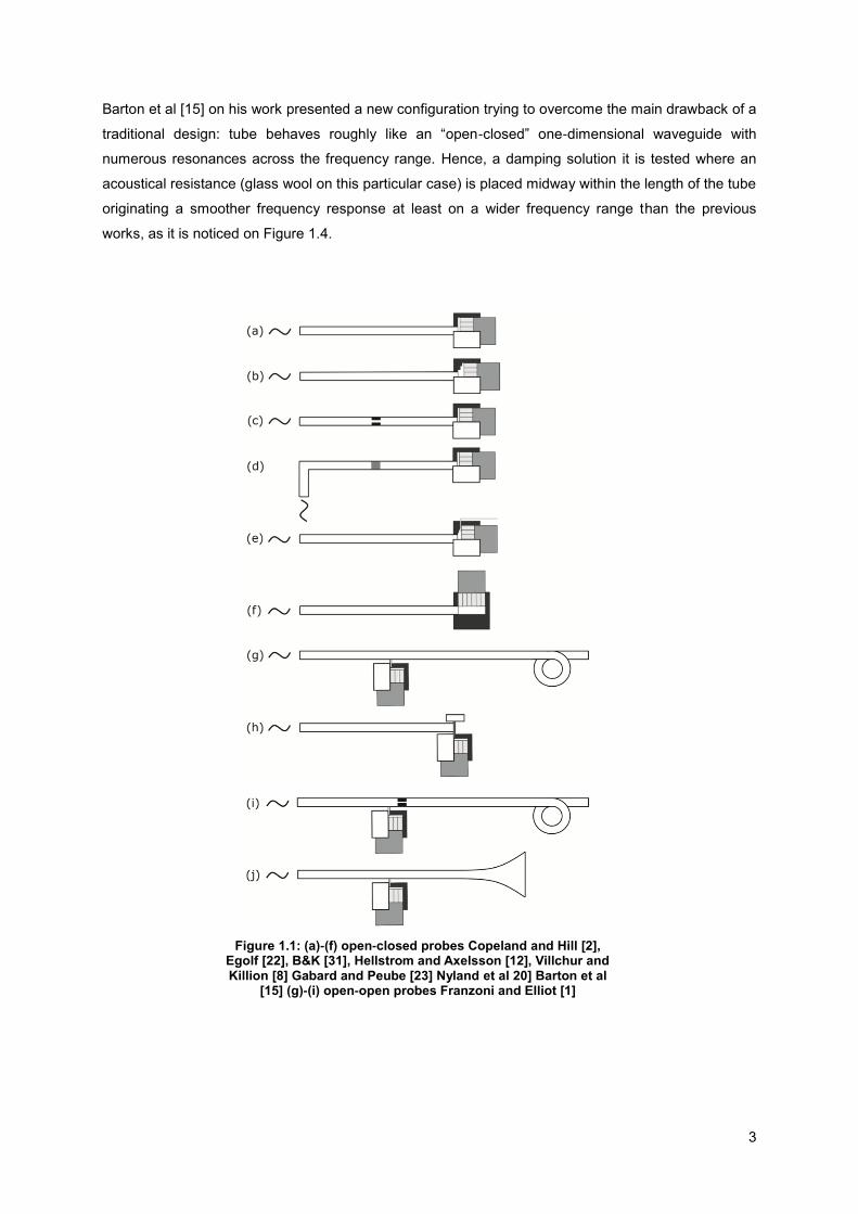
Figure 1.1: (a)-(f) open-closed probes Copeland and Hill [2], Egolf [22], B&K [31], Hellstrom and
Axelsson [12], Villchur and Killion [8] Gabard and Peube [23] Nyland et al 20] Barton et al [15] (g)-(i)
open-open probes Franzoni and Elliot [1] ............................................................................................... 3
Figure 1.2: Pressure response curves obtained by Copeland and Hill [2] .............................................. 4
Figure 1.3: Transfer function obtained by Egolf [22]................................................................................ 4
Figure 1.4: Pressure response curves obtained by Barton [15] .............................................................. 5
Figure 1.5: Transfer function obtained by Bertrand [14] .......................................................................... 6
Figure 1.6: Transfer function obtained by Gabard and Peube [24] ......................................................... 6
Figure 1.7: Transfer function obtained by Nyland et al [20] ..................................................................... 7
Figure 1.8: Transfer function obtained by Franzoni and Elliot [1] ............................................................ 8
Figure 1.9: Schematic view of the SP-Probe used in Tsuji et al work [25] .............................................. 8
Figure 1.10: Amplitude and phase delay obtained for the SP-Probe developed by Tsuji et al [25] ........ 9
Figure 1.11: (a) The solid line is the reference microphone output and the dashed line is the measured
static pressure signal. (b) HR effect removed numerically - obtained in Tsuji et al [25] .......................... 9
Figure 1.12: Modular assembly of CFM-56-5 combustion chamber ...................................................... 11
Figure 2.1: Review of analytical solutions for propagation constant as a function of shear wave
number, [26] ........................................................................................................................................... 17
Figure 2.2: Axial velocity profile for an outgoing wave in a infinitely long tube, [25], [30] ..................... 17
Figure 2.3 - Preliminary design concept for the mathematical modelling approach ............................. 18
Figure 2.4: Probe schematics adopted in the mathematical modelling ................................................. 20
Figure 3.1: Probe calibration schematics Type A- (a1) Acquisition and signal monitoring, (a2) Signal
generation, (a3) Interface and data processing..................................................................................... 22
Figure 3.2: Stiff PVC tube set-up for standing wave medium ............................................................... 23
Figure 3.3: Schematic description of experimental apparatus Type B .................................................. 25
Figure 3.4: Up-chirp pulse and down-chirp pulse example ................................................................... 26
Figure 3.5: a) Solidworks modeling of a swirler, (b) Real model 3D Print ............................................. 27
Figure 4.1: Probe general schematics and procedure to adapt a 4T-1V to 1T-1V ............................... 28
Figure 4.2: Schematics of Flexible pressure probe ............................................................................... 29
Figure 4.3: a) Solidworks model b) Calibration apparatus with flexible probe attached ....................... 29
Figure 4.4: Flexible pressure probe calibration curve with theoretical and experimental data ............. 30
Figure 4.5: Schematics of stainless steel pressure probe ..................................................................... 30
Figure 4.6: a) Solidworks model b) Calibration apparatus with stainless steel probe attached ............ 30
Figure 4.7: Stainless steel pressure probe calibration curve with experimental and theoretical data .. 31
Figure 4.8: Schematic of SP-Probe ....................................................................................................... 32
Figure 4.9: Detail with coordinate axis origin and end correction at tube T1 ........................................ 32
Figure 4.10: Solidworks model identified with main tubes and volume (T1,T2,T3, V4) ........................ 32
Figure 4.11: Probe sensitivity to external noise applying Equation (44) (R1=0.6mm) .......................... 34
Figure 4.12: Sound field spectra for three frequencies plotted against electronic noise (R1=0.6mm) . 34
xii
Figure 4.13: SP-Probe calibration curves (amplitude and phase)......................................................... 36
Figure 4.14: Standing waves developing inside SP-Probe as function of frequency and local
coordinates for SP-Probe with R1=0.6mm ............................................................................................ 37
Figure 4.15: Selected standing waves in SP-Probe at several frequencies ......................................... 38
Figure 4.16: Selected standing waves in SP-Probe (R1=0.6mm) at several frequencies (cont) .......... 39
Figure 4.17: "Polytropic constant", 𝒏, as function of 𝝈𝒔 as mentioned in [26] ....................................... 42
Figure 4.18: Comparison between the response of SP-Probe with and without viscous effects. a)
Standing waves in SP-Probe as function of frequency for the Non-viscous model, b) Acoustic transfer
function with and without viscous effects (R1=0.6mm) ......................................................................... 43
Figure 4.19: Standing waves in SP-Probe with R1=0.06mm present in tubes T2+T3 .......................... 44
Figure 4.20: Comparison between the response of SP-Probe with and without viscous effects. a)
Standing waves in SP-Probe for the Non-viscous model. b) Acoustic transfer function obtained with
and without viscous effects (R1=0.06mm) ............................................................................................ 45
Figure 4.21: T-Junction control surface for acoustic intensity computation .......................................... 46
Figure 4.22: Evolution in time of instantaneous acoustic energy in T-Junction for 200Hz and 6810 Hz.
............................................................................................................................................................... 47
Figure 4.23: Non-dimension acoustic energy balance in T-junction based on time integration of
instantaneous acoustic intensity ............................................................................................................ 49
Figure 4.24: Mass rate accumulation evolution in T-junction between probes with R1=0.06mm and
R1=0.6mm, with and without viscous effects. ....................................................................................... 49
Figure 4.25: Schematic description of parametric analysis for a set of pre-defined probe dimensions a)
frequency and amplitude for the first peak frequency are identified. b) Amplitude value is plotted
against the first peak frequency c) first peak freq plotted against HR frequency .................................. 50
Figure 4.26: Non-dimensional analysis using curve fitting .................................................................... 51
Figure 4.27: Non-dimensional analysis of first peak amplitude ............................................................. 52
Figure 4.28: a) 3D model of Stethoscope probe, b) real model of Stethoscope probe ......................... 53
Figure 4.29 - Stethoscope probe calibration curve for the case T2 obstructed (amplitude and phase) 54
Figure 4.30 - Stethoscope probe calibration curve with SDP-1000-L included (V5) ............................. 54
Figure 4.31: Comparison between Stethoscope probe response-sensor included with and without
viscous effects ....................................................................................................................................... 55
Figure 4.32: Probe general schematics and procedure to adapt 4T-1V to 3T-2V ................................ 55
Figure 4.33 :Stethoscope probe Sound field spectra for three different frequencies plotted against
electronic noise ...................................................................................................................................... 56
Figure 4.34: Stethoscope probe sensitivity when calibration tube was closed ..................................... 57
Figure 4.35: Stethoscope probe standing waves in T1, T2 and T3 ...................................................... 58
Figure 4.36: Experimental case study apparatus .................................................................................. 60
Figure 4.37: Tube + swirler and stethoscope probe attached ............................................................... 61
Figure 4.38: a1) Experimental apparatus a2) tube schematics identifying measurement points b)
measured signal FFT for Pos1, c) measured signal FFT for Pos2, d) measured signal FFT for Pos3, e)
measured signal FFT for Pos4 .............................................................................................................. 62

xiii
Figure 4.39: Measured signal FFT for 4 different angles plotted against a reference FFT (0º) for 4
positions-clockwise configuration .......................................................................................................... 63
Figure 4.40:Measured signal FFT for 4 different angles plotted against a reference FFT (0º) for 4
positions-counterclockwise configuration .............................................................................................. 63
Figure 4.41: Mean pressure collected data with SDP-1000-L ............................................................... 64
Figure B 1: Microphone B&K 4189 calibration apparatus ..................................................................... 72
Figure B 2: Microphone B&K 4189 model validation ............................................................................. 73
Figure B 3: Microphone B&K 4155 calibration apparatus ..................................................................... 75
Figure B 4: Microphone B&K 4155 model validation ............................................................................. 75
Figure B 5: Microphone B&K 4155 and 4189 calibration ...................................................................... 76
Figure B 6: Combined microphones model validation ........................................................................... 77
Figure B 7: Stainless steel probe calibration curve obtained with B&K 4155 as reference and B&K4189
attached to the probe ............................................................................................................................. 77

xiv
List of Tables
Table 2.1: Boundary conditions present in mathematical model ........................................................... 20
Table 3.1: List of material for experimental calibration system Type A ................................................. 21
Table 3.2- List of material for experimental calibration system Type B ................................................. 26
Table 4.1: SP-Probe dimensions ........................................................................................................... 32
Table 4.2: Boundary conditions of SP-Probe ........................................................................................ 33
Table 4.3: Boundary conditions considered for mathematical modelling .............................................. 56
Table 4.4: List of material used for experimental case study ................................................................ 59

xv
Nomenclature
Roman Symbols
𝑨, 𝑩
𝑪
Constants obtained from boundary conditions
Complex representation of harmonic quantities
𝒄 Speed of sound (≅ 343 𝑚/𝑠 for air at STP)
𝒅 Tube diameter
𝒇
𝑮
𝑯
Frequency
Microphone internal gain
Transfer function in digital signal processing
𝒊
𝑰
𝑱
=√−1 Imaginary unit
Amplitude of active intensity
Amplitude of reactive intensity
𝒌 Reduced frequency or wave number
𝑳 Tube length
𝑵 Arbitrary integer number
𝒏 Polytropic constant
𝒑 Amplitude of pressure perturbation
𝑹
𝒓
𝑺
𝒔
𝑻
𝒕
𝒖
𝑽
𝒗
𝒙
Tube radius
Co-ordinate in radial direction
Swirl number
Shear wave number
Amplitude of temperature perturbation
Time
Amplitude of velocity perturbation in axial direction
Volume
Amplitude of velocity perturbation in radial direction
Co-ordinate in axial direction

xvi
Greek Symbols
𝜷
𝚪
Dimensionless constant proportional to diaphragm deflection
Propagation constant
𝜸 Ratio of specific heats (1.4 for air at STP)
𝜹 Acoustic boundary layer
𝜼 Dimensionless co-ordinate in radial direction
𝝀 Thermal conductivity, air or wavelength
𝝁
𝝃
𝝆
𝝆𝒔
𝝈
𝚽
𝝓
𝝎
Dynamic viscosity
Dimensionless co-ordinate in axial direction
Amplitude of density perturbation
Mean density
Square root of Prantdl number
Dissipation function
Swirl vane angle
Angular frequency
Superscripts
𝚪′ Attenuation per unit distance in 𝝃 direction
𝚪′′ Phase shift per unit distance in 𝝃 direction
𝝈′
𝒑′
𝒖′
Dimensionless factor proportional to diaphragm deflection
Real part of pressure field
Real parte of velocity field

xvii
Subscripts
𝐂𝒑 Specific heat at constant pressure
𝐂𝒗
𝒅𝒉
𝒇𝒄
𝒇𝑶𝑪
𝒇𝑶𝑶
𝑮𝜽
Specific heat at constant volume
Vane pack hub diameter
Cut-off frequency for plane wave approximation
Resonance frequency of a open-closed tube
Resonance frequency of a open-closed tube
Momentum of tangential velocity
𝑮𝒙 Momentum of axial velocity
𝑱𝟎, 𝑱𝟐
𝑳𝒆𝒒
𝑴𝑻−𝒋𝒖𝒏𝒄𝒕𝒊𝒐𝒏
𝑴𝒗
𝒎𝒊𝒏̇
𝒎𝒐𝒖𝒕̇
𝑷𝟎
𝑷𝒓
𝑷𝒓𝒎𝒔
𝒑𝒊𝒏
𝒑𝒔
𝑹𝟎
𝑹𝒊
𝑺𝒏𝒆𝒄𝒌
𝑺𝒑𝟏
𝑻𝒄𝒚𝒄𝒍𝒆
𝑻𝒔
𝒖𝒊𝒏
Are respective the zeroth and second Bessel functions of the first kind
Equivalent length
Mass within the T-Junction structure
Mass within the instrument volume
Mass flow at the tube inlet
Mass flow at tube outlet
Ambient pressure amplitude
Prantdl number
Root mean square pressure
Pressure at tube inlet
Mean pressure
Specific air constant
Radius of each tube
Cross sectional area of Helmholtz cavity
Spectral density of pressure signal 1
Period of one oscillation cycle
Mean temperature
Velocity at tube inlet

xviii
𝒖𝒐𝒖𝒕 Velocity at tube outlet
𝑽𝟎 Microphone volume without any deflection
Other symbols
�̅� Fluid density
�̅� Total pressure
�̅� Absolute temperature
�̅� Velocity perturbation component in axial direction
�̅� Velocity perturbation component in radial direction
Acronyms
𝑨𝑻𝑭 Acoustic transfer function
𝑫𝑺𝑷 Digital signal processing
𝑬𝑮𝑻 Exhaust gas temperature
𝑭𝑭𝑻 Fast Fourier transform
𝑯𝑹 Helmholtz resonance
𝑷𝑽𝑪 Thermoplastic polymer
𝑺𝑷 Static-pressure
𝑺𝑷𝑳 Sound pressure level
𝑻𝑨𝑻 Turn around time
𝑻𝑭 Transfer function
𝑼𝑺𝑩
Universal serial bus
1
1 Introduction
1.1 Pressure Probes
What is sound? Sound is a vibration that propagates as a mechanical wave of pressure and
displacement, through some medium (such as air or water). Acoustics is the interdisciplinary science
that deals with the study of those particular waves. However, since the theme concerns a wide
spectrum of analysis, the emphasis will be towards a range of higher and lower frequencies, i.e.
ultrasound and infrasound.
In several practical situations, so diverse as in the field of wind engineering or in an industrial
environment, the necessity of measuring time-varying or dynamic surface pressures arises.
Nonetheless, some limitations may appear as for instance the physical impossibility of adding a simple
pressure transducer or even the economic infeasibility generated by that option, since the transducer
will be expensive in order to have a wide frequency response.
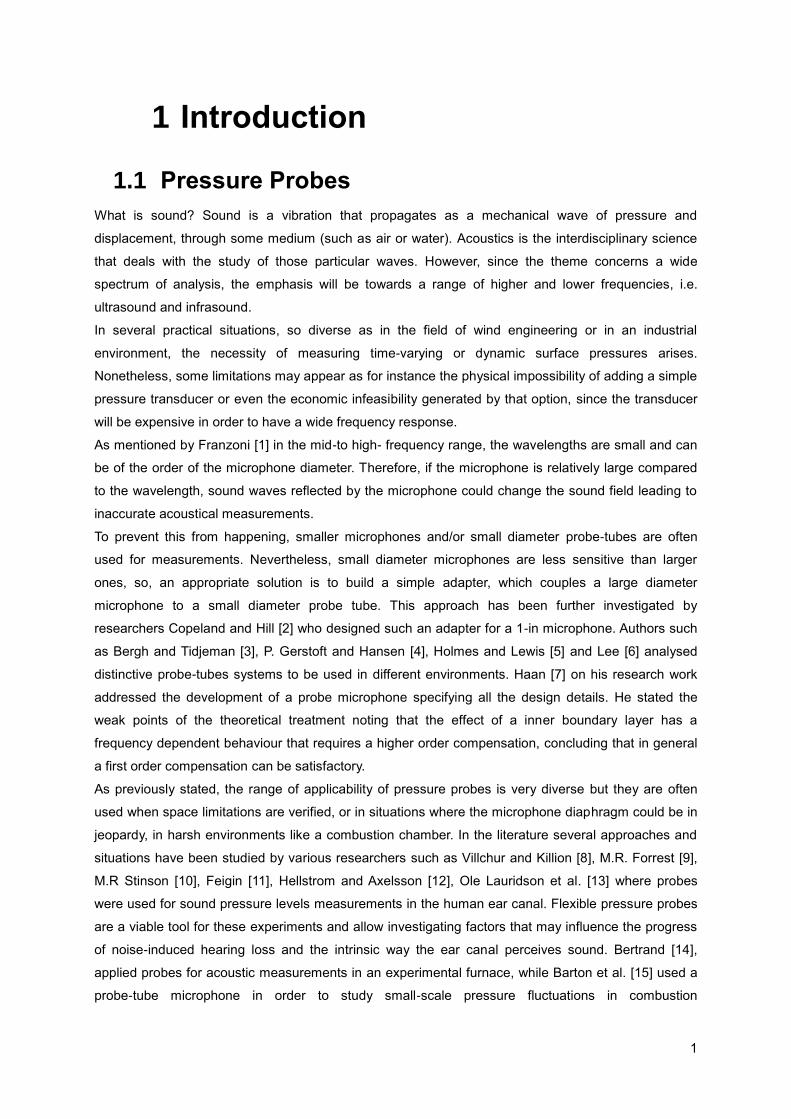
As mentioned by Franzoni [1] in the mid-to high- frequency range, the wavelengths are small and can
be of the order of the microphone diameter. Therefore, if the microphone is relatively large compared
to the wavelength, sound waves reflected by the microphone could change the sound field leading to
inaccurate acoustical measurements.
To prevent this from happening, smaller microphones and/or small diameter probe-tubes are often
used for measurements. Nevertheless, small diameter microphones are less sensitive than larger
ones, so, an appropriate solution is to build a simple adapter, which couples a large diameter
microphone to a small diameter probe tube. This approach has been further investigated by
researchers Copeland and Hill [2] who designed such an adapter for a 1-in microphone. Authors such
as Bergh and Tidjeman [3], P. Gerstoft and Hansen [4], Holmes and Lewis [5] and Lee [6] analysed
distinctive probe-tubes systems to be used in different environments. Haan [7] on his research work
addressed the development of a probe microphone specifying all the design details. He stated the
weak points of the theoretical treatment noting that the effect of a inner boundary layer has a
frequency dependent behaviour that requires a higher order compensation, concluding that in general
a first order compensation can be satisfactory.
As previously stated, the range of applicability of pressure probes is very diverse but they are often
used when space limitations are verified, or in situations where the microphone diaphragm could be in
jeopardy, in harsh environments like a combustion chamber. In the literature several approaches and
situations have been studied by various researchers such as Villchur and Killion [8], M.R. Forrest [9],
M.R Stinson [10], Feigin [11], Hellstrom and Axelsson [12], Ole Lauridson et al. [13] where probes
were used for sound pressure levels measurements in the human ear canal. Flexible pressure probes
are a viable tool for these experiments and allow investigating factors that may influence the progress
of noise-induced hearing loss and the intrinsic way the ear canal perceives sound. Bertrand [14],
applied probes for acoustic measurements in an experimental furnace, while Barton et al. [15] used a
probe-tube microphone in order to study small-scale pressure fluctuations in combustion

2
magnetohydrodynamics. Neise [16] studied the use of a probe attached to a microphone to be used
for sound measurement in turbulent flow and on the research of Toyoda et al [17] the development of a
probe to acquire direct pressure measurements appears to be very effective to educe the large-scale
vortical structures in a circular jet and also to collect importing data about the fluctuating static
pressure in turbulent flows. Several important researchers have been contributing to this scientific field
of measurement such as Kobashi [18], Kono & Nishi [19], Nyland et al [20] and Naka [21].
Pressure probes have been widely used and became a valuable tool for measuring real-time pressure
fluctuations, however the development is always a compromise between the range of practical
application and the best near-optimum systems possible. Near-optimum system is the transmission of
the perturbation signal through the probe to the microphone diaphragm without significant change in
its amplitude, for the largest frequency band. The ratio between the recorded signal (microphone
position) and original signal (perturbation) is called probe transfer function, TF, and the main concern it
is to obtain a flat amplitude TF (module equal to unity), meaning that the influence of the tube was
minimized. A phase lag is inevitable with such systems, but is desirable that it varies linearly with
frequency; such characteristic introduces only a fixed time delay and thus preserves the shape of the
pressure waves or impulses during the transmission process.
1.2 State-of-Art
As reported in the previous sub-chapter, one can allege that an appropriate solution for a probe
microphone design is to attach a large diameter microphone to a small diameter probe tube, acting the
latter like a transmission line.
There are in the literature several proposed probe-microphone systems with distinct configurations, as
shown in Figure 1.1. The first solutions presented, Figure 1.1 (a)-(b) with the microphone attached to
one end of the tube holds very similar characteristics to those experienced by the classical open-end
tube (quarter-wave resonators). One can even estimate the resonant frequencies using that concept
for the sake of order of magnitude. However, for more accurate results it is imperative to account for
the length and the microphone volume chamber. Copeland and Hill [2], Egolf [22] and Barton et al [15]
worked with these types of probes contributing for the progress on the subject.
Copeland and Hill [2] on his work compares the pressure response curves of the Bruel and Kjaer 4132
1-in. condenser microphone with that of the Bruel and Kjaer 4134 ½, each fitted with probe tubes. The
main objective was to design a probe tube, which would take advantage of the greater sensitivity of
the 1-in microphone to perform SPL measurements in the human ear canal. Figure 1.2 shows the
probe response for both microphones as also the probe schematic.
On his research Egolf [22] developed a method for the mathematical modelling of a probe tube
microphone using two basic parameters defined by Iberall [23] work which addresses the dynamics of
damped plane-wave propagation in cylindrical tubes. TF based on an electrical analogue four-pole
network model where each microphone is characterized by acoustic impedance. The model was
validated experimentally. Collected data is shown in Figure 1.3.
3
Barton et al [15] on his work presented a new configuration trying to overcome the main drawback of a
traditional design: tube behaves roughly like an “open-closed” one-dimensional waveguide with
numerous resonances across the frequency range. Hence, a damping solution it is tested where an
acoustical resistance (glass wool on this particular case) is placed midway within the length of the tube
originating a smoother frequency response at least on a wider frequency range than the previous
works, as it is noticed on Figure 1.4.
Figure 1.1: (a)-(f) open-closed probes Copeland and Hill [2], Egolf [22], B&K [31], Hellstrom and Axelsson [12], Villchur and Killion [8] Gabard and Peube [23] Nyland et al 20] Barton et al
[15] (g)-(i) open-open probes Franzoni and Elliot [1]

4
Egolf [22] as mentioned presents a TF expressed by 𝑇𝐹 =𝑍𝑝
𝐴𝑇𝑍𝑃+𝐵𝑇 that depends exclusively on 3
parameters: 𝑍𝑝 is the specific impedance of the probe microphone, 𝐴𝑇 and 𝐵𝑇 that represent two of
the four-pole parameters matrix
Figure 1.2: Pressure response curves obtained by Copeland and Hill [2]
Figure 1.3: Transfer function obtained by Egolf [22]

5
Figure 1.4: Pressure response curves obtained by Barton [15]
Later, Franzoni [1] discussed the pros and cons of some different configurations and mentioned some
disadvantages implied by the use of damping materials like reducing the probe’s signal-to-noise ratio.
As reported before, for accurate acoustic measurements it is crucial that the TF has a near flat
behaviour on a wide frequency spectrum combined with smooth resonance peaks if they exist. With
that in mind, Bertrand [14] worked on a microphone-probe assembly to be used inside a furnace to
study the resonance phenomena based on the principle of the damped Helmholtz resonator. For these
purposes, the sensitivity of the microphone probe must be as good as possible in the range of
frequencies of combustion noise emission, i.e. below 1000 Hz. However, when using a simple probe-
microphone a problem emerges, an amplification factor of +10dB appears within the range of
applicability, which is clearly in conflict with the smooth TF concept. Therefore, in order to solve it, a
damping mechanism it is tested and a 1 mm thick rubber seal is used with satisfactory results as
presented in Figure 1.5.
It is relevant to inform that no clear information is given about the rubber and the choice was only
made with empirical research (trial and error). Gabard and Peube [24] worked within the same
purpose: correcting the distortion introduced by the pneumatic line, however the authors followed
another path that consists in a restriction in the section, see Figure 1.6. A comparison between the
theoretical TF, with and without restriction, is shown and conclusions are taken regarding the optimum
position of the restriction section. The authors state that a compromise must be acknowledged
whether it is more relevant to have a smoother TF or a wider spectrum of frequency.

6
Nyland et al [20] analysed various geometries that allow a simultaneous measurement of time-
average pressure and simultaneously the protection of the pressure transducer from particles
entrained in the airstream. For the latter purpose the transducers have been mounted at right angles
to the axis of the probe. One important conclusion derived from Nyland et al [20] research consists of
the great correlation between the measured frequency response with the predictions made using the
equations of Iberall [23] and of Bergh and Tidjeman [30]. In Figure 1.7 a TF is presented using the
recursion formula deducted by Bergh and Tidjeman [30].
Figure 1.6: Transfer function obtained by Gabard and Peube [24]
Figure 1.5: Transfer function obtained by Bertrand [14]

7
Figure 1.7: Transfer function obtained by Nyland et al [20]
The last 4 configurations presented in Figure 1.1 are discussed in the work of Franzoni [1], where (g)-
(i) and (j) behave mainly has an open-open tube (half-wave resonators) and they are tested against
the usual design where the microphone is placed at the end of the tube. As mentioned earlier the
presence of the microphone at the end of the tube introduces non-desirable resonance peaks due to
the presence of standing waves induced by the microphone side branch. Therefore, the main concern
lies in the best way to minimize the presence of standing waves avoiding the use of damping material
(associated with a loss in signal-to-noise ratio) in the sound path between the source and receiver.
The author stated that the recommended design is a probe-tube adapter with a downstream
constriction followed by an anechoic termination. A TF is given in Figure 1.8 however no data is
provided regarding the phase TF.

8
Figure 1.8: Transfer function obtained by Franzoni and Elliot [1]
Tsuji et al [25] developed a new technique to measure pressure fluctuations, using a probe-tube
microphone. The design of the probe, Figure 1.9, is not innovative, however the approach used on the
calibration of the system has proved to be interesting to say the least. In this research pressure
fluctuations need to be measure accurately hence it is strictly necessary to characterize the influence
of the probe on the readings. For that purpose it is assumed that the frequency response of the
system is limited by the Helmholtz resonator caused by the tube and sensor cavity [17]. With this
simple HR model the amplitude ratio variation and phase delay between the output signal of the
pressure probe and the signal measured by the reference microphone was computed. A comparison
between the HR model and the measured amplitude ratio and phase delay are presented in Figure
1.10
Figure 1.9: Schematic view of the SP-Probe used in Tsuji et al work [25]

9
This HR model proved to be accurate for the sake of Tsuji’s [25] et al experiment as it is presented in
Figure 1.11; because although the original fluctuation measured by the probe differs significantly from
the one measured by the reference microphone, once the effect of HR is removed, the signals match
excellently. Tsuji et al [25] work proves an unequivocal bond between the resonance peak and the
cavity where the microphone is placed.
While working on the literature review the most common probe material found was stainless steel. This
provides rigid probes with stiffness, good finishing surface and especially, notable thermal capabilities
that are a requirement when the intent is to make direct measurements with microphones in hot
environments, like furnaces or combustion chambers, for instance. Nevertheless, in other fields,
flexible PVC or silicone tubes can suit the purpose much better.
It is important to mention that only pressure fluctuations measurements are taken with the presented
probe, hence being able to acquire a complete static pressure probe remains to be studied and
developing an accurate model is a priority.
Figure 1.10: Amplitude and phase delay obtained for the SP-Probe developed by Tsuji et al [25]
Figure 1.11: (a) The solid line is the reference microphone output and the dashed line is the measured
static pressure signal. (b) HR effect removed numerically - obtained in Tsuji et al [25]

10
1.3 Motivation and Objectives
The main objectives of this thesis were to increase the knowledge regarding static-pressure probes
design, and for that a careful evaluation (through the development of a powerful mathematical model)
of the dimensions impact in the acoustic transfer function was necessary, and also adopting a new
design that includes a pressure sensor allowing a complete characterization of the pressure field.
The motivation behind the study was to develop pressure probes to contribute efficiently the collection
of valuable data of a specific series gas turbine combustion chamber, the CFM-56-5. A gas turbine is a
type of internal combustion engine with a wide range of applicability, however the interest will remain
on jet engines, more specifically on turbofan jet engines where CFM-56 series are included.
CFM-56 series have particular standards concerning maintenance activities and also conceptually
they benefit from a modular approach, as it is illustrated in Figure 1.12, meaning that the reactor is
divided in independent modules that are assembled to form the reactor as a whole. This concept of
modular assembly introduces several technical advantages (shorter turn around time (TAT), less
maintenance costs) but also triggers new ideas concerning technological improvement due a virtual
independence of all the pieces that form the reactor.
And how can this work enhance this astute modular approach? Being able to access the combustion
chamber module formed by 4 main elements dome separately: components of dome, inner and outer
cowl and inner and outer liner. The concern is to upgrade the alignment process of fuel nozzles.
The alignment of fuel nozzles is a crucial process to achieve homogenous/optimum combustion. For
that reason, the role represented by each nozzle/swirl assembly cannot be disregarded. The fuel
nozzle is inserted and supported inside the primary swirl nozzle and an optimum alignment position is
meant when the fuel nozzle axis is centered with respect to the primary swirl nozzle axis contributing
effectively for a homogeneous mixture in all directions between the fuel and the primary flow of air. For
that particular reason, an offset will necessarily lead to a devious flow composition that will ultimately
result in different pressure and temperature distributions, reducing the efficiency and reactor’s life
cycle.
Nowadays, the nozzle alignment method is made by trial and error, meaning that on a first stage the
maintenance technician makes used of certified charts that specify reliable ranges regarding nozzle
position, secondly, and after all the modules are assembled, the reactor is taken to a test bench where
some measurements are taken, exhaust gas temperature (EGT) and the efficiency is computed. If the
efficiency isn’t in the range recommended by the manufacturer the reactor returns to the maintenance
sector where the position of the nozzles is modified. This works proposes a maintenance pack of
pressure probes: a new design capable of acquiring acoustical signatures of a reference swirl/nozzle
position, and a commonly used static-pressure probe useful to take pressure fluctuations
measurements at the outlet of a combustion chamber. Through an analogous case study deviations in
the pressure field were assessed and enhanced the possibility of a pre-test bench tool to be held by
technicians in the maintenance facilities avoiding a trial and error approach that leads to unnecessary
costs. One must note that the acoustical signatures are not to be acquired in a working engine, but in
a phase that precedes the trip to the test-bench. The premise is that this specific tool could be
valuable in qualitatively estimate how devious will be the flow inside the combustion chamber.

11
1.4 Thesis Outline
The remainder of this thesis is presented in five Chapters. Chapter 2 shows an overview of sound
propagation in tubes in which basic equations are established and the assumptions that ultimately
lead to the development of low reduced frequency model are presented. Chapter 3 exhibits two
distinct calibration techniques and the procedure that contributed to develop a swirler used in chapter
4.
Chapter 4 has four main sections; the first one consists in recalibrating two probes to raise the
applicability of the developed model; second and third show all the procedures and detailed analysis
regarding static pressure-probe (SP-Probe) and Stethoscope probe. Finally, the fourth section
expresses a case study aiming to perform a sensitivity analysis in changes on the flow characteristics.
Chapter 5 summarizes the main conclusions about the work and suggestions concerning stages to be
held in the future.
Figure 1.12: Modular assembly of CFM-56-5 combustion chamber

12
2 Theoretical Considerations
2.1 Introduction
Sound wave propagation in gases contained in cylindrical tubes throughout the centuries became a
topic in the acoustic field, mainly due to the development of an acoustic, a thermal and a viscous
boundary layer. These combinations of viscous effects are responsible for sound energy losses and
the problem became a classical one.
As stated in Tidjeman’s work [26], the analytical solutions given in literature can be divided roughly into
two groups. The first group includes solutions obtained by analytical approximations of the full
Kirchhoff solution and the second group uses the basic equations as a starting point. It deviates from
the first one by including simplified assumptions, ultimately leading to more simplified solutions. The
basic equations that are a pillar for both groups are the ones describing the motion of a fluid column in
a cylinder: Navier-Stokes equations in axial and radial directions, the equation of continuity, equation
of state and the energy equation. Since viscous effects are in the centre of the discussion it is
important to note that the impact of those effects increase when the radius of the tube decreases,
therefore one can neglect the effects for wide cylindrical tubes. For narrow cylindrical tubes (micro
size) the viscous dissipation term increases much faster than the diffusion term.
Within the second group, one model emerges regarding degree of applicability and simplicity; it is
defined as the low reduced frequency model and was obtained for the first time by Zwikker and Kosten
[27]. The low reduced frequency model assumes a constant pressure across the tube cross-section,
and the effects of inertia, viscosity, compressibility and thermal conductivity are accounted for.
On his research, Tidjeman [26] addressed the sound propagation in tubes considering that it
depends solely on two parameters, the shear wave number, 𝑠, also called Stokes number (Tidjeman
[26], Gabard and Peube [24]), and reduced frequency 𝑘. They are defined as:
𝒔 = 𝑹√𝝆𝒔𝝎
𝝁
(1)
𝒌 =
𝝎𝑹
𝒄
(2)
where 𝜌𝑠 is the mean density, 𝜔 is the angular frequency, 𝑅 is the tube radius, 𝜇 is the dynamic
viscosity and 𝑐 is the speed of sound.
The shear wave number, 𝑠, represents the ratio between the tube radius and the unsteady acoustic
boundary layer and the reduced frequency, 𝑘, gives the ratio between the tube radius and the
propagation wavelength.

13
Since the model itself is a simplified solution of a much full and complex model, a range of validity
must be taken into account, Tijdeman [26] defined as:
𝒌 ≪ 𝟏 𝒂𝒏𝒅
𝒌
𝒔≪ 𝟏
(3)
Kergomard [28] in is review of Tidjeman’s work [26] defined a stricter range, rewritten as:
𝒔𝟐
𝒌𝟐≫ 𝟏,
𝒔
𝒌𝟐≫ 𝟏 𝒂𝒏𝒅
𝒔𝟐
𝒌≫ 𝟏
(4)
Beltman [29] on his research illustrates the applicability of the low reduced frequency model stating
that for the majority of practical situations, the model is sufficient and the most efficient to describe
viscothermal wave propagation. Full-linearized Navier-Stokes model should only be used under
extreme conditions.
2.2 Basic Equations
In this section, the response of air inside a narrow tube is analytically described. The cylindrical
coordinates, 𝑥, 𝑟 and 𝜃 are used in this section. The flow is assumed to be axisymmetric. When the
concern is the propagation of sound inside a narrow tube, the flow should be treated as compressible.
For that particular reason the equation of continuity and Navier-Stokes equation for compressible flow
is considered. In addition, the equation of state and the energy equation are also accounted as
follows:
Equation of continuity:
𝝏𝝆
𝝏𝒕+ 𝛁 ∙ (𝝆𝑽) = 𝟎
(5)
Navier-Stokes equations of momentum conservation in the axial and radial directions:
�̅�
𝝏�̅�
𝝏𝒕+ �̅�
𝝏�̅�
𝝏𝒓+ �̅�
𝝏�̅�
𝝏𝒙= −
𝝏�̅�
𝝏𝒙+ 𝝁 [(
𝝏𝟐�̅�
𝝏𝒙𝟐 +𝝏𝟐�̅�
𝝏𝒓𝟐 +𝟏
𝒓
𝝏�̅�
𝝏𝒓) +
𝟏
𝟑
𝝏
𝝏𝒙(
𝝏�̅�
𝝏𝒙+
𝝏�̅�
𝝏𝒓+
�̅�
𝒓)]
(6)
�̅�
𝝏�̅�
𝝏𝒕+ �̅�
𝝏�̅�
𝝏𝒓+ �̅�
𝝏�̅�
𝝏𝒙= −
𝝏�̅�
𝝏𝒓
+ 𝝁 [(𝝏𝟐�̅�
𝝏𝒓𝟐 +𝝏𝟐�̅�
𝝏𝒙𝟐 +𝟏
𝒓
𝝏�̅�
𝝏𝒓−
�̅�
𝒓𝟐) +𝟏
𝟑
𝝏
𝝏𝒓(
𝝏�̅�
𝝏𝒙+
𝝏�̅�
𝝏𝒓+
�̅�
𝒓)]
(7)
The equation of state for an ideal gas:

14
�̅� = �̅�𝑹𝒐�̅� (8)
Energy equation:
�̅�𝒈𝑪𝒑 [
𝝏�̅�
𝝏𝒕+ �̅�
𝝏�̅�
𝝏𝒙+ �̅�
𝝏�̅�
𝝏𝒓] = 𝝀 [
𝝏𝟐�̅�
𝝏𝒓𝟐 +𝟏
𝒓
𝝏�̅�
𝝏𝒓+
𝝏𝟐�̅�
𝝏𝒙𝟐] +𝝏�̅�
𝝏𝒕+ �̅�
𝝏�̅�
𝝏𝒙+ �̅�
𝝏�̅�
𝝏𝒓+ 𝝁𝚽
(9)
where Φ is the dissipation function that represents the heat transfer caused by internal friction:
𝜱 = 𝟐 [(
𝝏�̅�
𝝏𝒙)
𝟐
+ (𝝏�̅�
𝝏𝒓)
𝟐
+ (�̅�
𝒓)
𝟐
] + [𝝏�̅�
𝝏𝒙+
𝝏�̅�
𝝏𝒓]
𝟐
−𝟐
𝟑[𝝏�̅�
𝝏𝒙+
𝝏�̅�
𝝏𝒓+
�̅�
𝒓]
𝟐
(10)
Once the governing equations are established, one can put the quantities in waveform, and the
following assumptions are made:
Flow is laminar throughout the system;
The sinusoidal disturbances are very small;
�̅� = 𝒄 ∙ 𝒖⟨𝒙,𝒓⟩𝒆𝒊𝝎𝒕; �̅� = 𝒄 ∙ 𝒗⟨𝒙,𝒓⟩𝒆
𝒊𝝎𝒕; �̅� = 𝒑𝒔(𝟏 + 𝒑𝒆𝒊𝝎𝒕) ; �̅�
= 𝝆𝒔(𝟏 + 𝝆⟨𝒙,𝒓⟩𝒆𝒊𝝎𝒕) ; �̅� = 𝑻𝒔(𝟏 + 𝑻⟨𝒙,𝒓⟩𝒆
𝒊𝝎𝒕)
(11)
The internal radius of the tube is small in comparison with its wavelength;
𝒌 =
𝝎𝑹
𝒄≪ 𝟏
(12)
Boundary layer thickness is small in comparison with the wavelength;
𝒌
𝒔≪ 𝟏
(13)
Radial velocity component, 𝑣, is small with respect to the axial velocity, 𝑢:
𝒗
𝒖≪ 𝟏 (14)
Where 𝜔 is angular frequency, 𝛾 is specific heat ratio, 𝑐 is speed of sound; 𝐶𝑝 is specific heat at
constant pressure; 𝜆 is thermal conductivity.
Substituting Eq. (11), Eqs. (5) – (9) can be simplified to:

15
𝒊𝝎𝒖 = −
𝟏
𝝆𝒔
𝝏𝒑
𝝏𝒙+
𝝁
𝝆𝒔[𝝏𝟐𝒖
𝝏𝒓𝟐 +𝟏
𝒓
𝝏𝒖
𝝏𝒓]
(15)
𝟎 =
𝝏𝒑
𝝏𝒓
(16)
𝒊𝝎𝝆 = −𝝆𝒔 [
𝝏𝒖
𝝏𝒙+
𝝏𝒗
𝝏𝒓+
𝒗
𝒓]
(17)
𝝆 =
𝜸
𝒄𝟐 (𝟏 +𝝆𝒔
𝑻𝒔
𝑻
𝝆)
(18)
𝒊𝝎𝝆𝒔𝒈𝑪𝒑𝑻 = 𝝀 [
𝝏𝟐𝑻
𝝏𝒓𝟐 +𝟏
𝒓
𝝏𝑻
𝝏𝒓] + 𝒊𝝎𝒑
(19)
The detailed procedure for solving Eqs. 15-19 is described in Bergh and Tijdeman [30]. Following
boundary conditions imposed on the unknown quantities 𝑝, 𝜌, 𝑇, 𝑢 and 𝑣:
At the rigid tube wall the axial and radial velocity must be zero: i.e, at 𝑟 = 𝑅, 𝑢 = 0 and 𝑣 = 0 ;
The radial velocity must be zero at the tube axis due to the axi-symmetry of the problem:
i.e, at 𝑟 = 0, 𝑣 = 0 and 𝑢, 𝑝, 𝜌 and 𝑇 have to remain finite;
The heat conductivity of the tube wall is large in comparison with the heat conductivity of the
fluid consequently the variation in temperature at the wall will be zero: i.e., at 𝑟 = 𝑅, 𝑇 =
0 (𝑖𝑠𝑜𝑡ℎ𝑒𝑟𝑚𝑎𝑙 𝑤𝑎𝑙𝑙𝑠)
After extensive algebra [30], the differential equation for pressure perturbation can be written in the
following form:
𝒑 {𝟏 +
𝜸 − 𝟏
𝜸
𝑱𝟐⟨𝒊𝟑/𝟐𝝈𝒔⟩
𝑱𝟎⟨𝒊𝟑/𝟐𝝈𝒔⟩} −
𝟏
𝜸
𝒅𝟐𝒑
𝒅𝝃𝟐
𝑱𝟐⟨𝒊𝟑/𝟐𝝈𝒔⟩
𝑱𝟎𝟑/𝟐⟨𝝈𝒔⟩
= 𝟎 (20)
In which solution for plane waves, takes on:
𝒑 = 𝑨𝒆𝜞𝝃 + 𝑩𝒆−𝜞𝝃 (21)
and Γ is the propagation constant that corresponds to the low frequency solution, given by:

16
𝜞 = √𝑱𝟎⟨𝒊𝟑/𝟐𝒔⟩
𝑱𝟐⟨𝒊𝟑/𝟐𝒔⟩√
𝜸
𝒏
(22)
𝒏 = [𝟏 +
𝜸 − 𝟏
𝜸
𝑱𝟐⟨𝒊𝟑/𝟐𝝈𝒔⟩
𝑱𝟎⟨𝒊𝟑/𝟐𝝈𝒔⟩]
−𝟏
(23)
𝒔 = 𝑹√𝝆𝒔𝝎
𝝁
(24)
𝝃 =𝝎𝒙
𝒄 (25)
𝝈 = √𝝁𝑪𝒑
𝝀
(26)
𝜸 =
𝑪𝒑
𝑪𝒗
(27)
The constants 𝐴 and 𝐵 can be determined by specifying additional boundary conditions at both ends
of the evaluated probe/tube configuration. Replacing the pressure equation in the solution for the other
acoustic variables, those become:
𝒖 =
𝒊𝜞
𝜸[𝟏 −
𝑱𝟎⟨𝒊𝟑/𝟐𝜼𝒔⟩
𝑱𝟎⟨𝒊𝟑/𝟐𝒔⟩] [𝑨𝒆𝜞𝝃 − 𝑩𝒆−𝜞𝝃]
(28)
𝒗 = 𝒊𝒌 [
𝟏
𝟐𝜼 {𝟏 +
𝑱𝟎⟨𝒊𝟑/𝟐𝒔⟩
𝑱𝟐⟨𝒊𝟑/𝟐𝒔⟩
𝜸
𝒏} +
𝜸 − 𝟏
𝒊𝟑/𝟐𝝈𝒔
𝑱𝟏⟨𝒊𝟑/𝟐𝝈𝒏𝒔⟩
𝑱𝟎⟨𝒊𝟑/𝟐𝝈𝒔⟩−
𝜸
𝒊𝟑/𝟐𝜼𝒔
𝑱𝟏⟨𝒊𝟑/𝟐𝜼𝒔⟩
𝑱𝟐⟨𝒊𝟑/𝟐𝒔⟩] [𝑨𝒆𝜞𝝃 + 𝑩𝒆−𝜞𝝃]
(29)
𝝆 = [𝟏 −
𝜸 − 𝟏
𝜸{𝟏 −
𝑱𝟎⟨𝒊𝟑/𝟐𝝈𝒏𝒔⟩
𝑱𝟎⟨𝒊𝟑/𝟐𝝈𝒔⟩}] [𝑨𝒆𝜞𝝃 + 𝑩𝒆−𝜞𝝃]
(30)
𝑻 =
𝜸 − 𝟏
𝜸[𝟏 −
𝑱𝟎⟨𝒊𝟑/𝟐𝝈𝒏𝒔⟩
𝑱𝟎⟨𝒊𝟑/𝟐𝝈𝒔⟩] [𝑨𝒆𝜞𝝃 + 𝑩𝒆−𝜞𝝃]
(31)
As addressed in Tidjeman [26] work the propagation constant for sound waves propagation in gases
contained in cylindrical tubes is a complex function, therefore has a real and an imaginary part. The
real part represents the energy attenuation per distance unit in the 𝜉 direction, and the imaginary part
represents the phase shift over the same distance. Tidjeman [26] stated the power of the low reduced
frequency model while reviewing theoretical propagation constant (expressed in terms of shear wave
number).

17
It is shown that the solution obtained for the first time by Zwikker and Kosten [27], passes continuously
from Rayleigh’s solution into the solution of Kirchhoff as stated by Figure 2.1.
As mentioned earlier, the “low reduced frequency solution” can be shown to be valid over the complete
range of shear wave numbers in the case 𝑘 ≪ 1 and 𝑘
𝑠≪ 1. Most of the probes already studied with
specific practical applications lie in the transition region narrow-to-wide, showing the importance of the
low reduced frequency solution. As illustrated by the Figure 2.1 one can reveal that “narrow” tube
solutions are valid for low values of 𝑠 and “wide” tube solutions for high values of this parameter,
however as large values of 𝑠 can be computed not only for large tube radius but also for high
frequencies, mean densities or pressure and small viscosity, this concept can be a bit misleading.
Since, axial velocity is an important quantity to understand how the propagation is made in a
transmission line, it is relevant to mention how it is affected by the shear wave number. The shear
wave number can be understood as a measure for the ratio of inertial and viscous effects, therefore if
the condition is a small shear wave number the viscous effects have a higher impact than inertial
forces, hence the velocity profile over the cross-section approaches a Poiseuille flow. On the other
hand, a large shear wave number indicates a plane-wave profile, shown in Figure 2.2.
Figure 2.2: Axial velocity profile for an outgoing wave in a infinitely long tube, [25], [30]
Figure 2.1: Review of analytical solutions for propagation constant as a function of shear wave number, [26]

18
2.3 Probe mathematical model and boundary
conditions
In this sub-chapter is addressed the probe configuration used in this work and all the required
specifications to achieve the desired transfer function. The probe transfer function is a very important
concept due to the ability in quantifying the impact of the probe on pressure fluctuations
measurements. In the work by Bergh and Tidjeman [3] a recursion formula based on the low
frequency model is presented regarding N tubes and N volumes in series. On this thesis despite the
use of the same model - low reduced frequency model - the path chosen is different in a way that the
formula derived by Bergh and Tidjeman [3] assumes that at each tube the termination will be in a
volume, followed by another tube.
Regarding the mathematical model specifically, the process relies on the definition of all variables
represented in sub-chapter 2.2 at all the individual sections of the tube, and solving a system of
equations using the software Mathematica. The general schematics of the probe are defined in the
Figure 2.3. The probe was designed taking into account a stethoscope configuration, contemplating in
one end a pressure sensor (5) and a microphone (4).
This “modular” approach can be very efficient when addressing each individual section, since it
provides a detailed vision of each parameter, ultimately leading to the computation of individual
transfer functions and phase behaviour.
Figure 2.3 - Preliminary design concept for the mathematical modelling approach
The schematics represented above have 4 cylindrical sections (1,2,3,5) and one volume (4). However
the model can be easily manipulated in order to fulfil various design requirements, i.e., making a probe
with less tubes. One can state that the essential requirements are in the boundary conditions, which

19
are obliged to be the same despite a change in design in order to be mathematically consistent and
assuring model interchange ability.
Conceptually, the design above can be defined as a coupled system consisting in 4 tubes and one
volume (Helmholtz cavity), as already discussed. With that in mind for each individual tube the
pressure is defined according to Equation 21:
𝒑𝒊𝒏 = 𝑨 + 𝑩 (32)
𝒑𝒐𝒖𝒕 = 𝑨𝒆𝜞𝝃 + 𝑩𝒆−𝜞𝝃 (33)
where “in” and “out” stands for the inlet and outlet of each element. Equation 34 and 35 sets the
solution for inlet and outlet axial velocities:
𝒖𝒊𝒏 =
𝒊𝜞
𝒄𝝆𝒔[𝟏 −
𝑱𝟎⟨𝒊𝟑/𝟐𝜼𝒔⟩
𝑱𝟎⟨𝒊𝟑/𝟐𝒔⟩] [𝑨 − 𝑩]
(34)
𝒖𝒐𝒖𝒕 =
𝒊𝜞
𝒄𝝆𝒔[𝟏 −
𝑱𝟎⟨𝒊𝟑/𝟐𝜼𝒔⟩
𝑱𝟎⟨𝒊𝟑/𝟐𝒔⟩] [𝑨𝒆𝚪𝝃 − 𝑩𝒆−𝚪𝝃]
(35)
Regarding the mass flow rates one can define as:
�̇�𝒊𝒏 = ∫ 𝝆𝒔𝒖𝒊𝒏𝟐𝝅𝒓𝒅𝒓 =
𝝅𝑹𝟐𝚪
𝒊𝒄[𝑱𝟐⟨𝒊𝟑/𝟐𝒔⟩
𝑱𝟎⟨𝒊𝟑/𝟐𝒔⟩]
𝑹
𝟎
[𝑨 − 𝑩] (36)
�̇�𝒐𝒖𝒕 = ∫ 𝝆𝒔𝒖𝒐𝒖𝒕𝟐𝝅𝒓𝒅𝒓 =
𝝅𝑹𝟐𝚪
𝒊𝒄[𝑱𝟐⟨𝒊𝟑/𝟐𝒔⟩
𝑱𝟎⟨𝒊𝟑/𝟐𝒔⟩]
𝑹
𝟎
[𝑨𝒆𝚪𝝃 − 𝑩𝒆−𝚪𝝃] (37)
Regarding the volume some considerations need to be addresse. Based on Bergh and Tijdeman [30]
it was assumed that within the microphone volume, density and pressure were the only time
dependent variables and the inner expansion takes place isentropically. Due to the fact that the
microphone diaphragm had a flexible surface, a dimensionless factor was considered, 𝜎′, and taken
into account using volume increase due to diaphragm deflection. Additionally, a parameter 𝑒𝑖𝜃 was
added to this factor, to express a phase delay between the expansion at the microphone volume and
diaphragm response.
This variation can be simplified to:
𝝏𝒎𝒗
𝝏𝒕=
𝒊𝝎𝜸𝑽𝟎
𝒄𝟐 (𝟏
𝜸+
𝝆𝒔𝒄𝟐
𝜸𝜷𝒆𝒊𝜽) 𝒑𝒆𝒊𝝎𝒕 ≡
𝒊𝝎𝜸𝑽𝟎
𝒄𝟐 (𝟏
𝜸+ 𝝈′𝒆𝒊𝜽) 𝒑𝒆𝒊𝝎𝒕
(38)
where 𝑝 stands for the pressure inside the cavity and 𝑉0 is the volume formed by the space between
the diaphragm and the outer case, the streaks of the microphone casing and the space between the
case and the outlet of the transmission line (probe). For mathematical purposes the volume is
computed as a generic equivalent cylindrical volume.

20
Since the suggested probe design has a junction connecting tube 1-2-3, one can assume due to
different behaviour induced by each tube (delay mostly), consequently the mass within the junction
volume can vary with time implying that 𝜕𝑚𝑣
𝜕𝑡≠ 0. From the physical point of view this condition relies
on the idea that a wave travelling from tube 1 to tube 2 or tube 3 in some point in time can be trapped
on that instrument volume by a wave travelling on the opposite direction (reflected wave). One must
take note that the volume that was once defined as 𝑉0, in this case needs to be changed to 𝑉𝑇−𝑗𝑢𝑛𝑐𝑡𝑖𝑜𝑛.
Overall, the boundary conditions computed mathematically for this probe can be observed on the
following table:
1 2 3 4 5
Inlet 𝑝01 =𝜌𝑠∙𝑐2
𝛾(𝐴1 + 𝐵1) 𝑝02 = 𝑝03 𝑝03 = 𝑝𝐿1
𝑝𝐿3 = 𝑝𝑉4
𝑝05 = 𝑝𝐿2
Outlet 𝑝𝐿1 = 𝑝02 = 𝑝03 �̇�𝐿2 = �̇�05 �̇�𝐿3 =
𝜕𝑚𝑣
𝜕𝑡
𝑢𝐿5 = 0
Table 2.1: Boundary conditions present in mathematical model
One additional boundary condition needs to be taken into account concerning the junction itself as
mentioned previously, hence:
𝝏𝒎𝑻−𝑱𝒖𝒏𝒄𝒕𝒊𝒐𝒏
𝝏𝒕= �̇�𝑳𝟏 − �̇�𝟎𝟐 − �̇�𝟎𝟑
(39)
It is relevant to address that all the constants used in the mathematical modelling of the probe are
displayed in Appendix A.
One must address the fact that the inlet at section 5 coincides with outlet of section 2 and the inlet of
section 4 corresponds to section 3 outlet.
Figure 2.4: Probe schematics adopted in the mathematical modelling

21
3 Experimental Apparatus
In this chapter different calibration techniques and some considerations concerning the experimental
assembly that will lead to the ultimate case study will be addressed. Regarding calibration procedure
two different techniques are used – a) using a PVC tube + speaker assembly controlled by a signal
generator emitting a sine wave with constant amplitude, and b) calibration by comparison using a
cavity with a speaker attached at the bottom. For the sake of understanding while addressing
distinctive calibration techniques one will define calibration Type A and Type B, respectively.
3.1 Acoustic Calibration setup Type A
The general setup used for experimental calibration of amplitude and phase delay transfer function is
presented in Figure 3.1 and will be divided roughly into 3 main sections:
Acquisition and signal monitoring – Figure 3.1 (a1);
Signal generation – Figure 3.1 (a2); Interface and data processing – Figure 3.1 (a3);
In Table 3.1 are listed the used devices.
Table 3.1: List of material for experimental calibration system Type A
Material used on experimental calibration Type A
PC
Matlab Software
USB DAQ Module DT-9841 SB
Rotel power amplifier RB-850
Speaker Pioneer - TS 6170i
Standing wave tube PVC
Tektronix TDS 1001C- EDU Oscilloscope
Tektronix AFG 3021B Function Generator
Sound level meter - type 2230 B&K and 2250 B&K
Microphone - type 4189 B&K and 4155 B&K
Micro. Preamplifier - model ZC0020 and ZC 0032

22
3.1.1 Interface and data processing
Probe calibration measurements were taken using a USB data acquisition module, DT9841-SB
controlled by a Matlab program. The program in its core can be divided in two sections – one mainly
dedicated to acquisition, and the other to data processing.
These two sections are crucial for high efficiency on the calibration procedure. The first has
significantly impact due to the fact of specifying the length of the time-file and acquisition rate. The
latter receives as input the time signal files of microphone + probe and with the aid of cross-spectral
density analysis computes the amplitude and phase delay between both signals. FFT algorithm and
cross-spectral analysis are embedded in the data processing section.
3.1.2 Signal Generation
The function generator, Tektronix AFG 31021 B, connected via USB to a PC generated the reference
signal. The signal produced by the function generator was controlled automatically using a Matlab
software program and connected to the data acquisition module DT9841-SB in order to acquire the
reference data. The reference signal produced was a sinusoidal wave with amplitude that could vary
according experimental conditions. The range of analysed frequencies is between 20Hz – 1000Hz, in
steps of 10Hz for lower frequencies and 50Hz for higher frequencies, or even a much narrow step. As
illustrated in Figure 3.1 (a2) this signal was amplified by a stereo power amplifier, model Rotel RB -
850 and finally connected to a loudspeaker, model TS-G170i, attached to one end of a PVC tube. The
existence of the tube is of much importance due to the ability to form an acoustic stationary medium,
however it has some physical constraints.
Figure 3.1: Probe calibration schematics Type A- (a1) Acquisition and signal monitoring, (a2) Signal generation, (a3) Interface and data processing

23
The plane wave proximity in a cylindrical tube is valid until a cut-off frequency, meaning that above that
frequency the calibration has no significant weight since pressure isn’t the same in radial direction.
According to Ekkels and Bree [30], that frequency is given by:
𝒇 𝒄 =𝒄
𝟏. 𝟕𝟏𝒅 (40)
where 𝑑 stands for tube diameter.
In the present setup, the tube diameter was 𝑑 = 0.18 m, leading to a cut-off frequency, under standard
temperature and pressure (STP) conditions, in the order of 1100Hz. Since the maximum tested
frequency is 1000Hz, one can assure that calibration is valid.
3.1.3 Signal Acquisition
The signal acquisition was done using a setup already described in Figure 3.1 (a1), combining two
microphones, and the USB data acquisition module, DT9841-SB controlled automatically by a Matlab
program.
Due to its very high degree of accuracy and reliability, the condenser microphone is accepted as the
standard acoustical transducer for all sound and noise measurements. The condenser microphone
shows a wide spectrum of properties such as: high stability under various environmental conditions,
flat frequency response over a wide frequency range, low distortion, very low internal noise and finally
high sensitivity. These properties ultimately turn the condenser microphone in an essential tool to
acoustical measurements.
On this thesis two microphones were used: type 4155B&K using a preamplifier model ZC0032 and
type 4189B&K using a preamplifier model ZC0020, both free field microphones. Free field
microphones are designed essentially to measure the sound pressure, as it existed before the
microphone was introduced into the sound field. At higher frequencies, the presence of the
microphone itself in the sound field disturbs the sound pressure locally. In general, the sound pressure
around a microphone cartridge increases because of reflections and diffraction, for that reason, the
Figure 3.2: Stiff PVC tube set-up for standing wave medium

24
frequency characteristics of a free-field microphone are designed to compensate for this increase in
pressure.
The main purpose behind the use of two different microphones is to simplify the calibration process in
order to obtain a first transfer function. Usually the calibration methodology consists in acquiring the
sound generated by the loudspeaker in three stages: 1) collecting a frequency spectrum with the
microphone itself 2) collecting a frequency spectrum with the same microphone attached with the
probe, and 3) compute cross-spectral densities of both signals in the frequency domain. The validation
procedure must be done with the same microphone, however for a first rough approximation one can
work with two different microphones.
The validation procedure, where the same microphone is used, implies necessarily microphone
detachment and reattachment being time-consuming and unpractical. The main advantage on working
with two different microphones with different parameters and characteristics is applying less effort on
computing an acoustic transfer function, nevertheless a detailed study of both microphones must be
done and one must understand and quantify how devious they perceive sound. With that in mind, a
basic behaviour study was developed and some basic relations were computed. These relations and
validation are displayed in detail in Appendix B.
One must note that the reference microphone and probe were place both at the same distance from
the loudspeaker in order to guarantee that SPL was equal in the tube cross-section. Regarding data
acquisition properties is important to address that a fast Fourier transforming operation, FFT,
transformed the time signals in frequency domain was made entirely by the developed software. The
program required from the user to assign the acquisition rate and the number of blocks (number of
points) that the time file would have. The time file has a relatively important role due to FFT algorithm,
because the number of specified blocks will define the FFT resolution, i.e., if you acquire a time file
with an acquisition rate of 20KHz and a sample with 200000 points, the maximum FFT resolution will
be ∆𝑓𝑟𝑒𝑞𝐹𝐹𝑇 = 0.153 𝐻𝑧, since FFT algorithm relies on 2𝑁 points to reproduce the frequency domain
with 𝑁 being an integer number. As stated the FFT resolution is a commitment between how much
points are necessary in the time file to achieve the desired resolution. In this work the FFT resolutions
used were 0.153Hz and 0.305Hz.
25
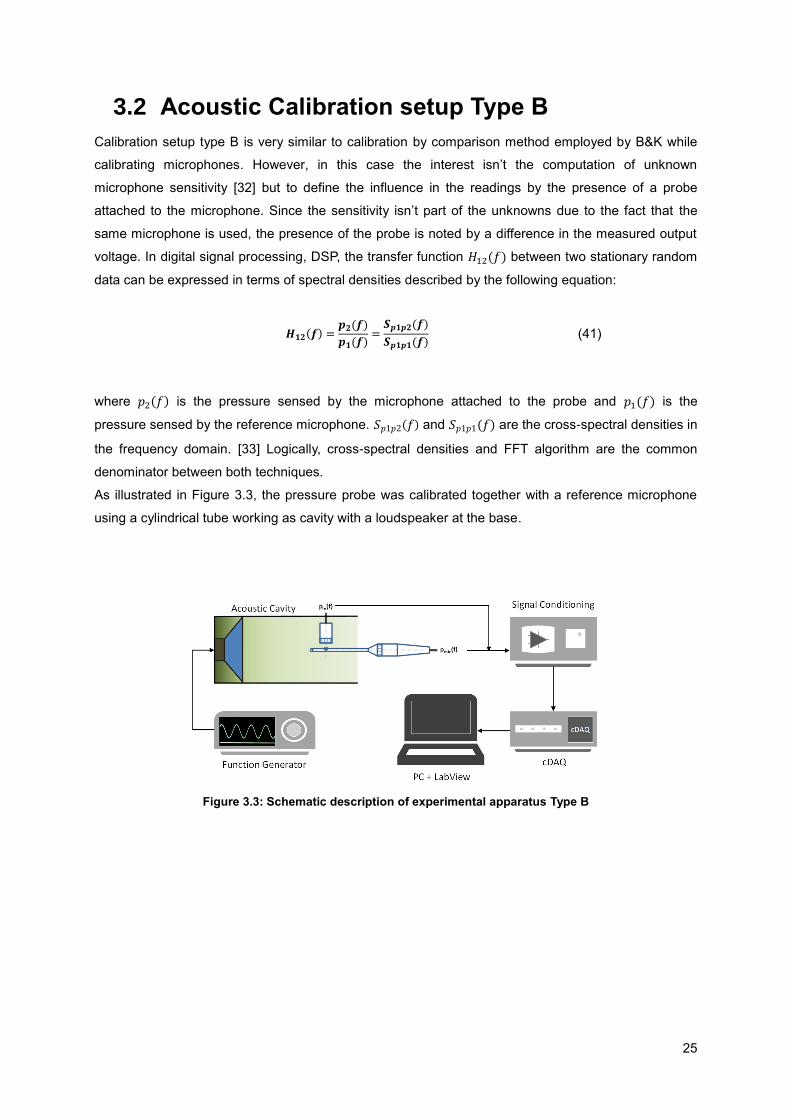
3.2 Acoustic Calibration setup Type B
Calibration setup type B is very similar to calibration by comparison method employed by B&K while
calibrating microphones. However, in this case the interest isn’t the computation of unknown
microphone sensitivity [32] but to define the influence in the readings by the presence of a probe
attached to the microphone. Since the sensitivity isn’t part of the unknowns due to the fact that the
same microphone is used, the presence of the probe is noted by a difference in the measured output
voltage. In digital signal processing, DSP, the transfer function 𝐻12(𝑓) between two stationary random
data can be expressed in terms of spectral densities described by the following equation:
𝑯𝟏𝟐(𝒇) =
𝒑𝟐(𝒇)
𝒑𝟏(𝒇)=
𝑺𝒑𝟏𝒑𝟐(𝒇)
𝑺𝒑𝟏𝒑𝟏(𝒇) (41)
where 𝑝2(𝑓) is the pressure sensed by the microphone attached to the probe and 𝑝1(𝑓) is the
pressure sensed by the reference microphone. 𝑆𝑝1𝑝2(𝑓) and 𝑆𝑝1𝑝1(𝑓) are the cross-spectral densities in
the frequency domain. [33] Logically, cross-spectral densities and FFT algorithm are the common
denominator between both techniques.
As illustrated in Figure 3.3, the pressure probe was calibrated together with a reference microphone
using a cylindrical tube working as cavity with a loudspeaker at the base.
Figure 3.3: Schematic description of experimental apparatus Type B

26
Material used on experimental calibration Type B
PC
LabView 2011 + NI Sound and Vibration Tooolkit
HP 3112 Function Generator
JBL Selenium (model 52V2A 50Wrms)
Cylindrical Tube
B&K 2690-A NEXUS Microphone Conditioner
NI CompactDAQ 4 Slot USB Chassis
NI 9234 (4 channel)
Microphone - type 4189-L-001 B&K
Micro. Preamplifier - model Type 2669-L Table 3.2- List of material for experimental calibration system Type B
Probe microphone entrance stands either perpendicular or aligned with the main axial direction of the
acoustic flow field, depending on the purpose of the probe itself.
Concerning signal generation as illustrated in Figure 3.3, a HP 3112A Function generator is used
generating a down-chirp signals with frequencies from 10 to 20000Hz. A chirp or sweep is a signal in
which the frequency increases “up-chirp” or decreases “down-chirp” with time. Therefore, in a defined
time interval a wide range of frequencies are analyzed. More specifically, in order to compute efficient
FFT’s the signal should be periodic and stationary, hence, once the time interval of the sweep signal
and the number of sweeps is defined one should acquire a time interval designated by the number of
sweeps times the time interval of each sweep (∆𝑡 = 𝑁𝑠𝑤𝑒𝑒𝑝𝑠 × ∆𝑡𝑠𝑤𝑒𝑒𝑝).
Calibration type A and B are very similar however the latter is less time consuming.
Figure 3.4: Up-chirp pulse and down-chirp pulse example

27
3.3 Development of a Swirler
In section 1 it was addressed the importance of annular combustors and how relevant was the
assembly of the fuel nozzle with the primary swirl nozzle. In this sub-chapter are introduced the
parameters that led to the development of an experimental swirler (Figure 3.5) used in the chapter 4 of
this thesis.
It is well documented in the literature the applicability of a swirler, mainly the influence in the flow
structure inside a combustor that is crucial to the system efficiency. The main role of a swirler is to
generate enough turbulence in the flow to rapidly mix the air with the fuel. This effect is achieved by
establishing a local low-pressure zone (Recirculation zone).
The swirl number usually characterizes the degree in which the flow effectively swirls. [33] Swirl
number definition relies on the ratio between the momenta of tangential velocity component, 𝐺𝜃, and
axial velocity component, 𝐺𝑥 as follows:
𝑺 =𝑮𝜽
𝑮𝒙=
∫ 𝒘𝒖𝒓𝒅𝒓𝑹
𝟎
∫ 𝒖𝒖𝒓𝒅𝒓𝑹
𝟎
(42)
Alternatively, they may be characterized directly in terms of vane swirl angle and nozzle geometry,
leading to:
𝑺 =𝟐
𝟑[𝟏 − (
𝒅𝒉𝒅
)𝟑
𝟏 − (𝒅𝒉
𝒅)𝟐
] 𝒕𝒂𝒏𝝓 (43)
where 𝑑 and 𝑑ℎ are nozzle and vane pack hub diameters respectively. This relation follows from
assumptions of plug flow axial velocity in the annular region, and very thin vanes at constant angle 𝜙
to the main direction, so imparting a constant swirl velocity to the flow. Equation 43 is deduced from
Equation 42 by integrating between 𝑅ℎ = 𝑑ℎ/2 to 𝑅 = 𝑑/2.
Usually the swirl number range in commercial aircrafts combustion chambers is 1.2. Since the hub
diameter is approximately 6 times smaller than the external diameter for a swirl number of 1.2 a 𝜙 of
45º degrees is computed.
Figure 3.5: a) Solidworks modeling of a swirler, (b) Real model 3D Print

28
4 Acoustic Probes - Theoretical and
Experimental Results
4.1 Introduction
The scope of this chapter is to address the power of the mathematical model in the calibration of
sound pressure probes, to be used in various environments. This chapter is divided in three main
sections: 1) The first approach was to calibrate the existing probes in the laboratory using a more
complex model and, therefore proving the model interchangeability and the theoretical model capacity
to predict experimental data; 2) The second approach states the applicability of the model for static-
pressure probes, and a detailed analysis allowed significantly by the mathematical model is presented;
3) The final stage is the calibration of a new probe system with a stethoscope type configuration.
4.2 Calibration of probes
Within the frame of this work this sub-chapter is relevant due to the fact of aiming to be the first trial
regarding the implemented mathematical model. Two pressure probes were calibrated, using Type A
calibration system, each one with different properties (probe material, dimensions). Conceptually
speaking the tested probes consist in a coupled system of 1Tube-1Volume, and therefore much
simpler than the implemented model. For that reason, it is clear that the main objective is to enhance
the robustness and versatility of the implemented model, allowing the user to work efficiently not only
with 4Tubes-1Volume but also with 1Tube-1Volume pressure probe systems.
Figure 4.1: Probe general schematics and procedure to adapt a 4T-1V to 1T-1V

29
- Case 1) 1T-1V Flexible pressure probe
The analysed probe structure resembles a Helmholtz resonator and therefore resonance effects must
be in some extent related with the response of a resonator. As already stated, the theoretical model
accounts for viscous, thermal effects and the inner development of an acoustic boundary layer. Figure
4.4 shows frequency response of the probe in amplitude and phase. Results exhibit good agreement
between theoretical and experimental data.
In order to understand the mechanism that induce resonance the first resonance peak is correlated
with the resonance frequency of a Helmholtz resonator according to 2𝜋𝑓𝐻𝑅 = 𝑐√𝑆𝑛𝑒𝑐𝑘
𝐿𝑒𝑞∙𝑉4 where 𝑆𝑛𝑒𝑐𝑘
stands for the cross section area of the tube (𝑆𝑛𝑒𝑐𝑘 = 𝜋𝑅12), 𝐿𝑒𝑞 = 𝐿1 + 1.4𝐷1 that takes into account
end effects [34] and V4 is the cavity volume. For this particular case computation of Helmholtz
resonance frequency gives 228,3Hz, when the model predicts a frequency of 170Hz. Nevertheless,
one must note that non-accordance is related with the sound propagation velocity that in the first case
is assumed to be constant, and in the second one is clearly dependent on the dynamic viscosity
through the shear wave number, 𝑠. When considering the development of a boundary layer, sound
velocity propagation will necessarily be smaller than without any viscosity effects (Helmholtz
resonance frequency case) and therefore the frequency of maximum amplitude will be smaller –
resonance occurs earlier.
It is important to address the fact that while increasing frequency the viscosity effects start to be
negligible and this is mainly controlled by the development of the acoustic boundary layer. The growth
of boundary layer (thickness) is governed by some key parameters: speed of sound at STP
conditions, 𝑐, and angular frequency, 𝜔, through the relation 𝛿 = √2.𝑐
𝜔. An important asset regarding
boundary layer thickness is the ability to state the impact of the layer in relation to the dimensions of
the tube itself, hence if the thickness is much smaller than the radius one can neglect viscous effects,
as addressed in chapter 2.
Figure 4.2: Schematics of Flexible pressure probe
Figure 4.3: a) Solidworks model b) Calibration apparatus with flexible probe attached

30
- Case 2) 1T-1V Stainless steel Pressure Probe
In this second case the adopted approach is the same than the previous sub-chapter. However, due to
the dimensions of the probe (much smaller in radius and much bigger tube length) it is observed that
highly dissipative effects appear and it is stated here that despite the physical mechanism of air
propagation is, once again, in some extent related to a Helmholtz resonator (one tube acting as a neck
Figure 4.4: Flexible pressure probe calibration curve with theoretical and experimental data
Figure 4.5: Schematics of stainless steel pressure probe
Figure 4.6: a) Solidworks model b) Calibration apparatus with stainless steel probe attached

31
conducting air to a cavity) the expected resonance dominant frequency of 80Hz is obliterated by the
effects of the boundary layer. As the radius decrease the effects of viscous interactions with the walls
increase, since the thickness of the acoustic boundary layer is of the same order of magnitude than
the radius and therefore these effects are extended to much higher frequencies and throughout the
length of the tube (shear wave number, 𝑠, is much lower than the previous case). “Energy wise” one
must address the fact that due to the viscous effects the fluid must feed the boundary layer and
therefore when the microphone detects the air coming from the tip it will be necessarily much “less
energetic”, and therefore a decrease in amplitude is expected, as illustrated in Figure 4.7.
4.3 Development of a SP-Probe
This chapter proposes a method of analysis regarding development and characterization of static
pressure-probes. This approach materializes due to a clear lack of understanding and fault procedure
while designing SP-probes. Several researchers owing interest towards an improved measurement
quality of fluctuating pressure in varied turbulent flows attempted to identify acoustic transfer functions
of these types of sensors, nonetheless the method employed wasn’t robust since despises explicitly
the impact of probe dimensions (e.g. lengths, hole size, microphone volume cavity). This fitted-model
(simplified Helmholtz model) approach [35] identifies reasonably the first resonance peak, however
fails in reproducing the correct amplitude on higher resonance modes and therefore constraining the
full understanding about the frequency response and the relative influence of probe dimensions.
Figure 4.7: Stainless steel pressure probe calibration curve with experimental and
theoretical data

32
The static-pressure probe (SP-Probe), illustrated in Figure 4.8, consists of a long stainless steel
capillary tube (outside diameter of the order of 1 mm) closed in one end with a conical enclosure
where a condenser microphone is inserted. The analysed probe is similar to the one used by [25].
Regarding SP-Probe calibration and model validation it is important to mention that the main results
present in this chapter were done with Type B calibration technique presented in chapter 3.
Probe dimensions are specified in the following table.
Description dimensions [m]
L1 0,00025*
R1 variable
L2 0,0127
R2 0,0005
L3 0,139
R3 0,0005
L4 0,00675
R4 0,0005
.* end correction
Table 4.1: SP-Probe dimensions
Figure 4.8: Schematic of SP-Probe
Figure 4.10: Solidworks model identified with main tubes and volume
(T1,T2,T3, V4)
Figure 4.9: Detail with coordinate axis origin and end correction at tube T1

33
4.3.1 Boundary conditions of SP-Probe
In this section one can rely on the model defined in chapter 2, however taken into account that for the
particular case of the SP-Probe is composed by three cylindrical sections and one volume, instead of
four sections and one volume, this is achieved by simply assuming that L5 is zero, proving the model
robustness and interchangeability.
For a more detailed review about the boundary conditions check the Table 4.2.
Tube 1 Tube 2 Tube 3 V4
Inlet 𝑝01 =𝜌𝑠∙𝑐2
𝛾(𝐴1 + 𝐵1) 𝑝02 = 𝑝03 𝑝03 = 𝑝𝐿1
𝑝𝐿3 = 𝑝𝑉4 Outlet 𝑝𝐿1 = 𝑝02 = 𝑝03 �̇�𝐿2 = �̇�05
�̇�𝐿3 =𝜕𝑚𝑣4
𝜕𝑡
Table 4.2: Boundary conditions of SP-Probe
One must recall equation 38 and equation 39 for the system of equations get closed and solvable.
4.3.2 Probe sensitivity
In real systems so well defined and different such as combustion chambers under acoustic resonance,
real engines and wind tunnels, the radiated noise can be in order of 100 dB. Hence, this external noise
contribution conclusively contaminates the signal measured with the static-pressure probe. The
concept of sensitivity as it is suggested by the term itself reflects how the probe reacts to the ambient,
and therefore it is meaningful to measure how much of that noise is sensed by the transducer. In
consequence the adopted procedure to compute sensitivity evolution in function of frequency
consisted in determine the ratio between two spectra: the first one with the static pressure working in a
standard way, and the second one the tube T1 was closed. Probe sensitivity is represented
accordingly:
𝑺𝒑𝒓𝒐𝒃𝒆 = 𝟐𝟎𝒍𝒐𝒈𝟏𝟎 [(
𝑷𝒎𝒊𝒄
𝑷𝒊𝒏)
𝑻𝟏 𝒐𝒑𝒆𝒏
÷ (𝑷𝒎𝒊𝒄
𝑷𝒊𝒏)
𝑻𝟏 𝒄𝒍𝒐𝒔𝒆𝒅
] (44)
The collected data depicted in Figure 4.11 quantifies the sensitivity to external noise of 90dB for
different frequencies.
The results show evidently that the SP-Probe is much more sensitive to waves entering through the
tube T1, rather than external noise that may interfere with the transducer readings. A value of
sensitivity of 0dB means that external noise prevails, and T1 has no preponderant influence.
Regarding the SP-Probe the sensitivity was quantified at about 36 dB for frequencies higher than
100Hz.

34
Another valuable information while calibrating is the “cut-off-frequency”, i.e. the frequency at which the
probe frequency response is in the order of magnitude of electronic noise consequently implying that
the probe has a maximum measurable frequency. Data collected while investigating the cut-off-
frequency is shown on Figure 4.12. Three distinct spectra for three frequencies are plotted against a
noise spectrum taken with the acquisition board input short-circuited. As the plot states probe signal
spectra undoubtedly captures the frequencies of 300Hz, 1200Hz and 6000Hz, generated by the
loudspeaker with 80dB, and is observed that all three spectra intersects the noise spectrum at 1kHz.
Hence, any signal that oscillates with a frequency higher than 1kHz with amplitude lower than 100dB
will be automatically embedded with electronic noise. On the other hand, if a signal with frequency
above 1kHz with amplitude higher than -100dB appears the probe will detect it, as it is illustrated by
the spectrum of 6000Hz in Figure 4.12.
Figure 4.11: Probe sensitivity to external noise applying Equation (44) (R1=0.6mm)
Figure 4.12: Sound field spectra for three frequencies plotted against electronic noise (R1=0.6mm)

35
4.3.3 Probe transfer function and standing waves
In this sub-chapter are shown acoustic transfer functions for four static pressure probes. The main
difference between them consist on successively decrease the entrance radius (R1) – 𝑅1 = 0.6𝑚𝑚,
𝑅1 = 0.288𝑚𝑚, 𝑅1 = 0.125𝑚𝑚 𝑎𝑛𝑑 𝑅1 = 0.06𝑚𝑚, allowing a better knowledge of how this variable
affects the probe response. As mentioned in sub-chapter 1.1 probe transfer functions are defined as
the ratio between the pressure signal measured by the microphone attached to one end of the probe
and an input pressure. This relation is obtained by the means of a reference microphone as it is
discussed in chapter 3; hence the results displayed on Figure 4.13 represent the amplitude ratio and
phase delay of the probe.
In general one must note that there is a very good agreement between experimental and analytical
results, confirming the strength and robustness of the mathematical model. It is relevant to focus on
the fact that the evolution of analytical trend follows the experimental data up to a frequency of 7kHz
upon which the signal is embedded in electronic noise (see sub-chapter 4.3.2). The methodology of
analysis throughout this section is based on acknowledging the behaviour of the curve, identifying the
fundamental frequency and its harmonics, and finding how each section affects both.
Results illustrate that probes with 𝑅1 ≥ 0.125 𝑚𝑚 have a first resonance peak in the range of 100-
200Hz, a second peak around 1kHz and the respective harmonics on the subsequent frequencies.
Naka [21] developed a similar SP-Probe and the trend is very comparable in the range up to 1kHz,
since no more information is given on higher frequencies. For the case where 𝑅1 = 0.06𝑚𝑚 is
employed one should note the complete obliteration of the first peak, suggesting that the first peak is
independent of the subsequent peaks. For the four distinctive cases one peculiar phenomenon is
observed: at frequency of about 7kHz a brusque decrease in amplitude response.
Since resonance is associated with one of the many standing wave patterns by which the SP-probe
reacts a more detailed analysis is conducted and limited to the cases where 𝑅1 = 0.6𝑚𝑚 and 𝑅1 =
0.06𝑚𝑚. These dimensions were chosen since represent generally probes used in flows with low-
pressure fluctuations amplitude signals and flows with high-pressure fluctuations, respectively.
Figure 4.14 portrays a collection of wave patterns that develop inside tube T1, and inside the “main
structure”, i.e. tubes T2+T3, and the data exposed on Figures 4.15 and 4.16 show selected wave
structures for specific frequencies.
Analysing the profile of waves along the Tube T1 it is clear that no half or quarter-wave are present.
For this tube the analogous open-open case, i.e. the appearance of any half wave should be around
686kHz. (𝐹𝑢𝑛𝑑𝑎𝑚𝑒𝑛𝑡𝑎𝑙𝑜𝑝𝑒𝑛−𝑜𝑝𝑒𝑛 =𝑐
2∗𝐿1, 𝑤𝑖𝑡ℎ 𝑐 = 343𝑚𝑠−1 𝑓𝑜𝑟 𝑇 = 298𝐾).
As mentioned earlier at a frequency of approximately 7kHz the amplitude ratio shows an abrupt
decrease, and therefore sense by tube T1 as a local disturbance. The odd event is present due to
internal resonance of tube T2 , see Figure 4.14 (b), that propagates through the T-Junction until the
end of T3. It is relevant to mention that at the tube entrance T1 the amplitude ratio is equal to one,
corresponding to the imposed boundary condition (detail in Figure 4.14 a) )
Tube T1 has a quasi-linear pressure evolution for all range of frequencies, consequently spatial
gradient is constant, meaning that is consistent of a typical inviscid system without compressibility
effects, i.e. tube T1 acts similar to a mass moving as block.

36
a) R1=0.6mm b) R1=0.288mm
a) R1=0.125mm b) R1=0.06mm
Figure 4.13: SP-Probe calibration curves (amplitude and phase)
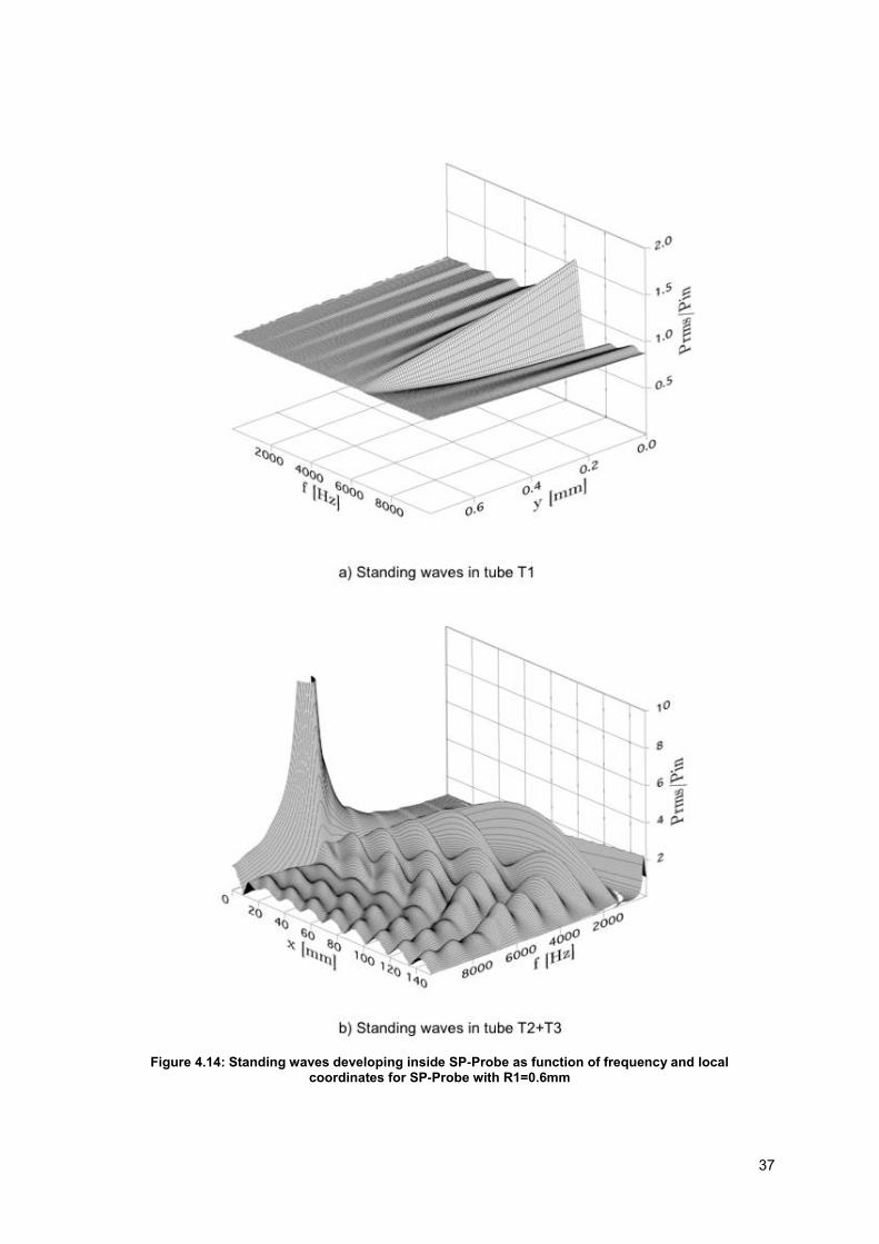
37
Figure 4.14: Standing waves developing inside SP-Probe as function of frequency and local coordinates for SP-Probe with R1=0.6mm

38
a) Pressure – f = 170Hz b) Phase – f = 170Hz
a) Pressure – f = 500Hz b) Phase – f = 500Hz
Figure 4.15: Selected standing waves in SP-Probe at several frequencies

39
a) Pressure – f = 2300Hz b) Phase – f = 2300Hz
a) Pressure – f = 6910Hz b) Phase – f = 6910Hz
Figure 4.16: Selected standing waves in
SP-Probe (R1=0.6mm) at several frequencies (cont)

40
Tubes T2 and T3 behave in a much more complex way, regarding Tube 2 one must note that,
exception made for the frequencies close to 7kHz, pressure distribution in this section is almost
constant (𝑃𝑟𝑚𝑠
𝑃𝑖𝑛≈ 1 ) for a wide range of frequencies and the phase evolution is almost zero. Since this
dynamic system is highly dissipative, as it is been mentioned on this work the pressure distribution
can’t be constant, hence with aid of the developed mathematical model was observed that the
pressure distribution has a maximum at the closed end and a slightly lower amplitude at the entrance
of the tube. It is assumed that amplitude distribution is almost constant due to small period of back and
forth waves being difficult for a wave with the correct proportion associated with an open-open or a
closed-open to appear, in other words the wavelength is large when compared with the length of the
tube. In conclusion no typical standing waves are installed. Nevertheless, as you increase frequency,
at 7000Hz a peak in amplitude stands out (see Figure 4.16 b)) it is therefore suggested that waves
travelling back and forth stayed inside the tube the right amount of time and resonance occurred.
This resonance is correlated to the fundamental frequency of a closed-open tube given by
(𝐹𝑢𝑛𝑑𝑎𝑚𝑒𝑛𝑡𝑎𝑙𝑜𝑝𝑒𝑛−𝑐𝑙𝑜𝑠𝑒𝑑 =𝑐
4∙𝐿2≅ 6752𝐻𝑧 𝑤𝑖𝑡ℎ 𝑐 =
343𝑚
𝑠𝑓𝑜𝑟 𝑇 = 293𝐾).
For frequencies between 500 ≤ 𝑓 ≤ 6500𝐻𝑧, as it is recognized by the shape of amplitude in Figure
4.14 b),T3 as a typical behaviour in this range of frequencies of a cascade of n-half waves, i.e.
harmonics of the fundamental with the dimensions of T3. It is interesting to state that a special
coupling is detected at around 6600Hz, approximately the resonance frequency of tube T2. At this
frequency tube T3 appears to be developing a 5th to 6
th harmonic of a half-standing wave (open-open)
and further analysis led to the conclusion that this coupling is correlated to the fundamental quarter-
wave developed in tube T2, i.e, the ratio between the lengths of both tubes is such that the
fundamental of T2 induce harmonics on the tube T3.
𝒇𝑶𝑪−𝑻𝟐 = 𝒇𝟓𝒕𝒉−𝑶𝑶 ⟺𝒄
𝟒. 𝑳𝟐=
𝟓
𝟐𝑳𝟑𝒄 ⟺
𝑳𝟑
𝑳𝟐= 𝟏𝟎
(45)
Figure 4.15 and Figure 4.16 shows amplitude pressure ratio and phase of all sections for a specific set
of frequencies. The selected frequencies are 170Hz, 500Hz, 2300Hz and 6590 Hz. They represent 3
peaks (170Hz, 2300Hz, and 6590Hz) and one valley (500Hz) of ATF represented in Figure 4.13 a).
Regarding 170Hz (Figure 4.15 a) b)), wave structure inside the SP-Probe is dominated by the linear
evolution of pressure along T3. Inviscid systems without any compressibility effects have similar
behaviour. It is suggested that the air present at tube T3 at this particular frequency moves as a block
and since T3 is attached to a volume and the wavelength is higher than the tube dimensions an
Helmholtz resonator behaviour is proposed, corroborated by the computation of the resonator’s
frequency, 2𝜋𝑓𝐻𝑅 = 𝑐√𝑆/(𝐿3 ∙ 𝑉) where 𝑉 is the resonator volume composed by cavity volume plus
residual volume between transducer diaphragm and protection grid and 𝑆 is the cross-sectional are of
T3, being very close to the studied frequency. Deviation from the theoretical value is mainly due to

41
dissipative effects, which also prevents the phase distribution to be zero. Instead phase evolves from
zero to −𝜋
2 suggesting that a flux of acoustic energy is travelling towards the microphone.
At 500Hz a valley appears and the wave structures almost match a quarter wave for the total length of
T2+T3, corroborated by the phase evolution, it must be addressed that at this frequency a transition
between typical standing waves occur. (half or quarter waves).
At 2300Hz Figure (4.16 a) b)) the theoretical data indicate that T3 has a second harmonic of a half
wave (a complete wave) being developed.
At last at 6590Hz an abrupt decrease in amplitude occurs; this frequency matches the resonance at
tube T2, coupled with the T3 5th-to-6
th harmonic as already mentioned. As displayed in Figure 4.16 the
amplitude of pressure distribution between both tubes is totally unbalanced, where most of acoustic
energy is drained at T2 and a small amount is transported towards the microphone.
In general, peak frequencies in the acoustic transfer function are clearly associated with the waves
installed at T3, exception made for 7kHz when T2 is under resonance, in this particular frequency T2
is somehow acting like a band-stop filter, highly attenuating that specific frequency.
It is relevant to point out that T1 position is highly relevant for T2 length and T1 radius has also an
important role on amplitude, see Figure 4.13, while decreasing the radius of T1 the first peak is clearly
attenuated.
4.3.4 Non-Viscous Model
In this section it is introduced a non-viscous approach useful to evaluate the importance of including
the viscous-thermal damping. The non-viscous modelling (referred as Non-Viscous model) follows
exactly the same procedure as defined in Chapter 2, with the same boundary conditions but obviously
with different conditions: the most clear one is to not define the propagation constant, eliminating the
contribution of an acoustic boundary layer and therefore neglecting the presence of viscous effects,
hence the pressure distribution and velocity field will be strictly function of the wave number, 𝑘, and the
axial coordinate, 𝑥, as seen in [35]. 𝐴 and 𝐵 are constants that are related with the boundary
conditions.
𝒑 = 𝑨𝒆−𝒊𝒌𝒙+𝝎𝒕 + 𝑩𝒆𝒊𝒌𝒙+𝝎𝒕 (46)
𝒖 =
𝑨
𝝆𝒄𝒆𝒊(𝝎𝒕−𝒌𝒙) −
𝑩
𝝆𝒄𝒆𝒊(𝝎𝒕+𝒌𝒙) (47)
When neglecting thermal viscous effects the exponent of polytropic expansion 𝑝𝑣𝑛 = 𝑐𝑜𝑛𝑠𝑡 is a real
number and takes the value associated with an adiabatic and reversible evolution 𝑛 = 𝛾 = 1.4. This is
equivalent to use the complex exponent n defined in Tijdeman with 𝑠 (shear wave number) going to
infinity, i.e. lim𝑠→∞ 𝑛 = 𝛾, as stated by the Figure 4.17.

42
Aided by this two powerful tools, theoretical data including viscous effects and without viscous effects
a comparison was made, only for the tube T2+T3, illustrated by Figure 4.18.
An important detail standing out automatically is that the prevailing standing waves are half-wave
types developed in T3, and at a frequency of 6340Hz a quarter wave type appears. This procedure
allows for a clear identification the peaks recognized in ATF’s, hence the first peak at 170Hz is
associated with a Helmholtz frequency of T3 and microphone housing, and all the subsequent peaks
are correlated with the half-waves present in T3.
Anti-resonance frequency noticed in the non-viscous model, at 7150Hz, is replaced in the viscous
model by a valley at 6590Hz, similar to a band-stop filter. Viscous damping is essential to this
particular behaviour.
This approach is repeated but for an entrance hole radius of 0.06 mm, Figure 4.20, standing wave
patterns differ from a radius of 0.6 in a way that in general the viscous model for R1=0.06mm detects
quarter-wave on T2+T3 and the non-viscous identifies half-wave patterns in a wide range of
frequencies.
Special attention is needed for the attenuation on the first peak around 170Hz; these types of changes
on ATF associated with the radius are directly connected with different development in wave structures
at each tube.
Figure 4.17: "Polytropic constant", 𝒏, as
function of 𝝈𝒔 as mentioned in [26]

43
Figure 4.18: Comparison between the response of SP-Probe with and without viscous effects. a) Standing waves in SP-Probe as function of frequency for the Non-viscous model, b) Acoustic transfer
function with and without viscous effects (R1=0.6mm)

44
Figure 4.19: Standing waves in SP-Probe with R1=0.06mm present in tubes T2+T3

45
Figure 4.20: Comparison between the response of SP-Probe with and without viscous effects. a) Standing waves in SP-Probe for the Non-viscous model. b) Acoustic transfer function obtained with and without
viscous effects (R1=0.06mm)

46
4.3.5 Acoustic Energy Balance in SP-Probe
An acoustic energy balance is employed to analyse the T-Junction branch of the probe, ultimately
enhancing some features regarding the band stop filter behaviour, associated with resonance at T2 for
≈ 7000 Hz, and the role of changing the entrance radius in the standing wave patterns. The control
volume is defined in Figure 4.21, note that positive values of acoustic intensity means that the flux is
entering, while negative values are associated with fluxes going outside the control volume. For a
detailed analysis regarding acoustic sound intensity consult Appendix C.
In Figure 4.22 it is shown the temporal evolution of acoustic intensity, (𝑝′𝑢′)1, (𝑝′𝑢′)2, (𝑝′𝑢′)3, for two
specific frequencies (200Hz and 6810Hz). Pressure distribution is a function of 𝑠 that is dependent of
the radius and 𝜉 (dimensionless coordinate) that is dependent of 𝑥. The shape of velocity profile has a
great impact on sound intensity since for higher frequencies the wall effects have lower influence, i.e.,
viscous effects decrease relatively to the inertial ones, hence for 200 Hz, 𝑠 = 4.5, is consistent with a
well know flow, the Poiseulle flow and for 6810 Hz the velocity profile behaves more uniform and flat
with small peaks near the walls.
For both frequencies the amount of instantaneous acoustic energy that enters T-Junction carried by
T1, is always much higher than the part leaving for T2 and T3 which is consistent with a dissipative
system. The acoustic boundary layer has a tremendous effect as it is the mechanism allowing this
event to happen, in conclusion some of the energy coming from the source (T1) goes directly to feed
the boundary layer, and the remaining energy is available to be conducted to T2 and T3.
Regarding 200Hz it is interesting to address that although T1 radius and T3 radius are quite different
the acoustic flux entering T-Junction is almost in phase with the outgoing flux to T3, and a small
amount is directed to T2 (almost neglected), leading to the assumption that for this frequency T2 is a
passive element.
However, for 6810 Hz when T2 is under resonance the acoustic energy flowing from T1 to T-Junction
goes directly to feed the resonance, leaving less energy to travel to T3.
At this stage we have conditions to consider the acoustic intensity over one cycle of oscillation and
over the cross section of T1, T2, and T3 according to Equation perform an acoustic energy balance
over the volume and compare net energy entering or leaving the T-Junction.
⟨𝒑′𝒖′⟩𝒊 = 𝟐𝝅 ∫ ∫ (𝒑′𝒖′)𝒊 𝒅𝒓𝒅𝒕
𝑹𝒊
𝒐
𝑻𝒄𝒚𝒄𝒍𝒆
𝟎
(48)
It is pertinent to address the fact that while ⟨𝑝′𝑢′⟩1 is always positive, ⟨𝑝′𝑢′⟩2 and ⟨𝑝′𝑢′⟩3 are always
negative. Energy entering T-junction and leaving T-junction, respectively.
Figure 4.21: T-Junction control surface for acoustic intensity computation

47
Figure 4.22: Evolution in time of instantaneous acoustic energy in T-Junction for 200Hz and 6810 Hz.

48
Analysing Figure 4.23 some interesting features stand out: 1) until the band-stop frequency of 7kHz,
all the acoustic energy flows to T3. This particularity is due resonance of tube T2 draining
approximately 90% of incoming energy. Since T3 is the transmission line between the entrance and
the microphone and less than 10% of input energy is travelling at this section, the ATF has an abrupt
decrease in amplitude. One striking characteristic that leads to the conclusion that at this frequency a
band-stop filter response occurs due to T2 is that the curve itself resembles the well-known response
of a band-stop filter. While energy is entering the T-Junction and travels to T2 a fundamental of a
quarter wave is developed and the energy is used to feed the fundamental, however a small amount
goes to T3 where a 5th
-to-6th harmonic of a half-wave coexists.
Once the radius decrease for 𝑅 = 0.06𝑚𝑚 an identical response is observed (data not shown), in this
case the pressure amplitude is lower when compared with 𝑅 = 0.6 𝑚𝑚, only because the amount of
energy coming from the source is 20 times lower.
The T-junction has a very important role on the development of standing waves due the fact that when
half-waves are present at T3 is consistent with the idea that T-junction behaves like an open end, on
the other hand when quarter waves tend to appear, the structure acts like a whole and T2 and T3 are
coupled acting like a closed-open tube. Regarding mathematical modelling the T-junction is a link
element between tubes and since the volume is very small it is assumed that the pressure is equal on
each section, nevertheless as already mentioned on Chapter 2, the model assumes that a rate of
accumulation might exist, see Figure 4.24.
Concerning the non-viscous model the mass rate accumulation has different order of magnitudes
depending on the radius but in general evolves almost linearly with the frequency (exception made
when resonance is present). The phase delay has a constant value of 𝜋
2 and is independent of the
radius.
As addressed before between probes with 𝑅1 = 0.6 𝑚𝑚 and 𝑅1 = 0.06 𝑚𝑚 some differences emerge,
and the rate of accumulation shows once more that pattern. For 𝑅1 = 0.6 𝑚𝑚, the rate of mass
accumulation shows a monotonic evolution with frequency and the phase delay value is constant with
the value of 𝜋/2; furthermore for 𝑅1 = 0.06 𝑚𝑚, |𝑑𝑚
𝑑𝑡| floats around 10−13. This behaviour is consistent
with a spring; reacting differently depending on how much mass can be contained and consequently
regulated by R1. Observing Figure 4.23 two cases arise: a) when phase delay is 𝜋
2 and b) phase delay
being ≅𝜋
3. For case a) T-junction seems to work as a motor to induce an acoustic open-end behaviour
in T2+T3 and is not observed any resistance to acoustic flow (phase delay is constant and equal to 𝜋
2,
a typical value of inviscid theory). For case b) is assumed that when phase delay relative to input
pressure is oscillating around 𝜋
3 the T-junction appears to be working as a communication vessel
between both tubes generating a coupling device that drives T2 and T3 to act like a closed-open tube.
The approach adopted here is just a simple way to address how changing R1 can activate such
different wave structures. It is important to mention that T-Junction was not modelled as a real
acoustic jet with a tri-dimensional and temporal complex evolution and any further analysis is out of
the scope of this thesis.

49
Figure 4.23: Non-dimension acoustic energy balance in T-junction based on time integration of instantaneous acoustic intensity
Figure 4.24: Mass rate accumulation evolution in T-junction between probes with R1=0.06mm and R1=0.6mm, with and without viscous effects.

50
4.3.6 Parametric Analysis of SP-Probe
Throughout the present analysis some evidence stand out concerning the dynamics of SP-Probe,
mainly the fact that ATF has apparently 3 major set of frequencies that govern the amplitude and
phase response:
- a low frequency peak with an high amplitude, related to Helmholtz resonator natural
frequency.
- A set of mid-frequencies associated with half and quarter wave standing waves developed in
tube T3 and T3+T2
- Band stop frequency that is controlled by resonance occurring in T2 as a quarter wave.
[25], stated that this first frequency on a SP-Probe similar to the one addressed in the present work
was directly connected to Helmholtz frequency. Aiming to achieve the same conclusion a new
correlation to predict the frequency and the correspondent amplitude was derived.
Performing several computations of acoustic transfer functions aided by mathematical model a series
of virtual SP-Probes were “manufactured”. The objective was to collect only the first peak amplitude
and respective frequency. After collecting data, the first peak is compared to Helmholtz resonator
frequency, 2𝜋𝑓𝐻𝑅 = 𝑐√𝑆/(𝐿3 ∙ 𝑉), where 𝑉 stands for the resonator volume composed by cavity volume
plus residual volume between the diaphragm of the transducer and the protection grid, while 𝑆 is the
cross sectional are (𝑆 = 𝜋 ∙ 𝑅32).
Figure 4.25: Schematic description of parametric analysis for a set of pre-defined probe dimensions a) frequency and amplitude for the first
peak frequency are identified. b) Amplitude value is plotted against the first peak frequency c) first peak freq plotted against HR frequency

51
- Analysis of first peak resonance
The evolution of first peak frequency versus Helmholtz frequency is quasi linear, a dispersion is
observed which can be claimed due to viscous-thermal effects and T-Junction non-linear response. In
order to account the effects mentioned before, it is suggested that the first peak frequency should be
correlated not only by the Helmholtz frequency but other geometrical parameters, such as L1, R1 and
L2. Using a non-linear modelling fit as described by:
𝒇𝟏𝒔𝒕𝑷𝒆𝒂𝒌 = 𝒂 ∙ (𝑳𝟏)𝜶 ∙ (𝑳𝟐)𝜷 ∙ (𝑹𝟏)𝜸 ∙ (𝒇𝑯𝑹)𝜽 (49)
The exponents 𝛼, 𝛽, 𝛾, 𝜃 are rational numbers to be determined by the non-linear fit. For the range of
geometries constraints defined in Figure 4.25, the non-linear fit data gives 𝑎 = 1.00773, 𝛼 =
−0.557, 𝛽 = 0.0026, 𝛾 = 0.496 and 𝜃 = 0.917 with a 𝑅2 = 0.9957. Figure 4.26 shows that curve fitting
collapsed all data points up to 𝑓𝐻𝑅0.917 = 1700. Since 𝛽 is too small one may assume that L2 has
negligible influence on the first peak, hence for a qualitative analysis and after some algebraic
operations it is proposed that the first peak frequency is almost proportional to the Helmholtz resonator
frequency with a dimensional correction,
𝒇𝟏𝒔𝒕𝑷𝒆𝒂𝒌 ∝ (𝒇𝑯𝑹) ∙ √𝑹𝟏
𝑳𝟏
(50)
As proved by the previous analysis the premise introduced by [25], in fact needs a correction factor
that takes into account geometric features.
Figure 4.26: Non-dimensional analysis using curve fitting

52
- Amplitude of first peak
On the scope of amplitude same procedure described above was performed, therefore collected data
between the amplitude of first peak and the related first peak is needed, hence using once more a non
linear model the relevancy of including other geometrical parameter is tested and presented in Figure
4.27.
Equation 51 states the computed relation between 𝐴𝑟 and the first peak.
𝑨𝒓 =
𝟎. 𝟎𝟎𝟎𝟎𝟑𝟓𝟑 ∙ 𝒇𝟏𝒔𝒕𝑷𝒆𝒂𝒌𝟏.𝟓𝟎𝟓 ∙ 𝑳𝟑𝟎.𝟓𝟒𝟖𝑹𝟏𝟏.𝟒𝟎𝟖
𝑳𝟏𝟏.𝟕𝟖𝟓𝑳𝟐𝟎.𝟎𝟏𝟓𝟗𝑹𝟐𝟎.𝟑
(51)
with 𝑅2 = 0.9912 as the global correlation coefficient.
The agreement of the curve fitting is reasonable and denotes a strictly linear relationship for
frequencies below 800Hz, yet for 800𝐻𝑧 ≤ 𝑓1𝑠𝑡𝑃𝑒𝑎𝑘1.505 ≤ 1000𝐻𝑧 the relative error between the data
and curve fitting is less than 10%. Besides the mentioned limitations is worth mentioning the collapse
of all the data in a single linear function allowing a clear qualitative analysis to be employed. For the
latter and using the relation expressed by equation 49, after some algebra and approximations a
proportionality law is deduced:
𝑨𝒓 ∝ (𝒇𝑯𝑹)𝟏.𝟓 ∙ (𝑹𝟏
𝑳𝟏)
𝟐
∙ √𝑳𝟑
𝑳𝟏∙ √
𝑹𝟏
𝑹𝟐
𝟒
(52)
Both equations 50 and 52 grant a new type of approach while designing this type of probes – a pre-
design capability.
Figure 4.27: Non-dimensional analysis of first peak amplitude

53
4.4 Development of a Stethoscope probe
At this stage a new probe system is evaluated. The suggested design displayed in Figure 4.28, and
the implemented sensors were supported by the opportunity to acquire an acoustical signature of an
aircraft combustion chamber with only air being injected, in order to detect the deviations in the
pressure field induced by the injectors misalignment. For that purpose a microphone is attached at
one end to measure pressure fluctuations and SDP-1000-L is attached at the other end to acquire
mean total/static pressure data. Hence, important information about pressure field can be collected.
Theoretical data regarding this probe was already scrutinized in chapter 2.
As mentioned for this particular design a new sensor (SDP-1000-L) is part of the main structure, and
unfortunately the manufacturer gives no relevant acoustic information, therefore the calibration
procedure followed a specific path in order to assess how the probe response is affected by its
presence.
Hence, in a first stage the tube that connects the sensor to the T-Junction system is blocked to
simulate the boundary condition of velocity at L=L2 equal to zero (see chapter 2 – i.e. L=L5=0
meaning that the tube doesn’t exist and the boundary condition is now at L=L2), an experimental ATF
data is collected and compared with theoretical data. The second stage is characterized by including
the sensor. This stage gains relevance due to the fact of focusing the problem towards the sensor,
leading to understanding its behaviour and ultimately fixing the mathematical model to respond
correctly to this type of structure. Both ATF are organized in Figure 4.29 and 4.30.
Figure 4.28: a) 3D model of Stethoscope probe, b) real model of Stethoscope probe
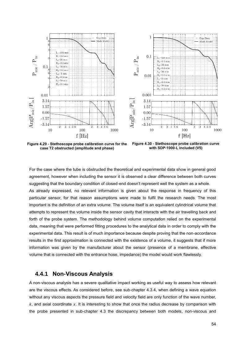
54
For the case where the tube is obstructed the theoretical and experimental data show in general good
agreement, however when including the sensor it is observed a clear difference between both curves
suggesting that the boundary condition of closed-end doesn’t represent well the system as a whole.
As already expressed, no relevant information is given about the response in frequency of this
particular sensor, for that reason assumptions were made to fulfil the research needs. The most
important is the definition of an extra volume. The volume itself is an equivalent cylindrical volume that
attempts to represent the volume inside the sensor cavity that interacts with the air travelling back and
forth of the probe system. The methodology behind volume computation relied on the experimental
data, meaning that were performed fitting procedures to the analytical data in order to comply with the
experimental data. This result is of much importance because despite proving that the non-accordance
results in the first approximation is connected with the existence of a volume, it suggests that if more
information was given by the manufacturer about the sensor (presence of a membrane, effective
volume that is connected with the entrance hose, impedance) the model would work flawlessly.
4.4.1 Non-Viscous Analysis
A non-viscous analysis has a severe qualitative impact working as useful way to assess how relevant
are the viscous effects. As considered before, see sub-chapter 4.3.4, when defining a wave equation
without any viscous aspects the pressure field and velocity field are only function of the wave number,
𝑘, and axial coordinate 𝑥. It is interesting to show that once the radius decrease by comparison with
the probe presented in sub-chapter 4.3 the discrepancy between both models, non-viscous and
Figure 4.29 - Stethoscope probe calibration curve for the case T2 obstructed (amplitude and phase)
Figure 4.30 - Stethoscope probe calibration curve with SDP-1000-L included (V5)

55
viscous, is even higher as the viscous-effects tend to increase their role – the boundary layer
developed inside the tube is in the order of magnitude of the radius.
For the ranges of shear wave number, s, present in this design the validity of the viscous model is
verified, stating once more the importance of considering viscous effects and the wide applicability of
the theoretical approach.
4.4.2 Boundary conditions of Stethoscope Probe
As mentioned before the addition of an extra volume, representing the presence of a sensor at section
5, to the model discussed on chapter 2 turns the 4 Tubes – 1 Volume in 3 Tubes – 2 volumes. In fact,
at section 5 where once were written the equations of a wave propagating in a cylindrical narrow tube
is now defined a volume.
Computed boundary conditions are displayed on the table:
Figure 4.31: Comparison between Stethoscope probe response-sensor included with and without viscous effects
Figure 4.32: Probe general schematics and procedure to adapt 4T-1V to 3T-2V

56
T1 T2 T3 V4 V5
Inlet 𝑝01 =𝜌𝑠∙𝑐2
𝛾(𝐴1 + 𝐵1)
𝑝02 = 𝑝03
𝑝03 = 𝑝𝐿1
𝑝𝐿3 = 𝑝𝑉4
𝑝𝑉5 = 𝑝𝐿2
Outlet 𝑝𝐿1 = 𝑝02 = 𝑝03 �̇�𝐿3 =
𝜕𝑚𝑣4
𝜕𝑡 �̇�𝐿2 =
𝜕𝑚𝑣5
𝜕𝑡
Table 4.3: Boundary conditions considered for mathematical modelling
The additional volume is defined as V5, all the mathematical considerations are the same of V4,
defined by equation 38, however 𝑉0 is changed to V5 and 𝑝 to 𝑝𝑣5.
Once again, it is relevant to state the importance of equation 39 and adding it to the equation system
is imperative.
4.4.3 Stethoscope probe sensitivity
Probe sensitivity was mentioned for the first time in sub-chapter 4.3.2. The same procedure was
implemented with the new design and important conclusions were derived, however in this case two
distinct fields of analysis were employed: a) Calibration tube open to environment b) Calibration tube
closed to environment.
Case a) is to resemble a working, therefore noisy, environment and focus how is T1 role in the
readings, i.e. if all the sound is coming directly from the tip or if the microphone can be contaminated
by the surroundings.
Case b) is to resemble a more protected probe with an adaptive casing for the T-Junction structure
and microphone housing leading to a working environment of several less dB than case a).
Experimental data for case b) illustrated by Figure 4.33 has three different spectra for three
frequencies and electronic noise obtained with the microphone connected offline to the acquisition
board. It is observed that for an environment of 88 dB the probe has problems distinguishing the
sound coming from the tip comparatively with sound coming from the surroundings, measured
sensitivity was approximately 0 dB. For the case b) the environment was at 77 dB and is clearer the
T1 role in the readings. The measured sensitivity was approximately 36.9 dB, Figure 4.34.
The electronic noise is of much importance because of the “cut-off frequency” however the
frequencies don’t harm the readings, since any amplitude above 72 dB (measure in the 50Hz –
network frequency) won’t be embedded in the electronic noise.
It is therefore suggested manufacturing a special casing system isolating the main structure to avoid
misleading results if the environment noise is above 77 dB.
Figure 4.33 :Stethoscope probe Sound field spectra for three different frequencies plotted against electronic noise

57
4.4.4 Stethoscope standing waves
Standing waves wise in this configuration it is observed by inspection of pressure distribution that T1
acts like an open-open tube developing throughout the length half waves and the respective n-
multiples, with n being an odd number (1,2,3). On one end T1 is connected to the atmosphere where
the sound source enters and the other end is connected to a T-junction acting like a communication
vessel where the imposed pressure is defined by T1 at x=L1 (boundary condition) confirmed by
checking the plots of T2 and T3 at x=0.
With the dimensions of T1, L1=534mm the fundamental half-wave should appear at 321Hz, however it
is stated here that because of assuming a constant sound velocity propagation (plane wave
approximation) and therefore neglecting viscous effects that actually due to the development of
boundary layer (more intense at low frequencies where inertial forces are less intense in comparison
with the viscous forces and the velocity profile approximates to Poiseulle flow) the sound velocity is
smaller than the classical value of 343 m/s (Air temperature of 20ºC) causing a shift to the left at
approximately 200Hz.
It is suggested that the same occurs with the second harmonic is present at ~ 400Hz. Concerning the
third harmonic an odd effect takes place because it seems that is non-existent and the idea behind it is
that for some reason the fact that the definition of an imposed boundary condition at T-Junction
combined with high dissipative effects tends to act as restrictive phenomena, reinforced by the
appearance of an approximate fourth harmonic at 1000Hz.
It is interesting to examine the increase in amplitude at 600Hz for T2, while the wave travels to x=L2,
and the opposite behaviour regarding T3 until the cavity where the microphone is housed suggesting
that the presence of the sensor at this frequency drains the energy coming from T1.
Figure 4.34: Stethoscope probe sensitivity when calibration tube was closed

58
Figure 4.35: Stethoscope probe standing waves in T1, T2 and T3

59
4.5 Collecting data with Stethoscope probe
In this sub-chapter the main objective is to perform a viable first stage proof of concept to recognize
the potential of this tool and the ability to distinguish shifts in the flow characteristics. As mentioned
before the suggested design emerged to respond effectively to the idea of collecting an optimal
acoustical signature of a combustion chamber composed by flame stabilizers and injectors. The
modular approach employed on the majority of aircrafts engines and the trial and error alignment
method, as described in chapter 2, implanted the possibility of overcoming this issue of various trips
between the test-bench and maintenance sector in a pre-test bench stage with only air being injected.
Experimental rig as it is described in section 4.5.1 attempts to be as analogous as possible to a
common flame stabilizer (swirler) and injector assembly, where the flame stabilizer is analogous to a
burner with only air at the exit and a tube with R = 21mm is at the top representing the position of the
injector inside the combustion chamber.
Regarding experimental procedure one must address the fact that four holes in a tube will be directly
connected to four different set of measurements, at each hole five different angles were analysed at
two different situations – clockwise and counter-clockwise, therefore for each tube 9 measurements
were analysed in a total of 36. Different angles will represent a change in the injector alignment
position in respect to the main axis of the swirler.
Compressed air is provided through a flow meter and it is fixed at 50 l/min.
4.5.1 Experimental rig
Experimental rig elements are displayed in the following table:
Material used for experimental rig
PC
Matlab Software
USB DAQ Module DT-9841 SB
Stethoscope probe
Swirler
Tube with measuring holes
Tektronix TDS 1001C- EDU Oscilloscope
Sensirion SDP 1000-L
Sound level meter - type 2250 B&K
Microphone - type 4189 B&K
Micro. Preamplifier - model ZC 0032
Flow meter Alicat Scientific Table 4.4: List of material used for experimental case study

60
4.5.2 Data Acquisition and post-processing data
The adopted configuration allows acquisition of pressure fluctuation through the microphone and
static/total pressure through SDP-1000L sensor. Microphone signal was directly connected to the USB
DAQ Module DT-9841SB and the latter controlled by a Matlab program. The acquisition rate was
10kHz and the time file would collect 100000 points with a resolution of 0.0001seconds. Regarding
FFT spectra from the time-file it would be selected 216 points, implying that the FFT resolution would
be fixed at 0.153Hz.
SDP-1000L sensor was connected to the oscilloscope second channel and the mean pressure was
measured in voltage directly from the screen.
At this stage probe acoustic transfer function (ATF) more specifically the amplitude in function of
frequency contribution has an important role because the measurements don’t represent the real
pressure fluctuations due to the contribution of the probe. Post-processing acquired data was
imperative and consists simply in dividing the data already collected by the amplitude of the probe at
each specific frequency.
Figure 4.36: Experimental case study apparatus

61
4.5.3 Results
One must note that experimental results attempt to work as an example on how reasonable the probe
will work in a real flow environment, hence is important to mention that despite some similarity degree
between experimental conditions and real conditions, the airflow present in a real combustion
chamber is several orders of magnitude higher, and therefore would be expected higher amplitude
pressure fluctuations where a small diameter probe is needed. For that reason, it is conclusive by
examining experimental data that if in a flow where the pressure fluctuations are significantly smaller
the probe detects substantial differences it would be expected an adequate response in real
environment.
In the following pages are displayed collected results where zero degrees condition illustrates the
“reference case” and then measurements for 4 different angles, 5º, 10º, 15º, 20º are plotted against
the reference for two different cases: clockwise and counter-clockwise. Mean pressure, total or static,
information is also displayed with the same procedure.
Details concerning flow characteristics and pressure fluctuation differences are out of the scope of this
thesis.
Figure 4.37: Tube + swirler and stethoscope probe attached

62
Figure 4.38: a1) Experimental apparatus a2) tube schematics identifying measurement points b) measured signal FFT for Pos1, c) measured signal FFT for Pos2, d) measured signal FFT for Pos3, e)
measured signal FFT for Pos4

63
Figure 4.39: Measured signal FFT for 4 different angles plotted against a reference FFT (0º) for 4 positions-clockwise configuration
Figure 4.40:Measured signal FFT for 4 different angles plotted against a reference FFT (0º) for 4 positions-counterclockwise configuration

64
Figure 4.41: Mean pressure collected data with SDP-1000-L
The plot represented above refers to mean pressure evolution in function of probe’s position. The blue
line represents counterclockwise case, the red line the clockwise case, the black line is the reference
case defined by 0 degrees condition. In yellow is illustrated the value read in the oscilloscope for
atmospheric pressure.
The sensor works as a mean static pressure or total pressure depending on the orientation relative to
the flow; hence if the flow is perpendicular to the hose, no dynamic pressure contribution is accounted
for. On the opposite, if the flow is parallel to the incoming flow, the sensor is reading total pressure.
Regarding pressure distribution one must enhance some features: at point 2-5º degrees
counterclockwise a maximum pressure fluctuations amplitude in respect to the reference is noted,
however the sensor in this position starts to act like a total pressure sensor, and since dynamic
pressure is increasing due to an hypothetic switch in the stagnation point, therefore an increase in
pressure is noticed.
A similar analysis can be done to other points of interest; however details in the flow characteristics
are out of the scope of this thesis.

65
5 Conclusion
5.1 Concluding remarks
In this thesis the main objective was to develop a pack of pressure probes to be integrated in the
maintenance sector of a commercial aircraft company: a static pressure probe only able to measure
pressure fluctuations and a second one with a more complex design that acquire simultaneously mean
total pressure and pressure fluctuations.
The path to achieve the desired plan started with the design of a mathematical model, based on the
low reduced frequency model, that would work mainly as a modular system, i.e., developed
conceptually as a 4Tubes-1Volume assembly but that could adequately function with much simpler
designs, assuming that the boundary conditions were the same.
To determine the model robustness and versatility a first trial with two much simpler designs was
computed and the model response was conclusive. A good agreement between experimental data and
theoretical data was accomplished and therefore the mathematical model proved to be a powerful tool
for the calibration of 1tube-1volume probes. While calibrating probes with this specific configuration,
1T-1V, was stated that the acoustic response is in some extent related to a classical Helmholtz
resonator.
With respect to the development of a typical static-pressure probe commonly used to analyse
pressure fluctuations in turbulent flows a set of important conclusions were derived:
- An acoustic response was computed for several geometries and the mathematical model
shown very good agreement with the experimental data.
- Through a mathematical non-viscous analysis the importance of viscous-thermal dissipation
while working with such small tubes (in order of 1mm) was assessed, and the results showed
to be conclusive. While decreasing the radius of the probe the viscous effect are
preponderant.
- This study identified three sets of frequencies that control the acoustic transfer function: a) a
low frequency peak associated with a Helmholtz resonance frequency with a correction that
takes into account geometric parameters. b) a set of mid-frequencies associated with the
development of a open-open and open-closed typical standing waves. c) a band-stop
frequency which is controlled by resonance of one of the tubes as a fundamental quarter wave
draining almost 95% of incoming acoustic energy.
In regard to the new suggested design, Stethoscope Probe, with a microphone in one end and a
pressure sensor on the other some important considerations must stand out:
- The mathematical model defined as the starting point was only validated correctly when the
tube where the sensor would be attached was blocked. Including a volume to the
mathematical model representing the sensor presence lead to a good agreement between the
experimental data and theoretical.

66
- Standing wave analysis in propagating tubes stated that the main tube worked as a open-
open tube, however the non-linearity induced by the T-Junction volume caused the non-
development of a third harmonic.
- A non-viscous analysis proved to be important since the design being much narrow than the
SP-Probe imply an increase in the effects of viscous-thermal damping.
- The implemented case study, analogous to the real behavior inside a combustion chamber,
stated the applicability of the probe on assessing deviations in flow characteristics.
Overall, the mathematical model proved to be a useful tool in predicting acoustic response with
various geometries, and with simpler designs.
The suggested pack of pressure probes proved to be adequate in a working environment, where the
SP-Probe would be valuable to assess pressure fluctuations at the outlet and the Stethoscope Probe
approach aimed to evaluate the performance inside the combustion chamber due to injectors
misalignment.
It is relevant to address that it would be far easier if acoustic response of the sensor was available,
more specifically the ratio between the pressure and the velocity (impedance) in function of frequency
that would work as a more accurate boundary condition.

67
5.2 Future work
This work allowed a better understanding on how to develop two types of probes, one able to measure
only pressure fluctuations and a second one with a more complex design that acquire simultaneously
mean pressure and pressure fluctuations. Regarding pressure probe design in general a few
improvements could be made to overcome the trial and error procedures associated with the
mathematical model, more specifically designing a program that runs the mathematical model as a
root but enables an optimization feature in a way that the user dictates a criterion in amplitude or even
specifies a range of frequencies where the amplitude must be at a precise value and the program, as
an output, delivers the dimensions that comply with the user needs with a certain confidence interval.
Another detail that urges to be addressed and improved is the microphone casing. The production
method used nowadays implies that for the same design a probability of a certain amount of leakage
in the microphone volume might occur and as enhanced by this work the volume of the cavity has
significant impact in the probe’s response, therefore it would be necessary to develop a method that
reduces leakage to a value near zero and exhibits the same residual volume at the top of the casing.
The main objective while designing stethoscope configuration probe was the potential in being used
by the technicians in a working environment as a evaluating tool assessing how misaligned were the
fuel nozzle in respect to the primary air nozzle, in consequence the next logical phase was to test in
real conditions and determine the degree of applicability with this type of configuration. Once the final
design is achieved an optimal acoustical signature (fuel nozzle aligned with the primary air nozzle)
needs to be measured and stored in a server for statistical purposes. As a preliminary testing device,
in order to be a working viable device it would be necessary to manufacture a casing that would
connect to combustion chamber module (easy coupling and easy de-coupling device) and also fed it
with pressurized air.
A real time streaming data embedded system would be appropriate to go along with the probe, the
idea behind this real time processing consists in giving guidance in the pre-alignment process and
also to work as a storage unit where information regarding hours of flight, time since the last visit to
the maintenance facilities, and where the most misaligned injectors are positioned would be collected.
All this collected data would work as a starting point to show some relations between the suggested
variables and the misalignment, ultimately leading as a predictive system – showing the probability of
occurrence through time and act like a warning mechanism.

68
6 References
[1] L.P Franzoni, C.M Elliot. (1998). An innovative design of a probe-tube attachment for a 1/2 in.
microphone. J. Acoustical Society of America (104), 2903-2910.
[2] A.B Copeland, D. Hill. (1910). Design of a probe-tube adapter for use with a 1-in condenser
microphone. J. Acoustical Society of America (48), 1036-1039.
[3] H. Bergh, H.Tijdeman. (1965). Theoretical and experimental results for the dynamic response of
pressure measuring systems. Rep. NLR-TR F.238, National Aero and Aeronautical Research Institute.
[4] P. Gerstoft, S.O Hansen. (1985). A new tubing system for the measurement of fluctuating
pressures. J. of Wing Engineerings and Industrial Aerodynamics (25), 335-354.
[5] J.D Holmes, R.E Lewis. (1987). Optimization of dynamics-pressure measurement system I.single
point measurements. J. of Wind Engineering and Industrial Aerodynamics (25), 249-273.
[6] M.F Lee. (1993). Dynamic response of pressure measuring systems. Research Paper - AD-A267
169, Defence Science and Technology Organization- Aeronautical Research Laboratory, Department
of Defence.
[7] R. E De Haan. Design of a probe microphone. Applied Sciences Res (22), 306-316.
[8] E. Villchur, M.C. Killion. (1975). Probe-tube microphone assembly. J. Acoustical Society of America
(57), 238-24'.
[9] M. R. Forrest. Protecting hearing in a military environment. Scand. Audiol. Sppl. (12), 186-193.
[10] M.R. Stinson. (1985). The spatial distribution of sound within scaled replicas of the human ear
canal. J. Acoustical Society of America (78), 1596-1602.
[11] J.A. Feigin, J.G. Kopun, P.G. Stelmachowicz, M.P. Gorga. (1989). Probe-tube microphone
measures of ear canal sound pressure levels in infants and children. Ear and Hearing (10), 254-258.
[12] P.A. Hellstrom, A. Axelsson. (1993). Miniature microphone tube measurements in the external
auditory canal. J. Acoustical Society of America (93), 907-919.
[13] O. Lauridson, C. Gunthersen. (1981). New probe microphone for investigating the acoustics of the
ear. J. Acoustical Society of America (69), 1496-1498.
[14] C. Bertrand. (1983). A microphone probe for noise measurements inside furnaces. J. Phys. E: Sci
Instrum (16).
[15] J. P. Barton, J.K. Koester, M. Mitchner. (1977). Probe-tube microphone for pressure fluctuation
measurements in harsh environments. J. Acoustical Society of Amercai (62), 1312-1314.
[16] W. Neise. (1975). The change of microphone sensitivity under mean flow conditions. J. of Sound
and Vibration (43), 53-605.

69
[17] K. Toyoda, T.Okamoto, Y. Shirahama. (1994). Eduction of vortical structures by pressure
measurements in noncircuar jets. Applied Scientific Research (53), 237-248.
[18] Y. Kobashi. (1957). Measurement of pressure fluctuations in the wake of cylinder. J. Phys Society
JPN (12-5), 533-543.
[19] Y. Kobashi, N. Kono, Nishi. (1960). Improvements of a pressure pickup for the measurements of
turbulence characteristics. J. Aerospace Sci. (27), 149-155.
[20] T.W. Nyland, D.R. Englund, R.C. Anderson. (1971). On the dynamics of short pressure probes-
some design factors affecting frequency response. Research Paper - NASA.TN-D-6151, NASA
Center: Glenn Research Center.
[21] Y. Naka. (2009). Simultaneous measurement of fluctuating velocity and pressure in turbulent free
shear flows. MSc Thesis, School of Science for Open and Environmental Systems, Keio University.
[22] D.P. Egolf. (1977). Mathematical modeling of a probe-tube microphone. J. Acoustical Society of
America (61), 200-205.
[23] A.S. Iberall. (1993). Attenuation of oscillatory pressures in instrument lines. Research Paper-2115
vol. 45, US Department of Commerce National Bureau of Standards.
[24] S. Gabard and J.Peube. (1998). The influence of narrow tube on the measurements of pressure
fluctuations. Acustica - Acta Acustica (84), 1151-1160.
[25] Y. Tsuji, J.H.M. Fransson, P.H. Alfredsson, A.V.Johansson. (2007). Pressure statistics and their
scaling in high-reynolds number turbulent boundary layers. J. of Fluid Mechanics (585), 1-40.
[26] H. Tijdeman. (1975). On the propagation of sound waves in cylindrical tubes. J. of Sound and
Vibration (39), 1-33.
[27] C. Zwikker, C.Kosten. (1949). Sound Absorbing Materials. Elsevier .
[28] J. Kergomard. (1985). Comments on "Wall effects on sound propagation in tubes". J. of Sound
and Vibration (98), 149-155.
[29] W. Beltman. (1999). Viscousthermal wave propagation including acousto-elastic interaction, Part
1: Theory. J. of Sound and Vibration (227), 557-586.
[30] P.Ekkels, H.E. de Bree. (2001). Acoustic course-introducing the microflown to the acoustic world.
[31] Bruel & Kjaer. (1971). Microphone calibration for accurante sound measurements.
[32] National Instruments. (2009). The fundamentals of FFT-Based signal analysis and measurement
in LabView and LabWindows/CVI.
[33] A.K. Gupta, D.J. Lilley, N.Syred. (1984). Swirl flows. (T. Walls, Ed.) UK Abacus Press.
[34] A.R. Frey, A.B. Coppens, L.E. Kinsler, J.V. Sanders. (1982). Fundamentals of Acoustics (Third
ed.). John Wiley and Sons.

70
[35] A. Iida, T. Otaguro, O. Kato, S. Shimode. (1999). Analysis of aerodynamic sound source with
measurement of static-pressure fluctuation. Japan Society of Mechanical Engineers (Serie B), 596-
604.
[36] Bruel & Kjaer. (1986). 2231 B7 7700 Instruction Manual.
[37] F. Fahy. (2002). Sound Intensity: Second Edition. CRC Press.
[38] F. Jacobsen. (2011). Sound intensity and its measurement and applications. Note no 31262,
Denmark: Technical University of Denmark.
[39] L.M.B.C Campos. (2011). Complex functions with applications to flows and fields. CRC Press.

71
Appendix A
Mathematical constants
Constants Variable name Symbol Value
Ratio of specific heats 𝛾 1.4
Mean Pressure 𝑝𝑠 101325.0 Pa
Mean temperature 𝑇𝑠 293.15K
Thermal conductivity, air 𝜆 0.025 W/(mK)
Specific heat at constant volume 𝐶𝑣 717.645 J/kgK
Specific heat at constant pressure 𝐶𝑝 1004.7 J/kgK
Mean density 𝜌𝑠 1.204
Dynamic viscosity 𝜇 0.00001805 Kg/m.s
Speed of sound c 343.237 m/s
Prantl number 𝑃𝑟 0.725
Molar mass M 28.9645 g/mol
Square root of Prantl number 𝜎 0.8515
Specific air constant 𝑅𝑜 287.058 J/kgK
𝑪𝒗 =
𝑹𝟎
𝜸 − 𝟏 (A.1)
𝑪𝒑 = 𝜸𝑪𝒗 (A.2)
𝒄 = √𝜸𝑹𝒐𝑻𝒔
𝑴
(A.3)

72
Appendix B
Microphone type 4189B&K and type 4155B&K
Microphone type 4189B&K and 4155 are both free-field microphones, meaning that both are optimized
to have a flat response in frequency at 0 degrees incidence. Since at higher frequencies, reflections
and diffractions causes a pressure increase in front of the diaphragm a correction must exist in order
to avoid an increased output voltage, this is only achieved while using free-field microphones.
Taking into account the fact that each used microphone has different parameters and an intrinsic
electronic behaviour it is important to relate one another quantifying how devious they perceive sound
coming from the same sound source. In this appendix is stated all the procedures that allowed
computation of microphone transfer function’s.
- Microphone type 4189B&K
One must define microphone amplitude transfer function as the ratio between the output voltage and
input voltage. This ratio is affected by the gain of the microphone, defined by the user.
Figure B 1: Microphone B&K 4189 calibration apparatus

73
As illustrated in Figure B.1 when the sound source (loudspeaker) emits sound waves, the microphone
detects the wave as an incident pressure, 𝑃𝑖𝑛, converting it into an output available for the user. This is
possible due to two main parameters: microphone sensitivity (quantifies how the diaphragm
membrane reacts to incident pressure) and the internal gain. Both parameters have mathematical
background, hence:
𝒅𝑩𝑺𝑷𝑳 = 𝟐𝟎 𝒍𝒐𝒈 (
𝑷𝒊𝒏
𝑷𝟎
) , 𝑷𝟎 = 𝟐 ∙ 𝟏𝟎−𝟓 [𝑵
𝒎𝟐] (B.1)
𝑺𝒆𝒏𝒔𝒕𝒚𝒑𝒆𝟒𝟏𝟖𝟗 =
𝑽𝒊𝒏
𝑷𝒊𝒏
[𝒎𝑽
𝑷𝒂] (B.2)
𝟏𝟎𝑮𝒂𝒊𝒏 = (
𝑽𝒐𝒖𝒕
𝑽𝒊𝒏
)𝟐𝟎, 𝑮𝒂𝒊𝒏 [𝒅𝑩] (B.3)
Therefore, the ratio between the output voltages of type 4189 in function of the gain and input voltage
is:
𝑽𝒐𝒖𝒕𝑮𝟏
𝑽𝒐𝒖𝒕𝑮𝟐
=√
(𝟏𝟎𝑮𝟏
𝟏𝟎𝑮𝟐∙
𝟏
𝑽𝒊𝒏𝟐
𝑽𝒊𝒏𝟏
𝟐𝟎)𝟐𝟎
(B.4)
Figure B 2: Microphone B&K 4189 model validation

74
Data shown in Figure B 2 represents the validation of equation (B.4) with experimental data acquired
by DT-9841 SB, for two sets of gain parameter, 0 dB against 5dB and 0dB against 10dB, for 20mV,
30mV, 40mV and 50mV excitation signal amplitude. As predicted the ATF (amplitude transfer function)
is independent of the frequency and amplitude of the source signal. This ratio is useful in case during
the calibration procedure the amplitude of the measured signal is in the order of magnitude of the
electronic noise, therefore to escape this noisy area that lead to inaccurate measurements an
amplification factor might be added. One must state that this procedure allows a wide range of
acoustic transfer functions, i.e., if the interest is to compute a relation between gain factor of 5dB and
10dB, it is only required to divide the already computed information as shown in Example 1:
Example 1:
𝑨𝑻𝑭(𝟓𝒅𝑩, 𝟏𝟎𝒅𝑩) = [
𝑨𝑻𝑭(𝟎𝒅𝑩, 𝟓𝒅𝑩)
𝑨𝑻𝑭(𝟎𝒅𝑩, 𝟏𝟎𝒅𝑩)]
−𝟏
(B.5)
- Microphone type 4155B&K
The microphone type 4155B&K is connected to Sound level meter type 2230. While in the previous
one the managing parameter is the internal gain, the latter becomes more sensitive to input excitation
when changing the scale of measurement. The measuring range starts at 24 dB to 130 dB, however if
the supplied 20 dB attenuator ZF 0020 is used the range starts at 30 dB and his extended to 150dB.
In this work the measuring range is 24dB to 130dB. Since the AC output for full scale is 1V rms and
the measuring range is clearly influenced by the range defined by the scale itself the suggested
governing equation for type 4155 B&K is:
𝑽𝒐𝒖𝒕 = 𝑩
(𝑽𝒐𝒖𝒕𝑴𝒂𝒙 − 𝑽𝒐𝒖𝒕𝑴𝑰𝑵)𝑭𝒖𝒍𝒍𝑺𝒄𝒂𝒍𝒆
𝑺𝒆𝒏𝒔 × 𝑷𝒐[𝟏𝟎𝒅𝑩𝑴𝒂𝒙/𝟐𝟎 − 𝟏𝟎𝒅𝑩𝑴𝒊𝒏/𝟐𝟎][𝑺𝒆𝒏𝒔 × 𝑷𝒊𝒏
− 𝑺𝒆𝒏𝒔𝑷𝒐𝟏𝟎𝒅𝑩𝑴𝒊𝒏/𝟐𝟎]
(B.6)
After some algebra and taken into account that the maximum output voltage is 1V rms, equation B.6
becomes:
𝑽𝒐𝒖𝒕 = 𝑩 [
𝟏𝟎𝒅𝑩𝒊𝒏/𝟐𝟎 − 𝟏𝟎𝒅𝑩𝑴𝒊𝒏/𝟐𝟎
𝟏𝟎𝒅𝑩𝑴𝒂𝒙/𝟐𝟎 − 𝟏𝟎𝒅𝑩𝑴𝒊𝒏/𝟐𝟎] [𝑽 𝒓𝒎𝒔] (B.7)
where B is an experimental constant that relates the model with experimental data.

75
Figure B 4: Microphone B&K 4155 model validation
The plot illustrated in Figure B.4 shows good agreement between the real output and the model
deduced. Collected data relates to two distinct cases: full scale in which the microphone has a wider
range of measurement but becomes less sensitive, and scale of 110dB more sensitive than the
previous one.
Figure B 3: Microphone B&K 4155 calibration apparatus

76
- Combining Microphone type 4189 and 4155
In some cases might be useful combining both microphones, i.e., acquiring the probe signal with 4189
and defining the reference with 4155, or even the opposite. In that particular case one must state the
output ratio in order to apply the correction factors associated with the use of microphones with
different characteristics and parameters, hence using B.6 with B.3 one must derive:
𝑽𝒐𝒖𝒕𝑻𝒚𝒑𝒆𝟒𝟏𝟓𝟓 = 𝑩
𝑽𝒐𝒖𝒕𝑻𝒚𝒑𝒆𝟒𝟏𝟖𝟗 − 𝑷𝟎𝟏𝟎𝒅𝑩𝒎𝒊𝒏/𝟐𝟎𝑨𝑺𝒆𝒏𝒔𝒕𝒚𝒑𝒆𝟒𝟏𝟖𝟗𝟏𝟎𝑮𝒂𝒊𝒏/𝟐𝟎
𝑨𝑺𝒆𝒏𝒔𝒕𝒚𝒑𝒆𝟒𝟏𝟖𝟗𝟏𝟎𝑮𝒂𝒊𝒏/𝟐𝟎𝑷𝟎[𝟏𝟎𝒅𝑩𝒎𝒂𝒙/𝟐𝟎 − 𝟏𝟎𝒅𝑩𝒎𝒊𝒏/𝟐𝟎] (B.8)
where B and A are experimental constants. Looking closer to equation (B.8) one should acknowledge
that can be rewritten in the form of:
𝑽𝒐𝒖𝒕𝑻𝒚𝒑𝒆𝟒𝟏𝟓𝟓 = 𝑴(𝑽𝒐𝒖𝒕𝑻𝒚𝒑𝒆𝟒𝟏𝟖𝟗 − 𝑲) (B.9)
Figure B 5: Microphone B&K 4155 and 4189 calibration

77
Figure B 6: Combined microphones model validation
- Probe calibration using both microphones
In Figure B.7 it is illustrated the probe calibration using a set of two distinctive microphones. As Figure
B7 states it in general a good agreement between experimental data and theoretical data is verified.
Experimental conditions are characterized by specific working parameters for each microphone, hence
to obtain the transfer function displayed the microphone 4189 was set at 15 dB for all frequencies and
microphone 4155 settings were at full scale.
Figure B 7: Stainless steel probe calibration curve obtained with B&K 4155 as reference
and B&K4189 attached to the probe

78
Appendix C
- Sound Intensity
On Frank Fahy’s book [37] this theme is addressed extensively starting with the classical approach of
transport of sound energy. This concept is commonly known as sound intensity.
Sound intensity is a vector that describes the flow of acoustic energy in a sound field. More
specifically, sound intensity concerns the time average of the net flow of sound energy per unit area,
for that reason the units are 𝐽/(𝑠 ∙ 𝑚2). Fahy [37] justifies this concept with the argument that the
vibrational potential and kinetic energies of fluid elements in the path of a transient sound wave are
zero before and after the wave passes. Therefore the temporary increase in energy and subsequent
decrease is associated with a transfer of energy between one element of fluid and the adjacent
element, and so on.
Since sound intensity has units of power per unit area, one can state that
𝑑𝑊
𝑑𝑡= 𝑭. 𝒖 = 𝑝𝛿𝑺. 𝒖
(C.1)
where 𝛿𝑺 is the elemental vector area which can be written as 𝛿𝑺𝒏, where n is the unit vector normal
to the surface, directed into the fluid receiving the work, hence the work rate per unit area may be
written as:
𝑑𝑊𝑑𝑡𝛿𝑺
= 𝑝. 𝒖𝒏
(C.2)
the quantity 𝒖𝒏 = 𝒖. 𝒏 is the component of particle velocity normal to the surface. The product of 𝑝𝒖𝒏 is
called instantaneous sound intensity I(t).
Conservation of Sound Energy
It was stated earlier that 𝐼(𝑡) = 𝑝(𝑡) ∙ 𝑢(𝑡), consequently combining the fundamental equations that
govern a sound field, the equation of conservation of mass, the adiabatic relation between changes in
the sound pressure and in the density, and Euler’s equation of motion one can write,
𝛁. 𝑰(𝒕) = −
𝝏𝒘(𝒕)
𝝏𝒕
(C.3)
where 𝑤(𝑡) is the sum of the potential and kinetic energy density. More details about the above
equation can be seen in the work of Jacobsen [38]. Applying the Gauss’s theorem one can define,
∫ ∇. 𝐼(𝑡)𝑑𝑆 = −
𝜕
𝜕𝑡(∫ 𝑤(𝑡)𝑑𝑉) = −
𝜕𝐸
𝜕𝑡
(C.4)

79
This equation expresses the simple fact that if there is a net outflow of sound energy through the
surface it will be necessarily equal to the (negative) rate of change in sound energy in the volume
enclosed by the surface due to the fact that energy is conserved. It is relevant to mention that this
equation neglects any effect of dissipation, i.e., any external force acting on the volume.
Complex Intensity: One dimensional harmonic sound fields
Consider the explicit form of instantaneous intensity, as mentioned already, as the product of pressure,
𝑝(𝑥, 𝑡) = 𝑃𝑒𝑥𝑝(𝑖∅𝑝)exp (𝑖𝜔𝑡) and particle velocity, 𝑢(𝑥, 𝑡) = 𝑈𝑒𝑥𝑝(𝑖∅𝑢)exp (𝑖𝜔𝑡), where ∅𝑝(𝑥) =
𝑡𝑎𝑛−1( 𝑅𝑠𝑖𝑛(𝜃+𝑘𝑥)−sin(𝑘𝑥)
cos(𝑘𝑥)+𝑅𝑐𝑜𝑠(𝜃+𝑘𝑥)) expresses the space dependent phase delay of pressure and ∅𝑢 is
analogous; 𝜔 = 2𝜋𝑓 is the angular frequency expressing the harmonic behavior of a sound field.
Making 𝐼(𝑥, 𝑡) = 𝑅𝑒(𝑝(𝑥, 𝑡)). 𝑅𝑒(𝑢(𝑥, 𝑡)) = 𝑃𝑈𝑐𝑜𝑠(𝜔𝑡 + ∅𝑝) 𝑐𝑜𝑠(𝜔𝑡 + ∅𝑢) and for the sake of simplicity
defining 𝑎 = 𝜔𝑡 + ∅𝑝 and 𝑏 = 𝜔𝑡 + ∅𝑢 one can obtain,
𝐼(𝑥, 𝑡) = 𝑃𝑈(cos(𝑎) cos(𝑏)) =
1
2𝑃𝑈[cos(𝑎 + 𝑏) + cos(𝑎 − 𝑏)]
=1
2𝑃𝑈[cos(𝜔𝑡 + ∅𝑝 + 𝜔𝑡 + ∅𝑢) + cos ( 𝜔𝑡 + ∅𝑝
− (𝜔𝑡 + ∅𝑢))]
=1
2𝑃𝑈[cos(2𝜔𝑡 + ∅𝑝 + ∅𝑢) + cos (∅𝑝 − ∅𝑢)
(C.5)
Introducing ∅𝑟 = ∅𝑝 − ∅𝑢 and applying some algebra one can derive
𝐼(𝑥, 𝑡) =
1
2𝑃𝑈[cos(2𝜔𝑡 + 2∅𝑝 + (∅𝑢 − ∅𝑝)) + cos(∅𝑝 − ∅𝑢))
=1
2𝑃𝑈 [cos (2𝜔𝑡 + 2∅𝑝 + (−∅𝑟)) + cos(∅𝑟))
(C.6)
Knowing that cos(𝑎 − 𝑏) = cos(𝑎) ∙ cos(𝑏) + sin(𝑎) sin (𝑏) the equation C.6 above results in:
𝐼(𝑥, 𝑡) =
1
2𝑃𝑈[cos (2(𝜔𝑡 + ∅𝑝)) ∙ cos(∅𝑟) + sin (2(𝜔𝑡 + ∅𝑝)) ∙ sin(∅𝑟)
+ cos(∅𝑟)]
(C.7)
which, can be rewritten as:
𝐼(𝑥, 𝑡) = 𝑅𝑒 {
1
2𝑃𝑈𝑒𝑥𝑝(𝑖∅𝑟)[1 + exp (−2𝑖(𝜔𝑡 + ∅𝑝))]}
(C.8)
A mathematically more compact form, which is analogous to the complex exponential representation
of harmonically varying quantities, is:

80
(𝑥, 𝑡) = 𝑅𝑒 {𝐶(𝑥) [1 + exp (−2𝑖(𝜔𝑡 + ∅𝑝))]}
𝐶(𝑥) = 𝐼(𝑥) + 𝑖𝐽(𝑥)
(C.9)
Therefore, by analogy the following relations may be derived
𝐶 = 𝐼 + 𝑖𝐽 =
1
2𝑃𝑈𝑒𝑥𝑝(𝑖∅𝑟)
(C.10)
|𝐶| =
1
2𝑃𝑈
(C.11)
𝐼 =
1
2𝑃𝑈𝑐𝑜𝑠(∅𝑟)
(C.12)
𝐽 =
1
2𝑃𝑈𝑠𝑖𝑛(∅𝑟)
(C.13)
where C is known as the ‘complex intensity’. The real part of C is the active intensity and the imaginary
part J is the reactive intensity. These two new quantities are important when sound fields so different
as a reverberant sound field or a field near a sound source that needs to be dealt with.
The reactive component represents the non-propagating oscillatory sound energy flux that is
characteristic of a sound field in which the sound pressure and the particle velocity are in quadrature
(90° out of phase) as for instance in the near field of a small source. It can be shown that the reactive
intensity is proportional to the gradient of the mean square pressure.
𝐽 =
∇(|𝑝|2)
4𝜌𝑐𝑘
(C.14)
and thus is orthogonal to surfaces of equal pressure.
Likewise, for the active intensity it can be shown that this quantity is orthogonal to surfaces of equal
phase, that is, the wavefronts. 𝑘 = 𝑤/𝑐 is the wavenumber. This component is associated with the
sound pressure and the particle velocity being in phase.
𝐼 = −
|𝑝|2
2𝜌𝑐
∇𝜑
𝑘
(C.15)
An important detail regarding the active and reactive intensities is that near a sound source the
reactive field is often stronger than the active field at low frequencies. However, as soon the distance
to the source increases, the weight of the reactive field decreases in comparison with the active, as a
result the active field mainly dominates the sound field. As addressed by Jacobsen, [38] in practice,

81
the reactive field may usually be assumed to be negligible at a distance greater than half a wavelength
from the source.