development and testing of a portable in-situ near …803/fulltext.pdf · development and testing...
TRANSCRIPT

Development and Testing of a Portable In-Situ Near-Surface Soil Characterization System
A Dissertation Presented
by
Ehsan Kianirad
to
The Department of Civil and Environmental Engineering
in partial fulfillment of the requirements for the degree of
Doctor of Philosophy
in the field of
Geotechnical and Geo-Environmental Engineering
Northeastern University Boston, Massachusetts
April, 2011

Abstract Rapid and accurate in-situ measurement of shallow soil properties is still a challenge
and there is a need for new and advanced devices and methods. The RapSochs (Rapid Soil
Characterization System) is newly developed as a man-portable instrument for rapid
comprehensive field characterization of near surface soil properties. Potential applications
include construction quality control, contingency site selection, and quick determination of
load carrying capacity of unfamiliar unpaved airfields and terrains. Sensing technologies
similar to Electronic Cone Penetrometer and a moisture sensor are combined in a small
impact driven system similar to DCP (Dynamic Cone Penetrometer) configuration. The main
objective of this research is to develop and assess methods to interpret geotechnical
properties from the RapSochs measurements.
Several real-size tests are conducted in different soil samples prepared in large soil
cells. The DCP is used as a benchmark for soil strength profiles and RapSochs performance
is compared with that of the DCP. An analytical physics-based energy model to predict soil-
instrument interaction in dynamic penetration is developed. The model is calibrated for
RapSochs and DCP and is used to explain the penetration process. It is shown that this model
is more accurate than the widely-used Dutch formula. The model is used to correlate the
RapSochs penetration rate to DCP and CBR (California Bearing Ratio). The RapSochs-CBR
correlation is proved to predict CBR with acceptable accuracy, higher resolution, and near-
to-ground surface measurements.
The Maximum Likelihood Estimation method is adopted for the average dynamic
cone and friction forces estimation. Cone and friction strength, and friction ratio profiles
similar to those measured by the CPT are developed based on estimated forces. The effect of
variable applied energy on the soil strength estimation is found to be insignificant. This
method is proven to provide acceptable estimation of the soil resistance in different soil
types. Soil classification to cohesive and cohesion-less materials is accomplished using a
chart developed based on cone and friction resistance. Effects of overburden, sample size,
boundary conditions, variable hammer drop height, and penetration rate on RapSochs
measurements are also assessed.
It is concluded that the RapSochs instrument provides consistent, repeatable and
reliable results in laboratory prepared homogenous soil samples. The algorithms and methods
to obtain strength profiles of in-place soil or compacted layers are developed. The estimation
of soil strength and friction resistance, soil classification, and correlation to CBR is achieved.
While the approach is developed specifically for RapSochs, it is applicable to a wide class of
dynamic penetrometers.

DeNevelopNear-S
ment aSurfac
Bosto
and Tee Soil C
by Eh
Ap
Copyright
on, Massach
esting oChara
hsan Kian
pril, 201
2011, Ehsan
husetts
of a Poacteriza
nirad
11
n Kianirad
ortableation S
P a g
e In-SitSystem
g e | ii
tu m

P a g e | i
، مهدي و زري، و مادربزرگ مهربانم، م، كيانا، پدر و مادرعزيزماين پايان نامه را به همسر .كنم حاجي مامان تقديم مي
This dissertation is dedicated to my loving wife, Kiana, my father and mother, Mehdi and Zari, and my dear grandmother, Hajimaman.

P a g e | ii
Acknowledgments
Countless people have supported and inspired me during my doctorial study. Without
them this work would not have succeeded. First of all, I wish to thank my adviser Professor
Akram N. Alshawabkeh for his outstanding support, helpful comments, and editing this
dissertation. I am very grateful for his help during the period of this research. Special thanks
to Mr. Ronald W. Gamache, the principal investigator on the project, without his cooperation
and assistance this research would not have been possible. I really enjoyed working with him
and I learned a lot from him. During last few years, I had the opportunity to work with
Professor Mishac Yegian on numerous projects. I truly thank him for all the things I learned
from him. I am sure these would help me in my future professional carrier. I would like to
thank Professor Arvin Farid, at Boise State University, for his contributions and comments. I
also wish to recognize with sincere appreciation help, collaboration, comments and
suggestions of Professor Luca Caracoglia, David Brady, Thomas Sheahan, Ferdi Hellweger,
and Dr. David Whelpley, at Northeastern University. I really appreciate all the students
assisted me with their hard-work during experiments with RapSochs: graduate students
Ibrahim El-Shawabkeh and Payam Bakhshi, undergraduate students Eilish Corey, David
Diaz, and Christopher Wiley, and high school students Patt Hongsmatip and Feng Wu. I also
appreciate helps of Dr. Eduard Kleyn, from South Africa, and Mr. Kaveh Mahdaviani, from
University of Alberta, Canada. I would like to thank Dr. Mina Hassan-Zahrae and Amir
Afkhami for hosting me in my first year in Boston and all their advices.
This work is partially supported by U.S. Army Corps of Engineers, Engineer
Research and Development Center (ERDC) under contract W912HZ-06-C-0063. The author
conveys his appreciation to TransTech Systems, Inc. and Applied Research Associates, Inc.
for their collaboration. The author would also like to thank the Bernard M. Gordon Center for
Subsurface Sensing and Imaging Systems (Gordon-CenSSIS) at Northeastern University for
their support.
Last but not least, I take this opportunity to express my deepest gratitude to my
beloved wife, Kiana, my father and mother, Mehdi and Zari, and my dear grandmother,
Hajimaman for their wholehearted support and patience during this study. I dedicate this
dissertation to them.

P a g e | iii
Table of Contents
Table of Contents ................................................................................................................... iii
List of Figures .......................................................................................................................... x
List of Tables ........................................................................................................................ xiv
Chapter 1: Introduction ......................................................................................................... 1
1-1- Problem Statement ........................................................................................................ 1
1-2- Research Objectives ...................................................................................................... 4
1-3- Scope of Work ............................................................................................................... 4
1-4- Dissertation Organization .............................................................................................. 5
Chapter 2: Background .......................................................................................................... 7
2-1- Introduction ................................................................................................................... 7
2-2- DCP ............................................................................................................................... 9
DCP Historical Developments ........................................................................................ 10
DCP Advantages ............................................................................................................. 24
DCP Disadvantages ........................................................................................................ 25
2-3- CPT.............................................................................................................................. 26
Soil Classification by CPT .............................................................................................. 30
2-4- Field Methods for Soil Characterization ..................................................................... 35
Airfield Cone Penetrometer ............................................................................................ 35

P a g e | iv
Trafficability Cone Penetrometer ................................................................................... 35
Rapid Compaction Control Device ................................................................................. 36
In-situ CBR ..................................................................................................................... 37
Falling Weight Deflectometers ....................................................................................... 38
Light Falling Weight Deflectometer ............................................................................... 39
Dynaflect ......................................................................................................................... 39
Clegg Impact Hammer Test ............................................................................................ 40
Soil Stiffness Gauge ........................................................................................................ 40
Seismic Pavement Analyzer ........................................................................................... 41
Standard Penetration Test ............................................................................................... 41
Pressuremeter .................................................................................................................. 42
Dilatometer ..................................................................................................................... 42
Field Vane Test ............................................................................................................... 43
Pocket Penetrometer ....................................................................................................... 44
Panda ............................................................................................................................... 44
Penetration Radar ............................................................................................................ 44
Methods for Determining In-place Density .................................................................... 44
Nuclear Density Gauge ................................................................................................... 45
Other Tests and Instruments ........................................................................................... 45
2-5- Dynamic Penetration and Imparted Energy ................................................................ 46
Chapter 3: Instrument and Sensors .................................................................................... 48
3-1- Introduction ................................................................................................................. 48
3-2- General Configuration ................................................................................................. 49
3-3- Penetrometer ................................................................................................................ 52
3-4- Impact System (Hammer and Anvil) .......................................................................... 53
3-5- Sensor Configuration................................................................................................... 55
Stress Sensors.................................................................................................................. 58
Accelerometer ................................................................................................................. 59

P a g e | v
Moisture Sensor .............................................................................................................. 60
Displacement................................................................................................................... 63
3-6- Electronics ................................................................................................................... 65
Main Processor (Processor Module) ............................................................................... 65
Measurement Electronics (Top Module) ........................................................................ 65
Signal Processing Electronics (Sensor Module or Tip Module) ..................................... 65
3-7- Software and Programs ............................................................................................... 66
Chapter 4: Materials and Methods ..................................................................................... 69
4-1- Introduction ................................................................................................................. 69
4-2- Soil Samples ................................................................................................................ 69
Sample Preparation ......................................................................................................... 70
Containers ....................................................................................................................... 74
Grain Size Distribution and Soil Classification .............................................................. 75
Compaction Curves ......................................................................................................... 77
Geotechnical Properties of Soil Samples ........................................................................ 78
4-3- Test Setup .................................................................................................................... 80
4-4- RapSoChs Test Procedure ........................................................................................... 81
General Test Sequence .................................................................................................... 81
Hammer Drop Height Procedure .................................................................................... 82
Data File Format ............................................................................................................. 83
Triggering ....................................................................................................................... 84
Calibration....................................................................................................................... 84
4-5- DCP Test Procedure .................................................................................................... 85
Testing sequence ............................................................................................................. 85
Chapter 5: Experimental Results ........................................................................................ 86
5-1- Test Identification ....................................................................................................... 86
5-2- Test Measurements ...................................................................................................... 88
RapSochs......................................................................................................................... 88
DCP ................................................................................................................................. 89
P a g e | vi
5-3- Database ...................................................................................................................... 89
Database Structure .......................................................................................................... 90
DCP MAT-Files .............................................................................................................. 90
RapSochs MAT-Files...................................................................................................... 91
Data Examination, Verification, and Correction ............................................................ 92
5-4- DCP Test Results ........................................................................................................ 93
Penetration Rate and Depth of DCP ............................................................................... 93
Presenting DCP Data ...................................................................................................... 94
DCP Index (DCPi) .......................................................................................................... 99
5-5- RapSochs Test Results .............................................................................................. 103
Penetration Rate and Depth of RapSochs ..................................................................... 103
Displacement, Acceleration, and Force Data ................................................................ 104
Acceleration Data and Calculation of Velocity ............................................................ 108
Presenting Penetration Data .......................................................................................... 110
Presenting Moisture Sensor Measurements .................................................................. 112
Additional Comments on Tests ..................................................................................... 116
Chapter 6: Analysis and Correlations .............................................................................. 117
6-1- Equivalent Quasi-Static Estimation of Dynamic Penetration Force ......................... 117
Theory of the Maximum Likelihood Estimation .......................................................... 118
A Simple Example ........................................................................................................ 120
Constant Force Estimation of Strain Gauges’ Signals .................................................. 122
Cone and Sleeve Resistance.......................................................................................... 126
Friction Ratio ................................................................................................................ 129
Typical Results.............................................................................................................. 130
Discussion ..................................................................................................................... 133
6-2- Theory of Dynamics in Dynamic Cone Penetrometers ............................................. 134
Introduction ................................................................................................................... 134
Penetration Stages ......................................................................................................... 134

P a g e | vii
Conservation of Mechanical Energy Relations ............................................................. 135
Energy Loss due to Soil Resistance .............................................................................. 138
Energy Loss due to Hammer and Anvil Collision ........................................................ 139
Energy Loss due to Hammer Rebound ......................................................................... 141
The Energy Model ........................................................................................................ 142
Coefficient of Restitution for RapSochs ....................................................................... 143
Validation of Coefficient of Restitution ....................................................................... 145
Dutch Equation ............................................................................................................. 150
Other Relationships used for DCP ................................................................................ 152
Developing a Multi-Degree of Freedom Model ........................................................... 153
Energy Loss due to Elastic Deformation of Penetrometer and Hammer ...................... 154
The Energy Model for DCP Data ................................................................................. 156
Distribution of Data ...................................................................................................... 159
Discussion ..................................................................................................................... 160
6-3- RapSochs Correlation to CBR................................................................................... 162
Available DCP- CBR Correlations ............................................................................... 162
CBR of Soil Samples .................................................................................................... 170
Theoretical Relation between RapSochs and DCP Penetration per Blow .................... 172
Statistical Correlations between RapSochs and DCP Penetration per Blow ................ 176
Comparison of Models .................................................................................................. 181
Estimation of DCP-PR and DCPi from RapSochs ....................................................... 183
Estimation of CBR from RapSochs .............................................................................. 188
CBR Profile of Soil by RapSochs ................................................................................. 191
6-4- Soil Classification Using RapSochs .......................................................................... 193
6-5- Testing and Instrumental Issues ................................................................................ 200
Overburden Effect (Effect of Confinement) ................................................................. 200
Sample Size and Boundary Effects ............................................................................... 203
Hammer Drop Height and Penetration Rate Effects ..................................................... 207

P a g e | viii
Chapter 7: Summary and Conclusions ............................................................................. 213
7-1- Summary ................................................................................................................... 213
7-2- Conclusions ............................................................................................................... 214
7-3- Recommendations for Future Instrument Improvement ........................................... 216
7-4- Suggestions for Future Research ............................................................................... 218
References ............................................................................................................................ 220
Appendices ........................................................................................................................... 236
Appendix A: Penetrometer Pullout Force in Clay ........................................................... 237
Introduction ................................................................................................................... 237
Background - Metal Piles Pullout in Clay .................................................................... 238
Soil Samples.................................................................................................................. 242
Sample Preparation ....................................................................................................... 242
Laboratory Pullout Test Apparatus and Procedure ....................................................... 243
Typical Result ............................................................................................................... 244
Soil Types and Maximum Pullout Force ...................................................................... 245
Scalability ..................................................................................................................... 247
Effect of Surcharge ....................................................................................................... 249
Effect of Different Water Content ................................................................................ 249
Discussion and Conclusion ........................................................................................... 250
Acknowledgement ........................................................................................................ 251
References ..................................................................................................................... 251
Appendix B: RapSochs Rev. 0 Operating Instructions ................................................... 254
Introduction ....................................................................................................................... 254
General Test Sequence ...................................................................................................... 254
Operation Procedure ......................................................................................................... 255
Data Display...................................................................................................................... 256
Operating Modes ............................................................................................................... 257
Converted File Creation .................................................................................................... 257
Raw Data File format ........................................................................................................ 258

P a g e | ix
.MAT Data File format ..................................................................................................... 258
RapSochs Assembly and Inspection Checklist ................................................................. 259
Pre-Test Inspection ....................................................................................................... 259
Assembly....................................................................................................................... 259
Pre-Test Assembly ........................................................................................................ 259
Post-Test Dis-assembly ................................................................................................. 260
Maintenance .................................................................................................................. 260
RapSochs VBTERM Command Interface ........................................................................ 260
Appendix C: List of MATLAB Codes ............................................................................... 262
Appendix D: DCP Procedure Checklist ............................................................................ 269
Appendix E: RapSochs Procedure Checklist ................................................................... 271
Appendix F: Hammer Drop Height in RapSochs Tests .................................................. 273
Appendix G: DCP Data ...................................................................................................... 282
Appendix H: DCP Graphs ................................................................................................. 287
Appendix I: RapSochs Penetration Rate .......................................................................... 293
Appendix J: RapSochs Moisture Data .............................................................................. 301
Appendix K: Calculated Susceptance and Conductance from Moisture Sensor .......... 313
Appendix L: RapSochs Soil Profile ................................................................................... 325

P a g e | x
List of Figures
Figure 1-1: Flowchart Showing the Research Approach. ....................................................... 5
Figure 2-1: Schematic of DCP Device. ................................................................................ 10
Figure 2-2: Schmertmann’s Soil Behavior Classification by Mechanical CPT (After Hunt
1984 and based on Schmertmann 1970, Sanglerat 1972, and Alperstein and
Leifer 1976). ...................................................................................................... 31
Figure 2-3: Douglas and Olsen’s Soil Behavior Classification by Electronic CPT (After
Douglas and Olsen, 1981). ................................................................................. 31
Figure 2-4: Robertson et al.’s Soil Behavior Classification by Electronic CPT (After
Robertson et al., 1986). ...................................................................................... 32
Figure 2-5: Robertson’s Soil Behavior Classification by Electronic CPT (After Robertson,
1990). ................................................................................................................. 32
Figure 2-6: Eslami and Fellenius’s Soil Behavior Classification by Electronical Piezocone
(After Eslami and Fellenius, 1997). ................................................................... 33
Figure 2-7: Airfield Cone Penetrometer (After Weintraub, 1993). ...................................... 35
Figure 2-8: Trafficability Cone Penetrometer (from U.S. Army and Air Force, 1994a). ..... 36
Figure 3-1: General Configuration of RapSochs. ................................................................. 50
Figure 3-2: Rapsochs and Support Structure during Testing. ............................................... 51
Figure 3-3: Middle and Lower Section of the Penetrometer and Sensor Module
Components. ...................................................................................................... 52
Figure 3-4: Assembeled Sensor Module and its Dimension. ................................................ 53
Figure 3-5: RapSochs Hammer Side and Top View. ............................................................ 54
Figure 3-6: DCP Hammer Side and Top View (After ASTM D6951). ................................ 55
Figure 3-7: Penetrometer Sensor Module including Tip and Moisture Sensor Module. ...... 57

P a g e | xi
Figure 3-8: Rapsochs Tip Sensor Module. ........................................................................... 58
Figure 3-9: Rapsochs Moisture Sensor. ................................................................................ 61
Figure 3-10: RapSochs Moisture Sensor Finite Element Modeling Shows the Penetration of
the Electromagnetic Field in Soil (From Analysis by TransTech Systems Inc.).
............................................................................................................................ 62
Figure 3-11: String Potentiometer Bolted to a Steel Plate beside the RapSochs Cone. ......... 64
Figure 3-12: Tip Electronics Assembly. ................................................................................. 66
Figure 3-13: A View of RapSochs User Interface. ................................................................. 68
Figure 4-1: Grain Size Distribution of the Original Materials.............................................. 71
Figure 4-2: Soil Samples at SoilBED Facilities of NU. ....................................................... 73
Figure 4-3: Compaction Curves of Soil Materials for Samples A) SIL and SIS, B) RSD,
RSC, and RSL, C) MS0, MS1, MS2, MS3, MS4, MS5, MS6, and GRV, and D)
BSC and BSL. .................................................................................................... 78
Figure 4-4: Moisture Content Profile of GRV after Draining. ............................................. 80
Figure 4-5: Running a test with RapSochs at SoilBED facilities of NU. ............................. 81
Figure 5-1: Relative Location of Tests in a Cuboid or Cylyndrical Container Identified by
Spot Number. ..................................................................................................... 87
Figure 5-2: Comparison of Different Presentation Methods of DCP Data. ........................ 97
Figure 5-3: Number of Blows versus Depth in SIL-06-D-S9 DCP Test. ............................ 98
Figure 5-4: Number of Blows versus Depth in SIL-06-D-S9 DCP Test and the Best Fitted
Line where the Slope is DCPi. ......................................................................... 101
Figure 5-5: Typical Signal Output of RapSochs Sensors for a Blow. ................................ 105
Figure 5-6: Comparison of Recorded and Reconstructed Acceleration Signal in GRV-02-R-
S5 Test, which Shows Several Exceedance of 1000 g Limit. .......................... 109
Figure 5-7: RS-PR and the Corresponding Hammer Drop Height versus Depth for SIL-04-
R-S6 Test. ........................................................................................................ 111
Figure 5-8: Position of the moisture sensor in the main rod. .............................................. 112
Figure 5-9: Measurements of RapSochs Moisture Sensor in SIL-04-R-S6. ....................... 113
Figure 5-10: Calculated Susceptance and Conductance of Moisture Sensor for SIL-04-R-S6
RapSochs Test. ................................................................................................. 115
Figure 6-1: The Observed Signal. ....................................................................................... 122
Figure 6-2: The Observed Signal and the Estimated Average Pulse. ................................. 122
Figure 6-3: A Proposed Estimation to Match the Recorded Signals. ................................. 123
Figure 6-4: Typical Result of the Estimation on the Recorded Tip and Sleeve Forces in
RSC, SIL, C6S and GRV Samples. ................................................................. 125
P a g e | xii
Figure 6-5: Comparison of Two Methods for Calculation of Friction Stresses in a Dynamic
Penetrometer with Friction Sleeve. .................................................................. 128
Figure 6-6: Friction resistance profile of SIL-05-R-S7 calculated and presented using two
methods. ........................................................................................................... 129
Figure 6-7: Typical Profile of Cone Resistance, Friction Resistance, Friction Ratio, and
Hammer Drop Height for Different Soil Types. .............................................. 131
Figure 6-8: Three Stages of a Blow during RapSochs Penetration Test. ........................... 135
Figure 6-9: Possible Rise and Fall of Hammer after the First Collision. ............................ 141
Figure 6-10: Energy Balance Diagram of RapSochs Test Results Using the Energy Model
Formula for Cr = 0.39. ..................................................................................... 144
Figure 6-11: Coefficient of Restitution versus Total Dynamic Force. ................................. 148
Figure 6-12: Coefficient of Restitution versus Velocity of Hammer before Collision. ....... 148
Figure 6-13: Energy balance of RapSochs test using the energy model and calculated Cr. . 149
Figure 6-14: Energy Balance of RapSochs Test Using the Dutch Equation. ....................... 152
Figure 6-15: A multi-degree freedom system representation of penetrometer-soil interaction
at different stages of one blow. ........................................................................ 154
Figure 6-16: Average of Tip Resistance of RapSochs tests in RSD sample. ....................... 157
Figure 6-17: Average of Tip Resistance estimated for RSD-01-D-S1 test. .......................... 157
Figure 6-18: Energy Balance Diagram of DCP Test Results Using the Energy Model
Formula for Cr = 0.73 and the Average Force Obtained from RapSochs Test
Results. ............................................................................................................. 158
Figure 6-19: Energy Balance Diagram of DCP Test Results using Dutch Equation and the
Average Force Obtained from RapSochs Test Results. ................................... 159
Figure 6-20: Plots of Some of DCPi-CBR Correlations. ...................................................... 168
Figure 6-21: Plot of DCP and CBR Test Data versus Correlation Equations (after Webster et
al., 1994). ......................................................................................................... 169
Figure 6-22: Estimated CBR Profile Derived from DCP-PR and DCPi in Soil Samples. ... 171
Figure 6-23: DCP-PR profile, Averaged DCP-PR and DCPi in the Same Test Conditions. 176
Figure 6-24: Averaged DCP-PR in RSC and Calculated Weighted Average DCP-PR for
Penetration Increment of each RapSochs Blow. .............................................. 177
Figure 6-25: RapSochs Hammer Drop Height Over RS-PR Ratio of Each Blow versus
Inverse of Corresponding Calculated DCP-PR. ............................................... 178
Figure 6-26: RapSochs RS-PR over Hammer Drop Height Ratio of Each Blow versus
Corresponding Calculated DCP-PR and the Best Linear Regression Line. .... 179
Figure 6-27: RapSochs Hammer Drop Height over RS-PR Ratio of Each Blow versus Inverse
of Corresponding Calculated DCP-PR and the Best Regression Line. ........... 180

P a g e | xiii
Figure 6-28: Comparison of Estimated DCP-PR Using Different Models. ......................... 182
Figure 6-29: Estimated DCP-PR from RS-PR in RSC-08-R-S3. ......................................... 184
Figure 6-30: DCP-PRRS profile, Averaged DCP-PRRS and Averaged DCP-PRRS in the Same
Test Conditions. ............................................................................................... 185
Figure 6-31: DCPi-CBR Correlations and Range of CBR due to ± 2mm DCPi Variability.190
Figure 6-32: CBRRS profile, Averaged CBRRS and Averaged CBR from DCP in the Same
Test Conditions. ............................................................................................... 192
Figure 6-33: RapSochs Data on Schmertmann’s Soil Behavior Classification Chart (After
Hunt 1984 and based on Schmertmann 1970, Sanglerat 1972, and Alperstein
and Leifer 1976) ............................................................................................... 194
Figure 6-34: RapSochs Data on Douglas and Olsen’s Soil Behavior Classification Chart
(After Douglas and Olsen, 1981). .................................................................... 194
Figure 6-35: RapSochs Data on Robertson et al.’s Soil Behavior Classification Chart (After
Robertson et al., 1986). .................................................................................... 195
Figure 6-36: RapSochs Data on Robertson’s Soil Behavior Classification Chart (After
Robertson, 1990). ............................................................................................. 195
Figure 6-37: RapSochs Data on Eslami and Fellenius’s Soil Behavior Classification Chart
(After Eslami and Fellenius, 1997). ................................................................. 196
Figure 6-38: Proposed Soil Behavior Classification for RapSochs. ..................................... 198
Figure 6-39: RapSochs Data on Proposed Soil Behavior Classification. ............................. 199
Figure 6-40: Data of All RapSochs Tests on Proposed Soil Behavior Classification. ......... 199
Figure 6-41: Soil Dilation around Penetration Spots at BSC. .............................................. 200
Figure 6-42: Estimate Cone Resistance Profile of RapSochs Tests. .................................... 206
Figure 6-43: Examples of RS-PR, RS-NPR, and Corresponding Hammer Drop Height
Profile. .............................................................................................................. 211

P a g e | xiv
List of Tables
Table 2-1: Different Types of Cone Penetration Tests in Site Characterization (After
Mayne, 2007). ...................................................................................................... 28
Table 4-1: List of Soil Samples and Their IDs. .................................................................... 71
Table 4-2: Soil Samples Diminsions. .................................................................................... 75
Table 4-3: Soil Classification and Grain Size Distribution of Soil Samples. ....................... 76
Table 4-4: Compaction Effort Used to Prepare Samples. ..................................................... 77
Table 4-5: Soil Samples Phase Properties. ........................................................................... 79
Table 5-1: List of all the Tests Conducted at NU (Including RapSochs and DCP Tests). ... 88
Table 5-2: The Variables in a DCP MAT-file Containing Original Data. ............................ 90
Table 5-3: List of Variables Containing Original Data in a RapSochs MAT-file. ............... 91
Table 5-4: Variables Added to RapSochs MAT-files Containing Data Examination
Information and Reliability of Each Blow. ......................................................... 93
Table 5-5: Variables Added into the DCP MAT-files Regarding Penetration Rate and
Depth. .................................................................................................................. 94
Table 5-6: Example DCP Data Used to Illustrate Different DCP Data Presentation Methods.
............................................................................................................................. 96
Table 5-7: DCPi Calculated for the Example DCP data Using Different Methods. ........... 100
Table 5-8: DCPi Obtained by Line Fitting to Number of Blows versus Depth and
Averaging. ......................................................................................................... 102
Table 5-9: Variables Added to RapSochs MAT-files Regarding Penetration Rate and Depth.
........................................................................................................................... 103
P a g e | xv
Table 5-10: Moisture Sensor Variables Containing Admittance Added to RapSochs MAT-
files. ................................................................................................................... 114
Table 6-1: Variables Added to RapSochs MAT-files Regarding Strain Gauges Estimation.
........................................................................................................................... 124
Table 6-2: Number of Tests for each Sample and Range of CBR Values. ......................... 160
Table 6-3: List of Some DCPi to CBR Correlations. .......................................................... 163
Table 6-4: CBR of Samples and Tests Estimated from DCPi Values. ............................... 170
Table 6-5: List of Proposed Models to Relate RapSochs Test Measurements to Equivalent
DCP-PR. ............................................................................................................ 181
Table 6-6: DCPi Obtained by Averaging the Estimated DCP-PR from RS-PR. ................ 187
Table 6-7: Average CBR of Samples and Tests Estimated from RapSochs and DCP. ...... 189
Table 6-8: DCP Depth Required to Measure Surface Layer Strength with No Overburden.
........................................................................................................................... 202
Table 6-9: Minimum Spacing between Tests and Distance to Container’s Side in each
Sample. .............................................................................................................. 204

P a g e | 1
Chapter 1: Introduction
1-1- Problem Statement
Evaluation of shallow soil properties is needed for construction and monitoring of
subgrades and pavement layers of roads, highways, railroads, helipads, and runways, paved
or unpaved. Rapid and accurate in-situ measurement of shallow soil properties is still a
challenge, and there is a need for new and advanced devices and methods (Newcomb and
Birgisson, 1999) capable of rapid comprehensive field assessment and immediate
characterization of soil properties important for mobility. According to the U.S. Army (1992)
field manual, an immediate assessment of the following soil conditions is important for
subgrade of roads and airfields:
1 - Adequate strength,
2- Resistance to frost action in areas where frost is a problem,
3 - Acceptable compression and expansion,
4 - Adequate drainage,
5 - Good compaction.
These properties are easily controlled in a design and build situation. However, rapid
and accurate assessment of these properties in the field is difficult; and accepted laboratory or
in-situ tests are not feasible in contingency or battlespace scenarios.
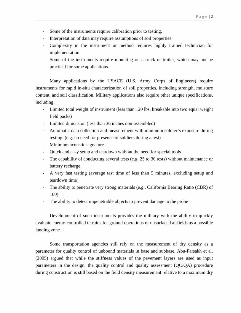
The drawbacks of available instruments or methods for rapid assessment of soil
properties in the field could be summarized as follows:
- Some of the available instruments are measuring only one parameter.
P a g e | 2
- Some of the instruments require calibration prior to testing.
- Interpretation of data may require assumptions of soil properties.
- Complexity in the instrument or method requires highly trained technician for
implementation.
- Some of the instruments require mounting on a truck or trailer, which may not be
practical for some applications.
Many applications by the USACE (U.S. Army Corps of Engineers) require
instruments for rapid in-situ characterization of soil properties, including strength, moisture
content, and soil classification. Military applications also require other unique specifications,
including:
- Limited total weight of instrument (less than 120 lbs, breakable into two equal weight
field packs)
- Limited dimension (less than 36 inches non-assembled)
- Automatic data collection and measurement with minimum soldier’s exposure during
testing (e.g. no need for presence of soldiers during a test)
- Minimum acoustic signature
- Quick and easy setup and teardown without the need for special tools
- The capability of conducting several tests (e.g. 25 to 30 tests) without maintenance or
battery recharge
- A very fast testing (average test time of less than 5 minutes, excluding setup and
teardown time)
- The ability to penetrate very strong materials (e.g., California Bearing Ratio (CBR) of
100)
- The ability to detect impenetrable objects to prevent damage to the probe
Development of such instruments provides the military with the ability to quickly
evaluate enemy-controlled terrains for ground operations or unsurfaced airfields as a possible
landing zone.
Some transportation agencies still rely on the measurement of dry density as a
parameter for quality control of unbound materials in base and subbase. Abu-Farsakh et al.
(2005) argued that while the stiffness values of the pavement layers are used as input
parameters in the design, the quality control and quality assessment (QC/QA) procedure
during construction is still based on the field density measurement relative to a maximum dry

P a g e | 3
density determined in laboratory. They suggested that since the performance of a material
depends on its stiffness or strength, the QC/QA method should measure the same properties.
Wu and Sargand (2007) showed that strength requirements for design are not met
necessarily while the subgrade and base were acceptable based on density tests. Wu and
Sargand (2007), after running tests on 10 road projects in state of Ohio, found that the quality
of the subgrade layer did not always fulfill the required structural strength. While any
correction measures after the road construction is very expensive and travel-disturbing,
correct estimation of subgrade strength and improvement measures during construction will
help to achieve a better, cost-effective, and long-lasting road.
The RapSochs (Rapid Soil Characterization System) is an instrument for in-situ
characterization of near surface soil properties. It is designed and developed in collaboration
between TransTech Systems Inc., Applied Research Association, and Northeastern
University to meet USACE’s requirements. An extension of proven cone penetrometer
technologies in combination with electrical impedance spectroscopy and other sensing
technologies are employed to develop a two-person portable instrument for a comprehensive
field assessment of soil properties. The applications for the instrument include:
1. A QC/QA tool for construction of roads, railways, runways, and foundation of
retaining walls and buildings,
2. Site selection for infrastructure facilities, roads, helipads, or runways during
contingency situations (earthquake, tsunami, landslide, etc.)
3. Rapid determination of load carrying capacity of unfamiliar airfields and terrains,
selection of optimal roots for ground supply vehicles and optimal locations for
landing strips, and prediction of soil deformation under vehicular traffic crossings on
soil surface in theater of operation.
The behavior of soil during a Cone Penetration Test (CPT), Standard Penetration Test
(SPT), Dynamic Cone Penetration (DCP) and other similar instruments has been widely
studied. However, interpretation of new instrument measurements for shallow depths based
on those instruments is not possible due to major differences in geometry and test
procedures.

P a g e | 4
1-2- Research Objectives
The primary objective of this research program is developing necessary methods,
algorithms, and empirical correlations, to interpret geotechnical properties from data
collected using the RapSochs devise. The other objective is to compare the performance with
that of DCP under controlled laboratory conditions in uniformly prepared samples. Tests are
also designed to evaluate electrical and mechanical performance of sensing technologies
during the dynamic penetration as well as the functional operation of the RapSochs
prototype. The other objective is to evaluate limitations of the current prototype and make
recommendations for changes in the design. To meet these objectives, understanding of the
physical principles of the penetration process into uniformly prepared soil sample and
development of a physics-based model is required as well.
1-3- Scope of Work
The in-situ moisture has considerable effects on base, subbase, and subgrade strength
and stiffness. The necessary capabilities, to provide comprehensive field assessment of soil
characteristics important for trafficability, are incorporated in the new man-portable
instrument. The instrument will be helpful in reducing errors in the true stiffness estimates
that are known to be dependent on moisture and soil type. However, moisture sensor
assessment and calibration was not part of our research. Only the algorithms to calculate and
present basic physical parameters are developed as part of this study.
Since flexible pavements do not fail as a result of soil strength failure, the AASHTO
guide for design of pavement structures (AASHTO, 1986 and 1993) recommends the use of a
soil parameter known as the Resilient Modulus (MR) to replace strength based parameters
such as CBR (Puppala, 2008). However, based on the main objectives and applications of
RapSochs, the overall strength of the terrain or subgrade is more important. In addition,
empirically based relationships are available to predict the type and number of aircraft passes
on the unsurfaced airfield, based on CBR. Therefore, the correlation to CBR is one of our
goals.
A large body of work has correlated the DCP to CBR. One purpose of tests in this
study is to prove the CBR measuring capability of the RapSochs by comparison with the
DCP in prepared materials. The DCP is used as a benchmark for soil strength profiles. Soil
P a g e | 5
samples properties are used to establish the ground truth for soil characteristics. Real-size
tests are conducted with the prototype version of the instrument in controlled environment at
an experimental facility at Northeastern University, herein referred to as SoilBED, using a
large soil cells.
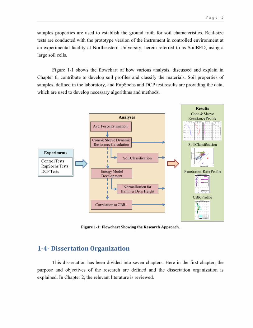
Figure 1-1 shows the flowchart of how various analysis, discussed and explain in
Chapter 6, contribute to develop soil profiles and classify the materials. Soil properties of
samples, defined in the laboratory, and RapSochs and DCP test results are providing the data,
which are used to develop necessary algorithms and methods.
Figure 1-1: Flowchart Showing the Research Approach.
1-4- Dissertation Organization
This dissertation has been divided into seven chapters. Here in the first chapter, the
purpose and objectives of the research are defined and the dissertation organization is
explained. In Chapter 2, the relevant literature is reviewed.
Ave. Force Estimation
Cone & Sleeve Resistance Profile
0 5 10 15 20
-700
-600
-500
-400
-300
-200
-100
0
Dept
h (m
m)
Cone Resistance (MPa)0 10 20 30 40 50
Friction Resistance (kPa)0 0.5 1 1.5 2
Friction Ratio (%)0 20 40 60
Hammer Drop Height (cm)
Soil Classification
0.1
1.0
10.0
100.0
1 10 100 1,00
Cone
Res
istan
ce, q
c(M
Pa)
Sleeve Friction, fs (KPa)
Correlation to CBR
CBR Profile0 10 20 30 40 50 60
0
0
0
0
0
0
0
0
CBR (%)
SIS-01-R-S5
SIS-02-R-S1
SIS-05-R-S4
SIS-07-R-S6
Averaged CBRRS
Averaged CBR
0 15 30 45 600
0
0
0
0
0
0
0
Hammer Drop Height (cm)
0 10 20 30 40
0
0
0
0
0
0
0
0
Penetration Rate (mm/blow)
SIL-04-R-S6
Drop HeightRS-PRRS-NPR
Penetration Rate Profile
Control TestsRapSochs TestsDCP Tests
Experiments
Analyses
Results
Energy Model Development
Cone & Sleeve DynamicResistance Calculation
Normalization for Hammer Drop Height
Soil Classification

P a g e | 6
The third chapter focuses on describing the configuration and specifications of the
RapSochs prototype revision zero, which was used in the experiments for this study. Details
of the sensor configurations, impact system, and related software and programs are
explained.
The fourth chapter presents the materials and methods. The soil sample preparation in
the laboratory and the geotechnical properties of the prepared samples are discussed. The
RapSochs testing procedure and details of the recorded file formats are explained. Later, the
DCP test procedure is presented.
In the fifth chapter, experimental tests data are presented. The chapter begins with an
explanation of the tests, measured parameters, database structure, and how each record is
accessible. The DCP test results are then presented and the effect of different methods of
DCP index calculation on the interpretation of data is discussed. The chapter, then,
introduces the RapSochs test results. Displacement, acceleration, and force measurements of
typical test results are presented and explained. Data of the moisture sensor is also presented
and calculation of electrical susceptance and conductance is described. The saved parameters
in the database and data mining procedure are discussed in the chapter too.
The sixth chapter concentrates on analysis of RapSochs data and development of
necessary algorithms and correlations. In the first section, a method to obtain a quasi-static
equivalent of the dynamic force is developed. It is demonstrated that cone and friction
resistance similar to CPT could be obtained from RapSochs records. The effect of variable
applied energy on the soil strength estimation is also studied. In the next section, dynamics
theory of dynamic cone penetrometers is discussed, and a model, based on Newtonian
mechanics which correlate soil parameters and instrument properties, is developed. The
model is then compared with the widely used Dutch formula. The next section describes the
RapSochs to CBR correlation. Various correlations are compared, and the best equation is
used to estimate CBR from RapSochs data. Then, soil behavior classification is examined
based on RapSochs data and charts are developed for CPT. The last section explains and
discusses effects of overburden, sample size, boundary conditions, hammer drop height, and
penetration rate on RapSochs measurements.
The seventh chapter summarizes the research conclusions and highlights the
outcomes. Recommendations to improve the instrument and suggestions for future research
are also summarized in this chapter.

P a g e | 7
Chapter 2: Background
2-1- Introduction
Techniques to assess ground conditions can be divided into laboratory tests and field
(or in-situ) tests. Traditionally, digging a test pit to obtain soil samples has been used for
shallow soil exploration. Machine-advanced or hand auger borings are also used to obtain
soil samples. The samples from such borings are usually highly disturbed and non-
representative. Different techniques to obtain representative soil samples during subsurface
exploration have been developed. Shelby tubes and piston samplers are used to obtain
undisturbed soil samples that are suitable for advanced laboratory testing to determine
engineering properties. Collected samples finally have to be transferred to laboratory for a
series of time-consuming, tedious, and costly testing methods.
The current practice for in-situ subsurface characterization (where depths to 50 feet
and beyond may be required) involves the use of the SPT (ASTM D1586), CPT (ASTM
D5778), flat plate dilatometer (ASTM D6635), or other methods. For shallow subsurface
characterization of natural soil, subgrade, or structural evaluation of pavement systems,
without boring or digging a test pit, various in-situ non-destructive tests have been developed
and used in different countries. Newcomb and Birgission (1999) categorized in-situ
nondestructive mechanical tests into three methods;
1. Deflection methods (e.g., the Falling Weight Deflectometer)
2. Small-load methods (e.g., the Clegg Impact Hammer)
3. Intrusive methods (e.g., Dynamic Cone Penetrometer)

P a g e | 8
RapSochs is a combination of CPT sensing technologies and electrical impedance
spectroscopy in a small impact driven system similar to portable DCP configuration for in-
situ characterization of near surface soil properties. In technologies that involve dynamic
sounding, recorded or measured data are indices as either, penetration per blow (e.g., DCP),
or number of blows needed for a specific penetration (e.g., SPT). The indices are usually
correlated to material properties (e.g., SPT N-values to undrained shear strength) or used
directly in design or evaluation (e.g., SPT N-values for calculation of net bearing capacity of
spread footings) after comprehensive experimental studies.
Due to the large forces required for CPT or dilatometer operation, the units are
vehicle mounted to provide the requisite reaction force. For this reason, the constant push
method of advancing the cone is not appropriate for a portable field device. However, most
of the research and practice related to sensing soil strength, type, and moisture in a
penetrometer configuration has been accomplished on CPT style devices. While a rigorous
theoretical analysis of quasi-static cone penetration is still difficult, the same approach to
dynamic penetration is more challenging, considering cost, instrumentation, and processing
limitations.
The only approach practical for portable use in the field is a variation of the standard
DCP. In its most basic form, the DCP consists of a rod fitted with a conical tip that is driven
into the soil by energy provided by a slide hammer. The hammer is dropped a fixed distance
onto an anvil attached to the rod thereby transferring the kinetic energy to the conic tip. If
the energy is high enough the soil fails in shear and the tip advances. The penetration of the
rod into the soil, as a result of the imparted energy, is related to the strength of the soil. To
provide the wide dynamic range, a dual mass hammer is utilized to better cover the range.
Other devices, such as the Sol Solution PANDA (Langton, 2001), use a fixed mass
hammer. However, the impact is controlled manually and measured electronically to better
cover the full range of soil strength encountered in the field. Alternatively, the USACE, U.S.
Army, and U.S. Air Force use the trafficability cone penetrometer and the airfield cone
penetrometer, which are pushed by a person into the soil. Those instruments, although still in
use, in most projects, are replaced by DmDCP (Dual Mass DCP) to evaluate soils
trafficability, predict ground strength for vehicle operations, or field testing for pavement and
airstrips design and construction.
P a g e | 9
Although several studies on CPT, SPT, and DCP are conducted in the past, they are
not directly applicable to RapSochs type applications. One critical issue associated with
interpretation of measured data is the dynamic impact compared to the quasi-static nature of
CPT type devices. Understanding of the recorded strain and acceleration signals is another
challenge in this project. On the other hand, while the mechanical behavior of soil under
static loading is well studied, the dynamic modeling of loading and failure of soil during a
penetration test is not sophistically formulated. This is one of the main reasons for the
experimental and statistical approach to correlate RapSochs properties and measurements to
soil characteristics.
This chapter starts with the introduction of DCP, the historical developments in
related researches and applications, followed by a discussion about advantages and
drawbacks of the instrument. An introduction of the CPT and incorporated sensing
technologies is also presented. Different types of CPT are compared and the measurements
and applications are explained. Later, other technologies, instruments, and test methods used
for near surface in-situ soil characterization, important for trafficability, are reviewed. The
measurements are explained and the advantages and disadvantages of instruments and
methods are discussed. Since the moisture content development and calibration was not
within the scope of this study, in-situ moisture content measurement technologies are not
discussed.
RapSochs is configured as a miniature pile driver that employs an impact system to
advance the cone into the soil. Because of the mechanism similarity, a short discussion on
pile driving equations, pile capacity evaluation and dynamic energy measurement is
presented in the last section.
2-2- DCP
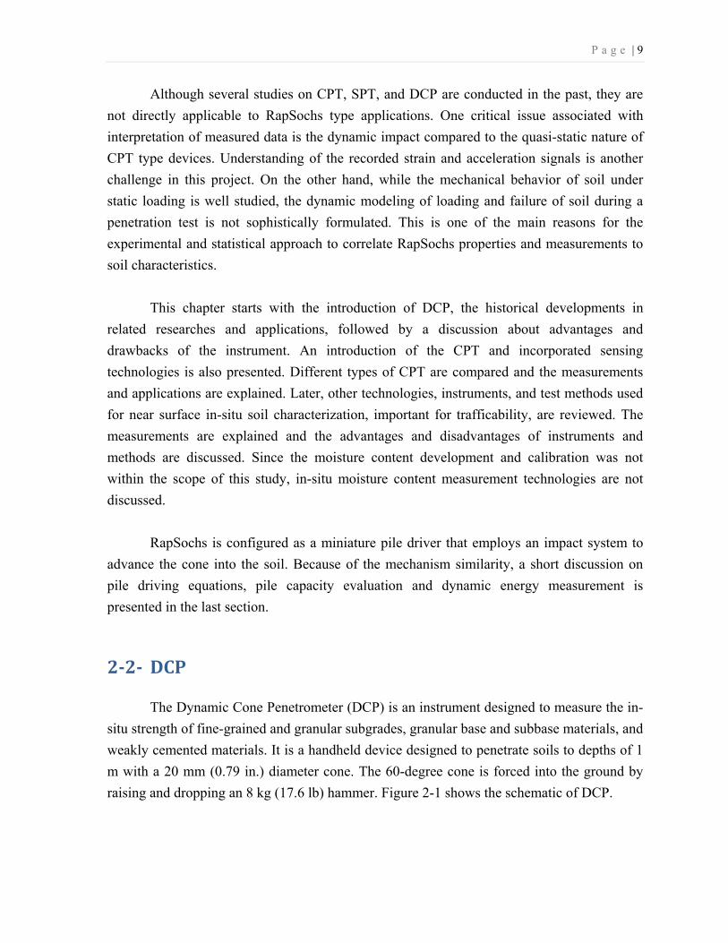
The Dynamic Cone Penetrometer (DCP) is an instrument designed to measure the in-
situ strength of fine-grained and granular subgrades, granular base and subbase materials, and
weakly cemented materials. It is a handheld device designed to penetrate soils to depths of 1
m with a 20 mm (0.79 in.) diameter cone. The 60-degree cone is forced into the ground by
raising and dropping an 8 kg (17.6 lb) hammer. Figure 2-1 shows the schematic of DCP.

P a g e | 10
Two people are usually required to run
a regular DCP test. However, in instrumented
types where data are logged by an electronic
device, the manpower is reduced to one
person. Application of DCP may be either
direct use of the DCPi for design and
evaluation or indirectly by correlations to other
parameters. The average penetration per blow
for a certain penetration depth is usually used
as an index for in-situ shear strength and it is
correlated to CBR, resilient modulus or other
soil parameters. However, there is no
consistent method to obtain the DCP index. In
this chapter, this index is referred to as DCPi
regardless of the method it is calculated. In
Chapter 4, the procedure to conduct a DCP test
is explained. In Chapter 5, DCPi calculation,
data presentation, and analysis of DCP test
results are discussed. In Chapter 6, existing
correlations to CBR are summarized. The
corresponding standard test method is ASTM
D6951, which was introduced in 2003.
DCP Historical Developments
Although early versions of the DCP
had a 30-degree cone, 60-degree cone become
more popular in latest years due to its
durability in high-strength materials. The cone
angle in the current ASTM method is 60
degrees.
Scala (1956) introduced the dynamic
cone penetrometer based on the previous
designs in Switzerland. The hammer drop
Figure 2-1: Schematic of DCP Device.
Anvil
Hammer, 8 Kg
Hammer Guide
Safety Handle
Steel Rod, 16 mm diameter
The Cone
20 mm
Cone angle 60°
Dro
p H
eig
ht, 5
75 m
m (
22.
6 in
)
Reference Point

P a g e | 11
height was 20 inches and the hammer weight was 20 lb. The cone angle was 30 degrees with
0.5 in2 surface area (0.8 inch = 20.3 mm diameter). Scala (1956) penetrometer was used with
an extension to investigate to a depth of 1.8 m below ground. He developed the theoretical
relationship between the applied energy, soil resistance and penetration rate, and he was the
first to develop the DCP-CBR correlation and use DCP for pavement design. Gawith and
Perrin (1962) reported the use of the same DCP in Australia and using a DCP-CBR
correlation curve. In South Africa, Van Vuuren (1969) introduced the modern DCP by
modifying the penetrometer, which has been in use in Australia. It was made of a 10-kg
hammer sliding on a 16-mm rod dropping from 460 mm height. The cone was 20 mm in
diameter. Van Vuuren (1969) presented the first DCP to in-situ CBR calibration for
moderately fine-grained soils.
Sowers and Hedges (1966) introduced a DCP device with a 15-lb (≈ 6.8-kg) hammer,
falling 20 in (508 mm) on the driving rod. The cone point was enlarged to minimize the
circumferential resistance. It was used for field exploration and verification of soil conditions
at individual footings. Their tests were performed in augured holes.
Since 1973, the DCP has been used in South Africa (Kleyn, 1975). The version used
in South Africa consisted of an 8-kg hammer dropping from 575 mm height with a 30-degree
cone, which was 20 mm in diameter. Kleyn (1975) is one of the pioneers who discovered the
linear relationship between DCPi and CBR on a log-log scale. After running tests on samples
with different moisture contents, compacted with the same effort, Kleyn (1975) concluded
that the DCP and CBR react in a similar manner to varying moisture content and dry density.
Trasvaal Provincial Administration (1978) in South Africa was the first organization to
suggest the use of a minimum DCPi values at different depth for pavement materials design
subjected to heavy, medium, and light traffic.
Kleyn et al. (1982) listed various applications of the DCP in pavement design, road
construction, and pavement evaluation and monitoring. They reported that the DCP measures
in-situ CBR rather than laboratory soaked CBR, and that the DCP correlates better with
pavement’s field performance than the laboratory soaked CBR. In a particular test, it was
demonstrated that DCP can detect the deterioration of pavement materials very well.
However, Kleyn and Savage (1982) excluded the cemented materials since they carry loads
in bending and are subject to fatigue damage. The DCP does not evaluate these materials in a
manner that relate to their behavior in the field. They presented a design and evaluation
method for thin surface unbound gravel pavements using DCP.

P a g e | 12
Smith and Pratt (1983) provided a correlation between DCPi (30-degree cone,
hammer weighted 9.08 kg, and dropping 508 mm) and in-situ CBR tests in clayey materials.
They concluded that the DCP results are as acceptable as the in-situ CBR while the
coefficient of variation (CV) of DCP tests is smaller than that of the in-situ CBR tests at the
same location. They compared the CBR values for materials molded at field moisture content
and density and in-situ CBR and recommended in-situ CBR and DCP measurements over
laboratory CBR tests for pavement evaluation.
Sampson (1984) reported that the DCP is used to estimate the bearing capacity of
subbase and base layers composed of coarse, granular, and stabilized materials. 2.54 mm and
5.08 mm penetration CBRs were used to obtain a DCP-CBR correlation using 60-degree
cone. Based on plasticity of the materials, different DCP-CBR correlations were proposed.
To improve the correlation, other soil parameters including grading modulus, plastic limit,
and dry density were incorporated into the correlation equation. It was concluded that, in
every case, the correlation of DCPi to the CBR of 5.08 mm penetration was better than that
of the 2.54 mm penetration.
In 1986, the Council for Scientific and Industrial Research (CSIR of South Africa)
developed the first software package for evaluation and analysis of DCP data, which has
been updated several times since then (CSIR Transportek, 2000).
Harison (1986, 1987), provided theoretical explanation for the linear log-log relation
of DCP and CBR. He performed 72 pairs of DCP and CBR tests on clay-like, well-graded
sand, and well-graded gravel samples prepared in standard CBR molds and presented
correlation equations. The regression analysis showed that the log-log model relates DCP and
CBR better than the inverse model. It was concluded that moisture content and dry density
have similar effects on CBR and DCP, and therefore, the DCP-CBR correlation may not be
affected by these variables. It was also concluded that the soaking process does not have a
significant effect on the calibration.
Livneh and Ishai (1987) used a dynamic cone penetrometer with a 30-degree cone for
pavement evaluation in Israel. Based on laboratory and field tests on a wide range of natural
and compacted materials, they suggested a correlation between DCPi and CBR. However,
they did not provide the soil classification and other material parameters. Based on the CBR
P a g e | 13
correlation, they developed methods for evaluation of airport and highway pavement as well
as evaluation of the dynamic stiffness modulus and load classification number.
Livneh (1987) concluded that the coefficient of variation of the CBR results for any
particular material is considerably higher than that of the DCP.
Chua (1988) developed a one-dimensional model for DCP penetration to back
calculate the elastic modulus of the soil. The model assumes a horizontal disc on which the
cone penetration causes a plastic deformation due to the plastic shock wave propagation. He
presented the results as series of graphs for different soils that correlate DCPi to elastic
modulus.
Chua and Lytton (1988) used a DCP with an accelerometer mounted on top of the
handle to analyze the dynamics of the system. A simple model of springs and dashpots
representing hammer-rod-soil interactions was developed. Capability of determination of the
damping ratio of the soil was demonstrated.
Harrison (1989) presented a new correlation between DCPi and CBR, which is
corrected to account for the confinement effects of laboratory CBR tests. He also reported
that the DCP test results in lower coefficient of variation than the CBR, and therefore, it is
more repeatable than CBR test.
Livneh (1989) showed that the CBR values derived from a DCP, with a 30-degree
cone, is different than that from a DCP with a 60-degree cone. The DCP and in-situ CBR
tests was performed on clay mixed with fine gravel and heavy clay (of subgrade of airfield
runways) and silty soil (of urban roads). It was concluded that in-situ CBR values obtained
from DCP tests can be used with plausible reliability. The effect of overburden pressure on
the results of tests in the above-mentioned materials was negligible. However, it was pointed
out that the difference in geographic areas may lead to changes in the empirical correlation
equations.
Ayers et al. (1989) examined DCPi to shear strength correlations for a range of
granular materials. The equations correlate the DCPi to deviator stress under different
confining pressures. The tested materials included sand, sandy gravel, and crushed dolomitic
ballast with different percentage of fines. They emphasized the role of the confining pressure

P a g e | 14
under field loading conditions. Ayers (1990) reported that overburden pressure, geometry of
the cone (diameter and angle) have a significant effect on DCP penetration.
Buncher and Christiansen (1991), after comparing Electric Cone Penetrometer results
with DCP and in-situ CBR, concluded that the DCP is very susceptible to skin friction in
cohesive soils. They reported that, in all cases, the DCP values increased as the depth
increased thru the cohesive soils.
De Beer (1991) presented a method to use DCP for flexible road design. He also
presented and empirical relationship between the elastic modulus and DCPi based on
calibration of the one-dimensional linear model with depth deflection measurements by
heavy vehicle simulator.
Livneh (1991) reported that, in-situ and in-the-CBR-mold DCP tests with 60° and 30° cone
showed significant different results. The DCP values for 30° cone were approximately 10%
greater than those obtained with the 60° cone. He also developed a correlation between CBR
and elastic modulus.
Webster et al. (1992) from USACE developed a correlation between DCP and in-situ
CBR based on tests in various materials. They also presented a procedure to use DCP for
evaluating unsurfaced soil or aggregate surfaced roads and airfields for military vehicles and
aircrafts. A Dual mass DCP (DmDCP), where the 17.6-lb (8-kg) hammer was convertible to
a 10.1-lb (5-kg) hammer, was used. A lighter hammer was used in materials with CBR values
of less than 10, and the cone penetration rate was multiplied by two to obtain an equivalent
penetration rate by a 17.6-lb hammer. This provision allows having a good resolution and
therefore more accurate measure of soil strength in weak materials. Use of disposable cone
was also introduced. In soils where the standard cone is difficult to remove, it eliminates the
need for an extraction jack or tremendously reduces the manpower needed to run several
tests. It was suggested in their work to stop the test, if the penetration of more than 25 mm
was not achieved after 10 blows since the hard material will damage the instrument. Their
work was a part of a project named “soil strength determination for non-paved operating
surfaces”.
Livneh et al. (1992) described a pneumatic automated DCP, which needs a
compressor for operation. That system was able to run up to 24 blows per minute. In their
paper, there is not a mention of any data collection system, so it may be assumed that it was

P a g e | 15
remained manual. They compared the DCP results from the automated and manual system.
Although the regression analysis showed that the automated DCP resulted lower values than
the manual DCP, but the statistical analysis indicated that they are identical. However, CBRs
from the automated system, calculated using Livneh’s equation (Livneh, 1987), were on
average 14% smaller than the ones obtained from the manual DCP. They examined the effect
of blow rate in sandy clay, but it was found not influential. They did not inspect the effect of
the penetrometer and guides weight as its effect is formulated in Dutch equation. The weight
of the automated system is not reported in their paper. The conclusion that DCP results are
identical but the calculated CBR is smaller is questionable.
Weintraub (1993) developed an automated DCP to be used for measurement of
unsurfaced airfield bearing strength. The mechanical design process and relevant details are
explained in his work. He also found that the results of DCP and the automated DCP are not
similar and have developed a correlation. After numerous tests, he validated the reliability
and consistency results of DCP.
Burnham and Johnson (1993) studied the use of the DCP for in-situ characterization
of soil profiles. The presented examples of its application in preliminary soil surveys,
embankment and back-fill construction control, structural evaluation of existing pavements,
and supplementing foundation testing for design purposes.
Webster et al. (1994) examined the minimum penetration depth required in DCP to
measure the strength of surface layers. The required depth is reported between 1 to 11 inches
(2.5 to 28 cm) for materials ranging from highly-plastic clay to poorly-graded sand. It was
also shown that the DCP can determine the thickness and location of a weak soil layer in a
pavement. They verified the DCP-CBR correlation proposed by Webster et al. (1992) and
proposed to use new correlations for CH (High-plasticity clay) and CL (Low-plasticity clay)
clays.
Ese et al. (1994) showed that a DCPi of less than 2.6 mm/blow in the well-graded
gravel base layer is critical to have a good serviceability in a road. It was concluded that the
DCP tests during thawing give the best correlation to the serviceability of a road in Norway.
They reported variation of DCP values due to variations of the moisture content. In DCP-
CBR correlation, for well-graded gravel with 9% to 19% fines, they showed that this
correlation is independent of moisture content and dry density. An automated DCP with
computerized data collection was developed to reduce the number of operators, overcome the

P a g e | 16
difficulties of running more DCP tests, reduce the instrument’s dependency to operator, and
to reduce the test time by automatic data recording.
Bratt et al. (1995) developed a DCPi to dry density correlation. They showed that
DCP could substitute moisture-density tests for compaction construction control of
embankment and subgrade inspection.
Truebe et al. (1995) used DCP to evaluate the strength of a low volume road of Forest
Service. They presented a DCP to in-situ CBR correlation for the aggregate surface and
subgrade.
Livneh et al. (1995) verified the vertical confinement effect of 1) granular layers, 2)
cohesive layers, and 3) rigid structural layers on clayey materials, as well as 4) the effect of
upper asphalt layers on the DCPi of granular materials. They concluded that the vertical
confinement does not have any effect on DCPi of a cohesive subgrade layer. However, DCP
measurement in granular soil depends on the vertical confinement. They recommended that
for pavement evaluation purposes any DCP measurement should be conducted through a
narrow boring in asphalt layer and not after removal of a wide strip of asphalt. Equations to
obtain unconfined DCPi based on confined DCPi for different top layers were presented.
They also described the theoretical background of vertical confinement effects and different
failure mechanisms. The DCP used in their research was a 30-degree angled cone.
Hassan (1996) examined existing correlations between DCPi and resilient modulus
for sand and fine-grained soils. The specimens were Oklahoma soils molded and compacted
in a 6-in-diameter and 12-in-height special mold. The DCPi was calculated by dividing the
sample depth (equal to the length of penetration, which is 12 in.) to the number of blows. The
experiment results showed that, in fine-grained soils, the increase in moisture content above
the optimum significantly increase DCPi, increase in soil dry density decreases DCPi, and an
increase in confining pressure does not significantly affect DCPi. In granular soils, it was
showed that the confining pressure is a significant factor affecting DCPi. However, this
effect is less for materials with higher coefficient of uniformity. They also found that the
maximum aggregate size has an insignificant effect on DCPi. A correlation between DCPi
and resilient modulus was developed in fine-grained soils at optimum moisture content. It
was stated that specific relationship may be developed for particular moisture state and
should not be generalized for all conditions.

P a g e | 17
MnDOT (1996) introduced a user guide to determine the fabrication details, test
procedures, applications, available methods, and correlations of DCP to be used in the
Minnesota department of transportation (MnDOT). This user guide is one of the few
instructions that covers the instruments specification and data recording and processing
procedures to details. It determines the combined weight of the upper shaft, anvil, lower
shaft, and cone to be 3.1 kg, approximately. In addition, dimensions and material properties
of hammer and anvil are determined. To record the instrument’s reading when one person
operates the DCP the use of video camera is proposed. To extract the DCP, use of a farm-
purpose jack is recommended, and striking the hammer against the handle is prohibited. The
penetration after each blow is used as DCPi. In a road subgrade, DCPi of greater than 25
mm/blow was considered as criteria for the need of remedial measures. In the pavement edge
drain backfill, DCPi of less than 75 mm/blow indicates satisfactory compaction. For various
base materials, limiting values of DCPi, assuming adequate confinement near the test
surface, are also proposed. Other applications of DCP are listed and using of automated DCP
with computerized data recording is reported.
Al-Refeai and Al-Suhaibani (1997) compared the DCP and CBR tests in laboratory
prepared samples of poorly-graded sand, silty sand, and clay and showed that both tests
respond in a similar manner to changing moisture content and dry density. They also
developed several DCPi-CBR correlations for the tested materials. They concluded that
variability in DCPi versus CBR data increases as the soil changes from fine-grained to
granular.
Burnham (1997) reported application of DCP as a quality control device during the
backfill compaction of pavement edge drain trenches and granular base layer compaction in
MnDOT. A limiting DCPi value for each particular subgrade soil and base type was
proposed as incorporated in MnDOT specifications. A relationship between DCPi and the
required remedial thickness of granular backfill/lime modification was presented.
Chai and Roslie (1998) correlated the number of blows required by DCP to penetrate
30 cm to subgrade modulus back-calculated from FWD.
Parker et al. (1998) developed and automated a version of DCP where the instrument
was mounted on a trailer. The system was designed to lift the hammer, record data, and
extract the rod after penetration.
P a g e | 18
Coonse (1999) performed DCP and CBR tests on remolded residual clayey soils in
laboratory. He demonstrated that the CBR and DCP show the same strength response
(although numerically inverse) to change in moisture content while the compaction effort is
constant and to change in compaction effort while the moisture is constant around optimum.
By comparing the results of CBR and DCP tests in soaked and unsoaked samples, he showed
that soaked specimen loose strength and both tests identified that. It was also showed that the
change of moisture content can greatly change the strength of the cohesive soil. He also
verified the effect of the mold size on DCP and CBR test results. A new DCP-CBR
correlation for CH and CL materials was also derived.
Chen et al. (1999) showed a strong correlation between a 30-degree DCP cone results
and the back-calculated elastic modulus from FWD (Falling Weight Deflectometer) in
mostly clayey and silty soils in Kansas. They presented the correlation equation along with
95 percent confidence lines in a plot based on test results.
Siekmeier et al. (1999) compared the elastic modulus obtained from DCP, SSG (Soil
Stiffness Gauge), FWD, and Portable FWD. The tests were performed on granular base and
subgrade of several road projects and mixture of clayey and silty sand of an embankment in
Minnesota. They used Webster et al. (1992, 1994) correlation of DCPi to CBR and then
Powell et al. (1984) correlation of CBR to elastic modulus. The DCPi was the average of
DCP penetration rate of the upper 75-mm and 150-mm, excluding the first drop.
Nazarian et al. (2000) instrumented a DCP with a load cell and an accelerometer to
measure the transferred energy to the anvil. They showed a typical force and velocity-time
histories up to one millisecond and plotted them versus normalized distance (i.e., equivalent
to the time that stress waves travel from anvil to tip). The force and velocity were then used
to calculate transferred energy using FV (Force-Velocity) method. They calculated the
energy transferred to soil by comparing the energy needed to penetrate a bucket filled with
30 cm of very loosely packed foam and the energy needed to penetrate a soil sample and
related it to the soil resistance. They have presented a plot of energy loss as a function of
penetration rate, where the energy loss is 75 to 120 KN-m for 50 to 2 mm/blow penetration
rates, respectively. While the total delivered energy by the 8-kg DCP hammer is about 45 N-
m, it is not clear how the energy loss could be more than 1000 times. They have mentioned
that further analysis is needed for reliably extracting information from their measurement.

P a g e | 19
Livneh et al. (2000) showed that the DCP-CBR correlation suggested by Livneh and
Ishai (1987) was valid for light to heavy clayey soils and there was no need for a separate
correlation as suggested by Webster et al. (1994). The CBR test they performed was on
undisturbed samples extracted from pits. They also compared the DCP test results of 1, 1.3,
1.5, and 2 meter long DCP rods. They showed that the results were different and a correction,
if DCP with longer rods were used, was needed.
Livneh (2000) developed a method and calibrated it to correct the effect of skin
friction forces on the DCP rod during testing in cohesive materials. He incorporated the
measured torque moments at different depths in the CBR correlation equation. His reason
was that occasionally the CBR values derived from DCP tastings are higher than the CBR
values obtained by other in-situ tests. However, the CBR-DCPi correlation that he used
results higher CBRs for DCPi’s between 2 to 80 mm/blow compared to Webster et al.
(1992)’s equation. But he mentioned that “improper penetration”, which mobilizes the skin
friction may be the reason. To minimize the effect of skin friction he suggested attaching a
base frame to the DCP apparatus in order to ensure vertical penetration. The length extension
of the standard penetrating rod to a total of about 2.0 m (by screwing on an additional 1.0-m
rod after the original rod) is also used and completely inserted into the pavement or subgrade.
He mentioned that such a procedure found to be necessary when the total thickness of the
pavement layers, including the relevant subgrade layers, exceeds the length of a standard
penetrating rod
George and Uddin (2000) used manual and trailer-mounted automated DCPs in their
research to determine the subgrade resilient modulus of subgrade soils in the state of
Mississippi. Test results showed no differences between the manual and automated DCP
measurements. Subgrade moduli were determined by laboratory triaxial tests and also by
analyzing the deflection profiles obtained from the FWD. The DCPi was correlated with
laboratory and back-calculated resilient modulus using two different models for fine-grained
and coarse-grained soils. For further improvement of the models, soil physical properties
were found necessary.
Chen et al. (2001) conducted more than 60 DCP tests on two test pavements on US-
281 near Jacsboro, TX. DCP test were conducted in 3 different procedures through asphalt
concrete, a narrow borehole in asphalt concrete and directly on the base of highway by
removing a wide strip of pavement. They presented equations to convert DCP results from
one type of tests to the other. For comparison of these tests they plotted the cumulative
P a g e | 20
number of blows versus depth with some adjustments. Average DCPi is used for correlations
to CBR and then to elastic modulus using the correlation proposed by Powell et al. (1984).
The elastic modulus obtained from DCP is then compared with those obtained by FWD-
MDD (Falling Weight Deflectometer-Multi Depth Deflectometer) tests and by resilient
modulus laboratory tests. They concluded that the elastic modulus of the base and subgrade
layers determined by DCP and FWD-MDD tests are very close and laboratory determined
subgrade modulus were slightly higher than those.
Gabr et al. (2001) developed a correlation between DCPi and liquid index and
Saturation ratio based on laboratory tests on piedmont residual soils of Davidson County, NC
with more than 60% fines. They used these correlations to predict the dry unit weight and
water content of the soil.
Konrad and Lachance (2001) used a 51-mm diameter cone in dynamic penetration
test in base and subbase materials, due to concerns regarding the effect of grain size on
penetration resistance. They also correlated the penetration index to the back-calculated
elastic modulus from plate load test in unbound base and subbase materials.
There is a DCP Data Acquisition System (DCP-DAS) developed by Applied
Research Associates Inc., which became commercially available before 2002. It uses a string
potentiometer to automatically measure the depth of penetration and number of drops.
However, the effect of the pulling force applied by the string potentiometer on DCP
measurements is not clear. DCP data is recorded in an electronic format that can be easily
accessed by a computer for further analysis. Automatic data acquisition allows one-person
operation, reducing testing cost, while improving the accuracy of the data collected (Vertek,
2010).
Rahim and George (2002) ran DCP and automated DCP (which is mounted on a
trailer) tests atop of subgrade through drilled holes at 12 sites in Mississippi. Shelby tube
samples were obtained and tested to calculate Resilient Modulus (MR) following AASHTO
TP46 Protocol. DCPi and other soil properties were then correlated to resilient modulus by
two different equations for coarse-grained and fine-grained soils. They found that other soil
state variables are significant in MR prediction.
Karunaprema & Edirisinghe (2002) tested clayey and silty gravel soils mixed in the
lab in Sri Lanka. They reported that a clear relationship between the soaked CBR and the

P a g e | 21
DCP value could not be defined as for unsoaked CBR. However, they found a significant
correlation between the DCP and the difference between the unsoaked and soaked CBR
value. In addition to developing DCP-CBR correlations, they also correlated moisture
content and DCP to dry density, compaction ratio, and optimum moisture content..
Herrick and Jones (2002) developed a dynamic penetrometer with a 2-kg hammer for
measuring soil compaction in agricultural and rangelands. They used an adjustable hammer
drop height to have the flexibility, which allowed them to use a single instrument on a broad
range of soils without any loss in sensitivity.
ASTM introduced the DCP standard test method in 2003 for shallow pavement
application (ASTM D6951-03). Later in 2009, the standard was revised (ASTM
D6951/D6951M-09).
Amini (2003) reviewed the application of DCP in pavement design and construction.
He warned the use of DCP for materials with an aggregate size larger than 50 mm (2 in.).
Abu-Farsakh et al. (2004) evaluated the use of DCP for quality control/assurance
evaluation of pavement layers and embankments during construction. The DCP and plate
load tests (PLT) were carried out in the laboratory on silty clay and clayey silt. The DCP,
PLT, and FWD tests were conducted on subgrade and base sections of several projects in the
state of Louisiana. Laboratory CBR tests were also performed on samples from the lab and
field tests. Correlations between DCPi and elastic modulus (from plate tests), unsoaked CBR,
and resilient modulus (from FWD) were developed. The DCPi was the average penetration
in the top 30 cm of soil. They suggested 5.5 mm/blow as the acceptance limit for the crushed
limestone base. They concluded that the DCP device can be used for evaluation of uniformity
of compaction, thickness, and stiffness of pavement layers and subgrade.
Rahim et al. (2004), developed a model based on the pore collapse theory and
cylindrical cavity expansion to predict DCP penetration resistance based on cohesion, angle
of internal friction, and initial porosity. The parametric study of the model reveled that for
small initial porosity, the penetration resistance is strongly depends on internal angle of
friction but it is not as sensitive to cohesion. They compared their prediction with DCP test
data, obtained by Mississippi department of transportation. In general, the reported angle of
internal frictions versus DCPis were scattered. Although the developed model can predict the
general trend of the average data, but it did not predict the internal friction with a reasonable

P a g e | 22
confidence level. The correlation between cohesion intercept and DCPi was also poor. The
initial porosity showed a better correlation to DCPi.
Amini (2004) reviewed the previous researches in application of DCP in the quality
control of compaction in backfill, base layer, and backfill around utilities.
Abu-Farsakh et al. (2005) conducted a series of DCP, PLT (plate load tests), FWD,
and CBR laboratory tests. They presented correlations between DCPi and the Elastic Moduli
of soil (obtained from Plate Load Test), unsoaked CBR values, and resilient modulus
(obtained from FWD tests). They concluded that DCP can be used reliably to evaluate the
stiffness and strength of pavement materials, in addition to verify the uniformity of
compaction. They also recommended the criteria of 5.5 mm/blow for crushed limestone
highway base and concluded that it results satisfactory stiffness and compaction level.
Chen et al. (2005) developed a correlation between DCPi and elastic modulus back-
calculated from FWD tests. They compared their relationship with the elastic modulus
obtained by using the DCPi-CBR correlation of Webster et al. (1992) and CBR to elastic
modulus correlation proposed by Powell et al. (1984). The DCPi was corrected to take into
account the effect of overburden pressure in case of conducting the test through a drilled hole
in the asphalt layer.
Edil and Benson (2005) conducted several tests on the exposed subgrade and subbase
to the maximum depth of 38 cm across the state of Wisconsin. The DCPi was obtained from
the weighted average of penetration rates without excluding any datapoints for further
analysis and correlations. A linear relationship was observed between SSG stiffness in
regular scale and DCPi averaged from depth 0 to 152 mm in logarithmic scale. They also
showed that in plots of DCPi versus unit weight or water content, a general pattern can be
observed but datapoints were so dispersed that a unique correlation could not be developed.
For the quality control of earthworks they proposed a procedure consisting of normalizing
the DCPi by the deviation of compaction moisture content from the optimum moisture
content and showed that, for compacted natural earthen materials, a value around -8.4 is an
indication of high relative compaction.
Dai and Kremer (2006) summarized specifications and implementation of the DCP
testing in Minnesota and other states. They performed tests with DCP (equipped with DCP-
DAS) and other tests on several construction projects in the State of Minnesota. A modified

P a g e | 23
DCP specification for road construction projects was recommended and a testing procedure
was suggested. The use of DCPi as the criteria in place of relative densities for the granular
fills was also discussed.
Ampadu and Arthur (2006) developed a correlation between DCPi and the level of
compaction based on tests on compacted gravel in a road construction site in Ghana. They
concluded that this correlation depends on the material and the water content, and the
proposed equation is not unique.
Swenson et al. (2006) studied moisture effects on the measurements of several
laboratory and field devices and their interpreted modulus values. They reported a significant
scatter of resilient modulus from DCP. Overall, the results showed that both moisture and
density had a measurable effect on the modulus of fine-grained soils. However, they found
that, DCP is effective in quantifying the uniformity of compacted soil volumes, and
estimating the apparent Young’s modulus through empirical formulas.
Wu and Sargand (2007) showed that DCP is a viable device for evaluation of base
and subgrade during construction. They concluded that DCP can greatly improve the quality
monitoring of pavement unbound materials, and therefore, enhance its performance. An
automated DCP was used in their research, and they reported that it reduces the required time
to run one test to one-fifth. However, very small or negative penetration rates were observed
in some of the tests, which they related to non-homogenous nature of subgrade soil and
presence of small rocks. It was not investigated if the automatic DCP is also participating in
the errors. They conducted two corrections to adjust the profile graphs to enhance
interpretation. To identify uniform layers from penetration rate profiles, a method proposed
in AASHTO 1986 was used. The average DCPi from tests on the base of 10 road projects in
Ohio is reported between 5 to 14 mm/blow. The average DCPi in asphalt concrete was
reported between 2 to 7 mm/blow. They suggested accepting of DCP into pavement design
methods, since the validity of DCP to measure the soil strength was proved, and in any
correlation, estimation errors are unavoidable. A set of DCP acceptance criteria and standard
was proposed.
Booth et al. (2008) raised concerns about legitimacy of DCP to CBR correlations
after comparing laboratory CBR values with those obtained from correlation equations from
tests in sandy slightly gravelly silt and silty very gravelly sand.

P a g e | 24
Puppala (2008) reviewed DCPi to resilient modulus correlations. He reported that the
DCP has been used by different transportation agencies for years to estimate the moduli of
compacted subgrades and granular soils. However, he warned that the majority of the
correlations are site specific and empirical in nature and their use for other soils requires a
careful examination and engineering judgment.
Siekmeier et al. (2009) proposed the minimum required DCPi values to be used for
construction quality assurance based on tests conducted on granular and fine-grained soil
samples prepared in the lab for a range of moisture contents and densities. They obtained
graphs which by knowing the grading number1 and the moisture content in granular soils and
plastic limit and the moisture content in fine-grained soil the minimum required DCPi can be
estimated.
DCP Advantages The advantages of DCP test are summarized by Livneh (1987), Ayers et al. (1989),
Webster et al. (1994), MnDOT (1996), Karunaprema and Edirisinghe (2002), and Wu and
Sargand (2007) and listed as follows.
- It characterizes the in-situ strength of soil,
- It characterizes the strength with depth,
- It could be used to determine the thickness and depth of underlying soil layers,
- It could be used to verify uniformity of compaction,
- It is repeatable and reliable,
- It can be used in soils with a wide range of particle sizes and strengths,
- It is man-portable,
- It is relatively inexpensive,
- It is sturdy and the maintenance is simple and inexpensive,
- It could be used in developing countries for evaluation and design purposes,
- It is simple enough to be used by an inexperienced person,
- It could be used to verify whether if a stabilized soil has achieved its potential
stiffness,
- It requires less penetration depth than the CPT to measure the surface layer strength,
- It is relatively fast and usually does not take more than 10 min (time varies depending
on the strength of the material and maximum depth of penetration). 1 The grading number is the sum of the percentages of particles passing specific sieves.
P a g e | 25
DCP Disadvantages
While the operation of DCP is physically arduous (Amini, 2003), the manual raise
and drop of the hammer could be a source of error in a DCP test. The user has to ensure that
the hammer is touching the bottom of the handle but not lifting the cone before it is allowed
to drop (Webster et al., 1992). The operator should be careful not to exert any downward or
upward force on the handle and not to influence the free fall of the hammer by hand
movement (Webster et al., 1992).
Utilization of skin friction can cause erroneous results in cohesive materials. After
comparing the Electric Cone Penetrometer results with DCP and in-situ CBR, Buncher and
Christiansen (1991) mentioned that the DCP is very susceptible to skin friction in cohesive
soils. For the same reason, Webster et al. (1992) suggested to limit the depth of penetration to
12 in. (about 30 cm) in highly plastic clays and clean and lubricate the rod after each test to
minimize sticking of clay to the rod. However, Webster et al. (1994) stated that oiling the rod
does not improve test results in CH soils significantly. Livneh et al. (1995) showed that the
inclined (15 degrees tilted) penetration in clayey materials yield 28% lower DCPi on average.
They reported that angled penetration is not unusual in deep DCP penetrations. The problem
of keeping the penetrometer perfectly vertical in manual operation of the DCP is also
mentioned by others (e.g., Wu and Sargand, 2007). Livneh et al. (1995) suggested using a
vertical supporting frame to overcome this problem. Livneh (2000) reported that occasionally
DCP predict higher CBR values due to inclined probe penetration, which utilizes the skin
friction forces. This increase in the resistance increases the DCPi value which will result in
higher CBR values consequently. To correct this effect, he incorporated the measured
torsional moments (i.e., the moment required to rotate the DCP at the place) at different
depth in the CBR correlation equation.
The other problem with DCP is the extraction of the instrument after deep tests in
some cases (Weintraub, 1993, Wu and Sargand, 2007). Using disposable cone tips as
suggested by Webster et al. (1992) may be one solution. However, ASTM 6951 suggests
using an extraction jack, if disposable cone tips are not used.
Ayers et al, (1989) has shown that the maximum aggregate size has a notable effect
on the test results. They found the maximum aggregate size of around 38 mm to be where the
DCP is no longer a viable test. However, Webster et al. (1992) reported that DCP is not
suitable for soils having significant amount of aggregates greater than 51 mm. Konrad and

P a g e | 26
Lachance, (2001) reported that use of DCP in pavements with aggregates larger than 20 mm
was questionable.
For tests in loose materials, the 8-kg hammer causes excess penetration (Webster et
al. 1992). In this case, no DCP measurement is possible close to surface in dry sand or gravel
(Webster et al., 1992) due to no confining pressure in the procedure. Using a different
hammer mass is suggested by ASTM 6951 after Webster et al. (1992). However, far less
experimental data for using a 4.6-kg hammer is reported in the literatures.
The manual reading and recording the number of blows and depth of the cone could
also cause some errors (Webster et al., 1992). Since the regular DCP test needs one operator
to lift and drop the hammer while keeping the instrument vertical, another operator should
keep track of the penetration after each blow. To address this problem, some innovation kits
are added to DCP. For instance, Kessler Inc. (Kessler Soils Engineering Products, Inc., 2007)
introduced a kit to write the number of blows for each set of blows on a removable tape along
the ruler, or use a magnetic ruler data collection device. Applied Research Associates Inc.
developed a DCP Data Acquisition System (DCP-DAS), which uses a string potentiometer to
automatically measure the depth of penetration and number of drops (Vertek, 2010).
Otherwise, data collection and analysis is time consuming, if no automated measurement
system and software are used.
MnDOT (1996) reported that for in situ foundation testing in addition to DCP tests,
soil samples should be obtained on a periodic basis to be used for soil classification and
moisture content determination. They mentioned that sand cone or nuclear density tests may
be taken for further investigation and compaction correlation.
2-3- CPT
The cone penetration testing (CPT) consists of pushing a cone penetrometer into the
soil and continuous measurements with depth. The test is also called static or quasi-static
penetration test. Cone penetrometers are available in different diameters and types. The
earlier version, known as mechanical cone penetrometer (originally called Dutch cone)
consisted of cylindrical rods with a conical point used to measure the end-bearing resistance
of the cone. With addition of a telescoping mechanical friction sleeve, measuring local soil
friction became possible in mechanical friction-cone penetrometer (also known as Begemann

P a g e | 27
friction-cone). In these instruments, the force is measured with a hydraulic or electric load
cell or proving ring. The measurements are in less than 20 cm increments. The corresponding
standard test method is ASTM D3441-05.
The more commonly used version is electric (or electronic) cone penetrometer. In
electric cone penetrometer, the tip is instrumented with transducers to measure the cone
resistance and side resistance continuously with depth. The configuration of the tip may vary
depending on design, but the friction sleeve is located right behind the cone, and its outside
diameter is always equal to the diameter of the base of the cone. The pushing system can
consist of a standard drill rig or a system mounted on a truck, track, trailer, all-terrain vehicle,
skid arrangement, or portable unit. The penetrometer is pushed into the ground at a rate of
200 mm/sec and measurements are collected in at least 50 mm intervals. Although electric
cone penetrometers provide finer resolution compared to mechanical cone penetrometers,
they are more likely to be damaged in hard materials (Mayne, 2007). ASTM D5778-07 is the
standard test method for electric cone penetrometers.
There are other types of penetrometers. Some are equipped to provide or measure
shear wave velocities, electric conductivities, acoustic emissions, temperature, images of soil,
and water samples. Some of the versions, which are more used in practice, are listed in Table
2-1. Lunne et al. (1997) and Mayne (2007) reviewed and discussed the history of the tests,
equipments and procedures in details. In this dissertation, the term CPT is interchangeably
used to refer to the electric cone penetrometer or the test in general regardless of the
penetrometer type.
The applications of CPT include site investigations for exploring soils for support of
embankments, retaining walls, pavement subgrades, and bridge foundations (Mayne, 2007).
The results are used to classify the materials in a soil profile and to obtain estimates of soil
properties (Newcomb and Birgisson, 1999). Various correlations are available between CPT
measurements and undrained shear strength, internal friction angle, the overconsolidation
ratio, soil behavior classification, mean-grain size, relative density, and SPT number (Lunne
et al., 1997). CPT is also a valuable test for quality control during ground modification,
because it allows a direct comparison of before and after modification (Mayne, 2007).

P a g e | 28
Table 2-1: Different Types of Cone Penetration Tests in Site Characterization (After Mayne, 2007).
Type Measurements Application
Mechanical Cone Penetrometer - Cone resistance
- Friction resistance*
Stratigraphic profiling, fill control,
natural sand, hard ground
Electric Friction Cone
Penetrometer (CPT)
- Cone resistance
- Friction resistance
Fill placement, natural sands, soils
above the groundwater table
Piezocone Penetrometer (CPTu) - Cone resistance
- Friction resistance
- Pore pressure
All soil types, (cone resistance is
corrected based on pore pressure)
Piezocone Penetrometer with
Dissipation
- Cone resistance
- Friction resistance
- Time readings of pore
pressure during decay
Normally conducted to 50%
dissipation in silts and clays
Seismic Piezocone Penetrometer - Cone resistance
- Friction resistance
- Pore pressure
- Shear waves
Provides soil stiffness with depth
Resistivity Piezocone Penetrometer - Cone resistance
- Friction resistance
- Pore pressure
- Electric conductivity
To detect freshwater-salt water
interface, Index to contaminant
plumes
NOTE: * In mechanical friction-cone penetrometer
Cone tip resistance is the most reliable and widely measured quantity in the CPT. Yu
and Mitchel (1998) reviewed some of the theories for the analysis of cone resistance and
discussed the limitations and advantages based on experimental data. However, the sleeve
friction is not recognized as being very precise (Robertson, 1990), and the standard deviation
in subtraction cone could be about 15% of the maximum capacity (ASTM D5778, 2007).
One of CPT’s main advantages is providing continuous repeatable and reliable data
with depth (Lunne et al., 1997), which helps detection of depth and thickness of different soil
layers. Therefore, if there is a critical layer or soft zone in the subsurface soil, CPT can detect
and locate it (Mayne, 2007). It is also suggested to use CPT to complement SPT test results,
considering that CPT is a faster and more economical test comparing with soil test boring.
While some of geotechnical firms and highway departments rely only on SPT as their

P a g e | 29
primary data source for bridge, wall, and roadway design, CPT resistance can be used to
complement the discrete values from the SPT to better define the soil profile. However,
rotary drilling operations to obtain soil samples for examination and laboratory testing are
still necessary (Mayne, 2007). From the environmental standpoint, no spoil is generated in
CPT. Thus, the method is less disruptive than drilling operations, and workers are exposed to
minimal amount of hazard or hazardous material in potentially contaminated sites (Mayne,
2007).
The CPT performs well in most soils, except in soils containing gravels, cobbles,
boulders, or cemented seams. In suitable soils, CPT data are less scattered than SPT ones
(Newcomb and Birgisson, 1999). Mayne (2007) reported the most common obstacles to CPT
use, among department of transportation of different states, include the presence of very hard
ground, cemented layers, or dense geomaterials, thereby preventing penetration. He reviewed
some methods which that help to overcome hard ground conditions. Among those solutions
he reported the work of Sanglerat et al. (1995), which uses a combined static-dynamic
penetrometer system to increase the maximum depth of penetration when hard materials are
met.
Webster et al., (1994) reported that U.S. Air Force used a C-130 transportable van
equipped with a mechanical friction-cone penetrometer to run CPT to the depth of 5 ft for
contingency airfield evaluation. The van was also equipped to perform CBR, pavement
coring, soil classification and other lab testing. They developed a correlation between tip
resistance and friction ratio to in-situ CBR. It was concluded that CPT is an effective device
for locating and measuring the strength of transition zones within a strong soil layer above
weaker materials. However, CPT requires a certain penetration depth before the surface layer
strength can be measured, and it cannot be used to measure the strength or thickness of a 15-
cm thick layer without any confinement.
The CPT is less sensitive to soil type compared to a piezocone. However, in the
particular application of our interest where the soil near the surface is unlikely to be fully
saturated, pore pressure measurement is not expected to be helpful in interpretation of test
results.

P a g e | 30
Soil Classification by CPT
Soil behavior classification charts are usually used for soil profiling and stratigraphy
during CPT and CPTu (Electronic Piezocone) tests. In CPT, conducted according to ASTM
D3441 or ASTM D5778, the cone resistance (qc) and sleeve friction (fs) are measured with
depth. The ratio of sleeve friction to cone resistance, called the friction ratio (Rf), is used in
the literature to correlate to soil type (Robertson, 1990). Soil behavior classification using the
sleeve and cone resistance is widely used in interpretation of CPT. Incorporation of
piezometer elements with the electronical cone penetrometer, led to what is known today as
the modern piezocones. CPTu, in addition to cone resistance and sleeve friction, provides
values of pore water pressure with depth. Pore water pressure behind the cone is also used in
different methods to improve the soil type classification. Douglas and Olsen (1981) clarified
that CPT classification charts do not provide precise predictions of soil type based on grain-
size distribution but provide a guide to soil behavior. Webster et al. (1994) showed that in
pavement structures, different soil layers and their thickness can be identified from cone
resistance and sleeve friction plots versus depth.
Lunne et al. (1997) and Fellenius and Eslami (2000) reviewed some of the soil
behavior classifications using CPT and CPTu. Figure 2-2 to 2-6 show examples of charts
proposed by Schmertmann (1970), Douglas and Olsen (1981), Robertson et al. (1986),
Robertson (1990), and Eslami and Fellenius (1997). There are other charts, reported in
literatures, which use the measured pore water pressure as the main parameter for soil
classification (e.g., Robertson et al., 1986, Robertson, 1990, Schneider et al., 2008). Since
RapSochs is developed for shallow soil classification, it does not measure pore water
pressure, and those charts are not discussed.

P a g e | 31
Figure 2-2: Schmertmann’s Soil Behavior Classification by Mechanical CPT (After Hunt 1984 and based
on Schmertmann 1970, Sanglerat 1972, and Alperstein and Leifer 1976).
Figure 2-3: Douglas and Olsen’s Soil Behavior Classification by Electronic CPT (After Douglas and
Olsen, 1981).
0.1
1
10
0 2 4 6 8 10
Cone
Res
ista
nce,
qc
(MPa
)
Friction Ratio, Rf (%)
Dense or Cemented Sands and Gravels
Loose Sands or Gravels
Silty-Sand Mixtures, ClayeySands and Silts
Sandy and Silty Clays
Insensitive Nonfissured inorganic Clays
Very Stiff
Stiff
Medium
Soft
Very Soft
Organic Clays, Peats
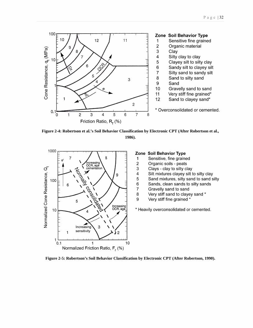
P a g e | 32
Figure 2-4: Robertson et al.’s Soil Behavior Classification by Electronic CPT (After Robertson et al.,
1986).
Figure 2-5: Robertson’s Soil Behavior Classification by Electronic CPT (After Robertson, 1990).
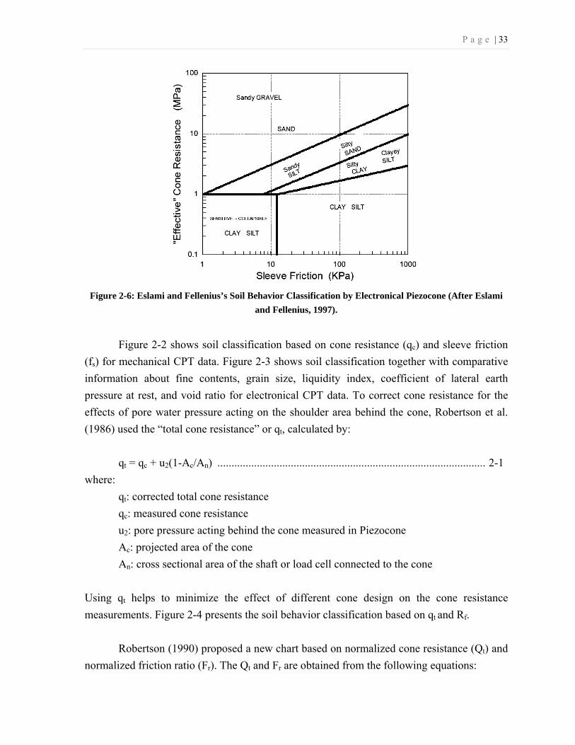
P a g e | 33
Figure 2-6: Eslami and Fellenius’s Soil Behavior Classification by Electronical Piezocone (After Eslami
and Fellenius, 1997).
Figure 2-2 shows soil classification based on cone resistance (qc) and sleeve friction
(fs) for mechanical CPT data. Figure 2-3 shows soil classification together with comparative
information about fine contents, grain size, liquidity index, coefficient of lateral earth
pressure at rest, and void ratio for electronical CPT data. To correct cone resistance for the
effects of pore water pressure acting on the shoulder area behind the cone, Robertson et al.
(1986) used the “total cone resistance” or qt, calculated by:
qt = qc + u2(1-Ac/An) ............................................................................................... 2-1
where:
qt: corrected total cone resistance
qc: measured cone resistance
u2: pore pressure acting behind the cone measured in Piezocone
Ac: projected area of the cone
An: cross sectional area of the shaft or load cell connected to the cone
Using qt helps to minimize the effect of different cone design on the cone resistance
measurements. Figure 2-4 presents the soil behavior classification based on qt and Rf.
Robertson (1990) proposed a new chart based on normalized cone resistance (Qt) and
normalized friction ratio (Fr). The Qt and Fr are obtained from the following equations:
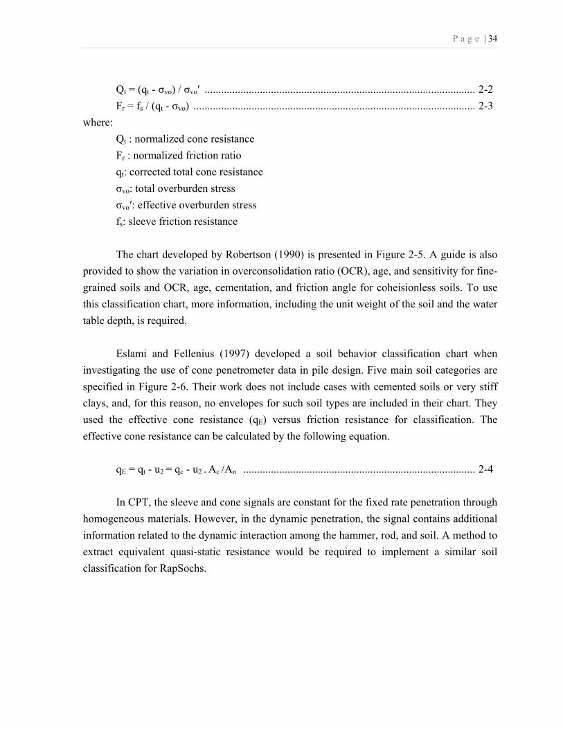
P a g e | 34
Qt = (qt - σvo) / σvo′ .................................................................................................. 2-2
Fr = fs / (qt - σvo) ...................................................................................................... 2-3
where:
Qt : normalized cone resistance
Fr : normalized friction ratio
qt: corrected total cone resistance
σvo: total overburden stress
σvo′: effective overburden stress
fs: sleeve friction resistance
The chart developed by Robertson (1990) is presented in Figure 2-5. A guide is also
provided to show the variation in overconsolidation ratio (OCR), age, and sensitivity for fine-
grained soils and OCR, age, cementation, and friction angle for coheisionless soils. To use
this classification chart, more information, including the unit weight of the soil and the water
table depth, is required.
Eslami and Fellenius (1997) developed a soil behavior classification chart when
investigating the use of cone penetrometer data in pile design. Five main soil categories are
specified in Figure 2-6. Their work does not include cases with cemented soils or very stiff
clays, and, for this reason, no envelopes for such soil types are included in their chart. They
used the effective cone resistance (qE) versus friction resistance for classification. The
effective cone resistance can be calculated by the following equation.
qE = qt - u2 = qc - u2 . Ac /An .................................................................................... 2-4
In CPT, the sleeve and cone signals are constant for the fixed rate penetration through
homogeneous materials. However, in the dynamic penetration, the signal contains additional
information related to the dynamic interaction among the hammer, rod, and soil. A method to
extract equivalent quasi-static resistance would be required to implement a similar soil
classification for RapSochs.

P a g e | 35
2-4- Field Methods for Soil Characterization
Various methods are developed in last few decades to determine strength, stiffness,
and bearing capacity of soil and rock under natural in-situ (in-place) conditions. In previous
sections, the DCP and CPT are explained. In this section, some of other popular field test
methods, important in characterization of natural soil, subgrade, or structural evaluation of
pavement systems, are reviewed. The discussion for each test includes a brief description of
the test method, the equipment and the uses of the data.
Airfield Cone Penetrometer
The airfield cone penetrometer is a 92 cm
long penetrometer with a T-shape handle on one
side and a 30-degree cone with a base diameter
of 1.28 cm (0.5 in.) on the other end. A person
pushes down the instrument at a rate of 13 to 25
mm/sec (0.5 to 1 in./sec), and the required force
is measured by a spring, and the airfield index is
read and recorded directly from the penetrometer
by another person (Fenwick, 1965). The airfield
cone index (AI) has a range of 0 to 15, which is
equivalent to CBR of 0 to 18 approximately
(Webster et al. 1992). A similar instrument called
trafficability penetrometer was in use by the U.S.
Army since 1959 (Fenwick, 1965). A major
disadvantage of the instrument is that it can not
penetrate crusts or thin base coarse layers while a
soft layer may lie underneath (Webster et al.
1992). Figure 2-7 shows the schematic of the
airfield cone penetrometer.
Trafficability Cone Penetrometer
The trafficability cone penetrometer consists of a 30-degree cone with a 0.5 inch-
square (3.2 cm2) base area, 0.8 inch (20 mm) diameter, a steel shaft 19 inches long and 3/8
Figure 2-7: Airfield Cone Penetrometer
(After Weintraub, 1993).
Spring
⅜˝ Rod

P a g e | 36
inches in diameter, a proving ring, a micrometer
dial, and a handle (U.S. Army and Air Force,
1994a). The proving ring is deformed in
proportion to the applied force when it is pushed
into the ground. The dial is ranging from 0 to
300 psi and the reading is called the soil’s cone
index (CI). CI is an index of the soil’s shearing
resistance. The trafficability cone penetrometer
is used to determine the shearing strength of
low-strength soils (U.S. Army and Air Force,
1994a). Correlations to CBR based on soil type
are also available (Shoop et al., 2008). It is a
simple instrument designed for quick and easy
field use to obtain an index of soil strength.
However, it is not appropriate for use in gravel.
Its application in military and agricultural
industry is also reported (Shoop et al., 2008). A
smaller cone, 0.2 inch-square (130 mm2) base
area, is used for harder soils and soils with fines
(Shoop et al., 2008). Figure 2-8 shows the
schematic of an airfield cone penetrometer.
Rapid Compaction Control Device
The Rapid Compaction Control Device (RCCD) is an impulse penetrometer with a
trigger system that is primarily used for quality control of compaction. The instrument
weighs about 6 kg and its dimensions are about 90cm by 30cm by 30cm. A spring loaded
steel rod with a tip cone is released by a trigger mechanism to penetrate the soil, and the
penetration depth is measured. The RCCD penetration depth is correlated with CBR and soil
classification of the backfill material. It provides the user with a quick reference regarding
the state of compaction of the reinstated material and is also used for evaluation of granular
material compaction for quality control and assurance. The cone penetration is limited to
78mm, which makes it impossible to complete three blows in weaker materials without
reaching the penetration limits (Dai and Kremer, 2006). The instrument can be operated by a
semi-skilled operator.
Figure 2-8: Trafficability Cone Penetrometer
(from U.S. Army and Air Force, 1994a).

P a g e | 37
In-situ CBR
The California Bearing Ratio (CBR) is originally devised by O. J. Porter of the
California State Highway Department, following an extensive investigation into flexible
pavement failure in California. Later, it was taken up by the U.S. Army Corps of Engineers
(USAEC) during World War II and adopted for airport pavement design. After the war, other
organizations became interested in the test as a mean of imperially measuring soil strength
for pavement design purpose. The original CBR test and procedures were subsequently
adopted to meet particular needs in various countries. The design practice of USACE and
USAF for surfaced and unsurfaced airfields is still based on CBR (U.S. Army and Air Force
1994b). However, most of state and federal highway organizations or agencies have replaced
CBR method with other pavement design methods.
CBR may be performed either in the field or in the laboratory on compacted
specimens. The laboratory CBR test method consists of using a circular piston (1.954-in =
50-mm diameter) to penetrate the material prepared in a mold at a constant rate. The CBR is
the ratio of the measured pressure required to penetrate 0.1 and 0.2 in (25 and 50 mm) to the
pressure required to penetrate a standard well-graded crusted stone. CBR can range from
higher than 100 for crushed coarse soils to less than 1 for fine-grained materials containing
high organic and moisture contents. The laboratory CBR test is described in ASTM
Standards D1883-07 and AASHTO T193.
The in-situ CBR test is very similar to the laboratory CBR test in principal. The
penetration load needed to push a piston of 2 in. (50.8 mm) diameter into the soil is
compared with the penetration load of a standard material. Proving rings or a load cell are
used to measure the reaction force at a penetration rate of 0.05 in (1.3 mm)/min until a total
penetration of 0.5 in. (13 mm) is reached. A truck usually provides the reaction load to push
the piston into the soil. The surcharge weight equivalent to the confining pressure of the
removed or planned pavement is usually used during the test, but it should never be less than
0.4 psi (≈ 2750 Pa). To obtain the CBR value, the penetration pressures measured at 0.1 and
0.2 in. are compared to standardized values of 1,000 and 1,500 psi (6.9 and 10.3 MPa),
respectively. The measured values are divided by their respective standardized value, and the
larger of the two values is reported as the CBR value, in percent. The procedure is described
in the standard test method ASTM D4429-09.
P a g e | 38
In in-situ CBR, there is no confinement effect due to the mold, and therefore in
general, it is expected that the absence of a rigid mold would result a lower CBR values for
granular materials compared with those obtained in laboratory. However, previous
experience shows that for fine-grained materials at the same moisture and density conditions,
the two tests give similar results.
The CBR strength parameter is used to estimate the bearing capacity of the pavement
subgrade, subbase, and base materials for design and analysis purposes. In pavement
evaluation, destructive test pits are usually dug to determine pavement layer thickness, and
in-situ CBR tests are conducted on the pavement materials (Webster et al, 1992). For most
military pavement applications, the CBR value of a soil is used as a measure of shear
strength. The CBR is used with empirical curves for designing and evaluation of unsurfaced,
aggregate surfaced, and flexible pavements for military roads and airfields. U.S. Air Force
has used CBR values with nomographs to determine allowable passes of certain aircrafts
(Webster et al, 1992).
The CBR test method is most appropriate and gives the most reliable results for fine-
grained soils (Shoop et al., 2008). It can also be used to characterize the strength of soil-
aggregate mixtures (e.g., subbases) and unbound aggregate base coarses (Shoop et al., 2008).
However, the in-situ CBR test is time-consuming and generally not practical for use for
military purposes and in theatre of operation (Webster et al, 1992). Since enormous number
of directly measured field CBR information and correlations are historically available, CBR
is still used and compared with other stiffness and strength parameters.
Falling Weight Deflectometers
The Falling Weight Deflectometer (FWD) is a trailer-mounted device that is used to
estimate the in-situ stiffness of pavement materials. It is designed to simulate the deflection
of a pavement surface caused by a fast-moving truck (Schmalzer, 2006). Dynamic impulse
caused by falling weights onto a set of rubber cushions is measured by combination of load
cells and linear array of geophones. The velocity-time histories measured by geophones are
integrated to determine the deflection (Siekmeier et al., 1999). The layer’s elastic modulus is
then back-calculated from the observed dynamic response of the pavement surface by elastic
layer analysis.

P a g e | 39
Deflections may be either correlated directly to pavement performance or used to
determine the in-situ material characteristics of the pavement layers. The application of test
results include structural evaluation of load carrying capacity, determination of overlay
thickness requirements for highway and airfield pavements, detection of voids in pavements,
and quantification of load transfer at joints and cracks in Portland cement concrete
pavements. While FWDs work well on finished pavement structures, they are difficult to use
on aggregate base, granular subbase, and soil subgrade due to the irregular surface and the
difficulty of maneuvering the FWD trailer on an active construction site (Skemier et al.,
2009). The temperature of the materials and cracks or other pavement surface distresses in
the pavement structure also affects the test results and must be considered in interpretation of
FWD test results (Schmalzer, 2006). Although the test is fast, nondestructive, and represents
actual loading conditions, but it is non-portable, expensive, requires operational experiences,
and inversion of data for properties may involve ambiguities (Edil & Benson, 2005). ASTM
D4694-09 is the standard test method for measuring deflections using FWD.
Light Falling Weight Deflectometer
The light falling weight deflectometer, abbreviated as LWD, consists of a 10-kg mass
falling on a loading plate, and an accelerometer or geophone, connected to a data acquisition
system. Similar to FWD, the in-situ modulus of a pavement layer is determined using the
dynamic impulse produced by the impact of the falling weight. The elastic stiffness of the
base or subgrade is estimated assuming that the underlying layer is a homogenous elastic
half-space. The main advantage of LWD is that it is fast, precise, accurate, and can be used
on large aggregate materials. ASTM E2583-07 is the standard test method for measuring
deflections using LWD. However, there are various versions of the instrument in the market
due to different manufacturers and different countries of origin. Portable FWD (PFWD) is
one of the popular versions used in several researches and projects.
Dynaflect
Dynaflect is a device for measuring the dynamic deflection of a surface or structure
caused by an oscillatory load. It consists of a dynamic force generator and a set of motion
transducers. It is usually a trailer mounted and equipped with a data acquisition and control
system. The oscillatory load is applied to the ground through a pair of counter-rotating
eccentric steel weights, and the deflection of the pavement is measured by geophones in
P a g e | 40
several distances. Theoretical and empirical formulations are used to determine the modules
of subgrade and base layers from deflection data (Puppala, 2008). ASTM D4602 (2008) is
the standard test method for testing pavements using cyclic-loading dynamic deflection
equipment.
Clegg Impact Hammer Test
The Clegg Impact Hammer is used either in the field or in a test mold to determine
the Impact Value (IV) of a soil. It consists of a hammer, a guide tube, and an electronic
measurement system. The acceleration during free fall and deceleration during impact of
hammer from a set height onto the soil surface under the device is measured by an
accelerometer built into the hammer. The peak deceleration of the hammer during the impact
is measured and the highest value of 4 blows is reported as IV. Various hammer weight of
0.5, 2.25, 4.5, 10, and 20 kg are used in the test. Based on ASTM D5874 (2007), the standard
hammer is 4.5 kg used for strength evaluation of unsaturated compacted fill, pavement
materials, soils, and soil-aggregates with maximum particle sizes less than 37.5 mm.
However, a lighter 0.5-kg hammer is also used for evaluation of fine-grained cohesionless,
highly organic, saturated, or highly plastic soils with a maximum particle size less than 9.5
mm (ASTM D5874, 2007). The IV is correlated to CBR, elastic modulus, and compaction
percentage.
Soil Stiffness Gauge
The Soil Stiffness Gauge (SSG also known as GeoGauge) is a portable nondestructive
testing device used to measure the stiffness of the soil or pavement layers directly beneath it.
A small dynamic load is applied by an electromechanical vibrator at different frequencies
between 100 to 200 Hz, and the oscillation of the soil surface is measured. The surface
stiffness, calculated from deflection measurements, is usually translated to the elastic
modulus for interpretation.
Seyman (2003) found that the results of the SSG are widely scattered and have low
correlation coefficients compared to DCP and LWD. The main disadvantages of the SSG are
that the measurement is limited to maximum of 30 cm deep, the applied load is in small-
strain range, and the measurement is influenced by layering of materials (Edil and Benson,
2005). In addition, an assumption regarding the Poisson's ratio of the pavement material has

P a g e | 41
to be made to determine elastic and shear modulus of soil and soil-aggregate mixtures.
ASTM D6758-08 is the standard test method for in-situ measurement of stiffness using SSG.
Seismic Pavement Analyzer
The seismic pavement analyzer, SPA, is an instrument which is used to determine the
elastic and shear modulii of pavement layers. The instrument measures the pavement’s
response to low- and high-frequency pneumatic hammer vibrations on several accelerometers
and geophones, over a wide range of distances (Baker et al., 1993). Then, shear wave
velocities are calculated by spectral analysis of surface waves and used to calculate modulii
of layers. The test is quick and takes less than 1 minute. However, the calculated modulus is
at small strain level of top few inches of the pavement layer. The instrument is available as
trailer-mounted or portable versions.
Standard Penetration Test
The Standard Penetration Test (SPT) is one of the most common ground investigation
methods. During boring, drilling is stopped and a standard split-barrel sampler (or other types
of samplers) is driven into the soil by hammer blows on top of the sampling rod. The
standard hammer weighs 63.5 kg (140 lb) and falls a distance of 760 mm (30 in.). The
number of blows required to penetrate a distance of 152.4 mm (6 in.) is recorded. The
number of blows to drive the sampler for 304.8 mm (12 in.) is known as N-value and
reported as SPT blow count. It is widely studied and noted that N-values can be severely
affected by energy efficiencies of the hammer system, as well as other parameters such as
borehole diameter, sampling method, sample liner, rod length, overburden pressure, and
other factors. Therefore, significant corrections are required before any further analysis.
However, repeatability and proper correction factors are still debatable (Mayne, 2007). SPT
N-values are correlated to different soil parameters and are used in various geotechnical
analyses. ASTM D1586 is the standard test method for performing the standard penetration
test and split-barrel sampling of soils.

P a g e | 42
Pressuremeter
A pressuremeter is an instrument for in-situ stress-strain test. It is a cylindrical probe
typically inserted in a borhole until it reaches a desired depth. The flexible rubber membranes
of the probe are then inflated radially and the pressure and volume changes are measured
continuously. Depending on whether it is a stress or strain controlled test, the pressuremeter
is expanded in equal pressure increments or equal volume increments. To obtain viable test
results, disturbance to the borehole wall must be minimized. Semi-empirical correlations are
used for interpretation of the measurements including estimation of the in-situ shear strength,
horizontal stress, bearing capacity, and settlement (Noori et al., 2005). Providing direct
measurements of soil compressibility and lateral stress while it is not affected by large
particles (i.e., gravels) are main advantages of the test. However, the test is time consuming
(6 to 8 tests per day), very sensitive to borehole disturbance, and requires a high level of
technical expertise (Noori et al., 2005). Clarke (1995) provides a comprehensive discussion
for the test procedure, and interpretation and analysis of the pressuremeter test. ASTM
D4719 (2007) 08 is the standard test for pre-bored pressuremeter testing in soils.
Dilatometer
The dilatometer, also known as flat plate dilatometer, is an in-situ intrusive device. It
consists of a 3.75-inch wide and 0.55-inch thick sharpened blade with a circular expandable
diaphragm located on one side. It is pushed into the ground and similar to the CPT the
penetration resistance is measured. After the dilatometer reaches to a desired depth
pressurized gas is used to expand the membrane. Both the pressure and inflation required
expanding the membrane and then returning the membrane to its original position are
measured. Tests are typically conducted at 8 to 12-inch intervals, and each test typically
requires 1 to 2 minutes to complete for each interval. Test results are used for evaluation of
site stratigraphy, assessment of homogeneity, estimation of at-rest lateral stresses, soil
classification, correlation with soil properties, and determination of the existence and depth
of firm layers, voids, cavities, and other discontinuities (ASTM D6635, 2007 and Noori et
al., 2005). The dilatometer is fast, inexpensive, and relatively versatile. It can be used in soils
ranging from soft to moderately stiff to provide several direct measurements of stress-strain
properties. The penetration of the blade affects the in-situ soil properties. Therefore, for
estimation of soil properties and prediction of soil behavior subjected to static or dynamic
loads, correlations are used (ASTM D6635, 2007). Calibration is needed to correlate to local

P a g e | 43
geologic environments and engineering soil properties, including material type, pore water
pressure, in-situ horizontal and vertical stresses, void ratio, relative density, modulus, shear
strength, and consolidation parameters (Noori et al., 2005). Compared to the pressuremeter,
the dilatometer has the advantage of reduced soil disturbance during penetration. ASTM
D6635 (2007) is the standard test method for performing the flat plate dilatometer.
Field Vane Test
The Vane Shear Test (VST) consists of four rectangular or tapered blades on the end
of a rod. The vanes are typically about 70 mm in diameter and 100 mm in height but may
vary in size depending on the purpose of the test (Shoop, 1993). The vanes of the instrument
are pressed into the soil at the bottom of a borehole until it reaches the desired depth. It is
then rotated by applying a torque at a constant rate of 0.1 degrees per second until the
material fails in shear along a cylindrical surface. The torque measured at failure gives the
undrained shear strength of the soil. At the same depth, a second test is performed to provide
the remolded strength and sensitivity of the soil (Noori et al., 2005).
This instrument is mainly used in soft clays, peat, or other soft or highly organic
materials and should not be used in stiff or hard soils (Noori et al., 2005). The VST is not
suitable for frictional soils, since there is no way to change the load normal to the shear
plane, but it is handy in silts and clays (Shoop, 1993). However, the presence of gravel, roots,
or sand layers may also affect test results (Noori et al., 2005). The vane shear strength is
higher than the equivalent unconsolidated undrained triaxial test results, due to silt content,
overconsolidation effects, the high rotation rate, and a correction factor is usually required
(Olsen, 1994). Test results may also be invalid for varved clays, fibrous peats, and other
deposits with a high degree of anisotropy (Noori et al., 2005). The test is rapid and
economical and is used extensively in field soil-exploration (Das, 2007).
Use of other types of shear vanes including a combination of cone and shear vane,
miniature shear vanes, and larger diameter vanes are also reported in literatures. ASTM
D2573 (2008) is the standard test method for field vane shear test in cohesive soils. A smaller
miniature vane has been used in laboratory tests to measure the shear strength of cohesive
soils. The standard test method is ASTM D4648.

P a g e | 44
Pocket Penetrometer
The pocket penetrometer is a spring-operated piston used to measure the compressive
strength of soil. The probe diameter is 0.25 inch (6.4mm) and it weighs around 0.15 kg. The
penetrometer foot is pushed into the material to a depth of 0.25 inch, and the compressive
strength is obtained by reading the calibrated scale on the device. It is used to evaluate the
consistency and approximate unconfined compressive strength of soils, and its use is
recommended by OSHA (Occupational Safety and Health Administration) for soil
classification in excavation jobs. ASTM is currently working on developing a new standard
for this instrument (ASTM WK27337).
Panda
The Sol Solution PANDATM is a lightweight hand held dynamic cone penetrometer
for testing soils and materials. It was developed in France and has been in use in some
European countries. A dead blow hammer weighing 2 kg is used to advance the probe into
the soil. The speed of the impact and the depth of cone penetration are measured. The Dutch
formula is used to calculate the corresponding dynamic cone resistance. Different cone
diameters are used for Panda tests (Gourves et al., 1997; and Langton, 2001).
Penetration Radar
There are several types of this equipment available in the market. The mechanism
includes sending short radar pulses through pavement materials and monitoring the
reflection. The radar is mounted on a vehicle and can be operated while the vehicle is on the
move. The data is usually analyzed to locate buried utilities, to determine layer thicknesses,
to detect developing holes, and to check the presence of subsurface groundwater.
Methods for Determining In-place Density
Traditionally, the field dry density of the pavement materials are compared to the
maximum dry density obtained from the Proctor test in the lab to verify the quality of the
pavement construction. This involves performing the sand cone test and moisture content
measurement of the pavement materials. Although the concept is simple, but the procedure is

P a g e | 45
time consuming, imprecise, and difficult to perform. Meanwhile, it is known now that
stiffness and strength are better indicators of pavement performance compared to material’s
density (Siekmeier et al., 2009) where knowing stiffness and strength helps engineers to
adopt their design to different conditions. In-place determination tests are either destructive
(e.g., Sand-Cone Method, ASTM D1556 and Rubber Balloon Method; ASTM D2167) or
nondestructive (e.g., Nuclear Methods, ASTM D6938 Standard Test Method for in-place
density and water content of soil and soil-aggregate by nuclear methods in shallow depth).
Nuclear Density Gauge
The Nuclear Density Gauge (NDG) is an instrument that uses a Gamma radiation or a
neutron source to measure in-place density or moisture content of natural soils, aggregates,
and asphalt treated bases and surfacing. Gauges usually contain a small Gamma source such
as Cesium-137 or neutron source such as Americium-241/Beryllium on the end of a
retractable rod.
A variety of nuclear gauges are commercially available. The typical weight of the
instrument is usually less than 15 kg. The gauge is placed in (or inserted into) the prepared
surface, and measurements are made. A calibration factor is used to relate the readings to
actual moisture content and in-place density.
The disadvantages of NDG includes limited measurements depth of 0.2 m, strict
regulations for transportation of the instrument, health risk due to exposure to radiation, and
measurement errors due to poor preparation of the testing area (Petersen et al., 2007). The
test should be performed on a flat surface, and sometimes it is necessary to fill voids so that
the probe is in full contact with soil. In natural soil, which may be covered with grass or plant
roots, the test seems impractical. ASTM D6938 is the standard test method for determination
of in-place density and water content of soil and soil-aggregate in shallow depth by nuclear
methods.
Other Tests and Instruments
There are other tests or instruments developed to evaluate subsoil characteristics or
measure different properties of soil. Some of the tests are listed.

P a g e | 46
- Borehole shear strength test: to measure the drained shear strength of in-situ soil.
- T-bar penetrometer: to measure the shear strength of clay (Stewart and Randolph,
1994)
- Seismic refraction testing: to obtain thickness and depth of soil and bedrock (ASTM
D5777 and ASTM D7128)
- Cross-hole seismic testing: to obtain seismic wave velocities of materials (ASTM
D4428)
- Down-hole seismic testing: to obtain seismic wave velocities of materials (ASTM
D7400)
- Spectral analysis of surface waves (SASW): to characterize the strength and thickness
of surface layers
- Soil-trafficability test set: to evaluate the trafficability of terrains for military
purposes (U.S. Army and Air Force, 1994a).
2-5- Dynamic Penetration and Imparted Energy
For several years, falling rams or dropping hammers were the only ways to drive a
pile. A number of approaches were developed and simple empirical formulas were
established to relate pile penetration per blow at the final stages of driving to the ultimate
resistance of a pile (Tomlinson, 1994). Bolomey (1974) compared different equations that
were established for pile driving and developed a chart based on these equations and different
assumptions. The chart relates penetration per blow to dynamic resistance for a dynamic
penetrometer where a 65-kg hammer is dropped from a 50 cm height on a 32 mm diameter
rod. Bolomey (1974) also compared the results for dynamic and static penetrometers.
Fragaszy et al. (1985) summarized several dynamic energy formulas that were developed for
pile driving. Terzaghi et al. (1996) discussed origin for some of the relations and their
validity in different conditions.
Use of most of these formulas as a mean to predict the static resistance of piles is
discredited. However, some standard methods allow the use of those formulas, if they are
verified by static tests or in similar conditions, or if they are used to predict stresses within
the pile to prevent fracture (Tomlinson, 1994). Although some of the pile formulas may be
better than others statistically, but the time-dependent aspects of the dynamic phenomena are
fundamentally neglected in all of these formulas (Terzaghi et al., 1996).

P a g e | 47
The current practice in measuring the transferred energy to SPT and driven piles are
based on stress wave energy measurements. ASTM has the designated standard of D4633 to
measure the applied energy to the penetrometer rod during dynamic penetrometer testing.
The standard is for specific applications in SPT but also applicable in other dynamic
penetrometer tests (ASTM D4633, 2010). Because of similarities, a similar approach can also
be used to calculate the energy transferred to the soil in RapSochs test.
Estimation of transferred energy by stress wave measurements can be calculated by
“force-squared (F2)” or “force-velocity (FV)” methods. Force-squared method is known to
produce significant errors when used to compute the transferred energy in dynamic systems
like SPT. It is believed that F-V method is the best technique to measure stress-wave energy
in a dynamic system. Detailed description of these two methods and errors that may be
generated, are available in ASTM D4633 (2010), Abou-matar and Goble (1997), and Sy and
Campanella (1991). Energy efficiency of SPT obtained by this approach is explained in
works of Odebrecht et al. (2005) discussed by Johnsen (2007), Schmertmann (2007), and
Odebrecht et al. (2007).
To use the FV method, the velocity is required to be measured accurately. This was
one of the main reasons for having the accelerometer in RapSochs probe. In Chapter 5, it is
explained that the use of the accelerometer to produce velocity by integration did not result in
a valid velocity-time history. Considering the issues with acceleration, the entire approach to
obtain the net energy transferred to soil is abandoned. However, in Chapter 6, an analytical-
empirical approach is considered and developed to evaluate the dynamics of the system.
P a g e | 48
Chapter 3: Instrument and Sensors
3-1- Introduction
The RapSochs (Rapid Soil Characterization System) is an instrument developed for
in-situ characterization of near surface soil properties. It was designed and developed in
collaboration between TransTech (TransTech System Inc.), ARA (Applied Research
Association) and NU (Northeastern University). This chapter describes the configuration and
specifications of the prototype revision zero (Rev. 0) which was used in the experiments
conducted for this study. This instrument was the first revision of the one developed under a
contract with United States Army Corps of Engineers, Engineer Research and Development
Center.
RapSochs is a portable soil characterization system developed based on established
ASTM D6951 Dynamic Cone Penetrometer and ASTM D5778 Electronic Cone
Penetrometer. It is configured as a miniature pile driver that employs an impact system to
advance the cone into the soil. The primary electrical and mechanical design was done by
TransTech and ARA. Northeastern University was engaged in the design process and to
cooperate in solving a number of issues raised during fabrication and testing of the first
prototype.
During the design phase, the possibility of confronting extremely large pullout forces
beyond the strength of two operators was raised. This issue needed to be addressed and
resolved. Due to the special design of the instrument (portable in unassembled form, packed
in two backpacks), there are limitations to provide stronger auxiliary motors for pullout.

P a g e | 49
Real-size and scaled-down experimental setups were developed to simulate the problem and
to evaluate the maximum pullout force that operators may face in the field. The study is
reported in Appendix A.
In this chapter, the specifications and features of the instrument are presented and
only issues and aspects, directly related to geotechnical engineering and mechanical behavior
of the soil that might affect soil reaction or data interpretation, are described or discussed. In
this dissertation, the term “RapSochs” refers to this revision of the instrument, unless
otherwise specified.
3-2- General Configuration
Figure 3-1 shows a schematic of the RapSochs instrument used for testing in this
study. This configuration includes the hammer, guide, penetrometer, string potentiometer,
top module, processor module, and a laptop computer for data collection and storage. Rev. 0
system is supported with a combination of a frame and guides to hold the instrument and
maintain vertical alignment. Figure 3-2 shows the RapSochs and supporting frame during a
test.
During testing, the hammer is raised and dropped manually for each blow. The guide,
which is an extension above the anvil, provides a guide for the sliding hammer. The
penetrometer includes an instrumented tip, in which several sensors are incorporated. Tip
strain (cone resistance) and sleeve strain (friction) are measured in a subtraction cone
configuration. An accelerometer is mounted behind the cone to measure axial acceleration, is
also used to sense the hammer impact and trigger the data acquisition sequence. An electrical
impedance spectroscopy (EIS) sensor measures the volumetric moisture contents of the soil.
A miniaturized electronics module in the penetrometer provides signal conditioning and
analog to digital conversion for tip sensors and provides the measurement circuit for the
moisture sensor. The string potentiometer, connected to the anvil with a metal string,
measures the displacement per blow. The maximum penetration depth is limited to 0.9 m due
to the penetrometer length.

P a g e | 50
Figure 3-1: General Configuration of RapSochs.
Skin Resistance Strain Gage
Tip Resistance Strain Gage
Moisture Sensor
Accelerometer
Thermometer
Anvil
Hammer
Dro
p H
eig
ht
String Potentiometer
String
Top Module
Processor Module
Connection Wires
Sensor Module
Heavy Steel Plate
Hammer Guide
Safety Handle
Penetrometer

P a g e | 51
Figure 3-2: Rapsochs and Support Structure during Testing.
The RapSochs system and the user-interface software are used to control sensors and
support the semi-manual mode of operation. They provide the user-interface and control the
data acquisition. Since the hammer is controlled manually in this revision, the operator has to
arm the system from the user interface. After arming of the Processor Module, which is
connected to the laptop computer, the top module will begin acquiring data at a 10 kHz rate.
Each data record is examined for a signal spike of a time-base distortion (TBD) magnitude to
indicate the hammer impact. This will trigger saving data at 10 kHz for a sufficient time
interval to capture the sensor’s response to the impact. Pre-trigger sensor’s data is used to
dynamically zero each sensor prior to the impact to remove the effects of drift and hysteresis.
At this point, the moisture sensor scans the electrical response of the soil matrix. After
completion of the moisture sensor scan, the system will be armed for the next blow. Data are
saved on the laptop in ASCII format in engineering units based upon the sensor calibration
data.
Hammer
String Potentiometer
Top Module
Processor Module
Penetrometer
Soil Container
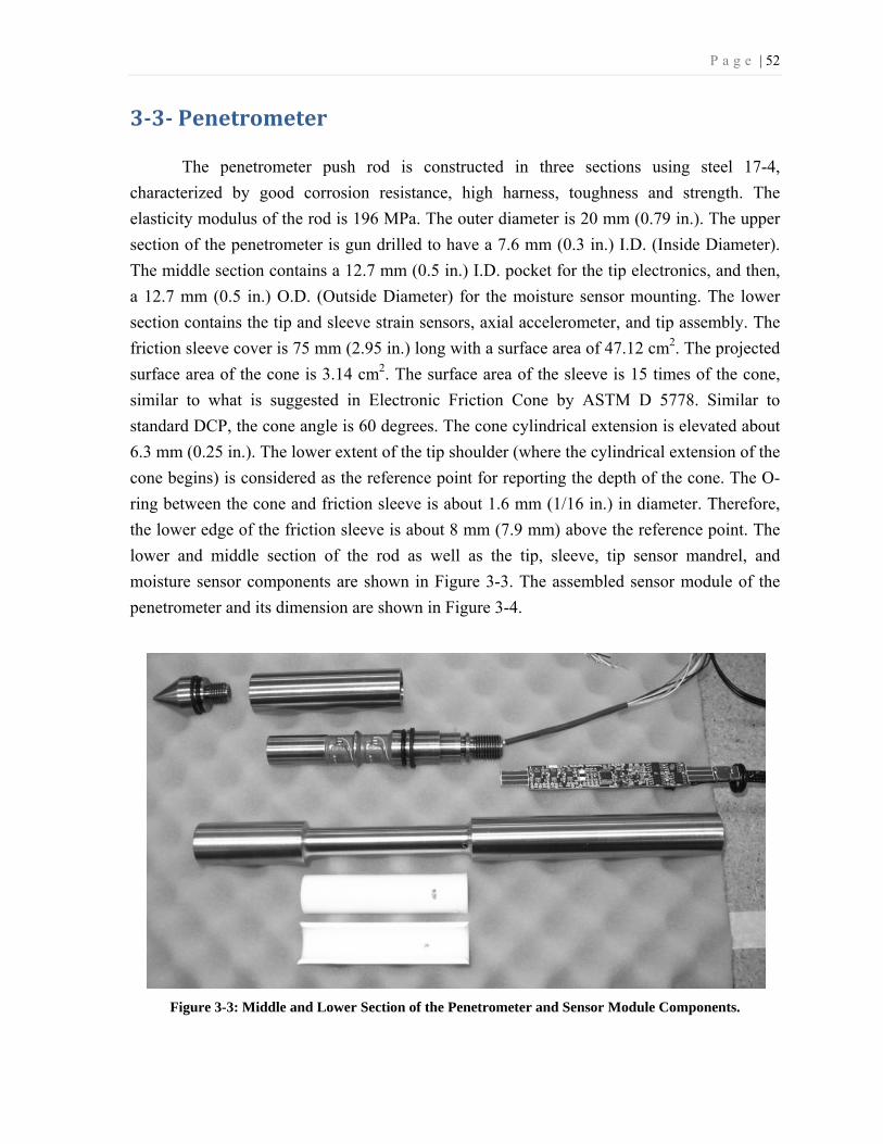
P a g e | 52
3-3- Penetrometer
The penetrometer push rod is constructed in three sections using steel 17-4,
characterized by good corrosion resistance, high harness, toughness and strength. The
elasticity modulus of the rod is 196 MPa. The outer diameter is 20 mm (0.79 in.). The upper
section of the penetrometer is gun drilled to have a 7.6 mm (0.3 in.) I.D. (Inside Diameter).
The middle section contains a 12.7 mm (0.5 in.) I.D. pocket for the tip electronics, and then,
a 12.7 mm (0.5 in.) O.D. (Outside Diameter) for the moisture sensor mounting. The lower
section contains the tip and sleeve strain sensors, axial accelerometer, and tip assembly. The
friction sleeve cover is 75 mm (2.95 in.) long with a surface area of 47.12 cm2. The projected
surface area of the cone is 3.14 cm2. The surface area of the sleeve is 15 times of the cone,
similar to what is suggested in Electronic Friction Cone by ASTM D 5778. Similar to
standard DCP, the cone angle is 60 degrees. The cone cylindrical extension is elevated about
6.3 mm (0.25 in.). The lower extent of the tip shoulder (where the cylindrical extension of the
cone begins) is considered as the reference point for reporting the depth of the cone. The O-
ring between the cone and friction sleeve is about 1.6 mm (1/16 in.) in diameter. Therefore,
the lower edge of the friction sleeve is about 8 mm (7.9 mm) above the reference point. The
lower and middle section of the rod as well as the tip, sleeve, tip sensor mandrel, and
moisture sensor components are shown in Figure 3-3. The assembled sensor module of the
penetrometer and its dimension are shown in Figure 3-4.
Figure 3-3: Middle and Lower Section of the Penetrometer and Sensor Module Components.

P a g e | 53
A slot is machined in the upper penetrometer section to provide an exit for the signal
and power cables to the tip electronics module. The push rod assembly also contains a mount
for the top electronics module that is attached via a visco-elastic shock mount to the lower
anvil surface. Except for the anvil joint, Loctite 224 thread locker is used on all threaded
joints to prevent joint loosening under the shock loads.
3-4- Impact System (Hammer and Anvil)
The RapSochs hammer is made of stainless steel and weighs 9090 g (20 lb). The rest
of the RapSochs including penetrometer, hammer guide, wires, and connections weigh 6300
g. The hammer consists of three cylinders bolted together with a longitudinal hole in the
middle for the hammer guide. This internal opening has a diameter of 15.9 mm (5/8 in.). The
guide for the sliding hammer is a rod with the length of 66 cm (26 in.) and diameter of 14.3
mm (9/16 in.), screwed to the top of the anvil. The dimensions of the hammer are shown in
Figure 3-5.
Figure 3-4: Assembeled Sensor Module and its Dimension.
76 mm
Moisture Sensor
75 mm
Friction Sleeve Cone
Reference Point
51 mm 8 mm

P a g e | 54
Figure 3-5: RapSochs Hammer Side and Top View.
In the current revision, the hammer is manually lifted by the operator to a specific
level and is then released. The sliding hammer pounds on the anvil and drive the instrument
into the soil. The anvil is 51 mm (2 in.) in diameter and is mounted on top of the upper
section of the penetrometer. A layer of rubber disk on the top of the anvil is used to allow for
energy transfer and reduce impact noise. Although some studies (e.g., Tsai et al., 2004)
suggest that the effect of hammer shape on the energy transfer is negligible; other studies in
pile driving and SPT literatures (e.g., Seed et al., 1985; Skempton, 1986; Odebrecht et al.,
2005) suggest that the efficiency is also influenced by the shape and diameter of the
striking/struck surfaces. Since the DCP penetrates into the hardest soil (2mm/blow in CBR
100), the existing manual DCP concept is used as a baseline configuration for the
hammer/anvil design. However, in ASTM D 6951, no specification or dimension of hammer
and anvil are indicated except the weight of the hammer. Figure 3-6 shows the shape of the
DCP hammer depicted in ASTM D 6951. This is the same as the shape of the Kessler DCP
hammer used in DCP tests conducted in this study.
103 mm
104 mm
102 mm
51 mm 18 mm

P a g e | 55
Figure 3-6: DCP Hammer Side and Top View (After ASTM D6951).
RapSochs hammer/anvil is different from DCP hammer/anvil in the following
aspects: 1) the RapSochs hammer is heavier than the DCP to improve energy efficiency, 2)
the shape of the RapSochs hammer is different from the typical DCP hammer shape, 3) in
DCP the anvil cross section is only slightly smaller than the hammer’s at the contact surface
while in RapSochs the anvil diameter is half the hammer diameter at the contact surface, and
4) in DCP the impact contact is metal to metal, but in RapSochs, a layer of rubber smoothes
the impulse (in other devices, such as the Sol Solution PANDATM (Gourves and Barjot,
1995), a “dead blow hammer” is used instead of a metal to metal contact to decrease the
impulse peak).
The drop height is variable in the RapSochs while is constant (57.4 cm or 22.6 in.) in
the DCP. The maximum hammer drop height in RapSochs is limited to 55.9 cm (22 in.).
Since the system efficiency and comparison between DCP and RapSochs is one of the
important aspects of this study, the energy transfer efficiency will be investigated in further
details in next chapters.
3-5- Sensor Configuration
The following sensing functions are provided in RapSochs:
1- Tip strain: from full bridge strain gauge,
2- Sleeve strain: using second strain gauge bridge,
3- Tip acceleration: from accelerometer,

P a g e | 56
4- Moisture content: using Moisture sensor,
5- Penetration/blow: from string potentiometer.
Figure 3-7 illustrates the physical layout of the sensor module in the tip implemented
in RapSochs. This module includes sensors for tip (bearing) and sleeve (friction) stresses,
electrical impedance spectroscopy (for moisture content) and acceleration. The sensor
module consists of two separate physical sections, the tip sensor module, shown in Figure 3-
8, and the moisture sensor module. All parts except the electrical insulators, moisture sensor
cover, and O-rings are constructed of an alloy of stainless steel hardened to 47 Rockwell.
Properties and configurations of each sensor are explained in the following sub-sections.

P a g e | 57
Figure 3-7: Penetrometer Sensor Module including Tip and Moisture Sensor Module.
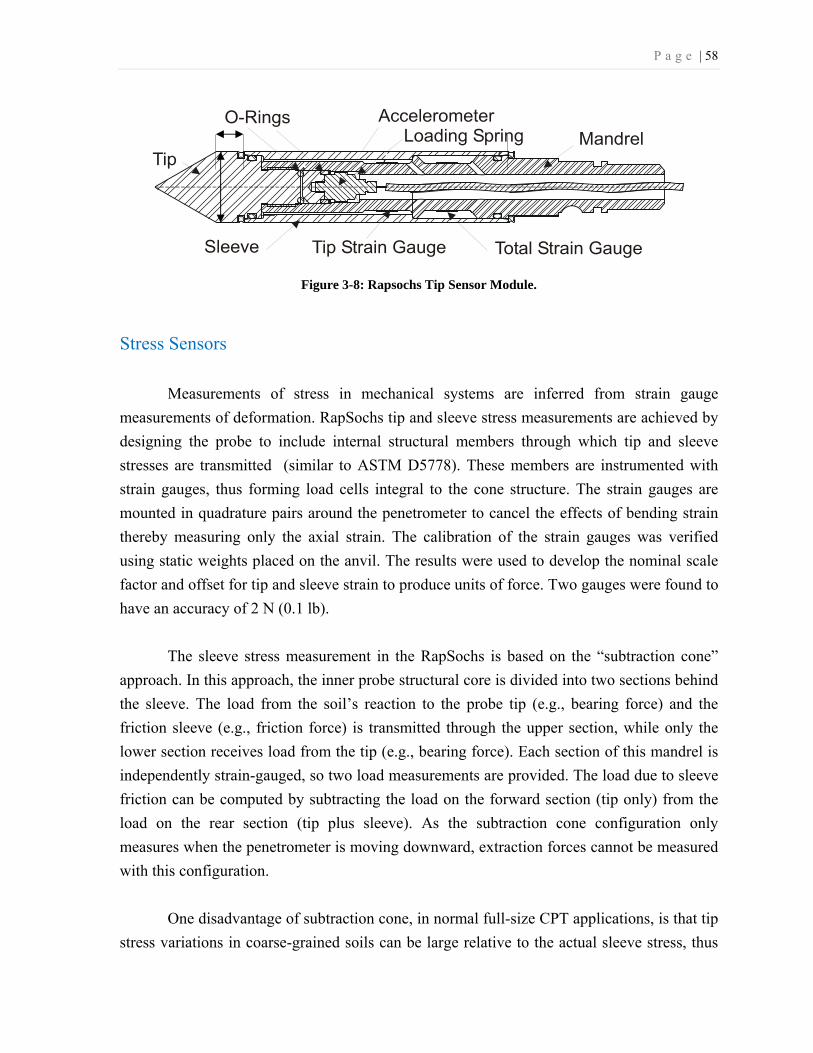
P a g e | 58
Figure 3-8: Rapsochs Tip Sensor Module.
Stress Sensors
Measurements of stress in mechanical systems are inferred from strain gauge
measurements of deformation. RapSochs tip and sleeve stress measurements are achieved by
designing the probe to include internal structural members through which tip and sleeve
stresses are transmitted (similar to ASTM D5778). These members are instrumented with
strain gauges, thus forming load cells integral to the cone structure. The strain gauges are
mounted in quadrature pairs around the penetrometer to cancel the effects of bending strain
thereby measuring only the axial strain. The calibration of the strain gauges was verified
using static weights placed on the anvil. The results were used to develop the nominal scale
factor and offset for tip and sleeve strain to produce units of force. Two gauges were found to
have an accuracy of 2 N (0.1 lb).
The sleeve stress measurement in the RapSochs is based on the “subtraction cone”
approach. In this approach, the inner probe structural core is divided into two sections behind
the sleeve. The load from the soil’s reaction to the probe tip (e.g., bearing force) and the
friction sleeve (e.g., friction force) is transmitted through the upper section, while only the
lower section receives load from the tip (e.g., bearing force). Each section of this mandrel is
independently strain-gauged, so two load measurements are provided. The load due to sleeve
friction can be computed by subtracting the load on the forward section (tip only) from the
load on the rear section (tip plus sleeve). As the subtraction cone configuration only
measures when the penetrometer is moving downward, extraction forces cannot be measured
with this configuration.
One disadvantage of subtraction cone, in normal full-size CPT applications, is that tip
stress variations in coarse-grained soils can be large relative to the actual sleeve stress, thus

P a g e | 59
adding noise to the sleeve stress data obtained via subtraction. Part of the reason for this
disadvantage is that standard CPT stress measurements are taken nearly instantaneously
about once a second. Variations that last a fraction of a second and are not representative of
the entire depth traveled between measurements can, therefore, find their way into CPT data.
However, in RapSochs: 1) data are inherently discretized by the distance traveled with each
blow of the drop hammer, 2) high-frequency data-acquisition and processing capability is
implemented, and 3) the penetration depth per blow is limited to obtain a better resolution of
soil layers. Therefore, RapSochs can perform oversampling and integration of stress
measurements to produce average stress data that are representative of the depth traveled due
to each hammer blow.
On the other hand, both the tip stress and sleeve stress measurements in conventional
CPT are obtained via internal strain gauge readings combined with the knowledge of probe
geometry and material properties (e.g., modulus of steel). The dynamic loading of the
RapSochs impact hammer will, however induce rapidly moving (5500 m/s) internal stress
waves and reflections in the probe system that will also be registered by the internal strain
gauges that measure tip and sleeve load. Therefore, the periodic component of the sleeve and
tip stress measurements cannot be simply “averaged out” in RapSochs as it is done in the
CPT data. The actual strain which is seen at rest is comprised of three terms: the dead weight,
the thermal drift, and the hysteresis. The hysteresis is the largest, so it swamps the dead
weight. That is why strain gauges must be zeroed prior to each use for accurate results.
Accelerometer
A PCB, Model 353B12 accelerometer, with a working range of +/-1000 g (gravity)
and a frequency response of 1 to 10,000 Hz, is mounted behind the tip to measure
acceleration. The frequency response matches with the dynamic data recorded at 10 kHz. The
main object of measuring acceleration was to calculate energy transferred to soil and to
detect the hammer impact to trigger data acquisition. The option to calculate the instrument
penetration by double integration of the acceleration did not provide accurate results, and the
string potentiometer remained the only displacement measurement device in the system. A
maximum of 1000 g measuring range of the acceleration was exceeded in several tests in
hard materials. However, it was very reliable for triggering data acquisition after any blow.

P a g e | 60
The accelerometer is positioned as far forward as possible so the motion it registers is
representative of the motion experienced by the tip. This approach frees the accelerometer
data of artifacts resulting from compression of the probe assembly under dynamic load,
internal stress waves, and off-axis noise due to lateral vibration of the probe. In this position,
the accelerometer measurements are most representative of the net motion of the tip relative
the soil. Since the penetrometer tip is replaceable and the accelerometer cannot be bolted or
glued to the tip, the accelerometer was spring loaded to the tip through two elastic O-rings.
This configuration reduces the peaks transferred to the accelerometer and permits easy tip
replacement.
The accelerometer was initially used to trigger the data acquisition after each blow.
The accelerometer did not work reliably in this respect during testing at NU. To continue the
test program without any interruption, the trigger function was configured to use the tip strain
signal later. It became clear that the accelerometer data may not be totally reliable due to
several reasons, and could not be used for energy and displacement measurements. The use
of the accelerometer to produce displacement by double-integration was found not valid due
to the effects of electronic noise, drift, hysteresis, temperature, and other factors. Considering
these issues with acceleration, the approach to obtain the net energy transferred to soil was
abandoned. However, other analytical and empirical methods are developed to evaluate the
system efficiency. The lack of accelerometer data limited the possibility of advanced data
analysis and interpretation of the dynamic response for the tests performed on different soil
samples.
Moisture Sensor
An electrical impedance spectroscopy (EIS) sensor is used to measure the volumetric
moisture. In the radio-frequency between 1 to 50 MHz, soil exhibits a relaxation due to
surface polarizations, which is the result of different permittivity and conductivity of soil
solids and water (Gamache, 2008b; Gamache, 2009b; and Rinaldi and Francisca, 1999). This
relaxation is called Maxwell-Wagner relaxation effect. It has been found that density and
moisture content of soil affect the electromagnetic response spectrum of excited soil.
TransTech has developed an instrument for use in road construction QC applications
based upon this technology. In a well-graded sandy soil, moisture determination accuracy of
1% has been achieved in the laboratory. The results are based upon previous calibration

P a g e | 61
using the same soil. As the moisture dominates the dielectric response of soil due to the fact
that the permittivity of water is 20 times higher than that of the soil solids, TransTech
believes that calculation of moisture alone, without previous calibration, may be possible.
The moisture sensor is 76 mm (3.00 inches) long, and the lower edge is 133 mm (5.25
inches) from the lower extent of the tip shoulder. The EIS moisture sensor consists of a
transmitter that transmits electromagnetic radiation into the soil and a receiver, spaced
approximately 64 mm (2.5 inches) from the transmitter, senses the received signal that has
been affected by the dielectric properties of the soil. The measured data consists of
frequency, magnitude, and phase of 60 frequencies ranging from 0.5 to 30 MHz. The sensor
takes impedance spectra at intervals between each penetration of RapSochs.
The EIS approach is currently used in Soil Density Gauge (SDG) or Electrical
Density Gauge (EDS) to measure the density and water content of soils (Gamache et al.,
2008b). This design is a cylindrical adaptation of the EIS sensor used in TransTech’s SDG.
The layout of moisture sensor and its components, including transmitter (Tx), receiver (Rx),
guard electrode, insulator and the cover are shown in Figure 3-9.
Figure 3-9: Rapsochs Moisture Sensor.
The outer surface of the first moisture sensor in Rev. 0 was comprised of electrical
shrink tubing that failed during the first test in a hard material (~CBR 50). The next cover
was rebuilt using a matrix of stone and epoxy for much greater abrasion resistance. The
matrix consisted of 86% washed crushed sieved stone particles passing sieve No. 80 (0.177
mm), retained on No. 100 (0.149 mm) and 14% Scotch-Weld DP-420 epoxy. The sensor
surface is 0.05 mm (~0.002 in.) below the penetrometer surface to further minimize the
chance of abrasion. The metal transmitter and receiver electrodes are covered by only 0.25
mm of the stone matrix. This configuration survived all tests conducted at NU, and numerous
tests conducted later at TransTech. The sensor surface showed only superficial scratches.

P a g e | 62
In order to force the electromagnetic field as deep as possible into the soil, to
maximize the measurement volume, the transmitter and receiver are insulated, and placed as
far away as possible from the metal core. Any current that may flow from the receiver to the
metal penetrometer could cause errors. To obtain accurate measurements, only the current
flowing from the transmitter into the receiver through the soil should be measured. A guard
electrode, placed between the receiver and the metal penetrometer core, is used to minimize
the potential for current losses. This helps to maintain the guard potential equal to the
receiver potential. With equal potential in the guard and receiver, no current losses would
occur, which eliminates the source of error. The details of the moisture sensor design
including size, spacing between the electrodes, and the insulation layer were developed by
TransTech using the COMSOL Multiphysics finite element modeling (FEM) software.
Figure 3-10 shows the modeling result of the final configuration. The measuring volume
extends out radially 19 mm (0.75 in.) from the rod surface and is about 38 mm (1.5 inch)
high. This provides reasonable spatial averaging for soil particle sizes up to 19 mm (0.75 in.).
Figure 3-10: RapSochs Moisture Sensor Finite Element Modeling Shows the Penetration of the
Electromagnetic Field in Soil (From Analysis by TransTech Systems Inc.).
P a g e | 63
The moisture measurement accuracy of this sensor was not investigated
independently before incorporation into RapSochs. However, the calibration analysis for
similar sensors developed by ARA showed that 70% of the data, obtained from multiple soil
types, fall within ± 4% range of actual volumetric moisture content. According to ASTM
D2216 for measuring soil water content, the coefficient of variation is reported to be 2.7%
for single-operator tests. Therefore for 95% confidence level, the variability of ± 5.4% is
expected based on ASTM D2216. In that standard, it is also mentioned that if results from
two tests do not differ more than 7.8% from the average, they are considered acceptable.
Although the new sensor needs a comprehensive calibration and validation before
commercialization, but in comparison to an acceptable standard method, the technology
sounds promising.
Displacement
A UniMeasure’s PA 50 cable extension transducer, also known as string
potentiometer, is used to record RapSochs advancement per blow. String potentiometer is a
device used to measure linear position using a flexible cable and a spring-loaded spool. The
device produces a DC voltage output linearly proportional to the length of the extended string
(which is spooled from a spring-loaded multi-revolution rotary potentiometer internal to the
device). The string potentiometer causes a relatively constant downward force measured to
be 10.2 N (in its manual it is reported to be 9.5 N). The maximum acceleration of the wire
rope is around 50 g, which means that it could only respond accurately to motions lower than
this acceleration. Figure 3-11 shows the string potentiometer grounded to a heavy steel plate
resting on the soil surface. The free end of the cable is attached to the anvil.

P a g e | 64
Figure 3-11: String Potentiometer Bolted to a Steel Plate beside the RapSochs Cone.
The string potentiometer provides a very reliable absolute position reference. Thus, it
does not require knowledge of the initial position to obtain the current position of the probe.
However, testing results indicated that the string potentiometer does not respond well to rapid
changes in rod position and exhibits a tendency to vibrate following hammer blows. In other
words, the dynamic response is affected by the vibration of the string potentiometer wire, and
it is not suitable for dynamic response analysis such as, velocity measurement or rebound of
the rod expected after the penetrometer stops shearing the soil. Therefore, it is used to
measure only the net penetration per blow.
Another disadvantage is a thin wire string outside of RapSochs that may easily wear
or break. This wire is a potential reliability issue as the unit can be readily damaged, if the
wire is released while extended. This happened twice during testing at NU and in both cases
resulted in total damage to the unit.
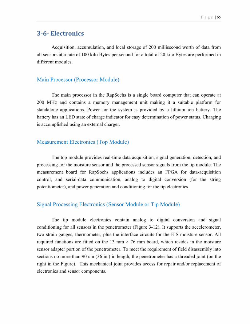
P a g e | 65
3-6- Electronics
Acquisition, accumulation, and local storage of 200 millisecond worth of data from
all sensors at a rate of 100 kilo Bytes per second for a total of 20 kilo Bytes are performed in
different modules.
Main Processor (Processor Module)
The main processor in the RapSochs is a single board computer that can operate at
200 MHz and contains a memory management unit making it a suitable platform for
standalone applications. Power for the system is provided by a lithium ion battery. The
battery has an LED state of charge indicator for easy determination of power status. Charging
is accomplished using an external charger.
Measurement Electronics (Top Module)
The top module provides real-time data acquisition, signal generation, detection, and
processing for the moisture sensor and the processed sensor signals from the tip module. The
measurement board for RapSochs applications includes an FPGA for data-acquisition
control, and serial-data communication, analog to digital conversion (for the string
potentiometer), and power generation and conditioning for the tip electronics.
Signal Processing Electronics (Sensor Module or Tip Module)
The tip module electronics contain analog to digital conversion and signal
conditioning for all sensors in the penetrometer (Figure 3-12). It supports the accelerometer,
two strain gauges, thermometer, plus the interface circuits for the EIS moisture sensor. All
required functions are fitted on the 13 mm × 76 mm board, which resides in the moisture
sensor adapter portion of the penetrometer. To meet the requirement of field disassembly into
sections no more than 90 cm (36 in.) in length, the penetrometer has a threaded joint (on the
right in the Figure). This mechanical joint provides access for repair and/or replacement of
electronics and sensor components.

P a g e | 66
Figure 3-12: Tip Electronics Assembly.
3-7- Software and Programs
The RapSochs system and user interface software was written using the C#
programming language and Visual Basic. The software communicates with the RapSochs
main processor using a standard serial communication port through a serial to USB
convertor. A tethered laptop computer provides the operator interface, controls the system,
and stores data. The non-real-time critical control and measurement functions are executed
on the external laptop computer. The real time measurement control and data acquisition are
performed by firmware executing in the top module.
Data is acquired from the strain gauges, accelerometer, as well as the string
potentiometer in response to a hammer impact for 0.2 seconds at a rate of 10 KHz (2048 data
points). The time is sufficient for all rebounds to occur and the penetrometer to come to rest.
The data acquisition starts by the software prior to the hammer drops and stops when 1948
data points after the hammer impact are collected. It makes the total collected data points of
2048 digital readings. The impact is detected by the rise of the signal from a user specified
sensor (the accelerometer or strain gauges). This provides 100 data points prior to the impact
that are used to perform auto zero of each sensor, thereby, removing offset and low rate drift
due to hysteresis and thermal effects. It also removes offsets and the dead-weight strain and
initial extension of the string potentiometer. To avoid aliasing, the sampling rate must exceed
the Nyquist rate. Based on Nyquist frequency (half the sampling frequency), the data rate is
high enough to sample the compression wave moving up and down the 1-meter-long
penetrometer at 5500 m/sec.

P a g e | 67
The data transfer from the top module to the external computer was changed from
ASCII format to binary to considerably facilitate the process. Three calibration and setup
files provide the data necessary to convert raw sensor data into engineering units and to
specify user settable control parameters necessary to initialize sensor and data acquisition
settings. These files are stored in ASCII format. The file formats are defined in Chapter 4 and
in Appendix B.
The user’s interaction with the software to operate and control the measurements
consists of the following steps,
1. On the setup screen, operator enters the Job ID for current test.
2. The software reads calibration files (calibration.dat, trigger.dat, and
moisture.dat) from the disk. The calibration.dat contains factors to convert the
raw sensor data to engineering units based upon sensor calibration data. The
trigger.dat defines the sensor to be used to detect the hammer impact and the
detection level. Finally, the moisture.dat file defines the frequency range and
transmit-signal level for the moisture sensor.
3. For the first blow of a test, depress the “Reset Test Indexes” button. Depress
“ON/RESET” to initialize all modules and arm the data acquisition. The Acquire
Tip and Moisture buttons then become available.
4. Depress the “Moisture” button to acquire a moisture sensor reading, and the
software converts spectra to engineering units.
5. Depress “Acquire Tip” to arm the data acquisition sequence. After the operator
drops the hammer and upon detection of the trigger, the 2048 points are converted
into engineering units.
6. The data are transferred from the top module to the laptop and saved as ASCII
files.
7. The raw moisture sensor and tip data are written to the disk in separate files.
The complete operation procedure of RapSochs is presented in Appendix B. Figure 3-
13 presents a view of the RapSochs user interface before arming the instrument.

P a g e | 68
Figure 3-13: A View of RapSochs User Interface.
The after-test analysis programs are written in MATLAB® language for technical
computing. The data acquired by the tests are converted into a central database for further
data analysis and data presentation. A list of major MATLAB® codes is provided in
Appendix C and the objective of each code is also explained.

P a g e | 69
Chapter 4: Materials and Methods
4-1- Introduction
The objectives of the experimental program include performing several tests with
RapSochs along with DCP in the soil samples prepared in the laboratory with different soil
types at different conditions. The collected data in the experimental program are the basis for
developing the necessary algorithms and procedures to extract geotechnical data from
RapSochs measurements. Comparison of RapSochs performance with that of DCP under
controlled laboratory conditions in uniformly prepared samples is another objective of the
plan.
The first part of this chapter describes the procedure for soil samples preparation. The
properties of prepared samples, used to establish the ground truth for the soil characteristics,
are also measured or calculated. Later in this Chapter, RapSochs and DCP test procedures are
described. Detailed procedures for assembly, maintenance, and calibration tests are presented
in Appendix B. All the tests are conducted in soil samples prepared in the laboratory at the
SoilBED facilities of NU.
4-2- Soil Samples
For the controlled testing at the SoilBED facilities, the preliminary plan was to cover
soil types that represent the corners of the Robertson’s curve (Robertson, 1990) including
gravelly sand, sensitive fine-grained, clay to silty clay, very stiff clayey sand, and sandy silt.

P a g e | 70
The test plan was modified, primarily because some concerns were raised during tests (e.g.,
penetration in high CBR materials and accuracy of moisture sensor calibration). Overall,
RapSochs was tested in eighteen different conditions of compaction, soil type and moisture
content. The prepared soil samples include:
- Poorly-graded sand,
- Well-graded sand with gravel,
- Sandy fat clay,
- Sandy silt, and
- Clayey sand,
which are prepared by mixing the primary soils, consisting of:
- Fine-grained sand,
- Medium-grained sand,
- Silt,
- Gravel, and
- Bentonite.
Samples were prepared to have soil strengths ranging from loose low-strength
material up to compacted soils with a CBR of 50. The list of soil samples prepared in the lab
for DCP and RapSochs tests is presented in Table 4-1. “Sample ID”, a 3-letter code, is used
to identify each soil sample for further reference based on the name of the soil sample.
Sample Preparation
A standard procedure, described below, was followed for sample preparation. The
soil types used for testing were either available naturally or they were mixed to make a new
soil to match testing needs. Available materials include: fine-grained sand, medium-grained
sand, silt, gravel, and bentonite. The grain size distribution curves of these soils, except
bentonite, are presented in Figure 4-1.

P a g e | 71
Table 4-1: List of Soil Samples and Their IDs.
Sample Name Sample ID
Beach Sand Compacted BSC
Beach Sand Loose BSL
Clay 60% and Sand C6S
Clayey Sand in Beige container CSB
Clayey Sand in Red container CSR
Gravel mixture GRV
Rocky Sand Compacted RSC
Rocky Sand Double compacted RSD
Rocky Sand Loose RSL
Silt compacted SIL
Silt Semi-compacted SIS
for Moisture Sensor test, w≈0% MS0
for Moisture Sensor test, w≈1% MS1
for Moisture Sensor test, w≈2% MS2
for Moisture Sensor test, w≈3% MS3
for Moisture Sensor test, w≈4% MS4
for Moisture Sensor test, w≈5% MS5
for Moisture Sensor test, w>6% (saturated) MS6
Figure 4-1: Grain Size Distribution of the Original Materials.
0
20
40
60
80
100
0.001 0.010 0.100 1.000 10.000 100.000
Perc
ent
Pas
sing
(%)
Sieve Openning (mm)
Silt
Medium-Grained Sand
Fine-Grained Sand
Gravel

P a g e | 72
Both types of sand are well-sorted (i.e. poorly graded) beach sand. The coarser sand
grains are subangular and slightly elongated and the finer sand grains are subrounded. The
grains of medium-grained sand tend to be randomly oriented when pluviated and compacted
to low or high densities (Mahmood et al., 1976). The silt was collected from New York State
and contains small percentage of sand and gravel. However, most of the silt was in the form
of clods and sample preparation required crushing, sieving through sieve No. 4 (4.75 mm
opening), and remixing to prepare uniform samples. The grain size distribution of the silt in
Figure 4-1 is for the sieved silt. The gravel is fine and has the uniformity and curvature of 3.1
and 1.2, respectively, and classified as poorly graded gravel.
The bentonite source is Volclay® general purpose granular bentonite (GPG-30),
known as Western Bentonite, produced by American Colloid Company. Its main mineral is
sodium montmorillonite (American Colloid Company, 2005). Once uniformly mixed with
water and compacted, the granular bentonite is treated similar to montmorillonite clay (Ito,
2006). The plastic and liquid limit of bentonite are measured 47% and 425%, respectively.
BSC and BSL are fine-grained sand. RSC, RSD and RSL are medium-grained sand.
SIL and SIS are silt. Batches of MS0, MS1, MS2, MS3, MS4, MS5, MS6, and GRV soils are
prepared by mixing 17% of fine-grained sand, 18% of medium-grained sand, and 70% of
gravel. C6S, CSB and CSR were basically bentonite-sand mixtures. CSB and CSR are
mixture of 70% (by dried weight) of medium-grained sand and 30% bentonite. The final
mixture is estimated to have 97%, 59%, and 31% by weight passing through No.10, No. 40,
and No. 200 U.S. sieves, respectively, and classified as Clayey Sand. C6S is a mixture of
60% bentonite and 40% of fine-grained sand.
The samples moisture content was selected based on standard compaction curves and
compaction effort that are planned for sample preparation. For preparation of BSC, GRV,
RSC, RSD, SIL, SIS, and MS0 to MS6, after the dry materials were mixed in a commercial
mixer, a predetermined amount of water was added, and mixing was continued. The soil-
water mix was then placed in the testing container and compacted in 5-cm (2-inch) lifts using
standard proctor hammer.
RSL and BSL were two loose samples prepared by pluviation of dry sand into the
containers. RapSochs and DCP tests on these samples were not possible due to lack of
strength. The soil was so loose that both devices sunk into the soil under their own weight.
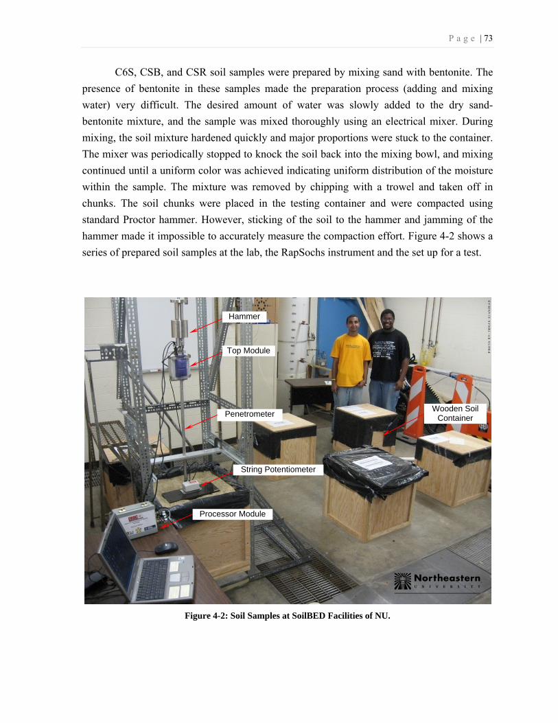
P a g e | 73
C6S, CSB, and CSR soil samples were prepared by mixing sand with bentonite. The
presence of bentonite in these samples made the preparation process (adding and mixing
water) very difficult. The desired amount of water was slowly added to the dry sand-
bentonite mixture, and the sample was mixed thoroughly using an electrical mixer. During
mixing, the soil mixture hardened quickly and major proportions were stuck to the container.
The mixer was periodically stopped to knock the soil back into the mixing bowl, and mixing
continued until a uniform color was achieved indicating uniform distribution of the moisture
within the sample. The mixture was removed by chipping with a trowel and taken off in
chunks. The soil chunks were placed in the testing container and were compacted using
standard Proctor hammer. However, sticking of the soil to the hammer and jamming of the
hammer made it impossible to accurately measure the compaction effort. Figure 4-2 shows a
series of prepared soil samples at the lab, the RapSochs instrument and the set up for a test.
Figure 4-2: Soil Samples at SoilBED Facilities of NU.
Hammer
String Potentiometer
Penetrometer
Top Module
Wooden Soil Container
Processor Module

P a g e | 74
Containers
Based on the test plan, the objective of each test, and soil types, samples are prepared in four
different types of containers: 1) wooden containers, 2) plastic cylindrical containers, 3) a
metallic container, and 4) Plaxiglass container. The inside dimensions of containers are
summarized in Table 4-2. Container size is selected to allow conducting as many tests as
possible while the preparation process is manageable. However, for metallic and plastic
containers, available sizes dictated the testing plan.
Samples BSC, BSL, RSC, RSD, RSL, SIL and SIS were prepared in wooden strongboxes.
The major reason for choosing wood was to reduce the effect of stress wave reflection of
more rigid boundaries as well as possible interference of other materials (e.g., metallic) on
moisture sensor measurements. Only the container of SIL material showed some signs of
bulging during sample preparation. The volume change of the container was used to evaluate
volumetric geotechnical properties of the soil. The dimensions of all boxes were verified
before and after testing to ensure no or minimal change due to penetration. The corner of
each box was sealed with Silicon sealant and the interior was painted with Minwax®
Helmsman Clear Gloss Spar Urethane to minimize any moisture loss through the wood and
then painted with a layer of oil-based Rust-Oleum® Protective Enamel, to protect the sealing
layer.
For the GRV sample, a metal container was used. The strength of the container was the only
reason to use metal instead of wood since the strength of the soil was predicted to be higher,
and the integrity of the container was a concern. The RapSochs penetration in high CBR
materials was verified using this sample and a 50 cm depth of penetration was achieved. MS0
to MS6 samples were prepared in plastic containers. The primary goal for tests in MS0 to
MS6 was to measure the moisture content. C6S sample was prepared in a plastic container as
well. The container’s wall thickness was 5 mm, and no dimension change prior and after
penetration test was observed. CSR is also prepared in a plastic container similar to MS0-6
containers. CSB was prepared in a Plexiglass box. Plexiglass is a very rigid material and if
joints hold, no deflection (in mm scale) is expected. Its transparency also made it possible to
observe the prepared sample, examine to see if air pockets are formed during preparation,
and check for any obvious boundary effect during penetration test. The effects of sample size
and boundary conditions on test results are discussed in Chapter 6.
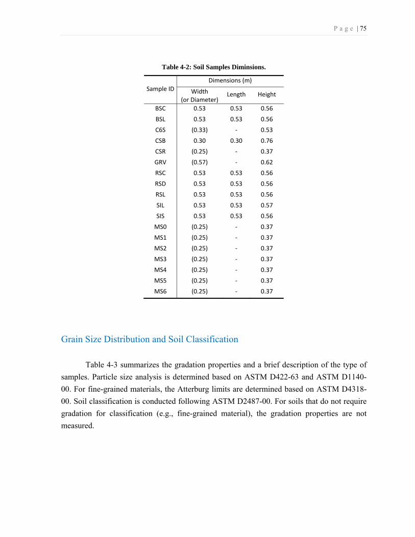
P a g e | 75
Table 4-2: Soil Samples Diminsions.
Sample IDDimensions (m)
Width(or Diameter)
Length Height
BSC 0.53 0.53 0.56
BSL 0.53 0.53 0.56
C6S (0.33) - 0.53
CSB 0.30 0.30 0.76
CSR (0.25) - 0.37
GRV (0.57) - 0.62
RSC 0.53 0.53 0.56
RSD 0.53 0.53 0.56
RSL 0.53 0.53 0.56
SIL 0.53 0.53 0.57
SIS 0.53 0.53 0.56
MS0 (0.25) - 0.37
MS1 (0.25) - 0.37
MS2 (0.25) - 0.37
MS3 (0.25) - 0.37
MS4 (0.25) - 0.37
MS5 (0.25) - 0.37
MS6 (0.25) - 0.37
Grain Size Distribution and Soil Classification
Table 4-3 summarizes the gradation properties and a brief description of the type of
samples. Particle size analysis is determined based on ASTM D422-63 and ASTM D1140-
00. For fine-grained materials, the Atterburg limits are determined based on ASTM D4318-
00. Soil classification is conducted following ASTM D2487-00. For soils that do not require
gradation for classification (e.g., fine-grained material), the gradation properties are not
measured.

P a g e | 76
Table 4-3: Soil Classification and Grain Size Distribution of Soil Samples.
Sample
ID USCS
Opening (mm) Uniformity
(Cu)
Curvature
(Cc) D60 D50 D30 D10
BSC SP (Poorly graded sand) 0.41 0.3 0.24 0.15 2.7 1.0
BSL SP (Poorly graded sand) 0.41 0.3 0.24 0.15 2.7 1.0
C6S CH (Sandy Fat Clay)** 0.075 <0.075
CSB SC (Clayey Sand)*** 0.51 0.42 ~0.075
CSR SC (Clayey Sand)*** 0.51 0.42 ~0.075
GRV SW (Well graded sand with gravel) 5.57 4.65 1.76 0.31 18 1.8
RSC SP (Poorly graded sand) 0.80 0.59 0.47 0.28 2.9 1.0
RSD SP (Poorly graded sand) 0.80 0.59 0.47 0.28 2.9 1.0
RSL SP (Poorly graded sand) 0.80 0.59 0.47 0.28 2.9 1.0
SIL ML (Sandy silt) <0.075 <0.075
SIS ML (Sandy silt) <0.075 <0.075
MS0-6* SW (Well graded sand with gravel) 5.57 4.65 1.76 0.31 18 1.8
NOTES: *Includes Sample MS0, MS1, MS2, MS3, MS4, MS5, and MS6.
** Plastic Limit =47 %, LL = 425% *** Plastic Limit =28 %, LL = 403%

P a g e | 77
Compaction Curves
Table 4-4 presents the compaction effort used to prepare each samples. Figure 4-3
shows the compaction curves of soil materials obtained following ASTM D698-00. The
compaction curves for sample C6S, CSB, and CSR are not obtained. Compaction properties
of bentonite and bentonite-sand materials are available in literatures (e.g., Ito, 2006; Tay et
al., 2001; Akgun et al., 2006; Filippo et al. 1998; and Ito and Komine, 2008). Based on
similar cases, the optimum moisture contents for CSB and CSR are estimated to be 10 to 20
percent and 25 to 35 percent for C6S. However for C6S, the variations in dry density are very
small for different water-content values. It should be mentioned that based on the moisture
content of samples presented in the next section, the CSB and CSR are prepared on the wet
side, and C6S is prepared on the dry side of compaction curve. As mentioned earlier, sticking
of the clay to the hammer and jamming of the hammer made it impossible to measure the
compaction effort for C6S, CSB, and CSR accurately.
Table 4-4: Compaction Effort Used to Prepare Samples.
Sample IDCompaction Effort
(kN-m/m3)
BSC ~600
BSL Pluviated
C6S Not Measured
CSB Not Measured
CSR Not Measured
GRV 600
RSC 300
RSD 600
RSL Pluviated
SIL 600
SIS 300
MS0 600
MS1 600
MS2 600
MS3 600
MS4 600
MS5 600
MS6 600
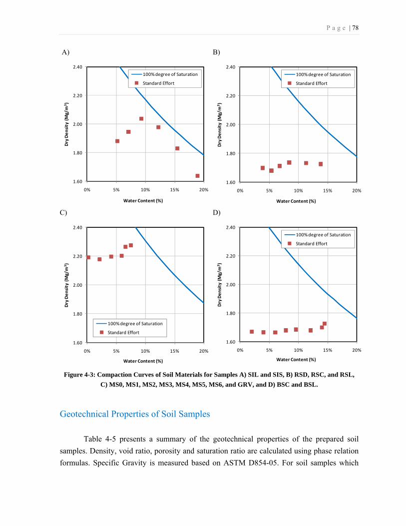
P a g e | 78
A) B)
C) D)
Figure 4-3: Compaction Curves of Soil Materials for Samples A) SIL and SIS, B) RSD, RSC, and RSL,
C) MS0, MS1, MS2, MS3, MS4, MS5, MS6, and GRV, and D) BSC and BSL.
Geotechnical Properties of Soil Samples
Table 4-5 presents a summary of the geotechnical properties of the prepared soil
samples. Density, void ratio, porosity and saturation ratio are calculated using phase relation
formulas. Specific Gravity is measured based on ASTM D854-05. For soil samples which
1.60
1.80
2.00
2.20
2.40
0% 5% 10% 15% 20%
Dry
Den
sity
(M
g/m
3 )
Water Content (%)
100% degree of Saturation
Standard Effort
1.60
1.80
2.00
2.20
2.40
0% 5% 10% 15% 20%
Dry
Den
sity
(M
g/m
3 )
Water Content (%)
100% degree of Saturation
Standard Effort
1.60
1.80
2.00
2.20
2.40
0% 5% 10% 15% 20%
Dry
Den
sity
(M
g/m
3 )
Water Content (%)
100% degree of Saturation
Standard Effort
1.60
1.80
2.00
2.20
2.40
0% 5% 10% 15% 20%
Dry
Den
sity
(M
g/m
3 )
Water Content (%)
100% degree of Saturation
Standard Effort
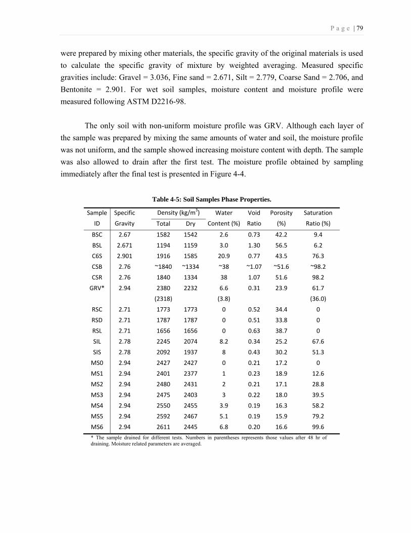
P a g e | 79
were prepared by mixing other materials, the specific gravity of the original materials is used
to calculate the specific gravity of mixture by weighted averaging. Measured specific
gravities include: Gravel = 3.036, Fine sand = 2.671, Silt = 2.779, Coarse Sand = 2.706, and
Bentonite = 2.901. For wet soil samples, moisture content and moisture profile were
measured following ASTM D2216-98.
The only soil with non-uniform moisture profile was GRV. Although each layer of
the sample was prepared by mixing the same amounts of water and soil, the moisture profile
was not uniform, and the sample showed increasing moisture content with depth. The sample
was also allowed to drain after the first test. The moisture profile obtained by sampling
immediately after the final test is presented in Figure 4-4.
Table 4-5: Soil Samples Phase Properties.
Sample
ID
Specific
Gravity
Density (kg/m3) Water
Content (%)
Void
Ratio
Porosity
(%)
Saturation
Ratio (%) Total Dry
BSC 2.67 1582 1542 2.6 0.73 42.2 9.4
BSL 2.671 1194 1159 3.0 1.30 56.5 6.2
C6S 2.901 1916 1585 20.9 0.77 43.5 76.3
CSB 2.76 ~1840 ~1334 ~38 ~1.07 ~51.6 ~98.2
CSR 2.76 1840 1334 38 1.07 51.6 98.2
GRV* 2.94 2380
(2318)
2232 6.6
(3.8)
0.31 23.9 61.7
(36.0)
RSC 2.71 1773 1773 0 0.52 34.4 0
RSD 2.71 1787 1787 0 0.51 33.8 0
RSL 2.71 1656 1656 0 0.63 38.7 0
SIL 2.78 2245 2074 8.2 0.34 25.2 67.6
SIS 2.78 2092 1937 8 0.43 30.2 51.3
MS0 2.94 2427 2427 0 0.21 17.2 0
MS1 2.94 2401 2377 1 0.23 18.9 12.6
MS2 2.94 2480 2431 2 0.21 17.1 28.8
MS3 2.94 2475 2403 3 0.22 18.0 39.5
MS4 2.94 2550 2455 3.9 0.19 16.3 58.2
MS5 2.94 2592 2467 5.1 0.19 15.9 79.2
MS6 2.94 2611 2445 6.8 0.20 16.6 99.6
* The sample drained for different tests. Numbers in parentheses represents those values after 48 hr of draining. Moisture related parameters are averaged.

P a g e | 80
Figure 4-4: Moisture Content Profile of GRV after Draining.
4-3- Test Setup
RapSochs and DCP penetration tests are conducted up to a depth between 305 mm
and 610 mm (12 to 24 inches), with most tests conducted up to 460 mm (18 inches). The total
possible penetration of the instrument is 910 mm (36 inches). A guide fixed on a frame was
used for all tests to support the RapSochs and DCP to keep it perpendicular to the soil surface
during testing. Figure 4-5 shows the assembled RapSochs set up ready for a test. The samples
were large enough so that multiple non-interfering penetrations are made for repeatability
and spatial averaging. The minimum spacing between penetrations was 5.9 times of cone
diameters. The effects of the boundary on test results are verified in next chapters.
-700
-600
-500
-400
-300
-200
-100
0
0% 2% 4% 6% 8% 10%
Dep
th (m
m)
Moisture Content

P a g e | 81
Figure 4-5: Running a test with RapSochs at SoilBED facilities of NU.
4-4- RapSoChs Test Procedure
The RapSochs tests are conducted following the instructions provided in Appendix B.
This is the latest revision of “RapSochs Rev. 0 Penetrometer Operating Instructions Revision
2 Phase 1” that was revised on 08/20/2007. In the instruction, the test sequence, operation
procedure, instrument assembly, inspection and maintenance are explained. The instruction is
revised three times to include changes in the software and/or instrument itself due to
improvement of the system. Summary of the instruction and explanation of other procedures
that are not included in the instruction is presented in this section. A one-page checklist
developed for testing at NU is also attached in Appendix E.
General Test Sequence 1. The system is assembled, checked, and initialized as described in the Operating
Instructions.
2. The RapSochs is placed on a 125 mm by 125 mm by 6 mm rigid metal plate on the
surface of the soil sample. The moisture sensor is activated to capture the initial

P a g e | 82
position of the rod. Then, the plate is removed, and the RapSochs is allowed to
penetrate by its own weight.
3. The operator raises the hammer to a predetermined height. The hammer is released
and dropped under its own weight. The drop height is determined based on the
procedure described in next subsection.
4. For each hammer blow, a dynamic data sequence is triggered by the impact of the
hammer and data are recorded.
5. After completion of the dynamic sequence, a moisture sensor reading is taken by the
operator after the penetrometer has stopped moving.
6. Steps 3 to 5 are repeated until the desired penetration depth is achieved. A MATLAB
script is used to check the penetration depth at any time to show the progress.
7. After the test reaches the desired depth, the instrument is disconnected from the
laptop and the main processor. Then, all connections are opened and removed,
including the string potentiometer. In soils with high adhesion, a system of pulleys
and cables are used to extract the penetrometer from the soil.
Hammer Drop Height Procedure
In general, the hammer drop height was adjusted to produce a penetration between 13 and 25
mm (0.5 and 1 inch) per blow. The procedure for determination of drop height was modified
once during a test series. In the first procedure followed for tests in GRV, BSC, RSC, RSD,
RSL, and the first test in SIL (for tests before 8/15/2007), the drop height started from 51 mm
(2 inches), and for any penetration less than 13 mm (0.5 inch), the drop height was increased
by 25 mm (1 inch). For tests conducted later, the drop height started from 127 mm (5 inches),
and any time that the penetration was less than 13 mm (0.5 inch) the drop height was
increased to 254, 381, 508 and 559 mm respectively (10, 15, 20 and 22 inches). In addition,
in order to assess the effect of variable hammer drop height, after the drop height was
established in 559 mm (22 inches), the drop height was decreased to 254 and 381 mm (10
and 15 inches) for few blows, and then back to 559 mm (22 inches) for the remaining blows.
The manual release of the hammer from a certain height is not very accurate. Experiences
showed that the precision is limited to ± 13 mm (0.5 in.).
P a g e | 83
Data File Format
A data block, 204.8 milliseconds long acquired at 10K samples/sec., is collected. The
total block is then 2048 samples long with 100 of the samples taken prior to the trigger event.
The data for each blow, including tip strain, sleeve strain, acceleration, string potentiometer
displacement, and tip temperature are stored in an ASCII file under the filename:
<JOB_ID>_tip_nn.dat
where nn is the file index which starts with 1 and is automatically incremented after each
blow. The converted data into engineering units are stored in:
<JOB_ID>_tip_nn_converted.dat
In a converted data file, data is saved in columns separated by at least one space in
signed ASCII format. The file contains five columns of data as follows.
Column1 XXXX.x Tip strain (lbf)
Column2 XXXX.x Total (sleeve + tip) strain (lbf)
Column3 XX.xx Axial acceleration (g)
Column4 XX.xx Displacement - String potentiometer (inches)
Column5 XX.XX Temperature (degree F)
The moisture sensor data are stored in a different file named:
<JOB_ID>_moisture_nn.dat
Moisture sensor data are saved in four-column format with the frequency in Hz.
Column1 Frequency (Hz)
Column2 Magnitude (dB)
Column3 Phase (degree)
Column4 String potentiometer (volt)
All “tip data”, “converted tip data”, and “moisture data” files are stored in one folder. In the
rest of this document, these files will be referred to as “data-files”.

P a g e | 84
Triggering
In early tests, the default triggering for data acquisition was the detection of positive
acceleration of 100 g above the static level of the accelerometer signal. In the second test in
GRV sample, concerns rose after observing a shift in the starting point of the captured data at
blow number 57 and after several failures in triggering. Although there was no problem with
triggering in the previous test in GRV, there was a small chance that the accelerometer may
have been damaged due to the high acceleration of the instrument during penetration tests in
high CBR material. Since then, the tip strain gage was used to trigger the data acquisition.
Calibration
The main purpose of the "calibration" procedure was to establish functionality. It was
not possible to establish a standard test that would produce an exact match of force and
acceleration each time. A 100 mm × 100 mm × 2.4 mm piece of Shore O Durometer 70
Sorbothane® is glued to the bottom of a 100 mm × 100 mm × 100 mm piece of pine wood
with a 60° depression cone is used for this procedure. The Sorbothane is put to reduce the
bouncing. Results are very repeatable using a 127 mm (5 inches) drop height. Maximum
measured force is around 4 kN. The fact that a block of wood, which wears over time, is used
for calibration resulted in some variability.
For calibration tests, the hammer dropped 127 mm (5 inches) for 3, times and the
moisture was measured afterward while for:
Blow 1 = moisture sensor uncovered
Blow 2 = moisture sensor covered with a rubber cylinder
Blow 3 = moisture sensor uncovered
The moisture sensor graphs resulted in a triangle-shape. The test graphically indicates
that all sensors are working, there is no communication problem, and the response has not
changed.

P a g e | 85
4-5- DCP Test Procedure
The DCP (also called Dual mass DCP or DmDCP) is a handheld device designed to
penetrate soils to a depth of 1 m with a 20 mm (0.79 in.) diameter cone. The 60-degree cone
is forced into the ground by raising and dropping a 8-kg (17.6-lb) hammer. In this study,
DCP is used as a benchmark for soil strength profiles. Side by side testing is conducted using
an ASTM D6951 certified DCP made by Kessler Soil Engineering Products, Inc. The
number of hammer drops and cone penetration are recorded for each test following ASTM D
6951. Data on cone penetration per hammer blow is translated into a DCP index value
(mm/blow). Individual DCP index values are reported for each test depth along the
corresponding CBR. The one page DCP test checklist is presented in the Appendix D.
Testing sequence
1) The DCP is held vertically, and the tip is seated such that the top of the widest part of the
tip is flush with the surface of the material to be tested.
2) The operator raises the hammer until it touches, but does not impact, the handle. The
hammer is then allowed to free-fall and impact the anvil. The number of blows per set and
corresponding cumulative penetration is recorded.
3) The operator reads the scale at the top of the attachment or holds the vertical scale to the
bottom of the widest part of the hammer and measures the cumulative penetration for a blow.
Based on ASTM D 6951-03, readings will normally be taken after a fixed number of blows,
that is, 1 blow for soft material, 5 blows for “normal” materials, and 10 blows for very
resistive materials. In our procedure data are recorded for any individual blow.
4) If after 5 blows the device has not advanced more than 2 mm or the handle has deflected
more than 75 mm from the vertical position, the test shall be stopped (Presence of aggregates
bigger than 51 mm or rock will either stop further penetration or deflects the drive rod).
Continuing to drop the hammer will damage the instrument.
5) Following completion of the test, the device should be extracted by driving the hammer
upward against the handle, if necessary.
P a g e | 86
Chapter 5: Experimental Results
In this chapter, the recorded data of RapSochs and DCP tests are presented. All data are
stored in a database to simplify accessing, plotting, and analysis. Collected data are explained
and examples of typical test results and the corresponding graphs are presented. The structure
of the database, data mining procedure, and codes are also described.
The term “RapSochs depth” or “DCP depth” is used to refer to the depth of the instrument’s
cone from the surface of the soil sample. This is the distance between the top of the shoulder
of the cone (above the cone, the connection point between the cone and the cylindrical
extension of the rod) and the soil surface. “Drop Height” is the hammer drop height in
RapSochs, which is variable. In the DCP test, hammer is dropped from a constant height of
575 mm.
5-1- Test Identification
In order to facilitate a concise and efficient presentation of results and analysis, “Test-ID” is
introduced in this section, which is different from the “Sample-ID” described in Chapter 4.
As mentioned in the previous chapter, a total of 42 RapSochs tests and 29 DCP tests were
conducted. Each test is assigned a Test-ID that identifies the Sample-ID, the order of the test,
the location of the test in the sample, and the type of the test (i.e., RapSochs test or DCP test).
Each Test-ID has a general form of:

P a g e | 87
AAA-nn-t-S#
where:
AAA: The Sample-ID, which identifies the soil sample,
nn: The order of the test in the soil sample (e.g., 02 means the second test in the sample),
t: An indication of the test type. “R” stands for RapSochs and “D” for DCP tests,
S#: The spot number, which identifies the location of the test in a sample.
The spot number refers to the test location in a soil sample. It is used to identify different
locations of testing in a soil sample. Figure 5-1 shows the relative location of tests in cubical
and cylindrical setups. In a cylindrical setup, testing spots are identified similar to those in
cubical setups but without S1, S3, S7, and S9. For example, RSL-07-R-S4 means the 7th
Rapsochs test in RSL sample at location S4. A list of all tests is provided in Table 5-1.
Figure 5-1: Relative Location of Tests in a Cuboid or Cylyndrical Container Identified by Spot Number.
S7 S8 S9
S4 S5 S6
S1 S2 S3
S8
S4 S5 S6
S2
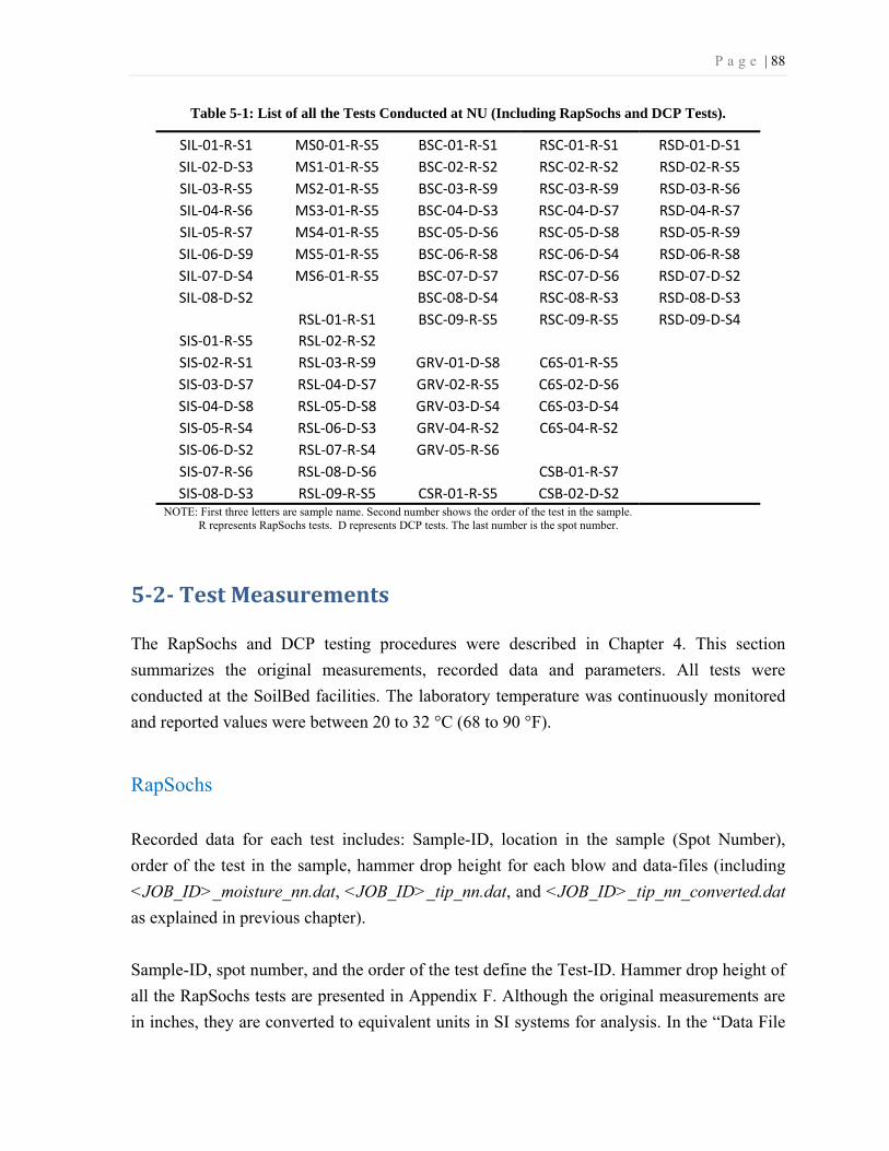
P a g e | 88
Table 5-1: List of all the Tests Conducted at NU (Including RapSochs and DCP Tests).
SIL-01-R-S1 MS0-01-R-S5 BSC-01-R-S1 RSC-01-R-S1 RSD-01-D-S1SIL-02-D-S3 MS1-01-R-S5 BSC-02-R-S2 RSC-02-R-S2 RSD-02-R-S5SIL-03-R-S5 MS2-01-R-S5 BSC-03-R-S9 RSC-03-R-S9 RSD-03-R-S6SIL-04-R-S6 MS3-01-R-S5 BSC-04-D-S3 RSC-04-D-S7 RSD-04-R-S7SIL-05-R-S7 MS4-01-R-S5 BSC-05-D-S6 RSC-05-D-S8 RSD-05-R-S9SIL-06-D-S9 MS5-01-R-S5 BSC-06-R-S8 RSC-06-D-S4 RSD-06-R-S8SIL-07-D-S4 MS6-01-R-S5 BSC-07-D-S7 RSC-07-D-S6 RSD-07-D-S2SIL-08-D-S2 BSC-08-D-S4 RSC-08-R-S3 RSD-08-D-S3
RSL-01-R-S1 BSC-09-R-S5 RSC-09-R-S5 RSD-09-D-S4SIS-01-R-S5 RSL-02-R-S2 SIS-02-R-S1 RSL-03-R-S9 GRV-01-D-S8 C6S-01-R-S5 SIS-03-D-S7 RSL-04-D-S7 GRV-02-R-S5 C6S-02-D-S6 SIS-04-D-S8 RSL-05-D-S8 GRV-03-D-S4 C6S-03-D-S4 SIS-05-R-S4 RSL-06-D-S3 GRV-04-R-S2 C6S-04-R-S2 SIS-06-D-S2 RSL-07-R-S4 GRV-05-R-S6 SIS-07-R-S6 RSL-08-D-S6 CSB-01-R-S7 SIS-08-D-S3 RSL-09-R-S5 CSR-01-R-S5 CSB-02-D-S2
NOTE: First three letters are sample name. Second number shows the order of the test in the sample. R represents RapSochs tests. D represents DCP tests. The last number is the spot number.
5-2- Test Measurements
The RapSochs and DCP testing procedures were described in Chapter 4. This section
summarizes the original measurements, recorded data and parameters. All tests were
conducted at the SoilBed facilities. The laboratory temperature was continuously monitored
and reported values were between 20 to 32 °C (68 to 90 °F).
RapSochs
Recorded data for each test includes: Sample-ID, location in the sample (Spot Number),
order of the test in the sample, hammer drop height for each blow and data-files (including
<JOB_ID>_moisture_nn.dat, <JOB_ID>_tip_nn.dat, and <JOB_ID>_tip_nn_converted.dat
as explained in previous chapter).
Sample-ID, spot number, and the order of the test define the Test-ID. Hammer drop height of
all the RapSochs tests are presented in Appendix F. Although the original measurements are
in inches, they are converted to equivalent units in SI systems for analysis. In the “Data File
P a g e | 89
Format” subsection of “RapSochs Test Procedure” of Chapter 4, the file format of raw data
recorded in a RapSochs test was explained. The raw data for all RapSochs tests are presented
on a CD-ROM along with this document where test results are organized by sample and test
IDs.
DCP
The data recorded during a DCP test includes the drop number and corresponding cumulative
penetration. The initial sinking of DCP due to its weight before starting a test was also
recorded. The distance between the bottom of the anvil and soil surface is measured after any
drop using a vertical scale. Subtracting the tip-to-anvil distance results in the depth of the
cone after each drop. Depth of the cone is the depth of the top of the shoulder of the cone
shown as the “reference point” in Figure 2-1. DCP measurements for all the DCP tests are
presented in Appendix G.
ASTM Standard D 6951-03 suggests to record DCP test data in a form where test data
includes “Number of Blows” between test readings and “Cumulative Penetration” after each
set of hammer blows. In all tests conducted, “Number of Blows” between test readings is
one. It means that DCP data are recorded for any individual blow. Other required information
according to ASTM D 6951-03 can be obtained from provided data in Appendix G.
5-3- Database
A database in MAT-files format was developed to facilitate data access, processing, and
mining. The format for the database was designed to be consistent with MATLAB®, the
programming language used for data analysis. MAT-files provide a flexible system that can
facilitate data entering, editing, mining, checking, processing, and analysis in MATLAB®.
MAT-files are binary files with double-precision and may contain different types of data,
including strings, matrices, multidimensional arrays, structures, and cell arrays. They are
saved MATLAB® workspace in files with “.mat” extension. This format makes it very easy
to enter, revise, and save data in MATLAB environment and can also be read and written
from external C or Fortran programs.

P a g e | 90
Database Structure
Each test data are stored in a separate MAT-file and are named based on Test-ID. There are
two different types of MAT-files; RapSochs MAT-files and DCP MAT-files. The variables
stored in each type are different since the test and measured parameters are different. Each
type can be recognized based on the file name which corresponds to the Test-ID.
To establish the database, all data-files of each test are stored together in a single MAT-file.
A MATLAB code developed for this task. All the codes which are developed for database
establishment and later in data analysis are listed in Appendix C and are available in the
folder “\m-files” on the CD-ROM along this document.
The resulting MAT-files of all DCP and RapSochs tests are stored on the CD-ROM in the
folder “\Database”. These MAT-files include raw data as well as the results of data analysis.
All new variables that are added to the database are explained in the related section. Table
5-1 also presents the list of MAT-files available at “\Database”.
DCP MAT-Files
In a DCP test, the distance of the bottom of the anvil from the soil surface is measured. The
distance from the bottom of the anvil to the top of the cone shoulder is 98.0 cm in the
Kessler’s DCP. Other parameters, including DCP-PR are obtained from this data. List of
variables available in a DCP MAT-file containing the experiment’s original measurements is
presented in Table 5-2. DCP test data are presented and discussed in “DCP data” section and
the necessary information is extracted from the original measurements.
Table 5-2: The Variables in a DCP MAT-file Containing Original Data.
Variable Description
DCP The distance between bottom of anvil and soil surface - The original
recorded data (cm)
Test_ID A character variable which contains Test-ID in “AAA-nn-D-S#” format.

P a g e | 91
RapSochs MAT-Files
Table 5-3 provides description of the variables that include original data and measurements
for any RapSochs test. The raw measured signals of string potentiometer, acceleration and
two strain gauges are added together in an n-by-1 array. Later in data analysis, other
variables are added to this database. RapSochs test data are presented and discussed in
“RapSochs data” section.
Table 5-3: List of Variables Containing Original Data in a RapSochs MAT-file.
Variable Description
Job Test information used in the lab for test and sample identification.
Later Test-ID is obtained from this information.
Test_ID A character variable shows Test-ID in “AAA-nn-R-S#” format.
moisture_Depth Position of the cone below the soil surface. The zero level is at the
sample surface and values below the surface are negative (mm).
moisture_Frequency Moisture Sensor’s frequency of operation (Hz). The data in each raw
belong to moisture sensor reading at the corresponding
moisture_Depth.
moisture_Magnitude Moisture Sensor’s measured magnitude (dB). The data in each raw
belong to moisture sensor reading at the corresponding
moisture_Depth.
moisture_Phase Moisture Sensor’s measured phase (degree). The data in each raw
belong to moisture sensor reading at the corresponding
moisture_Depth.
Spfm Output of string potentiometer, filtered with order 5 median filter
(which does not add any time delay), added together for all the blows
of a test (mm).
Accel Output of accelerometer, added together for all blows of a test (g)
str1 Output of the tip strain gauge, added together for all the blows of a test
(kN)
P a g e | 92
str2 Output of the strain gauge in the sleeve, added together for all the
blows of a test (kN)
drop_heights Hammer drop height (in.)
Data Examination, Verification, and Correction
The DCP procedure and data recording is simple, and there was no concern about the validity
of the measurements. However, in RapSochs revision 0.0, measurements are complex and
depend on operator’s accuracy and instrument’s functionality.
In the database development, several issues including data accuracy, different testing
procedures and problems, which occurred during testing needed to be addressed. For
instance, some blows did not exactly follow the procedure due to operational problems (e.g.,
hammer fall was not a free fall or the hammer was dropped from an unknown height) or
instrument mechanical failure (e.g., string potentiometer holder broke during a test). In
addition, due to hardware problems (e.g., electronic miscommunication) the data length for
some drops was not 2048 data points long as it should be. Other issues were rooted in data
analysis codes and individual mistakes. There were other defects that occurred during
generation of MAT-files. For example the length of variables in MAT files (str1, str2, …)
did not match with the sum of individual data files.
To address these issues, a comprehensive data validation procedure is conducted. Two new
variables are added to the database as a result of data validation. The drop_penetration_
reliability is a binary variable that may have a value of 0 or 1. If in a specific blow due to any
reason, the data is not reliable then this variable is 0 otherwise it is 1. The drop_data_length
includes the number of recorded data points of the string potentiometer, accelerometer, and
strain gauges for any individual blow. When a communication error happens, the value for
the corresponding blow is less than 2048. In addition, in cases that the instrument fails to
trigger, the variable has a value of zero. The RapSochs system is designed in a way that data
of all sensors are saved in <JOB_ID>_tip_nn.dat and <JOB_ID>_tip_nn_converted.dat
simultaneously. Therefore, the drop_data_length presents the number of data points of a
specific blow in spfm, accel, str1, and str2 variables. For any further analysis these variables
are checked first. It should be mentioned that in cases that drop_data_length is less than 2048
but not zero, no biased or unusual data in sensor measurements were observed. In most cases,
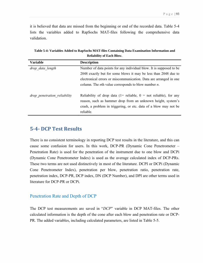
P a g e | 93
it is believed that data are missed from the beginning or end of the recorded data. Table 5-4
lists the variables added to RapSochs MAT-files following the comprehensive data
validation.
Table 5-4: Variables Added to RapSochs MAT-files Containing Data Examination Information and
Reliability of Each Blow.
Variable Description
drop_data_length Number of data points for any individual blow. It is supposed to be
2048 exactly but for some blows it may be less than 2048 due to
electronical errors or miscommunication. Data are arranged in one
column. The nth value corresponds to blow number n.
drop_penetration_reliability Reliability of drop data (1= reliable, 0 = not reliable), for any
reason, such as hammer drop from an unknown height, system’s
crash, a problem in triggering, or etc. data of a blow may not be
reliable.
5-4- DCP Test Results
There is no consistent terminology in reporting DCP test results in the literature, and this can
cause some confusion for users. In this work, DCP-PR (Dynamic Cone Penetrometer –
Penetration Rate) is used for the penetration of the instrument due to one blow and DCPi
(Dynamic Cone Penetrometer Index) is used as the average calculated index of DCP-PRs.
These two terms are not used distinctively in most of the literature. DCPI or DCPi (Dynamic
Cone Penetrometer Index), penetration per blow, penetration ratio, penetration rate,
penetration index, DCP-PR, DCP index, DN (DCP Number), and DPI are other terms used in
literature for DCP-PR or DCPi.
Penetration Rate and Depth of DCP
The DCP test measurements are saved in “DCP” variable in DCP MAT-files. The other
calculated information is the depth of the cone after each blow and penetration rate or DCP-
PR. The added variables, including calculated parameters, are listed in Table 5-5.

P a g e | 94
Table 5-5: Variables Added into the DCP MAT-files Regarding Penetration Rate and Depth.
Variable Description
dcp_sinkage_depth The depth of the top of the cone shoulder below the surface penetrated
into the soil under the instrument’s own weight (mm) before starting
the test. This distance is positive if the cone is below the surface.
dcp_drop_depth The depth of the top of the DCP cone shoulder after each blow. The
zero level is at the soil sample surface and values below the surface are
negative (mm). Data are arranged in one column. The nth value
corresponds to blow number n.
dcp_drop_penetration The penetration per blow (mm/blow). This is basically DCP-PR. Data
are arranged in one column. The nth value is corresponding to the
penetration caused by blow number n.
Presenting DCP Data
There is no unique method in the literature to plot DCP test results. Sometimes the
penetration per blow is presented in regular or logarithmic scale versus depth. The
cumulative number of hammer blows has also been plotted versus depth.
ASTM D 6951-03 suggests plotting penetration per blow versus the scale reading or total
depth. However, to define any layering in the soil profile, it is suggested to plot the
cumulative number of blows versus depth to examine changes in the slope. To define the
layer thickness the intersection of the lines representing the average slope of adjacent layers
should be found.
De Henau (1982) and Webster et al. (1994) presented DCP-PR as a broken vertical line from
each set of penetration on a logarithmic scale versus depth. Chua (1988), Siekmeier et al.
(1998), Gabr et al. (1999), and Siekmeier et al. (2009) plotted DCP-PR as data points versus
depth. Van Vuuren (1969) suggested plotting values versus the mid-point (average) depth.
Burnham and Johnson (1993) plotted the calculated CBR versus average depth. Edil and
Benson (2005) used two different methods for data presentation. The first method is similar
to Webster et al (1994) and the second method is to plot the penetration per blow as data
points versus the depth after the penetration. Abu-Farsakh et al. (2005) plotted DCP-PR
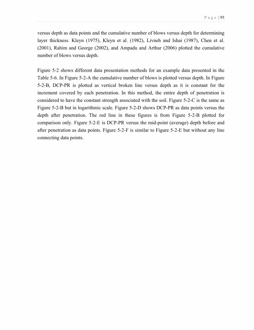
P a g e | 95
versus depth as data points and the cumulative number of blows versus depth for determining
layer thickness. Kleyn (1975), Kleyn et al. (1982), Livneh and Ishai (1987), Chen et al.
(2001), Rahim and George (2002), and Ampadu and Arthur (2006) plotted the cumulative
number of blows versus depth.
Figure 5-2 shows different data presentation methods for an example data presented in the
Table 5-6. In Figure 5-2-A the cumulative number of blows is plotted versus depth. In Figure
5-2-B, DCP-PR is plotted as vertical broken line versus depth as it is constant for the
increment covered by each penetration. In this method, the entire depth of penetration is
considered to have the constant strength associated with the soil. Figure 5-2-C is the same as
Figure 5-2-B but in logarithmic scale. Figure 5-2-D shows DCP-PR as data points versus the
depth after penetration. The red line in these figures is from Figure 5-2-B plotted for
comparison only. Figure 5-2-E is DCP-PR versus the mid-point (average) depth before and
after penetration as data points. Figure 5-2-F is similar to Figure 5-2-E but without any line
connecting data points.

P a g e | 96
Table 5-6: Example DCP Data Used to Illustrate Different DCP Data Presentation Methods.
Number of Blows
Cumulative Number of
Blows
Cumulative Penetration
(mm) Penetration Between
Readings (mm) DCP-PR
(mm/blow) 0 0 0 0 0 1 1 50 50 50 1 2 92 42 42 1 3 120 28 28 1 4 141 21 21 1 5 166 25 25 1 6 190 24 24 1 7 209 19 19 1 8 230 21 21 1 9 246 16 16 1 10 251 5 5 1 11 258 7 7 1 12 263 5 5 1 13 273 10 10 1 14 281 8 8 1 15 301 20 20 1 16 318 17 17 1 17 336 18 18 1 18 355 19 19 1 19 375 20 20 1 20 396 21 21 1 21 413 17 17 1 22 436 23 23 1 23 455 19 19 1 24 473 18 18 1 25 498 25 25
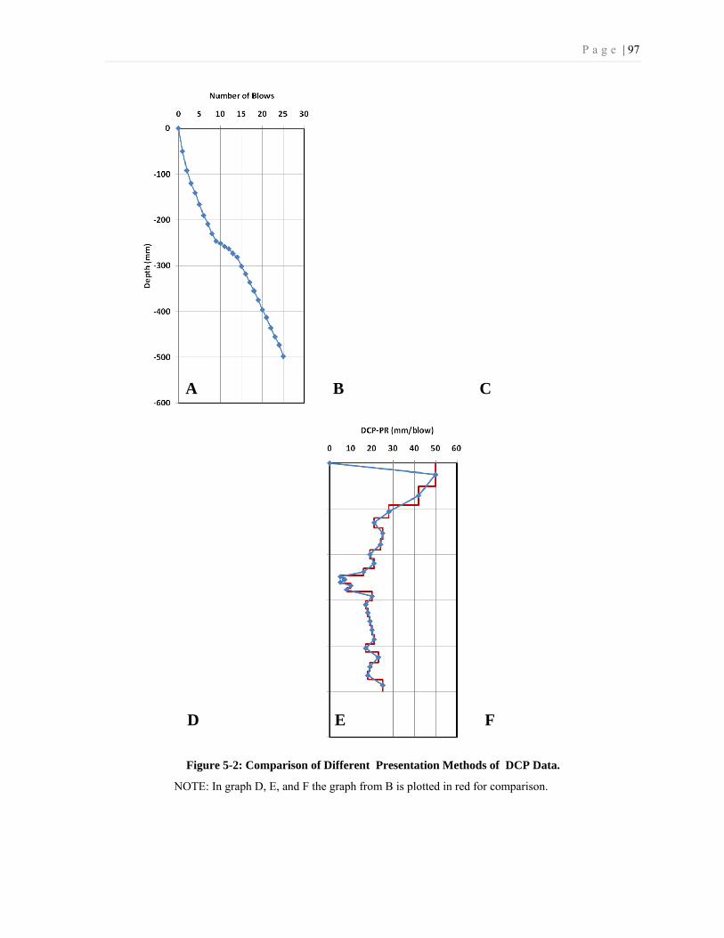
P a g e | 97
Figure 5-2: Comparison of Different Presentation Methods of DCP Data.
NOTE: In graph D, E, and F the graph from B is plotted in red for comparison.
A B C
F E D
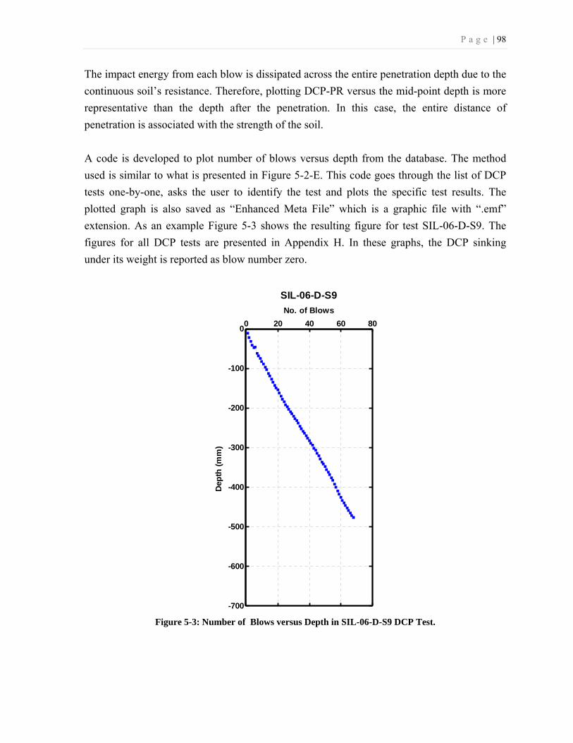
P a g e | 98
The impact energy from each blow is dissipated across the entire penetration depth due to the
continuous soil’s resistance. Therefore, plotting DCP-PR versus the mid-point depth is more
representative than the depth after the penetration. In this case, the entire distance of
penetration is associated with the strength of the soil.
A code is developed to plot number of blows versus depth from the database. The method
used is similar to what is presented in Figure 5-2-E. This code goes through the list of DCP
tests one-by-one, asks the user to identify the test and plots the specific test results. The
plotted graph is also saved as “Enhanced Meta File” which is a graphic file with “.emf”
extension. As an example Figure 5-3 shows the resulting figure for test SIL-06-D-S9. The
figures for all DCP tests are presented in Appendix H. In these graphs, the DCP sinking
under its weight is reported as blow number zero.
Figure 5-3: Number of Blows versus Depth in SIL-06-D-S9 DCP Test.
0 20 40 60 80
-700
-600
-500
-400
-300
-200
-100
0
No. of Blows
Dept
h (m
m)
SIL-06-D-S9
P a g e | 99
DCP Index (DCPi)
The DCPi is defined as an index either based on DCP-PR data or the slope of number of
blows versus depth. DCPi is used to estimate the shear strength or elastic modulus of soil
using empirical relationships. Methods for calculating DCPi vary (Siekmeier et al., 2009) and
there is no standard method defined in the literature.
To avoid confinement effect of granular materials on DCPi, Ayers et al. (1989) used the
average of DCP-PR in the 100 mm mid-depth of prepared uniform samples as DCPi. Gabr et
al. (1999) did not use the first DCP-PR in calculation of DCPi in tests conducted in standard
CBR molds. Siekmeier et al. (2009) recommended ignoring the first two DCP-PRs (they call
it as seating drops) and use the average of the next five DCP-PR to calculate DCPi. Kleyn
(1975), Kleyn et al. (1982) used the slope of each linear part of number of blows versus
depth as the index. Siekmeier et al. (2009) used the average DCP-PR for the 3rd to 7th drop.
Other researchers defined DCPi as the cumulative penetration between DCP readings divided
by number of hammer blows between test readings. However, ASTM D6951-03 suggests
taking the readings after a specific number of blows that is selected based on the resistance of
the material; e.g., 1 blow for soft materials, 5 blows for normal materials and 10 blows for
very resistive materials. The average penetration rate for each layer is recommended to be
used.
Webster et al. (1994) excluded transient zone’s data and used the average of DCP-PR of four
tests as DCPi in their study. The equation to calculate the average DCPi can be written as
(After Edil and Benson, 2005):
. = ∑ ( ) ................................................................... 5-1
where N is the total number of DCP-PR in a given penetration depth of interest. Livneh and
Ishai (1987), Chen et al. (2001), Rahim and George (2002), and Paige-Green (2009)
calculated average DCPi for each layer and used the result for any further analysis or
correlations without excluding any data points. CSIR Transportek, (2000) and, Edil and
Benson (2005) recommended using the weighted average DCPi obtained from:
. = ∑ ( ) . ......................................................... 5-2
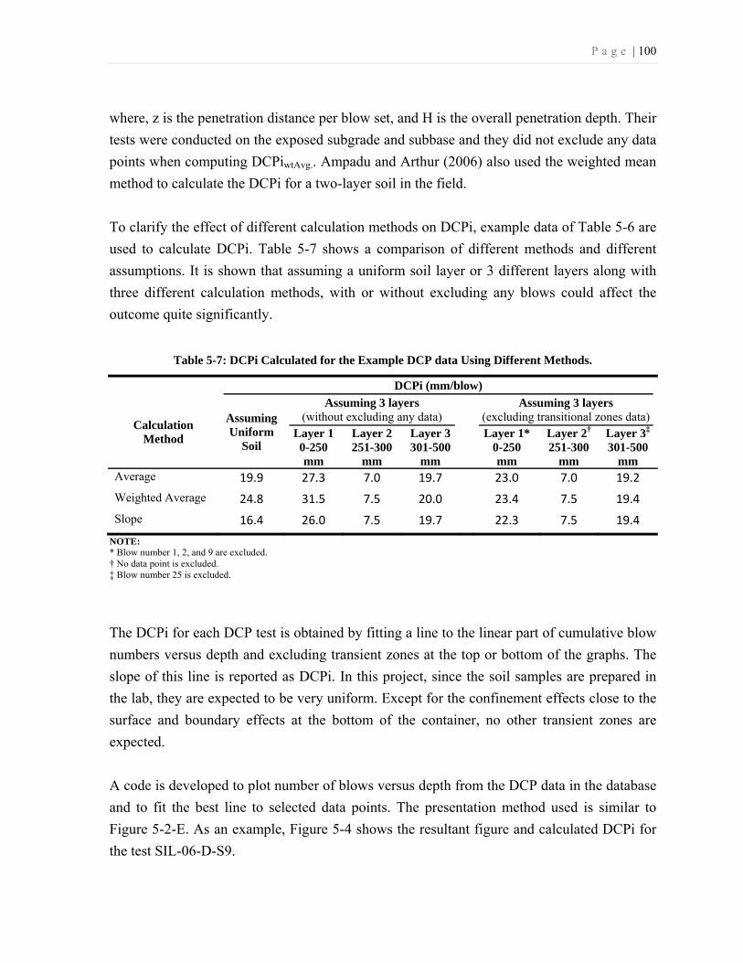
P a g e | 100
where, z is the penetration distance per blow set, and H is the overall penetration depth. Their
tests were conducted on the exposed subgrade and subbase and they did not exclude any data
points when computing DCPiwtAvg.. Ampadu and Arthur (2006) also used the weighted mean
method to calculate the DCPi for a two-layer soil in the field.
To clarify the effect of different calculation methods on DCPi, example data of Table 5-6 are
used to calculate DCPi. Table 5-7 shows a comparison of different methods and different
assumptions. It is shown that assuming a uniform soil layer or 3 different layers along with
three different calculation methods, with or without excluding any blows could affect the
outcome quite significantly.
Table 5-7: DCPi Calculated for the Example DCP data Using Different Methods.
DCPi (mm/blow)
Calculation Method
Assuming Uniform
Soil
Assuming 3 layers (without excluding any data)
Assuming 3 layers (excluding transitional zones data)
Layer 1 Layer 2 Layer 3 Layer 1* Layer 2† Layer 3‡ 0-250 mm
251-300 mm
301-500 mm
0-250 mm
251-300 mm
301-500 mm
Average 19.9 27.3 7.0 19.7 23.0 7.0 19.2
Weighted Average 24.8 31.5 7.5 20.0 23.4 7.5 19.4
Slope 16.4 26.0 7.5 19.7 22.3 7.5 19.4
NOTE: * Blow number 1, 2, and 9 are excluded. † No data point is excluded. ‡ Blow number 25 is excluded.
The DCPi for each DCP test is obtained by fitting a line to the linear part of cumulative blow
numbers versus depth and excluding transient zones at the top or bottom of the graphs. The
slope of this line is reported as DCPi. In this project, since the soil samples are prepared in
the lab, they are expected to be very uniform. Except for the confinement effects close to the
surface and boundary effects at the bottom of the container, no other transient zones are
expected.
A code is developed to plot number of blows versus depth from the DCP data in the database
and to fit the best line to selected data points. The presentation method used is similar to
Figure 5-2-E. As an example, Figure 5-4 shows the resultant figure and calculated DCPi for
the test SIL-06-D-S9.

P a g e | 101
Figure 5-4: Number of Blows versus Depth in SIL-06-D-S9 DCP Test and the Best Fitted Line where the
Slope is DCPi.
The graphs showing the best line fitted to data of all DCP tests results are also presented in
Appendix H and the calculated DCPi are summarized in Table 5-8 also presents DCPi values
obtained by averaging the DCP-PRs in parentheses. In Table 5-8 the average DCPi of tests
performed in a similar condition is also calculated. The DCPi in GRV and SIL are not
averaged for all the test results. For GRV, the GRV-01-D-S8 test was performed before
draining the sample and GRV-03-D-S4 was performed after allowing the sample drain for 24
hours. In addition, data points at a depth lower than 600 mm are excluded when calculating
DCPi because the tip was very close to the bottom of the container and they are affected by
container’s boundary. For SIL, the SIL-02-D-S3 test was performed 3 months before other
tests in SIL sample and the effect of aging on cementation could be detected in this case.
0 20 40 60 80
-700
-600
-500
-400
-300
-200
-100
0
No. of Blows
Dep
th (m
m)
SIL-06-D-S9
DCPi = 6.8 (mm/blow)
DataFitted Line
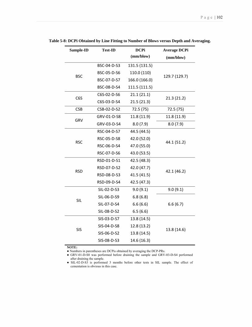
P a g e | 102
Table 5-8: DCPi Obtained by Line Fitting to Number of Blows versus Depth and Averaging.
Sample-ID Test-ID DCPi
(mm/blow)
Average DCPi
(mm/blow)
BSC
BSC-04-D-S3 131.5 (131.5)
129.7 (129.7) BSC-05-D-S6 110.0 (110)
BSC-07-D-S7 166.0 (166.0)
BSC-08-D-S4 111.5 (111.5)
C6S C6S-02-D-S6 21.1 (21.1)
21.3 (21.2) C6S-03-D-S4 21.5 (21.3)
CSB CSB-02-D-S2 72.5 (75) 72.5 (75)
GRV GRV-01-D-S8 11.8 (11.9) 11.8 (11.9)
GRV-03-D-S4 8.0 (7.9) 8.0 (7.9)
RSC
RSC-04-D-S7 44.5 (44.5)
44.1 (51.2) RSC-05-D-S8 42.0 (52.0)
RSC-06-D-S4 47.0 (55.0)
RSC-07-D-S6 43.0 (53.5)
RSD
RSD-01-D-S1 42.5 (48.3)
42.1 (46.2) RSD-07-D-S2 42.0 (47.7)
RSD-08-D-S3 41.5 (41.5)
RSD-09-D-S4 42.5 (47.3)
SIL
SIL-02-D-S3 9.0 (9.1) 9.0 (9.1)
SIL-06-D-S9 6.8 (6.8)
6.6 (6.7) SIL-07-D-S4 6.6 (6.6)
SIL-08-D-S2 6.5 (6.6)
SIS
SIS-03-D-S7 13.8 (14.5)
13.8 (14.6) SIS-04-D-S8 12.8 (13.2)
SIS-06-D-S2 13.8 (14.5)
SIS-08-D-S3 14.6 (16.3)
NOTE: Numbers in parentheses are DCPis obtained by averaging the DCP-PRs. GRV-01-D-S8 was performed before draining the sample and GRV-03-D-S4 performed
after draining the sample. SIL-02-D-S3 is performed 3 months before other tests in SIL sample. The effect of
cementation is obvious in this case.

P a g e | 103
5-5- RapSochs Test Results
RapSochs is a newly developed instrument without any specific data presentation strategies.
This section describes how basic parameters (e.g., depth of the RapSochs) are obtained from
the original data together with a procedure to access and plot RapSochs original data.
Examples of plots are also provided in each subsection.
Penetration Rate and Depth of RapSochs
The initial position of the rod, captured by the moisture sensor, is used to measure the cone
sinking under the RapSochs’s own weight. Similar to DCP, a term RS-PR (RapSochs
Penetration Rate) is introduced for the penetration per blow in the RapSochs tests. To extract
the RS-PR for an individual blow, the averages of the first and last 50 data points of the
string potentiometer signal are subtracted. In cases that the instrument did not trigger during
a blow, the penetration is calculated based on the previous and the following blow. The depth
of the RapSochs cone after any blow is also calculated by adding the sinkage depth to the
calculated depth from string potentiometer signals. The string potentiometer itself did not
exhibit drift or hysteresis as the strain gauges and the accelerometer. However, summation of
RS-PRs may not result the same depth due to the numerical errors. The new variables added
to RapSochs MAT-files are listed in Table 5-9.
Table 5-9: Variables Added to RapSochs MAT-files Regarding Penetration Rate and Depth.
Variable Description
sinkage_depth The distance of the RapSochs cone below the surface, penetrated into the
soil under the instrument’s own weight (mm). This distance is positive if the
cone is below the surface.
drop_depth Depth of the RapSochs cone shoulder after the penetration (mm). The zero
level is at the sample surface and values below the surface are negative.
Data are arranged in one column. The nth value corresponding to the depth
of the RapSochs after blow number n.
drop_penetration Penetration per blow (mm/blow). This is basically RS-PR. Data are
arranged in one column. The nth value corresponding to the penetration rate
due to the blow number n.
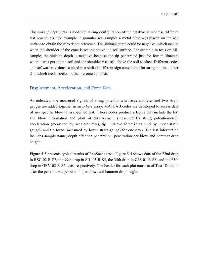
P a g e | 104
The sinkage depth data is modified during configuration of the database to address different
test procedures. For example in granular soil samples a metal plate was placed on the soil
surface to obtain the zero depth reference. The sinkage depth could be negative, which occurs
when the shoulder of the cone is resting above the soil surface. For example in tests on SIL
sample, the sinkage depth is negative because the tip penetrated just for few millimeters
when it was put on the soil and the shoulder was still above the soil surface. Different codes
and software revisions resulted in a shift or different sign convention for string potentiometer
data which are corrected in the presented database.
Displacement, Acceleration, and Force Data
As indicated, the measured signals of string potentiometer, accelerometer and two strain
gauges are added together in an n-by-1 array. MATLAB codes are developed to access data
of any specific blow for a specified test. These codes produce a figure that include the test
and blow information and plots of displacement (measured by string potentiometer),
acceleration (measured by accelerometer), tip + sleeve force (measured by upper strain
gauge), and tip force (measured by lower strain gauge) for one drop. The test information
includes sample name, depth after the penetration, penetration per blow and hammer drop
height.
Figure 5-5 presents typical results of RapSochs tests. Figure 5-5 shows data of the 22nd drop
in RSC-02-R-S2, the 99th drop in SIL-03-R-S5, the 35th drop in C6S-01-R-S8, and the 65th
drop in GRV-02-R-S5 tests, respectively. The header for each plot consists of Test-ID, depth
after the penetration, penetration per blow, and hammer drop height.

P a g e | 105
Figure 5-5: Typical Signal Output of RapSochs Sensors for a Blow.
0.02 0.04 0.06 0.08 0.1 0.12 0.14 0.16 0.18 0.2
0
10
20
Dis
plac
emen
t(m
m)
RSC-02-R-S2 , Depth = -429 (mm), Penetration = 14 (mm), Drop Height = 8 (in)
0.02 0.04 0.06 0.08 0.1 0.12 0.14 0.16 0.18 0.2-1000
-500
0
500
1000
Acc
eler
atio
n (g
)
0.02 0.04 0.06 0.08 0.1 0.12 0.14 0.16 0.18 0.2
0
2
4
6
Tip
+ S
leev
e For
ce (kN
)
0.02 0.04 0.06 0.08 0.1 0.12 0.14 0.16 0.18 0.2
0
2
4
6
Time (seconds)
Tip
For
ce (kN
)
0.02 0.04 0.06 0.08 0.1 0.12 0.14 0.16 0.18 0.2
0
10
20
Dis
plac
emen
t(m
m)
SIL-03-R-S5 , Depth = -374 (mm), Penetration = 3 (mm), Drop Height = 22 (in)
0.02 0.04 0.06 0.08 0.1 0.12 0.14 0.16 0.18 0.2-1000
-500
0
500
1000
Acc
eler
atio
n (g
)
0.02 0.04 0.06 0.08 0.1 0.12 0.14 0.16 0.18 0.2
0
2
4
6
Tip
+ S
leev
e For
ce (kN
)
0.02 0.04 0.06 0.08 0.1 0.12 0.14 0.16 0.18 0.2
0
2
4
6
Time (seconds)
Tip
For
ce (kN
)
A)
B)
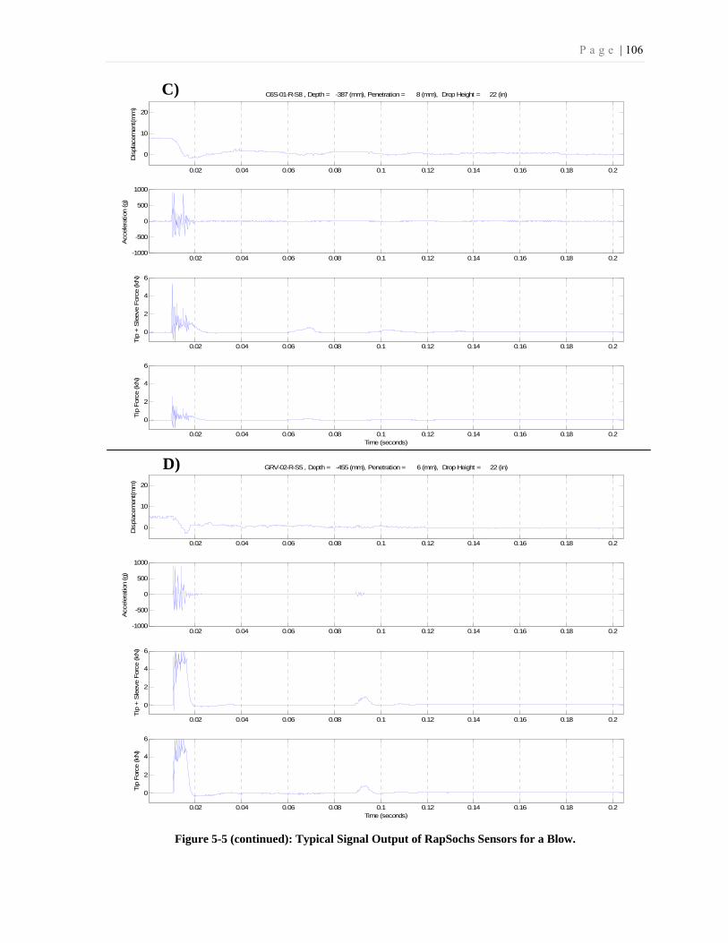
P a g e | 106
Figure 5-5 (continued): Typical Signal Output of RapSochs Sensors for a Blow.
0.02 0.04 0.06 0.08 0.1 0.12 0.14 0.16 0.18 0.2
0
10
20
Dis
plac
emen
t(m
m)
C6S-01-R-S8 , Depth = -387 (mm), Penetration = 8 (mm), Drop Height = 22 (in)
0.02 0.04 0.06 0.08 0.1 0.12 0.14 0.16 0.18 0.2-1000
-500
0
500
1000
Acc
eler
atio
n (g
)
0.02 0.04 0.06 0.08 0.1 0.12 0.14 0.16 0.18 0.2
0
2
4
6
Tip
+ S
leev
e For
ce (kN
)
0.02 0.04 0.06 0.08 0.1 0.12 0.14 0.16 0.18 0.2
0
2
4
6
Time (seconds)
Tip
For
ce (kN
)
0.02 0.04 0.06 0.08 0.1 0.12 0.14 0.16 0.18 0.2
0
10
20
Dis
plac
emen
t(m
m)
GRV-02-R-S5 , Depth = -455 (mm), Penetration = 6 (mm), Drop Height = 22 (in)
0.02 0.04 0.06 0.08 0.1 0.12 0.14 0.16 0.18 0.2-1000
-500
0
500
1000
Acc
eler
atio
n (g
)
0.02 0.04 0.06 0.08 0.1 0.12 0.14 0.16 0.18 0.2
0
2
4
6
Tip
+ S
leev
e For
ce (kN
)
0.02 0.04 0.06 0.08 0.1 0.12 0.14 0.16 0.18 0.2
0
2
4
6
Time (seconds)
Tip
For
ce (kN
)
C)
D)
P a g e | 107
The following sequence describes the physical response in a typical blow’s signals. The
sequence may differ based on the hammer drop height and soil properties.
1. Hammer hits the anvil.
2. The stress wave moves downward and as soon as it hits the cone the instrument
accelerates downward. In the acceleration-time history and force-time history graphs,
it takes around 0.01 seconds for the transducers to receive the first compression wave
caused by the hammer collision over the anvil.
3. The stress wave is also reflected and continues traveling up and down.
4. The anvil and hammer remain in contact for a while until, due to interaction with the
soil, rod and hammer. The hammer bounces back and may separate from the anvil
(moving upward or downward with the slower velocity).
5. Resistance of the soil decelerates the rod and rod finally stops.
6. Hammer collides with the anvil for the second time and it may or may not cause any
further penetration (another rebound and collision may also occur). In Figure 5-5 B
and D, pulses around 0.09 seconds oscillations in the strain gauge signals and
accelerometer data are signs of this phenomenon.
However for some drops, no observable sign of a second hit could be detected (Figure 5-5 A
and C). It may be due to the fact that during collision the hammer remains in contact with the
anvil and never separates or the energy of the hammer is so low that it does not cause a
second observable pulse. The first couple of penetrations in granular soils were among those
blows that did not generate any sign of a second collision.
The oscillation in the accelerometer and strain gauge signals during penetration are the result
of stress wave traveling up and down in the rod. The time interval for the stress wave to
travel from the anvil to the cone and back (2L/c) is calculated to be 3.6×10⁻⁴ seconds (where
L = 1 m is the penetrometer length and c = 5500 m/sec is the velocity of compression wave
in the rod).
P a g e | 108
Acceleration Data and Calculation of Velocity
In the course of analyzing the energy transferred by integration of internal stress waves and
velocity, the accelerometer output with respect to time was integrated to obtain the required
probe velocity information. As a check, a second integration was performed to verify that
displacement inferred from the accelerometer readings agreed with the “ground truth”
position information provided by the string potentiometer. It was expected that the double
integrated accelerometer data provide an accurate and less noisy indication of the position
with a more superior response time than the string potentiometer. However, accelerometers
are known to drift slightly due to various influences, including temperature. Since these data
were integrated, errors due to even minute drift would have the potential to compound. Using
buffered data acquired just prior to each blow and removing the effects from the data did not
solve the problem. Inspection of the signals revealed that the signal-to-noise ratio was
negligible.
Almost all calculated displacement-time histories showed a skyrocketing trend and did not
match the string potentiometer displacement data. Different type of filtering and baseline
correction techniques were applied to the acceleration data. These techniques included
typical baseline correction methods used in earthquake engineering to correct the recorded
digital acceleration data of strong motion instruments. Few acceleration (and consequently
displacement) time histories were corrected with success but finding a unique method
applicable to all recorded data was not achievable. During this process, other issues and
concerns were raised showing that the use of the current accelerometer to produce velocity
and displacement by integration is not a viable option in current revision of RapSochs.
While some researchers (e.g., Chua & Lytton, 1988; Odebrecht et al., 2005; and Abou-matar
and Goble, 1997) did not report any problem with integration of acceleration to calculate the
velocity in DCP and SPT tests using data acquisition of 10 kHz (512 digitized points in 0.05
sec), 16 kHz and 10 kHz, respectively, Schmertmann (2007) mentioned that the problem is
related to the low-resolution of accelerometers causing inaccuracy when integrated to
calculate velocity. ASTM D4633, a standard method for measurement of the energy that
enters a penetrometer rod during dynamic penetrometer testing, requires the use of an
accelerometer with a useable frequency response to at least 4.5 kHz. ASTM D4945 (2000)
for high-strain dynamic testing of piles requires that signals from transducers shall be

P a g e | 109
recorded so that frequency components have a low pass cut-off frequency of 1,500 Hz, and
when digitizing, the sample frequency shall be at least 5,000 Hz for each data channel. While
ASTM D4633 requires an accelerometer linear up to 10,000 g, ASTM D4945 (2000) requires
a limit of 1,000 g. Chua & Lytton (1988) reported a maximum acceleration of around 1400 g
below the DCP anvil. It is clear that the reported and required range and frequency for
accelerometers are different and vary among different references.
The working range of the accelerometer in RapSochs is 1000 g with a frequency response of
10 kHz. Although in acceleration-time histories exceedance of the working range were not
observed, signal reconstruction of the acceleration-time history using Whittaker-Shannon
interpolation formula showed that the accelerometer very often pass the acceleration limits of
±1000 g. Perfect reconstruction of a band-limited continuous time signal from its sampled
version is possible using the Whittaker-Shannon reconstruction formula, which makes use of
the ideal lowpass filter and its Sinc function impulse response. Figure 5-6 shows a
reconstructed acceleration signal for one blow in GRV-02-R-S5 test. Note that even though
the recorded signal does not show any value higher than 1000 g (98100 m/s2), the
reconstructed signal shows that the accelerometer has encountered acceleration higher than
1000 g for more than one time.
Figure 5-6: Comparison of Recorded and Reconstructed Acceleration Signal in GRV-02-R-S5 Test,
which Shows Several Exceedance of 1000 g Limit.
0.01 0.012 0.014 0.016 0.018 0.02 0.022-8000
-6000
-4000
-2000
0
2000
4000
6000
8000
10000
12000
Time (Sec)
Acc
eler
atio
n (m
/s2)
x-axis
Measured SignalReconstructed Signal
1000 g limit

P a g e | 110
Based on personal communication with TransTech team after facing this problem, the
replacement of an accelerometer meeting the required space limits of RapSochs tip,
measurements ranges, and frequency response was not possible at the time. Several
unsuccessful attempts were made by TransTech to damp the oscillation by replacement of the
tip facing O-ring with a visco-elastic material or placing a visco-elastic material between the
tip and the accelerometer assembly.
Furthermore, the accelerometer failed to trigger in several tests. The problem is thought to be
due to the effects of electronics noise, drift, hysteresis, and temperature. To continue test
program without any interruption, the trigger function was configured to use the tip strain
signal later.
Overall, the baseline accelerometer configuration did not work reliably in the Rev. 0 system
during testing at NU, and the use of the accelerometer to produce velocity by integration was
not found reliable.
Presenting Penetration Data
RS-PR data (penetration per blow in mm/blow) for all tests are presented in Appendix I in
separate graphs for each RapSochs test. RS-PR is shown versus the average depth during
penetration (similar to Figure 5-2-E) and not the drop depth. Since the hammer drop height is
not constant in a RapSochs test, it is also plotted on the second axis to give better
understanding of the sensitivity of the RapSochs penetration in the soil. Therefore, the RS-
PR data are not corrected for different applied energies. Figure 5-7 presents the RS-PR and
the corresponding hammer drop height of the SIL-04-R-S6 test as an example.

P a g e | 111
Figure 5-7: RS-PR and the Corresponding Hammer Drop Height versus Depth for SIL-04-R-S6 Test.
0 15 30 45 60-700
-600
-500
-400
-300
-200
-100
0
Hammer Drop Height (cm)
0 5 10 15 20
-700
-600
-500
-400
-300
-200
-100
0
RS-PR (mm/blow)
Dep
th (m
m)
SIL-04-R-S6
Drop HeightPenetration Rate

P a g e | 112
Presenting Moisture Sensor Measurements
The Moisture sensor is 76 mm (3.0 in.) long, and the
lower edge is 134 mm (5.25 in.) from the lower
extent of the tip shoulder (Figure 5-8). Therefore, at
a depth of 210 mm (8.25 in.), the sensor is fully
submerged. Since the surface of the soil sample near
the penetrometer may heave during a penetration
test, only moisture sensor measurements recorded at
a depth below 230 mm should be considered.
However, measurements above this depth will also
be presented to show the transition of the sensor’s
measurements in the air and before entering the soil
sample.
As mentioned, the most important phenomenon that affects the low radio frequency dielectric
spectrum of soils (at 0.2 to 30 MHz) is the Maxwell-Wagner (M-W) relaxation effect.
Gamache (2004) showed that typical well-graded sandy soils exhibit a single M-W relaxation
in the 1-10 MHz range. In the moisture sensor of RapSochs, the resultant signal modified by
the dielectric properties of the soil is measured. The measured data consists of magnitude (of
the voltage gain) and phase shift of 22 exciting frequencies ranges from 0.1 to 12 MHz.
The graphs showing measured magnitude and phase shift at the range of the frequencies of
all RapSochs tests are presented in Appendix J. As an example, Figure 5-9 shows moisture
sensor measurements in SIL-04-R-S6 test. In the presented contour map, the Y-axis is the
depth of the RapSochs cone and only at the depth of 210 mm or below the moisture sensor is
fully submerged. The X-axis is the frequency in MHz. The left figure shows the magnitude
measurements in dB and contours are in 5-dB increments shown in color based on the color
bar on the top of the graph. The right figure is the phase measurements in degrees and
contours are in 10-degree increments shown in color based on the corresponding color bar.
Figure 5-8: Position of the moisture
sensor in the main rod.
76 mm Moisture Sensor
134 mm

P a g e | 113
Figure 5-9: Measurements of RapSochs Moisture Sensor in SIL-04-R-S6.
In general, electrical impedance is represented as a complex quantity:
= ................................................................................................................ 5-3
where;
: Complex impedance
Z: Impedance magnitude
θ: Phase
i: Imaginary number
e: Exponential function
Using Euler's formula results in:
= ( + ) = + ........................................................... 5-4
0 2 4 6 8 10-600
-500
-400
-300
-200
-100
0
Frequency (MHz)
Dep
th (m
m)
Frequency (MHz)
Magnitude (dB) Phase (Degree)SIL-04-R-S6
0 2 4 6 8 10
-10 0 10 20 30 0 20 40 60 80 100 120

P a g e | 114
The admittance ( ) is the inverse of the impedance ( ). Similar to impedance the admittance
could be written as a complex number:
= + ............................................................................................................. 5-5
where:
G: Susceptance (S or Ω-1)
B: Conductance (S or Ω-1)
The unit of admittance, susceptance, and conductance is Siemens, which is equal to the
inverse of impedance measured in Ohms. The following equations are used to calculate
susceptance and conductance from moisture sensore’s direct measurements.
= 10^( /20) ( ) ................................................................................... 5-6 = 10^( /20) ( ) .................................................................................... 5-7
where:
M: Magnitude (dB)
P: Phase (degree)
Table 5-10 presents a summary of new variables added to RapSochs MAT-files.
Table 5-10: Moisture Sensor Variables Containing Admittance Added to RapSochs MAT-files.
Variable Description
moisture_G The real part of admittance called susceptance (S or Ω-1). The data
in each raw is for corresponding moisture_Depth and the exciting
frequency of moisture_Frequency.
moisture_B The imaginary part of admittance called conductance (S or Ω-1). The
data in each raw is for corresponding moisture_Depth and the
exciting frequency of moisture_Frequency.

P a g e | 115
Figure 5-10 shows the results of calculated susceptance and conductance for the SIL-04-R-S6
test as an example. In this contour map, the Y-axis is the depth of the RapSochs cone. At a
depth of 210 mm or below the moisture sensor is fully submerged. The X-axis is the
frequency in MHz. The left figure shows the susceptance contours in 2-siemens increments
based on the color bar on the top of the graph. The right figure is the conductance contours in
2 siemens increments based on the corresponding color bar. The graphs for all of the
RapSochs tests are presented in Appendix K.
Figure 5-10: Calculated Susceptance and Conductance of Moisture Sensor for SIL-04-R-S6 RapSochs
Test.
0 2 4 6 8 10-600
-500
-400
-300
-200
-100
0
Frequency (MHz)
Dept
h (m
m)
Frequency (MHz)
Susceptance (S or Ω -1) Conductance (S or Ω -1)
SIL-04-R-S6
0 2 4 6 8 10
0 5 10 15 20 0 5 10 15 20
P a g e | 116
Additional Comments on Tests
There are observations regarding some of the tests that are relevant and necessary to be
reported.
SIL-01-R-S1 and SIL-02-D-S3 tests were conducted 3 months before other tests in SIL
sample. The effect of aging and cementation is noticeable in this case. Also the moisture
sensor cover was damaged during SIL-01-R-S1 test. The cover ripped apart and damaged the
electronics and also affected the penetration of RapSochs. The instrument sent to TranTesh
for repair and the cover of the moisture sensor were then replaced by a mixture of epoxy and
crushed stone. The moisture sensor damage and failure can easily be observed in plotted
moisture sensor data presented in Appendix J.
In all the tests in RSL, the instrument penetrated to the bottom of the box or very close to the
bottom of the box under its own weight, and following the hammer drop height procedure
was not applicable. The only reliable data for those tests are the sinkage depth and moisture
measurements.
In GRV, the GRV-01-D-S8 test was performed after the sample was prepared. Then, the
sample was allowed to drain under gravity for 1 day. Then GRV-02-R-S5, GRV-03-D-S4,
and GRV-04-R-S2 tests were performed. The GRV-05-R-S6 test was performed 2 days after
allowing the sample to drain, and the moisture profile was obtained immediately after the
test.
In MS0-01-R-S5, the moisture sensor failed to record any data between hammer drop
numbers 9 to 15. This produced irregularity in contour lines from the depth of 160 mm to 240
mm in the moisture sensor plots.

P a g e | 117
Chapter 6: Analysis and Correlations
This chapter presents the analysis and correlations on RapSochs data to develop necessary
algorithms and correlations for data interpretation. In the first section, The Maximum
Likelihood Estimation (MLE) method is adopted to obtain a quasi-static equivalent of the
dynamic force is developed. The purpose is to obtain cone and friction resistance soil profile
similar to CPT. The effect of variable applied energy on the soil strength estimation is also
studied. In the next section, dynamic cone penetrometers theory is discussed and a model
based on Newtonian mechanics which correlate soil parameters and instrument properties is
developed. The model is then compared with widely used Dutch formula. The next section
describes the RapSochs to CBR correlation. Various correlations are compared and the best
equation is used to estimate CBR from RapSochs data. In the next section, soil behavior
classification by RapSochs is examined based on developed charts for CPT. The last section
explains and discusses effects of overburden, sample size, boundary conditions, hammer drop
height, and penetration rate on RapSochs measurements.
6-1- Equivalent Quasi-Static Estimation of Dynamic
Penetration Force
To use the measured forces for analyses, it is necessary to obtain a quasi-static equivalent of
the dynamic force. These analyses may include, soil classification (similar to charts used in
CPT analysis), normalization of the penetration rate based on received energy at the cone,
analysis of probe-soil interaction, or any other procedures similar to CPT data analysis. The

P a g e | 118
information carried by recorded signals need to be transformed to a simpler form or
improved by removing unwanted data for further interpretation.
In conventional CPT, both the tip stress and sleeve stress measurements are obtained via
internal strain gauge readings. However the dynamic loading of the RapSochs hammer
induces rapidly moving (5500 m/s) internal stress waves and reflections in the probe system
that will also be registered by the internal strain gauges that measure tip and sleeve load.
Therefore the periodic component of the sleeve and tip stress load measurements can not be
simply “averaged out” in RapSochs as is done with the CPT data. Preliminary data indicated
that analogs of CPT results are present in dynamic data (Gamache et al., 2008a). Gamache et
al. (2009a) reported that data equivalent to CPT sleeve and tip strain data can be obtained
from the dynamic data with appropriate signal processing. Gamache et al. (2009b) showed
that soil classification charts similar to available graphs for CPT (e.g., Robertson et al., 1986)
can be developed for RapSochs. We employed the digital signal filtering and selected the
maximum peak of the pulse as a representative of soil resistance. Although that method has
some application benefits, it does not yield a quasi-static estimation of the force which can be
used in equations like Dutch formula or be compared with CPT logs. Here we explain a new
method to extract features equivalent to quasi-static force from dynamic data.
To model the soil resistance as a constant force during each hammer drop, the Maximum
Likelihood (ML) theory is applied. The Maximum Likelihood Estimation (MLE) method is
one of the standard tools for parameter estimation (Blatt & Hero, 2007). In the next section,
the theoretical background of the method is introduced and discussed. A simple example is
presented to show the application of the method. A specific type of ML based estimator
called the Maximum Log-Likelihood Estimation has been developed to estimate a constant
force from the recorded force-time histories. The goal has been to match a square pulse to the
recorded data, where the magnitude will represents the quasi-static force. The method is then
used to obtain cone resistance, friction resistance and friction ratio from RapSochs data. The
results of the analysis for various tests are presented and discussed.
Theory of the Maximum Likelihood Estimation
Assume that some characteristic of the elements in a population can be represented by a
random variable X whose density is f (x ; θ), where the form of the density is assumed known
except that it contains an unknown parameter θ. If θ were known, the density function would

P a g e | 119
be completely specified, and there would be no need to make inferences about it. Further
assume that the values x1, x2, …, xn of a random sample X1, X2, …, Xn from f(x ; θ) can be
observed. On the basis of the observed sample values x1, x2, …, xn it is desired to estimate the
value of the unknown parameter θ or the value of some function, say τ(θ), of the unknown
parameter. This estimation can be made by point estimation. It is to let the value of some
statistic, say t(X1, X2, …, Xn), represent, or estimate, the unknown τ(θ); such a statistic t(X1,
X2, …, Xn) is called a point estimator. For example, if f(x ; θ) is the normal density, that is,
( ; ) = ( ; , ) = , ( ) = √ ...................................... 6-1
Where the parameter θ is (µ, σ), and if it is desired to estimate the mean, that is, τ(θ)=µ, then = (1/ ) ∑ is a possible point estimator of τ(θ) = µ. When we speak of estimating θ,
we are speaking of estimating the fixed yet unknown value that θ has. That is, we assume
that the random sample X1, X2, …, Xn came from the density f(x ; θ), where θ is unknown but
fixed.
There are two problems with point estimation: the first, to devise some means of obtaining a
statistic to use as an estimator; the second, to select criteria and techniques to define and find
a “best” estimator among many possible estimators.
One of the methods of finding the point estimator and probably the most important is the
maximum likelihood method. If L(θ) = L(θ; x1, x2, …, xn) is the likelihood function for the
random variables X1, X2, …, Xn and = ( x1, x2, …, xn) (a function of the observations x1,
x2, …, xn) is the value of θ which maximizes L(θ), then = (X1, X2, …, Xn) is the
maximum-likelihood estimate of θ for the sample x1, x2, …, xn. The most important cases are
those in which X1, X2, …, Xn is a random sample from some density f(x ; θ), so that the
likelihood function is L(θ)= f(x1 ; θ). f(x2 ; θ)… f(xn ; θ). Sometimes finding the maximum of
the Log L(θ) is easier than finding it for L(θ). We know that in this case Log L(θ) and L(θ)
have their maxima at the same value of θ.
If the likelihood function contains k parameters, that is, if,
L(θ1, θ2, …, θk)= ∏ (xi; θ1, θ2, …, θk) .............................................................. 6-2
P a g e | 120
Then the maximum-likelihood estimators of the parameters θ1, θ2, …, θk are the random
variables = (X1, X2, …, Xn), = (X1, X2, …, Xn), …, = (X1, X2, …, Xn) where
, , …, are the values which maximize L(θ1, θ2, …, θk).
The mathematical details of estimation and the theory of the statistic can be found in any
advanced statistics text. The theory in this section is summarized from Mood et al. (1974).
For more details readers are referred to Chapter VII of “Introduction to the Theory of the
Statistic”.
The major advantage of the MLE is that it can almost always be computed, either through
exact formulas or numerical techniques. For this reason, the MLE is one of the most common
estimation procedures used in practice (Scott and Nowak, 2004). It implements the likelihood
principle, often simple and easy to compute, have asymptotic optimality properties
(consistency and efficiency) and if an efficient estimator exists, it is the MLE (Scott and
Nowak, 2004).
The following example in discrete time is provided to clarify the application of MLE in a
simple signal processing problem. A simple basic derivation of the equation is derived to
show the application of the method in a simple problem.
A Simple Example
Assume that a hypothetical signal (yt) is observed in discrete time (t) from t = 0, 1, 2, …, T
(Figure 6-1, where T=700). We are interested to estimate the best square pulse to this signal.
Here, before and after the square pulse we assume that the amplitude of the signal should be
zero (but as is typical in any instrumentation, due to the noise the measured values are not
zero). If Hij is a square pulse estimate that starts at t=i and ends at t=j (where i<j ) then the
problem is to find the most likely hypothesis for Hij.
Under this hypothesis, following assumptions are made:
- For t < i and j < t : A random variable of yt has a normal distribution with mean 0
and variance σ2, in short yt ~ N(0, σ2), where σ2 is very small and samples are independent.
- For i ≤ t ≤ j : A random variable of yt has a normal distribution with mean h and
variance σ2, in short yt ~ N(h, σ2), where h is unknown, σ2 is very small and constant, and
samples are independent.

P a g e | 121
Therefore, the log-likelihood function is:
Lh (i,j) = ( + 1) (2 ) ∑ ( ) ∑ ( 0) .......... 6-3
The first term accounts for the magnitude of the normal PDF functions. This term is constant
and does not affect the maximization procedure. Therefore, maximizing Lh (i,j) | i<j & h>0
is the same as minimizing Mh (i,j) where;
Mh (i,j) = ∑ ( ) + ∑ ( 0) ..................................... 6-4
For a fixed i and j, “the best h” ( ) is:
= ∑ ............................................................................................... 6-5
Which is the average of yt at that window (i ≤ t ≤ j). So the best i and j can be obtained by
minimizing the Mean Square Error (MSE):
( , ) = ∑ ( ) ............................................................................ 6-6
MSE of an estimator is one of the ways to quantify the difference between the estimator and
the true value of the quantity being estimated. By iteration the minimum MSE can be
obtained and therefore the corresponding ( , , and ) are final answers. Using sweeping
iterations, the result of this procedure on the observed signal is obtained and presented in
Figure 6-2.
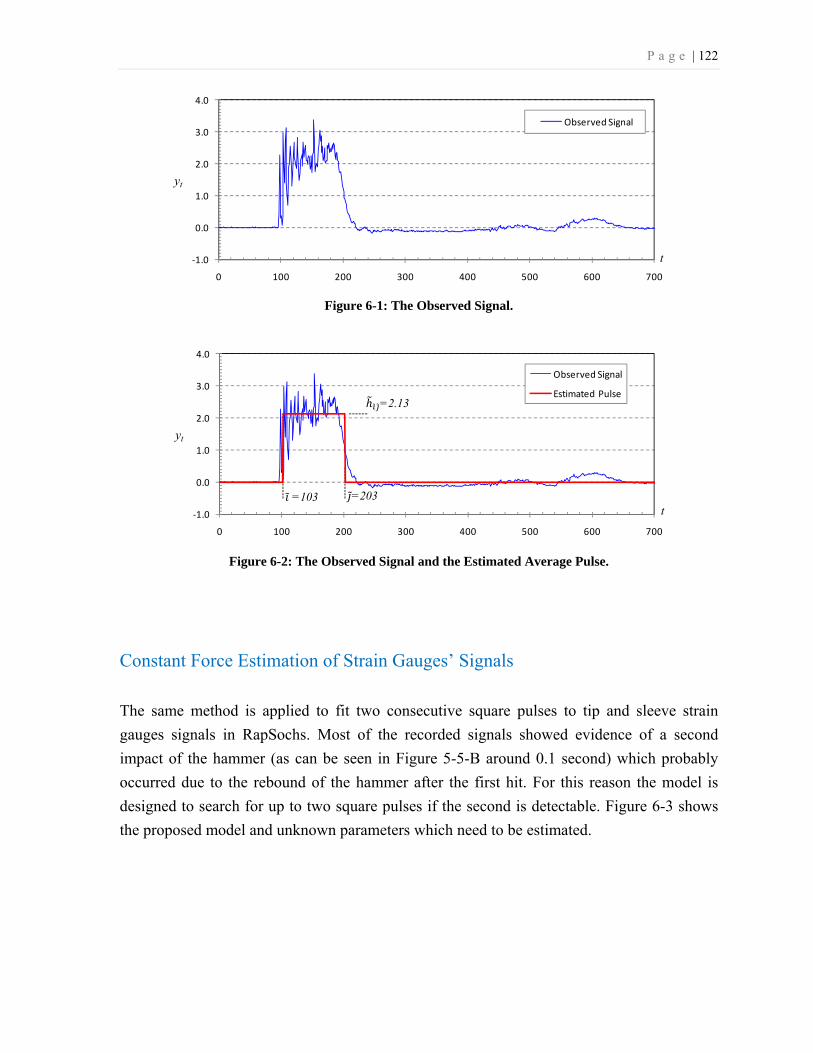
P a g e | 122
Figure 6-1: The Observed Signal.
Figure 6-2: The Observed Signal and the Estimated Average Pulse.
Constant Force Estimation of Strain Gauges’ Signals
The same method is applied to fit two consecutive square pulses to tip and sleeve strain
gauges signals in RapSochs. Most of the recorded signals showed evidence of a second
impact of the hammer (as can be seen in Figure 5-5-B around 0.1 second) which probably
occurred due to the rebound of the hammer after the first hit. For this reason the model is
designed to search for up to two square pulses if the second is detectable. Figure 6-3 shows
the proposed model and unknown parameters which need to be estimated.
-1.0
0.0
1.0
2.0
3.0
4.0
0 100 200 300 400 500 600 700
yt
Observed Signal
-1.0
0.0
1.0
2.0
3.0
4.0
0 100 200 300 400 500 600 700
yt
Observed Signal
Estimated Pulse
=203 =103
=2.13
t
t

P a g e | 123
Figure 6-3: A Proposed Estimation to Match the Recorded Signals.
The MLE is used for the estimation of the unknown parameters using sweeping iterations.
Use of Newton-Raphson iteration is not applicable in this problem due to the nature of the
recorded signal and its rapid changes in the magnitude that may lead to convergence failures.
To increase computational speed, the start and end of the searching windows of rise and fall
of the first and second pulses are defined by the user. A function is developed in MATLAB®
to assist the user to select the ranges graphically. The signal is plotted and user has to select
these ranges by drawing a window around the possible areas on the computer screen. Then
the program, for each possible combination of i, j, k, and l (as shown in Figure 5) in the
determined windows, estimates the magnitude of h1, h2, h3, and h4 and calculates the
corresponding MSE. The parameters i, j, k, l, h1, h2, h3, and h4 which result in the smallest
MSE are stored as the best estimates.
Table 6-1 presents the variables added to each RapSochs MAT-files as a result of MLE
analysis on strain gages signals. Figure 6-4 shows the strain gauges’ data and estimated
square pulses fitted to the 22nd drop in RSC-02-R-S2, the 99th drop in SIL-03-R-S5, the
35th drop in C6S-01-R-S8, and the 65th drop in GRV-02-R-S5 tests respectively.
y
t
Square Pulse Signal
i j k l
h1
h2
h3 h4

P a g e | 124
Table 6-1: Variables Added to RapSochs MAT-files Regarding Strain Gauges Estimation.
Variable Description
pulse1_features_range This is an n-by-8 matrix, where n is the total number of blows in the test.
The data in the mth row, corresponding to blow number m. The values in
each raw consist of 4 pairs corresponding the start and the end of the
searching window for i, j, k, and l for the output of the tip strain gauge data
saved in str1. The parameters i, j, k, and l are shown in Figure 6-3.
pulse1_features This is an n-by-9 matrix, where n is the total number of blows in the test.
The data in the mth row, corresponding to blow number m. In each row, the
first four values are i, j, k, and l and the second four values are h1, h2, h3, and
h4 respectively. The last number is the minimum MSE corresponding to the
best estimate. These parameters identify the square pulse fitting the output
of the tip strain gauge data saved in str1.
pulse2_features_range The same as pulse1_features_range but for outputs of the sleeve strain
gauge data saved in str2.
pulse2_features The same as pulse1_features but for outputs of the sleeve strain gauge data
saved in str2.

P a g e | 125
Figure 6-4: Typical Result of the Estimation on the Recorded Tip and Sleeve Forces in RSC, SIL, C6S
and GRV Samples.
0.02 0.04 0.06 0.08 0.1 0.12 0.14 0.16 0.18 0.2
0
2
4
6RSC-02-R-S2 , Drop Number 22, Depth = -429 (mm), Penetration = 14 (mm), Drop Height = 203 (mm)
Tip
+ S
leev
e For
ce (kN
)
0.02 0.04 0.06 0.08 0.1 0.12 0.14 0.16 0.18 0.2
0
2
4
6
Tip
For
ce (kN
) i= 0.0099, j= 0.0337, k= 0.0501, l= 0.0557, h1= 0.74, h2= 0.07, h3= 0.19, h4= 0.09
i= 0.0098, j= 0.0335, k= 0.0497, l= 0.0554, h1= 0.76, h2= 0.06, h3= 0.18, h4= 0.10
0.02 0.04 0.06 0.08 0.1 0.12 0.14 0.16 0.18 0.2
0
2
4
6SIL-03-R-S5 , Drop Number 99, Depth = -374 (mm), Penetration = 3 (mm), Drop Height = 559 (mm)
Tip
+ S
leev
e For
ce (kN
)
0.02 0.04 0.06 0.08 0.1 0.12 0.14 0.16 0.18 0.2
0
2
4
6
Tip
For
ce (kN
)
i= 0.0102, j= 0.0160, k= 0.0933, l= 0.0967, h1= 4.99, h2= 0.01, h3= 1.08, h4= 0.08
i= 0.0101, j= 0.0160, k= 0.0933, l= 0.0966, h1= 5.06, h2= -0.01, h3= 1.04, h4= 0.07
0.02 0.04 0.06 0.08 0.1 0.12 0.14 0.16 0.18 0.2
0
2
4
6C6S-01-R-S8 , Drop Number 35, Depth = -387 (mm), Penetration = 8 (mm), Drop Height = 559 (mm)
Tip
+ S
leev
e For
ce (kN
)
0.02 0.04 0.06 0.08 0.1 0.12 0.14 0.16 0.18 0.2
0
2
4
6
Tip
For
ce (kN
) i= 0.0101, j= 0.0208, k= 0.0625, l= 0.0715, h1= 0.41, h2= -0.01, h3= 0.12, h4= 0.03
i= 0.0101, j= 0.0205, k= 0.0635, l= 0.0717, h1= 1.01, h2= -0.01, h3= 0.32, h4= 0.05
0.02 0.04 0.06 0.08 0.1 0.12 0.14 0.16 0.18 0.2
0
2
4
6
8GRV-02-R-S5 , Drop Number 50, Depth = -374 (mm), Penetration = 5 (mm), Drop Height = 559 (mm)
Tip
+ S
leev
e For
ce (kN
)
0.02 0.04 0.06 0.08 0.1 0.12 0.14 0.16 0.18 0.2
0
2
4
6
8
Time (seconds)
Tip
For
ce (kN
)
i= 0.0107, j= 0.0175, k= 0.0976, l= 0.1021, h1= 4.50, h2= -0.03, h3= 0.79, h4= 0.06
i= 0.0107, j= 0.0175, k= 0.0975, l= 0.1021, h1= 4.59, h2= -0.01, h3= 0.81, h4= 0.06
Recorded Data
Estimated Square Pulse
Recorded Data
Estimated Square Pulse
P a g e | 126
Cone and Sleeve Resistance
The magnitude of the first square pulse obtained from MLE analysis on recorded signals at
lower and upper strain gauges is an estimate of the average cone or friction forces. The forces
may be converted to stresses following ASTM D5778 standards. They also could be
presented similar to CPT data charts. ASTM D5778 describes friction sleeve resistance fs as
the shear force applied to the friction sleeve divided by its surface area. Cone resistance, qc,
is the vertical force at the cone divided by the cone base area. Cone resistance and friction
sleeve resistance are calculated using following equations.
qc = Fc / Ac .............................................................................................................. 6-7
Where:
qc = cone resistance (Pa),
Fc = Estimated average force on cone (N)
Ac = cone base area, in RapSochs equals to 3.14 × 10⁻⁴ (m
2)
fs = (Fc+t - Fc) / As .................................................................................................... 6-8
Where:
fs = friction sleeve resistance (Pa),
Fc+t = Estimated average force on cone plus sleeve (N)
As = friction sleeve area, in RapSochs equals to 47.12 × 10⁻⁴ (m
2)
In CPT, data are recorded continuously with depth and based on ASTM standard D5778 at
least in 50 mm intervals for electronic friction cone. The data are usually plotted at the
midpoint of friction sleeve. 100 mm is the standard offset for 10 cm2 cones. In mechanical
CPTs, the mid-height of the friction sleeve is used when plotting.
In RapSochs, we assign the calculated cone resistance for each blow from the previous
position to the new position of the cone as a constant value. However, the situation is not that
clear for calculated friction resistance. During any blow we have obtained two average
forces; 1) cone force, and 2) cone plus sleeve force. Simple subtraction gives the sleeve
force. It is very obvious that the cone force represents the average force which the cone
experienced from the previous position to the new position. However since the sleeve is 75
mm long we have more than one choice for presenting friction stresses. We could either
assume that the calculated friction is representing the soil friction from midpoint of the
previous position of the sleeve to the midpoint of new position (method 1), or calculate the

P a g e | 127
average friction for each segment of soil based on all measured frictions in that segment
(method 2). In the RapSochs the mid-height of the sleeve is 45 mm above the cone shoulder.
Figure 6-5 shows comparison of two methods for calculating friction stresses in a dynamic
penetrometer with friction sleeve. Figure 6-6 shows comparison of two methods for SIL-05-
R-S7 test data. Method 1 shows fluctuation in the results and in contrast, Method 2 shows
less fluctuation. Also the procedure of Method 2 is more representative since it considers all
the measurements in any segment of the soil. Therefore we will use Method 2 for any further
analysis.
In CPT, data are usually plotted versus depth and connected with straight lines as “an
approximation for a continuous graph” (ASTM D5778, 1998). Here we plot test results as a
vertical line (constant value) for each penetration interval.

P a g e | 128
Figure 6-5: Comparison of Two Methods for Calculation of Friction Stresses in a Dynamic Penetrometer
with Friction Sleeve.
Skin Resistance
Sleeve
Friction Stress
Dep
th
Friction Resistance Measured Averaged Friction Resistance
Friction Stress
Dep
th
Method 1
Method 2

P a g e | 129
Figure 6-6: Friction resistance profile of SIL-05-R-S7 calculated and presented using two methods.
Friction Ratio
To obtain friction ratio by CPT, ASTM standard Method D5778 requires measurement of
cone and friction sleeve resistance at the same depth in the soil. The position of the cone is
taken as the reference depth and typically a previous cone resistance reading at the midpoint
of friction sleeve is used for calculation. 100 mm is the standard offset for 10 cm2 cones. It is
also noted that in ASTM standard Method D3441 for mechanical CPTs, the vertical distance
between the base of the cone and the mid-height of the friction sleeve should be taken into
account when plotting data or calculating friction ratio.
Here, since we have obtained a continuous profile of cone and friction resistance we can
calculate the friction ratio using the following equation.
Rf = 100.(fs / qc) ...................................................................................................... 6-9
Where:
Rf = friction ratio in percentage.
fs = friction sleeve resistance (Pa),
qc = cone resistance at the same depth as fs (Pa),
-700
-600
-500
-400
-300
-200
-100
0
Dept
h (m
m)
0 20 40 60 80 100Friction Resistance (kPa)
0 20 40 60 80 100Friction Resistance (kPa)
Method 2 Method 1

P a g e | 130
Typical Results
The typical results versus depth of four sets of tests are presented in Figure 6-7. The graphs
(from left) are cone resistance, sleeve friction resistance, friction ratio and hammer drop
height. The hammer drop height is also presented for comparison and to examine any
possible effect of applied energy in estimation of force and consequently on resistance profile
of the soil. Cone depth is used as the reference to plot hammer drop height. The similar
graphs for each individual RapSochs tests are presented in Appendix L.

P a g e | 131
Figure 6-7: Typical Profile of Cone Resistance, Friction Resistance, Friction Ratio, and Hammer Drop
Height for Different Soil Types.
0 1 2 3 4
-700
-600
-500
-400
-300
-200
-100
0De
pth
(mm
)
Cone Resistance (MPa)
RSC-02-R-S2
0 5 10 15 20 25Friction Resistance (kPa)
0 0.5 1 1.5 2Friction Ratio (%)
0 20 40 60Hammer Drop Height (cm)
0 5 10 15 20
-700
-600
-500
-400
-300
-200
-100
0
Dept
h (m
m)
Cone Resistance (MPa)
SIL-05-R-S7
0 20 40 60 80 100Friction Resistance (kPa)
0 0.5 1 1.5 2Friction Ratio (%)
0 20 40 60Hammer Drop Height (cm)

P a g e | 132
Figure 6-7 (Continued): Typical Profile of Cone Resistance, Friction Resistance, Friction Ratio, and
Hammer Drop Height for Different Soil Types.
0 0.5 1 1.5 2
-700
-600
-500
-400
-300
-200
-100
0D
epth
(mm
)Cone Resistance (MPa)
C6S-01-R-S8
0 30 60 90 120 150Friction Resistance (kPa)
0 5 10 15 20Friction Ratio (%)
0 20 40 60Hammer Drop Height (cm)
0 5 10 15 20
-700
-600
-500
-400
-300
-200
-100
0
Dept
h (m
m)
Cone Resistance (MPa)
GRV-02-R-S5
0 10 20 30 40 50Friction Resistance (kPa)
0 0.5 1 1.5 2Friction Ratio (%)
0 20 40 60Hammer Drop Height (cm)
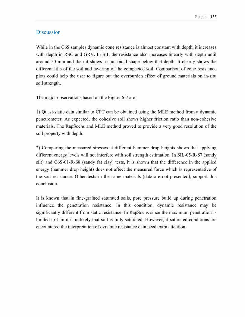
P a g e | 133
Discussion
While in the C6S samples dynamic cone resistance is almost constant with depth, it increases
with depth in RSC and GRV. In SIL the resistance also increases linearly with depth until
around 50 mm and then it shows a sinusoidal shape below that depth. It clearly shows the
different lifts of the soil and layering of the compacted soil. Comparison of cone resistance
plots could help the user to figure out the overburden effect of ground materials on in-situ
soil strength.
The major observations based on the Figure 6-7 are:
1) Quasi-static data similar to CPT can be obtained using the MLE method from a dynamic
penetrometer. As expected, the cohesive soil shows higher friction ratio than non-cohesive
materials. The RapSochs and MLE method proved to provide a very good resolution of the
soil property with depth.
2) Comparing the measured stresses at different hammer drop heights shows that applying
different energy levels will not interfere with soil strength estimation. In SIL-05-R-S7 (sandy
silt) and C6S-01-R-S8 (sandy fat clay) tests, it is shown that the difference in the applied
energy (hammer drop height) does not affect the measured force which is representative of
the soil resistance. Other tests in the same materials (data are not presented), support this
conclusion.
It is known that in fine-grained saturated soils, pore pressure build up during penetration
influence the penetration resistance. In this condition, dynamic resistance may be
significantly different from static resistance. In RapSochs since the maximum penetration is
limited to 1 m it is unlikely that soil is fully saturated. However, if saturated conditions are
encountered the interpretation of dynamic resistance data need extra attention.

P a g e | 134
6-2- Theory of Dynamics in Dynamic Cone Penetrometers
Introduction
The stress-strain relationship in a dynamic penetrometer is very complex. Theoretical and
numerical modeling requires many simplifying assumptions and detailed characterization of
the material properties, impact conditions, and energy efficiency. Verification of assumptions
and laboratory measurements and characterization of material properties are not always easy
to establish. Therefore, different empirical and mathematical models have been proposed for
dynamic penetration to correlate soil parameters to penetration per blow. Because of the
similar analogy in pile driving, SPT or other penetrometers; some of these models have been
developed to evaluate the bearing capacity of a driven pile or energy efficiency of SPT.
Most of the models presented in literatures are based on Newton’s laws and conservation of
energy. Proposed formulas are usually modified to account for energy losses during impact
and propagation of stresses (Fragaszy et al., 1985). In this section, a model based on basic
Newtonian mechanics and assumption of rigid bodies is developed. It is also compared with
the Dutch formula which is used in different instruments more than any other model.
Penetration Stages
Figure 6-8 shows three states of a typical blow during a full RapSochs penetration test. For
further discussion, any of these states are called a “stage”. At stage I or initial position, the
hammer is released from a known height, named “hammer drop height”. At stage II the
hammer strikes the anvil. This instant is also called collision. At stage III or final position,
both hammer and rod reach equilibrium with the soil and there is no further movement.
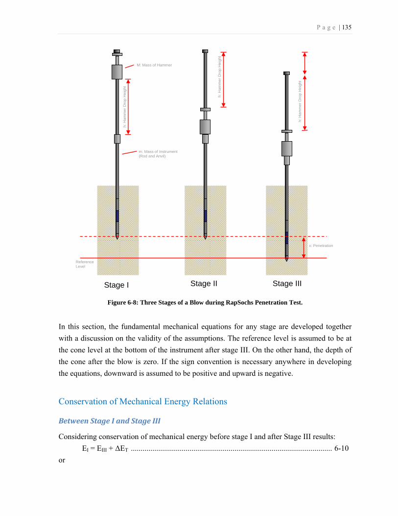
P a g e | 135
Figure 6-8: Three Stages of a Blow during RapSochs Penetration Test.
In this section, the fundamental mechanical equations for any stage are developed together
with a discussion on the validity of the assumptions. The reference level is assumed to be at
the cone level at the bottom of the instrument after stage III. On the other hand, the depth of
the cone after the blow is zero. If the sign convention is necessary anywhere in developing
the equations, downward is assumed to be positive and upward is negative.
Conservation of Mechanical Energy Relations
Between Stage I and Stage III
Considering conservation of mechanical energy before stage I and after Stage III results:
EI = EIII + ΔET ....................................................................................................... 6-10
or
m: Mass of Instrument (Rod and Anvil)
M: Mass of Hammer
x: Penetration
h:
Ha
mm
er
Dro
p H
eig
ht
Stage I Stage II Stage III
Reference Level
h:
Ha
mm
er
Dro
p H
eig
ht
h:
Ha
mm
er
Dro
p H
eig
ht

P a g e | 136
UI + KI = UIII + KIII + ΔET .................................................................................... 6-11
where:
EI: Total energy at Stage I
EIII: Total energy at Stage III
UI: Potential energy at Stage I
KI: Kinetic energy at Stage I
UIII: Potential energy at Stage III
KIII: Kinetic energy at Stage III
ΔET: Total energy loss
Since before releasing the hammer at Stage I and after Stage III when everything stops
moving there is no motion, the only terms in the total energy will be the potential energy. UI
+ KI = UIII + KIII + ΔET Equation 6-11 is rewritten as:
UI = UIII + ΔET ...................................................................................................... 6-12
ΔUI to III = ΔET ...................................................................................................... 6-13
m.g.x + M.g.(x+h) = ΔET ..................................................................................... 6-14
(m+M).g.x + M.g.h = ΔET ................................................................................... 6-15
where:
ΔUI to III = UI - UIII
M: Mass of hammer
m: Mass of instrument (without hammer)
g: Gravity
x: Penetration per blow
h: Hammer drop height
In Equation 6-16, ΔEt include the energy which is used to overcome the soil resistance and
move the penetrometer down, the elastic compression of soil and penetrometer, and
dissipated energy in collision of hammer and anvil as sound, vibration, and heating the
impacting bodies.
Between Stage I and Stage II
Considering conservation of mechanical energy exactly after stage I and before stage II
results:
EI = EII + ΔEFriction ................................................................................................. 6-16
or

P a g e | 137
UI + KI = UII + KII + ΔEFriction ............................................................................... 6-17
where:
ΔEFriction: Hammer energy loss due to friction and etc.
Assuming that the instrument is perfectly vertical, there is no friction between the
hammer and the guide, and air in not entrapped between hammer and anvil, then ΔEFriction is
equal to zero. If the system is not perfectly aligned vertical, then some of the energy could be
wasted due to vibration of the system. In similar systems, the errors caused by neglecting
these types of losses are not considered to interfere with correct interpretation of the results
(Bolomey, 1974).
Therefore by assuming ΔEFriction equal to zero, the velocity of hammer exactly before
collision can be calculated:
M.g.h = M (VH0)2
............................................................................................... 6-18
where:
VH0 : Velocity of hammer exactly before collision
So,
VH0 = 2g. h ........................................................................................................ 6-19
Before Stage II and after Stage II
Considering conservation of mechanical energy exactly before and after stage II, we have:
EII-ε = EII+ε + ΔECollision .......................................................................................... 6-20
or
UII-ε + KII-ε = UII+ε + KII+ε + ΔECollision ................................................................. 6-21
where:
ΔEH: Energy loss due to collision
There is no change in potential energy before and after the collision, so Equation 6-21
simplifies to:
UII-ε = UII+ε + ΔECollision ........................................................................................ 6-22
The velocity of the system before collision is zero:

P a g e | 138
M (VH0)2
= m.VS12
+ M.VH12 + ΔECollision .................................................. 6-23
where;
VH1 : Velocity of hammer exactly after collision
VS1 : Velocity of system exactly after collision
Therefore:
ΔECollision = M (VH0)2
- m.VS12
- M.VH12 ..................................................... 6-24
Energy Loss due to Soil Resistance
The system is not assumed isolated and external forces transfer energy to or from the
system. Soil applies the resisting force against penetration of the system. The work by soil is
a function of time and is a consequence of soil resistance acting on the cone and the
submerged part of the rod together. However for simplification we assume that the force is
constant during the penetration.
WSoil = Fd.x ........................................................................................................... 6-25
where:
WSoil : The mechanical work done on the soil
Fd : Average dynamic force applied by penetrometer during penetration
(= Average force applied by soil against penetration)
The force applied by the penetrometer is downward and it is positive based on our
sign convention. Likewise, the force which is acting on the penetrometer is upward and is
negative.
We can relate work done by soil to the energy loss due to soil resistance:
ΔESoil = - Fd.x ........................................................................................................ 6-26
Note that the Fd is comprise of friction force acting on the embedded length of the
penetrometer and tip resistance force.

P a g e | 139
Energy Loss due to Hammer and Anvil Collision
For the moment that hammer collide into the anvil we can write the general equation
for conservation of the linear momentum as:
M.VH0 + m.VS0 = M.VH1 + m.VS1 ....................................................................... 6-27
where:
VH0 : Velocity of hammer exactly before collision
VS0 : Velocity of system exactly before collision (equals to zero)
VH1 : Velocity of hammer exactly after collision (after rebound)
VS1 : Velocity of system exactly after collision
Since the velocity of the system exactly before collision is zero, Equation 6-27 could
be simplified to:
M.VH0 = M.VH1 + m.VS1 ....................................................................................... 6-28
The collision of hammer and anvil is not isolated and an external force (soil
resistance) act on the system. Also the hammer does not return to its original height and
hammer rebound is relatively small. Therefore the collision is more likely an inelastic
collision. In an elastic collision the kinetic energy of the system of colliding bodies can
change, but the total kinetic energy of the system does not change (Halliday et al, 1997). In
an inelastic collision, the kinetic energy of the system of colliding bodies is not conserved.
The kinetic energy that is lost is transferred to some other form of energy (e.g., thermal or
acoustic energy or vibration of the system). Nonetheless, the linear momentum of the system
is always conserved. So, the question is how much kinetic energy is lost by a system in the
collision. When the bodies stick together in a completely inelastic collision (also called
plastic collision), the amount of kinetic energy that is lost is the maximum allowed by the
conservation of linear momentum (Halliday et al, 1997).
Inelastic Collision
In dynamics, the “coefficient of restitution” is usually used to supplement the analysis
of inelastic collision. Coefficient of restitution, Cr, is defined as the ratio of the impulse
during restitution to that during deformation (Muvdi et al, 1997). A simplified equation for
Hammer-Anvil collision is:

P a g e | 140
Cr = VS VHVH VS .......................................................................................................... 6-29
where (VS1 - VH1) represents the relative velocity after impact and (VH0 - VS0) is the
relative velocity before impact. This equation shows that the coefficient of restitution is the
ratio of the relative velocity after impact to the relative velocity before impact.
Two special values of the coefficient of restitution are of considerable interest. If Cr
=0, the impact is termed perfectly plastic, or as we called it, perfect inelastic collision. We
note, from the defining equation for Cr, that this implies VS1 = VH1. This means that the two
bodies move off together after impact with a common velocity. If Cr =1, the impact is termed
perfectly elastic. This means that the relative velocity after impact equals the relative velocity
before impact. It is shown that the kinetic energy of the colliding bodies is conserved during
a perfectly elastic impact (provided we neglect relatively small impulses delivered by friction
forces during small time of impact). For values of Cr less than unity, there is a loss of energy
which is dissipated in sound or in heating the impacting bodies.
In the penetrometer, VS0 = 0. So the velocity of hammer after collision in Equation 6-
29 can be rewritten in terms of velocity of system after collision and velocity of hammer
before collision:
VH1 = VS1 – Cr.VH0 ................................................................................................ 6-30
Replacing this relationship into conservation of linear momentum formula (Equation 6-28)
results:
M.VH0 = M. (VS1 – Cr.VH0) + m. VS1 ................................................................... 6-31
M.VH0 = M.VS1 – Cr.M.VH0 + m. VS1 ................................................................. 6-32
M.VH0.(1+ Cr) = VS1.(m + M) ............................................................................... 6-33
VS1 = M.VH0.(1+ Cr) / (m + M) ............................................................................. 6-34
In the same way;
VH1 = VH0 (M – m. Cr) / (m + M) ......................................................................... 6-35
Note that this equation is not developed based on any assumption about the nature of
the collision yet. Therefore the value of the coefficient of restitution may dictate the type of
the collision to be elastic (perfectly elastic), inelastic or plastic (perfectly inelastic).

P a g e | 141
Substitution of Equation 6-34 and Equation 6-35 in Equation 6-24 and simplification results:
ΔECollision = .M(M ).VH0
2 (1- Cr2) ........................................................................ 6-36
It is obvious in Equation 6-36 that if the collision is elastic (Cr =1) then the energy
loss due to the collision is zero. Replacing of VH0 from Equation 6-19 results:
ΔECollision = .M. .(M ) (1- Cr
2) .................................................................................. 6-37
Energy Loss due to Hammer Rebound
Figure 6-9 shows the possible rise and fall of hammer after the first collision. After the first
collision (Figure 6-9c), the hammer is bouncing back upward (Figure 6-9d) and after
reaching to the top of the trajectory (Figure 6-9e) falls on the anvil and hits it for the second
time (Figure 6-9f). The following equations are developed for the motion of the hammer.
Figure 6-9: Possible Rise and Fall of Hammer after the First Collision.
Here we assume that the second hit is not sufficient to make any further penetration and
therefore the transferred energy due to the second hit is lost. Recorded displacement data of
RapSochs tests shows that when the hammer hits the anvil for the second time the
d) Rise of Hammer(After Rebound)
e) Hammer at top of trajectory
f) Before the second collision
VH1 VH2
VH = 0
b) Hammer free fall
VH0
c) The First Collision
a) Hammer is released
VH =0
Ham
mer
Dro
p H
eigh
t

P a g e | 142
penetrometer has already stopped moving downward and the second hit (if happens) does not
cause any further advancement. Also examining the accelerometer data showed that the
separation of hammer from anvil after the first collision happens a moment before that the
penetrometer stops moving downward. Therefore we ignore any further advancement of the
penetrometer after the hammer bounce back.
Therefore the total energy of the hammer after the collision is considered as the loss
energy:
ΔEHammer = EH1 .................................................................................................... 6-38
ΔEHammer = M.VH12
............................................................................................. 6-39
Where;
ΔEHammer : Energy loss due to hammer rebound or slow down after the collision,
EH1 : Energy of the hammer exactly after the first collision.
After substitution of VH1 from Equation 6-35 and VH0 from Equation 6-19 we have:
ΔEHammer = M. . .(M .C )(M ) ................................................................................. 6-40
The Energy Model If we neglect the dissipated energy through soil elastic deformation and other losses, then
total energy loss, ΔET, is equal to the summation of all energy losses. In summary
ΔET = ΔESoil + ΔECollision + ΔEHammer ..................................................................... 6-41
Replacing Equation 6-41 in Equation 6-16 give us:
(m+M).g.x + M.g.h = ΔESoil + ΔECollision + ΔEHammer ............................................ 6-42
In Equation 6-42, the terms on the left are the elements that cause the advancement of the
system to the soil and we call them “input energy”. On the opposite side, there are terms that
consume that energy and we call them “output energy”. Substitution of energy losses by
equations obtained in previous sections and simplification results:

P a g e | 143
(m+M).g.x + M.g.h = - Fd.x + .M. .(M ) (1- Cr2) + M. . .(M .C )(M ) ................... 6-43
Examining the terms of the equation shows that the only unknown parameter is the
coefficient of restitution. Assuming a constant Cr, it could be calculated by using Equation 6-
43 and regression analysis.
Coefficient of Restitution for RapSochs To obtain the coefficient of restitution for RapSochs, the data obtained in RapSochs tests in
different materials are used. In RapSochs, the hammer mass is 9090 g (20 lb) and rod, guide
and connections are 6300 g. The string potentiometer causes a relatively constant downward
force equivalent to 10.2 N (on its manual it is reported to be 9.5 N). Therefore, mRS = 6.3 kg,
MRS = 9.09 kg, and g = 9.81 m/s2 are constants.
For each blow the h (hammer drop height) is recorded and x (Penetration per blow) is
measured. Fd (the average dynamic force) is comprised of friction force acting on the
embedded length of the penetrometer and tip resistance force. Assuming that the average skin
friction along the rod remains constant during penetration, the friction force Fdf (dynamic
friction force) could be calculated from the average sleeve friction stresses profile. Tip
resistance force, Fdc (dynamic force at cone), is also obtained by MLE analysis for strain
gauge measurements of each blow. Therefore in Equation 6-43 all parameters except Cr are
known.
By regression analysis the coefficient of restitution is obtained to be 0.39 for RapSochs.
Figure 6-10 presents the “input energy” versus “output energy” of RapSochs test data for Cr =
0.39. There are more than 1400 data points plotted in this graph where each data point
represents one blow. The first blow of each test is excluded. The data includes all the tests in
different samples.

P a g e | 144
Figure 6-10: Energy Balance Diagram of RapSochs Test Results Using the Energy Model Formula for Cr
= 0.39.
Effect of Accuracy of Displacement Measurement
Even though the coefficient of determination (R-squared) in the analysis is very good, it was
decided to examine why the data diverge vertically at higher input energies. Examining the
data show that at higher input energy, the contribution of penetration per blow, x, to potential
input energy is very small but it has a higher effect on the right side of Equation 6-43. To
verify the sensitivity of the energy balance to penetration per blow, the same data are plotted
by just changing the “x” by plus and minus 1 mm while keeping other parameters constant.
The trend lines of the results are also plotted in Figure 6-10 as two dashed lines.
RapSochs String potentiometer which is used to measure advancement of the penetrometer
has an accuracy of ± 1 mm. Figure 6-10 shows clearly that it affects the input-output energy
balance equation and accurate measurement of penetration per blow is very important.
y = 1.00xR² = 0.96
0.0
10.0
20.0
30.0
40.0
50.0
60.0
70.0
0 10 20 30 40 50 60 70
Out
put E
nerg
y, (
N.m
)
Input Energy, E (N.m)
Equality Line±1 mm Constrained RegressionLinear (Constrained Regression)

P a g e | 145
Effect of Manual Operation of Hammer
Manual release of hammer from a certain height is not easy and is not always very accurate.
The inaccuracy is limited to ± 13 mm (0.5 inch). Although this range may be up to 10% of
the total energy of hammer when the hammer is dropped from 127 mm (5 inch) height, for
most of the tests it does not contribute to more than 3% in error. Examination of the effect of
inaccurate drop height of hammer on the constrained regression equation of energy balance
showed that by keeping the Cr constant it will not change the trend-line equation more than ±
1%.
Validation of Coefficient of Restitution
In previous section, the analysis showed a good result assuming a constant coefficient of
restitution, Cr. Another approach is adopted to verify the model and verify the parameters
that may affect Cr.
Considering the definition of coefficient of restitution (Equation 6-29), the velocity of the
hammer before the collision is known from Equation 6-19. If the velocity of hammer and
penetrometer after the collision are determined, then Cr can be calculated independently.
Velocity of Hammer after the First Collision
Conservation of energy for hammer motion after the rebound at the beginning of hammer rise
and moments before the second collision of hammer, ignoring air or hammer guide friction,
can be written (see Figure 6-9).
EH1 =EH2 ............................................................................................................... 6-44
M.VH12
= M.VH22
........................................................................................... 6-45
VH12
= VH22
.......................................................................................................... 6-46
where;
EH1 : Energy of the hammer exactly after the first collision,
EH2 : Energy of the hammer exactly before the second collision,
VH2 : Velocity of hammer exactly before second collision
The only force acting on the hammer between these two steps is gravity. Therefore hammer
has a constant acceleration of g downward. So;

P a g e | 146
VH2 = VH1+ g.tH1-2 ................................................................................................ 6-47
where;
tH1-2 : time interval between the first rebound and second collision of hammer.
Substitution of Equation 6-47 to Equation 6-46 results:
VH12
= (VH1+ g. tH1-2 )2
........................................................................................ 6-48
VH12
= VH12
+ 2 VH1.g. tH1-2 + g2. tH1-22
............................................................... 6-49
2 tH1-2.VH1 = - g. tH1-2 2
.......................................................................................... 6-50
VH1= - g. tH1-2 .................................................................................................... 6-51
Using MLE analysis results, from previous section, we can obtain an estimate of tH1-2. Based
on Figure 6-3, tH1-2 can be estimated as:
tH1-2 = k – j ............................................................................................................ 6-52
where;
k and j are defined in Figure 6-3.
The results of MLE analysis on the observed stress wave signal in the tip strain gauge
are used to estimate the time interval between the rebound and collision of hammer. It will
provide all the necessary unknown parameters to estimate the velocity of hammer exactly
after the first collision.
Velocity of System after the First Collision
Motion relationships for the system after the collision are not very simple since the
interaction between the instrument and the soil should be considered. However the following
equation can be considered for the system:
VS = x / tp ........................................................................................................... 6-53
where;
VS : Average velocity of the system during penetration
x : Penetration per blow
tp : Duration of the penetration
P a g e | 147
By using MLE analysis results, from the previous section, an estimate of tp is obtained. Based
on Figure 6-3, tp can be estimated as:
tp = l - i .................................................................................................................. 6-54
where;
l and i are defined in Figure 6-3.
The results of MLE analysis on the observed stress wave signal in the tip strain gauge
are used to estimate the duration of the penetration. Therefore, all unknown parameters are
provided to calculate the average velocity of the penetrometer after the first collision.
Parametric Dependency
The coefficients of restitution, obtained by calculation of parameters on the right side of
Equation 6-29, are plotted for each blow of RapSochs tests. Figure 6-11 shows the Cr versus
total dynamic force (tip + friction force) and Figure 6-12 shows the Cr versus hammer
velocity before the first collision (which is proportional to hammer drop height). The average
of values is 0.37, with standard deviation of 0.05.
To verify the use of a constant Cr, the calculated Cr are plotted against variables that may
affect it. In both figure data are spread almost equally around average, which is a good
indication that the data are random. They also show that for this range of impact velocities
and soil strength, Cr is independent of the collision speed and soil dynamic resistance. In
other words the assumption that Cr is constant is not a biased assumption. Also since the Cr is
a result of tests in different soil types with different strength it could be assumed that the
calculated Cr is a property of the Hammer-Anvil system.

P a g e | 148
Figure 6-11: Coefficient of Restitution versus Total Dynamic Force.
Figure 6-12: Coefficient of Restitution versus Velocity of Hammer before Collision.
0.0
0.2
0.4
0.6
0.8
1.0
0 1000 2000 3000 4000 5000 6000 7000
Coef
ficie
nt o
f Res
titu
tion
, Cr
Total Dynamic Force (N)
Data from RapSochs Tests
Average Cr=0.37
Average ± SD
0.0
0.2
0.4
0.6
0.8
1.0
0 1 2 3 4
Coef
ficie
nt o
f Res
titu
tion
, Cr
VH0 (m/sec)
Data from RapSochs Tests
Average Cr=0.37
Average ± SD

P a g e | 149
Comparison
The average coefficient of restitution obtained by calculation is 0.37 with standard deviation
of 0.05. It is very close to 0.39 which is obtained from data regression. In pile driving
literatures the typical values of Cr for steel-on-steel hammer-anvil is reported in the range of
0.4 to 0.5 (Kaniraj, 1988, and Varghese, 2005).
In Figure 6-13 the energy model of RapSochs test data are plotted again but by using the
calculated Cr. Although the convergence of data is better (higher R-squared), the constrained
regression shows a 2% error. These results are in good agreement with the regression
analysis which confirms the assumptions and analysis of both methods.
Figure 6-13: Energy balance of RapSochs test using the energy model and calculated Cr.
In general, it is concluded that:
- The energy model of Equation 6-43 could be used to predict the hammer-
instrument-soil interaction and response with acceptable accuracy, and
- Using a constant Cr in the energy model yields an acceptable result.
y = 1.02xR² = 0.98
0.0
10.0
20.0
30.0
40.0
50.0
60.0
70.0
0 10 20 30 40 50 60 70
Out
put E
nerg
y, (
N.m
)
Input Energy, E (N.m)
Equality Line±1 mm Constrained RegressionLinear (Constrained Regression)
P a g e | 150
Dutch Equation
Sanglerat (1972) and Cassan (1988) related the dynamic cone resistance (qd) to the test
conditions and instrument geometry according to the “Dutch formula”. This equation was
developed originally by Eytelwein (1820) to estimate the ultimate capacity of driven piles
(reported by Fragaszy et al., 1985). The equation is written as:
qd=1
A
EX
M
M+m ................................................................................................. 6-55
where;
qd: Dynamic cone resistance
A: Cross sectional area of the cone
Eh: Imparted hammer energy
x: Incremental penetration (or DCP-PR)
M: Mass of the hammer and
m: Mass of the Penetrometer
And dynamic cone resistance qd multiplied by A is equal to soil resistance force:
Fd = qd. A .............................................................................................................. 6-56
After substitution of Equation 6-56 in Equation 6-55 and rearranging, the following equation
is obtained:
Fd = Ex MM+m ................................................................................................... 6-57 Fd. x = E MM+m ................................................................................................... 6-58
If an ideal free fall of hammer is assumed, without any friction between hammer and guide or
any resistance due to air entrapped between hammer and anvil, then the imparted hammer
energy equals to the kinetic energy of hammer before the first collision and equals to
potential energy of hammer before releasing:
Eh = Eh1 = M.VH12
= M.g.h .............................................................................. 6-59

P a g e | 151
Equation 6-59 is equal to only the second term of Equation 6-16 on the left side. First term in
Equation 6-16 stands for the change in potential energy of hammer and rod due to
penetration. In the other words, the potential energy change of hammer and rod due to
penetration is ignored in “Dutch formula”.
Replacing Equation 6-59 in Equation 6-58 results:
Fd. x = M . .M+m ........................................................................................................ 6-60
In a different approach, if the contribution of change of potential energy on the left side of
Equation 6-43 in driving the system is ignored, and also if the energy of hammer after the
first collision is also assumed to contribute in driving the system, Equation 6-43 will be
simplified as:
M.g.h = - Fd.x + .M. .(M ) (1- Cr2) ......................................................................... 6-61
In this equation it is assumed that only the kinetic energy of hammer drives the system and
the energy is lost due to the inelastic collision and soil resistance. Rewriting the equation
results in:
Fd.x = M. . .(M C )(M ) ........................................................................................ 6-62
If a perfect inelastic collision (plastic collision) is assumed then Cr = 0 and therefore the
above equation become similar to Equation 6-60. It shows that the Dutch formula is
developed by assuming a perfect inelastic collision which the hammer energy after the
collision will also contribute to the advancement of the penetrometer. In a perfect inelastic
collision, the bodies stick together and the amount of kinetic energy that is lost is the
maximum allowed by the conservation of linear momentum.
Figure 6-14 shows the RapSochs tests data plotted on the energy balance chart using
Equation 6-61 for Cr = 0. The only reason that Equation 6-61 is selected to plot test results
and not Equation 6-62 or Equation 6-60 is that in this equation input and output energies are
on opposite side of the equation otherwise they are identical at Cr = 0. The figure also shows

P a g e | 152
the sensitivity to accuracy of displacement measurement. It is clear from the equation of the
trend line that there is 9% error in this model compared to our model. The convergence of
data points is good in this model but does not meet our model accuracy. Using higher values
of Cr in Equation 6-61 results in even higher error. In other word, regression analysis will not
yield a Cr with any better correlation.
Figure 6-14: Energy Balance of RapSochs Test Using the Dutch Equation.
Other Relationships used for DCP
There are not many investigations based on the analytical relationship, finite element
modeling or energy transfer efficiency of DCP. The following paragraphs summarize the
literature on this topic.
Scala (1956) developed the equations which consider the change of potential energy of
hammer and penetrometer based on the assumption that the collision is perfectly inelastic and
that the hammer energy after the collision participate in driving down the probe. By
assuming that the dynamic penetration resistance is twice of static resistance, Scala (1956)
found a good agreement between estimated static resistance and CBR measurements. This is
y = 0.91xR² = 0.94
0.0
10.0
20.0
30.0
40.0
50.0
60.0
70.0
0 10 20 30 40 50 60 70
Out
put E
nerg
y, (
N.m
)
Input Energy, E (N.m)
Equality Line±1 mm Constrained RegressionLinear (Constrained Regression)

P a g e | 153
the same model as used by Vaz & Hopmans (2001). However, Minasny and McBratney
(2005) argued that adding the potential energy change of the instrument and penetrometer as
the energy input is “superfluous and violates the law of energy conservation”. In contrast,
Stolf et al. (2005) argued that it should be included in the energy balance equations. Our
approach is supported by the argument of Vaz & Hopmans (2001) and Stolf et al. (2005).
Harison (1986, 1987) used an equation similar to Equation 6-62 to explain the log-log
correlation of DCP-CBR. He mentioned that this equation does not include all the energy
losses and that is the reason that for DCP-CBR correlations, Log(CBR) = Log(A) – Log(x)
equation should be replaced by Log(CBR) = Log(A) – B.Log(x) where A and B are constants
which are obtained by regression analysis. Compared with inverse model (former equation)
he concluded that log-log model (later equation) results in a better correlation.
Livneh et al. (2000) used the Dutch formula and called η = M/(m+M) the apparent energy-
transfer efficiency factor. They referenced to work done by Kramer (1994) to confirm that
the η is a good estimate of the energy efficiency of dynamic penetrometers. For their
standard DCP with M/m = 2.23 (m = 3.6 kg) they calculated the η = 0.69 (for our DCP, M/m
is 1.77 and m = 4.52 kg and apparent energy efficiency would be η = 0.64). Rahim et al.
(2004), assumed the energy transfer efficiency of 0.75 to calibrate their model with DCP tests
data. Herrick and Jones (2002) assumed 100% efficiency for their specific-designed near
surface penetrometer. Ampadu and Arthur (2006) also used Dutch formula to estimate cone
resistance.
Developing a Multi-Degree of Freedom Model
Even though our dynamic energy model showed acceptable results, a more realistic approach
could be considered to model hammer-instrument-soil interaction as a multi-degree freedom
system. An example of such a model is presented in Figure 6-15. The spring-dashpot model
of soil shown in this figure could be replaced by elasto-plastic spring-dashpot system for soil
resistance which is closer to real behavior of soil under dynamic loading. Other spring-
dashpots could be added to the side of the penetrometer to represent soil friction. The rigid
body which represents the penetrometer could also be replaced by an elastic material which
follows the Hooke's law. Such models are used widely in pile driveling analyses.

P a g e | 154
Figure 6-15: A multi-degree freedom system representation of penetrometer-soil interaction at different
stages of one blow.
The works of Chua (1988) and Chua & Lytton (1988) include modeling and instrumentation
of DCP to obtain elastic modulus and damping ratio of soil. However, energy related
parameters are not discussed directly in their papers. In pile driving and SPT analysis, many
works in this respect are available.
Energy Loss due to Elastic Deformation of Penetrometer and Hammer
Some of the equations developed for pile driving consider the strain energy. In this section,
the strain energy concept and the significance of this term in the energy balance formulas are
evaluated.
h:
Ha
mm
er
Dro
p H
eig
ht
Stage I, II & III
x: Penetration
m
M
m
M
m
M
P a g e | 155
Part of the energy delivered to the penetrometer causes elastic deformation of the system.
After the system stops moving, the rod which is compressed during penetration relaxes.
Since this energy is not acting in deriving the system, it could be assumed as lost energy. If
the material is assumed to follow Hook’s law, then the strain energy UED, stored in the
instrument due to elastic deformation of the rod during penetration, is equal to the elastic
work done by the soil resistance force on the rod:
UED = WED = F LEA ............................................................................................... 6-63
where;
UED: Strain energy
WED: Work done by soil resistance force on the rod
Fd: Average dynamic force applied by soil against penetration
L: Length of the instrument under loading
E: Elastic modulus (=196 GPa for steel 17-4)
Ai: Cross section of the instrument
To facilitate the analysis of a very complex system, the following assumptions to idealize the
behavior of the system are considered:
1) Any change in the potential energy of the rod itself (due to elastic deformation) is
disregarded, and the existence of strain energy in the rod due to its own weight is
ignored.
2) The stresses in the rod are assumed to remain within the linearly elastic range.
3) The stress distribution throughout the rod is assumed to be uniform and the
variation of the stress distribution due to the longitudinal stress wave travel through
the rod is ignored.
Energy Loss due to Elastic Deformation of RapSochs
Based on the dimensions of the RapSochs penetrometer, described in Chapter 3, the average
cross sectional area of penetrometer is calculated to be 2.26 × 10⁻⁴ m2 and the length is 1 m.
In case of non-cohesive soils (where the soil resistance is mainly from the tip of the
penetrometer) Equation 6-63 for RapSochs is:
URS(SI) = 1.13 × 10⁻⁸ × Fd2 ..................................................................................... 6-64
where;
Fd : Average dynamic force applied by soil against the RapSochs cone in N

P a g e | 156
The magnitude of this term compared to the kinetic energy of hammer before collision is
very small. The strain energy in RapSochs tests never exceed 1.2% of the kinetic energy of
the hammer and for most cases it remains below 0.7%. Therefore, this term is neglected to
simplify analysis.
Energy Loss due to Elastic Deformation of DCP
The average cross sectional area of DCP penetrometer is 2.01 × 10⁻⁴ m2 and the penetrometer
length is 1 m. In case of non-cohesive soils Equation 6-63 for DCP is:
UDCP(SI) = 1.27 × 10⁻⁸ × Fd 2 ................................................................................... 6-65
where;
Fd: Average dynamic force applied by soil against the DCP cone in N
Even though the force in DCP test was not measured, it is expected that in a similar soil and
in the same depth, the two instruments will face similar soil resistance. In that way, the above
mentioned argument for RapSochs is also valid for DCP. Therefore for the same reason, this
term is neglected in the calculations.
The Energy Model for DCP Data
In DCP the force during the penetration is not measured. However both instruments have a
similar cone dimensions and penetration mechanism. Therefore we expect that the measured
tip force by RapSochs at a certain depth be the same for the DCP.
The average stresses of RapSochs tests versus depth are obtained for each sample. Figure
6-16 shows a plot of tip stresses of several RapSochs tests in RSD and the calculated average
stress versus depth. The weighted average tip stress for the increment depth of each blow of
DCP is calculated. As an example, Figure 6-17 shows the estimated average tip stress for
RSD-01-D-S1 test.

P a g e | 157
Figure 6-16: Average of Tip Resistance of
RapSochs tests in RSD sample.
Figure 6-17: Average of Tip Resistance estimated
for RSD-01-D-S1 test.
Total mass of DCP (as tested at Northeastern University) is 12.52 kg. Based on ASTM 6951-
03, hammer mass is 8 kg (17.6 lb). Therefore mass of rod, guide and connections are 4.52 kg.
DCP has a fixed hammer drop height of 575 mm (22.6 in.).
Using data from DCP tests and the average force obtained by the method explained, the DCP
data are plotted in the energy balance diagram using Equation 6-43. Since the coefficient of
restitution is unknown, the regression is used to calculate the Cr. Figure 6-18 shows the
results for Cr= 0.73. It is believed that the smaller diameter of the penetrometer in DCP and
the lubrication of the penetrometer with oil will prevent and minimize the skin friction
resistance on the DCP. However, examination of the test data from C6S and CSB showed
that the assumption that cohesive soils do not stick to the DCP penetrometer and
consequently do not cause any circumferential frictions is not correct. Therefore, the data
points from these tests are excluded in calculating Cr and are not plotted in Figure 6-18.
0 1 2 3 4
-700
-600
-500
-400
-300
-200
-100
0De
pth
(mm
)Cone Resistance (MPa)
RSD-02-R-S5
RSD-03-R-S6
RSD-04-R-S7
RSD-05-R-S9
RSD-06-R-S8
Average
0 1 2 3 4
-700
-600
-500
-400
-300
-200
-100
0
Dep
th (m
m)
Cone Resistance (MPa)
RSD-01-D-S1
Average from RapSochs
Estimated for DCP
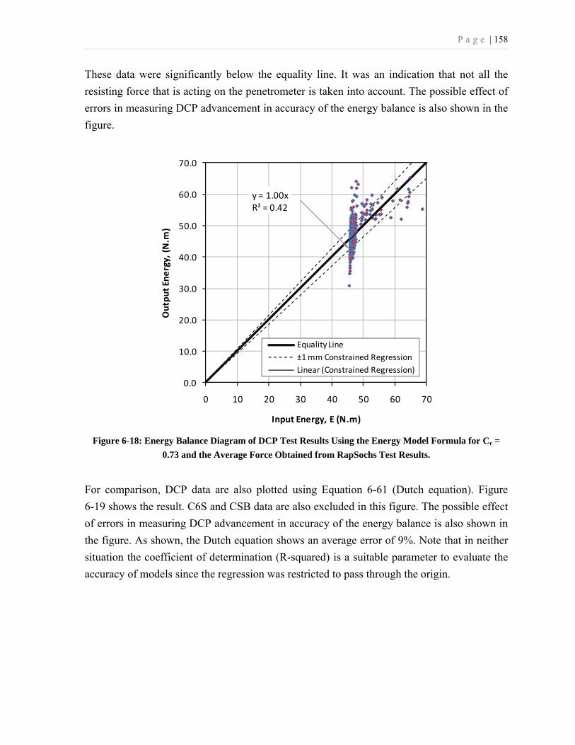
P a g e | 158
These data were significantly below the equality line. It was an indication that not all the
resisting force that is acting on the penetrometer is taken into account. The possible effect of
errors in measuring DCP advancement in accuracy of the energy balance is also shown in the
figure.
Figure 6-18: Energy Balance Diagram of DCP Test Results Using the Energy Model Formula for Cr =
0.73 and the Average Force Obtained from RapSochs Test Results.
For comparison, DCP data are also plotted using Equation 6-61 (Dutch equation). Figure
6-19 shows the result. C6S and CSB data are also excluded in this figure. The possible effect
of errors in measuring DCP advancement in accuracy of the energy balance is also shown in
the figure. As shown, the Dutch equation shows an average error of 9%. Note that in neither
situation the coefficient of determination (R-squared) is a suitable parameter to evaluate the
accuracy of models since the regression was restricted to pass through the origin.
y = 1.00xR² = 0.42
0.0
10.0
20.0
30.0
40.0
50.0
60.0
70.0
0 10 20 30 40 50 60 70
Out
put E
nerg
y, (
N.m
)
Input Energy, E (N.m)
Equality Line±1 mm Constrained RegressionLinear (Constrained Regression)

P a g e | 159
Figure 6-19: Energy Balance Diagram of DCP Test Results using Dutch Equation and the Average Force
Obtained from RapSochs Test Results.
For DCP data and based on presented figures, although it is not feasible to verify that the
energy balance model is more accurate than Dutch formula, it is definite that the Dutch
equation has a 9% error in predicting the hammer-instrument-soil interaction. Nonetheless,
one could conclude that assuming the coefficient of restitution about 0.73 for DCP, the
energy model predict the DCP interaction with soil more accurately than Dutch formula.
Distribution of Data
A total of 42 RapSochs tests and 29 DCP tests were conducted. Table 6-2 summarizes the
number of RapSochs and DCP tests and the range of CBR of the materials of each sample.
Number of recorded data in this table refers to total number of hammer blows. For example
in CSB sample it means that it took 14 hammer-blows to complete one RapSochs penetration
test and it took 3 hammer-blows to complete the only DCP test conducted on this sample.
y = 1.09xR² = 0.00
0.0
10.0
20.0
30.0
40.0
50.0
60.0
70.0
0 10 20 30 40 50 60 70
Out
put E
nerg
y, (
N.m
)
Input Energy, E (N.m)
Equality Line±1 mm Constrained RegressionLinear (Constrained Regression)
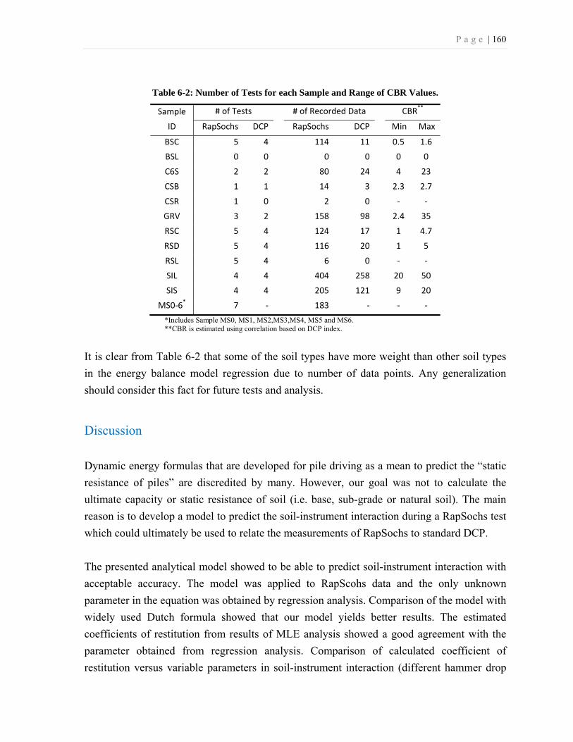
P a g e | 160
Table 6-2: Number of Tests for each Sample and Range of CBR Values.
Sample
ID
# of Tests # of Recorded Data CBR**
RapSochs DCP RapSochs DCP Min Max
BSC 5 4 114 11 0.5 1.6
BSL 0 0 0 0 0 0
C6S 2 2 80 24 4 23
CSB 1 1 14 3 2.3 2.7
CSR 1 0 2 0 - -
GRV 3 2 158 98 2.4 35
RSC 5 4 124 17 1 4.7
RSD 5 4 116 20 1 5
RSL 5 4 6 0 - -
SIL 4 4 404 258 20 50
SIS 4 4 205 121 9 20
MS0-6* 7 - 183 - - -
*Includes Sample MS0, MS1, MS2,MS3,MS4, MS5 and MS6. **CBR is estimated using correlation based on DCP index.
It is clear from Table 6-2 that some of the soil types have more weight than other soil types
in the energy balance model regression due to number of data points. Any generalization
should consider this fact for future tests and analysis.
Discussion
Dynamic energy formulas that are developed for pile driving as a mean to predict the “static
resistance of piles” are discredited by many. However, our goal was not to calculate the
ultimate capacity or static resistance of soil (i.e. base, sub-grade or natural soil). The main
reason is to develop a model to predict the soil-instrument interaction during a RapSochs test
which could ultimately be used to relate the measurements of RapSochs to standard DCP.
The presented analytical model showed to be able to predict soil-instrument interaction with
acceptable accuracy. The model was applied to RapScohs data and the only unknown
parameter in the equation was obtained by regression analysis. Comparison of the model with
widely used Dutch formula showed that our model yields better results. The estimated
coefficients of restitution from results of MLE analysis showed a good agreement with the
parameter obtained from regression analysis. Comparison of calculated coefficient of
restitution versus variable parameters in soil-instrument interaction (different hammer drop

P a g e | 161
height and different soil resistance) showed that Cr is independent of hammer impact
velocities and soil strength, and the assumption that Cr is constant is valid. For RapScoch Cr
is estimated to be 0.39.
DCP test data also used to compare Dutch formula and our energy model. Although it is not
feasible to examine the validity of the energy model for DCP data, it was obvious that the
Dutch equation carries an incorporated error for predicting soil-instrument interaction. The
coefficient of restitution for DCP instrument is estimated to be 0.73.
The sensitivity of the energy balance to penetration rate shows that any minor error in
measuring displacement has a greater error in the accuracy of transferred energy. The
recommended procedure by some researchers, to use the average penetration rate for DCP-
CBR (or any other) correlation, is believed to help reduce the corresponding error.
All the RapSochs and DCP tests data used for this analysis are performed in not fully
saturated soil samples. It is well known that in fine-grained saturated soils, pore pressure
build up during penetration influence the penetration resistance. How the dynamic resistance
may influence the energy balance relationship under this condition was not assessed in this
study. Therefore, the validity for using the proposed energy model for tests in fully saturated
soil is not verified.

P a g e | 162
6-3- RapSochs Correlation to CBR
A vast number of DCP-CBR empirical equations exist, which makes correlation of RapSochs
penetration per blow (RS-PR) to DCP-PR more reasonable than its direct correlation to in-
situ or laboratory CBRs. The problem is that in addition to the different geometry and
hammer weight of RapSochs, different drop height should be considered in developing a
RapSochs-DCP correlation.
In this study, the measured index of soil strength is DCPi which could be used to obtain the
CBR for each soil sample. The main purpose of this section is to correlate RapSochs data to
estimated CBR obtained from DCP tests.
Available DCP- CBR Correlations
The DCP is used as a benchmark for in-situ evaluation of shallow soil strength properties.
Extensive research has been performed and reported in literature to empirically relate DCPi
to CBR. While some of the relationships are graphical, others are formulated in the forms of
equations. The most used equation is in the form of:
logCBR = A – B LogDCPi .................................................................................. 6-66
where;
A and B are real numbers.
ASTM D6951/D6951M (2009) suggested that the selection of the appropriate correlation is
up to the professional judgment of the user. However, the USACE suggests using the
equations developed by Webster et al. (1992) and then modified for CL and CH soils by
Webster et al. (1994). Table 6-3 presents a list of some of these correlations.

P a g e | 163
Table 6-3: List of Some DCPi to CBR Correlations.
Equation Reference, Description and Comments
logCBR = 2.73-1.3(logDCPi)
logCBR = 2.7-1.3(logDCPi)
Kleyn (1975), DCPi is the slope of number of blows versus
depth. The anvil is a long hexagon nut*. Cone angle is 60°.
Laboratory compacted soaked CBR is tested in the standard
molds (D= 150 mm). DCP tests are conducted immediately after
the CBR test. Different pavement materials are tested. The first
equation is obtained from the TPA correlation presented in figure
9 and the second equation is the average from figure 10 of that
report. (Initial calibration was done with a 30° cone and later
converted to the 60° cone.)
logCBR = 2.555-1.145(logDCPi)
Smith and Pratt (1983), DCPi is the average of DCP-PR to
penetrate 50 mm into the surface, 30° angled cone, 9.08 kg
hammer falling 508 mm used, Correlated versus in-situ CBR. The
soil tested are clayey materials having LL around 40 and PL
around 15.
lnCBR =5.80-0.95(lnDCPi)
lnCBR =5.93-1.1(lnDCPi)
lnCBR =6.15-1.248(lnDCPi)
lnCBR =5.70-0.82(lnDCPi)
lnCBR =5.86-0.69(lnDCPi)
Sampson (1984), DCPi is the slope of number of blows versus
depth but the last reading before hitting the base plate is excluded.
Cone angle is 60°, CBR is done on the laboratory compacted
soaked samples and the DCP test are conducted immediately after
the CBR test. The presented equations are for; a) All tests, b)
Plastic materials only, c) Materials with PI> 6, d) Materials with
PI<6, e) Materials with PI=0.
logCBR = 2.81-1.32(logDCPi)
logCBR = 2.70-1.12(logDCPi)
logCBR = 2.56-1.16(logDCPi)
logCBR = 3.03-1.51(logDCPi)
logCBR = 2.55-0.96(logDCPi)
logCBR = 2.76-1.28(logDCPi)
logCBR = 2.83-1.33(logDCPi)
Harrison (1986), DCP is performed on samples prepared in
standard CBR molds while a circular steel plate which produce
the same surcharge weight as in CBR test was placed on the
surface. DCPi is the average of DCP-PR in the top 50 mm of the
sample surface while the first penetration is excluded. Cone angle
is 60°, CBR is done on the laboratory compacted soaked and
unsoaked samples, Tested on clay-like soils, well-graded sand,
and well-graded gravel materials, presented equations are for:
1) All materials. Application for clay, SW, and GW is limited to
CBR=2-17, CBR=17-45, and CBR=55-100 respectively.

P a g e | 164
Equation Reference, Description and Comments
2) Granular materials with DCPi < 10 mm/blow (the equation is
reported in Harrison, 1989)
3) Cohesive soils (MH) with DCPi = 10-70 mm/blow
4) Sand (SW) with DCPi =5-15 mm/blow
5) Gravel (GW) with DCPi =4-10 mm/blow
6) Soaked CBR (all materials)
7) Unsoaked CBR (all materials)
logCBR=2.20-0.71(logDCPi)1.5 Livneh (1987) and Livneh and Ishai (1987) / DCPi is the slope of
the number of blows vs. depth at a given linear depth segment.
Cone angle is 30°. From the presented figure it seems that the
anvil is a long hexagon nut*. CBR tests include soaked and
unsoaked laboratory and field testing. Laboratory tests are on
granular soils.
logCBR=2.55-1.14(logDCPi) Harrison (1989), DCPi is the average of DCP-PR in the top 50
mm of the sample surface while the first penetration is excluded.
Cone angle is 60°, CBR is done on the laboratory compacted
soaked and unsoaked samples but the correlation is corrected to
take into the account the confinement effects. The correlation is
for all types of materials.
CBR = 292 / DCPi1.12
Webster et al. (1992) / DCPi is the average of DCP-PR for 20, 10,
5, 3, 2, or 1 hammer blows. The field in-place CBR tests were
conducted following MIL-STD-621A. Based on data in SW, SC,
SM-SC, SP-SM, CL, CH, and GC materials.
CBR = 1/(0.017019×DCPi)2
Webster et al. (1994) / DCPi is the average of DCP-PR where
transition zone data at the top of the surface layer and between
soil layers are excluded and for the soil zone extending 15 cm
below the CBR test. The field in-place CBR tests were conducted
following MIL-STD-621A. For CL materials only when DCPi >
18 mm/blow.
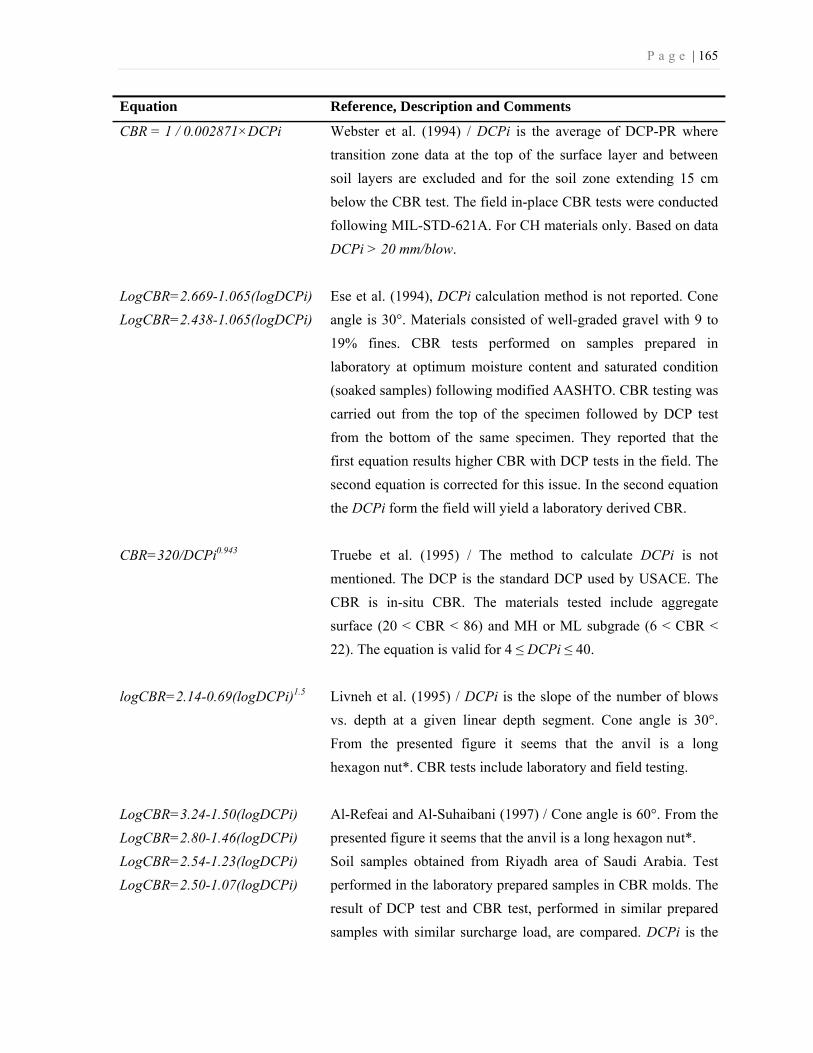
P a g e | 165
Equation Reference, Description and Comments
CBR = 1 / 0.002871×DCPi Webster et al. (1994) / DCPi is the average of DCP-PR where
transition zone data at the top of the surface layer and between
soil layers are excluded and for the soil zone extending 15 cm
below the CBR test. The field in-place CBR tests were conducted
following MIL-STD-621A. For CH materials only. Based on data
DCPi > 20 mm/blow.
LogCBR=2.669-1.065(logDCPi)
LogCBR=2.438-1.065(logDCPi)
Ese et al. (1994), DCPi calculation method is not reported. Cone
angle is 30°. Materials consisted of well-graded gravel with 9 to
19% fines. CBR tests performed on samples prepared in
laboratory at optimum moisture content and saturated condition
(soaked samples) following modified AASHTO. CBR testing was
carried out from the top of the specimen followed by DCP test
from the bottom of the same specimen. They reported that the
first equation results higher CBR with DCP tests in the field. The
second equation is corrected for this issue. In the second equation
the DCPi form the field will yield a laboratory derived CBR.
CBR=320/DCPi0.943
Truebe et al. (1995) / The method to calculate DCPi is not
mentioned. The DCP is the standard DCP used by USACE. The
CBR is in-situ CBR. The materials tested include aggregate
surface (20 < CBR < 86) and MH or ML subgrade (6 < CBR <
22). The equation is valid for 4 ≤ DCPi ≤ 40.
logCBR=2.14-0.69(logDCPi)1.5 Livneh et al. (1995) / DCPi is the slope of the number of blows
vs. depth at a given linear depth segment. Cone angle is 30°.
From the presented figure it seems that the anvil is a long
hexagon nut*. CBR tests include laboratory and field testing.
LogCBR=3.24-1.50(logDCPi)
LogCBR=2.80-1.46(logDCPi)
LogCBR=2.54-1.23(logDCPi)
LogCBR=2.50-1.07(logDCPi)
Al-Refeai and Al-Suhaibani (1997) / Cone angle is 60°. From the
presented figure it seems that the anvil is a long hexagon nut*.
Soil samples obtained from Riyadh area of Saudi Arabia. Test
performed in the laboratory prepared samples in CBR molds. The
result of DCP test and CBR test, performed in similar prepared
samples with similar surcharge load, are compared. DCPi is the
P a g e | 166
Equation Reference, Description and Comments
average of DCP-PRs needed to penetrate 50 mm in the soil while
the first blow is excluded.
1) The first equation: for poorly graded sand, 10 ≤ DCPi ≤ 50
mm/blow,
2) The second equation: for silty sand, 4 ≤ DCPi ≤ 35 mm/blow,
3) The third equation: for CL or ML, 4 ≤ DCPi ≤ 35 mm/blow,
4) The forth equation for all materials, 4 ≤ DCPi ≤ 50 mm/blow.
LogCBR=2.53-1.14(logDCPi)
Coonse (1999) / DCPi is the average of DCP-PR after the first
blow to the 116 mm deep in 150 mm diameter mold and to 200
mm deep in 250 mm diameter mold. The DCP test is performed
after conducting CBR test in the same mold following AASHTO
T-193 while the 44 N surcharge weight was on top of the mold.
Cone angle is 30°. From the presented figure it seems that the
anvil is not flat*. This equation is corrected to consider the
confinement effect of standard CBR molds, so it could be used
for estimating in-situ CBR.
Materials tested included remolded residual clayey soils from
Piedmont Geologic Region, North Carolina.
CH consists of 90% fines, LL= 55, PI =27.
CL consists of 65% fines, LL=33, PI=13.
CL consists of 63% fines, LL=30, PI=12.
The equation is valid for 25 ≤ DCPi ≤ 80. For lower DCPis it
overestimates the CBR.
LogCBR=2.53-1.14(logDCPi)
LogCBR=2.40-0.55(logDCPi)
Gabr et al. (1999) / Cone angle is 30°. Test program included
tests in lab and in the field in Davidson County, North Carolina.
In the laboratory, the DCP test is performed after conducting
CBR test in 150 mm diameter molds. In-situ tests conducted on
Piedmont subgrade soil and aggregate base coarse material
The first equation is for Piedmont subgrade soil. See the
description of Coonse (1999)’s equation for more details.
The second equation is for aggregate base coarse material
obtained from rock quarry (Before compaction: Cc= 0.75, Cu =
25, Passing sieve number 4 = 42%)
P a g e | 167
Equation Reference, Description and Comments
CBR=410 DCPi-1.27
CBR=66.66 DCPi2-330DCPi+563
CSIR Transportek (2000), The DCPi is the average or weighted
average of DCP-PR.
The first equation is for DCPi > 2 mm/blow and,
The second equation is for DCPi ≤ 2 mm/blow.
LogCBR=2.182-0.872(logDCPi)
LogCBR=1.145-0.336(logDCPi)
LogCBR=1.671-0.577(logDCPi)
LogCBR=1.966-0.667(logDCPi)
Karunaprema & Edirisinghe (2002) / The DCP is tested in a 280
mm diameter specimen prepared in the lab while a surcharge of
147 kg/m3 was on the sample. The method to calculate DCPi is
not mentioned, Cone angle is 60°.
For the first, second and third equations, materials tested include
residual clayey and silty sand (according to British Soil
Classification System) and for the fourth and fifth equations
materials are very clayey or silty gravel from Sri Lanka.
1) The first equation is correlated to remolded unsoaked CBR.
The samples were prepared at optimum moisture content and
maximum density following British Standard procedure.
2) The second equation is correlated to partially undisturbed
unsoaked CBR following British Standard procedure.
3) The third equation is correlated to remolded soaked CBR. The
samples were prepared at optimum moisture content and
maximum density following British Standard procedure.
The first, second and third equations are valid for DCPi between
7 to 75 mm/blow.
4) The forth equation is correlated to remolded unsoaked CBR,
following British Standard procedure, the equation is valid for
DCPi between 11 to 386 mm/blow.
CBR= 1161.1/DCPi1.52 Abu-Farsakh et al. (2005) / DCPi is the average of DCP-PR of
the top 300 mm. Cone angle is 60°. The laboratory CBR test is
performed on unsoaked samples according to ASTM D 1883.
Materials tested include CL, CL-ML, SP, GP, GW-GC, and
cement treated soil. The equation is valid for DCPi between 7.5
to 70 mm/blow.
NOTE: * A long hexagon nut which connects the hammer guide and the rod, also acts as anvil, which may not be totally flat at hammer-anvil contact surface.
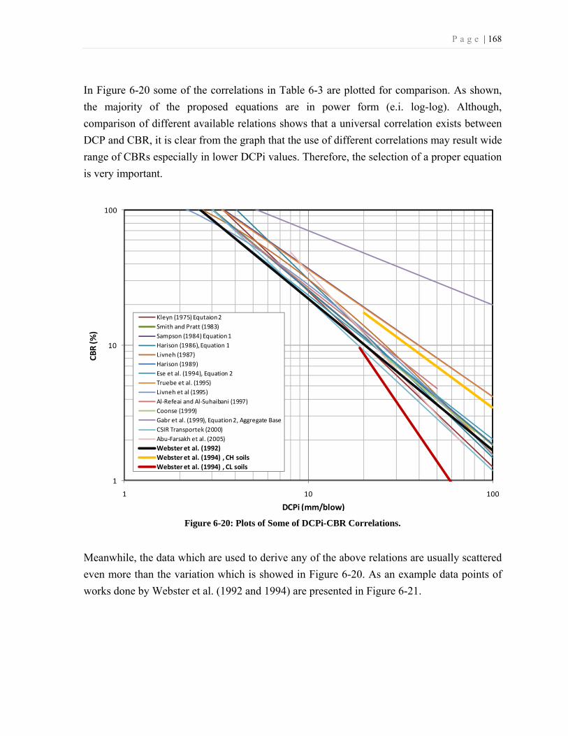
P a g e | 168
In Figure 6-20 some of the correlations in Table 6-3 are plotted for comparison. As shown,
the majority of the proposed equations are in power form (e.i. log-log). Although,
comparison of different available relations shows that a universal correlation exists between
DCP and CBR, it is clear from the graph that the use of different correlations may result wide
range of CBRs especially in lower DCPi values. Therefore, the selection of a proper equation
is very important.
Figure 6-20: Plots of Some of DCPi-CBR Correlations.
Meanwhile, the data which are used to derive any of the above relations are usually scattered
even more than the variation which is showed in Figure 6-20. As an example data points of
works done by Webster et al. (1992 and 1994) are presented in Figure 6-21.
1
10
100
1 10 100
CBR
(%)
DCPi (mm/blow)
Kleyn (1975) Equtaion 2Smith and Pratt (1983)Sampson (1984) Equation 1Harison (1986), Equation 1Livneh (1987)Harison (1989)Ese et al. (1994), Equation 2Truebe et al. (1995) Livneh et al (1995)Al-Refeai and Al-Suhaibani (1997) Coonse (1999) Gabr et al. (1999), Equation 2, Aggregate BaseCSIR Transportek (2000)Abu-Farsakh et al. (2005)Webster et al. (1992)Webster et al. (1994) , CH soilsWebster et al. (1994) , CL soils

P a g e | 169
Figure 6-21: Plot of DCP and CBR Test Data versus Correlation Equations (after Webster et al., 1994).
The difference in pore pressure and the confining effect of the rigid mold in the CBR
test is one of the known reasons that the laboratory CBR tests generally give higher values
than in-situ CBR (Smith and Pratt, 1983; Harison, 1989). It is also recognized that laboratory
CBR values may be greater than in-situ values due to the idealized compaction process
(Booth et al., 2008). The soaked and unsoaked process is shown to affect CBR results
significantly as well. The results of DCPs with 60° and 30° cone are different (Livneh, 1991).
Due to these considerations, the correlation equation proposed by Webster et al. (1994) is
selected to be used to find the in-situ CBR for CH and CL soils and the equation proposed by
Webster et al. (1992) for other materials. These relations are highlighted in Figure 6-20.
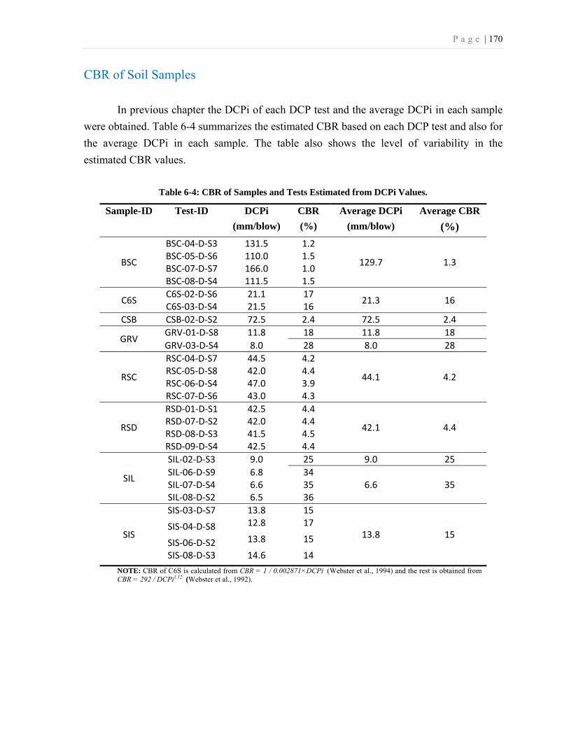
P a g e | 170
CBR of Soil Samples
In previous chapter the DCPi of each DCP test and the average DCPi in each sample
were obtained. Table 6-4 summarizes the estimated CBR based on each DCP test and also for
the average DCPi in each sample. The table also shows the level of variability in the
estimated CBR values.
Table 6-4: CBR of Samples and Tests Estimated from DCPi Values.
Sample-ID Test-ID DCPi
(mm/blow) CBR
(%) Average DCPi
(mm/blow) Average CBR
(%)
BSC
BSC-04-D-S3 131.5 1.2
129.7 1.3 BSC-05-D-S6 110.0 1.5BSC-07-D-S7 166.0 1.0BSC-08-D-S4 111.5 1.5
C6S C6S-02-D-S6 21.1 1721.3 16
C6S-03-D-S4 21.5 16CSB CSB-02-D-S2 72.5 2.4 72.5 2.4
GRV GRV-01-D-S8 11.8 18 11.8 18 GRV-03-D-S4 8.0 28 8.0 28
RSC
RSC-04-D-S7 44.5 4.2
44.1 4.2 RSC-05-D-S8 42.0 4.4RSC-06-D-S4 47.0 3.9RSC-07-D-S6 43.0 4.3
RSD
RSD-01-D-S1 42.5 4.4
42.1 4.4 RSD-07-D-S2 42.0 4.4RSD-08-D-S3 41.5 4.5RSD-09-D-S4 42.5 4.4
SIL
SIL-02-D-S3 9.0 25 9.0 25 SIL-06-D-S9 6.8 34
6.6 35 SIL-07-D-S4 6.6 35SIL-08-D-S2 6.5 36
SIS
SIS-03-D-S7 13.8 15
13.8 15 SIS-04-D-S8 12.8 17
SIS-06-D-S2 13.8 15
SIS-08-D-S3 14.6 14
NOTE: CBR of C6S is calculated from CBR = 1 / 0.002871×DCPi (Webster et al., 1994) and the rest is obtained from CBR = 292 / DCPi1.12 (Webster et al., 1992).

P a g e | 171
In the discussion presented in Chapter 5, how the DCPi is differentiated from DCP-PR was
explained. In Figure 6-22, the CBR values derived from DCP-PR are compared with the
average CBR values derived from DCPi in each soil samples. Since the CBR values, which
are derived from DCPi, are estimated for the entire sample they are plotted for the entire
depth of the test.
Figure 6-22: Estimated CBR Profile Derived from DCP-PR and DCPi in Soil Samples.
0 1 2 3 4 5 6
-700
-600
-500
-400
-300
-200
-100
0
Dept
h (m
m)
CBR (%)
BSC
BSC-04-D-S3
BSC-05-D-S6
BSC-07-D-S7
BSC-08-D-S4
Averaged
Average CBR
0 10 20 30 40 50 60
0
0
0
0
0
0
0
0
CBR (%)
C6S
C6S-02-D-S6
C6S-03-D-S4
Averaged
Average CBR
0 1 2 3 4 5 6
0
0
0
0
0
0
0
0
CBR (%)
CSB
CSB-02-D-S2
Average CBR
0 10 20 30 40 50 60
0
0
0
0
0
0
0
0
CBR (%)
GRV
GRV-01-D-S8
Average CBR
0 10 20 30 40 50 60
0
0
0
0
0
0
0
0
CBR (%)
GRV
GRV-03-D-S4
Average CBR
0 1 2 3 4 5 6
-700
-600
-500
-400
-300
-200
-100
0
Dept
h (m
m)
CBR (%)
RSC
RSC-04-D-S7
RSC-05-D-S8
RSC-06-D-S4
RSC-07-D-S6
Averaged
Average CBR
0 1 2 3 4 5 6
0
0
0
0
0
0
0
0
CBR (%)
RSD
RSD-01-D-S1
RSD-07-D-S2
RSD-08-D-S3
RSD-09-D-S4
Averaged
Average CBR
0 10 20 30 40 50 60
0
0
0
0
0
0
0
0
CBR (%)
SIL
SIL-02-D-S3
Average CBR
0 10 20 30 40 50 60
0
0
0
0
0
0
0
0
CBR (%)
SIL
SIL-06-D-S9
SIL-07-D-S4
SIL-08-D-S2
Averaged
Average CBR
0 10 20 30 40 50 60
0
0
0
0
0
0
0
0
CBR (%)
SIS
SIS-03-D-S7
SIS-04-D-S8
SIS-06-D-S2
SIS-08-D-S3
Averaged
Average CBR
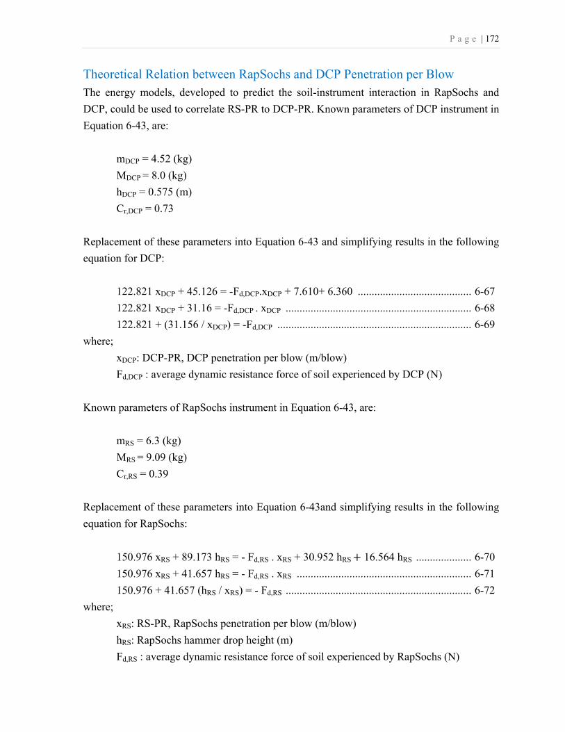
P a g e | 172
Theoretical Relation between RapSochs and DCP Penetration per Blow The energy models, developed to predict the soil-instrument interaction in RapSochs and
DCP, could be used to correlate RS-PR to DCP-PR. Known parameters of DCP instrument in
Equation 6-43, are:
mDCP = 4.52 (kg)
MDCP = 8.0 (kg)
hDCP = 0.575 (m)
Cr,DCP = 0.73
Replacement of these parameters into Equation 6-43 and simplifying results in the following
equation for DCP:
122.821 xDCP + 45.126 = -Fd,DCP.xDCP + 7.610+ 6.360 ......................................... 6-67
122.821 xDCP + 31.16 = -Fd,DCP . xDCP ................................................................... 6-68
122.821 + (31.156 / xDCP) = -Fd,DCP ...................................................................... 6-69
where;
xDCP: DCP-PR, DCP penetration per blow (m/blow)
Fd,DCP : average dynamic resistance force of soil experienced by DCP (N)
Known parameters of RapSochs instrument in Equation 6-43, are:
mRS = 6.3 (kg)
MRS = 9.09 (kg)
Cr,RS = 0.39
Replacement of these parameters into Equation 6-43and simplifying results in the following
equation for RapSochs:
150.976 xRS + 89.173 hRS = - Fd,RS . xRS + 30.952 hRS + 16.564 hRS .................... 6-70
150.976 xRS + 41.657 hRS = - Fd,RS . xRS ............................................................... 6-71
150.976 + 41.657 (hRS / xRS) = - Fd,RS ................................................................... 6-72
where;
xRS: RS-PR, RapSochs penetration per blow (m/blow)
hRS: RapSochs hammer drop height (m)
Fd,RS : average dynamic resistance force of soil experienced by RapSochs (N)

P a g e | 173
Model 1
If the dynamic resistance of soil, in exactly the same condition and same depth, is assumed to
be identical in RapSochs and DCP (Fd,RS = Fd,DCP), then the RS-PR and DCP-PR could be
correlated using Equation 6-69 and 6-72.
122.821 + (31.156 / xDCP) = 150.976 + 41.657 (hRS / xRS) ................................... 6-73
(31.156 / xDCP) = 28.155 + 41.657 (hRS / xRS) ....................................................... 6-74
31.156 xRS = 28.155 xRS . xDCP + 41.657 hRS . xDCP .............................................. 6-75
31.156 xRS = (28.155 xRS + 41.657 hRS ) . xDCP ..................................................... 6-76
xDCP = 31.156 xRS /(28.155 xRS + 41.657 . hRS ) .................................................... 6-77
xDCP = xRS / (0.904 xRS + 1.337 hRS ) ..................................................................... 6-78
Equation 6-78 is rewritten as the familiar form of:
- = -. - . ............................................................................. 6-79
where:
DCP-PR is the equivalent penetration per blow estimated for DCP (m/blow)
RS-PR is the measured penetration of one blow in RapSochs (m/blow)
hRS is the hammer drop height in a RapSochs blow (m)
This equation is referred to as Model 1 for further analysis.
Model 2
Note that Model 1 has inherited some errors due to the assumption that the dynamic
resistance of soil is identical in RapSochs and DCP. The dynamic resistance of soil is
comprised of friction force acting on the embedded length of the penetrometer and tip
resistance force.
Fd = Fdc + Fdf ......................................................................................................... 6-80
where:
Fd : dynamic resistance force of soil acting on the penetrometer
Fdc : dynamic cone tip resistance force acting on the cone of penetrometer
Fdf : dynamic resistance friction force acting on the embedded length of penetrometer
Rewritten and rearranged for RapSochs and DCP, results in:

P a g e | 174
Fdc,RS = Fd,RS - Fdf,RS .............................................................................................. 6-81
Fdc,DCP = Fd,DCP - Fdf,DCP ......................................................................................... 6-82
where:
Fd,RS : total dynamic resistance force of soil acting on the RapSochs penetrometer
Fdc,RS : dynamic cone tip resistance force acting on the cone of RapSochs
Fdf,RS : dynamic resistance friction force acting on the embedded length of RapSochs
Fd,DCP : total dynamic resistance force of soil acting on the DCP penetrometer
Fdc,DCP : dynamic cone tip resistance force acting on the cone of RapSochs
Fdf,DCP : dynamic resistance friction force acting on the embedded length of RapSochs
Although assuming an equal tip resistance in RapSochs and DCP due to similar geometry
sounds valid, assuming an equal friction resistance certainly imposes some errors. Therefore,
the equality is expected to be between cone tip resistances of both instruments:
Fdc,DCP = Fdc,RS ....................................................................................................... 6-83
Replacing Equation 6-81 and 6-82 in Equation 6-83 results:
Fd,DCP - Fdf,DCP = Fd,RS - Fdf,RS ................................................................................ 6-84
The friction resistance in RapSochs could be estimated from the friction resistance profile
obtained from MLE analysis of strain gauges. For 50 cm penetration, the maximum total
friction force are about 22%, 960%, 1600%, 17%, 21%, 30%, 14%, and 50% of the cone tip
force in BSC, C6S, CSB, GRV, RSC, RSD, SIL, and SIS samples, respectively. It shows that
the friction force is not negligible even in granular materials. Meanwhile, assuming a
negligible circumferential friction in DCP due to smaller diameter of penetrometer may be
correct in granular and cemented materials, but it is not necessarily correct in all cohesive
soils. Particularly, it is mentioned in previous section that the friction is developed around the
penetrometer during DCP tests in cohesive soils. Livneh (2000) developed a method to
correct the effect of skin friction forces on the DCP rod during testing in cohesive materials,
but in a typical DCP test the friction resistance is not measured.
Assuming that Fdf,DCP is negligible and Fdf,RS could be estimated from RapSochs
measurements, Equation 6-69, 6-72, and 6-84 results:

P a g e | 175
122.821 + (31.156 / xDCP) = 150.976 + 41.657 (hRS / xRS) - Fdf,RS ...................... 6-85
(31.156 / xDCP) = 28.155 + 41.657 (hRS / xRS) - Fdf,RS ........................................... 6-86
xDCP = xRS / (0.904 xRS + 1.337 hRS - 0.0321 Fdf,RS . xRS) ..................................... 6-87
Equation 6-87 is rewritten as the familiar form of:
- = -. - . . . - . . ................................................ 6-88
This equation is referred to as Model 2 for further analysis.
Model 3
For comparison, the Dutch formula could be used to relate RS-PR to DCP-PR. The Dutch
formula, Equation 6-62, for RapSochs with substitution of known parameters is:
Fd, RS = 52.669 (hRS / xRS) ...................................................................................... 6-89
For DCP the Dutch equation is simplified to:
Fd,DCP = 28.834 / xDCP ............................................................................................ 6-90
Assuming identical dynamic resistance results in;
28.834 / xDCP = 52.669 (hRS / xRS) ......................................................................... 6-91
xDCP = 0.547 (xRS / hRS) ......................................................................................... 6-92
or in the familiar form of:
- = 0.547 - ......................................................................................... 6-93
This equation is referred to as Model 3 for further analysis.

P a g e | 176
Statistical Correlations between RapSochs and DCP Penetration per Blow
A code is developed to obtain the average of DCP-PR in each sample. The results are
shown in Figure 6-23 along with the DCPi obtained in each sample for similar test
conditions.
Figure 6-23: DCP-PR profile, Averaged DCP-PR and DCPi in the Same Test Conditions.
The average DCP-PR is then used to obtain the corresponding weighted average for
each penetration increment in RapSochs. Figure 6-24 shows an example of weighted average
DCP-PR calculated for each penetration increment (RS-PR) of RSC-08-R-S3 test along the
averaged DCP-PR in RSC sample. Such a calculation basically provides the average DCP-
PR in each penetration increment of a RapSochs test.
0 100 200 300
-700
-600
-500
-400
-300
-200
-100
0
Dep
th (m
m)
DCP-PR (mm/blow)
BSC
BSC-04-D-S3
BSC-05-D-S6
BSC-07-D-S7
BSC-08-D-S4
Averaged
DCPi
0 25 50 75 100
0
0
0
0
0
0
0
0
DCP-PR (mm/blow)
C6S
C6S-02-D-S6
C6S-03-D-S4
Averaged
DCPi
0 25 50 75 100
0
0
0
0
0
0
0
0
DCP-PR (mm/blow)
CSB
CSB-02-D-S2
DCPi
0 25 50 75 100
0
0
0
0
0
0
0
0
DCP-PR (mm/blow)
GRV
GRV-01-D-S8
DCPi
0 25 50 75 100
0
0
0
0
0
0
0
0
DCP-PR (mm/blow)
GRV
GRV-03-D-S4
DCPi
0 50 100 150 200
-700
-600
-500
-400
-300
-200
-100
0
Dep
th (m
m)
DCP-PR (mm/blow)
RSC
RSC-04-D-S7
RSC-05-D-S8
RSC-06-D-S4
RSC-07-D-S6
Averaged
DCPi
0 50 100 150 200
0
0
0
0
0
0
0
0
DCP-PR (mm/blow)
RSD
RSD-01-D-S1
RSD-07-D-S2
RSD-08-D-S3
RSD-09-D-S4
Averaged
DCPi
0 25 50 75 100
0
0
0
0
0
0
0
0
DCP-PR (mm/blow)
SIL
SIL-02-D-S3
DCPi
0 25 50 75 100
0
0
0
0
0
0
0
0
DCP-PR (mm/blow)
SIL
SIL-06-D-S9
SIL-07-D-S4
SIL-08-D-S2
Averaged
DCPi
0 25 50 75 100
0
0
0
0
0
0
0
0
DCP-PR (mm/blow)
SIS
SIS-03-D-S7
SIS-04-D-S8
SIS-06-D-S2
SIS-08-D-S3
Averaged
DCPi

P a g e | 177
Figure 6-24: Averaged DCP-PR in RSC and Calculated Weighted Average DCP-PR for Penetration
Increment of each RapSochs Blow.
Based on the form of Model 1 and Model 3, the correlation analyses are used to obtain
unknown constants that best match with the results of the experiments.
Model 4
Based on Model 1, the following general form is assumed:
- = - + C ......................................................................................... 6-94
where;
C1 and C2 are unknown constants
Figure 6-25 present the data points of ratio of hammer drop height over RS-PR versus the
inverse of calculated DCP-PR corresponding to each blow of RapSochs. Data points of tests
in cohesive soils (C6S and CSB) and BSC-09-R-S5 are excluded for regression analysis. The
results of Test BSC-09-R-S5 were suspected to be affected by the boundary effects caused by
spacing of tests. This issue is discussed later in this chapter. In cohesive soils, as explained in
Model 2, the assumption of equal resistance in DCP and RapSochs is not correct which
0 50 100 150 200
-700
-600
-500
-400
-300
-200
-100
0
Dept
h (m
m)
DCP-PR (mm/blow)
RSC-08-R-S3
Average in the Sample
Estimated for each RS Blow

P a g e | 178
makes the form of the equation fundamentally incorrect and will add errors in the regression
analysis. First blows in all tests and blows where the cone was not completely embedded are
not included in the analysis.
Figure 6-25: RapSochs Hammer Drop Height Over RS-PR Ratio of Each Blow versus Inverse of
Corresponding Calculated DCP-PR.
From the regression analysis the C1= 1.0557 and C2=0.956. The Equation 6-94 based on the
regression is:
- = 1.0557 - + 0.956 ............................................................................ 6-95
After rearranging it gives the following equation, which will be referred to as Model 4:
- = -. - . ........................................................................... 6-96
y = 1.0557x + 0.956R² = 0.7599
1
10
100
1,000
1 10 100 1,000
1/D
CP-P
R (m
/blo
w)
hRS/RS-PR
Data
Constrained Linear Regression
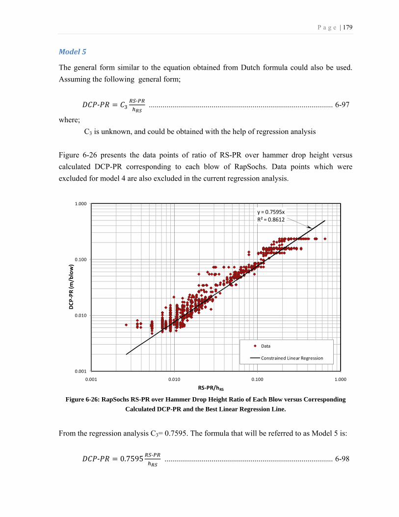
P a g e | 179
Model 5
The general form similar to the equation obtained from Dutch formula could also be used.
Assuming the following general form;
- = - .............................................................................................. 6-97
where;
C3 is unknown, and could be obtained with the help of regression analysis
Figure 6-26 presents the data points of ratio of RS-PR over hammer drop height versus
calculated DCP-PR corresponding to each blow of RapSochs. Data points which were
excluded for model 4 are also excluded in the current regression analysis.
Figure 6-26: RapSochs RS-PR over Hammer Drop Height Ratio of Each Blow versus Corresponding
Calculated DCP-PR and the Best Linear Regression Line.
From the regression analysis C3= 0.7595. The formula that will be referred to as Model 5 is:
- = 0.7595 - ...................................................................................... 6-98
y = 0.7595xR² = 0.8612
0.001
0.010
0.100
1.000
0.001 0.010 0.100 1.000
DCP
-PR
(m/b
low
)
RS-PR/hRS
Data
Constrained Linear Regression

P a g e | 180
Model 6
In Model 5 the regression is influenced by higher values of DCP-PR while in Model 4 lower
values of DCP-PR (and therefore higher values of 1/DCP-PR) contribute more in defining
the regression. For this reason, the best matching regression are determined without limiting
the equation to any specific formula.
Figure 6-27 presents the data points of ratio of hammer drop height over RS-PR versus the
inverse of calculated DCP-PR corresponding to each blow of RapSochs. The power form
equation was resulted the highest R-squared of 0.94. Data points which were excluded for
Model 4 are also excluded in the current regression analysis.
Figure 6-27: RapSochs Hammer Drop Height over RS-PR Ratio of Each Blow versus Inverse of
Corresponding Calculated DCP-PR and the Best Regression Line.
The following equation is obtained from regression analysis and will be referred to as Model
6 for further analysis:
- = 1.2471 - . ......................................................................... 6-99
y = 1.2471x0.9757
R² = 0.9494
1
10
100
1,000
1 10 100 1,000
1/D
CP-P
R (m
/blo
w)
hRS/RS-PR
Data
Constrained Linear Regression

P a g e | 181
Comparison of Models The proposed models are listed in Table 6-5. Figure 6-28 A to F shows the estimated DCP-
PR calculated using Model 1 to Model 6 versus weighted average DCP-PR calculated for
each RS-PR. Data points which were excluded in Model 4 are not used in developing these
charts either.
Table 6-5: List of Proposed Models to Relate RapSochs Test Measurements to Equivalent DCP-PR.
Model # Equation
Model 1 - = -0.904 - + 1.337
Model 2 - = -0.904 - + 1.337 0.0321. - . .
Model 3 - = 0.547 -
Model 4 - = -0.956 - + 1.0557
Model 5 - = 0.7595 -
Model 6 - = 1.2471 - .
NOTE: All parameters are in SI units. DCP-PR (m/blow), RS-RP (m/blow), hRS (m), Fdf,RS (N)
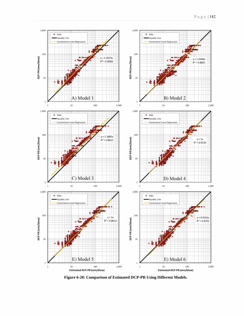
P a g e | 182
Figure 6-28: Comparison of Estimated DCP-PR Using Different Models.
y = 1.2073xR² = 0.9068
1
10
100
1,000
1 10 100 1,000
DCP
-PR
(mm
/blo
w)
Data
Equality Line
Constrained Linear Regression
y = 1.0346xR² = 0.8891
1
10
100
1,000
1 10 100 1,000
DCP
-PR
(mm
/blo
w)
Data
Equality Line
Constrained Linear Regression
y = 1.3885xR² = 0.8612
1
10
100
1,000
1 10 100 1,000
DCP
-PR
(mm
/blo
w)
Data
Equality Line
Constrained Linear Regression
y = 1xR² = 0.9154
1
10
100
1,000
1 10 100 1,000
DCP
-PR
(mm
/blo
w)
Data
Equality Line
Constrained Linear Regression
y = 1xR² = 0.8612
1
10
100
1,000
1 10 100 1,000
DCP
-PR
(mm
/blo
w)
Estimated DCP-PR (mm/blow)
Data
Equality Line
Constrained Linear Regression
y = 0.9161xR² = 0.8702
1
10
100
1,000
1 10 100 1,000
DCP
-PR
(mm
/blo
w)
Estimated DCP-PR (mm/blow)
Data
Equality Line
Constrained Linear Regression
D) Model 4
B) Model 2
E) Model 6
A) Model 1
C) Model 3
E) Model 5

P a g e | 183
Among theoretical models, Model 2 results in the least average error of 3% while Models 1
and 3 have an average error of 21% and 39%, respectively. Although the coefficient of
determination is not the highest in Model 2, it is not very different in these 3 Models.
Among statistical models, Models 4 and 5 have an average error of 0% while Model 6
underestimates the DCP-PR by for 8% on average. However Model 4 has a higher coefficient
of determination and data points are shown to be divided more evenly around the equality
line.
Note that in the plots displayed in Figure 6-28, the constrained regression lines are
significantly influenced by higher values of DCP-PRs. Since any variation in smaller DCP-
PR estimation will cause much greater variation in estimated CBR, the regression line of
1/DCP-PR versus estimated 1/DCP-PR was also evaluated. Plots from this analysis are not
presented here; however, the results again show that Model 4 produces the minimum error of
less than 1%. Model 4 was by far the best model while the next best, Model 6, had the
average error of 5%.
Therefore Model 4 is selected as the best model for RS-PR to DCP-PR correlation. Model 4
is based on the energy model which was developed in previous section and then calibrated to
match experimental data.
Estimation of DCP-PR and DCPi from RapSochs To distinguish between DCP-PRs obtained from DCP tests and estimated DCP-PRs from
RapSochs tests we add subscript RS to DCP-PRs obtained in this way. Model 4 is therefore
rewritten as:
- = -. - . .................................................................... 6-100
where:
DCP-PRRS is the estimated DCP-PR from RapSochs tests results.
A code is developed to use Equation 6-100 to estimate the equivalent DCP-PR based on RS-
PR. It is also used to plot the measured RS-PR, DCP-PRRS, averaged DCP-PR which is
obtained from DCP tests, and hammer drop height corresponding to RS-PRs for each
RapSochs test. Figure 6-29 shows an example of outputs for test RSC-08-R-S3.

P a g e | 184
Figure 6-29: Estimated DCP-PR from RS-PR in RSC-08-R-S3.
For all the RapSochs tests, including tests in clayey materials, the DCP-PRRS is obtained.
DCP-PRRS profiles of tests in similar conditions are plotted along with the calculated average
DCP-PRRS. The averaged DCP-PR which was calculated from DCP tests are also overlaid for
comparison. Figure 6-30 shows the profiles of estimated DCP-PRRS, averaged DCP-PRRS,
and averaged DCP-PR.
0 8 16 24 32-700
-600
-500
-400
-300
-200
-100
0
Hammer Drop Height (cm)
0 100 200 300 400
-700
-600
-500
-400
-300
-200
-100
0
Penetration Rate (mm/blow)
Dep
th (m
m)
RSC-08-R-S3
Drop HeightRS-PRDCP-PRRSAveraged DCP-PR

P a g e | 185
Figure 6-30: DCP-PRRS profile, Averaged DCP-PRRS and Averaged DCP-PRRS in the Same Test
Conditions.
Figure 6-30 shows that in non-cohesive soils the method yields estimation of DCP-PR with
acceptable accuracy. In these soil types, while DCP is giving one penetration increment close
to soil surface, the RapSochs provides a smoother transient zone. In CSB the DCP profile is
not complete up to the soil surface and no comments could be made regarding the accuracy
of the estimation. However it shows that RapSochs can provide data where DCP cannot. In
C6S, the model underestimates the DCP-PR. In this project, the number of tests conducted in
cohesive materials is limited, and not all soil conditions are tested. Therefore, at this time,
deriving a relationship between RS-PR and DCP-PR is not statistically possible in cohesive
soils.
0 100 200 300 400
-700
-600
-500
-400
-300
-200
-100
0D
epth
(mm
)Penetration Rate (mm/blow)
BSC
BSC-01-R-S1
BSC-02-R-S2
BSC-03-R-S9
BSC-06-R-S8
Averaged DCP-PRRS
Averaged DCP-PR
0 25 50 75 100
0
0
0
0
0
0
0
0
Penetration Rate (mm/blow)
C6S
C6S-01-R-S8
C6S-04-R-S2
Averaged DCP-PRRS
Averaged DCP-PR
0 100 200 300 400
0
0
0
0
0
0
0
0
Penetration Rate (mm/blow)
CSB
CSB-01-R-S8
Averaged DCP-PRRS
Averaged DCP-PR
0 25 50 75 100
0
0
0
0
0
0
0
0
Penetration Rate (mm/blow)
GRV
GRV-02-R-S5
Averaged DCP-PRRS
Averaged DCP-PR
0 25 50 75 100
0
0
0
0
0
0
0
0
Penetration Rate (mm/blow)
GRV
GRV-04-R-S2
GRV-05-R-S6
Averaged DCP-PRRS
Averaged DCP-PR
0 100 200 300 400
-700
-600
-500
-400
-300
-200
-100
0
Dep
th (m
m)
Penetration Rate (mm/blow)
RSC
RSC-01-R-S1
RSC-02-R-S2
RSC-03-R-S9
RSC-08-R-S3
RSC-09-R-S5
Averaged DCP-PRRS
Averaged DCP-PR
0 100 200 300 400
0
0
0
0
0
0
0
0
Penetration Rate (mm/blow)
RSD
RSD-02-R-S5
RSD-03-R-S6
RSD-04-R-S7
RSD-05-R-S9
RSD-06-R-S8
Averaged DCP-PRRS
Averaged DCP-PR
0 15 30 45 60
0
0
0
0
0
0
0
0
Penetration Rate (mm/blow)
SIL
SIL-01-R-S1
Averaged DCP-PRRS
Averaged DCP-PR
0 15 30 45 60
0
0
0
0
0
0
0
0
Penetration Rate (mm/blow)
SIL
SIL-03-R-S5
SIL-04-R-S6
SIL-05-R-S7
Averaged DCP-PRRS
Averaged DCP-PR
0 15 30 45 60
0
0
0
0
0
0
0
0
Penetration Rate (mm/blow)
SIS
SIS-01-R-S5
SIS-02-R-S1
SIS-05-R-S4
Averaged DCP-PRRS
Averaged DCP-PR
P a g e | 186
In the next step, DCPiRS (DCPi estimated from RapSochs test) is calculated for each
RapSochs test by averaging the estimated DCP-PRRS after the transient zone data points are
excluded. To find the transient zone, data points from the soil surface are checked one by
one. If the DCP-PRRS is smaller than the average of DCP-PRRSs plus one standard deviation
it is included. Otherwise it is excluded from data points and average and standard deviation
are calculated for the rest of data and the next DCP-PRRS is checked to verify if it is in the
transient zone or not. The iteration is continued until the first data point within the acceptable
range of average plus one standard deviation is found. The blows above that point are
considered to be in transient zone. A similar procedure is also followed to find the transient
zone close to the bottom of the container. Starting from the last penetration measurement, if
the data point is greater than average minus one standard deviation of DCP-PRRSs, it is
included. Otherwise it is considered to be in transient zone.
The calculated DCPiRSs are summarized in Table 6-6. Average DCPiRS for tests in similar
test conditions are also calculated. Average DCPi which were obtained from DCP tests are
also presented for comparison.

P a g e | 187
Table 6-6: DCPi Obtained by Averaging the Estimated DCP-PR from RS-PR.
Sample-ID Test-ID DCPiRS
(mm/blow)
Average DCPiRS
(mm/blow)
Average DCPi
(mm/blow)
BSC
BSC-01-R-S1 150.0
122.3 129.7
BSC-02-R-S2 99.0
BSC-03-R-S9 131.8
BSC-06-R-S8 108.5
BSC-09-R-S5* 74.8
C6S C6S-01-R-S8 13.6
14.1 21.3 C6S-04-R-S2 14.5
CSB CSB-01-R-S8 129.2 129.2 72.5
GRV
GRV-02-R-S5* 9.3 9.3 11.8
GRV-04-R-S2 8.5 8.2 8.0
GRV-05-R-S6 8.0
RSC
RSC-01-R-S1 48.0
45.2 44.1
RSC-02-R-S2 50.0
RSC-03-R-S9 43.0
RSC-08-R-S3 41.0
RSC-09-R-S5 44.0
RSD
RSD-02-R-S5 40.0
44.2 42.1
RSD-03-R-S6 41.3
RSD-04-R-S7 47.3
RSD-05-R-S9 44.6
RSD-06-R-S8 48.0
SIL
SIL-01-R-S1* 10.5 10.5 9.0
SIL-03-R-S5 7.3
8.1 6.6 SIL-04-R-S6 8.3
SIL-05-R-S7 8.6
SIS
SIS-01-R-S5 15.0
17.1 13.8 SIS-02-R-S1 17.9
SIS-05-R-S4 17.9
SIS-07-R-S6 17.6
NOTE: BSC-09-R-S5 is excluded in calculation of Average DCPiRS due to concerns about the test spacing which affects the
boundary conditions of tests and test interference. GRV-02-R-S5 was performed before draining the sample and GRV-04-R-S2 and GRV-04-R-S2 were performed after
draining the sample. SIL-01-R-S1 was performed 3 months before other tests in SIL sample. The effect of cementation is obvious in this case.

P a g e | 188
Estimation of CBR from RapSochs
CBR could be calculated by the equation developed by Webster et al. (1992) or other
relationships listed in Table 6-3. The calculated DCPiRS should be used instead of DCPi in
those formulas. Table 6-7 summarizes the estimated CBR for each RapSochs test and also for
the average DCPiRS of each sample. The average CBR obtained from DCP tests are also
reported for comparison.
For measured CBR in laboratory compacted soil samples, one data set shows the coefficient
of variation to be 6.9% (compacted per ASTM D698 test method) or 9.2% (compacted per
ASTM D1557 test method) based on seven repetitions (ASTM D1883, 2007). For in-situ
CBR test, no precision is reported in ASTM D4429 (2009). The coefficient of variation for
DCP tests in the same material or same location is reported to be 10% by Harrison (1989),
40% by Smith and Pratt (1983), and 23% by Livneh (1987). The interesting point is they all
reported higher coefficient of variation for CBR tests than for DCP tests. Therefore it could
be concluded that DCP test is more reproducible than CBR.
ASTM D6951-03 Method for DCP indicates that the within-field-laboratory repeatability,
standard deviation has been determined to be less than 2 mm/blow. In Figure 6-31, the effect
of plus and minus 2 mm error in DCP measurement on the estimation of CBR using
equations of Webster et al. (1992) and Webster et al. (1994) are shown. For instance, if the
real CBR is about 50, penetration variation in the range of plus and minus 2 mm/blow means
CBR range of 35 to 85 percent. In this respect, the estimated CBRs for non-cohesive soils are
within the acceptable range of repeatability reported for DCP.
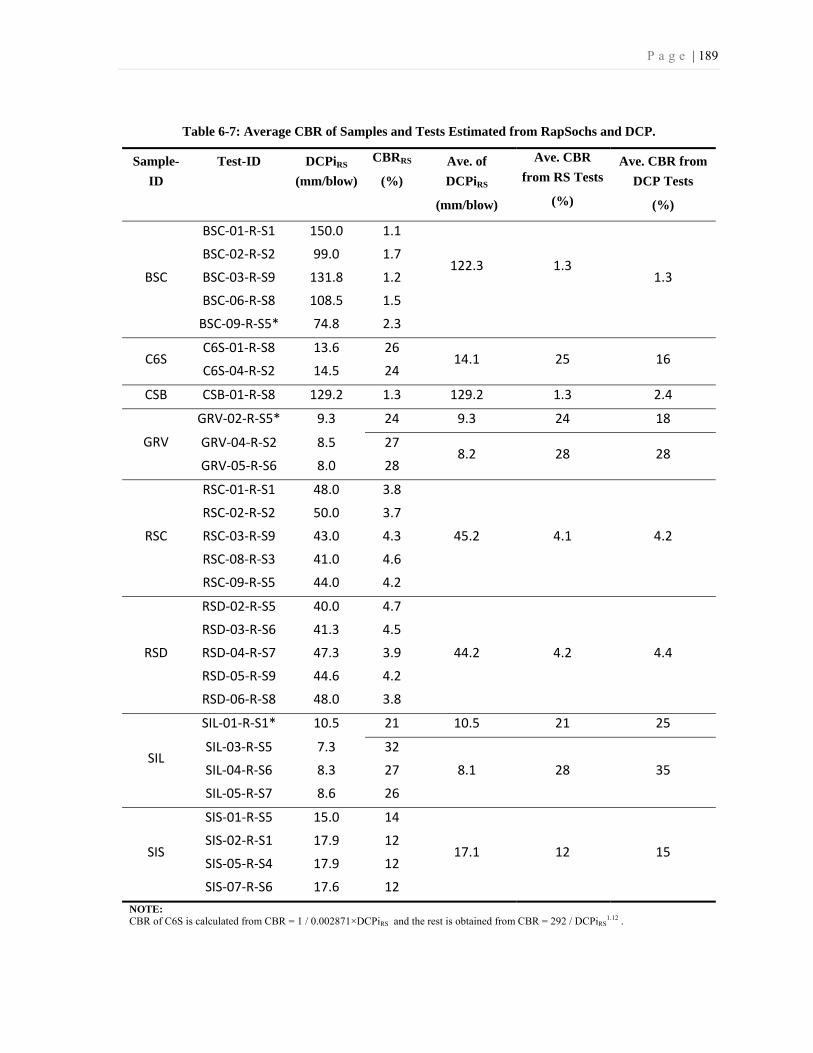
P a g e | 189
Table 6-7: Average CBR of Samples and Tests Estimated from RapSochs and DCP.
Sample-
ID
Test-ID DCPiRS
(mm/blow)
CBRRS
(%)
Ave. of
DCPiRS
(mm/blow)
Ave. CBR
from RS Tests
(%)
Ave. CBR from
DCP Tests
(%)
BSC
BSC-01-R-S1 150.0 1.1
122.3 1.3 1.3
BSC-02-R-S2 99.0 1.7
BSC-03-R-S9 131.8 1.2
BSC-06-R-S8 108.5 1.5
BSC-09-R-S5* 74.8 2.3
C6S C6S-01-R-S8 13.6 26
14.1 25 16 C6S-04-R-S2 14.5 24
CSB CSB-01-R-S8 129.2 1.3 129.2 1.3 2.4
GRV
GRV-02-R-S5* 9.3 24 9.3 24 18
GRV-04-R-S2 8.5 27 8.2 28 28
GRV-05-R-S6 8.0 28
RSC
RSC-01-R-S1 48.0 3.8
45.2 4.1 4.2
RSC-02-R-S2 50.0 3.7
RSC-03-R-S9 43.0 4.3
RSC-08-R-S3 41.0 4.6
RSC-09-R-S5 44.0 4.2
RSD
RSD-02-R-S5 40.0 4.7
44.2 4.2 4.4
RSD-03-R-S6 41.3 4.5
RSD-04-R-S7 47.3 3.9
RSD-05-R-S9 44.6 4.2
RSD-06-R-S8 48.0 3.8
SIL
SIL-01-R-S1* 10.5 21 10.5 21 25
SIL-03-R-S5 7.3 32
8.1 28 35 SIL-04-R-S6 8.3 27
SIL-05-R-S7 8.6 26
SIS
SIS-01-R-S5 15.0 14
17.1 12 15 SIS-02-R-S1 17.9 12
SIS-05-R-S4 17.9 12
SIS-07-R-S6 17.6 12
NOTE: CBR of C6S is calculated from CBR = 1 / 0.002871×DCPiRS and the rest is obtained from CBR = 292 / DCPiRS
1.12 .
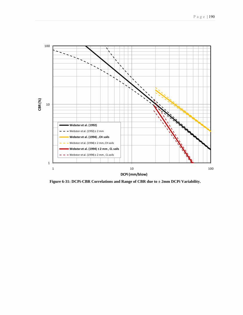
P a g e | 190
Figure 6-31: DCPi-CBR Correlations and Range of CBR due to ± 2mm DCPi Variability.
1
10
100
1 10 100
CBR
(%)
DCPi (mm/blow)
Webster et al. (1992)
Webster et al. (1992) ± 2 mm
Webster et al. (1994) , CH soils
Webster et al. (1994) ± 2 mm, CH soils
Webster et al. (1994) ± 2 mm , CL soils
Webster et al. (1994) ± 2 mm , CL soils

P a g e | 191
CBR Profile of Soil by RapSochs
There is also interest to obtain CBR profiles for soils similar to graphs presented in Figure
6-22. An equation for estimation of CBR from RapSochs test results could be developed by
substitution of the Equation 6-100 that relates RS-PR to equivalent DCP-PR in the equation
proposed by Webster et al. (1992). The notation CBRRS is used to refer to the CBR value that
is estimated by RapSochs test results. Since Equation 6-100 is a function of RS-PR and hRS
in SI units and Webster et al. (1992)’s equation for DCP is in mm, Equation 6-100 is
multiplied by 1000 to be consistent with Webster et al. (1992)’s convention. Substituting and
simplifying results in:
= -. - . . ............................................................... 6-101
= 292 . - . - . .......................................................... 6-102 = 159 . 0.000956 + 0.0010557 - .
.................................... 6-103 = 159 0.000956 + 0.0010557 - . ........................................ 6-104 = 0.152 + 0.1678 - .
............................................................... 6-105
where;
RS-PR is the penetration of one blow in RapSochs (m/blow)
hRS is the hammer drop height of a RapSochs blow (m)
CBRRS is the estimated CBR from RapSochs (%)
In Figure 6-32 the CBRRS profile from RapSochs tests is obtained based on Equation 6-105
and the results for similar test conditions are over plotted. Averaged CBRRS and averaged
CBR obtained from DCP tests are also plotted. Data points in transition zones at the top and
bottom of the soil sample which were not used to derive CBR are not eliminated in this
figure.
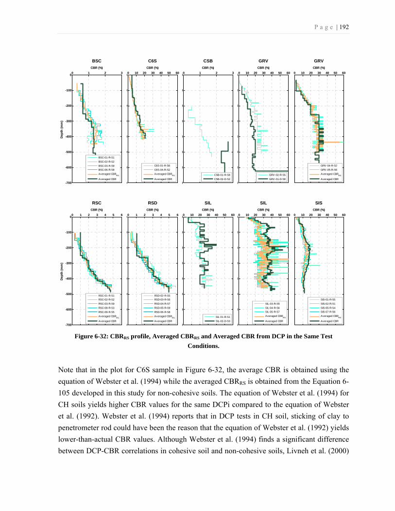
P a g e | 192
Figure 6-32: CBRRS profile, Averaged CBRRS and Averaged CBR from DCP in the Same Test
Conditions.
Note that in the plot for C6S sample in Figure 6-32, the average CBR is obtained using the
equation of Webster et al. (1994) while the averaged CBRRS is obtained from the Equation 6-
105 developed in this study for non-cohesive soils. The equation of Webster et al. (1994) for
CH soils yields higher CBR values for the same DCPi compared to the equation of Webster
et al. (1992). Webster et al. (1994) reports that in DCP tests in CH soil, sticking of clay to
penetrometer rod could have been the reason that the equation of Webster et al. (1992) yields
lower-than-actual CBR values. Although Webster et al. (1994) finds a significant difference
between DCP-CBR correlations in cohesive soil and non-cohesive soils, Livneh et al. (2000)
0 1 2 3
-700
-600
-500
-400
-300
-200
-100
0
Dep
th (m
m)
CBR (%)
BSC
BSC-01-R-S1
BSC-02-R-S2
BSC-03-R-S9
BSC-06-R-S8
Averaged CBRRS
Averaged CBR
0 10 20 30 40 50 60
0
0
0
0
0
0
0
0
CBR (%)
C6S
C6S-01-R-S8
C6S-04-R-S2
Averaged CBRRS
Averaged CBR
0 1 2 3
0
0
0
0
0
0
0
0
CBR (%)
CSB
CSB-01-R-S8
CSB-02-D-S2
0 10 20 30 40 50 60
0
0
0
0
0
0
0
0
CBR (%)
GRV
GRV-02-R-S5
GRV-01-D-S8
0 10 20 30 40 50 60
0
0
0
0
0
0
0
0
CBR (%)
GRV
GRV-04-R-S2
GRV-05-R-S6
Averaged CBRRS
Averaged CBR
0 1 2 3 4 5 6
-700
-600
-500
-400
-300
-200
-100
0
Dep
th (m
m)
CBR (%)
RSC
RSC-01-R-S1
RSC-02-R-S2
RSC-03-R-S9
RSC-08-R-S3
RSC-09-R-S5
Averaged CBRRS
Averaged CBR
0 1 2 3 4 5 6
0
0
0
0
0
0
0
0
CBR (%)
RSD
RSD-02-R-S5
RSD-03-R-S6
RSD-04-R-S7
RSD-05-R-S9
RSD-06-R-S8
Averaged CBRRS
Averaged CBR
0 10 20 30 40 50 60
0
0
0
0
0
0
0
0
CBR (%)
SIL
SIL-01-R-S1
SIL-02-D-S3
0 10 20 30 40 50 60
0
0
0
0
0
0
0
0
CBR (%)
SIL
SIL-03-R-S5
SIL-04-R-S6
SIL-05-R-S7
Averaged CBRRS
Averaged CBR
0 10 20 30 40 50 60
0
0
0
0
0
0
0
0
CBR (%)
SIS
SIS-01-R-S5
SIS-02-R-S1
SIS-05-R-S4
SIS-07-R-S6
Averaged CBRRS
Averaged CBR
P a g e | 193
found their DCP-CBR correlation to be valid for light to heavy clayey soils and they reported
no need for a separate correlation.
Whether good agreement between averaged CBR and averaged CBRRS is by chance or it is
fundamentally correct, more tests in cohesive soils (CH and CL) are required to have a
statistically acceptable correlation between RapSochs test data and CBR. For further field
tests, Equation 6-105, which is validated for non-cohesive soils and shows a good agreement
with CBR soil profiles, is suggested for use in all materials.
6-4- Soil Classification Using RapSochs
In CPT, the sleeve and cone signals are constant for fixed rate penetration through
homogeneous materials. However, in the dynamic penetration, the signal contains additional
information related to the dynamic interaction among the hammer, rod and the soil. In
RapSochs, the MLE analysis on tip and sleeve strain gauges signals can provide average
estimates of cone resistance and friction sleeve resistance. Here, cone resistance (qc), friction
sleeve resistance (fs), and friction ratio (Rf) of RapSochs tests, determined in previous
sections, could be used to compare different soil behavior classification charts.
Classification charts developed by Schmertmann (1970), Douglas and Olsen (1981),
Robertson et al. (1986), Robertson (1990), and Eslami and Fellenius (1997) were reviewed in
Chapter 2. Figure 6-33 to 6-37 show the RapSochs test data plotted on classification charts
together with the envelopes that define each zone. One test for each sample is selected to
facilitate assessment of the graphs. Each data point represents one blow in a RapSochs test.
The first blow for each test is excluded from data. Data from BSC-02-R-S2, C6S-01-R-S8,
CSB-01-R-S8, GRV-05-R-S6, RSC-02-R-S2, RSD-04-R-S7, SIL-05-R-S7, SIS-05-R-S4,
and tests in MS0 to MS5 are presented in the figures. The legend of each graph only presents
the sample-ID and the soil classification of the material in parentheses.

P a g e | 194
Figure 6-33: RapSochs Data on Schmertmann’s Soil Behavior Classification Chart (After Hunt 1984 and
based on Schmertmann 1970, Sanglerat 1972, and Alperstein and Leifer 1976)
Figure 6-34: RapSochs Data on Douglas and Olsen’s Soil Behavior Classification Chart (After Douglas
and Olsen, 1981).
0.1
1
10
0 2 4 6 8 10 12 14 16 18
Cone
Res
ista
nce,
qc
(MPa
)
Friction Ratio, Rf (%)
BSC (SP)
C6S (CH)
CSB (SC)
GRV (SW, with Gravel)
MS0-5 (SW with gravel)
RSC (SP)
RSD (SP)
SIL (ML, Sandy Silt)
SIS (ML, Sandy Silt)
0.1
1
10
100
0 2 4 6 8 10 12 14 16 18
Cone
Res
ista
nce,
qc
(MPa
)
Friction Ratio, Rf (%)
BSC (SP)
C6S (CH)
CSB (SC)
GRV (SW, with Gravel)
MS0-5 (SW with gravel)
RSC (SP)
RSD (SP)
SIL (ML, Sandy Silt)
SIS (ML, Sandy Silt)0.0 0.2 0.4 0.6 0.8 1.0

P a g e | 195
Figure 6-35: RapSochs Data on Robertson et al.’s Soil Behavior Classification Chart (After Robertson et
al., 1986).
Figure 6-36: RapSochs Data on Robertson’s Soil Behavior Classification Chart (After Robertson, 1990).
0.1
1
10
100
0 2 4 6 8 10 12 14 16 18
Cone
Res
ista
nce,
qc
(MPa
)
Friction Ratio, Rf (%)
BSC (SP)
C6S (CH)
CSB (SC)
GRV (SW, with Gravel)
MS0-5 (SW with gravel)
RSC (SP)
RSD (SP)
SIL (ML, Sandy Silt)
SIS (ML, Sandy Silt)
1
10
100
1000
10000
0.1 1.0 10.0
Nor
mal
ized
Con
e Re
sist
ance
, Q
t
Normalized Friction Ratio, Fr (%)
BSC (SP)
C6S (CH)
CSB (SC)
GRV (SW, with Gravel)
MS0-5 (SW with gravel)
RSC (SP)
RSD (SP)
SIL (ML, Sandy Silt)
SIS (ML, Sandy Silt)
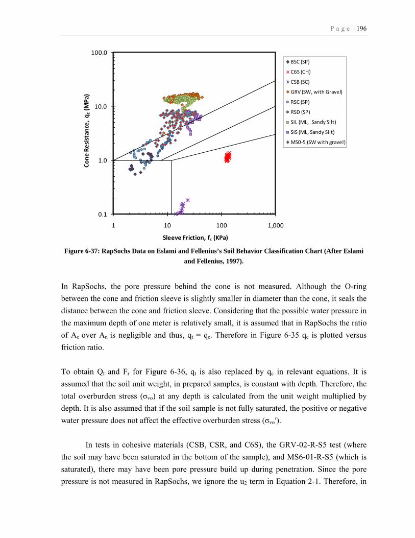
P a g e | 196
Figure 6-37: RapSochs Data on Eslami and Fellenius’s Soil Behavior Classification Chart (After Eslami
and Fellenius, 1997).
In RapSochs, the pore pressure behind the cone is not measured. Although the O-ring
between the cone and friction sleeve is slightly smaller in diameter than the cone, it seals the
distance between the cone and friction sleeve. Considering that the possible water pressure in
the maximum depth of one meter is relatively small, it is assumed that in RapSochs the ratio
of Ac over An is negligible and thus, qt = qc. Therefore in Figure 6-35 qc is plotted versus
friction ratio.
To obtain Qt and Fr for Figure 6-36, qt is also replaced by qc in relevant equations. It is
assumed that the soil unit weight, in prepared samples, is constant with depth. Therefore, the
total overburden stress (σvo) at any depth is calculated from the unit weight multiplied by
depth. It is also assumed that if the soil sample is not fully saturated, the positive or negative
water pressure does not affect the effective overburden stress (σvo′).
In tests in cohesive materials (CSB, CSR, and C6S), the GRV-02-R-S5 test (where
the soil may have been saturated in the bottom of the sample), and MS6-01-R-S5 (which is
saturated), there may have been pore pressure build up during penetration. Since the pore
pressure is not measured in RapSochs, we ignore the u2 term in Equation 2-1. Therefore, in
0.1
1.0
10.0
100.0
1 10 100 1,000
Cone
Res
ista
nce,
qc
(MPa
)
Sleeve Friction, fs (KPa)
BSC (SP)
C6S (CH)
CSB (SC)
GRV (SW, with Gravel)
RSC (SP)
RSD (SP)
SIL (ML, Sandy Silt)
SIS (ML, Sandy Silt)
MS0-5 (SW with gravel)

P a g e | 197
Figure 6-37, qc is plotted versus friction resistance. However, any possible contribution of
this term may only affect C6S and CSB data points since data from CSR-01-R-S5, GRV-02-
R-S5, and MS6-01-R-S5 are not presented in this figure.
In Figure 6-33, 6-34 and 6-35 there is an obvious distinction between cohesion-less and
cohesive materials. However, for cohesion-less materials due to confinement effects, the
cone resistance close to soil surface is small and increases with depth. Also due to the fact
that the friction ratio is the result of friction resistance over cone resistance, the data points
for cohesion-less materials follow Douglas and Olsen’s soil classification lines for constant
friction resistance. A zoomed-in plot in Figure 6-34 shows this trend.
In Figure 6-33, the horizontal line which separates cemented and dense sand and gravel from
loose materials is helpful. However the cemented and dense sand and gravel zone should be
extended to cemented or dense silt since the data points of tests in SIL and SIS are also
located in the same zone. Figure 6-35, does not predict the soil types precisely. But the order
of soil types matches the data.
In Figure 6-36, normalization as suggested by Robertson (1990) helped to overcome the
effects of overburden even in CSB (clayey sand). However, RapSochs could detect the water
elevation by the moisture sensor (but not the exact soil unit weight). Even the assumption of
constant unit weight with depth in cohesion-less materials (which is not necessarily true)
could affect normalization, especially for data points close to soil surface. The other issue
with this type of normalization is the trend of higher Qt values close to soil surface due to
smaller effective vertical stress, which may result in misleading interpretation. Nonetheless,
most of data points fall outside of the proposed chart. The fact that the primary purpose of the
normalization was to extend the soil classification to CPT data obtained in depth beyond 30
meter, shows that the chart should be adjusted for any application in interpretation of
RapSochs.
The major benefit of the method that is used to depict the data points in Figure 6-37 is that no
modification or change in the direct measurements are required. Cone resistance is plotted
versus friction resistance. The benefit in depicting test results in cohesive soil is that it will
not spread the data points unnecessarily. That is not achieved in other methods of presenting
data. However, data points for test conducted in cohesion-less materials are not separated as
clearly as in Robertson (1990) chart. The poor differentiation between poorly graded sand
and well graded sand and silt, as compared to Figure 6-36, is better than in other charts.

P a g e | 198
Distinctive classification of cohesive soils from cohesion-less soils is achieved in all of the
above mentioned charts. But detailed classification beyond that is not completely validated.
Since the number of tests in cohesive soils is limited and materials like sensitive soils, peat,
and very stiff fine-grained are not tested in the lab, drawing a conclusion about the best
possible chart appropriate for RapSochs is not possible. However, the chart by Eslami and
Fellenius (1997) has benefits, compared to other charts. Meanwhile, the comparative
information (e.g., fine contents, grain size, and void ratio) from Douglas and Olsen (1981)
also match our data. Those trend guides are translated to the format of qc versus fs and
presented on a modified chart for interpretation of RapSochs dynamic data in Figure 6-38.
The line which separates cohesion-less materials from cohesive materials is almost the same
as the vertical line in Figure 2-2 of Schmertmann’s soil behavior classification.
The data presented in Figure 6-33 to 6-37 are also shown in Figure 6-39. In Figure 6-40,
available data points for all RapSochs tests (except MS6-01-R-S5 and BSC-09-R-S5) are
presented to check the variability of other tests in each sample. It also shows that the data
points of selected tests, which used to plot over soil behavior charts, are good representation
of RapSochs test results.
Figure 6-38: Proposed Soil Behavior Classification for RapSochs.
0.1
1.0
10.0
100.0
1 10 100 1,000
Cone
Res
ista
nce,
qc
(MPa
)
Sleeve Friction, fs (KPa)
Void Ratio
Grain Size or Cementation
Fine Contents
Cohesive
Cohesion-Less

P a g e | 199
Figure 6-39: RapSochs Data on Proposed Soil Behavior Classification.
Figure 6-40: Data of All RapSochs Tests on Proposed Soil Behavior Classification.
0.1
1.0
10.0
100.0
1 10 100 1,000
Cone
Res
ista
nce,
qc
(MPa
)
Sleeve Friction, fs (KPa)
BSC (SP)
C6S (CH)
CSB (SC)
GRV (SW, with Gravel)
RSC (SP)
RSD (SP)
SIL (ML, Sandy Silt)
SIS (ML, Sandy Silt)
MS0-5 (SW with Gravel)
0.1
1.0
10.0
100.0
1 10 100 1,000
Cone
Res
ista
nce,
qc
(MPa
)
Sleeve Friction, fs (KPa)
BSC (SP)
C6S (CH)
CSB (SC)
GRV (SW, with Gravel)
RSC (SP)
RSD (SP)
SIL (ML, Sandy Silt)
SIS (ML, Sandy Silt)
MS0-5 (SW with Gravel)

P a g e | 200
6-5- Testing and Instrumental Issues
Overburden Effect (Effect of Confinement)
The effect of overburden pressure on SPT and CPT tests is well known and is incorporated
into equations and chart to for interpretation of test results. Figure 6-41 shows a picture of the
BSC sample surface after completion of all RapSochs and DCP tests. It clearly shows the soil
dilation occurs around the penetration locations. The soil dilation is visible up to about 3
times the rod diameter. The same behavior was observed around the penetration location in
all cohesion-less materials except loose sand.
Figure 6-41: Soil Dilation around Penetration Spots at BSC.

P a g e | 201
Livneh et al. (1995) verified the vertical confinement effect of 1) granular layers, 2) cohesive
layer, and 3) rigid structural layer on clayey materials; as well as the effect of upper asphalt
layer on the DCPi of granular materials. The DCP used in their research was a 30 degrees
angled cone. Using a theoretical approach and considering the Terzaghi’s bearing capacity
equation, it was concluded that in clay subgrade at the depth of 10 cm and beyond the DCP is
not subject to vertical confinement effects. The experimental tests on clay layers also showed
that the DCPi of the tests from 0 to 0.2 meter deep is identical to that of 0.5 to 0.7 meter deep
(where it is dug to 0.5 m and then the DCP test is conducted). Conversely, the confinement
effect of granular materials has a significant effect on DCP penetration. In tests on granular
base materials, they showed that the DCPi values of tests after drilling an asphalt core were
54% of those obtained after removal of a wide asphalt strip on average. However they did not
report details of their tests and materials and how deep the penetration was conducted. In
general, they concluded that the vertical confinement does not have any effect on DCPi of a
cohesive subgrade layer. However, DCP measurement in granular soil depends on the
vertical confinement.
To minimize the effect of overburden on DCP test measurements, some researchers
suggested disregarding the first couple of blows. Van Vuuren (1969) excluded the first
couple of blows. Dai and Kremer, (2006) reported that two hammer blows are required to
properly seat the DCP. Siekmeier et al. (2009) did not include the first two DCP-PRs in
calculation of the DCPi to minimize the confinement effects. They called the first two drops
as seating drops. Also they showed that disregarding two or three drops in granular materials
results in different modulus estimates because of different DCPi values. They advised to
exclude the first three drops and use the next five drops to calculate DCPi in granular
materials. They disregarded the first two drops in fine-grained materials and used the next
five drops to calculate DCPi.
Webster et al. (1994) reported that lack of confinement at the top of the surface layer affects
DCP measurements. The penetration depth required for measuring the actual strength of the
surface soil layer is estimated based on transient zones above the linear part of DCP
penetration. The same method is used in this study to determine the transient zones. Data
points at those regions were excluded in order to calculate DCPis. Rounded estimation of
transient zones is presented in Table 6-8 along the reported values of Webster et al. (1994)
for various soil types.

P a g e | 202
Table 6-8: DCP Depth Required to Measure Surface Layer Strength with No Overburden.
Soil Type Penetration Depth Required (mm)
Webster et al. (1994) Current Experiment
CH 25 250
CL 76 -
SC 102 400
SW-SM 102 -
SW - 250
SM 127 -
GP 127 -
SP 279 250-400
ML - 50-100
For all soil types, our estimates are higher than Webster et al. (1994). However, data
presented by Ayers et al. (1989) confirms our estimation for well graded sand. They reported
that DCP-PR did not display large variations deeper than 230 mm (9 in.) in the uniform
prepared sand or gravel. In pile capacity estimation in homogeneous sand, the critical
embedment ratio (length of embedment over diameter of pile), where beyond that depth the
point resistance assumed to be uniform is about 16 to 18. Applying that concept to DCP or
RapSochs instrument, results the critical depth of 320 to 360 mm.
Webster et al. (1994) stated that the penetration depth required to measure the surface layer
strength is related to the gradation and plasticity characteristics of the materials. Our
experiment shows that for the same material the degree of compaction also affects the
minimum required penetration. Since, the soil samples in their research exhibit higher
strength (in terms of CBR) comparing to tested materials in our research, observing higher
required penetration depth to get to the constant DCP-PR is not surprising. It also confirms
that the overburden effects will be higher in low-strength comparing to high-strength
materials. It should also be mentioned that since, the liner part of the number of blows versus
depth is selected (where DCP-PR is constant) the average or weighted average method will
not result a different DCPi.
One of the problems with existing DCP technology is that there is no confinement at the
surface for cohesion-less materials and therefore measurements cannot be made in the top
soil. In the version used for tests at NU no extra surcharge is used to provide the confinement

P a g e | 203
as well. However, in the final version of RapSochs a base plate will provide an approximate
confinement of 3.4 kPa (0.5 psi). If we assume an average unit weight of 15,000 N/m3 for
soil then the applied pressure is equivalent to about 23 cm of soil. This extra pressure will
allow us to measure the soil strength in shallower depth. The required depth from soil surface
would be between 0 to the maximum of 17 cm based on the soil type as suggested by our
data.
Addition of a base plate in the final version of RapSochs, and any change in the weight of the
instrument or the base area in future revisions of the instrument should be considered in
interpretation of RapSochs results. In general, RapSochs requires a thicker surface layers for
non-plastic coarser-grained materials to measure strength compare to plastic or cemented
fine-grained soils.
Sample Size and Boundary Effects
Ayers et al. (1989) reported testing the DCP on sand, gravel and crushed dolomitic ballast
(passing 2 inch/50.8 mm opening sieve) in 12-inches-diameter and 18-inches-deep steel
mold. They referenced to a technical report prepared by authors (which is not available to
us), that the boundary effect of a mold is significant if the mold diameter is less than 8 times
of the maximum aggregate size. The maximum grain size of materials tested at NU is 12 mm
(½ in.) which belongs to gravel (used to prepare samples of GRV, MS0, MS1, MS2, MS3,
MS4, MS5 and MS6). In those tests the location of tests are more than 8×12 = 96 mm away
from the container’s interior surface.
Kleyn (1975) in verifying the effect of the length of the mold on DCP results concluded that
the use of longer mold (twice the length of standard CBR mold which is about 178 mm)
showed no significant difference in DCPi. By comparing the DCP penetration in 150 mm,
200 mm, and 250 mm diameter molds he concluded that the effect of the mold diameter is
negligible in 250 mm diameter molds. This experiment was conducted in different gravels.
Comparison of DCPis in 150 and 250 mm diameter molds showed a linear trend on
logarithmic scale where the difference is smaller for higher DCPi materials. The effect was
found negligible between the 200 mm and 250 mm molds. However, DCPis in 150 mm
diameter mold was 25% and 12% smaller than DCPis in 250 mm diameter mold at 6 and 28
mm/blow DCPis respectively. In 200 mm diameter mold the radius of mold is 10 times the
radius of the cone base.

P a g e | 204
Coonse (1999) verified the effect of mold diameter on DCP test in cohesive soil by
comparing the DCPi in 150 mm and 250 mm diameter molds. The results showed that for
samples where DCPi is between 10 to 25 mm/blow, the results are identical but for softer
materials (where the DCPi is higher) a difference is observed. At DCPi of 50 mm/blow the
difference reported is around 25%.
Friton (1990) reported the work of Farrell and Greacen (1966) that they calculated the plastic
region around a 60-degrees penetrometer in compressible soils to be around 6 to 10 times the
radius of the cone base.
Table 6-9 is summarized the minimum spacing between tests and distance from the container
side in different containers. In non cohesive soils, the minimum distance from the container
is more than 10 times the radius of the cone. The spacing distance between penetration tests
are 16 times of the cone radius. It provides each test a minimum radius of 80 mm, 8 times the
radius of the cone, from the effected regions around the adjacent penetration location. In
cohesive soil samples these distances are shorter but they are not less than 6 times the cone
radius.
Table 6-9: Minimum Spacing between Tests and Distance to Container’s Side in each Sample.
Sample ID
Spacing between
Tests (mm)
Distance to
Container* (mm)
BSC 159 106
BSL 159 106
C6S 125 76
CSB 127 86
CSR N/A 125
GRV 178 107
RSC 159 106
RSD 159 106
RSL 159 106
SIL 159 106
SIS 159 106
MS0-6* N/A 125
NOTES: *From the penetration point **Includes Sample MS0, MS1, MS2, MS3, MS4, MS5 and MS6.

P a g e | 205
To examine any possible effects of test spacing on the penetration results we have compared
the RapSochs estimated tip stress profile of tests in the same samples to find any trend based
on sequence of tests. Comparison of DCP-PR profiles could also be helpful to examine this
effect. Figure 6-42 shows estimated tip resistance profiles of RapSochs tests in each sample.
The estimated cone tip stress are overplotted to help comparison of results and evaluation of
differences based on sequence of tests in each sample.
In RSC, RSD, and GRV, data are scattered and no meaningful trend is observed. In C6S, the
tip stresses of C6S-04-R-S2 are higher than those of C6S-01-R-S8. However, comparison of
DCP test results shows an inverse trend. Therefore the difference is more likely the result of
heterogeneous compaction effort. In MS0 to MS6, CSB, and CSR, there are not other tests to
give us a benchmark for comparison. In SIS, the first test at spot-5, SIS-01-R-S5, shows
higher strength than other RapSochs tests. We would have expected to see higher resistance
if other tests have been affected by the first test. However, lower resistance is observed in
those results. It is believed that heterogeneous compaction effort may have been the reason
for the differences. In SIL, as mentioned in Chapter 5, SIL-01-R-S1 was conducted 3 months
before other tests. The effect of aging and cementation is noticeable in this case. Also the
moisture sensor cover damaged during this test which may also have caused a resistance
against penetration. In SIL-03-R-S5, which is conducted at the center of sample, higher
resistance is shown. Similar to SIS, we believe that heterogeneous compaction effort during
preparation may have been the cause.
In BSC, the cone resistance of BSC-09-R-S5 is noticeably higher than other RapSochs tests.
Only in this case we are suspected that the boundary effects may have contributed to further
compaction of soil sample and therefore higher estimated resistance. Whether it is due to
boundary effect or heterogeneous compaction we could not determine it with certainty.
Examination of DCP test results does not show an increase in soil resistance (lower DCP-
PRs) in later tests. For this reason only results of BSC-09-R-S5 are excluded in RapSochs to
CBR correlation.
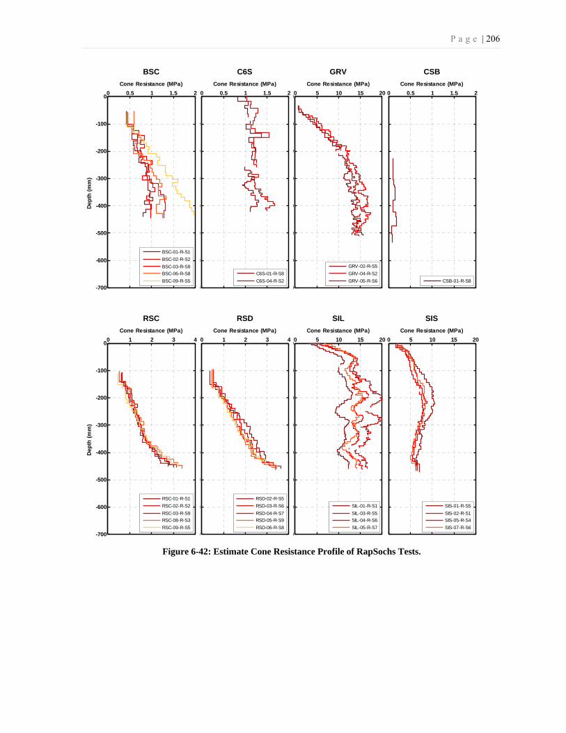
P a g e | 206
Figure 6-42: Estimate Cone Resistance Profile of RapSochs Tests.
0 0.5 1 1.5 2
-700
-600
-500
-400
-300
-200
-100
0De
pth
(mm
)Cone Resistance (MPa)
BSC
BSC-01-R-S1
BSC-02-R-S2
BSC-03-R-S9
BSC-06-R-S8
BSC-09-R-S5
0 0.5 1 1.5 2
0
0
0
0
0
0
0
0
Cone Resistance (MPa)
C6S
C6S-01-R-S8
C6S-04-R-S2
0 5 10 15 20
0
0
0
0
0
0
0
0
Cone Resistance (MPa)
GRV
GRV-02-R-S5
GRV-04-R-S2
GRV-05-R-S6
0 0.5 1 1.5 2
0
0
0
0
0
0
0
0
Cone Resistance (MPa)
CSB
CSB-01-R-S8
0 1 2 3 4
-700
-600
-500
-400
-300
-200
-100
0
Dept
h (m
m)
Cone Resistance (MPa)
RSC
RSC-01-R-S1
RSC-02-R-S2
RSC-03-R-S9
RSC-08-R-S3
RSC-09-R-S5
0 1 2 3 4
0
0
0
0
0
0
0
0
Cone Resistance (MPa)
RSD
RSD-02-R-S5
RSD-03-R-S6
RSD-04-R-S7
RSD-05-R-S9
RSD-06-R-S8
0 5 10 15 20
0
0
0
0
0
0
0
0
Cone Resistance (MPa)
SIL
SIL-01-R-S1
SIL-03-R-S5
SIL-04-R-S6
SIL-05-R-S7
0 5 10 15 20
0
0
0
0
0
0
0
0
Cone Resistance (MPa)
SIS
SIS-01-R-S5
SIS-02-R-S1
SIS-05-R-S4
SIS-07-R-S6

P a g e | 207
In general, due to the methodology used to prepare soil samples it is possible that the
compaction effort was not distributed perfectly on the surface of each layer. Examination of
test results also suggested that any interference of tests due to spacing is unlikely except in
the BSC-09-R-S5 test. Nonetheless, the only error that any possible boundary effects may
cause in our analysis would be in RapSochs to CBR correlation. Since the possible boundary
effect on DCP test results is similar to effects on RapSochs test results, we do not expect any
error or bias in our analysis. However, results of BSC-09-R-S5 were excluded in our
analysis. Any further interpretation of test data should be undertaken with great care.
Hammer Drop Height and Penetration Rate Effects
There are extensive works mentioned in literature which cover quasi-static penetration rate
effects in CPT. Based on ASTM D 3441 (2005) the penetration rate during Mechanical Cone
Penetration Test should be maintained 10 to 20 mm/sec (2 to 4 ft/min) ± 25 %. ASTM D
5778 (2005) requires a constant rate of 20 mm/sec for electric friction CPT. The International
Reference Test Procedure requires that the rate of penetration should be constant at 20 mm/s
(Lunne, Robertson, & Powell, 1997) with the same tolerance of 25 %. In CPT additional
understanding about soil behavior is obtained by deviating from the standard rate of
penetration (Lunne, Robertson, & Powell, 1997). Penetration rate or strain rate effects on
measuring soil properties during cone penetration or similar mechanisms in different soil
types and in penetration rates of 0.059 – 3210 mm/sec is studied. However, most of the tests
were performed with the rates slower than the standard rate of 20 mm/s for CPT.
For clays, most of the CPT rate effect studies have shown an increase in the cone resistance
with an increasing rate of penetration. However most testing in sands indicates that for rates a
little slower than a penetration rate of 20 mm/s there is little effect on the cone resistance. For
faster rates of penetration an increase in cone resistance may occur as a result of dilatancy
and higher negative pore pressure (Lunne, Robertson, & Powell, 1997).
Juran & Tumay (1989) in field verification and calibration tests of the DPCPT (Dual-pore-
pressure PiezoCone Penetration Test) conducted 19 tests with four different types of cone
penetrometers. Among their objective of those penetration tests was to evaluate the effect of
the penetration rate on the measured soil response parameters. For the 15-cm2 cone at
P a g e | 208
penetration rates of 0.2 cm/s and 10 cm/s it was found that the penetration rate have no
appreciable effect on tip resistance in sand and clay. However, it has a significant effect on
the pore water pressures measured in the sand.
Dayal (1980) reported studies of the effect of penetration rate of a free fall penetrometer on
remolded clay and sand samples. In velocity range of 0.1 to 600 cm/sec he reported no major
difference in failure pattern and no significant effects on the cone and friction resistance of
granular soils. However he reported an increase in cone and friction resistance with increases
in penetration velocity in cohesive soils. An empirical relationship is presented which relates
the dynamic soil resistance to (almost) static soil resistance.
While in the RapSoch hammer velocity exactly before collision (assuming no friction) is
between 100 to 331 cm/sec (corresponding to 2 inches to 22 inches drop height) the average
velocity of the penetrometer is calculated between 94 to 320 cm/sec after the collision based
on the calculated coefficient of restitution. It was one of the concerns that how different
hammer drop height and consequently different penetration rate may affect the RS-PR, DCP-
PRRS, cone resistance, and friction resistance estimation.
The effect of variable hammer drop height in RapSochs is studied by using different drop
heights in C6S, SIL, and SIS samples. In those tests after the drop height was established in
22 inches (55.9 cm), the drop height was decreased to 15 and 10 inches (38.1 and 25.4 cm),
and then back to 22 inches for the remained blows.
Effects on Cone and Friction Resistance
In quasi-static estimation of dynamic force the presented figures for typical tests in SIL and
C6S showed no significant changes in estimated cone resistance and friction resistance due to
different hammer drop height. Similar results observed in SIS (see Appendix L). In these
tests when the hammer drop height reached to maximum, different hammer drop heights
were tried to examine its effect on cone and friction resistance.
In MS0 to MS6, and GRV the hammer drop height adjusting procedure followed strictly and
when the hammer drop height reached to maximum, different hammer drop heights where
not tried. In those tests, the cone resistance shows a non linear increase with depth until it
gets to a more or less a constant resistance which is very apparent in GRV. In contrast, the
friction profile does not follow any clear trend and the changes with depth are very different
P a g e | 209
in similar tests. However we could say that in deeper depth usually the friction is higher
comparing to friction close to surface.
In BSC, RSC, and RSD, the hammer drop height never reached to maximum. In these tests,
the cone resistance profile also shows an increase with depth. While the hammer drop height
is also increased with depth (to keep the penetration rate less than 13 mm per blow) it is
difficult to judge whether the cone resistance increase is due to overburden effect or it is due
to increase of applied energy. However for the same hammer drop height the cone resistance
is generally higher at deeper depth. Thus the observed increase with depth is most probably
due to overburden effects in granular soils. For friction resistance, while in BSC and RSC no
special pattern is observed, in RSD the friction increases more or less monotonically with
depth.
In CSB, cone resistance almost remains constant with depth but the friction resistance
increases with depth. However, the number of penetration tests and blows in that material are
limited thus drawing any specific conclusion is not possible.
In general, different hammer drop height does not show any significant interference in cone
and friction resistance estimation and we conclude that the hammer drop height adjustment
procedure is not affecting soil resistance estimation using MLE.
Effects on RS-PR
As it was shown in Figure 5-7 in Chapter 5, and for the similar graphs presented in Appendix
I, RS-PR is affected significantly from the hammer drop height. Early in this chapter we
developed an energy formula which relates the variable parameters in a RapSochs blow. If
our observations that the cone and friction resistance are not influenced by different hammer
drop height is correct, then based on the Equation 6-72 the ratio of hammer drop height over
the penetration is constant. In the other words, RapSochs penetration rate normalized by
hammer drop height should be constant in similar soil conditions.
RS-NPR (RapSochs Normalized Penetration Rate) is introduced which is a RS-PR
normalized for maximum RapSochs hammer drop height of 55.9 cm (22 inches). It could be
calculated from the following equation:
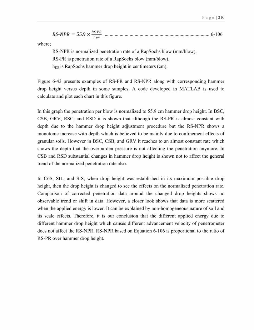
P a g e | 210
- = 55.9 - ..................................................................................... 6-106
where;
RS-NPR is normalized penetration rate of a RapSochs blow (mm/blow).
RS-PR is penetration rate of a RapSochs blow (mm/blow).
hRS is RapSochs hammer drop height in centimeters (cm).
Figure 6-43 presents examples of RS-PR and RS-NPR along with corresponding hammer
drop height versus depth in some samples. A code developed in MATLAB is used to
calculate and plot each chart in this figure.
In this graph the penetration per blow is normalized to 55.9 cm hammer drop height. In BSC,
CSB, GRV, RSC, and RSD it is shown that although the RS-PR is almost constant with
depth due to the hammer drop height adjustment procedure but the RS-NPR shows a
monotonic increase with depth which is believed to be mainly due to confinement effects of
granular soils. However in BSC, CSB, and GRV it reaches to an almost constant rate which
shows the depth that the overburden pressure is not affecting the penetration anymore. In
CSB and RSD substantial changes in hammer drop height is shown not to affect the general
trend of the normalized penetration rate also.
In C6S, SIL, and SIS, when drop height was established in its maximum possible drop
height, then the drop height is changed to see the effects on the normalized penetration rate.
Comparison of corrected penetration data around the changed drop heights shows no
observable trend or shift in data. However, a closer look shows that data is more scattered
when the applied energy is lower. It can be explained by non-homogeneous nature of soil and
its scale effects. Therefore, it is our conclusion that the different applied energy due to
different hammer drop height which causes different advancement velocity of penetrometer
does not affect the RS-NPR. RS-NPR based on Equation 6-106 is proportional to the ratio of
RS-PR over hammer drop height.
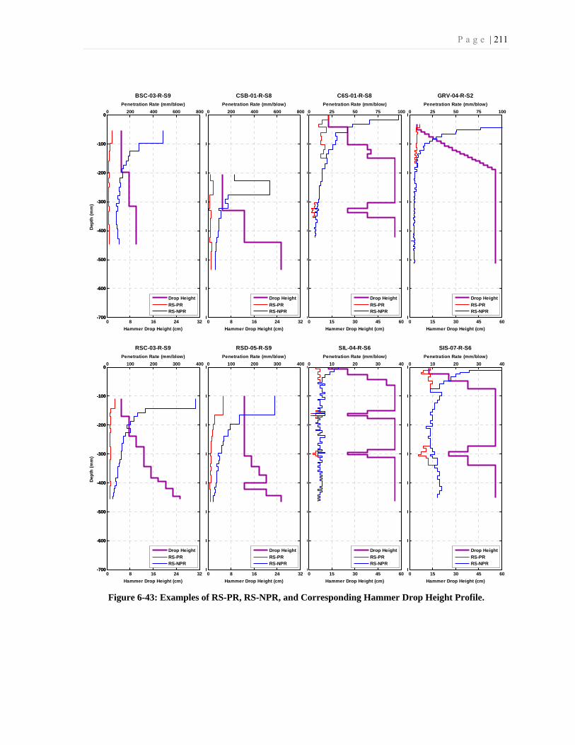
P a g e | 211
Figure 6-43: Examples of RS-PR, RS-NPR, and Corresponding Hammer Drop Height Profile.
0 8 16 24 32-700
-600
-500
-400
-300
-200
-100
0
Hammer Drop Height (cm)
0 200 400 600 800
-700
-600
-500
-400
-300
-200
-100
0
Penetration Rate (mm/blow)
Dep
th (m
m)
BSC-03-R-S9
Drop HeightRS-PRRS-NPR
0 8 16 24 320
0
0
0
0
0
0
0
Hammer Drop Height (cm)
0 200 400 600 800
0
0
0
0
0
0
0
0
Penetration Rate (mm/blow)
CSB-01-R-S8
Drop HeightRS-PRRS-NPR
0 15 30 45 600
0
0
0
0
0
0
0
Hammer Drop Height (cm)
0 25 50 75 100
0
0
0
0
0
0
0
0
Penetration Rate (mm/blow)
C6S-01-R-S8
Drop HeightRS-PRRS-NPR
0 15 30 45 600
0
0
0
0
0
0
0
Hammer Drop Height (cm)
0 25 50 75 100
0
0
0
0
0
0
0
0
Penetration Rate (mm/blow)
GRV-04-R-S2
Drop HeightRS-PRRS-NPR
0 8 16 24 32-700
-600
-500
-400
-300
-200
-100
0
Hammer Drop Height (cm)
0 100 200 300 400
-700
-600
-500
-400
-300
-200
-100
0
Penetration Rate (mm/blow)
Dep
th (m
m)
RSC-03-R-S9
Drop HeightRS-PRRS-NPR
0 8 16 24 320
0
0
0
0
0
0
0
Hammer Drop Height (cm)
0 100 200 300 400
0
0
0
0
0
0
0
0
Penetration Rate (mm/blow)
RSD-05-R-S9
Drop HeightRS-PRRS-NPR
0 15 30 45 600
0
0
0
0
0
0
0
Hammer Drop Height (cm)
0 10 20 30 40
0
0
0
0
0
0
0
0
Penetration Rate (mm/blow)
SIL-04-R-S6
Drop HeightRS-PRRS-NPR
0 15 30 45 600
0
0
0
0
0
0
0
Hammer Drop Height (cm)
0 10 20 30 40
0
0
0
0
0
0
0
0
Penetration Rate (mm/blow)
SIS-07-R-S6
Drop HeightRS-PRRS-NPR

P a g e | 212
Effects on DCP-PRRS
The equation which is used to correlate RS-PR to DCP-PRRS is developed based on the
energy model equation. We showed that the ratio of RS-PR normalized for hammer drop
height is not affected by hammer drop height. Therefore regardless of the hammer drop
height, the ratio of hammer drop height over RS-PR remains constant in similar soil
condition and depth. Hence DCP-PR in Equation 6-95 which is later rewritten as Equation 6-
96 remains constant too. Therefore the DCP-PRRS is not affected by hammer drop height
also.
Effects of Blow Rate
In our tests with RapSochs, the raise and drop of hammer was manual. Also we had to wait
for few seconds to make sure that all data are transferred into the laptop before activating the
moisture sensor measurement manually. If no problem occurred during a test the time
interval between each blow was usually not higher than two minutes. However, in some rare
cases that time interval exceeded two minutes. We did not measure the time intervals
independently but if one is interested, these times could be extracted by looking into the
creation time of ASCII files.
In the final version of RapSochs the desired test time is less than 5 minutes for 100 cm
penetration. The blow cycle (hammer lift-drop and communications-processing) at the final
version should be less than 1.2 seconds to meet the 5 minutes limit in a material with RS-PR
equal to 4 mm/blow.
Livneh et al. (1992) by comparison of manual and automated DCP showed that the DCP
results are independent of the blow-rate in sandy clay. The range that they examined the rate
effects of automated DCP was between 0.4 to 1 blows per second. Therefore, we do not
expect that the different blow rate in the final version of RapSochs comparing to the current
prototype makes any differences. However, in the future field tests with RapSochs, this effect
should be investigated more closely specially for tests in clayey soils as well as tests in
saturated soils.

P a g e | 213
Chapter 7: Summary and Conclusions
7-1- Summary
The RapSochs (Rapid Soil Characterization System) is developed as a man-portable
instrument for rapid comprehensive field characterization of near-surface soil properties. The
primary goal of this research is to develop necessary methods to interpret geotechnical
properties from the newly developed instrument. The research addressed the following.
- Review and assessment of the literature on soil characterization instruments,
- Laboratory real-size testing in homogenous samples,
- Developing the database and algorithms for recording, quality control, correction,
accessing, analysis, and presentation of data,
- Developing algorithms for dynamic cone and friction resistance estimation,
- Developing a model to predict soil-instrument interaction in dynamic penetration,
- Developing a RapSochs to CBR correlation, and
- Developing a soil behavior classification chart.
A detailed description of the first revision of the instrument is provided. Several real-
size tests were conducted in SP, SW, ML, SC, and CH samples prepared in laboratory in
large soil cells. An analytical physics-based energy model was developed to predict soil-
instrument interaction in near-surface dynamic penetration. The model was calibrated for
RapSochs and DCP and used to explain the penetration process. The model correlates the
instrument properties (i.e., penetrometer and hammer mass, coefficient of restitution,
hammer drop height) to soil resistance and penetration rate. The model was used to correlate

P a g e | 214
RapSochs penetration rate to DCP data. This model together with the DCP-CBR correlation
was used to develop a RapSochs-CBR correlation.
Assessment of the moisture sensor performance was not within the scope of this
study. However, early tests and analysis showed a good sensitivity of the sensor in granular
materials that can be used to provide a soil moisture profile. Discussion of the moisture
sensor and its performance are summarized by Gamache et al. (2008b).
The Maximum Likelihood Estimation (MLE) method was adopted for the average
dynamic cone and friction force estimation. Cone and friction strength and friction ratio
profiles were developed based on estimated forces. The effect of variable applied energy on
the soil strength estimation was also studied. Soil classification following the USCS system
was examined based on charts developed for CPT. Effects of overburden, sample size,
boundary conditions, hammer drop height, and penetration rate on RapSochs measurements
were also assessed.
7-2- Conclusions
The following conclusions are drawn from this study.
• The RapSochs instrument provides relatively reliable, consistent, and repeatable
results in laboratory prepared homogenous soil samples. RapSochs can provide in-
situ strength profiles of in place soil or compacted layers. Interpretation of RapSochs
data for accurate near-surface soil characterization is feasible. The estimation of soil
strength and friction resistance, soil behavior classification, and correlation to CBR
was achieved. Combined with the soil moisture estimation, RapSochs is a valuable
instrument for rapid soil characterization. Correlation of RapSochs data to elastic
modulus, porosity, and mean grain size of soil is also feasible.
• The MLE method can accurately estimate the average dynamic cone and friction
forces. Cone and friction resistance values similar to those measured by the CPT can
be obtained from RapSochs records. Soil classification to cohesive and cohesionless
materials was accomplished using the chart developed based on the cone and friction
resistance measured by the RapSochs. The chart also provides comparative

P a g e | 215
information including fine contents, grain size, and void ratio trend change adapted
from previous studies with CPT.
• No significant interferences are expected due to the variable hammer drop height on
cone and friction resistance estimation. In other words, it is concluded that the
hammer drop height adjustment procedure does not affect the soil resistance
estimation using MLE. Different hammer drop heights, which cause different
advancement velocity of the penetrometer do not affect the RS-NPR (Normalized
penetration rate of a RapSochs) either.
• An energy model was developed based on Newtonian physics to assess the interaction
between the hammer, penetrometer, and soil to provide a better understanding of the
dynamic penetration process. The model predicts the hammer-instrument-soil
interaction and response with an acceptable accuracy. The model predictions are more
accurate than the widely-used Dutch formula.
• RapSochs hammer drop height and penetration rate were correlated to the materials
CBR value. This correlation predicts CBR with acceptable accuracy compared with
CBR values derived from the DCP. RapSochs can replace DCP for CBR estimation
with higher resolution of data and measurements near to ground surface.
• Electronics in the sensor tip can withstand the shock and vibration induced by the
hammer impact in the hardest materials. The tip and sleeve strain gauges proved to be
very reliable. However, accelerometer and string potentiometer were problematic.
Improvement measures are recommended for future work.
• The current revision of RapSochs is operated manually, which can be problematic
and not practical due to challenges in raising and dropping the hammer. It is expected
that the automated version will solve this problem. In the newer revision, where the
control system is fully automated, there is no need for the presence of an operator.
In general, RapSochs was shown to be a consistent and reliable method for testing of
soil strength and can be used in different materials with a wide range of strength. The
theoretical basis of the data interpretation was developed and verified. With some
improvements in the design and development of a data analysis package, it can potentially
become a practical field testing instrument. However, further experimental testing in the real

P a g e | 216
field are still necessary for development of better correlations to include wider ranges of
materials in various conditions.
While the technique discussed in this dissertation has been developed specifically for
RapSochs, it is applicable to a wide class of dynamic penetrometers. In this respect, the
RapSochs instrument has served as a "model" used to develop and refine the techniques
needed to extract soil properties.
7-3- Recommendations for Future Instrument Improvement
For further improvement of the instrument and to develop a commercially available revision,
the following recommendations are provided.
• During this study several issues raised (e.g., difficulty in extraction of the instrument
after deep tests, electrical and mechanical problems, damage of moisture sensor
cover). With the help of TransTech Systems Inc. some of the problems were
addressed and solved. For the commercial revision, the durability of mechanical parts
(including the moisture sensor cover) should be improved. A maintenance procedure
and replacement criteria for the cone should be developed, and methodologies for
calibration of the sensors after a certain number of tests need to be considered.
• Electronics in the sensor tip withstood the shock and vibration induced by the
hammer impacts in the hardest materials. However, the sensing technologies showed
a different performance during the dynamic penetration. While the tip and sleeve
force measurements are reliable, accelerometer and string potentiometer are
problematic.
• The string potentiometer is suitable for depth and penetration measurements.
However, it exhibits disadvantages in regards with the dynamic response to
penetration and mechanical problems due to the string and its connection. The low
resolution of the sensor and the vibration of the string made recorded data unsuitable
for more advanced analysis (e.g., to obtain velocity by differentiation). Replacement
with other types of displacement measuring sensors, with less vulnerability and better
dynamic response, would be very beneficial.

P a g e | 217
• The accelerometer did not work as expected in the RapSochs configuration. Part of
the problem is the resolution and oversaturation of the accelerometer. Replacement of
the current accelerometer with one with at least ±1500 g range and higher sampling
rate is recommended. Acceleration data from further tests could be used to obtain
velocity-time histories which could potentially lead to more accurate transferred
energy measurements. Removing the accelerometer can be the other option. The
MLE analysis results in very stable soil strength profiles. Since the results are
satisfactory, removing the accelerometer could reduce the cost of manufacturing and
post-test data analysis.
• The pull-out of the instrument after penetration is one of the concerns. In contrast
with DCP, RapSochs has a relatively expensive cone head that cannot be expended in
the soil. An extraction jack needs to be designed and tested to be included in the
RapSochs package.
• Addition of a strain gauge below the anvil will also make it possible to measure the
total force required to drive the penetrometer in addition to the cone and friction
resistance. Since the friction acting on the probe, as it is advancing though the soil,
may change from the friction measurement at friction sleeve, it will help to obtain a
more accurate required force to drive down the probe.
• All the experimental work in this research are conducted in laboratory controlled
conditions and temperature. Effects of extreme conditions (e.g., freezing or hot
temperature, corrosion environment, high humidity) on the instrument measurement
and accuracy need to be studied. In the interpretation of measured data, seasonal
adjustments should be considered since soil and probe properties change with
moisture and temperature. Those procedures and algorithms need to be developed for
the final instrument.
• Using MLE analysis to match a two consecutive square pulse to recorded data is
computationally intensive. The one square pulse matching reduces the computational
time significantly. If the data from the second pulse is not going to be used it will be
much faster to estimate the magnitude of the main pulse. Digital signal filtering can
be implemented to overcome computational disadvantages of the MLE method and
obtain the real time approximation of the penetration resistance. The MLE results can
be used as the criteria in the design of a digital filter.

P a g e | 218
• The cone cylindrical extension is about 6.3 mm (0.25 in.) in RapSochs. In electric
CPT for penetrometers with diameter of 36 or 44 mm, the thickness of the extension
should be between 3 to 7 mm (ASTM D 5778, 2007). To be proportional to the
dimensions of ASTM D 5778, the thickness of the extension in RapSochs should be
limited to 2 to 4 mm. MnDOT (1996) limits this dimension to about 3 mm for DCP.
• The database and algorithms for recording and analysis of data were developed as
part of this study. The database structure and codes of algorithms could be used as the
basis for the design and development of a software package required to accompany
future versions of the RapSochs when commercialized.
7-4- Suggestions for Future Research
There are many research opportunities for development and improvement of rapid in-situ site
characterization using RapSochs. Some of the opportunities are listed and discussed in the
following.
In order to assess the RapSochs performance on a larger range of materials, field testing will
be necessary. One possibility is to perform tests at the NSF and FHWA sponsored National
Geotechnical Engineering Sites (NGES). There are five well-characterized sites around the
U.S. with different soil formations with a wide range of materials. Additional laboratory tests
on different soil types and in different saturation ratio will also be beneficial. Correlations
and models developed based on tested materials could be extended to cover large ranges of
materials or could be modified for materials with different responses. Possible correlations to
the elastic modulus, resilient modulus, porosity, mean grain size, horizontal lateral pressure,
relative density, plasticity index, angle of internal friction, OCR (Over Consolidation Ratio),
and undrained shear strength of soil could be studied.
One of the reasons for having a thermometer in RapSochs is to verify if the soil temperature
is below the freezing point. Sets of experiments are required to measure the sensitivity of the
sensor to the ambient temperature and the time duration needed to achieve temperature
equilibrium with the surrounding soil.
P a g e | 219
The accelerometer was added to the instrument to provide velocity-time histories to calculate
transferred energy at the tip of the cone. However, due to several reasons, it was not
successful. Replacement of the accelerometer or string potentiometer with ones capable of
producing reliable velocity-time histories in conjunction with a higher sampling rate of strain
gauges would open new opportunities for dynamic analysis to better understand hammer-
penetrometer-soil interaction. A computer model (e.g., Finite Element Modeling) of the
hammer-penetrometer-soil interaction could also be used to determine the sensitivity of the
RapSochs to different soil properties (e.g., elastic modulus, Poisson's ratio) and could
possibly open new insights into in-situ measurement of soil mechanical properties.
The number of tests on fully-saturated or close to fully-saturated samples was limited. Since
water in the soil cannot easily be dissipated during the dynamic penetration shock, more
studies on the effect of excess pore water pressure on estimated properties and penetration
rate are required. The dissipation of excess pore-pressure is also very influential on undrained
strength of fine-grained soils. During the tests with RapSochs, the time interval between each
hammer drop was about 20 to 30 seconds. The final automated version of RapSochs will
operate at about 10 times faster. The effect of hammer blow rate on strength estimation needs
to be studied.
In the CPT literature, there are few or no data and analysis for near-surface test results.
However, constant push mini-cones have been used by a few in the pavement applications.
Side-by-side tests with RapSochs and mini-cones or CPT could determine the limits,
advantages, and disadvantages of quasi-static versus dynamic penetration for near-surface
applications.

P a g e | 220
References
AASHTO T-193 (2003). "Standard Method of Test for the California Bearing Ratio",
Standard Specifications for Transportation Materials and Methods of Sampling and
Testing, American Association of State Highway and Transportation Officials,
Washington, D.C.
AASHTO (1993). "AASHTO Guide for Design of Pavement Structures", National
Cooperative Highway Research Program, American association of state highway and
transportation officials, ISBN 1560510552, 640 pp.
AASHTO (1986). "AASHTO Guide for Design of Pavement Structures", National
Cooperative Highway Research Program, American association of state highway and
transportation officials, Washington, DC.
Abou-matar H., and G. G. Goble (1997). “SPT Dynamic Analysis and Measurements”,
Journal of Geotechnical and Geoenvironmental Engineering, Volume 123, Issue 10,
pp. 921-928 (October 1997).
Abu-Farsakh, M. Y. , K. Alshibli, M. Nazzal, and E. Seyman, (2004). Assessment of In-Situ
Test Technology for Construction Control of Base Courses and Embankments,
Technical Report, Louisiana Transportation Research Center, Baton Rouge, LA
70808, FHWA/LA.04/385.
Abu-Farsakh, Murad Y., Munir D. Nazzal, Khalid Alshibli and Ekram Seyman, (2005).
"Application of Dynamic Cone Penetrometer in Pavement Construction Control",
Transportation Research Record, 1913, TRB, National Research Council,
Washington, D.C., pp. 52-61.

P a g e | 221
Akgün, H., M. K. Koçkar, Ö. Aktürk (2006). “Evaluation of a Compacted Bentonite/Sand
Seal for Underground Waste Repository Isolation”, Environmental Geology, Volume
50, Issue 3, pp 331-337, DOI: 10.1007/s00254-006-0212-6.
Al-Refeai, T. A., A. S. Al-Suhaibani (1997). "Prediction of CBR Using Dynamic Cone
Penetrometer", Journal of King Saud University, Volume 9, Engineering Sciences
(2), pp. 191-204, Riyadh, Saudi Arabia.
American Colloid Company (2005). “Technical Data Sheet. Volclay GPG 30”, Arlington
Heights, IL, American Colloid Company. 1 p.
Amini F. (2003). "Potential Applications of Dynamic and Static Cone Penetrometers in
MDOT Pavement Design and Construction ", Report Number FHWA/MS-DOT-RD-
03-162, pp 31.
Amini, F. (2004). “Dynamic Cone Penetrometer in Quality Control of Compaction: State-of-
the-Art Report”, Geotechnical engineering for transportation projects : proceedings of
Geo-Trans 2004, July 27-31, 2004, Los Angeles, California / sponsored by the Geo-
Institute of the American Society of Civil Engineers ; edited by Mishac K. Yegian,
Edward Kavazanjian, pp 1023-1030.
Ampadu, S.I., and T.D. Arthur (2006). “The Dynamic Cone Penetrometer in Compaction
Verification on a Model Road Pavement”, Geotechnical Testing Journal, Volume 29,
Issue 1 (January 2006).
Ayers, M. E., M. R. Thompson, and D. R. Uzarski (1989).” Rapid Shear Strength Evaluation
of In-Situ Granular Materials”, In Transportation Research Record 1227, TRB,
National Research Council, Washington, D.C., 1989, pp. 134–146.
Ayers, M. E. (1990). “Rapid Shear Strength of In Situ Granular Materials Utilizing the
Dynamic Cone Penetrometer”, Ph.D. Dissertation, University of Illinois, Urbana, IL,
1990.
ASTM D422 (1963). “Standard Test Method for Particle-Size Analysis of Soils”, ASTM
International, West Conshohocken, PA, www.astm.org.
ASTM D698 (2000) “ASTM D698-00a Standard Test Methods for Laboratory Compaction
Characteristics of Soil Using Standard Effort (12,400 ft-lbf/ft3 (600 kN-m/m3))”
ASTM International, West Conshohocken, PA, 2003, www.astm.org.
ASTM D854 (2005). “Standard Test Methods for Specific Gravity of Soil Solids by Water
Pycnometer”, ASTM International, West Conshohocken, PA, 2003, www.astm.org.
ASTM D1140 (2000), “Standard Test Methods for Amount of Material in Soils Finer than
No. 200 (75-μm) Sieve”, ASTM International, West Conshohocken, PA, 2003,
www.astm.org.

P a g e | 222
ASTM D1557 (2007). “Standard Test Methods for Laboratory Compaction Characteristics of
Soil Using Modified Effort (56,000 ft-lbf/ft (2,700 kN-m/m))”, ASTM International,
West Conshohocken, PA, 2003, www.astm.org.
ASTM D1586 (1999). “Standard Test Method for Standard Penetration Test (SPT) and Split-
Barrel Sampling of Soils”, ASTM International, West Conshohocken, PA, 2003,
www.astm.org.
ASTM D1883 (2007). “Standard Test Method for CBR (California Bearing Ratio) of
Laboratory-Compacted Soils”, ASTM International, West Conshohocken, PA, 2003,
www.astm.org.
ASTM D2216 (1998). “Standard Test Methods for Laboratory Determination of Water
(Moisture) Content of Soil and Rock by Mass”, ASTM International, West
Conshohocken, PA, 2003, www.astm.org.
ASTM D2487 (2000). “Standard Practice for Classification of Soils for Engineering
Purposes (Unified Soil Classification System)”, ASTM International, West
Conshohocken, PA, 2003, www.astm.org.
ASTM D3441 (2005). “Standard Test Method for Mechanical Cone Penetration Tests of
Soil”, ASTM International, West Conshohocken, PA, 2003, www.astm.org.
ASTM D4318 (2000). “Standard Test Methods for Liquid Limit, Plastic Limit, and Plasticity
Index of Soils”, ASTM International, West Conshohocken, PA, 2003, www.astm.org.
ASTM D4429 (2009). “Standard Test Method for CBR (California Bearing Ratio) of Soils in
Place”, ASTM International, West Conshohocken, PA, 2003, www.astm.org.
ASTM D4633 (2010). “Standard Test Method for Energy Measurement for Dynamic
Penetrometers”, ASTM International, West Conshohocken, PA, 2003, www.astm.org.
ASTM D4945 (2000). “Standard Test Method for High-Strain Dynamic Testing of Deep
Foundations”, ASTM International, West Conshohocken, PA, 2003, www.astm.org.
ASTM Standard D5778 (2007). "Standard Test Method for Electronic Friction Cone and
Piezocone Penetration Testing of Soils." ASTM International, West Conshohocken,
PA, 2003, DOI: 10.1520/D5778-07, www.astm.org.
ASTM Standard D6951 (2003). "Standard Test Method for Use of the Dynamic Cone
Penetrometer in Shallow Pavement Applications." ASTM International, West
Conshohocken, PA, 2003, www.astm.org.
ASTM Standard D6951 / D6951M (2009). "Standard Test Method for Use of the Dynamic
Cone Penetrometer in Shallow Pavement Applications." ASTM International, West
Conshohocken, PA, 2003, DOI: 10.1520/ D6951_D6951M-09, www.astm.org.
ASTM E2583 (2007).””,ASTM International, West Conshohocken, PA, 2003,
www.astm.org.

P a g e | 223
Baker, M. R., K. Crain, S. Nazarian (1993). "Seismic Pavement Analyzer Operations Manual
with Technical Specifications", Strategic Highway Research Program, National
Research Council, Washington, DC, ISBN 0309057523, 61 pp.
Blatt, D. and Hero, A.O. (2007). “On Tests for Global Maximum of the Log-Likelihood
Function,” Information Theory, Volume: 53, Issue: 7, pp 2510-2525, July 2007,
ISSN: 0018-9448.
Bolomey, H. (1974) "Dynamic Penetration-Resistance Formulae", Proc., European
Symposium on Penetration Testing; ESOPT, Stockholm, Sweden, June 5-7, 1974,
Volume 2:2, pp 39-46.
Booth, J., G. Keeton, R. Gosling (2008). "Some observations on determining CBR and the
use of stiffness as an alternative", Advances in Transportation Geotechnics, Aug.
2008, CRC Press, ISBN: 978-0-415-47590-7.
Bratt, T., J. Twardowski, and R. Wahab (1995). “Dynamic Cone Penetrometer Application
for Embankment/Subgrade Inspection.” Proceedings, International Symposium on
Cone Penetration Testing – CPT’95, Linkoping, Sweeden, pp 421-427.
Buncher, M. S. and D. J. Christiansen (1992) “USAF’s New Contingency Soils/Pavement
Testing Van”, Proc., Road and Airport Pavement Response Monitoring Systems
Conference, West Lebanon, New Hampshire, ASCE, Washington, D.C., 1992, pp.
27–40.
Burnham, T. R. and D. Johnson (1993). “In-Situ Foundation Characterization Using the
Dynamic Cone Penetrometer”, Report MN-93/05. Minnesota Department of
Transportation, Maplewood, 1993.
Burnham, T. R. (1997). “Application of Dynamic Cone Penetrometer to Minnesota
Department of Transportation Pavement Assessment Procedures,” Report No.
MN/RC 97/19, Minnesota Department of Transportation, St. Paul, MN.
Cassan, M. (1988). “Les essays in situ en mechanique des sols Volume 1 realization et
interpretation”, Eyrolles, 1988, pp146-151.
Chai, G. and N. Roslie (1998). “The Structural Response and Behavior Prediction of
Subgrade Soils Using Falling Weight Deflectometer in Pavement Construction”,
Proceedings of 3rd International Conference on Road and Airfield Pavement
Technology, Beijing, China, April 1998.
Chen, J., M. Hossain, and T. M. LaTorella (1999). “Use of Falling Weight Deflectometer and
Dynamic Cone Penetrometer in Pavement Evaluation”, In Transportation Research
Record: Journal of the Transportation Research Board, No. 1655, TRB, National
Research Council, Washington, D.C., 1999, pp. 145–151.

P a g e | 224
Chen, D. H., J. N. Wang, and J. Bilyeu (2001). “Application of Dynamic Cone Penetrometer
in Evaluation of Base and Subgrade Layers”, Transportation Research
Record,Transportation Research Board of the National Academies, ISSN 0361-1981,
Volume 1764, Pages 1-10.
Chen, D. H., D. F. Lin, P. H. Liau, and J. Bilyeu (2005). “A Correlation Between Dynamic
Cone Penetrometer Values and Pavement Layer Moduli”, Geotechnical Testing
Journal, Volume 28, Issue 1, January 2005, pp. 42–49.
Chua, K. M. (1988). "Determination of CBR and Elastic Modulus of Soils Using a Portable
Pavement Dynamic Cone Penetrometer", Penetration Testing 1988, Proceedings of
the First International Symposium on Penetration Testing (ISOPT -1, 1988),
USAISOFT-1, 20-24 March, 1988, Orlando, Florida, USA, J. De Ruiter (ed.),
Balkema, Rotterdam, ISBN 90 6191 801 4, pp 407-414.
Chua, K. M., and R. L. Lytton (1989). "Dynamic Analysis Using the Portable Pavement
Dynamic Cone Penetrometer," Transportation Research Record 1192, TRB, National
Research Council, Washington, D.C., pp. 27-38, 1989.
Clarke, B.G. (1995). “Pressuremeters in Geotechnical Design”, Chapman & Hall, Glasgow,
UK, ISBN: 0 7514 0041 6,384 pages.
Coonse, J.W. (1999). “Estimating California Bearing Ratio of Cohesive Piedmont Residual
Soil Using The Scala Dynamic Cone Penetrometer”, M.Sc. thesis, The North
Carolina State University, 1999, 91 pages.
CSIR Transportek (2000). “WinDCP 4.0, Analysis and Classification of DCP Survey Data;
Windows Version” (Software package manual), Division of Roads and Transport
Technology, CSIR, Pretoria, South Africa., Available online at:
http://asphalt.csir.co.za/DCP/index.htm, Accessed: February 25, 2010.
Dai, S., and C. Kremer (2006). “Improvement and Validation of Mn/DOT DCP
Specifications for Aggregate Base Materials and Select Granular Test”, Report No.
MN/RC-2005-32, Minnesota Department of Transportation, Maplewood, Minnesota,
USA, January 2006, Available on line at: http://www.lrrb.org/PDF/200532.pdf.
Das, B.M. (2007). “Principles of Foundation Engineering”, Sixth Edition, Thomson, ISBN
0495082465, 750 p.
Dayal, U. (1980). “Free fall penetrometer: a performance evaluation”, Applied Ocean
Research, Volume 2, Issue 1, January 1980, Pages 39-43, doi:10.1016/0141-
1187(80)90046-2.
De Beer, M. (1991). “Use of the Dynamic Cone Penetrometer (DCP) in the Design of Road
Structures,” Tenth African Regional Conference on Soil Mechanics and Foundation

P a g e | 225
Engineering, Maseru, Lesotho, September 1991. Geotechnics in the African
Environment, Blight, et al (eds.), Balkema, Rottedam, Vol. 1, 1991, pp. 167-183.
De Henau, A. (1982), “The Use of a Light Percussion Sounding Apparatus in Road
Engineering”, Penetration Testing: Proceedings of the Second European Symposium
on Penetration Testing, ESOPT II, May, 24-27, 1982, Amsterdam, Netherlands, pp
271-276, A. A. Balkema Pub., Rotterdam.
Douglas, B. J. and R. S. Olsen, (1981). "Soil Classification using Electric Cone
Penetrometer", Symposium on Cone Penetration Testing and Experience,
Geotechnical Engineering Division, Proceeding of the ASCE National Convention,
St. Louis, pp 209-227.
Edil, T. B. and C. H. Benson, (2005). “Investigation of the DCP and SSG as Alternative
Methods to Determine Subgrade Stability”, Wisconsin Highway Research Program,
WHRP 05-14, SPR# 0092-01-05.
Ese, D., J. Myre, P. Noss, and E. Vaernes, (1994) “The Use of Dynamic Cone Penetrometer
(DCP) for Road Strenghtening Design in Norway,” Norwegian Road Research
Laboratory, Publication No. 79, Papers from Norwegian Road Research Laboratory
presented in the 4th International Conference on the Bearing Capacity of Roads and
Airfield in Minneapolis, Minnesota, USA, 1994, Printed in Oslo, Norway, June 1995,
pp. 9-22.
Eslami, A. and B.H. Fellenius (1997) "Pile Capacity by Direct CPT and CPTu Methods
Applied to 102 Case Histories", Canadian Geotechnical Journal, 34(6) 886-904.
Farrell, D. A., and E. L. Greacen (1966). “Resistance of fine probes in compressible soil”.
Aust. J. Soil Res. 4: 1-17.
Fellenius, B. H., and A. Eslami (2000). “Soil profile interpreted from CPTu data”, Year 2000
Geotechnics, Geotechnical Engineering Conference, Asian Institute of Technology,
Bangkok, Thailand, November 27 - 30, 2000, 18 p.
Fenwick, W. B. (1965). “Description and Application of Airfield Cone Penetrometer”,
Instruction Report No. 7, U.S. Army Engineering Waterways Experimental Station,
Vicksburg, MS, USA, October 1965, pp 4, Accession Number : AD0800746.
Fragaszy, R. J., J. D. Higgins, E. C. Lawton (1985). “Development of Guidlines for
Construction Control of Pile Driving and Estimation of Pile Capacity”, WA-RD 68.1,
Final Report, June 1985, Washington State Department of Transportation.
Gabr, M.A., P. C. Lambe, J. W. Coonse, K. P. Hopkins, (1999). “Dynamic Cone
Penetrometer Criteria for Evaluation of Subgrade and Aggregate Base Courses”,
Report Number FHWA/NC/2002-013, North Carolina Department of Transportation,

P a g e | 226
Research and Analysis Group, Raleigh, North Carolina, August, 1999, pp 115, OCLC
number 59714476.
Gabr M. A., J. Coonse, P. C. Lambe (2001). “A Potential Model for Compaction Evaluation
of Piedmont Soils Using Dynamic Cone Penetrometer (DCP)”, Geotechnical Testing
Journal, Volume 24, Issue 3 (September 2001).
Gamache, R. W. (2004). “Development of an In-Process Soil Compaction Measurement
Instrument”, NYSERDA Final Report, 24-2004, March 2004.
Gamache, R.W., Alshawabkeh, A.N., Kianirad, E. (2008a). “A Rapid Field Soil
Characterization System.” Proceedings of GeoCongress 2008, New Orleans, LA,
March 9-12, 2008, pp. 308-315, DOI: 10.1061/40972(311)39.
Gamache, R.W., Kianirad, E., Pluta, S., Spinelli, D. (2008b). “Minimally Invasive
Technologies for Measurement of Water in Pavement Systems.” International
Symposium on Asphalt Pavements and Environment, Zurich, Switzerland, August 18-
20, 2008.
Gamache, R.W., Kianirad, E., Alshawabkeh, A.N. (2009a). “An Automatic Portable Near
Surface Soil Characterization System.” Recent Advancement in Soil Behavior, In Situ
Test Methods, Pile Foundations, and Modeling: Selected Papers from the 2009
GeoHunan International Conference, GeoHunan 2009, August 3-6 2009, Hunan,
China. Geotechnical Special Publication No. 192, pp 89-94.
Gamache, R.W., Kianirad, E., Pluta, S.E., Jersey, S., Alshawabkeh, A.N. (2009b). “A Rapid
Field Soil Characterization System for Construction Control.” 88th Transportation
Research Board meeting, January 11-15, 2009, Washington, D.C, 12p.
Gawith, A. H., Perrin, C. C. (1962). “Development in the Design and Construction of
Bituminous Surfaced Pavements in the State of Victoria, Australia”, Proceedings of
the International Conference on the Structural Design of Asphalt Pavements, Ann
Arbor, University of Michigan, pp 897-910.
George, K.P. and Uddin, W. (2000). “Subgrade Characterization for Highway Pavement
Design”, Final Report, Submitted to Mississippi Department of Transportation, The
University of Mississippi, December 2000, Report Number: FHWA/MS-DOT-RD-
00-131.
Gourves, R., and R. Barjot (1995). “The Panda Ultra Light Dynamic Penetrometer”, Proc
11th Euro. Conf. on Soil Mechanics and Foundation Engineering, 28th May – 1st
June 1995 Copenhagen.
Gourves, R., Oudjehane, F. and Zhou, S. (1997). “The In-situ Characterization of the
Mechanical Properties of Granular Media with the Help of Penetrometers,” 3rd
International Conference on Micromécanique of Granular Media, Durham: Powders
P a g e | 227
& grains 97, 18-23 May 1997, North Carolina, Editors: Robert P. Behringer, James T.
Jenkins, ISBN 9054108843, pp. 57–60.
Harrison, J. A. (1986). “Correlation of CBR and Dynamic Cone Penetrometer Strength
Measurement of Soils”, Australian Road Research, Vol. 16, No. 2, 1986, pp. 130–
136.
Harison, J. A. (1987). “Correlation Between California Bearing Ratio and Dynamic Cone
Penetrometer Strength Measurement of Soils”, Technical Note 463, Institution of
Civil Engineers Proceedings, Volume 83, Issue 4, December 1987, pages 833 - 844.
Harison, J. A. (1989). “In situ CBR Determination by DCP Testing Using a Laboratory-
Based Correlation,” Technical Note no.2, Australian Road Research , 19(4),1989, pp.
313-317.
Hassan, A.B. (1996). “The Effects of Material Parameters on Dynamic Cone Penetrometer
Rresults for fine-grained soils and granular materials”, Ph.D. dissertation, Oklahoma
State University, 1996, 134 pages.
Herrick, J. E. and T. L. Jones (2002). “A Dynamic Cone Penetrometer for Measuring Soil
Penetration Resistance”, DIVISION S-6 NOTES, Soil Science Society of America
Journal 66:1320-1324 (2002).
Hunt, R.E. (1984). “Geotechnical Engineering Investigation Manual”, New York, McGraw-
Hill, 983 pp.
Ito, H. (2005). “Compaction Properties of Granular Bentonites”, Applied Clay Science,
Volume 31, pp 47-55.
Ito, K., and H. Komine (2008). “Dynamic Compaction Properties of Bentonite-Based
Materials”, Engineering Geology, Volume 98, Issues 3-4, 22 May 2008, Pages 133-
143, ISSN 0013-7952, DOI: 10.1016/j.enggeo.2008.01.005.
Johnsen, L. F. (2007). Discussion of “Energy Efficiency for Standard Penetration Tests”, by
Edgar Odebrecht, Fernando Schnaid, Marcelo Maia Rocha, and George de Paula
Bernardes, Journal of Geotechnical and Geoenvironmental Engineering, Vol. 133,
No. 4, April 2007, pp. 486-487.
Juran, I., and M. T. Tumay (1989). “Soil Stratification Using The Dual-Pore-Pressure
Piezocone Test”, Transportation Research Record, No. 1235, pp 68-78, ISBN: 0-309-
04962-8.
Kaniraj, S. R. (1988). “Design Aids in Soil Mechanics and Foundation Engineering”, Tenth
reprint 2008, Tata McGraw-Hill, New Delhi, 698 pp., ISBN 978-0-07-451714-7.
Karunaprema, K.A.K., and A.G.H.J. Edirisinghe (2002). “A Laboratory Study to Establish
Some Useful Relationships for the Use of Dynamic Cone Penetrometer”, The
P a g e | 228
Electronic Journal of Geotechnical Engineering, Volume 7, 2002,
http://www.ejge.com/.
Kessler Soils Engineering Products, Inc. (2007). “K-100 Models with Quick Connect Pin
User's Manual”, KSE DCP Dynamic Cone Penetrometer, Springfield, VA, Available
at: http://www.kesslerdcp.com/DCP_Manual_K100%20Models_OCT2007.pdf.
Kleyn, E.G. (1975). “The Use of the Dynamic Cone Penetrometer (DCP)”, Report L2/74,
Transvaal Roads Department, Pretoria, South Africa, July, 1975, 35 or 50 Pages.
Kleyn, E. G., J. H. Maree, and P. F. Savage (1982). “The Application of a Portable Pavement
Dynamic Cone Penetrometer to Determine In Situ Bearing Properties of Road
Pavement Layers and Subgrades in South Africa”, Penetration Testing: Proceedings
of the Second European Symposium on Penetration Testing, ESOPT II, May, 24-27,
1982, Amsterdam, Netherlands, pp 277-282, A. A. Balkema Pub., Rotterdam.
Kleyn E. G., and P. F. Savage (1982). “Application of Pavement DCP to Determine the
Bearing Properties and Performance of Road Pavements”, Proceedings of the
International Symposium on Bearing Capacity of roads and Airfields, Trondheim,
Norway, June 23-25, 1982, (Editors: R. S. Nordal and R. Saetersdal), pp 238-246.
Konrad, J. M., and D. Lachance (2001). “Use of In Situ Penetration Tests in Pavement
Evaluation” Canadian Geotechnical Journal, Vol. 38, No. 5, pp. 924-935.
Kramer, H. j. (1994). “Geratesitige Einglussparameter bei ramm und Drucksondierungen und
ihre Auswirkungen auf den Eindringswiderstrand”, Dissertation for Degree of Dr.
Ing., Karlsruhe University.
Langton, D. D. (2001). “The PANDA, Light-weight Penetrometer for Soil Investigation and
Monitoring Material Compaction”, Description in details, Soil Solution Ltd,
Cheshire, UK.
Livneh, M. (1987). “The Use of Dynamic Cone Penetrometer in Determining the Strength of
Existing Pavements and Subgrades”, Proceedings of 9th Southeast Asian
Geotechnical Conference, Bangkok, Thailand, December 7-11, 1987, Southeast Asian
Geotechnical Society (Publisher), Volume 2, Section 9, pp. 1-10.
Livneh, M. (1989). “Validation of Correlations between a Number of Penetration Tests and
In Situ California Bearing Ratio Tests,” Transportation Research Record 1219, TRB,
National Research Council, Washington, D.C., pp. 56-67.
Livneh, M. (1991). “Verification of CBR and Elastic Modulus Values Derived from Local
DCP Tests”, Proceedings of 9th Asian Regional Conference on Soil Mechanics and
Foundation Engineering, Bangkok, Thailand, December 9-13, 1991, Southeast Asian
Geotechnical Society (Publisher), ISBN 9740772927, pp. 45-50.

P a g e | 229
Livneh, M. (2000). “Friction Correction Equation for the Dynamic Cone Penetrometer in
Subsoil Strength Testing”, Transportation Research Record 1714, TRB, National
Research Council, Washington, D.C., pp. 89-97.
Livneh, M. and I. Ishai (1987). “Pavement and Material Evaluation by a Dynamic Cone
Penetrometer”, Proceedings of 6th International Conference on the structural Design
of Asphalt Pavements, Ann Arbor, Michigan. July 1987, pp.665-676.
Livneh, M., I. Ishai, and N. A. Livneh (1992). “Automated DCP Device Versus Manual DCP
Device”, Road and Transport Research. Vol. 1, No. 4, 1992, pp 48-61.
Livneh, M., I. Ishao, and N. A. Livneh (1995). “Effect of Vertical Confinement on Dynamic
Cone Penetrometer Strength Values in Pavement and Subgrade Evaluations”,
Transportation Research Record 1473, TRB, National Research Council, Washington,
D.C., pp. 1-8.
Livneh, M., N. A. Livneh, I. Ishai (1999). “The Israeli Experience with the Regular and
Extended Dynamic Cone Penetrometer for Pavement and Subsoil Strength
Evaluation, Nondestructive Testing of Pavements and Backcalculation of Moduli”,
ASTM STP 1375, S. D. Tayabji and E. O. Lukanen, Eds., American Society for
Testing and Materials, West Conshohocken, PA, 1999, ISBN 0-8031-2858-4, pp.
189-213.
Lunne, Tom, Peter K. Robertson, and John J. M. Powell (1997). “Cone Penetration Testing
in Geotechnical Practice”, Blackie Academic and Professional, an imprint of
Chapman and Hall, London, UK, ISBN 0751403938.
Mahmood, A., J. K. Mitchell, and U. Lindblom (1976). “Effect of Specimen Preparation
Method on Grain Arrangement and Compressibility in Sand”, Soil Specimen
Preparation for Laboratory Testing, A symposium presented at the Seventy-eighth
Annual Meeting, Montreal, Canada, June 1975, American Society for Testing and
Materials, ASTM Special Technical Publication 599,Published, PA, pp 169-192 p.
Mayne, P. W. (2007). “Cone Penetrating Testing”, NCHRP Synthesis 368, Transportation
Research Board, 125 pp., ISBN 978-0-309-09784-0.
Minasny, Budiman and Alex B. McBratney (2005). Comments on “Simultaneous
Measurement of Soil Penetration Resistance and Water Content with a Combined
Penetrometer–TDR Moisture Probe” and “A Dynamic Cone Penetrometer for
Measuring Soil Penetration Resistance”, Soil Sci Soc Am J 2005 69: 925-926.
MnDOT (1996). “User Guide to the Dynamic Cone Penetrometer”, Office of Minnesota
Road Research, Minnesota Department of Transportation, Maplewood, MN, USA,
Available online at: http://www.dot.state.mn.us/materials/researchdocs/User_Guide.pdf,
Accessed on April 24, 2010.
P a g e | 230
Mood, A.M., F.A. Graybill, and D. C. Boes (1974). Introduction to the Theory of Statistics,
Third Edition, McGraw-Hill, ISBN 0-070-42864-6.
Muvdi, B. B., A. W. Al-Khafaji, J. W. McNabb (1997). “Dynamics for Engineers”, Springer-
Verlag New York, ISBN 0-387-94798-1.
Nazarian, S., V. Tandon, K. Crain, and D. Yuan (2000). “Use of Instrumented Dynamic
Cone Penetrometer in Pavement Characterization”, Nondestructive Testing of
Pavements and Backcalculation of Moduli: Third Volume, ASTM STP 1357, S. D.
Tayabji and E. O. Lukanen, Eds., American Society for Testing and Materials, West
Conshohocken, PA, 2000, ISBN 0-8031-2858-4, pp. 214-228.
Newcomb, D.E. and B. Birgisson (1999). “Measuring In-Situ Mechanical Properties of
Pavement Subgrade Soils”, NCHRP synthesis 278, NCHRP Project 20-5, Synthesis
Topic 29-08, Transportation Research Board, National Research Council,
Washington, DC., 1999.
Noori, P., J. A. Palmer, D. A. Boomhower, D. L. Woods, E. Hawkes, L. A. Pierson, and G.
Machan (2005). “Geotechnical Policies and Procedures Manual”, Nevada Department
of Transportation, Materials Division, Carson, Nevada, 308 pp., Available online at:
http://www.nevadadot.com/reports_pubs/Geo_PPManual/pdfs/Geo_PPM.pdf,
Accessed: January 12, 2010.
Odebrecht, E., F. Schnaid, M. M. Rocha, and G. de Paula Bernardes (2005). “Energy
Efficiency for Standard Penetration Tests”, J. Geotech. and Geoenvir. Engrg.,
Volume 131, Issue 10, pp. 1252-1263 (October 2005).
Odebrecht, E., F. Schnaid, M. M. Rocha, and G. de Paula Bernardes (2007). Closure to
“Energy Efficiency for Standard Penetration Tests” by Edgar Odebrecht, Fernando
Schnaid, Marcelo Maia Rocha, and George de Paula Bernardes, J. Geotech. and
Geoenvir. Engrg., Volume 133, Issue 4, pp. 488-490.
Olsen, R. S. (1994). “Normalization and Prediction of Geotechnical Properties Using the
Cone Penetrometer Test (CPT)”, Technical Report GL-94-29, August 1994, U.S.
Army Corps of Engineers, Waterways Experiment Station, Vicksburg, MS, 322 pp.
Paige-Green, P. (2009). “Lessons learned during regular monitoring of in situ pavement
bearing capacity conditions”. 8th International Conference on the Bearing Capacity of
Roads, Railways, and Airfields (BCRA), Illinois, USA, 29 June-2 July 2009. pp 1-12.
Parker, F., M. Hammons, and J. Hall (1998). “Development of an Automated Dynamic Cone
Penetrometer for Evaluating Soils and Pavement Materials”, Final Report, Project
No. FLDOT-ADCP-WPI #0510751, Florida Department of Transportation,
Gainesville, Florida.
P a g e | 231
Petersen, J. S., S. A. Romanoschi, and M. Hossain, (2007), “Development of stiffness-based
specifications for in-situ embankment compaction quality control”, Kansas
Department of Transportation, Report No. K-TRAN: KSU-04-6, August 2007.
Powell, W. D, J. F. Potter, H. C. Mayhew, and M. E. Nunn (1984). “The Structural Design of
Bituminous Roads”, TRRL Laboratory Report 1132, 62 pp.
Puppala, A.J. (2008). “Estimating Stiffness of Subgrade and Unbound Materials for
Pavement Design”, NCHRP Synthesis 382, Transportation Research Board, 139 pp.,
ISBN 978-0-309-09811-3.
Rahim, A. M., and K. P. George (2002). “Automated Dynamic Cone Penetrometer for
Subgrade Resilient Modulus Characterization”, Transportation Research
Record,Transportation Research Board of the National Academies, ISSN 0361-1981,
Volume 1806, Pages 70-77.
Rahim, A., S. N. Prasad, and K. P. George (2004). “Dynamic Cone Penetration Resistance of
Soil - Theory and Evaluation”, Geotechnical engineering for transportation projects :
proceedings of Geo-Trans 2004, July 27-31, 2004, Los Angeles, California,
sponsored by the Geo-Institute of the American Society of Civil Engineers ; edited by
Mishac K. Yegian, Edward Kavazanjian, pp1755-1766.
Rinaldi V. A., and F. M. Francisca. (1999). “Impedance Analysis of Soil Dielectric
Dispersion (1 MHz – 1 GHz)”, Journal of Geotechnical & Geoenvironmental Science,
Vol. 125, No.2, 1999
Robertson, P. K. (1990). “Soil classification using the cone penetration test”, Canadian
Geotechnical Journal, 27(1), 151-158.
Robertson, P.K., R.G. Campanella, D. Gillesple, and J. Grieg (1986), “Use of Piezometer
Cone Data”, Proceedings, Use of In Situ Tests in Geotechnical Engineering (GSP 6),
In-situ '86. ASCE Specialty Conference, Blacksburg, VA, pp. 1263-1280.
Sampson, L. R. (1984). “Investigation of the Correlation between CBR and DCP”, National
Institute for Transport and Road Research, CSIR, Pretoria, South Africa, Technical
Note TS/33/84, December 1984.
Sanglerat, G. (1972). “The Penetrometer and Soil Exploration”, Developments in
Geotechnical Engineering 1, Elsevier Publishing Company, Amsterdam, ISBN 0-444-
40976-9.
Sanglerat, G., M. Petit-Maire, F. Bardot, and P. Savasta (1995). “Additional Results of the
AMAP Sols Static-Dynamic Penetrometer”, Proceedings, International Symposium
on Cone Penetration Testing, Vol. 2, Swedish Geotechnical Society Report 3:95, Oct.
4–5, 1995, Linköping, Sweden, pp. 85–91.

P a g e | 232
Scala, A. J. (1956). “Simple Methods of Flexible Pavement Design Using Cone
Penetrometer”, Proceedings of the Second Australian – New Zealand Conference on
Soils Mechanics Foundation Engineering, Christ Church, New Zealand, New Zealand
Engineering, Vol. 11, No. 2, 1956, pp. 34-44.
Schmalzer, P. N. (2006). “Long-Term Pavement Performance Program Manual for Falling
Weight Deflectometer Measurements”, U.S. Department of Transportation, Federal
Highway Administration, Research Development and Technology, McLean, VA,
Publication No. FHWA-HRT-06-132, December 2006, 79 pp.
Schmertmann, J. H., and A. Palacios (1979). “Energy Dynamics of SPT”, Journal of the
Geotechnical Engineering Division, Vol. 105, No. 8, August 1979, pp. 909-926.
Schmertmann J. H. (2007). Discussion of “Energy Efficiency for Standard Penetration Tests”
by Edgar Odebrecht, Fernando Schnaid, Marcelo Maia Rocha, and George de Paula
Bernardes, Journal of Geotechnical and Geoenvironmental Engineering, Vol. 133,
No. 4, April 2007, pp. 487-488.
Schneider, J.A., M.F. Randolph, P.W. Mayne, and N. Ramsey (2008). “Analysis of factors
influencing soil classification using normalized piezocone tip resistance and pore
pressure parameters”. ASCE Journal of Geotechnical and Geoenvironmental
Engineering, 134(11), 1569-1586.
Seed, H.B., K. Tokimatsu, L. F. Harder, and R. M. Chung (1985). “Influence of SPT
procedures in soil liquefaction resistance evaluations”. ASCE Journal of Geotechnical
Engineering, Vol. 111, No. 12, pp. 1425-1445.
Seyman, E. (2003). “Laboratory Evaluation of In-situ Tests as Potential Quality
Control/Quality Assurance Tools”, Master Thesis, Louisiana State University.
Shoop, S. A. (1993). “Terrain Characterization for Trafficability”, CREEL Report 93-6, U.S.
Army Corps of Engineers, Cold Regions Research and Engineering Laboratory,
Hanover, NH, p. 30, June 1993.
Shoop, S. A., D. Diemand, W. L. Wieder, G. Mason, and P. M. Seman (2008). “Opportune
Landing Site Program: Predicting California Bearing Ratio from Trafficability Cone
Index Values”, Technical Report, ERDC/CRREL TR-08-17, U.S. Army Engineer
Research and Development Center, Cold Regions Research and Engineering
Laboratory, Hanover, October 2008.
Siekmeier, J., T. Burnham, and D. Beberg (1998). “Mn/DOT's New Base Compaction
Specification Based on the Dynamic Cone Penetrometer”, Proceedings: 46th Annual
Geotechnical Engineering Conference, University of Minnesota, Minneapolis,
Minnesota, February 20, 1998.
P a g e | 233
Siekmeier, J. A., D. Young, and D. Beberg (1999). “Comparison of the Dynamic Cone
Penetrometer with Other Tests During Subgrade and Granular Base Characterization
in Minnesota”, Nondestructive Testing of Pavements and Backcalculation of Moduli:
Third Volume. ASTM 1375, S. D. Tayabji and E. O. Lukanen, Eds., American
Society for Testing Materials, West Conshohocken, PA, ISBN 0-8031-2858-4, pp.
175-188.
Siekmeier, J., C. Pinta, S. Merth, J. Jensen, P. Davich, F. Camargo, M. Beyer (2009). “Using
the Dynamic Cone Penetrometer and Light Weight Deflectometer for Construction
Quality Assurance”, Report No. MN/RC 2009-12, , Minnesota Department of
Transportation, Maplewood, Minnesota, USA, February 2009, Available on line
at:http://www.lrrb.org/PDF/200912.pdf.
Skempton, A.W. (1986). "Standard Penetration Test Procedures and the effects in sands of
overburden pressure, relative density, particle size, aging and overconsolidation"
Geotechnique, vol. 36, no. 3, pp. 425-557.
Smith, R. B., and D. N. Pratt (1983). “A Field Study of In Situ California Bearing Ratio and
Dynamic Cone Penetrometer Testing for Road Subgrade Investigation”, Australian
Road Research, Vol. 13, No. 4, 1983, pp. 285–293.
Sowers, G. F., and C. S. Hedges (1966). “Dynamic Cone for Shallow In-Situ Penetration
Testing,” Vane Shear and Cone Penetration Resistance Testing of In-Situ Soils,
ASTM STP 399, Am. Soc. Testing Mats., 1966, p. 29-38, DOI: 10.1520/STP44629S.
Stewart, D. P., and M. F. Randolph (1994). “T-bar penetration testing in soft clay”, J.
Geotech. Engrg., 120(12), 2230–2235.
Stolf, R., K. Reichardt, and C. M. P. Vaz (2005). Response to "Comments on 'Simultaneous
Measurement of Soil Penetration Resistance and Water Content with a Combined
Penetrometer-TDR Moisture Probe' and 'A Dynamic Cone Penetrometer for
Measuring Soil Penetration Resistance'", Soil Sci. Soc. Am. J., May 6, 2005; 69(3):
927 - 929.
Sy, A. and R. G. Campanella (1991). “An alternative method of measuring SPT energy”,
Proc. 2nd Int. Conf. Recent Advances in Geotechnical Earthquake Engineering and
Soil Dynamics, St. Louis, Mo., 499-505.
Tay, Y. Y., D. I. Stewart, T. W. Cousens (2001). “Shrinkage and desiccation cracking in
bentonite-sand landfill liners”, Engineering Geology, Volume 60, Issues 1-4, June
2001, Pages 263-274, ISSN 0013-7952, DOI: 10.1016/S0013-7952(00)00107-1.
Terzaghi, K., R. B. Peck, and G. Mesri (1996). Soil Mechanics in Engineering Practice, 3rd
Ed., John Wiley & Sons, Inc., USA, ISBN 0-47 1-08658-4, 644 pp.

P a g e | 234
Tomlinson, M. J. (1994). Pile Design and Construction Practice, 4th Edition, E & FN Spoon,
London, ISBN 0-419-18450-3, 411 pp.
Trasvaal Provincial Administration – TPA (1978). “Pavement and materials design manual”,
Transvaal Roads Department, Report No. L1/78, Pretoria, South Africa.
Truebe, M.A., G.L. Evans, and P. Bolander (1995). “Lowell Test Road: Helping Improve
Road Surfacing Design,” Proc. 6th International Conference on Low-Volume Roads,
volume 2, Transportation Research Board, National Research Council, 1995, pp 98-
107.
Tsai, J-S, Y-J Liou, F-J Liu, and C-H Chen, (2004). “Effect of Hammer Shape on Energy
Transfer Measurement in the Standard Penetration Test”, Soils and Foundations,
Volume 44, Issue 3, june 2004, pp 103-114.
U.S. Army (1992). Military Soils Engineering, Field Manual 5-410, Department of the Army,
Washington, DC, 23 December 1992, 500 pp.
U.S. Army and Air Force (1994a). Planning and Design of Roads, Airfields, and Heliports in
the Theater of Operations (Road Design), Field Manual, No. 5-430-00-1, Volume 1,
Washington, DC, 26 August 1994, 491 pp.
U.S. Army and Air Force (1994b). Planning and Design of Roads, Airfields, and Heliports in
the Theater of Operations (Airfield and Heliport Design), Field Manual, No. 5-430-
00-2, Volume 2, Washington, DC, 29 September 1994, 537 pp.
Van Vuuren, D. J. (1969). “Rapid Determination of CBR with the Portable Dynamic Cone
Penetrometer,” The Rhodesian Engineer, Vol. 7, No.5, pp. 852-854.
Varghese, P.C. (2005). Foundation Engineering, Prentice-Hall of India, New Delhi, 592 pp.,
ISBN 81-203-2652-0.
Vaz C. M. P. and J. W. Hopmans (2001). “Simultaneous Measurement of Soil Penetration
Resistance and Water Content with a Combined Penetrometer–TDR Moisture Probe”,
Soil Sci. Soc. Am. J., 2001 65: 4-12.
Vertek (2010). "Dynamic Cone Penetrometer and Data Acquisition System (DCP/DAS)",
Vertek's DCP-DAS Data Sheet, Available online at:
http://vertekcpt.com/sites/vertekcpt.com/files/dcp_das.pdf, Accessed: December, 2010.
Webster, S. L., R. H. Grau, and T. P. Williams (1992). Description and Application of Dual
Mass Dynamic Cone Penetrometer, Report GL-92-3, Department of the Army,
Washington, DC, May 1992, pp 48.
Webster, S.L., R. W. Brown, and J. R. Porter (1994). Force Projection Site Evaluation Using
the Electric Cone Penetrometer (ECP) and the Dynamic Cone Penetrometer (DCP),
Technical Report No. GL-94-17, Air Force Civil Engineering Support Agency, U.S.
Air Force, Tyndall Air Force Base, FL, April 1994.
P a g e | 235
Weintraub, D. (1993). Development of an Automated Airfield Dynamic Cone Penetrometer
(AADCP) Prototype and the Evaluation of Unsurfaced Airfield Seismic Surveying
Using Spectral Analysis of Surface Waves (SASW) Technology, PhD Dissertation,
University of Florida, 1993, 309 pp.
Wu, S., S. Sargand (2007). Use of Dynamic Cone Penetrometer in Subgrade and Base
Acceptance, Ohio Department of Transportation, Report No. FHWA/ODOT-2007/01,
April 2007, Available online at: http://www.dot.state.oh.us/Divisions/TransSysDev
/Research/reportsandplans/Reports /2007/Pavements/14817-FR.pdf, accessed on Mar 29,
2010.
Yu, H.S, and J. K. Mitchel (1998). “Analysis of Cone Resistance: Review of Methods”, J.
Geotech. and Geoenvir. Engrg. Volume 124, Issue 2, pp. 140-149.

P a g e | 236
Appendices

P a g e | 237
Appendix A: Penetrometer Pullout Force in Clay
Introduction Recently we were engaged in design and development of an instrument for in-situ
characterization of near surface soil in the field. Capabilities include measurement of
strength, moisture content, and soil classification to the depth of 1 meter. An extension of
proven cone penetrometer technologies in combination with electrical impedance
spectroscopy and other new sensing technologies are employed to develop a two-person
portable instrument for a comprehensive field assessment of soil characteristics. During the
design phase, the possibility of confronting extremely large pullout forces beyond the
strength of two operators was raised. This issue needs to be addressed and resolved. Due to
the special design of the instrument (portable in unassembled form, packed in two
backpacks), there were also some limitations to provide stronger auxiliary motors for pullout.
The behavior of soil during a CPT (Cone Penetrometer Test), SPT and other similar
instruments has been widely studied. However extraction of these instruments after tests was
never a concern. In CPT and MCP (Miniature Cone Penetrometer) a heavy truck provides
enough power to pullout the rod. In the case of DCP (Dynamic Cone Penetrometer), the
special design of the instrument – the rod diameter is smaller than that of the cone diameter -
allows the freedom of leaving the cone in the soil when a person cannot pull it out. Since the
new instrument has sophisticated sensors in and near the cone and the rod has the same
diameter as cone, leaving the cone in the soil is not practical and doesn’t ease the pullout.
The behavior of piles subject to pull out is very similar to rod pullout in our case. Literatures
available on pile pullout can be divided to two categories. Some has reported test with real

P a g e | 238
size piles (e.g. Begamann, 1965) and some did laboratory scale tests. From another point of
view we can separate literatures based on whether the focus was on sand or clayey soil. In
this paper, the review is restricted to laboratory scale experiments of metal pile pullout tests
in clay.
To extract the DCP, use of a modified farm-purpose jack is recommended and striking the
hammer against the handle is prohibited (Mn/Road, 1996). Livneh et al. (1992) reported
using a piston in pneumatic automated DCP to extract the rod after testing.
Background - Metal Piles Pullout in Clay Mayerhof (1981) investigated the short-term ultimate bearing capacity of rigid vertical and
batter piles and pile groups in clay. He used rough steel piles of 13 mm diameter and up to 30
cm length. In his experiments piles are driven into the clay and then loaded to failure within
10 minutes. Tests include the whole range of compression and tension inclined loading.
Das and Seeley (1982) presented the laboratory test results of ultimate uplift capacity of piles
in saturated clay. Model piles were up to 66 cm long with diameter of 38 mm. The soil is
mixed and then compacted in layers with the model pile located at its position. Step load is
applied in about five-minutes intervals.
Das & Moreno (1985) presented test results of studies on ultimate resistance of vertical
square and rectangular anchors. Model plates had a thickness of 9.5 mm, width of 38.1 and
50.8 mm different height to width ratio. After proper placement of the desired anchor, moist
clay was compacted in the container using a flat-bottomed rammer.
Das (1989) presented a review of studies of the uplift capacity of metal piles embedded in
clayey soils. In addition, some laboratory model test results for uplift capacity of piles in
near-saturated clay, using a 50.8 mm aluminum pile having a length of 533 mm, have been
provided. The model pile was placed in the box and the moist soil was compacted in 51 mm
layers. For Pullout, step loading is applied. He finally developed an equation for estimating
the empirical adhesion factor (α).
Das & Shin (1993) presented laboratory model test results for the ultimate uplift capacity of
rigid vertical aluminum piles embedded in saturated or near-saturated clay. The model piles
were placed in the box before moist soil was compacted in 51 mm layers. Shin et al (1993)

P a g e | 239
have used the same test data results of Das & Shin (1993) and calculated the adhesion factor
α for metal piles and compared it with other researchers’ results.
Veeresh and Narasimha Rao (1996) and Narasimha Rao and Veeresh (1996) were compared
vertical pullout capacity of batter anchor piles in marine clays with vertical piles using model
aluminum piles of 19 mm diameter and up to 76 cm length. In their experiments the soil
sample is prepared around the model piles where they were kept at their positions. Narasimha
et al. (2006) repeated some of studies focused on application of anchor piles for mooring
systems.
Al-Mhaidib (2001) has examined the loading rate effect on uplift capacity of model piles in
laboratory. A 30-mm outside diameter closed-end smooth steel pile was used in his study.
Exact embedded depth of piles are not reported in the article but all test were run using the
same procedure to prepare soil samples while the pile was held vertically in the center of
container. Total of five uplift tests were performed with different pullout rate of 0.01, 0.05,
0.1, 0.5 and 1 mm/min. He showed that the ultimate upload load has a logarithmic relation
with the rate.
It is important to point out that in all the experiments except Das & Shin (1993) the suction
force is eliminated by special test set up or venting the bottom of the pile.
Davie and Sutherland (1978) indicated that when the width of container is about eight times
of pile diameter the side effect of container is insignificant. Prakash (1964) is indicated the
same criteria for laterally loaded piles on direction of loading (The original work of Prakash
(1964) was not available to authors, Reported by Narasimha Rao & Veeresh, 1996).
Das & Shin (1993) reported that the clay suction is very important in very soft to soft
saturated clayey soil and as the strength of clay increase the magnitude of the suction force
decreases.
Piles derived in the clay and pulled out have a linear pullout resistance. But when the soil
sample is prepared around the pile it shows a nonlinear behavior. But when the soil is
compared by compacting since the lower soil layers received more energy it can not be
judged because in most cases the compaction procedure is not clearly discussed.
P a g e | 240
Zimnik et al. (2000) studied parameters influence adhesion of stiff clay to steel surface. The
shear stress required to shear the clay over a steel surface in a direct shearbox was
investigated. Results showed a great influence of the steel roughness, contact time and
mineral type. They reported that shear strength increased linearly with normal stress. They
also concluded that shear adhesive strength increase with increasing roughness of the steel
plate over which the clay slides and also increasing contact time. However their results
showed that the effect of roughness on adhesive shear strength is negligible when the normal
stress is around 50 kPa but it could change as high as 40% when the normal stress is around
170 kPa in range of roughness between 1.2 to 8.4 um.
The shape of the curves are very similar to the results of soil nail pullout tests which were
performed with cement grouted nail in a Completely Decomposed Granite soil reported by
Chu and Yin (2005). However, in their experiments the pullout tests ware conducted at a
displacement rate of 0.5 mm/min.
There are some other studies (e.g. Fuglsang and Steensen-Bach, 1991, Supachawarote et al.
2004, Cho and Bang, 2002, and Narasimha Rao et al., 1997) that suction pile or suction
caisson pullout is studied. Although there are some differences, especially in geometry of
model piles, but there are behaviors that are similar. Among those is observation of suction
and noticeable tensile strength of clay.
There are studies by Cho & Bang (2002), Chow & Wong (2004), Das & Seeley (1982), Das
& Shin (1993) and Shin et al (1993) were the pullout capacity of piles in clay is addressed.
However, they are not actually applicable or helpful to answer our challenge in this case.
In pile pullout capacity the soil behavior is mostly studied when the pile has been sitting
there for a relatively long time after driving or installation where in our case the entire
process should be accomplished less than five minutes. The instrument will be driven in the
first 3 feet of the soil. Dimension of the rod is not comparable to the typical dimensions of
piles and studied length/diameter ratio. Rapid insert and extraction make it different from
piles under pullout forces where excess pore pressure has dissipated after a while.
A real-size experimental setup was developed to simulate the problem in the SoilBED
facility of Northeastern University. At the first step, to find the worst case scenario
(maximum pullout force) samples of pure Bentonite (Montmorillonite), Bentonite mixed
with sand, and Boston Blue Clay were tested. As expected, higher extraction forces were
observed in the highly plastic Bentonite. Next, two pilot-scale setups were developed to

P a g e | 241
study the scalability of the problem, due to difficulties of clay sample preparation in large
volumes. Different samples of pure Bentonite were prepared at different conditions and
tested for penetrometer pullout at various depths and scales. The effects of different
parameters including depth of penetration and scalability (diameter of the rod) on pullout
force were also investigated. Then the variation of the pullout force as a function of moisture
content and dry density was assessed for the above mentioned case.
A summary of maximum normalized net pullout force based on data reported by other
researcher is prepared at Table A-1. In all the cases the model pile was located at its position
before preparing the soil around it. The maximum Normalized Net Pullout Force is 9.9
(kN/m2) reported by Das (1989). He has also reported a summary of in other researcher’s
results in what he called “Deduced adhesion” which is the same as “Normalized Net Pullout
Force” the highest value reported is 12.6 KPa. Since none of these tests were conducted
modeling driving and pullout in a short time it was not clear if their finding can be extended
to our problem or not.
Table A-1: normalized net pullout force reported by others.
Reference (Test Series)
Dia
met
er
Dep
th o
f
Mod
el P
ile
Su
rrou
nd
ing
Are
a
Net Ultimate
Pullout Force
(A-C)
Normalized Net
Pullout Force
(A-C)/Area
(cm) (cm) (cm2) (N) (kN/m2)
Das & Seeley, 1982 (1) 3.81 45.7 547.2 400 7.3
Das & Seeley, 1982 (2) 3.81 30.5 364.8 280 7.7
Das, 1989 (A) 5.08 45.7 729.7 720 9.9
Das, 1989 (B) 5.08 25.4 405.4 390 9.6
Das & Shin, 1993 (A) 2.54 30.5 243.2 190 7.8
Das & Shin, 1993 (B) 2.54 30.5 243.2 205 8.4
Veeresh & Narasimha, 1996 1.9 28.5 170.1 36 2.1
Narasimha et al., 2006 2.54 25.4 202.7 42 2.1

P a g e | 242
Soil Samples
The maximum pullout force was expected to occur in stiff clay. Three different samples of
clay are used to find out the maximum pullout force. The soils used in the experiment are:
• BVG (or Bentonite): Volclay GPG, general purpose granular Bentonite known as
Western Bentonite is produced by American Colloid Company.
• BBC: Boston Blue Clay: a disturbed sample molded into a container. The natural
water content is 41%.
• MBS: Mixture of 30% BVG and 70% of poorly graded sand. The final mixture had
97%, 59% and 31% by weight, respectively, passing through No.10, No. 40 and No.
200 U.S. sieves, the soil is classified as Clayey Sand.
Atterberg limits of the three soil types are summarized in Table A-2. The Atterberg limits of
MBS shows that Bentonite dominated the fine material behavior of the sample. The BBC
was the only sample obtained naturally and merely remolded in a proper container while
other two types of soil were prepared in the lab. In the next section preparation procedure is
explained.
TableA-2: Water content of three soil types and their Atterberg limits.
Sample Plastic Limit (%) Liquid Limit (%)
BVG 47 425
BBC ~20 ~45
MBS 28 403
Sample Preparation To make a sample from granular Bentonite, the desired amount of water was slowly poured
on Bentonite or mixture of sand and Bentonite and mixed thoroughly using an electrical
mixer. The mixer had to be periodically stopped to knock the mixture back into the bowl.
After the mixture became uniform, it hardened quickly and stuck to the container. It was
removed by chipping with a trowel and taken off in chunks. These were placed in the
container and then compacted with a standard Proctor hammer. Howell et al. (1997)
discussed the effect of mixing procedure on properties of sand-processed clay soil mixture.
Although the degree of saturation was not measured for the samples, it certainly can be
mentioned that none of the samples were saturated.

P a g e | 243
Three different size containers were used in the experiment as follows:
• Large Container: for full scale experiment, a Plexiglas box with dimension of 30 × 30
cm area and 150 cm height.
• Medium Container: for medium scale experiments, a plastic cylindrical container
with internal height of 33 cm and internal diameter of 33 cm.
• Small Container: for small scale experiments: a plastic cylindrical container with
internal height of 15.2 cm and internal diameter of 7.6 cm. There was a concern that
maybe plastic container can not provide a rigid boundary condition. The initial outer
diameter before preparing the sample, after preparation and after insert of the rod was
measured and no considerable change observed.
Laboratory Pullout Test Apparatus and Procedure For pullout tests, the container is situated upon a flat surface. On top of the bucket a wooden
guide that has holes with a diameter a little bigger than the diameter of the rod, is mounted.
The guide is leveled and the rod is inserted in the guide and let to sit over the surface of the
soil. A circular piece of metal, with a slit for the hammer that is used as an anvil, is attached
to the rod. The standard Proctor hammer is dropped, driving the rod into the soil. Each drop
and the amount of displacement of the rod are recorded. After the rod has been put in the
predetermined depth, the anvil and guide are removed with as little movement as possible to
hesitate any shaking of the rod.
Then the instrumentation, including a two way 1000 lb load cell and matching accessories
and a Linear Variable Differential Transformer (LVDT) was used to measure are attached.
The setup is showed in the Figure A-1. These instruments were connected to a data
acquisition box linked to a computer for data logging. The load cell was connected between
the rod and hoist’s hook.
For Pull-out the rod and the hook should be aligned in the center to prevent any eccentricity
and consequently any lateral force during the test. One experiment showed that an uneven
pullout could affect the results considerably. A bracket is used to connect the rod to LVDT.

P a g e | 244
Figure A-1: Pullout Test Setup.
It is known that clay behavior is rate dependent. Since a very strong hoist is used to pullout
the rod in all the cases, it confirmed that the pullout rate remained perfectly constant in all the
tests. The pullout rate is 4.2 cm/s with the variance of 0.004, obtained from analysis of
LVDT’s data. In all of the experiments, displacement is measured primarily for quality
control to be sure that the pullout rate remains constant and that the rod doesn’t move in the
pretest preparation and connecting of the apparatus. These data are also valuable to develop a
relation between displacement and ultimate pullout force.
Typical Result Using a load cell alone to measure the downward acting force has some limitations. In this
way, effect of acceleration is ignored on the measured force. Since using an accelerometer
just makes the test more complicated by providing a higher accuracy which is not necessary
for the purpose of the experiments, load cell results need to be corrected for the acceleration.
Figure A-2 shows a typical curve obtained by measuring the force using the load cell. The
peak of the graph is known to be the effect of acceleration in the beginning of pullout when
the speed of the rod gets to a certain velocity from zero. Without an accelerometer,
separating this term is not accurate but possible. Lifting a certain weight with the same setup
showed that the main part of observed peak is the effect of motion acceleration added to the
weight of the loads. Examination showed that the maximum measured force is approximately
13% higher than the actual weight of the loads. Daniel & Howie (2005) explained these
effects in their discussion.

P a g e | 245
Figure A-2: A typical graph obtained by measuring the pull out force using a load cell.
Therefore the net ultimate pullout force is calculated by subtracting the force measured at
point C from the force at point A. The measured force at point C is the actual weight of the
rod and other apparatus connected to the load cell. The net ultimate pullout force divided by
the surrounding area of rod gives the normalized net pullout force. It should be mentioned
that the surrounding area is the depth of penetration (from the soil surface to the shoulder of
cone) multiplied by perimeter of the rod. The tip area of the rod is ignored in calculations of
the area.
Soil Types and Maximum Pullout Force The three samples of BVG, BBC and MBS are used to find that in which soil type the
maximum pullout force may be observed. The BVG and MBS samples were prepared with
the water content of 65% and 40% respectively, while BBC had the natural moisture of 41%.
A rod with diameter of 2.1 cm (0.83 in.) was inserted into the sample by using standard
Proctor hammer. Number of blows versus penetration was recorded for all the tests. This
information gives a good picture of soil strength in different samples. The number of blows
versus penetration is presented in Figure A-3.
0
50
100
150
200
250
300
350
0 1 2 3 4 5 6 7
Forc
e (N
)
time (s)
A
B (max)
C

P a g e | 246
Figure A-3: Cone Penetration Resistance in the Soil Samples.
It can be seen that BVC shows a higher strength than other samples. Even the preparation
procedure, water content, dry density and void ratio of samples were slightly different but for
the primary tests it was not the main concern. Average values of normalized net pullout force
and other information are presented in Table A-3. It can be seen that BVC again shows a
highest pullout force which is very higher than other two samples. The difference between
the forces was relatively huge that the other parameters that participate in variation of pullout
can be ignored.
Table A-3: Average values observed and calculated for three different soil types.
Sample
Type-
Number Dia
met
er
Dep
th o
f
Pen
etra
tion
Su
rrou
nd
in
g A
rea
A B C
Net Ultimate
Pullout Force
(A-C)
Normalized Net
Pullout Force
(A-C)/Area
(cm) (cm) (cm2) (N) (N) (N) (N) (kN/m2) BVG-1 2.1 23.2 153.6 451 490 27 423 27.6
BVG-2 2.1 20.8 137.9 397 425 28 368 26.7
BVG-3 2.1 21.4 142.0 429 447 25 404 28.4
BVG-4 2.1 14.3 94.7 304 315 25 278 29.4
BVG-5 2.1 8.0 52.7 169 191 24 145 27.6
BBC-1 2.1 32.2 213.5 289 306 28 261 12.2
BBC-3 2.1 26.4 174.6 250 271 13 237 13.6
BBC-4 2.1 25.2 167.0 237 254 16 221 13.2
MBS-1 2.1 70.2 464.6 403 529 28 375 8.1
MBS-2 2.1 43.2 286.0 290 341 31 259 9.1
MBS-3 2.1 29.2 193.5 219 247 28 191 9.9
0
5
10
15
20
25
30
0 10 20 30
Dep
th (c
m)
Number of Blows
BBC
MBS
BVG

P a g e | 247
Scalability The worst case scenario in measuring the maximum possible pull-out force is found to
happen in the BVG samples. Due to difficulty of working with clay, it was our concern to
know if the pullout force is scalable in different depth using rods with different diameters.
Scalability in depth is examined in a full-scale experiment with MSB sample which we
expects that the dominate behavior be similar to BVG due to similar fine material. A full-
scale sample of MSB was prepared in a Plexiglas container to height of 4 feet. The original
rod with a diameter of 0.83 inch is inserted in the sample and then pulled out. Figure A-4-a
shows the penetration effort used to push the rod and Figure A-4-b shows the net ultimate
pullout force. It can be seen that the results show a good linear trend. However, it is
important to notice that it doesn’t pass the zero. The same trend is observed in results of other
researchers even in all those cases the model pile was placed at the place before preparing the
soil sample (Figure A-5).
Figure A-4: Scalability in MSB a) Penetration b) Pullout.
0
5
10
15
20
25
30
0 20 40 60 80
Number of Blows
Dept
h of
Pen
etra
tin (i
nch)
y = 0.39x - 5.51
R2 = 1.00
0 20 40 60 80 100
Net Ultimate Pullout force (lb)
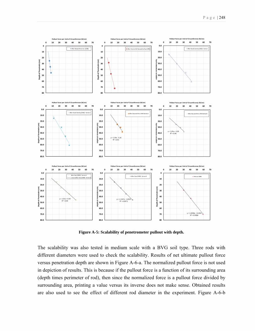
P a g e | 248
Figure A-5: Scalability of penetrometer pullout with depth.
The scalability was also tested in medium scale with a BVG soil type. Three rods with
different diameters were used to check the scalability. Results of net ultimate pullout force
versus penetration depth are shown in Figure A-6-a. The normalized pullout force is not used
in depiction of results. This is because if the pullout force is a function of its surrounding area
(depth times perimeter of rod), then since the normalized force is a pullout force divided by
surrounding area, printing a value versus its inverse does not make sense. Obtained results
are also used to see the effect of different rod diameter in the experiment. Figure A-6-b
0
10
20
30
40
50
60
70
80
0 10 20 30 40 50 60 70
Dep
th o
f Pen
etra
tin
(cm
)Pullout Force per Unit of Circumference (N/cm)
After Narasimha et al. (2006)
0
10
20
30
40
50
60
70
80
0 10 20 30 40 50 60 70
Dep
th o
f Pen
etra
tin
(cm
)
Pullout Force per Unit of Circumference (N/cm)
After Veeresh & Narasimha Rao (1996)
0.0
10.0
20.0
30.0
40.0
50.0
60.0
70.0
80.0
0 10 20 30 40 50 60 70
Dep
th o
f Pen
etra
tin
(cm
)
Pullout Force per Unit of Circumference (N/cm)
After Das & Seeley (1982) - Series I
0.0
10.0
20.0
30.0
40.0
50.0
60.0
70.0
80.0
0 10 20 30 40 50 60 70
Dep
th o
f Pen
etra
tin
(cm
)
Pullout Force per Unit of Circumference (N/cm)
After Das & Seeley (1982) - Series II
y = 1.59x - 5.26R² = 0.91
0.0
10.0
20.0
30.0
40.0
50.0
60.0
70.0
80.0
0 10 20 30 40 50 60 70
Dep
th o
f Pen
etra
tin
(cm
)
Pullout Force per Unit of Circumference (N/cm)
After Das and Shin 1993-Series A
y = 1.05x + 5.09R² = 0.96
0.0
10.0
20.0
30.0
40.0
50.0
60.0
70.0
80.0
0 10 20 30 40 50 60 70
Dep
th o
f Pen
etra
tin
(cm
)
Pullout Force per Unit of Circumference (N/cm)
After Das and Shin 1993-Series B
y = 1.01x + 0.39R² = 0.99
0.0
10.0
20.0
30.0
40.0
50.0
60.0
70.0
80.0
0 10 20 30 40 50 60 70
Dep
th o
f Pen
etra
tin
(cm
)
Pullout Force per Unit of Circumference (N/cm)
After Das (1989) - Series A
Linear (After Das (1989) - Series A)
y = 1.1347x - 1.6025R² = 0.9972
0.0
10.0
20.0
30.0
40.0
50.0
60.0
70.0
80.0
0 10 20 30 40 50 60 70
Dep
th o
f Pen
etra
tin
(cm
)
Pullout Force per Unit of Circumference (N/cm)
After Das (1989) - Series B
y = 1.4098x - 14.004R² = 0.9988
0
10
20
30
40
50
60
70
80
0 10 20 30 40 50 60 70
Dep
th o
f Pen
etra
tin
(cm
)
Pullout Force per Unit of Circumference (N/cm)
Tests on MSB

P a g e | 249
shows the same results but versus different rod diameter where for the specific depth data
point obtained from Figure A-6-a.
Figure A-6: Pullout Scalability a) in depth and b) with different rod diameter in BMG.
Effect of Surcharge The Medium size BVG sample is tested with different surcharge loads, with a rod diameter
of 1.3 cm and a depth of penetration of about 24 cm. The three different surcharges of 0, 8.3
kPa and 37 kPa are applied to the sample. The results did not show any considerable
variation of pullout force, which in stiff clay was expected. While the average normalized net
pullout force was 27 kN/m2 the variance was only 0.14.
Effect of Different Water Content It was found necessary to see the effect of water content on maximum pullout force. It was
expected to observe the net ultimate pullout force to be around the plastic limit of BVG. A
variety of BVG samples with different water contents were prepared in small containers.
Every container was filled to the top while every layer of soil was compacted by a standard
proctor hammer. The total number of blows for compaction was 15 for the samples of series
A and 10 for the samples of series B. depth of penetration is 12 cm in all the tests. Variation
of dry weight and net ultimate pullout force versus water content are shown in Figure A-7-a
and A-7-b respectively.
y = 0.06x - 0.30R² = 0.99
y = 0.16x - 0.29R² = 1.00
0
5
10
15
20
25
30
0 100 200 300 400 500
Dep
th o
f P
enet
ratio
n (c
m)
Net Ultimate Pullout Force (N)
d=2.1 cm
d=1.3 cm
d=0.6 cm
x = 102.36y+8.15R2 = 1
x = 66.5y +4.80x = 33.25y +2.40
0.0
0.5
1.0
1.5
2.0
2.5
0 100 200 300 400 500
Rod
Dia
met
er (c
m)
Net Ultimate Pullout Force (N)
24 cm
16 cm
8 cm
Depth of Penetration

P a g e | 250
Figure A-7: Effect of Water Content on Pullout Force in BVG a) Dry Unit Weight b) Net Ultimate
Pullout Force.
Discussion and Conclusion In this paper work undertaken at NEU SoilBED facilities is described and the results are
presented to give an insight into the soil-rod interaction during pullout. The pullout test was
conducted using three rods, having a diameter of 0.6, 1.3 and 2.1 cm (0.25, 0.5 and 0.83
inches). The maximum pullout force observed in the BVG soil types. The scalability of the
experiment using smaller rod and shallower penetration is also studied.
Water content was found to be an important factor affecting pullout. The net ultimate pullout
force change dramatically with water content. The water content of 25% in BVG sample
gave the maximum net ultimate observed pullout force of 173 lb for just 4.5 inches of
penetration. It is expected that the maximum pullout force for the real device with the rod
diameter of 0.79 inches and maximum depth of penetration of 36 inches be up to 2200 lb.
This force will be beyond the strength of two operators. However, for a layered soil (drier in
surface wetter in depth) which is more probable to confront in the field smaller magnitude is
expected.
The resistance of rod against pullout comes from three major sources, skin frictional
resistance, soil tensile resistance, and suction generated at the base of the rod as movement
occurs. All of these factors are greatly affected by the generation of negative pore pressures
in the soil due to movement of the rod. Suctions are generated at the base of the rod in all
0.0
2.5
5.0
7.5
10.0
12.5
15.0
0 20 40 60 80 100
Dry
Uni
t Wei
ght
(kN
/m3 )
Water Content (%)
Series A
Series B
0
150
300
450
600
750
900
0 20 40 60 80 100
Net
Ulti
mat
e Pu
llout
For
ce (
N)
Water Content (%)
Series A
Series B
P a g e | 251
soils owing to the opening up of a void as the rod moves. However, since clay has much
lower permeability, the suction can be much greater than in the sand. Cho and Bang (2002)
and Fuglsang and Steensen-Bach (1991) reported passive suction as high as 100 (kPa) at the
top of small-scale suction piles in clay. At the circumference of the rod, undrained shearing
strength of the soil when the rod is pulled quickly will result in negative pore pressure
generation in dense soils (stiff clay). These pore pressures will alter the effective stress state
of the soil and will hence have a great impact on the stress-strain behavior of the rod. In
wetter samples, a further contribution to pullout resistance is provided by suction generated
at the base of the rod as it moves. One reason to prove existence of suction during pullout
was the sound caused by breaking the vacuum.
We did not evaluate the suction. The problem was mainly due to distorting of the sample
when we tried to cut a sample after penetration. Providing a void underneath of the main
sample and penetrate deep enough to that layer was not also achievable.
Further investigation are necessary to be able to separate different factors participate in the
net ultimate pullout force. Undrained shear strength of the soil may be needed to be measured
in further experiments. Those data showed to have a good correlation to the net ultimate
pullout force (Shin et al, 1993). The evaluation of the worst case then may be available by
comparing the results to the highest reported undrained shear strength for near surface soils.
It is expected that the maximum pullout force for the device under development (with the rod
diameter of 2 cm (0.79 inches) and maximum depth of penetration of 0.9 m) will be up to
10.6 kN, which definitely is beyond the strength of two operators. However, for a layered
soil (drier at the surface and moisture increasing with depth), which may be more typical of
field conditions, a smaller magnitude is expected.
Acknowledgement The authors would also like to thank Ms. Eilish Corey, an undergraduate student at
Northeastern University, for her invaluable contribution and help.
References Al-Mhaidib, A.I., (2001). “Effect of Rate of Loading on Uplift Capacity of a Model Pile in
Clay”, Proceedings of the International Offshore and Polar Engineering Conference, v
2, 2001, p 656-661.

P a g e | 252
Awad, A., and Ayoub, A. (1976). "Ultimate uplift capacity of vertical and inclined piles in
cohesionless soil." Proc., 5th Conf. on Soil Mechanics and Foundation Engineering,
Budapest, Hungary, 221–227.
Cho Y., Bang S. (2002). Analytical validation of pullout loading capacity of suction piles in
clay, Transportation Research Record, No. 1808, pp. 180-185, ISSN 0361-1981.
Chow S. H., Wong, K. S. (2004). Model Pile Pull-Out Tests Using Polyethylene Sheets to
Reduce Downdrag on Cast In Situ Piles, Geotechnical Testing Journal, Volume 27,
Issue 3 (May 2004).
Chu, L., and J. Yin (2005) “A Laboratory Device to Test the Pull-Out Behavior of Soil
Nails”, Geotechnical Testing Journal, Volume 28, Issue 5 (September 2005).
Daniel, C.R. and Howie, J.A. (2005). Discussion of “Effect of Hammer Shape on Energy
Transfer Measurement in the Standard Penetration Test” Tsai, J-S, Liou, Y-J, Liu, F-J
and Chen, C-H, Soils and Foundations, Vol. 44 No. 3 June 2004. Soils and
Foundations, Vol. 45, No. 5, pp. 121-126.
Das, B. M., Seeley G. R. (1982). Uplift Capacity of Piles in Saturated Clay, Soils and
Foundations, Volume 22, Number 1, pp 91-94.
Das, B. M., A. J. Tarquin, R. Moreno (1985). Model tests for pullout resistance of vertical
anchors in clay, Journal Title: Civil engineering for practicing and design engineers,
Volume: 4, Issue: 2, PP 191-209, ISSN/ISBN: 0277-3775.
Das, B. M. (1989). Uplift capacity of metal piles in clay, Proceedings of the Eighth
International Conference on Offshore Mechanics and Arctic Engineering, The Hague,
The Netherlands, March 19-23, 1989.
Das, B. M. and Eun C. Shin (1993). Uplift Capacity of Rigid Vertical Metal Piles in Clay
Under Inclined Pull, International Journal of Offshore and Polar Engineering, Vol. 3,
No.3, September 1993, pp 231-235, ISSN 1053-5381.
Davie J. R. and Sutherland H. B. (1978) Modeling of Clay Uplift Resistance, Journal of
geotechnical Engineering, ASCE, Vol.104, GT6, pp 755-760.
Fuglsang, L.D and J. O. Steensen-Bach, (1991). Breakout Resistance of Suction Piles in
Clay, Proceedings of International Conference: centrifuge 91,A. A. Balkema,
Rotterdam, Netherlands, 1991, pp. 153-159.
Howell Jl, Shackelford CD, Amer NH, Stern RT (1997). Compaction of Sand-Processed
Clay Soil Mixture, Geotechnical Testing Journal, Volume 20, Issue 4 (December
1997), pp 443-458.
Narasimha Rao, S. and Veeresh, C., (1996) "Behaviour of Batter Anchor Piles in Marine
Clay Subjected to Vertical Pull Out", 6th International Offshore and Polar.

P a g e | 253
Narasimha Rao, S., R. Ravi, and C. Ganapathy (1997). “Pullout Behaviour of Model Suction
Anchors in Marine Clays”, 7th International Offshore and Polar Enginering
Conference, ISOPE - 97, Honololu, Hawaii, USA, Vol.1, pp.740-743.
Narasimha Rao, S., K. Hema Lathaa, B. Pallavia, and S. Surendrana (2006). “Studies on
pullout capacity of anchors in marine clays for mooring systems”, Applied Ocean
Research, Volume 28, Issue 2, April 2006.
Prakash, S. (1961). Behavior of pile groups subjected to lateral loads, PhD thesis, University
of Illinois, USA.
Shin, E. C., B. M. Das, V. K. Puri, S. C. Yen, E. E. Cook (1993). Ultimate uplift capacity of
model rigid metal piles in clay, Geotechnical and Geological Engineering, Vol. 11,
No. 3, pp 203-215, 1993-09-01.
Supachawarote C., M.F. Randolph, and S. Gourvenec (2004). “Inclined Pull-out Capacity of
Suction Caissons”, Proceedings of the 14th International Offshore and Polar
Engineering Conference, Toulon, France, pp 500-506.
Veeresh C. and Narasimha Rao S. (1996). "Vertical pullout capacity of model batter anchor
piles in marine clays", Marine Georesources & Geotechnology, Volume 14, Number
3, 1996, pp. 205-215.
Zimnik, A.R.; L.R. van Baalen, P.N.W. Verhoef, D.J.M.Ngan-Tillard (2000). The adherence
of clay to steel surfaces. GeoEng 2000 an International Conference on Geotechnical
& Geological Engineering, Melbourne, Australia, 19-24 November 2000. p.
UW0838:1-6. Article on CDrom. ISBN: 1-58716-068-4.

P a g e | 254
Appendix B: RapSochs Rev. 0 Operating
Instructions
Introduction
The Rev 0. RapSochs will differ from the deliverable version (Rev. 1) in a number of ways.
1. Battery power will be provided by a 12 volt battery array where BB2590 Lion 15 volt batteries will be used in Rev 1.
2. The Rev. 0 system will be tethered to a laptop computer for operator interface and control. In the Rev. 1 system a single board computer internal to the system will be used.
3. Hammer actuation will be manually powered instead of controlled by a servo system. 4. A string potentiometer will be used for displacement measurement. In the final
version the displacement may be developed from double integration of the acceleration signal, eliminating the need for the external string pot.
5. The recorded data will not have identifying header information; it will just be a set of columns of ASCII data in engineering units.
General Test Sequence
1. The system is assembled, checked, and initialized as described in the Operation Section below.

P a g e | 255
2. The operator raises the hammer by a predetermined amount and allows it to drop. The drop height will be proportional to the estimated strength of the material. The drop height should be adjusted to produce a penetration between 0.5 and 1 inch per blow.
3. For each hammer blow a dynamic data sequence will be triggered by the impact of the hammer. A data block 200 milliseconds long acquired at 10K samples/sec. will be taken. The total block is then 2048 samples long, with 100 of the samples taken prior to the trigger event. The data for each blow will be stored in an ASCII file with filename = <JOB ID>::_tip_nn.dat where nn is the file index which starts with 1 and is automatically incremented after each blow. The moisture sensor file name is the same as the dynamic data except that the string “tip” is prelaced by the string “moisture”. A second file is produced with filename = <JOB ID>::_tip_nn_converted.dat that contains the tip strain, sleeve strain, acceleration, string pot, and TIP temperature in engineering units. All files are stored in the C:\technical\testing\rapsochs\rawdata\ folder.
4. After completion of the dynamic sequence, a moisture sensor reading is taken by the operator after the penetrometer has stopped moving.
5. Steps 2-5 are repeated until the desired penetration depth has been achieved. The MatLab script “RapSochs_Data_Dump.m” can be run at any time to show progress. In order to prevent damage to the penetrometer the sequence must be stopped just prior to reaching the bottom of the sample. Based upon the actual sample depth, a mark should be placed on the penetrometer rod (or a tape measure or other measuring means) to insure that the penetrometer does not impact the floor.
Operation Procedure
1. Insure the battery in the Processor module is charged. To charge connect the charger to the connector labeled “charger”. To fully charge dead batteries will take 2.5-3 hours. When the batteries are fully charged the “Charging” LED will go out. Remove the charger cable from the Processor module. The instrument will not function if the charger is left plugged in. Battery life will be 4-8 hours of continuous operation. To provide maximum battery life, turn off the system after each test.
2. Insure the system is completely assembled and inspected prior to each test. (see RapSochs Assembly and Operability Checklist). It is important that this procedure be followed. Damage to the system could result from loose mechanical joints or failure to clean and inspect the tip and moisture sensor.
3. Insures all cables are connected. The “Ext Comm” cable must be plugged into the upper USB port on the back of the laptop.
4. Press the “ON” button on the Processor Module to power up the processor. 5. Activate the ‘RapSochs GUI’ on the laptop Desktop. 6. Depress “Continue” on the splash screen. 7. Depress “Setup” on the Main Menu screen. 8. On the Setup screen enter the JOB ID for the current test. The JOB ID will become
the root of the name of the data files created during the test. Only characters legal in windows file names may be used. Select “Operate” when done.
9. For the first blow of a test only, depress the “Reset Test Indexes” button.

P a g e | 256
10. Depress “ON/RESET” to enable power to the TOP and TIP modules. The Acquire Tip and Moisture buttons should become available.
11. Depress the “Moisture” button to acquire a moisture sensor reading, while the tip is resting on the plate. This gives us the value of the stringpot at the surface which will later be used to determine the sinking penetration due to the weight of the penetrometer.
12. Depress “Acquire Tip” to arm the data acquisition sequence. After several diagnostic lines, the message “BIG Acquisition armed…” should appear in the data window.
13. Raise the hammer by an amount that will cause 0.5-1 inch of penetration. This value will have to be determined empirically. For very hard materials, the maximum penetration achievable for the maximum 20 inch drop will be less than 0.5 in. For low CBR materials, such as clay, drop heights of ~4-5 inches are appropriate.
14. The raw data will be echoed to the screen and the file written to the disk. 15. After the first blow of a test it is strongly recommended to display the raw data (using
the procedure described in Data Display below) to insure the penetrometer is working properly. Display of the data will also provide the penetration per blow to allow determination of the drop height necessary to produce 0.5-1 inch penetration. Do not close the RapSochs GUI to activate Matlab.
16. Check the total penetration to insure that the maximum established for the test has not been exceeded.
17. Repeat steps 11-15 until the test is complete. Moisture readings are not necessary after every dynamic blow. It is suggested that they are taken only when the sensor is submerged. Note that at any time during the sequence it is realized that an incorrect action has been performed, such as depressing “Acquire TIP”, when it was desired to depress “Moisture”, the operation can be aborted by pressing “ON/RESET”. This operation will close and files and then re-enable the Moisture and Acquire Tip buttons.
18. Depress “OFF” to remove power from the TOP/TIP modules 19. Depress “OFF” on the processor module to power down the system. 20. Remove the penetrometer from the hole immediately, especially in saturated
materials. The system does have a complete o-ring system to keep moisture from the electronics and sensors but I’d rather not push our luck.
21. Clean the tip as described below before the soil dries out. This is especially important in clays where the material can become like stone if it dries out.
Data Display
The following files can be run at any time during a test as the data files are written immediately after each data block is acquired. To check the results during or after any test, activate Matlab and open the file RapSochs_data_dump.m. Click ‘Run’. At the prompt enter the root (JOB ID from the test) of the filename. Then enter the thickness of the plate used to support the penetrometer during the initial moisture test. Two figures are produced. Figure 1 is a plot of the conductivity and susceptance vs depth from the moisture sensor. Generally, the conductance and susceptance

P a g e | 257
increase with increasing volumetric moisture content. Thus a soil sample with constant gravimetric moisture but with increasing density with depth would show increasing volumetric moisture. Figure 2 is a concatenation of the dynamic data (in engineering units). After plotting the data, the Matlab command window will ask if the test is completed. If not, continue taking data. Typing “n” will replot any new data that has since been gathered, and re-prompt “Is the test complete?”. This can be done between every hammer blow if need be. When the test is complete, reply to the prompt with “y” and a new prompt will ask about generating a .MAT file. If a .MAT file is not necessary, reply to the prompt with an “n”, and the program will complete. If a .MAT file is desired, reply with a “y”. This will bring about a long list of prompts asking for key information specific to the test:
1. A description of the test can be written. Any pertinent details or problems involved in the process or conditions of the experiment.
2. The hammer drop height in inches. 3. The USCS soil classification of the soil. 4. The soil density in pcf. 5. The soil moisture in % gravimetric. 6. The plastic limit of the soil. 7. The liquid limit of the soil. 8. The optimum moisture of the soil in % gravimetric (from the proctor test). 9. The peak dry density of the soil in pcf (from the proctor test). 10. The coefficient of curvature of the soil (from the gradation). 11. The coefficient of uniformity of the soil (from the gradation). 12. The maximum particle size of the soil in mm.
If any of this information is unknown or unimportant, a return carriage will bring about the next prompt.
Operating Modes
In addition to the above described normal operating mode, dynamic and moisture sensor scans can be taken independently. For example repeated moisture sensor scans could be taken to determine repeatability and/or stability of the moisture level in the soil.
Converted File Creation
If for any reason the “Converted” file is not created after a blow (due to for example a crash) and the raw data file is intact, the following procedure can be used.
1. Start the RapSochs GUI as described above in Operation Procedure steps 1-7.
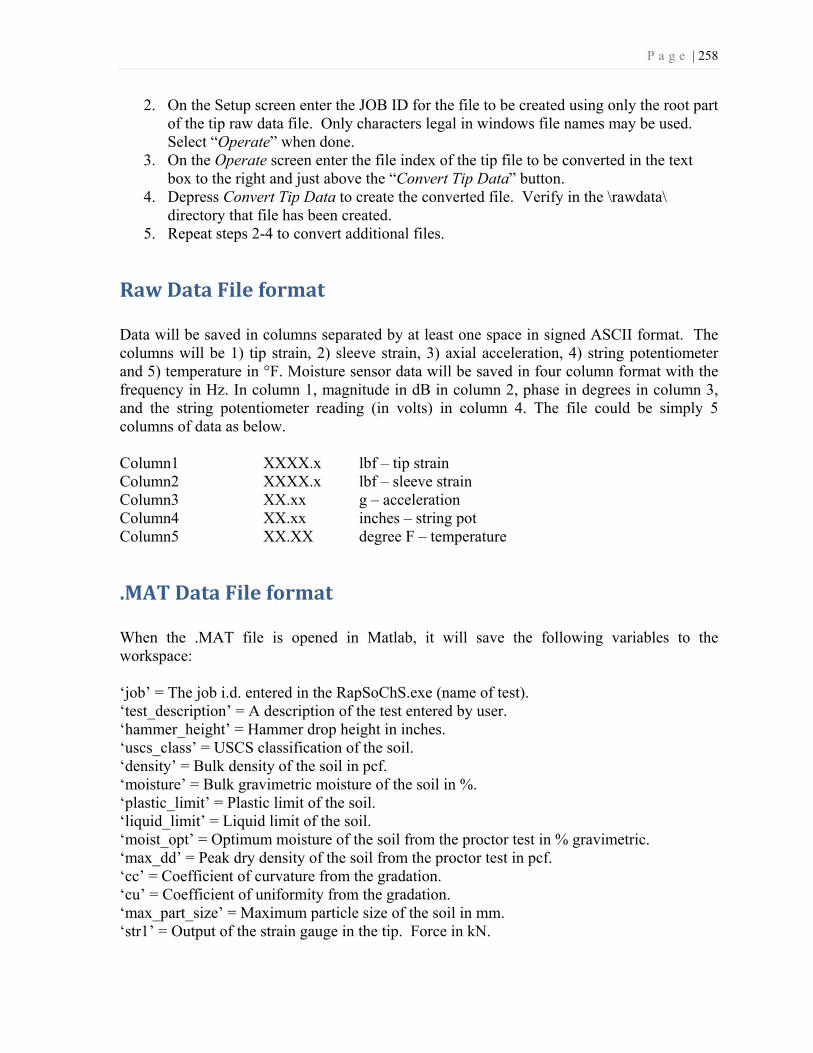
P a g e | 258
2. On the Setup screen enter the JOB ID for the file to be created using only the root part of the tip raw data file. Only characters legal in windows file names may be used. Select “Operate” when done.
3. On the Operate screen enter the file index of the tip file to be converted in the text box to the right and just above the “Convert Tip Data” button.
4. Depress Convert Tip Data to create the converted file. Verify in the \rawdata\ directory that file has been created.
5. Repeat steps 2-4 to convert additional files.
Raw Data File format
Data will be saved in columns separated by at least one space in signed ASCII format. The columns will be 1) tip strain, 2) sleeve strain, 3) axial acceleration, 4) string potentiometer and 5) temperature in °F. Moisture sensor data will be saved in four column format with the frequency in Hz. In column 1, magnitude in dB in column 2, phase in degrees in column 3, and the string potentiometer reading (in volts) in column 4. The file could be simply 5 columns of data as below. Column1 XXXX.x lbf – tip strain Column2 XXXX.x lbf – sleeve strain Column3 XX.xx g – acceleration Column4 XX.xx inches – string pot Column5 XX.XX degree F – temperature
.MAT Data File format
When the .MAT file is opened in Matlab, it will save the following variables to the workspace: ‘job’ = The job i.d. entered in the RapSoChS.exe (name of test). ‘test_description’ = A description of the test entered by user. ‘hammer_height’ = Hammer drop height in inches. ‘uscs_class’ = USCS classification of the soil. ‘density’ = Bulk density of the soil in pcf. ‘moisture’ = Bulk gravimetric moisture of the soil in %. ‘plastic_limit’ = Plastic limit of the soil. ‘liquid_limit’ = Liquid limit of the soil. ‘moist_opt’ = Optimum moisture of the soil from the proctor test in % gravimetric. ‘max_dd’ = Peak dry density of the soil from the proctor test in pcf. ‘cc’ = Coefficient of curvature from the gradation. ‘cu’ = Coefficient of uniformity from the gradation. ‘max_part_size’ = Maximum particle size of the soil in mm. ‘str1’ = Output of the strain gauge in the tip. Force in kN.

P a g e | 259
‘str2’ = Output of the strain gauge in the sleeve. Force in kN. ‘accel’ = Output of the accelerometer in multiples of g. ‘sp’ = Output of the string potentiometer in mm (median filtered). ‘vel’ = Velocity as calculated from the string potentiometer in m/s. ‘sinkage_depth’ = Distance below the surface that the tip sank under the weight of the
penetrometer.
RapSochs Assembly and Inspection Checklist
Pre-Test Inspection 1. At the completion of each test the portion of the penetrometer that was in the soil
should be cleaned with a cloth moistened with distilled water. It is not necessary to remove all soil from the x-ring grooves. The x-rings are tight and could be damaged by attempting to pick soil out of the grooves.
2. All mechanical joints must be tight. Using a wrench (channel locks, vice grip, or similar) above the penetrometer to sensor head connection and one on the cone tip, insure all three joints are tight. The force is transmitted through the mechanical joists on flat loading lands. If the joint is loose, the force will be transmitted instead through the threads which will cause thread distortion. Further there is a hidden mechanical joint just above the upper x-ring. If this joint becomes loose, the fine wires from the sensors could become twisted and fail. This will necessitate returning the unit to TransTech for repair.
3. Inspect the moisture sensor (blue area) to insure the plastic cover is intact. The cover has been coated with acrylic clearcoat to provide abrasion strength and sealing. Grooves have been filled with epoxy. Any exposed copper electrodes must be sealed prior to testing using five minute epoxy or super glue.
4. Insure the TOP module is centered on the purple foam pieces and the clamps are tight.
Assembly Generally in order to place the penetrometer into the soil test fixture, the upper section (above the anvil) must be removed. Do not remove the anvil! The system will be supplied with all cables removed. Generally, only the string potentiometer cable need be removed (at the string pot), and the TOP to Processor cables at the processor to move the system around. The TOP to penetrometer cables should always be left attached as the coax connectors are somewhat fragile.
Pre-Test Assembly 1. Install a guide in the desired position in the test cell. 2. Lower the penetrometer through the guide to the soil surface. Using a level, insure the
penetrometer is perpendicular to the surface. Locate the string potentiometer below the hook on the anvil and attach the string. Attach the string potentiometer cable.

P a g e | 260
3. Place the hammer (small side up) onto the slide and screw the slide rod into the anvil. During the installation do not allow the anvil to rotate as this could damage the cables from the penetrometer to the TOP module. Insure it is tight using a wrench.
4. Attach the TOP to processor cables. 5. Follow the Operation procedure to conduct the test.
Post-Test Dis-assembly Dis-assembly is the reverse of assembly. Again insure the anvil does not rotate when removing the slide rod from the anvil as this could damage the cable between the penetrometer and the TOP module.
Maintenance X-ring replacement. If an x-ring fails, remove the broken ring from the groove. Clean the groove with distilled water and a suitable soft cloth and dry. Stretch a new x-ring over the tip and slide into the grove. Insure the ring is not twisted in the groove (use a magnifier to inspect). A twisted ring will fail quickly.
RapSochs VBTERM Command Interface
If data is to be saved, a log file must be opened prior to using <dump> commands. Except for moisture sensor data, which is provided in engineering units, the results of the dump commands are in raw A/D counts (0-4095). If conversion to engineering units is required, the sensor calibration factors, excitation voltages, and channel gains must be known. Prior to issuing commands insure the battery is charged, the system is on, and the “RAPSOCHS SW Version 1.0” announcement is shown in the VBTERM command window. The following commands are supported: General commands: <MBON><CR> Turn power on to the measurement board <MBOFF><CR> Turn power off to the measurement board Moisture sensor commands: <f1=><nnn><CR> where nnn is the start frequency in KHz. <f2=><nnn><CR> where nnn is the stop frequency in KHz. Note if f2<f1, then the system runs continuously at f1…good for troubleshooting <st=><nnn><CR> where nnn is the # of frequency steps per decade (logarithmic spacing) <tx=><nnn><CR> where nnn is the TX level (0-1023) where 1023 ~=8VPP <rf=><nnn><CR> where nnn is the reference level. Should be <200 to avoid overvoltage at the 8302 input

P a g e | 261
<ph=><nnn><CR> where nnn is the phase offset of the reference (0-359.9°). Not sure whether lead or lag. <de=><nnn><CR> where nnn is the interfrequency delay (in ms?). Default = 80, range (10-300). Not functional at this time. <go><CR> take 1 moisture spectrum and display results on screen Dynamic sensor commands: <acq0><CR> do TOP A/D acquisition (temp, stringpot, moisture sensor data) single sample <dump0> display TOP acquisition results on screen <acq1> do complete acquisition (TIP/TOP). 0.2 seconds of data saved at 10 KHz. (2000 samples, 10 channels) <dump1> dump 2000 sample buffer to screen (or logfile). Sample organization is: 0a 0b 1a 1b 2a 2b 3a 3b 4a 4b 5a 5b where the numeric is the channel number and a,b designate TOP and TIP respectively.

P a g e | 262
Appendix C: List of MATLAB Codes
This appendix presents the list of MATLAB codes used for database establishment and data
analysis. All the codes developed in MATLAB are restored as M-files which are source
codes in MATLAB. They are files in ASCII format with extension ".m". An m-file may be
either a list of commands or a function with input and output variables. All the codes are
available in the folder “\m-files” on the CD-ROM along this document. In the following table
only main codes are listed. In a main code different functions may be called to do some of
the analysis. Those functions are not listed in this table.
Name and Path of the Code / Description \m-files\01-Data to Mat\RAPSOCHs_Data_Dump_Rev2.m
This code reads data-files of a RapSochs test (raw data in DAT format) and put them
together in a MAT-file. The code does not put "moisture data" in MAT-files.
\m-files\01-Data to Mat\Adding Moisture Data to database\RAPSOCHs_Moisture_Dump2.m
This code reads moisture measurements data-files of a RapSochs test (raw data in
DAT format) and put them together in the corresponding MAT-file.
\m-files\02-RS-Plot_RapSochs_Raw_Data\ RapSochs_one_drop_data.m
This code, after running, goes through the list of RapSochs tests one-by-one and
allows the user to select one test and a specific blow and plots the displacement,
acceleration and cone and sleeve force measurement for that blow.

P a g e | 263
Name and Path of the Code / Description \m-files\02-RS-Plot_RapSochs_Raw_Data\RapSochs_one_drop_data_ask.m
This code, after running asks for the Test-ID and the blow number to plot the
displacement, acceleration and cone and sleeve force measurement for that blow.
\m-files\03-DCP-calculation\Calculate_Depth_for_DCP.m
This code, after running, goes through list of DCP tests one-by-one and asks if the
user wants to calculate the DCP depth and save it into the corresponding MAT-file.
\m-files\04-DCP-No.of-Blows-vs-Depth\Plot_NoBlows_vs_Depth.m
This code plots number of blows versus depth from the DCP MAT-files.
\m-files\05-DCPi-best fitting\Plot_NoBlows_vs_Depth_DCPi.m
This code plots number of blows versus depth from the database and fits the best line
to selected data points.
\m-files\06-RS-Penetration_per_blow/Penetration_per_individual_blow_02.m
This code calculates the RS-PR from string potentiometer signal and adds the new
parameter to the database.
\m-files\07-RS-Plot_moisture_data/Plot_Moisture_data.m
This code is used to plot the measurement data of moisture sensor.
\m-files\08-RS-Adding_B_&_G\RAPSOCHs_Moisture_BG.m
This code is used to calculate the susceptance and conductance of moisture data and
to add the computed parameters to the RapSochs MAT-files.
\m-files\09-RS-PRvsHammerDrop\Plot_RS_PR_HammerDrop.m
This code is used to plot RS-PR and hammer drop height verses depth.
\m-files\10-RS-Plot_Moisture_B&G\Plot_Moisture_BG.m
This code is used to plot susceptance and conductance as contour figures.
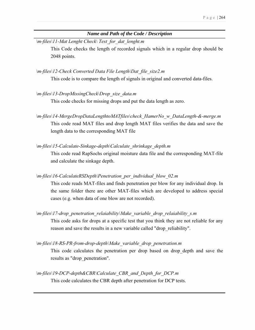
P a g e | 264
Name and Path of the Code / Description \m-files\11-Mat Lenght Check\ Test_for_dat_lenght.m
This Code checks the length of recorded signals which in a regular drop should be
2048 points.
\m-files\12-Check Converted Data File Length\Dat_file_size2.m
This code is to compare the length of signals in original and converted data-files.
\m-files\13-DropMissingCheck\Drop_size_data.m
This code checks for missing drops and put the data length as zero.
\m-files\14-MergeDropDataLengthtoMATfiles\check_HamerNo_w_DataLength-&-merge.m
This code read MAT files and drop length MAT files verifies the data and save the
length data to the corresponding MAT file
\m-files\15-Calculate-Sinkage-depth\Calculate_shrinkage_depth.m
This code read RapSochs original moisture data file and the corresponding MAT-file
and calculate the sinkage depth.
\m-files\16-CalculateRSDepth\Penetration_per_individual_blow_02.m
This code reads MAT-files and finds penetration per blow for any individual drop. In
the same folder there are other MAT-files which are developed to address special
cases (e.g. when data of one blow are not recorded).
\m-files\17-drop_penetration_relaiability\Make_variable_drop_relaiability_s.m
This code asks for drops at a specific test that you think they are not reliable for any
reason and save the results in a new variable called "drop_reliability".
\m-files\18-RS-PR-from-drop-depth\Make_variable_drop_penetration.m
This code calculates the penetration per drop based on drop_depth and save the
results as "drop_penetration".
\m-files\19-DCP-depth&CBR\Calculate_CBR_and_Depth_for_DCP.m
This code calculates the CBR depth after penetration for DCP tests.

P a g e | 265
Name and Path of the Code / Description \m-files\20-Plot-a-Drop-close-to-a-specific-depth\Isolate_one_drop_data2.m
This code plots data of a drop closest to a given depth for a specified test.
\m-files\21-Max_of_filtered_force\Isolate_one_drop_data_03_calculate_F.m
This code is used to filter strain gauge signals and to compare the original and filtered
signal and calculate the maximum of filtered signal as the estimation of resistance
force.
\m-files\22-Lenght&average_of_ForceData\Isolate_one_drop_data_02.m
This code is used to estimate the duration of penetration and average force based on
energy spectrum of filtered signal.
\m-files\23-Number_of_tests\Number_of_tests.m
This code gives number of RapSochs or DCP blows in each test.
\m-files\25-Frequency_Domain\plot_a_test_in_frequency_domain.m
This code isolates data of a specific drop and plots the signal in frequency domain.
\m-files\26-Most Likely Estimation\Isolate_one_drop_data_3_STR1.m
\m-files\26-Most Likely Estimation\Isolate_one_drop_data_3_STR2.m
These codes isolate data of a specific drop and ask for range of i,j,k,l, run the
maximum likelihood estimator and save the results at the M-files. The first code is for
lower strain gauge and the second code is for upper strain gauge.
\m-files\36-Probability_Distribution_of_F\Probability_Distribution_of_F.m
This code asks if user wants to see raw data of a specific RapSochs Tests by asking
Test-IDs one-by-one, after confirming, it asks for Drop No. and isolates RapSochs
raw data of a specific drop and plots Probability Density of force signal as
histograms.
\m-files\37-Ploting Square Pulse Estimation\RapSochs_one_drop_Force_pulse.m
This code asks if the user wants to see raw data of a specific RapSochs Tests by
asking Test-IDs one-by-one, after confirming, it asks for Drop No. and isolates
RapSochs "STR1" & "STR2" raw data of the specific drop and plots the raw data and
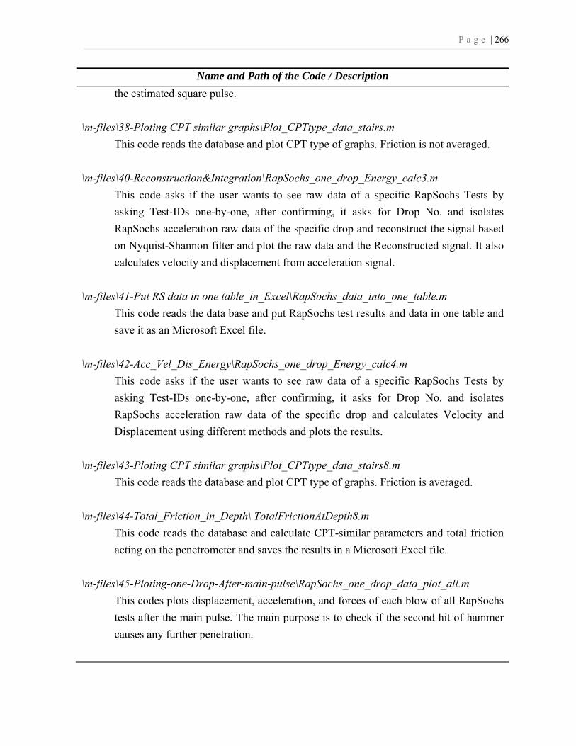
P a g e | 266
Name and Path of the Code / Description the estimated square pulse.
\m-files\38-Ploting CPT similar graphs\Plot_CPTtype_data_stairs.m
This code reads the database and plot CPT type of graphs. Friction is not averaged.
\m-files\40-Reconstruction&Integration\RapSochs_one_drop_Energy_calc3.m
This code asks if the user wants to see raw data of a specific RapSochs Tests by
asking Test-IDs one-by-one, after confirming, it asks for Drop No. and isolates
RapSochs acceleration raw data of the specific drop and reconstruct the signal based
on Nyquist-Shannon filter and plot the raw data and the Reconstructed signal. It also
calculates velocity and displacement from acceleration signal.
\m-files\41-Put RS data in one table_in_Excel\RapSochs_data_into_one_table.m
This code reads the data base and put RapSochs test results and data in one table and
save it as an Microsoft Excel file.
\m-files\42-Acc_Vel_Dis_Energy\RapSochs_one_drop_Energy_calc4.m
This code asks if the user wants to see raw data of a specific RapSochs Tests by
asking Test-IDs one-by-one, after confirming, it asks for Drop No. and isolates
RapSochs acceleration raw data of the specific drop and calculates Velocity and
Displacement using different methods and plots the results.
\m-files\43-Ploting CPT similar graphs\Plot_CPTtype_data_stairs8.m
This code reads the database and plot CPT type of graphs. Friction is averaged.
\m-files\44-Total_Friction_in_Depth\ TotalFrictionAtDepth8.m
This code reads the database and calculate CPT-similar parameters and total friction
acting on the penetrometer and saves the results in a Microsoft Excel file.
\m-files\45-Ploting-one-Drop-After-main-pulse\RapSochs_one_drop_data_plot_all.m
This codes plots displacement, acceleration, and forces of each blow of all RapSochs
tests after the main pulse. The main purpose is to check if the second hit of hammer
causes any further penetration.

P a g e | 267
Name and Path of the Code / Description \m-files\46-AverageTipForceforEachTest\Plot_AverageTipForce.m
This code reads the database and plots cone resistance profile of all tests in the same
soil sample and calculates the average cone resistance and plots it also.
\m-files\47-AverageTipForceforDCP\Force_Penet4_writetoExcel.m
This code reads the database, and estimates the weighted average of cone resistance
for each DCP blow from averaged RapSochs cone resistance data.
\m-files\48-DCP_Average_CBR\Plot_AverageCBR.m
This code reads the database and plot CBR of DCP-PR and Average CBR in each
sample.
\m-files\49-Average-DCP-PR\Calc_AverageDCP_PR_save.m
This code will read the database and plot DCP-PR, Averaged DCP-PR, and DCPi in
each sample.
\m-files\50-RS-DCP-correlation\Corresponding_DCPPR_of_RSPR2.m
This code reads the a RapSochs test data from a MAT-file and the corresponding
sample-ID mat-file and puts the corresponding average DCP-PR in a table with other
RapSochs data. This code is used to develop RS-PR to DCP-PR statistical
correlations.
\m-files\51-BoundaryEffect\Plot_AllTipForce_inAnySAmple.m
This code reads the database and plot cone resistance of RapSochs tests in each
sample and plots the profile. The resulted graph is used to show the possible effects
of sequence of tests in test results.
\m-files\52-DCPestimatedfromRS-PRandHammerDropHeight\Plot_RS_PR_and_Es_DCP_
PR_ and_HammerDrop.m
This code plots RS-PR, hammer drop height, Estimated DCP-PR from a RapSochs
test and averaged DCP-PR profile from DCP tests in a sample.

P a g e | 268
Name and Path of the Code / Description \m-files\54-DCPPRrs-DCPirs\Calc_AverageDCPPRrs_compare_1.m
This code reads the database and plots DCP-PRRS profiles obtained from RapSochs
tests and averaged DCP-PRRS and averaged DCP-PR obtained from DCP tests in each
sample.
\m-files\55-CBRprofilefromRS\Calc_AverageCBRrs_compare_1.m
This code reads the database and plots CBRRS and averaged CBRRS obtained from
RapSochs tests and averaged CBR obtained from DCP tests in each sample.
\m-files\56-NormalizedRS-PR\Plot_RS_PR_and_Norm_RS_PR_and_HammerDrop.m
This code reads the database and then checks the drop_penetration_reliability. It
calculates the Normalized RS-PR and plots it with RS-PR and hammer drop height
versus depth.
All the data-files of RapSochs tests are organized in the folder “\RapSochs_Raw_Data” by
Sample-ID and Test-ID in folders and subfolders respectively. The path in codes which read
or combine data-files should be modified to address this folder when running on a computer.
The final version of all MAT-files (including the results of latest analysis) is presented in the
folder “\Database”. The path in codes which read from or restore data to MAT-files should
be modified to address this folder when running on a computer. The file, “aTestlist.mat”,
located in the same folder contains a list of all MAT-files name (without MAT extension, the
same as Test-IDs) to help calling and accessing the available data.

P a g e | 269
Appendix D: DCP Procedure Checklist

P a g e | 270

P a g e | 271
Appendix E: RapSochs Procedure Checklist

P a g e | 272

P a g e | 273
Appendix F: Hammer Drop Height in RapSochs
Tests
BSC-01-R-S1
Drop no.
Drop Height
(in) 1 2 2 2 3 2 4 2 5 2 6 2 7 2 8 3 9 3
10 3 11 3 12 3 13 3 14 3 15 3 16 3 17 3 18 3 19 3 20 3 21 3 22 3
BSC-02-R-S2
Drop no.
Drop Height
(in) 1 2 2 2 3 2 4 2 5 2 6 2 7 2 8 2 9 2
10 3 11 3 12 3 13 3 14 4 15 4 16 4 17 4 18 5 19 5 20 5 21 5 22 5 23 5
BSC-03-R-S9
Drop no.
Drop Height
(in) 1 2 2 2 3 2 4 2 5 2 6 2 7 2 8 3 9 3
10 3 11 3 12 3 13 3 14 3 15 3 16 4 17 4 18 4 19 4 20 4 21 4 22 4 23 4
BSC-06-R-S8
Drop no.
Drop Height
(in) 1 2 2 2 3 2 4 2 5 2 6 2 7 2 8 2 9 3
10 3 11 3 12 3 13 4 14 4 15 4 16 5 17 5 18 5 19 5 20 5 21 5 22 5
BSC-09-R-S5
Drop no.
Drop Height
(in) 1 2 2 2 3 2 4 2 5 2 6 2 7 3 8 3 9 4
10 4 11 4 12 4 13 4 14 5 15 5 16 5 17 5 18 6 19 6 20 6 21 6 22 7 23 7 24 7

P a g e | 274
C6S-01-R-S5
Drop no.
Drop Height
(in) 1 5 2 5 3 5 4 10 5 10 6 10 7 10 8 15 9 16
10 15 11 22 12 22 13 22 14 22 15 22 16 22 17 22 18 22 19 22 20 22 21 22 22 15 23 15 24 15 25 10 26 10 27 10 28 10 29 15 30 15 31 15 32 22 33 22 34 22 35 22 36 22 37 22 38 22 39 22 40 22
C6S-04-R-S2
Drop no.
Drop Height
(in) 1 5 2 5 3 5 4 10 5 10 6 10 7 15 8 15 9 15
10 22 11 22 12 22 13 22 14 22 15 22 16 22 17 22 18 22 19 22 20 22 21 22 22 22 23 22 24 15 25 15 26 15 27 10 28 10 29 10 30 10 31 15 32 15 33 15 34 12 35 22 36 22 37 22 38 22 39 22 40 22
CSB-01-R-S7
CSR-01-R-S5
Drop no.
Drop Height
(in) 1 2 2 2 3 2 4 2 5 2 6 2 7 5 8 5 9 5
10 5 11 5 12 10 13 10 14 10
Drop no.
Drop Height
(in) 1 2 2 2
GRV-02-R-S5
Drop no.
Drop Height
(in) 1 2 2 2 3 3 4 4 5 5 6 6 7 7 8 8 9 9
10 10 11 10 12 12 13 13 14 14 15 15 16 16 17 17 18 18 19 19 20 20 21 21 22 22 23 22 24 22 25 22 26 22 27 22 28 22 29 22 30 22 31 22 32 22 33 22 34 22 35 22 36 22 37 22 38 22 39 22 40 22 41 22 42 22 43 22 44 22 45 22 46 22 47 22 48 22 49 22 50 22
Cont
Drop no.
Drop Height
(in) 51 22 52 22 53 22 54 22 55 22 56 22 57 22 58 22 59 22 60 22 61 22 62 22 63 22 64 22 65 22 66 22 67 22 68 22 69 22 70 22 71 22 72 22 73 22 74 22 75 22 76 22

P a g e | 275
GRV-04-R-S2
Drop no.
Drop Height
(in) 1 2 2 2 3 3 4 4 5 5 6 6 7 7 8 8 9 9
10 10 11 11 12 12 13 13 14 14 15 15 16 16 17 17 18 18 19 19 20 20 21 21 22 22 23 22 24 22 25 22 26 22 27 22 28 22 29 22 30 22 31 22 32 22 33 22 34 22 35 22 36 22 37 22 38 22 39 22 40 22 41 22 42 22 43 22 44 22 45 22 46 22 47 22 48 22 49 22 50 22
Cont
Drop no.
Drop Height
(in) 51 22 52 22 53 22 54 22 55 22 56 22 57 22 58 22 59 22 60 22 61 22 62 22 63 22 64 22 65 22 66 22 67 22 68 22 69 22 70 22 71 22 72 22 73 22 74 22 75 22 76 22 77 22 78 22 79 22 80 22 81 22 82 22
GRV-05-R-S6
Drop no.
Drop Height
(in) 1 2 2 2 3 3 4 4 5 5 6 6 7 7 8 8 9 9
10 10 11 10 12 12 13 13 14 14 15 15 16 16 17 17 18 18 19 19 20 20 21 21 22 22 23 22 24 22 25 22 26 22 27 22 28 22 29 22 30 22 31 22 32 22 33 22 34 22 35 22 36 22 37 22 38 22 39 22 40 22 41 22 42 22 43 22 44 22 45 22 46 22 47 22 48 22 49 22 50 22
Cont
Drop no.
Drop Height
(in) 52 22 53 22 54 22 55 22 56 22 57 22 58 22 59 22 60 22 61 22 62 22 63 22 64 22 65 22 66 22 67 22 68 22 69 22 70 22 71 22 72 22 73 22 74 22 75 22 76 22 77 22 78 22 79 22 80 22 81 22 82 22 83 22 84 22 85 22 86 22 87 22 88 22 89 22
MS6-01-R-S5
Drop no.
Drop Height
(in) 1 5 2 5 3 5 4 10 5 10 6 10 7 11 8 15 9 15
10 15 11 22 12 22 13 22 14 22 15 22 16 22 17 22 18 22 19 22 20 22 21 22 22 22 23 22 24 22 25 22 26 22 27 22 28 22 29 22 30 22 31 22 32 22 33 22 34 22 35 22 36 22 37 22 38 22 39 22 40 22 41 22 42 22 43 22 44 22 45 22 46 22 47 22 48 22 49 22

P a g e | 276
MS0-01-R-S5
Drop no.
Drop Height
(in) 1 5 2 5 3 5 4 10 5 10 6 10 7 15 8 15 9 15
10 22 11 22 12 22 13 22 14 22 15 22 16 22 17 22 18 22 19 22 20 22 21 22
MS1-01-R-S5
Drop no.
Drop Height
(in) 1 5 2 5 3 5 4 10 5 10 6 10 7 15 8 15 9 15
10 22 11 22 12 22 13 22 14 22 15 22 16 22 17 22 18 22 19 22 20 22 21 22 22 22
MS2-01-R-S5
Drop no.
Drop Height
(in) 1 5 2 5 3 5 4 10 5 10 6 10 7 15 8 15 9 15
10 22 11 22 12 22 13 22 14 22 15 22 16 22 17 22 18 22 19 22 20 22 21 22 22 22 23 22 24 22
MS3-01-R-S5
Drop no.
Drop Height
(in) 1 5 2 5 3 5 4 10 5 10 6 10 7 15 8 15 9 15
10 22 11 22 12 22 13 22 14 22 15 22 16 22 17 22 18 22 19 22 20 22 21 22 22 22
MS4-01-R-S5
Drop no.
Drop Height
(in) 1 5 2 5 3 5 4 10 5 10 6 10 7 15 8 15 9 15
10 22 11 22 12 22 13 22 14 22 15 22 16 22 17 22 18 22 19 22 20 22 21 22 22 22
MS5-01-R-S5
Drop no.
Drop Height
(in) 1 5 2 5 3 5 4 10 5 10 6 10 7 15 8 15 9 15
10 22 11 22 12 22 13 22 14 22 15 22 16 22 17 22 18 22 19 22 20 22 21 22 22 22 23 22
MS1-01-R-S5
Drop no.
Drop Height
(in) 1 2 3 4 5 6 10 7 15 8 15 9 15
10 22 11 22 12 22 13 22 14 22 15 22 16 22 17 22 18 22 19 22 20 22 21 22 22 22
MS2-01-R-S5
Drop no.
Drop Height
(in) 1 2 3 4 5 6 7 8 15 9 15
10 22 11 22 12 22 13 22 14 22 15 22 16 22 17 22 18 22 19 22 20 22 21 22 22 22 24 22
MS3-01-R-S5
Drop no.
Drop Height
(in) 1 2 3 4 5 6 7 8 9 15
10 22 11 22 12 22 13 22 14 22 15 22 16 22 17 22 18 22 19 22 20 22 21 22 22 22
MS4-01-R-S5
Drop no.
Drop Height
(in) 1 2 3 4 5 6 7 8 15 9 15
10 22 11 22 12 22 13 22 14 22 15 22 16 22 17 22 18 22 19 22 20 22 21 22 22 22

P a g e | 277
RSC-01-R-S1
Drop no.
Drop Height
(in) 1 2 2 2 3 2 4 3 5 3 6 3 7 3 8 4 9 4
10 4 11 4 12 5 13 5 14 5 15 5 16 5 17 6 18 6 19 6 20 6 21 7 22 8 23 8 24 9 25 9
RSC-02-R-S2
Drop no.
Drop Height
(in) 1 2 2 2 3 2 4 2 5 3 6 3 7 3 8 3 9 4
10 4 11 4 12 4 13 5 14 5 15 5 16 5 17 5 18 6 19 6 20 7 21 8 22 8 23 8 24 9
RSC-03-R-S9
Drop no.
Drop Height
(in) 1 2 2 2 3 2 4 3 5 3 6 3 7 3 8 3 9 4
10 4 11 4 12 5 13 5 14 5 15 5 16 5 17 6 18 6 19 6 20 7 21 8 22 8 23 9 24 9 25 10
RSC-08-R-S3
Drop no.
Drop Height
(in) 1 2 2 2 3 2 4 3 5 3 6 3 7 3 8 3 9 4
10 4 11 4 12 5 13 5 14 5 15 5 16 5 17 6 18 6 19 6 20 7 21 8 22 8 23 9 24 9 25 10 26 11
RSC-09-R-S5
Drop no.
Drop Height
(in) 1 2 2 2 3 2 4 2 5 2 6 3 7 3 8 4 9 4
10 4 11 4 12 5 13 5 14 5 15 5 16 6 17 6 18 7 19 7 20 8 21 8 22 9 23 10 24 11

P a g e | 278
RSD-02-R-S5
Drop no.
Drop Height
(in) 1 2 2 2 3 2 4 3 5 3 6 3 7 4 8 4 9 4
10 5 11 6 12 6 13 7 14 8 15 8 16 8 17 8 18 9 19 10 20 10 21 10 22 11 23 11 24 11 25 11
RSD-03-R-S5
Drop no.
Drop Height
(in) 1 2 2 2 3 2 4 3 5 3 6 3 7 4 8 4 9 4
10 5 11 5 12 5 13 6 14 7 15 7 16 7 17 7 18 7 19 8 20 8 21 9 22 9 23 10 24 11 25 11
RSD-04-R-S7
Drop no.
Drop Height
(in) 1 5 2 5 3 5 4 5 5 5 6 5 7 5 8 6 9 6
10 6 11 6 12 7 13 7 14 8 15 8 16 8 17 8 18 9 19 10 20 10 21 10 22 11
RSD-05-R-S9
Drop no.
Drop Height
(in) 1 5 2 5 3 5 4 5 5 5 6 5 7 5 8 5 9 5
10 6 11 6 12 6 13 7 14 7 15 8 16 8 17 5 18 5 19 5 20 8 21 8 22 10 23 10
RSD-06-R-S8
Drop no.
Drop Height
(in) 1 5 2 5 3 5 4 5 5 5 6 5 7 5 8 5 9 6
10 6 11 6 12 7 13 7 14 8 15 8 16 8 17 9 18 9 19 9 20 10 21 11
RSL-01-R-S1
Drop no.
Drop Height
(in) 1 2 2 2
RSL-02-R-S2
Drop no.
Drop Height
(in) 1 2
RSL-03-R-S9
Drop no.
Drop Height
(in) 1 2
RSL-07-R-S4
Drop no.
Drop Height
(in) 1 0.5
RSL-09-R-S5
Drop no.
Drop Height
(in) 1 0
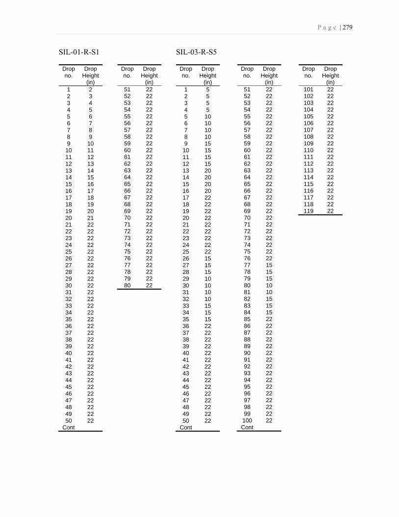
P a g e | 279
SIL-01-R-S1
Drop no.
Drop Height
(in) 1 2 2 3 3 4 4 5 5 6 6 7 7 8 8 9 9 10
10 11 11 12 12 13 13 14 14 15 15 16 16 17 17 18 18 19 19 20 20 21 21 22 22 22 23 22 24 22 25 22 26 22 27 22 28 22 29 22 30 22 31 22 32 22 33 22 34 22 35 22 36 22 37 22 38 22 39 22 40 22 41 22 42 22 43 22 44 22 45 22 46 22 47 22 48 22 49 22 50 22
Cont
Drop no.
Drop Height
(in) 51 22 52 22 53 22 54 22 55 22 56 22 57 22 58 22 59 22 60 22 61 22 62 22 63 22 64 22 65 22 66 22 67 22 68 22 69 22 70 22 71 22 72 22 73 22 74 22 75 22 76 22 77 22 78 22 79 22 80 22
SIL-03-R-S5
Drop no.
Drop Height
(in) 1 5 2 5 3 5 4 5 5 10 6 10 7 10 8 10 9 15
10 15 11 15 12 15 13 20 14 20 15 20 16 20 17 22 18 22 19 22 20 22 21 22 22 22 23 22 24 22 25 22 26 15 27 15 28 15 29 10 30 10 31 10 32 10 33 15 34 15 35 15 36 22 37 22 38 22 39 22 40 22 41 22 42 22 43 22 44 22 45 22 46 22 47 22 48 22 49 22 50 22
Cont
Drop no.
Drop Height
(in) 51 22 52 22 53 22 54 22 55 22 56 22 57 22 58 22 59 22 60 22 61 22 62 22 63 22 64 22 65 22 66 22 67 22 68 22 69 22 70 22 71 22 72 22 73 22 74 22 75 22 76 22 77 15 78 15 79 15 80 10 81 10 82 15 83 15 84 15 85 22 86 22 87 22 88 22 89 22 90 22 91 22 92 22 93 22 94 22 95 22 96 22 97 22 98 22 99 22 100 22 Cont
Drop no.
Drop Height
(in) 101 22 102 22 103 22 104 22 105 22 106 22 107 22 108 22 109 22 110 22 111 22 112 22 113 22 114 22 115 22 116 22 117 22 118 22 119 22
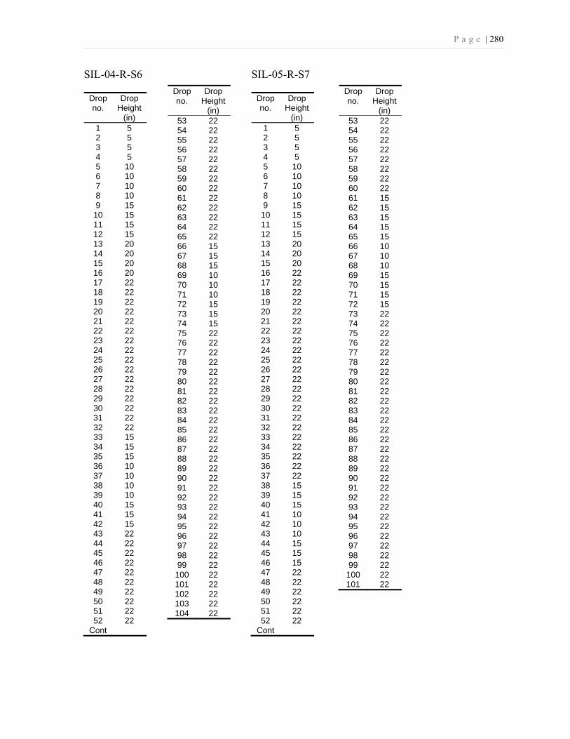
P a g e | 280
SIL-04-R-S6
Drop no.
Drop Height
(in) 1 5 2 5 3 5 4 5 5 10 6 10 7 10 8 10 9 15
10 15 11 15 12 15 13 20 14 20 15 20 16 20 17 22 18 22 19 22 20 22 21 22 22 22 23 22 24 22 25 22 26 22 27 22 28 22 29 22 30 22 31 22 32 22 33 15 34 15 35 15 36 10 37 10 38 10 39 10 40 15 41 15 42 15 43 22 44 22 45 22 46 22 47 22 48 22 49 22 50 22 51 22 52 22
Cont
Drop no.
Drop Height
(in) 53 22 54 22 55 22 56 22 57 22 58 22 59 22 60 22 61 22 62 22 63 22 64 22 65 22 66 15 67 15 68 15 69 10 70 10 71 10 72 15 73 15 74 15 75 22 76 22 77 22 78 22 79 22 80 22 81 22 82 22 83 22 84 22 85 22 86 22 87 22 88 22 89 22 90 22 91 22 92 22 93 22 94 22 95 22 96 22 97 22 98 22 99 22 100 22 101 22 102 22 103 22 104 22
SIL-05-R-S7
Drop no.
Drop Height
(in) 1 5 2 5 3 5 4 5 5 10 6 10 7 10 8 10 9 15
10 15 11 15 12 15 13 20 14 20 15 20 16 22 17 22 18 22 19 22 20 22 21 22 22 22 23 22 24 22 25 22 26 22 27 22 28 22 29 22 30 22 31 22 32 22 33 22 34 22 35 22 36 22 37 22 38 15 39 15 40 15 41 10 42 10 43 10 44 15 45 15 46 15 47 22 48 22 49 22 50 22 51 22 52 22
Cont
Drop no.
Drop Height
(in) 53 22 54 22 55 22 56 22 57 22 58 22 59 22 60 22 61 15 62 15 63 15 64 15 65 15 66 10 67 10 68 10 69 15 70 15 71 15 72 15 73 22 74 22 75 22 76 22 77 22 78 22 79 22 80 22 81 22 82 22 83 22 84 22 85 22 86 22 87 22 88 22 89 22 90 22 91 22 92 22 93 22 94 22 95 22 96 22 97 22 98 22 99 22 100 22 101 22

P a g e | 281
SIS-01-R-S5
Drop no.
Drop Height
(in) 1 5 2 5 3 5 4 5 5 10 6 10 7 10 8 10 9 15
10 15 11 15 12 15 13 22 14 22 15 22 16 22 17 22 18 22 19 22 20 22 21 22 22 22 23 22 24 22 25 22 26 22 27 22 28 22 29 22 30 22 31 22 32 22 33 22 34 22 35 22 36 22 37 15 38 15 39 15 40 11 41 22 42 10 43 10 44 10 45 10 46 15 47 15 48 15 49 22 50 22
Cont
Drop no.
Drop Height
(in) 51 22 52 22 53 22 54 22 55 22 56 22 57 22 58 22 59 22 60 22
SIS-02-R-S1
Drop no.
Drop Height
(in) 1 5 2 5 3 5 4 10 5 10 6 10 7 15 8 15 9 15
10 22 11 22 12 22 13 22 14 22 15 22 16 22 17 22 18 22 19 22 20 22 21 22 22 22 23 22 24 22 25 22 26 22 27 22 28 15 29 15 30 15 31 10 32 10 33 10 34 10 35 15 36 15 37 15 38 15 39 22 40 22 41 22 42 22 43 22 44 22 45 22 46 22 47 22 48 22 49 22
SIS-05-R-S4
Drop no.
Drop Height
(in) 1 5 2 5 3 5 4 10 5 10 6 10 7 15 8 15 9 15
10 22 11 22 12 22 13 22 14 22 15 22 16 22 17 22 18 22 19 22 20 22 21 22 22 22 23 22 24 15 25 15 26 15 27 10 28 10 29 10 30 10 31 10 32 15 33 15 34 15 35 15 36 15 37 22 38 22 39 22 40 22 41 22 42 22 43 22 44 22 45 22 46 22 47 22 48 22
SIS-05-R-S4
Drop no.
Drop Height
(in) 1 5 2 5 3 5 4 10 5 10 6 10 7 15 8 15 9 15
10 22 11 22 12 22 13 22 14 22 15 22 16 22 17 22 18 22 19 22 20 22 21 22 22 22 23 22 24 22 25 22 26 22 27 22 28 22 29 22 30 15 31 15 32 15 33 10 34 10 35 10 36 15 37 15 38 15 39 15 40 22 41 22 42 22 43 22 44 22 45 22 46 22 47 22 48 22

P a g e | 282
Appendix G: DCP Data
In the following tables, the “distance” is the distance between bottom of anvil and soil
surface. It is basically the scale reading which is measured after any drop. The value reported
for “drop number” zero is the sinkage of DCP due to its weight prior to any test. Therefore it
is the pretest depth of DCP. The anvil to cone shoulder distance is 98.0 cm in the Kessler’s
DCP.
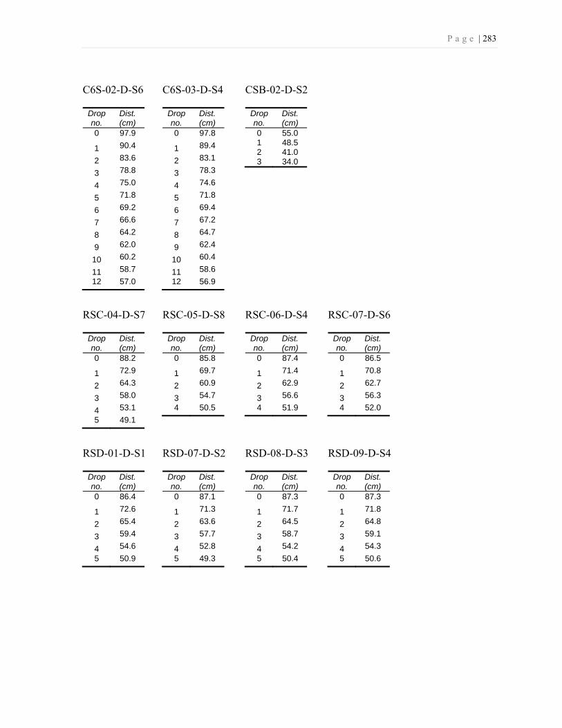
P a g e | 283
C6S-02-D-S6
Drop no.
Dist. (cm)
0 97.9
1 90.4
2 83.6
3 78.8
4 75.0
5 71.8
6 69.2
7 66.6
8 64.2
9 62.0
10 60.2
11 58.7
12 57.0
C6S-03-D-S4
Drop no.
Dist. (cm)
0 97.8
1 89.4
2 83.1
3 78.3
4 74.6
5 71.8
6 69.4
7 67.2
8 64.7
9 62.4
10 60.4
11 58.6
12 56.9
CSB-02-D-S2
Drop no.
Dist. (cm)
0 55.0 1 48.5 2 41.0 3 34.0
RSC-04-D-S7
Drop no.
Dist. (cm)
0 88.2
1 72.9
2 64.3
3 58.0
4 53.1
5 49.1
RSC-05-D-S8
Drop no.
Dist. (cm)
0 85.8
1 69.7
2 60.9
3 54.7
4 50.5
RSC-06-D-S4
Drop no.
Dist. (cm)
0 87.4
1 71.4
2 62.9
3 56.6
4 51.9
RSC-07-D-S6
Drop no.
Dist. (cm)
0 86.5
1 70.8
2 62.7
3 56.3
4 52.0
RSD-01-D-S1
Drop no.
Dist. (cm)
0 86.4
1 72.6
2 65.4
3 59.4
4 54.6
5 50.9
RSD-07-D-S2
Drop no.
Dist. (cm)
0 87.1
1 71.3
2 63.6
3 57.7
4 52.8
5 49.3
RSD-08-D-S3
Drop no.
Dist. (cm)
0 87.3
1 71.7
2 64.5
3 58.7
4 54.2
5 50.4
RSD-09-D-S4
Drop no.
Dist. (cm)
0 87.3
1 71.8
2 64.8
3 59.1
4 54.3
5 50.6

P a g e | 284
SIL-02-D-S3
Drop no.
Dist. (cm)
0 98.6 1 98.0 2 94.6 3 93.5 4 92.6 5 91.7 6 90.7 7 89.7 8 88.8 9 87.8
10 86.7 11 85.8 12 84.8 13 83.9 14 83.1 15 82.3 16 81.3 17 80.4 18 79.8 19 78.9 20 78.2 21 77.5 22 76.7 23 75.9 24 75.0 25 74.0 26 73.0 27 72.0 28 71.0 29 70.1 30 69.2 31 68.4 32 67.6 33 66.8 34 65.8 35 64.9 36 64.0 37 63.2 38 62.3 39 61.4 40 60.5 41 59.5 42 58.5 43 57.5 44 56.4 45 55.3 46 54.3 47 53.4 48 52.5 49 51.6
SIL-06-D-S9
Drop no.
Dist. (cm)
0 98.7 1 97.0 2 95.9 3 94.9 4 94.0 5 93.3 6 93.5 7 91.8 8 91.2 9 90.6
10 89.8 11 89.1 12 88.4 13 87.7 14 86.8 15 86.1 16 85.3 17 84.6 18 83.8 19 83.2 20 82.6 21 81.8 22 81.0 23 80.3 24 79.6 25 78.9 26 78.3 27 77.7 28 77.1 29 76.6 30 76.0 31 75.4 32 74.8 33 74.2 34 73.4 35 72.8 36 72.2 37 71.6 38 71.0 39 70.4 40 69.8 41 69.2 42 68.6 43 67.9 44 67.3 45 66.6 46 65.9 47 65.1 48 64.4 49 63.8 50 63.2
Cont
Drop no.
Dist. (cm)
51 62.5 52 61.8 53 61.1 54 60.4 55 59.7 56 58.8 57 58.0 58 57.1 59 56.2 60 55.4 61 54.7 62 54.0 63 53.3 64 52.7 65 52.1 66 51.5 67 50.9 68 50.3
SIL-07-D-S4
Drop no.
Dist. (cm)
0 98.8 1 96.9 2 95.9 3 94.9 4 94.0 5 93.3 6 92.6 7 91.9 8 91.2 9 90.6
10 90.0 11 89.2 12 88.5 13 87.7 14 87.0 15 86.1 16 85.3 17 84.6 18 83.9 19 83.2 20 82.5 21 81.8 22 81.2 23 80.5 24 79.8 25 78.9 26 78.6 27 78.0 28 77.5 29 76.9 30 76.5 31 75.9 32 75.3 33 74.7 34 74.1 35 73.4 36 72.7 37 71.9 38 71.2 39 70.5 40 69.8 41 69.2 42 68.6 43 68.0 44 67.4 45 66.7 46 66.0 47 65.4 48 64.7 49 64.0 50 63.4
Cont
Drop no.
Dist. (cm)
51 62.8 52 62.2 53 61.7 54 61.0 55 60.4 56 59.7 57 59.0 58 58.3 59 57.6 60 56.8 61 56.1 62 55.3 63 54.6 64 54.0 65 53.4 66 52.8 67 52.2 68 51.5 69 51.0 70 50.3

P a g e | 285
SIL-08-D-S2
Drop no.
Dist. (cm)
0 98.9 1 97.0 2 95.8 3 95.0 4 94.2 5 93.4 6 92.7 7 92.1 8 91.4 9 90.9
10 90.2 11 89.6 12 88.9 13 88.2 14 87.5 15 86.7 16 86.0 17 85.4 18 84.7 19 84.1 20 83.5 21 82.8 22 82.2 23 81.6 24 80.9 25 80.3 26 79.7 27 79.2 28 78.7 29 78.2 30 77.6 31 77.0 32 76.5 33 76.0 34 75.4 35 74.7 36 74.0 37 73.3 38 72.5 39 71.7 40 70.9 41 70.1 42 69.5 43 68.9 44 68.3 45 67.6 46 67.0 47 66.4 48 65.7 49 65.1 50 64.4
Cont
Drop no.
Dist. (cm)
51 63.7 52 63.1 53 62.5 54 61.9 55 61.2 56 60.6 57 59.8 58 59.0 59 58.3 60 57.5 61 56.7 62 55.9 63 55.2 64 54.5 65 53.8 66 53.1 67 52.5 68 51.9 69 51.3 70 50.7 71 50.1
GRV-01-D-S8
Drop no.
Dist. (cm)
0 90.8
1 85.4
2 82.6
3 80.3
4 78.2
5 76.2
6 74.7
7 73.2
8 71.7
9 70.3
10 68.9
11 67.6
12 66.2
13 64.7
14 63.5
15 62.3
16 61.2
17 60.0
18 58.8
19 57.5
20 56.3
21 55.2
22 54.1
23 53.0
24 51.9
25 50.8
26 49.7
27 48.6
28 47.6
29 46.6
30 45.3
31 44.3
32 43.0
33 41.7
34 40.4
35 39.2
36 37.9
37 36.7
38 35.6
39 35.4
40 35.3
GRV-03-D-S4
Drop no.
Dist. (cm)
0 94.9 1 87.7 2 85.1 3 83.0 4 81.3 5 79.9 6 78.6 7 77.5 8 76.4 9 75.3
10 74.3 11 73.3 12 72.2 13 71.4 14 70.6 15 69.8 16 69.0 17 68.2 18 67.4 19 66.5 20 65.7 21 64.9 22 64.1 23 63.3 24 62.6 25 61.8 26 61.0 27 60.3 28 59.5 29 58.7 30 58.0 31 57.2 32 56.4 33 55.6 34 54.9 35 54.1 36 53.4 37 52.6 38 51.8 39 51.0 40 50.2 41 49.4 42 48.7 43 47.9 44 47.0 45 46.1 46 45.3 47 44.5 48 43.7 49 42.8 50 94.9
Cont
Drop no.
Dist. (cm)
51 42.0
52 41.2
53 40.4
54 39.6
55 38.8
56 38.1
57 37.4
58 36.8
59 36.3
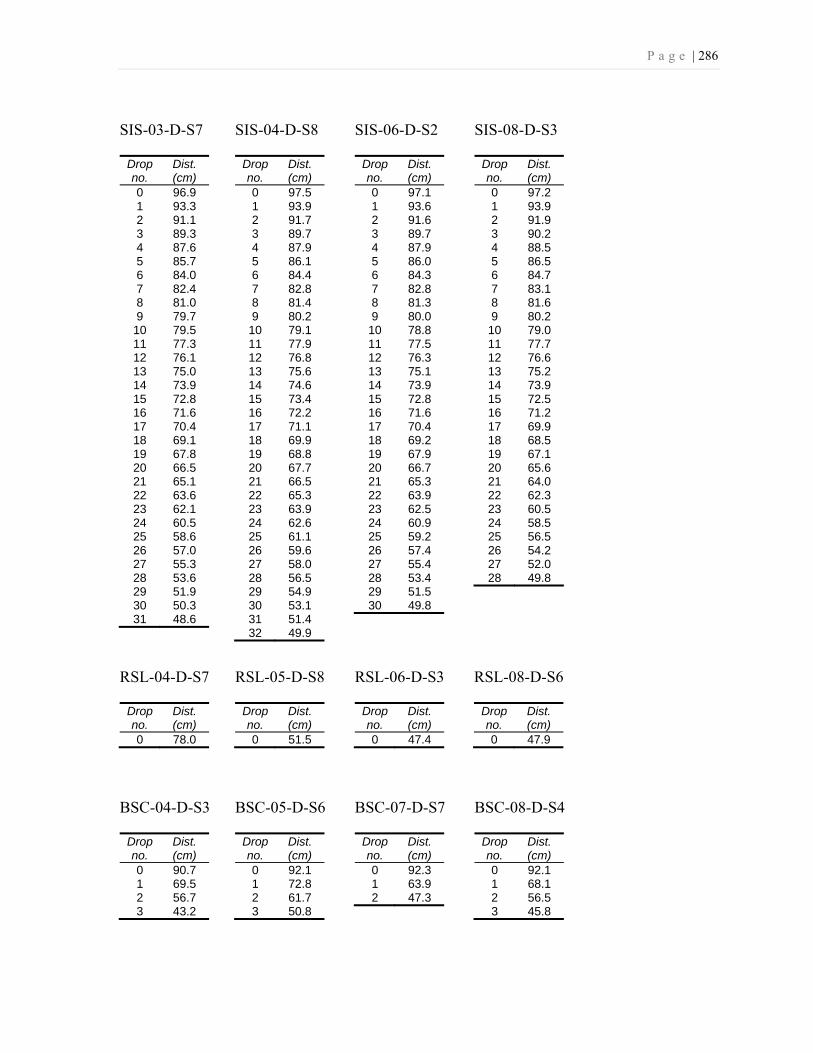
P a g e | 286
SIS-03-D-S7
Drop no.
Dist. (cm)
0 96.9 1 93.3 2 91.1 3 89.3 4 87.6 5 85.7 6 84.0 7 82.4 8 81.0 9 79.7
10 79.5 11 77.3 12 76.1 13 75.0 14 73.9 15 72.8 16 71.6 17 70.4 18 69.1 19 67.8 20 66.5 21 65.1 22 63.6 23 62.1 24 60.5 25 58.6 26 57.0 27 55.3 28 53.6 29 51.9 30 50.3 31 48.6
SIS-04-D-S8
Drop no.
Dist. (cm)
0 97.5 1 93.9 2 91.7 3 89.7 4 87.9 5 86.1 6 84.4 7 82.8 8 81.4 9 80.2
10 79.1 11 77.9 12 76.8 13 75.6 14 74.6 15 73.4 16 72.2 17 71.1 18 69.9 19 68.8 20 67.7 21 66.5 22 65.3 23 63.9 24 62.6 25 61.1 26 59.6 27 58.0 28 56.5 29 54.9 30 53.1 31 51.4 32 49.9
SIS-06-D-S2
Drop no.
Dist. (cm)
0 97.1 1 93.6 2 91.6 3 89.7 4 87.9 5 86.0 6 84.3 7 82.8 8 81.3 9 80.0
10 78.8 11 77.5 12 76.3 13 75.1 14 73.9 15 72.8 16 71.6 17 70.4 18 69.2 19 67.9 20 66.7 21 65.3 22 63.9 23 62.5 24 60.9 25 59.2 26 57.4 27 55.4 28 53.4 29 51.5 30 49.8
SIS-08-D-S3
Drop no.
Dist. (cm)
0 97.2 1 93.9 2 91.9 3 90.2 4 88.5 5 86.5 6 84.7 7 83.1 8 81.6 9 80.2
10 79.0 11 77.7 12 76.6 13 75.2 14 73.9 15 72.5 16 71.2 17 69.9 18 68.5 19 67.1 20 65.6 21 64.0 22 62.3 23 60.5 24 58.5 25 56.5 26 54.2 27 52.0 28 49.8
RSL-04-D-S7
Drop no.
Dist. (cm)
0 78.0
RSL-05-D-S8
Drop no.
Dist. (cm)
0 51.5
RSL-06-D-S3
Drop no.
Dist. (cm)
0 47.4
RSL-08-D-S6
Drop no.
Dist. (cm)
0 47.9
BSC-04-D-S3
Drop no.
Dist. (cm)
0 90.7 1 69.5 2 56.7 3 43.2
BSC-05-D-S6
Drop no.
Dist. (cm)
0 92.1 1 72.8 2 61.7 3 50.8
BSC-07-D-S7
Drop no.
Dist. (cm)
0 92.3 1 63.9 2 47.3
BSC-08-D-S4
Drop no.
Dist. (cm)
0 92.1 1 68.1 2 56.5 3 45.8

P a g e | 287
Appendix H: DCP Graphs

P a g e | 288
0 2 4 6
-700
-600
-500
-400
-300
-200
-100
0
No. of BlowsD
epth
(mm
)
BSC-04-D-S3
DCPi = 131.5 (mm/blow)
DataFitted Line
0 2 4 6
-700
-600
-500
-400
-300
-200
-100
0
No. of Blows
Dep
th (m
m)
BSC-05-D-S6
DCPi = 110.0 (mm/blow)
DataFitted Line
0 2 4 6
-700
-600
-500
-400
-300
-200
-100
0
No. of Blows
Dep
th (m
m)
BSC-07-D-S7
DCPi = 166.0 (mm/blow)
DataFitted Line
0 2 4 6
-700
-600
-500
-400
-300
-200
-100
0
No. of Blows
Dep
th (m
m)
BSC-08-D-S4
DCPi = 111.5 (mm/blow)
DataFitted Line
0 5 10 15 20
-700
-600
-500
-400
-300
-200
-100
0
No. of Blows
Dep
th (m
m)
C6S-02-D-S6
DCPi = 21.1 (mm/blow)
DataFitted Line
0 5 10 15 20
-700
-600
-500
-400
-300
-200
-100
0
No. of Blows
Dep
th (m
m)
C6S-03-D-S4
DCPi = 21.5 (mm/blow)
DataFitted Line

P a g e | 289
0 2 4 6
-700
-600
-500
-400
-300
-200
-100
0
No. of BlowsD
epth
(mm
)
CSB-02-D-S2
DCPi = 72.5 (mm/blow)
DataFitted Line
0 20 40 60 80
-700
-600
-500
-400
-300
-200
-100
0
No. of Blows
Dep
th (m
m)
GRV-01-D-S8
DCPi = 11.8 (mm/blow)
DataFitted Line
0 20 40 60 80
-700
-600
-500
-400
-300
-200
-100
0
No. of Blows
Dep
th (m
m)
GRV-03-D-S4
DCPi = 8.0 (mm/blow)
DataFitted Line
0 2 4 6
-700
-600
-500
-400
-300
-200
-100
0
No. of Blows
Dep
th (m
m)
RSC-04-D-S7
DCPi = 50.5 (mm/blow)
DataFitted Line
0 2 4 6
-700
-600
-500
-400
-300
-200
-100
0
No. of Blows
Dep
th (m
m)
RSC-05-D-S8
DCPi = 52.0 (mm/blow)
DataFitted Line
0 2 4 6
-700
-600
-500
-400
-300
-200
-100
0
No. of Blows
Dep
th (m
m)
RSC-06-D-S4
DCPi = 55.0 (mm/blow)
DataFitted Line
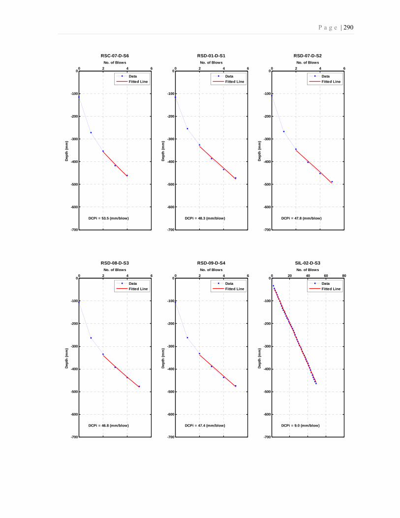
P a g e | 290
0 2 4 6
-700
-600
-500
-400
-300
-200
-100
0
No. of BlowsD
epth
(mm
)
RSC-07-D-S6
DCPi = 53.5 (mm/blow)
DataFitted Line
0 2 4 6
-700
-600
-500
-400
-300
-200
-100
0
No. of Blows
Dep
th (m
m)
RSD-01-D-S1
DCPi = 48.3 (mm/blow)
DataFitted Line
0 2 4 6
-700
-600
-500
-400
-300
-200
-100
0
No. of Blows
Dep
th (m
m)
RSD-07-D-S2
DCPi = 47.8 (mm/blow)
DataFitted Line
0 2 4 6
-700
-600
-500
-400
-300
-200
-100
0
No. of Blows
Dep
th (m
m)
RSD-08-D-S3
DCPi = 46.8 (mm/blow)
DataFitted Line
0 2 4 6
-700
-600
-500
-400
-300
-200
-100
0
No. of Blows
Dep
th (m
m)
RSD-09-D-S4
DCPi = 47.4 (mm/blow)
DataFitted Line
0 20 40 60 80
-700
-600
-500
-400
-300
-200
-100
0
No. of Blows
Dep
th (m
m)
SIL-02-D-S3
DCPi = 9.0 (mm/blow)
DataFitted Line

P a g e | 291
0 20 40 60 80
-700
-600
-500
-400
-300
-200
-100
0
No. of BlowsD
epth
(mm
)
SIL-06-D-S9
DCPi = 6.8 (mm/blow)
DataFitted Line
0 20 40 60 80
-700
-600
-500
-400
-300
-200
-100
0
No. of Blows
Dep
th (m
m)
SIL-07-D-S4
DCPi = 6.6 (mm/blow)
DataFitted Line
0 20 40 60 80
-700
-600
-500
-400
-300
-200
-100
0
No. of Blows
Dep
th (m
m)
SIL-08-D-S2
DCPi = 6.5 (mm/blow)
DataFitted Line
0 10 20 30 40
-700
-600
-500
-400
-300
-200
-100
0
No. of Blows
Dep
th (m
m)
SIS-03-D-S7
DCPi = 13.8 (mm/blow)
DataFitted Line
0 10 20 30 40
-700
-600
-500
-400
-300
-200
-100
0
No. of Blows
Dep
th (m
m)
SIS-04-D-S8
DCPi = 12.8 (mm/blow)
DataFitted Line
0 10 20 30 40
-700
-600
-500
-400
-300
-200
-100
0
No. of Blows
Dep
th (m
m)
SIS-06-D-S2
DCPi = 13.8 (mm/blow)
DataFitted Line

P a g e | 292
0 10 20 30 40
-700
-600
-500
-400
-300
-200
-100
0
No. of BlowsD
epth
(mm
)
SIS-08-D-S3
DCPi = 14.6 (mm/blow)
DataFitted Line

P a g e | 293
Appendix I: RapSochs Penetration Rate

P a g e | 294
0 8 16 24 32-700
-600
-500
-400
-300
-200
-100
0
Hammer Drop Height (cm)
0 20 40 60 80
-700
-600
-500
-400
-300
-200
-100
0
RS-PR (mm/blow)De
pth
(mm
)
BSC-01-R-S1
Drop HeightPenetration Rate
0 8 16 24 320
0
0
0
0
0
0
0
Hammer Drop Height (cm)
0 20 40 60 80
0
0
0
0
0
0
0
0
RS-PR (mm/blow)
BSC-02-R-S2
Drop HeightPenetration Rate
0 8 16 24 320
0
0
0
0
0
0
0
Hammer Drop Height (cm)
0 20 40 60 80
0
0
0
0
0
0
0
0
RS-PR (mm/blow)
BSC-03-R-S9
Drop HeightPenetration Rate
0 8 16 24 32-700
-600
-500
-400
-300
-200
-100
0
Hammer Drop Height (cm)
0 20 40 60 80
-700
-600
-500
-400
-300
-200
-100
0
RS-PR (mm/blow)
Dept
h (m
m)
BSC-06-R-S8
Drop HeightPenetration Rate
0 8 16 24 320
0
0
0
0
0
0
0
Hammer Drop Height (cm)
0 20 40 60 80
0
0
0
0
0
0
0
0
RS-PR (mm/blow)
BSC-09-R-S5
Drop HeightPenetration Rate
0 8 16 24 320
0
0
0
0
0
0
0
Hammer Drop Height (cm)
0 20 40 60 80
0
0
0
0
0
0
0
0
RS-PR (mm/blow)
CSR-01-R-S5
Drop HeightPenetration Rate

P a g e | 295
0 15 30 45 60-700
-600
-500
-400
-300
-200
-100
0
Hammer Drop Height (cm)
0 10 20 30 40
-700
-600
-500
-400
-300
-200
-100
0
RS-PR (mm/blow)De
pth
(mm
)
C6S-01-R-S8
Drop HeightPenetration Rate
0 15 30 45 600
0
0
0
0
0
0
0
Hammer Drop Height (cm)
0 10 20 30 40
0
0
0
0
0
0
0
0
RS-PR (mm/blow)
C6S-04-R-S2
Drop HeightPenetration Rate
0 8 16 24 320
0
0
0
0
0
0
0
Hammer Drop Height (cm)
0 20 40 60 80
0
0
0
0
0
0
0
0
RS-PR (mm/blow)
CSB-01-R-S8
Drop HeightPenetration Rate
0 15 30 45 60-700
-600
-500
-400
-300
-200
-100
0
Hammer Drop Height (cm)
0 5 10 15 20
-700
-600
-500
-400
-300
-200
-100
0
RS-PR (mm/blow)
Dept
h (m
m)
GRV-02-R-S5
Drop HeightPenetration Rate
0 15 30 45 600
0
0
0
0
0
0
0
Hammer Drop Height (cm)
0 5 10 15 20
0
0
0
0
0
0
0
0
RS-PR (mm/blow)
GRV-04-R-S2
Drop HeightPenetration Rate
0 15 30 45 600
0
0
0
0
0
0
0
Hammer Drop Height (cm)
0 5 10 15 20
0
0
0
0
0
0
0
0
RS-PR (mm/blow)
GRV-05-R-S6
Drop HeightPenetration Rate
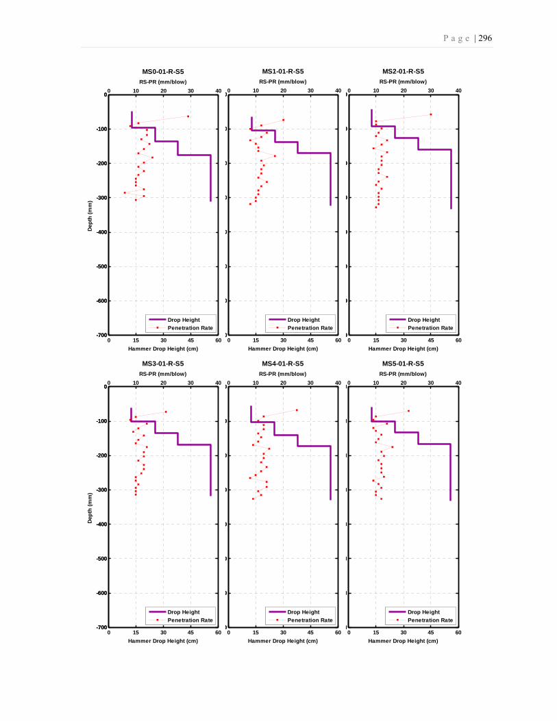
P a g e | 296
0 15 30 45 60-700
-600
-500
-400
-300
-200
-100
0
Hammer Drop Height (cm)
0 10 20 30 40
-700
-600
-500
-400
-300
-200
-100
0
RS-PR (mm/blow)De
pth
(mm
)
MS0-01-R-S5
Drop HeightPenetration Rate
0 15 30 45 600
0
0
0
0
0
0
0
Hammer Drop Height (cm)
0 10 20 30 40
0
0
0
0
0
0
0
0
RS-PR (mm/blow)
MS1-01-R-S5
Drop HeightPenetration Rate
0 15 30 45 600
0
0
0
0
0
0
0
Hammer Drop Height (cm)
0 10 20 30 40
0
0
0
0
0
0
0
0
RS-PR (mm/blow)
MS2-01-R-S5
Drop HeightPenetration Rate
0 15 30 45 60-700
-600
-500
-400
-300
-200
-100
0
Hammer Drop Height (cm)
0 10 20 30 40
-700
-600
-500
-400
-300
-200
-100
0
RS-PR (mm/blow)
Dept
h (m
m)
MS3-01-R-S5
Drop HeightPenetration Rate
0 15 30 45 600
0
0
0
0
0
0
0
Hammer Drop Height (cm)
0 10 20 30 40
0
0
0
0
0
0
0
0
RS-PR (mm/blow)
MS4-01-R-S5
Drop HeightPenetration Rate
0 15 30 45 600
0
0
0
0
0
0
0
Hammer Drop Height (cm)
0 10 20 30 40
0
0
0
0
0
0
0
0
RS-PR (mm/blow)
MS5-01-R-S5
Drop HeightPenetration Rate
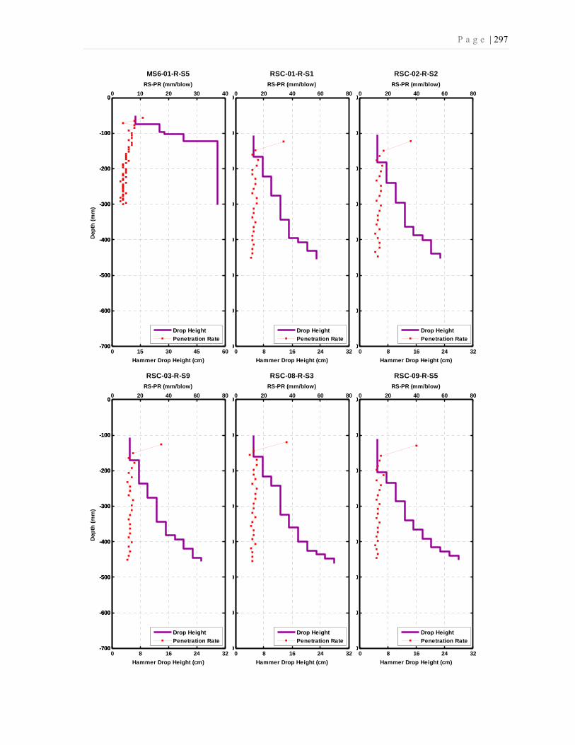
P a g e | 297
0 15 30 45 60-700
-600
-500
-400
-300
-200
-100
0
Hammer Drop Height (cm)
0 10 20 30 40
-700
-600
-500
-400
-300
-200
-100
0
RS-PR (mm/blow)De
pth
(mm
)
MS6-01-R-S5
Drop HeightPenetration Rate
0 8 16 24 320
0
0
0
0
0
0
0
Hammer Drop Height (cm)
0 20 40 60 80
0
0
0
0
0
0
0
0
RS-PR (mm/blow)
RSC-01-R-S1
Drop HeightPenetration Rate
0 8 16 24 320
0
0
0
0
0
0
0
Hammer Drop Height (cm)
0 20 40 60 80
0
0
0
0
0
0
0
0
RS-PR (mm/blow)
RSC-02-R-S2
Drop HeightPenetration Rate
0 8 16 24 32-700
-600
-500
-400
-300
-200
-100
0
Hammer Drop Height (cm)
0 20 40 60 80
-700
-600
-500
-400
-300
-200
-100
0
RS-PR (mm/blow)
Dept
h (m
m)
RSC-03-R-S9
Drop HeightPenetration Rate
0 8 16 24 320
0
0
0
0
0
0
0
Hammer Drop Height (cm)
0 20 40 60 80
0
0
0
0
0
0
0
0
RS-PR (mm/blow)
RSC-08-R-S3
Drop HeightPenetration Rate
0 8 16 24 320
0
0
0
0
0
0
0
Hammer Drop Height (cm)
0 20 40 60 80
0
0
0
0
0
0
0
0
RS-PR (mm/blow)
RSC-09-R-S5
Drop HeightPenetration Rate

P a g e | 298
0 8 16 24 32-700
-600
-500
-400
-300
-200
-100
0
Hammer Drop Height (cm)
0 20 40 60 80
-700
-600
-500
-400
-300
-200
-100
0
RS-PR (mm/blow)De
pth
(mm
)
RSD-02-R-S5
Drop HeightPenetration Rate
0 8 16 24 320
0
0
0
0
0
0
0
Hammer Drop Height (cm)
0 20 40 60 80
0
0
0
0
0
0
0
0
RS-PR (mm/blow)
RSD-03-R-S6
Drop HeightPenetration Rate
0 8 16 24 320
0
0
0
0
0
0
0
Hammer Drop Height (cm)
0 20 40 60 80
0
0
0
0
0
0
0
0
RS-PR (mm/blow)
RSD-04-R-S7
Drop HeightPenetration Rate
0 8 16 24 32-700
-600
-500
-400
-300
-200
-100
0
Hammer Drop Height (cm)
0 20 40 60 80
-700
-600
-500
-400
-300
-200
-100
0
RS-PR (mm/blow)
Dept
h (m
m)
RSD-05-R-S9
Drop HeightPenetration Rate
0 8 16 24 320
0
0
0
0
0
0
0
Hammer Drop Height (cm)
0 20 40 60 80
0
0
0
0
0
0
0
0
RS-PR (mm/blow)
RSD-06-R-S8
Drop HeightPenetration Rate

P a g e | 299
0 15 30 45 60-700
-600
-500
-400
-300
-200
-100
0
Hammer Drop Height (cm)
0 5 10 15 20
-700
-600
-500
-400
-300
-200
-100
0
RS-PR (mm/blow)De
pth
(mm
)
SIL-01-R-S1
Drop HeightPenetration Rate
0 15 30 45 600
0
0
0
0
0
0
0
Hammer Drop Height (cm)
0 5 10 15 20
0
0
0
0
0
0
0
0
RS-PR (mm/blow)
SIL-03-R-S5
Drop HeightPenetration Rate
0 15 30 45 60-700
-600
-500
-400
-300
-200
-100
0
Hammer Drop Height (cm)
0 5 10 15 20
-700
-600
-500
-400
-300
-200
-100
0
RS-PR (mm/blow)
Dept
h (m
m)
SIL-04-R-S6
Drop HeightPenetration Rate
0 15 30 45 600
0
0
0
0
0
0
0
Hammer Drop Height (cm)
0 5 10 15 20
0
0
0
0
0
0
0
0
RS-PR (mm/blow)
SIL-05-R-S7
Drop HeightPenetration Rate

P a g e | 300
0 15 30 45 60-700
-600
-500
-400
-300
-200
-100
0
Hammer Drop Height (cm)
0 5 10 15 20
-700
-600
-500
-400
-300
-200
-100
0
RS-PR (mm/blow)De
pth
(mm
)
SIS-01-R-S5
Drop HeightPenetration Rate
0 15 30 45 600
0
0
0
0
0
0
0
Hammer Drop Height (cm)
0 5 10 15 20
0
0
0
0
0
0
0
0
RS-PR (mm/blow)
SIS-02-R-S1
Drop HeightPenetration Rate
0 15 30 45 60-700
-600
-500
-400
-300
-200
-100
0
Hammer Drop Height (cm)
0 5 10 15 20
-700
-600
-500
-400
-300
-200
-100
0
RS-PR (mm/blow)
Dept
h (m
m)
SIS-05-R-S4
Drop HeightPenetration Rate
0 15 30 45 600
0
0
0
0
0
0
0
Hammer Drop Height (cm)
0 5 10 15 20
0
0
0
0
0
0
0
0
RS-PR (mm/blow)
SIS-07-R-S6
Drop HeightPenetration Rate
P a g e | 301
Appendix J: RapSochs Moisture Data

P a g e | 302
0 2 4 6 8 10-700
-600
-500
-400
-300
-200
-100
0
Frequency (MHz)
Dept
h (m
m)
Magnitude (dB)
Frequency (MHz)
Phase (Degree)
BSC-01-R-S1
0 2 4 6 8 10
-10 0 10 20 30 0 20 40 60 80 100 120
0 2 4 6 8 10-700
-600
-500
-400
-300
-200
-100
0
Frequency (MHz)
Dep
th (m
m)
Magnitude (dB)
Frequency (MHz)
Phase (Degree)
BSC-02-R-S2
0 2 4 6 8 10
-10 0 10 20 30 0 20 40 60 80 100 120
0 2 4 6 8 10-700
-600
-500
-400
-300
-200
-100
0
Frequency (MHz)
Dept
h (m
m)
Magnitude (dB)
Frequency (MHz)
Phase (Degree)
BSC-03-R-S9
0 2 4 6 8 10
-10 0 10 20 30 0 20 40 60 80 100 120
0 2 4 6 8 10-700
-600
-500
-400
-300
-200
-100
0
Frequency (MHz)
Dept
h (m
m)
Magnitude (dB)
Frequency (MHz)
Phase (Degree)
BSC-06-R-S8
0 2 4 6 8 10
-10 0 10 20 30 0 20 40 60 80 100 120

P a g e | 303
0 2 4 6 8 10-700
-600
-500
-400
-300
-200
-100
0
Frequency (MHz)
Dep
th (m
m)
Magnitude (dB)
Frequency (MHz)
Phase (Degree)
BSC-09-R-S5
0 2 4 6 8 10
-10 0 10 20 30 0 20 40 60 80 100 120
0 2 4 6 8 10-700
-600
-500
-400
-300
-200
-100
0
Frequency (MHz)
Dep
th (m
m)
Magnitude (dB)
Frequency (MHz)
Phase (Degree)
C6S-01-R-S8
0 2 4 6 8 10
-10 0 10 20 30 0 20 40 60 80 100 120
0 2 4 6 8 10-700
-600
-500
-400
-300
-200
-100
0
Frequency (MHz)
Dep
th (m
m)
Magnitude (dB)
Frequency (MHz)
Phase (Degree)
C6S-04-R-S2
0 2 4 6 8 10
-10 0 10 20 30 0 20 40 60 80 100 120
0 2 4 6 8 10-700
-600
-500
-400
-300
-200
-100
0
Frequency (MHz)
Dep
th (m
m)
Magnitude (dB)
Frequency (MHz)
Phase (Degree)
CSB-01-R-S8
0 2 4 6 8 10
-10 0 10 20 30 0 20 40 60 80 100 120
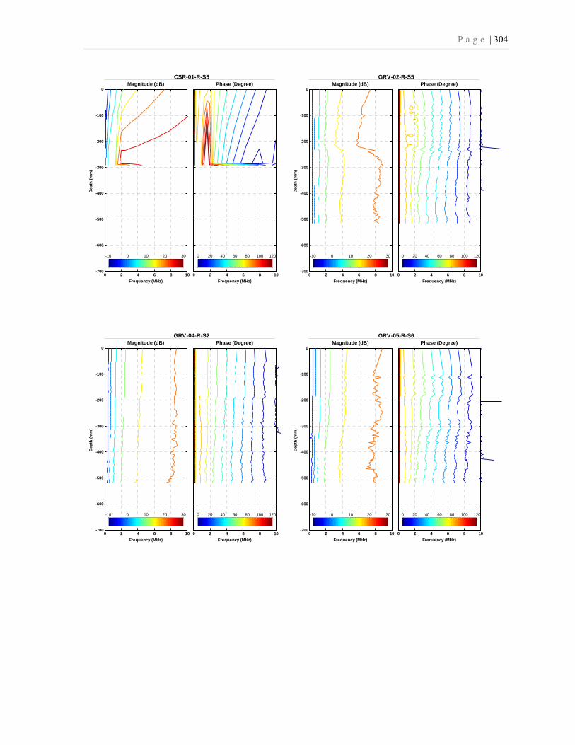
P a g e | 304
0 2 4 6 8 10-700
-600
-500
-400
-300
-200
-100
0
Frequency (MHz)
Dep
th (m
m)
Magnitude (dB)
Frequency (MHz)
Phase (Degree)
CSR-01-R-S5
0 2 4 6 8 10
-10 0 10 20 30 0 20 40 60 80 100 120
0 2 4 6 8 10-700
-600
-500
-400
-300
-200
-100
0
Frequency (MHz)
Dep
th (m
m)
Magnitude (dB)
Frequency (MHz)
Phase (Degree)
GRV-02-R-S5
0 2 4 6 8 10
-10 0 10 20 30 0 20 40 60 80 100 120
0 2 4 6 8 10-700
-600
-500
-400
-300
-200
-100
0
Frequency (MHz)
Dep
th (m
m)
Magnitude (dB)
Frequency (MHz)
Phase (Degree)
GRV-04-R-S2
0 2 4 6 8 10
-10 0 10 20 30 0 20 40 60 80 100 120
0 2 4 6 8 10-700
-600
-500
-400
-300
-200
-100
0
Frequency (MHz)
Dep
th (m
m)
Magnitude (dB)
Frequency (MHz)
Phase (Degree)
GRV-05-R-S6
0 2 4 6 8 10
-10 0 10 20 30 0 20 40 60 80 100 120
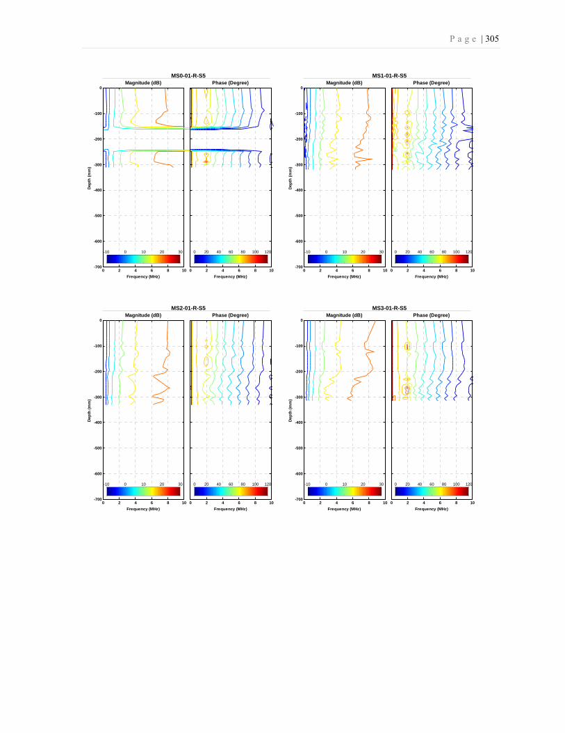
P a g e | 305
0 2 4 6 8 10-700
-600
-500
-400
-300
-200
-100
0
Frequency (MHz)
Dep
th (m
m)
Magnitude (dB)
Frequency (MHz)
Phase (Degree)
MS0-01-R-S5
0 2 4 6 8 10
-10 0 10 20 30 0 20 40 60 80 100 120
0 2 4 6 8 10-700
-600
-500
-400
-300
-200
-100
0
Frequency (MHz)
Dep
th (m
m)
Magnitude (dB)
Frequency (MHz)
Phase (Degree)
MS1-01-R-S5
0 2 4 6 8 10
-10 0 10 20 30 0 20 40 60 80 100 120
0 2 4 6 8 10-700
-600
-500
-400
-300
-200
-100
0
Frequency (MHz)
Dep
th (m
m)
Magnitude (dB)
Frequency (MHz)
Phase (Degree)
MS2-01-R-S5
0 2 4 6 8 10
-10 0 10 20 30 0 20 40 60 80 100 120
0 2 4 6 8 10-700
-600
-500
-400
-300
-200
-100
0
Frequency (MHz)
Dep
th (m
m)
Magnitude (dB)
Frequency (MHz)
Phase (Degree)
MS3-01-R-S5
0 2 4 6 8 10
-10 0 10 20 30 0 20 40 60 80 100 120
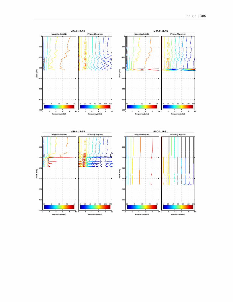
P a g e | 306
0 2 4 6 8 10-700
-600
-500
-400
-300
-200
-100
0
Frequency (MHz)
Dep
th (m
m)
Magnitude (dB)
Frequency (MHz)
Phase (Degree)
MS4-01-R-S5
0 2 4 6 8 10
-10 0 10 20 30 0 20 40 60 80 100 120
0 2 4 6 8 10-700
-600
-500
-400
-300
-200
-100
0
Frequency (MHz)
Dep
th (m
m)
Magnitude (dB)
Frequency (MHz)
Phase (Degree)
MS5-01-R-S5
0 2 4 6 8 10
-10 0 10 20 30 0 20 40 60 80 100 120
0 2 4 6 8 10-700
-600
-500
-400
-300
-200
-100
0
Frequency (MHz)
Dep
th (m
m)
Magnitude (dB)
Frequency (MHz)
Phase (Degree)
MS6-01-R-S5
0 2 4 6 8 10
-10 0 10 20 30 0 20 40 60 80 100 120
0 2 4 6 8 10-700
-600
-500
-400
-300
-200
-100
0
Frequency (MHz)
Dep
th (m
m)
Magnitude (dB)
Frequency (MHz)
Phase (Degree)
RSC-01-R-S1
0 2 4 6 8 10
-10 0 10 20 30 0 20 40 60 80 100 120

P a g e | 307
0 2 4 6 8 10-700
-600
-500
-400
-300
-200
-100
0
Frequency (MHz)
Dep
th (m
m)
Magnitude (dB)
Frequency (MHz)
Phase (Degree)
RSC-02-R-S2
0 2 4 6 8 10
-10 0 10 20 30 0 20 40 60 80 100 120
0 2 4 6 8 10-700
-600
-500
-400
-300
-200
-100
0
Frequency (MHz)
Dep
th (m
m)
Magnitude (dB)
Frequency (MHz)
Phase (Degree)
RSC-03-R-S9
0 2 4 6 8 10
-10 0 10 20 30 0 20 40 60 80 100 120
0 2 4 6 8 10-700
-600
-500
-400
-300
-200
-100
0
Frequency (MHz)
Dep
th (m
m)
Magnitude (dB)
Frequency (MHz)
Phase (Degree)
RSC-08-R-S3
0 2 4 6 8 10
-10 0 10 20 30 0 20 40 60 80 100 120
0 2 4 6 8 10-700
-600
-500
-400
-300
-200
-100
0
Frequency (MHz)
Dep
th (m
m)
Magnitude (dB)
Frequency (MHz)
Phase (Degree)
RSC-09-R-S5
0 2 4 6 8 10
-10 0 10 20 30 0 20 40 60 80 100 120
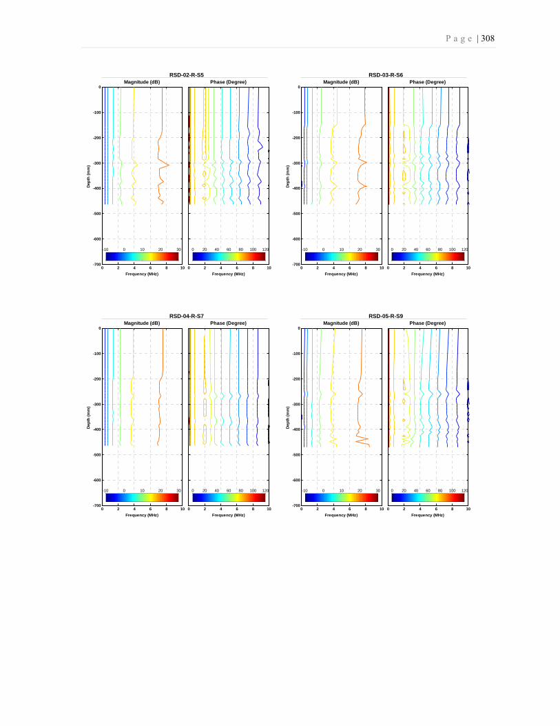
P a g e | 308
0 2 4 6 8 10-700
-600
-500
-400
-300
-200
-100
0
Frequency (MHz)
Dep
th (m
m)
Magnitude (dB)
Frequency (MHz)
Phase (Degree)
RSD-02-R-S5
0 2 4 6 8 10
-10 0 10 20 30 0 20 40 60 80 100 120
0 2 4 6 8 10-700
-600
-500
-400
-300
-200
-100
0
Frequency (MHz)
Dep
th (m
m)
Magnitude (dB)
Frequency (MHz)
Phase (Degree)
RSD-03-R-S6
0 2 4 6 8 10
-10 0 10 20 30 0 20 40 60 80 100 120
0 2 4 6 8 10-700
-600
-500
-400
-300
-200
-100
0
Frequency (MHz)
Dep
th (m
m)
Magnitude (dB)
Frequency (MHz)
Phase (Degree)
RSD-04-R-S7
0 2 4 6 8 10
-10 0 10 20 30 0 20 40 60 80 100 120
0 2 4 6 8 10-700
-600
-500
-400
-300
-200
-100
0
Frequency (MHz)
Dep
th (m
m)
Magnitude (dB)
Frequency (MHz)
Phase (Degree)
RSD-05-R-S9
0 2 4 6 8 10
-10 0 10 20 30 0 20 40 60 80 100 120

P a g e | 309
0 2 4 6 8 10-700
-600
-500
-400
-300
-200
-100
0
Frequency (MHz)
Dep
th (m
m)
Magnitude (dB)
Frequency (MHz)
Phase (Degree)
RSD-06-R-S8
0 2 4 6 8 10
-10 0 10 20 30 0 20 40 60 80 100 120
0 2 4 6 8 10-700
-600
-500
-400
-300
-200
-100
0
Frequency (MHz)
Dep
th (m
m)
Magnitude (dB)
Frequency (MHz)
Phase (Degree)
RSL-01-R-S1
0 2 4 6 8 10
-10 0 10 20 30 0 20 40 60 80 100 120
0 2 4 6 8 10-700
-600
-500
-400
-300
-200
-100
0
Frequency (MHz)
Dep
th (m
m)
Magnitude (dB)
Frequency (MHz)
Phase (Degree)
RSL-02-R-S2
0 2 4 6 8 10
-10 0 10 20 30 0 20 40 60 80 100 120
0 2 4 6 8 10-700
-600
-500
-400
-300
-200
-100
0
Frequency (MHz)
Dep
th (m
m)
Magnitude (dB)
Frequency (MHz)
Phase (Degree)
RSL-03-R-S9
0 2 4 6 8 10
-10 0 10 20 30 0 20 40 60 80 100 120

P a g e | 310
0 2 4 6 8 10-700
-600
-500
-400
-300
-200
-100
0
Frequency (MHz)
Dep
th (m
m)
Magnitude (dB)
Frequency (MHz)
Phase (Degree)
RSL-07-R-S4
0 2 4 6 8 10
-10 0 10 20 30 0 20 40 60 80 100 120
0 2 4 6 8 10-700
-600
-500
-400
-300
-200
-100
0
Frequency (MHz)
Dep
th (m
m)
Magnitude (dB)
Frequency (MHz)
Phase (Degree)
RSL-09-R-S5
0 2 4 6 8 10
-10 0 10 20 30 0 20 40 60 80 100 120
0 2 4 6 8 10-700
-600
-500
-400
-300
-200
-100
0
Frequency (MHz)
Dep
th (m
m)
Magnitude (dB)
Frequency (MHz)
Phase (Degree)
SIL-01-R-S1
0 2 4 6 8 10
-10 0 10 20 30 0 20 40 60 80 100 120
0 2 4 6 8 10-700
-600
-500
-400
-300
-200
-100
0
Frequency (MHz)
Dep
th (m
m)
Magnitude (dB)
Frequency (MHz)
Phase (Degree)
SIL-03-R-S5
0 2 4 6 8 10
-10 0 10 20 30 0 20 40 60 80 100 120

P a g e | 311
0 2 4 6 8 10-700
-600
-500
-400
-300
-200
-100
0
Frequency (MHz)
Dep
th (m
m)
Magnitude (dB)
Frequency (MHz)
Phase (Degree)
SIL-04-R-S6
0 2 4 6 8 10
-10 0 10 20 30 0 20 40 60 80 100 120
0 2 4 6 8 10-700
-600
-500
-400
-300
-200
-100
0
Frequency (MHz)
Dep
th (m
m)
Magnitude (dB)
Frequency (MHz)
Phase (Degree)
SIL-05-R-S7
0 2 4 6 8 10
-10 0 10 20 30 0 20 40 60 80 100 120
0 2 4 6 8 10-700
-600
-500
-400
-300
-200
-100
0
Frequency (MHz)
Dep
th (m
m)
Magnitude (dB)
Frequency (MHz)
Phase (Degree)
SIS-01-R-S5
0 2 4 6 8 10
-10 0 10 20 30 0 20 40 60 80 100 120
0 2 4 6 8 10-700
-600
-500
-400
-300
-200
-100
0
Frequency (MHz)
Dep
th (m
m)
Magnitude (dB)
Frequency (MHz)
Phase (Degree)
SIS-02-R-S1
0 2 4 6 8 10
-10 0 10 20 30 0 20 40 60 80 100 120

P a g e | 312
0 2 4 6 8 10-700
-600
-500
-400
-300
-200
-100
0
Frequency (MHz)
Dep
th (m
m)
Magnitude (dB)
Frequency (MHz)
Phase (Degree)
SIS-05-R-S4
0 2 4 6 8 10
-10 0 10 20 30 0 20 40 60 80 100 120
0 2 4 6 8 10-700
-600
-500
-400
-300
-200
-100
0
Frequency (MHz)
Dep
th (m
m)
Magnitude (dB)
Frequency (MHz)
Phase (Degree)
SIS-07-R-S6
0 2 4 6 8 10
-10 0 10 20 30 0 20 40 60 80 100 120

P a g e | 313
Appendix K: Calculated Susceptance and
Conductance from Moisture Sensor

P a g e | 314
0 2 4 6 8 10-600
-500
-400
-300
-200
-100
0
Frequency (MHz)
Dep
th (m
m)
Frequency (MHz)
Susceptance (S or Ω -1) Conductance (S or Ω -1)
BSC-01-R-S1
0 2 4 6 8 10
0 5 10 15 20 0 5 10 15 20
0 2 4 6 8 10-600
-500
-400
-300
-200
-100
0
Frequency (MHz)
Dep
th (m
m)
Frequency (MHz)
Susceptance (S or Ω -1) Conductance (S or Ω -1)
BSC-02-R-S2
0 2 4 6 8 10
0 5 10 15 20 0 5 10 15 20
0 2 4 6 8 10-600
-500
-400
-300
-200
-100
0
Frequency (MHz)
Dep
th (m
m)
Frequency (MHz)
Susceptance (S or Ω -1) Conductance (S or Ω -1)
BSC-03-R-S9
0 2 4 6 8 10
0 5 10 15 20 0 5 10 15 20
0 2 4 6 8 10-600
-500
-400
-300
-200
-100
0
Frequency (MHz)
Dep
th (m
m)
Frequency (MHz)
Susceptance (S or Ω -1) Conductance (S or Ω -1)
BSC-06-R-S8
0 2 4 6 8 10
0 5 10 15 20 0 5 10 15 20

P a g e | 315
0 2 4 6 8 10-600
-500
-400
-300
-200
-100
0
Frequency (MHz)
Dep
th (m
m)
Frequency (MHz)
Susceptance (S or Ω -1) Conductance (S or Ω -1)
BSC-09-R-S5
0 2 4 6 8 10
0 5 10 15 20 0 5 10 15 20
0 2 4 6 8 10-600
-500
-400
-300
-200
-100
0
Frequency (MHz)
Dep
th (m
m)
Frequency (MHz)
Susceptance (S or Ω -1) Conductance (S or Ω -1)
C6S-01-R-S8
0 2 4 6 8 10
0 5 10 15 20 0 5 10 15 20
0 2 4 6 8 10-600
-500
-400
-300
-200
-100
0
Frequency (MHz)
Dep
th (m
m)
Frequency (MHz)
Susceptance (S or Ω -1) Conductance (S or Ω -1)
C6S-04-R-S2
0 2 4 6 8 10
0 5 10 15 20 0 5 10 15 20
0 2 4 6 8 10-600
-500
-400
-300
-200
-100
0
Frequency (MHz)
Dep
th (m
m)
Frequency (MHz)
Susceptance (S or Ω -1) Conductance (S or Ω -1)
CSB-01-R-S8
0 2 4 6 8 10
0 5 10 15 20 0 5 10 15 20
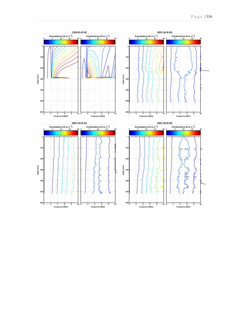
P a g e | 316
0 2 4 6 8 10-600
-500
-400
-300
-200
-100
0
Frequency (MHz)
Dep
th (m
m)
Frequency (MHz)
Susceptance (S or Ω -1) Conductance (S or Ω -1)
CSR-01-R-S5
0 2 4 6 8 10
0 5 10 15 20 0 5 10 15 20
0 2 4 6 8 10-600
-500
-400
-300
-200
-100
0
Frequency (MHz)
Dep
th (m
m)
Frequency (MHz)
Susceptance (S or Ω -1) Conductance (S or Ω -1)
GRV-02-R-S5
0 2 4 6 8 10
0 5 10 15 20 0 5 10 15 20
0 2 4 6 8 10-600
-500
-400
-300
-200
-100
0
Frequency (MHz)
Dep
th (m
m)
Frequency (MHz)
Susceptance (S or Ω -1) Conductance (S or Ω -1)
GRV-04-R-S2
0 2 4 6 8 10
0 5 10 15 20 0 5 10 15 20
0 2 4 6 8 10-600
-500
-400
-300
-200
-100
0
Frequency (MHz)
Dep
th (m
m)
Frequency (MHz)
Susceptance (S or Ω -1) Conductance (S or Ω -1)
GRV-05-R-S6
0 2 4 6 8 10
0 5 10 15 20 0 5 10 15 20

P a g e | 317
0 2 4 6 8 10-600
-500
-400
-300
-200
-100
0
Frequency (MHz)
Dep
th (m
m)
Frequency (MHz)
Susceptance (S or Ω -1) Conductance (S or Ω -1)
MS0-01-R-S5
0 2 4 6 8 10
0 5 10 15 20 0 5 10 15 20
0 2 4 6 8 10-600
-500
-400
-300
-200
-100
0
Frequency (MHz)
Dep
th (m
m)
Frequency (MHz)
Susceptance (S or Ω -1) Conductance (S or Ω -1)
MS1-01-R-S5
0 2 4 6 8 10
0 5 10 15 20 0 5 10 15 20
0 2 4 6 8 10-600
-500
-400
-300
-200
-100
0
Frequency (MHz)
Dep
th (m
m)
Frequency (MHz)
Susceptance (S or Ω -1) Conductance (S or Ω -1)
MS2-01-R-S5
0 2 4 6 8 10
0 5 10 15 20 0 5 10 15 20
0 2 4 6 8 10-600
-500
-400
-300
-200
-100
0
Frequency (MHz)
Dep
th (m
m)
Frequency (MHz)
Susceptance (S or Ω -1) Conductance (S or Ω -1)
MS3-01-R-S5
0 2 4 6 8 10
0 5 10 15 20 0 5 10 15 20
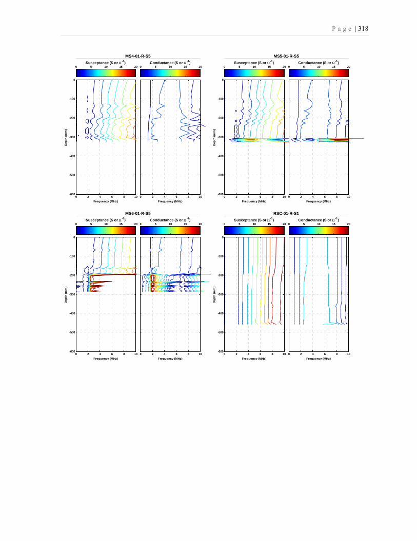
P a g e | 318
0 2 4 6 8 10-600
-500
-400
-300
-200
-100
0
Frequency (MHz)
Dep
th (m
m)
Frequency (MHz)
Susceptance (S or Ω -1) Conductance (S or Ω -1)
MS4-01-R-S5
0 2 4 6 8 10
0 5 10 15 20 0 5 10 15 20
0 2 4 6 8 10-600
-500
-400
-300
-200
-100
0
Frequency (MHz)
Dep
th (m
m)
Frequency (MHz)
Susceptance (S or Ω -1) Conductance (S or Ω -1)
MS5-01-R-S5
0 2 4 6 8 10
0 5 10 15 20 0 5 10 15 20
0 2 4 6 8 10-600
-500
-400
-300
-200
-100
0
Frequency (MHz)
Dep
th (m
m)
Frequency (MHz)
Susceptance (S or Ω -1) Conductance (S or Ω -1)
MS6-01-R-S5
0 2 4 6 8 10
0 5 10 15 20 0 5 10 15 20
0 2 4 6 8 10-600
-500
-400
-300
-200
-100
0
Frequency (MHz)
Dep
th (m
m)
Frequency (MHz)
Susceptance (S or Ω -1) Conductance (S or Ω -1)
RSC-01-R-S1
0 2 4 6 8 10
0 5 10 15 20 0 5 10 15 20

P a g e | 319
0 2 4 6 8 10-600
-500
-400
-300
-200
-100
0
Frequency (MHz)
Dep
th (m
m)
Frequency (MHz)
Susceptance (S or Ω -1) Conductance (S or Ω -1)
RSC-02-R-S2
0 2 4 6 8 10
0 5 10 15 20 0 5 10 15 20
0 2 4 6 8 10-600
-500
-400
-300
-200
-100
0
Frequency (MHz)
Dep
th (m
m)
Frequency (MHz)
Susceptance (S or Ω -1) Conductance (S or Ω -1)
RSC-03-R-S9
0 2 4 6 8 10
0 5 10 15 20 0 5 10 15 20
0 2 4 6 8 10-600
-500
-400
-300
-200
-100
0
Frequency (MHz)
Dep
th (m
m)
Frequency (MHz)
Susceptance (S or Ω -1) Conductance (S or Ω -1)
RSC-08-R-S3
0 2 4 6 8 10
0 5 10 15 20 0 5 10 15 20
0 2 4 6 8 10-600
-500
-400
-300
-200
-100
0
Frequency (MHz)
Dep
th (m
m)
Frequency (MHz)
Susceptance (S or Ω -1) Conductance (S or Ω -1)
RSC-09-R-S5
0 2 4 6 8 10
0 5 10 15 20 0 5 10 15 20

P a g e | 320
0 2 4 6 8 10-600
-500
-400
-300
-200
-100
0
Frequency (MHz)
Dep
th (m
m)
Frequency (MHz)
Susceptance (S or Ω -1) Conductance (S or Ω -1)
RSD-02-R-S5
0 2 4 6 8 10
0 5 10 15 20 0 5 10 15 20
0 2 4 6 8 10-600
-500
-400
-300
-200
-100
0
Frequency (MHz)
Dep
th (m
m)
Frequency (MHz)
Susceptance (S or Ω -1) Conductance (S or Ω -1)
RSD-03-R-S6
0 2 4 6 8 10
0 5 10 15 20 0 5 10 15 20
0 2 4 6 8 10-600
-500
-400
-300
-200
-100
0
Frequency (MHz)
Dep
th (m
m)
Frequency (MHz)
Susceptance (S or Ω -1) Conductance (S or Ω -1)
RSD-04-R-S7
0 2 4 6 8 10
0 5 10 15 20 0 5 10 15 20
0 2 4 6 8 10-600
-500
-400
-300
-200
-100
0
Frequency (MHz)
Dep
th (m
m)
Frequency (MHz)
Susceptance (S or Ω -1) Conductance (S or Ω -1)
RSD-05-R-S9
0 2 4 6 8 10
0 5 10 15 20 0 5 10 15 20

P a g e | 321
0 2 4 6 8 10-600
-500
-400
-300
-200
-100
0
Frequency (MHz)
Dep
th (m
m)
Frequency (MHz)
Susceptance (S or Ω -1) Conductance (S or Ω -1)
RSD-06-R-S8
0 2 4 6 8 10
0 5 10 15 20 0 5 10 15 20
0 2 4 6 8 10-600
-500
-400
-300
-200
-100
0
Frequency (MHz)
Dep
th (m
m)
Frequency (MHz)
Susceptance (S or Ω -1) Conductance (S or Ω -1)
RSL-01-R-S1
0 2 4 6 8 10
0 5 10 15 20 0 5 10 15 20
0 2 4 6 8 10-600
-500
-400
-300
-200
-100
0
Frequency (MHz)
Dep
th (m
m)
Frequency (MHz)
Susceptance (S or Ω -1) Conductance (S or Ω -1)
RSL-02-R-S2
0 2 4 6 8 10
0 5 10 15 20 0 5 10 15 20
0 2 4 6 8 10-600
-500
-400
-300
-200
-100
0
Frequency (MHz)
Dep
th (m
m)
Frequency (MHz)
Susceptance (S or Ω -1) Conductance (S or Ω -1)
RSL-03-R-S9
0 2 4 6 8 10
0 5 10 15 20 0 5 10 15 20

P a g e | 322
0 2 4 6 8 10-600
-500
-400
-300
-200
-100
0
Frequency (MHz)
Dep
th (m
m)
Frequency (MHz)
Susceptance (S or Ω -1) Conductance (S or Ω -1)
RSL-07-R-S4
0 2 4 6 8 10
0 5 10 15 20 0 5 10 15 20
0 2 4 6 8 10-600
-500
-400
-300
-200
-100
0
Frequency (MHz)
Dep
th (m
m)
Frequency (MHz)
Susceptance (S or Ω -1) Conductance (S or Ω -1)
RSL-09-R-S5
0 2 4 6 8 10
0 5 10 15 20 0 5 10 15 20
0 2 4 6 8 10-600
-500
-400
-300
-200
-100
0
Frequency (MHz)
Dep
th (m
m)
Frequency (MHz)
Susceptance (S or Ω -1) Conductance (S or Ω -1)
SIL-01-R-S1
0 2 4 6 8 10
0 5 10 15 20 0 5 10 15 20
0 2 4 6 8 10-600
-500
-400
-300
-200
-100
0
Frequency (MHz)
Dep
th (m
m)
Frequency (MHz)
Susceptance (S or Ω -1) Conductance (S or Ω -1)
SIL-03-R-S5
0 2 4 6 8 10
0 5 10 15 20 0 5 10 15 20

P a g e | 323
0 2 4 6 8 10-600
-500
-400
-300
-200
-100
0
Frequency (MHz)
Dep
th (m
m)
Frequency (MHz)
Susceptance (S or Ω -1) Conductance (S or Ω -1)
SIL-04-R-S6
0 2 4 6 8 10
0 5 10 15 20 0 5 10 15 20
0 2 4 6 8 10-600
-500
-400
-300
-200
-100
0
Frequency (MHz)
Dep
th (m
m)
Frequency (MHz)
Susceptance (S or Ω -1) Conductance (S or Ω -1)
SIL-05-R-S7
0 2 4 6 8 10
0 5 10 15 20 0 5 10 15 20
0 2 4 6 8 10-600
-500
-400
-300
-200
-100
0
Frequency (MHz)
Dep
th (m
m)
Frequency (MHz)
Susceptance (S or Ω -1) Conductance (S or Ω -1)
SIS-01-R-S5
0 2 4 6 8 10
0 5 10 15 20 0 5 10 15 20
0 2 4 6 8 10-600
-500
-400
-300
-200
-100
0
Frequency (MHz)
Dep
th (m
m)
Frequency (MHz)
Susceptance (S or Ω -1) Conductance (S or Ω -1)
SIS-02-R-S1
0 2 4 6 8 10
0 5 10 15 20 0 5 10 15 20

P a g e | 324
0 2 4 6 8 10-600
-500
-400
-300
-200
-100
0
Frequency (MHz)
Dep
th (m
m)
Frequency (MHz)
Susceptance (S or Ω -1) Conductance (S or Ω -1)
SIS-05-R-S4
0 2 4 6 8 10
0 5 10 15 20 0 5 10 15 20
0 2 4 6 8 10-600
-500
-400
-300
-200
-100
0
Frequency (MHz)
Dep
th (m
m)
Frequency (MHz)
Susceptance (S or Ω -1) Conductance (S or Ω -1)
SIS-07-R-S6
0 2 4 6 8 10
0 5 10 15 20 0 5 10 15 20

P a g e | 325
Appendix L: RapSochs Soil Profile
The soil profile includes: cone resistance, friction resistance, friction ratio, and hammer drop
height for each RapSochs test.
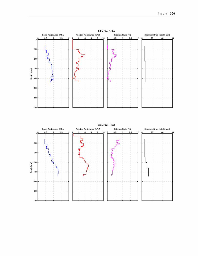
P a g e | 326
0 0.5 1 1.5 2
-700
-600
-500
-400
-300
-200
-100
0
Dep
th (m
m)
Cone Resistance (MPa)
BSC-01-R-S1
0 2 4 6 8 10Friction Resistance (kPa)
0 0.5 1 1.5 2Friction Ratio (%)
0 20 40 60Hammer Drop Height (cm)
0 0.5 1 1.5 2
-700
-600
-500
-400
-300
-200
-100
0
Dep
th (m
m)
Cone Resistance (MPa)
BSC-02-R-S2
0 2 4 6 8 10Friction Resistance (kPa)
0 0.5 1 1.5 2Friction Ratio (%)
0 20 40 60Hammer Drop Height (cm)
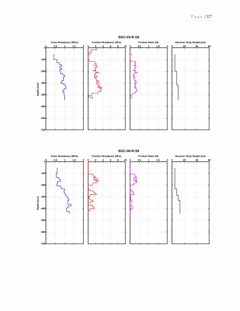
P a g e | 327
0 0.5 1 1.5 2
-700
-600
-500
-400
-300
-200
-100
0
Dept
h (m
m)
Cone Resistance (MPa)
BSC-03-R-S9
0 2 4 6 8 10Friction Resistance (kPa)
0 0.5 1 1.5 2Friction Ratio (%)
0 20 40 60Hammer Drop Height (cm)
0 0.5 1 1.5 2
-700
-600
-500
-400
-300
-200
-100
0
Dept
h (m
m)
Cone Resistance (MPa)
BSC-06-R-S8
0 2 4 6 8 10Friction Resistance (kPa)
0 0.5 1 1.5 2Friction Ratio (%)
0 20 40 60Hammer Drop Height (cm)
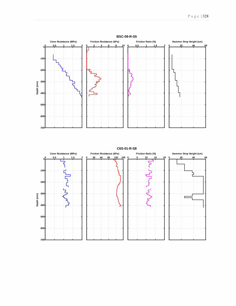
P a g e | 328
0 0.5 1 1.5 2
-700
-600
-500
-400
-300
-200
-100
0
Dept
h (m
m)
Cone Resistance (MPa)
BSC-09-R-S5
0 2 4 6 8 10Friction Resistance (kPa)
0 0.5 1 1.5 2Friction Ratio (%)
0 20 40 60Hammer Drop Height (cm)
0 0.5 1 1.5 2
-700
-600
-500
-400
-300
-200
-100
0
Dept
h (m
m)
Cone Resistance (MPa)
C6S-01-R-S8
0 30 60 90 120 150Friction Resistance (kPa)
0 5 10 15 20Friction Ratio (%)
0 20 40 60Hammer Drop Height (cm)

P a g e | 329
0 0.5 1 1.5 2
-700
-600
-500
-400
-300
-200
-100
0
Dept
h (m
m)
Cone Resistance (MPa)
C6S-04-R-S2
0 30 60 90 120 150Friction Resistance (kPa)
0 5 10 15 20Friction Ratio (%)
0 20 40 60Hammer Drop Height (cm)
0 0.5 1 1.5 2
-700
-600
-500
-400
-300
-200
-100
0
Dept
h (m
m)
Cone Resistance (MPa)
CSB-01-R-S8
0 5 10 15 20 25Friction Resistance (kPa)
0 5 10 15 20Friction Ratio (%)
0 20 40 60Hammer Drop Height (cm)
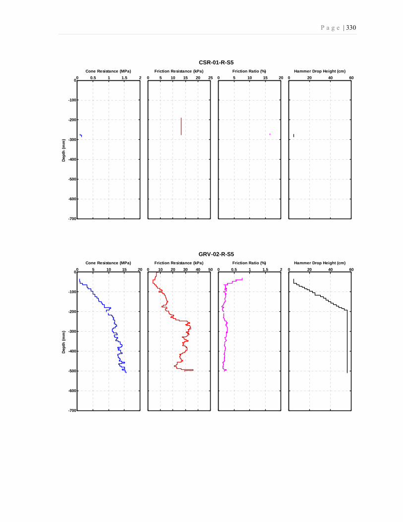
P a g e | 330
0 0.5 1 1.5 2
-700
-600
-500
-400
-300
-200
-100
0
Dept
h (m
m)
Cone Resistance (MPa)
CSR-01-R-S5
0 5 10 15 20 25Friction Resistance (kPa)
0 5 10 15 20Friction Ratio (%)
0 20 40 60Hammer Drop Height (cm)
0 5 10 15 20
-700
-600
-500
-400
-300
-200
-100
0
Dept
h (m
m)
Cone Resistance (MPa)
GRV-02-R-S5
0 10 20 30 40 50Friction Resistance (kPa)
0 0.5 1 1.5 2Friction Ratio (%)
0 20 40 60Hammer Drop Height (cm)
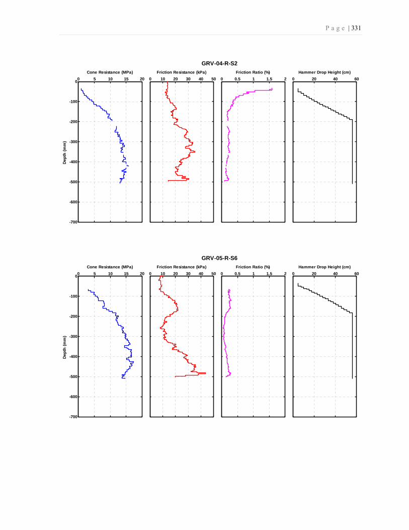
P a g e | 331
0 5 10 15 20
-700
-600
-500
-400
-300
-200
-100
0
Dept
h (m
m)
Cone Resistance (MPa)
GRV-04-R-S2
0 10 20 30 40 50Friction Resistance (kPa)
0 0.5 1 1.5 2Friction Ratio (%)
0 20 40 60Hammer Drop Height (cm)
0 5 10 15 20
-700
-600
-500
-400
-300
-200
-100
0
Dept
h (m
m)
Cone Resistance (MPa)
GRV-05-R-S6
0 10 20 30 40 50Friction Resistance (kPa)
0 0.5 1 1.5 2Friction Ratio (%)
0 20 40 60Hammer Drop Height (cm)
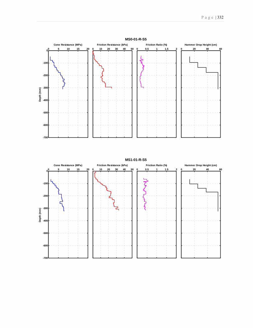
P a g e | 332
0 5 10 15 20
-700
-600
-500
-400
-300
-200
-100
0
Dept
h (m
m)
Cone Resistance (MPa)
MS0-01-R-S5
0 10 20 30 40 50Friction Resistance (kPa)
0 0.5 1 1.5 2Friction Ratio (%)
0 20 40 60Hammer Drop Height (cm)
0 5 10 15 20
-700
-600
-500
-400
-300
-200
-100
0
Dept
h (m
m)
Cone Resistance (MPa)
MS1-01-R-S5
0 10 20 30 40 50Friction Resistance (kPa)
0 0.5 1 1.5 2Friction Ratio (%)
0 20 40 60Hammer Drop Height (cm)

P a g e | 333
0 5 10 15 20
-700
-600
-500
-400
-300
-200
-100
0
Dept
h (m
m)
Cone Resistance (MPa)
MS2-01-R-S5
0 10 20 30 40 50Friction Resistance (kPa)
0 0.5 1 1.5 2Friction Ratio (%)
0 20 40 60Hammer Drop Height (cm)
0 5 10 15 20
-700
-600
-500
-400
-300
-200
-100
0
Dept
h (m
m)
Cone Resistance (MPa)
MS3-01-R-S5
0 10 20 30 40 50Friction Resistance (kPa)
0 0.5 1 1.5 2Friction Ratio (%)
0 20 40 60Hammer Drop Height (cm)

P a g e | 334
0 5 10 15 20
-700
-600
-500
-400
-300
-200
-100
0
Dept
h (m
m)
Cone Resistance (MPa)
MS4-01-R-S5
0 10 20 30 40 50Friction Resistance (kPa)
0 0.5 1 1.5 2Friction Ratio (%)
0 20 40 60Hammer Drop Height (cm)
0 5 10 15 20
-700
-600
-500
-400
-300
-200
-100
0
Dept
h (m
m)
Cone Resistance (MPa)
MS5-01-R-S5
0 10 20 30 40 50Friction Resistance (kPa)
0 0.5 1 1.5 2Friction Ratio (%)
0 20 40 60Hammer Drop Height (cm)

P a g e | 335
0 1 2 3 4
-700
-600
-500
-400
-300
-200
-100
0
Dept
h (m
m)
Cone Resistance (MPa)
RSC-01-R-S1
0 5 10 15 20 25Friction Resistance (kPa)
0 0.5 1 1.5 2Friction Ratio (%)
0 20 40 60Hammer Drop Height (cm)
0 1 2 3 4
-700
-600
-500
-400
-300
-200
-100
0
Dept
h (m
m)
Cone Resistance (MPa)
RSC-02-R-S2
0 5 10 15 20 25Friction Resistance (kPa)
0 0.5 1 1.5 2Friction Ratio (%)
0 20 40 60Hammer Drop Height (cm)

P a g e | 336
0 1 2 3 4
-700
-600
-500
-400
-300
-200
-100
0
Dept
h (m
m)
Cone Resistance (MPa)
RSC-03-R-S9
0 5 10 15 20 25Friction Resistance (kPa)
0 0.5 1 1.5 2Friction Ratio (%)
0 20 40 60Hammer Drop Height (cm)
0 1 2 3 4
-700
-600
-500
-400
-300
-200
-100
0
Dept
h (m
m)
Cone Resistance (MPa)
RSC-08-R-S3
0 5 10 15 20 25Friction Resistance (kPa)
0 0.5 1 1.5 2Friction Ratio (%)
0 20 40 60Hammer Drop Height (cm)
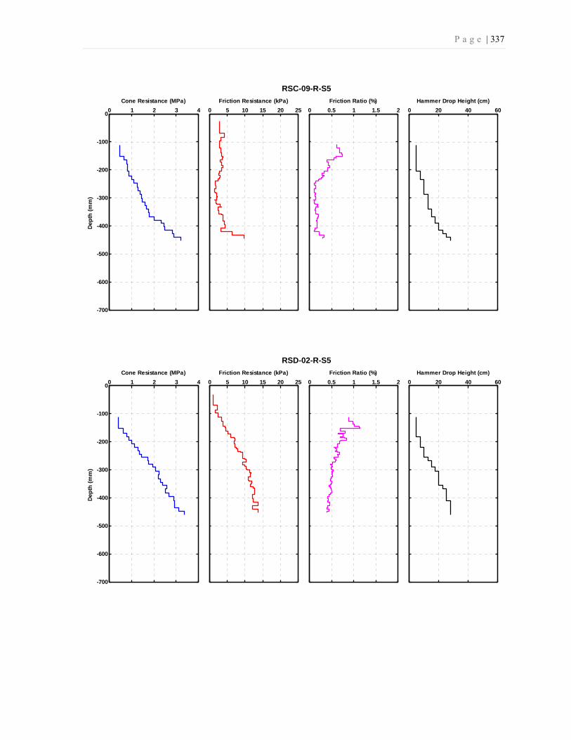
P a g e | 337
0 1 2 3 4
-700
-600
-500
-400
-300
-200
-100
0
Dept
h (m
m)
Cone Resistance (MPa)
RSC-09-R-S5
0 5 10 15 20 25Friction Resistance (kPa)
0 0.5 1 1.5 2Friction Ratio (%)
0 20 40 60Hammer Drop Height (cm)
0 1 2 3 4
-700
-600
-500
-400
-300
-200
-100
0
Dept
h (m
m)
Cone Resistance (MPa)
RSD-02-R-S5
0 5 10 15 20 25Friction Resistance (kPa)
0 0.5 1 1.5 2Friction Ratio (%)
0 20 40 60Hammer Drop Height (cm)

P a g e | 338
0 1 2 3 4
-700
-600
-500
-400
-300
-200
-100
0
Dept
h (m
m)
Cone Resistance (MPa)
RSD-03-R-S6
0 5 10 15 20 25Friction Resistance (kPa)
0 0.5 1 1.5 2Friction Ratio (%)
0 20 40 60Hammer Drop Height (cm)
0 1 2 3 4
-700
-600
-500
-400
-300
-200
-100
0
Dept
h (m
m)
Cone Resistance (MPa)
RSD-04-R-S7
0 5 10 15 20 25Friction Resistance (kPa)
0 0.5 1 1.5 2Friction Ratio (%)
0 20 40 60Hammer Drop Height (cm)
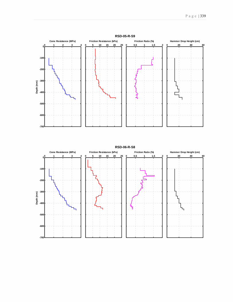
P a g e | 339
0 1 2 3 4
-700
-600
-500
-400
-300
-200
-100
0
Dept
h (m
m)
Cone Resistance (MPa)
RSD-05-R-S9
0 5 10 15 20 25Friction Resistance (kPa)
0 0.5 1 1.5 2Friction Ratio (%)
0 20 40 60Hammer Drop Height (cm)
0 1 2 3 4
-700
-600
-500
-400
-300
-200
-100
0
Dept
h (m
m)
Cone Resistance (MPa)
RSD-06-R-S8
0 5 10 15 20 25Friction Resistance (kPa)
0 0.5 1 1.5 2Friction Ratio (%)
0 20 40 60Hammer Drop Height (cm)
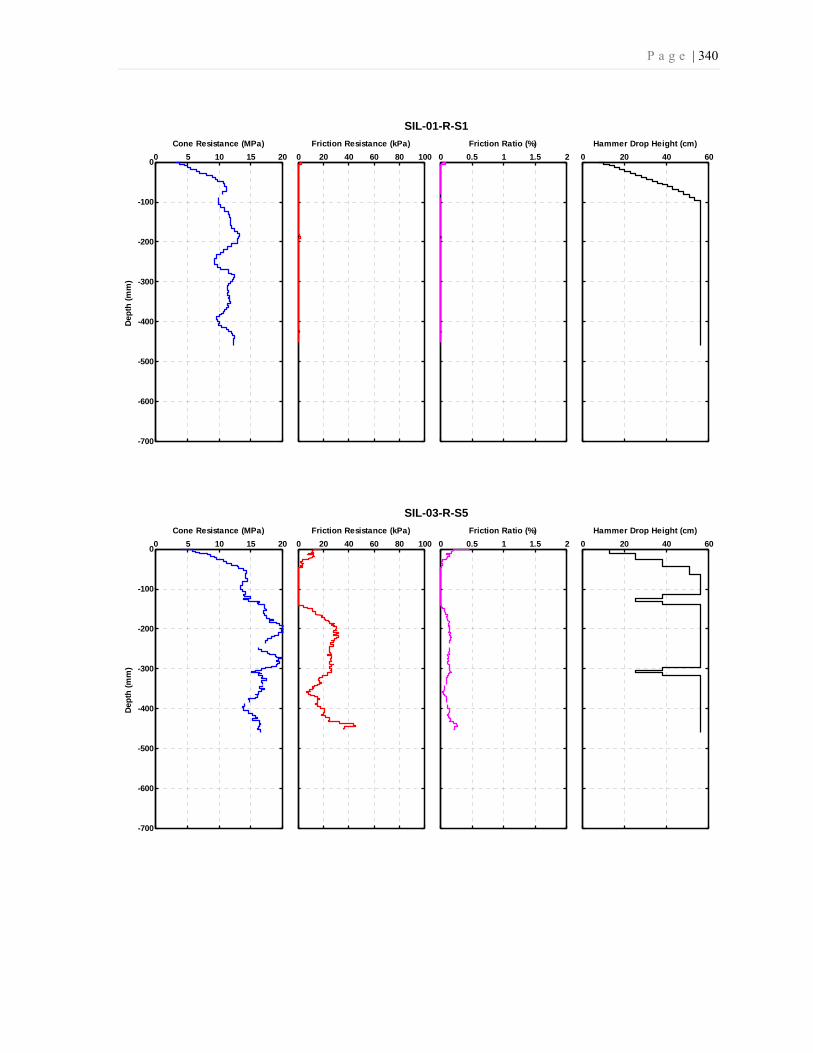
P a g e | 340
0 5 10 15 20
-700
-600
-500
-400
-300
-200
-100
0
Dept
h (m
m)
Cone Resistance (MPa)
SIL-01-R-S1
0 20 40 60 80 100Friction Resistance (kPa)
0 0.5 1 1.5 2Friction Ratio (%)
0 20 40 60Hammer Drop Height (cm)
0 5 10 15 20
-700
-600
-500
-400
-300
-200
-100
0
Dept
h (m
m)
Cone Resistance (MPa)
SIL-03-R-S5
0 20 40 60 80 100Friction Resistance (kPa)
0 0.5 1 1.5 2Friction Ratio (%)
0 20 40 60Hammer Drop Height (cm)
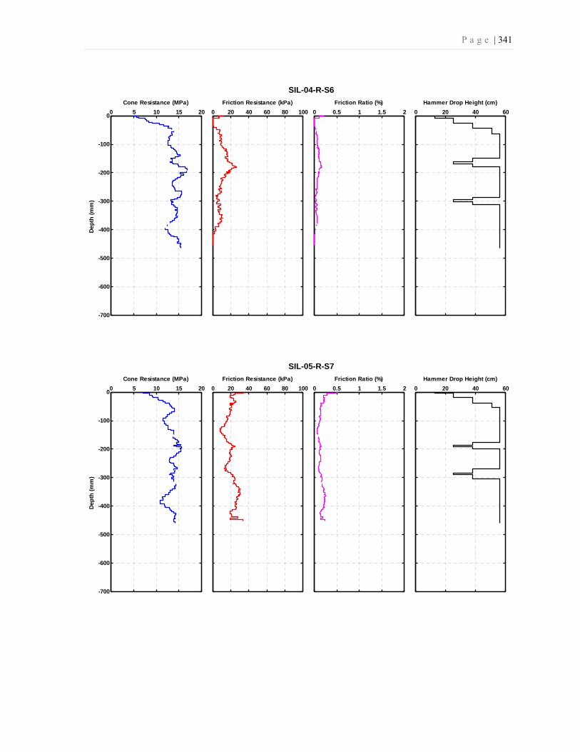
P a g e | 341
0 5 10 15 20
-700
-600
-500
-400
-300
-200
-100
0
Dept
h (m
m)
Cone Resistance (MPa)
SIL-04-R-S6
0 20 40 60 80 100Friction Resistance (kPa)
0 0.5 1 1.5 2Friction Ratio (%)
0 20 40 60Hammer Drop Height (cm)
0 5 10 15 20
-700
-600
-500
-400
-300
-200
-100
0
Dept
h (m
m)
Cone Resistance (MPa)
SIL-05-R-S7
0 20 40 60 80 100Friction Resistance (kPa)
0 0.5 1 1.5 2Friction Ratio (%)
0 20 40 60Hammer Drop Height (cm)
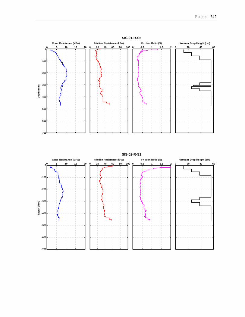
P a g e | 342
0 5 10 15 20
-700
-600
-500
-400
-300
-200
-100
0
Dept
h (m
m)
Cone Resistance (MPa)
SIS-01-R-S5
0 20 40 60 80 100Friction Resistance (kPa)
0 0.5 1 1.5 2Friction Ratio (%)
0 20 40 60Hammer Drop Height (cm)
0 5 10 15 20
-700
-600
-500
-400
-300
-200
-100
0
Dept
h (m
m)
Cone Resistance (MPa)
SIS-02-R-S1
0 20 40 60 80 100Friction Resistance (kPa)
0 0.5 1 1.5 2Friction Ratio (%)
0 20 40 60Hammer Drop Height (cm)

P a g e | 343
0 5 10 15 20
-700
-600
-500
-400
-300
-200
-100
0
Dept
h (m
m)
Cone Resistance (MPa)
SIS-05-R-S4
0 20 40 60 80 100Friction Resistance (kPa)
0 0.5 1 1.5 2Friction Ratio (%)
0 20 40 60Hammer Drop Height (cm)
0 5 10 15 20
-700
-600
-500
-400
-300
-200
-100
0
Dept
h (m
m)
Cone Resistance (MPa)
SIS-07-R-S6
0 20 40 60 80 100Friction Resistance (kPa)
0 0.5 1 1.5 2Friction Ratio (%)
0 20 40 60Hammer Drop Height (cm)

Boston, Massachusetts
April, 2011