1

Development and Use of Engineering Standards for

Computational Fluid Dynamics for Complex Aerospace

Systems

Hyung B. Lee

Bettis Laboratory, West Mifflin, Pennsylvania, United States

Urmila Ghia

University of Cincinnati, Cincinnati, Ohio, United States

Sami Bayyuk

ESI Group US R&D, Huntsville, Alabama, United States

William L. Oberkampf

WLO Consulting, Austin, Texas, United States

Christopher J. Roy

Virginia Tech, Blacksburg, Virginia, United States

John A. Benek

Air Force Research Laboratory, Wright-Patterson AFB, Ohio, United States

Christopher L. Rumsey

NASA Langley Research Center, Hampton, Virginia, United States

Joseph M. Powers

University of Notre Dame, Notre Dame, Indiana, United States

Robert H. Bush

Pratt and Whitney, East Hartford, Connecticut, United States

Mortaza Mani

Boeing Research and Technology, St. Louis, Missouri, United States

ABSTRACT

Computational fluid dynamics (CFD) and other advanced modeling and simulation (M&S) methods are

increasingly relied on for predictive performance, reliability and safety of engineering systems. Analysts,

designers, decision makers, and project managers, who must depend on simulation, need practical techniques

and methods for assessing simulation credibility. The AIAA Guide for Verification and Validation of

Computational Fluid Dynamics Simulations (AIAA G-077-1998 (2002)), originally published in 1998, was the

first engineering standards document available to the engineering community for verification and validation

(V&V) of simulations. Much progress has been made in these areas since 1998. The AIAA Committee on

Standards for CFD is currently updating this Guide to incorporate in it the important developments that

have taken place in V&V concepts, methods, and practices, particularly with regard to the broader context of

predictive capability and uncertainty quantification (UQ) methods and approaches.

This paper will provide an overview of the changes and extensions currently underway to update the AIAA

Guide. Specifically, a framework for predictive capability will be described for incorporating a wide range of

error and uncertainty sources identified during the modeling, verification, and validation processes, with the

goal of estimating the total prediction uncertainty of the simulation. The Guide’s goal is to provide a

foundation for understanding and addressing major issues and concepts in predictive CFD. However, this

https://ntrs.nasa.gov/search.jsp?R=20160010173 2018-07-13T13:15:58+00:00Z

2

Guide will not recommend specific approaches in these areas as the field is rapidly evolving. It is hoped that

the guidelines provided in this paper, and explained in more detail in the Guide, will aid in the research,

development, and use of CFD in engineering decision-making.

1. Introduction and Overview

Computational fluid dynamics (CFD) and other advanced modeling and simulation (M&S) methods are increasingly

relied on for predictive performance, reliability and safety of engineering systems. Analysts, designers, decision

makers, and project managers, who must depend on simulation, need practical techniques and methods for assessing

simulation credibility. The AIAA Guide for Verification and Validation of Computational Fluid Dynamics

Simulations (AIAA G-077-1998 (2002)), originally published in 1998, was the first engineering standards document

available to the engineering community for verification and validation (V&V) of simulations. Much progress has

been made in these areas since 1998. The AIAA Committee on Standards for CFD is currently updating this Guide

to incorporate in it the important developments that have taken place in V&V concepts, methods, and practices,

particularly with regard to the broader context of predictive capability and uncertainty quantification (UQ) methods

and approaches.

The goal of the updated AIAA Guide (Guide Update) is to provide a foundation for understanding and addressing

major issues and concepts in predictive CFD. Predictive CFD is the application of CFD computations to problems or

conditions for which these computations have not been validated, and is, in turn, enabled by the implementation and

practice of systematic, focused and structured programs for V&V and UQ. To that end, AIAA Guide will explain

how verification, validation, and uncertainty quantification can form a comprehensive framework for estimating

predictive uncertainty of M&S. This framework is comprehensive in the sense that it treats all types of uncertainty,

incorporates uncertainty due to mathematical form of the model, provides a procedure for including estimates of

numerical error in the predictive uncertainty, and provides a means for propagating parameter uncertainty through

the model to the system response quantity of interest. The framework, thus, provides a means to estimate and

quantify the total predictive uncertainty and, in turn, a way to convey the total predictive uncertainty of a simulation

result to decision makers. However, at this point the Guide will not recommend specific approaches in these areas as

the field is still rapidly evolving. It is hoped that in the near term the Guide will aid in the research, development,

and use of CFD as a predictive tool, especially in support of engineering decision-making.

In practice, it is envisioned that the AIAA Guide Update will educate and inform the software and methods

developers, analysts, technical management and decision-makers on the value of and the need to conduct V&V and

UQ for M&S. Specifically, the Guide Update will show:

1) Why V&V and UQ are important and needed in support of M&S;

2) How V&V and UQ contribute to improving the credibility of M&S and supporting decision

making;

3) Who is responsible for conducting specific elements of V&V and UQ; and

4) Guidelines for accomplishing various activities in V&V and UQ.

This paper proposes a framework for predictive capability that incorporates a wide range of error and uncertainty

sources identified during the modeling, verification, and validation processes, with the goal of estimating the total

prediction uncertainty of the M&S. Specifically, it describes the framework and its main components and outlines

the main methods and approaches for quantification of uncertainty and for propagating uncertainty in predictive

M&S. It also discusses how predictive capability relies on V&V and UQ, as well as other factors that affect

predictive capability.

The described framework will be included and featured in the upcoming AIAA Guide Update as a set of general

guidelines for predictive CFD. It is envisioned that over time the AIAA Guide will foster and support the use of

predictive CFD in engineering design, virtual prototyping, certification, risk analysis, and high-consequence

decision-making.

3

2. Fundamental Concepts in Verification, Validation, and Uncertainty Quantification

For scientific simulations, one starts with governing equations. These equations describe the system of interest, and

encapsulate knowledge of physics, chemistry, and mathematics. The equations constitute a mathematical model of

the physical world, and may be made up of submodels, or accept other submodels as input to the problem to be

solved. The equations are often field equations – partial differential equations (PDEs) or integro-differential

equations – that describe a time-varying solution over some volume of space or material, subject to initial and

boundary conditions. Submodels could describe the particular response of a material, of interactions between

materials such as chemical reactions, or some aspect of the governing equations that is approximated or makes the

equations easier to solve.

The problem, then, is to find a solution to the mathematical model given the initial and boundary conditions and the

appropriate submodels. One approach to obtaining solutions is through numerical simulations. The governing

equations are discretized by algorithms, or numerical methods, and as a result the mathematical model is

transformed to a discrete model, or a computational model. Solutions of the computational model (numerical

solutions) are approximate solutions of the mathematical model. To obtain numerical solutions, the computational

model is implemented in software on a computer; this implementation is often called a computer code, and an

execution of the code is called a simulation. The numerical methods considered here have one or more parameters

that specify the number of discrete degrees of freedom, such as the number of elements, the number of particles, or

the number of discrete wave numbers, and these parameters control the accuracy and the computational cost of the

simulation.

Verification and validation are the primary processes for assessing and quantifying the accuracy and reliability of

numerical simulations. The V&V definitions used in this paper are those adopted from the original AIAA Guide for

Verification and Validation of Computational Fluid Dynamics Simulations (AIAA Guide) [1]:

Verification is the process of determining that a model implementation accurately represents the

developer’s conceptual description of the model and the solution to the model.

Validation is the process of determining the degree to which a model is an accurate representation of the

real world from the perspective of the intended uses of the model.

In essence, verification provides evidence that the model is solved right. Verification does not address whether the

model has any relationship to the real world. Verification activities only evaluate whether the model, the

mathematical and computer code representation of the physical system, is solved accurately. Verification is

composed of two types of activities: code verification and solution verification. Code verification deals with

assessing: (a) the adequacy of the numerical algorithms to provide accurate numerical solution to the PDEs assumed

in the mathematical model; and (b) the fidelity of the computer programming to implement the numerical algorithms

to solve the discrete equations. Solution verification deals with the quantitative estimation of numerical accuracy of

solutions to the PDEs computed by the code. The primary emphasis in solution verification is significantly different

from that in code verification because there is no known exact solution to the PDEs of interest. As a result, we

believe solution verification is more correctly referred to as numerical error estimation; that is, the primary goal is

estimating the numerical accuracy of given solution, typically for nonlinear PDEs with singularities, discontinuities,

and complex geometries. For this type of PDE, numerical error estimation is fundamentally empirical (a posteriori),

i.e., the conclusions are based on evaluation and analysis of solution results from the code.

Validation, on the other hand, provides evidence that the right model is solved. This perspective implies that the

model is solved correctly, or verified. However, multiple errors or inaccuracies can cancel one another and give the

appearance of a validated solution. Verification is the first step of the validation process and, while not simple, it is

much less complex than the more comprehensive nature of validation. Validation addresses the question of the

fidelity of the model to specific conditions of the real world. The terms “evidence” and “fidelity” both imply the

concept of “estimation of tolerance,” not simply “yes” or “no” answers.

The goal of validation is to determine the predictive capability of a computational model for its intended use. This is

accomplished by comparing computational predictions (simulation outcomes) to observations (experimental

outcomes). The approach of validation is to measure the agreement between the simulation outcomes from a

4

computational model and the experimental outcomes from appropriately designed and conducted experiments, i.e.,

validation experiment. A validation metric is the basis for comparing simulation outcomes with experimental

outcomes and, as such, serves as a measure that defines the level of accuracy and precision of a simulation.

Validation metrics should be established during the validation (or accuracy) requirement phase of the V&V program

planning and development. In selecting the validation metric, the primary consideration should be what the model

must predict in conjunction with what types of data could be available from the experiment. Additionally, the

metrics should provide a measure of agreement that includes uncertainty requirements, e.g., experimental and

modeling uncertainties in dimensions, materials, loads, and responses. In most cases, assessing the predictive

capability of a computational model over the full range of its intended use cannot be based solely upon data already

available at the beginning of the V&V program. The challenge is to define and conduct a set of experiments that will

provide a stringent-enough test of the model that the decision maker will have adequate confidence to employ the

model for predicting the reality of interest. If the model predicts the experimental outcomes within the

predetermined accuracy requirements, the model is considered validated for its intended use.

Uncertainty Quantification is the process of characterizing all uncertainties in the model and experiment, and

quantifying their effect on the simulation and experimental outcomes. UQ is a closely related activity to V&V and

essential for verifying and validating simulation models. The goal of UQ, along with V&V, is to enable modelers

and analysts to make precise statements about the degree of confidence they have in their simulation-based

predictions. In this context, UQ can be defined as the

Identification (Where are the uncertainties?),

Characterization (What form they are in?),

Propagation (How they evolve during the simulation?), and

Analysis (What are their impacts?),

of all uncertainties in simulation models. As such, in UQ of simulation models, all significant sources of error and

uncertainty in model simulations must be identified and treated to quantify their effects on the simulation results.

These sources of error and uncertainty include: systematic and stochastic measurement error; ignorance; limitations

of theoretical models; limitations of numerical representations of those models; limitations on the accuracy and

reliability of computations, approximations, and algorithms; and human error. Specifically, UQ assesses the

confidence in model predictions and allows resource allocation for fidelity improvements.

Figure 1 shows a framework from the ASME Guide for Verification and Validation in Computational Solid

Mechanics (ASME Guide) [2] for organizing these different model assessment techniques, i.e., verification,

validation and uncertainty quantification, with the goal of assessing accuracy of numerical simulation results for an

intended use. Figure 1 also identifies the various activities and products involved in V&V and UQ assessments

along the respective modeling and experimental branches. The framework recognizes that there are numerical errors

and uncertainties as well as errors and uncertainties in experimental data.

In the assessment activity of code verification, the modeler uses the computational model on a set of problems with

known solutions. These problems typically have much simpler geometry, loads, and boundary conditions than the

validation problems, to identify and eliminate algorithmic and programming errors. Then, in the subsequent activity

of solution (calculation) verification, the version of the computational model to be used for validation problems (i.e.,

with the geometries, loads and boundary conditions typical of those problems) is used for identifying sufficient mesh

resolution to produce an adequate solution tolerance, including the effects of finite precision arithmetic. Solution

verification yields a quantitative estimate of the numerical precision and discretization accuracy for calculations

made with the computational model for use in validation assessments. Thus, code and solution verification serve as

the basis for estimating numerical errors and uncertainty.

Validation attempts to quantify the accuracy of the mathematical model through comparisons with experimental

measurements. To that end, validation experiments are performed to generate data for assessing the accuracy of the

mathematical model via simulation outcomes produced by the verified computational model. A validation

experiment is a physical realization of a properly posed applied mathematics problem with initial conditions,

boundary conditions, material properties, and external forces. To qualify as a validation experiment, the geometry of

the object being tested (e.g., a component, subassembly, assembly, or full system), the initial conditions and the

boundary conditions of the experiment, and all of the other model input parameters must be prescribed as

5

completely and accurately as possible. Ideally, this thoroughness on the part of the experimenter will provide as

many constraints as possible, requiring few assumptions on the part of the modeler. All of the applied loads,

multiple response features, and changes in the boundary conditions should be measured; and uncertainties in the

measurements should be reported.

Figure 1. A framework for V&V and UQ (from [2]).

Validation of mathematical models must take into account the uncertainties associated with both simulation results

and experimental data. As such, throughout the modeling (left branch of Figure 1) and experimental (right branch of

Figure 1) processes, and especially during the uncertainty quantification activity, all significant sources of

uncertainty in model simulations and experimental measurements must be identified and treated to quantify their

effects on the assessment of model accuracy, i.e., a comparison of simulation outcomes (simulation results with

estimates of uncertainty) with experimental outcomes (experimental measurements with estimate of uncertainty).

Model validation, thus, is the basis for quantifying model-form errors and uncertainty. Clearly, any large numerical

errors or uncertainties, or large experimental errors or uncertainties, will make it difficult to isolate differences

between the mathematical model and the reality it attempts to describe. As shown in Figure 1, the various

assessment techniques are combined so that ultimately, a probabilistic comparison can be made between the

mathematical model that the code seeks to express and the physical model that the experiments attempt to observe.

6

If the agreement between the experimental and simulation outcomes is unacceptable, the model and/or the

experiment can be revised. Model revision is the process of changing the basic assumptions, structure, parameter

estimates, boundary values, or initial conditions of a model to improve agreement with experimental outcomes.

Experiment revision is the process of changing experimental test design, procedures, or measurements to improve

agreement with simulation outcomes. Whether the model or the experiment (or both) are revised depends upon the

judgment of the model developer and experimenter.

In simulations involving complex physics or multidisciplinary engineering systems, strict adherence to V&V and

UQ procedures commonly becomes impractical. For example, when all of the important physical modeling

parameters are not known a priori, some of the parameters are considered adjustable. Or when grid-resolved

solutions are not attainable because of the computer resources needed for the simulation, adjustments must be made

to improve agreement with the experimental data. When these types of activities occur, the term calibration,

parameter estimation, or model updating more appropriately describes the process than does validation.

Model calibration is the process of adjusting input parameters of the model to obtain the best match between

simulation results and experimental measurements. In a similar vein, model parameters may be adjusted to match

results from a more sophisticated model, e.g., adjusting turbulence model parameters to match results from direct

numerical simulations (DNS). Depending on the model parameter being calibrated, calibration often restricts the

applicability of the model to the domain of the data used to calibrate the parameter. As such, calibration is a model

development activity, but is often confused or combined with model assessment activities. For example, after

calibrating a model parameter to match experimental data, a claim that the code is validated for similar conditions is

often (erroneously) made. Another common practice is to refine or coarsen the mesh for a numerical simulation until

the results agree with experimental data; this is a calibration of a numerical simulation parameter (the mesh

resolution) but is often claimed to be validation or solution verification.

Although not shown explicitly on the modeling branch of the framework shown in Figure 1, UQ also examines the

mapping between the uncertain model inputs to a code and the code’s results, namely UQ estimates the effects of the

input uncertainty on the simulation results. This process is known as propagation of input parameter uncertainties

through the model to the output parameters to quantify the parameter uncertainty. In the context of the assessment

of numerical simulation results, inputs can include parameters that define the geometry, the material models,

physical models, and the boundary and initial conditions. For these types of inputs, uncertainty quantification

estimates how much the simulation results may vary when these inputs are not known, are known imprecisely, or

have inherent variability. Another type of input includes parameters associated with the numerical method, or

possibly a choice between several methods.

3. Perspective of Validation, Calibration, and Prediction

The goal of model V&V and UQ is to enable scientists and analysts to make precise statements about the degree of

confidence they have in their simulation-based predictions. The AIAA Guide defines prediction as “use of a

computational model to foretell the state of a physical system under conditions for which the computational model

has not been validated.” The predictive accuracy of the model must then reflect the strength of the inference being

made from the validation database to the prediction. Thus, validation database represents reproducible evidence that

a model has achieved a given level of accuracy in the solution of specified problems. From this perspective,

validation comparisons do not directly allow one to make claims about the accuracy of predictions; they only allow

inferences to be made. For physical processes that are well understood both physically and mathematically, the

inference can be quite strong. For complex physical processes, the inference can be quite weak. The value and

consequence of such an inference degrade as the physical process becomes more complex. The quantification of the

inference in prediction is presently an important topic of research [3]. If necessary, one can improve the predictive

accuracy of the model through additional experiments, information, and/or experience.

The requirement that the V&V process quantify the predictive accuracy of the model underscores the key role of

uncertainty quantification in the model-validation process. In this context, nondeterminism refers to the existence of

errors and uncertainties in the outputs of computational simulations due to inherent and/or subjective uncertainties in

the model. Likewise, the measurements that are made to validate these simulation outcomes also contain errors and

uncertainties. While the experimental outcome is used as the reference for comparison, the V&V process does not

7

presume the experiment to be more accurate than the simulation. Instead, the goal is to quantify the uncertainties in

both experimental and simulation results such that the model fidelity requirements can be assessed (validation) and

the predictive accuracy of the model quantified.

Although there is increasing consistency in the formal definition of the term “validation” [1, 2], in practice there are

three key, and distinct, aspects in validation [4]: (1) quantification of the accuracy of the computational model by

comparing its responses with experimentally measured responses, (2) interpolation or extrapolation of the

computational model to conditions corresponding to the intended use of the model, and (3) determination if the

estimated accuracy of the computational model, for the conditions of the intended use, satisfies the accuracy

requirements specified. The definition of validation, given at the beginning of Section 2, is not particularly clear,

however, about the identification of these aspects. Consequently, this definition of validation can be interpreted to

include all three aspects, or interpreted to only include the first aspect. Figure 2 depicts these three aspects, as well

as the input information required by these aspects.

Figure 2. Three aspects of model validation (from [4]).

It is clear from Figure 2 that the quantification of model accuracy (aspect 1) obtained by comparing responses from

the computational model with experimentally measured responses is distinctively different from prediction, e.g.,

extrapolation of the model beyond the domain of validation to the conditions of the intended use (aspect 2). The

interpolation or extrapolation of the model for its intended use must include the estimated uncertainty in the

prediction, which is then compared with the accuracy requirements so that a decision can be made whether the

prediction accuracy is adequate (aspect 3). The most recent engineering standards document devoted to V&V,

referred to as the ASME Guide [2], considers all three aspects of validation to be fundamentally combined in the

term “validation.” The AIAA Guide, on the other hand, takes the view that “validation” is only concerned with the

first aspect, i.e., assessment of model accuracy by comparison with experimental responses. Uncertainty is involved

in this assessment, both in terms of experimental measurement uncertainty and in terms of the computational

simulation, primarily because input quantities needed from the experiment either are not available or are imprecisely

characterized. The second and third aspects (aspects 2 and 3) are treated in the AIAA Guide as separate activities

related to predictive capability. The AIAA Guide recognizes that predictive capability uses the assessed model

accuracy as input and that predictive capability also incorporates (a) additional uncertainty estimation resulting from

interpolation or extrapolation of the model beyond the existing experimental database to future applications of

8

interest and (b) comparison of the accuracy requirements needed by a particular application relative to the estimated

accuracy of the model for that specific extrapolation to the applications of interest.

In practice, model validation can be viewed as two steps: (1) quantitatively comparing the computational and

experimental results for the System Response Quantity (SRQ) of interest, and (2) determining whether there is

acceptable agreement between the model and the experiment for the intended use of the model. The first step in

validation deals with accuracy assessment of the model. Figure 3 depicts several important aspects of validation, as

well as issues of prediction and calibration of models. The left-center portion of Figure 3 shows the first step in

validation. The figure illustrates that the same SRQ must be obtained from both the computational model and the

physical experiment. The SRQ can be any type of physically measurable quantity, or it can be a quantity that is

based on, or inferred from, measurements. For example, the SRQ can involve derivatives, integrals, or more

complex data processing of computed or measured quantities such as the maximum or minimum of functionals over

a domain. The SRQs are commonly one of three mathematical forms: (1) a deterministic quantity, i.e., a single

value, such as a mean value or a maximum value over a domain; (2) a probability measure, such as a probability

density function or a cumulative distribution function; or (3) a probability-box (also called a p-box). Each of these

forms can be functions of a parameter or multiple parameters in the computational model, such as a temperature or a

Mach number; a function of spatial coordinates, such as Cartesian coordinates (x, y, z); or a function of both space

and time. If both the computational and experimental SRQs are deterministic quantities, the validation metric will

also be a deterministic quantity. If either of the SRQs is a probability distribution or p-box, the result of the

validation metric could be a number, probability distribution, or p-box, depending on the construction of the

validation metric.

Figure 3. Validation, calibration, and prediction (from [5]).

Another feature that should be stressed in Figure 3 is the appropriate interaction between computation and

experimentation that should occur in a validation experiment. To achieve the most value from the validation

experiment, there should be in-depth, forthright, and frequent communication between computationalists and

experimentalists during the planning and design of the experiment. Also, after the experiment has been completed,

the experimentalists should measure and provide to the computationalists all the important input quantities needed to

conduct the computational simulation. Examples of these quantities are actual freestream conditions attained in a

wind-tunnel experiment (versus requested conditions), as-fabricated model geometry (versus as-designed), and

actual deformed model geometry due aerodynamics loads and heating. What should not be provided to the

computationalists in a rigorous validation activity is the measured SRQ. Stated differently, it is our view that a blind

computational prediction be compared with experimental results so that a true measure of predictive capability can

be assessed in the validation metric.

9

The second step in validation deals with comparing the validation metric result with the accuracy requirements for

the intended use of the model. That is, validation, from a practical or engineering perspective, is not a philosophical

statement of truth. The second step in validation, depicted in the right-center portion of Figure 3, is an engineering

decision that is dependent on the accuracy requirements for the intended use of the model. Accuracy requirements

are, of course, dependent on many different kinds of factors. Some examples of these factors are: (a) the complexity

of the model, the physics, and the engineering system of interest; (b) the difference in hardware and environmental

conditions between the engineering system of interest and the validation experiment; (c) the increase in uncertainty

due to extrapolation of the model from the validation conditions to the conditions of the intended use; (d) the risk

tolerance of the decision makers involved; and (e) the consequence of failure or underperformance of the system of

interest.

The right-center portion of Figure 3 shows the comparison of the validation metric result with the preliminary

accuracy requirement for the application of interest. This is referred to as a preliminary requirement because, as

shown in Figure 4, the conditions of application of interest, i.e., the application domain, may be different from the

validation domain. If they are different, as is the usual case, then only preliminary accuracy requirement can be

applied. If the model passes these preliminary accuracy requirements, then the model prediction would be made

using extrapolation or interpolation of the model. Accuracy requirements for the application, i.e., final accuracy

requirements, would be made after the model has been extrapolated or interpolated to the conditions of the

application of interest. Setting preliminary accuracy requirements is also useful if the preliminary model accuracy is

inadequate. For instance, it may be concluded that the assumptions and approximations made in the conceptual

model are inadequate to achieve the accuracy needed. This may necessitate a reformulation of the model, as opposed

to calibration of model parameters, at a later stage. In addition, preliminary accuracy assessment provides a natural

mechanism for adjusting and adapting the final accuracy requirements to cost and schedule requirements of the

engineering system of interest. For example, trade-offs can be made between required final accuracy, system design,

and performance, in addition to cost and schedule.

If the preliminary accuracy requirements are not met, then one has two options, as shown in Figure 3. First, the

dashed-line upper feedback loop provides for any of the activities referred to as model updating, model calibration,

or model tuning. Depending on the ability to determine parameters, either by direct measurement or by inference

from a model, we have divided parameter updating into three categories: parameter measurement, parameter

estimation, and parameter calibration. If the model parameters are updated, one could proceed again and perform the

comparison via the validation metric. It is now very likely that the validation metric result would be significantly

reduced, implying much better agreement between the model and the experimental results. The parameter updating

may be physically justifiable, or it may simply be expedient. How to determine the scientific soundness of updating,

and its impact on predictive capability, is a very difficult issue. Second, the lower feedback loop could be taken if:

(a) improvements or changes are needed in experimental measurements, such as improved diagnostic techniques; (b)

additional experiments are needed to reduce experimental uncertainty; or (c) additional experiments are needed that

are more representative of the application of interest.

The right portion of Figure 3 deals with the issue of use of the model to make prediction for the conditions of the

application of interest. It should be noted that Figure 3 is completely consistent with the diagram showing the three

aspects of validation (Figure 2). Also, Figure 3 is conceptually consistent with the ASME Guide diagram in Figure

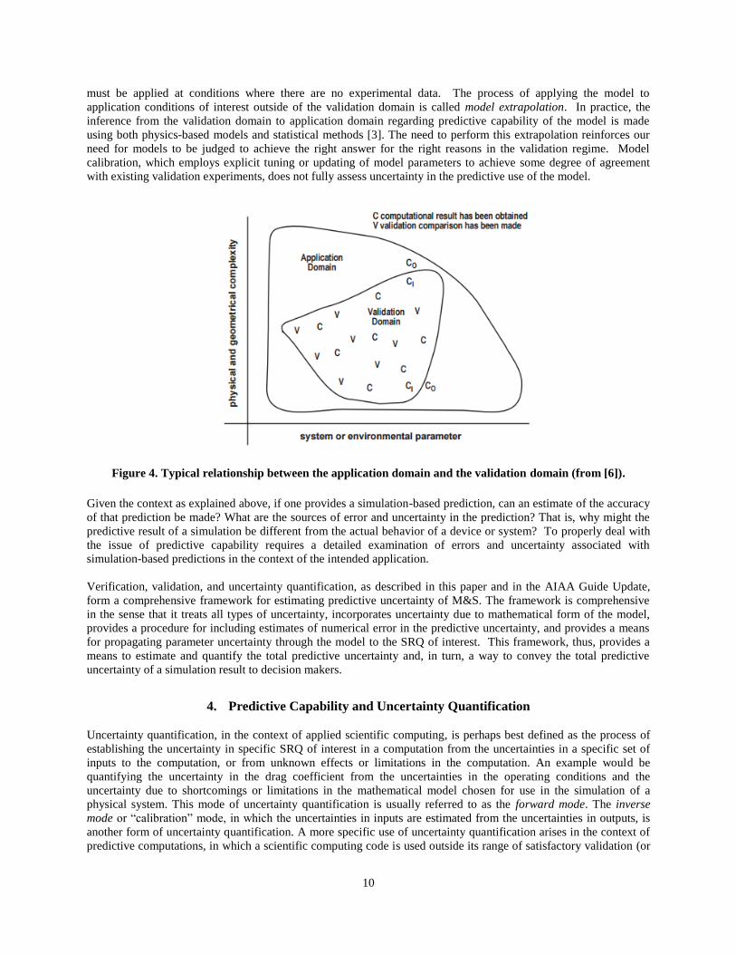
1. To better understand the relationship between validation and prediction, consider Figure 4. The validation

domain in the figure suggests three features. First, in this region we have high confidence that the relevant physics is

understood and modeled at a level that is commensurate with the needs of the application. Second, this confidence

has to be quantitatively demonstrated by satisfactory agreement between simulations and experiments in the

validation database for some range of applicable parameters in the model. And third, the boundary of the domain

indicates that outside this region there is degradation in confidence in the quantitative predictive capability of the

model. Stated differently, outside the validation domain the model is credible, but its quantitative capability has not

been demonstrated. The application domain, sometimes referred to as the operating envelope of the system, is

generally larger than the validation domain and indicates the region where predictive capability is needed from the

model for the applications of interest.

It is generally too expensive (or even impossible) to obtain experimental data over the entire multidimensional space

of model input parameters for the application of interest. In many cases, it is not even possible to obtain

experimental data at the application conditions of interest. As a result, the more common case is that the model

10

must be applied at conditions where there are no experimental data. The process of applying the model to

application conditions of interest outside of the validation domain is called model extrapolation. In practice, the

inference from the validation domain to application domain regarding predictive capability of the model is made

using both physics-based models and statistical methods [3]. The need to perform this extrapolation reinforces our

need for models to be judged to achieve the right answer for the right reasons in the validation regime. Model

calibration, which employs explicit tuning or updating of model parameters to achieve some degree of agreement

with existing validation experiments, does not fully assess uncertainty in the predictive use of the model.

Figure 4. Typical relationship between the application domain and the validation domain (from [6]).

Given the context as explained above, if one provides a simulation-based prediction, can an estimate of the accuracy

of that prediction be made? What are the sources of error and uncertainty in the prediction? That is, why might the

predictive result of a simulation be different from the actual behavior of a device or system? To properly deal with

the issue of predictive capability requires a detailed examination of errors and uncertainty associated with

simulation-based predictions in the context of the intended application.

Verification, validation, and uncertainty quantification, as described in this paper and in the AIAA Guide Update,

form a comprehensive framework for estimating predictive uncertainty of M&S. The framework is comprehensive

in the sense that it treats all types of uncertainty, incorporates uncertainty due to mathematical form of the model,

provides a procedure for including estimates of numerical error in the predictive uncertainty, and provides a means

for propagating parameter uncertainty through the model to the SRQ of interest. This framework, thus, provides a

means to estimate and quantify the total predictive uncertainty and, in turn, a way to convey the total predictive

uncertainty of a simulation result to decision makers.

4. Predictive Capability and Uncertainty Quantification

Uncertainty quantification, in the context of applied scientific computing, is perhaps best defined as the process of

establishing the uncertainty in specific SRQ of interest in a computation from the uncertainties in a specific set of

inputs to the computation, or from unknown effects or limitations in the computation. An example would be

quantifying the uncertainty in the drag coefficient from the uncertainties in the operating conditions and the

uncertainty due to shortcomings or limitations in the mathematical model chosen for use in the simulation of a

physical system. This mode of uncertainty quantification is usually referred to as the forward mode. The inverse

mode or “calibration” mode, in which the uncertainties in inputs are estimated from the uncertainties in outputs, is

another form of uncertainty quantification. A more specific use of uncertainty quantification arises in the context of

predictive computations, in which a scientific computing code is used outside its range of satisfactory validation (or

11

outside its validation domain). This more specific meaning of uncertainty quantification is best defined as predictive

uncertainty, and this more specific meaning is the one covered in this paper and targeted in the AIAA Guide Update.

It is widely understood and accepted that uncertainties, whether random or systematic, arise because of the inherent

randomness in physical systems, modeling idealizations, experimental variability, measurement inaccuracy, etc.,

and cannot be ignored. This fact complicates the already difficult process of model validation by creating an unsure

target — a situation in which neither the simulated nor the observed behavior of the system is known with certainty.

In this context, nondeterminism refers to the existence of errors and uncertainties in the results of M&S because of

inherent and/or subjective uncertainties in the model inputs or model form. Likewise, the measurements that are

made to validate these simulation outcomes also contain errors and uncertainties. In fact, while the experimental

outcome is used as the reference, the V&V process does not presume the experiment to be more accurate than the

simulation. Instead, the goal is to quantify the uncertainties in both experimental and simulation results such that the

model requirements can be assessed and the predictive accuracy of the model quantified.

Once code verification has established that a code correctly implements the numerical methods as intended, there

remain three sources of error and uncertainty in predictions from M&S. The first is numerical methods as they

provide approximate solutions to the governing equations (numerical uncertainty). The second source of error or

uncertainty is that the inputs needed for the simulation are not known precisely (parameter uncertainty). For

example, the device to be simulated can only be constructed to within manufacturing tolerances; parameters in a

model or submodel may not be known precisely, or may be subjective estimates from experts. A third source of

error and uncertainty is that the governing equations do not adequately describe the physics; the real device or

system is affected by some phenomena that are not included in the model or submodels (model form uncertainty).

Different model assessment techniques – solution verification, validation, and uncertainty quantification – are used

to estimate the errors and uncertainty from these three different sources. In any simulation, all three sources of error

and uncertainty are present and contribute to the uncertainty in the prediction. From this it should be clear that

estimating errors or uncertainty from just a single source, e.g., performing uncertainty quantification without

validation or any form of verification, cannot provide the total uncertainty in a prediction.

Eliminating uncertainty in a prediction is neither practical nor necessary. It is sufficient to control, or manage, the

uncertainty to an acceptable level for making the decisions that motivated the simulations. If the level of uncertainty

is too high, the different assessments identify the largest sources of uncertainty and indicate where effort should be

spent to reduce the uncertainty, e.g., reducing discretization error, improving physics modeling, or more precisely

defining the problem. In addition, an understanding of the sources of the uncertainty can provide guidance on how to

reduce uncertainty in the prediction in the most efficient and cost effective manner. Information on the magnitude,

composition, and sources of uncertainty in simulation predictions is critical in the decision-making process for

natural and engineered systems. Without forthrightly estimating and clearly presenting the total uncertainty in a

prediction, decision makers are ill advised, possibly resulting in inadequate safety, reliability, and performance of

the system.

4.1 Types of Uncertainty

Uncertainty and error can be categorized as error, irreducible uncertainty, and reducible uncertainty. Errors create a

reproducible (i.e., deterministic) bias in the prediction and can theoretically be reduced or eliminated. Errors can be

acknowledged (detected) or unacknowledged (undetected). Examples include inaccurate model form,

implementation errors in the computational code, nonconverged computational models, etc. While there are many

different ways to classify uncertainty, we will use the taxonomy prevalent in the risk assessment community that

categorizes uncertainties according to their fundamental essence [7 – 10]. Thus, uncertainty is classified as either a)

aleatory – the inherent variation in a quantity that, given sufficient samples of the stochastic process, can be

characterized via a probability distribution, or b) epistemic – where there is insufficient information concerning the

quantity of interest to specify either a fixed value or a precisely known probability distribution. In scientific

computing, there are many sources of uncertainty including the model inputs, the form of the model, and poorly-

characterized numerical approximation errors. All of these sources of uncertainty can be classified as either purely

aleatory, purely epistemic, or a mixture of aleatory and epistemic uncertainty.

12

4.1.1 Aleatory Uncertainty

Aleatory uncertainty (also called irreducible uncertainty, stochastic uncertainty, or variability) is uncertainty due to

inherent variation or randomness and can occur among members of a population or due to spatial or temporal

variations. Aleatory uncertainty is generally characterized by a probability distribution, most commonly as either a

probability density function (PDF) – which quantifies the probability density at any value over the range of the

random variable – or a cumulative distribution function (CDF) – which quantifies the probability that a random

variable will be less than or equal to a certain value (see Figure 5). Here we will find it more convenient to describe

aleatory uncertainties with CDFs. An example of an aleatory uncertainty is a manufacturing process that produces

parts that are nominally 0.5 meters long. Measurement of these parts will reveal that the actual length for any given

part will be different than 0.5 meters. With sufficiently large number of samples, both the form of the CDF and the

parameters describing the distribution of the population can be determined. The aleatory uncertainty in the

manufactured part can only be changed by modifying the fabrication or quality control processes; however, for a

given set of processes, the uncertainty due to manufacturing is considered irreducible.

a) probability density function (PDF) b) cumulative distribution function (CDF)

Figure 5. Example of probability distributions.

4.1.2 Epistemic Uncertainty

Epistemic uncertainty (also called reducible uncertainty or ignorance uncertainty) is uncertainty that arises due to a

lack of knowledge on the part of the analyst, or team of analysts, conducting the modeling and simulation. If

knowledge is added (through experiments, improved numerical approximations, expert opinion, higher fidelity

physics modeling, etc.) then the uncertainty can be reduced. If sufficient knowledge is added, then the epistemic

uncertainty can, in principle, be eliminated. Epistemic uncertainty is traditionally represented as either an interval

with no associated probability distribution or a probability distribution that represents degree of belief of the

analyst, as opposed to frequency of occurrence discussed in aleatory uncertainty. In this paper, we will represent

epistemic uncertainty as an interval-valued quantity, meaning that the true (but unknown) value can be any value

over the range of the interval, with no likelihood or belief that any value is more true than any other value. The

Bayesian approach to uncertainty quantification characterizes epistemic uncertainty as a probability distribution that

represents the degree of belief on the part of the analyst [11 – 13].

The distinction between aleatory and epistemic uncertainty is not always easily determined during characterization

of input quantities or the analysis of a system. For example, consider the manufacturing process mentioned above,

where the length of the part is described by a probability distribution, i.e., it is an aleatory uncertainty. However, if

we are only able to measure a small number of samples (e.g., three) from the population, then we will not be able to

accurately characterize the probability distribution. In this case, the uncertainty in the length of the parts could be

characterized as a combination of aleatory and epistemic uncertainty. By adding information, i.e., by measuring

more samples of manufactured parts, then the probability distribution (both its form and its parameters) could be

more accurately characterized. When one obtains a large number of samples, then one can characterize the

uncertainty in length as a purely aleatory uncertainty given by a precise probability distribution, i.e., a probability

distribution with fixed values for all of the parameters than define the chosen distribution.

13

In addition, the classification of uncertainties as either aleatory or epistemic depends on the question being asked. In

the manufacturing example given above, if one asks “What is the length of a specific part produced by the

manufacturing process?” then the correct answer is a single true value that is not known, unless the specific part is

accurately measured. If instead, one asks “What is the length of any part produced by the manufacturing process?”

then the correct answer is that the length is a random variable that is given by the probability distribution determined

using the measurement information from a large number of sampled parts.

4.2 Sources of Uncertainty

For a complete uncertainty quantification framework, all of the possible sources of uncertainty must be identified

and characterized. When fixed values are known precisely (or with very small uncertainty), then they can be treated

as deterministic. Otherwise, they should be classified as either aleatory or epistemic and characterized with the

appropriate mathematical representation. Sources of uncertainty can be broadly categorized as occurring in model

inputs, numerical approximations, or in the form of the mathematical model. We will briefly discuss each of these

categories below; see Ref. [3] for a complete description.

4.2.1 Model Inputs

Model inputs include not only parameters used in the model of the system, but also data from the surroundings (see

Figure 6). Model input data includes things such as geometry, constitutive model parameters, and initial conditions,

and can come from a range of sources including experimental measurement, theory, other supporting simulations, or

even expert opinion. Data from the surrounding includes boundary conditions and system excitation (mechanical

forces or moments acting on the system, forcing fields such as gravity and electromagnetism, etc.). Uncertainty in

model inputs can be either aleatory or epistemic.

Figure 6. Schematic of model input uncertainty (from [3]).

4.2.2 Numerical Approximation

Since complicated differential equation-based models rarely admit exact solutions for practical problems,

approximate numerical solutions must be used. The characterization of the numerical approximation errors

associated with a simulation is called verification [1, 2]. It includes discretization error, iterative convergence error,

round-off error, and also errors due to coding mistakes. Discretization error arises due to the fact that the spatial

domain is decomposed into a finite number of nodes/elements and, for unsteady problems, time is advanced with a

finite time step. Discretization error is one of the most difficult numerical approximation errors to estimate and is

also often the largest of the numerical errors. Iterative convergence errors are present when the discretization of the

model results in a simultaneous set of algebraic equations that are solved approximately or when relaxation

techniques are used to obtain a steady-state solution. Round-off errors occur due to the fact that only a finite number

of significant figures can be used to store floating point numbers on digital computers. Finally, coding mistakes can

occur when numerical algorithms are implemented into a software tool. Since coding mistakes are, by definition,

unknown errors (they are generally eliminated when they are identified), their effects on the numerical solution are

extremely difficult to estimate.

14

For cases where numerical approximation errors can be estimated, their impact on the SRQs of interest can be

eliminated, given that sufficient computing resources are available. If this is not possible, they should generally be

converted to epistemic uncertainties due to the uncertainties associated with the error estimation process itself. Some

researchers argue that numerical approximation errors can be treated as random variables and that the variance of the

contributors can be summed to obtain an estimate of the total uncertainty due to numerical approximations [14, 15].

We believe this approach is unfounded and that traditional statistical methods cannot be used. Estimates of

numerical approximation errors are analogous to bias (systematic) errors in experimental measurements; not random

measurement errors. As is well known, bias errors are much more difficult to identify and quantify than random

errors.

4.2.3 Model Form

The form of the model results from all assumptions, conceptualizations, abstractions, and mathematical formulations

on which the model relies such as ignored physics or physics coupling in the model [3]. The characterization of

model form uncertainty is commonly estimated in model validation. Since the term validation can have different

meanings in various communities, we expressly define it to be: assessment of model accuracy by way of comparison

of simulation results with experimental measurements. This definition is consistent with Refs. [1, 2]. Although

model validation has been a standard procedure in science and engineering for over a century, our approach takes

two additional steps. First, it statistically quantifies the disagreement between the simulation results and all of the

conditions for which experimental measurements are available. Second, it extrapolates this error structure from the

domain of available experimental data to application conditions of interest where experimental data are not

available. This approach was presented in Ref. [16]. In this approach, model form uncertainty is treated as epistemic.

It should be noted that the experimental data used for model validation also contains aleatory uncertainty, and may

include significant epistemic uncertainty due to unknown bias errors. While there are well-established methods for

treating aleatory uncertainty in experimental data (e.g., see Ref. [17]), it is generally the bias errors that are most

damaging to model validation efforts. Figure 7 presents the astronomical unit (the mean distance between the earth

and the sun) as measured by various researchers over time, along with their estimated uncertainty [18]. It is striking

to note that in each case, the subsequent measurement falls outside the uncertainty bounds given for the previous

measurement. This example suggests that epistemic uncertainty due to bias errors are generally underestimated (or

neglected) in experimental measurements. When possible, methods should be employed that convert correlated bias

errors into random uncertainties by using techniques such as Design of Experiments [19 – 21].

Figure 7. Measurements of the Astronomical Unit (A.U.) over time including estimated uncertainty (data from [18]).

15

4.3 Uncertainty Framework

This section gives a broad overview of a complete framework for assessing the predictive uncertainty of scientific

computing applications to be included in the upcoming AIAA Guide Update. The framework is complete in the

sense that it treats both types of uncertainty (aleatory and epistemic) and incorporates uncertainty due to the form of

the model and any numerical approximations used. Only a high-level description of this uncertainty framework is

given here, additional details can be found in Ref. [3]. A novel aspect of the framework is that it addresses all

sources of uncertainty in scientific computing including uncertainties due to the form of the model and numerical

approximations. The purpose of this framework is to be able to estimate the uncertainty in a SRQ for which no

experimental data are available. That is, the mathematical model, which embodies approximations to the relevant

physics, is used to predict the uncertain SRQ, which includes input uncertainties, numerical approximation

uncertainties, and an extrapolation of the model form uncertainty to the conditions of interest. The basic steps in the

uncertainty framework are described next, with emphasis on aspects of the framework that are new in the field of

predictive uncertainty.

4.3.1 Identify All Sources of Uncertainty

All potential sources of uncertainty in model inputs must be identified. If an input is identified as having little or no

uncertainty, then it is treated as deterministic, but such assumptions must be justified and understood by the decision

maker using the simulation results. The goals of the analysis should be the primary determinant for what is

considered as fixed versus what is considered as uncertain. The general philosophy that should be used is: consider

an aspect as uncertain unless there is a strong and convincing argument that the uncertainty in the aspect will result

in minimal uncertainty in all of the SRQs of interest in the analysis.

As discussed earlier, sources of uncertainty are categorized as occurring in model inputs, numerical approximations,

or in the form of the mathematical model. We point out that there are types of model form uncertainty that are

difficult to identify. These commonly deal with assumptions in the conceptual model formulation or cases where

there is a very large extrapolation of the model. Some examples are a) assumptions concerning the environment

(normal, abnormal, or hostile) to which the system is exposed, b) assumptions concerning the particular scenarios

the system is operating under, e.g., various types of damage or misuse of the system, and c) cases where

experimental data are only available on subsystems, but predictions of complete system performance are required.

Sometimes, separate simulations are conducted with lower-fidelity models (using different assumptions) to help

identify the additional sources of uncertainty in the model inputs or the model form.

4.3.2 Characterize Uncertainties

By characterizing a source of uncertainty we mean a) assigning a mathematical structure to the uncertainty and b)

determining the numerical values of all of the needed elements of the structure. Stated differently, characterizing the

uncertainty requires that a mathematical structure be given to the uncertainty and all parameters of the structure be

numerically specified such that the structure represents the state of knowledge of every uncertainty considered. The

primary decision to be made concerning the mathematical structure for each source is: should it be represented as a

purely aleatory uncertainty, a purely epistemic uncertainty, or a mixture of the two?

For purely aleatory uncertainties, the uncertainty is characterized as a precise probability distribution, i.e., a CDF is

given with fixed quantities for each of the parameters of the chosen distribution. For purely epistemic uncertainties,

such as numerical approximations and model form, the uncertainty is characterized as an interval. For an uncertainty

that is characterized as a mixture of aleatory and epistemic uncertainty, then an imprecise probability distribution is

given. This mathematical structure is a probability distribution with interval-valued quantities for the parameters of

the distribution. This structure represents the ensemble of all probability distributions that exist whose parameters

are bounded by the specified intervals. This structure commonly arises in characterization of information from

expert opinion. For example, suppose a new manufacturing process is going to be used to produce a component.

Before inspection samples can be taken from the new process, a manufacturing expert could characterize its features

or performance as an imprecise probability distribution.

4.3.3 Estimate Uncertainty due to Numerical Approximation

Recall that the sources of numerical approximation error include discretization, incomplete iteration, and round off.

Methods for estimating discretization error include Richardson extrapolation [24], discretization error transport

16

equations [25, 26], and residual/recovery methods in finite elements [27 – 29]. Regardless of the approach used for

estimating the discretization error, the reliability of the estimate depends on the solutions being in the asymptotic

grid convergence range [3, 30], which is extremely difficult to achieve for complex scientific computing

applications. Various techniques are available for estimating iterative convergence errors (e.g., see Ref. [3]). Round-

off errors are usually small, but can be reduced if necessary by increasing the number of significant figures used in

the computations (e.g., by going from single to double precision). Since errors due to the presence of unknown

coding mistakes or algorithm inconsistencies are difficult to characterize, their effects should be minimized by

employing good software engineering practices and using specific techniques for scientific computing software such

as order of accuracy verification (e.g., see Refs. [3, 24, 31]).

Because of the difficulties of obtaining accurate estimates of the different numerical approximation errors, in most

cases they should be converted to and explicitly represented as epistemic uncertainties. The simplest method for

converting error estimates to uncertainties is to use the magnitude of the error estimate to apply bands above and

below the fine grid simulation prediction, possibly with an additional factor of safety included. For example,

Roache’s Grid Convergence Index [24, 32] is a method for converting the discretization error estimate from

Richardson extrapolation to an uncertainty. The resulting uncertainty is epistemic since additional information (i.e.,

grid levels, iterations, digits of precision) could be added to reduce it. When treating epistemic uncertainties as

intervals, the proper mathematical method for combining uncertainties due to discretization (UDE), incomplete

iteration (UIT), and round off (URO) is to simply sum the uncertainties.

UNUM = UDE + UIT + URO (1)

It can easily be shown that UNUM is a guaranteed bound on the total numerical error, given that each contributor is an

accurate bound.

Implementing Eq. (1) in practice is a tedious and demanding task, even for relatively simple simulations because of

two features. First, Eq. (1) must be calculated for each SRQ of interest in the simulation. For example, if the SRQs

are pressure, temperature, and three velocity components in a flowfield, then that UNUM should be calculated for each

quantity over the domain of the flow field. Second, each of the SRQs varies as a function of the uncertain input

quantities in the simulation. One common technique for limiting the computational effort involved in making all of

these estimates is to determine the locations in the domain of the partial differential equations and the conditions for

which the input uncertainties are believed to produce the largest values of UDE, UIT, and URO. The resulting

uncertainties are then applied over the entire physical domain and application space. This simplification is a

reasonable approach, but it is not always reliable because of potentially large variations in the SRQs over the domain

of the differential equation, and because of nonlinear interactions between input uncertainties.

4.3.4 Propagate Input Uncertainties through the Model (Estimation of Parameter Uncertainty)

When the uncertainties in the model input parameters have been established, these uncertainties can be propagated

through the model to establish expected uncertainties on the simulation output quantities. Methods for calculating

and propagating input uncertainties in simulation codes can be divided into probabilistic methods and non-

probabilistic methods. The former employ or assume that variables (whether inputs or outputs) have a known or

discernible PDF, while the latter do not assume any knowledge of the PDF. Probabilistic methods for propagating

uncertainties can be further divided into sampling methods and methods that use spectral expansions of the

probabilistic variations.

When probabilistic or nondeterministic methods are used to propagate input uncertainties through the model, then

the numerical convergence of the propagation technique itself must also be considered. The key issue in

nondeterministic simulations is that a single solution to the mathematical model is no longer sufficient. A set, or

ensemble, of calculations must be performed to map the uncertain input space to the uncertain output space.

Sometimes, this is referred to as ensemble simulations instead of nondeterministic simulations. Figure 8 depicts the

propagation of input uncertainties through the model to obtain output uncertainties. The number of individual

calculations needed to accurately accomplish the mapping depends on four key factors: a) the nonlinearity of the

partial differential equations, b) the dependency structure between the uncertain quantities, c) the nature of the

uncertainties, i.e., whether they are aleatory or epistemic uncertainties, and d) the numerical methods used to

compute the mapping. The number of mapping evaluations, i.e., individual numerical solutions of the mathematical

17

model, can range from tens to hundreds of thousands. As noted, many techniques exist for propagating input

uncertainties through the mathematical model to obtain uncertainties in the SRQs.

There are commonly one or more system outputs (i.e., SRQs) that the analyst is interested in predicting with a

simulation code. When uncertain model inputs are aleatory, there are a number of different approaches for

propagating this uncertainty through the model. The simplest approach is sampling (e.g., Monte Carlo) where inputs

are sampled from their probability distribution and then used to generate a sequence of SRQs; however, sampling

methods tend to converge slowly as a function of the number of samples. Other approaches that can be used to

propagate aleatory uncertainty include perturbation methods and polynomial chaos (both intrusive and non-intrusive

formulations). Furthermore, when a response surface approximation of an SRQ as a function of the uncertain model

inputs is available, then any non-intrusive method discussed above (including sampling) can be computed

efficiently.

Figure 8. Propagation of input uncertainties to obtain output uncertainties (from [3]).

When all uncertain inputs are characterized by intervals, i.e., they are purely epistemic, there are two popular

approaches for propagating these uncertainties to the SRQs. The simplest is sampling over the input intervals to

estimate the interval bounds of the SRQs. However, the propagation of interval uncertainty can also be formulated

as a bound-constrained optimization problem: given the possible interval range of the inputs, determine the resulting

minimum and maximum values of the SRQs. Thus, standard approaches for constrained optimization such as local

gradient-based searches and global search techniques can be used.

When some uncertain model inputs are aleatory and others are epistemic, then a segregated approach to uncertainty

propagation should be used [22, 41]. For example, in an outer-loop, samples from the epistemic uncertain model

inputs may be drawn. For each of these sample-values, the aleatory-uncertain model inputs are propagated assuming

a fixed sample-value of the epistemically-uncertain quantity. The completion of each step in the outer loop results in

a possible (because of limited knowledge) CDF of the SRQ. The end result of the segregated uncertainty

propagation process will be an ensemble of possible CDFs of the SRQ, the outer bounding values of which are used

to form a p-box. Note that the bounding values of the p-box come from any combination of individual CDFs, or

portions of individual CDFs, that were generated. An advantage of this segregated approach is that the inner aleatory

uncertainty propagation loop can be achieved using any of the techniques described above for propagating

probabilistic uncertainty (i.e., it is not limited to simple sampling approaches).

An example of Monte Carlo sampling method used for propagating both aleatory and epistemic uncertainty in model

inputs through the model to determine the effects on the SRQ is described below. As noted, although both aleatory

and epistemic uncertainties can be propagated using sampling methods, they must each be treated independently

because they characterize two different types of uncertainty. Sampling an aleatory uncertainty implies a sample is

taken from a random variable and that each sample is associated with a probability. Sampling an epistemic

uncertainty implies a sample is taken from a range of possible values. The sample has no probability or frequency of

occurrence associated with it; we only know it is possible, given the information available concerning the input

quantity.

4.3.4.1 Aleatory Uncertainty

Recall that aleatory uncertainties are represented with a CDF (e.g., see Figure 5b). For Monte Carlo sampling, a

sample is chosen between 0 and 1 based on a uniform probability distribution. Then this probability is mapped using

the CDF characterizing the input uncertainty to determine the corresponding value of the input quantity (see top of

18

Figure 9). When more than one uncertain input is present (e.g., x1, x2, and x3), Monte Carlo sampling randomly (and

independently) picks probabilities for each of the input parameters as shown in Figure 9. Once the input parameter

samples are chosen, the model is used to compute a SRQ (y) for each sample. This sequence of SRQs is then ordered

from smallest to largest, making up the abscissa of the CDF of the SRQ. The ordinate is found by separating the

corresponding probabilities into equally-spaced divisions, where each division has a probability of 1/N, where N is

the total number of Monte Carlo samples (see bottom of Figure 9). The CDF of the SRQ is the mapping of the

uncertain inputs through the model to obtain the uncertainty in the model outputs.

Figure 9. Monte Carlo sampling to propagate aleatory uncertainties through a model (from [3]).

A more advanced approach for propagating aleatory uncertainty through the model is to use polynomial chaos [33].

Polynomial chaos methods approximate both stochastic model inputs and output (i.e., SRQ) using series expansions

to replace stochastic equations by deterministic systems that are then finitely truncated and solved discretely. While

initial polynomial chaos implementations were code intrusive, more recently non-intrusive forms of polynomial

chaos have become popular. When only a few aleatory uncertain variables are present (e.g., less than ten), then

polynomial chaos can significantly reduce the number of samples required for statistical convergence of the CDF.

However, the method has a notable limitation in that for large number of random variables, polynomial chaos

becomes very computationally expensive and traditional sampling methods are typically more feasible.

4.3.4.2 Combined Aleatory and Epistemic Uncertainty

When aleatory and epistemic uncertainties occur in the input quantities, the sampling for each type of uncertainty

must be separated. As mentioned above, each of the samples obtained from an aleatory uncertainty is associated

with a probability of occurrence. When a sample is taken from an epistemic uncertainty, however, there is no

probability associated with the sample. The sample is simply a possible realization over the interval-valued range of

the input quantity. For example, if one takes a sample from each of the epistemic uncertainties, and then one

19

computes the aleatory uncertainty as just described, the computed CDF of the SRQ can be viewed as a conditional

probability. That is, the computed CDF is for the condition of the given vector of fixed samples of the epistemic

uncertainties. This type of segregated sampling between aleatory and epistemic uncertainties is usually referred to as

double-loop or nested sampling.

For epistemic uncertainties, Latin hypercube sampling (LHS) is recommended [34, 35]. For LHS over a single

uncertain input, the probabilities are separated into a number of equally-sized divisions and one sample is randomly

chosen in each division. Since there is absolutely no structure over the range of the interval of the epistemic

uncertainty, an appropriate structure for sampling would be a combinatorial design. The number of samples, M, of

the epistemic uncertainties must be sufficiently large to insure satisfactory coverage of the combinations of all of the

epistemic uncertainties in the mapping to the SRQs. Based on the work of Refs. [35 – 37], we recommend that a

minimum of three LHS samples be taken for each epistemic uncertainty, in combination with all of the remaining

epistemic uncertainties [3]. For example, if m is the number of epistemic uncertainties, the minimum number of

samples would increase as m3. Recall that for each of these combinations, one must compute all of the samples for

the aleatory uncertainties. For more than about four or five epistemic uncertainties, the total number of samples

required for convergence becomes extraordinarily large.

For each sample of all of the epistemic uncertainties, combined with all of the probabilistic samples for the aleatory

uncertainties, a single CDF of the SRQ will be produced. After all of the epistemic and aleatory samples have been

computed, one has an ensemble of M CDFs. The widest extent of the ensemble of CDFs is used to form a p-box [16,

22, 23]. The probability box is a special type of CDF that contains information on both aleatory and epistemic

uncertainties (see Figure 10). A probability box expresses both epistemic and aleatory uncertainty in a way that does

not confound the two. A probability box shows that an SRQ cannot be displayed as a precise probability, but it is

now an interval-valued probability. For example, in Figure 10, for a given value of the SRQ, the probability that that

value will occur is given by an interval-valued probability. That is, no single value of probability can describe the

uncertainty, given the present state of knowledge. Likewise, for a given probability value of the SRQ, there is an

interval-valued range for the SRQ of interest. Stated differently, the probability box accurately reflects the system

response given the state of knowledge of the input uncertainties.

Figure 10. Sampling to propagate combined aleatory and epistemic uncertainties through a model

(from [3]).

4.3.5 Estimate Model Form Uncertainty

Model form uncertainty is due to aggregation of all assumptions and approximations in the formulation of the model

[3]. Model form uncertainty is estimated through the process of model validation. As mentioned above, there are

two aspects to estimating model form uncertainty. First, we quantitatively estimate the model form uncertainty at the

20

conditions where experimental data are available (i.e., within the validation domain) using a mathematical operator

referred to as a validation metric. During the last ten years there has been a flurry of activity dealing with the

construction of validation metrics [5, 16, 38 – 40]. Second, we extrapolate the error structure expressed by the

validation metric to the application conditions of interest (i.e., over the application domain). As is common in

scientific computing, no experimental data is available for the application conditions of interest. Then the

extrapolated model form uncertainty is included in the prediction of the model at the conditions of interest as an

epistemic uncertainty. This section discusses both of these topics.

4.3.5.1 Validation Metrics

Validation metrics provide a means by which the accuracy of a model can be assessed relative to experimental

observations by providing measures of the agreement/disagreement between the model and experimental data [3].

The field of validation metrics is currently an area of active research with a number of different methods and

approaches, but for the purposes of this section, we limit our discussion to the description and comparison of two of

the leading approaches for assessing and estimating model form uncertainty: 1) Bayesian validation methods and 2)

stochastic validation metrics.

Although we previously referred to parameter estimation and model updating as model calibration, many

researchers and practitioners in the field refer to these approaches using model updating techniques as model

validation. Often in science and engineering applications there are parameters within a model whose values are not

known from theory or prior measurements. The best values – or a multivariate probability distribution – for these

parameters for a given application must be inferred from new measurements. This inference process is calibration.

In practice, the problem of model calibration is often formulated as finding the parameters that minimize the squared

difference between the model-computed data (the predicted data) and the actual experimental data. As such, whereas

in uncertainty propagation we are interested in the forward propagation of uncertainty, in model updating, we are

interested in the inverse problem of uncertainty analysis, in which experimental data are used to calibrate the

parameters of a computer model. This approach, however, does not allow for explicit treatment of uncertainty or

error in the model itself: the model is considered the “true” deterministic representation of reality. In other words,

updating assumes that the model itself is correct. While this approach does have utility, it is far from an accurate

mathematical treatment of the true model calibration problem in which both the computed data and experimental

data have error bars.

More recently, research in the Bayesian statistics community has yielded advances in formal statistical methods that

address calibration under uncertainty. While calibration is still used to tune unknown calibration parameters of the

computer model, the addition of a discrepancy function has been used to capture model discrepancy (also termed

model bias or model inadequacy) due to underlying missing physics, numerical approximations, and other

inaccuracies of the computer model that would exist even if all calibration parameters are known. In particular, these

methods formulate a model for calibration data that includes an experimental error term (similar to standard

regression) and a model discrepancy term, with a Gaussian process chosen to model the discrepancy. Bayesian

approaches [42 – 51] are then used to update the statistical parameters associated with the discrepancy term and with

the model parameters. The purpose of updating is generally to reduce uncertainty in the parameters through the

application of additional information (e.g., new experimental data). The expectation is that the reduced uncertainty

increases the predictive content of the calibration.

The Bayesian updating approach in the context of predictive modeling and simulation is presented in Figure 3 in

which a general flowchart for model updating (calibration), validation, and prediction processes are shown. The

goal of model updating is to create an updated model that integrates the computer model simulations and

experimental data to better predict in regions where experimental data have not been collected. We denote the

controllable inputs (i.e., design variables) by the vector = [x1, …, xd]T and the calibration parameters, which are

unknown model parameters, by the vector . A calibration parameter is defined as any physical

parameter that can be specified as an input to the computer model and that is unknown or not measureable when

conducting the physical experiments [46]. The iterative model updating process begins by simulating the computer

model response, (X,Ɵ), at a set of Nm input sites

and corresponding calibration parameter

values

, where each

is a combination of input and calibration parameter settings at

which the simulation is run. One then observes the physical experimental response, , at a set of Ne input sites

21

, often using design of experiments methods [19 – 21] to select the input sites. After collecting

the data, an updated model is created using various formulations and methods of inference. There are three possible

Bayesian model updating formulations: 1) discrepancy function with no calibration parameters, 2) calibration

parameters with no discrepancy function, and 3) calibration parameters with discrepancy function.

The first model updating formulation considers a discrepancy function with no calibration parameters. A Bayesian

approach is considered in references [42, 55], which model the system as

(2)

where ye(x) is the experimental response, y

m(x) denotes the computer model response, δ(x) is the additive

discrepancy function, and ε accounts for the experimental uncertainty. Experimental uncertainty is typically

assumed to follow a normal distribution with mean 0 and variance λ, denoted ε ~ N(0,λ). The advantage of

considering only a discrepancy function is that a Bayesian closed form solution exists, since the discrepancy

function is nearly directly observable from the collected simulations and experimental data. The obvious limitation

of the formulation in Equation 2 is its inability to account for the effects of unknown calibration parameters.

A second formulation incorporates calibration parameters with no discrepancy function. This formulation assumes

the model

(3)

where ym(x,θ) is the computer model response as a function of x and θ, and θ

∗ (a r × 1 vector of constants) denotes

the true values of the unknown calibration parameters over the course of the physical experiments. Various

methods, such as nonlinear least squares, can be used to estimate θ∗ [53], although this is not trivial if the input (x)

values are not the same over the physical experimental and simulation runs. For this reason, many instances of this

approach [54] only consider calibration parameters and omit x when fitting the model.

Figure 11(a) shows a hypothetical example of ym(x, ) for different values of , together with y

e(x) with no

experimental uncertainty or model discrepancy (i.e., ym(x, )). With no model discrepancy, there exists a value of

such that the computer model response is in perfect agreement with the physical response, and this value is

precisely . In contrast, for the simple case of = 0, Figure 11(b) illustrates the problem with not including a

discrepancy function in the model when model discrepancy truly exists. In this case, there is no value of for

which the computer model response will be in perfect agreement with the experimental response. However,

inclusion of a discrepancy function will allow the model of Equation (3) to agree with the experimental response.

Figure 11. Example of a response considering a calibration parameter (a) without and (b) with the

need for a discrepancy function (from [61]).

The third formulation [46, 48, 56] combines the two approaches above into one model updating formulation

represented by

(4)

22

The formulation in Equation 4 addresses parameter uncertainty, model discrepancy, experimental uncertainty, and

interpolation uncertainty. A quantification of the latter is a by-product of the Gaussian process metamodeling. To

quantify uncertainty in the calibration parameters and discrepancy function, the modular Bayesian approach is used

to calculate their posterior distributions. Notice that the discrepancy function in Equation 4 is not directly

observable from the collected data, since the true value of θ is unknown. Because Equation 4 accounts for several

different forms of uncertainty and also includes x, one can view it as providing a comprehensive and widely

applicable model updating formulation for calibration under uncertainty.

The majority of the approaches for model updating consider either calibration only [53, 54] or discrepancy function

only [42, 55], and few consider both calibration and a discrepancy function [46, 48, 52, 56, 58, 59 – 60] together.

The model updating formulation of Kennedy and O’Hagan [46] is one such approach that incorporates both

calibration parameters and a discrepancy function, and we believe this to be the most applicable approach for

calibration under uncertainty and for assessing and estimating model form uncertainty. However, it is noted that

one of the main challenges in model updating is the difficulty in distinguishing between the effects of calibration

parameters versus model discrepancy. This issue or effect is known as a lack of identifiability of calibration

parameters in conjunction with the model discrepancy. Identifiability refers to whether the single true value of a

model’s calibration parameters can theoretically be inferred [45] based on the available data.

Most of the existing model updating techniques [46, 48, 52, 56] treat the process as a black-box and have the

objective of improving the experimental response prediction but with little regard to identifying the true model

calibration parameters and model discrepancy. Loeppky et al. [58] explored the identifiability issue and concluded

that accurate prediction of the experimental response is often possible, even if the individual calibration parameters

and discrepancy function are not identified precisely. Furthermore, they concluded that the true values of the

calibration parameters are only attainable when the model discrepancy between simulation and reality is neither

present nor included in the model updating formulation. Higdon et al. [56] found that in some simple cases the

calibration parameters and discrepancy function can be accurately identified, but in other cases their effects cannot

be distinguished even though the response predictions may be reasonable.

In discussing model updating, we also wish to emphasize the difference between calibration and validation.

Calibration of a computational model is adjusting a set of model parameters associated so that we maximize the

model agreement with a set of experimental data (or, in certain cases, a set of numerical benchmarks). Validation of

a computational model is quantifying our belief in the predictive capability of a computational model through

comparison with a set of experimental data. Uncertainty in both the data and the model is critical and must be

mathematically understood to do both calibration and validation correctly. Therefore, to assess the predictive

capability of a model, one would have to conduct model validation as a follow-up process that determines whether

the updated model accurately reflects reality based on additional experimental response data and various validation

metrics [3]. As shown in Figure 3, if the validation assessment indicates that the model is inadequate, one can either

collect more data to further update the model or refine/revise the computer model by changing its physics.

An alternative to Bayesian model updating methods for assessing and estimating model form uncertainty is the use

of stochastic validation metrics. While there are many possible stochastic validation metrics, in this paper and in the

AIAA Guide Update, we will focus on one implementation called the area validation metric [16], which is a

mathematical metric that provides quantitative assessment of disagreement between a stochastic model output and

experimental measurements of the same system response quantity. When only aleatory uncertainties are present in

the model inputs, then propagating these uncertainties through the model produces a CDF of the SRQ. Experimental

measurements are then used to construct an empirical CDF of the SRQ. The area between these two CDFs is

referred to as the area validation metric d (also called the Minkowski L1 norm) and is given by

(5)

where F(x) is the CDF from the simulation, Sn(x) is the CDF from the experiment, and x is the SRQ. The area

validation metric d has the same units as the SRQ and thus provides a measure of the evidence for disagreement

between the simulation and the experiment [16]. Note that the area validation metric represents an epistemic

uncertainty because it embodies the bias effect of all of the assumptions and approximations in the formulation of

the mathematical model, as compared to measurements of the SRQ in nature. Note that the area validation metric

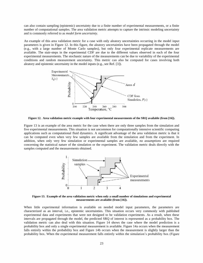
23

can also contain sampling (epistemic) uncertainty due to a finite number of experimental measurements, or a finite

number of computational samples. The area validation metric attempts to capture the intrinsic modeling uncertainty

and is commonly referred to as model form uncertainty.

An example of this area validation metric for a case with only aleatory uncertainties occurring in the model input

parameters is given in Figure 12. In this figure, the aleatory uncertainties have been propagated through the model

(e.g., with a large number of Monte Carlo samples), but only four experimental replicate measurements are

available. The stair-steps in the experimental CDF are due to the different values observed in each of the four

experimental measurements. The stochastic nature of the measurements can be due to variability of the experimental

conditions and random measurement uncertainty. This metric can also be computed for cases involving both

aleatory and epistemic uncertainty in the model inputs (e.g., see Ref. [3]).

Figure 12. Area validation metric example with four experimental measurements of the SRQ available (from [16]).

Figure 13 is an example of the area metric for the case when there are only three samples from the simulation and

five experimental measurements. This situation is not uncommon for computationally intensive scientific computing

applications such as computational fluid dynamics. A significant advantage of the area validation metric is that it

can be computed even when very few samples are available from the simulation and from the experiment. In

addition, when only very few simulation or experimental samples are available, no assumptions are required

concerning the statistical nature of the simulation or the experiment. The validation metric deals directly with the

samples computed and the measurements obtained.

Figure 13. Example of the area validation metric when only a small number of simulations and experimental

measurements are available (from [16]).

When little experimental information is available on needed model input parameters, the parameters are

characterized as an interval, i.e., epistemic uncertainties. This situation occurs very commonly with published

experimental data and experiments that were not designed to be validation experiments. As a result, when these

intervals are propagated through the model, the predicted SRQ of interest is represented as a probability box. The

validation metric can also deal with this situation. Figure 14 shows the case where the model prediction is a

probability box and only a single experimental measurement is available. Figure 14a occurs when the measurement

falls entirely within the probability box and Figure 14b occurs when the measurement is slightly larger than the

probability box. When the experimental measurement falls entirely within the simulation’s probability box (Figure

24

14a), then the area validation metric is zero. When a portion of the experimental measurement falls outside of the

probability box (Figure 14b), then the area validation metric is nonzero. Recall that the area validation metric is the

smallest area between the probability box and the experimental CDF. That is, the validation metric reflects the

evidence for disagreement between the model and the experiment. When the simulation is a probability box due to

insufficient information provided by the validation experiment, the model is given more leeway in comparing with

the experiment, as is appropriate.

a) b)

Figure 14. Example of area validation metric computed at one location in the model input parameter space: aleatory

uncertainties only (left) and combined aleatory and epistemic uncertainties (right) (from [16]).

4.3.5.2 Model Extrapolation

Numerous validation experiments would be required to estimate the validation metric over the entire space of model

input parameters for the application of interest. In many cases, however, it is not even possible to obtain

experimental data at the application conditions of interest. As a result, the more common case is that the model must

be applied at conditions where there are no experimental data. Consider a simple example when there are only two

input parameters for the model: α and β (Figure 15). The validation domain consists of the set of points in this

parameter space where experiments have been conducted and the validation metric has been computed (denoted by a

“V” in Figure 15). The application domain, sometimes referred to as the operating envelope of the system, is

generally larger than the validation domain. Thus, one must choose between either extrapolating the validation

metric outside of the validation domain or performing additional validation experiments. In Figure 15, conditions for

candidate validation experiments are given by a “C”.

Figure 15. Model validation relative to experimental data (from [3]).

25

In the past, it has been common practice to either a) ignore the model form uncertainty in the predictions for the

application conditions or b) calibrate and update adjustable parameters in the mathematical model so that improved

agreement could be obtained with the available experimental data at conditions “V”. We, however, believe a more

forthright approach is to explicitly account for the mismatch between the model and the experiments and include this

mismatch as additional uncertainty in the predictions of the SRQ in the application domain. When the validation

metric results are extrapolated to new conditions, there is a subsequent increase in the uncertainty due to the

extrapolation process itself. It should be stressed that this extrapolation is a statistical extrapolation of the

uncertainty structure of the validation metric that has been observed over the validation domain. The extrapolation

of the uncertainty structure is completely separate from any extrapolation of the simulation prediction results to

conditions where experimental data are not available. A common example of the latter is the use of an aerodynamics

model to extrapolate from wind tunnel conditions (where data exist) to flight Reynolds numbers.

It is noted that model extrapolation can occur in terms of input parameters and extrapolation to higher levels in the

validation hierarchy. Large extrapolations may commonly involve large changes in coupled physics, e.g., heating

effects on structural dynamics, and large changes in geometry or subsystem interactions, e.g., abnormal or hostile

environments. It is our firm belief that large extrapolations must be based on physics inference, not statistical

inference as there is no rigorous mathematical basis for quantifying the uncertainty in computationally estimated

SRQ of interest. Above all, large extrapolations should result in large increase in uncertainty.

4.3.6 Determine Total Uncertainty in the SRQ The total prediction uncertainty can be estimated by combining the propagated uncertainty from the model inputs

(aleatory and epistemic) with the uncertainty due to the form of the model and the uncertainty due to the numerical

error estimation process. In the described imprecise probability approach to uncertainty quantification, the total

uncertainty in the SRQ at the application conditions of interest is computed as follows. First, one begins with the

probability box that was generated by propagating the aleatory and epistemic uncertainties in the model input

parameters through the model (recall Figure 8 and Figure 10). Next, the area validation metric is appended to the

sides of the probability box, thus showing that the epistemic uncertainty in the SRQ has increased due to model form

uncertainty. As discussed above, if extrapolation of the model form uncertainty is required, then it is the

extrapolated d values that are appended to the SRQ probability box. This process is shown graphically in Figure 16.

Finally, the uncertainty due to numerical approximations is treated as an additional epistemic uncertainty and, in a

similar fashion as the model form uncertainty, it is appended to the probability box of the SRQ.

Figure 16. Increase in predictive uncertainty due to the addition of model form uncertainty (from [3]).

This approach for representing total uncertainty in the predicted SRQ of interest provides valuable information to

decision makers using the results from the simulations. The width of the original probability box provides

information on the effects of epistemic uncertainties in the model inputs on the predicted SRQ. The shape, or the

range, of the two bounding CDFs of the probability box provides information on the effects of aleatory uncertainties

in the model inputs. The validation metric d that is appended to the probability box of the SRQ tells the decision

maker the magnitude of the uncertainty that is due to model form uncertainty. Finally, UNUM that is appended to the

26

probability box informs the decision maker of the magnitude of the uncertainty due to numerical approximations. In

limited testing of this approach, it has been found that the contribution of model form uncertainty has been a

dominant contributor to the uncertainty in the predicted SRQ, even for relatively accurate models of the system of

interest [3, 16].

5. Conclusions

The framework for verification, validation, and uncertainty quantification in scientific computing presented here and

to be included in the upcoming AIAA Guide represents a conceptual shift in the way that scientific and engineering

predictions are presented to decision makers. The philosophy of the present approach is to rigorously segregate

aleatory and epistemic uncertainties in input quantities, and explicitly account for numerical approximation errors

and model form uncertainty directly in terms of the predicted quantities of interest. In this way, the decision maker is

clearly and unambiguously shown the uncertainty in the predicted system response. For example, if the model has

been found to be relatively inaccurate in previous comparisons with experimental data, the decision maker will

starkly see this in any new predictions; as opposed to a newly calibrated model based on recent experiments. We

believe this philosophy of presenting predictions to decision makers is needed to reduce the often seen failure in

under estimating predictive uncertainty. We believe that with this clearer picture of the uncertainties, the decision

maker is better served. This approach is particularly important for predictions of high-consequence systems, such as

those where human life, the public safety, national security, or the future of a company is at stake.

References

1. AIAA, “Guide for the Verification and Validation of Computational Fluid Dynamics Simulations,” American

Institute of Aeronautics and Astronautics, AIAA-G-077-1998, Reston, VA, 1998.

2. ASME, “Guide for Verification and Validation in Computational Solid Mechanics,” American Society of

Mechanical Engineers, ASME Standard V&V 10-2006, New York, NY, 2006.

3. Oberkampf, W. L. and Roy, C. J., Verification and Validation in Scientific Computing, Cambridge University

Press, New York, 2010.

4. Oberkampf, W. L. and Trucano, T. G., "Verification and Validation Benchmarks," Nuclear Engineering and

Design, 238(3), 2008, pp. 716 – 743.

5. Oberkampf, W. L. and Barone, M. F., “Measures of Agreement between Computation and Experiment:

Validation Metrics,” Journal of Computational Physics, Vol. 217, No. 1, 2006, pp. 5 – 36.

6. Oberkampf, W. L., Trucano, T. G., and Hirsch, C., “Verification, Validation, and Predictive Capability,” Applied

Mechanics Reviews, Vol. 57, No. 5, 2004, pp. 345 – 384.

7. Morgan, M. G. and Henrion, M., Uncertainty: A Guide to Dealing with Uncertainty in Quantitative Risk and

Policy Analysis, 1st Ed., Cambridge University Press, Cambridge, UK, 1990.

8. Cullen, A. C. and Frey, H. C., Probabilistic Techniques in Exposure Assessment: A Handbook for Dealing with

Variability and Uncertainty in Models and Inputs, Plenum Press, New York, 1999.

9. Vose, D., Risk Analysis: A Quantitative Guide, 3rd

Ed., Wiley, New York, 2008.

10. Haimes, Y. Y., Risk Modeling, Assessment, and Management, 3rd

Ed., John Wiley, New York, 2009.

11. Bedford, T. and Cooke R., Probabilistic Risk Analysis: Foundations and Methods, Cambridge University Press,

Cambridge, UK, 2001.

12. Ghosh, J. K., Delampady, M., and Samanta, T., An Introduction to Bayesian Analysis: Theory and Methods,

Springer, Berlin, 2006.

13. Sivia, D. and Skilling, J., Data Analysis: A Bayesian Tutorial. 2nd

Ed., Oxford University Press, Oxford, 2006.

14. Coleman, H. W. and Stern F., “Uncertainties and CFD Code Validation,” Journal of Fluids Engineering. Vol.

119, 1997, pp. 795 – 803.

15. Stern, F., Wilson, R. V., Coleman H. W., and Paterson E. G., “Comprehensive Approach to Verification and

Validation of CFD Simulations-Part 1: Methodology and Procedures,” Journal of Fluids Engineering, Vol. 123,

No. 4, 2001, pp. 793 – 802.

27

16. Ferson, S., Oberkampf, W. L., and Ginzburg, L., “Model Validation and Predictive Capability for the Thermal

Challenge Problem,” Computer Methods in Applied Mechanics and Engineering. Vol. 197, 2008, pp. 2408 –

2430.

17. Coleman, H. W. and Steele, W. G., Experimentation, Validation, and Uncertainty Analysis for Engineers, Wiley,

New York, 1999.

18. Youden, W. J., “Enduring Values,” Technometrics, Vol. 14, No. 1, 1972.

19. Montgomery, D. C., Design and Analysis of Experiments, 5th

Ed., John Wiley, Hoboken, NJ, 2000.

20. Box, G. E. P., Hunter, J. S., and Hunter, W. G., Statistics for Experimenters: Design, Innovation, and Discovery,

2nd

Ed., John Wiley, New York, 2005.

21. Oberkampf, W. L. and Aeschliman D. P., “Joint Computational/Experimental Aerodynamics Research on a

Hypersonic Vehicle: Part 1, Experimental Results,” AIAA Journal, Vol. 30, No. 8, 1992, pp. 2000 – 2009.

22. Ferson, S. and Ginzburg L. R., “Different Methods are Needed to Propagate Ignorance and Variability,”

Reliability Engineering and System Safety, Vol. 54, 1996, pp. 133 – 144.

23. Ferson, S. and Hajagos J. G., “Arithmetic with Uncertain Numbers: Rigorous and (Often) Best Possible

Answers,” Reliability Engineering and System Safety. Vol. 85, Nos. 1-3, 2004, pp. 135 – 152.

24. Roache, P. J., Verification and Validation in Computational Science and Engineering, Hermosa Publishers, New

Mexico, 1998.

25. Cavallo, P. A. and Sinha, N., “Error Quantification for Computational Aerodynamics Using an Error Transport

Equation,” Journal of Aircraft, Vol. 44, No. 6, 2007, pp. 1954 – 1963.

26. Shih, T. I-P. and Williams, B. R., “Development and Evaluation of an A Posteriori Method for Estimating and

Correcting Grid-Induced Errors in Solutions of the Navier-Stokes Equations,” AIAA Paper 2009-1499, 2009.

27. Ainsworth, M. and Oden, J. T., “A Posteriori Error Estimation in Finite Element Analysis,” Computer Methods

in Applied Mechanics and Engineering, Vol. 142, No. 1-2, 1997, pp. 1 – 88.

28. Ainsworth, M. and Oden, J. T., A Posteriori Error Estimation in Finite Element Analysis, Wiley Interscience,

New York, 2000.

29. Zienkiewicz, O. C. and Zhu, J. Z., “The Superconvergent Patch Recovery and A Posteriori Error Estimates, Part

2: Error Estimates and Adaptivity,” International Journal for Numerical Methods in Engineering, Vol. 33, 1992,

pp. 1365 – 1382.

30. Roy, C. J., “Review of Discretization Error Estimators in Scientific Computing,” AIAA Paper 2010-0126, 2010,

Orlando, FL.

31. Roy, C. J., “Review of Code and Solution Verification Procedures for Computational Simulation,” Journal of

Computational Physics, Vol. 205, No. 1, 2005, pp. 131 – 156.

32. Roache, P. J., “Perspective: A Method for Uniform Reporting of Grid Refinement Studies,” Journal of Fluids

Engineering, Vol. 116, 1994, pp. 405 – 413.

33. Ghanem, R. and Spanos, P., Stochastic Finite Elements: A Spectral Approach, Springer Verlag, 1991.

34. Helton, J. C., “Uncertainty and Sensitivity Analysis in the Presence of Stochastic and Subjective Uncertainty,”

Journal of Statistical Computation and Simulation, Vol. 57, 1997, pp. 3 – 76.

35. Sallaberry, C. J., Helton, J. C., and Hora, S. C., “Extension of Latin Hypercube Samples with Correlated

Variables,” Reliability Engineering and System Safety, Vol. 93, 2008, pp. 1047 – 1059.

36. Ferson, S. and Tucker W. T., “Sensitivity in Risk Analyses with Uncertain Numbers,” Sandia National

Laboratories, SAND2006-2801, Albuquerque, NM, 2006.

37. Kreinovich, V., Beck, J., Ferregut, C., Sanchez, A., Keller, G.R., Averill M., and Starks, S.A., “Monte-Carlo-

Type Techniques for Processing Interval Uncertainty, and Their Potential Engineering Applications,” Reliable

Computing. Vol. 13, 2007, pp. 25 – 69.

38. Coleman, H. W. and Stern, F., “Uncertainties and CFD Code Validation,” Journal of Fluids Engineering, Vol.

119, 1997, pp. 795 – 803.

39. Stern, F., Wilson, R. V., Coleman, H. W., and Paterson, E. G., “Comprehensive Approach to Verification and

Validation of CFD Simulations-Part 1: Methodology and Procedures,” Journal of Fluids Engineering, Vol. 123,

No. 4, 2001, pp. 793 – 802.

40. Oberkampf, W. L. and Trucano, T. G., “Verification and Validation in Computational Fluid Dynamics,”

Progress in Aerospace Sciences, Vol. 38, No. 3, 2002, pp. 209 – 272.

41. Roy, C. J. and Oberkampf, W. L., “A Comprehensive Framework for Verification, Validation, and Uncertainty

Quantification in Scientific Computing,” Computer Methods in Applied Mechanics and Engineering, Vol. 200,

Issues 25-28, 2011, pp. 2131 – 2144.

42. Chen, W., Xiong, Y., Tsui, K. L., and Wang, S., "A Design-driven Validation Approach using Bayesian

Prediction Models," Journal of Mechanical Design, Vol. 130, Issue 2, 2008, pp. 021101.

28

43. Anderson, M. C., Hasselman, T. K., and Carne, T. G., “Model Correlation and Updating of a Nonlinear Finite

Element Model using Crush Test Data,” 17th

International Modal Analysis Conference (IMAC) on Modal

Analysis, Paper No. 376, Kissimmee, FL, Proceedings of the Society of Photo-Optical Instrumentation

Engineers, 1999, pp. 1511 – 1517.

44. Hanson, K. M., “A Framework for Assessing Uncertainties in Simulation Predictions,” Physica D, Vol. 133,

1999, pp. 179 – 188.

45. Lancaster, T., An introduction to modern Bayesian econometrics, Blackwell Publishing, Malden, MA, 2004.

46. Kennedy, M. C., and O'Hagan, A., “Bayesian Calibration of Computer Models,” Journal of the Royal Statistical

Society: Series B, Vol. 63, Issue 3, 2001, pp. 425 – 464.

47. Hasselman, T. K., Wathugala, G. W., and Crawford, J., “A Hierarchical Approach for Model Validation and

Uncertainty Quantification,” Fifth World Congress on Computational Mechanics, Vienna, Austria, Vienna

University of Technology, 2002.

48. Bayarri, M. J., Berger, J. O., Paulo, R., Sacks, J., Cafeo, J. A., Cavendish, J., Lin, C. H., and Tu, J., “A

Framework for Validation of Computer Models,” Technometrics, Vol. 49, Issue 2, 2007, pp. 138 – 154.

49. O’Hagan, A., “Bayesian Analysis of Computer Code Outputs: A Tutorial,” Reliability Engineering and System

Safety, Vol. 91, Issues 10 – 11, 2006, pp. 1290 – 1300.

50. Trucano, T. G., Swiler, L. P., Igusa, T., Oberkampf, W. L., and Pilch, M., “Calibration, Validation, and

Sensitivity Analysis: What’s What,” Reliability Engineering and System Safety, Vol. 91, Issues 10 – 11, 2006,

pp. 1331 – 1357.

51. Babuska, I., Nobile, F., and Tempone, R., “A Systematic Approach to Model Validation based on Bayesian

Updates and Prediction Related Rejection Criteria,” Computer Methods in Applied Mechanics and Engineering,

Vol. 197, Issues 29 – 32, 2008, pp. 2517 – 2539.

52. Xiong, Y., Chen, W., Tsui, K. L., and Apley, D. W., “A Better Understanding of Model Updating Strategies in

Validating Engineering Models,” Computer Methods in Applied Mechanics and Engineering, Vol. 198, Issues 15

– 16, 2009, pp. 1327 – 1337.

53. Lindgren, L. E., Alberg, H., and Domkin, K., “Constitutive Modelling and Parameter Optimization,” 7th

International Conference on Computational Plasticity, Barcelona, Spain, 2003.

54. McFarland, J., Mahadevan, S., Romero, V., and Swiler, L., “Calibration and Uncertainty Analysis for Computer

Simulations with Multivariate Output,” AIAA Journal, Vol. 46, Issue 5, 2008, pp. 1253 – 1265.

55. Wang, S., Tsui, K. L., and Chen, W., “Bayesian Validation of Computer Models,” Technometrics, Vol. 51, Issue

4, 2009, pp. 439 – 451.

56. Higdon, D., Kennedy, M. C., Cavendish, J., Cafeo, J., and Ryne, R., “Combining Field Data and Computer

Simulations for Calibration and Prediction,” SIAM Journal on Scientific Computing, Vol. 26, Issue 2, 2004, pp.

448 – 466.

57. Higdon, D., Nakhleh, C., Gattiker, J., and Williams, B., “A Bayesian Calibration Approach to the Thermal

Problem,” Computer Methods in Applied Mechanics and Engineering, Vol. 197, 2010, pp. 2431 – 2441.

58. Loeppky, J., Bingham, D., and Welch, W., “Computer Model Calibration or Tuning in Practice," University of

British Columbia, Research Technical Report,Vancouver, BC, CA, 2006.

59. Rougier, J., “Probabilistic Inference for Future Climate Using an Ensemble of Climate Model Evaluations,”

Climate Change, Vol. 81, Issues 3 – 4, 2007, pp. 247 – 264.

60. Liu, F., Bayarri, M. J., Berger, J. O., Paulo, R., and Sacks, J., “A Bayesian Analysis of the Thermal Challenge

Problems,” Computer Methods in Applied Mechanics and Engineering, Vol. 197, Issues 29 – 32, 2009, pp. 2457

– 2466.

61. Arendt, P., Apley, D., and Chen, W., “Quantification of Model Uncertainty: Calibration, Model Discrepancy,

and Identifiability,” Journal of Mechanical Design, Vol. 134, Issue 10, 2012, pp. 100908.