development and validation of a 3d similarity method for...
TRANSCRIPT

1
Development and validation of a 3D similarity method for
virtual screening
A study submitted in fulfilment for the degree of MPhil.
By Mr Daniel Butler
Information school
Apr 2013

2
Acknowledgements
I would like to give genuine thanks to the following people for their recent support,
encouragement and help which has aided me greatly to finish this thesis. They have really
helped me to remain focused and interested in the subject of Chemoinformatics.
Primarily, many thanks to Prof. Val Gillet, whom I have relied upon heavily to apply fairness
to my case and who has absolutely done so, as well as teaching me some interesting new
ways to approach the subject of ChemoInformatics. Thanks also to Dr Eleanor Gardiner for
her advice on graph theory approaches. Thanks to Prof. Peter Willett for delivering some
interesting lectures on the theories in the field and for valuable feedback.
Thanks to the Sheffield Chemoinformatics group for their support. In particular, many
thank to Dr Christoph Muller who has been a great friend to me and whom I owe a great
many thanks for his excellent introduction to the R tool. Also many thanks to Dr Richard
Martin for support with test data and for referencing his thesis results.
Many thanks to Dr Steve Maddock for allowing much flexibility on his graphics course
which has allowed me to create the bespoke molecular graphics environment which
enabled the generation of the molecular images which are used in several areas of this
thesis, for example figure 4.24.
Thanks to Dr Daniel Robinson for his interesting insights. Thanks to Dr Tim Dudgeon and
ChemAxon for keeping me involved in the industry and motivated. I hope to continue to
work with ChemAxon in future.
Finally, thanks to my family for their advice and support.
3
Abstract
A predictive 3D similarity workflow approach has been developed using a set of modular
Java computer programs that implement algorithms that aim to capture the key
components of a 3D similarity search and aim to incorporate methods that address both
the similar property principle and molecular recognition paradigms. This approach will
expect as input a single query molecule conformation (at least one conformer is required
per molecule) and will identify molecules that are similar to it when compared with a target
database of 3D conformations.
This workflow is achieved by first mapping each of the molecular conformation’s geometric
coordinates, together with atomic property data, to abstract representative models
referred to as fuzzy pharmacophore objects. A geometric partitioning approach maps full
geometric atomic coordinates to a reduced point representation for a molecule in order to
capture the overall global shape of the molecule in relatively few points. This sort of
“reduced points” approach for molecular representation was first suggested by (Glick et
al., 2002) in the context of Protein active site identification. Pharmacophore classifications
are applied to the molecular fragments via mapping of internal constituent group atoms
and their properties in order to assign the amount of potential interaction type present.
The classifications are Hydrophobic, Aromatic, Acceptor, Donor and Hydrophilic and each
atom can be mapped to several of these type definitions. Thus we have assigned a
biologically relevant code to each of the fragments. These fuzzy pharmacophore object
abstract representations will naturally provide a summary level description of a whole
molecule in a relatively small number of geometric points.
Two such objects are then aligned to minimise the RMSD between points and the volume
and properties overlap is evaluated in order to derive global 3D similarity scores for each
alignment. One alignment method is to systematically align representations and is in
essence a triangle and tetrahedron matching search technique. The second alignment
method is based on graph theory and parameterised maximal common substructure or
clique detection is applied to a correspondence graph constructed using two
representations, followed by minimal RMSD alignment of the evaluated Bron-Kerbosch
cliques with the Kabsch rotation algorithm. This provides an alternative and more efficient
approach to systematic alignment since the systematic approach is limited to aligning four

4
points maximum. A volume and property overlap scoring function is used to compare two
such fuzzy pharmacophore objects and the resultant Tanimoto coefficient is used for
ranking. Initially representations of similar size and with equivalent numbers of points
(typically three to six points) are compared and are considered shape searches.
Subsequently, objects of different scales and representations are compared in a sub-shape
search sense, whereby a smaller object could feasibly be searched for within a larger
object. The graph theoretical approach to alignment and clique detection facilitates shape
and sub-shape search automatically by including the entire representation or just the
cliques in scoring.
In principle there are many potential ways to overlay two molecules and the sub-shapes or
fragments contained within each molecule. Each alignment can score differently and
certain alignment orientations will maximise or minimise certain aspects of the scoring
criteria. Hence, several key alignments are feasible between two conformations which may
define some or all of each molecule that is biologically active in a given context. An
alignment and associated maximal volume and properties overlap score is used to rank
order the molecules by normalised similarity. When applied to a target database evaluated
similarity measures are used to order the list for proposed biological activity. The overall
workflow is thus described as a hybrid shape / properties comparison and fragment based
biosteric similarity search. The volume distribution and by implication shape, as well as
mass derived pharmacophore feature density overlap scores, are determined and thus this
aims to capture both shape and pharmacophore search.
5
Thesis - table of contents
Chapter 1 - Introduction .........................................................................................................13
1.1 - Biological molecules and medicinal chemistry .............................................................. 13
1.2 - Thesis structure .............................................................................................................. 16
Chapter 2 - An overview of virtual screening .........................................................................17
2.1 - Introduction ................................................................................................................... 17
2.2 - Virtual screening techniques ......................................................................................... 17
2.2.1 - Ligand based virtual screening ........................................................................ 17
2.2.2 - Substructure search ........................................................................................ 18
2.2.3 - Similarity search .............................................................................................. 18
2.2.4 - Pharmacophore classification and elucidation ............................................... 20
2.2.5 - Pharmacophore database search ................................................................... 21
2.2.6 - Machine learning methods ............................................................................. 22
2.2.7 - Structure based virtual screening ................................................................... 22
2.2.8 - Docking and scoring ........................................................................................ 23
2.2.9 - QSAR ............................................................................................................... 23
2.2.10 - Evaluation of virtual screening methods ...................................................... 24
2.3 - Summary ........................................................................................................................ 25
Chapter 3 - 3D similarity search methods ...............................................................................26
3.1 - Introduction ................................................................................................................... 26
3.2 - Alignment-independent 3D similarity methods ............................................................ 28
3.3 - Alignment-dependent 3D similarity methods ............................................................... 31
3.3.1 - Overview ............................................................................................................. 31
3.3.2 - Graph theoretical methods ................................................................................. 32
3.3.3 - Surface area representation ............................................................................... 33
3.3.4 - Spherical grid field representation ..................................................................... 34
3.3.5 - Grid field representation .................................................................................... 35
3.3.6 - Atom and reduced points field representation .................................................. 36
3.3.7 - Shape and hybrid approaches ............................................................................ 40
3.3.8 - Pharmacophore and reduced points concepts ................................................... 43
3.3.9 - Triangle matching using geometric hashing ....................................................... 44
3.4 - Conformations and molecular flexibility ........................................................................ 44
3.5 - Evaluation and comparison of 2D and 3D methods ...................................................... 47

6
3.6 - Summary ........................................................................................................................ 47
Chapter 4 - Reduced points fuzzy pharmacophore vector representations and their usage in
3D similarity scoring functions and molecule correlation vectors .........................................49
4.1 - Introduction and method context ................................................................................. 49
4.2 - Overview of method ...................................................................................................... 50
4.3 - Molecular representation .............................................................................................. 52
4.3.1 - K-means basic partitioning approach ............................................................. 52
4.3.2 - Fuzzy pharmacophore point classification vector (characterisation) ............. 54
4.4 - Search and alignment approaches employed ............................................................... 57
4.4.1 - Two alignment methods are investigated ...................................................... 57
4.4.2 - Alignment method using clique detection and Kabsch algorithm .................. 58
4.4.2.1 - Correspondence graph(s) ........................................................................ 58
4.4.2.2 - Node type equivalence ............................................................................ 58
4.4.2.3 - Edge distance tolerance ........................................................................... 61
4.4.2.4 - Bron-Kerbosch clique detection algorithm .............................................. 63
4.4.2.5 - Kabsch pair-wise alignment algorithm .................................................... 63
4.4.2.6 - Overall workflow using Bron-Kerbosch clique detection followed by
Kabsch alignment ................................................................................................... 65
4.4.3 - Systematic exhaustive alignment ................................................................... 66
4.4.3.1 - Alignment up to four points..................................................................... 66
4.4.3.2 - Single point alignment ............................................................................. 67
4.4.3.3 - Two point alignment ................................................................................ 67
4.4.3.4 - Three point alignment ............................................................................. 68
4.4.3.5 - Four point alignment using sets of three points ...................................... 68
4.4.3.6 - Torsion angle for alignment of two planes .............................................. 69
4.4.3.7 - Optimisation along the +Z-axis ................................................................ 69
4.5 - Scoring function and similarity coefficient .................................................................... 70
4.5.1 - Scoring method and alignments ..................................................................... 70
4.5.2 - Sphere volume overlap function..................................................................... 71
4.5.3 - Normalising the volume scores and Tanimoto coefficient ............................. 73
4.5.4 - Percentage pharmacophore type weighted overlap function ....................... 73
4.5.5 - Scoring the systematic alignment ................................................................... 75
4.5.6 - Scoring the clique and Kabsch alignment ....................................................... 76
4.5.7 - Evaluated similarity coefficients ..................................................................... 76

7
4.6 - Implementation Details ................................................................................................. 79
4.6.1 - Data pre-processing steps required ................................................................ 79
4.6.2 - Software platforms and libraries .................................................................... 80
4.7 - Chapter Summary .......................................................................................................... 81
Chapter 5 - Results for rigid search of two alignment methods using the DUD data set of
actives and decoys ..................................................................................................................82
5.1 - Introduction ................................................................................................................... 82
5.2 - Experimental details ...................................................................................................... 82
5.2.1 - Validation data sets used for virtual screening experiments ............................. 82
5.2.2 - Method variables and parameters ..................................................................... 83
5.2.3 - Ranking measures ............................................................................................... 85
5.3 - Thrombin ........................................................................................................................ 87
5.3.1 - Thrombin data set ............................................................................................... 87
5.3.2 - Thrombin results and discussion ......................................................................... 87
5.4 - DUD ................................................................................................................................ 96
5.4.1 - DUD experiments ..................................................................................................96
5.4.2 - DUD results and discussion ...................................................................................98
5.5 - Results of eight targets from DUD ................................................................................106
5.5.1 - Further eight DUD experiments ..........................................................................106
5.5.2 - Discussion of eight experiments ..........................................................................107
5.6 - Conclusion of overall method effectiveness over these data sets ...............................119
Chapter 6 - Conclusions and future work .............................................................................121
6.1 - Conclusions .................................................................................................................. 121
6.2 - Suggestions for future work ........................................................................................ 124
6.2.1 - Extending the partitioning approach ...................................................................124
6.2.2 - Use of smart search algorithm and non-deterministic representation set .........124
6.2.3 - Comparing molecules of different K representations .........................................125
6.2.4 - Flexible search .................................................................................................... 126
6.2.5 - Gaussian function to model rigid or flexible fragment .......................................127
6.2.6 - Use of radial distribution functions at atom level for superposition query
generation .............................................................................................................................128
6.2.7 - Use of a field graph at the fragment level ...........................................................130
6.2.8 - Using structural and active site data for included or excluded volume ..............130

8
6.3 - Conclusion .................................................................................................................... 132
Bibliography ......................................................................................................................... 133

9
List of figures
Figure 3.1 - The most commonly used Similarity coefficients Tanimoto, Carbo and
Hodgkin/Dice are defined for reference. Q and T are identity overlap and C is the evaluated
overlap of Q and T.
Figure 4.1 - From random starting molecular orientation, weighted graphs are constructed
for the query Q and target T molecule. Examples are HSP90 and COX2.The latter molecule is
aligned and scored for properties overlap in figure 4.24.
Figure 4.2 - The molecule “Nevariprine” is partitioned into 4 points using the deterministic
K-means algorithm (heavy atoms only (non-Hydrogen)). The sphere radii are derived from
average cluster distance.
Figure 4.3 - Pharmacophore classes and the characteristic vector defined for each point.
Figure 4.4 - Flow diagram for the assignment of a characteristic vector for each reduced
point from initial input molecule or existing representation. Atom capitalisation in the
SMARTS definitions indicates aliphatic atoms whereas lower case indicates aromatic atoms.
Figure 4.5 - Volume mode defined.
Figure 4.6 - Radius tolerance defined.
Figure 4.7 - Partial mode defined.
Figure 4.8 - Exact mode defined.
Figure 4.9 - Edge tolerance defines if an edge is placed in the correspondence graph.
Figure 4.10 - Self reference nodes are invalid and are not allowed to form.
Figure 4.11 - Flow diagram for correspondence graph node and edge mapping logic. Vertex
and edge equality rules are described in 4.4.2.2 and 4.4.2.3.
Figure 4.12 - A correspondence graph is formulated using both representations and user
specified node and edge tolerances. Each node in representation A (A1-A4) is compared for
mapping with each node in representation B (B1-B4). Surviving nodes are then tested for
distance tolerance yielding the correspondence graph (orange). Failing nodes in this case
are A1-B1,A1-B3,A1-B4,A2-B1,A2-B2,A2-B3,A3-B1,A3-B2,A3-B4,A4-B1,A4-B2,A4-B4.

10
Figure 4.13 - The set of maximal cliques is identified and extracted from the correspondence
graph. In this case, the isolated green triangle shown is a maximal clique.
Figure 4.14 - Diagram depicting Kabsch alignment of clique contributing nodes (green) from
each four point representation.
Figure 4.15 - Flow diagram for correspondence graph, clique detection and Kabsch
alignment.
Figure 4.16 - Single point (K=1) alignment.
Figure 4.17 - Two point (K=2) alignment.
Figure 4.18 - Three point (K=3) alignment.
Figure 4.19 - Four point (K=4) alignment.
Figure 4.20 - Optimisation along the +Z-axis by shifting one representation by a small
increment.
Figure 4.21 - No overlap and no score contribution.
Figure 4.22 - Sphere overlap geometry.
Figure 4.23 - Sphere centroids are exactly aligned.
Figure 4.24 - Several crystal query structures (from DUD) are aligned (clique/Kabsch) and
scored in shape mode with high scoring actives found for the set. Parameters are K=4,
distance tolerance=2.0, radius tolerance=2.0, node match mode=EXACT).
Figure 4.25 - Molecule pre-processing flow diagram.
Figure 5.1 - The queries for four results (highlighted in green in table 5.3) using K=4. The
sphere size is generated using the computed radius.
Figure 6.1 - The K-means does not accommodate bridge sharing of atoms (the group
membership is currently mutually exclusive).
Figure 6.2 - The molecule Gleevec represented (relatively well) by the K-means at K=5.
Figure 6.3 - Radial distribution function ���� = �� ∗ ����� can be used to model a
Hydrogen 1s orbital and for use as higher orbital representation. The overlap of these
functions could be used to score an elucidation / alignment method.

11
Figure 6.4 - Extracting an active site negative image. The midpoints of all chords formed
between all active site atoms can be used as the dense data set to be partitioned and then
used as a K point ‘spacer template’ which can be incorporated into an elucidation or search.

12
List of abbreviations
ACC - ACCeptor
ARO - AROmatic
AUC - Area Under the Curve
CLIP - Candidate Ligand Identification Procedure
COMFA - COmparative Molecular Field Analysis
DON - DONor
DUD - Directory of Useful Decoys
EF - Enrichment Factor
FBSS - Field Based Similarity Search
FDA - Food & Drug Administration
GUI - Graphical User Interface
MACCS - Molecular ACCess System
MCS - Maximium Common Substructure
MEP - Molecular Electrostatic Potential
MOE - Molecular Operating Environment
NMR - Nuclear Magnetic Resonance
PHI - HydroPHIlic
PHO - HydroPHObic
PH4 - Pharmacophore types : ACC,ARO,DON,PHI or PHO
QSAR/SAR - Quantitative Structure Activity Relationship
RMSD - Root Mean Square Deviation
SEAL - Steric & Electrostatic ALignment
SMARTS - Simplified Molecular Arbitrary Target Specification
USR - Ultrafast Shape Recognition
VDW - Van Der Waals
1D/2D/3D - Dimensions in space usually denoted x,y,z.

13
Chapter 1 - Introduction
1.1 - Biological molecules and medicinal chemistry
Human beings and many higher order animals are constituted from and intrinsically rely
upon naturally occurring carbon and heteroatom based molecules as well as some heavy
metals such as calcium, iron, zinc and of course the most ubiquitous of substances, water.
Thus, there has been an innate need for a variety of such organic molecules by people
throughout human history. Based on this need, more recently humans have observed and
then copied nature directly, creating synthetic organic molecules and thus the academic
subject of organic chemistry has emerged. Furthermore, organic molecules which can be
used as human and animal medicines in order to relieve inflictions and to cure illness and
stop disease and suffering have been of particular high priority. Thus an understanding of
molecular structure and function within the context of animal cell models is a key research
area. The core concepts of molecular structure and the transformative chemical reactions
found within organic chemistry form the basis for biology and biochemistry theories since
many of the naturally observed molecules are pivotal to the internal mechanisms and
correct functioning of living organisms via chemical reactions. The correct operation of cells
is controlled directly by protein found within the aqueous cell environment. In order to
sustain life, these proteins are in a constant equilibrium state with each other and many
other dissolved small organic compounds in the cell (Teague et al., 2003). Disease often
arises when normal functioning is interrupted and this can occur due to both genetic and
environmental factors. Thus, the field of medicinal chemistry has emerged which attempts
to apply rational concepts, in order to discover new drug molecules whose inherent
properties correct or regulate errant biological processes. The primary concern in this area
is with molecular structure and the functional rationalisation of the intrinsic shape and
properties of biologically active molecules. Although often leading to complex behaviour,
the chirality or handedness of molecules can be a predominant feature. Protein active sites
are inherently chiral due to their constitution of amino acids each of which is also chiral.
This is shown by the Thalidomide case which exemplifies that molecular recognition is a
three dimensional (3D) concept and that effects are based upon the 3D shape and property
distribution of a molecule (Corey et al., 2007; Stryer et al., 1995).
As an inventive species, in more recent times, human beings have developed synthetic
chemistry techniques in order to create useful medicinal molecules, hopefully for the

14
benefit of society. As such, we are primarily concerned with the classes of organic
molecules that can act as drugs. There are many classes of chemical compounds that have
the physical structural and functional properties to interact with proteins within enzyme
reaction mechanisms. Important classes of molecules include the amino acids, alkaloids,
heterocyclic molecules, vitamins and steroids. One method of identifying potential drug
molecules is to try and synthesise and test natural product mimics. In particular, molecules
found from animal, vegetation and marine sources have been found to have profoundly
interesting structures and equally extreme effects on the human body and have been used
effectively by many early civilisations for healing purposes. The synthesis of these and
similar molecules is now a highly prized and often an academically challenging endeavour
(Nicolaou et al., 1996). The reactions encountered during such challenges are often then
published and applied to create new synthetic molecules of interest. Thanks to many
advances in synthetic organic chemistry techniques, many chemical transformations are
well documented and are available for general use.
Modern drug discovery efforts and the pharmaceuticals industry can now use some of the
more robust reactions to routinely synthesise complex organic molecules which can be
entirely novel. It is often stated that the number of known synthesised organic molecules is
considerably smaller than the number that it might be possible to synthesise. The actual
possible chemical space is effectively infinite and there are more molecules feasible than
matter in the universe available to construct them (Fink et al., 2007). More recently, solid
phase combinatorial chemistry techniques have been developed in order to facilitate even
more efficient molecule production methods and as a result a greater variety of synthetic
molecules can be created, often using simple synthetic transformations. Molecules of
interest are tested for biological activity and this is often referred to as screening. Putative
active molecules can have their structures modified to optimise their properties in order to
become drug candidates and this is referred to as lead optimisation. Clinical trials with
animal and humans are often the next phases in order to develop a viable medicine.
However despite these scientific advances, drug discovery is an economically inefficient
exercise largely due to the fact that vast numbers of molecules need to be tested and thus
material costs are high and the end result is often relatively few active molecules that are
developed into acceptable marketable drugs.
In conjunction with the medicinal chemistry efforts described above, rational drug design
and computational chemistry techniques have also been developed that aim to apply

15
additional logic and relevant mathematical concepts to the field of drug discovery. Often
such techniques can be applied using very powerful computers to complete the
calculations involved and as such the virtual screening paradigm has evolved. Virtual
screening attempts to emulate on a computer the predictive equivalent to high throughput
screening. The term covers a variety of computational methods that can be applied in order
to prioritise compounds for biological screening with the aim of increasing the chance of
finding active compounds compared to screening compounds at random. Rational drug
design commences with the identification of a protein structure to regulate. Often the aim
is to decrease the protein’s activity in an errant biological process within organisms cells. If
it is possible to modulate the protein’s natural function by using a small molecule then such
proteins are often referred to as being “druggable” (Brenke et al., 2009). Organic
molecules that are considered as potential drugs should be “drug-like” in terms of their
solubility and ease of transport to the affected cells within the organism. These properties
are often summarised by drug-like filters such as the Lipinski rule of five (Lipinski et al.,
2001).
The core principles used to provide a sensible framework for modelling organic molecules
within rational drug design are the similar property principle and 3D molecular recognition.
The similar property principle states that molecules that have similar structural properties
should have similar biological activities (Johnson et al., 1990). Thus given a molecule of
known activity, similarity search can be used to rank order a dataset of molecules on
similarity to the active. The top scoring candidates are then good candidates for testing.
Molecular recognition is based on the fundamental assumption of the lock and key concept
(Walsh et al., 1979), which assumes that any given molecule that interacts favourably with
a receptor will have, to some extent, exhibit complementary shape and property
distributions to that receptor’s active site based upon 3D atomic positions. An active site is
a critical portion of a biological molecule that acts as an interface to other molecules over
space. Organic molecules act as regulators which control enzyme reaction mechanisms and
protein conformation populations which are in equilibrium and are integral to biological
activity cascade pathways in the cell (Teague et al., 2003). This interaction controls the
behaviour and morphology of the complex and the change of shape of the protein from an
active form to an inactive form and vice versa. Small molecules are recognised in a highly
selective manner by proteins and this status has evolved over a very long time period since
the beginnings of life on our primitive Earth (Stryer et al., 1995).

16
3D similarity methods aim to capture the shape and 3D properties of molecules based on
the concept of molecular recognition. For a small molecule to be able to bind to a protein it
should have complementary size, shape electron density to the active site of the protein.
Although many 3D similarity methods have been developed, the complexity of modelling
molecular recognition is such that the methods are limited in their accuracy. As such it is a
difficult task to develop an approach that accurately correlates 3D molecular structure with
biological activity. Hence, it is not considered to be a currently solved problem, due to the
inherently complex electronic nature of molecules (Fukui et al., 1997).
The primary aim of the work described in this thesis is to develop a novel 3D similarity
method for comparing two molecules and deriving a numerical similarity index. Given an
input query organic molecule of biological interest, the method can be used to iteratively
process and score a set of target organic molecules. The molecules can then be rank
ordered on similarity to the query. The effectiveness of the method is evaluated by
measuring the extent to which known active molecules are ranked higher than inactive
compounds, often referred to as decoys. Molecules are numerically evaluated on their
similarity to the query molecule in terms of basic 3D shape and property distribution. The
rationale is that molecules evaluated to be similar to the query defined by such 3D criteria,
should exhibit approximately equivalent biological behaviour and thus should be good
candidates for biological testing.
1.2 – Thesis structure
The structure of this thesis is as follows. Chapter 2 explores virtual screening concepts and
approaches in further detail. The virtual screening techniques that have evolved into
operation are reviewed in order to place similarity search in general context. Chapter 3
reviews the existing 3D similarity search techniques and discusses representation,
alignment, scoring and flexible search in order to set the scene for the following chapter.
Chapter 4 explains in detail the approach developed to complete the rigid molecule shape
and sub-shape 3D similarity search method. Chapter 5 presents the results of the rigid
scoring function for two different alignment methods as applied to sets of virtual screening
test data. Chapter 6 presents conclusions followed by suggestions for how these methods
might be extended and improved.

17
Chapter 2 – An overview of virtual screening
2.1 - Introduction
Virtual screening is the application of computational techniques to prioritise molecules
(either real or virtual) for biological testing. Virtual screening includes both ligand and
structure based approaches. A ligand based approach is when only small molecule data is
available and thus the nature of the protein active site can only be inferred by the set of
active molecules available. A structure based approach is when information about the
protein receptor is available to consider and this is usually in the form of protein crystal
coordinates with or without a ligand bound in the active site. The availability of data largely
dictates which virtual screening approach can be adopted (Wilton et al., 2003). It is the job
of the virtual screening protocol to prioritise a set of compounds such that those selected
for testing have a greater chance of exhibiting activity than a random selection of
compounds. There are numerous virtual screening approaches and the key classes of
approach are presented below. A review of virtual screening in the context of real
screening can be found here (Walters et al., 1998).
2.2 – Virtual screening techniques
2.2.1 - Ligand based virtual screening
In the absence of protein structural data, then virtual screening is referred to as ligand
based. When known data is limited to a single active molecule then substructure search
and similarity search methods are the most relevant screening approaches to adopt. If an
active series of molecules is available then pharmacophore elucidation may be attempted
to derive the best query for a subsequent search. If both active and inactive molecules are
known, then machine learning methods can be used to derive a model which can then be
used to predict the activities of unknown compounds.

18
2.2.2 - Substructure search
Graph based substructure search is a 2D method (more recently extended to 3D) of
searching for molecules that contain a given fragment and are therefore potentially part of
the same chemical series and so should adhere to the similar property principle and
produce biologically similar molecules. A substructure search will return a list of molecules
that contain the substructure with no notion of ranking. A substructure search can produce
a diverse set of molecules from a single query and the same substructure can be found in
both simple and complex molecules. A substructure search is usually composed of two
stages. First a fast screen is completed using a fragment based fingerprint to eliminate
~99% of molecules that cannot match followed by a detailed subgraph matching
procedure. One downside of this method is that if a molecule identified by this approach is
already patented then it is likely all the other hits are too as it is normal for an entire series
of molecules to be patented. Patents are often submitted as “Markush” structures which
normally are constructed as a core structural template with connected points of variation.
Graph theoretical methods and substructure search are reviewed extensively by Leach
(Leach et al., 2007c). Substructure search use in virtual screening is reviewed by (Merlot et
al., 2003).
2.2.3 - Similarity search
The similar property principle (Johnson et al., 1990) was introduced in chapter 1 and states
that molecules with similar structures are likely to have similar biological properties and
activities. There are many possible ways to represent molecules and compare similarity
between two molecules and much research has been completed on systematic molecular
similarity comparisons (Good et al., 1998; Martin et al., 2002; Willett et al., 1998).
However, while the general principle holds there are also many counter examples where
similarity does not correlate with biological activity well. This is exemplified by so called
activity cliffs that are examples of pairs of molecules that by most derived similarity indexes
are determined to be highly similar but due to the absence of a single key functional group,
the actual biological activity is highly diminished between the two molecules (Leach A et
al., 2001b; Tropsha et al., 2008). Activity cliffs do however highlight the key nature of
specific molecular recognition which is described above. Similarity search usually involves
the use of global similarity indexes to compare and rank molecules on the assumption that

19
rank order reflects or relates to biological activity. Similarity search is usually adopted at
the initial stages of drug discovery projects when data is limited, to a single, or several
active molecules.
The similarity between two different molecules is an abstract concept with no absolute
measure in existence, the closest concept to real physical similarity perhaps being the
continuous charge distribution field (Carbo et al., 1980). Similarity search therefore relies
upon the generation and use of numerical descriptors to represent the molecules.
Similarity search descriptors are sometimes classified as 1D, 2D and 3D which infers
increasing sophistication in the representation of the molecules. As complexity of the
descriptors increases so does the computation required to derive that representation. A
study of the effectiveness of simple descriptors is given by (Bender et al., 2005). 2D
fingerprint descriptors are usually represented as binary vectors where each bit represents
a substructural fragment. For a given molecule, a bit is set to one if the substructure is
present in the molecule otherwise it is set to zero. Examples of 2D fingerprints include
DAYLIGHT, MACCS and UNITY fragment based fingerprints (Wild et al., 2000). Topological
shape indices are another example of molecular descriptors that are based on molecular
connectivity (Hall et al., 2001; Leach et al., 2007a). 3D descriptors are arguably the most
sophisticated descriptors and allow comparisons based on molecular surface area, volume
and shape. 3D similarity methods are discussed in chapter 3.
A similarity coefficient is required in order to quantify the similarity of a pair of molecules
based on the chosen molecular descriptors. There are a number of such coefficients in
common use which are constructed from the descriptors in slightly different ways and thus
can potentially give different results. Perhaps the most common coefficient in use is the
Tanimoto coefficient. For molecules A and B represented by binary fingerprints the
Tanimoto coefficient is given by c / (a+b-c) where c is the number of bits set to one in
common, a is the number of bits set to one in molecule A and b is the number of bits set to
one in molecule B (Willett et al., 1998). A comparison of the derivation and merits of
different similarity coefficients related to molecular size is discussed by (Holliday et al.,
2003). A review of similarity search and some useful descriptors is given by (Glen et al.,
2006). Which descriptors are most relevant to biological activity is still under debate with
one area of focus being on competing 2D and 3D representations (Brint et al., 1987a).

20
2.2.4 - Pharmacophore classification and elucidation
A pharmacophoric feature is a functional group which is classified in terms of potential
interaction behaviours with other groups. Several fundamental pharmacophore type
classifications are established which are listed as follows (Wolber et al., 2008). The
Hydrophobic classification is any atom or group of atoms that do not mix well with water,
typically carbon in any hybridisation state or any of the halogens. Hydrophobic groups tend
to mix together to exclude water as typified by micelles. The Aromatic type is any group of
atoms such as carbon or indeed heteroatoms (O,N) that are considered by the Huckel rules
to be part of an aromatic system. Aromatic groups can interact with each other via π
stacking orbital interactions in several orientations. Hydrogen bond donors are any group of
atoms that can donate a Hydrogen bond. Typically this means an electronegative atom with
a hydrogen atom attached usually limited to N, O. Hydrogen bond acceptors are atoms that
can accept a Hydrogen bond. Typically this means any atom that has at least one electron
pair that it can donate to form an H-bond with an appropriate donor. Hydrophilic is a
further classification that describes affinity for water and is essentially similar to acceptor.
Atoms or functional groups which contain a formal charge are also sometimes used as
pharmacophore features.
A pharmacophore is the 3D arrangement (Leach et al., 2010) of such functional groups that
are required for activity or binding to a protein. Different functional groups that interact in
the same way are referred to as being biosteric, for example NH and OH or Cl and CF3. An
early recognition of pharmacophore groups was made by Ehlrich in 1909 who commented
that a pharmacophore is “a molecular framework that carries the essential features
responsible for a drug’s biological activity”. A more modern definition of a pharmacophore
by Nicklaus in 1998 is “The minimum structural features necessary for enzyme binding”
(Milne et al., 1998). Pharmacophores can be defined in 2D or 3D whereby 2D topological
pharmacophores are defined by biosteric groups that are separated by bond distances.
However 3D pharmacophores, as defined by feature distance constraints, are considered to
be a more realistic interpretation since molecular recognition as described above is known
to be a 3D event. A pharmacophore can be derived from a series of active molecules and
normally involves generating a 3D alignment of the molecules in order to attempt to
identify the geometry of the features they have in common. The pharmacophore can then
be used as a query in database search.

21
The alignment is usually completed using the most rigid molecule as a template and then
increasingly flexible molecules, according to rotational bond count. Molecules are aligned
according to their common features and the best alignment is chosen by evaluating a
scoring function which usually consists of several terms almost always including a volume
and energy term. Many approaches to pharmacophore elucidation exist, the first being the
active analogues approach (Marshall et al., 1979), and more recent examples are
GALAHAD (Richmond et al., 2006) MOE’s GUI and alignment methods (Labute et al., 2001)
and PHASE (Dixon et al., 2006). If a protein structure is available then docking is the most
popular virtual screening method of choice employed (see below), however, alternative
ways to build structural data into similarity and pharmacophore methods are increasingly
being explored (Ebalunode et al., 2008). For example, excluded volume information can be
used in query construction to avoid steric clash between the ligand and protein.
2.2.5 - Pharmacophore database search
The primary use of an elucidated pharmacophore is in a database search so as to identify
molecules that contain the same features in the same geometric arrangement. This can be
achieved using 3D substructure searching with the query being defined by the
pharmacophore. Similar to 2D substructure search, 3D substructure search is best
approached by first completing a fast screening step using 3D fingerprints in order to
eliminate molecules that cannot match as they simply do not have a particular geometric
arrangement of features. 3D fingerprints are binary fingerprints that indicate the presence
or absence of geometric features such as a pair of atoms at a specified distance, or a
valence or torsion angle for a given pattern of atoms. Database molecules that pass the
screening step are subjected to a more intensive geometric search which usually involves a
subgraph isomorphism substructure search for example using the Ullmann algorithm
(Ullmann et al., 1976). Conformation flexibility of the database structures is handled either
by generating an ensemble of conformers each of which is treated as rigid or by
implementing a flexible search method (Brint et al., 1987a; Leach et al., 2007c; Sheridan
et al., 1989; Warr et al., 1998).

22
2.2.6 - Machine learning methods
Machine learning is a relatively recent concept which is employed when activity data is
available for both active and inactive molecules. The molecules with known activities form
a training set that is input to the machine learning method which then attempts to learn a
model which best separates the training set into actives and inactives. Once the optimum
model is determined it is possible to apply it to predict the probabilities of activity of
molecules in a given test set. Two common examples of machine learning methods are
Binary Kernel Discrimination (BKD) and Support Vector Machines (SVM). In the case of BKD
a chemical similarity kernel function is trained. The relative success of this method is
reported as being dependent upon the number of false actives in the training set and the
choice of similarity coefficient used in the kernel function (Chen et al., 2006a). For SVM’s a
hyper-plane is defined which separates active and inactive observations for a given
descriptor. Unclassified points (molecules in the test set), are assigned as active or inactive
based upon distance and sign relative to the hyper-plane. Molecules that are furthest on
the positive side of the defined hyper-plane have highest predicted activity (Warmuth et
al., 2003).
2.2.7 - Structure based virtual screening
The static and dynamic 3D structure of proteins can be obtained by using techniques such
as X-ray crystallography or NMR spectroscopy. Many structures have been resolved to date
and many more will be in future with the availability of the synchrotron light source. Much
of this data is compiled and available for use from the Protein Data Bank (RCSB et al.,
2010). If the crystal structure data of the protein is available then this can be incorporated
into the virtual screening approach. In the case of pharmacophore search, if a bound ligand
exists then this can be used to define a pharmacophore query and knowledge of the active
site can be used to define excluded volumes so as to build into the query an effective size
and shape constraint. However, the most popular structure-based virtual screening method
is protein-ligand docking which is discussed further below. Proteins can exhibit
homogeneous or heterogeneous activity and are categorised as such to help explain the
level of structural diversity shown within their set of known actives.

23
2.2.8 - Docking and scoring
Frequently when protein structural information is available then docking is employed in
order to determine the estimated binding affinity between a given small molecule and a
protein structure. Docking is a general term which encapsulates methods that predict the
likely interaction pose of two molecule conformations and score the pose according to
predicted free energy change of binding. The docking problem can be thought of as a
combination of a search strategy to traverse the six degrees of freedom in the search space
and a scoring function which attributes an energy value to a complex formed between
protein and ligand in a particular pose state. Docking programs are evaluated using known
protein-ligand complexes where the target pose is typically that of the natural substrate
bound crystal structure and generally any method that can reproduce the same pose within
2 Å root mean square deviation (RMSD) is considered to be accurate.
Docking is useful for predicting the binding mode of known actives and for the
identification of new molecules that are predicted to bind well which is how it is used in
virtual screening, The state of the art docking treats each ligand as flexible and proteins as
semi-flexible. The best methods predict experimental pose data ~70% of time (Leach et al.,
2006; Warren et al., 2006). However they are more limited in the ability to predict binding
affinities accurately over an entire active series. Picking the correct docking program for a
given target can produce better results with a particular class of proteins. Building the
correct physical chemistry model is a key aspect of docking. The original docking tool,
‘DOCK’ (Moustakas et al., 2006) uses spheres to define an active site and then sphere
centres are mapped to atom centres in a small molecule. Examples of much cited docking
tools which consider protein side chain flexibility are GOLD and FlexX and a study which
compares these approaches is given by (Sato et al., 2006). Several reviews of docking are
available (Taylor et al., 2002; Warren et al., 2006).
2.2.9 – QSAR
Many of the virtual screening techniques described previously are employed at the lead
generation phase to suggest new molecules for enquiry. Quantitative structure-activity
relationship (QSAR) techniques are often used during the later lead optimisation stage,
when sets of actives and inactives are already well defined. A QSAR model can be
constructed which aims to capture the exact nature of the relationship between the

24
numerical descriptors (real or calculated) and the biological activity in terms of a linear or
non-linear numerical correlation (Cramer et al., 1988). If a suitable model is derived it can
be used to assess new molecules for predicted activity and when used in a predictive way is
a type of virtual screening. The early days of QSAR were dominated by Corwin Hansch who
pioneered the use of physical properties such as log P (Logarithm of Octanol:water
partition ratio, considered to relate to cell permeability) and physical constants such as
NMR resonance effect parameters and adopted the established Hammett equations for use
in building correlation models against biological activity using such physical variables
(Hansch et al., 2011; Hansch et al., 1991).
Comparative Molecular Field Analysis (Cramer et al., 1988) is a grid-based QSAR approach
which can be used to correlate molecular field data with biological activity in order to
determine a QSAR model. Partial least squares is used to define the relationship between a
molecule’s field grid representation and its biological activity. A 3D grid is constructed
around a molecule so that the 3D Cartesian coordinates of all atoms are entirely enveloped
by it. As such the molecule is represented as a scalar field. At each lattice point, two
interaction energy values are evaluated to model the steric and electrostatic fields for the
entire molecule (over all atoms) with a probe sp3 Carbon atom and a +1 charge. The steric
contribution is modelled using the Lennard-Jones (6-12) potential parameterised using the
Tripos force field. The electrostatic or coulombic interaction is modelled using 1/r and
assigned Gasteiger/Marselli atomic charges. Two molecular field grids are aligned and
compared by fixing one and traversing the degrees of freedom of the other. A technique
termed “Field fitting” is used, that drives the alignment, based on the minimisation of
RMSD of both of the evaluated interaction energies over all lattice points and as such
molecules are aligned according to how similar they are with respect to the two interaction
characteristics.
2.2.10 – Evaluation of virtual screening methods
A predictive virtual screening method will produce a list of molecules to test in a relevant
biological assay. This list will either be in ranked order in the case of a similarity search or
docking experiments, or simply a “Boolean” hit list in the case of a substructure or
pharmacophore search. The next step in the process is to test the molecules for biological
activity in the relevant assay and use the results in a new round of virtual screening to
determine if the results correlate with the predictions. This type of iterative feedback

25
mechanism is standard practice in scientific approaches, used to refine hypotheses. Ideally
one might compare virtual screening predictions to real assay results in order to evaluate
the effectiveness of different methods at identifying new drug molecules. However, this is
often untenable in terms of the material cost associated and so standard test sets of
molecules with known associated biological activity referred to as “actives” can be used to
test the effectiveness of a given virtual screening method. Example sets available are the
DUD (Huang et al., 2006), WOMBAT (Good et al., 2008) and MUV (Rohrer et al., 2009)
data sets. Further to this, non-active “decoys” can be introduced, to determine if the
protocol is identifying the correct molecules and enrichment rates, relative to a random
selection. Thus it is possible to quantify how useful a method is at identifying active
molecules. The Enrichment factor (EF), Recall and Area under curve (AUC) measures
employed in chapter 5 are discussed in a recent evaluation of 3D ranking methods in virtual
screening (Kirchmair et al., 2008). A good evaluation of the performance and limitations of
3D similarity search using the DUD set is given by (Venkatraman et al., 2010). Please also
see section 3.5 which presents an evaluation of 2D and 3D methods.
2.3 - Summary
This chapter has described an overview of virtual screening approaches. Often when data is
limited to a few actives a ligand based approach is adopted, such as similarity search. If an
active series is available then a pharmacophore elucidation might be possible. If protein
structural information is available then pharmacophore search can be extended to include
or exclude volume and also then docking experiments are possible. If inactives are also
known then machine learning methods can be used for building a predictive model. The
next chapter describes the methods used for 3D similarity searching in more detail.
26
Chapter 3 - 3D similarity search methods
3.1 - Introduction
This chapter presents a discussion of three dimensional (3D) similarity approaches that
have been developed to date for use in virtual screening experiments. A variety of
approaches have been introduced and then further developed concurrently by different
authors, over a number of years. Thus this review is organised by method rather than
chronologically. Each method is broadly categorised on four key attributes and thus the aim
is to present concepts and components and how they are interleaved in the various
methods. Firstly, the molecular representation and any operations required in order to
map a molecule to the internal molecular, structural or spatial representation. Second, the
search and alignment method employed to superpose two molecular representations, if an
alignment is required. Third, the scoring function(s) used to evaluate the quality of the
alignment of two representations or, more generally, if no superposition is applied, the
scoring function used to indicate the quantitative similarity of the two molecules. The last
aspect is the method by which conformational flexibility is optionally handled. Method
performance is also mentioned briefly if it is obvious that a substantial number of
operations are being executed to achieve the similarity calculation.
3D similarity searching is a relatively new phenomenon essentially derived from the
fundamental idea that if molecules exhibit similar electron density over space, then they
will have similar characteristic properties, as originally proposed by Carbo (Carbo et al.,
1980). 3D similarity approaches vary in complexity. At the simplest level 3D features are
captured as binary vectors which represent the presence or absence of geometric features.
The binary vectors can then be compared using a similarity coefficient to give an alignment-
independent similarity method. Alignment methods are computationally more complex
since they require a superposition step. Various approaches have been developed including
graph representations and representing the surface, shape and electrostatic field
properties of molecules. This chapter begins with a discussion of alignment-independent
methods which are then followed by methods that require an alignment step. Each
similarity search program normally requires as input a query molecule or a pre-aligned
active series of molecules which is then mapped to an internal representation to use as the
query (if several active molecules are available, this query might be the result of a

27
pharmacophore elucidation or other superposition process). A target database of drug-like
molecules is converted to conformers to search. Each conformer is converted to a format
that is directly comparable with the query molecule representation. A comprehensive
discussion on alignment dependence of similarity search methods is given previously by
Lemmen (Lemmen et al., 2000).
Chirality, or optical isomerism, is a highly important consideration in drug design.
Handedness is born out of the fact that a tetravalent Carbon atom with four different
bonded attachments always has two mirror image forms referred to as enantiomers (Corey
et al., 2007). This is a result of the tetrahedron shape it forms through the necessary sp3
hybridisation state required for the four covalent bonds. Proteins are constructed from a
small set of amino acids all of which are chiral except for the simplest Glycine. This leads to
the fact that proteins themselves contain many chiral centres and thus any protein and its
active sites are likely to have diastereoisomeric properties where diastereoisomers are
molecules that contain more than one chiral centre and are not meso compounds. Thus,
small molecule enantiomers can exhibit remarkably different biological properties within a
given active site. The most often cited example of the biological effects of chirality is the
thalidomide tragedy. Unresolved enantiomers administered as a mixture resulted in foetal
abnormalities caused by one of the enantiomers (the other enantiomer cured morning
sickness). To avoid complications often drug companies will aim to develop symmetrical
heterocyclic molecules or employ asymmetric synthesis techniques (Procter G et al., 1996).
Other forms of isomerism have a less dramatic effect on the activity (Corvalan et al., 2009).
It is now an FDA requirement for the chirality of a drug molecule to be absolutely defined.
3D similarity search scores should inherently consider the difference between enantiomeric
forms of the same molecule but it is possible that some approaches will not.

28
3.2 – Alignment-independent 3D similarity methods
Several 3D similarity methods are alignment-independent, i.e. they are based on
descriptors of molecules that can be compared independent of a molecular alignment step.
This can lead to significantly faster processing compared to alignment-dependent methods
since achieving a relevant alignment is normally a computationally intensive phase, see 3.3
below. Examples of methods that are independent of an alignment step are discussed here.
Several alignment-independent 3D similarity methods use a representation generated from
a molecular surface definition. Atoms are modelled as intersecting spheres of different radii
(typically Van Der Waals radii) centred at the atomic nuclei with the union of spheres giving
rise to a hypothetical molecular surface (and volume).
Pharmacophore keys employ bit string vector representations generated by mapping
distance restrained 3 or 4 point configurations which are extracted from a molecule and
binned into a bit string vector. The approach has been extended from 3 to 4 points which
encode stereochemistry but require a longer vector. In this approach, all the possible
arrangements of pharmacophore typed atoms (donor/acceptor) and the distances that
define the relationship between these annotated points are determined (there can be
several extracted from a single conformer) and binned into a binary (1 or 0) vector for a set
of conformers that represent the molecule. As such the molecule is represented by the
presence or not of specific arrangements of typed points within a range of distance
tolerances. Pharmacophore keys can be compared using a similarity coefficient without the
need for any further superposition or alignment making this potentially a very rapid
approach. The representation is a pharmacophore distribution and hence the similarity
score is a global measure since it considers whole molecules (Leach A et al., 2001a). In a
related approach Autocorrelation vectors use eight atomic properties, two examples of
which are VDW radii and Electronegativity. Heavy atom (any atom, except Hydrogen and
often is one of C,N,0,S) pairs are allocated to discrete bins which represent a specified bond
separation count / distance. Partitioning which represents the distance between atomic
properties (between 0-20.3 Å) for all property combinations yields the autocorrelation
vector representation. Auto-correlation vectors of equal dimensions can be compared
rapidly by Euclidean distance difference over all elements and rigid search is implemented
without alignment and by using a sum of element distance score (Rhodes et al., 2006).

29
Representations can be constructed using the concept of pharmacophore points as
discussed in the previous chapter. In the SQUID approach the concept of Potential
Pharmacophore Points (PPPs) is used. Each derived PPP represents the centre of one of six
feature types which include cationic, anionic, polar, hydrogen bond donor, acceptor and
hydrophobic (Renner et al., 2004). An associated radius which defines both feature
fuzziness and model resolution is defined. PPPs represent local feature density maxima
which have defined cluster radii which control the fuzziness of the representation in terms
of size and numbers of points. This has a direct effect on the feature weighting, since
feature density is weighted based upon local atom membership within the defined
proximity. A correlation vector of 420 dimensions is constructed from a set of PPPs and the
inter-point distances between them. Twenty evenly spaced distance bins each contain
character classifications based upon combinations of possible PPP interaction types. All
PPP pair combinations are mapped to suitable bins in order to give the correlation vector
representation. No alignment is necessary between two correlation vector representations
which can be compared using a similarity coefficient.
Reduced point representations are found in several alignment-independent based
methods. An example of a reduced point representation (non-pharmacophore) is in the
Ultra fast Shape Recognition approach (USR), where a molecule is considered as a 3D
system of bound particles. A binning of inter-atomic distances is completed for four defined
reference points within the molecule. These points include the centroid and several
extrema relative to the centroid. The distances to all other atoms are used as the basis for a
distribution with characteristic mean, variance and skewness values. For each of the four
points, statistical measures are determined and a shape vector of length 12 real valued
elements is constructed. USR is alignment-independent and all derivation is completed on
internally sampled atomic coordinates. The speed of the method is “ultra fast” due to the
independence of a computationally demanding molecular alignment stage. The Manhattan
distance is used to compare two vector representations with 1 being the most similar and 0
being most dissimilar (Ballester et al., 2011).
The solvent accessible molecular surface is defined using a probe sphere with a radius
equivalent to a water molecule which is rolled over the VDW surface spheres as defined
above. The locus defined by the moving sphere centre defines the solvent accessible
surface (Richards et al., 1983). The Connolly molecular surface or re-entrant surface is
similar to the above definition except it is the inward facing path traced by the probe

30
sphere surface rather than one defined by the sphere centre (Connolly et al., 1983).
Accurate VDW radii have been determined from various X-ray crystallography experiments.
Correlation with the De-Broglie equation suggests the VDW radius of an atom corresponds
to the distance between the nuclei and outermost electron (Bondi et al., 1964).
In the Ray tracing approach to similarity searching, a solvent accessible surface is defined
for a molecule. The surface is triangulated using an algorithm which partitions the surface
into evenly spaced triangles. A ray is projected from a random chosen triangle on the
surface and is optically reflected using the correct incidence angle onto a different path
which then interacts with new surface elements in the ray’s path. This is allowed to
continue until a specified number of valid reflections are completed giving a distribution of
items referred to as “ray-trace segments”. In this way the internal volume occupied by the
molecule is traced out, until some termination criterion has been met. Segment culling is
also applied which deliberately removes ray segments that define local reflections and do
not contribute to global shape distributions. The set of ray traced segments for a molecule
are then represented as a distance based distribution histogram which bins each segment
according to length. Two such histograms can then be compared and scored using a
similarity measure based on relatively simple “difference” statistics. The histograms
effectively represent shape as defined by the bounded surface area. The method was
extended to capture inverse protein surface properties. Although no alignment is necessary
to compare two molecules, it can be a computationally intensive approach if a fine
resolution of the representation is used (Zauhar et al., 2003).
In the Molprint3d method, molecular surface points are characterised according to
interaction energies which are evaluated at each point on the defined surface based on a
number of different probe types. These energies are mapped from continuous values to
discrete ones in order to construct a binary vector which is a surface interaction fingerprint
of the molecule. Two fingerprint vectors can be compared using the Tanimoto coefficient
(Bender et al., 2004).

31
3.3 – Alignment-dependent 3D similarity methods
3.3.1 - Overview
Molecular alignment is a general term used to describe the approach of overlaying
chemical structures in order to facilitate evaluation of a similarity score or to derive a
pharmacophore hypothesis by establishing common feature overlap (Richmond et al.,
2006). A useful review of molecular alignment methods was compiled by (Lemmen et al.,
2000) who categorises alignment approaches in terms of the molecular representation, as
either atom centred (Gaussian) or point based scalar fields, the scoring function to optimise
over all space (RMSD or overlap integral) and how flexibility is modelled - rigid or flexible
(ensemble or dynamic rotational) in the search. Most methods are based on
representations of whole molecules. However, it is clear that sub-shape alignment is
becoming an increasingly important concept since frequently only portions of molecules
are involved in molecular recognition. Principal moment alignment is a common way of
placing molecules into a normalised form such that each molecule’s principal moment
extends down a common axis and each molecule’s second moment exists in a common
plane – this provides a good starting point for further comparisons but is not guaranteed to
give the ideal alignment in terms of potential interaction overlap. A recent discussion on
molecular alignment (Chen et al., 2006b) suggests that the final accuracy of an alignment is
primarily dependent upon the choice of initial template molecule, used as query, often this
is chosen to be the least flexible molecule.
In alignment-dependent similarity searching, often the optimal alignment is determined
using a scoring function. In order to maximise the value of a scoring function in the least
number of steps, two molecular representations are often first aligned by superimposing
their geometric or mass weighted centroids and this is often referred to as putting the
molecules into the same frame of reference. The internal principal moments can also be
aligned with the axes. Subsequently, derived superpositions are scored iteratively after
local transformations (rotational/translational) are applied by the search protocol which
can be implemented in either a deterministic or non-deterministic (random) fashion. In
order to make alignment tenable, the continuous nature of superposition must be made
discrete by conducting the search at a specified resolution. Thus, a local maximum score at

32
a specified resolution can be obtained. There is no known analytical method of determining
if the true global maximum has been observed at any point in a search and as such, search
approaches need to be either completed exhaustively, or terminated after a given number
of operations or if some threshold value in the score is achieved. Implementing
computational parallelisation using hardware and software, randomisation elements or use
of pertinent information about the search states already observed (i.e. Genetic Algorithms,
Simplex optimiser, Quasi-Newton) can also achieve maxima more rapidly.
3.3.2 – Graph theoretical methods
Many alignment-based approaches employ graph theoretical techniques and in particular
clique detection methods are prevalent. A clique is defined as a fully connected graph
(Johnston et al., 1976). Each clique represents a mapping between a set of points in one
representation query Q and a set of points in the other representation target T. When
comparing two molecules, a correspondence graph, which is a node/vertex mapping
between two graphs, is constructed and maps equivalent points in the two graph
representations according to node type. Thus each node in the correspondence graph
represents a pair of nodes, one from each molecule. Edges are formed in the
correspondence graph if the corresponding distances within the original graphs are within
some tolerance. The Bron-Kerbsoch algorithm (Bron et al., 1973) is a well established and
rapid method for the identification and extraction of all the cliques that exist in a
correspondence graph (Brint et al., 1987b). The Bron-Kerbosch method grows cliques via
search pruning (Calzals et al., 2008).
CLIP (Candidate Ligand Identification Program) is a 3D similarity approach which compares
pharmacophore points using graph theoretical methods (Rhodes et al., 2003). Sets of
pharmacophore points are identified within a molecule based upon mappings of atom
types to pharmacophores such as Oxygen or Nitrogen to donor/acceptor and represented
as the nodes of a graph. The mappings identified by the cliques are then scored based on
the number of nodes in the mapping.
The Bron-Kerbsoch algorithm is a key component of the methods described in the thesis
chapter 4.

33
3.3.3 – Surface area representation
Several examples of clique detection algorithms can be found with molecular surface
representations. The surface patch alignment method defines surface patches on a
Connolly molecular surface. Each point and associated circular patch is classified as
belonging to one of six classes of surface type based upon local maximum and minimum
curvature. Curvature is defined as the rate of change of angle at a point with respect to
distance travelled along a trajectory that is on the local surface. Molecules are represented
as sets of characterised surface points. A correspondence graph is constructed between
two surface point representations according to the node classifications. The Bron-Kerbosch
clique detection algorithm is then applied in order to identify the sets of matching patches
between two molecular surface representations. The cliques extracted are then used to
align the two molecules by similar surface patch overlap using a suitable transformation.
This is reported as local search rather than a global comparison since it is only possible to
overlap a fraction of each surface which is assumed to share binding characteristics to the
protein surface. RMSD of the mappings represented by cliques found gives a partial shape
match index (Cosgrove et al., 2000).
In the Surfcomp tool a solvent accessible molecular surface is subject to an initial
triangulation and is partitioned into approximately equal sized patches each represented
by a point (Hofbauer et al., 2004). Critical points are defined as convex, concave and saddle
points by use of a canonical curvature surface fitting technique. The point set representing
the molecular surface is then relaxed in order to give a uniform distribution of points about
the surface of equal area. Points are chemically typed using local atomic properties such as
donor, acceptor and electrostatic potential. Surface regions defined in the proximity of the
critical points are mapped from 3D to 2D using harmonic shape filtering in order to derive a
circular representation of the surface characteristics. A correspondence graph is
constructed between two critical point representations that are to be assessed for
similarity. Nodes are mapped to each other based on a fuzzy chemical environment
similarity criterion between 0 and 1. The 2D surface region patches represent a 3D
potential energy surface and are also compared for similarity using a correlation coefficient
at the node equality stage. A distance criterion between nodes is also implemented to
define edges in the correspondence graph. The Bron-Kerbosch algorithm is applied to
extract the cliques formed in the correspondence graph. The nodes mapped in the cliques
identified are aligned using least squares fitting for subsequent scoring. Cliques of typically

34
2-4 points were identified for scoring by the search stage. The two critical point sets that
constitute the clique are aligned via centre of gravity superposition and a rigid body
transformation used to minimise RMSD. Typically alignments below 2 Å total RMSD are
retained for solution clustering and the final RMSD is effectively the score index, with a
smaller RMSD indicating a better solution. Similarity scoring occurs at the node equality
stage of the correspondence graph construction and is intrinsically part of the final score.
The authors concluded that the method was best suited for partial surface similarity
matching.
Further approaches that compare molecular surface representations by alignment and
scoring exist. In the Surface point matching approach two uniform surface point
representations of molecules are compared using a function of RMSD to give a similarity
coefficient between two molecules. The Kabsch algorithm (Kabsch et al., 1976), which
defines a rotation to align two sets of points, is used to generate the transformation
required to align sets of surface points with the minimal RMSD. It is stated that either
clique detection of surface points via correspondence graph or substructure overlay of
small sets of atoms would give the best starting alignment for input into the Kabsch
alignment (Baum et al., 2006).
The Kabsch algorithm is a key component of the methods described in the thesis chapter 4.
3.3.4 – Spherical grid field representation
An early example of use of a spherical icosahedral grid is Superposition by PERMutation
(SPERM). Atomic properties such as steric, electrostatic and hydrophobic contributions for
each atom in the molecule are projected on to the points of an icosahederal approximation
of a sphere. The distance between the defined VDW surface and each tessellation point is
used in the calculation which assigns a property magnitude to each point. The effect of the
molecule’s atoms can be evaluated at each node in the icosahederal in a spherical manner
which encapsulates the whole molecule. Two such icosahedral grids are aligned by origin
and one is fixed in orientation. Both molecules are evaluated initially at their principal
moment aligned superposition. The query molecule is transformed through many
rotational states to provide a set of grids for comparison to a target. An approach is
adopted that eliminates degenerate rotations using the symmetry properties of the
icosahederal. The RMSD difference between each property integrated over all grid points is
calculated and the alignment chosen that minimises RMSD. An RMSD score of 0 means the

35
two molecules are equivalent at that rotational state and any other RMSD is a measure of
dissimilarity and thus is convertible into a measure of similarity (Perry et al., 1992).
In the Spherical Harmonics approach, an icosahedral spherical grid is used in order to
provide sample points in space near to the molecular surface and at each vertex the all
atom probability density function is evaluated in order to indicate the proximity of mass to
surface area (Mavridis et al., 2007; Ritchie et al., 1999). A 3D molecular surface envelope
defined by a characteristic radial distance function can be approximated using the
expansion of a set of spherical harmonic basis functions up to a specified resolution and
about an origin such as the centre of mass of a molecule. The spherical harmonics functions
are a known set of complex tabulated trigonometric/exponential functions that operate on
the spherical polar coordinates that define spherical projections such as the set that define
a surface approximation. The spherical harmonic functions operate upon the spherical
coordinates defined for each vertex and the assigned probability density at each vertex to
“stretch” the “real” molecular surface on to the sphere. A high probability density will
indicate the propensity for a local “knob” near a vertex and a low density a “hole”. The low
order harmonics define spheres and ellipsoids and finally complex lumpy shapes emerge
simulating globular molecular surfaces. With a slight re-arrangement of the expression a
vector of characteristic coefficients for the expansion can be extracted that define surface
and shape as a set of global descriptors. Two such vector representations of different
molecules can be compared and scored using a simple distance difference function over
each element. A Quasi-Newton method is used to search and define the minimal distance
between the coefficients and the maximal overlap of the surfaces. The descriptors
evaluated can be rotated during the search and surface overlay optimised. The nature of
the expansion ensures that each element is directly comparable. Low order spherical
harmonics can capture the main features of a molecular surface for the purposes of fast
shape search and surface similarity comparison.
3.3.5 – Grid field representation
There are several approaches that use non-spherical or rectangular grids to encapsulate
field based representations. BRUTUS is a grid field rigid body molecular superposition and
similarity search method. A field based alignment of charge distribution and defined VDW
shape are completed. Representations are rectangular grids and interpolation (constructing
new data points based upon existing data points) is used to define a further intermediate

36
grid by which nearest neighbour points are mapped. This new grid, located ‘between grids’
can then used with an alignment to evaluate similarity. Different atomic partial charge
distribution models are used and compared and the study concluded that it is possible to
use relatively coarse grids effectively for similarity searching. An initial set of starting
alignments are determined systematically using coarse transformations and then gradient
based optimisation is employed to determine the optimal solutions. The search is
implemented by holding one of the molecular energy fields static while rotating and
translating the other molecule field grid representation. In this way it is stated that the field
should not need to be re-evaluated after each rotation/transformation. The Brutus method
uses the Hodgkin index, shown in figure 3.1, which is defined as twice the common
descriptor overlap normalised by the properties of the two objects, as the similarity
coefficient of two grid energy field representations of different molecules (Ronkko et al.,
2006; Tervo et al., 2005).
Tanimoto
�� + � − �
Carbo
��� × �
Hodgkin/Dice
��� + �
Figure 3.1 - The most commonly used Similarity coefficients Tanimoto, Carbo and
Hodgkin/Dice are defined for reference. Q and T are identity overlap and C is the
evaluated common overlap of Q and T.
3.3.6 – Atom and reduced points field representation
SEAL Steric and Electrostatic Alignment is an electrostatic grid based approach with atoms
represented as weighted Gaussian functions. The Gaussian pre-factor is set to the sum of a
number of terms which involve the product of the partial charges and the VDW radii from
each contributing atom which is raised by an integer power to further differentiate atom
type volumes. The search is implemented using rotations and translations of one molecule
with respect to the other in an exhaustive fashion. All transformations are about the centre
of mass (not the geometric centroid) which for both molecules are initially mapped to the

37
origin. Quaternions are utilised to apply rotations in conjunction with a rational function
optimisation and “golden section search”. The search is reported as being computationally
demanding. Maximal volume and point charge alignment is the primary aim of the tool and
good results were observed with the approach (Kearsley et al., 1992; Smith et al., 1991).
As such a volume overlap and electrostatic overlay score is combined within a single
expression and summed over all atom combinations. Similarity values are reported in the
range from -1 to 0 where -1 is a perfect alignment. A later report describes how multiple
molecule overlays are achieved by scoring composite super molecules with successive
molecules in a series (Feher et al., 2000).
Gaussian approximations of atomic electron density were used by Good et al, in order to
compare two molecules on electrostatic overlap. Electrostatic potential is normally
evaluated outside of the VDW defined surface. Electrostatic potential is the potential
between an H+ ion at a point in space and all points of interest (charged atoms). Atom
based Gaussian approximation with 2 or 3 Gaussian terms are used to model Molecular
Electrostatic Potential for atoms at specified distance in space. A Gaussian expansion
approximates a coulombic type 1/r expression. Representations are aligned using simple
rules and least squares fitting to judge the best fit for scoring. The scoring employs the
Hodgkin index (figure 3.1), equivalent to the Dice coefficient (Good et al., 1992; Good et
al., 1993).
Accurate, high-order, hard-sphere overlap approximations to volume and surface area
were originally defined by (Gibson et al., 1987) but these are computationally exensive to
compute. Grant et. al. recognised that the volume of a molecule could be calculated much
more efficiently if the atoms are modelled by Gaussian functions (with the function
decaying rapidly so that the atoms are treated as “soft” spheres) rather than using hard
spheres such as those in a CPK space-filling model. They then developed a shape based
similarity method in which Gaussian representations are used to enable volume overlap of
two molecules to be calculated rapidly (Grant et al., 1995). A review article on the cross
over from grid based to Gaussian based evaluation of MEP and volume overlap is given by
(Good et al., 1998). Molecules can be treated as atom based field representations using
Gaussian or radial distribution functions to model local electron density, whereby each
atomic nucleus has a characteristic mathematical decay function negating the need for
large computationally intensive grid representations. Thus, grid based field approximations
have been subsequently replaced by Gaussian based approximations to a field and also

38
hybrid approaches have been defined. In a given molecule, atoms are modelled as
intersecting spheres of different radii centred at the atomic nuclei.
Reduced grids or field graph based representations such as FBSS (Field Based Similarity
Search) employ clique detection alignment. The search is implemented and explored using
two different combinations of representation and search approach. FBSS MEP using GA
uses atom based Gaussian representations and is scored for MEP overlap and similarity
after an alignment using a genetic algorithm based search. A genetic algorithm is used to
control and explore the rotations and translations of the rigid search in order to determine
the optimal alignment for similarity scoring between molecules. The Carbo index (figure
3.1) is used to score, which is the common descriptor overlap divided by the root of the
product of the identities (Wild et al., 1996). FBSS MEP using Field Graphs employs the
concept of a field graph. The field graph consists of maximal positive and negative MEP
vertices extracted from the grid representation of the MEP. Two field graphs are compared
using the Bron-Kerbosch maximal common subgraph isomorphism algorithm giving a field
graph alignment as determined by the set of cliques evaluated. Effectively a smart search
strategy is built around Gaussian based MEP similarity scoring (Thorner et al., 1996;
Thorner et al., 1997).
FlexS is a similarity search method which is built around the alignment technology RIGFIT -
(Rigid body Superposition). The representation is based upon Gaussian functions as applied
to model volume and four physio-chemical properties of atoms. Steric (VDW) contribution,
partial charge, hydrophobic and hydrogen bond potential weightings are used to represent
a molecule which is partitioned into rigid fragment constituents. The tool will align multiple
sets of Gaussian fields one fragment at a time. The function is optimised using a three
phase search which optimises rotations and translations. The RIGFIT search is the most
complex part. After an initial process to determine a number of starting point orientations,
the first two phases are executed and described as separate rotational and translational
optimisations in Fourier space. Rotations are applied by quaternions and translations
completed by the application of Fourier transforms. A further real space optimisation is
then completed in order to fine tune the approximate alignments. The RIGFIT approach is
that of rigid fragment placement and alignment which will align fragments and
subsequently whole molecules. The Hodgkin index (figure 3.1) is used as a suitable
normalised guide to optimised alignment of the Gaussian function overlap. For the latter,

39
the index indicates how chemically similar two molecules are. FlexS and RIGFIT are
reported separately (Lemmen et al., 1998a; Lemmen et al., 1998b).
The FieldAlign program by Cresset is a field graph approach which uses a reduced form of a
grid using points defined at interaction energy extrema. An Oxygen probe atom is used to
evaluate a scalar interaction value at 120 initial field points placed on a solvent accessible
molecular surface. Four potential physical interactions types are evaluated at each grid
point using equations that operate on atomic distance and charge as defined by the XED
force field. Each point is characterised with steric, electrostatic (+/-) and hydrophobic type
interactions thus the field point extrema are assigned an evaluated magnitude. The
representation can thus be considered as a potential interaction grid. This initial grid is
reduced to define a set of extrema points for each interaction type. Two field graphs
representing two molecules are first aligned using a clique detection algorithm followed by
least squares fitting in order to give a set of best possible starting alignments.
The nodes are matched by type and a penalty applied for distance deviation between two
points in the correspondence graph. The initial alignments are simplex optimised in order
to give the field super-position that maximises the similarity coefficient. Similarity is
measured using a normalised field overlay measure based on the Dice coefficient which
takes into account the magnitudes of the potential energy at the points. Points in one field
are used to sample points in another field. This approach models potential molecular
behaviour over space as oppose to structural similarity and thus the method is reported as
being applicable to scaffold hopping over several target classes (Cheeseright et al., 2006).
In the ShaEP method, field points are annotated around a molecule according to some
simple geometric rules such as ring normal and bond projections. At each point in the grid,
all atoms in the molecule are used to compute an electrostatic potential using Coulomb’s
law and a shape density value using a Gaussian representation for each atom. The
continuous values are mapped to discrete ones in order to label the nodes and the
representation is considered as a minimal potential interaction grid. Two field graphs are
compared using a maximally connected common subgraph isomorphism (clique detection)
algorithm. Vertices and edges are first compared for compatibility during correspondence
graph construction which defines node equality by a tolerance of 0.5 between electrostatic
potential and the dot product of the shape descriptor greater than 0.86. A distance
tolerance of less than 1 Å for edge tolerance is applied. The cliques are optimally aligned
using the scoring function as guide and the superposition amended using “dual

40
quaternions” which simulate a “screwing” motion of one graph relative to another. The
aligned field points identified and mapped during the clique detection stage are scored
using a combined weighted Gaussian/volume overlap and electrostatic score. The
weighting used is the difference between the electrostatic potential score evaluated at
each mapped point. These are normalised in order to give a comparable similarity measure.
The tool is reported to overlay many crystal bound ligand coordinates with themselves with
over half having accuracy of under 0.5 RMSD (Vainio et al., 2009).
An alignment dependent method, developed at Sheffield referenced in chapter 5 is
summarised here. A molecular field representation generated by the GRID program
(Goodford et al., 1985) and is mapped to a wavelet thumbnail extrema representation via
a compression algorithm that is widely utilised in the area of electronics and signal analysis.
Input fields calculated using different probe types and at arbitrary molecular orientations
are transformed into the compressed representation, which is subsequently aligned using
the Bron-Kerbosch clique detection algorithm. The alignments with the smallest RMSD are
retained as solutions to score and scoring is achieved by constructing a Tanimoto
coefficient (figure 3.1) of the two aligned representations which yields the overall similarity
score of query and target molecule. Compression extent was initially examined in order to
ensure that key field information is retained in the representation (Martin et al., 2010).
3.3.7 – Shape and hybrid approaches
3D Shape based methods are based on the assumption that two molecules that have the
same volume (defined by Gaussian atom representations) are also considered to be
equivalent in terms of shape (OpenEye, 2002; OpenEye 2008). These approaches have used
the atom based Gaussian functions in the construction of the molecular representation.
ROCS or Rapid Overlay of Chemical Structures is such a 3D similarity shape search method.
Individual atoms are modelled as simple characteristic spherical Gaussian functions that are
suitably parameterised to reflect the specific electron decay characteristics of each atom.
This representation can be used to define an overlap between two atom types
parameterised by distance. Once converted to a spherical coordinate representation,
integration to give an expression for volume overlap between such atom types is
completed. As such obtaining the volume overlap between two atom types over discrete
distances is relatively fast from a list of pre-evaluated volume overlap values. Both the

41
query and target molecules are initially aligned by geometric centroid. The six degrees of
freedom (three rotational and three translational) are traversed systematically by affine
transformations of one of the molecules and the volume overlap scoring function re-
evaluated for each superposition until a maximum is found. Clearly, this sort of alignment
approach is potentially highly demanding computationally although ROCS addresses this
with the use of fast look up table. A normalised Tanimoto shape similarity coefficient
between 0 and 1 is used to score the alignment. An extension to the basic approach is
ROCS (colour) which includes user defined chemical property overlap and similarity using
the colour force field which is described as the “Mills and Dean” implementation (Mills et
al., 1996). Six types of chemical functionality are identified (donor, acceptor, cation, anion,
hydrophobe and ring system) using Simplified Molecular Arbitrary Target Specification
(SMARTS) and included in the alignment to give a chemical overlap score. A pH of 7 is
assumed for the protonation state and additional bespoke Simplified Molecular Arbitrary
Target Specification (SMARTS) definitions can be included by the user. This approach has
been widely adopted in the industry to compare the shape similarity or volume overlap of
two molecules (OpenEye, 2002; OpenEye 2008). In a recent development and associated
enrichment study, the negative images of several protein active sites were extracted using
a detailed geometric casting algorithm. This data structure termed a “pseudo ligand” was
used to build queries in the tool Shape4 which is a shape property search tool created using
the ROCS shape toolkits. When compared to ROCS and ROCS (colour for several target
proteins the results were reported as comparable. This approach is an early adopter of
integrating protein structural data into a 3D similarity approach (Ebalunode et al., 2008).
Some approaches are effective hybrids of grid and Gaussian field representations.
CatShape is an example of a multi stage method that employs a volume overlap followed
by surface fitting stage. Initially a shape database for all conformers is created that
captures key volume and moment information for a fast shape search screen, which is used
to rapidly filter molecules. Each molecule is orientated by its three principal moments and
bounded in a suitable box. A set of indices including the principal moments and volume are
generated to represent a molecule as a fingerprint and this is referred to as a shape filter
database which is the basis for the comparative screening of molecules in terms of size and
shape. A relatively limited search is conducted in order to maximise the volume overlap
between two molecules. Since the molecules are already aligned, further adjustments in
alignment are required for fine tuning and this is termed the grid based electrostatic fit
stage of the filtered molecules. A grid is deployed and points defined within the VDW

42
surface of the molecule, as defined by a compound of spheres at each atom as well as
points defined on the surface, are used to define a molecular volume. The surface defined
is subsequently used as a boundary definition in an electrostatic fitting operation. Thus at
each surface and volumetric grid point a potential interaction energy consisting of a VDW
and electrostatic term is assigned. The search consists of 6 minor rotations of ~5 degrees
each and translations of ~0.5 Å. The second stage of scoring involves fitting volumetric grid
points of one molecule into the surface bounded space and determining the VDW and
electrostatic interaction energy between the volume grid of one molecule and the surface
grid of another (Hahn et al., 1997).
Feature Map Vectors (FMV) is another example where both grid and Gaussian constructs
are used in the representation. A grid is placed around a canonically orientated molecule
(PMA) and grid points evaluated and assigned values according to their proximity to a VDW
surface. Further terminal points defining shape/dimension extremes and skeleton points
defining the molecule’s “back bone” are determined and assigned one of six chemical
feature types as well as vectors based upon local principal moments. Chemical feature
points are represented in 3D space each characterised by a weighted Gaussian function. A
systematic alignment of all combinations of triangles as extracted from the terminal and
skeleton points is completed. Geometric triangle matching (using side length and angle
criterion) are then used to rapidly eliminate dissimilar molecules based upon vertex RMSD.
Triangle pairs that survive this phase are promoted for feature, direction, (sub-) shape
scoring and similarity scoring. A simple chemical feature score at each vertex for Boolean
chemical type matching thus further eliminates alignments. A direction score is applied to
the vectors assigned at each vertex in order to measure their divergence using the angle
between them. The vectors represent local moments and volume distribution. A detailed
Shape/Volume alignment scoring using the scalar field grid points is employed in order to
determine a Tanimoto score between 0 and 1. A final feature map vector score between
two feature maps is defined by the proximity of the overlap of weighted Gaussian
representation aligned by sub-shape alignment. A Tanimoto coefficient is used in scoring. A
pharmacophore elucidation and alignment phase for molecules of quite different sizes are
found to be equivalent and indeed many active series crystal structures show large
variation in size and features. The feature map alignments were reported as being close to
those of the reported crystal structure (Landrum et al., 2006; Putta et al., 2003).

43
3.3.8 – Pharmacophore and reduced points concepts
Some alignment-based similarity approaches employ the concept of pharmacophore
classification in their construction as well as the concept of reduced points. In the MOE
flexible pharmacophore alignment module from the Chemical Computing Group
(www.chemcomp.com) an approach for the alignment of small molecules is stated. This
method is a 3D similarity approach whereby molecules are aligned and scored in a multi-
objective fashion. Atoms are represented as a set of spherical Gaussians each with an
assigned pre-factor weighting to model a particular property. Properties such as volume,
donor/acceptor, Aromaticity, Surface exposure and physical properties such as log P and
molar refractivity are assigned as weights (Booleans or Percentages) to each atom giving it
a characteristic vector of features to be modelled as feature densities that decay with
distance. Two Gaussian representations can be superposed and the feature density overlap
can be determined using an integrated exponential product overlap expression over all
atom combinations between each molecule. The first stage of alignment involves an initial
overlay of three random atoms from each molecule. A random Incremental Pulse Search is
implemented which is described as a hybrid of a random search with an energy
minimisation. For each comparison a ceiling number of tests are defined and RMSD value is
used to determine if a better alignment has been achieved. A good alignment is deemed as
one that yields a maximal overlap of volume as well as all the pharmacophore and other
properties with a minimal amount of internal strain energy. A vector of Tanimoto
coefficients is output as a fingerprint with a similarity index between 0 and 1 for each
pharmacophore property type. Different alignments can yield different maxima across all
properties. A particular parameterisation whereby emphasis is placed on volume, aromatic
and donor/acceptor feature types is reported to replicate crystal structures well (Labute et
al., 2001).
A pharmacophore concept is also used in the FEPOPS (Feature Point Pharmacophores)
method, which uses reduced point representation of a molecule (Jenkins et al., 2004). The
3D coordinates of each conformation are partitioned by the K-means algorithm, up to four
points. Each point is assigned 5 features according to atom group membership. Feature
types include physical assignments such as LogP and pharmacophore classification such as
donor/acceptor. Four feature points are used since it is claimed these more adequately
describe the shape than three points while retaining chirality information. Conformers are
generated using enumerated protonation states and a suitable partial charge model

44
assigned. Conformers are merged into representatives using the clustering algorithm K-
medoids. A representative set of conformers is then mapped to vector representations
which encode the feature types as pharmacophore type classifications such as partial
charge and log P in addition to donor/acceptor. FEPOPS does not carry out a full alignment,
instead alignment is simulated by imposing an order on the features in the vector according
to the sum of charge magnitude at each point, which is used to map or align similar points
in the query and target representations. This alignment then facilitates a Pearson
correlation coefficient scoring approach with a linear score index between -1 and 1.
Reduced point representations have been used in 2D similarity search methods (Gillet et
al., 2003) where rings and linkers were used to construct the representation. Rings are
defined as aromatic or aliphatic rings and linkers are variable size aliphatic chains that
connect rings and other functional groups.
3.3.9 – Triangle matching using geometric hashing
LigMatch is a ligand based reduced points method which aims to systematically match
triangles with atom typed vertices but is related to a more complex method that also
involves a grid representation of a protein active site. The reduced point representation is
all the heavy atom triplets, which are extracted from the query and target “atom
constellations” within a specified atomic distance cut-off. This yields two sets of triangle
coordinates to be compared with each vertex containing an array of atom types present
which are element matched using a geometric hashing approach. These atom types are
limited to [C,N,O,S,P]. All triplets are aligned using a least squares routine which derives a
rotational and translational matrix to align two triangles with minimal RMSD. The score is
derived using the number of incident atoms between each triangle vertex after alignment
and is referred to as the atom-atom score (Kinnings et al., 2009).
3.4 – Conformations and molecular flexibility
Sir Derek Barton was an early pioneer to attribute observed molecular properties directly
to observed molecular conformation (Barton et al., 1956). In general a single molecule can
adopt many distinct (and in principle, an infinite possible number of) 3D arrangements. If
one also considers the possible tautomeric and protonation states for a molecule then this
further increases the different 3D arrangements possible. Considering a small molecule in
isolation (vacuum) then the rotational bonds can potentially provide complete free rotation

45
of one fragment or functional group with respect to another and thus the global flexibility
of a molecule is often considered to be related to the number of rotational bonds present.
However, the actual number of conformers is likely to be considerably less due to potential
energy or steric barriers to rotation when large groups are eclipsed, whereby one fragment
effectively physically blocks the free rotation of the other. In addition, intra-molecular
interactions whereby a stable arrangement is adopted by forming non-bonding interactions
between atoms or groups in the same molecule over potentially a relatively large distance
can also control the conformations adopted. Considering the small molecule in solvent is
also required since this is the medium in which it is normally found. Solvent effects are
highly influential on the actual conformations adopted in solution, for example, water
molecules can “bridge” an intra-molecular interaction. If we consider the small molecule in
the context of approaching the receptor active site then the so called inductive effect might
also operate. The conformation of the small molecule is changed based on its proximity to
the receptor possibly instigated initially by long range forces such as Van der Waals. The
electron density is gradually polarised / perturbed in the presence of the large molecule.
Clearly, the natural conformers that are adopted by a molecule are complex to model and
the discrete poses are often rationalised using a conformational energy argument which
may consider several of the effects mentioned here (Leach et al., 2007b; Smellie et al.,
1995).
Chemical databases typically consist of molecules stored as 2D topological representations
(Leach et al., 2007c). Chemical databases in 2D can be converted to 3D conformers by
using a structure generation program such as CONCORD or CORINA (Sadowski et al., 1994).
Conformational analysis techniques are applied to generate 3D conformers using QM/MD
and molecular mechanics techniques. Conformer generation is a computationally intensive
process which is usually only completed once with the conformers stored. A description of
a typical molecular mechanics force field for conformer generation is given by (Leach et al.,
2007b). The number of conformers produced is often controlled by an energy threshold.
The recent resurgence of interest in many 3D virtual screening approaches is largely the
result of the emergence of accurate force fields which facilitate the rapid generation of
vast databases of artificial 3D molecular conformations (Halgren et al., 1998). A typical
drug-like molecule can potentially map to several hundred different discrete conformations
over all space. Conformation generation carefully places the atom in space depending,

46
often considering both bonding and longer range non-bonding interactions. Artificial
conformer generation protocols should reproduce the static bioactive poses as determined
by X-ray crystallography within the ensemble of allowed conformations produced else few
relevant poses will be discovered (Bostrom et al., 2003). Ideally, conformations are
generated that consider intra-molecular and solvent effects. If such considerations are
absent then such approaches may not be ideal for virtual screening if they do not consider
the conformations adopted in solution.
The methods by which conformational flexibility is handled, is thus a further facet of many
3D similarity search approaches and a common aim is to extend standard rigid search to
incorporate flexible search, to account for inherent molecular flexibility. In this way, it is
assumed that the molecules are being modelled more accurately by including some or all of
the possible conformations they can adopt. Flexibility is normally modelled in one of two
ways. The first method, implements single torsional bond rotations at a specified resolution
in order to define the possible conformers of a single molecule and this is often completed
at program run time. Examples of tools that adopt this flexible search approach are
FlexS/RIGFIT, MOE (random or pre-defined rotations are inherent in the search strategy),
FEPOPS (VDW clash are eliminated and similar conformers merged) and FBSS (torsional
angle steps are built into GA chromosomes) which all implement flexible search in this way.
The alternative and more often adopted approach is to use a set of conformers which are
enumerated in advance and this is usually termed as the “ensemble approach”. Such
conformers are often required to be significantly different, normally using RMSD or energy
as a measure of the difference of each individual conformer and thus a representative set
of conformers is possible. Each conformer is then individually scored using a rigid search
method and results summarised. Examples of tools that adopt this approach are ROCS,
SEAL / Catshape (a diverse representative set is used in both these cases), ShaEP, LigMatch,
Feature map Vectors, Surface patch alignment, Pharmacophore keys (ensembles of
conformers are mapped to bins) and FBSS (field graphs). Flexibility adds significant
computational overhead since more data states are required to be processed. In theory,
flexible search is a more accurate model of possible real molecule behaviours but in reality
the gain in accuracy is currently difficult to quantify. The accuracy of the molecular overlay
of several important approaches is discussed relative to experimentally derived X-ray
crystal structures and initial choice of query template is found to be more influential than
the actual alignment method. Further to this, the accuracy of molecular overlay can
actually decrease dramatically when introducing flexible search (Chen et al., 2006b).
47
3.5 – Evaluation and comparison of 2D and 3D methods
Despite the 3D nature of molecular recognition, an important study has shown that 2D
representations such as DAYLIGHT, UNITY2D and MACCS show a greater propensity to
resolve actives from decoys in virtual screening experiments when compared to 3D
similarity methods (Brown et al., 1996). Of the 3D methods investigated, interestingly it
was noted that the 3D potential pharmacophore points (PPP) approach which encodes
atoms that can form non-covalent interactions and other inherently 2D information into
three point triangle representations, tended to give results comparable to 2D descriptors.
ROCS and the colour force field is considered as another bench mark method for 3D
similarity searching. This approach is based upon molecular volume overlap additionally
including Nitrogen and Oxygen chemical properties. The accuracy of ROCS, FlexS and SEAL
are compared and discussed in the study by (Chen et al., 2006b). The first two approaches
(ROCS/FlexS) are found to be equivalent in terms of method overlay accuracy and the
quality of the input query molecule used as template was determined as the most
important factor in achieving sensible replication of the X-ray determined ligand
coordinates. A comparison of several field based (Gaussian and grid based) search tools
CatShape, FBSS, ROCS is given by (Moffat et al., 2008). It was shown that ROCS colour and
UNITY 2D fingerprints actually gave the best results and also that flexible search only yields
marginal improvements over rigid search. The method FEPOPS, which also employs a PPP
approach (with four points deemed as appropriate to resolve chirality) is stated as giving
results that are comparable to 2D methods such as DAYLIGHT and MACCS fingerprints
(Jenkins et al., 2004). Molprint3D results are reported as being comparable to 2D
fingerprints (Bender et al., 2004).
3.6 – Summary
This chapter has aimed to discuss 3D similarity concepts and present an overview of a
range of 3D similarity approaches that have been developed and adopted in rational drug
design. The majority of 3D similarity methods aim to achieve an alignment of surface,
volume (and by implication shape) or chemical properties such as electrostatic fields. A few
are alignment independent and have been developed with an often stated increased
performance as a significant benefit. However, it is questionable if any of these methods
resolve chirality sufficiently. Summary level approaches that aim to introduce speed

48
enhancements are also emerging but their use is questionable, since accuracy relative to
the full atom shape description and scores is not apparent (Nicholls et al., 2010).
Application of flexible search often does not improve results. Sub-shape search methods
are rapidly emerging since frequently only fragments of a given active molecule are actually
involved in the molecular recognition and binding with the rest of the molecule being
solvated in water. This is a particularly important consideration in a pharmacophore
hypothesis or elucidation phase since a global similarity alignment may not achieve the
correct contextual pharmacophore overlay. The use of rectilinear grids for representing
fields has been replaced by atom based mathematical functions which simulate molecular
fields by modelling electron density. The introduction of “field graphs”, molecule grid
representations of extrema points, which are relatively reduced in size and only include key
energetic points over space, is another more efficient way to model the interaction
potential and spatial environment about a molecule. The next chapter presents a novel 3D
similarity summary level approach that aims to compare molecular volume and biological
property distribution (Pharmacophores) overlap using two distinct alignment methods. A
further discussion on evaluating the effectiveness of similarity search methods is briefly
mentioned in chapter 5 of this thesis before results are presented and discussed.

49
Chapter 4 - Reduced points fuzzy pharmacophore vector
representations and their usage in 3D similarity scoring functions and
molecule correlation vectors
4.1 – Introduction and method context
This chapter presents a novel ligand-based 3D similarity search approach which endeavours
to solve the problem of identifying 3D equivalences, between biologically active molecules.
This approach is suggested as a hybrid shape/pharmacophore search method and is
described in terms of the molecular representation, the alignment methods applied to pairs
of such representations and the scoring function applied to two superposed
representations which evaluates the quality of the alignment. The molecular
representation is described as “Reduced points fuzzy pharmacophore vectors” and is a
summary description of a molecule in terms of shape and pharmacophoric properties
distributions. Since there will generally be fewer points in the representation than atoms in
the molecule this is considered a reduced point representation. The term “fuzzy” is used
since the representation reflects an amount of pharmacophore type character in a
specified region of space (volume) and thus crudely models the presence of electronic
characteristics relevant to biological interactions. An alignment-based approach is
considered necessary in order to be able to resolve the important drug-like molecule
property of chirality (Leach et al., 2010) by the use of volume (implied shape) and
properties overlap. The defined points generally represent molecular fragments, each with
a specific amount of pharmacophore type character, rather than atoms or functional
groups as is the case with many other similarity methods (OpenEye et al., 2002; Rhodes et
al., 2003).
The use of K-means to derive a reduced representation is also employed in the FEPOPS
method as described in chapter 3 (Jenkins et al., 2004). FEPOPS alignment and scoring
features make it significantly different to the method described in this chapter, confirming
the novelty of this approach (Please refer to the description in section 3.3.8). The main
difference in this approach is that a full alignment is carried out with the resulting
alignment scored on volume and property overlap. Also FEPOPS is restricted to four point
representations, whereas here represenations of up to six points are explored in order to
investigate the optimum level of reduction. The field graph approach described in chapter 3

50
by (Thorner et al., 1997) is also based on reduced points and although there are similarities
with the alignment methods used, the representations are completely different. Here all
atoms are represented whereas the field graph approach is based on extrema, extracted
from the molecular electrostatic potential.
4.2 – Overview of method
Initially, the atomic coordinate data for a given molecule are partitioned in 3 dimensions
using a deterministic K-means algorithm into a user-defined number of K atom clusters
each represented as a point in 3D space. Each point defined by the K-means is the
geometric centroid of the atomic coordinates of the cluster. Each point is represented as a
sphere with radius determined as the average distance from the centroid to the
constituent atoms in the given cluster. Each point also has an associated data vector which
describes the key information about the point including the amount of potential interaction
behaviour classified by five pharmacophore types which are hydrophobic, aromatic,
acceptor, donor and hydrophilic. For each point and each pharmacophore type a
percentage by mass of the atoms present that can exhibit such behaviour is derived using
the mass of each atom in the cluster. By varying K, different levels of representation are
possible ranging from a single point and associated vector (K=1) representing a whole
molecule, up to as many points and associated vectors as there are atoms in the molecule
so that each point can represent a molecule, a molecular fragment or an atom.
Any number of target molecules T of interest can be represented in a similar way and then
pair-wise comparison to a query molecule Q is possible via a suitable alignment approach
and scoring method. Two pair-wise alignment methods are implemented and investigated.
One is a systematic exhaustive approach which is based upon iterative triangle and
tetrahedron matching. The other method, which is potentially more efficient and scalable,
implements two well established algorithms in Chemoinformatics. A correspondence graph
is constructed between two reduced point representations (simple graphs) and the Bron-
Kerbosh algorithm (Bron et al., 1973) is used to search the correspondence graph and
identify cliques which represent mappings between the representations. The Kabsch
algorithm (Kabsch et al., 1976) is then used to align the representations to a minimal RMSD
arrangement based on the clique mapped points. In both cases the resulting alignments are
scored using both a simple geometric volume (sphere overlap) and a volume score that is
weighted by pharmacophore properties.

Figure 4.1 below presents an illustration of the basic representation employed. The more
alike two molecule objects are in terms of their size, volume (and by
increasing K) and chemical property distribution, at any specified level of description, then
the higher the similarity score should evaluate to at that level. A fundamental assumption
is that volume, shape and distribution
Figure 4.1 - From random starting
constructed for the query Q and target T molecule.
latter molecule is aligne
51
Figure 4.1 below presents an illustration of the basic representation employed. The more
alike two molecule objects are in terms of their size, volume (and by implication shape with
increasing K) and chemical property distribution, at any specified level of description, then
the higher the similarity score should evaluate to at that level. A fundamental assumption
is that volume, shape and distribution of properties contribute directly to biological activity.
From random starting molecular orientation, weighted graph
for the query Q and target T molecule. Examples are HSP90 and COX2.
aligned and scored for properties overlap in figure 4.
Figure 4.1 below presents an illustration of the basic representation employed. The more
implication shape with
increasing K) and chemical property distribution, at any specified level of description, then
the higher the similarity score should evaluate to at that level. A fundamental assumption
contribute directly to biological activity.
eighted graphs are
Examples are HSP90 and COX2.The
properties overlap in figure 4.24.

4.3 – Molecular representation
4.3.1 - K-means basic partitioning approach
The K-means is a general purpose algorithm used in statistics and machine learning which
can be used to find the natural
basic set of 3D points to represent a molecule, its heavy atom
partitioned using the basic K
points each of which represents
3D reduced points molecular representations was implemented by
order to identify active sites within protein structures. See figure 4.2 below for application
of K-means to a 3D molecule
retain natural pharmacophore elements such as rings
possible that atoms that constitute
reduced points. Single atom clusters are
figure 4.2 it does a reasonable job depending upon the
the effects of this phenomenon can be found in
Figure 4.2 - The molecule
K-means algorithm (heavy atoms
average cluster distance.
There are two ways in which the K
conditions and these are
approach, K random seed points
iteratively refined. However
52
Molecular representation
means basic partitioning approach
means is a general purpose algorithm used in statistics and machine learning which
can be used to find the natural cluster centres of a given data set. In order to derive the
basic set of 3D points to represent a molecule, its heavy atomic coordinate
partitioned using the basic K-means algorithm. This effectively defines the molecule as K
which represents one cluster of atoms. The first use of K
3D reduced points molecular representations was implemented by (Glick et al., 2002)
order to identify active sites within protein structures. See figure 4.2 below for application
means to a 3D molecule. The K-means partitioning approach is not
retain natural pharmacophore elements such as rings or chemical functional groups
that constitute such substructures can be separated
ingle atom clusters are another possible artefact. In most
a reasonable job depending upon the judicious choice of K.
the effects of this phenomenon can be found in the results chapter 5.
The molecule “Nevariprine” is partitioned into 4 points using
(heavy atoms only (non-Hydrogen)). The sphere radi
average cluster distance.
There are two ways in which the K-means algorithm is approached depending upon starting
are deterministic and non-deterministic. In the non
approach, K random seed points are generated in the vicinity of the molecule and are
owever when random starting points are used a different solution
means is a general purpose algorithm used in statistics and machine learning which
cluster centres of a given data set. In order to derive the
coordinates are initially
means algorithm. This effectively defines the molecule as K
atoms. The first use of K-means to generate
(Glick et al., 2002) in
order to identify active sites within protein structures. See figure 4.2 below for application
not guaranteed to
functional groups. It is
be separated into different
most cases such as
choice of K. A discussion of
using the deterministic
radii are derived from
means algorithm is approached depending upon starting
deterministic. In the non-deterministic
generated in the vicinity of the molecule and are
random starting points are used a different solution

53
(from a possible set of solutions) is possible each time the algorithm is run - one of which
may be the deterministic solution. The “Lloyds” algorithm (Lloyd et al., 1982) is a
deterministic approach that always produces the same solution and so is the more suitable
option for this method during algorithm development. The set of K points is determined in
an iterative (deterministic) fashion as follows. In the case where K equals one then a single
point is simply the geometric centroid of all atoms determined by the average coordinate
over each of the three dimensions x,y,z as in equation 4.1 below.
Equation 4.1
K���������x�, y�, z�� = $�x�n�
�&', y�n , z�n�
Where K�������� is the derived geometric centroid with coordinates, x�, y�, z�and n is the
number of atoms in the molecule. x�, y� and z� are the ith atomic coordinates.
If K>1 an iterative refinement procedure is performed to identify successive points that
succinctly represent the input molecule in terms of natural data clusters.
1. The initial seed point (K=1) used in the partitioning is the geometric centroid
(equation 4.1) determined over all atoms and thus all atoms are members of the
initial cluster.
2. Next, the atom is identified that is furthest from its parent centroid point and is
considered as the next seed point.
3. All atoms are then re-assigned to the point that they are closest to. In this way new
cluster membership is defined including assigning atoms to the new seed cluster
point.
4. Each point K is then re-positioned to be the geometric centroid of the atoms that it
now represents
5. Steps 3 and 4 are then iteratively repeated until the points converge, that is until
step 4 (above) no longer produces any change in the K point placements. The
variance is the within-cluster sum of squares and is a minimum as specified in
equation 4.2. Each cluster point k in K has an exclusive set of atom elements j
associated with it. Each atom can only belong to a single cluster and sharing is not
permitted between clusters in the standard algorithm. For each new level of K the
process starts again at step 2.

54
The basic K-means approach can naturally lead to fragments in the molecule that are quite
different in size and thus comparative scores between molecules may become artificially
low. Suggested extensions to the basic K-means approach are described in chapter 6 as
such improved annotations are likely to be an immediate next requirement for
substantially improving the results for this approach. The K means algorithm minimises the
variation in the set at each point and Equation 4.2 is effectively minimised over all points K
in order to achieve a global optimum solution.
Equation 4.2
J = �$$‖a�+ − μ+‖-./
�&'
0
+&'�
Where J is the within-cluster sum of squares, K is the number of cluster points used to
represent a molecule, S+ is the set of atoms in cluster k and a�+ is the ith atom in S+.
4.3.2 - Fuzzy Pharmacophore point classification vector (characterisation)
Each point k of K is assigned a characteristic vector which describes the pharmacophoric
character of the point based on the atoms that the point represents. Five categories of
pharmacophore classification are considered and contributions are derived by summing
over each atom in the cluster. These are hydrophobic, aromatic, acceptor, donor and
hydrophilic. In order to model the amount of pharmacophore at a point k, heavy atom
(non-Hydrogen) atomic masses are used to contribute to a percentage by mass for each
pharmacophore type classification. This approach is used in the first instance, since it is
assumed atomic mass is a reasonable method to model the proportional amounts of
constituent atoms and thus matter composition or density within a sphere. A complexity is
that atoms can contribute to more than one type in a single point, a typical example being
aromatic carbon which is both hydrophobic and aromatic. Mappings from atoms to
classification types are achieved using the SMARTS definitions. In addition the x, y and z
coordinates for the point and the scalar radius value r are also stored in the vector. The
latter is the radius of the sphere centred at the point and is evaluated as the average
distance from the point to each member atom. In the relatively rare case where a point
represents a single atom then the VDW radius for the atom type is used as default radius.
This vector of attributes is subsequently required in calculations at both the search,
alignment and scoring phases which follow in this method. Each pharmacophore type has a

55
value between 0 and 100% which is the mass of the atoms that can match the type divided
by the mass of all the atoms represented by the point. For example a benzene ring would
yield 100% in both the aromatic and hydrophobic classes and 0% in the other three classes
i.e. the values assigned across all classes do not sum to 100%. There is no “charged”
pharmacophore type defined, rather it is suggested later that assigned charges should be
treated separately in order to derive a complementary field based score for each point k
(see chapter 6 on suggestions for further work). In summary, each point k in a molecule’s
representation is characterised as shown in figure 4.3 below. A summary of the steps to
generate the representation is depicted in the flow diagram in figure 4.4.
Hydrophobic - Carbon in any hybridisation state and any Halogen (Cl,Br,I and F) atoms PHO.
Aromatic - Aromatic Carbon, Nitrogen, Oxygen or Sulphur atoms ARO.
Acceptor – Nitrogen, Oxygen or Sulphur atoms with/without implicit H atoms ACC.
Donor - Nitrogen and Oxygen only with implicit H atoms DON.
Hydrophilic - Nitrogen and Oxygen atoms PHI.
[x, y, z, r, 4%PHO9, 4%ARO9, 4%ACC9, 4%DON9, 4%PHI9] Figure 4.3 - Pharmacophore classes and the characteristic vector defined for each point.
Heavy atoms such as Chlorine and Iodine are included in the hydrophobic pharmacophore
classification. Inclusion of these atoms could have a significant effect on the % by mass
value assigned for a point and subsequently the evaluated scores and observed results. The
occurrence of Iodine in drug-like molecules is relatively low and so it is assumed this effect
would be relatively rare but Chlorine atoms occur frequently (Corey et al., 2007). Effects
relating to Chlorine/Iodine are discussed in the results chapter 5 for data sets containing
those atoms.

Figure 4.4 - Flow diagram for the assignment of a characteristic vector for each reduced
point from initial input molecule or existing representation.
SMARTS definitions indicates
atoms.
56
Flow diagram for the assignment of a characteristic vector for each reduced
point from initial input molecule or existing representation. Atom capitalisation
indicates aliphatic atoms whereas lower case indicates aromatic
Flow diagram for the assignment of a characteristic vector for each reduced
Atom capitalisation in the
lower case indicates aromatic

57
4.4 - Search and alignment approaches employed
4.4.1 – Two alignment methods are investigated
Two alignment methods are compared in this study. Each alignment method is applied to a
pair of “Reduced point fuzzy pharmacophore vector” representations in order to identify a
suitable superposition to score. The first approach can be considered to be an exhaustive
triangle and tetrahedron alignment which uses the Euclidean origin 0 as well as the
common axes (+Z) and planes (+YZ) as reference alignments. In order to compare two
different (potentially scalene, different sides and angles) triangles (3 points) exhaustively
where one is held static and the other is moved requires consideration of six separate
alignments with potentially different associated scores. In order to compare two
tetrahedrons (4 points) exhaustively, each of which contains 4 triangles, requires 4 * 4 * 6 =
96 discrete alignments. Above 4 points the number of alignments is too large to consider
exhaustively and thus the systematic approach only deals with three or four point
representations in this study. Aligning triangles in this way is significantly faster than the
clique approach described below hence it provides a useful alternative method with which
to compare to the clique approach.
The second method is a combination of applied graph theoretical techniques and the
Kabsch alignment algorithm. In this method a correspondence graph between two reduced
representations is processed by the Bron-Kerbosch clique detection algorithm to identify
cliques. The molecules are aligned by applying the Kabsch algorithm which operates on a
set of mapped clique points to determine the transformations required in order to
minimise the RMSD between the points defined by the clique mapping. The transformation
is applied to the entire representation of one molecule in order to align it with the other
molecule. The graph based approach is applicable to any number of points in the
representation and so can align and score representations consisting of more than four
points. These algorithms are introduced and discussed in chapter 3.

58
4.4.2 – Alignment method using clique detection and Kabsch algorithm
4.4.2.1 - Correspondence graph(s)
In order to generate an alignment for scoring, a correspondence graph is constructed using
the reduced point representations of two molecules. The two input molecular
representations can each be thought of as simple graphs. The correspondence graph is a
representation of all the possible valid mappings between the two input representations at
a specified parameterisation. The correspondence graph is based upon node and edge
equivalence rules. Each node in the correspondence graph represents a pair-wise mapping
of points: one from each input reduced point representation. Edges are placed in the
correspondence graph if the user-defined distance tolerance is satisfied by the node
member points.
4.4.2.2 - Node type equivalence
Each node in one input graph is compared with each node in the other based on the vector
of properties assigned at each node, which include the pharmacophore properties and the
sphere radii. Different levels of node equivalence are possible. Figures 4.5 to 4.8 describe
the equivalence modes. Successfully mapped input graph nodes represent a single node in
the correspondence graph. The ‘~’ operator used below denotes the specified test, if both
are equal to zero or both are > 0%.
Volume mode - No pharmacophore equivalence constraints are enforced for any node
mapping. This is the least strict setting which will generate many node mappings in the
correspondence graph. See figure 4.5 below. In order to limit the score to spheres of a
similar size a radius tolerance is specified.

Figure 4.5 - Volume mode defined
Radius tolerance - A radius tolerance is used in the node equality test so that the
difference in radii between the two points is within a certain specified tolerance (figure
4.6). Thus spheres that have dissimilar radii are not valid mappings and do not result in
nodes in the correspondence graph.
Figure 4.6 - Radius tolerance
Partial mode – The node equivalence test treats each pharmacophore type as a Boolean
value with true indicating that the % by mass for that type is > 0 and false indicating that %
by mass is 0. The numerical values are used later in scoring. Partial mode then treats two
nodes A and B as equivalent if the Boolean values for PHO or ARO are the same and
of the Boolean values for
AND/OR logic implemented
59
SphereS � 2x, y, z, r@
Volume mode defined.
A radius tolerance is used in the node equality test so that the
between the two points is within a certain specified tolerance (figure
hat have dissimilar radii are not valid mappings and do not result in
nodes in the correspondence graph.
SD~SFif|rD � rF| J r��K��L���
adius tolerance defined.
The node equivalence test treats each pharmacophore type as a Boolean
value with true indicating that the % by mass for that type is > 0 and false indicating that %
. The numerical values are used later in scoring. Partial mode then treats two
nodes A and B as equivalent if the Boolean values for PHO or ARO are the same and
of the Boolean values for ACC, DON or PHI are the same. See figure 4.7 which
AND/OR logic implemented. A radius tolerance is also (optionally) specified as in figure 4.6.
A radius tolerance is used in the node equality test so that the
between the two points is within a certain specified tolerance (figure
hat have dissimilar radii are not valid mappings and do not result in
The node equivalence test treats each pharmacophore type as a Boolean
value with true indicating that the % by mass for that type is > 0 and false indicating that %
. The numerical values are used later in scoring. Partial mode then treats two
nodes A and B as equivalent if the Boolean values for PHO or ARO are the same and if any
ee figure 4.7 which depicts the
specified as in figure 4.6.

�PHOD~PHOFORARO
Figure 4.7 - Partial mode defined
Exact mode – The node equivalence test also treats each pharmacophore type as a Boolean
value (present or absent). Two nodes A and B are considered equivalent if the values for all
five pharmacophore types are the same. This is the strictest setting which should
the fewest node equivalences and smallest correspondence graphs. S
shows the AND/OR logic implemented
figure 4.6.
�PHOD~PHOFANDARO
Figure 4.8 - Exact mode
60
SD~SFIF
AROD~AROF�AND�ACCD~ACCFORDOND~DON
Partial mode defined.
The node equivalence test also treats each pharmacophore type as a Boolean
value (present or absent). Two nodes A and B are considered equivalent if the values for all
five pharmacophore types are the same. This is the strictest setting which should
the fewest node equivalences and smallest correspondence graphs. See figure 4.8 which
shows the AND/OR logic implemented. A radius tolerance is also (optionally
SD~SFIF
AROD~AROFANDACCD~ACCFANDDOND~DON
Exact mode defined.
DONFORPHID~PHIF)
The node equivalence test also treats each pharmacophore type as a Boolean
value (present or absent). Two nodes A and B are considered equivalent if the values for all
five pharmacophore types are the same. This is the strictest setting which should generate
ee figure 4.8 which
optionally) specified as in
DONFANDPHID~PHIF�

4.4.2.3 - Edge distance tolerance
Edges are formed between nodes in the correspondence graph based upon distances in the
input graphs and using a specifie
shows two correspondence graph nodes. Node A1
A1 in molecule A and node B1 in molecule B. Similarly another mapping exists between A2
in molecule A and B2 in mole
difference in distance between the nodes A1 and A2 in molecule A
between nodes B1 and B2 in molecule B
Figure 4.9 - Edge tolerance defines if an edge is placed in the correspondence graph
It is important at this stage that
form. An edge cannot be placed under any circums
either of the input graphs (figure 4.10).
Figure 4.10 - Self reference nodes are invalid and are not allowed to form
Figure 4.11 shows a flow diagram of events to generate a correspondence graph.
61
Edge distance tolerance
Edges are formed between nodes in the correspondence graph based upon distances in the
input graphs and using a specified distance tolerance d��K��L��� parameter
shows two correspondence graph nodes. Node A1-B1 represents a mapping between node
A1 in molecule A and node B1 in molecule B. Similarly another mapping exists between A2
in molecule A and B2 in molecule B. An edge is formed in the correspondence graph if the
distance between the nodes A1 and A2 in molecule A, dDbetween nodes B1 and B2 in molecule B, dF, is less than the specified distance tolerance
dD~dFif|�dD − dF�| J d��K��L���
dge tolerance defines if an edge is placed in the correspondence graph
It is important at this stage that edges involving self referencing nodes are not allowed to
n edge cannot be placed under any circumstances for a node back to itself from
either of the input graphs (figure 4.10).
elf reference nodes are invalid and are not allowed to form
Figure 4.11 shows a flow diagram of events to generate a correspondence graph.
Edges are formed between nodes in the correspondence graph based upon distances in the
parameter. Figure 4.9
B1 represents a mapping between node
A1 in molecule A and node B1 in molecule B. Similarly another mapping exists between A2
cule B. An edge is formed in the correspondence graph if the
, and the distance
is less than the specified distance tolerance:
dge tolerance defines if an edge is placed in the correspondence graph.
self referencing nodes are not allowed to
tances for a node back to itself from
elf reference nodes are invalid and are not allowed to form.
Figure 4.11 shows a flow diagram of events to generate a correspondence graph.

Figure 4.11 - Flow diagram for
Vertex and edge equality rules are described in 4.4.2.2 and 4.4.2.3.
The construction of a correspondence graph from two input graphs is illustrated in figure
4.12 below.
Figure 4.12 - A correspondence graph
specified node and edge tolerance
for mapping with each node in representation B (B1
for distance tolerance
case are A1-B1,A1-B3,A1
62
ow diagram for correspondence graph node and edge mapping logic
dge equality rules are described in 4.4.2.2 and 4.4.2.3.
The construction of a correspondence graph from two input graphs is illustrated in figure
correspondence graph is formulated using both representations
node and edge tolerances. Each node in representation A (A1
for mapping with each node in representation B (B1-B4). Surviving nodes
ce tolerance yielding the correspondence graph (orange). Failing nodes in this
B3,A1-B4,A2-B1,A2-B2,A2-B3,A3-B1,A3-B2,A3-B4,A4
node and edge mapping logic.
The construction of a correspondence graph from two input graphs is illustrated in figure
formulated using both representations and user
s. Each node in representation A (A1-A4) is compared
. Surviving nodes are then tested
Failing nodes in this
B4,A4-B1,A4-B2,A4-B4.

Finally the correspondence graph is available for input into the Bron
detection algorithm to search and identif
prior to point alignment and overlap scoring.
4.4.2.4 - Bron-Kerbosch clique detection algorithm
The set of maximal cliques as identified by the Bron
is then extracted from the correspondence graph for subsequent alignment and scoring.
The maximal cliques are defined as the set of cliques that
cliques. The Java implementation for the Bron
(Samudrala et al., 1998)
algorithms is given by (Johnston et al., 1976)
identification.
Figure 4.13 - The set of
correspondence graph.
4.4.2.5 - Kabsch pair-wise
The Kabsch algorithm (Kabsch et al., 1976)
vector that will align two sets of points for which a 1:1 mapping exists so that the RMSD of
the mapped points is minimised. The translation vector superimposes the geometric
centroids of the points represented in the extracted clique since the geometric centroids
63
Finally the correspondence graph is available for input into the Bron-Kerbosch clique
algorithm to search and identify all the maximal connected sub
prior to point alignment and overlap scoring.
Kerbosch clique detection algorithm
he set of maximal cliques as identified by the Bron-Kerbosch (Bron et al., 1973)
is then extracted from the correspondence graph for subsequent alignment and scoring.
ues are defined as the set of cliques that are not subgraph
ava implementation for the Bron-Kerbosch algorithm used is that of
(Samudrala et al., 1998). A further detailed account of Bron-Kerbosch and clique
(Johnston et al., 1976). Figure 4.13 aims to demonstrate clique
The set of maximal cliques is identified and extracted from the
correspondence graph. In this case, the isolated green triangle shown
wise alignment algorithm
(Kabsch et al., 1976) identifies both a rotation matrix and translation
will align two sets of points for which a 1:1 mapping exists so that the RMSD of
the mapped points is minimised. The translation vector superimposes the geometric
centroids of the points represented in the extracted clique since the geometric centroids
Kerbosch clique
y all the maximal connected subgraphs or cliques
(Bron et al., 1973) algorithm
is then extracted from the correspondence graph for subsequent alignment and scoring.
ubgraphs of any other
Kerbosch algorithm used is that of
Kerbosch and clique
e 4.13 aims to demonstrate clique
identified and extracted from the
is a maximal clique.
both a rotation matrix and translation
will align two sets of points for which a 1:1 mapping exists so that the RMSD of
the mapped points is minimised. The translation vector superimposes the geometric
centroids of the points represented in the extracted clique since the geometric centroids

64
must be first aligned in order to determine the correct rotation matrix U. The maths
required to extract this rotation is relatively straightforward and is quite well known in this
field and is briefly described below. The Kabsch algorithm has been used more extensively
in Bioinformatics than Chemoinformatics applications and was briefly mentioned in
Chapter 3 as a component of another 3D alignment method (Baum et al., 2006). The sets
of points in each representation that constitute the clique mapping are aligned from their
respective starting positions so that the RMSD between the mapped points is minimised.
The Kabsch algorithm is achieved by completion of the following steps:
1. Let CQ be the n by 3 matrix whose rows are the x,y,z coordinates of the mapped
points in Q and CT be the n by 3 matrix whose rows are the x,y,z coordinates of the
mapped points in T, where n is the size of the clique. CQ and CT are placed in the
same reference frame by translating the centroid of each to the origin 0.
2. A 3 × 3 covariance matrix M = CPQCQ is formed (NB T indicates matrix transpose).
M will capture the extent to which the ordered input data CQ and CT exhibit
variance. The singular value decomposition theorem (Press et al., 2007) states that
M can be written as in equation 4.3.
Equation 4.3
M = V. S.WQ
Where V is the left singular vectors (eigenvectors or MMQ), W is the right singular
vectors (eigenvectors of MQM). S is the square roots of the eigenvalues of either
MQM or MMQ. S (or the diagonal of S) is known as the non-zero Singular values.
3. The sign of the determinant d of M is then extracted.
Equation 4.4
d � sign�determinant�M�� Where M is the covariance matrix.
4. Matrices from the singular value decomposition are re-cast to give the required
matrix U, also called the “rotation vector” U in equation 4.5. The rotation is
subsequently applied to the target representation to minimise the RMSD with the
query.

Equation 4.5
Where matrix U defines
Figure 4.14 illustrates the
Figure 4.14 - Diagram depicting K
from each four point representation
4.4.2.6 - Overall workflow using Bron
alignment
In summary, in order to generate an alignment for scoring two “Reduced
pharmacophore vector” objects the two simple graph representations are input into a
correspondence graph construction stage, with specified user parameterisation (node
equivalence and edge distance tolerance). Next, the correspondence graph is
the Bron-Kerbosch clique detection algorithm and the set of maximal cliques which are
greater than or equal to size 3 are extracted. Finally all sets of paired points in the cliques
identified above are input into the Kabsch algorithm and the
65
U = W. Z1 0 00 1 00 0 d] . VQ
defines the required rotation to align CT with CQ with minimum RMSD
Figure 4.14 illustrates the Kabsch alignment as described by the steps above.
Diagram depicting Kabsch alignment of clique contributing nodes
representation.
orkflow using Bron-Kerbosch clique detection followed by Kabsch
In summary, in order to generate an alignment for scoring two “Reduced
pharmacophore vector” objects the two simple graph representations are input into a
correspondence graph construction stage, with specified user parameterisation (node
equivalence and edge distance tolerance). Next, the correspondence graph is
Kerbosch clique detection algorithm and the set of maximal cliques which are
greater than or equal to size 3 are extracted. Finally all sets of paired points in the cliques
identified above are input into the Kabsch algorithm and the resulting minimal RMSD
with minimum RMSD.
steps above.
absch alignment of clique contributing nodes (green)
Kerbosch clique detection followed by Kabsch
In summary, in order to generate an alignment for scoring two “Reduced point fuzzy
pharmacophore vector” objects the two simple graph representations are input into a
correspondence graph construction stage, with specified user parameterisation (node
equivalence and edge distance tolerance). Next, the correspondence graph is treated with
Kerbosch clique detection algorithm and the set of maximal cliques which are
greater than or equal to size 3 are extracted. Finally all sets of paired points in the cliques
resulting minimal RMSD

alignments are scored according to the volume and property scoring functions discussed in
section 4.5. A summary diagram of the overall workflow is given in figure 4.15.
Figure 4.15 - Flow diagram for
alignment.
4.4.3 - Systematic exhaustive alignment
4.4.3.1 – Alignment up to
An exhaustive systematic alignment approach was also developed in order to align two
representations by points/sphere centroids. This was achiev
origin, axes and planes as common alignment references prior to scoring. In this way an
alternative search method could act as a comparative benchmark for the graph based
alignment approach for 3 and 4 point representations. It i
representations above 4 points would become computationally very difficult indeed since
the number of combinations of possible alignments soon expands to an untenable number
of comparisons. For each level of representation the ali
optimisation approach was also implemented and is discussed.
the alignment of up to 3 or 4 points easily and in this context can be thought of as triangle
or tetrahedron matching
adopted both historically and in more contemporary methods
Kinnings et al., 2009; Mason et al., 1999a; Mason et al., 1999b)
66
alignments are scored according to the volume and property scoring functions discussed in
. A summary diagram of the overall workflow is given in figure 4.15.
Flow diagram for correspondence graph, clique detection and Kabsch
Systematic exhaustive alignment
Alignment up to four points
An exhaustive systematic alignment approach was also developed in order to align two
representations by points/sphere centroids. This was achieved by using the Euclidean
origin, axes and planes as common alignment references prior to scoring. In this way an
alternative search method could act as a comparative benchmark for the graph based
alignment approach for 3 and 4 point representations. It is clear that to align two
representations above 4 points would become computationally very difficult indeed since
the number of combinations of possible alignments soon expands to an untenable number
of comparisons. For each level of representation the alignment is described below. An
optimisation approach was also implemented and is discussed. Systematic search will allow
the alignment of up to 3 or 4 points easily and in this context can be thought of as triangle
or tetrahedron matching. Three and four point molecular representations have been
both historically and in more contemporary methods (Jenkins et al., 2004;
Kinnings et al., 2009; Mason et al., 1999a; Mason et al., 1999b).
alignments are scored according to the volume and property scoring functions discussed in
. A summary diagram of the overall workflow is given in figure 4.15.
detection and Kabsch
An exhaustive systematic alignment approach was also developed in order to align two
ed by using the Euclidean
origin, axes and planes as common alignment references prior to scoring. In this way an
alternative search method could act as a comparative benchmark for the graph based
s clear that to align two
representations above 4 points would become computationally very difficult indeed since
the number of combinations of possible alignments soon expands to an untenable number
gnment is described below. An
Systematic search will allow
the alignment of up to 3 or 4 points easily and in this context can be thought of as triangle
representations have been
(Jenkins et al., 2004;

4.4.3.2 – Single point alignment
The query is aligned to the target molecule by placing each point on the universe origin via
a single translation of each representation to the origin 0
Figure 4.16 - Single point (
4.4.3.3 – Two point alignment
Two molecule representations are aligned by placing one point on the universe origin and
the other point/node projecting along the +Z
required to compare two representations for this level
can be rotated about its mid
applied by nudging the smaller of the two representations along the +Z
larger of the two representations and then re
a single translation and two
configurations. See figure 4.17.
Figure 4.17 - Two point (
67
nt alignment
The query is aligned to the target molecule by placing each point on the universe origin via
a single translation of each representation to the origin 0 – see figure 4.16.
Single point (K=1) alignment.
ignment
Two molecule representations are aligned by placing one point on the universe origin and
the other point/node projecting along the +Z-axis. There are two possible arrangements
required to compare two representations for this level whereby one of t
can be rotated about its mid-point by π and re-aligned. Simple optimisation can also be
applied by nudging the smaller of the two representations along the +Z
larger of the two representations and then re-scoring. A two point representation requires
a single translation and two rotations in order to initially align correctly both possible
configurations. See figure 4.17.
Two point (K=2) alignment.
The query is aligned to the target molecule by placing each point on the universe origin via
see figure 4.16.
Two molecule representations are aligned by placing one point on the universe origin and
axis. There are two possible arrangements
one of the representations
. Simple optimisation can also be
applied by nudging the smaller of the two representations along the +Z-axis within the
scoring. A two point representation requires
rotations in order to initially align correctly both possible

4.4.3.4 – Three point alignment
Two molecule representations are aligned by placing one point/node on the universe o
0 with another point/node projecting down the +Z
the +YZ plane. There are
triangle is scalene (no equal sides or angles) and that each point/node
follows that if one triangle is held static
to superimpose another
nudging the smaller of the two representations defined on
the two representations and then re
translation and two rotations followed by a torsion angle plane rotation in order to initially
align correctly for each configurati
Figure 4.18 - Three point (
4.4.3.5 – Four point alignment using sets of three points
Two molecule representations are aligned by placing one point/node on the universe origin
0 with another point/node projecting dow
plane. Finally the fourth point will exist somewhere else in the 3D Euclidean space. As
described above, there are
three point representations.
in nature. In each tetrahedron there are 4 triangles and thus
compare all combinations of triangles
68
Three point alignment
Two molecule representations are aligned by placing one point/node on the universe o
0 with another point/node projecting down the +Z-axis and the third point/node placed in
plane. There are six possible ways to place a single triangle, assuming that the
triangle is scalene (no equal sides or angles) and that each point/node is different. It
that if one triangle is held static then there are six possible combinations
superimpose another three point representation. Optimisation can also be applied by
nudging the smaller of the two representations defined on the +Z-axis within the larger of
the two representations and then re-scoring. A three point representation requires a single
translation and two rotations followed by a torsion angle plane rotation in order to initially
align correctly for each configuration. See figure 4.18.
Three point (K=3) alignment.
Four point alignment using sets of three points
Two molecule representations are aligned by placing one point/node on the universe origin
0 with another point/node projecting down the +Z-axis and a third point placed in the +YZ
plane. Finally the fourth point will exist somewhere else in the 3D Euclidean space. As
described above, there are six possible arrangements to align and compare two different
three point representations. An assumption is made that all points are potentially different
In each tetrahedron there are 4 triangles and thus 4 * 4 * 6 =
compare all combinations of triangles in one tetrahedron with all combinations in another
Two molecule representations are aligned by placing one point/node on the universe origin
axis and the third point/node placed in
to place a single triangle, assuming that the
is different. It
combinations required
can also be applied by
axis within the larger of
scoring. A three point representation requires a single
translation and two rotations followed by a torsion angle plane rotation in order to initially
Two molecule representations are aligned by placing one point/node on the universe origin
axis and a third point placed in the +YZ
plane. Finally the fourth point will exist somewhere else in the 3D Euclidean space. As
possible arrangements to align and compare two different
n assumption is made that all points are potentially different
= 96 possible ways to
with all combinations in another.

A four point representation requires a single translation and
torsion angle plane rotation in order to initially align each triangle correctly within each
tetrahedron. See figure 4.19.
Figure 4.19 - Four point (
4.4.3.6 – Torsion angle for alignment of two planes
In the case of 3 and 4 point representations a torsion angle is required which is defined
between two planes in order to rotate the plane defined by 3 points into the +YZ plane.
This requires finding the surfa
the +Z-axis and the point that is to be aligned with the +YZ plane. Both planes share the
common vector +Z-axis at this stage in the processing and the angle between the planes
defines the rotation required. See equation 4.
Equation 4.6
Where ω is the angle defined between two planes
n_F respectively.
4.4.3.7 – Optimisation along the +Z
As mentioned an optional optimi
than 1 i.e. 2, 3 and 4. One set of points that is placed on the +Z
a defined increment and the scoring re
69
oint representation requires a single translation and two rotation
torsion angle plane rotation in order to initially align each triangle correctly within each
tetrahedron. See figure 4.19.
Four point (K=4) alignment.
Torsion angle for alignment of two planes
In the case of 3 and 4 point representations a torsion angle is required which is defined
between two planes in order to rotate the plane defined by 3 points into the +YZ plane.
This requires finding the surface normal between the +YZ plane and the plane defined by
axis and the point that is to be aligned with the +YZ plane. Both planes share the
axis at this stage in the processing and the angle between the planes
equired. See equation 4.6.
cosω = n_D.n_F
is the angle defined between two planes A and B with normal unit vectors
Optimisation along the +Z-axis
As mentioned an optional optimisation step is possible for representation levels greater
than 1 i.e. 2, 3 and 4. One set of points that is placed on the +Z-axis can be nudged along by
a defined increment and the scoring re-evaluated. This can actually occur for every triangle
rotations followed by a
torsion angle plane rotation in order to initially align each triangle correctly within each
In the case of 3 and 4 point representations a torsion angle is required which is defined
between two planes in order to rotate the plane defined by 3 points into the +YZ plane.
ce normal between the +YZ plane and the plane defined by
axis and the point that is to be aligned with the +YZ plane. Both planes share the
axis at this stage in the processing and the angle between the planes
normal unit vectors n_D and
sation step is possible for representation levels greater
axis can be nudged along by
evaluated. This can actually occur for every triangle

and tetrahedron alignment ensuring the optimisation is attempted for all alignments. The
default setting for this increment is currently 0.01. Figure 4.20 illustrates this additional
translation of the representation along the Z
Figure 4.20 - Optimisation along the +Z
increment.
4.5 - Scoring function and similarity
4.5.1 – Scoring method and alignments
Given two aligned representations
the quality of the alignment. This is achieved by evaluating either a volume
a volume and properties overlap
clique size is also reported and will be ident
score, since the cliques are extracted prior to scoring. Since three points are needed in
order to generate an alignment, cliques of size less than three are eliminated with scores
set to zero. These score se
compared for the given alignment.
alignments irrespective of how the alignment was achieved. The best score witnessed for
each of the volume and property objectives is retained and reported hence it is possible
that the maximal volume and properties scores are obtained from different alignments,
however all scores will be based on the same clique size. It is important to distinguish
between the ways the scoring might be employed for the shape and sub
the Clique / Kabsch approach. The sub
scoring whereas the shape mode considers the entire representation. The variation
possible within the basic scoring model is now elucidated.
70
edron alignment ensuring the optimisation is attempted for all alignments. The
default setting for this increment is currently 0.01. Figure 4.20 illustrates this additional
translation of the representation along the Z-axis in order to optimise the alignme
Optimisation along the +Z-axis by shifting one representation by a small
Scoring function and similarity coefficient
Scoring method and alignments
Given two aligned representations then the superposition obtained can be scored to assess
the quality of the alignment. This is achieved by evaluating either a volume
properties overlap score. For the Clique / Kabsch approach the identified
clique size is also reported and will be identical in size for both the volume and properties
score, since the cliques are extracted prior to scoring. Since three points are needed in
order to generate an alignment, cliques of size less than three are eliminated with scores
set to zero. These score sets measure the 3D similarity between the two molecules being
compared for the given alignment. The scoring scheme is applied in an identical way to all
alignments irrespective of how the alignment was achieved. The best score witnessed for
me and property objectives is retained and reported hence it is possible
that the maximal volume and properties scores are obtained from different alignments,
however all scores will be based on the same clique size. It is important to distinguish
the ways the scoring might be employed for the shape and sub
the Clique / Kabsch approach. The sub-shape mode considers only the clique spheres in
as the shape mode considers the entire representation. The variation
ithin the basic scoring model is now elucidated.
edron alignment ensuring the optimisation is attempted for all alignments. The
default setting for this increment is currently 0.01. Figure 4.20 illustrates this additional
axis in order to optimise the alignment.
by shifting one representation by a small
ined can be scored to assess
the quality of the alignment. This is achieved by evaluating either a volume overlap score or
For the Clique / Kabsch approach the identified
ical in size for both the volume and properties
score, since the cliques are extracted prior to scoring. Since three points are needed in
order to generate an alignment, cliques of size less than three are eliminated with scores
ts measure the 3D similarity between the two molecules being
in an identical way to all
alignments irrespective of how the alignment was achieved. The best score witnessed for
me and property objectives is retained and reported hence it is possible
that the maximal volume and properties scores are obtained from different alignments,
however all scores will be based on the same clique size. It is important to distinguish
the ways the scoring might be employed for the shape and sub-shape scoring in
shape mode considers only the clique spheres in
as the shape mode considers the entire representation. The variation

4.5.2 – Sphere volume overlap function
For an alignment of two
derived from two molecules, query Q and target T then a
sphere overlap is defined by equation 4.
Equation 4.7
Where x,y,z and r are the coordinates and radii of spheres
The radius of each sphere i
atoms in the cluster point. If the two spheres do not overlap then they do not contribute to
the overlap score and SOVEquation 4.8
Where d is the distance between two spheres j and k and
Figure 4.21 - No overlap
If two spheres overlap, then the common overlap volume is based upon the distance
between the two sphere centroids and the radius of each sphere. This volume can be
thought of as the sum of the two lens cap contributions that define the discus of the sphere
intersection as illustrated in figure 4.22.
defined as shown in equation 4.
Equation 4.9
71
Sphere volume overlap function
an alignment of two “Reduced point fuzzy pharmacophore vector”
derived from two molecules, query Q and target T then a simple initial “Boolean” tes
sphere overlap is defined by equation 4.7.
(xb – x+�2 + (yb – y+)2 + (zb – z+)2 < (rb+ r+)2
Where x,y,z and r are the coordinates and radii of spheres j and k, one from each molecule.
The radius of each sphere is defined by the average distance between the centroid and the
atoms in the cluster point. If the two spheres do not overlap then they do not contribute to
SOVb+ � 0. Equation 4.8 is satisfied and figure 4.21 shows the case.
d >= rb+ r+
distance between two spheres j and k and rband r+ are the
No overlap and no score contribution.
If two spheres overlap, then the common overlap volume is based upon the distance
between the two sphere centroids and the radius of each sphere. This volume can be
thought of as the sum of the two lens cap contributions that define the discus of the sphere
intersection as illustrated in figure 4.22. The distance between the centroids
equation 4.9.
d = [(xc – x+)2 + (yb – y+)2 + (zb – z+)2 ]1/2
representations
simple initial “Boolean” test for
, one from each molecule.
s defined by the average distance between the centroid and the
atoms in the cluster point. If the two spheres do not overlap then they do not contribute to
is satisfied and figure 4.21 shows the case.
are the radii of j and k
If two spheres overlap, then the common overlap volume is based upon the distance
between the two sphere centroids and the radius of each sphere. This volume can be
thought of as the sum of the two lens cap contributions that define the discus of the sphere
The distance between the centroids for j and k is

Where d is the distance and x,y and z are the coordinates of two spheres j and k
respectively. Two spheres give a volume overlap
4.10 which is derived from a simpler 2D circle
al.).
Equation 4.10
SOVb+ � πer
Where d is a non-zero distance
spheres j and k respectively
Figure 4.22 - Sphere overlap geometry
If two spheres overlap, and the sphere centroids are exactly aligned as in figure 4.23, then
the common overlap volume is the volume of the smaller of the two spheres based upon
the radius of each sphere.
Equation 4.11
Ifthe
IftheWhere rband r+ are the radii of two spheres j and k respectively
Figure 4.23 - Sphere centroids are exactly aligned
72
distance and x,y and z are the coordinates of two spheres j and k
Two spheres give a volume overlap SOVb+according to the following equation
which is derived from a simpler 2D circle-circle intersection approach
erb � r+ � df-�d- + 2drb � 3rb- � 2dr+ � 6rb � r12d
distance as defined in equation 4.9 and rband r+
respectively. SOVb+ is the volume overlap.
Sphere overlap geometry.
If two spheres overlap, and the sphere centroids are exactly aligned as in figure 4.23, then
the common overlap volume is the volume of the smaller of the two spheres based upon
the radius of each sphere. One of the variants in equation 4.11 below is used.
theexpressionr+ i rbistruethenSOVb+ �43π
theexpressionrb i r+istruethenSOVb+ �43π
are the radii of two spheres j and k respectively
Sphere centroids are exactly aligned.
distance and x,y and z are the coordinates of two spheres j and k
according to the following equation
circle intersection approach (Weisstein et
r+ � 3r+-�
are the radii of two
If two spheres overlap, and the sphere centroids are exactly aligned as in figure 4.23, then
the common overlap volume is the volume of the smaller of the two spheres based upon
below is used.
r+l
rbl

73
A molecule overlap volume (MOVPQ) is thus definable as a summation of sphere overlap
values over all spheres in query (Q) and target (T). as shown in equation 4.12 below.
Equation 4.12
MOVPQ = $$SOVb+0
+&'
c
b&'
Where MOVPQ is the summation over all combinations of points J and K in the query Q and
target T, respectively.
4.5.3 – Normalising the volume scores and Tanimoto coefficient
Finally the molecule overlap volume is normalised in order to give a Tanimoto index
norm_MOVPQ as in equation 4.15, with a value between 0 and 1. The query and target
volumes (VP,VQ) used in this equation are the summation of sphere volumes as in equation
4.13 and 4.14.
Equation 4.13
VP = $VolumeeQbfc
b&'
Where VPis the total volume, J is the number of spheres defined, for query molecule Q.
Equation 4.14
VQ =$Volume(T+)0
+&'
Where VQ is the total volume, K is the number of spheres defined, for target molecule T.
Equation 4.15
norm_MOVPQ = MOVPQVP + VQ −MOVPQ
Where norm_MOVPQ is the Tanimoto or normalised coefficient for overlap of molecules Q
and T. VP and VQ are described above. norm_MOVPQis referred to as the volume score V, in
chapter 5.

74
4.5.4 – Percentage pharmacophore type weighted overlap function
In addition to a pure volume overlap score, a properties overlap score can also be derived
by using the % by mass value for each pharmacophore type in each of the points in the
“Reduced point fuzzy pharmacophore vector” representations. Thus, the notion of a fuzzy
property distribution is modelled and scored, by multiplying the volume overlap of two
spheres using the percentage by mass for each pharmacophore type. If no such interaction
type exists (% by mass equals zero in either representation) then a score of zero will be
evaluated for that interaction type. This scoring should give a good indication of the
overlap of biological property distribution for each alignment. The overlap volume of
spheres j and k weighted by property is given in equation 4.16.
Equation 4.16
PHO_SOVb+ = Qb%massqrs × T+%massqrs × SOVb+
Where PHO_SOVb+ is the mass weighted volume overlap using Qb and T+ % by mass for the
Hydrophobic (PHO) pharmacophore type.
The overlap of molecules Q and T weighted by pharmacophore property is achieved by
summation over all spheres, to give the molecule score as shown in equation 4.17 below.
Equation 4.17
PHO_MOVPQ = $$PHO_SOVb+0
+&'
c
b&'
Where PHO_MOVPQ is the summation over all combinations of points j and k in the query Q
and target T respectively and PHO_SOVb+ is the mass weighted volume overlap of the j th
and k th spheres, for the Hydrophobic (PHO) pharmacophore type.
This score is then normalised to between 0 and 1 by evaluating the identity equivalent of
the pharmacophore type for the query Q and target T (equation 4.18, 4.19 and 4.20).
Equation 4.18
PHO_MOVP = $Qb.%bymassqrs- × VolumeeQbfc
b&'

75
Where PHO_MOVP is the volume of the query molecule Q.
Equation 4.19
PHO_MOVQ = $T+. %bymassqrs- × Volume(T+)G0
+&'
Where PHO_MOVQ is the identity volume of the target molecule T.
Equation 4.20
norm_PHO_MOVPQ = PHO_MOVPQPHO_MOVP + PHO_MOVQ − PHO_MOVPQ
Where norm_PHO_MOVPQ is the Tanimoto or normalised coefficient for overlap of
molecules Q and T, for the Hydrophobic (PHO) pharmacophore type.
This process is repeated for each of the five pharmacophore types (PHO, ARO, ACC, DON
and PHI) to give a set of 5 pharmacophore coefficients (each between 0 and 1) which are
then summed to give a final property score P with value between 0 and 5 (identity = 5).
Without prior knowledge of the activity class, it is reasonable that no further weighting
scheme is applied to any particular pharmacophore class. See equation 4.21.
Equation 4.21
P = (norm_PHO_MOVPQ + norm_ARO_MOVPQ + norm_ACC_MOVPQ + norm_DON_MOVPQ
+ norm_PHI_MOVPQ)
Where P is the sum over all pharmacophore types giving a value between 0 and 5.
4.5.5 – Scoring the systematic alignment
Two representations are aligned exhaustively by attempting all possible superpositions and
then scored. The best scores evaluated for volume and properties (V and P) over all
possible alignments are retained and reported for each query and target comparison. The
best volume and properties scores may in fact be from two different alignments. Both the
volume V and properties P scoring schemes derived can be applied directly after both
alignment methods.

76
4.5.6 – Scoring the clique and Kabsch alignment
In the clique and Kabsch alignment approach it is possible to differentiate between shape
and sub-shape modes. In “Shape” mode, after the alignment all the points in each
representation are considered in the scoring phase. The best scores evaluated for volume
and properties (V and P) over all possible alignments are retained and reported for each
query and target comparison. The volume and properties scores may be from two different
alignments. For Sub-shape scoring, only the clique portions of the representations are
included in scoring irrespective of the rest of either the query or target. In both cases, the
clique size is also reported.
Equation 4.22
MOVPQ = $ $ SOVb+vK�wx�0
+&'
vK�wx�c
b&'
PH4_MOVPQ = $ $ Qb.%bymassyz{ × T+.%bymassyz{ × SOVb+vK�wx�0
+&'
vK�wx�c
b&'
Where this example is generalised and PH4 represent all five pharmacophore types.
4.5.7 – Evaluated similarity coefficients
For each alignment method, a set of similarity coefficients for the best volume and
properties scores observed are reported. For the systematic alignment, the first element of
the vector is the maximum volume objective found MAX(V)and the second element is the
maximum properties sum is also reported MAX(P). As can be seen from the previous
equations, the properties score is highly dependent upon the volume scores so in reality
they are closely related and in many cases they will be from the same alignment.
Equation 4.23 shows the output for systematic coefficients observed.
Equation 4.23
Coef|icients � }2MAX�V� ,MAX�P�]�

77
Where V is in the range 0 to 1 and P is in the range 0 to 5.
In the case of Clique/Kabsch alignment in the third element the clique size is also reported.
This may also help to indicate the extent of the commonality between the structures.
Equation 4.24 shows the output coefficients. Both Shape and sub-shape correlation vectors
are identical in structure in that the clique size and identity will be equivalent for these two
modes. Please see figure 4.24 below for some example alignments and scores.
Equation 4.24
Coef|icients � 2MAX�V� , MAX�P�,MAX�cliquesize�] Where V is in the range 0 to 1 and P is in the range 0 to 5.

78
COX2 query aligned with ZINC active, clique size of 4 and property score P=3.56
GR query aligned with ZINC active, clique size of 4 and property score P=3.72
SAHH query aligned with ZINC active, clique size of 4 and property score P=4.06
Figure 4.24 - Several crystal query structures (from DUD) are aligned (clique/Kabsch) and
scored in shape mode with high scoring actives found for the set. Parameters are K=4,
distance tolerance=2.0, radius tolerance=2.0, node match mode=EXACT).

79
4.6 - Implementation details
4.6.1 - Data pre-processing steps required
Initially molecules require some pre-processing prior to mapping to the “Reduced point
fuzzy pharmacophore vector” representation. This pre-processing simply ensures that the
representation mapping protocol will consistently receive suitable 3D conformation data
points with the desired protonation state and that each atom is correctly represented by a
suitable SMARTS encoding which is then used to correctly assign pharmacophore type
information. Molecules are read in from SDF files and handled using ChemAxon’s basic
molecule instantiation. Each molecule is aromatized and further de-protonated. Normal
usage would expect just the heavy atoms since H atoms in isolation map to no
Pharmacophore type. During enrichment studies the input data might be crystal derived
data in which case minimal further treatment should be applied. However, if the molecule
is from a 2D source originally at least one 3D conformation is required and thus should
need to be generated and this can be achieved initially using an available 3D function to
map from 2D to 3D coordinates. After this simple treatment, which primarily will aromatize
and add implicit hydrogen atoms to Heteroatoms and then present heavy atoms for
partitioning, the data is in a suitable state to map to the internal representation. The basic
workflow of events that can occur is based upon two simple Boolean input parameters,
“IsCrystalStructure” and “IncludeHAtoms”, as depicted in figure 4.25. During any
enrichment studies “IsCrystalStructure” is set to true because the data is experimental
crystal data and thus should not be treated with any 3D force field. Also “IncludeHAtoms”
is set to false and this means that H atoms will not be included in the points derivation
rather just the heavy atoms are included – see figure 4.25 for pre-processing events.

Figure 4.25 - Molecule pre
4.6.2 - Software platforms and libraries
In the development and testing of this approach the following softwa
been used: Java SE v1.6, Java3D and NetBeans v6.5, jchem.jar molecule file handling
libraries (ww.chemaxon.com), Jgrapht graph libraries (
Jama Matrix libraries (http://math.nist.gov/javanumerics/jama/
“MAPS3D” (Molecular Alignment and Pharmacophore Search 3D) is the accompanying tool
which implements the methods described in chapter 4.
reports V, as well as each of the five
Diagrams in this document were created
created using a molecular viewer tool which was created
package and Instant JChem (IJC) were also used during results processing in chapter 5.
80
Molecule pre-processing flow diagram.
Software platforms and libraries
In the development and testing of this approach the following software and libraries have
: Java SE v1.6, Java3D and NetBeans v6.5, jchem.jar molecule file handling
maxon.com), Jgrapht graph libraries (http://jgrapht.sourceforge.net/
http://math.nist.gov/javanumerics/jama/). The executable jar file
“MAPS3D” (Molecular Alignment and Pharmacophore Search 3D) is the accompanying tool
plements the methods described in chapter 4. The associated
each of the five pharmacophore scores as well as the sum value
Diagrams in this document were created using Power Point and the molecular images were
molecular viewer tool which was created by the author
package and Instant JChem (IJC) were also used during results processing in chapter 5.
re and libraries have
: Java SE v1.6, Java3D and NetBeans v6.5, jchem.jar molecule file handling
http://jgrapht.sourceforge.net/) and
). The executable jar file
“MAPS3D” (Molecular Alignment and Pharmacophore Search 3D) is the accompanying tool
The associated “MAPS3D” tool also
scores as well as the sum value P.
molecular images were
by the author. The R statistics
package and Instant JChem (IJC) were also used during results processing in chapter 5.

81
4.7 – Chapter summary
This chapter has described a new approach to 3D similarity search based upon a reduced
points representation, two alignment methods and a volume and pharmacophoric
properties overlap scoring scheme. This new approach pertains to be approaching a logical
hybrid of shape and pharmacophore search and is able to identify and score both shape
and sub-shape matches. The next chapter presents and discusses the results of the two
alignment methods and the scoring functions for several data sets in terms of the rank
order measures Enrichment Factor (EF), Recall and AUC (area under curve).
In figure 4.24 several discrete alignments are displayed using the method described in
chapter 4. The visualisation of the query and target with the associated P scores shows that
this method provides quite reasonable results in terms of the scores generated and the
equivalence to the visual alignment of the query and target molecules for these scores.
Molecules of similar scale and representation can be aligned and scored well with this
method. Two of the classes (independently identified) in the figure, COX2 and SAHH, were
noted by the authors of a recent article, as “better suited” to three dimensional
approaches. They concluded that some sets of actives are chemically or topologically
similar and probably bind to the same active site via a similar mechanism (Venkatraman et
al., 2010).

82
Chapter 5 – Results for rigid search of two alignment methods using
the DUD data set of actives and decoys
5.1 - Introduction
This chapter presents the results of applying the 3D similarity approaches introduced in
chapter 4 to some known virtual screening validation data sets, which cover a broad range
of protein classes. The validation sets contain compounds that are known to be active
together with decoy compounds which are presumed inactive. The rank ordered lists
generated by applying the method were evaluated on how well the actives are ranked with
high order relative to the decoys. Several evaluation measures were used to determine the
optimum parameters for the method and then enable a direct comparison to other known
approaches. The methods have been applied to a Thrombin data set (Hendlich et al., 2003)
and the DUD data set (Huang et al., 2006). Use of the latter more comprehensive DUD data
set, allowed the method’s effectiveness to be determined directly relative to other existing
methods which have also been validated using this set. In this chapter, we first describe the
data sets and the experimental details in terms of the parameters and then review the
generated results of several parameterisations as applied to the Thrombin data set and
then the DUD data set for each experimental state.
5.2 - Experimental details
5.2.1 – Validation data sets used for virtual screening experiments
Various data sets were used in these virtual screening experiments. The first of these is
referred to as the Thrombin set and consists of 18 actives originally obtained from
Relibase+ and processed using the MOE protonation routine, which adds explicit hydrogen
atoms (Hendlich et al., 2003). In the experiments, seven of the active compounds were
used as queries to search against the rest of the actives and an additional 143 decoy
molecules from the ZINC database (Irwin et al., 2005). This set was compiled by Martin
(Martin et al., 2010) and comprises handpicked actives known for exhibiting four recurrent

83
hydrogen bond interactions with the Thrombin protein backbone and which contain a large
number of potential hydrogen bond donors and acceptors.
The second of these sets is the Directory of Useful Decoys or DUD data as compiled by
Huang (Huang et al., 2006). This set consists of 40 query classes each with an associated
variable number of actives and decoys sourced from the ZINC database (Irwin et al., 2005).
The decoys for each activity class were carefully chosen to contain molecules with similar
physical properties (e.g. molecular weight, calculated LogP) but with dissimilar topology
(connectivity) to the actives. For each activity class, the primary crystal structure reference
molecule was used as the query in the conformation extracted from the protein-ligand
complex. The actives and decoys which were used as target molecules were processed with
no further conformers generated. A third data set was also employed, which was a reduced
set of eight of the DUD classes each with a well defined set of queries, actives and eight
times as many decoys as actives per set. For each of these, the results were averaged over
the multiple queries, to allow comparison with experiments reported by Martin (Martin et
al., 2010).
The tests were rigid search only and the starting orientations which were used to generate
the representations were directly read in from the SDF files without any initial
randomisation. In the case of the DUD set it was noted that some minor valence errors
existed in some of the queries and these required modification by addition of a +1 charge
to certain N atoms, however the methods under scrutiny here do not consider charge and
so this had no effect on the results. In the case of the Thrombin set some 1120 distinct
similarity comparisons were completed for each experimental parameterisation. In the
case of the DUD set some 106939 distinct similarity comparisons were completed for each
experimental parameterisation.
5.2.2 – Method variables and parameters
The following aspects of the methodology were considered as variables in these virtual
screening experiments. Two distinct alignment methods were compared. The first was
systematic alignment (with incremental optimisation) as discussed in Chapter 4 which
contains no internal parameters. This method aligns two representations with equal

84
numbers of points where the number of points K was three or four. The systematic
alignment optimisation increment was set to 0.01 Å.
The second alignment method was the clique method discussed in Chapter 4. This
approach has several associated variables which need to be parameterised. The variables
associated with a correspondence graph are the edge distance tolerance (D), radius
tolerance (R) and node equivalence mode (M) all of which are important when defining the
nodes in the graph. For the clique alignment approach, it is also possible to distinguish
between shape and sub-shape mode by including all nodes when scoring the superposition
(shape) or by limiting the scoring to the nodes of the clique (sub-shape). For these
experiments the radius tolerance was constant at 2.0 Å. The edge distance tolerance was
varied with K as indicated in section 5.3.2. The equivalence modes considered in the
correspondence graph construction were partial and exact. For the clique alignment
method, K was varied from three to six points inclusively. Each comparison was based on
the same K level representation for both the query and target molecule in all experiments.
For both alignment methods, two scoring functions were employed once a superposition
had been achieved and were used to indicate the numerical quality of the alignment. The
first of these considered the volume overlap V of the two aligned representations. The
second included within the volume overlap the concept of weighted pharmacophoric
properties P (by atom mass) for each point in the representation of the molecule. The
volume V and properties P scoring functions used are as described in chapter 4 and were
the same for both alignment methods allowing the direct comparison of the alignment
methods.
To summarise, the experimental variables are: systematic or clique based alignment
method; representation level K; shape or sub-shape mode; volume only, V, or volume and
property, P, score and the correspondence graph parameters associated with the clique
alignment method.

85
5.2.3 – Evaluation measures
Several measures were used to indicate the effectiveness of active retrieval and are
defined here. The active ratio is defined in equation 5.1 first since it is used as part of other
definitions.
Equation 5.1
Active ratio = D������
D�������������
Where “Actives” is the number of known actives and “Decoys” is the number of known
decoys in the experimental data set.
The enrichment factor (EF) is defined in equation 5.2 and is based upon the top 10
positions of the ranked list with the higher number of actives “a” found giving better
scores. This measure does not consider the entire ranked set and thus is not easily
comparable if different sized data sets are used (Kirchmair et al., 2008).
Equation 5.2
Enrichment Factor (EF) = (a / 10) / (Active ratio)
Where “a” is the number of actives found in the top 10 ranked positions and “active ratio”
is defined in equation 5.1 above.
The recall is defined in equation 5.3 as the percentage of the total actives found in the top
X percent of the ranked list (the sum of actives and decoys). Recall values for the
experiments are reported for the top 5% and 10% of the ranked lists. Recall values are in
the range of 0 to 100 % inclusive.
Equation 5.3
Recall@X% = (a found in top X of ranked list * 100) / Actives
Where “Actives” is the number of known actives and X is the number of positions defined
to include by either the top 5% or 10% constraint of the entire ranked list count.
The final measure is Area Under the Curve (AUC) as defined in equation 5.4 where Se
denotes selectivity (the true positive rate) and Sp denotes specificity (the false positive
rate). The AUC varies from 0.5 to 1.0, with the value of 0.5 indicating that the actives are

86
distributed at random throughout the ranked list. This is a useful property of this measure
since it can assist in building statistical significance arguments using 0.5 as the null
hypothesis (random) and values greater than it as the alternative hypothesis (non-random).
The AUC measure considers the entire ranked list of molecules.
Equation 5.4
AUC = ∑ �Se��'��&' )(Sp��' −Sp�) Where n is the total number of items in the ranked list, Selectivity “Se” is the “true positive
rate” and Specificity “Sp” is the “false positive rate”.
In virtual screening, it is often the top one or two percent of the list that is of interest
rather than the whole list. However the AUC is used in the experiments reported here to
allow comparison of the method developed in chapter 4 with more established methods
reported in the literature.
All measures were coded in Java according to the equations defined above except for AUC
in equation 5.4. A version of the AUC measure is defined in equation 5.4 and is similar to
the trapezoid rule numerical integration (Kirchmair et al., 2008). The R software was used
to calculate the “Wilcoxon” AUC values reported in these results (R Core Team et al.,
2012).

87
5.3 - Thrombin
5.3.1 – Thrombin data set
The seven different queries (table 5.1) from the Thrombin data set described above were
processed along with a number of ZINC actives and decoys. In each case 143 decoys were
present along with the designated query and 17 other actives giving a total of 161
compounds. No Iodine atoms are found in any of the molecules although a small number
(5% of total) contain Chlorine.
Query Query filename (sdf)
2a2x LIMNA9_501_pdb2a2x_1
1k21 LIMIGN_999_pdb1k21_1
1mu6 LIMCDA_201_pdb1mu6_1
1ae8 LIMAZL_600_pdb1ae8_1
1nzq LIM162_179_pdb1nzq_1
2feq LIM34P_1_pdb2feq_1
2bvx LIM5CB_1246-H_pdb2bvx_1
Table 5.1 – Table of Thrombin active references used
5.3.2 – Thrombin results and discussion
In total 18 separate experiment parameterisations were completed for each of the 7
queries in table 5.1. The alignment method was either systematic or clique and for the
latter both shape and sub-shape matching was included. K is the level of representation
used for both query and each target molecule. Each experiment yields both a volume V and
properties P normalised overlap score. The correspondence graph parameter radius R is
constant at 2.0 Å. D was set at 2.0 Å for K=3,4 and for K=5,6 D of 1.0 Å was used. The
equivalence modes exact and partial were also examined and these modes differ in the
logic that is applied at the graph node matching stage with exact implementing a slightly
stricter matching criterion than partial mode.

88
Results are displayed in table 5.2 below in terms of EF (top 6.25% of rank order), Recall at
5% and 10% and AUC measures averaged over the seven queries. The raw data for each of
the 7 queries and for all the experiments can be found in appendix A. A discussion of the
observed data is given below.
Alignment
( Mode)0
K D EF V EF P Recall V
@ 5%
Recall P
@ 5%
Recall V
@10%
Recall P
@10%
AUC V AUC P
System -
shape
3 n/a 6.32 6.46 36.14 39.50 46.22 41.18 0.57 0.58
4 n/a 7.40 6.59 40.34 36.97 56.30 48.74 0.91 0.76
Clique
Shape
(Exact)
3 2 4.03 4.03 25.21 25.21 25.21 25.21 0.58 0.58
4 2 6.05 6.05 33.61 32.77 39.5 39.5 0.67 0.67
5 1 6.05 6.18 33.61 34.45 38.65 38.65 0.64 0.63
6 1 7.26 6.59 38.66 37.82 52.94 46.22 0.75 0.75
Clique
Sub-shape
(Exact)
3 2 4.03 4.03 25.21 25.21 25.21 25.21 0.58 0.58
4 2 5.91 6.05 32.77 31.93 40.34 39.5 0.67 0.67
5 1 4.57 5.24 24.37 28.57 36.97 37.81 0.63 0.63
6 1 6.05 6.86 31.93 36.97 48.74 52.94 0.75 0.75
Clique
Shape
(Partial)
3 2 6.59 6.59 36.98 40.34 44.54 44.54 0.69 0.69
4 2 7.53 7.26 41.18 40.34 52.94 51.26 0.77 0.75
5 1 7.93 7.26 42.02 37.82 67.23 53.78 0.89 0.84
6 1 8.47 8.20 42.86 42.86 68.91 59.66 0.88 0.85
Clique
Sub-shape
(Partial)
3 2 6.59 6.59 36.98 40.34 44.54 44.54 0.69 0.69
4 2 3.76 5.78 21.01 30.25 37.82 45.38 0.69 0.7
5 1 2.55 4.84 14.29 25.21 22.69 36.97 0.67 0.72
6 1 2.55 3.63 14.28 21.85 17.65 27.73 0.56 0.62
Table 5.2 – Thrombin average results over the seven queries defined in table 5.1.
Definitions of EXACT and PARTIAL are given in chapter 4, p57 and 58. For K=3, shape and
sub-shape scores are identical as expected.
The systematic alignment method gives increasing scores from K=3 to K=4 for all (except
one) of the observed measures – the four point volume score is very high using the AUC
measure and might be considered an outlier. Systematic alignment seems to be at least of

89
a comparable order with the clique approaches at K=3 and K=4 (based on partial node
matching). Only a shape mode is considered since sub-shape is not applicable for this
method. The data is plotted in the shape mode graphs 5.1 to 5.4 below (V denoted blue
and P denoted red). The volume V scores appear to be better than the properties P scores.
For the clique alignment, when K=3, the shape and sub-shape modes should generate the
same result since the minimum number of nodes necessary to generate an alignment and
score is three. This is confirmed to be the case and this data is highlighted in yellow in table
5.2 Further results are plotted in graphs 5.1 to 5.4 for shape mode and 5.5 to 5.8 for sub-
shape mode for this alignment method. The shape mode EF, AUC and Recall measures
increase from K=3 to 6 (graphs 5.1 to 5.4) and presumably might continue to rise above six
points, although these experiments were not conducted. Over all parameters and queries,
AUC is often much greater than 0.5 suggesting this method is significantly better than
random (at 0.5) with the best AUC score ~0.9 . Some high EF and recall values are also
witnessed, the best EF being ~8.5 and recall @ 10% being ~69% (all highlighted in green in
table 5.2).
The best scores were found, across all measures when using partial match, shape mode
with K=5 or 6. Conversely, if we examine the sub-shape graphs for partial mode, K=3 is the
most discriminating and the effect drops with K (sub-shape are graphs 5.5 to 5.8). This
suggests that extracting and scoring sub-shapes does not work well in this mode. This
might be rationalised by considering that the decoy sub-shape scoring might actually
improve here and thus the retrieval measure value decreases as false actives are found and
scored highly. The clique alignment exact mode will exclude clique sizes of less than three
and so many actives and decoys may be eliminated during processing with an assigned zero
score and with an effect on the measures. For exact sub-shape mode we also see a general
trend towards increasing values of the retrieval measures with increasing K (graphs 5.5 to
5.8). The properties scores P have little apparent effect in shape mode but an increased
effect in sub-shape mode relative to the volume only V score. The number of actives
retrieved for each query using the exact mode, in the top 10 rank slots is tabulated below
in table 5.3. The representation of the structure of the three best scoring queries at K=4
from table 5.3 can be observed in figure 5.1 below. In this instance it appears that natural
pharmacophores and rings largely remain intact often encompassed within a larger
fragment (COOH, NH and hydrophobic groups), with an even volume distribution over the
spheres in the representation. The JKlustor ‘compr’ (ChemAxon et al., 2012) clustering

90
method from ChemAxon was used to compute a dissimilarity index on these sets. The
actives and decoys are evaluated dissimilar (0.68), the actives are quite similar (0.55) and
the decoys are quite dissimilar (0.64) indicating this method is identifying a cluster of
actives in a diverse target set. Chlorine was present in one query (2bvx) but not in the other
bad performers (1ae8/1mu6) so logically is exerting no detrimental effects here.
Figure 5.1 - The queries for four results (highlighted in green in table 5.3) using K=4. The
sphere size is generated using the computed radius.
Overall this data set has helped show both alignment methods in a relatively good light,
since we see good results for both alignment methods at K=4. In the clique case the results
are then subsequently improved upon by the clique alignment with an increased
representation level K=5 and 6. Shape /partial mode works well but the sub-shape mode
shows an oddly converse effect indicating a bias towards shape only search. For Exact
mode shape and sub-shape mode show more similar behaviours. Behaviour tending
towards a filtering mechanism with K=4 is feasible to be used with exact search mode to
pick out true positives in over half of cases (light green Table 5.3 below). Other indications
suggest a strict clique criterion like Exact mode in conjunction with sub-shape and
properties scoring can also be used effectively to distinguish actives from decoys (graphs
5.5 to 5.8).

91
Query filename (sdf) K=3
(Exact)
K=4
(Exact)
K=5
(Exact)
K=6
(Exact)
LIMNA9_501_pdb2a2x_1 6 9 9 10
LIMIGN_999_pdb1k21_1 6 9 9 8
LIMCDA_201_pdb1mu6_1 3 3 3 5
LIMAZL_600_pdb1ae8_1 1 3 2 6
LIM162_179_pdb1nzq_1 6 9 9 9
LIM34P_1_pdb2feq_1 6 9 9 9
LIM5CB_1246-H_pdb2bvx_1 2 3 4 7
Table 5.3 – Thrombin actives found in top 10 for each of the seven stated queries using
exact shape mode (D=2,R=2). 2bvx does contain Chlorine atom, 1ae8/1mu6 do not.
Results for this data set are now placed in context relative to work completed by Martin et
al at Sheffield (Martin et al., 2010) discussed in chapter 3. The average AUC results for the
GRID / wavelet compression approach for this Thrombin set were reported in the range
0.749 to 0.979 dependent upon probe type selected, as seen in table 4.2 of that thesis
(Martin et al., 2010). A value of 0.991 was further evaluated using the ROCS colour
method. A similar summary of AUC values for best alignment methods and K level
(highlighted in green in table 5.2) for the methods presented here is AUC values of 0.65 to
0.89 indicating that this approach is less effective at retrieving actives than the reported
method, although there are clearly some parameterisations, where the AUC ranking
measures do overlap significantly.

92
Graph 5.1 – Thrombin set: K vs AVG (EF) – shape
Graph 5.2 – Thrombin set: K vs AVG (AUC) – shape
0
1
2
3
4
5
6
7
8
9
3 4 5 6
AV(EF)
K
K vs AVG (EF) - shape
System V
System P
Partial/Clique V
Partial/Clique P
Exact/Clique V
Exact/Clique P
0.5
0.55
0.6
0.65
0.7
0.75
0.8
0.85
0.9
0.95
3 4 5 6
AVG(AUC)
K
K vs AVG(AUC) - shape
System V
System P
Partial/Clique V
Partial/Clique P
Exact/Clique V
Exact/Clique P

93
Graph 5.3 – Thrombin set: graph of K vs AVG (Recall@5%) – shape
Graph 5.4 – Thrombin set: graph of K vs AVG (Recall@10%) – shape
0
5
10
15
20
25
30
35
40
45
50
3 4 5 6
AVG (Recall %)
K
K vs AVG(Recall@5%) - shape
System V
System P
Partial/Clique V
Partial/Clique P
Exact/Clique V
Exact/Clique P
0
10
20
30
40
50
60
70
80
3 4 5 6
AVG
(Recall %)
K
K vs AVG(Recall@10%) - shape
System V
System P
Partial/Clique V
Partial/Clique P
Exact/Clique V
Exact/Clique P

94
Graph 5.5 – Thrombin set: graph of K vs AVG (AUC) sub-shape
Graph 5.6 – Thrombin set: graph of K vs AVG (EF) sub-shape
0.5
0.55
0.6
0.65
0.7
0.75
0.8
0.85
0.9
0.95
1
3 4 5 6
AVG(AUC)
K
K vs AVG (AUC) - sub-shape
Partial/Clique V
Partial/Clique P
Exact/Clique V
Exact/Clique P
0
1
2
3
4
5
6
7
8
3 3.5 4 4.5 5 5.5 6
AVG(EF)
K
K vs AVG(EF) - sub-shape
Parial/Clique V
Partial/Clique P
Exact/Clique V
Exact/Clique P

95
Graph 5.7 – Thrombin set: graph of K vs sub-shape AVG (Recall@5%) – sub-shape
Graph 5.8 – Thrombin set: graph of K vs sub-shape AVG (Recall@10%) – sub-shape
0
5
10
15
20
25
30
35
40
45
3 4 5 6
AVG
(Recall %)
K
K vs AVG(Recall@5%) - sub-shape
Partial/Clique V
Partial/Clique P
Exact/Clique V
Exact/Clique P
0
10
20
30
40
50
60
3 4 5 6
AVG
(Recall %)
K
K vs AVG(Recall@10%) - sub-shape
Partial/Clique V
Partial/Clique P
Exact/Clique V
Exact/Clique P

96
5.4 - DUD
5.4.1 – DUD experiments
Forty different protein active classes exist within the DUD data set. In each class there
exists a single query for each class (named xtal-lig in all cases). In these experiments this
single molecule was used as the query and processed against a variable number of ZINC
actives (DUD lead like set) and decoys (Irwin et al., 2005). The query molecule was
compared to all of the available actives and decoys in the set of experiments, hence
(actives+decoys) comparisons were completed for each experimental parameterisation and
for each target class and then the results averaged and discussed below. The different
protein classes and associated numbers are tabulated in the table 5.4 below.
The JKlustor ‘compr’ clustering method from ChemAxon was used to compute a
dissimilarity index on these sets. The actives and decoys are evaluated very dissimilar
(0.74), the actives are also quite dissimilar (0.71) and the decoys are very dissimilar (0.74)
indicating this method is attempting to identify diverse actives from a diverse target set,
the most challenging arrangement. This data set was also determined to contain a small
amount of Iodine atoms (0.67% of all actives and decoys). Specifically the classes ALR2,
EGFR, COX2 and AMPC showed most significant amounts with ~2% of the molecules in each
class containing Iodine. Also, 16% of the DUD actives contain Chlorine atoms and 21% of
the DUD decoys contain Chlorine atoms.
Protein class from DUD Actives Decoys Total
ACE - Angiotensin-converting enzyme 46 1796 1842
ACHE - Acetylcholine esterase 99
3859
3958
ADA - Adenosine deaminase 23 927 950
ALR2 - Aldose reductase 26 986 1012
AmpC - AmpC beta lactamase 21 786 807
AR - Androgen receptor 68 2848 2916
CDK2 - Cyclin dependent kinase 2 47 2070 2117
COMT - Catechol O-methyltransferase 11 468 479
COX-1 - Cyclooxygenase 1 23 910 933

97
COX-2 - Cyclooxygenase 2 212 12606 12818
DHFR - Dihydrofolate reductase 190 8350 8540
EGFr - Epidermal growth factor receptor kinase 365 15560 15925
ER_agonist - Estrogen receptor agonist 63 2568 2631
ER_antagonist - Estrogen receptor antagonist 18 1058 1076
FGFr1 - Fibroblast growth factor receptor kinase 71 3462 3533
FXa - Factor Xa 64 2092 2156
GART - glycinamide ribonucleotide transformylase 8 155 163
GPB - Glycogen phosphorylase beta 52 2135 2187
GR - Glutocorticoid receptor 32 2585 2617
HIVPR - HIV protease 4 9 13
HIVRT - HIV reverse transcriptase 34 1494 1528
HMGR - Hydroxymethylglutaryl-CoA reductase 25 1423 1448
HSP90 - Human heat shock protein 90 kinase 23 975 998
InhA - Enoyl ACP reductase 57 2707 2764
MR - Mineralcorticoid receptor 13 636 649
NA - Neuraminidase 49 1713 1762
P38 - P38 mitogen activated protein kinase 137 6779 6916
PARP - Poly(ADP-ribose) polymerase 31 1350 1381
PDE5 - Phosphodiesterase V 26 1698 1724
PDGFrb - Platlet derived growth factor receptor kinase 124 5603 5727
PNP - Purine nucleoside phosphorylase 25 1036 1061
PPARg - Peroxisome proliferator activated receptor gamma 6 40 46
PR - Progesterone receptor 22 920 942
RXRa - Retinoic X receptor alpha 18 575 593
SAHH - S-adenosyl-homocysteine hydrolase 33 1346 1379
SRC - Tyrosine kinase SRC 98 5679 5777
Thrombin - Thrombin 23 1148 1171
TK - Thymidine kinase 22 891 913
Trypsin - Trypsin 9 718 727
VEGFr2 - Vascular endothelial growth factor receptor kinase 48 2712 2760
Table 5.4 – DUD protein class and active, decoys and total counts [Contains Iodine]

98
Each experiment conducted for the DUD data is indicated by a row in the table 5.5 below.
In total 10 separate parameterisation experiments were completed and averaged over
each of the 40 queries above. (The sub-shape experiments are omitted). The alignment
method is either systematic or clique. K is the level of representation used for both query
and each target molecule. Each experiment yields both a volume V and properties P
normalised overlap score. The correspondence graph parameter radius R is constant at 2 Å.
The graph distance parameter D was set to 2.0 Å or 1.0 Å as shown in the table. The
equivalence modes exact and partial are also examined. Results are displayed in table 5.5
below in terms of Recall at 5 and 10% and AUC measures averaged over the 40 queries and
sets in table 5.4.
5.4.2 – DUD results and discussion
The results for the set of experiments in terms of the Recall and AUC measures are defined
in table 5.5 below. The raw data for each of the 40 queries and for all the experiments can
be found in appendix B. A discussion of the observed data is given below the table.
Alignment
(mode)
K D Avg
Recall
V 5%
Avg
Recall
P 5%
Avg
Recall
V 10%
Avg
Recall
P 10%
Avg
AUC
V
Avg
AUC
P
System-
shape
3 n/a 20.14 20.55 26.36 28.2 0.63 0.65
4 n/a 20.16 22.55 28.76 28.71 0.63 0.65
Clique
shape
Exact
3 2 14.96 14.51 15.75 15.77 0.56 0.56
4 2 20.21 20.92 24.84 25.98 0.59 0.59
5 1 23.21 24.03 28.84 29.89 0.61 0.61
6 1 25.24 23.61 36.16 33.65 0.65 0.65
Clique
shape
Partial
3 2 19.16 20.4 24.4 25.72 0.64 0.64
4 2 16.74 19.91 23.16 24.86 0.61 0.62
5 1 17.9 18.84 23.42 25.13 0.60 0.62
6 1 17.62 17.23 23.78 23.92 0.60 0.61
Table 5.5 – DUD average results over the 40 stated queries for ten experimental
parameterisations. The best observed values are highlighted in green.

99
From graph 5.9 we observe, the systematic alignment shape method gives approximately
equivalent AUC values for K=3 and K=4 which are comparable with the best clique result
observed at K=6, ~0.65. The best observed AUC scores were seen with this approach and
the properties are superior to the volume scores. Exact mode shows significantly different
behaviour than partial mode. In graph 5.9 we can see that in partial shape mode as K
increases, then the AUC value appears to steadily decrease which is perhaps contrary to
expectation and is inconsistent when compared to the single class Thrombin result. Exact
mode shows a steady almost linear increase with K in line with what was observed for
Thrombin. Graphs 5.10 and 5.11 similarly show that the recall values decline slightly with
increasing K for partial mode. Exact mode shows a steady almost linear increase with K in
line with what was observed for Thrombin and exact mode from graph 5.9, indicating this
mode becoming more effective as K increases. Properties scores are better than the
volume equivalents. By extrapolation for this parameterisation K=7 or 8 could be a better
level of representation with exact mode. The recall values for systematic alignment,
increase from K=3 to K=4 can be seen in graphs 5.10 and 5.11. For the exact clique
alignment method, the recall values also increase for increasing K and at K=5 and 6 they
exceed the values seen for the systematic alignment reaching 25% and 35% for @5% and
@10% respectively. This is most likely due to an increase in the discrimination of the
representation applied to each molecule. Again, properties scores are often superior to the
volume scores indicating pharacophore weighting is a useful paradigm.
There is a lot of variation over the 40 classes and it may be that we witness some of the
effects of the diversity of the actives and decoys in each class. We can see from graphs 5.12
that a large spread of results is seen for any given parameterisation. Other methods
applied to the DUD set can similarly show much variation in results as discussed recently
(Venkatraman et al., 2010). Overall the magnitude of the best results is AUC ~0.65 to 2
decimal places which is witnessed for three parameterisations, two of which were the
systematic alignment method. These AUC results are on average better than random (0.5).
Contributing to this spread of AUC values observed from 0.5 to 0.9 will be artefacts of the
partition algorithm applied which can give non-ideal, uneven sized cluster points for some
molecules and values of K.
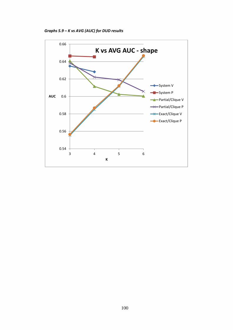
100
Graphs 5.9 – K vs AVG (AUC) for DUD results
0.54
0.56
0.58
0.6
0.62
0.64
0.66
3 4 5 6
AUC
K
K vs AVG AUC - shape
System V
System P
Partial/Clique V
Partial/Clique P
Exact/Clique V
Exact/Clique P

101
Graph 5.10 – K vs AVG (Recall@5%) for DUD results
Graph 5.11 – K vs AVG (Recall@10%) for DUD results
0
5
10
15
20
25
30
3 4 5 6
AVG
Recall@5%
K
K vs AVGRecall@5% - shape
System V
System P
Partial/Clique V
Partial/Clique P
Exact/Clique V
Exact/Clique P
0
5
10
15
20
25
30
35
40
3 4 5 6
AVG
Recall@10%
K
K vs AVG Recall@10% - shape
System V
System P
Partial/Clique V
Partial/Clique P
Exact/Clique V
Exact/Clique P

102
Graphs 5.12 –Spread of AUC results for 40 DUD classes, K=4, Volume and Properties
scores for both Parital/Clique/Shape and Systematic alignments
In table 5.6 below the K representation for several of the DUD reference queries: RXR,
SAHH and AR can be viewed. In the case of RXR we observe both the AUC decrease with
increasing K, from 0.75 to 0.69 and 0.54. It seems that K=3 is the best shape representation
here, with K=4 and 5 not capturing the shape particularly well, with two “incorrectly”
placed points retained between K=4 and 5 which disrupt the natural ring pharmacophores.
In the case of the SAHH query, we observe the AUC measures increase with increasing K for
0
0.1
0.2
0.3
0.4
0.5
0.6
0.7
0.8
0.9
1 6 11 16 21 26 31 36
AUC
DUD
DUD/AUC K=4 Exact
Vol
Prop
0
0.1
0.2
0.3
0.4
0.5
0.6
0.7
0.8
0.9
1
1 6 11 16 21 26 31 36
AUC
DUD
DUD/AUC K=4 systematic
Vol
Prop

103
the clique method from 0.7 to 0.75 and 0.79. It seems the K-means is behaving relatively
well for this query in that it captures the shape and internal heteroatom functionality to
some extent despite not representing rings perfectly. In the case of AR we see AUC
decrease from 0.78 to 0.71 and then 0.67 with increasing K. The shape is perhaps slightly
more correctly captured for K=4. We might also be witnessing the effects of an uneven
volume distribution and again points offset from the ring centres. In all cases we can see
some tendency for the points not to sit inside rings and this undoubtedly will decrease the
effectiveness of our representation. The representation could be modified to share bridge
atoms, as suggested in chapter 6 which should give a more accurate representation. These
examples reflect the general observation in graph 5.9 for partial match mode.
K RXR SAHH AR
3
0.75 0.7 0.78
4
0.69
0.75
0.71
5
0.54 0.79 0.67
Table 5.6 – Selected DUD query RXR, SAHH and AR representation for K=3,4,5. AUC values
for (V score, Clique/Partial Mode) are shown in bottom centre of each cell. The best
observed AUC values are highlighted in green.

104
In table 5.7 below, for the PDGFRB query we see the P score recall @10% values increase
with K from 11.29% to 12.90% and 21.77%. One might say the K=5 is the best
representation because it defines the rings well with points placed fairly neatly in the ring
centres and the amide linker. The scale is captured well using even sized spheres
distributed over the whole molecule. In the case of PARP query, the P score recall @10% is
equivalent for K= 3 and 4 at 19.35% and rises for K=5 to 32.36%. In this case the rings and
pharmacophore groups are being captured more correctly and there is a relatively even
volume distribution over the entire molecule. In the case of Trypsin query, we notice the P
score recall @10% rise from K=3 at 44.44% to K=4 at 66.67% followed by a sudden drop off
at K=5 to 11.11%. This might be rationalised by the rings and linkers being quite well
represented at K=3 and 4. At K=5 there are too many small cluster points which will reduce
the possible overlap scores. One of the ring points is also not well represented, breaking up
a natural pharmacophore and placing the points the “wrong way round”.
Any apparent effects of a potential bias in the scoring due to large Iodine mass can be
deduced by considering the classes COX2, EGFR, ALR2 and AMPC all of which contain high
levels of Iodine in the decoy sets as well as having the two highest actives and decoy counts
over the entire DUD set. COX2 gave good AUC scores over most of the parameterisations
whereas the other three did not exhibit good AUC values. Hence, a logical deduction that
Iodine is not a major factor that affects the observed results can be concluded. Please see
5.4.1 which discussed Iodine composition in the DUD set. Ten percent of the forty classes
contain Iodine with each of the four cases containing ~2%, predominantly (99%) are seen in
the decoys set.
The conclusion for this data set is complex, considering the amount of variability in the
observed result of a single parameterisation and over all K. Scale and ideal K representation
which captures correctly the whole molecule, without splitting pharmacophores and that
of comparing molecules of different “ideal K” should assist in better retrieval and
distinguish of actives. The number of points in a representation is less important than the
fact that we should only use a single point per ring system, with the points placed in the
ring centroids. Small cluster points will have a detrimental effect on volume overlap. For
example PDGFRB at K=5 is a good representation and one might imagine a better
representation of Trypsin for K=4 and above. The sharing of bridge atoms will help towards
a better partition approach. All the molecules in table 5.6 exemplify this to some extent.

105
K PDGFRB PARP Trypsin
3
11.29
19.35
44.44
4
12.90
19.35
66.66
5
21.77
32.36
11.11
Table 5.7 – Selected DUD query PDGFRB, PARP and Trypsin representation for K=3,4,.
Percentage recall @10% values for (P score, Clique/Partial Mode) are shown in bottom
centre of each cell. The best observed recall@10% values are highlighted in green.
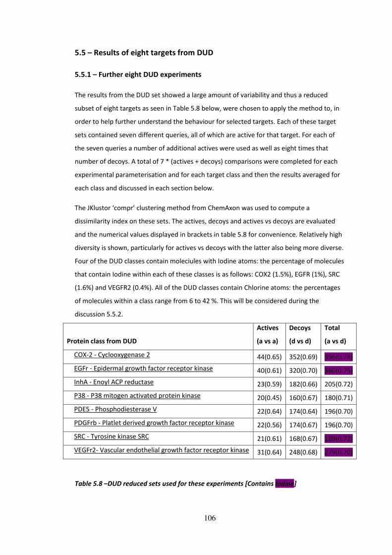
106
5.5 – Results of eight targets from DUD
5.5.1 – Further eight DUD experiments
The results from the DUD set showed a large amount of variability and thus a reduced
subset of eight targets as seen in Table 5.8 below, were chosen to apply the method to, in
order to help further understand the behaviour for selected targets. Each of these target
sets contained seven different queries, all of which are active for that target. For each of
the seven queries a number of additional actives were used as well as eight times that
number of decoys. A total of 7 * (actives + decoys) comparisons were completed for each
experimental parameterisation and for each target class and then the results averaged for
each class and discussed in each section below.
The JKlustor ‘compr’ clustering method from ChemAxon was used to compute a
dissimilarity index on these sets. The actives, decoys and actives vs decoys are evaluated
and the numerical values displayed in brackets in table 5.8 for convenience. Relatively high
diversity is shown, particularly for actives vs decoys with the latter also being more diverse.
Four of the DUD classes contain moleciules with Iodine atoms: the percentage of molecules
that contain Iodine within each of these classes is as follows: COX2 (1.5%), EGFR (1%), SRC
(1.6%) and VEGFR2 (0.4%). All of the DUD classes contain Chlorine atoms: the percentages
of molecules within a class range from 6 to 42 %. This will be considered during the
discussion 5.5.2.
Protein class from DUD
Actives
(a vs a)
Decoys
(d vs d)
Total
(a vs d)
COX-2 - Cyclooxygenase 2 44(0.65) 352(0.69) 396(0.74)
EGFr - Epidermal growth factor receptor kinase 40(0.61) 320(0.70) 360(0.75)
InhA - Enoyl ACP reductase 23(0.59) 182(0.66) 205(0.72)
P38 - P38 mitogen activated protein kinase 20(0.45) 160(0.67) 180(0.71)
PDE5 - Phosphodiesterase V 22(0.64) 174(0.64) 196(0.70)
PDGFrb - Platlet derived growth factor receptor kinase 22(0.56) 174(0.67) 196(0.70)
SRC - Tyrosine kinase SRC 21(0.61) 168(0.67) 189(0.72)
VEGFr2- Vascular endothelial growth factor receptor kinase 31(0.64) 248(0.68) 279(0.70)
Table 5.8 –DUD reduced sets used for these experiments [Contains Iodine]

107
5.5.2 – Discussion of eight experiments
For these eight DUD classes this discussion now aims to assess the method retrieval rates in
terms of two simple indicators: Does any single data point actually represent a good
retrieval in terms of any of the measures or parameterisations and do any of the protein
classes exhibit the overall behaviour witnessed for the well behaved Thrombin set in terms
of K. Full results are shown in graphs 5.13 to 5.20 and the best AUC value for each data set
is shown in table 5.9 alongside the best results reported by Martin for the wavelet method
(Martin et al., 2010) and the evaluated ROCS colour (OpenEye et al., 2002) result.
Protein
class
(Graphs)
Best observed
MAPS3D method
(C or S@K(V/P))
Best
observed
Wavelet
(Dry/AUC)
ROCS
colour
Comparable to method?
COX2 (5.13) 0.74 (C@K=3,4,5,P)
0.89 0.75 ROCS
EGFR
(5.14)
0.60 (S@K=4 V & C@K=6,P)
0.60 0.81 Wavelet
INHA (5.15) 0.74 (S@K=3,P)
0.73 0.59 Wavelet
P38 (5.16) 0.77 (C@K=5,V)
0.83 0.79 ROCS
PDE5 (5.17) 0.79 (S@K=3,V & C@K=3,V)
0.75 0.88 Wavelet
PDGFRB
(5.18) 0.67
(S@K=4,P) 0.85 0.76 x
SRC (5.19) 0.80 (S@K=3,V)
0.91 0.88 ROCS
VEGFR2
(5.20) 0.64
(S@K=3,P) 0.84 0.80 x
Table 5.9 – Assessment of 8 DUD classes in graph sets 5.13 to 5.20. Data from Martin
thesis tables 8.4 and 8.10 are re-produced in table 5.9 alongside the best noted scores
from this approach with the associated parameterisation.
KEY : Clique/Systematic@K=n,Volume/Properties. AUC >0.7, 0.69>=AUC> 0.6 and
AUC=<0.6. Error of 0.05 AUC units is assumed.

108
The classes that show the best response are INHA, P38, PDE5, COX2 and SRC (green in table
5.9) and to some extent PDGFRB and VEGFR2 (yellow in table 5.9). The one that showed
poorest response is EGFR (red in table 5.9). The COX2 and P38 are also useful in that they
show that the five point representation can outperform the systematic alignment at K=3,4
even without an optimisation step. There are also examples of properties scores that are
better than the volume scores and associated retrieval of actives. Logically, the presence of
Iodine has little or no detrimental effects if we consider that PDGFRB (no Iodine) and
EGFR/VEGFR2 (small amounts) and the fact that COX2 (good result) has the most at 1.5%.
Similarly COX2 (42%) and PDE5 (6%) contain the extrema of Chlorine content yet are both
relatively close and have reasonably good scores.
Many of the observed results are significantly better than random (0.5) and the colour
coding explained in table 5.9 attempts to qualitatively assess how good each score can be
categorised. The best observed ‘COX2’ AUC result is 0.74, obtained using Clique alignment
and with K=3,4 or 5 and is directly comparable to ROCS colour 0.75 but the best wavelet
result is significantly better than either at 0.89. The best observed ‘EGFR’ AUC result is 0.60
obtained using either alignment method and is comparable with the wavelet result 0.60
but the best ROCS colour result is significantly better than either at 0.81. The best observed
‘INHA’ AUC result is 0.74 obtained using the systematic alignment K=3 and shows an
improvement on ROCS colour 0.59 and is similar to the wavelet result 0.73. The best
observed ‘P38’ AUC result is 0.77 obtained using parameters Clique alignment K=5 which is
the same order as the best ROCS colour result 0.79 but the wavelet result is slightly better
still at 0.83. The best observed PDE5 result is 0.79 obtained using either alignment method
at K=3 and is the same order of magnitude as the ROCS colour and wavelet result. ROCS
colour is best at 0.88 and the wavelet score is 0.75. The best observed ‘PDGFRB’ result is
0.67 obtained using systematic alignment parameters K=4 which is less than ROCS colour
0.76 with the wavelet approach significantly better 0.85. The best observed ‘SRC’ result is
0.80 obtained using the systematic alignment K=3. This result is good but does not improve
upon either the ROCS colour 0.88 or wavelet approaches 0.91. The best observed ‘VEGFR2’
result is 0.64 obtained using the systematic alignment parameters K=3. This result is
significantly worse than either ROCS colour 0.80 or the wavelet approach 0.84 which show
good results here. The JKlustor values do not assist in any rational argument in this case
since we can see relatively close dissimilarity conditions for (COX2, SRC) and (EGFR,
VEGFR2), (highlighted in yellow in table 5.8) which score relatively well and poorly
respectively.
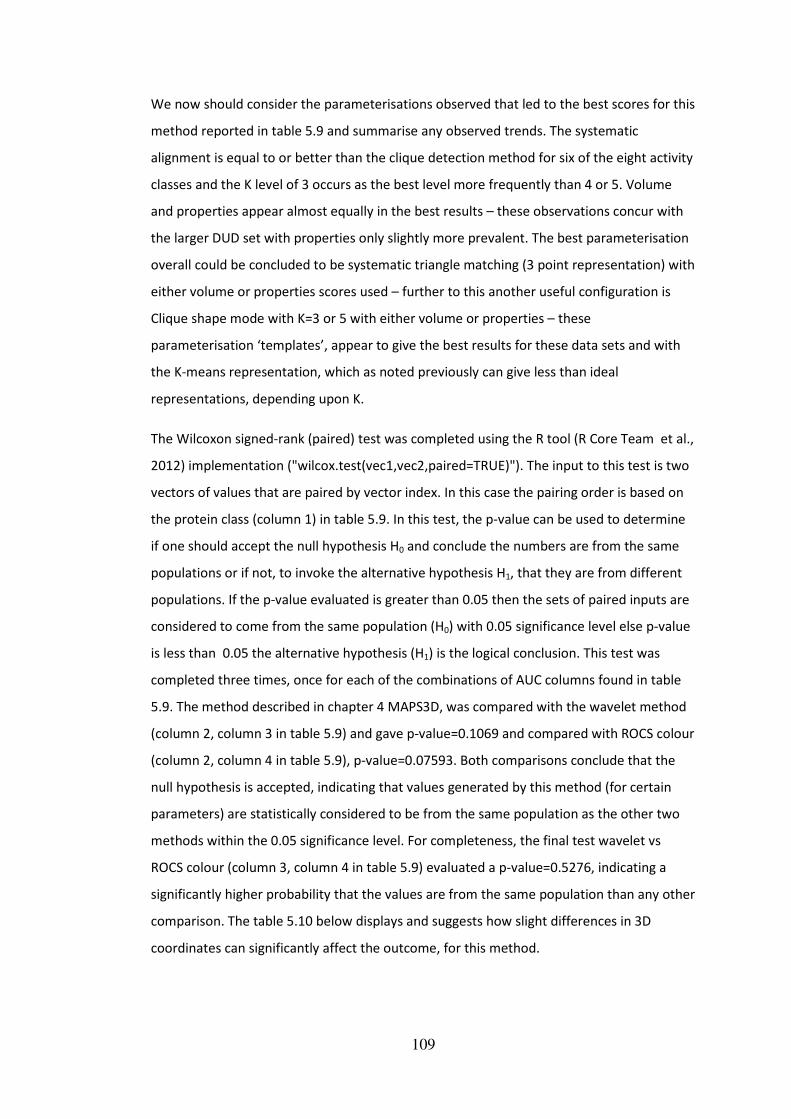
109
We now should consider the parameterisations observed that led to the best scores for this
method reported in table 5.9 and summarise any observed trends. The systematic
alignment is equal to or better than the clique detection method for six of the eight activity
classes and the K level of 3 occurs as the best level more frequently than 4 or 5. Volume
and properties appear almost equally in the best results – these observations concur with
the larger DUD set with properties only slightly more prevalent. The best parameterisation
overall could be concluded to be systematic triangle matching (3 point representation) with
either volume or properties scores used – further to this another useful configuration is
Clique shape mode with K=3 or 5 with either volume or properties – these
parameterisation ‘templates’, appear to give the best results for these data sets and with
the K-means representation, which as noted previously can give less than ideal
representations, depending upon K.
The Wilcoxon signed-rank (paired) test was completed using the R tool (R Core Team et al.,
2012) implementation ("wilcox.test(vec1,vec2,paired=TRUE)"). The input to this test is two
vectors of values that are paired by vector index. In this case the pairing order is based on
the protein class (column 1) in table 5.9. In this test, the p-value can be used to determine
if one should accept the null hypothesis H0 and conclude the numbers are from the same
populations or if not, to invoke the alternative hypothesis H1, that they are from different
populations. If the p-value evaluated is greater than 0.05 then the sets of paired inputs are
considered to come from the same population (H0) with 0.05 significance level else p-value
is less than 0.05 the alternative hypothesis (H1) is the logical conclusion. This test was
completed three times, once for each of the combinations of AUC columns found in table
5.9. The method described in chapter 4 MAPS3D, was compared with the wavelet method
(column 2, column 3 in table 5.9) and gave p-value=0.1069 and compared with ROCS colour
(column 2, column 4 in table 5.9), p-value=0.07593. Both comparisons conclude that the
null hypothesis is accepted, indicating that values generated by this method (for certain
parameters) are statistically considered to be from the same population as the other two
methods within the 0.05 significance level. For completeness, the final test wavelet vs
ROCS colour (column 3, column 4 in table 5.9) evaluated a p-value=0.5276, indicating a
significantly higher probability that the values are from the same population than any other
comparison. The table 5.10 below displays and suggests how slight differences in 3D
coordinates can significantly affect the outcome, for this method.

110
It should be stated that one of the other two approaches always produced an actual better
result, with one exception class ‘INHA’. In many cases this method was very close to the
other results, for example P38, PDE5 and to a lesser extent COX2, SRC, PDGFRB and
VEGFR2. EGFR which scored relatively poorly compared to ROCS colour. Three point
representations feature a lot, as do four and five but these are not as prominent as
compared to Thrombin which shows a smooth rise for increasing K. Properties scores
feature slightly more than volume but for the best noted scores however one might
conclude that volume and properties are synonymous. Trends are less comparable to the
Thrombin set but are consistent with the average DUD observations. Two queries from the
INHA set are aligned and scored for K=3 points as explained in table 5.10. The
representations generated are dependent upon the specific input coordinates, with a single
atom having a large effect on the outcome. This phenomenon is suggested to be an
artefact of the K-means.
Bad – ring split Good - rings and linkers Reasonable – alignment and
score
Table 5.10 – Example of two INHA queries aligned and scored using K=3, scoring V=0.67
and P=2.89. The Volume and internal functionality is aligned reasonably well with three
points. However, one can see with the red spheres the rings and linkers are captured well
however with the white spheres this is not the case and a ring is disrupted. The subtle
difference is an extra atom in the linker in the case of red and for white one of the rings is
not aromatic and is “more 3D” as a result. Hence even in this case with very small atomic
differences, volume overlap will be unnecessarily lost for this alignment and this is
certainly reflected in these scores.

111
Graphs 5.13 – COX2 results
22.5
33.5
44.5
55.5
66.5
7
3 4 5 6
AVG(EF)
K
COX2 K vs AVG(EF)
System V
System P
Partial/Clique V
Partial/Clique P
Exact/Clique V
Exact/Clique P
0
5
10
15
20
25
30
35
40
3 4 5 6
AVG
(Recall@10 %)
%
K
COX2 K vs AVG(RECALL@10%)
System V
System P
Partial/Clique V
Partial/Clique P
Exact/Clique V
Exact/Clique P
0.5
0.55
0.6
0.65
0.7
0.75
0.8
3 4 5 6
AVG(AUC)
K
COX2 K vs AVG(AUC)
System V
System P
Partial/Clique V
Partial/Clique P
Exact/Clique V
Exact/Clique P

112
Graphs 5.14 – EGFR results
2
2.5
3
3.5
4
4.5
3 4 5 6
AVG(EF)
K
EGFR K vs AVG(EF)
System V
System P
Partial/Clique V
Partial/Clique P
Exact/Clique V
Exact/Clique P
0
5
10
15
20
25
30
3 4 5 6
AVG
(Recall@10 %)
%
K
EGFR K vs AVG(RECALL@10%)
System V
System P
Partial/Clique v
Partial/Clique P
Exact/Clique V
Exact/Clique P
0.52
0.53
0.54
0.55
0.56
0.57
0.58
0.59
0.6
0.61
3 4 5 6
AVG(AUC)
K
EGFR K vs AVG(AUC)
System V
System P
Partial/Clique V
Partial/Clique P
Exact/Clique V
Exact/Clique P

113
Graphs 5.15 – INHA results
2
2.5
3
3.5
4
4.5
5
5.5
6
3 4 5 6
AVG(EF)
K
INHA K vs AVG(EF)
System V
System P
Partial/Clique V
Partial/Clique P
Exact/Clique V
Exact/Clique P
0
5
10
15
20
25
30
35
40
45
3 4 5 6
AVG
(Recall@10 %)
%
K
INHA K vs AVG(RECALL@10%)
System V
System P
Partial/Clique V
Partial/Clique P
Exact/Clique V
Exact/Clique P
0.5
0.55
0.6
0.65
0.7
0.75
0.8
3 4 5 6
AVG(AUC)
K
INHA K vs AVG(AUC)
System V
System P
Partial/Clique V
Partial/Clique P
Exact/Clique V
Exact/Clique P

114
Graphs 5.16 – P38 results
2
2.5
3
3.5
4
4.5
5
5.5
6
3 4 5 6
AVG(EF)
K
P38 K vs AVG(EF)
System V
System P
Partial/Clique V
Partial/Clique P
Exact/Clique V
Exact/Clique P
0
5
10
15
20
25
30
35
40
45
3 4 5 6
AVG
(Recall@10 %)
%
K
P38 K vs AVG(RECALL@10%)
System V
System P
Partial/Clique V
Partial/Clique P
Exact/Clique V
Exact/Clique P
0.5
0.55
0.6
0.65
0.7
0.75
0.8
3 4 5 6
AVG(AUC)
K
P38 K vs AVG(AUC)
System V
System P
Partial/Clique V
Partial/Clique P
Exact/Clique V
Exact/Clique P

115
Graphs 5.17 – PDE5 results
0
1
2
3
4
5
6
7
3 4 5 6
AVG(EF)
K
PDE5 K vs AVG(EF)
System V
System P
Partial/Clique V
Partial/Clique P
Exact/Clique V
Exact/Clique P
0
10
20
30
40
50
60
3 4 5 6
AVG
(Recall@10 %)
%
K
PDE5 K vs AVG(RECALL@10%)
System V
System P
Partial/Clique V
Partial/Clique P
Exact/Clique V
Exact/Clique P
0.5
0.55
0.6
0.65
0.7
0.75
0.8
0.85
3 4 5 6
AVG(AUC)
K
PDE5 K vs AVG(AUC)
System V
System P
Partial/Clique V
Partial/Clique P
Exact/Clique V
Exact/Clique P

116
Graphs 5.18 – PDGFRB results
0
1
2
3
4
5
6
3 4 5 6
AVG(EF)
K
PDGFRB K vs AVG(EF)
System V
System P
Partial/Clique V
Partial/Clique P
Exact/Clique V
Exact/Clique P
0
5
10
15
20
25
30
35
40
45
3 4 5 6
AVG
(Recall@10 %)
%
K
PDGFRB K vs AVG(RECALL@10%)
System V
System P
Partial/Clique V
Partial/Clique P
Exact/Clique V
Exact/Clique P
0.5
0.52
0.54
0.56
0.58
0.6
0.62
0.64
0.66
0.68
3 4 5 6
AVG(AUC)
K
PDGFRB K vs AVG(AUC)
System V
System P
Partial/Clique V
Partial/Clique P
Exact/Clique V
Exact/Clique P

117
Graphs 5.19 – SRC results
0
1
2
3
4
5
6
7
8
3 4 5 6
AVG(EF)
K
SRC K vs AVG(EF)
System V
System P
Partial/Clique V
Partial/Clique P
Exact/Clique V
Exact/Clique P
0
10
20
30
40
50
60
3 4 5 6
AVG
(Recall@10 %)
%
K
SRC K vs AVG(RECALL@10%)
System V
System P
Partial/Clique V
Partial/Clique P
Exact/Clique V
Exact/Clique P
0.5
0.55
0.6
0.65
0.7
0.75
0.8
0.85
3 4 5 6
AVG(AUC)
K
SRC K vs AVG(AUC)
System V
System P
Partial/Clique V
Partial/Clique P
Exact/Clique V
Exact/Clique P

118
Graphs 5.20 – VEGFR2 results
2
2.5
3
3.5
4
4.5
5
5.5
6
6.5
7
3 4 5 6
AVG(EF)
K
VEGFR2 K vs AVG(EF)
System V
System P
Partial/Clique V
Partial/Clique P
Exact/Clique V
Exact/Clique P
0
5
10
15
20
25
30
35
40
45
3 4 5 6
AVG
(Recall@10 %)
%
K
VEGFR2 K vs AVG(RECALL@10%)
System V
System P
Partial/Clique V
Partial/Clique P
Exact/Clique V
Exact/Clique P
0.5
0.55
0.6
0.65
3 4 5 6
AVG(AUC)
K
VEGFR2 K vs AVG(AUC)
System V
System P
Partial/Clique V
Partial/Clique P
Exact/Clique V
Exact/Clique P

119
5.6 – Conclusion of overall method effectiveness over these data sets
The Thrombin results show improving results for increasing levels of representation, which
might be considered the intuitive behaviour for an apparently well behaved homogeneous
data set. The magnitude of the results and the trends are generally encouraging compared
to other methods reported in the literature indicating that for this data set this method can
work well. All the stated measures for shape comparison show an increase for increasing
levels of representation K, with the partial matching mode giving the best results. The
clique/partial alignment method outperforms the systematic alignment method with 5
points and above but the systematic alignment also gives good results for 3 and 4 points.
The volume scores V more often outperform the properties P and perhaps the converse is
closer to expectation, since the inclusion of properties attempts to improve the chemical
representation. The sub-shape scores are less conclusive and show the behaviour of
decrease with K, thus indicating that whole molecule matching is preferable.
The whole DUD set exhibits a lot of variation across the 40 protein classes with some
showing good response and others showing little or no response and this seems to be no
different to other 3D methods applied to this data set which can also show a large spread
of AUC values. For the systematic alignment we see K=3,4 gave approximately the same
AUC values but both recall measures increase from K=3 to 4. Exact mode results increase
almost linearly with K for AUC and recall. Partial mode shows a drop off with increasing K.
The properties scores are always better than the volume scores which is a more
encouraging conclusion, assuming pharmacophore properties are exerting an effect. The
systematic alignment gives the better results than clique alignment (K=3 to 6).
All data reported initially are averaged and hence it is not as clear cut as the Thrombin case
which is for a single activity class. The partitioning algorithm yielding non-perfect
representations at certain K levels and the possible need for a clique optimisation might
contribute to the difference. The recall data does tend to portray a slightly better picture of
the average results than AUC showing generally increasing values over increasing K, similar
to Thrombin.
Examining eight of the DUD protein classes in detail we find that several of the classes
show some good results. The method performed best on P38, PDE5, PDGFRB and to some
extent COX2, INHA and SRC. VEGFR2 and EGFR show relatively poor response. This method

120
has been directly compared to Sheffield wavelet thumbnail and ROCS colour in this chapter
and the compared results showed no significant difference within a 0.05 significance level.
It was observed that the clique alignment method with K=5 can outperform the systematic
alignment K=3,4 for some of these sets but not often. This might lead to the conclusion that
basic three point representation and ‘Triangle matching’, scoring using either volume or
properties is actually on average the most effective method. Example of other triangle or
three point representation based methods are defined in the literature (Bonachera et al.,
2006; Kinnings et al., 2009). The presence of Iodine or Chlorine was shown not to have any
detrimental or bias effects on the results. The results were not as good as those exhibited
by ROCS colour or the wavelet method, however triangle alignment can be very fast and so
there is some utility as a faster pre-screening step.
Both alignment methods have some utility and of course the systematic alignment is only
able to deal with three or four points, so for larger molecules based on scale, the clique
alignment method should be the dominant option. One of the major over-sights of this
approach was not considering scale appropriately and always matching similar levels of
representation without considering, the three internal principal moments which help to
identify the relative sizes of molecules. The shape mode seems to be more effective in
resolving actives and decoys which makes sense also since in the entire representation
(more information) is being considered (sub-shape can give false actives).
A limitation of the K-means algorithm was identified, it was shown that the K-means can
naturally produce artificially small points that contain only 1 or 2 atoms and this can also be
detrimental to performance, since the available overlap volume can reduce sharply. Also
non-ideal “ring breaker” representations are possible. It appears that the level of K used
will only be beneficial to the scoring if the number of points represents the major rings and
fragments correctly and it is clear that comparing molecules with the same K is incorrect if
scale is not considered suitably. Suggestions for improvement of the partition algorithm are
made in the next chapter 6.

121
Chapter 6 – Conclusions and future work
6.1 – Conclusions
This thesis has included a literature search in the areas of virtual screening, rational drug
design and 3D similarity search. The development of a novel three dimensional similarity
searching method is then described. A set of Java programs has been developed that
executes the method workflows described in Chapter 4. This method has been applied to
some industry standard test data sets and the results observed and discussed in Chapter 5.
The rest of this chapter describes suggested ways to improve on the basic methods and
approaches defined in chapter 4.
The previous chapter 5 described three sets of experiments that have aimed to validate the
method described in chapter 4. The first experimental set was the single target class of
Thrombin actives and showed that the method behaves largely as might be presumed for a
homogeneous set of actives. As the number of points increased then the retrieval
increased however perhaps more surprising was the properties scores often did not
outperform the volume scores. The sub-shape scores were also less discriminating.
The second experimental set examined was the forty DUD targets. This data set showed a
lot of variation with this method in that some classes showed promise with actives scoring
well with the queries and with visual alignments and associated scores that seem quite
reasonable to analysis and visual inspection (Figure 4.24). The trends on the whole show
properties scores to be more discriminating than volume but it is much less clear about the
best level of representation for the entire set. Some of the classes showed very little
propensity to be resolved via this method at all and so at best it would appear it could be
used for only some of the protein classes in this set. The alignment methods proved to be
largely comparable with some cases where the clique approach with K>4 gave better
results than the systematic approach, particularly with the exact mode.
The final set of experiments concentrated on eight of the DUD classes which were also
used in validation experiments of other 3D similarity methods reported in the literature. In
some cases, the method compared well with the established methods with the values
showing some clear overlap and also a fairly normal distribution of response was observed
over the eight targets with several relatively good, several average and some poor results

122
observed. In most cases, this method does not perform to the same standard as the bench
mark ROCS colour method but in most cases it is of the same order of magnitude. In one of
the eight cases it did outperform ROCS colour in terms of AUC scores (INHA). Looking in
more detail at the components of the method we can describe potential improvements
that could be investigated.
• The K-means representation used proved to be useful to some extent in some
cases and parameterisations. The concept of scale was not well implemented in
that identical levels of representation K, were always compared irrelevant of
molecular size. Using a standard unit size sphere, for example using the radius of a
six member ring as standard, could be used to place points in a new
representation. The K-means can give representations with non-ideal point
placements as Table 5.10 shows in the simplest of cases with minor structural
modifications a detrimental effect is seen using K-means (rings split). Comparing
molecules represented by different numbers of “ring units” is likely to give
markedly improved results and in particular the sub-shape results should also
improve with a better implementation of scale.
• Both alignment methods and scoring approaches seem perfectly reasonable to
investigate further with a possible improved representation. Assuming that some
larger molecules will certainly have to be represented with more than four points
then the clique method would certainly be required in the alignment step.
• The scoring functions used could be tuned further to include more atom or
chemical information or extended with alternative scoring such as simple counts of
pharmacophore typed atoms rather than using atomic masses.
• Flexible search was not investigated here and indeed would be unlikely to improve
the picture until such a time as the representation or partitioning approach is
improved upon. Representative (extrema and average) conformers are a
reasonable input for this.
• Alignment of three point representations just using the Kabsch algorithm is another
possible avenue to investigate.

123
There is evidence to suggest the method is working as intended with trends being observed
which are reasonable with some data sets. Does the method identify biologically similar
molecules as was the original intention? Yes, there is evidence to suggest this is occurring
in some cases with visual and numerical evidence to support this. Does the method
discriminate sufficiently between different molecules? To some extent the retrieval rates
show some good discrimination for some classes but this method by no means out
performs other established similarity methods. Is there any correlation with the scores and
biological activity? The method shows some correlation with biological activity but certainly
with open questions. Is the method fast enough for real sized searches? For a real
environment with very large data sets this method as currently implemented would
struggle to perform to an acceptable standard. Fingerprinting the representation does help
speed up method execution. Processing of the cliques was noted in particular as the rate
determining step for that alignment method and the systematic alignment method did
perform significantly faster (matching triangles with this method is rapid). Overall, it can be
said that this approach is novel relative to its peers and does show some initial promise.
The next sections describe ways in which the method and performance may be improved
to achieve better results. From the author’s perspective it has certainly been a considerable
learning experience in the field.
124
6.2 – Suggestions for future work
6.2.1 – Extending the partitioning approach
Alternative reduced graphs in two dimensions have been applied to 2D similarity search
where the performance is comparable to Daylight fingerprints (Gillet et al., 2003). The
reduction schemas applied are based on ring systems and functional groups defined using
SMARTS strings. It should be possible to extend the 2D graph representation to 3D, which
could then form the input to the alignment methods developed here. The K-means
algorithm does not always result in the partitioning of molecules into fragments of similar
sizes and can in some cases give less than ideal centroid placements. Spheres that are of
different sizes have a detrimental effect on similarity comparison (in some cases the K-
means assigns a single atom to a point). The K-means is potentially good to identify an
initial set of well distributed seed starting points that can then be used as initial conditions.
Such extension schemes could include rules to allow the sharing of atoms across clusters
(bridge atoms), ensuring ring systems are always retained intact where possible with ring
centred points and also smarter ways to identify successive points in the representation
generation. Further to this the points are derived geometrically to start with but could be
weighted so as to reflect the centre of mass of the atoms. Figure 6.1 below shows an
example of a point that is not aligned with the ring centroid since the points cannot share
the bridge atoms.
Figure 6.1 - The K-means does not accommodate bridge sharing of atoms (the group
membership is currently mutually exclusive).
6.2.2 – Use of smart search algorithm and non-deterministic representation set
The K-means can be non-deterministic if seeded with K random coordinate starting points.
This in turn leads to a set of solutions, one of which was always observed as equal to the

125
deterministic solution. Speculation on the nature of the deterministic solution always
appearing in the solution set for non-deterministic algorithm is not analysed further here.
Clearly there could be scope to investigate a set of non-deterministic representations
generated in conjunction with a smarter search algorithm which might be used to
determine representations that approach ideal. The ideal value for the number of points
required to represent a (drug-like) molecule is also part of the research question, however
other approaches suggest 3, 4 and possibly 5 point pharmacophores are assumed to give
an adequate level of description. However one must consider that pharmacophores are
normally considered a substructure and thus these heuristics might not apply to
partitioned whole molecules but might apply to portions of active “sub-shapes”. The
representation is essentially molecular fragments which are not discrete classical chemical
functional groups that are identified by a SMARTS.
6.2.3 - Comparing molecules of different K representations
The current method is restricted to comparing molecules that are reduced to the same
number of K points. While this may be a reasonable approach for molecules that are of
similar sizes it is unlikely to be optimal where the query and target molecules are
significantly different in size. A more effective approach may be to choose K so that each
node represents a different structural feature such as a ring or aliphatic fragment or so that
each K represents a fixed number of atoms. Thus the level of reduction would be molecule
dependent. Since the clique alignment approach can accept any number of points for query
and target this could be used directly with any new representation of any number of points
for either. An example of where the K-means does a provide a reasonable representation is
the molecule Gleevec shown in Figure 6.2 below.
Figure 6.2 - The molecule Gleevec represented (relatively well) by the K-means at K=5.

126
6.2.4 – Flexible search
A suggested way to include flexible search in this approach is to build information about
inherent molecular flexibility into the representation so that there is still only a single
representation object to handle for each molecule within any given search context. This
could potentially reduce the search time for flexible search relative to employing the
ensemble approach or exhaustively searching through rotational bonds, both of which
become less tractable as the inherent flexibility increases. As such, flexible search as
described here should add little or no additional over-head since the radius r value is the
only term modified. The approach requires that some representative conformers are
generated similar to the ensemble approach. Two important criteria regarding any
molecule’s flexibility are the number of rotational bonds present and the associated RMSD
for an ensemble of conformations. The latter is derived experimentally.
For each sphere, k a flexibility weighting could be applied to the radius according to the
number of rotatable bonds present in its constituent atoms. A suggested function is
defined below in equation 6.1 which shows a function that should return a simple number
that slightly increases the size of the local sphere representation based upon the fractional
number of rotational bonds present and thus provides a basis for investigation.
Equation 6.1
k. |lexibler = f �k. r ∗ �1 +k.Rotatablebondcountk. Totalbondcount ��Where “k.r” is the kth sphere radius and the other terms are the sums of rotatable and
non-rotatable bond counts defined in the kth sphere
A common way of handling conformational flexibility is the ensemble approach where a
representative set of conformations is used to represent a flexible molecule. Within any
ensemble set there is usually an RMSD value associated with each conformer relative to
some reference lowest energy conformation for that molecule. Thus a useful numerical
index for flexibility is defined by the average RMSD or average internal strain energy value
of the range of conformers from the minimal or lowest energy instance and helps indicate
the amount of variability over the set of atoms in the molecule.

127
Each conformation is a query in its own right however, the interest is mainly how similar
molecules behave irrespective of the ensemble of conformations. In order to derive a single
representation object for search, we should still need to generate a small number of
representative conformers with the ensemble approach and then use the RMSD
information in the construction of the flexible representation. Given an ensemble of
conformers and an associated maximal RMSD for a set of conformers we can build the
global flexibility into each member sphere radii as well as incorporating the local flexibility
as defined above. A simple function to combine both “local” and “global” flexibility is
suggested in equation 6.2 below.
Equation 6.2
k. |lexibler= f �k. r ∗ �1 +k. Rotatablebondcountk. Totalbondcount � + �1 + k. HeavyAtomCount ∗ RMSDHeavyAtomCount �2 �Where “k.r” is the kth sphere radius and the other terms are the sums of rotatable and
non-rotatable bond counts and the heavy atom count defined in the kth sphere, the global
heavy atom count and the RMSD defined for the ensemble, if it exists.
The issue is then where to position the centroid of the sphere and one option would be to
use the group centroid. This is of course a speculative research question and it has been
noted in chapter 3 that flexible search often adds absolutely no observed value to similarity
type approaches.
6.2.5 - Gaussian function to model rigid or flexible fragment
During group level scoring exactly when hard or soft sphere should be employed is likely to
be related to the distance between two points during any given overlap comparison (Grant
et al., 1995).The original Grant/Pickup work suggested that a choice between the two
representations was actually based upon the distance between two points. It is also
pertinent to consider the use of soft sphere representations to model flexible groups. Since
it is difficult to parameterise a non-spherical Gaussian to represent a fragment perhaps a
spherical Gaussian can be used to model flexibility at the fragment level i.e. the spherical
Gaussian parameterisation for a fragment is derived in conjunction with the modified
flexible index above so that the effects of matter over the flexible space decays in some
fashion and is not uniform. This seems a more realistic way to model a fragment that is

128
mobile and rapidly moving or rotating in space and thus exerts some form of centripetal
force. One might expect more mass to be found closer to the source of rotation rather than
further away, to some extent. The Gaussian function parameterisation can be extracted by
using the hard sphere rigid or flexible radius in order to give a spherical Gaussian
representation in 3D with a density component. This representation may be integrated
quickest in conjunction with a look up table which stores the parameterisation and
evaluated integrals. See equation 6.3 below.
Equation 6.3
��� = 2.7 ∗ � �� �� �-�� ∗ � sin ����
� ∗ � ��-��
Where r is the sphere radius and b is the required Gaussian pre-factor and Vhs is the hard
sphere volume.
6.2.6 - Use of radial distribution functions at atom level for superposition query
generation
Use of an active series alignment, to derive pharmacophore hypotheses is a well known
technique, the original being termed the active analogue approach (Marshall et al., 1979)
with many other similar approaches such as GASP, GALAHAD, CATALYST and DISCO (Patel
et al., 2002), which are all well established methods of deriving accurate query data for any
given search problem domain. Many molecules are geometrically aligned, compared and
scored in order to compile a dense object for logical hypotheses extraction. Ultimately, the
reduced point representation of a molecule is run to “completion” we end up dealing with
an all atom representation. Query derivation or elucidation might yield a denser “super
molecule” object for input into the database search process. This data object sourced from
a set of coordinates and might be the result of an active series alignment perhaps based
upon a similar overlap scoring function and alignment approach to the database search. An
all atom comparison and score during an elucidation phase followed by a reduced points
extraction method to derive a query object clearly exists using this approach. In the past
atoms have been represented as hard spheres and soft spheres and any discussion of the
merits of using a soft sphere approach primarily include a more accurate depiction of
electron density decay with distance from a specific atomic nucleus. At the group or
fragment level the use of spherical or non-spherical Gaussians electron density might be
difficult to parameterise correctly and at the atomic level a simple Gaussian may not reflect

129
more complex higher atomic number atoms very well which also contain non-spherical
atomic orbitals. Characteristic single atom density decay can be more accurately
approximated by use of radial distribution functions which are higher forms of the Gaussian
function which include power series in with an additional �� term. The alignment and
comparison of two or more molecules in order to maximise the volume and properties
overlap of an active series might be based upon the use of radial distribution functions to
represent atoms. Clearly, in this approach atoms and fragments will require different
functional forms and parameterisations. This could provide a super molecule object which
could be used for subsequent combinatorial extraction of speculative hypothesis source for
“Reduced point fuzzy pharmacophore vectors”. Once an alignment is complete one will
have a dense set of points to which we can apply our representation approaches in order to
derive a set of objects as query. Use of the all atom density overlap criterion to generate
the dense point set which is then used to derive the representation source will require
scoring of all representative conformers in an active series. Figure 6.3 shows the use of an
exponential function to model an S orbital.
10 5 0 5 10
1
2
1S orbital
e distance from nucleus
e den
sity
A eb r⋅( )
2−
⋅
r
Figure 6.3 - Radial distribution function ���� = �� ∗ � ¡���� can be used to model a
Hydrogen 1s orbital and for use as higher orbital representation. The overlap of these
functions could be used to score an elucidation / alignment method.
Please see equation 6.4 for associated integral.
Equation 6.4
¢f�x, y, z�dv =�� � f�r, θ, ω�dv�
� = � Ae¤� �� r�dr ∗ � sinθdθ¥
� ∗ � dω-¥�
Where n is an integer and A and b are characteristic exponential factors. This is the
spherical coordinates form of the integral.

130
6.2.7 - Use of a field graph at the fragment level
Since it is a difficult task to correctly parameterise and construct a (non-spherical) Gaussian
function that correctly represents an arbitrary fragment as a field then it might be
pertinent to employ an icosahedral field graph approximation for each point (k) in order to
simulate a local scalar or vector field. It is assumed that this sort of treatment might be a
way to extend the scoring for molecules that exhibit high volume and property overlap. The
VDW and electrostatic contribution of each fragment could be determined at each vertex
and a scalar (VDW) or vector (electrostatic) field defined using a [+1,0,-1] probe. It is
suggested that this platonic solid is scaled such that each vertex sits upon a sphere that is
slightly larger (1 Å) than the maximal distance between the centroid and furthest atom
member in each cluster point and in fact an alternative radius such as in equation 6.1 could
be used here. Clearly such an approach could use existing formal charge or would require
the use of a partial charge assignment algorithm for the heavy atoms. Alignment of a net
dipole vector for each fragment is also another possible avenue to explore. Heavy atom
partial charge could be assigned using the orbital electronegativity plug-in, for example
from ChemAxon. Please see equation 6.5 below which describes a possible scoring
approach.
Equation 6.5
¦§��� = $$[+1,0,−1]¨ ∗©ª4«¬��ª¨-�
¨&'
ª&'
Where ©ª is kth point charge, �ª¨ is distance between kth point and j th probe evaluation
point and ¬� is a vacuum permittivity constant.
6.2.8 – Using Structural and active site data for included or excluded volume
If a protein structure is available, an active site shape could be extracted by taking a “cast”
of the active site and mapping this point set to an “inverse object” or “pseudo ligand” that
is contained with the convex hull of what is effectively a 3D graph of the active site.
Inversion of these characteristics in the space defines an ideal complementary set of points
in terms of required interactions. It seems that one way this could be achieved is by taking
the geometric mid-points between all atom combinations and then applying a slightly

modified version of the representation generation approach in order to define the effective
inverse. This could then be included in an active series alignment as
template prior to active series overlay in rotational bond or biological
example. This could be thought of as a simple kind
docking approach whereby
template for further alignments
structure based 3D similarity approach
subsequently extracted
active series alignment and elucidation stage such as described in 6.2.1 above. Complex
crystal water molecules can be treated as discrete points also in
and used in mass weighting in the H
Figure 6.4 - Extracting an active site negative image
between all active site atoms can be used as the dense data set to be partitioned and
then used as a K point ‘spacer template’ which can be incorporated into an elucidation or
search.
131
modified version of the representation generation approach in order to define the effective
inverse. This could then be included in an active series alignment as the starting point
template prior to active series overlay in rotational bond or biological activity order, for
example. This could be thought of as a simple kind of pharmacophore or fragment level
whereby an active site inverse template is derived and used as a
alignments (Ebalunode et al., 2008). This would then become a
structure based 3D similarity approach with the aim to enhance the accuracy of the queries
extracted (Goto et al., 2004). Such data could also be incorporated into an
active series alignment and elucidation stage such as described in 6.2.1 above. Complex
al water molecules can be treated as discrete points also in this approach and treated
and used in mass weighting in the H-bond donor/acceptor categories.
Extracting an active site negative image. The midpoints of all chords formed
all active site atoms can be used as the dense data set to be partitioned and
then used as a K point ‘spacer template’ which can be incorporated into an elucidation or
modified version of the representation generation approach in order to define the effective
the starting point
activity order, for
harmacophore or fragment level
s derived and used as a
. This would then become a
aim to enhance the accuracy of the queries
Such data could also be incorporated into an
active series alignment and elucidation stage such as described in 6.2.1 above. Complex
this approach and treated
. The midpoints of all chords formed
all active site atoms can be used as the dense data set to be partitioned and
then used as a K point ‘spacer template’ which can be incorporated into an elucidation or

132
6.3 – Conclusion
Some ways to extend the methods in chapter 4 are suggested here. Partitioning scheme
modifications are suggested as the primary change, in order to create a more accurate or
effective representation that does not split up natural ring pharmacophoric ring systems.
Modified representations generated and compared at different K levels are almost
certainly a crucial next step for the existing representation. Alternatively, another reduced
point representation can be used with the alignment and scoring methods discussed in
Chapter 4. In addition the non-deterministic K-means could be investigated in conjunction
with a genetic algorithm. A flexible search approach can be defined using rotational bond
and RMSD data but it was noted in the literature that often this will yield no improvements.
The use of a look up table to pre-compute each representation prior to alignment will yield
a performance increase. A field based approach could be annotated using icosahedral
approximations and an electrostatic scoring function to model charge distribution which is
not included in the current model. The negative image of a protein active site could be
extracted and built into the query. Some simple data fusion rules might be used with
different alignments and scores to derive indexes that correlate better with observed
biological activity. Deriving an accurate query using multiple molecule overlay and accurate
radial distribution atomic functions is also possible.

133
Bibliography
Ballester P.J. (2011) "Ultrafast shape recognition: method and applications". Future
Medicinal Chemistry 3:65-78. DOI: 10.4155/fmc.10.280. Barton D.H.R., Cookson, R. C. (1956) "The principles of conformational analysis". Quarterly
Reviews 10:44-82. DOI: 10.1039/qr9561000044. Baum D., Hege, H. C. (2006) A point-matching based algorithm for 3D surface alignment of
drug-sized molecules, in: M. R. Berthold, et al. (Eds.), Computational Life Sciences Ii, Proceedings, Springer-Verlag Berlin, Berlin. pp. 183-193.
Bender A., Glen, R. C. (2005) "Discussion of measures of enrichment in virtual screening: Comparing the information content of descriptors with increasing levels of sophistication". Journal of Chemical Information and Modeling 45:1369-1375. DOI: 10.1021/ci05000177.
Bender A., Mussa, H. Y., Gill, G. S., Glen, R. C. (2004) "Molecular surface point environments for virtual screening and the elucidation of binding patterns (MOLPRINT 3D)". Journal of Medicinal Chemistry 47:6569-6583. DOI: 10.1021/jm049611i.
Bonachera F., Parent, B., Barbosa, F., Froloff, N., Horvath, D. (2006) "Fuzzy tricentric pharmacophore fingerprints. 1. Topological fuzzy pharmacophore triplets and adapted molecular similarity scoring schemes". Journal of Chemical Information
and Modeling 46:2457-2477. DOI: 10.1021/ci6002416. Bondi A. (1964) "Van Der Waals volumes + radii". Journal of Physical Chemistry 68:441-&.
DOI: 10.1021/j100785a001. Bostrom J., Greenwood, J. R., Gottfries, J. (2003) "Assessing the performance of OMEGA
with respect to retrieving bioactive conformations". Journal of Molecular Graphics
& Modelling 21:449-462. DOI: 10.1016/s1093-3263(02)00204-8. Brenke R., Kozakov, D., Chuang, G. Y., Beglov, D., Hall, D., Landon, M. R., Mattos, C., Vajda,
S. (2009) "Fragment-based identification of druggable 'hot spots' of proteins using Fourier domain correlation techniques". Bioinformatics 25:621-627. DOI: 10.1093/bioinformatics/btp036.
Brint A.T., Willett, P. (1987a) "Pharmacophoric pattern-matching in files 3D chemical structures - Comparison of geometric searching algorithms". Journal of Molecular
Graphics 5:49-56. Brint A.T., Willett, P. (1987b) "Algorithms for the identification of 3-dimensional maximal
common substructures". Journal of Chemical Information and Computer Sciences 27:152-158. DOI: 10.1021/ci00056a002.
Bron C., Kerbosch, J. (1973) "Finding all cliques of an undirected graph". Communications of
the Acm 16:575-577. DOI: 10.1145/362342.362367. Brown R.D., Martin, Y. C. (1996) "Use of structure activity data to compare structure-based
clustering methods and descriptors for use in compound selection". Journal of
Chemical Information and Computer Sciences 36:572-584. DOI: 10.1021/ci9501047. Calzals F., Karande, C. (2008) "A note on the problem of reporting maximal cliques".
Theoretical Computer Science 407:564-568. DOI: 10.1016/j.tcs.2008.05.010. Carbo R., Leyda, L., Arnau, M. (1980) "How similar is a molecule to another - An electron-
density measure of similarity between 2 molecular structures". International
Journal of Quantum Chemistry 17:1185-1189. DOI: 10.1002/qua.560170612. Cheeseright T., Mackey, M., Rose, S., Vinter, A. (2006) "Molecular field extrema as
descriptors of biological activity: Definition and validation". Journal of Chemical
Information and Modeling 46:665-676. DOI: 10.1021/ci050357s. ChemAxon. (2012) JKlustor / Compr.

134
Chen B.N., Harrison, R. F., Pasupa, K., Willett, P., Wilton, D. J., Wood, D. J., Lewell, X. Q. (2006a) "Virtual screening using binary kernel discrimination: Effect of noisy training data and the optimization of performance". Journal of Chemical
Information and Modeling 46:478-486. DOI: 10.1021/ci0505426. Chen Q., Higgs, R. E., Vieth, M. (2006b) "Geometric accuracy of three-dimensional
molecular overlays". Journal of Chemical Information and Modeling 46:1996-2002. DOI: 10.1021/ci060134h.
Connolly M.L. (1983) "Solvent accessible surfaces of Proteins and Nucleic acids". Science 221:709-713. DOI: 10.1126/science.6879170.
Corey E., Czako, B., Laszlo, K. (2007) Molecules and Medicine Wiley-Interscience, New Jersey.
Corvalan N.A., Zygadlo, J. A., Garcia, D. A. (2009) "Stereo-selective activity of Menthol on GABA(A) receptor". Chirality 21:525-530. DOI: 10.1002/chir.20631.
Cosgrove D.A., Bayada, D. M., Johnson, A. P. (2000) "A novel method of aligning molecules by local surface shape similarity". Journal of Computer-Aided Molecular Design 14:573-591. DOI: 10.1023/a:1008167930625.
Cramer R.D., Patterson, D. E., Bunce, J. D. (1988) "Comparative molecular field analysis (COMFA) .1. Effect of shape on binding of steroids to carrier proteins". Journal of
the American Chemical Society 110:5959-5967. DOI: 10.1021/ja00226a005. Dixon S.L., Smondyrev, A. M., Knoll, E. H., Rao, S. N., Shaw, D. E., Friesner, R. A. (2006)
"PHASE: a new engine for pharmacophore perception, 3D QSAR model development, and 3D database screening: 1. Methodology and preliminary results". Journal of Computer-Aided Molecular Design 20:647-671. DOI: 10.1007/s10822-006-9087-6.
Ebalunode J.O., Ouyang, Z., Liang, J., Zheng, W. F. (2008) "Novel approach to structure-based pharmacophore search using computational geometry and shape matching techniques". Journal of Chemical Information and Modeling 48:889-901. DOI: 10.1021/ci700368p.
Feher M., Schmidt, J. M. (2000) "Multiple flexible alignment with SEAL: A study of molecules acting on the colchicine binding site". Journal of Chemical Information
and Computer Sciences 40:495-502. DOI: 10.1021/ci9900682. Fink T., Reymond, J. L. (2007) "Virtual exploration of the chemical universe up to 11 atoms
of C, N, O, F: Assembly of 26.4 million structures (110.9 million stereoisomers) and analysis for new ring systems, stereochemistry, physicochemical properties, compound classes, and drug discovery". Journal of Chemical Information and
Modeling 47:342-353. DOI: 10.1021/ci600423u. Fukui K., Fujimoto, H. (1997) Frontier Orbitals and Reaction Paths - selected papers of
Kenichi Fukui World Scientific, Singapore. Gibson K.D., Scheraga, H. A. (1987) "Exact calculation of the volume and surface are of
fused hard sphere with unequal atomic radii". Molecular Physics 62:1247-1265. DOI: 10.1080/00268978700102951.
Gillet V.J., Willett, P., Bradshaw, J. (2003) "Similarity searching using reduced graphs". Journal of Chemical Information and Computer Sciences 43:338-345. DOI: 10.1021/ci025592e.
Glen R.C., Adams, S. E. (2006) "Similarity metrics and descriptor spaces - Which combinations to choose?". QSAR & Combinatorial Science 25:1133-1142. DOI: 10.1002/qsar.200610097.
Glick M., Robinson, D. D., Grant, G. H., Richards, W. G. (2002) "Identification of ligand binding sites on proteins using a multi-scale approach". Journal of the American
Chemical Society 124:2337-2344. DOI: 10.1021/ja016490s.

135
Good A.C., Hodgkin, E. E., Richards, W. G. (1992) "Utilization of Gaussian functions for the rapid evaluation of Molecular Similarity". Journal of Chemical Information and
Computer Sciences 32:188-191. DOI: 10.1021/ci00007a002. Good A.C., Oprea, T. I. (2008) "Optimization of CAMD techniques 3. Virtual screening
enrichment studies: a help or hindrance in tool selection?". Journal of Computer-
Aided Molecular Design 22:169-178. DOI: 10.1007/s10822-007-9167-2. Good A.C., Richards, W. G. (1993) "Rapid evaluation of shape similarity using Gaussian
functions". Journal of Chemical Information and Computer Sciences 33:112-116. DOI: 10.1021/ci00011a016.
Good A.C., Richards, W. G. (1998) "Explicit calculation of 3D molecular similarity". Perspectives in Drug Discovery and Design 9-11:321-338.
Goodford P.J. (1985) "A computational procedure for determining energetically favourable binding sites on biologically important macromolecules". Journal of Medicinal
Chemistry 28:849-857. DOI: 10.1021/jm00145a002. Goto J., Kataoka, R., Hirayama, N. (2004) "Ph4Dock: Pharmacophore-based protein-ligand
docking". Journal of Medicinal Chemistry 47:6804-6811. DOI: 10.1021/jm0493818. Grant J.A., Pickup, B. T. (1995) "A Gaussian description of molecular shape". Journal of
Physical Chemistry 99:3503-3510. DOI: 10.1021/j100011a016. Hahn M. (1997) "Three-dimensional shape-based searching of conformationally flexible
compounds". Journal of Chemical Information and Computer Sciences 37:80-86. DOI: 10.1021/ci960108r.
Halgren T.A. (1998) "Characterization of MMFF94, MMFF94s, and other widely available force fields for conformational energies and for intermolecular-interaction energies and geometries". Abstracts of Papers of the American Chemical Society 216:U702-U702.
Hall L.H., Kier, L. B. (2001) "Issues in representation of molecular structure - The development of molecular connectivity". Journal of Molecular Graphics &
Modelling 20:4-18. DOI: 10.1016/s1093-3263(01)00097-3. Hansch C. (2011) "The advent and evolution of QSAR at Pomona College". Journal of
Computer-Aided Molecular Design 25:495-507. DOI: 10.1007/s10822-011-9444-y. Hansch C., Leo, A., Taft, R. W. (1991) "A survey of Hammett substituent constants and
resonance and field parameters". Chemical Reviews 91:165-195. DOI: 10.1021/cr00002a004.
Hendlich M., Bergner, A., Gunther, J., Klebe, G. (2003) "Relibase: Design and development of a database for comprehensive analysis of protein-ligand interactions". Journal of
Molecular Biology 326:607-620. DOI: 10.1016/s0022-2836(02)01408-0. Hofbauer C., Lohninger, H., Aszodi, A. (2004) "SURFCOMP: A novel graph-based approach
to molecular surface comparison". Journal of Chemical Information and Computer
Sciences 44:837-847. DOI: 10.1021/ci0342371. Holliday J.D., Salim, N., Whittle, M., Willett, P. (2003) "Analysis and display of the size
dependence of chemical similarity coefficients". Journal of Chemical Information
and Computer Sciences 43:819-828. DOI: 10.1021/ci034001x. Huang N., Shoichet, B. K., Irwin, J. J. (2006) "Benchmarking sets for molecular docking".
Journal of Medicinal Chemistry 49:6789-6801. DOI: 10.1021/jm0608356. Irwin J.J., Shoichet, B. K. (2005) "ZINC - A free database of commercially available
compounds for virtual screening". Journal of Chemical Information and Modeling 45:177-182. DOI: 10.1021/ci049714+.
Jenkins J.L., Glick, M., Davies, J. W. (2004) "A 3D similarity method for scaffold hopping from the known drugs or natural ligands to new chemotypes". Journal of Medicinal
Chemistry 47:6144-6159. DOI: 10.1021/jm049654z.

136
Johnson A.M., Maggiora, G. M. (1990) Concepts and applications of molecular similarity, New York.
Johnston H.C. (1976) "Cliques of a graph - Variations on Bron-Kerbosch algorithm". International Journal of Computer & Information Sciences 5:209-238. DOI: 10.1007/bf00991836.
Kabsch W. (1976) "Solution for the best rotation to relate 2 sets of vectors". Acta
Crystallographica Section A 32:922-923. DOI: 10.1107/s0567739476001873. Kearsley S.K., Smith, G. . (1992) "An alternative method for the alignment of molecular
structures : Maximising electrostatic and steric overlap". Tetrahedron Computer
Methodology 3:615-633. Kinnings S.L., Jackson, R. M. (2009) "LigMatch: A multiple structure-based ligand matching
method for 3D virtual screening". Journal of Chemical Information and Modeling 49:2056-2066. DOI: 10.1021/ci900204y.
Kirchmair J., Markt, P., Distinto, S., Wolber, G., Langer, T. (2008) "Evaluation of the performance of 3D virtual screening protocols: RMSD comparisons, enrichment assessments, and decoy selection - What can we learn from earlier mistakes?". Journal of Computer-Aided Molecular Design 22:213-228. DOI: 10.1007/s10822-007-9163-6.
Labute P., Williams, C., Feher, M., Sourial, E., Schmidt, J. M. (2001) "Flexible alignment of small molecules". Journal of Medicinal Chemistry 44:1483-1490. DOI: 10.1021/jm0002634.
Landrum G.A., Penzotti, J. E., Putta, S. (2006) "Feature-map vectors: a new class of informative descriptors for computational drug discovery". Journal of Computer-
Aided Molecular Design 20:751-762. DOI: 10.1007/s10822-006-9085-8. Leach A. (2001a) Molecular modelling : Principles and applications, Chapter 12, p674
Pearson Education Limited, Harlow. Leach A. (2001b) Molecular modelling - principles and applications, Harlow. Leach A., Gillet, V. . (2007a) An introduction to Chemoinformatics - Chapter 3 Springer,
Dordrecht. Leach A., Gillet, V. . (2007b) An introduction to Chemoinformatics - Appendix 2, Dordrecht. Leach A., Gillet, V. . (2007c) An introduction to Chemoinformatics - Chapter 2 Springer,
Dordrecht. Leach A.R., Gillet, V. J., Lewis, R. A., Taylor, R. (2010) "Three-dimensional pharmacophore
methods in drug discovery". Journal of Medicinal Chemistry 53:539-558. DOI: 10.1021/jm900817u.
Leach A.R., Shoichet, B. K., Peishoff, C. E. (2006) "Prediction of protein-ligand interactions. Docking and scoring: Successes and gaps". Journal of Medicinal Chemistry 49:5851-5855. DOI: 10.1021/jm060999m.
Lemmen C., Hiller, C., Lengauer, T. (1998a) "RigFit: A new approach to superimposing ligand molecules". Journal of Computer-Aided Molecular Design 12:491-502. DOI: 10.1023/a:1008027706830.
Lemmen C., Lengauer, T. (2000) "Computational methods for the structural alignment of molecules". Journal of Computer-Aided Molecular Design 14:215-232. DOI: 10.1023/a:1008194019144.
Lemmen C., Lengauer, T., Klebe, G. (1998b) "FLEXS: A method for fast flexible ligand superposition". Journal of Medicinal Chemistry 41:4502-4520. DOI: 10.1021/jm981037l.
Lipinski C.A., Lombardo, F., Dominy, B. W., Feeney, P. J. (2001) "Experimental and computational approaches to estimate solubility and permeability in drug discovery and development settings". Advanced Drug Delivery Reviews 46:3-26. DOI: 10.1016/s0169-409x(00)00129-0.

137
Lloyd S.P. (1982) "Least-squares quantization in PCM". Ieee Transactions on Information
Theory 28:129-137. DOI: 10.1109/tit.1982.1056489. Marshall G.R., Barry, C. D., Bosshard, H. E., Dammkoehler, R. A., Dunn, D. A. (1979)
"Conformational parameter in drug design - active analog approach". Abstracts of
Papers of the American Chemical Society:29-29. Martin R. (2010) Wavelet approximation of GRID fields for virtual screening, Sheffield
Information studies, University of Sheffield, Sheffield. Martin Y.C., Kofron, J. L., Traphagen, L. M. (2002) "Do structurally similar molecules have
similar biological activity?". Journal of Medicinal Chemistry 45:4350-4358. DOI: 10.1021/jm020155c.
Mason J.S., Cheney, D. L. (1999a) "Ligand-receptor 3-D similarity studies using multiple 4-point pharmacophores". Pacific Symposium on Biocomputing. Pacific Symposium
on Biocomputing 4:456-67. Mason J.S., Morize, I., Menard, P. R., Cheney, D. L., Hulme, C., Labaudiniere, R. F. (1999b)
"New 4-point pharmacophore method for molecular similarity and diversity applications: Overview of the method and applications, including a novel approach to the design of combinatorial libraries containing privileged substructures". Journal of Medicinal Chemistry 42:3251-3264. DOI: 10.1021/jm9806998.
Mavridis L., Hudson, B. D., Ritchie, D. W. (2007) "Toward high throughput 3D virtual screening using spherical harmonic surface representations". Journal of Chemical
Information and Modeling 47:1787-1796. DOI: 10.1021/ci7001507. Merlot C., Domine, D., Cleva, C., Church, D. J. (2003) "Chemical substructures in drug
discovery". Drug Discovery Today 8:594-602. DOI: 10.1016/s1359-6446(03)02740-5.
Mills J.E.J., Dean, P. M. (1996) "Three-dimensional hydrogen-bond geometry and probability information from a crystal survey". Journal of Computer-Aided
Molecular Design 10:607-622. DOI: 10.1007/bf00134183. Milne G.W.A., Nicklaus, M. C., Wang, S. (1998) "Pharmacophores in drug design and
discovery". SAR and QSAR in Environmental Research 9:23-+. DOI: 10.1080/10629369808039147.
Moffat K., Gillet, V. J., Whittle, M., Bravi, G., Leach, A. R. (2008) "A comparison of field-based similarity searching methods: CatShape, FBSS, and ROCS". Journal of
Chemical Information and Modeling 48:719-729. DOI: 10.1021/ci700130j. Moustakas D.T., Lang, P. T., Pegg, S., Pettersen, E. Kuntz, I. D., Brooijmans, N., Rizzo, R. C.
(2006) "Development and validation of a modular, extensible docking program: DOCK 5". Journal of Computer-Aided Molecular Design 20:601-619. DOI: 10.1007/s10822-006-9060-4.
Nicholls A., McGaughey, G. B., Sheridan, R. P., Good, A. C., Warren, G., Mathieu, M., Muchmore, S. W., Brown, S. P., Grant, J. A.,Haigh, J. A., Nevins, N., Jain, A. N., Kelley, B. (2010) "Molecular shape and medicinal chemistry: A perspective". Journal
of Medicinal Chemistry 53:3862-3886. DOI: 10.1021/jm900818s. Nicolaou K., Sorensen, E. (1996) Classics in Total Synthesis VCH Publishers, New York. OpenEye. (2002) "ROCS". Patel Y., Gillet, V. J., Bravi, G., Leach, A. R. (2002) "A comparison of the pharmacophore
identification programs: Catalyst, DISCO and GASP". Journal of Computer-Aided
Molecular Design 16:653-681. DOI: 10.1023/a:1021954728347. Perry N.C., Vangeerestein, V. J. (1992) "Database searching on the basis of 3-dimensional
molecular similarity using the SPERM program". Journal of Chemical Information
and Computer Sciences 32:607-616. DOI: 10.1021/ci00010a006. Press W., Teukolsky, S., Vetterling, W., Flannery, B. . (2007) Numerical recipes - The art of
scientific computing. 3 rd ed. Cambridge university press, Cambridge.

138
Procter G. (1996) Asymmetric Synthesis. Putta S., Eksterowicz, J., Lemmen, C., Stanton, R. (2003) "A novel subshape molecular
descriptor". Journal of Chemical Information and Computer Sciences 43:1623-1635. DOI: 10.1021/ci0256384.
R Core Team. (2012) R: A language and environment for statistical computing, Vienna, Austria.
RCSB. (2010) "http://www.rcsb.org/pdb/home/home.do". Renner S., Schneider, G. (2004) "Fuzzy pharmacophore models from molecular alignments
for correlation-vector-based virtual screening". Journal of Medicinal Chemistry 47:4653-4664. DOI: 10.1021/jm031139y.
Rhodes N., Clark, D. E., Willett, P. (2006) "Similarity searching in databases of flexible 3D structures using autocorrelation vectors derived from smoothed bounded distance matrices". Journal of Chemical Information and Modeling 46:615-619. DOI: 10.1021/ci0503863.
Rhodes N., Willett, P., Calvet, A.,Dunbar, J. B.,Humblet, C. (2003) "CLIP: Similarity searching of 3D databases using clique detection". Journal of Chemical Information and
Computer Sciences 43:443-448. DOI: 10.1021/ci025605o. Richards F.M., Lee, B. (1983) "The intepretation of protein structures : Estimation of static
accessability". Journal of Molecular Biology 55:379-400. Richmond N.J., Abrams, C. A., Wolohan, P. R. N., Abrahamian, E., Willett, P., Clark, R. D.
(2006) "GALAHAD: 1. Pharmacophore identification by hypermolecular alignment of ligands in 3D". Journal of Computer-Aided Molecular Design 20:567-587. DOI: 10.1007/s10822-006-9082-y.
Ritchie D.W., Kemp, G. J. L. (1999) "Fast computation, rotation, and comparison of low resolution spherical harmonic molecular surfaces". Journal of Computational
Chemistry 20:383-395. DOI: 10.1002/(sici)1096-987x(199903)20:4<383::aid-jcc1>3.3.co;2-d.
Rohrer S.G., Baumann, K. (2009) "Maximum unbiased validation (MUV) data sets for virtual screening based on PubChem bioactivity data". Journal of Chemical Information
and Modeling 49:169-184. DOI: 10.1021/ci8002649. Ronkko T., Tervo, A. J., Parkkinen, J., Poso, A. (2006) "BRUTUS: Optimization of a grid-based
similarity function for rigid-body molecular superposition. II. Description and characterization". Journal of Computer-Aided Molecular Design 20:227-236. DOI: 10.1007/s10822-006-9052-4.
Sadowski J., Gasteiger, J., Klebe, G. (1994) "Comparison of automatic 3-dimensional model builders using 639 X-ray structures". Journal of Chemical Information and Computer
Sciences 34:1000-1008. DOI: 10.1021/ci00020a039. Samudrala R., Moult, J. (1998) "A graph-theoretic algorithm for comparative modeling of
protein structure". Journal of Molecular Biology 279:287-302. DOI: 10.1006/jmbi.1998.1689.
Sato H., Shewchuk, L. M., Tang, J. (2006) "Prediction of multiple binding modes of the CDK2 inhibitors, anilinopyrazoles, using the automated docking programs GOLD, FlexX, and LigandFit: An evaluation of performance". Journal of Chemical Information and
Modeling 46:2552-2562. DOI: 10.1021/ci600186b. Sheridan R.P., Nilakantan, R., Rusinko, A., Bauman, N., Haraki, K. S., Venkataraghavan, R.
(1989) "3DSEARCH - A system for 3-dimensional substructure searching". Journal of
Chemical Information and Computer Sciences 29:255-260. DOI: 10.1021/ci00064a005.
Smellie A., Kahn, S. D., Teig, S. L. (1995) "Analysis of conformational coverage .1. Validation and estimation of coverage". Journal of Chemical Information and Computer
Sciences 35:285-294.

139
Smith G.M., Kearsley, S. K. (1991) "An automatic method for the alignment of molecular structures - Optimizing the overlap of atom based properties, in particular the steric and electrostatics features". Abstracts of Papers of the American Chemical
Society 202:18-CINF. Stryer L. (1995) Biochemistry, San Fransisco. Taylor R.D., Jewsbury, P. J., Essex, J. W. (2002) "A review of protein-small molecule docking
methods". Journal of Computer-Aided Molecular Design 16:151-166. DOI: 10.1023/a:1020155510718.
Teague S.J. (2003) "Implications of protein flexibility for drug discovery". Nature Reviews
Drug Discovery 2:527-541. DOI: 10.1038/nrd1129. Tervo A.J., Ronkko, T., Nyronen, T. H., Poso, A. (2005) "BRUTUS: Optimization of a grid-
based similarity function for rigid-body molecular superposition. 1. Alignment and virtual screening applications". Journal of Medicinal Chemistry 48:4076-4086. DOI: 10.1021/jm049123a.
Thorner D.A., Wild, D. J., Willett, P., Wright, P. M. (1996) "Similarity searching in files of three-dimensional chemical structures: Flexible field-based searching of molecular electrostatic potentials". Journal of Chemical Information and Computer Sciences 36:900-908. DOI: 10.1021/ci960002w.
Thorner D.A., Willett, P., Wright, P. M., Taylor, R. (1997) "Similarity searching in files of three-dimensional chemical structures: Representation and searching of molecular electrostatic potentials using field-graphs". Journal of Computer-Aided Molecular
Design 11:163-174. DOI: 10.1023/a:1008034527445. Tropsha A., Varnek A. (2008) Chemoinformatics approaches to virtual Screening,
Cambridge. Ullmann J.R. (1976) "Algorithm for subgraph isomorphism ". Journal of the Acm 23:31-42.
DOI: 10.1145/321921.321925. Vainio M.J., Puranen, J. S., Johnson, M. S. (2009) "ShaEP: Molecular overlay based on shape
and electrostatic potential". Journal of Chemical Information and Modeling 49:492-502. DOI: 10.1021/ci800315d.
Venkatraman V., Perez-Nueno, V. I.. Mavridis, L., Ritchie, D. W. (2010) "Comprehensive comparison of ligand-based virtual screening tools against the DUD data set reveals limitations of current 3D methods". Journal of Chemical Information and Modeling 50:2079-2093. DOI: 10.1021/ci100263p.
Walsh C.T. (1979) Enzyme reaction mechanisms W. H. Freeman & co, San Fransisco. Walters W.P., Stahl, M. T., Murcko, M. A. (1998) "Virtual screening - an overview". Drug
Discovery Today 3:160-178. DOI: 10.1016/s1359-6446(97)01163-x. Warmuth M.K., Liao, J., Ratsch, G., Mathieson, M., Putta, S., Lemmen, C. (2003) "Active
learning with support vector machines in the drug discovery process". Journal of
Chemical Information and Computer Sciences 43:667-673. DOI: 10.1021/ci025620t. Warr W., Willett, P. (1998) The principles and practice of 3D database searching - Chapter 4
American Chemical Society. Warren G.L., Andrews, C. W., Capelli, A. M., Clarke, B., LaLonde, J., Lambert, M. H., Lindvall,
M., Nevins, N., Semus, S. F., Senger, S., Tedesco, G., Wall, I. D., Woolven, J. M., Peishoff, C. E., Head, M. S. (2006) "A critical assessment of docking programs and scoring functions". Journal of Medicinal Chemistry 49:5912-5931. DOI: 10.1021/jm050362n.
Weisstein E.W. "Sphere-Sphere Intersection." From MathWorld--A Wolfram Web Resource (2012).
Wild D.J., Blankley, C. J. (2000) "Comparison of 2D fingerprint types and hierarchy level selection methods for structural grouping using Ward's clustering". Journal of
Chemical Information and Computer Sciences 40:155-162. DOI: 10.1021/ci990086j.

140
Wild D.J., Willett, P. (1996) "Similarity searching in files of three-dimensional chemical structures. Alignment of molecular electrostatic potential fields with a genetic algorithm". Journal of Chemical Information and Computer Sciences 36:159-167. DOI: 10.1021/ci9500851.
Willett P., Barnard, J. M., Downs, G. M. (1998) "Chemical similarity searching". Journal of
Chemical Information and Computer Sciences 38:983-996. DOI: 10.1021/ci9800211. Wilton D., Willett, P.,Lawson, K.,Mullier, G. (2003) "Comparison of ranking methods for
virtual screening in lead-discovery programs". Journal of Chemical Information and
Computer Sciences 43:469-474. DOI: 10.1021/ci025586i. Wolber G., Seidel, T., Bendix, F., Langer, T. (2008) "Molecule-pharmacophore
superpositioning and pattern matching in computational drug design". Drug
Discovery Today 13:23-29. DOI: 10.1016/j.drudis.2007.09.007. Zauhar R.J., Moyna, G., Tian, L. F., Li, Z. J., Welsh, W. J. (2003) "Shape signatures: A new
approach to computer-aided ligand and receptor-based drug design". Journal of
Medicinal Chemistry 46:5674-5690. DOI: 10.1021/jm030242k.

141
Appendix A – Thrombin results data
EF & AUC LIMNA9_501_pdb2a2x_1
K D R M SHAPE EF(V) EF(P) R_AUC(V) R_AUC(P) ACTIVES DECOYS TOTAL
3 2 2 1 shape 7.53 7.53 0.77 0.77 17 143 160
3 2 2 1 sub-shape 7.53 7.53 0.77 0.77 17 143 160
3 2 2 2 shape 5.65 5.65 0.62 0.62 17 143 160
3 2 2 2 sub-shape 5.65 5.65 0.62 0.62 17 143 160
3 4 2 1 shape 7.53 7.53 0.81 0.83 17 143 160
3 4 2 1 sub-shape 7.53 7.53 0.81 0.83 17 143 160
3 0 0 0 shape 7.53 7.53 0.56 0.60 17 143 160
4 2 2 1 shape 8.47 8.47 0.77 0.78 17 143 160
4 2 2 1 sub-shape 2.82 7.53 0.69 0.72 17 143 160
4 2 2 2 shape 8.47 8.47 0.77 0.77 17 143 160
4 2 2 2 sub-shape 8.47 8.47 0.77 0.77 17 143 160
4 0 0 0 shape 8.47 8.47 0.93 0.78 17 143 160
5 1 2 1 shape 9.41 8.47 0.95 0.92 17 143 160
5 1 2 1 sub-shape 1.88 5.65 0.69 0.80 17 143 160
5 1 2 2 shape 8.47 8.47 0.72 0.72 17 143 160
5 1 2 2 sub-shape 7.53 8.47 0.72 0.72 17 143 160
6 1 2 1 shape 9.41 8.47 0.95 0.92 17 143 160
6 1 2 1 sub-shape 3.76 6.59 0.64 0.69 17 143 160
6 1 2 2 shape 9.41 7.53 0.78 0.77 17 143 160
6 1 2 2 sub-shape 6.59 7.53 0.78 0.78 17 143 160

142
EF &AUC LIMIGN_999_pdb1k21_1
K D R M SHAPE EF(V) EF(P) R_AUC(V) R_AUC(P) ACTIVES DECOYS TOTAL
3 2 2 1 shape 7.53 7.53 0.74 0.74 17 143 160
3 2 2 1 sub-shape 7.53 7.53 0.74 0.74 17 143 160
3 2 2 2 shape 5.65 5.65 0.61 0.61 17 143 160
3 2 2 2 sub-shape 5.65 5.65 0.61 0.61 17 143 160
3 4 2 1 shape 7.53 7.53 0.80 0.82 17 143 160
3 4 2 1 sub-shape 7.53 7.53 0.80 0.82 17 143 160
3 0 0 0 shape 6.59 7.53 0.58 0.63 17 143 160
4 2 2 1 shape 8.47 8.47 0.73 0.72 17 143 160
4 2 2 1 sub-shape 3.76 7.53 0.66 0.67 17 143 160
4 2 2 2 shape 8.47 8.47 0.77 0.77 17 143 160
4 2 2 2 sub-shape 8.47 9.41 0.77 0.77 17 143 160
4 0 0 0 shape 7.53 8.47 0.87 0.76 17 143 160
5 1 2 1 shape 8.47 9.41 0.88 0.87 17 143 160
5 1 2 1 sub-shape 2.82 6.59 0.67 0.75 17 143 160
5 1 2 2 shape 8.47 8.47 0.72 0.72 17 143 160
5 1 2 2 sub-shape 8.47 8.47 0.72 0.72 17 143 160
6 1 2 1 shape 8.47 9.41 0.90 0.86 17 143 160
6 1 2 1 sub-shape 1.88 3.76 0.55 0.66 17 143 160
6 1 2 2 shape 7.53 9.41 0.84 0.85 17 143 160
6 1 2 2 sub-shape 7.53 7.53 0.84 0.84 17 143 160

143
E & AUC LIMCDA_201_pdb1mu6_1
K D R M SHAPE EF(V) EF(P) R_AUC(V) R_AUC(P) ACTIVES DECOYS TOTAL
3 2 2 1 shape 6.59 6.59 0.61 0.61 17 143 160
3 2 2 1 sub-shape 6.59 6.59 0.61 0.61 17 143 160
3 2 2 2 shape 2.82 2.82 0.54 0.54 17 143 160
3 2 2 2 sub-shape 2.82 2.82 0.54 0.54 17 143 160
3 4 2 1 shape 6.59 6.59 0.60 0.59 17 143 160
3 4 2 1 sub-shape 6.59 6.59 0.60 0.59 17 143 160
3 0 0 0 shape 6.59 6.59 0.60 0.52 17 143 160
4 2 2 1 shape 4.71 4.71 0.54 0.50 17 143 160
4 2 2 1 sub-shape 3.76 3.76 0.56 0.57 17 143 160
4 2 2 2 shape 2.82 2.82 0.60 0.60 17 143 160
4 2 2 2 sub-shape 2.82 2.82 0.60 0.60 17 143 160
4 0 0 0 shape 5.65 5.65 0.89 0.69 17 143 160
5 1 2 1 shape 7.53 6.59 0.91 0.83 17 143 160
5 1 2 1 sub-shape 3.76 5.65 0.67 0.63 17 143 160
5 1 2 2 shape 2.82 3.76 0.51 0.51 17 143 160
5 1 2 2 sub-shape 1.88 2.82 0.53 0.51 17 143 160
6 1 2 1 shape 5.65 4.71 0.75 0.68 17 143 160
6 1 2 1 sub-shape 3.76 2.82 0.55 0.53 17 143 160
6 1 2 2 shape 4.71 3.76 0.66 0.64 17 143 160
6 1 2 2 sub-shape 4.71 5.65 0.65 0.66 17 143 160

144
EF & AUC LIMAZL_600_pdb1ae8_1
K D R M SHAPE EF(V) EF(P) R_AUC(V) R_AUC(P) ACTIVES DECOYS TOTAL
3 2 2 1 shape 3.76 4.71 0.76 0.77 17 143 160
3 2 2 1 sub-shape 3.76 4.71 0.76 0.77 17 143 160
3 2 2 2 shape 0.94 0.94 0.50 0.50 17 143 160
3 2 2 2 sub-shape 0.94 0.94 0.50 0.50 17 143 160
3 4 2 1 shape 3.76 4.71 0.76 0.77 17 143 160
3 4 2 1 sub-shape 3.76 4.71 0.76 0.77 17 143 160
3 0 0 0 shape 3.76 5.65 0.55 0.55 17 143 160
4 2 2 1 shape 6.59 7.53 0.78 0.79 17 143 160
4 2 2 1 sub-shape 1.88 3.76 0.61 0.63 17 143 160
4 2 2 2 shape 2.82 2.82 0.54 0.54 17 143 160
4 2 2 2 sub-shape 1.88 2.82 0.54 0.54 17 143 160
4 0 0 0 shape 7.53 3.76 0.91 0.74 17 143 160
5 1 2 1 shape 5.65 4.71 0.77 0.74 17 143 160
5 1 2 1 sub-shape 1.88 2.82 0.64 0.66 17 143 160
5 1 2 2 shape 1.88 1.88 0.51 0.51 17 143 160
5 1 2 2 sub-shape 1.88 1.88 0.51 0.51 17 143 160
6 1 2 1 shape 8.47 9.41 0.93 0.93 17 143 160
6 1 2 1 sub-shape 0.94 0.94 0.52 0.53 17 143 160
6 1 2 2 shape 5.65 4.71 0.76 0.76 17 143 160
6 1 2 2 sub-shape 6.59 6.59 0.78 0.77 17 143 160

145
EF & AUC LIM162_179_pdb1nzq_1
K D R M SHAPE EF(V) EF(P) R_AUC(V) R_AUC(P) ACTIVES DECOYS TOTAL
3 2 2 1 shape 7.53 7.53 0.65 0.65 17 143 160
3 2 2 1 sub-shape 7.53 7.53 0.65 0.65 17 143 160
3 2 2 2 shape 5.65 5.65 0.62 0.62 17 143 160
3 2 2 2 sub-shape 5.65 5.65 0.62 0.62 17 143 160
3 4 2 1 shape 7.53 7.53 0.80 0.81 17 143 160
3 4 2 1 sub-shape 7.53 7.53 0.80 0.81 17 143 160
3 0 0 0 shape 7.53 7.53 0.58 0.56 17 143 160
4 2 2 1 shape 8.47 8.47 0.83 0.81 17 143 160
4 2 2 1 sub-shape 4.71 6.59 0.77 0.78 17 143 160
4 2 2 2 shape 8.47 8.47 0.77 0.77 17 143 160
4 2 2 2 sub-shape 8.47 7.53 0.77 0.77 17 143 160
4 0 0 0 shape 9.41 8.47 0.92 0.78 17 143 160
5 1 2 1 shape 9.41 9.41 0.96 0.96 17 143 160
5 1 2 1 sub-shape 3.76 7.53 0.82 0.92 17 143 160
5 1 2 2 shape 8.47 8.47 0.77 0.76 17 143 160
5 1 2 2 sub-shape 5.65 7.53 0.75 0.76 17 143 160
6 1 2 1 shape 9.41 9.41 0.93 0.91 17 143 160
6 1 2 1 sub-shape 2.82 4.71 0.52 0.65 17 143 160
6 1 2 2 shape 8.47 7.53 0.82 0.81 17 143 160
6 1 2 2 sub-shape 5.65 6.59 0.81 0.82 17 143 160

146
EF & AUC LIM34P_1_pdb2feq_1
K D R M SHAPE EF(V) EF(P) R_AUC(V) R_AUC(P) ACTIVES DECOYS TOTAL
3 2 2 1 shape 6.59 6.59 0.65 0.65 17 143 160
3 2 2 1 sub-shape 6.59 6.59 0.65 0.65 17 143 160
3 2 2 2 shape 5.65 5.65 0.61 0.61 17 143 160
3 2 2 2 sub-shape 5.65 5.65 0.61 0.61 17 143 160
3 4 2 1 shape 6.59 6.59 0.82 0.82 17 143 160
3 4 2 1 sub-shape 6.59 6.59 0.82 0.82 17 143 160
3 0 0 0 shape 5.65 4.71 0.57 0.54 17 143 160
4 2 2 1 shape 8.47 8.47 0.84 0.82 17 143 160
4 2 2 1 sub-shape 5.65 7.53 0.78 0.80 17 143 160
4 2 2 2 shape 8.47 8.47 0.72 0.72 17 143 160
4 2 2 2 sub-shape 8.47 8.47 0.72 0.72 17 143 160
4 0 0 0 shape 8.47 8.47 0.91 0.76 17 143 160
5 1 2 1 shape 9.41 8.47 0.98 0.88 17 143 160
5 1 2 1 sub-shape 0.94 3.76 0.56 0.67 17 143 160
5 1 2 2 shape 8.47 8.47 0.73 0.72 17 143 160
5 1 2 2 sub-shape 4.71 5.65 0.71 0.71 17 143 160
6 1 2 1 shape 9.41 8.47 0.84 0.81 17 143 160
6 1 2 1 sub-shape 1.88 2.82 0.56 0.62 17 143 160
6 1 2 2 shape 8.47 8.47 0.73 0.73 17 143 160
6 1 2 2 sub-shape 6.59 7.53 0.72 0.72 17 143 160

147
EF & AUC LIM5CB_1246-H_pdb2bvx_1
K D R M SHAPE EF(V) EF(P) R_AUC(V) R_AUC(P) ACTIVES DECOYS TOTAL
3 2 2 1 shape 6.59 5.65 0.63 0.64 17 143 160
3 2 2 1 sub-shape 6.59 5.65 0.63 0.64 17 143 160
3 2 2 2 shape 1.88 1.88 0.53 0.53 17 143 160
3 2 2 2 sub-shape 1.88 1.88 0.53 0.53 17 143 160
3 4 2 1 shape 6.59 5.65 0.65 0.65 17 143 160
3 4 2 1 sub-shape 6.59 5.65 0.65 0.65 17 143 160
3 0 0 0 shape 6.59 5.65 0.56 0.63 17 143 160
4 2 2 1 shape 7.53 4.71 0.87 0.81 17 143 160
4 2 2 1 sub-shape 3.76 3.76 0.74 0.73 17 143 160
4 2 2 2 shape 2.82 2.82 0.51 0.51 17 143 160
4 2 2 2 sub-shape 2.82 2.82 0.51 0.51 17 143 160
4 0 0 0 shape 4.71 2.82 0.92 0.80 17 143 160
5 1 2 1 shape 5.65 3.76 0.76 0.66 17 143 160
5 1 2 1 sub-shape 2.82 1.88 0.61 0.61 17 143 160
5 1 2 2 shape 3.76 3.76 0.50 0.50 17 143 160
5 1 2 2 sub-shape 1.88 1.88 0.50 0.50 17 143 160
6 1 2 1 shape 8.47 7.53 0.86 0.85 17 143 160
6 1 2 1 sub-shape 2.82 3.76 0.61 0.64 17 143 160
6 1 2 2 shape 6.59 4.71 0.69 0.68 17 143 160
6 1 2 2 sub-shape 4.71 6.59 0.68 0.68 17 143 160
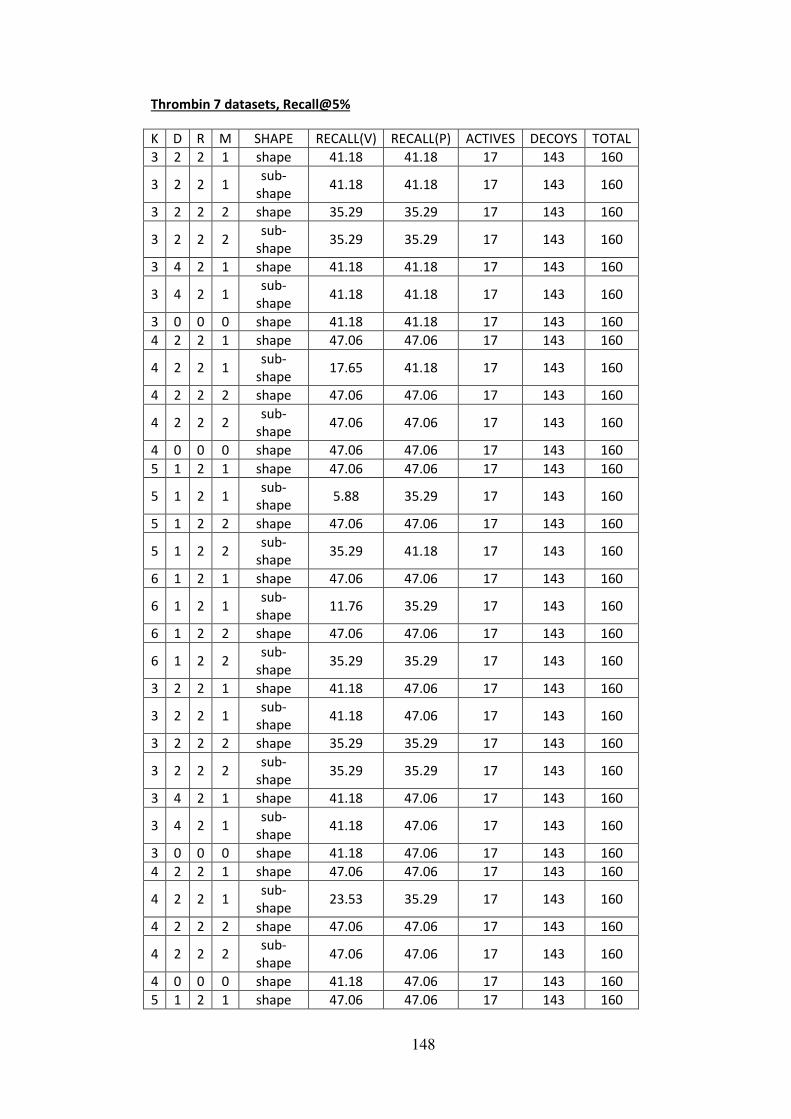
148
Thrombin 7 datasets, Recall@5%
K D R M SHAPE RECALL(V) RECALL(P) ACTIVES DECOYS TOTAL 3 2 2 1 shape 41.18 41.18 17 143 160
3 2 2 1 sub-
shape 41.18 41.18 17 143 160
3 2 2 2 shape 35.29 35.29 17 143 160
3 2 2 2 sub-
shape 35.29 35.29 17 143 160
3 4 2 1 shape 41.18 41.18 17 143 160
3 4 2 1 sub-
shape 41.18 41.18 17 143 160
3 0 0 0 shape 41.18 41.18 17 143 160 4 2 2 1 shape 47.06 47.06 17 143 160
4 2 2 1 sub-
shape 17.65 41.18 17 143 160
4 2 2 2 shape 47.06 47.06 17 143 160
4 2 2 2 sub-
shape 47.06 47.06 17 143 160
4 0 0 0 shape 47.06 47.06 17 143 160 5 1 2 1 shape 47.06 47.06 17 143 160
5 1 2 1 sub-
shape 5.88 35.29 17 143 160
5 1 2 2 shape 47.06 47.06 17 143 160
5 1 2 2 sub-
shape 35.29 41.18 17 143 160
6 1 2 1 shape 47.06 47.06 17 143 160
6 1 2 1 sub-
shape 11.76 35.29 17 143 160
6 1 2 2 shape 47.06 47.06 17 143 160
6 1 2 2 sub-
shape 35.29 35.29 17 143 160
3 2 2 1 shape 41.18 47.06 17 143 160
3 2 2 1 sub-
shape 41.18 47.06 17 143 160
3 2 2 2 shape 35.29 35.29 17 143 160
3 2 2 2 sub-
shape 35.29 35.29 17 143 160
3 4 2 1 shape 41.18 47.06 17 143 160
3 4 2 1 sub-
shape 41.18 47.06 17 143 160
3 0 0 0 shape 41.18 47.06 17 143 160 4 2 2 1 shape 47.06 47.06 17 143 160
4 2 2 1 sub-
shape 23.53 35.29 17 143 160
4 2 2 2 shape 47.06 47.06 17 143 160
4 2 2 2 sub-
shape 47.06 47.06 17 143 160
4 0 0 0 shape 41.18 47.06 17 143 160 5 1 2 1 shape 47.06 47.06 17 143 160

149
5 1 2 1 sub-
shape 17.65 29.41 17 143 160
5 1 2 2 shape 47.06 47.06 17 143 160
5 1 2 2 sub-
shape 47.06 47.06 17 143 160
6 1 2 1 shape 47.06 47.06 17 143 160
6 1 2 1 sub-
shape 11.76 23.53 17 143 160
6 1 2 2 shape 47.06 47.06 17 143 160
6 1 2 2 sub-
shape 41.18 47.06 17 143 160
3 2 2 1 shape 41.18 41.18 17 143 160
3 2 2 1 sub-
shape 41.18 41.18 17 143 160
3 2 2 2 shape 17.65 17.65 17 143 160
3 2 2 2 sub-
shape 17.65 17.65 17 143 160
3 4 2 1 shape 41.18 41.18 17 143 160
3 4 2 1 sub-
shape 41.18 41.18 17 143 160
3 0 0 0 shape 41.18 41.18 17 143 160 4 2 2 1 shape 29.41 29.41 17 143 160
4 2 2 1 sub-
shape 23.53 23.53 17 143 160
4 2 2 2 shape 17.65 17.65 17 143 160
4 2 2 2 sub-
shape 17.65 17.65 17 143 160
4 0 0 0 shape 35.29 35.29 17 143 160 5 1 2 1 shape 41.18 29.41 17 143 160
5 1 2 1 sub-
shape 23.53 29.41 17 143 160
5 1 2 2 shape 17.65 23.53 17 143 160
5 1 2 2 sub-
shape 11.76 17.65 17 143 160
6 1 2 1 shape 29.41 29.41 17 143 160
6 1 2 1 sub-
shape 23.53 17.65 17 143 160
6 1 2 2 shape 23.53 17.65 17 143 160
6 1 2 2 sub-
shape 29.41 29.41 17 143 160
3 2 2 1 shape 11.76 29.41 17 143 160
3 2 2 1 sub-
shape 11.76 29.41 17 143 160
3 2 2 2 shape 5.88 5.88 17 143 160
3 2 2 2 sub-
shape 5.88 5.88 17 143 160
3 4 2 1 shape 11.76 29.41 17 143 160
3 4 2 1 sub-
shape 11.76 29.41 17 143 160
3 0 0 0 shape 11.76 35.29 17 143 160

150
4 2 2 1 shape 35.29 41.18 17 143 160
4 2 2 1 sub-
shape 11.76 17.65 17 143 160
4 2 2 2 shape 11.76 11.76 17 143 160
4 2 2 2 sub-
shape 11.76 11.76 17 143 160
4 0 0 0 shape 41.18 23.53 17 143 160 5 1 2 1 shape 29.41 23.53 17 143 160
5 1 2 1 sub-
shape 11.76 11.76 17 143 160
5 1 2 2 shape 11.76 11.76 17 143 160
5 1 2 2 sub-
shape 11.76 11.76 17 143 160
6 1 2 1 shape 41.18 47.06 17 143 160
6 1 2 1 sub-
shape 5.88 5.88 17 143 160
6 1 2 2 shape 23.53 29.41 17 143 160
6 1 2 2 sub-
shape 29.41 35.29 17 143 160
3 2 2 1 shape 41.18 47.06 17 143 160
3 2 2 1 sub-
shape 41.18 47.06 17 143 160
3 2 2 2 shape 35.29 35.29 17 143 160
3 2 2 2 sub-
shape 35.29 35.29 17 143 160
3 4 2 1 shape 41.18 47.06 17 143 160
3 4 2 1 sub-
shape 41.18 47.06 17 143 160
3 0 0 0 shape 41.18 47.06 17 143 160 4 2 2 1 shape 47.06 47.06 17 143 160
4 2 2 1 sub-
shape 29.41 35.29 17 143 160
4 2 2 2 shape 47.06 47.06 17 143 160
4 2 2 2 sub-
shape 41.18 41.18 17 143 160
4 0 0 0 shape 47.06 47.06 17 143 160 5 1 2 1 shape 47.06 47.06 17 143 160
5 1 2 1 sub-
shape 17.65 41.18 17 143 160
5 1 2 2 shape 47.06 47.06 17 143 160
5 1 2 2 sub-
shape 23.53 35.29 17 143 160
6 1 2 1 shape 47.06 47.06 17 143 160
6 1 2 1 sub-
shape 17.65 29.41 17 143 160
6 1 2 2 shape 47.06 47.06 17 143 160
6 1 2 2 sub-
shape 29.41 41.18 17 143 160
3 2 2 1 shape 41.18 41.18 17 143 160 3 2 2 1 sub- 41.18 41.18 17 143 160
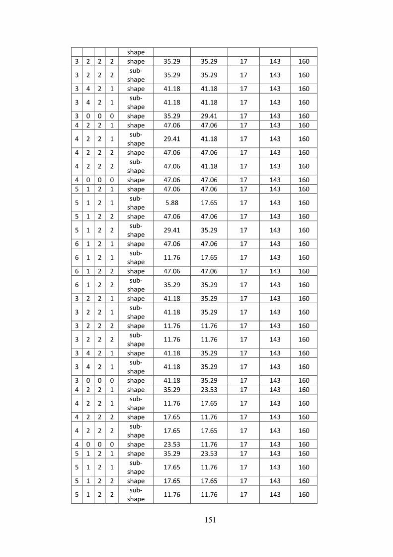
151
shape 3 2 2 2 shape 35.29 35.29 17 143 160
3 2 2 2 sub-
shape 35.29 35.29 17 143 160
3 4 2 1 shape 41.18 41.18 17 143 160
3 4 2 1 sub-
shape 41.18 41.18 17 143 160
3 0 0 0 shape 35.29 29.41 17 143 160 4 2 2 1 shape 47.06 47.06 17 143 160
4 2 2 1 sub-
shape 29.41 41.18 17 143 160
4 2 2 2 shape 47.06 47.06 17 143 160
4 2 2 2 sub-
shape 47.06 41.18 17 143 160
4 0 0 0 shape 47.06 47.06 17 143 160 5 1 2 1 shape 47.06 47.06 17 143 160
5 1 2 1 sub-
shape 5.88 17.65 17 143 160
5 1 2 2 shape 47.06 47.06 17 143 160
5 1 2 2 sub-
shape 29.41 35.29 17 143 160
6 1 2 1 shape 47.06 47.06 17 143 160
6 1 2 1 sub-
shape 11.76 17.65 17 143 160
6 1 2 2 shape 47.06 47.06 17 143 160
6 1 2 2 sub-
shape 35.29 35.29 17 143 160
3 2 2 1 shape 41.18 35.29 17 143 160
3 2 2 1 sub-
shape 41.18 35.29 17 143 160
3 2 2 2 shape 11.76 11.76 17 143 160
3 2 2 2 sub-
shape 11.76 11.76 17 143 160
3 4 2 1 shape 41.18 35.29 17 143 160
3 4 2 1 sub-
shape 41.18 35.29 17 143 160
3 0 0 0 shape 41.18 35.29 17 143 160 4 2 2 1 shape 35.29 23.53 17 143 160
4 2 2 1 sub-
shape 11.76 17.65 17 143 160
4 2 2 2 shape 17.65 11.76 17 143 160
4 2 2 2 sub-
shape 17.65 17.65 17 143 160
4 0 0 0 shape 23.53 11.76 17 143 160 5 1 2 1 shape 35.29 23.53 17 143 160
5 1 2 1 sub-
shape 17.65 11.76 17 143 160
5 1 2 2 shape 17.65 17.65 17 143 160
5 1 2 2 sub-
shape 11.76 11.76 17 143 160

152
6 1 2 1 shape 41.18 35.29 17 143 160
6 1 2 1 sub-
shape 17.65 23.53 17 143 160
6 1 2 2 shape 35.29 29.41 17 143 160
6 1 2 2 sub-
shape 23.53 35.29 17 143 160

153
Thrombin 7 datasets, Recall@10%
K D R M SHAPE RECALL(V) RECALL(P) ACTIVES DECOYS TOTAL 3 2 2 1 shape 47.06 47.06 17 143 160
3 2 2 1 sub-
shape 47.06 47.06 17 143 160
3 2 2 2 shape 35.29 35.29 17 143 160
3 2 2 2 sub-
shape 35.29 35.29 17 143 160
3 4 2 1 shape 47.06 47.06 17 143 160
3 4 2 1 sub-
shape 47.06 47.06 17 143 160
3 0 0 0 shape 47.06 47.06 17 143 160 4 2 2 1 shape 58.82 52.94 17 143 160
4 2 2 1 sub-
shape 41.18 52.94 17 143 160
4 2 2 2 shape 58.82 58.82 17 143 160
4 2 2 2 sub-
shape 58.82 52.94 17 143 160
4 0 0 0 shape 58.82 52.94 17 143 160 5 1 2 1 shape 76.47 58.82 17 143 160
5 1 2 1 sub-
shape 17.65 52.94 17 143 160
5 1 2 2 shape 52.94 52.94 17 143 160
5 1 2 2 sub-
shape 52.94 52.94 17 143 160
6 1 2 1 shape 76.47 76.47 17 143 160
6 1 2 1 sub-
shape 23.53 52.94 17 143 160
6 1 2 2 shape 58.82 52.94 17 143 160
6 1 2 2 sub-
shape 58.82 52.94 17 143 160
3 2 2 1 shape 47.06 47.06 17 143 160
3 2 2 1 sub-
shape 47.06 47.06 17 143 160
3 2 2 2 shape 35.29 35.29 17 143 160
3 2 2 2 sub-
shape 35.29 35.29 17 143 160
3 4 2 1 shape 47.06 47.06 17 143 160
3 4 2 1 sub-
shape 47.06 47.06 17 143 160
3 0 0 0 shape 52.94 47.06 17 143 160 4 2 2 1 shape 52.94 52.94 17 143 160
4 2 2 1 sub-
shape 41.18 52.94 17 143 160
4 2 2 2 shape 58.82 58.82 17 143 160
4 2 2 2 sub-
shape 58.82 58.82 17 143 160
4 0 0 0 shape 52.94 58.82 17 143 160 5 1 2 1 shape 58.82 58.82 17 143 160

154
5 1 2 1 sub-
shape 17.65 47.06 17 143 160
5 1 2 2 shape 52.94 52.94 17 143 160
5 1 2 2 sub-
shape 52.94 52.94 17 143 160
6 1 2 1 shape 70.59 58.82 17 143 160
6 1 2 1 sub-
shape 11.76 29.41 17 143 160
6 1 2 2 shape 58.82 58.82 17 143 160
6 1 2 2 sub-
shape 58.82 64.71 17 143 160
3 2 2 1 shape 41.18 41.18 17 143 160
3 2 2 1 sub-
shape 41.18 41.18 17 143 160
3 2 2 2 shape 17.65 17.65 17 143 160
3 2 2 2 sub-
shape 17.65 17.65 17 143 160
3 4 2 1 shape 41.18 41.18 17 143 160
3 4 2 1 sub-
shape 41.18 41.18 17 143 160
3 0 0 0 shape 47.06 41.18 17 143 160 4 2 2 1 shape 29.41 35.29 17 143 160
4 2 2 1 sub-
shape 23.53 23.53 17 143 160
4 2 2 2 shape 17.65 17.65 17 143 160
4 2 2 2 sub-
shape 17.65 17.65 17 143 160
4 0 0 0 shape 41.18 35.29 17 143 160 5 1 2 1 shape 70.59 58.82 17 143 160
5 1 2 1 sub-
shape 29.41 35.29 17 143 160
5 1 2 2 shape 23.53 23.53 17 143 160
5 1 2 2 sub-
shape 17.65 23.53 17 143 160
6 1 2 1 shape 52.94 35.29 17 143 160
6 1 2 1 sub-
shape 23.53 17.65 17 143 160
6 1 2 2 shape 47.06 29.41 17 143 160
6 1 2 2 sub-
shape 35.29 41.18 17 143 160
3 2 2 1 shape 41.18 41.18 17 143 160
3 2 2 1 sub-
shape 41.18 41.18 17 143 160
3 2 2 2 shape 5.88 5.88 17 143 160
3 2 2 2 sub-
shape 5.88 5.88 17 143 160
3 4 2 1 shape 41.18 41.18 17 143 160
3 4 2 1 sub-
shape 41.18 41.18 17 143 160
3 0 0 0 shape 41.18 35.29 17 143 160

155
4 2 2 1 shape 52.94 47.06 17 143 160
4 2 2 1 sub-
shape 23.53 29.41 17 143 160
4 2 2 2 shape 17.65 17.65 17 143 160
4 2 2 2 sub-
shape 23.53 23.53 17 143 160
4 0 0 0 shape 58.82 41.18 17 143 160 5 1 2 1 shape 58.82 41.18 17 143 160
5 1 2 1 sub-
shape 17.65 17.65 17 143 160
5 1 2 2 shape 11.76 11.76 17 143 160
5 1 2 2 sub-
shape 11.76 11.76 17 143 160
6 1 2 1 shape 58.82 64.71 17 143 160
6 1 2 1 sub-
shape 5.88 5.88 17 143 160
6 1 2 2 shape 47.06 41.18 17 143 160
6 1 2 2 sub-
shape 47.06 52.94 17 143 160
3 2 2 1 shape 47.06 47.06 17 143 160
3 2 2 1 sub-
shape 47.06 47.06 17 143 160
3 2 2 2 shape 35.29 35.29 17 143 160
3 2 2 2 sub-
shape 35.29 35.29 17 143 160
3 4 2 1 shape 47.06 47.06 17 143 160
3 4 2 1 sub-
shape 47.06 47.06 17 143 160
3 0 0 0 shape 47.06 47.06 17 143 160 4 2 2 1 shape 58.82 64.71 17 143 160
4 2 2 1 sub-
shape 41.18 52.94 17 143 160
4 2 2 2 shape 52.94 52.94 17 143 160
4 2 2 2 sub-
shape 52.94 52.94 17 143 160
4 0 0 0 shape 64.71 64.71 17 143 160 5 1 2 1 shape 82.35 82.35 17 143 160
5 1 2 1 sub-
shape 35.29 52.94 17 143 160
5 1 2 2 shape 52.94 52.94 17 143 160
5 1 2 2 sub-
shape 52.94 52.94 17 143 160
6 1 2 1 shape 76.47 70.59 17 143 160
6 1 2 1 sub-
shape 17.65 41.18 17 143 160
6 1 2 2 shape 52.94 52.94 17 143 160
6 1 2 2 sub-
shape 47.06 58.82 17 143 160
3 2 2 1 shape 47.06 47.06 17 143 160 3 2 2 1 sub- 47.06 47.06 17 143 160

156
shape 3 2 2 2 shape 35.29 35.29 17 143 160
3 2 2 2 sub-
shape 35.29 35.29 17 143 160
3 4 2 1 shape 47.06 41.18 17 143 160
3 4 2 1 sub-
shape 47.06 41.18 17 143 160
3 0 0 0 shape 47.06 35.29 17 143 160 4 2 2 1 shape 64.71 58.82 17 143 160
4 2 2 1 sub-
shape 52.94 58.82 17 143 160
4 2 2 2 shape 52.94 52.94 17 143 160
4 2 2 2 sub-
shape 52.94 52.94 17 143 160
4 0 0 0 shape 64.71 58.82 17 143 160 5 1 2 1 shape 82.35 52.94 17 143 160
5 1 2 1 sub-
shape 5.88 29.41 17 143 160
5 1 2 2 shape 52.94 52.94 17 143 160
5 1 2 2 sub-
shape 47.06 47.06 17 143 160
6 1 2 1 shape 70.59 52.94 17 143 160
6 1 2 1 sub-
shape 17.65 17.65 17 143 160
6 1 2 2 shape 58.82 52.94 17 143 160
6 1 2 2 sub-
shape 52.94 52.94 17 143 160
3 2 2 1 shape 41.18 41.18 17 143 160
3 2 2 1 sub-
shape 41.18 41.18 17 143 160
3 2 2 2 shape 11.76 11.76 17 143 160
3 2 2 2 sub-
shape 11.76 11.76 17 143 160
3 4 2 1 shape 41.18 41.18 17 143 160
3 4 2 1 sub-
shape 41.18 41.18 17 143 160
3 0 0 0 shape 41.18 35.29 17 143 160 4 2 2 1 shape 52.94 47.06 17 143 160
4 2 2 1 sub-
shape 41.18 47.06 17 143 160
4 2 2 2 shape 17.65 17.65 17 143 160
4 2 2 2 sub-
shape 17.65 17.65 17 143 160
4 0 0 0 shape 52.94 29.41 17 143 160 5 1 2 1 shape 41.18 23.53 17 143 160
5 1 2 1 sub-
shape 35.29 23.53 17 143 160
5 1 2 2 shape 23.53 23.53 17 143 160
5 1 2 2 sub-
shape 23.53 23.53 17 143 160

157
6 1 2 1 shape 76.47 58.82 17 143 160
6 1 2 1 sub-
shape 23.53 29.41 17 143 160
6 1 2 2 shape 47.06 35.29 17 143 160
6 1 2 2 sub-
shape 41.18 47.06 17 143 160

158
Appendix B - 40 DUD queries
Shape AUC Volume and Properties values
QUERY/CLASS K D R M AUC (V) AUC (P) ACE 3 4 2 1 0.691438 0.67427 ACE 3 4 2 2 0.501393 0.501393 ACE 3 0 0 0 0.605165 0.630822 ACE 4 2 2 1 0.603076 0.611184 ACE 4 2 2 2 0.562947 0.562014 ACE 4 0 0 0 0.616604 0.590838 ACE 5 1 2 1 0.585927 0.601072 ACE 5 1 2 2 0.502368 0.504311 ACE 6 1 2 1 0.578697 0.568669 ACE 6 1 2 2 0.629181 0.614909
ACHE 3 4 2 1 0.657332 0.6433 ACHE 3 4 2 2 0.579045 0.579683 ACHE 3 0 0 0 0.528525 0.516175 ACHE 4 2 2 1 0.609302 0.660629 ACHE 4 2 2 2 0.767535 0.77029 ACHE 4 0 0 0 0.585356 0.657022 ACHE 5 1 2 1 0.590435 0.664471 ACHE 5 1 2 2 0.693503 0.691404 ACHE 6 1 2 1 0.565997 0.651821 ACHE 6 1 2 2 0.769726 0.766984 ADA 3 4 2 1 0.633275 0.676621 ADA 3 4 2 2 0.531857 0.531857 ADA 3 0 0 0 0.567894 0.613563 ADA 4 2 2 1 0.5241 0.560851 ADA 4 2 2 2 0.509439 0.509807 ADA 4 0 0 0 0.622664 0.544989 ADA 5 1 2 1 0.53714 0.556038 ADA 5 1 2 2 0.52627 0.524603 ADA 6 1 2 1 0.607217 0.510118 ADA 6 1 2 2 0.639285 0.629191 ALR2 3 4 2 1 0.654998 0.597189 ALR2 3 4 2 2 0.581988 0.581927 ALR2 3 0 0 0 0.648165 0.622843 ALR2 4 2 2 1 0.525244 0.55205 ALR2 4 2 2 2 0.66066 0.659098 ALR2 4 0 0 0 0.578212 0.525166 ALR2 5 1 2 1 0.546701 0.527763 ALR2 5 1 2 2 0.619249 0.626904 ALR2 6 1 2 1 0.57294 0.625693 ALR2 6 1 2 2 0.661927 0.68116 AMPC 3 4 2 1 0.578721 0.572328 AMPC 3 4 2 2 0.500637 0.500637 AMPC 3 0 0 0 0.518734 0.651431 AMPC 4 2 2 1 0.603094 0.59906 AMPC 4 2 2 2 0.503185 0.503185

159
AMPC 4 0 0 0 0.594359 0.574841 AMPC 5 1 2 1 0.537701 0.616894 AMPC 5 1 2 2 0.503817 0.503817 AMPC 6 1 2 1 0.516257 0.514377 AMPC 6 1 2 2 0.511355 0.511673
ANP/SRC 3 4 2 1 0.551336 0.53794 ANP/SRC 3 4 2 2 0.53375 0.53394 ANP/SRC 3 0 0 0 0.761952 0.773009 ANP/SRC 4 2 2 1 0.51885 0.510868 ANP/SRC 4 2 2 2 0.576967 0.581592 ANP/SRC 4 0 0 0 0.533148 0.576627 ANP/SRC 5 1 2 1 0.583679 0.527182 ANP/SRC 5 1 2 2 0.544151 0.544716 ANP/SRC 6 1 2 1 0.546624 0.528962 ANP/SRC 6 1 2 2 0.500588 0.503071
AR 3 4 2 1 0.778106 0.798138 AR 3 4 2 2 0.541983 0.541682 AR 3 0 0 0 0.587236 0.727583 AR 4 2 2 1 0.705887 0.678413 AR 4 2 2 2 0.622237 0.616597 AR 4 0 0 0 0.618334 0.686496 AR 5 1 2 1 0.668255 0.597872 AR 5 1 2 2 0.638696 0.638626 AR 6 1 2 1 0.668699 0.526848 AR 6 1 2 2 0.763704 0.737192
CDK2 3 4 2 1 0.65707 0.686538 CDK2 3 4 2 2 0.530048 0.529601 CDK2 3 0 0 0 0.553197 0.550122 CDK2 4 2 2 1 0.513322 0.52012 CDK2 4 2 2 2 0.538615 0.538872 CDK2 4 0 0 0 0.563136 0.617145 CDK2 5 1 2 1 0.527755 0.533406 CDK2 5 1 2 2 0.50925 0.509307 CDK2 6 1 2 1 0.511754 0.522541 CDK2 6 1 2 2 0.501327 0.507522 COMT 3 4 2 1 0.502141 0.502141 COMT 3 4 2 2 0.5 0.5 COMT 3 0 0 0 0.698184 0.64308 COMT 4 2 2 1 0.62663 0.656706 COMT 4 2 2 2 0.531633 0.528908 COMT 4 0 0 0 0.736218 0.68795 COMT 5 1 2 1 0.612906 0.623613 COMT 5 1 2 2 0.550029 0.550905 COMT 6 1 2 1 0.626436 0.513724 COMT 6 1 2 2 0.539031 0.538544 COX1 3 4 2 1 0.504545 0.519181 COX1 3 4 2 2 0.5 0.5 COX1 3 0 0 0 0.592383 0.61506 COX1 4 2 2 1 0.547253 0.645904 COX1 4 2 2 2 0.518917 0.518917
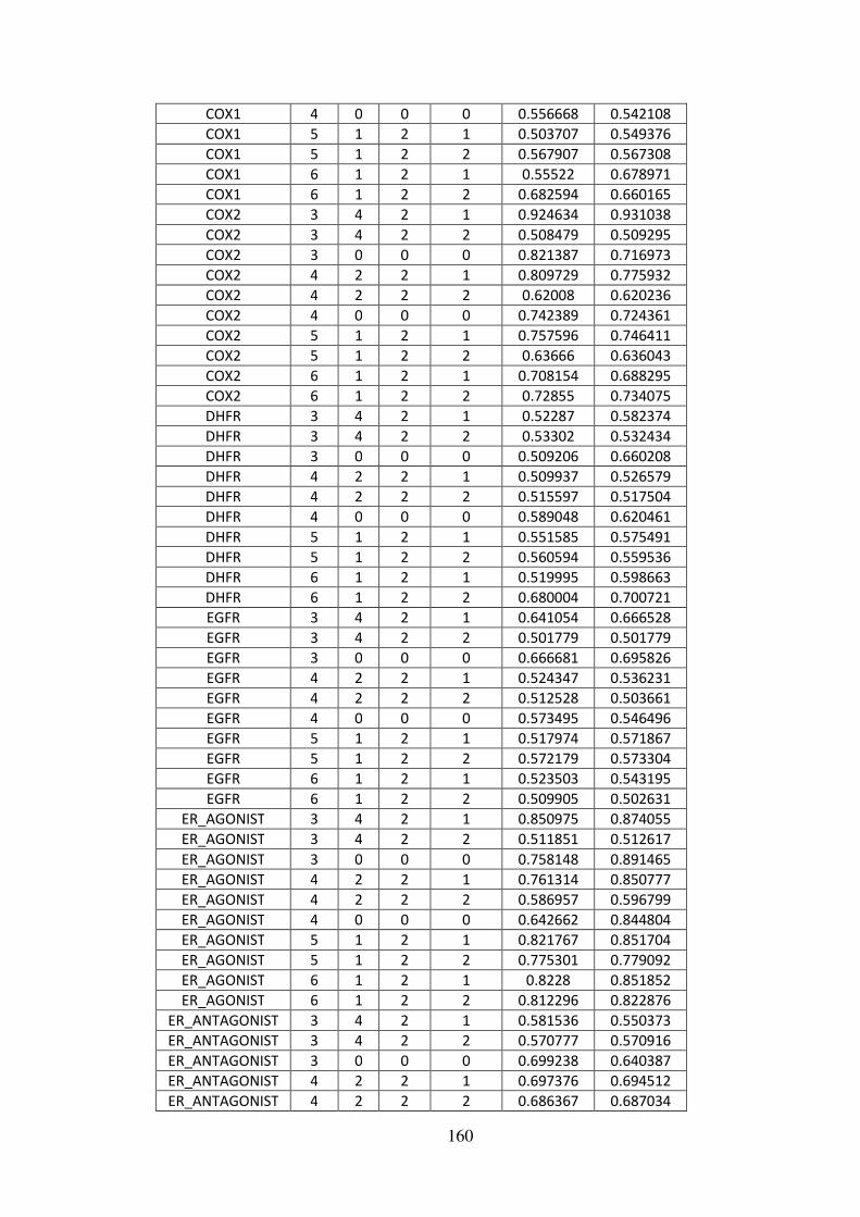
160
COX1 4 0 0 0 0.556668 0.542108 COX1 5 1 2 1 0.503707 0.549376 COX1 5 1 2 2 0.567907 0.567308 COX1 6 1 2 1 0.55522 0.678971 COX1 6 1 2 2 0.682594 0.660165 COX2 3 4 2 1 0.924634 0.931038 COX2 3 4 2 2 0.508479 0.509295 COX2 3 0 0 0 0.821387 0.716973 COX2 4 2 2 1 0.809729 0.775932 COX2 4 2 2 2 0.62008 0.620236 COX2 4 0 0 0 0.742389 0.724361 COX2 5 1 2 1 0.757596 0.746411 COX2 5 1 2 2 0.63666 0.636043 COX2 6 1 2 1 0.708154 0.688295 COX2 6 1 2 2 0.72855 0.734075 DHFR 3 4 2 1 0.52287 0.582374 DHFR 3 4 2 2 0.53302 0.532434 DHFR 3 0 0 0 0.509206 0.660208 DHFR 4 2 2 1 0.509937 0.526579 DHFR 4 2 2 2 0.515597 0.517504 DHFR 4 0 0 0 0.589048 0.620461 DHFR 5 1 2 1 0.551585 0.575491 DHFR 5 1 2 2 0.560594 0.559536 DHFR 6 1 2 1 0.519995 0.598663 DHFR 6 1 2 2 0.680004 0.700721 EGFR 3 4 2 1 0.641054 0.666528 EGFR 3 4 2 2 0.501779 0.501779 EGFR 3 0 0 0 0.666681 0.695826 EGFR 4 2 2 1 0.524347 0.536231 EGFR 4 2 2 2 0.512528 0.503661 EGFR 4 0 0 0 0.573495 0.546496 EGFR 5 1 2 1 0.517974 0.571867 EGFR 5 1 2 2 0.572179 0.573304 EGFR 6 1 2 1 0.523503 0.543195 EGFR 6 1 2 2 0.509905 0.502631
ER_AGONIST 3 4 2 1 0.850975 0.874055 ER_AGONIST 3 4 2 2 0.511851 0.512617 ER_AGONIST 3 0 0 0 0.758148 0.891465 ER_AGONIST 4 2 2 1 0.761314 0.850777 ER_AGONIST 4 2 2 2 0.586957 0.596799 ER_AGONIST 4 0 0 0 0.642662 0.844804 ER_AGONIST 5 1 2 1 0.821767 0.851704 ER_AGONIST 5 1 2 2 0.775301 0.779092 ER_AGONIST 6 1 2 1 0.8228 0.851852 ER_AGONIST 6 1 2 2 0.812296 0.822876
ER_ANTAGONIST 3 4 2 1 0.581536 0.550373 ER_ANTAGONIST 3 4 2 2 0.570777 0.570916 ER_ANTAGONIST 3 0 0 0 0.699238 0.640387 ER_ANTAGONIST 4 2 2 1 0.697376 0.694512 ER_ANTAGONIST 4 2 2 2 0.686367 0.687034

161
ER_ANTAGONIST 4 0 0 0 0.777744 0.632242 ER_ANTAGONIST 5 1 2 1 0.724647 0.684838 ER_ANTAGONIST 5 1 2 2 0.621066 0.621595 ER_ANTAGONIST 6 1 2 1 0.534249 0.588485 ER_ANTAGONIST 6 1 2 2 0.67155 0.670355
FGFR 3 4 2 1 0.514371 0.508928 FGFR 3 4 2 2 0.504334 0.504334 FGFR 3 0 0 0 0.638749 0.559067 FGFR 4 2 2 1 0.54649 0.506072 FGFR 4 2 2 2 0.547015 0.546992 FGFR 4 0 0 0 0.506566 0.549654 FGFR 5 1 2 1 0.552429 0.552033 FGFR 5 1 2 2 0.54102 0.540691 FGFR 6 1 2 1 0.534941 0.520803 FGFR 6 1 2 2 0.536552 0.537331 FXA 3 4 2 1 0.632921 0.650212 FXA 3 4 2 2 0.531198 0.531758 FXA 3 0 0 0 0.507715 0.568689 FXA 4 2 2 1 0.540744 0.565047 FXA 4 2 2 2 0.5519 0.545696 FXA 4 0 0 0 0.5481 0.543674 FXA 5 1 2 1 0.573578 0.650085 FXA 5 1 2 2 0.640685 0.639242 FXA 6 1 2 1 0.542096 0.529128 FXA 6 1 2 2 0.66079 0.664033
GART 3 4 2 1 0.671672 0.630682 GART 3 4 2 2 0.581169 0.581169 GART 3 0 0 0 0.677354 0.524351 GART 4 2 2 1 0.63474 0.627029 GART 4 2 2 2 0.536932 0.525346 GART 4 0 0 0 0.549919 0.670049 GART 5 1 2 1 0.655438 0.719562 GART 5 1 2 2 0.6447 0.656221 GART 6 1 2 1 0.700893 0.659497 GART 6 1 2 2 0.752995 0.760829 GPB 3 4 2 1 0.711016 0.723428 GPB 3 4 2 2 0.683166 0.68194 GPB 3 0 0 0 0.506159 0.575414 GPB 4 2 2 1 0.593013 0.536533 GPB 4 2 2 2 0.744469 0.759408 GPB 4 0 0 0 0.564604 0.781207 GPB 5 1 2 1 0.522799 0.533528 GPB 5 1 2 2 0.854163 0.849024 GPB 6 1 2 1 0.733621 0.766149 GPB 6 1 2 2 0.776945 0.758146 GR 3 4 2 1 0.581107 0.557228 GR 3 4 2 2 0.536913 0.537019 GR 3 0 0 0 0.705965 0.542148 GR 4 2 2 1 0.620291 0.627279 GR 4 2 2 2 0.526287 0.526287

162
GR 4 0 0 0 0.679928 0.675959 GR 5 1 2 1 0.519411 0.510464 GR 5 1 2 2 0.595838 0.595801 GR 6 1 2 1 0.589742 0.582935 GR 6 1 2 2 0.579148 0.578942
HIV-PR 3 4 2 1 0.6875 0.59375 HIV-PR 3 4 2 2 0.75 0.75 HIV-PR 3 0 0 0 0.65625 0.5625 HIV-PR 4 2 2 1 0.609375 0.59375 HIV-PR 4 2 2 2 0.5 0.5 HIV-PR 4 0 0 0 0.555556 0.8125 HIV-PR 5 1 2 1 0.84375 0.96875 HIV-PR 5 1 2 2 0.765625 0.765625 HIV-PR 6 1 2 1 0.796875 0.6875 HIV-PR 6 1 2 2 0.5 0.5 HIVRT 3 4 2 1 0.739638 0.708531 HIVRT 3 4 2 2 0.586896 0.604732 HIVRT 3 0 0 0 0.642223 0.555627 HIVRT 4 2 2 1 0.518813 0.55117 HIVRT 4 2 2 2 0.505486 0.504078 HIVRT 4 0 0 0 0.665104 0.535135 HIVRT 5 1 2 1 0.573395 0.508481 HIVRT 5 1 2 2 0.527708 0.525757 HIVRT 6 1 2 1 0.615372 0.574936 HIVRT 6 1 2 2 0.551884 0.550855 HMGA 3 4 2 1 0.577243 0.63384 HMGA 3 4 2 2 0.658263 0.671533 HMGA 3 0 0 0 0.563924 0.637131 HMGA 4 2 2 1 0.67305 0.673313 HMGA 4 2 2 2 0.539072 0.522588 HMGA 4 0 0 0 0.581294 0.698158 HMGA 5 1 2 1 0.548833 0.523066 HMGA 5 1 2 2 0.732519 0.73948 HMGA 6 1 2 1 0.529395 0.512855 HMGA 6 1 2 2 0.799831 0.784346 HSP90 3 4 2 1 0.887319 0.865967 HSP90 3 4 2 2 0.630793 0.630956 HSP90 3 0 0 0 0.778135 0.719674 HSP90 4 2 2 1 0.674583 0.612657 HSP90 4 2 2 2 0.641096 0.642587 HSP90 4 0 0 0 0.708345 0.636993 HSP90 5 1 2 1 0.523681 0.618555 HSP90 5 1 2 2 0.592358 0.570932 HSP90 6 1 2 1 0.701701 0.642005 HSP90 6 1 2 2 0.702504 0.693978 INHA 3 4 2 1 0.603571 0.52949 INHA 3 4 2 2 0.50567 0.505696 INHA 3 0 0 0 0.542994 0.534355 INHA 4 2 2 1 0.679805 0.708181 INHA 4 2 2 2 0.553275 0.555105

163
INHA 4 0 0 0 0.619173 0.629354 INHA 5 1 2 1 0.512768 0.589243 INHA 5 1 2 2 0.570841 0.571854 INHA 6 1 2 1 0.512682 0.562193 INHA 6 1 2 2 0.601015 0.601163 MR 3 4 2 1 0.565657 0.606787 MR 3 4 2 2 0.503937 0.503937 MR 3 0 0 0 0.947184 0.824292 MR 4 2 2 1 0.912417 0.829468 MR 4 2 2 2 0.651992 0.656184 MR 4 0 0 0 0.921563 0.688221 MR 5 1 2 1 0.829921 0.730346 MR 5 1 2 2 0.725694 0.722746 MR 6 1 2 1 0.685403 0.574358 MR 6 1 2 2 0.825136 0.795008 NA 3 4 2 1 0.74373 0.745561 NA 3 4 2 2 0.528157 0.539405 NA 3 0 0 0 0.573837 0.600214 NA 4 2 2 1 0.62292 0.597909 NA 4 2 2 2 0.542743 0.548787 NA 4 0 0 0 0.670644 0.642154 NA 5 1 2 1 0.589488 0.61853 NA 5 1 2 2 0.504743 0.505746 NA 6 1 2 1 0.655839 0.628192 NA 6 1 2 2 0.504932 0.50768 P38 3 4 2 1 0.538847 0.546829 P38 3 4 2 2 0.548656 0.549127 P38 3 0 0 0 0.502848 0.509631 P38 4 2 2 1 0.579719 0.547261 P38 4 2 2 2 0.503503 0.507317 P38 4 0 0 0 0.527243 0.617622 P38 5 1 2 1 0.641622 0.617147 P38 5 1 2 2 0.58436 0.57924 P38 6 1 2 1 0.540136 0.524044 P38 6 1 2 2 0.588735 0.584344
PARP 3 4 2 1 0.575588 0.504113 PARP 3 4 2 2 0.539324 0.538272 PARP 3 0 0 0 0.599034 0.502702 PARP 4 2 2 1 0.601306 0.543533 PARP 4 2 2 2 0.586575 0.587102 PARP 4 0 0 0 0.500813 0.663239 PARP 5 1 2 1 0.538284 0.67737 PARP 5 1 2 2 0.639284 0.646148 PARP 6 1 2 1 0.620017 0.755566 PARP 6 1 2 2 0.73371 0.810194 PDE5 3 4 2 1 0.727914 0.729738 PDE5 3 4 2 2 0.518268 0.518268 PDE5 3 0 0 0 0.518574 0.6213 PDE5 4 2 2 1 0.532761 0.594012 PDE5 4 2 2 2 0.505496 0.505462

164
PDE5 4 0 0 0 0.534779 0.61671 PDE5 5 1 2 1 0.586963 0.542111 PDE5 5 1 2 2 0.536082 0.536161 PDE5 6 1 2 1 0.568141 0.555687 PDE5 6 1 2 2 0.586555 0.591576
PDGFRB 3 4 2 1 0.619564 0.611092 PDGFRB 3 4 2 2 0.535893 0.536109 PDGFRB 3 0 0 0 0.704699 0.644979 PDGFRB 4 2 2 1 0.534314 0.50517 PDGFRB 4 2 2 2 0.535737 0.541592 PDGFRB 4 0 0 0 0.666894 0.608104 PDGFRB 5 1 2 1 0.504985 0.523412 PDGFRB 5 1 2 2 0.50664 0.501216 PDGFRB 6 1 2 1 0.566537 0.566671 PDGFRB 6 1 2 2 0.508154 0.500961
PNP 3 4 2 1 0.567769 0.581256 PNP 3 4 2 2 0.539111 0.539111 PNP 3 0 0 0 0.527852 0.50742 PNP 4 2 2 1 0.516174 0.523382 PNP 4 2 2 2 0.553431 0.572 PNP 4 0 0 0 0.598106 0.5297 PNP 5 1 2 1 0.70858 0.624678 PNP 5 1 2 2 0.738647 0.746976 PNP 6 1 2 1 0.556618 0.569565 PNP 6 1 2 2 0.745952 0.755053
PPAR 3 4 2 1 0.602564 0.561966 PPAR 3 4 2 2 0.508547 0.510684 PPAR 3 0 0 0 0.903846 0.965812 PPAR 4 2 2 1 0.651709 0.65812 PPAR 4 2 2 2 0.512821 0.512821 PPAR 4 0 0 0 0.944444 0.878205 PPAR 5 1 2 1 0.606838 0.551282 PPAR 5 1 2 2 0.538462 0.538462 PPAR 6 1 2 1 0.564103 0.606838 PPAR 6 1 2 2 0.594017 0.619658
PR 3 4 2 1 0.533139 0.593753 PR 3 4 2 2 0.50596 0.505911 PR 3 0 0 0 0.589376 0.566995 PR 4 2 2 1 0.512291 0.751632 PR 4 2 2 2 0.542391 0.542391 PR 4 0 0 0 0.631319 0.625155 PR 5 1 2 1 0.500346 0.635844 PR 5 1 2 2 0.524457 0.524457 PR 6 1 2 1 0.637773 0.635548 PR 6 1 2 2 0.54837 0.523939
RXR 3 4 2 1 0.745403 0.77555 RXR 3 4 2 2 0.807673 0.806547 RXR 3 0 0 0 0.724303 0.855038 RXR 4 2 2 1 0.691444 0.690718 RXR 4 2 2 2 0.802711 0.813964

165
RXR 4 0 0 0 0.667212 0.709565 RXR 5 1 2 1 0.540505 0.601045 RXR 5 1 2 2 0.78794 0.800329 RXR 6 1 2 1 0.725319 0.774729 RXR 6 1 2 2 0.894406 0.911973
SAHH 3 4 2 1 0.702382 0.646615 SAHH 3 4 2 2 0.596211 0.596211 SAHH 3 0 0 0 0.762874 0.830087 SAHH 4 2 2 1 0.754492 0.77829 SAHH 4 2 2 2 0.616224 0.616735 SAHH 4 0 0 0 0.766403 0.799115 SAHH 5 1 2 1 0.790014 0.809784 SAHH 5 1 2 2 0.74105 0.742988 SAHH 6 1 2 1 0.586982 0.740539 SAHH 6 1 2 2 0.802076 0.815124
Thrombin 3 4 2 1 0.591865 0.598328 Thrombin 3 4 2 2 0.502161 0.502502 Thrombin 3 0 0 0 0.684091 0.721732 Thrombin 4 2 2 1 0.612714 0.655794 Thrombin 4 2 2 2 0.663148 0.663394 Thrombin 4 0 0 0 0.623157 0.716993 Thrombin 5 1 2 1 0.595391 0.596206 Thrombin 5 1 2 2 0.525321 0.525549 Thrombin 6 1 2 1 0.574713 0.508472 Thrombin 6 1 2 2 0.540673 0.54327
TK 3 4 2 1 0.593871 0.624438 TK 3 4 2 2 0.640679 0.640577 TK 3 0 0 0 0.530005 0.641599 TK 4 2 2 1 0.591905 0.602656 TK 4 2 2 2 0.732083 0.762436 TK 4 0 0 0 0.560981 0.547651 TK 5 1 2 1 0.530746 0.669842 TK 5 1 2 2 0.722957 0.742467 TK 6 1 2 1 0.533657 0.669178 TK 6 1 2 2 0.770761 0.783631
Trypsin 3 4 2 1 0.619092 0.636913 Trypsin 3 4 2 2 0.545328 0.545328 Trypsin 3 0 0 0 0.574384 0.833023 Trypsin 4 2 2 1 0.595665 0.666822 Trypsin 4 2 2 2 0.712847 0.718116 Trypsin 4 0 0 0 0.611266 0.648845 Trypsin 5 1 2 1 0.648381 0.634976 Trypsin 5 1 2 2 0.562529 0.562064 Trypsin 6 1 2 1 0.556563 0.599179 Trypsin 6 1 2 2 0.622579 0.611731 VEGFR2 3 4 2 1 0.570511 0.562969 VEGFR2 3 4 2 2 0.500434 0.501226 VEGFR2 3 0 0 0 0.517245 0.506374 VEGFR2 4 2 2 1 0.582649 0.564206 VEGFR2 4 2 2 2 0.584113 0.582807

166
VEGFR2 4 0 0 0 0.597612 0.623463 VEGFR2 5 1 2 1 0.593434 0.529801 VEGFR2 5 1 2 2 0.537413 0.534504 VEGFR2 6 1 2 1 0.530966 0.57224 VEGFR2 6 1 2 2 0.502328 0.507354

167
DUD 40 Shape Volume/Properties and Recall@5% and 10%
K D R M RECALL
(V) 5%
RECALL (P) 5%
RECALL (V)
10%
RECALL (P)
10% ACTIVES DECOYS TOTAL
3 4 2 1 4.35 4.35 4.35 4.35 46 1796 1842 3 4 2 2 2.17 2.17 2.17 2.17 46 1796 1842 3 0 0 0 17.39 10.87 19.57 15.22 46 1796 1842 4 2 2 1 8.7 6.52 8.7 8.7 46 1796 1842 4 2 2 2 15.22 15.22 23.91 23.91 46 1796 1842 4 0 0 0 10.87 13.04 13.04 15.22 46 1796 1842 5 1 2 1 4.35 6.52 10.87 6.52 46 1796 1842 5 1 2 2 8.7 13.04 15.22 15.22 46 1796 1842 6 1 2 1 6.52 13.04 13.04 15.22 46 1796 1842 6 1 2 2 15.22 10.87 34.78 26.09 46 1796 1842 3 4 2 1 22.22 17.17 33.33 23.23 99 3859 3958 3 4 2 2 21.21 21.21 21.21 21.21 99 3859 3958 3 0 0 0 19.19 18.18 26.26 22.22 99 3859 3958 4 2 2 1 17.17 26.26 30.3 35.35 99 3859 3958 4 2 2 2 41.41 40.4 54.55 55.56 99 3859 3958 4 0 0 0 19.19 28.28 26.26 38.38 99 3859 3958 5 1 2 1 15.15 21.21 21.21 30.3 99 3859 3958 5 1 2 2 35.35 35.35 43.43 45.45 99 3859 3958 6 1 2 1 14.14 19.19 24.24 31.31 99 3859 3958 6 1 2 2 30.3 31.31 51.52 39.39 99 3859 3958 3 4 2 1 17.39 13.04 21.74 21.74 23 927 950 3 4 2 2 4.35 4.35 4.35 4.35 23 927 950 3 0 0 0 8.7 13.04 13.04 17.39 23 927 950 4 2 2 1 13.04 13.04 17.39 17.39 23 927 950 4 2 2 2 13.04 13.04 17.39 17.39 23 927 950 4 0 0 0 13.04 13.04 13.04 17.39 23 927 950 5 1 2 1 4.35 4.35 13.04 4.35 23 927 950 5 1 2 2 4.35 4.35 4.35 8.7 23 927 950 6 1 2 1 4.35 8.7 26.09 8.7 23 927 950 6 1 2 2 39.13 13.04 43.48 39.13 23 927 950 3 4 2 1 15.38 7.69 19.23 11.54 26 986 1012 3 4 2 2 26.92 26.92 26.92 26.92 26 986 1012 3 0 0 0 11.54 7.69 11.54 11.54 26 986 1012 4 2 2 1 11.54 3.85 19.23 7.69 26 986 1012 4 2 2 2 23.08 19.23 42.31 42.31 26 986 1012 4 0 0 0 7.69 3.85 11.54 11.54 26 986 1012 5 1 2 1 15.38 11.54 19.23 19.23 26 986 1012 5 1 2 2 23.08 23.08 26.92 23.08 26 986 1012 6 1 2 1 11.54 7.69 11.54 11.54 26 986 1012 6 1 2 2 11.54 11.54 30.77 34.62 26 986 1012 3 4 2 1 9.52 9.52 9.52 9.52 21 786 807 3 4 2 2 4.76 4.76 4.76 4.76 21 786 807 3 0 0 0 9.52 9.52 9.52 9.52 21 786 807 4 2 2 1 9.52 9.52 9.52 14.29 21 786 807 4 2 2 2 4.76 4.76 4.76 4.76 21 786 807

168
4 0 0 0 9.52 14.29 9.52 19.05 21 786 807 5 1 2 1 4.76 4.76 9.52 9.52 21 786 807 5 1 2 2 9.52 9.52 9.52 9.52 21 786 807 6 1 2 1 4.76 4.76 14.29 14.29 21 786 807 6 1 2 2 9.52 9.52 14.29 14.29 21 786 807 3 4 2 1 32.35 38.24 38.24 45.59 68 2848 2916 3 4 2 2 10.29 10.29 10.29 10.29 68 2848 2916 3 0 0 0 26.47 38.24 30.88 45.59 68 2848 2916 4 2 2 1 36.76 42.65 42.65 50 68 2848 2916 4 2 2 2 29.41 29.41 29.41 29.41 68 2848 2916 4 0 0 0 30.88 41.18 35.29 52.94 68 2848 2916 5 1 2 1 30.88 33.82 41.18 33.82 68 2848 2916 5 1 2 2 33.82 33.82 33.82 33.82 68 2848 2916 6 1 2 1 32.35 10.29 47.06 14.71 68 2848 2916 6 1 2 2 33.82 25 52.94 35.29 68 2848 2916 3 4 2 1 8.51 6.38 14.89 8.51 47 2070 2117 3 4 2 2 4.26 4.26 6.38 6.38 47 2070 2117 3 0 0 0 14.89 8.51 17.02 19.15 47 2070 2117 4 2 2 1 8.51 4.26 12.77 8.51 47 2070 2117 4 2 2 2 4.26 4.26 6.38 6.38 47 2070 2117 4 0 0 0 4.26 6.38 14.89 8.51 47 2070 2117 5 1 2 1 6.38 6.38 6.38 10.64 47 2070 2117 5 1 2 2 6.38 6.38 6.38 6.38 47 2070 2117 6 1 2 1 4.26 4.26 10.64 6.38 47 2070 2117 6 1 2 2 10.64 8.51 12.77 17.02 47 2070 2117 3 4 2 1 9.09 9.09 9.09 9.09 11 468 479 3 4 2 2 9.09 9.09 9.09 9.09 11 468 479 3 0 0 0 36.36 18.18 36.36 27.27 11 468 479 4 2 2 1 9.09 9.09 9.09 9.09 11 468 479 4 2 2 2 9.09 9.09 18.18 18.18 11 468 479 4 0 0 0 36.36 9.09 36.36 9.09 11 468 479 5 1 2 1 9.09 9.09 9.09 18.18 11 468 479 5 1 2 2 27.27 18.18 27.27 27.27 11 468 479 6 1 2 1 9.09 18.18 9.09 18.18 11 468 479 6 1 2 2 27.27 27.27 27.27 27.27 11 468 479 3 4 2 1 21.74 21.74 21.74 26.09 23 910 933 3 4 2 2 4.35 4.35 4.35 4.35 23 910 933 3 0 0 0 21.74 30.43 21.74 30.43 23 910 933 4 2 2 1 21.74 17.39 21.74 17.39 23 910 933 4 2 2 2 8.7 8.7 8.7 8.7 23 910 933 4 0 0 0 21.74 26.09 30.43 30.43 23 910 933 5 1 2 1 21.74 26.09 26.09 26.09 23 910 933 5 1 2 2 26.09 21.74 26.09 26.09 23 910 933 6 1 2 1 21.74 26.09 21.74 34.78 23 910 933 6 1 2 2 26.09 13.04 34.78 26.09 23 910 933 3 4 2 1 59.91 67.45 75.47 76.42 212 12606 12818 3 4 2 2 24.53 24.53 25.47 25.94 212 12606 12818 3 0 0 0 58.49 42.45 62.74 50 212 12606 12818 4 2 2 1 31.6 30.66 44.34 45.75 212 12606 12818 4 2 2 2 27.36 27.36 27.36 27.36 212 12606 12818

169
4 0 0 0 34.43 24.06 46.7 36.32 212 12606 12818 5 1 2 1 26.42 31.6 36.32 43.4 212 12606 12818 5 1 2 2 30.66 30.66 32.55 32.55 212 12606 12818 6 1 2 1 39.15 39.15 43.87 44.34 212 12606 12818 6 1 2 2 34.91 34.91 43.87 41.51 212 12606 12818 3 4 2 1 4.74 10 9.47 21.58 190 8350 8540 3 4 2 2 2.63 2.63 7.89 8.42 190 8350 8540 3 0 0 0 4.21 17.37 7.89 30.53 190 8350 8540 4 2 2 1 8.42 16.32 12.63 18.42 190 8350 8540 4 2 2 2 2.63 3.68 7.89 8.42 190 8350 8540 4 0 0 0 11.05 14.21 20 22.11 190 8350 8540 5 1 2 1 11.58 14.21 18.42 27.37 190 8350 8540 5 1 2 2 13.16 13.68 21.58 21.58 190 8350 8540 6 1 2 1 10 20.53 16.32 30.53 190 8350 8540 6 1 2 2 16.32 34.21 35.26 43.68 190 8350 8540 3 4 2 1 4.93 1.92 8.77 3.56 365 15560 15925 3 4 2 2 0.82 0.82 0.82 0.82 365 15560 15925 3 0 0 0 5.75 4.11 8.22 6.85 365 15560 15925 4 2 2 1 5.21 8.77 10.68 13.15 365 15560 15925 4 2 2 2 8.22 10.96 13.42 18.63 365 15560 15925 4 0 0 0 4.93 3.01 9.04 10.96 365 15560 15925 5 1 2 1 4.66 8.22 9.59 17.81 365 15560 15925 5 1 2 2 18.63 17.81 24.66 23.29 365 15560 15925 6 1 2 1 5.75 5.48 9.59 8.49 365 15560 15925 6 1 2 2 9.04 8.49 17.26 14.79 365 15560 15925 3 4 2 1 46.03 60.32 68.25 74.6 63 2568 2631 3 4 2 2 12.7 12.7 12.7 12.7 63 2568 2631 3 0 0 0 25.4 58.73 44.44 71.43 63 2568 2631 4 2 2 1 36.51 55.56 52.38 63.49 63 2568 2631 4 2 2 2 22.22 26.98 26.98 30.16 63 2568 2631 4 0 0 0 23.81 63.49 38.1 74.6 63 2568 2631 5 1 2 1 34.92 36.51 47.62 60.32 63 2568 2631 5 1 2 2 44.44 46.03 63.49 60.32 63 2568 2631 6 1 2 1 38.1 60.32 52.38 69.84 63 2568 2631 6 1 2 2 41.27 63.49 71.43 71.43 63 2568 2631 3 4 2 2 1.41 1.41 33.33 33.33 71 3462 3533 3 0 0 0 19.72 5.63 27.78 27.78 71 3462 3533 4 2 2 1 11.27 4.23 44.44 55.56 71 3462 3533 4 2 2 2 1.41 1.41 44.44 44.44 71 3462 3533 4 0 0 0 9.86 7.04 50 50 71 3462 3533 5 1 2 1 16.9 14.08 61.11 44.44 71 3462 3533 5 1 2 2 1.41 2.82 55.56 38.89 71 3462 3533 6 1 2 1 12.68 1.41 38.89 38.89 71 3462 3533 3 4 2 1 33.33 33.33 33.33 33.33 18 1058 1076 3 4 2 2 27.78 27.78 50 50 18 1058 1076 3 0 0 0 33.33 44.44 15.49 11.27 18 1058 1076 4 2 2 1 38.89 38.89 1.41 1.41 18 1058 1076 4 2 2 2 50 50 19.72 14.08 18 1058 1076 4 0 0 0 33.33 33.33 19.72 7.04 18 1058 1076 5 1 2 1 44.44 33.33 1.41 1.41 18 1058 1076

170
5 1 2 2 38.89 38.89 21.13 8.45 18 1058 1076 6 1 2 1 33.33 22.22 25.35 32.39 18 1058 1076 6 1 2 2 44.44 44.44 2.82 2.82 18 1058 1076 3 4 2 1 12.68 9.86 15.49 8.45 71 3462 3533 6 1 2 2 5.63 4.23 8.45 12.68 71 3462 3533 3 4 2 1 12.5 12.5 25 26.56 64 2092 2156 3 4 2 2 12.5 12.5 12.5 12.5 64 2092 2156 3 0 0 0 15.63 14.06 20.31 21.88 64 2092 2156 4 2 2 1 4.69 7.81 9.38 10.94 64 2092 2156 4 2 2 2 10.94 15.63 20.31 20.31 64 2092 2156 4 0 0 0 7.81 10.94 14.06 17.19 64 2092 2156 5 1 2 1 6.25 25 10.94 32.81 64 2092 2156 5 1 2 2 31.25 29.69 35.94 35.94 64 2092 2156 6 1 2 1 6.25 10.94 9.38 12.5 64 2092 2156 6 1 2 2 37.5 37.5 37.5 37.5 64 2092 2156 3 4 2 1 12.5 12.5 12.5 12.5 8 155 163 3 4 2 2 12.5 12.5 12.5 12.5 8 155 163 3 0 0 0 12.5 12.5 25 12.5 8 155 163 4 2 2 1 25 37.5 37.5 37.5 8 155 163 4 2 2 2 25 25 25 37.5 8 155 163 4 0 0 0 25 37.5 37.5 50 8 155 163 5 1 2 1 25 37.5 37.5 37.5 8 155 163 5 1 2 2 37.5 50 50 62.5 8 155 163 6 1 2 1 25 12.5 37.5 12.5 8 155 163 6 1 2 2 37.5 37.5 50 37.5 8 155 163 3 4 2 1 13.46 9.62 17.31 25 52 2135 2187 3 4 2 2 44.23 44.23 48.08 48.08 52 2135 2187 3 0 0 0 9.62 13.46 11.54 17.31 52 2135 2187 4 2 2 1 1.92 9.62 5.77 15.38 52 2135 2187 4 2 2 2 36.54 44.23 51.92 55.77 52 2135 2187 4 0 0 0 11.54 34.62 21.15 51.92 52 2135 2187 5 1 2 1 7.69 15.38 9.62 19.23 52 2135 2187 5 1 2 2 38.46 36.54 55.77 53.85 52 2135 2187 6 1 2 1 15.38 25 26.92 40.38 52 2135 2187 6 1 2 2 17.31 13.46 40.38 30.77 52 2135 2187 3 4 2 1 18.75 21.88 21.88 21.88 32 2585 2617 3 4 2 2 15.63 15.63 15.63 15.63 32 2585 2617 3 0 0 0 43.75 18.75 43.75 28.13 32 2585 2617 4 2 2 1 25 21.88 28.13 25 32 2585 2617 4 2 2 2 12.5 12.5 12.5 12.5 32 2585 2617 4 0 0 0 40.63 25 43.75 28.13 32 2585 2617 5 1 2 1 28.13 25 31.25 28.13 32 2585 2617 5 1 2 2 25 25 25 25 32 2585 2617 6 1 2 1 31.25 25 31.25 28.13 32 2585 2617 6 1 2 2 25 25 25 25 32 2585 2617 3 4 2 1 25 25 25 25 4 9 13 3 4 2 2 25 25 25 25 4 9 13 3 0 0 0 25 25 25 25 4 9 13 4 2 2 1 25 25 25 25 4 9 13 4 2 2 2 25 25 25 25 4 9 13
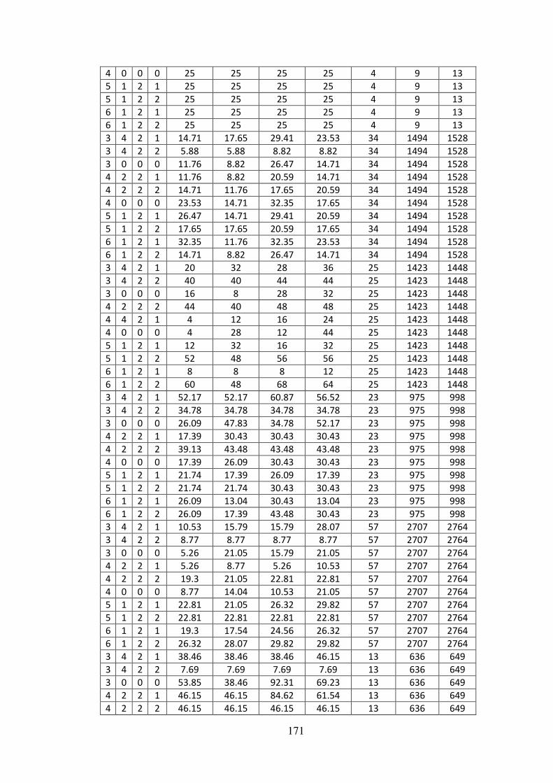
171
4 0 0 0 25 25 25 25 4 9 13 5 1 2 1 25 25 25 25 4 9 13 5 1 2 2 25 25 25 25 4 9 13 6 1 2 1 25 25 25 25 4 9 13 6 1 2 2 25 25 25 25 4 9 13 3 4 2 1 14.71 17.65 29.41 23.53 34 1494 1528 3 4 2 2 5.88 5.88 8.82 8.82 34 1494 1528 3 0 0 0 11.76 8.82 26.47 14.71 34 1494 1528 4 2 2 1 11.76 8.82 20.59 14.71 34 1494 1528 4 2 2 2 14.71 11.76 17.65 20.59 34 1494 1528 4 0 0 0 23.53 14.71 32.35 17.65 34 1494 1528 5 1 2 1 26.47 14.71 29.41 20.59 34 1494 1528 5 1 2 2 17.65 17.65 20.59 17.65 34 1494 1528 6 1 2 1 32.35 11.76 32.35 23.53 34 1494 1528 6 1 2 2 14.71 8.82 26.47 14.71 34 1494 1528 3 4 2 1 20 32 28 36 25 1423 1448 3 4 2 2 40 40 44 44 25 1423 1448 3 0 0 0 16 8 28 32 25 1423 1448 4 2 2 2 44 40 48 48 25 1423 1448 4 4 2 1 4 12 16 24 25 1423 1448 4 0 0 0 4 28 12 44 25 1423 1448 5 1 2 1 12 32 16 32 25 1423 1448 5 1 2 2 52 48 56 56 25 1423 1448 6 1 2 1 8 8 8 12 25 1423 1448 6 1 2 2 60 48 68 64 25 1423 1448 3 4 2 1 52.17 52.17 60.87 56.52 23 975 998 3 4 2 2 34.78 34.78 34.78 34.78 23 975 998 3 0 0 0 26.09 47.83 34.78 52.17 23 975 998 4 2 2 1 17.39 30.43 30.43 30.43 23 975 998 4 2 2 2 39.13 43.48 43.48 43.48 23 975 998 4 0 0 0 17.39 26.09 30.43 30.43 23 975 998 5 1 2 1 21.74 17.39 26.09 17.39 23 975 998 5 1 2 2 21.74 21.74 30.43 30.43 23 975 998 6 1 2 1 26.09 13.04 30.43 13.04 23 975 998 6 1 2 2 26.09 17.39 43.48 30.43 23 975 998 3 4 2 1 10.53 15.79 15.79 28.07 57 2707 2764 3 4 2 2 8.77 8.77 8.77 8.77 57 2707 2764 3 0 0 0 5.26 21.05 15.79 21.05 57 2707 2764 4 2 2 1 5.26 8.77 5.26 10.53 57 2707 2764 4 2 2 2 19.3 21.05 22.81 22.81 57 2707 2764 4 0 0 0 8.77 14.04 10.53 21.05 57 2707 2764 5 1 2 1 22.81 21.05 26.32 29.82 57 2707 2764 5 1 2 2 22.81 22.81 22.81 22.81 57 2707 2764 6 1 2 1 19.3 17.54 24.56 26.32 57 2707 2764 6 1 2 2 26.32 28.07 29.82 29.82 57 2707 2764 3 4 2 1 38.46 38.46 38.46 46.15 13 636 649 3 4 2 2 7.69 7.69 7.69 7.69 13 636 649 3 0 0 0 53.85 38.46 92.31 69.23 13 636 649 4 2 2 1 46.15 46.15 84.62 61.54 13 636 649 4 2 2 2 46.15 46.15 46.15 46.15 13 636 649

172
4 0 0 0 76.92 53.85 100 53.85 13 636 649 5 1 2 1 53.85 46.15 61.54 53.85 13 636 649 5 1 2 2 61.54 53.85 61.54 61.54 13 636 649 6 1 2 1 38.46 23.08 53.85 30.77 13 636 649 6 1 2 2 38.46 38.46 76.92 61.54 13 636 649 3 4 2 1 24.49 26.53 40.82 40.82 49 1713 1762 3 4 2 2 4.08 4.08 4.08 4.08 49 1713 1762 3 0 0 0 20.41 20.41 28.57 30.61 49 1713 1762 4 2 2 1 14.29 18.37 26.53 28.57 49 1713 1762 4 2 2 2 6.12 6.12 8.16 8.16 49 1713 1762 4 0 0 0 14.29 24.49 32.65 34.69 49 1713 1762 5 1 2 1 16.33 12.24 22.45 18.37 49 1713 1762 5 1 2 2 4.08 6.12 12.24 12.24 49 1713 1762 6 1 2 1 22.45 20.41 32.65 22.45 49 1713 1762 6 1 2 2 10.2 8.16 14.29 16.33 49 1713 1762 3 4 2 1 25.55 28.47 28.47 32.85 137 6779 6916 3 4 2 2 16.06 16.79 18.25 18.25 137 6779 6916 3 0 0 0 28.47 24.09 32.85 28.47 137 6779 6916 4 2 2 1 10.22 5.11 16.79 11.68 137 6779 6916 4 2 2 2 4.38 4.38 4.38 4.38 137 6779 6916 4 0 0 0 11.68 5.11 17.52 8.76 137 6779 6916 5 1 2 1 17.52 14.6 38.69 29.93 137 6779 6916 5 1 2 2 32.12 22.63 32.12 31.39 137 6779 6916 6 1 2 1 13.14 7.3 27.74 19.71 137 6779 6916 6 1 2 2 18.25 8.03 23.36 21.9 137 6779 6916 3 4 2 1 16.13 19.35 19.35 19.35 31 1350 1381 3 4 2 2 9.68 9.68 12.9 12.9 31 1350 1381 3 0 0 0 6.45 16.13 9.68 19.35 31 1350 1381 4 2 2 1 6.45 9.68 9.68 19.35 31 1350 1381 4 2 2 2 22.58 22.58 29.03 29.03 31 1350 1381 4 0 0 0 32.26 32.26 35.48 45.16 31 1350 1381 5 1 2 1 22.58 25.81 29.03 32.26 31 1350 1381 5 1 2 2 35.48 35.48 38.71 38.71 31 1350 1381 6 1 2 1 32.26 48.39 35.48 51.61 31 1350 1381 6 1 2 2 32.26 22.58 38.71 51.61 31 1350 1381 3 4 2 1 15.38 7.69 19.23 19.23 26 1698 1724 3 4 2 2 3.85 3.85 3.85 3.85 26 1698 1724 3 0 0 0 15.38 7.69 15.38 7.69 26 1698 1724 4 2 2 1 7.69 11.54 7.69 11.54 26 1698 1724 4 2 2 2 3.85 3.85 11.54 11.54 26 1698 1724 4 0 0 0 3.85 15.38 11.54 15.38 26 1698 1724 5 1 2 1 19.23 7.69 23.08 15.38 26 1698 1724 5 1 2 2 7.69 11.54 19.23 19.23 26 1698 1724 6 1 2 1 7.69 11.54 11.54 15.38 26 1698 1724 6 1 2 2 11.54 19.23 26.92 26.92 26 1698 1724 3 4 2 1 8.87 8.87 8.87 11.29 124 5603 5727 3 4 2 2 12.1 12.9 14.52 14.52 124 5603 5727 3 0 0 0 8.87 9.68 10.48 12.1 124 5603 5727 4 2 2 1 3.23 8.87 7.26 12.9 124 5603 5727 4 2 2 2 11.29 18.55 17.74 24.19 124 5603 5727

173
4 0 0 0 6.45 8.06 8.87 12.9 124 5603 5727 5 1 2 1 4.03 15.32 15.32 21.77 124 5603 5727 5 1 2 2 10.48 16.13 16.13 18.55 124 5603 5727 6 1 2 1 2.42 4.84 4.03 12.1 124 5603 5727 6 1 2 2 9.68 9.68 16.94 15.32 124 5603 5727 3 4 2 1 8 8 12 12 25 1036 1061 3 4 2 2 12 12 12 12 25 1036 1061 3 0 0 0 16 16 20 28 25 1036 1061 4 2 2 1 12 12 12 20 25 1036 1061 4 2 2 2 20 20 20 20 25 1036 1061 4 0 0 0 28 20 44 20 25 1036 1061 5 1 2 1 8 8 8 16 25 1036 1061 5 1 2 2 44 56 60 60 25 1036 1061 6 1 2 1 16 12 24 24 25 1036 1061 6 1 2 2 56 60 60 64 25 1036 1061 3 4 2 1 16.67 16.67 16.67 16.67 6 40 46 3 4 2 2 16.67 16.67 16.67 16.67 6 40 46 3 0 0 0 16.67 16.67 16.67 16.67 6 40 46 4 2 2 1 16.67 16.67 16.67 16.67 6 40 46 4 2 2 2 16.67 16.67 16.67 16.67 6 40 46 4 0 0 0 16.67 16.67 16.67 16.67 6 40 46 5 1 2 1 16.67 16.67 16.67 16.67 6 40 46 5 1 2 2 16.67 16.67 16.67 16.67 6 40 46 6 1 2 1 16.67 16.67 16.67 16.67 6 40 46 6 1 2 2 16.67 16.67 33.33 16.67 6 40 46 3 4 2 1 18.18 13.64 18.18 18.18 22 920 942 3 4 2 2 9.09 9.09 9.09 9.09 22 920 942 3 0 0 0 18.18 9.09 27.27 22.73 22 920 942 4 2 2 1 13.64 13.64 22.73 13.64 22 920 942 4 2 2 2 9.09 9.09 9.09 9.09 22 920 942 4 0 0 0 13.64 13.64 31.82 13.64 22 920 942 5 1 2 1 18.18 9.09 27.27 9.09 22 920 942 5 1 2 2 9.09 9.09 9.09 9.09 22 920 942 6 1 2 1 9.09 4.55 18.18 4.55 22 920 942 6 1 2 2 9.09 9.09 9.09 9.09 22 920 942 3 4 2 1 22.22 38.89 33.33 50 18 575 593 3 4 2 2 72.22 61.11 72.22 72.22 18 575 593 3 0 0 0 16.67 50 22.22 72.22 18 575 593 4 2 2 1 5.56 22.22 5.56 33.33 18 575 593 4 2 2 2 33.33 27.78 55.56 50 18 575 593 4 0 0 0 22.22 50 50 55.56 18 575 593 5 1 2 1 16.67 16.67 16.67 27.78 18 575 593 5 1 2 2 11.11 22.22 27.78 44.44 18 575 593 6 1 2 1 22.22 33.33 33.33 55.56 18 575 593 6 1 2 2 38.89 44.44 66.67 66.67 18 575 593 3 4 2 1 27.27 24.24 30.3 30.3 33 1346 1379 3 4 2 2 6.06 6.06 6.06 6.06 33 1346 1379 3 0 0 0 33.33 33.33 51.52 42.42 33 1346 1379 4 2 2 1 30.3 48.48 60.61 60.61 33 1346 1379 4 2 2 2 36.36 39.39 39.39 39.39 33 1346 1379

174
4 0 0 0 36.36 54.55 51.52 60.61 33 1346 1379 5 1 2 1 57.58 51.52 60.61 60.61 33 1346 1379 5 1 2 2 57.58 60.61 60.61 60.61 33 1346 1379 6 1 2 1 39.39 48.48 42.42 66.67 33 1346 1379 6 1 2 2 60.61 63.64 72.73 78.79 33 1346 1379 3 4 2 1 6.12 5.1 8.16 8.16 98 5679 5777 3 4 2 2 10.2 10.2 10.2 10.2 98 5679 5777 3 0 0 0 7.14 4.08 7.14 8.16 98 5679 5777 4 2 2 1 16.33 13.27 17.35 20.41 98 5679 5777 4 2 2 2 17.35 19.39 25.51 25.51 98 5679 5777 4 0 0 0 10.2 12.24 16.33 16.33 98 5679 5777 5 1 2 1 4.08 4.08 8.16 15.31 98 5679 5777 5 1 2 2 14.29 14.29 16.33 16.33 98 5679 5777 6 1 2 1 2.04 8.16 9.18 11.22 98 5679 5777 6 1 2 2 12.24 10.2 17.35 15.31 98 5679 5777 3 4 2 1 4.35 4.35 8.7 4.35 23 1148 1171 3 4 2 2 4.35 4.35 4.35 4.35 23 1148 1171 3 0 0 0 4.35 4.35 17.39 13.04 23 1148 1171 4 2 2 1 8.7 8.7 8.7 8.7 23 1148 1171 4 2 2 2 4.35 4.35 4.35 4.35 23 1148 1171 4 0 0 0 13.04 4.35 17.39 4.35 23 1148 1171 5 1 2 1 4.35 4.35 4.35 4.35 23 1148 1171 5 1 2 2 4.35 4.35 8.7 8.7 23 1148 1171 6 1 2 1 4.35 4.35 8.7 13.04 23 1148 1171 6 1 2 2 13.04 4.35 17.39 17.39 23 1148 1171 3 4 2 1 9.09 13.64 13.64 22.73 22 891 913 3 4 2 2 36.36 31.82 40.91 40.91 22 891 913 3 0 0 0 18.18 18.18 27.27 27.27 22 891 913 4 2 2 1 18.18 27.27 18.18 31.82 22 891 913 4 2 2 2 31.82 36.36 45.45 50 22 891 913 4 0 0 0 18.18 18.18 22.73 27.27 22 891 913 5 1 2 1 13.64 27.27 13.64 40.91 22 891 913 5 1 2 2 13.64 27.27 36.36 50 22 891 913 6 1 2 1 13.64 22.73 13.64 40.91 22 891 913 6 1 2 2 40.91 31.82 45.45 63.64 22 891 913 3 4 2 1 33.33 44.44 44.44 44.44 9 718 727 3 4 2 2 11.11 11.11 11.11 11.11 9 718 727 3 0 0 0 44.44 44.44 44.44 55.56 9 718 727 4 2 2 1 55.56 66.67 55.56 66.67 9 718 727 4 2 2 2 44.44 44.44 44.44 55.56 9 718 727 4 0 0 0 55.56 44.44 55.56 55.56 9 718 727 5 1 2 1 11.11 11.11 11.11 11.11 9 718 727 5 1 2 2 11.11 11.11 33.33 33.33 9 718 727 6 1 2 1 22.22 11.11 33.33 22.22 9 718 727 6 1 2 2 11.11 11.11 44.44 22.22 9 718 727 3 4 2 1 10.42 8.33 16.67 16.67 48 2712 2760 3 4 2 2 10.42 6.25 10.42 10.42 48 2712 2760 3 0 0 0 18.75 12.5 27.08 22.92 48 2712 2760 4 2 2 1 16.67 18.75 22.92 22.92 48 2712 2760 4 2 2 2 12.5 14.58 16.67 16.67 48 2712 2760

175
4 0 0 0 12.5 12.5 25 22.92 48 2712 2760 5 1 2 1 6.25 8.33 18.75 10.42 48 2712 2760 5 1 2 2 2.08 2.08 6.25 10.42 48 2712 2760 6 1 2 1 6.25 2.08 12.5 6.25 48 2712 2760 6 1 2 2 6.25 6.25 8.33 10.42 48 2712 2760

176
Appendix C - DUD 8 reduced sets – averages EF, AUC and Recall @10%
COX2 EF, AUC
shape K D R M EF(V) EF(P) ACTIVE DECOY TOTAL AUC(V) AUC(P)
3 0 0 0 2.83 4.5 44 352 396 0.58 0.63
3 4 2 0 3.09 4.11 44 352 396 0.76 0.69
3 4 2 1 3.34 4.5 44 352 396 0.71 0.74
3 4 2 2 3.09 3.34 44 352 396 0.55 0.55
4 0 0 0 4.11 5.91 44 352 396 0.62 0.69
4 2 2 0 4.24 6.04 44 352 396 0.63 0.74
4 2 2 1 5.01 5.66 44 352 396 0.72 0.74
4 2 2 2 6.17 6.3 44 352 396 0.68 0.68
5 1 2 0 4.24 5.53 44 352 396 0.6 0.72
5 1 2 1 5.4 5.53 44 352 396 0.71 0.74
5 1 2 2 6.56 6.3 44 352 396 0.66 0.66
6 1 2 0 3.73 5.27 44 352 396 0.64 0.68
6 1 2 1 4.11 5.01 44 352 396 0.67 0.67
6 1 2 2 5.91 6.17 44 352 396 0.67 0.67
sub-shape
K D R M EF(V) EF(P) ACTIVE DECOY TOTAL AUC(V) AUC(P)
4 2 2 0 2.7 5.79 44 352 396 0.63 0.74
4 2 2 1 4.5 4.89 44 352 396 0.69 0.73
4 2 2 2 6.56 6.3 44 352 396 0.68 0.68
5 1 2 2 6.43 5.79 44 352 396 0.66 0.65
6 1 2 2 4.5 4.11 44 352 396 0.66 0.65
Recall@10%
K D R M EF(V) EF(P) RECALL(V) RECALL(P) ACTIVES DECOYS TOTAL 3 0 0 0 2.83 4.5 12.66 20.78 44 352 396 3 4 2 0 3.08 4.11 14.61 21.75 44 352 396 3 4 2 1 3.34 4.49 18.51 24.03 44 352 396 3 4 2 2 3.08 3.33 12.99 13.64 44 352 396 4 0 0 0 4.11 5.91 22.73 30.52 44 352 396 4 2 2 0 4.23 6.03 24.03 36.04 44 352 396 4 2 2 1 5 5.64 28.9 34.42 44 352 396 4 2 2 2 6.16 6.29 34.41 36.36 44 352 396 5 1 2 0 4.23 5.51 20.13 33.44 44 352 396 5 1 2 1 5.39 5.52 25.65 33.44 44 352 396 5 1 2 2 6.54 6.29 34.74 35.06 44 352 396 6 1 2 0 3.72 5.26 22.73 30.52 44 352 396 6 1 2 1 4.1 5 25.65 30.2 44 352 396 6 1 2 2 5.9 6.16 32.14 27.92 44 352 396

177
EGFR EF, AUC
shape K D R M EF(V) EF(P) ACTIVE DECOY TOTAL AUC(V) AUC(P)
3 0 0 0 4.11 4.24 40 320 360 0.58 0.53
3 4 2 0 4.37 3.6 40 320 360 0.63 0.58
3 4 2 1 3.21 3.09 40 320 360 0.53 0.54
3 4 2 2 2.57 2.06 40 320 360 0.55 0.54
4 0 0 0 3.6 2.7 40 320 360 0.6 0.56
4 2 2 0 3.09 2.06 40 320 360 0.6 0.57
4 2 2 1 2.57 2.06 40 320 360 0.59 0.57
4 2 2 2 2.83 3.09 40 320 360 0.57 0.57
5 1 2 0 2.19 3.09 40 320 360 0.54 0.54
5 1 2 1 2.57 3.09 40 320 360 0.55 0.57
5 1 2 2 3.21 3.73 40 320 360 0.53 0.53
6 1 2 0 2.7 3.34 40 320 360 0.54 0.54
6 1 2 1 3.6 3.34 40 320 360 0.55 0.6
6 1 2 2 2.96 3.34 40 320 360 0.54 0.54
sub-shape
K D R M EF(V) EF(P) ACTIVE DECOY TOTAL AUC(V) AUC(P)
4 2 2 0 1.29 1.54 40 320 360 0.56 0.55
4 2 2 1 1.03 1.8 40 320 360 0.57 0.57
4 2 2 2 1.93 2.06 40 320 360 0.57 0.57
5 1 2 2 2.31 2.7 40 320 360 0.53 0.53
6 1 2 2 2.57 2.19 40 320 360 0.55 0.54
Recall@10%
K D R M EF(V) EF(P) RECALL(V) RECALL(P) ACTIVES DECOYS TOTAL 3 0 0 0 4.11 4.24 27.14 18.93 40 320 360 3 4 2 0 4.36 3.59 26.07 20.36 40 320 360 3 4 2 1 3.21 3.08 18.21 15 40 320 360 3 4 2 2 2.57 2.05 12.86 12.5 40 320 360 4 0 0 0 3.6 2.7 21.07 18.21 40 320 360 4 2 2 0 3.08 2.05 17.5 18.93 40 320 360 4 2 2 1 2.56 2.05 15 15.71 40 320 360 4 2 2 2 2.82 3.08 16.07 16.43 40 320 360 5 1 2 0 2.18 3.08 11.79 16.43 40 320 360 5 1 2 1 2.57 3.08 14.29 18.93 40 320 360 5 1 2 2 3.21 3.72 16.07 17.14 40 320 360 6 1 2 0 2.69 3.33 13.21 16.07 40 320 360 6 1 2 1 3.59 3.33 16.07 16.43 40 320 360 6 1 2 2 2.95 3.33 15.71 16.43 40 320 360
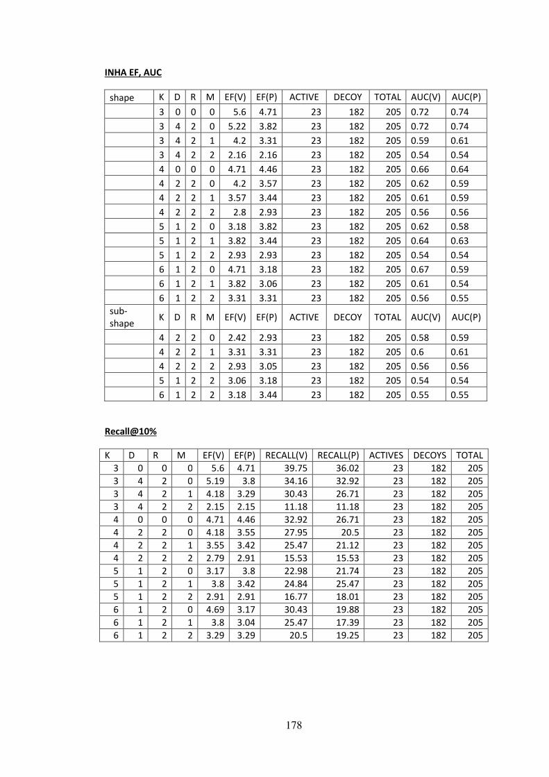
178
INHA EF, AUC
shape K D R M EF(V) EF(P) ACTIVE DECOY TOTAL AUC(V) AUC(P)
3 0 0 0 5.6 4.71 23 182 205 0.72 0.74
3 4 2 0 5.22 3.82 23 182 205 0.72 0.74
3 4 2 1 4.2 3.31 23 182 205 0.59 0.61
3 4 2 2 2.16 2.16 23 182 205 0.54 0.54
4 0 0 0 4.71 4.46 23 182 205 0.66 0.64
4 2 2 0 4.2 3.57 23 182 205 0.62 0.59
4 2 2 1 3.57 3.44 23 182 205 0.61 0.59
4 2 2 2 2.8 2.93 23 182 205 0.56 0.56
5 1 2 0 3.18 3.82 23 182 205 0.62 0.58
5 1 2 1 3.82 3.44 23 182 205 0.64 0.63
5 1 2 2 2.93 2.93 23 182 205 0.54 0.54
6 1 2 0 4.71 3.18 23 182 205 0.67 0.59
6 1 2 1 3.82 3.06 23 182 205 0.61 0.54
6 1 2 2 3.31 3.31 23 182 205 0.56 0.55
sub-shape
K D R M EF(V) EF(P) ACTIVE DECOY TOTAL AUC(V) AUC(P)
4 2 2 0 2.42 2.93 23 182 205 0.58 0.59
4 2 2 1 3.31 3.31 23 182 205 0.6 0.61
4 2 2 2 2.93 3.05 23 182 205 0.56 0.56
5 1 2 2 3.06 3.18 23 182 205 0.54 0.54
6 1 2 2 3.18 3.44 23 182 205 0.55 0.55
Recall@10%
K D R M EF(V) EF(P) RECALL(V) RECALL(P) ACTIVES DECOYS TOTAL 3 0 0 0 5.6 4.71 39.75 36.02 23 182 205 3 4 2 0 5.19 3.8 34.16 32.92 23 182 205 3 4 2 1 4.18 3.29 30.43 26.71 23 182 205 3 4 2 2 2.15 2.15 11.18 11.18 23 182 205 4 0 0 0 4.71 4.46 32.92 26.71 23 182 205 4 2 2 0 4.18 3.55 27.95 20.5 23 182 205 4 2 2 1 3.55 3.42 25.47 21.12 23 182 205 4 2 2 2 2.79 2.91 15.53 15.53 23 182 205 5 1 2 0 3.17 3.8 22.98 21.74 23 182 205 5 1 2 1 3.8 3.42 24.84 25.47 23 182 205 5 1 2 2 2.91 2.91 16.77 18.01 23 182 205 6 1 2 0 4.69 3.17 30.43 19.88 23 182 205 6 1 2 1 3.8 3.04 25.47 17.39 23 182 205 6 1 2 2 3.29 3.29 20.5 19.25 23 182 205

179
P38 EF, AUC
shape K D R M EF(V) EF(P) ACTIVE DECOY TOTAL AUC(V) AUC(P)
3 0 0 0 4.63 4.11 20 160 180 0.56 0.62
3 4 2 0 4.37 3.86 20 160 180 0.7 0.7
3 4 2 1 3.86 3.47 20 160 180 0.68 0.68
3 4 2 2 2.57 2.44 20 160 180 0.53 0.53
4 0 0 0 4.5 5.27 20 160 180 0.71 0.72
4 2 2 0 3.47 3.86 20 160 180 0.62 0.58
4 2 2 1 4.24 4.63 20 160 180 0.66 0.64
4 2 2 2 3.6 3.34 20 160 180 0.59 0.59
5 1 2 0 5.4 5.27 20 160 180 0.72 0.73
5 1 2 1 5.14 5.27 20 160 180 0.77 0.75
5 1 2 2 5.79 5.27 20 160 180 0.66 0.65
6 1 2 0 4.76 4.63 20 160 180 0.7 0.71
6 1 2 1 4.89 4.63 20 160 180 0.71 0.67
6 1 2 2 5.27 4.63 20 160 180 0.68 0.67
sub-shape
K D R M EF(V) EF(P) ACTIVE DECOY TOTAL AUC(V) AUC(P)
4 2 2 0 3.21 3.34 20 160 180 0.59 0.56
4 2 2 1 4.11 4.24 20 160 180 0.64 0.63
4 2 2 2 3.47 3.47 20 160 180 0.59 0.59
5 1 2 2 5.14 5.79 20 160 180 0.66 0.66
6 1 2 2 4.5 4.24 20 160 180 0.67 0.66
Recall@10%
K D R M EF(V) EF(P) RECALL(V) RECALL(P) ACTIVES DECOYS TOTAL 3 0 0 0 4.63 4.11 31.43 24.29 20 160 180 3 4 2 0 4.35 3.84 29.29 27.86 20 160 180 3 4 2 1 3.84 3.45 23.57 23.57 20 160 180 3 4 2 2 2.56 2.43 15 14.29 20 160 180 4 0 0 0 4.5 5.27 35 35 20 160 180 4 2 2 0 3.45 3.84 23.57 26.43 20 160 180 4 2 2 1 4.22 4.61 27.86 30.71 20 160 180 4 2 2 2 3.58 3.33 26.43 24.29 20 160 180 5 1 2 0 5.37 5.24 36.43 35.71 20 160 180 5 1 2 1 5.12 5.25 38.57 36.43 20 160 180 5 1 2 2 5.76 5.24 38.57 35 20 160 180 6 1 2 0 4.73 4.61 34.29 32.14 20 160 180 6 1 2 1 4.86 4.61 33.57 31.43 20 160 180 6 1 2 2 5.25 4.61 35.71 30.71 20 160 180

180
PDE5 EF, AUC
shape K D R M EF(V) EF(P) ACTIVE DECOY TOTAL AUC(V) AUC(P)
3 0 0 0 6.37 3.82 22 174 196 0.79 0.68
3 4 2 0 5.35 4.2 22 174 196 0.82 0.79
3 4 2 1 4.84 3.94 22 174 196 0.79 0.76
3 4 2 2 1.65 1.65 22 174 196 0.52 0.52
4 0 0 0 3.82 3.69 22 174 196 0.75 0.72
4 2 2 0 3.43 3.44 22 174 196 0.63 0.63
4 2 2 1 3.94 3.44 22 174 196 0.67 0.65
4 2 2 2 3.18 3.18 22 174 196 0.57 0.57
5 1 2 0 3.18 3.56 22 174 196 0.68 0.65
5 1 2 1 3.69 3.94 22 174 196 0.71 0.66
5 1 2 2 2.67 2.67 22 174 196 0.55 0.55
6 1 2 0 3.18 2.92 22 174 196 0.63 0.59
6 1 2 1 3.31 3.31 22 174 196 0.64 0.6
6 1 2 2 3.05 3.05 22 174 196 0.57 0.56
sub-shape
K D R M EF(V) EF(P) ACTIVE DECOY TOTAL AUC(V) AUC(P)
4 2 2 0 3.05 2.92 22 174 196 0.59 0.57
4 2 2 1 3.44 3.18 22 174 196 0.59 0.58
4 2 2 2 2.8 2.92 22 174 196 0.57 0.56
5 1 2 2 2.54 2.54 22 174 196 0.55 0.55
6 1 2 2 2.67 2.67 22 174 196 0.57 0.57
Recall@10%
K D R M EF(V) EF(P) RECALL(V) RECALL(P) ACTIVES DECOYS TOTAL 3 0 0 0 6.37 3.82 48.7 27.92 22 174 196 3 4 2 0 5.32 4.18 38.96 33.12 22 174 196 3 4 2 1 4.81 3.93 37.66 28.57 22 174 196 3 4 2 2 1.65 1.65 8.44 9.09 22 174 196 4 0 0 0 3.82 3.69 28.57 25.97 22 174 196 4 2 2 0 3.42 3.42 28.57 25.97 22 174 196 4 2 2 1 3.93 3.42 29.87 25.97 22 174 196 4 2 2 2 3.17 3.17 20.13 19.48 22 174 196 5 1 2 0 3.17 3.54 22.08 21.43 22 174 196 5 1 2 1 3.67 3.92 26.62 25.33 22 174 196 5 1 2 2 2.66 2.66 16.23 15.58 22 174 196 6 1 2 0 3.17 2.91 22.73 23.38 22 174 196 6 1 2 1 3.29 3.29 25.32 22.08 22 174 196 6 1 2 2 3.04 3.04 21.43 21.43 22 174 196

181
PDGFRB EF, AUC
shape K D R M EF(V) EF(P) ACTIVE DECOY TOTAL AUC(V) AUC(P)
3 0 0 0 5.6 4.84 22 174 196 0.56 0.6
3 4 2 0 4.58 4.33 22 174 196 0.56 0.58
3 4 2 1 4.71 4.58 22 174 196 0.57 0.58
3 4 2 2 1.14 1.14 22 174 196 0.51 0.51
4 0 0 0 5.35 5.22 22 174 196 0.61 0.67
4 2 2 0 4.33 4.58 22 174 196 0.6 0.62
4 2 2 1 4.33 4.71 22 174 196 0.61 0.62
4 2 2 2 2.8 2.67 22 174 196 0.55 0.55
5 1 2 0 3.31 3.94 22 174 196 0.59 0.58
5 1 2 1 3.94 3.82 22 174 196 0.6 0.59
5 1 2 2 3.31 3.18 22 174 196 0.57 0.57
6 1 2 0 3.82 3.18 22 174 196 0.59 0.6
6 1 2 1 3.69 2.93 22 174 196 0.58 0.56
6 1 2 2 3.82 3.94 22 174 196 0.63 0.62
sub-shape
K D R M EF(V) EF(P) ACTIVE DECOY TOTAL AUC(V) AUC(P)
4 2 2 0 2.92 3.31 22 174 196 0.59 0.61
4 2 2 1 2.92 3.43 22 174 196 0.58 0.62
4 2 2 2 2.92 2.92 22 174 196 0.55 0.55
5 1 2 2 3.18 3.69 22 174 196 0.57 0.57
6 1 2 2 3.94 3.82 22 174 196 0.65 0.65
Recall@10%
K D R M EF(V) EF(P) RECALL(V) RECALL(P) ACTIVES DECOYS TOTAL 3 0 0 0 5.6 4.84 33.11 29.87 22 174 196 3 4 2 0 4.56 4.3 27.92 26.62 22 174 196 3 4 2 1 4.69 4.56 27.27 27.27 22 174 196 3 4 2 2 1.14 1.14 5.85 5.85 22 174 196 4 0 0 0 5.35 5.22 40.26 38.31 22 174 196 4 2 2 0 4.3 4.56 33.12 34.41 22 174 196 4 2 2 1 4.31 4.69 35.06 34.42 22 174 196 4 2 2 2 2.79 2.66 14.94 16.23 22 174 196 5 1 2 0 3.29 3.93 24.03 25.32 22 174 196 5 1 2 1 3.93 3.8 27.27 25.97 22 174 196 5 1 2 2 3.29 3.17 20.13 19.48 22 174 196 6 1 2 0 3.8 3.16 24.67 22.73 22 174 196 6 1 2 1 3.67 2.91 24.68 19.48 22 174 196 6 1 2 2 3.8 3.93 27.27 26.62 22 174 196

182
SRC EF, AUC
shape K D R M EF(V) EF(P) ACTIVE DECOY TOTAL AUC(V) AUC(P)
3 0 0 0 7.46 5.27 21 168 189 0.8 0.74
3 4 2 0 5.91 4.24 21 168 189 0.74 0.71
3 4 2 1 3.98 3.47 21 168 189 0.63 0.62
3 4 2 2 1.93 1.93 21 168 189 0.53 0.53
4 0 0 0 5.66 4.11 21 168 189 0.73 0.71
4 2 2 0 3.98 3.21 21 168 189 0.66 0.62
4 2 2 1 3.6 3.73 21 168 189 0.63 0.63
4 2 2 2 3.34 3.21 21 168 189 0.56 0.56
5 1 2 0 3.73 3.21 21 168 189 0.64 0.64
5 1 2 1 3.6 3.6 21 168 189 0.6 0.6
5 1 2 2 3.98 3.85 21 168 189 0.58 0.58
6 1 2 0 4.11 2.44 21 168 189 0.63 0.58
6 1 2 1 3.08 2.96 21 168 189 0.6 0.58
6 1 2 2 3.6 2.95 21 168 189 0.58 0.57
sub-shape
K D R M EF(V) EF(P) ACTIVE DECOY TOTAL AUC(V) AUC(P)
4 2 2 0 2.44 2.44 21 168 189 0.58 0.59
4 2 2 1 3.08 3.21 21 168 189 0.62 0.63
4 2 2 2 3.34 3.21 21 168 189 0.56 0.56
5 1 2 2 3.73 3.47 21 168 189 0.58 0.58
6 1 2 2 2.31 2.44 21 168 189 0.57 0.57
Recall@10%
K D R M EF(V) EF(P) RECALL(V) RECALL(P) ACTIVES DECOYS TOTAL 3 0 0 0 7.46 5.27 53.06 36.05 21 168 189 3 4 2 0 5.88 4.22 38.1 34.02 21 168 189 3 4 2 1 3.97 3.45 27.89 27.21 21 168 189 3 4 2 2 1.92 1.92 10.89 10.89 21 168 189 4 0 0 0 5.66 4.11 36.74 31.97 21 168 189 4 2 2 0 3.97 3.2 27.21 23.81 21 168 189 4 2 2 1 3.58 3.71 26.53 24.49 21 168 189 4 2 2 2 3.33 3.2 18.37 18.37 21 168 189 5 1 2 0 3.71 3.2 27.21 25.17 21 168 189 5 1 2 1 3.58 3.58 23.13 23.13 21 168 189 5 1 2 2 3.97 3.84 23.13 22.45 21 168 189 6 1 2 0 4.09 2.43 27.89 17.69 21 168 189 6 1 2 1 3.07 2.94 23.81 19.05 21 168 189 6 1 2 2 3.58 2.94 23.13 21.77 21 168 189

183
VEGFR2 EF, AUC
shape K D R M EF(V) EF(P) ACTIVE DECOY TOTAL AUC(V) AUC(P)
3 0 0 0 6.69 5.91 31 248 279 0.64 0.64
3 4 2 0 5.14 5.27 31 248 279 0.65 0.65
3 4 2 1 5.14 4.88 31 248 279 0.63 0.63
3 4 2 2 2.18 2.18 31 248 279 0.51 0.51
4 0 0 0 3.86 3.6 31 248 279 0.61 0.61
4 2 2 0 2.95 2.83 31 248 279 0.6 0.56
4 2 2 1 3.34 3.34 31 248 279 0.61 0.58
4 2 2 2 2.7 2.57 31 248 279 0.53 0.53
5 1 2 0 4.11 3.34 31 248 279 0.6 0.57
5 1 2 1 4.49 3.47 31 248 279 0.58 0.57
5 1 2 2 2.7 3.08 31 248 279 0.53 0.53
6 1 2 0 4.24 3.47 31 248 279 0.62 0.58
6 1 2 1 3.08 3.21 31 248 279 0.6 0.56
6 1 2 2 3.6 3.08 31 248 279 0.55 0.55
sub-shape
K D R M EF(V) EF(P) ACTIVE DECOY TOTAL AUC(V) AUC(P)
4 2 2 0 2.05 2.31 31 248 278.71 0.55 0.55
4 2 2 1 2.31 2.95 31 248 278.71 0.58 0.57
4 2 2 2 2.7 2.57 31 248 278.71 0.53 0.53
5 1 2 2 2.83 3.6 31 248 278.71 0.53 0.53
6 1 2 2 3.08 3.6 31 248 278.71 0.55 0.55
Recall@10%
K D R M EF(V) EF(P) RECALL(V) RECALL(P) ACTIVES DECOYS TOTAL 3 0 0 0 6.69 5.91 38.71 35.94 31 248 279 3 4 2 0 5.13 5.25 27.19 27.19 31 248 279 3 4 2 1 5.13 4.87 25.35 24.88 31 248 279 3 4 2 2 2.18 2.18 7.84 7.84 31 248 279 4 0 0 0 3.86 3.6 23.96 26.73 31 248 279 4 2 2 0 2.95 2.82 18.89 18.89 31 248 279 4 2 2 1 3.33 3.33 20.28 20.74 31 248 279 4 2 2 2 2.69 2.56 11.52 11.98 31 248 279 5 1 2 0 4.1 3.33 20.74 20.28 31 248 279 5 1 2 1 4.48 3.46 23.04 20.28 31 248 279 5 1 2 2 2.69 3.07 15.21 16.59 31 248 279 6 1 2 0 4.23 3.46 22.58 18.89 31 248 279 6 1 2 1 3.08 3.2 17.97 18.43 31 248 279 6 1 2 2 3.59 3.08 23.5 21.66 31 248 279