development and verification of the generic...
TRANSCRIPT
DEVELOPMENT AND
VERIFICATION OF THE GENERICTHREE DIMENSIONAL FINITE VOLUME
SOLVER
By
M. K. Harsha Perera
M.Phil., The University of Southampton, UK., 2002M.Eng., The University of Southampton, UK., 1999
A THESIS SUBMITTED IN PARTIAL FULFILMENT OF THE REQUIREMENTS FOR THE DEGREE OF
MASTER OF APPLIED SCIENCE
in
THE FACULTY OF GRADUATE STUDIES(The Department of Mechanical Engineering)
We accept this thesis as conforming to the required standard
................................................
................................................
.....................…........................
................................................
THE UNIVERSITY OF BRITISH COLUMBIA
December 2003
© M. K. Harsha Perera, 2003
ii
Abstract
The generic finite volume solver, ANSLib, has been extended to three
dimensions and used to verify the accurate computa tion of three - dimensional
advection - diffusion and Poisson problems. A simple cubic domain has been
selected as the domain of interest. Over this domain a steady state solution was
computed for each model problem with 2 nd , 3 rd and 4 th order accurate schemes.
Gauss quadratu re is used to evaluate the flux integral to 2 nd , 3 rd and 4 th order
accuracy. The flux scheme makes use of the centred scheme to model the
viscous term and a simple upwind scheme to model the advective fluxes. In
both cases the existing k- exact least - square reconstruction code is used to
obtain the solution at each Gauss integration point to 2 nd , 3 rd and 4 th order
accuracy. Newton - Krylov implicit time advance is used to obtain the steady
state solution, implemented using the GMRES algorithm.
Prior to subjecting ANSLib code to physical model problems, the code was first
tested for the correct enforcement of boundary constraints, accurate
implementa tion of the solution reconstruction, and flux integral evaluation in
three dimensions. Relevant changes were made to the code to obtain the
desired behaviour.
Analytical solutions for the advection - diffusion and Poisson equations were
derived to satisfy Dirichlet and Neumann boundary conditions; these were used
to compute the resulting discretized error in numerically converged solutions.
Accuracy assessment was done through a comparison of error norms for
different mesh sizes for each test problem. Localized errors on the domain for
each problem at steady state were plotted. The efficiency of the code to obtain
numerical converged solution was reported.

iii
Table of Contents
ABSTRACT..................................................................................................................................II
LIST OF FIGURES......................................................................................................................V
LIST OF TABLES.....................................................................................................................VII
ACKNOWLEDGEMENT...........................................................................................................IX
1INTRODUCTION.....................................................................................................................1
1.1U NSTRUCTURED HIGH ORDER METHODS..............................................................................21.2O BJECTIVE AND SCOPE.......................................................................................................31.3T HESIS STRUCTURE...........................................................................................................3
2GENERIC SOLVER...................................................................................................................5
2.1G ENERIC SOLVER DEVELOPMENT...........................................................................................52.2O PERATION OF THE ANSLIB SOLVER...................................................................................62.3C ONCLUSION...................................................................................................................7
3THREE- DIMENSIONAL FLOW SOLVER...........................................................................9
3.1S PATIAL DISCRETIZATION................................................................................................10Higher order methods for the convective terms ...................................................12Higher order methods for the viscous terms .........................................................14
3.2S OLUTION UPDATE TECHNIQUES.........................................................................................14Time stepping ...................................................................................................................16
3.3C ONCLUSION.................................................................................................................17
4HIGHER ORDER RECONSTRUCTION AND VERIFICATION..................................18
4.1 K- EXACT RECONSTRUCTION..............................................................................................184.2V ERIFICATION TEST PROGRAMS..........................................................................................20
Boundary Condition treatment ...................................................................................224.3C ONCLUSION.................................................................................................................24
5MODEL VERIFICATION......................................................................................................25
5.1F LUX INTEGRAL TEST.......................................................................................................25Advection - diffusion .......................................................................................................26Poisson ..............................................................................................................................29
5.2S TEADY STATE SOLUTION.................................................................................................32Advection - diffusion results ........................................................................................33Poisson results .................................................................................................................42
5.3C ONCLUSION.................................................................................................................42
6CONCLUSIONS AND FUTURE WORK............................................................................44
7BIBLIOGRAPHY.....................................................................................................................46
AAPPENDIX A..........................................................................................................................48
AGAUSS QUADRATURE FOR A TRIANGLE...................................................................................48

iv
BGAUSS QUADRATURE FOR A TETRAHEDRON.............................................................................48CPARALLEL AXIS THEOREM....................................................................................................49DEXACT INTEGRATION FORMULA OVER TETRAHEDRON.................................................................49ECALCULATING ORDER OF ACCURACY FROM ERROR NORMS...........................................................51FANALYTICAL SOLUTION METHODS..........................................................................................52
GAdvection - diffusion ....................................................................................................52HPoisson .............................................................................................................................54

v
List of FiguresFIGURE 2 - 1 FLOW CHART SHOWING THE INTERACTION OF VARIOUS OBJECTS IN THE ANSLIB CODE. THE
RED AND LIGHT BLUE BOXES ARE SOME OF THE CLASSES. THE GREEN LINES SHOW THE INTERACTION OF
THE DRIVER PROGRAM WITH THE OBJECTS, AND THE BLACK LINES SHOW SOME INFORMATION PASSING
BETWEEN OBJECTS. THE RED BOXES ARE AFFECTED BY THE THIRD DIMENSION...................................7
FIGURE 3- 3.1 UNSTRUCTURED MESH OVER A CUBIC DOMAIN.........................10
FIGURE 4- 4.1 ORDER OF ACCURACY OF THE RECONSTRUCTION OFFUNCTION IN EQ. (4.4A) FOR THE INTERIOR CONTROL VOLUMES..................22
FIGURE 4- 4.2 THE BOUNDARY FACE DIRECTIONS AND LABELS FOR THECUBIC DOMAIN.......................................................................................................................23
FIGURE 5- 5.1 THE L2 ERROR NORM FOR THE ADVECTION- DIFFUSION FLUXTEST FOR VARIOUS MESH SIZES.....................................................................................29
FIGURE 5- 5.2 THE L2 ERROR NORM FOR THE POISSON FLUX TEST FORVARIOUS MESH SIZES...........................................................................................................30
FIGURE 5- 5.3 THE L2 ERROR NORM FOR THE ADVECTION- DIFFUSIONPROBLEM AT STEADY STATE FOR VARIOUS MESH SIZES....................................33
FIGURE 5- 5.4 THE SUB FIGURES (A)- (D) SHOWS THE SOLUTIONS TO THEADVECTION- DIFFUSION PROBLEM ALONG THE GEOMETRY AT X=0, 0.3, 0.6AND 1. ........................................................................................................................................34
FIGURE 5- 5.5 ERROR BETWEEN THE EXACT AND 2ND ORDER ACCURATESOLUTION AFTER NUMERICAL CONVERGENCE OF THE ADVECTION-DIFFUSION PROBLEM...........................................................................................................37
FIGURE 5- 5.6 ERROR BETWEEN THE EXACT AND 3RD ORDER ACCURATESOLUTION AFTER NUMERICAL CONVERGENCE OF THE ADVECTION-DIFFUSION PROBLEM...........................................................................................................37
FIGURE 5- 5.7 ERROR BETWEEN THE EXACT AND 4TH ORDER ACCURATESOLUTION AFTER NUMERICAL CONVERGENCE OF THE ADVECTION-DIFFUSION PROBLEM...........................................................................................................38
FIGURE 5- 5.8 THE COMPUTATIONAL TIME TAKEN FOR THE STEADY- STATESOLUTION OF THE ADVECTION- DIFFUSION PROBLEM FOR VARIOUSMESHES .....................................................................................................................................40
FIGURE 5- 5.9 THE L2 RESIDUAL NORM FOR THE ADVECTION- DIFFUSIONPROBLEM FOR THE 2ND ORDER ACCURATE METHOD..........................................41
FIGURE 5- 5.10 THE L2 RESIDUAL NORM FOR THE ADVECTION- DIFFUSIONPROBLEM FOR THE 3RD ORDER ACCURATE METHOD..........................................41

vi
FIGURE 5- 5.11 THE L2 RESIDUAL NORM FOR THE ADVECTION- DIFFUSIONPROBLEM FOR THE 4TH ORDER ACCURATE METHOD..........................................42
FIGURE 5- 5.12 THE L2 ERROR NORM FOR THE POISSON PROBLEM ATSTEADY STATE FOR VARIOUS MESH SIZES ...............................................................43
FIGURE 5- 5.13 THE SUB FIGURES (A)- (C) SHOWS THE SOLUTIONS TO THEPOISSON PROBLEM ALONG THE GEOMETRY AT X=0, 0.3, AND 0.6. ................35
FIGURE 5- 5.14 ERROR BETWEEN THE EXACT AND 2ND ORDER ACCURATESOLUTION AFTER NUMERICAL CONVERGENCE FOR THE POISSON PROBLEM.38
FIGURE 5- 5.15 ERROR BETWEEN THE EXACT AND 3RD ORDER ACCURATESOLUTION AFTER NUMERICAL CONVERGENCE FOR THE POISSON PROBLEM.38
FIGURE 5- 5.16 ERROR BETWEEN THE EXACT AND 4TH ORDER ACCURATESOLUTION AFTER NUMERICAL CONVERGENCE FOR THE POISSON PROBLEM.39
FIGURE 5- 5.17 THE COMPUTATIONAL TIME TAKEN FOR THE STEADY-STATE SOLUTION OF THE POISSON PROBLEM FOR VARIOUS MESHES...........40
FIGURE 5- 5.18 THE L2 RESIDUAL NORM FOR THE POISSON PROBLEM FORTHE 2ND ORDER ACCURATE METHOD........................................................................41
FIGURE 5- 5.19 THE L2 RESIDUAL NORM FOR THE POISSON PROBLEM FORTHE 3RD ORDER ACCURATE METHOD........................................................................41
FIGURE 5- 5.20 THE L2 RESIDUAL NORM FOR THE POISSON PROBLEM FORTHE 4TH ORDER ACCURATE METHOD........................................................................42
FIGURE A- 7.1 TETRAHEDRON CONTROL VOLUME.................................................50

vii
List of TablesTABLE 4- 4.1 NUMBER OF CELLS USED IN THE THREE DIMENSIONAL LEAST-SQUARE RECONSTRUCTION STENCIL...........................................................................19
TABLE 4- 4.2 ALL DIRICHLET CONSTRAINED BOUNDARY CONDITION TEST...24
TABLE 4- 4.3 DIRICHLET- NEUMANN CONSTRAINED BOUNDARYCONDITION TEST..................................................................................................................24
TABLE 5- 5.1 THE CALCULATED ERROR NORMS AND ORDER OF ACCURACYFOR ADVECTION- DIFFUSION FLUX TEXT FOR 2ND ORDER ACCURATEMETHOD....................................................................................................................................27
TABLE 5- 5.2 THE CALCULATED ERROR NORMS AND ORDER OF ACCURACYFOR ADVECTION- DIFFUSION FLUX TEXT FOR 3RD ORDER ACCURATEMETHOD....................................................................................................................................28
TABLE 5- 5.3 THE CALCULATED ERROR NORMS AND ORDER OF ACCURACYFOR ADVECTION- DIFFUSION FLUX TEXT FOR 4TH ORDER ACCURATEMETHOD....................................................................................................................................28
TABLE 5- 5.4 THE CALCULATED ERROR NORMS AND ORDER OF ACCURACYFOR POISSON FLUX TEST FOR THE 2ND ORDER ACCURATE METHOD..........31
TABLE 5- 5.5 THE CALCULATED ERROR NORMS AND ORDER OF ACCURACYFOR POISSON FLUX TEST FOR THE 3RD ORDER ACCURATE METHOD..........31
TABLE 5- 5.6 THE CALCULATED ERROR NORMS AND ORDER OF ACCURACYFOR POISSON FLUX TEST FOR THE 4TH ORDER ACCURATE METHOD..........32
TABLE 5- 5.7 THE CALCULATED ERROR NORMS AND ORDER OF ACCURACYFOR ADVECTION- DIFFUSION PROBLEM FOR THE 2ND ORDER ACCURATEMETHOD....................................................................................................................................35
TABLE 5- 5.8 THE CALCULATED ERROR NORMS AND ORDER OF ACCURACYFOR ADVECTION- DIFFUSION PROBLEM FOR THE 3RD ORDER ACCURATEMETHOD....................................................................................................................................35
TABLE 5- 5.9 THE CALCULATED ERROR NORMS AND ORDER OF ACCURACYFOR ADVECTION- DIFFUSION PROBLEM FOR THE 4TH ORDER ACCURATEMETHOD....................................................................................................................................35
TABLE 5- 5.10 THE CALCULATED ERROR NORMS AND ORDER OFACCURACY FOR POISSON PROBLEM FOR THE 2ND ORDER ACCURATEMETHOD....................................................................................................................................36

viii
TABLE 5- 5.11 THE CALCULATED ERROR NORMS AND ORDER OFACCURACY FOR POISSON PROBLEM FOR THE 3RD ORDER ACCURATEMETHOD....................................................................................................................................36
TABLE 5- 5.12 THE CALCULATED ERROR NORMS AND ORDER OFACCURACY FOR POISSON PROBLEM FOR THE 4TH ORDER ACCURATEMETHOD....................................................................................................................................36
TABLE A- 7.1 GAUSS POINTS AND WEIGHT FOR A TRIANGLE............................48
TABLE A- 7.2 GAUSS POINTS AND WEIGHT FOR A TETRAHEDRON.................48
TABLE A- 7.3 SAMPLE TABLE OF L2 ERROR NORMS FOR EACH MESH ...........51

ix
Acknowledgement
I would like to say thanks to my supervisors, Dr Carl Ollivier- Gooch and Dr
Kendal Bushe, for their great guidance, support and patience throughou t my
years of study in UBC. I am grateful for my student colleagues in the research
group for their assistance in countless occasions.


1
1 Introduction
Computa tional Fluid Dynamics (CFD) is a numerical tool used mainly to identify
detailed physics and to assist in the optimal design of experiments. It computes
the flow patterns for a given set of initial and boundary conditions. The
computed flow field provides a good measure of the governing fluid and
thermal forces. The combination of a versatile CFD program and an experienced
user is necessary for the generation and an interpretation of computational
results for efficient application of CFD. The CFD code must be verified to prove
that the algorithm performs to expectations, and validated to prove that
computed solutions are accurate with respect to experimental data. Before each
new application, the user must carry out a verification and validation study.
However, a code with prior verification on similar problems will provide insight
into the codes’ ability to solve problems. Code verification forms an important
part of CFD application and development.
In nearly every thermo - fluid problem three - dimensionality of the problem is
relevant. A generic finite volume solver called ANSLib (Advanced Numerical
Simulation Library) will be extended to three dimensions so it will be able to
solve physically realistic problems. ANSLib has generic high order solution
methods and they are currently working well in two dimensions in both
structured and unstructured discretized domains. The high order accurate
methods are smart in the sense that they provide an efficient means of
obtaining an accurate solution on a coarse grid while maintaining monotonicity.
In this thesis the process of ANSLib program development to include the three
dimensional functionality is reveal through a verification study. Sample
problems including advection - diffusion problem and Poisson problem will be
solved using the developed three - dimensional ANSLIb solver, and some
characteristics of the generic algorithms will be shown.

2
1.1 Unstructured High Order Methods
Computa tional methods are constantly required to deliver more accurate
solutions over complex configurations. Unstructured mesh methods have
emerged as a means of delivering this requirement. Discretizing the complex
geometry with an unstructured mesh method has replaced the traditional
block- structured mesh techniques, which requires more user interaction in
producing a good quality mesh. An unstructured mesh enables straightforward
adaptive meshing techniques to be applied to its elements, which are often
triangular in two- dimensions and tetrahedral in three - dimensions.
Most commercial software packages (e.g. Fluent 5, CFX- 4.2 ) make the costly
step of using a finer mesh to provide an accurate solution, since in these
programs the order of accuracy is second order at best. Considering that a fast
second order scheme requires a larger mesh, a highly accurate solution method
could achieve the same level of accuracy on a coarser mesh, and at the same
time be computa tionally inexpensive. Higher - order solution reconstruction
methods have been successfully applied to compressible flow problems, and
have provided a low cost option over the low order fine mesh computa tions.
Originally, these schemes had been applied to accurately resolve
discontinuities 1. However, the principles upon which these methods are built
can be equally be applied to incompressible flows, where it is necessary to
resolve steep solution gradients in the solution domain to high order accuracy,
with a minimal amount of numerical smearing.
The advective fluxes can be computed with an upwind scheme on unstructured
meshes. In general, high order upwind schemes are oscillatory and require
limiters to damp them down. They need approximate Riemann solvers to
accurately evaluate fluxes at mesh cell faces. Such methods are computat ionally
very expensive. The k- exact reconstruction is used in a modified way in ANSLib
that has the properties of both non- oscillatory and good convergence, thus
producing a high order solution. For diffusion fluxes, the same k- exact
reconstruction scheme can be used to obtain higher order accurate solution.
The Gauss quadrature is used to evaluate the flux integral over the cell faces, as

3
well as to evaluate the source term. In ANSLib an explicit multistage scheme
and an implicit Newton - Krylov scheme are available to solve the discretized
equations. The implicit time advance will be used in three dimensions since the
Newton - Krylov scheme, which uses the Generalized Minimal Residual (GMRES)2,
has the added advantage of being able to accelerate the rate of convergence.
1.2 Objective and scope
The ANSLib solver, which had been verified for two- dimensional problems , will
be developed and verified in three dimensions. The verification process for the
three - dimensional case will be conducted in two stages. The first stage is to
verify the performance of the generic algorithms in three dimensions. The
algorithms will be tested for high- order solution reconstruction, mesh pre -
processing, Gauss integration, and flux integration. The second stage is to
verify that the model equations solved to steady state shows the desired order
of accuracy. The global and local numerical errors will be reported, as well as
the residual convergence histories and computa tional efficiency for each order
of accuracy.
1.3 Thesis structure
The operation of the ANSLib solver and the requirements for three - dimensional
functionality is explained in chapter two. Some generic solver attributes are
discussed.
In chapter three, the discretization and iterative schemes found in the ANSLib
solver are compared with existing numerical schemes found in the literature.
The discretization techniques discussed are high- order methods with an
emphasis on unstructured grid technique. The upwinding used in most
unstructured solvers requires either explicit or implicit solution methods;
implicit methods incorporating solution acceleration have proven to be the
most efficient.

4
The existing k- exact type reconstruction technique in ANSLib solver is
explained in chapter four. After making the necessary adjustments to the
three - dimensional mesh class, the implementation of the reconst ruction
scheme is checked in three dimensions. Tests were conducted to show that the
given reconstruction algorithm function in three dimensions satisfactorily, as
well as how the reconstruction scheme reconstructs the boundary solutions.
In chapter five, flux integration and steady state verification tests are
conducted on the advection - diffusion and Poisson model problems, where the
exact analytical solutions are used to compare the accuracy of the computed
solution. The model verification results include performance of the 2 nd , 3 rd and
4 th order schemes with respect to overall accuracy, convergence, and
computa tional time.
Lastly, in chapter six the thesis is concluded with a discussion of the overall
status of the code and future plans.

5
2 Generic Solver
Generic solvers are able to perform numerical computa tions on many different
physical problems governed by different Partial Differential Equations given
that they can be expressed in some generic form using the same numerical
procedure. Most generic solvers are built using C/C+ + Object - Oriented
Programming (OOP) techniques, which allows programmers to define shared
procedures on common mesh classes (structured and unstructured meshes),
and include linear system solvers to function independently of other classes.
Programmers can also control volume integration, surface integration, flux
accumulation, error norm evaluation for all mesh elements. There is a common
post - processing class as well. ANSLib contains this integration of object classes
and more, where common tasks and common data management are done to
make it an effective generic solver.
2.1 Generic solver development
The design of a generic solver is an evolving art undertaken by many
researchers. Programs using the finite element (FE) method were employed in
the past as generic solvers 3. These programs required the user to have in- depth
knowledge of the internal finite - element algorithms when tackling new physical
problems or when introducing new discretization techniques. Jinn- Liang Liu et
al.4 used OOP to implement both the FE and finite volume (FV) methods for
solving various mathematical problems using adaptive implementa tion, which
had not been previously addressed. ANSLib, on the other hand, allows the
maximum flexibility in the numerical schemes with the least dependence on the
physics 5. It provides a robust and general numerical support while being
independent of the underlying mesh topology. The ANSLib code provides an
environment that can be used to represent many different mathematical models
found in CFD and Computa tional Solid Mechanics (CSM). The CSM models that
were originally solved using FE techniques can now be solved using the same FV
algorithms found in CFD. Developments undertaken in the two dimensional
6
ANSLib infrastructure include automatic mesh generation on complex
geometries and coupling CSM with CFD models on a single global domain 6.
Generic solvers need robust solver algorithms, since they must be able to solve
many differently conditioned systems of equations on irregular meshes. Hence,
the solver algorithms require a thorough verification and validation before
being applied realistic problems.
2.2 Operation of the ANSLib solver
The ANSLib generic solver software is operated by the Driver program, which
reads user input and selects the instructions to execute. For example, the user
may provide the following command information: name of a model program
(e.g. Poisson ), three - dimensional, unstructured, steady state, 3 rd order, krylov,
30 krylov subspaces, 50 iterations, residual limit (e.g. 1.0e - 13), and restart. With
this information, the Driver program initializes the necessary classes and
program variables, then coordinates the program’s execution. Figure 2- 1 shows
a flow diagram of this process. The green lines represent the Driver program’s
execution from left to right.
The physics object is created by the Driver program, which is linked to the
problem definition functions in a model program, e.g. Poisson . The model
program’s various functions define the flux discretization of various terms in
the model problem for interior and boundary control volumes, provide a
platform specifying the boundary conditions, initialise solutions, and define the
source term. The program also has optional functions for the definition of exact
solution and exact solution divergence, which can be used to test the flux
integral and to determine the discretiza tion error of a numerically converged
solution. When the Driver program executes the chosen iterative method
(Multistage, e.g. Runge- Kutta or Newton - Krylov), the iterative method will need
the flux class. The purpose of the flux class is mainly to accumulate fluxes
using the physics class. The physics class is linked to functions in model
programs such as Poisson . In this way, the information regarding the
discretized model gets into the iterative solver. The black arrows in Figure 2- 1

7
show only a few interactions between classes. The FieldQuant class deals with
issues related to the storage of the solution. The Recon class deals with
reconstruction of the solution, and the Integrate program has set of functions
which can supply information for solution integration over control volumes,
and computes error norms.
When the iteration count or residual limit is reached, control returns to the
Driver program. The final step is to execute the appropriate action in the
output class, where restart files are written and the solution is formatted into
files appropriate for visualisation and analysis.
2.3 Conclusion
It is clear from Figure 2- 1 that the ANSLib solver uses object oriented
programming techniques, and that solver actions are governed by what each
class decides to do. This important object - oriented programming property
allows ANSLib to expand, and facilitate independent maintenance and testing of
classes with respect to certain other classes. The original code had no prior
implementa tion of any three dimensional flow models, nor had any code
segment been verified in three dimensions. Adding three dimensionality to the
original generic two dimensional ANSLib code implementa tion requires
modification, assessment and testing of only the red coloured boxes.

8

9
3 Three - Dimensional Flow Solver
An unstructured tetrahedral mesh is used to discretized the domain. In each
tetrahedral control volume, the model partial differential equation is integrated
10
and transformed into a surface integral form. The flux integral is solved using
Gauss - quadrature and the fluxes are evaluated at each gauss point that lies on
the triangular face. Existing k- exact reconstruction is used in ANSLib to
reconstruct the solution at each gauss point to high order accuracy, as
discussed in section 3.1 in relation to other high order schemes used to
evaluate the fluxes. The reconstructed high order solution is used to evaluate
the fluxes to high order accuracy at each Gauss integration point. In section 3.2 ,
solution advance schemes are explained, with emphasis on implicit time
advance.
3.1 Spatial Discretization
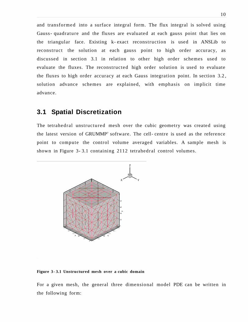
The tetrahedral unstructured mesh over the cubic geometry was created using
the latest version of GRUMMP7 software. The cell- centre is used as the reference
point to compute the control volume averaged variables. A sample mesh is
shown in Figure 3- 3.1 containing 2112 tetrahedral control volumes.
Figure 3 - 3.1 Unstructured mesh over a cubic domain
For a given mesh, the general three dimensional model PDE can be written in
the following form:

11
)z,y,x(Sz
)z,y,x(
y
)z,y,x(
x
)z,y,x(
t
)z,y,x( =∂
∂+∂
∂+∂
∂+∂
∂ HGFU
(3.1)
where U is the solution vector, S is the source term, and F, G, and H are the flux
terms. The finite volume form can be written as:
( ) 0SdAHGFV1
dtd
Ai
=−⋅+++ ∫∂
nkjiUi
(3.2)
where Vi is the cell size for the ith control volume, A is the cell face area, and n
is the outward pointing normal. The flux integral can be approximately by the
Gauss - quadrature:
( )∑∫ ⋅≈⋅∆∂
j jj )x(wAdAi
nUFnF
(3.3)
where w j is the Gauss weight, and U(x j) is the solution evaluated at the j th Gauss
location. Table of Gauss locations and weights for a triangle and for a
tetrahedron are given in Table A- 7.1 and Table A- 7.2 respectively, in Appendix
A. The flux vector is evaluated with a simple upwind scheme:
( ) ( ) nF(U ,F(UnUF ⋅≈⋅ +− ))x())x()x( jjj
(3.4)
where U+ (x j) is the U reconst ructed on the outside of CV, and U- (x j) is U
reconstructed on the inside of CV. The flux direction is chosen according to the
direction of the solution velocity vector. The convective and viscous flux terms
on the right hand side of Eq. (3.4) are evaluated at a given Gauss point by a
higher order method.

12
Higher order methods for the convective terms
A general low order upwind method usually has excessive numerical dissipation
and exhibits strong smearing of solution, leading to poor accuracy and
resolution. Higher order methods in upwind schemes are constructed by
reconstructing approximations to higher - order derivatives of the solution
variables on either side of the control volume face. They can be used to
extrapolate more accurate values to either side of the control volume face. The
resulting interface values are discontinuous, but the jump in discontinuities
decreases with increasing order of accuracy of the scheme. Third order upwind
schemes, such as the QUICK scheme applied in structured discretization,
improves the accuracy of the computa tion by increasing the order of the
leading order truncation error, however the solution displays unphysical
oscillations in regions of steep gradients, causing numerical instability. Thus, all
high- order schemes need to reduce or prevent spurious oscillations. Applying a
limiter based on the solution gradient improves the monotonicity of the upwind
schemes resulting in a much more robust scheme.
The Flux Corrected Transpor t (FCT)8 and Total Variation Diminishing (TVD)
methods are other high order methods that began with structured meshes. In
both schemes, a limited amount of anti - diffusive flux is added to attain
monotonicity. In addition, these schemes employ non- linear limiters on all
regions of the flow field, which may adversely affect the convergence. Van Leer 9
devised the Monotonic Upstream - Centred Scheme for Conservation Laws
(MUSCL) to achieve a higher order accurate solution. MUSCL schemes rely on a
piecewise - polynomial reconstruction procedure using nonlinear limiters to
enforce the monotonicity. A Riemann solver is often employed to calculate the
flux at the interface for given right and left interface states on solution domains
with discontinuities. However, an exact solution to a Riemann problem is too
costly, therefore the approximate Riemann solver from Osher 10 and Roe 11 is
used for this purpose. MUSCL schemes were applied initially to structured
meshes, and then later to unstructured meshes. Another scheme to improve the
flux evaluation is the fluctuation splitting scheme 12 , which provides an

13
alternative to Riemann solvers incorpora ting upwinding, however they have
second order accuracy only at steady state.
All the schemes discussed above, for the most part, do not guarantee in the
absence of oscillations in the multi - dimensional case 13 . However, Barth and
Jespersen 14 created a multidimensional limiter for unstructured meshes that
satisfied the monotonicity principle in multidimensions. In this scheme, the
reconstructed distribution in the control volume is bounded everywhere by the
values of the neighbours. However, their scheme suffered from convergence
difficulties, and a method to solve the problem came at the expense of
monotonicity 15 .
There have been many high- order, non- linear, stable “shock- capturing”
schemes developed for the compressible flows 16 . The philosophy behind these
schemes is to accurately resolve the rapid transition regions or shocks in a
stable and globally correct fashion, yet at the same time have a high resolution
over the smooth part of the flow. Thus, when fully resolving the flow is
impossible or too costly (e.g. combus tion flows) ENO (Essentially Non-
Oscillatory) or WENO (Weighted ENO) schemes on a coarse grid can be used to
obtain at least partial information about the flow.
Weinann and Shu 17 successfully applied high order ENO schemes to two
dimensional incompressible flows in order to resolve shear roll - ups. Both
WENO and ENO schemes use the concept of adaptive stencils in the
reconstruction procedure, based on the local smoothness of the numerical
solution, to automatically achieve high order accuracy and nonoscillatory
properties near discontinuities. ENO uses one out of many candidate stencils
whereas WENO uses the convex combination of all candidate stencils, each
assigned with a nonlinear weight depending on the local smoothness of the
numerical solution based on that stencil.
Another higher order scheme initially applied to capture discontinui ties is Barth
and Fredrickson’s 18 k- exact reconstruction. It involves the reconstruction of
variables satisfying the properties of conservation of the mean, k- exactness
14
(able to reconst ruct exact polynomials of degree ≤ k), and compact support.
Combining the properties of k- exact reconstruction and data dependent ENO
schemes, Ollivier - Gooch 19 , has constructed the DD- L2- ENO scheme. It employs
a least square technique to estimate the higher order derivatives and provide a
better approximation on distorted meshes.
The k- exact reconstruction scheme has the following properties:
• Conservation of the mean value of the function in each CV
• uniformly accurate with no overshoots
• good steady state convergence
• computa tionally efficient
• easily implemented on arbitrary meshes
The higher - order k- exact reconstruction used in the three - dimensional ANSLib
solver will be slightly different from the DD- L2- ENO19 scheme in the sense
that the data dependent weight function is not calculated, and the latter is
especially needed to evaluate discontinous solutions. Details on this
reconstruction scheme and its verification are given in chapter 4 .
Higher order methods for the viscous terms
Viscous terms are diffusive in nature, and are usually centrally differenced.
Higher order methods for diffusive fluxes have not received much attention.
Ollivier - Gooch and Van Altena 20 showed that k- exact type reconstruction could
be used to compute viscous fluxes to higher than second order accuracy. This
scheme uses the same k- exact type reconstruction discussed for advective
fluxes and it has been implemented in ANSLib.
3.2 Solution update techniques
The Eq. (3.2) is discretized to obtain the system of coupled ordinary differential
equations
15
0)(RV1
dtd =+ UUi
(3.5)
where R(U) is the spatial discretized terms, and V is the cell volume. The Eq.
(3.5) can be solved by either explicit or implicit methods. Explicit methods
include the family of linear multi - step methods, such as the Runge- Kutta
schemes. They are stable for a range of Courant numbers where the maximum
time step is proportional to local cell size. Thus, due to the time step
restriction, convergence to a steady state is slow.
An implicit scheme can be obtained by evaluating the spatially discretized term
at the new time level, n+1. After linearizing about the current time level, Eq.
(3.6) is obtained.
)(t
V nURUUR −=∆
∂∂+
∆
(3.6)
where UR
∂∂
is the Jacobian matrix, ∆U is the change in solution vector which the
system must solve for, and ∆t is the time step. The updated solution is
UUU ∆+=+ n1n . If the Jacobian is exactly linearized, a large sparse matrix must
be inverted, which is computa tionally expensive.
Therefore, the Jacobian is often replaced with a first order discretiza tion. The
system of equations can then be solved using iterative methods, but the
convergence is slow. In order to increase the convergence pre - conditioned
GMRES methods are used 21 . The Incomplete Lower Upper (ILU) factoriza tion
could be used as the pre - conditioner to create a more efficient rate of
convergence. However, such a scheme still consumes considerable memory,
especially when many dependent variables are present. A solution is to use the
matrix free method, which evaluates the matrix vector product by finite -
difference techniques:

16
ε−∆ε+=∆⋅
∂∂ )(R)(R UUU
UUR
(3.7)
where ε is chosen as the square root of machine zero. A pre- conditioned,
matrix- free GMRES method is expected to be most efficient. The three -
dimensional ANSLib code uses this matrix free implicit Newton - Krylov solver,
but without pre - conditioning.
Time stepping
The time step given in Eq. (3.6) is calculated by Eq. (3.8).
∫∂
⋅⋅=∆
A
i,imax
ii
dAC
Vt
n
(3.8)
C)(
C 2
j,Ri,L
j,Ri,Li,pseudo ×
−
⋅−=
xx
nxx
(3.9)
where Cmax is the fastest wave entering the control volume and it is determined
from the flux function. For advective fluxes it is the advective velocity, and for
the diffusive fluxes the Cmax term will contain a pseudo wavespeed component,
Cpseudo,i for the control volume, i. An estimate of an equivalent pseudo -
wavespeed is given by Eq. (3.9). In Eq. (3.9), the i and j are control volume
indices on either side of the cell face, and the constant C is related to the
diffusion coefficient. The denominator of Eq. (3.8), which shows an integration
of wavespeeds around control volume, i, is evaluated using gauss - quadrature.
For steady - state solutions, local value of the timestep for each control volume
is used.

17
3.3 Conclusion
The spatial discretization is performed on an unstructured mesh using an
upwind scheme over a cubical domain. The solutions at quadratu re points on
the cell faces are evaluated to high order of accuracy using k- exact
reconstruction. The advective flux at each Gauss point is evaluated using simple
upwind method, where the left or right solution states are reconstructed to high
order accuracy. The diffusive fluxes are evaluated using a central method. The
flux integral and source term will be computed using Gauss - quadratu re. The
reconstruction order of accuracy will match the order of accuracy of the Gauss
integration. For compressible flows ENO and WENO schemes provided the most
robust and non- oscillatory accurate solution. Principles used in these schemes
can be applied for incompressible problems as well. The resulting discretized
equations are solved to the steady state by implicit time advancement using a
matrix- free Newton - Krylov solver.

18
4 Higher Order Reconstruction andVerification
The k- exact reconstruction scheme discussed in section 3.1 has been
implemented in the ANSLib code. However, the implementation in three
dimensions has not been verified. In section 4.1 , the k- exact reconstruction is
briefly described in stages, and techniques to verify each stage are given with
results. For more detailed information on k- exact reconstruction and DD- L2-
ENO, the reader is referred to the publications of Bath and Frederickson 18 and
Ollivier - Gooch 19 respectively.
4.1 k- exact reconstruction
The reconstruction polynomial is a solution expansion, φ iR(x- x i), and is given by
Eq. (4.1).
T.O.H)x)(xz(zxzu
2)z(z
zu
)z)(zy(yzy
u2
)y(yyu
)yy)(x(xyxu
2)x(x
xu
)z(zz
u)y(y
y
u)x(x
x
u)(
ii
i
22i
i
2
2
ii
i
22i
i
2
2
ii
i
22i
i
2
2
i
i
i
i
i
iii
Ri
+−−∂∂
∂+−∂∂+
−−∂∂
∂+−∂∂+
−−∂∂
∂+−∂∂+
−∂∂+−
∂∂+−
∂∂+φ=−φ
xx
(4.1)
where φ i is the value of the reconstruction solution. The reconstruction solution
and its derivatives are evaluated at the reference point (xi,y i,z i). The coefficients
of the expansion are chosen to conserve the mean value in the control volume
and to minimise error in representing smooth solutions, as shown in Eq. (4.2).

19
T.O.HdV)x)(xz(zV1
xzu
dV)z(zV1
zu
dV)z)(zy(yV1
zyu
dV)y(yV21
yu
dV)y)(yx(xV1
yxu
dV)x(xV21
xu
dV)zz(V
1
z
udV)y(y
V
1
y
udV)x(x
V
1
x
u
dV)(V1
i
iiii
2
i
2i
ii
2
2
i
iiii
2
i
2i
ii
2
2
i
iiii
2
i
2i
ii
2
2
i
i
iii
i
iii
i
iii
i
iR
ii
+⋅−−∂∂
∂+⋅−∂∂+
⋅−−∂∂
∂+⋅−∂∂+
⋅−−∂∂
∂+⋅−∂∂+
⋅−∂∂+⋅−
∂∂+⋅−
∂∂+φ
=⋅−φ
∫∫
∫∫
∫∫
∫∫∫
∫
xx
(4.2)
where Vi is the cell volume. The volume averaged monomials, the moments, can
be expressed using Green’s theorem to convert it to a boundary integral, and
they can be integrated exactly using Gaussian quadrature with points and
weights over triangles as shown in Table A- 7.1 . The expansion must be carried
out through the k th derivative, then the reconstruction can be said to be k-
exact. The mean value of solution given by the left hand term of Eq. (4.2) and
the moments are known. The least - squares method attempts to minimise the
error in predicting the mean value of the reconstruction polynomial for control
volumes within a fixed stencil. In this way the derivatives at x i are chosen 19 . All
geometrical terms are pre- processed, and computed only once.
The reconstruction stencil is compact, i.e. only cells that lie within a small
neighbourhood near the cell centre are used. The required number of cells for
the least - square reconstruction for each order in three - dimensions are shown
in Table 4- 4.1 , and they are the upper limit used to solve the least - square
reconstruction matrix. This number exceeds the number of derivatives that
must be solved for in order to obtain the k- exact reconstruction.
Table 4 - 4.1 Number of cells used in the three dimensional least - square reconstructionstencil
Order
Required number of cells instencil
2 43 154 30

20
The least - square problem is solved using Householder transformation in order
reduce the coefficient matrix to upper triangular form. With this method,
solutions that are more accurate can be obtained, especially for ill- conditioned
matrices, because normal equation methods will have conditioning problems.
The back substitution is used to yield the required derivatives. These
derivatives are then used to compute solutions at the Gauss points up to k th
order accuracy.
4.2 Verification test programs
All test programs were conducted on a cubical domain with an unstructured
mesh with 1166 control volumes.
In the reconstruction scheme, integration over surface triangles and tetrahedral
volumes is carried out. Using the IntegTest program the gauss weights and
gauss points were checked with up to 4 th order accuracy, as well as confirming
the integration itself. The results from the IntegTest program confirms that
mesh class is able to supply appropriate Gauss weights and Gauss point
locations to perform the integration. The test functions are monomials,
therefore the numerical integration using Gauss quadrature is exact. The
computed solution is then compared with the exact monomial integrals.
Integration was checked for each order of accuracy (2nd , 3 rd , and 4 th ) at a
tolerance limit of 1.0e - 13 . All monomial integrations were passed.
In the MeshTest program verifies that mesh pre - processing done correctly. The
exact volume integration of monomials is compared with the computed
monomials. The number of monomials required for the 3 rd order accuracy is 10,
and for the 4 th order accuracy is 20. The monomials are computed as a pre -
processing step in the mesh class. The exact volume integral of monomials can
be found from formulas given in section 7 , and for higher order monomials
Maple software is used to compute the exact integral using the formula given in
Eq. (A.7). The Gauss quadrature is used to compute integrals of monomials to
high order accuracy. The tolerance limit between the exact and the computed

21
monomials is 1.0e - 13 . For each order of accuracy the respective number of
monomials passed the test.
In the MomentTest program the moments of control volumes about the cell
centre (the reference location) are checked. The moments are computed for the
entire domain and the results are compared with the generalization of the
parallel axis theorem given in section 7 . The program was run once again for
each order of accuracy. The largest error was smaller than ±1.0e - 14 .
After checking the components of the reconstruction in three - dimensions the
order of accuracy of the whole reconstruction routine was checked up to 4 th
order accuracy by the ReconTest program. A set of test functions corresponding
to monomials of order 3 or lower is integrated to give control volume averages
over an entire mesh. This data is then reconst ructed for each control volume
and checked by evaluating the monomial at a test point near the CV reference
point on each cell. The gradients of monomials are tested in a similar way. The
comparison between the reconstructed value and the exact value gave a
maximum error smaller than 1.0e - 13 .
A sinusoidal test function given by Eq. (4.4a) below was used to test the interior
control volume reconstruction. Such a function cannot be represented exactly
using monomials. The L2 error norm between the reconstructed and exact (Eq.
(4.4a)) is plotted against number of control volumes as shown in Figure 4- 4.1 .
The last three points were used to draw a least - square fit line, and the gradient
of this line for 2 nd , 3 rd , and 4 th order methods gave computed order of accuracy
values of 1.7, 2.9, and 3.8 respectively. The reconstruction scheme performs
well to expected order of accuracy.

22
y = -0.5787x - 0.1561R2 = 1
y = -0.9828x + 0.6387R2 = 0.9942
y = -1.2713x + 0.9083R2 = 0.9865
-5.5
-5
-4.5
-4
-3.5
-3
-2.5
-2
-1.5
-1
2 2.5 3 3.5 4 4.5 5
Log10 number of control volume
Log1
0 of
L2
erro
r no
rm
2nd order
3rd order
4th order
1.7 order of accuracy
3.8 order of accuracy
2.9 order of accuracy
Figure 4 - 4.1 Order of accuracy of the reconstruction of function in Eq. (4.4a) for the interiorcontrol volumes
Boundary Condition treatment
For the boundary cells the solutions must be constrained to enforce the
Dirichlet and Neumann boundary conditions. The boundary constraints are
enforced at the boundary Gauss integration points. On the adjacent control
volume, the constraints are added to the least - squares reconstruction. The test
program ConstraintTest computes the reconstructed values with and without
the boundary constraints for each order of accuracy. The tolerance limit once
again was 1.0e - 13 . In all cases the unconst rained reconstruction was inaccurate,
as expected. Three solutions used to initialize the domain are given by Eq.
(4.4a- c). The use of three solutions also tested the Field Quant class in handling
more than one solution in the three dimensional runs.
)zsin()ysin()xsin()z,y,x(T πππ=
(4.4a)

23
)z2sin()y2sin()x2sin()z,y,x(T πππ=
(4.4b)
)z4sin()y4sin()x4sin()z,y,x(T πππ=
(4.4c)
Figure 4 - 4.2 The boundary face directions and labels for the cubic domain
The error in constrained reconstruction was evaluated. Table 4- 4.2 and Table
4- 4.3 shows the number of errors reported for the two test cases when the
tolerance limit is 1e - 13 . The first test case have all Dirichlet conditions on all six
boundary faces, and the second test case have one Neumann condition on the
‘East’ face and Dirichlet boundary conditions on all other faces (boundary faces
can be identified in Figure 4- 4.2 ).
It can be seen that in Table 4- 4.2 the high- order pre- processing (column one)
results in more boundary Gauss points at which constraints must be satisfied.
This result in having more constraints than degree of freedom, and makes it
impossible to satisfy all the constraints simultaneously. Therefore when all the
six boundary conditions on a cube are Dirichlet then 2 nd and 4 th order accurate

24
reconstruction with the same order accurate moments leads to no errors in
boundary reconstruction. However the third order scheme produces some
errors. When one boundary is Neumann at ‘West’ face and the rest are Dirichlet
in Table 4- 4.3 , then once again the 2 nd and 4 th orders perform equally well for
all three solutions.
Table 4 - 4.2 All Dirichlet constrained boundary condition test
Order of meshMoments
Order ofreconstruction
Dirichletwall
Dirichlet‘East’ face
Dirichlet‘West’ face
2 2 0 0 03 2 39 18 110
3 10 2 0
4 2 82 36 1723 0 0 564 0 0 0
Table 4 - 4.3 Dirichlet - Neumann constrained boundary condition test
Order of meshMoments
Order ofreconstruction
Dirichletwall
Dirichlet‘East’ face
Neumann‘West’ face
2 2 0 0 03 2 39 18 110
3 10 2 0
4 2 82 36 1723 0 0 564 0 0 0
4.3 Conclusion
The k- exact reconstruction implementat ion was discussed together with
various means of testing it. It appears that Gauss - quadratu re can provide a
very accurate monomial integral and flux integral. The least - squares technique
worked well in three dimensions and the boundary constrained reconstruction
achieved acceptable level of accuracy, apart from the 3 rd order accurate scheme.

25
5 Model Verification
The numerical algorithm used to solve the given problem consists of a spatial
discretization and an iterative solver. It is essential that the numerical
algorithm used to solve the flow equations be reliable, accurate and efficient.
The efficiency is measured by the computa tional effort required to solve a
problem to a given numerical convergence level. Therefore, the convergence
rate of the iterative solver measures the computa tional effort. The accuracy of
the numerically converged solution depends on spatial discretization, which
introduces flux evaluation errors and reconstruction errors. In this chapter, the
accuracy of the discretized solution and computa tional efficiency are assessed.
In section 5.1 , the order of accuracy in evaluating the flux integral is calculated.
In section 5.2 , numerically converged steady state solution of the advection -
diffusion and Poisson problems are used to assess both the accuracy of the
method used and the efficiency of the three - dimensional solver. The accuracy
of each order method is computed by calculating the error in computation with
respect to the exact analytical solutions. The rate of convergence of the
Newton - Krylov iterative scheme is graphed to show the computa tional effort
required to achieve the converged solution.
5.1 Flux integral test
A flux test is carried out over a control volume for the model problems to verify
that the flux integration is done accurately. The error in surface flux evaluation
is computed by comparing it with the volume integral of flux divergence (as
shown in Eq. (5.1)) evaluated to 6 th order accuracy.
∫∫∂∂
⋅++=⋅++∇AV
dA)HGF(dV)HGF( nkjikji
(5.1)

26
where the F, G, and H are the flux terms. For an advection - diffusion and a
Poisson problem, the exact analytical solutions are used to compute the flux
divergence. The initial solution is set to the exact solution. The error in the flux
integration test is used to calculate the global error norms, the L1, L2 and Linf
(L∞), as defined in Eq. (A.9) to Eq. (A.11) in Appendix A. Out of all the error
norms L2 norm is chosen to measure the error and used in computing the order
of accuracy of the method. The error is proportional to the size of control
volume to the power k, where k is the order of accuracy. Since the size of
control volume is propor tional to the cube root of the number of cells, the error
can be expressed in terms of the number of cells occupying the domain.
Therefore, the order of accuracy can be determined by evaluating the slope of a
log- log plot of the L2 error norms versus the number of control volumes, which
then is multiplied by three. (The formula is given in Eq. (A.12) in Appendix A).
Advection- diffusion
Consider an advection - diffusion problem over a three - dimensional cube.
Assuming that the velocity field is constant, and the dependen t variable is the
scalar tempera ture T with a diffusion coefficient α. The advection - diffusion
equation is solved over the domain with Dirichlet and Neumann boundary
conditions as shown below.
∂∂+
∂∂+
∂∂α=
∂∂+
∂∂+
∂∂
2
2
2
2
2
2
z
T
y
T
x
T
z
Tw
y
Tv
x
Tu (5.2)
a,x0 << b,y0 << cz0 <<
( )
( )( )( )( )( ) 0
0
0
0
0
nm
====
=
π
π=
cy,x,T
y,0x,T
zb,x,T
zx,0,T
zy,a,T
cz
sinb
ysinzy,0,T
x

27
These equations are solved to obtain the exact solution given by Eq. (A.18), and
the flux divergence is given by Eq. (A.22). The domain size is such that ‘a’, ‘b’,
and ‘c’ are all one, and the ‘m’ and ‘n’ values in the sine function of the first
boundary condition equation are set to one. The diffusion coefficient for the
flux test is set to 0.001. The constant velocity is just constant x- componen t of
the velocity, and it is also of magnitude one.
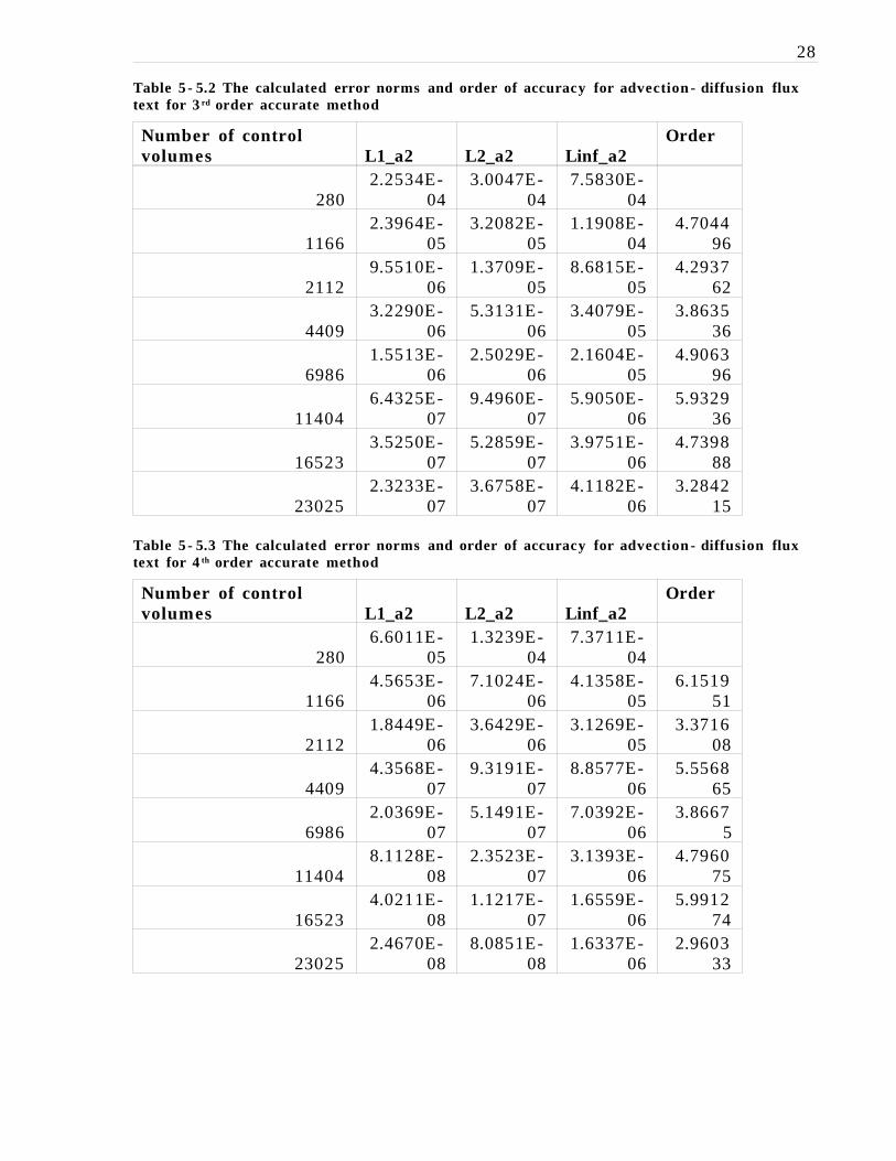
The error norms were calculated for each order of accuracy method and are
shown in Table 5- 5.1 to Table 5- 5.3 . The plot of the L2 error norms are shown
in Figure 5- 5.1 . The last three points for each order of accuracy method are
used to draw a least - square fit linear curve. Its slope will represent the
accuracy of the advection - diffusion flux for each order of accuracy method
used. The linear equation and the R2 value of the fitted line are shown in Figure
5- 5.1 . From the gradients of the curves it is clear that 4 th order has a steeper
gradient than the 3 rd order, which in turn has a steeper gradient than the 2 nd
order method. The second order method behaves like 3.26 order, 3 rd order
method behaves like 4.07 order, and 4 th order method behaves like 4.59 order.
The flux integration seems to be working very well.
Table 5 - 5.1 The calculated error norms and order of accuracy for advection - diffusion fluxtext for 2 nd order accurate method
Number of controlvolumes L1_a2 L2_a2 Linf_a2
Order
2806.4287E-
048.1713E-
042.6734E-
03
11661.0349E-
041.7014E-
041.4166E-
033.2999
24
21124.5679E-
056.5627E-
052.6730E-
044.8108
75
44092.0060E-
053.8282E-
053.0421E-
042.1970
23
69861.1313E-
052.3429E-
052.8402E-
043.2004
84
114045.4223E-
069.1606E-
068.6344E-
055.7486
42
165233.4483E-
065.7102E-
065.0388E-
053.8242
23
230252.4524E-
064.2775E-
063.2843E-
052.6117
47
28
Table 5 - 5.2 The calculated error norms and order of accuracy for advection - diffusion fluxtext for 3 rd order accurate method
Number of controlvolumes L1_a2 L2_a2 Linf_a2
Order
2802.2534E-
043.0047E-
047.5830E-
04
11662.3964E-
053.2082E-
051.1908E-
044.7044
96
21129.5510E-
061.3709E-
058.6815E-
054.2937
62
44093.2290E-
065.3131E-
063.4079E-
053.8635
36
69861.5513E-
062.5029E-
062.1604E-
054.9063
96
114046.4325E-
079.4960E-
075.9050E-
065.9329
36
165233.5250E-
075.2859E-
073.9751E-
064.7398
88
230252.3233E-
073.6758E-
074.1182E-
063.2842
15
Table 5 - 5.3 The calculated error norms and order of accuracy for advection - diffusion fluxtext for 4 th order accurate method
Number of controlvolumes L1_a2 L2_a2 Linf_a2
Order
2806.6011E-
051.3239E-
047.3711E-
04
11664.5653E-
067.1024E-
064.1358E-
056.1519
51
21121.8449E-
063.6429E-
063.1269E-
053.3716
08
44094.3568E-
079.3191E-
078.8577E-
065.5568
65
69862.0369E-
075.1491E-
077.0392E-
063.8667
5
114048.1128E-
082.3523E-
073.1393E-
064.7960
75
165234.0211E-
081.1217E-
071.6559E-
065.9912
74
230252.4670E-
088.0851E-
081.6337E-
062.9603
33

29
y = -1.0876x - 0.6353R2 = 0.9887
y = -1.3553x - 0.5357R2 = 0.9895
y = -1.5292x - 0.4484R2 = 0.9652
-10
-9
-8
-7
-6
-5
-4
-3
-2
1 2 3 4 5 6
Log 10 of number of control volumes
Log
10
of L
2 er
ror n
orm
2nd Order
3rd Order
4th Order
Figure 5 - 5.1 The L2 error norm for the advection - diffusion flux test for various mesh sizes
Poisson
The Poisson problem over a three - dimensional cube is considered. The
dependent variable is the scalar temperature, T. The advection - diffusion
equation is solved over the domain solely with Dirichlet boundary conditions as
shown below. The values of ‘a’, ‘b’, ‘c’, ‘m’, and ‘n’ are all one, as explained in
the previous section.
)z,y,x(fT2 =∇
(5.7)
a,x0 << b,y0 << cz0 <<

30
( )
( )( )( )( )( ) 0
0
0
0
0
nm
=====
π
π=
cy,x,T
y,0x,T
zb,x,T
zx,0,T
zy,a,T
cz
sinb
ysinzy,0,T
where the source term is
π
π
π=
cn
sinb
msin
ar
sin)z,y,x(f (5.8)
The ‘r’ value in the source term is set to one. The final solution is given by Eq.
(A.39), and the flux divergence used in flux test is given by Eq. (A.41).
y = -0.9963x + 0.4254R2 = 0.9989
y = -0.9804x - 0.1733R2 = 1
y = -0.9787x - 0.2355R2 = 0.9984
-6
-5.5
-5
-4.5
-4
-3.5
-3
-2.5
-2
2 3 4 5
Log 10 of number of control volumes
Log
of L
2 er
ror n
orm
2nd Order
3rd Order
4th Order
Figure 5 - 5.2 The L2 error norm for the Poisson flux test for various mesh sizes

31
The error norms were calculated for each order method and they are shown in
Table 5- 5.1 to Table 5- 5.3 . The plot of the L2 error norms is shown in Figure 5-
5.2 . The last three points for each order of accuracy method are used to draw a
least - square fit linear curve. The linear equation and the R2 value of the fitted
line are shown. Unlike the advection - diffusion case, the slopes of the 3 rd and 4 th
order methods are almost the same and the data points are much close
together. It appears that the 4 th order flux integral does not create any
significant reduction in error for the Poisson problem. The 2 nd method behaves
like 2.99 order, the 3 rd order method behaves like 2.94, and the 4 th order
method behaves like 2.94 order.
Table 5 - 5.4 The calculated error norms and order of accuracy for Poisson flux test for the2 nd order accurate method
Number of controlvolumes L1 L2 Linf
Order
2804.55E-
038.01E-
033.88E-
02
11661.35E-
032.24E-
031.23E-
022.6804
87
21126.41E-
041.00E-
035.27E-
034.0685
7
44093.55E-
046.08E-
044.55E-
032.0322
73
69862.17E-
043.93E-
043.54E-
032.8436
2
114041.28E-
042.43E-
042.03E-
032.9356
79
165238.75E-
051.65E-
041.79E-
033.1493
41
230256.59E-
051.21E-
041.45E-
032.8031
33
Table 5 - 5.5 The calculated error norms and order of accuracy for Poisson flux test for the3 rd order accurate method
Number of controlvolumes L1 L2 Linf
Order
2802.96E-
034.55E-
031.50E-
02
11667.17E-
041.02E-
034.06E-
033.1461
63

32
21123.25E-
044.31E-
042.40E-
034.3436
03
44091.64E-
042.30E-
041.58E-
032.5618
8
69861.01E-
041.61E-
041.87E-
032.3157
74
114045.37E-
057.06E-
053.86E-
045.0477
94
165233.72E-
054.91E-
052.04E-
042.9332
07
230252.68E-
053.55E-
053.13E-
042.9505
28
Table 5 - 5.6 The calculated error norms and order of accuracy for Poisson flux test for the4 th order accurate method
Number of controlvolumes L1 L2 Linf
Order
2802.23E-
033.17E-
031.06E-
02
11665.99E-
048.58E-
042.77E-
03 2.7474
21122.72E-
043.51E-
041.00E-
034.5168
81
44091.32E-
041.75E-
046.07E-
042.8439
67
69868.15E-
051.08E-
045.51E-
043.1457
7
114044.68E-
056.18E-
052.67E-
043.4100
46
165233.30E-
054.40E-
051.63E-
042.7496
31
230252.35E-
053.10E-
051.24E-
043.1521
9
5.2 Steady state solution
The advection - diffusion and Poisson problems are again selected for the steady
state verification. In all the computa tional runs, the residual error norms were
less than 1.0e - 13 . The residual here defines the difference in flux integral from
one iteration to the next. The initial solution value chosen was equal to (1- x).
The error is evaluated using the difference between the exact solution and the
converged numerical solution. The diffusion coefficient for the advection -
diffusion problem was 0.001 and the velocity field is only in the x- direction

33
with a magnitude of one. In all cases, where appropriate, local time stepping
was chosen without any under - relaxation.
Advection- diffusion results
The cross - sectional solution for the advection - diffusion problem at various
positions along the x- direction of the geometry is shown in Figure 5- 5.4 . The
solution is very smooth and decreases in magnitude along the x- direction.
y = -0.726x + 0.5817R2 = 0.9867
y = -1.019x + 0.7554R2 = 0.9968
y = -1.073x + 0.2404R2 = 0.9996
-6
-5
-4
-3
-2
-1
0
0 1 2 3 4 5 6
Log 10 of number of control volumes
Lo
g 10
of
L2
err
or
norm
2nd Order
3rd Order
4th Order
Figure 5 - 5.3 The L2 error norm for the advection - diffusion problem at steady state forvarious mesh sizes

34
(a)
(b)
(c)
(d)
Figure 5 - 5.4 The sub figures (a)- (d) shows the solutions to the advection- diffusion problemalong the geometry at x=0, 0.3, 0.6 and 1.
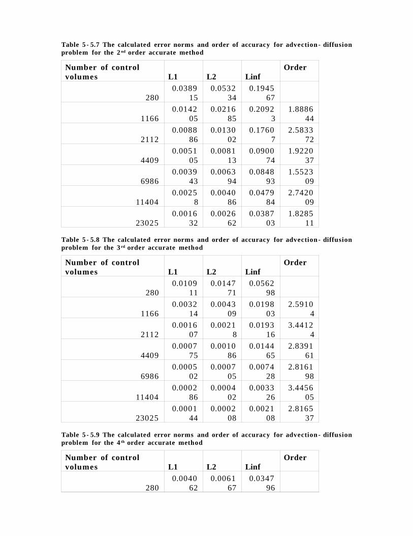
Table 5 - 5.7 The calculated error norms and order of accuracy for advection - diffusionproblem for the 2 nd order accurate method
Number of controlvolumes L1 L2 Linf
Order
2800.0389
150.0532
340.1945
67
11660.0142
050.0216
850.2092
31.8886
44
21120.0088
860.0130
020.1760
72.5833
72
44090.0051
050.0081
130.0900
741.9220
37
69860.0039
430.0063
940.0848
931.5523
09
114040.0025
80.0040
860.0479
842.7420
09
230250.0016
320.0026
620.0387
031.8285
11
Table 5 - 5.8 The calculated error norms and order of accuracy for advection - diffusionproblem for the 3 rd order accurate method
Number of controlvolumes L1 L2 Linf
Order
2800.0109
110.0147
710.0562
98
11660.0032
140.0043
090.0198
032.5910
4
21120.0016
070.0021
80.0193
163.4412
4
44090.0007
750.0010
860.0144
652.8391
61
69860.0005
020.0007
050.0074
282.8161
98
114040.0002
860.0004
020.0033
263.4456
05
230250.0001
440.0002
080.0021
082.8165
37
Table 5 - 5.9 The calculated error norms and order of accuracy for advection - diffusionproblem for the 4 th order accurate method
Number of controlvolumes L1 L2 Linf
Order
2800.0040
620.0061
670.0347
96

11660.0006
740.0009
150.0060
934.0130
34
21120.0003
520.0005
090.0042
522.9626
3
44090.0001
360.0002
030.0016
813.7535
62
69868.26E-
050.0001
320.0018
842.8121
06
114044.32E-
057.60E-
050.0019
293.3619
07
230251.85E-
053.65E-
050.0008
353.1306
34
Table 5- 5.7 to Table 5- 5.9 show the computed orders of accuracy of the 2 nd , 3 rd
and 4 th order methods, and Figure 5- 5.3 summarizes the L2 error norm. From
these results it is clear that 2 nd and 3 rd order methods behave better than
expected, while the 4 th order method behaves only slightly better than a 3 rd
order scheme.
The solution error after numerical convergence is graphically presented in
Figure 5- 5.5 to Figure 5- 5.7 for 2 nd to 4 th order accurate solution. This is the
local error between the computed and the exact. The green triangles or ‘dirty’
yellow coloured triangles represent very small errors and only triangles
coloured red and blue show the largest local error in the domain. For the 2 nd
order method, high magnitude errors occur frequently at the block corners. The
3 rd order accurate solution produces the significant magnitude of error, as can
be seen in Figure 5- 5.6 , on the outlet face. Similarly 4 th order accurate solution
produces the largest error on this outlet face, and compared with the 3 rd order
method the 4 th order method has errors of high magnitude on this outlet face.
On the outlet face, Neumann boundary conditions are enforced. It appears the
reason 4 th order method does not produce 4 th order accurate solution is because
the error introduced at the outlet boundary does not decrease sufficiently.
Hence, there may be a boundary condition evaluation or a boundary condition
enforcement problem that requires further investigation.

Figure 5 - 5.5 Error between the exact and 2 nd order accurate solution after numericalconvergence of the advection- diffusion problem
Figure 5 - 5.6 Error between the exact and 3 rd order accurate solution after numericalconvergence of the advection- diffusion problem

Figure 5 - 5.7 Error between the exact and 4 th order accurate solution after numericalconvergence of the advection- diffusion problem

The computational efficiency of the methods implemented by the ANSLib code
is assessed by plotting the L2 error norm versus the computa tional time taken
to achieve the numerical converged solution, as shown in Figure 5- 5.8 . The data
points represent various meshes (defined in Table 5- 5.7 ) of increasing number
of control volumes as the computa tional time increases. For a given level of
accuracy corresponding to an L2- norm value, it is clear that a 4 th order method
achieves a numerically converged solution on a much coarser mesh than either
3 rd or 2 nd order methods. A 4 th order method progressively consumes larger
amounts of time on finer meshes. However, for a given level of accuracy the 4 th
order method takes less time than either of the lower order methods. For the
advection - diffusion problem there exists an exponential reduction in accuracy
for increasing computa tional time. This implies that the lower order solution
methods would need very fine meshes and would require long computa tional
times in order to reach a given level of high order accuracy. However, the low
order methods may reach asymptotic convergence faster than the high order
methods.
y = -0.6111x - 0.1929R2 = 0.993
y = -0.791x - 0.2385R2 = 0.9892
y = -0.8982x - 0.2468R2 = 0.9995
-5
-4.5
-4
-3.5
-3
-2.5
-2
-1.5
-1
1 1.5 2 2.5 3 3.5 4 4.5 5
Log10 of computational time (sec.)
Log
10 o
f L2
err
or n
orm
2nd Order
3rd Order
4th Order

Figure 5 - 5.8 The computational time taken for the steady - state solution of the advection -diffusion problem for various meshes
The rate of convergence for each order method for various mesh sizes is shown
in Figure 5- 5.9 to Figure 5- 5.11 . For all methods up to 23025 control volumes,
the number of iterations needed for convergence is less than 15. From Figure 5-
5.11 and Figure 5- 5.8 it is apparent that the reason 4 th order method takes
longer is that the cost per iteration is high. In the 4 th order method the number
of monomials that should be evaluated is almost twice as many as are needed
for the 3 rd order method leading to a larger least - squares matrix. In addition,
there are 16 Gauss points per control volume on which the fluxes must be
calculated, which add to the computational time. The 3 rd and 4 th order methods
converge with a slightly smaller number of iterations compared to the 2 nd order
method. For the finest mesh all schemes show deviation from the usual quicker
rate of convergence. The solution update become smaller after the residual
decrease beyond 1.0e - 6. It seems some error term gets build- up up to this point
and starts to affect the solution update. The matrix vector product of the
Jacobian and the solution update vectors in GMRES algorithm may be badly
conditioned.

Figure 5 - 5.9 The L2 residual norm for the advection - diffusion problem for the 2 nd orderaccurate method
Figure 5 - 5.10 The L2 residual norm for the advection - diffusion problem for the 3 rd orderaccurate method

Figure 5 - 5.11 The L2 residual norm for the advection - diffusion problem for the 4 th orderaccurate method
Poisson results
The solution at three different cross - sections along the geometry in x- axis is
shown in Figure 5- 5.13 . The solution at the ‘East’ face, where x=0 (refer to
Figure 4- 4.2 ), quickly reduces in magnitude leaving the ‘West’ face, where
x=1.0, with only a small magnitude of solution.

y = -0.6776x + 0.2896R2 = 0.98
y = -1.0684x + 0.9632R2 = 0.985
y = -1.1802x + 0.5609R2 = 0.9684
-6
-5.5
-5
-4.5
-4
-3.5
-3
-2.5
-2
-1.5
-1
1 1.5 2 2.5 3 3.5 4 4.5 5 5.5 6
Log of number of Control volumes
Lo
g 10
of
L2
err
or
norm
2nd Order
3rd Order
4th Order
Figure 5 - 5.12 The L2 error norm for the Poisson problem at steady state for various meshsizes
The order of accuracy of the 2 nd , 3 rd and 4 th order methods are shown in Table
5- 5.10 to Table 5- 5.12 , and Figure 5- 5.12 summarizes the order of accuracy of
these methods. It is clear that the gradient used to compute the order of
accuracy fluctuates a little, but it is reduced in magnitude as the mesh becomes
finer. Considering the last three points least - square trend lines were drawn to
show the order of accuracy of methods. Once again, the last three points are
assumed to be in the asymptotic convergence region, where an expected order
of accuracy is reached. It can be seen that the 2 nd order method behaves like
2.03 order accuracy, the 3 rd order method behaves like 3.21 order accuracy, and
the 4 th order scheme behaves like 3.54 order accuracy.


(a)
(b)
(c)
Figure 5 - 5.13 The sub figures (a)- (c) shows the solutions to the Poisson problem along thegeometry at x=0, 0.3, and 0.6.

Table 5 - 5.10 The calculated error norms and order of accuracy for Poisson problem for the2 nd order accurate method
Number of controlvolumes L1 L2 Linf
Order
2800.0142
090.0268
960.2170
03
11660.0061
770.0135
380.1539
361.4436
19
21120.0039
350.0082
630.0986
012.4935
32
44090.0027
830.0062
650.1068
141.1283
84
69860.0023
040.0050
340.0585
561.4259
5
114040.0015
140.0032
490.0485
182.6808
52
230250.0010
140.0022
170.0387
291.6313
6
Table 5 - 5.11 The calculated error norms and order of accuracy for Poisson problem for the3 rd order accurate method
Number of controlvolumes L1 L2 Linf
Order
2800.0054
360.0099
230.0634
99
11660.0015
80.0030
330.0371
752.4929
26
21120.0008
230.0015
130.0229
053.5117
48
44090.0005
330.0010
430.0161
91.5147
97
69860.0003
640.0007
570.0183
072.0904
03
114040.0002
150.0003
880.0097
024.0899
46
230250.0001
160.0002
080.0053
642.6575
24
Table 5 - 5.12 The calculated error norms and order of accuracy for Poisson problem for the4 th order accurate method
Number of controlvolumes L1 L2 Linf
Order
2800.0021
080.0038
560.0307
35
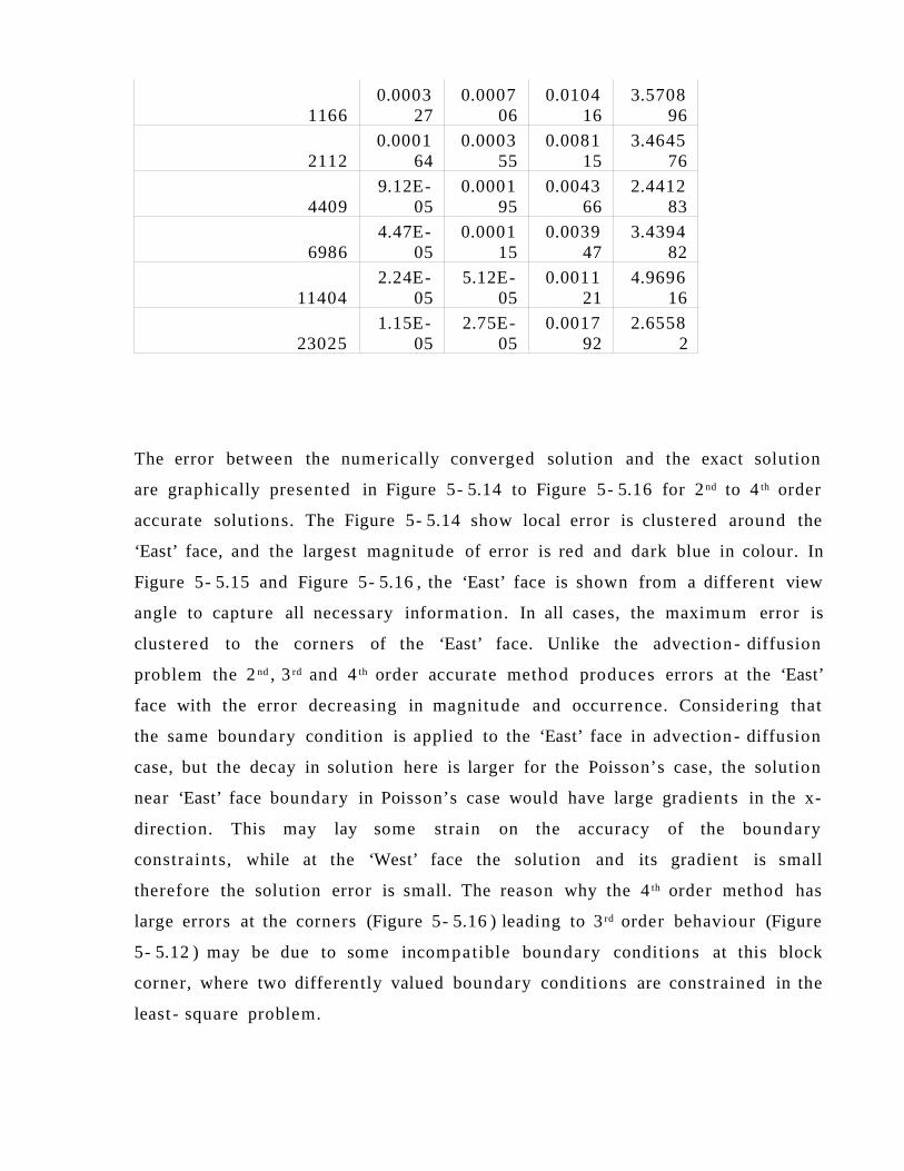
11660.0003
270.0007
060.0104
163.5708
96
21120.0001
640.0003
550.0081
153.4645
76
44099.12E-
050.0001
950.0043
662.4412
83
69864.47E-
050.0001
150.0039
473.4394
82
114042.24E-
055.12E-
050.0011
214.9696
16
230251.15E-
052.75E-
050.0017
922.6558
2
The error between the numerically converged solution and the exact solution
are graphically presented in Figure 5- 5.14 to Figure 5- 5.16 for 2 nd to 4 th order
accurate solutions. The Figure 5- 5.14 show local error is clustered around the
‘East’ face, and the largest magnitude of error is red and dark blue in colour. In
Figure 5- 5.15 and Figure 5- 5.16 , the ‘East’ face is shown from a different view
angle to capture all necessary information. In all cases, the maximum error is
clustered to the corners of the ‘East’ face. Unlike the advection - diffusion
problem the 2 nd , 3 rd and 4 th order accurate method produces errors at the ‘East’
face with the error decreasing in magnitude and occurrence. Considering that
the same boundary condition is applied to the ‘East’ face in advection - diffusion
case, but the decay in solution here is larger for the Poisson’s case, the solution
near ‘East’ face boundary in Poisson’s case would have large gradients in the x-
direction. This may lay some strain on the accuracy of the boundary
constraints, while at the ‘West’ face the solution and its gradient is small
therefore the solution error is small. The reason why the 4 th order method has
large errors at the corners (Figure 5- 5.16 ) leading to 3 rd order behaviour (Figure
5- 5.12 ) may be due to some incompatible boundary conditions at this block
corner, where two differently valued boundary conditions are constrained in the
least - square problem.

Figure 5 - 5.14 Error between the exact and 2 nd order accurate solution after numericalconvergence for the Poisson problem
Figure 5 - 5.15 Error between the exact and 3 rd order accurate solution after numericalconvergence for the Poisson problem
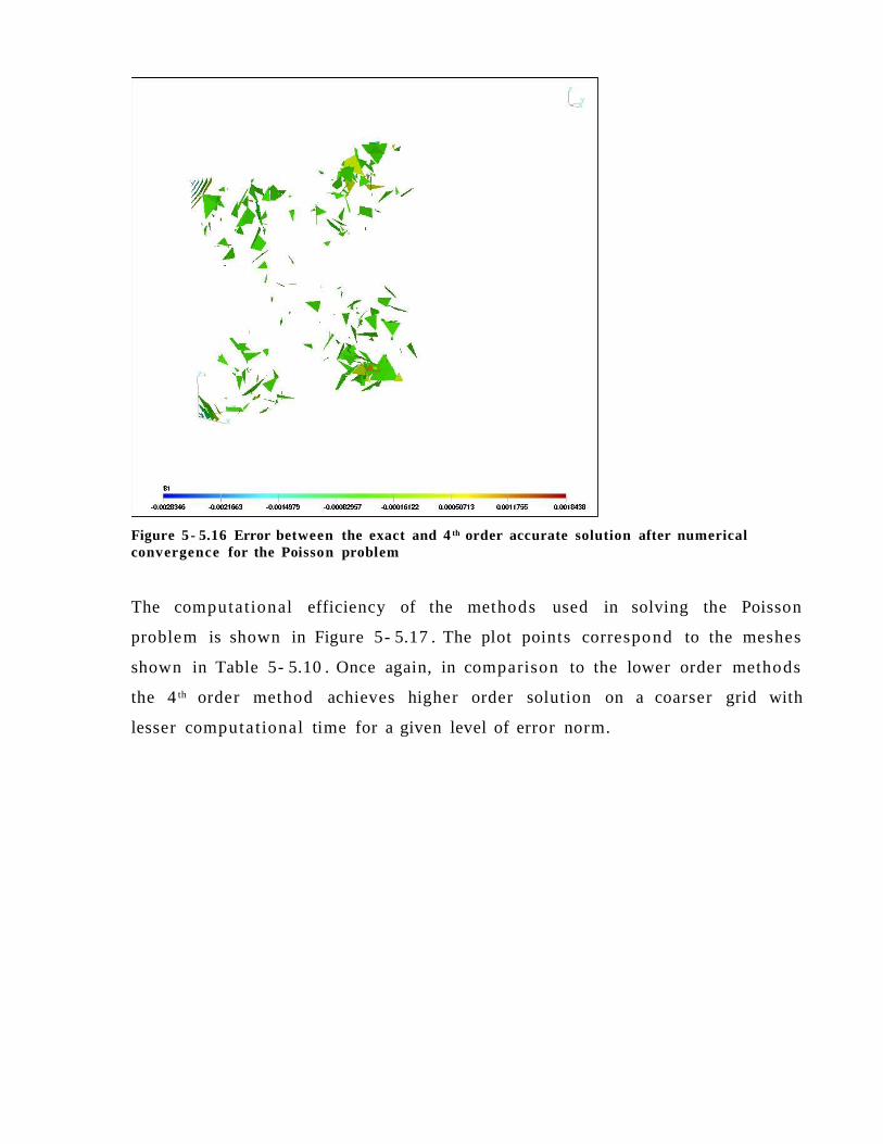
Figure 5 - 5.16 Error between the exact and 4 th order accurate solution after numericalconvergence for the Poisson problem
The computational efficiency of the methods used in solving the Poisson
problem is shown in Figure 5- 5.17 . The plot points correspond to the meshes
shown in Table 5- 5.10 . Once again, in comparison to the lower order methods
the 4 th order method achieves higher order solution on a coarser grid with
lesser computa tional time for a given level of error norm.
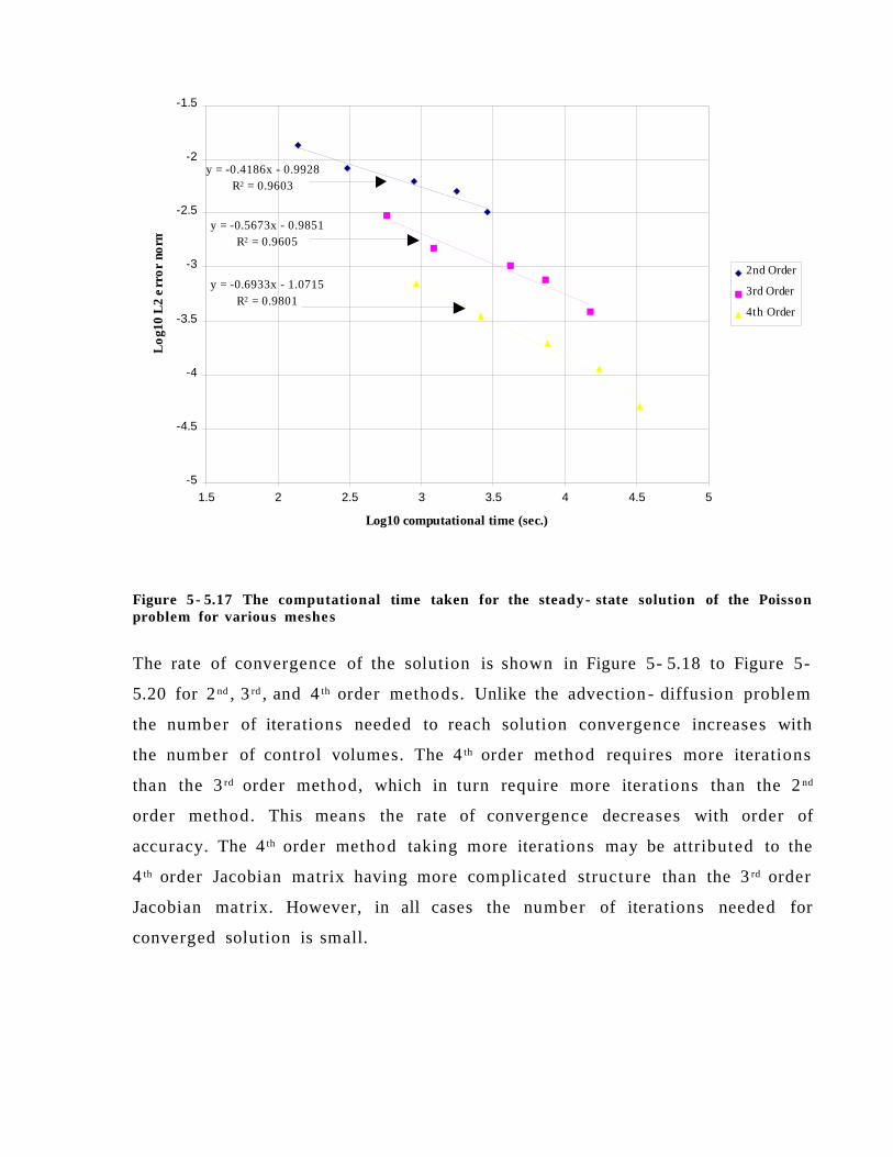
y = -0.5673x - 0.9851R2 = 0.9605
y = -0.4186x - 0.9928R2 = 0.9603
y = -0.6933x - 1.0715R2 = 0.9801
-5
-4.5
-4
-3.5
-3
-2.5
-2
-1.5
1.5 2 2.5 3 3.5 4 4.5 5
Log10 computational time (sec.)
Lo
g10
L2
err
or
norm
2nd Order
3rd Order
4th Order
Figure 5 - 5.17 The computational time taken for the steady- state solution of the Poissonproblem for various meshes
The rate of convergence of the solution is shown in Figure 5- 5.18 to Figure 5-
5.20 for 2 nd , 3 rd , and 4 th order methods. Unlike the advection - diffusion problem
the number of iterations needed to reach solution convergence increases with
the number of control volumes. The 4 th order method requires more iterations
than the 3 rd order method, which in turn require more iterations than the 2 nd
order method. This means the rate of convergence decreases with order of
accuracy. The 4 th order method taking more iterations may be attributed to the
4 th order Jacobian matrix having more complicated structure than the 3 rd order
Jacobian matrix. However, in all cases the number of iterations needed for
converged solution is small.
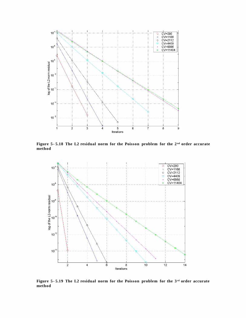
Figure 5 - 5.18 The L2 residual norm for the Poisson problem for the 2 nd order accuratemethod
Figure 5 - 5.19 The L2 residual norm for the Poisson problem for the 3 rd order accuratemethod

Figure 5 - 5.20 The L2 residual norm for the Poisson problem for the 4 th order accuratemethod
5.3 Conclusion
The flux test results showed that the surface flux evaluations performed using
the Flux class and the Integrate program were good enough to carry out steady
state analysis. For a given error norm value the 4 th order method achieves
convergence on a coarse mesh, while finer meshes would be required for the 3 rd
and 2 nd order methods. Also the time taken to achieve a given level of accuracy
for the 4 th order method is considerably smaller than for the 2 nd order method,
while the 3 rd order method lies somewhere in between. In the advection -
diffusion problem for 3 rd and 4 th order methods showed the largest local error
localized at the ‘West’ face or the outlet, while for the Poisson problem it was at
the ‘East’ face or the inlet. In both cases for 2 nd order method, the errors cluster
at the four corners. The number of overall iterations needed for numerical
convergence is small for both the advection - diffusion problem and the Poisson
problem. The 4 th order method consumes the largest amount of time per
iteration due to a large number of Taylor expansion terms in the least - squares

matrix, and having a large number of Gauss points on which the fluxes are
evaluated.
6 Conclusions and Future Work
The program classes in ANSLib code use abstract data types, which play a
central role in object - oriented programming in allowing what is being done to
be separate from how it is done. ANSLib generic solver separates the
implementa tion of physics from numerics, so that the end user will not need to
modify the code when new physics are introduced. The flow chart in Figure 2- 1
showed that flux integration and time advance are separate entities, and the
dimensional changes to the program became independen t as well. This allowed
code development and verification to be carried out in three dimensions easily
and quickly.
Various test cases were run in order to verify the solution reconstruction, flux
integration and iterative time advancement to steady state in three dimensions.
The flux integration testing was a crude approximation to testing the exact flux
integral, but it served as a good means of determining inconsistencies in flux
integration using Gauss quadratu re. It was apparent that Gauss quadrature is a
very accurate means of integrating monomial functions, and to resolve 2 nd and
4 th order Dirichlet and Neumann boundary conditions. The order of accuracy of
the 4 th order did came very close to being 4 th order accurate in steady state
analysis. Also it is clear that the 4 th order accurate method is the best method to
use to obtain a numerically converged solution for a given level of error norm,
since the mesh sizes required and computa tional time used in achieving the
results are superior to 2 nd or 3 rd order methods.
The final results from flux integration and steady state runs allowed the three
dimensional code to be fully verified in solving linear problems. The code
verification must be done to solve a Navier - Stokes problem, then it may be
proved that problems with sufficient complexity can be solved. For example,
the exact analytical unsteady three dimensional Navier - Stokes solutions given
by Ethier and Steinman 22 would be a good benchmark problem to solve. In order
to tackle non- linear problems it is the solver classes and the definition of
fluxes in the physics description program that are expected to be modified. The

Newton - Krylov solver may needs to be upgraded with preconditioning, since
preliminary runs on a three - dimensional Navier - Stokes problem showed poor
numerical convergence. Improvements in the area of accuracy may be made
with the three dimensional data - dependent reconstruction, where the data -
dependent weight no longer serve as a means of determining discontinuities in
the solution domain, but instead resolving sharp gradients in incompressible
flows. Accuracy may also be improved by creating a layer of small size control
volumes at all boundaries.

7 Bibliography[1] Harten, A., “Uniformly High Order Accurate Essentially Non- oscillatorySchemes, III”, Journal of Computa tional Physics, 131:3- 47 (1997)
[2] Saad, Y., Schultz, M., “GMRES: A generalized minimum residual algorithmfor solving nonsymmetric linear systems”, SIAM Journal on Scientific andStatistical Computing, 7(3): 856- 869 (1986).
[3] Zimmermann, T., Dubois - Pelerin, Y., Bomme, P., “Object - oriented finiteelement programming: I. Governing Principles”, Computer Methods in appliedMechanics and Engineering, 98:291 - 303 (1992).
[4] Liu, J- L., Lin, I- J., Shih, M- Z., Chen, R- R., Hsieh, M- C., “Object - orientedprogramming of adaptive finite element and finite volume methods”, AppliedNumerical Mathematics, 21:439- 467 (1996).
[5] Ollivier - Gooch, C., “A toolkit for numerical simulation of PDEs: I.Fundamentals of generic finite - volume simulation”, Computer Methods inApplied Mechanics and Engineering, 192:1147 - 1175 (2003).
[6] Boivin, C., “Infrastructure for Solving Generic Multiphysics problems”, PhDthesis, Department of Mechanical Engineering, University of British Columbia,Vancouver, Canada.
[7] GRUMMP: Two dimensional and three dimensional unstructured gridgenerator. Available from website<ht tp: / / t e t r a.mech.ubc.ca /GRUMMP/index.html >
[8] Boris, J.P., and Book, D.L., “Flux corrected transpor t: I, SHASTA, a fluidtransport algorithm that works”, Journal of Computa tional Physics, 11:38- 69(1973)
[9] Van Leer, B., “Towards the ultimate conservative difference scheme V. Asecond order sequel to Godunov’s method”, Journal of Computa tioinal Physics,32:101- 136 (1979)
[10] Osher, S., “Riemann solvers, the entropy condition and differenceapproximations”, SIAM Journal of Numerical Analysis, 21(2):217- 235 (1984)
[11] Roe, P.L., “”Approximate Reimann solvers, parameter vectors anddifference schemes”, Journal of Computational Physics, 43(2):357- 372 (1981)
[12] Deconinck, H., Paillere, H., Struijs, R., Roe, P.L., “Multidimensional upwindschemes based on fluctuation - splitting of conservation laws”, Computa tionalMechanics, 11:323- 340 (1993)
[13] Venkatakrishnan, V., “A Perspective on Unstructured Grid Flow Solvers”,AIAA Journal, 34(3):533 (1996)

[14] Barth, T.J., Jespersen, D.C., “The design and application of upwind schemeson unstructured meshes”, AIAA Paper 89- 0366 (1989)
[15] Venkatakrishnan, V., “On the accuracy of limiters and convergence tosteady state solutions”, AIAA Paper 93- 0880 (1993)
[16] Harten, A., “High resolution schemes for hyperbolic conservation laws”,Journal of Computational Physics, 49:357 (1983)
[17] Weinan, E., Shu, C- W., “A Numerical Resolution Study of High OrderEssentially Non- oscillatory Schemes Applied to Incompressible Flow”, Journalof Computa tional Physics, 110:39- 46 (1994)
[18] Barth, T.J., Fredrickson, P.O., “Higher order solution of the Euler equationson unstructured grids using quadratic reconstruction”, AIAA Paper 90- 0013(1990)
[19] Ollivier- Gooch, C.F., “Quasi - ENO schemes for unstructured meshes basedon unlimited data - dependent least - squares reconstruction”, Journal ofComputa tional Physics, 133:6- 17 (1997)
[20] Ollivier- Gooch, C., Altena, M. V., “A High- Order - Accurate UnstructuredMesh Finite - Volume Scheme for the Advection - Diffusion Equation”, Journal ofComputa tional Physics, 181: 729- 752 (2002)
[21] Venkatakrishnan, V., Mavriplis, D.J., “Implicit solvers for unstructuredmeshes”, Journal of computa tional physics, 105(1):83- 91 (1993)
[22] Ethier, C. R., Steinman, D. A., “Exact fully 3D Navier- Stokes solutions forbenchmarking”, International Journal for Numerical Methods in Fluids, 19(5):369- 375 (1994)
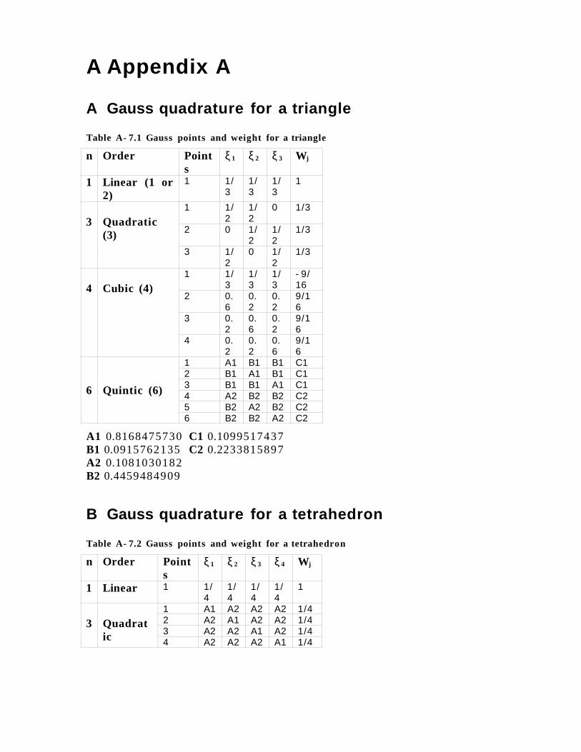
A Appendix A
A Gauss quadrature for a triangle
Table A- 7.1 Gauss points and weight for a triangle
n Order Points
ξ 1 ξ 2 ξ 3 Wj
1 Linear (1 or2)
1 1/3
1/3
1/3
1
3 Quadratic(3)
1 1/2
1/2
0 1/3
2 0 1/2
1/2
1/3
3 1/2
0 1/2
1/3
4 Cubic (4)1 1/
31/3
1/3
- 9/16
2 0.6
0.2
0.2
9/16
3 0.2
0.6
0.2
9/16
4 0.2
0.2
0.6
9/16
6 Quintic (6)
1 A1 B1 B1 C12 B1 A1 B1 C13 B1 B1 A1 C14 A2 B2 B2 C25 B2 A2 B2 C26 B2 B2 A2 C2
A1 0.8168475730 C1 0.1099517437B1 0.0915762135 C2 0.2233815897A2 0.1081030182B2 0.4459484909
B Gauss quadrature for a tetrahedron
Table A- 7.2 Gauss points and weight for a tetrahedron
n Order Points
ξ 1 ξ 2 ξ 3 ξ 4 Wj
1 Linear 1 1/4
1/4
1/4
1/4
1
3 Quadratic
1 A1 A2 A2 A2 1/42 A2 A1 A2 A2 1/43 A2 A2 A1 A2 1/44 A2 A2 A2 A1 1/4

4 Cubic1 1/
41/4
1/4
1/4
- 4/5
2 1/3
1/6
1/6
1/6
9/20
3 1/6
1/3
1/6
1/6
9/20
4 1/6
1/6
1/3
1/6
9/20
5 1/6
1/6
1/6
1/3
9/20
20
5351A
+=
20
552A
−=
C Parallel axis theorem
The total moment of x is the sum of moment about the centroid plus the
contribution from points around the centroid for each control volume, n. Some
formulae for x and xy moments are shown here.
[ ]∑ ∫=
+=N
1ncn
T
dV.xxVV1
x
(A.1)
[ ]∑ ∫∫∫=
+++=N
1nccccn
T
yxdV.xydV.yxdV.xyVV1
xy
(A.2)
D Exact integration formula over tetrahedron

Figure A- 7.1 Tetrahedron control volume
The centroid of a tetrahedron is located at point (0,0,0), hence the global
coordinates sum equal to zero.
04z3z2z1z
04y3y2y1y
04x3x2x1x
=+++=+++=+++
(A.3)
Then the integration formulas for x, x2, and xy are as follows
∫ =V
0dV.x
(A.4)
∫ +++=V
22222
20
V)4x3x2x1x(dV.x
(A.5)
∫ +++=V
2
20
V)4y4x3y3x2y2x1y1x(dV.x
(A.6)
where V is the volume. In general the integral of polynomial in terms of the
volume coordinates ξ 1, ξ 2, ξ 3, and ξ 4 is

∫ ++++=ξξξξ
V
d4
c3
b2
a1 )V6(
)!3dcba(
!d!c!b!adV.
(A.7)
E Calculating order of accuracy from error norms
The error is defined as the difference between the exact and computed solution.
)z,y,x(u)z,y,x(uE iiicompiiiexacti −=(A.8)
The error norms are defined as
i
ii
N
E1L
∑=
(A.9)
i
i
2i
N
E2L
∑=
(A.10)
ii
EmaxLinfL =∞=
(A.11)
If the L2- norm is given for two meshes as shown in Table A- 7.3 .
Table A- 7.3 Sample table of L2 error norms for each mesh
Mesh ControlVolumes
L2-norm
M1 L21
M2 L22
Then the order of accuracy is calculated by the following equation.
Order of accuracy, =
2
1
1
2
MM
log
2L2L
log
3
(A.12)

F Analytical solution methods
G Advection- diffusion
∂∂+
∂∂+
∂∂α=
∂∂+
∂∂+
∂∂
2
2
2
2
2
2
z
T
y
T
x
T
z
Tw
y
Tv
x
Tu
(A.13)
a,x0 << b,y0 << cz0 <<
( )
( )( )( )( )( ) 0
0
0
0
0
nm
====
=
π
π=
cy,x,T
y,0x,T
zb,x,T
zx,0,T
zy,a,T
cz
sinb
ysinzy,0,T
x
(A.14)
By the method of separation of variables assume the solution to be in the form
S(z)Q(x).R(y).z)y,T(x, =
(A.15)
Substituting Eq. (A.15) to Eq. (A.13), and then dividing by Eq. (A.15) leads to an
equation, which can be separated in to left and right side of the equality sign
based on the property that one side must be independent of a variable, while
the other side is dependent on this variable. Since one side depend on the
variable which could be x, y, or z, and the other side does not each side must be
equate to a constant. Using these constants (λ, µ) and assuming that velocity
components are constants and u=U, and v=w=0, the following three equations
are formed.
0QQU
Q =µ+′α
−′′
(A.16)

( ) 0RR =µ−λ+′′
(A.17)
0SS =λ−′′
(A.18)
These equations are solved to obtain the exact solution
( )[ ]
π
π+−= γγγ
czn
sinb
ymsineeeCz)y,T(x, xxx
1221
(A.19)
where
22
2
ee
eC
21
21 γγ
γ
γ−γγ−=
(A.20)
222
2,1c
n
b
m
2
U
2
U
π+
π+
α±
α=γ
(A.21)
The divergence of fluxes for advection - diffusion problem is given as
( ) ( )( )( )( )
( )( )AaaaC2
AaaaC
AaUaaUCTTu
22112
2222
221
211
2222111
+−α π+
γ+γ−γα
γ+γ−γ=∇α−∇
-
(A.22)
where α is the diffusion coefficient, and
)zsin()ysin(A ππ=(A.23)
x1
1ea γ=(A.24)

x2
2ea γ=(A.25)
21
2
eee
C21
21 γγ
γ
γ−γγ−=
(A.26)
22
2,1 22
U
2
U π+
α±
α=γ
(A.27)
H Poisson
The Poisson problem over a three dimensional rectangular domain is described
as follows.
)z,y,x(fT2 =∇
(A.28)
a,x0 << b,y0 << cz0 <<
( )
( )( )( )( )( ) 0
0
0
0
0
nm
=====
π
π=
cy,x,T
y,0x,T
zb,x,T
zx,0,T
zy,a,T
cz
sinb
ysinzy,0,T
(A.29)
where the source term
π
π
π=
cn
sinb
msin
ar
sin)z,y,x(f
(A.30)
Assume the solution can be written in the form

)z,y,x(V)z,y,x(Uz)y,T(x, +=
(A.31)
where U(x,y,z) is a particular solution to the Poisson equation and V(x,y,z) is the
solution of the associated homogeneous equation, i.e.
)z,y,x(fU2 =∇
(A.32)
0V2 =∇
(A.33)
Let
π
π
π=
cn
sinb
msin
ar
sinA)z,y,x(U , then substituting to Eq. (4.12) gives
constant A as
222
c
n
b
m
a
r
1A
π+
π+
π
−=
(A.34)
Since U(x,y,z) is obtained the solution of the Dirichlet problem must be solved
Boundary on
Domain on
)z,y,x(TUV
0V2
+−==∇
(A.35)
( )
( )( )( )( )( ) 0cb,x,V
0y,0x,V
0zb,x,V
0zx,0,V
0zy,a,V
czn
sinb
ymsinzy,0,V
=====
π
π=
(A.36)
By the method of separation of variables assume the solution to be in the form

S(z)Q(x).R(y).z)y,V(x, =
(A.37)
The method of separation of variable, as was done in previous section, leads to
the equation,
π
π
γ+
γ
γγ−=
cz
sin.b
ymsin
ax
coshax
sinh)sinh()cosh(
)z,y,x(V
(A.38)
This gives the final solution
π
π
γ+
γ
γγ−
π=
czr
sin.b
ymsin
ax
coshax
sinh)sinh()cosh(
ax
sinA)z,y,x(T
(A.39)
where
22
c
n
b
m
π+
π=γ
(A.40)
The divergence of Poisson problem is simply made to zero by reversing the sign
of the source term.
( )( ) 0fT =−∇∇
(A.41)

Bibliography

1 Harten, A., “Uniformly High Order Accurate Essentially Non- oscillatorySchemes, III”, Journal of Computa tional Physics, 131:3 - 47 (1997)
2 Saad, Y., Schultz, M., “GMRES: A generalized minimum residualalgorithm for solving nonsymmetric linear systems”, SIAM Journal onScientific and Statistical Computing, 7(3): 856- 869 (1986).
3 Zimmermann, T., Dubois - Pelerin, Y., Bomme, P., “Object - oriented finiteelement programming: I. Governing Principles”, Computer Methods inapplied Mechanics and Engineering, 98:291 - 303 (1992).
4 Liu, J- L., Lin, I- J., Shih, M- Z., Chen, R- R., Hsieh, M- C., “Object - orientedprogramming of adaptive finite element and finite volume methods”,Applied Numerical Mathematics, 21:439- 467 (1996).
5 Ollivier - Gooch, C., “A toolkit for numerical simulation of PDEs: I.Fundamentals of generic finite - volume simulation”, Computer Methodsin Applied Mechanics and Engineering, 192:1147 - 1175 (2003).
6 Boivin, C., “Infrastructure for Solving Generic Multiphysics problems”,PhD thesis, Department of Mechanical Engineering, University of BritishColumbia, Vancouver, Canada.
7 GRUMMP: Two dimensional and three dimensional unstructured gridgenerator. Available from website<http: / / t e t ra.mech.ubc.ca /GRUMMP/index.html>
8 Boris, J.P., and Book, D.L., “Flux corrected transpor t: I, SHASTA, a fluidtransport algorithm that works”, Journal of Computa tional Physics,11:38- 69 (1973)
9 Van Leer, B., “Towards the ultimate conservative difference scheme V. Asecond order sequel to Godunov’s method”, Journal of Computa tioinalPhysics, 32:101 - 136 (1979)
10 Osher, S., “Riemann solvers, the entropy condition and differenceapproximations”, SIAM Journal of Numerical Analysis, 21(2):217- 235(1984)
11 Roe, P.L., “”Approximate Reimann solvers, parameter vectors anddifference schemes”, Journal of Computational Physics, 43(2):357- 372(1981)
12 Deconinck, H., Paillere, H., Struijs, R., Roe, P.L., “Multidimensionalupwind schemes based on fluctuation - splitting of conservation laws”,Computa tional Mechanics, 11:323 - 340 (1993)

13 Venkatakrishnan, V., “A Perspective on Unstructured Grid Flow Solvers”,AIAA Journal, 34(3):533 (1996)
14 Barth, T.J., Jespersen, D.C., “The design and application of upwindschemes on unstructu red meshes”, AIAA Paper 89- 0366 (1989)
15 Venkatakrishnan, V., “On the accuracy of limiters and convergence tosteady state solutions”, AIAA Paper 93- 0880 (1993)
16 Harten, A., “High resolution schemes for hyperbolic conservation laws”,Journal of Computational Physics, 49:357 (1983)
17 Weinan, E., Shu, c- W., “A Numerical Resolution Study of High OrderEssentially Non- oscillatory Schemes Applied to Incompressible Flow”,Journal of Computational Physics, 110:39- 46 (1994)
18 Barth, T.J., Fredrickson, P.O., “Higher order solution of the Eulerequations on unstructured grids using quadra tic reconstruction”, AIAAPaper 90- 0013 (1990)
19 Ollivier - Gooch, C.F., “Quasi - ENO schemes for unstructured meshesbased on unlimited data - dependent least - squares reconstruction”,Journal of Computational Physics, 133:6 - 17 (1997)
20 Ollivier - Gooch, C., Altena, M. V., “A High- Order - Accurate UnstructuredMesh Finite- Volume Scheme for the Advection - Diffusion Equation”,Journal of Computational Physics, 181: 729- 752 (2002)
21 Venkatakrishnan, V., Mavriplis, D.J., “Implicit solvers for unstructuredmeshes”, Journal of computa tional physics, 105(1):83- 91 (1993)
22 Ethier, C. R., Steinman, D. A., “Exact fully 3D Navier - Stokes solutions forbenchmarking”, International Journal for Numerical Methods in Fluids, 19(5):369- 375 (1994)