development economics - unirc.it...euromodel – development economics page 4 of 43 departures....

Euromodel – DEVELOPMENT ECONOMICS

page 1 of 43

DEVELOPMENT ECONOMICS


page 2 of 43

Training Needs of Reference The module presents a simple analytical treatment of some fundamental issues in the field of Development Economics. This module aims at providing a general but rigorous knowledge of the main theories explaining economic growth and the structural change of an economy throughout its development process. The target of the module, therefore, is whoever wants to have a basic knowledge of some macroeconomic and microeconomic aspects of the development process. The module count for 2 ECTS: the effort required for a comprehensive and active understanding is around 50 hours of wok; of which one third will be devoted to lectures.


page 3 of 43

Table of contents Introduction ......................................................................................................................... 3 Part 1 - A quantitative perspective on development. A review of growth models ............. 4 1.1 The neoclassical perspective on economic growth....................................................... 4 1.1.1 The Solow model ....................................................................................................... 5 1.2 Some notes on the endogenous growth models ............................................................ 8 1.2.1 The AK model............................................................................................................ 8 1.2.2 Spill over effects in the endogenous growth models ................................................. 9 Part 2 - Some critical assessments of the standard neoclassical approach: possible refinements and alternative growth models. .................................................................... 10 2.1 Economic decline in poor economies. The case of the poverty trap .......................... 11 2.2 An alternative approach to growth: the case of post-Keynesian growth models........ 13 2.3 Some policy implication of the heterodox perspective on growth: the case of a growth-enhancing trade policy ......................................................................................... 15 Part 3 – The microeconomic aspects of development: the structural change of the productive pattern and the migration from the countryside.............................................. 17 3.1 The structural change of the productive system from agriculture to industry: The Lewis model (1954) .......................................................................................................... 17 3.1.1 Technical Progress in agriculture............................................................................. 23 3.2 Migrations: The Harris-Todaro Model (1970)............................................................ 25 EXERCISES AND ASSIGNMENTS ................................................................................. 30 MAIN REFERENCES ....................................................................................................... 32 INTERNET WEBSITES .................................................................................................... 35 CONFERENCES .............................................................................................................. 37 HOT ISSUES AND RESEARCH TOPICS ....................................................................... 38 GLOSSARY ...................................................................................................................... 39 Introduction In This module we present a simple analytical treatment of some fundamental issues in the field of Development Economics. In particular, we will analyse both the “macroeconomic” issue of economic growth and the “microeconomic” aspects of development, mainly the process of industrialization and the migration from countryside to cities. We will raise some empirical controversies to stimulate debate among the readers. In this light, the formal analysis we carry out simply aims at providing readers with the necessary tools to consciously participate in current debate on development strategies.

The Solow model will constitute the basic theoretical scheme for analysing the specific issue of economic growth. The role of capital accumulation and of technological progress for the long run improvement of living standards will be thus observed from the standpoint of neoclassical theory. A further in depth analysis of the mechanisms feeding economic growth will lead us to consider also some features of the more recent “endogenous growth” models. Particular attention will be focus on the role of human capital at R&D efforts as additional factors affecting economic dynamic.

The discrepancies between the current evidence on worldwide growth performances and the implications of the Solow model seem to demand for some departures from the standard neoclassical approach. In this regard, the module takes into account two kinds of


page 4 of 43

departures. First of all, it considers the case of poverty traps explaining the economic decline of the African continent. Then, it briefly sketches out the post-Keynesian/Structuralist view on the income disparities between developed countries and developing countries. Some considerations on the role of trade policies for igniting economic growth in backward economies are proposed as well. The Lewis model will constitute the conceptual framework for examining the microeconomic aspects of economic development. In particular, the Lewis model will help us to describe the structural change of an economy from a prevalently agrarian economy to a modern industrial economy. The issues of the role of labour supply, agricultural surplus and rural productivity in feeding industrialization are therefore observed from the Lewis standpoint. Some brief considerations on the role of technological progress in agriculture are provided as well.

The Harris-Todaro model will be the benchmark for the analysis of the other side of structural changes: urbanisation and the birth of the informal sector in highly densely populated urban area. This model mainly focuses on the arbitrage between urban expected wage and rural wage as the main factor explaining mass immigration towards city. This approach also considers the technical-institutional factors, such as wage rigidities and rural productivity, which influence equilibrium condition and policy measures’ effectiveness. Part 1 - A quantitative perspective on development. A review of growth models Economic development is a very complex multi-faceted process. It takes into account, or it should take into account, multiple aspects of human living, education and health standards for instance, but more in general all the progresses against the various uncertainties of life. In a way, economic development may be defined as the pattern of opportunities and capabilities a person has or can concretely acquire to satisfy its human wants. Economic growth, therefore, is not the unique dimension of economic development. Nevertheless, it is probably the leading one. Actually, day-by-day experience seems to suggest that almost all the multiple aspects of human development depend heavily on rising labour productivity and growing income per capita (Ray, 1999). Indeed, it is quite difficult to imagine backward economies improving their lacking educational and health standards without a sustained growth of their material wealth. At the same time, it seems equally challenging that people may pursue their own human aspirations without the disposal of sufficient economic resources (at least higher than mere subsistence!). If we may therefore conceive economic growth without development, otherwise we find rather difficult to imagine human/economic development without growth. According to such a growth-centred perspective of development, the first section of this module aims at enquiring into the issue of economic growth. In particular, it provides a simple analytical treatment of some fundamental contributions in the theory of growth. The first model that will be analysed is the very traditional neoclassical model by Solow (1956). Some basic notes on the more recent “endogenous growth models” will then conclude our brief review of the theory of growth. 1.1 The neoclassical perspective on economic growth The neoclassical perspective on economic growth represents an important piece of economic growth theory. Surely, it is a completely disputable perspective, and later we


page 5 of 43

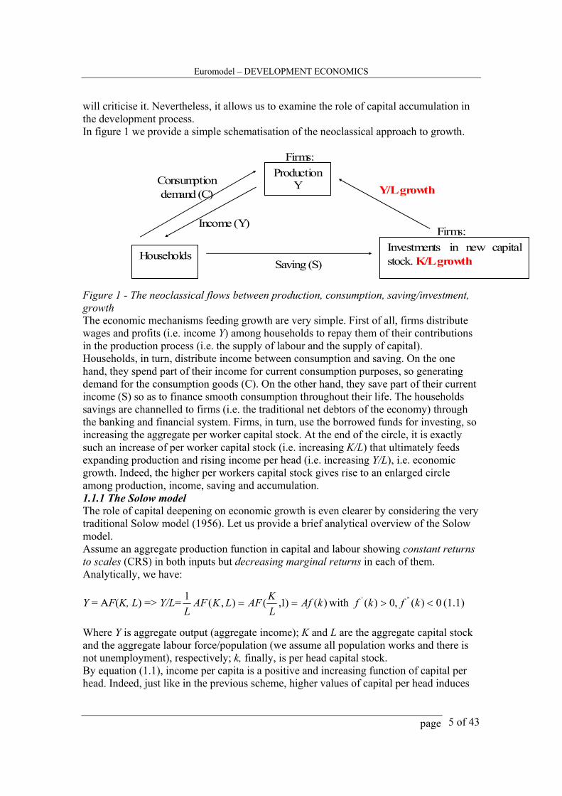
will criticise it. Nevertheless, it allows us to examine the role of capital accumulation in the development process. In figure 1 we provide a simple schematisation of the neoclassical approach to growth.

ProductionY

Households

Income (Y)

Consumption demand (C)

Firms: Investments in new capital stock. K/L growth Saving (S)

Y/L growth

Firms:

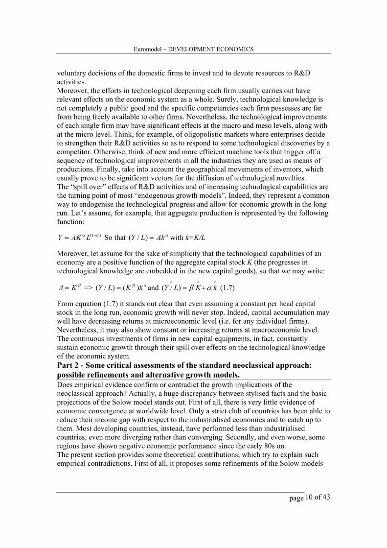
Figure 1 - The neoclassical flows between production, consumption, saving/investment, growth The economic mechanisms feeding growth are very simple. First of all, firms distribute wages and profits (i.e. income Y) among households to repay them of their contributions in the production process (i.e. the supply of labour and the supply of capital). Households, in turn, distribute income between consumption and saving. On the one hand, they spend part of their income for current consumption purposes, so generating demand for the consumption goods (C). On the other hand, they save part of their current income (S) so as to finance smooth consumption throughout their life. The households savings are channelled to firms (i.e. the traditional net debtors of the economy) through the banking and financial system. Firms, in turn, use the borrowed funds for investing, so increasing the aggregate per worker capital stock. At the end of the circle, it is exactly such an increase of per worker capital stock (i.e. increasing K/L) that ultimately feeds expanding production and rising income per head (i.e. increasing Y/L), i.e. economic growth. Indeed, the higher per workers capital stock gives rise to an enlarged circle among production, income, saving and accumulation. 1.1.1 The Solow model The role of capital deepening on economic growth is even clearer by considering the very traditional Solow model (1956). Let us provide a brief analytical overview of the Solow model. Assume an aggregate production function in capital and labour showing constant returns to scales (CRS) in both inputs but decreasing marginal returns in each of them. Analytically, we have:

Y = AF(K, L) => Y/L= )()1,(),(1 kAfLKAFLKAF

L== with 0)(,0)( ''' <> kfkf (1.1)

Where Y is aggregate output (aggregate income); K and L are the aggregate capital stock and the aggregate labour force/population (we assume all population works and there is not unemployment), respectively; k, finally, is per head capital stock. By equation (1.1), income per capita is a positive and increasing function of capital per head. Indeed, just like in the previous scheme, higher values of capital per head induces


page 6 of 43

allow the productive process to expand and income per head to increase. Nevertheless, income per capita shows decreasing marginal returns in capital per head. Therefore, any additional unit if capital per head, although increasing (Y/L), will produce constantly smaller variations of income per capita. In the Solow model, the dynamic of income per capital depends on capital deepening. Let us describe the motion rule of per head capital stock through the following equations:

∧∧∧∧

−== LKLKk )/( (1.2) dK

LKsFK −=∧ ),( (1.3) nL =

∧

(1.4)

Where “hat” variables identify percentage variations (i.e. growth rates). Equation (1.2) describes the growth rate of per head capital stock as the difference between the growth rate of aggregate capital stock K (in upper case) and the growth rate of population L. Equation (1.3) defines the growth rate of aggregate capital stock as the difference between the gross investments (i.e. sF(K,L)/K) and the depreciation rate (d). Equation (1.4), finally, gives the growth rate of population, here assumed as exogenous and equal to n. Substituting equations (1.3) and (1.4) in equation (1.2), we obtain:

)()()()/(

)/),(()(),( dnk

ksAfdnLK

LLKFsAdnK

LKsAFk +−=+−=+−=∧

Knowing that kkk ∗=∧•

, where kk ∆=•

is the variation of per head capital stock, we obtain the following expression for the k dynamic:

kdnksAfk )()( +−=•

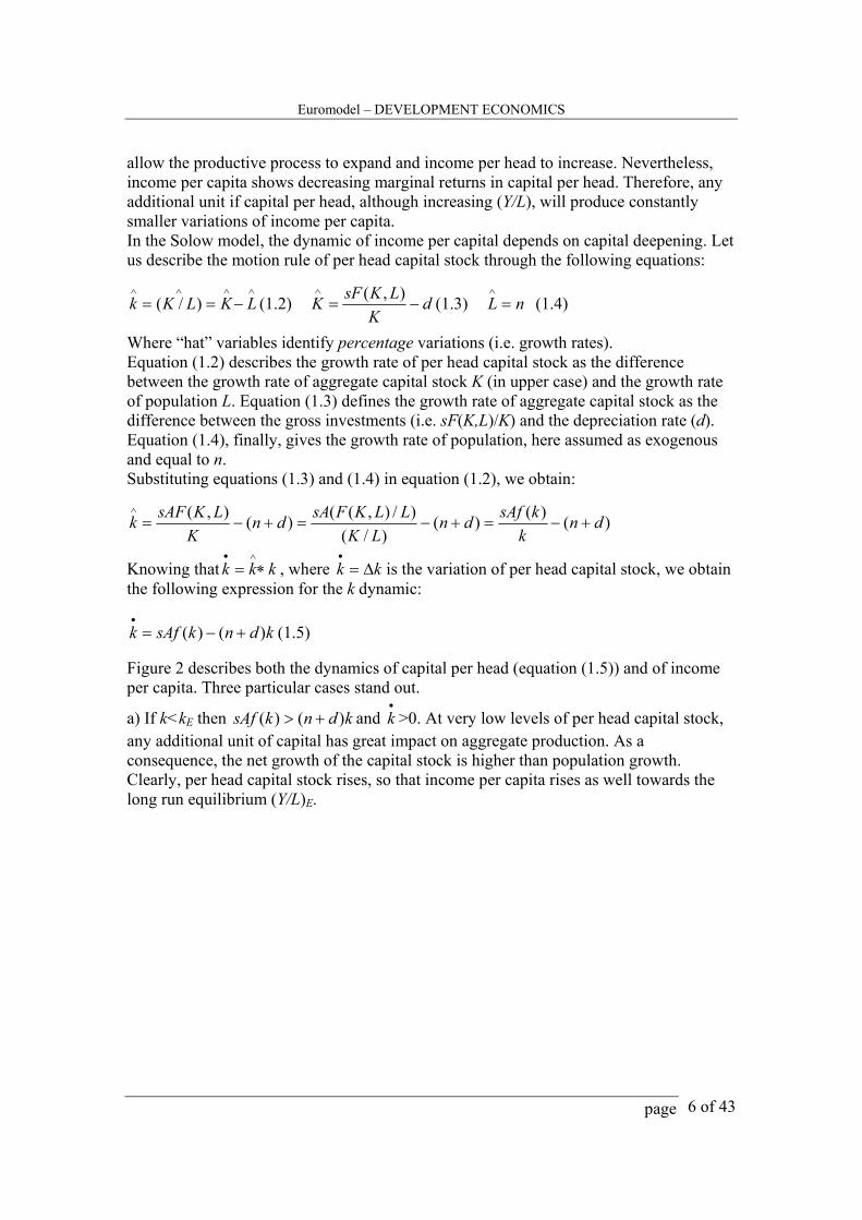
(1.5) Figure 2 describes both the dynamics of capital per head (equation (1.5)) and of income per capita. Three particular cases stand out.

a) If k<kE then kdnksAf )()( +> and •

k >0. At very low levels of per head capital stock, any additional unit of capital has great impact on aggregate production. As a consequence, the net growth of the capital stock is higher than population growth. Clearly, per head capital stock rises, so that income per capita rises as well towards the long run equilibrium (Y/L)E.


page 7 of 43

Y/L

k kE

sAf(k)-(n+d)k

sAf(k)-(n+d)k > 0 sAf(k)-(n+d)k < 0

sAf(k)

Af(k)

(n+d)k

(Y/L)E

Figure 2 – Capital per head accumulation and rising income per capita in the Solow model

b) If k=kE then kdnksAf )()( += and •

k =0. We are in the stable equilibrium point. At this level of per head capital stock, the net percentage increase of capital stock is just equal to the population growth. Per head capital stock, therefore, is constant with income per capita.

c) If k>kE then kdnksAf )()( +< and •

k <0. In this case, per head capital stock is very high. Due to the decreasing marginal returns of capital, any additional unit of capital has really small effects on aggregate production. Net capital accumulation, therefore, is lower than the population growth, so that per head capital stock shrinks towards the equilibrium kE. Clearly, also income per capital decreases towards the long run equilibrium level (Y/L)E. The Solow model bears relevant implications for long run growth and for the economic performances of different economies at different stages of development. We want to stress the following two points. a) In the long run (i.e. when k = kE), income per capital will keep on growing only in presence of exogenous technological progress. Indeed, with (Y/L) = Af(k) and k = kE, the effects of increasing capital per head will vanish in the long run. Income per capita, therefore, will increase only assuming technological improvements raising A values (or labour saving technological improvements). Assuming “x” as the instantaneous rate of technological progress, in the long run income per capital will grow exactly at the same pace. b) Neglecting the issue of long run growth, the Solow model implies that poor countries will necessary grow. At the very beginning of capital accumulation (when k is low), the returns of capital accumulation are particularly high (tending to ∞ when k tends to 0). Net investments (sAf(k) - dk), therefore, will be positive and higher than population growth,


page 8 of 43

so that per head capital stock will inevitably rise. Consequently, income per capital will also grow, tending toward the long run equilibrium. More importantly, the Solow model seems to imply economic convergence among different economies. On the one hand, economic systems having the same parametrical settings (i.e. equal saving rate “s”, depreciation rate “d” and population growth “n”) will reach exactly the same long run level of income per capita. On the other hand, transitional growth (i.e. the growth path leading to the long run equilibrium) is proportional to the distance from the long run steady state. The further away an economy is from the long run equilibrium, the higher its growth rate will be. If we reasonably assume poorer countries to be further away than richer economies from the long run equilibrium, then worldwide convergence would occur. According to the Solow framework, soon or later poorer economies should catch up to developed economies, reaching similar degrees of development. 1.2 Some notes on the endogenous growth models The “Growth accounting” tries to estimate the contributions to the economic growth of the productive factors’ accumulation and of technological progress. Since the early works in this field of investigation (Abramovitz (1956) and Solow (1957)), the technological progress has turned out to be the leading force of economic growth. The improvements in Total Factor productivity (TFP henceforth), in fact, have seemed to count for almost the seven-eighth of the overall economic growth. Such a result sounds a bit disappointing for the neoclassical theory of growth, which traditionally assumes as exogenous, and thus substantially unexplained, what seems to be the main fuel of economic growth. During the most recent years, at least since the mid 80s on, the economic research has thus tried to squeeze down the degree of “our ignorance about growth (Abramovitz (1956))” and to reduce the importance of exogenous technological progress. In doing that, the economic research has followed two main strategies. On the one hand, the empirical works have tried to capture and include as much “residuals” as possible in the accumulation of the productive factors. Indeed, it has been reasonably argued, technological progress is not divided from capital accumulation, but it is more likely embedded in the adoption of new machine tools. On the other hand, the theoretical works have tried to endogenise the technological progress by conceiving it as planned outcome of voluntary decisions of the economic agents, mainly firms. In the following pages we briefly analyse some theoretical contributions of the so-called “new growth theory”. In particular we will focus on the very simple AK model by Rebelo (1991) and on the “spill over effects” models a la Romer (1986). 1.2.1 The AK model The dynamic behaviour of the Solow model relies heavily on the assumption of decreasing returns to capital. This sounds like a completely reasonable assumption. It is quite reasonable to conceive that rising capital stock will have constantly smaller effects on output when it combines with other fixed productive inputs (lands or unskilled labour, for instance). The assumption of decreasing returns to capital, however, may be convincingly dropped whenever we adopted a broader perspective on capital, considering also the human capital. Indeed, the quality and the ability of workers likely influence the productivity of physical capital. More skilled workers, for example, can master more quickly how to use new machines. Otherwise, high skilled workers can move down faster on their own experience curve. In analytical terms, a broader perspective on capital that takes into


page 9 of 43

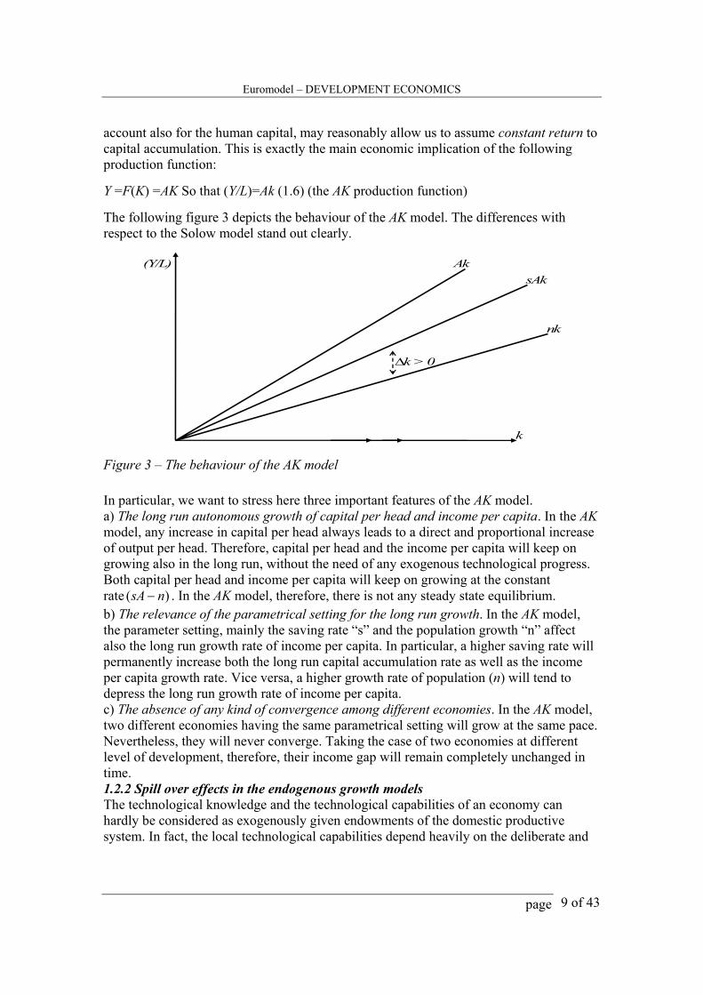
account also for the human capital, may reasonably allow us to assume constant return to capital accumulation. This is exactly the main economic implication of the following production function: Y =F(K) =AK So that (Y/L)=Ak (1.6) (the AK production function) The following figure 3 depicts the behaviour of the AK model. The differences with respect to the Solow model stand out clearly.

(Y/L) Ak sAk

nk

k

∆k > 0

Figure 3 – The behaviour of the AK model In particular, we want to stress here three important features of the AK model. a) The long run autonomous growth of capital per head and income per capita. In the AK model, any increase in capital per head always leads to a direct and proportional increase of output per head. Therefore, capital per head and the income per capita will keep on growing also in the long run, without the need of any exogenous technological progress. Both capital per head and income per capita will keep on growing at the constant rate )( nsA − . In the AK model, therefore, there is not any steady state equilibrium. b) The relevance of the parametrical setting for the long run growth. In the AK model, the parameter setting, mainly the saving rate “s” and the population growth “n” affect also the long run growth rate of income per capita. In particular, a higher saving rate will permanently increase both the long run capital accumulation rate as well as the income per capita growth rate. Vice versa, a higher growth rate of population (n) will tend to depress the long run growth rate of income per capita. c) The absence of any kind of convergence among different economies. In the AK model, two different economies having the same parametrical setting will grow at the same pace. Nevertheless, they will never converge. Taking the case of two economies at different level of development, therefore, their income gap will remain completely unchanged in time. 1.2.2 Spill over effects in the endogenous growth models The technological knowledge and the technological capabilities of an economy can hardly be considered as exogenously given endowments of the domestic productive system. In fact, the local technological capabilities depend heavily on the deliberate and


page 10 of 43

voluntary decisions of the domestic firms to invest and to devote resources to R&D activities. Moreover, the efforts in technological deepening each firm usually carries out have relevant effects on the economic system as a whole. Surely, technological knowledge is not completely a public good and the specific competencies each firm possesses are far from being freely available to other firms. Nevertheless, the technological improvements of each single firm may have significant effects at the macro and meso levels, along with at the micro level. Think, for example, of oligopolistic markets where enterprises decide to strengthen their R&D activities so as to respond to some technological discoveries by a competitor. Otherwise, think of new and more efficient machine tools that trigger off a sequence of technological improvements in all the industries they are used as means of productions. Finally, take into account the geographical movements of inventors, which usually prove to be significant vectors for the diffusion of technological novelties. The “spill over” effects of R&D activities and of increasing technological capabilities are the turning point of most “endogenous growth models”. Indeed, they represent a common way to endogenise the technological progress and allow for economic growth in the long run. Let’s assume, for example, that aggregate production is represented by the following function:

)1( αα −= LAKY So that αAkLY =)/( with k=K/L Moreover, let assume for the sake of simplicity that the technological capabilities of an economy are a positive function of the aggregate capital stock K (the progresses in technological knowledge are embedded in the new capital goods), so that we may write:

βKA = => αβ kKLY )()/( = and ∧∧∧

+= kKLY αβ)/( (1.7) From equation (1.7) it stands out clear that even assuming a constant per head capital stock in the long run, economic growth will never stop. Indeed, capital accumulation may well have decreasing returns at microeconomic level (i.e. for any individual firms). Nevertheless, it may also show constant or increasing returns at macroeconomic level. The continuous investments of firms in new capital equipments, in fact, constantly sustain economic growth through their spill over effects on the technological knowledge of the economic system. Part 2 - Some critical assessments of the standard neoclassical approach: possible refinements and alternative growth models. Does empirical evidence confirm or contradict the growth implications of the neoclassical approach? Actually, a huge discrepancy between stylised facts and the basic projections of the Solow model stands out. First of all, there is very little evidence of economic convergence at worldwide level. Only a strict club of countries has been able to reduce their income gap with respect to the industrialised economies and to catch up to them. Most developing countries, instead, have performed less than industrialised countries, even more diverging rather than converging. Secondly, and even worse, some regions have shown negative economic performance since the early 80s on. The present section provides some theoretical contributions, which try to explain such empirical contradictions. First of all, it proposes some refinements of the Solow models


page 11 of 43

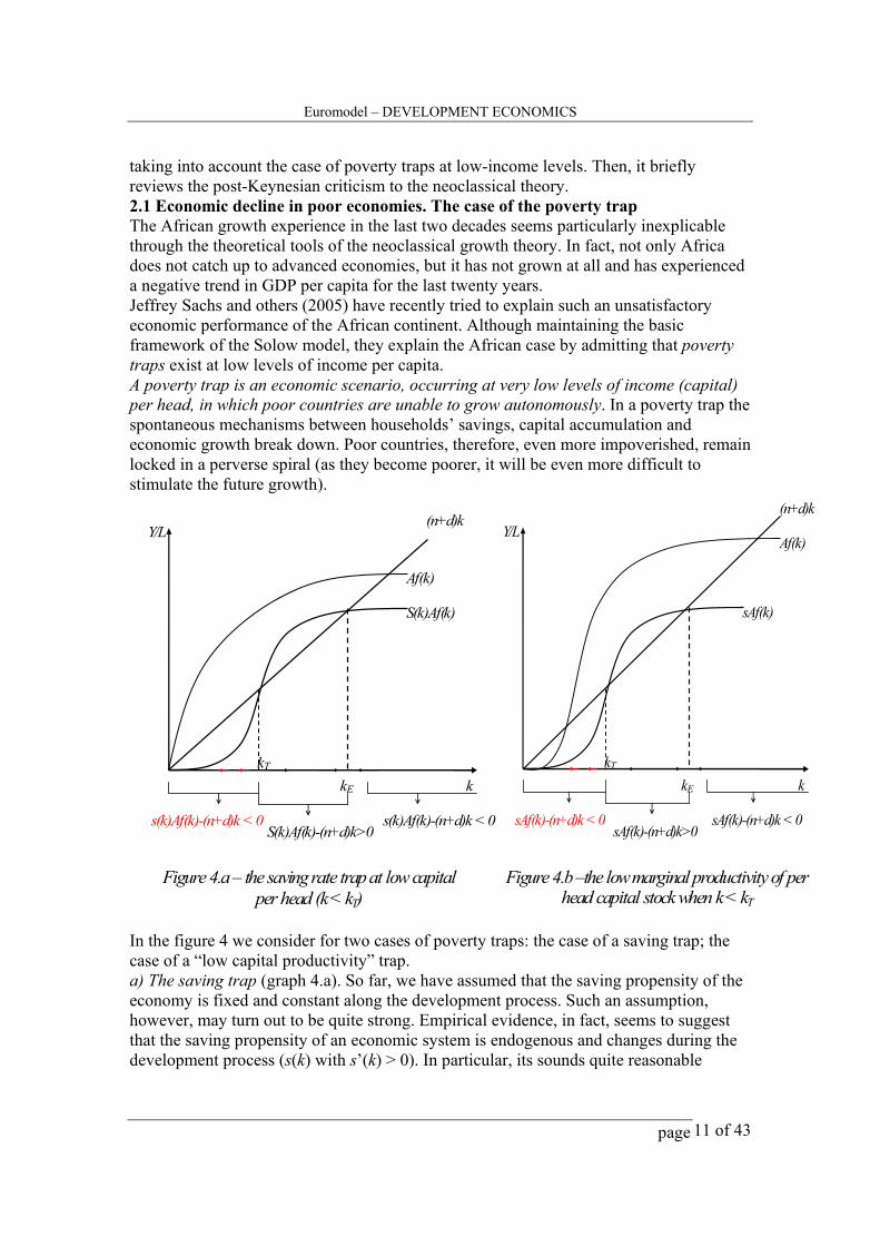
taking into account the case of poverty traps at low-income levels. Then, it briefly reviews the post-Keynesian criticism to the neoclassical theory. 2.1 Economic decline in poor economies. The case of the poverty trap The African growth experience in the last two decades seems particularly inexplicable through the theoretical tools of the neoclassical growth theory. In fact, not only Africa does not catch up to advanced economies, but it has not grown at all and has experienced a negative trend in GDP per capita for the last twenty years. Jeffrey Sachs and others (2005) have recently tried to explain such an unsatisfactory economic performance of the African continent. Although maintaining the basic framework of the Solow model, they explain the African case by admitting that poverty traps exist at low levels of income per capita. A poverty trap is an economic scenario, occurring at very low levels of income (capital) per head, in which poor countries are unable to grow autonomously. In a poverty trap the spontaneous mechanisms between households’ savings, capital accumulation and economic growth break down. Poor countries, therefore, even more impoverished, remain locked in a perverse spiral (as they become poorer, it will be even more difficult to stimulate the future growth).

Y/L

k kE

S(k)Af(k)-(n+d)k>0 s(k)Af(k)-(n+d)k < 0 s(k)Af(k)-(n+d)k < 0

kT

Af(k)

S(k)Af(k)

(n+d)k

Figure 4.b –the low marginal productivity of per head capital stock when k < kT

Y/L

k kE

sAf(k)-(n+d)k>0 sAf(k)-(n+d)k < 0 sAf(k)-(n+d)k < 0

kT

Af(k)

sAf(k)

(n+d)k

Figure 4.a – the saving rate trap at low capital per head (k < kT)

In the figure 4 we consider for two cases of poverty traps: the case of a saving trap; the case of a “low capital productivity” trap. a) The saving trap (graph 4.a). So far, we have assumed that the saving propensity of the economy is fixed and constant along the development process. Such an assumption, however, may turn out to be quite strong. Empirical evidence, in fact, seems to suggest that the saving propensity of an economic system is endogenous and changes during the development process (s(k) with s’(k) > 0). In particular, its sounds quite reasonable


page 12 of 43

thinking that “s” is an increasing function of per head capital stock. At low level of income and capital per head, the saving rate “s” may also be very low, sometimes negative. In poor economies, people are forced to use almost their income for survival, so leaving very little room for saving. Otherwise, when capital and income per head are quite high, also the saving rate may be high: people are enough money to completely satisfy their survival needs and to constantly increase their wealth as well (by accumulating new capital stock). According to the previous neoclassical framework, the low saving rate of poor countries tend to depress capital accumulation. The net investments, if positive, will be likely lower than population growth. Capital per worker, therefore, will shrink rather than increase as much as income per capital. In such a context, clearly, the autonomous mechanisms feeding development no longer work. According to figure 4.a, they will work again only when a minimum threshold level of the capital stock and income per capita is reached. Indeed, only once the economy has accumulated a per head capital stock equal to kT (and the corresponding income per capital (Y/L)T) people’s savings will prove to be sufficient for sustaining spontaneous capital accumulation and economic growth. Before such a threshold level of capital, however, the economic system will be unable to grow. Quite the opposite, it will inevitably and “naturally” decline. The economy lies in a poverty trap. b) The “low productivity of capital” trap (graph 4.b). The dynamic behaviour of the standard neoclassical model heavily relies on the assumption of high marginal productivity of capital at low levels of working capital stock. The neoclassical assumption on the marginal productivity of capital, however, sounds quite unrealistic. At low level of the capital stock, when some fundamental public infrastructures are lacking, additional units of productive capital will have likely quite small effects on production. Think, for instance, of the case of a poor country lacking of widespread electricity infrastructure. In such a context, it proves to be really useless to built up new firms and to introduce modern productive techniques. The new machines, in fact, will not work without electricity, the effects of new capital goods on aggregate income thus being very low if nil. In case of increasing returns to scale and low marginal productivity of capital at low levels of capital stock, “autonomous” growth may not happen. On the contrary, according to figure 4.b, due to net investments lower than population growth, the economy will decline. Once again, therefore, we deal with a poverty trap. Before the minimum threshold level of the capital stock kT is built, say fundamental public infrastructure, the economy is unable to grow endogenously, but it will decline indefinitely. Only once the threshold level of capital stock kT is reached, i.e. once roads, ports and electricity networks have been established, the economy can start growing autonomously. The existence of poverty traps impeding economic development in backward economies clearly calls for “violent” development strategies. Indeed, it seems necessary to hit the economy with shocking measures in order to bring it outside the mud of underdevelopment. Weak economic measures, smooth investment plans, for example, might prove to be unable to reach the threshold level of the capital stock igniting spontaneous growth. On the contrary, a huge amount of integrated investment flows might do it. Even more explicit, the existence of poverty traps calls for a “big push” strategy. We might enquire here what kind of big push a poor economy needs. Should the


page 13 of 43

big push work on the supply-side of the economy, by giving rise to a huge amount of saving and physical investments, like Sachs tends to advice? Otherwise, should the big push take the form of a demand side push to growth and investments, as some historical cases of development seem to suggest? We leave these questions as open issues to be discussed in class. 2.2 An alternative approach to growth: the case of post-Keynesian growth models. Even admitting for spontaneous economic growth in developing countries at any level of the aggregate capital stock, the neoclassical-type “convergence” hypothesis finds very low empirical support. Actually, economic convergence appears as exceptional phenomena concerning a quite strict group of countries rather than a well-established rule. Some refinements of the original Solow model, in particular the human capital adding model by Romer, Mankiw and Weil (1992), have tried to reconcile the neoclassical framework with the current empirical evidence. Although they fit better with the current data on growth performances, such refinements do not seem capable to convincingly explain the case of poor economies even more falling behind the developed countries (Ros, 2000). Clearly, alternative theoretical approaches can provide different insights on economic development by bringing into the picture some aspects actually disregarded by mainstream economics. In the present section, we briefly review the post-Keynesian/structuralist perspective on economic development. The following three points grasp the post-Keynesian criticism to the neoclassical approach. As it will be clearer later on, all these points compose a conceptual framework in which aggregate demand, and in particular the constraints to demand expansion, matter for growth. a) The “inverted” saving-investments relation. Neoclassical theory identifies the accumulation of the productive factors and the technological progress as the leading forces of economic development. In particular, with both the labour force growth rate and the technological progress taken as exogenous, capital accumulation is uniquely determined by disposable saving. The post-Keynesian models completely invert this relation. Indeed, in post-Keynesian frameworks, the causal relation runs from investments to savings, with the former determining the latter after appropriate adjustments in aggregate quantities. The “inverted” relation between investments and savings in turn means nothing but the aggregate demand matters for capital accumulation and economic growth. The desire investments by local entrepreneurs, in fact, are not exogenous, but they depend positively on the aggregate demand and the capacity utilization of working capital stock. High aggregate demand and sustained economic activity can thus stimulate fast capital accumulation and high economic growth. b) The “demand-led” endogeneity of the technological progress. Technological progress mainly consists of the structural change of the domestic productive system towards complex and diversified productive patterns. The creation of new industries and of new fields of productions, especially manufacturing and capital goods productions (which lie at the base of the increasing division of labour and of the rise in labour productivity), in turn rely heavily on sound economic conditions. Recalling Smith, technological progress is likely to occur when the dimensions of the markets are sufficiently high, the economy is growing and an expanding aggregate demand lead entrepreneurs to look for new, more advanced and more productive techniques. Once again, demand conditions matter for


page 14 of 43

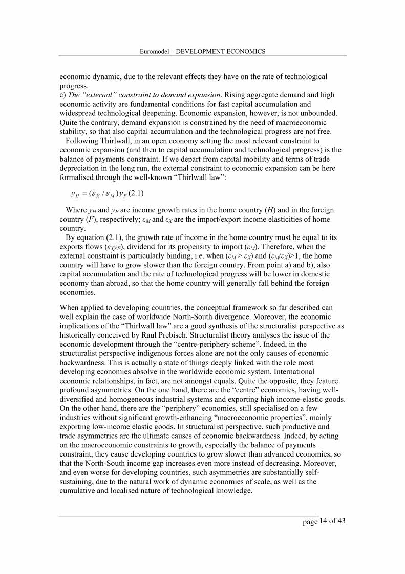
economic dynamic, due to the relevant effects they have on the rate of technological progress. c) The “external” constraint to demand expansion. Rising aggregate demand and high economic activity are fundamental conditions for fast capital accumulation and widespread technological deepening. Economic expansion, however, is not unbounded. Quite the contrary, demand expansion is constrained by the need of macroeconomic stability, so that also capital accumulation and the technological progress are not free. Following Thirlwall, in an open economy setting the most relevant constraint to economic expansion (and then to capital accumulation and technological progress) is the balance of payments constraint. If we depart from capital mobility and terms of trade depreciation in the long run, the external constraint to economic expansion can be here formalised through the well-known “Thirlwall law”:

FMXH yy )/( εε= (2.1) Where yH and yF are income growth rates in the home country (H) and in the foreign country (F), respectively; εM and εX are the import/export income elasticities of home country. By equation (2.1), the growth rate of income in the home country must be equal to its exports flows (εXyF), dividend for its propensity to import (εM). Therefore, when the external constraint is particularly binding, i.e. when (εM > εX) and (εM/εX)>1, the home country will have to grow slower than the foreign country. From point a) and b), also capital accumulation and the rate of technological progress will be lower in domestic economy than abroad, so that the home country will generally fall behind the foreign economies. When applied to developing countries, the conceptual framework so far described can well explain the case of worldwide North-South divergence. Moreover, the economic implications of the “Thirlwall law” are a good synthesis of the structuralist perspective as historically conceived by Raul Prebisch. Structuralist theory analyses the issue of the economic development through the “centre-periphery scheme”. Indeed, in the structuralist perspective indigenous forces alone are not the only causes of economic backwardness. This is actually a state of things deeply linked with the role most developing economies absolve in the worldwide economic system. International economic relationships, in fact, are not amongst equals. Quite the opposite, they feature profound asymmetries. On the one hand, there are the “centre” economies, having well-diversified and homogeneous industrial systems and exporting high income-elastic goods. On the other hand, there are the “periphery” economies, still specialised on a few industries without significant growth-enhancing “macroeconomic properties”, mainly exporting low-income elastic goods. In structuralist perspective, such productive and trade asymmetries are the ultimate causes of economic backwardness. Indeed, by acting on the macroeconomic constraints to growth, especially the balance of payments constraint, they cause developing countries to grow slower than advanced economies, so that the North-South income gap increases even more instead of decreasing. Moreover, and even worse for developing countries, such asymmetries are substantially self-sustaining, due to the natural work of dynamic economies of scale, as well as the cumulative and localised nature of technological knowledge.


page 15 of 43

2.3 Some policy implication of the heterodox perspective on growth: the case of a growth-enhancing trade policy Following the post-Keynesian perspective on development, the productive and trade patterns of an economy are fundamental factors in determining its own growth path. According to the Thirlwall law, the industrialization process and the development of high income elastic productions may boost economic development by increasing the potential for exporting and by slackening the external constraint to growth. However, the existing comparative advantages, as well as the cumulative and localised nature of technological knowledge can fix the productive asymmetries between developing economies and developed countries. In particular, they may impede developing countries to spontaneously transform their own economic systems and to develop fully industrialised productive structures. In such a case, the need of “policy interventions” and of some specific development strategies emerges. International trade and, in particular, trade policy are usually among the most advocated fields where to adopt pro-development measures. In this regard, neoclassical literature generally stresses the welfare-enhancing effects of free trade arrangements. Their arguments are generally static: there are welfare losses in terms of consumer surplus due to trade barriers; there are welfare gains due to trade specialization according to comparative advantages or economies of scale. The neoclassical perspective, however, seems to forget that welfare gains in terms of higher consumer surplus and higher utility firstly require consumers to have any purchasing power, i.e. they require consumers to have any income to spend on consumption. In the case of developing economies income (and therefore purchasing power) largely lacks, so that income growth may be a more immediate parameter for assessing the “welfare consequences” of development strategies. When we shift from a static perspective to a dynamic perspective (i.e. income growth), the general belief in the welfare enhancing properties of free trade may turn out to be wrong. Actually, complete trade liberalization and free trade may slow down growth, while more cautious, somehow more protective trade policies can boost economic dynamic. In the following pages we present a very simple model by Rodriguez and Rodrik (2001) showing that, in presence of “dynamic” differences among industries, trade protection may actually increase the economic growth of developing country. Let assume a small perfect competitive open economy producing both a manufactured good and an agricultural good. Moreover, let us take the price of manufactures on the world market as numeraire, so that we normalise manufactured good’s price to unity. Finally, imagine that both productions use only labour inputs, but manufacturing is subject to learning by doing, according to the following functions:

α)( Mtt

Mt LMX = (2.2) with M

ttMt LMXM θθ ==

•

(2.3)

α)1( Mt

At LAX −= (2.4)

α)1( M

tMttt LALMY −+= (2.5)

Where Xt

M and XtA are the manufacturing and the agricultural outputs, respectively; Lt

M is the population share employed in manufacture (the total population is normalised to 1); θ


page 16 of 43

is the multiplicative factor governing learning-by-doing (as described by equation (2.3)). Equation (2.5), finally, gives us the total output of the economy. Due to the labour mobility, the labour remuneration in both sectors has to be equal instantaneously, so that the following equation (2.6) must always apply:

11 )()1( −− =− αα Mtt

Mt LMLA (2.6) => 0)()1( 11 =−−= −− αα M

ttMt LMLAF (2.6)

Due to the effect of learning-by-doing, both the manufacturing employment and aggregate output grow. In particular, we have:

(a))1(

)1()(//

αθ α

−−

=∂

∂∂−=

∂∂ M

tMt

Mt

Mt

Mt LLL

LFtF

tL

So that: ααθ ))(1)](1/([ Mt

Mt

Mt LLL −−=∧

(2.7)

(b) ∧

−∧∧∧

−−++= Mt

Mt

Mtt

Mtttt LLLLMY 1)1)[(1()( λααλ So that, substituting from (a), we get:

)]()1(

[)( Mttt

Mtt LLY −

−+=

∧

λα

αλθ α (2.8)

In equations (2.7) and (2.8), the “hat” variables stand for growth rates, while λt represents the share of manufacturing production over aggregate income: ])1()(/[)()/( αααλ M

tMtt

Mttt

Mtt LALMLMYX −+== .

Now, Let’s compare a free trade setting and the case of a trade tariff on imported manufactured goods. In the case of free trade, the spontaneous “transitional” growth rate of the economy will

be equal to αθλ )()( MttFTt LY =

∧

, once checked that, when trade taxation lacks, λt = LtM. In

the long run, instead, when all people will be employed in manufacture, the growth rate will be equal to θ. The introduction of a trade tariff on manufactured goods changes the dynamic transition of the economy. Indeed, the tariff protection modifies the relative price of the manufactured good from 1 to (1+τ), so fostering the shift of labour force from agriculture to industry. On the one hand, such a change has a positive effect on the growth rate. When the industrial sector expands faster, in fact, the productive gains from learning-by-doing arise earlier. On the other hand, however, the trade tariffs introduce some distortions of the market mechanisms, which may eventually damper growth. Analytically, in fact, when τ >0 we have λt < Lt

M, so that the second part of equation (2.8) turns out to be negative. In general, differentiating equation (2.8) with respect τ and rearranging, we obtain the following condition:

FTM

tTPM

t YY )()(∧∧

> and 0)/( >∂∂∧

τMtY if )1()/( αα

αλλ −>+∂∂ M

t

tMtt L

L (2.9)

When condition (2.9) holds, the introduction of tariffs on imported manufactured goods increases the growth rate of the economy with respect to the case of free trade.


page 17 of 43

Clearly, the trade policy growth-enhancing case arises when the positive effects of tariffs on learning by doing overcome the static losses in terms of the efficient allocation of resources. Indeed, this point emerges clearly from condition (2.9). On the one hand, the higher Mt parameter and learning-by doing are, the higher will be also (∂λt/∂Lt

M), so that condition (2.9) more easily holds. On the other hand, the higher is (λt/Lt

M), the lower will be the static distortions in the allocation of resources. Once again, therefore, trade policy will likely improve the growth performances of the developing country. So far, we have shown the possible effects on economic dynamic of an “active” trade policy assuming that manufacturing productions already exist in the developing economy. In such a context, trade tariffs on manufactured imports may boost economic growth by accelerating the spontaneous development of the industrialization process. Now try to complicate a bit the analysis and imagine the case of a developing economy that produces agricultural goods only. Now the introduction of “infant industry” measures can be even more important than before, if not fundamental, for economic growth. Without such measures, in fact, the spontaneous work of comparative advantages at worldwide level would probably impede any form of industrialization of the developing economy. Due to the absence of the beneficial effects of learning-by doing linked with the manufacturing productions, in turn, also the economy will not grow at all. In fact, its income per capita will remain constantly equal to A:

0=∧

tY if LtM=0 so that (Yt/L)=Yt=A for any t

In such a case, “infant industry” measures not only may increase economic growth, but can concretely ignite it by making industrialization viable in the backward economy. The initial adoption of pro-industrialization measures, therefore, although distorting market mechanisms, may ensure the developing economy to grow in the short-medium run, as well as to reach a long run growth rate equal to θ. Part 3 – The microeconomic aspects of development: the structural change of the productive pattern and the migration from the countryside. A further in depth analysis of the development process cannot stop to the macro-aggregated level. Indeed, economic development implies also profound changes in the productive structure of the economy, in the division of labour among different sectors, in the geographic locations of people and the relative dimensions of urban areas with respect to the countryside. In the present section we will focus on the microeconomic aspects of the development process. First of all, we will focus on the role of the agricultural sector in feeding the structural change of an economy from a prevalently agrarian economy to a modern industrial economy. In this regard, we will present the milestone model by Lewis (1954). Then, we will also focus on the socially relevant issue of the urbanization and of the migration of people from the countryside to the cities. This second issue will be analysed through the very traditional Harris-Todaro model (1970). 3.1 The structural change of the productive system from agriculture to industry: The Lewis model (1954) The historical analysis of economic development highlights that the development process usually coincides with the structural change of the productive pattern from a prevalently


page 18 of 43

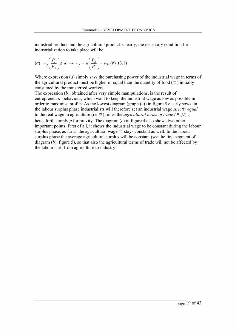
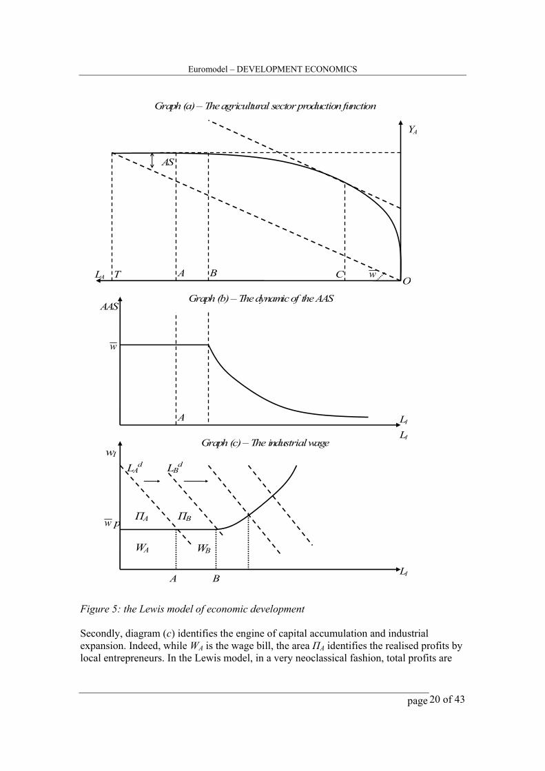
agrarian economy to a modern industrial economy (Chenery and Syrquin, 1986). Following Kaldor (1967), there are at least three good reasons to believe that industrialization is the leading force of economic take off and that the structural change counts for large part of the Solow-type exogenous TFP growth (Montobbio, 2002). - The labour productivity in the industrial sector is initially higher than in agriculture; - The rate of growth of labour productivity in the industrial sector is initially higher than in agriculture, due to increasing returns to scale at industry level (Young, 1928; Kaldor, 1967); - The expansion of the industrial activities triggers relevant spill over on other productions, mainly through technological linkages (Stiglitz and Greenwald, 2005). The process of industrialization, however, is not completely a spontaneous and self-sustaining process. On the one hand, ongoing industrialization requires people to move from countryside to the cities. On the other hand, industrialization needs the agricultural sector to produce an agricultural surplus to be marketed in urban areas. The process of structural change, therefore, heavily relies on the characteristics and the behaviour of the agricultural sector. The linkages between industrialization and the dynamic of the agricultural sector represent the core issue of the present paragraph. The role of the agricultural sector in feeding industrialization is here described through the milestone model by Lewis (1954). Imagine being at the very beginning of the development process in a simple agrarian economy. The productive system is very poor and the labour productivity is so low that all people are employed in agricultural activities so as to produce their own subsistence. In such a “primordial” context, agriculture still behaves in a pre-capitalist fashion. Indeed, the agriculture is in a phase of labour surplus, where the marginal productivity of labour is equal to zero (too many people working on a fixed amount of land eventually reduce the labour marginal productivity to zero), and each person is paid the average product. Now let us consider a small reduction in the labour force employed in agriculture (LA), which decreases from point T to point A in the highest diagram (graph (a)) in the following figure 4. Assuming as constant the wage rate in agriculture at the initial average product w (so that workers are now paid a bit less than their average product) then, given that total output remains unchanged, an agricultural surplus opens up (AS in the highest diagram). During this initial labour surplus phase the average agricultural surplus AAS (i.e. the ratio between the agricultural surplus and the number of workers moved away from agriculture – in other words, the quantity of agricultural surplus each moved away worker might buy) remains constant and equal to w . Graphically, this appears clear in the middle diagram (b) of figure 5. In such a context, a process of industrialization is clearly feasible, due to the movement of workers away from agriculture. The process of industrialization, however, will effectively take place if and only if the industrial wage paid to the transferred workers, in real terms, is at least the same quantity of food they received when they were employed in agriculture (i.e. w ). Otherwise, in fact, agricultural workers will not move from agriculture at all (unless they are forced to). If we define wI as the industrial wage in terms of the industrial product, the industrial wage in terms of the agricultural good will be wI(PI/PA). It is simply the real industrial wage rate times the terms of trade between the


page 19 of 43

industrial product and the agricultural product. Clearly, the necessary condition for industrialization to take place will be:

(a) wIwA

I

PP

≥

→ pwwIw

I

A

PP

==

(b) (3.1)

Where expression (a) simply says the purchasing power of the industrial wage in terms of the agricultural product must be higher or equal than the quantity of food ( w ) initially consumed by the transferred workers. The expression (b), obtained after very simple manipulations, is the result of entrepreneurs’ behaviour, which want to keep the industrial wage as low as possible in order to maximise profits. As the lowest diagram (graph (c)) in figure 5 clearly sows, in the labour surplus phase industrialists will therefore set an industrial wage strictly equal to the real wage in agriculture (i.e. w ) times the agricultural terms of trade ( IA PP ), henceforth simply p for brevity. The diagram (c) in figure 4 also shows two other important points. First of all, it shows the industrial wage to be constant during the labour surplus phase, as far as the agricultural wage w stays constant as well. In the labour surplus phase the average agricultural surplus will be constant (see the first segment of diagram (b), figure 5), so that also the agricultural terms of trade will not be affected by the labour shift from agriculture to industry.


page 20 of 43

AAS

wI

LI

LI

AS

wLA

YA

ΠA w p

WA WB

ΠB

A B

w

Graph (a) – The agricultural sector production function

Graph (b) – The dynamic of the AAS

Graph (c) – The industrial wage

T A

A

LAd LB

d

B O

C

LI

Figure 5: the Lewis model of economic development Secondly, diagram (c) identifies the engine of capital accumulation and industrial expansion. Indeed, while WA is the wage bill, the area ПA identifies the realised profits by local entrepreneurs. In the Lewis model, in a very neoclassical fashion, total profits are


page 21 of 43

assumed to be automatically invested back into the industrial activities (there is not any investment function), thus feeding industrialization. First, the realised profits allow entrepreneurs to enlarge the capital stock so as to expand their production activities. Then, due to the increase in capital stock and production activity, also the labour demand from the industrial sector rises (it shifts up from LA

d to LBd). The industrial demand

therefore draws away new workers from agriculture: agricultural employment decreases until point B (diagram (a)), while industrial employment rises until point B (diagram (c)). At point B, the accumulation process continues. In fact, the amount of profits has risen from ΠA to (ΠA + ΠB) and it is reinvested to buy new capital. The demand for labour rises even more and so on. We also want to mention here that in the labour surplus phase of economic development the industrialization process probably generates an increasingly unequal distribution of aggregate income. As noted above, in the labour surplus phase new industrial labour is forthcoming at the fixed real wage w . Despite the fact that the marginal productivity of labour in the industrial sector is increasing, the real wage earned by each worker remains constant. In the labour surplus phase, therefore, the fruits of industrial expansion are not equally distributed. Labour is becoming more and more productive but this only translates into higher profits (ΠA -> ΠA + ΠB and so on). It is in any case worth stressing here that this unpleasant distributive result of development at the very beginning of the economic take off is seen by Lewis as an element that helps the economy grow and industrialise faster. As already shown, in fact, industrialisation comes from capital accumulation and capital accumulation comes from profits. Remembering that long run income per capita growth depends mainly on the industrialization process, an initial unequal income distribution facilitating initial industrialization may be desiderable for long run development. We can say something more on the linkages between ongoing industrialization and the agricultural sector? Indeed, we can argue something very relevant on the importance of labour productivity in the agricultural sector. In this regard, let us analyse what happens when the economy comes out the labour surplus phase (T - B in diagram (a)) and enters the disguised unemployment phase (B – C in diagram (a)). Once entered the disguised unemployment phase, the average agricultural surplus begins to decline, since total output goes down (the highest diagram (a)). Keeping constant the agricultural wage at w , also the average agricultural surplus thus begins to decline (the middle diagram (b), figure 4). As one can reasonably aspect, therefore, since less agricultural output is marketed, food (agriculture) price starts rising. From equation (3.1), the increase in p pushes the industrial wage up, in order to make industrial workers able to buy w units of food and hence maintaining the appropriate incentive to move to industry. However, at a closer inspection, even if the industrial workers are getting a higher industrial wage, it is simply impossible for them to buy w units of food. Actually, there is not enough to go around. Indeed, from diagram (a), if also each industrial worker bought w , total agriculture production should be equal to OT; however, this is not the case. It follows that, at the disguised unemployment phase, industrial workers will have to consume a mix of industrial and agricultural products. This is exactly the turning point for understanding the role of agricultural productivity on industrialization. Indeed, under what conditions will the potential “migrants” continue to accept to move to industry? Clearly, they will if and only if w is not too close to the subsistence level (if it were, it


page 22 of 43

could not be reduced!). This is to say if and only if agriculture is sufficiently productive to favour and keep alive the industrialisation process. In any case, potential “migrants” will only accept an industrial wage higher than the one prevailing in the labour surplus phase. This is clearly shown in diagram (c). When the labour demand crosses point B, the industrial wage becomes an increasing function at the beginning of the disguised-unemployment phase. Clearly, the increasing trends of the industrial wage will continue also when the disguised unemployment phase comes to an end. Indeed, once point C is reached in the upper diagram, in the CO region we will have wMPL > . Agriculture, therefore, is likely to become a fully capitalistic sector where wages are set according to the profit-maximisation rule. It follows that as labour moves from agriculture to industry, agricultural wage goes up, and the industrial wage (see the lowest diagram) must increase even faster: it must not only compensate for higher terms of trade (p), but also for higher incomes in the agricultural sector. To summarise, the basic ideas of economic development behind the Lewis model are: a) The engine of growth is industrialization and capital accumulation. Lewis does not take into account any problem of demand. Indeed, in the Lewis model saving is automatically reinvested and there are not Keynesian-type preoccupations about effective demand and the realization of profits. b) Capital accumulation and industrialization, however, are limited by the ability of the economy to produce a surplus of food (the lower the surplus → the higher p → the higher the industrial wage → the weaker the incentive to invest in the industrial sector). The productivity level of the agricultural sector thus matters for making industrialization viable c) As development proceeds, there is a process of rural – urban migration and urbanisation. Moreover, the agriculture good terms of trade p increase. Food prices rise because a smaller and smaller number of farmers must support an increasing number of industrial workers. The policy implications of such a view are very controversial and hotly debated. Consider, for instance, the role of agriculture. Even if we accept the residual role given to agriculture in the Lewis framework (agriculture as a source of cheap labour and supplier of a food surplus), the question is: how are these potentialities of agriculture best exploited? By taxing agriculture, which would expand industrial labour supply (it is easier to convince people to move away from agriculture when agriculture is taxed), or by subsidising agriculture (for instance by helping farmers buy relevant inputs like water, fertilisers, etc.), which would expand agricultural production and the available surplus of food? And what happens when agriculture does not coincide with food production alone, but it includes the production of non-food items as well? Again, provided that technical progress in agriculture is good for growth and industrialisation (since it raises the surplus of food), are we sure that in a poor economy there are the appropriate incentives to introduce better agricultural techniques of production? In this respect, what is the role of land reforms and land redistribution? How is the Lewis picture modified by the introduction of international trade and globalisation? Is the kind of development process depicted in the model necessarily associated with a worsening income distribution (growth for whom?) or some more pleasant outcome may be envisaged? Once again, we leave open these issues to stimulate an active debate amongst the readers.


page 23 of 43

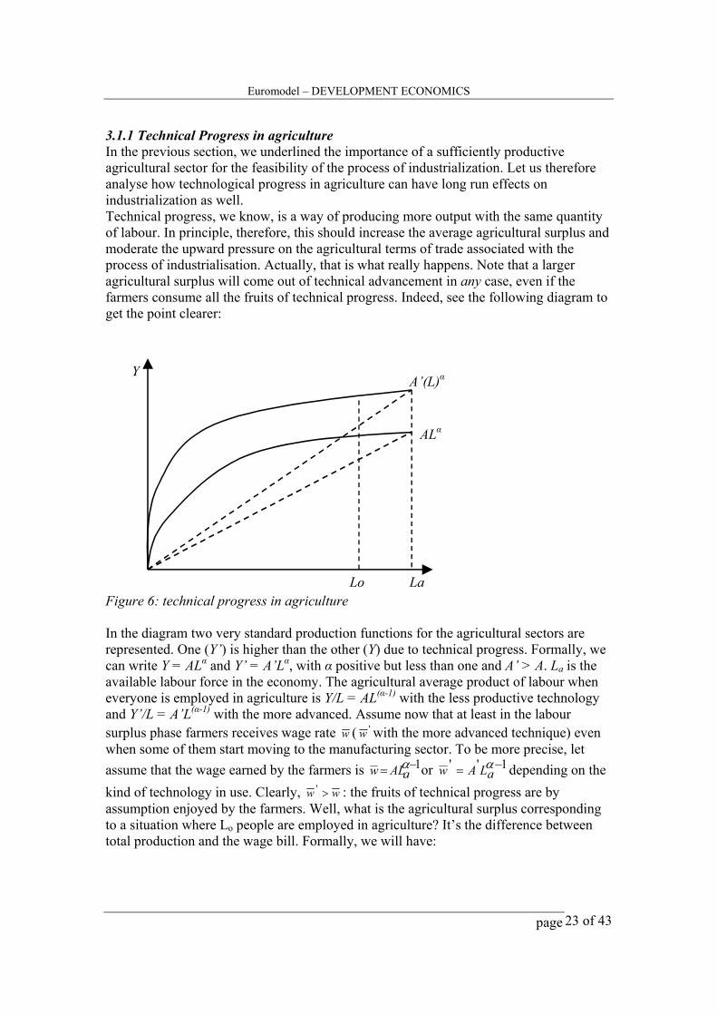
3.1.1 Technical Progress in agriculture In the previous section, we underlined the importance of a sufficiently productive agricultural sector for the feasibility of the process of industrialization. Let us therefore analyse how technological progress in agriculture can have long run effects on industrialization as well. Technical progress, we know, is a way of producing more output with the same quantity of labour. In principle, therefore, this should increase the average agricultural surplus and moderate the upward pressure on the agricultural terms of trade associated with the process of industrialisation. Actually, that is what really happens. Note that a larger agricultural surplus will come out of technical advancement in any case, even if the farmers consume all the fruits of technical progress. Indeed, see the following diagram to get the point clearer:

Y

La Lo

ALα

A’(L)α

Figure 6: technical progress in agriculture In the diagram two very standard production functions for the agricultural sectors are represented. One (Y’) is higher than the other (Y) due to technical progress. Formally, we can write Y = ALα and Y’ = A’Lα, with α positive but less than one and A’ > A. La is the available labour force in the economy. The agricultural average product of labour when everyone is employed in agriculture is Y/L = AL(α-1) with the less productive technology and Y’/L = A’L(α-1) with the more advanced. Assume now that at least in the labour surplus phase farmers receives wage rate w ( 'w with the more advanced technique) even when some of them start moving to the manufacturing sector. To be more precise, let assume that the wage earned by the farmers is 1−= α

aALw or 1'' −= αaLAw depending on the

kind of technology in use. Clearly, ww >' : the fruits of technical progress are by assumption enjoyed by the farmers. Well, what is the agricultural surplus corresponding to a situation where Lo people are employed in agriculture? It’s the difference between total production and the wage bill. Formally, we will have:


page 24 of 43

−−=−−= 0

11 LaLoLAoLaALoALAS αααα => in the case of the less productive techniques,

or

−−=−−= 0

1'1''' LaLoLAoLaLAoLAAS αααα => in the case of the more productive

technique Since A’ > A, we will have AS’ > AS. As sketched out before, even assuming that farmers will fully enjoy the fruits of technical change, the technological progress will undoubtedly increase the agricultural surplus as well. A higher agricultural surplus sold in cities markets, in turn, will likely compensate the upward pressure on the agricultural terms of trade provoked by the transfer of people in the course of the industrialisation process. Following the mechanism of the Lewis model, there is therefore no doubt that labour saving technical progress in agriculture is potentially very good for industrialization and economic development. The picture so far described, however, is not completely bright. Indeed, there are two main problems to be emphasised, both of them concerning the feasibility of technological progress in agriculture. a) The effective nature of technological progress. Agricultural technical advancements are not necessarily labour saving. On the contrary, they could be labour using and, if they are, there will be a weak incentive at least for the smallholder producers to introduce them. To see why, one has to think of Africa and look at Table 1: Table 1: Non-agricultural to agricultural income ratio. Developing regions 1950-60 1960-70 1970-80 1980-1990 Africa 7.05 8.33 8.74 7.79 Asia 1.87 3.37 3.31 3.57 Latin America 2.42 3.00 2.81 2.51 Other 1.88 2.17 2.15 2.25 Source: UNCTAD, TDR 1998, p.140 It is clear from the table that the ratio of non-agricultural to agricultural value-added per worker is much higher in Africa than elsewhere in the world. This differential is one of the key indicators of “urban bias” in Africa, but it is ultimately based on lack of investment in African agriculture and agricultural infrastructures. This differential underlies the attractiveness to farm households of “straddling” between the agricultural and non-agricultural sectors and may explain why labour using technical progress is not adopted: “..to the extent that off-farm employment opportunities are available, there is a continual pressure for productive labour to be diverted from agriculture. Under these conditions, there may be little incentive to adopt high-yielding crop varieties, which can require greater labour inputs [italics is ours]. Rather, the types of innovation which are attractive are those which save households labour time and thus enable the diversion of labour from the farm” (UNCTAD, Trade and Development Report, 1998). b) The institutional regime prevailing in poor agrarian economies. The second problem with agricultural technical progress is due to one of the most pervasive interlinked contracts in poor countries, that between a farmer who is also a borrower and a landlord


page 25 of 43

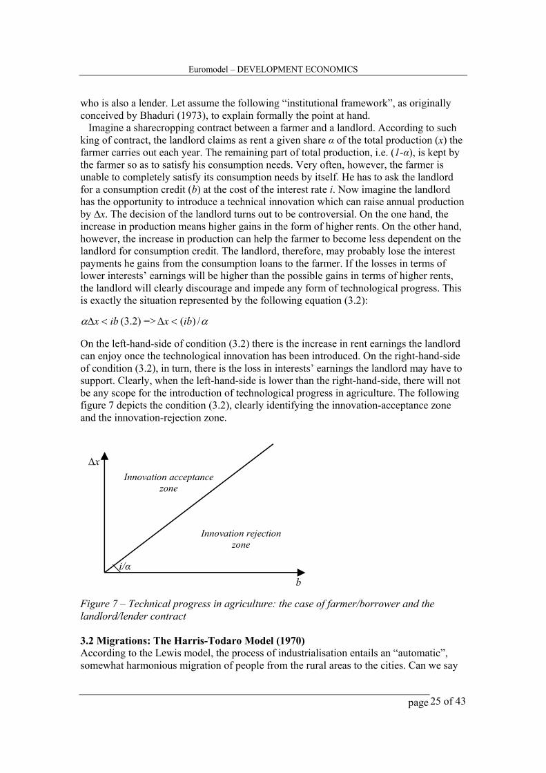
who is also a lender. Let assume the following “institutional framework”, as originally conceived by Bhaduri (1973), to explain formally the point at hand. Imagine a sharecropping contract between a farmer and a landlord. According to such king of contract, the landlord claims as rent a given share α of the total production (x) the farmer carries out each year. The remaining part of total production, i.e. (1-α), is kept by the farmer so as to satisfy his consumption needs. Very often, however, the farmer is unable to completely satisfy its consumption needs by itself. He has to ask the landlord for a consumption credit (b) at the cost of the interest rate i. Now imagine the landlord has the opportunity to introduce a technical innovation which can raise annual production by ∆x. The decision of the landlord turns out to be controversial. On the one hand, the increase in production means higher gains in the form of higher rents. On the other hand, however, the increase in production can help the farmer to become less dependent on the landlord for consumption credit. The landlord, therefore, may probably lose the interest payments he gains from the consumption loans to the farmer. If the losses in terms of lower interests’ earnings will be higher than the possible gains in terms of higher rents, the landlord will clearly discourage and impede any form of technological progress. This is exactly the situation represented by the following equation (3.2):

ibx <∆α (3.2) => α/)(ibx <∆ On the left-hand-side of condition (3.2) there is the increase in rent earnings the landlord can enjoy once the technological innovation has been introduced. On the right-hand-side of condition (3.2), in turn, there is the loss in interests’ earnings the landlord may have to support. Clearly, when the left-hand-side is lower than the right-hand-side, there will not be any scope for the introduction of technological progress in agriculture. The following figure 7 depicts the condition (3.2), clearly identifying the innovation-acceptance zone and the innovation-rejection zone.

x∆

b i/α

Innovation acceptance zone

Innovation rejection zone

Figure 7 – Technical progress in agriculture: the case of farmer/borrower and the landlord/lender contract 3.2 Migrations: The Harris-Todaro Model (1970) According to the Lewis model, the process of industrialisation entails an “automatic”, somewhat harmonious migration of people from the rural areas to the cities. Can we say


page 26 of 43

more on this migration process? Can we add, on top of the agricultural and the manufacturing sector, an urban informal sector to the picture? After all, in many poor countries there is a large urban population engaged in an extremely diverse set of activities outside the direct scrutiny of the State and not covered by labour unions. Is creating new employment opportunities in the city always a good idea? Or is there the risk of providing people the incentive to move too fast to the city, so as to create all the problems inevitably associated with the concentration of a large mass of people in a relatively small area? After all, many cities in Africa, Latin America and Asia are growing at 5-7 per cent per year, which is likely to be above any realistic possibility of giving these people a job. These questions can be addresses through the help of the model developed Harris-Todaro (1970). The key institutional assumptions of the model awkward with many highly visible features of some developing countries: - The rural labour market is competitive; - The wage paid by modern firms in the city is fixed above the market clearing level, either because unions’ activities or governmental legislation (for instance minimum wage regulations) or efficiency wage considerations; - There is an informal sector in which urban residents not otherwise employed can earn their living out of activities outside the control of the state and performed using their labour force alone. Let Lr be the rural population, employed in agriculture on a fixed amount of land. Agricultural output is determined by the standard production function g(Lr) and sold on a world market at a price normalised to unity. Since the rural labour market is assumed to be competitive, rural wages will be equal to the marginal productivity of labour (g’(Lr):

)(' rLgrw = (3.3) with 0)('' <rLg The urban population is either employed in manufacturing (Lm) or working in the informal sector (Lu). Total population is normalised to 1, so that Lr + Lm + Lu = 1. To simplify, assume that the wage paid in the informal urban sector is equal to zero. The institutionally fixed manufacturing wage, instead, is wm. The manufacturing firms aim at profit maximization, so that their demand for labour is implicitly determined by

)(' mLfmw = (3.4) with 0)('' <mLf

Where f(Lm) is the manufacturing production function and )(' mLf is the marginal productivity of manufacturing labour. The probability for an urban resident of getting a job in the manufacturing sector is equal to the number of jobs divided by the number of urban residents. The expected urban income, therefore, will be equal to this probability multiplied by the manufacturing wage (remember that the wage of people employed in the informal urban sector is zero!): wE = [Lm(wm)/(Lm(wm) + Lu)]wm. Now, given this framework, what are the main forces leading to migrations? In the Harris-Todaro model, migration is due to the arbitrage of people between the agricultural wage and the expected urban wage. Indeed, migration will happen if the expected wage one gets by moving to cities is higher than the wage rate gained being employed in


page 27 of 43

agriculture sector. Moreover, people will keep on moving to cities until the following equilibrium condition is reached:

EwmwmwmLuL

mwmLrw =

+=

)(

)( Or mwmLmLuLrw =+ )( (EC)

The following figure 8 depicts the labour demand in agriculture (equation (3.3)), the labour demand in the modern sector (equation (3.4)), the equilibrium condition (EC), as well as the equilibrium point EQ. Clearly, the equilibrium point EQ is given by the intersection between the equilibrium condition “EC” (which is represented as a rectangular hyperbola passing through the point ),( **

mm Lw ) and the labour demand in the agricultural sector. Figure 8 also shows an example of the adjustment process towards the equilibrium point EQ. Imagine, for instance, that at the very beginning of the story the agricultural wage is equal to wr

0. At the same time, imagine that the modern sector wage is equal to wm*, the

labour force employed in the modern sector is Lm* and the urban population is equal to

Lm*+Lu. From figure 8, it appears clear that the equilibrium condition is not met. Quite

the opposite, we have wr(Lm+Lu)<Lmwm, i.e. the wage rate in agriculture is lower then the expected wage in the city (wE). Clearly, People living in the rural areas decide to migrate to the city.

Figure 8: the adjustment towards the equilibrium in the Harris-Todaro model Notwithstanding the migration flow towards the city, the manufacturing wage stays constant, due to institutional rigidities. As consequence, also the formal employment Lm does not change. The new urban residents therefore simply increase the informal urban sector Lu, thus reducing the probability to get a well-paid formal job. At the same time, the reduction of the rural labour force increases the agricultural marginal product and

*mw

*rw

E

EQ

0*um LL + **

um LL +

0rw

(3.4)(3.3)

C


page 28 of 43

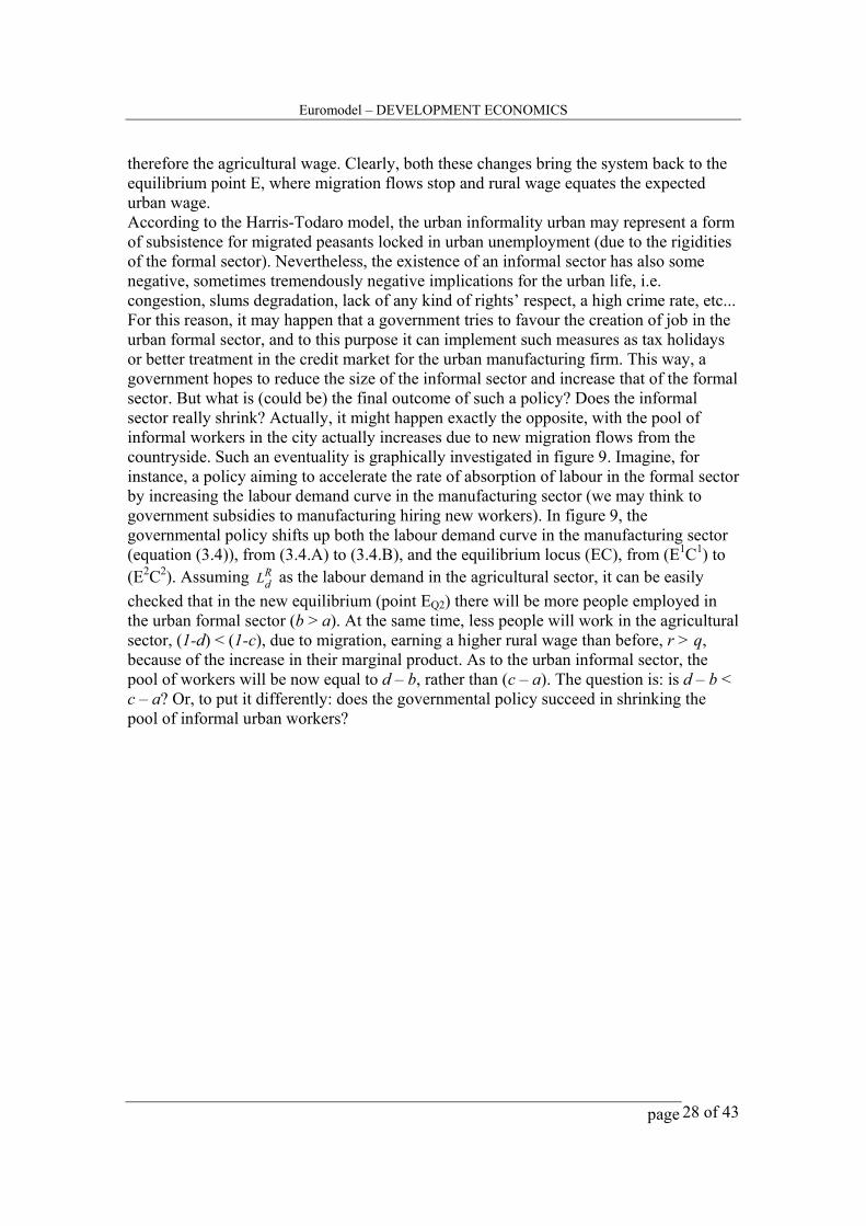
therefore the agricultural wage. Clearly, both these changes bring the system back to the equilibrium point E, where migration flows stop and rural wage equates the expected urban wage. According to the Harris-Todaro model, the urban informality urban may represent a form of subsistence for migrated peasants locked in urban unemployment (due to the rigidities of the formal sector). Nevertheless, the existence of an informal sector has also some negative, sometimes tremendously negative implications for the urban life, i.e. congestion, slums degradation, lack of any kind of rights’ respect, a high crime rate, etc... For this reason, it may happen that a government tries to favour the creation of job in the urban formal sector, and to this purpose it can implement such measures as tax holidays or better treatment in the credit market for the urban manufacturing firm. This way, a government hopes to reduce the size of the informal sector and increase that of the formal sector. But what is (could be) the final outcome of such a policy? Does the informal sector really shrink? Actually, it might happen exactly the opposite, with the pool of informal workers in the city actually increases due to new migration flows from the countryside. Such an eventuality is graphically investigated in figure 9. Imagine, for instance, a policy aiming to accelerate the rate of absorption of labour in the formal sector by increasing the labour demand curve in the manufacturing sector (we may think to government subsidies to manufacturing hiring new workers). In figure 9, the governmental policy shifts up both the labour demand curve in the manufacturing sector (equation (3.4)), from (3.4.A) to (3.4.B), and the equilibrium locus (EC), from (E1C1) to (E2C2). Assuming R

dL as the labour demand in the agricultural sector, it can be easily checked that in the new equilibrium (point EQ2) there will be more people employed in the urban formal sector (b > a). At the same time, less people will work in the agricultural sector, (1-d) < (1-c), due to migration, earning a higher rural wage than before, r > q, because of the increase in their marginal product. As to the urban informal sector, the pool of workers will be now equal to d – b, rather than (c – a). The question is: is d – b < c – a? Or, to put it differently: does the governmental policy succeed in shrinking the pool of informal urban workers?


page 29 of 43

Figure 9: a pro-urban/formal sector policy A priori, we simply cannot answer to this question. But we can say something, notably that the answer ultimately depends on the slope of the labour demand curve in the agricultural sector. Indeed, imagine that the relevant agricultural demand curve is

'RdL ,

which is flatter than RdL . In this case the effect of the governmental policy is to reduce

even more the number of agricultural workers (there will be more migrants to the city), so that in the new equilibrium there will be e – b informal urban workers, which is clearly greater than d – b. So, in general, the flatter the agricultural labour demand curve, the more likely is that the absolute size of the urban informal sector goes up despite the aim of the policy is to reinforce the urban formal sector. Basically, the free choice of the peasants to move to the city can render the governmental policy even counterproductive. There are two points worth stressing, the first related to the relative size of the urban informal sector, and the second to the economic meaning of the slope of the labour demand curve in the agricultural sector. As to the first point, from the equilibrium condition (EC) we can immediately infer that after the introduction of the governmental policy the relative size of the urban informal sector (its size measured as a fraction of the total urban sector) must have diminished, irrespective of what happens to its absolute size. However, what really matters in policy and social terms (congestion, crime rates, diffusion of diseases, etc.) is the absolute size, the relative being quite insignificant. Regarding the slope of the agricultural labour demand curve, it is clearly a measure of the elasticity of labour demand to the real wage. The flatter the curve is, the more responsive is the labour demand. In the limit, with a horizontal curve, agricultural labour demand is perfectly elastic at a given wage rate and we are back to the Lewis case of surplus labour. In such a case, any increase in the manufacturing formal employment will be accompanied by an equivalent (in percentage terms) increase in the urban informal

b c d e o 1

m r

s q

RdL

'RdL

a

(3.4.A)

E1

C1

E2

C2

EQ1

EQ2

wm (3.4.B) wr


page 30 of 43

employment. The city is larger than before, but the proportional expansion of the formal and informal sectors has compromised the realisation of the government’s objectives. This general principle can be applied to other policies as well, not necessarily linked to formal labour demand: “ ..policies aimed at directly reducing urban congestion (say, by building more roads), reducing pollution (say, by building a subway), or increasing the provision of health (say, by building new public hospitals) might all have the paradoxical effect of finally worsening these indicators......because fresh migrations in response to the improved conditions ends up exacerbating the very conditions that the initial policy attempted to ameliorate” (Ray, 1999). EXERCISES AND ASSIGNMENTS Could you briefly describe the logical mechanism behind economic growth in the very traditional neoclassical model? What are the main implications for long run growth of such an analytical framework (think to the Solow model)? Imagine that population growth is not exogenous and constantly equal to “n”, but it depends on per head capital stock as proxy of the wealth of the economy. In particular, assume that there is a negative relationship between population growth and per head capital stock. Can you represent graphically such a possibility by aptly modifying the original Solow model diagram? Can you represent the case of a poverty trap as induced by endogenous population growth? Can you summarise in a few words the main departures of the “new growth theory” from the traditional neoclassical framework a la Solow? What are the most relevant implications for long run growth of the endogenous growth models (focus in particular on their implications in terms of conditional convergence and North-South uneven development)? Try to summarise the basic features of the Keynesian-Structuralist approach to growth and development. What is the role of trade relations in determining the growth possibility of a developing country? Most of economic literature believes free trade is beneficial for growth. Are there any economic rationale fostering an opposite view and claiming protection as useful for economic development? Summarise briefly both the positions in favour and against free trade. Could you briefly summarize the concept of economic development behind the Lewis model, and the reasons it gives so much emphasis on “structural change”? What are the main phases of structural change? Explain the concept of disguised unemployment. What should be the optimal level of agricultural employment if this sector worked in a capitalistic way? Give an analytical support to your answer.


page 31 of 43

Describe the role that agricultural wage rate plays in the industrialization process. What are the main ways in which the former influences the latter? Might it play a different role if we adopted a Keynesian rather than a Lewis-type perspective? In a Lewis-type economy what might be the effects on the ongoing process of industrialization of income taxes on agricultural revenues? And what the effects on the ongoing process of industrialization of agricultural subsidies fostering the expansion of foodstuff productions? Provide some logical arguments that support your answer. Imagine an African country whose production consists essentially of agricultural goods devoted to exports. In addition, internal consumptions or investment goods are imported from abroad. This country exports, moreover, are affected by low price elasticity: Any unit of surplus on international market can be sold and allocated due to more than proportional reductions in corresponding prices. Might a public intervention to control and manage exports flows be required? Could it improve the above considered economic scenario? Why? What are the effects of technological improvements on agricultural surplus? How can they affect ongoing industrialization? Describe briefly some different kinds of technological changes that may occur in agricultural productions. Remembering in particular what said about the African context, can you explain why some specific aspects of technological change can hamper and impede its implementation? Explain the “institutional constraints” that might impede the introduction of technological progress. Following the Bhaduri framework, what are the effects of an increase in the interest rate I that the landlord-lender applies to the tenants-borrower? What about the product share that, according to the sharecropping contract, is claimed by the landlord? Imagine a micro-credit government policy aiming at providing financial resources to farmers. What might be the effects of such a policy for the incentive to the introduction of technological improvements in the Bhaduri model? Plot the equilibrium condition in the Harris-Todaro model and describe the logical process that leads to its achievement. What is the equilibrium condition and its underlying economic meaning? What happens if w*

m rises? What role does labour demand elasticity to wage rate in the agricultural sector have in determining the dimension of urban informality? Plot the results we obtain by imagining higher or lower values of this variable (labour demand elasticity). What effect might a public policy that increases wage rate flexibilities in the modern sector have on the Harris-Todaro equilibrium condition? Would Keynes agree with this proposal (suggestion: to answer this last question, think about a theoretical approach


page 32 of 43

considering demand-side aspects of economic system rather than exclusively supply side ones)? How does an increasingly productive agricultural sector affect the equilibrium condition of the Harris-Todaro model? Describe it in a few words and give a graphical representation of your answer. MAIN REFERENCES Abramovitz, M. (1956), Resource and Output Trends in the United States since 1870, American Economic Review, 46: 5 – 23. Arrow, K. (1962), The Economic Implications of Learning by Doing, Review of Economic Studies, 29: 155 – 173. Bardhan P, Srinivasan T.N. (1971), Crop sharing tenancy in agriculture: A theoretical and empirical Analysis, American Economic Review 61: 48-64; Bardhan, P. (1980), Interlocking factor markets and agrarian development: A review of issues, Oxford Economic Papers 32: 82-89; Bardhan, P. (1984), Land, Labour and rural poverty, New York, Columbia University Press. Bhardan, P. and C. Udry (1999), Development Microeconomics, Oxford, England, Oxford University Press. Basu, K. (1984), Implicit interest rates, usury and isolation in backward agriculture, Cambridge Journal of Economics, 8: 145-59; Basu, K. (1990), Agrarian structure and economic underdevelopment, Chur, Switzerland, Harvard Accademy; Basu, K. (1997), Analytical Development Economics. The Less Developed Economy Revisited, Cambridge, MA. and London, England, The MIT Press; Beladi, H., and Marjit, S. (1996), An analysis of rural-urban migration and protection, Canadian Journal of Economics, 29: 930-40; Bhaduri, A. (1973), A study in agricultural backwardness under semi-feudalism, Economic Journal 83:120-37; Bhaduri, A. (1977), On the formation of usurious interest rates in backward agriculture, Cambridge Journal of Economics, 1: 341-52; Bhaduri A. (1983), The economic structure of backward agriculture, London, Academic Press;


page 33 of 43

Bhagwati, J.N., and Srinivasan T.N. (1974), On reanalysing the Harris-Todaro model: Policy ranking in the case of sector-specific sticky wages, American Economic Review, 64: 502-8; Bravemarman, A., and Stiglitz, J. (1982), Sharecropping and the interlinking of agrarian markets, American Economic Review, 72: 695- 715; Cardoso, E.A.. (1981), Food supply and inflation, Journal of Development Economics, 8: 269-84; Chenery H. and Syrquin M. (1986), Typical Pattern of Transformation, in Chenery H., Robinson S., and Syrquin M. (1986), Industrialization and Growth, New York, Oxford University Press. Chenery H. and Srinivasan T.N. (1988), Handbook of Development Economics, Amsterdam, North Holland; Fields, G. (1975), Rural-urban migration, urban unemployment and underemployment, and job-search activity in LDCs, Journal of Development Economics, 2:165-87; Furtado, C. (1964), Development and underdevelopment, Berkeley, University of California Press; Griffin, A. (1974), The political economy of agrarian change, London, Mcmillan; Harris, J.R., and Todaro, M.P. (1970), Migration, unemployment and development: A two-sector analysis, American Economic Review 60:126-42; Hirschman, A. (1958), The Strategy of economic Development, New Haven, Yale University Press; Hoff, K., and Stiglitz, J. (1994), Some surprising analytics of rural credit subsidies, University of Maryland, Mimeo; Jorgenson, D.W. (1967), Surplus agricultural labour and the development of a dual economy, Oxford Economic Papers, 19: 288-312; Kaldor, N. (1967), Strategic Factors in Economic Development, Ithaca, Cornell University. Kalecki, M. (1976), Essays on developing economies, Hassocks, UK, Harvest Press; Kotwal, A. (1985), The role of consumption credit and agrarian tenancy, Journal of Development Economics, 18: 273-95;


page 34 of 43

Lewis, W.A. (1954), Economic development with unlimited supplies of labour, Manchester School 28:139-91; Lewis, W.A. (1958), Unlimited labour: Further notes, Manchester School 32:1-32; Mankiw, G., Romer, D., and Weil, D., (1992), A Contribution to the Empirics of Economic Growth, Quarterly Journal of Economics, 107: 407 – 437. Mazumdar, D. (1976), The rural-urban wage gap, migration and the shadow wage, Oxford Economic Papers, 28: 406-25; Montobbio, F. (2002), An Evolutionary Model of Industrial Growth and Structural Change, Structural Change and Industrial Dynamics, 13: 387 – 414. Mukherji, B. (1975), Peasants in semi-feudal agriculture: A note on A. Bhaduri model, Indian Economic Review, 10: 49-61; Naqvi, N. (1990), Technological stagnation, tenurial laws and adverse selection: Comment, American Economic Review, 80: 935- 40; Neary, P. (1981), On the Harris-Todaro model with inter-sectoral capital mobility, Economica, 48: 219-34; Newberry, D.M.G. (1975), The choice of rental-contract in peasant agriculture, in Reynolds L.G. (ed.), Agriculture in developing theory, New Haven, Yale University Press; Nurske R. (1953), Problems of capital formation in underdeveloped countries, New York, Oxford University Press. Prebisch, R. (1959) Commercial Policies in underdeveloped countries, American Economic Review, 49: 251-73; Ray, D. (1999), Development Economics. Ranis, G., and Fei, J.C.H. (1961), A theory of economic development, American Economic Review, 51: 533-65; Rebelo, S. (1991), Long Run Policy Analysis and Long Run Growth, Journal of Political Economy, 99: 500 – 521. Rodriguez F., Rodrik D. (2001), Trade policy and economic growth: a skeptic’s guide to the cross-nation evidence, Macroeconomics Annual 2000, MIT Press. Romer, P. (1986), Increasing Returns and Long Run Growth, Journal of Political Economy, 94: 1002 – 1037.


page 35 of 43

Romer, P. (1990), Endogenous Technological Change”, Journal of Political Economy, 98: S71 – S102. Ros, J. (2000), Development Economics and the Theory of Growth, Indiana, Michigan University Press. Rosenstein-Rodan, P.N. (1943), Problems of industrialization in eastern and south-eastern Europe, Economic Journal, 53: 202-11; Sachs, J. (2005), The End of Poverty: How We Can Make it Happen in our Lifetime, London, Penguin Books. Sen, A. (1966), Peasant and dualism with or without surplus labour, Journal of Political Economy, 74: 425-50; Srinivasan, T.N. (1979), Agricultural backwardness under semi-feudalism: Comment, Economic Journal 89:416-19; Solow, R. (1956), A contribution to the theory of Economic Growth, Quarterly Journal of Economics, 70: 65 – 94. Solow, R. (1957), Technical Change and the Aggregate Production Function, Review of Economics and Statistics, 39: 312 – 320. Stiglitz, J.E. (1974), Incentives and risk sharing in sharecropping, Review of Economic Studies 41:219-55; Taylor, L. (1983), Structuralist Macroeconomics: Applicable Models for the Third World, New York, Basic Books. Thirlwall, A.P. (1979), The Balance of Payments Constraint as an Explanation of International Growth Rate Differences, Banca Nazionale del Lavoro Quarterly Review, 32: 45 – 53. Todaro, M.P. (1969), A model of labour migration and urban unemployment in less developed countries, American Economic Review, 59: 138-48; Todaro, M.P. (1976), Internal migration in developing countries, Geneva, International Labour Organization; UNCTAD (1998), Trade and Development Report 1998, Geneva. INTERNET WEBSITES WWW.WORLDBANK.ORG The wide spectrum of World Bank researches concerns also microeconomic issues like agriculture and rural development and poverty. One can find really lots of


page 36 of 43

contributions on these issues just looking at the “publications” section in the home page. Once on the mask for advanced search, just introduce the field of interest into the appropriate space. The list of required contributions will appear. WWW.UNCTAD.ORG Look for the link “Development of Africa”. Agricultural issues are enquired in the area devoted to “Least developed countries”. In this case, search by clicking on the link “programs” in the homepage. WWW.ILO.ORG This is the website of the International Labour Organization. The link “informal economy” in the homepage sends you to publications, events and activities on this issue. WWW.ECLAC.ORG/DDPE/DESAROLLOAGRICOLA The website of the division of productive development and management (and agricultural development) at ECLAC, the Economic Commission For Latin American and the Caribbean. WWW.WIDER.UNU.EDU The Wider Institute traditionally gives great emphasis to the problem of income distribution and inequality. This website provides a quite extended range of Wider publications on this theme (among other issues). They are available clicking on the link “publications”. WWW.ECONOMICS.OX.AC.UK The website of the Department of Economics at Oxford University. A research group on development economics is currently active. Their contributions can be found by following these steps: homepage ->Research, Working papers and Centres ->Development economics. Specific works on African economies are available. WWW.IDS.AC.UK/IDS The website of the Institute for Development Studies at Sussex University, United Kingdom. Its main research topics concern industrial strategies, food security and famine, poverty and inequality, education and social security. It is possible to find some contributions on these issues clicking on “publications” directly from the homepage. WWW.GDNET.ORG The website of Global Development Network. One can find a wide range of papers on “Microeconomics of growth” by clicking on “activities” from the homepage and then on “global research projects”. These contributions are often targeted on specific geographic areas. WWW.ZED.DE The website of the Centre for Development Research. “Economic and Technological change” and “Ecology and Natural resources management” stand out among their


page 37 of 43

principal research topics. One can find the desired contributions by clicking on the list of treated issues directly from the homepage. WWW.GRADE.UNITN.IT The website of Grade, the Group of Research and Analysis on Development at the University of Trento in Italy. On its website one can find some contributions on agrarian economy, poverty analysis at microeconomic level, and on the informal sector. To find their publications follow these steps: homepage -> activities -> publications. WWW.DAGLIANO.UNIMI.IT The website of Centre Luca Dagliano. Institutional and microeconomic determinant of poverty appear among their research issues as well as European integration with Eastern countries. It is possible to find contributions about specific issues by looking at the publications section and enter the working papers page. WWW.MST.ORG.BR The website of the movement of “Sem Terra” (“Without Land”) for land reform and redistribution in Brazil. WWW.INOMICS.COM Inomics is an Internet service especially tailored to the needs of economists. At this site you can find job openings for economists, conference announcements, a human-edited directory as well as a database of research papers in economics. From the homepage you can subscribe to a weekly update on new conference calls. CONFERENCES Here follows a list of the principal conferences and meetings on development. Poverty Reduction, Equity and Growth First PEGNet Workshop, Kiel, Germany, from 28 April to 28 April 2006 www.ifw-kiel.de Education and Development Third International Conference, Preveza, Greece, from 26 May 2006 to 27 May 2007 www.preveza.teiep.gr Poverty and Economic Policy Addis Abeba, Ethiopia, from 17 June 2006 to 25 June 2006 www.pep-net.org Inequity, Poverty and Development: The Role of Markets and Institutions Canazei (Trento), Italy, from 2 July to 8 July 2006 www.dse.univr.it Early Economic Developments First Conference, Copenhagen, Denmark, from 31 August to 1 September 2006 www.econ.ku.dk


page 38 of 43

Development Strategies – A Comparative View Brighton, United Kingdom, from 7 September 2006 to 9 September 2006 www.brighton.ac.uk HOT ISSUES AND RESEARCH TOPICS We suggest some open issues that represent promising fields for future researches. 1- Information asymmetries in the financial sector, micro-finance and productivity enhancing plans for rural and small-medium enterprises. Information asymmetries play a leading role in restraining financial resources that small (rural and small-medium enterprises) agents can obtain from financial institutions. Objective difficulties in screening debtors’ behaviour represent an important factor in rationing financing. The impossibilities to offer real guarantees that might ensure credits decreases more and more the chances of matching between lenders and borrowers. Local agents, however, really need financial resources to upgrade their productive structures; close productivity gaps and effectively compete on international markets. Impressive bankruptcies of small and medium enterprises in developing countries often result from the explosive mix of abrupt changes in institutional environment and lacks of funds. Micro-finance from no-profit organization or governmental authorities might represent partial solutions of this problem. It is interesting for future researches to analyse alternative way for financing small and medium enterprises. In addition future researches might enquire the “game rules” needed for avoiding moral-hazard problems, inefficiencies and failures of micro-finance and/or public funding programs. 2- The fight against informality. The need of increased flexibility of labour market versus structural changes in the productive structure and public intervention in developing countries. High productive heterogeneity (i.e. large productivity gaps between few “high productive” branches of productive system and the “low productivity” remaining majority) constitutes a typical feature of developing countries. Productive heterogeneity relies on large informal sectors, including small production activities and low-skilled/unregulated autonomous works. A debate between different interpretations of the causes of the informal sector is still in progress. Someone stress the need for liberalising and augmenting flexibility of labour markets. Institutional rigidities avoid greater competitions and impede to absorb informal employment (or open unemployment). Moreover, informal employment sometimes has voluntary aspects. Others, on the contrary, emphasise an exactly opposite standpoint. What matters are structural problems concerning too narrow and widely lacking productive structures. The reduction of informality can be realistically pursued only by deep changes of local productive systems. The debate still offers room for new contributions. Different theoretical approaches can be adopted: mainstream micro-founded ones, as well as structuralist-evolutionist ones. 3- Income distribution, inequality and economic performance: new perspectives after the “political economics models” of the 90s.


page 39 of 43

A model by Bourguignon (1990) highlights the relations among dual economies, structural changes and income distribution. In particular, it focuses on Lorenz curve changes during development process. Moreover, it stresses the political problems that increasingly unequal income distribution can raise rather than economic ones. Nevertheless, some theoretical works in the mid-90s have tried to combine political issues and economic implications of income distribution. Income inequality may induce voters to ask for redistributive policies. Redistributive policies in turn might affect growth performance, depending on the concrete measures they adopt. Theoretically different result from traditional belief (from the age of former Kusnetzian enquires) seems to emerge. High inequality may hamper income growth, due to the specific redistributive policies it may induce (usually discouraging investments). The question, however, still appears controversial. Inequality might reduce growth due to the redistributive measures it provoke. But if this is the case, inequalities “per se” do not appear to be the “direct” source of economic slowdown. The real ones are redistributive policies, i.e. redistributive attempts. The question, thus, still deserves researches, possibly also with alternative theoretical schemes than typical mainstream ones. We are thinking about post-Keynesian frameworks, the structuralist approach, but also the neoclassical ones that take into account the problem of child labour and the accumulation of human capital. 4- Trade and commercial regimes, technological behaviours of local agents and the linkages of domestic productive systems. Economic literature usually gives great relevance to technological progress as a leading factor for economic development. Technological behaviours of local agents, however, are strongly influenced by the institutional environment and the competitive scenario of the domestic economic system. New contributions recently emerge. They questioned how trade and commercial regimes, as well as financial ones, affect the technological parabola of local firms, entire industries or the national economy as a whole. Moreover, they address analysis well beyond strictly atomistic microeconomic instances. These contributions consider the impact of institutional changes at meso level, on firms networking and productive linkages. Indeed, productive linkages represent a really important aspect of structural change towards a fully developed economic system. Wide room is thus opened up for new researches on the relations among microeconomic technological behaviours, local production networks and economic development. In particular, empirical investigations might be required. They might check for the results of governmental projects that aim at enhancing local embedness of productive activities. GLOSSARY Income per head: Is the ratio between aggregate income (GDP) and population. This is a rough indicator of the wealth of a nation: neglecting distributional issues, a higher income per head generally implies higher living standards of people. Economic growth: Is usually measured by the rise (or fall) in GDP per head. It is the year-to year percentage variation in income per head. In formula: [∆(Y/L)/(Y/L)] = [(Y/L)t+1 – (Y/L)t]/(Y/L)t


page 40 of 43

Capital per worker: Is the ratio between overall capital stock and the employed labour force (in the Solow model equal to population, for sake of simplicity). It is an additional indicator of the degree of development of an economy. Aggregate Investments: Is the yearly increase in the total amount of capital stock an economic system may dispose of. The gross investments are the total amount of new capital means of productions (machines). Net investments are the effective increase in working capital stock, once taken into account for the obsolescence of installed capital stock. The depreciation rate is nothing but the rate at which past capital equipment has to be replaced each time. Production function: Is the functional relation between the productive factors (inputs) employed in the production process that every firm carries out and the output of the production process. The production function is nothing but a way for analytically representing the “black box” that transforms productive inputs in final output. Marginal productivity of capital (or labour): Is the additional increase in total output obtained by adding a unit more of capital (or labour) input while keeping constant the other productive factor. In formula, it is the partial differentiation of total output with respect to one productive input (capital or labour: ∂Y/∂K (or ∂Y/∂L). Decreasing returns: Decreasing marginal returns deals with the effects that an additional unit of a productive factor (it may be either capital or labour) has on aggregate output, keeping the other input constant. Let consider the marginal productive of capital, for instance. Decreasing marginal returns to capital apply when any additional unit of capital constantly produces less increase in the aggregate output. Geometrically, a production function showing decreasing marginal returns to capital behaves as much as the function f(k) in figure 2 does. It is a positively sloped but concave function. Increasing/constant/decreasing returns to scale: Increasing, decreasing, or constant returns to scale simply concern to the reproducibility properties of the production process. Constant returns to scale (CRS henceforth), for instance, means that the production process can be always reproduced on a constant scale. In presence of CRS, when all the inputs double (triple, quadruple...), aggregate production doubles (triple, quadruple) as well. Increasing (decreasing) returns to scale, otherwise, imply that the production process reproduces on an increasing (decreasing) scale. In presence of increasing returns to scale, when all the inputs double (triple, quadruple...), the aggregate production rises by more than proportional (it increase by more than double, triple, quadruple...). In presence of decreasing returns to scale, finally, when all the inputs double (triple, quadruple...), aggregate production increases by less than proportional (it increases by less than double, triple, quadruple...). Long run steady state: It is a state of things that persists unchanged indefinitely, once the economy has reached it. In growth models, the long run equilibrium is a condition in which variables do not change at all (in the Solow model, the long run per worker capital


page 41 of 43

stock and the income per capita). Otherwise, all variables (capital accumulation, consumption, income) grow at the same pace. The convergence hypothesis: In the Solow model, it is the general trend of differently developed economies to reach the same level of income per head in the long run, should they present the same saving propensity, the same growth rate of population, and the same rate of capital depreciation. The main corollary of the convergence hypothesis is that less developed countries should grow faster than developed economies during the adjustment path towards the long run steady state. Technological progress: Technological progress consists of the general improvements in the technical knowledge and in the technological capabilities any production activity relies on. In economics, it appears as increments in the quantity of output that do not accrue from the simple accumulation of new productive factors (capital and labour). Graphically, by assuming a neoclassical-type production function and keeping constant the productive factors (the per worker capital stock in the Solow model, for instance), technological progress is nothing but the upward shift of the production function. Learning by doing: Is the increase in the productivity of the productive factors, mainly labour, due to the continuous repetition of given production activities. Learning by doing may be intended as the increasing rapidity with which a worker carries out a particular action, due to the ability acquired by repeating it continuously. Otherwise, learning by doing may be the incremental technical improvements a firm may introduce in the production process, once accumulated the sufficient experience about the production process functioning. Spillover effects: In endogenous growth models, they are the positive externalities that accrue to the whole economy from the R&D activities or the capital deepening of any singular firms. In the endogenous growth models, the spillover effects are fundamental factors for endogenous growth in the long run. Import flow income elasticity: Is the ratio between the percentage variation of the total imports of an economy and the percentage variation of income of the same economy. It ideally represents the positive relation between domestic income and the domestic demand for imported goods. Export flow income elasticity: Is the ratio between the percentage variation of the foreign demand for domestic products and the percentage variation of foreign income. It represents the positive relationship it is expected to exist between foreign income and the demand from abroad for domestic goods. Structural change: According to Chenery and Syrquin (1986), it is the productive shift of an economic system from a prevalently agrarian economy to a fully developed industrial economy. In other words, the structural change of an economy mainly consists of the development of widespread industrial sectors absorbing resources, essentially labour, from the countryside.


page 42 of 43

Surplus labour phase: In a dual economy model a la Lewis is the state of things of an economy at the very beginning of the development process, when labour force is totally concentrated in the agricultural sector with nil (or even negative) marginal productivity. Disguised unemployment: In a dual economy model a la Lewis, disguised unemployed are those who have a job, but are less productive than they would be should they be employed in the modern sector. In other and hopefully more transparent words, disguised unemployed are those who would be unemployed in a fully capitalistic world. Agricultural Surplus: Is the amount of agricultural output that exceeds the survival needs of farmers and can be marketed on city markets. The average agricultural surplus is the ratio between the agricultural surplus and the number of farmers moved in the cities and working in the modern sector. Terms of trade: In the Lewis model, is the ratio between the nominal price of the agricultural product and the nominal price of the manufactured good. It says nothing but the quantity of manufactured good a person can buy by selling one unit of agricultural product. Sharecropping contract: In the agricultural sector, it is a tenurial arrangement between a tenant peasant and the landlord of the field. In a sharecropping tenant system, the landlord gives the land to a tenant with the agreement that the landlord will receive a fixed proportion of the yearly output. It is different from a fixed-rent system, in which the landlord gives the land for a constant annual rent, the remaining being the income of the tenant. Migration: Is the geographical shift of population from the countryside to the cities due to the development process and the industrial-biased structural change of the productive system. Informal sector: In developing countries, it is mainly that part of urban population engaged in an extremely diverse set of activities, usually outside the direct scrutiny of the State, not covered by labour unions, and showing very low productivity levels compared with formal activities. Urban expected wage: In the Harris-Todaro model, this is the average wage a peasant can expect to get by moving to cities, once weighted the formal sector wage and the informal sector wage for the correspondent probabilities of getting a formal job and of remaining locked in informal activities. Wage elasticity of agricultural labour supply: In the Harris-Todaro model, it is the ration between the percentage variation of agricultural labour employment and the percentage variation of the wage rate in the agricultural sector. The wage elasticity of the agricultural labour supply affects the slope of the labour demand curve in agriculture. A higher wage elasticity means nothing but a flatter labour demand curve in the agricultural sector.


page 43 of 43

Otherwise, a lower wage elasticity implies a steeper labour demand curve in agriculture (N.B: It have to cleared up that the Harris-Todaro model assumes a Lewis-type agrarian economy, where farmers are self-employed people working in a pre-capitalistic environment. In such a framework, therefore, labour supply is the same thing as labour demand).

development economics - unirc.it...euromodel – development economics page 4 of 43 departures....

Documents