development in modeling cyclic loading of sands based on kinematic hardening

INTERNATIONAL JOURNAL FOR NUMERICAL AND ANALYTICAL METHODS IN GEOMECHANICSInt. J. Numer. Anal. Meth. Geomech. 2009; 33:1641–1658Published online 26 February 2009 in Wiley InterScience (www.interscience.wiley.com). DOI: 10.1002/nag.783

Development in modeling cyclic loading of sands based onkinematic hardening

Mohammad Maleki1,∗,†, Bernard Cambou2 and Philppe Dubujet3

1Faculty of Engineering, Bu-Ali Sina University, Hamedan, Iran2LTDS-G8, Ecole Centrale de Lyon, France3LTDS-G8, Ecole Centrale de Lyon, France

SUMMARY

In this paper, there is presented an elastoplastic constitutive model to predict sandy soils behavior undermonotonic and cyclic loadings. This model is based on an existing model (Cambou-Jafari-Sidoroff) thattakes into account deviatoric and isotropic mechanisms of plasticity. The flow rule used in the deviatoricmechanism is non-associated and a mixed hardening law controls the evolution of the yield surface. Inthis research the critical state surface and history surface, which separates the virgin and cyclic statesin stress space, are defined. Kinematic hardening modulus and stress–dilatancy law for monotonic andcyclic loadings are effectively modified. With taking hardening modulus as a function of deviatoric andvolumetric plastic strain and with defining the history surface and stress reversal, the model has the abilityto predict the sandy soils’ behavior. All of the model parameters have clear physical meanings and can bedetermined from usual laboratory tests. In order to validate the model, the results of homogeneous testson Hostun and Toyoura sands are used. The results of validation show a good capability of the proposedmodel. Copyright q 2009 John Wiley & Sons, Ltd.

Received 12 April 2008; Revised 8 January 2009; Accepted 15 January 2009

KEY WORDS: sand; constitutive model; elastoplasticity; cyclic behavior; kinematic hardening; stressreversal; validation

1. INTRODUCTION

The use of numerical analysis in geotechnical engineering is increasing day to day. The complexbehavior of soils under different loading paths have led, in the literature, to different proposals

∗Correspondence to: Mohammad Maleki, Faculty of Engineering, Bu-Ali Sina University, Hamedan, Iran.†E-mail: maleki [email protected]

Copyright q 2009 John Wiley & Sons, Ltd.

1642 M. MALEKI, B. CAMBOU AND P. DUBUJET

of constitutive models in this field. For this reason, the choice of a constitutive model andthe definition of its parameters are two fundamental problems, which have to be solved bygeotechnical engineers. The complexity degree of these models depends essentially on thenumber of behavior aspects that are taken into account and on the quality of modeling theseaspects. Therefore, the definition of a constitutive model simple and easy to understand, havinga clear strategy of parameters’ identification, is an open topic and demands more work in thiscontext.

A number of constitutive models have been developed to simulate sand cyclic behavior particu-larly cyclic mobility and/or flow liquefaction. The majority of these models are based on boundingsurface concept [1, 2], or on multisurface framework [3–5]. Among the notable recent advanced isthe successful implementation of state-dependent-dilatancy concept [6–8]. This concept is imple-mented by explicit incorporation of the void ratio into the constitutive model, which allows thevarious soil response characteristics to be reproduced within a unified plasticity framework. Wecan cite also the works of Yong et al. [9] in which the accumulated shear deformation associatedwith cyclic mobility is modeled by a strain–space yield domain, within classical multisurface(stress–space) plasticity formulation.

In this work, there is presented a constitutive model with the aim of fulfilling the two previouslymentioned objectives to describe sandy soils behavior under monotonic and cyclic loading paths.Contrary to the models based on bounding surface concept in which the plastic modulus is definedby considering the image of stress state on bounding surface, the present model is directly basedon kinematics hardening concept. A history surface separating cyclic and virgin domain in stressspace is defined. The hardening modulus in cyclic regime is a function of deviatoric and volumetricplastic strain. The effort is made in this study to model cyclic behavior of sand in drainedand undrained conditions. In fact, for a given soil it is sufficient to define only a set of modelparameters for drained and undrained conditions. This model has been developed from the existingCambou-Jafari-Sidoroff (CJS) model [10–14]. The CJS is an elastoplastic model that considers twoplastic mechanisms: isotropic and deviatoric. In the first mechanism, the yield surface is a planeperpendicular to the hydrostatic axis. The evolution of the yield surface in the second mechanismis controlled by a mixed hardening law. In the present study, based on experimental results,particularly for cyclic stress paths, the developments, in comparison with the basic model, are asfollows:

• Only the kinematic part of the mixed hardening law is taken into account, which allows avery small elastic domain to be considered.

• Introducing the critical state concept and definition of a critical state surface.• Definition of a history surface separating the virgin and cyclic states in the stress space.• Modification of the hardening modulus for monotonic and cyclic loadings.• Modification of the stress–dilatancy law for virgin and cyclic states.

All of model parameters have specified physical meanings and can be defined easily from thephysical characteristics of soils and results of triaxial tests. In the last part of this paper, the resultsof triaxial and hollow cylindrical tests on Hostun and Toyoura sands [15, 16] have been used forvalidation of the developed model. For this purpose at the first step, the static and cyclic parametersof the model have been determined using monotonic and cyclic triaxial results, respectively. Thena set of monotonic (extension) and cyclic triaxial and hollow cylinder tests have been simulatedand compared with experimental results.

Copyright q 2009 John Wiley & Sons, Ltd. Int. J. Numer. Anal. Meth. Geomech. 2009; 33:1641–1658DOI: 10.1002/nag

DEVELOPMENT IN MODELING CYCLIC LOADING OF SANDS 1643

2. ELASTIC MECHANISM

A hypoelastic formulation is considered for the elastic part of the model as

�ei j =si j2G

+ I19K

�i j (1)

in which �ei j is the increment of the elastic strain tensor, si j the increment of the deviatoric stress

tensor (si j = �i j −(�kk/3)�i j ),�i j the Kronecker symbol, I1= �kk, whereas G and K are the elasticshear and bulk modulus, respectively. These two parameters are related to the first invariant ofstress tensor as follows:

G=G0

(I13Pa

)n

(2)

K =K e0

(I13Pa

)n

(3)

where Pa is the reference pressure equal to 100 kPa. In addition, n,G0 and K e0 are three parameters

of the elastic mechanism.

3. ISOTROPIC PLASTIC MECHANISM

The yield surface in this mechanism is a plane, perpendicular to the hydrostatic axis in the principalstress space as follows:

f i(I1,Q)= I13

−Q=0 (4)

The associated flow rule takes the following form:

�ii j =�i� f i

��i j= �i

3�i j (5)

The evolution of the yield surface is controlled by the following simple isotropic hardening law:

Q=K p0

(Q

Pa

)n

q (6)

in which K p0 is a parameter of the model, and Q and q are the internal variables. The relation

between Q and q, according to thermodynamic principals, takes the following expression:

q=−�� f i

�Q=�i= �ikk (7)

In the above equations the superscript i means isotropic. The initial value of Q is characterizedby the biggest isotropic stress state that soil has experienced in its history. The initial position ofyield surface is then characterized by this initial value of Q.



4. DEVIATORIC PLASTIC MECHANISM

The yield surface in deviatoric plastic mechanism is given by

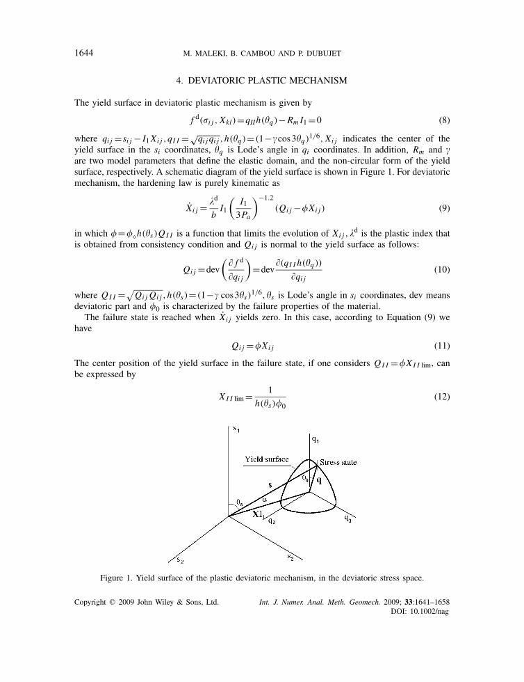
f d(�i j , Xkl)=qIIh(�q)−Rm I1=0 (8)

where qi j =si j − I1Xi j ,qI I =√qi jqi j ,h(�q)=(1−�cos3�q)1/6, Xi j indicates the center of the

yield surface in the si coordinates, �q is Lode’s angle in qi coordinates. In addition, Rm and �are two model parameters that define the elastic domain, and the non-circular form of the yieldsurface, respectively. A schematic diagram of the yield surface is shown in Figure 1. For deviatoricmechanism, the hardening law is purely kinematic as

Xi j = �d

bI1

(I13Pa

)−1.2

(Qi j −�Xi j ) (9)

in which �=�◦h(�s)QI I is a function that limits the evolution of Xi j ,�d is the plastic index that

is obtained from consistency condition and Qi j is normal to the yield surface as follows:

Qi j =dev

(� f d

�qi j

)=dev

�(qI I h(�q))

�qi j(10)

where QI I =√Qi j Qi j ,h(�s)=(1−� cos3�s)1/6,�s is Lode’s angle in si coordinates, dev means

deviatoric part and �0 is characterized by the failure properties of the material.The failure state is reached when Xi j yields zero. In this case, according to Equation (9) we

have

Qi j =�Xi j (11)

The center position of the yield surface in the failure state, if one considers QI I =�XI I lim, canbe expressed by

XI I lim= 1

h(�s)�0(12)

Figure 1. Yield surface of the plastic deviatoric mechanism, in the deviatoric stress space.



From Figure 1, we can deduce the following relation:

qI I = sI I − I1XI I cos()

cos(�s−�q)(13)

Substitution of Equations (12) and (13) in Equation (8) results in a limit envelope (failure surface)for the evolution of the yield surface as follows:

f r=sI I h(�s)−Rr I1=0 (14)

in which

Rr = I1 cos()

�0+ h(�s)cos(�s−�q)

h(�q)Rm I1 (15)

The value of �0 is, therefore, obtained by

�0= cos()

Rr − h(�s)

h(�q)Rm cos(�s−�q)

(16)

In the axisymmetric triaxial case �q =�s and =0; therefore, the expression of �0 takes thefollowing form:

�0= 1

Rr −Rm(17)

The concept of critical state is introduced in the model by choosing the following expressionfor Rr :

Rr = Rcr+ ln

(3PcrI1

)(18)

in which and Rcr are two parameters of the model. The critical state pressure Pcr, based oncritical state concept, is a function of plastic volumetric strain as follows:

Pcr= Pcr0 exp(c�pv) (19)

where Pcr0 is initial critical state pressure associated with initial void ratio (eo),1c is the slope of

the critical state line in �pv − ln(P) coordinates. In Equation (18) the effects of material densityand confining stress are taken into account. At the critical state we have I1=3Pcr and therefore,Rr = Rcr. The evolution of Rr , from the value corresponding to maximum resistance, to Rcr,provides an evolution of yield surface and allows the strain softening phenomena to be modeled.An envelope corresponding to critical state, that is characterized by Rcr, can be defined in stressspace (Figure 2) as

f cr=sI I h(�s)−Rcr I1=0 (20)



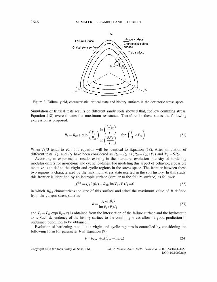
Figure 2. Failure, yield, characteristic, critical state and history surfaces in the deviatoric stress space.

Simulation of triaxial tests results on different sandy soils showed that, for low confining stress,Equation (18) overestimates the maximum resistance. Therefore, in these states the followingexpression is proposed:

Rr = Rcr+ ln

(Pf

Pm

) ln

(3PcrI1

)

ln

(3Pf

I1

) for

(I13

<Pm

)(21)

When I1/3 tends to Pm , this equation will be identical to Equation (18). After simulation ofdifferent tests, Pm and Pf have been considered as Pm = Pa ln ((Pcr+Pa)/Pa) and Pf =5Pcr.

According to experimental results existing in the literature, evolution intensity of hardeningmodulus differs for monotonic and cyclic loadings. For modeling this aspect of behavior, a possibletentative is to define the virgin and cyclic regions in the stress space. The frontier between thesetwo regions is characterized by the maximum stress state exerted in the soil history. In this study,this frontier is identified by an isotropic surface (similar to the failure surface) as follows:

f his=sI I h(�s)−Rhis ln(Pc/P)I1=0 (22)

in which Rhis characterizes the size of this surface and takes the maximum value of R definedfrom the current stress state as

R= sI I h(�s)

ln(Pc/P)I1(23)

and Pc= Pcr exp(Rcr/) is obtained from the intersection of the failure surface and the hydrostaticaxis. Such dependency of the history surface to the confining stress allows a good prediction inundrained condition to be obtained.

Evolution of hardening modulus in virgin and cyclic regimes is controlled by considering thefollowing form for parameter b in Equation (9):

b=bmon+z(bcyc−bmon) (24)



where z is defined by

z= Rhis−R

Rhis−Rcyc(25)

According to this expression, z varies between 0 and 1. In cyclic regime, R is equal to Rcyc, whichresults in z=1 or b=bcyc. In the case of monotonic loadings, R is equal to Rhis and therefore, ztakes the value of 0. Rhis−Rcyc defines a transition zone for continuous transfer between virginand cyclic domains. In this study we consider Rcyc=0.95Rhis.

The kinematic hardening equation in the basic model (Equation (9)), due to its relatively linearform, cannot reproduce just the nonlinear behavior of soil. To improve the response of the modelunder monotonic and cyclic loadings, according to the experimental results, bmon and bcyc aredefined as follows:

bmon=bm(1−(1−�m)m) (26)

where m =(Rme/Rr )2 , Rme is the biggest value of R=sI I h(�s)/I1 (Rme changes only in virgin

domain). In addition �m and bm are two model parameters. In the above derivation, m variesbetween 0 and 1. Therefore, bmon will change from a minimum value (bm) to a maximum value(�mbm). Simulations of different triaxial tests showed that �m can be considered as a constantdefault parameter. We have considered �m =10 that allows a simple form for bmon according tothe following equation:

bmon=bm(1+9m) (27)

The expression chosen for bcyc is given by

bcyc=bc(�c−(�c−1)c) exp(−d2�pv) (28)

The choice of a similar form of m for c is not compatible with cyclic behavior of soils. Therefore,c is defined as a function of plastic deviatoric strain as

c=exp(−d∗1 k) (29)

The evolution of k takes the following form that allows a better modeling of hysteresis behavior:

k= 1

(1+�)

(1−�

qi j Xi j

|qkl Xkl |)epI I (30)

where epI I =√epi j e

pi j , e

pi j = �pi j −(�pv/3)�i j ,�

pv is the plastic volumetric strain and d2,�c,bc and �

are cyclic parameters of the model. Furthermore, d∗1 is a function that allows us to consider the

influence of previous loading cycles in undrained conditions. The experimental results for sandysoils indicate that, in undrained condition, the rate of pore water pressure evolution becomes lowerafter the first few shearing cycles. However, if the cyclic loading is continued, this rate increases.For this reason, d∗

1 takes the following expression:

d∗1 =d1

⎛⎜⎜⎝Rhis ln

(3PcI1

)

Rr

⎞⎟⎟⎠

m

(31)



where m and d1 are parameters of the model. It was found that parameter m can be consideredconstant with a value of two. The variable k in Equation (30) is initialized to zero for everyreverse of stress. The incorporation of volumetric plastic strain in Equation (28) allows the cyclicdensification in drained condition to be modeled. During cyclic loading, c is equal to one. Fora semi-cycle, in the starting point (stress reverse point), bcyc takes its minimum value (bc). If ashearing loading is pursued, the plastic deformation increases and bcyc tends to bc�c.

4.1. Flow rule in the deviatoric plastic mechanism

The flow rule in the deviatoric plastic mechanism is non-associated and expressed by

�dpi j =�dGi j (32)

where Gi j is the derivative of plastic potential function. The dilatancy law for the basic versionof the model is as follows:

�dpv =

(sI IscI I

−1

) |si j edpi j |sI I

(33)

in which is a parameter of the model and scI I corresponds to the characteristic state that definesa surface similar to the failure surface in the stress space (Figure 2) as

scI I h(�s)−Rc I1=0 (34)

in which Rc is a model parameter. The characteristic surface separates the contractancy anddilatancy states of material. Equation (33) can be also expressed by

�dpi j �i j −

(sI IscII

−1

) |si j edpi j |sI I

= �dpi j ni j =0 (35)

In this expression ni j is the tangent tensor to the plastic potential function. Using edpi j = �dpi j −(�dpv /3)�i j ,ni j takes the following form:

ni j = ′ si jsI I

−�i j√ ′2+3

(36)

where ′ = ((sI I /scI I )−1

)sign(si j e

dpi j ).

The term of sign(si j edpi j ) allows us to eliminate the dilation in plastic unloading. Inner product

of � f d/��i j (normal to yield surface) and ni j leads to have the following expression for Gi j :

Gi j = � f d

��i j−

(� f d

��klnkl

)ni j (37)

The recent experimental results concerning stress–dilatancy relationships of sandy soils, particu-larly the works of Shahnazari and Towhata [17], indicate that for each complete cycle after primaryloading, the stress–dilatancy curve consists of two approximate parallel nonlinear segments of



Table I. Role or physical meaning and method for determination of parameters.

Parameter Role or/and physical meaning Definition method

n Controls the dependency of elastic Conformity on loading and unloadingparameters to the mean stress curves in isotropic triaxial test

K eo Controls the elastic response in Conformity on loading and unloading

isotropic loading curves in isotropic triaxial testKpo Controls the plastic response in Conformity on loading and unloading

isotropic loading curves in isotropic triaxial testGo Controls the elastic response in Related to initial slope of q−�1 curve

deviatoric loading (unloading segment)Rm Characterizes the size of yield surface From yield surface equation for stress

(elastic domain) state corresponding to �1∼=10−4 in q−�1curve

Controls the failure state Using the peak points in q−�1 curvesbm Hardening parameter in virgin region Conformity on q−�1 curves in virgin

loading� Controls the asymmetric form of Using the critical state point in q−�1

failure or critical state surface curves in compression and extension orconformity on Lade’s failure surface [18]

Rcr Characterizes the size of critical state Using the critical state point in q−�1surface curves. (Rcr is directly related to

critical state line slope (M))Rc Characterizes the size of characteristic state Using characteristic stress state in q−�1

surface curves, in which ��v =0, and solvingcharacteristic state surface equation—forfirst estimation Rc∼= Rcr

m Controls the intensity of plastic volume Using mean slope of �v −�1 curve inchanges due to deviatoric loading in virginregion

dilation state and solving stress–dilatancyrelationship of the model

Pco Critical state parameter, introducing Initial void ratio and critical state linethe compacity state of material (�v −ln(Pc)) allows Pco to be obtained

easilyc Critical state parameter controlling the 1/c is the slope of the critical

intensity of Pcr (critical state pressure) state line in the �v −ln(P) planebc,�,�c,d1, Cyclic parameters of model Using cyclic triaxial test in drained ord2, c undrained conditions—for first

estimation:bc∼= bm

3 and c∼= m2

positive slopes and two nearly vertical segments immediately after stress reversals. These resultsalso show that the stress–ditatancy relationship during the primary loading is different from stress–dilatancy relationship of the subsequent cycles. For this reason, the dilatancy modulus in the presentmodel in monotonic (primary loading) and cyclic region is considered to be different.

= mon+z( cyc− mon) (38)

The dilatancy modulus for monotonic loading is given by

mon= m((1−�m)�m−1) (39)



Figure 3. Simulation of drained compression triaxial tests for determination of staticparameters of the proposed model.

Figure 4. Simulation of a drained cyclic triaxial test for determination of model cyclic parameters,in comparison with Figure 5.

in which �m takes the following form:

�m =(Rme

Rc

)2

(40)

that allows a nonlinear form for the stress–dilatancy relationship to be taken into account. The �mchanges from zero to one in contractancy domain. In dilatancy domain �m is a constant equal to one. m and �m are the model parameters. In cyclic domain the dilatancy modulus is given by

cyc= c((1−�c)�c−1) (41)



Figure 5. Drained cyclic triaxial test results, which are used for the definitionof the model cyclic parameters [15].

Figure 6. Validation of the model on drained extension triaxial tests.

According to the cyclic experimental results, �c is assessed by the following expression:

�c=(XmI I

XmeI I

)2

(42)

where XmI I =

√(Xi j −Xm

i j )(Xi j −Xmi j ), X

mi j is equal to Xi j in stress reversal position. Xm

i j is taken

constant until the next reverse of loading. The XmeI I is the biggest value of Xm

I I . mon and cycchange from the maximum values (− m and − c) to the minimum values (−� m and −� c).



Figure 7. Validation of the model on drained cyclic triaxial test, in comparison with Figure 8.

Figure 8. Drained cyclic triaxial tests, which are used for validation of the model [15].

From triaxial test simulations, it was found that �m and �c can be considered as a constant withdefault value of three. Therefore, the mon and cyc take the following simple forms:

mon=− m(1+2�m) (43)

cyc=− c(1+2�c) (44)

5. IDENTIFICATION OF MODEL PARAMETERS

All of the model parameters can be determined easily using usual laboratory test results. Mostof the parameters are related to characteristics of triaxial tests by simple relationships [12]. To



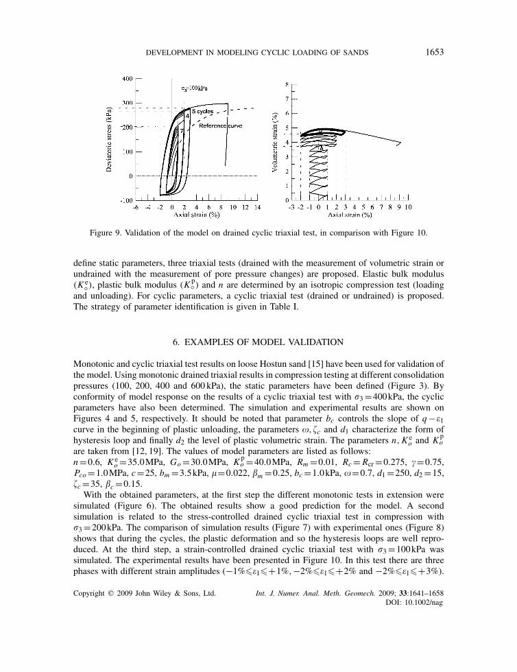
Figure 9. Validation of the model on drained cyclic triaxial test, in comparison with Figure 10.

define static parameters, three triaxial tests (drained with the measurement of volumetric strain orundrained with the measurement of pore pressure changes) are proposed. Elastic bulk modulus(K e◦), plastic bulk modulus (K p◦ ) and n are determined by an isotropic compression test (loadingand unloading). For cyclic parameters, a cyclic triaxial test (drained or undrained) is proposed.The strategy of parameter identification is given in Table I.

6. EXAMPLES OF MODEL VALIDATION

Monotonic and cyclic triaxial test results on loose Hostun sand [15] have been used for validation ofthe model. Using monotonic drained triaxial results in compression testing at different consolidationpressures (100, 200, 400 and 600 kPa), the static parameters have been defined (Figure 3). Byconformity of model response on the results of a cyclic triaxial test with �3=400kPa, the cyclicparameters have also been determined. The simulation and experimental results are shown onFigures 4 and 5, respectively. It should be noted that parameter bc controls the slope of q−�1curve in the beginning of plastic unloading, the parameters �,�c and d1 characterize the form ofhysteresis loop and finally d2 the level of plastic volumetric strain. The parameters n,K e

o and K po

are taken from [12, 19]. The values of model parameters are listed as follows:n=0.6, K e

o =35.0MPa, Go=30.0MPa, K po =40.0MPa, Rm =0.01, Rc= Rcr=0.275, �=0.75,

Pco=1.0MPa, c=25, bm =3.5kPa, =0.022, m =0.25, bc=1.0kPa, �=0.7, d1=250, d2=15,�c=35, c=0.15.

With the obtained parameters, at the first step the different monotonic tests in extension weresimulated (Figure 6). The obtained results show a good prediction for the model. A secondsimulation is related to the stress-controlled drained cyclic triaxial test in compression with�3=200kPa. The comparison of simulation results (Figure 7) with experimental ones (Figure 8)shows that during the cycles, the plastic deformation and so the hysteresis loops are well repro-duced. At the third step, a strain-controlled drained cyclic triaxial test with �3=100kPa wassimulated. The experimental results have been presented in Figure 10. In this test there are threephases with different strain amplitudes (−1%��1�+1%,−2%��1�+2% and −2%��1�+3%).



Figure 10. Drained cyclic triaxial test, including three parts (a), (b) and (c) with different amplitudes ofstrain, which are used for validation of the model [15].

The volumetric strain for points A, B and C (from [15]) are, respectively, 2.9, 4.35 and 5.8%. InFigure 9 the predicted variations of deviatoric stress (q) and of volumetric strain with axial strainhave been presented. The comparison of measured and predicted stress–strain curves indicates thatthe proposed model is capable of reproducing, quantitatively and qualitatively, the cyclic behaviorof soil. The predicted volume change deviates only slightly from the experimental results.

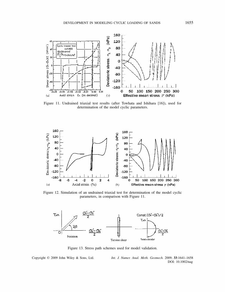
The results of undrained cyclic triaxial and hollow cylinder tests on Toyoura sand [16] havebeen used as another example of validation. At the first step, using existing results in the literature[16, 20], the monotonic parameters were estimated. The cyclic parameters were also identifiedusing the results of an undrained cyclic triaxial tests. The experimental and simulation resultsfor cyclic parameters determination are shown in Figures 11 and 12, respectively. Then, with theobtained parameters the model was validated in respect to the stress paths presented in Figure 13.



Figure 11. Undrained triaxial test results (after Towhata and Ishihara [16]), used fordetermination of the model cyclic parameters.

Figure 12. Simulation of an undrained triaxial test for determination of the model cyclicparameters, in comparison with Figure 11.

Figure 13. Stress path schemes used for model validation.



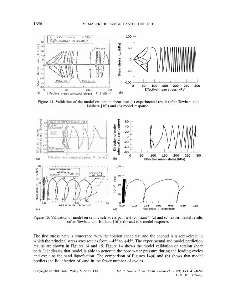
Figure 14. Validation of the model on torsion shear test: (a) experimental result (after Towhata andIshihara [16]) and (b) model response.

Figure 15. Validation of model on semi-circle stress path test (constant ): (a) and (c); experimental results(after Towhata and Ishihara [16]), (b) and (d); model response.

The first stress path is concerned with the torsion shear test and the second is a semi-circle inwhich the principal stress axes rotates from −45◦ to +45◦. The experimental and model predictionresults are shown in Figures 14 and 15. Figure 14 shows the model validation on torsion shearpath. It indicates that model is able to generate the pore water pressure during the loading cyclesand explains the sand liquefaction. The comparison of Figures 14(a) and (b) shows that modelpredicts the liquefaction of sand in the fewer number of cycles.



n=0.6, K eo =20.0MPa, Go=20.0MPa, K p

o =50.0MPa, Rm =0.01, Rc= Rcr=0.32, �=0.7, Pco=1.0MPa, c=25, bm =1.0kPa, =0.02, m =0.4, bc=1.2kPa,�=0.5, d1=250, d2=10.0, �c=25, c=0.3.

The simulation of second stress path is shown in Figure 15. It can be seen that model is capableof generating the excess pore water pressure under continuous rotation of principal stress axeseven when the deviator stress ((�1−�3)/2) is held constant during loading. This figure also showsthat after some cycles, the cyclic mobility creating the large strains occurs. In comparison withthe experimental results (Figures 15(a) and (c)), we observe that the model predicts the cyclicmobility in more number of cycles.

7. CONCLUSIONS

The following major results can be emphasized from the present study:

1. The application of a simple criterion in order to separate quality and intensity of hardeningmodulus in virgin and cyclic zones, in constitutive model having a simple kinematic hardeninglaw, allows cyclic behavior of sandy soils to be modeled easily.

2. The model is able to take into account hardening and softening behavior of sand.3. The model simulates the behavior of sand in drained and undrained conditions, in monotonic

and cyclic (in particular hysteretic behavior) loadings, in compression and extension loadingpaths.

4. The failure surface depends on mean stress, density and stress path. In addition, the lowconfinement stress effect is well modeled.

5. The critical state concept is introduced in the model.6. In the proposed model the contractive and dilative responses of sand, in monotonic and cyclic

loadings, are well modeled.7. All of the model parameters have physical meanings and can be defined easily from laboratory

tests results.

REFERENCES

1. Dafalias YF, Herrmann LR. Bonding surface formulation of soil plasticity. In Soil Mechanics—Transient andCyclic Loads, Pande GN, Zienckiewicz OC (eds), Chapter 10. Wiley: New York, 1982; 253–282.

2. Dafalias YF. Bounding surface plasticity I: mathematical foundation and hypoplasticity. Journal of EngineeringMechanics 1986; 112:966–987.

3. Iwan WD. On the class of models for the yielding behavior of continuous and composite system. Journal ofApplied Mechanics (ASME) 1967; 34:612–617.

4. Prevost JH. Plasticity theory for soil stress–strain behavior. Journal of Engineering Mechanics 1978;104-EM5:1177–1194.

5. Mroz Z, Norris VA, Zienkiewicz OC. An anisotropic hardening model for soils and its application to cyclicloading. International Journal for Numerical and Analytical Methods in Geomechanics 1978; 2:203–221.

6. Li XS, Dafalias YF. Dilatancy for cohesionless soils. Geotechnique 2000; 50:449–460.7. Manzari MT, Dafalias YF. A critical state two-surface plasticity model for sand. Geotechnique 1997; 47:255–272.8. Li XS. A sand model with state-dependent dilatancy. Geotechnique 2002; 52:173–186.9. Yong Z, Elgamal A, Parra E. Computational model for cyclic mobility and associated shear deformation. Journal

of Geotechnical and Geoenvironmental Engineering (ASCE) 2003; 129:1119–1120.10. Cambou B, Jafari K. Modele de comportement des sols non coherents. Revue Francaise de Geotechnique 1988;

44:43–55.



11. Cambou B, Jafari K. A constitutive model for granular materials based on two plasticity mechanisms. InConstitutive Equations for Granular Non-cohesive Soils, Saada AS, Bianchini GF (eds). Balkema: Rotterdam,1989; 149–167.

12. Maleki M. Modelisation hierarchisee du comportement des sols. Ph.D. Thesis, Ecole Centrale de Lyon, France,1998.

13. Maleki M, Dubujet Ph, Cambou B. Modelisation hierarchisee du comportement des sols. Revue Francaise deGenie Civil 2000; 4:895–928.

14. Maleki M. A constitutive model for sands. Journal of Isfahan University of Technology—Esteghlal 2008;27(1):51–65.

15. Mohkam M. Contribution a l’etude experimentale et theorique du comportement des sables sous chargementscycliques. Ph.D. Thesis, Institute of National Polytechnique de Grenoble, France, 1983.

16. Towhata I, Ishihara K. Undrained strength of sand undergoing cyclic rotation of principal stress axes. Soils andFoundations 1985; 25:135–147.

17. Shahnazari H, Towhata I. Tortion shear tests on cyclic stress-dilatancy relationship of sand. Soils and Foundations2002; 42:105–121.

18. Lade PV. Elastoplastic stress–strain theory for cohesionless soils with curved yield surface. International Journalof Solids and Structures (ASCE) 1977; 13:1019–1035.

19. Allouani M. Identification des lois de comportement des sols; definition de la strategie et de la qualite del’identification. Ph.D. Thesis, Ecole Centrale de Lyon, France, 1993.

20. Ishihara K. Liquefaction and flow failure during earthquakes, the 33rd Rankine lecture. Geotechnique 1993;43:351–415.


development in modeling cyclic loading of sands based on kinematic hardening

Documents