development of a coagulation coefficient measurement ... the time of this writing our first child,...
TRANSCRIPT

PHD Thesis
Development of a coagulation coefficient measurement device (CMD) for the measurement of the coagulation coefficient of nanoparticles in
the size range from 10 to 1000 nm
Dipl.-Ing. Bernhard Andreas Heiden Graz, 17th of January 2006
written at the Institute for Internal Combustion Engines and Thermodynamics
Traffic and Environment Section Graz University of Technology
Advisors:
Ao.Univ.-Prof. Dipl.-Ing. Dr. techn. Peter Johann Sturm Adjunct Prof. Dr. Athanasios G. Konstandopoulos

Acknowledgements
My sincerest thanks go to all who have contributed to this work. First of all is Ao. Univ.-Prof.
Dr. techn. Peter Sturm who had the initial idea of investigating this very fundamental problem
of aerosol technology. He was the primary person responsible for the sponsorship by the FVT
(Forschungsgesellschaft für Verbrennungskraftmaschinen und Thermodynamik), which made
the experiments, necessary for this kind of basic research1, possible. His generosity with time
insight and friendship both personal and professional are well known and it is to him I am
most indebted. I am also indebted to Adjunct Prof. Athanasios Konstandopoulos who was
willing to be my associate advisor, in spite of his very busy schedule, especially as he is one
of the experts in this reemerging field of nanoparticle research. The head of the Institute for
Internal Combustion Engines and Thermodynamics and all my colleagues are due my thanks,
especially Univ.-Prof. Dr. techn. Rudolf Pischinger, em. Univ.-Prof. Dr. techn. Helmut
Eichelseder, Ao.univ. Prof. Dr. Raimund Almbauer, Dipl.- Ing. Dr. Gerhard Pretterhofer for
discussing ideas, Dipl.-Ing. Dr. Hannes Rodler for helping with instruments and social
integration in the group as well as Dipl.-Ing. Michael Bacher, my co researchers, Mag.
Dr. Dietmar Öttl, Dipl.-Ing. Christian Kurz, Mag. Marlene Hinterhofer, Mag. Silvia
Vogelsang and the secretary Sabine Hartinger, Sabine Minarik and Alexandra Stiermair. I
enjoyed also the cooperation with the group under the direction of Univ.-Prof. Dr. techn-
Stefan Hausberger especially Dipl.-Ing. Martin Rexeis, Dipl.-Ing. Thomas Vuckovic, Dr.
Jürgen Blasnegger, Dipl.-Ing. Michael Zallinger. My thanks also go to Dipl.-Ing. Dieter
Engler, who introduced me in the use of the SMPS and CPC and all the other particulate
measurement equipment from the institute as well as to the former assistant Dipl.-Ing. Dr.
Mario Ivanišin for scientific exchange. Additionally I would like to thank the staff of the
laboratory for the help in the mechanical setup, especially Siegfried Gimpl, Günter Rumpf for
manufacturing parts of the CMD and indeed all others who are to numerous to mention.
1 This sampling system has been completely founded by the FVT (Research society of combustion engines and
thermodynamics) at the Institute for Internal Combustion Engines and Thermodynamics of the University of
Technology Graz.
Acknowledgements
4/177 Development of the CMD for the coagulation coefficient measurement
Dipl.-Ing. Helmut Wurm from National Instruments is due a special thank for fruitful,
repeated and personal assistance concerning the Labview Hard- and Software integration.
My diploma students Dipl.-Ing. Emil Bakk and Bernd Brugger are due thanks for having
supported the work of the CMD by their enthusiasm and work around the clock to prepare the
measurements in Munich and at the AVL Graz. Dr. Armin Messerer is due thanks for the
measurements at the TU-Munich. Dr. Schindler of the AVL is due thanks for the support with
the measurements with the CAST. My old friend Dipl.-Ing. Günter Jaritz is due many thanks
for building the electrical circuits of the CMD and discussing ideas as also for measurement
assistance in Munich. I am also indebted to Dr. Werner Schaffenberger who helped me in the
theoretical segment in clarifying the mathematical concepts. My thanks also go to Mr. Steven
Fowler, M.H. for editing the text for American English.
Last but not least, my personal thank goes to my wife, Bianca, who listened to my long
discussions about this topic, and who continually gave me motivation. As she is expecting at
the time of this writing our first child, who is according to the last ultra sound a boy.
I dedicate this work to our son.

Kurzfassung
Da die Luftverschmutzung von Nanopartikeln im Größenbereich von 10 bis 1000 nm einen
großen Einfluss auf die menschliche Gesundheit hat und der Dispersionsprozess von der
Emissionsquelle bis zur Immissionssenke noch nicht sehr gut prognostiziert werden kann, ist
es notwendig das Wachstumsverhalten von Aerosolen weiter zu untersuchen. Zu diesem
Zweck wurde ein mobiles Koagulationsmessgerät (CMD) entwickelt. Dieses dient dazu den
Koagulationskoeffizienten (K) von Aerosolen mit einem Durchmesser zwischen 10 und
1000 nm zu messen. Dabei ist K ist ein grundlegendes Maß für das Wachstum von Aerosolen.
Ein konstanter Konzentrationsaerosolreaktor, der aufgrund des veränderlichen Volumens
unterschiedliche Größenverteilungsmessungen ein und desselben Aerosols ermöglicht, wurde
zum ersten Mal gebaut, getestet und mit LABVIEW prozessautomatisiert. Eine bestehende
Theorie, die auf der allgemeinen dynamischen Gleichung (GDE) basiert, wurde für das CMD
angepasst und, unter Berücksichtigung von Koagulation und Diffusion, auf die Form einer
speziellen logistischen Gleichung gebracht. Die Anzahlkonzentrationsabnahmemessung
erlaubt zusammen mit der entwickelten Theorie die Auswertung des Koagulations-
koeffizienten mit einer Reihe von verschiedenen Methoden. Die sich daraus ergebenden
Koagulationskoeffizienten sind weitgehend kohärent mit Werten aus der Literatur. Die zwei
kontinuierlichen Konzentrationsmessmethoden, ergaben in Bezug auf die zwei
diskontinuierlichen Methoden für den Grenzfall kurzer Zeiten einen im Mittel um den Faktor
5 höheren Koagulationskoeffizienten. Die Ursache könnten Fluktuationen des Koagulations-
koeffizienten oder eine unterschiedliche Aerosolverdünnung sein. Zukünftiger
Forschungsinhalt ist die Anwendung des CMD auf die Unterscheidbarkeit von Aerosolen
oder der Partikelform und zur Bestimmung eines allgemeinen K.


Abstract
As nanoparticles in air pollution have a high impact on human health and the dispersion of
these particles can not be predicted very well, clarification of aerosol growth is necessary. A
mobile coagulation measurement device (CMD) was developed, measuring the coagulation
coefficient (K) of nanoparticles, where K is a basis quantity for the kinetics of aerosols. A
constant concentration aerosol reactor has been built, tested and automated with LABVIEW
for the first time, allowing for a variable volume and time dependent concentration
measurements of the same aerosol. A theory was adapted for the CMD based on the
fundamental general dynamics equation (GDE), which is reduced to the form of a special
logistic equation, taking coagulation and diffusion into account. The measurement of the
number concentration decay and of their distribution allows, together with the developed
theory, for the evaluation of K with a number of different methods. The resulting values of K
reflected that from the literature. The two continuous concentration measurement methods
yielded, compared to the two discontinuous methods, for the limiting case of short times, an
average 5 times higher K. The cause might have been fluctuations of K or the influence of
different aerosol dilution. Future research areas are the application of the CMD to the
distinction of various aerosols, the investigation of the particle form, and derivation of a
general K.

Content
Acknowledgements .................................................................................................................... 3
Kurzfassung................................................................................................................................ 5
Abstract ...................................................................................................................................... 7
Content ....................................................................................................................................... 9
List of principal symbols.......................................................................................................... 13
Indices .................................................................................................................................. 18
Introduction .............................................................................................................................. 19
Air pollution and impact on human health........................................................................... 19
Choice of measurement quantities ....................................................................................... 19
Necessity of a new characteristic aerosol quantity............................................................... 20
Core of the thesis.................................................................................................................. 20
Overview .............................................................................................................................. 22
I Theory .............................................................................................................................. 23
I.1 Problem formulation ................................................................................................ 23
I.2 Aerosol characterization........................................................................................... 24
I.2.1 On the lognormal size distribution interpretation ................................................ 24
I.2.2 Application to fractal aggregates.......................................................................... 25
I.2.3 The lognormal size distribution............................................................................ 26
I.3 Aerosol dynamics relevant for the coagulation coefficient...................................... 27
I.3.1 General Dynamics Equation (GDE)..................................................................... 27
I.3.2 Diffusions coefficient D ....................................................................................... 30
I.3.3 Coagulation coefficient K .................................................................................... 31
I.3.3.1 Smoluchowski equation ............................................................................... 31
I.3.3.2 Approximation of applicability of the Smoluchowski Equation.................. 31
I.3.4 Determination of the coagulation coefficient K................................................... 33
I.3.4.1 Theory of loss by coagulation and diffusion................................................ 33
I.3.4.2 Method (1) - Constant Volume Batch Reactor (CV) for short times ........... 35
I.3.4.3 Method (2) - Constant Volume Batch Reactor (CV) for long times........... 37

Content
10/177 Development of the CMD for the coagulation coefficient measurement
I.3.4.4 Method (4) - Constant Concentration Reactor (CC) for long times............ 37
I.3.4.5 Method (3) - Constant Concentration Reactor (CC) for short times........... 40
I.3.5 Predicted application of the measurement of the quantity K ............................... 42
I.3.5.1 Fractal dimension determination.................................................................. 42
I.3.5.2 Primary particle diameter ............................................................................. 44
II Description of the CMD................................................................................................... 45
II.1 Principle of operation of the CMD........................................................................... 45
II.2 Setup of the CMD .................................................................................................... 46
II.2.1 System setup..................................................................................................... 46
II.2.1.1 Standard SMPS system ................................................................................ 46
II.2.1.2 CMD system................................................................................................. 47
II.2.2 Settler ............................................................................................................... 50
II.2.3 Effective flow rate............................................................................................ 51
II.2.3.1 Settler volume determination ....................................................................... 52
II.2.3.2 Total time calculation................................................................................... 56
II.2.3.3 Pressure drop ................................................................................................ 56
II.2.3.4 Pressure and temperature dependence.......................................................... 58
II.2.3.5 Gas dependence............................................................................................ 63
II.3 Operation of the CMD.............................................................................................. 63
II.3.1 Path concept ..................................................................................................... 63
II.3.2 Operation concept ............................................................................................ 64
II.3.2.1 Complex operation types.............................................................................. 65
II.3.2.2 Simple operation types ................................................................................. 67
II.3.3 Labview software implementation ................................................................... 69
II.3.3.1 Structure ....................................................................................................... 69
II.3.3.2 Main menu.................................................................................................... 70
II.3.3.3 Initialization ................................................................................................. 71
II.3.3.4 Measurement ................................................................................................ 72
II.4 Fundamental considerations..................................................................................... 76
II.4.1 Reactor characterization................................................................................... 76
II.4.2 Residence times................................................................................................ 78
II.4.2.1 Overall residence time for measurement...................................................... 79
II.4.2.2 Settler ........................................................................................................... 80

Indices
Development of the CMD for the coagulation coefficient measurement 11/177
II.4.2.3 DMA............................................................................................................. 82
II.4.2.4 CPC .............................................................................................................. 85
II.4.3 Dilution............................................................................................................. 86
II.4.3.1 Dilution in the CPC...................................................................................... 86
II.4.3.2 Dilution due to incomplete filling ................................................................ 87
II.4.4 Impaction, deposition and other effects ........................................................... 87
III Measurements of the coagulation coefficient with the CMD ...................................... 89
III.1 Monodisperse aerosols ............................................................................................. 89
III.1.1 Control measurement ....................................................................................... 93
III.1.2 Results: Smoluchowski coagulation plot ......................................................... 94
III.2 Polydisperse aerosols ............................................................................................... 95
III.2.1 Measurement of the coagulation coefficient of polydisperse aersols by means
of size distribution measurements - Incense Measurements ............................................ 95
III.2.2 Measurement of the coagulation coefficient of polydisperse aersols by means
of a number distribution measurement............................................................................. 99
III.2.2.1 Polydisperse Coagulation I (Method 4) ................................................... 99
III.2.2.2 Polydisperse Coagulation II (Method 3) ................................................ 103
IV Conclusions ................................................................................................................ 109
IV.1 Theory of coagulation and diffusion ...................................................................... 109
IV.2 Coagulation Measurement Device (CMD) ............................................................ 110
IV.3 Coagulation coefficient .......................................................................................... 112
IV.4 Outlook................................................................................................................... 113
Literature ................................................................................................................................ 115
Figures.................................................................................................................................... 119
Tables ..................................................................................................................................... 125
Index....................................................................................................................................... 129
Appendix A Detailed specifications .................................................................................. 131
Tubes .................................................................................................................................. 131
Detailed residence times and flow chart ............................................................................ 132
Settler ................................................................................................................................. 136
Appendix B Visual Basic programs for the lognormal size distribution....................................... 137
Appendix C Labview 7.1 software implementation of the CMD....................................... 141
Detailed main front panel................................................................................................... 141

Content
12/177 Development of the CMD for the coagulation coefficient measurement
Software hierarchy ............................................................................................................. 141
CMD stepper motor control ............................................................................................... 145
Software variables in the Labview 7.1 implementation..................................................... 146
Devices and corresponding programs ................................................................................ 152

List of principal symbols
Var Description Unit # Particle(s) ~ [] Denotes units inside the brackets ~ A Lacunarity ~ A “Area” ~ Abbr. Abbreviation ~
AIMS Aerosol instrument manager software of the standard SMPS system (e.g. DMA 3081 and CPC 3010) ~
ASETTLER Inner surface area of the settler inside m2 ASF Flow sensor ASF1430 from Sensirion ~ ASP Differential pressure sensor from Sensirion ASP1400 ~ B Second virial coefficient ~ bool Boolean ~
C Cunningham-Knudsen-Weber-Millikan correction factor for the diffusion coefficient ~
CAST
Soot particle generator for production of defined particle number concentrations from Matter-Engineering www.matter-engineering.com ~
CC Cumulative Counts since the last measurement from the CPC - CC Constant Concentration reactor ~ CD Compact disc ~ CMD Coagulation measurement device ~ CNC Condensation nuclei counter ~ CPC Condensation particle counter ~ cs Terminal settling velocity m/s csf Terminal settling velocity of fractal particles m/s CSTR Continuously Stirred Tank Reactor ~ CT Cumulative Time of the last measurement from the CPC s CV Constant volume reactor ~ D Diffusion coefficient m2/s Df Fractal dimension ~ di_SETTLER Inner diameter of the settler m dm Differential mass kg dm Mean settler diameter m
dm Collision diameter – distance between the centers of two molecules m
DMA Differential mobility analyzer ~ dN Differential particle concentration #/cm3 dN0 Differential particle concentration of CPC measurement #/cm3 dN00 Differential particle concentration of CPC dilution air #/cm3 do_SETTLER Outer diameter of the settler m
List of principal symbols
14/177 Development of the CMD for the coagulation coefficient measurement
Var Description Unit Dp Diffusion coefficient of particle with diameter dp m2/s dp Diameter of Particle nm Dp0 Diffusion coefficient of particle with primary diameter dp0 m2/s dp0 Diameter of primary particle of a fractal aggregate nm dp1 Pressure drop impactor (cm H2O) cm H2O dp2 Pressure drop across the bypass orifice mm H20 dp3 Differential pressure of ASP1400 (CMD settler) Pa dpg Geometric mean diameter of particle nm
dpmax Diameter of Particle MAXimum that could be measured with SMPS nm
dpmin Diameter of Particle MINimum that could be measured with SMPS nm
DRVi i=1..3 manual needle valves ~ dV Differential volume cm3
EK-H2 Evaluation Kit EK-H2 from Sensirion; microcontroller access kit for the humidity sensors. The sensor SHT75 was used. ~
Ft With of one fold of the settler m Fz Number of fold of the settler ~ g Gravitational constant m/s2 GDE General dynamics equation ~ Gilibrator 2 Calibration bubble flow meter from Sensidyne ~ GMEAMOD Variable in the CMD program for setting the operation ~ h Diffusion layer thickness m
HASOTEC Company for the used stepper motor hardware www.hasotec.com ~
HCX001A6V Absoluter pressure sensor from SensorTechnics ~ I Particle current according to nucleation law INNOFLEX Company for settler production www.faltenbalg.de ~ K Coagulation coefficient cm3_gas/(#*s) k Boltzmann constant: k=R/NA=1.38*10-23 J/K Ka Apparent coagulation coefficient cm3_gas/(#*s)
Kac Apparent coagulation coefficient for constant concentration reactor cm3_gas/(#*s)
Km Mean coagulation coefficient cm3_gas/(#*s) Kp Coagulation coefficient of particle with diameter dp cm3_gas/(#*s) Kp0 Coagulation coefficient of primary particle with diameter dp0 cm3_gas/(#*s) L Length Length L Particle wall diffusion frequency 1/s L_Settler_min Settler minimum size due to folds m
L0 Particle wall diffusion frequency for constant concentration reactor 1/s
L0m Mean L0 1/s LABVIEW Labview 7.1 Software from National Instruments www.ni.com ~ LDMA DMA Characteristic Length m Lmax Settler maximum actual size m Lmin Settler minimum actual size m LMS Least mean squares fit ~ lpm Liter per minute ~

Indices
Development of the CMD for the coagulation coefficient measurement 15/177
Var Description Unit m.v. Measurement value ~
Mathcad® Mathematic software package from Mathsoft www.mathsoft.com ~
Matter-Engineering
www.matter-engineering.com ~
MDP Monodisperse particle diameter nm MG Molecular weight kg/mol N Number of scan intervals - N Particle concentration #/cm3 N∞ Total particle concentration #/cm3 n(v),n( v ) Volume distribution #/(L3_particle*L3_gas) n0 Initial number concentration #/cm3 N0 Initial total particle concentration #/cm3 NA Avogadro constant NA=6.022*1023 #_gas/mol NBR Antistatic rubber mixture of the settler from INNOFLEX ~ nd Particle size distribution function #/(cm3*nm) NI National Instruments (see Labview) ~ Np Number of particles in a fractal aggregate ~ Np, primary Total number of primary particles in volume V ~ NSM number of single measurements - ntot Total particle counts since last measurement # operation A series of paths see II.3.2 ~ p Pressure mbar p0 Ambient air pressure mbar p1 Absolute pressure (SMPS sensor) mbar p2 Absolute pressure sensor CMD (settler) mbar path Valve setting leading to a fluid path in the CMD see II.3.1 ~ ps Standard pressure (1013mbar) mbar
Q Effective constant flow rate of the settler as a function of the stepper motor velocity lpm=l/min
R Gas constant: R=8.31441 J/(mol*K) r2 Pearson’s regression coefficient ~
rd Is proportional to dN; The actual particle concentration of the CPC #/cm3
Re Reynolds number ~ Rex Local Reynolds number ~ rgbx Command code SMCard SM41 (HASOTEC) ~ ri_DMA DMA Inner Radius m ro_DMA DMA Outer Radius m ROTDRV1 Rotations of needle valve DRV1 Rot(ations) rpm Rotations per minute ~ RS232 Serial interface ~ RSV Unidirectional valve ~ S Surface area m2 S/V Surface area to volume ratio of the settler m2/m3 Sc Schmidt number ~ sccm Standard cubic centimeter ~ SCT SCan Time in seconds. Scan time for one size distribution s

List of principal symbols
16/177 Development of the CMD for the coagulation coefficient measurement
Var Description Unit measurement
SEM Scanning electron microscopy ~ Sensidyne www.sensidyne.com ~ Sensirion www.sensirion.com ~ SensorTechnics www.sensortechnics.com ~ sff Safety factor for increasing filling time ~ SHT75 Humidity sensor form Sensirion (see also Sensirion) ~ Shx Local Sherwood number ~ SM-41-PCI PCI Interface card from HASOTEC for stepper motor control ~ SMPS Scanning mobility particulate sizer ~
SMPS 3081 Standard SMPS system from TSI containing the classifier 3081, the DMA 3080 and the CPC 3010 ~
SPFA Speed factor for the stepper motor ~ t Time s, min T Temperature °C T1 Cabinet temperature °C T2 Sheath flow temperature °C T3 Bypass flow temperature °C T4 CPC Condenser temperature °C T5 CPC Saturator temperature °C T6 ASP temperature °C T7 CMDC temperature Pt100 °C T8 CMD Balg: Humidity temperature sensor on EK-H2 °C tCLEAN Time for STEP Cleaning of the CMD Balg s tCOAGUL Time for STEP coagulation s
td Residence time of the CPC 3010 and the standard tubing from the SMPS DMA to the SMPS CPC. s
td’ Calculated td s
tf Is the residence time in the SMPS DMA from the AIMS software tf is the same as τ3 s
tFILL Time for STEP filling the probe into the CMD Balg s tMEAS Time for STEP Measurement with the SMPS s Ts Standard temperature (20°C) °C TSI TSI Aerosol Instrumentation Company (www.tsi.com) ~ ttotal Time total s
ttotal Total time of measurement x; total time of all measurements of one settler probe min
u Velocity, bulk velocity L/time ;m/s UV Ultraviolet radiation ~ v Volume of particle m3 V (Gas) Volume m3,length3 v, v Volume L3 V/S Volume to Surface area ratio of the settler m3/m2 v0 Volume of primary particle of an fractal aggregate m3 V0 Volume of air in the path between SMPS DMA & SMPS CPC l
V0S Volume of air in the path between SMPS DMA & SMPS CPC according to AIMS software and standard setting l
V0S’ Calculated V0S l

Indices
Development of the CMD for the coagulation coefficient measurement 17/177
Var Description Unit V1 Volume of air in the path between settler and SMPS in l V2 Volume of air inside the SMPS between input and DMA l V3 Volume inside the SMPS DMA l V4 Volume of air in the path between SMPS and CPC for the CMD l
V5 Volume of air in the path between settler and CPC for settler measurement mode without DMA volume l
V6 Volume of gas in the CPC 3010 in the sample flow line between inlet and laser particle measurement in the CPC l
V7 (Total) Effective volume in the settler that can be pressed out l
V70 Total gas volume of the settler or when the settler is in the end switch position on the bottom. l
V7min Settler rest volume when empty l
V9 Volume of air in the path between settler and CPC in (part of path 4) l
vb Bulk velocity of the particles m/s vBALG Velocity of "BALG" Upm vd Minimum volume l Vi i=1..8 magnetic two way valves ~ vi Virtual instrument – this is a program module in Labview ~ vi’ See vi ~ Vmax Maximum volume of the settler l VMi i=1..2 manual two way ball valves ~ Vmin Effective minimum volume of the settler l vMOT Motor control velocity (from SM card) - appr. motor velocity Upm Vp (Gas) Flow rate l/min Vp1 Sample Flow rate SMPS lpm Vp2 Sheath Flow rate SMPS lpm Vp3 Bypass Flow rate SMPS lpm Vp4s, Vp4 Flow rate ASF Sensor sccm, lpm Vp6 Flow rate of the CPC dilution air Lpm Vp7 Identical with Q; lpm xi i=1..3 Cartesian coordinates x,y,z L (length) xq Transformation factor between dN and dN/dlog(dp) ~
ZIMM Company for machine components and elements www.zimm-austria.com ~
∆L Difference between Lmax and Lmin m α Leakage ratio ~ α° Contraction number ~ β Particle transfer coefficient m/s βx Local particle transfer coefficient m/s β Collision frequency function cm3_gas/(#*s) δ Flow rate percentage increase ~ φ1 Relative humidity sensor CMD % γ Settler correction of dm for real volume [time/time] γ Total time ratio: t/ttotal ~ κ Differential pressure correction factor ~ λ Mean free path of the gas m µ Dynamic viscosity kg/(m*s)

List of principal symbols
18/177 Development of the CMD for the coagulation coefficient measurement
Var Description Unit ρg,ρ Gas density kg/m3 ρL Density of air kg/m3 ρp Particle density kg/m3 σg Geometric standard deviation ~ τ Residence time s τCPC Residence time in the CPC 3010 s τi Residence time according to Vi i=0..6;9 s
τtot Total residence time for settler measurement from the settler to the CPC s
τtot0
Total residence time for settler measurement from the DMA to the CPC for SMPS measurement setup (standard SMPS measurement) s
τtrans Total residence time for settler measurement from the DMA to the CPC for CMD measurement setup s
τΙ Time dp is shifted to concentration because of residence time between DMA and CPC s
τΙΙ Time the raw data are shifted to the beginning of measurement mode s
ζ Sample to sheath flow volume ratio of the DMA ~
Indices Index Description B Bulk D Distribution F Fractal L Leakage, air M, m Mean max Maximum min Minimum P Particle P0 Referring to primary particle s,S Standard tot Total u Infinite volume
Introduction
Air pollution and impact on human health Air pollution of anthropogenic nanoparticles is in the size range of 10 to 1000 nm, mainly
caused by combustion processes in industry, traffic and domestic fuel use. The lung is
primarily affected by the deposition of such particles (Oberdörster 2001; Oberdörster 2004),
causing pulmonary emphysema (Sturm and Hofmann 2004) and other lung diseases.
Nanoparticles can also be found in the blood vessels, causing cardiovascular diseases (Schulz
2004), as well as in every organ linked to illnesses like Parkinson’s disease (Gatti and
Montanari 2004; Hudson and others 2001), and even in the brain (Oberdörster and others
2004). Inflammatory reactions are caused due to particulate matter in the lungs, depending on
the NO2/NO ratio (Morin 2004), which is important for traffic emissions.
As a consequence there is evidence that nanoparticles reduce life expectancy
significantly and they have a high impact on human health.
Choice of measurement quantities To estimate the effect of particle emissions on health effects or their dispersion concentration,
three methods are available:
a.) In situ measurements or measurements nearby the emission source.
b.) Model measurement or measurement of the emission in a model of the real situation,
for emission dispersion calculation.
c.) Theoretical calculations of the emission dispersion by means of numerical
simulations.
As measurement or model measurement is an expensive tool, simulation of the particle
concentration evolution will be applied. First there exists a wide spectrum of emission
dispersion models (Zenger 1998) which are able to simulate gases but they are not so
successful for nanoparticle concentration predictions. They need additional relevant particle
dispersion parameters for increasing prediction accuracy.

Introduction
20/177 Development of the CMD for the coagulation coefficient measurement
To predict the health effects it is therefore of importance to find the relevant quantities of the
physical problem of pollution dispersion. It has been found that there is a strong dependency
of particle size and lung deposition (Heiden 2005), which can be extended to particle form.
Particle number size distribution measurements were done, e.g. for typical traffic situations
like in the urban background at a curbside location and in a tunnel. They were found to be in
the range of 103 to 105 #/cm3 (Sturm and others 2003). Particle number concentration
measurements and their relationship to the particle lung deposition were made for different
European cities (Mitsakou and others 2005), showing significant particle lung deposition.
For these reasons it can be concluded that the human health effects are related directly to
measurement quantities as the particle number concentration, particle diameter, particle form
and/or the particle size distribution.
Necessity of a new characteristic aerosol quantity
When looking at different size distributions it can be found that, given a similar
emission/dispersion situation and the same mass concentration, different size distributions
may exist (Heiden and others 2005), and that the same size distribution may appear the same
for different aerosols. It is, therefore, insufficient to measure either the particle mass alone or
the particle size distribution to yield clear information about the particle concentration over
time. This leads to a high degree of uncertainty in prediction of the concentration.
Therefore, time dependent aerosol quantities appear to be most apt to increase the
accuracy of the particle concentration prediction. One process of particle growth is
coagulation2. Its characteristic quantity is the coagulation coefficient K, on which I focused
my work. This quantity has not been measured in a standardized way up to now and it seems
to be fundamental for prediction of the evolution of the particle concentration over time due
to coagulation, as it affects all methods of determining health effects, from measurements of a
new quantity to theoretical calculations by means of this quantity K. Furthermore, systematic
measurements of K allow for developing coagulation theories for nanoparticles.
Core of the thesis The coagulation measurement device (CMD) is the core unit referred to in this work. The aim
of such an instrument is to measure the kinetics of coagulation of nanoparticle aerosols. It was
my aim to build a portable instrument for measuring the coagulation coefficient in the
2 Others are condensation, nucleation, chemical reaction etc.

Core of the thesis
Development of the CMD for the coagulation coefficient measurement 21/177
nanoparticle size range. In the literature, single measurements of the coagulation of
nanoparticles were often made during the last century. The measurements were made mainly
with particle number concentration measurements (Husar 1971; Rooker and Davies 1979) or
even with particle number size distribution measurements (Schnell and others 2004). Some
kind of closed batch reactor is the usual method of measuring the coagulation kinetics,
because an aerosol cannot easily be kept constant in concentration. For example large bags
were often used with a large volume to surface ratio, allowing for increasing neglect of wall
diffusion. All of these methods show the problem of the reactor being physically very large
and, therefore, not portable. Scaling down the size of the reactor, the aerosol volume sampled
cannot be neglected compared to the volume of the settler3. For a closed, constant volume
reactor this means that the pressure drops. To compensate for this I developed the constant
concentration reactor4 allowing for a theoretically constant thermodynamic state with respect
to pressure and temperature.
Figure 1 Built CMD5
The CMD, including the constant concentration reactor and the commercial SMPS system
(Scanning Mobility Particulate Sizer System) from TSI, is shown in Figure 1. It has been built
3 Aerosol batch reactor or container for coagulation (in general any reaction) and subsequent particle concentration measurement. 4 Constant concentration refers to an ideal (not real existing) state of no coagulation and no deposition to the reactor walls.

Introduction
22/177 Development of the CMD for the coagulation coefficient measurement
at the laboratory of Internal Combustion Engines and Thermodynamics at the Graz University
of Technology from 2004 to 2005. The programming and process automation was imple-
mented with the Labview 7.1 Software, allowing for significant time and cost savings6.
There have been made two diploma theses on the CMD (Bakk 2005; Brugger 2005)
looking at the fail-safe analysis of the CMD, and on routines for the normal measurement
mode of the CMD.
Overview This thesis consists of four main chapters. The first refers to the theoretical background of the
system, the underlying physics, the theory of simultaneous coagulation and diffusion first
adapted for the concept of the constant concentration reactor and its derivation for practical
application.
The second chapter contains the description of the CMD. What it consists of, the basic
components, experiments related to the build CMD and application diagrams when measuring
with the CMD to keep overview of the basics of the CMD system. The principles of operation
are explained as well as the practical use of the Labview software I developed for the CMD
during development.
The third chapter contains a selection of experiments demonstrating the principal use
of the CMD for different concepts of measurement the coagulation coefficient. Main
applications are the measurement of the mono- and polydisperse coagulation coefficient, with
different methods.
In the fourth chapter the results are summarized and an outlook is given for the CMD,
mainly intended to be a fundamental research instrument. E.g. with additional hardware, the
temperature dependency or additional reactor type equivalent measurements7 could be
investigated.
In the Appendices additional information is given for the detailed specifications of
some key elements of the CMD, visual basic programs for calculating the logarithmic normal
distribution from experimental data and an overview over the Labview program hierarchy.
The Labview programs are also available on the accompanying CD.
5 A detailed description is given in chapter II and in the appendices. 6 Comparable results from 40 coagulation coefficients from (Rooker and Davies 1979) can be done with the CMD in one week compared to two years project duration. 7 Other than the constant concentration reactor; e.g. Continuously Stirred Tank Reactor (CSTR) with variable residence time (see section II.4.4).

I Theory
I.1 Problem formulation Combustion generated nanoparticles are a main concern for air pollution and its health risks.
There are still open questions about the residence time8 in the atmosphere and the laws of
growth of nanoparticles, which are typically found in the transition regime9 in the size range
between approximately 10 nm and one micrometer. It is not well understood in a theoretical
sense, especially concerning coagulation. For this problem there are mainly two
approximations at the end of this range, one of statistical thermodynamics and one deduced
out of the Einstein approximation for Brownian motion (Friedlander 2000).
Both regimes together can be expressed as coagulation kernel β or K in the
Smoluchowski equation in the transition regime by interpolation first accomplished by
Fuchs (Fuchs 1989).
Measurement of physical quantities in the transition regime is both important for
understanding the underlying physics and the atmospheric processes. Experimental
investigations of particle evolution are available for special cases of aerosols and a limited
number of physical quantities. The basic description for this process is given by the
Smoluchowski equation (Smoluchowski 1917), which is part of the GDE10 or equation (I-17).
The aim of the work is to investigate the physical process of coagulation in the transition
regime in a systematic and flexible way, as for this purposes no standard measuring procedure
is available. To fill this gap, an aerosol coagulation coefficient measurement device (CMD)
has been developed to measure systematically the coagulation coefficient, which corresponds
to the coagulation kernel of the Smoluchowski equation. By means of this a more precise and
mobile measurement of the coagulation coefficient comes into reach, with the future goal of
establishing it as standard measurement quantity (Heiden and Sturm 2005).
8 See section II.4.2 for definition. 9 This is where the Knudsen number is about 1 (see section I.3.2 for Knudsen number definition). 10 General dynamics equation.
Theory
24/177 Development of the CMD for the coagulation coefficient measurement
I.2 Aerosol characterization
I.2.1 On the lognormal size distribution interpretation
A very useful form to describe the distributions of nanoaerosols is to use the lognormal size
distribution. It fits for the most parts of unimodal sources very well. Up to now there has been
no theoretical explanation for this, though a good overview is given in (Friedlander 2000;
Hinds 1999). In the following a short deduction for the relation between the quantities
dN/dlog(dp) and dN, with respect to dV/dlog(dp) is given.
The most important function is the continuous size distribution. When dN [#/cm3_gas]
is the number of particles per unit volume of gas given in the diameter range dp to d(dp) this
can be formulated as: dN nd dp( )⋅ d dp( )⋅ (I-1)
In this defining equation, nd(dp,t) [#/(cm3_gas*nm_particle)] is the particle size distribution
function for the general case. With reference to the units, that means that particles are related
to a certain air volume, which equates to a size particle concentration and a characteristic
length for the particles.
It is now of importance to relate these basic quantities to the common dN/dlog(dp)
interpretation of the particles.
The variable dN refers to the particle concentration in a size interval, which can be
measured directly with a CPC/CNC11, this is normally then plugged into the dN/dlog(dp)
interpretation. Differentiating the general equation for the relation between the natural and the
decadic logarithm (I-2) gives (I-3).
ln dp( ) ln10 log dp( )⋅ (I-2)
1dp
d dp( )⋅ ln10 dlog dp( )⋅
(I-3)
Together with (I-1) the transformation equation for the two distributions is given in (I-4). dN
dlog dp( ) nd dp⋅ ln 10( )⋅ nd dp⋅ 2.3⋅ (I-4)
To calculate now the relation between dN and dN/dlog(dp) it is at first unsatisfactory to
calculate nd from (I-4) and then dN from (I-1) leading to fluctuations of the transformed
equation. To avoid fluctuation we introduce a mean value xq, where the index i corresponds to
11 Condensation Particle Counter; Condensation Nuclei Counter

Aerosol characterization
Development of the CMD for the coagulation coefficient measurement 25/177
the measured values of the size distribution and ∆dpi is the mean difference between the
diameters.
xq1m
1
m
i
dpiln 10( )⋅
∆dpi∑=
⋅1m
1
m
i
dpi2.3⋅
∆dpi∑=
⋅
∆dpi
dpi 1+dpi 1−
−
2 i = 2..m-1
∆dpidpi 1+
dpi−
i = 1
∆dpidpi
dpi 1−−
i = m
(I-5)
Then we get a practical formula for the transformation of the distributions dN and
dN/dlog(dp):
dNdlog dp( ) dN xq⋅ (I-6)
By means of the definition of a spherical particle, the relation between the dN/dlog(dp) and
dV/dlog(dp) is maintained. Defining the volume V
V V1⌠⎮⌡
d dp( )nddp
3π⋅
6⋅
⌠⎮⎮⎮⌡
d
(I-7)
we get together with (I-3) dV/dlog(dp) as a function of dp and nd:
dVdlog dp( )
ln 10( ) π⋅ dp4
⋅ nd dp( )⋅
61.2056dp
4⋅ nd dp( )⋅
(I-8)
Assuming constant density ρp the mass distribution follows out of (I-8):
dmdlog dp( ) ρp
dVdlog dp( )⋅
(I-9)
I.2.2 Application to fractal aggregates
When we want to use (I-8) for any particle form which can be described with the fractal
dimension Df we first look at the common definition of the fractal dimension for particle
diameters12:
Npvv0
Adpdp0
⎛⎜⎜⎝
⎞
⎠
Df
⋅
(I-10)
Np is the number of particles in one aggregate, v the volume of the particle, v0 the volume of
the primary particle A, the lacunarity, dp the overall diameter of the particle, dp0 the primary
12 e.g. (Mandelbrot 1987); (Friedlander 2000)

Theory
26/177 Development of the CMD for the coagulation coefficient measurement
particle diameter and Df the fractal dimension. A is usually set for a constant of one, which
leads to deviations of the description for small aggregates. We then get the fractal volume of
the particle:
v Adp0
⎛⎝
⎞⎠
3π⋅
6⋅
dpdp0
⎛⎜⎜⎝
⎞
⎠
Df
⋅
(I-11)
Substituting now (I-11) in (I-7) and using again (I-3) we get the more general solution for
dV/dlog(dp):
dVdlog dp( ) A
ln 10( ) π⋅
6⋅ dp0
⎛⎝
⎞⎠
3 Df−⋅ dp
Df 1+⋅ nd dp( )⋅ 1.206 dp0
⎛⎝
⎞⎠
3 Df−⋅ dp
Df 1+⋅ nd dp( )⋅
(I-12)
It can be remarked that different methods of particle sampling lead to different particle size
distribution functions with reference to their density.
I.2.3 The lognormal size distribution
The lognormal size distribution is a good approximation for a lot of unimodal nanoaerosols,
although the reasons are not well understood. It is a distribution which appears as a normal
distribution when the x-axis has the logarithmic scale. It can be written as size distribution
function in the form:
nd dp( )N∞
2 π⋅ dp⋅ ln σg( )⋅e
ln dp( ) ln dpg( )−( )2−
2 ln σg( )2⋅
⎡⎢⎢⎣
⎤⎥⎥⎦⋅
(I-13)
N∞ [#/cm3] is the total particle concentration, σg the geometric standard deviation and dpg the
geometric mean diameter.
The distribution function nd is related with (I-4) to dN/dlog(dp). For a given
dN/dlog(dp) the total number concentration N∞ can be calculated with the following equation:
N∞1
ln 10( )1
n 1−
i
dNdlog dp( )
⎛⎜⎝
⎞⎠i 1+
dNdlog dp( )
⎛⎜⎝
⎞⎠i
−
ln
dNdlog dp( )
⎛⎜⎝
⎞⎠i 1+
dNdlog dp( )
⎛⎜⎝
⎞⎠ i
⎡⎢⎢⎢⎢⎣
⎤⎥⎥⎥⎥⎦
lndpi 1+
dpi
⎛⎜⎜⎝
⎞
⎠⋅∑
=
1ln 10( )
1
n 1−
i
mdNi∑=
(I-14)
The index i goes from 1 to n-1 where n is the number of samples for the distribution, and
mdN is the mean differential distribution. The geometric mean diameter dpg and the geometric
standard deviation σg can then be calculated from the experiments with:

Aerosol dynamics relevant for the coagulation coefficient
Development of the CMD for the coagulation coefficient measurement 27/177
d pg e
1
n 1−
i
lnd pi 1+
d pi−
lnd pi 1+
d pi
⎛⎜⎜⎝
⎞
⎠
⎛⎜⎜⎜⎝
⎞
⎟
⎠
∑=
(I-15)
σg e
1
n 1−
i
lndpi 1+
dpi−
lndpi 1+
dpi
⎛⎜⎜⎝
⎞
⎠
⎛⎜⎜⎜⎝
⎞
⎟
⎠
ln dpg( )−⎛⎜⎜⎜⎝
⎞
⎟
⎠
2
∑=
(I-16)
In the Appendices, visual basic programs for gaining the lognormal size distribution
parameters from grouped experimental data for dN/dlog(dp) or dN(dp) are printed.
I.3 Aerosol dynamics relevant for the coagulation coefficient
I.3.1 General Dynamics Equation (GDE)
The aerosol dynamics in general can be described by the GDE in (I-17), according to
(Friedlander 2000)13. It can describe the motion and the growth process of the particulates. N∞
is the total particle concentration, usually, and also in my experiments, measured with the
CPC. In equation (I-17) it is looked at the volume distribution which is integrated from a
minimum volume vd to infinite volume u.
In the first term dN∞/dt the time dependence of the total size concentration is given.
The second term describes the change of particles due to convective motion of the particles
with the bulk velocity vB which pass the observed volume in the time interval dt. The index i
corresponds to Einstein’s sum convention.
tN∞
dd
vBxi
N∞∂
∂⋅+
vd
u
vv
Idd
⌠⎮⎮⌡
d 2xi vd
uvD n v( )⋅
⌠⎮⌡
d∂
∂
2+
12 vd
uv
0
vv⎯
β v⎯
v v⎯
−,( ) n v⎯( )⋅ n v v
⎯−( )⋅
⌠⎮⌡
d⌠⎮⌡
d⋅+
vd
uv
0
vv⎯
β v v⎯
,( ) n v( )⋅ n v⎯( )⋅
⌠⎮⌡
d⌠⎮⌡
d−x3 vd
uvcs n⋅
⌠⎮⎮⌡
ddd
−+
...
(I-17)
The third term describes the nucleation, where the variable I is the particle current according
to a nucleation law. The fourth term describes the diffusion losses, e.g. through wall
deposition by wall collision, with D the diffusion coefficient and n=n(v) the particle size
distribution for the volume. The fifth and sixth term describes the coagulation with β as the
collision frequency function14. The fifth term describes the gaining of particles of dv due to
13 p. 311 ff. 14 β is also called coagulation kernel.

Theory
28/177 Development of the CMD for the coagulation coefficient measurement
growth from the collision of particles with smaller diameter (particle with volume d v collide
with particles with volume d( vv − )), whereas the sixth term describes the loss of particles
with volume dv due to all collisions of particles with volume d v that collide with particles
with volume dv. The seventh term describes the loss due to the gravitational settling of
spherical particles, where cs is the terminal settling velocity, gained from the Stokes law
(Friedlander 2000)15 also considering the buoyant forces:
csdp
2 g⋅
18 µ⋅ρp ρg−( )⋅
(I-18)
ρp and ρg are the particle and gas density, dp is the diameter of the particle and µ is the
viscosity of the gas. Replacing the volume of the particle by the fractal volume defined by
(I-10) the terminal settling velocity csf can be gained for fractal particles:
csf Adp
dp0
⎛⎜⎝
⎞
⎠
Df 3−
⋅ cs⋅
(I-19)
The fractal particle contrary to a spherical one leads to a drastic decrease in particle settling
velocity as the fractal dimension is always ≤ 3 and the particle size dp/dp0 increases. This is
also shown for illustration in Figure 2 for A=1, different particle size ratios dp/dp0 and fractal
dimensions Df. This can be also observed for macro fractal particles like snow flakes or
springs.
50 1000.1
1
10
100
Df=3 ;dp/dp0=10Df=1.78; dp/dp0=10Df=1 ;dp/dp0=10Df=1.78 ;dp/dp0=20
cs [L/time]
csf [
L/tim
e]
Figure 2 Corrected settling factor csf for fractal particles as a function of the settling velocity cs for spherical particles. Decreasing fractal dimension Df and decreasing particle size dp leads to a
15 p. 15; this equation is a result of the gravity, buoyant and Stokes resistant forces.
cs [length/time] Df=3; dp/dp0=10 Df=1.78; dp/dp0=10 Df=1; dp/dp0=10 Df=1.78; dp/dp0=20
c sf [
leng
th/ti
me]

Aerosol dynamics relevant for the coagulation coefficient
Development of the CMD for the coagulation coefficient measurement 29/177
decreasing settling velocity. The value Df=1.78 is the value for Brownian coagulation in the three dimensional space often applied for soot particles (Jullien and Botet 1987) p.88.
For our application, the GDE can be simplified. The first term stays as we regard the time
dependency. The convective forces can be neglected as there was no stirring experiment and
the gas motion velocity v can be neglected Re<<1016. Nucleation effects are assumed to be
neglected, as the thermodynamic state (p, T, V) stays constant. This effect can not be
neglected, when there is evidence of a condensable vapor and hence nucleation. The
nucleation rate is highly nonlinear with temperature. Therefore this quantity has to be
observed very accurately in the case of possible nucleation.
It is assumed, that the diffusion losses cannot be neglected as well as the coagulation.
The gravitational settling can be neglected for nanoparticles below 1 µm, as the observed
ones, especially in relative short time ranges.
The resulting equation of the particle concentration in time, dependant on the wall
deposition and the coagulation is given as:
tN∞
dd 2xi vd
uvD n v( )⋅
⌠⎮⌡
d∂
∂
2 12 vd
uv
0
vv⎯
β v⎯
v v⎯
−,( ) n v⎯( )⋅ n v v
⎯−( )⋅
⌠⎮⌡
d⌠⎮⌡
d⋅+
vd
uv
0
vv⎯
β v v⎯
,( ) n v( )⋅ n v⎯( )⋅
⌠⎮⌡
d⌠⎮⌡
d−+
...
(I-20)
Neglecting the coagulation leads to:
tN∞
dd 2xi vd
uvD n v( )⋅
⌠⎮⌡
d∂
∂
2
(I-21)
When the surface to volume ratio S/V is large enough then the deposition on the wall can be
neglected equation (I-20) is leading to:
tN∞
dd
12 vd
uv
0
vv⎯
β v⎯
v v⎯
−,( ) n v⎯( )⋅ n v v
⎯−( )⋅
⌠⎮⌡
d⌠⎮⌡
d⋅
vd
uv
0
vv⎯
β v v⎯
,( ) n v( )⋅ n v⎯( )⋅
⌠⎮⌡
d⌠⎮⌡
d−+
...
(I-22)
16 In practical this condition is fulfilled best near the walls in the diffusion boundary layer, where the later
derived theory of loss by coagulation and diffusion is applied. In the bulk the Reynolds number Re is about 1 to
10

Theory
30/177 Development of the CMD for the coagulation coefficient measurement
I.3.2 Diffusions coefficient D
The Diffusion coefficient for particles in air according to the Einstein relation can be gained
from (I-27):
Dk T⋅ C⋅
3 π⋅ d p⋅ µ⋅
(I-23)
C is the Cunningham-Knudsen-Weber-Millikan correction factor:
C 1 Kn 1.257 0.4 e
1.1−Kn⋅+
⎛⎜⎝
⎞⎠⋅+
(I-24)
Knλd p
2
(I-25)
C is an empirical function of the Knudsen number. The Knudsen number as defined below is
the ratio of the mean free path of the gas λ and the particle radius dp/2. The mean free path of
the gas is:
λMG
2 N A⋅ ρ⋅ π⋅ d m2
⋅
(I-26)
MG is the molecular weight; NA is the Avogadro constant, ρ the density of the gas and dm the
collision diameter of the gas17. For air the collision diameter dm=3.7*10-10 [m]. For standard
air18 the mean free path is 0.066 [µm] e.g.(Hinds 1999) p.21.
The usually defined diffusion constant is a function of two materials, describing the
material flux of one material into the other, according to Fick’s equation. In general the
diffusion depends on all the components of the medium in which diffusion occurs. For the
usual diffusion constant referring to two components as for the multicomponent pendant it is
to be expected that C will depend on the gas in which particles are suspended and hence is not
valid for gases other than air. There is also a temperature dependence of the diffusion
coefficient which is not included in the Cunningham correction factor (equation (I-24)), as the
experiments were done at room temperature (Rudyak and Krasnolutskii 2001; Rudyak and
Krasnolutskii 2002).
In the above mentioned papers, Rudyak and Krasnotlutskii have introduced a new
approach for determining the temperature dependent particle diffusion coefficient, taking into
account that one gas particle interacts with multiple surface particles. It would be of scientific
17 Distance between the centers of two colliding molecules 18 p=1.013 [bar] and T=293 [K]

Aerosol dynamics relevant for the coagulation coefficient
Development of the CMD for the coagulation coefficient measurement 31/177
interest to study this effect in temperature regions above and below room temperature on the
diffusion coefficient as the link to the coagulation coefficient.
I.3.3 Coagulation coefficient K
I.3.3.1 Smoluchowski equation
The coagulation constant K19 is defined as20:
K4 k⋅ T⋅3 µ⋅
C⋅ 4 π⋅ d p⋅ D⋅
(I-27)
k is the Boltzmann constant, T the absolute temperature, µ the dynamic viscosity and C the
Cunningham correction factor. There is a relation between the coagulation constant and the
particle diffusion constant in the Brownian regime.
The Smoluchowski equation (Smoluchowski 1917) for monodisperse coagulation can
then be written as equation (I-28) which is a special case for the GDE regarding only
coagulation with a constant coagulation coefficient K.
tN ∞
dd
K− N ∞2⋅
(I-28)
N∞ is the particle concentration for the complete size distribution over time. The solution is,
N ∞N 0
1 t K⋅ N 0⋅+
(I-29)
where t is the coagulation time and N0 is the initial particle concentration.
I.3.3.2 Approximation of applicability of the Smoluchowski Equation
Equation (I-29) is depicted in Figure 3, for the coagulation constant K=54*10-10 according to
(Rooker and Davies 1979), and can be used for a rough determination of the particle
concentration over the time, given an initial particle concentration. This is useful for
approximation of the particle concentration decay after the coagulation time t. The measured
coagulation constant will vary around the first approximation, depending on the temperature
and the different types of aerosols.
19 K is also called coagulation coefficient, collision frequency β see section I.3.1 or coagulation kernel. 20 There is confusion in the literature about the factor of two in the coagulation coefficient. According to (Rooker
and Davies 1979) this is due to an error in the theoretical derivation.
Theory
32/177 Development of the CMD for the coagulation coefficient measurement
10 100 1 .103 1 .104 1 .1051 .103
1 .104
1 .105
1 .106
1 .107
N0=10^7 [#/cm^3]N0=10^6 [#/cm^3]N0=10^5 [#/cm^3]N0=10^4 [#/cm^3]
K=54*10^-10 [cm^3/s]
t [s]
Nu
[#/c
m^3
]
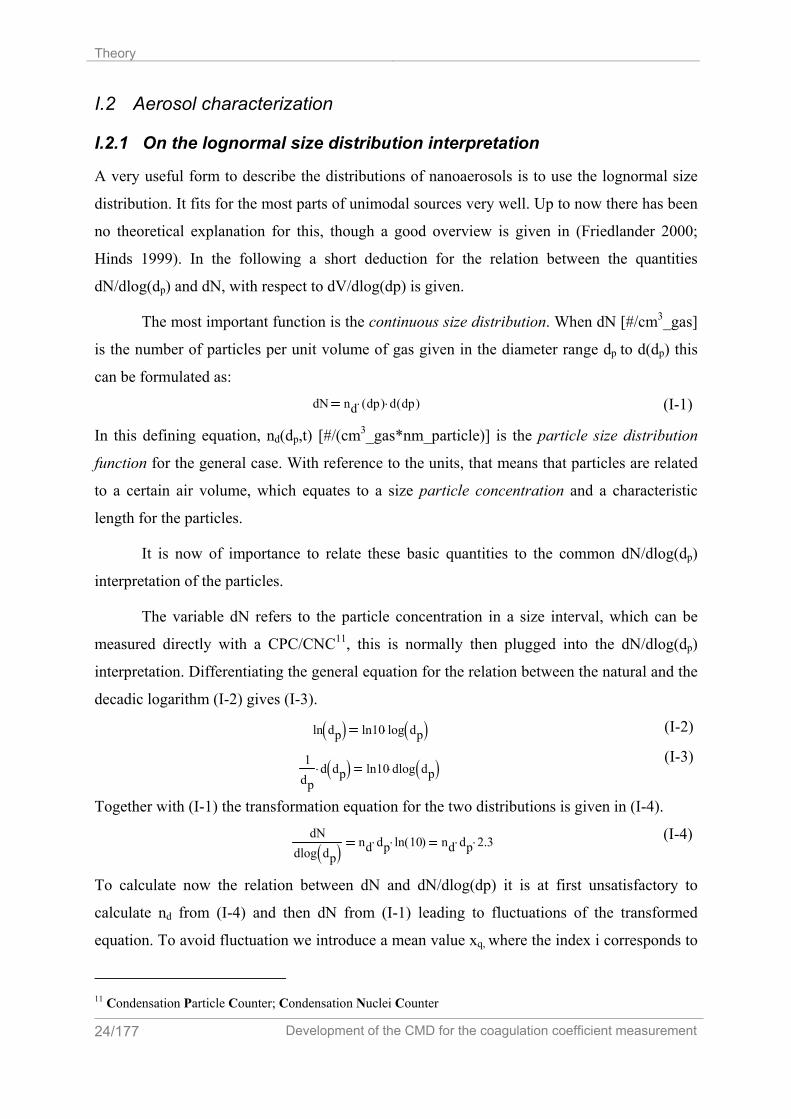
Figure 3 Solution of the Smoluchowski equation for different initial concentration and a
constant coagulation coefficient K=54*10 [cm3/s]. As it is necessary to have a difference in concentration measurement to determine the
coagulation coefficient, it is useful to compare the initial concentration with the actual
concentration over time. Hence we define the concentration decrease α:
αN∞
N0
(I-30)
Together with (I-29) we get the following equations for N∞ and N0:
α N0 t,( ) 11 t K⋅ N0⋅+
(I-31)
α N∞ t,( ) 1 t K⋅ N∞⋅− (I-32)
Equations (I-31) and (I-32) are depicted in Figure 4 for four different coagulation times t, for
a fixed coagulation coefficient K. The dotted curves depict the initial concentration N0
according to (I-31) the lined curves the concentration N∞ according to (I-32) after a certain
coagulation time t.
Given a desired concentration N0=2*105 [#/cm3] and a desired concentration decrease
α the end concentration N∞=1.2*105 [#/cm3] after the coagulation time of 600 [s] can be
gained by following the black arrows.
N∞ [#
/cm
3 ]
N0=107 [#/cm3] N0=106 [#/cm3] N0=105 [#/cm3] N0=104 [#/cm3]

Aerosol dynamics relevant for the coagulation coefficient
Development of the CMD for the coagulation coefficient measurement 33/177
1 .103 1 .104 1 .105 1 .106 1 .1070
0.1
0.2
0.3
0.4
0.5
0.6
0.7
0.8
0.9
1
Nu: t=600[s]N0: t=600[s]Nu: t=1200[s]N0: t=1200[s]Nu: t=1800[s]N0: t=1800[s]Nu: t=2400[s]N0: t=2400[s]
K=54*10^-10 [cm^3/s]
N,N0 [#/cm^3]
alph
a [-
]
Figure 4 Solution of the Smoluchowski equation for a different concentration decrease α and the corresponding actual as the initial particle concentration N and N0; Different coagulation times t
are used as a parameter. The coagulation coefficient is constant K= 54*10-10 [cm3/s].
I.3.4 Determination of the coagulation coefficient K
I.3.4.1 Theory of loss by coagulation and diffusion
The general dynamics equation can be simplified for a constant coagulation coefficient K, as
it is done in the Smoluchowski equation (I-27). Fick’s second law of diffusion can be written
for diffusion only applying a constant diffusion coefficient with respect to particle size and
using the coordinate independent Laplace operator:
tN∞
dd
D− ∆N∞⋅ div D grad N∞( )⋅( )−
(I-33)
The particle concentration gradient dN∞/dt is hence proportional to the divergence of the
gradient of N∞ which is also:
N∞N#V
(I-34)
N# are the total particles and V is the reference volume. Assuming natural convection in the
coagulation reactor (CMD) a diffusion layer of thickness h remains, in which only diffusion
takes place. This assumption corresponds to the “two film theory” for mass transport (Pflügl
α [-
]
N∞, N0 [#/cm3] N∞: t=600[s] N0: t=600[s] N∞: t=1200[s] N0: t=1200[s] N∞: t=1800[s] N0: t=1800[s] N∞: t=2400[s] N0: t=2400[s]
Theory
34/177 Development of the CMD for the coagulation coefficient measurement
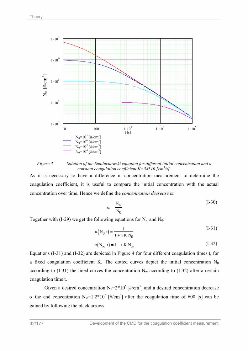
and Rentz 2000)21. If the particle concentration is zero on the wall and N∞ in the core of the
coagulation reactor then the gradient is constant over the whole surface:
grad N∞( )
N∞
h
(I-35)
When we now equate the flux of the particles from the container volume V through the
surrounding surface S according to the Gauss integral law the diffusion results in:
tN∞
dd
1V
− Vdiv DN∞
h⋅
⎛⎜⎝
⎞⎠
⌠⎮⎮⎮⌡
d⋅1V
− SDN∞
h⋅
⌠⎮⎮⎮⌡
d⋅
(I-36)
Figure 5 Principal surface, volume and particle concentration relation of the settler
The solution of equation (I-36) is,
βDh
(I-37)
LSV
Dh
⋅SV
β⋅
(I-38)
tN∞
dd
SV
−Dh
⋅ N∞⋅SV
− β⋅ N∞⋅ L− N∞⋅
(I-39)
where β [m/s] is the particle transfer coefficient in analogy to the mass transfer coefficient,
and L [1/s] is the particle wall diffusion frequency. The equation is valid for a small diffusion
layer of thickness h compared to the characteristic length of the reactor.
21 p. 182; Corresponding to this theory, the concentration gradient is linear from a constant value at the wall
(layer) to a constant concentration in the core. A constant velocity u from the bulk to the wall and no velocity
boundary layer is regarded. In this case the particle transfer coefficient β=D/h. To take into account also the
velocity boundary layer, the “Grenzschicht Theorie” (boundary layer theory), for the flow over a plate, can be
applied, leading to a different solution for laminar and turbulent flow, which is also dependent on the length of
the plate (settler actual effective length). For laminar flow βx is proportional to D2/3 (from exact solution
Shx=0.332*Rex1/2*Sc1/3). For turbulent flow βx is proportional to D0.57 (from exact solution
Shx=0.0296*Rex4/5*Sc0.43), with βx=D/x*Shx, where D is the particle diffusion coefficient, Shx the local particle
Sherwood number βx*x/D, x the actual length coordinate parallel to the flow direction, Sc the Schmidt number
ν/D, and Rex the local Reynolds number u*x/ν.
N∞ 0
→
n
h
S dS SV
Aerosol dynamics relevant for the coagulation coefficient
Development of the CMD for the coagulation coefficient measurement 35/177
Simplifying (I-20) and introducing of (I-39) leads to
tN∞
dd
K N∞2
⋅ L N∞⋅+⎛⎝
⎞⎠−
(I-40)
which describes simultaneous coagulation and deposition. K is the coagulation coefficient and
L is the previously defined particle wall diffusion frequency. Equation (I-40) can also be
identified with the logistic equation (Soldov and Ochkov 2005)22 which is a general equation
for growth limited by saturation. The growth corresponds to the coagulation coefficient; the
saturation corresponds to the loss due to wall diffusion. Equation (I-40) is the base equation of
the four methods listed in Table 1 and derived in the next sections for gaining the coagulation
coefficient K. Method (1) is the method derived from Rooker and Davies, where method (2)
is the more general solution of method (1) for long residence times. Methods (1)&(2) are
valid for a constant volume batch reactor (CV), whereas methods (3)&(4) are valid for the
constant concentration (CC) coagulation reactor23 used in this work. Method (1) and (3) are
used for short times and (2)&(4) for long time measurement of an aerosol.
Table 1 Methods of the determination of the coagulation coefficient K; CV denotes the constant volume and CC the constant concentration reactor;
Method Restrictions Description Reactor type (1) t 0 Method of Rooker and Davies
(Rooker and Davies 1979) CV
(2) t: 0..∞ (general method) Like method of Rooker and Davies adapted for long times
CV
(3) γ 0 Method developed in this work for the constant concentration reactor and analogous to method (1)
CC
(4) γ: 0..∞ (general method) Method developed in this work for the constant concentration reactor and analogous to method (2)
CC
I.3.4.2 Method (1) - Constant Volume Batch Reactor (CV) for short times
According to Rooker and Davies (Rooker and Davies 1979), a method for determining the
coagulation equation can be derived. First an apparent coagulation coefficient Ka is
introduced:
K a K 1L
K N ∞⋅+⎛
⎜⎝
⎞⎠
⋅
(I-41)
22 p.10ff 23 Definition see section II.4.1 p. 76

Theory
36/177 Development of the CMD for the coagulation coefficient measurement
This coagulation coefficient appears in the settler due to deposition on the wall and due to
coagulation. In the case of an infinite surface, Ka becomes K. For practical application only
Ka can be measured directly. Under the assumption that Ka is constant, which is true for short
coagulation times, relative to the concentration, equation (I-40) can be written as follows:
tN ∞
dd
K a− N ∞2⋅
(I-42)
This can be integrated like the Smoluchowski equation (I-28),
1N t2
1N t1
− K a t 2 t 1−( )⋅
(I-43)
where ti (i=1,2) denote two different times with constant Ka. In the Smoluchowski plot (1/N∞
is plotted against t) this can be seen when Ka is a straight line. Ka is dependent on the particle
concentration N∞, and as K≈N∞2
and L≈N∞ Ka will differ, for different wall diffusion
characteristics.
Equation (I-41) can now be integrated for constant K and L, by making a
decomposition into partial fractions and using the defining equation (I-41) for Ka and for times
ti (i=1,2):
L− t 2 t 1−( )⋅
t 1
t 2
N ∞1
N ∞
⌠⎮⎮⌡
dKL
t 1
t 2
N ∞1
KL
N ∞⋅ 1+
⌠⎮⎮⎮⌡
d⋅− ln
1L
K N t1⋅+
1L
K N t2⋅+
⎛⎜⎜⎜⎜⎝
⎞
⎟⎟
⎠
lnKa t1,
Ka t2,
⎛⎜⎝
⎞⎠
(I-44)
Hence,
Ka t2, Ka t1, eL t 2 t 1−( )⋅
⋅ (I-45)
According to Rooker and Davies, this equation cannot be used for evaluation of L, as the
assumption that L and K are constant is not valid over long periods of time, and Ka is a
function of L.
For short periods of time Ka is constant for different particle concentrations N∞. This
leads to the following experimental method: Having one material of nanoparticles dispersed
in a gas24 with different particle concentrations the apparent coagulation coefficients can be
calculated as slopes in the Smoluchowski plot (1/N∞ against t). Then from equations (I-38)
and (I-41) the coefficients L, K, β, and h can be calculated:
24 Most commonly air

Aerosol dynamics relevant for the coagulation coefficient
Development of the CMD for the coagulation coefficient measurement 37/177
LKa t2, Ka t1,−
1N t2
1N t1
−
(I-46)
K Ka t1,L
N t1− Ka t2,
LN t2
−
β LVS
⋅
hDL
SV
⋅
If there are more than two apparent coagulation coefficients Ka available for the experiments,
then Ka is plotted as a function of the initial particle concentration N∞. The least mean squares
fit of equation (I-41) yields to the coefficients for L and K and with equation (I-46) also to β
and h.
To fulfill the conditions of the theory the size of the dimensions of the coagulation
container has to be large compared to the diffusion layer h. Otherwise the geometry of the
container has also to be taken into account in equation (I-36).
I.3.4.3 Method (2) - Constant Volume Batch Reactor (CV) for long times
For the case that the coagulation times are long and hence Ka is not constant any more, the
detailed solution of equation (I-45) has to be calculated. This is done by inserting (I-41) in
equation (I-45). The total particle concentration N∞ can then be calculated as a function of
time t, setting t2=t and t1=0 and N(t)=N0 as:
N ∞ t( )L
K 1L
K N 0⋅+⎛
⎜⎝
⎞⎠
eL t⋅⋅ 1−⎡⎢⎣
⎤⎥⎦
⋅
(I-47)
I.3.4.4 Method (4) - Constant Concentration Reactor (CC) for long times
The method of Rooker and Davies was applied for evaluation of the coagulation coefficient.
The surface to volume ratio is in the same order of magnitude for the built CMD than that of
Rooker and Davies. The main difference is that the volume is variable as the CMD is a
constant concentration reactor (see section II.4.1, p.76). The CMD allows for a coagulation
coefficient K determination by means of a single concentration measurement or the
examination of the particle concentration decrease for the apparent coagulation coefficient Ka.

Theory
38/177 Development of the CMD for the coagulation coefficient measurement
Mathematically the volume of the constant concentration reactor can be described by (I-48).
For obtaining the equation describing the concentration as a function of time coagulation and
diffusion the volume in (I-40) has to be replaced by:
V t( ) V70 Vp 7 t⋅−
(I-48)
V70 is the initial total volume of the settler, Vp7 is the constant settler flow due to geometrical
considerations and t is the time the measurement takes place.
In section II.2.3 it is derived that Vp7 is inverse proportional to ttotal25
. Assuming that
the volume for the empty settler is very small compared to the initial settler volume then Vp7
is also approximately proportional to V70. Defining the total time ratio γ,
equation (I-48) can be written as:
We define L0 according to equation (I-51) as a function of the initial conditions. These are the
surface to volume ratio S/V70 (see Table 2) and the particle transfer coefficient β or S/V70, the
Diffusion coefficient D and the diffusive layer h.
(I-51)
With equation (I-51) L can be written in equation (I-52) as a function of γ and a constant
particle wall diffusion frequency L0.
L γ( )L 0
1 γ−≡
(I-52)
The governing equation for the constant concentration reactor can be yielded inserting
equation (I-52) into (I-40) and substituting t according to equation (I-49):
γ
N ∞
t total
dd
K N ∞2⋅
L 01 γ−
N ∞⋅+⎛⎜⎝
⎞
⎠−
(I-53)
ttotal is constant for a measurement as the sample flow rate Vp4 is constant and can be gained
from equation (II-11).
To solve equation (I-53) we substitute N∞ with yα in equation (I-53). From this we see that
α=-1. As a consequence we substitute N∞ with y−1 in equation (I-53) yielding the following
inhomogeneous differential equation:
25 Total time for emptying the settler.
γt
t total
(I-49)
V t( ) V70 1 γ−( )⋅
(I-50)

Aerosol dynamics relevant for the coagulation coefficient
Development of the CMD for the coagulation coefficient measurement 39/177
γy
1t total
⋅dd
L 01 γ−
y⋅− K
(I-54)
The solution for the homogenous part is,
y h C1
1 γ−⎛⎜⎝
⎞⎠
L 0 t total⋅
(I-55)
where the variable C is the integration constant. Making the variation of constants and
inserting the in homogenous solution yields an equation for C:
γCd
dK t total⋅ 1 γ−( )
L 0 t total⋅⋅
(I-56)
After integration C is:
C
K t total⋅ 1 γ−( )L 0 t total⋅ 1+
⋅
L 0 t total⋅ 1+−
(I-57)
After insertion in equation (I-55) and simplification the particular solution is:
y p
1 γ−( ) K⋅ t total⋅
L 0 t total⋅ 1+−
(I-58)
The complete solution is then the superposition of homogenous and inhomogeneous solution
and resubstitution of N∞:
1N ∞
y y p y h+ 1 γ−( ) L 0− t total⋅C⋅
1 γ−( ) K⋅ t total⋅
L 0 t total⋅ 1+−
(I-59)
With the initial condition N∞=N0 and γ=0 the integration constant C gets:
C1
N 0
K t total⋅
L 0 t total⋅ 1++
(I-60)
Simplification of equation (I-59) and (I-60) yields for N∞:
N ∞L 0 t total⋅ 1+
1 γ−( ) K⋅ t total⋅
11
K N 0⋅
1t total
L 0+⎛⎜⎝
⎞⎠
⋅+
1 γ−( )L 0 t total⋅ 1+
1−
⎡⎢⎢⎢⎣
⎤⎥⎥⎥⎦
⋅
(I-61)
This is the predicted concentration for a complete measurement run from γ=0 to γ=1, and
simultaneous coagulation and diffusion. Equation (I-61) is shown in Figure 6 for different
initial particle concentrations N0, and typical constant values for K and L=L0 for the
experiments of Rooker and Davies.
Theory
40/177 Development of the CMD for the coagulation coefficient measurement
0 0.1 0.2 0.3 0.4 0.5 0.6 0.7 0.8 0.9100
1 .103
1 .104
1 .105
1 .106
1 .107
N0=10^8N0=10^7N0=10^6N0=10^5N0=10^4
gamma [-]
Nu
[#/c
m^3
]
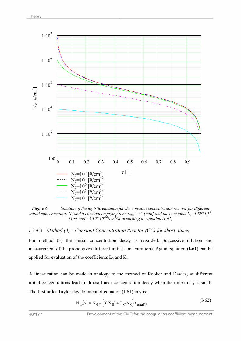
Figure 6 Solution of the logistic equation for the constant concentration reactor for different
initial concentrations N0 and a constant emptying time ttotal =75 [min] and the constants L0=1.89*10-4 [1/s] and =56.7*10-10[cm3/s] according to equation (I-61)
I.3.4.5 Method (3) - Constant Concentration Reactor (CC) for short times
For method (3) the initial concentration decay is regarded. Successive dilution and
measurement of the probe gives different initial concentrations. Again equation (I-61) can be
applied for evaluation of the coefficients L0 and K.
A linearization can be made in analogy to the method of Rooker and Davies, as different
initial concentrations lead to almost linear concentration decay when the time t or γ is small.
The first order Taylor development of equation (I-61) in γ is:
N ∞ γ( ) N 0 K N 02⋅ L 0 N 0⋅+( ) t total⋅ γ⋅−
(I-62)
γ [-]
N∞ [#
/cm
3 ]
N0=108 [#/cm3] N0=107 [#/cm3] N0=106 [#/cm3] N0=105 [#/cm3] N0=104 [#/cm3]

Aerosol dynamics relevant for the coagulation coefficient
Development of the CMD for the coagulation coefficient measurement 41/177
Subsequent derivation in γ yields to:
γN ∞
1t total
⋅dd
K N 02⋅ L 0 N 0⋅+( )−
(I-63)
After resubstitution of γ with equation (I-49), substitution of L0 with L and N0 with N∞
equation (I-40) is obtained. This is the basis equation for the general theory for loss by
coagulation and diffusion.
In analogy to equation (I-41) an apparent coagulation coefficient can be introduced:
Kac N0( ) K 1L0
K N0⋅+
⎛⎜⎝
⎞
⎠⋅
(I-64)
Combining equations (I-63) and (I-64) yields equation (I-65).
Kac N0( ) γN∞
dd
N02 ttotal⋅
−
(I-65)
As a result for small times or when γ 0 Kac is a function of the declining particle
concentration slopes, the total measurement time ttotal, which is a function of sample flow, and
the initial particle concentration N0.
A least mean squares fit for equation (I-64) for all different N0 and one coagulation
run with this method gives then the coagulation coefficient K and the variable L0 for the
settler, or the constant concentration reactor in general.26
I.3.4.5.1 Graphical method
From equation (I-65) a graphical method27 for determination of the coagulation coefficient
can be derived. For γ 0, equivalent with the beginning of the measurement, when t 0,
equation (I-65) can further be simplified to:
tN ∞
dd
K ac− N 02⋅
(I-66)
As for t 0 the concentration N∞ is equal to the initial concentration N0 this results in
1N0 ∆ t⋅
Kac,
(I-67)
which can be interpreted geometrically according to Figure 7. The apparent coagulation
coefficient Kac is inverse proportional to the area spanned by the initial concentration N0 and
26 See section II.4.1 p. 76 27 Which is also applicable for the simplified calculation of the coagulation coefficient K.

Theory
42/177 Development of the CMD for the coagulation coefficient measurement
the time ∆t gained by section of the tangent in N0 with the x-axis28. The resulting apparent
coagulation coefficient Kac is then a function of the initial concentration N0. With least mean
squares fit of equation (I-64), the coagulation coefficient K and the diffusion frequency L0
results.
Figure 7 Graphical method to determine the apparent coagulation coefficient Kac according to equation (I-67). The method is described in the text.
I.3.5 Predicted application of the measurement of the quantity K
As the coagulation constant K is determined experimentally, other quantities can be
calculated. To characterize the fractal properties of particles a method for determination of the
fractal dimension Df and the primary particle dp0, is sketched shortly. The experimental results
for K as the resulting Df, and dp0 can then be compared with numerical simulations for the
evolution of fractal aggregates in this field, see e.g. (Kostoglou and Konstandopoulos 2001).
I.3.5.1 Fractal dimension determination
The way of determining the fractal dimension shall be described in short. In the Brownian
regime29 the equation (I-27) can be transformed for two different particle diameters to:
28 This is a result of the tangent in equation (I-66) for γ 0. 29 Particles (much) larger then the mean free path λ, or where the Stokes-Einstein relation for the diffusion
coefficient is valid.
Kac=1/A=1/(N0*∆t)
A
A
N
t
N0
N0
∆t ∆t
Aerosol dynamics relevant for the coagulation coefficient
Development of the CMD for the coagulation coefficient measurement 43/177
d p1d p2
K d p1( ) D d p2( )⋅
K d p2( ) D d p1( )⋅
(I-68)
Both the coagulation constant and the diffusion constant are a function of the particle
diameter. For this purpose, the coagulation constant has to be measured for monodisperse
particles. Next the definition equation of the fractal particles (I-10) can be, for this condition,
set as:
N p1N p2
d p1d p2
⎛⎜⎝
⎞
⎠
D f
(I-69)
Together with (I-68) and solving for the fractal dimension Df we get:
D f
lnN p1N p2
⎛⎜⎝
⎞
⎠
lnK d p1( ) D d p2( )⋅
K d p2( ) D d p1( )⋅( )⎡⎢⎣
⎤⎥⎦
(I-70)
Assuming that no particle loss at the wall occurs, that N∞,i is referred to the same volume, V,
and no primary particles are generated, then the number of all primary particles, Np,primary, in a
closed volume, V, stays constant for fractal growth30. Let the index i=1 be the state at the time
t and i=2 the state at the time t+∆t, then according to equation (I-71) the gas particle
concentration N∞,i decreases, whereas the average particle number, Npi, in each fractal particle
increases and the total primary particle concentration, N∞,primary, is constant for coagulation
neglecting other particle losses. Equation (I-71) is then, for this case, the population balance
equation for primary particle concentration, N∞,primary, which is defined by the ratio of the total
number of all primary particles, Np,primary, and the reference volume, V.
Np1 N∞ 1,⋅ Np2 N∞ 2,⋅Np primary,
VN∞ primary, const
(I-71)
As Npi is inverse proportionally to the particle concentration for coagulation, the unknown
ratio for Npi is:
Np1Np2
N∞ 2,
N∞ 1,
(I-72)
For a coagulating aerosol equation (I-70) can then be written31:
30 This is also the case when the particle concentration N∞ stays constant. 31 This is only valid for ideal particle coagulation without other particle losses; for the case of additional losses
equation (I-71) has to be modified accordingly.

Theory
44/177 Development of the CMD for the coagulation coefficient measurement
D f
lnN∞ 2,
N∞ 1,
⎛⎜⎝
⎞⎠
lnK d p1( ) D d p2( )⋅
K d p2( ) D d p1( )⋅( )⎡⎢⎣
⎤⎥⎦
(I-73)
With equation (I-73) the fractal dimension Df can be solved for two paired monodisperse
coagulation constants, K(dpi), the particle concentrations, N∞,i, and the diffusion constants,
D(dpi), according to equation (I-23).
This method is only an approximation, because, for the coagulation, a polydisperse
aerosol is necessarily developing. Therefore, it is not possible to determine the declining
concentrations for one monodisperse aerosol with known concentrations, although
monodisperse coagulation constants can be measured for monodisperse aerosols with
different diameters. The effects of deposition may have also significant influence, which can
be taken into account, e.g. by equation (I-61).
I.3.5.2 Primary particle diameter
To characterize a fractal particle it is necessary to know the primary particle diameter dp0. It
can be measured most commonly by electron microscopy or online with the optical dispersion
quotient process (Zahoransky and others 2000).
When the primary particle diameter dp0 and also the fractal dimension Df is known, Np
can be calculated from the definition equation (I-10) for a particle of size dp. With the
diffusion coefficient Dp the coagulation coefficient Kp for the particle of size dp and the
diffusion coefficient of the primary particle Dp0, the coagulation coefficient of the primary
particle can be calculated with equation (I-74).
Kp0 KpDp0
expln Np( )
Df
⎛⎜⎝
⎞
⎠Dp⋅
⎛⎜⎝
⎞
⎠
⋅
(I-74)
Evaluation of different coagulation coefficients Kp for different particle diameters dp result in
the same coagulation coefficient Kp0. In an iterative process a new primary particle dp0 can be
assumed, leading to a better adaptation of the experimental values of Kp and the resulting Kp0
in equation (I-74).

II Description of the CMD
In this chapter the CMD will be introduced, first by its principles of operation, its physical,
mechanical and electrical systems and total system setup over some fundamental issues with
the software implementation of the whole CMD system.
II.1 Principle of operation of the CMD The CMD system is a complete system of several measurement instruments combined
through the LABVIEW integration process. The basic setup of the CMD is shown in Figure 8.
The first basic instrument for the CMD system is an instrument to measure the particle
size distribution. For this purpose the SMPS 308132 (scanning mobility particulate sizer) was
used with DMA (differential mobility analyzer) technology, and the CPC (condensation
particle counter).
The second system is the settler system of the CMD, mainly a constant concentration
reactor. One possible operation is as follows: First one sample is vacuumed into the settler.
Then the time needed for decay of particle number concentration – the residence time for
reaction (coagulation sedimentation, settling) – is measured. A (smaller) sample is taken from
the settler. The last to steps are repeated n times. The difference between the measured
concentrations, measured with the modified standard SMPS system, gives us evidence about
the decay in concentration and hence the coagulation constant. The constant concentration
reactor is therefore tunable in time and gives evidence about the real time behavior of
coagulation of aerosols, especially in cases when the volume tends to infinity. Concerning
experimental setup a limited volume has to be taken into account.
32 SMPS system from TSI containing the classifier 3081, the DMA 3080 and the CPC 3010.

Description of the CMD
46/177 Development of the CMD for the coagulation coefficient measurement
SMPSDMA
SMPS CPC
Abluft
TUG 23.9.2004
Settler/Mixer M
T,p
phi
Vp
Aerosol-K-messgerät
S1
V2
V3V4
V6
V5
M1
T1
P1PHI1
PU1
C1
D1
Q1
Probe
V1
Kürzel Bezeichnung--------------------------------------D1 DMAC1 CPCV1-V4 3-WegventileV5-V6 2-WegVentileS1 SettlerT1 TemperatursensorP1 DrucksensorM1 SchrittmotorQ1 DurchflußsensorM1 SchrittmotorPHI1 FeuchtigkeitssensoD1 DMAPU1 Pumpe
Figure 8 Basic Setup of the CMD
II.2 Setup of the CMD
II.2.1 System setup
The system used in this work consists mainly of two self contained systems: The standard
SMPS system - used for comparison - and the introduced new CMD system.
II.2.1.1 Standard SMPS system
The standard SMPS system as stand alone application is depicted in Figure 9. First, there is
first the SMPS classifier unit, with the orange case including the recycle flow sheath air
control system and the DMA. The yellow case depicts the DMA unit transforming the
polydisperse aerosol into a monodisperse one. Ambient air that passes the clean air filter
Abbr. Description --------------------------------- D1 DMA C1 CPC V1-V4 3 way valves V5-V6 2 way valves S1 Settler T1 Settler temperature
sensor P1 Settler pressure
sensor M1 Stepper motor Q1 Flow sensor PHI1 Settler humidity
sensor
exhaust
SMPS Classifier

Setup of the CMD
Development of the CMD for the coagulation coefficient measurement 47/177
RLF2 is mixed with the monodisperse output of the transformer. This diluted particle
concentration is then counted with the CPC (condensation particle counter) (Ivanišin and
others 2005).
SMPS SYSTEM
SMPS classifier
SMPS CPC
dN
τ 6
τ 3
DMA in
DMA out
SMPS poly out
SMPS in
T1T2p1
Vp1Vp2
SMPS mono out
RLF 2
DRV3
PU1
ambient air
CPC tube
probe in
CPC in
CPC out
τ 0
τ 2
Figure 9 Flow chart of the standard SMPS system
II.2.1.2 CMD system
In the CMD system (Figure 10) the SMPS system is integrated. There are three basic
subsystems with an optional fourth:
1. The Settler system
2. The Valve system
3. The SMPS system
4. An alternative measurement system e.g. for particle or mass concentration

Description of the CMD
48/177 Development of the CMD for the coagulation coefficient measurement
CMD SYSTEM University of Technology Graz 2005
SMPS SYSTEM
SMPS CPC
SMPS classifier
ALTERNATIVE MEASUREMENT SYSTEM
VALVE SYSTEM
SETTLER SYSTEM
V2
V5
V4
V3V1
V6
P R
A
R
A
P
P
R A
P
R
A
P
R
A
P
A
R
V7
A
P
V8 P
A
M1
Msettler
PU1
Vp4
T1T2p1
Vp1Vp2
DRV1
RSV
VM1
alternative measurement
system
PU2
DRV2
VM2
ambient air
RLF 1
ambient air
RLF 2
DRV3
p2
dp3T7φ1
dNSMPS poly out
pump intakeSMPS in CPC out
CPC in
settler top
settler bottom
SMPS mono out
DMA in
DMA out
ASF
CPC tube
τ 4τ 6
τ 8
τ 1
τ 2
τ 3τ 5
VM3
probe in
probe in
Figure 10 Flow chart of the CMD system

Setup of the CMD
Development of the CMD for the coagulation coefficient measurement 49/177
In the actual setup the SMPS system and the valve system is in one case, and the settler
system in another33. The whole CMD system and its individual components are described in
(Bakk 2005; Brugger 2005) in detail.
The settler system is a system with a constant concentration reactor also known as “the
accordion”34. It is a variable volume reactor whose volume is varied by a stepper motor M1
(Figure 10) with connected gear35. On the top and on the bottom there are magnetic valves
V7, V8 for shutting in the aerosol probe to maintain a constant thermodynamic state of the
aerosol system. A total pressure sensor p2 is mounted on the top. A differential pressure dp3, a
temperature T7 and a humidity sensor φ1 is mounted on the bottom of the settler.
The valve system consists of the magnetic two way valves V1-V6 and the flow sensor
Vp4, which is passed in the most of the paths. The flow sensor has a high measurement
accuracy, as has been shown by comparison to a primary bubble flow meter (Bakk 2005;
Brugger 2005). Two manual ball valves VM1-VM2 also have been integrated. They allow for
(VM2) the optional filtering the inlet air of the whole system through the filter RLF1, and
thereby cleaning the whole system, which is important for cleaning the settler and for (VM1)
measurement with an alternative measurement system instead of the CPC. The regulating
needle valve DRV1 is used to manually set up the filling flow rate of the settler. A one
direction valve (RSV) to protect the CPC has also been integrated (Brugger 2005)36.
The SMPS standard system - consisting of the DMA classifier, CPC and the pump -
has been modified by extending the connecting tube from “SMPS mono out” to “CPC tube”
with the valve system, as well as the SMPS sample inlet “SMPS in”. The needle valve DRV1
together with a clean air filter RLF2 is regulating the sample flow that is vacuumed from the
DMA and the filter RLF2 through the CPC. The temperatures for the cabinet T1, for the
sheath flow recycle T2, as well as the absolute pressure in the classifier unit p2 and the flow
rates for the sample flow Vp1 and the sheath flow Vp2 are measured and transmitted via the
serial interface to the monitoring PC and continuously logged for the measurement mode. The
same takes place with the particle size concentration dN37 of the CPC.
33 The settler system can be fully closed for future temperature regulation. 34 Oral note of A. Konstandopoulos, Zurich 2005 35 The gear system is from ZIMM, www.zimm-austria.com: Specifications: BG:SHZ-02-LR, miniature spindle
lifting gear i=12:1, 0.25mm / rotation 36 For normal operation this valve is recommended to be removed because of high particle losses. 37 This is the parameter rd of the CPC or the actual measured particle concentration [#/cm3]

Description of the CMD
50/177 Development of the CMD for the coagulation coefficient measurement
II.2.2 Settler
The basic parameters of the coagulation settler are given in Table 2 and shown in Figure 11.
The inner and outer diameters are given with di_SETTLER and do_SETTLER. The length L_SETTLER
is the outer size of diameter. The width of one fold Ft of the settler calculates from the
difference of the diameter divided by two. The number of folds Fz is Lmax divided by Ft
according to the producer38. The length of the the minimal volume is restricted to the
thickness of the folds and is approximately: L_SETTLER_min=Fz*2.5/1000. The settler area
ASETTLER is defined by (II-1).
A SETTLER Fz 2⋅ d o_SETTLER2 d i_SETTLER
2−( )⋅ 2 d i_SETTLER⋅+⎡⎣ ⎤⎦π
4⋅
(II-1)
Table 2 Main settler parameters Name Description Value Unit
producer Innoflex ~ [~] material NBR-rubber; 1mm (temp. resistant - 90°C) ~ [~] Product S21177; Scheibenbalg39 144-204-500-144-144 ~ [~] di_SETTLER Inner diameter 0.144 [m] do_SETTLER Outer diameter 0.204 [m] L_SETTLER Length 0.5 [m] Ft Width of folds 0.030 [m] Fz Number of folds 14 [~] L_SETTLER_min Minimum size due to folds (.05m) 0.036 [m]
spec
ifict
ion
ASETTLER Inner surface 0.500 [m2] dm Theoretical mean diameter 0.174 [m] γ Correction of dm for real volume 0.833 [~] Lmin Minimum actual size 0.003 [m] Lmax Maximum actual size 0.428 [m] ∆L Lmax-Lmin .0425 [m] d7 Effective inner diameter 0.145 [m] d7’ Outlet diameter for pressure difference 0.006 [m] V7 Effective measured press out volume 7.0 [l] V7min Rest volume 0.05 [l] V70 Actual total volume 7.05 [l] V70/S Volume to surface ratio 0.0140 [m3/m2]
actu
al se
tup
S/V70 Surface to volume ratio 71 [m2/m3]
38 The settler is a standard “Faltenbalg” (bellow) from Innoflex. The material is made of NBR-rubber which is
made of special antistatic mixture; the advantage is that particles will not be attracted due to static charge; the
disadvantage is that the settler is not resistant to UV radiation or ozone. 39 Bellow

Setup of the CMD
Development of the CMD for the coagulation coefficient measurement 51/177
Figure 11 Settler in the end switch positions For the actual setup the approximated mean diameter dm is corrected with the numerically
derived γ resulting in the effective settler diameter d7. Lmin and Lmax are the lengths in the end
positions of the settler40. The volumes of the settler are defined in (II-21). The effective
volume that can be used for a number of measurements is V7. It is the volume that can be
pressed out by the stepper motor. The minimum volume is V7min. The actual total free volume
of the settler is V70 which is relevant for filling the settler.
V 7 d m γ⋅ L max⋅( )2 d i_SETTLER2 L min⋅+⎡⎣ ⎤⎦
π
4⋅ 103⋅
V 7min d i_SETTLER2 π
4⋅ L min⋅ 103⋅
(II-2)
V 70 V 7min V 7+ The ratio between total area and volume “V/S” and “S/V” are given for comparison with
other experiments. They can also be used to compare measurements with the actual settler
with a different S/V ratio, and hence a different deposition to coagulation ratio.
II.2.3 Effective flow rate41
An experiment was set up to measure the flow rate Vp442 over time while pressing out the
40 When the end switches are pressed, or when the settler has its actual maximum or minimum possible volume 41 The relations for the leakage flow dilution in this section are restricted to path 3 (see section II.3.1). For a
different path different relations are to be expected, especially for the quantities α and VpL whereas Vp7 should
stay constant (quantities are explained later in this section). 42 With the ASF1430 flow sensor from SENSIRION (www.sensirion.com).

Description of the CMD
52/177 Development of the CMD for the coagulation coefficient measurement
total volume of the settler. The input parameter SPFA (selection of constant speed factor)43
for the stepper motor control is only dependent on the stepper motor hardware. As output, the
flow rate Vp4 and the total time ttotal needed to press out the effective settler volume was
measured. The results are given in Figure 12. Drawing a line from the chosen SPFA44 to the
pink line and then going down to the brown curve yields the total time ttotal and the flow rate
Vp4. In Figure 12, the maximum deviations of the mean value for the flow rate measurement
are also given. The start and stop measurement values, including acceleration of the flow rate,
were not regarded for the mean value.
Vp4 = 5.1938*ttotal-0.9304
R2 = 0.9993
0.0
0.1
0.2
0.3
0.4
15 25 35 45 55 65 75ttotal (min)
V p4 [
l/min
]
6810121416182022242628303234
SPFA Vp4_mean
SPFA
Potenziell(Vp4_mean)
Figure 12 Flow rates Vp4 of the flow sensor ASF 1430 for different times of emptying and filling
the settler; the parameter SPFA denotes the speed factor of the stepper motor in the LABVIEW software. It is proportional to the stepper motor steps per time unit.
II.2.3.1 Settler volume determination
Assuming a settler volume V7 leading to the settler exhaust flow Vp7 when compressed. Vp7 is
only determined by the movement of the stepper motor and the connected gear, therefore it is
43 The speed factor is the software parameter needed for the HASOTECH (www.hasotech.com) stepper motor
control card. As it is approximately proportional to a defined number of steps per time unit, the SPFA is nearly
linear with time. 44 Is needed as input parameter in the LABVIEW Software and is proportional to the number of steps with the
stepper motor
Potential fit
Vp4
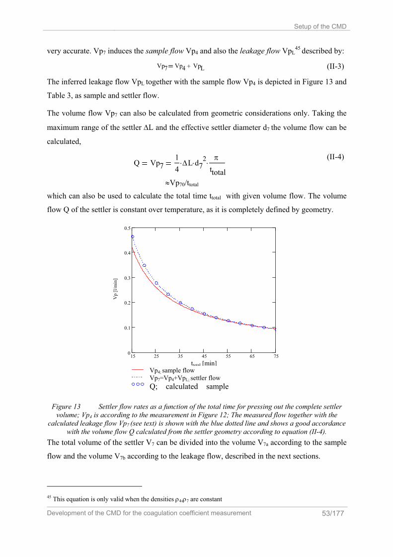
Setup of the CMD
Development of the CMD for the coagulation coefficient measurement 53/177
very accurate. Vp7 induces the sample flow Vp4 and also the leakage flow VpL45
described by:
The inferred leakage flow VpL together with the sample flow Vp4 is depicted in Figure 13 and
Table 3, as sample and settler flow.
The volume flow Vp7 can also be calculated from geometric considerations only. Taking the
maximum range of the settler ∆L and the effective settler diameter d7 the volume flow can be
calculated,
which can also be used to calculate the total time ttotal with given volume flow. The volume
flow Q of the settler is constant over temperature, as it is completely defined by geometry.
15 25 35 45 55 65 750
0.1
0.2
0.3
0.4
0.5
Vp4Vp7=Vp4+VpLQ
ttotal [min]
Vp
[l/m
in]
Figure 13 Settler flow rates as a function of the total time for pressing out the complete settler volume; Vp4 is according to the measurement in Figure 12; The measured flow together with the
calculated leakage flow Vp7 (see text) is shown with the blue dotted line and shows a good accordance with the volume flow Q calculated from the settler geometry according to equation (II-4).
The total volume of the settler V7 can be divided into the volume V7a according to the sample
flow and the volume V7b according to the leakage flow, described in the next sections.
45 This equation is only valid when the densities ρ4,ρ7 are constant
Vp7 Vp4 VpL+ (II-3)
Q Vp714
∆L⋅ d72⋅
πttotal
⋅
≈Vp70/ttotal
(II-4)
Vp4; sample flow Vp7=Vp4+VpL; settler flow Q; calculated sample
ttotal [min]

Description of the CMD
54/177 Development of the CMD for the coagulation coefficient measurement
II.2.3.1.1 Sample flow
The effective flow rate experiment was used, according to Figure 14 and (II-5), for the
determination of the total effective settler volume V7a46
, where ρ4 is the density at the
V7a Vp4ρ4ρ7
⋅ ttotal⋅
(II-5)
flow sensor or approximately in the SMPS and ρ7 the density in the settler47.
V = -0.0003ttotal2 + 0.0361ttotal + 5.7536
6.0
6.1
6.2
6.3
6.4
6.5
6.6
6.7
6.8
6.9
7.0
15 25 35 45 55 65 75
ttotal (min)
V 7 (l
)
VPolynomisch (V)
Figure 14 Calculation of the total effective settler volume according to the measurement in Figure 12 and equation (II-5).
The error for the ASF measurements is +-1 % of the measurement value, and is also shown in
Figure 14. A constant straight line should have been expected. The curved shape indicates a
leakage somewhere in the measurement line although none had been expected as intensive
testing had been performed. The sequence of the measurements had no influence on the curve
shape, which means that the leakage flow is reproducible. The approximated volume of the
settler, achieved for the maximum measured total time ttotal is V7=7[l], for all measurements.
This was inferred from the decreasing leakage flow for long periods depicted in Figure 1348.
II.2.3.1.2 Leakage and total flow
To consider a leakage flow we define the leakage ratio α where VpL is the leakage flow rate:
46 When there is no leakage then V7a=V7 47 For constant states ρ4/ρ7=1; the densities can be calculated with the later defined viral equation. 48 The real volume is probably slightly higher, as can be calculated from the dimensions of the settler.
V7 V7 Polynomial fit
V7

Setup of the CMD
Development of the CMD for the coagulation coefficient measurement 55/177
αVpLVp4
(II-6)
The continuity equation can then be fulfilled according to Figure 15:
Vp7ρ4ρ7
Vp4⋅ 1 α+( )⋅
(II-7)
Figure 15 Scheme of the settler flow Vp7 the leakage flow VpL and the measured flow Vp4 for the mass balance
When we take into account that the total volume of the settler must be the integral of the total
measurement time ttotal according to,
V70
ttotaltVp7
⌠⎮⌡
d Vp7 ttotal⋅
(II-8)
where the flow rate Vp7 can be regarded constant over the time ttotal, as also the measured
sample flow Vp4 is constant over time, neglecting the flow acceleration we can write (II-7) for
the settler volume total V7
V7 Vp4 1 α+( )⋅ρ4ρ7
⋅ ttotal⋅
(II-9)
In the limiting case of no leakage flow α=0 and (II-9) is reduced to (II-5). From (II-9) α can
be resolved which is needed for the temperature adaptation of the flow rate49:
α
V7 ρ7⋅
Vp4 ρ4 ttotal⋅⋅1−
(II-10)
The results from the experiments for α and other parameters are shown in Table 3 for ttotal.
The real flow rate in the settler Vp7 can then be calculated by the known α and (II-7).
49 See also section II.2.3.4 p.58
Settler ρ7*Vp7, T7,p2 V7=V7a+V7b
Flow sensor ASF 1430 ρ4*Vp4, T,p
Leak ρ4*VpL, T,p

Description of the CMD
56/177 Development of the CMD for the coagulation coefficient measurement
Table 3 ttotal=time for one run of the effective flow rate experiments; α=leakage ratio; Vp4=sample flow rate; Vp7=settler flow rate; dp3=differential pressure settler; T7=temperature settler, mean T7m=298.3 [K]; mean p2m=.9819 [bar]; ρ4=ρ7=1.147 [kg/m3] orange values are
extrapolated; ttotal [min] 5 10 15 20 25 30 35 40 45 50 55 60 65 70 75
α [-] 0.207 0.151 0.119 0.096 0.079 0.066 0.054 0.045 0.036 0.029 0.022 0.016 0.010 0.005 0 Vp4 [l/min] 1.162 0.610 0.418 0.320 0.260 0.219 0.190 0.168 0.150 0.136 0.125 0.115 0.107 0.100 0.094
Vp7 [l/min] 1.403 0.701 0.468 0.351 0.281 0.234 0.200 0.175 0.156 0.140 0.128 0.117 0.108 0.100 0.094
dp3 [Pa] 3.301 1.498 0.944 0.680 0.527 0.428 0.359 0.309 0.270 0.239 0.215 0.194 0.177 0.163 0.151
T7 [°C] 25.3 25.3 22.8 23.0 24.3 25.5 26.3 26.4 25.9 25.3 24.9 24.9 25.4 26.2 26.5
II.2.3.2 Total time calculation
The time needed for emptying the settler ttotal as a function of the measured sample flow Vp4
can be seen in Figure 12 and calculated according to the polynomial fit equation there.
Alternatively ttotal can be calculated from equation (II-7) and (II-4) according to,
t totalρ 7ρ 4
∆L d m2⋅ π⋅
1 α+( ) Vp 4⋅ 4⋅⋅
(II-11)
ttotal is then constant for one coagulation experiment, supposing constant sample flow and
constant settler and ambient temperatures. α is a function of the sample flow Vp4 and the
actual leakage according to Table 3 and the defining equation (II-6).
II.2.3.3 Pressure drop
The pressure drop dp3 for the total times was measured at the settler outlet, for “breathing in”
(move UP) and “out” (move DOWN). The results are shown in Figure 16. There is a very
small pressure difference of maximal ~0.9 [Pa] which has negligible influence on the density
change of air. There is a hysteresis indicating that the breathing in is easier than the breathing
out. A very good approximation can be given with a potential fitting although the
measurement took place at very low pressure differences50, and the whole experiment lasted
several days. In addition similarity can be seen compared to the volume flow measurement.
Indeed there exists proportionality between pressure drop and volume flow51, hence the
pressure drop measurement can also be used for volume flow measurement52. A short method
for determining the settler and the sample flow is introduced in the following.
50 The measurement range of the differential pressure sensor is ±100 [Pa]. 51 The ASF 1430 sensor from Sensirion uses this relationship. 52 e.g. after calibration with the bubble flow meter.

Setup of the CMD
Development of the CMD for the coagulation coefficient measurement 57/177
pressure drop
y = 20.676x-1.1399
R2 = 0.9988
y = 10.01x-1.0177
R2 = 0.9984
0
0.1
0.2
0.3
0.4
0.5
0.6
0.7
0.8
0.9
15 20 25 30 35 40 45 50 55 60 65 70 75ttotal [min]
dp3 [
Pa]
DOWNUPPotenziell (DOWN)Potenziell (UP)
Figure 16 Pressure difference measurements for the sensor ASP 1400 for different times of emptying and filling the settler.
II.2.3.3.1 Sample flow determination from the pressure difference measurements
When we assume no leakage flow from the settler to the ambient air, and no friction we can
calculate, from the Bernoulli equation, the settler flow Vp7, which will occur according to the
measured pressure difference ∆p=dp3:
Vp 7∆p
ρ 7
d 74 2⋅
π4
⎛⎜⎝
⎞⎠
2
⋅
1
α2 d 7'
d 7
⎛⎜⎝
⎞
⎠
4
⋅
1−
⋅
(II-12)
The effective settler inner and outer diameters53 are d7 and d7’ respectively. The density is ρ7
for isothermal differential pressure measurement and α° is the contraction number e.g.
according to (Oertel 2001)54. Equation (II-12) can be simplified with the assumption that
d7>>d7’ leading to:
Vp 7 α ∆pd 7'
2 π⋅
2 2 ρ 7⋅⋅⋅
(II-13)
To allow for the measured flow including leakage flow a differential pressure correction
factor κ is introduced. Equation (II-13) then becomes:
53 At the differential pressure measurement site. 54 p.153
DOWN UP Potential fit down Potential fit up
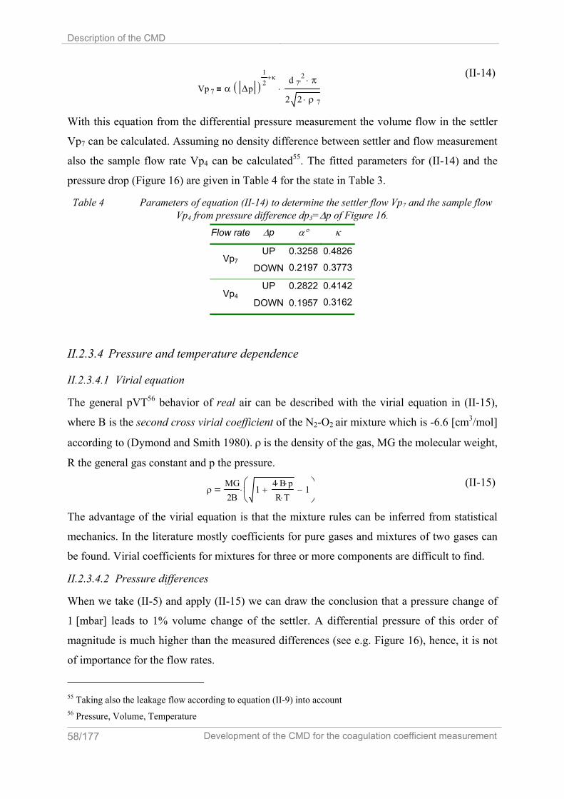
Description of the CMD
58/177 Development of the CMD for the coagulation coefficient measurement
Vp 7 α ∆p( )12
κ+ d 7'2 π⋅
2 2 ρ 7⋅⋅
(II-14)
With this equation from the differential pressure measurement the volume flow in the settler
Vp7 can be calculated. Assuming no density difference between settler and flow measurement
also the sample flow rate Vp4 can be calculated55. The fitted parameters for (II-14) and the
pressure drop (Figure 16) are given in Table 4 for the state in Table 3.
Table 4 Parameters of equation (II-14) to determine the settler flow Vp7 and the sample flow Vp4 from pressure difference dp3=∆p of Figure 16.
Flow rate ∆p α° κ
UP Vp7
DOWN
0.3258
0.2197
0.4826
0.3773
UP 0.2822Vp4
DOWN 0.1957
0.4142
0.3162
II.2.3.4 Pressure and temperature dependence
II.2.3.4.1 Virial equation
The general pVT56 behavior of real air can be described with the virial equation in (II-15),
where B is the second cross virial coefficient of the N2-O2 air mixture which is -6.6 [cm3/mol]
according to (Dymond and Smith 1980). ρ is the density of the gas, MG the molecular weight,
R the general gas constant and p the pressure.
ρMG2B
14 B⋅ p⋅R T⋅
+ 1−⎛⎜⎝
⎞⎠
⋅
(II-15)
The advantage of the virial equation is that the mixture rules can be inferred from statistical
mechanics. In the literature mostly coefficients for pure gases and mixtures of two gases can
be found. Virial coefficients for mixtures for three or more components are difficult to find.
II.2.3.4.2 Pressure differences
When we take (II-5) and apply (II-15) we can draw the conclusion that a pressure change of
1 [mbar] leads to 1% volume change of the settler. A differential pressure of this order of
magnitude is much higher than the measured differences (see e.g. Figure 16), hence, it is not
of importance for the flow rates.
55 Taking also the leakage flow according to equation (II-9) into account 56 Pressure, Volume, Temperature
Setup of the CMD
Development of the CMD for the coagulation coefficient measurement 59/177
II.2.3.4.3 Temperature
Temperature changes have a greater influence on the settler gas volume V7. A gas volume
change of 1% at standard state57 can be affected by ~3 [K] temperature difference. As the
physical settler volume is constant, this leads to an increased/decreased sample flow Vp4 in
the measurement mode which has to be considered.
Under normal operation the temperature is constant in the settler as during the
measurement in the SMPS, CPC. In case of future investigations of aerosols at higher than
ambient temperatures, two cases can be investigated: A.) The probe is heated up in the settler
B.) The settler is filled with an aerosol above ambient temperature. In both cases the aerosol is
kept at a constant temperature and afterwards cooled down by a heat exchanger. In the
following, method B is described more extensively.
II.2.3.4.4 Constant temperature settler and SMPS system difference measurement
As, due to safety reasons58, the SMPS measurement is only possible up to a temperature of
50 [°C]. Higher temperature measurements have to be cooled down for particle concentration
measurement.
The settler flow rate Vp7 is physically determined by the stepper motor and
consequently constant for all temperatures, at the same pressure (see also Table 3). First the
aerosol is sampled at an above ambient temperature, then the valves are closed and the
temperature is kept constant. Making a size distribution measurement, the flow is cooled
down. The pressure stays approximately constant, but the density increases leading to a net
lower sample flow rate Vp4. The time ttotal - e.g. for the effective flow rate experiment see
p.51 ff. - stays the same. The apparent particle concentration increases as the volume flow is
lower than at the original temperature in the settler. The total particles measured stay the
same, the referred volume changes. For these reasons it can be concluded that for a given
temperature difference between settler and SMPS-system ∆t=T7-T2 the particle concentration
has to be corrected59.
___________________________________________________________________________
57 Ts=20 [°C] ,ps=1013 [mbar] 58 The radioactive source mounting could be damaged. 59 In this consideration no particle concentration change due to particle loss (deposition, coagulation etc.) or
formation (nucleation etc.) has been regarded.

Description of the CMD
60/177 Development of the CMD for the coagulation coefficient measurement
CONCLUSION
A positive temperature difference between settler and sample flow will lead to a decreased
sample flow and an increased particle concentration and vice versa.
METHOD FOR GAINING PARTICLE CORRECTION
For correcting the particle concentration, the first equation (II-7) is resolved for Vp4 according
to the temperature difference ∆t, which is implicitly described with the density and the virial
equation (II-15). Vp7 and α are constant for each ttotal according to Table 3. The calculated
Vp4 should then be identical with the measured one. The flow rate correction factor δ+1 is
then Vp7/Vp4 which is also the correction factor for the real particle concentration. The flow
rate percentage increase δ can then be written:
p1,T2 is the pressure temperature state in the SMPS cabinet which is approximately the same
as at the ASF 1430 sensor. p2, T7 is the state in the settler for the pressure and temperature and
α is the experimental correction factor from Table 3, which is constant for a constant
temperature at the flow sensor T4 ≈ T2 and the leak at ambient air TL.
_________________________________________________________________________
In Figure 17 and Table 5 the dependency of the measured flow rate from the settler flow rate
is given for different temperatures in the settler T7 and a constant T4=20°C according to (II-7).
In Figure 18 and Table 6 the percentage increase of the flow rate Vp4 is given, to
calculate the flow rate Vp7 or to calculate the percentage increase of the particle concentration
in the settler for T4=20°. The basic equation for this calculation is equation (II-16).
As can be seen δ=α in Table 6 and Vp4 in Table 5 equals to Vp4 in Table 3 for
T4=20°C and T7=20°C, as this is the isothermal case.
δVp 7Vp 4
1− 1 α+( )1
4B p 1⋅
R T 2⋅+ 1−
14B p 2⋅
R T 7⋅+ 1−
⋅ 1−
(II-16)

Setup of the CMD
Development of the CMD for the coagulation coefficient measurement 61/177
15 25 35 45 55 65 750
0.05
0.1
0.15
0.2
0.25
0.3
0.35
0.4
0.45
0.5
T7=0°CT7=20°CT7=40°CT7=60°CT7=80°CT7=100°C
ttotal [min]
Vp4
[l/m
in]
Figure 17 Volume flow Vp4 at T4=20°C as a function of different settler temperatures T7 and the total measurement time ttotal. The ambient temperature T2 is also 20°C.
15 20 25 30 35 40 45 50 55 60 65 70 7510
5
0
5
10
15
20
25
30
35
40
45
50
T7=0°CT7=20°CT7=40°CT7=60°CT7=80°CT7=100°C
ttotal [min]
delta
[%]
Figure 18 δ in % at T4=20°C as a function of different settler temperatures T7 and the total measurement time ttotal . The ambient temperature T2 is also 20°C.
δ [−
]
ttotal [min] T7=0°C T7=20°C T7=40°C T7=60°C T7=80°C T7=100°C
T7=0°C T7=20°C T7=40°C T7=60°C T7=80°C T7=100°C
ttotal [min]
Vp 4
[l/m
in]
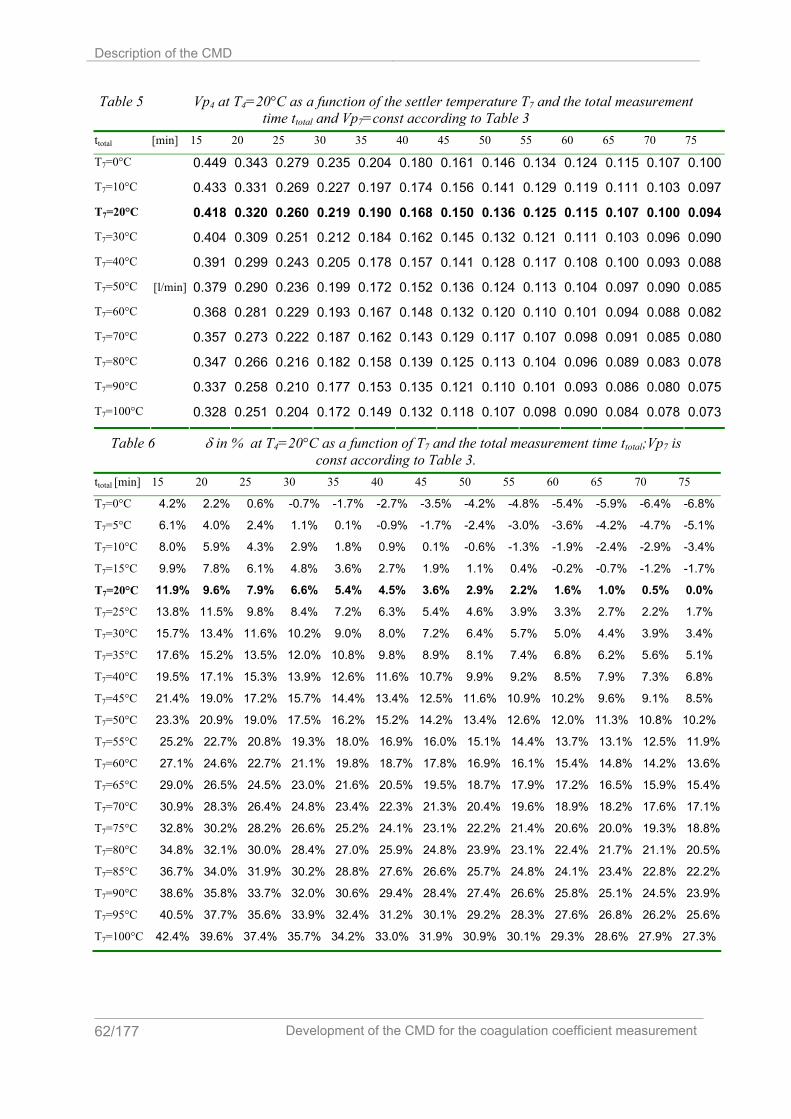
Description of the CMD
62/177 Development of the CMD for the coagulation coefficient measurement
Table 5 Vp4 at T4=20°C as a function of the settler temperature T7 and the total measurement time ttotal and Vp7=const according to Table 3
ttotal [min] 15 20 25 30 35 40 45 50 55 60 65 70 75
T7=0°C 0.449 0.343 0.279 0.235 0.204 0.180 0.161 0.146 0.134 0.124 0.115 0.107 0.100
T7=10°C 0.433 0.331 0.269 0.227 0.197 0.174 0.156 0.141 0.129 0.119 0.111 0.103 0.097
T7=20°C 0.418 0.320 0.260 0.219 0.190 0.168 0.150 0.136 0.125 0.115 0.107 0.100 0.094
T7=30°C 0.404 0.309 0.251 0.212 0.184 0.162 0.145 0.132 0.121 0.111 0.103 0.096 0.090
T7=40°C 0.391 0.299 0.243 0.205 0.178 0.157 0.141 0.128 0.117 0.108 0.100 0.093 0.088
T7=50°C 0.379 0.290 0.236 0.199 0.172 0.152 0.136 0.124 0.113 0.104 0.097 0.090 0.085
T7=60°C 0.368 0.281 0.229 0.193 0.167 0.148 0.132 0.120 0.110 0.101 0.094 0.088 0.082
T7=70°C 0.357 0.273 0.222 0.187 0.162 0.143 0.129 0.117 0.107 0.098 0.091 0.085 0.080
T7=80°C 0.347 0.266 0.216 0.182 0.158 0.139 0.125 0.113 0.104 0.096 0.089 0.083 0.078
T7=90°C 0.337 0.258 0.210 0.177 0.153 0.135 0.121 0.110 0.101 0.093 0.086 0.080 0.075
T7=100°C
[l/min]
0.328 0.251 0.204 0.172 0.149 0.132 0.118 0.107 0.098 0.090 0.084 0.078 0.073
Table 6 δ in % at T4=20°C as a function of T7 and the total measurement time ttotal;Vp7 is const according to Table 3.
ttotal [min] 15 20 25 30 35 40 45 50 55 60 65 70 75
T7=0°C 4.2% 2.2% 0.6% -0.7% -1.7% -2.7% -3.5% -4.2% -4.8% -5.4% -5.9% -6.4% -6.8%
T7=5°C 6.1% 4.0% 2.4% 1.1% 0.1% -0.9% -1.7% -2.4% -3.0% -3.6% -4.2% -4.7% -5.1%
T7=10°C 8.0% 5.9% 4.3% 2.9% 1.8% 0.9% 0.1% -0.6% -1.3% -1.9% -2.4% -2.9% -3.4%
T7=15°C 9.9% 7.8% 6.1% 4.8% 3.6% 2.7% 1.9% 1.1% 0.4% -0.2% -0.7% -1.2% -1.7%
T7=20°C 11.9% 9.6% 7.9% 6.6% 5.4% 4.5% 3.6% 2.9% 2.2% 1.6% 1.0% 0.5% 0.0%
T7=25°C 13.8% 11.5% 9.8% 8.4% 7.2% 6.3% 5.4% 4.6% 3.9% 3.3% 2.7% 2.2% 1.7%
T7=30°C 15.7% 13.4% 11.6% 10.2% 9.0% 8.0% 7.2% 6.4% 5.7% 5.0% 4.4% 3.9% 3.4%
T7=35°C 17.6% 15.2% 13.5% 12.0% 10.8% 9.8% 8.9% 8.1% 7.4% 6.8% 6.2% 5.6% 5.1%
T7=40°C 19.5% 17.1% 15.3% 13.9% 12.6% 11.6% 10.7% 9.9% 9.2% 8.5% 7.9% 7.3% 6.8%
T7=45°C 21.4% 19.0% 17.2% 15.7% 14.4% 13.4% 12.5% 11.6% 10.9% 10.2% 9.6% 9.1% 8.5%
T7=50°C 23.3% 20.9% 19.0% 17.5% 16.2% 15.2% 14.2% 13.4% 12.6% 12.0% 11.3% 10.8% 10.2%
T7=55°C 25.2% 22.7% 20.8% 19.3% 18.0% 16.9% 16.0% 15.1% 14.4% 13.7% 13.1% 12.5% 11.9%
T7=60°C 27.1% 24.6% 22.7% 21.1% 19.8% 18.7% 17.8% 16.9% 16.1% 15.4% 14.8% 14.2% 13.6%
T7=65°C 29.0% 26.5% 24.5% 23.0% 21.6% 20.5% 19.5% 18.7% 17.9% 17.2% 16.5% 15.9% 15.4%
T7=70°C 30.9% 28.3% 26.4% 24.8% 23.4% 22.3% 21.3% 20.4% 19.6% 18.9% 18.2% 17.6% 17.1%
T7=75°C 32.8% 30.2% 28.2% 26.6% 25.2% 24.1% 23.1% 22.2% 21.4% 20.6% 20.0% 19.3% 18.8%
T7=80°C 34.8% 32.1% 30.0% 28.4% 27.0% 25.9% 24.8% 23.9% 23.1% 22.4% 21.7% 21.1% 20.5%
T7=85°C 36.7% 34.0% 31.9% 30.2% 28.8% 27.6% 26.6% 25.7% 24.8% 24.1% 23.4% 22.8% 22.2%
T7=90°C 38.6% 35.8% 33.7% 32.0% 30.6% 29.4% 28.4% 27.4% 26.6% 25.8% 25.1% 24.5% 23.9%
T7=95°C 40.5% 37.7% 35.6% 33.9% 32.4% 31.2% 30.1% 29.2% 28.3% 27.6% 26.8% 26.2% 25.6%
T7=100°C 42.4% 39.6% 37.4% 35.7% 34.2% 33.0% 31.9% 30.9% 30.1% 29.3% 28.6% 27.9% 27.3%

Operation of the CMD
Development of the CMD for the coagulation coefficient measurement 63/177
II.2.3.5 Gas dependence
The settler flow Vp7 is independent of the gas and constant, as it is physically determined by
the geometry and the stepper motor control. The volume flow Vp4 may vary due to a different
pressure difference and hence a different leakage flow. The flow sensor for the flow Vp4 has
to be calibrated for the gas. This can be done, e.g., with a settler measurement (ideally)
without leakage flow. Gas mixtures can be calculated, e.g., with equation (II-16), which is of
importance for the leakage flow mixture calculation or, e.g., the complex operation
“Polydisperse Coagulation II” (see section II.3).
II.3 Operation of the CMD
II.3.1 Path concept
For the measurement of the particle concentration over time the path concept has been
established. It denotes a certain configuration of the valves, leading to a fluid path in the
tubing of the CMD. The path the fluid takes according to the setting of the valves is shown in
Table 7, with the names according to Figure 10.
Table 7 CMD paths: green=filling or cleaning; orange=settler measuring; blue=like standard SMPS measuring
Path Short name Detailed path 1 Probe Fill Mono Probe in V1 ASF V2 SMPS classifier V3
V4 V5 V7 Settler V8 V6 PU1 exhaust 2 Probe Measure60 Probe in V1 ASF V2 SMPS classifier V3
V4 CPC V6 PU1 exhaust 3 Settler Measure Settler V7 V5 V1 ASF V2 SMPS classifier V3
V4 CPC V6 PU1 exhaust 4 Settler Count Settler V7 V5 V1 ASF V2 V3 V4 CPC V6
PU1 exhaust 5a Probe Fill Poly Probe in VM2 V1 ASF V2 V3 V4 V5 V7
Settler V8 V6 PU1 exhaust 5b Settler Clean Ambient air RLF1 VM2 V1 ASF V2 V3 V4 V5 V7
Settler V8 V6 PU1 exhaust 6 Probe Count Probe in V1 ASF V2 V3 V4 CPC V6 PU1 exhaust
The six paths are as follows:
1. The path “Probe fill mono” serves to fill the settler with a probe of a specified
diameter MDP (monodisperse particle diameter)61. The air flow is vacuumed in
through the SMPS classifier. The particle diameter of the DMA is set to the
monodisperse filling diameter MDP with the CMD software.
60 Or waiting for coagulation, deposition, sedimentation etc. 61 Monodisperse means that the particle size distribution has a very narrow standard deviation.
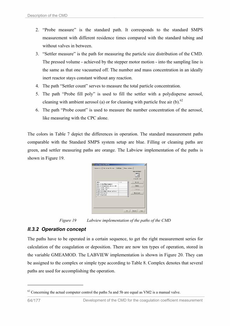
Description of the CMD
64/177 Development of the CMD for the coagulation coefficient measurement
2. “Probe measure” is the standard path. It corresponds to the standard SMPS
measurement with different residence times compared with the standard tubing and
without valves in between.
3. “Settler measure” is the path for measuring the particle size distribution of the CMD.
The pressed volume - achieved by the stepper motor motion - into the sampling line is
the same as that one vacuumed off. The number and mass concentration in an ideally
inert reactor stays constant without any reaction.
4. The path “Settler count” serves to measure the total particle concentration.
5. The path “Probe fill poly” is used to fill the settler with a polydisperse aerosol,
cleaning with ambient aerosol (a) or for cleaning with particle free air (b).62
6. The path “Probe count” is used to measure the number concentration of the aerosol,
like measuring with the CPC alone.
The colors in Table 7 depict the differences in operation. The standard measurement paths
comparable with the Standard SMPS system setup are blue. Filling or cleaning paths are
green, and settler measuring paths are orange. The Labview implementation of the paths is
shown in Figure 19.
Figure 19 Labview implementation of the paths of the CMD
II.3.2 Operation concept
The paths have to be operated in a certain sequence, to get the right measurement series for
calculation of the coagulation or deposition. There are now ten types of operation, stored in
the variable GMEAMOD. The LABVIEW implementation is shown in Figure 20. They can
be assigned to the complex or simple type according to Table 8. Complex denotes that several
paths are used for accomplishing the operation.
62 Concerning the actual computer control the paths 5a and 5b are equal as VM2 is a manual valve.

Operation of the CMD
Development of the CMD for the coagulation coefficient measurement 65/177
Figure 20 Labview implementation of the operations of the CMD
Table 8 Operations of the CMD
Each operation is explained in detail in the following sections.
II.3.2.1 Complex operation types
The actual complex operation types are depicted in Figure 21 and Figure 22, the bold words
denote the operations. They are:
1. Monodisperse Coagulation and
2. Polydisperse Coagulation.
3. Polydisperse Coagulation I
4. Polydisperse Coagulation II
II.3.2.1.1 Mono- and Polydisperse Coagulation
The flow chart for the first two operations 1 & 2 is shown in Figure 21. For the operation
“Monodisperse Coagulation” first the settler is cleaned with path 5. Either the clean air filter
RLF1 is used setting the manual valve VM2 or ambient air is filled into the settler. The
subsequent step is to fill the probe into the settler, setting a monodisperse diameter MDP at
the DMA. For the operation “Polydisperse Coagulation” the settler is first filled with a
polydisperse probe at the “probe in” air inlet with path 5. Then with path2 the valves V7-V8
Operation name type 1 Monodisperse Coagulation Complex2 Polydisperse Coagulation Complex3 Ambient Size Distribution Simple 4 Settler Size Distribution Simple 5 Ambient Concentration Simple 6 Settler Concentration Simple 7 Settler Cleaning Simple 8 Monodisperse Filling Simple 9 Polydisperse Coagulation I Complex
10 Polydisperse Coagulation II Complex

Description of the CMD
66/177 Development of the CMD for the coagulation coefficient measurement
are closed to keep a constant settler probe. Then enough time is given to allow for the
coagulation in the settler.
For mono- and polydisperse coagulation measurement (complex operation 1 & 2) the
sequence is now the same; first measuring the particle size distribution in path3, then waiting
for coagulation. This procedure is done NSM (number of simple (single) measurements)
times until the actual measurement is NSMA=NSM. The settler is then cleaned and returns to
the starting end position.
monodisperse/ polydisperse
path5
path1 path2
MONO POLY
path3
path2
NMSA=NSMNo
path5
Monodisperse Coagulation Polydisperse Coagulation
Yes
Figure 21 The complex operations “Monodisperse Coagulation” and “Polydisperse Coagulation”
II.3.2.1.2 Polydisperse Coagulation I,II
The operations ”Polydisperse Coagulation I” and “-II” use only the concentration
measurements with the CPC without using the SMPS classifier. Hence with this method only
the coagulation of a polydisperse aerosol can be determined.
The flow chart is depicted in Figure 22. First in both operations the settler is cleaned,
and filled with path 5. This can be accomplished by first applying the single operation
“Settler Cleaning”, then switching the manual valve VM2 to “probe in”. After filling path 5
the manual valve VM2 should be switched to the clean air filter again.

Operation of the CMD
Development of the CMD for the coagulation coefficient measurement 67/177
Then the particle concentration is measured with path 4. For the operation “Polydisperse
Coagulation I” this is done when the settler volume has been emptied, then the initial state is
reestablished. For the operation “Polydisperse Coagulation II” a certain time smaller than ttotal
for the counting measurement has to be entered in the Labview software for path 4. Path 5a
serves then as dilution of the settler with clean ambient air, while the stepper motor is driving
to the starting initial position63.
Polydisperse Coagulation I/IIpath5 path5a
Method I Method II
NMSA=NSMNo
path5
Polydisperse Coagulation I Polydisperse Coagulation II
Yes
path4
path5
Figure 22 Complex operations Polydisperse Coagulation I and II
The complex operation “Polydisperse Coagulation I” and “Polydisperse Coagulation II” refer
directly to the theoretical justified coagulation coefficient retrieving methods given in I.3.4.4
and I.3.4.5 respectively. This theoretical foundation is then used in the experimental part in
chapter III for evaluation of the coagulation coefficient.
II.3.2.2 Simple operation types
The simple operation types are denoted by the application of one path to one operation. They
are depicted in Figure 23, with the operations in bold. Each operation can be repeated NSM
63 For the operation “Polydisperse Coagulation I” it is recommended for the current setting to make only one
single measurement, as the filling operation has to be accomplished manually by VM2.

Description of the CMD
68/177 Development of the CMD for the coagulation coefficient measurement
times. They can be used to measure a set of measurements manually, or e.g. for filling,
cleaning etc. In general a complex operation should be implemented, when the sequence of
paths is known, to fully use the capabilities of the LABVIEW automation. This is very
important for reproducibility.
• The “Ambient Size distribution” operation measures the size distribution that can also
be measured with the standard SMPS system. The residence time between SMPS
classifier and CPC is longer, hence the parameter td. The residence time τ4 (Figure 9)
instead of τ0 (Figure 10) has to be taken.
Ambient/Settler
Size distribution or number
concentration
YES
path2 path6
YES
Measure/Filling
NO
Size distribution or number
concentration
YES
NO
path3
YES
path4 path1 path5 a/b
Mono or Poly
NO
NOYES
NO
Ambient Size Distribution
Ambient Concentration
Settler Size Distribution
Settler Concentration
Monodisperse Filling
Settler Cleaning(Polydisperse Filling)
Figure 23 Decision chart for the simple operations of the CMD denoted with bold letters. • The “Ambient Concentration” operation measures the total number concentration of
the CPC from the ambient in, without any other device.
• The operation “Settler Size Distribution” measures size distribution from the settler,
like in the complex paths individually.
• The operation “Settler Concentration” measures the particle number concentration of
the settler alone.
• “Monodisperse Filling” denotes the filling of the settler with a monodisperse particle
source.
• The operation “Settler Cleaning” denotes the cleaning with the clean air filter as noted
above in the complex operation (setting by manual valve VM2). This operation can
also be used to fill the settler with an aerosol at the “probe in” inlet, which is
polydisperse or monodisperse in dependence of the aerosol source.

Operation of the CMD
Development of the CMD for the coagulation coefficient measurement 69/177
II.3.3 Labview software implementation
Implementation of the CMD integrates all valves, sensor measurements, the stepping motor
control and the measurement instruments like the SMPS64 or the CPC of the Labview
software. Additional hardware can be implemented by adding modules into the Labview
platform.
In this section first a short overview is given of the most important features that were
used for programming the LABVIEW main application. More details of the programming
language can be found in (Jamal and Hagestedt 2001; National Instruments 2003; National
Instruments 2004). Then an overview of the most important programming features and the
main program modules65 is given: The main66-, initialization-67 and measurement-68 program.
II.3.3.1 Structure
The basic principle is to program in modules. The detailed software implementation and the
variables definition is given in the appendix and on the accompanying CD. The implemented
CMD program makes use of the following features of Labview:
• Modules
• State Machines
• Parallel Processing
II.3.3.1.1 Modules
Modules, so called vi’s (virtual instrument) split the task in logical operations, and they aim at
keeping the overview over the total program architecture.
The modules were programmed for the sensors, the valves, and the measurement
instruments first. For example, the previously introduced path concept was applied first in the
basis valve control program.
64 SMPS 3081: System from TSI containing the classifier 3081, the DMA 3080 and the CPC 3010 65 In Labview, the subroutines are called sub-vi, each program is called a vi. The name refers to the file extension
*.vi and means “virtual instrument”. 66 CMDC_Menu.vi 67 CMDC_Initialization.vi 68 CMDC_Measurement.vi

Description of the CMD
70/177 Development of the CMD for the coagulation coefficient measurement
The modules build the basis of the programming hierarchy, which have been built into a
hierarchy of state machines and parallel processes for simultaneous measurement.
II.3.3.1.2 State Machines
A state machine is a LABVIEW program with certain architecture. It is implemented in a
CASE programming structure. Different states are switched to, using a CASE for each state.
The path and the operation concept were used as base for the state machine programming.
The State machine is also useful in general program structuring. Different programs
branching from the main program are also states of a state machine e.g. the main menu in
Figure 24.
II.3.3.1.3 Parallel Processing
The exact parallel processing is implemented in LABVIEW with “while loops” by means of
“notifiers”, that are exchanging data between the while loops. These can trigger simultaneous
measurement start, which is important for exact parallel measurement of the sensor and
instrument data.
One exception is the serial measurement. Four instruments and sensors are plugged to
one serial interface card. These are: SMPS, CPC, ASF, ASP. They respond in the same
sequence as denoted, because the used serial card is not capable of parallel processing. As a
consequence the minimum time interval of all measurements in parallel is approximately 3[s],
which can be reduced by switching of sensors69.
II.3.3.2 Main menu
The main menu can be seen in Figure 24. In this case each button denotes a separate state in
the state machine. There are four programs that can be called:
1.) Initialization: This program serves for initialization and control of all sensors
the stepper motor and the valves.
2.) File: This program chooses the measurement protocol file. A standard file
“Testxx.xls” can be chosen by the button Standard file.
3.) The button “All measurements” calls the sub-vi “CMDC Measurement”
4.) Coagulation Coefficient is not yet programmed, and should serve for the
automatic statistical evaluation of the measurements including the calculation
of the coagulation coefficient.
69 Variable SM in Figure 54

Operation of the CMD
Development of the CMD for the coagulation coefficient measurement 71/177
Figure 24 Main application window of the CMD-Program: „CMDC_Menu.vi“
II.3.3.3 Initialization
The program window for the Initialization vi is shown in Figure 25. There are initialization
and or control programs for the CMD accessible. The programs are briefly described as
follows:
SMPS
INIT: This program initializes the sheath flow rate of the SMPS
BASIS: Most of the measurement values available from the SMPS can be seen.
They are read out from the SMPS microcontroller via RS232 (serial interface).
They are identical with the information available at SMPS display.
CPC STATE: Reads all the measurement values available for the CPC via RS232.
Figure 25 Application window of the CMD-Program: „CMDC_Initialization.vi“ ASF INFO: Reads out the information of the ASF flow sensor via RS232

Description of the CMD
72/177 Development of the CMD for the coagulation coefficient measurement
ASP MEASC: Makes a measurement of the ASP differential pressure sensor
via RS232
HUM MEASC: Makes a measurement of the humidity sensor SHT75 via
RS232. The evaluation kit EK-H7 is used for the microprocessor
control and serial connection with the sensor.
STATES STATESC: Is used to test the different paths in section (II.3.1), setting
the valves to the corresponding states.
DAQ P2T7C: Data Acquisition Hardware from NI (National Instruments)
SC-2345 (Signal conditioning). A Pt 100 platinum sensor T7 and the
pressure sensor HCX001A6V p2 from the settler are accessed (see
Figure 10).
SM RUNC: Stepper motor control program. The different modes of
accessing the stepper motor can be tested. The stepper motor control
program from HASOTEC70 (see Figure 58) has to be started before
main program execution. It has to be taken care that the valves are in
the right position (right path), before running the program. In case of
continuous running of the stepper motor, the end switches from the
settler can be used to stop the running of the stepper motor.
II.3.3.4 Measurement
This is the main program for the CMD. All measurement automation tasks can be
accomplished with this program. The control window can be seen in Figure 26. As this
window contains all important information for measuring, it will be explained in detail,
beginning with the variable name.
PATH: In the first deactivated line the path including the name of the protocol file previously
chosen can be seen. It can not be changed.
COMMENT: In the next line a comment can be inserted for each measurement. It appears in
the protocol file in the first line for each measurement that has been started with the start
button.
70 The program “SM4xDRV.EXE” is the driver program of the HASOTEC SM-41 PCI card for the stepper
motor control. This program has to be started and closed once before access in LABVIEW is possible.

Operation of the CMD
Development of the CMD for the coagulation coefficient measurement 73/177
ROTDRV: Number of rotations set by the manual valve DRV1. The number to flow rate
relationship is attached at DRV1 on the instrument which is also shown as result of the
calibration measurements (Figure 27, p. 81).
GMEAMOD: A dropdown list can be accessed in the variable GMEAMOD. Here all the
operations possible can be chosen for the measurement (see section II.3.2). The operation that
can be seen is the complex operation “Monodisperse Coagulation”.
TIMER: The variable timer on the left side is deactivated, as the timer is chosen on the right
side, explained later.
NSM: denotes the number of single (simple) measurement performed. Concerning simple
measurements the number of these is denoted.
NSMA: is the actual count number of NSM.
SF (starting flag) is true when a measurement is running otherwise false.
TTOTAL: The total calculated measurement time due to the setting in seconds.
TTOTALA: The total actual measurement time in seconds that has passed.
PATHS: Denotes the actual path that is set.
PATHi: i=1..6 time information and control of the different paths; Each line is only active
when the corresponding path is actually set. The STOP buttons STPi can end the control of
the actual path. The path times are:
1: TMFILL/TFILLA: The monodisperse filling time and actual time of path
2: TCOAGUL/TCOAGULA: The monodisperse filling time and actual time of path
3: TSMEAS/TSMEASA: Settler measuring path and actual time of path
4: TCOUNT/TCOUNTA: Settler counting time and actual time of path
5: TPFILL/TPFILLA: Polydisperse filling or settler cleaning time and actual time of
path
5a: TDILUTE/ TDILUTEA: Settler diluting time and actual time of path
6: TPCOUNT/TPCOUNTA: Polydisperse counting time and actual time of path
V1-8: Depicts the actual setting of the valves ON/OFF=LIGHT GREEN/DARK GREEN
together with the path.
SPFA: is the setting of the speed of the stepper motor, either turning the button or setting the
value. The speed factor SPFA corresponds to a flow rate shown in Figure 12 p.52.
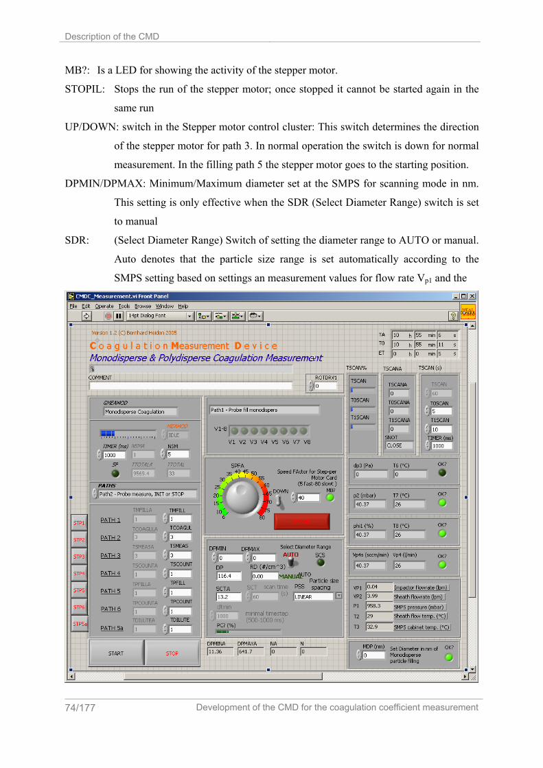
Description of the CMD
74/177 Development of the CMD for the coagulation coefficient measurement
MB?: Is a LED for showing the activity of the stepper motor.
STOPIL: Stops the run of the stepper motor; once stopped it cannot be started again in the
same run
UP/DOWN: switch in the Stepper motor control cluster: This switch determines the direction
of the stepper motor for path 3. In normal operation the switch is down for normal
measurement. In the filling path 5 the stepper motor goes to the starting position.
DPMIN/DPMAX: Minimum/Maximum diameter set at the SMPS for scanning mode in nm.
This setting is only effective when the SDR (Select Diameter Range) switch is set
to manual
SDR: (Select Diameter Range) Switch of setting the diameter range to AUTO or manual.
Auto denotes that the particle size range is set automatically according to the
SMPS setting based on settings an measurement values for flow rate Vp1 and the

Operation of the CMD
Development of the CMD for the coagulation coefficient measurement 75/177
Figure 26 Application window of the CMD-Program:”CMDC_Measurement.vi”; this is the central window controlling all measurements
impactor. When the flow rate is small the impaction is low and hence the
maximum diameter is high.
DP: Is the actual set diameter of the CMD software at the SMPS, it is determined
corresponding to the time plan and the settings for DPMIN/DMAX and PSS.
RD: Is the actual read particle size concentration of the CPC [#/cm3]
SCT/SCTA: Scanning time beginning from the setting of DPMIN at the SMPS classifier
and actual time
PSS: Particle Size Spacing mode: LINEAR/LOGARITHMIC; Depending on the mode
the particle diameter difference ∆dp between scanning intervals is calculated in the
manner of equal distances for the LOGARITHMIC scales or for LINEAR size
spacing in the linear scale.
dtmin: Equal to timer on the right setting (deactivated) (ms).
PC?%: Percentage of success for the actual scanning process.
DPMINA/DPMAXA: Actual setting of the minimum/maximum diameter read from the SMPS
in nanometer.
N/NA: The number of N different particle size scans determined by the user setting and
the actual number of the scanning diameter.
T0/TA/ET:Starting time, Difference time and actual time
TSCAN/TSCANA: Calculated and actual total time for measuring path 3 set by the
scanning times T0SCAN and T1SCAN.
T0SCAN/T0SCANA: Scanning start time and actual scanning start time. For this time
interval the path for the measurement path 3 is set waiting for the aerosol to flow
into the SMPS. After this time, the scanning can begin.
T1SCAN/T1SCANA: Time set for scanning mode and corresponding actual time at the
SMPS.
TIMER (ms): Sets the timing interval for the logging of the measurement data in the protocol
file. It is restricted to approximately 3s for all sensors in operation.
SNOT intern notifier (see above II.3.3.1.3, p.70). Variable indicating the states of the
SCAN Modus.
TSCAN/TSCAN0/TSCAN1: Progress indicators of each scanning mode.

Description of the CMD
76/177 Development of the CMD for the coagulation coefficient measurement
The LEDS on the right side denote the correct operation of the sensors. They can be partly
turned off to increase measurement time interval TIMER in the variable SM (Figure 54).
dp3(Pa)/ T6(°C): Actual sensor values for the differential pressure sensor ASP1400 dp3 and
the temperature measurement on this sensor. T6 represents not the ambient
temperature.
p2(mbar)/T7(°C): Actual NI-DAQ measurement of the pressure and the temperature in the
settler.
phi1(%)/T8(°C): Actual relative humidity measurement phi1 and the corresponding
temperature measurement on the sensor T8. These values can also be read on
the digital display of the attached microcontroller evaluation kit EK-H2.
Vp4s(sccm/min)/Vp4(l/min): Standard flow measurement with the flow sensor ASF1430. The
corresponding actual flow rate Vp4 [l/min] is calculated by means of the
measurements p2 and T7, the standard state Ts=20 [°C] ,ps=1013 [mbar] and the
ideal gas law.
The following measurement values are read from the SMPS classifier microcontroller:
VP1: SMPS impactor flow rate [l/min]
VP2: SMPS sheath flow rate [l/min]
P1: SMPS pressure [mbar]
T2 : SMPS sheath flow temperature [°C]
T3: SMPS cabinet temperature [°C]
MDP(nm): Monodisperse particle diameter which is set for monodisperse filling of the
CMD. The OK LED indicates that the command is sent successfully to the
SMPS.
START: The start button starts the measurement series after setting all variables above.
STOP: This button is used to leave this program and go back to the main menu.
II.4 Fundamental considerations
II.4.1 Reactor characterization
The settler proposed is a constant concentration reactor. This is a reactor whose ideal
concentration is constant. This can be explained by its operation. In the measurement mode
the sample flow volume is vacuumed off the settler while simultaneously pumping it out.
With this method

Fundamental considerations
Development of the CMD for the coagulation coefficient measurement 77/177
• mixing of the batch volume with ambient air
• dilution
• pressure and temperature change can be avoided.
Under the ideal condition of no coagulation deposition or settling of particles the mass m and
the number concentration N is constant, explaining the constant concentration reactor (see
Table 9).
The constant concentration reactor is comparable with a discontinuous stirred tank
reactor (dCSTR)71 (Moser 1988) with constant volume process. The concentration profile is a
function of time and not of space. The reaction is the coagulation, deposition or settling of
particles. The variable volume allows for a constant concentration which is comparable with a
constant volume process for incompressible fluids, without reaction.
Under real conditions either deposition, coagulation or both will occur,72 which is
shown in Table 9.
Table 9 Classification of important ideal physical states relevant for the CMD
Con
stan
t co
ncen
trat
ion
Dep
ositi
on
Coa
gula
tion
Coa
gula
tion
& D
epos
ition
dN/dt 0 0 <>0 <>0 dm/dt 0 <>0 0 <>0
The number concentration gradient dN/dt can be measured with the CMD. For the mass,
gradient dm/dt, e.g. a TEOM73, or a filter measurement is necessary74.
Determining the decay in mass and number concentrations allows for distinguishing
between deposition and coagulation as a function of measurement mode.
An advantage of the constant concentration reactor is that the pressure variation of the
thermodynamic state is minimized (T, p=constant). This conserves, probably, the state of
nanoaerosols also in the case of nucleation processes, as condensation and evaporation is a
function of the vapor pressure, and hence of the thermodynamic state. Therefore it is expected
that liquid aerosols can also be investigated.
71 This is a batch reactor with a stirrer. First the reactor is filled discontinuously after the reaction it is emptied. 72 Settling can be neglected for nanoparticles except for long time ranges. 73 Tapered element microbalance 74 The accuracy of the mass measurement has to be very high and or the measurement time has to be very long.
Description of the CMD
78/177 Development of the CMD for the coagulation coefficient measurement
With defined state transitions e.g. warming, additional insight in particle growth mechanisms
is gained. A constant concentration reactor, like that presented here allows for investigation of
the real aerosol like behavior at constant conditions for low concentrations with tunable
measurement uncertainty75 in a systematic way.
II.4.2 Residence times
There are several paths in CMD each with several residence times according to the overall
flow rate. This overall (sample) flow rate is factored in by the ASF flow sensor VP4 and the
SMPS differential pressure measurement VP1. The flow rates are decisive for the particle size
distribution measurement for several reasons:
• They are limiting the process of possible measurement of coagulation
• They limit the range of measuring time, and parameter settings of the CMD, as e.g.
filling time; scanning start time etc.
• They allow the correct interpretation and shifting measurement parameters especially
the particle diameter of the size distribution.
The concept of residence time τ [s] is closely linked to the flow rate as can be seen of the
defining equation:
Vp [l/min] is the general flow rate and V [l] is the volume. By means of the residence time a
statistical mean time of particles in a certain volume is described, valid for any type of
reactor76. The SMPS sheath flow for example, is, in terms of process terminology, a recycle
flow reactor. The CMD settler is, with respect to coagulation, a batch reactor, where the
waiting time equals the residence time, with respect to filling a fed batch reactor.
Following the individual residence times and their dependencies are described for the
whole CMD system.
75 Depending on number concentration and the time of coagulation the coagulation measurement accuracy
increases. 76 e.g.: batch reactor, fed batch reactor, recycle flow reactor and tube reactor
τV
V p60⋅
(II-17)

Fundamental considerations
Development of the CMD for the coagulation coefficient measurement 79/177
II.4.2.1 Overall residence time for measurement
II.4.2.1.1 Standard SMPS system
The residence times for the standard SMPS measurement with the AIMS (Aerosol Instrument
Manager Software)77 software is given in Table 10. There is a short connector tube between
the SMPS monodisperse output and the CPC. This tube leads to the residence time τ0, which
is “included” as a standard factor td in the AIMS software, together with the residence time of
the CPC (τ6)78. When a longer connector tube is used, there has to be a correction made to this
factor, according to the equations given in chapter II.4.3.1 p.86.
Table 10 Residence times for the standard SMPS system Residence time Path
τ0 DMA out CPC in τ3 DMA in DMA out τ6 CPC in CPC
A second standard factor tf [s] is also calculated for each measurement79, which is identical
with the residence time τ3 defined in (II-21). As τ3 is dependant on the sheath flow and the
sample flow rate it is very important to have a calibrated sample flow (e.g. with the bubble
flow meter “Gilibrator 2” in the standard SMPS measurement. This is even more important as
the integrated differential pressure flow measurement for the sample flow (Vp1 [l/min]) shows
a drift with time. Pollution leads to a different differential pressure, and hence a different flow
rate. In the case of the measurement of cigarette smoke, the impactor had been polluted after
the measurement of one cigarette with a 0.5 [mm] long “wire” approximately 1 [mm] in
diameter, leading to a significant change in flow rate.
The wrong size distribution finally leads to a wrong particle diameter. A correction
can be made afterwards according to (II-21), if the “real” sample and sheath flow is known.
Some remark is given to the use of the AIMS software. The parameters that are put in
for the sample flow are decisive for the following size distribution calculation80. It has to be
taken care to take the actual sample flow values of the SMPS display or, for example, flow
77 original software for the SMPS system from TSI (www.tsi.com) 78 See also in the subsequent chapter II.4.2.3 p.82 and II.4.2.4 p.85 79 This quantity is calculated automatically in the AIMS Software and can not be change by the user 80 There is no possibility for the AIMS software to get measurement results from the SMPS as the data
connection is only between computer and the serial interface of the CPC. The CPC itself is connected with the
SMPS classifier by a data cable transmitting the signal for the DMA high voltage to be set.

Description of the CMD
80/177 Development of the CMD for the coagulation coefficient measurement
rates measured with the bubble flow meter. Otherwise the peak of the size distribution will be
shifted. This is even more important as the SMPS sample flow measurements is sensitive to
pollution.
II.4.2.1.2 CMD system
The most important residence times for the CMD system are given in Table 11.
Table 11 Residence times for the CMD system and the starting and endpoints for the related paths. These are part of different main paths listed in Table 7.
Residence time Path Main paths
Formula
τ1 Settler bottom SMPS in 3 V1/Vp4 τ2 SMPS in DMA in 3,1,2 V2/Vp4 τ3 DMA in DMA out 3,1,2 V3/(Vp2+Vp4) τ4 DMA out CPC in 3,2 V4/Vp4 τ5= τ1+ τ2+ τ4 Settler bottom DMA in & DMA out CPC in 3 (V1+V2+V4)/Vp4
τ6 CPC in CPC 3,4,6,2 1.48 [s] τ7, τ70 Settler top Settler bottom 5a,5b,1 V7/Vp4 τ8 ≈ tFILL Ambient air Settler bottom 5a,5b V8/Vp4 τ9 Settler bottom CPC in 4 V9/Vp4 τ10 Ambient air/probe in SMPS in 1,2 V10/Vp4 τ11 DMA out settler bottom 1 V11/Vp4 τ12 Ambient air/probe in CPC in 6 V12/Vp4
II.4.2.2 Settler
There are three operating modes for the settler:
1. Filling
2. Waiting for Coagulation and deposition
3. Measurement
According to these modes different residence times are of importance. The minimal filling
time tFILL (τ8 [min]) for the settler is, at first approximation, the same as ttotal in Figure 2881, as
this is the residence time for the settler in the fed batch operation mode. It is defined as:
τ 8V 8
V p460⋅
(II-18)
V8 [l] is the volume from the path between aerosol inlet including the total volume of the
settler V70 [l], and Vp4 [l/min] the filling flow rate, adjusted with the needle valve DRV1. Due
to the separate needle valve DRV1 the flow rate can be higher than for the measurement
mode, and so the minimum filling time is lower. The upper flow rate is limited to the
81 Assuming constant flow rate for filling and measurement mode
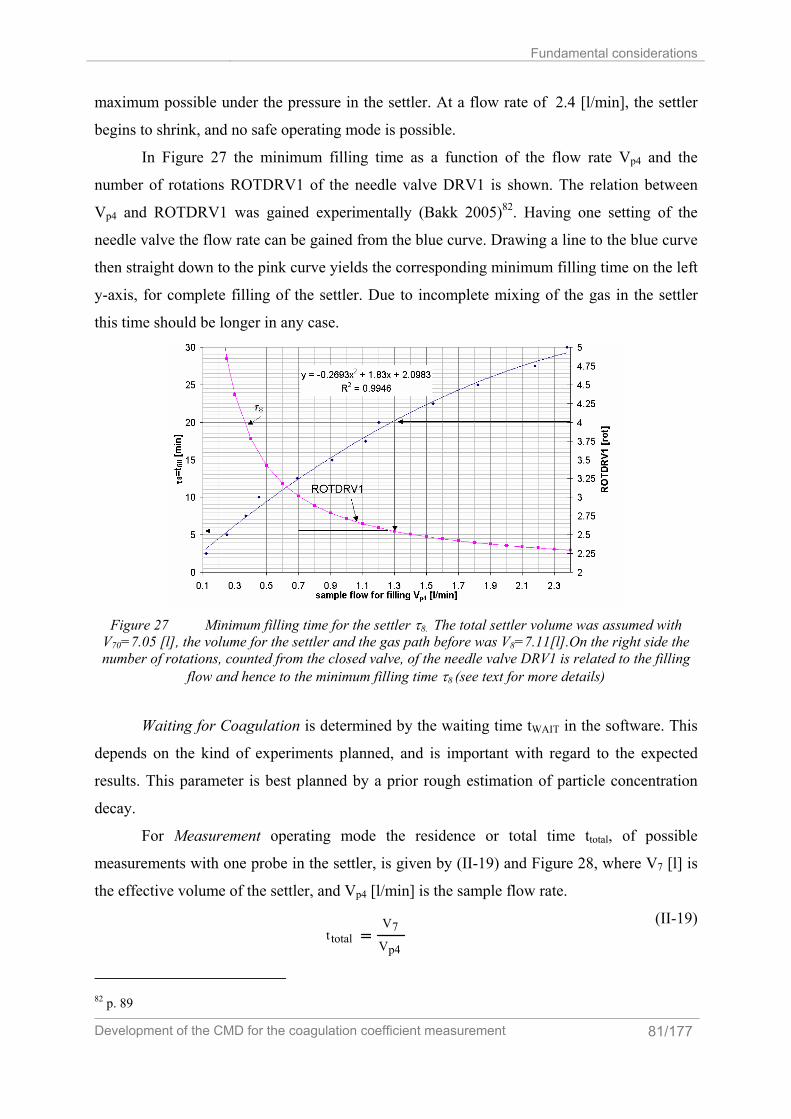
Fundamental considerations
Development of the CMD for the coagulation coefficient measurement 81/177
maximum possible under the pressure in the settler. At a flow rate of 2.4 [l/min], the settler
begins to shrink, and no safe operating mode is possible.
In Figure 27 the minimum filling time as a function of the flow rate Vp4 and the
number of rotations ROTDRV1 of the needle valve DRV1 is shown. The relation between
Vp4 and ROTDRV1 was gained experimentally (Bakk 2005)82. Having one setting of the
needle valve the flow rate can be gained from the blue curve. Drawing a line to the blue curve
then straight down to the pink curve yields the corresponding minimum filling time on the left
y-axis, for complete filling of the settler. Due to incomplete mixing of the gas in the settler
this time should be longer in any case.
Figure 27 Minimum filling time for the settler τ8. The total settler volume was assumed with
V70=7.05 [l], the volume for the settler and the gas path before was V8=7.11[l].On the right side the number of rotations, counted from the closed valve, of the needle valve DRV1 is related to the filling
flow and hence to the minimum filling time τ8 (see text for more details)
Waiting for Coagulation is determined by the waiting time tWAIT in the software. This
depends on the kind of experiments planned, and is important with regard to the expected
results. This parameter is best planned by a prior rough estimation of particle concentration
decay.
For Measurement operating mode the residence or total time ttotal, of possible
measurements with one probe in the settler, is given by (II-19) and Figure 28, where V7 [l] is
the effective volume of the settler, and Vp4 [l/min] is the sample flow rate.
t totalV7
Vp4
(II-19)
82 p. 89

Description of the CMD
82/177 Development of the CMD for the coagulation coefficient measurement
The maximum measurement time tMEAS for a number of NSM single measurements with the
CMD is:
Equation (II-20) is depicted in Figure 28 for application and Figure 53 in the appendix for a
broader time range. When the sample flow rate Vp4 and the number of measurements is fixed
then the total measurement time ttotal of all single measurements can be seen in Figure 28 on
the left side, and the maximum measurement time of one measurement run on the right side.
For example, for the sample flow rate Vp4=0.3 [l/min] and 8 measurements the total
measurement time ttotal ~23 [min] and each single measurement is ~170 [s] long.
Figure 28 Total measurement time possible when emptying the settler as a function of the sample flow Vp4 and the number of the measurements (NSM) on the right y-axis; The total measurement time
as a function of Vp4 can be read on the left y-axis (calculation see equation (II-20)).
II.4.2.3 DMA
The sheath flow in the SMPS DMA is a recycle flow and hence enhances the sample flow.
The residence time τ3 from the voltage setting to the way out of the reactor is determined by:
τ3V3
Vp1 11ζ
+⎛⎜⎝
⎞⎠
⋅
60⋅
(II-21)
V p1
V p2ζ
(II-22)
tMEAS1
NSM
V7
Vp4⋅ 60⋅
(II-20)
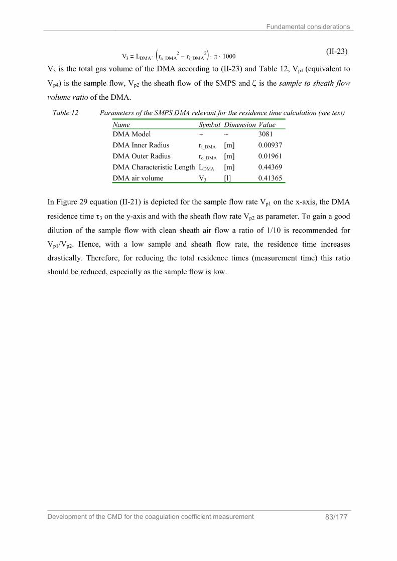
Fundamental considerations
Development of the CMD for the coagulation coefficient measurement 83/177
V3 LDMA ra_DMA2 ri_DMA
2−( )⋅ π⋅ 1000⋅ (II-23)
V3 is the total gas volume of the DMA according to (II-23) and Table 12, Vp1 (equivalent to
Vp4) is the sample flow, Vp2 the sheath flow of the SMPS and ζ is the sample to sheath flow
volume ratio of the DMA.
Table 12 Parameters of the SMPS DMA relevant for the residence time calculation (see text) Name Symbol Dimension Value DMA Model ~ ~ 3081 DMA Inner Radius ri_DMA [m] 0.00937 DMA Outer Radius ro_DMA [m] 0.01961 DMA Characteristic Length LDMA [m] 0.44369 DMA air volume V3 [l] 0.41365
In Figure 29 equation (II-21) is depicted for the sample flow rate Vp1 on the x-axis, the DMA
residence time τ3 on the y-axis and with the sheath flow rate Vp2 as parameter. To gain a good
dilution of the sample flow with clean sheath air flow a ratio of 1/10 is recommended for
Vp1/Vp2. Hence, with a low sample and sheath flow rate, the residence time increases
drastically. Therefore, for reducing the total residence times (measurement time) this ratio
should be reduced, especially as the sample flow is low.

Description of the CMD
84/177 Development of the CMD for the coagulation coefficient measurement
0 0.1 0.2 0.3 0.4 0.5 0.6 0.7 0.8 0.9 12
4
6
8
10
12
14
16
18
20
22
24
Vp2=10[l/min]Vp2=9 [l/min]Vp2=8 [l/min]Vp2=7 [l/min]Vp2=6 [l/min]Vp2=5 [l/min]Vp2=4 [l/min]Vp2=3 [l/min]Vp2=2 [l/min]Vp2=1 [l/min]Vp2=10*Vp1
Vp1 (lpm)
tau3
(s)
Figure 29 Residence time τ3 for the SMPS DMA as a function of the sample flow Vp1 and the sheath flow Vp2. As a recommendation from TSI the ratio of sheath flow to sample flow should be at
least ten. The residence time for this ratio is shown with the thick blue line.
τ 3 [s
]
Vp1 [l/min] Vp2=10[l/min] Vp2= 9[l/min] Vp2= 8[l/min] Vp2= 7[l/min] Vp2= 6[l/min] Vp2= 5[l/min] Vp2= 4[l/min] Vp2= 3[l/min] Vp2= 2[l/min] Vp2= 1[l/min] Vp2= 10*Vp1 [l/min]
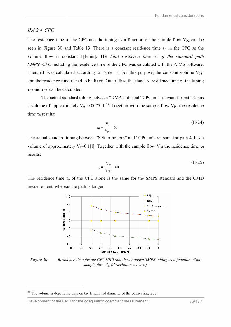
Fundamental considerations
Development of the CMD for the coagulation coefficient measurement 85/177
II.4.2.4 CPC
The residence time of the CPC and the tubing as a function of the sample flow VP2 can be
seen in Figure 30 and Table 13. There is a constant residence time τ6 in the CPC as the
volume flow is constant 1[l/min]. The total residence time rd of the standard path
SMPS>CPC including the residence time of the CPC was calculated with the AIMS software.
Then, rd’ was calculated according to Table 13. For this purpose, the constant volume V0S’
and the residence time τ6 had to be fixed. Out of this, the standard residence time of the tubing
τ0S and τ0S’ can be calculated.
The actual standard tubing between “DMA out” and “CPC in”, relevant for path 3, has
a volume of approximately V0=0.0075 [l]83. Together with the sample flow VP4, the residence
time τ0 results:
τ0V0
VP460⋅
(II-24)
The actual standard tubing between “Settler bottom” and “CPC in”, relevant for path 4, has a
volume of approximately V0=0.1[l]. Together with the sample flow Vp4 the residence time τ9
results:
τ 9V 9
V P460⋅
(II-25)
The residence time τ6 of the CPC alone is the same for the SMPS standard and the CMD
measurement, whereas the path is longer.
Figure 30 Residence time for the CPC3010 and the standard SMPS tubing as a function of the
sample flow Vp1 (description see text).
83 The volume is depending only on the length and diameter of the connecting tube.

Description of the CMD
86/177 Development of the CMD for the coagulation coefficient measurement
Table 13 Data according to Figure 30
Vp2 td τ0S td' τ0S' [l/min] [s] [s] [s] [s] 1 1.779 0.296 1.767 0.284 0.9 1.810 0.327 1.799 0.316 0.55 2.007 0.524 2.000 0.516 0.4 2.198 0.714 2.193 0.710 0.3 2.430 0.947 2.430 0.947
V0S' [l] 0.00473 td'=V0S'/Vp2*60+τ6
τ6 [s] 1.4835 τ0S=τ6−td
Vp6 [l/min] 0.0247244 τ0S'=V0S'/Vp2*60
The residence times for the path “(SMPS) DMA out CPC” for the actual standard SMPS
measurement (τ0+τ6) and the CMD measurements (τ4+τ6) are depicted in Figure 31.
residence time for the CPC 3010 and actual SMPS/CMD tubing
05
101520253035404550556065
0.1 0.2 0.3 0.4 0.5 0.6 0.7 0.8 0.9 1sample flow Vp1 or Vp4 [l/min]
resi
denc
e tim
e τ
[s]
t0+t6
t4+t6
t9+t6
τ0+τ6
τ4+τ6
τ9+τ6
Figure 31 Residence times for the standard SMPS system τ0+τ6 and the CMD system τ4+τ6 or
τ9+τ6 as a function of the sample flow Vp1 or Vp4
II.4.3 Dilution
Dilution of the aerosol flow occurs in several cases of the measurement process. First, in the
bypass filter of the CPC and second in the settler when the settler is not filled long enough.
II.4.3.1 Dilution in the CPC
In the CPC an inherent dilution of the sampling line takes place. The CPC inlet consists of a
needle valve DRV3, a clean air filter RLF2 and a T connector for the sampling line. The CPC
case inlet is regulated to a constant volume flow of Vp6=1 [l/min]. As a consequence, the
sample flow Vp1 is always diluted, except in the case that the sample flow is 1 [l/min]. This
Fundamental considerations
Development of the CMD for the coagulation coefficient measurement 87/177
means that the particle concentration has to be recalculated according to dilution. Under the
assumption of no losses due to mixing equation (II-26), this gives the differential particle
balance. The particle concentration dN0 is the measured particle concentration of the CPC in
the time interval t+∆t. The particle concentration of the filtered air is dN00. This term is
assumed to be 0.
dN0 dNVp1Vp6
⋅ dN00 1Vp1Vp6
−⎛⎜⎝
⎞
⎠⋅+
(II-26)
Then the effective particle concentration before dilution is:
dNdN0Vp1
Vp6⋅
(II-27)
II.4.3.2 Dilution due to incomplete filling
The residence time for the filling of the CPC is quite large especially when the filling flow
rate is low and the total volume is filled in (compare Figure 27). When the filling time tFILL is
lower than the residence time τ8, then a mixing with the settler aerosol takes place. To
determine the incomplete mixing, future experiments could be done, by measuring the aerosol
mixing concentration as a function of incomplete filling time. This function would also reveal
the time necessary for asymptotic filling of the settler in such a way that the settler
concentration equals the probe concentration. Without further information about this fact, a
safety factor sff for the filling time, e.g. sff=2 is useful:
tFILL' tFILL sff⋅ (II-28)
II.4.4 Impaction, deposition and other effects
Inertial impaction is a function of several parameters like the gas velocity the size of the
particles and the geometry. There are several aspects regarding impaction and deposition
important for the CMD.
1. Impaction can pollute the measurement equipment. This can lead to damage of the
sensors, or distorted measurement values. Therefore an impactor before the inlet of the
CMD is recommended.
2. Concerning the magnetic valves, a small diameter leads to high velocities. Together
with the geometry, impaction is most probably at higher sample flow rates. They
should be avoided for this reason. Electrical ball point valves would be more effective
in avoiding impaction, but they are costly (4 times higher prices).
Description of the CMD
88/177 Development of the CMD for the coagulation coefficient measurement
3. The used PVC pipes are not ideally suited for tubing as they can cause higher
deposition rates. Antistatic tubes might give better results concerning deposition,
although the effect has not been shown to be significant in the experiments.
4. The flexible tubing has the disadvantage of a possible difference in flow resistance.
Metal pipes on the other hand, would have the disadvantage of a high thermal
conductivity, which might lead to condensation or phase transitions.
5. The thermophoretic effect could be used to avoid particle deposition, by heating the
wall temperature some degree above the gas temperature.
6. As the valves are heated in operation the thermophoretic effect can be expected as a
function of valve and gas flow temperature.
7. The settler is not resistant to UV radiation. That means experiments can only be made
in the “darkness” of the black NBR-Settler. For investigation of UV and sunlight
radiation a transparent and UV-resistant settler type should be used. Experiments of
this type were made by Husar (Friedlander 2000; Husar 1971) showing significant
coagulation due to smog with organic precursors.
8. Solvents of the settler diffusing could have an influence on both particle coagulation
and particle concentration counting.
9. The CMD settler can also be optionally operated as a continuous stirred tank reactor
(CSTR)84(Moser 1988)85. In this case, the settler is mixed by the stirrer and the
particle size concentration measurement, e.g. path 2 is done with valves V7/V8 open.
The optional valve VM3 is switched to “probe in” (Figure 10). This system has a
residence time depending on the actual settler volume and the sample flow Vp4.
84 This reactor performance has a constant output concentration depending on the residence time and the initial
concentration. 85 p. 113