Take the steps...

Transportation Research

Research...Knowledge...Innovative Solutions!

2007-49

Development of a Computer Programfor Selecting Peak Dynamic Sensor Responses

from Pavement Testing

DEVELOPMENT OF A COMPUTER PROGRAM FOR SELECTING PEAK DYNAMIC SENSOR RESPONSES FROM PAVEMENT TESTING

Final Report

Prepared by

Thomas R. Burnham Minnesota Department of Transportation

Office of Materials 1400 Gervais Avenue

Maplewood, MN 55109-2043

Ahmed Tewfik Seshan Srirangarajan

Department of Electrical and Computer Engineering University of Minnesota

200 Union Street S.E. Room 4-178 EECS Building

Minneapolis, MN 55455

August 2007

Published by

Minnesota Department of Transportation Office of Investment Management

Research Services Section 395 John Ireland Boulevard, MS 330

St. Paul, MN 55155

The contents of this report reflect the views of the authors who are responsible for the facts and accuracy of the data presented herein. The contents do not necessarily reflect the views or policies of the Minnesota Department of Transportation at the time of publication. This report does not constitute a standard, specification, or regulation.

Technical Report Documentation Page 1. Report No. MN/RD – 2007-49

2. 3. Recipient’s Accession No.

5. Report Date August 2007

4. Title and Subtitle

DEVELOPMENT OF A COMPUTER PROGRAM FOR SELECTING PEAK DYNAMIC SENSOR RESPONSES FROM PAVEMENT TESTING 6.

7. Author(s) Thomas R. Burnham, Ahmed Tewfik, Seshan Srirangarajan

8. Performing Organization Report No. T9RC0500 10. Project/Task/Work Unit No.

9. Performing Organization Name and Address

Minnesota Department of Transportation Office of Materials and Road Research 1400 Gervais Avenue Maplewood, MN 55109

11. Contract © or (G)rant No. 13. Type of Report and Period Covered Final Report

12. Sponsoring Organization Name and Address Minnesota Department of Transportation 395 John Ireland Boulevard Mail Stop 330 St. Paul,, MN 55155 14. Sponsoring Agency Code

15. Supplementary Notes http://www.lrrb.org/PDF/200749.pdf 16. Abstract (Limit: 200 words) The Minnesota Department of Transportation (Mn/DOT) routinely collects response data from pavement sensors as part of its pavement research studies. The largest source of response data is collected at the Minnesota Road Research (MnROAD) facility. To efficiently extract peak and baseline values from dynamic sensor responses, the University of Minnesota in 2001 developed an automated process for Mn/DOT researchers using the MATLAB® program. As time went on, sensor data format and computer operating system changes resulted in antiquation of the original peak-picking program. In 2006, the University of Minnesota was again secured to update the program using a current version of MATLAB®. Significant improvements were also made toward automating the peak and baseline response selection, and accommodating flexible data input types. This report combines the task reports and program user guide from the project into one source, to serve as a reference for future changes in the program. The computer program developed in this project has significantly increased dynamic response data processing from MnROAD and other pavement research studies.

17. Documentation Analysis/Descriptors Pavements, Sensor response, Peak response selection

18. Availability Statement No restrictions. Document available from: National Technical Information Services, Springfield, VA 22161

19. Security Class (this report) Unclassified

20. Security Class (this page) Unclassified

21. No. Of Pages 53

22. Price

ACKNOWLEDGMENTS The authors would like to acknowledge the effort of Ted Snyder from the Minnesota Department of Transportation, who worked closely with the developers during program development and validation testing.

TABLE OF CONTENTS CHAPTER 1 INTRODUCTION .............................................................................. 1 Introduction ........................................................................................ 1 CHAPTER 2 TASK 1 – PEAK RESPONSE LOCATION AND SIGNAL DENOISING ....................................................................................... 3 Task Objective .................................................................................... 3 Development Team Task Report ...................................................... 3 Abstract ............................................................................................... 3 Research Objective ............................................................................ 3 Literature Review .............................................................................. 3 Subset Selection ............................................................................ 3 Deconvolution ............................................................................... 4 Research Update ................................................................................ 4 Signal Model ................................................................................. 4 Potential Techniques for Locating Peaks in Sensor Response . 5 1. Template Matching Algorithm ......................................... 5 2. Deconvolution...................................................................... 6 3. Velocity Estimation ............................................................ 8 Technique for Reducing Background Noise .............................. 8 Conclusion ........................................................................................ 10 References ......................................................................................... 10 CHAPTER 3 TASK 2 – BASELINE RESPONSE DETERMINATION ............ 11 Task Objective .................................................................................. 11 Development Team Task Report .................................................... 11 Abstract ............................................................................................. 11 Research Objective .......................................................................... 11 Introduction ...................................................................................... 11 Research Update .............................................................................. 11 Signal Model ............................................................................... 11 Wavelet Denoising ...................................................................... 12 Template Matching Algorithm ................................................. 12 1. Determining Time Shifts tk or Peak Locations ............... 12 2. Track Shifting Baseline .................................................... 13 3. Determining Amplitude Scale Factors ak ....................... 13 Reporting Baseline ..................................................................... 14 Results ......................................................................................... 14 Conclusion ........................................................................................ 18 References ......................................................................................... 18

CHAPTER 4 TASK 3 – PEAK AND TROUGH RESPONSE DETERMINATION ........................................................................ 19 Task Objective .................................................................................. 19 Development Team Task Report .................................................... 19 Abstract ............................................................................................. 19 Research Objective .......................................................................... 19 Introduction ...................................................................................... 19 Research Update .............................................................................. 19 Spectrogram ............................................................................... 19 Denoising Using Filtering .......................................................... 20 Peak and Trough Detection ....................................................... 21 Inflection Points .......................................................................... 23 Detection Threshold ................................................................... 25 Results ......................................................................................... 26 Conclusion .................................................................................. 27 References ................................................................................... 27 CHAPTER 5 TASK 4 – ENHANCE PROGRAM USABILITY ........................ 29 Task Objective .................................................................................. 29 Development Team Task Report .................................................... 29 Abstract ............................................................................................. 29 Introduction ...................................................................................... 29 User Interface Description .............................................................. 29 Start-up Screen ........................................................................... 29 Peak-Picking Modes ................................................................... 30 1. Auto Mode ........................................................................ 30 2. Manual Mode .................................................................... 30 3. Semi-Auto Mode................................................................ 30 4. Output Correction Mode.................................................. 31 5. Sensor Label Correction Mode........................................ 31 6. Output File Split Mode..................................................... 31 Input File Formats ..................................................................... 31 1. Data Delimiter .................................................................. 31 2. Trigger Data ..................................................................... 31 3. Supplemental Time Stamp .............................................. 31 4. Sensor Designators ........................................................... 31 Baseline Selection ............................................................................. 32 Number of Axles ............................................................................... 32 Plotting Feature ................................................................................ 32 Result and Output File Format ...................................................... 33 Auto-Processing Mode ..................................................................... 33 Manual Processing Mode ................................................................ 34 Semi-Auto Mode ............................................................................... 34 Platform Requirements ................................................................... 34 Conclusion ........................................................................................ 34

CHAPTER 6 PROJECT SUMMARY ................................................................... 35 Appendix A – 2001 Peak-Pick program Information Appendix B – 2006 Peak-Pick Program User’s Guide

LIST OF FIGURES LIST OF FIGURES Figure 1.1 Typical signal response from strain sensor during pavement load testing . 1 Figure 2.1 Observed Sensor Response............................................................................... 4 Figure 2.2 Determining approximate peak locations by correlation ............................. 5 Figure 2.3 Reconstruction of sensor response using template signals and approximate

peak locations .....…………………………………………………………….... 5 Figure 2.4 Convolution with template signal …………………………………………… 6 Figure 2.5 Deconvolution to determine peak locations ................................................... 6 Figure 2.6 Observed sensor response with axle response overlap and the result of

convolution with template signal.................................................................... 7 Figure 2.7 Deconvolution approach ................................................................................ 7 Figure 2.8 Denoised waveform after use of Biorthogonal (BIOR) wavelet ................. 9 Figure 2.9 Denoised waveform after use of Daubechies (DB) wavelet ......................... 9 Figure 3.1 Observed Sensor Response .......................................................................... 12 Figure 3.2 Determining the peak locations by convolution ......................................... 12 Figure 3.3 Flowchart for first part of the template matching algorithm .................. 13 Figure 3.4 The original waveform, two plots showing the de-noised waveform and the template fit ....................................................................................... 15 Figure 3.5 Template matching results for another data set ……………..……..…… 16 Figure 3.6 Template matching results for a waveform with “inverted” peaks resulting

from the material undergoing compression ............................................... 17 Figure 4.1 (a) Raw sensor response; (b) Spectrogram of the signal in (a); and (c) De-

noised signal resulting from low-pass filtering ........................................... 20 Figure 4.2 Averaged Spectrogram ……………………………………………………... 22

LIST OF FIGURES (con’t.) Figure 4.3 Local maxima (Δ) detected using the peak and trough detection algorithm,

outlined above ……………………………………………………………. 23

Figure 4.4 The different points of interest in a sample raw sensor response ……… 24 Figure 4.5 The different points of interest in a sample raw sensor response ……… 25 Figure 4.6 Peak and trough detection results ………………………………..….…… 26 Figure 4.7 Peak and trough detection results ………………………………………… 26 Figure 4.8 Peak and trough detection results for a waveform with troughs ……… 27 Figure 5.1 Start-up screen for Peak-Pick program …………………………..……… 30 Figure 5.2 Input Header Formats ………………………………………………..…… 32 Figure 5.3 Results (output) file format …..……………………………………………. 33

EXECUTIVE SUMMARY As part of its pavement research studies, the Minnesota Department of Transportation (Mn/DOT) routinely collects pavement response data from embedded electronic sensors. These sensors measure both environmental responses (static) and vehicle load responses (dynamic). Dynamic responses include strain, deflection, and pressure. At this time, Mn/DOT’s largest source of response data is collected at the Minnesota Road Research (MnROAD) facility. Load response data is also collected from other roadways in Minnesota. Data from dynamic load response sensors is typically collected by a laptop computer in the field, and then brought to the office for processing and analysis. From this data, researchers are typically interested in capturing baseline and peak signal responses. With significant volumes of data being generated by the MnROAD facility, an automated process was needed to improve analysis efficiency. In 2001, Mn/DOT worked with a team of researchers from the University of Minnesota Department of Electrical and Computer Engineering (ECE) to develop an automated “peak-picking” computer program using MathWork’s MATLAB® program. As time went on, sensor data format and computer operating system changes resulted in antiquation of that original peak-picking program. In this project, a new team of researchers from the University of Minnesota Department of Electrical and Computer Engineering (ECE) successfully developed an updated and significantly improved “peak-picking” program for automatically processing dynamic pavement load response signals. Using the latest version of MathWork’s MATLAB® programming language, the new program accommodates various sensor input types, and includes auto, semi-auto and manual peak value selection modes. This report was assembled to document the development process of the revised peak-pick program. The report combines project task reports and the program user guide into one source, to serve as a reference for future changes to the program. Each chapter begins with the task objective as outlined by Mn/DOT researchers, followed by an associated task report, written by the University of Minnesota development team during the project. Early use of the revised peak-pick program has demonstrated a significant improvement in the quantity and quality of dynamic response data processed from MnROAD and other pavement research studies. Most asphalt pavement testing responses, with high signal-to-noise ratio signal responses, can be batch processed using the fully automated mode. Concrete pavement responses, often with lower signal-to-noise ratios, can be efficiently processed using the semi-automatic mode. One of the more useful features of the program is the ability to process data from pavement testing sites other than the MnROAD facility. This report was assembled to document the development process of the revised peak-pick program. It will serve as a valuable reference, in case future updates to the peak-picking program are necessary.

i

CHAPTER 1 INTRODUCTION

Introduction As part of its pavement research studies, the Minnesota Department of Transportation (Mn/DOT) routinely collects pavement response data from embedded electronic sensors. These sensors measure both environmental responses (static) and vehicle load responses (dynamic). Dynamic responses include strain, deflection, and pressure. At this time, Mn/DOT’s largest source of response data is collected at the Minnesota Road Research (MnROAD) facility. Load response data is also collected from other roadways in Minnesota. Data from dynamic load response sensors is typically collected by a laptop computer in the field, and then brought to the office for processing and analysis. From this data, researchers are typically interested in capturing baseline and peak signal responses. In the late 1990’s, data was simply transferred to electronic spreadsheets and plotted manually for analysis. See Figure 1.1 for a typical plot. With significant volumes of data being generated by the MnROAD facility, it was determined that an automated process was needed to improve analysis efficiency.

Cell 31 11-08-05_2731-LE-102

-150

-100

-50

0

50

100

150

200

250

1.7 1.9 2.1 2.3 2.5 2.7 2.9 3.1 3.3

Time (seconds)

Stra

in (x

10-6

)

Figure 1.1 Typical signal response from strain sensor during pavement load testing.

In 2001, Mn/DOT worked with a team of researchers from the University of Minnesota Department of Electrical and Computer Engineering (ECE) to develop an automated “peak-picking” computer program using MathWork’s MATLAB® program. Information on that effort can be found in Appendix A. As time went on, sensor data format and computer operating system changes resulted in antiquation of that original peak-picking program. In 2006, a team of

researchers from the University of Minnesota ECE was again secured to update the program using a more current version of the MATLAB® program. Significant improvements were made in automation of the peak and baseline response selection, as well as permitting more flexible data input types. Early use of the revised peak-pick program has demonstrated a significant improvement in the quantity and quality of dynamic response data processed from MnROAD and other pavement research studies. This report was assembled to document the development process of the revised peak-pick program. The report combines project task reports and the program user guide into one source, to serve as a reference for future changes to the program. Each chapter begins with the task objective as outlined by Mn/DOT researchers. Following that, the associated task report, written by the University of Minnesota development team, is listed.

2

CHAPTER 2 TASK 1 – PEAK RESPONSE LOCATION AND

SIGNAL DENOISING Task Objective Dynamic load response data collected from electronic sensors can be best understood when plotted on a response versus time graph using an electronic spreadsheet program. The items of most interest to pavement researchers are baseline values and peak response values. The difference between the baseline and the peak response defines how the pavement responds to dynamic loads. Signal responses from embedded pavement sensors can be significantly affected by background electrical noise, depending on the signal-to-noise ratio. In fact, many dynamic signal responses from concrete pavement sensors are often of the same magnitude as the background electrical noise. The objectives of this task were to determine a method of signal denoising, and to identify the location of the peak values within a signal response. Development Team Task Report Abstract In this chapter, three different peak-picking methodologies are presented along with some preliminary results. Use of wavelet denoising to reduce the background noise in the sensor waveforms is also outlined with some preliminary results. The three peak-picking approaches are: (i) Template matching using correlation or distance ratios, (ii) Deconvolution and (iii) Velocity Estimation. The pros and cons of each approach are also outlined. Research Objective The offline peak-picking program, being developed, would automate the process of identifying the peaks and troughs in the sensor response waveforms. The sensor responses are gathered during experiments in which trucks pass over pavement dynamic load sensors. Literature Review Subset Selection: Classical subset selection has been addressed in many signal processing applications. For example, Fourier bases are suitable for signals which are rich in harmonics while wavelet dictionaries can be used for signals that include transients. Hence, over-complete dictionaries1 are required to deal with inherently complex signals [1]. In the subset selection problem (SSP), it is required to find the best signal representation for a signal vector using an over-complete dictionary. It is known that SSP is NP-hard2 [2], thus several strategies have been developed for

1 The number of entries in the dictionary is greater than the dimension of the data. 2 Non-deterministic polynomial-time hard; for more details please refer to any text on complexity theory.

3

solving the SSP. One approach would be to find a solution that minimizes the l1 or the l2 norm3. Mallat et. al. developed the Matching Pursuit (MP) technique [3] in which the signal is iteratively decorrelated from the basis vector which has maximum correlation with the residual. Deconvolution: Deconvolution is a process used to reverse the effects of convolution on recorded data. In general, the object of deconvolution is to find the solution of a convolution equation of the form:

hgf =+ ε* where h is some recorded signal, and f is the signal we wish to recover, but has been convolved with some other signal g before we recorded it. The function g might represent the transfer function of an instrument or a driving force that was applied to a physical system and ε is the noise that has entered the recorded signal. Many algorithms for estimating f have been studied in the literature such as CLEAN, maximum entropy method (MEM) etc. Research Update Signal Model: A typical response of the pavement dynamic load sensors is given in Figure 2.1. The five peaks in the response correspond to the five axles of the truck. We model each of these peaks as shifted and amplitude scaled versions of a template signal. Thus,

( ) ( ) ( ) ( )ttwttpatsk

kkk β++−= ∑=

5

1

where s(t) is the sensor response, pk(t) are the template signals, β (t) is the shifting baseline and w(t) is noise. ak and tk represent the amplitude scaling and time shift, respectively.

Figure 2.1. Observed Sensor Response

3 L1-norm of x = and L2-norm of x = , where x = [x∑

=

N

iix

1|| ∑

=

N

iix

1

2|| 1 x2… xN]T is a vector.

4

Potential Techniques for locating peaks in sensor responses: 1. Template Matching Algorithm: In this approach we select a template signal for each peak in the response. It is observed that the five axles have somewhat different responses, thus it is best to have each peak correspond to a different template signal. The observed response is convolved with a mirror-image of the template signal. The peaks in the convolution result and the knowledge of which template signal was used for convolution, enable us to determine the locations of the templates so as to obtain a good fit for the original waveform. This process is illustrated in Figure 2.2.

0 500 1000 1500 2000 2500 3000 3500-5

0

5

10Sensor Data

Convolution with template

signal

Observed sensor response

Approximate peak locations

0 500 1000 1500 2000 2500 3000 35000

0

0

0

0

0

0

Figure 2.2. Determining approximate peak locations by correlation The actual peak locations would be around these approximate locations. Our algorithm would find the “best” approximation or fit to the observed response with the criterion being the squared error between the observed and the reconstructed response. Figure 2.3 illustrates this approach.

Possible peaks locations

Solid lines represent the approximate peak locations

Approximations using template signals for the peaks

Figure 2.3. Reconstruction of sensor response using template signals and approximate peak

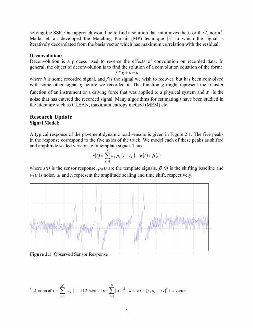
locations The result of convolving an observed sensor response with a template signal is shown in Figure 2.4.

5

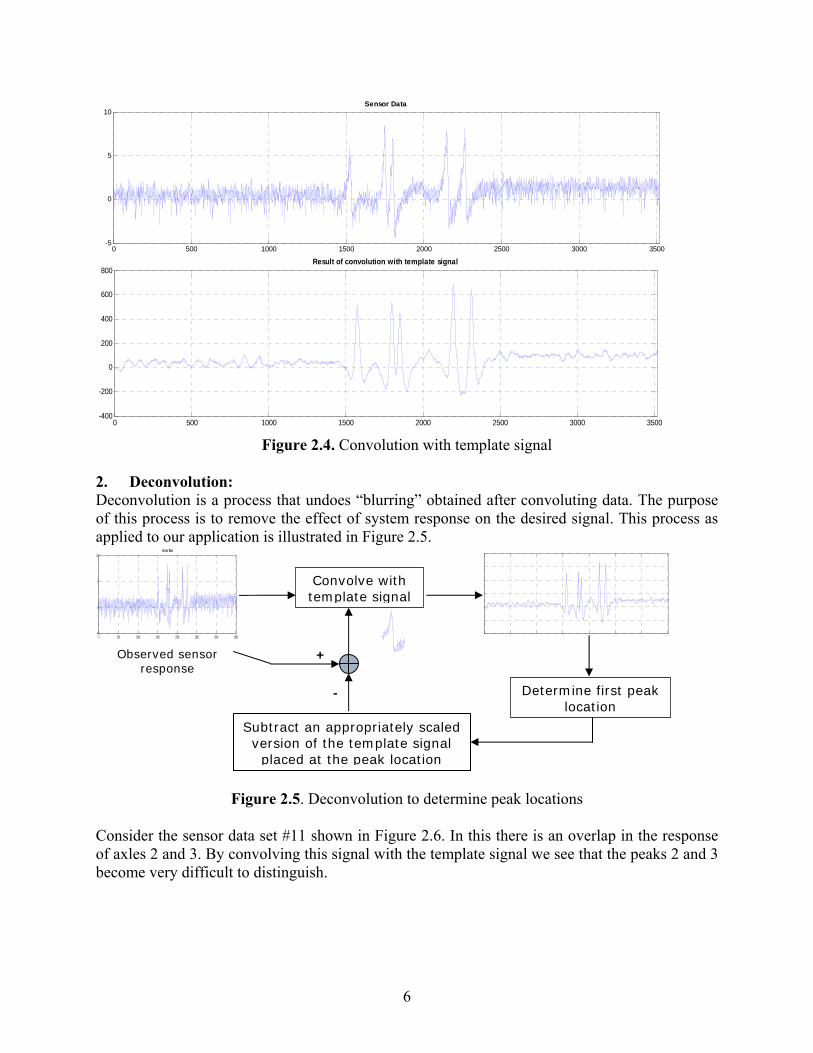
Figure 2.4. Convolution with template signal

2. Deconvolution: Deconvolution is a process that undoes “blurring” obtained after convoluting data. The purpose of this process is to remove the effect of system response on the desired signal. This process as applied to our application is illustrated in Figure 2.5.

Figure 2.5. Deconvolution to determine peak locations Consider the sensor data set #11 shown in Figure 2.6. In this there is an overlap in the response of axles 2 and 3. By convolving this signal with the template signal we see that the peaks 2 and 3 become very difficult to distinguish.

0 500 1000 1500 2000 2500 3000 3500-400

-200

0

200

400

600

800Result of convolution with template signal

Sensor Data10

0 500 1000 1500 2000 2500 3000 3500-5

0

5

0 500 1000 1500 2000 2500 3000 3500-5

0

5

10Sensor Data

Convolve with template signal

Observed sensor response

0

0

0

0

0

Determine first peak location

0 500 1000 1500 2000 2500 3000 35000

0

+

-

Subtract an appropriately scaled version of the template signal

placed at the peak location

6

1400 1600 1800 2000 2200 2400200

400

600

800

1000

1200

1400

1400 1600 1800 2000 2200 24000

5

10

15

20

Figure 2.6. Observed sensor response with axle response overlap and the result of convolution with template signal

Instead, use of the deconvolution approach outlined above, results in identifying all the five peaks. This is illustrated in Figure 2.7. The third plot in this figure is the residual signal after subtracting appropriately scaled versions of the template at the four peak locations (obtained by convolution) from the original response.

0 500 1000 1500 2000 2500 3000 35000

5

10

15

20Sensor response signal

0 500 1000 1500 2000 2500 3000 35000

0.5

1

1.5

2x 104 Result of convolution with template signal

0 500 1000 1500 2000 2500 3000 3500-35

-30

-25

-20

-15Waveform obtained after subtracting 4 peaks (at the locations obtained from convolution with template)

Figure 2.7. Deconvolution approach

7

3. Velocity Estimation: Another approach to determine approximate peak locations is to use the known truck dimensions. Using the known separation between the axles and an estimate of the truck velocity, the separation between the peaks can be estimated. But there are a few uncertainties involved in applying this technique, namely: • Due to the nature of concrete pavements it is not certain if the peaks in the sensor response

correspond to the truck axles’ passing over the sensor; and • The velocity of the truck is not uniform over a given trace, which questions the use of an

estimate of the velocity for locating the peaks. Due to the difficulties mentioned above the use of this approach seems rather difficult. Our goal would be to not rely on the truck dimensions for locating the peaks. Technique for reducing background noise in sensor responses: Wavelet Denoising: Wavelet denoising, simply stated, is the process of signal extraction from data but done via wavelets [4]. This is quite different from traditional filtering approaches - it is nonlinear, due to a thresholding step. Denoising by soft thresholding (given data = signal + noise), involves the following steps [5]: • Step 1: perform a suitable wavelet transform of the noisy data; (the wavelet basis may be

chosen based on various factors including computational burden, and ability to compress the l2 energy of the signal into a very few, very large coefficients);

• Step 2: perform a soft thresholding of the wavelet coefficients where the threshold depends on the noise variance; (when wavelet bases are chosen as in step 1, thresholding kills the effect of the noise without killing the effect of the signal);

• Step 3: the coefficients obtained from step 2 are then padded with zeros to produce a legitimate wavelet transform and this is inverted to obtain the signal estimate.

Examples shown in Figures 2.8 and 2.9 illustrate how the noise is largely suppressed while features in the original signal remain sharp after denoising by the above approach (in contrast with traditional linear methods of smoothing which trade-off noise suppression against a broadening of signal features). We tried a number of wavelet transforms. The use of Daubechies (DB) and Biorthogonal (BIOR) wavelets seemed to give the best results. BIOR wavelets worked better in cases where the axle responses were very close or were overlapping; DB tends to merge these responses into one while the BIOR preserves the somewhat distinguishable peaks in the original signal.

8

0 500 1000 1500 2000 2500 3000 3500-10

-5

0

5

10

15

0 500 1000 1500 2000 2500 3000 3500-2

0

2

4

6

8Sensor data set # 11 de-noised with BIOR wavelet (Nr = 3, Nd = 3)

Figure 2.8. Denoised waveform after use of Biorthogonal (BIOR) wavelet

0 500 1000 1500 2000 2500 3000 3500-5

0

5

10

15

0 500 1000 1500 2000 2500 3000 3500-4

-2

0

2

4

6

8

10Sensor data set # 24 de-noised with DB wavelet (order = 3, level = 5)

Figure 2.9. Denoised waveform after use of Daubechies (DB) wavelet

9

Conclusion ored a number of approaches for locating the peaks in the observed sensor

ferences: honiemy and A. H. Tewfik, “Bounded Subset Selection with Noninteger

[2]. to Linear Systems”, SIAM J. Comp., vol. 24,

[3]. g, “Matching Pursuit with Time-Frequency Dictionaries”, IEEE

[4]. 2/2.html. Theory,

We have explresponse. Preliminary results using these approaches have been presented. Wavelet de-noising has been shown to reduce the background noise in the sensor waveforms to a large extent. Re[1]. M. Alg

Coefficients”, EUSIPCO 2004, pp. 317-320. B. Natarajan, “Sparse Approximate Solutionspp. 227-234, Apr 1995. S. Mallat and Z. ZhanTrans. on Signal Processing, vol. 41, no. 12, pp. 3397-3415, Dec 1993. --, “Wavelet-based Denoising”, http://www.isr.umd.edu/CAAR/proposal/

[5]. D. L. Donoho, “De-noising by Soft-Thresholding”, IEEE Trans. on Informationvol. 41, pp. 613-627, May 1995.

10

CHAPTER 3

TASK 2 – BASELINE RESPONSE DETERMINATION Task Objective As described in the Task 1 objectives, a pavement’s response is defined by the difference between the baseline and the peak response. Due to variable material behaviors, such as the viscoelastic properties of asphalt, the measured baseline values of a dynamic load response can shift over the short time a response is being recorded. Any shifting of the baseline value must be taken into consideration when analyzing dynamic response data. The objective of this task was to identify dynamic response baseline values, including any possible shifts over a given signal response.

Hairline cracks

Development Team Task Report Abstract In this chapter, we detail the results of our study for tracking shifting baselines in the sensor response waveform and recommend one specific approach. The approach presented blends the template matching method with the output from a moving average filter to enable tracking shifting baselines. Research Objective The offline peak-picking program, being developed, would automate the process of identifying the peaks and troughs in the sensor response waveforms. But due to the baselines in different parts of the waveform being significantly different, it becomes important to track this baseline, so as to get an estimate of the strength of the peak (or trough) referenced to the baseline. Thus the objective for this task is to track the shifting baseline. Introduction The moving average is a mathematical technique used to eliminate aberrations and reveal the real trend in a collection of data points. In addition the moving average is a prototype of the finite impulse response (FIR) filter which can be used to eliminate a slowly drifting baseline from a higher frequency signal [1]. This baseline drift can be eliminated without changing or disturbing the characteristics of the waveform. Research Update Signal Model: A typical response of the pavement dynamic load sensors is given in Figure 3.1. The five peaks in the response correspond to the five axles of the truck. The signal model we propose to use consists of three templates: one for the 1st peak and two doublets (one for the 2nd and 3rd peaks and one for the 4th and 5th peaks). We model each of these peaks as shifted and amplitude scaled versions of the template signal. Thus,

(1) ( ) ( ) ( ) ( )ttwttpatsk

kkk β++−= ∑=

3

1

11

where s(t) is the sensor response, pk(t) are the template signals, β (t) is the shifting baseline and w(t) is noise. ak and tk represent the amplitude scaling and time shift, respectively.

Figure 3.1. Observed Sensor Response Wavelet De-noising: Before doing any analysis of the observed waveform we use the wavelet de-noising technique [2, 3] to reduce the background noise in the waveform. The details of this de-noising technique were given in the Task #1 report. Template Matching Algorithm: 1. Determining Time shifts tk or Peak locations: As a first step in trying to fit the signal model to the sensor response, we convolve the de-noised waveform with one of the templates. The peaks in the convolution result and the knowledge of which template signal was used for convolution, enable us to determine the locations of the templates so as to obtain a good fit for the original waveform. This process is illustrated in Figure 3.2.

Sensor Data

Figure 3.2. Determining the peak locations by convolution

To make the template matching algorithm more robust in determining the correct peak locations, we propose an enhancement. This technique is illustrated in Figure 3.3 by means of a flowchart.

0 500 1000 1500 2000 2500 3000 3500-5

0

5

10

Convolution with template

signal

Observed sensor response

Approximate peak location

0

0 500 1000 1500 2000 2500 3000 35000

0

0

0

0

0

12

Convolve the de-noised waveform with the template for peak #1

Determine a few possible peak#1 locations

Reconstruct the waveform using peak locations 2-4 and each possible peak 1 location

Determine locations for the other 4 peaks by convolving with appropriate templates

Select the “best” reconstruction

Figure 3.3. Flowchart for first part of the template matching algorithm

Using the convolution result from the first peak template, we determine a few (3 or 4) possible locations for the first peak. Then for each of these possibilities we determine the locations for peaks 2-4. The “best” reconstruction (in terms of squared error etc) is selected.

2. Track Shifting Baseline: In our signal model, β (t) represents the shifting baseline in the observed sensor response. Using a moving average filter with a sufficiently long window length gives a good estimate of the shifting baseline. Selecting a window length presents a tradeoff: using a short window makes the result very sensitive to local variations in the waveform which may not constitute a baseline shift, while using a very long window might introduce a delay between when the baseline shift occurs in the waveform and when the same is detected in the filter output. We split the process of tracking the baseline into two parts. We use a minimization procedure (outlined in the next subsection) to determine the baseline in the region where the templates are used to fit the peaks and the moving average technique is used to determine the baseline for the rest of the waveform. 3. Determining amplitude scale factors ak: We solve a minimization problem (2) for the part of the waveform which will be fitted with the template. For each template, let ak and β k represent the amplitude scale factor and the baseline.

( )( )23

1,)(min ∑

=

−−−k

kkkkdattpats

kk

ββ

(2)

13

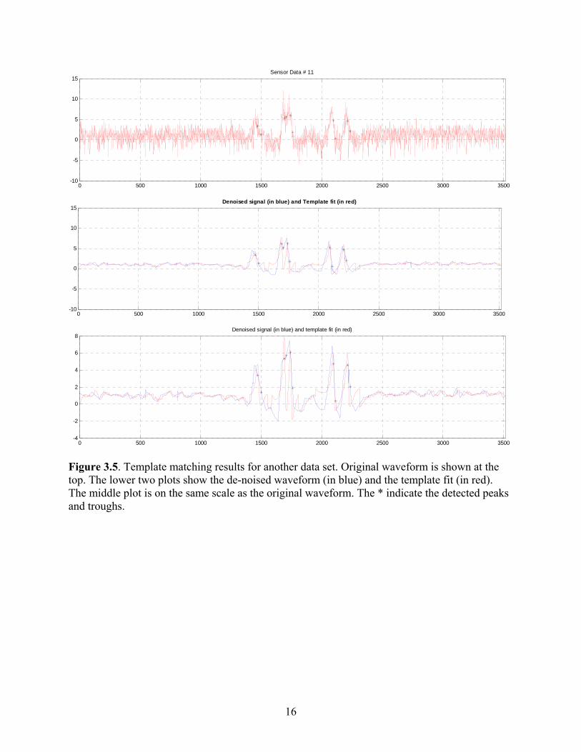
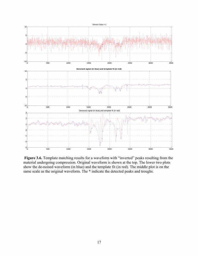
In (2), sd(t) represents the de-noised signal, specifically the parts of the signal which are being fitted with the templates. Thus, β (t) equals β k’s (constants) for the regions fitted by the templates and equals the moving average filter output elsewhere. Reporting Baseline: The template matching method provides β (t), the baseline values over the length of the waveform. Typically one is interested in the initial baseline and the jump (if any) in the baseline between peaks 2-3 and 4-5. To simplify the process of reporting the baseline, it has been agreed to report one value for the baseline. This value would be an average of the first 100 samples. If a significant change in slope is detected in this initial series of samples, or other significant jumps in the baseline (throughout the signal) are detected, the signal will be assigned for manual peak-picking. Results: The template matching algorithm outlined above is applied to de-noised signal. The results shown here were obtained using a moving average filter with window length of 40 samples. Figures 3.4 and 3.5 illustrate the results of this algorithm. In these figures, the top half shows the original waveform and the lower half shows the de-noised signal (in blue) and the template fit (in red). The peaks and troughs are identified using the templates; their locations are mapped to the original waveform but the strength is assigned based on the de-noised signal to limit the effect of noise on the peak and trough values reported. Figure 3.4 shows the result for a somewhat “clean” signal and Figure 3.5 shows the same for a slightly noisy signal (“semi-clean”). It is seen that the technique outlined here is able to track the shifting baseline in the waveform and obtain a good fit for a large percentage of the waveforms. However, there are still some issues with applying these techniques for waveforms that contain “inverted” peaks which are the result of the material being under compression rather than tension. Figure 3.6 shows the template matching results for one of the waveforms in which the material is under compression. The difficulty arises from the fact good templates still need to be defined for these waveforms.

14

0 500 1000 1500 2000 2500 3000 3500-4

-2

0

2

4

6Sensor Data # 6

0 500 1000 1500 2000 2500 3000 3500-4

-2

0

2

4

6Denoised signal (in blue) and template fit (in red)

0 500 1000 1500 2000 2500 3000 3500-2

-1

0

1

2

3

4Denoised signal (in blue) and template fit (in red)

Figure 3.4. The original waveform is shown at the top. The lower two plots show the de-noised waveform (in blue) and the template fit (in red). The middle plot is on the same scale as the original waveform. The * indicate the detected peaks and troughs.

15

0 500 1000 1500 2000 2500 3000 3500-10

-5

0

5

10

15Sensor Data # 11

0 500 1000 1500 2000 2500 3000 3500-10

-5

0

5

10

15Denoised signal (in blue) and Template fit (in red)

0 500 1000 1500 2000 2500 3000 3500-4

-2

0

2

4

6

8Denoised signal (in blue) and template fit (in red)

Figure 3.5. Template matching results for another data set. Original waveform is shown at the top. The lower two plots show the de-noised waveform (in blue) and the template fit (in red). The middle plot is on the same scale as the original waveform. The * indicate the detected peaks and troughs.

16

0 500 1000 1500 2000 2500 3000 3500-10

-5

0

5

10Sensor Data # 1

0 500 1000 1500 2000 2500 3000 3500-10

-5

0

5

10Denoised signal (in blue) and template fit (in red)

0 500 1000 1500 2000 2500 3000 3500-3

-2

-1

0

1

2

3Denoised signal (in blue) and template fit (in red)

Figure 3.6. Template matching results for a waveform with “inverted” peaks resulting from the material undergoing compression. Original waveform is shown at the top. The lower two plots show the de-noised waveform (in blue) and the template fit (in red). The middle plot is on the same scale as the original waveform. The * indicate the detected peaks and troughs.

17

Conclusion The report outlined the template matching algorithm which incorporates a technique for tracking the shifting baseline in the waveform. Results indicate the efficacy of this approach in achieving the desired results. References: [6]. M. R. Weimer, “A Closer Look at the Advanced CODAS Moving Average Algorithm”,

DATAQ Instruments Inc., http://www.dataq.com/applicat/articles/an14.htm. [7]. --, “Wavelet-based Denoising”, http://www.isr.umd.edu/CAAR/proposal/2/2.html. [8]. D. L. Donoho, “De-noising by Soft-Thresholding”, IEEE Trans. on Information Theory,

vol. 41, pp. 613-627, May 1995.

18

CHAPTER 4 TASK 3 – PEAK AND TROUGH RESPONSE DETERMINATION

Task Objective Once the baseline and the peak values are located within a signal response, they must be chosen and classified as a “peak” or “trough” response. Due to variable vehicle speeds, the true peak responses (corresponding to a vehicle tire) may not occur at fixed locations within a signal response. The objective of this task was to automatically identify dynamic response values as “peak” or “trough”, given variable vehicle speed signal responses. Development Team Task Report Abstract In this chapter, we detail the results of our study for peak and trough detection and recommend one specific approach. The wavelet de-noising approach followed by template matching had the disadvantage of not being able to adapt to the variation in the separation between peaks 2 & 3 or peaks 4 & 5 (or troughs). An alternative approach based on low-pass filtering, presented here, will be shown to perform remarkably better. Research Objective The offline peak-picking program, being developed, would automate the process of identifying the peaks and troughs in the sensor response waveforms. The wavelet de-noising followed by template matching was the approach being pursued for peak and trough detection. This was outlined in the earlier task reports as well. This approach was found to fall short of expectations when the separation between peaks (or troughs) varied. Thus, the objective of this task is to look for alternative approaches, which would adapt to the variations in the sensor responses, such as the varying separation between peaks/troughs. Introduction The sensor responses show a significant amount of variability in factors such as the separation between the peaks (or troughs), the signal and the noise levels. The template-matching method is not able to handle the variability in peak separation without increasing the computational cost by an extremely large factor4. The results from low-pass filtering of the sensor responses indicate it might be possible to use a simpler peak and trough detection algorithm, which is much more adaptable to the variability in the responses. Our study and the results from the peak and trough detection algorithm are presented next. Research Update Spectrogram: The spectrogram is the result of calculating the frequency spectrum of windowed frames of a signal. It is a three-dimensional plot of the energy of the frequency content of a signal as it

4 The time-scaling in the peak responses could be handled by increasing the size of the template dictionary to include many of the time-scaled waveforms, with the additional computational cost incurred in trying to find the best fit to a given sensor waveform from a large dictionary.

19

changes over time [1]. Often the spectrogram is reduced to two dimensions by indicating the intensity (or energy) with more intense colors. The horizontal axis represents time, the vertical axis is frequency and the intensity of each point in the image represents amplitude of a particular frequency at a particular time. Figure 4.1(a) shows a raw sensor response and in Figure 4.1(b) the spectrogram of this waveform is depicted. A careful observation of the spectrogram shows that most of the signal energy is concentrated in low frequencies below 20 Hz. In addition, a number of pure frequency tones can be identified from the spectrogram (one just below 40 Hz, another just above 60 Hz and yet another close to 100 Hz). To verify that these are indeed noise components and the desired signal is at low frequencies, low-pass filtering with a cutoff at 30 Hz was employed. The resulting waveform is shown in Figure 4.1(c).

500 1000 1500 2000 2500 3000 3500

-6

-4

-2

0

2

Sensor Data # 16

Spectrogram of sensor data

20 40 60 80 100 120 140 160 180 200

20

40

60

80

100

120

500 1000 1500 2000 2500 3000 3500

-4

-3

-2

-1

0

1Denoised signal

(c)

(b)

(a)

Figure 4.1. (a) Raw sensor response; (b) Spectrogram of the signal in (a); and (c) De-noised signal resulting from low-pass filtering

Most of the background noise is suppressed and the peaks are easily identifiable. Further, we calculated the normalized and averaged spectrogram for a data set with 25 sensor waveforms collected with the same set-up and under the same conditions. This averaged spectrogram is shown in Figure 4.2. This confirms the observations we made above regarding the low frequency signal content and most of the noise appearing as pure frequency tones. De-noising Using Filtering: Thus the obvious way to preserve the low frequency signal content while eliminating noise appearing as higher frequency tones is to do low-pass filtering. As shown in Figure 4.1(c), low-pass filtering is able to reduce the background noise to a large extent. An additional step could be to use the averaged spectrogram to identify all the frequency tones in a given sensor data set and

20

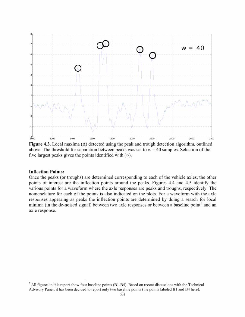
use multiple notch filters to eliminate each of these frequencies. This additional filtering step was applied to a few data sets and results did not show a significant improvement when compared with the low-pass filtered signal. Thus, low-pass filtering with a cut-off frequency at 30 Hz was deemed sufficient to de-noise the raw sensor waveform. We also tried using lower cutoff frequencies for the low pass filter. It was observed that if the peaks appeared very close or there was an overlap between them, the low-pass filtering would merge them together or make it very difficult to distinguish for the peak and trough detection. Peak and Trough Detection: We analyze the low-pass filtered, de-noised signal to determine the peaks (or troughs) corresponding to the axle responses. The first step in this detection algorithm is to locate all local maxima (or minima). Local maxima are defined as points that have a fall on either side of them or a fall on one side and a plateau on the other. The next step is starting with the strongest local maxima eliminate the ones which are closer than a certain number of sample points (w) [2]. This step helps in eliminating false peaks. If there are more than one local maxima within w samples of each other, only the strongest is retained. After this pruning of the list of local maxima, the five strongest (or less depending on the number of vehicle axles) are chosen. This is illustrated in Figure 4.3. To overcome the limitation of having to use a fixed threshold w for the peak separation, which would be akin to limiting the separation between peaks, we use an adaptive procedure that starts with a large threshold for the separation between peaks and progressively reduces this threshold until certain conditions are met by the chosen peaks. These conditions are based on the strengths of the peaks and some reasonable relationships between the peak locations. The strength condition ensures that all the selected peaks are at least larger than a certain fraction of the strongest peak. The peak strengths for this condition are measured with respect to the local baseline. The conditions relating the peak locations are extremely slack and are only used to lower the probability of reporting false peaks.

21

Averaged Spectrogram for a set of 25 waveforms

Time (in samples)

Freq

uenc

y (in

Hz)

20 40 60 80 100 120 140 160 180 200

20

40

60

80

100

120

-0.5

0

0.5

1

1.5

2

2.5

22

Figure 4.2. Averaged Spectrogram. The intensity of each point in the image represents the relative energy of a particular frequency at a particular instant of time.

1000 1200 1400 1600 1800 2000 2200 2400 2600 2800-2

-1

0

1

2

3

4

5

6

7

8

w = 40

Figure 4.3. Local maxima (Δ) detected using the peak and trough detection algorithm, outlined above. The threshold for separation between peaks was set to w = 40 samples. Selection of the five largest peaks gives the points identified with (○). Inflection Points: Once the peaks (or troughs) are determined corresponding to each of the vehicle axles, the other points of interest are the inflection points around the peaks. Figures 4.4 and 4.5 identify the various points for a waveform where the axle responses are peaks and troughs, respectively. The nomenclature for each of the points is also indicated on the plots. For a waveform with the axle responses appearing as peaks the inflection points are determined by doing a search for local minima (in the de-noised signal) between two axle responses or between a baseline point5 and an axle response.

23

5 All figures in this report show four baseline points (B1-B4). Based on recent discussions with the Technical Advisory Panel, it has been decided to report only two baseline points (the points labeled B1 and B4 here).

0 500 1000 1500 2000 2500 3000 350014

16

18

20

22

24

26

28

0 500 1000 1500 2000 2500 3000 350016

17

18

19

20

21

22

23

24

25

26Denoised Signal

IP3

B1

AX1

IP1

IP2

B2

B3 B4

IP4

AX4 AX5

AX3

AX2

IP5

IP6

IP7 IP8

Figure 4.4. The different points of interest in a sample raw sensor response. The peaks (AX),

inflection points (IP) and baseline points (B) are identified on the de-noised signal.

24

500 1000 1500 2000 2500 3000 3500

22

24

26

28

30

32

500 1000 1500 2000 2500 3000 3500

23

24

25

26

27

28

29

30

B1B2

B3

IP1

IP2

AX1AX2

AX3

AX4

AX5

IP3

IP4

IP5IP6

IP7

IP8

Notes: 1) If a local "IP#" is not found, just assign it a value equal to the local B# (baseline value) 2) For each IP# and AX#, assign it as a peak or trough in relation to the local baseline value

B4

Figure 4.5. The different points of interest in a sample sensor response. The peaks (AX),

inflection points (IP) and baseline points (B) are identified on the de-noised signal.

Detection Threshold: In order to determine if the peak and trough detection algorithm can automatically analyze a certain waveform we use the ratio between the de-noised signal peak magnitude above the baseline and the average noise standard deviation. The average noise standard deviation is computed as follows:

1. Divide the sensor waveform into a number of non-overlapping segments. Compute the standard deviation for each of these segments. (We have used 10 such segments.)

2. Use an outlier test to eliminate the segments that contain the axle responses and hence show a larger standard deviation.

3. After eliminating these segments, compute the average standard deviation over the remaining segments. This average value is used as a measure of the noise standard deviation (σnoise).

Let Mpeak_b represent the de-noised signal peak magnitude above the baseline. Then for the detection algorithm to be able to analyze the sensor waveform, the following condition should be satisfied:

noisebpeak kM σ≥_ where k = 6.5. This value for k was determined based on a representative sample of 25 data sets. First, a visual inspection of the data was done to decide sets were too noisy and would be better analyzed manually. The ratio Mpeak_b/σnoise was computed for each set. The value of k was chosen, based on these ratios, so as to maximize the distance between the two classes (analyzable vs. noisy).

25

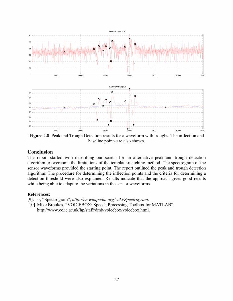
Results: Some results of the peak and trough detection algorithm followed by the detection of inflection points are shown in Figures 4.6 - 4.8.

500 1000 1500 2000 2500 3000 3500

-4

-3

-2

-1

0

1

2

Sensor Data # 7

500 1000 1500 2000 2500 3000 3500

-1.5

-1

-0.5

0

0.5

1

Denoised Signal

Figure 4.6. Peak and Trough Detection results. Inflection and baseline points are also shown.

500 1000 1500 2000 2500 3000 3500

-6

-4

-2

0

2

Sensor Data # 16

500 1000 1500 2000 2500 3000 3500-5

-4

-3

-2

-1

0

1

Denoised Signal

Figure 4.7. Peak and Trough Detection results. Inflection and baseline points are also shown.

26

500 1000 1500 2000 2500 3000 3500

22

24

26

28

30

32

Sensor Data # 20

500 1000 1500 2000 2500 3000 3500

23

24

25

26

27

28

29

30

Denoised Signal

Figure 4.8. Peak and Trough Detection results for a waveform with troughs. The inflection and

baseline points are also shown. Conclusion The report started with describing our search for an alternative peak and trough detection algorithm to overcome the limitations of the template-matching method. The spectrogram of the sensor waveforms provided the starting point. The report outlined the peak and trough detection algorithm. The procedure for determining the inflection points and the criteria for determining a detection threshold were also explained. Results indicate that the approach gives good results while being able to adapt to the variations in the sensor waveforms. References: [9]. --, “Spectrogram”, http://en.wikipedia.org/wiki/Spectrogram. [10]. Mike Brookes, “VOICEBOX: Speech Processing Toolbox for MATLAB”,

http://www.ee.ic.ac.uk/hp/staff/dmb/voicebox/voicebox.html.

27

28

29

CHAPTER 5 TASK 4 – ENHANCE PROGRAM USABILITY

Task Objective In the development of any computer program, it is important to insure that has a friendly user interface. This means the program inputs and outputs must be easily understood by the users. Since this program was developed for pavement researchers, it requires a basic understanding of dynamic load response testing. The objectives of this task were to design a comprehensible program user interface that allows flexibility in the program inputs and modes of operation. Development Team Task Report Abstract In this chapter, we describe the various parts of the user interface of the peak-peaking program (henceforth referred to as “the program”) being developed for MnDOT. The program is being implemented in Matlab®. The user interface is being developed keeping in mind the ease of use and the speed of analysis, while providing maximum flexibility to the user. Introduction The offline data peak-picking program significantly improves the process of identifying the peaks and troughs in the sensor response waveforms. The objectives for this task were to implement the various operating modes for the program and the format for reporting the results of the analysis, which were decided in consultation with the Technical Advisory Panel (TAP). User Interface Description Start-up Screen: When the program is started, the screen shown in Figure 5.1 will show up.

Figure 5.1. Start-up screen for Peak-Pick Program

Peak-Picking Modes: The program can be operated in any of six modes, which offer the user a lot of flexibility. Auto, Manual and Semi-auto modes allow for batch processing of data files. The only limitation is that all the files selected in a single batch should be of the same file type with identical file features (data delimiter, trigger data, number of axles, etc).

1. Auto mode: This is the auto-processing mode that automatically picks peaks for the data sets input by the user. Some waveforms might be classified as noisy for auto-processing based on an internally set threshold and will be labeled as “not analyzed”.

2. Manual mode: This is the manual peak-picking mode that allows the user to step through the sensor waveforms one at a time and select the axle responses by using mouse clicks on the raw sensor waveform or the de-noised waveform displayed by the program. The user only needs to identify the responses corresponding to the axles; the program will accordingly pick the inflection points and the baseline points.

3. Semi-auto mode: The semi-auto mode offers most flexibility to the user. In this mode the program will display the auto-processing results for each waveform one at a time. It will then allow the user to decide if the results are appropriate to be stored, if the user would like to manually select the axle responses, or if the result for this waveform can be deleted, as it is too noisy even for the user to analyze manually.

30

31

4. Output Correction mode: This mode will allow the user to select a results file and delete the rows corresponding to one or more of the sensors. This will be useful if the user feels that any of the sensor waveforms were not analyzed correctly and need to be deleted from the results file.

5. Sensor Label Correction Mode: This mode will allow the user to select a results file and specify new sensor identifiers. This mode is useful when the input file that was analyzed did not use the MnROAD format for assigning sensor designators.

6. Output File Split Mode: This mode will allow the user to select output files generated by the program in modes 1, 2 or 3 above and split this file into multiple files each corresponding to a different sensor model (CE, CD, PG etc). This mode allows batch processing of the output files.

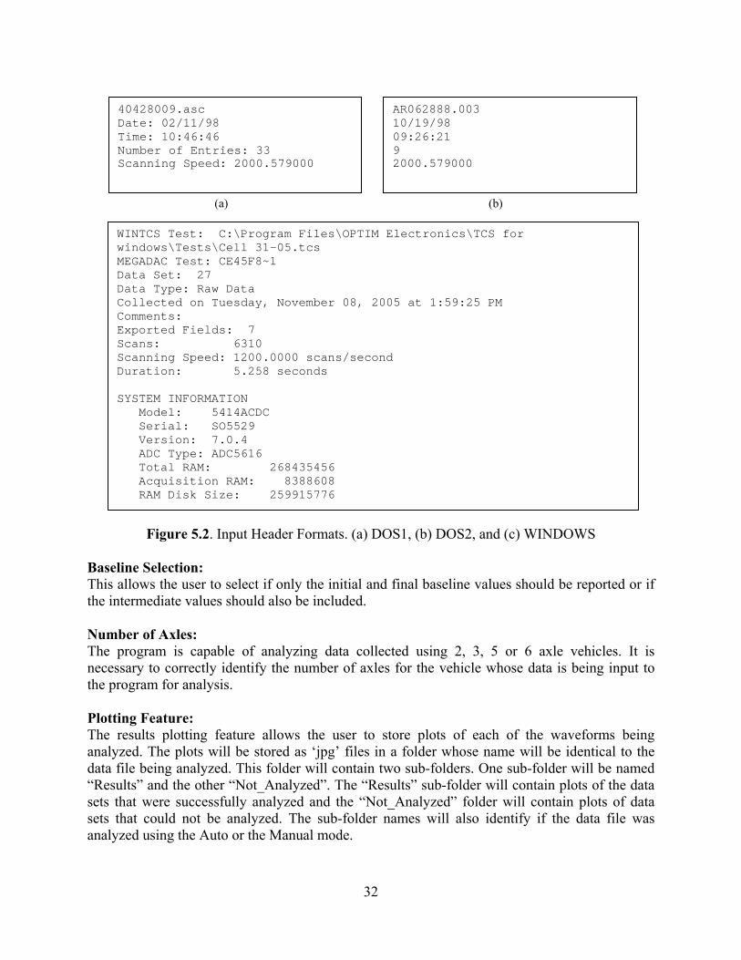
Input File Formats: The program is capable of handling three input file formats: DOS1, DOS2 and the WINDOWS format. These formats differ mainly in their headers that are illustrated in Figure 5.2. In addition, there are a number of features of the input files, which need to be explicitly identified on the start-up screen of the program. Some of these features are listed below.

1. Data Delimiter: The data delimiter used in the input files can be a comma, space, or a tab. With ‘space’ being selected as the data delimiter, the program can handle one or more spaces between the data.

2. Trigger Data: Some of the data files contain a column labeled trigger. It is necessary to identify this to the program so that it does not try to analyze the trigger information.

3. Supplemental Time Stamp: Some input files contain supplemental time stamps in the form of IRIGB or CIRIG information, which are time information in a different format. It is essential to indicate the presence or absence of this information in the data file(s) being analyzed.

4. Sensor Designators: This allows the user to specify if the sensor designators in the input files follow the MnROAD format or not. Some testing done outside the MnROAD facility might have different designators, in which case the program will assign them generic designators such as “Sensor #1”, “Sensor #2” etc. Please note that the “other” (non-MnROAD designators) option can be chosen only with the WINDOWS type input files.

32

(a) (b)

WINTCS Test: C:\Program Files\OPTIM Electronics\TCS for windows\Tests\Cell 31-05.tcs MEGADAC Test: CE45F8~1 Data Set: 27 Data Type: Raw Data Collected on Tuesday, November 08, 2005 at 1:59:25 PM Comments: Exported Fields: 7 Scans: 6310 Scanning Speed: 1200.0000 scans/second Duration: 5.258 seconds SYSTEM INFORMATION Model: 5414ACDC Serial: SO5529 Version: 7.0.4 ADC Type: ADC5616 Total RAM: 268435456 Acquisition RAM: 8388608 RAM Disk Size: 259915776

AR062888.003 10/19/98 09:26:21 9 2000.579000

40428009.asc Date: 02/11/98 Time: 10:46:46 Number of Entries: 33 Scanning Speed: 2000.579000

Figure 5.2. Input Header Formats. (a) DOS1, (b) DOS2, and (c) WINDOWS Baseline Selection: This allows the user to select if only the initial and final baseline values should be reported or if the intermediate values should also be included. Number of Axles: The program is capable of analyzing data collected using 2, 3, 5 or 6 axle vehicles. It is necessary to correctly identify the number of axles for the vehicle whose data is being input to the program for analysis. Plotting Feature: The results plotting feature allows the user to store plots of each of the waveforms being analyzed. The plots will be stored as ‘jpg’ files in a folder whose name will be identical to the data file being analyzed. This folder will contain two sub-folders. One sub-folder will be named “Results” and the other “Not_Analyzed”. The “Results” sub-folder will contain plots of the data sets that were successfully analyzed and the “Not_Analyzed” folder will contain plots of data sets that could not be analyzed. The sub-folder names will also identify if the data file was analyzed using the Auto or the Manual mode.

If the plotting feature is turned off, only the “Not_Analyzed” plots will be stored. This will be useful if you have a large amount of data to analyze and are concerned about enough disk space or would like to have the program run faster by skipping the step of storing the images. Result and Output File Format: As mentioned above the plots of the results will be stored when the plotting feature is on. In addition, the information about the points picked in each of data sets analyzed successfully will be stored in a comma-delimited ASCII text file. The output file format is shown in Figure 5.3. This file is in a format compatible with the MnROAD Oracle® database.

33

53,CE,67,05/30/2003,0,3,2,2.1117,B1,8.4164,B,19.3977,12/22/2006 53,CE,67,05/30/2003,0,3,2,3.2233,IP1,8.7926,P,19.3977,12/22/2006 53,CE,67,05/30/2003,0,3,2,4.2242,AX1,5.1369,T,19.3977,12/22/2006 53,CE,67,05/30/2003,0,3,2,4.3042,IP2,7.7407,T,19.3977,12/22/2006 53,CE,67,05/30/2003,0,3,2,4.39,IP3,7.292,P,19.3977,12/22/2006 53,CE,67,05/30/2003,0,3,2,4.5517,AX2,-2.5921,T,19.3977,12/22/2006 53,CE,67,05/30/2003,0,3,2,4.5792,IP4,-0.21288,T,19.3977,12/22/2006 53,CE,67,05/30/2003,0,3,2,4.6308,AX3,-3.8815,T,19.3977,12/22/2006 53,CE,67,05/30/2003,0,3,2,4.8383,IP5,8.0849,P,19.3977,12/22/2006 53,CE,67,05/30/2003,0,3,2,4.97,IP6,8.1701,P,19.3977,12/22/2006 53,CE,67,05/30/2003,0,3,2,5.255,AX4,-3.2795,T,19.3977,12/22/2006 53,CE,67,05/30/2003,0,3,2,5.2933,IP7,1.4986,T,19.3977,12/22/2006 53,CE,67,05/30/2003,0,3,2,5.3333,AX5,-0.33963,T,19.3977,12/22/2006 53,CE,67,05/30/2003,0,3,2,6.1408,IP8,8.2622,P,19.3977,12/22/2006 53,CE,67,05/30/2003,0,3,2,7.2633,B2,8.0414,B,19.3977,12/22/2006

Figure 5.3. Results (Output) File Format The first three elements in each row are the sensor identifiers (cell, model and the sequence numbers). The fourth element is the date when the data collection was carried out. Elements 5 through 7 indicate the data collection time (Hours, Minutes and Seconds). Element 8 is the elapsed time since the start of the data trace for this sensor. Element 9 is the point identifier (B1, IP2 etc). This identifies each point as a baseline, inflection or axle response point. Element 10 is the value of the response at each of these points. Element 11 identifies each point as a peak, trough or baseline point. Element 12 is the signal-to-noise ratio (SNR) of the sensor waveform. Finally, element 13 is the date when the data was analyzed using the program. A second ASCII text file will be created listing the sensor waveforms that were not analyzed by the program. Note that when analyzing data files with non-MnROAD type sensor designators, the cell, model and sequence numbers each will be assigned generic identifiers such as “Sensor #1” etc. The user will need to use the Sensor Label Correction mode to change these sensor labels or identifiers. Auto-Processing Mode: In the auto mode, after making all the selections on the start-up screen, upon clicking the submit button, the program will ask the user to navigate and select all the input data files. To select multiple data files use the shift key or the control key. Upon selecting the input files, the program will prompt the user to navigate and select the directory to store the results and output files.

34

After this step, the program starts analyzing the data sets, displaying each of results as a plot for a very short time. At the completion of the data analysis, the program will display a dialog box indicating that the analysis is complete. Manual Processing Mode: The manual processing mode works the same way as the auto mode including the step for selecting a directory to store the results and output files. After this step, the program will display each of the waveforms along with the de-noised signal, allowing the user to select the axle response peaks or troughs using left-clicks of the mouse. The peak selection “cycles” through, such that only the latest peaks selected (corresponding to the total number of axles) is saved. This allows the user to correct peak-picking errors. The user will use a right-click of the mouse to indicate when he/she is done selecting the points. The program captures these points and determines inflection points around them as well as the baseline points. The result is then displayed for a very short time after which the program moves to the next data set. After all the data sets have been analyzed, the program will display a dialog box to indicate that the processing is complete. Semi-Auto Mode: This is similar to the auto-mode except that after analyzing each data set, the result is displayed as a plot and the user is presented with three options: accept the auto-processing results, discard the auto-processing results and manually pick the axle responses, or delete this data set. The last option will imply that this data set will not be stored in the results file and instead will be recorded as “not analyzed”. Platform Requirements: The program has been developed in Matlab®, but it is also available in a compiled executable program form that can be run on a machine without Matlab®. In the absence of Matlab®, Matlab® Component Runtime (MCR) needs to be installed on the computer for the program to run. More information about this will be included in the user manual provided with the program. Conclusion The report described the different parts of the user interface of the peak-pick program. The rationale for the different modes and options available with the program were also explained.

35

CHAPTER 6 PROJECT SUMMARY

In this project, a team from the University of Minnesota Department of Electrical and Computer Engineering (ECE) successfully developed an updated computer program for automatically processing dynamic pavement load response signals. Using MathWork’s MATLAB® programming language (version 7.2.0, R2006a), an efficient and flexible peak-pick program was created that significantly improved peak and baseline response selection. To accommodate various signal processing needs, several operating modes and input options were incorporated, including auto, semi-auto and manual peak selection. Early use of the revised peak-pick program has demonstrated a significant improvement in the quantity and quality of dynamic response data processed from MnROAD and other pavement research studies. Most asphalt pavement testing responses, with high signal-to-noise ratio signal responses, can be batch processed using the fully automated mode. Concrete pavement responses, often with lower signal-to-noise ratios, can be efficiently processed using the semi-automatic mode. One of the more useful features of the program is the ability to process data from pavement testing sites other than the MnROAD facility. A comprehensive user’s guide for the program can be found in Appendix B. This report was assembled to document the development process of the revised peak-pick program. It will serve as a valuable reference, in case future updates to the peak-picking program are necessary.

A-1

Appendix A 2001 Peak-Pick Program Information

Mn/Road Offline Data Peak-picking ProgramUser Manual. Rev.l

Prepared on 7/3/2001by Wing C. Lau (wlau@ece.umn.edu)

University of Minnesota ECE Department

*Acknowledgment.Iwould like to thank Prof. Alouini and Ebbini of the ECE department for their gIidance of the project andalso all the Mn/Road researchers for their input and effort to make the project possible.

A) Introduction.This manual is intended for users who will be using the Mn/Road offline data peak­picking program. There is no specific requirement for the application. All the usersshould go through this manual before starting the program. The manual acts like atutorial, which will help users to be familiar with the operations and functions of theprogram. This is the first draft of the manual, any suggestions and comments arewelcomed, please direct them to my email account: wlau@ece.umn.edu. If you areinterested in modifying or enhancing the program, please refer to the "DevelopmentManual" instead of this end-users' manual.

B) Getting Started.First of all, the peak-picking program is running on top of Matlab, one need to startMatlab before invoking the program.

Step 0: Start Matlab by double clicking the Matlab icon.Then, one should check to make sure all the peak-picking files (listfile.m,pp l.m, megadacpp l.m, megadacpp l.mat, guiback.m, ddenoise.m,dlmhdrloadl.m) are located under the Matlab search path. Under File ->Set Path ... The Set_Path box should look like this (Problems usually arisewhen this is not set correctly):

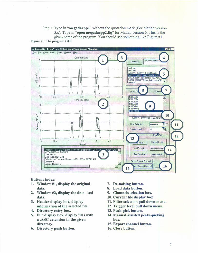
Step 1: Type in "megadacppl" without the quotation mark (For Matlab version5.x). Type in "open megadacpp2.fig" for Matlab version 6. This is thegiven name of the program. You should see something like Figure #1.

Figure #1: The program GUI.

.•j Figure No.1: MnlRoad Ollline Oala Peak-picking Algorithm II!!!III!JEJ

Buttons index:1. Window #1, display the original

data.2. Window #2, display the de-noised

data.3. Header display box, display

information of the selected file.4. Directory entry box.5. File display box, display files with

a .ASC extension in the givendirectory.

6. Directory push button.

7. De-noising button.8. Load data button.9. Channels selection box.10. Current file display box11. Filter selection pull down menu.12. Trigger level pull down menu.13. Peak-pick button.14. Manual assisted peaks-picking

box.

15. Export channel button.16. Close button.

2

Please be familiar with Figure #1 because the following instructions are referenced to thebuttons index.

Step 2: Changing to the directory which contains the data files.

Go to index "4" to type in the absolute directory path. Then click on the Directorybutton "6" to load all the files with .ASC extension in the File display box "5".

CeII33"'1 19991118 coJdSC.AS CCeII33"'1-19991209 - coJderOC.ASCCeII33t 1'9991221 coldest·1SC.ASCCeII33t-20000223- threshold test.ASCcoidASC - -cold2.ASC

Step 3: Loading a specific file and the corresponding channels in the file.

After you selected a file in the File display box "5" (wintertruckI.asc is selectedin Figure # 1), click on the Load data button "8" to load all the channels into theChannels selection box "9". If the data file has a header, the information will beloaded into the Header display box "3", otherwise it will be left empty. If there isno specific labels for the channels, it will be labeled as Time, Channel_I,Channel_ 2, and etc.

Step 4: Changing channels.

Now, by selecting the channel in the Channels selection box "9" (C33PK003 isselected in Figure #1), you will be able to see that the corresponding channel isdisplayed on Window #1 "1".

Step 5: Filter selection.

One can use the pull-down menu "11" to select either using wavelets filtering orlow-pass filtering.

3

Step 6: Trigger level selection is from 1 to 5.

It is also a pull-down menu "12". The higher the trigger level, the more the peaksor troughs the program will pick up.

Step 7: Peak-picking.

After selected all the parameters (Filter type and trigger level) , click on the Peak­picking button "14" will show the result in Window #2 "2".

Step 8: Manual assisted peaks-picking box (#14).

One shouldn't go directly to this section without first doing the automatic peaks­picking.

This manual assist box consists of four different buttons,1. Add Peaks.

2. Add Troughs.3. Add Baseline.4. Remove Points.

5. Manual P-P. (will be discussed in a later section.)

An example is illustrated here.

4

Original Data250

200 ._._ _---.---._ .._---~._. __ ..~-_.~------------.-. __ .------.-- _---

> 150E

··

-- .•. --- .•... -- -~-- .. --- -- .•. - ...•.. - -- ---··

.....-- -- -- -t ..----- -- ---~ .·,·

-----------9----------

,,,.............. - ......•..

---~~---------_ ..•.. _ .. _-_ ..._-- ----------.

h~--mh--I~-_h_------ -- -- ----.. -.--------- ----------- -----------

,

Some of the points are picked and some of them are missed. So, we can use themanual assist buttons to add peaks, troughs or baseline. After you click on any of thesebuttons, you click on the points you wanted on the second window. For example, I wouldlike to add three troughs on the graph. I left-click on the 15t and 2nd troughs and right­click (it means that you finished your selection) on the final troughs. The graph will berefreshed and display the new information.

250

50 ~-----------~----------,,

200

> 150E~;o~1oo

oo

···,,-----------t-----------····-----------f-----------··

.. _---- .. - _----~---------_ .. ~_ .. _--------. ,··,

--f---------I~-----------1-----------

------------ ---.--------_ ..... --------, ,. ,..·

r-----------~-----------

3

Adding peaks and troughs should follow a similar procedure. When you want toremove some points from the graph, you follow the same procedure by clicking on the"Remove Points" button, left-clicking your selections, and finishing with right-clickingyour final point. For example, we would like to remove all the peaks from the graph andadd two baseline points. The new graph should look like the following graph.

5

250

2D0

>150E•...o

~ 100

--------···············~·······t----~····**·----·-··--------*._---------,,,,--~---------M-~----- ---~-----------,··--~---------"1t-----------i-----------·

50 r-----------:-------,.

Step 9: Outputting the desired channel.

,,~._---------,-----------

For outputting individual channels to separate files (Export Current Channel):

If the result of the peak-picking is satisfactory, one may output that particularchannel by clicking on the Export current channel button "IS". An Excel file witha pre-determined name (original file name_channel name.xls) will be exported tothe current working Matlab directory. If you want to export another channel, youneed to repeat step 4 to step 8. If you are not satisfied with the peak-pickingresult, you should repeat step 5 to step 8 before outputting the file.

For outputting multiple channels to one single file (Append Current Channel):

After you finished your first processed channel and click on this button, a filename XXXXXX_append.xls is created. Subsequently, when you process another channeland click this button, the output data is appended to the same file.

SteplO: Ending the program.

After you are finished, click on the Close button" 16" to exit the program.

C) Manual peak-picking method (no need to use this but retain as a reference).

If all the automatic methods fail, we have to resolve to the primitive manual peak­picking.

Step 1:

Step 5:

One can follow all the steps of the previous section until step 4. So, wecan start with Step 5.

Instead of the filter selection, we need to push the De-noising button "7"a wavelets de-noised version of the signal is displayed in Windows #2.

6

Step 6:

Step 7:

Observe the de-noised signal and remember the number of peaks andtroughs you would like to pick out.

Push the Manual P-P button "17", a diagonal box will be displayed andask you the no. of peaks you would like to pick out.

After you entered the numbers, you can start pointing the mouse pointerand select the points by clicking the left-mouse button on Window #2 "2".

The same procedure goes for picking troughs. A similar dialog box willshow up and ask for the number of troughs you would like to pick out.

After all the pickings are done, Window #2 "2" will display the peaks andtroughs as red circles.

Outputting the desired channel is the same as Step 9 of the previoussection.

D) Output file format.

This is a typical output file format.

December 21, 1999 at 951 :37 AMDecember 21 , 1999 at 9:51 :37 AM

December 21 , 1999 at 9:51 :37 AMTuesday, December 21 . 1999 at 9:51 :37 AM

Tuesday, December 21, 1999 at 951 :37 AMTuesday, December 21 , 1999 at 9:51 :37 AM

~JTuesday, December 21 . 1999 at 9:51 :37 AM9iiTuesday, December 21 . 1999 at 9:51 :37 AM

.i161Tuesday, December 21, 1999 at 9:51 :37 AM

11.Fuesday, December 21, 1999 at 9:51 :37 AM12:Tuesday, December 21, 1999 at 9:51 :37 AM

1iITuesdav. December 21, 1999 at 9:51 :37AM

1.04751.07851.0865

1.0941.1075

1.1231.3565

1.4311.444

1.45451.4635

1.4855

1

23456789

1011

12

257.84 t

258.27 P261.25 259.21 P261.25 257.95 t

261.25 259.48p261.25 263.11 t261.25 256.05 t

261.25 261.52 P261.25 254.4 t

261.25 255.11 t

261.25 257.82

9.745

9.7459.7459.7459.7459.7459.7 45

9.745:9.7459.7459.745

9.745

7

E) Troubleshooting

1) Make sure that the Matlab search path is set correctly.2) Try to restart Matlab and the application.3) Consult the "development manual" and listings ofthe .m files

F) Appendices/References.

-buildgui.pdf (How to build OUI in Matlab using "guide.")-using_ml.pdf (How to use Matlab in general)

8

B-1

APPENDIX B

2006 Peak-Pick Program User’s Guide

B-2

MnROAD Offline Data Peak-Picking Program

User Guide

January 2007

Developed by:

Seshan Srirangarajan and Dr. Ahmed H. Tewfik

Department of Electrical and Computer Engineering

University of Minnesota, Twin Cities

B-3

Table of Contents

1 INTRODUCTION ....................................................................................................................................................4

2 RUNNING THE PROGRAM..................................................................................................................................5 2.1 MACHINE WITH MATLAB® INSTALLED .................................................................................................................5 2.2 MACHINE WITHOUT MATLAB® .............................................................................................................................5

3 USER INTERFACE: START-UP SCREEN..........................................................................................................6 3.1 PEAK PICKING MODES..........................................................................................................................................6 3.2 DATA DELIMITER .................................................................................................................................................7 3.3 BASELINE SELECTION...........................................................................................................................................7 3.4 DATA FILE TYPE...................................................................................................................................................7 3.5 RESULTS PLOTTING FEATURE...............................................................................................................................7 3.6 TRIGGER DATA.....................................................................................................................................................7 3.7 SUPPLEMENTARY TIME STAMP.............................................................................................................................7 3.8 NUMBER OF VEHICLE AXLES................................................................................................................................7 3.9 SENSOR DESIGNATORS .........................................................................................................................................7

4 INPUT FILE FORMATS.........................................................................................................................................8

5 PROGRAM OPERATING MODES ......................................................................................................................8 5.1 AUTO MODE .........................................................................................................................................................8 5.2 MANUAL MODE..................................................................................................................................................10 5.3 SEMI-AUTO MODE..............................................................................................................................................10 5.4 OUTPUT CORRECTION MODE..............................................................................................................................11 5.5 SENSOR LABEL CORRECTION MODE...................................................................................................................11 5.6 OUTPUT FILE SPLIT MODE..................................................................................................................................11

6 RESULT AND OUTPUT FILE FORMAT ..........................................................................................................11 6.1 POINTS REPORTED..............................................................................................................................................11 6.2 RESULT PLOTS....................................................................................................................................................13 6.3 OUTPUT FILE FORMAT......................................................................................................................................133

7 GUIDE FOR FUTURE DEVELOPMENT ........................................................................................................154

User Guide MnROAD Offline Data Peak-Picking Program

B-4

Introduction

The MnROAD Offline Data Peak-Picking Program was developed by a team from the Department of Electrical and Computer Engineering, University of Minnesota for the Minnesota Department of Transportation (MnDOT). The developers would like to acknowledge the invaluable assistance provided by the members of the Technical Advisory Panel (TAP).

We will henceforth refer to the MnROAD Offline Data Peak-Picking Program as “the program”. This document has been provided to instruct a user on the features and operation of the program. The program has been developed in Matlab® to take advantage of many signal processing tools available. The user interface has been developed keeping in mind the ease of use and the speed of analysis, while providing maximum flexibility to the user.

User Guide MnROAD Offline Data Peak-Picking Program

Running the Program

The program has been written in Matlab® (version 7.2.0, R2006a) but it is not restricted to users who have Matlab® installed on their machines.

Machine with Matlab® Installed Follow these steps to get the program running on a machine with Matlab® installed:

1. Copy all the program m-files into a separate folder

2. Start Matlab® and change the current directory to the folder where you stored the program files. Then, on the Matlab® command prompt type peak_pick_gui and hit enter. The program will be ready to go.

OR

2. You can double-click the batch file (run.bat) provided with the program files. This will start Matlab® and the program for you. Please note that the batch file provided assumes that the Matlab® root is on the Windows path variable.

Machine without Matlab® The executable version of the program can be run on machines without Matlab®. Follow the steps below to get the program running:

1. Copy all the program files corresponding to the executable version into a single folder.

2. Install Matlab® Component Runtime (MCR) using the MCRInstaller.exe file. This file comes with the executable version of the program. (If you have access to a machine with Matlab®, this file is located at: $Matlab\toolbox\compiler\deploy\win32\mcrinstaller.exe)

3. Double click on peak_pick_gui.exe to start the program. The program creates an archive folder and starts the MCR to run the program.

B-5

User Guide MnROAD Offline Data Peak-Picking Program

User Interface: Start-up Screen

Once the program is started using one of the methods outlined in the previous section, the screen shown in Figure 3.1 will show up.

Figure 3.1. Start-up Screen for the Peak-Pick program

We next describe each of the options on the start-up screen.

Peak Picking Modes The user can choose from six peak picking modes based on his/her requirements. These modes are:

- Auto Mode - Semi-Auto Mode - Manual Mode - Output Correction Mode - Sensor Label Correction Mode - Output File Split Mode

B-6

User Guide MnROAD Offline Data Peak-Picking Program

Each of these modes will be described in Section 5.

Data Delimiter The data delimiter used in the input files can be a comma, space or tab. When ‘space’ is selected as the data delimiter, the program can handle one or more spaces between the data.

Baseline Selection This allows the user to specify if only the initial and final baseline values should be reported or the intermediate values should also be included. This option might be useful as asphalt traces show significant baseline shift in a single trace and hence intermediate baseline values will be important. Concrete on the other hand typically does not show a significant baseline shift and hence only the initial and the final baseline values might be important. Data File Type The program is capable of reading data from three file formats: DOS1, DOS2 and WINDOWS. These formats are described further in Section 4.

Results Plotting Feature This option can be used to turn on or off the feature for storing the result plots of each of the waveforms analyzed by the program. More information on this is provided in Section 6.

Trigger Data Some of the data files contain a column labeled trigger. It is necessary to identify this to the program so that it does not try to analyze the trigger information. Supplementary Time Stamp Some input files contain supplementary time stamps in the form of IRIGB or CIRIG information, which are time information in a different format. It is essential to indicate the presence or absence of this information in the data file(s) being analyzed. Number of Vehicle Axles The program is capable of analyzing data collected using 2, 3, 5 or 6 axle vehicles. It is necessary to correctly identify the number of axles for the vehicle whose data is being input to the program for analysis.

The program allows for batch processing of data files. But it is important to note that all the files selected in a single batch should be of the same file type with identical file features (data delimiter, trigger data, number of axles etc). Sensor Designators This allows the user to specify if the sensor designators in the input files follow the MnROAD format or not. Some testing done outside the MnROAD facility might have different designators, in which case the program will assign them generic designators such as “Sensor #1”, “Sensor #2”

B-7

User Guide MnROAD Offline Data Peak-Picking Program

etc. Please note that the “other” (non-MnROAD designators) option can be chosen only with the WINDOWS type input files.

Input File Formats

The program is capable of handling three input file formats: DOS1, DOS2 and WINDOWS. These formats differ mainly in their header content and organization. Figure 4.1 illustrates the three header formats.

(a) (b)

(c)

WINTCS Test: C:\Program Files\OPTIM Electronics\TCS for windows\Tests\Cell 31-05.tcs MEGADAC Test: CE45F8~1 Data Set: 27 Data Type: Raw Data Collected on Tuesday, November 08, 2005 at 1:59:25 PM Comments: Exported Fields: 7 Scans: 6310 Scanning Speed: 1200.0000 scans/second Duration: 5.258 seconds SYSTEM INFORMATION Model: 5414ACDC Serial: SO5529 Version: 7.0.4 ADC Type: ADC5616

AR062888.003 10/19/98 09:26:21 9 2000.579000

40428009.asc Date: 02/11/98 Time: 10:46:46 Number of Entries: 33 Scanning Speed: 2000.579000

Figure 4.1. Input File Header Formats: (a) DOS1, (b) DOS2, and (c) WINDOWS format.

B-8

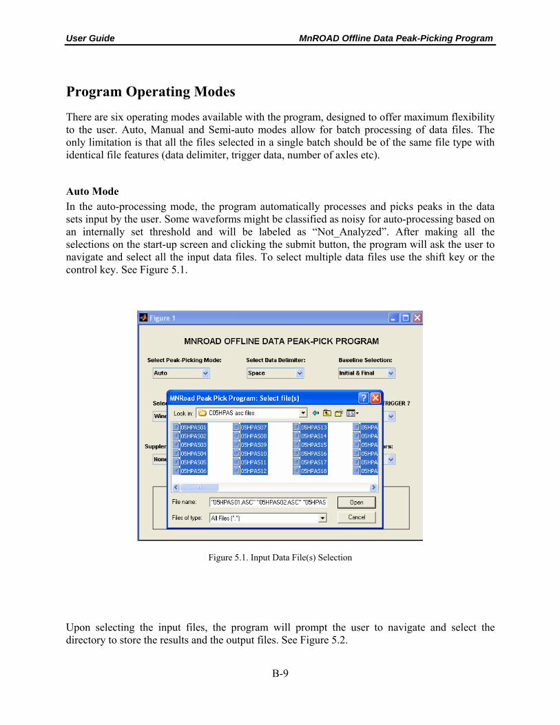
User Guide MnROAD Offline Data Peak-Picking Program

Program Operating Modes

There are six operating modes available with the program, designed to offer maximum flexibility to the user. Auto, Manual and Semi-auto modes allow for batch processing of data files. The only limitation is that all the files selected in a single batch should be of the same file type with identical file features (data delimiter, trigger data, number of axles etc).

Auto Mode In the auto-processing mode, the program automatically processes and picks peaks in the data sets input by the user. Some waveforms might be classified as noisy for auto-processing based on an internally set threshold and will be labeled as “Not_Analyzed”. After making all the selections on the start-up screen and clicking the submit button, the program will ask the user to navigate and select all the input data files. To select multiple data files use the shift key or the control key. See Figure 5.1.

Figure 5.1. Input Data File(s) Selection

Upon selecting the input files, the program will prompt the user to navigate and select the directory to store the results and the output files. See Figure 5.2.

B-9

User Guide MnROAD Offline Data Peak-Picking Program

Figure 5.2. Selection of directory to store results

After this step, the program starts analyzing the data sets, displaying each of the results as a plot for a very short time. At the completion of the data analysis, the program will display a dialog box indicating that the analysis is complete.

Manual Mode The manual processing mode works similarly to the auto mode including the step for selecting a directory to store the results and output files. After this step, the program will display each of the waveforms along with the de-noised signal, allowing the user to select the axle response peaks or troughs using left-clicks of the mouse. If the user clicks more points than the number of axles (n) specified, the program will only capture the last n points. The user will use a right-click of the mouse to indicate when he/she is done selecting the points. The program captures these points and determines inflection points around them as well as the baseline points. The result is then displayed for a very short time after which the program moves to the next data set.

After all the data sets have been analyzed, the program will display a dialog box to indicate that the processing is complete.

B-10

User Guide MnROAD Offline Data Peak-Picking Program

Semi-Auto Mode The semi-auto processing mode is similar to the auto-processing mode except that after analyzing each data set, the result is displayed as a plot and the user is presented with three options:

- Accept the auto-processing results: When this option is selected, the results will be stored in the output file and the program moves ahead to analyze the next data set.

- Manually pick the axle responses: This option will discard the auto-processing results and allow the user to manually select the axle responses as in the manual processing mode.

- Delete this data set: When this is selected the results of this data set will not be stored in the results file and instead will be recorded as “not analyzed”.

Output Correction Mode This mode will allow the user to select a results file and specify the sensor identifier or designator whose results are to be deleted. This mode will be useful if the user feels that any of the sensor waveforms were not analyzed correctly and need to be deleted from the results file. Each sensor is assigned an identifier which consists of its cell number (e.g. 53, C11), model number (e.g. CE) and sequence number (e.g. 018, 50). These three elements together as one string form the sensor identifier (e.g. 53CE018, C11CE50). Sensor Label Correction Mode This mode will allow the user to select a results file and specify new sensor identifiers. This mode is useful when the input file that was analyzed did not use the MnROAD format for assigning sensor designators. Output File Split Mode This mode will allow the user to select output files generated by the program in one of the peak-picking modes (auto, semi or manual) and split this file into multiple files each corresponding to a different sensor model (CE, CD, PG etc). This mode allows batch processing of the output files. Result and Output File Format Points Reported The program reports three types of points to aid the user in analyzing the data trace.

- Axle Response Points: These are the points identified as the response due to the vehicle axles. These can either be peaks or troughs and are assigned identifiers starting with ‘AX’.

- Inflection Points: These are tails of the axle responses and are identified as the local maxima or minima around the axle responses. These are assigned identifiers starting with ‘IP’.

B-11

User Guide MnROAD Offline Data Peak-Picking Program

- Baseline Points: These are points representative of the baseline in the response. The intermediate baseline points will be reported only with the appropriate baseline selection. The baseline points are assigned identifiers starting with ‘B’.

The axle response and inflection points are also classified as peak (P) or trough (T). This classification is done by comparing the value at these points to the initial baseline or the nearest baseline. All these points are identified in Figure 6.1 and 6.2. In Figure 6.1, the axle response points appear as troughs whereas in Figure 6.2, these appear as peaks.

500 1000 1500 2000 2500 3000 3500

22

24

26

28

30

32

500 1000 1500 2000 2500 3000 3500

23

24

25

26

27

28

29

30

B1B2

B3

IP1

IP2

AX1AX2

AX3

AX4

AX5

IP3

IP4

IP5IP6

IP7

IP8

B4

Figure 6.1. The different points of interest in a sample waveform with axle responses as troughs. The axle responses (AX), inflection points (IP) and baseline points (B) are identified on the de-noised signal.

B-12

User Guide MnROAD Offline Data Peak-Picking Program

0 500 1000 1500 2000 2500 3000 350014

16

18

20

22

24

26

28

0 500 1000 1500 2000 2500 3000 350016

17

18

19

20

21

22

23

24

25

26Denoised Signal

IP3

B

AX

IP1IP2

BB B

IP4

AX AX

AX3

AX

IP5

IP6

IP7IP8

Figure 6.2. The different points of interest in a sample waveform with axle responses as peaks. The axle responses (AX), inflection points (IP) and baseline points (B) are identified on the de-noised signal.

Result Plots The results plotting feature allows the user to store plots of each of the waveforms being analyzed. The plots will be stored as ‘jpg’ files in a folder whose name will be the input data file name pre-fixed with ‘pp’ (to indicate it has been analyzed or peak picked). This folder will contain two sub-folders. One sub-folder will be named “Results” and the other “Not_Analyzed”. The “Results” sub-folder will contain plots of the data sets that were successfully analyzed and the “Not_Analyzed” folder will contain plots of data sets that could not be analyzed. The sub-folder names will also identify if the data file was analyzed using the Auto or the Manual mode.

When the plotting feature is turned off, only the “Not_Analyzed” plots will be stored. This will be useful if the user has a large amount of data to analyze and is concerned about enough disk space or would like to have the program run faster by skipping the step of storing the images.

Output File Format As mentioned above the plots of the results will be stored when the plotting feature is on. In addition, the information about the points picked in each of the data sets analyzed successfully will be stored in a comma-delimited ASCII text file. The output file format is shown in Figure 6.3. This file is in a format compatible with the MnROAD Oracle® database.

B-13

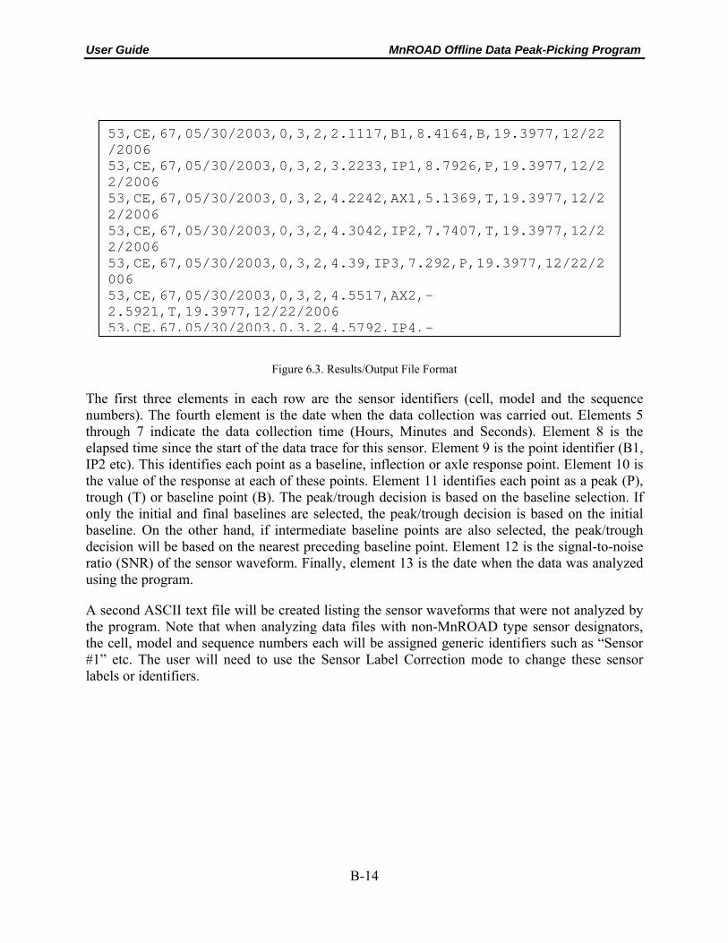
User Guide MnROAD Offline Data Peak-Picking Program

53,CE,67,05/30/2003,0,3,2,2.1117,B1,8.4164,B,19.3977,12/22/2006 53,CE,67,05/30/2003,0,3,2,3.2233,IP1,8.7926,P,19.3977,12/22/2006 53,CE,67,05/30/2003,0,3,2,4.2242,AX1,5.1369,T,19.3977,12/22/2006 53,CE,67,05/30/2003,0,3,2,4.3042,IP2,7.7407,T,19.3977,12/22/2006 53,CE,67,05/30/2003,0,3,2,4.39,IP3,7.292,P,19.3977,12/22/2006 53,CE,67,05/30/2003,0,3,2,4.5517,AX2,-2.5921,T,19.3977,12/22/2006 53,CE,67,05/30/2003,0,3,2,4.5792,IP4,-

Figure 6.3. Results/Output File Format

The first three elements in each row are the sensor identifiers (cell, model and the sequence numbers). The fourth element is the date when the data collection was carried out. Elements 5 through 7 indicate the data collection time (Hours, Minutes and Seconds). Element 8 is the elapsed time since the start of the data trace for this sensor. Element 9 is the point identifier (B1, IP2 etc). This identifies each point as a baseline, inflection or axle response point. Element 10 is the value of the response at each of these points. Element 11 identifies each point as a peak (P), trough (T) or baseline point (B). The peak/trough decision is based on the baseline selection. If only the initial and final baselines are selected, the peak/trough decision is based on the initial baseline. On the other hand, if intermediate baseline points are also selected, the peak/trough decision will be based on the nearest preceding baseline point. Element 12 is the signal-to-noise ratio (SNR) of the sensor waveform. Finally, element 13 is the date when the data was analyzed using the program.

A second ASCII text file will be created listing the sensor waveforms that were not analyzed by the program. Note that when analyzing data files with non-MnROAD type sensor designators, the cell, model and sequence numbers each will be assigned generic identifiers such as “Sensor #1” etc. The user will need to use the Sensor Label Correction mode to change these sensor labels or identifiers.

B-14

User Guide MnROAD Offline Data Peak-Picking Program

Guide for Future Development

This section has been written to help the user if he/she wishes to modify or add to the program. We have tried to give an overview of the Matlab® code and the functionality provided by each of the code modules by means of a flowchart. The flowchart in Figure 7.1 shows the different code modules, their functionality and the relationships between the modules.

peak_pick_gui.m Start-up screen for the program

and passes program control based on mode selection

peak_pick_auto.m Auto-processing mode

peak_pick_manual.m Manual processing

mode

peak_pick_semi.m Semi-auto processing

mode

Functions performed: Input file header

processing, de-noising of the raw sensor

waveforms, compute noise standard deviation

locpeak.m Use findpeaks.m to determine the axle response locations

loc_check.m Do axle response locations satisfy

certain conditions?

inflexdet_peak.m Determine inflection and baseline points

Yes

No (Re-compute with different threshold for minimum separation between axle responses)

cellwrite.m Write results to the

output file

1(a) 1(b) 1(c)

2

3(a)

3(b)

4

5 6

Figure 7.1. Program Flow Illustration

B-15