development of a dynamic artificial neural network model

HAL Id: hal-01923873http://hal.univ-smb.fr/hal-01923873

Submitted on 15 Nov 2018

HAL is a multi-disciplinary open accessarchive for the deposit and dissemination of sci-entific research documents, whether they are pub-lished or not. The documents may come fromteaching and research institutions in France orabroad, or from public or private research centers.

L’archive ouverte pluridisciplinaire HAL, estdestinée au dépôt et à la diffusion de documentsscientifiques de niveau recherche, publiés ou non,émanant des établissements d’enseignement et derecherche français ou étrangers, des laboratoirespublics ou privés.

Development of a dynamic artificial neural networkmodel of an absorption chiller and its experimental

validationAmine Lazrak, François Boudehenn, Sylvain Bonnot, Gilles Fraisse, Antoine

Leconte, Philippe Papillon, Bernard Souyri

To cite this version:Amine Lazrak, François Boudehenn, Sylvain Bonnot, Gilles Fraisse, Antoine Leconte, et al.. Devel-opment of a dynamic artificial neural network model of an absorption chiller and its experimentalvalidation. Renewable Energy, Elsevier, 2016, 86, pp.1009 - 1022. �10.1016/j.renene.2015.09.023�.�hal-01923873�

http://hal.univ-smb.fr/hal-01923873

https://hal.archives-ouvertes.fr

Development of a dynamic artificial neural network model of an absorption 1

chiller and its experimental validation 2

Amine Lazraka, b, c, François Boudehennb, Sylvain Bonnotb, Gilles Fraissec, Antoine Leconteb, 3

Philippe Papillonb, Bernard Souyric 4

a ADEME, Angers (France) 5

b CEA LITEN INES, Le Bourget du Lac, (France) 6

c CNRS, LOCIE, Université de Savoie, Le Bourget du Lac (France) 7

HIGHLIGHTS 8

• A commercial absorption chiller has been tested in dynamic operating conditions on a semi-virtual test bench. 9

• The absorption chiller was modelled in a dynamic way using artificial neural networks. 10

• The model is validated using experimental data. 11

• The neural model predictions are very satisfactory, absolute relative errors of the transferred energy are in 0.1-12

6.6%. 13

ABSTRACT 14

Thermally driven chillers powered by waste-heat or solar energy such as absorption chillers could be more 15

appropriate than commercial air-conditioners that use electricity-powered compression cycles. The more the latter 16

are installed in cities the more heat is released and thus the outdoor temperature increases. As a consequence, 17

performance efficiency of the systems based on compression cycles will reduce. In this case those systems will 18

consume a big deal of electricity. However, absorption chillers still face a big impediment to their commercial 19

development for small capacity installations in buildings. The aim of this paper is to present a methodology to model 20

and evaluate the energy performance of such systems so that users could have reliable information about the long-21

term performance of their systems in the wanted boundary conditions before the installation of the product. 22

Absorption chillers behavior could be very complex and unpredictable especially when the boundary conditions are 23

variable. The system dynamic must be then included in the model. Artificial neural networks (ANNs) have proved to 24

be suitable to tackle such complex problems, particularly when the physical phenomena inside the system are 25

difficult to be modelled. Reliable “black box” ANN modelling is able to identify global models of the system without 26

any advanced knowledge of its internal operating principles. The knowledge of the system’s global inputs and 27

outputs is sufficient. The proposed methodology was applied to evaluate a commercial absorption chiller. Predictions 28

of the ANN model developed were compared, with a satisfactory degree of precision, to two days of experimental 29

measures. The neural model predictions are very satisfactory, absolute relative errors of the transferred energy are in 30

0.1-6.6%. 31

KEY-WORDS 32

Thermal systems, Absorption chiller, Performance estimation, Dynamic modelling, Artificial neural networks, 33

System testing. 34

35

36

1. Introduction 37

From more than ten years now, the development of air-conditioning offers more and more comfort and safety to 38

people. Major part (approximately 99%) of commercial air-conditioners use electricity-powered compression cycles. 39

This system must face a paradox: the more air-conditioners installed in a city, the more heat is released to urban 40

atmosphere, and the more ambient air temperature increases, decreasing the performance efficiency of air-41

conditioners and increasing the cooling load of building [1]. In fine, peak electricity demand for cooling must be 42

tripled [2]. According to Pons et al. [1], part of the solution could be the use of thermally driven chillers powered by 43

waste-heat or solar energy. 44

The major part of thermally driven chillers available on the market is absorption chiller. The basic physical process 45

consists of at least two chemical components, one of them serving as the refrigerant and the other as the sorbent. 46

The operation of such systems is well documented and is not described here [3]. Main advantages of this technology 47

are the continuous thermodynamic cycle and the high thermal coefficient of performance (COPth), compared to 48

adsorption chiller. 49

Absorption chillers are available on the market in a wide range of capacities and designed for different applications. 50

However, only very few systems are available in a range below 100 kW of cooling capacity. 75% of these systems 51

are single effect absorption chillers [4]. Absorption chillers behavior is highly dependent on the climatic conditions 52

and building quality (i.e. on the boundary conditions) [5]. This is why systems could have poor energy performance 53

in some environments. For this reason it becomes necessary that users could have reliable information about the 54

long-term performance of the system in the wanted boundary conditions. This requires reliable and faithful models 55

of absorption chillers under reals conditions. 56

Two types of models can be used to predict behavior and performances of absorption chillers: physical and 57

empirical ones. Physical models describe all the thermodynamic cycle of the absorption chiller, heat exchangers 58

performances and compute then heating and cooling capacity and temperatures of external fluids. On the contrary 59

simplified models only focused on external fluids computing temperatures and power by a set of non-physical 60

equations fitted with experimental data. Examples of those types of models are well studied and compared in steady 61

states conditions in [6] and [7]. 62

Among simplified models, Artificial Neural Networks (ANNs) seems to be the most powerful mathematic tool to 63

solve this modelling problem. In fact, it was shown that ANNs are universal function approximators [8], so they can 64

be used to approximate the system function. ANNs were applied successfully to solve complex, non-linear, dynamic 65

and multivariable problems. They tolerate errors, imprecisions and missing data too [9]. ANNs were extensively 66

used during the last decade and have been especially used to solve prediction modelling problems in renewable 67

energy thermal systems [10], [11], [12], [13], [14], [15]. In the following are presented selected studies that focus on 68

modelling absorption chiller systems: 69

• In [16] authors developed an ANN based model of an adsorption chiller. The ANN has 6 inputs (3 inlet 70

temperatures and 3 flow rates) and 3 outputs (3 outlet temperatures). The model developed is able to predict 71

with a high accuracy, error less than 2°C, the output temperatures. However, because it was trained using a 72

quasi-steady state database, the ANN cannot predict the short-term behavior of the system; 73

• In [17] (another similar study is presented in [18] as well) authors developed an ANN based model of a 74

solar-driven absorption chiller. The model developed was able to predict with a low error both the COPth 75

and the system cooling capacity. For this study only 5 inputs were relevant to model the whole system e.g. 76

the inlet and outlet temperatures of the evaporator and generator, and the average temperature of the hot 77

storage tank. The inputs of the modelling configuration used are not suitable to evaluate the performance of 78

an absorption chiller when only inlet temperatures and flow rates are available; 79

• In [19] authors modelled a double effect absorption chiller in steady state using neural networks. The model 80

was validated using experimental data of about 250 samples. The used ANN predicted the performance of 81

the absorption chiller quite accurately (R² greater than 0.99); 82

• In [20] authors have developed a control system based on an inverse ANN model. The static ANN model, 83

which is an analytical function, leads to a short computing time and as a consequence make this 84

methodology suitable for the on-line control of absorption cooling systems. 85

Further studies where static ANNs were used to model or optimize absorption chillers could be consulted in [21], 86

[22], [23] and [24]. 87

The presented studies focus only on steady or quasi-steady state behavior of the system and the modelling 88

configuration used in some of them cannot be helpful to predict the long term absorption chiller energy 89

performance. Dynamic simulation plays a very important role in the description of the real performance of an 90

energy conversion system, especially during the activation stage or part-load operation. Such a problem is extremely 91

relevant for absorption chillers, where the high mass of the internal components and the accumulation of the fluids 92

inside the vessels usually make the transient period longer than for mechanical compression chillers [25]. The 93

carried literature shows that there is a need of a complete method to model absorption chillers in order to predict 94

their energy performance. The current work presents a methodology to model absorption chillers in a dynamic way. 95

Indeed, the proposed method does not assume any prior knowledge about the system to be modelled or its 96

components. This makes the method generic and more relevant for a future tool to evaluate absorption chillers 97

energy performance within the framework of a certification context. This methodology is based on a short dynamic 98

test and the identification of a “black box” dynamic model of the system using ANN. 99

2. The absorption chiller 100

The absorption chiller used in this study is a single effect water-lithium bromide chiller manufactured by the German 101

company EAW with a nominal cooling capacity of 15 kW. The nominal thermal COP specified by the manufacturer 102

[26] is 0.71. The hydraulic specifications of the chiller are presented in Table 1. 103

Table 1: Hydraulic specifications of the 15 kW cooling capacity EAW absorption chiller [26] 104

EAW Wegracal SE 15 Capacities Inlet/outlet nominal

temperatures Inlet min/max temperatures

Flowrates Pressure drops

[kW] [°C] [°C] [m 3/h] [mbars]

Evaporator 15 17 / 11 6 / - 1.9 400

Generator 21 90 / 80 70 / 95 1.8 400

Absorber-Condenser 35 30 / 36 25 / 40 5 900

In order to be representative, the characterization of the absorption chiller must be realized under operating 105

conditions equivalent to those of a real system. For this, a semi virtual testing method is used. This method is based 106

on the use of a solar cooling system model under TRNSYS, which defines at each time step the operating conditions 107

(temperatures and flow rates) applied to the chiller. Then a dynamical test bench transforms the numerical 108

information of the system model into real physical values at each time step. 109

The methodology used for the dynamical characterization of the absorption chiller is based on the dynamical study of 110

solar combi-system (SCS) developed at INES. This protocol estimates the SCS performances on 12 days 111

representative of the 12 months of a year [27]. Despite the fact that this methodology is difficult to transfer directly 112

to solar cooling system, it is possible to test the solar cooling system on three representative days of the different 113

conditions met during the summer period and corresponding to a day with a high cooling demand and a medium 114

irradiation (day 1), a day with a high cooling demand and a high irradiation (day 2) and a day with a low cooling 115

demand and a high irradiation (day 3). These three days are chosen between June the 1st and September the 30th in 116

the Carpentras (south of France) weather data file, used for the test of the system. For each test day (8 hours), 117

absorption chiller is tested and the rest of the system is simulated with TRNSYS. During the other period, the 118

complete system, including the absorption chiller, is simulated. One advantage of this methodology is that it is able 119

to define good initial conditions of the system (building, storage, etc.) at the beginning of the physical test of the 120

chiller. Compiling the 3 days, is it possible to have representative experimental data of operating chiller conditions 121

integrated into a solar cooling system. 122

The semi-virtual test bench consists mainly on a boiler room able to supply hot (54 kW at 180°C) and cold (150 kW 123

at -10°C) water with two distribution loops, and on test modules of 25 or 50 kW able to reproduce the desired 124

dynamical thermal loads within these range of temperature, Fig. 1. This test bench allows testing of various thermal 125

systems for space heating, air conditioning and DHW preparation for different kind of applications (single or 126

multifamily houses, small industry, small tertiary buildings). The operating conditions of each module are 127

representative of all or part of a system and their behavior is controlled by a TRNSYS numerical model linked. With 128

this method, a component or several components are characterized in a semi virtual environment, in fact by 129

emulating some of the components of the system and the climatic conditions to which it is subjected. In the case of 130

application, the climatic conditions, the solar loop, the heat rejection loop and the building are emulated. 131

132

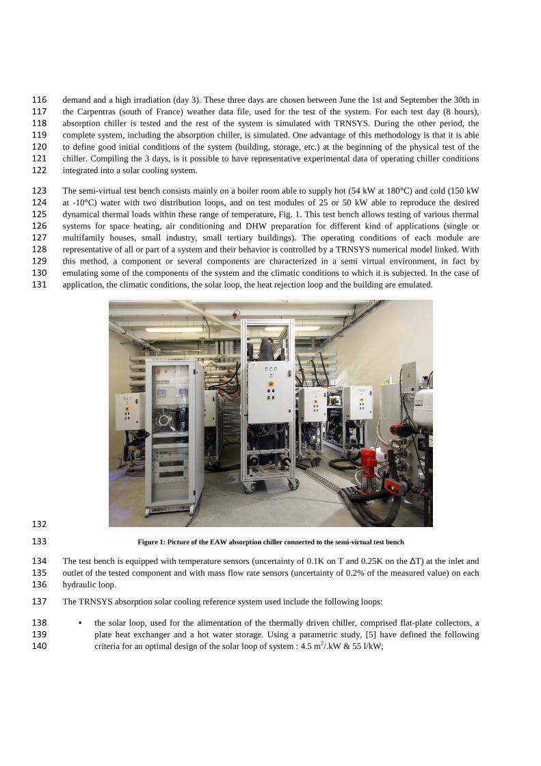
Figure 1: Picture of the EAW absorption chiller connected to the semi-virtual test bench 133

The test bench is equipped with temperature sensors (uncertainty of 0.1K on T and 0.25K on the ∆T) at the inlet and 134

outlet of the tested component and with mass flow rate sensors (uncertainty of 0.2% of the measured value) on each 135

hydraulic loop. 136

The TRNSYS absorption solar cooling reference system used include the following loops: 137

• the solar loop, used for the alimentation of the thermally driven chiller, comprised flat-plate collectors, a 138

plate heat exchanger and a hot water storage. Using a parametric study, [5] have defined the following 139

criteria for an optimal design of the solar loop of system : 4.5 m2/.kW & 55 l/kW; 140

• the heat rejection of the chiller is connected to a closed circuit cooling tower, designed at nominal values 141

provided by the chiller manufacturer; 142

• the cold loop uses a heat exchanger like fan-coils able to transfer the cold water power provided by the 143

chiller into cold air power introduced in the building. In order to adjust the cooling power provided by the 144

chiller to the cooling demand of the building, the cooling power dissipated by the fan-coils into the building 145

(Pcool) is calculated using the maximal cooling demand of the building (PSFH60), the nominal cooling power 146

of the chiller (PN), the effective cooling power of the fan coils (Pfc) and the effectiveness of the fan coils 147

(ηfc), with the following equation: 148

( ) ( )NfcfcSFHcool PPPP ⋅⋅= η60 eq 1 149

The climatic conditions and the building used for the simulation have been defined by the IEA-SHC Task 150

32 [28]: Carpentras (FRANCE) and a 60 kWh.m-2.year-1 single family house (SFH 60) with an air change 151

rate of 0.4 volume per hour. 152

Two controls are used, one on the solar heat production (comparison between the solar collector temperature and the 153

storage tank temperature with two hysteresis of +5°C and of -2°C) and one on the internal temperature of the 154

building (26°C with a hysteresis of -1°C). 155

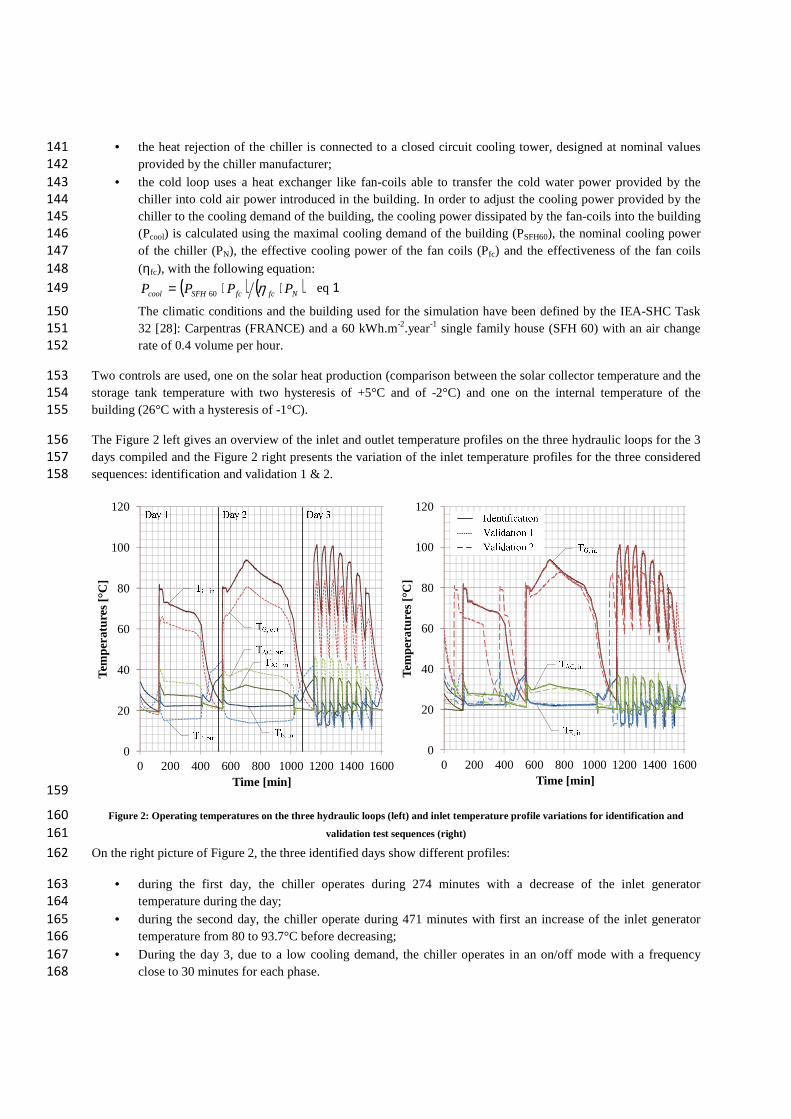
The Figure 2 left gives an overview of the inlet and outlet temperature profiles on the three hydraulic loops for the 3 156

days compiled and the Figure 2 right presents the variation of the inlet temperature profiles for the three considered 157

sequences: identification and validation 1 & 2. 158

0

20

40

60

80

100

120

0 200 400 600 800 1000 1200 1400 1600

Tem

pera

ture

s [°

C]

Time [min]

0

20

40

60

80

100

120

0 200 400 600 800 1000 1200 1400 1600

Tem

pera

ture

s [°

C]

Time [min] 159

Figure 2: Operating temperatures on the three hydraulic loops (left) and inlet temperature profile variations for identification and 160

validation test sequences (right) 161

On the right picture of Figure 2, the three identified days show different profiles: 162

• during the first day, the chiller operates during 274 minutes with a decrease of the inlet generator 163

temperature during the day; 164

• during the second day, the chiller operate during 471 minutes with first an increase of the inlet generator 165

temperature from 80 to 93.7°C before decreasing; 166

• During the day 3, due to a low cooling demand, the chiller operates in an on/off mode with a frequency 167

close to 30 minutes for each phase. 168

Changing the boundary conditions (designs of the solar loop and of the closed circuit cooling tower), it is possible to 169

change the inlet temperatures profiles on each loop. The three considered profiles for this study are presented on the 170

Figure xx right. The “Identification” and “Validation 1” temperature profiles are very close, contrary to the 171

Validation 2 temperature profiles lower in terms of inlet temperature at the generator. The temperature and mass 172

flow rate variations for each profile are described in Table 2. 173

Table 2: Temperature and mass flow rate variations for the different day for each profile 174

Identification Validation 1 Validation 2 Average Min. Max. Average Min. Max. Average Min. Max. TE, in [°C] 22.2 11.4 45.4 22.0 10.2 44.8 22.6 10.6 45.7 ME [kg/h] 1900.8 1891.3 1900.6 2191.2 1892.3 2192.5 1900.3 1240.9 2241.8 TG, in [°C] 80.9 62.2 101.4 80.6 62.0 101.1 77.0 61.8 90.8 MG [kg/h] 1900.0 1855.7 1899.9 1905.9 1895.8 1903.5 1900.0 1886.1 1904.6 TAC, in [°C] 29.4 17.6 37.2 29.4 17.6 37.5 28.3 17.6 37.2 MAC [kg/h] 5005.9 4986.9 5100.0 5006.1 4981.7 5100.0 5007.8 4982.3 5100.0

During the operating mode of the absorption chiller, the thermal losses to the environment of the absorption chiller 175

can be ignored regarding the heat transfers between the system and its boundary conditions. For this reason the 176

ambient temperature was not considered in the model input configuration. 177

3. The modelling approach 178

3.1. The ANN theory 179

ANN theory is clearly presented in [29] and [30]. ANNs are parametric analytical functions whose concept takes 180

inspiration from the human central nervous system. A neuron, the basic element of an ANN, can compute values 181

from a weighted summation of its inputs (eq. 2). The summation coefficients are called synaptic weights. The 182

subscript denotes the neuron number. The neural operation is presented in eq. 1. The function is called the neural 183

activation function (AF). 184

eq. 2 185

Inter-connected neurons constitute what is commonly called a neural network. There are several network 186

architectures and each one is more suiTable for a specific problem than others. The most famous architecture for 187

prediction and fitting problems is the class of the multi-layer perceptron (MLP). A MLP is a feed-forward network 188

built of neurons, arranged in layers. It has an input layer, one or more hidden layers and an output layer. In Figure 3 a 189

MLP, with inputs, neurons in the hidden layer and outputs, is represented. The th output of the network can be 190

obtained using eq. 3. 191

eq. 3 192

Modelling a system using an ANN means building the appropriate network architecture (hidden layers, neurons, 193

AFs) and identifying the different weights. 194

195

Figure. 3: Formal representation of a neuron (left), example of a neural network MLP with one hidden layer (right) 196

The ANN learning or training is the process of determination of an ensemble of weights so that the underlying 197

function approximates the real system function. In fact, the objective of the training process is to minimize, for a 198

specific ANN structure, a cost function, with respect to weights, knowing a set of data (training data). 199

Usually, the resulting models fit with high accuracy the learning data set (especially when a lot of neurons are used 200

e.g. a lots of parameters). However, the model prediction precision may be very poor for unseen data (e.g. over-201

fitting). In some cases, this means that the resulting model has learned only characteristics of the training data set and 202

not the system behavior. In other cases probably the optimizer has been stacked in a local minimum. The learning 203

strategies are ways to deal with those optimization algorithms and the neural network structure in order to get a 204

model that has good generalization ability e. g. accurate estimations for unseen data. 205

One must be aware that the most optimization algorithms commonly used are local methods. In fact, they are valid 206

for a region near the minimum. This is why a good way of preventing the algorithms to be stacked on a local poor 207

minimum is to train the ANN several times with different starting points (weights initialization). 208

Training using Cross-Validation and Early Stopping are examples of the most famous learning strategies that are 209

commonly used to prevent over-fitting. The both methods are based on a data set to do validation which must be 210

taken from data available for training. Physical system tests are expensive and usually time consuming. The short 211

time of the system test, which is long, in this study, of only one day, restricts the amount of available data for 212

training. Therefore it is necessary to use a learning strategy that can use a restricted data set without compromising 213

the generalization ability of the model. For this reason it is relevant to use Bayesian regularization method for the 214

learning process. Typically, training aims to minimize the sum of squared errors ( ) see (eq. 4) with the target 215

data at the sequence time and the ANN output at the same time. 216

eq. 4 217

Bayesian regularization modifies the objective function by adding an additional term: the sum of squares of the 218

network weights (eq. 5) where is a vector of parameters to be determined (synaptic weights), and are two 219

constant parameters calculated using a Bayesian regularization methodology [31]. By constraining the size of 220

weights the training process produce an ANN with good generalization ability [32]. In fact, by keeping the weights 221

small the ANN response will be smooth and so the over-fitting is supposed to be prevented. In this study the 222

objective function minimization is done using the Levenberg-Marquardt algorithm. 223

eq. 5 224

Usually, training algorithms (even if coupled to an adequate training strategy) do not necessarily guarantee the 225

production of efficient networks based on row data. This is why it is essential to carry out some data pre-processing 226

before training. By normalizing or standardizing the input and target data vectors, the ANN training will be easier 227

and faster, and all vectors will be equally taken into account during the learning process. Equation 6 will be used to 228

pre-treat the training data in order to fall between and (normalization bounds); represents a vector 229

(input or output of the model) of data over time. 230

eq. 6 231

and represent the minimum and maximum values of each variable. 232

Generally ANNs do not give good results in extrapolation. One way to reduce the effect of this problem is to select 233

carefully the normalization bounds in eq. 6. 234

3.2. The system modelling process 235

Determination of the modelling input-output configuration is crucial to develop a reliable and exploitable model. The 236

goal of this study is to develop a model able to predict the energy performance of the system (COP) and its cooling 237

capacity. To do so, it is necessary to predict the outlet temperatures at the level of the evaporator and the generator. 238

These two unknown variables are then used as model outputs and the other ones which are control variables e. g. 239

inlet temperatures (condenser, evaporator and generator) and the three flow rates (condenser, evaporator and 240

generator) are used as model inputs. In order to make the ANN learn the dynamic of the system, delayed outputs 241

must be used as inputs too (by feeding them back). This two outlet temperatures (evaporator and generator), 242

physically, are affected by the outlet temperature of the condenser. This is why it is relevant to add it as output of the 243

model in order to be used as a delayed input. The resulting input-output modelling configuration is presented in 244

Figure. 4. 245

The absorption chiller was tested in a dynamic way as described in section 2. 246

To determine the optimal model that describes best the system dynamic behaviour, several ANN with different 247

number of neurons (from 1 to 15) were trained. All the models contain one hidden layer and tangent hyperbolic or 248

linear function as the AF. Three normalization bounds: ±1, ±0.3 and ±0.8 were investigated as well. As said in 249

section 3.1 in order to prevent the minimization algorithm getting stuck in local minima each network is retrained 15 250

times using the Nguyen–Widrow algorithm developed in [33]. Because the true output (actual data) is available 251

during the training of the network, the actual outputs are used instead of feeding back the predicted outputs, as shown 252

in Figure. 4. This has the advantage to use an accurate delayed output as an input so the network will learn more 253

efficiently. 254

Input delays

ANN

Input delays

255

Figure. 4 :Open loop architecture 256

The Bayesian information criterion (BIC) was chosen to select the most relevant network [29], [34]. It is defined by 257

the following: 258

eq. 7 259

where is the number of model weights and the size of the learning data. 260

The BIC is calculated using only the training data and in a closed loop architecture (see Figure 5), in which only 261

available data, e.g. inputs and the initial values of the outputs, are used to predict the outputs (long-term model 262

simulation). The open loop architecture is used only during training. The BIC selects ANNs with a small size. This is 263

advantageous because parsimonious ANNs have a better generalization power as stated in [35]. 264

Input delays

ANN

Feedback delays 265

Figure. 5 : Closed loop architecture 266

The whole training and selection process was developed in MATLAB R2012b and is represented in Figure 6 267

n = 1 and i = 1

Net creation “n” neurons

Net initialization

Training in “open loop”

Testing in “closed loop”

BIC calculation

Net back-up

Max number of initialization

reached?

Max number of neurons reached?

Best net selection

n = n + 1

i = i + 1

Yes

No

No

Yes

Time delay (TD) = 1

Inputs and feedback outputs TD set up

Max number of time delays reached?

No

Yes

AF = tangent hyperbolic

AF = linear

Normalization bounds in ± 0.3

Normalization bounds in ± 0.8

Normalization bounds in ± 1

TD = TD+1

268

Figure. 6: Representation of the training process algorithm 269

270

4. Results and discussion 271

4.1. The selection of the model 272

A number of 4050 –15(number of neurons) 15(number of initializations) 3(number of normalization intervals) 273

3(number of TD) 2(number of AF) – models were trained. In Figure 7 and 8 the BIC values, corresponding to 274

each created model, are visually represented. Black squares are more packed in the region where the number of 275

neurons is lower than 10 neurons. The BIC penalizes the complexity of the model where complexity refers to the 276

number of parameters in the model. This is in accordance with what is stated in section 3.2. It can be observed also 277

that the penalization is more strong when the normalization interval is equal to [-0.3 0.3] especially in the case of the 278

linear AF. However, some models with a high number of parameters have a low BIC value (compared to other 279

models with the same AF, TD and normalization interval). This observation can be explained by the fact that their 280

is quite low. The comparison between the BIC values of the ANNs selected for each model features 281

(normalization interval, TD and AF) is given in Table 3 and 4. The best model, based on the BIC, among all the 4050 282

created ANNs is the model that comes from the 2nd initialization, has 9 neurons in the hidden layer, TD equals to 1, 283

tangent hyperbolic AF and a normalization interval equals to [-1, 1]. 284

Normalization interval = [-0.3 0.3] TD =1

Initialization number

Ne

uron

s n

umbe

r

5 10 15

2

4

6

8

10

12

140

0.1

0.2

0.3

0.4

0.5

0.6

0.7

0.8

0.9

1



Ne

uron

s n

umbe

r

5 10 15

2

4

6

8

10

12

140

0.1

0.2

0.3

0.4

0.5

0.6

0.7

0.8

0.9

1



Ne

uron

s n

umbe

r

5 10 15

2

4

6

8

10

12

140

0.1

0.2

0.3

0.4

0.5

0.6

0.7

0.8

0.9

1



Ne

uron

s n

umbe

r

5 10 15

2

4

6

8

10

12

140

0.1

0.2

0.3

0.4

0.5

0.6

0.7

0.8

0.9

1



Ne

uron

s n

umbe

r

5 10 15

2

4

6

8

10

12

140

0.1

0.2

0.3

0.4

0.5

0.6

0.7

0.8

0.9

1



Ne

uron

s n

umbe

r

5 10 15

2

4

6

8

10

12

140

0.1

0.2

0.3

0.4

0.5

0.6

0.7

0.8

0.9

1

Normalization interval = [-1 1] TD =1


Ne

uron

s n

umbe

r

5 10 15

2

4

6

8

10

12

140

0.1

0.2

0.3

0.4

0.5

0.6

0.7

0.8

0.9

1



Ne

uron

s n

umbe

r

5 10 15

2

4

6

8

10

12

140

0.1

0.2

0.3

0.4

0.5

0.6

0.7

0.8

0.9

1



Ne

uron

s n

umbe

r

5 10 15

2

4

6

8

10

12

140

0.1

0.2

0.3

0.4

0.5

0.6

0.7

0.8

0.9

1

285 Figure. 7: Visual representation of the model selection process when the tangent hyperbolic AF is used in the output layer. BIC values 286 were normalized between 0 and 1 to have a better visualization. Each square represents an ANN model that has a specific number of 287

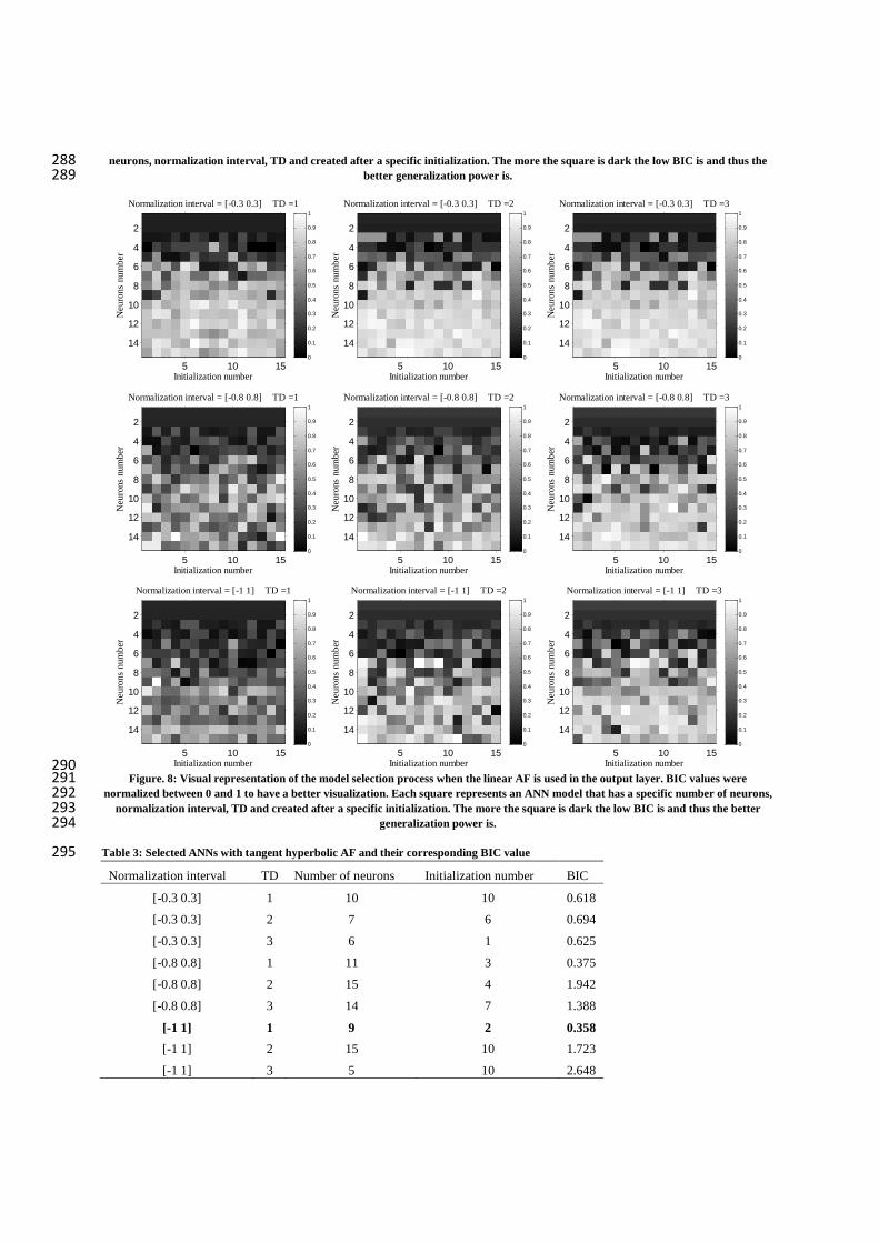
neurons, normalization interval, TD and created after a specific initialization. The more the square is dark the low BIC is and thus the 288 better generalization power is. 289



Ne

uron

s nu

mb

er

5 10 15

2

4

6

8

10

12

140

0.1

0.2

0.3

0.4

0.5

0.6

0.7

0.8

0.9

1



Ne

uron

s nu

mb

er

5 10 15

2

4

6

8

10

12

140

0.1

0.2

0.3

0.4

0.5

0.6

0.7

0.8

0.9

1



Ne

uron

s nu

mb

er

5 10 15

2

4

6

8

10

12

140

0.1

0.2

0.3

0.4

0.5

0.6

0.7

0.8

0.9

1



Ne

uron

s nu

mb

er

5 10 15

2

4

6

8

10

12

140

0.1

0.2

0.3

0.4

0.5

0.6

0.7

0.8

0.9

1



Ne

uron

s nu

mb

er

5 10 15

2

4

6

8

10

12

140

0.1

0.2

0.3

0.4

0.5

0.6

0.7

0.8

0.9

1



Ne

uron

s nu

mb

er

5 10 15

2

4

6

8

10

12

140

0.1

0.2

0.3

0.4

0.5

0.6

0.7

0.8

0.9

1



Ne

uron

s nu

mb

er

5 10 15

2

4

6

8

10

12

140

0.1

0.2

0.3

0.4

0.5

0.6

0.7

0.8

0.9

1



Ne

uron

s nu

mb

er

5 10 15

2

4

6

8

10

12

140

0.1

0.2

0.3

0.4

0.5

0.6

0.7

0.8

0.9

1



Ne

uron

s nu

mb

er

5 10 15

2

4

6

8

10

12

140

0.1

0.2

0.3

0.4

0.5

0.6

0.7

0.8

0.9

1

290 Figure. 8: Visual representation of the model selection process when the linear AF is used in the output layer. BIC values were 291

normalized between 0 and 1 to have a better visualization. Each square represents an ANN model that has a specific number of neurons, 292 normalization interval, TD and created after a specific initialization. The more the square is dark the low BIC is and thus the better 293

generalization power is. 294

Table 3: Selected ANNs with tangent hyperbolic AF and their corresponding BIC value 295

Normalization interval TD Number of neurons Initialization number BIC

[-0.3 0.3] 1 10 10 0.618

[-0.3 0.3] 2 7 6 0.694

[-0.3 0.3] 3 6 1 0.625

[-0.8 0.8] 1 11 3 0.375

[-0.8 0.8] 2 15 4 1.942

[-0.8 0.8] 3 14 7 1.388

[-1 1] 1 9 2 0.358

[-1 1] 2 15 10 1.723

[-1 1] 3 5 10 2.648

Table 4: Selected ANNs with linear AF and their corresponding BIC value 296

Normalization interval TD Number of neurons Initialization number BIC

[-0.3 0.3] 1 4 1 0.965

[-0.3 0.3] 2 6 15 1.135

[-0.3 0.3] 3 4 7 0.699

[-0.8 0.8] 1 5 6 0.790

[-0.8 0.8] 2 5 9 0.411

[-0.8 0.8] 3 7 9 0.735

[-1 1] 1 6 14 0.752

[-1 1] 2 6 5 0.867

[-1 1] 3 5 5 0.668

The Figure 9 presents a comparison between predictions of the selected ANN and the experimental results for the 297

outlet temperatures of each hydraulic loop. This first comparison is based on the identification data. The absolute 298

relative instantaneous error is calculated equation 8, where is the estimate of the variable . This relative error is 299

calculated only when the absorption chiller is operating e.g. when there is a flow rate in each hydraulic loop, 300

otherwise the error is set to zero. 301

eq. 8 302

The ANN predictions are very close to the experimental data. Outlet instantaneous temperature errors are, in the 303

whole, less than 6% for the generator and the condenser-absorber and less than 10% for the evaporator. The learning 304

of the latter seems to be more difficult. The mean error values are presented on the Table 5, they do not include the 305

zero values. The mean values are less than 3% which means that the performance of the ANN training process is 306

good. However, to effectively test the generalization ability of the artificial neural model it is necessary to use a set 307

of experimental unseen data. 308

Table 5: Mean relative error values for the identification step 309 TE, out TG, out TAC, out Identification 2.9% 0.9% 0.9%

0

10

20

30

40

50

60

70

80

90

100

0

10

20

30

40

50

60

0 200 400 600 800 1000 1200 1400 1600

Abs

olut

e re

lati

ve e

rror

[%

]

Tem

pera

ture

s [°

C]

Time [min]

0

10

20

30

40

50

60

70

80

90

100

0

10

20

30

40

50

60

70

80

90

0 200 400 600 800 1000 1200 1400 1600

Abs

olut

e re

lati

ve e

rror

[%

]

Tem

pera

ture

s [°

C]

Time [min]

0

10

20

30

40

50

60

70

80

90

100

0

5

10

15

20

25

30

35

40

45

50

0 200 400 600 800 1000 1200 1400 1600A

bsol

ute

rela

tive

err

or [

%]

Tem

pera

ture

s [°

C]

Time [min]

TE, out

Err

TE, out

TAC, out

Err

TAC, out

TG, out

Err

TG, out

310

Figure 9: Outlet temperature comparisons between numerical and experimental results for each hydraulic loops 311

4.2. Comparison with field test data 312

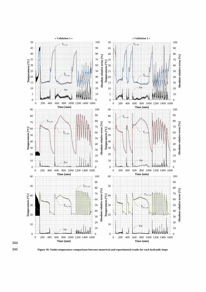
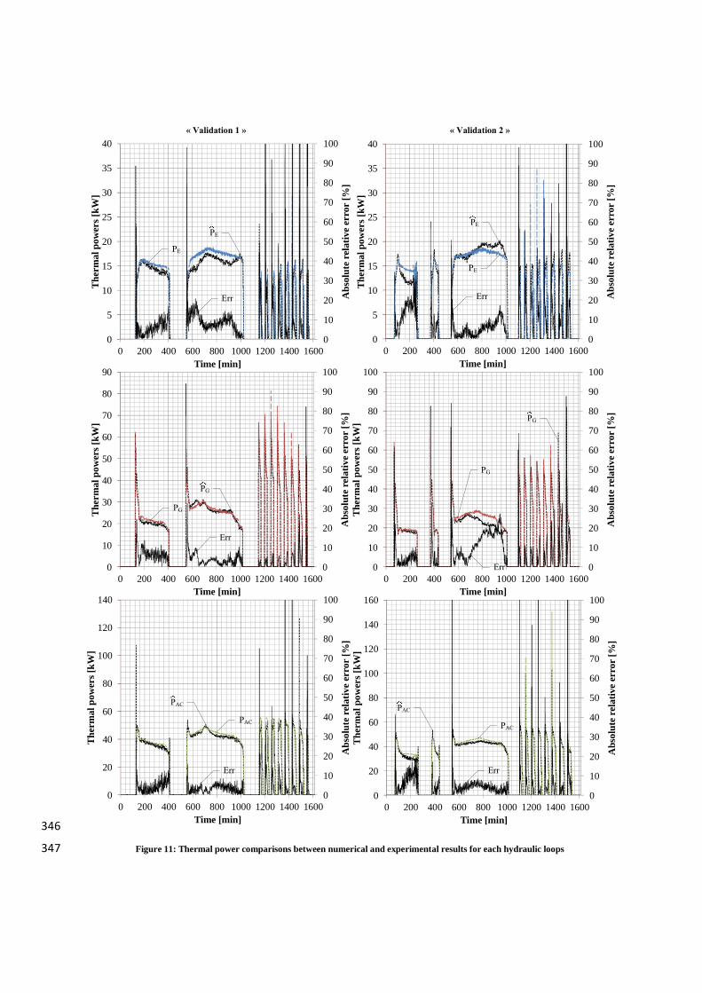
The Figure 10 presents a comparison between the numerical (ANN predictions) and experimental results for the 313

outlet temperatures of each hydraulic loop whereas the Figure 11 presents a comparison between the numerical and 314

experimental results for the thermal powers of each hydraulic loop. The thermal powers are calculated by the 315

equation 9 where is the flow rate of the considered loop and the heat capacity of the heat-transfer fluid. 316

eq. 9 317

The mean error values on temperatures and thermal power are presented on the Table 6. 318

Table 6: Mean relative error values 319 TE, out PE TG, out PG TAC, out PAC Validation 1 4.9% 8.7% 1.1% 4.4% 1.2% 6.6% Validation 2 5.0% 9.3% 2.1% 9.3% 1.6% 7.9%

In general the ANN predicts with a good precision degree each temperature for both data sets “validation 1” and 320

“validation 2”. In fact, mean error values of the outlet temperature in each hydraulic loop are less than 5%. As 321

expected, the prediction of the outlet evaporator temperature by the ANN is less accurate than the two other outlet 322

temperature variables. However, the corresponding instantaneous errors are low, still less than 10%. The neural 323

model seems reproducing with a very satisfactory precision degree the dynamic of the system, even in the on-off 324

operating mode from 1100min to 1600min. 325

The figures show that the ANN performances on the “validation 1” data are better than on the “validation 2” data. 326

This can be explained by the fact that the “validation 1” data are close to the data used during the learning process. 327

Some oscillations or big differences between the ANN predictions and the test field data can be noticed in the 328

beginning. During this period the system is off, no flow rate in the hydraulic loops, there is no heat transfer between 329

the system and its boundary conditions except the thermal losses to the environment. In the modelling configuration 330

of the system the ambient temperature was not taken into account, this explains why the ANN was not able to predict 331

well the outlet temperatures in this period. However, even when the absorption chiller is off but during the test 332

process the model gives a good estimation of the temperatures. This shows than the ANN could be able to model 333

systems even when a potential influential variable was not included in the inputs configuration set. 334

The mean error values for the thermal powers predictions are about 9% which is bigger than the values found for the 335

temperature predictions. This is a mathematical amplification which depends on the value of the inlet temperature 336

when calculating the powers. 337

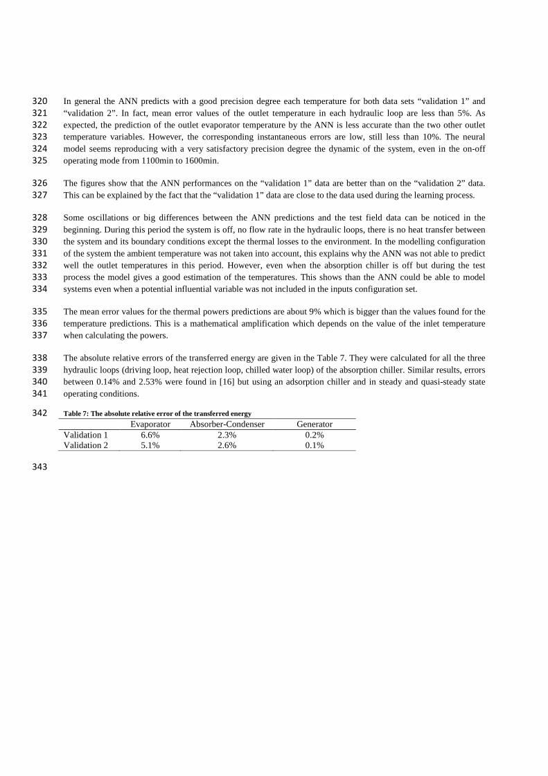
The absolute relative errors of the transferred energy are given in the Table 7. They were calculated for all the three 338

hydraulic loops (driving loop, heat rejection loop, chilled water loop) of the absorption chiller. Similar results, errors 339

between 0.14% and 2.53% were found in [16] but using an adsorption chiller and in steady and quasi-steady state 340

operating conditions. 341

Table 7: The absolute relative error of the transferred energy 342 Evaporator Absorber-Condenser Generator Validation 1 6.6% 2.3% 0.2% Validation 2 5.1% 2.6% 0.1%

343

0

10

20

30

40

50

60

70

80

90

100

0

5

10

15

20

25

30

35

40

45

50

0 200 400 600 800 1000 1200 1400 1600

Abs

olut

e re

lati

ve e

rror

[%

]

Tem

pera

ture

s [°

C]

Time [min]

0

10

20

30

40

50

60

70

80

90

100

0

10

20

30

40

50

60

70

80

90

0 200 400 600 800 1000 1200 1400 1600

Abs

olut

e re

lati

ve e

rror

[%

]

Tem

pera

ture

s [°

C]

Time [min]

0

10

20

30

40

50

60

70

80

90

100

0

10

20

30

40

50

60

0 200 400 600 800 1000 1200 1400 1600

Abs

olut

e re

lati

ve e

rror

[%

]

Tem

pera

ture

s [°

C]

Time [min]

0

10

20

30

40

50

60

70

80

90

100

0

5

10

15

20

25

30

35

40

45

50

0 200 400 600 800 1000 1200 1400 1600A

bsol

ute

rela

tive

err

or [

%]

Tem

pera

ture

s [°

C]

Time [min]

0

10

20

30

40

50

60

70

80

90

100

0

10

20

30

40

50

60

70

80

90

0 200 400 600 800 1000 1200 1400 1600

Abs

olut

e re

lati

ve e

rror

[%]

Tem

pera

ture

s [°

C]

Time [min]

0

10

20

30

40

50

60

70

80

90

100

0

10

20

30

40

50

60

0 200 400 600 800 1000 1200 1400 1600

Abs

olut

e re

lati

ve e

rror

[%

]

Tem

pera

ture

s [°

C]

Time [min]

TE, out

Err

TE, out

TE, out

Err

TE, out

TG, out

Err

TG, out

TG, out

Err

TG, out

TAC, out

Err

TAC, out

TAC, out

Err

TAC, out

« Validation 2 »« Validation 1 »

344

Figure 10: Outlet temperature comparisons between numerical and experimental results for each hydraulic loops 345

0

10

20

30

40

50

60

70

80

90

100

0

5

10

15

20

25

30

35

40

0 200 400 600 800 1000 1200 1400 1600

Abs

olut

e re

lati

ve e

rror

[%]

The

rmal

pow

ers

[kW

]Time [min]

0

10

20

30

40

50

60

70

80

90

100

0

10

20

30

40

50

60

70

80

90

100

0 200 400 600 800 1000 1200 1400 1600

Abs

olut

e re

lati

ve e

rror

[%

]

The

rmal

pow

ers

[kW

]

Time [min]

0

10

20

30

40

50

60

70

80

90

100

0

20

40

60

80

100

120

140

160

0 200 400 600 800 1000 1200 1400 1600

Abs

olut

e re

lati

ve e

rror

[%

]

The

rmal

pow

ers

[kW

]

Time [min]

0

10

20

30

40

50

60

70

80

90

100

0

20

40

60

80

100

120

140

0 200 400 600 800 1000 1200 1400 1600

Abs

olut

e re

lati

ve e

rror

[%]

The

rmal

pow

ers

[kW

]

Time [min]

0

10

20

30

40

50

60

70

80

90

100

0

10

20

30

40

50

60

70

80

90

0 200 400 600 800 1000 1200 1400 1600

Abs

olut

e re

lati

ve e

rror

[%

]

The

rmal

pow

ers

[kW

]

Time [min]

0

10

20

30

40

50

60

70

80

90

100

0

5

10

15

20

25

30

35

40

0 200 400 600 800 1000 1200 1400 1600A

bsol

ute

rela

tive

err

or [

%]

The

rmal

pow

ers

[kW

]

Time [min]

PE

Err

PE

« Validation 2 »« Validation 1 »

PE

Err

PE

PG

Err

PG

PG

Err

PG

PAC

Err

PAC

PAC

Err

PAC

346

Figure 11: Thermal power comparisons between numerical and experimental results for each hydraulic loops 347

5. Conclusion 348

In the present paper, the results of the development of a methodology to model absorption chillers for building 349

applications are presented. This can be applied to systems as found on the market and there is no need to create a 350

physical model of the system which could be very difficult and time consuming. The dynamic ANN models 351

developed are able to predict, with a good level of precision, outlet temperatures and the transferred energy of all 352

the three hydraulic loops (driving loop, heat rejection loop, and chilled water loop). In fact, the ANN generalization 353

ability makes possible to predict the system’s behaviour in various conditions (by changing the loads), different 354

from the ones used during the ANN learning process. Absolute relative prediction errors are almost within the 355

range of 1.1-5% for outlet temperatures and 1-6.6% for the transferred energy. The proposed approach will be 356

helpful in the context of energy performance guarantees. Moreover, ANN simulation takes only a few seconds. This 357

is ideal for engineers and designers to compare different solutions and select the system most suitable for a given 358

building and location. 359

Although in this study the neural model was used in the simulation mode which means that predictions are done for 360

long-term, there is a good agreement between the neural model predictions and the measured data. Usually, short 361

term predictions are more accurate. Therefore ANN models could be used in advanced control systems (predictive 362

control) in order to asses effectively the absorption system operation. 363

Acknowledgments 364

This study has been supported and funded by the French Agency for Environment and Energy Management 365

(ADEME), the 490 National Institute of Nuclear Sciences and Techniques (INSTN) and the French National 366

Research Agency (ANR) in the framework of the “ABCLIMSOL” project sponsored by Prebat program 2007. 367

References 368

369

[1] M. Pons, G. Agniès, F. Boudéhenn, P. bourdoukan, J. Castaing-Lasvignottes, G. Evola, A. Le Denn, O.

Marc, N. Mazet, D. Stitou and F. Lucas, "Performance comparison of six solar-powered air-

conditioners operated in five places," Energy, vol. 46, no. 1, p. 471–483, 2012.

[2] M. Santamouris, N. Papanikolaou, I. Livada, I. Koronakis, C. Georgakis and A. Argiriou, "On the

impact of urban climate on the energy consumption of buildings," Solar Energy, vol. 70, no. 3, pp.

201-216, 2001.

[3] H. Henning, "Solar assisted air conditioning of buildings – an overview," Applied Thermal

Engineering, vol. 27, no. 10, pp. 1734-1749, 2007.

[4] «List of market available chillers compatible with solar cooling. Highlights of SHC Task 48, Quality

Assurance and Support Measures for Solar Cooling,» 2012.

[5] F. Boudéhenn, M. Albaric, N. Chatagnon, J. Heinz, N. Benabdelmoumene and P. Papillon, "Dynamical

studies with a semi-virtual testing approach for characterization of small scale absorption chiller,"

Graz, Autriche, 2010.

[6] F. Boudéhenn, S. Bonnot, H. Demasles and A. Lazrak, “Comparison of Different Modeling Methods

for a Single Effect Water-Lithium Bromide Absorption Chiller,” in EUROSUN, 16-19/09/2014, Aix-Les-

Bains – France, 2014.

[7] D. J. Swider, “A comparison of empirically based steady-state models for vapor-compression liquid

chillers,” Applied Thermal Engineering, vol. 23, p. 539–556, 2003.

[8] G. Cybenko, «Approximation by Superpositions of a Sigmoidal Function,» Math. Control Signals

Systems, vol. 2, pp. 303-314, 1989.

[9] S. A. Kalogirou, «Artificial neural networks in renewable in renewable energy systems application: a

review,» Renewable and Sustainable Energy Reviews, vol. 5, pp. 373-401, 2001.

[10] S. Yilmaz et K. Atik, «Modeling of mechanical cooling system with variable cooling capacity by using

artificial neural network,» Applied Thermal Engineering, vol. 27, pp. 2308-2313, 2007.

[11] M. W. Ahmad, M. Eftekhari, T. Steffen et A. M. Danjuma, «Investigating the performance of a

combined solar system with heat pump for houses,» Energy and Buildings, vol. 63, pp. 138-146,

2013.

[12] F. Almonacid, C. Rus, P. Perez-Higueras et L. Hontoria, «Estimation of the energy of a PV generator

using artificial neural network,» Renewable Energy, vol. 34, pp. 2743-2750, 2009.

[13] P. Vig et I. Farkas, «Neural network Modeling of thermal stratification in a solar DHW storage,» Solar

Energy, vol. 84, pp. 801-806, 2010.

[14] S. Kalogirou, E. Mathioulakis et V. Belessiotis, «Artificial neural networks for the performance

prediction of large solar systems,» Renewable Energy, vol. 63, pp. 90-97, 2014.

[15] A. S. Kalogirou, «Artificial neural networks and Genetic Algorithms in Energy Applications in

Buildings,» Advanced in building energy research, vol. 3, pp. 83-120, 2009.

[16] P. Frey, S. Fischer et H. Drück, «Artificial Neural Network modelling of sorption chillers,» Solar

Energy, vol. 108, p. 525–537, 2014.

[17] S. Rosiek et F. Batlles, «Performance study of solar-assisted air-conditioning system provided with

storage tanks using artificial neural networks,» International Journal of Refrigeration, vol. 34, pp.

1446-1454, 2011.

[18] S. Rosiek and F. Batlles, “Modelling a solar-assisted air-conditioning system installed in CIESOL

building using an artificial neural network,” Renewable Energy, vol. 35 , pp. 2894-2901, 2010.

[19] H. Manohar, R. Saravanan et S. Renganarayanan, «Modelling of steam fired double effect vapour

absorption chiller using neural network,» Energy Conversion and Management, vol. 47 , p. 2202–

2210, 2006.

[20] J. Labusa, J. Hernández, J. Bruno and A. Coronas, “Inverse neural network based control strategy for

absorption chillers,” Renewable Energy, vol. 39, pp. 471-482, 2012.

[21] T. Chow, G. Zhang, Z. Lin et C. Song, «Global optimization of absorption chiller system by genetic

algorithm and neural network,» Energy and Buildings, vol. 34, pp. 103-109, 2002.

[22] V. Congradac et F. Kulic, «Recognition of the importance of using artificial neural networks and

genetic algorithm to optimize chiller operation,» Energy and Buildings , vol. 47 , p. 651–658, 2012.

[23] A. Şencan, “Performance of ammonia–water refrigeration systems using artificial neural networks,”

Renewable Energy, vol. 32, no. 2, p. 314–328, 2007.

[24] A. Şencan, K. A. Yakut and S. A. Kalogirou, “Thermodynamic analysis of absorption systems using

artificial neural network,” Renewable Energy, vol. 31, no. 1, p. 29–43, 2006.

[25] G. Evola, N. Le Pierres, F. boudéhenn and P. Papillon, " Proposal and validation of a general model

for the transient simulation of single-stage LiBr/water absorption chillers," International Journal of

Refrigeration , vol. 36 , pp. 1015-1028, 2013 .

[26] "EAW, 2012. Technische Beschreibung, Absorptionskälteanlagen WEGRACAL SE 15.," [Online].

Available: http://www.eaw-energieanlagenbau.de..

[27] A. Leconte, G. Achard et P. Papillon, «Global approach test improvement using a neural network

model identification to characterise solar combisystem performances,» Solar Energy, vol. 86, pp.

2001-2016, 2012.

[28] R. Heimrath et M. Haller, «Project Report A2 of Subtask A: The Reference Heating System, the

Template Solar System,» A Report of IEA SHC – Task 32, 2007.

[29] G. Dreyfus, Neural networks methodology and applications, Springer, 2005.

[30] M. Norgaard, O. Ravn, N. Poulsen et L. Hansen, Neural networks for modelling and control of

dynamic systems, Springer, 2000.

[31] F. Forsee and M. Hagan, “ Gauss-Newton approximation to Bayesian learning,” in IEEE international

conference on neural networks , Houston, TX, USA, 1997.

[32] MacKay, chez Proceedings of the International Joint Conference on Neural Networks, 1992.

[33] D. Nguyen et B. Widrow, «Improving the learning speed of 2-layer neural networks by choosing

initial values of the adaptative weights,» Proceeding of the International Joint Conference on Neural

Networks, vol. 3, pp. 21-26, 1990.

[34] M. Qia and G. P. Zhangb, "An investigation of model selection criteria for neural network time series

forecasting," European Journal of Operational Research, vol. 132, no. 3, p. 666–680, 2001.

[35] A. Khosravi, Nahavandi, D. Creighton and Saeid, “Quantifying uncertainties of neural network-based

electricity price forecasts,” Applied Energy, vol. 112, p. 120–129, 2013.

[36] W. Yaïci et E. Entchev, «Performance prediction of a solar thermal energy system using artificial

neural networks,» Applied Thermal Engineering, 2014.

[37] G. Cybenko, "Approximation by Superpositions of a Sigmoidal Function," Math. Control Signals

Systems, vol. 2, pp. 303-314, 1989.

370

371

development of a dynamic artificial neural network model

Documents