Development of a dynamic model for

start-up optimization of coal-�red power

plants

EVA ANDERSSON

Master's Degree Project

Stockholm, Sweden June 2013

XR-EE-RT 2013:010

Abstract

The expansion of renewable energies and the deregulations of the energy market are in-creasing the demand of regulating power. In absence of hydropower, thermal power is oftenused for this purpose instead. This thesis focuses on the Vattenfall owned power plant Jän-schwalde located in Germany. The goal is to optimize the start-up procedure, so that thestart-up time is reduced without causing too much thermal stress on the important thick-walled components in the boiler. By reducing the start-up time, the plant can become morepro�table, �exible and better suited to regulate the electricity market.

A start-up model was built in Dymola and validated against measurement data and a sim-ulation model of Jänschwalde, which is too complex to use for optimization purposes. TheJModelica.org platform was used for the optimization part of the project. It was possibleto �nd optimal solutions for the start-up process of the Jänschwalde power plant, but theconvergence of the optimization algorithm was very dependent on the optimization optionsused and the scaling of the plant model. Further work includes development of the compo-nents used in the start-up model, re�ning the discretization and scaling for the optimizationproblem.

1

Contents

1 Introduction 5

1.1 Aim of Thesis . . . . . . . . . . . . . . . . . . . . . . . . . . . . . . . . . . . . . . 51.2 Structure of thesis . . . . . . . . . . . . . . . . . . . . . . . . . . . . . . . . . . . 5

2 Background 7

2.1 Power Plant . . . . . . . . . . . . . . . . . . . . . . . . . . . . . . . . . . . . . . . 72.1.1 Overview . . . . . . . . . . . . . . . . . . . . . . . . . . . . . . . . . . . . 72.1.2 The Steam Cycle . . . . . . . . . . . . . . . . . . . . . . . . . . . . . . . . 82.1.3 Start-up Procedure . . . . . . . . . . . . . . . . . . . . . . . . . . . . . . . 9

2.2 Theory . . . . . . . . . . . . . . . . . . . . . . . . . . . . . . . . . . . . . . . . . . 102.2.1 Balance Equations . . . . . . . . . . . . . . . . . . . . . . . . . . . . . . . 102.2.2 Stress Calculation . . . . . . . . . . . . . . . . . . . . . . . . . . . . . . . 132.2.3 Optimization Problem . . . . . . . . . . . . . . . . . . . . . . . . . . . . . 15

3 Programs and Tools 19

3.1 Modelica . . . . . . . . . . . . . . . . . . . . . . . . . . . . . . . . . . . . . . . . . 193.2 Dymola . . . . . . . . . . . . . . . . . . . . . . . . . . . . . . . . . . . . . . . . . 193.3 Optimica . . . . . . . . . . . . . . . . . . . . . . . . . . . . . . . . . . . . . . . . 193.4 JModelica . . . . . . . . . . . . . . . . . . . . . . . . . . . . . . . . . . . . . . . . 193.5 Media Models . . . . . . . . . . . . . . . . . . . . . . . . . . . . . . . . . . . . . . 21

4 Modelling 23

4.1 Complex model of Jänschwalde . . . . . . . . . . . . . . . . . . . . . . . . . . . . 234.2 Components . . . . . . . . . . . . . . . . . . . . . . . . . . . . . . . . . . . . . . . 26

4.2.1 Connector . . . . . . . . . . . . . . . . . . . . . . . . . . . . . . . . . . . . 264.2.2 Boundary conditions . . . . . . . . . . . . . . . . . . . . . . . . . . . . . . 264.2.3 Combustor . . . . . . . . . . . . . . . . . . . . . . . . . . . . . . . . . . . 274.2.4 Heat exchanger . . . . . . . . . . . . . . . . . . . . . . . . . . . . . . . . . 294.2.5 Header and Separator . . . . . . . . . . . . . . . . . . . . . . . . . . . . . 304.2.6 Turbine . . . . . . . . . . . . . . . . . . . . . . . . . . . . . . . . . . . . . 30

4.3 Model used for optimization . . . . . . . . . . . . . . . . . . . . . . . . . . . . . . 30

5 Validation 33

5.1 Superheater . . . . . . . . . . . . . . . . . . . . . . . . . . . . . . . . . . . . . . . 335.2 Start-up model . . . . . . . . . . . . . . . . . . . . . . . . . . . . . . . . . . . . . 34

6 Optimization 38

6.1 Problem speci�cations . . . . . . . . . . . . . . . . . . . . . . . . . . . . . . . . . 386.2 Optimization options . . . . . . . . . . . . . . . . . . . . . . . . . . . . . . . . . . 386.3 Initialization . . . . . . . . . . . . . . . . . . . . . . . . . . . . . . . . . . . . . . 39

7 Results 40

8 Discussion and Conclusions 46

8.1 Modelling . . . . . . . . . . . . . . . . . . . . . . . . . . . . . . . . . . . . . . . . 468.2 Optimization . . . . . . . . . . . . . . . . . . . . . . . . . . . . . . . . . . . . . . 47

A Description of components 51

2

List of Figures

1 Illustration of a coal-�red power plant. Coal is burnt in the furnace to heat upwater in the heat exchangers. The hot steam is used to drive a steam turbine,which generates electricity to the power grid [Ignou,2013]. . . . . . . . . . . . . . 7

2 The Carnot Cycle presented in an temperature-entropy (T-S) diagram. The heatQIN is added to the system and QLOSS is lost to a cooling medium. The heatengine operates between TH and TL (with TH > TL) and the total e�ciency isgiven by (1). . . . . . . . . . . . . . . . . . . . . . . . . . . . . . . . . . . . . . . 8

3 The Rankine Cycle presented in an temperature-entropy (T-S) diagram. HeatQIN is added to the system in several steps of the steam cycle and QLOSS is lostwhen the steam is condensed. The steam is reheated to improve the e�ciency ofthe plant. . . . . . . . . . . . . . . . . . . . . . . . . . . . . . . . . . . . . . . . . 9

4 Measurement data of a hot start-up. The two upper subplots shows the tempera-ture and pressure for live steam and reheated steam. In the middle, the generatorand �ring power is presented next to the live steam mass �ow rate. The two lowersubplots shows revolutions per minute (RPM) for the turbine and the openinglevel of the high-pressure and low-pressure bypass valves. . . . . . . . . . . . . . 11

5 Model of a heat exchanger, where heat is transferred from �ue gas to steamthrough a wall segment. . . . . . . . . . . . . . . . . . . . . . . . . . . . . . . . . 12

6 A cross-sectional illustration of a header. . . . . . . . . . . . . . . . . . . . . . . 147 Life-time in terms of load cycles N of components related to stress amplitude ∆σ,

at T = 100 ◦C and T = 550 ◦C. . . . . . . . . . . . . . . . . . . . . . . . . . . . . 158 An element ne in the interval [ti, ti+1],containing three Radau points q1, q2 and q3. 179 An overview of the complex model of Jänschwalde, owned by Vattenfall. The

complete steam cycle is included in the model. The water is heated, used to drivethe turbine, reheated and �nally condensed and cooled. The total number ofequations and unknowns is 16,927. . . . . . . . . . . . . . . . . . . . . . . . . . . 23

10 The superheater section is one subcomponent from the model shown in Figure9. The �gure shows four superheaters (SH) and three reheaters (RH) from thecomplex model of the Jänschwalde power plant. The circles represent connectorsfor �ue gas (green), water (blue) and coal (brown), and are used to link thecomponent to other submodels or boundary conditions. . . . . . . . . . . . . . . 24

11 The furnace section in Figure 9, which contains the combustion process and theevaporator. . . . . . . . . . . . . . . . . . . . . . . . . . . . . . . . . . . . . . . . 25

12 The ECO & SH1 section from Figure 9, which shows the economizer and onesuperheater. . . . . . . . . . . . . . . . . . . . . . . . . . . . . . . . . . . . . . . . 25

13 The �gure shows how well the process models P1, P1D, P0 and P0D, generatedin the System Identi�cation Toolbox in Matlab, �ts the reference data. . . . . 28

14 Model used for start-up optimization. The heat exchangers modelled are thesuperheaters (SH), reheaters (RH) and the evaporator (Evap). Other componentsinclude wall and volume components to calculate stress levels in headers andseparators and components to represent boundary conditions. The model has oneinput du connected to the integrator component which describes how the loadis changed du

dt . There are three outputs to the right for live steam temperature,header stress and separator stress. . . . . . . . . . . . . . . . . . . . . . . . . . . 31

15 Temperatures of in- and out�owing water, for the complex superheater and thestart-up superheater. . . . . . . . . . . . . . . . . . . . . . . . . . . . . . . . . . 33

3

16 Temperatures of in- and out�owing �ue gas, for the complex superheater and thestart-up superheater. The temperature curves for in�owing �ue gas are equal forboth superheaters. . . . . . . . . . . . . . . . . . . . . . . . . . . . . . . . . . . . 34

17 Comparison between reference data, complex simulation model and start-up modelat steady-state with full load. . . . . . . . . . . . . . . . . . . . . . . . . . . . . . 35

18 Comparison of the complex simulation model of Jänschwalde (dotted lines) andmeasurement data (solid lines) from the actual plant, when the system wasramped from 100% load to 60% and back again to 100% load. . . . . . . . . . . 36

19 Simulation of the start-up model when the system was ramped from 100% loadto 60% and back again to 100% load. The start-up model is not a�ected bydisturbances, compared to the systems shown in Figure 18. . . . . . . . . . . . . 37

20 Plot of coal �ow u and the control signal dudt , with blocking factors [1, 1, 2, 6]. . . 3921 Initial optimization with blocking factors [1,1,2,6]. The weight parameters in (20)

are chosen as α = 0.01, β = 0.01. The steady-state value Tref is reached for thelive steam exiting the last superheater SH4. . . . . . . . . . . . . . . . . . . . . . 41

22 Initial optimization with blocking factors [1,1,2,6]. The weight parameters in (20)are chosen as α = 0.0004, β = 0.01. The steady-state value for Tref is not reachedduring 2000 seconds. . . . . . . . . . . . . . . . . . . . . . . . . . . . . . . . . . . 41

23 Initial optimization with blocking factors [1,1,2,6]. The weight parameters in (20)are chosen as α = 0.0025, β = 0.01. The �nal value of the steam temperature inSH4 is 1040K. . . . . . . . . . . . . . . . . . . . . . . . . . . . . . . . . . . . . . 42

24 Optimization with uniformly distributed blocking factors [2, 2, 2, 2, 2, 2, 2, 2] andne = 16. The stress amplitude is approximately 135MPa. . . . . . . . . . . . . . 43

25 Optimization with a high blocking factor at the end of the interval [2, 2, 2, 2, 2, 2, 6]and ne = 16. The stress amplitude is approximately 210MPa. . . . . . . . . . . 44

26 Optimization with blocking factors [1, 1, 1, 1, 1, 5] and ne = 10. The stress ampli-tude is approximately 200MPa. . . . . . . . . . . . . . . . . . . . . . . . . . . . 44

27 Optimization with blocking factors [5, 1, 1, 1, 1, 1] and ne = 10. The stress ampli-tude is approximately 125MPa. . . . . . . . . . . . . . . . . . . . . . . . . . . . 45

List of Tables

1 Start-ups at Jänschwalde during 2012 . . . . . . . . . . . . . . . . . . . . . . . . . 102 Optimization options for JMUs . . . . . . . . . . . . . . . . . . . . . . . . . . . . . 213 Optimization options for the IPOPT solver . . . . . . . . . . . . . . . . . . . . . 214 Process models used in the System Identi�cation Toolbox . . . . . . . . . . . . . 285 Steam temperatures out of each heat exchanger component at a steady-state

simulation with full load. . . . . . . . . . . . . . . . . . . . . . . . . . . . . . . . . 356 Speci�cation of values used for Tref and constraints. . . . . . . . . . . . . . . . . 397 Summary of parameter values used for di�erent problem set-ups. . . . . . . . . . 408 Summary of blocking factors used for di�erent problem set-ups. . . . . . . . . . 43

4

1 Introduction

Recent development in the electricity market has started and will continue to change how powerplants are operated. The increase in renewable energies is increasing the demand of regulatingpower needed, to balance production and consumption of electricity, so that the frequency of theelectricity grid is kept constant. In addition to this, the deregulations of the electricity marketsmakes it possible for the consumers to also produce electricity. The Swedish market has accessto hydropower, which is a very good regulating power since it can be switched on and o� almostinstantly. In other countries it is common the use thermal power plants instead. Besides havinga large environmental impact, thermal power plants require a longer start-up time.

This thesis will focus on the start-up procedure of the German power plant Jänschwalde, ownedby Vattenfall. The goal is to �nd a model that describes the behaviour of the power plantsu�ciently well and can be used for optimization. By formulating the start-up procedure asan optimization problem, one can also take into account economical and environmental factors,for example by reducing the fuel consumption during the start-up. During start-ups there arecertain components, that can be exposed to heavy thermal stress. Too much thermal stress, willshorten the components life-time and therefore constraints on stress levels are needed.

Several studies on start-up optimization have been done in the past, but most of them considerCombined Cycle Power Plants, for example [Lind & Sällberg, 2012], [Casella et al.,2011] and[Casella, Donida & Åkesson, 2011]. The Combined Cycle Power Plants consists of both a gasturbine and a steam turbine, and are run with gas. The model derived in this thesis will bedi�erent from previous work, mainly because Jänschwalde is run with brown coal, which intro-duces delays in the overall system. Another di�erence is that Jänschwalde only has turbines thatare driven by steam. A very detailed model of Jänschwalde is under development at Vattenfall.However, the high complexity of it makes it unsuitable for optimization purposes. There existssome studies on coal-�red boilers, including for example [Franke, Rode & Krüger, 2003]. Themodels and optimization methods from those studies are unfortunately not public.

1.1 Aim of Thesis

The aim of the thesis is mainly to develop a dynamic model of Jänschwalde, that can be usedfor optimization purposes. Another goal is to try out the optimization techniques within theJModelica.org platform [JModelica.org,2013], to see if they can be applied to a dynamic modelof a coal-�red power plant. The �nal goal is to use di�erent optimization options and try to �ndoptimal solutions for the start-up problem.

Since the actual power plant is very complex, there are many simpli�cations that must be donein order to model it. The model developed within this thesis only contains the most importantcomponents relevant for the start-up, which are located in the boiler.

1.2 Structure of thesis

In Chapter 2 a brief introduction to coal-�red power plants is given. The mathematical equationsthat are used for the modelling are explained and derived. It is also shown how the dynamicoptimization problem can be transferred to a non-linear programming problem, which can besolved by the chosen optimization algorithm.

5

The relevant programs and how they are used are brie�y explained in the Chapter 3. The chap-ter also includes examples on how the JModelica.org platform is used for optimization.

In the beginning of Chapter 4 the complex simulation model of Jänschwalde, owned by Vat-tenfall, is described. The components used in the start-up model are explained and the mostimportant code is included. The start-up model is compared to the complex model and mea-surement data from the real plant in Chapter 5.

Chapter 6 includes the optimization set-ups used and the outcomes are presented in Chapter7. Finally, the model and the optimization outcomes are evaluated in Chapter 8. Furtherimprovements and sources of error are also discussed.

6

2 Background

This chapter is divided into two parts. First an introduction to coal-�red power plant is given,where the steam cycle and the start-up procedure are presented. The second part describes themathematical theories, that are needed to understand the dynamic model and the optimizationtechniques used.

2.1 Power Plant

The subject of study is the power plant Jänschwalde, which is owned by Vattenfall[Vattenfall,2012].It is the largest lignite power plant in Germany, consisting of 6 blocks with 500MW installedcapacity each [Saarinen, Boman & Funkquist, 2011]. The power plant started operating in 1981and has an electrical e�ciency of 36%.

2.1.1 Overview

A basic illustration of a simple coal-�red power plant is shown in Figure 1. The coal is burnt inthe furnace to produce �ue gas and ash. The heat from the �ue gas is used to warm the feed-water and convert it to steam in the boiler. The feedwater goes through di�erent types of heatexchangers, including the economizer, the evaporator and several superheaters. The superheatedsteam is then expanded in the steam turbine. The turbine is connected to a generator, which isused to generate electricity to the power grid. Finally the steam is condensed and cooled down,before it re-enters the boiler [Ignou,2013].

Since the power plant at Jänschwalde is much more complicated than this example, a moredetailed description of the steam cycle will be given in Section 2.1.2. In this thesis the mainfocus will be on the boiler, because it contains the components that are exposed to the highestlevels of stress.

Figure 1: Illustration of a coal-�red power plant. Coal is burnt in the furnace to heat up water in theheat exchangers. The hot steam is used to drive a steam turbine, which generates electricity to the powergrid [Ignou,2013].

7

2.1.2 The Steam Cycle

The e�ciency of the power plant can be evaluated by looking at the Rankine cycle, which is amodi�cation of the Carnot cycle. The Carnot cycle is an ideal process, where all processes arereversible and no heat is lost to the surrounding environment [Alvarez, 2006]. It is a theoreticalmodel, which maximizes the e�ciency of a heat engine. The Carnot cycle consists of fourthermodynamic steps, which are shown in a temperature-entropy diagram in Figure 2. In thisexample the heat engine is working in the two-phase region, meaning that the water exists inboth liquid and vaporized states at the same time.

Figure 2: The Carnot Cycle presented in an temperature-entropy (T-S) diagram. The heat QIN is addedto the system and QLOSS is lost to a cooling medium. The heat engine operates between TH and TL(with TH > TL) and the total e�ciency is given by (1).

Carnot cycle

1→ 2: First the medium is expanded at a constant temperature TH , by absorbing heat QIN .2 → 3: The next step consists of an adiabatic expansion of the gas, in which no heat is lostto the surrounding environment. The temperature decreases to TL and the entropy is constantsince no heat is added to or subtracted from the system.3 → 4: The medium is compressed at the constant temperature TL and the heat QLOSS istransferred to a cooling medium.4 → 1: Finally the medium is adiabatically compressed, until the temperature TH is achievedand the cycle is complete.

The Carnot e�ciency η of the heat engine is given by the work done by the system W , dividedby the heat added to the system QIN :

η =W

QIN=QIN −QLOSS

QIN= 1− QLOSS

QIN= 1− TL

TH. (1)

Equation (1) shows that it is desirable to have a large di�erence between TL and TH , to get ahigh Carnot e�ciency.

A coal-�red power plant is better described by the Rankine cycle with reheat [Ignou,2013]. ARankine cycle that operates in the one- and two-phase region, is shown in Figure 3.

8

Figure 3: The Rankine Cycle presented in an temperature-entropy (T-S) diagram. Heat QIN is addedto the system in several steps of the steam cycle and QLOSS is lost when the steam is condensed. Thesteam is reheated to improve the e�ciency of the plant.

Rankine cycle with reheat

1→ 2 First the water is compressed by a pump and the temperature is increased.2→ 3 The temperature of the water is further increased in the pre-heaters and the economizer,by addition of heat QIN .3 → 4 Next, the water is evaporated into steam. The evaporator operates in the two phaseregion, containing both water and steam.4→ 5 The steam temperature is further increased in the superheaters.5→ 6 In the next step, steam is expanded in the high pressure turbine to generate electricity.6→ 7 After the high pressure turbine, the steam is reheated and led to the low pressure turbine.7→ 8 The steam is expanded again and electricity is generated in the low pressure turbine.8→ 1 Finally the steam is condensed completely.

The e�ciency of the actual process can never be higher than the Carnot e�ciency [Alvarez, 2006].The best ways to achieve a high e�ciency is to have small energy losses throughout the cycle,and a very high di�erence between the maximal and minimal water temperature in the cycle.

A di�erence between Figure 2 and 3, is that the water is superheated to only exist in a vaporizedstate, so that a very high maximal temperature can be reached. The life-time of the turbinecan be improved by using superheated steam which is very dry, to generate electricity. Anotherdi�erence is the reheating step, which is another way to increase the e�ciency of the cycle. Thesteam is only partially expanded in the high pressure turbine, reheated and then completelyexpanded in the low-pressure turbine.

2.1.3 Start-up Procedure

The start-up procedure of Jänschwalde can be divided into three di�erent phases.

(i) First the ignition oil burners are started up, to quickly start the combustion process inthe furnace. Then the coal mills are started up and the combustion medium is gradually

9

Table 1: Start-ups at Jänschwalde during 2012

Start-up type Stand-still time Occurrences 2012

Hot t ≤ 12 h 4Warm 12 h < t < 48 h 6Cold 48 h ≤ t 15

shifted from oil to coal during the start-up. Meanwhile the temperature and pressure ofthe live steam are ramped up. During this stage the power plant is not producing anyelectricity, since the live steam bypasses the steam turbine.

(ii) The next phase is to accelerate the steam turbine, which is started once you have reachedstable steam conditions. The turbine is accelerated until it reaches 3000 revolutions perminute.

(iii) In the last phase, the bypass valve is gradually closed so that the live steam enters thesteam turbine. The production of electricity begins and the load is increased until the �naloutput capacity is reached.

The length of the start-up is highly dependent of the stand-still time of the power plant, sinceit takes a long time for the metal parts to cool down. Start-ups are therefore categorized intohot,warm and cold start-ups according to Table 1. In Figure 4 measurement data are presentedfor a hot start. The ignition oil burners are initiated in the interval t ∈ [15, 30] min and the coalmills are started when t ∈ [40, 70] min, which is represented by the change in �ring power.

Stable steam conditions for the live steam mass �ow and pressure are reached for t ≈ 100min,but one can observe that the turbine is started at t ≈ 75min which indicates an overlap betweenphase 1 and 2. In the lower right corner, the opening of the high- and low-pressure valves areshown. When the valves are open, the steam is bypassed the turbine. The valves are closed att ≈ 150min, meaning that the steam goes through the turbine, which generates electricity. The�nal phase of the start-up includes increasing the load (�ring power) and live steam �ow rate,which is done in the interval t ∈ [150, 210] min.

2.2 Theory

A thermal power plant consists of several heat exchangers, which warms up the water graduallyduring the steam cycle. Therefore the theory behind a heat exchanger component will be givenin this section. Since the start-up process is limited by stress in thick-walled components, thestress calculation will be presented as well. Finally the dynamic optimization problem is set upand transferred to a non-linear programming problem.

2.2.1 Balance Equations

In Figure 5 a model of a heat exchanger is shown, which can be used in thermal power plants.The component consists of two sides, containing �ue gas and steam which are divided by awall. The �ue gas is obtained from the combustion process and is assumed to have a highertemperature than the wall.

10

Figure 4: Measurement data of a hot start-up. The two upper subplots shows the temperature andpressure for live steam and reheated steam. In the middle, the generator and �ring power is presentednext to the live steam mass �ow rate. The two lower subplots shows revolutions per minute (RPM) forthe turbine and the opening level of the high-pressure and low-pressure bypass valves.

11

Hot �ue gas with enthalpy hgas,in, mass �ow rate qgas,in and pressure pgas,in enters the gas sideof the heat exchanger. Since the wall temperature is lower than the gas temperature, heat Qgaswill be transferred to the wall according to the second law of thermodynamics. The �ue gasthen exits the heat exchanger with enthalpy hgas,out, mass �ow rate qgas,out and pressure pgas,out.The process of the steam side works in the corresponding way, except that heat Qwater is addedto the system.

Figure 5: Model of a heat exchanger, where heat is transferred from �ue gas to steam through a wallsegment.

The dynamics of each side of the heat exchanger are given by the balance equations,

dMm

dt= qm,in − qm,out, (2a)

dUmdt

= qm,inhm,in − qm,outhm,out +Qflow,m, (2b)

pm,in − pm,out = fmq2m,inρm

, (2c)

with m ∈ {gas, steam}, mass of the matter Mm, internal energy Um, density of the mediumρm and a constant fm [Krüger, Franke & Rode, 2004]. fm describes the pressure drop and canbe found experimentally. For the balance equations heat �ow rate Qflow,m = dQm

dt , is used todescribe at which rate the heat is transferred.

For this application it is more convenient to use pressure p and enthalpy h as state variablesinstead of massM and internal energy U . The pressure p and temperature T for di�erent stagesof the process are measured in the real plant. It is however easier to use enthalpy h instead oftemperature T , because the right-hand side of the energy balance equation is expressed in termsof enthalpy.

The mass of the matter Mm can be expressed in terms of volume Vm and density of the matterρm. Since the tank volume Vm is constant, the balance equations can be rewritten in the following

12

way:

dMm

dt= Vm

dρmdt

(3a)

= Vm

[∂ρm∂hm

∣∣∣∣p

dhmdt

+∂ρm∂pm

∣∣∣∣h

dpmdt

]= qm,in − qm,out, (3b)

dUmdt

=d(Vmρmhm − pmVm)

dt= Vm

[d(ρmhm)

dt− dpm

dt

](3c)

= Vm

[hm

dρmdt

+ ρmdhmdt− dpm

dt

](3d)

= Vm

[hm

∂ρm∂hm

∣∣∣∣p

dhmdt

+ hm∂ρm∂pm

∣∣∣∣h

dpmdt

+ ρmdhmdt− dpm

dt

](3e)

= Vm

[(hm

∂ρm∂hm

∣∣∣∣p

+ ρm

)dhmdt

+

(hm

∂ρm∂pm

∣∣∣∣h

− 1

)dpmdt

](3f)

= qm,inhm,in − qm,outhm,out +Qflow,m. (3g)

In section 4.2.4 the mass balance

Vm

[∂ρm∂hm

∣∣∣∣p

dhmdt

+∂ρm∂pm

∣∣∣∣h

dpmdt

]= qm,in − qm,out, (4)

and the energy balance

Vm

[(hm

∂ρm∂hm

∣∣∣∣p

+ρm

)dhmdt

+

(hm

∂ρm∂pm

∣∣∣∣h

−1

)dpmdt

]= qm,inhm,in−qm,outhm,out+Qflow,m, (5)

is used to model the dynamics of gas and water in the heat exchangers.

To calculate how much heat is transferred between the gas and water side, equations for thewall segment must be included. The change in temperature of the wall, depends on the heatcapacity cp,wall, the mass Mwall and how much heat is added or subtracted.

Mwallcp,walld(Twall)

dt=

∑m∈gas,steam

Qflow,m, (6)

where Qm is given by

Qflow,m = αwall,mAwall,m(Tm − Twall), (7)

with the heat transfer coe�cient αwall,m and the area of exposure Awall,m between the wall andthe medium m [Alvarez, 2006].

2.2.2 Stress Calculation

During the start-up, the thick-walled components are a�ected by thermal stress σT and mechan-ical stress σm, due to changes in temperature and pressure [Meinke, 2012]. The thick-walledcomponents that are considered most critical during start-up are the separator and the headers.

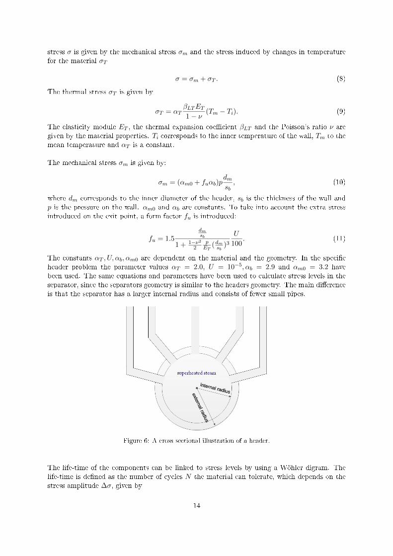
A header consists of a large hollow pipe and many smaller pipes, which can be seen in Figure 6.The steam enters or exits the header through the smaller pipes, which introduces extra stressat the exit points. In the stress calculations the worst case scenarios are considered. The total

13

stress σ is given by the mechanical stress σm and the stress induced by changes in temperaturefor the material σT

σ = σm + σT . (8)

The thermal stress σT is given by

σT = αTβLTET1− ν

(Tm − Ti). (9)

The elasticity module ET , the thermal expansion coe�cient βLT and the Poisson's ratio ν aregiven by the material properties. Ti corresponds to the inner temperature of the wall, Tm to themean temperature and αT is a constant.

The mechanical stress σm is given by:

σm = (αm0 + fuαb)pdmsb, (10)

where dm corresponds to the inner diameter of the header, sb is the thickness of the wall andp is the pressure on the wall. αm0 and αb are constants. To take into account the extra stressintroduced on the exit point, a form factor fu is introduced:

fu = 1.5

dmsb

1 + 1−ν22

pET

(dmsb )3U

100. (11)

The constants αT , U, αb, αm0 are dependent on the material and the geometry. In the speci�cheader problem the parameter values αT = 2.0, U = 10−5, αb = 2.9 and αm0 = 3.2 havebeen used. The same equations and parameters have been used to calculate stress levels in theseparator, since the separators geometry is similar to the headers geometry. The main di�erenceis that the separator has a larger internal radius and consists of fewer small pipes.

Figure 6: A cross-sectional illustration of a header.

The life-time of the components can be linked to stress levels by using a Wöhler digram. Thelife-time is de�ned as the number of cycles N the material can tolerate, which depends on thestress amplitude ∆σ, given by

14

∆σ =σmax − σmin

2, (12)

were σmax and σmin are the maximal and minimal values of the total stress during the start-up.

In Figure 7 a Wöhler curve is shown, which has been developed to analyse life-times of compo-nents in thermal power plants [Meinke, 2012]. The total number of start-ups for 2012 was 25,which can be seen in Table 1. If one assumes that a power plant is operated for 60 years and isstarted up 25 times/year, the total number of start-ups becomes 1500. Figure 7 shows that thestress amplitude ∆σ must be below 700MPa, to not wear out a header that operates around550 ◦C. For the separator, a slightly higher stress amplitude is tolerated, since it operates at≈ 350 ◦C.

Figure 7: Life-time in terms of load cyclesN of components related to stress amplitude ∆σ, at T = 100 ◦Cand T = 550 ◦C.

2.2.3 Optimization Problem

A dynamic model often consists of di�erential and algebraic equations, and together theyform a Di�erential Algebraic (DAE) system [Ljung & Glad, 2004]. A di�erential equationdescribes the relationship between a function and its derivative [Edsberg, 2008]. Two typi-cal di�erential equations are the balance equations for mass and energy, seen in (4) and (5).The algebraic equations ensures the physical and thermodynamical relations in the model[Biegler, Cervantes & Wächter, 2002], for example (7), which describes how heat is transferredbetween media. A general di�erential equation

F (x(t), x(t), u(t), t) = 0, ∀t ∈ [t0, tf ] (13)

15

can be rewritten by introducing x(t) = (z(t), y(t))T to separate the di�erential variables z, whosederivatives appear in the DAE system, from the algebraic variables y. Equation (13) is thentransformed to:

F (z(t), z(t), y(t), u(t), t) = 0, ∀t ∈ [t0, tf ]. (14)

By di�erentiating (14) with respect to time, an Ordinary Di�erential Equation (ODE) systemcan be obtained. The number of times n the system must be di�erentiated, before an ODE sys-tem is achieved corresponds to the di�erential index of the DAE [Ljung & Glad, 2004]. Thereforean ODE system corresponds to a DAE system of index 0.

A general formulation of a DAE optimization problem is given by [Wächter, 2002]:

minz(t),y(t),u(t),tf ,p

ϕ(z(tf ), y(tf ), tf , p) (15a)

s.tdz(t)

dt= F (z(t), y(t), u(t), t, p) (15b)

0 = G(z(t), y(t), u(t), t, p) (15c)

z(0) = z0 (15d)

0 = Hs(z(ts), y(ts), u(ts), ts, p) for s ∈ [1, ..., ns] (15e)

The variable bounds are given by:

zL ≤ z(t) ≤ zU

yL ≤ y(t) ≤ yU

uL ≤ u(t) ≤ uU

pL ≤ p ≤ pU

tLf ≤ tf ≤ tUf

ϕ is a scalar objective function,

F are the right hand sides of di�erential equation constraints,

G are algebraic state pro�le vectors of index one,

Hs are additional point conditions at �xed times ts,

z are di�erential state pro�le vectors,

z0 are the initial values of z,

y are algebraic state pro�le vectors,

u are control pro�le vectors,

p is a time-independent parameter vector,

tf is the �nal time.

In the general formulation the algebraic equations have been collected from (14) to form (15c).Point conditions have been de�ned at certain �xed times and all variables used are bounded byupper and lower values. To solve the problem numerically, the dynamic optimization problemis transferred to an non-linear programming (NLP) problem. This is done by introducing adiscretization so that the state and control pro�les are approximated by a family of polynomialson �nite elements (t0 < t1 < . . . < tne < tf ) [Biegler, Cervantes & Wächter, 2002]. The dis-cretization is further re�ned by placing Radau collocation points ncp within each element, seeFigure 8.

16

t ti i+1

q q q1 2 3

Figure 8: An element ne in the interval [ti, ti+1],containing three Radau points q1, q2 and q3.

Interior Point Method

After the discretization, the NLP problem can be formulated in the following way:

minx∈Rn

f(x) (16a)

s.t c(x) = 0 (16b)

xL ≤ x ≤ xU . (16c)

where x = (dzdt i,q, zi, yi,q, ui,q, t, p)T and q = 1, . . . , ncp and i = 1, . . . , ne [Wächter & Biegler, 2006].

The objective function f(x) : Rn → R and equality constraints c(x) : Rn → Rm should be twicecontinuously di�erentiable and m < n. The variables x have an upper xU ∈ Rn and lower boundxL ∈ Rn and xU ≥ xL [Wächter & Biegler, 2006].

To demonstrate the interior point method, the following cost function will be used

minx∈Rn

f(x) (17a)

s.t c(x) = 0 (17b)

x(i) ≥ 0 for i ∈ I. (17c)

with I ∈ 1, ..., n is the set of indices of bounded variables [Wächter, 2002]. In (16c) the variableshad upper and lower bounds, but it is easier to demonstrate the algorithm with the new prob-lem formulation only consisting of variables with an lower bound of zero [Wächter, 2002]. Thesolution and algorithm for the problem (17) can be applied to the problem (16), for example ifthe �rst problem is rede�ned with slack variables [Wächter, 2002].

17

The interior point method is also referred to as a barrier method, and is de�ned accordingly

minx∈Rn

ϕµ(x) := f(x)− µn∑i=1

ln(x(i)) (18)

s.t c(x) = 0. (19)

A barrier function ϕµ(x) is introduced where an logarithmic barrier term is added to the problem[Wächter, 2002]. In that way the variable bounds from (17c) are included in the objectivefunction. If the variables approach the variable bounds in (17c), the barrier function becomesarbitrarily large and therefore the local solution x?µ is in the interior of the set, meaning that itful�ls x(i)?µ > 0 for all i ∈ I. When the barrier function µ → 0 the solution x?µ converges to x?which is a solution to the original optimization problem de�ned by (17) [Wächter, 2002].

18

3 Programs and Tools

The dynamic start-up model has been developed in the Modelica environment Dymola. TheJModelica.org platform was used for the optimization part, with the Modelica language extensionOptimica. The programs and how they are used are brie�y described in this chapter.

3.1 Modelica

Modelica is an open programming language, which is used to model and simulate complex physi-cal systems. The language is object-oriented, allowing you to inherit properties from submodels.Modelica is equation-based which makes it easier to combine di�erent kinds of physical systems.A Modelica model can be a combination of a variety of mechanical, electrical, thermodynamicalor other types of components. Another bene�t with using the Modelica language is that itcan handle DAEs. If the modelling is instead done in Simulink [MathWorks,2013], you need tomanually convert the DAEs to ODEs, to be able to simulate the model [Modelica.org,2013].

3.2 Dymola

Dymola is a commercial Modelica environment, which for example can be used for modellingand simulation. In Dymola you can switch between working in graphical and code-based envi-ronment. The changes you make in the graphical environment are automatically converted intoModelica code. In the modelling environment it is also possible to browse the open-source Mod-elica standard library and use those components to build models. The simulation environmentis mainly used to simulate models and plot results. Other features include 3D-animations ofresults and the possibility to export models to formats that can be handled by other simulationsoftware, such as Simulink [Modelica.org,2013].

3.3 Optimica

Optimica is an extension of the Modelica language, which makes it possible for the user toformulate dynamic optimization problems [Åkesson, 2008]. The Optimica extension includes theclass optimization with class attributes such as objective, startTime and �nalTime. Optimicacan be used to express di�erent types of optimization problems, for example minimize a costfunction or minimize the �nal time. It is also possible to specify constraints for the optimizationproblems, that must be ful�lled for the optimal solution.

3.4 JModelica

JModelica is an open source platform, that can be used to optimize and simulate Modelicamodels. The project started at the Department of Automatic Control at Lund University andnow the development is done by Modelon AB and in academia [JModelica.org,2013]. JModelicasupports the extension Optimica, which makes it possible to formulate and solve many types ofdynamic optimization problems.

Three �les are generally needed to formulate and solve a dynamic optimization problem, theModelica model (.mo), the Optimica speci�cations (.mop) and a Python script �le (.py). TheModelica and Optimica code is compiled in the Optimica compiler to generate C code. The Ccode is then compiled and connected to numerical solvers, to solve the optimization problem[Åkesson, Gäfvert & Tummescheit 2009].

19

Simulation and Optimization

JModelica has three di�erent types of model objects FMUModel, JMUModel and CasadiModel.These objects can be used for simulation and optimization. In this project only the �rst twoobject types are used and will therefore be described brie�y.

The main di�erences between a FMUModel and an JMUModel, is that only the JMUModel canbe used for optimization, since it supports the Optimica attributes. A JMUModel can onlybe created in the JModelica.org environment and used together with Modelica and Optimicacode[Modelon AB,2012]. FMUModels, on the other hand, can be created from other modellingand simulation environments since it follows the FMI(Functional Mock-up Interface) standard.

The FMUModel is used to simulate the model and the result is later used as an initial guessfor the optimization problem, which is handled by an JMUModel. To begin with the functionscompile_fmu and load_fmu are imported in the Python script �le.

from pymodelica import compile_fmu

from pyfmi import load_fmu

init_fmu = compile_fmu('simModel ',['Heatexch_opt.mo','Water_poly '])

init_model = load_fmu(init_fmu)

init_res = init_model.simulate(start_time =0, final_time =4000)

The function compile_fmu needs the model name ('simModel')and the Modelica �le ('Hea-texch_opt') as input. Additional packages that contain functions or models needed for thesimulation, can be added as arguments. In the examples shown in this section, the media modelfor water ('Water_poly') is added in this way. Finally the model can be simulated, by calling thefunction simulate with start and �nal time. Additional options for compilations and simulationsof FMUs can be found in the JModelica.org Userguide [Modelon AB,2012].

The next step is to �nd an optimal solution to the problem. As previously, the functionsneeded are imported and a compilation is done. The function compile_jmu needs an additionalargument, which is the Optimica �le ('heatopt.mop').

from pymodelica import compile_jmu

from pyjmi import JMUModel

jmu_name=compile_jmu("heatopt.Opt1" ,['Heatexch_opt.mo','heatopt.mop','

Water_poly '])

opt_result = JMUModel(jmu_name)

res=opt_result.optimize ()

For the optimization problem in this report it was necessary to de�ne optimization options,to improve the convergence of the optimization algorithm. The options are de�ned by usingthe function optimization_options and an example in which the number of elements n_e arechanged is shown below.

opts=opt_result.optimize_options ()

opts['n_e']=20

res=opt_result.optimize(options=opts)

The options used for this thesis project can be found in Table 2 and all available options can befound in the JModelica User Guide [Modelon AB,2012].

IPOPT

The JModelica platform uses a simultaneous optimization algorithm with based orthogonalcollocation using Lagrange polynomials on Radau points [JModelica.org,2013]. The process

20

Table 2: Optimization options for JMUs

Options Description

n_e Number of elements that the optimization interval is dividedin. The default number of elements is 50.

n_cp Number of collocation points for each element in n_e. Thedefault number of collocations points is 3.

blocking_factors Blocking factors are used to keep the control pro�le con-stant for nearby elements. Blocking factors are not used inthe default case, but can improve the convergence of the op-timization algorithm. The blocking factors [2,1,6,1] makesu0 = u1, u3 = u4 = u5 = u6 = u7 = u8, while u2 and u9 isnot dependent on nearby elements. The sum of the elementsmust equal the number of elements n_e.

result_�le_name Writes results to a text �le.init_traj An initial trajectory is used as a �rst guess for the optimiza-

tion. problem

Table 3: Optimization options for the IPOPT solver

Options Description

tol Decides to convergence tolerance. If the (scaled) NLP erroris smaller than the value of tol, the optimization algorithmwill be successfully terminated. For this project 5× 10−4 isused and the default values is 10−8.

max_iter Maximum iterations allowed for the optimization problem.In this project 100-300 is used and the default value is 3000.

makes it possible to transfer di�erential algebraic equations (DAE) used in the dynamic model,into a large-scale NLP problem [Åkesson, Gäfvert & Tummescheit 2009]. The NLP problem issolved with the IPOPT(Interior Point OPTimizer) solver [IPOPT,2013], which is an open-sourcesolver appropriate for large-scale problems. There are several options for the IPOPT solver thatcan be changed, to suit ones optimization problem. The options are changed in the Pythonscript �le, in the following way:

opts['IPOPT_options ']['tol']=5e-4

In Table 3 descriptions of the IPOPT options used in this thesis project is presented. In thisproject the IPOPT solver MA27 have been used, instead of the standard solver MUMPS. MA27is better at handling large-scale problems and is also more robust.

3.5 Media Models

In Modelica it is convenient to use media models, to describe the behaviour of the di�erent mediaused in the model. Media models are very useful when working with �uid models, because theycan describe the non-linear behaviour of the �uid in a good way. For thermodynamic systems atypical problematic process to describe is when water is evaporated to steam, because the water

21

exists in two phases.

In the Modelica standard library you can �nd media models for air, water, ideal gases, incom-pressible media and compressible liquids. If the medium only consists of one substance youusually need two states, to derive the thermodynamical properties. If your medium consists ofseveral substances, you might need the composition of the medium to use media models. Someof the more common gas mixtures, for example air, has a default composition that is used if theuser doesn't de�ne a composition.

The media models combine equations, tables and substance speci�c constants to de�ne themedium properties. It is therefore important to verify that your model operates in a region thatis supported by the media model.

In this project it has been crucial to have a good media model for water. The standard model inModelica WaterIF97, is unfortunately not supported by the optimization algorithms in JMod-elica. Instead the media model Water_poly developed by Modelon is used, where polynomialexpansions around the phase limit is used to calculate the thermodynamical properties. Wa-ter_poly is not as extensive as WaterIF97, but su�cient to describe the variables and constantsneeded for a simple model of a heat exchanger.

22

4 Modelling

The complex model of Jänschwalde is presented in this chapter and the important componentsare pointed out. Further on the components developed within this thesis project are describedand the complete start-up model is shown at the end of the chapter.

4.1 Complex model of Jänschwalde

Figure 9: An overview of the complex model of Jänschwalde, owned by Vattenfall. The complete steamcycle is included in the model. The water is heated, used to drive the turbine, reheated and �nallycondensed and cooled. The total number of equations and unknowns is 16,927.

In Figure 9 a complex model of a block in the Jänschwalde power plant is shown, which wasinitially developed by Modelon in a previous Research and Development project. The modelhas been further developed by Vattenfall Research and Development in collaboration with theUniversity of Rostock. The model consists of 16,927 unknowns and therefore requires a greatamount of simulation time. The model has been validated against measurement data fromthe real plant and managed to describe the process well in steady-state, especially when 100%load was used as input [Saarinen, Boman & Funkquist, 2011]. The model can not be used forstart-up optimization because of it's complexity, but has been used to validate components andsimulation models developed within this thesis project.

Since the goal of this thesis project was to �nd a model that could be used for start-up op-timization, the main focus was to develop a model with less complexity. The strategy wasto:

• Only include the components that are most important for the start-up.

• Reduce the complexity of the components to achieve a short simulation time.

• Use simpler models to describe media.

23

The furnace section in Figure 11 includes the combustion process and the evaporator. The modelincludes two combustor components, since the combustion is incomplete in the �rst component.In the evaporator water is evaporated to steam, which continues on to the superheater section.

Most components that occur in the start-up model are from the superheater section, shownin Figure 10. The purpose of the superheater section is to gradually heat up the steam so itcan drive the turbines. The steam from the evaporator enters the component SHS, but then itcontinues to the section ECO and SH1, shown in Figure 12. After SH1 the steam goes back tothe superheater section. The economizer is not included in the start-up model, because it is notconsidered crucial for the start-up scenario.

Figure 10: The superheater section is one subcomponent from the model shown in Figure 9. The �gureshows four superheaters (SH) and three reheaters (RH) from the complex model of the Jänschwaldepower plant. The circles represent connectors for �ue gas (green), water (blue) and coal (brown), andare used to link the component to other submodels or boundary conditions.

24

Figure 11: The furnace section in Figure 9, which contains the combustion process and the evaporator.

Figure 12: The ECO & SH1 section from Figure 9, which shows the economizer and one superheater.

25

4.2 Components

The modelling has been done in Dymola, with the language Modelica 3.2. The majority of thecomponents used have been developed within this thesis project. The simulation models includesome components from Blocks in the Modelica Standard Library as well. A summary of thecomponents can be found Appendix A.

4.2.1 Connector

A very basic component that is needed for modelling is a connector. Connectors are used to linkdi�erent components together. In this project two types of connectors have been created called�owport and �owport_heat. An example of �owport, which is used to transport �uids and gasesis shown below.

connector flowport "1-D transfer of fluid/gas"

flow Water_poly.Units.MassFlowRate m_flow "Mass flow rate";

stream Water_poly.Units.SpecificEnthalpy h_outflow "Specific

Enthalpy";

Water_poly.Units.Pressure p "Pressure";

end flowport;

The connector contains the three variables mass �ow ratem_flow, speci�c enthalpy h_outflowand pressure p. The package Units in Water_poly is used to describe the variables and the typeMassFlowRate is shown as an example below.

type MassFlowRate =

Modelica.SIunits.MassFlowRate(min =-1000, max =1000, nominal =100);

It is advantageous to use Units because it helps the user to detect errors in equations. A warn-ing will be given during the compilation phase if there are any dimensional errors in the model,which could imply incorrect equations. The nominal value is used by the optimization algorithmfor scaling, and can be modi�ed to suit ones optimization problem. For dimensionless variablesthe declaration Real can be used.

Another interesting thing to observe is the usage of the type stream. In older versions of Modelicaonly two types �ow and potential have been used to describe interaction between components.The old approach can still be used for many types of systems, for example electrical and mechan-ical systems, but is insu�cient when dealing with thermodynamic systems [Franke et al., 2009].The main problem is that the �ow can be bi-directional in �uid models and that the enthalpy isdependent on the �ow direction. With stream variables it is possible to formulate the balanceequations, so that the result is dependent on the �ow direction. Another approach could be tointroduce Boolean unknowns to represent the �ow direction, but then the system would be non-linear and singular around zero �ow [Franke et al., 2009]. An example of how stream variablesare used is presented in section 4.2.4.

4.2.2 Boundary conditions

To be able to simulate the start-up model one needs to de�ne boundary conditions for the waterand gas side, also called sinks and sources when working in Modelica environments. Two com-ponents are used, called MassFlowBoundary and PressureBoundary.

For MassFlowBoundary, four parameters must be speci�ed, mass �ow rate, speci�c enthalpy,pressure and hydraulic conductance. The component also includes Boolean parameters, which

26

gives the user a possibility to choose a nominal value or an external signal as input. The codeassociated with the mass �ow rate is demonstrated below as an example.

parameter Water_poly.Units.HydraulicConductance G=0 "

HydraulicConductance";

parameter Water_poly.Units.MassFlowRate m_flow0 =0 "Nominal mass

flowrate"

annotation (Dialog(enable=not use_mdot_in));

parameter Boolean use_mdot_in=false

"If true, mass flow rate is set from input connector mdot_in else

from m_flow0"

annotation (Evaluate=true,HideResult=true,choices(

__Dymola_checkBox=true), Dialog(group="Options"));

Modelica.Blocks.Interfaces.RealInput mdot_in if use_mdot_in;

protected

Modelica.Blocks.Interfaces.RealInput m_flow;

equation

port.m_flow = -m_flow + (port.p - p0)*G;

if not use_mdot_in then

m_flow = m_flow0 "Flow rate set by parameter";

end if;

connect(m_flow, mdot_in);

In the graphical interface the Boolean variable use_mdot_in, can be changed to "True" by usinga check box. In that case the connector RealInput mdot_in will appear, which can be connectedto a another component that describes the signal. Some useful components that can be used toevaluate the dynamic response of the system is Ramp and Step from Sources in the ModelicaStandard Library. In the equation section you can see that m_flow is equal to mdot_in, if theBoolean variable is True. Otherwise m_flow is given by the parameter m_flow0, which canbe changed in the code or in the graphical interface.

The example includes a parameter G, that represents the hydraulic conductance. This parame-ter was introduced to relax the boundary conditions and makes larger models easier to initialize.The downside is that mass �ow rate that exits the component (port.m_flow) can deviate fromthe value de�ned in the component. However, if a small value of G is used (≈ 0.01) the deviationis often acceptable.

The structure of the component PressureBoundary is similar to MassFlowBoundary, but it onlyhas three variables, pressure p, speci�c enthalpy h_outflow and hydraulic resistance R. In thiscase the hydraulic resistance is used to relax the boundary conditions.

4.2.3 Combustor

The combustion process in a power plant is very complex and depends on many di�erent factors,of which only some can be measured. One complication is that coal, air and �ue gas consists ofseveral di�erent substances. In the complicated model this problem was solved by introducingtransformation matrices between fuel and �ue gas. The transformation matrices insure thatthe chemical reactions are ful�lled when fuel and air are burnt. A very simple example is thechemical reaction C + O2− > CO2, which requires one mole coal C and one mole oxygen O2

to produce one mole carbon dioxide CO2. If there is a lack of oxygen, only a part of the coalcan be transformed to carbon dioxide. When transformation matrices are used to describe the

27

(a) The gas temperature is used as input and gasenthalpy is used as output.

(b) The mass �ow rate of coal is used as input andmass �ow rate of �ue gas is used as output.

Figure 13: The �gure shows how well the process models P1, P1D, P0 and P0D, generated in the SystemIdenti�cation Toolbox in Matlab, �ts the reference data.

combustion process, a very accurate description of the reality is obtained. The downside is thatthe matrices introduce large systems of equation, because the combustion consists of severalchemical reactions. In the complex model seven chemical reactions are used, to give an approxi-mate description of the real process. This is still a bit too complex for the start-up model, sinceit requires much computational time.

Instead a simple model of a combustor was developed by using the System Identi�cation ToolboxinMatlab with data from the complex model of the Jänschwalde power plant. Two sets of datawere used to identify the relationship between �ue gas temperature and enthalpy, see Figure 13a,and mass �ow rate of coal and �ue gas, see Figure 13b. The data sets were divided in estimationand validation data and then di�erent process models in Table 4 were used for identi�cation.

Table 4: Process models used in the System Identi�cation Toolbox

Model Description

P0 K

P0D K exp(−Td · s)

P1 K1+Tp1·s

P1D K exp(−Td·s)1+Tp1·s

When the four di�erent process models were tried out, it turned out that a constant relationbetween input and output gave the best performance for both cases. The two di�erent constantsobtained by the system identi�cation were used in the combustor component together withtypical equations for a boundary component described in previous section.

28

4.2.4 Heat exchanger

The component heatexchanger was built to represent the superheaters (SH), reheaters (RH) andthe evaporator in the plant. The equations used are described by (4) to (7), in Section 2.2.1.The component consists of four connectors water_in, water_out, gas_in and gas_out, andeach component has three variables representing mass �ow rate, pressure and enthalpy.

The dynamics of the component are given by the balance equations for mass and energy. Therelevant code for the waterside and the wall component is given below.

Water_poly.Units.SpecificEnthalpy h "Enthalpy of water";

Water_poly.Units.Pressure p "Pressure of water";

Water_poly.Units.Density rho = Water_poly.Functions.density_ph(p,h)

"Water Density";

Real ddhp = Water_poly.Functions.ddhp_ph(p,h)

"Water density derivative w.r.t h at constant p";

Real ddph = Water_poly.Functions.ddph_ph(p,h)

"Water density derivative w.r.t p at constant h";

equation

// water side

V*(ddhp*der(h)+ddph*der(p))=water_in.m_flow+water_out.m_flow; //

mass balance

V*(der(h)*(rho+h*ddhp) + der(p)*(h*ddph-1))=water_in.m_flow*

actualStream(water_in.h_outflow)+water_out.m_flow*actualStream(

water_out.h_outflow)-Q_L; // energy balance

water_in.p=water_out.p;

//wall between gas and water side

M*c_p_wall*der(T_wall)=Q_L+Q_G;

Q_L=A_wall*alpha_wall_water *( T-T_wall);

initial equation

p=p0;

T_wall=T_wall_0;

h=h0;

This component includes initial conditions for the states pressure p, speci�c enthalpy h and walltemperature T_wall. It also includes the constant parameters volume of water tank V , mass ofmetal wall M , speci�c heat capacity of metal wall c_p_wall, area of metal wall in contact withwater A_wall and coe�cient of heat transfer alpha_wall_water. Functions from Water_polywere used to evaluate the density ρ, and the partial derivatives of ρ. For the �ue gas side a staticmass and energy balance was used, because there were no good media models simple enough forthe optimization phase available.

In the energy balance the usage of stream variables is demonstrated. The operator actualStreammeans

actualStream(water_in.h_outflow) ==

if water_in.m_flow > 0 then inStream(water_in.h_outflow)

else water_in.h_outflow

according to [Franke et al., 2009]. If the inStream operator is de�ned in the following way

inStream(water_in.h_outflow)=h_water_in;

water_in.h_outflow=h_water_out;

29

you get an energy balance which is correct also if the �ow shifts direction. The �ow entering thecomponent is by convention de�ned as positive, while the �ow leaving a component is de�nedas negative.

In the heatexchanger model one can also observe that the pressure is equal for the �uid en-tering and exiting the component. The pressure drop is instead handled in the componentV alve_linear. Except for inducing a pressure drop, the component is needed when connectingseveral heat exchangers together, so that all �ow variables entering a heat exchanger have thesame sign.

4.2.5 Header and Separator

To calculate stress levels in the header and separator two components are used. The �rst com-ponent is called Volume and is used to describe the dynamics of the water. The componentis similar to the water side of the heatexchanger component, but has a connector called �ow-port_heat that is connected to the Wall_component.

The Wall_component is a cylindrical component, discretized in the radial direction. The tem-perature T and heat �ow rate Q_flow, from the connector are used as boundary conditions forthe inlet of the cylinder. The components is discretized in two elements and Fourier's equationis used to describe the temperature distribution. The stress calculations from Section 2.2.2, isused to calculate stress that occur because of pressure and thermal changes.

The model library developed within this project also contains a more detailed version of aseparator, inspired by the component BensonSeparator developed for a library called Ther-malPower(version 1.5). Unfortunately it could not be used for optimization purposes, since itmade it hard for the problem to converge.

4.2.6 Turbine

In the turbine steam is expanded, which causes a drop in pressure for the medium. The processcan be described by the Stodola equation [Stodola, 1945], which relates the mass �ow rate ofthe steam m_flow_in, the steam temperature T_in, and pressure for the entering and exitingsteam p_in and p_out.

m_flow_in=Kt*Heatexch_opt.Functions.regRoot ((p_in ^2- p_out ^2)/T_in);

Kt is a turbine speci�c constant, that can be estimated from experimental data. The functionregRoot(x) from the Modelica standard library is used instead of sqrt(x), to calculate the squareroot. regRoot(x) is an approximation of sqrt(x), that makes sure that the derivative of

√x is

�nite and smooth in x = 0.

4.3 Model used for optimization

Figure 14 shows the model that is used for start-up optimization. The components used in thestart-up model include one evaporator, �ve superheaters, three reheaters, two volume compo-nents, two wall components, one coal combustor, one sink for �ue gas, two sources and sinksfor water. A description of these components is given in Appendix A. The biggest di�erencesbetween the start-up model and the actual plant are:

• The separator component has been simpli�ed. The real plant has a separator with one inletand two outlets for water and steam. The purpose of the separator is to split steam and

30

Figure 14: Model used for start-up optimization. The heat exchangers modelled are the superheaters(SH), reheaters (RH) and the evaporator (Evap). Other components include wall and volume componentsto calculate stress levels in headers and separators and components to represent boundary conditions.The model has one input du connected to the integrator component which describes how the load ischanged du

dt . There are three outputs to the right for live steam temperature, header stress and separatorstress.

31

water, so that the steam continues to the �rst superheater and water is recirculated back tothe evaporator. In the start-up model the separator only has one outlet for steam/water,because it made the optimization problem easier to solve.

• Thermal radiation is not modelled. In reality the high temperatures cause radiation, thata�ects the lower components in the boiler, mainly the evaporator and SHS.

• Spray water is not modelled, which is used to control the steam temperatures betweensuperheaters.

• Heat losses to surroundings are not included in the model.

• System Identi�cation techniques have been used to simplify complex components, like thecombustor.

• Time delays do not exist in the start-up model

• There are no material models for metals, so constants are used to describe the materialproperties in walls.

32

5 Validation

5.1 Superheater

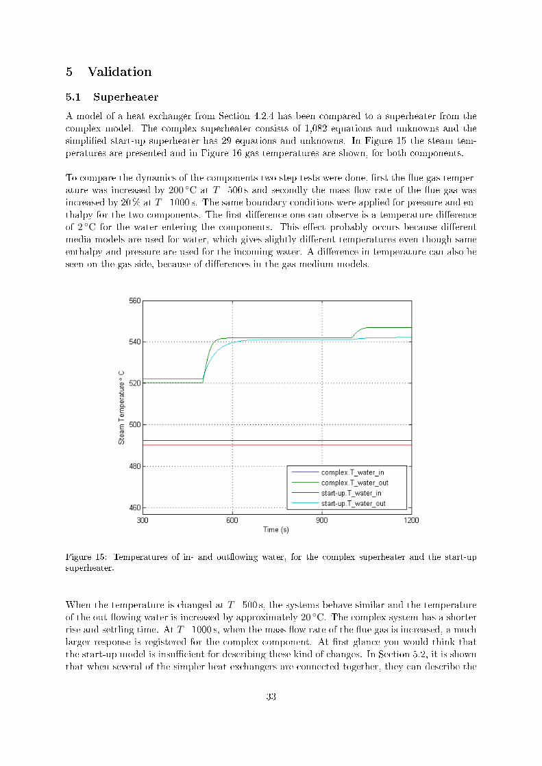
A model of a heat exchanger from Section 4.2.4 has been compared to a superheater from thecomplex model. The complex superheater consists of 1,082 equations and unknowns and thesimpli�ed start-up superheater has 29 equations and unknowns. In Figure 15 the steam tem-peratures are presented and in Figure 16 gas temperatures are shown, for both components.

To compare the dynamics of the components two step tests were done, �rst the �ue gas temper-ature was increased by 200 ◦C at T=500 s and secondly the mass �ow rate of the �ue gas wasincreased by 20% at T=1000 s. The same boundary conditions were applied for pressure and en-thalpy for the two components. The �rst di�erence one can observe is a temperature di�erenceof 2 ◦C for the water entering the components. This e�ect probably occurs because di�erentmedia models are used for water, which gives slightly di�erent temperatures even though sameenthalpy and pressure are used for the incoming water. A di�erence in temperature can also beseen on the gas side, because of di�erences in the gas medium models.

Figure 15: Temperatures of in- and out�owing water, for the complex superheater and the start-upsuperheater.

When the temperature is changed at T=500 s, the systems behave similar and the temperatureof the out-�owing water is increased by approximately 20 ◦C. The complex system has a shorterrise and settling time. At T=1000 s, when the mass �ow rate of the �ue gas is increased, a muchlarger response is registered for the complex component. At �rst glance you would think thatthe start-up model is insu�cient for describing these kind of changes. In Section 5.2, it is shownthat when several of the simpler heat exchangers are connected together, they can describe the

33

Figure 16: Temperatures of in- and out�owing �ue gas, for the complex superheater and the start-upsuperheater. The temperature curves for in�owing �ue gas are equal for both superheaters.

complex model owned by Vattenfall quite well. In the complex model the steam temperatureis reduced by using spray water. It shows that the start-up model, without spray water, is asu�cient description of the large model, including spray water.

It was possible to change parameters in the start-up model, so that a higher response was re-ceived when the mass �ow rate changed, but then the start-up model could not be used todescribe the real plant. Some explanations for the deviations between models include di�erentmedia and material models and that the wall in the complicated model is discretized.

5.2 Start-up model

To validate the complete start-up model, a steady-state simulation for the full load case wasdone and compared with reference data from the plant and the result is shown in Table 5. Datafrom the actual plant have been used to represent the boundary conditions for pressure and mass�ow rate. Boundary conditions for enthalpy have been picked from a steady-state simulation ofthe detailed model.

The overall performance of the model is considered good, since the relative errors are small,which can be seen in Table 5. The large di�erence for the component SHS, is probably becausethermal radiation is neglected.

In Figure 17, the steam temperatures from Table 5 are shown, together with the steady-state

34

Table 5: Steam temperatures out of each heat exchanger component at a steady-state simulation withfull load.

Heat exchangers SHS SH1 SH2 SH3 SH4 RH1 RH2

Reference ◦C 373 406 451 492 534 481 540Start-up model ◦C 359 413 452 496 536 483 544Absolute error -14 7 1 4 2 2 4Relative error -3.8 % 1.7 % 0.22 % 0.81 % 0.37 % 0.41 % 0.74 %

Figure 17: Comparison between reference data, complex simulation model and start-up model at steady-state with full load.

temperatures from a full load simulation of the complex model. The conclusion is that the boilerof the power plant can be fairly well represented by the start-up model. There exists some devia-tions in steam temperatures for both the complex model and the start-up model, but both modelscan be used to simulate the behaviour of the real process. The start-up model consists of 457unknowns and equations and is therefore possible to use for optimization purposes in JModelica.

In [Saarinen, Boman & Funkquist, 2011] ramp tests were done to compare the complex simula-tion model of Jänschwalde with measurement data from the plant, see Figure 18. The systemswere ramped from 100% load to 60% load during 19 minutes. The system was given time tostabilize at 60% load and then ramped up again to full load during 20min. In Figure 19 thesame ramps were applied to the start-up model, to ramp up and down the coal �ow. The feed-water �ow rate was also ramped to replicate the real experiment.

When looking at the system responses for the complex model and the start-up model, it showsthat both systems respond immediately to load changes, when live steam temperatures are eval-

35

Figure 18: Comparison of the complex simulation model of Jänschwalde (dotted lines) and measurementdata (solid lines) from the actual plant, when the system was ramped from 100% load to 60% and backagain to 100% load.

uated. The measurement data shows that the real system has a time delay of approximately20min when the system is ramped down. However the response is not as slow for the real sys-tem, when the load is ramped up again. If the delay is neglected all three systems have aboutthe same rise time. The settling time can not be evaluated for the real system, since the steamtemperatures �uctuate because of disturbances in the real plant.

For all systems the steam temperatures in SH1, SH2, SH3 and SH4 decreases when the loadis ramped down. For SHS the steam temperature increases for the start-up model, while it isapproximately constant in Figure 18. When the load is ramped up, the complex model hasan overshoot that is larger compared to the start-up model and the measurement data. Thesuperheater component also had a very large step response compared to the start-up model,when the mass �ow rate was changed in Section 5.1. It is therefore possible that the response istoo high for the superheater components, which causes some of the overshoot seen in Figure 17.

36

Figure 19: Simulation of the start-up model when the system was ramped from 100% load to 60% andback again to 100% load. The start-up model is not a�ected by disturbances, compared to the systemsshown in Figure 18.

37

6 Optimization

6.1 Problem speci�cations

The optimization problem is de�ned by an objective function, constraints and an optimizationinterval. The objective function ϕ is de�ned by a quadratic cost function, which is minimizedover an optimization interval. Since ϕ should be minimized, deviations between the live steamtemperature TSH4 and the reference value Tref are penalized. Changes in the control variabledudt are also penalized, since it is desirable to reach steady-state (dudt = 0) quickly. The objectivefunction is de�ned as

ϕ =

∫ tf

t0

(α(TSH4 − Tref )2 + β

(du

dt

)2)dt, (20)

with α ≥ 0, β ≥ 0. The constraints are given by the stress levels in the header and the separator

σmin,header ≤ σheader ≤ σmax,header, (21)

σmin,separator ≤ σseparator ≤ σmax,separator. (22)

Calculations of σheader and σseparator are done in the Dymola model shown in Figure 14. If onehas de�ned minimum and maximum attributes for the variables in the Dymola model, theseattributes will also be used as constraints in the optimization in JModelica.

The objective function

ϕ =

∫ tf

t0

dt, (23)

was also considered for the optimization problem, with the constraints de�ned by (21) and (22).The objective function (23) actually minimizes the �nal time tf , while (20) minimizes deviationsfrom the steady-state values and changes in the control signal over the interval. However, it wasnot possible to get the IPOPT solver to converge with the objective function in (23).

6.2 Optimization options

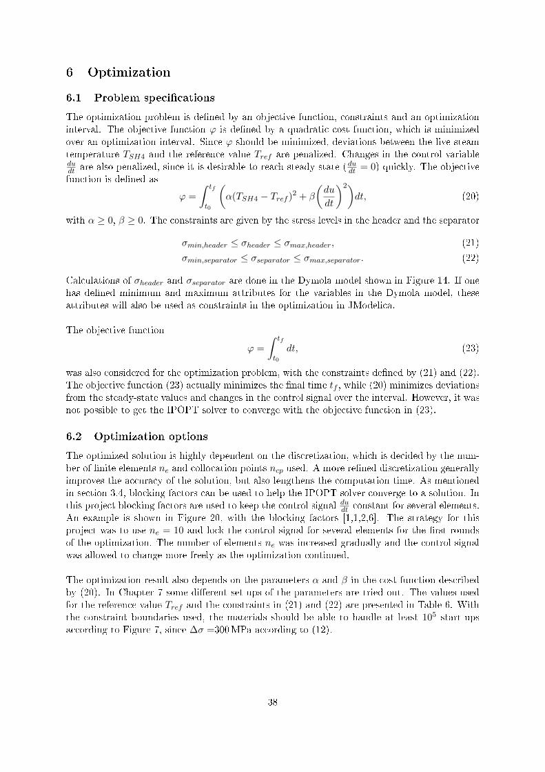
The optimized solution is highly dependent on the discretization, which is decided by the num-ber of �nite elements ne and collocation points ncp used. A more re�ned discretization generallyimproves the accuracy of the solution, but also lengthens the computation time. As mentionedin section 3.4, blocking factors can be used to help the IPOPT solver converge to a solution. Inthis project blocking factors are used to keep the control signal dudt constant for several elements.An example is shown in Figure 20, with the blocking factors [1,1,2,6]. The strategy for thisproject was to use ne = 10 and lock the control signal for several elements for the �rst roundsof the optimization. The number of elements ne was increased gradually and the control signalwas allowed to change more freely as the optimization continued.

The optimization result also depends on the parameters α and β in the cost function describedby (20). In Chapter 7 some di�erent set-ups of the parameters are tried out. The values usedfor the reference value Tref and the constraints in (21) and (22) are presented in Table 6. Withthe constraint boundaries used, the materials should be able to handle at least 105 start-upsaccording to Figure 7, since ∆σ =300MPa according to (12).

38

Figure 20: Plot of coal �ow u and the control signal dudt , with blocking factors [1, 1, 2, 6].

Table 6: Speci�cation of values used for Tref and constraints.

Parameter Value

Tref 806Kσmin,header -200MPaσmax,header 400MPaσmin,separator 800MPaσmax,separator 1400MPa

6.3 Initialization

It was very hard for the IPOPT solver to converge to a solution, without using an initial trajec-tory as a start-guess. To solve this problem, a simulation of the model was done with constantload. It is important that the initial guess is within the constraints de�ned by the optimizationproblem, so that is why a steady-state simulation was used. The �nal values of the state-variableswere used as initial values for the optimization problem. In this way, some of the large transientsthat occur during the initialization phase can be avoided.

The input trajectory from the simulation problem was used as a starting guess. It is easier forthe optimization algorithm to converge to a solution, if the starting guess is close to the optimalsolution. That is why numerical optimization techniques often consist of an iterative process.Generally it is easier to start with a very rough discretization. If an optimal solution is found,it can be used to initiate the same optimization problem, with a re�ned discretization.

39

7 Results

Variations of weight parameters in cost function

The �rst step was to investigate how di�erent values of α and β in the objective function (20)a�ected the outcome of the optimization. The blocking factors were set to [1,1,2,6] and thenthe parameters α and β were varied for the di�erent problem set-ups. For the 6 experiments,the same optimization and IPOPT options were used: ne = 10, ncp = 3, max_iter = 300 andtol = 5e− 4.

Table 7: Summary of parameter values used for di�erent problem set-ups.

Experiment α β Final value of TSH4 ≈ Tref Number of iterations

1 10−2 10−1 N/A N/A2 10−2 4× 10−2 Yes 393 10−2 10−2 Yes 414 1.6× 10−3 10−2 No 405 2.5× 10−3 10−2 No 346 4× 10−4 10−2 No 407 10−4 10−2 No 36

When the parameter settings for Experiment 1 was used from Table 7, the maximum numberof iterations was reached by the IPOPT solver, so the optimization algorithm was terminatedunsuccessfully. The IPOPT solver managed to converge to a solution for the other experimentset-ups and the number of iterations needed was between 36 and 41. The total computationtime for those cases was between 84 and 98 seconds.

The result for Experiment 3 is shown in Figure 21. The steady-state value for the steam tem-perature in SH4 (Tref ) was reached at T ≈ 800 s. The stress amplitude for the header was ≈150MPa, while the stress amplitude was very small for the separator. The maximum coal �owwas very high, 43% over the steady-state value at T =200 s.

In Figure 22 the optimization result is shown for Experiment 6 in Table 7. The steady-statevalue Tref for the temperature is not reached during the optimization interval of 2000 s. Thestress amplitudes are smaller, since the steam temperature increases at a smaller pace.

An interesting result was obtained for Experiment 5. The IPOPT solver converged to a solu-tion, with very high temperature levels, which are shown in Figure 23. The �nal temperatureof the steam exiting superheater SH4, is 234K over the reference temperature Tref . The stressamplitude for the header is ≈ 170MPa for this case.

40

Figure 21: Initial optimization with blocking factors [1,1,2,6]. The weight parameters in (20) are chosen asα = 0.01, β = 0.01. The steady-state value Tref is reached for the live steam exiting the last superheaterSH4.

Figure 22: Initial optimization with blocking factors [1,1,2,6]. The weight parameters in (20) are chosenas α = 0.0004, β = 0.01. The steady-state value for Tref is not reached during 2000 seconds.

41

Figure 23: Initial optimization with blocking factors [1,1,2,6]. The weight parameters in (20) are chosenas α = 0.0025, β = 0.01. The �nal value of the steam temperature in SH4 is 1040K.

Variations in blocking factors

The next step was to try di�erent blocking factors to see how the optimization outcome wasa�ected. The parameter settings α = 10−2, β = 4 × 10−2,ncp = 3, max_iter = 100 andtol = 5e − 4 were used for all experiment set-ups in Table 8. First an initial optimization wasdone with blocking factors [1, 1, 2, 6], then di�erent blocking factors were tried out according toTable 8.

Di�erent tactics were used to design the blocking factors. If the blocking factors were uniformlydistributed, the optimization algorithm generally converged. An example can be seen in Figure24 with blocking factors [2, 2, 2, 2, 2, 2, 2, 2] and ne = 16. The stress amplitude reaches 135MPa.There are some oscillations in the system, so therefore another approach was tried where thecontrol signal was locked for several elements at the end of the interval. In Figure 25, the op-timization outcome is shown when the blocking factors [2, 2, 2, 2, 2, 2, 6] were used. The controlsignal is slightly positive for the last six elements, which results in an inclining coal �ow. Thestress amplitude is approximately 210MPa, which is higher compared to when the blocking fac-tors [2, 2, 2, 2, 2, 2, 2, 2] were used.

The stress level is highly dependent on the blocking factors used and to illustrate this, twocases are compared. In Figure 26 the result of the optimization is shown for blocking factors[1, 1, 1, 1, 1, 5] and ne = 10. The system stabilize fast, but the stress amplitude is high ≈200MPa. For the result in Figure 27, the blocking factors [5, 1, 1, 1, 1, 1] and ne = 10 are used.The system is slow, but the stress amplitude is much lower ≈ 125MPa.

42

Table 8: Summary of blocking factors used for di�erent problem set-ups.

Experiment Blocking factors ne Iterations

1 [1, 1, 1, 1, 1] 5 292 [2, 2, 2, 2, 2] 10 193 [1, 1, 1, 1, 1, 5] 10 114 [5, 1, 1, 1, 1, 1] 10 585 [1, 1, 1, 1, 1, 1, 1, 1, 1, 1] 10 N/A6 [2, 2, 2, 2, 2, 2] 12 157 [1, 1, 2, 2, 6] 12 118 [2, 2, 2, 2, 6] 14 749 [2, 2, 2, 2, 2, 2, 2] 14 1310 [1, 1, 2, 2, 2, 6] 14 N/A11 [2, 2, 2, 2, 2, 2, 2, 2] 16 912 [2, 2, 2, 2, 2, 6] 16 913 [1, 2, 2, 2, 9] 16 N/A14 [1, 1, 2, 2, 3, 3, 4] 16 N/A15 [2, 2, 2, 2, 2, 2, 2, 2, 2] 18 N/A16 [2, 4, 4, 4] 18 N/A

Figure 24: Optimization with uniformly distributed blocking factors [2, 2, 2, 2, 2, 2, 2, 2] and ne = 16. Thestress amplitude is approximately 135MPa.

43

Figure 25: Optimization with a high blocking factor at the end of the interval [2, 2, 2, 2, 2, 2, 6] andne = 16. The stress amplitude is approximately 210MPa.

Figure 26: Optimization with blocking factors [1, 1, 1, 1, 1, 5] and ne = 10. The stress amplitude isapproximately 200MPa.

44

Figure 27: Optimization with blocking factors [5, 1, 1, 1, 1, 1] and ne = 10. The stress amplitude isapproximately 125MPa.

45

8 Discussion and Conclusions

8.1 Modelling

Sources of error and further developments

The start-up model developed in this project is su�cient for describing some start-up scenariosat the Jänschwalde power plant, but of course many improvements can be made. To betterdescribe the real process, the model should include time delays so that a change in coal �ow,does not a�ect the steam temperatures in the whole system immediately. Introducing delayswill probably cause problems in the optimization phase, so it is important to carefully considerhow delays should be implemented in a good way.

A more detailed model of the separator, where some of the feedwater is recirculated back tothe evaporator was developed. The separator could be used for some steady-state simulations,but problems often occurred when boundary conditions were varied. To include the detailedseparator, one has to use level control to stabilize the ratio between vaporized and liquid waterin the separator. To recirculate the water back to the evaporator, one needs to introduce a pumpto get an accurate pressure level. Otherwise the circulated water has a lower pressure then thewater within the evaporator, which makes the water �ow in the wrong direction.

Another improvement would be to develop media models for coal and �ue gas, so the user canvary the composition of substances in each medium. Media models can also be used to describethe non-linear relationship between temperature and �ue gas more accurately. It would be goodto develop a material model for the metal components in the walls, which would make it possibleto have material properties that depend on the metal temperature.

For the model of the heat exchanger, the next step would be to include an option that allowsthermal radiation. In that way the steam temperature of the heat exchanger SHS can beincreased, since these components are exposed to a large fraction of the thermal radiation. It isalso possible to discretize the heat exchanger component to more accurately describe the processof heat transfer. However, it is not recommended to use a discretized model for the optimizationphase since it requires much more computational time.

Limitations

The largest limitation in the start-up model is that it contains many boundary conditions. If onewants to consider another start-up scenario, there are many parameters that must be changedmanually. It is also troublesome to simulate the complete start-up scenario, since it requireschanges in the boundary conditions, for example that the enthalpy and pressure of the incomingfeedwater is increased. An attempt was done to replace the boundary components between thelast superheater and the �rst reaheater in the steam cycle with a turbine model, in Figure 14.However, it was hard to get accurate steady-state values for the steam pressure since the steampressure in and out of the component were allowed to vary freely.

It has not been possible to validate the model for the �rst phase of the start-up. Start-up datafrom the plant was requested, but heavily delayed. However, old measurement data could beused to validate the model in the steady-state region. The old data was ordered to validatethe complex model of Jänschwalde, so that is why only steady-state reference data has been ofinterest previously.

46

8.2 Optimization

Optimization Result

The results from the optimization part of the project, showed how much the optimization out-come depended on the variable settings used. It was not surprising how the optimized solutionchanged when the weight parameters α and β were varied. If a very small value of α was used,the problem did not reach the steady-state temperatures for full load. The best case scenariowould have been if the objective function

∫ tft0dt could have been used instead. It actually mini-

mizes the �nal time, instead of the deviations from the full load steady-state case over time, soone does not need to consider weight parameters.

The blocking factors had a large impact on the solution and the ideal case would be if the NLPproblem could converge without using blocking factors. It was easier to �nd blocking factors thatmade the optimization problem converge, when smaller values of ne was used. For ne = 18, theoptimization problem could not be initialized because of problem with memory. The numberof iterations varied for the di�erent experiments. It can not be concluded that a �ner dis-cretization requires more iterations. There are no general methods for choosing blocking factors.It can be a very time demanding trial and error process, which is unique for each problem set-up.

The maximum value of the stress amplitude obtained from the experiments was ∆σ = 210MPafor the header. It corresponds to over 106 load cycles, according to Figure 7. The variablebounds used for header and separator stress, was not reached during any of the optimizationoutcomes presented in Chapter 7. However, experiments were done with much harder constraintson stress levels. The constraints made it very hard for the optimization algorithm to converge toa solution. In [Krüger, Franke & Rode, 2004], stress constraints were used, but the optimizationproblem was solved with Matlab. In [Lind & Sällberg, 2012] the JModelica.org platform wasused to solve the optimization problem, but with temperature constraints instead. It should bepossible to solve the optimization problem with stress constraints, but it might be easier if oneused temperature constraints instead. The stress level for the separator varied very little, for thedi�erent problem set-ups in Chapter 7. This is mainly because a constant boundary conditionwas used for the enthalpy of the incoming feedwater. The separator is close to the water source,so it was not subject to high temperature changes. Since the future goal of the start-up modelis to include the complete start-up procedure, the separator was kept, even though it didn'timpose any constraints on the current optimization problem.

Further work

This thesis project has shown that it is possible to optimize the start-up procedure of a coal-�redpower plant, but more work is needed before the result can be applied to the real plant. Oneneeds to include the whole start-up scenario, so that correct stress levels from the Wöhler dia-gram in Figure 7 can be used. Secondly, one needs to investigate conditions from the real plantthat impose constraints on variables, for example how fast the coal �ow can change. The largestproblem during the optimization phase of this project, was to �nd settings where the optimiza-tion algorithm converged to a solution. Other important factors that a�ect the outcome arethe model set-up, start-values, scaling of variables, the optimization interval and constraints, tomention a few. Further work includes trimming the nominal values in the media model packageWater_poly, since they a�ect the scaling of the optimization problem. About 15 di�erent unitsare used in the start-up model, so there are many di�erent set-ups that can be explored in orderto improve the scaling.

47

The discretization is another area that can be further developed. The main focus would be totry many di�erent sets of blocking factors and compare the result. In this project a Pythonfunction was developed, that iterated through di�erent blocking factors. Unfortunately, thefunction was unexpectedly interrupted several times because of errors during the compilationphase or problems with memory for the IPOPT solver. Since the JModelica.org platform is underdevelopment, these bugs will hopefully be �xed in the near future. The optimization could alsobe tried on a computer suited to handle large numerical calculations. Since it would require lesscomputational time, one could also try to increase the maximum number of iterations used.

Experience with JModelica

The JModelica.org platform is a powerful tool, especially when you want to optimize dynamicmodels. The programs are however not very user-friendly at the moment, especially for userswith little experience of programming in Python. It would be good if a future version of theJModelica.org platform contained a graphical interface. It is also a bit tedious that you needthree di�erent �le types (.mo, .mop, .py) to run optimization problems. It would be easier if theenvironments for modelling, optimization and execution of algorithm could be better integrated.

Another suggestion is to develop a Modelica library, with models, functions and media modelsthat can be used in the JModelica.org environment. In this project, the trial and error methodhave been used to see if some components can be used for optimization. The problems that haveoccurred, have often been during the compilation phase. It has been hard to decode many ofthe error messages, so a better documentation of the algorithms would be good as well.

Conclusions

The most important lesson learned is to not make models more complicated then they have tobe, especially when you want to use them for dynamic optimization. When new add-ons areintroduced, it is good to evaluate how the model accuracy and the simulation time are a�ected.The system performance must be evaluated regularly and not only at the end of the project.

The optimization phase of the project was tricky and very time-demanding. More time mustbe spent on the model and the optimization parameters, before the results can be applied tothe real plant. If all the suggested improvements are implemented on the start-up model, it willmost likely be very hard to optimize in the JModelica.org environment. A recommendation isto use two models, one for optimization and another for simulation. The optimization modelshould be kept very simple, but include the whole start-up scenario. The optimization resultcould then be used together with a more complicated simulation model, to get a more accuratedescription of the start-up scenario.

48

References

[Alvarez, 2006] Alvarez H. (2006). Energiteknik del 1 Studenlitteratur AB, Lund.

[Biegler, Cervantes & Wächter, 2002] Biegler, L., Cervantes, A. and Wächter, A. (2002). Ad-vances in simultaneous strategies for dynamic process optimization Chemical EngineeringScience Volume 57, Issue 4, February 2002, pp. 575�593.

[Casella, Donida & Åkesson, 2011] Casella, F., Donida, F. and Åkesson, J. (2011). Object-Oriented Modeling and Optimal Control: A Case Study in Power Plant Start-Up In: 18thIFAC World Congress, pp. 7043-7048. Milano, Italy, 2011.

[Casella et al.,2011] Casella, F., Farina, M., Righetti, F., Scattolini, R., Faille, D., Davelaar, F.,Tica, A., Gueguen, H. and Dumur, D. (2011). An optimization procedure of the start-up ofCombined Cycle Power Plants In: 18th IFAC World Congress, pp. 7043-7048. Milano, Italy,2011.

[Edsberg, 2008] Edsberg L. (2008). An Introduction to Computation and Modeling for Di�er-ential Equations John Wiley and Sons, Inc, Hobokem, New Jersey.

[Franke, Rode & Krüger, 2003] Franke, R., Rode, M. and Krüger, K. (2003). On-line Opti-mization of Drum Boiler Startup In: 3rd International Modelica Conference, pp. 287-296.Linköping, Sweden, 2003.

[Franke et al., 2009] Franke, R., Casella, F., Otter, M., Sielemann, M., Elmqvist, H., Mattson,S and Olsson, H. (2009). Stream Connectors - An Extenstion of Modelica for Device-OrientedModeling of Convective Transport Phenomena In: Proceedings 7th International ModelicaConference, pp. 108-121. Como, Italy, 2009.

[IPOPT,2013] IPOPT (2013). IPOPT Documentation - Computational Infrastructure for Op-erations Research <http://www.coin-or.org/Ipopt/documentation>[Accessed 2013-05-22].

[Krüger, Franke & Rode, 2004] Krüger, K., Franke, R. and Rode, M. (2004). Optimization ofboiler start-up using a nonlinear boiler model and hard constraints Energy, 29:2239�2251.

[Ignou,2013] Study Material, IGNOU School of Engineering & Technology (2013). Introductionto Power Plants <http://www.ignou.ac.in/upload/Unit-1-58.pdf>, [Accessed 2013-05-15].

[JModelica.org,2013] JModelica.org (2013). JModelica.org. <http://jmodelica.org>[Accessed2013-05-02].

[Lind & Sällberg, 2012] Lind, A. and Sällberg, E. (2012). Optimization of the Start-up Procedureof a Combined Cycle Power Plant Department of Automatic Control, Lund University.

[Ljung & Glad, 2004] Ljung, L. and Glad, T. (2004). Modellbygge och simulering Studenlitter-atur AB, Lund.

[MathWorks,2013] MathWorks (2013). Simulink - Simulation and Model-Based Design.<http://www.mathworks.se/products/simulink> [Accessed 2013-05-22].

[Meinke, 2012] Meinke, S. (2012). Modellierung thermischer Kraftwerke vor dem Hintergrundsteigender Dynamikanforderungen aufgrund zunehmender Windenergie- und Photovoltaikein-speisung. Lehrstuhl für Technische Thermodynamik, Universität Rostock.

49

[Modelica.org,2013] Modelica.org (2013). Modelica and the Modelica Association .<https://www.modelica.org>[Accessed 2013-05-13].

[Modelon AB,2012] Modelon AB (2012). JModelica.org User Guide, Version 1.8.<http://www.jmodelica.org/api-docs/usersguide/JModelicaUsersGuide-1.8.1.pdf> [Ac-cessed 2013-05-15].

[Saarinen, Boman & Funkquist, 2011] Saarinen, L., Boman, K. and Funkquist J. (2011). Dy-namic Model of a Boiler at the Jänschwalde plant Vattenfall Research and Development,2011. U 11:77.

[Stodola, 1945] Stodola, A. (1945). Steam and Gas Turbine, vol. 1 Peter Smith, New York.

[Vattenfall,2012] Vattenfall AB (2012). Jänschwalde | Vattenfall's Power Plants.<http://powerplants.vattenfall.com/node/288> [Accessed 2013-02-13].

[Wächter, 2002] Wächter, A. (2002). An Interior Point Algorithm for Large-Scale Nonlinear Op-timization with Applications in Process Engineering PhD thesis, Carnegie Mellon University,Pittsburgh, PA, USA.

[Wächter & Biegler, 2006] Wächter, A and Biegler, L. (2006). On the implementation of aninterior-point �lter line-search algorithm for large-scale nonlinear programming Mathemati-cal Programming, Ser. A 106, 25�57.

[Åkesson, 2008] Åkesson, J. (2008). Optimica - An Extension of Modelica Supporting DynamicOptimization In 6th International Modelica Conference 2008. Modelica Association, March2008.

[Åkesson, Gäfvert & Tummescheit 2009] Åkesson, J. (2009). JModelica - an Open Source Plat-form for Optimization of Modelica Models In 6th Vienna International Conference on Math-ematical Modelling. Vienna, Austria, 2009.

50

A Description of components

Component name Comment Figure

CombustorDescribes relationship between coal �ow and �uegas

Integrator From the Modelica Standard Library

MassFlowBoundary_gas Gas source

MassFlowBoundary_steam Steam source

PressureBoundary_steam Steam sink

PressureBoundary_gas Gas sink

RealInput From the Modelica Standard Library

RealOutput From the Modelica Standard Library

Reheater Heat exchanger used to describe reheaters

Superheater Heat exchanger used to describe superheaters

Turbine Turbine model

VolumeUsed to calculate stress levels together with theWall component

Valve_LinearA component used to describe pressure drop forwater

WallUsed to calculate stress levels together with theVolume component

WallBoundaryA boundary condition which describes heat lossto the surroundings

51