development of a fast aerodynamic tool using meta … total drag calculated by mses for a...

Development of afast aerodynamic tool usingmeta-modeling techniques

R. Veldhuizen

Tech

nisc

heUn

iver

siteit

Delf

t

DEVELOPMENT OF A FAST AERODYNAMICTOOL USING META-MODELING TECHNIQUES

by

R. Veldhuizen

in partial fulfillment of the requirements for the degree of

Master of Sciencein Aerospace Engineering

at the Delft University of Technology,to be defended publicly on Friday April 17th, 2015 at 13:00.

Thesis Registration Number: 025#15#MT#FPP

Student number: 1369202Supervisor: Dr. ir. R. VosThesis committee: Prof. dr. ir. L. L. M. Veldhuis, TU Delft

Dr. ir. F. F. J. Schrijer, TU DelftDr. Ing. M. Weismüller Airbus Operations GmbH

An electronic version of this thesis is available at http://repository.tudelft.nl/.

http://repository.tudelft.nl/

SUMMARY

There is a need for a wave drag method that combines the speed of handbook methods with the accuracyof computational methods. Especially determining the onset of wave drag as well as the initial drag rise isimportant in initial design stages. Meta-models allow this by capturing the trends present in previously com-puted data, providing an accurate and fast representation. In this report, it is investigated what gains can beachieved by applying the meta-modeling method GT-Approx to the aerodynamic tool MSES.The total drag calculated by MSES for a supercritical airfoil was verified using wind tunnel experiments. Itwas found that aerodynamic characteristics and pressure distributions are accurate up until M = 0.76.

GT-Approx was critically evaluated to determine what accuracies are attainable, and how the resolution ofthe input data influences these accuracies. Initially the fitting capabilities of GT-Approx are tested. With amaximum error of 0.11% the fit is accurate. The errors increase when GT-Approx is used to predict values fordata points that are not present in the data set. Especially in the case of extrapolation, the errors grow expo-nentially. If GT-Approx is used to predict values in between data-points, thus performing an interpolation,the results are better, with average errors of 2 drag counts. However, when predicting difficult regions, such asthe drag coefficient near the drag rise, the errors increase. The prediction errors for high M are large, reaching6.1 drag counts for cdw and 5.9 drag counts for cdv .In an effort to reduce these errors, the influences of resolution increases are investigated. Upon increasingthe resolutions, the errors decrease. Especially increasing the M-resolution and cl -resolution yields large im-provements. The average error for the higher Mach numbers reduces from 6.0 drag counts to 2.0 drag countsif the resolution is quadrupled. The average errors also reduce significantly, as shown in Table 1.

Initial Final

Variable Resolution ∆cdv [×10−4] ∆cdw [×10−4] Resolution ∆cdv [×10−4] ∆cdw [×10−4]

Re 20.0 ×106 1.85 0.38 5.00×106 1.63 0.20

cl 0.1 1.73 1.00 0.025 1.33 0.42

M 0.1 3.15 3.05 0.025 1.27 0.40tc 0.02 2.36 0.69 0.01 2.33 0.51

Table 1: Overview of initial and final resolutions and their accuracy.

Two A320 variants are evaluated using GT-Approx and a direct application of MSES. The performance of GT-Approx is good. An average difference of 0.21 drag counts between MSES and GT-Approx was achieved, withan in-calculation computation time of 5.13×10−4 s per calculation instead of 5.58 s using a direct applicationof MSES.GT-Approx is extended to a quasi-3D method, using the simple sweep method. This quasi-3D method is usedto calculate the value of CDw for two test cases. The calculated values of CDw are compared with CFD data.It was found that the region of validity of the quasi-3D method is highly limited. Up until 60% of the wing,root and tip effects, fuselage effects and engine installation effects render any comparison useless. Beyondthis value the first test case showed no correlation, whereas the second showed reasonable accuracy. Due tolack of more 3D CFD data, no clear explanation for the difference was found.In general it is concluded that the combination of an aerodynamic tool with a meta-model is able to combinelow computation times with high accuracy, but only if the aerodynamic model is accurate.

iii

ACKNOWLEDGMENTS

This report is part of a Master Thesis, performed as a part of the Master Flight Performance and Propulsion atthe Faculty of Aerospace Engineering of the Delft University of Technology. This Master Thesis was performedat the Non-Specific Design Skills - Weights and Aerodynamics department of the Future Projects Office at Air-bus Operations GmbH.

First of all, I would like to thank everybody at Airbus. Specifically Michael Weismüller, for making it possiblefor me to perform my Master Thesis within Airbus and being my daily supervisor. I would like to thank himfor providing excellent advice and clear guidance, for providing me with the necessary information and dataand all the help given. Thanks to Martin Schimmöller and all my other colleagues of EIXDS for accepting meinto the team, and providing a helpful and constructive working environment.I would also like to thank Bruno Moorthamers and Ali Cabac for helping me find the right contacts withinAirbus, leading to this thesis.

I would also like to express my gratitude towards Roelof Vos, my supervisor at the TU Delft. He has proveninvaluable. Without his critical remarks, thought provoking questions, useful suggestions and meticulousreading this thesis would not be the same.Furthermore I would like to thank Ferry Schrijer and Leo Veldhuis for completing my graduation committee.

Finally I would like to thank all my friends in Delft, Tianjin, Hamburg and all other places around the worldfor making my study time an enjoyable one.Lastly I would like to thank my family for supporting me during my studies.

Roy VeldhuizenDelft, April 7, 2015

v

CONTENTS

Summary iii

Acknowledgments v

List of Figures ix

List of Tables xi

1 Introduction 1

2 Wave drag estimation methods 32.1 Current wave drag estimation method at Airbus . . . . . . . . . . . . . . . . . . . . . . . . . 32.2 Computational Methods . . . . . . . . . . . . . . . . . . . . . . . . . . . . . . . . . . . . . 42.3 Performance Comparison. . . . . . . . . . . . . . . . . . . . . . . . . . . . . . . . . . . . . 6

3 Meta-modeling method selection 93.1 Meta-modeling concept . . . . . . . . . . . . . . . . . . . . . . . . . . . . . . . . . . . . . 93.2 Wave drag application . . . . . . . . . . . . . . . . . . . . . . . . . . . . . . . . . . . . . . 103.3 Airbus in-house meta-modeling: GT-Approx . . . . . . . . . . . . . . . . . . . . . . . . . . . 10

4 Meta-modeling method validation 134.1 Outlier detection . . . . . . . . . . . . . . . . . . . . . . . . . . . . . . . . . . . . . . . . . 134.2 Fitting Capabilities of GT-Approx . . . . . . . . . . . . . . . . . . . . . . . . . . . . . . . . . 144.3 Predictive Capabilities of GT-Approx . . . . . . . . . . . . . . . . . . . . . . . . . . . . . . . 14

4.3.1 Method . . . . . . . . . . . . . . . . . . . . . . . . . . . . . . . . . . . . . . . . . . 144.3.2 Prediction of drag as a function of Re values . . . . . . . . . . . . . . . . . . . . . . . . 154.3.3 Prediction of drag as a function of t

c values . . . . . . . . . . . . . . . . . . . . . . . . 164.3.4 Prediction of drag as a function of M values . . . . . . . . . . . . . . . . . . . . . . . . 164.3.5 Prediction of drag as a function cl values. . . . . . . . . . . . . . . . . . . . . . . . . . 17

4.4 GT-Approx computation times . . . . . . . . . . . . . . . . . . . . . . . . . . . . . . . . . . 184.5 Conclusion concerning GT-Approx abilities . . . . . . . . . . . . . . . . . . . . . . . . . . . . 18

5 Meta modeling resolution sensitivities 195.1 Method . . . . . . . . . . . . . . . . . . . . . . . . . . . . . . . . . . . . . . . . . . . . . . 195.2 Resolution increases . . . . . . . . . . . . . . . . . . . . . . . . . . . . . . . . . . . . . . . 20

5.2.1 Mach resolution . . . . . . . . . . . . . . . . . . . . . . . . . . . . . . . . . . . . . . 205.2.2 Thickness resolution . . . . . . . . . . . . . . . . . . . . . . . . . . . . . . . . . . . . 225.2.3 cl resolution . . . . . . . . . . . . . . . . . . . . . . . . . . . . . . . . . . . . . . . . 235.2.4 Reynolds number resolution . . . . . . . . . . . . . . . . . . . . . . . . . . . . . . . . 245.2.5 Final resolutions . . . . . . . . . . . . . . . . . . . . . . . . . . . . . . . . . . . . . . 26

5.3 Targeted Resolution increases. . . . . . . . . . . . . . . . . . . . . . . . . . . . . . . . . . . 285.4 Final Resolutions . . . . . . . . . . . . . . . . . . . . . . . . . . . . . . . . . . . . . . . . . 29

6 3D method extension 316.1 Region of Validity . . . . . . . . . . . . . . . . . . . . . . . . . . . . . . . . . . . . . . . . . 316.2 3D method implementation . . . . . . . . . . . . . . . . . . . . . . . . . . . . . . . . . . . 32

6.2.1 Airfoil Geometry . . . . . . . . . . . . . . . . . . . . . . . . . . . . . . . . . . . . . . 336.2.2 Effective Mach number . . . . . . . . . . . . . . . . . . . . . . . . . . . . . . . . . . 346.2.3 Effective Reynolds number. . . . . . . . . . . . . . . . . . . . . . . . . . . . . . . . . 346.2.4 cl input . . . . . . . . . . . . . . . . . . . . . . . . . . . . . . . . . . . . . . . . . . 346.2.5 CDw determination . . . . . . . . . . . . . . . . . . . . . . . . . . . . . . . . . . . . 35

vii

viii CONTENTS

6.3 Test case: comparison between MSES and GT-Approx . . . . . . . . . . . . . . . . . . . . . . 356.4 Test case: comparison between GT-Approx and CFD . . . . . . . . . . . . . . . . . . . . . . . 38

6.4.1 A320 . . . . . . . . . . . . . . . . . . . . . . . . . . . . . . . . . . . . . . . . . . . . 386.4.2 A320-PL7A . . . . . . . . . . . . . . . . . . . . . . . . . . . . . . . . . . . . . . . . . 39

7 Conclusion and recommendations 417.1 Conclusion . . . . . . . . . . . . . . . . . . . . . . . . . . . . . . . . . . . . . . . . . . . . 417.2 Recommendations . . . . . . . . . . . . . . . . . . . . . . . . . . . . . . . . . . . . . . . . 41

Bibliography 43

A Python Code 47A.1 Test case implementation . . . . . . . . . . . . . . . . . . . . . . . . . . . . . . . . . . . . . 47

A.1.1 MSES implementation . . . . . . . . . . . . . . . . . . . . . . . . . . . . . . . . . . . 53A.1.2 VGK implementation . . . . . . . . . . . . . . . . . . . . . . . . . . . . . . . . . . . 56

A.2 Meta-modeling method validation implementation . . . . . . . . . . . . . . . . . . . . . . . 63A.3 Meta-modeling resolution sensitivities implementation . . . . . . . . . . . . . . . . . . . . . 78A.4 3D method extension implementation . . . . . . . . . . . . . . . . . . . . . . . . . . . . . . 82

LIST OF FIGURES

2.1 Converged computational grid used in MSES. . . . . . . . . . . . . . . . . . . . . . . . . . . . . . . 42.2 Converged computational grid used in MSES. . . . . . . . . . . . . . . . . . . . . . . . . . . . . . . 52.3 Comparison of different wave drag prediction methods. . . . . . . . . . . . . . . . . . . . . . . . . 7

3.1 Differences between direct calculation and meta-model calculation. . . . . . . . . . . . . . . . . 93.2 Overview of examples of different fitting strategies. . . . . . . . . . . . . . . . . . . . . . . . . . . . 11

4.1 Example of outlier detection. . . . . . . . . . . . . . . . . . . . . . . . . . . . . . . . . . . . . . . . . 134.2 Development of the two drag components and the error versus Re. . . . . . . . . . . . . . . . . . 154.3 Development of the two drag components and the error versus t

c . . . . . . . . . . . . . . . . . . . 164.4 Development of the two drag components and the error versus M . . . . . . . . . . . . . . . . . . 164.5 Development of the two drag components and the error versus cl . . . . . . . . . . . . . . . . . . . 174.6 Zoom of development of cdw and the error versus cl . . . . . . . . . . . . . . . . . . . . . . . . . . . 174.7 Model building time and computation time versus number of data points. . . . . . . . . . . . . . 18

5.1 GT-Approx prediction error versus M-grid spacing. . . . . . . . . . . . . . . . . . . . . . . . . . . . 205.2 GT-Approx prediction error versus M for different resolutions. . . . . . . . . . . . . . . . . . . . . 215.3 GT-Approx prediction error versus t

c -grid spacing. . . . . . . . . . . . . . . . . . . . . . . . . . . . 225.4 GT-Approx prediction error versus t

c for different resolutions. . . . . . . . . . . . . . . . . . . . . . 235.5 GT-Approx prediction error versus cl -grid spacing. . . . . . . . . . . . . . . . . . . . . . . . . . . . 235.6 GT-Approx prediction error versus cl for different resolutions. . . . . . . . . . . . . . . . . . . . . 245.7 GT-Approx prediction error versus Re-grid spacing. . . . . . . . . . . . . . . . . . . . . . . . . . . . 255.8 GT-Approx prediction error versus Re for different resolutions. . . . . . . . . . . . . . . . . . . . . 265.9 Interpolation distance for the error estimation and the application. . . . . . . . . . . . . . . . . . 275.10 Estimation error for the linear resolution increase and the targeted resolution increase versus

M-resolution . . . . . . . . . . . . . . . . . . . . . . . . . . . . . . . . . . . . . . . . . . . . . . . . . 28

6.1 Development of circulation and local lift coefficient over the wing . . . . . . . . . . . . . . . . . . 316.2 Region of validity of quasi 3D method. . . . . . . . . . . . . . . . . . . . . . . . . . . . . . . . . . . 326.3 Comparison of the two test case geometries. . . . . . . . . . . . . . . . . . . . . . . . . . . . . . . . 336.4 A320 planform with airfoil stations. . . . . . . . . . . . . . . . . . . . . . . . . . . . . . . . . . . . . 336.5 Selection of circulations for the two planforms. . . . . . . . . . . . . . . . . . . . . . . . . . . . . . 346.6 Selection of lift coefficient distribution. . . . . . . . . . . . . . . . . . . . . . . . . . . . . . . . . . . 356.7 Comparison between MSES and GT-Approx approximation for A320-PL7A with CL = 0.625. . . . 366.8 Comparison between pressures calculated by MSES and GT-Approx for CL = 0.625. . . . . . . . . 366.9 Comparison between GT-Approx and CFD calculations for both test cases with CL = 0.625. . . . 386.10 Comparison between CFD pressure distribution of a similar case and GT-Approx A320-PL7A . . 39

ix

LIST OF TABLES

1 Overview of initial and final resolutions and their accuracy. . . . . . . . . . . . . . . . . . . . . . . iii

2.1 Characteristics of SC(2)-0711 test case airfoil. . . . . . . . . . . . . . . . . . . . . . . . . . . . . . . 62.2 Comparison between wind tunnel data and data generated by MSES. . . . . . . . . . . . . . . . . 8

3.1 Input and output variables of meta-modeling approach. . . . . . . . . . . . . . . . . . . . . . . . . 10

4.1 Overview of parameter ranges used to generate the meta-model . . . . . . . . . . . . . . . . . . . 144.2 Average differences between MSES and GT-Approx fit . . . . . . . . . . . . . . . . . . . . . . . . . 14

5.1 Overview of ∆cdv and ∆cdw versus ∆M . . . . . . . . . . . . . . . . . . . . . . . . . . . . . . . . . . 215.2 Overview of ∆cdv and ∆cdw versus ∆ t

c . . . . . . . . . . . . . . . . . . . . . . . . . . . . . . . . . . . 225.3 Overview of ∆cdv and ∆cdw versus ∆cl . . . . . . . . . . . . . . . . . . . . . . . . . . . . . . . . . . . 245.4 Overview of ∆cdv and ∆cdw versus ∆Re . . . . . . . . . . . . . . . . . . . . . . . . . . . . . . . . . . 255.5 Overview of resolutions obtained to assured adequate prediction accuracy. . . . . . . . . . . . . 265.6 Overview of final resolutions. . . . . . . . . . . . . . . . . . . . . . . . . . . . . . . . . . . . . . . . . 265.7 Overview of final recommended resolutions and their accuracy. . . . . . . . . . . . . . . . . . . . 275.8 Overview of recommended resolutions and their accuracy. . . . . . . . . . . . . . . . . . . . . . . 295.9 Overview of predicted and actual accuracy. . . . . . . . . . . . . . . . . . . . . . . . . . . . . . . . . 29

xi

NOMENCLATURE

c = Airfoil chord, [m]

c⊥ = Effective airfoil chord, perpendicular to the sweepline, [m]

cd = 2D drag coefficient, [-]

cdv = 2D viscous drag coefficient, [-]

cdw = 2D wave drag coefficient, [-]

c f = 2D friction coefficient, [-]

cl = 2D lift coefficient, [-]

cldes= 2D design lift coefficient, [-]

cm = 2D moment coefficient

cp = 2D pressure coefficient, [-]

CDw = 3D wave drag coefficient, [-]

CL = 3D lift coefficient, [-]

CP = 3D pressure coefficient, [-]

h0∞ = Free stream specific total enthalpy, [m2s2]

m = Mass flow, [kgs−1]

M = Mach number, [-]

M∞ = Free stream Mach number, [-]

Mcr = Critical Mach number, [-]

MDD = Drag divergence Mach number, [-]

MDDcl =0.40 = Drag divergence Mach number at cl = 0.40, [-]



MLSH = Mach number just ahead of the shock, [-]

M⊥ = Effective Mach number, perpendicular to the sweepline, [-]

M AC = Mean Aerodynamic Chord, [m]

pexi t = Pressure at exit plane, [Nm−2]

p∞ = Free stream pressure, [Nm−2]

qexi t = Velocity at exit plane, [ms−1]

q+∞ = Velocity at infinity behind airfoil, [ms−1]

Re = Reynolds number, [-]

Rewi ng = Reynolds number based on the mean aerodynamic chord, [-]

Re⊥ = Effective Reynolds number, perpendicular to the sweepline, [-]tc = Thickness to chord ratio, [-]

V∞ = Free stream velocity, [ms−1]

V⊥ = Effective free stream velocity, perpendicular to the sweepline, [ms−1]xc = Chordwise distance to chord ratio, [-]

X = Distance from the nose along the symmetrical axis of the aircraft, [m]

xiii

xiv LIST OF TABLES

α = Angle of attack, [deg]

∆ tc = Thickness-ratio calculation interval, [-]

∆cdcombi ned= Combined wave drag coefficient error, [-]

∆cd∆cl= Fitting difference as a function of the 2D lift coefficient calculation interval, [-]

∆cd∆M = Fitting difference as a function of the Mach number calculation interval, [-]

∆cd∆Re = Fitting difference as a function of the Reynolds calculation interval, [-]

∆cd∆ t

c= Fitting difference as a function of the thickness calculation interval, [-]

∆cdv = 2D viscous drag coefficient difference between GT-Approx and MSES, [-]

∆cdw = 2D wave drag coefficient difference between GT-Approx and MSES, [-]

∆cl = 2D lift coefficient calculation interval, [-]

∆ f i t = Average fitting difference between data and GT-Approx, [-]

∆M = Mach calculation interval, [-]

∆Re = Reynolds number calculation interval, [-]

η = Relative spanwise wing station, based on original A320 semi-span [-]

κA = Airfoil technology factor, [-]

κw = Airfoil curvature, z−zshx−xsh

, [-]

Λ = Sweep angle, [deg]

Λ0.25c = Quarter chord sweep angle, [deg]

Λ0.50c = Half chord sweep angle, [deg]

ρ∞ = Free stream air density, [kgm−3]

ν∞ = Free stream air kinematic viscosity, [m2s]

1INTRODUCTION

Fossil fuels are getting scarcer [1], and there is a driving demand to lower the fuel usage of aircraft. Most of thecurrent day transport aircraft fly at transonic speeds [2], and as consequence of this, experience additionaldrag caused by shock waves. In a good aircraft design, wave drag is a relatively small part of the total drag incruise [3]. But if a wing is not designed properly, wave drag can become significantly large [4].Transonic flows are hard to calculate because both subsonic and supersonic flows coexist [5]. It is possible toaccurately calculate these flows using high fidelity CFD (Computation Fluid Dynamics) methods, but thesemethods are not feasible for early design stages. Also, even CFD codes cannot accurately predict flows in hightransonic conditions. In the conceptual design phase emphasis lies on quick and low fidelity methods. Suchmethods exist for both subsonic [6] as well as supersonic flows [7], but no such method is available for tran-sonic flows. This poses difficulties in early design stages, as it is hard to predict loads with fast and accuratemethods. In practice, either handbook methods or computational methods are used. However, both are notadequate for this tasks. The handbook methods are quick, as they rely on general trend lines and empiricalmethods to provide answers, but they lack accuracy [8] and are not able to evaluate new, or radically differentairfoils. Computational methods are very flexible, but have significant computing times, and sometimes haveissues converging [9].In the initial design stages many important and far-reaching decisions have to be made [10]. Therefore thereis a need for a method which delivers the required accuracy, but without large computation times. This allowsa better trade-off to be made in initial design stages.

The main question answered in this thesis is:

What possibilities are there to improve the stability, accuracy and speed of wave drag models byapplying meta-modeling techniques?

This main question is broken down into the following subquestions:

• What wave drag model is able to effectively predict wave drag?• What meta-model method is able to effectively represent the wave-drag model?• What possibilities are there in combining a wave drag model with a wave drag model?

This project investigates the possibility to combine an accurate wave drag model with meta-modeling meth-ods, thus providing an accurate answer with low computation times. A meta-model is in essence, a modelof a model [11]. Thus, several calculations of a model are performed, and from these calculations trends arerecognized. Based on these trends, a new model is developed, the meta-model. This method is being usedmore and more in the last decades [12]. It has also been used before in aerospace optimizations [13–15].Chapter 2 treats current and proposed methods for wave drag prediction. These methods are compared, anda suitable aerodynamic method is chosen. Then, in Chapter 3 a general overview of meta-modeling meth-ods is given, after which a suitable method is selected. Subsequently, the meta-modeling method is criticallyevaluated in Chapter 4. The dependency on the input data is thoroughly investigated in Chapter 5. Then theaerodynamic model is combined with the meta-modeling method and extended into a 3D application. This3D application is then verified against CFD data in Chapter 6. Finally, the conclusions and recommendationsare presented in Chapter 7.

1

2WAVE DRAG ESTIMATION METHODS

This chapter investigates the different methods that are available for estimating wave drag. Section 2.1 treatshandbook methods that are used at Airbus today for airfoil wave drag estimation. Subsequently, Section 2.2treats computational methods to estimate the wave drag. Finally in Section 2.3 the performance of the differ-ent methods is compared. After this an aerodynamic method is selected for further application.

2.1. CURRENT WAVE DRAG ESTIMATION METHOD AT AIRBUSIn this section the current wave drag estimation method in preliminary design stages at Airbus is treated.This method relates airfoil characteristics and flight conditions to the drag divergence Mach number. Subse-quently empirical formulas are used to estimate the value of the wave drag coefficient.The drag divergence Mach number is the Mach number at which the wave drag rapidly increases due tostrong shocks and the associated boundary layer separation. For this thesis the value of the drag divergenceMach number MDD is defined as the Mach number at which the value of the derivative of the wave drag firstreaches the value of 0.1 [16], as shown in Equation 2.1.

∂cdw

∂M

∣∣∣∣M=MDD

= 0.1 (2.1)

KORN-LOCK-MASON METHOD (KLM METHOD)Korn found that the drag divergence Mach number is a function of the thickness to chord ratio t

c , lift coeffi-cient cl , and an airfoil technology factor [17]. The empirical Korn Equation is as follows:

MDD + cl

10+ t

c= κA (2.2)

The value of κA is dependent of the airfoil section, and shows how well an airfoil is designed for transonicconditions. For typical current supercritical airfoils it is equal to 0.95. It is possible to apply the simple sweeptheory to the Korn equation, as done by Malone and Mason [18]:

MDD = κA

cosΛ0.25c−

tc

cos2Λ0.25c− cl

10 ·cos3Λ0.25c(2.3)

Lock [19] derived an empirical formula for the value of cdw at Mach numbers higher than Mcr, shown inEquation 2.4 .

cdw = 20(M −Mcr)4 (2.4)

Or combined with the definition of MDD from Equation 2.1:

Mcr = MDD −(

0.1

80

)1/3

(2.5)

It is possible to determine the value of MDD based on airfoil parameters and flight characteristics using Equa-tion 2.3. This value can then be used to calculate the value of Mcr using Equation 2.5. Finally it is possible todetermine the development of cdw with M by using Equation 2.4. This method is known as the Korn-Lock-Mason method, and shows reasonable results [5]. At Airbus this method is calibrated to fit existing data, andsubsequently used to predict the wave drag for future aircraft.

3

4 2. WAVE DRAG ESTIMATION METHODS

2.2. COMPUTATIONAL METHODSFor every aerodynamic computation, the Navier-Stokes equations need to be solved. However, difficultiesarise in solving these full equations at realistic conditions. Therefore assumptions are applied to simplify theequations. In this subsection two programs using different assumptions are investigated. Both these methodsare 2D methods, for simplicity and speed reasons. The two investigated methods are:

• Viscous Garabian-Korn, solution to the full potential equations assuming irrotational, inviscid, isen-tropic flow, empirically adjusted to incorporate effects of a viscous boundary layer.

• MSES, solving the Euler equations, which ignores viscous terms, coupled with a viscous boundary layer.

VISCOUS-GARABEDIAN-KORN ( VGK) METHOD - FULL POTENTIAL EQUATIONS

The VGK-method [20] uses the mixed differencing method. This means that for subsonic flow a central dif-ferencing scheme is used, whereas a forward differencing scheme is used when the flow is supersonic. Thisscheme is applied to the full potential equations coupled with a viscous boundary layer.

Boundary layer evaluationThe laminar boundary is calculated with Thwaites’ single formula method [21], extended with compressibilityeffects by the Stewartson-Illingword transformation [22]. VGK employs a turbulent boundary layer methodcalled the lag-entrainment method of Green. In this method, the momentum integral equation, the entrain-ment equation, and an equation based on the turbulent enerqy equation are solved simultaneously [23].VGK is a full potential method, and empirical adjustments are used to incorporate the effects of shocks.

TransitionNo explicit method is used for transition prediction, and VGK relies heavily on the user to supply the ap-propriate transition position. Separation prediction is based on the value of the local value of the frictioncoefficient c f , following from the boundary layer evaluation. If this value drops below the limit of 2.0×10−6,separation is assumed.

Computational GridInitially it performs a number of calculations on a coarse grid with 80 radial lines, and 15 circumferentiallines. The resulting potential field is then transferred to the fine grid, which contains 160 radial lines and30 circumferential lines. As can be seen from Figure 2.1, VGK automatically produces a denser grid near theleading edge and trailing edge, and the circumferential lines are denser near the airfoil.

−0.2 0.0 0.2 0.4 0.6 0.8 1.0 1.2xc [−]

−0.20

−0.15

−0.10

−0.05

0.00

0.05

0.10

0.15

0.20

z c[−

]

(a) Computational grid around airfoil

−0.2 −0.1 0.0 0.1 0.2xc [−]

−0.20

−0.15

−0.10

−0.05

0.00

0.05

0.10

0.15

0.20

z c[−

]

(b) Zoom of the leading edge region

Figure 2.1: Converged computational grid used in MSES.

Wave drag estimationWave drag is calculated using the flow field characteristics just ahead of the chock, using the method derivedby Lock [24, 25] . The resulting expression is:

cdw = 0.243

κw

[1+0.2M 2∞

M∞

]3 (MLSH −1

)4 (2−MLSH

)MLSH

(1+0.2M 2

LSH

) (2.6)

Where MLSH , is the Mach number just ahead of the shock, and κw is the curvature of airfoil around the shocklocation [20]. Because of its calculation speed, VGK is frequently used in optimizations [26, 27].

2.2. COMPUTATIONAL METHODS 5

MSES - EULER EQUATIONS

MSES 2.95 [28] is an Euler code, coupled with a viscous boundary layer method. These two methods are cou-pled using the boundary layer thickness. It is a finite volume code, solved on a streamline grid. Accordingto the summary [28]: “The range of validity includes low-Reynolds numbers and transonic Mach numbers”.MSES is frequently used for aerodynamic optimizations [29, 30].

Boundary layer evaluationMSES assumes the laminar boundary layer flow to consist of one parameter Falkner-Skan velocity profiles[31]. Based on this assumption, it is possible to provide laminar closure using the momentum and shapeparameter equations, together with empirical relations obtained from the solved Falkner-Skan equation [32].The turbulent flows are modeled following the method of Swafford [33]. To achieve this, an empirical relationfor the skin-friction coefficient is used. Using this value, it is possible to construct an estimate for the turbu-lent velocity profile. This profile is constructed by matching the inner and outer solution. , it consists out ofthe sum of an inner solution containing the laminar sublayer, and an outer layer, which contains the wake.The turbulent development of the flow is estimated using Green’s Lag entrainment method.Drela states “The turbulent dissipation coefficient is composed of a wall and wake contribution, each of whichis composed of a shear stress scale, and a velocity scale.” [32]The first of these contributions solely depends on the local conditions, where as the second is only dependenton the upstream history .

TransitionThe onset of transition is predicted based on the en-method. In order to save computational effort and in-crease stability, this method is not implemented directly. The amplification equation is discretized and lin-earized, instead of evaluating the full integral as in the en-method.

Computational GridThe equations are solved on an intrinsic streamline grid, as shown in Figure 2.2. As such, the grid containsa multitude of stream tubes. This greatly simplifies the constant mass and energy equations, as they aretransformed to constant mass flux and total enthalpy in a streamtube [32]. Another benefit is that there is nonumerical diffusion of entropy or enthalpy, as information only travels along the stream tubes. The only formof interaction between the streamtubes happens via geometry and pressure. It can be seen that around theairfoil the grid is very dense, especially near the leading edge. In MSES, the left edge of the grid is located 4chords ahead of the leading edge, whereas the right edge of the grid is 5 chords behind the trailing edge, asrecommended by the manual [34].

(a) Computational grid around airfoil

(b) Zoom of the leading edge region

Figure 2.2: Converged computational grid used in MSES.


Wave Drag CalculationOnce the computation is converged, the wave drag is calculated in the following way :

1) The pressure and velocity are sampled at the exit plane pexit and qexit

2) The isentropic relation between pexit and p∞ is used to determine the velocity at infinity, (q+∞):

pexit

(1− q2

exit

2h0∞

)− γγ−1

= p∞(1− q2+∞

2h0∞

)− γγ−1

(2.7)

3) This value is used in the integration over all the stream tubes using:

cdw = 2

ρ∞V 2∞

∫ (V∞−q+∞

)dm (2.8)

2.3. PERFORMANCE COMPARISONIn order to assess how accurate all the methods are, they are compared for a well-known test case. To fullyasses the transonic capabilities a NASA second phase supercritical airfoil, with a design lift coefficient of 0.7and a thickness of 11%, the SC(2)-0711 is chosen as the test case. The data is obtained from wind-tunnelexperiments performed by Harris and Blackwell [35], airfoil 5. Harris and Blackwell provide a cd vs M plot, aswell as pressure distributions for cl = 0.4,cl = 0.55 and cl = 0.70.

Characteristic Value

cldes0.70

tc 0.1094

MDDcl =0.40 0.788

MDDcl =0.55 -†

MDDcl =0.70 0.790

Λ0.25c 0xc transition strip 0.05

Table 2.1: Characteristics of SC(2)-0711 test case airfoil.† The drag divergence criterion was not met.

The exact implementation in Python can be found in Section A.1.The results of all the investigated methods can be seen in Figure 2.3 and Table 2.2. A plot of cd versus M forvarious values of cl is shown in Figure 2.3. Here it can be seen that the KLM-method, shown by the stripedcyan graph, shows good results. However, the drag creep at cl = 0.4 is not present. Also, the sudden drag riseat cl = 0.7 is not predicted. VGK experiences convergence problems with higher Mach numbers.

VGK is the quickest computation method of the two computational methods considered. It requires 0.51 sper calculation, but the results are not accurate. The predicted values of cd are too low, and convergenceproblems are experienced. MSES, requiring 5.88 s per calculation, is accurate in predicting the absolute valueof cd . MSES correctly predicts the initial value of cd as well as the following drag creep. As expected it isthe method with the highest fidelity that provides the most accurate results. However, also for MSES issuesremain. MSES has problems predicting the sudden drag rise and for higher Mach numbers the error grows.Furthermore, Figure 2.3 shows that convergence is not always guaranteed. This can be seen at cl = 0.4, M =0.75 and cl = 0.7, M = 0.72.

2.3. PERFORMANCE COMPARISON 7

0.006

0.008

0.010

0.012

0.0142D

dra

gco

effici

ent,c d

[−]

cl = 0.40

0.006

0.008

0.010

0.012

0.014

0.016

0.018

0.020

2Dd

rag

coeffi

cien

t,c d

[−]

cl = 0.55

0.60 0.65 0.70 0.75 0.80Mach number, M [−]

0.005

0.010

0.015

0.020

0.025

0.030

0.035

0.040

2Dd

rag

coeffi

cien

t,c d

[−]

cl = 0.70

Test data MSES VGK KLM

Figure 2.3: Comparison of different wave drag prediction methods.

Another benefit of using a computational method is that these methods can calculate the pressure distribu-tion. In Table 2.2, a comparison of MSES and wind tunnel pressure distributions for cl = 0.7 is shown. It canbe seen that the pressure distribution as well as the characteristics are accurate up until M = 0.76. Only thevalue of α shows a large difference. This can be attributed to the interference effects of the wall [35]. AfterM = 0.76, the shocks grow in strength, and MSES is not able to deliver accurate results. Although the pressuredistribution for M = 0.78 is clearly wrong, the prediction for cd is accurate. This can only be fortuitous, andstems from two errors canceling out, for example an underestimation of viscous drag counteracting an over-estimation of wave drag.


As MSES is able to give a good estimate for the absolute value of cd , accurately determines the drag-creepand delivers good pressure distributions up until M = 0.76, this method is selected as the wave-drag methodused. A range of validity up until M = 0.76 combined with a typical half chord sweep of 20◦ [36] means thatflight Mach numbers up until 0.81 can be accurately calculated. It should be noted here that this conclusionis based on a single test case. Although MSES has been verified for other test cases as well [30, 32], it is notguaranteed that MSES will deliver accurate results for every case.

−2.0

−1.5

−1.0

−0.5

0.0

0.5

1.0

1.52Dp

ress

ure

coeffi

cien

t,c p

[−] M=0.60

−1.5

−1.0

−0.5

0.0

0.5

1.0

1.52Dp

ress

ure

coeffi

cien

t,c p

[−] M=0.76

0.0 0.2 0.4 0.6 0.8 1.0xc [−]

−1.0

−0.5

0.0

0.5

1.0

1.52Dp

ress

ure

coeffi

cien

t,c p

[−] M=0.78

Test data MSES

Value α,[ ◦ ] cd, [×10−4] cm, [−]Test data 2.25 95.0 -0.162MSES 0.76 96.4 -0.159Difference -1.49 1.4 0.003

Value α, [◦] cd, [×10−4] cm, [−]Test data 1.75 105.1 -0.179MSES -0.16 107.5 -0.183Difference -1.91 2.4 -0.004

Value α, [◦] cd, [×10−4] cm, [−]Test data 1.20 109.8 -0.168MSES -0.24 116.7 -0.195Difference −1.44 6.9 -0.027

Table 2.2: Comparison between wind tunnel data and data generated by MSES.

3META-MODELING METHOD SELECTION

Now that a suitable aerodynamic model has been found, it is necessary to investigate the possibilities anddrawbacks of using meta-models. Section 3.1 discusses the general concept of meta-modeling. Subsequentlythe application of meta-modeling on wave drag data is discussed in Section 3.2. Finally, the Airbus in-housemeta-modeling tools and their application are discussed in Section 3.3.

3.1. META-MODELING CONCEPTAs mentioned before, meta-models are mathematical models of physical models. Normally the physicalmodel is executed for every different set of inputs encountered, as shown in 3.1a.However, in the case of large numbers of calculations, this can lead to long computation times. A way to re-duce the computation time during optimizations is to apply a meta-model. For this application this meansthat MSES is run for a given range of input parameters (called the input grid) to create an grid of output values,the output grid. Using the input grid and the output grid it is possible to create a mathematical representationof the aerodynamic model, a meta-model, as shown in 3.1b. All the calculations are performed beforehand,and only the fast mathematical model is used inside the optimization loop.

MSESInput Output

(a) Direct application

MSESInput grid Output grid

Meta-modelInput Output

(b) Meta-model application

Figure 3.1: Differences between direct calculation and meta-model calculation.

9

10 3. META-MODELING METHOD SELECTION

3.2. WAVE DRAG APPLICATIONFor the meta-modeling approach it is not possible to have the airfoil coordinates as an input, as this wouldlead to an exceptional amount on input variables. Therefore, only t

c is chosen as an input parameter. TheSC(2)-0711 is scaled based on the thickness, to allow a variation of airfoils.It should be noted here that the original Supercritical Airfoils collection is not a family of airfoils that is derivedby scaling. Therefore, the SC(2)-0711 scaled to 10% thickness, will not look the same as the actual SC(2)-0710.However, as a large variety of thicknesses are required, the scaling method is used to generate SupercriticalAirfoils with varying thickness. The input and output for the meta modeling approach are shown in Table 3.1.

Table 3.1: Input and output variables of meta-modeling approach.

Input OutputRe α

cl cm

M cdvtc cdw

cp distribution

This representation is orders of magnitude quicker than a direct application, but as it is a mathematical modelcare should be taken to ensure accurate results. One of the limitations of the meta-modeling method is thatit can only be used within a pre-determined design space. It is not possible to approximate values for inputsthat are outside the input-grid. It is therefore not possible to evaluate radically new designs using an inputgrid of older airfoils. It is possible to use this method within a pre-determined design space, for example aretwist of an existing wing, or to use it to further optimize an initial design.

3.3. AIRBUS IN-HOUSE META-MODELING: GT-APPROXAt Airbus an in-house algorithmic core called MACROS is present. This core contains a collection of meta-modeling tools. This collection, called GT-Approx [37], is an implementation of many different meta-models.It is developed by DATADVANCE, which is a joint venture between the Airbus-Group and the Institute forInformation Transmission Problems of the Russian Academy of Sciences.In this collection, many meta-modeling methods are available. GT-Approx automatically determines whichis the best fitting method based on several features of the input grid. The selection is done based on:

• Dimension of the input gridThis is the number of variables that is given as an input. Some methods can only be used for onedimensional data.

• Sample size of the input gridThis is the number of individual data points that is given to the program. Some methods will lead toexceptionally large computation times for a large amount of data points.

• Number of non-converged calculations in the input gridMost of the methods require a full factorial grid, as shown in 3.2a. If some data points are not present,the data set is divided into smaller full factorial grids as shown in 3.2b. The fitting method is thenapplied to these smaller grids. It can be seen that with the omission of 7 data points, many smallergrids are necessary. If a few data points are missing this is possible but if too many calculations did notconverge, the number of smaller grids will increase substantially, leading to large computation times.If this is the case, GT-approx will automatically switch to one dimensional spline fitting, as shown in3.2c. This means that instead of fitting a surface, the data points will be fitted using a collection of one

dimensional splines.

The data grid provided by the aerodynamic methods is not a full factorial grid. This is because of non-convergence, calculated values that are considered unrealistic and outliers. The result is a so called incom-plete tensor. As such, GT-approx will approximate the data using a collection of one dimensional splines. Themethod used for fitting these splines is called Splines with Tension.

3.3. AIRBUS IN-HOUSE META-MODELING: GT-APPROX 11

(a) Full grid (b) Incomplete grid divided into smallerfull grids

(c) Incomplete grid divided into onedimensional sets

Figure 3.2: Overview of examples of different fitting strategies.

This method is a generalization of spline methods. In essence, this is a one dimensional method, that canbe applied to each dimension at a time. The heuristic procedure to determine the tension parameters isoutlined by Pruess [38]. This method starts with zero tension parameters, calculates derivatives, and adjuststhe tension parameters such that local monotonicity and convexity are preserved. This method is well suitedfor incomplete tensor data. When applied to multi-dimensional data, the result is a collection of Cubic B-Splines [37].

4META-MODELING METHOD VALIDATION

Now that a meta-model is selected it is important to investigate if the meta-modeling method selected isable to accurately represent the data generated by MSES. Section 4.1 discusses the outlier detection applied.The second section treats the ability of the meta-modeling method to fit the data generated by MSES. InSection 4.3 the predictive capabilities of GT-Approx are treated. Section 4.4 discusses the computation timesof GT-Approx. In Section 4.5 the conclusions concerning the abilities of GT-Approx are presented.

4.1. OUTLIER DETECTIONIn order to effectively fit the data generated by MSES it is important to apply pre-processing. Any outlierscan have a great influence on the fitting accuracy, and should therefore be removed. First, all unphysical datapoints are removed. This means that any negative values of cdw or cdv are deemed unreliable, and thereforeremoved. Figure 4.1 shows an example of the second phase of outlier selection applied. Here cdw is plottedagainst M . The figure shows the 4th order polynomial, and the 3σ-confidence interval. This confidenceinterval is intentionally made large to ensure that only extreme outliers are removed. It has proven difficultto fit the entire Mach range due to the rapid increase of cdw at higher values of M . If the entire range of M isfitted, many valid data points near the drag rise are deemed outliers.

0.2 0.3 0.4 0.5 0.6 0.7 0.8 0.9

Mach number, M [−]

−0.01

0.00

0.01

0.02

0.03

0.04

0.05

0.06

2Dd

rag

coeffi

cien

t,c dw

[−]

MSES dataPolynomial fit

Poly. fit + 3σPoly. fit - 3σ

Outlier

Figure 4.1: Example of outlier detection.

13

14 4. META-MODELING METHOD VALIDATION

4.2. FITTING CAPABILITIES OF GT-APPROXIn this subsection the fitting capabilities of GT Approx are evaluated. If GT-Approx is not able to generate anaccurate fit, it will not be able to produce accurate results for other data points. To this end, a sample batch isgenerated, with the ranges of parameters as shown in Table 4.1. The SC(2)-0711 airfoil is taken as a basis forscaling. The exact parameters and characteristics of MSES can be found in Equation 2.2.These data-points are calculated using MSES and subsequently a meta-model of this data is generated byGT-Approx. Then the absolute difference between the source data and GT-Approx-data, denoted by ∆fit isevaluated. All the MSES data is accurately represented by GT-Approx as is shown by Table 4.2 where it can beseen that the relative error does not exceed 0.11%.

Table 4.1: Overview of parameter ranges used to generate the meta-model

Variable Minimum, [-] Maximum, [-] Stepsize, [-]tc 0.10 0.14 0.01

Re 20.0 ×106 60.0×106 10.0×106

cl 0.30 0.80 0.05

M 0.40 0.80 0.05

Table 4.2: Average differences between MSES and GT-Approx fit

Variable α cdv cdw cm

Average value 1.20 [deg] 7.80×10−3 [-] 8.00×10−3 [-] 0.18 [-]

∆fit 1.30×10−3 [deg] 1.00×10−6 [-] 3.70×10−7[-] 1.30×10−5[-]

Error 0.11 [%] 1.30×10−2 [%] 4.60×10−2 [%] 7.40×10−3[%]

4.3. PREDICTIVE CAPABILITIES OF GT-APPROXAt this point, the fitting capabilities of GT-Approx have been evaluated. It is necessary to investigate if GT-Approx is also able to predict data. In this section it is investigated how accurate GT-Approx can determineresults for data-points that have not been previously calculated with MSES.

4.3.1. METHODThe following steps are employed to asses the predictive qualities:

1) From the source data as used in Section 4.2 data is removed for a particular value of a single variable(for example all data points containing Re = 20.0×106).

2) This set is used to create the meta-model.

3) This meta-model is used to calculate the results for the removed data. In case of the example this wouldmean, the meta-model is used estimate values for Re = 20.0×106 .

4) These values are compared to the results calculated by MSES, and the average difference is calculated.Thus for the example of Re = 20.0× 106, the resulting value is the difference between the GT-Approxprediction and MSES calculation for Re = 20.0×106, averaged over all the values of cl , t

c and M .

This procedure is repeated for the whole range of Re, and subsequently plotted. This is done for all the inputvariables, to see how well GT-Approx is capable of predicting missing values.

4.3. PREDICTIVE CAPABILITIES OF GT-APPROX 15

4.3.2. PREDICTION OF DRAG AS A FUNCTION OF Re VALUESThe prediction error development for values of Re is shown in Figure 4.2. The graphs denote the averagevalue calculated by MSES, averaged over all the values of t

c , cl and M . The error bars show the differencebetween the MSES calculations and the GT-Approx calculations. From this figure, several conclusions can bedrawn:

1) GT-Approx is not good at extrapolating. It can be seen that the errors for the two outer values aresignificantly higher than the error for the inner values. If one of the outer two values (for exampleRe = 20× 106) is removed from the source data, and the remaining points are used by GT-Approx topredict results for this value, GT-Approx is not interpolating, but extrapolating. As a consequence theerror increases significantly. This also occurs for the other variables. It is concluded that GT-Approx isgood at interpolating, but not good at extrapolating.

2) Although the accuracy has decreased compared to the fitting case treated in Section 4.2, in general,the fit for interpolating values is still very good. For the inner values the error bars are hardly distin-guishable. The average errors for the inner values are 1.85 drag counts for cdv and 0.38 drag counts forcdw .

Further more, the general trends in the graph make sense. The wave drag does not change much with increas-ing Reynolds number, whereas the viscous drag decreases with increasing Reynolds numbers. The largest partof viscous drag is caused by surface friction because of shear stress in the boundary layer [39]. For a turbulentboundary layer, the shear friction is given by White [40]:

τ=µ∂u

∂y−ρu′v ′ (4.1)

It is possible to rewrite Equation 4.1 in terms of the Reynolds number:

τ= ρV c

Re

∂u

∂y−ρu′v ′ (4.2)

Equation 4.2 shows that for increasing Reynolds numbers the shear friction τwill decrease, leading to a lowervalue of cdv . This fact is also present in Figure 4.2.

20 30 40 50 60

Reynolds number, Re [−]

−20

0

20

40

60

80

100

2Dd

rag

coeffi

cien

t,c d

[−]

×10−4

×106

cdv cdw

Figure 4.2: Development of the two drag components and the error versus Re.


4.3.3. PREDICTION OF DRAG AS A FUNCTION OF tc VALUES

A similar procedure is performed for the prediction of tc values. The result of this can be seen in

Figure 4.3. This figure shows similar result as before, large errors for extrapolating, and small errors forinterpolating. Furthermore it can be seen that the value of cdv increases with increasing t

c . However,contrary to the KLM-method, Figure 4.3 shows that cdw does not increase with increasing values of t

c .This can be attributed to the number of converged calculations. For higher values of t

c , convergencewill be more difficult. This means that even for moderate values of M , calculations might not converge.Only converged calculations are used for the calculation of the average. If only calculations for lowvalues of M converge, this will lead to a lower value average value of cdw .

10 11 12 13 14Thickness to chord ratio, t

c[−]

−20

0

20

40

60

80

100

2Dd

rag

coeffi

cien

t,c d

[−]

×10−4cdv cdw

Figure 4.3: Development of the two drag components and the error versus tc .

4.3.4. PREDICTION OF DRAG AS A FUNCTION OF M VALUESThe predicting capabilities of GT-Approx with respect to values of M are investigated. The results canbe seen in Figure 4.4. Again, the lines show the values of cdw calculated by MSES, and averaged overall the values of t

c , cl and Re. The error bars show the difference between the MSES calculations andthe GT-Approx calculations. Here it can be seen that the approximation also shows the increase at theedges due to extrapolation, as well as increases towards higher Mach numbers due to more complexdata to be modeled. It can be seen that the error increases progressively, and at higher Mach numbersis as large as the value of cdw itself.

0.4 0.5 0.6 0.7 0.8


−20

0

20

40

60

80

100

120

140

160

2Dd

rag

coeffi

cien

tc d

[−]

×10−4cdv cdw

Figure 4.4: Development of the two drag components and the error versus M .

4.3. PREDICTIVE CAPABILITIES OF GT-APPROX 17

4.3.5. PREDICTION OF DRAG AS A FUNCTION cl VALUESAlso, the prediction for cl values is investigated. The result can be found in Figure 4.5. Again, it can be seenthat for the value of cdv the outer predictions are significantly worse than the inner values. However, forcdw the extrapolation at the lower values of cl no large extrapolation error occurs. A zoomed plot shown inFigure 4.6 shows that the error for cl = 0.3 is significantly larger than the neighboring interpolated value.It can also be seen that on average, the prediction increases with increasing values of cl . This can be explainedby the fact that for higher values of cl , the changes for increasing Mach numbers will become more fierce, andthus more difficult to predict accurately. Again, the general trends show that the value of cdw and cdv do notincrease significantly with increasing of cl . This can be explained that the airfoil is optimized for cl = 0.7.Only for high values of cl the value of cdw increases significantly.

0.3 0.4 0.5 0.6 0.7 0.8

Airfoil lift coefficient, cl [−]

0

10

20

30

40

50

60

70

80

90

2Dd

rag

coeffi

cien

t,c d

×10−4cdv cdw

Figure 4.5: Development of the two drag components and the error versus cl .

0.29 0.30 0.31 0.32 0.33 0.34 0.35 0.36


0

1

2

3

4

5

6

2Dd

rag

coeffi

cien

t,c d

×10−4cdw

Figure 4.6: Zoom of development of cdw and the error versus cl .


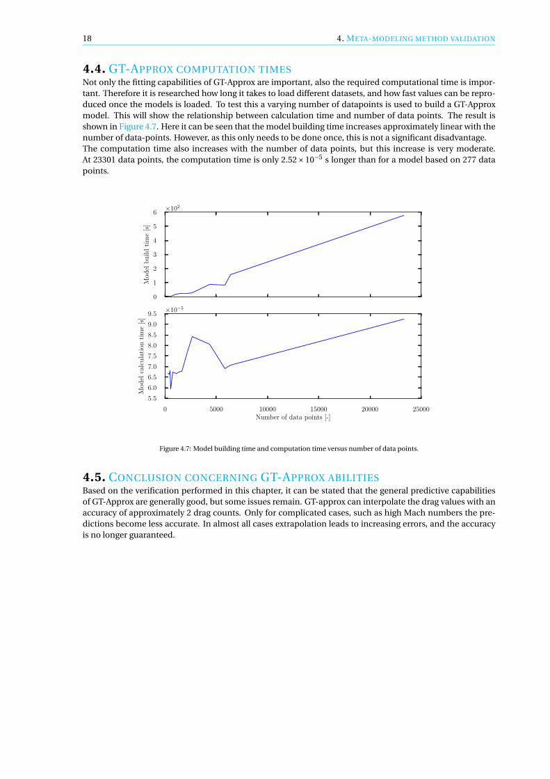
4.4. GT-APPROX COMPUTATION TIMESNot only the fitting capabilities of GT-Approx are important, also the required computational time is impor-tant. Therefore it is researched how long it takes to load different datasets, and how fast values can be repro-duced once the models is loaded. To test this a varying number of datapoints is used to build a GT-Approxmodel. This will show the relationship between calculation time and number of data points. The result isshown in Figure 4.7. Here it can be seen that the model building time increases approximately linear with thenumber of data-points. However, as this only needs to be done once, this is not a significant disadvantage.The computation time also increases with the number of data points, but this increase is very moderate.At 23301 data points, the computation time is only 2.52×10−5 s longer than for a model based on 277 datapoints.

0

1

2

3

4

5

6

Mod

elb

uild

tim

e[s

]

×102

0 5000 10000 15000 20000 25000Number of data points [-]

5.5

6.0

6.5

7.0

7.5

8.0

8.5

9.0

9.5

Mod

elca

lcu

lati

onti

me

[s]

×10−5

Figure 4.7: Model building time and computation time versus number of data points.

4.5. CONCLUSION CONCERNING GT-APPROX ABILITIESBased on the verification performed in this chapter, it can be stated that the general predictive capabilitiesof GT-Approx are generally good, but some issues remain. GT-approx can interpolate the drag values with anaccuracy of approximately 2 drag counts. Only for complicated cases, such as high Mach numbers the pre-dictions become less accurate. In almost all cases extrapolation leads to increasing errors, and the accuracyis no longer guaranteed.

5META MODELING RESOLUTION

SENSITIVITIES

As can be seen from Chapter 4, the accuracy of GT-Approx varies significantly with the omission of certainvalues. This is because the performance of GT-Approx is highly dependent on input grid. Efforts are under-taken to improve the estimation quality, specifically the prediction of cdw for values of M . This is the onlyvariable that shows large errors for interpolation values.In this chapter the influence of the various resolutions is investigated to examine what resolution is requiredto achieve the necessary accuracy. First, the method is explained in Section 5.1. Subsequently increases inresolution are investigated in Section 5.2. Non-uniform resolution increases are discussed in Section 5.3.Finally in Section 5.4 the effect of combined resolution increases is assessed and the final resolutions arepresented.

5.1. METHODThe resolutions are evaluated using the following steps:

1) The source data, generated before as discussed in Section 4.2, is adjusted to contain higher or lowerresolution data.

2) For all the variables, the procedure as explained in Section 4.2 is performed.

3) The average relative errors and absolute differences in drag counts for all the estimations are calculated.

4) These values are plotted versus the resolution to discern any trends and locate the origin of the errors.

Using this procedure it is possible to see if adding additional data will change the quality of the predictionsand for which variables.

19

20 5. META MODELING RESOLUTION SENSITIVITIES

5.2. RESOLUTION INCREASESIncreasing the resolution of the source datawill lead to smaller interpolation intervals, and thus smaller inter-polation errors. A smaller resolution might also mitigate the effects caused by missing data points. Becauseof the nature of the calculations done by MSES it might be the case that the calculation for M = 0.7,cl = 0.65fails, whereas a calculation for M = 0.7,cl = 0.66 might converge. Therefore, more data for difficult calcula-tions can be obtained by performing more MSES calculations. This allows GT-Approx to better understandthe trends, and thus provide better estimations. However, as this requires a large amount of extra data points,it will lead to larger MSES-computation times as well as longer times required to build the meta-models. Thefollowing resolution increases are considered:

• Mach resolution• cl resolution• Thickness resolution• Reynolds number resolution

5.2.1. MACH RESOLUTIONThe influence of resolution increases of all the variables have been examined. The influence of ∆M is inves-tigated in order to improve the Mach accuracy. Specifically the higher Mach values showed significant errors.To investigate the influence of the data spacing a range of spacings (denoted by ∆M) are evaluated, with thebaseline resolution indicated in bold:

• 0.10• 0.05• 0.025• 0.0125• 0.00625

The results are shown in Figure 5.1 and Table 5.1. Substantial gains can be achieved by decreasing the stepsize ∆M . For example, halving the value of ∆M of the baseline sample reduces the average prediction errorof cdv by 32%, and the average prediction error concerning cdw by 65%. Upon decreasing ∆M to 0.0125 theimprovement with respect to the baseline increases to 60% and 87% for cdv and cdw respectively. Furtherdecreasing the value of ∆M to 0.00625 does not result in significant gains.

0.1 0.05 0.025 0.0125 0.00625

M -grid spacing interval, ∆M [−]

0

2

4

6

8

10

12

GT

-Ap

pro

xer

ror,

∆c d

[−]

×10−4cdv cdw

Figure 5.1: GT-Approx prediction error versus M-grid spacing.

5.2. RESOLUTION INCREASES 21

Table 5.1: Overview of ∆cdv and ∆cdw versus ∆M

∆M, [-] ∆cdv , [10−4] Improvement, [%] ∆cdw , [10−4] Improvement, [%]

0.10 11.709 -271.29 10.697 -251.13

0.05 3.153 0.00 3.046 0.00

0.025 2.124 32.65 1.066 64.99

0.0125 1.271 59.70 0.405 86.69

0.00625 1.291 59.04 0.412 86.46

Besides evaluating the average differences, it is also important to investigate the influence of the resolutionon the ability of GT-Approx to recreate the behavior present in the MSES data. In order to examine this, thebehavior of ∆cdw and ∆cdv versus M is plotted for various resolutions, as can be seen from Figure 5.2. Here itcan be seen that increasing the M-resolution has allowed GT-Approx to improve the approximation for higherMach numbers. It can be seen that for the baseline step size of ∆M = 0.05, the difference between MSES andGT-Approx is 4 drag counts for M = 0.70, and larger than 10 drag counts for M = 0.75.Halving ∆M has greatly reduced the errors, and for ∆M = 0.0125, both drag parts show an error of less thantwo drag counts for both M = 0.70 and M = 0.75. Also, the conclusion that further decreasing the step sizedoes not yield any additional gains is confirmed, as can be seen when the plots for ∆M = 0.0125 and ∆M =0.00625 are compared. ∆M = 0.0125 is chosen as the best compromise between accuracy and number ofcomputations.

0.0

2.0

4.0

6.0

8.0

10.0

∆c d

[−]

×10−4 ∆M =0.05

0.0

2.0

4.0

6.0

8.0

10.0

∆c d

[−]

×10−4∆M =0.025

0.40 0.50 0.60 0.70 0.80


0.0

2.0

4.0

6.0

8.0

10.0

∆c d

[−]

×10−4 ∆M =0.0125

0.40 0.50 0.60 0.70 0.80


0.0

2.0

4.0

6.0

8.0

10.0

∆c d

[−]

×10−4∆M =0.00625

cdv cdwcdv cdwcdv cdwcdv cdwcdv cdw

Figure 5.2: GT-Approx prediction error versus M for different resolutions.


5.2.2. THICKNESS RESOLUTIONAlthough the thickness resolution is already quite large, reasonable results are obtained for the predictionconcerning thickness values. Therefore, it might be possible to further reduce the resolution to save calcula-tion time. The following thickness ratio intervals are assessed:

• 0.02• 0.01• 0.005• 0.0025• 0.00125

0.02 0.01 0.005 0.0025 0.00125tc-grid spacing interval, ∆ t

c[−]

0.0

0.5

1.0

1.5

2.0

2.5

3.0

3.5

4.0

GT

-Ap

pro

xer

ror,

∆c d

[−]

×10−4cdv cdw

Figure 5.3: GT-Approx prediction error versus tc -grid spacing.

Table 5.2: Overview of ∆cdv and ∆cdw versus ∆ tc

∆ tc , [-] ∆cdv , [×10−4] Improvement [%] ∆cdw , [×10−4] Improvement, [%]

0.02 3.035 -28.81 1.304 -87.51

0.01 2.356 0.00 0.695 0.00

0.005 2.337 0.786 0.511 26.47

0.00025 3.927 -66.66 0.345 50.37

0.000125 -6.65 18.63 0.285 58.94

From Figure 5.3, it can be seen that reducing the resolution is not feasible, as the error grows significantly.Decreasing the resolution causes both the drag errors to increase, although the improvement for cdv is small.After this, the error for cdw decreases. However, the value of cdv is not at a global minimum. As can be seenfrom Figure 5.4 this is because there is a very large prediction error for the cdv at t

c = 0.11. The resolution of∆ t

c = 0.005 is chosen as the final resolution.


0.0

2.0

4.0

6.0

8.0

10.0∆c d

[−]

×10−4 ∆ tc

=0.01

0.0

2.0

4.0

6.0

8.0

10.0

∆c d

[−]

×10−4∆ tc

=0.005

0.10 0.11 0.12 0.13 0.14Thickness to chord ratio, t

c[−]

0.0

2.0

4.0

6.0

8.0

10.0

∆c d

[−]

×10−4 ∆ tc

=0.0025

0.10 0.11 0.12 0.13 0.14Thickness to chord ratio, t

c[−]

0.0

2.0

4.0

6.0

8.0

10.0

∆c d

[−]

×10−4∆ tc

=0.00125

cdv cdwcdv cdwcdv cdwcdv cdw

Figure 5.4: GT-Approx prediction error versus tc for different resolutions.

5.2.3. cl RESOLUTIONAs is shown in Subsection 4.3.5 the baseline resolution shows some difficulties in approximating the valuescalculated by MSES. Therefore, the influence of the cl -resolution is investigated to see if it is possible to im-prove the approximation. The following resolutions are evaluated:

• 0.1• 0.05• 0.025• 0.0125• 0.00625

0.1 0.05 0.025 0.0125 0.00625

cl-grid spacing interval, ∆cl [−]

0.0

0.5

1.0

1.5

2.0

2.5

3.0

3.5

GT

-Ap

pro

xer

ror,

∆c d

×10−4cdv cdw

Figure 5.5: GT-Approx prediction error versus cl -grid spacing.


Table 5.3: Overview of ∆cdv and ∆cdw versus ∆cl

∆cl, [-] ∆cdv , [10−4] Improvement [%] ∆cdw , [10−4] Improvement, [%]

0.1 3.284 -89.70 2.925 -191.69

0.05 1.731 0.00 1.002 0.00

0.025 1.446 16.44 0.552 44.94

0.0125 1.333 22.98 0.424 57.64

0.00625 1.408 18.63 0.283 71.73

Figure 5.5 and Table 5.3 show that up until ∆cl = 0.0125 the accuracy improves with increasing resolution.However, when the stepsize is increased to 0.00625, the increase in accuracy is not significant. The errorin cdw still decreases marginally, but the value of cdv starts to increase. Because the error distribution in thebaseline prediction was rather erratic, as shown by Figure 4.5, the improvements in cl are further investigated.This is done to see if any improvements are achieved for higher cl or, that the general estimation quality hasincreased.

0.0

1.0

2.0

3.0

4.0

∆c d

[−]

∆cl =0.05

0.0

1.0

2.0

3.0

4.0

∆c d

[−]

×10−4∆cl =0.025

0.30 0.40 0.50 0.60 0.70 0.80


0.0

1.0

2.0

3.0

4.0

∆c d

[−]

∆cl =0.0125

0.30 0.40 0.50 0.60 0.70 0.80


0.0

1.0

2.0

3.0

4.0

∆c d

[−]

×10−4∆cl =0.00625


Figure 5.6: GT-Approx prediction error versus cl for different resolutions.

Figure 5.6 shows that the erratic behavior persists, also for higher resolutions. Furthermore it can be seenthat the estimation accuracy of cdw increases significantly, whereas the estimation improvement of cdv isless strong. This confirms the trends shown in Figure 5.5. Based on the results presented in Figure 5.5 andFigure 5.6 a value of ∆cl = 0.0125 is chosen as optimal.

5.2.4. REYNOLDS NUMBER RESOLUTIONFor the Reynolds number, the predictions were already accurate. However, it might be possible to improvethe accuracy further by increasing the resolution. For every step, the value of ∆Re is halved. The originalvalue is indicated in bold. The resolutions investigated are:

• 20.0×106

• 10.0×106

• 5.00×106

• 2.50×106

• 1.25×106


20.0 10.0 5.00 2.50 1.25

Re-grid spacing interval, ∆Re [−]

0.0

0.5

1.0

1.5

2.0

2.5

3.0

GT

-Ap

pro

xer

ror,

∆c d

[−]

×10−4

×106

cdv cdw

Figure 5.7: GT-Approx prediction error versus Re-grid spacing.

Table 5.4: Overview of ∆cdv and ∆cdw versus ∆Re

∆Re, [×106] ∆cdv , [×10−4] Improvement [%] ∆cdw , [×10−4] Improvement, [%]

20.0 2.682 -44.73 0.699 -80.70

10.0 1.853 0.00 0.387 0.00

5.00 1.812 2.19 0.367 5.03

2.50 1.633 11.83 0.205 46.95

1.25 1.507 18.64 0.150 61.05

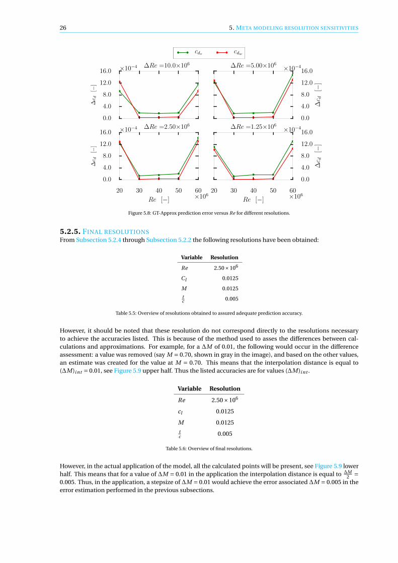
From Figure 5.7 and Table 5.4 it can be seen that no large gains can be achieved by increasing the Reynoldsnumber. This was expected from the results of Subsection 4.3.2, as it showed a good approximation for allvalues but the outer two points. It can also be seen that doubling the resolution not give any significant gains,but further increasing the resolution does give moderate improvements. Table 5.4 shows that increasing thestepsize to ∆Re = 1.25×106 does not improve the accuracy by much. Figure 5.8 shows that the behavior ofthe error does not change much. Therefore it is decided to maintain a value of ∆Re = 2.50×106.


0.0

4.0

8.0

12.0

16.0

∆c d

[−]

∆Re =10.0×106×10−4

0.0

4.0

8.0

12.0

16.0

∆c d

[−]

∆Re =5.00×106×10−4

20 30 40 50 60

Re [−]

0.0

4.0

8.0

12.0

16.0

∆c d

[−]

×106

∆Re =2.50×106×10−4

20 30 40 50 60

Re [−]

0.0

4.0

8.0

12.0

16.0

∆c d

[−]

×106

∆Re =1.25×106×10−4


Figure 5.8: GT-Approx prediction error versus Re for different resolutions.

5.2.5. FINAL RESOLUTIONSFrom Subsection 5.2.4 through Subsection 5.2.2 the following resolutions have been obtained:

Variable Resolution

Re 2.50×106

Cl 0.0125

M 0.0125

tc 0.005

Table 5.5: Overview of resolutions obtained to assured adequate prediction accuracy.

However, it should be noted that these resolution do not correspond directly to the resolutions necessaryto achieve the accuracies listed. This is because of the method used to asses the differences between cal-culations and approximations. For example, for a ∆M of 0.01, the following would occur in the differenceassessment: a value was removed (say M = 0.70, shown in gray in the image), and based on the other values,an estimate was created for the value at M = 0.70. This means that the interpolation distance is equal to(∆M)i nt = 0.01, see Figure 5.9 upper half. Thus the listed accuracies are for values (∆M)i nt .

Variable Resolution

Re 2.50×106

cl 0.0125

M 0.0125tc 0.005

Table 5.6: Overview of final resolutions.

However, in the actual application of the model, all the calculated points will be present, see Figure 5.9 lowerhalf. This means that for a value of ∆M = 0.01 in the application the interpolation distance is equal to ∆M

2 =0.005. Thus, in the application, a stepsize of ∆M = 0.01 would achieve the error associated ∆M = 0.005 in theerror estimation performed in the previous subsections.


M=0.69 M=0.70 M=0.71

M=0.69 M=0.70 M=0.71

ΔMint

ΔMint

Figure 5.9: Interpolation distance for the error estimation (above) and the application (below).

Thus the accuracy that belongs to a certain ∆M mentioned in Subsection 5.2.1 corresponds to the actualresolution twice ∆M . This reasoning also holds for the other variables, making the final recommended reso-lutions:

Table 5.7: Overview of final recommended resolutions and their accuracy.

Variable Resolution ∆cdv [×10−4] ∆cdw [×10−4]

Re 5×106 1.63 0.20

cl 0.025 1.33 0.42

M 0.025 1.27 0.40tc 0.01 2.33 0.51


5.3. TARGETED RESOLUTION INCREASESBesides linearly increasing the resolutions it is also possible to increase the number of data points for a regionwhere more accuracy is required. For the low Mach numbers the development is rather smooth, whereas forhigher Mach numbers, sudden and fierce increases might be present. To save computation time, it is pro-posed to increase the resolution at locations where more accuracy is needed: at high Mach numbers. Furthermore it was found in Subsection 5.2.1 that the main improvements in the approximation where achieved forhigher Mach numbers. For the lower Mach numbers, increasing the resolution yielded little to no improve-ment. Therefore it seems logical to omit the lower Mach resolution-increases. Therefore, it is proposed toonly add increased resolution data for values larger than M = 0.6. Again the absolute errors versus resolutionare compared, this can be seen in Figure 5.10.

0.0

1.0

2.0

3.0

4.0

GT

-Appro

xer

ror,

∆c d

[−] ×10−4 Linear resolution increase

0.1 0.05 0.025 0.0125

M -grid spacing interval, ∆M [−]

0.0

1.0

2.0

3.0

GT

-Appro

xer

ror,

∆c d

[−] ×10−4 Targeted resolution increase

cdv cdw

Figure 5.10: Estimation error for the linear resolution increase (above) and the targeted resolution increase (below) versus M-resolution.

It can be seen that the targeted resolution increase does not have the expected behavior. Increasing the reso-lution hardly increases the accuracy. This can be explained by the method used by GT Approx. In case of anincomplete tensor approach, GT Approx tries to reconstruct the complete tensor, but with wide margins. Byapplying a targeted resolution increase this behavior is invoked. GT Approx is expecting the same resolutionfor both higher and lower Mach numbers. Since these values are not present, GT-Approx tries to reconstructthese values. Following this strategy it can be seen that the quality hardly increases for targeted resolutionincreases. Therefore this option is dismissed as a feasible option for accuracy improvement.

5.4. FINAL RESOLUTIONS 29

5.4. FINAL RESOLUTIONSThe procedure as explained in Subsection 5.2.1 is also applied to the other variables. The resulting step sizesare shown in Table 5.8.

Variable Resolution ∆cdv [×10−4] ∆cdw [×10−4]

Re 5.00×106 1.63 0.20

cl 0.025 1.33 0.42

M 0.025 1.27 0.40tc 0.01 2.33 0.51

Table 5.8: Overview of recommended resolutions and their accuracy.

It is important to investigate how all the individual resolutions and their accuracies combine to a total accu-racy. It is assumed that the errors are independent, and thus according to Dekking et al [41], the error for allthe different variables combined can be estimated using Equation 5.1.

∆cdcombi ned=

√(∆cd∆Re

)2 +(∆cd∆cl

)2 +(∆cd∆M

)2 +(∆cd

∆ tc

)2

(5.1)

To validate the combined error, the approximation accuracy is calculated for a range of test-locations. Thiswill determine what the accuracy is when interpolation for multiple dimensions is necessary. To this end,a so called offset-dataset was generated. For example, for the Mach-numbers, if the first three calculatedpoints are M = 0.4,0.425 and 0.475, the offset values are taken as M = 0.4125,0.4375. This maximizes theinterpolation distance. For all these points, the GT Approx values are compared with data calculated by MSES.This leads to the average errors, which are compared to the expected errors in Table 5.9.

Table 5.9: Overview of predicted and actual accuracy.

Variable ∆cdv , [×10−4] ∆cdw , [×10−4]

Predicted 3.35 0.81

Offset test case 2.01 0.82

As can be seen from Table 5.9, the error for the wave drag is as expected, where the viscous drag is lower thanthe expected value. This is because the different interpolation accuracies are not completely independent.This means that the estimation for a certain value of M is not only a function of ∆M , but also a functionof ∆Re, ∆ t

c and ∆cl . This invalidates the assumption made in Equation 5.1, thus explaining the difference.From this test it can be concluded that the errors behave approximately as expected. and that the combinedresolutions will indeed provide enough accuracy.

63D METHOD EXTENSION

Up until this point the tool developed was only focused on 2D airfoil prediction. However, to make this tool asuitable tool for preliminary aircraft design and evaluation, it is necessary to extend the method into the thirddimension. The extension into the third dimension is done by applying a quasi 3D method. This methodentails dividing the wing into a number of 2D sections. The local 3D conditions for these sections are thencalculated. These local conditions are then used to estimate the 3D performance of the wing.First in Section 6.1 the region of validity of the quasi-3D method is discussed. In Section 6.2 the implementa-tion of the model is treated. Then, the test cases are evaluated using a direct application of MSES and usingGT-Approx in Section 6.3. Finally in Section 6.4 the results of GT-Approx are compared with the CFD data.

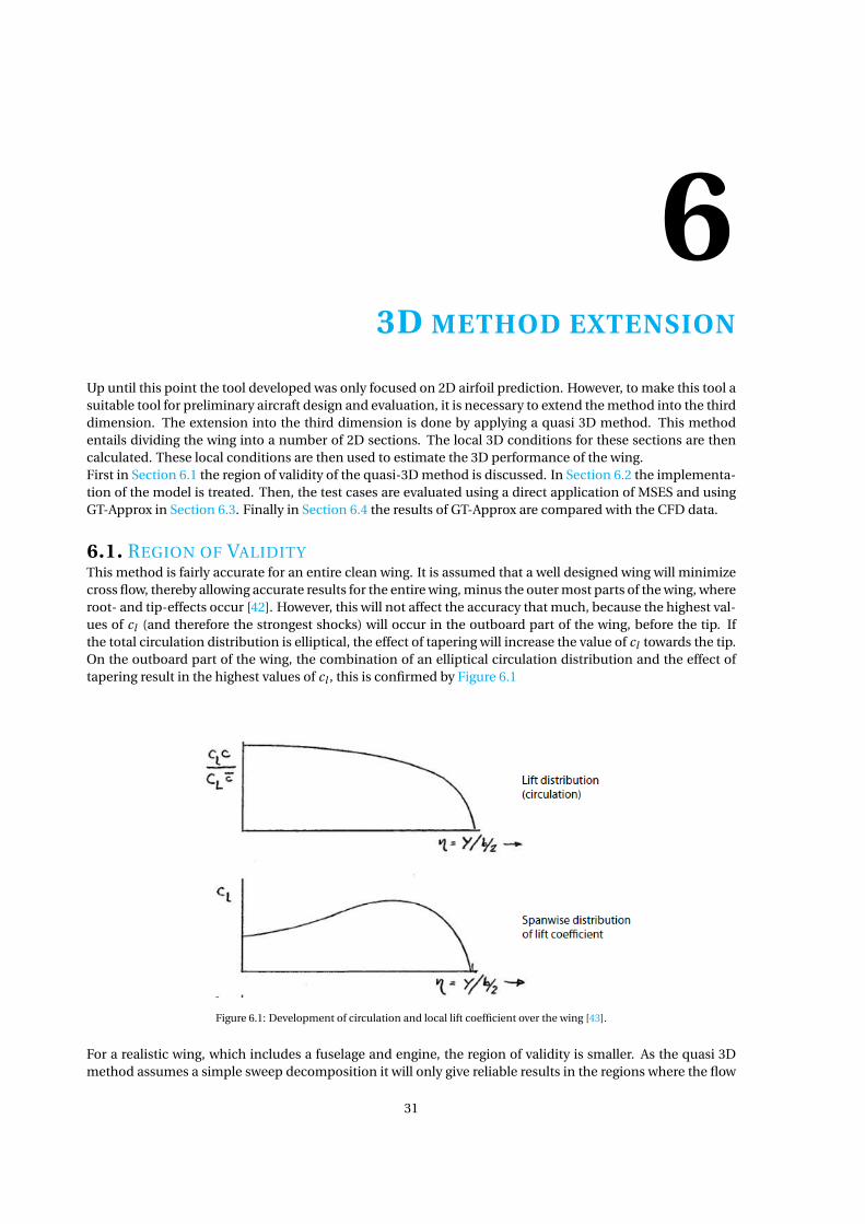
6.1. REGION OF VALIDITYThis method is fairly accurate for an entire clean wing. It is assumed that a well designed wing will minimizecross flow, thereby allowing accurate results for the entire wing, minus the outer most parts of the wing, whereroot- and tip-effects occur [42]. However, this will not affect the accuracy that much, because the highest val-ues of cl (and therefore the strongest shocks) will occur in the outboard part of the wing, before the tip. Ifthe total circulation distribution is elliptical, the effect of tapering will increase the value of cl towards the tip.On the outboard part of the wing, the combination of an elliptical circulation distribution and the effect oftapering result in the highest values of cl , this is confirmed by Figure 6.1

Figure 6.1: Development of circulation and local lift coefficient over the wing [43].

For a realistic wing, which includes a fuselage and engine, the region of validity is smaller. As the quasi 3Dmethod assumes a simple sweep decomposition it will only give reliable results in the regions where the flow

31

32 6. 3D METHOD EXTENSION

Figure 6.2: Region of validity of quasi 3D method.

is perpendicular to the chord line. To asses for which regions this is the case, the isobars for a typical Airbusaircraft are examined. Here it can be seen that for inboard regions the flow is highly three dimensional, andthe isobars are not aligned with the sweep line. The region around η= 0.34 is heavily influenced by the engineplacement. The shock occurs on the engine, leaving the area of the wing behind the engine in relatively lowspeeds, preventing shock waves on the wing. The effect of the engine spreads outboard and inboard, andstrong influences can be seen from the root up until η = 0.6. These effects prevent any useful comparisonbetween the quasi 3D method and CFD calculations for values of η≤ 0.6.

6.2. 3D METHOD IMPLEMENTATIONTo investigate the accuracy of the 3D extension, two test cases are investigated:

• A320The original A320 wing

• A320-PL7aA modification of the original A320 wing, incorporating a chord and span extension, wing retwist andmodified airfoil shapes

The main goal for this modification was to reduce the induced drag by achieving a more elliptic loading. Toachieve this more loading was shifted outboard.This will increase the value of cl on the outboard wing resulting in an increase in wave drag. For both thesecases, calculations using DLR’S TAU CFD code [44] have been performed. For both wings, CFD results areavailable for Re = 2.57×107, M = 0.78, CL values ranging from 0.4 to 0.75 in steps of 0.025.

6.2. 3D METHOD IMPLEMENTATION 33

6.2.1. AIRFOIL GEOMETRYFor both the wings, the wing planforms are known. In this thesis, not the entire wing is evaluated. Near the tipthe wing is shaped according to 3D flow phenomena like the tip effect. This leads to distorted airfoil profiles,which have no meaning in a quasi-3D method like this one. The relevant parts of both planforms are shownare shown in Figure 6.3.

0.0 0.2 0.4 0.6 0.8 1.0

Relative spanwise station, η [−]

0

2

4

6

8

10

Dis

tan

cefr

omn

ose,X

[m]

A320

A320 0.50 x/c

A320-PL7A

A320-PL7A 0.50 x/c

Figure 6.3: Comparison of the two test case geometries.

It should be noted here that η is based on the original A320 reference span, as per Airbus standard. For twentyequidistant locations on the η-range shown in the image airfoil geometries are extracted. The distribution ofairfoil stations of the A320 planform is shown in Figure 6.4.

0.0 0.2 0.4 0.6 0.8 1.0


0

2

4

6

8

10

Dis

tan

cefr

omn

ose,X

[m]

A320 Airfoil station

Figure 6.4: A320 planform with airfoil stations.


6.2.2. EFFECTIVE MACH NUMBERTo incorporate the effect of wing sweep, a correction is necessary. The simple sweep theory proposes to usethe speed perpendicular to the sweep line, as shown by Equation 6.1.

M⊥ = M∞ cosΛ0.25c (6.1)

However, based on experience and empirical results, Torenbeek [45] proposes the following correction:

M⊥ = M∞√

cosΛ0.25c (6.2)

However, it was found that a better agreement with data was obtained using Λ0.50c . This makes sense, as theshock usually lies at 50% chord [46]. The effective Mach number calculation is adjusted to:

M⊥ = M∞√

cosΛ0.50c (6.3)

6.2.3. EFFECTIVE REYNOLDS NUMBER

The test-case data calculations were performed for a Reynolds number of 2.57×107. The formula for theReynolds number is given by:

Rewi ng = ρ∞V∞ M AC

ν∞(6.4)

Since M AC is known, it is possible to calculate the local Reynolds number as:

Re⊥ = ρ∞V⊥c⊥ν∞

=(ρ∞V∞ cosΛ0.50c

ν∞

)c cosΛ0.50c =

(Rewi ng

M AC

)c cos2Λ0.50c = Rewi ng

( c

M AC

)cos2Λ0.50c (6.5)

6.2.4. cl INPUTIn order to ensure comparability with the test-case, the values generated by the CFD code are used as input forthe GT-approx model. As mentioned, lift distributions for CL = 0.4−0.75 are available. Two of the circulationsas calculated by the CFD code are shown in Figure 6.5.

0.0 0.2 0.4 0.6 0.8 1.0


Cir

cula

tion

,c l·c c

[−]

low CL

high CL

A320 A320-PL7AA320 A320-PL7A

Figure 6.5: Selection of circulations for the two planforms.

From Figure 6.5 it can be seen that the modifications have indeed increased the value of the circulation inthe outboard section on the wing, as was targeted. This has made the circulation distribution more elliptical,and will decrease the induced drag. To obtain the local lift coefficient, the effect of the local chord needs tobe incorporated. The values from Figure 6.5 are multiplied with the average chord, and divided by the localchord to obtain the local lift coefficient, as shown in Figure 6.6.

6.3. TEST CASE: COMPARISON BETWEEN MSES AND GT-APPROX 35

0.0 0.2 0.4 0.6 0.8 1.0


Air

foil

lift

coeffi

cien

t,c l

[−]

low CL

high CL

A320 A320-PL7AA320 A320-PL7AA320 A320-PL7AA320 A320-PL7A

Figure 6.6: Selection of lift coefficient distribution.

Figure 6.6 shows that the local lift distribution looks like a typical lift distribution, as shown in Figure 6.1. Theoutboard increase of the circulation has led to higher values of the local lift coefficient. This will increase thewave drag.

6.2.5. CDw DETERMINATIONNow that all the input variables have been corrected to the effective values, it is possible to determine thevalue of effective cdw⊥ . This value needs to be converted back to the streamwise direction, to determine theactual drag experienced. This is done using a method proposed by Drela [47]. This method proposes thefollowing formula:

CDw = cdw⊥ cos3Λ0.50c (6.6)

6.3. TEST CASE: COMPARISON BETWEEN MSES AND GT-APPROXFor this test case, the following algorithm was executed:

1) Based on the geometry, for every of the 20 spanwise locations the following values are determined:Re⊥, M⊥,cll ocal

.

2) From these values the boundaries are determined, Re⊥min ,Re⊥max , M⊥mi n ,M⊥max and cllocalmi n

,cllocalmax.

3) For all spanwise locations the airfoils are extracted

4) For the variable ranges as determined in step 2), MSES is used to calculate values at the intervals asdetermined in Section 5.4 to form the input data-set for GT-Approx.

5) Based on this data-set, a GT-Approx model is generated.

6) For every spanwise location the actual value of Re⊥, M⊥,cllocaland η are given as input to the GT-Approx

model, in order to predict outputs.

7) For every spanwise location the calculation is also performed with MSES using the same input- param-eters.

The final result is shown against data calculated by MSES directly in Figure 6.7. From this it can be seen thatGT-Approx is able to predict the results with good accuracy. The average difference between GT-Approx andMSES for values of η> 0.60 is equal to 0.21 drag counts.


0.6 0.7 0.8 0.9 1.0

Relative spanwise wing station, η [−]

3Dd

rag

coeffi

cien

t,CDw

[−]

MSES GT-Approx

Figure 6.7: Comparison between MSES and GT-Approx approximation for A320-PL7A with CL = 0.625.

The pressure distributions generated by GT-Approx and MSES are also compared. The result of this can beseen in Figure 6.8. The general comparison is good. GT-Approx accurately predicts the pressures. However,some features look somewhat different. At η= 0.6, around X = 21m, some differences can be seen. However,these differences are small.

0.6 0.7 0.8 0.9 1.0Relative spanwise station, η [−]

19

20

21

22

23

24

25

Dis

tan

cefr

omth

en

ose,X

[m]

A320-PL7A MSES

0.6 0.7 0.8 0.9 1.0Relative spanwise station, η [−]

A320-PL7A GT-Approx

Figure 6.8: Comparison between pressures calculated by MSES and GT-Approx for CL = 0.625.

6.3. TEST CASE: COMPARISON BETWEEN MSES AND GT-APPROX 37

When the running times are compared, the advantage of GT-Approx becomes apparent. For GT-Approx, threedifferent computation times are required:

• Model preparation timeThe time needed to generate the output grid using MSES. For this calculation, a grid of 2.16×104 datapoints was used. A typical calculation of MSES requires 5.58 s, thus giving a model preparation time of33 hours, 25 minutes and 43 seconds. As these calculations are not dependent on each other it possibleto greatly reduce the computation by using parallel computing.

• Model loading timeThe time needed to initialize the model, which required once. For this calculation, a model loadingtime of 12 minutes and 34 seconds was needed.

• Model calculation timeThe time required to generate a single calculation, thus generating a single set of outputs from a singleset of inputs. 5.13×10−4 s was needed to perform a single calculation in this case.

The benefit of using GT-Approx is that both the model preparation time and the model loading time can beperformed outside an iterative multi disciplinary design loop. An issue using iterative design loops is thatthe disciplines are dependent on each other, and it is not possible to perform calculation simultaneously,therefore it is of vital importance to reduce the computation time per iteration. For one wing evaluation(using 20 span wise locations) MSES required 1.12×102 s. For the same calculation, GT-Approx required1.03×10−2 s.If only the Model loading time and the model calculation time are included (because the model preparationcan be done before), GT-Approx is faster for computations that contain more than 7 wing evaluations.In general it is concluded that GT-Approx is able to achieve the accuracy required for initial design stages, butwith greatly reduced computation times per iteration.


6.4. TEST CASE: COMPARISON BETWEEN GT-APPROX AND CFDIn the previous subsection it was proven that GT-Approx is able to recreate the data generated by MSES. Toasses the quality of GT-Approx it is validated against CFD calculations. The CDw calculated by GT-Approx iscompared with CFD calculations in Figure 6.9

0.6 0.8 1.0


3Dw

ave

dra

gco

effici

ent,CDw

[−]

A320

0.6 0.7 0.8 0.9 1.0


A320-PL7A

GT-Approx A320

CFD A320

GT-Approx A320-PL7A

CFD A320-PL7A

Figure 6.9: Comparison between GT-Approx and CFD calculations for both test cases with CL = 0.625.

6.4.1. A320For the A320, the calculations lack any resemblance. The wave drag predicted by GT-Approx shows a strongcorrelation with the cl distribution, whereas the CFD-calculations do not. The cl , shown in Figure 6.6 peaksat η = 0.7, and shows a moderate descent after that. This is also visible in the wave drag calculated by GT-Approx. The CFD calculations show a different distribution, with a maximum wave drag at η= 0.8. From thisit is concluded that the quasi 3D application of MSES is too sensitive to cl , and not sensitive enough for theeffects of the local geometry. On the outboard section the quasi 3D and full 3D method should achieve similarresults, as shown by Mariens [27]. One possible explanation could be that Mariens compared the total dragwhereas in this work only the value of CDw is compared. As no further data for the 3D case is present, detailedresearch is not possible.

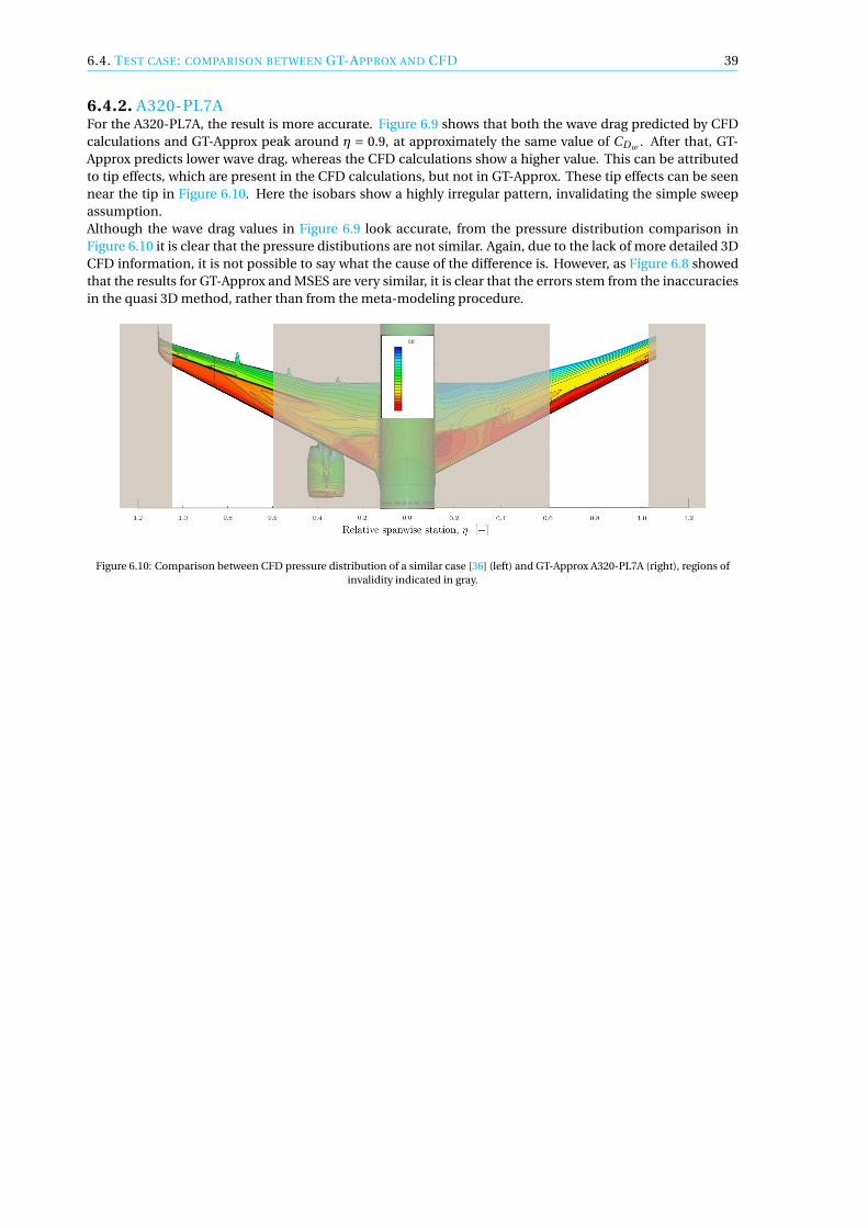
6.4. TEST CASE: COMPARISON BETWEEN GT-APPROX AND CFD 39

6.4.2. A320-PL7AFor the A320-PL7A, the result is more accurate. Figure 6.9 shows that both the wave drag predicted by CFDcalculations and GT-Approx peak around η = 0.9, at approximately the same value of CDw . After that, GT-Approx predicts lower wave drag, whereas the CFD calculations show a higher value. This can be attributedto tip effects, which are present in the CFD calculations, but not in GT-Approx. These tip effects can be seennear the tip in Figure 6.10. Here the isobars show a highly irregular pattern, invalidating the simple sweepassumption.Although the wave drag values in Figure 6.9 look accurate, from the pressure distribution comparison inFigure 6.10 it is clear that the pressure distibutions are not similar. Again, due to the lack of more detailed 3DCFD information, it is not possible to say what the cause of the difference is. However, as Figure 6.8 showedthat the results for GT-Approx and MSES are very similar, it is clear that the errors stem from the inaccuraciesin the quasi 3D method, rather than from the meta-modeling procedure.

Figure 6.10: Comparison between CFD pressure distribution of a similar case [36] (left) and GT-Approx A320-PL7A (right), regions ofinvalidity indicated in gray.

7CONCLUSION AND RECOMMENDATIONS

7.1. CONCLUSIONIt is concluded that aerodynamic tool MSES is an accurate 2D method and that the meta-modeling methodGT-Approx is able to accurately reproduce complex data generated by MSES. It is possible to improve theaccuracy of the meta-modeling method by adding more data points. Accuracies of 0.21 drag counts areachieved, whilst reducing the in-the-loop computation time from 5.58 s to 5.13×10−4 s per calculation.However, the comparison of MSES data reproduced by GT-Approx with CFD data showed that a quasi 3Dapplication of MSES does not lead to accurate results. For one of the two test cases reasonable results forthe wave drag prediction were achieved, whereas the second test case showed no correlation. The pressuredistribution also lacked resemblance. Because of lack of more detailed data no cause for this difference wasfound.In general it is concluded that the combination of an aerodynamic tool with a meta-model can be a successfulone, but that is highly dependent on the accuracy and the application of the aerodynamic model.

7.2. RECOMMENDATIONSAs is shown in this work, the combination of a meta-modeling method with a computational aerodynamicmethod is not a feasible one. The main reason for this lies in the errors generated by the quasi 3D method-ology. The transition from 2D to 3D can not be modeled in a simple way using the simple sweep theorem.It is therefore recommended to further investigate methodologies that are able to accurately represent thetransition from 2D to 3D.Furthermore it was established that the predictive capabilities of GT-Approx are highly dependent on the dataprovided. The accuracy was greatly increased by simply adding more data points. However, using Design ofExperiment methodologies it is possible to add additional points in an intelligent way such that the increasein accuracy is maximized. This can greatly reduce the amount of data points required, whilst still achievingsimilar accuracies.Another possibility to improve the meta-modeling procedure is so-called Data Fusion. These methods aregeared towards combining lower and higher fidelity data. Data Fusion allows the usage of higher fidelity datafor a few difficult cases with lower fidelity cases for easier cases. MSES experienced many problems for dif-ficult cases, such as high M , high cl calculations. For this case, Data Fusion could employ MSES for easiercalculations combined with CFD calculations for the more difficult cases. This could greatly improve theaccuracy or alternatively decrease the number of points required to reach a certain accuracy.

41

BIBLIOGRAPHY

[1] S. SHARIAR and E. TOPAL, When will fossil fuel reserves be diminished? Energy Policy 37, pp. 181 (2009).

[2] L. JENKINSON, P. SIMPKIN, and D. RHODES, Civil Jet Aircraft Design (Arnold, 1999).

[3] J. ROSKAM and E. CHUAN-TAU, Airplane Aerodynamics and Performance (DARcorporation, 1997).

[4] G. SCHRAUF, Katnet, key aerodynamic technologies for aircraft performance improvement, in Fifth Com-munity Aeronautical Days (2006).

[5] O. GUR, W. MASON, and J. SCHETY, Full-configuration drag estimation, Journal of Aircraft 47, pp. 1356(2010).

[6] M. DRELA, Xfoil: An analysis and design system for low reynolds number airfoils, in Proceedings of theConference Notre Dame, Indiana, USA, Vol. 54, edited by T. MUELLER (1989) pp. pp 1–12.

[7] J. D. ANDERSON JR., Fundamentals of Aerodynamics (McGraw-Hill, 2001).

[8] D. SCHOLZ and S. CIORNEI, Mach number, relative thickness, sweep and lift coefficient of the wing - anempirical investigation of parameters and equations, in Deutscher Luft- und Raumfahrtkongreß (2005).

[9] J. SCHULZE, Development of a drag prediction method for flexible aircraft over a complete cruise flightmission, Master’s thesis, Technische Universität Darmstadt (2013).

[10] American Institute of Aeronautics and Astronautics, White paper on industrial experience with mdo,AIAA Technical Committee on Multidisiplinary Design Optimization (MDO) (1999).

[11] J. KLEIJNEN, Regression metamodels for generalizing simulation results, IEEE Transactions on SystemsMan and Cybernetics 9, pp. 93 (1979).

[12] F. VIANA and R. HAFTKA, Using multiple surrogates for metamodeling, in 7th ASMO-UK/ISSMO Interna-tional Conference on Engineering Design Optimization (2008).

[13] J. AUDET, C. DENNIS, D. MOORE, A. BOOKER, and P. FRANK, A surrogate-model-based method for con-strained optimization, in 8th Symposium on Multidisciplinary Analysis and Optimization (2000).

[14] S. KOZIEL and L. LEIFSSON, Multi-objective airfoil design using variable-fidelity cfd simulations andresponse surface surrogates, in 10th AIAA Multidisciplinary Design Optimization Specialist Conference(2014).

[15] S. KOZIEL and L. LEIFSSON, Multi-fidelity design optimization of transonic airfoils using physics-basedsurrogate modeling and shape-preserving response prediction, Journal of Computational Science 1, pp.98 (2010).

[16] J. ROSKAM, Airplane Design: Part VI: Preliminary Calculation of Aerodynamic, Thrust and Power Char-acteristics (DARcorporation, 2000).

[17] P. GARABEDIAN and D. KORN, A Theory of Supercritical Wing Sections: With Computer Programs andExamples, Volume 2 (Springer, 1975).

[18] B. MALONE and W. MASON, Multidisciplinary optimization in aircraft design using analytic technologymodels, Journal of Aircraft 32, pp. 431 (1995).

[19] W. HILTON, High Speed Aerodynamics (Longmans, Green & Co., Ltd.;, 1952).

[20] M. FREESTONE, VGK method for two-dimensional aerofoil sections, IHS ESDU, part 1: principles andresults ed. (2004).

43

44 BIBLIOGRAPHY

[21] B. THWAITES, Approximate calculation of the laminar boundary-layer, Aerodynamics Quarterly 1, 245(1949).

[22] K. STEWARTSON, Correlated compressible and incompressible boundary layers, Proc. R. Soc. Lond. SeriesA 200, 84 (1949).

[23] J. GREEN, D. WEEKS, and J. BROOMAN, Prediction of turbulent boundary-layers and wakes in com-pressible flow by a lag-entrainment method, R.A.E. Farnborough, aeronautical research council reports& memoranda no 3791 ed. (1977).

[24] R. LOCK, A method of determining the wave drag and its spanwise distribution on a finite wing in tran-sonic flow, IHS ESDU (1987).

[25] R. LOCK, Prediction of the drag of wings at subsonic speeds by viscous/inviscid interaction techniques,AGARD Report , 723 (1985).

[26] M. PADULO, J. MAGINOT, and M. GUENOV, Airfoil design under uncertainty with robust geometric pa-rameterization, in 50th AIAA/ASME/ASCE/AHS/ASC Structures, Structural Dynamics, and Materials Con-ference (2009).

[27] J. MARIENS, A. ELHAM, and M. VAN TOOREN, Influence of weight modelling on the outcome of wingdesign using multidisciplinary design optimisation techniques, Aeronautical Journal 117, pp. 871 (2013).

[28] M. DRELA, Mses multi-element airfoil desing/analysis software summary, (1994).

[29] D. LEE, L. GONZALEZ, J. PERIAUX, and E. ONATE, Robust aerodynamic design optimisation of morphingaerofoil/wing using distributed moga, in 28TH INTERNATIONAL CONGRESS OF THE AERONAUTICALSCIENCES (2012).

[30] J. DRIVER and Z. D.W., Numerical aerodynamic optimization incorporating laminar-turbulent transitionprediction, AIAA JOURNAL 45, pp. 1810 (2007).

[31] D. R. HARTREE, On an equation occurring in falkner and skan’s approximate treatment of the equations ofthe boundary layer, Mathematical Proceedings of the Cambridge Philosophical Society 33, pp 223 (1937).

[32] M. DRELA, Two-Dimensional Transonic Aerodynamic Desing and Analysis Using The Euler Equations,Ph.D. thesis, Massachusets Institute of Technology (1985).

[33] T. SWAFFORD, Analytical approximation of two-dimensional separated turbulent boundary-layer veloc-ity profiles, AIAA Journal 21, pp 923 (1983).

[34] M. DRELA, A User’s Guide to MSES 3.05, MIT Department of Aeronautics and Astronautics (2007).

[35] C. HARRIS and J. BLACKWELL JR., Wind-Tunnel Investigation Of Effects of Rear Upper Surface Modifica-tion On An NASA Supercritical Airfoil, Tech. Rep. (NASA, 1972).

[36] R. NORTHAM, 36m Baseline TEX Development - Aero Design - Draft, Tech. Rep. (Airbus, 2014).

[37] D. YAROTSKY, M. BELYAEV, A. KRYMOVA, E. ZAYTSEV, Y. YANOVICH, and E. BURNAEV, GT ApproxGeneric Tool for Approximation, DATADVANCE, 1st ed. (2013), inhouse document.

[38] S. PRUESS, An algorithm for computing smoothing splines in tension, Computing 19, pp. 365 (1977).

[39] E. TORENBEEK, Advanced Aircraft Design (Wiley, 2013).

[40] F. M. WHITE, Viscous fluid flow, edited by L. BEAMESDERFER and J. Morriss (McGra, 1991).

[41] F. DEKKING, C. KRAAIKAMP, H. LOPUHAÄ, and L. MEESTER, A Modern Introduction to Probability andStatistics: Understanding Why and How (Springer-Verlag, 2005).

[42] J. MARIENS, Wing Shape Multidisciplinary Design Optimization, Master’s thesis, Delft University ofTechnology (2012).

[43] E. OBERT, Aerodynamic design of transport aircraft (IOS Press, 2009).

http://raphael.mit.edu/drela/msessum.ps

BIBLIOGRAPHY 45

[44] Unknown, Description of DLR TAU Code, DLR (Retrieved: Oct 2014).

[45] E. TORENBEEK, Synthesis of Subsonic Airplane Design (Kluwer Academic Publishers, 1984).

[46] D. Schuster, Lessons learned in the selection and development of test cases for the aeroelastic predictionworkshop: Rectangular supercritical wing, in Aerospace Sciences Meetings (American Institute of Aero-nautics and Astronautics, 2013) pp. –.

[47] M. Drela, N+3 Aircraft Concept Designs and Trade Studies - Volume 2 (Appendices): Design Methodolo-gies for Aerodynamics, Structures, Weight, and Thermodynamic Cycles (Appendix A: TASOPT - TransportAircraft System OPTimization), Tech. Rep. Final Report NASA/CR-2010-216794/VOL2 (NASA, 2010).

http://tau.dlr.de/fileadmin/documents/TAU_main.pdf

http://dx.doi.org/ 10.2514/6.2013-784

APYTHON CODE

A.1. TEST CASE IMPLEMENTATIONThis section contains the code used to verify the different methods against windtunnel data.

comparefig.py This script loads the test-data, and generates the plots to compare the computational meth-ods with the data.

# −*− coding : utf−8 −*−" " "Created on Mon Jun 23 14:43:31 2014

@author : THC0LQ" " "import cPickle as pickleimport matplotlib . pyplot as p l timport numpy as npimport scipy . interpolate as interpolatefrom scipy . interpolate import interp1dimport matplotlib as mplmpl . rc ( ’ t e x t ’ , usetex = True )mpl . rc ( ’ font ’ , * * { ’ family ’ : ’ s e r i f ’ , ’ s e r i f ’ : [ ’Computer Modern ’ ] } )# t e s t d at a[ TestCD040 , TestM040]= pickle . load ( open( "CNtest−0.4.p" , "rb" ) )[ TestCD055 , TestM055]= pickle . load ( open( "CNtest−0.55.p" , "rb" ) )[ TestCD070 , TestM070]= pickle . load ( open( "CNtest−0.7.p" , "rb" ) )

#handbookt e x t _ f i l e = open( "handbook04 . t x t " , " r " )handbook = t e x t _ f i l e . read ( ) . s p l i t ( ’ , ’ )handbook040 = [ f l o a t ( x ) for x in handbook ] [ 1 : ]handbook040=handbook040 [ : 3 ] + handbook040 [ 4 : ]t e x t _ f i l e = open( "handbook055 . t x t " , " r " )handbook = t e x t _ f i l e . read ( ) . s p l i t ( ’ , ’ )handbook055 = [ f l o a t ( x ) for x in handbook ] [ 1 : ]handbook055=handbook055 [ : 3 ] + handbook055 [ 4 : ]t e x t _ f i l e = open( "handbook070 . t x t " , " r " )handbook = t e x t _ f i l e . read ( ) . s p l i t ( ’ , ’ )handbook070 = [ f l o a t ( x ) for x in handbook ] [ 1 : ]handbook070=handbook070 [ : 3 ] + handbook070 [ 4 : ]

#import pdb

47

48 A. PYTHON CODE

#pdb . s e t _ t r a c e ( )import os#os . get#computationalresultsmat070 = pickle . load ( open( os . getcwd ( ) +" \\ res 100\\ savetgoed −0.7.p" , "rb" )

,→ )resultsmat055 = pickle . load ( open( os . getcwd ( ) +" \\ res 100\\ savet −0.55.p" , "rb" ) )resultsmat040 = pickle . load ( open( os . getcwd ( ) +" \\ res 100\\ savetgoed −0.4.p" , "rb" )

,→ )s i z e s =np . shape ( resultsmat070 )Machrange = np . linspace ( 0 . 6 , 0 . 8 1 , s i z e s [ 1 ] )p= [ ]q = [ ]r = [ ]p l t . rc ( ’ f i g u r e ’ , f i g s i z e =(11.5 ,15) )f i x , ax = p l t . subplots ( 3 , 1 , sharex= ’ col ’ , sharey= ’row ’ )f i x . subplots_adjust ( top =0.85)f = p l t . gcf ( )f . set_size_inches ( 8 . 2 7 , 1 1 . 6 9 )

ax [ 0 ] . plot ( TestM040 , TestCD040 , linewidth =2.0)p . extend ( ax [ 0 ] . plot ( Machrange , resultsmat040 [ 0 , : , 2 ] , linewidth =2.0 , c= ’ r ’ ) )p . extend ( ax [ 0 ] . plot ( Machrange , resultsmat040 [ 1 , : , 2 ] , linewidth =2.0 , c= ’ g ’ ) )p . extend ( ax [ 0 ] . plot ( Machrange , resultsmat040 [ 2 , : , 2 ] , linewidth =2.0 , c= ’ c ’ ) )ax [ 0 ] . tick_params ( axis = ’ y ’ , l a b e l s i z e =18)#ax [ 0 ] . t e x t ( 0 . 5 6 , 0.011 , ’ $C_L$ =0.40 ’ , f o n t s i z e =40 ,# bbox = { ’ f a c e c o l o r ’ : ’ white ’ , ’ alpha ’ : 0 , ’ pad ’ : 1 0 } )handbookf=handbook040color =[ ’b ’ , ’ g ’ , ’ r ’ , ’ c ’ , ’m’ , ’ y ’ , ’ k ’ ]import numpy as npy=np . linspace ( −0.01 ,0.07 ,100)import pdbfrom matplotlib . l i n e s import Line2Dmarkers = [ ]

for m in Line2D . markers :try :

i f len (m) == 1 and m ! = ’ ’ :markers . append(m)

except TypeError :pass

del markers [ 4 ]del markers [ 2 ]ax [ 1 ] . set_ylim ([−0.0025 , 0 . 0 1 5 ] )#pdb . s e t _ t r a c e ( )h,= ax [ 0 ] . plot (np . array ( [ f l o a t ( handbookf [ 0 ] ) ] * len ( y ) ) , y , c= ’b ’ , l i n e s t y l e = ’−− ’ )#d . append (h)h,= ax [ 0 ] . plot (np . array ( [ f l o a t ( handbookf [ 1 ] ) ] * len ( y ) ) , y , c= ’ r ’ , l i n e s t y l e = ’−− ’ )#d . append (h)h,= ax [ 0 ] . plot (np . array ( [ f l o a t ( handbookf [ 2 ] ) ] * len ( y ) ) , y , c= ’ g ’ , l i n e s t y l e = ’−− ’ )#d . append (h)h,= ax [ 0 ] . plot (np . array ( [ f l o a t ( handbookf [ 3 ] ) ] * len ( y ) ) , y , c= ’ # ffa500 ’ , l i n e s t y l e = ’−− ’ )#d . append (h)h,= ax [ 0 ] . plot (np . array ( [ f l o a t ( handbookf [ 4 ] ) ] * len ( y ) ) , y , c= ’b ’ , l i n e s t y l e = ’ : ’ )#d . append (h)h,= ax [ 0 ] . plot (np . array ( [ f l o a t ( handbookf [ 5 ] ) ] * len ( y ) ) , y , c= ’ r ’ , l i n e s t y l e = ’ : ’ )

A.1. TEST CASE IMPLEMENTATION 49

#d . append (h)h,= ax [ 0 ] . plot (np . array ( [ f l o a t ( handbookf [ 6 ] ) ] * len ( y ) ) , y , c= ’ g ’ , l i n e s t y l e = ’ : ’ )#d . append (h)# e l s e :# ax [ 0 ] . plot ( [ f l o a t ( handbookf [ k ] ) , f l o a t ( handbookf [ k ] ) ] , [ −0 . 0 1 , 0 . 0 7 ] , l i n e s t y l e

,→ = ’−− ’ , linewidth =4.0)TestM=TestM040TestCD=TestCD040data=resultsmat040 [ 0 , : , 2 ]CDdat=data [np . i s f i n i t e ( data ) ]Mdat=Machrange [np . i s f i n i t e ( data ) ]Mdat=Mdat[− s i z e s [ 1 ] / 3 : ]CDdat=CDdat[− s i z e s [ 1 ] / 3 : ]

tck=interpolate . splrep (Mdat , CDdat , s =0)# reconstruction of datafitCD=interpolate . splev (Mdat , tck , der =0)# d e r i v a t i v e of calc datafitCDd=interpolate . splev (Mdat , tck , der =1)# f i t to adjusted datatcka=interpolate . splrep (Mdat , fitCDd −0.1 , s =0)# f i t T e s t = i n t e r p o l a t e . splev ( TestM , tck2 , der =0)root=min( interpolate . sproot ( tcka , mest=10) )f1=interp1d (Mdat , CDdat)CDroot=f1 ( root )ax [ 0 ] . s e t _ y l a b e l ( ’$C_d \ : [−]$ ’ , fonts iz e =18)ax [ 0 ] . set_ylim ([−0.0025 , 0 . 0 1 5 ] )tck2=interpolate . splrep ( TestM , TestCD , s =0)# reconstruction of t e s t d a t af i tCDtest =interpolate . splev ( TestM , tck2 , der =0)# d e r i v a t i v e of calc dataf i tCDtestd=interpolate . splev ( TestM , tck2 , der =1)# f i t to adjusted datatckta=interpolate . splrep ( TestM , fitCDtestd −0.1 , s =0)# f i t T e s t = i n t e r p o l a t e . splev ( TestM , tck2 , der =0)r o o t t e s t =interpolate . sproot ( tckta , mest=10)f2=interp1d ( TestM , TestCD )CDroottest=f2 ( r o o t t e s t )ax [ 0 ] . plot ( root , CDroot , ’ r * ’ , markersize =20)ax [ 0 ] . plot ( roottest , CDroottest , ’b* ’ , markersize =20)ax [ 0 ] . s e t _ t i t l e ( r ’ $C_l =0.40$ ’ , fo nts i z e =18)ax [ 0 ] . tick_params ( axis = ’ y ’ , pad=15)#box = ax [ 0 ] . get_posi t ion ( )#ax [ 0 ] . s e t _ p o s i t i o n ( [ box . x0 , box . y0 , box . width * 0 . 8 , box . height ] )

ax [ 1 ] . plot ( TestM055 , TestCD055 , linewidth =2.0)p . extend ( ax [ 1 ] . plot ( Machrange , resultsmat055 [ 0 , : , 2 ] , linewidth =2.0 , c= ’ r ’ ) )p . extend ( ax [ 1 ] . plot ( Machrange , resultsmat055 [ 1 , : , 2 ] , linewidth =2.0 , c= ’ g ’ ) )p . extend ( ax [ 1 ] . plot ( Machrange , resultsmat055 [ 2 , : , 2 ] , linewidth =2.0 , c= ’ c ’ ) )ax [ 1 ] . s e t _ y l a b e l ( ’$C_d \ : [−]$ ’ , fonts iz e =18)ax [ 1 ] . tick_params ( axis = ’ y ’ , l a b e l s i z e =18)ax [ 1 ] . tick_params ( axis = ’ y ’ , pad=15)

50 A. PYTHON CODE

#ax [ 1 ] . t e x t ( 0 . 5 6 , 0.011 , ’ $C_L$ =0.55 ’ , f o n t s i z e =40 ,# bbox = { ’ f a c e c o l o r ’ : ’ white ’ , ’ alpha ’ : 0 , ’ pad ’ : 1 0 } )handbookf=handbook055ax [ 1 ] . set_ylim ([−0.0025 , 0 . 0 1 5 ] )h,= ax [ 1 ] . plot (np . array ( [ f l o a t ( handbookf [ 0 ] ) ] * len ( y ) ) , y , c= ’b ’ , l i n e s t y l e = ’−− ’ )#d . append (h)h,= ax [ 1 ] . plot (np . array ( [ f l o a t ( handbookf [ 1 ] ) ] * len ( y ) ) , y , c= ’ r ’ , l i n e s t y l e = ’−− ’ )#d . append (h)h,= ax [ 1 ] . plot (np . array ( [ f l o a t ( handbookf [ 2 ] ) ] * len ( y ) ) , y , c= ’ g ’ , l i n e s t y l e = ’−− ’ )#d . append (h)h,= ax [ 1 ] . plot (np . array ( [ f l o a t ( handbookf [ 3 ] ) ] * len ( y ) ) , y , c= ’ # ffa500 ’ , l i n e s t y l e = ’−− ’ )#d . append (h)h,= ax [ 1 ] . plot (np . array ( [ f l o a t ( handbookf [ 4 ] ) ] * len ( y ) ) , y , c= ’b ’ , l i n e s t y l e = ’ : ’ )#d . append (h)h,= ax [ 1 ] . plot (np . array ( [ f l o a t ( handbookf [ 5 ] ) ] * len ( y ) ) , y , c= ’ r ’ , l i n e s t y l e = ’ : ’ )#d . append (h)h,= ax [ 1 ] . plot (np . array ( [ f l o a t ( handbookf [ 6 ] ) ] * len ( y ) ) , y , c= ’ g ’ , l i n e s t y l e = ’ : ’ )#d . append (h)

# i f k<4:# ax [ 1 ] . plot ( [ f l o a t ( handbookf [ k ] ) , f l o a t ( handbookf [ k ] ) ] , [ −0 . 0 1 , 0 . 0 7 ] , l i n e s t y l e

,→ = ’ : ’ , linewidth =4.0)# e l s e :# ax [ 1 ] . plot ( [ f l o a t ( handbookf [ k ] ) , f l o a t ( handbookf [ k ] ) ] , [ −0 . 0 1 , 0 . 0 7 ] , l i n e s t y l e

,→ = ’−− ’ , linewidth =4.0)#box = ax [ 1 ] . get_posi t ion ( )#ax [ 1 ] . s e t _ p o s i t i o n ( [ box . x0 , box . y0 , box . width * 0 . 8 , box . height ] )

TestM=TestM055TestCD=TestCD055data=resultsmat055 [ 0 , : , 2 ]CDdat=data [np . i s f i n i t e ( data ) ]Mdat=Machrange [np . i s f i n i t e ( data ) ]Mdat=Mdat[− s i z e s [ 1 ] / 3 : ]CDdat=CDdat[− s i z e s [ 1 ] / 3 : ]

tck=interpolate . splrep (Mdat , CDdat , s =0)# reconstruction of datafitCD=interpolate . splev (Mdat , tck , der =0)# d e r i v a t i v e of calc datafitCDd=interpolate . splev (Mdat , tck , der =1)# f i t to adjusted datatcka=interpolate . splrep (Mdat , fitCDd −0.1 , s =0)# f i t T e s t = i n t e r p o l a t e . splev ( TestM , tck2 , der =0)root=min( interpolate . sproot ( tcka , mest=10) )f1=interp1d (Mdat , CDdat)CDroot=f1 ( root )

tck2=interpolate . splrep ( TestM , TestCD , s =0)# reconstruction of t e s t d a t af i tCDtest =interpolate . splev ( TestM , tck2 , der =0)# d e r i v a t i v e of calc dataf i tCDtestd=interpolate . splev ( TestM , tck2 , der =1)


# f i t to adjusted datatckta=interpolate . splrep ( TestM , fitCDtestd −0.1 , s =0)# f i t T e s t = i n t e r p o l a t e . splev ( TestM , tck2 , der =0)r o o t t e s t =interpolate . sproot ( tckta , mest=10)f2=interp1d ( TestM , TestCD )CDroottest=f2 ( r o o t t e s t )ax [ 1 ] . plot ( root , CDroot , ’ r * ’ , markersize =20)ax [ 1 ] . plot ( roottest , CDroottest , ’b* ’ , markersize =20)ax [ 1 ] . s e t _ t i t l e ( r ’ $C_l =0.55$ ’ , fo nts i z e =20)

h0,= ax [ 2 ] . plot ( TestM070 , TestCD070 , linewidth =2.0)p . extend ( ax [ 2 ] . plot ( Machrange , resultsmat070 [ 0 , : , 2 ] , linewidth =2.0 , c= ’ r ’ ) )p . extend ( ax [ 2 ] . plot ( Machrange , resultsmat070 [ 1 , : , 2 ] , linewidth =2.0 , c= ’ g ’ ) )p . extend ( ax [ 2 ] . plot ( Machrange , resultsmat070 [ 2 , : , 2 ] , linewidth =2.0 , c= ’ # ffa500 ’ ) )ax [ 2 ] . s e t _ y l a b e l ( ’$C_d \ : [−]$ ’ , fonts iz e =18)ax [ 2 ] . tick_params ( axis = ’ y ’ , l a b e l s i z e =18)ax [ 2 ] . tick_params ( axis = ’ x ’ , l a b e l s i z e =18)ax [ 2 ] . tick_params ( axis = ’ x ’ , pad=15)#ax [ 2 ] . t e x t ( 0 . 5 6 , 0.011 , ’ $C_L$ =0.70 ’ , f o n t s i z e =40 ,# bbox = { ’ f a c e c o l o r ’ : ’ white ’ , ’ alpha ’ : 0 , ’ pad ’ : 1 0 } )#box = ax [ 2 ] . get_posi t ion ( )#ax [ 2 ] . s e t _ p o s i t i o n ( [ box . x0 , box . y0 , box . width * 0 . 8 , box . height ] )handbookf=handbook070#h=np . zeros ( 9 )d= [ ]# p l t . xlim ( ( 0 . 6 5 , 0.90001) )

# f o r k , nr in enumerate ( handbookf ) :h,= ax [ 2 ] . plot (np . array ( [ f l o a t ( handbookf [ 0 ] ) ] * len ( y ) ) , y , c= ’b ’ , l i n e s t y l e = ’−− ’ )d . append(h)h,= ax [ 2 ] . plot (np . array ( [ f l o a t ( handbookf [ 1 ] ) ] * len ( y ) ) , y , c= ’ r ’ , l i n e s t y l e = ’−− ’ )d . append(h)h,= ax [ 2 ] . plot (np . array ( [ f l o a t ( handbookf [ 2 ] ) ] * len ( y ) ) , y , c= ’ g ’ , l i n e s t y l e = ’−− ’ )d . append(h)h,= ax [ 2 ] . plot (np . array ( [ f l o a t ( handbookf [ 3 ] ) ] * len ( y ) ) , y , c= ’ # ffa500 ’ , l i n e s t y l e = ’−− ’ )d . append(h)h,= ax [ 2 ] . plot (np . array ( [ f l o a t ( handbookf [ 4 ] ) ] * len ( y ) ) , y , c= ’b ’ , l i n e s t y l e = ’ : ’ )d . append(h)h,= ax [ 2 ] . plot (np . array ( [ f l o a t ( handbookf [ 5 ] ) ] * len ( y ) ) , y , c= ’ r ’ , l i n e s t y l e = ’ : ’ )d . append(h)h,= ax [ 2 ] . plot (np . array ( [ f l o a t ( handbookf [ 6 ] ) ] * len ( y ) ) , y , c= ’ g ’ , l i n e s t y l e = ’ : ’ )d . append(h)#h,= ax [ 2 ] . plot (np . array ( [ f l o a t ( handbookf [ 7 ] ) ] * len ( y ) ) , y , c = ’# ffa500 ’ , l i n e s t y l e = ’ : ’ )#d . append (h)# h,= ax [ 2 ] . plot (np . array ( [ f l o a t ( handbookf [ k ] ) ] * len ( y ) ) , y , l i n e s t y l e = ’None ’ , marker=

,→ markers [ k ] )# h,= ax [ 2 ] . plot (np . array ( [ f l o a t ( handbookf [ k ] ) ] * len ( y ) ) , y , l i n e s t y l e = ’None ’ , marker=

,→ markers [ k ] )# h,= ax [ 2 ] . plot (np . array ( [ f l o a t ( handbookf [ k ] ) ] * len ( y ) ) , y , l i n e s t y l e = ’None ’ , marker=

,→ markers [ k ] )

# i f k<4:

52 A. PYTHON CODE

# h,= ax [ 2 ] . plot ( [ f l o a t ( handbookf [ k ] ) , f l o a t ( handbookf [ k ] ) ] , [ −0 . 0 1 , 0 . 0 7 ] ,,→ l i n e s t y l e = ’ : ’ , linewidth =4.0)

# d . append (h)# e l s e :# h,= ax [ 2 ] . plot ( [ f l o a t ( handbookf [ k ] ) , f l o a t ( handbookf [ k ] ) ] , [ −0 . 0 1 , 0 . 0 7 ] ,

,→ l i n e s t y l e = ’−− ’ , linewidth =4.0)# d . append (h)

TestM=TestM070TestCD=TestCD070data=resultsmat070 [ 0 , : , 2 ]CDdat=data [np . i s f i n i t e ( data ) ]Mdat=Machrange [np . i s f i n i t e ( data ) ]Mdat=Mdat[− s i z e s [ 1 ] / 3 : ]CDdat=CDdat[− s i z e s [ 1 ] / 3 : ]

tck=interpolate . splrep (Mdat , CDdat , s =0)# reconstruction of datafitCD=interpolate . splev (Mdat , tck , der =0)# d e r i v a t i v e of calc datafitCDd=interpolate . splev (Mdat , tck , der =1)# f i t to adjusted datatcka=interpolate . splrep (Mdat , fitCDd −0.1 , s =0)# f i t T e s t = i n t e r p o l a t e . splev ( TestM , tck2 , der =0)root=min( interpolate . sproot ( tcka , mest=10) )f1=interp1d (Mdat , CDdat)CDroot=f1 ( root )print len (d)

tck2=interpolate . splrep ( TestM , TestCD , s =0)# reconstruction of t e s t d a t af i tCDtest =interpolate . splev ( TestM , tck2 , der =0)# d e r i v a t i v e of calc dataf i tCDtestd=interpolate . splev ( TestM , tck2 , der =1)# f i t to adjusted datatckta=interpolate . splrep ( TestM , fitCDtestd −0.1 , s =0)# f i t T e s t = i n t e r p o l a t e . splev ( TestM , tck2 , der =0)r o o t t e s t =interpolate . sproot ( tckta , mest=10)f2=interp1d ( TestM , TestCD )CDroottest=f2 ( 0 . 7 9 0 )h1,= ax [ 2 ] . plot ( root , CDroot , ’ r * ’ , markersize =20)h2,= ax [ 2 ] . plot ( roottest , CDroottest , ’b* ’ , markersize =20)ax [ 2 ] . s e t _ t i t l e ( r ’ $C_l =0.70$ ’ , fonts i z e =20)len (d)#pdb . s e t _ t r a c e ( )namepool = [ ’ Test data ’ , ’MSES ’ , ’VGK ’ , ’TSFOIL2 ’ , ’ Toorenbeek Extended ’ , ’ Shevell ’ , ’ Kroo

,→ ’ , ’KLM’ , ’ Jenkinson ’ , ’Raymer ’ , r ’B\ " { o } t t g e r ’ , ’$M_{DD} $ MSES ’ , ’$M_{DD} $ Test,→ Case ’ ]

p l t . f iglegend ( ( h0 , p [ 0 ] , p [ 1 ] , p [ 2 ] , d [ 0 ] , d [ 1 ] , d [ 2 ] , d [ 3 ] , d [ 4 ] , d [ 5 ] , d [ 6 ] , h1 , h2 ) ,namepool ,,→ loc = ’ upper center ’ , prop={ ’ s i z e ’ : 1 5 } , ncol =3 , labelspacing =0. )

p l t . xlim ( ( 0 . 6 5 , 0.90001) )p l t . ylim ((−0.0025 , 0.015) )p l t . x label ( ’$M \ : \ : \ : [−]$ ’ , fonts iz e =18)


#ax [ i ] . tick_params ( axis = ’ y ’ , pad=15)# p l t . y l a be l ( ’ $C_D$ ’ , f o n t s i z e =40)#figManager = p l t . get_current_fig_manager ( )#figManager . window . showMaximized ( )p l t . gcf ( ) . subplots_adjust ( l e f t =0.15)f . s a v e f i g ( ’MDDcomp. pdf ’ )# f . s a v e f i g ( ’ Z : \ \ Thesis \ \ Thesis Report \ \ Images \ \MDDcomp. pdf ’ )p l t . show ( )

A.1.1. MSES IMPLEMENTATIONMSESmain.pyThis is the master file used to generate the MSES output, it calls the other slave functions.

# −*− coding : utf−8 −*−" " "Created on Fri May 09 15:37:28 2014

@author : THC0LQ" " "def MSESmain( a i r f o i l , state , calctype ) :

import pdb# i f 1==1:

import MSESbladeimport MSESMSETrunimport MSESMSESwriteimport MSESMSESrunimport MSESMSESread# print a i r f o i lrunname= ’ try2 ’numit=1000MSESblade . MSESblade ( a i r f o i l , runname)MSESMSETrun.MSESMSETrun( s t a t e )

s t a t e =map( f l o a t , s t a t e )MSESMSESwrite . MSESMSESwrite( state , runname , calctype )

# pdb . s e t _ t r a c e ( )MSESMSESrun.MSESMSESrun(runname , numit )Coeffs=MSESMSESread . MSESMSESread ( )return Coeffs

importcode.pyThis script loads the airfoil data from the text files.

# −*− coding : utf−8 −*−" " "Created on Thu May 08 16:51:47 2014

@author : THC0LQ" " "def importpy ( f i l e s ) :

import numpy as npfor nr ,name in enumerate ( f i l e s ) :

l i = [ i . s t r i p ( ) . s p l i t ( ) for i in open(name) . readlines ( ) ]myarray = np . asarray ( l i )

# print myarray

54 A. PYTHON CODE

matrix = myarray . astype (np . f l o a t )xcor = matrix [ : , 0 ]yup = matrix [ : , 1 ]ylow = matrix [ : , 2 ]a i r f o i l =np . vstack ( ( xcor , yup , ylow ) )a i r f o i l = a i r f o i l . Treturn a i r f o i l

MSESblade.pyThis script generates the MSET blade input file.

# −*− coding : utf−8 −*−" " "Created on Mon May 12 16:58:35 2014

@author : THC0LQ" " "

def MSESblade ( a i r f o i l , runname) :import numpy as npimport osx=np . concatenate ( ( a i r f o i l [ : : −1 , 0 ] , a i r f o i l [ : , 0 ] ) )vals = np . concatenate ( ( a i r f o i l [ : : −1 , 2 ] , a i r f o i l [ : , 1 ] ) )a i r f o i l =np . vstack ( ( x , vals ) )a i r f o i l = a i r f o i l . Tf = open( os . path . dirname ( os . path . realpath ( _ _ f i l e _ _ ) ) + ’ \\ blade . ’+runname , ’wt ’ )f . write ( ’ A359_0520 \n ’ )f . write ( ’ −4.00000 5.00000 −5.5 5.5 \n ’ )for i ,name in enumerate ( a i r f o i l ) :

i f a i r f o i l [ i ] [ 1 ] < = 0 :f . write ( ’ ’+" { : 1 . 5 f } " . format ( a i r f o i l [ i ] [ 0 ] ) + ’ ’+" { : 1 . 5 f } " . format (

,→ a i r f o i l [ i ] [ 1 ] ) + ’ \n ’ )else :

f . write ( ’ ’+" { : 1 . 5 f } " . format ( a i r f o i l [ i ] [ 0 ] ) + ’ ’+" { : 1 . 5 f } " . format (,→ a i r f o i l [ i ] [ 1 ] ) + ’ \n ’ )

f . close ( )

MSESMSESwrite.pyThis script calls MSET, to convert the MSET blade input file to an MSES blade input file.

# −*− coding : utf−8 −*−" " "Created on Mon May 12 13:16:51 2014

@author : THC0LQ" " "def MSESMSESwrite( state , runname , calctype ) :

import osf = open( os . path . dirname ( os . path . realpath ( _ _ f i l e _ _ ) ) + ’ \\mses . ’+runname , ’wt ’ )f . write ( ’ 3 4 5\n ’ )i f ’ alpha ’ in calctype :

f . write ( ’ 3 4 5\n ’ )i f ’CL ’ in calctype :

f . write ( ’ 3 4 6\n ’ )f . write ( ’ ’+" { : 1 . 5 f } " . format ( s t a t e [ 3 ] ) + ’ ’+" { : 1 . 5 f } " . format ( s t a t e [ 1 ] ) + ’

,→ ’+" { : 1 . 5 f } " . format ( s t a t e [ 2 ] ) + ’ 16.50000 \n ’ )f . write ( ’ 4 2\n ’ )


f . write ( ’ ’+" { : 1 . 4 f } " . format ( s t a t e [ 0 ] / ( 1 0 * * 8 ) ) + ’E+08 5.0 \n ’ )f . write ( ’ ’+" { : 1 . 5 f } " . format ( s t a t e [ 4 ] ) + ’ ’+" { : 1 . 5 f } " . format ( s t a t e [ 4 ] ) + ’ \

,→ n ’ )f . write ( ’ .99000 1.00000 \n ’ )f . close

MSESMSESrun.pyThis script calls executes MSES.


@author : THC0LQ" " "import os , fnmatchdef f ind ( pattern , path ) :

r e s u l t = [ ]for root , dirs , f i l e s in os . walk ( path ) :

for name in f i l e s :i f fnmatch . fnmatch (name, pattern ) :

r e s u l t . append( os . path . join ( root , name) )return r e s u l t

def MSESMSESrun(runname , numit ) :# i f 1==1:# runname= ’ try2 ’

import oscurdir = os . getcwd ( )from subprocess import CalledProcessError , Popen , PIPE# d e l e t e previous f i l e sr e s f i l e s = [ os . path . join ( dirpath , f )

for dirpath , dirnames , f i l e s in os . walk ( curdir )for f in fnmatch . f i l t e r ( f i l e s , ’da* ’ ) ]

# print r e s f i l e sfor name in r e s f i l e s :

os . remove (name)cmd = os . path . dirname ( os . path . realpath ( _ _ f i l e _ _ ) ) +" \\mses . exe "+runname

# print cmdinput_data = os . l inesep . join ( [ s t r ( numit ) , ’ 0 ’ ] )p = Popen(cmd, stdin=PIPE , stdout=PIPE , bufsize =0)p . communicate( input_data . encode ( ’ a s c i i ’ ) )i f p . returncode != 0 :

raise CalledProcessError (p . returncode , cmd)

MSESMSESread.pyAfter a MSES run, this file reads the output file into Python.


@author : THC0LQ" " "def MSESMSESread ( ) :# i f 1==1:

import osimport numpy as np

56 A. PYTHON CODE

f = open( os . path . dirname ( os . path . realpath ( _ _ f i l e _ _ ) ) +" \\ daflow . try2 " , " r " )Co2 = { ’CD1 ’ : [ ] , ’CD2 ’ : [ ] , ’CDV’ : [ ] , ’CDP’ : [ ] , ’CDF ’ : [ ] , ’CL ’ : [ ] , ’CM’ : [ ] , ’ALP ’ : [ ] , ’

,→ DISTRI ’ : [ ] }xcor = [ ]pres = [ ]try :

while f . t e l l ( ) != os . f s t a t ( f . f i l e n o ( ) ) . s t _ s i z e :l i n e = f . readline ( )i f ’ MA RE ALP CA CM’ in l i n e :

data= f . readline ( )s p l i t t e d =data . s p l i t ( )Co2[ ’CD1 ’ ]=np . i n fCo2[ ’CD2 ’ ]= f l o a t ( s p l i t t e d [ 7 ] )Co2[ ’CDV’ ]= f l o a t ( s p l i t t e d [ 8 ] )Co2[ ’CDP’ ]=np . i n fCo2[ ’CDF ’ ]=np . i n fCo2[ ’CL ’ ]= f l o a t ( s p l i t t e d [ 3 ] )Co2[ ’CM’ ]= f l o a t ( s p l i t t e d [ 4 ] )Co2[ ’ALP ’ ]= f l o a t ( s p l i t t e d [ 2 ] )

i f "# X/C CP Z/C D1S ME THETA CFUE,→ H12" in l i n e :end = Falsewhile end i s False :

values= f . readline ( )s p l i t =values . s p l i t ( )try :

i f f l o a t ( s p l i t [ 0 ] ) <1:xcor=np . append( xcor , f l o a t ( s p l i t [ 0 ] ) )pres=np . append( pres , f l o a t ( s p l i t [ 1 ] ) )

else :1==1

except :end = True

d i s t r i =np . concatenate ( ( xcor . reshape (−1 ,1) , pres . reshape (−1 ,1) ) , ax is =1)Co2[ ’ DISTRI ’ ]= d i s t r i

except :Co2[ ’CD1 ’ ]=np . i n fCo2[ ’CD2 ’ ]=np . i n fCo2[ ’CDV’ ]=np . i n fCo2[ ’CDP’ ]=np . i n fCo2[ ’CDF ’ ]=np . i n fCo2[ ’CL ’ ]=np . i n fCo2[ ’CM’ ]=np . i n fCo2[ ’ALP ’ ]=np . i n fCo2[ ’ DISTRI ’ ]=np . i n f

return Co2

A.1.2. VGK IMPLEMENTATIONvgk_control_multiple_inputs.pyThis is the master file used to generate the VGK output, it calls the other slave functions.

# −*− coding : utf−8 −*−" " "Created on Wed Feb 26 10:10:50 2014

@author : THC0LQ


" " "# i f 1==1:def vgk ( a i r f o i l , state , calctype ) :##

import osimport timeimport vgk_delete_input_f i les as delete_inimport vgk_create_nam_file as namimport v g k _ c r e a t e _ s i r _ f i l e as s i rimport v g k _ cr e at e _ v i n_ f i l e as vinimport vgk_read_results as readimport v g k _ d e l e t e _ r e s u l t _ f i l e s as delete_resfrom subprocess import CalledProcessError , Popen , PIPEi f ’ alpha ’ in calctype :

calcpar = [ s t a t e [ 4 ] , s t a t e [ 4 ] , False ]i f ’CL ’ in calctype :

calcpar = [ s t a t e [ 4 ] , s t a t e [ 4 ] , True ]# print calcpar

names=[None] *4# write a i r f o i l to . dat

AF= ( [ ’ A i r f o i l 5 ’ , ’ SC20411 ’ , ’ a i r f o i l . dat ’ ] )f = open( ’ a i r f o i l . dat ’ , ’wt ’ )f . write (AF[0]+ ’ \n ’ )iorg = len ( a i r f o i l )f . write ( ’ 0 ’+ s t r ( iorg ) + ’ ’+ s t r ( iorg ) + ’ 0.0 1.0 \n\n ’ )

for i , nr in enumerate ( a i r f o i l ) :i f a i r f o i l [ i ,1] >=0:

f . write ( ’ ’+" { : 1 . 6 f } " . format ( a i r f o i l [ i , 0 ] ) + ’ ’+" { : 1 . 6 f } " . format ( a i r f o i l,→ [ i , 1 ] ) + ’ \n ’ )

else :f . write ( ’ ’+" { : 1 . 6 f } " . format ( a i r f o i l [ i , 0 ] ) + ’ ’+" { : 1 . 6 f } " . format ( a i r f o i l [

,→ i , 1 ] ) + ’ \n ’ )for i , nr in enumerate ( a i r f o i l ) :

i f a i r f o i l [ i ,2] >=0:f . write ( ’ ’+" { : 1 . 6 f } " . format ( a i r f o i l [ i , 0 ] ) + ’ ’+" { : 1 . 6 f } " . format ( a i r f o i l

,→ [ i , 2 ] ) + ’ \n ’ )else :

f . write ( ’ ’+" { : 1 . 6 f } " . format ( a i r f o i l [ i , 0 ] ) + ’ ’+" { : 1 . 6 f } " . format ( a i r f o i l [,→ i , 2 ] ) + ’ \n ’ )

f . close ( )names[0]= ’ matlvgk ’names[ 1 ] = AF[ 0 ]names[ 2 ] = AF[ 2 ]names[ 3 ] = AF[1]+ ’ _Re ’+ s t r ( s t a t e [ 0 ] / ( 1 0 * * 6 ) ) + ’ e6 ’s i r . v g k _ c r e a t e _ s i r _ f i l e (names)

nam. vgk_create_nam_file (names)try :

vin . v g k _ cr e a t e _ v i n_ f i l e (names , state , calcpar )except :

time . sleep ( 0 . 2 )vin . v g k _ cr e a t e _ v i n _ f i l e (names , state , calcpar )

os . system ( "vgk . exe" + " < "+names[0]+ " . s i r " )#read f i l e s

58 A. PYTHON CODE

Coeffs = read . vgk_read_results (names[0]+ " .FUL" )

return Coeffs

vgk_create_sir_file.pyThis script generates a SIR file, which is contains the name of the project.



def v g k _ c r e a t e _ s i r _ f i l e (names) :import globimport osf i l e s = glob . glob ( ’ * . s i r ’ )for i in f i l e s :

os . remove ( i )# c r e a t e f i l e name

s i r d i r =os . getcwd ( )# c r e a t e f i l e namefilename = s i r d i r + ’ / ’+ names[0]+ ’ . SIR ’

#open f i l ef = open( filename , ’wt ’ )f . write (names[0]+ ’ \n ’ )f . close

vgk_create_nam_file.pyThis script generates a NAM file, which contains a directory which contains the name of all the necessaryfiles.


@author : THC0LQ" " "def vgk_create_nam_file (names) :

import globimport os#remove old .namf i l e s = glob . glob ( ’ * .nam’ )for i in f i l e s :

os . remove ( i )# c r e a t e f i l e namenamdir=os . getcwd ( )filename = namdir + ’ / ’+names[0]+ ’ .NAM’

#open f i l ef = open( filename , ’wt ’ )f . write (names[0]+ ’ .NAM\n ’ )f . write (names[0]+ ’ . VIN\n ’ )f . write (names[0]+ ’ . IEH\n ’ )f . write (names[0]+ ’ .VEH\n ’ )f . write (names[0]+ ’ .FUL\n ’ )f . write (names[0]+ ’ . BRF\n ’ )


f . write (names[0]+ ’ .GRD\n ’ )f . write (names[0]+ ’ .UNF\n ’ )f . write ( ’ 1\n ’ )f . write (names[2]+ ’ ’+ ’ \n ’ )f . write ( ’ 1\n ’ )f . write ( ’ 1\n ’ )f . close ( )

vgk_create_vin_file.pyThis script generates a VIN file, which contains a the flight parameters, as well as configuration parameters.


@author : THC0LQ" " "def v g k _ c r e a te _ v i n_ f i l e (names , state , calcpar ) :

import globimport os

f i l e s = glob . glob ( ’ * . VIN ’ )for i in f i l e s :

os . remove ( i )# c r e a t e f i l e namevindir=os . getcwd ( )filename =vindir + ’ / ’ + names[0]+ ’ . VIN ’

#open f i l ef = open( filename , ’wt ’ )f . write ( ’ 4 ’+names[1]+ ’ \n ’ )f . write ( ’ \n ’ )f . write ( ’ 160 0 ’+ ’ ’+" { : 1 . 4 f } " . format ( s t a t e [ 3 ] ) )f . write ( ’ ’ " { : 1 . 4 f } " . format ( s t a t e [ 2 ] ) + ’ 0.00001.9001.0000.8000.250

,→ 0 ’+ ’ \n ’ )f . write ( ’ 01000 30 1 0.000001 100.00 ’+ ’ \n ’ )f . write ( ’ 1000 1 ’+ ’ \n ’ )f . write ( ’ −1 1 ’+ ’ \n ’ )f . write ( ’ 100 1 0.0000 0.0000 0.00001.9001.0000.8000.250 1 ’+ ’ \n ’

,→ )f . write ( ’ 1 1 0 81 1 ’+ s t r ( s t a t e [ 2 ] ) + ’ 0.00000 ’ ) # s t r i n g c a t

,→ problem?print calcpar [ 2 ]i f calcpar [ 2 ] :

f . write ( ’ 1 ’ )f . write ( s t r ( " { : 6 . 4 f } " . format ( s t a t e [ 1 ] ) ) )

else :f . write ( ’ 0 0.0000 ’ )

f . write ( ’ 0.5000 ’+ ’ \n ’ )f . write ( ’ 0.1500 0.0010 0 ’+ ’ ’+ s t r ( " { : 1 . 3 E} " . format ( s t a t e [ 0 ] ) ) + ’ ’+"

,→ { : 5 . 4 f } " . format ( calcpar [ 0 ] ) + ’ ’+" { : 5 . 4 f } " . format ( calcpar [ 1 ] ) + ’,→ 0.0500 1 ’+ ’ \n ’ )

f . write ( ’ 10 5 0 0.0000000 0.0000000 ’+ ’ \n ’ )f . write ( ’ 1 −1 ’+ ’ \n ’ )f . write ( ’ 200 1 0.0000 0.0000 0.00001.9001.0000.8000.250 1 ’+ ’ \n ’

,→ )

60 A. PYTHON CODE

f . write ( ’ 1 1 0 160 1 ’+ s t r ( s t a t e [ 2 ] ) + ’ 0.00000 ’ ) # s t r i n g c a t,→ problem?

i f calcpar [ 2 ] :f . write ( ’ 1 ’ )f . write ( s t r ( " { : 6 . 4 f } " . format ( s t a t e [ 1 ] ) ) )

else :f . write ( ’ 0 0.0000 ’ )

f . write ( ’ 0.5000 ’+ ’ \n ’ )f . write ( ’ 0.0750 0.0010 1 ’+ ’ ’+ s t r ( " { : 1 . 3 E} " . format ( s t a t e [ 0 ] ) ) + ’ ’+"

,→ { : 5 . 4 f } " . format ( calcpar [ 0 ] ) + ’ ’+" { : 5 . 4 f } " . format ( calcpar [ 1 ] ) + ’,→ 0.0500 1 ’+ ’ \n ’ )

f . write ( ’ 10 5 0 0.0000000 0.0000000 ’+ ’ \n ’ )

f . write ( ’ 0 0 ’+ ’ \n ’ )f . close ( )

vgk_read_results.pyAfter a VGK run, this file reads the output file into Python.

## −*− coding : utf−8 −*−# " " "#Created on Thu Feb 20 12:27:26 2014##@author : THC0LQ# " " "# Function d e f i n i t i o n i s heredef vgk_read_results ( FUL_file ) :# Add both the parameters and return them . "

import osimport numpy as npfrom operator import itemgetter

# i n i t i a l i s e d i s t r i l i s td i s t r i = [ ]# i n i t i a l i s e end c r i t e r i o nend = False# i n i t i a l i s e d i c t i o n a r i e sCo2 = { ’CD1 ’ : [ ] , ’CD2 ’ : [ ] , ’CDV’ : [ ] , ’CDP’ : [ ] , ’CDF ’ : [ ] , ’CL ’ : [ ] , ’CM’ : [ ] , ’ALP ’ : [ ] , ’

,→ DISTRI ’ : [ ] }

f = open( FUL_file , ’ r ’ )#obtain l a s t 10 l i n e sf . seek (−101 ,2)l i n e = f . readline ( )# s e t convergence to divergedconvergence= ’ diverged ’

#loop to determine convergencewhile f . t e l l ( ) != os . f s t a t ( f . f i l e n o ( ) ) . s t _ s i z e :

# i f CD1 or CD2 i s found −> convergedi f ’ * * * * * * * ’ in l i n e :

convergence= ’ diverged ’e l i f ’CDV+CD2 ’ in l i n e or ’CDV+CD1 ’ in l i n e :


convergence= ’ converged ’# e l s e −> diverged

l i n e = f . readline ( )

# diverged loopi f convergence i s ’ diverged ’ :

# write i n f i n i t i e sCo2[ ’CD1 ’ ]=np . i n fCo2[ ’CD2 ’ ]=np . i n fCo2[ ’CDV’ ]=np . i n fCo2[ ’CDP’ ]=np . i n fCo2[ ’CDF ’ ]=np . i n fCo2[ ’CL ’ ]=np . i n fCo2[ ’CM’ ]=np . i n fCo2[ ’ALP ’ ]=np . i n fCo2[ ’ DISTRI ’ ]=np . i n f

# converged loopi f convergence i s ’ converged ’ :

# begin of f i l ef . seek ( 0 , 0 )while f . t e l l ( ) ! = os . f s t a t ( f . f i l e n o ( ) ) . s t _ s i z e :

i f " SUM OF UPPER−SURFACE AND LOWER−SURFACE WAVE−DRAG,→ CONTRIBUTIONS" in l i n e :#move to next l i n ef . readline ( )

# print ( f )#place values in s t r i n gdata = f . readline ( ) ;#takeout dataCDW= [ f l o a t ( data [ 7 : 1 3 ] ) , f l o a t ( data [ 1 9 : 2 5 ] ) ] ;

i f " T X Z CP P/P0 EML",→ in l i n e :while end i s False :

#save l i n evalues= f . readline ( )# s p l i t in partss p l i t =values . s p l i t ( )try :

#convert f i r s t indice to f l o a tf l o a t ( s p l i t [ 0 ] )

except :# i f f i r s t indice i s not a f l o a t , end loopend = True

#add parts to d i s t r i b u t i o ntry :

d i s t r i . append ( [ s p l i t [ 1 ] , s p l i t [ 3 ] ] )except :

1==1# print d i s t r i

l i n e = f . readline ( )

62 A. PYTHON CODE

d i s t r i = np . array ( d i s t r i , ’ f l o a t ’ )zero = d i s t r i [ 1 : , 0 ] . argmin ( )

lower= d i s t r i [ zero + 1 : , : ]upper= d i s t r i [ : zero , : ]d i s t r i =np . concatenate ( ( upper [ : : −1 ] , lower [ : : −1 ] ) , ax is =0)

#go to a b i t before the endf . seek (−400 ,2)linem= f . readline ( )while f . t e l l ( ) ! = os . f s t a t ( f . f i l e n o ( ) ) . s t _ s i z e :

#check f o r EM, write a l l values to variablesi f " EM =" in linem :

EMline = linem . s p l i t ( )# EM = EMline [ 2 ]

ALP = EMline [ 5 ]lineCL = f . readline ( )CLline = lineCL . s p l i t ( )CL = CLline [ 2 ]CM = CLline [ 5 ]lineCDP = f . readline ( )CDPline = lineCDP . s p l i t ( )CDP = CDPline [ 2 ]CDF = CDPline [ 5 ]lineCDV = f . readline ( )CDVline = lineCDV . s p l i t ( )CDV = CDVline [ 2 ]break

linem = f . readline ( )# write a l l values to s t r u c tCo2[ ’CD1 ’ ]= f l o a t (CDW[ 0 ] )Co2[ ’CD2 ’ ]= f l o a t (CDW[ 1 ] )Co2[ ’CDV’ ]= f l o a t (CDV)Co2[ ’CDP’ ]= f l o a t (CDP)Co2[ ’CDF ’ ]= f l o a t (CDF)Co2[ ’CL ’ ]= f l o a t (CL)Co2[ ’CM’ ]= f l o a t (CM)Co2[ ’ALP ’ ]= f l o a t (ALP)Co2[ ’ DISTRI ’ ]= d i s t r i

return Co2

vgk_delete_input_files.pyAfter a the data has been read, this script deletes all files generated.

# −*− coding : utf−8 −*−" " "Created on Thu Feb 27 13:54:49 2014


# −*− coding : utf−8 −*−

A.2. META-MODELING METHOD VALIDATION IMPLEMENTATION 63

" " "Created on Thu Feb 27 13:46:26 2014

@author : THC0LQ" " "def vgk_delete_input_f i les ( ) :

import globimport ostypes = ( ’ * .NAM’ , ’ * . SIR ’ , ’ * . VIN ’ )f i les_grabbed = [ ]for f i l e s in types :

f i les_grabbed . extend ( glob . glob ( f i l e s ) )for i in f i les_grabbed :

os . remove ( i )

A.2. META-MODELING METHOD VALIDATION IMPLEMENTATIONmain.pyThis file calls all the scripts used in the meta-modeling method validation implementation.

# −*− coding : utf−8 −*−" " "Created on Thu Aug 28 14:04:14 2014


#Fast Aerodynamics Tool using MSES and MACROS combination#Developed by Roy Veldhuizen roy . veldhuizen@airbus .com#EIXDS

from A 3 2 0 a i r f o i l s import a i r f o i l c a pfrom Grid_gen import MSESrunfrom gtapp import f i t r u nimport numpy as npimport pickleimport cPickle as cpickleimport pdbimport matplotlib . pyplot as p l tfrom matplotlib . t i c k e r import MaxNLocatorimport matplotlib as mplfrom o u t l i e r import cleanup

mpl . rc ( ’ t e x t ’ , usetex = True )

DoMSES=0GTAPP=1mode= ’ f i t t i n g ’ #or predict ingmeaneval=1print ’MSES calc ’+ s t r (DoMSES)print ’GTAPP ’+ s t r (GTAPP)print ’Mode ’+modeprint ’ Value Evaluation ’ + s t r ( meaneval )

#var=0 #0 f o r Re , 1 f o r CL , 2 f o r M, 3 f o r t

64 A. PYTHON CODE

nrofvals =4avg=np . zeros ( ( nrofvals , 4 ) )avgd=np . zeros ( ( nrofvals , 2 ) )s e l e c t i o n r e s u l t =np . zeros ( ( 5 , 4 ) )s e l e c t i o n r e s u l t d =np . zeros ( ( 5 , 2 ) )

for selnr , selectiongrade in enumerate (np . array ( [ 0 ] ) ) :# f o r var in range ( nrofvals ) :

var=0i f 1==1:

vareval =2 #evaluated variable , 1 f o r CDV, 2 f o r CDW,10 f o r CDW+CDV 99 f o r,→ pressure

MinRe = 20*10**6MaxRe = 60*10**6dRe = 10*10**6

Mincl = 0.3Maxcl = 0.8dcl = 0.05

MinMach = 0.4MaxMach =0.80dMach = 0.05

Mint=10Maxt=14dt=1

etaorg=np . array ( [ 0 , 0 . 0 9 3 , 0 . 1 8 6 , 0 . 2 3 3 , 0 . 2 7 9 , 0 . 6 5 1 , 0 . 8 8 4 ] )corr=1−np .max( etaorg )etarange=np . add ( etaorg , corr )

trange = np . arange ( Mint , Maxt+dt , dt )Rerange = np . arange (MinRe , MaxRe+dRe , dRe)CLrange = np . arange ( Mincl *1000 ,( Maxcl*0.999+ dcl ) *1000 , dcl *1000) /1000Machrange = np . arange (MinMach*100 ,(MaxMach*0.999+dMach) *100 ,dMach*100) /100

i f var ==3:varrange=trange

# varrange=etarangei f var ==0:

varrange=Rerangei f var ==1:

# varrange=CLrange [ [ 0 , 2 , 5 , 8 , 1 0 ] ]varrange=CLrange

i f var ==2:varrange=Machrange

# varrange=Machrange [ [ 0 , 2 , 4 , 6 , 8 ] ]

try :varrange=varrange [ i t e r a b l e s ]

# varrange=varrange [ i t e r a b l e s ]

# varrange = [ 0 . 6 5 ]print ’ evaluated vals ’ + s t r ( varrange )


except :varrange=varrangeprint ’no i t e r a b l e s selected , doing f u l l range ’

i f DoMSES:NrofX=300A i r f o i l f i l e = ’ A320_wing_old . plb ’a i r f o i l c a p ( NrofX , A i r f o i l f i l e )# e x t r a c t s the a i r f o i l s , and writes them to a . p f i l e#format of . p f i l e :# 0 u l# . p o# . p w# . e e# 1 r r# stacked in the third dimension

MSESrun( A i r f o i l f i l e , Rerange , CLrange , Machrange , varrange )

i f GTAPP:i f selectiongrade ==−1:

dataten=pickle . load (open( "O: \ \ENGINEERING\\EIX\\DS\\3_Team_All\\10,→ _Student_Work\\20140304_Veldhuizen_Roy \\ Thesis \\ Software \\,→ Multiple runs folder \\Comparison campaign\\whole t \\,→ resultstencomb14 . p" , "rb" ) )

datapten=pickle . load (open( "O: \ \ENGINEERING\\EIX\\DS\\3_Team_All\\10,→ _Student_Work\\20140304_Veldhuizen_Roy \\ Thesis \\ Software \\,→ Multiple runs folder \\Comparison campaign\\whole t \\,→ distritencomb14 . p" , "rb" ) )

dataten=dataten [ : : 2 , : , : , : , : , : ] #check f o r r i g h t s e l e c t i o ndatapten=datapten [ : : 2 , : , : , : , : , : ]dataten , datapten , xcors , l i m i t s = cleanup ( dataten , datapten )

i f selectiongrade ==0:dataten=pickle . load (open( "O: \ \ENGINEERING\\EIX\\DS\\3_Team_All\\10

,→ _Student_Work\\20140304_Veldhuizen_Roy \\ Thesis \\ Software \\,→ Multiple runs folder \\Comparison campaign\\whole t \\,→ resultstencomb14 . p" , "rb" ) )

datapten=pickle . load (open( "O: \ \ENGINEERING\\EIX\\DS\\3_Team_All\\10,→ _Student_Work\\20140304_Veldhuizen_Roy \\ Thesis \\ Software \\,→ Multiple runs folder \\Comparison campaign\\whole t \\,→ distritencomb14 . p" , "rb" ) )

dataten , datapten , xcors , l i m i t s = cleanup ( dataten , datapten )dataten=np . vstack ( ( dataten ) )datapten=np . vstack ( ( datapten ) )

f i g = p l t . f i g u r e ( 1 )ax1 = f i g . add_subplot ( 1 , 2 , 1 , projection= ’ 3d ’ )

66 A. PYTHON CODE

viewold=dataten [ ( dataten [ : , 0 ] == 2 0 e6 ) & ( dataten [: , −1]==14) , : ]l1 ,= ax1 . plot ( viewold [ : , 1 ] , viewold [ : , 2 ] , viewold [ : , 4 ] , ’o ’ , markersize

,→ =5 , zdir= ’ z ’ , c= ’ r ’ )

i f selectiongrade >=1:datatenx=pickle . load (open( "O: \ \ENGINEERING\\EIX\\DS\\3_Team_All

,→ \\10_Student_Work\\20140304_Veldhuizen_Roy \\ Thesis \\ Software \\,→ Multiple runs folder \\Comparison campaign\\ double t \\,→ resultstencomb14 . 5 . p" , "rb" ) )

dataptenx=pickle . load (open( "O: \ \ENGINEERING\\EIX\\DS\\3_Team_All,→ \\10_Student_Work\\20140304_Veldhuizen_Roy \\ Thesis \\ Software \\,→ Multiple runs folder \\Comparison campaign\\ double t \\,→ distritencomb14 . 5 . p" , "rb" ) )

datatenx , dataptenx , xcorsx , l i m i t s x =cleanup ( datatenx , dataptenx )dataten=np . vstack ( ( dataten , datatenx ) )datapten=np . vstack ( ( datapten , dataptenx ) )

i f selectiongrade ==2:datatenx2=pickle . load (open( "O: \ \ENGINEERING\\EIX\\DS\\3_Team_All

,→ \\10_Student_Work\\20140304_Veldhuizen_Roy \\ Thesis \\ Software \\,→ Multiple runs folder \\Comparison campaign\\quad t \\,→ resultstencomb14 . 2 5 . p" , "rb" ) )

dataptenx2=pickle . load (open( "O: \ \ENGINEERING\\EIX\\DS\\3_Team_All,→ \\10_Student_Work\\20140304_Veldhuizen_Roy \\ Thesis \\ Software \\,→ Multiple runs folder \\Comparison campaign\\quad t \\,→ distritencomb14 . 2 5 . p" , "rb" ) )

datatenx2 , dataptenx2 , xcorsx2 , l i mi ts x2 =cleanup ( datatenx2 , dataptenx2 )dataten=np . vstack ( ( dataten , datatenx , datatenx2 ) )datapten=np . vstack ( ( datapten , dataptenx , dataptenx2 ) )

i f selectiongrade ==3:datatenx3=pickle . load (open( "O: \ \ENGINEERING\\EIX\\DS\\3_Team_All

,→ \\10_Student_Work\\20140304_Veldhuizen_Roy \\ Thesis \\ Software \\,→ Multiple runs folder \\Comparison campaign\\ oct t \\ old pickle \\,→ resultstencomb14 . 1 2 5 .p" , "rb" ) )

dataptenx3=pickle . load (open( "O: \ \ENGINEERING\\EIX\\DS\\3_Team_All,→ \\10_Student_Work\\20140304_Veldhuizen_Roy \\ Thesis \\ Software \\,→ Multiple runs folder \\Comparison campaign\\ oct t \\ old pickle \\,→ distritencomb14 . 1 2 5 .p" , "rb" ) )

datatenx3 , dataptenx3 , xcorsx3 , l i mi ts x3 =cleanup ( datatenx3 , dataptenx3 )dataten=np . vstack ( ( dataten , datatenx , datatenx2 , datatenx3 ) )datapten=np . vstack ( ( datapten , dataptenx , dataptenx2 , dataptenx3 ) )

datapten=datapten [ : , 0 : 5 ]i f vareval ==99:

pickle .dump(np . zeros ((3 ,1 ,7+np . shape ( datapten ) [ 1 ] ) ) , open( "means . p",→ , "wb" ) )


else :pickle .dump(np . zeros ( ( 3 , 1 , 7 ) ) , open( "means . p" , "wb" ) )

i f mode== ’ f i t t i n g ’ :f i t t i n g =1

else :f i t t i n g =0

#compare varrange with available valuesi f var ==3:

varrange= [ x for x in np . unique ( dataten [ : , −1 ] ) for y in varrange i f,→ x == y ]

else :varrange= [ x for x in np . unique ( dataten [ : , var ] ) for y in varrange i f

,→ x == y ]for i t e r v a r in [ varrange [ index ] for index in [ 0 , −1 ] ] :

print varrange

dataten [ : , [ 0 , 1 , 2 , −1 ] ] =np . round ( dataten [ : , [ 0 , 1 , 2 , −1 ] ] , 3 )f i t r u n ( i t e r v a r , f i t t i n g , var , varrange , vareval , dataten , datapten , l imits ,

,→ xcors )figManager = p l t . get_current_fig_manager ( )figManager . window . showMaximized ( )p l t . s a v e f i g ( ’Z : \ \ Thesis \\ Thesis Report \\Images\\ f i t p l o t . pdf ’ )p l t . s a v e f i g ( ’Z : \ \ Thesis \\ Exec Summary t r a n s f e r \\Images\\ f i t p l o t . pdf ’ )pdb . set_trace ( )

i f meaneval :p l t . rc ( ’ font ’ , * * { ’ s i z e ’ : ’ 30 ’ } )divs=np . zeros ( ( 1 , 4 ) )datams=np . zeros ( ( 1 , 2 ) )

charvals=pickle . load (open( "means . p" , "rb" ) )for t in np . unique ( charvals [ 0 , charvals [ 0 , : , 1 ] ! = 0 , 1 ] ) :

data=charvals [ 0 , charvals [ 0 , : , 1 ] = = t , : ]datam=np .mean( data , axis =0)order=charvals [ 1 , charvals [ 0 , : , 1 ] = = t , : ]orderm=np .mean( order , axi s =0)div=np . divide (datam , orderm )

print tprint datamprint div

divs=np . vstack ( ( divs , div [ 2 : 6 ] ) ) #take out relevant valuesdatams=np . vstack ( ( datams , datam [ [ 2 , 3 ] ] ) )

divs=np . delete ( divs , 0 , 0 )datams=np . delete ( datams , 0 , 0 )

r e l =divs [ 1 : −1 , : ] # ignore s i d e sreld=datams [ 1 : −1 , : ]avg [ var , : ] = np .mean( rel , ax is =0)avg [ var , 2 ] = np .mean( r e l [ r e l [ : , 2 ] ! = f l o a t ( ’ i n f ’ ) , 2 ] )avgd [ var , : ] = np .mean( reld , axi s =0)

68 A. PYTHON CODE

r e s u l t =np .mean( avg , axis =0)resultd=np .mean( avgd , axi s =0)s e l e c t i o n r e s u l t [ selnr , : ] = r e s u l ts e l e c t i o n r e s u l t d [ selnr , : ] = resultdpickle .dump( s e l e c t i o n r e s u l t , open( " s e l r e s . p" , "wb" ) )pickle .dump( select ionresultd , open( " selresd . p" , "wb" ) )pdb . set_trace ( )

Grid_gen.pyThis script generates the input data necessary for meta-modeling.

# −*− coding : utf−8 −*−" " "Created on Thu May 08 17:13:18 2014


#import importcode as ipimport osimport numpy as np#import matplotlib . pyplot as p l t#import c Pi c kl e as p i c k l e#import hickle as hklimport pickleimport MSESbladeimport MSESMSETrunimport MSESMSESwriteimport MSESMSESreadimport MSESMSESrunimport pdb#import s P i c k l e#import t a b l e simport t imeit

import globdef MSESrun( filename , Rerange , CLrange , Machrange , varrange ) :

a i r f o i l s =pickle . load (open( filename+" . p" , "rb" ) )# pdb . s e t _ t r a c e ( )

s t a r t = timeit . default_timer ( )

#pdb . s e t _ t r a c e ( )#mint=10#maxt=14#dt=1

# trange= range (np . shape ( a i r f o i l s ) [ 2 ] )

runnumber = len ( Machrange )

print varrangeprint Machrangeprint Rerangeprint CLrange


r e s u l t s t e n =np . zeros ( ( len ( varrange ) , len ( Rerange ) , len ( CLrange ) , len ( Machrange ),→ , 1 , 9 , ) )

d i s t r i t e n =np . zeros ( ( len ( varrange ) , len ( Rerange ) , len ( CLrange ) , len ( Machrange ),→ ,2 ,181) )

trans =0.28

runname= ’ a359_0268_cl030 ’print Machrangenp . savetxt ( ’machs . ’+ s t r (runname) , Machrange , delimiter= ’ , ’ , fmt= ’ %1.4 f ’ )run=1

# pdb . s e t _ t r a c e ( )

i f run==1:for a , t in enumerate ( varrange ) :

# pdb . s e t _ t r a c e ( )a i r f o i l f a c = a i r f o i l s [ : , : , a ]for name in glob . glob ( ’mblade * . * ’ ) :

os . remove (name)MSESblade . MSESblade ( a i r f o i l f a c , runname)for name in glob . glob ( ’mdat * . * ’ ) :

os . remove (name)MSESMSETrun.MSESMSETrun(runname, 1 )for b , Re in enumerate ( Rerange ) :

for c , CL in enumerate ( CLrange ) :

s t a t e =[Re , CL, 1 , 0 . 6 , trans ]print [ t , Re , CL, 1 , 0 . 6 , trans ]for name in glob . glob ( ’msweep * . * ’ ) :

os . remove (name)for name in glob . glob ( ’da * . * ’ ) :

os . remove (name)

MSESMSESwrite . MSESMSESwrite( state , runname)os . system ( "mpolarbatch . bat " )

resultsmat , distr imat = MSESMSESread . MSESMSESread(runname ,,→ runnumber , Machrange )

ind=np . where ( resultsmat [ : , 0 , 2 ] = = 0 ) [ 0 ]for p in ind :

s t a t e =[Re , CL, 1 , Machrange [p ] , trans ]print [ t , Re , CL, 1 , Machrange [p ] , trans ]for name in glob . glob ( ’msweep* . * ’ ) :

os . remove (name)for name in glob . glob ( ’da * . * ’ ) :

os . remove (name)MSESMSESwrite . MSESMSESwrite( state , runname)MSESMSESrun.MSESMSESrun(runname,100)resultsmats , distr imats = MSESMSESread . MSESMSESread(runname

,→ , 1 , Machrange )

70 A. PYTHON CODE

resultsmat [p , : , : ] = resultsmatsdistr imat [p , : , : ] = distr imats

resultsmat [ : , 0 , 8 ] = t

r e s u l t s t e n [ a , b , c , : , : , : ] = resultsmatd i s t r i t e n [ a , b , c , : , : , : ] = distr imatpickle .dump( resultsten , open( " resultstencomb "+ s t r ( t ) +" . p" , "wb"

,→ ) )pickle .dump( d i s t r i t e n , open( ’ distritencomb ’+ s t r ( t ) +" . p" , "wb" ) )

stop = timeit . default_timer ( )tottime = stop − s t a r tprint tottime

outlier.pyThis script removes outliers based on a curve fitting procedure.

# −*− coding : utf−8 −*−" " "Created on Wed Nov 26 20:02:45 2014

@author : Roy" " "from __future__ import print_functionfrom __future__ import divis ionimport pdb#pdb . s e t _ t r a c e ( )#from read import read#from sweep import sweepimport numpy as np

from scipy import arange , array , exp#from Grid_gen import MSESrunimport numpy as npimport matplotlib . pyplot as p l t

import os

import numpy as npimport statsmodels . api as smimport matplotlib . pyplot as p l tfrom statsmodels . sandbox . regression . predstd import wls_prediction_std

def extrap1d ( interpolator ) :xs = interpolator . x


ys = interpolator . y

def pointwise ( x ) :i f x < xs [ 0 ] :

return ys [ 0 ] + ( x−xs [ 0 ] ) * ( ys [1]−ys [ 0 ] ) /( xs [1]−xs [ 0 ] )e l i f x > xs [ −1]:

return ys [−1]+(x−xs [−1]) * ( ys[−1]−ys [−2]) / ( xs[−1]−xs [−2])else :

return interpolator ( x )

def ufunclike ( xs ) :return array (map( pointwise , array ( xs ) ) )

return ufunclikedef maxoccur ( input ) :

uniqw , inverse = np . unique ( input , return_inverse=True )freq=np . bincount ( inverse )maxval=max(uniqw [ freq >len ( input ) /50])minval=min(uniqw [ freq >len ( input ) /50])return maxval , minval

from pylab import *from warnings import warn

class OutlierDetector ( object ) :

def _ _ i n i t _ _ ( s e l f , N) :" " "Generates some simple s t a t i s t i c s on the previous N data points

S = OutlierDetector ( )S . update ( 4 )S . update (120)" " "s e l f . __index = 0s e l f . __N = Ns e l f . __x = np . zeros (N) # previous N data pointss e l f . __x2 = np . zeros (N) # square of each of the previous N data pointss e l f . __mean = 0s e l f . __var = 0s e l f . __cnt = 0

def get_mean ( s e l f ) :return s e l f . __mean

def get_var ( s e l f ) :return s e l f . __var

def get_std ( s e l f ) :return np . sqrt ( s e l f . __var )

def get_data ( s e l f ) :return s e l f . __x

def update ( s e l f , point ) :" " "Adds a new datapoint and updates the s t a t i s t i c s" " "o u t l i e r = False

72 A. PYTHON CODE

i f s e l f . __cnt > s e l f . __N :i f point > s e l f . __mean + 3*np . sqrt ( s e l f . __var ) :

point = s e l f . __mean + 3*np . sqrt ( s e l f . __var )o u t l i e r = True

e l i f point < s e l f . __mean − 3*np . sqrt ( s e l f . __var ) :point = s e l f . __mean − 3*np . sqrt ( s e l f . __var )o u t l i e r = True

else :s e l f . __cnt += 1

prev_point = s e l f . __x [ s e l f . __index ]

try :s e l f . __x [ s e l f . __index ] = points e l f . __x2 [ s e l f . __index ] = point ** 2

except :warn( " Inval id datapoint , skipping . " )return False

s e l f . __mean = s e l f . __mean − prev_point / s e l f . __N + point / s e l f . __Ns e l f . __var = sum( s e l f . __x2 ) / s e l f . __N − ( s e l f . __mean ** 2) # could be

,→ f a s t e r

s e l f . __index = ( s e l f . __index + 1) % s e l f . __Nreturn o u t l i e r

def cleanup ( resultsmatn , distrimatn ) :dataten=np . zeros ( [ 1 , 9 ] )d i s t r i t e n =np . zeros ( [ 1 , 181])nrofstd=3

xcors=distrimatn [ 0 , 0 , 0 , 0 , : ]

clmax , clmin = maxoccur ( resultsmatn [ . . . , 1 ] [ resultsmatn [ . . . , 1 ] ! = 0 ] )Mmax,Mmin = maxoccur ( resultsmatn [ . . . , 2 ] [ resultsmatn [ . . . , 2 ] ! = 0 ] )Remax, Remin = maxoccur ( resultsmatn [ . . . , 0 ] [ resultsmatn [ . . . , 0 ] ! = 0 ] )tmax , tmin= maxoccur ( resultsmatn [ . . . , −1 ] [ resultsmatn [ . . . , −1 ] ! = 0 ] )l imit2 =np . round ( [ [ Remin , clmin , Mmin, tmin ] , [ Remax, clmax , Mmax, tmax ] ] , 3 )

for t , t v a l in enumerate (np . unique ( resultsmatn [ . . . , −1 ] ) ) :

for Re , Reval in enumerate (np . unique ( resultsmatn [ . . . , 0 ] ) [ 1 : ] ) :

for M, Mval in enumerate (np . unique ( resultsmatn [ . . . , 2 ] ) [ 1 : ] ) :

i f 1==1:sampleold=np . hstack ( ( resultsmatn [ t , Re , : ,M, 0 , : ] , distrimatn [ t , Re

,→ , : ,M, 1 , : ] ) ) . Tsample=sampleold [ : , sampleold [ 0 , : ] ! = 0 ]i f np . shape ( sample ) [1]==0:

continue

maxpos=sample [ 5 , : ] . argmax ( )


mask=np . equal ( range ( len ( sample [ 5 , : ] ) ) >maxpos , False )sample=sample [ : , mask]maxpos=sample [ 4 , : ] . argmax ( )mask=np . equal ( range ( len ( sample [ 4 , : ] ) ) >maxpos , False )sample=sample [ : , mask]minpos=sample [ 5 , : ] . argmin ( )mask=np . equal ( range ( len ( sample [ 5 , : ] ) ) <minpos , False )sample=sample [ : , mask]minpos=sample [ 4 , : ] . argmin ( )mask=np . equal ( range ( len ( sample [ 4 , : ] ) ) <minpos , False )sample=sample [ : , mask]i f np . shape ( sample ) [1] <9:

continue

mask=(sample [ 0 , : ] ! = 0 ) & ( sample [ 0 , : ] = = 0 )border=np . where ( sample [ 5 , : ] > =max( sample [ 5 , : ] ) / 1 . 5 ) [ 0 ] [ 0 ]

i f ( border>len ( sample [ 1 , : ] ) −2) or ( border <2) :border=np . round ( len ( sample [ 1 , : ] ) * 0 . 7 5 )

x1 = sample [ 1 , : ] [ : border ]X1 = np . column_stack ( ( x1 , x1 * *2 , x1 * *3 , x1 * * 4 ) )X1 = sm. add_constant (X1)y1 = sample [ 5 , : border ]model1 = sm. OLS( y1 , X1)r e s u l t s 1 = model1 . f i t ( )prstd1 , i v _ l , iv_u = wls_prediction_std ( r e s u l t s 1 )o u t l i e r s 1 =abs ( r e s u l t s 1 . f i t t e d v a l u e s−y1 ) >nrofstd * prstd1mask [ : len ( o u t l i e r s 1 ) ]=mask [ : len ( o u t l i e r s 1 ) ]+ o u t l i e r s 1

i f np . any (mask==True ) :

f i g = p l t . f i g u r e ( 1 )f i g . subplots_adjust ( l e f t =0.15 , top =0.85 ,bottom=0.15)ax = f i g . add_subplot ( 1 , 1 , 1)

mpl . rc ( ’ t e x t ’ , usetex = True )mpl . rc ( ’ font ’ , * * { ’ family ’ : ’ s e r i f ’ , ’ s e r i f ’ : [ ’Computer

,→ Modern ’ ] } )

ax . tick_params ( axis = ’ y ’ , pad=15)ax . tick_params ( axis = ’ x ’ , pad=15)ax . tick_params ( axis = ’ y ’ , l a b e l s i z e =12)ax . tick_params ( axis = ’ x ’ , l a b e l s i z e =12)ax . s e t _ y l a b e l ( ’ 2D drag c o e f f i c i e n t , $c_ {d_w} \ : \ : \ : [−]$ ’ ,

,→ fo nts iz e =12)ax . s e t _ x l a b e l ( ’Mach number, $M \ : \ : \ : [−]$ ’ , fonts iz e =12)data ,= ax . plot ( sample [ 1 , : ] , sample [ 5 , : ] , ’ ro ’ , l ab el =" data " )f i t ,= ax . plot ( x1 , r e s u l t s 1 . f i t t e d v a l u e s , ’ r ’ , l a be l ="OLS" )boundl ,= ax . plot ( x1 , r e s u l t s 1 . f i t t e d v a l u e s−nrofstd * prstd1 , ’ r

,→ −− ’ )bound,= ax . plot ( x1 , nrofstd * prstd1+ r e s u l t s 1 . f i t t e d v a l u e s , ’ r :

,→ ’ )

74 A. PYTHON CODE

outl ,= ax . plot ( sample [ 1 ,mask ] , sample [ 5 ,mask ] , ’ * r ’ , markersize,→ =15)

f i g . legend ( ( data , f i t , bound , boundl , outl ) , [ r ’MSES data ’ , r ’,→ Polynomial f i t ’ , r ’ Poly . f i t + 3$\sigma$ ’ , r ’ Poly . f i t −,→ 3$\sigma$ ’ , r ’ Outl ier ’ ] , loc = ’ upper center ’ , prop={ ’,→ s i z e ’ : 1 2 } , ncol =3 , labelspacing = 0 . )

p l t . s a v e f i g ( os . getcwd ( ) + ’ \\ Outl iers \\ eta− ’+ s t r ( t v a l ) + ’RE− ’+,→ s t r ( Reval ) + ’M− ’+ s t r ( Mval ) + ’ . pdf ’ )

# pdb . s e t _ t r a c e ( )p l t . close ( )

sample=sample [ : , mask==False ]sample [ 5 , sample [ 5 , : ] < 0 ] = 0datamat=sample [ : 9 , : ] . Tdatapmat=sample [ 9 : , : ] . Tdataten=np . vstack ( ( dataten , datamat ) )d i s t r i t e n =np . vstack ( ( d i s t r i t e n , datapmat ) )

return dataten [ 1 : , : ] , d i s t r i t e n [ 1 : , : ] , xcors , l i mit2

cl0.pyThis script collects all the differences, and generates the pictures, in this case as a function of cl .

# −*− coding : utf−8 −*−" " "Created on Mon Oct 06 10:40:17 2014


# −*− coding : utf−8 −*−" " "Created on Tue Sep 30 11:04:23 2014

@author : THC0LQ" " "import pickleimport pdbimport matplotlib . pyplot as p l timport numpy as npimport matplotlib as mplfrom matplotlib . t i c k e r import ScalarFormatter , FormatStrFormatterimport matplotlib as mp#mp. rcParams [ ’ font . s i z e ’ ] = f o n t _ s i z emp. rcParams [ ’ axes . linewidth ’ ] = 0.1mp. rcParams [ ’ patch . linewidth ’ ] = 0.1mp. rcParams [ ’ x t i c k . minor . width ’ ] = 0.1mp. rcParams [ ’ x t i c k . major . width ’ ] = 0.1mp. rcParams [ ’ y t i c k . minor . width ’ ] = 0.1mp. rcParams [ ’ y t i c k . major . width ’ ] = 0.1class FixedOrderFormatter ( ScalarFormatter ) :

" " " Formats axis t i c k s using s c i e n t i f i c notation with a constant order ofmagnitude " " "def _ _ i n i t _ _ ( s e l f , order_of_mag =0 , useOffset=True , useMathText=False ) :

s e l f . _order_of_mag = order_of_mag


ScalarFormatter . _ _ i n i t _ _ ( s e l f , useOffset=useOffset ,useMathText=useMathText )

def _set_orderOfMagnitude ( s e l f , range ) :" " " Over−riding t h i s to avoid having orderOfMagnitude r e s e t elsewhere " " "s e l f . orderOfMagnitude = s e l f . _order_of_mag

mpl . rc ( ’ t e x t ’ , usetex = True )mpl . rc ( ’ font ’ , * * { ’ family ’ : ’ s e r i f ’ , ’ s e r i f ’ : [ ’Computer Modern ’ ] } )vardim= ’CL ’meshlabels =[ r ’ $0 .02 $ ’ , r ’ $0 .01 $ ’ , r ’ $0 .005$ ’ , r ’ $0.0025$ ’ , r ’ $0.00125$ ’ ]import osselresmin2=pickle . load (open( os . path . dirname ( os . path . dirname ( os . getcwd ( ) ) ) +" \\

,→ picture_gen \\ Pred_pics_dev \\ Multiple runs \\ "+vardim+" \\low − 2\\ s e l r e s . p" , "rb,→ " ) )

selresmin2d=pickle . load (open( os . path . dirname ( os . path . dirname ( os . getcwd ( ) ) ) +" \\,→ picture_gen \\ Pred_pics_dev \\ Multiple runs \\ "+vardim+" \low − 2\\ selresd . p" , "rb,→ " ) )

selresmin2data=pickle . load (open( os . path . dirname ( os . path . dirname ( os . getcwd ( ) ) ) +" \\,→ picture_gen \\ Pred_pics_dev \\ Multiple runs \\ "+vardim+" \\low − 2\\ database . p" , ",→ rb" ) )

s e l r e s 2 =pickle . load (open( os . path . dirname ( os . path . dirname ( os . getcwd ( ) ) ) +" \\,→ picture_gen \\ Pred_pics_dev \\ Multiple runs \\ "+vardim+" \\2\\ s e l r e s . p" , "rb" ) )

selres2d=pickle . load (open( os . path . dirname ( os . path . dirname ( os . getcwd ( ) ) ) +" \\,→ picture_gen \\ Pred_pics_dev \\ Multiple runs \\ "+vardim+" \\2\\ selresd . p" , "rb" ) )

selres2data=pickle . load (open( os . path . dirname ( os . path . dirname ( os . getcwd ( ) ) ) +" \\,→ picture_gen \\ Pred_pics_dev \\ Multiple runs \\ "+vardim+" \\2\\ database . p" , "rb" ) )




r e s u l t s =selresmin2r e s u l t s [ −2 , : ]= s e l r e s 2 [ 0 , : ]r e s u l t s [ −1 , : ]= s e l r e s 3 [ 0 , : ]

resultsd=selresmin2dresultsd [ −2 , : ]= selres2d [ 0 , : ]resultsd [ −1 , : ]= selres3d [ 0 , : ]#datatype=1a l l d a t a =np . column_stack ( ( selresmin2data [ : , 1 : , : ] , selres2data [ : , 1 : , : ] , selres3data

,→ [ : , 1 : , : ] ) )

zeros=np . where ( a l l d a t a [ 0 , : , 0 ] = = 0 )var=1datamin1= a l l d a t a [ : , zeros [ 0 ] [ var ] + 1 : zeros [ 0 ] [ var + 1 ] , : ]data0= a l l d a t a [ : , zeros [ 0 ] [ var +4]+1: zeros [ 0 ] [ var + 5 ] , : ]data1= a l l d a t a [ : , zeros [ 0 ] [ var +8]+1: zeros [ 0 ] [ var + 9 ] , : ]data2= a l l d a t a [ : , zeros [ 0 ] [ var +12]+1: zeros [ 0 ] [ var + 1 3 ] , : ]

#pdb . s e t _ t r a c e ( )

76 A. PYTHON CODE

i f var ==3:data3= a l l d a t a [ : , zeros [ 0 ] [ var + 1 6 ] + 1 : : , : ]

else :data3= a l l d a t a [ : , zeros [ 0 ] [ var +16]+1: zeros [ 0 ] [ var + 1 7 ] , : ]

varrange=np . unique ( data1 [ 0 , : , 1 ] )

means=np . zeros ( ( 3 , len ( varrange ) ,np . s i z e ( datamin1 , 2 ) , 5 ) )

for nr , varreq in enumerate ( varrange ) :# pdb . s e t _ t r a c e ( )

means [ : , nr , : , 0 ] = np .mean( datamin1 [ : , datamin1 [ 0 , : , 1 ] = = varreq , : ] , ax is =1)means [ : , nr , : , 1 ] = np .mean( data0 [ : , data0 [ 0 , : , 1 ] = = varreq , : ] , ax is =1)means [ : , nr , : , 2 ] = np .mean( data1 [ : , data1 [ 0 , : , 1 ] = = varreq , : ] , ax is =1)means [ : , nr , : , 3 ] = np .mean( data2 [ : , data2 [ 0 , : , 1 ] = = varreq , : ] , ax is =1)means [ : , nr , : , 4 ] = np .mean( data3 [ : , data3 [ 0 , : , 1 ] = = varreq , : ] , ax is =1)

meansr=np .mean(means [ : , 1 : −1 , : , : ] , ax is =1)t e s t =np .mean(means [ : , 2 : −2 : 2 , : , 0 ] , ax is =1)meansr [ : , : , 0 ] = t e s tr e s u l t s 2 =np . divide ( meansr [ 0 , : ] , meansr [ 1 , : ] )f i g = p l t . f i g u r e ( 1 )f i g . subplots_adjust ( top =0.9 , bottom=0.15)

ax = f i g . add_subplot ( 1 , 1 , 1)ax . yaxis . set_major_formatter ( FixedOrderFormatter (−4) )a= p l t . errorbar (np . unique ( data1 [ 0 , : , 1 ] ) ,means [ 1 , : , 3 , 1 ] , yerr=means [ 0 , : , 3 , 1 ] , fmt= ’ ro

,→ − ’ )b= p l t . errorbar (np . unique ( data1 [ 0 , : , 1 ] ) ,means [ 1 , : , 4 , 1 ] , yerr=means [ 0 , : , 4 , 1 ] , fmt= ’go

,→ − ’ )p l t . setp ( a [ 0 ] , color= ’ r ’ )p l t . setp ( a [ 1 ] , color= ’ g ’ )p l t . xlim ( [ 0 . 2 9 , 0 . 8 1 ] )p l t . y label ( r ’ 2D drag c o e f f i c i e n t , $c_d$ ’ , fo nts i z e =12)ax . tick_params ( axis = ’ y ’ , pad=15)ax . tick_params ( axis = ’ x ’ , pad=15)ax . yaxis . set_major_formatter ( FixedOrderFormatter (−4) )p l t . tick_params ( axi s = ’ y ’ , which= ’ major ’ , l a b e l s i z e =12)p l t . tick_params ( axi s = ’ x ’ , which= ’ major ’ , l a b e l s i z e =12)f i g . legend ( [ a , b ] , [ r ’ $c_ { d_v } $ ’ , r ’ $c_ {d_w} $ ’ ] , prop={ ’ s i z e ’ : 1 2 } , loc= ’ upper center ’ ,

,→ ncol =4)p l t . x label ( r ’ A i r f o i l l i f t c o e f f i c i e n t , $c_l \ : \ : \ : [−]$ ’ , fonts iz e =12)

p l t . s a v e f i g ( os . path . dirname ( os . path . dirname ( os . path . dirname ( os . getcwd ( ) ) ) ) + ’ \\,→ Thesis Report \\Images\\ c l v e r l o o p t e s t . pdf ’ )

p l t . s a v e f i g ( os . path . dirname ( os . path . dirname ( os . path . dirname ( os . getcwd ( ) ) ) ) + ’ \\ Exec,→ Summary t r a n s f e r \\Images\\ c l v e r l o o p t e s t . pdf ’ )

f i g = p l t . f i g u r e ( 2 )f i g . subplots_adjust ( top =0.9 , bottom=0.15)ax = f i g . add_subplot ( 1 , 1 , 1)ax . yaxis . set_major_formatter ( FixedOrderFormatter (−4) )b= p l t . errorbar (np . unique ( data1 [ 0 , : , 1 ] ) ,means [ 1 , : , 4 , 1 ] , yerr=means [ 0 , : , 4 , 1 ] , fmt= ’go

,→ − ’ )p l t . setp ( a [ 0 ] , color= ’ r ’ )p l t . setp ( a [ 1 ] , color= ’ g ’ )


p l t . xlim ( [ 0 . 2 9 , 0 . 3 6 ] )p l t . ylim ( [ 0 , 6 e−4])p l t . y label ( r ’ 2D drag c o e f f i c i e n t , $c_d$ ’ , fo nts i z e =12)ax . tick_params ( axis = ’ y ’ , pad=15)ax . tick_params ( axis = ’ x ’ , pad=15)ax . yaxis . set_major_formatter ( FixedOrderFormatter (−4) )p l t . tick_params ( axi s = ’ y ’ , which= ’ major ’ , l a b e l s i z e =12)p l t . tick_params ( axi s = ’ x ’ , which= ’ major ’ , l a b e l s i z e =12)f i g . legend ( [ b ] , [ r ’ $c_ {d_w} $ ’ ] , prop={ ’ s i z e ’ : 1 2 } , loc= ’ upper center ’ , ncol =4)p l t . x label ( r ’ A i r f o i l l i f t c o e f f i c i e n t , $c_l \ : \ : \ : [−]$ ’ , fonts iz e =12)

p l t . s a v e f i g ( os . path . dirname ( os . path . dirname ( os . path . dirname ( os . getcwd ( ) ) ) ) + ’ \\,→ Thesis Report \\Images\\ c l v e r l o o pte s t z . pdf ’ )

p l t . s a v e f i g ( os . path . dirname ( os . path . dirname ( os . path . dirname ( os . getcwd ( ) ) ) ) + ’ \\ Exec,→ Summary t r a n s f e r \\Images\\ c l v e r l o o pt e st z . pdf ’ )

# p l t . show ( )

#pdb . s e t _ t r a c e ( )# f o r grade in range ( 1 ,np . s i z e (means , 3 ) ) :# print grade## pdb . s e t _ t r a c e ( )# f i g = p l t . f i g u r e ( 1 )# f i g . subplots_adjust ( top =0.9)# ax = f i g . add_subplot ( 2 , 2 , grade )## ax = f i g . add_subplot ( 2 , 1 , 1)## pdb . s e t _ t r a c e ( )## p l t . y l ab e l ( r ’ $ \ f r a c { \ Delta_ { f i t } } { Order } \ : \ : \ : [−]$ ’ , f o n t s i z e =30)## p l t . gca ( ) . xaxis . set_major_locator ( MaxNLocator ( 8 , prune = ’ both ’ ) )### pdb . s e t _ t r a c e ( )### varrange , np . divide (means [ 0 , : , 3 , grade ] , means [ 1 , : , 3 , grade ] ) , ’ c ’## A= p l t . plot ( varrange [ . . . , ~ np . isnan (means [ 0 , : , 2 , grade ] ) ] , np . divide (means [ 0 , : , 2 ,

,→ grade ] , means [ 1 , : , 2 , grade ] ) [ . . . , ~ np . isnan (means [ 0 , : , 2 , grade ] ) ] , ’ b ’ , varrange,→ [ . . . , ~ np . isnan (means [ 0 , : , 2 , grade ] ) ] , np . divide (means [ 0 , : , 3 , grade ] , means [ 1 , : , 3 ,,→ grade ] ) [ . . . , ~ np . isnan (means [ 0 , : , 2 , grade ] ) ] , ’ g ’ , varrange [ . . . , ~ np . isnan (means,→ [ 0 , : , 2 , grade ] ) ] , np . divide (means [ 0 , : , 4 , grade ] , means [ 1 , : , 4 , grade ] ) [ . . . , ~ np . isnan,→ (means [ 0 , : , 2 , grade ] ) ] , ’ r ’ , varrange [ . . . , ~ np . isnan (means [ 0 , : , 2 , grade ] ) ] , np .,→ divide (means [ 0 , : , 5 , grade ] , means [ 1 , : , 5 , grade ] ) [ . . . , ~ np . isnan (means [ 0 , : , 2 , grade,→ ] ) ] , ’ c ’ )

## p l t . tick_params ( axis = ’ both ’ , which= ’ major ’ , l a b e l s i z e =30)## p l t . y s c a l e ( ’ log ’ )## ax = f i g . add_subplot ( 3 , 1 , 2)## p l t . y s c a l e ( ’ log ’ )## p l t . y l ab e l ( r ’ $ \ Delta C_d \ : \ : \ : [ counts ] $ ’ , f o n t s i z e =30)## ax . set_xlim ( [ 0 . 4 , 0 . 8 ] )## p l t . plot ( varrange , datams [ : , 0 ] * 1 0 * * 4 , ’ g ’ , varrange , datams [ : , 1 ] * 1 0 * * 4 , ’ r ’ , )## p l t . gca ( ) . xaxis . set_major_locator ( MaxNLocator ( 8 , prune = ’ both ’ ) )#### ax = f i g . add_subplot ( 2 , 1 , 2)## ax . set_xlim ( [ 0 . 4 , 0 . 8 ] )# ax . set_ylim ( [ 0 , 1 0 ] )## p l t . y s c a l e ( ’ log ’ )#

78 A. PYTHON CODE

## ax . set_ylim ( [ 0 , 6 ] )## pdb . s e t _ t r a c e ( )# A= p l t . plot ( varrange [ . . . , ~ np . isnan (means [ 0 , : , 2 , grade ] ) ] , means [ 0 , : , 3 , grade ] [ . . . , ~

,→ np . isnan (means [ 0 , : , 2 , grade ] ) ] * 1 0 * * 4 , ’ g ’ , varrange [ . . . , ~ np . isnan (means [ 0 , : , 2 ,,→ grade ] ) ] , means [ 0 , : , 4 , grade ] [ . . . , ~ np . isnan (means [ 0 , : , 2 , grade ] ) ] * 1 0 * * 4 , ’ r ’ , )

## pdb . s e t _ t r a c e ( )## ax . s e t _ t i c k s ( [ ] )## p l t . t e x t ( 0 . 5 , 0 . 8 , r ’ $ \ Delta \ f r a c { t } { c }=$ ’+ meshlabels [ grade ] ,

,→ horizontalalignment = ’ center ’ , f o n t s i z e =30 , transform = ax . transAxes )# i f grade==4 or grade==3 or grade==2 or grade ==1:# i f grade==4 or grade ==3:# p l t . xlabel ( r ’ $ \ f r a c { t } { c } \ : \ : \ : [−]$ ’ , f o n t s i z e =40)## p l t . x t i c k s ( [0 .1 0*10 0 ,0 . 11*10 0 ,0 .12*10 0 ,0 . 13*10 0 ,0 .14*10 0] , [ r ’ $0 .10 $ ’ , r ’ $0

,→ .11 $ ’ , r ’ $0 .12 $ ’ , r ’ $0 .13 $ ’ , r ’ $0 .14 $ ’ ] )# ax . tick_params ( axis = ’ x ’ , pad=15)# p l t . tick_params ( axis = ’ x ’ , which= ’ major ’ , l a b e l s i z e =30)# e l s e :# p l t . setp ( ax . g e t _ x t i c k l a b e l s ( ) , v i s i b l e =False )# i f grade==1 or grade ==3:# p l t . y l a be l ( r ’ $ \ Delta C_d \ : \ : \ : [ counts ] $ ’ , f o n t s i z e =30)# ax . tick_params ( axis = ’ y ’ , pad=15)# p l t . tick_params ( axis = ’ y ’ , which= ’ major ’ , l a b e l s i z e =30)# i f grade==2 or grade ==4:# p l t . y l a be l ( r ’ $ \ Delta C_d \ : \ : \ : [ counts ] $ ’ , f o n t s i z e =30)# ax . tick_params ( axis = ’ y ’ , pad=15)# p l t . tick_params ( axis = ’ y ’ , which= ’ major ’ , l a b e l s i z e =30)# ax . yaxis . t i c k _ r i g h t ( )# ax . yaxis . s e t _ l a b e l _ p o s i t i o n ( " r i g h t " )

A.3. META-MODELING RESOLUTION SENSITIVITIES IMPLEMENTATIONadditionCL.pyThis script adjusts the input data to contain a higher resolution, and determines the improvement in differ-ences, in this case as a function of cl .

# −*− coding : utf−8 −*−" " "Created on Mon Oct 06 12:15:59 2014


# −*− coding : utf−8 −*−" " "Created on Tue Sep 30 11:04:23 2014

@author : THC0LQ" " "import pickleimport pdbimport matplotlib . pyplot as p l timport numpy as npimport matplotlib as mpfont_size =12#mp. rcParams [ ’ font . s i z e ’ ] = f o n t _ s i z e

A.3. META-MODELING RESOLUTION SENSITIVITIES IMPLEMENTATION 79

mp. rcParams [ ’ axes . linewidth ’ ] = 0.1mp. rcParams [ ’ patch . linewidth ’ ] = 0.1mp. rcParams [ ’ x t i c k . minor . width ’ ] = 0.1mp. rcParams [ ’ x t i c k . major . width ’ ] = 0.1mp. rcParams [ ’ y t i c k . minor . width ’ ] = 0.1mp. rcParams [ ’ y t i c k . major . width ’ ] = 0.1from matplotlib . t i c k e r import ScalarFormatter , FormatStrFormatter

class FixedOrderFormatter ( ScalarFormatter ) :" " " Formats axis t i c k s using s c i e n t i f i c notation with a constant order ofmagnitude " " "def _ _ i n i t _ _ ( s e l f , order_of_mag =0 , useOffset=True , useMathText=False ) :

s e l f . _order_of_mag = order_of_magScalarFormatter . _ _ i n i t _ _ ( s e l f , useOffset=useOffset ,

useMathText=useMathText )def _set_orderOfMagnitude ( s e l f , range ) :

" " " Over−riding t h i s to avoid having orderOfMagnitude r e s e t elsewhere " " "s e l f . orderOfMagnitude = s e l f . _order_of_mag

import matplotlib as mplmpl . rc ( ’ t e x t ’ , usetex = True )mpl . rc ( ’ font ’ , * * { ’ family ’ : ’ s e r i f ’ , ’ s e r i f ’ : [ ’Computer Modern ’ ] } )

vardim= ’CL ’meshlabels =[ r ’ $0 . 1 $ ’ , r ’ $0 .05 $ ’ , r ’ $0 .025$ ’ , r ’ $0.0125$ ’ , r ’ $0.00625$ ’ ]import os# [20**10*6 ,10*10**6 ,5*10**6 ,2 .5*10**6 ,1 .25*10**6]selresmin2=pickle . load (open( os . path . dirname ( os . path . dirname ( os . getcwd ( ) ) ) +" \\

,→ picture_gen \\ Pred_pics_dev \\ Multiple runs \\ "+vardim+" \\low − 2\\ s e l r e s . p" , "rb,→ " ) )

selresmin2d=pickle . load (open( os . path . dirname ( os . path . dirname ( os . getcwd ( ) ) ) +" \\,→ picture_gen \\ Pred_pics_dev \\ Multiple runs \\ "+vardim+" \low − 2\\ selresd . p" , "rb,→ " ) )

selresmin2data=pickle . load (open( os . path . dirname ( os . path . dirname ( os . getcwd ( ) ) ) +" \\,→ picture_gen \\ Pred_pics_dev \\ Multiple runs \\ "+vardim+" \\low − 2\\ database . p" , ",→ rb" ) )







r e s u l t s =selresmin2r e s u l t s [ −2 , : ]= s e l r e s 2 [ 0 , : ]r e s u l t s [ −1 , : ]= s e l r e s 3 [ 0 , : ]

resultsd=selresmin2d

80 A. PYTHON CODE

resultsd [ −2 , : ]= selres2d [ 0 , : ]resultsd [ −1 , : ]= selres3d [ 0 , : ]#datatype=1a l l d a t a =np . column_stack ( ( selresmin2data [ : , 1 : , : ] , selres2data [ : , 1 : , : ] , selres3data

,→ [ : , 1 : , : ] ) )zeros=np . where ( a l l d a t a [ 0 , : , 0 ] = = 0 )var=1datamin1= a l l d a t a [ : , zeros [ 0 ] [ var ] + 1 : zeros [ 0 ] [ var + 1 ] , : ]data0= a l l d a t a [ : , zeros [ 0 ] [ var +4]+1: zeros [ 0 ] [ var + 5 ] , : ]data1= a l l d a t a [ : , zeros [ 0 ] [ var +8]+1: zeros [ 0 ] [ var + 9 ] , : ]data2= a l l d a t a [ : , zeros [ 0 ] [ var +12]+1: zeros [ 0 ] [ var + 1 3 ] , : ]data3= a l l d a t a [ : , zeros [ 0 ] [ var +16]+1: zeros [ 0 ] [ var + 1 7 ] , : ]

varrange=np . unique ( data1 [ 0 , : , 1 ] )

means=np . zeros ( ( 3 , len ( varrange ) ,np . s i z e ( datamin1 , 2 ) , 5 ) )

for nr , varreq in enumerate ( varrange ) :means [ : , nr , : , 0 ] = np .mean( datamin1 [ : , datamin1 [ 0 , : , 1 ] = = varreq , : ] , ax is =1)means [ : , nr , : , 1 ] = np .mean( data0 [ : , data0 [ 0 , : , 1 ] = = varreq , : ] , ax is =1)means [ : , nr , : , 2 ] = np .mean( data1 [ : , data1 [ 0 , : , 1 ] = = varreq , : ] , ax is =1)means [ : , nr , : , 3 ] = np .mean( data2 [ : , data2 [ 0 , : , 1 ] = = varreq , : ] , ax is =1)means [ : , nr , : , 4 ] = np .mean( data3 [ : , data3 [ 0 , : , 1 ] = = varreq , : ] , ax is =1)

meansr=np .mean(means [ : , 1 : −1 , : , : ] , ax is =1)t e s t =np .mean(means [ : , 2 : −2 : 2 , : , 0 ] , ax is =1)meansr [ : , : , 0 ] = t e s tr e s u l t s 2 =np . divide ( meansr [ 0 , : ] , meansr [ 1 , : ] )

for grade in range ( 1 ,np . s i z e (means, 3 ) ) :print gradef i g = p l t . f i g u r e ( 1 )f i g . subplots_adjust ( top =0.85 ,bottom=0.15 , r i g h t =0.85)ax = f i g . add_subplot ( 2 , 2 , grade )

ax . set_xlim ( [ 0 . 3 , 0 . 8 ] )ax . set_ylim ( [ 0 , 4 . 0 e−4])f i g . subplots_adjust ( hspace = 0 . 3 )

A= p l t . plot ( varrange [ . . . , ~ np . isnan (means [ 0 , : , 2 , grade ] ) ] , means [ 0 , : , 3 , grade ] [ . . . , ~,→ np . isnan (means [ 0 , : , 2 , grade ] ) ] , ’ g.− ’ , varrange [ . . . , ~ np . isnan (means [ 0 , : , 2 ,,→ grade ] ) ] , means [ 0 , : , 4 , grade ] [ . . . , ~ np . isnan (means [ 0 , : , 2 , grade ] ) ] * 1 , ’ r .− ’ , )

i f grade==4 or grade==3 or grade==2 or grade ==1:ax . s e t _ t i t l e ( r ’ $\ Delta c_l =$ ’+meshlabels [ grade ] , fo nts i z e =12)i f grade==4 or grade ==3:

p l t . x label ( r ’ A i r f o i l l i f t c o e f f i c i e n t , $c_l \ : \ : \ : [−]$ ’ , fonts iz e =12)p l t . y t i c k s (np . multiply ( [ 0 , 1 , 2 , 3 , 4 ] , 1 e−4) , [ r ’ $0 . 0 $ ’ , r ’ $1 . 0 $ ’ , r ’ $2 . 0 $ ’ , r ’ $3 . 0 $

,→ ’ , r ’ $4 . 0 $ ’ ] )p l t . x t i c k s ( [ 0 . 3 , 0 . 3 5 , 0 . 4 , 0 . 4 5 , 0 . 5 , 0 . 5 5 , 0 . 6 , 0 . 6 5 , 0 . 7 , 0 . 7 5 , 0 . 8 ] , [ r ’ $0 .30 $ ’ , ’ ’

,→ , r ’ $0 .40 $ ’ , ’ ’ , r ’ $0 .50 $ ’ , ’ ’ , r ’ $0 .60 $ ’ , ’ ’ , r ’ $0 .70 $ ’ , ’ ’ , r ’ $0 .80 $ ’ ] )ax . tick_params ( axis = ’ x ’ , pad=15)p l t . tick_params ( axi s = ’ x ’ , which= ’ major ’ , l a b e l s i z e =12)

else :p l t . setp ( ax . g e t _ x t i c k l a b e l s ( ) , v i s i b l e =False )

A.3. META-MODELING RESOLUTION SENSITIVITIES IMPLEMENTATION 81

p l t . setp ( ax . g e t _ y t i c k l a b e l s ( ) , v i s i b l e =False )i f grade==1 or grade ==2:

p l t . setp ( ax . g e t _ x t i c k l a b e l s ( ) , v i s i b l e =False )i f grade==1 or grade ==3:

p l t . y label ( r ’ $\ Delta c_d \ : \ : \ : [−]$ ’ , fonts iz e =12)ax . tick_params ( axis = ’ y ’ , pad=15)p l t . tick_params ( axi s = ’ y ’ , which= ’ major ’ , l a b e l s i z e =12)

ax . yaxis . set_major_formatter ( FixedOrderFormatter (−4) )locs , l a b e l s = p l t . y t i c k s ( )p l t . y t i c k s (np . multiply ( [ 0 , 1 , 2 , 3 , 4 ] , 1 e−4) , [ r ’ $0 . 0 $ ’ , r ’ $1 . 0 $ ’ , r ’ $2 . 0 $ ’ , r ’ $3 . 0 $

,→ ’ , r ’ $4 . 0 $ ’ ] )

i f grade==2 or grade ==4:locs , l a b e l s = p l t . y t i c k s ( )p l t . y t i c k s ( locs , map( lambda x : "%.1 f " % x , locs *1e4 ) )

ax . t e x t ( 0 . 8 8 , 1 .02 , r ’ $\ times 10^{−4}$ ’ , fo nts i z e =12 , transform = ax .,→ transAxes )

p l t . y label ( r ’ $\ Delta c_d \ : \ : \ : [−]$ ’ , fonts iz e =12)ax . tick_params ( axis = ’ y ’ , pad=15)p l t . tick_params ( axi s = ’ y ’ , which= ’ major ’ , l a b e l s i z e =12)ax . yaxis . t i c k _ r i g h t ( )ax . yaxis . set_ label_posi t ion ( " r i g h t " )ax . yaxis . s e t _ t i c k s _ p o s i t i o n ( ’ both ’ )

f i g . legend (A , [ r ’ $c_ { d_v } $ ’ , r ’ $c_ {d_w} $ ’ ] , prop={ ’ s i z e ’ : 1 2 } , loc= ’ upper center ’ ,,→ ncol =4)

p l t . s a v e f i g ( os . path . dirname ( os . path . dirname ( os . path . dirname ( os . getcwd ( ) ) ) ) + ’ \\,→ Thesis Report \\Images\\ CLCLresverg . pdf ’ )

p l t . s a v e f i g ( os . path . dirname ( os . path . dirname ( os . path . dirname ( os . getcwd ( ) ) ) ) + ’ \\ Exec,→ Summary t r a n s f e r \\Images\\ CLCLresverg . pdf ’ )

p l t . close ( )f i g = p l t . f i g u r e ( 2 )f i g . subplots_adjust ( top =0.90 ,bottom=0.15)ax = f i g . add_subplot ( 1 , 1 , 1)ax . tick_params ( axis = ’ x ’ , pad=15)ax . tick_params ( axis = ’ y ’ , pad=15)p l t . y label ( r ’ $\ f r a c { \ Delta_ { f i t } } { Order } \ : \ : \ : [−]$ ’ , fonts iz e =12)p l t . y label ( r ’GT−Approx error , $\ Delta c_d$ ’ , fo nts iz e =12)p l t . x t i c k s ( [ 0 , 1 , 2 , 3 , 4 ] , meshlabels )p l t . tick_params ( axi s = ’ both ’ , which= ’ major ’ , l a b e l s i z e =12)p l t . x label ( r ’ $c_l$−grid spacing i n te r v a l , $\ Delta c_l \ : \ : \ : [−]$ ’ , fonts iz e =12)ax . yaxis . set_major_formatter ( FixedOrderFormatter (−4) )

a= p l t . plot ( [ 0 , 1 , 2 , 3 , 4 ] ,np . multiply ( meansr [ 0 , 3 , : ] , 1 ) , ’ g.− ’ , [ 0 , 1 , 2 , 3 , 4 ] ,np . multiply (,→ meansr [ 0 , 4 , : ] , 1 ) , ’ r .− ’ )

f i g . legend ( a , [ r ’ $c_ { d_v } $ ’ , r ’ $c_ {d_w} $ ’ ] , prop={ ’ s i z e ’ : 1 2 } , loc= ’ upper center ’ , ncol =4)

p l t . s a v e f i g ( os . path . dirname ( os . path . dirname ( os . path . dirname ( os . getcwd ( ) ) ) ) + ’ \\,→ Thesis Report \\Images\\ CLresverg . pdf ’ )

82 A. PYTHON CODE

p l t . s a v e f i g ( os . path . dirname ( os . path . dirname ( os . path . dirname ( os . getcwd ( ) ) ) ) + ’ \\ Exec,→ Summary t r a n s f e r \\Images\\ CLresverg . pdf ’ )

p l t . close ( )

A.4. 3D METHOD EXTENSION IMPLEMENTATIONprototype_combined-etags.pyThis script adjusts extends the method into 3D, and compares the result with previously generated CFD data.

# −*− coding : utf−8 −*−" " "Created on Thu Oct 09 13:33:48 2014

@author : THC0LQ" " "from __future__ import divis ionfrom da . macros import gtapproxfrom A 3 2 0 a i r f o i l s import a i r f o i l c a pfrom Grid_gen import MSESrunfrom gtapp import f i t r u nimport numpy as npimport cPickle as pickleimport hickle as hkl#import p i c k l eimport pdbimport matplotlib . pyplot as p l tfrom matplotlib . t i c k e r import MaxNLocatorimport matplotlib as mplfrom o u t l i e r import cleanupimport osfrom read import readfrom sweep import sweepfrom scipy import interpolatefrom math import log10 , f l o o rimport mathfrom scipy . interpolate import griddatafont_size =12import matplotlib as mpfont_size =12

mp. rcParams [ ’ font . s i z e ’ ] = font_sizemp. rcParams [ ’ axes . linewidth ’ ] = 0.1mp. rcParams [ ’ patch . linewidth ’ ] = 0.1mp. rcParams [ ’ x t i c k . minor . width ’ ] = 0.1mp. rcParams [ ’ x t i c k . major . width ’ ] = 0.1mp. rcParams [ ’ y t i c k . minor . width ’ ] = 0.1mp. rcParams [ ’ y t i c k . major . width ’ ] = 0.1# ! import code ; code . i n t e r a c t ( l o c a l =vars ( ) )from matplotlib . t i c k e r import ScalarFormatter , FormatStrFormatter

class FixedOrderFormatter ( ScalarFormatter ) :" " " Formats axis t i c k s using s c i e n t i f i c notation with a constant order ofmagnitude " " "def _ _ i n i t _ _ ( s e l f , order_of_mag =0 , useOffset=True , useMathText=False ) :

s e l f . _order_of_mag = order_of_magScalarFormatter . _ _ i n i t _ _ ( s e l f , useOffset=useOffset ,

useMathText=useMathText )def _set_orderOfMagnitude ( s e l f , range ) :

A.4. 3D METHOD EXTENSION IMPLEMENTATION 83

" " " Over−riding t h i s to avoid having orderOfMagnitude r e s e t elsewhere " " "s e l f . orderOfMagnitude = s e l f . _order_of_mag

mpl . rc ( ’ t e x t ’ , usetex = True )#mpl . rc ( ’ t e x t ’ , usetex = True )mpl . rc ( ’ font ’ , * * { ’ family ’ : ’ s e r i f ’ , ’ s e r i f ’ : [ ’Computer Modern ’ ] } )#pdb

DoMSES=0GTAPP=1mode= ’ f i t t i n g ’ #or predict ingmeaneval=1A320app=1A i r c r a f t = ’ A320 ’A320test=1geocap=1

print ’MSES calc ’+ s t r (DoMSES)print ’GTAPP ’+ s t r (GTAPP)print ’Mode ’+modeprint ’ Value Evaluation ’ + s t r ( meaneval )#pdb . s e t _ t r a c e ( )

from scipy import arange , array , exp

def extrap1d ( interpolator ) :xs = interpolator . xys = interpolator . y

def pointwise ( x ) :i f x < xs [ 0 ] :

return ys [ 0 ] + ( x−xs [ 0 ] ) * ( ys [1]−ys [ 0 ] ) /( xs [1]−xs [ 0 ] )e l i f x > xs [ −1]:

return ys [−1]+(x−xs [−1]) * ( ys[−1]−ys [−2]) / ( xs[−1]−xs [−2])else :

return interpolator ( x )

def ufunclike ( xs ) :return array (map( pointwise , array ( xs ) ) )

return ufunclike

def round_to_n ( x , n) :i f n < 1 :

raise ValueError ( "number of s i g n i f i c a n t d i g i t s must be >= 1" )# Use %e format to get the n most s i g n i f i c a n t d i g i t s , as a s t r i n g .format = "%." + s t r (n−1) + "e"as_str ing = format % xreturn f l o a t ( as_str ing )

#import numpy as npdef f ind_nearest ( array , value ) :

idx = (np . abs ( array−value ) ) . argmin ( )return array [ idx ]

84 A. PYTHON CODE

filename= A i r c r a f t + ’ . plb ’owndir=Trueselect ion =[1 ,2 ,4 ,5 ,6 ,11 ,14 ,19]roundval=2wingdir=os . path . dirname ( os . path . dirname ( os . getcwd ( ) ) ) +" \\A320\\Wing\\ "

i f geocap :NrofX=100a i r f o i l c a p ( NrofX , ’A320 ’ )a i r f o i l c a p ( NrofX , ’A320neo ’ )a i r f o i l s n e o =hkl . load ( ’A320neo . hkl ’ )a i r f o i l s =hkl . load ( ’A320 . hkl ’ )philocal , A i r f o i l d a t a =sweep ( wingdir )deltaY= A i r f o i l d a t a [0 ,0 ,0 ,1] − A i r f o i l d a t a [ 1 , 0 , 0 , 1 ]A i r f o i l d a t a [ 0 , : , 0 , 1 ] = A i r f o i l d a t a [ 0 , : , 0 , 1 ] − deltaYbref =16.95658a i r f o i l s [ 0 , : , : ] = etarange=np . round ( A i r f o i l d a t a [ 0 , : , 0 , 1 ] / bref , roundval )a i r f o i l s n e o [ 0 , : , : ] = etarangeneo=np . round ( A i r f o i l d a t a [ 1 , : , 0 , 1 ] / bref , roundval )hkl .dump( a i r f o i l s , ’A320 . hkl ’ )hkl .dump( a i r f o i l s n e o , ’A320neo . hkl ’ )

i f A320app :#gather input :

CLdir=os . path . dirname ( os . path . dirname ( os . getcwd ( ) ) ) +" \\A320\\ A i r f o i l s \\Drag\\ "CDdir=os . path . dirname ( os . path . dirname ( os . getcwd ( ) ) ) +" \\A320\\CFD\\ "

philocal , A i r f o i l d a t a =sweep ( wingdir )deltaY= A i r f o i l d a t a [0 ,0 ,0 ,1] − A i r f o i l d a t a [ 1 , 0 , 0 , 1 ]A i r f o i l d a t a [ 0 , : , 0 , 1 ] = A i r f o i l d a t a [ 0 , : , 0 , 1 ] − deltaY

CLy=read ( CDdir )# pdb . s e t _ t r a c e ( )

MAC=4.19cbar =3.609R e f l i g h t =25.7*10**6Mflight =0.78rhovmu= R e f l i g h t /MAC

maxY=np .max( A i r f o i l d a t a [ : , : , 0 , 1 ] , ax is =1)minY=np . min( A i r f o i l d a t a [ : , : , 0 , 1 ] , ax is =1)cloc=np .max( A i r f o i l d a t a [ : , : , 1 : , 0 ] , ax is =2)−np . min( A i r f o i l d a t a [ : , : , 1 : , 0 ] , ax i s =2)Reloc=rhovmu* cloc

o f f s e t Y = A i r f o i l d a t a [ : , : −1 , 0 , 1 ] + 0 . 5 *np . d i f f ( A i r f o i l d a t a [ 0 , : , 0 , 1 ] )fold=extrap1d ( interpolate . interp1d ( o f f s e t Y [ 0 , : ] , phi local [ 0 , : ] ) )fnew=extrap1d ( interpolate . interp1d ( o f f s e t Y [ 1 , : ] , philocal [ 0 , : ] ) )phiint=np . concatenate ( ( fold ( A i r f o i l d a t a [ 0 , : , 0 , 1 ] ) [np . newaxis , . . . ] , fnew (

,→ A i r f o i l d a t a [ 1 , : , 0 , 1 ] ) [np . newaxis , . . . ] ) , ax is =0)Rel=Reloc *np . cos ( phiint ) **2Ml=Mflight *np . sqrt (np . cos ( phiint ) )CLyorg=np . copy (CLy)CLy [ 0 , : , 1 : , : ] [ np . l o g i c a l _ o r (CLy [ 0 , : , 1 : , 0 ] > =maxY[ 0 ] ,CLy [ 0 , : , 1 : , 0 ] < =minY [ 0 ] ) ]=0


CLy [ 1 , : , 1 : , : ] [ np . l o g i c a l _ o r (CLy [ 1 , : , 1 : , 0 ] > =maxY[ 1 ] ,CLy [ 1 , : , 1 : , 0 ] < =minY [ 1 ] ) ]=0

ymax=np . linspace (minY [ 0 ] ,maxY[ 0 ] , 2 0 )ymaxn=np . linspace (minY [ 1 ] ,maxY[ 1 ] , 2 0 )fmax=extrap1d ( interpolate . interp1d ( A i r f o i l d a t a [ 0 , : , 0 , 1 ] , cloc [ 0 , : ] ) )fmaxn=extrap1d ( interpolate . interp1d ( A i r f o i l d a t a [ 1 , : , 0 , 1 ] , cloc [ 1 , : ] ) )clocintmax=np . concatenate ( ( fmax (ymax) [np . newaxis , . . . ] , fmaxn(ymaxn) [np . newaxis

,→ , . . . ] ) , ax is =0)phiintmax=np . concatenate ( ( fold (ymax) [np . newaxis , . . . ] , fnew (ymaxn) [np . newaxis

,→ , . . . ] ) , ax is =0)Relocmax=rhovmu* clocintmaxRelmax=Relocmax*np . cos ( phiintmax ) **2Mlmax=Mflight *np . sqrt (np . cos ( phiintmax ) )

#remove tagCLy=CLy [ : , : , 1 : , : ]

# i n t e r p o l a t e chords f o r c l locat ion sfold=interpolate . interp1d ( A i r f o i l d a t a [ 0 , : , 0 , 1 ] , cloc [ 0 , : ] )fnew=interpolate . interp1d ( A i r f o i l d a t a [ 1 , : , 0 , 1 ] , cloc [ 1 , : ] )

# pdb . s e t _ t r a c e ( )

cold=fold (CLy[ 0 , 0 ,CLy [ 0 , 0 , : , 0 ] ! = 0 , 0 ] )cnew=fnew (CLy[ 1 , 0 ,CLy [ 1 , 0 , : , 0 ] ! = 0 , 0 ] )#remove c dependency

cl l oco ld =np . divide (CLy [ 0 , : , CLy [ 0 , 0 , : , 0 ] ! = 0 , 1 : ] * cbar * bref , cold [ : , None, None ] )cllocnew=np . divide (CLy [ 1 , : , CLy [ 1 , 0 , : , 0 ] ! = 0 , 1 : ] * cbar * bref , cnew [ : , None, None ] )c l l oco ld [ : , : , 1 ] = np . divide (CLy [ 0 , : , CLy [ 0 , 0 , : , 0 ] ! = 0 , 2 ] * bref , 1 )cllocnew [ : , : , 1 ] = np . divide (CLy [ 1 , : , CLy [ 1 , 0 , : , 0 ] ! = 0 , 2 ] * bref , 1 )

boundaries=np . zeros ( ( 2 , 3 , 2 ) )boundaries [ : , 0 , 0 ] =np . min( Rel , axis =1)boundaries [ : , 0 , 1 ] =np .max( Rel , axis =1)boundaries [ : , 1 , 0 ] =np . min(Ml , axis =1)boundaries [ : , 1 , 1 ] =np .max(Ml , axis =1)boundaries [ : , 2 , 0 ] = [ np . min( cl l ocol d ) ,np . min( cllocnew ) ]boundaries [ : , 2 , 1 ] = [ np .max( cl l ocol d ) ,np .max( cllocnew ) ]

i f A i r c r a f t == ’ A320 ’ :boundaries=boundaries [ 0 ]

i f A i r c r a f t == ’A320neo ’ :boundaries=boundaries [ 1 ]

MinRe = boundaries [ 0 , 0 ]MaxRe = boundaries [ 0 , 1 ]dRe = 5*10**6

Mincl =0.2Maxcl=0.8dcl = 0.1

# dcl =0.1

MinMach = 0.5

86 A. PYTHON CODE

MaxMach = boundaries [ 1 , 1 ]dMach = 0.1

Rerange = np . sort (np . append(np . arange (MinRe−dRe , MaxRe+2*dRe , dRe) ,MaxRe) )CLrange = np . sort (np . append(np . arange ( Mincl−dcl , Maxcl+2* dcl , dcl ) , Maxcl ) )Machrange = np . sort (np . append(np . arange (MinMach−dMach,MaxMach+2*dMach,dMach) ,

,→ MaxMach) )# pdb . s e t _ t r a c e ( )else :

MinRe = 20*10**6MaxRe = 60*10**6dRe = 10*10**6

i f DoMSES:

numcal=len ( Rerange ) * len ( etarange ) * len ( Machrange ) * len ( CLrange )trans=0a , b=MSESrun( A i r c r a f t , Rerange , CLrange , Machrange , etarange , trans )

i f GTAPP:print ’GTAPP in progress ’p l o tv al =99 #evaluated variable , 1 f o r CDV, 2 f o r CDW,10 f o r CDW+CDV 99 f o r

,→ pressureplot =1#values that need to be varied per plot

# pdb . s e t _ t r a c e ( )

# pdb . s e t _ t r a c e ( )# pdb . s e t _ t r a c e ( )

i f mode== ’ f i t t i n g ’ :f i t t i n g =1

else :f i t t i n g =0

#load data , e i t h e r from t h i s d i r e c t o r y or from other d i r e c t o r yi f DoMSES==1:

dataten=hkl . load ( os . getcwd ( ) + ’ \\ r e s u l t s t e n t e s t ’+ s t r ( etarange [−1])+ ’ . hkl ’ )datapten=hkl . load ( os . getcwd ( ) + ’ \\ d i s t r i t e n t e s t ’+ s t r ( etarange [−1])+ ’ . hkl ’ )

else :i f owndir==True :

datatendorg=hkl . load ( os . path . dirname ( os . path . dirname ( os . getcwd ( ) ),→ ) +" \\ database − improved singl e \\ d e t a i l − neo\\,→ r e s u l t s t e n t e s t 1 . 0 3 2 . hkl " )

dataptendorg=hkl . load ( os . path . dirname ( os . path . dirname ( os . getcwd ( ) ),→ ) +" \\ database − improved singl e \\ d e t a i l − neo\\,→ d i s t r i t e n t e s t 1 . 0 3 2 . hkl " )

datatenrorg=hkl . load ( os . path . dirname ( os . path . dirname ( os . getcwd ( ) ),→ ) +" \\ database − improved singl e \\ range − neo\\,→ r e s u l t s t e n t e s t 1 . 0 3 2 . hkl " )

dataptenrorg=hkl . load ( os . path . dirname ( os . path . dirname ( os . getcwd ( ) ),→ ) +" \\ database − improved singl e \\ range − neo\\,→ d i s t r i t e n t e s t 1 . 0 3 2 . hkl " )


datatend , dataptend , xcorsd , l imitsd = cleanup ( datatendorg ,,→ dataptendorg )

datatenr , dataptenr , xcorsnr , l i m i t s r = cleanup ( datatenrorg ,,→ dataptenrorg )

datatenneo=np . vstack ( ( datatend , datatenr ) )dataptenneo=np . vstack ( ( dataptend , dataptenr ) )

limitsneo=l imitsdxcorsneo=xcorsd

datatendorgold=hkl . load ( os . path . dirname ( os . path . dirname ( os . getcwd,→ ( ) ) ) +" \\ database − improved singl e \\ d e t a i l − A320\\,→ r e s u l t s t e n t e s t 0 . 9 6 8 . hkl " )

dataptendorgold=hkl . load ( os . path . dirname ( os . path . dirname ( os . getcwd,→ ( ) ) ) +" \\ database − improved singl e \\ d e t a i l − A320\\,→ d i s t r i t e n t e s t 0 . 9 6 8 . hkl " )

datatenrorgold=hkl . load ( os . path . dirname ( os . path . dirname ( os . getcwd,→ ( ) ) ) +" \\ database − improved singl e \\ range − A320\\,→ r e s u l t s t e n t e s t 0 . 9 6 8 . hkl " )

dataptenrorgold=hkl . load ( os . path . dirname ( os . path . dirname ( os . getcwd,→ ( ) ) ) +" \\ database − improved singl e \\ range − A320\\,→ d i s t r i t e n t e s t 0 . 9 6 8 . hkl " )

datatendold , dataptendold , xcorsdold , l imitsdold = cleanup (,→ datatendorgold , dataptendorgold )

datatenrold , dataptenrold , xcorsnrold , l i m i t s r o l d = cleanup (,→ datatenrorgold , dataptenrorgold )

datatenold=np . vstack ( ( datatendold , datatenrold ) )dataptenold=np . vstack ( ( dataptendold , dataptenrold ) )

l i m i t s o l d =limitsdoldxcorsold=xcorsdold

else :

datatenx=hkl . load ( "O: \ \ENGINEERING\\EIX\\DS\\3_Team_All\\10,→ _Student_Work\\20140304_Veldhuizen_Roy \\ Thesis \\ Software \\,→ Protoype CL clean − 0025\\ r e s u l t s t e n t e s t 0 . 2 0 9 . hkl " )

dataptenx=hkl . load ( "O: \ \ENGINEERING\\EIX\\DS\\3_Team_All\\10,→ _Student_Work\\20140304_Veldhuizen_Roy \\ Thesis \\ Software \\,→ Protoype CL clean − 0025\\ d i s t r i t e n t e s t 0 . 2 0 9 . hkl " )

dataten=hkl . load ( "O: \ \ENGINEERING\\EIX\\DS\\3_Team_All\\10_Student_Work,→ \\20140304_Veldhuizen_Roy \\ Thesis \\ Software \\ Protoype CL clean −,→ 005\\ r e s u l t s t e n t e s t 0 . 2 0 9 . hkl " )

datapten=hkl . load ( "O: \ \ENGINEERING\\EIX\\DS\\3_Team_All\\10,→ _Student_Work\\20140304_Veldhuizen_Roy \\ Thesis \\ Software \\,→ Protoype CL clean − 005\\ d i s t r i t e n t e s t 0 . 2 0 9 . hkl " )

datatenrest , dataptenrest , xcorsrest , l i m i t s r e s t = cleanup ( dataten ,,→ datapten )

datatenx , dataptenx , xcorsx , l i m i t s x = cleanup ( datatenx , dataptenx )

dataten=np . vstack ( ( datatenx , datatenrest ) )datapten=np . vstack ( ( dataptenx , dataptenrest ) )

88 A. PYTHON CODE

i f A i r c r a f t == ’A320neo ’ :dataten=datatenneodatapten=dataptenneol i m i t s =limitsneoxcors=xcorsneo

i f A i r c r a f t == ’ A320 ’ :dataten=datatenolddatapten=dataptenoldl i m i t s = l i m i t s o l dxcors=xcorsold

dataten [ : , [ 0 , 1 , 2 , 8 ] ] = np . round ( dataten [ : , [ 0 , 1 , 2 , 8 ] ] , roundval )plotvar1=3 #0 f o r Re , 1 f o r CL , 2 f o r M, 3 f o r t

plotvar1req=np . round (0.1160 , roundval )plotvar2=0 #0 f o r Re , 1 f o r CL , 2 f o r M, 3 f o r t

plotvar2req=np . round (18.1 e6 , roundval )plotvar3=1plotvar3req=10

etarangesel=np . unique ( dataten [ : , −1 ] )Rerangesel=np . unique ( dataten [ : , 0 ] )plotvar1req=np . array ( [ etarangesel [ 0 ] ] )plotvar2req=np . array ( [ Rerangesel [ −1]])

i f A320test :print ’ A320test in progress ’

inputmatrix=np . zeros ( ( len (ymax) , 4 ) )inputmatrix [ : , 0 ] = Relmax [ 0 , : ]inputmatrix [ : , 2 ] =Mlmax [ 0 , : ]inputmatrix [ : , 3 ] = ymax/ bref

inputmatrixneo=np . zeros ( ( len (ymaxn) , 4 ) )inputmatrixneo [ : , 0 ] = Relmax [ 1 , : ]inputmatrixneo [ : , 2 ] =Mlmax [ 1 , : ]inputmatrixneo [ : , 3 ] =ymaxn/ bref

resultsneo=np . zeros ( ( 8 ,np . shape ( inputmatrixneo ) [ 0 ] , 9 ) )distr ineo =np . zeros ( ( 8 ,np . shape ( inputmatrixneo ) [ 0 ] , 2 , 1 8 1 ) )r e s u l t s o l d =np . zeros ( ( 8 ,np . shape ( inputmatrixneo ) [ 0 ] , 9 ) )d i s t r i o l d =np . zeros ( ( 8 ,np . shape ( inputmatrixneo ) [ 0 ] , 2 , 1 8 1 ) )

CLnum=14

CLs=CLyorg [ 0 , : , 0 , 0 ]CLnum=10np . arange ( 0 , 1 5 , 2 )

for CLnum in [ 9 ] :CL=CLyorg [ 0 ,CLnum, 0 , 0 ]f1=extrap1d ( interpolate . interp1d (np . unique (CLy [ 0 , : , CLy [ 0 , 0 , : , 0 ] ! = 0 , 0 ] ) ,

,→ cl l oco ld [ : ,CLnum, 0 ] ) )


fCDW1=extrap1d ( interpolate . interp1d (np . unique (CLy [ 0 , : , CLy [ 0 , 0 , : , 0 ] ! = 0 , 0 ] ) ,,→ cl l oco ld [ : ,CLnum, 1 ] ) )

inputmatrix [ : , 1 ] = f1 (ymax)CDWexold=fCDW1(ymax)

outputmatrix=hkl . load ( ’GTout . hkl ’ )inputmatrix=hkl . load ( ’GTin . hkl ’ )

f2=extrap1d ( interpolate . interp1d (np . unique (CLy [ 1 , : , CLy [ 1 , 0 , : , 0 ] ! = 0 , 0 ] ) ,,→ cllocnew [ : ,CLnum, 0 ] ) )

fCDW2=extrap1d ( interpolate . interp1d (np . unique (CLy [ 1 , : , CLy [ 1 , 0 , : , 0 ] ! = 0 , 0 ] ) ,,→ cllocnew [ : ,CLnum, 1 ] ) )

inputmatrixneo [ : , 1 ] = f2 (ymaxn)CDWex=fCDW2(ymaxn)

inputmatrixneo=np . round ( inputmatrixneo , roundval )

outputmatrixneo=hkl . load ( ’GToutneo . hkl ’ )inputmatrixneo=hkl . load ( ’GTinneo . hkl ’ )

resultsneo=hkl . load ( ’ resultsneo . hkl ’ )distr ineo =hkl . load ( ’ distr ineo . hkl ’ )r e s u l t s o l d =hkl . load ( ’ r e s u l t s o l d . hkl ’ )d i s t r i o l d =hkl . load ( ’ d i s t r i o l d . hkl ’ )

f i g = p l t . f i g u r e ( 7 )f i g . subplots_adjust ( top =0.79 ,bottom=0.15)ax = f i g . add_subplot ( 1 , 2 , 1)p l t . y label ( r ’ 3D wave drag c o e f f i c i e n t , $C_ {D_w} \ : \ : \ : [−]$ ’ , fonts iz e =12)p l t . x label ( r ’ Relat ive spanwise station , $\ eta \ : \ : \ : [−]$ ’ , fonts iz e =12)

MSES2,= p l t . plot (np . round ( inputmatrix [ : , −1 ] , roundval ) ,np . multiply ( r e s u l t s o l d [,→ CLnum/ 2 , 0 : , 5 ] * 1 0 * * 4 ,np . power (np . cos ( phiintmax [ 0 , : ] ) , 3 ) ) , ’ r ’ )

CDWexold=fCDW1(ymax)exper2 ,= p l t . plot (ymax/ bref , CDWexold, ’ r−− ’ )p l t . tick_params ( axi s = ’ y ’ , which= ’ major ’ , l a b e l s i z e =12)p l t . tick_params ( axi s = ’ x ’ , which= ’ major ’ , l a b e l s i z e =12)ax . tick_params ( axis = ’ y ’ , pad=15)ax . tick_params ( axis = ’ x ’ , pad=15)ax . s e t _ x t i c k s (np . arange ( 0 , 1 . 2 1 , 0 . 2 ) )ax . set_ylim ( [ 0 , 3 0 ] )ax . set_xlim ( [ 0 . 6 , 1 . 2 ] )ax . s e t _ t i t l e ( ’A320 ’ , fo nts i z e =12)

ax = f i g . add_subplot ( 1 , 2 , 2)ax . s e t _ t i t l e ( ’A320−PL7A ’ , fonts i z e =12)p l t . tick_params ( l a b e l l e f t = ’ o f f ’ )p l t . x label ( r ’ Relat ive spanwise station , $\ eta \ : \ : \ : [−]$ ’ , fonts iz e =12)ax . tick_params ( axis = ’ x ’ , pad=15)p l t . tick_params ( axi s = ’ x ’ , which= ’ major ’ , l a b e l s i z e =12)

90 A. PYTHON CODE

MSES,= p l t . plot (np . round ( inputmatrixneo [ : , −1 ] , roundval ) ,np . multiply (,→ resultsneo [CLnum/ 2 , : , 5 ] * 1 0 * * 4 ,np . power (np . cos ( phiintmax [ 1 , : ] ) , 3 ) ) , ’b ’ )

CDWex=fCDW2(ymaxn)ax . set_ylim ( [ 0 , 3 0 ] )ax . set_xlim ( [ 0 . 6 , 1 . 2 ] )exper ,= p l t . plot (ymaxn/ bref ,CDWex, ’b−− ’ )

f i g . legend ( (MSES2, exper2 ,MSES, exper ) , [ r ’GT−Approx A320 ’ , ’CFD A320 ’ , r ’GT−,→ Approx A320−PL7A ’ , ’CFD A320−PL7A ’ ] , prop={ ’ s i z e ’ : 1 2 } , loc= ’ upper center ’,→ , ncol =2)

p l t . s a v e f i g ( os . path . dirname ( os . path . dirname ( os . path . dirname ( os . getcwd ( ) ) ) ),→ + ’ \\ Thesis Report \\Images\\CFDcomp. pdf ’ )

p l t . s a v e f i g ( os . path . dirname ( os . path . dirname ( os . path . dirname ( os . getcwd ( ) ) ) ),→ + ’ \\ Exec Summary t r a n s f e r \\Images\\CFDcom. pdf ’ )

development of a fast aerodynamic tool using meta … total drag calculated by mses for a...

Documents