development of a framework for the calibration of rpas, a

University of Texas at El Paso University of Texas at El Paso

ScholarWorks@UTEP ScholarWorks@UTEP

Open Access Theses & Dissertations

2020-01-01

Development Of A Framework For The Calibration Of RPAS, A 3D Development Of A Framework For The Calibration Of RPAS, A 3D

Finite Element Analysis Tool For Rigid Pavements Finite Element Analysis Tool For Rigid Pavements

Abbasali Taghavighalesari University of Texas at El Paso

Follow this and additional works at: https://scholarworks.utep.edu/open_etd

Part of the Civil Engineering Commons

Recommended Citation Recommended Citation Taghavighalesari, Abbasali, "Development Of A Framework For The Calibration Of RPAS, A 3D Finite Element Analysis Tool For Rigid Pavements" (2020). Open Access Theses & Dissertations. 3045. https://scholarworks.utep.edu/open_etd/3045

This is brought to you for free and open access by ScholarWorks@UTEP. It has been accepted for inclusion in Open Access Theses & Dissertations by an authorized administrator of ScholarWorks@UTEP. For more information, please contact [email protected].

https://scholarworks.utep.edu/

https://scholarworks.utep.edu/open_etd

https://scholarworks.utep.edu/open_etd?utm_source=scholarworks.utep.edu%2Fopen_etd%2F3045&utm_medium=PDF&utm_campaign=PDFCoverPages

http://network.bepress.com/hgg/discipline/252?utm_source=scholarworks.utep.edu%2Fopen_etd%2F3045&utm_medium=PDF&utm_campaign=PDFCoverPages

https://scholarworks.utep.edu/open_etd/3045?utm_source=scholarworks.utep.edu%2Fopen_etd%2F3045&utm_medium=PDF&utm_campaign=PDFCoverPages

mailto:[email protected]

DEVELOPMENT OF A FRAMEWORK FOR THE CALIBRATION OF RPAS

A 3D FINITE ELEMENT ANALYSIS TOOL FOR RIGID PAVEMENTS

ABBASALI TAGHAVIGHALESARI

Doctoral Program in Civil Engineering

APPROVED:

Cesar J. Carrasco, Ph.D., Chair

Soheil Nazarian, Ph.D., Co-Chair

Cesar Tirado, Ph.D.

Calvin M. Stewart, Ph.D.

Richard Rogers, P.E.

Saurav Kumar, Ph.D.

Stephen L. Crites, Jr., Ph.D.

Dean of the Graduate School

Copyright ©

by

Abbasali TaghaviGhalesari

2020

Dedication

To My Love

Setare

To My Parents

Hosseinali And Rahimeh

And To MMERFF

DEVELOPMENT OF A FRAMEWORK FOR THE CALIBRATION OF RPAS

A 3D FINITE ELEMENT ANALYSIS TOOL FOR RIGID PAVEMENTS

by

ABBASALI TAGHAVIGHALESARI, M.Sc.

DISSERTATION

Presented to the Faculty of the Graduate School of

The University of Texas at El Paso

in Partial Fulfillment

of the Requirements

for the Degree of

DOCTOR OF PHILOSOPHY

Department of Civil Engineering

THE UNIVERSITY OF TEXAS AT EL PASO

May 2020

v

Acknowledgements

I would first like to express my sincere gratitude and appreciation to my advisor, Dr. Cesar

Carrasco, whose in-depth knowledge, guidance, support and encouragement were the major source

of motivation in my studies.

I would like to extend my gratitude to Dr. Soheil Nazarian for providing me with the

opportunity to work as a Research Assistant at the Center for Transportation Infrastructure System

(CTIS) at The University of Texas at El Paso.

I wish to thank my dissertation committee members, Mr. Richard B. Rogers, Dr. Cesar

Tirado, Dr. Calvin M. Stewart, and Dr. Saurav Kumar. I highly appreciate their great ideas and

invaluable comments and feedbacks throughout this research.

I would like to recognize Southern Plain Transportation Center (SPTC) for funding part of

my research through project SPTC14.1-94. I am very thankful for the help from Mr. Benjamin

Worel, Dr. Michael Vrtis, and Dr. Bernard Izevbekhai at Minnesota Department of Transportation

for their continuous support in providing MnROAD test data, and Dr. Navneet Garg and Mr. Ryan

Rutter at FAA William J. Hughes Technical Center for their assistance in collecting test data at

NAPTF.

I would like to thank all the graduate and undergraduate students and staff at CTIS, who

not only helped me in the completion my research work but also contributed to the having great

quality time through extracurricular activities.

I would like to specially thank my wife, Setare Ghahri Saremi, for her love, patience,

support, understanding, and contribution to this research. Last but not least, I am grateful for the

support from my wonderful parents, Hosseinali and Rahimeh, and my great brother and sisters.

Abbasali TaghaviGhalesari

May 2020

vi

Abstract

The accurate analysis of rigid pavements requires a reliable modeling procedure based on

integrating mechanistic analysis methods (i.e. closed-form solutions or numerical methods) and

empirical observations (i.e. field measurements and laboratory test results). The use of the finite

element method to model the response of rigid pavements has increased in recent decades due to

its capability to incorporate the complexity of material behavior, traffic information, and

environmental condition. Researchers from the University of Texas at El Paso developed the

software Rigid Pavement Analysis System (RPAS) to comprehensively analyze the response of

concrete pavements under different geometric configurations, foundation models, temperature

gradient profiles and traffic loads by using the finite element method. Despite a few comparative

studies that have been carried out during the development of this program, the implemented models

and approaches may need improvement through a well-established calibration process. Therefore,

this research aims to calibrate RPAS through a comparison with analytical solutions and field

measurements. At the early stage of this study, a pre-validation was conducted in which field

pavement critical responses and laboratory tests were compared with the responses predicted by

RPAS. While a reasonable agreement between the responses was observed, it is the goal of the

work presented here to develop and implement a calibration process that reduces the existing

discrepancies. To this end, a series of studies that included verification and validation were

conducted on a variety of pavement sections under different loading conditions. The calibration

process of RPAS utilizes a multi-objective optimization algorithm that produces a list of

calibration factors that are applied to the foundation moduli which was found, through a sensitivity

study, to have a significant impact on pavement responses and also large variability. The

calibration factors obtained ranged from 0.75 to 1.60 with most being close to 1.00 which, given

the high variability in the foundation moduli, confirms the capability of RPAS in predicting the

pavement responses with a good accuracy. The accuracy of RPAS after applying the calibration

factors was assessed using a reliability metric that indicates a successful calibration process that

vii

brings the results produced by RPAS to within engineering expected thresholds. Ultimately, this

research provides transportation agencies and pavement design engineers with a more reliable tool

for the analysis of concrete pavements in comparison with the existing analysis tools.

viii

Graphical Abstract

ix

Table of Contents

Acknowledgements ....................................................................................................................v

Abstract .................................................................................................................................... vi

Graphical Abstract ................................................................................................................. viii

Table of Contents ..................................................................................................................... ix

List of Tables .......................................................................................................................... xii

List of Figures ........................................................................................................................ xiv

1. Introduction .......................................................................................................................1

1.1. Problem Statement ............................................................................................................2

1.2. Objectives of Research .....................................................................................................3

1.3. Significance of Study ........................................................................................................5

1.4. Structure of Dissertation ...................................................................................................5

2. Theoretical Background ....................................................................................................7

2.1. Rigid Pavement System ....................................................................................................7

2.2. Rigid Pavement Analysis Techniques and Tools............................................................10

Concrete slab ...................................................................................................................11

Joints ...............................................................................................................................12

Supporting layers ............................................................................................................14

Traffic loading ................................................................................................................15

Environmental loading ....................................................................................................16

Finite Element Modeling ................................................................................................16

2.3. Model Validation Process ...............................................................................................19

2.4. Optimization Techniques ................................................................................................23

Multi-objective optimization ..........................................................................................23

Overview of MOOPs ......................................................................................................24

Pareto optimal solution ...................................................................................................25

x

3. Rigid Pavement Analysis System (RPAS) .....................................................................27

3.1. Modeling Pavement Slab ................................................................................................27

Finite Element Modeling of the Slab ..............................................................................28

3.2. Modeling Temperature in the Slab .................................................................................31

Finite Element Modeling of the Thermal Loads .............................................................32

3.3. Modeling Load Transfer Devices ...................................................................................34

Finite Element Modeling of the Dowels and Tie-bars ....................................................34

3.4. Modeling the Contact between Pavement Layers ...........................................................35

3.5. Modeling Supporting Layers ..........................................................................................37

Finite Element Modeling of the Foundation Elements ...................................................38

4. Field Test Data Collection and Pre-Validation ...............................................................40

4.1. MnROAD ........................................................................................................................40

MnROAD Description ....................................................................................................40

MnROAD database .........................................................................................................42

Static sensor response .....................................................................................................42

Dynamic sensor response ................................................................................................44

Field monitoring..............................................................................................................48

4.2. National Airport Pavement Test Facility (NAPTF) ........................................................68

Construction Cycle 2.......................................................................................................70



5. Verification .....................................................................................................................90

5.1. Calculation Verification ..................................................................................................90

Mesh size in RPAS .........................................................................................................91

Determination of solution approximation error ..............................................................94

5.2. Bench-Marking ...............................................................................................................95

Pavement Response Due to Tire Loading .......................................................................95

Thermal Load Bench-Marking .....................................................................................109

Combined Tire and Thermal Load Bench-marking ......................................................114

xi

Dynamic Effects Of Heavy Traffic Loading ................................................................118

6. Calibration ....................................................................................................................120

6.1. Sensitivity Analysis ......................................................................................................120

GSA Factorial ...............................................................................................................122

Results of GSA .............................................................................................................124

6.2. Calibration Test Dataset ................................................................................................127

6.3. Calibration Process .......................................................................................................129

6.4. Analysis of Generated Calibration Factors ...................................................................132

7. Validation......................................................................................................................144

7.1. Validation Metrics ........................................................................................................144

7.2. Reliability Assessment Results .....................................................................................146

7.3. Numerical Example ......................................................................................................152

8. Summary and Conclusions ...........................................................................................156

8.1. Summary .......................................................................................................................156

8.2. Conclusions ...................................................................................................................157

8.3. Recommendations for Future Research ........................................................................159

References ..............................................................................................................................161

Appendix A ............................................................................................................................169

A-1. Three-Layer Pavement ..................................................................................................169

A-2. Four-Layer Pavement....................................................................................................176

Curriculum Vitae ...................................................................................................................184

xii

List of Tables

Table 4-1. FWD sensor Spacing at MnROAD ............................................................................. 48

Table 4-2. Summary of Material Properties of MnROAD Cell 32 from Experimental and Field

Testing (MnROAD Data Library 2019) ....................................................................................... 51



Table 4-4. Comparison of Peak Values of Strain Under Truck Loading Measured at MnRAOD

Cell 52 and Calculated Using RPAS ............................................................................................ 62



Table 4-6. Construction Cycles for Testing of Rigid Pavements at NAPTF ................................ 70

Table 4-7. Correlated Modulus of CC-2 Main Test Sections from Field Testing (NAPTF Data

Library 2019) ................................................................................................................................ 73

Table 4-8. Material Properties Used for Modeling CC-4, Extracted from Field and Laboratory

Testing........................................................................................................................................... 80


Testing........................................................................................................................................... 87

Table 5-1. Input Variables to Determine Mesh Convergence ...................................................... 92

Table 5-2. Input Variables Used for Verification ....................................................................... 107

Table 5-3. Coefficients for temperature change profiles ............................................................ 113

Table 6-1. Common Range of GSA Input Parameters Recommended in Design Specifications.

..................................................................................................................................................... 123

Table 6-2. Input Variables Used for Sensitivity Analysis. ......................................................... 124

Table 6-3. Variable Importance of Input Parameters Obtained from GSA ................................ 125

Table 6-4. The Generated Calibration Factors for the Deflection (SOF) of Two-Layer Pavements

at NAPTF CC-2 .......................................................................................................................... 133

Table 6-5. The Data of Deflection and (b) Strain at the Bottom of Slab Used for Generating the

Calibration Factors using MOF for Two-Layer Pavements at NAPTF CC-2 ............................ 134


at NAPTF CC-2 Utilizing Winkler Foundation .......................................................................... 137

xiii

Table 6-7. The Generated Calibration Factors for the Deflection (SOF) of Three-Layer

Pavements at MnROAD Cell 32 ................................................................................................. 139


Calibration Factors using MOF for Three-Layer Pavements at MnROAD Cell 32 ................... 140

Table 7-1. Reliability Metric r for Different Validation Accuracy Requirements v for Three-

Layer Pavements by Utilizing SOF ............................................................................................ 151


Layer Pavements by Utilizing MOF ........................................................................................... 151

Table A-1. The Generated Calibration Factors for the Deflection (Using SOF) of Three-Layer

Pavements ................................................................................................................................... 170

Table A-1. Continued................................................................................................................. 171

Table A-2. The Generated Calibration Factors for the Deflection and Strain in Slab (Using

MOF) of Three-Layer Pavements ............................................................................................... 173

Table A-3. The Generated Calibration Factors for the Deflection (Using SOF) of Four-Layer

Pavements ................................................................................................................................... 177

Table A-4. The Generated Calibration Factors for the Deflection and Strain in Slab (Using

MOF) of Four-Layer Pavements ................................................................................................. 180

xiv

List of Figures

Figure 2-1. (a) Jointed Plain Concrete Pavement (JPCP) With Tie-Bars and No Dowels, (b) JPCP

With Tie-Bars and Dowels, (c) Jointed Reinforced Concrete Pavements (JRCP) With Tie-Bars

and Dowels, (d) Continuously Reinforced Concrete Pavements (CRCP) (Mallick and El-Korchi

2018) ............................................................................................................................................... 9

Figure 2-2. Application of Dowels and Tie-Bars, Dowel Deformation Under Load

(pavementinteractive.org) ............................................................................................................. 14

Figure 2-3. Schematic View of a Pareto Optimal Front ............................................................... 26

Figure 3-1. (a) Five Degrees of Freedom in the 9-Node Quadrilateral Element Used to Model

Bonded Pavements (b) Kinematics of Two Plates in Contact* (Zokaei-Ashtiani et al. 2014) ..... 28

Figure 3-2. Constitutive Contact-Friction Relationship (a) Normal Contact Function (b)

Frictional Constraint Function (Bhatti 2006) ................................................................................ 36

Figure 3-3. Numbering of the Developed Second-order 27-Node Hexahedron Element (node 27

at the Origin of ξ, η, ζ Coordinates) (Aguirre 2020) ..................................................................... 38

Figure 4-1. MnROAD NRRA Sections (a) I-94 Westbound Original and Mainline (b) Low

Volume Road (LVR) (Van Deusen et al. 2018) ........................................................................... 41

Figure 4-2. Building and Installation of Temperature Sensing Arrays (Tree) At MnROAD ....... 43

Figure 4-3. Weight Distribution and Axle Configuration of the 102 kips Navistar Tractor with

Fruehauf Trailer Used at MnROAD (1994-current) As Heavy Load Configuration (MnROAD

Data Library 2019) ........................................................................................................................ 45

Figure 4-4. Weight Distribution, Axle Configuration and Tire Size Measurements of the 80 kips

Mack Tractor with Fruehauf Trailer Used at MnROAD (1994-current) As Legal Load

Configuration (MnROAD Data Library 2019) ............................................................................. 46

Figure 4-5. Weight Distribution and Axle Configuration of the 80 kips Workstar Tractor with

Towmaster Trailer Used at MnROAD (2012-current) As Legal Load Configuration (MnROAD

Data Library 2019) ........................................................................................................................ 47

Figure 4-6. FWD Test Locations for Each Testing Panel in Every LVR Or Mainline Cell

(MnROAD Data Library 2019) .................................................................................................... 49

Figure 4-7. MnROAD Cell 32 section and sensor layout (modified from Burnham 2002). ........ 50

xv

Figure 4-8. (a) Actual Temperature Distribution Measured at Different Time Intervals on The

Test Day at MnROAD Cell 32 (b) Non-Linear Temperature Profile Used for MnROAD Sections

After Considering Built-in Temperature Profile. .......................................................................... 53

Figure 4-9. Maximum Basin Deflection from FWD Tests Versus the Deflections from RPAS

Analyses and The NSE Between Simulated and Observed Deflections in Cell 32. ..................... 55

Figure 4-10. (a) Comparison of Measured Dynamic Strain Sensor Responses at Cell 32 with

Those Obtained Using RPAS For Different Material Properties (b) The Comparison of Peak

Values of Dynamic Strains by Utilizing Different Moduli (c) Numerical Evaluation of The

Goodness of Calculated Responses Using RPAS. ........................................................................ 56

Figure 4-11. MnROAD Cell 52 Section and Sensor Layout ........................................................ 58

Figure 4-12. Temperature distribution measured at different times on the test day at MnROAD

Cell 52 ........................................................................................................................................... 59


Analyses and The NSE Between Simulated and Observed Deflections in Cell 52. ..................... 61

Figure 4-14. MnROAD Cell 613 Section and Sensor Layout. ..................................................... 64


Test Day in MnROAD Cell 613 ................................................................................................... 66

Figure 4-16. Maximum Basin Deflection from FWD Tests versus the Deflections from RPAS

Analyses and the NSE Between Simulated and Observed Deflections in Cell 613. .................... 67

Figure 4-17. Comparison of Measured Dynamic Strain Sensor Responses with Those Obtained

Using RPAS For Different Material Properties ............................................................................ 68

Figure 4-18. National Airport Pavement Test Facility (NAPTF Database 2019). ....................... 69

Figure 4-19. Layout of CC-2 Test Items at NAPTF (Brill et al. 2005) ........................................ 71

Figure 4-20. Structural Design Data For CC-2 Test Items (Ricalde and Daiutolo 2005) ............ 72

Figure 4-21. (a) Gear Load Configuration and (b) Traffic Wander Pattern for CC-2 Traffic Tests

(Brill et al. 2005) ........................................................................................................................... 74

Figure 4-22. (a) Maximum Basin Deflection at the Center Of Slab From HWD Tests In CC-2

NAPTF versus The Deflections Calculated From RPAS Analyses (b) Comparison of Strain

Responses at the Top and Bottom of Concrete Slab From Two Consecutive Sensors Along The

Longitudinal/Transverse Joints of Different Sections From Accelerated Testing and The RPAS

Strain Responses. .......................................................................................................................... 77

xvi

Figure 4-23. Layout of CC-4 Test Items at NAPTF (a) Longitudinal Cross-Section Showing

Transverse Joints (b) Transverse Cross-Section Showing Longitudinal Joints (Stoffels et al.

2008) ............................................................................................................................................. 79

Figure 4-24. (a) Gear Load Configuration and (b) Traffic Wander Pattern for CC-4 traffic tests 81

Figure 4-25. Overlay and Underlay Joint Arrangements and The Modeled Section of The

Pavement ....................................................................................................................................... 82

Figure 4-26. Comparison of Dynamic Strain Responses Developed in Overlay and Underlay

from RPAS Analyses and Field Measurements ............................................................................ 83

Figure 4-27. Layout of CC-6 Test Items at NAPTF Pavement Plan Showing Three Test Items

and Transverse Cross-Section Showing Pavement Structure (McQueen and Hayhoe 2014) ...... 85

Figure 4-28. (a) Gear load configuration and (b) traffic wander pattern for CC-6 traffic tests .... 88

Figure 4-29. Comparison of the dynamic strain responses of pavement from RPAS and field

measurement at CC-6 .................................................................................................................... 89

Figure 5-1. Configuration of Uniform and Non-uniform Mesh ................................................... 91

Figure 5-2. (a) Horizontal Stress Convergence for Varied Soil Thicknesses (b) Correlation

between the Layer Thickness and number of elements required to reach convergence. .............. 93

Figure 5-3. Comparison of Pavement Responses from Westergaard’s Solution and RPAS with

Winkler Foundation (a) Tensile Stress of Slab (b) Surface Deflection ........................................ 98


3D Foundation (a) Tensile Stress of Slab (b) Surface Deflection ................................................ 99

Figure 5-5. Comparison of Pavement Responses from Multi-Layer Elastic Theory (MLET) and

RPAS with 3D Foundation (a) Tensile Stress of Slab (b) Surface Deflection (c) Compressive

Strain at The Top of Subgrade .................................................................................................... 102

Figure 5-6. Comparison of Pavement Responses from EVERFE Program and RPAS with 3D

Foundation (a) Tensile Stress of Slab Under Single Tire Loading (b) Surface Deflection (c)

Tensile Stress of Slab Under Axle Loading ................................................................................ 104

Figure 5-7. Comparison of The Pavement Responses From RPAS, ABAQUS and Field

Measurements at NAPTF CC-2 In Term Of (A) Maximum Basin Deflection from HWD Test (B)

Dynamic Strain at The Top and Bottom of Concrete Slab Near the Longitudinal Joint ............ 107

Figure 5-8. Comparison of Maximum Responses in RPAS and ABAQUS ............................... 109

xvii

Figure 5-9. Comparison of The Thermal Curling Stress in A Plate Due to The Linear

Temperature Profile from RPAS And Westergaard’s Solution with Applying Bradbury’s

Correction Factors for Finite Length .......................................................................................... 111

Figure 5-10. Non-linear Temperature Profiles Considered for Verification .............................. 113

Figure 5-11. Comparison of The Pavement Responses from RPAS and Analytical Solution

(Vinson 1999) In Terms of (a) Stress at The Top of The Slab (b) Stress at The Bottom of The

Slab (c) Strain at The Top of The Slab (d) Strain at The Bottom of The Slab ........................... 114

Figure 5-12. Comparison of The Maximum Stresses Caused by The Combined Curling and Tire

Loading From RPAS and Westergaard’s Solution (With Applying Bradbury’s Correction

Factors) for The Pavement with a Liquid Foundation (a) Daytime (Positive) Temperature Profile

(b) Nighttime (Negative) Temperature Profile (c) RPAS And EVERFE versus Westergaard In

Daytime (d) RPAS and EVERFE versus Westergaard In Nighttime ......................................... 116

Figure 5-13. Comparison of The Maximum Stresses Caused by The Combined Curling and Tire

Loading from RPAS with 3D Foundation and Westergaard (Liquid Foundation) ..................... 118

Figure 6-1. The procedure of generating calibration factors using single or multiple objective

function(s) ................................................................................................................................... 131

Figure 6-2. Load-Deflection Relationship and Generated Calibration Factors for The Two-Layer

Pavement (a) Using SOF (By Incorporating FWD Data) (b) Using MOF (By Incorporating FWD

and Dynamic Strain Data) (Refer to Tables 6-4 and 6-5, Respectively) .................................... 135

Figure 6-3. The Distribution Fitted to The Calibration Factors of Two-Layer Pavements

Generated Based on the (a) SOF (Using Deflection Data) (b) MOF (Deflection and Strain Data)

..................................................................................................................................................... 136


Generated Based on the SOF (Using Deflection Data) Utilizing Spring (Winkler) Foundation 138

Figure 6-5. The Distribution Fitted to The Calibration Factors of Three-Layer Pavements at

MnROAD Cell 32 Generated Based on SOF (By Incorporating the Deflection Data) (a) CF1 for

Base Layer (b) CF2 for Subgrade Layer ..................................................................................... 141


MnROAD Cell 32 Generated Based on MOF (By Incorporating the Deflection and Strain Data)

(a) CF1 For Base Layer (b) CF2 For Subgrade Layer ................................................................ 142

xviii

Figure 7-1. Validity Assessment of RPAS for Three-Layer Pavement Systems (a) Correlation

Before Calibration (b) Correlation After Calibration Using SOF .............................................. 147


Before Calibration (b) Correlation After Calibration Using MOF ............................................. 148

Figure 7-3. The Distribution of the Percent Absolute Difference Between the Deflections From

Experimental and RPAS Predictions (D) For Three-Layer Pavements Using (a) Not Calibrated

Model (b) Calibrated Model Utilizing SOF ................................................................................ 149

Figure 7-4. The Distribution of the Percent Absolute Difference Between the Experimental and

RPAS Predictions (D) For Three-Layer Pavements For (a) Deflections (b) Strain Response Using

MOF ............................................................................................................................................ 150

Figure 7-5. (a) Comparison of the Three-Layer Pavement Response from Field Measurements

and Modeling With 3D And Spring Foundation (a) Pavement Surface Deflection Under FWD

Test (b) Longitudinal Strain at The Bottom of Concrete Slab at MnROAD Cell 32. ................ 154

Figure 7-6. Comparison of Three-Layer Pavement Surface Deflection from FWD Measurements

at MnROAD Cell 32 and Finite Element Simulation Using Calibrated RPAS Model. ............. 155

Figure A-1. The Distribution Fitted to The Calibration Factors of Three-Layer Pavements

Generated Based on SOF (By Incorporating the Deflection Data) (a) CF1 for Base Layer (b) CF2

for Subgrade Layer ..................................................................................................................... 172


Generated Based on MOF (By Incorporating the Deflection and Strain Data) (a) CF1 For Base

Layer (b) CF2 For Subgrade Layer ............................................................................................. 175

Figure A-3. The Distribution Fitted to The Calibration Factors of Four-Layer Pavements

Generated Based on SOF (By Incorporating the Deflection) (a) CF1 For Base 1 Layer (b) CF2

For Base 2 Layer (C) CF3 For Subgrade Layer .......................................................................... 178


Generated Based on MOF (By Incorporating the Deflection and Strain in Slab) (a) CF1 For Base

1 Layer (b) CF2 For Base 2 Layer (C) CF3 For Subgrade Layer ............................................... 182

1

1. Introduction

Since 1891 when the first Portland cement concrete pavement (PCCP) was placed in Ohio,

different types of rigid pavements are utilized that are classified into four main categories: jointed

plain concrete pavement (JPCP), continuous reinforced concrete pavement (CRCP), jointed

reinforced concrete pavement (JRCP), and pre-stressed concrete pavement (PCP) (Rao et al. 2013).

The focus of most rigid pavement analysis tools is on the capability to analyze the response of

JPCP and CRCP because they are the commonly used types of rigid pavements. The mechanistic-

empirical pavement design guide (MEPDG) identifies the JPCP as a concrete pavement with

transverse joints with or without load transfer devices (dowels), no distributed steel, and with tied

or untied longitudinal joints, over one or more unbound or stabilized foundation layers. CRCP, on

the other hand, is defined as concrete pavement with longitudinal joints, longitudinal

reinforcement at or above mid-depth, and with or without transverse construction joints. Although

joints serve to minimize transverse cracking from temperature gradient, to relief drying gradient

shrinkage stresses and to hold shrinkage cracks tightly closed, they may be critical sections as the

distress (e.g., spalling, joint faulting, fatigue damage, poor load transfer, punchout) typically

occurs near the slab edge closest to the applied repeated heavy axle loads (Zollinger and Barenberg

1989, Grater and McCullough 1994, NCHRP 1-37A). To attain the accurate prediction of

pavement thermo-mechanical responses, it is necessary to consider the combined effect of material

properties of PCC slab and the underlying layers (i.e., subbase, base and subgrade) as well as the

environmental and traffic loads in the M-E design procedure. Hence, the investigation on durability

properties of concrete pavement in terms of abrasion resistance as well as changing temperature

gradient (warping and curling, freeze-thaw resistance) and moisture conditions over time through

the depth of the PCC slab was conducted by several researchers (Gjorv et al. 1990, Ioannides and

Khazanovich 1998, Hiller and Roesler 2009, Li et al. 2011, Huang et al. 2017).

While a considerable amount of research has been devoted to the development of the

analysis tools and methods for PCC pavements (Tabatabaie and Barenberg 1980, Tayabji and

2

Colley 1986, Khazanovich 1994, Kim et al. 2001, Carrasco et al. 2011), further studies are still

needed to present a reliable tool that is properly calibrated and provide accurate results.

1.1. Problem Statement

A brief review of the specifications of the state DOTs indicate that most of the rigid

pavement design methods are still based on the 1993 AASHTO Guide for Design of Pavement

Structures, which utilizes empirical design methods and has led to designs that are not necessarily

effective in terms of performance, and consequently, on their construction and maintenance costs.

There is also no uniform approach among the states that have implemented mechanistic procedures

(Bordelon 2009). However, mechanistic-empirical (M-E) design method is being increasingly

adopted by highway agencies to enhance the design effectiveness. TxDOT, just as other state

DOTs, implemented M-E procedure for the design of CRCPs through the program CRCP-ME (Ha

et al. 2011) and have identified the M-E design for JPCP in an ongoing research project.

To achieve a reliable and efficient pavement design, the development of an analysis tool

capable of accurately predicting the pavement critical responses is of primary importance. This

tool must be capable of predicting the pavement’s mechanical response for varied types of

materials and traffic and environmental loads. Another important aspect of PCC pavement analysis

is associated with the contact conditions along the slab-foundation interface, which may

significantly impact the mechanical behavior of the pavement. It is important not only due to the

influence of traffic loading characteristics on the slab response but also because of the thermal

loading that may induce bending stress (from curling and thus separation of slab from the soil), as

wells as compressive or tensile stress (due to expansion or contraction as a result of sliding friction

at the interface) within the slab. To address these issues, a number of rigid pavement analysis tools

have been developed since 1979, namely ILLI-SLAB, ISLAB, JSLAB, EVERFE, CRCP-10,

which will be discussed in the next chapter. To overcome the limitations of the aforementioned

tools to take advantage of the modern finite element (FE) programming tools and to avoid the

complexity of implementation by pavement design engineers, NYSLAB was developed at The

3

University of Texas at El Paso, which is capable of comprehensively analyze jointed plain concrete

pavements’ (JPCPs) responses for different geometric configurations (no limit on the number of

slab and soil layers), foundation models (accounting for normal and shear stiffness), linear/non-

linear temperature gradient profiles and traffic load configurations. All complications related to

appropriate discretization and modeling are handled internally by the software. In the most recent

version of this software renamed RPAS, the capacity of the program was expanded to predict the

stresses and strains in CRCP, taking into account the complex interaction between the

reinforcement steel and concrete as well as the slab-foundation interaction. Hexahedron solid

elements were employed to model the foundation layers to determine the critical responses

throughout the depth of the pavement layers without dealing with the problems associated with the

calculation of modulus of subgrade reaction. However, the software has not yet been calibrated

through a comparison with the existing analytical solutions and field measurement data.

1.2. Objectives of Research

A thorough investigation of the literature indicates that most of the pavement design

specifications such as MEPDG rely on some type of analysis program (i.e. a model based on finite

element method, elastic layer theory, etc.) to calculate critical pavement responses (deflections,

stresses, and strains) and then to establish performance prediction models. Thus, it is essential to

develop an accurate and reliable pavement analysis program to realistically predict the behavior

of a given pavement under any possible traffic and environmental loads. Hence, the primary

purpose of this research is to calibrate the PCC pavement analysis tool developed at The University

of Texas at El Paso, called RPAS. The field calibration of the program requires data on pavement

responses such as maximum concrete stresses, steel stresses, base deformations and subgrade

strains within a critical section. In addition, the field investigations should provide important input

information (e.g., material properties, loading information, environmental condition, etc.) to

undertake the calibration. To have a comprehensive framework with no limitation, the calibration

4

process will be defined based on the assumption that enough data would available. The main

objectives of this research can be summarized as,

1. Review and document the capabilities of the RPAS software, main features, advantages and

limitations: As mentioned earlier, this software was developed to address the limitations of the

existing rigid pavement analysis tools. Thus, one of the objectives of this study is to investigate

the structure and basic components of the program as well as the supplementary features

provided to improve the analysis procedure for calibration purposes.

2. Defining a comprehensive methodology for identifying the main influencing factors on the

response of concrete pavement: One of the limitations of the existing literature to explore the

important parameters in modeling is that they are mainly based on a local sensitivity analysis

(one-at-a-time technique), which tests the sensitivity of outputs for a certain input by keeping

the rest of inputs constant. To avoid the possible errors caused by employing this technique

due to interdependence of different parameters, a procedure will be developed based on a

global sensitivity analysis.

3. Establishment of a calibration framework: The most significant contribution of this study to

the existing literature is to develop a framework for the calibration of the program. A brief

review of the literature indicates that most of the analysis tools are either verified against

analytical solutions or validated against laboratory data, which cannot be considered as the

predictive capability of the software to analyze an arbitrary problem. However, this research

attempts to establish and implement the calibration algorithm(s) in a way that the reliability

level of the results and a range of data on which the software is calibrated can be determined.

4. Implementing the capability of re-calibration for new sets of data and site condition: One of

the main concerns in the calibration process is the applicability of the suggested framework for

an unseen set of data, which obviously is not feasible for a comparison of the observed data

and predicted values. This feature will be considered as a part of the calibration algorithm(s)

to address the mentioned issue.

5

1.3. Significance of Study

The contribution of this research to the field of pavement engineering is to provide

transportation agencies and pavement design engineers with a more representative method for the

analysis of PCC pavement. At the early stage of the research, a sensitivity analysis by simulating

cases with the typical pavement characteristics and critical loading condition will be conducted to

find the most influencing factors, and consequently, to collect the most appropriate data from field

measurements and laboratory tests. The databases will cover a wide variety of designs and regions

(site conditions). As a prerequisite of calibration, a computational verification and cross-model

validation will be performed to compare the results among different models for similar analyses.

Then, instead of using a calibration coefficient that may lead to the corresponding uncertainties in

the analysis procedure, a framework will be established to find a range of data on which the

software is calibrated. The established framework can be continuously implemented as new

information and more high quality field test data becomes available. A validity study will be

performed to identify the level of reliability for each category. Therefore, in addition to the

advantages of RPAS software in finding the critical response of pavement in any section and

predicting the critical sections where the distress (e.g., faulting, transverse and longitudinal

cracking) can occur, this research contributes to determining the significant factors that affect the

behavior of rigid pavements and defining a promising methodology for the field calibration of

pavement analysis programs.

1.4. Structure of Dissertation

Chapter 2 provides a thorough review on the modeling techniques and computer programs

that are available for the analysis of rigid pavements. The methods that have been previously

employed for the validation of analysis tools as well as the recommended procedure in this study

were presented. An overview of the optimization methods is given that can be used to minimize

the resulting errors in the calibration and validation process. Chapter 3 discusses the technical

details of the formulation of rigid pavement, foundation layers, interaction of the pavement layers,

6

and modeling the thermal loading that were implemented in RPAS. Chapter 4 describes the two

major sources of collecting pavement field data for the purpose of validation: MnROAD and

NAPTF. Different pavement structures (thickness and number of layers), loading condition (truck

loading, environmental loading, accelerated loading), pavement material properties (different

concrete mixtures, bound and unbound base, natural and stabilized subgrade) as the main factors

affecting the design of rigid pavements are considered. A preliminary study is performed to

evaluate the performance of RPAS prior to calibration and validation. Chapter 5 presents the

verification process through a convergence study and bench-marking. A review of the existing

analytical solutions for the analysis of rigid pavements and the comparison of responses predicted

using these methods with those from RPAS are presented. Chapter 6 explains the calibration

process proposed in this study and the implementation of sensitivity analysis in this process. After

calibration, a set of calibration factors is processed and applied to RPAS calibration parameters.

Chapter 7 provides an overview of the existing validation and reliability assessment metrics and

demonstrates the performance of RPAS in identifying the pavement critical responses after

applying the appropriate calibration factors. Chapter 8 presents a summary and conclusion of this

study and provides practical application of the proposed calibration process. It also states the

limitations of the study and provides recommendations for future studies.

7

2. Theoretical Background

This chapter contains an overview of the current methods and techniques used in the

analysis of concrete pavements. Since most of these methods are based on the numerical

simulation, the procedure available for the evaluation of the developed tool and minimization of

the error in the results are reviewed.

2.1. Rigid Pavement System

Rigid pavement systems consist of a number of Portland cement concrete (PCC) slabs

placed over one or more foundation layer(s) (base, subbase, and subgrade). In a rigid pavement

system, the concrete slab is the stiffest structural element that provides major bearing capacity

against the applied loads. Pavement slabs can be composed of layers with different material

properties and thicknesses, with the interface between them considered either bonded or unbonded.

The slab layers are usually placed over an unstabilized or stabilized base course.

Unstabilized or unbound base courses may be composed of densely graded or open-graded

granular materials. Stabilized bases are usually composed of granular materials bounded with

cement, asphalt, lime or fly ash blend, or other agents. Base layers can also contribute to the load

resistance system. However, their main roles (as defined in some design guides) are to provide a

uniform platform for pavement slabs, contribute to the subgrade drainage and frost protection,

reduce shrinkage and swelling potential of subgrade, and prevent subgrade pumping (Hammons

and Ioannides 1997).

One or more subbase layer may also be used in the pavement foundation system. Subbases

are usually made with lesser quality granular materials to replace soft and compressible soils. Like

base layer, subbase layers can be bonded or unbonded. In addition, they can provide strength to

the pavement system and offer frost and swelling protection.

The last layer in a rigid pavement system is subgrade, which is either natural or compacted

soil. The subgrade strength property is represented by resilient modulus, which is a function of soil

classification, compaction and moisture content.

8

There are three conventional types of concrete pavements: jointed plain concrete pavement

(JPCP), (see Figures 2-1a and 2-1b), jointed reinforced concrete pavement (JRCP), (see Figure

1c), and continuously reinforced concrete pavement (CRCP), (see Figure 1d). For all conventional

rigid pavement types, a concrete slab is usually poured directly on a subgrade, base, or subbase.

All the three common rigid pavements carry traffic loading through flexural strength of the

concrete. However, they differ in the slab dimensions, joint details, and the type and amount of

reinforcement they use. In addition to the conventional rigid pavements, two other types of rigid

pavements are being used: precast and prestressed concrete pavement (PCP) and roller-compacted

concrete pavement (RCCP). Prestressed concrete pavements make use of preapplication of

compressive stress to the concrete to reduce the tensile crack potential. PCPs can be installed

quickly on separate lanes with the minimum impact on the traffic as a durable long-lasting repair.

Roller-compacted concrete pavement is a type of non-reinforced concrete pavement placed with

high-density paving equipment and compacted with vibratory rollers. RCCPs are mainly used in

industrial facilities and highway pavements with speed limits of 45 mph (unless diamond grinding

is utilized) and are utilized when strength, speed of construction, durability, and economy are

primary needs.

9

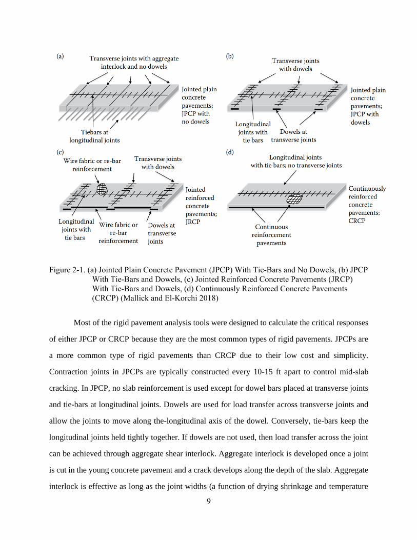
Figure 2-1. (a) Jointed Plain Concrete Pavement (JPCP) With Tie-Bars and No Dowels, (b) JPCP

With Tie-Bars and Dowels, (c) Jointed Reinforced Concrete Pavements (JRCP)

With Tie-Bars and Dowels, (d) Continuously Reinforced Concrete Pavements

(CRCP) (Mallick and El-Korchi 2018)

Most of the rigid pavement analysis tools were designed to calculate the critical responses

of either JPCP or CRCP because they are the most common types of rigid pavements. JPCPs are

a more common type of rigid pavements than CRCP due to their low cost and simplicity.

Contraction joints in JPCPs are typically constructed every 10-15 ft apart to control mid-slab

cracking. In JPCP, no slab reinforcement is used except for dowel bars placed at transverse joints

and tie-bars at longitudinal joints. Dowels are used for load transfer across transverse joints and

allow the joints to move along the-longitudinal axis of the dowel. Conversely, tie-bars keep the

longitudinal joints held tightly together. If dowels are not used, then load transfer across the joint

can be achieved through aggregate shear interlock. Aggregate interlock is developed once a joint

is cut in the young concrete pavement and a crack develops along the depth of the slab. Aggregate

interlock is effective as long as the joint widths (a function of drying shrinkage and temperature

10

effects) remain narrow. Repeated heavy loads across the transverse joint can cause the aggregate

bond to wear down along the crack wall, rendering the aggregate shear bond ineffective, resulting

in faulting, a bumpy ride, and, in poor support conditions, to joint failure.

CRCPs are heavily reinforced concrete slabs with no contraction joints. The characteristic

cracking pattern consists of cracks typically spaced every 2.0–8.0 ft. They are held tightly together

by reinforcing steel, allowing for aggregate interlock and shear transfer. If this aggregate shear

interlock is not maintained and compromised, then punchout failure at the pavement edge occurs

(especially if tied shoulders or stabilized foundation are not utilized), which is a typical distress in

CRCP. The amount of reinforcing steel used in the longitudinal direction is typically 0.6%–0.8%

of the cross–sectional area of the concrete, with less being used as temperature steel and support

of longitudinal steel in the transverse direction. The cost of CRCP is much higher than that of JPCP

or JRCP because of the heavy reinforcing steel used. However, CRCPs may prove cost-effective

in high-traffic-volume roadways due to their better long-term performance compared to the other

types of concrete pavements (Mallick and El-Korchi 2018).

Structural analysis and design of pavements is based on the concept of estimating and

limiting stresses and deformations to prevent excessive damage and deterioration of pavements.

Overstressed rigid pavements due to traffic loads and environmental effects will result in pavement

distress such as fatigue cracking, faulting, pumping, punchouts, and curling and warping. The

objective of pavement design is to recommend a pavement structure and configuration, including

slab thickness, slab length, mix design, reinforcement requirements, joint details, and foundation

support.

2.2. Rigid Pavement Analysis Techniques and Tools

Traditionally, for analysis of stresses and deflections in rigid pavements, a simplified

idealization of the concrete pavement as a rigid slab resting on a spring-like foundation was

employed. The slab is much stiffer than the supporting base or foundation material, and therefore

carries a significant portion of induced stresses. The load-carrying mechanism in concrete

11

pavement is similar to beam action, although a concrete slab is much wider than the beam and

should be considered as a plate. The supporting layers of rigid pavement slabs are typically

simplified as a Winkler or liquid foundation, which is a conceptual model that considers the

foundation as a series of closely-spaced, isolated vertical springs. In recent decades, finite element

method (FEM) facilitated analyzing complex concrete pavement structures (including joints, load

transfer devices, voids, non-homogeneous materials) and producing accurate and more reliable

solutions over shorter period of time.

CONCRETE SLAB

The first idealization of a rigid pavement system was introduced by Westergaard in the

1920’s. He represented it as a case of slab-on-grade (Westergaard 1926). In that case, the rigid

pavement was modeled as a thin plate resting on an infinite number of independent springs. The

stiffness of those independent springs, with constant value, characterized the subgrade rigidity in

Westergaard’s model. The magnitude of spring stiffness was represented as the modulus of

subgrade reaction with the unit of force per area per unit deflection. When the slab is loaded

vertically down, the springs tend to push back; when the environment-related loads are pulling up

on the slab, the springs tend to pull down toward the foundation. This behavior will result in tensile

(or compressive) bending stress at the bottom (or top) of the concrete slab. This induced stress will

be controlled in design by a number of factors such as restrained temperature and moisture

deformation, externally applied loads, volume changes of the supporting material and frost action,

continuity of subgrade support through plastic deformation, or materials loss due to pumping

action.

Simple and approximate closed-form solutions and analytical models have been developed

through making simplification assumptions. With the assumption of modeling the concrete slab

by an infinite thin plate resting on an elastic foundation (a set of axial springs), the moment due to

bending in x and y directions is given by the following equation:

12

3 2 2

2 2 212(1 )xx

EhM

x y

= +

− (2-1)

where E , , and h are the elastic modulus, Poisson’s ratio, and thickness of the slab,

respectively, and denotes the deflection of the springs.

The stiffness term in Eq. (2-1) was used by Westergaard (1927) to derive the radius of

relative stiffness , which is used in many of the stress and deflection equations of rigid

pavements.

3

4212(1 )

Eh

k=

− (2-2)

where k is the modulus of subgrade reaction.

By utilizing the parameter in the analytical solution, the relationships for the calculation

of stress and deflection in slabs due to traffic and temperature loading have been developed, that

are discussed in more details in Chapter 5.

Westergaard’s initial analytical modeling had been adopted as a promising method for

reliable design and was used as a design basis for new analysis tools. Westergaard extended his

procedure to calculate stresses and deflections in rigid pavements due to interior, edge and corner

loads. Although Westergaard’s procedure had reached a certain level of maturity in idealization of

rigid pavements, thereafter, several investigations were conducted to improve its model. The poor

assumption regarding the modeling of thin slab layer and foundation as well as the restricted

capabilities in considering tire loading position, thermal loads, and modeling load transfer devices

were the main drawbacks of the Westergaard’s method. Furthermore, using the k-value does not

allow the engineer to analyze the impact of heavy loads or weak soils on the stresses and strains

in the foundation layers.

JOINTS

Joints are often served to relief stresses and control cracking. In JPCP, load transfer devices

(dowels, tie-bars) or mechanisms (aggregate interlock) are used in both the longitudinal joints and

13

transverse joints to facilitate movements and transfer load caused by traffic and environmental

effect from one slab to adjacent slab. In JRCP, dowels are used at the transverse contraction joints

and the reinforcement controls the cracks caused by temperature and moisture effects. The

subsequent benefit of using load transfer devices are to prevent faulting, reduce slab deflections,

control mid-slab cracking, reduce pumping and bending stresses in slabs due to loss of base support

and finally provide a smooth, safe and comfortable ride.

Figure 2-2 shows the application of tie-bars and dowels as well as the mechanism of

developing stress in dowels under applied load. Top estimate the stress in dowels, an analytical

solution was proposed by Friberg (1940). This solution uses the original solution by Timoshenko

because it assumes the dowel to be a beam and the concrete to be a Winkler foundation. The

maximum deformation of concrete under the dowel shown by 0y in Figure 2-2, can be expressed

as:

0 3

(2 )

4

t

d d

P zy

E I

+= (2-3)

where tP is the load applied on the dowel, is the relative stiffness of the dowel embedded

in concrete, z is the joint width, dE and dI are the Young’s modulus and moment of inertia of

the dowel, respectively. dI and are defined as follows:

41

64dI d= (2-4)

4

4 d d

Kd

E I = (2-5)

where K is the modulus of dowel support, and d is the diameter of the dowel.

Therefore, the bearing stress on a dowel can be calculated as:

0 3

(2 )

4

tb

d d

KP zKy

E I

+= = (2-6)

The finite element expressions of the load transfer device modeling are presented in

Chapter 3.

14

Tie-bars

Dowels

Figure 2-2. Application of Dowels and Tie-Bars, Dowel Deformation Under Load

(pavementinteractive.org)

SUPPORTING LAYERS

The idealization of concrete pavement supporting layers was performed using different

foundation models such as Winkler, Boussinesq, Vlasov, Kerr, Pasternak, and ZSS foundation

(Tayabji and Colley 1986), Khazanovich et al. 2000, Huang 2004, Carrasco et al. 2011). Winkler

model or dense liquid foundation considers the foundation layer as vertical springs independent of

the displacement or pressure produced by the neighboring nodes. The vertical pressure produced

on the Winkler foundation surface, ( , )q x y is proportional to the vertical deflection ( , )w x y with

a constant of spring axial stiffness (K):

( , ) K ( )q x y w x, y= (2-7)

where K Ak= in which k is the Winkler parameter and A is the associated surface area.

15

As the actual soil is continuous, it is capable of providing shear interaction. Winkler’s

idealization of subgrade does not have any mechanism to provide an interaction between adjacent

springs or the so-called shear-interaction. This deficiency of the Winkler idealization is improved

by modeling the subgrade as a two-parameter medium, such as Vlasov model, which provides

shear interaction between individual spring elements. The parameters in Vlasov model to

characterize the normal and shear stiffnesses are obtained from soil elastic properties and layer

dimensions. However, an iterative procedure is required to estimate these parameters (Vallabhan

and Das 1989).

Elastic solid foundations are better representations of the soil behavior compared to spring

foundations because it considers a continuous surface deflection. Boussinesq model is one of the

well-known solid foundations for which the following solution was developed for the deflection

of point j due to a point load applied iP at i , ijw (Pickett et al. 1952):

2

,

(1 )i sij

s i j

Pw

E r

−= (2-8)

where sE and s are the Young’s modulus and Poisson’s ratio of the soil and ,i jr is the

distance between points i and j .

The most recent types of foundation models are the three-dimensional solid elements that

have been recently implemented in several numerical analysis as well as in RPAS program.

TRAFFIC LOADING

The load applied on the pavement surface due to traffic is considered in the design using

truck load distribution in terms of factors such as average annual daily traffic (AADT), growth

factor, lane distribution, and directional distribution. In AASHTO 1993, equivalent single-axle

load (ESAL) was used as an indicator of traffic flow. MEPDG considers the actual traffic load

spectra that will be projected over the period of service life of pavement.

For analysis purposes, the tire load is modeled from a simplified single circular tire print

to the full tire configurations with a rectangular tire print. The latter is used in RPAS. Although

the scanning of tire pressure and tire prints showed a higher pressure at the center of tire and a

16

combined shape of circle and rectangle, a uniform distribution of each tire pressure is assumed in

numerical modeling.

ENVIRONMENTAL LOADING

The major factors considered as the environmental load on pavements are the thermal

effects due to air temperature (and convection) and the moisture intrusion. The former causes

thermal curling while the latter induces warping. These two types of deformation in slab produce

bending stresses due to internal and external restraints. Several researchers (Westergaard 1927,

Bradbury 1938, Choubane and Tia 1992, Mohamed and Hansen 1996) investigated the effect of

temperature on the pavement responses. However, the actual modeling of thermal curling requires

taking a non-linear temperature profile within the slab and the concrete built-in curling into account

(Rao and Roesler, 2005, Hansen et al. 2006). Further explanations on the theoretical solutions and

the procedure of taking environmental loads into account for pavement analysis are given in

Chapter 3.

In general, mathematical modeling of the stress state of a concrete slab on a supporting

foundation layer system is very complex due to variation in materials, non-linear behavior,

changing moisture and temperature conditions, changing support conditions, and complex

interactions between components. Several computer modeling tools have been developed that will

incorporate one or more of the above components. A list of these computer programs and their

advantages or disadvantages will be presented later in this section.

FINITE ELEMENT MODELING

Traditional available analytical solutions may not realistically account for complex loads,

mixed boundary conditions, and arbitrary geometry. The advance of computer algorithms led to

the development of rigid pavement analysis software that consider more complexities in the

modeling procedure. Given the complexity of all the parameters that influence the state of stress

in a rigid pavement, finite element methods are being used to determine the response of rigid

pavements such as stresses, strains, and deflections using a mechanistic approach. Extensive

17

research has been devoted to the development of FE-based analysis tool to predict the behavior of

rigid pavements. A number of these tools were generally developed to analyze the stiffness of the

slabs on liquid or solid elastic foundation (Cheung and Zinkiewicz 1965), while others are being

particularly applied to the analysis of jointed slabs on elastic solids, listed in the following sections.

although general-purpose finite element packages, such as ABAQUS and ANSYS, have powerful

ability to handle with complex problems, they can be difficult to learn and use effectively, model

generation can be time-consuming, simulation times can be long in the case of 3D analysis, and

extracting results of interest can be difficult.

Some of the programs developed specifically for rigid pavements using finite element

method include ILLI-SLAB (Tabatabie and Barenberg 1980), WESLIQID (Chou 1981), JSLAB

(Tayabji and Colley 1986), KOLA (Kok 1990), FEACONS-IV (Choubane and Tia 1992),

KENSLAB (Huang 1993), ISLAB (Khazanovich et al. 2000), and EVERFE (Davids et al., 1998).

Most of these programs can analyze multi-wheel loading of one- or two-layered medium thick

plates resting on a Winkler or liquid foundation or an elastic solid. Some of the listed programs in

this section were used for bench-marking purposes and will be discussed in further detail in

Chapter 5.

WESLIQUID

Huang and Wang (1974) used the FE method for the analysis of jointed slabs on liquid

foundations, later extended by Huang for solid foundations. This research resulted in the

development of the WESLIQUD program by Chou (1981) that facilitated calculating stresses and

deflections in PCC slab and the subgrade with or without joints and cracks.

ILLI-SLAB

Firstly developed at the University of Illinois (Tabatabaie and Barenberg 1980), ILLI-

SLAB was an FE program written in FORTRAN® for the analysis of rigid pavement slabs

discretized into rectangular four-node elements with three degrees of freedom (DOF) per node.

PCC layer was modeled based on classical medium-thick elastic plate theory. Winkler foundation,

18

modeled as vertical spring elements, was the initial form of modeling underlying layers in ILLI-

SLAB and then elastic solid foundation has been added. ILLI-SLAB is capable of the analysis of

PCC layers as classical medium-thick elastic plates, taking into consideration a temperature

difference between the top and the bottom of the slab, mechanical load transfer through aggregate

interlock, dowels, or a combination of them at the joints between slabs, and bonded or unbonded

base condition (by assuming strain compatibility and neglecting shear stress at the interface,

respectively).

ISLAB

To eliminate some of the limitations of ILLI-SLAB by introducing semi-infinite elements

in horizontal dimensions, Khazanovich (1994) developed ILSL2 that was capable of considering

the effects of subgrade deformation under slab edges using Totsky model. This program offered a

variety of subgrade model options such as the Pasternak model, Kerr model and ZSS model

(Khazanovich and Ioannides 1994). Khazanovich et al. (2000) at the ERES Division of Applied

Research Associates improved ILSL2 by development of ISLAB2000 to overcome finite element

modeling limitations, enable curling analysis of slabs (and allowing slab and subgrade separation),

and obtain the pavement responses due to temperature, traffic, and construction loading.

JSLAB

First version of JSLAB was developed by Tayabji and Colley (1986) based on an early

version of ILLI-SLAB incorporating the Portland Cement Association’s (PCA’s) thickness design

procedure to compute the critical stresses and deflections in JPCP, JRCP, and CRCP under

different loading conditions. Several limitations of this program such as neglecting the self-

weights, two-execution stage for thermal analysis, limited number of slabs for curling analysis,

not finding the location and value of the maximum stress, and incapability to calculate the subgrade

stress have been eliminated in JSLAB92 by verification of the program by conducting a

comparison with other numerical and theoretical solutions (e.g., BISAR, FAA's H5l). However,

the program has been revised in JSLAB 2004 to incorporate six subgrade models (spring, Winkler,

19

Boussinesq, Vlasov, Kerr, and ZSS foundation), partial contact in slab/base interface,

nonuniformly spaced circular or noncircular dowels in joints, warping effects due to moisture, a

linear temperature and moisture distribution within a single layer pavement system, and perform

the time history analysis under moving loads at specified locations.

EVERFE

This 3D finite element analysis tool was developed by the collaboration of University of

Washington and WSDOT to present a program capable of capturing detailed local response, on

which 2D programs are limited. The program is also capable of modeling multiple slabs (up to

nine slabs), extended shoulder, dowels (including mislocation or looseness) and tie-bars, load

configurations, linear or non-linear aggregate interlock shear transfer at the skewed or normal

joints, the contact between the slab and up to three bonded and/or unbonded base layers, and non-

linear modeling of thermal gradient (Davids et al. 1998). Even though the utilized modeling has

been experimentally verified and was improved in later versions (Davids et al. 2003), it has still

limitations on the subgrade modeling by a dense liquid (Winkler) model and axle loading within

the slab length.

2.3. Model Validation Process

Once the best computer program for the analysis of rigid pavement has been developed,

the validation process of this tool will be initiated. However, two major steps preceding the model

validation are verification and calibration.

Verification is defined as “the process of determining that a computational model

accurately represents the underlying mathematical model and its solution” (Schwer 2006).

Verification consists of bench-marking (or code verification) and calculation verification. Bench-

marking is defined as establishing confidence that the mathematical model and solution algorithms

are working correctly. Comparison of computer code outputs with analytical solutions is the most

popular bench-marking technique, which requires manufactured solutions to expand the number

and complexity of analytical solutions and even comparing the results with the existing modeling

20

tools. Calculation verification is associated with establishing confidence that the discrete solution

of the mathematical model is accurate. It includes estimating the errors in the numerical solution

due to discretization, comparing numerical solutions at more meshes with increasing mesh

resolution to determine the rate of solution convergence.

Calibration (or model parameter estimation) is defined as “the process of adjusting physical

modeling parameters in the computational model to improve agreement with experimental data”

(Schwer 2006, Kennedy and O’Hagan 2001). A computer model will have a number of context-

specific inputs that define a particular situation in which the model is to be used. When the values

of one or more of these context-specific inputs are unknown, experimentation is used to learn about

them. In current practice, model calibration consists of searching for a set of values of the unknown

inputs such that the measured data fit as closely as possible to the corresponding outputs of the

model. These values are considered as estimates of the context-specific inputs, and the model is

then used to estimate the behavior of the process in this context by setting these inputs to their

estimates. To achieve the highest possible agreement between the results of experimentations and

those from simulations, a multi-objective optimization process will be implemented to minimize

the errors while adjusting the inputs.

Generally, computer (or mathematical) model validation is defined as the “process of

determining the degree to which a computer model is an accurate representation (within some

tolerance) of the real world from the perspective of the intended model applications.” (U.S. DOE

2000, AIAA 1998). This validation is accomplished through the comparison of estimation from a

model to experimental results. The main reasons of model validation include the need to replace

experimentation with model predictions with some degree of accuracy, necessity to prove the

reliability of a structure under a broad range of operating conditions or environments (which is

very expensive to be done in the field), and to assure that the design modifications yield acceptable

system behavior.

Before a well-structured validation comparison can be performed, there are several

decisions that must be made and some criteria that must be defined:

21

1. Specify the model use and purpose: Comparison of the current model relative to the

ultimate system of interest (the physical system and its associated environment) to a

particular level of accuracy.

2. Specify the conceptual model: The conceptual model of the physical system is the set of

assumptions and descriptions of physical processes representing the behavior of the

system of interest, and from which the mathematical model and the pre-validation

experiments can be constructed.

3. Specify pre-validation experiments: These experiments must be specified early in the

planning process in order to develop the details of the computational model, which

contains the appropriate components to be considered.

4. Specify the mathematical model (mathematical equations, boundary conditions,

excitations, initial conditions, etc.).

5. Specify the computational model (the numerical implementation of the mathematical

model in the form of numerical discretization, solution algorithm, and convergence

criteria): To assure that the features of the mathematical model are captured with

sufficient accuracy to guarantee positive validation results.

6. Specify the physical system response measures of interest: The response measures of

interest are the quantities that are functions of system behavior or response to be used in

the comparison of model predictions to experimental system predictions, which can be

inferred from excitations and responses of the experiment and the model.

7. Specify validation metrics: The precise mathematical means for comparing model

predicted response measures to response measures computed from experimental

responses (e.g., statistical parameters such as RMSE).

8. Specify the domain of comparison: The region of environment space and model and

physical system parameter space within which experiment responses will be measured

and model predictions will be made. The results of the comparison are normally specified

22

only for that domain unless a careful extrapolation implies that the results are useful over

an extended domain.

9. Specify adequacy or accuracy criteria (validation requirements): Adequacy and accuracy

criteria define the values that validation metrics must assume in order for the model to

be judged valid.

After the validation is performed, two actions can be taken regarding the use of the

computer model. If the model is valid, it can be used as the basis for development of the model in

the next step of the hierarchy (in modular programming of the computer code) or it can be used to

make predictions of structural response within the domain of comparison. If the mode is not valid,

the source of errors can be found in the following categories:

• Additional, un-modeled sources of randomness exist: Identify the additional sources of

randomness, perform calibration testing, specify the probability models for the additional

sources of randomness, re-validate.

• Insufficient physics included in the model: Augment the model physics (such as non-

linear behavior in structural response), perform calibration testing to identify the

parameters of the physics model, re-validate.

• Inadequate data were collected during calibration and/or validation experiments

(Sensitivity of the validation conclusion to the amount of data): Collection of additional

data and improvement of model parameters, followed by revalidation.

• Form of the response measure of interest may be too difficult for the model to predict

correctly: Modify the response measures and re-validate (not simply change from one

response measure to another).

• The adequacy or accuracy criteria used during the validation comparisons are too stringent

for the model to satisfy (modelers, experimentalists, and validation analysts may have

been too optimistic about the potential for model accuracy): Modify the adequacy criteria

and re-validate.

23

2.4. Optimization Techniques

To minimize the error in the predictions from a computer model with respect to the

experimental data for verification, calibration and validation purposes, several mathematical

optimization techniques are available. In mathematics, conventional optimization problems are

usually stated in terms of minimization. An optimization (minimization) problem can be

represented in the following way:

Given a function :f A→ (from some set A to real numbers), find an element 0 Ax such that

0( ) f( )f x x for all Ax .

Typically, A is some subset of the Euclidean space ℝn, often specified by a set of

constraints, equalities or inequalities that the members of A have to satisfy. The domain A of f is

called the search space or the choice set, while the elements of A are called candidate solutions or

feasible solutions. The function f is called an objective function (or loss function, cost function

energy function. A feasible solution that minimizes (or maximizes) the objective function is called

an optimal solution. In Machine Learning, it is always necessary to continuously evaluate the

quality of a data model by using a cost function where a minimum implies a set of possibly optimal

parameters with an optimal (lowest) error (Miettinen 2012, Hwang and Masud 2012).

MULTI-OBJECTIVE OPTIMIZATION

Many real-world practical engineering and scientific application problems involve

simultaneous optimization of several competing objectives. To these problems, there is often no

single optimal solution, but rather a set of alternative solutions. These solutions are considered to

be the best because no other solutions in the decision space (feasible solution space) are superior

to them when considering all the target objectives. One objective is improved always at the expense

of other objectives at the same time for these multi-objective optimization problems.

As such, a multi-objective optimization problem (MOOP) is an optimization problem that

involves multiple objective functions. Adding more than one objective to an optimization problem

24

adds complexity. For example, to optimize a structural design, one would desire a design that is

both light and rigid. When two objectives conflict, a trade-off must be created. There may be one

lightest design, one stiffest design, and an infinite number of designs that are some compromise of

weight and rigidity.

To avoid long computational time, stochastic approaches seem to be particularly suitable

in solving MOOPs. Evolutionary algorithms (EAs), which are the meta-stochastic methods that

simulate the process of natural biological evolution, have been verified to be an effective and

efficient tool for MOOPs as they have the capability to process a set of solutions in parallel and

explore big search space in a reasonable time. Among the biological-inspired EAs, the most known

approaches are the genetic algorithms (GAs), and recently, one of the most popular pioneering

work with respect to the GAs for solving MOOPs is Pareto optimal front genetic algorithms.

OVERVIEW OF MOOPS

Generally, MOOPs contain several objectives to be minimized. Without the loss of

generality, we assume that the optimization can be described as a minimization problem with m

objectives and n variables, which in mathematical terms can be expressed as follows:

1 2Minimize : F(x) ( (X), (X),..., (X))

( ) 0, 1, 2,...,s.t.

( ) 0, 1, 2,...,

T

m

i

j

f f f

g X i k

h X j l

=

=

= =

(2-9)

where 1 2( , ,..., )nX x x x= is a solution vector, is the decision space, ( )ig X and

( )jh X are the optional inequality and equality constraints, respectively. The aim is to find a

solution vector subject to the constraints, which minimizes the objective values. However, since

the characters of these functions 1 2(X), (X),..., (X)mf f f are usually in conflict with each other,

when multi-objectives reach the optimal simultaneously, the result of which is a set of compromise

solutions, i.e. the so-called Pareto optimal set.

25

PARETO OPTIMAL SOLUTION

As previously stated, in multi-objective optimization, there does not typically exist a

feasible solution that minimizes all objective functions simultaneously. Therefore, attention is paid

to Pareto optimal solutions; that is, solutions that cannot be improved in any of the objectives

without degrading at least one of the other objectives (see Figure 2-3).

Pareto solutions are also called nondominated solutions, Pareto efficient solutions, or

noninferior solutions. To better understand this concept, the following terms must be defined:

Pareto dominate: A vector (1) (1) (1) (1)

1 2( , ,..., )nx x x x= is said to dominate another vector

(2) (2) (2) (2)

1 2( , ,..., )nx x x x= , note as (1) (2)x x if and only if:

(1) (2) (1) (2)( 1, 2,..., , ( ) ( )) ( 1, 2,..., , ( ) ( ))i i i ii k f x f x i m f x f x .

Pareto optimal: For a given multi-objective problem, a solution (1)x is the Pareto

optimal if and only if:

(2) (1) (2):x x x .

Pareto optimal set: The set P in the decision variable space consisting of all Pareto

optimality vectors:

(1) (2) (2) (1)| :P x x x x= .

Pareto optimal front: The plot of a set PF which includes the values of all objective

functions corresponding to the solution in P (Yuan et al. 2015):

1 2( ) ( ( ), ( ),.., ( )) |T

mPF F x f x f x f x x P= = .

A solution is said to be Pareto-optimal if it is not dominated by any other solutions in .

As can be seen in Figure 2-3, each of the boxed points, including points A and B, represent Pareto

optimal solutions and a set of these points is called Pareto optimal set. However, point C is not a

Pareto optimal solution because it was dominated by both points A and B. The red line connecting

the Pareto optimal solutions shows the Pareto optimal front PF.

26

Figure 2-3. Schematic View of a Pareto Optimal Front

The goal of multi-objective intelligence algorithms is to find a uniformly distributed front

PFknown from multi-objective EAs that approximates the real Pareto-optimal front PFtrue (Van

Veldhuizen and Lamont 2000).

27

3. Rigid Pavement Analysis System (RPAS)

Researchers from the University of Texas at El Paso developed the Rigid Pavement

Analysis System (RPAS) as a tool for evaluating responses of jointed concrete pavement systems

under environmental and vehicle loadings. By improving several features of the previous version

of this pavement analysis tool, namely NYSLAB (Carrasco et al. 2009), RPAS makes use of the

FE method coded in MATLAB® and was developed with the purpose of calculating pavement

responses due to any arbitrary vehicle loading configuration and temperature profile using

different foundation models.

3.1. Modeling Pavement Slab

There is no explicit limit in the number of concrete and foundation layers that can be

modeled in RPAS and no limit in the number of jointed slabs that can be included in the analysis.

Pavement slab layers are modeled as plate elements that account for the shear deformation as they

become significant for relatively thick plates. When two or more pavement slab layers are

modeled, the interface between them can be considered either bonded or unbonded. In bonded

slabs, shear stresses can be transferred through their interface and no sliding or separation can

occur between them. On the other hand, unbonded slabs can separate and move relative to each

other and shear tractions, due to friction, can be produced in their interface. To model the contact

between two unbonded slabs, in addition to an isoparametric 18-node interface element (Zokaei-

Ashtiani et al. 2014), a new non-linear contact and friction model was introduced which will be

explained below.

Bonded pavement slabs are modeled as composite laminated plates in RPAS using the first

order shear deformation theory (FSDT) or laminated plate theory. The laminated domain is

discretized using nine-node isoparametric quadrilateral elements (Figure 1a), each element having

five degrees of freedom (DOF) per node: two in-plane displacements in the x and y directions (

xU , yU ), vertical deflection in z ( zU ), and two rotations about y and x axes ( x , y ) (Figure

28

1b). These dependent variables ( xU , yU , zU , x , y ) are approximated using the Lagrange

interpolation function (Zokaei-Ashtiani et al. 2014).

(a) (b)

Figure 3-1. (a) Five Degrees of Freedom in the 9-Node Quadrilateral Element Used to Model

Bonded Pavements (b) Kinematics of Two Plates in Contact* (Zokaei-Ashtiani et

al. 2014)

* xU , yU , zU , x , y are the five degrees of freedom, and are the local coordinates, xV and

yV are

the relative displacement vectors, G is the gap between the plates caused by deformation under traffic or thermal

loading, superscripts (t) and (b) represent the top and the bottom surface of the interface elements, respectively.

FINITE ELEMENT MODELING OF THE SLAB

The first order shear deformation theory (FSDT) or Mindlin laminated plate theory as an

extension of the Mindlin plate theory to composite laminates was used in RPAS to model the slabs.

This model is capable of capturing shear deformations, which are important in the modeling of

thick slabs. Considering a laminated plate with total thickness of h composed of N orthotropic

layer which are completely bonded together (Figure 3-1), the position (u,v,w) of each arbitrary

point in the laminate after deformation can be expressed as

),(),(),,( 0 yxzyxuzyxu x+=

29

),(),(),,( 0 yxzyxvzyxv y+= (3-1)

),(),,( 0 yxwzyxw =

where u0, v0, w0 are the displacements of that arbitrary point in the laminate mid-plane (z

=0), and x, y are the rotations about the y and x axes, respectively. Therefore, the strain tensor

can be expressed as (Reddy 2004):

[

𝜖𝑥𝑥𝜖𝑦𝑦𝛾𝑥𝑦

] = [

𝜖0𝑥𝑥𝜖0𝑦𝑦

𝛾0𝑥𝑦

] + [

𝜖1𝑥𝑥𝜖1𝑦𝑦

𝛾1𝑥𝑦

] =

[

𝜕𝑢0𝜕𝑥𝜕𝑣0𝜕𝑦

𝜕𝑢0𝜕𝑦

+𝜕𝑣0𝜕𝑥 ]

+ 𝑧

[

𝜕∅𝑥𝜕𝑥𝜕∅𝑦

𝜕𝑦

𝜕∅𝑥𝜕𝑦

+𝜕∅𝑦

𝜕𝑥 ]

(3-2)

[𝛾𝑦𝑧𝛾𝑥𝑧] =

[ 𝜕𝑤0𝜕𝑦

+ ∅𝑦

𝜕𝑤0𝜕𝑥

+ ∅𝑥]

(3-3)

where xx, yy, xy are the in-plane strains which are linear through the laminate thickness, and yz,

xz are out of plane shear strains which are constant through the thickness.

By applying the principle of virtual displacement into the governing equation of FSDT, the

equilibrium equations can be derived as follows:

0=

+

y

N

x

N xyxx

(3-3)

0=

+

y

N

x

N yyxy

(3-4)

0=+

+

q

y

V

x

V yx (3-5)

0=

+

+−

y

M

x

MV

xyxxx (3-6)

0=

+

+−

y

M

x

MV

yyxy

y (3-7)

30

where, Nxx, Nyy, Nxy denote in-plane force resultants, Mxx, Myy, and Mxy denote Moment resultants,

Vx, Vy are out-of-plane shear force resultants in the laminate, and q is the distributed load applied

to the laminate.

Using laminate constitutive equation for N-layer of lamina with orthotropic material and

using Hooke’s law, the resultant forces and moments in a matrix form can be expressed as the

following constitutive equations:

+

=

xy

yy

xx

xy

yy

xx

xy

yy

xx

BBB

BBB

BBB

AAA

AAA

AAA

N

N

N

1

1

1

332313

232212

131211

0

0

0

332313

232212

131211

(3-8)

+

=

xy

yy

xx

xy

yy

xx

xy

yy

xx

DDD

DDD

DDD

BBB

BBB

BBB

M

M

M

1

1

1

332313

232212

131211

0

0

0

332313

232212

131211

(3-9)

11 12

21 22

x xz

y yz

V As Ask

V As As

=

(3-10)

where, Aij are called extensional stiffness, Dij are bending stiffness, Bij are bending-extensional

coupling stiffness, and Asij are shear stiffness, which are defined in terms of stiffness and thickness

of each layer.

By applying the principle of virtual displacement and expanding the equilibrium equations,

the finite element model of the first-order shear deformation theory for linear and static case will

be obtained as:

[𝐾𝑒]{𝑈𝑒} = {𝐹𝑒}

[ [𝐾11] [𝐾12] [𝐾13] [𝐾14] [𝐾15]

[𝐾12]𝑇 [𝐾22] [𝐾23] [𝐾24] [𝐾25]

[𝐾13]𝑇 [𝐾23]𝑇 [𝐾33] [𝐾34] [𝐾35]

[𝐾14]𝑇 [𝐾24]𝑇 [𝐾11]𝑇 [𝐾44] [𝐾45]

[𝐾15]𝑇 [𝐾25]𝑇 [𝐾35]𝑇 [𝐾45]𝑇 [𝐾55]]

{

𝑢𝑒

𝑣𝑒

𝑤𝑒

𝜙𝑥𝑒

𝜙𝑥𝑒}

=

{

𝐹1 − 𝐹𝑇

1

𝐹2 − 𝐹𝑇2

𝐹3

𝐹4 − 𝐹𝑇4

𝐹5 − 𝐹𝑇5}

(3-11)

31

where the elements of the sub-matrices [𝐾𝛼𝛽] for 𝛼 = 1, 2, … , 5 and their numerical integral

expressions are defined using the Gauss quadrature method (Zokaei-Ashtiani 2014). These

elements are expressed as a function of extensional stiffness, bending stiffness, and bending-

extensional coupling stiffness as defined above.

3.2. Modeling Temperature in the Slab

Uniform temperature-change, within the depth of the pavement slabs during daily

temperature variation, can cause thermal expansion and contraction in concrete slabs. In RPAS,

the impact of horizontal interaction between adjacent jointed slabs, due to thermal expansion in

producing additional compressive stress, is considered in the mathematical model. RPAS can

simulate a non-linear temperature profile throughout the slab thickness, allowing for the modeling

of partial contact between the slab and foundation due to curling (Zokaei-Ashtiani et al. 2014).

The pavement temperature measured at various depths ( z =depth from mid-plane of the slab) and

times of day can be curve-fitted to a three-dimensional polynomial as follows:

2 3

0 1 2 3T a a z a z a z = + + + (3-12)

where 0a contributes to the expansion or contraction of the neutral plane of the concrete

slab, 1a is associated with the linear temperature difference between the top and bottom of slab,

2a and 3a affect the non-linear temperature profile that produce internal stresses in the PCC slab

regardless of its external constraints.

However, an accurate modeling of the effect of thermal loads on the concrete pavement

requires considering the non-linear built-in (set) temperature profile ( )SetT z (also called the zero-

stress temperature profile in AASHTO MEPDG) in addition to the non-uniform temperature

profile due to temperature change ( )T z (Mohamed and Hansen 1997, Chen et al. 2014). Built-in

temperature profile is developed in the newly constructed slabs during concrete setting and its

32

magnitude depends on the time of placement, curing quality, the ambient conditions and the

mixture properties. Thus, the effective temperature profile should be defined as

( ) ( )SetT T z T z = − . This effective temperature profile will also be non-linear and thus in addition

to the stress caused by the linear component of temperature profile, ( )Th linear , a residual thermal

stress distribution, ( )Th res must be calculated. RPAS uses the finite element formulation to

calculate this residual stress; however, an analytical solution can be obtained using Eq. (3-13). To

derive this analytical solution, the slab was modeled as a plate with linear elastic and isotropic

material behavior that is assumed to be totally restrained against deformation. By applying

Hooke’s law and considering the stress state in two dimensions, Eq. (3-13) can be obtained:

3

12( ) ( ) ( )

1

T TTh res

M NEz z

h h

= − + + −

(3-13)

where E , , and h are Young’s modulus, Poisson’s ratio, and thickness of the slab,

respectively, z is the distance from slab mid-depth, and the effect of built-in temperature ( ( )SetT z

) is taken into account in the calculation of ( ) z T = ( =concrete’s coefficient of thermal

expansion) as well as in the calculation of TM and TN , which are the constants corresponding to

bending moment and normal force at the slab mid-depth.

FINITE ELEMENT MODELING OF THE THERMAL LOADS

The truck load in RPAS is modeled as equivalent series of point loads. However, the

resultant thermal forces and thermal moments for each laminated plate (bonded pavement slabs)

can be expressed as:

=

+

=N

k

Z

Z

kk

T

k

k

dzTQN1

)()(1

(3-14)

=

+

=N

k

Z

Z

kk

T

k

k

dzzTQM1

)()(1

(3-15)

33

where Q is the stiffness components which is the function of modulus of elasticity and Poisson’s

ratio and α is the coefficient of thermal expansion for each layer in the N-layer laminate,

𝑄𝑖𝑗𝑘 =

𝐸(𝑘)

1 − 𝜈(𝑘)2

[ 1 𝜈(𝑘) 0𝜈(𝑘) 1 0

0 01 − 𝜈(𝑘)

2 ] (3-16)

𝛼(𝑘) = [𝛼𝛼0] (3-17)

The total laminate constitutive equations become,

{{𝑁}

{𝑀}} = [

[𝐴] [𝐵]

[𝐵] [𝐷]] {{𝜀0}

{𝜀1}} − {

{𝑁𝑇}

{𝑀𝑇}} (3-18)

where, the matrices N and M are the total resultant force and moment in the laminate defined by

Zokaei-Ashtiani (2014). In the finite element model of the laminate, the contribution of thermal

loads is added to the force vector (Eq. 3-11) as,

=

sT

iT dxdyN

x

NF 1

(3-19)

=

sT

i

T dxdyNy

NF 2

(3-20)

=

sT

i

T dxdyMx

NF 4

(3-21)

=

sT

iT dxdyM

y

NF 5

(3-22)

where, Ni is the interpolation function (Zokaei-Ashtiani 2014).

34

3.3. Modeling Load Transfer Devices

Adjacent slabs in a jointed concrete pavement system in RPAS can be connected with

dowels, tie-bars and aggregate or key interlock, or a combination of those load transfer devices

through their joints. Dowels and tie-bars are used in the transverse and longitudinal joints,

respectively, and can be placed in uniform or non-uniform intervals.

FINITE ELEMENT MODELING OF THE DOWELS AND TIE-BARS

Beam elements were used to model dowels and tie-bars in RPAS. For this reason, a Timoshenko

beam is used for the modeling of short-beam (thick- beam) elements. Thus, the stiffness matrix of

dowels and tie-bars account for two degrees of freedom. However, the total stiffness matrix of

those elements should include the components corresponding to all the degrees of freedom

considered in the modeling of pavement slabs. Therefore, the total stiffness matrix for dowels and

tie-bars considering five degrees of freedom per node of a beam element are derived as:

[𝐾𝑑𝑜𝑤𝑒𝑙]

=

[ 0 0 0 0 0 0 0 0 0 00 𝐷 0 0 0 0 −𝐷 0 0 00 0 𝐷 6𝐿𝐶 0 0 0 −𝐷 6𝐿𝐶 00 0 6𝐿𝐶 (4 + ∅)𝐶𝐿2 0 0 0 −6𝐿𝐶 (2 − ∅)𝐶𝐿2 00 0 0 0 0 0 0 0 0 00 0 0 0 0 0 0 0 0 00 −𝐷 0 0 0 0 𝐷 0 0 00 0 −𝐷 −6𝐿𝐶 0 0 0 𝐷 −6𝐿𝐶 00 0 6𝐿𝐶 (2 − ∅)𝐶𝐿2 0 0 0 −6𝐿𝐶 (4 + ∅)𝐶𝐿2 00 0 0 0 0 0 0 0 0 0]

(𝑢)𝐿(𝑣)𝐿(𝑤)𝐿(∅𝑥)𝐿(∅𝑦)𝐿(𝑢)𝑅(𝑣)𝑅(𝑤)𝑅(∅𝑥)𝑅(∅𝑦)𝑅

(3-23)

35

[𝐾𝑡𝑖𝑒]

=

[ 𝐷 0 0 0 0 −𝐷 0 0 0 00 𝐴𝑡𝐸𝑡/𝐿 0 0 0 0 −𝐴𝑡𝐸𝑡/𝐿 0 0 00 0 𝐷 −6𝐿𝐶 0 0 0 −𝐷 −6𝐿𝐶 00 0 −6𝐿𝐶 (4 + ∅)𝐶𝐿2 0 0 0 6𝐿𝐶 (2 − ∅)𝐶𝐿2 00 0 0 0 0 0 0 0 0 0−𝐷 0 0 0 0 𝐷 0 0 0 00 −𝐴𝑡𝐸𝑡/𝐿 0 0 0 0 𝐴𝑡𝐸𝑡/𝐿 0 0 00 0 −𝐷 6𝐿𝐶 0 0 0 𝐷 6𝐿𝐶 00 0 −6𝐿𝐶 (2 − ∅)𝐶𝐿2 0 0 0 6𝐿𝐶 (4 + ∅)𝐶𝐿2 00 0 0 0 0 0 0 0 0 0]

(𝑢)𝐿(𝑣)𝐿(𝑤)𝐿(∅𝑥)𝐿(∅𝑦)𝐿(𝑢)𝑅(𝑣)𝑅(𝑤)𝑅(∅𝑥)𝑅(∅𝑦)𝑅

(3-24)

where L is the joint spacing, 3(1 )

LTD LTDE IC

L =

+ ( LTDE , LTDI = the elastic modulus and moment

of inertia of the load transfer devices (dowel or tie bar), respectively), and 2

24 (1+ )LTD LTD

LTD

I

A L

=

( LTD =Poisson’s ratio of the load transfer devices, LTDA =effective cross-section of the load

transfer devices), 1

1 1

12

D

DCI C

=

+

( DCI =dowel-concrete interaction parameter, equal to

1.5×106 psi/in for practical purposes), tE and tA are the elastic modulus and cross-section area of

tie bars, u , v , w are the displacements of load transfer devices in longitudinal (x), transverse (y)

and vertical (z) directions, respectively, x and y denote the rotation of the load transfer devices

in x and y directions, and the subscripts R and L show the degree of freedom on right and left end

of the load transfer devices.

3.4. Modeling the Contact between Pavement Layers

The mechanical behavior of pavement is significantly influenced by the contact properties

as well as frictional characteristics of pavement layers. Thus, an appropriate constitutive

relationship for the slab-foundation interface needs to be defined. In addition to the existing gap

element (to model the contact) and 2-D interface elements (to model both contact and friction)

36

(Carrasco et al. 2011, Zokaei-Ahtianai 2014), a new model has been implemented that associates

the normal and frictional properties of each point of contact to the relative displacement of the

corresponding nodes in two contacting surfaces (Bhatti 2006). As indicated in Figure 3-2a, the

constitutive behavior for the normal contact must satisfy consistency condition, that is the contact

force exists only if the gap between two contacting surfaces is closed i.e., either gap g or force

nF must be zero.

Therefore, the normal constraint function can be approximated by the following equation:

2

( , ) 02 2

n nn

g F g Fg F

+ − = − + =

(3-25)

where is a small positive number, controlling the smoothness of the friction function in

Figure 3-2b, which leads to a more efficient numerical convergence of the contact-friction solution

as opposed to the linear or bilinear functions such as Coulomb model.

(a) (b)

Figure 3-2. Constitutive Contact-Friction Relationship (a) Normal Contact Function (b)

Frictional Constraint Function (Bhatti 2006)

Regarding the tangential component of contact force, the frictional properties of the

surfaces and the physical condition (i.e., sticking or sliding) play important role. The frictional

37

constitutive equation in the tangential direction, which correlates the frictional tractions tF to the

tangential relative displacements v , is expressed as follows (see Figure 3-2b):

2( , ) arctan( )t

n

F vv

F

= − (3-26)

where is the coefficient of friction between the two surfaces.

The use of this non-linear model, as opposed to the commonly used 1D spring connections

between contacting nodes, allows for the proper distribution of the normal and tangential stiffness

and tractional forces for non-uniform meshes and, as a consequence, allows the for the friction and

separation between layers due to slab curling to be realistically represented.

3.5. Modeling Supporting Layers

Three different foundation models are included in RPAS to idealize the behavior of the

foundation system: Winkler, Vlasov and 3-D solid foundation (Carrasco et al. 2011, Aguirre 2020).

Both the Winkler and Vlasov foundation models consider the slab supporting layers as an infinite

set of linear elastic springs. These foundation models have been commonly used by different

modeling programs for the purpose of modeling JCP, such as ILLI-SLAB (Tabatabaie and

Barenberg 1980) and JSLAB (Tayabji and Colley 1986). To improve on the models, a 3-D solid

foundation model was developed and incorporated into RPAS. In this model, the soil is discretized

using 27-node hexahedron elements for each slab supporting layer (Figure 3-3). Compared to the

standard 8-node hexahedron element, second order elements have demonstrated to require fewer

elements for a given accuracy. This comparison will be made in the next section.

38

Figure 3-3. Numbering of the Developed Second-order 27-Node Hexahedron Element (node 27

at the Origin of ξ, η, ζ Coordinates) (Aguirre 2020)

The 3-D modeling of the foundation layer, in comparison to the use of subgrade reaction

k, uses the moduli (modulus of elasticity and Poisson’s ratio) for each supporting layer.

Furthermore, this method allows for the calculation of responses at any given depth for each

foundation layer. An extension of the foundation layers beyond the edge of the slabs was also

developed to more realistically model the edge deflections and stresses close to the pavement edge.

FINITE ELEMENT MODELING OF THE FOUNDATION ELEMENTS

The finite element expression of the Winkler and Vlasov foundation models are well

documented in Zokaei-Ashtiani (2014). This section describes the finite element modeling of the

3D foundation (Aguirre 2020). In this model, each foundation layer is discretized using 27-node

hexahedron elements. Compared to the standard 8-node hexahedron element, second order

elements have demonstrated to require fewer elements for a given accuracy. For the 27-node

element shown in Figure 3-3, there are 81 element degrees of freedom (DOF), i.e., three DOFs for

horizontal (longitudinal and transverse) and vertical translations associated with the 27 integration

points.

After defining the shape functions and arranging the terms by their DOFs, the 27-node element

strain vector can be computed by appropriate differentiation as follows:

39

(3-27)

Finally, the element stiffness matrix can be obtained by

dVT

V

k BDB= (3-28)

where D is the material property matrix and is written as follows:

1 0 0 0

1- 0 0 0

1- 0 0 0

1-20 0 0 0

2(1+ )(1-2 )D

−

E= 0

1-20 0 0 0 0

2

1-20 0 0 0 0

2

(3-29)

where E is the Young’s modulus and is the Poisson’s ratio. As will be discussed in Chapter 6,

the moduli of foundation layer will be targeted to apply the calibration factors.

40

4. Field Test Data Collection and Pre-Validation

This chapter provides an introduction of the data collected on the pavement test sections in

MnROAD and National Airfield Pavement Test Facility (NAPTF). The data processing method

was explained for different types of tests (accelerated pavement testing, truck loading, FWD and

HWD testing). A preliminary comparison of RPAS predictions of the pavement responses with

the measured responses (pre-validation) has been performed.

4.1. MnROAD

Minnesota Road Research Project (MnROAD) is a cold region pavement research facility

owned and operated by the Minnesota Department of Transportation (MnDOT). The facility is

located on westbound I-94, northwest of the Twin Cities metropolitan area, was initially

constructed between 1990 and 1993 and opened to traffic in 1994.

MNROAD DESCRIPTION

Thus far, MnROAD has four separate experimental roadway segments (Van Deusen et al.

2018):

• A 2.7-mile, two-lane, westbound I-94 Mainline (Figure 4-1a) with average traffic of

26,500 vehicles per day (13% trucks) providing approximately 750,000 flexible and

1,000,000 rigid ESALs per year.

• A 2.5-mile, two-lane closed loop Low-Volume Road (LVR) (Figure 4-1b) with the traffic

provided by an 80-kip, 5-axle, tractor/trailer combination. This traffic loading is applied

approximately 70 laps a day to the inside lane, whereas the outer lane is preserved for the

study of environmental effects.

• A 1000-foot long, two-lane roadway in the MnROAD stockpile area that is being utilized

for testing the impact of implements of husbandry (farm implements, towed vehicles to

transport agricultural machinery, tools and chemicals) on low-volume roads. This area is

used by contractors to test placement methods before proceeding to test sections.

41

• A 2.7-mile newly constructed segment (originally constructed in 1973), a series of asphalt

overlay and partial-depth spall repair test sections on the original westbound concrete

pavement lanes of I-94. This segment is used seven days per month when the traffic is

diverted from the MnROAD mainline for monitoring or construction and thus receives

about one-third cumulative ESALs of that that mainline I-94 experiences.

(a)

(b)

Figure 4-1. MnROAD NRRA Sections (a) I-94 Westbound Original and Mainline (b) Low

Volume Road (LVR) (Van Deusen et al. 2018)

Since its initial construction in 1993, MnROAD has progressed through three phases.

Phase-I (1994-2007) primarily investigated concrete and asphalt structural (thickness) designs.

Phase-II (2008-2015) focused on partnerships with government, academia, and industry, led by

42

MnDOT through the former Transportation Engineering and Road Research Alliance. Phase-III

(2016-current) has begun with the construction of eight flexible pavement sections as part of a

National Cracking Performance Test experiment with a partnership with the National Center for

Asphalt Technology (NCAT). During 2017 construction season, 35 new and unique test sections

were added to address National Road Research Alliance (NRRA) high-priority research topics,

conceived and planned by NRRA Rigid, Flexible, Preventive Maintenance, and Geotechnical team

members.

In general, MnROAD enables researchers to evaluate pavement performance under real,

physical conditions (traffic and environment), examine the interaction between factors such as

moisture, frost, traffic loading, construction, and materials through use of an extensive

instrumentation network, design customized experiments supporting specific research needs, and

develop tools and methods based on actual performance data to improve design, construction, and

maintenance of pavements.

MNROAD DATABASE

Pavement performance in MnROAD was being monitored since the initial opening to

traffic in 1994 through laboratory testing (inspection, sampling, and testing of subgrade,

bound/unbound base materials, concrete, and asphalt surface materials), static and dynamic sensor

response (for environmental measurements and load response measurements, respectively), and

field monitoring (e.g. stiffness, strength, distress measurements) over the life of each test cell.

MnROAD monitoring begins with initial measurements after construction and follows pavement

performance throughout its life. Forensic investigations are completed after each research project’s

conclusion. MnROAD database allows researchers to accurately record methodology and pertinent

information for research and design purposes (MnROAD Data Library 2019).

STATIC SENSOR RESPONSE

Static or environmental measurements in MnROAD are usually made continuously for the

life of the sensor or the cell. The time periods for data collection are most commonly 15 minutes.

43

Environmental measurements include temperature, moisture content, relative humidity, soil

pressure, pore water pressure, strain, electrical resistivity. As one of the important factors in the

analysis of stresses in concrete pavements, temperature profile data should be collected within the

slabs and combined with the effect of repeated wheel loading. Temperature sensing at MnROAD

is predominately accomplished with thermocouples but thermistors are also integrated into other

instruments. To record the temperature data within the depth of the pavement, thermocouple arrays

(trees) of varying lengths and numbers of sensors were constructed and installed in a drilled hole

at the final base grade (just prior to paving) (see Figure 4-2). Thermocouple leads are connected

to the data logger where the temperature is calculated by an internal function and stored in degrees

Celsius.

Figure 4-2. Building and Installation of Temperature Sensing Arrays (Tree) At

MnROAD

44

DYNAMIC SENSOR RESPONSE

Dynamic or load response measurements at MnROAD consist of collecting data seasonally

from pavement sensors in response to dynamic loads applied using the test vehicle to provide

uniform pavement loading. The test cells are closed to public traffic during scheduled data

collections and load response is acquired in real time. Load response measurements may include

stress, strain, displacement, pore water pressure, and accelerometer data. Dynamic strain

measurements were taken as the 18-wheel, 5-axle, tractor trailer (weighed a total of 80,000 lb or

102,000 lb) to provide a known dynamic load to test the dynamic sensor instrumentation. The truck

traveled slowly (at a speed of approximately 5 mph) forward and backward, systematically moved

laterally across the instrumented slabs containing the embedded dynamic strain sensors. This slow

speed should allow valid application of the data in future studies comparing measured load

response to static load finite element models. To monitor the location of the tires with respect to

the test slabs, a special video camera was mounted over the leading drive axle of the truck

(passenger side). Measuring strips were painted on the instrumented slabs such that the camera

captured the lateral location of the tire in the lane as it passed.

Truck driver operates the vehicle around 6 hours of driving or 80 laps a day and truck is

tracked using Real Time Kinematic (RTK) GPS-based vehicle tracking system for accurate

recording of the truck location as well as a GPS-based vehicle tracking system (VTS) to track the

location of a vehicle’s tires during load response testing. Throughout the test period, different

vehicles of heavy (102 kips) load configuration (1994-2008) in the outside lane and Minnesota

highway legal 80 kips loading configuration (1994-current) were utilized. Therefore, depending

on the year of the test, the type of the vehicle must be considered in the modeling.

Navistar Tractor with Fruehauf Trailer was used for loading during 1997 to 2011. The

weights of this tractor are depicted in Figure 4-3 and the description and trailer configuration were

similar to the Mack tractor-trailer. It has also been operated in legal and heavy load configurations.

This truck uses Michelin XDA 11R24.5 for drive tires and Michelin XZA1+ LRG 11R24.5 for

steer tires with tire pressure set to 100 psi.

45

Mack Tractor with Fruehauf Trailer was used for dynamic loading during 1994 to 2011

and the weights and description of this tractor and trailer configuration used at MnROAD are

depicted in Figure 4-4. This truck was operated in two forms of legal (gross weight of 80 kips) and

heavy (gross weight of 102 kips) load configurations in inside and outside lanes, respectively. It

runs with Michelin XDA 11R24.5 MS drive tires and XZA 11R24.5 steer tires with the tire

pressure of 100 psi.

For the sections tested under truck loading after 2012, a WorkStar Tractor with Towmaster

trailer was used. This truck uses Michelin XDN2 11R22.5 drive tires and Continental 11.4R22.5

HSU steer tires with tire pressure set to 100 psi. Figure 4-5 shows the weights and description of

this tractor and trailer configuration used at MnROAD.

Figure 4-3. Weight Distribution and Axle Configuration of the 102 kips Navistar Tractor with

Fruehauf Trailer Used at MnROAD (1994-current) As Heavy Load Configuration

(MnROAD Data Library 2019)

46

Figure 4-4. Weight Distribution, Axle Configuration and Tire Size Measurements of the 80

kips Mack Tractor with Fruehauf Trailer Used at MnROAD (1994-current) As

Legal Load Configuration (MnROAD Data Library 2019)

47

Figure 4-5. Weight Distribution and Axle Configuration of the 80 kips Workstar Tractor with

Towmaster Trailer Used at MnROAD (2012-current) As Legal Load

Configuration (MnROAD Data Library 2019)

PCC strain response due to dynamic loads are recorded using concrete embedment strain

gauges (CE, MM, etc.) that are embedded into the concrete surface layer near the top and bottom

of the slab at various locations throughout a particular panel. Peak responses were selected from a

dynamic strain versus time plot for each forward pass of the truck. Since the sensors are embedded

48

in the slab, and thus are not located at the surface or very bottom of the slab, their measured values

had to be linearly extrapolated to the surfaces using plane strain theory. Although as-built survey

measurements were taken following the construction of test sections, local variations in the

thickness of the slab only allow an estimate of the accurate depth of the sensors. Therefore, the

values used in this analysis are only close approximations of the true dynamic strain response.

Once load test data acquisition is complete (using either Optim Electronics MEGADAC units or

National Instruments units), the resulting output are fed into data processing software to

automatically select peak sensor response (peak-picking) and eliminate the noise. For this purpose,

the spectrogram of the raw sensor waveform was plotted and the cutoff frequency that most of the

signal energy is concentrated on was determined. This frequency for MnROAD was 30 Hz. Thus,

a low-pass filtering with a cutoff at 30 Hz was employed to denoise the dynamic sensor data so

that the processed data are in a format comparable to the modeling outputs (Burnham et al. 2007).

FIELD MONITORING

The data collected through field monitoring at MnROAD includes strength (falling weight

deflectometer FWD, lightweight deflectometer LWD) strength (dynamic cone penetrometer DCP,

nuclear density, moisture content), ride (lightweight profiler), distress (crack survey, PCC joint

faulting, lane/shoulder dropoff, rutting), texture (sand patch, friction tester, circular texture meter),

noise (on-board sound intensity, sound absorption). However, for the purpose of validating the

analysis tool, FWD test data on concrete pavements were considered. MnROAD uses Dynatest

Model 8000 device with the geophone sensor spacing shown in Table 4-1 for measure the response

of a pavement layer system to a dynamic (impulse) load in order to evaluate the structural capacity

of the system as well as to back-calculate the modulus of the underlying layers. In this table, sensor

number 10 was utilized to conduct load transfer efficiency testing of PCC transverse joints.

Table 4-1. FWD sensor Spacing at MnROAD

Sensor number 1 2 3 4 5 6 7 8 9 10

Distance from center

of loading plate (in.) 0 8 12 18 24 36 48 60 72 -12

49

Since 1998, FWD testing has been conducted with the trailer facing in the direction of

traffic loading for all PCC test cells to consider the impact of traffic loading direction on the

development of transverse joint faulting. Prior to 2008, the deflections at each test point were

collected for three drops at each load level of 6000, 9000, and 15000 lb and after 2008 the

deflections only one drop per load level were recorded. Figure -6 illustrates the typical test pattern

concrete pavements, representing five distinct locations on the PCC slabs: center, midedge, corner,

joint after, and joint before.

Figure 4-6. FWD Test Locations for Each Testing Panel in Every LVR Or Mainline Cell

(MnROAD Data Library 2019)

MnROAD Cell 32

Cell 32 is located on the low-volume loop at MnROAD, which is a closed-access portion

of MnROAD that is loaded by a single MnDOT tractor-trailer that drives laps around the loop.

Figure 4-7 illustrates the pavement structure and the pavement cross-section with the cell layout

and instrumentation locations. Panels were 12 ft. wide with undoweled joints every 10 ft.

Various types of instrumentation were installed during construction of Cell 32. Particularly

relevant to this study, dynamic strain gauges (Tokyo Sokki Kenkyujo model PML-60) and

thermocouples (fabricated by MnROAD staff) cast into pavement at various depths were utilized.

Figure 4-7 shows the depths and locations of these sensors. Dynamic strain sensors only collect

data when they were activated during MnROAD dynamic load testing under the known loading

from the MnROAD truck. For truck loading, the (80 kips) Mack tractor with Fruehauf trailer was

50

used in Cell 32. More details on sensor installation and data collection can be found in MnROAD

Data Library (2019).

Figure 4-7. MnROAD Cell 32 section and sensor layout (modified from Burnham 2002).

Falling weight deflectometer (FWD) data were also used for comparison against RPAS in

this study. FWD testing was routinely conducted as part of MnROAD’s normal data collection

activities. The deflections at each test point were collected for three drops at each load levels of

6000, 9000, and 15000 lb. Five distinct locations on the PCC slabs namely slab center, midedge

(0.5 ft. from slab edge), corner, joint before (2.5 ft. from slab edge), and joint after (mirrored joint

before with respect to the transverse joint) were selected for FWD testing. The MnROAD Cell 32

data, based on testing from field cores and laboratory specimens, are summarized in Table 4-2.

The data set on the truck loading and FWD tests collected on July 18, 2000 was considered for this

study.

51


Testing (MnROAD Data Library 2019)

Pavement

layer

Property Value Unit #Observations CV

% Min. Avg. Max.

Concrete

slab

(1012 ft)

Astro turf

(E28)avg*

From cores:

From

cylinder

specimens:

3,378

4,333

3,567

4,495

3,700

4,702

ksi

ksi

3

3

15.0

4.2

Poisson’s

ratio, ( )c avg

From cores:

From

cylinder

specimens:

0.11

0.11

0.12

0.155

0.13

0.16

-

-

3

3

3.0

4.5

Unit weight, ( )c avg

145 149 152 pcf 10 0.4

Thickness, tc

From cores:

From design:

5.3

-

5.4

5.0

5.6

-

in.

in.

12

-

13.0

-

CTE†

From

cylinder

specimens:

4.8

5.3

5.4

o/ F

6

1.2

Gravel

base

(Class 1f)

(Mr)b,avg‡ 9,040 12,40

0

19,300 psi 12 9.0

Poisson’s

ratio, ( )b avg

- 0.30 - - -

Unit weight,

b,( )wet avg 131 147 151 pcf 16 2.5

Thickness, tb

From design:

-

6.0

-

in.

-

-

Subgrade

(Clay:

R=12)

(Mr)SG,avg‡ 2,800 9,400 18,500 psi 15 31.4

Poisson’s

ratio, ( )SG avg

- 0.45 - - -

Unit weight,

SG,( )wet avg 108 127 129 pcf 15 1.4

▪ subscripts c, b, and SG show material property corresponding to concrete, base and subgrade layers,

respectively.

* E28 = 28-day Elastic modulus

† CTE = Coefficient of thermal expansion

‡ Mr = Resilient modulus

52

As indicated in Table 4-2, there is a significant variation in the modulus of the pavement

layers as measured in laboratory tests. As a rational alternative to using laboratory test results,

FWD tests were carried out at the locations where sensors were installed, and material properties

were back-calculated using BAKFAA program (developed by FAA) based on layered elastic

theory.

The pavement temperature measured on the test day at various depths and times of day

were curve-fitted to a three-dimensional polynomial and are plotted in Figure 4-8a. Since most of

the FWD and dynamic testing at MnROAD were conducted after 11:00 a.m., an average curve

related to afternoon measurement (2:00 p.m.) was selected as a representative temperature

throughout the slab depth. As discussed earlier, the non-linear built-in (set) temperature profile

( )SetT z was considered in addition to the non-uniform temperature profile due to temperature

change ( )T z (see Figure 4-8b). A target value of 1 °F/in. of slab depth was suggested as built-in

temperature gradient in previous studies in order to minimize JCP cracking (Mohamed and Hansen

1997, Beckemeyer et al. 2002, Joshaghani and Zollinger 2019). Thus, a three-dimensional

polynomial below was fitted to the MnROAD data and used in RPAS to consider the temperature

differences throughout the depth of the slab:

2 3( ) 75.515 0.606 0.079 0.188ModelT z z z z = − − − (4-1)

53

(a)

(b)


Test Day at MnROAD Cell 32 (b) Non-Linear Temperature Profile Used for

MnROAD Sections After Considering Built-in Temperature Profile.

65 70 75 80 85

0

1

2

3

4

5

Temperature (oF)

54

Comparison of FWD Test Responses

FWD deflections recorded at MnROAD vary at each test sequence with the coefficient of

variation (CV) of 10 to 15%. It should be noted that although FWD loading system produces a

transient impulse load to the pavement surface, neglecting this dynamic effect introduces a very

small error to the to the predicted responses, particularly for concrete pavements (Ong et al. 1991,

Hamim et al. 2018). Figure 4-9 shows the comparison between the deflection measured during

FWD testing of MnROAD Cell 32 and those calculated using RPAS. In most cases, the deflections

calculated using RPAS are in well agreement with those from the FWD measurements. A pre-

validation through comparison of the deflections in Figure 4-9 shows that all the deflections are

within ±20% limit. Taking into consideration all the responses from testing and modeling, they

reasonably agree with the adjusted-R2=0.85.

To better describe the difference between the modeling results in RPAS and FWD test

results, the Nash-Sutcliffe Efficiency (NSE) coefficient was used (Nash and Sutcliffe 1970). This

statistical metric is recommended when several observations slightly vary under the same

condition, but the simulation can only produce a single response.

2

1

2

1

( )

1

( )

nobs sim

i i

i

nobs mean

i

i

Y Y

NSE

Y Y

=

=

−

= −

−

(4-2)

where obs

iY denotes the observed responses, sim

iY is the simulated or modeled response(s),

and meanY is the average of the observed responses. NSE ranges 1NSE− , where NSE = 1

corresponds to a perfect match of model to the observation and NSE = 0 indicates that model

predictions are as accurate as the mean of the observed data. The values of NSE shown in Figure

4-9 indicate that, except for the case of center loading, a good agreement between the responses

can be observed. A plausible explanation for the larger difference in the center loading can be the

uncertainties involved in the field testing conditions. As shown below in the full-scale testing under

more controlled conditions (NAPTF comparison), a much better agreement between the results of

FWD in center loading was observed.

55


Analyses and The NSE Between Simulated and Observed Deflections in Cell 32.

Comparison of Truck Loading Responses

The results of RPAS analyses for a range of material properties (Table 4-2) were compared

against dynamic strain measurement at MnROAD Cell 32 for pre-validation. The strain response

was taken from the measurements in sensor 120 as shown in Figure 4-7. Figure 4-10a shows the

strain at the bottom of the slab calculated by RPAS using the lower bound (minimum) resilient

modulus of the foundation layers LB_Mr, upper bound (maximum) resilient modulus UB_Mr, and

average resilient modulus as measured from laboratory testing of several samples at each test cell

(see Table 4-2) as well as using back-calculated resilient modulus, BC_Mr. To obtain the strain

response with respect to time, the movement of truck along the traffic direction was simulated by

using the truck speed (ranging from 4.5 to 5.7 mph) and the tire configuration. Again, it should be

noted that the measured strains from embedded strain gauges have been extrapolated to the

surfaces using linear extrapolation.

0

5

10

15

20

25

30

35

40

45

50

0 10 20 30 40 50

Measure

d v

ert

ical

defle

ction f

rom

FW

D (

mil)

Calculated vertical deflection from RPAS (mil)

Adj-R2=0.85

Center

MidEdge

Corner

Joint After

Joint Before 1:1

1:1.2

1:0.8

Nash-Sutcliffe Efficiency

(NSE)

Center

6 kips 9 kips 15 kips

-30.1 -52.5 -17.9

MidEdge


-0.5 -0.7 -1.8

Corner


-9.8 -8.2 -3.5

Joint After


-0.9 -0.7 -1.8

Joint Before


-1.9 -1.3 -2.4

56

(a)

(b)

(c)

Figure 4-10. (a) Comparison of Measured Dynamic Strain Sensor Responses at Cell 32 with

Those Obtained Using RPAS For Different Material Properties (b) The

Comparison of Peak Values of Dynamic Strains by Utilizing Different Moduli (c)

Numerical Evaluation of The Goodness of Calculated Responses Using RPAS.

As can be seen in Figure 4-10a, there is a difference of up to 60% between the peaks and

troughs of the curves associated with the use of the upper and lower bounds of the resilient modulus

-20

-10

0

10

20

30

40

50

60

70

0 2 4 6 8 10 12 14 16

Dyn

am

ic s

tra

in a

t th

e b

ott

om

of sla

b (

µε)

Time (sec)

Dynamic strain sensor

RPAS_Average Mr

RPAS_LB Mr

RPAS_UB Mr

RPAS_BC Mr

Incorporated

Modulus 1st axle 2nd axle 3rd axle 4th axle 5th axle

Measured 34.1 34.4 33.8 39.3 38.5

LB-Mr 57.8 59.7 48.1 60.1 48.9

UB-Mr 40.3 36.8 36.7 37.2 37.2

Average-Mr 46.8 43.9 41.6 44.4 42.1

BC-Mr 41.5 37.7 38.3 38.1 38.8 Unit: Microstrain

Incorporated

modulus

Peaks Troughs Peaks and Troughs

RMSE ( ) RMSE ( ) Adj-R2 RMSE ( )

LB-Mr 19.73 7.50 0.93 12.95

UB-Mr 3.43 6.17 0.92 4.94

Average-Mr 8.39 5.82 0.93 6.41

BC-Mr 4.19 6.90 0.91 5.50

1

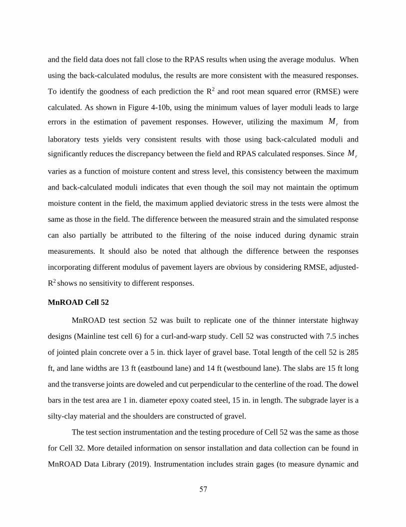
57

and the field data does not fall close to the RPAS results when using the average modulus. When

using the back-calculated modulus, the results are more consistent with the measured responses.

To identify the goodness of each prediction the R2 and root mean squared error (RMSE) were

calculated. As shown in Figure 4-10b, using the minimum values of layer moduli leads to large

errors in the estimation of pavement responses. However, utilizing the maximum rM from

laboratory tests yields very consistent results with those using back-calculated moduli and

significantly reduces the discrepancy between the field and RPAS calculated responses. Since rM

varies as a function of moisture content and stress level, this consistency between the maximum

and back-calculated moduli indicates that even though the soil may not maintain the optimum

moisture content in the field, the maximum applied deviatoric stress in the tests were almost the

same as those in the field. The difference between the measured strain and the simulated response

can also partially be attributed to the filtering of the noise induced during dynamic strain

measurements. It should also be noted that although the difference between the responses

incorporating different modulus of pavement layers are obvious by considering RMSE, adjusted-

R2 shows no sensitivity to different responses.

MnROAD Cell 52

MnROAD test section 52 was built to replicate one of the thinner interstate highway

designs (Mainline test cell 6) for a curl-and-warp study. Cell 52 was constructed with 7.5 inches

of jointed plain concrete over a 5 in. thick layer of gravel base. Total length of the cell 52 is 285

ft, and lane widths are 13 ft (eastbound lane) and 14 ft (westbound lane). The slabs are 15 ft long

and the transverse joints are doweled and cut perpendicular to the centerline of the road. The dowel

bars in the test area are 1 in. diameter epoxy coated steel, 15 in. in length. The subgrade layer is a

silty-clay material and the shoulders are constructed of gravel.

The test section instrumentation and the testing procedure of Cell 52 was the same as those

for Cell 32. More detailed information on sensor installation and data collection can be found in

MnROAD Data Library (2019). Instrumentation includes strain gages (to measure dynamic and

58

environmental loads), thermocouples, moisture sensors, and under-slab pressure plates. The data

analyzed in this study came from dynamic strain sensors and thermocouples. For truck loading,

the (102 kips) Navistar tractor with Fruehauf trailer was used in Cell 52. Figure 4-11 shows the

depths and locations of these sensors in test section 52.

Figure 4-11. MnROAD Cell 52 Section and Sensor Layout

Figure 4-12 shows the non-linear temperature variation throughout the concrete slab in July

26, 2000, that was used for the analysis. As explained for Cell 32, the temperature profile measured

at 2:00 p.m. was used for modeling FWD and truck loading tests. The three-dimensional

59

polynomial below fitted to the Cell 52 temperature data and used in RPAS to consider the

temperature differences throughout the depth of the slab was as follows:

2 3( ) 86.527 2.635 0.116 0.0004ModelT z z z z = − + + (4-3)

Figure 4-12. Temperature distribution measured at different times on the test day at MnROAD

Cell 52

The MnROAD Cell 52 data, based on testing from field cores and laboratory specimens,

are summarized in Table 4-3. The data set on FWD test collected on July 26, 2000 and the truck

loading test data collected on July 18, 2001 were considered for this study.

65 70 75 80 85 90 95 100

0

1.5

3

4.5

6

7.5

Temperature (oF)

60



Pavement

layer

Property Value Unit #Observations CV

% Min. Avg. Max.

Concrete

slab

(1512 ft)

Astro Turf

1.0”

Dowel

(E28)avg*

From cores:

From

cylinder

specimens:

3,400

3,925

4,410

4,370

4,745

5,030

ksi

ksi

5

6

12.0

8.3

Poisson’s

ratio, ( )c avg

From cores:

From

cylinder

specimens:

0.10

0.12

0.11

0.13

0.13

0.14

-

-

3

3

8.7

13.0


145 149 151 pcf 4 1.9

Thickness, tc

From cores:

From design:

7.5

-

7.8

7.5

8.2

-

in.

in.

3

-

4.2

-

CTE†

From

cylinder

specimens:

5.3

5.3

5.3

o/ F

2

0

Gravel

base

(Class 4)

(Mr)b,avg‡ 17,700 27,560 46,600 psi 18 34.4

Poisson’s

ratio, ( )b avg

- 0.30 - - -

Unit weight,

b,( )wet avg 136 143 148 pcf 18 3.5

Thickness, tb

From design:

-

5.0

-

in.

-

-

Subgrade

(Clay:

R=12)

(Mr)SG,avg‡ 16,950 27,000 47,020 psi 30 26.8

Poisson’s

ratio, ( )SG avg

- 0.40 - - -

Unit weight,

SG,( )wet avg 134 136 137 pcf 10 1.2


respectively.

* E28 = 28-day Elastic modulus


‡ Mr = Resilient modulus

61

As seen in Table 4-3, similar to Cell 32, the moduli of the pavement foundation layers from

laboratory tests show a considerable variation as compared to the concrete slab. Therefore, the

back-calculated moduli of supporting layers from FWD test data were utilized in the rest of

analyses. The results of pre-validation for FWD testing shown in Figure 4-13 indicates a good

agreement.

Center Corner MidEdge JointAfter

Applied Pressure (psi)

NSE values:


Analyses and The NSE Between Simulated and Observed Deflections in Cell 52.

0

5

10

15

20

25

30

35

40

45

50

0 10 20 30 40 50

Measure

d v

ert

ical

defle

ction f

rom

FW

D (

mil)


Adj-R2=0.79

Center

MidEdge

Corner

Joint After 1:1

1:1.2

1:0.8

Center MidEdge Corner JointAfter

Load 1 -0.02 -3.12 -3.34 -18.01

Load 2 -0.85 -2.98 -2.52 -5.64

Load 3 -0.69 -4.17 -8.73 -5.85

62

For truck loading, a Navistar tractor with Fruehauf trailer with the weight of 102 kips was

used in Cell 52. As can be seen in Figure 4-13, as opposed to Cell 32, the truck loading in outside

lane was used for comparison in this study. Table 4-4 summarizes the peak values of dynamic

strain measured at Cell 52 in July 18, 2001 compared to those from RPAS analysis using average

and back-calculated moduli of foundation layer. As shown, peak strains calculated utilizing

resilient modulus from laboratory testing and back-calculation yield higher calculated responses

compared to the measured ones but the peak strains obtained using back-calculated moduli are in

better agreement with the measured strains, where the maximum difference changes from 68%

using average Mr to 33% with the back-calculated moduli.

Table 4-4. Comparison of Peak Values of Strain Under Truck Loading Measured at MnRAOD

Cell 52 and Calculated Using RPAS

Source of utilized

Moduli

Location of record under truck load

1st Axle 2nd Axle 3rd Axle 4th Axle 5th Axle

Measured 12 28 22 22 27

Average Mr 19 34 37 36 39

Back-calculation 16 28 29 27 33 All the values above show the dynamic strain under truck loading in microstrain.

MnROAD Cell 613

Cell 613 is intended to be a model for sustainable concrete pavement design. Ideally, it

would be preferable to reuse the in-place pavement materials in the newly constructed test cell. In

this case, however, recycled material came from the contractor’s stockpile in Maple Grove, MN.

This concrete was verified to come from previous pavements produced under MnDOT

specifications. Recycled concrete was crushed to a controlled maximum size of 1.5 inch and

minimal material passing the No. 200 sieve. Project special provisions further required that there

be less than 5% passing the No. 4 sieve. The final mix design included 75% replacement of the

coarse aggregate with recycled concrete aggregate. Pavement design consisted of 7.5-inch-thick

63

slabs with 15 ft long by 12 ft wide panels. Transverse joints included 1-inch diameter epoxy coated

steel dowels, and longitudinal joints were tied with 0.5-inch diameter, 30-inch long rebars. The

original research plan included studying two different narrow width neoprene preformed seals.

However, saw cut widths were incompatible with the very narrow seals, so only the wider (0.25-

inch wide) seals were installed in the joints.

Figure 4-14 and Table 4-5 show the properties of pavement section Cell 613 as well as the

arrangement of static and dynamic sensors. The pavement temperature was measured on the test

day at various depths and times of day were curve-fitted to a three-dimensional polynomial, as

illustrated in Figure 4-15. As explained above, the temperature profile measured at 2:00 p.m. was

used for modeling FWD and truck loading tests. The three-dimensional polynomial below fitted

to the Cell 613 temperature data and used in RPAS to consider the temperature differences

throughout the depth of the slab was as follows:

2 3( ) 92.000 4.253 0.144 0.155ModelT z z z z = − + + (4-4)

64

Figure 4-14. MnROAD Cell 613 Section and Sensor Layout.

65



Pavement

layer

Property Value Unit #Obser

vations

CV %

Min. Avg. Max.

Concrete

slab

(1512 ft)

(75%

RCA)

1.0” Dowel

(E28)avg*

From cores:

From cylinder

specimens:

4,050

3,978

5,152

4,045

5,435

4,130

ksi

ksi

5

4

12.0

3.6

Poisson’s ratio, ( )c avg

From cores:

From cylinder

specimens:

0.14

0.11

0.24

0.14

0.28

0.16

-

-

3

3

8.7

13.0


146 147 149 pcf 4 1.9

Thickness, tc

From cores:

From design:

-

7.9

7.5

-

in.

in.

3

-

4.2

-

CTE†

From cores:

4.8

4.9

5.0

o/ F

3

0

Gravel

base

(Class 1)

(Mr)b1,avg‡ 17,920 20,040 29,500 psi 18 34.4

Poisson’s ratio,

1( )b avg - 0.30 - - - -

Unit weight,

b1,( )wet avg 141 157 159 pcf 18 3.5

Thickness, tb1

From design:

-

2.5

-

in.

-

-

Gravel

base

(Class 5)

(Mr)b2,avg‡ 16,650 20,580 31,790 psi 12 22.6

Poisson’s ratio,

2( )b avg - 0.35 - - - -

Unit weight,

b2,( )wet avg 132 144 147 pcf 12 2.1

Thickness, tb2

From design:

- 5.0 - in. - -

Subgrade

(Clay:

R=12)

(Mr)SG,avg‡ 7,955 16,860 24,030 psi 30 24.9

Poisson’s ratio, ( )SG avg

- 0.45 - - - -

Unit weight,

SG,( )wet avg 115 120 127 pcf 30 3.3


respectively.

* E28 = 28-day Elastic modulus, ‡ Mr = Resilient modulus


66


Test Day in MnROAD Cell 613

As in previous sections, the relatively high variation of the moduli of the foundation layers

made the use of back-calculated moduli a more accurate alternative than laboratory derived moduli

for modeling purpose. The results of RPAS analyses based on the material properties (Table 4-5)

were compared against FWD test results as well as dynamic strain measurement at MnROAD Cell

613, which are shown in Figures 4-16 and 4-17. For truck loading, a WorkStar Tractor with

Towmaster trailer was used in Cell 613. As can be seen, the calculated deflections from RPAS are

in a reasonable agreement (NSEmax=-2.5, Adj-R2=0.95) with the measured deflections. In terms of

strain at the slab (Figure 4-17), as in Cell 32 and 52, utilizing back-calculated moduli (BC_Mr) of

the foundation layers results in a better agreement between the responses.

60 70 80 90 100 110

0

1.5

3

4.5

6

7.5

Temperature (oF)

67

Center Corner MidEdge

NSE values:

Figure 4-16. Maximum Basin Deflection from FWD Tests versus the Deflections from RPAS

Analyses and the NSE Between Simulated and Observed Deflections in Cell 613.

0

5

10

15

20

25

30

35

40

45

50

0 10 20 30 40 50

Measure

d v

ert

ical

defle

ction f

rom

FW

D (

mil)


Adj-R2=0.95

Center

MidEdge

Corner 1:1

1:1.2

1:0.8

Center MidEdge Corner

Load 1 -0.3 -0.3 -2.2

Load 2 -0.9 -1.1 -2.5

Load 3 0.9 0.9 0.5

68

Note: Avg_Mr is for the average moduli and BC_Mr is for the back-calculated moduli

Figure 4-17. Comparison of Measured Dynamic Strain Sensor Responses with Those Obtained

Using RPAS For Different Material Properties

4.2. National Airport Pavement Test Facility (NAPTF)

Federal Aviation Administration (FAA) operates a full-scale accelerated airport pavement

test facility known as the National Airport Pavement Test Facility (NAPTF) located at the William

J. Hughes Technical Center near Atlantic City, New Jersey, USA. The primary objective of the

NAPTF is to generate full-scale pavement response and performance data for development and

verification of airport pavement design criteria. Since completing the construction of NAPTF in

1999, FAA has conducted eight construction cycles for various purposes. Each construction cycle

(CC) includes pavement construction, instrumentation installation, traffic testing to failure, post

traffic testing, and demolition of the test item. The testing facility consists of a fully enclosed

instrumented test pavement track (900 ft long by 60 ft wide). The rail-based test vehicle is capable

of simulating aircraft weighing up to 1.3 million pounds with up to 20 test wheels configured to

represent two complete landing gear trucks, wheel loads independently adjustable up to 75,000 lb.

per wheel, controlled aircraft wander simulation, and fully automated computerized data

acquisition system (see Figure 4-18). The test track is divided into independent test items on three

subgrade classifications: low strength, medium strength, and high strength. In the first four

-10

-5

0

5

10

15

20

25

30

0 2 4 6 8 10 12

Dynam

ic s

train

at

the b

ott

om

of

sla

b (

µε)

Time (sec)

SensorMeasurement

Avg_Mr

BC_Mr

69

construction cycles, each pavement test item is designated by its construction cycle (CC) number

and three characters. The first character denotes the subgrade strength (L-low, M-medium, and H-

high). The second character denotes the type of pavement (F-flexible or R-rigid). The third

character denotes the type base (S-stabilized, C-conventional, or G-grade). At NAPTF, a variety

of embedded (static or dynamic) sensors are used in each CC to capture instrumentation data based

on the testing objectives. Static sensors collect temperature, moisture, and crack data on an hourly

basis. Dynamic sensors are triggered by the vehicle operation to measure the pavement responses

such as strain and deflection during traffic loading.

Construction cycles can be categorized as rigid or flexible test pavement (odd numbers

indicate flexible pavement testing and even numbers show rigid pavement testing), except for CC-

1 that includes testing both pavement types. Table 4-6 shows a list of construction cycles for testing

rigid pavements and the purpose of each test.

Figure 4-18. National Airport Pavement Test Facility (NAPTF Database 2019).

70

Table 4-6. Construction Cycles for Testing of Rigid Pavements at NAPTF

Construction Cycle Purpose

Construction Cycle 1 To provide full-scale test data to:

• support the new computer-based design procedures that were under

development by FAA

• be used in airplane landing gear design and configuration studies

Construction Cycle 2 The main experiment was intended to compare the performance of

three types of rigid pavements: concrete slabs on stabilized bases

(MRS), concrete slabs on aggregate bases (MRC), and concrete

slabs placed directly on subgrade (MRG). Other components

include:

Test Strip – to study the effects of slab size and mix design on

pavement curling during the early age of the concrete.

Single Slab – to provide experience for the design, placement, and

monitoring of the actual PCC test items.

Twin Slab – to compare the behavior of the slab with no fly ash

content vs. slab with high fly ash content.

Construction Cycle 4 To improve the understanding of the influence of design

parameters on unbonded concrete overlays of rigid airfield

pavements

Construction Cycle 6 To determine the effect of concrete flexural strength on rigid

pavement structural life.

Construction Cycle 8 Phase 1 Overload: The primary objective of Phase 1 was to

develop rational overload criteria for rigid pavements.

Phase 2 Overlay: The primary object of Phase 2 was to test the

performance of a PCC overlay on an existing PCC with Structural

Condition Index (SCI) in the 50-80 range.

Phase 3 Joint Comparison: The primary objective of Phase 3 was

to compare the performance of Type E (doweled construction) and

nonstandard sinusoidal keyed longitudinal joints.

Phase 4 Strength & Fatigue: The primary objective of Phase 4 was

to obtain slab strength (rupture strength) for full-scale slabs under

a monotonically increasing aircraft gear load, as well as the fatigue

strength of rigid pavement slabs under non-wandered traffic.

CONSTRUCTION CYCLE 2

The primary objectives of the CC-2 tests were to evaluate the pavement performance with

different supporting layer properties, to study the influence of 4-wheel and 6-wheel gear traffic on

the pavement life, and to assess pavement performance using structural condition index (SCI)

71

versus traffic repetitions. The interior and edge stresses under gear loads as well as shrinkage and

curling measurement were other objectives of this construction cycle tests.

The CC-2 consisted of three test items of 75 ft. long by 60 ft. wide, separated by 25 ft. long

rigid transitions. Each 75-ft test section comprised of 4 transverse slabs by 5 longitudinal slabs

(see Figure 4-19). In main test items, a 12-in. concrete slab with the nominal dimensions of 15 ft.

by 15 ft. was placed on medium-strength subgrade (CBR=7~8) area replaced from CC-1. The slab

size was selected of based on the results of a previous experiment conducted at the NAPTF, which

led to the reduction of corner cracking due to curling when using a smaller size slab. A high amount

of (50%) of Class-C fly ash was used in the cementitious mix of concrete to provide a thicker curl

resistant slab.

Figure 4-19. Layout of CC-2 Test Items at NAPTF (Brill et al. 2005)

As mentioned in Table 4-7, three configurations of concrete slabs on stabilized

(Econocrete) base (MRS), concrete slabs on conventional granular base (MRC), and concrete slabs

on grade (MRG) were tested. Figure 4-20 shows the pavement structure for CC-2 test items.

72

Figure 4-20. Structural Design Data For CC-2 Test Items (Ricalde and Daiutolo 2005)

Target elastic moduli for CC-2 pavement layers were 4,000,000 psi for the concrete slab

(P-501), 700,000 psi for the stabilized base layer (P-306), 10,500 psi for Subgrade (Clay CH) layer

and the modulus of the granular base (P-154) was variable. To monitor meeting these target values,

almost three cylinders and four beams from each slab were taken for laboratory testing of concrete

and more than 150 CBR tests and several plate load tests were carried out, with at least one CBR

test on each lift during construction to determine the material properties of the base and subgrade

layers. CBR tests were conducted on randomly selected locations, preferably within the wheel

tracks mirrored on both south and north sides and the acceptable range of the average CBR was

set to 5.5 to 8.0. According to the NAPTF database and existing reports on CC-2, the unit weight

of the slabs, granular base, stabilized, and subgrade were considered as 149 pcf, 145 pcf, 147 pcf,

and 140 pcf, respectively. Poisson’s ratio of the slabs, granular base, stabilized, and subgrade were

also assumed as 0.15, 0.35, 0.20, 0.45.

Table 4-7 summarizes the layer configurations in MRC, MRG, and MRS test items, results

of testing field cured samples, and material properties of the supporting pavement layers. Other

material properties such as unit weight and Poisson’s ratio were extracted from the NAPTF

database and existing reports on CC-2.

Sta

tion 6

25

Sta

tion 3

00

73

Table 4-7. Correlated Modulus of CC-2 Main Test Sections from Field Testing (NAPTF Data

Library 2019)

MRC MRG MRS

Pavement

layer

Modulus

(psi)

Pavement

layer

Modulus

(psi)

Pavement

layer

Modulus

(psi)

Concrete slab

– 12 in. 3,422,000†

Concrete slab

– 12 in. 3,336,000†

Concrete slab –

12 in. 3,450,000†

Granular

Subbase

(P-154) – 10

in.

16,500‡ Econocrete

(P-306) – 6 in. 72,000‡

Subgrade 13,500‡ Subgrade 13,500‡

Granular

Subbase

(P-154) – 8.6 in.

16,500‡

Subgrade 13,500‡ † Correlated from compressive strength of field cured samples at 28 days using ACI 318 correlation

‡ Correlated from CBR values using correlation 1500rM CBR=

As mentioned earlier, the tire loads in NAPTF are adjustable independently so that the

effect of different tire configurations can be evaluated. As one of the objectives of CC-2 testing,

the influence of 4-wheel and 6-wheel gear traffic on the pavement life was evaluated. Gear load

configuration shown in Figure 4-21a was used in CC-2 traffic testing and the lateral wander of the

traffic follows the pattern illustrated in Figure 4-21b. As shown, the pavement was trafficked by a

6-wheel gear configuration on the north side and a 4-wheel gear configuration on the south. The

selected load was 55,000 lb. per wheel at 210 psi tire pressure.

74

(a)

(b)

Figure 4-21. (a) Gear Load Configuration and (b) Traffic Wander Pattern for CC-2 Traffic

Tests (Brill et al. 2005)

Temperature and moisture information were measured using static sensors (e.g.

thermistors, vibrating wire strain gauges) embedded at different locations of the test pavement.

Dynamic strain sensors were installed at 1.5 in. from the top of slab to capture the critical strains

due to reverse slab bending away from the landing gear in order to analyze top-down cracking.

Another set of dynamic strain sensors were installed at 1.5 in. from the bottom of slab to record

the critical strains under aircraft loading gear, which are associated with the bottom-up cracking

75

of the concrete slab. The coordinates of the load location on the test area change with the traffic

wander for each track according to the pattern illustrated in Figure 4-21.

Comparison of HWD Responses

FAA standard configuration (12-in. diameter plate, three impact loads of 12-kips, 24, kips,

and 36-kips after seating) was used in HWD testing using Kuab Model 240. HWD tests were

performed on the slab centers (to verify pavement uniformity and study the effect of support

condition) and on both sides of the outboard longitudinal joints opposite the slab centers (to check

the load transfer efficiency at joints) (Ricalde and Daiutolo 2005) at intervals of 15 test vehicle

wanders. Figure 4-22a demonstrates the comparison of maximum basin deflection at MRC, MRG

and MRS with those obtained from RPAS analysis. A very good agreement between the results of

HWD tests and RPAS can be inferred from the figure and the statistical metric NSE is close to

unity, which confirms this close agreement.

Comparison of Accelerated Loading Responses

To validate the performance of RPAS in modeling heavy aircraft loads on JCPs, the

longitudinal and transverse strain responses from 4-wheel gear loading on the south side of the

pavement section with different supporting conditions were compared against the responses from

RPAS. In each case, two sensors at the inbound of longitudinal joints (S04 and S10 for MRC, S32

and S42 for MRG and S48 and S62 for MRS) and two sensors at the inbound of transverse joints

(S02 and S08 for MRC, S24 and S30 for MRG and S46 and S52 for MRS) were selected for

comparison. Figure 4-22b demonstrates the comparison of the measured longitudinal strains near

the longitudinal joints and those calculated by RPAS (with the maximum RMSE of 18.3 µε)

indicate a good agreement (upper three subplots). The biggest difference appears on the MRS case

although there is also significant difference between the S48 and S62 sensors with the results of

RPAS falling right on the average of the two. For the transverse joint (lower three subplots) the

76

biggest RMSE is 19.1µε appearing in the MRS case. It is important to note that, just in the case

of the S48 and S62 sensors above, the sensors in the MRC and MRS in these transverse joint strains

also show significant differences. It is only in the MRG case that the two sensors show consistent

measurements and RPAS under predicts the strain by 20% which will require further analysis to

identify the source of the difference.

Similar to the cases from the HWD testing comparison, the program yields the best prediction for

cases with conventional pavement section, MRC at longitudinal joints. There are larger errors in

strain responses at transverse joints which may occur due to different load transfer mechanism.

Some of the sources of errors in the predictions include the dynamic effect of accelerated loading

and non-uniformity of in-place pavement properties.

77

(a)

(b)

Figure 4-22. (a) Maximum Basin Deflection at the Center Of Slab From HWD Tests In CC-2

NAPTF versus The Deflections Calculated From RPAS Analyses (b) Comparison

of Strain Responses at the Top and Bottom of Concrete Slab From Two

Consecutive Sensors Along The Longitudinal/Transverse Joints of Different

Sections From Accelerated Testing and The RPAS Strain Responses.

0

5

10

15

0 5 10 15

Measure

d v

ert

ical

deflection f

rom

HW

D (m

il)


Adj-R2=0.97

MRC

MRG

MRS

1:1

1:1.1

1:0.9

Nash-Sutcliffe Efficiency

(NSE)

MRC


0.997 0.999 0.999

MRG


0.996 0.998 0.997

MRS


0.969 0.929 0.936

-150 -100 -50 0 50 100 150

To

p s

train

Bo

tto

m s

tra

in

Longitudinal strain in pavement (µε) near

the longitudinal joint

MRC section RPAS S04 S10

RMSE=9.5µε

-150 -100 -50 0 50 100 150

To

p s

train

Bo

tto

m s

tra

in



MRG section RPAS S32 S42

RMSE=13.1µε

-150 -100 -50 0 50 100 150

To

p s

train

Bo

tto

m s

tra

in



MRS section RPAS S48 S62

RMSE=18.3µε

0 20 40 60 80 100

Bo

tto

m s

tra

in


the transverse joint

MRC section RPAS S02 S08

RMSE=17.0 µε

0 20 40 60 80

Bo

tto

m s

tra

in



MRG section RPAS S24 S30

RMSE=12.5 µε

0 20 40 60 80

Bo

tto

m s

tra

in



MRS section RPAS S46 S52

RMSE=19.1 µε

78


The primary objectives of the CC-4 tests were to enhance the knowledge about the

influence of design parameters on unbonded concrete overlays of airfield pavements and thus

enabling improvement of design methodologies. CC-4 consisted of two separate components:

baseline tests on new rigid pavements, and validation test on damaged rigid pavements. verifying

failure mechanisms, formulating overall life prediction, and determining effects of discontinuities

(mismatched joints and cracks) on stresses and deflections are the objectives of the baseline tests.

As in CC-2, the performance of pavements was evaluated under different support conditions,

subjected to 4-wheel and 6-wheel gear traffic loading, and using structural condition index (SCI).

The present study will only consider baseline tests on new pavements.

CC-4 consisted of a 300-foot test pavement that had three structural cross-sections and was

constructed on the medium-strength (CBR=6~9) subgrade. The baseline experiment consists of

six test items, in three structural sections of varying thicknesses constructed on the medium-

strength subgrade, separated by transition slabs in both the longitudinal and transverse directions.

As shown in Figure 4-23, each test item consists of 12 slabs of 12.512.5 ft, that is, 12.5-ft wide

lanes, with a 10-ft transition slab between the test items. Overlay slabs were dowelled in

longitudinal and transverse directions but not to the transition slabs, whereas the underlay slabs

were designed to be undoweled to provide greater discontinuities in support. The concrete mix was

designed to be identical to that in CC-2. The design thickness of overlay and underlay concrete

pavements are shown in the pavement structure diagram in Figure 4-23b.

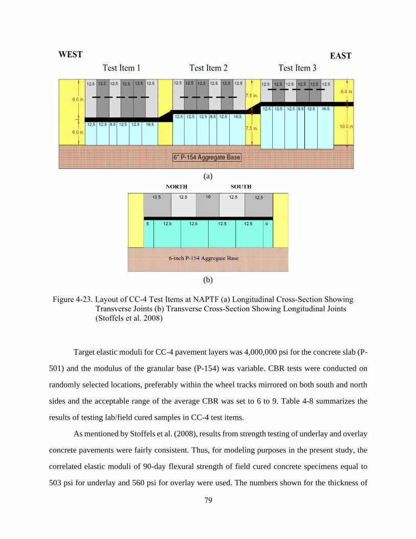
79

(a)

(b)

Figure 4-23. Layout of CC-4 Test Items at NAPTF (a) Longitudinal Cross-Section Showing

Transverse Joints (b) Transverse Cross-Section Showing Longitudinal Joints

(Stoffels et al. 2008)

Target elastic moduli for CC-4 pavement layers was 4,000,000 psi for the concrete slab (P-

501) and the modulus of the granular base (P-154) was variable. CBR tests were conducted on

randomly selected locations, preferably within the wheel tracks mirrored on both south and north

sides and the acceptable range of the average CBR was set to 6 to 9. Table 4-8 summarizes the

results of testing lab/field cured samples in CC-4 test items.

As mentioned by Stoffels et al. (2008), results from strength testing of underlay and overlay

concrete pavements were fairly consistent. Thus, for modeling purposes in the present study, the

correlated elastic moduli of 90-day flexural strength of field cured concrete specimens equal to

503 psi for underlay and 560 psi for overlay were used. The numbers shown for the thickness of

80

pavement layers are the average of the thicknesses measured on a 10 by 10 ft grid. However, based

on the coordinates of the section being modeled, the actual measured thickness was used.

As indicated in Table 4-8, the resilient modulus of base and subgrade layers were correlated

with the reported CBR values and have been confirmed with the k-values of 143 psi/in. on the

north side and 146 psi/in. on the south side, averaged from several plate load tests.

According to the NAPTF database and existing reports on CC-4, the unit weight of the

overlay slab, underlay slab, granular base and subgrade were considered as 155 pcf, 152 pcf, 147

pcf, and 140 pcf, respectively. Poisson’s ratio of the slabs, granular base, and subgrade were

assumed as 0.15, 0.35, and 0.45.


Testing

Pavement layer Test

item

Modulus

(psi)

Poisson’s

ratio

Thickness

(in.)*

Unit weight

(pcf)

Concrete

slab

OL**

1

2

3

3,840,000†

0.15

8.7

7.4

5.7

155

UL**

1

2

3

4,276,000†

6.3

7.5

9.9

152

Granular

Subbase

(P-154)

1

2

3

16,200‡

15,800‡

16,250‡

0.35

5.7

5.6

4.7

147

Subgrade

1

2

3

11,700‡

11,325‡

12,900‡

0.45 - 140

* As-built thicknesses, measured on a 10 10 grid

** OL=overlay, UL=underlay

† Correlated from flexural strength of field cured samples at 90 days using ACI 318 correlation

7635c rE f=

‡ Correlated from CBR values using correlation 1500rM CBR=

As in CC-2 testing, the influence of 4-wheel and 6-wheel gear traffic on the pavement life

was evaluated in CC-4. Gear load configuration shown in Figure 4-24a was used in CC-4 traffic

testing and the lateral wander of the traffic follows the pattern illustrated in Figure 4-24b. As

81

shown, the pavement was trafficked by a 6-wheel gear configuration on the north side and a 4-

wheel gear configuration on the south. The applied load was 45,000 lb. to 65,000 lb. per wheel at

an inflated tire pressure of 230 psi. For modeling purposes, depending on the date and time of the

test, the exact magnitude of each tire load and pressure were used, as reported in the CC-4 database.

(a)

(b)

Figure 4-24. (a) Gear Load Configuration and (b) Traffic Wander Pattern for CC-4 traffic tests

82

Temperature and moisture information were measured using static sensors (e.g.


Dynamic strain sensors were installed at 1.5 in. from the top of slab to capture the critical strains

due to reverse slab bending away from the landing gear in order to analyze top-down cracking.

Another set of dynamic strain sensors were installed at 1.5 in. from the bottom of slab to record

the critical strains under aircraft loading gear, which are associated with the bottom-up cracking

of the concrete slab. The coordinates of the load location on the test area change with the traffic

wander for each track according to the pattern illustrated in Figure 4-24.

Figure 4-25 illustrates the overlay and underlay joint arrangements and the modeled section

of the pavement. The results of RPAS modeling of this accelerated loading compared to those of

field measurements are shown in Figure 4-26. As can be seen, there is reasonable agreement

between the measured strain responses and those calculated using RPAS in both overlay and

underlay. The maximum dynamic strain percent differences occur at points 2 and 4 which is

expected since it is at these points that the absolute strains are the lowest. The maximum difference

at a peak strain points is of 59% and it is expected that the calibration process will reduce it.

Figure 4-25. Overlay and Underlay Joint Arrangements and The Modeled Section of The

Pavement

83

Figure 4-26. Comparison of Dynamic Strain Responses Developed in Overlay and Underlay

from RPAS Analyses and Field Measurements

-30

-25

-20

-15

-10

-5

0

5

10

15

0 2 4 6 8 10 12

Dynam

ic s

train

(µε)

Time (sec)

(a) RPAS

Overlay/Top

Point Difference1 5 %2 59%3 14%4 93%5 8 %

-20

-10

0

10

20

30

40

0 2 4 6 8 10 12

Dynam

ic s

tra

in (

µε)

Time (sec)

(b)

RPAS

Overlay/Bottom

Point Difference1 8 %2 44%3 2 %4 65%5 9 %

-15

-10

-5

0

5

10

0 2 4 6 8 10 12

Dyn

am

ic s

tra

in (

µε)

Time (sec)

(c) RPAS

Underlay/Top

Point Difference1 19%2 47%3 21%4 46%5 1 %

-10

-5

0

5

10

15

20

0 2 4 6 8 10 12

Dynam

ic s

train

(µε)

Time (sec)

(d)

RPAS

Underlay/Bottom

Point Difference1 19%2 1 %3 18%4 9 %5 21%

84


The primary objective of the CC-6 tests was to determine the effect of concrete flexural

strength on rigid pavement structural life. For this purpose, three test items of rigid pavement with

similar cross sections and varying concrete flexural strength were designed. Comparison of the

influence of different stabilized base materials (hot-mix asphalt and Econocrete) on the rigid

pavement performance was another objective of this study. Two types of isolation joints, thickened

edge and steel-reinforced, have also been compared. All the test items were designed on the

medium-strength subgrade. The performance of the pavements was evaluated by applying a 4-

wheel gear traffic loading on both north and south sides.

CC-6 consisted of a 300 ft long by 60 ft wide test pavement that had three test items of

MRS-1, MRS-2, and MRS-3, having the concrete 28-day target flexural strength of 500, 750, and

1000 psi, respectively (see Figure 4-27a). Each test item consisted of 10 slabs of 15 15 ft by 12-

in. thick with a 10-ft transition slab between the test items. The slabs were doweled on all sides,

except for slab edges abutting the shoulder and the isolation joints located in the transition areas.

The 6-in. stabilized base layer was HMA P-403 on the north side and Econocrete P-306 on the

south side. A 10-in. granular subbase layer was placed below this stabilized base layer and the

pavement was constructed on the medium-strength (average CBR=8) subgrade (Figure 4-27b).

85

Figure 4-27. Layout of CC-6 Test Items at NAPTF Pavement Plan Showing Three Test Items

and Transverse Cross-Section Showing Pavement Structure (McQueen and

Hayhoe 2014)

The target strengths indicated in Figure 4-27 might not necessarily be achieved during

construction and thus the material characterization and testing was carried out to assess the

pavement uniformity using both destructive and nondestructive (e.g. FFRC, PSPA, GPR, HWD)

testing.

In CC-6, the strength of concrete layer was evaluated using compressive and flexural

strength tests on core samples and laboratory casted specimens as well as nondestructive (e.g.

FFRC, PSPA) testing. The average 28-day compressive strength was estimated as 4,012 psi on the

north side and 4,386 psi on the south side. The average flexural strength of concrete layer was

generally above the target values. For instance, the average flexural strength of concrete in MRS-

1 on the north side was 650 psi, which is higher than the target value of 500 psi. However, for

modeling purposes, the target values were used for comparison with other tests to derive modulus

of concrete layers in order to consider a more conservative design. Table 4-9 summarizes the

results of testing lab or field cured samples in CC-6 test items and the average values of each

parameter.

86

CBR and plate load tests were conducted after the construction of each pavement layer at

certain stations before and after trafficking. These tests have been conducted at the offset of 15 ft

from the centerline, mirrored on north and south sides of the test section. The results of these tests

were compared to verify that the obtained modulus of each pavement layer from the existing

correlations match within a reasonable tolerance. For the purpose of this study, the as-built material

properties prior to trafficking were utilized. From the results of plate load tests, the average k-

values of subgrade, subbase, and base layers were 132, 205, 416 psi/in. on the north side (HMA

base) and 139, 214, 850 psi/in. on the south side (Econocrete base), respectively. The CBR values

of subgrade were 6.5 on the north side and 7.2 on the south side. The results of resilient modulus

tests has shown an average resilient modulus of 11,600 psi for the north side and 12,300 psi for

the south side, which confirms the validity of using the correlation 1500rM CBR= . Even though

the average material properties for the pavement layers on the north and south side have been

reported here, the values from laboratory or field measurements at each test item were used for

modeling. The unit weight of the concrete slab, stabilized base (HMA/Econ), granular subbase,

and subgrade were considered as 148 pcf, 143/146 pcf, 149 pcf, and 155 pcf, respectively,

according to the NAPTF database and existing reports on CC-6. Poisson’s ratio of the slab,

stabilized base (HMA/Econ), granular subbase, and subgrade were assumed as 0.15, 0.30/0.25,

0.35, and 0.45 (see Table 4-9).

87


Testing

Pavement layer Test

item*

Modulus

(psi)

Poisson’s

ratio

Thickness

(in.)

Unit

weight

(pcf)

Concrete Slab

(P-501)

N

S

3,610,000†

3,775,000† 0.15 12 148

Stabilized

Base

HMA

(P-403) N 60,000‡ 0.30

6

143

Econ

(P-306) S 1,432,000† 0.25 146

Granular Subbase

(P-154)

N

S

24,200‡

25,500‡ 0.35 10 149

Subgrade N

S

11,600‡

12,300‡ 0.45 - 155

* N=North side, S=South side

† From correlation with compressive strength of field cured samples using ACI 318 correlation,

confirmed with fracture testing by Stoffels et al. (2014)

‡ Correlated from CBR values using correlation 1500rM CBR= , confirmed with k-values

In CC-6 testing, the influence of airplane gear loading on the pavement performance was

evaluated. As opposed to CC-2 and CC-4, gear load configuration consists of two identical 4-

wheel gears on both north side and south side of the test pavement (see Figure 4-28a). Wheel loads

varied in three levels of 45,000, 52,000, and 70,000 lb. per wheel at different testing periods. MRS-

1 was only trafficked with the first load level that was sufficient to cause failure in this low-strength

concrete test item. The nominal inflated tire pressure was 250 psi, although the actual tire pressures

were reported in CC-6 database and have been used for modeling. The wander pattern used for the

traffic testing was designed in a way that it simulates a normal distribution of aircraft traffic (Figure

4-28b). For modeling, 50,000 lb load and the pressure of 230 psi were used.

88

(a)

(b)

Figure 4-28. (a) Gear load configuration and (b) traffic wander pattern for CC-6 traffic tests

The hourly temperature and moisture information were measured using static sensors (e.g.


Dynamic strain sensors were installed at 1.0 in. from the top of and bottom of the slabs to capture

89

top-down and bottom-up cracking potential. These sensors are triggered by movements of the load

vehicle. The coordinates of the load location on the test area change with the traffic wander for

each track according to the pattern illustrated in Figure 4-28.

A comparison of the dynamic strain responses of pavement from RPAS and field

measurement at CC-6 is made in Figure 4-29. As can be seen, there is a reasonable agreement in

the variation of the measured and calculated pavement responses. The maximum differences at

peak strain points is of 23% and it is expected that the calibration process will reduce it.

Figure 4-29. Comparison of the dynamic strain responses of pavement from RPAS and field

measurement at CC-6

-150

-100

-50

0

50

100

150

0 2 4 6 8 10

Dyn

am

ic s

train

(µε)

Time (sec)

(a) RPAS

Top of Slab

Point Difference1 23%2 59%3 17%

-150

-100

-50

0

50

100

150

0 2 4 6 8 10

Dynam

ic s

train

(µε)

Time (sec)

(b)

RPAS

Bottom of Slab

Point Difference1 9 %2 57%3 2 %

90

5. Verification

This chapter discusses the verification process that includes the calculation verification and

bench-marking of RPAS against existing analytical solutions and numerical analyses. The purpose

of verification is to check how close the code outputs are to the closed-form or numerical solution

of the problem and attempt to minimize the generated error.

5.1. Calculation Verification

Calculation verification is associated with establishing confidence that the discrete solution

of the mathematical model is accurate, which includes estimating the errors in the numerical

solution due to discretization. This discretization error ( h ), that is also called solution

approximation error, is used to quantify the uncertainty in the predictions. Several methods are

available in the literature (Babuška and Rheinboldt 1978, Rangavajhala et al. 2011) to estimate

discretization error in finite element analysis. The Richardson extrapolation (RE) method has been

commonly applied to quantifying the solution approximation error (Sankararaman and Mahadevan

2015). In this method, the finite element analysis is repeated for three different mesh sizes

( 1 2 3h h h ) and the corresponding finite element solutions

( 1 1 2 2 3 3(h ) , (h ) , (h )FE FE FEy y y = = = ) are recorded. If a relationship for the calculation of the

true solution is available, the obtained three equations could have been solved simultaneously to

estimate the solution approximation error, h . However, in most cases of finite element analysis,

by considering the assumption of constant mesh size ratio (i.e., 3 2 2 1/ /r h h h h= = ), the following

closed-form solution can be used to estimate h , and, correspondingly, the real solution y

(Sankararaman and Mahadevan 2015):

1 hy = − (5-1)

2 1 ( 1)p

h r − = − (5-2)

where y is the real solution, 1 2 3, , are the finite element solution for different mesh

sizes, r is the mesh size ratio, and p is a variable that is a function of r and the solutions

1 2 3, , .

91

The above process based on Richardson extrapolation method has been used in this study

that will be discussed later in this chapter. However, the study in the following section was

performed to determine the range of mesh sizes to be used in the RE method.

MESH SIZE IN RPAS

RPAS has the capability of generating uniform and non-uniform meshes with any level of

refinement in the horizontal plane, as shown in Figure 5-1. The non-uniform mesh is automatically

generated in the model by increasing the number of elements in the region close to the point of

application of the vehicle loads and on the edges of the slabs when more than one concrete slab is

modeled. To identify the element size that results in the convergence of solutions, Carrasco et al.

(2011) developed a single slab with a single-tire load model. The control parameters used to

characterize convergence were the pavement maximum deflection and normal bending stress.

Based on their results, for a uniform mesh, an element size of no more than 12 in. in each direction

is required. The non-uniform mesh beneath the tires and at the slab edges was obtained by

subdividing each element in these regions into at least four elements (see Figure 5-1).

(a) Uniform Mesh (b) Non-Uniform Mesh

Figure 5-1. Configuration of Uniform and Non-uniform Mesh

92

Upon the incorporation of the 3-D solid foundation, a new convergence study is developed

to determine the number of elements required throughout the depth of each foundation layer. A

single slab (150 in. by 100 in.) under a single tire load of 9 kips and a single-axle load of 18 kips

with a pressure of 120 psi was applied at the center of the slab. Three different pavement structures

were analyzed for this purpose: slab on subgrade (G), conventional pavement, i.e. slab on a base

layer over subgrade (C), and slab on the stabilized base, granular base, and subgrade (S). Table

5- 1 shows the analysis cases used to determine the number of elements required for each soil

thickness and pavement structure; a total of 128 cases.

Table 5-1. Input Variables to Determine Mesh Convergence

On Grade (G) Conventional (C) Stabilized (S)

Pavement

layer

Modulus

(ksi)

Pavement

layer

Modulus

(ksi)

Pavement

layer

Modulus

(ksi)

Concrete slab –

t = 10 in.

5,000

Concrete slab –

t =10 in. 5,000

Concrete slab –

10 in. 5,000

Granular Base –

t = 2,4,8,12 in. 100

Stabilized Base –

t = 2,4,6,10 in. 500

Subgrade –

t = 6,10,20,30

in.

30 Subgrade –

t = 8,20,30 in. 30

Granular Base –

t = 2,4,8,12 in. 100

Subgrade –

t = 12,20,30 in. 30

- Concrete slab was modeled as plate element and all soil layers were modeled using the solid 27-node

element.

- All cases were analyzed under both single tire and axle loading.

The maximum horizontal (longitudinal and transverse) stresses underneath the tire load at

the surface of the soil layer were the control parameter used to characterize convergence. The

horizontal stress was normalized with respect to the stress obtained from the number of elements

that provided less than one percent difference from the previous recorded stress. Figure 5-2a

provides the normalized stress converge results for soil thicknesses, t = 6, 10 and 20 in. on (G)

cases. The rest of the cases were analyzed similarly. It is assumed that the maximum element size

in each layer is primarily dependent on its thickness. To confirm this assumption, the correlation

between layer thickness and the number of elements for convergence of the horizontal stress was

93

plotted in Figure 5-2b. As can be seen, there is almost a one-to-one relationship between the layer

thickness (in inch) and the number of elements.

Figure 5-2. (a) Horizontal Stress Convergence for Varied Soil Thicknesses (b) Correlation

between the Layer Thickness and number of elements required to reach

convergence.

0.2

0.4

0.6

0.8

1

1.2

1 3 5 7 9 11 13 15 17 19 21

Norm

aliz

ed S

tress

No. of Elements

(a)

t = 6 in. t = 10 in. t = 20 in.

y = 0.99xR² = 0.98

2

4

6

8

10

12

14

16

18

20

2 4 6 8 10 12 14 16 18 20

No.

of E

lem

ents

Layer Thickness (in.)

(b)

94

Based on the results, the maximum element size that allows the stress to converge was

achieved when the slab on the stabilized layer (S) under single tire load was analyzed. This can be

due to low variation of stress within the pavement depth as a result of high stiffness. In this case,

the maximum element size of slightly over 2 in. for the first layer and two vertical elements in the

subsequent layers were determined. On the other hand, the minimum necessary thickness to reach

the convergence was observed when the slab was placed directly on the subgrade layer (G), which

was almost 1 in. for the first layer and three vertical elements for the subsequent layers. Therefore,

to ensure that the stress in the foundation layers converge based on the criterion of maximum one

percent difference, it is recommended that the first foundation below the slab to be discretized in

1-in. thick elements and the rest of the layers to be divided into more than three vertical elements.

Although this recommendation addresses the possible convergence issues, it is necessary to

quantify the solution approximation error due to discretization and incorporate it in the finite

element analysis of concrete pavement system.

DETERMINATION OF SOLUTION APPROXIMATION ERROR

As discussed earlier, the pavement model in RPAS is discretized in horizontal plane based

on the location of tire loads and slab edges. In vertical direction, once the decision on the element

size or number of elements is made, the solution approximation error ( h ) can be estimated. To

demonstrate the process, an example from the analyses in the previous section is presented here.

Let’s consider the pavement with the 10-in. concrete slab over a 4-in. stabilized base, an 8-in.

granular base, and a 20-in. subgrade (S case) in Table 5-1 subjected to single tire load of 9 kips.

Three element size of 0.5, 1, and 2 in. were considered for the stabilized base layer and the

magnitude of horizontal stress at the top of this layer were recorded for each mesh size, i.e. 11.2,

11.0, and 10.7 psi, respectively. The reason for this small difference in the magnitude of stresses

is the considered narrow range of element size that have been determined based on the convergence

analysis in the previous section. Using equations (5-1) through (5-2), we obtain:

95

0.585

11.0 11.20.40

(2 1)h

−= = −

− (5-3)

Therefore, the solution approximation error in this case will be equal to -0.40 psi, which is

less than 4% error and can be utilized to correct the finite element solution of stresses. It is

recommended that this process to be incorporated before the calibration process of RPAS (or any

other finite element analysis tool) is initiated to integrate the verification with the calibration and

validation process.

5.2. Bench-Marking

The failure of a numerical code to reproduce an analytical solution is a critical issue. As

discussed in Chapter 2, the practice of comparing numerical and analytical solutions is referred to

as bench-marking (Oreskes et al. 1994). This term that is commonly used in geodetic practice

denotes the reference of the solution (obtained from numerical code) to an accepted standard

(analytical solution) whose absolute value can never be known. Therefore, bench-marking is a

multi-level process in which a complex engineering system is divided into multiple subsystems.

For instance, the slab under a point load is initially analyzed and compared with the close-form

solutions and, subsequently, the foundation layers and then the temperature loading are considered

to perform next levels of bench-marking. The range of the input parameters used for bench-

marking were selected based on recommended values in design specifications, that are specified

in Chapter 6.

PAVEMENT RESPONSE DUE TO TIRE LOADING

As discussed in the previous section, verification begins with the comparison of the

developed code with the analytical solution for a simplified system (with restricted features,

physics, etc.) and then will be expanded to more advanced comparisons. Thus, as the first level of

bench-marking, RPAS results under traffic loading were compared with the Westergaard’s

solution (Westergaard 1926) for the pavement over a single layer foundation and Burmister’s

solution (Burmister 1943) based on multi-layered elastic theory (MLET) employing BISAR

96

program (De Jong et al. 1973). Then, a series of finite element analysis using EVERFE (Davids et

al. 1998) was performed in which the slab was modeled using 3D elements. Finally, the all-purpose

3D finite element program ABAQUS was utilized to compare the results of RPAS against fully

3D analysis of multi-layered pavement with several slabs.

Westergaard’s solution

The study of the stresses and deflections due to applied loading and temperature curling

made by Westergaard (1926, 1927, 1939) is considered as the earliest and more extensive

theoretical research in this field. The analytical expression of the deflection and stress at the bottom

of concrete pavement was presented based on the static equilibrium between a homogeneous,

isotropic, and linear elastic concrete pavement slab of semi-infinite length and an elastic

foundation (subgrade), assuming the frictionless contact between the slab and the subgrade. The

slab was modeled as a thin plate on a soil represented by a set of axial force springs. Therefore,

the reactive force between the pavement and the subgrade at any given point was assumed to be

normal to the surface of the subgrade and proportional to the deflection of the slab at that point,

independent of the deflections at other points. A single wheel load is modeled as a distributed load

on a circular, semicircular, elliptical, or semielliptical contact area at the center of an infinite slab.

The tensile stress at the bottom of the slab and the surface deflection under a uniform circular load

od radius a at the center of the slab can be calculated as (Westergaard 1926, 1939):

2

3(1 )[ln( ) 0.6159]

2l

P

h b

+= + (5-4)

2

0 2

11 ln 0.673

8 2 2

P a a

k

= + −

(5-5)

where P is the equivalent applied load, and h are the Poisson’s ratio and the thickness

of the slab, respectively, is the radius of relative stiffness 3 2 0.25[ /12(1 ) ]Eh k= − in which P

is the elastic modulus of the slab and k is the modulus of subgrade reaction, and b is defined as:

2 2

when 1.724

1.6 0.675 when 1.724

a a hb

a h h a h

=

+ − (5-6)

97

where a is the radius of the circular loaded area. As can be seen, the self-weight of the slab

and the geostatic stress caused by the weight of the foundations layers is neglected in the

calculations.

To ensure that the numerical modeling of balance and constitutive equations in RPAS are

performed correctly and to verify the capability of RPAS to calculate the stress and deflection of

pavement under uniform circular loading, an analysis factorial of 5,292 cases were conducted.

These analyses were performed using a simple model of pavement (using plate elements) with a

Winkler foundation. The analysis factorial consists of SlabE =3,500-6,000 ksi (500 ksi increment),

Slabt =6-14 in. (one inch increment), k value− =25-300 pci (50 pci increment), total load of P =4.5-

30 kips with the radius of a =4-8 in. Although assuming the finite dimensions for the slab is in

contrast with the Westergaard’s assumption, a stress convergence study was performed to ensure

that the assumed width and length of the slab of 300 in. are sufficient for the decay of the responses

away from the loaded region and elimination of the effect of boundaries. Figure 5-3 illustrates a

comparison of the tensile stress of the slab and the surface deflection calculated from Eq. (5-4)

through (5-5) and RPAS program. The residuals (difference between the predicted and calculated

stresses) were quantified using the root mean square error ( RMSE ). As shown, in terms of the

stress due to internal circular loading in Figure 5-3a, it can be generally said that the calculated

stresses from RPAS are consistent with those from Westergaard’s solution. It was observed that

RPAS tends to predict higher stresses than those from Westergaard’s solution by approximately

5%. The RMSE value (25.7 psi) and the intercept of the line fitted to the data points (3.915) is

negligible in the scale of the predicted-calculated space. The comparison of surface deflections

Westergaard’s solution and RPAS program in Figure 5-3b shows that the deflections from RPAS

are almost 10% higher than those from Westergaard’s solution. The RMSE value of 0.002 in. in

this scale of responses (ranging from 0 to 0.1 in.) indicates the good agreement of the results. In

addition to the influence of infinite layer assumption in Westergaard’s method, different

formulations of the two methods are the reasons of the small discrepancies observed in Figure 5- 3.

98


Winkler Foundation (a) Tensile Stress of Slab (b) Surface Deflection

As another level comparison, the 3D 27-node solid elements were utilized for modeling

the foundation and the non-linear contact model was implemented to model the slab-foundation

interface. Since the analysis of pavement using 3D foundation requires more computational time,

36 representative cases from the aforementioned ranges were selected with the constant SlabE

=4,500 ksi and a =6 in. The variable parameters included Slabt =6-12 in. (with 3-inch increments),

k =25, 100, 250 pci, total load of P =4.5-30 kips. To find the modulus of the foundation layer

equivalent to the listed k -values, the area method was used. The equivalent moduli for k -values

of 25, 100, and 250 pci were determined to be 10,285, 41,140, and 102,850 psi. As shown in Figure

5-4, both the stresses and deflections predicted with RPAS by implementing 3D foundation are

smaller than those from Westergaard’s solution, which utilizes the liquid (Winkler) foundation.

The difference in the calculated and predicted deflections (identified by the slope of the fitted line

equal to 0.260) is more pronounced than the difference in the stresses (identified by the slope of

the fitted line equal to 0.713). This might be due to the higher influence of the k value in the

calculation of surface deflection using Eq. (5-5) than in the calculation of stress using Eq. (5-4),

where the k -value is only incorporated in the calculation of . The critical loads on pavements are

usually greater than 9 kips, as defined in equivalent single-axle load, ESAL. However, if only the

y = 1.050x + 3.915R² = 0.999

04

00

800

120

01

60

0

0 400 800 1200 1600

Pre

dic

ted

inte

rna

l str

es

s σ

l(p

si)

(R

PA

S)

Calculated internal stress σl (psi) (Westergaard 1926)

(a)

1:1

RMSE=25.7 psi

y = 1.101x + 0.000R² = 0.999

00

.02

0.0

40

.06

0.0

80

.10

.12

0 0.02 0.04 0.06 0.08 0.1 0.12

Pre

dic

ted

su

rfa

ce

de

fle

ctio

n ω

0(i

n.)

(R

PA

S)

Calculated surface deflection ω0 (in.) (Westergaard 1939)

(b)

1:1

RMSE=0.002 in.

99

responses associated with the applied load of equal or less than 9 kips are considered in Figure 5-

4, the differences between the calculated and predicted responses would be smaller with the

RMSE of 43.8 psi and 0.007 in. for the stress and deflection.

A plausible explanation for the large differences observed in Figure 5-4 is the limitation of

the procedure for estimating the k -values of different pavement layer configurations. Since all the

supporting layers are represented by a single value, it is highly probable that two layer

configurations of various thickness and elastic properties of layers yield the same k -value (due to

the same deflection under the same applied load) although they are totally different in terms of the

load transfer and interaction between the layers and the responses contributing to the development

of pavement deformations and stresses. It should also be noted that the k-value does not consider

the shear stiffness while 3D foundation includes the interaction of the surrounding points and thus

yields more accurate responses. A more detailed investigation of the effect of foundation models

on the pavement responses and the need to incorporate 3D foundation models in the analysis and

design of concrete pavements was studied by authors (TaghaviGhalesari et al. 2020a and 2020b).


3D Foundation (a) Tensile Stress of Slab (b) Surface Deflection

y = 0.713x + 11.160R² = 0.988

04

00

800

120

0

0 400 800 1200

Pre

dic

ted

inte

rna

l str

es

s σ

l(p

si)

(R

PA

S:

3D

fou

nd

atio

n)

Calculated internal stress σl (psi) (Westergaard 1926)

(a)

1:1

RMSE=115.7 psi

y = 0.260x + 0.000R² = 0.998

00

.01

0.0

20

.03

0.0

40

.05

0 0.01 0.02 0.03 0.04 0.05

Pre

dic

ted

su

rfa

ce

de

fle

ctio

n ω

0(i

n.)

(R

PA

S:

3D

fou

nd

atio

n)

Calculated surface deflection ω0 (in.) (Westergaard 1939)

(b)

1:1

RMSE=0.016 in.

100

Multi-layered elastic theory

Layered elastic theory (LET) was first developed by Burmister (1943) by using strain

continuity equations at the layer interface for a two-layer system and was later extended for three-

layer (Burmister 1945) and multi-layer systems (Huang 1967). This analytical solution was based

on the assumption that all materials are homogeneous, isotropic, and linear elastic of finite

thickness (except for the lowest layer) and infinite areal extent. The weight of all the materials is

also ignored. The wheel load is applied as a circular uniformly loaded area. Like Westergaard’s

solutions, the influence of wheel load applied close to cracks or joints as well as the actual contact

area shape with loading cannot be captured in LET due to the assumption of infinite layer area

dimensions and uniform loading. To determine the longitudinal stresses and deflections in a multi-

layer system under a vertical load, the following equations can be used (Huang 1967):

1

1

( ) ( )* 10

( ) ( )

0

( )( ) ( ) {[ (1 )] [ (1 )] }

2 ( )[ ]

i i

i i

m m

l i i i i i

m m

i i i

J mmJ m A C m e B D m e

mJ m C e D e

−

−

− − − −

− − − −

= − + + + − −

+ −

(5-7)

1( ) ( )*

0 0

1( ) ( ){[ (2 4 )] [ (2 4 )]i im m

i i i i i i i

i

J m A C m e B D m eE

−− − − −+

= − − − − − + − + (5-8)

where m is a parameter, J0 and J1 are the Bessel functions of first kind order 0 and order

one, respectively, /d D = ( d =horizontal distance from the load centerline, D =distance from

surface to upper boundary of the lowest layer), /z D = (z is the depth from the surface), subscript

i denotes that the quantity corresponds to thi pavement layer, , , , A B C D are constants of

integration to be determined from boundary and continuity (layer bonding) conditions. The

superscript * indicates that the above equations estimate stress and deflection of the pavement

under a vertical load of 0 ( )mJ m , therefore, the Hankel transform can be used to obtain these

stresses and deflections under a uniformly distributed circular area with the radius and the

magnitude of q :

*

10

( )R

R q J m dmm

= (5-9)

in which /a D = and *R is the stress/deflection due to the load 0 ( )mJ m .

101

The multi-layer elastic theory (MLET) that has been incorporated in this study uses the

BISAR software. In BISAR, in addition to modeling each layer using their elastic properties ( E ,

) and thicknesses, different loading condition and layer bonding by considering the slip and

interlayer shear transfer can be modeled. The loading condition is identified by magnitude of load

and contact radius/pressure as well as load configuration. The bonding condition can be considered

as (fully bonded or partially bonded layers.

To compare the pavement responses from RPAS with 3D foundation with those from

MLET, a total of 216 pavement sections was established. The modulus of the slab was fixed at

SlabE =4,500 ksi and the radius of the applied load was set to a =6 in. The variable parameters

comprised of Slabt =6-12 in. (with 3-inch increments), BaseE = 50, 150, 500 ksi, Baset =4, 6, 10 in.,

SubgradeE =8 and 18 ksi, total load of P =4.5, 9, 16, 30 kips. The result of the comparison between

the tensile stress in the slab, pavement surface deflection, and the compressive strain at the top of

subgrade, as the key parameters influencing the fatigue and rutting of the pavement, are plotted in

Figure 5-5. As can be seen, the responses from MLET and RPAS compare very well for all three

metrics. The highest discrepancy between the two models was observed in the deflections (see

Figure 5-5b), where the slope of the fitted line was 0.827. This difference can be due to different

formulations and assumptions of the MLET and finite element analysis, such as the limitation of

MLET in assuming the concrete layer as infinite. The highest agreement was observed between

the compressive strain at the top of subgrade from the two models, where the slope of the fitted

line was 1.020 (see Figure 5-5c). This better agreement could occur because subgrade layer is more

similar to an infinite medium. The discrepancy of the strain data with the RMSE of 29.3 was

observed, which is due to different formulations implemented in two models. It should be noted

that the RMSE values plotted on graphs in each figure must be evaluated relative to the scale of

data. For instance, the RMSE value of 29.3 still shows small percentage of the data that range

from 0 to 650 .

102

Figure 5-5. Comparison of Pavement Responses from Multi-Layer Elastic Theory (MLET)

and RPAS with 3D Foundation (a) Tensile Stress of Slab (b) Surface Deflection

(c) Compressive Strain at The Top of Subgrade

Finite element analysis

As mentioned earlier, one of the limitations of the Westergaard’s solution is that it uses a

liquid (Winkler) foundation to model all the underlying layers, which is not only incapable of

transferring the shear loads but also requires the estimation of the support of all foundation layers’

stiffnesses by a single number k -value. Although the costly plate load test is used for determining

y = 0.872x + 22.893R² = 0.968

02

50

500

750

100

0

0 250 500 750 1000

Pre

dic

ted

inte

rna

l str

es

s σ

l (p

si)

(R

PA

S: 3

D fo

un

da

tio

n)

Calculated internal stress σl (psi) (MLET)

(a)

1:1

RMSE=46.7 psi

y = 0.827x + 0.000R² = 0.977

00.0

10.0

20.0

3

0 0.01 0.02 0.03

Pre

dic

ted

su

rfa

ce

de

fle

ctio

n ω

0(i

n.)

(R

PA

S:

3D

fou

nd

atio

n)

Calculated surface deflection ω0 (in.) (MLET)

(b)

1:1

RMSE=0.002 in.

y = 1.020x - 3.937R² = 0.952

02

00

400

600

800

0 200 400 600 800

Pre

dic

ted

co

mp

res

siv

e s

tra

in in

su

bg

radeε

v(µε)

(R

PA

S:

3D

fou

nd

atio

n)

Calculated compressive strain in subgrade εv (µε) (MLET)

(c)

1:1

RMSE=29.3 µε

103

this parameter in the field, no direct laboratory procedure was developed for this purpose and there

is a debate on this value among researchers. On the other hand, even though MLET incorporates

the elastic properties ( E , ) of each layer in the calculations, it has certain limitations in

considering the effect of boundary conditions on the responses. Thus, the aforementioned methods

of the analysis of the stress, strain and deflection at different layers are limited when dealing with

the load transfer across the pavement edge or slab joints. Finite element method enables addressing

these limitations. This study makes use of two three-dimensional finite element tools, EVERFE

and ABAQUS, for verification purposes.

EVERFE

This 3D finite element analysis tool was developed by the collaboration of University of

Washington and WSDOT to present a program capable of capturing detailed local response, on

which 2D programs are limited. The program is also capable of modeling multiple slabs (up to

nine slabs), extended shoulder, dowels (including mislocation or looseness) and tie-bars, load

configurations, linear or non-linear aggregate interlock shear transfer at the skewed or normal

joints, the contact between the slab and up to three bonded and/or unbonded base layers, and non-

linear modeling of thermal gradient (Davids et al. 1998). Even though the utilized modeling has

been experimentally verified and was improved in later versions (Davids et al. 2003), it has still

limitations on the subgrade modeling by a dense liquid (Winkler) model and axle loading within

the slab length.

To compare the pavement responses from EverFE with those from RPAS, a total of 72

pavement sections was established. The modulus of the slab was fixed at SlabE =4,500 ksi and the

radius of the applied load was set to a =6 in. The variable parameters comprised of Slabt =6-12 in.

(with 3-inch increments), BaseE = 50, 500 ksi, Baset =4, 10 in., SubgradeE =8 and 18 ksi, total load of

P =4.5, 9, 16 kips. A few of these cases were repeated for pavement under axle loading. Figure

5-6 shows the comparison of the stress in the slab and the pavement surface deflections from

EVERFE and RPAS from the same factorials used in previous section.

104

Figure 5-6. Comparison of Pavement Responses from EVERFE Program and RPAS with 3D

Foundation (a) Tensile Stress of Slab Under Single Tire Loading (b) Surface

Deflection (c) Tensile Stress of Slab Under Axle Loading

As indicated in Figure 5-6, the results of the stress comparisons for both single tire load

and axle loading agree well, with the slope of 1.120 and 1.035, respectively. The RMSE values

of 49.7 and 45.4 psi obtained for single and axle loading are very small compared to the range of

the values that range from 0 to 600 or 300 psi, respectively. However, the deflections from

EVERFE program are greatly higher (slope of the fitted line is 0.365) than those from RPAS. The

reason for this high difference is the use of Winkler foundation for the subgrade layer in EVERFE.

y = 1.120x + 10.498R² = 0.893

02

50

500

750

100

0

0 250 500 750 1000

Pre

dic

ted

inte

rna

l str

es

s σ

l (p

si)

(R

PA

S: 3

D fo

un

da

tio

n)

Calculated internal stress σl (psi) (EVERFE)

(a)

1:1

RMSE=49.7 psi

y = 0.365x - 0.003R² = 0.390

00.0

10.0

20.0

3

0 0.01 0.02 0.03

Pre

dic

ted

su

rfa

ce

de

fle

ctio

n ω

0(i

n.)

(R

PA

S:

3D

fou

nd

atio

n)

Calculated surface deflection ω0 (in.) (EVERFE)

(b)

1:1

RMSE=0.016 in.

y = 1.035x + 16.743R² = 0.689

02

50

500

0 250 500

Pre

dic

ted

inte

rna

l str

es

s σ

l (p

si)

(R

PA

S: 3

D fo

un

da

tio

n)

Predicted internal stress σl (psi) (EVERFE)

(a)

1:1

RMSE=45.4 psi

(c)

105

As it was observed in several studies by authors (Aguirre et al. 2019 and 2020, TaghaviGhalesari

et al. 2020a), the deflections predicted by Winkler foundation are higher than the deflections

measured in the field. It must be noted that the reason of the agreement in the stress is that the

stress is mainly caused by the bending of the slab that will be developed after the slab settled even

more than reality.

ABAQUS

This all-purpose finite element analysis tool has been widely used and verified for

pavement analysis in 2D and 3D calculations (such as Uddin et al. 1995, Aure and Ioannides 2010,

Gamez et al. 2018). The capabilities of ABAQUS in solving pavement engineering problems

include various material models (linear and non-linear elastic, viscoelastic, and elasto-plastic),

solid and shell element to model the slab, static and harmonic/transient dynamic loading

simulation, interface modeling with friction, cracking propagation modeling, and temperature

change analysis (SIMULIA 2016).

The example considered to compare the results of RPAS against ABAQUS is a

conventional pavement section (i.e., consisting of a slab, a base, and a subgrade layer) constructed

at National Airport Pavement Testing Facility (NAPTF) construction cycle 2 (CC-2). This section

was selected to ensure that the pavement response predictions from both programs are consistent

with the field measurements. The conventional pavement section at NAPTF CC-2 consisted of a

12-inch concrete slab placed on a 10-inch gravel base and a clay subgrade (R=12), having the

modulus of 3,422, 16.5, and 13.5 ksi, respectively. The concrete slabs were 15 ft long and 15 ft

wide. This section was instrumented with static sensors (vibrating wire sensors and thermocouples)

measuring the moisture and temperature distribution within the pavement depth as well as dynamic

sensors measuring the responses under a 6-wheel gear traffic loading and heavy weight

deflectometer (HWD) tests. The applied load for gear traffic was 55,000 lb. per wheel at 210 psi

tire pressure and the HWD loads were 12, 24, and 36 kips. Further details on the pavement testing

106

facility, instrumentation and measurement techniques, and test database can be found in NAPTF

Data Library (2019) and TaghaviGhalesari (2020a).

The modeling of this pavement section in ABAQUS uses plate elements for the concrete

slabs and beam elements for the dowels. The soil foundation was modeled using 20-node solid

elements and were expanded beyond the slab edges (as in RPAS) to accurately model the field

condition. The contact between the slab and foundation layer was modeled using the tangential

and hard contact interactions. The loading was applied as a uniformly distributed pressure at the

surface of the pavement.

Figure 5-7 compares the pavement responses in terms of surface deflection as well as the

dynamic strain at the top and bottom of the concrete slab (near the longitudinal joints) from RPAS,

ABAQUS, and field measurements. As can be seen, a good agreement between the results of

predictions from FE tools and field measurements was observed. RPAS predictions generally show

less deviations from the field measurements. For instance, the maximum difference of deflections

and strain between RPAS predictions and measurements are 3.8 and 8.7%, respectively; whereas

these values for ABAQUS are 12.8 and 7.6%, respectively.

107

Figure 5-7. Comparison of The Pavement Responses From RPAS, ABAQUS and Field

Measurements at NAPTF CC-2 In Term Of (A) Maximum Basin Deflection from

HWD Test (B) Dynamic Strain at The Top and Bottom of Concrete Slab Near the

Longitudinal Joint

* S04 and S10 show sensor measurements at two consecutive slabs

Another example was also solved using ABAQUS and RPAS model composed of 27-

noded elements in RPAS, a single slab on top of a single-layered foundation model. Table 5-2 lists

the properties of the pavement layers considered.

Table 5-2. Input Variables Used for Verification

Property Concrete slab* Subgrade

Modulus (ksi) 4,000 30

Poisson’s ratio 0.15 0.35

Thickness (in.) 10 40 * dimension of the slab is 15 by 12 ft

The contact between the two layers was represented by the non-linear contact function

available in RPAS. A similar model with the same material properties was also created in the all-

purpose FE computer program, ABAQUS. Similar to the model developed in RPAS, the concrete

slab was discretized using plate elements and soil layer was modeled using 8-node solid elements.

The normal contact between the two layers was defined using the hard contact interaction option

0

2

4

6

8

10

12

0 2 4 6 8 10 12

Measure

d m

axim

um

basin

deflection f

rom

H

WD

test

(mil)

Calculated maximum basin deflection from the FE tool (mil)

(a)

RPAS (R2=0.99)

ABAQUS (R2=0.98)

1:1.1

1:1 1:0.9

-150 -100 -50 0 50 100 150

Horizontal strain response near the longitudinal joint (microstrain)

(b)

ABAQUS

RPAS

S04

S10

Bott

om

Top s

train

108

in ABAQUS. Friction between the concrete and soil layer was neglected in both models. The load

dimensions were chosen after performing a mesh convergence study to fit a uniform mesh in RPAS

with an element size of 12 in. in the longitudinal and transverse direction and 8 in. in the vertical

direction. The size of the 8-node elements in ABAQUS was 3 in. in both longitudinal and

transverse directions and 2 in. in the vertical direction. The pressure load applied to both models

consisted of 100 psi with rectangular dimensions of 24 in. in length and 24 in. in width; 4 loaded

elements were required in RPAS and 64 loaded elements were required in ABAQUS to cover the

total load area due to the refinement of the mesh.

As part of the evaluation of the developed computer code (RPAS), verification is

performed to ensure that the relevant numerical algorithms and mathematical equations were

accurately and consistently implemented in the code. Figure 5-8 illustrates the pavement responses

for the cases mentioned above through the depth of the longitudinal cross-sectional area of the soil

layer at the center of the load obtained from RPAS. The maximum responses were extracted and

compared against the corresponding response from ABAQUS. As shown, there is a small

difference (less than 9%) between the responses obtained from the two models. This difference

may be associated with the different element formulation and contact constitutive relationship in

the models. Based on the comparison between maximum responses, it can be concluded that the

3-D solid foundation model in RPAS adequately simulates the supporting layers.

109

Figure 5-8. Comparison of Maximum Responses in RPAS and ABAQUS

THERMAL LOAD BENCH-MARKING

This section discusses the bench-marking of the temperature modeling in RPAS with

respect to analytical solutions. The multi-level bench-marking of the temperature modeling in

RPAS includes verifying a plate under linear temperature gradient (Westergaard 1927, Bradbury

1938), as well as a plate under non-linear temperature profile (Vinson 1999). For this study, a 300

300 in. slab with thickness varied from 6 to 12 in. and elastic modulus from 3,500 to 6,000 ksi.

A simple support condition was modeled at the edges of the slab and the bottom of the model was

fixed against translational degrees of freedom. The coefficient of thermal expansion (CTE) has

been varied from T = 6 o4.5 10 in./in./ F− to

T = 6 o5.5 10 in./in./ F− . The temperature difference

between the top and the bottom of the slab was varied from NighttimeT =-40 to -10 o F (10 o F

increment) for the night time and DaytimeT =10 to 40 o F (10 o F increment) for the daytime, which

are the highest and lowest typical values measured in the field and implemented in the previous

studies.

110

Plate under linear temperature gradient

The curling analysis of a plate without a tire load is not sensitive to the positive or negative

temperature gradient because both will result in the same curling stresses that are only different in

their signs. Thus, the curling analyses of the plates in this study were conducted using the daytime

temperature profiles and the nighttime analyses were performed to confirm this conclusion but

they are not presented here for the brevity.

The bending analysis of a plate under a linear temperature gradient will lead to the

following equation to calculate the curling stress:

,2(1 )

TT Linear

E T

=

− (5-10)

To correct for the finite length (and width) of the slab, based on the solution proposed by

Westergaard (1927), Bradbury (1938) developed a chart to determine the stress correction factors

xC and yC to be implemented as follows:

2( )

2(1 )

TT y x

E TC C

= +

− (5-11)

Although in the first glance, it appears that Eq. (5-11) is independent of the thickness of

the slab, the effect of the thickness is considered in the calculation of the correction factors xC and

yC . As seen the non-linear variation of the temperature throughout the depth is not considered in

this solution and the curling stress only depends on the temperature at the top and the bottom of

the slab assuming a linear temperature profile. However, the necessity of non-linear modeling of

the temperature profile, which is a more representative of the field condition, will be discussed

later.

Figure 5-9 compares the maximum curling stress in the slab from Westergaard’s solution

with considering the length correction factor with the maximum curling stress from RPAS. As

shown, the predicted curling stresses from RPAS are consistent with the calculated curling stresses

from Westergaard’s solution with a good level of accuracy, where the slope of the fitted line is

0.946 and RMSE is 19.9 psi. This slight difference can be attributed to the differences in

assumptions made by the two models.

111

Figure 5-9. Comparison of The Thermal Curling Stress in A Plate Due to The Linear

Temperature Profile from RPAS And Westergaard’s Solution with Applying

Bradbury’s Correction Factors for Finite Length

Plate under non-linear temperature profile

It is now well established that the temperature throughout the depth of concrete slab in a

pavement system varies as a non-linear function and thus merely taking the temperature at the top

and bottom of the slab in the calculation of the curling stress may lead to the errors that can be

significant in thick slabs. This non-linear temperature variation can be expressed with three

components: a uniform temperature that causes expansion or contraction, a linear gradient that

causes the bending of slab, and a non-linear component that is equivalent to the difference between

the total temperature change and the first two components. The first component is typically ignored

as it will not induce any stresses to jointed concrete pavements. The third (non-linear) is not

accounted for in conventional concrete pavement analysis since it is difficult to be predicted as a

representation of the field condition (Hiller et al. 2010). Therefore, an accurate prediction of the

curling stresses in the slab requires taking two components of linear (Eq. 5-11) and non-linear

component in Eq. (5-12) (Mohamed and Hansen 1997, Vinson 1999), i.e.

y = 0.946x + 3.017R² = 0.995

020

040

060

080

0

0 200 400 600 800

Longitudin

al

str

ess in

sla

b d

ue t

o lin

ear

therm

al

curlin

g (

psi)

from

RP

AS

Longitudinal stress in slab due to linear thermal curling (psi) from Westergaard solution

ΔT=10 F

ΔT=20 F

ΔT=30 F

ΔT=40 F

1:1

RMSE=19.9 psi

112

, ,T T Linear T Nonlinear = + (5-12)

* *

, 3

12( ) ( )

1T Nonlinear

E M Nz z

h h

= − + +

− (5-13)

where E , , and h are elastic modulus, Poisson’s ratio, and thickness of the slab,

respectively, z is the distance from slab mid-depth, ( ) Tz T = , in which

( ) ( ) ( )SetT z T z T z = − , ( )T z is the temperature variation function and ( )setT z is built-in

temperature profile, *M and *N are the constants corresponding to bending moment and normal

force at the slab mid-depth. ( )T z can be expressed as a cubic function that can be defined by

fitting to the temperature at four different depth throughout the depth of the slab:

2 3

0 1 2 3( )T z a a z a z a z= + + + (5-14)

The contribution of each coefficient 0 1 2 3, , ,a a a a to the Eq. (5-14) was explained by

Zokaei-Ashtiani et al. (2014). Note that the weight of the slab was not taken into account in the

development of these solutions.

To verify the capability of RPAS to take into account the non-linear temperature profile, a

total of 288 cases were analyzed in which Slabt =6-12 in. (three inches increment) SlabE =3,500-

6,000 ksi, Slab =0.15, T =64.5 10− to

6 o5.5 10 in./in./ F− . The temperature profiles were

considered as listed in Table 5-3 and shown in Figure 5-10, according to Zokaei-Ashtiani (2014)

Zokaei-Ashtiani et al. (2014). As mentioned earlier, for a plate that is only subjected to temperature

change profile treats positive or negative temperature loading in almost the same way. Therefore,

the results of the comparison between the analytical solution and RPAS will be presented using

positive temperature profiles for brevity.

113

Table 5-3. Coefficients for temperature change profiles

Profile T Deviation a0 a1 a2 a3

N1 -15 Low -16.3 -1.5000 -0.0476 0.000

N2 -15 High -15.0 -1.5720 -0.1008 0.003

N3 -20 Low -23.0 -2.0000 -0.0800 0.000

N4 -20 High -20.5 -2.1457 -0.1780 -0.006

P1 15 Low 16.3 1.5000 0.0476 0.000

P2 15 High 15.0 1.5720 0.1008 -0.003

P3 20 Low 23.0 2.0000 0.0800 0.000

P4 20 High 20.5 2.1457 0.1780 0.006

Figure 5-10. Non-linear Temperature Profiles Considered for Verification

Figure 5-11 shows a comparison between the stresses and strains at the top and bottom of

the plate under non-linear temperature profile calculated by the Eq (5-13) and analyzed using

RPAS. As shown, the stresses predicted by RPAS are slightly (in average, less than 3% for the

stress at the top of plate and 6% at the bottom of the plate) larger than those calculated using the

analytical solution. This small difference was expected due to different calculations methodologies

and does not have to be symmetric for the responses at the top and bottom of the plate. Moreover,

a very good agreement between RPAS and analytical solution for the strain responses at the top

and bottom of the plate was observed.

0 10 20 30 40

-4.5

-3.0

-1.5

0.0

1.5

3.0

4.5

Temperature difference from set temperature, ΔT(z)

(oF)

Pave

ment

depth

, z

(in.)

(a)

P4

P3

P2

P1

Top of slab

Bottom of slab

z

114

Figure 5-11. Comparison of The Pavement Responses from RPAS and Analytical Solution

(Vinson 1999) In Terms of (a) Stress at The Top of The Slab (b) Stress at The

Bottom of The Slab (c) Strain at The Top of The Slab (d) Strain at The Bottom of

The Slab

COMBINED TIRE AND THERMAL LOAD BENCH-MARKING

Bench-marking of RPAS for the modeling of a slab under linear temperature gradient as

the first step in multi-level bench-marking have verified the performance of this program;

however, the distresses in the pavements are mainly developed as a result of a combined

temperature and tire loading. As opposed to the curling of a plate, investigation of the combined

effect of thermal and tire loading on the pavement requires studying both positive and negative

y = 0.973x + 0.000R² = 0.999

-600

-500

-400

-300

-200

-100

0

-600 -500 -400 -300 -200 -100 0

from

analy

tical

solu

tion (

psi)

from RPAS (psi)

(a)

P1

P2

P3

P4

1:1

RMSE=9.2 psi

y = 0.941x + 7.656R² = 0.995

010

020

030

040

0

0 100 200 300 400

from

analy

tical

solu

tion (

psi)

from RPAS (psi)

(b)

P1

P2

P3

P4

1:1

RMSE=16.9 psi

y = 1.000x - 0.000R² = 1.000

0.0

E+

05

.0E

-51

.0E

-41

.5E

-4

0.0E+0 5.0E-5 1.0E-4 1.5E-4

from

analy

tical

solu

tion (

µε)

from RPAS (µε)

(c)

P1

P2

P3

P4

1:1

RMSE=0.15 µε

y = 1.000x + 0.000R² = 1.000

0.0

E+

05

.0E

-51

.0E

-41

.5E

-4

0.0E+0 5.0E-5 1.0E-4 1.5E-4

from

analy

tical

solu

tion (

µε)

from RPAS (µε)

(d)

P1

P2

P3

P4

1:1

RMSE=0.15 µε

115

temperature profiles because the tire load always exerts upward curling to the slab while the curling

caused by temperature loading varies during the day (downward curling due to positive

temperature change) and night (upward curling due to negative temperature change).

Furthermore, as discussed by TaghaviGhalesari et al. (2020b), considering the contribution

of the underlying pavement layers is a key factor in the prediction of the future damages induced

to the pavement. Therefore, the support condition was modified in this section by varying the k -

value or equivalent modulus of the foundation layer.

The bench-marking in this section consists of comparing the responses of a pavement

simulated in RPAS with a spring foundation against Westergaard’s solution or with a 3D

foundation against EVERFE software. The thickness of the slab was Slabt =6-12 in. (three inches

increment) and the applied tire load was P =4.5, 9, 16, 30 kips. The parameters that were constant

in all the analyses include SlabE =4,500 ksi, Slab =0.15, T = 6 o5 10 1/ F− , and a =6 in. The

positive and negative temperature changed were similar to those considered in the previous

section. The modulus of the foundation layer was based on the k-values of 25 to 250 pci to be

implemented in the Westergaard’s model or the equivalent modulus of the foundation layer

estimated using the area method for 3D foundation modeling. Thus, the total of 144 cases were

studied.

A realistic way to incorporate the thermal effect in the analysis of a concrete pavement

under tire loading is to run the analysis for a pavement subjected to only temperature loading and

use the obtained curling stresses as the initial conditions for the analysis of the slab under tire

loading. This procedure was also tested in this study; nevertheless, the effect of this two-step

analysis as compared to applying the temperature and tire loading simultaneously was negligible.

Pavement with liquid foundation under combined loading

Figure 5-12 illustrates a comparison between the maximum stress developed in the slab

due to the combined curling and tire loading from Westergaard’s solution and RPAS analyses.

116

Figure 5-12. Comparison of The Maximum Stresses Caused by The Combined Curling and

Tire Loading From RPAS and Westergaard’s Solution (With Applying

Bradbury’s Correction Factors) for The Pavement with a Liquid Foundation (a)

Daytime (Positive) Temperature Profile (b) Nighttime (Negative) Temperature

Profile (c) RPAS And EVERFE versus Westergaard In Daytime (d) RPAS and

EVERFE versus Westergaard In Nighttime

As shown in Figure 5-12, the difference between predicted and calculated stresses are very

small in the ranges of the responses, showing the RMSE of 74.6 psi and 70.6 psi for positive and

negative temperature profiles, respectively. In average, the predicted stresses are approximately

less than 5% different from the calculated stresses. The higher discrepancy of the data in the high

y = 0.955x + 58.598R² = 0.958

050

010

00

15

00

20

00

0 500 1000 1500 2000

Longitudin

al

str

ess in

sla

b d

ue t

o c

om

bin

ed l

oadin

g a

nd

therm

al

curlin

g (

psi) f

rom

RP

AS

Longitudinal stress in slab due to combined loading and thermal curling (psi) from Westergaard solution

(a)

ΔT=10 F

ΔT=20 F

ΔT=30 F

ΔT=40 F

1:1

RMSE=74.6 psi

y = 1.026x - 8.524R² = 0.954

-100

0-5

00

050

010

00

15

00

-1000 -500 0 500 1000 1500

Longitudin

al

str

ess in

sla

b d

ue t

o c

om

bin

ed l

oadin

g a

nd

therm

al

curlin

g (

psi) f

rom

RP

AS


(b)

ΔT=-10 F

ΔT=-20 F

ΔT=-30 F

ΔT=-40 F

1:1

RMSE=70.6 psi

y = 0.955x + 58.598R² = 0.958

y = 0.582x + 91.151R² = 0.875

050

010

00

15

00

20

00

0 500 1000 1500 2000

Longitudin

al

str

ess in

sla

b d

ue t

o c

om

bin

ed l

oadin

g a

nd

therm

al

curlin

g (

psi) f

rom

num

erical

tools


(c) Daytime RPAS

EVERFE

1:1

RMSEEVERFE=232 psi

RMSERPAS=74.6 psi

y = 1.026x - 8.524R² = 0.954

y = 0.817x - 6.036R² = 0.957

-1000

-500

0

500

1000

1500

-1000 -500 0 500 1000 1500

Longitudin

al

str

ess in

sla

b d

ue t

o c

om

bin

ed l

oadin

g a

nd

therm

al

curlin

g (

psi) f

rom

num

erical

tools


(d) Nighttime

RPAS

EVERFE

1:1

RMSEEVERFE=78 psi

RMSERPAS=70.6 psi

117

temperature change occurred with the large thickness of Slabt =12 in., which can be attributed to

the slightly different distribution of thermal stresses in two models.

The same analyses were repeated using EVERFE program and the results were plotted in

Figures 5-12c and 5-12d regardless of the temperature change.

It can be seen in Figure 5-12, the difference between the results from EVERFE program

and Westergaard’s solution (slope of the fitted line equal to 0.582 and 0.817 and RMSE of 232 psi

and 78 psi for daytime and nighttime, respectively) is larger than those between RPAS and

Westergaard’s solution, particularly for the daytime. The reason for this large deviation might be

different formulation of modeling the slab with 3D elements in EVERFE as compared to plate

modeling in Westergaard’s solution.

Pavement with 3D foundation under combined loading

Similar cases as in the previous section were analyzed using RPAS implementing the 3D

solid foundation and the result of this comparison was plotted in Figure 5-13. As shown and was

expected from the analysis of pavement with 3D foundation under tire only loading, the stresses

from Westergaard’s method (liquid foundation) are quite higher than those from RPAS

predictions. A better agreement of the data was observed between the responses in daytime than

in the nighttime. By forcing the intercept of the fitted line to the origin, the slope of this line will

increase from 0.654 to 0.828. However, in the nighttime, a different pattern for the stress responses

was observed. This difference occurs not only in terms of the magnitude but also in terms of the

sign, i.e. tensile or compressive stress. Most of the stresses from RPAS range between 0 and 500

psi whereas the stresses from Westergaard’s method vary from -500 to 500 psi. This high

difference will result in two pavement designs that are highly different. The largest difference

occurred in the cases with high load level (30,000 kips) where RPAS predicts a higher contribution

of the tire loading than the temperature loading, which contradicts the Westergaard’s solution. This

was discussed by Ioannides et al. (1999), where they explained that the complex interaction among

118

the governing variables under nighttime condition cannot be captured using Westergaard’s

solution.

Therefore, it is essential to employ a more accurate solution for the prediction of the

combined load and curling stresses in the pavements (TaghaviGhalesaeri et al. 2020d). The aim of

the verification and bench-marking analyses in this study is to minimize this error and correct the

developed tool RPAS that can consider all the influencing variables on the behavior of the

pavement by modeling 3D foundation and the interaction between the layers using the non-linear

contact model.

Figure 5-13. Comparison of The Maximum Stresses Caused by The Combined Curling and

Tire Loading from RPAS with 3D Foundation and Westergaard (Liquid

Foundation)

DYNAMIC EFFECTS OF HEAVY TRAFFIC LOADING

When pavement is subjected to heavy traffic loads, the dynamic effects resulting from the

vertical motion of the tire load must be taken into account in the calculation of pavement responses.

This dynamic impact is caused by the excitation of the suspension of the vehicles by the

irregularities at the road surface or pavement roughness. One way of accounting for the dynamic

y = 0.654x + 140.559R² = 0.777

y = 0.533x + 176.651R² = 0.750

0

500

1000

1500

2000

-1000 -500 0 500 1000 1500 2000

Longitudin

al

str

ess in

sla

b d

ue t

o c

om

bin

ed l

oadin

g a

nd

therm

al

curlin

g (

psi) f

rom

RP

AS

: 3D

foundation


Daytime

Nighttime

1:1

RMSEDay=181 psi

RMSENight=245 psi

119

effects is to model the full interaction between the vehicle and the pavement by simulating the

actual or random road surface profile (Han et al. 2017). This type of detailed, time-consuming

analysis is necessary when a sudden irregularity on the road surface was developed due to

construction errors (e.g. at approach slab of bridges) or pavement damage. Further, this analysis is

usually conducted for a short time period at a certain pavement section involving a small number

of vehicles (Eymard et al. 1990). An alternative is to use a dynamic load coefficient (DLC) to

modify the static load. The latter method is justifiable because the full interaction analysis is only

necessary when the natural period of the suspension system of the vehicle is comparable with the

natural period of the pavement system. However, the previous studies indicated that the natural

period of the conventional vehicles and trucks range from 2.5 to 6.5 seconds (Barbosa 2011),

whereas the natural period of a layered soil system (according to the equation 4 (2 1) sH n V− ,

H=soil depth above the bedrock, n=mode number, Vs=shear wave velocity, presented by Kramer

1996) and the pavement system ranges between 0.1 and 0.6 seconds (Ye et al. 2018, Prażnowski

and Mamala 2016). These values indicate that in most cases, modeling of the dynamic effects of

the traffic loading does not require considering the full vehicle-pavement interaction. Thus, a study

conducted at the University of Texas at El Paso on the estimation of the DLC based on the type

(leaf spring system) and properties (stiffness, damping, sprung/unsprung mass, pitch inertia) of the

truck suspension system, tire stiffness and configuration, as well as road roughness (IRI) is

recommended for the readers’ reference (Misaghi 2011).

120

6. Calibration

This chapter provides the results of a sensitivity analysis performed on a conventional

pavement structure of varying characteristics in order to identify the most important factors

influencing a rigid pavement response. A calibration process was proposed that uses multi-

objective optimization to minimize the differences between field data and simulation results.

6.1. Sensitivity Analysis

Numerical models implemented in computer codes are generally designed in a way that

they can be implemented in a wide range of applications. However, prior to using these models for

practical applications, they must be calibrated by utilizing good-quality experimental data from

calibrated sensors. Although the computer models provide deterministic responses that may not

represent the real behavior of a system as good as the field tests, they can be used as a fast and

affordable tool to reproduce the field conditions if calibrated at the desired level of accuracy

(Kennedy and O'Hagan 2001). As an integral part of the calibration procedure, a sensitivity

analysis is defined as the study of how uncertainty (or variability) in the output of a model can be

apportioned to different sources of uncertainty (or variability) in the model input (Saltelli et al.

2008). Sensitivity analysis helps to identify a candidate set of important factors influencing the

results by simulating cases with the typical characteristics as well as critical conditions. Sensitivity

analysis methods are categorized into two main groups of local sensitivity analysis (LSA) and

global sensitivity analysis (GSA). Most of the sensitivity analyses described in the literature are

based on the derivative of an output jY with respect to an input iX , /j iY X , which are

categorized as LSA. Although the derivative-based approaches (or LSAs) have the attraction of

being very efficient in computer time, they have limitations when the inputs are stochastic and

when the problem is non-linear. Furthermore, LSA is largely applied using one-at-time (OAT)

method, where only one parameter changes values independently between consecutive simulations

and the rest of parameters are kept constant. This makes the predictions prone to a type of error

where an important factor or a critical combination of input factors is neglected (type II error in

121

statistical context) (Hastie et al. 2017). GSA, however, explores all the input factors and assesses

the sensitivity by varying all the parameters simultaneously, which is far more effective and

informative than estimating derivatives at a single data point.

Several authors have implemented similar approaches to the sensitivity analysis of

pavement modeling tools. Hall and Beam (2005) performed a sensitivity analysis on the input

parameters of mechanistic-empirical (M-E) design guide and assessed their influence on the

distress models in jointed concrete pavements, that is, cracking, faulting, and roughness. They

stated the main limitation of their study to be not considering the interaction of input parameters

due to the OAT procedure employed in the analysis. Guclu et al. (2009) studied the sensitivity of

the distress models of jointed and continuous concrete pavements in M-E design software to the

input variables, focusing on the Iowa condition and concluded that discrepancy of the results with

the field data can be reduced through a local calibration of the software for each area. Ceylan et

al. (2013) conducted a series of sensitivity analysis on the M-E design software using multivariate

linear regressions (MVLR) and artificial neural networks (ANN) and concluded that, under a

certain traffic and weather condition, concrete layer properties are the most important factor on the

jointed concrete pavement response and the properties of the subgrade can affect the smoothness

of pavements.

Generally, most of the previous studies are limited to LSA. To avoid the possible errors

caused by employing this technique due to the interdependence of various parameters, the

calibration procedure of RPAS will be based on a GSA by modeling cases with typical pavement

characteristics and critical loading conditions. This will also lead to efficient and cost-effective

data collection from field measurements and laboratory testing while including a wide variety of

designs and site conditions as well as reducing the number of processes to be modeled and the

number of parameters to be estimated. For this purpose, Random Decision Forest (RDF) and the

variable importance score (VIS) of each input parameter was utilized for various pavement

performance indicators of interest. To find the variable importance score (VIS), the values of each

input variable is permuted among the data and the out-of-bag (OOB) error is again computed. VIS

122

is thus calculated by finding the differences between the OOB errors before and after permutation

and by normalizing them with respect to standard deviation of the differences. The GSA process

used in this study was discussed in detail by Breiman (2001), Hastie et al. (2017), Loh and Shih

(1997), and TaghaviGhalesari et al. (2020a, 2020c). This GSA method has several advantages over

other methods such as considering the inter-dependence of variables, capability of incorporating

fast classification algorithms, eliminating common errors in the predictors in the fitting process.

GSA FACTORIAL

The sensitivity analysis in this paper was conducted by varying key input variables

including moduli and thickness of concrete (PCC) slab, base, and subgrade layers. The pavement

performance outputs used in GSA were the pavement surface deflection, longitudinal stress at the

bottom of concrete layer, longitudinal stress at the mid-depth of base layer, vertical strain at the

top of subgrade layer, and deflection-based load transfer efficiency at joints as the critical

pavement responses (Rogers et al. 2017). A set of cases developed to cover the ranges of

commonly encountered pavement material properties and layer configuration from existing

specification and recommendations is presented in Table 6-1.

Based on the values listed in Table 6-1 a sensitivity analysis factorial was developed and

is listed in Table 6-2. The chosen factorial resulted in 4,860 simulations. It must be noted that not

all combinations of the listed inputs are practically plausible. For example, at a low loading level,

a thick concrete pavement on a stiff, stabilized base layer cannot be considered as a realistic design

scenario. Thus, GSA was conducted over all model inputs (set I) as well as the cases with practical

combinations of input values (set II) separately.

The concrete pavement considered in the sensitivity analysis consisted of four jointed plain

concrete slabs, each of length and width of 15 ft, loaded near one joint with a 18,000 lb load

representing an equivalent single axle load (ESAL), that is commonly used to evaluate traffic

impact on pavement performance and design. The effect of temperature gradient on the pavement

responses was not included in this sensitivity analysis because of (1) the problem becomes very

123

nonlinear due to separation of concrete slab from soil and will skew the results (2) there will be

numerous variations of temperature profiles (degree of nonlinearity, shape and magnitude of the

profile) that will make the quantification of the results highly difficult. The joints are dowelled

with diameter of dowels ranging from 1.0 to 1.5 in. depending on the thickness of the slab and the

distance between them is set to 12 in.

Table 6-1. Common Range of GSA Input Parameters Recommended in Design Specifications.

Pavement

layer

Property Unit Range Source

Concrete slab Elastic

modulus

ksi

3,000-4,000 MEPDG

3,000-6,000 FHWA*

5,000 TxDOT**

Poisson’s ratio - 0.20 MEPDG

0.15-0.20 FHWA

0.15 TxDOT

Thickness in. JPCP: min=6

CRCP: min=7

MEPDG

JPCP: 7-14

CRCP: 6-10

FHWA

JPCP: 6-12

CRCP: 7-13

TxDOT

Base Elastic

modulus

ksi 45-2,000 (GB/SB†) MEPDG

20-40 (only GB†) FHWA

50-2,000 (GB/SB†) TxDOT

Poisson’s ratio - 0.10-0.35 MEPDG ‡

FHWA

0.25-0.30 TxDOT

Thickness in. ‡ MEPDG

‡ FHWA

2-6 TxDOT

Subgrade Elastic

modulus

ksi 8-18 MEPDG

5-10 FHWA

8-45 TxDOT

Poisson’s ratio 0.35-0.40 MEPDG ‡

FHWA

0.35-0.40 TxDOT

Thickness in. 12-18 ft Other * Adapted from Rao et al. (2012)

** Adapted from Texas Pavement Manual (2019)

† GB: granular base, SB: stabilized base

‡ No recommended value(s)

124

Table 6-2. Input Variables Used for Sensitivity Analysis.

Property Concrete slab Base Subgrade

Modulus (ksi) 3,000-5,000-6,000 20-50 (15 ksi increment)

100-500-2,000

5-8-10-13-18

Thickness (in.) 6-14 (1-inch

increment)

2-12 (2 inches increment) 50

Number of cases 27 36 5

Total number of cases: 27 36 5 4,860 =

RESULTS OF GSA

Since most pavements are constructed on local material, the practical GSA factorial was

based on three different cases of poor subgrade ( SGE = 5-8 ksi), fair subgrade ( SGE = 10 ksi), and

good subgrade ( SGE = 13-18 ksi), corresponding to the default values in MEPDG. Concrete slabs

with high thickness range (PCC

t = 10-12 in.) over stiff or stabilized ( BaseE = 100-2000 ksi), thin

base layers (Base

t = 2-6 in.) were considered for the poor subgrade cases; however, concrete slabs

of low thickness (PCC

t = 6-10 in.) over soft or granular base layers ( BaseE =20-50 ksi) of high

thickness (Base

t =8-12 in.) were utilized in good subgrade condition. A lower number of cases were

modeled with fair subgrade condition having the intermediate values.

Table 6-3 shows the variable importance scores of each input parameter produced by the

global sensitivity analysis performed using random decision forests, where maxw is the pavement

surface deflection under the tire, PCC is the tensile stress developed at the bottom of concrete

layer, ,mid Base is the longitudinal stress at the mid-depth of base layer, ,V SG is the compressive

strain at the top of the subgrade layer, and LTE is the deflection-based joint load transfer

efficiency.

125

Table 6-3. Variable Importance of Input Parameters Obtained from GSA

Property Variable importance score (VIS)

All Cases (set I) Practical Cases (set II)

maxw PCC ,mid Base ,V SG LTE maxw PCC ,mid Base ,V SG LTE

PCCE -6.67 5.32 5.14 -6.77 2.63 -2.34 0.23 0.56 -2.25 0.91

PCCt -3.67 -10.25 -3.27 -3.68 7.75 -0.57 -3.09 -0.59 -1.37 2.53

BaseE -8.11 -2.39 8.61 -8.11 -1.64 -0.96 -0.53 3.09 -2.65 -0.61

Baset -1.80 -3.23 -1.66 -2.95 -0.99 -0.96 -1.51 -1.36 -1.19 -0.36

SGE -18.48 -3.02 -2.79 -12.23 -3.20 -3.72 -0.51 -0.32 -3.72 -1.15

PCCE , BaseE ,

SGE : the elastic modulus of the concrete slab, base, and subgrade layers

PCCt , Baset : the thickness of the concrete slab and the base layer

maxw : pavement surface deflection under the tire

PCC : tensile stress at the bottom of concrete layer under the tire

,mid Base : longitudinal stress at the mid-depth of base layer

,V SG : vertical (compressive) strain at the top of subgrade

LTE: load transfer efficiency

Since VIS is a standard metric for comparing the importance of each parameter in the

model, it can be easily interpreted. Note that VIS values from set I should not be compared with

those in set II due to different normalization algorithms in GSA. A positive value of VIS shows a

direct relationship whereas a negative value denotes an inverse relationship. In this section, the

results of GSA on set I is initially analyzed and after finding the most important factors from this

analysis, they are compared with the important factors obtained from GSA on set II.

As shown in Table 6-3, the pavement surface deflection under the tire is mainly affected

by the subgrade modulus, which was discussed on previous studies (Kannekanti and Harvey 2005).

The base modulus BaseE was found to be the second most important factor influencing the

pavement surface deflection which contradicts previous studies (Zhou 2013).

The PCC , which is considered the main factor contributing to the development of bottom-

up fatigue cracking, is inversely affected by the PCCt (and, correspondingly, the diameter of

dowels). This conclusion can be confirmed by considering the Westergaard’s solution for edge

loading where the slab bending stress has an inverse relationship with the square of slab thickness.

It should be noted that this statement is true in the absence of temperature loading, which was

126

neglected in the GSA. PCCE is the second most influential factor that has a direct relationship to

PCC . It is worth mentioning that unlike what has been done elsewhere using LSA and reported

in the literature, PCCt and PCCE cannot be considered independet parameters in the design process

and in our study this dependance was cosidered when defining what we call the practical cases.

The results descibed above indicate that the contribution of the supporting layers is not small and

cannot be neglected in the analysis and design of concrete pavement. Slab dimension could have

been considered as another important factor in the calculation of PCC but since the typical range

of 10 to 15 ft. is implemented in practice (FHWA 2019) and is fixed throughout a pavement

section, its effect has not been considered in this study.

One of the advantages of RPAS is its capability to capture the pavement responses

throughout its depth, including the foundation. This enables studying the ,mid Base , which is an

indicator of the stress distribution in thick base layers. The results in Table 6-3 also show that

,mid Base is highly and positively affected by the modulus of this layer ( BaseE ), followed by PCCE .

This agrees with the high percentage cracks observed in the field when using a stabilized base

layer underneath the concrete slab. A thin stress-relieving layer between the pavement layers can

be added to relax the stresses in these cases. The beneficial contribution of the modulus of subgrade

layer ( SGE ) to the ,mid Base implies the possiblity of using low-strength material for base layer

when there is a good subgrade, which has been considered in set II of the analyses.

The ,V SG is also an important factor in the design of pavements with the goal of preventing

permanent deformations. As can be seen in Table 6-3, ,V SG is highly dependent on the modulus

of the subgrade layer followed by the moduli of base and the concrete slab. As expected, this

finding agrees with the results observed in pavement surface deflection and indicates the

significance of the foundation layer properties in the pavement performance. As the thickness of

the concrete slab increases, load transfer efficiency (LTE) of the joints prominently increases,

which may also correspond to the increase of the diameter of dowels. As expected, another

important factor influencing LTE is the modulus of the subgrade layer.

127

By comparing the practical combinations of pavement parameters (set II) with the analysis

of all cases (set I) considered in GSA, it is seen that the overall behavior of both sets is the very

similar; however, in some cases and as expected, the range of VIS values is lower for the reduced

practical set II. The parameters SGE and PCCE are the most influential factors on the pavement

surface deflection but the contribution of BaseE has decreased in set II compared to the cases in set

I. This is due to the fact that several nonpractical pavement structures (e.g. thick base layer under

a thick slab or strong base over the good subgrade condition) that overemphasizing the role of base

layer in pavement deflection were eliminated. Furthermore, a lower influence of the slab modulus

on the stress developed in base and concrete slab was observed in the practical cases compared to

the analysis of set I. Thus, BaseE and Baset are the main factors affecting the ,mid Base , which is a more

reasonable conclusion as observed in engineering practice. Other conclusions made based on the

analysis of set I are still valid for practical combinations of pavement structure.

The findings from the sensitivity analysis demonstrates that RPAS predicts pavement

responses that agree with the general understanding of pavement mechanics and field observations.

More importantly, it indicated the significance of considering the contribution of the supporting

layers to the response of JCPs, which are not always included in the mechanistic-empirical designs.

6.2. Calibration Test Dataset

To ensure the efficiency and robustness of a calibration process, the calibration

experimental dataset must contain a wide range of pavement material properties (e.g., concrete

mixture, stabilized foundation layer), pavement structure (e.g., thickness, configuration of layers),

slab configurations (e.g., bonded or unbonded, slab dimensions, load transfer devices), and loading

condition (e.g., truck loading, impact loading). Therefore, one of the aims of data collection was

to take into consideration the variety of measurements. Furthermore, the data were collected from

field tests were measured at different locations on the slab (e.g., center, corner, edge). A summary

128

of the considered pavement tests sections is given here, and the details of pavement properties and

testing condition can be found in Chapter 4.

To establish a test dataset that is as comprehensive as possible, three test cells at MnROAD

pavement test facility were selected. Cell 32 was a conventional pavement designed to assess the

performance of undoweled thin concrete slab for highways. Cell 52 was a conventional doweled

pavement with larger slabs that was designed for curl-and-warp study. Cell 613 consisted of a

doweled slab over two base layers and a subgrade, a sustainable pavement design where 75%

recycled concrete aggregate was used in the concrete mixture. In addition to the environmental

loading, the traffic loading at MnROAD facility was applied through FWD test device as well as

80-kip or 102-kip semi-truck trailers with different tire configurations at different tests sections.

Furthermore, the data from three construction cycles CC-2, CC-4, and CC-6 at NAPTF

were collected. CC-2 consisted of a constant-thickness slab on three different pavement foundation

configurations: concrete slab on the subgrade, conventional concrete pavement, and the slab on

the stabilized base. CC-4 consisted of three combinations of bonded (overlay, asphalt interlayer,

underlay) slabs with different thicknesses. CC-6 consisted of the concrete slab over two types of

stabilized base: asphalt treated base and cement stabilized base. The environmental loading at

NAPTF was controlled to the small variation of temperature throughout the pavement depth. The

traffic loading was applied by HWD test device as well as accelerated pavement test facility at

different magnitudes, pressures, and tire configurations.

As mentioned in Chapter 4, the first set of available data at each section were utilized to

eliminate the possibility of analyzing the pavement with deteriorated properties, particularly in the

case of accelerated loading. The collected data were categorized into three groups of two-layer

pavement (2L), three-layer pavement (3L), and four-layer pavement (4L) to be fed into the

calibration and validation analyses. For 2L, the total 16 FWD tests data and 6 dynamic strain data

were used. For 3L, the total 340 FWD/HWD tests data and 16 dynamic strain data were utilized.

For 4L, the total 138 FWD/HWD tests data and 15 dynamic strain data were used in this study.

129

It should be noted that uniform pseudorandom number generator was used to divide the

dataset into two sets of DC (70% of the entire data) for calibration and DV (30% of the entire data)

for validation purposes.

6.3. Calibration Process

The process of fitting a model (or computer code) to experimental data by adjusting the

input parameters is known as calibration and it seeks to reduce the model prediction errors. The

sources of this error or uncertainty in computer modeling are classified as parameter uncertainty,

model inadequacy, residual variability, parametric variability, observation error, and code

uncertainty (Kennedy and O’Hagan 2001).

After collecting the data for calibration, they are processed to be used in calibration process.

In general, to conduct the calibration process, two groups of model input parameters need to be

identified. First, those parameters that are not considered to be significant contributors to the

difference between the model and experimental results because they have low variability such as

the thickness of the PCC slab. These parameters will be identified as the vector 1( ,..., x )nx=x

which does not need to be calibrated. Second, those parameters that are known to significantly

impact the discrepancies because they have a large variability such as the foundation moduli. They

will be identified as the vector 1( ,..., )nt t=t and are the ones that will be calibrated to minimize the

discrepancies. Given these two groups of parameters, the calibration process will generate a vector

of calibration factors ( , )CF x t that will then be applied to the parameters t to produce a calibrated

model.

The calibration of RPAS in this study is based on the Pareto front multi-objective

constrained optimization algorithm as explained in Chapter 2. The objective functions are the

differences between model outputs and the field test data for the pavement deflection, ( , )RPASd x t

and fieldd as well as the strain in slab , ( , )s RPASε x t and fieldε . To characterize the properties of the

supporting layers, their constitutive relation must be taken into consideration. Since concrete

pavements response under conventional loads are characterized through linear elastic analysis,

130

their constitutive equation will be based on the stress-strain relationship (Hooke’s law). That is,

for the study presented here, only the moduli of the foundation layers were selected for calibration.

This results in the re-definition of the deflections and strains produce by RPAS as *( , )RPASd x E and

*

, ( , )s RPASε x E , where *E are the moduli of the foundation layers. Therefore, the optimization

(minimization) problem can be expressed as finding the vector: * * * *

1 2[ , ,..., ]TmE E E=E that

minimizes the discrepancies between modeled and field responses as:

min ,d se e such that

* 2

* 2

,

*

[ ( , ) ]

[ ( , ) ( ) ]

( )

1, 2,...,m

RPAS field

d c

field

s RPAS s field

s c

s field

ll i ulE E i

−=

−

=

=

d x E de

d

ε x E εe

ε

E

(6-1)

where m is the number of soil layers, llE and ulE are positive values denoting the lower

limit and upper limit of the moduli based on typical soil properties, and c is a small number

denoting the calibration accuracy requirement.

Now that both the calibration inputs E ( t in the above statement) and calibration output

*E are known, the vector of calibration factors CF can be extracted from:

* ( )( )=E CF E (6-2)

The diagram in Figure 6-1 shows how the calibration factors are generated utilizing data

from different sources, MnROAD and NAPTF. As can be seen, for each pavement tested, the

calibration process was performed in two levels: (a) using a single objective function (SOF) that

minimizes the difference between measured deflection and predicted deflection using RPAS ( de ),

and (b) using a multiple objective function (MOF) that simultaneously minimizes the difference

between the pavement maximum deflection ( de ) and strain in the slab ( se ) from measurement and

predicted by RPAS. Since 70% of the data are randomly selected for calibration, the dataset used

131

in SOF may be different from those in MOF. Although MOF is more comprehensive, SOF can be

used when the deflection of pavement is of greater importance to the designer and it can reduce

the computational cost.

Figure 6-1. The procedure of generating calibration factors using single or multiple objective

function(s)

The 3D foundation was used to model pavement underlying layers unless otherwise stated,

as in section 6.4. In those cases, Eq. (6-2) will be changed to * ( )( )=k CF k , where k is the vector

of k-values of the foundation layer(s). Further explanations on the selecting the correct calibration

factors CF and their incorporation in the validation process are given in the following section and

next chapter.

132

6.4. Analysis of Generated Calibration Factors

By having the vector of calibration factors, CF , the calibration factor to be applied to each

case can be obtained using deterministic or stochastic method. To determine the calibration factors

using the deterministic method, the average (or median) of their absolute values can be taken into

account. Another approach would be to plot the calibration factors against the impact stiffness

(P/D0 ) (P=FWD load, D0=maximum basin deflection) and/or strain in the slab ( c ) and develop

an equation to calculate the calibration factor for a pavement structure. In the stochastic method to

estimate the calibration factor, the probability distribution function of CF can be plotted and

according to a limit (set by the user, depending on the skewness of data), the CF

corresponding to can be determined as the constant calibration factor to be applied to an arbitrary

pavement structure. However, the deterministic method using the median of CF was used in the

following section for different pavement structures.

Figure 6-2 and Tables 6-4 and 6-5 show an example of the outputs of the calibration process

for the 2-layer pavement using single- and multi objective function. Using the data in Table 6-5,

Figure 6-2a shows the plot of load-deflection of the 2-layer pavement (11 randomly selected test

data as 70% of the total of 16 FWD tests) and the corresponding calibration factors against the

load-deflection ratio (P/D0 ) or impact stiffness. Note that 12-36 kips are the target loads to be

applied in FWD tests and are slightly different from P. As can be seen, the measured deflections

at higher applied loads show a wider range of variation compared to those for lower load level.

The corresponding calibration factor graph indicates that a higher calibration factor (typically

greater than the average of 1.0967) must be utilized when the applied load increases. In other

words, at higher loads, RPAS slightly overpredicts the deflections that need higher calibration

factor to correct for this error. Furthermore, aside from the average value of calibration factor, the

developed correlation between the impact stiffness and calibration factor can be used for future

predictions.

133

Figure 6-2b illustrates the data in Table 6-5 on the generation of calibration factors for the

two-layer pavement system at NAPTF CC-2 by integrating the FWD and dynamic strain data in

the process. This figure indicates that the load-deflection behavior remained the same, although

another set of random data were selected. Even though the accelerated pavement loading data are

not displayed in this plot, their effect can be seen as the higher discrepancy in the calibration

factors. This behavior was expected because calibration factors are not necessarily in direct

relationship with the values of impact stiffness, as opposed to CF in Figure 6-2a. Although the

fitted line changed in the slope to some extent, the average calibration factor remained almost the

same, which can be due to the uniformity of data that were collected on the same test site. This

behavior was not observed in the rest of analysis shown in the appendix A.


at NAPTF CC-2

FWD Load,

P (lb)

Max.

Deflection,

D0 (mil)

Given Modulus

of Soil†

(psi)

Calibrated

Modulus of Soil

(psi)

Calibration

Factor, CF‡

36,317 10.9 13,467 12,638 0.9385 36,475 9.3 13,467 17,262 1.2818 24,189 6.5 13,467 15,596 1.1581 24,262 6.3 13,467 16,664 1.2374 24,214 7.0 13,467 13,557 1.0067 36,341 10.5 13,467 13,578 1.0082 24,303 6.3 13,467 16,717 1.2414 36,438 9.3 13,467 17,228 1.2792 12,037 3.7 13,467 11,978 0.8894 24,149 7.2 13,467 12,779 0.9489 12,207 3.4 13,467 14,472 1.0746

Median:

1.0857

† Correlated from CBR values, as described in Chapter 4.

‡ The ratio of calibrated modulus of soil to the correlated one.

134


Calibration Factors using MOF for Two-Layer Pavements at NAPTF CC-2

(a)

FWD

Load, P

(lb)

Max.

Deflection,

D0 (mil)

Given

Modulus of

Soil (psi)

Calibrated

Modulus of

Soil (psi)

Calibration

Factor, CF

24,149 7.2 13,467 14,400 1.0693

36,438 9.3 13,467 16,386 1.2167

36,341 10.5 13,467 14,262 1.0590

36,414 9.6 13,467 16,578 1.2310

12,130 3.6 13,467 12,817 0.9517

12,235 3.3 13,467 14,952 1.1102

24,303 6.3 13,467 16,664 1.2374

24,262 6.3 13,467 15,892 1.1801

12,037 3.7 13,467 12,278 0.9117

12,086 3.3 13,467 14,661 1.0887

36,317 10.9 13,467 13,596 1.0096 Median: 1.0928

(b)

APT† Load (kips) Strain in Slab

( )‡

55.0 L1:-113.3

L2:102.7

L3:-114.7

L4:113.5

T1:57.3

T2:58.7 † Accelerated Pavement Testing

‡ Dynamic strain due to accelerated gear loading

measured near longitudinal (L) and transverse (T) joints

Therefore, to develop a consistent procedure to determine the best calibration factor for

different pavement structures, the deterministic method explained in Section 6.3 by utilizing the

median of calibration factors was used. Using the median calibration factor eliminates the effect

of outliers in CF. For example, from Figure 6-3a corresponding to the deflection data using SOF,

a calibration factor of CF =1.0857 was obtained and from Figure 6-3b that is associated with the

deflection and strain data using MOF, a calibration factor of CF =1.0928 was calculated.

135

(a)

(b)

Figure 6-2. Load-Deflection Relationship and Generated Calibration Factors for The Two-Layer

Pavement (a) Using SOF (By Incorporating FWD Data) (b) Using MOF (By

Incorporating FWD and Dynamic Strain Data) (Refer to Tables 6-4 and 6-5,

Respectively)

y = 0.0006x - 1.0121R² = 0.9992

0.00

0.20

0.40

0.60

0.80

1.00

1.20

1.40

3200 3300 3400 3500 3600 3700 3800 3900 4000

Calib

ration F

acto

r, C

F

Impact Stiffness, P/D0 (kips/in.)

12-kip

24-kip

36-kip

y = 0.0004x - 0.4117R² = 0.8602

0.00

0.20

0.40

0.60

0.80

1.00

1.20

1.40

3200 3300 3400 3500 3600 3700 3800 3900 4000

Calib

ration F

acto

r, C

F

Impact Stiffness, P/D0 (kips/in.)

12-kip

24-kip

36-kip

136

(a) Median CF1: 1.0857

(b) Median CF2: 1.0928


Generated Based on the (a) SOF (Using Deflection Data) (b) MOF (Deflection

and Strain Data)

137

As mentioned before, the calibration process was conducted using 3D foundation model.

However, to demonstrate the effect of using spring foundation, the calibration factors generated

by incorporating Winkler foundation into RPAS calculations for the above example (two-layer

pavement at NAPTF CC-2) will be shown here. The equivalent k-value as the initial input was

found using the empirical results presented in ACPA (2020), which replaced the old correlation

/19.4rk M= . Based on this reference, the initial subgrade resilient modulus of 13,467 psi is

equivalent to 241 pci. After running the calibration process using Winkler foundation, the

calibration factors presented in Table 6-6 and Figure 6-4 were produced. As can be seen, larger

calibration factors are required when the spring model is utilized for the foundation layers. The

median of the generated calibration factors (2.4652) is greater than twice that calculated using 3D

foundation (1.0857). This comparison indicates that the results obtained using the 3D foundation

are more accurate than those using the spring (Winkler) foundation, which was also demonstrated

in Chapter 5.


at NAPTF CC-2 Utilizing Winkler Foundation

FWD Load,

P (lb)

Max.

Deflection,

D0 (mil)

Given k-value

of Soil†

(pci)

Calibrated

k-value of Soil

(psi)

Calibration

Factor, CF‡

12207 3.4 241 556 2.3081

24149 7.2 241 490 2.0320

36438 9.3 241 671 2.7833

36341 10.5 241 522 2.1649

36475 9.3 241 672 2.7868

36414 9.6 241 628 2.6052

24303 6.3 241 650 2.6961

12130 3.6 241 489 2.0287

12235 3.3 241 594 2.4652

24262 6.3 241 647 2.6854

12037 3.7 241 454 1.8854 Median:

2.4652

† Adapted from ACPA (2020)

‡ The ratio of calibrated k-value of soil to the correlated one.

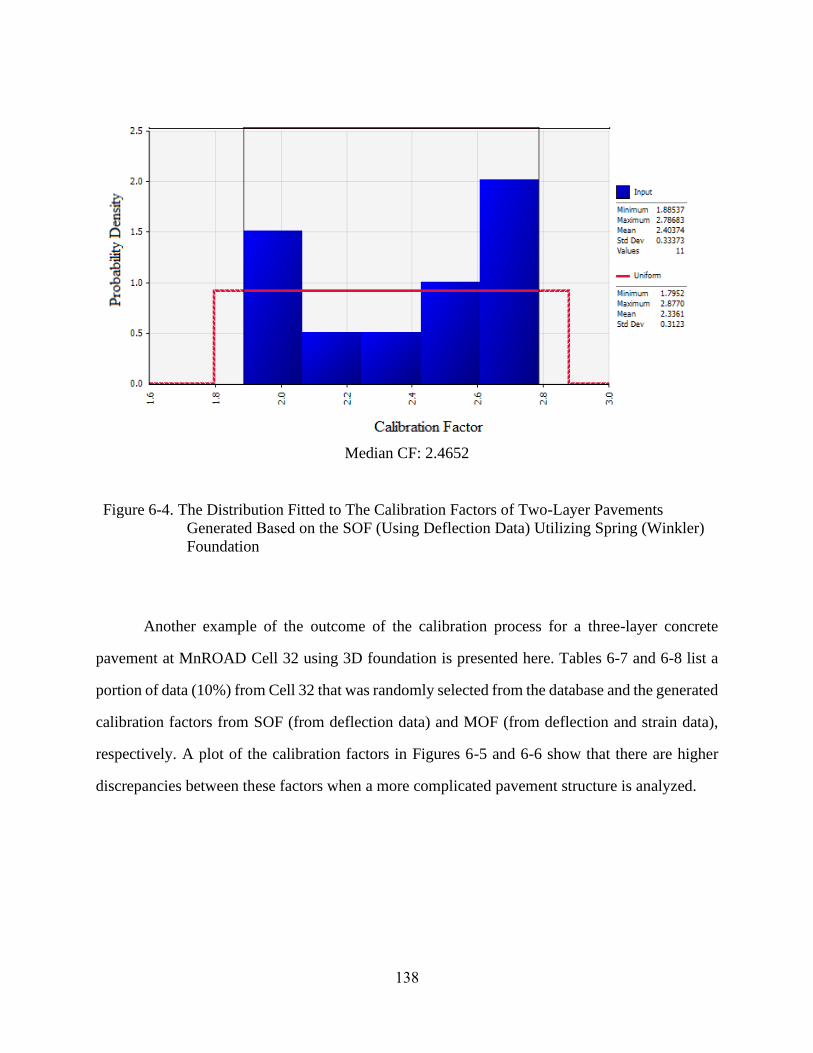
138

Median CF: 2.4652


Generated Based on the SOF (Using Deflection Data) Utilizing Spring (Winkler)

Foundation

Another example of the outcome of the calibration process for a three-layer concrete

pavement at MnROAD Cell 32 using 3D foundation is presented here. Tables 6-7 and 6-8 list a

portion of data (10%) from Cell 32 that was randomly selected from the database and the generated

calibration factors from SOF (from deflection data) and MOF (from deflection and strain data),

respectively. A plot of the calibration factors in Figures 6-5 and 6-6 show that there are higher

discrepancies between these factors when a more complicated pavement structure is analyzed.

139

Table 6-7. The Generated Calibration Factors for the Deflection (SOF) of Three-Layer Pavements at MnROAD Cell 32

FWD

Load, P

(lb)

Max.

Deflection,

D0 (mil)

Given

Modulus of

Base (psi)

Given

Modulus of

Subgrade

(psi)

Calibrated

Modulus of

Base (psi)

Calibrated

Modulus of

Subgrade

(psi)

Calibration

Factor of

Base,

CF1

Calibration

Factor of

Subgrade,

CF2 9,136 5.7 16,500 10,400 23,084 8,434 1.399 0.811

8,739 24.7 16,500 10,400 18,414 13,385 1.116 1.287

14,782 29.8 16,500 10,400 21,714 10,598 1.316 1.019

6,106 4.8 16,500 10,400 18,480 12,532 1.120 1.205

6,106 4.5 16,500 10,400 16,517 8,330 1.001 0.801

14,623 35.5 16,500 10,400 20,345 13,239 1.233 1.273

5,773 13.7 16,500 10,400 18,447 11,970 1.118 1.151

14,925 23.4 16,500 10,400 16,154 12,480 0.979 1.200

14,893 56.2 16,500 10,400 17,325 14,300 1.050 1.375

14,925 31.3 16,500 10,400 14,157 8,694 0.858 0.836

5,837 10.2 16,500 10,400 15,692 12,917 0.951 1.242

15,512 12.5 16,500 10,400 18,579 12,324 1.126 1.185

14,386 46.6 16,500 10,400 15,560 9,433 0.943 0.907

14,544 41.3 16,500 10,400 22,044 13,822 1.336 1.329

5,742 13.7 16,500 10,400 18,431 10,327 1.117 0.993

Median: 1.1170 1.1850

140

Table 6-8. The Data of Deflection and (b) Strain at the Bottom of Slab Used for Generating the Calibration Factors using MOF for

Three-Layer Pavements at MnROAD Cell 32

(a)

FWD

Load, P

(lb)

Max.

Deflection,

D0 (mil)

Given

Modulus of

Base (psi)

Given

Modulus of

Subgrade

(psi)

Calibrated

Modulus of

Base (psi)

Calibrated

Modulus of

Subgrade

(psi)

Calibration

Factor of

Base,

CF1

Calibration

Factor of

Subgrade,

CF2 5,710 17.9 16,500 10,400 18,893 13,853 1.145 1.332 6,122 4.6 16,500 10,400 15,329 13,229 0.929 1.272

14,782 29.8 16,500 10,400 14,025 12,272 0.850 1.180 5,805 12.3 16,500 10,400 15,824 13,021 0.959 1.252

15,337 12.9 16,500 10,400 22,985 13,822 1.393 1.329 8,993 14.4 16,500 10,400 16,599 9,578 1.006 0.921 5,837 10.2 16,500 10,400 14,223 10,774 0.862 1.036 8,771 21.5 16,500 10,400 21,120 10,764 1.280 1.035 9,215 6.3 16,500 10,400 14,157 10,868 0.858 1.045

14,275 45.4 16,500 10,400 22,275 10,244 1.350 0.985 8,152 36.2 16,500 10,400 20,906 12,386 1.267 1.191 9,009 12.9 16,500 10,400 14,702 11,305 0.891 1.087 8,882 17.5 16,500 10,400 16,517 8,580 1.001 0.825

14,719 35.4 16,500 10,400 20,675 13,822 1.253 1.329 14,893 30.2 16,500 10,400 18,051 14,144 1.094 1.360

Median: 1.0060 1.1800

(b)

Truck Load (kips) Strain in Slab

( )‡

12.0

16.9

16.6

15.6

18.4

34.2

34.4

33.8

39.3

38.5

‡ Dynamic strain due to truck loading measured

beneath the tire

141




MnROAD Cell 32 Generated Based on SOF (By Incorporating the Deflection

Data) (a) CF1 for Base Layer (b) CF2 for Subgrade Layer

142




MnROAD Cell 32 Generated Based on MOF (By Incorporating the Deflection

and Strain Data) (a) CF1 For Base Layer (b) CF2 For Subgrade Layer

Tables A-1 through A-4 (and Figures A-1 through A-4) in Appendix A list the calibration

factors for three-, and four-layer concrete pavements.

143

An important outcome of the calibration results shown here and in appendix A is that even

for the complex pavement structures, the calibration factors range between 0.75 and 1.60. Since

the analysis for three- and four-layer pavements were performed for the test sections at different

locations and different properties, this range of calibration factors indicates the capability of RPAS

in making accurate prediction of pavement responses and calibration will improve this accuracy.

This was confirmed by the several studies conducted in Chapters 4 and 5 on the pre-validation and

bench-marking of RPAS, where small errors between the predictions and measured responses were

observed. Upon availability of more data, the calibration can be even further improved.

144

7. Validation

This chapter provides the results of the validation of RPAS using a set of field data

randomly selected for this purpose. Different validation metrics are reviewed, and the reliability

of the program (utilizing 3D foundation) based on the provided test data in the calibration and

validation stages will be assessed.

7.1. Validation Metrics

As described in section 6.2, the field test dataset was divided into a calibration dataset and

a validation dataset. The calibration dataset was used in Chapter 6 above to calculate calibration

factors and in this Chapter the validation dataset will be used to assess the calibration process and

the resulting calibration factors. This process is called model validation and it is important to

highlight that it is conducted with a dataset that was excluded from the calibration process.

Researchers have been developing different types of validation metrics that express the accuracy

of a computational model through comparison with experimental data. Available approaches for

quantitative model validation are based on statistical confidence intervals (Oberkampf and Barone

2006), computing distance between the model prediction and experimental data by computing the

area metric (Roy and Oberkampf 2011, Ferson et al. 2008), normalizing residuals (Hills and Leslie

2003), classical statistics-based hypothesis testing (Urbina et al. 2003), Bayesian hypothesis

testing (Gelfand and Dey 1994, Geweke 2007, Mahadevan and Rebba 2005), and reliability

analysis-based techniques (Thacker and Paez 2014). Liu et al. (2011) and Ling and Mahadevan

(2013) investigated several of these validation approaches in detail and discussed their practical

implications in engineering. While some of these approaches compute validation metrics, some

other approaches focus on directly estimating the so-called model form error (Rebba et al. 2006)

as the difference between the model prediction and the underlying physical phenomenon the model

seeks to represent.

Another important issue related to model validation is the topic of extrapolating the model

to application conditions under which experiments may not have been performed. Typically, there

145

are two types of extrapolation. The first type is where the model is validated at certain input values,

but prediction needs to be performed at other input values that are not contained in the validation

domain. The second type of extrapolation is where validation is performed using a simplified

system (with restricted features, physics, etc.) and the desired prediction is of the original system.

While regression-based techniques have been developed for the first type of extrapolation (Roy

and Oberkampf 2011); model extrapolation, in general, is still a challenging issue and researchers

are currently studying this problem.

In this study, a reliability analysis-based technique was used in which a model reliability

metric ( r ) is calculated. This reliability metric that computes the probability that the model is

valid and will be described here. Suppose a set of experimental data Y that can be expressed in

general form of 1 21 2 1 2 1 2

1 2, ,..., , , ,..., ,..., , ,...,

km m mn

Y y y y y y y y y y= , in which each subset 1

through n indicates the replicates experimental data for the same input, i.e., same test spot and

loading condition on pavement in the field. The numerical analysis (from RPAS) will return the

prediction 1 2, ,... n = from that shows a single prediction corresponding to each test case.

Let’s define D as the percent absolute difference between the experimental data (considering the

average of each case, all the data, or any other statistical measure of data) and the model

predictions. A small number v (in percent) denotes the validation accuracy requirement, which

will be set by the user (e.g., engineer, practitioner) as a target metric of model validation. The

reliability metric r can be defined as ( )v vr P D = − , indicating the probability that the

difference between the experimental data and model predictions fall within the tolerance interval

of validation accuracy requirement. A plot of experimental (measured) data against model

predictions are presented before and after calibration. The correlation between these two variables

as well as the prediction limits can be also used to somewhat evaluate the validity of the calibrated

model.

146

7.2. Reliability Assessment Results

Once the calibration factor is generated from the calibration process explained in Chapter

6 and the median of CF is calculated, it will be applied to unseen data for validation. An example

of the application of the proposed calibration and validity assessment on the three-layer pavement

sections from MnRAOD Cells 32 and 52, as well as NAPTF CC-2 using the single-objective

function (SOF) is shown in Figure 7-1. Like in the previous chapter, not all the utilized data were

shown in this graph for brevity. The data used for this figure are listed in Table A-1 of Appendix

A.

As can be seen in Figure 7-1, even though the equations showing the correlations in both

graphs are very similar, the residuals for the fitted data before calibration are much higher

( 2 0.77R = ) than those in the calibrated model ( 2 0.99R = ). These larger residuals indicate a

lower reliability of the model.

147

(a) (b)


Before Calibration (b) Correlation After Calibration Using SOF

By utilizing the multi-objective function (MOF) for the calibration of three-layer pavement

systems, the validity of the calibration process was assessed in Figure 7-2a for deflection and

Figure 7-2b for strain responses. Again, note that only a portion of the entire data are visualized

here. As can be seen, an improvement in deflection (R2 increased from 0.90 to 0.99) and strain (R2

increased from 0.98 to 0.99) response was observed after calibrating RPAS and the prediction limit

became narrower.

148

Before Calibration After Calibration

(a)

Before Calibration After Calibration

(b)


Before Calibration (b) Correlation After Calibration Using MOF

The calibrated model can also be assessed for the level of validity in terms of the reliability

metric r . Figures 7-3 and 7-4 show the distribution of D as the percent absolute difference between

149

the experimental data and RPAS predictions associated with the data used in Figures 7-1 and 7-2,

respectively, using SOF and MOF. The summary of RPAS reliability results based on the

difference D shown these figures are presented in Tables 7-1 and 7-2.

(a)

(b)

Figure 7-3. The Distribution of the Percent Absolute Difference Between the Deflections From

Experimental and RPAS Predictions (D) For Three-Layer Pavements Using (a)

Not Calibrated Model (b) Calibrated Model Utilizing SOF

150

(a)

(b)

Figure 7-4. The Distribution of the Percent Absolute Difference Between the Experimental and

RPAS Predictions (D) For Three-Layer Pavements For (a) Deflections (b) Strain

Response Using MOF

151


Layer Pavements by Utilizing SOF

Accuracy

Requirements,

v (%)

Reliability Metric, r

N/C† C‡

1 0.05 0.19

5 0.13 0.64

10 0.25 0.86

15 0.50 0.96 † N/C: Not-Calibrated Model ; ‡C: Calibrated Model


Layer Pavements by Utilizing MOF

Accuracy

Requirements,

v (%)

Reliability Metric, r

Deflection response Strain response

N/C† C‡ N/C† C‡

1 0.03 0.05 0.05 0.08

5 0.19 0.60 0.25 0.38

10 0.40 0.95 0.45 0.65

15 0.58 0.99 0.60 0.78 † N/C: Not-Calibrated Model ; ‡C: Calibrated Model

As shown above, the level of reliability significantly increases after calibration. At a certain

v , it can be seen that the corresponding reliability metrics for calibrated models (for both

deflections and strains) are higher than those from non-calibrated models. As can be seen in Table

7-1, when using the calibrated model, if the pavement design engineer decides to set the accuracy

requirement at 1%, there will be only 19% probability that the predicted pavement responses from

RPAS are within ±1% difference from measured responses. By increasing the accuracy

requirement to 5%, the reliability of the pavement responses will greatly increase to 64%. In a

typical design, the designer targets the accuracy requirement of 10%, from which the predictions

from the calibrated model in RPAS are 86% in agreement with the field measurements listed

above. In other words, in this set of validity analysis, 86% of the predictions from RPAS fall within

±10% difference with the field data. The same conclusions can be drawn for the reliability metrics

obtained by utilizing MOF in Table 7-2.

152

As observed from the trend of the change of reliability metric of calibrated model with the

respect to the accuracy requirement, there is a drastic increase in the reliability if the accuracy

requirement is increased from 1 to 10%. This conclusion confirms the typical threshold value of

10% for the difference between the measured and calculated responses in the analysis of

pavements. This trend was not observed for non-calibrated model and, if achievable, reaching the

reliability of 70 to 80% needs using a wide range of accuracy requirement that may not be

acceptable to pavement designer or transportation agencies.

7.3. Numerical Example

To better understand the effect of implementing the results from the sensitivity analysis

into the calibration process of RPAS, an example was designed based upon the analysis of a

pavement section in MnROAD Cell 32. In this example, two separate analyses were performed in

RPAS using two different foundation models. For case I, the properties of the pavement foundation

layers were assumed according to the recommended values in AASHTO (1993) and were entered

into RPAS using a spring foundation model. Case II consisted of running RPAS utilizing a 3D

solid foundation model by using the measured or back-calculated moduli of the foundation layers

obtained from laboratory and field testing of the pavement section. A comparison between the

responses obtained from these two models and the responses measured in field was made before

and after applying the calibration factor to evaluate the importance of the implementation of GSA

in the calibration process.

The pavement section studied in this example was described in Chapter 4; however, a brief

description of this test section is presented here. This pavement consists of a 5-inch concrete slab

placed on a 6-inch gravel base and a clay subgrade (R=12). The concrete slabs were 10 ft long and

12 ft wide. MnROAD Cell 32 was instrumented with static sensors (vibrating wire sensors and

thermocouples) measuring the moisture and temperature distribution within the pavement depth

as well as dynamics sensors measuring the responses under an 80-kip semi-trailer truck loading

and falling weight deflectometer (FWD) tests.

153

The modulus and Poisson’s ratio of the concrete layer were defined as 4,445 ksi and 0.155,

respectively. These values were measured from testing of cylinder specimens in the laboratory and

were used for both cases I and II because they are also close to typical design values. The stiffness

of the foundation layer for case I was determined from the typical values for fair to good subgrade

in AASHTO (1993), i.e. 400 pci, whereas for case II, the moduli of 26,000 and 10,000 ksi were

used for base and subgrade layers, respectively, according to back-calculation results. Further

details on the back-calculated material properties and pavement configuration can be found in

TaghaviGhalesari et al. (2020a). It should be noted that the effect of temperature loading has not

been included in this study to achieve a similar comparison for both cases I and II.

Figure 7-5 illustrates the comparison of deflection and strain responses of the studied

pavement section using cases I and II analyses. The percent difference between the results from

case I or II and those from field measurements are shown below each location of pavement that

was tested. As expected, there is a significant difference between responses predicted with spring

model and 3D foundation (cases I and II, respectively), which had been shown in previous studies

by Aguirre et al. (2019) and Luo et al. (2017). Modeling the supporting layers using the 3D solid

foundation (case II) results in better agreement between the pavement deflections at different

locations (16-29% difference) as compared to those using traditional method (case I) by utilizing

the spring foundation (19-73% difference). The strains at the bottom of the concrete slab in

dynamic sensor CE 120 in MnROAD Cell 32 that are shown in Figure 7-5b are also more

consistent (less than 19% difference) with the RPAS modeling with 3D foundation that using a

spring model (up to 70% difference). Therefore, the accurate modeling of the properties of the

foundation layers using RPAS 3D foundation model will significantly improve the prediction of

the pavement responses and, subsequently, will lead to more efficient pavement designs.

154

Figure 7-5. (a) Comparison of the Three-Layer Pavement Response from Field Measurements

and Modeling With 3D And Spring Foundation (a) Pavement Surface Deflection

Under FWD Test (b) Longitudinal Strain at The Bottom of Concrete Slab at

MnROAD Cell 32.

An efficient way of calibration is to use a more comprehensive test dataset for calibration

and running the calibration process using multi-objective minimization of the error function, which

has been implemented earlier in this chapter. These calibration factors can be adjusted based on

the GSA results. A simple type of this approach was employed in this section in a way that 70%

0

10

20

30

40

50

60

70

6-kip 9-kip 15-kip 6-kip 9-kip 15-kip 6-kip 9-kip 15-kip 6-kip 9-kip 15-kip 6-kip 9-kip 15-kip

Pave

ment

Surface D

efle

ction (

mil)

(a) Field Measurement Case I Case II

----------------------- ------------------------- ------------------------ ------------------------ ------------------------

Center MidEdge Corner JointAfter JointBefore

Case I: 29% Case I: 16% Case I: 22% Case I: 19% Case I: 16%Case II: 54% Case II: 19% Case II: 73% Case II: 37% Case II: 44%

0

10

20

30

40

50

60

70

1st Axle 2nd Axle 3rd Axle 4th Axle 5th Axle

Dynam

ic S

train

at

the B

ott

om

of

Sla

b (

µε)

(b) Field Measurement Case I Case II

-------------------- -------------------- -------------------- --------------------- --------------------Case I: 19% Case I: 9% Case I: 13% Case I: 18% Case I: 1%Case II: 70% Case II: 61% Case II: 62% Case II: 29% Case II: 60%

155

of data were used in the comparative study in Figure 7-5 and the remained 30% of field data were

used for comparison against the 3D modeling results (case II) after application of the calibration

factors derived from Pareto optimal front of error values. Figure 7-6 shows the deflection responses

after calibration using the GSA results. As seen, the magnitudes of error have decreased from 29%

to less than 6%. This high improvement in the perdition of pavement responses makes RPAS a

reliable tool to be used by pavement design engineers and transportation agencies

(TaghaviGhalesari et al. 2020c).

Figure 7-6. Comparison of Three-Layer Pavement Surface Deflection from FWD

Measurements at MnROAD Cell 32 and Finite Element Simulation Using

Calibrated RPAS Model.

0

10

20

30

40

50

6-kip 9-kip 15-kip 6-kip 9-kip 15-kip 6-kip 9-kip 15-kip 6-kip 9-kip 15-kip 6-kip 9-kip 15-kip

Pave

ment

Surface D

efle

ction (

mil)

(a) Field Measurement (Test Set) Case II (Calibrated)

----------------------- ------------------------- ------------------------ ------------------------ ------------------------

Center MidEdge Corner JointAfter JointBefore

6% 3% 5% 6% 4%

156

8. Summary and Conclusions

Several analysis tools have been developed to predict the thermo-mechanical response of

concrete pavements. Most of these tools use the finite element method to calculate bending

stresses, strains and deflections in the concrete slabs caused by self-weight, tire loading, and

thermal curling. RPAS is a software developed at the University of Texas at El Paso to model the

behavior of concrete pavements and improve over the accuracy and capabilities of the previously

developed tools. However, prior to the work presented in this dissertation there were only a limited

number of studies conducted on the verification and validation of RPAS against analytical

solutions and experimental data. To improve on the reliability of RPAS, a framework integrating

a verification, calibration and validation process was proposed and implemented in this study.

8.1. Summary

A review of different types of concrete pavements, key factors influencing pavement

response, modeling techniques and tools was conducted to understand the load transfer and

interaction mechanisms of concrete pavements. Since the main focus of this study was the

improvement of the reliability of RPAS using experimental data thorough a review of field and

laboratory test methods, data collection and processing was conducted. The approaches and

statistical metrics for the verification, calibration and validation of RPAS were presented.

As the initial step toward RPAS model validation, the data collected from pavement tests

sections at MnROAD and NAPTF test facilities were processed and catalogued. The pavement

structure and test condition were modeled in RPAS for the initial comparison called pre-validation.

This step was performed to assess the performance of RPAS in modeling the pavement response

before applying the calibration process.

Verification of RPAS consisted of two stages consisting of calculation verification and

bench-marking. For the first stage, a stress convergence study was performed to find the error

introduced to the model caused by the discretization, which is called solution approximation error.

For the second stage a multi-level bench-marking was implemented, in which the comparison of

157

RPAS predictions with the analytical solutions was performed from a simplified problem (a plate

under distributed load) and then was expanded to a more complicated 3D model created in other

finite element tools.

Before the calibration was conducted a global sensitivity analysis using random decision

forests was conducted to find the relative importance of the various input parameters on the

calculation of the critical responses of concrete pavements. The results of this sensitivity analysis

indicated that pavement moduli were among the most influential parameters. This coincided with

the fact that foundation moduli have a large variability as observed in the field data and thus it was

the reason that the moduli was selected for calibration. The calibration process consisted then of

calibrating/correcting the moduli of the pavement foundation layers to find a reasonable agreement

between the model predictions and field measurements. This calibration process used a multi-

objective optimization to minimize the error of predictions while considering both the deflection

and strain response of the test and model pavements. The Pareto Optimal Front algorithm was used

for this multi-objective optimization. The calibration factors were generated as the ratio of the

calibrated to the original moduli of foundation layers from laboratory tests or back-calculation.

Finally, by applying the calibration factors to the models, a validation of the predictions

from RPAS was conducted. For this purpose, a reliability metric was proposed that calculates the

probability of the differences between the RPAS results and the field data being within an

acceptable range.

8.2. Conclusions

Based on the mathematical and statistical analyses conducted in this study utilizing the

empirical data, the following conclusions were drawn:

1. In general, uncalibrated RPAS results show a reasonable agreement with deflections

measured in the field. However, the stresses and strains calculated at the top and bottom

of the concrete slab can, in certain cases, result in discrepancies of up to 50% between

158

RPAS and field measurements indicating the need for the calibration process presented

here.

2. The results of global sensitivity analysis showed the significance of the contribution of

pavement foundation layers on the critical responses of concrete pavements. This

conclusion not only identified the foundation moduli as a parameter to focus on during

the calibration process, but also highlights the issue of design guides such as MEPDG

that assume a low importance for the properties of the foundation layers.

3. The first part of the verification of RPAS was calculation verification, that was based

on finding the numerical error due to discretization of the foundation layers. The results

indicated that to minimize this error, the first soil layer beneath the concrete slab must

be discretized into elements with a vertical dimension of 1 in. Once this step was

completed, the verified (corrected) model was used for bench-marking. This multi-

level process showed a great agreement (r-square>0.9) between various analytical

solutions and RPAS calculations for simple problems as the lowest level of bench-

marking. The following higher levels included more complicated problems of

pavement modeling using other advanced numerical tools in which RPAS results

showed a good agreement with discrepancies of up to 11% for the longitudinal stress

in slabs.

4. The calibration process included a multi-objective optimization that was used to

calibrate the moduli of the foundation layers to minimize the difference between the

field and numerical results. The calibration factors were generated for two-, three-, and

four-layer pavement systems. The statistical distribution of these calibration factors

was obtained and the median was selected to define the calibrated moduli to be used in

RPAS. The range of calibration factors were between 0.75 and 1.60 with most being

close to 1.00. After applying these calibration factors, the validation process was

conducted.

159

5. One of the methods used to validate the responses of the calibrated RPAS model was

to plot the correlations plots of measured and predicted response of different pavement

structures before and after calibration. These graphs included the prediction limits as

well as the discrepancy (r-square) of the data points. The results indicated narrow

prediction confidence limits and a high accuracy (r2=0.99) of the calibrated model. In

addition to these plots, a reliability metric r that represents the probability of the

differences between RPAS results and field data being within an acceptable range. This

metric was calculated for the model before and after calibration. The values of the

reliability metric were shown to significantly improve after calibration. For example,

by assuming the accuracy requirement of 15%, the reliability of three-layer pavements

increased from 50% to 96%.

6. The results shown in this dissertation demonstrate that the verification, calibration

and validation method implemented here have resulted in a calibrated RPAS model

that produces reliable concrete pavement responses.

8.3. Recommendations for Future Research

While the extensive effort to complete the work presented in this dissertation resulted in a

significantly improved RPAS model, there are still many areas for potential improvement. The

following recommendations are made for future research:

1. An improvement to the concrete pavement model would be to use three-dimensional

hexahedron elements to discretize the slab. With this improvement, the steel

reinforcement and its interaction with the surrounding concrete can be properly

modeled. In addition, using these elements would allow for the modeling of the dowel

bar looseness or misalignment that can have a prominent effect on dowel’s mechanical

performance due to its modified effective length. These improvements could also lead

to the capability of modeling crack propagation, if the ultimate goal is to expand this

160

analysis tool to a design tool. Although the implementation of these three-dimensional

elements could lead to additional capabilities, they would have to be weighed against

the significant increase in required computational power.

2. The warping caused moisture intrusion into the pavement layers can significantly

impact the development of bending stresses in concrete slab and can also have a

negative impact on the mechanical properties of the foundation layers. Adding a model

for moisture intrusion would also improve RPAS capabilities.

3. During the process to collect data to be used for calibration and validation purposes, a

significant effort was made to gather as much data as possible from different types of

pavement structures, tire loading, environmental conditions and material properties.

However, the data available was limited to two pavement test facilities. It is

recommended that more data be gathered from laboratories, test facilities and field tests

across the nation to be implemented in the calibration process. This effort could then

lead to various calibrated versions of RPAS specific to a particular district or state. As

mentioned in Chapter 6, the framework presented here can be used for re-calibration

additional data becomes available.

4. During the verification, benchmarking, calibration and validation process numerous

statistical and data analysis algorithms were utilized. These algorithms were selected

based on their wide-spread use for similar applications. However, the field of machine

learning and statistical analysis in general is always expanding and new algorithms are

being developed. For future work it is recommended to assess the performance of other

algorithms to further improve on the calibrated version of RPAS.

161

References

AASHTO. 1993. Guide for Design of Pavement Structures. American Association of State

Highway and Transportation Officials, Washington, D.C.

ACPA (2020): http://www.apps.acpa.org/apps/kvalue.aspx

Aguirre, N. 2020. Development of A Numerical Simulation Tool for Continuously Reinforced

Concrete Pavements. PhD Dissertation, University of Texas at El Paso, El Paso, TX.

Aguirre, N., TaghaviGhalesari, A., Carrasco, C. 2019. A Comparison of Concrete Pavement

Responses using Finite Element Method with Foundation Springs and 3-D Solid Elements,

International Airfield and Highway Pavements Conference, Chicago, IL.

Aguirre, N., TaghaviGhalesari, A., Rogers, R., Carrasco, C., Nazarian, S. 2020. Influence of

Foundation Layer Properties in a Concrete Pavement System Subjected to Heavy Vehicle

Loads, International Conference on Transportation Geotechnics, Chicago, IL.

Anderson, M. P., Woessner, W. W., Hunt, R. J. (2015). Applied Groundwater Modeling:

Simulation of Flow and Advective Transport. 2nd Edition, Academic press, San Diego,

CA.

ASME, (2006). Guide for Verification and Validation in Computational Solid Mechanics, The

American Society of Mechanical Engineers, ASME V&V 10-2006.

AIAA (American Institute of Aeronautics and Astronautics) 1998. Guide for the Verification and

Validation of Computational Fluid Dynamics Simulations, AIAA-G-077-1998, Reston,

VA, American Institute of Aeronautics and Astronautics.

Aure, T. W., Ioannides, A. M. 2010. Simulation of Crack Propagation in Concrete Beams with

Cohesive Elements In ABAQUS. Transportation research record, 2154(1), 12-21.

Babuška I., Rheinboldt WC. (1978). A-Posteriori Error Estimates for The Finite Element Method.

Int J Numer Methods Eng, 12(10): 1597–615.

Barbosa, R. S. 2011. Vehicle Dynamic Response Due to Pavement Roughness. Journal of the

Brazilian Society of Mechanical Sciences and Engineering, 33(3), 302-307.

Beckemeyer, C., Khazanovich, L., Thomas Yu, H. 2002. Determining Amount of Built-in Curling

in Jointed Plain Concrete Pavement: Case study of Pennsylvania I-80. Transportation

Research Record, 1809(1), 85-92.

Bhatti, M. A. 2006. Advanced Topics in Finite Element Analysis of Structures: with

Mathematica and MATLAB Computations. New York: John Wiley.

Bradbury, R. D. 1938. Reinforced Concrete Pavements, Wire Reinforcement Institute,

Washington, D.C.

Breiman, L. 2001. Random forests. Machine learning, 45(1), 5-32.

Brill, D. R., Hayhoe, G. F., Ricalde, L. 2005. Analysis of CC2 Rigid Pavement Test Data from the

FAA’s National Airport Pavement Test Facility. In Proc. 7th International Conference on

the Bearing Capacity of Roads, Railways, and Airfields, Trondheim, Norway.

http://www.apps.acpa.org/apps/kvalue.aspx

162

Burmister, D. M. 1943. The Theory of Stresses and Displacements in Layered Systems and

Applications to the Design of Airport Runways, Highway Research Board 23, 126-144.

Burmister, D. M. 1945. The General Theory of Stresses and Displacements in Layered Soil

Systems, Journal of Applied Physics, 16, 84-94,126-127, 296-302.

Burnham, T. R. 2002. Construction Report for Mn/ROAD PCC Testcells 32, 52, and 52. Report

No. MN/RC 2002-04. Minnesota Department of Transportation, Research Services

Section, St. Paul, MN, USA.

Burnham, T. R., Tewfik, A., Srirangarajan, S. 2007. Development of A Computer Program for

Selecting Peak Dynamic Sensor Responses from Pavement Testing (No. MN/RD-2007-

49). Minnesota. Dept. of Transportation.

Carrasco, C., Limouee, M., Celaya, M., Abdallah, I. Nazarian, S. (2009). NYSLAB: A Software

for Analysis of Jointed Pavements. Final Report. Report Number: FHWA-RD-07-1008-

01.

Carrasco, C., Limouee, M., Tirado, C., Nazarian, S., and Bendaña, J. 2011. Development of

NYSLAB: Improved Analysis Tool for Jointed Pavement. Transportation Research

Record: Journal of the Transportation Research Board, (2227), 107-115.

Ceylan, H., Gopalakrishnan, K., Kim, S., Schwartz, C. W., Li, R. 2013. Global Sensitivity Analysis

of Jointed Plain Concrete Pavement Mechanistic–Empirical Performance Predictions.

Transportation Research Record, 2367(1), 113-122.

Chen, L., Feng, D., Quan, L. 2014. Inclusion of Built-In Curling Temperature Profile in Curling-

Stress Determination for Rigid Pavement. Journal of Transportation Engineering, 141(4),

06014003.

Cheung, Y. K., Zinkiewicz, O. C. 1965. Plates and Tanks on Elastic Foundations - An Application

of Finite Element Method. International Journal of Solids and structures, 1(4), 451-461.

Chou, Y. T. 1981. Structural Analysis Computer Programs for Rigid Multicomponent Pavement

Structures with Discontinuities—WESLIQID and WESLAYER. Report 2, Manual for the

WESLIQID finite element program, Tech. Report GL-81-6, Vicksburg, MS: U.S. Army

Waterways Experiment Station.

Choubane, B. and M. Tia. 1992. Nonlinear Temperature Gradient Effect on Maximum Warping

Stresses in Rigid Pavements. Transportation Research Record No. 1370. Washington, DC:

Transportation Research Board, National Research Council, pp. 11–19.

Davids, W. G., G. M. Turkiyyah, J. P. Mahoney. 1998. EverFE: Rigid Pavement Three-

Dimensional Finite Element Analysis Tool. Transportation Research Record: Journal of

the Transportation Research Board, 1629 (1): 41-49.

Davids, W., Wang, Z., Turkiyyah, G., Mahoney, J., Bush, D. 2003. Three-dimensional finite

element analysis of jointed plain concrete pavement with EverFE 2.2. Transportation

Research Record: Journal of the Transportation Research Board 1853, 92-99.

De Jong, D. L. Peatz M. G. F, Korswagen, A. R. 1973. Computer Program BISAR Layered

Systems Under Normal and Tangential Loads, External Report AMSR .0006 .73; Konin

Klijke Shell-Laboratorium, Amsterdam.

163

Eymard, R., Guerrier, F., Jacob, B. 1990. Dynamic Behavior of Bridge under Full Traffic. In

Bridge Evaluation, Repair and Rehabilitation (pp. 293-306). Springer, Dordrecht.

Ferson, S., Oberkampf, W.L., Ginzburg, L. 2008. Model Validation and Predictive Capability for

The Thermal Challenge Problem. Comput Methods Appl Mech Eng, 197(29), 2408–30.

FHWA 2019. Concrete Pavement Joints, Technical Advisory T 5040.30. Federal Highway

Administration. Washington, D.C. https://www.fhwa.dot.gov/pavement/ta504030.pdf.

Friberg, B. F. 1940. Design of Dowels in Transverse Joints of Concrete Pavements, Transactions,

ASCE, 105, 1076–1095.

Gamez, A., Hernandez, J. A., Ozer, H., Al-Qadi, I. L. 2018. Development of Domain Analysis for

Determining Potential Pavement Damage. Journal of Transportation Engineering, Part B:

Pavements, 144(3), 04018030.

Gelfand, A. E., Dey, D. K. Bayesian Model Choice: Asymptotics And Exact Calculations. J R Stat

Soc Ser B (Methodol) 1994:501–14.

Geweke, J. 2007. Bayesian Model Comparison and Validation. Am Econ Rev, 97(2), 60–4.

Gjorv, O. E., Baerland, T., Ronning, H. R. 1990. Abrasion Resistance of High Strength Concrete

Pavements. Concrete International, 12(1), 45-48.

Grater, S. F., McCullough, B. F. 1994. Analysis of Jointed Concrete Pavement. Report

FHWA/TX-95-1244-10, Center for Transportation Research, The University of Texas at

Austin.

Guclu, A., Ceylan, H., Gopalakrishnan, K., Kim, S. 2009. Sensitivity Analysis of Rigid Pavement

Systems Using the Mechanistic-Empirical Design Guide Software. Journal of

Transportation Engineering, 135(8), 555-562.

Ha, S., Yeon, J., Choi, B., Jung, Y., Zollinger, D. G., Wimsatt, A., Won, M. C. 2011. Develop

Mechanistic-Empirical Design for CRCP (No. FHWA/TX-11-0-5832-1), Texas Tech

Univ., Lubbock, TX.

Hall, K. D., Beam, S. 2005. Estimating the Sensitivity of Design Input Variables for Rigid

Pavement Analysis with A Mechanistic–Empirical Design Guide. Transportation Research

Record, 1919(1), 65-73.

Hamim, A., Yusoff, N. I. M., Ceylan, H., Rosyidi, S. A. P., El-Shafie, A. 2018. Comparative Study

on Using Static and Dynamic Finite Element Models to Develop FWD Measurement on

Flexible Pavement Structures. Construction and Building Materials, 176, 583-592.

Hammons, M. I., Ioannides, A. M. 1997. Mechanistic Design and Analysis Procedure for Doweled

Joints in Concrete Pavements. International Purdue Conference on Concrete Pavement

Design and Materials for High Performance, Vol. 3, Indianapolis, Indiana, USA.

Han, W., Yuan, Y., Huang, P., Wu, J., Wang, T., Liu, H. 2017. Dynamic Impact of Heavy Traffic

Load On Typical T-Beam Bridges Based on WIM Data. Journal of Performance of

Constructed Facilities, 31(3), 04017001.

Hansen, W., Y. Wei, D. L. Smiley, Y. Peng, and E. A. Jensen. (2006). Effects of Paving Conditions

on Built-in Curling and Pavement Performance. International Journal of Pavement

Engineering, 7 (4): 291-296.

https://www.fhwa.dot.gov/pavement/ta504030.pdf

164

Hastie, T., Friedman, J., Tibshirani, R. 2017. The Elements of Statistical Learning, New York:

Springer series in statistics.

Hiller, J. E., Roesler, J. R. 2009. Simplified Nonlinear Temperature Curling Analysis for Jointed

Concrete Pavements. Journal of Transportation Engineering, 136(7), 654-663.

Hills, R. G., Leslie, I.H. 2003. Statistical Validation of Engineering and Scientific Models:

Validation Experiments to Application. Technical report. Albuquerque, NM, USA;

Livermore, CA, USA: Sandia National Labs.

Huang, K., Zollinger, D. G., Shi, X., Sun, P. 2017. A Developed Method of Analyzing

Temperature and Moisture Profiles in Rigid Pavement Slabs. Construction and Building

Materials, 151, 782-788.

Huang, Y. H., 1967. Stresses and Displacements in Viscoelastic Layered Systems Under Circular

Loaded Areas, Proceedings, 2nd International Conference on the Structural Design of

Asphalt Pavements, pp. 225–244.

Huang, Y. H. 1993. Pavement Analysis and Design. Englewood Cliffs, NJ: Prentice Hall.

Hwang, C. L., Masud, A. S. M. 2012. Multiple Objective Decision Making Methods And

Applications: A State-Of-The-Art Survey, Vol. 164, Springer Science & Business Media,

New York, U.S.

Ioannides, A. M., Khazanovich, L. 1998. Nonlinear Temperature Effects on Multilayered Concrete

Pavements. Journal of Transportation Engineering, 124(2), 128-136.

Ioannides, A. M., Davis, C. M., Weber, C. M. 1999. Westergaard Curling Solution Reconsidered.

Transportation Research Record, 1684(1), 61-70.

Joshaghani, A., Zollinger, D. G. 2019. Assessment of Concrete Pavement Set Gradient Based on

Analysis of Slab Behavior and Field Test Data. Transportation Research Record,

0361198119849900.

Kannekanti, V. N., Harvey, J. T. 2005. Sensitivity Analysis of 2002 Design Guide Rigid Pavement

Distress Prediction Models, Report No UCPRC-DG-2006-01, California Department of

Transportation, Office of Roadway Research, Sacramento, CA, USA.

Kennedy, M. C., O'Hagan, A. 2001. Bayesian Calibration of Computer Models. Journal of the

Royal Statistical Society: Series B (Statistical Methodology), 63(3), 425-464.

Khazanovich, L. 1994. Structural Analysis of Multi-Layered Concrete Pavement Systems. PhD

Dissertation. University of Illinois at Urbana-Champaign.

Khazanovich, L. and A. M. Loannides. 1994. Structural Analysis of Unbonded Concrete Overlays

Under Wheel And Environmental Loading, Transportation Research Record No. 1449.

Washington, DC: Transportation Research Board.

Khazanovich, L., H. Yu, S. Rao, K. Galasova, E. Shats, R. Jones. 2000. ISLAB2000-Finite

Element Analysis Program for Rigid and Composite Pavements. User’s Guide.

Champaign, IL: ERES Consultants.

Kim, S. M., Won, M., McCullough, B. F. 2001. CRCP-10 Computer Program User's Guide (No.

FHWA/TX-0-1831-4,). Center for Transportation Research, Bureau of Engineering

Research, The University of Texas at Austin.

165

Kok, A. W. M. 1990. A PC Program for The Analysis of Rectangular Pavements Structures.

Proceedings, Second International Workshop on the Design and Rehabilitation of Concrete

Pavements, Sigüenza, Spain, pp. 113–120.

Kramer, S. 1996. Geotechnical Earthquake Engineering. Prentice-Hall, Inc. New Jersey, 348-422.

Li, W., Pour-Ghaz, M., Castro, J., Weiss, J. 2011. Water Absorption and Critical Degree of

Saturation Relating to Freeze-Thaw Damage in Concrete Pavement Joints. Journal of

Materials in Civil Engineering, 24(3), 299-307.

Ling, Y., Mahadevan, S. 2013. Quantitative Model Validation Techniques: New insights. Reliabil

Eng Syst Saf, 111, 217–31.

Liu, Y, Chen, W, Arendt, P, Huang, HZ. Toward A Better Understanding of Model Validation

Metrics. Trans ASME J Mech Des 2011;133(7):071005.

Loh, W. Y., Shih, Y. S. 1997. Split Selection Methods for Classification Trees. Statistica sinica,

815-840.

Luo, X., Gu, F., Zhang, Y., Lytton, R. L., Zollinger, D. 2017. Mechanistic-Empirical Models for

Better Consideration of Subgrade and Unbound Layers Influence on Pavement

Performance. Transportation Geotechnics, 13, 52-68.

Mahadevan, S, Rebba, R. Validation of Reliability Computational Models Using Bayes Networks.

Reliab Eng Syst Saf 2005;87(2):223–32.

Mallick, R.B., El-Korchi, T. 2018. Pavement Engineering, Principles and Practice, Third Edition,

CRC Press, Boca Raton, FL.

McQueen, R. D., Hayhoe, G. F. 2014. Construction Cycle 6 (CC-6) Revisited: Fatigue Analysis

and Economic and Design Implications, FAA Worldwide Airport Technology Transfer

Conference, Galloway, New Jersey, USA.

Miettinen, K. 2012. Nonlinear Multiobjective Optimization, Vol. 12, Springer Science & Business

Media, New York, U.S.

Misaghi, S. M. 2011. Impact of Truck Suspension and Road Roughness on Loads Exerted to

Pavements. MSc Thesis, The University of Texas at El Paso.

MnROAD Data Library 2019: http://www.dot.state.mn.us/mnroad/data/index.html

Mohamed, A., Hansen, W. 1997. Effect of Nonlinear Temperature Gradient on Curling Stress in

Concrete Pavements. Transportation Research Record: Journal of the Transportation

Research Board, 65-71.

NAPTF Data Library 2019: https://www.airporttech.tc.faa.gov/Airport-Pavement/National-

Airport-Pavement-Test-Facility/NAPTV.

Nash, J. E., Sutcliffe, J. V. 1970. River Flow Forecasting Through Conceptual Models Part I—A

Discussion of Principles. Journal of hydrology, 10(3), 282-290.

NCHRP 1-37A. 2004. Guide for Mechanistic–Empirical Design of New and Rehabilitated

Pavement Structures. Final Report, TRB, National Research Council, Washington, D.C.

Oberkampf, W. L., Barone, M. F. 2006. Measures of Agreement Between Computation and

Experiment: Validation Metrics. J Comput Phys, 217(1), 5–36.

http://www.dot.state.mn.us/mnroad/data/index.html

https://www.airporttech.tc.faa.gov/Airport-Pavement/National-Airport-Pavement-Test-Facility/NAPTV

https://www.airporttech.tc.faa.gov/Airport-Pavement/National-Airport-Pavement-Test-Facility/NAPTV

166

Ong, C. L., Newcomb, D. E., Siddharthan, R. 1991. Comparison of Dynamic and Static

Backcalculation Moduli for Three-Layer Pavements. Transportation Research Record,

1293, 86-92.

Oreskes, N., Shrader-Frechette, K., Belitz, K. (1994). Verification, Validation, and Confirmation

of Numerical Models In The Earth Sciences. Science, 263(5147), 641-646.

Pickett, G. and G. K. Ray. (1951). Influence Charts for Rigid Pavements. American Society of

Civil

Engineers Transactions.

Prażnowski, K., Mamala, J. 2016. Classification of The Road Surface Condition on The Basis Of

Vibrations Of The Sprung Mass In A Passenger Car. In IOP Conference Series: Materials

Science and Engineering 148(1): 012022. IOP Publishing Press.

Rangavajhala S, Sura V, Hombal V, Mahadevan S. 2011. Discretization Error Estimation in

Multidisciplinary Simulations. AIAA J, 49(12): 2673–712.

Rao, C., Titus-Glover, L., Bhattacharya, B. B., Darter, M. I., Stanley, M., Von Quintus, H. L. 2012.

Estimation of Key PCC, Base, Subbase, and Pavement Engineering Properties from

Routine Tests and Physical Characteristics, Report No. FHWA-HRT-12-030, FHWA

Office of Infrastructure Research and Development, McLean, VA.

Rao, S., Roesler, J. R. (2005). Characterizing Effective Built-In Curling from Concrete Pavement

Field Measurements. Journal of Transportation Engineering, 131(4), 320-327.

Rebba, R., Mahadevan, S., Huang, S. 2006. Validation and Error Estimation of Computational

Models. Reliab Eng Syst Saf, 91(10), 1390–7

Reddy, J. N. 2004. Mechanics of Laminated Composite Plates and Shells: Theory and Analysis.

CRC

Ricalde, L., Daiutolo, H. 2005. New Rigid Pavement Construction and Testing at the FAA

National Airport Pavement Test Facility (NAPTF). In Proc. of the Fifth International

Conference on Road and Airfield Pavement Technology, Seoul, Korea.

Rogers, R., Plei, M., Aguirre, N., Taghavi Ghalesari, A. 2017. Optimizing Structural Design for

Overlaying HMA Pavements with A Concrete Pavement Using Critical Stresses/Strains.

In Proc., TRB 11th University Transportation Center (UTC) Spotlight Conference:

Rebuilding and Retrofitting the Transportation Infrastructure, Washington, DC.

Roy, C. J., Oberkampf, W. L. 2011. A Comprehensive Framework for Verification, Validation,

And Uncertainty Quantification in Scientific Computing. Comput Methods Appl Mech

Eng, 200(25–28), 2131–44.

Saltelli, A., Ratto, M., Andres, T., Campolongo, F., Cariboni, J., Gatelli, D., Saisana, M.,

Tarantola, S. 2008. Global Sensitivity Analysis: The Primer. John Wiley & Sons.

Sankararaman, S., Mahadevan, S. 2015. Integration of Model Verification, Validation, And

Calibration for Uncertainty Quantification in Engineering Systems. Reliability

Engineering & System Safety, 138, 194-209.

167

Schwer, L.E., 2006. Guide for Verification and Validation in Computational Solid Mechanics,

ASME 20th International Conference on Structural Mechanics in Reactor Technology,

Espoo, Finland.

SIMULIA. 2016. ABAQUS 6.16 Documentation. Dassault Systèmes, Simulia Corporation,

Providence, RI.

Stoffels, S., Lopez, M., Yeh, L., Jeong, Y., Barzegari, S., Kermani, B. 2014. Fracture

Characterization and SEM Examination of NAPTF CC6 Concrete Mixes, FAA Worldwide

Airport Technology Transfer Conference, Galloway, New Jersey, USA.

Stoffels, S., Morian, D., Ioannides, A., Wu, S., Sadasivam, S., Yeh, L., Yin, H. 2008. Improved

Overlay Design Parameters for Concrete Airfield Pavements. Innovative Pavement

Research Foundation Report FAA-01-G-002-04-2, Conneaut Lake, PA.

Tabatabaie, A. M., Barenberg, E. J. 1980. Structural Analysis of Concrete Pavement Systems.

Transportation Engineering Journal, 106 (5): 493-506.

TaghaviGhalesari, A., Aguirre, N., Carrasco, C., Vrtis, M., Garg, N. 2020a. Evaluation of the

Response from the Rigid Pavement Analysis System (RPAS) Program for the

Characterization of Jointed Concrete Pavements, Road Material and Pavement Design,

https://doi.org/10.1080/14680629.2020.1747522.

TaghaviGhalesari, A., Aguirre, N., Carrasco, C., Vrtis, M., Garg, N. 2020b. Verification and

Validation of the Response of a 3-D Finite Element Model for the Characterization of

Jointed Concrete Pavements, TRB 99th Annual Meeting, Washington D.C.

TaghaviGhalesari, A., Aguirre, N., Carrasco. 2020c. Application of Sensitivity Analysis in The

Calibration Process of a Concrete Pavement Analysis Software. International Conference

on Transportation and Development, Seattle, WA.

TaghaviGhalesari, A., Aguirre, N., Carrasco. 2020d. Verification Process of Rigid Pavement

Analysis System, Journal of Transportation Engineering, Part A: Pavements, Submitted.

Tayabji, S. D., Colley, B. E. 1986. Analysis of Jointed Concrete Pavements. Report FHWA/RD-

86-041, Federal Highway Administration, Office of Engineering and Highway Operations,

VA.

Texas Department of Transportation 2019. TxDOT Pavement Manual, Austin, TX.

Thacker, B. H., Paez, T.L. 2014. A simple Probabilistic Validation Metric for The Comparison of

Uncertain Model and Test Results. In: The 16th AIAA non-deterministic approaches

conference.

U.S. Department of Energy. 2000. Advanced Simulation and Computing (ASCI) Program Plan,

01-ASCI-Prog-01, Sandia National Laboratories, Albuquerque, New Mexico.

Uddin, W., Hackett, R. M., Joseph, A., Pan, Z., Crawley, A. B. 1995. Three-Dimensional Finite-

Element Analysis of Jointed Concrete Pavement with Discontinuities. Transportation

Research Record, 1482, 26-32.

Urbina, A., Paez, T. L., Hasselman, T., Wathugala, W., Yap, K. 2003. Assessment of Model

Accuracy Relative to Stochastic System Behavior. In: The 44th

AIAA/ASME/ASCE/AHS/ASC structures, structural dynamics, and materials conference.

https://doi.org/10.1080/14680629.2020.1747522

168

Vallabhan, C. G. and Y. Das. (1988). Parametric Study of Beams on Elastic Foundations. Journal

of Engineering Mechanics, 114 (12): 2072-2082.

Van Deusen, D. A., Burnham, T. R., Dai, S., Geib, J., Hanson, C., Izevbekhai, B. I., Johnson, E.,

Palek, L., Siekmeier, J., Vrtis, M., Worel, B. (2018). Report on 2017 MnROAD

Construction Activities, Report No. MN/RC 2018-16, Minnesota. Dept. of Transportation.

Research Services & Library.

Van Veldhuizen, D. A., Lamont, G. B. 2000. On Measuring Multiobjective Evolutionary

Algorithm Performance. In Proc. 2000 Congress on Evolutionary Computation, IEEE

2000, 1, 204-211.

Vinson, J. R. 1999. The Behavior of Sandwich Structures of Isotropic and Composite Materials.

CRC Press.

Wang, H., Li, M. 2015. Evaluation of Effects of Variations in Aggregate Base Layer Properties on

Flexible Pavement Performance. Transportation Research Record, 2524(1), 119-129.

Westergaard, H. M. 1926. Stresses in Concrete Pavements Computed by Theoretical Analysis.

Public Roads, 7(2), 25-35.

Westergaard, H. M. 1927. Theory of Concrete Pavement Design. Proceedings, Highway Research

Board, Part 1(7), 175–181.

Westergaard, H. M. 1939. Stresses in Concrete Runways of Airports, Highway Research Board

19, 197–202.

Ye, Z., Lu, Y., Wang, L. (2018). Investigating the Pavement Vibration Response for Roadway

Service Condition Evaluation. Advances in Civil Engineering, 2018.

Yuan, X., Chen, Z., Yuan, Y., Huang, Y., Zhang, X. (2015). A Strength Pareto Gravitational

Search Algorithm for Multi-Objective Optimization Problems. International Journal of

Pattern Recognition and Artificial Intelligence, 29(06), 1559010.

Zhou, W. 2013. Effect of Pavement Support Condition on CRCP Behavior and Performance, PhD

Dissertation, Texas Tech University, Lubbock, TX, USA.

Zokaei-Ashtiani, M. A. (2014). Enhanced Finite Element Modeling of The Thermo-Mechanical

Responses of Jointed PCC Pavements Under Environmental and Traffic Loads. PhD

Dissertation, University of Texas at El Paso, El Paso, TX.

Zokaei-Ashtiani, M. A., Carrasco, C., Nazarian, S. 2014. Finite Element Modeling of Slab–

Foundation Interaction on Rigid Pavement Applications. Computers and Geotechnics, 62,

118-127.

Zollinger, D. G., Barenberg, E. J. 1989. A Mechanistic Based Design Procedure for Jointed

Concrete Pavements. Proceedings, 4th International Conference on Concrete Pavement

Design and Rehabilitation, Purdue University, Report No: FHWA-RD-89-208.

169

Appendix A

This appendix lists the calibration factors generated from the process explained in Chapter

6. Similar to Chapter 6, the results in this appendix are listed in the following order for three-layer

and four-layer pavements:

1. A list of calibration factors from utilizing the FWD/HWD deflection data (single

variable optimization)

2. A list of calibration factors from simultaneous utilization of the FWD/HWD deflection

data and dynamic strain data from either accelerated or truck loading.

3. Figures plotting the trend of the obtained calibration factors against a variable such as

impact stiffness.

A-1. Three-Layer Pavement

The data used for obtaining the calibration factors for the three-layer pavement systems

were collected from MnROAD Cells 32 and 52 as well as NAPTF CC-2. Although the entire

dataset used for three-layer movement included a higher number of data (see Section 6.4 in Chapter

6), only a portion (15 percent) of the data utilized in calibration are shown here for brevity.

Tables A-1 through A-2 as well as Figures A-1 through A-2 show the generated calibration factors

for the three-layer pavements.

170

Table A-1. The Generated Calibration Factors for the Deflection (Using SOF) of Three-Layer Pavements

FWD

Load, P

(lb)

Max.

Deflection,

D0 (mil)

Given

Modulus of

Base (psi)

Given

Modulus of

Subgrade

(psi)

Calibrated

Modulus of

Base (psi)

Calibrated

Modulus of

Subgrade

(psi)

Calibration

Factor of

Base,

CF1

Calibration

Factor of

Subgrade,

CF2 5,932 4.88 16,500 10,400 18,522 11,951 1.1225 1.1492

14,988 31.30 16,500 10,400 20,862 13,027 1.2644 1.2526 14,814 29.29 16,500 10,400 12,228 8,454 0.7411 0.8128 9,215 6.26 16,500 10,400 19,775 14,006 1.1985 1.3468

24,141 7.70 16,045 13,467 14,284 14,652 0.8903 1.0880 14,322 29.65 27,560 27,000 29,310 21,652 1.0635 0.8019 14,703 28.54 16,500 10,400 12,534 9,305 0.7597 0.8947 14,719 14.96 27,560 27,000 34,682 31,242 1.2584 1.1571 8,739 24.72 16,500 10,400 16,716 10,606 1.0131 1.0198

14,909 58.46 16,500 10,400 12,470 8,868 0.7558 0.8527 9,247 5.91 16,500 10,400 24,851 13,818 1.5061 1.3286 9,231 7.13 16,500 10,400 19,097 13,286 1.1574 1.2775 5,995 16.46 27,560 27,000 24,621 23,841 0.8933 0.8830

14,750 17.99 27,560 27,000 34,103 25,814 1.2374 0.9561 5,916 7.09 27,560 27,000 32,274 27,461 1.1710 1.0171 8,882 19.29 16,500 10,400 26,819 13,840 1.6254 1.3308 8,850 19.80 16,500 10,400 25,320 9,641 1.5345 0.9270 9,025 17.83 27,560 27,000 33,599 25,408 1.2191 0.9410 9,009 17.40 27,560 27,000 32,560 26,217 1.1814 0.9710

14,211 31.06 27,560 27,000 34,902 25,381 1.2664 0.9400 14,687 18.66 27,560 27,000 33,085 26,301 1.2005 0.9741 14,275 45.35 16,500 10,400 13,753 10,774 0.8335 1.0360 8,882 23.31 27,560 27,000 25,007 23,949 0.9074 0.8870 5,757 14.88 16,500 10,400 19,869 12,530 1.2042 1.2048

171

Table A-1. Continued.

FWD

Load, P

(lb)

Max.

Deflection,

D0 (mil)

Given

Modulus of

Base (psi)

Given

Modulus of

Subgrade

(psi)

Calibrated

Modulus of

Base (psi)

Calibrated

Modulus of

Subgrade

(psi)

Calibration

Factor of

Base,

CF1

Calibration

Factor of

Subgrade,

CF2 8,787 20.00 16,500 10,400 24,959 12,183 1.5126 1.1715 8,485 27.48 16,500 10,400 15,731 9,152 0.9534 0.8800

14,512 24.76 27,560 27,000 41,014 35,432 1.4882 1.3123 5,710 13.50 16,500 10,400 25,858 14,171 1.5672 1.3626 8,739 24.45 16,500 10,400 18,912 9,211 1.1462 0.8857 6,011 21.18 27,560 27,000 21,060 16,813 0.7642 0.6227 6,122 3.54 27,560 27,000 26,869 25,840 0.9749 0.9570

15,020 24.13 16,500 10,400 15,405 8,902 0.9336 0.8560 5,995 16.54 27,560 27,000 24,598 25,542 0.8925 0.9460 5,710 17.01 16,500 10,400 18,869 8,944 1.1436 0.8600

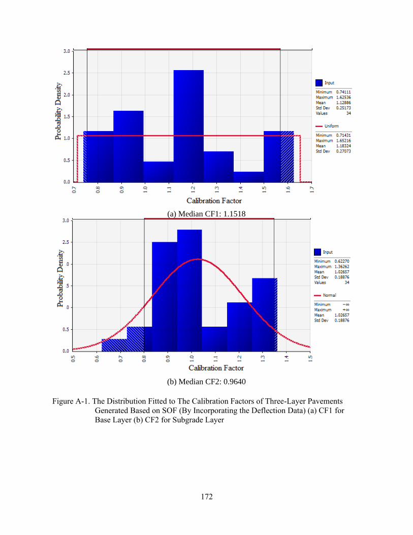
172




Generated Based on SOF (By Incorporating the Deflection Data) (a) CF1 for

Base Layer (b) CF2 for Subgrade Layer

173

Table A-2. The Generated Calibration Factors for the Deflection and Strain in Slab (Using MOF) of Three-Layer Pavements

(a)

FWD

Load, P

(lb)

Max.

Deflection,

D0 (mil)

Given

Modulus of

Base (psi)

Given

Modulus of

Subgrade

(psi)

Calibrated

Modulus of

Base (psi)

Calibrated

Modulus of

Subgrade

(psi)

Calibration

Factor of

Base,

CF1

Calibration

Factor of

Subgrade,

CF2 6,249 3.31 27,560 27,000 34,753 34,371 1.2610 1.2730 9,072 11.46 27,560 27,000 25,024 33,615 0.9080 1.2450 14,084 36.46 27,560 27,000 34,863 28,836 1.2650 1.0680 9,278 14.69 27,560 27,000 24,914 25,650 0.9040 0.9500 14,322 29.65 27,560 27,000 27,064 29,133 0.9820 1.0790 9,231 6.65 16,500 10,400 17,754 11,669 1.0760 1.1220 8,882 24.21 27,560 27,000 32,190 29,916 1.1680 1.1080 5,710 14.53 16,500 10,400 14,768 13,499 0.8950 1.2980 6,027 12.56 27,560 27,000 30,536 34,398 1.1080 1.2740 5,567 18.27 16,500 10,400 16,121 10,109 0.9770 0.9720 5,995 4.53 16,500 10,400 20,130 10,088 1.2200 0.9700 14,322 44.84 16,500 10,400 19,239 13,364 1.1660 1.2850 8,628 27.95 16,500 10,400 19,833 12,262 1.2020 1.1790 6,154 4.06 27,560 27,000 24,143 24,408 0.8760 0.9040 8,787 23.19 27,560 27,000 28,304 32,697 1.0270 1.2110 9,183 7.13 16,500 10,400 15,378 9,994 0.9320 0.9610 9,056 10.94 27,560 27,000 23,591 31,779 0.8560 1.1770 5,599 18.23 16,500 10,400 17,606 9,568 1.0670 0.9200 8,961 17.99 16,500 10,400 15,048 9,162 0.9120 0.8810 9,263 6.46 16,500 10,400 19,289 13,198 1.1690 1.2690 8,993 17.72 27,560 27,000 30,261 23,085 1.0980 0.8550 9,247 14.49 27,560 27,000 35,194 33,831 1.2770 1.2530 8,818 22.44 16,500 10,400 14,784 11,804 0.8960 1.1350 5,900 10.51 16,500 10,400 20,576 10,535 1.2470 1.0130 14,671 18.66 27,560 27,000 24,363 29,997 0.8840 1.1110

174


FWD

Load, P

(lb)

Max.

Deflection,

D0 (mil)

Given

Modulus of

Base (psi)

Given

Modulus of

Subgrade

(psi)

Calibrated

Modulus of

Base (psi)

Calibrated

Modulus of

Subgrade

(psi)

Calibration

Factor of

Base,

CF1

Calibration

Factor of

Subgrade,

CF2 14,179 42.48 27,560 27,000 33,100 30,051 1.2010 1.1130

5,805 15.71 27,560 27,000 23,674 23,166 0.8590 0.8580

8,961 19.41 27,560 27,000 28,304 27,837 1.0270 1.0310 8,930 17.95 16,500 10,400 14,042 10,972 0.8510 1.0550 14,290 48.23 27,560 27,000 34,092 35,019 1.2370 1.2970 5,995 7.20 27,560 27,000 32,411 27,918 1.1760 1.0340 8,739 24.45 16,500 10,400 15,626 10,296 0.9470 0.9900 5,710 17.24 16,500 10,400 15,048 11,846 0.9120 1.1390 14,988 31.30 16,500 10,400 16,731 11,773 1.0140 1.1320

(b)

APT Load

(kips)

Strain in Slab

( )

12.0

16.9

16.6

15.6

18.4

12.4

21.4

23.4

22.1

23.1

55.0

55.0

55.0

55.0

55.0

55.0

34.2

34.4

33.8

39.3

38.5

12.0

28.0

22.0

22.0

27.0

L: -114.7

L: 101.3

L: -110.7

L: 98.7

T: 94.7

T: 68.0

175




Generated Based on MOF (By Incorporating the Deflection and Strain Data) (a)

CF1 For Base Layer (b) CF2 For Subgrade Layer

176

A-2. Four-Layer Pavement

The data used for obtaining the calibration factors for the four-layer pavement systems

were collected from MnROAD Cells 613 as well as NAPTF CC-2 and CC-6. The difference

between these test sections and the conventional pavement sections is the existence of an additional

base layer above the granular base layer. This additional base layer is another granular layer while

CC-2 and CC-6 include a cement-stabilized or an asphalt-treated base layer. This dataset shows

the variety of the test data used in the calibration to assess the performance of the developed

calibration procedure.

Although the entire dataset used for four-layer movement included a higher number of data (see

Section 6.4 in Chapter 6), only a portion (20 percent) of the data utilized in calibration are shown

here for brevity. Tables A-3 through A-4 as well as Figures A-3 through A-4 show the generated

calibration factors for the three-layer pavements.

177

Table A-3. The Generated Calibration Factors for the Deflection (Using SOF) of Four-Layer Pavements

FWD

Load,

P (lb)

Max.

Deflection

D0 (mil)

Given Modulus

of Base 1

(psi)

Given Modulus

of Base

2 (psi)

Given Modulus

of

Subgrade

(psi)

Calibrated

Modulus of

Base 1 (psi)

Calibrated

Modulus of

Base 2 (psi)

Calibrated

Modulus of

Subgrade

(psi)

Calibration

Factor of

Base 1,

CF1

Calibration

Factor of

Base 2,

CF2

Calibration

Factor of

Subgrade,

CF3

9,147 25.18 20,040 20,580 16,860 25,170 25,046 14,533 1.2560 1.2170 0.8620

6,573 3.19 20,040 20,580 16,860 23,126 24,490 16,826 1.1540 1.1900 0.9980

9,739 5.01 20,040 20,580 16,860 27,916 19,407 15,697 1.3930 0.9430 0.9310

11,918 30.22 20,040 20,580 16,860 24,810 21,835 15,073 1.2380 1.0610 0.8940

12,380 6.57 60,000 24,200 11,600 74,760 29,088 10,022 1.2460 1.2020 0.8640

12,422 7.31 20,040 20,580 16,860 27,996 18,152 16,894 1.3970 0.8820 1.0020

6,551 3.70 20,040 20,580 16,860 23,507 25,252 20,552 1.1730 1.2270 1.2190

12,320 4.11 1,432,000 25,500 12,300 1,158,488 20,961 11,156 0.8090 0.8220 0.9070

9,016 26.67 20,040 20,580 16,860 15,611 17,452 19,676 0.7790 0.8480 1.1670

24,181 5.30 72,000 16,045 13,467 84,528 17,152 11,959 1.1740 1.0690 0.8880

11,846 2.60 72,000 16,045 13,467 60,624 13,975 10,854 0.8420 0.8710 0.8060

6,145 15.10 20,040 20,580 16,860 18,958 23,338 18,023 0.9460 1.1340 1.0690

12,335 6.04 20,040 20,580 16,860 26,433 24,037 13,859 1.3190 1.1680 0.8220

6,452 9.75 20,040 20,580 16,860 21,563 25,087 15,359 1.0760 1.2190 0.9110

6,376 8.83 20,040 20,580 16,860 17,836 21,197 18,833 0.8900 1.0300 1.1170

12,291 6.48 20,040 20,580 16,860 24,128 23,770 17,888 1.2040 1.1550 1.0610

36,244 8.80 72,000 16,045 13,467 73,368 14,328 12,147 1.0190 0.8930 0.9020

36,472 18.69 60,000 24,200 11,600 83,760 24,781 12,458 1.3960 1.0240 1.0740

6,518 8.08 20,040 20,580 16,860 15,551 22,247 17,568 0.7760 1.0810 1.0420

178




Generated Based on SOF (By Incorporating the Deflection) (a) CF1 For Base 1

Layer (b) CF2 For Base 2 Layer (C) CF3 For Subgrade Layer

179

(c) Median CF3: 09310

Figure A-3. Continued.

180

Table A-4. The Generated Calibration Factors for the Deflection and Strain in Slab (Using MOF) of Four-Layer Pavements

(a) FWD

Load,

P (lb)

Max.

Deflection

D0 (mil)

Given Modulus

of Base 1

(psi)

Given Modulus

of Base

2 (psi)

Given Modulus

of Subgrade

(psi)

Calibrated

Modulus of Base 1

(psi)

Calibrated

Modulus of

Base 2 (psi)

Calibrated

Modulus of

Subgrade

(psi)

Calibration

Factor of

Base 1,

CF1

Calibration

Factor of

Base 2,

CF2

Calibration

Factor of

Subgrade,

CF3

36,472 18.69 60,000 24,200 11,600 78,420 22,675 9,698 1.3070 0.9370 0.8360

9,728 5.63 20,040 20,580 16,860 18,056 28,730 15,208 0.9010 1.3960 0.9020

12,329 4.23 1,432,000 25,500 12,300 1,493,576 33,227 12,755 1.0430 1.3030 1.0370

9,519 14.72 20,040 20,580 16,860 21,122 23,770 15,090 1.0540 1.1550 0.8950

11,875 25.98 20,040 20,580 16,860 15,210 28,380 14,297 0.7590 1.3790 0.8480

12,039 17.99 20,040 20,580 16,860 21,142 22,165 16,658 1.0550 1.0770 0.9880

11,975 4.95 1,432,000 25,500 12,300 1,784,272 28,892 13,149 1.2460 1.1330 1.0690

6,397 10.72 20,040 20,580 16,860 26,633 20,415 12,982 1.3290 0.9920 0.7700

24,181 5.50 72,000 16,045 13,467 64,800 14,088 14,706 0.9000 0.8780 1.0920

12,427 6.50 60,000 24,200 11,600 45,960 31,605 15,289 0.7660 1.3060 1.3180

12,380 6.57 60,000 24,200 11,600 60,900 21,465 15,254 1.0150 0.8870 1.3150

36,639 9.55 1,432,000 25,500 12,300 1,958,976 33,278 10,369 1.3680 1.3050 0.8430

11,864 28.48 20,040 20,580 16,860 24,709 17,966 22,120 1.2330 0.8730 1.3120

11,776 30.60 20,040 20,580 16,860 16,272 21,732 22,120 0.8120 1.0560 1.3120

12,211 2.80 72,000 16,045 13,467 85,464 15,836 17,453 1.1870 0.9870 1.2960

11,590 35.23 20,040 20,580 16,860 16,272 18,028 14,044 0.8120 0.8760 0.8330

24,285 9.98 1,432,000 25,500 12,300 1,147,032 35,675 11,820 0.8010 1.3990 0.9610

9,487 14.48 20,040 20,580 16,860 27,495 17,740 13,303 1.3720 0.8620 0.7890

9,224 23.80 20,040 20,580 16,860 15,511 24,058 21,851 0.7740 1.1690 1.2960

181


(b) APT Load

(kips)

Strain in Slab

( )

11.7

17.7

16.5

16.8

17.1

55.0

55.0

55.0

55.0

55.0

55.0

50.0

50.0

21.8

24.3

24.2

25.1

24.5

L1:-104

L2:126.7

L3:110.7

L4:77.3

T1:54.7

T2:73.3

L5:-82.4

L6:72.5

182




Generated Based on MOF (By Incorporating the Deflection and Strain in Slab)

(a) CF1 For Base 1 Layer (b) CF2 For Base 2 Layer (C) CF3 For Subgrade Layer

183

(c) Median CF3: 0.988

Figure A-4. Continued.

184

Curriculum Vitae

Mr. Abbasali TaghaviGhalesari, M.Sc., E.I.T., obtained his B.Sc. in Civil Engineering in

2010 and his M.Sc. in Geotechnical Engineering in 2013. His M.Sc. thesis was on the development

of a numerical model for the analysis and optimum design of piled raft foundations based on field

test data. He later extended his research to the analysis of offshore foundations and fiber-reinforced

soil. After four years of professional work as a geotechnical engineer and technical manager in

several building, railway and highway projects, he started his Ph.D. at The University of Texas at

El Paso in 2017. His research at Center for Transportation Infrastructure Systems (CTIS) was

focused on the development and calibration of RPAS, an analysis tool for concrete pavements

through successful completion of SPTC14.1-94 research project. During his Ph.D. studies, he

received Frank B. Cotton Trust Scholarship and Graduate School Grant. He also served as an

Assistant Instructor at the Department of Civil Engineering at The University of Texas at El Paso.

Mr. TaghaviGhalesari is currently working as a Project Manager at The Transtec Group Inc.,

working on several research projects funded by state and federal transportation agencies.

development of a framework for the calibration of rpas, a

Documents