development of a meteorological, agricultural, …

DEVELOPMENT OF A METEOROLOGICAL, AGRICULTURAL, STREAM HEALTH,

AND HYDROLOGICAL (MASH) COMPREHENSIVE DROUGHT INDEX

By

Elaheh Esfahanian

A DISSERTATION

Submitted to

Michigan State University

in partial fulfillment of

the requirements for the degree of

Biosystems Engineering – Doctor of Philosophy

2016

ABSTRACT

DEVELOPMENT OF A METEOROLOGICAL, AGRICULTURAL, STREAM HEALTH,

AND HYDROLOGICAL (MASH) COMPREHENSIVE DROUGHT INDEX

By

Elaheh Esfahanian

Droughts are one of the costliest of natural disasters, posing a significant threat to both

man-made and natural systems. Hundreds of drought indices are currently available for the

monitoring of drought magnitude, severity, and extent; however, most of these indices were

primarily designed for the analysis of drought’s impact on human concerns, such as crop

production and freshwater supplies, and do not consider greater environmental aspects such as

stream health. To the best of my knowledge, no universal drought index has been developed with

the ability to comprehensively quantify different aspects of drought (e.g. meteorological,

agricultural, hydrological, and stream health). In addition, there is no general agreement for

drought definition even within each drought category. This means that different drought indices,

even in the same category, can report contradictory results.

In order to address these issues, we designed a study based on the following research objectives:

1) development of an index capable of determining the impact of drought on aquatic ecosystems

and stream health; 2) creation of a universal drought index for the measurement of multiple

impacts of drought (e.g. meteorological, hydrological, agricultural, and stream health); and 3)

determination of a predictive drought model that is able to capture both the categorical and

overall impacts of drought. To address the first objective, we coupled a soil and water

assessment tool (SWAT) with a regional-scale habitat suitability model to investigate drought

conditions in the Saginaw River Watershed. Using the ReliefF algorithm as our variable

selection method along with partial least squared regression, six predictive stream health drought

models were developed to monitor stream health drought conditions. Of these models, the

version with five flow-related variables was determined to be the best tool for predicting both

stream health and drought severity. For objective two, thirteen commonly used drought indices

from the following categories were integrated to devise a definition of drought that is both

categorical and universal: meteorological (4 indices), hydrological (4 indices), agricultural (4

indices), and stream health (1 index). The three closest indices to each other in each category

were selected and then averaged to obtain the categorical drought scores; next, the simple

average method was used to aggregate the categorical scores, which then provided the universal

drought score. For objective three, the ReliefF algorithm was used to select the best variable set

for each of the categorical drought scores as well as for the universal drought score. The highest

ranked variables were then used in the development of the various predictive drought models via

the adaptive network-based fuzzy inference system. The adaptive network-based fuzzy inference

system successfully produced four predictive drought models, including the three categorical

models (meteorological, agricultural, and hydrological) and the universal drought model.

iv

Dedicated to my loving husband, Alireza,

and my wonderful parents, Vahid and Maryam

v

ACKNOWLEDGEMENTS

I would like to thank all the people who have helped and supported me throughout my

journey. First, I would like to thank my major advisor Dr. Pouyan Nejadhashemi for always

being ready to provide me with invaluable help, advice, and input. I am extremely grateful for all

the encouragement, motivation, support, and direction throughout my time in the program. In

addition, I would like to thank my co-advisor, Dr. Jade Mitchell, and my committee members,

Dr. Timothy Harrigan and Dr. Nathan Moore, for all their guidance and support.

I would also like to thank Zhen Zhang (Statistics) and Ying Tang (Geography) for their

contributions to different aspects of my research. And many thanks to Barb and Jaime Lynn, who

made the paperwork and administrative side of the process so easy and convenient for me.

A big “thank you” to my lab mates and friends for making my time here so special.

Thanks Fariborz Daneshvar, Melissa Rojas-Downing, Matthew Herman, Mohammad Abouali,

Umesh Adhikari, Pouyan Hatami, Sean Woznicki, Georgina Sanchez, and Subhasis Giri for all

the laughter and great memories.

A special “thank you” to my parents, Vahid and Maryam, for their unconditional support

and encouragement during the pursuit of my graduate degree: they have always been there for

me; and to my sister, Shiva, for always being ready to cheer me up. I would also like to thank Dr.

Abdol Esfahanian and his lovely wife for their endless support, and for making my life so much

easier while I was thousands of miles away from home.

Finally, many thanks to my lovely husband, Alireza Ameli, for always being there for me

no matter what. His endless love, support, and understanding have helped me to make it across

the finish line!

vi

TABLE OF CONTENTS

LIST OF TABLES ........................................................................................................................................ x

LIST OF FIGURES .................................................................................................................................... xii

KEY TO ABBREVIATIONS .................................................................................................................... xiv

1. INTRODUCTION ................................................................................................................................ 1

2. LITERATURE REVIEW ..................................................................................................................... 4

2.1. Overview ................................................................................................................................... 4

2.2. Drought Definitions .................................................................................................................. 4

2.3. Drought Classification .............................................................................................................. 5

2.4. Modern Impact of Drought around the Globe ........................................................................... 7

2.5. Causes of Drought ..................................................................................................................... 9

2.6. Drought Indices ....................................................................................................................... 11

2.6.1. Palmer drought severity index ............................................................................................ 17

2.6.1.1. Applications ................................................................................................................ 18

2.6.1.2. Advantages .................................................................................................................. 18

2.6.1.3. Limitations .................................................................................................................. 18

2.6.2. Standardized precipitation index ......................................................................................... 19

2.6.2.1. Applications ................................................................................................................ 20

2.6.2.2. Advantages .................................................................................................................. 21

2.6.2.3. Limitations .................................................................................................................. 21

2.6.3. Crop moisture index ............................................................................................................ 22

2.6.3.1. Advantages .................................................................................................................. 22

2.6.3.2. Limitations .................................................................................................................. 22

2.6.4. Palmer hydrological drought index ..................................................................................... 23

2.6.5. Base-flow index .................................................................................................................. 23

2.6.5.1. Applications ................................................................................................................ 24

2.6.5.2. Advantages .................................................................................................................. 24

2.6.5.3. Limitations .................................................................................................................. 24

2.6.6. Surface water supply index ................................................................................................. 25

2.6.6.1. Advantages .................................................................................................................. 25

2.6.6.2. Limitations .................................................................................................................. 25

2.6.7. Normalized difference vegetation index ............................................................................. 26

vii

2.6.7.1. Applications ................................................................................................................ 26

2.6.7.2. Advantages .................................................................................................................. 27

2.6.7.3. Limitations .................................................................................................................. 27

2.6.8. Vegetation condition index ................................................................................................. 28

2.6.8.1. Applications ................................................................................................................ 28

2.6.8.2. Advantages .................................................................................................................. 29

2.6.8.3. Limitations .................................................................................................................. 29

2.6.9. Recent developments in drought indices ............................................................................. 29

2.6.9.1. Effective precipitation ........................................................................................................ 29

2.6.9.2. Reconnaissance drought index ........................................................................................... 30

2.6.9.3. Flow duration curve ........................................................................................................... 30

2.6.9.4. Standardized runoff index .................................................................................................. 30

2.6.9.5. Water balance derived drought index ................................................................................ 31

2.6.9.6. Reclamation drought index ................................................................................................ 31

2.6.9.7. Indices based on soil moisture ........................................................................................... 31

2.6.9.8. Indices based on remote sensing ........................................................................................ 32

2.6.9.9. Drought monitor ............................................................................................................... 33

2.7. Climate Change ....................................................................................................................... 33

2.7.1. Drought and Climate Change .............................................................................................. 35

2.8. Bioassessment ......................................................................................................................... 36

2.8.1. Stream Health ...................................................................................................................... 43

2.8.1.1. Fish as Indicators ............................................................................................................... 43

2.8.1.1.1. Index of biotic integrity ............................................................................................... 44

2.8.1.2. Macroinvertebrates as indicators ....................................................................................... 45

2.8.1.2.1. Benthic index of biotic integrity .............................................................................. 46

2.8.1.2.2. Hilsenhoff biotic index ............................................................................................ 47

2.8.1.2.3. Ephemeroptera, Plecoptera, and Trichoptera Index ................................................. 47

2.8.2. Effects of climate change on bioassessment programs ....................................................... 48

2.9. Drought Risk Assessments ...................................................................................................... 48

2.10. Drought Modeling ................................................................................................................... 50

2.10.1. Drought forecasting............................................................................................................. 50

2.10.2. Probabilistic characterization of drought ............................................................................ 54

2.10.3. Spatio-temporal drought analysis ........................................................................................ 56

2.10.4. Drought modeling under climate change scenarios ............................................................ 57

2.10.5. Land data assimilation systems ........................................................................................... 59

2.10.6. Drought Management ......................................................................................................... 60

viii

2.11. Summary ................................................................................................................................. 62

3. INTRODUCTION TO METHODOLOGY AND RESULTS ............................................................ 64

4. DEFINING DROUGHT IN THE CONTEXT OF STREAM HEALTH ........................................... 66

4.1. Abstract ................................................................................................................................... 66

4.2. Introduction ............................................................................................................................. 66

4.3. Materials and Methodology .................................................................................................... 70

4.3.1. Study area ............................................................................................................................ 70

4.3.2. Modeling process ................................................................................................................ 71

4.3.3. Soil and Water Assessment Tool ........................................................................................ 72

4.3.4. SWAT model calibration and validation ............................................................................. 73

4.3.5. Regional-scale Habitat Suitability Model ........................................................................... 74

4.3.6. Drought Model Input Variables .......................................................................................... 77

4.3.7. Variable Selection: ReliefF algorithm ................................................................................ 78

4.3.8. Partial Least Square Regression .......................................................................................... 80

4.3.9. Climate Models ................................................................................................................... 82

4.4. Results & Discussions ............................................................................................................. 86

4.4.1 SWAT Model Calibration and Validation .......................................................................... 86

4.4.2 Variable Selection ............................................................................................................... 87

4.4.3.1. Current Drought Severity Model ................................................................................ 87

4.4.2.2. Future Drought Severity Model .................................................................................. 89

4.4.3 Drought Severity Model ...................................................................................................... 89

4.4.3.1. PLSR predictively for median flow ............................................................................ 89

4.4.3.2. Accuracy, precision, and sensitivity of drought models in predicting drought zones . 95

4.4.4 Drought model performance under future climate scenarios .............................................. 97

4.4.5 The impact of climate change on future drought ................................................................ 98

4.5. Conclusion ............................................................................................................................ 101

4.6. Acknowledgments ................................................................................................................. 102

5. DEVELOPMENT AND EVALUATION OF A COMPERHENSIVE DROUGHT INDEX .......... 104

5.1. Abstract ................................................................................................................................. 104

5.2. Introduction ........................................................................................................................... 105

5.3. Materials and Methodology .................................................................................................. 109

5.3.1. Study area .......................................................................................................................... 109

5.3.2. Modeling process .............................................................................................................. 111

5.3.3. Categorical drought index development ........................................................................... 112

ix

5.3.3.1 Meteorological Drought Indices ................................................................................... 113

5.3.3.2 Agricultural Drought Indices ........................................................................................ 114

5.3.3.3 Hydrological Drought Indices ....................................................................................... 115

5.3.3.4 Stream Health drought Index ........................................................................................ 116

5.3.4. Input parameters ................................................................................................................ 117

5.3.5. Transformation and Clustering ......................................................................................... 119

5.3.6. Aggregation ....................................................................................................................... 120

5.3.7. Drought indices comparison ............................................................................................. 121

5.3.8. Drought model development ............................................................................................. 122

5.3.8.1. Parameter selection ................................................................................................... 122

5.3.8.2. Development of predictive drought models .............................................................. 123

5.4. Results and Discussions ........................................................................................................ 125

5.4.1 Statistical Analysis of Drought Indices ............................................................................. 125

5.4.2 Categorical Drought Indices ............................................................................................. 127

5.4.3 Comparison of Categorical Drought Scores and MASH .................................................. 128

5.4.4 Variable Selection ............................................................................................................. 131

5.4.5 Categorical and MASH drought models ........................................................................... 133

5.4.6 Identifying the drought vulnerable areas ........................................................................... 136

5.5. Conclusion ............................................................................................................................ 138

5.6. Acknowledgements ............................................................................................................... 139

6. CONCLUSIONS ............................................................................................................................... 140

7. FUTURE RESEARCH RECOMMENDATIONS ............................................................................ 142

APPENDICES .......................................................................................................................................... 143

APPENDIX A: Study One .................................................................................................................... 144

APPENDIX B: Study Two ................................................................................................................... 161

REFERENCES ......................................................................................................................................... 179

x

LIST OF TABLES

Table 1. Summary of popular drought indices ............................................................................................ 12

Table 2. Classification of SPI values (adapted from McKee et al., 1993; 1995) ........................................ 20

Table 3. Biological response to increasing levels of stress (adapted from USEPA, 2011b; Davies and

Jackson, 2006)............................................................................................................................................. 41

Table 4. Stressor identification process (adapted from USEPA, 2000; USEPA, 2011b) ........................... 42

Table 5. Reference table of drought zones (adapted from Hamilton and Seelbach, 2011) ......................... 77

Table 6. CMIP5 models developer, name, resolution, and components (Petkova et al., 2013; IPCC, 2013)

.................................................................................................................................................................... 84

Table 7. Statistical criteria for SWAT model calibration and validation for nine USGS gauging stations

within the Saginaw Bay Watershed ............................................................................................................ 86

Table 8. Top 15 ranked variables ................................................................................................................ 89

Table 9. Current Drought Severity Model performances............................................................................ 90

Table 10. Future Drought Severity Model performances ........................................................................... 91

Table 11. Confusion matrix for drought zones: First model ....................................................................... 96

Table 12. Confusion matrix for drought zones: Fourth Model ................................................................... 96

Table 13. Overall first model performance against 47 future climate scenarios ......................................... 97

Table 14. ANFIS models frameworks and characteristics ........................................................................ 124

Table 15. p-values from pairwise comparison of drought indices. Red colored p-values indicate no

significant mean differences at the 0.05 level. .......................................................................................... 129

Table 16. Frequency of drought indices combinations in each drought category over 30-year period .... 130

Table 17. Top five ranked variables that were used for development of the drought predictive models. 132

Table 18. Best ANFIS models for each drought category and MASH ..................................................... 134

Table S1. Selected variables for development of current and future drought severity models. ................ 151

xi

Table S2. Confusion matrix for drought zones: Second model ................................................................ 156

Table S3. Confusion matrix for drought zones: Third model ................................................................... 156

Table S4. Confusion matrix for drought zones: Fifth Model .................................................................... 157

Table S5. Confusion matrix for drought zones: Sixth Model ................................................................... 157

Table S6. The first drought model performance using RCP 8.5 (maximum and minimum values are

presented in red) ........................................................................................................................................ 158


presented in red) ........................................................................................................................................ 159


presented in red) ........................................................................................................................................ 160

Table S9. Meteorological drought indices, reference, input parameters, procedure, classification, and

index value ................................................................................................................................................ 164

Table S10. Agricultural drought indices, reference, input parameters, procedure, classification, and index

value .......................................................................................................................................................... 165

Table S11. Hydrological drought indices, reference, input parameters, procedure, classification, and index

value .......................................................................................................................................................... 167

Table S12. Stream health drought index, reference, input parameters, procedure, classification, and index

value .......................................................................................................................................................... 168

Table S13. Input parameters ..................................................................................................................... 169

Table S14. Mean difference (numbers in black) and standard deviation (numbers in red) among drought

indices ....................................................................................................................................................... 175

Table S15. Saginaw River watershed calibration and validation results .................................................. 176

Table S16. Transformed drought categories * .......................................................................................... 177

Table S17. Transformed non-drought categories * ................................................................................... 178

xii

LIST OF FIGURES

Figure 1. Saginaw Bay Watershed .............................................................................................................. 71

Figure 2. Drought zones variable selection and modeling process ............................................................. 72

Figure 3. Fish response curve to flow reduction (adapted from Zorn et al., 2008) ..................................... 76

Figure 4. ReliefF ranking histogram map ................................................................................................... 88

Figure 5. The variance explained percentage for each PLSR for the Current Drought Severity Model: a)

First model, b) Second model, c) Third model. .......................................................................................... 92

Figure 6. The comparison of measured vs. predicted median flow histogram for the Current Drought

Severity Model, a) First model, b) Second model, c) Third model. ........................................................... 94

Figure 7. Probability of increasing drought conditions under projected climate change (2040-2060)

compare to current condition (1990-2010). ................................................................................................ 99

Figure 8. Percent change in (a) temperature and (b) precipitation from current (1980-2000) to future

climate change (2040-2060)...................................................................................................................... 100

Figure 9. Saginaw River Watershed ......................................................................................................... 110

Figure 10. Categorical drought scores development and modeling process ............................................. 112

Figure 11. Measured versus modeled histograms of categorical drought and MASH: (a) CMI, (b) CHI, (c)

CAI, and (d) MASH. ................................................................................................................................. 135

Figure 12. Drought vulnerable areas based on MASH in the Saginaw River watershed.......................... 137

Figure S1.Locations of precipitation, temperature, and streamflow monitoring stations ......................... 144

Figure S2. Distribution of median flow values ......................................................................................... 145

Figure S3. Sample histogram of ranking for parameter #20 (average flow rate from 23 months prior to the

month of interest) ...................................................................................................................................... 146

Figure S4. The relationship of MSE with the number of PLSR components for Current Drought Severity

Models: a) First Model, b) Second Model, c) Third Model. ..................................................................... 147

Figure S5.The relationship of MSE with the number of PLSR components for Future Drought Severity

Models: a) Fourth Model, b) Fifth Model, c) Sixth Model. ...................................................................... 148

xiii

Figure S 6. The variance explained percentage for each PLSR for the Future Drought Severity Model: a)

Fourth Model, b) Fifth Model, c) Sixth Model. ........................................................................................ 149

Figure S7. The comparison of measured vs. predicted median flow histogram for the Future Drought

Severity Model: a) Fourth Model, b) Fifth Model, c) Sixth Model. ......................................................... 150

Figure S8. Location of temperature, precipitation, and streamflow gauging stations .............................. 161

Figure S9. Measured versus modeled histograms of categorical drought and MASH: (a) CMI, (b) CHI, (c)

CAI, and (d) MASH .................................................................................................................................. 162

Figure S10. Drought vulnerable areas based on categorical drought indices in the Saginaw River

watershed: (a) meteorological, (b) hydrological, (c) agricultural, (d) stream health ................................ 163

xiv

KEY TO ABBREVIATIONS

A: Agricultural

ADI: Aggregate Drought Index

AMO: Atlantic Multidecadal Oscillation

ANFIS: Adaptive Neuro-Fuzzy Interference System

ANN: Artificial Neural Network

ARI: Adverse Resource Impacts

ARIMA: Autoregressive Integrated Moving Average

ARS: Agricultural Research Service

AVHRR: Advanced Very High Resolution Radiometer

BCG: Biological Condition Gradient

BFI: Baseflow Index

B-IBI: Benthic Index of Biotic Integrity

BMP: Best Management Practice

CADDIS: Causal Analysis/Diagnosis Decision Information System

CAI: Categorical Agricultural Index

CART: Classification and Regression Tree

CDF: Cumulative Distribution Function

CDI: Combined Drought Index

CDL: Cropland Data Layer

CHI: Categorical Hydrological Index

CMI: Categorical Meteorological Index

xv

CMI: Crop Moisture Index

CMIP5: Coupled Model Intercomparison Project Phase 5

CPC: Climate Prediction Center

CSHI: Categorical Stream Health Index

CWA: Clean Water Act

DEP: Deviation of EP from MEP

DM: Drought Monitor

DMAPS: Drought Monitoring and Prediction System

DMSNN: Direct Multistep Neural Network

DSI: Drought Severity Index

DSS: Decision Support System

EDI: Effective Drought Index

ENSO: El Nino Southern Oscillation

EP: Effective Precipitation

EPA: Environmental Protection Agency

EPT: Ephemeroptera, Plecoptera, and Trichoptera Index

ETDI: Evapotranspiration Deficit Index

FDC: Flow Duration Curve

FL: Fuzzy Logic

GCMs: General Circulation Models

GPCC-DI: Global Precipitation Climatology Centre Drought Index

H: Hydrological

HBI: Hilsenhoff Biotic Index

xvi

HDI: Hybrid Drought Index

HRUs: Hydrologic Response Units

HUC: Hydrologic Unit Code

IBI: Index of Biotic Integrity

IPCC: Intergovernmental Panel on Climate Change

LPD: Liter per Day

M: Meteorological

MASH: Meteorological, Agricultural, Stream health, and Hydrological

MCDA: Multi-Criteria Decision Analysis

MEP: Mean of Effective Precipitation

MFs: Membership Functions

MMIs: Multimetric Indices

MSE: Mean Square Error

NAO: North Atlantic Oscillation

NCDC: National Climatic Data Center

NDMC: National Drought Mitigation Center

NDVI: Normalized Difference Vegetation Index

NDWI: Normalized Difference Water Index

NED: National Elevation Dataset

NIR: Near Infrared

NLDAS: North American Land Data Assimilation System

NOAA: National Oceanic and Atmospheric Administration

NPDES: National Pollutant Discharge Elimination System

xvii

NPS: Nonpoint Source

NRCS: USDA Natural Resources Conservation Service

NSE: Nash-Sutcliffe Efficiency Coefficient

NSF-DOE-NCAR: National Science Foundation, Department of Energy, National Center for

Atmospheric Research

NWS: National Weather Service

PBIAS: Percent Bias

PDI: Precipitation Drought Index

PDO: Pacific Decadal Oscillation

PDSI: Palmer Drought Severity Index

PHDI: Palmer Hydrological Drought Index

PLSR: Partial Least Square Regression

PMDI: Palmer Modified Drought Index

PMF: Probability Mass Function

RCMs: Regional Climate Models

RCPs: Representative Concentration Pathways

RD: Rainfall Deciles

RDAI: Regional Drought Area Index

RDI: Reclamation Drought Index

RDI: Reconnaissance Drought Index

RMSE: Root Mean Square Error

RMSNN: Recursive Multistep Neural Network

RSR: Root-Mean-Squared Error-Observations Standard Deviation Ratio

xviii

S: Stream Health

SAF: Severity-Area-Frequency

SARIMA: Seasonal Autoregressive Integrated Moving Average

SEP: Standardized Value of DEP

SHI: Stream Health Index

SI: Stressor Identification

SMDI: Soil Moisture Deficit Index

SMI: Soil Moisture Index

SPEL: Standardized Precipitation Evapotranspiration Index

SPI: Standardized Precipitation Index

SRI: Standardized Runoff Index

SSURGO: Soil Survey Geographic

SWAT: Soil and Water Assessment Tool

SWDI: Soil Water Deficit Index

SWIR: Short-Wave Infrared

SWSI: Surface Water Supply Index

TDI: Temperature Drought Index

TMDLs: Total Maximum Daily Loads

UK: United Kingdom

UN-ISDR: United Nations International Strategy for Disaster Reduction

USGS: US Geological Survey

VCI: Vegetation Condition Index

VCI: Vegetation Condition Index

xix

VDI: Vegetation Drought Index

VegDRI: Vegetation Drought Response Index

VegOut: Vegetation Outlook

VIC: Variable Infiltration Capacity

VIS: Visible

WBI: Water balance Derived Drought Index

WDCC: Western Drought Coordination Council

WET: Whole effluent toxicity

WQS: Water Quality Standards

Z-index: Palmer Moisture Anomaly Index

1

1. INTRODUCTION

Drought is a natural event that occurs in most climate zones as an effect of the long-term

reduction of precipitation within a region. Of all existing natural hazards, drought is the most

detrimental in terms of human impact (Wilhite, 2000b; Mishra and Singh, 2010). Globally,

drought causes approximately $8 billion in damage annually, making it the world’s costliest type

of natural disaster (Wilhite, 2000b; Keyantash and Dracup, 2002). Although a natural

phenomenon, various human activities can directly trigger droughts by impeding the ability of

the land to capture and hold water, including: intensive farming, excessive irrigation,

deforestation, the over-exploitation of available water, and erosion (Wilhite, 2000a; Mishra and

Singh, 2010).

Droughts are generally classified as being meteorological, agricultural, or hydrological

(Wilhite and Glantz, 1985; American Meteorological Society, 1997; McMahon and Finlayson,

2003; Dai, 2011): meteorological droughts are a result of a prolonged period of below-average

precipitation caused by anomalies in atmospheric circulation patterns (Dai, 2011). Agricultural

drought is caused by a period of soil moisture loss triggered by a shortage of precipitation

(Mishra and Singh, 2010; Dai, 2011). Hydrological drought is caused by a period of reduction in

streamflow, runoff, and inflow to reservoirs as a result of precipitation deficiency (Whitmore,

2000). It is difficult to determine the exact start and end dates of a drought, as the various

impacts of a given drought increase slowly, accumulate over time, and can even remain after the

end of the drought (Mishra and Singh, 2010). These characteristics have led to drought being

known as a “creeping phenomenon” (Whitmore, 2000; Mishra and Singh, 2010).

Several indices have already been developed to monitor and quantify different types of

drought; these indices are the primary tools for the assessment of drought severity, duration, and

2

intensity (Heim, 2002; Mishra and Singh, 2010). Each drought index requires specific input

parameters to measure drought; however, precipitation is typically used, either alone or in

combination with other parameters (Heim, 2002; Mishra and Singh, 2010; Sheffield and Wood,

2011). In the case of meteorological drought, precipitation is traditionally the primarily

parameter used; soil moisture content is commonly used for agricultural drought (along with the

secondary parameters of precipitation and evapotranspiration); and hydrological drought

parameters typically include streamflow and precipitation (Dai, 2011).

Most drought indices quantify drought impact based on effects on human activities such

as agricultural production while neglecting environmental sustainability effects like stream

health; to rectify this oversight, the goal of the first study was to investigate the impacts of

drought on stream health. The specific objectives were:

Identification of a method of variable selection for determination of the most influential

parameters in the development of stream health drought models.

Development of a predictive model for quantifying the aggregate risk of drought on stream

health.

Evaluation of the impact of climate change on stream health drought models.

The effects of drought are non-structural and spatially extensive (Wilhite et al., 2000c);

resulting in widespread impacts on different sectors, including hydrology, meteorology,

agriculture, natural ecosystems, and human wellbeing. There is currently no universal definition

used for drought, since each sector measures it differently (Whitmore, 2000; Heim, 2002;

Svoboda et al., 2002); this absence of a universal definition is itself one of the main obstacles to

the effective study of drought (Mishra and Singh, 2010).

3

Despite recent advances in the scientific study of drought, monitoring methods are still in

need of significant improvement; these changes would streamline drought preparation and

management practices, as well as reduce vulnerability to drought in several different sectors

(Svoboda et al., 2002). One method of improving drought monitoring is the combination of

existing indices to better evaluate the overall impacts of a drought (Zargar et al., 2011).

Meanwhile, hundreds of indices have been developed for each drought category due to the fact

that no general agreement exists on how to formulate categorical drought indices (e.g.

meteorological, agricultural, or hydrological). This means that different drought indices can

report contradictory results.

The goal of the second study was the creation of a universal definition by introducing an

overall drought index that considers multiple aspects of drought, including the meteorological,

agricultural, hydrological, and stream health. This universal definition would substantially

improve the current system of drought monitoring, thereby enabling decision-makers to more

effectively allocate resources for the reduction of drought’s impacts across different sectors.

The objectives of the second study are:

Definition of the four categorical drought indices (meteorological, agricultural, hydrological,

and stream health) based on commonly used drought indices.

Creation of a universal definition of drought via the combination of the categorical scores.

Selection of the best variable sets for construction of predictive drought models.

Development of predictive drought models for each drought category as well as the universal

drought index.

4

2. LITERATURE REVIEW

2.1. Overview

This literature review provides an overview of drought concepts and characterizations,

risk assessment, and modeling. Section 2.2 provides drought definitions, which explain direct

drought causation. Section 2.3 contains drought classifications that identify the impacts of

drought on different sectors. Section 2.4 describes the global impacts of drought. Section 2.5

discusses the indirect causes of drought considering atmospheric and hydrological interactions.

Section 2.6 describes the various drought indices that are used to measure drought

characterizations such as severity, duration, intensity, frequency, and spatial extent. Following

these sections, a discussion of climate change and its impact on drought, bioassessment and

stream health (including the benefits of bioassessment and newly established tools, stream health

indicators, and the effects of climate change on current bioassessment programs). Drought risk

assessment is later addressed, including results from past studies that developed the current

drought risk analysis guidelines. Lastly, drought modeling and its various components are

discussed, including drought forecasting, probabilistic characterization of drought,

spatiotemporal drought analysis, drought modeling using climate change scenarios, land data

assimilation systems, and drought management.

2.2. Drought Definitions

Simply defined, a drought is an extended deficit in the amount of water compared to

normal conditions governed by the hydrological cycle. The hydrological cycle is the movement

of water through land, ocean, and atmosphere; its main components are precipitation,

evaporation, run-off, snow-melt, and soil and groundwater storage (Sheffield and Wood, 2011).

Due to the large number of diverse definitions for droughts, determination of a universal and

5

precise definition of drought has proven unfeasible (Yevjevich, 1967; Mishra and Singh, 2010).

Drought definitions are categorized as either conceptual or operational: conceptual definitions

utilize relative concepts to describe drought in simple terms, while operational definitions are

much more in-depth. Operational definitions are used to identify the frequency, severity,

duration, and termination of drought, and are used in preparation for future droughts (SOEST,

2003; Mishra and Singh, 2010). Some of the most commonly used definitions are provided

below:

The smallest daily streamflow value of the year (Gumbel, 1963);

Extended periods during which lack of moisture results in crop failure (Unger, 1984);

A sustained decrease in the amount of precipitation normally received in a specific area

(WMO, 1986);

A naturally occurring phenomenon that results when precipitation levels fall significantly

below normally recorded levels, causing severe hydrological imbalances that negatively

impact land resource production systems (UN Secretary-General, 1994);

A sustained period (e.g. a season, a year, or several years) of deficient rainfall anomalous to

the statistical multi-year mean of a given region (Schneider, 1996).

2.3. Drought Classification

Droughts are typically categorized as one of four major types: meteorological,

hydrological, agricultural, and socio-economic (Wilhite and Glantz, 1985; American

Meteorological Society, 1997); however, Mishra and Singh (2010) introduced groundwater

drought as a new type of drought. Similarly, Sheffield and Wood (2011), instead of socio-

economic category, introduced ecological and regional categories as new types of drought in

6

order to focus on the environmental impacts of drought (ecological drought) rather than the

socio-economic impacts.

A meteorological drought occurs when there is a significant deviation from the mean

precipitation in a region over an extended period of time; precipitation data are used to

identify and analyze this type of drought (Mishra and Singh, 2010; Sheffield and Wood,

2011).

Hydrological drought refers to a period of deficiency in the supply of water (both surface and

subsurface) of a given water resource management system (Panu and Sharma, 2002; Mishra

and Singh, 2010; Sheffield and Wood, 2011). The following datasets are used to analyze

hydrological droughts: streamflow, lake and reservoir levels, and groundwater levels (Mishra

and Singh, 2010; Sheffield and Wood, 2011).

Agricultural drought is defined as a period of soil moisture deficiency leading to a reduction

in the moisture supply available for crops and other types of vegetation (Panu and Sharma,

2002; Sheffield and Wood, 2011); this type of drought is driven by meteorological and

hydrological droughts (Sheffield and Wood, 2011). Several drought indices have been used

to study agricultural drought, featuring a combination of hydrometeorological variables such

as precipitation, soil moisture, and temperature (Mishra and Singh, 2010).

Socio-economic drought refers to a combination of meteorological, hydrological, and

agricultural droughts which result in adverse social and economic impacts on humans. This

type of drought differs from those in the other three categories due to its direct link to the

relationship between supply and demand for a given economic good (i.e., water): when the

demand for water exceeds the supply, the result is a socio-economic drought (American

Meteorological Society, 2004; Mishra and Singh, 2010; Sheffield and Wood, 2011).

7

Groundwater drought is defined as a lack of groundwater recharge over a prolonged period of

time as a result of low precipitation and high evapotranspiration. This type of drought is

mainly associated with low groundwater heads, small groundwater gradients, low

groundwater storage, and low well yields (shallow wells may even dry up) (van Lanen and

Peters, 2000; Mishra and Singh, 2010). Groundwater levels and gradients are used to

quantify the effects of this kind of drought (van Lanen and Peters, 2000).

Ecological drought measures the impacts of drought on ecosystems and it is caused by a

reduction in soil moisture due to low precipitation (causing a reduction in

evapotranspiration), which adversely affects local vegetation (Sheffield and Wood, 2011).

Regional drought is defined as a period during which more than 70% of a given area (within

a larger region) is affected by drought (Fleig et al., 2011).

2.4. Modern Impact of Drought around the Globe

Droughts affect many sectors of society, including the economy, agriculture, industry,

infrastructure, and tourism. Drought may have led to the declines of Sumer in pre-Roman times,

and to the Mayan civilization in the past millennium. In the 20th century, droughts have caused

the most detrimental economic and social impacts of all natural disasters (Mishra and Singh,

2010; Sheffield and Wood, 2011). In recent decades, multiple continents have been severely

affected by drought (Mishra and Singh, 2010). Drought has also proven the costliest natural

disaster in the United States, with average annual damages estimated at approximately $6-$8

billon (Mishra and Singh, 2010; Sheffield and Wood, 2011). Droughts accounts for 41% of the

total estimated cost of all weather-related disasters in the U.S. (Cook et al., 2007; Mishra and

Singh, 2010). Regional droughts in 1988 (central US) and 1996 (state of Texas) resulted in

estimated losses of $46 billion (Sheffield and Wood, 2011).

8

In the past two centuries, various regions of Canada (particularly the Canadian prairies)

have experienced severe droughts. The prairies are one of the most drought-prone regions due to

their high precipitation variability; in 2001-2002, one of the most severe prairie droughts on

record caused significant damage to water-related resources. In the 1890s, 1930s, and 1980s

Canada’s southern regions experienced multi-year droughts. During the 20th century, western

Canada experienced at least 40 long-term droughts, and eastern Canada also suffered from major

drought events (Environment Canada, 2004; Mishra and Singh, 2010).

Over the past 30 years, Europe has experienced several major droughts, resulting in

economic losses of €100 billion (Sheffield and Wood, 2011; European Communities, 2012). In

2003, a prolonged drought associated with a heat wave that affected large parts of Europe cost

more than €8.7 billion (Feyen and Dankers, 2009; Mishra and Singh, 2010; European

Communities, 2012). Lehner et al. (2006) conducted a study on the possible impact of global

climate change on drought frequency in Europe and concluded that, based on their proposed

climate change scenarios, southern and southeastern Europe are more likely to experience

significant increases in drought frequency than northern and northeastern Europe.

In Asia, agricultural production has declined in recent decades due to increasing water

stress, which is a result of rising temperatures, a reduction in the number of rainy days, and the

increasing frequency of El Nino events (Bates et al., 2008; Mishra and Singh, 2010). From 1998-

2001, central and southwestern Asia experienced a severe drought and consequent famine which

affected over 60 million people, particularly in Iran, Afghanistan, Pakistan, Tajikistan,

Uzbekistan, and Turkmenistan (Barlow et al., 2002; Mishra and Singh, 2010). Since the late

1990s, most of northern China has experienced prolonged, severe droughts resulting in

substantial economic and social losses (Zou et al., 2005; Mishra and Singh, 2010). India is one of

9

the most drought-prone countries, having experienced at least one drought per three-year period

over the last five decades (Mishra and Singh, 2010).

Drought is also a recurring event in Australia, especially in the southern and eastern parts

of the country in part because its rainfall is more strongly governed by El Nino. The “millennium

drought” (1996-2010) was the country’s worst recorded drought since European settlement

began (Bond et al., 2008; Mishra and Singh, 2010).

West Africa experienced a drought of unprecedented severity in the Sahel from the late

1960s to the mid-1980s which led to widespread famine and hundreds of thousands of deaths

(Mishra and Singh, 2010; Sheffield and Wood, 2011). A slightly less severe drought occurred in

East Africa during the mid-1980s which also caused famine and many deaths. In South Africa,

multiple drought events occurred between the 1980s and early 1990s that were related to the El

Nino Southern Oscillation (ENSO) (Sheffield and Wood, 2011).

2.5. Causes of Drought

The causes of drought are complex, as they are the outcome of the interaction of

atmospheric and hydrological processes; drought is an extreme state of the hydrological cycle in

which precipitation is below normal levels. Once established, dry hydrological conditions within

a region cause the depletion of moisture from the upper layers of soil, subsequently causing a

reduction in evapotranspiration rates and the sequential lowering of atmospheric relative

humidity. Such decreases in relative humidity reduce the probability of rainfall (Bravar and

Kavvas, 1991; Mishra and Singh, 2010); precipitation can also be reduced by both an increase in

albedo and the accumulation of increase of fine particles in the air (Panu and Sharma, 2002;

Nagarajan, 2009). Increases in albedo lower surface temperatures, resulting in local heat loss.

10

Lower surface temperatures cause a reduction in lifting air masses, which leads to a reduction in

precipitation. Local heat loss causes a temperature gradient that induces a circulation capable of

maintaining equilibrium with warmer surroundings, thereby depressing precipitation.

Additionally, increases in the number of fine particles in the air can overseed clouds, which also

can reduce precipitation (Panu and Sharma, 2002).

Another causation factor of drought are oceanic circulations that affect weather and

climate; these circulations, with average patterns of current and heat storage, cause climate

variations. Significant climatic variations occur when warm water from the western Pacific

Ocean flows into the eastern-central equatorial Pacific Ocean (e.g. off the coast of Peru) (Panu

and Sharma, 2002; Nagarajan, 2009). These anomalies in sea surface temperature create the El

Nino effect, which has been associated with the onset of many recent droughts (Panu and

Sharma, 2002; Nagarajan, 2009). The opposite occurs in the La Nina phenomena, which refers to

the periodic cooling of sea surface temperatures in the eastern-central tropical Pacific Ocean

(NOAA, 2012). These anomalies in sea surface temperature are due to large-scale atmospheric

circulations which follow quasi-periodic cycles or oscillation (Panu and Sharma, 2002; Sheffield

and Wood, 2011). Among these, ENSO has proven the most significant driver of global climate

change, and oscillates approximately every two-to-seven years in the tropical Pacific Ocean

(Sheffield and Wood, 2011). El Nino and La Nina are extreme phases of the ENSO, and

represent warm and cold phases, respectively (Panu and Sharma, 2002; NOAA, 2012); the

ENSO also affects hydrological features such as precipitation and streamflow over catchments

(Panu and Sharma, 2002). There are other climate oscillations serving as primary drivers of

regional climate variation which can act in other timescales, allowing them to interact with the

ENSO. These climate oscillations include the North Atlantic Oscillation (NAO), the Pacific

11

Decadal Oscillation (PDO), and the Atlantic Multidecadal Oscillation (AMO). The NAO affects

the climate in eastern North America, Europe, and North Africa. The PDO manifests in the

northern Pacific Ocean with a timescale of 20-to-30 years, and can interact with ENSO; it can

also modify climate on a global scale. The AMO affects climate in the North Atlantic, especially

in North America and Europe (Sheffield and Wood, 2011). However, like the weather,

atmospheric drought is essentially unpredictable for timescales more than a month in advance

despite significant efforts to improve our understanding.

2.6. Drought Indices

Several drought indices have been developed to monitor drought conditions. Drought

indices are prime tools for assessing drought effects and parameters; the parameters defined by

these indices are duration, intensity, severity, and spatial extent. Each drought index requires

different input parameters and uses a unique method to measure drought. The precipitation

parameter is used in all indices, either alone or in combination with other meteorological

parameters such as soil moisture and temperature (Heim, 2002; Mishra and Singh, 2010;

Sheffield and Wood, 2011). Table 1 summarizes the most commonly used drought indices,

including their respective strengths and limitations. In the following sections, some of the

meteorological, agricultural, hydrological, and ecological drought indices were further explained.

12

Table 1. Summary of popular drought indices

Index (References) Description and Use Strengths Weaknesses

Meteorological Drought

Palmer Drought Severity

Index (PDSI)

(Palmer, 1965; Alley 1984;

Dai et al., 2004; Hayes,

2006; Mishra and Singh,

2010; Sheffield and Wood,

2011)

Utilizes a water balance

model to depict departure

of soil moisture from a

given region (compared

to normal conditions)

Uses precipitation and

temperature as input

parameters

Widely used by US

governmental agencies

Good measure of

intensity and duration

of long-term drought

Facilitates direct

comparisons between

different regions and

timeframes

Considers basic effects

of surface warming

Values vary widely

for extreme and

severe drought

classifications and

frequencies in

different locations

May lag in detecting

emerging droughts by

several months

All precipitation

assumed to be rain

Rainfall Deciles (RD)

(Gibbs and Mahar, 1967;

Hayes, 2006; Sheffield and

Wood, 2011; Zargar et al.,

2011)

Divides monthly

precipitation events into

deciles (10% each)

Can be computed for any

chosen period

Used primarily in

Australia

Relatively simple to

calculate

Provides a precise

statistical measurement

of precipitation

Precipitation records

covering extended

periods needed to

accurately calculate

deciles

Standardized Precipitation

Index (SPI)

(McKee et al., 1993;

Edwards and McKee, 1997;

Heim, 2002; Mishra and

Singh, 2010; Sheffield and

Wood, 2011)

Based on probability of

precipitation

Calculated for any

location with long-term

monthly precipitation

record

Quantifies precipitation

deficit for multiple

timescales

Solely based on

precipitation

Temporal flexibility

and versatility

Consistent

classifications of severe

and extreme drought

frequencies in any

location and timescale

For different lengths

of precipitation

records, SPI value

discrepancies can be

obtained as a result of

different distributions

Dependent on nature

of probability

distribution

13

Table 1. (cont’d)

Percent of Normal

(Hayes, 2006; Sheffield and

Wood, 2011; Zargar et al.,

2011)

Calculated by dividing

actual precipitation by

normal precipitation

Normal precipitation

typically considered to be

a 30-year mean

Timescales can vary

between one month and

one year

Simple and transparent

Effective for comparing

a single region and a

specific period (within

a given year)

Without normal

distribution, mean

and median values

differ, causing

inaccuracy

Unable to compare

drought across

multiple seasons or

regions

Agricultural Drought

Palmer Moisture Anomaly

Index (Z-index)

(Palmer, 1965; Dai et al.,


2011; Zargar et al., 2011)

Calculates monthly

standardized anomaly of

available moisture

Used for monitoring

short-term droughts

Input parameters:

precipitation, streamflow,

and temperature

Rapid response to

changing conditions

Not used for

monitoring long-term

droughts

Antecedent

conditions not

considered

Crop Moisture Index (CMI)

(Palmer, 1968; Hayes,



2011)

Monitors short-term

moisture supply (week-

to-week) across crop

regions

Derived from Palmer

Index

Requires weekly

temperature and

precipitation values

Quick response to

changing conditions

Can be used to compare

moisture conditions at

different locations

Easily computed from

precipitation and

temperature data

Not applicable to

monitoring of long-

term droughts

Rapid response to

short-term changing

conditions provides

misleading

information for

monitoring of long-

term conditions

14

Table 1. (cont’d)

Hydrological Drought

Palmer Hydrological

Drought Index (PHDI)

(Palmer, 1965; Heim, 2000;

Keyantash and Dracup,


2010; Zargar et al., 2011)

Analyzes precipitation

and temperature in the

PDSI water balance

model

Used for water supply

monitoring and

qualification of

hydrological impacts of

long-term drought

conditions

Input parameters:

precipitation,

temperature, and

streamflow/runoff

Used to monitor long-

term droughts

Same as PDSI

Baseflow Index (BFI)

(Institute of Hydrology,

1980; Gustard et al., 1992;

Zaidman et al., 2001;

Tallaksen and van Lanen,


2011)

Ratio of baseflow to total

flow

Used for low-flow

estimation and

groundwater recharge

assessment

Estimates low-flow

indices at the ungauged

site

Stored water in the

basin used to quantify

flow

Sensitive to missing

data

Requires long-term

records to separate

baseflow from total

flow

Surface Water Supply Index

(SWSI)

(Shafer and Dezman,1982;

Heim, 2002; Hayes, 2006;

Mishra and Singh, 2010;

Calculated based on

monthly weighted sum of

non-exceedance

probabilities of

snowpack, streamflow,

precipitation, and

Simple to calculate and

represent water supply

conditions

Allows comparison of

water supply

availability among

The weight of each

hydrological

component in SWSI

equation varies with

spatial scale

Index measurement is

15

Table 1. (cont’d)

Sheffield and Wood, 2011) reservoir storage

components

Monitors abnormalities in

surface water supplies

Developed in response to

PDSI’s limitations

Used for river basins in

western US

regions with different

variability

unique for each basin,

making comparison

between different

basins difficult

Ecological Drought

Normalized Difference

Vegetation Index (NDVI)

(Rouse et al.,1974; Singh et

al., 2003; Kogan, 2005;

Sheffield and Wood, 2011;

Brian et al., 2012)

Difference between near

infrared and visible

reflectance divided by

sum of two wavebands

Advanced, very high-

resolution radiometer

(AVHRR)-based index

used to monitor

vegetation conditions and

distributions

Detecting drought onset

and measuring its

intensity and duration

Measures general

vegetative conditions in

large area of coverage

Provides high spatial

resolution of near real-

time data for entire

globe

Successfully used to

identify stressed and

damaged crops and

pastures

Difficult to separate

influences such as

weather on vegetative

health

Atmospheric

conditions, especially

cloud cover,

considerably reduce

index values and

cause noise

Vegetation Condition

Index (VCI)

(Unganai and Kogan, 1998;

Heim 2002; Quiring and

Ganesh, 2010; Mishra and

Singh, 2010; Wardlow et

A pixel-wise

normalization of NDVI to

control local differences

in ecosystem productivity

Suitable for monitoring of

agricultural droughts

A potentially global

Provides real-time data

with high spatial

resolution for

monitoring drought

Captures rainfall

dynamics more

accurately than NDVI,

Limited utility during

the cold season

16

Table 1. (cont’d)

al., 2012 ) standard of measuring

times of drought onset,

intensity, duration, and

impact on vegetation

particularly in

heterogeneous areas

Enables comparisons of

impact of weather on

areas with different

environmental

resources

Regional Drought

Regional Drought Area

Index (RDAI)

(Bhalme and Mooley, 1980;

Fleig et al., 2010, 2011;

Sheffield and Wood, 2011)

Divides area affected by

drought by the total area

of region

Based on daily

streamflow

Quantifies spatial

extent of droughts

Requires spatially

continuous or

regional data

Drought Severity Index

(Dai et al., 2010; Sheffield

and Wood, 2011)

Area-weighted intensity

over the drought area

Quantification of

average severity of

drought over a region

Same as above

17

2.6.1. Palmer drought severity index

The Palmer drought severity index (PDSI) was developed as a climatological tool to

measure drought intensity, onset, and end date (Palmer, 1965; Alley, 1984). PDSI has been

widely utilized in the U.S. by agencies such as the U.S. National Weather Service (NWS), the

Climate Prediction Center (CPC), and the U.S. National Drought Monitor (Sheffield and Wood,

2011). This regional drought index uses precipitation and temperature for estimating moisture

supply and demand within a two-layer, bucket-type soil model via the water balance equation

(Alley, 1984; Dai et al., 2004; Mishra and Singh, 2010). PDSI represents the soil moisture

departure within a specific region, as compared to the normal conditions, by using a water

balance model (Sheffield and Wood, 2011). Dry and wet conditions are classified into 11

categories based on their PDSI values: extremely wet (PDSI ≥ 4.00), very wet (3.00 ≤ PDSI

≤3.99), moderately wet (2.00 ≤ PDSI ≤2.99), slightly wet (1.00 ≤ PDSI ≤1.99), incipient wet

spell (0.50 ≤ PDSI ≤0.99), near normal (0.49 ≤ PDSI ≤-0.49), incipient drought (-0.50 ≤ PDSI

≤-0.99), mild drought (-1.00 ≤ PDSI ≤ -1.99), moderate drought (-2.00 ≤ PDSI ≤ -2.99), severe

drought (-3.00 ≤ PDSI ≤ -3.99), and extreme drought (PDSI ≤ -4.00) (Heddinghaus and Sabol,

1991). Several modified versions of PDSI have been developed, such as the Palmer Moisture

Anomaly Index (Z-index), Palmer hydrological drought index (PHDI) (Palmer, 1965), and the

Palmer modified drought index (PMDI) (Heddinghaus and Sabol, 1991). The Z-index is an

intermediate term within PDSI calculating the monthly-standardized anomaly of available

moisture (Palmer 1965, Zargar et al., 2011). This index is used to quantify agricultural drought

impacts for short-term drought conditions (Zargar et al., 2011). The PHDI is used for water

supply monitoring and for the qualification of the hydrological impacts of long-term drought

conditions (Karl, 1986; Mishra and Singh, 2010; NCDC, 2013). And the PMDI was defined as a

18

real-time version of the PDSI for operational purposes (Heddinghaus and Sabol, 1991; Mishra

and Singh, 2010).

2.6.1.1. Applications

PDSI has proven valuable for use in many types of studies, including drought forecasting

(Kim and Valdes, 2003; Ozger et al., 2009); exploration of the periodic behavior of droughts

(Rao and Padmanabham, 1984); drought assessment over large geographic areas (Johnson and

Kohne, 1993); the study of hydrologic trends and assessment of potential fire severity

(Heddinghaus and Sahol, 1991); investigation of spatial and temporal drought characteristics

(Lawson et al., 1971; Klugman, 1978; Karl and Koscielny, 1982; Diaz, 1983; Soule, 1992; Jones

et al., 1996); and illustration of the areal extent and severity of various drought episodes (Palmer,

1967; Karl and Quayle, 1981).

2.6.1.2. Advantages

PDSI has proven to be is a reliable measure of the intensity and duration of long-term

droughts, and has been utilized for many years (Mishra and Singh, 2010; NCDC, 2013). It uses

precipitation and surface air temperature for its inputs, then outputs evaporation and run-off,

taking into account the basic effects of surface warming occurring in the 21st century (Dai et al.,

2004; Sheffield and Wood, 2011). PDSI can also be used to evaluate wet situations (Alley,

1984), and is a standard measure of surface moisture conditions that facilitate direct comparisons

of PDSI between different regions and timeframes (Alley, 1984; Dai et al., 2004).

2.6.1.3. Limitations

PDSI has several limitations, which have been detailed in multiple studies (Alley, 1984;

Karl and Knight, 1985; Heddinghaus and Sahol, 1991; McKee et al., 1995). These limitations

include the arbitrary selection of values for quantifying the intensity of drought and monitoring

19

the onset and end of a given drought or wet spell (Alley, 1984; Heddinghaus and Sahol, 1991);

and that PDSI is better suited for evaluation of the agricultural impacts of drought than for

determining the impacts of hydrologic droughts (Hayes et al., 1999). Additionally, the lag time

between precipitation fall and runoff generated is not considered, which can result in values that

are several months behind the actual values of emerging droughts (Hayes et al. 1999; Sheffield

and Wood, 2011). PDSI also assumes no runoff occurrence until all soil layers have become

saturated, which can lead to the underestimation of the runoff (Hayes et al., 1999; Mishra and

Singh, 2010); and all precipitation is assumed to be rain, therefore snowfall, snow cover, and

frozen ground are not considered, resulting in the potential inaccuracy of PDSI values

determined for winter months and areas at high elevations (Hayes et al., 1999; Mishra and Singh,

2010; Sheffield and Wood, 2011). PDSI values also vary widely for extreme and severe drought

classifications as well as frequencies in different locations (Hayes et al., 1999); and PDSI

responds slowly to the conditions of a developing drought and also retains values reflecting a

drought well after it has ended (Hayes et al., 1999; Mishra and Singh, 2010). Furthermore, PDSI

is sensitive to both temperature and precipitation, often leading to a few months’ lag time in its

response to temperature and precipitation anomalies (Karl, 1986; Mishra and Singh, 2010).

These rather significant limitations were the primary reason for the development of SPI, which

was designed to resolve some of the most problematic issues inherent in PDSI.

2.6.2. Standardized precipitation index

McKee et al. (1993) developed the standardized precipitation index (SPI) as a probability

tool to estimate the intensity and duration of drought events. SPI can be calculated for any

location with a long-term monthly precipitation record of the desired time period. Computation

of the SPI requires the fitting of a probability distribution to the historical precipitation records

20

for the timescale(s) of interest in order to define the relationship of the probability to the

precipitation. The fitted probability distribution is then normalized to a standard normal

distribution using the inverse normal (Gaussian) function. In a standard normal distribution, the

mean and variance SPI for the location and desired time period are 0 and 1, respectively.

Therefore, for any observed precipitation data, the SPI value is the deviation from the entire

standard normal distribution (McKee et al., 1993; Edwards and McKee, 1997; Heim, 2002;

Mishra and Singh, 2010).

Table 2 represents the classification scale for the SPI values. The index is negative for

drought situations (less than median precipitation) and positive for wet conditions (greater than

median precipitation). Negative values of SPI represent a higher probability of drought

occurrence and more severe droughts (McKee et al., 1993; Hayes et al., 1999; NCDC, 2013).

Table 2. Classification of SPI values (adapted from McKee et al., 1993; 1995)

Class Index Value

Extremely wet SPI ≥ 2.0

Very wet 1.5 ≤ SPI < 2.0

Moderately wet 1.0 ≤ SPI <1.5

Near normal -1.0 ≤ SPI < 1.0

Moderate drought -1.5 ≤ SPI < -1.0

Severe drought -2.0 ≤ SPI < -1.5

Extreme drought SPI < -2.0


SPI has proven valuable for widespread applications within drought studies, including

forecasting (Mishra and Desai, 2005a; Cancelliere et al., 2007; Mishra et al., 2007), spatio-

temporal analysis (Mishra and Desai, 2005b; Mishra and Singh, 2009), and climate impact

studies (Mishra and Singh, 2009).

21

2.6.2.2. Advantages

One of SPI’s advantages is its simplicity as it is solely based on precipitation; making

drought assessment possible without the use of additional hydrometeorological

measurements (Hayes et al., 1999; Mishra and Singh, 2010). SPI’s second advantage is its

temporal flexibility and versatility; it can be applied to a variety of timescales, from small

timescale monitoring of water supplies (including soil moisture, which is important for

agricultural production), to large timescale monitoring of water resources such as

groundwater supplies, river flow, and lake water levels (Hayes et al., 1999; Livada and

Assimakopoulos, 2007; Mishra and Singh, 2010). SPI’s third advantage is its consistent

classification of severe and extreme drought frequencies for any given location and

timescale, as a result of its normal distribution (Hayes et al., 1999).


The length of the precipitation record plays an important role in calculating SPI values;

discrepancies in SPI values can be obtained as a result of having different distributions due to

varying lengths of precipitation records. Users should be aware of this inconsistency when

interpreting and making decisions based on SPI values. Wu et al. (2005) conducted a study to

evaluate the effect of precipitation record length on SPI calculation; they concluded that the

different records of varying lengths with similar gamma distributions over different time periods

result in consistent SPI values. However, discrepancies were observed for precipitation records

of varying lengths with different gamma distributions (Wu et al., 2005; Mishra and Singh, 2010).

SPI’s other limitation is its dependence on the nature of its probability distribution, as

different SPI values are obtained when multiple types of probability distribution are used. This

dependency causes bias in the SPI values when long timescales (longer than 24 months) are

22

involved; additionally, in the case of short timescales, the calculated SPI is not normally

distributed for dry climates (Mishra and Singh, 2010). Some of the probability distributions used

to simulate precipitation distribution when computing SPI values are gamma distributions

(McKee et al., 1993; Edwards and McKee, 1997; Mishra and Singh, 2009); Pearson type III

distributions (Guttman, 1998); and lognormal, extreme value, and exponential distributions

(Todorovic and Woolhiser, 1976; Madsen et al., 1998; Lloyd-Hughes and Saunders, 2002; Wu et

al., 2007). This also makes it so that SPI cannot really be compared spatially unless two pixels

have the same maximum and same shape parameters.

2.6.3. Crop moisture index

The crop moisture index (CMI) was developed by Palmer (1968) and uses a

meteorological approach for the monitoring of the short-term moisture supply (week-to-week) of

various crop regions (Hayes, 2006; Mishra and Singh, 2010; Sheffield and Wood, 2011). CMI

was derived from the Palmer drought severity index and requires weekly temperature and

precipitation values in order to be computed (Hayes, 2006; Mishra and Singh, 2010).

2.6.3.1. Advantages

CMI responds rapidly to changing conditions and is easily computed using precipitation

and temperature data (Hayes, 2006; Mishra and Singh, 2010; Sheffield and Wood, 2011). And,

because it is weighted by both location and time, CMI can also be used to compare moisture

conditions at different locations (Hayes, 2006).


CMI is not effective for monitoring of long-term drought (Hayes, 2006; Mishra and

Singh, 2010; Sheffield and Wood, 2011) since its rapid response to short-term changing

conditions is misleading when monitoring long-term changing conditions (Hayes, 2006; Mishra

23

and Singh, 2010). In addition, Juhasz and Kornfield (1978) conducted a sensitivity analysis of

CMI and reported that this index might erroneously indicate wetter conditions as temperature

increases, as a result of the anomaly term formulation of evapotranspiration.

2.6.4. Palmer hydrological drought index

The Palmer hydrological drought index (PHDI) was introduced by Palmer (1965) for the

purpose of assessing hydrological droughts. This index is a derivative of PDSI and uses the same

water balance assessment on a two-layer soil model (Karl and Knight, 1985; Keyantash and

Dracup, 2002). The PHDI can quantify the severity of either a drought or a wet spell, and is

based on daily inflow (precipitation) and soil moisture storage (Karl and Knight, 1985; Sheffield

and Wood, 2011). The principle that differentiates PHDI from PDSI is that the PHDI responds

more slowly to the changes in weather leading to the termination of either a drought or a wet

spell. In other words, PHDI rebounds gradually towards the normal state and only indicates the

termination of a drought when the moisture deficit actually vanishes (Johnson and Kohne, 1993;

Heim, 2000; Keyantash and Dracup, 2002). This characteristic of PHDI makes it suitable for the

assessment of hydrological drought, which is a slower developing phenomenon than

meteorological drought (Keyantash and Dracup, 2002).

The PHDI is used for water supply monitoring and qualifying the hydrological impacts of

long-term drought conditions (Karl, 1986; Mishra and Singh, 2010; NCDC, 2013). Its limitations

are the same as those of the PDSI; however, this index can also monitor long-term drought

conditions (Sheffield and Wood, 2011).

2.6.5. Base-flow index

The Institute of Hydrology (now the Centre for Ecology & Hydrology) introduced the

base-flow index (BFI) as an indicator of catchment permeability (Zaidman et al., 2001; Tallaksen

24

and van Lanen, 2004). The BFI was first developed in the United Kingdom (UK) for use in

determining the low flow characteristics of rivers (Tallaksen and van Lanen, 2004). The BFI is

the ratio of the base flow to the total flow, which is calculated by applying smoothing and

separation rules on a daily mean flow hydrograph (Gustard et al., 1992; Tallaksen and van

Lanen, 2004; Sheffield and Wood, 2011). BFI values range from 0.1 for a flashy river with an

impermeable catchment to nearly 1.0 for a very stable river with a permeable catchment (Gustard

et al., 1992; Tallaksen and van Lanen, 2004).


The BFI has many potential areas of application, including low-flow estimation and

groundwater recharge assessment. This index is widely used in countries such as the UK, Canada

(Pilon and Condie, 1986), Fiji (Green, 1986), Zimbabwe (Meigh, 1987), New Zealand (National

Water and Soil Conservation Authority, 1984), Norway (Tallaksen, 1986), and Australia (Nathan

and McMahon, 1990a).

2.6.5.2. Advantages

The BFI is frequently used to estimate low-flow indices at ungauged sites and is closely

related to other low-flow indices (Tallaksen and van Lanen, 2004). It can also quantify the flow

from stored water within a basin (Gustard et al., 1992; Sheffield and Wood, 2011).


The BFI’s primary limitation is that long records are required in order to separate base

flow from total flow (Sheffield and Wood, 2011). It is also sensitive to missing data; one day of

missing data can cause the omission of several days’ worth of data from the base-flow separation

(Tallaksen and van Lanen, 2004).

25

2.6.6. Surface water supply index

The surface water supply index (SWSI) was developed by Shafer and Dezman (1982) as

a hydrological drought index for monitoring abnormalities in surface water supplies (Hayes,

2006; Mishra and Singh, 2010). SWSI is calculated based on the monthly weighted sum of the

non-exceedance probabilities of snowpack, streamflow, precipitation, and reservoir storage

components. For winter data, only snowpack, precipitation, and reservoir storage is used to

compute SWSI; for summer months, only streamflow, precipitation, and reservoir storage

components are used in the calculation of SWSI (Garen, 1993; Mishra and Singh, 2010).

2.6.6.1. Advantages

SWSI is used as a complement to the PDSI since it accounts for snow accumulation,

subsequent runoff, and large topographic variation across a region (Hayes, 2006). SWSI is

simple to calculate and represent water supply conditions (Hayes, 2006; Sheffield and Wood,

2011). Since the non-exceedance probabilities are used as the normalizing technique in

calculating SWSI, it allows comparison of water supply availability among regions with different

variability (Garen, 1993).


The weight of each hydrological component in the SWSI equation varies with the spatial

scale (one basin to another) and the temporal scale (season or month). This variation is due to the

differences in hydroclimatic variability which results in SWSIs with different statistical

properties (Garen, 1993; Heim, 2002; Mishra and Singh, 2010); SWSI measurements are unique

for each basin, making it difficult to compare SWSI values between multiple basins (Hayes,

2006; Sheffield and Wood, 2011).

26

2.6.7. Normalized difference vegetation index

The normalized difference vegetation index (NDVI) is an advanced, very high-resolution

radiometer (AVHRR)-based index proposed by Rouse et al. (1974) to monitor vegetation

conditions and distributions but cannot directly quantify drought. AVHRR is used by the

National Oceanic and Atmospheric Administration (NOAA) series of Polar-orbiting Operational

Environmental Satellites (Kogan, 2005; Brian et al., 2012). It is a five-channel passive scanning

radiometer and its radiance is used to monitor drought conditions caused by sensitivity to

changes in leaf chlorophyll, moisture content, and thermal conditions. AVHRR’s five channels

cover visible, near-infrared, mid-infrared, and thermal infrared regions of the electromagnetic

spectrum. NDVI is derived from channels 1 and 2 (visible and near infrared) based on the known

radiometric properties of plants (Kogan, 2005; Quiring and Ganesh, 2010). NDVI values range

between -1 to 1, where negative values indicate the presence of features such as clouds, water,

and snow; near zero values indicate no vegetation; and values near 1 indicate the highest possible

density of vegetation. This index is defined as NDVI= (NIR – VIS)/(NIR + VIS), where NIR

stands for near-infrared and VIS stands for visible. Healthy vegetation generally reflects more

near-infrared wavelengths than visible light wavelengths, while unhealthy vegetation shows little

difference between visible and near-infrared reflected radiation (Singh et al., 2003; Boken et al.,

2005; Quiring and Ganesh, 2010).


NDVI has been proven to be a useful tool for: 1) mapping changes in vegetation cover

and measuring drought impact in regions around the world (Anyamba et al., 2001; Gutman 1990;

Ji and Peters, 2004; Singh et al., 2003); 2) providing accurate descriptions of continental land

cover, vegetation classification and vegetation phenology (Tucker et al., 1987; Trapley et al.,

27

1984; Justice et al., 1985); 3) monitoring rainfall and drought, crop growth conditions and crop

yields (Kogan 1987, Dabrowska-Zielinska et al., 2002); and 4) detecting drought onset and

measuring drought intensity and duration (Kogan 1995; Seiler et al., 2000; Quiring and Ganesh,

2010).

2.6.7.2. Advantages

NDVI measures general vegetative conditions over large areal regions, and has been

successfully used to identify stressed and damaged crops and pastures. Also, because NDVI is an

AVHRR-based index, it can provide high spatial resolution of near real-time data for the entire

globe (Sheffield and Wood, 2011).


Although NDVI has been used in a wide range of applications for drought monitoring, it

does have limitations. First, it is difficult to separate out other influences, such as weather

components, on vegetation health (Singh et al., 2003). Second, the presences of noise in AVHRR

data restricts remote sensing of vegetation. Atmosphere components, especially clouds,

considerably reduce NDVI values and cause noise (Guttman 1991; Singh et al., 2003). Third, in

some semiarid environments, both soil characteristics and reflectance of lower plant

communities such as mosses, lichens, algae, and cyanobacteria can lead to misinterpretation of

drought conditions (Wardlow et al., 2012). Fourth, in tropical forests, the vegetation greenness

within a pixel may saturate and make NDVI insensitive to increasing amounts of vegetation

(Ripple, 1985; Ingram et al., 2005). Fifth, NDVI uses a limited amount of the total spectral

information available within an image, which results in less information on vegetation coverage

(Foody et al., 2001; Ingram et al., 2005). Sixth, for nonhomogeneous land cover, NDVI values

are normally higher for more favorable environmental conditions such as forests, and lower for

28

less favorable environmental conditions such as dry steppes (Unganai and Kogan, 1998). There

is also a time lag between NDVI green-up and rainfall, so any detection of drought has to

account for time differentials.

2.6.8. Vegetation condition index

The vegetation condition index (VCI) is also an AVHRR-based index developed by

Kogan (1990). This index is a pixel-wise normalization of NDVI to control local differences in

ecosystem productivity but cannot directly quantify drought. Pixel-based normalization

minimizes the effect of short-term signals and also amplifies long-term ecological signals

(Quiring and Ganesh, 2010; Wardlow et al., 2012). VCI, like NDVI, is computed from satellite

AVHRR radiance (visible and near-infrared) (Mishra and Singh, 2010). It is defined as VCI =

100 (NDVI -NDVImin) / (NDVImax - NDVImin) and ranges from 0 to 100 for minimum and

maximum NDVI, respectively. High values of VCI indicate healthy vegetation conditions

(optimal) and low values of VCI indicate poor vegetation condition (unhealthy and unfavorable)

(Singh et al., 2002; Quiring and Ganesh, 2010).


VCI has been used for detecting and tracking drought in several regions around the

world, including the U.S. (Kogan, 1995), China (Kogan and Sullivan, 1993), parts of the former

Soviet Union (Kogan and Sullivan, 1993), Argentina (Seiler et al., 2000), Africa (Unganai and

Kogan, 1998), and Kazakhstan (Gitelson et al., 1998). Besides successfully detecting and

tracking drought, VCI can also be used to detect vegetation stress due to excessive wetness for

both localized/short-term and widespread/long-term droughts (Kogan, 1995; Heim, 2002; Singh

et al., 2003). Additionally, VCI is a potential global standard for measuring the time of drought

onset, intensity, duration, and impact on vegetation. Studies such as Gitelson et al. (1998), Kogan

29

(1997), and Unganai and Kogan (1998) have indicated that VCI is suitable for monitoring

agricultural droughts. However, according to Bayarjargal et al. (2006), Bhuiyan et al. (2006),

Singh et al. (2003), and Vicente-Serrano (2006), VCI is not appropriate for monitoring

meteorological droughts in some regions.

2.6.8.2. Advantages

VCI, like NDVI, provides real-time data with high spatial resolution for monitoring

drought (Heim, 2002; Quiring and Ganesh, 2010). Rainfall dynamics are best captured by VCI,

particularly in heterogeneous areas, and VCI also quantifies the impact of weather on vegetation.

In addition, it is possible to use VCI for comparing the impact of weather in areas with different

environmental resources (i.e., ecological and climatic) (Unganai and Kogan, 1998).


VCI has limited utility during the cold season, since it is based on vegetation analysis;

therefore, it is primarily useful for the summer growing season (Heim 2002; Mishra and Singh,

2010).

2.6.9. Recent developments in drought indices

2.6.9.1. Effective precipitation

Effective precipitation (EP) can more precisely monitor an ongoing drought and its

duration, since it is a summed value of daily precipitation with a time-dependent reduction

function (Byun and Wilhite, 1999; Mishra and Singh, 2010). The mean of EP (MEP), the

deviation of EP from MEP (DEP), and the standardized value of DEP (SEP) are the three

additional indices which complement EP (Mishra and Singh, 2010).

30

2.6.9.2. Reconnaissance drought index

The reconnaissance drought index (RDI) was developed by Tsakiris and Vangelis (2005)

to monitor the severity of meteorological droughts. In this index, the ratio between the

precipitation and potential evapotranspiration records is first fitted into a lognormal probability

distribution, and is then transformed into a standard normal distribution. Zarch et al. (2011)

modified the RDI by using gamma distribution instead of lognormal distribution; it was

concluded that, in most cases (i.e., different locations and timescales), RDI performs better with

gamma distribution.

2.6.9.3. Flow duration curve

The flow duration curve (FDC) was developed by Tallaksen and van Lanen (2004) for

hydrological drought assessment using streamflow data. The streamflow data for a specific time

period are ranked, their exceedance probabilities are calculated, and the calculated probabilities

are then divided into five groups. These groups are comprised of: 0-10% (high flow), 10-40%

(moist conditions), 40-60% (mid-range flow), 60-90% (dry conditions), and 90-100% (low flow)

(Tallaksen and van Lanen, 2004; USEPA, 2011a).

2.6.9.4. Standardized runoff index

Shukla and Wood (2008) developed standardized runoff index (SRI) based on the SPI

concept to characterize hydrologic drought. The SRI integrates hydrologic processes that define

seasonal loss in streamflow caused by climate impact. They concluded that SRI is a suitable

complement to SPI for illustrating hydrological drought on monthly-to-seasonal scales (Shukla

and Wood, 2008; Mishra and Singh, 2010).

31

2.6.9.5. Water balance derived drought index

Vasiliades et al. (2011) created the water balance derived drought index (WBI) to assess

hydrological drought characteristics. In order to calculate the WBI, a water balance model is

used to simulate streamflow data for a specific time period. The simulated streamflow data is

then normalized using Box-Cox transformation, and the transformed streamflow data is

converted into a standard normal distribution (Zargar et al., 2011; Vasiliades et al., 2011). The

results show that the WBI is a good indicator of both hydrological drought severity and duration

(Vasiliades et al., 2011).

2.6.9.6. Reclamation drought index

The reclamation drought index (RDI) was introduced by Weghorst (1996) to identify the

onset and end of a drought period (Weghorst, 1996; Niemeyer, 2008). This index can also be

used as a tool for defining drought severity and duration (Hayes, 2006; Niemeyer, 2008), and is

similar to the SWSI in that it is calculated at the river basin level. The RDI can also incorporate

air temperature-variable demand and duration (Hayes, 2006; Zargar et al., 2011), in addition to

the SWSI input parameters (precipitation, streamflow, snowpack, and reservoir storage), thus

making it capable of analyzing both climate and water supply factors. RDI values range from 4

to -4, with 4 representing extremely wet conditions, and -4 representing extreme drought. Since

the RDI is unique for each river basin, it cannot be used for inter-basin comparisons (Hayes,

2006).

2.6.9.7. Indices based on soil moisture

Narasimhan and Srinivasan (2005) developed the soil moisture deficit index (SMDI) and

the evapotranspiration deficit index (ETDI) to improve the spatial and temporal resolutions used

in agricultural drought monitoring. Weekly soil moisture and evapotranspiration were simulated

32

using the calibrated hydrologic model soil and water assessment tool (SWAT). The SMDI and

ETDI both feature higher spatial (16km2) and temporal (weekly) resolutions than the SPI or

PDSI indices, with resolutions of 7,000-100,000 km2, monthly (Narasimhan and Srinivasan,

2005; Mishra and Singh, 2010). Hunt et al. (2009) developed the soil moisture index (SMI),

which is capable of determining drought onset as well as identifying soil discharge. The SMI is a

continuous function that provides the relative position of the actual water content between the

wilting point and the field capacity (Hunt et al., 2009; Mishra and Singh, 2010; Combe et al.,

2014). Recently, Martínez-Fernández et al., 2015 developed the soil water deficit index, which is

effective for the monitoring of agricultural drought. This index uses soil water observations such

as moisture content, available water content, and field capacity to calculate soil water deficits.

2.6.9.8. Indices based on remote sensing

The normalized difference water index (NDWI) was introduced by Gao (1996) in order

to determine the water content of vegetation and spongy mesophyll in vegetation canopies. This

satellite-derived index is a combination of NIR and short-wave infrared (SWIR) bands (Delbart

et al., 2005; Mishra and Singh, 2010); in order to obtain information on the water content of

vegetation, indices based on the NIR and SWIR bands have proven more reliable than those

using the NIR and VIS bands (e.g. NDVI). As a result of the VIS, the NDVI represents the

chlorophyll rather than the water content (which is located in the strong chlorophyll absorption

region) (Chen et al., 2005). NDWI may also be a more sensitive index for drought monitoring

than the NDVI as a result of its dependence on both the desiccation and wilting of a given

vegetation canopy (Mishra and Singh, 2010).

33

2.6.9.9. Drought monitor

A weekly drought monitor (DM) tool was introduced by the NOAA, USDA, and NDMC

in order to consolidate and centralize drought assessment. The DM is a synthesis of different

drought indices and incorporates climatic data and professional input from all levels. This tool

categorizes drought on a scale from zero-to-four (D0 to D4), where D0 represent abnormally dry

areas and D4 represent exceptional drought events (i.e., a drought of record). Three labels are

used to indicate the sectors affected by drought: ‘A’ represents agricultural impacts, ‘W’

hydrological impacts, and ‘F’ a high risk of wildfire. The drought monitor map identifies the

general drought area, labels individual droughts by their intensity, as well as drought impact on

different sectors (Svoboda, 2000; Heim, 2002; Mishra and Singh, 2010). Although DM map

simplicity makes it attractive for both public and different applied areas. It has the limitation of

presenting several drought temporal scales on one map, which can be misleading (Heim 2002;

Mishra and Singh, 2010).

2.7. Climate Change

According to the U.S. Environmental Protection Agency (EPA), climate change refers to

any significant, lasting change in temperature, precipitation, or wind patterns over several

decades (USEPA, 2014). Climate change is occurring and our planet is warming (USEPA, 2014;

IPCC, 2013); over the past century, earth’s average surface air temperature has increased by

approximately 0.8°C (1.4°F). This increase in temperature has been mainly occurring since the

mid-1970s, with the period between 1983 and 2012 being the warmest three decades on record in

over 800 years (Royal Society, 2014). Over the next century, earth’s average temperature is

projected to rise by another 2°F to 11.5°F (USEPA, 2014). A wide range of observations have

been recorded confirming this warming trend, including an increase in ocean temperatures, a rise

34

in sea level, the decline of snow and ice cover in the Northern Hemisphere, and an increase in the

concentrations of greenhouse gasses (Royal Society, 2014). This rapid increase in global

temperatures is anomalous when comparing observations with models, the long-term records,

and fingerprint studies, suggesting that these recent changes are not solely due to natural causes

such as variation in the sun’s output and in earth’s orbit around the sun, volcanic eruptions, or

internal fluctuations in the climate system (Royal Society, 2014). Besides these types of natural

variability, human activities are causing climate change by increasing greenhouse gas

concentrations in the atmosphere (Sheffield and Wood, 2011). By 2012, human activities had

increased atmospheric CO2 by approximately 40% (compared to levels in the 19th century), with

most of the increase having occurred since 1970. Concentrations of other greenhouse gases such

as methane and nitrous oxide are also increasing as a result of human activities (Royal Society,

2014), which have significantly disturbed the balance of the natural carbon cycle via the burning

of fossil fuels, deforestation, and other drastic changes in land use.

In nature, CO2 is continuously exchanged between the atmosphere, plants, animals, and

the oceans; natural processes such as photosynthesis, respiration, the decomposition of plants and

animals, and the continuous exchange of gas between the atmosphere and oceans keeps the

carbon cycle in balance. However, since the rate at which human activities release CO2 into the

atmosphere is now substantially faster than the rate at which natural processes can restore the

balance, large amounts of CO2 will remain in the atmosphere for thousands of years (Royal

Society, 2014). The Intergovernmental Panel on Climate Change (IPCC) Fifth Assessment

reported with 95% certainty that human activity is the dominant cause of observed warming

since the mid-20th century (IPCC, 2013). Many different climate models have been used to

simulate the multitude of factors affecting climate change; however, it should be noted that the

35

recent warming trends were only replicated in cases where climate models included human

influences on the atmosphere.

Climate change also affects aquatic ecosystems, biological, and ecological processes. The

recent increase in air temperature has caused a significant rise in water temperature and

hydrological variability (Bates et al., 2008; Britton et al., 2010). As a result, a notable change has

been observed in species composition and range, organism abundance, phenology, and

biodiversity (Walther et al., 2002; Root et al., 2003; Bates et al., 2008; Hellmann et al., 2008).

2.7.1. Drought and Climate Change

Climate change can lead to significant changes in the frequency of extreme climate

events such as droughts, floods, heat waves, and extreme rainfall (IPCC, 2013). Drought

frequency, intensity, and duration have increased in many regions since the 1970s, especially in

the tropics and subtropics, the Mediterranean, and West Africa; while the frequency and intensity

of droughts in central North America and northwestern Australia have decreased since 1950

(IPCC, 2013). In the early 21th century, the likelihood of changes in the intensity of future

droughts are considered to be very low; however, in the late 21th century, drought risk will likely

increase in presently dry regions (IPCC, 2013). Moreover, while the IPCC’s Fourth Assessment

concluded that it is more likely that human influence has contributed to observed trends of

drought (Bates et al., 2008), the update to the IPCC assessment does not support this theory. The

IPCC’s Fifth Assessment reported a low confidence in the theory that human activities have had

any significant effect on drought changes; this determination was primarily based on modeling

uncertainties and low agreement between scientific studies (IPCC, 2013). However, the Working

Group I AR5 Summary for Policymakers concluded that it is likely that the number of areas

affected by drought will increase over time.

36

Evapotranspiration and soil moisture also play important roles in drought development;

and more regions are experiencing drought as a result of recent increases in temperature and

decrease in land precipitation, which results in both evapotranspiration and the reduction of soil

moisture (IPCC, 2013; Dai et al., 2004).

2.8. Bioassessment

The 1972 amendments made to the Federal Water Pollution Control Act of 1948,

collectively called the Clean Water Act (CWA), established regulations for the discharge of

pollutants into bodies of water, with the objective of restoring and maintaining the ecological

integrity (chemical, physical, and biological) of the nation’s water supplies (USEPA, 2011b;

USEPA, 2014). Biological integrity refers to an areas’ ability to support and maintain a balanced,

integrated, adaptive community of organisms with a species composition, diversity, and

functional organization comparable to that of its natural habitat (Frey, 1977; Karr and Dudley,

1981; USEPA, 2011b). With the passage of the CWA, significant effort was put into the

improvement of water quality resource systems by developing thresholds and criteria for

discharging specific contaminants into bodies of water (Karr and Dudley, 1981; USEPA, 2011b).

Although there have been major improvements in the quality of water resources and significant

reduction in point-source pollutant discharge over the past four decades, valuable aquatic

resources are still being lost (Jelks et al., 2008; USEPA, 2011b).

These losses are further proof that there is a pressing need for analytical tools such as

biological assessment that can operate at the ecosystem scale and directly measure the effects of

different stressors on the biological integrity of aquatic ecosystems. Biological assessment is an

important tool of water quality management as it helps address challenges such as habitat loss,

hydrological alteration, invasive species, climate change, storm water, and nutrient loads

37

(USEPA, 2011b). These assessments are then used to measure the overall ecological integrity of

a given aquatic ecosystem via surveys and other direct measurements of the waterbody’s resident

biota (USEPA 2011c; USEPA, 2011b). Resident biota are species that spend all or part of their

lives in aquatic environments, and are effective monitors of stream conditions. Biological

assessments depict the relationship between stressors and their impact on an aquatic ecosystem

(i.e., biological responses), which can be used to predict the environmental outcomes of potential

water quality management actions (USEPA, 2011b).

The primary aim of the CWA is the restoration of the ecological integrity of water

resource systems, and it employs many different regulatory and non-regulatory approaches to

achieve this goal. Biological assessment plays an important role in supporting these approaches;

its many benefits are detailed below:

1) Water Quality Standards (WQS): This is the regulation that designates waterbody uses, sets

criteria to protect these uses, and establishes anti-degradation policies to protect waterbodies

from pollutants. Bioassessment results can be used in individual states’ WQS programs to

determine if a given body of water sustains healthy aquatic life. They can also provide

information on the species composition of a particular site, which can be used to adjust the

chemical water quality to match the chemical sensitivity of the resident species (USEPA,

2000; USEPA, 2011b).

2) Development of Total Maximum Daily Loads (TMDLs): Under section 303(d) of the CWA,

states are required to develop a list of all impaired and threatened waters requiring TMDL

development. Biological assessment provides valuable ecological evaluations of the status of

individual bodies of water, based on the severity of the incurred biological damage,

waterbodies are prioritized for TMDLs (USEPA, 2000; USEPA, 2011b).

38

3) National Pollutant Discharge Elimination System (NPDES) Permits: Under section 402 of

the CWA, discharging point-source pollutants into U.S. waters require an NPDES permit,

which can be issued by the individual states or the EPA. NPDES permits ensure that all

affected waterbodies achieve their WQS. Biological assessments can directly measure the

combined impacts of stressors on resident biota, allowing states and tribes to use

bioassessment results independently or in combination with chemical or whole effluent

toxicity (WET) data to determine the effectiveness of permit controls (USEPA, 2000;

USEPA, 2011b).

4) Nonpoint Source (NPS) Pollution: Unlike point-source pollution, NPS pollution is difficult to

control because it comes from diverse sources such as land runoff, precipitation, atmospheric

deposition, and hydromodification. Many states have reported that NPS pollution is the

leading cause of water quality impairment. Biological assessments are the most effective and

sensitive indicators of the cumulative effects of multiple chemical and non-chemical

unpredictable stressors caused by NPS pollution. Biological impairment caused by NPS

pollution can also be determined using biological assessment, and restoration efforts such as

voluntary best management practices (BMPs) can then be used to improve degraded water

(USEPA, 2000; USEPA, 2011b).

There are various well-developed biological assessment programs whose benefits are

based on their ability to characterize the biological conditions of a waterbody relative to U.S.

WQS; integrate the cumulative effects of multiple stressors from a variety of sources; detect

aquatic life deterioration caused by unmeasured stressors and unknown sources of impairment;

provide field data on biotic response variables to support the development of empirical stressor

39

response models; and inform water quality and natural resource managers, stakeholders, and the

public of the projected environmental outcomes of any potential future actions (USEPA, 2011b).

New tools have recently been established to improve the use of biological assessments in

water quality management and further help states to develop more robust biological assessment

programs. Three of these new tools are listed below and explained in greater depth in the

following sections:

1) The Biological Assessment Program Review: This tool evaluates the biological assessment

program rigor that indicates how well the information obtained from the assessment program

can support management decision making. A template is provided that helps states evaluate

and upgrade the technical capabilities of their biological assessment programs by

determining the best places to invest resources (USEPA, 2011b).

2) The Biological Condition Gradient (BCG): A conceptual model that describes the change of

10 ecological attributes in response to a gradient of increasing anthropogenic stress. The

gradient is divided into six levels, with level 1 representing no/low level of stress and level 6

representing a high level of stress. The 10 ecological attributes are taxonomic composition

and tolerance (attributes I-V), nonnative taxa (attribute VI), organism condition (attribute

VII), ecosystem function (attribute VIII), the spatial and temporal extent of detrimental

effects (attribute IX), and ecosystem connectivity (attribute X) (Davies and Jackson, 2006).

This model provides a way of mapping different biological indicators on a common scale of

biological conditions to facilitate comparisons between programs and the development of a

universal set of biological criteria. The ability to calibrate this model to the unique

characteristics of individual geographical regions helps states and tribes to more precisely

study their biological community in terms of aquatic life uses, CWA objectives, and potential

40

management actions. The BCG provides a framework (Table 3) that synthesizes existing

field observations with expert knowledge into testable hypotheses (Davies and Jackson,

2006; USEPA, 2011b). This framework helps water quality managers define their desired

environmental conditions, monitor and assess existing environmental conditions, select

management measures to reach their desired conditions, measure the effectiveness of their

restoration projects, and better communicate with stakeholders (USEPA, 2011b).

41

Table 3. Biological response to increasing levels of stress (adapted from USEPA, 2011b; Davies

and Jackson, 2006)

Level of

Exposure

to

Stressors

Biological Condition

Level 1 Level 2 Level 3 Level 4 Level 5 Level 6

Natural

structural,

functional, and

taxonomic

integrity is

preserved

Structure &

function similar

to natural

community with

some additional

taxa & biomass;

ecosystem level

functions fully

maintained

Evident changes

in structure due

to loss of some

rare native taxa;

shifts in relative

abundance;

ecosystem level

functions fully

maintained

Moderate

changes in

structure due to

replacement of

some sensitive

ubiquitous taxa

by more tolerant

taxa; ecosystem

functions largely

maintained

Sensitive taxa

markedly

diminished;

conspicuously

unbalanced

distribution of

major taxonomic

groups;

ecosystem

function shows

reduced

complexity &

redundancy

Extreme changes

in structure and

ecosystem

function;

wholesale

changes in

taxonomic

composition;

extreme

alterations from

normal densities

Watershed, habitat,

flow regime and water

chemistry as naturally occurs

Chemistry, habitat,

flow regime severely altered

from natural conditions

3) Stressor Identification (SI) and Causal Analysis/Diagnosis Decision Information System

(CADDIS): The SI was developed in 2000 by the U.S. Environmental Protection Agency’s

(EPA) Offices of Water and Research and Development to identify unknown stressors within

impaired waters. The SI is an iterative process that can be applied at any level of biological

organization for any type of water body. This process is prompted by the information provided

by a given biological assessments indicating biological impairment, and helps identify the

stressors causing the reported impairment. The core components of the SI process are: listing of

the potential causes of impairment, analyzing evidence using new and existing data, and

42

characterizing causes in order to accurately determine the most likely stressor(s) causing

impairment (USEPA, 2000; USEPA, 2011b). Table 4 represents an overview of the stressor

identification process within the context of water quality management. Decision-maker and

stakeholder involvement plays an important role in defining the scope of each investigation as

well as in the listing of potential causes; additional data can be added to the stressor

identification step at any point in the process (USEPA, 2011b). CADDIS is the online

application of SI, and provides scientists and engineers with useful guidelines for use in the

evaluation of potential causes of aquatic system impairment (USEPA, 2011b; USEPA, 2016).

Table 4. Stressor identification process (adapted from USEPA, 2000; USEPA, 2011b)

1. Detect Biological Impairment

2. Stressor identification

a. List candidate causes

b. Analyze evidence

c. Characterize causes

3. Identify and apportion sources

4. Management action: Eliminate or control causes;

monitor results

5. Biological condition restored or protected

Dec

isio

n-m

ak

er a

nd

stak

ehold

er i

nvolv

emen

t Acq

uir

e data

an

d itera

te

pro

cess as n

ecessary

43

2.8.1. Stream Health

In order to conduct bioassessment analysis, first stream health should be defined.

In general, a healthy stream is a flourishing, sustainable ecosystem that is resilient to stress and

maintains its societal values over time (Meyer, 1997). Biological monitoring is an essential tool

for the assessment of the health of biological communities living within a given stream system

(Loeb and Spacie, 1994; USEPA, 2012a); many biological monitoring methods exist to measure

the ecological conditions of stream systems. Of these, biological indicators have proven their

value as a tool capable of detecting low levels of nonpoint-source pollutants, changes in physical

habitats, and the effects of long-term disturbance events on aquatic ecosystems (Barbour et al.,

1999; Nerbonne and Vondracek, 2001; Flinders et al., 2008). Fish and macroinvertebrate

communities are commonly used as indicators in water-quality assessments (Barbour et al.,

1999; Flinders et al., 2008; Carlisle et al., 2013); the best application is a combined measurement

of both fish and macroinvertebrate communities, as the two groups offer complementary

information regarding water quality, resulting in a complete assessment of overall stream health

(Flinders et al., 2008; Carlisle et al., 2013).

2.8.1.1. Fish as Indicators

Fish play many important roles within aquatic ecosystems, and thus are invaluable

indicators of stream health (Karr, 1981; Carlisle et al., 2013). Their primary roles are as a source

of food for other aquatic and terrestrial species, as well as the main consumers of

macroinvertebrates and algae (Carlisle et al., 2013). Several advantages of using fish as

indicators are: 1) the relative ease of collecting specimens and identifying them to species level;

2) they are reflective of integrated environmental health (described below); 3) they are good

long-term indicators of water quality across river networks due to their mobility and long

44

lifespan; 4) they are located at the top of the aquatic food chain; and 5) they have known life

history, distribution, and environmental requirements (Karr, 1981; Barbour et al., 1999; USEPA,

2012a ; Carlisle et al., 2013). In addition, fish assemblages cover a variety of trophic levels,

including omnivores, herbivores, insectivores, planktivores, and piscivores, which provides an

integrative view of stream environmental health (Karr, 1981; EPA, 2012a). Lastly, the effect of

toxicity and stress can be evaluated through missing taxa, as well as growth and reproductive

depression (Karr, 1981).

2.8.1.1.1. Index of biotic integrity

The index of biotic integrity (IBI) was introduced by James Karr (1981) as a

bioassessment tool for the evaluation of the biological integrity in streams (Karr, 1981; Karr,

1991). The IBI covers a range of ecological levels, from individuals within a population to entire

ecosystems, in order to evaluate human effects on stream health (Karr, 1991). There are twelve

IBI metrics for the Midwestern U.S., which have been divided into three groups: species richness

and composition, trophic composition, and fish abundance and condition. The species richness

and composition group, comprising six different metrics, evaluates the total number of native

fish species; as well as the number of benthic, water-column, long-lived, intolerant, and tolerant

species. The trophic composition group, using three metrics, assesses the percentage of

individuals categorized as omnivores, insectivores, and piscivores in order to evaluate the trophic

composition of the entire fish community. The fish abundance and condition group, also with

three metrics, evaluates population density and fish condition by measuring the number of

individuals in each sample, the percentage of hybrids, and the percentage of fish with disease or

anomalies (Karr, 1991). Each metric is rated from 1-to-5, and the sum of these ratings provides

their IBI value. A score of 5 indicates the study site has a slight deviation from the undisturbed

45

condition, 3 indicates a moderate deviation, and 1 indicates a strong deviation from the

undisturbed condition. The IBI values obtained by adding together the 12 metric scores are

categorized into six groups, ranging from excellent to no fish; these groups represent the

integrity class of the site (Karr, 1981; Karr, 1991). Since IBI is a region-specific index,

modification of the selected metrics is required before it can be used on any geographical region

outside of the Midwestern U.S.

The substantial differences in biological communities and fish distribution between

regions necessitate further modification of the IBI’s metrics (Miller et al., 1988; Karr, 1991).

Many stream health studies have modified these metrics in order to study an individual site

within a specific region (Mebane et al., 2003; Meador et al., 2008; Zhu & Chang, 2008; Angradi

et al., 2009; Navarro-Llacer, Baeza, & de las Heras, 2010; Launois et al., 2011; Pelletier et al.,

2012; Musil et al., 2012). Musil et al. (2012) successfully modified ten of the IBI metrics to

assess stream health in Europe; the resulting index was named the European fish index. Wan et

al. (2010) modified nine IBI metrics to evaluate conditions within Minnesota streams; they

named their new index the Minnesota fish index of biotic integrity.

2.8.1.2. Macroinvertebrates as indicators

Macroinvertebrates are organisms without backbones that are large enough to be seen

with the naked eye. They inhabit all types of water and include insects in their larval form,

crayfish, clams, snails, and worms (Carlisle et al., 2013; USEPA, 2012a). Macroinvertebrate

assemblages are commonly studied as a means of assessing water quality, and are good

indicators of localized conditions due to their limited migration and immobile lifestyle. Since

they have sensitive life stages, complex lifecycles, and dissimilarity in their pollution tolerance,

they respond quickly to stressors and are affected by even short-term environmental variations

46

(Barbour et al., 1999; Carlisle et al., 2013; USEPA, 2012a). Their wide range of pollution

tolerance and trophic levels allows for the determination of the cumulative impacts of pollution.

In addition, macroinvertebrates can inhabit freshwater systems for a year or more and therefore

can monitor environmental conditions over relatively extended periods of time (Barbour et al.,

1999; Carlisle et al., 2013; USEPA, 2012a). Further, the sampling of macroinvertebrates is

relatively simple, similar to the process used with fish, and it is easy to identify family levels

(Barbour et al., 1999; USEPA, 2012a). Many macroinvertebrate indices and metrics have been

developed to evaluate stream health and integrity including the Benthic index of biotic integrity,

Hilsenhoff biotic index, and Ephemeroptera, Plecoptera, and Trichoptera Index which are the

most commonly used in the assessment of the biological condition of streams.

2.8.1.2.1. Benthic index of biotic integrity

The Benthic index of biotic integrity (B-IBI) is a multi-metric index originally developed

by Karans and Karr (1994) for the study of streams in the Tennessee Valley. The B-IBI was

modeled after the fish IBI and focuses on taxa richness, composition, and biological processes.

It uses thirteen original metrics which are both relatively uncorrelated and reactive to human

disturbances of the environment (Karans and Karr, 1994; Fore et al., 1996). These metrics

include total taxa richness; taxa richness of intolerant snails, mussels, mayflies, caddisflies, and

stoneflies; relative abundance of corbicula, oligochaetes, omnivores, filterers, grazers, and

predators; dominance; and total abundance (Karans and Karr, 1994). Each metric is compared to

the undisturbed site and then given a score of 1 (severe impact), 3 (moderate impact), or 5 (little

to no human impact). The combined metric scores determine the final B-IBI value (Karans and

Karr, 1994). Some modifications have been made to the B-IBI metrics in order to evaluate

stream health in different regions using various sampling methods (Fore and Karr, 1996;

47

Lammert and Allen, 1999): Lammert and Allen (1999) modified B-IBI to account for taxonomic

differences in southeastern Michigan by only using nine of the 13 metrics and adjusting the

scoring criteria to work for the Raisin River in southeast Michigan.

2.8.1.2.2. Hilsenhoff biotic index

The Hilsenhoff biotic index (HBI), also called the biotic index, was introduced by

Hilsenhoff (1987) to evaluate organic and nutrient pollution within streams. This index is based

on the tolerance values of the organic pollutants assigned to each taxon (Hilsenhoff, 1987;

Barbour et al., 1999). This pollution-tolerance index is used to summarize tolerance information

from macroinvertebrate communities and can target multiple types of stressors (Lenat, 1993).

The HBI is calculated by multiplying the tolerance value of each taxon by the abundance of that

taxon; it is summed across the taxa and then divided by the number of individuals in the sample

(Lenat, 1993; Fore et al., 1996). Both the tolerance values and HBI range from 0 to 10. For the

tolerance values, a value of 10 is assigned to taxa known to occur in severely polluted streams,

and a value of 0 is assigned to the taxa collected in undisturbed streams with very high water

quality. An HBI rating of 0 indicates excellent water quality with no pollution, while a rating of

10 indicates very poor water quality and severe pollution (Hardy et al., 2004). Different

modifications have been made to the HBI in order to take into account the effects of different

types of pollutants, ecoregions, stream sizes, and seasons (Lenat, 1993).

2.8.1.2.3. Ephemeroptera, Plecoptera, and Trichoptera Index

The Ephemeroptera, Plecoptera, and Trichoptera index (EPT) was introduced by Lenat

(1988) as a method of relating taxa richness to its appropriate water quality classification. The

EPT index is named after the three most common, most intolerant insect groups in the benthic

macroinvertebrate community. These organisms are very sensitive to environmental

48

perturbations and pollutants, making them valuable indicators of water quality; both EPT taxa

richness and percent abundance metrics are used in classifying water quality (Lenat, 1988). EPT

taxa richness is the total number of Ephemerortera (mayflies), Plecoptera (stoneflies), and

Trichoptera (caddisflies) present (Lenat, 1988; Goetz and Fiske, 2013); while the EPT percent

abundance (%) is calculated by dividing the taxa richness by the total number of taxa (Cuceiro et

al., 2012). The five water quality classifications are excellent, good, good-fair, fair, and poor

(Lenat, 1988). The value of the EPT index decreases with decreasing water quality (Barbour et

al., 1996; Compin and Cereghino, 2003).

2.8.2. Effects of climate change on bioassessment programs

Many of the activities used in bioassessment programs are climatically sensitive,

including assessment design, implementation, and environmental management. Bioassessment

program designs rely on multimetric indices (MMIs) and predictive models created using

ecological traits to detect impairment. Since ecological traits are sensitive to temperature

changes, the MMIs and predictive models should also be affected by climate change. The

selection of reference sites and determination of reference conditions in individual bioassessment

programs are also influenced by climate change, as it impacts reference conditions and can even

cause shifts within a community’s composition. As a result of these factors, the successful

implementation of bioassessment programs requires long-term stations capable of detecting

changes in biotic conditions due to climate-related trends (USEPA, 2012b).

2.9. Drought Risk Assessments

Among natural disasters, drought (emergence) is the most difficult to detect due to its

unpredictable timing, variable duration, cumulative severity and extent, and non-structural

impacts (Wu and Wilhite, 2004; Whitmore, 2000). Drought causes a complex set of direct and

49

indirect impacts; direct impacts of drought include reduction in the productivity of both cropland

and forests, increasing danger of fire, diminishing water levels, and loss of livestock (SOEST,

2003; Paul Venton, 2012). Indirect impacts of drought are characterized as the consequences of

these direct impacts (SOEST, 2003). In addition, drought effects can be further categorized into

economic, environmental, and social impacts. Economic impacts include declines in crop yields,

food insecurity, income lost by farmers, and the forced sale of household assets and land.

Environmental impacts are comprised of reservoir depletion; livestock losses; soil erosion; loss

of biodiversity; and the reduction of air, water, and landscape quality. Social impacts of drought

include declines in public safety, health, dislocation, water use conflicts, and quality of life issues

(SOEST, 2003; Paul Venton, 2012). Based on these drought characteristics and impacts,

applying established risk assessment principles to drought is a logical step.

According to the United Nations’ International Strategy for Disaster Reduction (UN-

ISDR), “general risk” is defined as “the combination of the probability of an event and its

negative consequences,” while the term “drought risk” refers to “the potential loss of lives,

reduced health status, livelihoods, assets and ecosystem services in connection with drought,

which could occur in a particular community or a society over a specific time period in the

future” (UN-ISDR, 2009). Drought risk is a function of the frequency of occurrence, severity of

drought, and its vulnerability (Knutson, et al., 1998; SOEST, 2003). Drought risk analysis

consists of drought risk assessment and drought risk management. Drought risk assessment

identifies and quantifies drought risk and its vulnerabilities (Hayes et al., 2004; Paul Venton,

2012), and drought risk management identifies the best management strategies for minimizing

the adverse effects of droughts (Hayes et al., 2004).

50

The National Drought Mitigation Center (NDMC) and the Western Drought Coordination

Council (WDCC) developed user-friendly guidelines to help individual communities conduct

their own drought risk analyses (Knutson, et al., 1998; Hayes et al., 2004). In addition to the

aforementioned guidelines, Wilhite (1991) developed a 10-step drought planning methodology

which includes risk assessment guidelines for drought planners. This methodology focuses on

the key elements of the drought planning process, such as drought preparedness and management

(Wilhite et al., 2000a). In the U.S., the states of New Mexico, Texas, Hawaii, Georgia, Nebraska,

and Colorado; and the tribal governments of the Navajo, Zuni, and Hopi Nations have already

performed their own drought risk analyses and developed individual drought mitigation plans

(Hayes et al., 2004).

2.10. Drought Modeling

Understanding drought modeling and its components is crucial for water resource

planning and management. There have been significant improvements made in drought modeling

over the past three decades. Six different components are used in modeling drought: forecasting,

probabilistic characterization, spatio-temporal analysis, impact of climate change, land data

assimilation systems, and drought management (Mishra and Singh, 2011). Reviews of the

different drought modeling components are provided in the following subsections.

2.10.1. Drought forecasting

Drought forecasting is one of the main components of drought hydrology, and plays an

important role in drought management and mitigation. A major challenge for researchers is the

development of methods capable of accurately predicting drought onset and end points for

periods months and years in advance (Mishra and Singh, 2011). Different methods of forecasting

drought, including their applications, advantages, and limitations, are discussed below.

51

1) Regression models estimate the relationship between a dependent variable with one or more

independent variables. The value of the dependent variable is predicted by using independent

variables in the regression analysis. The value of the dependent variable is represented by a

drought quantifying parameter such as a drought index. Independent variables with available

data include explanatory variables such as precipitation, temperature, and soil moisture

(Mishra and Singh, 2011). A regression model was developed by Kumar and Panu (1997) to

predict agricultural drought using the grain yield of a main crop as the dependent variable;

this model is capable of forecasting the severity of an agricultural drought several months in

advance. The onset of a drought in northeastern Brazil was predicted using multiple linear

regressions (Liu and Negron-Juarez, 2001), using NDVI for the dependent variable and

multiple ENSO indices for the independent variables (Liu and Negron-Juarez, 2001; Mishra

and Singh, 2011). Despite their frequent use, regression models do have limitations, such as

its assumption of a linear relationship between all dependent and independent variables. This

assumption makes these types of models less viable for use in long-term forecasting. Another

limitation is the difficulty in understating the model’s underlying mechanisms (Mishra and

Singh, 2011).

2) Time series models effectively consider the sequential linear correlation between

observations. A time series for a specific drought quantifying parameter is modeled based on

previous observations for forecasting drought (Mishra and Singh, 2011). The autoregressive

integrated moving average (ARIMA) and seasonal autoregressive integrated moving average

(SARIMA) are the two most commonly used time series models for this type of application

(Box et al., 1994; Mishra and Singh, 2011). The primary advantages of these two models are

their forecasting capability; and their ability to perform systematic searches for the

52

identification, estimation, and performance of diagnostic checks during model development

(Mishra and Desai, 2005a; Mishra and Singh, 2011). ARIMA and SARIMA were used to

forecast drought in India’s Kansabati River Basin; an SPI series served as the drought

quantifying parameters. The predicted results using the best model had a strong agreement

with the actual recorded data (Mishra and Desai, 2005a). Durdu (2010) also used the ARIMA

modeling approach to forecast drought in the Büyük Menderes River Basin in western

Turkey, also using an SPI series as the drought quantifying parameters. Although these

models are both powerful and flexible, they do have limitations: ARIMA can only model

linear relationships between time series; and the estimated parameters’ values are always

assumed to be constant during the series period, which is not always an accurate assumption

(Yanovitzky and VanLear, 2007).

3) Probability models such as Markov chain are often used for drought forecasting and the

quantification of the uncertainties associated with drought-causing hydro-meteorological

variables. The Markov chain is a stochastic process in which each subsequent value of the

process is solely dependent on the current value, and not on the preceding sequence of values

(Mishra and Singh, 2011). Both homogenous and non-homogeneous Markov chain models

were used to derive a conditional scheme for the prediction of short-term drought classes at

several sites in Alentejo, Portugal (Paulo et al., 2005). Also, by using first-order Markov

chains, Ochola and Kerkides (2003) were able to correctly predict the number and duration

of dry spells in Kenya over a given period.

4) Artificial neural network models are flexible nonlinear models with high predictive accuracy

that can estimate any complex nonlinear relationship with the appropriate number of

nonlinear processing units. Artificial neural network (ANN) models generally consist of three

53

layers: the input layer, the hidden layer, and the output layer (used for forecasting purposes)

(Mishra and Desai, 2006; Mishra and Singh, 2011). The quantifying drought parameters are

introduced in the input layer; the hidden layer processes the input information using the

appropriate nonlinear transfer functions, and the output layer forecasts the future values of

different lead times (Mishra and Desai, 2006; Morid et al., 2007; Mishra and Singh, 2011).

The advantages of using ANN techniques are: 1) they remain robust in the presence of noisy

or missing inputs, even within small subsets of data; 2) their capacity to adapt quickly to

changing environemnts; 3) their ability to determine relationships between different input

samples (Dawson and Wilby, 1998); and 4) definition of the intermediate relationship

between inputs and outputs is not required (Morid et al., 2007). Morid et al. (2007) also

conducted a drought forecasting study in the Tehran Province of Iran using ANN models to

predict qualitative values of drought indices. The effective drought index (EDI) and the SPI

were the predictands, and various combinations of past rainfall records and climate indices

(including the SOI and NAO) were the predictors. A comparison between linear stochastic

models with recursive multistep neural networks (RMSNN) and direct multistep neural

networks (DMSNN) was conducted by Mishra and Deasi (2006) for drought forecasting

purposes. Their results indicated that RMSNN and DMSNN are useful for short-term and

long-term drought forecasting, respectively. The limitations of ANN techniques include their

black box nature, their empirical nature of model development, higher computational burden,

and their proneness to over fitting (Mishra and Singh, 2011).

5) Hybrid models are useful models for predicting drought since they have the potential to

extract the benefits of individual models, enabling them to forecast drought with better

accuracy and higher lead times (Mishra and Singh, 2011). Kim and Valdes (2003) proposed a

54

hybrid model to forecast drought in Mexico’s Conchos River Basin. Their hybrid model was

an integration of wavelet transforms and neural networks. The PDSI was the drought index

used, and the results indicated that utilization of the hybrid model improved the neural

networks’ ability to forecast an indexed regional drought. Bacanli et al. (2009) studied the

applicability of the adaptive neuro-fuzzy interference system (ANFIS) for drought

forecasting using SPI in Anatolia, Turkey. The ANFIS method is an integration of ANN and

fuzzy logic (FL). Their results indicated that ANFIS provides high accuracy and reliability,

and generally performs better than ANN (Bacanli, 2009).

2.10.2. Probabilistic characterization of drought

Droughts have a probabilistic characterization (Sen, 1980a; Mishra et al., 2009a; Mishra and

Singh, 2011), which plays an important role in the efficient planning and management of water

resources, especially in arid and semi-arid regions (Serinaldi et al., 2009; Mishra and Singh,

2011). Severity, duration, intensity, frequency, and area are the essential parameters for

characterizing drought; various probabilistic analyses can be used to characterize drought

parameters. These probabilistic analyses include univariate drought analysis, bivariate drought

analysis, and multivariate drought analysis using copula (Mishra and Singh, 2011).

1) Univariate drought analysis is a traditional approach for characterizing droughts which uses

probability distribution functions to fit the sample frequency distribution (Cancelliere and

Salas, 2004; Serinaldi et al., 2009; Mishra and Singh, 2011). In this approach, each of the

drought parameters are considered to be independent and are investigated separately,

therefore, the correlation between the different variables is not defined (Tallaksen et al.,

1997; Fernandez and Salas, 1999a,b; and Cancelliere and Salas, 2004; Chen et al., 2011). In

recent years it has been recognized that drought parameters are generally both dependent and

55

stochastically associated (Serinaldi et al., 2009; Michele et al., 2013); hence, the better

approach is to derive the joint distribution of drought parameters (Mishra and Singh, 2011).

Cancelliere and Salas (2004) derived a probability mass function (pmf) of drought length and

its first-order moments. A periodic Markov chain was assumed to estimate the drought

occurrence probability within a given length of time. Cebrian and Abaurrea (2006) developed

a stochastic model consisting of a Poisson cluster process and a marked process for

describing drought severity. The Poisson cluster represented drought occurrence and the

marked process represented the series of duration, deficit, and maximum intensity (Cebrian

and Abaurrea, 2006).

2) Bivariate drought analysis deals with two drought variables, most commonly, the duration

and severity of drought. This approach characterizes drought by deriving a joint distribution

of the drought variables (Chen et al., 2011; Mishra and Singh, 2011). Although bivariate

distributions are commonly applied in drought analysis, they also have various drawbacks.

First, bivariate distributions involve complex mathematical deviations or parameters fitted

from either generated or observed data (Shiau, 2006; Chen et al., 2011). Second, bivariate

models cannot be applied to marginal distributions within different families. For instance,

these models cannot be used to correlate hydrological variables with marginal gamma and

Gumbel distributions (Frees and Valdez, 1998; Shiau, 2006, Mishra and Singh, 2011).

Several studies have been conducted to evaluate drought bivariate characteristics (Shiau and

Shen, 2001; Gonzalez and Valdes, 2003; Kim et al., 2003b; Salas et al., 2005; Kim et al.,

2006; Mishra et al., 2009; Cancelliere and Salas, 2010). Shiau and Shen (2001) formulated a

joint distribution of drought duration and severity to investigate drought characteristics and

the frequency and risk of occurrence for hydrologic droughts. Gonzalez and Valdes (2003)

56

investigated the frequency and risk of the occurrence of droughts in terms of their duration

and severity using PDSI (Gonzalez and Valdes, 2003).

3) Multivariate drought analysis using copula. Droughts are multivariate events with correlated

random variables. It is difficult to develop joint multivariate drought models due to the

significant mathematical treatments, data requirements, and limited availability of models

(Shiau and Modarres, 2009; Mishra and Singh, 2011); multivariate drought analysis using

copula overcomes these limitations and also provides uncertainty reduction in its estimates of

the frequency distribution parameters (Shiau, 2006; Song and Singh, 2010; Chowdhary and

Singh, 2010; Mishra and Singh, 2011). Copulas are functions that create multivariate

distribution functions by joining together univariate distribution functions. Multivariate

distribution construction using copulas models the dependent structure of random variables

independently from their marginal distributions (Shiau, 2006; Mishra and Singh, 2011).

Several recent studies have used copulas to analyze the multivariate probability of drought.

Shiau (2006) derived joint drought duration (exponential distribution) and severity (gamma

distribution) by utilizing two-dimensional copulas and defining the drought characteristics

via SPI. Song and Singh (2010) used a trivariate Plackett copula to construct the joint

distribution function of drought duration, severity, and inter-arrival time based on streamflow

data from the Wei River Basin.

2.10.3. Spatio-temporal drought analysis

Spatio-temporal drought analysis (i.e., regional drought analysis) also plays an important

role in the short- and long-term management of water resources. The spatial coverage of drought

duration, intensity, and severity is crucial for the study of a drought’s impact and regional

behavior (Panu and Sharma, 2002; Mishra and Singh, 2011). In regional drought analysis, the

57

spatial distributions of climatic and hydrologic variables are investigated at different thresholds

in order to classify the severity of a drought in a given region (Shin and Salas, 2000; Mishra and

Singh, 2011). Climatic and hydrologic variables such as precipitation, soil moisture, streamflow,

and the moisture content of the air have been used in several regional drought analysis studies

(Shin and Salas, 2000). Alegria and Watkin (2007) performed a regional drought analysis by

conducting a meteorological drought intensity-duration-frequency analysis using both the annual

and warm season precipitation records of Sonora, Mexico. Vicente-Serrano (2006) analyzed

differences in drought spatial patterns on the Iberian Peninsula using a wide range of

precipitation characteristics; this analysis was conducted over different timescales using SPI.

2.10.4. Drought modeling under climate change scenarios

Earth’s surface temperature has significantly increased since the mid-1970s (Royal

Society, 2014); and the duration, intensity, and areal extent of these changes in climate differ at

the regional and even the local level (Mishra and Singh, 2011). General circulation models

(GCMs) are powerful tools for assessing climate change impacts on drought. These global

models simulate atmospheric processes and their interactions with the land and oceans over

different timescales; and also account for the greenhouse gas concentrations in the atmosphere

(Gosh and Mujumdar, 2007; Sheffield and Wood, 2011). The GCMs are linked to multiple

projections of CO2 emission rates, thus producing different climate change scenarios. These

scenarios indicate future greenhouse gas emission rates and also analyze the impact and

vulnerability of potential climate changes (Gosh and Mujumdar, 2007). GCMs can successfully

model large-scale processes and smoothly varying fields such as surface pressure; however, their

coarse spatial resolution prevents them from modeling fine-scale (150-200km) processes and

non-smooth fields such as precipitation (Gosh and Mujumdar, 2007; Sheffield and Wood, 2011).

58

Therefore, in order to model hydrologic variables, it is necessary to downscale the GCM outputs.

After downscaling, large-scale GCM outputs can be used to model hydrological and drought

variables at smaller scales (e.g. local scale) (Gosh and Mujumdar, 2007; Mishra and Singh,

2011).

Of the various downscaling techniques, dynamic downscaling and statistical downscaling

are the two main methods used to overcome the GCM’s spatial resolution limitations (Mishra

and Singh, 2009b). In dynamic downscaling, regional climate models (RCMs) are derived from

GCM outputs using one-way nesting approaches at fine-grid scales (Jones et al., 1995; Gosh and

Mujumdar, 2007). RCMs (i.e., limited-area models) have higher spatial resolutions (50km) and

are applied at the regional scale (Gosh and Mujumdar, 2007; Sheffield and Wood, 2011). On the

other hand, statistical downscaling produces future scenarios by statistically relating meso-scale

climate features (most commonly atmospheric circulation) to regional scale hydrological

variables (Wilby et al., 1998; Wetterhall et al., 2003; Gosh and Mujumdar, 2007). Statistical

downscaling’s advantages over those of dynamic downscaling are: (1) it adjusts quickly to new

areas, requires few parameters; (2) has fewer computational demands; and (3) has lower

implementation costs (Wilby et al., 2000; Wetterhall et al., 2005; Gosh and Mujumdar, 2007;

Khan and Coulibaly, 2010). Blenkinsop and Fowler (2007) used six RCMs to develop a drought

index based on monthly precipitation anomalies; the precipitation anomalies derived from the

GCMs were dynamically downscaled and used to investigate future drought scenarios for six

catchments across Europe. Mishra and Singh (2009b) constructed severity-area-frequency (SAF)

curves using six GCMs in two different scenarios to investigate the impact of climate change on

India’s Kansabati River Basin The SPI was used as drought index and a statistical downscaling

method was applied. The results indicated that, compared to the historical records, there will

59

likely be more severe droughts of greater spatial extent between 2001 and 2050 (Mishra and

Singh, 2009b).

2.10.5. Land data assimilation systems

Obtaining hydrological data remains a challenge due to the scarcity and inadequacy of

hydrometric stations around the world (Sheffield and Wood, 2011; Mishra and Singh, 2011).

Mishra and Coulibaly (2009) reported that, in recent decades, there has even been a reduction in

the number of hydrometric stations as a result of war, natural disasters, lack of funding, and

insufficient institutional agendas. This continual decrease in the number of hydrometric stations

will continue to affect drought monitoring; however, remote sensing is an important tool for

combating these issues, as it provides high spatial and temporal resolution data on both the

regional and global scale (Sheffield and Wood, 2011; Mishra and Singh, 2011). Remote sensing

is vital to the decision-making process as it provides invaluable data for use in monitoring

drought conditions via satellite-borne sensors (Mishra and Singh, 2011). Satellite observations

have significantly improved the accuracy and spatial extent of modern hydrological models as a

result of their ability to measure hydrological variables such as precipitation, evaporation, soil

moisture, total water storage, and lake and river levels (Sheffield and Wood, 2011; Mishra and

Singh, 2011). However, there are several challenges associated with remote sensing, including

the limited penetration depth of measured light (just a centimeters into soil or a single meter into

snowpack); interference caused by vegetation, clouds, and radio frequencies; temporal and

spatial coverage disconnections; and limited atmospheric windows due to strong atmospheric

absorption and radiation scattering (National Research Council, 2007; Sheffield and Wood,

2011; Mishra and Singh, 2011; Rodell, 2012). In order to mitigate these issues, the best approach

is the combination of satellite observations with different hydrological models. Data assimilation

60

is an effective means of merging observations with models (Sheffield and Wood, 2011; Mishra

and Singh, 2011); in fact, data from multiple sources with different resolutions and accuracies

can be integrated via data assimilation (Mishra and Singh, 2011).

In recent decades, several studies have been conducted to estimate soil moisture using the

North American land data assimilation system (NLDAS). The NLDAS is a multi-institutional

project that creates accurate land surface model (LSM) datasets from observed and modeled

atmospheric data (Robock et al., 2003; Luo and Wood, 2008; Mishra and Singh, 2011). Robock

et al. (2003) evaluated real-time NLDAS land surface models for use in the calculation of land

hydrology on the southern Great Plains during the warm season. Luo and wood (2007) later

developed a drought monitoring and prediction system (DMAPS) by using real-time NLDAS

forcing in a variable infiltration capacity (VIC) land surface model. Their results indicated that

DMAPS can provide near real-time qualitative assessment of drought, and can even predict the

onset of a drought several months in advance (Luo and wood, 2007). In addition, Luo and Wood

(2008) used real-time NLDAS forcing to drive the VIC land surface model to estimate soil

moisture values.

2.10.6. Drought Management

Droughts are the costliest of all natural disasters, and have become much more frequent

in their occurrence in recent years. The potential impacts of drought include a rise in water

demand, hydro-meteorological variability, and societal vulnerability; because of this, it is vital to

effectively manage water resources during drought periods (Merabtene et al., 2002; Mishra and

Singh, 2011). Drought management’s primary aim is to minimize the threat of water shortage in

order to satisfy the continuous water demand (Merabtene et al., 2002). The most important

61

aspects of drought management are the decision support system (DSS) approaches and multi-

criteria decision analysis (MCDA), which are discussed below (Mishra and Singh, 2011):

1) DSS are user-friendly graphical model interfaces for water resource systems. DSS is based on

the integration of different models and its outputs are provided to policy makers so they can

issue warning or suggest preparedness action plans (Mishra and Singh, 2011). Merabtene et

al. (2002) developed a DSS to evaluate drought vulnerability of the water supply system as

well as optimal water supply strategies for Fukuoka City, Japan. Their proposed DSS was

introduced to minimize the risks of drought damage and improve utilization of water

resource systems during times of drought (Merabtene et al. 2002). Pallotino et al. (2005)

proposed a DSS based on the scenario analysis approach. They examined a set of statistically

independent hydrological scenarios in order to obtain a robust decision policy. Their results

indicated that this DSS could be easily adopted by practitioners and end-users of the water

resource systems in Sardinia, Italy (Pallottino et al., 2005).

2) MCDA is an integration tool for use in assessing alternative options. The aim of MCDA is to

identify alternative actions based on appropriate quantitative and qualitative assessment

criteria, enabling decision-makers to make informed decisions regarding potential set of

alternatives. Effective drought management involves the combination of different

perspectives, including meteorological, hydrological, ecological, environmental, and socio-

economic. Using MCDA in drought management is advisable for making decisions regarding

preliminary planning for drought impact and the implementation of strong drought

management plans (Traore and Fontane, 2007; Mishra and Singh, 2011). However, MCDA

method have some limitations that should be considered, including difficulty in

understanding the risks associated with prolonged or persistent drought conditions (if risks

62

are unquantified) and the challenge of translating into publically understandable terms

(Mishra and Singh, 2011). Rossi et al. (2005) used simulation models with MCDA in order to

assess drought mitigation strategies on a water supply system in Sicily, Italy. The effect of

several drought mitigation alternatives were assessed using the simulation model, and the

MCDA was applied to economically, environmentally, and socially rank alternatives. Their

results indicated that the proposed methodology could be adopted in the decision-making

process for comparing drought mitigation strategies (Rossi et al., 2005). Traore and Fontane

(2007) developed a method to manage drought impacts based on MCDA using strategic,

tactical, and emergency measures for the Niger River in Mali, Africa. Their results revealed

the importance of considering tactical and emergency management as well as strategic

objectives in managing drought impacts (Traore and Fontane, 2007).

2.11. Summary

Drought is a natural phenomenon that it is expected to affect more areas in the future due

to climate change. Overall, the majority of existing drought indices were developed to study and

evaluate drought impacts on human needs such as crop production and freshwater supplies;

however, drought impacts are not limited to human concerns. Other components, such as natural

habitat and stream health are also affected by drought; thus, in order to attain sustainable water

management, all relevant areas of drought impact must be considered. To the best of my

knowledge, no study has been conducted to evaluate the impact of drought on stream health,

which is a major indicator of environmental sustainability. The main purposes of this study are:

1) to evaluate the impacts of drought on stream health by the development of a new index based

on the bioassessment approach; 2) to develop an overall/comprehensive drought index that

63

considers different drought impacts, including meteorological, agricultural, hydrological, and

stream health.

64

3. INTRODUCTION TO METHODOLOGY AND RESULTS

This dissertation consists of two research papers that have been submitted to scientific

journals. The first study focuses on development of a new index to capture drought impact on

aquatic ecosystems. The second study builds upon the first by introducing a comprehensive

drought index that incorporates different aspects of droughts, including meteorological,

agricultural, hydrological, and stream health.

The first paper, entitled “Defining Drought in the Context of Stream Health,” introduces

a new concept of stream health drought. To accomplish this, a hydrological model was calibrated

and validated using observed streamflow data obtained from nine monitoring stations within the

Saginaw Bay Watershed. The hydrological model outputs (daily streamflow data for all stream

segments) were used as input data for a regional-scale habitat suitability model capable of

quantifying the impact of flow reduction on fish assemblages. In order to develop the drought

predictive models, 66 physiographical and climatological variables were examined; due to the

large number of variables, the ReliefF algorithm was used to rank the most influential variables.

The top-ranked variables were then used to develop six predictive drought models using the

partial least square regression technique. The final model was selected based on goodness-of-fit

(R2) and accuracy measures. Finally, the performance of the best predictive drought model was

examined based on 47 different climate scenarios.

The second paper, entitled “Development and Evaluation of a Comprehensive Drought

Index,” utilizes the stream health drought index introduced in the first study, along with relevant

meteorological, agricultural, and hydrological indices, in order to develop an

overall/comprehensive drought index. To accomplish this, 13 commonly used drought indices

were selected and normalized; four for each meteorological, agricultural, and hydrological

65

drought category and one for the stream health category. The three closet drought indices to each

other in each category were identified and averaged; then the scores for each drought category

were averaged to obtain the overall score. Predictive categorical and overall drought models

were developed based on the categorical and overall drought scores. In order to obtain the

drought predictive models, 90 variables were used (the same variables that were used to calculate

the 13 original drought indices); due to the large number of variables, the ReliefF algorithm was

used to rank and select the best set of variables. The selected variables were then used in an

adaptive neuro-fuzzy inference system to develop four predictive drought models: one predictive

model was developed for each drought category (i.e., meteorological, agricultural, and

hydrological), and the last was developed as the overall drought model.

66

4. DEFINING DROUGHT IN THE CONTEXT OF STREAM HEALTH

4.1. Abstract

Droughts affect many sectors, such as agriculture, economic, social, human health, and

ecosystems. Many drought indices have been developed; yet, none of them quantifies the

impacts of drought on stream health. The purpose of this study is to define a new drought index

capable of assessing fish vulnerability. To accomplish this, a hydrological model, called the Soil

and Water Assessment Tool, and the Regional-scale Habitat Suitability model were integrated in

order to understand the state of drought within 13,831 stream segments within the Saginaw Bay

Watershed. The ReliefF algorithm was used as the variable selection method, and partial least

squared regression was used to develop two sets of predictor models capable of determining

current and future drought severities. Forty-seven different climate scenarios were used to

investigate drought model predictability of future climate scenarios. The results indicated that the

best drought model has a high capability for predicting future drought conditions with R2 values

ranging from 0.86 to 0.89. In general, the majority of reaches (94%) will experience higher

drought probability under future climate scenarios compare to current conditions. The procedure

introduced in this study is easily transferable to other watershed to measure the impacts of

drought on stream health.

Key words: Great Lakes; Stream Health; Climate Change; Risk

4.2. Introduction

Droughts are temporary events that can occur almost in all climatic zones and are related

to the reduction in received precipitation during a period of time (Wilhite et al., 2014; Mishra

and Singh, 2010). Drought ultimately impacts both surface and groundwater resources (Mishra

and Singh, 2010). Droughts rank first, among all the natural hazards that affect the human well-

67

being (Wilhite, 2000b; Mishra and Singh, 2010); and they are the most costly natural disasters of

the world (Wilhite, 2000b; Keyantash and Dracup, 2002). Globally, droughts cause an average of

$6 to $8 billion in damages annually (Wilhite, 2000b; Keyantash and Dracup, 2002). Therefore,

it is important to predict the timing and extent of droughts to help with development of

mitigation strategies.

Drought is typically classified as either meteorological, hydrological, agricultural, or

ecological drought (Wilhite and Glantz, 1985; American Meteorological Society, 1997;

McMahon and Finlayson, 2003; Sheffield and Wood, 2011). Moreover, for each type of drought

several drought indices have been developed. Meteorological droughts occur when there is a

significant deviation from the mean precipitation in a region (Mishra and Singh, 2010; Sheffield

and Wood, 2011). The Standardized Precipitation Index (McKee et al., 1993, 1995; Mishra and

Desai, 2005a, 2005b; Cancelliere et al., 2007; Mishra et al., 2007; Mishra and Singh, 2009a) and

Percent of Normal (Hayes, 2006; Sheffield and Wood, 2011; Zargar et al., 2011) are examples of

commonly used meteorological drought indices. Hydrological droughts refer to a period of

deficiency in the supply of water (both surface and subsurface water) (Panu and Sharma, 2002;

Mishra and Singh, 2010; Sheffield and Wood, 2011). Streamflow, lake/reservoir levels, and

groundwater levels are the parameters that are used to define hydrological drought (Mishra and

Singh, 2010; Sheffield and Wood, 2011). Common hydrological drought indices are the Palmer

Hydrological Drought Index (Palmer, 1965; Heim, 2000; Keyantash and Dracup, 2002; Mishra

and Singh, 2010; Zargar et al., 2011), the Baseflow Index (Institute of Hydrology, 1980; Gustard

et al., 1992; Zaidman et al., 2001; Tallaksen and van Lanen, 2004; Sheffield and Wood, 2011),

and the Surface Water Supply Index (Shafer and Dezman,1982; Heim, 2002; Hayes, 2006;

Mishra and Singh, 2010; Sheffield and Wood, 2011). Agricultural droughts are defined as a

68

period of soil moisture deficiency, which reduces moisture supply for vegetation and crop yield

(Panu and Sharma, 2002; Sheffield and Wood, 2011). This type of drought is driven by

meteorological and hydrological droughts (Sheffield and Wood, 2011). Several drought indices

have been used to study agricultural drought including the Palmer Drought Severity Index (Alley

1984; Rao and Padmanabham, 1984; Johnson and Kohne, 1993; Kim and Valdes, 2003; Dai et

al., 2004; Özger et al., 2009) and the Crop Moisture Index (Palmer, 1968; Hayes, 2006; Mishra

and Singh, 2010; Sheffield and Wood, 2011). These indices use a combination of

hydrometeorological variables such as precipitation, soil moisture, and temperature to analyze

agricultural drought (Mishra and Singh, 2010). Ecological drought indices measure the impacts

of drought on ecosystems (Sheffield and Wood, 2011); yet, few indices have been developed to

quantify these impacts. Examples include the Normalized Difference Vegetation Index that is

generally used to monitor the health of a canopy (Rouse et al., 1974; Singh et al., 2003; Kogan,

2005) and Vegetation Condition Index (Kogan, 1995; Singh et al., 2003; Quiring and Ganesh,

2010; Wardlow et al., 2012).

In general, a concept of drought that has been received the least attention is

ecohydrological aspects of drought that can be summarized as stream health. A healthy stream is

an ecosystem that is flourishing, sustainable, resilient to stress, and maintains its societal values

over time (Meyer, 1997). Many biological monitoring methods exist to measure the ecological

conditions of stream systems. Among these methods, biological indicators are widely used for

detecting the presence of point and non-point source pollutants, changes in physical habitat, and

the effects of long-term disturbance events on ecosystems (Barbour et al., 1999; Nerbonne and

Vondracek, 2001; Flinders et al., 2008). Fish are the most commonly used biological

communities for water-quality assessments (Barbour et al., 1999; Flinders et al., 2008; Carlisle et

69

al., 2013). Fish are sources of food for aquatic and terrestrial species, while being primary

consumers of macroinvertebrates and algae (Carlisle et al., 2013). This links fish communities to

other biotic characteristics of the ecosystem, which allows fish to be representative of the larger

picture within the stream system. Furthermore, fish are relatively easy to collect and identify,

provide long-term and regional impacts due to their mobility and lifespan, and their

environmental requirements are well-known (Karr, 1981; Barbour et al., 1999; Carlisle et al.,

2013). Additionally, fish assemblages cover a variety of trophic levels such as omnivores,

herbivores, insectivores, planktivores, and piscivores, which provides an integrative view of

stream environmental health (Karr, 1981; Barbour et al., 1999).

Flow is a key driver of stream ecological processes that affect aquatic organism

performance, distribution, and abundance (Hart and Finelli, 1999; Bunn and Arithington, 2002).

Alteration of flow regimes especially during dry seasons can significantly affect the ecosystem

health (Stewart-Koster et al., 2010; Hamaamin et al., 2013). Drought perturbs stream ecological

conditions by altering native biological communities such as fish assemblages (Lake, 2003).

Drought can cause reductions and alterations in fish populations and their structure by reducing

spawning and recruitment (Lake, 2003). Therefore, it is important to quantify the impacts of

drought on stream biota.

In this study, we are defining a new drought index in the context of stream health. In

general, the majority of drought indices are sensitive to the impacts of drought to human usages

including drinking or crop production neglecting other aspects of environmental sustainability

such as stream health. Therefore, this study is unique because it uses fish integrity as an indicator

to define drought. By coupling the hydrologic model with a regional-scale habitat suitability

model, the drought model will be developed capable of identifying drought zones for all streams

70

within the study area. This allows targeting the streams that are more prone to degradation due to

extreme climatological conditions allowing mitigation practices to be more effectively deployed.

4.3. Materials and Methodology

4.3.1. Study area

The study area for this study is the Saginaw Bay Watershed located in the east central

region of Michigan’s Lower Peninsula; with a total area of 16,122 km2, its final outlet drains into

Lake Huron, Figure 1. Most of this area is agricultural and forest lands (37% and 37%,

respectively), with the agricultural lands dominated by corn and soybean crops. The remaining

lands are pasture (9.5%), urban (7.5%), wetlands (8%), and water (1%). The Saginaw Bay

Watershed is Michigan’s largest 6-digit hydrologic unit code (HUC 040802) and consists of six

8-digit HUC watersheds, the Tittabawassee (HUC 04080201), Pine (HUC 04080202),

Shiawassee (HUC 04080203), Flint (HUC 04080204), Cass (HUC 04080205), and Saginaw

(HUC 04080206).There are 13,831 stream segments within the Saginaw Bay Watershed with

different sizes and temperatures; with the majority of streams being warm water streams

(Einheuser et al., 2013). The Saginaw Bay Watershed has been designated as area of concern by

the US Environmental Protection Agency due to fish consumption advisories caused by

excessive agrochemical utilization and contaminated sediments (USEPA, 2013).

71

Figure 1. Saginaw Bay Watershed

4.3.2. Modeling process

The goal of the modeling process is to predict drought zones based on stream health. In

order to accomplish this goal, a multi-step modeling process was developed (Figure 2). First, the

Soil and Water Assessment Tool, a hydrological model, was used to obtain daily streamflow data

(1972-2012) for all stream segments in the Saginaw Bay Watershed. The daily streamflow data

was used as an input into a regional-scale habitat suitability model in order to assess the impacts

of flow fluctuation on fish assemblages. Next, the changes in fish assemblages were translated

into drought zones. Knowing drought zones for each stream segment, it was hypostasized that a

72

drought predictive model could be developed using physiographical and climatological variables.

Selected variables were then used to accomplish two general goals: 1) develop a drought model

capable of determining current drought severity (using ReliefF algorithm) and 2) develop a

drought forecast model capable of predicting future drought severity (using time series

variables). Finally, the partial least square regression was used to create drought predictive

models using the previously selected variables.

Figure 2. Drought zones variable selection and modeling process

4.3.3. Soil and Water Assessment Tool

In this study, the Soil and Water Assessment Tool (SWAT) was used to simulate daily

streamflow data for 13,831 stream segments of the Saginaw Bay watershed. SWAT is a

73

physically based, continuous time model developed by the US Department of Agriculture -

Agricultural Research Service (Gassman et al., 2007). In this spatially explicit model, a

watershed is delineated into multiple subwatersheds, which are further segmented into

hydrologic response units (HRUs) with homogenous land cover, soil, slope, and management

practices. This model uses physiographical and climatological characteristics of a region to

simulate streamflow, runoff, soil erosion, as well as nutrient, sediment, and pesticide loadings

(Gassman et al., 2007; Neitsch et al., 2011).

Different sources were used to obtain the physiographical and climatological data needed

to run SWAT model. The National Elevation Dataset (NED) of the US Geological Survey

(USGS) with a spatial resolution of 10 m was used to represent the topography data of the region

(NED, 2014). The Natural Resources Conservation Service (NRCS) Soil Survey Geographic

(SSURGO) database was used to identify soil characteristics in the area of interest (NRCS,

2014a). The 2012 Cropland Data Layer (CDL) of the United States Department of Agriculture-

National Agricultural Statistics Service (USDA-NASS) with a spatial resolution of 30 m was

used to represent land use/land cover data (NASS, 2012). Climatological data were obtained

from 16 precipitations and 13 temperature National Climatic Data Center (NCDC) stations.

Daily precipitation and temperature data were obtained at these stations for the period of 1972 to

2012.

4.3.4. SWAT model calibration and validation

The SWAT model was calibrated and validated against the observed daily streamflow

data of nine USGS gauging stations (presented in the Supplementary Material, Figure S1) from

2001 to 2010. The first half of this period (2001 to 2005) was used for calibration and the second

half (2006 to 2010) was used for validation. Three statistical variables were used to examine the

74

quality of calibration and validation: Nash-Sutcliffe model efficiency coefficient (NSE), root-

mean-squared error-observations standard deviation ratio (RSR), and percent bias (PBIAS).

Passing criteria for these three variables are NSE > 0.5, RSR < 0.7, and PBIAS < ±25 on a

monthly basis (Moriasi et al., 2007).

4.3.5. Regional-scale Habitat Suitability Model

The calibrated SWAT model was run from 1972 to 2012 in order to obtain the

streamflow data needed for a regional-scale habitat suitability model. This model was created

with the goal of introducing regional environmental flow standards for Michigan Rivers (Zorn et

al., 2008). Environmental flow is defined as the quantity and quality of the water flow required

to sustain freshwater ecosystems (Poff et al., 2010). Therefore, developing standards for

environmental flow can protect aquatic ecosystem from adverse impacts. The regional-scale

habitat suitability model predicts the effect of flow reduction on fish assemblages during summer

months (July, August, and September) (Zorn et al., 2008; Hamilton and Seelbach, 2011). In

Michigan, summer months are the period with the lowest flow for most streams and one of the

most biologically stressful periods. In order to characterize this period, an index flow was

developed. The index flow is the median of the daily flow values of the lowest summer month of

the flow regime (Hamilton and Seelbach, 2011). Critical flow reduction will be calculated based

on the percentage of index flow. In this model, about 40 fish species were used as stream health

indicators. The fish data were obtained from fish surveys at 1,720 sites from 1980 to 2006. Three

habitat variables were used to define the optimal fish species habitat conditions. These variables

were catchment area, July mean water temperature, and base flow yield. The fish species were

divided into characteristic and thriving species. Characteristic species were defined as those

species that have all three of their habitat variable scores within 1.5 standard deviations of the

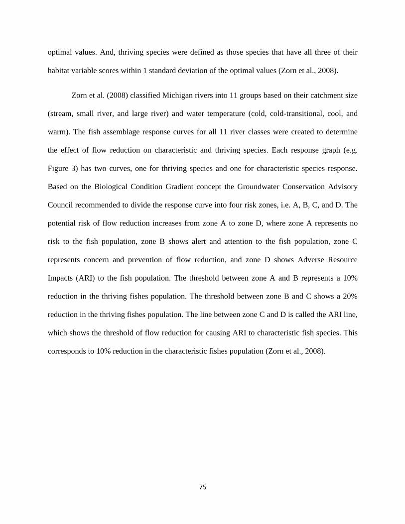
75

optimal values. And, thriving species were defined as those species that have all three of their

habitat variable scores within 1 standard deviation of the optimal values (Zorn et al., 2008).

Zorn et al. (2008) classified Michigan rivers into 11 groups based on their catchment size

(stream, small river, and large river) and water temperature (cold, cold-transitional, cool, and

warm). The fish assemblage response curves for all 11 river classes were created to determine

the effect of flow reduction on characteristic and thriving species. Each response graph (e.g.

Figure 3) has two curves, one for thriving species and one for characteristic species response.

Based on the Biological Condition Gradient concept the Groundwater Conservation Advisory

Council recommended to divide the response curve into four risk zones, i.e. A, B, C, and D. The

potential risk of flow reduction increases from zone A to zone D, where zone A represents no

risk to the fish population, zone B shows alert and attention to the fish population, zone C

represents concern and prevention of flow reduction, and zone D shows Adverse Resource

Impacts (ARI) to the fish population. The threshold between zone A and B represents a 10%

reduction in the thriving fishes population. The threshold between zone B and C shows a 20%

reduction in the thriving fishes population. The line between zone C and D is called the ARI line,

which shows the threshold of flow reduction for causing ARI to characteristic fish species. This

corresponds to 10% reduction in the characteristic fishes population (Zorn et al., 2008).

76

Figure 3. Fish response curve to flow reduction (adapted from Zorn et al., 2008)

In order to define drought zones, first, the index flow for each stream in Saginaw Bay

Watershed is determined. The SWAT model was run for 41 years, i.e. from 1972 to 2012, to

simulate the daily streamflow data. Using this data, the lowest daily median flow values of the

lowest summer month were calculated for each stream. Based on the Zorn et al. (2008) model

criteria, four drought zones (A, B, C, and D) were defined: Zone A, representing the no drought

condition, Zone B, showing the moderate drought condition, Zone C, indicating the severe

drought conditions, and Zone D, referring to the extreme drought conditions. This information

was used to create the reference table of drought zones (Table 5). Using the reference table,

drought condition can be identified for each stream segment by multiplying the index flow

(obtained from the SWAT model for the period of study 1972 to 2012) to correspondent value of

Table 5.

77

Table 5. Reference table of drought zones (adapted from Hamilton and Seelbach, 2011)

Ecological Stream Types Zone A Zone B Zone C Zone D

Cold Streams >86% None >80%-86% ≥80%

Cold Small Rivers >89.5% None

>79%-

89.5% ≥79%

Cold Transitional Streams None >96% None ≥96%

Cold Transitional Small

Rivers None >98% None ≥98%

Cold Transitional Large

Rivers None >97% None ≥97%

Cool Streams >94% >85%-94% >75%-85% ≥75%

Cool Small Rivers >85% >81%-85% >75%-81% ≥75%

Cool Large Rivers >86% >81%-86% >75%-81% ≥75%

Warm Streams >90% >82%-90% >76%-82% ≥76%

Warm Small Rivers >92% >87%-92% >83%-87% ≥83%

Warm Large Rivers >90% >84%-90% >78%-84% ≥78%

4.3.6. Drought Model Input Variables

In this study, a total of 66 variables were initially considered for development of the

drought model as independent variables. These variables were categorized as follows:

precipitation (25 variables), streamflow (24 variables), land use (8 variables), soil (8 variables),

and drainage area (1 variable).

The precipitation variables included the total precipitation for the month of interest, the

total precipitation of each of the previous 12 months, and the average precipitation in past 𝑛 ∈

{1,2, ⋯ ,12} months was included, i.e. 𝑝𝑛̅̅ ̅ = ∑𝑝𝑖

𝑛+1

𝑛0 , where 𝑝𝑖 is the precipitation of the i-th

month before the month of interest. To further elaborate on the last group, the independent

variable for n = 1 correspond to the average precipitation of the month of interest and one month

before that; when setting n = 2 that corresponds to the average precipitation of the month of

interest and that of the previous two months; and so on. The monthly average flow rates of the

prior 1 to 24 months were also considered as independent variables. The land use was

categorized as agricultural, forested, urban, and water areas. The actual area (4 variables) and

78

percentage of these land uses (4 variables) for the area above each stream segment were

calculated summing up to eight land use variables. Soil data was divided into four hydrologic

soil groups of A, B, C, and D (NRCS, 2007). The soil groups were categorized based on their

infiltration and water transmission rates. Group A soils, with gravel or sand texture, consist of

gravel or sand (>90%) and clay (<10%). These soils have high infiltration and water

transmission rates. Group B soils have a loamy sand or sandy loam texture and consist of 10-

20% clay and 50-90% sand. These soils have moderate infiltration and water transmission rates.

Group C soils, with loam or silt loam texture, have 20-40% clay and less than 50% sand. These

soils have low infiltration and water transmission rates. Group D soils, with clayey texture, have

more than 40% clay and less than 50% sand. The infiltration and water transmission rates of

these soils are very slow (Cronshey et al., 1986; NRCS, 2007). Like the land use variables, the

actual area and percentage values of each soil groups were calculated for each subbasin adding

up to eight soil variables. The last variable was drainage area, which was calculated as the total

area above the outlet of each stream segment.

4.3.7. Variable Selection: ReliefF algorithm

The ReliefF algorithm is a commonly used method for feature selection (Robnik-Sikonja

and Kononenko, 2003). This method ranks the independent variables according to their relevance

or importance in classifying or predicting the dependent variable (Kononenko, 1994; Robnik-

Sikonja and Kononenko, 2003). The ReliefF algorithm is the improved version of the Relief

algorithm, which was originally developed for binary classification (Kira and Rendell, 1992b;

Robnik-Sikonja and Kononenko, 2003). ReliefF is capable of handling data with strong

dependencies or outliers (Kononenko, 1994; Robnik-Sikonja and Kononenko, 2003; Mahlein et

al., 2013).

79

For any given sample, ReliefF searches for the nearest neighborhoods of the same-class,

also known as hits, and of the different-class, also known as misses. With k being the number of

each neighborhood samples, there will be k nearest hits and k nearest misses for each sample.

The nearest hits and misses are usually defined by the Euclidean distance (L2 norm) or

Manhattan distance (L1 norm). The relevance of variables are determined by the sum of the

Euclidean distance, or the Manhattan distance, between the nearest hits and nearest misses of all

samples (Robnik-Sikonja and Kononenko, 2003; Mahlein et al., 2013), as follows:

𝑊𝑖 = 𝑊𝑖 − ||𝑠𝑖 − 𝑁𝐻𝑖||𝑛

+ ||𝑠𝑖 − NMi||n

Where, n is equal to 1 for the Manhattan distance and is equal to 2 for the Euclidean

distance, si is the i-th sample, NHi is a set of k nearest-hit to the si, and NMi is a set of k nearest-

miss to the si, and Wi is the weight of the feature. This equation is set up in such a way that each

feature is penalized, if it differs greatly from that of the nearest-hits, and rewarded otherwise, in

case of nearest-misses.

ReliefF runtime scales linearly with the number of independent variables, i.e. if the

number of independent variables are doubled, the algorithm would take twice as long. However,

the computational requirement of the algorithm increases non-linearly with increasing sample

size. This means that if the number of observations are doubled, the time needed to perform the

required computation will increase more than twice. This is mostly due to the sorting and the

distance calculation of each sample to all the other samples, which results to 𝑛(𝑛 − 1) 2⁄ distinct

distance values that are required to determine the nearest-hits and nearest-misses. In this study,

there were more than 6.6 million observations (13831 streams × 40 years ×12 months), where

each observation has 66 independent variables. Having these many observations made it

impossible to use a single ReliefF run. Therefore, a subset of 10,000 samples was randomly

80

selected from the original data set, and ranked. This procedure was repeated 2500 times;

resulting in 2500 different rankings for each independent variable. A histogram of the ranking

for each independent variable was constructed and averaged to determine the final score.

Selected variables were then used to accomplish two general goals: 1) Develop the most

accurate drought model capable of determining current drought severity for all stream segments

within the study area. This model is called the Current Drought Severity Model and was tested

by using three sets of variables (the top 5, 10, and 15 ranked variables obtained from ReliefF)

(Table S1). 2) Develop the most accurate drought forecast model capable of predicting future

drought severity. This model is called the Future Drought Severity Model and was tested against

three sets of variables that include all precipitation and streamflow variables from 6, 12, and 18

months prior to the month of interest.

4.3.8. Partial Least Square Regression

The partial least square regression (PLSR) is a statistical approach used for modeling

linear relations between multivariate measurements (de Jong, 1993; Wold et al., 2001). However,

the main advantage of PLSR over general linear regressions is its ability to deal with strongly

collinear, noisy, incomplete, and large arrays of independent variables (Wold et al., 2001;

Carrascal et al., 2009).

In order to train, test, and select the best PLSR model, 10-fold cross validation was used.

In 10-fold cross-validation, the dataset is randomly divided into 10 equally sized exclusive

subsets or folds. Nine folds of the data are used for training (90%) and the remaining (1-fold) is

used for testing (10%) (Hamaamin et al., 2013). This process was repeated 10 times with a new

non-overlapping testing fold until all folds were used for testing the PLSR model.

81

For the development of both current and future drought severity models, PLSR was used

to predict the relationship between the median flow of each stream segment for the month of

interest (dependent variable) and the independent variables (Table S1). The initial test showed

that the observed median flow is highly skewed (Figure S2); therefore, the dependent and

independent variables were transformed using 𝑙𝑜𝑔10 before the model development.

In order to evaluate the performance of these models, the accuracy, precision, and

sensitivity of each model, in predicting drought zones, were determined. Accuracy refers to the

overall correctness of the model (Eq. 1). Precision is an estimate of how correct the model

outputs are for each class (Eq 2). Sensitivity (Eq. 3) refers to the model ability to correctly pick

instances of a certain class (Aruna et al., 2011). Accuracy, precision and sensitivity are

calculated as follows:

𝑎𝑐𝑐𝑢𝑟𝑎𝑐𝑦 =𝑇𝑃+𝑇𝑁

𝑃+𝑁 (1)

𝑝𝑟𝑒𝑐𝑖𝑠𝑖𝑜𝑛 =𝑇𝑃

𝑇𝑃+𝐹𝑃 (2)

𝑠𝑒𝑛𝑠𝑖𝑡𝑖𝑣𝑖𝑡𝑦 =𝑇𝑃

𝑃=

𝑇𝑃

𝑇𝑃+𝐹𝑁 (3)

Where, P stands for the number of positive cases and N stands for the number of negative

cases. The definition of positive and negative changes depending on what is being evaluated. For

example, if the model is evaluating the presence or absence of the drought, then P indicates the

number of observations point that drought is present and N represents those observations that

show no sign of drought. While considering the definition of the positive and negative, TP stands

for True Positive, meaning observations that are positive and they are correctly classified as

positive. TN stands for True Negative, meaning observations that are negative and they are

correctly classified as negative. FP, stands for False Positive, meaning the observations that are

82

negative but mistakenly classified as Positive. Finally, FN stands for False Negative, meaning

the observations that are positive but mistakenly classified as negative.

4.3.9. Climate Models

In this study, 16 different general circulation models (GCMs) from the Coupled Model

Intercomparison Project Phase 5 (CMIP5) were used. CMIP5 aims to provide a multi-model

dataset including long term and near term experiments that offer better understanding of climate

change and climate variability (Taylor et al., 2012). The long-term experiments were used in this

study, which range from mid-1900 to 2100 and beyond (Taylor et al., 2012). The names,

modeling centers, atmospheric resolutions, and their components are listed in Table 6. For each

GCM, data driven by three Representative Concentration Pathways (RCPs) scenarios (RCP4.5,

RCP6.0, and RCP8.5 (Moss et al., 2010) was extracted for the future period of 2040-2060 and

the historical period of 1980-2000. The latter is referred to as the control period data.

Additionally, the weather station data for daily observation for the same time period as control

data were obtained from the NCDC and used as the baseline in the analysis. The locations of

these weather stations are presented in Figure S1.

The climate is projected to change significantly in the future and such changes are

associated with large uncertainty, which cannot be neglected for impact assessments, especially

when extreme situations are of the primary concern (IPCC, 2013). In impact assessment studies,

one way to take uncertainty into consideration is by adopting an ensemble approach where the

ensemble could refer to differences in the models, emission scenarios, initial conditions, etc.

(Parker, 2013). In the current study, the ensemble was constructed based on different GCMs and

emission scenarios. Although many other downscaling methods like quantile mapping, multiple

regression, and artificial neural networks exist in the literatures (Maraun et al., 2010; Winkler et

83

al., 2011a and 2011b; Hessami et al., 2008; Sailor et al., 2000; Hewitson and Cran et al. 1996;

Schoof and Pryor et al., 2001), the delta method is chosen in the current study due to its ability to

produce a large ensemble of projections (Winkler et al., 2011b). The delta method is also widely

used in hydrological studies (Morrison et al., 2002; Merritt et al., 2006; Adam et al., 2009; Elsner

et al., 2010; Dessu and Melesse, 2013; Woznicki and Nejadhashemi, 2014).

The assumptions of the delta methods are as following: a) relative change is better

simulated by GCMs compared to absolute values (Fowler et al, 2007; Loukas et al., 2007), b) the

number and temporal sequence of wet days remains unchanged (Fowler et al, 2007; Dessu et al.,

2013; Htut et al., 2014), c) the GCMs biases for both mean and variability will be similar for the

control and future periods, ignoring GCMs biases in the distribution of simulated variables

(Boyer et al., 2010; Winkler et al., 2011b; Htut et al., 2014), and d) the spatial pattern and

temporal variability of the present climate is maintained in the future (Diaz-Nieto and Wilby,

2005; Boyer et al., 2010).

The delta method was used to downscale the climate data to allow local scale analysis

and for the impact model, which requires data inputs at daily time steps. The variables used in

the delta method included the daily maximum temperature, daily minimum temperature, and

daily total precipitation. In the delta method, the difference/ratio between the future and control

period were calculated for the monthly averaged daily temperature/precipitation, and then

applied to the observed daily time series. The temperature change factors are additive and can be

negative values. On the other hand, the precipitation change factors are calculated as ratios with

precipitation being zero bounded (Woznicki and Nejadhashemi, 2012).

84

Table 6. CMIP5 models developer, name, resolution, and components (Petkova et al., 2013; IPCC, 2013)

Modeling Center/ID Model Atmospheric Resolution

(latitude × longitude)

Components

The First Institute of

Oceanography/FIO

FIO-ESM 2.8° × 2.8° Atm1,Aero2,LS4,O5,OB6,SI7

Institut Pierre-Simon

Laplace/IPSL

IPSL-CM5A-LR 3.75° × 1.9° Atm1,Aero2,LS4,O5,OB6,SI7

IPSL-CM5A-MR 2.5° × 1.25° Atm1,Aero2,LS4,O5,OB6,SI7

Atmosphere and Ocean Research

Institute (The University of

Tokyo), National Institute for

Environmental Studies, and Japan

Agency for Marine-Earth Science

and Technology /MIROC

MIROC5 1.41° × 1.39° Atm1,Aero2,LS4,O5,SI7

Japan Agency for Marine-Earth

Science and Technology,

Atmosphere and Ocean Research

Institute (The University of

Tokyo), and National Institute for

Environmental Studies/MIROC

MIROC-ESM 2.81° × 1.77° Atm1,Aero2,LS4,O5,OB6,SI7

MIROC-ESM-

CHEM

2.81° × 1.77° Atm1,Aero2,AtmCH3,

LS4,O5,OB6,SI7

Met Office Hadley Centre

/MOHC

HadGEM2-ES 1.875° × 1.25° Atm1,Aero2,AtmCH3,

LS4,O5,OB6,SI7

Meteorological Research Institute

/MRI

MRI-CGCM3 1.125° × 1.125° Atm1,Aero2,LS4,O5,SI7

NASA Goddard Institute for

Space Studies /NASA GISS

GISS-E2-R 2.5° × 2.0° Atm1,Aero2,AtmCH3,

LS4,O5, SI7

GISS-E2-H 2.5° × 2.0° Atm1,Aero2,AtmCH3,

LS4,O5, SI7

85

Table 6. (cont’d)

National Center for Atmospheric

Research/NCAR

CCSM4 1.25° v 0.9° Atm1,Aero2, LS4,O5, SI7

National Institute of

Meteorological Research/Korea

Meteorological Administration

/NIMR/KMA

HadGEM2-AO 1.875° × 1.25° Atm1,Aero2, LS4,O5, SI7

NOAA Geophysical Fluid

Dynamics Laboratory/NOAA

GFDL

GFDL-CM3 2.5° × 2.0° Atm1,Aero2,AtmCH3,

LS4,O5, SI7

GFDL-ESM2G 2.5° × 2.0° Atm1,Aero2,

LS4,O5,OB6,SI7

GFDL-ESM2M 2.5° × 2.0° Atm1,Aero2,

LS4,O5,OB6,SI7

National Science Foundation,

Department of Energy, National

Center for Atmospheric Research

(NSF-DOE-NCAR)

CESM1(CAM5) 1.25° × 0.9° Atm1,Aero2, LS4,O5, SI7

1 Atmosphere; 2 Aerosol; 3 Atmospheric Chemistry; 4 Land Surface; 5 Ocean; 6 Ocean Biogeochemistry; 7 Sea Ice

86

4.4. Results & Discussions

4.4.1 SWAT Model Calibration and Validation

The results of SWAT model calibration and validation, using statistical criteria, such as

NSE, RSR, and PBIAS, are presented in Table 7. The reported NSE, RSR, and PBIAS are the

overall values for both the calibration and validation for the period of 2001 to 2010. The SWAT

model met the statistical criteria for all nine USGS stations according to evaluation criteria,

defined by Moriasi et al. (2007), the performance rating for all of the stations are in the range of

very good, good, and satisfactory. Therefore, the model can be used to simulate streamflow data

for the region satisfactorily.

Table 7. Statistical criteria for SWAT model calibration and validation for nine USGS

gauging stations within the Saginaw Bay Watershed

USGS

Station

NSE*

(performance rating)

RSR**


PBIAS***


04144500 0.64

(Satisfactory)

0.60

(Satisfactory)

14.27

(Good)

04148140 0.54

(Satisfactory)

0.68

(Satisfactory)

-9.68

(Very Good)

04148500 0.71

(Good)

0.54

(Good)

16.34

(Satisfactory)

04147500 0.63

(Satisfactory)

0.61

(Satisfactory)

-1.53

(Very Good)

04151500 0.64

(Satisfactory)

0.60

(Satisfactory)

13.77

(Good)

04154000 0.54

(Satisfactory)

0.68

(Satisfactory)

9.65

(Very Good)

04155500 0.61

(Satisfactory)

0.63

(Satisfactory)

9.84

(Very Good)

04156000 0.73

(Good)

0.52

(Good)

6.44

(Very Good)

87

Table 7. (cont’d)

04157000 0.80

(Very Good)

0.45

(Very Good)

10.90

(Good)

* Nash-Sutcliffe model efficiency coefficient,

** Root-mean-squared error-observations standard deviation ratio,

*** Percent bias.

4.4.2 Variable Selection

4.4.3.1.Current Drought Severity Model

The ReliefF algorithm was used for the development of the most accurate drought model

capable of determining current drought severity for all streams. The ranking of all 66 variables is

presented in the histogram map (Figure 4). The y-axis represents the 66 independent variables,

and the x-axis represents their ranking. The color in Figure 4 shows how often a variable has

obtained a certain rank during the 2500 different random sampling. The final number was

normalized to scale between 0 and 1 (abundance). The dark blue indicates that the variable never

obtained that rank. As the color spectrum moves from dark blue to dark red, it indicates that the

variable obtained that rank more often than other independent variables. As an example, Figure

S3 shows the histogram of the ranking of variable #20 (average flow rate from 23 months prior

to the month of interest). This variable mostly obtained rank 7 during 2500 iterations. Therefore,

in Figure 4, on line 20, rank 7 is being shown the most red. The final ranking for each variable

was determined based on the average of these 2500 different ranking.

In general, the average flow rate variables were ranked much higher than any other type

of variables (Figure 4). This is mainly due to the high correlation between median flow and

average flow rate. After the average flow rate variables, the precipitation variables were ranked

the highest. This indicates that the stream system in general is less flashy during the dry season

and more influenced by the groundwater system. Therefore, the median flow is not as dependent

88

on precipitation as it was to the average flow rate. Finally, the physiological variables were

shown to be the least related to the changes in the median flow indicating that the changes to the

median flow are insensitive to the total drainage area, land use, and soil type.

Figure 4. ReliefF ranking histogram map

Out of the 66 original variables, the top 5, 10, and 15 ranked variables were used to

develop three sets of drought models. The list of the top 15 ranked variables are presented in

Table 8. All of the top ranked variables are related to flow rate. The only difference between the

variables is the month from which the flow rate was calculated.

Ph

ysi

og

rap

hic

al

Var

iable

s

Aver

age

Flo

w

rate

Var

iable

s

Pre

cipit

atio

n

Var

iable

s

Abundan

ce

89

Table 8. Top 15 ranked variables

Ranking Variables

1 Average flow rate from 1 month prior to the month of interest

2 Average flow rate from 2 months prior to the month of interest














4.4.2.2.Future Drought Severity Model

The future drought severity model should be capable of predicting drought conditions for

all streams within an area of interest. The results from the ReliefF analysis showed that the

physiological variables were the least related to the median flow. Therefore, they were not

considered for the model development (Table S1). Overall, three sets of variables, all from 6, 12,

and 18 months prior to the month of interest, were used in order to predict the future drought

severity 6, 12, and 18 months in advanced, respectively. These variables included all average

flow rate and precipitation variables for their respected period (Table S1).

4.4.3 Drought Severity Model

4.4.3.1.PLSR predictively for median flow

The statistical analysis of the Current Drought Severity Model performances is presented

in Table 9. Three models were developed using the top 5, 10, and 15 ranked variables. 10-fold

cross validation was used to insure that the models were not over-trained or over-fitted by

increasing the number of PLSR components. Mean Square Error (MSE) obtained from the 10-

90

fold cross validation decreased asymptotically by increasing the number of PLSR components

(Figure S4). This shows that the model is not over-fitted because the MSE values do not

increased when incorporating more PLSR components.

The performance of each model was studied on all streams and on stream orders (1 to 7).

In the case of all streams, there is little to no change in R2 values (0.86) between the three models

(Table 9). This indicates that including additional variables does not improve the models’

performances. When comparing the models’ performances based on different stream orders,

stream order 6 and 7 (<2% of all streams) are exceptions in which R2 values slightly improve as

the number of independent variables increase (Table 9). However, improvement in model

predictability is minimal (R2 for stream order 6 will be changed from 0.64 in model 1 to 0.66 for

the model 3) while the number of independent variables tripled from 5 to 15, respectively.

As presented in Figure 5, the first, second, and third PLSR models were able to explain

86.5%, 87% and 87.1% of the variance of the output (median flow), respectively. Since the

difference between these three models are not considerable; the first model, which requires the

least number of independent variables, was selected as the best predictive Current Drought

Severity Model for this study.

Table 9. Current Drought Severity Model performances

Model Number of

Variables

R2

Stream order

(All) (1) (2) (3) (4) (5) (6) (7)

First 5 0.86 0.74 0.71 0.72 0.76 0.81 0.64 0.74

Second 10 0.86 0.74 0.72 0.72 0.76 0.81 0.66 0.76

Third 15 0.86 0.74 0.72 0.72 0.76 0.81 0.66 0.76

The statistical analyses for the Future Drought Severity Model performances are shown

in Table 10. Similar to the Current Drought Severity Model, three models were evaluated using

91

three sets of variables (flow rate and precipitation variables from 6, 12, and 18 months prior to

the month of interest). The same procedure (10-fold cross validation) was used for the fourth,

fifth, and sixth models to make sure the models are not over-fitted by increasing the number of

PLSR components. The MSE of the Future Drought Severity Models was similar to the Current

Drought Severity Models, where the MSE values decreased asymptotically by increasing the

number of PLSR components, Figure S5.

Among these models, the fourth and fifth models have higher R2 values (0.85) and thus

perform better than the sixth model (R2 = 0.76). Similarly, with respect to the stream order, both

the fourth and fifth model performed better than the sixth model. The lower R2 value for the sixth

model is due to its PLSR model deficiency in explaining the output variance (Figure S6). The

fourth and the fifth model can explain more about 84% of the variance; however, the sixth model

can explain 75% of the variance at most, Figure S6. This could be due to the fact that the

variables used to predict drought 18 months in advance are not sensitive enough to detect future

drought conditions.

Table 10. Future Drought Severity Model performances

Model Number of

Variables

R2

Stream order

(All) (1) (2) (3) (4) (5) (6) (7)

Fourth 34 0.85 0.71 0.67 0.67 0.71 0.76 0.58 0.69

Fifth 16 0.85 0.69 0.66 0.66 0.69 0.74 0.56 0.67

Sixth 7 0.76 0.53 0.46 0.46 0.50 0.61 0.32 0.49

92

Figure 5. The variance explained percentage for each PLSR for the Current Drought Severity Model: a) First model, b) Second model,

c) Third model.

(a) (b) (c)

93

The histogram of measured and predicted median flow obtained from the Current and

Future Drought Severity Models are presented in Figures 6 and S7, respectively. The horizontal

axis represents the 𝑙𝑜𝑔10 of the median flow values and the vertical axis represents the number of

counts. Overall, the histogram of the predicted median flows is very similar to the histogram of

the measured flows for all models. However, the peak in the predicted histogram is higher than

the peak in the measured histogram. This can be explained due to the fact that the predictive

models overestimate the median flows for all stream orders (Table 10) and overestimate the

median flows for stream orders 6 and 7 (Table 9). This difference was most pronounced for the

sixth model (Figure S7). Therefore, it is expected that the error level is higher at the higher and

lower median flow rates due to the shift from the two tails of the distribution for the sixth model

to the peak of the median flow rates. This also explains the lower R2 values for the sixth model

(R2 = 0.76).

94

(a) (b) (c)

Figure 6. The comparison of measured vs. predicted median flow histogram for the Current Drought Severity Model, a) First model,

b) Second model, c) Third model.

95

4.4.3.2.Accuracy, precision, and sensitivity of drought models in predicting drought

zones

For each model, drought zones were identified by comparing the predicted median flow

values against the reference table for the drought zones (Table 5). The results from the six

drought severity models are summarized in six confusion matrices (Tables 11-12 and S2-S5).

The diagonal of the matrix shows the number of zones that have been correctly classified by the

model. The overall accuracy of the model is determined by dividing the sum of the diagonal

values by the sum of the all values of the matrix. As seen in Tables 11-12 and S2-S5, the first

model through fifth model have an accuracy higher than 70%. However, the sixth model has

accuracy of only 59%. This reflects the conclusions drawn in the previous section that the sixth

model has a lower predictability than the other developed models.

In general, all models have lower sensitivities and precisions for zone B and C compared

to zone A and D. Especially for zone C, all cases had a sensitivity and precision percentage

below 8%. This low predication is due to the small range that zone B and C cover. As mentioned

earlier, there are eleven different classes of streams based on their sizes and temperature (Zorn et

al., 2008), and each of these classes have specific index flow zoning ranges. For zone B and C

and all stream classes, the zoning ranges cover only 10% or less of the index flow, while the

remaining index flow reduction is covered by zone A and D. Therefore, accurately predicting

these small ranges can be difficult, which ultimately reduce the sensitivity and precision of the

models for zones B and C.

When comparing the performance of the Current Drought Severity Models, the first

model performed the best. The first model had a higher accuracy, precision, and sensitivity

compared to the other models. Among the Current Drought Severity Models (Tables 11, S2, and

96

S3), the first model has higher precision in classifying zone A (83%), and lower precision in

classifying zone D (67%). In addition, it has a higher sensitivity in classifying zone D (66%), and

slightly lower sensitivity in classifying zone A (84%). Therefore, it was concluded that the first

model is the best among the Current Drought Severity Models.

Among the Future Drought Severity Models, the fourth model performed slightly better

than the fifth model. The fourth model has a slightly better accuracy (71%), a better precision in

classifying zone D (62%), and a better sensitivity in classifying zone A (84%) compared to the

fifth model. The sixth model, as expected, has a low accuracy (59%), precision, and sensitivity

among all models. Therefore, it was concluded that the fourth model is the best among the Future

Drought Severity Models.

Table 11. Confusion matrix for drought zones: First model

Drought

Zone

Predicted

A B C D Sensitivity

Act

ual

A 3,410,732 99,090 82,247 484,990 84%

B 89,968 85,271 10,230 87,386 31%

C 66,450 8,292 9,082 66,863 6%

D 530,891 78,431 57,450 1,272,877 66%

Precision 83% 31% 6% 67% Accuracy =

74%

Table 12. Confusion matrix for drought zones: Fourth Model

Drought

Zone

Predicted

A B C D Sensitivity

Act

ual

A 3,400,622 81,426 66,065 503,081 84%

B 107,300 82,647 6,523 75,077 30%

C 83,139 6,350 6,304 54,046 4%

D 756,301 85,320 52,635 1,026,748 53%

Precision 78% 32% 5% 62%

Accuracy =

71%

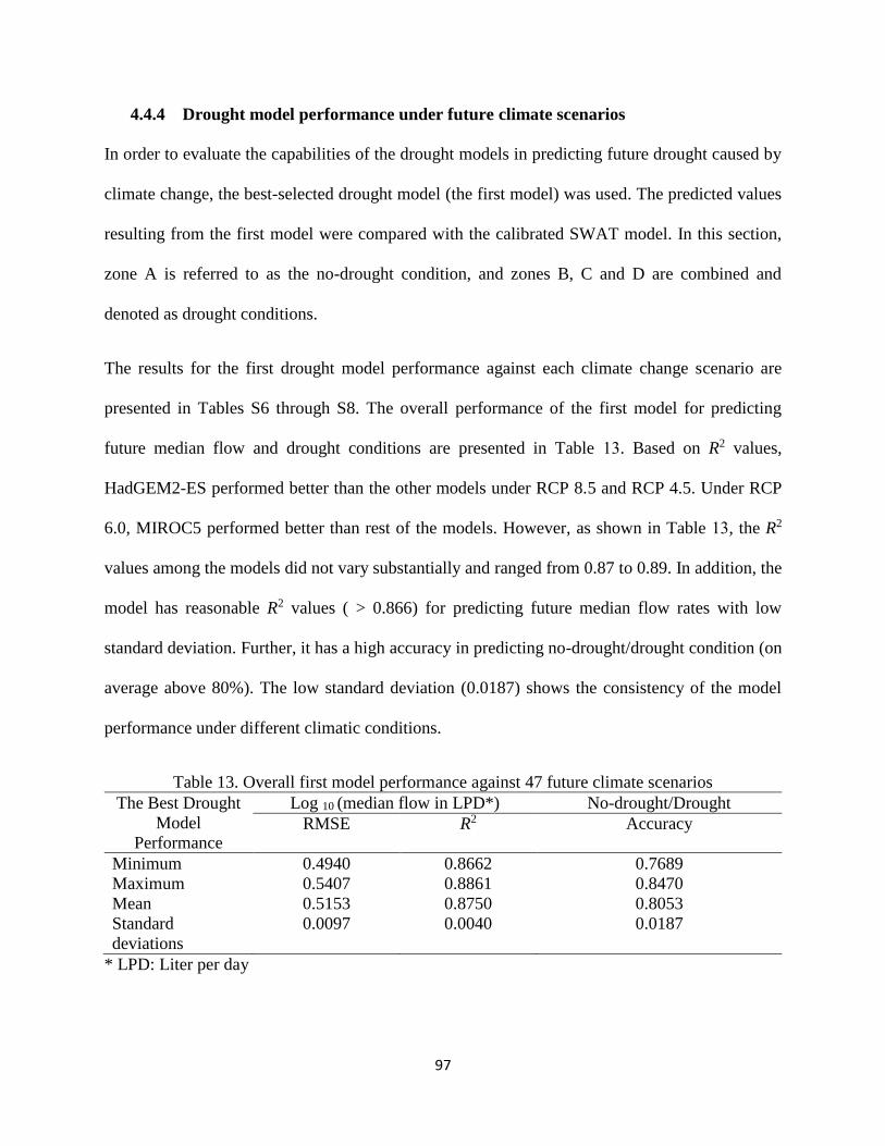
97

4.4.4 Drought model performance under future climate scenarios

In order to evaluate the capabilities of the drought models in predicting future drought caused by

climate change, the best-selected drought model (the first model) was used. The predicted values

resulting from the first model were compared with the calibrated SWAT model. In this section,

zone A is referred to as the no-drought condition, and zones B, C and D are combined and

denoted as drought conditions.

The results for the first drought model performance against each climate change scenario are

presented in Tables S6 through S8. The overall performance of the first model for predicting

future median flow and drought conditions are presented in Table 13. Based on R2 values,

HadGEM2-ES performed better than the other models under RCP 8.5 and RCP 4.5. Under RCP

6.0, MIROC5 performed better than rest of the models. However, as shown in Table 13, the R2

values among the models did not vary substantially and ranged from 0.87 to 0.89. In addition, the

model has reasonable R2 values ( > 0.866) for predicting future median flow rates with low

standard deviation. Further, it has a high accuracy in predicting no-drought/drought condition (on

average above 80%). The low standard deviation (0.0187) shows the consistency of the model

performance under different climatic conditions.

Table 13. Overall first model performance against 47 future climate scenarios

The Best Drought

Model

Performance

Log 10 (median flow in LPD*) No-drought/Drought

RMSE R2 Accuracy

Minimum 0.4940 0.8662 0.7689

Maximum 0.5407 0.8861 0.8470

Mean 0.5153 0.8750 0.8053

Standard

deviations

0.0097 0.0040 0.0187

* LPD: Liter per day

98

4.4.5 The impact of climate change on future drought

The first model, which is the best model, was run for the 47 future climate scenarios for

the period of 2040 to 2060 to understand the impacts of climate change on drought in the context

of stream health. In addition, the status of drought conditions for the current period, 1990 to

2010, was evaluated to provide a reference condition in which future drought will be evaluated

against. The future and current drought conditions were compared with each other using a

cumulative distribution function (CDF) for all reaches within the Saginaw Bay Watershed,

Figure 7. The probability of increasing drought conditions is categorized into three equal

intervals. Reaches drawn as green show lower climb in drought probability while reaches drawn

in red show higher probability of drought occurrences under future climate conditions. In

general, the majority of the reaches (94%) will experience higher drought probability under

future climate scenarios compare to current conditions. Specifically the mid-section of the

watershed will experience the highest probabilities (66.68% to 100%) for future drought. In

order to understand the possible causation for the increased drought in this region, the percent

change maps for the two main drivers of drought (precipitation and temperature) were created

(Figure 8). The percent change map of average temperature, Figure 8a, shows warmer

temperatures are expected for all streams in the region due to an increase in average air

temperature (2.3 °C). However, the region with the lowest increase in of precipitation (3.22% to

4.31%) was almost identical to the region of the worst future drought conditions (66.68% to

100%). This indicates that the stream system in the area of interest (high drought probability

region) is predominately fed by surface runoff (sensitive to precipitation patterns), while the rest

of the watershed is predominately groundwater fed.

99

Figure 7. Probability of increasing drought conditions under projected climate change (2040-

2060) compare to current condition (1990-2010).

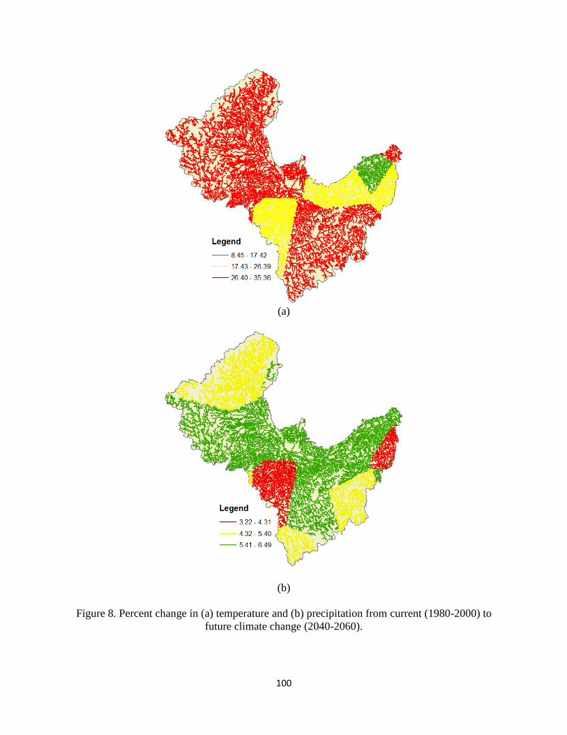
100

Figure 8. Percent change in (a) temperature and (b) precipitation from current (1980-2000) to

future climate change (2040-2060).

(a)

(b)

101

4.5. Conclusion

Drought is the world’s most costly natural disaster (Wilhite, 2000b; Keyantash and

Dracup, 2002), affecting both human and natural systems. Several drought indices have been

developed to study the impacts of drought on the human dimension. However, this study is

unique since the objective was to define a new drought index and predictive model as a proxy for

stream health.

The concept of the index flow was adapted from the Regional-scale Habitat Suitability

Model to define the drought zones (Zorn et al., 2008). Initially, 66 variables were considered for

development of the drought model. Variables were selected to develop two sets of models: 1) the

most accurate drought model capable of determining current drought severity and 2) the most

accurate drought forecast model capable of predating future drought severity. For the Current

Drought Severity Models, the ReliefF algorithm was used to identify the top 15 ranked variables

and for the Future Drought Severity Models, three models using some variables from 6, 12, and

18 months prior to the month of interest, respectively, were used. In general average flow rate

and precipitation were among the highest ranked variables that were used for development of

drought models.

Six drought models were developed using PLSR. The drought models were evaluated for

median flow, classifying drought zones, and no-drought/drought conditions. Among the Current

Drought Severity Models, the first model with five variables, having the highest R2 (0.86) and

accuracy (0.74), was selected as the best; while the fourth model with 34 variables, having the

highest R2 value (0.85) and accuracy (0.71), was selected as the best model among the Future

Drought Severity Models. Overall, the first model was selected as the best model to predict

drought severity.

102

The first model predictability was also tested using 47 future climate models, in which R2

values varied from 0.87 to 0.89. In addition, the average accuracy of the no-drought/drought ratio

is 0.81. The future and current drought conditions were compared with each other using CDF

curves and maps for all reaches within the Saginaw Bay Watershed. Approximately 7.2% of

streams are expected to experience high increase (66.68% to 100%) in drought frequency under

future climate scenarios. This region is highly correlated to the region that will experience the

lowest increase in precipitation (3.22% to 4.31%), while the average temperature rises for the

entire watershed is about 2.3 °C.

This study introduced a new concept of evaluating the impact of drought as a proxy for

the stream health. This is important since the introduced concept and modeling techniques can

provide a road map for better allocation of resources to mitigate the impacts of the climate

change on aquatic systems. The technique presented here is robust and transferable to other

watersheds around the world. Due to limitations of the delta method, future studies should

explore additional resources of climate data and methods for downscaling and bias correction in

the development of the climate change ensemble.

4.6. Acknowledgments

This work is supported by the USDA National Institute of Food and Agriculture, Hatch

project MICL02212. Also, we would like to thank the climate modeling groups (listed in Table

6 of this paper) for producing and making their model outputs available. Additional thanks go to

the World Climate Research Programme's Working Group on Coupled Modelling, which

maintains the CMIP database and promotes the sharing of climate model outputs. Furthermore,

we would like to thank the U.S. Department of Energy's Program for Climate Model Diagnosis

and Intercomparison, which provides coordinating support and development of software

103

infrastructure in partnership with the Global Organization for Earth System Science Portals. The

climate projections were developed with funding from the National Science Foundation under

Grant BCS-0909378. Any opinions, findings, and conclusions or recommendations expressed in

this material are those of the authors and do not necessarily reflect the views of the National

Science Foundation.

104

5. DEVELOPMENT AND EVALUATION OF A COMPERHENSIVE DROUGHT

INDEX

5.1. Abstract

Droughts are known as the world’s costliest natural disasters impacting a variety of

sectors. Despite their wide range of impacts, no universal drought definition has been defined.

The goal of this study is to define a universal drought index that considers drought impacts on

meteorological, agricultural, hydrological, and stream heath categories. Additionally, predictive

drought models are developed to capture both categorical (meteorological, hydrological, and

agricultural) and overall impacts of drought. In order to achieve these goals, thirteen commonly

used drought indices were aggregated to develop a universal drought index named MASH. The

thirteen drought indices consist of four drought indices from each meteorological, hydrological,

and agricultural categories, and one from the stream health category. Cluster analysis was

performed to find the three closet indices in each category. Then the closet drought indices were

averaged in each category to create the categorical drought score. Finally, the categorical drought

scores were simply averaged to develop the MASH drought index. In order to develop predictive

drought models for each category and MASH, the ReliefF algorithm was used to rank 90

variables and select the best variable set. Using the best variable set, the adaptive neuro-fuzzy

inference system (ANFIS) was used to develop drought predictive models and their accuracy

was examined using the 10-fold cross validation technique. The models’ predictabilities ranged

from R2 = 0.75 for MASH to R2 = 0.98 for the hydrological drought model. The results of this

study can help managers to better position resources to cope with drought by reducing drought

impacts on different sectors.

105

Keywords: Meteorological drought; Hydrological drought; Agricultural drought; Stream health

drought; Drought monitoring; Drought predictive model

5.2. Introduction

Droughts are common and recurring phenomena affecting many sectors such as

agriculture, water supply, economic, social, and ecosystems (Heim, 2002). Droughts’ impacts on

these sectors make it difficult to develop a universal/all-embracing definition of drought, since

each sector measures drought differently (Whitmore, 2000; Heim, 2002). Drought definitions are

generally categorized into meteorological, agricultural, hydrological, socioeconomic, and stream

health (American Meteorological Society, 1997; Heim, 2002; Esfahanian et al., 2016).

Meteorological drought is generally defined as a period of precipitation deficiency (several

months or years) compared to a long term average (Whitmore, 2000; Heim, 2002; Mishra and

Singh, 2010; Sheffield and Wood, 2011). The impacts of meteorological drought are a reduction

in infiltration, runoff, deep percolation, and ground water recharge (NDMC, 2016). Agricultural

drought is defined as a period of soil moisture deficiency resulting from precipitation shortage

for a short period of time (few weeks duration) (Heim 2002; Sheffield and Wood, 2011). The

impacts of agricultural drought are a reduction in crop biomass and yield, and plant growth

(Heim, 2002; NDMC, 2016). Hydrological drought is defined as a period of deficiency in water

supply due to prolong precipitation shortage (Heim, 2002). The impacts of hydrological drought

are a significant reduction in streamflow, groundwater, reservoir, and lake levels (Whitmore,

2000; Heim, 2002; NDMC, 2016). The concept of socioeconomic drought, which is not the

subject of this study, is based on the impacts of meteorological, agricultural, and hydrological

droughts on the supply and demand of some economic goods (Heim, 2002; NDMC, 2016).

106

Finally, stream health drought is defined as a period of deficiency in streamflow causing

irreversible impacts on aquatic ecosystems (Esfahanian et al., 2016).

Several drought indices have been developed to monitor and quantify drought. Drought

indices are primarily tools to investigate drought duration, intensity, severity, and spatial extent

(Mishra and Singh, 2010). Each drought index requires specific input parameters in order to

measure drought. Precipitation is usually used alone or in combination with other parameters for

this matter (Heim, 2002; Mishra and Singh, 2010; Sheffield and Wood, 2011). Usually for

meteorological drought, precipitation is the primarily parameter (Dai, 2010). For agricultural

drought, soil moisture content is commonly used with the secondary parameters of precipitation

and/or evapotranspiration (Dai, 2010). For hydrological drought, streamflow is often used beside

precipitation (Dai, 2010). Finally for stream health drought, index flow, stream size, and stream

temperature are used to capture fish vulnerability to drought. The index flow is defined as the

median of the summer month with the lowest daily flowrate for the given period (Hamilton and

Seelbach, 2011; Esfahanian et al., 2016).

Despite the current progress in understanding the science behind droughts, there is still a

need to improve drought monitoring methods, which will ultimately improve drought preparation

and management practices, and reduce drought vulnerability on different sectors (Svoboda et al.,

2002). One way to improve drought-monitoring techniques is to combine the existing indices to

better capture the overall impacts of drought (Zargar et al., 2011) because results from

categorical droughts can be significantly different, which can be both confusing and misleading.

In general, the methods used for combining drought indices can be classified as: 1) decision

matrix analysis (Svoboda et al., 2002; Balint et al., 2011; Zieses et al., 2014); 2) classification

107

and regression tree (CART) analysis (Tadesse and Wardlow, 2007; Brown et al., 2008); and 3)

regression technique (Keyantash and Dracup, 2004; Karamouz et al., 2009).

In the decision matrix analysis, multiple criteria are first identified to guide the final

outcome. This technique was used by Svoboda et al. (2002) to create the Drought Monitor,

which is a composite of meteorological drought indices (such as Palmer Drought Severity Index

and Standardized Precipitation Index), and hydrologic and remote sensing information. The

relationship between the Drought Monitor components and drought severity were defined using

the decision matrix analysis (Scoboda et al., 2002). Additionally, the Combined Drought Index

(CDI) was introduced by Balint et al. (2011), which is the combination of the Precipitation

Drought Index (PDI), Temperature Drought Index (TDI), and Vegetation Drought Index (VDI).

The weighted average of the PDI, TDI, and VDI indices were used to compute the CDI. The

assigned weight for the PDI was 50% and 25% weight was assigned for each TDI and VDI

indices (Balint et al., 2011). Zieses et al. (2014) developed the Global Precipitation Climatology

Centre Drought Index (GPCC-DI) with 1° grid spatial resolution, which is a combination of the

Modified Standardized Precipitation Index (SPI-DWD) and Standardized Precipitation

Evapotranspiration Index (SPEI). The GPCC-DI is calculated by taking the average of SPI-DWD

and SPEI indices for each grid cell (Zieses et al., 2014).

The CART analysis is a tree-building technique, which constructs a set of decision rules

to build predictive models. This technique was used by Tadesse and Wardlow (2007) to develop

the Vegetation Outlook (VegOut) to predict future vegetation conditions. In this tool

meteorological drought indices (Standardized Precipitation Index and Palmer Drought Severity

Index), oceanic indices (such as Southern Oscillation Index, and Multivariate El Niño and

Southern Oscillation Index), and satellite and biophysical data were combined using a rule-based

108

regression tree method. A year later, Brown et al. (2008) introduced a new index named

Vegetation Drought Response Index (VegDRI) based on the CART concept. In this index,

meteorological drought indices (Standardized Precipitation Index and Palmer Drought Severity

Index), satellite-based vegetation measures, and biophysical information (such as land cover and

soil available water capacity) were combined using CART analysis in order to develop the

VegDRI empirical models for different seasons.

The regression technique estimates the linear and nonlinear behavior between the

dependent and independent variables. This technique was used by Keyantash and Dracup (2004)

to develop an Aggregate Drought Index (ADI) that considers meteorological, hydrological, and

agricultural categories of drought. In this index, six hydrologic variables including precipitation,

streamflow, reservoir storage, evapotranspiration, soil moisture, and snow water content were

aggregated using principle component analysis (Keyantash and Dracup, 2004). In addition, the

Hybrid Drought Index (HDI) was developed by Karamouz et al. (2009) using this technique.

This index is a combination of the Standardized Precipitation Index, the Palmer Drought Severity

Index, and the Surface Water Supply Index (Karamouz et al., 2009). An artificial neural network

technique was used to predict the HDI based on the three drought indices (Karamouz et al.,

2009).

Given the lack of a universal drought definition in monitoring drought, the goal of this

study is to introduce a universal drought definition that considers several aspects of drought

including meteorological, agricultural, hydrological, and stream health. This universal definition

can improve drought monitoring, which can help decision makers to better allocate the resources

to reduce drought impacts on different sectors. The objectives of this study are to: (1) define

categorical drought indices (meteorological, agricultural, and hydrological) based on commonly

109

used drought indices; (2) define a universal definition of drought by combining the categorical

scores; (3) select the best variable sets to construct predictive drought models; (4) develop

predictive drought models for each drought category and the universal drought index.

5.3. Materials and Methodology

5.3.1. Study area

The Saginaw River Watershed is the largest watershed in Michigan, and is located in the

eastern part of central Michigan (Figure 1). The watershed has a total area of 16,122 km2 and

drains into Lake Huron. This area has a population of about 1.4 million in 22 counties (PSC,

2012). The dominant landuse is agricultural and forest lands (37% each), and the remaining

landuses are pasture (9.5%), urban (7.5%), wetlands (8%), and water (1%). There are 145

subbasins in the Saginaw River Watershed, with the majority of them being warmwater streams.

The elevation in the watershed ranges from 328 m to 176 m above mean sea level. The region

consists of four different hydrologic soil groups A (24%), B (58%), C (16%), and D (1%). This

watershed has been one of the most studied regions in the Great Lakes having high diversity in

flora and fauna, agriculture, and recreational opportunities (Selzer et al., 2014). From the

meteorological standpoint, Saginaw River Watershed has an average annual precipitation of 816

mm, and an average annual temperature of 9 °C, which is very similar to the State average values

(U.S. climate data, 2016). From the agricultural standpoint, this region is one of the most

productive agricultural regions in Michigan in which corn, soybean, and sugar beets are the main

crops (U.S. Department of Agriculture, National Agricultural Statistical Service, 2011; Selzer et

al., 2014). From the hydrological standpoint, this region is a rich resource for recreation activities

such as walleye fisheries (Selzer et al., 2014). The value of recreational activities in this region is

around $15.9 million annually (Selzer et al., 2014). From the stream health standpoint, the

110

Saginaw River Watershed provides habitats for more than 90 fish spices and it has the largest

contiguous freshwater costal wetland in the United States (PSC, 2012; Selzer et al., 2014).

However, the rapid industrial and population growth in the 20th century have caused significant

ecosystem degradation in this region (Selzer et al., 2014). Some segments and the outlet of the

watershed have been designated as a Great Lakes area of concern by the US Environmental

Protection Agency due to degraded fisheries, fish consumption advisories, loss of recreational

values, and sediment contamination (USEPA, 2015).

Figure 9. Saginaw River Watershed

111

5.3.2. Modeling process

The goal of this study is to define a new combined drought index which considers

different aspects of drought including meteorological (M), agricultural (A), stream health (S),

and hydrological (H). This new drought index is named MASH. The process started by

calculating 13 drought indices for all subbasins within the Saginaw River watershed. For each

drought category, except stream health for which only one drought index exists, four commonly

used drought indices were selected. The modeling process consists of two phases: The

Categorical Drought Index Development phase in which the overall drought index is defined for

each drought category and MASH, and the Drought Model Development phase in which

predictive models are developed to estimate the categorical drought indices and MASH (Figure

2).

In the Categorical Drought Index Development phase, all 13 drought indices are

calculated on a monthly basis for 145 subbasins within the study area over a 34-year-period

(1979-2012). In order to make the indices comparable within each category, the value of each

index was classified and then normalized using a linear scaling technique. Next within each

category (meteorological, agricultural, and hydrological) cluster analysis was performed to

calculate the categorical drought index based on the average value of the closest three out of four

indices. The MASH index then was calculated by averaging the categorical drought indices.

In the Drought Model Development phase, the ReliefF algorithm was used for ranking

the input variables for the drought predictive models (three categorical and one MASH). For

each drought predictive model, all combinations of the top two and three variables (out of the top

five ranked variables) were used for the model development using the adaptive neuro-fuzzy

112

inference system (ANFIS). The accuracy of the developed models were then validated using the

10-fold cross validation technique.

Figure 10. Categorical drought scores development and modeling process

5.3.3. Categorical drought index development

The goal of this phase is to define the overall drought scores for each drought category

(meteorological, agricultural, hydrological, and stream health). Therefore, in the first step, we

Legend Input/Output Model/Process

113

will define the common drought indices within each drought category, which will be further used

for development of the categorical and universal drought indices.

5.3.3.1 Meteorological Drought Indices

Palmer Drought Severity Index (PDSI), Rainfall Deciles (RD), Standardized Precipitation

Index (SPI), and Reconnaissance Drought Index (RDI) were the four meteorological indices

selected for this study. These indices are commonly used to monitor meteorological drought

(Keyantash and Dracup, 2002; Hayes, 2006; Dai, 2010; Sheffield and Wood, 2011; Moorhead et

al., 2015). The reference, input parameters, and description of each of these indices are presented

in Table S9. All of these indices use precipitation as the input parameter to monitor drought

(Hayes, 2006). The PDSI uses additional parameters such as temperature, available water

content, and solar radiation while the SPI and RD only use precipitation and the RDI uses

potential evapotranspiration in addition to precipitation.

Advantages/disadvantages: The RD, SPI, and RDI are computationally less complex

compared to PDSI, since the latter needs a greater number of parameters for calculation (Hayes,

2006). The PDSI considers evaporation by comparing the actual soil moisture (precipitation plus

available water content) to the soil moisture demand of a region (potential evapotranspiration)

(Heim, 2002; Dai, 2010). On the other hand, the RD and SPI do not consider evaporation (Dai,

2010). The RDI is more comprehensive compared to the SPI, due to considering the balance

between the input (precipitation) and the output (potential evapotranspiration) (Tsakiris and

Vangelis, 2005; Zargar et al., 2011). RD, SPI, and RDI require long-term precipitation data;

however, the PDSI does not need long-term climatological data (Dai, 2010). The SPI and RDI

can be measured for different time scales such as 1-month, 3-months, 6-months, up to 48

months, yet RD and PDSI cannot be used for different time scales (Keyantash and Dracup, 2002;

114

Tsakiris and Vangelis, 2005; Dai, 2010). Based on several studies conducted on drought indices,

it was concluded that the SPI is more preferable compared to PDSI (Guttman, 1998; Hayes et al.,

1999; Hayes et al., 2000). This was due to SPI’s simplicity and clear assessment of drought

intensity, duration, and spatial extent (Hayes et al., 2000; Zargar et al., 2011). However, the

PDSI was indicated to be very complex and difficult to interpret (Zargar et al., 2011). This was

supported by another study that evaluated the performance of meteorological drought indices

based on six criteria of robustness, tractability, transparency, sophistication, expendability, and

dimensionality (Keyantash and Dracup, 2002). The results of this study indicated that among all

meteorological drought indices, the SPI and RD have the highest rank (the best among studied

indices), and the PDSI has the lowest rank (Keyantash and Dracup, 2002; Zargar et al., 2011).

The RDI was not included in this comparison.

5.3.3.2 Agricultural Drought Indices

For this study, the Palmer Moisture Anomaly Index (Z-index), Soil Moisture Deficit

Index (SMDI), Evapotranspiration Deficit Index (ETDI), and Soil Water Deficit Index (SWDI)

were selected as the agricultural drought indices. The Z-index is one of the most widely used

indices for capturing agricultural drought (Dai, 2011). The SMDI and ETDI have high spatial

and temporal resolutions in monitoring agricultural drought (Narasimhan and Srinivasan, 2005).

The SWDI was recently introduced, and uses soil water observations to analysis agricultural

drought (Martinez-Fernandez et al., 2015). The reference, input parameters, and description for

each of these indices are presented in Table S10. The SMDI only uses the soil moisture, and the

ETDI only uses evapotranspiration as the input parameters to estimate drought condition

(Narasimhan and Srinivasan, 2005). In addition, the SWDI only uses soil water storage

115

parameters such as soil moisture, available water content, field capacity, and wilting point for

agricultural drought assessment (Martinez-Fernandez et al., 2015).

Advantages/Disadvantages: The Z-index is more computationally intensive compared to

the other three indices, since it considers precipitation, temperature, available soil water content

and other parameters (a total of eight variables) in its calculation (Palmer, 1965; Jacob et al.,

2013; Ficklin et al., 2015). In contrast, the SMDI and ETDI only use soil moisture and

evapotranspiration (potential and actual), respectively (Narasimhan and Srinivasan, 2005).

However, the challenging part for calculating the SMDI will be acquiring soil moisture data

(Moorhead et al., 2015). The SWDI is more comprehensive compared to SMDI in capturing soil

moisture deficit, since it uses several soil parameters while the SMDI only uses one parameter

(soil moisture). The spatial and temporal resolutions of SMDI and ETDI are higher compared to

the Z-index. The Z-index has a coarse spatial resolution of 7,000 to 100,000 km2 and monthly

temporal resolution (Narasimhan and Srinivasan, 2005). On the other hand, the SMDI and ETDI

have high spatial resolution of 16 km2 and a weekly temporal resolution (Narasimhan and

Srinivasan, 2005). The SMDI and ETDI with finer spatial and temporal resolutions can improve

monitoring soil moisture and evapotranspiration deficits compare to the Z-index.

5.3.3.3 Hydrological Drought Indices

In this study the Palmer Hydrological Drought Index (PHDI), Flow Duration Curve

(FDC), Standardized Runoff Index (SRI), and Water Balance Derived Drought (WBI) were used

as the hydrological drought indices. The PHDI is one of the most commonly used indices to

monitor hydrological drought (Dai, 2011) while the FDC, SRI, and WBI were more recently

developed (Tallaksen and van Lanen, 2004; Shukla and Wood, 2008; Vasiliades et al., 2011).

The reference, input parameters, and description for each of these indices are presented in table

116

S11. These new indices only use runoff to monitor hydrological drought (Tallaksen and van

Lanen, 2004; Shukla and Wood, 2008; Vasiliades et al., 2011). However, the PHDI is more

computationally intense, since it uses eight different climatological data for calculating

hydrological drought (Palmer, 1965; Jacob et al., 2013; Ficklin et al., 2015).

Advantages/Disadvantages: The SRI and WBI need long-term historical data to be

reliable for drought monitoring. However, the PHDI and FDC do not require long-term

streamflow data. The normalization approach is used to calculate the SRI and WBI indices,

which is similar to the SPI index (Shukla and Wood, 2008; Vasiliades et al., 2011). The SRI and

WBI use different distributions in order to normalize the runoff data. The SRI uses a log normal

distribution while the WBI uses the Box-Cox transformation (Shukla and Wood, 2008;

Vasiliades et al., 2011). Then the transformed data are standardized into a normal distribution

with a mean of zero and standard deviation of one (Shukla and Wood, 2008; Vasiliades et al.,

2011). However, for the FDC calculation the threshold level approach is used (Tallaksen and van

Lanen, 2004; USEPA, 2011a). In this approach, the threshold levels are defined based on a

specific percentile flow for a certain period of time. The streamflow data for the selected time

intervals are ranked, and their exceedance probabilities are calculated (Tallaksen and van Lanen,

2004; USEPA, 2011a). Then based on the defined thresholds, the wet and dry condition of the

region can be determined.

5.3.3.4 Stream Health drought Index

In contrary with other drought indices, only one index was defined for the stream health

drought. The reference, input parameters, and description for the stream health drought index is

presented in Table S12. This index uses long-term median and average flow rate to monitor

stream health drought (Esfahanian et al., 2016). The index was developed based on the concept

117

of the regional-scale habitat sustainability model (Zorn et al., 2008; Hamilton and Seelbach,

2011), which predicts the effect of flow reduction on fish assemblages during the low flow

period that is the most stressful for the fish assemblage. In the regional-scale habitat

sustainability model, an index flow was defined as a threshold to evaluate the proportion of fish

assemblage reduction (Zorn et al., 2008). The index flow is the median of the daily flow rate

values for the summer month (July, August, and September) with the lowest average flow rate

within a given period (Hamilton and Seelbach, 2011). The stream health drought conditions were

defined considering different percent of index flow reduction, stream size, and stream

temperature (Zorn et al., 2008; Esfahanian et al. (2016). The general associated ranges of drought

classes are presented in Table S4. The index flow was calculated for each stream in the study

area. Then it was multiplied by the general associated drought ranges to obtain the specific

drought class for each stream on a monthly basis.

The stream health drought index model uses monthly median flows and average flow

rates as the input data to predict the stream health drought condition for the future month based

on the river continuum concept (Vannote et al., 1980; Esfahanian et al., 2016). The input data to

the stream health drought index model can either be obtained directly by monitoring (e.g. United

States Geological Survey-National Water Information System) or indirectly through hydrological

modeling (e.g. using the Soil and Water Assessment Tool-SWAT). However, the initial

calculation of the index flow required long-term flow data and understanding of the stream

habitat that can limit the use of this technique in regions where rich datasets are not available.

5.3.4. Input parameters

The name, source, and description of all parameters used to estimate the 13

aforementioned drought indices are presented in Table S13. In general, seven different sources

118

were used to obtain the input data for drought indices calculation. The precipitation and

temperature data were obtained from the National Climatic Data (NCDC) stations (16

precipitation and 13 temperature stations). The National Elevation Dataset of the US Geological

Survey (USGS) with a spatial resolution of 30 m was used to obtain elevation data (NED, 2014).

The soil characteristic data such as available water content were obtained from the Natural

Resources Conservation Service (NRCS) Soil Survey Geographic (SSURGO) database (NRCS,

2014). The data warehouse provided by Abatzolgou (2013) was used to obtain solar radiation,

wind speed, and relative humidity data. The average annual albedo data were obtained from

Barkstrom (1984). The intermediate palmer parameters such as potential evapotranspiration, and

index of drought severity were obtained from the MATLAB tool developed by Jacob et al.

(2013) and modified by Ficklin et al. (2015). The remaining hydrological and climatological

parameters such as actual and potential evapotranspiration, soil moisture, field capacity,

available water content, and streamflow were obtained from a hydrological model (SWAT),

which is developed by the USDA Agricultural Research Service (USDA-ARS). This physically

based model was calibrated and validated using observed monthly streamflow data for nine

USGS gauging stations. The calibration period was from 2001 to 2005, and the validation period

was from 2006 to 2010. Three statistical methods were used to evaluate the model calibration

and validation performances. These methods are Nash-Sutcliffe efficiency (NSE), root mean

square error observations standard deviation ratio (RSR), and percent bias (PBIAS). The model

performs satisfactorily if NSE > 0.5, RSR ≤ 0.7, and PBIAS < ± 25 on a monthly time step

(Moriasi et al., 2007). The calibration and validation information for each USGS streamflow

gauging station is provided in Table S15. The locations of each USGS streamflow gauging

stations are presented in Figure S8.

119

5.3.5. Transformation and Clustering

As shown in Tables S9 to S12, each drought index has different associated ranges, and

classifications of drought magnitude. Some of the indices are categorized into more detailed

classes compared to others that have a boarder classification of wet and dry conditions. For

instance, the PDSI is classified into 11 wet and dry categories. However, the SPI is classified

into seven dry and wet categories. In order to make the indices comparable, a similar

classification should be used. In this study, four drought categories including initial, moderate,

severe, and extreme drought were identified and associated ranges were assigned to them (Table

S16). Similarly, four non-drought categories including initial, moderate, severe, and extreme wet

conditions were identified and associated ranges were assigned to them (Table S17).

In order to obtain the overall drought score for each category and MASH, the drought

indices were normalized to become comparable (Tables S16 and S17). The linear scaling

technique was used to assign eight ranges (-100 to <-75,-75 to <-50,-50 to <-25,-25 to <0, 0 to

<25, 25 to <50, 50 to <75, and 75 to 100) based on the defined classification (initial, moderate,

severe, and extreme). Based on the normalized ranges, the calculated values for each drought

index were transformed into a number between -100 and 100. The following equations (1 to 8)

were used to normalize each drought index:

Initial Drought 𝐼𝑁 =𝐼−𝑎

𝑏−𝑎 (25 − 0) (1)

Moderate Drought 𝐼𝑁 =𝐼−𝑏

𝑐−𝑏 (50 − 25) + 25 (2)

Severe Drought 𝐼𝑁 =

𝐼 − 𝑐

𝑑 − 𝑐 (75 − 50) + 50

(3)

Extreme Drought 𝐼𝑁 =

𝐼 − 𝑑

𝑒 − 𝑑 (100 − 75) + 75

(4)

Initial Wet 𝐼𝑁 =𝐼−𝑎

𝑏−𝑎 (0 − 25) (5)

Moderate Wet 𝐼𝑁 =𝐼−𝑏

𝑐−𝑏 (25 − 50) − 25 (6)

120

Severe Wet 𝐼𝑁 =

𝐼 − 𝑐

𝑑 − 𝑐 (50 − 75) − 50

(7)

Extreme Wet 𝐼𝑁 =

𝐼 − 𝑑

𝑒 − 𝑑 (75 − 100) − 75

(8)

where, 𝐼𝑁 is the normalized drought/wet index value, 𝐼 is the initial drought/wet index

value, 𝑎 to 𝑏 are the associated range of the initial drought/wet category, 𝑏 to 𝑐 is the associated

range of the moderate drought/wet category, 𝑐 to 𝑑 are the associated range of the severe

drought/wet category, and 𝑑 to 𝑒 are the associated range of the extreme drought/wet category.

In order to obtain the categorical drought scores for each subbasin, cluster analysis was

performed. The cluster analysis allows for identifying a more collective drought score since there

is not a universal definition of drought within each category. The cluster analysis finds the

closest three indices out of four within each category (except the stream health index) for each

month and then finds the average of three closest indices. In the case that there is a tie between

two sets of three indices, the average of four indices is calculated.

5.3.6. Aggregation

Since no preference was considered for each drought category, the simple averaging

method was used to calculate the MASH score (equation (9)) for each month over the 34 year

period:

𝑀𝐴𝑆𝐻 = 𝐶𝑀𝐼 + 𝐶𝐻𝐼 + 𝐶𝐴𝐼 + 𝐶𝑆𝐻𝐼

4 (9)

where, MASH is the overall score of all four categorical drought scores, CAI is the

categorical agricultural score, CHI is the categorical hydrological score, CSHI is the categorical

stream health score, CMI is the categorical meteorological score. The MASH score is a number

between -100 and 100.

121

5.3.7. Drought indices comparison

A paired T-test is frequently adopted for testing the difference between paired

observations for two variables. However, the usual T-test assumes the samples are independent

and normally distributed. The independence assumption can be violated due to the fact that

observations within the same location (subbasin) can be correlated. Similarly, the observations

during the same recorded time (year/month) can be correlated. Therefore, we consider a model-

based approach to test the mean difference by adjusting for such correlations. We use a linear

mixed-effects model (Pinheiro and Bates, 2006) with two nonnested random effects on location

and recorded time respectively to model the difference:

𝑌𝑖𝑗 = 𝜇 + 𝛼𝑖 + 𝛽𝑗 + 𝜀𝑖𝑗 (10)

where, 𝑌𝑖𝑗 is the observed difference between two variables for subbasin 𝑖 = 1,2, … , 𝑁 =

145 and 𝑗 = 1,2, . . , 𝑇 = 408 recorded time (month) from 1979 to 2012. The parameter 𝜇

represents the grand mean of the difference 𝑌𝑖𝑗. 𝛼𝑖 is a random effect on the subbasin to account

for the correlation between observations within the same subbasin, with its dispersion parameter

measuring the variability due to subbasin. 𝛽𝑗 is a random effect on the recorded time to account

for the correlation between observations within the same recorded time, with its dispersion

parameter measuring the variability due to recorded time. 𝜀𝑖𝑗 is the residual with its dispersion

parameter measuring the unexplained variability. By adjusting for the correlations, our goal is to

test the null hypothesis 𝜇 = 0 versus the alternative hypothesis 𝜇 ≠ 0. The associated p-value is

calculated based on Satterthwaite's approximations for the degree of freedom and is implemented

in the R package lmerTest (Kuznetsova et al., 2016). We applied the method to each pair of

drought indices.

122

5.3.8. Drought model development

In this phase, drought predictive models were developed for three of the drought

categories (metrological, hydrological, and agriculture) and MASH. It is important to note that

no predictive drought model is need for stream health since: 1) only one index was defined for

this category; and 2) the stream health index can be directly reported from the observed

streamflow data. In order to select the best variable set for the drought models, the ReliefF

algorithm was used. Then the top five ranked variables were incorporated into the ANFIS.

Finally, the 10-fold cross validation technique was used to determine the validity of the

predictive models.

5.3.8.1. Parameter selection

The ReliefF algorithm is a commonly used feature selection method, which is capable of

handling data with strong dependencies (Kononenko, 1994; Robnik-Sikonja and Kononenko,

2003). This method is the improved version of the Relief algorithm enabling feature selection for

numerical datasets (Kira and Rendell, 1992b; Kononenko, 1994; Robnik-Sikonja and

Kononenko, 2003). In this method, the independent variables are ranked based on their relevance

in predicting the dependent variable (Kononenko, 1994; Robnik-Sikonja and Kononenko, 2003).

With k being the number of each neighborhood samples, this algorithm searches for k of the

nearest neighbors of the same class, also known as nearest hits, and k of the nearest neighbors of

the different class, also known as nearest misses, for each sample. Therefore, there will be k

nearest hits and k nearest misses for each sample. The relevance of the variables for all samples

is defined using the following equation:

𝑊𝑖 = 𝑊𝑖 −1

𝑘∑|𝑠𝑖 − 𝐻𝑖| +

1

𝑘∑|𝑠𝑖 − 𝑀𝑖| (10)

123

where, 𝑊𝑖 is the weight of the feature, 𝑘 is the number of each neighborhood samples, 𝑠𝑖 is the i-

th sample, 𝐻𝑖 is the k nearest hits to 𝑠𝑖, and 𝑀𝑖 is the k nearest misses to 𝑠𝑖.

The input data, categorical meteorological, agricultural, hydrological, and the MASH

scores were used in the ReliefF algorithm to rank the best variable set. The top five ranked

variables were used to develop the predictive drought models.

5.3.8.2. Development of predictive drought models

The categorical and MASH predictive drought models were created using the Sugeno-

type fuzzy inference system (Takagi and Sugeno, 1985). The Sugeno-type fuzzy inference

system has been widely used in modeling complex environmental and ecological systems, water

resource problems, and drought forecasting (El-Sebakhy et al., 2007; Kisi et al., 2006; Bacanli et

al., 2009; Einheuser et al., 2013, Hamaamin et al., 2013; Woznicki et al., 2015; Woznicki et al.

2016). In this technique, graphical membership functions (MFs) are used to represent the degree

of membership of the input variables. Degree of memberships of zero and one represent no and

full membership, respectively (Kaehler, 2006).

There are some challenges associated to modeling with fuzzy logic such as defining the

membership function parameters and designing fuzzy rules (Bacanli et al., 2009). Due to these

limitations, the ANFIS method was developed to improve the development of membership

functions. ANFIS is a combination of fuzzy logic and artificial neural network (ANNs) methods

which has the benefits of both methods in one framework (Bacanli et al., 2009). This multi-layer

network uses ANNs to create MFs and minimize the output errors to be used in fuzzy logic

(Jang, 1993).

124

The Fuzzy Logic Toolbox in MATLAB R2015b was used to develop ANFIS models

(MathWorks, 2016). Five membership function shapes in combinations of 2, 3, or 4 were tested

for each variable. The membership function shapes are triangular, trapezoidal, generalized bell,

Gaussian, and Gaussian composite. The first two functions are linear and the remaining functions

are nonlinear and fit better for ecological data (Marchini et al., 2011). Furthermore, there are two

possible outputs for the membership functions, linear and constant. All possible combinations of

two and three sets of variables out of top five ranked were used to create the predictive models.

Information describing all of the possible combinations are presented in Table 14. As a result, a

total of 3,600 models were created for the three drought categories and MASH adding up to

14,400 models.

The 10-fold cross validation technique was used to train, test, and select the best ANFIS

model. The dataset is randomly and equally divided into 10 exclusive subsets (folds) in the 10-

fold cross validation. Nine folds of the data are used for training (90%) and the remaining one

fold is used for testing (10%). This process was repeated 10 times and each time the fold used for

testing was substituted with one of the folds used in model training. Therefore, in this process the

total of 144,000 models were trained and tested in order to select the best ANFIS models for the

three drought categories and MASH. The final selection is based on the lowest Root Mean

Square Error (RMSE) of the 10-fold cross validation. In case of a tie in RMSE, 𝑅2 was used as

tiebreaker.

Table 14. ANFIS models frameworks and characteristics

Number

of input

variables

Possible

combinations

of input

variables

Number of

membership

functions

Membership

function

shapes

Output

membership

function

Sum of

combinations

2 10 32 5 2 900

3 10 33 5 2 2,700

125

5.4. Results and Discussions

5.4.1 Statistical Analysis of Drought Indices

As discussed in the introduction section, there is no universal drought definition even

within each drought category. This means that different drought indices, even in the same

category (e.g. meteorological) can report diverse level of drought severity. In order to test this

hypothesis, four commonly used drought indices in each category (methodological, hydrological,

and agricultural) were tested using a linear mixed-effects model (Pinheiro and Bates, 2006). This

model tests the mean difference between each pair of drought indices within each category. The

results of this statistical analysis for each drought category are presented in Table 15. Each

number in this table indicates the p-value between each pair of indices. p-values larger than 0.05

(in red) show no significant mean differences.

In the meteorological category, none of the indices had a significant mean difference. The

similarity between the meteorological indices can be due to having similar approaches in

monitoring meteorological drought. In most cases, a long-term historical precipitation record is

used to calculate drought severity. In the hydrological category, only the SRI and WBI indices

have a significant mean difference. This difference can be explained by examining the different

normalization approaches used to calculate the hydrological drought for each index. SRI fits the

historical runoff records into a log normal distribution, and then transforms it a standardized

normalized distribution. However, the WBI uses the Box-Cox for transforming of the historical

runoff records, and then transforms it into a standardized normalized distribution. In the

agricultural category, the SMDI and ETDI are the only indices that have no significant mean

difference. The similarity between the SMDI and ETDI can be due to using the same crop

growth model in their calculations. Overall, in the meteorological and hydrological categories

126

most of the pairs showed similar behavior. However, in the agricultural category only one pair

out of six pairs showed similar behavior.

For all drought indices, the mean difference and standard deviation values are presented

in Table S14. For the meteorological indices (PDSI, RD, SPI, and RDI), the mean differences are

small ranging from -1.32 to 1.29; however, the standard deviations are large and ranging from

10.72 to 58.97. Similarly, for the hydrological indices (PHDI, FDC, SRI, and WBI), the mean

differences are small ranging from -0.06 to 1.97; and the standard deviations are large and

ranging from 8.81 to 47.54. Therefore, despite the fact that for both meteorological and

hydrological indices the long-term averages can be very similar, the results for individual events

can be quite different. Finally, for the agricultural indices (Z-Index, SMDI, ETDI, and SWDI),

the mean differences and standard deviations are both large ranging from -5.56 to 67.12, and

34.53 to 44.13, respectively. This indicates that there is a large contradiction between the

agricultural indices for both long-term averages and individual events.

Regarding the categorical drought indices, CMI is not significantly different from other

meteorological indices. While the mean varies from -0.15 to 1.14, the standard deviation is large

ranging from 14.45 (RDI) to 50.34 (RD). The categorical hydrological index (CHI) does not

have any significant mean difference with the PHDI, FDC, and SRI since the mean difference

ranges of 0.12 to 1.56, and the standard deviation ranges from 9.35 to 36.34. However, similar to

the CMI, the standard deviation is large, which can be misleading. In fact with each drought

level having a range of 25 the CHI could be off by up to two drought levels. Comparing the CHI

to with all other categorical and drought indices, no significant mean difference was observed

with any of the meteorological indices and the Z-index. The meteorological indices have a mean

difference range of 0.03 to 1.36, and a standard deviation range of 32.69 to 44.52 with the CHI.

127

In addition, the Z-index mean difference and standard deviation with the CHI are 0.73 and 32.12,

respectively. Therefore, it can be concluded that CHI can be a good alternative to both

meteorological and hydrological drought indices but caution should be exercised due to the

possibility of large standard deviation. The categorical agricultural index (CAI) has no similarity

with any of the agricultural indices or other drought indices. This implies that diversity in

defining agricultural indices are much larger compare to hydrological and metrological drought

categories. Finally, the categorical stream health index (CSHI) has no similarity with any of the

drought indices, which implies that the CSHI should be separately calculated and combined with

existing indices to capture the overall drought condition.

5.4.2 Categorical Drought Indices

As described in the methodology section, cluster analysis was used in order to define a

universal drought definition for each drought category. The three closest indices out of four in

each drought category (methodological, hydrological, and agricultural) were identified and

averaged for each month for over 30 years in the Saginaw River Watershed. In the case that there

was two sets of three indices that had equal means, a set of four indices were selected and

averaged. The results of this analysis are summarized in Table 16. What is unique about this

analysis is that in contrary with similar studies (Scoboda et al., 2002; Karamouz et al., 2009) the

indices were not combined to develop a new index for each category; rather the most common

drought definition in each category was identified by averaging the closet drought scores. This

helped define the near universal drought index known as the categorical drought index.

In the meteorological category, the combination of PDSI, SPI, and RDI was identified as

the most selected combination in 62.7% of the time. Moreover, the combination of all four

indices was the least selected combination (0.02%). In the hydrological category, the

128

combination of FDC, SRI, and WBI was identified as the most selected combination (49.68%).

The PHDI, SRI, and WBI combination was selected as second with a small difference (7.96%)

from the first ranked set. The least selected combination was the all four indices combination

(0.01%). Finally, in the agricultural category, the Z-index, SMDI, and ETDI combination was

identified as the most selected combination for 69.44% of the time. The Z-index, ETDI, and

SWDI combination was selected as a distance second (12.21%) and the remaining combinations

were selected about 9% of the time. The combination of all four indices was not selected at all.

Therefore, it can be concluded that the RD, PHDI, and SWDI are the most different indices in

meteorological, hydrological, and agricultural categories, respectively.

5.4.3 Comparison of Categorical Drought Scores and MASH

The linear mixed-effects model was used to evaluate the mean difference between

categorical (CMI, CHI, CAI, CSHI) and MASH scores. The results indicate that among the

categorical drought scores, only CMI and CHI do not have a significant mean difference with

each other (Table 15). However, the standard division is large (29.98), which reduces the

reliability of using these indices interchangeably. Additionally, the MASH index did not show

similar behavior to any of the categorical drought indices. This implies that the MASH is not

biased toward any of the categorical drought indices while representing the overall drought

conditions.

129

Table 15. p-values from pairwise comparison of drought indices. Red colored p-values indicate no significant mean differences at the

0.05 level.

Drought Index

Meteorological Hydrological Agricultural Stream

Health Overall

PDSI RD SPI RDI CMI PHDI FDC SRI WBI CHI Z-Index SMDI ETDI SWDI CAI CSHI MASH

PDSI

RD

0.43

SPI

0.98 0.58

RDI

0.96 0.59 0.94

CMI 0.85 0.56 0.78 0.81

PHDI

0.03 0.91 0.39 0.39 0.32

FDC

0.95 0.48 0.98 0.99 0.94 0.33

SRI

0.88 0.45 0.93 0.95 0.96 0.23 0.95

WBI

0.61 0.26 0.66 0.66 0.45 0.08 0.58 0.003

CHI

0.97 0.38 0.95 0.94 0.81 0.17 0.88 0.39 0.09

Z-Index

0.46 0.33 0.22 0.19 0.052 0.11 0.56 0.36 0.75 0.47

SMDI

6e-06 0.03 0.003 0.003 0.0003 0.008 0.0004 4e-06 0 1e-06 4.1e-05

ETDI

0.04 0.47 0.04 0.04 0.02 0.43 0.11 0.02 0.003 0.02 0.003 0.08

SWDI

0 0 0 0 0 0 0 0 0 0 0 0 0

CAI 3e-06 0.002 2e-05 1.5e-05 0 2e-06 0.0004 0 1e-06 0 2e-06 0 0 0

CSHI 0 0 0 0 0 0 0 0 0 0 0 0 0 0 0

MASH

0 8.6e-05 0 0 0 0 0 0 0 0 0 0.0006 6e-06 0 0 0

130

Table 16. Frequency of drought indices combinations in each drought category over 30-year period

Combinations

ranking

Meteorological Indices Hydrological Indices Agricultural Indices

PDSI RD SPI RDI Frequency

(%)

PHDI FDC SRI WBI Frequency

(%)

Z-index SMDI ETDI SWDI Frequency

(%)

First x x x 62.70 x x x 49.68 x x x 69.44

Second x x x 26.16 x x x 41.71 x x x 12.21

Third x x x 5.94 x x x 4.92 x x x 9.86

Fourth x x x 5.18 x x x 3.68 x x x 8.49

Fifth x x x x 0.02 x x x x 0.01 x x x x 0.00

131

5.4.4 Variable Selection

The ReliefF algorithm was used to rank the best variable set for each predictive drought

model. The top five selected variables for each drought category and MASH are presented in

Table 17. The best two and three variable combinations of the top five ranked variables for the

ANFIS predictive drought models were also identified in Table 17. As it was expected, the

results indicate that variables related to precipitation data were ranked the highest for the

meteorological category. The Gamma-precipitation, Gamma P-PET, and precipitation percentile

are intermediate variables used to calculate the SPI, RDI, and RD, respectively. The Gamma-

precipitation was obtained from fitting the monthly precipitation data into a gamma distribution.

The Gamma P-PET was obtained from fitting the monthly precipitation divided by the monthly

potential evapotranspiration data into a gamma distribution. And the precipitation percentile was

obtained from ranking the cumulative precipitation of three months before the month of interest.

For the hydrological category, the variables obtained from streamflow were mostly ranked as the

highest variables. The streamflow exceedance probability, log-normal streamflow, and severity

index for a wet/dry spell are used to calculate the FDC, SRI, and Palmer index, respectively. The

streamflow exceedance probability was obtained from ranking monthly average streamflow data.

The log-normal streamflow was obtained from fitting the monthly streamflow data into a log

normal distribution. And the severity index for a wet/dry spell was obtained from the Ficklin et

al. (2015) MATLAB code. For the agricultural category, the variables obtained from

evapotranspiration deficit were ranked the highest most often. The monthly water stress

anomaly, monthly soil moisture deficit, and Gamma P-PET are used to calculate the ETDI,

SMDI, and the RDI, respectively. The monthly water stress anomaly was calculated from actual

and potential monthly evapotranspiration. The monthly soil moisture deficit was obtained using

132

average, maximum and minimum monthly soil moisture. And the Gamma P-PET is the same

variable that was selected for the meteorological category. Finally for MASH, streamflow

related variables were ranked the highest most often. The log-normal streamflow and streamflow

exceedance probability were both selected as the top variables in the hydrological category as

well. And the precipitation percentile variable was also selected as the top ranked variable in the

meteorological category. Overall, it can be concluded that precipitation, streamflow, and

evapotranspiration variables have a high influence on meteorological, hydrological, and

agricultural drought, respectively. Meanwhile for MASH, the streamflow variables have the

highest influence on determining the overall drought.

Table 17. Top five ranked variables that were used for development of the drought predictive

models.

Category Ranked Variables

Meteorological 1 Gamma-precipitation

2 Gamma P-PET*,**

3 Precipitation percentile**

4 Dry/wet spell severity index*,**

5 Precipitation

Hydrological 1 Streamflow exceedance probability**

2 Log-normal streamflow*,**

3 Severity index for an established wet/dry spell*,**

4 Dry/wet spell severity index

5 Precipitation percentile

Agricultural 1 Monthly water stress anomaly*,**

2 Monthly soil moisture deficit*,**

3 Gamma P-PET**

4 Gamma-precipitation


MASH 1 Log-normal streamflow*,**

2 Streamflow exceedance probability


4 Gamma-precipitation*,**

5 Monthly water stress anomaly** * The best two variables set used in developing the final ANFIS drought models

** The best three variables set used in developing the final ANFIS drought models.

133

5.4.5 Categorical and MASH drought models

The best ANFIS models for each drought category and MASH, including their statistical

analysis and ANFIS configuration, are presented in Table 18. The ANFIS configuration consists

of the input and output membership functions, and the number of membership functions. For all

best selected models using two variables, the Gaussian membership function and linear output

membership function were selected. For the best models selected using three variables, triangular

and generalized bell were selected in addition to Gaussian membership functions. However,

trapezoidal and Gaussian composite membership functions were never selected. The dominant

combination for the number of membership functions were 4, 4 for two variables and 4, 4, 4 for

three variables. The statistical analyses preformed on the models were found to be generally

acceptable and consistent. The R2 of the drought models range from 0.64 to 0.97 for two

variables and from 0.75 to 0.98 for three variables. The meteorological and hydrological drought

models have the highest R2 of 0.91 and 0.97 using two variables and 0.95 and 0.98 using three

variables, respectively. Furthermore, the RMSE values for both meteorological and hydrological

drought models are low (below 10). Among the categorical drought models, the agricultural

drought model had the lowest R2 value and the highest RMSE value. The MASH drought model

had a R2 of 0.72 and RMSE of 18.93 using two variables, and a R2 of 0.75 and RMSE of 18.18

using three variables. It can be concluded that the predictive models developed from three

variables are more reliable than those developed from two variables, due to higher R2 and lower

RMSE values.

134

Table 18. Best ANFIS models for each drought category and MASH

Drought

Model Number of

Variables

ANFIS Configuration

RMSE R2 Shape

MFs

(MFs) Output

MFs

Meteorological 2 Gauss1 (4,4) Linear 8.87 0.91

3 Bell2 (4,4,4) Linear 6.18 0.95

Hydrological 2 Gauss (4,3) Linear 6.29 0.97

3 Gauss (4,4,4) Linear 4.82 0.98

Agricultural 2 Gauss (4,4) Linear 20.53 0.64

3 Triangle3 (4,4,4) Linear 16.32 0.77

MASH 2 Gauss (4,4) Linear 18.93 0.72

3 Gauss (4,4,4) Linear 18.18 0.75 1 Gaussian; 2 Generalized bell; 3 Triangular

The measured versus modeled histogram for the categorical drought models and MASH

are presented in Figure 3 for three variables and Figure S9 for two variables. The x-axis

represents the categorical drought and MASH scores and the y-axis represent the number of

events. Overall, the histograms of measured scores are similar to the modeled ones. However, the

predicted histogram of the agricultural model has a higher peak compared to the measured

histogram for both two and three variables models. In the modeled histogram, the peak occurred

almost 8000 times; however, in the measured histogram, the peak occurred about 6000 times.

This can be due to the high RMSE and low R2 values of the agricultural model, which can results

a shift in frequency classes. The histograms for the MASH model looked better than the

agricultural model, but still have different peak values. The modeled histogram has a higher peak

value (more than 8000) than the measured histogram (less than 8000) for two variables.

However, using three variables improved the peaks in the predicted histogram.

135

Figure 11. Measured versus modeled histograms of categorical drought and MASH: (a) CMI, (b) CHI, (c) CAI, and (d) MASH.

(a) (b)

(c) (d)

136

5.4.6 Identifying the drought vulnerable areas

Identifying the drought prone areas is an important step toward developing mitigation

strategies and actions to reduce drought impacts and vulnerability (Wilhite et al., 2014). In this

section of the study, the goals are: 1) to demonstrate the application of MASH in identifying

drought prone areas in the Saginaw River Watershed and 2) to compare the drought prone areas

identified by MASH against drought prone areas identified by categorical drought indices.

Drought prone areas were divided into three equal intervals of high, medium, and low priorities

based on the number of drought events that occurred over the period of study (1979 to 2012).

The map of drought prone areas based on MASH is presented in Figure 4 and the drought prone

areas for the categorical drought indices are presented in Figure S10. The areas drawn as green

show lower vulnerability while areas drawn in red show higher vulnerability to drought.

Identifying drought prone areas, especially high propriety areas, can help policy makers and

watershed managers to deploy mitigation strategies more effectively.

In the Saginaw River Watershed, 9% of the watershed was identified as high propriety

areas based on the MASH index. In order to compare the high propriety areas of MASH with the

categorical drought the term “hit” was used to define overlap while “miss” defines not overlap.

The stream health category has the highest hit (69.85%) and the hydrological category had the

lowest hit (9.23%). This indicates that 69.85% of high propriety areas for the categorical stream

health drought match the high propriety areas of MASH; while only 9.23% of high propriety

areas of hydrological category match with the high propriety areas of MASH. After the stream

health category, the agricultural category has the highest hit with 56.56%, and the meteorological

category has 10.29% hit, which is fairly close to the hydrological category. Overall, the stream

health category had the highest overlap with the MASH index.

137

The percentages that each categorical drought score missed in identifying the high

propriety areas compared to MASH were also calculated. The results indicate that the

agricultural category had the highest miss (79.06%) and the stream health had the lowest miss

(14.43%). This shows that the agricultural category failed to identify the overall high propriety

areas 79.06% of the time, while the stream health category failed 14.43% of the time. Although

the agricultural category was identified to have the second highest hit percentage of 56.56%, it

also missed identifying high propriety areas 79.06% of the time. Therefore, it can be concluded

that the agricultural category is less representative of the overall drought condition identified by

MASH. After the agriculture category, the hydrological and meteorological categories were

identified to have the highest miss of 64.24% and 61.07%, respectively.

Figure 12. Drought vulnerable areas based on MASH in the Saginaw River watershed

138

5.5. Conclusion

Despite the importance of understanding the overall impacts of droughts, no universal

definition exists (Whitmore, 2000). Meanwhile, many drought indices have been developed to

capture the impacts of drought. The goal of this study is to define an overall drought index.

Thirteen commonly used drought indices were used that commonly represent

meteorological, hydrological, agricultural, and stream health categories. Cluster analysis was

used to find the closest three drought indices in each drought category and then averaged the

scores to create categorical drought scores, which later were used to define the overall drought

score named MASH.

The ReliefF algorithm was used to identify the top ranked variables that were later used

to develop the predictive drought models. The results of the ReliefF algorithm indicated that

precipitation, streamflow, and evapotranspiration were the most influential variables of

meteorological, hydrological, and agricultural drought categories, respectively. In addition, the

streamflow variables were selected as the top ranked variables for the overall drought.

The predictive drought models were developed using ANFIS with two input variables

and three input variables. The results of the predictive models using three input variables was

better compared to using two input variables. The R2 values were 0.95 for meteorological, 0.98

for hydrological, 0.77 for agricultural drought categories, and 0.75 for MASH.

The drought prone areas identified by MASH were compared with the drought prone

areas identified by meteorological, hydrological, agricultural, and stream health categories. The

results indicated that the stream health category had the highest hit (69.85%) and the

hydrological category has the lowest hit (9.23%) compared to MASH. In addition, the

139

agricultural category had the highest miss (79.06%) and the stream health had the lowest miss

(14.43%). Overall, the stream heath category had the closest identification of high propriety

areas to MASH.

This study introduced a comprehensive drought index (MASH) capable of quantifying

drought with respect to metrological, agricultural, stream health, and hydrological aspects.

Future studies should include other aspects of drought such as economic and social, which can

further improve the general understanding of drought impacts on human and natural systems.

5.6. Acknowledgements

This work is supported by the USDA National Institute of Food and Agriculture, Hatch

project MICL02212.

140

6. CONCLUSIONS

This research introduced new concepts for use in quantifying both individual and overall

impacts of drought via the introduction of new indices, providing valuable information for

decision makers to better allocate limited resources for drought mitigations. In the first study, a

new index was developed capable of predicting the drought severity in the context of stream

health. Different physiographical and climatological variables were then employed to develop

drought monitoring and forecasting models. In the second study, the newly developed stream

health drought index was used in conjunction with 12 other drought indices representing the

meteorological, hydrological, and agricultural components of drought; thereby creating a

comprehensive new drought index. Finally, predictive models were developed to estimate the

comprehensive drought index and the four categorical drought indices. The following

conclusions were based on the results of the two studies:

The average flowrate parameters were the top-ranked variables used in the development of

the stream health drought models.

The introduction of stream health drought models allowed us to measure the impacts of

drought on aquatic ecosystems, enabling policymakers to improve water resource

management methods via use of bioassessment.

The developed stream health drought model is highly reliable for the study of future

climatological conditions, thereby helping to mitigate the impacts of climate change on

aquatic ecosystems.

The application of stream health drought models under future climate scenarios revealed that

the majority of streams (93.6%) within the study area are expected to experience higher

probability of degradation by the mid-21st century.

141

The precipitation, streamflow, and evapotranspiration variables were the most influential

parameters used in the development of the categorical (i.e., meteorological, hydrological, and

agricultural) drought models.

The streamflow variables were the top-ranked variables for development of the overall

MASH drought model.

Categorical drought indices are recommended for use in monitoring sectorial drought, rather

than a single index.

The universal drought index introduced in this study provides a comprehensive view of

drought impacts on climate, hydrology, agriculture, and stream health.

142

7. FUTURE RESEARCH RECOMMENDATIONS

This research added a new dimension to drought study by introducing drought in the

context of stream health. In addition, a universal drought index was presented that accounts for

meteorological, agricultural, hydrological, and stream health aspects of droughts. However,

additional research should be performed on the applicability of these new developed models

beyond the study area. The following are potential areas to expand upon in future research:

Evaluation of the performance of developed drought models in different regions with

different climate variabilities

Development of additional stream health drought indices to capture the impacts of drought

on different components of aquatic species (e.g. macroinvertebrates, plants, snails, etc.).

Examination of the uncertainty associated with the input data and model components.

Uncertainty can be simply defined as a lack of exact knowledge (Refsgaard et al., 2007),

which is an important consideration in modeling. Accounting for uncertainty throughout the

modeling process will ultimately improve decision analysis by providing accurate pictures of

likely outcomes.

Evaluation of additional indices within each drought category (e.g. meteorological,

agricultural, and hydrological) in order to better define drought conditions.

Incorporation of the economic and social aspects into drought assessment in order to better

understand its overall impact on human and natural systems.

Development of an early warning system within the decision support platform that is capable

of predicting the comprehensive drought index.

143

APPENDICES

144

APPENDIX A: Study One

Figure S1.Locations of precipitation, temperature, and streamflow monitoring stations

145

Figure S2. Distribution of median flow values

146

Figure S3. Sample histogram of ranking for parameter #20 (average flow rate from 23 months

prior to the month of interest)

147

Figure S4. The relationship of MSE with the number of PLSR components for Current Drought

Severity Models: a) First Model, b) Second Model, c) Third Model.

(b)

(a)

(c)

148

Figure S5.The relationship of MSE with the number of PLSR components for Future Drought

Severity Models: a) Fourth Model, b) Fifth Model, c) Sixth Model.

(b)

(c)

(a)

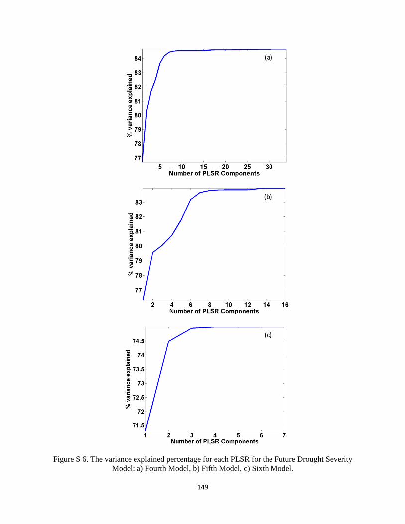
149

Figure S 6. The variance explained percentage for each PLSR for the Future Drought Severity

Model: a) Fourth Model, b) Fifth Model, c) Sixth Model.

(a)

(b)

(c)

150

(a) (b) (c)

Figure S7. The comparison of measured vs. predicted median flow histogram for the Future Drought Severity Model: a) Fourth

Model, b) Fifth Model, c) Sixth Model.

151

Table S1. Selected variables for development of current and future drought severity models.

Category

Variable

Current Drought

Severity Model

Future Drought Severity

Model

Ranking Top Ranked

Variables Time scale based variables

5 10 15 6

months

12

months

18

months

Precipitation 54 Precipitation for the month of

interest

55 Precipitation from one month

prior to the month of interest

62 Precipitation from two months


66 Precipitation from three months


65 Precipitation from four months


59 Precipitation from five months


60 Precipitation from six months


x

63 Precipitation from seven months


x

57 Precipitation from eight months


x

61 Precipitation from nine months


x

64 Precipitation from ten months


x

58 Precipitation from eleven months


x

56 Precipitation from twelve months


x x

152

Table S1. (cont’d)

32 Two months average

precipitation ending with the

month of interest

34 Three months average


month of interest

30 Four months average


month of interest

38 Five months average


month of interest

37 Six months average precipitation

ending with the month of interest

x

35 Seven months average


month of interest

x

33 Eight months average


month of interest

x

29 Nine months average


month of interest

x

28 Ten months average precipitation

ending with the month of interest

x

27 Eleven months average


month of interest

x

25 Twelve months average


month of interest

x x

26 Thirteen months average x x

153



month of interest

Streamflow 1 Average flow rate from one

month prior to the month of

interest

x x x

2 Average flow rate from two

months prior to the month of

interest

x x x

7 Average flow rate from three


interest

x x

11 Average flow rate from four


interest

x

15 Average flow rate from five


interest

x

19 Average flow rate from six


interest

x

20 Average flow rate from seven


interest

x

16 Average flow rate from eight


interest

x

14 Average flow rate from nine


interest

x x

10 Average flow rate from ten


interest

x x x

154


6 Average flow rate from eleven


interest

x x x

4 Average flow rate from twelve


interest

x x x x x

5 Average flow rate from thirteen


interest

x x x x x

9 Average flow rate from fourteen


interest

x x x x

13 Average flow rate from fifteen


interest

x x x

18 Average flow rate from sixteen


interest

x x

22 Average flow rate from

seventeen months prior to the

month of interest

x x

23 Average flow rate from eighteen


interest

x x x

24 Average flow rate from nineteen


interest

x x x

21 Average flow rate from twenty


interest

x x x


one months prior to the month of

x x x

155


interest


two months prior to the month of

interest

x x x x


three months prior to the month

of interest

x x x x x


four months prior to the month

of interest

x x x x x x

Land use 48 Agriculture

44 Percent Agriculture

42 Forest

39 Percent Forest

53 Urban

52 Percent Urban

40 Water

36 Percent Water

Soil 51 Group A

45 Percent Group A

49 Group B

43 Percent Group B

47 Group C

46 Percent Group C

50 Group D

41 Percent Group D

Total

Drainage

Area

31 Total Area

156

Table S2. Confusion matrix for drought zones: Second model

Drought

Zone

Predicted

A B C D Sensitivity

Act

ual

A 3,475,503 96,794 78,135 424,041 85%

B 98,613 86,999 10,552 76,635 32%

C 73,124 9,531 9,780 58,201 6%

D 575,476 89,683 66,157 1,206,881 62%


74%

Table S3. Confusion matrix for drought zones: Third model

Drought

Zone

Predicted

A B C D Sensitivity

Act

ual

A 3,504,238 96,727 75,344 395,412 86%

B 102,626 88,060 10,722 71,336 32%

C 76,366 9,811 9,959 54,460 7%

D 600,376 94,258 69,978 1,172,227 61%


74%

157

Table S4. Confusion matrix for drought zones: Fifth Model

Drought

Zone

Predicted

A B C D Sensitivity

Act

ual

A 3,374,769 82,711 66,849 544,987 83%

B 104,756 81,446 6,460 79,932 30%

C 81,633 6,204 5,906 56,798 4%

D 776,502 82,185 51,095 1,026,000 53%

Precision %78 32% 5% 60% Accuracy =

70%

Table S5. Confusion matrix for drought zones: Sixth Model

Drought

Zone

Predicted

A B C D Sensitivity

Act

ual

A 3,013,851 112,807 93,637 854,265 74%

B 100,057 66,561 6,319 99,903 24%

C 79,508 5,999 6,034 59,135 4%

D 1,109,043 94,052 53,437 683,459 35%


59%

158

Table S6. The first drought model performance using RCP 8.5

(maximum and minimum values are presented in red)

Model Name R2 Log 10 (median flow in LPD*)

RMSE

HadGEM2-ES 0.8861 0.5036

FIO-ESM 0.8798 0.5097

MIROC-ESM-CHEM 0.8780 0.5070

MIROC5 0.8776 0.5060

GISS-E2-H 0.8775 0.5056

MIRCO-ESM 0.8767 0.5108

GISS-E2-R 0.8766 0.5039

HadGEM2-AO 0.8764 0.5104

CESM1-CAM5 0.8755 0.5134

IPSL-CM5A-MR 0.8742 0.5261

GFDL-CM3 0.8741 0.5041

CCSM4 0.8740 0.5192

IPSL-CM5A-LR 0.8734 0.5203

GFDL-ESM2M 0.8715 0.5312

MRI-CGCM3 0.8681 0.5206

GFDL-ESM2G 0.8662 0.5183


159



Model Name R2

Log 10 (median flow in

LPD*)

RMSE

MIROC5 0.8796 0.5101


IPSL-CM5A-MR 0.8765 0.5251

CESM1-CAM5 0.8764 0.5132

HadGEM2-AO 0.8761 0.5246

MIRCO-ESM 0.8753 0.5143

HadGEM2-ES 0.8752 0.5094

FIO-ESM 0.8748 0.5161

GISS-E2-H 0.8739 0.5175

IPSL-CM5A-LR 0.8732 0.5200

GISS-E2-R 0.8726 0.5109

GFDL-CM3 0.8723 0.5066 GFDL-ESM2G 0.8706 0.5206

MRI-CGCM3 0.8690 0.5216

CCSM4 0.8688 0.5284

GFDL-ESM2M 0.8687 0.5313


160



Model Name R2

Log 10 (median flow in

LPD*)

RMSE

HadGEM2-ES 0.8861 0.4940

MIROC5 0.8798 0.5007

GISS-E2-R 0.8780 0.4968

HadGEM2-AO 0.8776 0.5055

CCSM4 0.8775 0.5272

MIRCO-ESM 0.8767 0.5135


FIO-ESM 0.8764 0.5180

CESM1-CAM5 0.8755 0.5161

IPSL-CM5A-MR 0.8742 0.5260

IPSL-CM5A-LR 0.8741 0.5208

GFDL-CM3 0.8740 0.5115

GFDL-ESM2G 0.8734 0.5206

MRI-CGCM3 0.8715 0.5289

GFDL-ESM2M 0.8681 0.5407


161

APPENDIX B: Study Two

Figure S8. Location of temperature, precipitation, and streamflow gauging stations

162

Figure S9. Measured versus modeled histograms of categorical drought and MASH: (a) CMI, (b) CHI, (c) CAI, and (d) MASH

(a) (b)

(c) (d)

163

Figure S10. Drought vulnerable areas based on categorical drought indices in the Saginaw River watershed: (a) meteorological, (b)

hydrological, (c) agricultural, (d) stream health

164

Table S9. Meteorological drought indices, reference, input parameters, procedure, classification, and index value Meteorological Indices (References) Input Parameter Procedure Classification Index value

Palmer Drought Severity Index

(PDSI)

(Palmer, 1965; Jacob et al., 2013;

Ficklin et al., 2015)

Precipitation,

Temperature,

Solar radiation,

Wind speed,

Relative humidity,

Available water

content, Albedo,

Elevation

Measures moisture supply

and demand within a two-

layer bucket-type soil

model using the water

balance equation

Extreme drought

Severe drought

Moderately drought

Mild drought

Incipient drought

Near normal

Incipient wet spell

Slightly wet

Moderately wet

Very wet

Extremely wet

PDSI ≤ -4.0

-3.0 ≤ PDSI < -4.0

-2.0 ≤ PDSI < -3.0

-1.0 ≤ PDSI < -2.0

-0.5 ≤ PDSI < -1.0

0.5 < PDSI < -0.5

0.5 ≤ PDSI < 1.0

1.0 ≤ PDSI < 2.0

2.0 ≤ PDSI < 3.0

3.0 ≤ PDSI < 4.0

PDSI ≥ 4.0

Rainfall Deciles (RD)

(Gibbs and Maher, 1967)

Precipitation Dividing a long-term


distribution into

deciles(10% parts)

Much below normal

Below normal

Near normal

Above normal

Much above normal

Deciles 1-2

Deciles 3-4

Deciles 5-6

Deciles 7-8

Deciles 9-10

Standardized Precipitation Index

(SPI)

(McKee et al., 1993)

Precipitation

Fitting a probability

distribution to a historical

precipitation records, and

transforming it into a

standardized normalized

distribution

Extreme drought

Severe drought

Moderately drought

Near normal

Moderately wet

Very wet

Extremely wet

SPI ≤ -2.0

-2.0 < SPI < -1.5

-1.5 ≤ SPI < -1.0

-1.0 ≤ SPI < 1.0

1.0 ≤ SPI <1.5

1.5 ≤ SPI < 2.0

SPI ≥ 2.0

Reconnaissance Drought Index

(RDI)

(Tsakiris and Vangelis, 2005; Zarch

et al., 2011)

Precipitation,

Potential

evapotranspiration

(PET)

Fitting a probability

distribution to a historical

precipitation/PET records,

and transforming it into a


distribution

Extreme drought

Severe drought

Moderately drought

Near normal

Moderately wet

Very wet

Extremely wet

RDI ≤ -2.0

-2.0 < RDI < -1.5

-1.5 ≤ RDI < -1.0

-1.0 ≤ RDI < 1.0

1.0 ≤ RDI <1.5

1.5 ≤ RDI < 2.0

RDI ≥ 2.0

165

Table S10. Agricultural drought indices, reference, input parameters, procedure, classification, and index value Agricultural Indices (References) Input Parameter Procedure Classification Index Value

Palmer Moisture Anomaly Index

(Z-index)

(Palmer, 1965; Jacob et al., 2013;

Ficklin et al., 2015)

Precipitation,

Temperature, Solar

radiation, Wind

speed, Relative

humidity, Available

water content,

Albedo, Elevation

Measures the soil moisture anomaly for

the current month in the Palmer model

Extreme drought

Severe drought

Moderately drought

Near normal

Moderately moist

Very moist

Extremely moist

Z-index ≤ -2.75

-2.75 < Z-index ≤ -2.0

-2.0 < Z-index < -1.25

-1.25< Z-index < 1.0

1.0 ≤ Z-index < 2.5

2.5 ≤ Z-index < 3.5

Z-index ≥ 3.5

Soil Moisture Deficit Index

(SMDI)

(Narasimhan and Srinivasan,

2005)

Soil Moisture Uses a high-resolution hydrologic model

coupled with a crop growth model to

calculate weekly soil moisture deficit

SMDI𝑗 = SMDI𝑗−1 +𝑆𝐷𝑗

50 − 0.5SMDI𝑗−1

SMDI𝑗 = 0.5SMDI𝑗−1 +𝑆𝐷𝑗

50

SMDIj: SMDI during any week

SDj: weekly soil water deficit (%)

Extreme drought

Severe drought

Moderately drought

Mild drought

Incipient drought

Near normal

Incipient wet spell

Slightly wet

Moderately wet

Very wet

Extremely wet

SMDI ≤ -4.0

-3.0 ≤ SMDI < -4.0

-2.0 ≤ SMDI < -3.0

-1.0 ≤ SMDI < -2.0

-0.5 ≤ SMDI < -1.0

0.5 < SMDI < -0.5

0.5 ≤ SMDI < 1.0

1.0 ≤ SMDI < 2.0

2.0 ≤ SMDI < 3.0

3.0 ≤ SMDI < 4.0

SMDI ≥ 4.0

Evapotranspiration Deficit Index

(ETDI)

(Narasimhan and Srinivasan,

2005)

Potential

evapotranspiration,

actual

evapotranspiration

Uses a high-resolution hydrologic model

coupled with a crop growth model to

calculate weekly evapotranspiration

deficit

𝐸𝑇𝐷𝐼𝑗 = 0.5𝐸𝑇𝐷𝐼𝑗−1 +𝑊𝑆𝐴𝑗

50

ETDIj: ETDI during any week

WSAj: weekly water stress anomaly

Extreme drought

Severe drought

Moderately drought

Mild drought

Incipient drought

Near normal

Incipient wet spell

Slightly wet

Moderately wet

Very wet

Extremely wet

ETDI ≤ -4.0

-3.0 ≤ ETDI < -4.0

-2.0 ≤ ETDI < -3.0

-1.0 ≤ ETDI < -2.0

-0.5 ≤ ETDI < -1.0

0.5 < ETDI < -0.5

0.5 ≤ ETDI < 1.0

1.0 ≤ ETDI < 2.0

2.0 ≤ ETDI < 3.0

3.0 ≤ ETDI < 4.0

ETDI ≥ 4.0

166


Soil Water Deficit Index (SWDI)

(Martinez-Fernandez et al., 2015)

Soil moisture,

Available water

content, Field

capacity, Wilting

point

Uses soil water observations to calculate

soil water deficit

𝑆𝑊𝐷𝐼 = (𝜃−𝜃𝐹𝐶

𝜃𝐴𝑊𝐶) 10

θ: soil moisture content

θFC: field capacity

θAWC: available water content which is

the difference between θFC and θWP

No drought

Mild

Moderate

Severe

Extreme

SWDI ≥ 0

-2 < SWDI < 0

-5 < SWDI ≤ -2

-10 < SWDI ≤ -5

SWDI ≤ -10

167

Table S11. Hydrological drought indices, reference, input parameters, procedure, classification, and index value Hydrological Indices

(References)

Input Parameter Procedure Classification Index value

Palmer Hydrological

Drought Index (PHDI)

(Palmer, 1965; Jacob et al.,

2013; Ficklin et al., 2015)

Precipitation,

Temperature,

Solar radiation,

Wind speed,

Relative humidity,

Available water

content, Albedo,

Elevation

Measures moisture

supply and demand

within a two-layer

bucket-type soil model

using the water balance

equation

Extreme drought

Severe drought

Moderately drought

Near normal

Moderately moist

Very moist

Extremely moist

PHDI ≤ -4.0

-3.0 ≤ PHDI < -4.0

-2.0 ≤ PHDI < -3.0

-2.0 < PHDI < 2.0

2.0 ≤ PHDI < 3.0

3.0 ≤ PHDI < 4.0

PHDI ≥ 4.0

Flow Duration Curve (FDC)

(Tallaksen and van Lanen,

2004)

Streamflow

Measuring the

cumulative probability

of the streamflow for a

specific time period

High flows

Moist conditions

Mid-range flows

Dry condition

Low flows

0-10%

10-40%

40-60%

60-90%

90-100%

Standardized Runoff Index

(SRI)

(Shukla and Wood, 2008)

Runoff Fitting a log normal

distribution to a

historical runoff

records, and

transforming it into a


distribution

Extremely wet

Severely wet

Moderately wet

Near normal

Moderately drought

Severe drought

Extreme drought

SRI ≥ 2.0

1.5 ≤ SRI < 2.0

1.0 ≤ SRI < 1.5

-1.0 ≤ SRI < 1

-1.5 ≤ SRI < -1.0

-2.0 < SRI ≤ 1.5

SRI ≤ -2.0

Water Balance Derived

Drought Index (WBI)

(Vasiliades et al., 2011)

Runoff Normalizing historical

runoff records using

Box-Cox

transformation, and

standardizing it into a

standard normal

distribution

Extremely wet

Severely wet

Moderately wet

Near normal

Moderately drought

Severe drought

Extreme drought

WBI ≥ 2.0

1.5 ≤ WBI < 2.0

1.0 ≤ WBI < 1.5

-1.0 ≤ WBI < 1

-1.5 ≤ WBI < -1.0

-2.0 < WBI ≤ 1.5

WBI ≤ -2.0

168

Table S12. Stream health drought index, reference, input parameters, procedure, classification,

and index value Stream

Health Index

(Reference)

Input

Parameter

Procedure Classification Index value*

Stream

Health Index

(SHI)

(Esfahanian

et al., 2016)

Streamflow Calculating

monthly

median

flowrate and

Index flow

values for

each stream

Extreme

drought

Cold Streams: SHI≥0.8×IF

Cold Small Rivers: SHI≥0.79×IF

Cold Transitional Streams: SHI≥0.96×IF

Cold Transitional Small Rivers: SHI≥0.98×IF

Cold Transitional Large Rivers: SHI≥0.97×IF

Cool Transitional Streams: SHI≥0.75×IF

Cool Transitional Small Rivers: SHI≥0.75×IF

Cool Transitional Large Rivers: SHI≥0.75×IF

Warm Streams: SHI≥0.76×IF

Warm Small Rivers: SHI≥0.83×IF

Warm Large Rivers: SHI≥0.78×IF

Severe

drought

Cold Streams: 0.8×IF<SHI≤0.86×IF

Cold Small Rivers: 0.79×IF<SHI≤0.895×IF

Cold Transitional Streams: None

Cold Transitional Small Rivers: None

Cold Transitional Large Rivers: None

Cool Transitional Streams:

0.75×IF<SHI≤0.85×IF

Cool Transitional Small Rivers:

0.75×IF<SHI≤0.81×IF

Cool Transitional Large Rivers:

0.75×IF<SHI≤0.81×IF

Warm Streams: 0.76×IF<SHI≤0.82×IF

Warm Small Rivers: 0.83×IF<SHI≤0.87×IF

Warm Large Rivers: 0.78×IF<SHI≤0.84×IF

Moderate

drought

Cold Streams: None

Cold Small Rivers: None

Cold Transitional Streams: SHI>96%×IF

Cold Transitional Small Rivers: SHI>98% ×IF

Cold Transitional Large Rivers: SHI>97% ×IF

Cool Transitional Streams:

0.85×IF<SHI≤0.94×IF

Cool Transitional Small Rivers:

0.81×IF<SHI≤0.85×IF

Cool Transitional Large Rivers:

0.81×IF<SHI≤0.86×IF

Warm Streams: 0.82×IF<SHI≤0.90×IF

Warm Small Rivers: 0.87×IF<SHI≤0.92×IF

Warm Large Rivers: 0.84×IF<SHI≤0.90×IF

Initial

Drought

Cold Streams: SHI>0.86×IF

Cold Small Rivers: SHI>0.895×IF

Cold Transitional Streams: None

Cold Transitional Small Rivers: None

Cold Transitional Large Rivers: None

Cool Transitional Streams: SHI>0.94×IF

Cool Transitional Small Rivers: SHI>0.85×IF

Cool Transitional Large Rivers: SHI>0.86×IF

Warm Streams: SHI>0.9×IF

Warm Small Rivers: SHI>0.92×IF

Warm Large Rivers: SHI>0.9×IF

169

Table S13. Input parameters Input Parameters Drought Indices Source/description

Meteorological Drought Agricultural Drought Hydrological Drought Stream

Health

Drought

PDSI RD SPI RDI Z-index SMDI ETDI SWDI PHDI FDC SRI WBI SHI

Precipitation (mm) x x x x x x Precipitation stations

of National Climatic

Data Center (NCDC)

http://www.ncdc.noa

a.gov/data-

access/land-based-

station-data

Total 3-month

precipitation (mm)

x Total precipitation

for the preceding

three months

Precipitation

percentile

x Historical ranking of

total 3-month

precipitation for each

month

Gamma-

precipitation

x Fitted gamma

probability density

function for the


Potential

evapotranspiration

(mm)

x x Hydrological model

(soil and water tool

assessment (SWAT))

Evapotranspiration

(mm)

x Hydrological model

(soil and water tool

assessment (SWAT))

P-PET ratio x Ratio of monthly

precipitation to

monthly potential

evapotranspiration

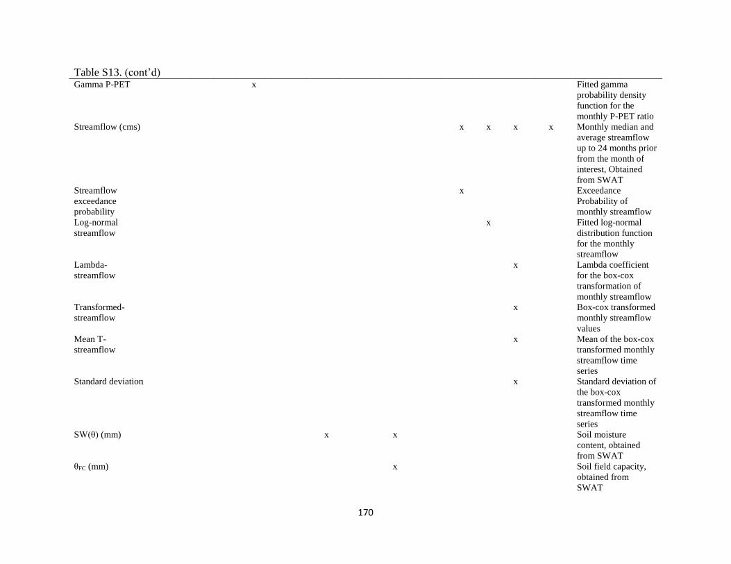
170


Gamma P-PET x Fitted gamma

probability density

function for the

monthly P-PET ratio

Streamflow (cms) x x x x Monthly median and

average streamflow

up to 24 months prior

from the month of

interest, Obtained

from SWAT

Streamflow

exceedance

probability

x Exceedance

Probability of

monthly streamflow

Log-normal

streamflow

x Fitted log-normal

distribution function

for the monthly

streamflow

Lambda-

streamflow

x Lambda coefficient

for the box-cox

transformation of

monthly streamflow

Transformed-

streamflow

x Box-cox transformed

monthly streamflow

values

Mean T-

streamflow

x Mean of the box-cox

transformed monthly

streamflow time

series

Standard deviation x Standard deviation of

the box-cox

transformed monthly

streamflow time

series

SW(θ) (mm) x x Soil moisture

content, obtained

from SWAT

θFC (mm) x Soil field capacity,

obtained from

SWAT

171


θAWC (mm) x Available water

content, Obtained

from SWAT

Palmer potential

evapotranspiration

(mm)

x x x Obtained from

Ficklin et al.(2015)

Matlab code

(modified version of

Jacob et al.,2013)

Palmer percentage

probability

x x x Obtained from


Matlab code


Jacob et al.,2013)

Palmer_X1 x x x Severity index for a

wet spell that is

being established

Obtained from


Matlab code


Jacob et al.,2013).

Severity index for a

wet spell that is

becoming

established.


dry spell that is being

established

Obtained from


Matlab code


Jacob et al.,2013).

Severity index for a

drought that is

becoming

established.

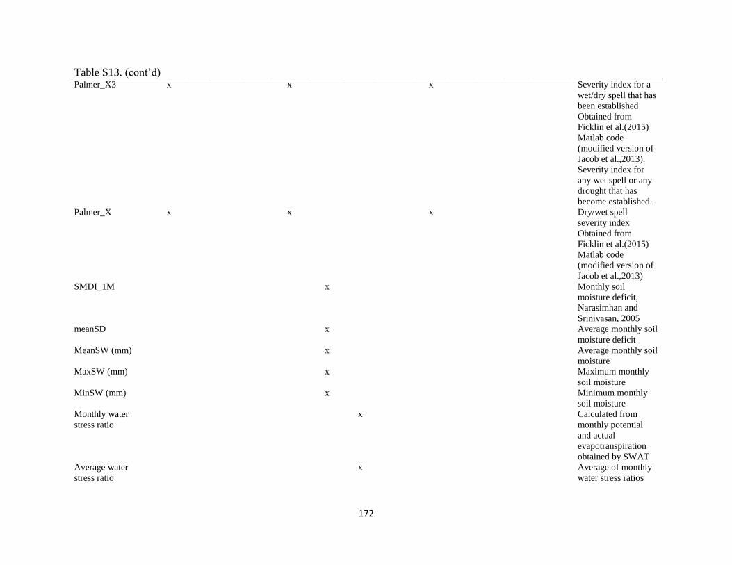
172



wet/dry spell that has

been established

Obtained from


Matlab code


Jacob et al.,2013).

Severity index for

any wet spell or any

drought that has

become established.

Palmer_X x x x Dry/wet spell

severity index

Obtained from


Matlab code


Jacob et al.,2013)

SMDI_1M x Monthly soil

moisture deficit,

Narasimhan and

Srinivasan, 2005

meanSD x Average monthly soil

moisture deficit

MeanSW (mm) x Average monthly soil

moisture

MaxSW (mm) x Maximum monthly

soil moisture

MinSW (mm) x Minimum monthly

soil moisture

Monthly water

stress ratio

x Calculated from

monthly potential

and actual

evapotranspiration

obtained by SWAT

Average water

stress ratio

x Average of monthly

water stress ratios

173


Maximum water

stress ratio

x Maximum monthly

water stress ratios

Minimum water

stress ratio

x Minimum monthly

water stress ratios

Monthly water

stress anomaly (%)

x Monthly water stress

anomaly

ETDI_1M Monthly

evapotranspiration

deficit

Temperature (°C) x x x Minimum and

maximum

temperature values,

obtained from NCDC

temperature stations

http://www.ncdc.noa

a.gov/data-

access/land-based-

station-data

Solar Radiation

(W/m2)

x x x Abatzolgou (2013),

http://metdata.northw

estknowledge.net/

Wind Speed (m/s) x x x Abatzolgou (2013),


estknowledge.net/

Relative Humidity

(%)

x x x Abatzolgou (2013),


estknowledge.net/

Available water

content (mm)

x x x x Natural Resources

Conservation Service

(NRCS) Soil Survey

Geographic

(SSURGO) database

https://www.arcgis.c

om/home/item.html?i

d=a23eb436f6ec4ad6

982000dbaddea5ea

174


Albedo x x x Average annual

values from

Barkstrom (1984)

Elevation (m) x x x National Elevation

Dataset of the US

Geological Survey

(USGS) with a

spatial resolution of

30 m

http://nationalmap.go

v/elevation.html

175

Table S14. Mean difference (numbers in black) and standard deviation (numbers in red) among drought indices

Drought

Index

Meteorological

Hydrological

Agricultural

Stream

Health

Overall

PDSI

RD

SPI

RDI

CMI

PHDI

FDC

SRI

WBI

CHI

Z-Index

SMDI

ETDI

SWDI

CAI

CSHI MASH

PDSI

0 0

RD

-1.32

45.67

0

0

SPI

-0.04

38.93

1.29

58.97

0

0

RDI

-0.07 38.29

1.26 58.63

-0.03 10.72

0 0

CMI -0.18

28.81

1.14

50.34

-0.15

14.96

-0.12

14.45

0

0

PHDI

-1.52

22.93

-0.2

46.75

-1.48

45.57

-1.45

44.86

-1.34

37.04

0

0

FDC

-0.08 44.54

1.24 53.14

-0.05 49.86

-0.02 51.11

0.1 45.5

1.44 47.54

0 0

SRI

-0.14

32.43

1.18

44.22

-0.10

32.68

-0.07

33.71

0.04

27.81

1.38

35.91

-0.06

28.69

0

0

WBI

0.45

32.64

1.78

44.26

-0.49

32.92

0.52

33.80

0.64

28.07

1.97

35.9

0.54

30.11

0.59

8.81

0

0

CHI

0.03 32.69

1.36 44.52

0.071 35.16

0.1 36.17

0.22 29.98

1.56 36.34

0.12 24.26

0.17 9.35

-0.42 10.57

0 0

Z-Index

0.77

30.08

2.09

55

0.8

17.84

0.84

17.85

0.95

15.29

2.29

38.40

0.85

45.81

0.91

30.33

0.32

30.83

0.73

32.12

0

0

SMDI

-4.79

36.68

-3.47

46.42

-4.76

46.50

-4.73

45.65

-4.61

39.52

-3.27

39.65

-4.71

49

-4.65

37.94

-5.25

37.87

-4.83

38.49

-5.56

40.96

0

0

ETDI

-2.76 40.71

-1.44 52.78

-2.73 35.52

-2.7 35.33

-2.58 32.40

-1.24 44.85

-2.68 52.73

-2.62 35.88

-3.22 35.32

-2.8 37.86

-3.53 34.53

2.03 39.17

0 0

SWDI

62.33

41.23

63.65

51.60

62.36

35.94

62.39

35.62

62.51

33.14

63.85

43.54

62.41

56.18

62.47

34.68

61.87

33.87

62.29

38.04

61.56

36.98

67.12

44.13

65.09

34.88

0

0

CAI

4.51

31.27

5.83

48.82

4.54

30.66

4.57

30.23

4.69

25.27

6.03

37.05

4.59

45.49

4.64

30.51

4.05

30.52

4.47

31.83

3.74

24.99

9.3

27.38

7.27

25.12

-57.82

36.50

0

0

CSHI -36.86 74.54

-35.54 78.74

-36.83 80.86

-36.8 81.55

-36.68 77.27

-35.34 75.44

-36.78 66.81

-36.72 69.62

-37.32 69.62

-36.9 68.13

-37.63 77.64

-32.07 75.53

-34.1 79.55

-99.19 82.87

-41.37 74.98

0 0

MASH

-8.13

30.56

-6.8

45.84

-8.09

32.57

-8.06

33.11

-7.94

26.52

-6.61

35.57

-8.04

33.53

-7.99

22.04

-8.58

22.26

-8.16

21.55

-8.9

28.38

-3.33

34.65

-5.36

34.45

-70.45

38.89

-12.63

25.38

28.74

53.71

0

0

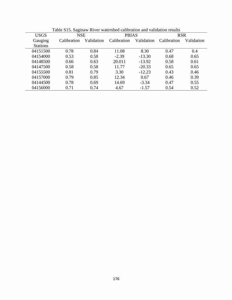
176

Table S15. Saginaw River watershed calibration and validation results

USGS

Gauging

Stations

NSE PBIAS RSR

Calibration Validation Calibration Validation Calibration Validation

04151500 0.78 0.84 11.08 8.30 0.47 0.4

04154000 0.53 0.58 -2.39 -13.30 0.68 0.65

04148500 0.66 0.63 20.011 -13.92 0.58 0.61

04147500 0.58 0.58 11.77 -20.33 0.65 0.65

04155500 0.81 0.79 3.30 -12.23 0.43 0.46

04157000 0.79 0.85 12.34 0.67 0.46 0.39

04144500 0.78 0.69 14.69 -3.34 0.47 0.55

04156000 0.71 0.74 4.67 -1.57 0.54 0.52

177

Table S16. Transformed drought categories *

Drought index

General associated ranges

(normalized associated ranges)

Initial drought

(0 to <25)

Moderate drought

(25 to <50)

Severe drought

(50 to <75)

Extreme drought

(75 to 100)

PDSI -1.0 < PDSI < 0 -3.0 < PDSI ≤ -1.0 -4.0 < PDSI ≤ -3.0 PDSI ≤ -4.0

RD 0.3 < Decile < 0.5 0.2< Decile ≤ 0.3 0.1 <Decile ≤ 0.2 Decile ≤ 0.1

SPI -1.0 < SPI < 0 -1.5 < SPI ≤ -1.0 -2< SPI ≤ -1.5 SPI ≤ -2.0

RDI -1.0 < RDI < 0 -1.5 < RDI ≤ -1.0 -2< RDI ≤ -1.5 RDI ≤ -2.0

Z-index -1.0 < Z < 0 -3.0 <Z ≤ -1.0 -4.0 < Z ≤ -3.0 Z ≤ -4.0

SMDI -1.0< SMDI < 0 -3.0 < SMDI ≤ -1.0 -4.0<SMDI ≤ -3.0 SMDI ≤ -4.0

ETDI -1.0< ETDI < 0 -3.0 < ETDI ≤ -1.0 -4.0< ETDI ≤ -3.0 ETDI ≤ -4.0

SWDI -2.0< SWDI < 0 -5.0 < SWDI ≤ -2.0 -10.0< SWDI ≤ -5.0 SWDI ≤ -10.0

PHDI -1.0< PHDI < 0 -3.0 < PHDI ≤ -1.0 -4.0< PHDI ≤ -3.0 PHDI ≤ -4.0

FDC 0.5 < FDC < 0.6 0.6 ≤ FDC < 0.75 0.75 ≤ FDC < 0.9 FDC ≥ 0.9

SRI -1.0 < SRI < 0 -1.5 < SRI ≤ -1.0 -2.0 < SRI ≤-1.5 SRI ≤ -2.0

WBI -1.0 < WBI < 0 -1.5 < WBI ≤ -1.0 -2.0 < WBI ≤ -1.5 WBI ≤ -2.0

CSHI (Cool-Stream) 0.94×IF<MMF≤1×IF 0.85×IF<MMF≤0.94×IF 0.75×IF<MMF≤0.85×IF 0×IF<MMF≤0.75×IF

CSHI Cool-Small Rivers 0.85×IF<MMF≤1×IF 0.81×IF<MMF≤0.85×IF 0.75×IF<MMF≤0.81×IF 0×IF<MMF≤0.75×IF

CSHI Cool-Large Rivers 0.86×IF<MMF≤1×IF 0.81×IF<MMF≤0.86×IF 0.75×IF<MMF≤0.81×IF 0×IF<MMF≤0.75×IF

CSHI Warm-Stream 0.9×IF<MMF≤1×IF 0.81×IF<MMF≤0.9×IF 0.76×IF<MMF≤0.81×IF 0×IF<MMF≤0.76×IF

CSHI Warm-Small Rivers 0.92×IF<MMF≤1×IF 0.87×IF<MMF≤0.92×IF 0.83×IF<MMF≤0.87×IF 0×IF<MMF≤0.83×IF

CSHI Warm-Large Rivers 0.9×IF<MMF≤1×IF 0.84×IF<MMF≤0.9×IF 0.78×IF<MMF≤0.84×IF 0×IF<MMF≤0.78×IF

* CSHI: Categorical stream health drought index; IF: Index flow; MMF: Monthly median flow

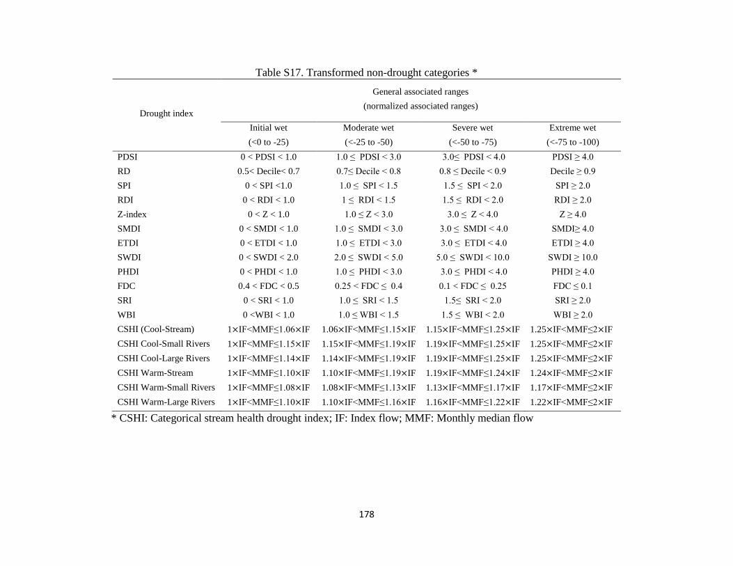
178

Table S17. Transformed non-drought categories *

Drought index

General associated ranges

(normalized associated ranges)

Initial wet

(<0 to -25)

Moderate wet

(<-25 to -50)

Severe wet

(<-50 to -75)

Extreme wet

(<-75 to -100)

PDSI 0 < PDSI < 1.0 1.0 ≤ PDSI < 3.0 3.0≤ PDSI < 4.0 PDSI ≥ 4.0

RD 0.5< Decile< 0.7 0.7≤ Decile < 0.8 0.8 ≤ Decile < 0.9 Decile ≥ 0.9

SPI 0 < SPI <1.0 1.0 ≤ SPI < 1.5 1.5 ≤ SPI < 2.0 SPI ≥ 2.0

RDI 0 < RDI < 1.0 1 ≤ RDI < 1.5 1.5 ≤ RDI < 2.0 RDI ≥ 2.0

Z-index 0 < Z < 1.0 1.0 ≤ Z < 3.0 3.0 ≤ Z < 4.0 Z ≥ 4.0

SMDI 0 < SMDI < 1.0 1.0 ≤ SMDI < 3.0 3.0 ≤ SMDI < 4.0 SMDI≥ 4.0

ETDI 0 < ETDI < 1.0 1.0 ≤ ETDI < 3.0 3.0 ≤ ETDI < 4.0 ETDI ≥ 4.0

SWDI 0 < SWDI < 2.0 2.0 ≤ SWDI < 5.0 5.0 ≤ SWDI < 10.0 SWDI ≥ 10.0

PHDI 0 < PHDI < 1.0 1.0 ≤ PHDI < 3.0 3.0 ≤ PHDI < 4.0 PHDI ≥ 4.0

FDC 0.4 < FDC < 0.5 0.25 < FDC ≤ 0.4 0.1 < FDC ≤ 0.25 FDC ≤ 0.1

SRI 0 < SRI < 1.0 1.0 ≤ SRI < 1.5 1.5≤ SRI < 2.0 SRI ≥ 2.0

WBI 0 <WBI < 1.0 1.0 ≤ WBI < 1.5 1.5 ≤ WBI < 2.0 WBI ≥ 2.0

CSHI (Cool-Stream) 1×IF<MMF≤1.06×IF 1.06×IF<MMF≤1.15×IF 1.15×IF<MMF≤1.25×IF 1.25×IF<MMF≤2×IF

CSHI Cool-Small Rivers 1×IF<MMF≤1.15×IF 1.15×IF<MMF≤1.19×IF 1.19×IF<MMF≤1.25×IF 1.25×IF<MMF≤2×IF

CSHI Cool-Large Rivers 1×IF<MMF≤1.14×IF 1.14×IF<MMF≤1.19×IF 1.19×IF<MMF≤1.25×IF 1.25×IF<MMF≤2×IF

CSHI Warm-Stream 1×IF<MMF≤1.10×IF 1.10×IF<MMF≤1.19×IF 1.19×IF<MMF≤1.24×IF 1.24×IF<MMF≤2×IF

CSHI Warm-Small Rivers 1×IF<MMF≤1.08×IF 1.08×IF<MMF≤1.13×IF 1.13×IF<MMF≤1.17×IF 1.17×IF<MMF≤2×IF

CSHI Warm-Large Rivers 1×IF<MMF≤1.10×IF 1.10×IF<MMF≤1.16×IF 1.16×IF<MMF≤1.22×IF 1.22×IF<MMF≤2×IF

* CSHI: Categorical stream health drought index; IF: Index flow; MMF: Monthly median flow

179

REFERENCES

180

REFERENCES

Abatzoglou, J.T., 2013. Development of gridded surface meteorological data for ecological

applications and modelling. International Journal of Climatology 33, 121–131.

Adam, J.C., Hamlet, A.F., Lettenmaier, D.P., 2009. Implications of global climate change for

snowmelt hydrology in the twenty-first century. Hydrological Processes 23, 962–972.

Alegria, M.H., Watkin Jr., D.W., 2007. Annual and warm season drought intensity– duration–

frequency analysis for Sonora, Mexico. Journal of Climate 20, 1897–1909.

Alley, W.M., 1984. The Palmer drought severity index: limitations and assumptions. Journal of

climate and applied meteorology 23, 1100–1109.

American Meteorological Society, 1997. Meteorological drought-Policy statement. Bulletin of

the American Meteorological Society 78, 847-849.

American Meteorological Society, 2004. Statement on meteorological drought. Bulletin of the

American Meteorological Society 85, 771–773.

Angradi, T.R., Pearson, M.S., Jicha, T.M., Taylor, D.L., Bolgrien, D.W., Moffett, M.F.,

Blocksom, K.A., Hill, B.H., 2009. Using stressor gradients to determine reference expectations

for great river fish assemblages. Ecological Indicators 9, 748–764.

Anyamba, A. C., Tucker, C. J., and Eastman, J. R. 2001. NDVI anomaly patterns over Africa

during the 1997/98 ENSO warm event. International Journal of Remote Sensing, 22 (10): 1847–

1859.

Aruna, S., Rajagopalan, S.P., Nandakishore, L.V., 2011. Knowledge based analysis of various

statistical tools in detecting breast cancer. Computer Science & Information Technology 2, 37–

45.

Bacanli, U.G., Firat, M., Dikbas, F., 2009. Adaptive neuro-fuzzy inference system for drought

forecasting. Stochastic Environmental Research and Risk Assessment 23, 1143–1154.

Balint, Z., Mutua, F.M., Muchiri, P., 2011. Drought monitoring with the combined drought

index. FAO-SWALIM: Nairobi, Kenya 3–25.

Barbour, M.T., Gerritsen, J., Griffith, G.E., Frydenborg, R., McCarron, E., White, J.S., Bastian,

M.L., 1996. A framework for biological criteria for Florida streams using benthic

macroinvertebrates. Journal of the North American Benthological Society 185–211.

181

Barbour, M.T., Gerritsen, J., Snyder, B.D., Stribling, J.B., 1999. Rapid Bioassessment Protocols

for use in Streams and Wadeable Rivers: Periphyton, Benthic Macroinvertebrates and Fish,

second ed. (EPA 841-B-99-002. U.S.).

Barkstrom, B.R., 1984. The earth radiation budget experiment (ERBE). Bulletin of the American

Meteorological Society 65, 1170–1185.

Barlow, M., Cullen, H., Lyon, B., 2002. Drought in central and southwest Asia: La Niña, the

warm pool, and Indian Ocean precipitation. Journal of Climate 15, 697–700.

Bates, B.C., Kundzewicz, Z.W., Wu, S., Palutikof, J.P. (Eds.), 2008. Climate Change and Water.

Technical Paper, International Panel on Climate Change (IPCC) Secretariat, Geneva.

Bayarjargal, Y., Karnieli, A., Bayasgalan, M., Khudulmur, S., Gandush, C., Tucker, C.J., 2006.

A comparative study of NOAA–AVHRR derived drought indices using change vector analysis.

Remote Sensing of Environment 105, 9–22.

Bhalme, H.N., Mooley, D.A., 1980. Large-scale droughts/floods and monsoon circulation.

Monthly Weather Review 108, 1197–1211.

Blenkinsop, S., Fowler, H.J., 2007. Changes in European drought characteristics projected by the

PRUDENCE regional climate models. International Journal of Climatology 27, 1595–1610.

Boken, V.K., Cracknell, A.P., Heathcote, R.L., 2005. Monitoring and predicting agricultural

drought: a global study. Oxford University Press.

Bond, N.R., Lake, P.S., Arthington, A.H., 2008. The impacts of drought on freshwater

ecosystems: an Australian perspective. Hydrobiologia 600, 3–16.

Box, G.E.P., Jenkins, G.M., Reinsel, G.C., 1994. Time Series Analysis-, ‘Forecasting and

Control’. Prentice-Hall, Englewood Cliffs, NJ.

Boyer, C., Chaumont, D., Chartier, I., Roy, A.G., 2010. Impact of climate change on the

hydrology of St. Lawrence tributaries. Journal of hydrology 384, 65–83.

Brian D.Wardlow, Martha C. Anderson, James P. Verdin, 2012. Remote Sensing of

Drought.Taylor & Francis Group.

Britton, J.R., Cucherousset, J., Davies, G.D., Godard, M.J., Copp, G.H., 2010. Non-native fishies

and climate change: predicting species responses to warming temperatures in a temperature

region. Freshwater Biology 55, 1130-1141.

Bravar, L., Kavvas, M.L., 1991. On the physics of droughts. I. A conceptual framework. Journal

of Hydrology 129, 281–297.

182

Brown, J.F., Wardlow, B.D., Tadesse, T., Hayes, M.J., Reed, B.C., 2008. The Vegetation

Drought Response Index (VegDRI): A new integrated approach for monitoring drought stress in

vegetation. GIScience & Remote Sensing 45, 16–46.

Bunn, S.E., Arthington, A.H., 2002. Basic principles and ecological consequences of altered

flow regimes for aquatic biodiversity. Environmental management 30, 492–507.

Byun, H.-R., Wilhite, D.A., 1999. Objective quantification of drought severity and duration.

Journal of Climate 12, 2747–2756.

Cancelliere, A., Salas, J.D., 2004. Drought length properties for periodic-stochastic hydrologic

data. Water Resources Research 40.

Cancelliere, A., Di Mauro, G., Bonaccorso, B., Rossi, G., 2007. Drought forecasting using the

standardized precipitation index. Water resources management 21, 801–819.

Cancelliere, A., Salas, J.D., 2010. Drought probabilities and return period for annual streamflows

series. Journal of Hydrology 391, 77–89.

Carlisle, D.M., Meador, M.R., Short, T.M., Tate, C.M., Gurtz, M.E., Bryant, W.L., Falcone, J.A.,

Woodside, M.D., 2013. The quality of our Nation’s waters–ecological health in the Nation’s

streams, 1993-2005. US Geological Survey.

Carrascal, L.M., Galván, I., Gordo, O., 2009. Partial least squares regression as an alternative to

current regression methods used in ecology. Oikos 118, 681–690.

Cebrián, A.C., Abaurrea, J., 2006. Drought analysis based on a marked cluster Poisson model.

Journal of Hydrometeorology 7, 713–723.

Chen, D., Huang, J., Jackson, T.J., 2005. Vegetation water content estimation for corn and

soybeans using spectral indices derived from MODIS near-and short-wave infrared bands.

Remote Sensing of Environment 98, 225–236.

Chen, Lu, Singh, Vijay P., and Guo, Shenglian, 2011. Drought Analysis Based on Copulas.

Symposium on Data-Driven Approaches to Droughts.Paper 45.

Chen, L., Singh, V.P., Shenglian, G., Hao, Z., Li, T., 2011. Flood coincidence risk analysis using

multivariate copula functions. Journal of Hydrologic Engineering 17, 742–755.

Chowdhary, H., Singh, V.P., 2010. Reducing uncertainty in estimates of frequency distribution

parameters using composite likelihood approach and copula-based bivariate distributions. Water

Resources Research 46.

Combe, M., Vilà-Guerau de Arellano, J., Ouwersloot, H.G., Jacobs, C.M.J., Peters, W., 2015.

Two perspectives on the coupled carbon, water and energy exchange in the planetary boundary

layer. Biogeosciences 12, 103–123.

183

Compin, A., Céréghino, R., 2003. Sensitivity of aquatic insect species richness to disturbance in

the Adour–Garonne stream system (France). Ecological Indicators 3, 135–142.

Cook, E.R., Seager, R., Cane, M.A., Stahle, D.W., 2007. North American drought:

reconstructions, causes, and consequences. Earth-Science Reviews 81, 93–134.

Couceiro, S.R.M., Hamada, N., Forsberg, B.R., Pimentel, T.P., Luz, S.L.B., 2012. A

macroinvertebrate multimetric index to evaluate the biological condition of streams in the

Central Amazon region of Brazil. Ecological Indicators 18, 118–125.

Cronshey, R., 1986. Urban hydrology for small watersheds. US Dept. of Agriculture, Soil

Conservation Service, Engineering Division.

Dabrowska-Zielinska, K., Kogan, F., Ciolkosz, A., Gruszczynska, M., Kowalik, W., 2002.

Modelling of crop growth conditions and crop yield in Poland using AVHRR-based indices.

International Journal of Remote Sensing 23, 1109–1123.

Dai, A., Trenberth, K.E., Qian, T., 2004. A global dataset of Palmer Drought Severity Index for

1870-2002: Relationship with soil moisture and effects of surface warming. Journal of

Hydrometeorology 5, 1117–1130.

Dai, A., 2011. Drought under global warming: a review. Wiley Interdisciplinary Reviews:

Climate Change 2, 45–65.

Davies, S.P., Jackson, S.K., 2006. The biological condition gradient: a descriptive model for

interpreting change in aquatic ecosystems. Ecological Applications 16, 1251–1266.

Dawson, C.W., Wilby, R., 1998. An artificial neural network approach to rainfall-runoff

modelling. Hydrological Sciences Journal 43, 47–66.

De Jong, S., 1993. SIMPLS: an alternative approach to partial least squares regression.

Chemometrics and intelligent laboratory systems 18, 251–263.

Delbart, N., Kergoat, L., Le Toan, T., Lhermitte, J., Picard, G., 2005. Determination of

phenological dates in boreal regions using normalized difference water index. Remote Sensing of

Environment 97, 26–38.

Dessu, S.B., Melesse, A.M., 2013. Impact and uncertainties of climate change on the hydrology

of the Mara River basin, Kenya/Tanzania. Hydrological Processes 27, 2973–2986.

Diaz, H.F., 1983. Some aspects of major dry and wet periods in the contiguous United States,

1895–1981. Journal of Climate and Applied Meteorology. 22, 3–16.

http://journalseek.net/cgi-bin/journalseek/journalsearch.cgi?field=issn&query=0733-3021

184

Diaz-Nieto, J., Wilby, R.L., 2005. A comparison of statistical downscaling and climate change

factor methods: impacts on low flows in the River Thames, United Kingdom. Climatic Change

69, 245–268.

Durdu, Ö.F., 2010. Application of linear stochastic models for drought forecasting in the Büyük

Menderes river basin, western Turkey. Stochastic Environmental Research and Risk Assessment

24, 1145–1162.

Edwards, D.C., McKee, T.B., 1997. Characteristics of 20th Century Drought in the United States

at Multiple Scales. Atmospheric Science Paper No. 634, May 1–30.

Einheuser, M.D., Nejadhashemi, A.P., Wang, L., Sowa, S.P., Woznicki, S.A., 2013. Linking

biological integrity and watershed models to assess the impacts of historical land use and climate

changes on stream health. Environmental management 51, 1147–1163.

El-Sebakhy, E.A., Raharja, I., Adem, S., Khaeruzzaman, Y., 2007. Neuro-fuzzy systems

modeling tools for bacterial growth, in: IEEE/ACS International Conference on Computer

Systems and Applications, pp. 374–380.

Elsner, M.M., Cuo, L., Voisin, N., Deems, J.S., Hamlet, A.F., Vano, J.A., Mickelson, K.E., Lee,

S.-Y., Lettenmaier, D.P., 2010. Implications of 21st century climate change for the hydrology of

Washington State. Climatic Change 102, 225–260.

Environment Canada, 2004. Threats to Water Availability in Canada. National Water Research

Institute, Burlington, Ontario. NWRI Scientific Assessment Report Series No. 3 and ACSD

Science Assessment Series No. 1. p. 128.

Esfahanian, E., Nejadhashemi, A. P., Abouali, M., Daneshvar, F., Ameli, A., Herman, M., Tang,

Y.,2016. Defining Drought in the context of Stream Health. Ecological Engineering 94, 668-681.

European Communities, 2012. Report on the review of the European water scarcity and drought

policy. Brussels, 14.11.2012.

Fernández, B., Salas, J.D., 1999a. Return period and risk of hydrologic events. I: mathematical

formulation. Journal of Hydrologic Engineering 4, 297–307.

Fernández, B., Salas, J.D., 1999b. Return period and risk of hydrologic events. II:Applications.

Journal of Hydrologic Engineering 4, 308–316.

Feyen, L., Dankers, R., 2009. Impact of global warming on streamflow drought in Europe. J.

Geophys. Res. 114, D17116.

Ficklin, D.L., Letsinger, S.L., Gholizadeh, H., Maxwell, J.T., 2015. Incorporation of the

Penman–Monteith potential evapotranspiration method into a Palmer Drought Severity Index

Tool. Computers & Geosciences 85, 136–141.

185

Fleig, A.K., Tallaksen, L.M., Hisdal, H., Stahl, K., Hannah, D.M., 2010. Inter-comparison of

weather and circulation type classifications for hydrological drought development. Physics and

Chemistry of the Earth, Parts A/B/C 35, 507–515.

Fleig, A.K., Tallaksen, L.M., Hisdal, H., Hannah, D.M., 2011. Regional hydrological drought in

north-western Europe: linking a new Regional Drought Area Index with weather types.

Hydrological Processes 25, 1163–1179.

Flinders, C.A., Horwitz, R.J., Belton, T., 2008. Relationship of fish and macroinvertebrate

communities in the mid-Atlantic uplands: Implications for integrated assessments. Ecological

Indicators 8, 588-598.

Food and Agriculture Organization (FAO). (1983). Guidelines: Land evaluation for Rainfed

Agriculture. Rome: FAO Soils Bulletin 52.

Foody, G.M., Cutler, M.E., Mcmorrow, J., Pelz, D., Tangki, H., Boyd, D.S., Douglas, I., 2001.

Mapping the biomass of Bornean tropical rain forest from remotely sensed data. Global Ecology

and Biogeography 10, 379–387.

Fore, L.S., Karr, J.R., Wisseman, R.W., 1996. Assessing invertebrate responses to human

activities: evaluating alternative approaches. Journal of the North American Benthological

Society 212–231.

Fowler, H.J., Blenkinsop, S., Tebaldi, C., 2007. Linking climate change modelling to impacts

studies: recent advances in downscaling techniques for hydrological modelling. International

journal of climatology 27, 1547–1578.

Frees, E.W., Valdez, E.A., 1998. Understanding relationships using copulas. North American

actuarial journal 2, 1–25.

Frey, D.G., 1977. Biological integrity of water: an historical approach. The integrity of water.

US Environmental Protection Agency, Washington, DC 127–140.

Gao, B.-C., 1996. NDWI—A normalized difference water index for remote sensing of vegetation

liquid water from space. Remote sensing of environment 58, 257–266.

Garen, D.C., 1993. Revised surface-water supply index for western United States. Journal of

Water Resources Planning and Management 119, 437–454.

Gassman, P.W., Reyes, M.R., Green, C.H., Arnold, J.G., 2007. The soil and water assessment

tool: historical development, applications, and future research directions. Transactions of the

ASABE 50, 1211–1250.

Ghosh, S., Mujumdar, P.P., 2007. Nonparametric methods for modeling GCM and scenario

uncertainty in drought assessment. Water Resources Research 43.

186

Gibbs, W., and Maher, J. 1967. Rainfall deciles as drought indicators. Bur. Meteorol. Bull. 48,

117.

Gitelson, A.A., Buschmann, C., Lichtenthaler, H.K., 1998. Leaf chlorophyll fluorescence

corrected for re-absorption by means of absorption and reflectance measurements. Journal of

plant physiology 152, 283–296.

Goetz, S., Fiske, G.J., 2013. On the Relationship Between Stream Biotic Diversity and

Exurbanization in the Northeastern USA, in: Geospatial Tools for Urban Water Resources.

Springer, pp. 61–78.

González, J., Valdés, J.B., 2003. Bivariate drought recurrence analysis using tree ring

reconstructions. Journal of Hydrologic Engineering 8 (5), 247–258.

Green, I.R.A., Stephenson, D., 1986. Criteria for comparison of single event models. Hydrol Sci.

J. 31, 395–411.

Gumbel, E.J., 1963a. Statistical forecast of droughts. Hydrological Sciences Journal 8, 5–23.

Gustard, A., Bullock, A., Dixon, J.M., 1992. Low flow estimation in the United Kingdom.

Institute of Hydrology.

Gutman, G.G., 1990. Towards monitoring droughts from space. Journal of Climate 3, 282–295.

Guttman, N.B., 1991. A sensitivity analysis of the Palmer Hydrologic Drought Index1. Wiley

Online Library.

Guttman, N.B., 1998. Comparing the Palmer Drought Index and the Standardized Precipitation

Index. JAWRA Journal of the American Water Resources Association 34, 113–121.

Hallack-Alegria, M., Watkins Jr, D.W., 2007a. Annual and warm season drought intensity-

duration-frequency analysis for Sonora, Mexico. Journal of Climate 20, 1897–1909.

Hamaamin, Y.A., Nejadhashemi, A.P., Einheuser, M.D., 2013. Application of fuzzy logic

techniques in estimating the regional index flow for Michigan. Transactions of the ASABE 56,

103–115.

Hamilton, D.A., Seelbach, P.W., 2011. Michigan’s water withdrawal assessment process and

internet screening tool. Fisheries Division Special Report 55.

Hardy, M.A., Maret, T.R., George, D.L., 2004. Reconnaissance of chemical and biological

quality in the Owyhee River from the Oregon state line to the Owyhee Reservoir, Oregon, 2001–

02. US Geological Survey.

Hart, D.D., Finelli, C.M., 1999. Physical-biological coupling in streams: the pervasive effects of

flow on benthic organisms. Annual Review of Ecology and Systematics 363–395.

187

Hayes, M.J., Svoboda, M.D., Wilhite, D.A., Vanyarkho, O.V., 1999. Monitoring the 1996

drought using the standardized precipitation index. Bulletin of the American Meteorological

Society 80, 429–438.

Hayes, M.J., Svoboda, M.D., Wilhite, D.A., 2000. Monitoring drought using the standardized

precipitation index Drought, in: A Global Assessment, Vol. 1. Routledge, New York, pp. 168–

180.

Hayes, M.J., Wilhelmi, O.V., Knutson, C.L., 2004. Reducing drought risk: bridging theory and

practice. Natural Hazards Review 5, 106–113.

Hayes MJ. Drought indices. What Is Drought? Lincoln, Nebraska: National Drought Mitigation

Center, 2006. Available at: http://www.civil.utah.edu/~cv5450/swsi/indices.htm.

Heddinghaus, T.B., Sahol, P., 1991. A Review of the Palmer Drought Severity Index and Where

Do We Go From Here? In: Proc. 7th Conf. on Applied Climatology, September 10-13, 1991,

American Meteorological Society, Boston, Massachusetts, pp. 242–246.

Heim, R. R., Jr., 2000: Drought indices: A review. Drought: A Global Assessment, D. A.

Wilhite, Ed., Routledge, 159–167.

Heim Jr, R.R., 2002. A review of twentieth-century drought indices used in the United States.

Bulletin of the American Meteorological Society 83, 1149.

Hellmann, J.J., Byers, J.E., Bierwagen, B.G., Dukes, J.S., 2008. Five potential consequences of

climate change for invasive species. Conservation Biology 22, 534–543.

Hessami, M., Gachon, P., Ouarda, T.B., St-Hilaire, A., 2008. Automated regression-based

statistical downscaling tool. Environmental Modelling & Software 23, 813–834.

Hewitson, B.C., Crane, R.G., 1996. Climate downscaling: techniques and application. Climate

Research 7, 85–95.

Hilsenhoff, W.L., 1987. An improved biotic index of organic stream pollution. Great Lakes

Entomologist 20, 31–40.

Htut, A.Y., Shrestha, S., Nitivattananon, V., Kawasaki, A., 2014. Forecasting climate change

scenarios in the Bago River Basin, Myanmar. Journal of Earth Science & Climatic Change 5,1.

Hunt, E.D., Hubbard, K.G., Wilhite, D.A., Arkebauer, T.J., Dutcher, A.L., 2009. The

development and evaluation of a soil moisture index. International Journal of Climatology 29,

747–759.

http://www.civil.utah.edu/~cv5450/swsi/indices.htm

188

Ingram, J.C., Dawson, T.P., Whittaker, R.J., 2005. Mapping tropical forest structure in

southeastern Madagascar using remote sensing and artificial neural networks. Remote Sensing of


Institute of Hydrology 1980. Low Flow Studies report. Wallingford, UK.

IPCC, 2013: Climate Change 2013: The Physical Science Basis. Contribution of Working Group

I to the Fifth Assessment Report of the Intergovernmental Panel on Climate Change [Stocker,

T.F., D. Qin, G.-K. Plattner, M. Tignor, S.K. Allen, J. Boschung, A. Nauels, Y. Xia, V. Bex and

P.M. Midgley (eds.)]. Cambridge University Press, Cambridge, United Kingdom and New York,

NY, USA, 1535 pp.

Jacobi, J., Perrone, D., Duncan, L.L., Hornberger, G., 2013. A tool for calculating the Palmer

drought indices. Water Resources Research 49, 6086–6089.

Jang, J.-S.R., 1993. ANFIS: adaptive-network-based fuzzy inference system. Systems, Man and

Cybernetics, IEEE Transactions on 23, 665–685.

Jelks, H.L., S.J. Walsh, N.M. Burkhead, S. Contreras-Balderas, E. Diaz-Pardo, D.A.

Hendrickson, J. Lyons, N.E. Mandrak, F. McCormick, J.S. Nelson, S.P. Plantania, B.A. Porter,

C.B. Renaud, J.J. SchmitterSoto, E.b. Taylor, and M.L. Warren, Jr. 2008. Conservation status of

imperiled North American freshwater and diadromous fishes. Fisheries 33 (8):372-407.

Ji, L., Peters, A.J., 2004. A spatial regression procedure for evaluating the relationship between

AVHRR-NDVI and climate in the northern Great Plains. International Journal of Remote

Sensing 25, 297–311.

Johnson, W.K., Kohne, R.W., 1993. Susceptibility of reservoirs to drought using Palmer index.

Journal of Water Resources Planning and Management 119, 367–387.

Jones, R.G., Murphy, J.M., Noguer, M., 1995. Simulation of climate change over europe using a

nested regional-climate model. I: Assessment of control climate, including sensitivity to location

of lateral boundaries. Quarterly Journal of the Royal Meteorological Society 121, 1413–1449.

Jones, P.D., Hulme, M., Brifta, K.R., Jones, C.G., Mitchell, J.F.B., Murphy, J.B., 1996. Summer

moisture accumulation over Europe in the Hadley center general circulation model based on the

Palmer drought severity index. International Journal of Climatology. 16 (2), 155–172.

Juhasz, T., Kornfield, J., 1978. The Crop Moisture Index: unnatural response to changes in

temperature. Journal of Applied Meteorology 17, 1864–1866.

Justice, C.O., Townshend, J.R.G., Holben, B.N., Tucker, C.J., 1985. Analysis of the phenology

of global vegetation using meteorological satellite data. International Journal of Remote Sensing

6, 1271–1318.

189

Kaehler, S.D., 2006. Fuzzy Logic Tutorial, the newsletter of Seattle Robotics Society (encoder).

Available at: http://www.seattlerobotics.org/encoder/mar98/fuz/flindex.html

Karamouz, M., Rasouli, K., Nazif, S., 2009. Development of a hybrid index for drought

prediction: case study. Journal of Hydrologic Engineering 14, 617–627.

Karl, T.R., Quayle, R.G., 1981. The 1980 summer heat wave and drought in historical

perspective. Monthly Weather Review 109, 2055–2073.

Karl, T.R., Koscielny, A.J., 1982. Drought in the United States: 1895–1981. Journal of

Climatology 2, 313–329.

Karl, T.R., Knight, R.W., 1985. Atlas of Monthly Palmer Hydrological Drought Indices

(1931–1983) for the Contiguous United States. Historical Climatology Series 3–7, National

Climatic Data Center, Asheville, North Carolina.

Karl, T.R., 1986. The sensitivity of the Palmer drought severity index and Palmer’s Z-index to

their calibration coefficients including potential evapotranspiration. Journal of Climate and

Applied Meteorology 25, 77–86.

Karr, J.R., and D.R. Dudley. 1981. Ecological perspectives on water quality goals.

Environmental Management 5:55–68.

Karr, J.R., 1991. Biological integrity: a long-neglected aspect of water resource management.

Ecological applications 1, 66–84.

Karr, J.R., 1996. Ecological integrity and ecological health are not the same. Engineering within

ecological constraints 97, 109.

Kerans, B.L., Karr, J.R., 1994. A benthic index of biotic integrity (B-IBI) for rivers of the

Tennessee Valley. Ecological applications 4, 768–785.

Keyantash, J., Dracup, J.A., 2002. The quantification of drought: an evaluation of drought

indices. The drought monitor. Bull. Am. Meteorol. Soc. 83 (8), 1167– 1180.

Keyantash, J.A., Dracup, J.A., 2004. An aggregate drought index: Assessing drought severity

based on fluctuations in the hydrologic cycle and surface water storage. Water Resources

Research 40.

Khan, M.S., Coulibaly, P., 2010. Assessing hydrologic impact of climate change with

uncertainty estimates: Bayesian neural network approach. Journal of Hydrometeorology 11, 482–

495.

Kim, T.-W., Valdés, J.B., 2003. Nonlinear model for drought forecasting based on a conjunction

of wavelet transforms and neural networks. Journal of Hydrologic Engineering 8, 319–328.

190

Kim, T.-W., Valdés, J.B., Yoo, C., 2003. Nonparametric approach for estimating return periods

of droughts in arid regions. Journal of Hydrologic Engineering 8, 237–246.

Kim, T.-W., Valdés, J.B., Yoo, C., 2006. Nonparametric approach for bivariate drought

characterization using Palmer drought index. Journal of Hydrologic Engineering 11, 134–143.

Kira, K., Rendell, L.A., 1992. A practical approach to feature selection, in: Proceedings of the

Ninth International Workshop on Machine Learning. pp. 249–256.

Kisi, O., Karahan, M.E., Şen, Z., 2006. River suspended sediment modelling using a fuzzy logic

approach. Hydrological Processes 20, 4351–4362.

Klugman, M.R., 1978. Drought in the upper Midwest, 1931-1969. Journal of Applied

Meteorology 17, 1425–1431.

Knutson, C., Hayes, M., Phillips, T., 1998. How to Reduce Drought Risk. Western Drought

Coordination Council: Preparedness and Mitigation Working Group.

Kogan, F.N., 1987. Vegetation index for a real analysis of crop conditions. In: Proceedings of the

18th Conference on Agricultural and Forest Meteorology, AMS, W. Lafayette, Indiana, 15–18

September 1987, Indiana, USA, pp. 103–106.

Kogan, F.N., 1990. Remote sensing of weather impacts on vegetation in non-homogeneous

areas. International Journal of Remote Sensing 11, 1405–1419.

Kogan, F., Sullivan, J., 1993. Development of global drought-watch system using

NOAA/AVHRR data. Advances in Space Research 13, 219–222.

Kogan, F.N., 1995. Droughts of the late 1980s in the United States as derived from NOAA polar-

orbiting satellite data. Bulletin of the American Meteorological Society 76, 655–668.

Kogan, F.N., 1997. Global drought watch from space. Bulletin of the American Meteorological

Society 78, 621–636.

Kogan, F.N., 2005. NOAA/AVHRR satellite data based indices for monitoring agricultural

droughts. New York: Oxford University Press.

Kononenko, I., 1994. Estimating attributes: analysis and extensions of RELIEF, in: Machine

Learning: ECML-94. Springer, pp. 171–182.

Kumar, V., Panu, U., 1997. Predictive assessment of severity of agricultural droughts based on

agro-climate factors1. JAWRA Journal of the American Water Resources Association 33, 1255–

1264.

Kuznetsova, A., Brockhoff, P.B., Christensen, R.H.B., 2016. lmerTest: tests in linear mixed

effects models. R package version 2.0-30.

191

Lake, P.S., 2003. Ecological effects of perturbation by drought in flowing waters. Freshwater

biology 48, 1161–1172.

Lammert, M., Allan, J.D., 1999. Assessing biotic integrity of streams: effects of scale in

measuring the influence of land use/cover and habitat structure on fish and macroinvertebrates.

Environmental Management 23, 257–270.

Launois, L., Veslot, J., Irz, P., Argillier, C., 2011. Development of a fish-based index (FBI) of

biotic integrity for French lakes using the hindcasting approach. Ecological Indicators 11, 1572–

1583.

Lawson, M.P., Reiss, A., Phillips, R., Livingston, K., 1971. Nebraska Droughts A Study of Their

Past Chronological and Spatial Extent with Implications for the Future. Occasional Papers No. 1.

Department of Geography, University of Nebraska, Lincoln, p. 147.

Lehner, B., Döll, P., Alcamo, J., Henrichs, T., Kaspar, F., 2006. Estimating the impact of global

change on flood and drought risks in Europe: a continental, integrated analysis. Climatic Change

75, 273–299.

Lenat, D.R., 1988. Water quality assessment of streams using a qualitative collection method for

benthic macroinvertebrates. Journal of the North American Benthological Society 222–233.

Lenat, D.R., 1993. A biotic index for the southeastern United States: derivation and list of

tolerance values, with criteria for assigning water-quality ratings. Journal of the North American

Benthological Society 279–290.

Liu, W.T., Juárez, R.N., 2001. ENSO drought onset prediction in northeast Brazil using NDVI.

International Journal of Remote Sensing 22, 3483–3501.

Livada, L., Assimakopoulos, V.D., 2007. Spatial and temporal analysis of drought in Greece

using the standardized precipitation index (SPI). Theoretical and Applied Climatology 89, 143-

153.

Lloyd-Hughes, B., Saunders, M.A., 2002. A drought climatology for Europe. International

journal of climatology 22, 1571–1592.

Loeb, S. L., and A. Spacie, editors. 1994. Biological monitoring of aquatic systems. Lewis, Boca

Raton, Florida, USA.

Loukas, A., Vasiliades, L., Tzabiras, J., 2007. Evaluation of climate change on drought impulses

in Thessaly, Greece. European Water 17, 17–28.

Luo, L., Wood, E.F., 2007. Monitoring and predicting the 2007 US drought. Geophysical

Research Letters 34, L22702.

192

Luo, L., Wood, E.F., 2008. Use of Bayesian mering techniques in a multimodel seasonal

hydrologic ensemble prediction system for the Eastern United States. Journal of

Hydrometeorology. 9, 866–884.

Madsen, H., Mikkelsen, P.S., Rosbjerg, D., Harremoës, P., 1998. Estimation of regional

intensity-duration-frequency curves for extreme precipitation. Water Science and Technology

37, 29–36.

Mahlein, A.-K., Rumpf, T., Welke, P., Dehne, H.-W., Plümer, L., Steiner, U., Oerke, E.-C.,

2013. Development of spectral indices for detecting and identifying plant diseases. Remote

Sensing of Environment 128, 21–30.

Maraun, D., Wetterhall, F., Ireson, A.M., Chandler, R.E., Kendon, E.J., Widmann, M., Brienen,

S., Rust, H.W., Sauter, T., Theme\s sl, M., others, 2010. Precipitation downscaling under climate

change: Recent developments to bridge the gap between dynamical models and the end user.

Reviews of Geophysics 48.

Marchini, A., 2011. Modelling ecological processes with fuzzy logic approaches, in: Modelling

Complex Ecological Dynamics. Springer, pp. 133–145.

Martínez-Fernández, J., González-Zamora, A., Sánchez, N., Gumuzzio, A., 2015. A soil water

based index as a suitable agricultural drought indicator. Journal of Hydrology 522, 265–273.

Matallo, H., 2013, Drought vulnerability and risk assessment. United nations convention to

combat desertification.

MathWorks, 2016. Fuzzy Logic Toolbox. Available at:

http://www.mathworks.com/products/fuzzy-logic/ (accessed 4.12.16).

McKee, T.B., Doesken, N.J., Kleist, J., others, 1993. The relationship of drought frequency and

duration to time scales, in: Proceedings of the 8th Conference on Applied Climatology.

American Meteorological Society Boston, MA, USA, pp. 179–183.

McKee, T.B., Doesken, N.J., Kleist, J., 1995. Drought monitoring with multiple time scales, in:

Proceedings of the 9th Conference on Applied Climatology. American Meteorological Society

Dallas, Boston, MA, pp. 233–236.

McMahon, T.A., Finlayson, B.L., 2003. Droughts and anti-droughts: the low flow hydrology of

Australian rivers. Freshwater Biology 48, 1147–1160.

Meador, M.R., Carlisle, D.M., Coles, J.F., 2008. Use of tolerance values to diagnose water-

quality stressors to aquatic biota in New England streams. Ecological Indicators 8, 718–728.

Mebane, C.A., Maret, T.R., Hughes, R.M., 2003. An index of biological integrity (IBI) for

Pacific Northwest rivers. Transactions of the American Fisheries Society 132, 239–261.

193

Meigh, J.R., 1987. Low flow analysis of selected catchments in Malawi and Zimbabwe.

Preliminary report on the Basement Aquifer Project, Institute of Hydrology, Wallingford, UK.

Merabtene, T., Kawamura, A., Jinno, K., Olsson, J., 2002. Risk assessment for optimal drought

management of an integrated water resources system using a genetic algorithm. Hydrological

Processes 16, 2189–2208.

Merritt, W.S., Alila, Y., Barton, M., Taylor, B., Cohen, S., Neilsen, D., 2006. Hydrologic

response to scenarios of climate change in sub watersheds of the Okanagan basin, British

Columbia. Journal of Hydrology 326, 79–108.

Meyer, J.L., 1997. Stream health: incorporating the human dimension to advance stream

ecology. Journal of the North American Benthological Society 439–447.

Michele, C., Salvadori, G., Vezzoli, R., Pecora, S., 2013. Multivariate assessment of droughts:

frequency analysis and dynamic return period. Water Resources Research 49, 6985–6994.

Miller, D.L., Hughes, R.M., Karr, J.R., Leonard, P.M., Moyle, P.B., Schrader, L.H., Thompson,

B.A., Daniels, R.A., Fausch, K.D., Fitzhugh, G.A., others, 1988. Regional applications of an

index of biotic integrity for use in water resource management. Fisheries 13, 12–20.

Mishra, A.K., Desai, V.R., 2005a. Drought forecasting using stochastic models. Stochastic

Environmental Research and Risk Assessment 19, 326–339.

Mishra, A.K., Desai, V.R., 2005b. Spatial and temporal drought analysis in the Kansabati river

basin, India. International Journal of River Basin Management 3, 31–41.

Mishra, A.K., Desai, V.R., 2006. Drought forecasting using feed forward recursive neural

network. Int. J. Ecol. Model. 198, 127–138.

Mishra, A.K., Desai, V.R., Singh, V.P., 2007. Drought forecasting using a hybrid stochastic and

neural network model. Journal of Hydrologic Engineering 12, 626–638.

Mishra, A.K., Coulibaly, P., 2009. Developments in hydrometric network design: A review.

Reviews of Geophysics 47.

Mishra, A.K., Singh, V.P., 2009a. Analysis of drought severity–area–frequency curves using a

general circulation model and scenario uncertainty. Journal of Geophysical Research. 114,

D06120.

Mishra, A.K., Singh, V.P., Desai, V.R., 2009b. Drought characterization: a probabilistic

approach. Stochastic Environmental Research and Risk Assessment. 23 (1), 41–55.

Mishra, A.K., Singh, V.P., 2010. A review of drought concepts. Journal of Hydrology 391, 202–

216.

194

Mishra, A.K., Singh, V.P., 2011. Drought modeling – A review. Journal of Hydrology 403, 157-

175.

Moorhead, J.E., Gowda, P.H., Singh, V.P., Porter, D.O., Marek, T.H., Howell, T.A., Stewart,

B.A., 2015. Identifying and Evaluating a Suitable Index for Agricultural Drought Monitoring in

the Texas High Plains. JAWRA Journal of the American Water Resources Association 51, 807–

820.

Moriasi, D.N., Arnold, J.G., Van Liew, M.W., Bingner, R.L., Harmel, R.D., Veith, T.L., 2007.

Model evaluation guidelines for systematic quantification of accuracy in watershed simulations.

Transactions of the ASABE 50, 885–900.

Morid, S., Smakhtin, V., Bagherzadeh, K., 2007. Drought forecasting using artificial neural

networks and time series of drought indices. International Journal of Climatology. 27 (15), 2103.

Morrison, J., Quick, M.C., Foreman, M.G., 2002. Climate change in the Fraser River watershed:

flow and temperature projections. Journal of Hydrology 263, 230–244.

Moss, R.H., Edmonds, J.A., Hibbard, K.A., Manning, M.R., Rose, S.K., Van Vuuren, D.P.,

Carter, T.R., Emori, S., Kainuma, M., Kram, T., others, 2010. The next generation of scenarios

for climate change research and assessment. Nature 463, 747–756.

Musil, J., Horkỳ, P., Slavík, O., Zbořil, A., Horká, P., 2012. The response of the young of the

year fish to river obstacles: Functional and numerical linkages between dams, weirs, fish habitat

guilds and biotic integrity across large spatial scale. Ecological indicators 23, 634–640.

Nagarajan, R., 2009, Drought assessment. Center of studies in Resources Engineering Indian

Institute of Technology Bombay, India. Springer.

Narasimhan, B., Srinivasan, R., 2005. Development and evaluation of Soil Moisture Deficit

Index (SMDI) and Evapotranspiration Deficit Index (ETDI) for agricultural drought monitoring.

Agricultural and Forest Meteorology 133, 69–88.

Nathan, R.J., McMahon, T.A., 1990a. Evaluation of automated techniques for base flow and

recession analyses. Water Resources Research. 26, 1465–1473.

National Oceanic and Atmospheric Administration (NOAA), 2012. Frequently asked questions

about El Nino and La Nina. Available at:

http://www.cpc.ncep.noaa.gov/products/analysis_monitoring/ensostuff/ensofaq.shtml

National Research Council, 2007. Earth Science and Application from space: National

Imperatives for the Next Decade and Beyond, ed. R.A. Andres and B. Moore III, 465 pp,

National Academic Press, Washington, D.C.

National Water and Soil Conservation Authority 1984. An index for base flows. Streamland 24,

Water and soil directorate, Ministry of Works and Dev., Wellington, N.Z.


195

Navarro-Llácer, C., Baeza, D., de las Heras, J., 2010. Assessment of regulated rivers with indices

based on macroinvertebrates, fish and riparian forest in the southeast of Spain. Ecological

Indicators 10, 935–942.

NCDC, 2013. Climate of 2013-April, U.S. Palmer Drought Indices. Available at:

https://www.ncdc.noaa.gov/oa/climate/research/prelim/drought/palmer.html

NDMC, 2016. Types of Drought. Available at:

http://drought.unl.edu/DroughtBasics/TypesofDrought.aspx (accessed 4.12.16).

NED, 2014. National Elevation Dataset. Available at: http://nationalmap.gov/elevation.html

(accessed 4.12.16).

Neitsch, S.L., Arnold, J.G., Kiniry, J.R., Williams, J.R., 2011. Soil and water assessment tool

theoretical documentation version 2009. Texas Water Resources Institute.

Nerbonne, B. A. & B. Vondracek, 2001. Effects of local land use on physical habitat, benthic

macroinvertebrates, and fish in the Whitewater River, Minnesota, USA. Environmental

Management 28: 87–99.

Niemeyer, S., 2008. New drought indices. Water Management 80, 267–274.

NRCS, 2007. Chapter 7: Hydrologic Soil Groups. National Engineering Handbook: Section 4:

Part 630, Hydrologic Engineering. Washington, D.C.: U.S. Dept. of Agriculture, Soil

Conservation Service.

NRCS, 2014.Web Soil Survey. Available at:

http://websoilsurvey.sc.egov.usda.gov/App/WebSoilSurvey.aspx (accessed 4.12.16).

Ochola, W.O., Kerkides, P., 2003. A Markov chain simulation model for predicting critical wet

and dry spells in Kenya: analysing rainfall events in the Kano plains. Irrigation and Drainage 52

(4), 327–342.

Özger, M., Mishra, A.K., Singh, V.P., 2009. Low frequency drought variability associated with

climate indices. Journal of Hydrology 364, 152–162.

Pallottino, S., Secchi, G.M., Zuddas, P., 2005. A DSS for water resources management under

uncertainty by scenario analysis. Environ. Model. Softw. 20 (8), 1031– 1042.

Palmer, W.C., 1965. Meteorological drought. Weather Bureau Research Paper No. 45, US

Department of Commerce, Washington, DC.58 pp.

Palmer, W.C., 1967. The abnormally dry weather of 1961–1966 in the Northeastern United

States. In: Jerome, S. (Ed.), Proceedings of the Conference on the Drought in the Northeastern

United States, New York University Geophysical Research Laboratory Report TR-68-3, pp. 32–

56.

196

Palmer, W.C. 1968. Keeping track of crop moisture conditions, nationwide: The new crop

moisture index. Weatherwise, 21 (4): 156–161.

Panu, U.S., Sharma, T.C., 2002. Challenges in drought research: some perspectives and future

directions. Hydrological Sciences Journal 47, S19–S30.

Parker, W.S., 2013. Ensemble modeling, uncertainty and robust predictions. Wiley

Interdisciplinary Reviews: Climate Change 4, 213–223.

Paul Venton, 2012, Drought risk assessment: practitioner’s perspectives from Africa and Asia.

United Nations Development Programme.

Paulo, A.A., Ferreira, E., Coelho, C., Pereira, L.S., 2005. Drought class transition analysis

through Markov and Loglinear models, an approach to early warning. Agric. Water Manage. 77,

59–81.

Pelletier, M.C., Gold, A.J., Gonzalez, L., Oviatt, C., 2012. Application of multiple index

development approaches to benthic invertebrate data from the Virginian Biogeographic

Province, USA. Ecological Indicators 23, 176–188.

Petkova, E.P., Horton, R.M., Bader, D.A., Kinney, P.L., 2013. Projected heat-related mortality in

the US urban northeast. International journal of environmental research and public health 10,

6734–6747.

Pilon, P.J., Condie, R., 1986. Median drought flows at ungauged sites in southern Ontario, in:

Proceedings of the 16th Canadian Hydrology Symposium: Drought—the Impending Crisis. pp.

189–196.

Pinheiro, J., Bates, D., 2006. Mixed-effects models in S and S-PLUS. Springer Science &

Business Media.

Poff, N.L., Richter, B.D., Arthington, A.H., Bunn, S.E., Naiman, R.J., Kendy, E., Acreman, M.,

Apse, C., Bledsoe, B.P., Freeman, M.C., others, 2010. The ecological limits of hydrologic

alteration (ELOHA): a new framework for developing regional environmental flow standards.

Freshwater Biology 55, 147–170.

PSC, 2012. Saginaw Bay Watershed and Area of Concern. Prepared by Public Sector

Consultants, Inc. for the Planning & Zoning Center at MSU as part of a Great Lakes Restoration

Initiative project. Lansing, MI. Available at:

http://www.pscinc.com/LinkClick.aspx?fileticket=Hi_PFZU-xOI%3D&tabid=65 (accessed

3.01.16).

Qiao, F., Song, Z., Bao, Y., Song, Y., Shu, Q., Huang, C., Zhao, W., 2013. Development and

evaluation of an Earth System Model with surface gravity waves. Journal of Geophysical

Research: Oceans 118, 4514–4524.

http://www.pscinc.com/LinkClick.aspx?fileticket=Hi_PFZU-xOI%3D&tabid=65

197

Quiring, S.M., Ganesh, S., 2010. Evaluating the utility of the Vegetation Condition Index (VCI)

for monitoring meteorological drought in Texas. Agricultural and Forest Meteorology 150, 330–

339.

Rao, A.R., Padmanabhan, G., 1984. Analysis and modeling of Palmer’s drought index series.

Journal of hydrology 68, 211–229.

Refsgaard, J.C., van der Sluijs, J.P., Højberg, A.L., Vanrolleghem, P.A., 2007. Uncertainty in the

environmental modelling process–a framework and guidance. Environmental modelling &

software 22, 1543–1556.

Ripple, W. J. ,1985. Asymptotic relationship characteristics of grass vegetation.

Photogrammetric Engineering and Remote Sensing, 51, 1915 – 1921

Robnik-Šikonja, M., Kononenko, I., 2003. Theoretical and empirical analysis of ReliefF and

RReliefF. Machine learning 53, 23–69.

Robock, A., Luo, L., Wood, E.F., Wen, F., Mitchell, K.E., Houser, P.R., Schaake, J.C.,

Lohmann, D., Cosgrove, B., Sheffield, J., others, 2003. Evaluation of the North American Land

Data Assimilation System over the southern Great Plains during the warm season. Journal of

Geophysical Research: Atmospheres 108.

Rodell, M. (2012). Satellite Gravimetry Applied to Drought Monitoring. In M. C. Brian D.

Wardlow, Remote Sensing of Drought. Taylor & Francis Group. National Research Council,

Transforming Remote Sensing Data into Information and Applications. Washington, DC: The

National Academies Press.

Root, T.L., Price, J.T., Hall, K.R., Schneider, S.H., Rosenzweig, C., Pounds, J.A., 2003.

Fingerprints of global warming on wild animals and plants. Nature 421:57-60.

Rossi, G., Cancelliere, A., Giuliano, G., 2005. Case study: multicriteria assessment of drought

mitigation measures. Journal of Water Resources Planning and Management. 131 (6), 449–457.

Rouse, J.W. Jr., R.H. Haas, D.W. Deering, J.A. Schell, and J.C. Harlan, 1974. Monitoring the

vernal advancement and retrogradation (green wave effect) of natural vegetation. NASA/ GSFC

type III final report. National Aeronautics and Space Administration, Greenbelt, MD.

Royal Society, 2014. Climate change evidence and causes. An overview from the Royal Society

and the US National Academy of Sciences.

Sailor, D.J., Hu, T., Li, X., Rosen, J.N., 2000. A neural network approach to local downscaling

of GCM output for assessing wind power implications of climate change. Renewable Energy 19,

359–378.

198

Salas, J.D., Fu, C., Cancelliere, A., Dustin, D., Bode, D., Pineda, A., Vincent, E., 2005.

Characterizing the severity and risk of drought in the Poudre River, Colorado. Journal of Water

Resources Planning and Management 131, 383–393.

Schoof, J.T., Pryor, S.C., 2001. Downscaling temperature and precipitation: A comparison of

regression-based methods and artificial neural networks. International Journal of Climatology 21,

773–790.

Seiler, R.A., Kogan, F., Wei, G., 2000. Monitoring weather impact and crop yield from NOAA

AVHRR data in Argentina. Advances in Space Research 26, 1177–1185.

Selzer, M.D., Joldersma, B., Beard, J., 2014. A reflection on restoration progress in the Saginaw

Bay watershed. Journal of Great Lakes Research 40, 192–200.

Şen, Z., 1980a. Regional drought and flood frequency analysis: Theoretical consideration.

Journal of hydrology 46, 265–279.

Serinaldi, F., Bonaccorso, B., Cancelliere, A., Grimaldi, S., 2009. Probabilistic characterization

of drought properties through copulas. Physics and Chemistry of the Earth 34 (10–12), 596–605.

Schneider, S.H. (Ed.), 1996. Encyclopaedia of Climate and Weather. Oxford University Press,

New York.

Shafer, B.A., Dezman, L.E., 1982. Development of a Surface Water Supply Index (SWSI) to

assess the severity of drought conditions in snowpack runoff areas, in: Proceedings of the

Western Snow Conference. Colorado State University Fort Collins, CO, pp. 164–175.

Sheffield, J., Wood, E.F., 2011. Drought: past problems and future scenarios. Earthscan

Publication Ltd.

Shiau, J.-T., Shen, H.W., 2001. Recurrence analysis of hydrologic droughts of differing severity.


Shiau, J.T., 2006. Fitting drought duration and severity with two-dimensional copulas. Water

Resources Management. 20, 795–815.

Shiau, J.-T., Modarres, R., 2009. Copula-based drought severity-duration-frequency analysis in

Iran. Meteorological Applications 16, 481–489.

Shin, H.-S., Salas, J.D., 2000. Regional drought analysis based on neural networks. Journal of

Hydrologic Engineering 5, 145–155.

Shukla, S., Wood, A.W., 2008. Use of a standardized runoff index for characterizing hydrologic

drought. Geophysical Research Letters 35.

199

Singh, V.P., et al., 2002. Vegetation and temperature condition indices from NOAA AVHRR

data for drought monitoring over India. International Journal of Remote Sensing, volume 24, No.

22, 4393-4402.

Singh, R.P., Roy, S., Kogan, F., 2003. Vegetation and temperature condition indices from

NOAA AVHRR data for drought monitoring over India. International Journal of Remote

Sensing 24, 4393–4402.

Smakhtin, V.U., 2001. Low flow hydrology: a review. Journal of hydrology 240, 147–186.

SOEST (University of Hawaii, school of ocean, earth science and technology), 2003. Drought

risk and vulnerability assessment and GIS mapping project. Commision on Water Resource

Management, Department of Land and Natural Resources State of Hawaii.

Song, S.B., Singh, V.P., 2010. Frequency analysis of droughts using the Plackett copula and

parameter estimation by genetic algorithm. Stochastic Environmental Research and Risk

Assessment. 24, 783–805.

Soulé, P.T., 1992. Spatial patterns of drought frequency and duration in the contiguous USA

based on multiple drought event definitions. International Journal of Climatology 12, 11–24.

Stanford, L.L., Spacie, A., 1994. Biological monitoring of aquatic systems. CRC Press.

Stewart-Koster, B., Bunn, S.E., Mackay, S.J., Poff, N.L., Naiman, R.J., Lake, P.S., 2010. The use

of Bayesian networks to guide investments in flow and catchment restoration for impaired river

ecosystems. Freshwater Biology 55, 243–260.

Stocker, T.F., Qin, D., Plattner, G.K., Tignor, M., Allen, S.K., Boschung, J., Nauels, A., Xia, Y.,

Bex, B., Midgley, B.M., 2013. IPCC, 2013: climate change 2013: the physical science basis.

Contribution of working group I to the fifth assessment report of the intergovernmental panel on

climate change.

Svoboda, M., 2000. An introduction to the drought monitor. Drought Network News 12, 15–20.

Svoboda, M., LeComte, D., Hayes, M., Heim, R., others, 2002. The drought monitor. Bulletin of

the American Meteorological Society 83, 1181-1190.

Tadesse, T., Wardlow, B., 2007. The vegetation outlook (VegOut): a new tool for providing

outlooks of general vegetation conditions using data mining techniques. In seventh IEEE

International Conference on Data Mining Workshops (ICDM Workshops), IEEE, pp. 667–672.

Takagi, T., Sugeno, M., 1985. Fuzzy identification of systems and its applications to modeling

and control. Systems, Man and Cybernetics, IEEE Transactions on 116–132.

Tallaksen, L. 1986. An evaluation of the Base Flow Index (BFI). Dept. of Geography,

University of Oslo.

200

Tallaksen, L.M., Madsen, H., Clausen, B., 1997. On the definition and modeling of stream

drought duration and deficit volume. Hydrological Sciences Journal–Journal des Sciences

Hydrologiques 42 (1), 15–33.

Tallaksen, L.M., Van Lanen, H.A., 2004. Hydrological drought: processes and estimation

methods for streamflow and groundwater. Developments in Water Sciences 48, Elsevier B.V.,

Amesterdam.

Tarpley, J.D., Schneider, S.R., Money, R.L., 1984. Global vegetation indices from the NOAA-7

meteorological satellite. Journal of Climate and Applied Meteorology 23, 491–494.

Taylor, K.E., Stouffer, R.J., Meehl, G.A., 2012. An overview of CMIP5 and the experiment

design. Bulletin of the American Meteorological Society 93, 485–498.

Todorovic, P., Woolhiser, D., 1976. Stochastic structure of the local pattern of precipitation. In:

Shen, H.W. (Ed.), Stochastic Approaches to Water Resources, Vol. 2. Colorado State University,

Fort Collins, CO.

Traore, Z.N., Fontane, D.G., 2007. Managing drought impacts: Case study of Mali, Africa.


Tsakiris, G., Vangelis, H., 2005. Establishing a drought index incorporating evapotranspiration.

European Water 9, 3–11.

Tsakiris, G., Loukas, A., Pangalou, D., Vangelis, H., Tigkas, D., Rossi, G., Cancelliere, A.,

others, 2007. Drought characterization. Drought management guidelines technical annex 85–102.

Tucker, C.J., Choudhury, B.J., 1987. Satellite remote sensing of drought conditions. Remote

sensing of Environment 23, 243–251.

U.S. Department of Agriculture, National Agricultural Statistical Service, 2011. National

Agriculture Statistic Services. Available at:

http://www.nass.usda.gov/Statistics_by_State/Michigan/Publications/Annual_Statistical_Bulletin

/stats11/cntyrnk.pdf (accessed 3.01.16).

Unganai, L.S., Kogan, F.N., 1998. Drought Monitoring and Corn Yield Estimation in Southern

Africa from AVHRR Data. Remote sensing environment, 63:219-232.

Unger, P.W., 1984. Guidelines: land evaluation for rainfed agriculture. Food & Agriculture Org.

UN-ISDR (United Nations International Strategy for Disaster Reduction). 2009. UNISDR

terminology on disaster risk reduction. Geneva: UNISDR. 30 p. Available at:

http://www.preventionweb.net/files/7817_UNISDRTerminologyEnglish.pdf (accessed 8.8.14).

http://www.nass.usda.gov/Statistics_by_State/Michigan/Publications/Annual_Statistical_Bulletin/stats11/cntyrnk.pdf

http://www.nass.usda.gov/Statistics_by_State/Michigan/Publications/Annual_Statistical_Bulletin/stats11/cntyrnk.pdf

201

University of Hawaii, school of ocean, earth science and technology (SOEST), 2003. Drought

risk and vulnerability assessment and GIS mapping project. Commision on Water Resource

Management.

UN Secretariat General, 1994. United Nations Convention to Combat Drought and

Desertification in Countries Experiencing Serious Droughts and/or Desertification, Particularly

in Africa. Paris.

U.S. climate data, 2016. Available at: http://www.usclimatedata.com/ (accessed 2.2.16).

USEPA (U.S. Environmental Protection Agency), 2000a. Stressor Identification Guidance

Document. EPA/82/B-00/025. Wahington, D.C.

USEPA (U.S. Environmental Protection Agency), 2011a. An approach for estimating stream

health using flow duration curves and indices of hydrologic alteration. AgriLIFE RESEARCH &

EXTENSION, Texas A&M System, 21- 24.

USEPA (U.S. Environmental Protection Agency), 2011b, A primer on Using biological

assessment to support water quality management, Office of Water, Washington, DC EPA 810-R-

11-01.

USEPA (U.S. Environmental Protection Agency), 2012a. Chapter 4 Macroinvertebrates and

Habitat. Available at: http://water.epa.gov/type/rsl/monitoring/vms40.cfm

USEPA (U.S. Environmental Protection Agency), 2012b. Implications of climate change for

bioassessment programs and approaches to account for effects. Global Change Research

Program, National Center for Environmental Assessment, Washington, DC; EPA/600/R-

11/036A. Available from the National Technical Information Service, Springfield, VA, and

online at http://www.epa.gov/ncea.

USEPA (U.S. Environmental Protection Agency), 2013. Great Lakes areas of concerns. Saginaw

River and bay area of concern. Available at: http://www.epa.gov/glnpo/aoc/saginaw-

river/index.html

USEPA (U.S. Environmental Protection Agency), 2014, Summary of the clean water act.

Available at: http://www2.epa.gov/laws-regulations/summary-clean-water-act

USEPA (U.S. Environmental Protection Agency), 2015. Great Lakes areas of concerns. Saginaw

River and bay area of concern. Available at: http://www.epa.gov/glnpo/aoc/saginaw-

river/index.html (accessed 1.1.16).

USEPA (U.S. Environmental Protection Agency), 2016. CADDIS Volume 1: Stressor

identification. Available at: https://www3.epa.gov/caddis/si_home.html (accessed 3.1.16).

http://water.epa.gov/type/rsl/monitoring/vms40.cfm

http://www.epa.gov/glnpo/aoc/saginaw-river/index.html

http://www.epa.gov/glnpo/aoc/saginaw-river/index.html

https://www3.epa.gov/caddis/si_home.html

202

Van Lanen, H.A.J., Peters, E., 2000. Definition, effects and assessment of groundwater droughts.

In: Vogt, J.V., Somma, F. (Eds.), Drought and Drought Mitigation in Europe. Kluwer Academic

Publishers, Dordrecht, pp. 49–61.

Vannote, R.L., Minshall, G.W., Cummins, K.W., Sedell, J.R., Cushing, C.E., 1980. The river

continuum concept. Canadian journal of fisheries and aquatic sciences 37, 130–137.

Vasiliades, L., Loukas, A., Liberis, N., 2011. A water balance derived drought index for Pinios

River Basin, Greece. Water Resources Management 25, 1087–1101.

Vicente-Serrano, S.M., 2006. Differences in spatial patterns of drought on different time scales:

an analysis of the Iberian Peninsula. Water Resour. Manage. 20, 37– 60.

Walther, G.-R., Post, E., Convey, P., Menzel, A., Parmesan, C., Beebee, T. J. C., Fromentin, J.-

M., Hoegh-Gudberg, O. & Bairlein, F. ,2002.Nature 416, 389–395.

Wan, H., Chizinski, C.J., Dolph, C.L., Vondracek, B., Wilson, B.N., 2010. The impact of rare

taxa on a fish index of biotic integrity. Ecological Indicators 10, 781–788.

Wardlow, B.D., Anderson, M.C., Verdin, J.P., 2012. Remote sensing of drought: Innovative

monitoring approaches. CRC Press.

Watanabe, M., Suzuki, T., O’ishi, R., Komuro, Y., Watanabe, S., Emori, S., Takemura, T.,

Chikira, M., Ogura, T., Sekiguchi, M., others, 2010. Improved climate simulation by MIROC5:

mean states, variability, and climate sensitivity. Journal of Climate 23, 6312–6335.

Available at:


Weghorst, K. 1996. The reclamation drought index: guidelines and practical applications.

cedb.asce.org, ASCE, Denver, Colo.

Wetterhall, F., S. Halldin, and C. Xu (2005), Statistical precipitation downscaling in central

Sweden with the analogue method, J. Hydrol., 306, 174-190.

Whitmore, J.S., 2000. Drought management on farmland. Springer Science & Business Media.

Wilby, R. L., H. Hassan, and K. Hanaki, 1998, Statistical downscaling of hydrometeorological

variables using general circulation model output, J. Hydrol., 205, 1 – 19.

Wilby, R.L., Hay, L.E., Gutowski, W.J., Arritt, R.W., Takle, E.S., Pan, Z., Leavesley, G.H.,

Clark, M.P., 2000. Hydrological responses to dynamically and statistically downscaled climate

model output. Geophysical Research Letters 27, 1199–1202.

Wilhite, D.A., Glantz, M.H., 1985. Understanding: the drought phenomenon: the role of

definitions. Water international 10, 111–120.

203

Wilhite, DA, 1991. Drought planning: A process for state government. Water Resources Bulletin

27(1):29–38.

Wilhite, D.A., 2000a. Drought as a natural hazard: concepts and definitions in: A Global

Assessment, Vol. 1. Routledge, New York, pp. 1-18.

Wilhite, D.A., 2000b. Drought: A Global Assessment, Vols. 1 and 2. Routledge, New York, 89-

104, 1 and 2, Routledge, New York, pp. 129–448.

Wilhite, D.A., Hayes, M.J., and Knutson, C.L., 2000c. Drought preparedness planning: building

institutional capacity. National Drought Mitigation Center.

Wilhite, D.A., Sivakumar, M.V., Pulwarty, R., 2014. Managing drought risk in a changing

climate: The role of national drought policy. Weather and Climate Extremes 3, 4–13.

Winkler, J. A., Guentchev, G., S., Perdinan, Tan P., -N., Zhong, S., Liszewska, M., Abraham, Z.,

Niedz´wiedz´, T., Ustrnul, Z., 2011a, Climate scenario development and applications for

local/regional climate change impact assessments: An overview for the non-climate scientist.

Part I: Scenario development using downscaling methods. Geography Compass 5(6) 275-300.

Winkler, J. A., Guentchev, G. S., Liszewska, M., Perdinan, Tan, P. –N., 2011b. Climate scenario

development and applications for local/regional climate change impact assessments: An

overview for the non-climate scientist. Part II: Considerations when using climate change

scenarios. Geography Compass 5(6), 301-328.

Wold, S., Sjöström, M., Eriksson, L., 2001. PLS-regression: a basic tool of chemometrics.

Chemometrics and intelligent laboratory systems 58, 109–130.

World Meteorological Organization (WMO), 1986. Report on Drought and Countries

Affected by Drought During 1974–1985, WMO, Geneva, p. 118.

Woznicki, S.A., Nejadhashemi, A.P., 2012. Sensitivity Analysis of Best Management Practices

Under Climate Change Scenarios1. Wiley Online Library.

Woznicki, S.A., Pouyan Nejadhashemi, A., 2014. Assessing uncertainty in best management

practice effectiveness under future climate scenarios. Hydrological Processes 28, 2550–2566.

Woznicki, S.A., Nejadhashemi, A.P., Ross, D.M., Zhang, Z., Wang, L., Esfahanian, A.-H., 2015.

Ecohydrological model parameter selection for stream health evaluation. Science of the Total


Woznicki, S.A., Nejadhashemi, A.P., Abouali, M., Herman, M.R., Esfahanian, E., Hamaamin,

Y.A., Zhang, Z., 2016. Ecohydrological modeling for large-scale environmental impact

assessment. Science of the Total Environment 543, 274–286.

204

Wu, H., Wilhite, D.A., 2004. An operational agricultural drought risk assessment model for

Nebraska, USA. Natural Hazards 33, 1–21.

Wu, H., Hayes, M.J., Wilhite, D.A., Svoboda, M.D., 2005. The effect of the length of record on

the standardized precipitation index calculation. International Journal of Climatology 25, 505–

520.

Wu, H., Svoboda, M.D., Hayes, M.J., Wilhite, D.A., Wen, F., 2007. Appropriate application of

the standardized precipitation index in arid locations and dry seasons. International Journal of

Climatology 27, 65–79.

Yanovitzky, I., VanLear, A., 2007. Time Series Analysis: Traditional and Contemporary

Approaches, Chapter 4 in Advanced data analysis methods for communication research book.

Yevjevich, V.M., 1967. An objective approach to definitions and investigations of continental

hydrologic droughts. Hydrology Paper No. 23, Colorado State University.

Zaidman, M. D., et al., 2001. Spatio-temporal development of streamflow droughts in north-west

Europe. Hydrology and Earth System Sciences, 5(4), 733-751.

Zarch, M.A.A., Malekinezhad, H., Mobin, M.H., Dastorani, M.T., Kousari, M.R., 2011. Drought

monitoring by reconnaissance drought index (RDI) in Iran. Water resources management 25,

3485–3504.

Zargar, A., Sadiq, R., Naser, B., Khan, F.I., 2011. A review of drought indices. Environmental

Reviews 19, 333–349.

Zargar, A., 2012. Handling uncertainty in hydrologic analysis and drought risk assessment using

dempster-shafer theory. Doctor of Philosophy dissertation, University of British Columbia.

Zhu, D., Chang, J., 2008. Annual variations of biotic integrity in the upper Yangtze River using

an adapted index of biotic integrity (IBI). Ecological Indicators 8, 564–572.

Ziese, M., Schneider, U., Meyer-Christoffer, A., Schamm, K., Vido, J., Finger, P., Bissolli, P.,

Pietzsch, S., Becker, A., 2014. The GPCC Drought Index–a new, combined and gridded global

drought index. Earth System Science Data 6, 285–295.

Zorn, T. G., Seelbach, P. W., Rutherford, E. S., Wills, T. C., Cheng, S. -T., Wiley, M. J., 2008. A

regional-scale habitat suitability model to assess the effects of flow reduction on fish

assemblages in Michigan streams. Michigan Department of Natural Resources, Fisheries

Research Report 2089, Ann Arbor.

Zou, X., Zhai, P., Zhang, Q., 2005. Variations in droughts over China: 1951–2003. Geophysical

Research Letters 32.

development of a meteorological, agricultural, …

Documents