development of a regional coastal and open ocean ... of a regional coastal and open ocean forecast...
TRANSCRIPT

Development of a Regional Coastaland Open Ocean Forecast System
Allan R. Robinson (PI) and Pierre F.J. Lermusiaux
Division of Engineering andApplied Sciences
Department of Earth andPlanetary Sciences
http://www.deas.harvard.edu/~robinson
6.2: N00014-97-1-0239

Long-Term Goal
To develop, validate, and demonstrate an advanced relocatable regional ocean prediction system
for the real-time forecasting and simulation of interdisciplinary multiscale oceanic fields
and their associated errors and uncertainties, which incorporates both
autonomous adaptive modeling and autonomous adaptive optimal sampling
ObjectivesTo extend the HOPS-ESSE assimilation, real-time
forecast and simulation capabilities to a single interdisciplinary state vector of ocean physical-
acoustical-biological fields.
To continue to develop and to demonstrate the capability of multiscale simulations and forecasts
for shorter space and time scales via multiple space-time nests (Mini-HOPS), and for longer scales via the nesting of HOPS into other basin
scale models.

ObjectivesTo evaluate quantitatively fields and
parameterizations and to model errors adequately for adaptive sampling, adaptive modeling and
multi-model ensemble combinations.
To extend the conceptual, algorithmic and software structure of HOPS-ESSE to facilitate the exchange and sharing of components with other models and
systems and importantly to evolve HOPS into a multi-model ensemble system with web-based
infrastructure.

ApproachTo achieve regional field estimates as realistic and
valid as possible, an effort is made to acquire and assimilate both remotely sensed and in situ synoptic
multiscale data from a variety of sensors and platforms in real time or for the simulation period, and a combination of historical synoptic data and feature models are used for system initialization.
ApproachReal time exercises and predictive skill experiments in
various regions are carried out to provide fields for operational and scientific purposes and to test
methodology in collaboration with other institutions and scientists including, the NATO Undersea
Research Centre (NURC) and ONR multi-institutional projects.
A careful step-by-step approach to the research is maintained, so as to contribute successfully to our
complex system objectives.
ApproachForecasting and regional dynamics are intimately linked and
several scientists are supported both under our 6.2 (operational system development) and 6.1 (fundamental
dynamics) projects, including:
the PI, Dr. Pierre F.J. Lermusiaux, Dr. Patrick J. Haley, Jr., Mr. Wayne G. Leslie, post-doctoral fellow Dr. X. San Liang
(now at Courant Institute, NYU) and graduate student Oleg G. Logoutov.
Ongoing work is in close collaboration with “Physical and Interdisciplinary Regional Ocean Dynamics and Modeling
Systems (Dr. Pierre F.J. Lermusiaux, PI).

Outline
1. Adaptive Sampling and Adaptive Modeling
2. Flux and Term-by-Term Balances
3. Near-Inertial and Tidal Modeling
4. AOSN-II Re-analysis Fields
5. Free Surface HOPS
6. Multi-Scale Energy and Vorticity Analysis
7. Multi-Model Estimates
8. Harvard/NURC Collaborative Research
9. Mini-HOPS and Real-time Exercises
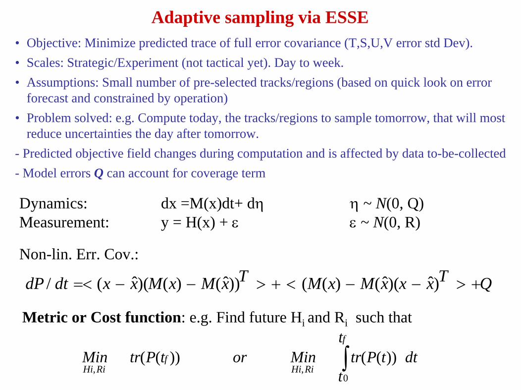
Adaptive sampling via ESSE
Metric or Cost function: e.g. Find future Hi and Ri such that
dtt
ttPtrMinortPtrMin
f
RiHif
RiHi ∫0
,,))(())((
Dynamics: dx =M(x)dt+ dη η ~ N(0, Q)Measurement: y = H(x) + ε ε ~ N(0, R)
Non-lin. Err. Cov.:
• Objective: Minimize predicted trace of full error covariance (T,S,U,V error std Dev). • Scales: Strategic/Experiment (not tactical yet). Day to week.• Assumptions: Small number of pre-selected tracks/regions (based on quick look on error
forecast and constrained by operation)• Problem solved: e.g. Compute today, the tracks/regions to sample tomorrow, that will most
reduce uncertainties the day after tomorrow.- Predicted objective field changes during computation and is affected by data to-be-collected- Model errors Q can account for coverage term
QTxxxMxMTxMxMxxdtdP +>−−<+>−−=< )ˆ)(ˆ()(())ˆ()()(ˆ(/
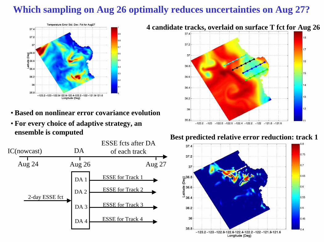
Which sampling on Aug 26 optimally reduces uncertainties on Aug 27?
4 candidate tracks, overlaid on surface T fct for Aug 26
ESSE fcts after DA of each track
Aug 24 Aug 26 Aug 27
2-day ESSE fct
ESSE for Track 4
ESSE for Track 3
ESSE for Track 2
ESSE for Track 1DA 1
DA 2
DA 3
DA 4
IC(nowcast) DA
Best predicted relative error reduction: track 1
• Based on nonlinear error covariance evolution • For every choice of adaptive strategy, an
ensemble is computed

- Objective: Minimize ESSE error standard deviation of temperature field- Scales: Strategic/Tactical- Assumptions
- Speed of platforms >> time-rate of change of environment- Objective field fixed during the computation of the path and not affected by new data
- Problem solved: assuming the error is like that now and will remain so for the next few hours, where do I send my gliders/AUVs?
- Method: Combinatorial optimization (Mixed-Integer Programming, using Xpress-MP code)- Objective field (err. stand. dev.) represented as discrete piecewise-linear fct: solved exactly by MIP- Constraints imposed on vehicle displacements dx, dy, dz for meaningful path
Optimal Paths Generation for a “fixed” objective field(Namik K. Yilmaz, P. Lermusiaux and N. Patrikalakis)
Example forTwo and Three Vehicles, 2D objective field
Grey dots: starting points White dots: MIP optimal end points

PhysicalModel
BiologicalModel
BiologicalModel
BiologicalModel
...[communicates to]
...
PhysicalModel
BiologicalModel
[communicates with]
(current)(current)
time
PhysicalModel
BiologicalModel
PhysicalModel
Biological Model
(1)(2)
(1)
(1)
(2) (3)
(2) (3)
. . .
. . .
(Nbio)
(Nphy)
PhysicalModel
Biological Model
(3)(2)
(current models )
(current models )
Towards Real-time Adaptive Physical and Coupled Models
• Model selection based on quantitative dynamical/statistical study of data-model misfits
• Mixed language programming (C function pointers and wrappers for functional choices) to be used for numerical implementation
• Different Types of Adaptation:• Physical model with multiple parameterizations in parallel (hypothesis testing) • Physical model with a single adaptive parameterization (adaptive physical evolution)
• Adaptive physical model drives multiple biological models (biology hypothesis testing)• Adaptive physical model and adaptive biological model proceed in parallel

Quasi-Automated Real-time Physical Calibration during AOSN-II
Prior to AOSN-II, ocean models calibrated to historical conditions judged to be similar to these expected in August 2003.
Ten days in the experiment: • Parameterization of the transfer of atmos. fluxes to upper layers (SBL mixing) adapted to new 2003 data
• 20 sets of parameter values and 2 mixing models tested
• Configuration with smallest RMSE/higher PCC improved upper-layer T and S fields, and currents
SST Prior Adaptation
SST AfterAdaptation

Harvard Generalized Adaptable Biological Model
(R.C. Tian, P.F.J. Lermusiaux, J.J. McCarthy and A.R. Robinson, HU, 2004)
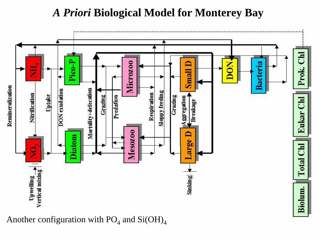
A Priori Biological Model for Monterey Bay
Another configuration with PO4 and Si(OH)4
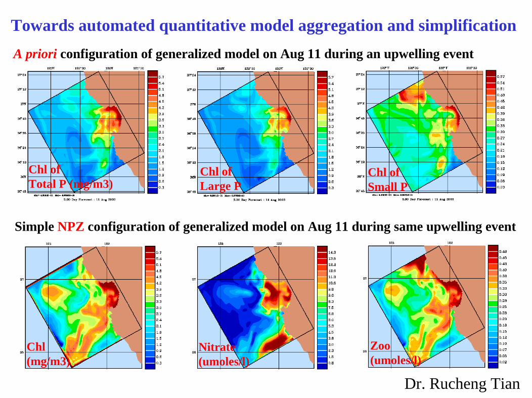
Nitrate (umoles/l)
Chl (mg/m3)
Chl of Total P (mg/m3)
Chl of Large P
A priori configuration of generalized model on Aug 11 during an upwelling event
Towards automated quantitative model aggregation and simplification
Simple NPZ configuration of generalized model on Aug 11 during same upwelling event
Chl of Small P
Zoo (umoles/l)
Dr. Rucheng Tian

Aug. 8 Aug. 13 Aug. 15
Aug.8 Aug. 13 Aug.15 Aug. 22
Chl
HOPS
NO3
HOPS
Cross-Section in Chl µg/l and NO3: Observations (S. Haddock et al) vs Simulations
Aug. 22
10
0
10
0
30
0
5
15
5
30
15
0
Aug 06 - Aug 18: UpwellingAug 19 - Aug 23: RelaxationAug 27 - Aug 30: Upwelling
• Several Chl hot-spots position and amplitudes, and nutricline tilts, captured but bio. model vertical resolution not sufficient
PROCESSES1.Deeper nutricline
and stronger blooms during upwelling
2.Much smaller scale hot-spots and shallower nutricline during relaxation (oceanic driven sub-mesoscales)

North Section
WestSection
SouthSection
Temp. Lev 1
Flux Balances and Term-by-term Balances
North section South section
West section Surface
1) Heat Flux Balances: 4 fluxes normal to each side of Pt. AN box, averaged over first upwelling period
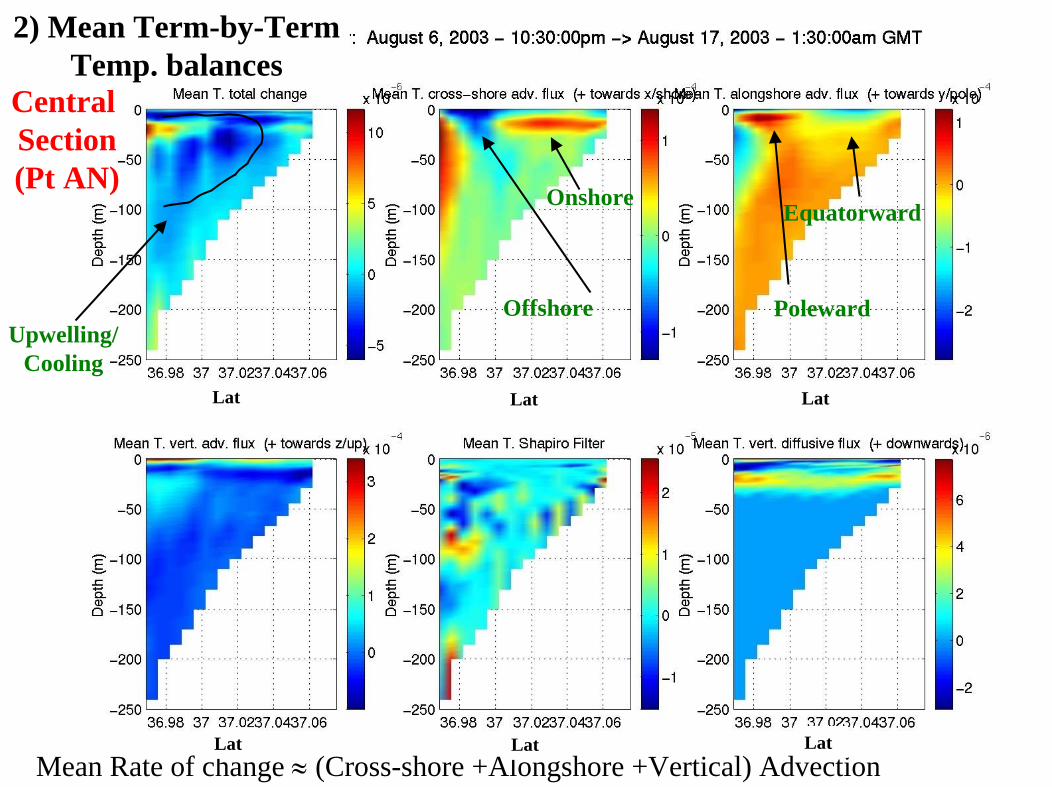
Central Section (Pt AN)
• Flux: Rate at which quantity flows through a surface[Quantity * m/s] or [(Quantity *m3/s ) /m2]For heat: W/m2 through any surface
• Term: Rate of change of single term in PE[Quantity/sec] For Temp.: oC/s
Central Section(Pt AN)
2) Mean Term-by-TermTemp. balances
Mean Rate of change ≈ (Cross-shore +Alongshore +Vertical) Advection
Offshore
Onshore
Upwelling/Cooling
Poleward
Equatorward
Lat Lat Lat
Lat Lat Lat

Central Section(Pt AN)
Snapshot Term-by-Term Temp. balances
Mean Rate of change ≈ (Cross-shore +Alongshore +Vertical) Advection
Vert. diff. almost zero
except at base of thermo.
Lat Lat Lat
Lat Lat Lat
Dep
th (m
)
Dep
th (m
)
Dep
th (m
)
Dep
th (m
)
Dep
th (m
)
Dep
th (m
)
Complex 3D non-homogenous upwelling (eddies, meanders of upwelling current and jets, etc)

•Spectra Results-Diurnal band obvious in 1-5m HOPS (not measured by M2)
-Spectra similar within mesoscale to inertial band.
-Semi-diurnal in HOPS forced by wind -Too low energy for sub-inertial scales: add deterministic (tides) and/or stochastic forcing (ESSE)
AOSN-II Motivations forNear-Inertial and Tidal Modeling
• Model-Data Comparisons
- Data-driven model with no tides vs. Data at M1/M2 (T,S,U,V)
M2 Data Time series M2 HOPS Time Series
M2 Data Spectra M2 HOPS Spectra
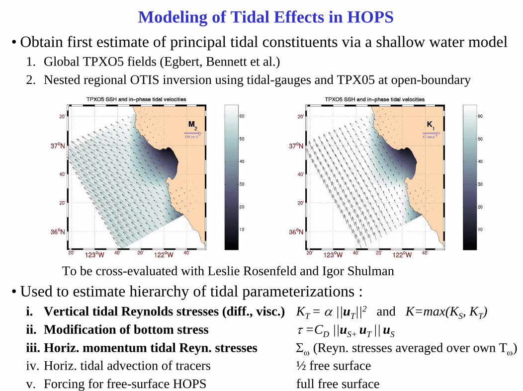
Modeling of Tidal Effects in HOPS• Obtain first estimate of principal tidal constituents via a shallow water model
1. Global TPXO5 fields (Egbert, Bennett et al.)2. Nested regional OTIS inversion using tidal-gauges and TPX05 at open-boundary
To be cross-evaluated with Leslie Rosenfeld and Igor Shulman• Used to estimate hierarchy of tidal parameterizations :
i. Vertical tidal Reynolds stresses (diff., visc.) KT = α ||uT||2 and K=max(KS, KT)ii. Modification of bottom stress τ =CD ||uS+ uT || uS
iii. Horiz. momentum tidal Reyn. stresses Σω (Reyn. stresses averaged over own Tω)iv. Horiz. tidal advection of tracers ½ free surfacev. Forcing for free-surface HOPS full free surface

T section across Monterey-BayTemp. at 10 m
No-tides
Two 6-day model runs
Tidal effects• Vert. Reyn.
Stress• Horiz.
Momentum Stress

AOSN-II Re-Analysis
30m Temperature: 6 August – 3 September (4 day intervals)
Descriptive oceanography of re-analysis fields and and real-time error fields initiated at the mesoscale.
Description includes: Upwelling and relaxation stages and transitions, Cyclonic circulation in Monterey Bay, Diurnal scales, Topography-induced small scales, etc.

AOSN-II Re-Analysis
Ano Nuevo
MontereyBay
Point Sur
18 August 22 August
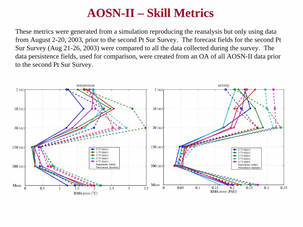
AOSN-II – Skill MetricsThese metrics were generated from a simulation reproducing the reanalysis but only using data from August 2-20, 2003, prior to the second Pt Sur Survey. The forecast fields for the second Pt Sur Survey (Aug 21-26, 2003) were compared to all the data collected during the survey. The data persistence fields, used for comparison, were created from an OA of all AOSN-II data prior to the second Pt Sur Survey.

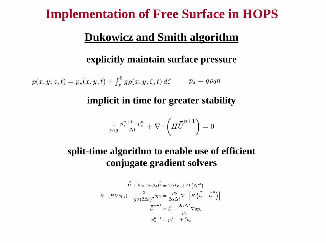
Implementation of Free Surface in HOPS
Validated for MREA-03 and AOSN-II
Explicitly maintain surface pressure
Allow vertical levels to deform according to free surface,related to surface pressure via
Compute surface pressure with Dukowicz and Smith algorithm• implicit in time for greater stability• split-time algorithm to enable use of efficient conjugate
gradient solvers
Adaptations for use in HOPS• synoptic initialization• open boundary conditions
–including barotropic tidal forcing• assimilation• two-way nesting (ongoing)

Implementation of Free Surface in HOPS
20 day simulation spanning Aug 6-26, 2003Assimilate CTDs, gliders and aircraft SST from Aug 7-20, 2003
Compare to Pt Sur CTDs from Aug 21-25, 2003
• Overall comparable skill• Significant improvement in main thermocline
AOSN-II Validation

Multi-Scale Energy and Vorticity AnalysisMS-EVA is a new methodology utilizing multiple scale window decompositionin space and time for the investigation of processes which are:• multi-scale interactive• nonlinear• intermittent in space• episodic in time
Through exploring:• pattern generation and • energy and enstrophy
- transfers- transports, and- conversions
MS-EVA helps unravel the intricate relationships between events on different scales and locations in phase and physical space. Dr. X. San Liang

Multi-Scale Energy and Vorticity AnalysisWindow-Window Interactions:
MS-EVA-based Localized Instability TheoryPerfect transfer:A process that exchanges energy among distinct scale windows which does not create nor destroy energy as a whole.In the MS-EVA framework, the perfect transfers are represented as field-like variables. They are of particular use for real ocean processes which in nature are non-linear and intermittent in space and time.
Localized instability theory:BC: Total perfect transfer of APE from large-scale window to meso-scale window.BT: Total perfect transfer of KE from large-scale window to meso-scale window.BT + BC > 0 => system locally unstable; otherwise stableIf BT + BC > 0, and• BC ≤ 0 => barotropic instability;• BT ≤ 0 => baroclinic instability;• BT > 0 and BC > 0 => mixed instability

Multi-Scale Energy and Vorticity AnalysisAOSN-II
M1 Winds
Temperature at 10m
Temperature at 150m

Wavelet Spectra
Surface Temperature
Surface Velocity
Monterey Bay
Pt. AN
Pt. Sur
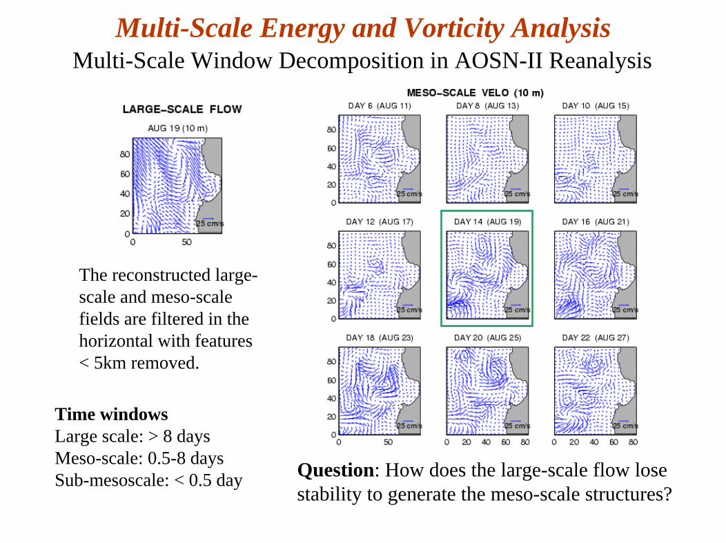
Multi-Scale Energy and Vorticity AnalysisMulti-Scale Window Decomposition in AOSN-II Reanalysis
Time windowsLarge scale: > 8 daysMeso-scale: 0.5-8 daysSub-mesoscale: < 0.5 day
The reconstructed large-scale and meso-scale fields are filtered in the horizontal with features < 5km removed.
Question: How does the large-scale flow lose stability to generate the meso-scale structures?

• Both APE and KE decrease during the relaxation period• Transfer from large-scale window to mesoscale window occurs to account for
decrease in large-scale energies (as confirmed by transfer and mesoscale terms)
Large-scale Available Potential Energy (APE)
Large-scale Kinetic Energy (KE)
Windows: Large-scale (>= 8days; > 30km), mesoscale (0.5-8 days), and sub-mesoscale (< 0.5 days)Dr. X. San Liang
• Decomposition in space and time (wavelet-based) of energy/vorticity eqns.Multi-Scale Energy and Vorticity Analysis

Multi-Scale Energy and Vorticity AnalysisMS-EVA Analysis: 11-27 August 2003
Transfer of APE fromlarge-scale to meso-scale
Transfer of KE fromlarge-scale to meso-scale
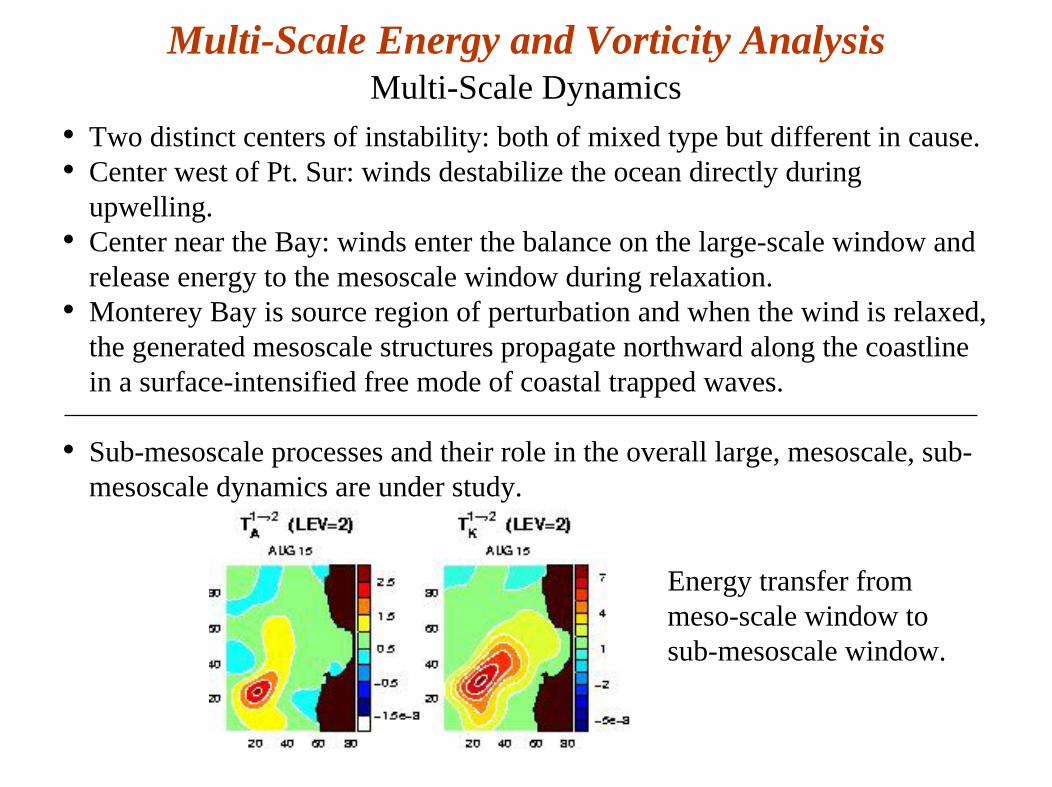
Multi-Scale Energy and Vorticity AnalysisMulti-Scale Dynamics
• Two distinct centers of instability: both of mixed type but different in cause.• Center west of Pt. Sur: winds destabilize the ocean directly during
upwelling.• Center near the Bay: winds enter the balance on the large-scale window and
release energy to the mesoscale window during relaxation.• Monterey Bay is source region of perturbation and when the wind is relaxed,
the generated mesoscale structures propagate northward along the coastline in a surface-intensified free mode of coastal trapped waves.
• Sub-mesoscale processes and their role in the overall large, mesoscale, sub-mesoscale dynamics are under study.
Energy transfer from meso-scale window to sub-mesoscale window.

Strategies For Multi-Model Adaptive ForecastingError Analyses and Optimal (Multi) Model Estimates
• Error Analyses: Learn individual model forecast errors in an on-line fashion through developed formalism of multi-model error parameter estimation
• Model Fusion: Combine models via Maximum-Likelihood based on the current estimates of their forecast errors
3-steps strategy, using model-data misfits and error parameter estimation
1. Select forecast error covariance and bias parameterization
2. Adaptively determine forecast error parameters from model-data misfitsbased on the Maximum-Likelihood principle:
3. Combine model forecasts via Maximum-Likelihood based on the current estimates of error parameters (Bayesian Model Fusion) O. Logoutov
Where is the observational data
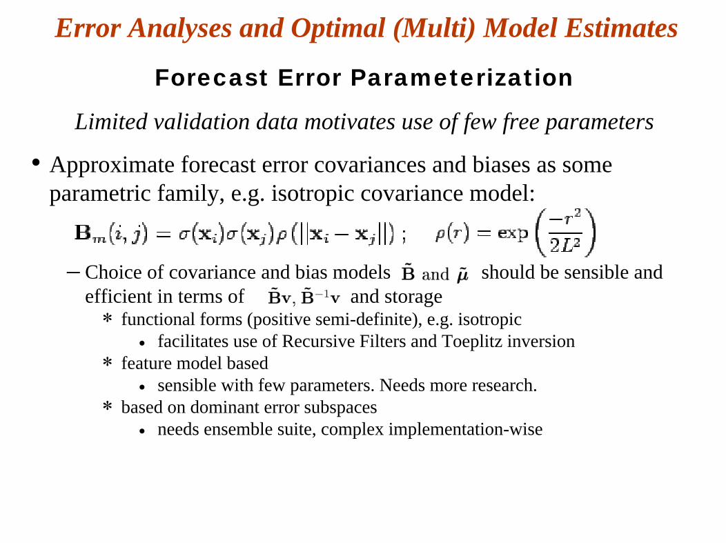
Forecast Error Parameterization
Limited validation data motivates use of few free parameters
• Approximate forecast error covariances and biases as some parametric family, e.g. isotropic covariance model:
– Choice of covariance and bias models should be sensible and efficient in terms of and storage∗ functional forms (positive semi-definite), e.g. isotropic
• facilitates use of Recursive Filters and Toeplitz inversion∗ feature model based
• sensible with few parameters. Needs more research.∗ based on dominant error subspaces
• needs ensemble suite, complex implementation-wise
Error Analyses and Optimal (Multi) Model Estimates

Error Parameter Tuning
Learn error parameters in an on-line fashion from model-data misfits based on Maximum-Likelihood
• We estimate error parameters via Maximum-Likelihood by solving the problem:
(1)
Where is the observational data, are the forecast error covariance parameters of the M models
• (1) implies finding parameter values that maximize the probability of observing the data that was, in fact, observed
• By employing the Expectation-Maximization methodology, we solve (1) relatively efficiently
Error Analyses and Optimal (Multi) Model Estimates

Error Analyses and Optimal (Multi) Model EstimatesAn Example of Log-Likelihood functions for error
parameters
LengthScale
Variance
HOPS
HOPS
ROMS
ROMS
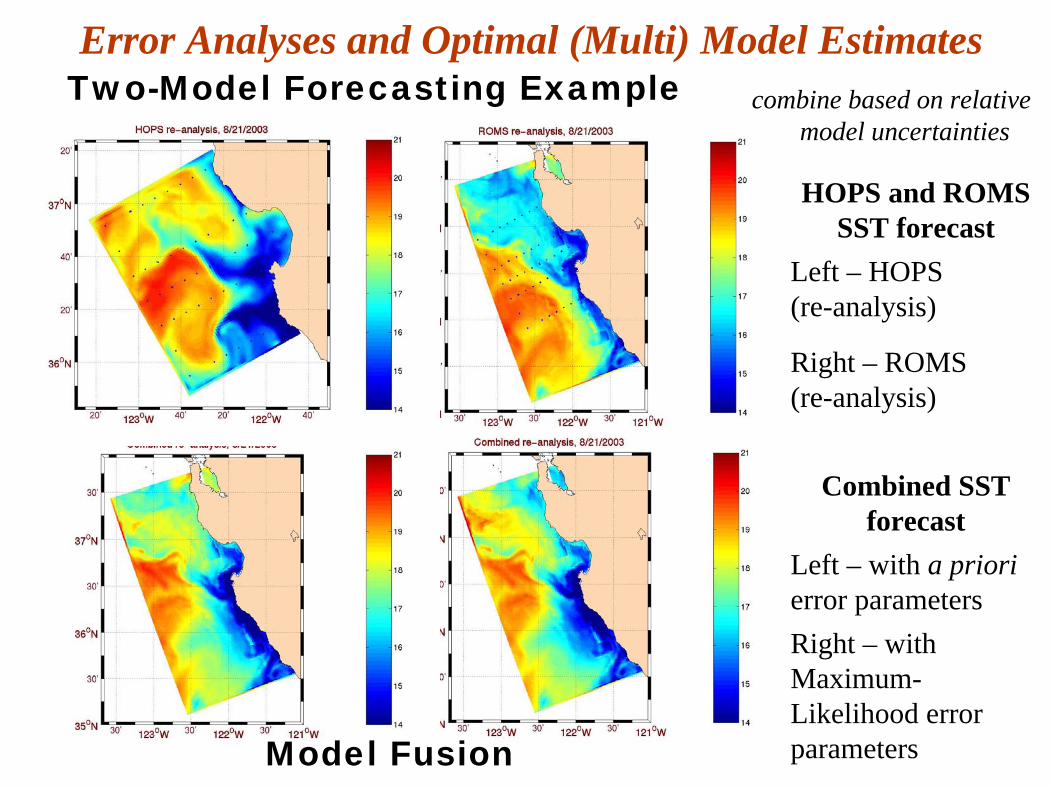
Error Analyses and Optimal (Multi) Model EstimatesTwo-Model Forecasting Example
Combined SST forecast
Left – with a priorierror parametersRight – with Maximum-Likelihood error parameters
HOPS and ROMS SST forecast
Left – HOPS(re-analysis)
Right – ROMS(re-analysis)
combine based on relative model uncertainties
Model Fusion

1. HOPS/ESSE transitioned with updates routinely used by Centre and Joint Research Project 2005-2008a) JRP Deterministic and Stochastic Regional Forecasting
2. Current Collaboration Topicsa) Multi-Scale Energy and Vorticity Analysisb) Error Analyses and Optimal (Multi) Model Estimatesc) Mini-HOPS
3. Recent and Upcoming Field Exercisesa) MREA03 – Corsican Channel b) MREA04 – Portuguese Coastal Watersc) DART05 – Adriatic Sead) 2006 – Demonstration of Mini-HOPS concept for harbor
protection – series of day cruises with NRV Leonardo
Harvard/NURC Collaborative Research:Real-time Field Exercises

Mini-HOPS
• Designed to locally solve the problem of accurate representation of sub-mesoscale synopticity
• Involves rapid real-time assimilation of high-resolution data in a high-resolution model domain nested in a regional model
• Produces locally more accurate oceanographic field estimates and short-term forecasts and improves the impact of local field high-resolution data assimilation
• Dynamically interpolated and extrapolated high-resolution fields are assimilated through 2-way nesting into large domain models
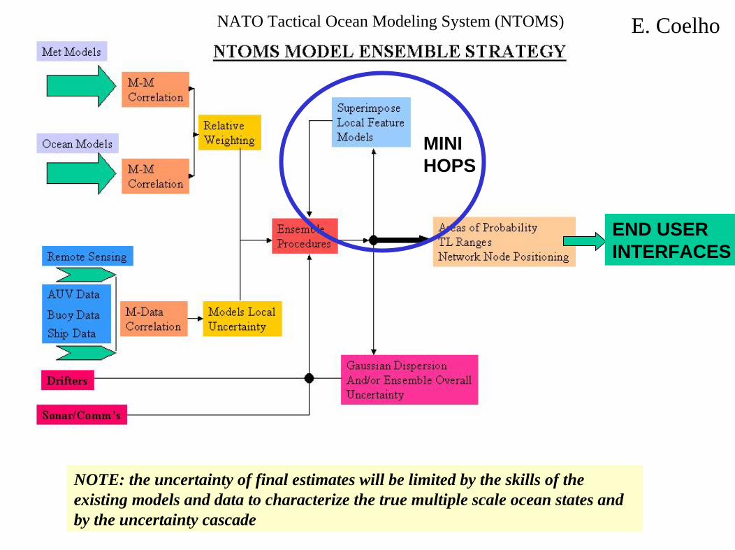
NOTE: the uncertainty of final estimates will be limited by the skills of the existing models and data to characterize the true multiple scale ocean states and by the uncertainty cascade
MINIHOPS
END USERINTERFACES
E. CoelhoNATO Tactical Ocean Modeling System (NTOMS)
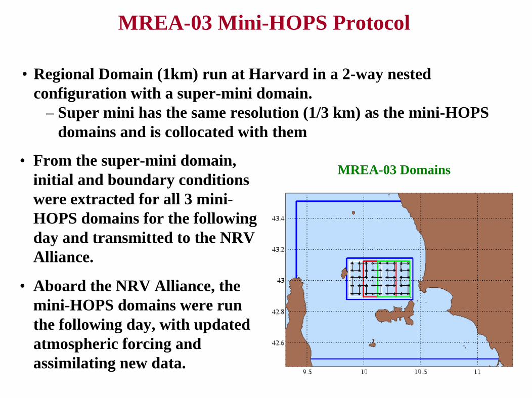
MREA-03 Mini-HOPS Protocol
• From the super-mini domain, initial and boundary conditions were extracted for all 3 mini-HOPS domains for the following day and transmitted to the NRV Alliance.
• Aboard the NRV Alliance, the mini-HOPS domains were run the following day, with updated atmospheric forcing and assimilating new data.
MREA-03 Domains
• Regional Domain (1km) run at Harvard in a 2-way nested configuration with a super-mini domain.
– Super mini has the same resolution (1/3 km) as the mini-HOPS domains and is collocated with them

Mini-HOPS for MREA-03
• During experiment:– Daily runs of regional and super mini at Harvard– Daily transmission of updated IC/BC fields for mini-HOPS
domains– Mini-HOPS successfully run aboard NRV Alliance
Prior to experiment, several configurations were tested leading to selection of 2-way nesting with super-mini at Harvard
Mini-HOPS simulation run aboard NRV Alliance in Central mini-HOPS domain (surface temperature and velocity)

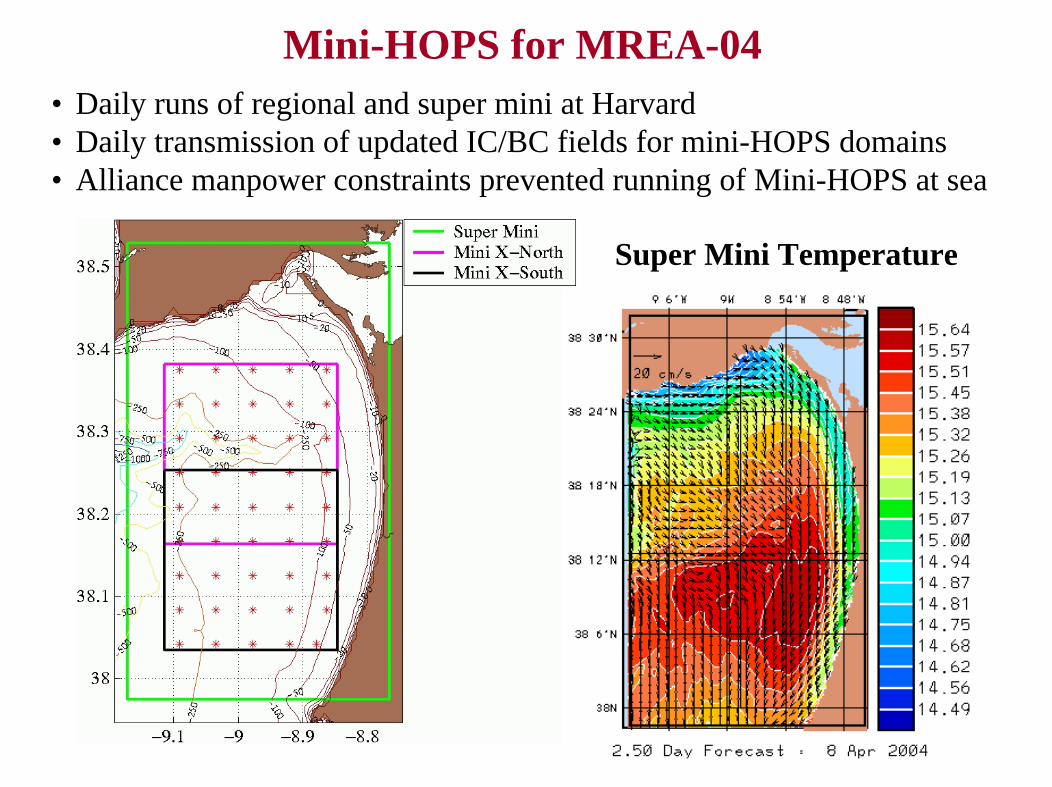
Mini-HOPS for MREA-04• Daily runs of regional and super mini at Harvard• Daily transmission of updated IC/BC fields for mini-HOPS domains• Alliance manpower constraints prevented running of Mini-HOPS at sea
Regional Domain1km resolution
Super Mini Domain1/3 km resolution

a) AREG surface salinity; b) zoom of the AREG surface velocity; c) surface chlorophyll-a map from SeaWIFS (same colour scale as Fig. 3); d) zoom of HOPS surface salinity (colour scale going from 35 –orange– to 38.8 –cyan) and velocity fields; all maps for July 2, 2004.
a b
c d
Improvement of forecasting accuracy with high resolution relocatable ocean models: a successful experiment in the western Adriatic Sea (June-July 2004): A. RUSSO, et al.
DART-05 – Adriatic Sea – Aug/Sep 2005 DART - Dynamics of the Adriatic in Real-Time
Mesoscale, sub-mesoscale dynamics of coastal currents and eddies
shedding from head of Gargano Peninsula.
NRL/NURC JRP – J. Book/M. Rixen
with HOPS forecasting for high-resolution dynamics and
adaptive sampling

E. Coelho

EXTRA VUGRAFS
Mini-HOPS for MREA-04• Daily runs of regional and super mini at Harvard• Daily transmission of updated IC/BC fields for mini-HOPS domains• Alliance manpower constraints prevented running of Mini-HOPS at sea
Super Mini Temperature

Real-time Regional Applications
HOPS provided real-time forecasts during the period 6-10 April 2004. A regional survey during 31 March - 6 April 2004 provided the initial state. HOPS performed real-time forecasting and ocean and model data transfers were carried out between the NRV Alliance and Harvard University. The Mini-HOPS concept was utilized in real-time to locally solve the problem of accurate representation of sub-mesoscale synopticity. This concept involves rapid real-time assimilation of high-resolution data in a high-resolution locally nested model domain around observational platforms. HOPS provided 2-way nested output in regional and sub-regional domains. These outputs provided initial and boundary data for shipboard Mini-HOPS simulations. Real-time forecasts included an evaluation of model bias and RMS error every day, in routine fashion and were also used for onboard acoustic calculations
MREA04 – Portuguese Atlantic CoastMarch/April 2004
Regional Domain Super Mini Domain

Mini-HOPS
Future work
BCs more compatible with assimilationIncorporation of coasts in Mini Domains
Future experiments in collaboration with NURC:
Implementation of Mini-HOPS in Harbor protection initiatives
Locations: Italy-Black Sea-Baltic
Type: The Italy and Black Sea will be more related with DAT and homeland protection initiatives. The Baltic sea will be in conjunction with a MCM exercise.

Fiel
d U
ncer
tain
ty
Resolution (grid-time spacing)
Op..Modeling
Real-timeModeling
NTOMS
Goal:
Local high resolution data collectionStart with an operational model runNest three 20x20Km 50% superimposed domains on a regional HOPS domainPerform assimilation cycles within one inertial periodProvide and monitor hourly outputs for 24-48 hours forecasts
E. Coelho
MREA03

MREA03 Modeling Domains
Channel domain• 1 km resolution• Spans initialization
survey
Mini-HOPS• 1/3 km resolution• Span high-resolution
survey
Super Mini-HOPS• 1/3 km resolution• 2 km buffer

MREA03 – Ligurian Sea – May/June 2003
Prior to the MREA04 exercise, a re-analysis of the HOPS forecasts of the May-June 2003 MREA03 exercise was performed. This led to dramatically improved detailed agreement of model results with observed profiles. This re-analysis was motivated by observations of recurring mismatches between HOPS near surface structure and that observed in the CTD profiles. The general stability of the simulations was first improved with parameter tuning and slight modifications to the filtering and open boundary algorithms. Sensitivity studies on the model parameters (especially vertical mixing) produced a moderate improvement in the bias and RMS error between the simulation fields and a set of generally troublesome profiles. A much larger improvement was obtained by redistributing the vertical model levels to better resolve the near surface fields. Moderate improvement came by correcting the pre-processing of atmospheric fields to construct the net heat flux. A final, smaller, improvement came by revising the initialization procedures.

T0, S0 on 17 June 2003
HOPS and mini-HOPS in MREA03
• Web-distributed nowcasts and forecasts 11-17 June 2003
• Web-distributed mini-HOPS domain initial and boundary conditions 11-17 June 2003
• Channel domain forecasts run at Harvard
• Mini-HOPS domain forecasts run aboard NRV Alliance – real-time, in the field, demonstration of concept
• Post-experiment re-analysis and model tuning to improve model/data profile comparisons

MREA04 Modeling Domains
Regional domain• 1 km resolution• Spans initialization
survey
Super Mini-HOPS• 1/3 km resolution• Extended to coasts
(reducing coastal currents)
• 5 km buffer
Mini-HOPS• 1/3 km resolution• Span high-resolution
survey

HOPS and mini-HOPS in MREA04Daily evolution of temperature at 10m from 6 April – 10 April.
Superimposed upon the temperature field are vectors of sub-tidal velocity.
HOPS Regional Domain
NRL Nowcast 10 Apr.
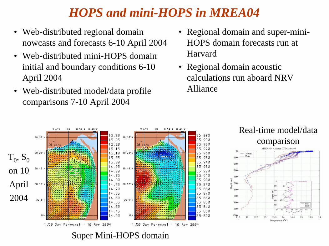
T0, S0
on 10 April 2004
HOPS and mini-HOPS in MREA04• Web-distributed regional domain
nowcasts and forecasts 6-10 April 2004• Web-distributed mini-HOPS domain
initial and boundary conditions 6-10 April 2004
• Web-distributed model/data profile comparisons 7-10 April 2004
• Regional domain and super-mini-HOPS domain forecasts run at Harvard
• Regional domain acoustic calculations run aboard NRV Alliance
Real-time model/data comparison
Super Mini-HOPS domain

Results of Re-analysis and Dynamical Model TuningReal-time Model/Data Comparison Re-analysis Model/Data Comparison
ModelTemp.
ObservedTemp. Bias residue
< .25oC
• Tuned parameters for stability and agreement with profiles (especially vertical mixing)• Improved vertical resolution in surface and thermocline• Corrected input net heat flux• Improved initialization and synoptic assimilation in dynamically tuned model

Mini-HOPSMREA03 – “OSSE”
Direct Extended Minis Super Mini
Simplest Configuration IC/BC’s at proper scales IC/BC’s at proper scalesFine scale data “memory”
Boundary mismatchMaintenance Uclin Most complex configuration Intermed. complex
Not generalizable
Mini-HOPS
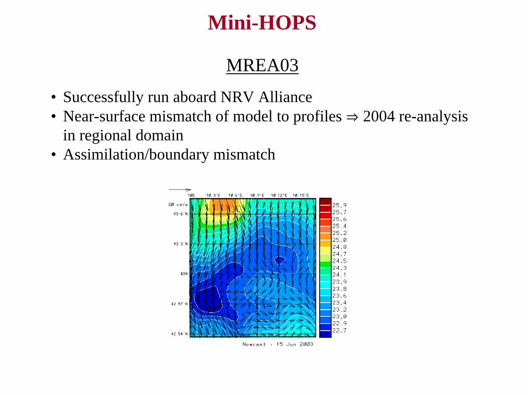
MREA03
• Successfully run aboard NRV Alliance• Near-surface mismatch of model to profiles fl 2004 re-analysis
in regional domain• Assimilation/boundary mismatch

Mini-HOPS for MREA-03
• During experiment:– Daily runs of regional and super mini at Harvard– Daily transmission of updated IC/BC fields for mini-HOPS
domains– Mini-HOPS successfully run aboard NRV Alliance
• Near-surface mismatch of model to profiles fl 2004 re-analysis in regional domain
• Assimilation/boundary mismatch
Prior to experiment, several configurations were tested leading to selection of 2-way nesting with super-mini at Harvard
Mini-HOPS simulation run aboard NRV Alliance in Central mini-HOPS domain
Mini-HOPS
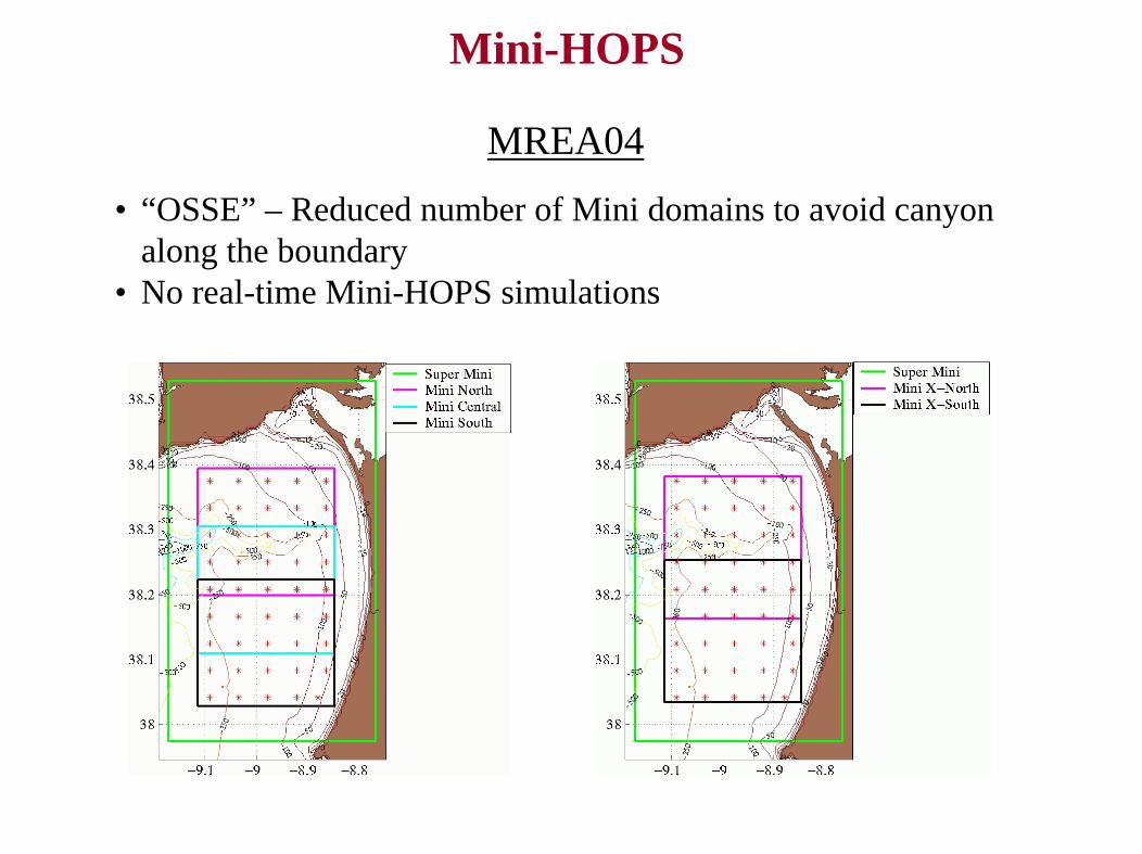
MREA04
• “OSSE” – Reduced number of Mini domains to avoid canyon along the boundary
• No real-time Mini-HOPS simulations
Implementation of Free Surface in HOPS
Dukowicz and Smith algorithm
split-time algorithm to enable use of efficient conjugate gradient solvers
explicitly maintain surface pressure
implicit in time for greater stability
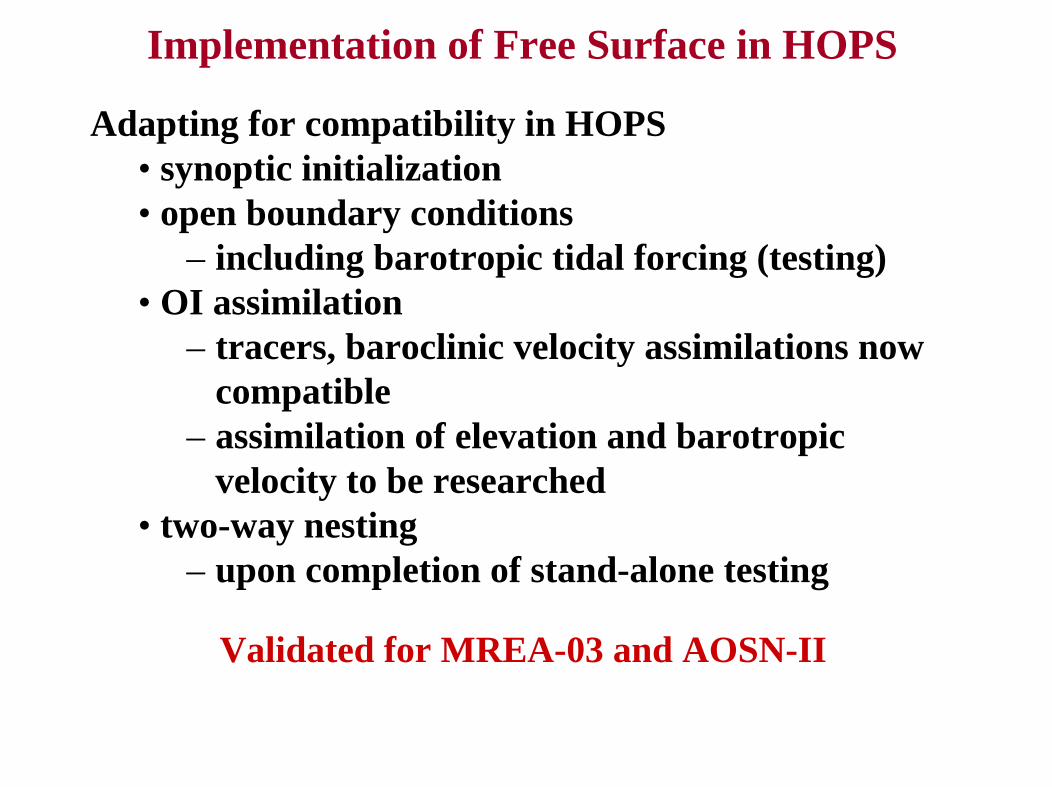
Implementation of Free Surface in HOPS
Adapting for compatibility in HOPS• synoptic initialization• open boundary conditions
– including barotropic tidal forcing (testing)• OI assimilation
– tracers, baroclinic velocity assimilations now compatible
– assimilation of elevation and barotropic velocity to be researched
• two-way nesting– upon completion of stand-alone testing
Validated for MREA-03 and AOSN-II

Real-time Regional Applications
2005- FAF05: July, Isola Pianosa (near Elba)- DART05: August/September, Adriatic- ASAP: November (?), Virtual experiment, Monterey Bay
2006- ASAP: June (?), Monterey Bay- MREA06: Time not yet determined, location not yet determined