çksVhu …Mh lajpuk dh rqyuk ds fy, xzkQ F;ksjh vk/kkfjr

midj.k dk fodkl

Development of a Tool for Comparison of Protein 3D Structure using graph theoretic approach

;w ch vaxMh U. B. Angadi —".k dqekj prqosZnh K. K. Chaturvedi eksusUæ xzksoj Monendra Grover lq/khj JhokLro Sudhir Srivastava

ifj¸kkstuk fjiksVZ

PROJEC T R E PORT

d`f"k tSolwpuk dsUnz

CENTRE OF AGRICULTURAL BIOINFORMATICS

आई. सी. ए. आर. - आई. ए. एस. आर. आई./पी. आर. -01/2017

I.C.A.R.-I.A.S.R.I./P.R.-01/2017 Institute Project Code: AGENIASRIL201400500024I; PIMS:XX10767

ससथान पररयोजना कोड:AGENIASRIL201400500024; PIMS: IXX10767

Hkk d` vuq i & Hkkjrh; d`f"k lkaf[;dh vuqla/kku laLFkku

ykbcszjh ,osU;w] iwlk uà fnYyh&110012

ICAR- Indian Agricultural Statistics Research Institute Library Avenue, Pusa, New Delhi – 110012

2017

Project Report

Title of the project

“Development of a Tool for Comparison of Protein 3D

Structure using graph theoretic approach”

IRC PROCEEDING PROJECT NO. : AGENIASRISIL201400500024

PROJECT CODE NO. : IXX10767

Submitted by U. B. Angadi

K. K. Chaturvedi

M. Grover

Sudhir Srivastava

Centre for Agricultural Bioinformatics

ICAR-Indian Agricultural Statistics Research Institute, Pusa,

New Delhi

आमख

vkt nqfu;k Hkj esa vk.kfod tho foKku ç;ksx'kkykvksa vkSj lwpuk çkS|ksfxdh ds Bksl ç;kl ds

dkj.k vkt vuqØe vkSj lajpukRed vkadM+ksa dh ,d cM+h ek=k lkoZtfud tSfod MsVkcsl esa mIyC/k

gSa A vuqØe vkSj lajpukRed ;qfädj.k ds lkFk dq'ky lk/kuksa rFkk mpp dksfV ds fo'ys"k.kkRed

midj.kksa dks Hkh fMtkbu djus dh ck;ksbuQ‚jeSfVDl esa ,d dsaæh; pqukSrh gSa A bl rjg ds fo'ks"k

midj.k vuqØe.k MsVk ,oa lwpuk dks tSojklk;fud vkSj tSoHkkSfrdh Kku esa cnyus rFkk buesa fn;s

gq, lajpukRed] dk;kZRed vkSj fodkl laca/kh lajpukvks dks le>us ds fy, vko';d gSA tSfod

vuqØe vkSj lajpuk MsVk ds fo'ys"k.k esa çfr:i lqesyu (pattern matching) ,d egRoiw.kZ dne

gSA çfr:i lqesyu çksVhu 3 Mh lajpukvksa dk v/;;u] vU; çksVhu ds lkFk fodkloknh vkSj

lajpukRed laca/k Kkr djus esa ,d egRoiw.kZ Hkwfedk fuHkkrk gS rFkk thofoKkfu;ksa dks lajpukvksa

vkSj fodkl ls tqM+s fofHkUu igyqvksa dks le>us esa enn djrk gS A çksVhu 3 Mh lajpukvksa ds

MsVkcsl vf/kd cM+s gksus dh otg ls gesa u;s mUur ,o de le; ysus okys midj.k vkSj

rqyukRed rjhdksa dh vko';drk gSA 3 Mh lajpuk dh rqyuk miyC/k MsVkcsl esa fofo/krk] fo'ys"k.k

rFkk oSKkfud var– Zf"V dks le>us esa ,d egRoiw.kZ Hkwfedk fuHkkrk gSaA ;g /;ku j[kuk egRoiw.kZ gS

fd bu MsVkcsl fd of) dk eryc dsoy ek=k ugha gS] cfYd fofo/krk] tfVyrk] Hks|rk vkSj

,d:irk Hkh gSaA blfy,] rqyukRed midj.k dks u dsoy mPp 'kq)rk rFkk foLr`r vk;ke dh

vko';drk gksrh gS] cfYd lajpukvksa dh c<+rh la[;k ls fuiVus ds fy;s de le; esa fudkyuk Hkh

gSA çksVhu vuqØe.k fof'k"V :i ls vius ewy ifjos'k esa ,d lajpuk dks fu/kkZfjr djrk gSA çksVhu

ds dk;Z dks le>us esa ;g lajpukRed tkudkjh vf/kd egRoiw.kZ gSA Ms<+ n'kd ds ckn Hkh çksVhu

lajpuk dh rqyuk vkt dh çeq[k 'kks/k çkFkfedrk ds :i esa çpfyr gS] rFkk cgqr 'kks/k ys[k bl~

fn'kk esa çdkf'kr gks jgs gSA foxr o"kksaZ esa gq, çxfr ds rjhdksa esa lq/kkj tkjh gSA vr% vHkh Hkh

çksVhu lajpuk dh rqyuk ,d [kqyh pqukSrh gSA

lkfgR; dh leh{kk ds vk/kkj ij] xzkQ fl)kar vk/kkfjr rduhfd;ksa dk bLrseky çksVhu rqyuk ds

fy, fd;k tk ldrk gSA xzkQ e‚My dks fofHkUu xzkQ ekinaMksa dk mi;ksx dj cuk;k tk ldrk

gSA vke rkSj ij] xzkQ fl)kar dk mi;ksx tfVy LFkkfud lajpuk dks ifjHkkf"kr ,oa le>us ds fy,

fd;k tkrk gS ftlds ijek.kq vkil esa tfVyrk ls tqM+s gq, gS rFkk ,d nwljs ij fuHkZj gSA ijek.kq

ds Lrj ij fo'ys"k.k xzkQ fl)kafrd fof/k 3 Mh lajpuk fo'ys"k.k ds fy, fdlh vU; fof/k dh

rqyuk esa csgrj ifj.kke ns ldrk gSA bu egRoiw.kZ fcanqvksa dks /;ku esa j[krs gq, ifj;kstuk çksVhu

…Mh lajpuk dh rqyuk ds fy, xzkQ F;ksjh vk/kkfjr midj.k dk fodkl rS;kj fd;k x;k gSA

geus 1½ xzkQ foHkktu vkSj 2½ xzkQ xq.kksa dk mi;ksx djds çksVhu 3 Mh lajpuk dh rqyuk djus ds

fy, nks u;h fof/k;ksa dks fodflr fd;k gSA nksuksa fodflr fof/k;ksa dks MATLAB esa ykxw fd;k x;k

gSA fodflr rjhdksa dks nks orZeku esa mIyC/k loksZÙke rjhdksa tSls lhbZ (CE) vkSj ts,Q,Vhlh,Vh

¼jFATCAT½ ds lkFk 100 çksVhu csapekdZ MkVklsV ij SCOP MkVkcsl ds lkFk ijh{k.k fd;k x;k

gSA fodflr dh x;h fof/k;ka le; ,oa mR—"Vrk dh –f"V ls mIyC/k rduhfd;ksa ls csgrj lkfcr

fl) gqbZA

लखकगण

PREFACE

Today, large volume of sequence and structural data is publically available in the

form of biological databases based on integrated effort of molecular biology laboratories

throughout the world and advances in information technology. A global challenge in

bioinformatics is the rationalization of the huge amount of sequences and structural data with

a view not only to derive efficient and useful meaning from this data, but also for designing

sharper analytical tools. The analytical tools are required for conversion of sequence

data/information into biochemical and biophysical properties and to decipher the structural,

functional and evolutionary clues encoded in the data. Pattern matching is one of main

important aspects in the analysis of biological sequence and structure data. The alignment and

comparison of protein 3D structures are very important and fundamental task in structural

biology to study evolutionary and structural relatedness with other proteins and helps

biologists to understand various functions and evolution from these structures to identify its

structural neighbors. In addition to this, databases of three-dimensional protein structures

became so large that fast search tools and comparison methods are required. The 3D structure

comparison play a key role in understanding the diversity of structure space by analyzing and

deriving interesting scientific insights in the existing vast structural databases. It is important

to note that an increase in deposited structures does not just contain quantity, but also variety,

complexity, vulnerability, and singularity. Hence, comparison tools are essentially required

not only to improve accuracy and coverage but also reduce time complexity. Protein

sequence uniquely determines a structure in its native environment. This structural

information is vital in understanding the function of a protein. In last one and an half decade,

the research on protein structure comparison has been taken up on priority basis and numbers

of research articles were exists in literature. There are incremental advances over previous

efforts, and still methods are being development for further improvement.

The graph theory approaches can be used for protein 3D structure comparison. Graph

models can be created using various graph parameters. Generally, graph theory is used to

represent/decipher complex spatial structures which are mutually connected and dependent.

The 3D structure of protein is a complex structure. The atom level analysis may yield better

result in 3D structure analysis than any other method. Considering these important points, the

project has been formulated to develop a tool for comparison of protein 3D structure using

graph theoretic approach.

We have developed two novel methods for comparison of 3D structure based on 1)

graph partition and 2) graph properties. Both methods have been implemented in MATLAB

by writing codes for various functions. The performance of the developed methodologies is

tested with two existing best methods such as CE and jFATCAT on 100 proteins benchmark

dataset with SCOP (Structural Classification Of Proteins) database. The proposed methods

performed better in terms of classification accuracy and time complexity.

AUTHORS

Table of Contents

SL.

NO.

PARTICULARS PAGE

NUMBERS

1 PROJECT DETAILS 1

2 CHAPTER –I : INTRODUCTION 2-13

3 CHAPTER-II: GRAPH

PARTITIONING/CLUSTE

RING AND ALIGNMENT

15-27

4 CHAPTER-III : GRAPH PROPERTIES

AND MACHINE

LEARNING

TECHNIQUES

29-40

5 CHAPTER – IV : SUMMERY AND

CONCLUSION

41-42

6 REFERENCES 43-45

7 ANNEXURE-I: MATLAB

CODES

i-xx

Project Report

Development of a Tool for Comparison of Protein 3D Structure using graph theoretic

approach

1. Institute Project Code: IRC Proceeding Project No. : AGENIASRISIL201400500024 Project

Code No. : IXX10767

2. Project Title : Development of a Tool for Comparison of Protein 3D Structure using graph

theoretic approach

3. Key Words : Protein 3D structure, comparison/alignment, graph theory

4. (a) Name of the Lead Institute : Indian Agricultural Statistics Research Institute

(b) Name of Division/ Regional Center/ Section : Centre for Agricultural Bioinformatics

5. (a) Name of the Collaborating Institute(s), if any . NIL

(b) Name of Division/ Regional Center/ Section of Collaborating Institute(s)

6. Project Team(Name(s) and designation of PI, CC-PI and all project Co-PIs, with time

proposed to be spent)

S.

No.

Name,

designation and

institute

Status

in the

project

Time

to be

spent

(%)

Work components to be assigned to

individual scientist

1 U B Angadi, Sr.

Scientist

PI 40 Review of relevant literature,

Parameters selection, Construction of

graph matrix and graph model, Graph

Comparison, Evaluation

2 K K Chaturvedi CPI-1 30 Review of relevant literature,

Construction of graph matrix and graph

model, Graph Comparison

3 Monendra

Grover

CPI-2 25 Parameters selection,

4 Sudhir Srivastava CPI-3 25 Parameters selection , Graph

Comparison, Evaluation(till 1/8/2015)

7. Priority Area to which the project belongs : DEVELOPMENT OF STATISTICAL

TECHNIQUES FOR GENETICS/COMPUTATIONAL BIOLOGY AND APPLICATIONS

OF BIOINFORMATICS IN AGRICULTURAL RESEARCH

(If not already in the priority area, give justification)

8. Project Duration: Date of Start: 18/03/2014 Likely Date of Completion: 15/4/2017

9. (a) Objectives

To convert 3D structure of protein to graph model using graph theoretic approach

To compare 3D structures using graph theoretic models and data mining techniques

(b) Practical utility

Useful for 3D structure comparison,

3D structure search in the database,

Classification/analysis of 3D structures.

1

2

CHAPTER –I: INTRODUCTION

GENESIS AND RATIONALE OF THE PROJECT

Protein sequence uniquely determines a structure in its native environment. This structural information

is vital in understanding the function of a protein. The structural information of protein is classified into

primary, secondary, tertiary and quaternary. The primary structure of a protein refers to the amino acid

sequence of the polypeptide chain, which is formed during the process of protein biosynthesis and it is

held together by covalent or peptide bonds. The secondary structure refers to highly regular local sub-

structures defined by the patterns of hydrogen bonds between the peptide chains. The alpha helix and

the beta strand are considered as the major secondary structures, which represent a way of saturating all

the hydrogen bond donors and acceptors in the peptide backbone. Tertiary structure is the particular

arrangement of secondary structure elements in three dimensional spaces. Quaternary structure is a

larger assembly of several protein molecules. Proteins are versatile biological molecules that perform

numerous functions in a living organism. These functions are at two levels; one at molecular level

(physical/chemical activity) and cellular level (signalling /metabolic pathways activity). In nature,

protein 3D structure is more conserved than protein sequence. Hence, 3D structure can provide

significant insights about protein function. The intimate relationship between protein structure and

function has been well established (Perutz 1960).

The quantitative comparison of protein 3D structures is an important and fundamental task in

structural biology to study evolutionary and structural relatedness with other proteins and helps

biologists to understand various aspects of function, evolution from these structures and identify its

structural neighbours. In addition to this, databases of three-dimensional protein structures are very

large and increasing day by day. Hence, fast search tools and comparison methods are needed. The 3D

structure comparison play a key role in understanding the diversity of structure space by analysing and

deriving interesting scientific insights from the existing vast structural databases. It is important to note

that an increase in deposited structures does not just imply quantity, but also variety, complexity, and

singularity. Hence, efficient methods require for protein structure comparison for not only high

accuracy but also fast execution to cope up with the increasing number of structures.

KNOWLEDGE/TECHNOLOGY GAPS

Since one and an half decade, the research on protein structure comparison has been taken up on

priority and numbers of research articles were published. There are incremental advances over previous

efforts, and still methods continue to improve. Hence there is still an open challenge for protein

structure comparison. Despite of extensive research, the accuracy of their alignments has not been

benchmarked or compared. They are not capable to report whether the computed similarity is optimal

according to the corresponding scoring function used in structure comparison.

The alignment of protein structures is a difficult task, and its accuracy may depend on the

method or program used. The major approaches to structure comparisons are based on Cα and

Secondary Structure Elements (SSEs) alignments, Comparing intramolecular & inter-residue distances

(SSAP, DALI), Matching main-chain fragments by CE (Combinatorial Extension) & dynamic

programming by representing proteins as a set of Cα distances for octamers (i.e., between eight

consecutive residues in the structure) and each pair of octameric fragments that can be aligned within a

given threshold is considered in an Aligned Fragment Pair (AFP). Secondary Structure Elements

methods (VAST, SARF, MATRAS) use the Cα atoms to generate a set of vectors of connecting

residues. Such vectors effectively represent the structure in two dimensions providing both position and

directionality.

One of the disadvantages of using the SSEs is that active sites are frequently small and

contained in the coiled regions, and it is particularly important to align these correctly. Methods based

on decomposition of protein structures to smaller blocks are most likely to suffer from combinatorial

3

complexity. Another method of curbing combinatorial complexity is by using the scoring function

based on the rigid-body superposition, possibly allowing for “hinges” between superposable rigid parts.

Root Mean Square Deviation (RMSD) values are considered as reliable indicators of variability

when applied to very similar proteins, like alternative conformations of the same protein. On the other

hand, RMSD data calculated for structure pairs of different sizes cannot be directly compared, because

the RMSD value obviously depends on the number of atoms included in the structural alignment.

RMSD is a good indicator for structural identity, but less so for structural divergence.

Well-designed method or tool is needed to address the below mentioned issues while comparing 3D

protein structures.

Accurate and Fast Methods for Multiple Structure Alignment: Existing methods for

multiple structure alignment are reaching unprecedented levels of coverage and accuracy.

Currently, the PDB contains 93,788 proteins. A full set of comparisons approximately requires

K2x10

9 (K is no of SSEs) comparisons to be computed and stored. Faster and more biologically

meaningful clustering and classification algorithms are needed.

Flexible Structure Alignment: Biological features that depend on flexibility have yet to be

considered as part of the alignment procedure.

Biologically Relevant Alignments: Existing methods usually focus on optimizing geometrical

similarities between two or more structures and not contemplate with biological information.

Few methods are able to account for additional biological (chemical, physical, or evolutional)

information that might lead to more accurate alignments.

Biologically Relevant Division of the Structural Space: Defining and identifying unique

structural units that are recurrent between protein structures remains an unresolved issue.

LITERATURE REVIEW

National level

Bhattacharya et al. (2007) proposed a protein structure comparison scheme, which is capable of

detecting correct alignments even in difficult cases, e.g., non-topological similarities. This method

computes protein structure alignments by comparing, small substructures, called neighbourhoods.

Deshmukh et al. (2008) proposed GIPSCo (Geometric Invariant based Protein Structure

Comparison) that compares a protein pair by using geometric invariants of local geometry of the

backbone structures. The method first generates a list of aligned fragment pairs (AFPs) using the

geometric invariants of the local geometry and then these structurally similar AFPs are assembled using

a graph theoretic approach to maximum weighted clique to obtain global structural alignment between

two proteins.

Shivashankar et al. (2011) and group have proposed an improved representation of protein

structures using latent dirichlet allocation (LDA) topic model. In this, they compared the proposed

representations and retrieval framework on the benchmark dataset developed by Kolodny and co-

workers (2002). Further, they also demonstrated that LDA indeed models relationships between

fragments in protein structures effectively and another important contribution of this work is stated that

proposed multi-viewpoint homology detection framework is able to effectively find close, as well as,

remote homologous proteins for a query protein structure.

International Level

Holm and Sander (1993) developed (DALI) pair wise structural alignment using residues-

residues distance from protein co-ordinates to form distance matrix (DM). This DM decomposed into

elementary contact patterns. Subsequently, submatrices formed and decomposed into large consistent

4

set of pairs. Furter, Monte Carlo procedure have been used to optimize similarity. Finally, alignment or

superimposition has been obtained.

The SARF (Spatial ARangement of backbone Fragments) (Alexandrov 1996) is arrangements of

fragments in a pair of proteins; it measures similarity using RMSD between Cα atoms and statistical

significance of the similarities. Then take searching common spatial arrangement of backbone

fragments in a pair of proteins.

Vector Alignment Search Tool (VAST) (Gibrat et al. 1996) calculates a p-value for the best

substructure superposition as the probability; this score would be seen by chance in drawing SSE pairs

at random, Generates the possible number of alternative substructure alignments of SSEs in the protein

pair. The p-value calculation makes use of an empirical distribution of superposition scores for

randomly aligned fragment pairs and the search space is determined by a combinatorial formula giving

the number of possible SSE alignments, Here is used the statistical theory of BLAST (Basic Local

Alignment Search Tool).

Singh and Brutlag (1997) have proposed hierarchical protein structure superposition using both

Secondary Structure and atomic representations.

Local Secondary Structure Superposition: Compare pairs of vectors from target and

query protein using orientation independent scoring functions. Select the pair that results in

the best local secondary structure alignment and transform the query protein to minimize

the RMSD between this pair of vectors. Using dynamic programming, compare all vectors

from the target and query proteins based on orientation independent and orientation

dependent scores. Transform the query protein to minimize the RMSD between the atoms

of the aligned secondary structure elements.

Atomic Superposition: For every atom in the query protein, find the nearest atom (within a

threshold distance) on the target protein. Transform the query protein to minimize the

RMSD between these pairs of atoms. Iterate until the RMSD converges.

Core Superposition: Find the best core of correctly aligned and sequentially ordered atoms

and minimize the RMSD between them. Iterate until the RMSD converges.

Taylor (1999) has developed a tool using by incorporating a random element into an iterative

double dynamic programming algorithm. The maximum scores from repeated comparisons from a pair

of structures converged on a value that was taken as the global maximum. Finally, this has been

characterized the alignment by their alignment length and root-mean-square deviation (RMSD).

Shindyalov and Bourne (1998) have developed protein structure alignment by incremental

combinatorial extension (CE) of the optimal path. This involves a combinatorial extension of an

alignment path defined by aligned fragment pairs (AFP). AFPs are pairs of confer similar fragments

based on local geometry and one from each protein. Combinations of AFPs that represented possible

continuous alignment paths are selectively extended or discarded, leading to a single optimal alignment.

Carugol and Pongor (2001) have employed normalized root-mean-square distance for comparing

protein three-dimensional structures. A very popular quantity RMSD used to express the structural

similarity between equivalent atoms in two structures, defined as where d is the distance between each

of the n pairs of equivalent atoms in two optimally superposed structures. The RMSD is 0 for identical

structures, and its value increases as the two structures become more different.

Kawabata (2003) has developed server MATRAS (MArkov TRAnsition of protein Structure

evolution) for protein 3D structure comparison based on transition matrix and Markov transition

probability for calculating environment, distance and SSE scores then finally calculating similarity

between two proteins using these scores. The server has three main services. The first one is a pairwise

3D alignment, which is simply align two structures. The second service is a multiple 3D alignment,

which compares several protein structures. In which pairwise 3D alignments are assembled in the

5

proper order. The third service is a 3D library search, which compares one query structure against a

large number of library structures.

Zemla (2003) has proposed LGA (Local-Global Alignment) method to facilitate the comparison of

protein structures or fragments of protein structures in sequence dependent and sequence independent

modes.

Zotenko et al., (2007) employed Structural foot printing methods (SEGF); In this method, first is

selection of a representative set of structural fragments as models and then map a protein structure to a

vector in which each dimension corresponds to a particular model and "counts" the number of times the

model appears in the structure. It used contiguous segments (thirty-two residues long) of protein

backbone as structural fragments. The conformation of a backbone segment is captured by a set of

fourteen shape descriptors introduced by Rogen et al (1996). This method measures structural similarity

based on the presence/absence of common structural fragments.

Wohlers et.al. (2010) and his team introduced a general mathematical model for optimal alignment

of inter-residue distance matrices. The proposed model is based on an integer linear programming

(ILP) formulation of Caprara et al. (2004). This computes a pair wise alignment of two protein

structures that maximizes the number of common contacts. Two residues are in contact if they are in

some sort of chemical interaction, e.g. by hydrogen bonding and whenever the distance between two

residues is below a predefined distance threshold, the residues are considered to be in contact.

Lagrangian relaxation uses to compute alignments, which leads to an iterative double dynamic

programming (DP) algorithm and every optimal solution of the relaxed problem provides an upper

bound on the optimal score of the original problem.

Nguyen and Madhusudhan (2011) have developed the algorithm consists of four sequential steps, as

follows.

Extracting features: Residues in a protein are represented by the Cartesian coordinates of one

representative atom (typically the Ca), side-chain solvent accessibility and secondary structure.

Forming cliques: all possible internal pair-wise distances between the representative atoms are

computed and defined a clique as a subset of n points, where the Euclidean distance between

any pair within the clique is within a predefined threshold.

Clique matching: The objective is to compute a one to one mapping between amino acid

residues of the two structures.

Based on a formalism for representing and comparing local structure called Local Descriptors of

Protein Structure (LDPS) (Daniluk and Lesyng 2011). All of the local descriptors in each structure are

identified as they are compared against each other. Pairs of similar descriptors are then used as building

blocks for the alignment. Further it has Identified all residues in contact with the descriptor’s central

residue. Elements are then built by including two additional residues along the main-chain, both

upstream and downstream of each contact residue.

6

BRIEF ABOUT THE PROJECT

Based on the review of literature, the graph theory approaches can be used for protein

comparison. Many graph models can be created using various graph parameters. Generally, graph

theory is used to represent/decipher complex spatial structure which mutual connected and depended.

As we know that 3D structure of protein is a complex structure. The atoms level analysis may yield

better result for 3D structure analysis than any other method. Considering these important points, the

project is formulated for comparison of 3D protein structure using graph theoretic approach. This

research will also leads to application of graph theory to other bioinformatics area such as biological

networks (PPI, protein function prediction, disease network, drug-drug relation etc.

The above discussed methods are based on alignment of SSEs, Cα coordinates and geometry of

residues. None of the these methods used graphical methods for quantification of 3D structure of

protein. Further, based on extensive literature survey given below, graph theoretic approach can be

employed for comparison of 3D structures.

Demonstrated calculation of free energy for all-atom models of protein structures using GBP

(Generalized Belief Propagation) and Markov Random Field model for protein structure

(Kamisetty et al., 2008).

A chain graph model built on a causally connected series of segmentation conditional random

fields (SCRFs) (Liu et a., 2009) has been proposed to predict protein folds with structural

repeats using segmentation conditional random field and position weight matrix.

A graph theoretical algorithm to identify backbone clusters of residues in proteins (Patra and

Vishveshwara, 2000) to cluster protein sites with the highest degree of interactions. This based

on adjacency matrix of 3D structure and eigenvectors.

Described graph-theoretic (Artymiuk et al. 1994) by subgraph-isomorphism methods for the

representation and searching of three-dimensional patterns of side-chains in protein structures.

Razavian and his team (2010) developed Time-Varying Gaussian Graphical Models for

Molecular Dynamics Data. Based learning sparse, maximum aposteriori (MAP) estimate to

learn structure using topology, parameters of the model, L1-regularization of the negative log-

likelihood to ensure sparsity (density), and a kernel to ensure smoothly varying topology and

parameters over time.

A novel methodology presented to track a simple 3D biological event/structures and

quantitatively analyse the underlying structural change over time using graph theory (Lund

2009). Raland and his team (Luth et al., 1992) has explained for assessing quality of protein

model with 3D profiles.

Graph theoretical (Frommel et al., 2003) approach for screening hierarchy of the protein. The

approach encompass Molecular Surface Patches (MSP) and defined similarity matrix,

considered the similarity matrix as weighted graph (similarity Graph) and performed random

permutation of the edges and then hierarchy screening the protein.

In view of above point from the published literature, the project was taken on comparison of 3D

protein structure using graph theory, graph properties and machine learning techniques.

GRAPH THEORY

A graph is a symbolic representation of a network or connected components. It implies an

abstraction of the reality so it can be simplified as a set of linked nodes or components.

7

Graph theory is a branch of mathematics concerned about how networks can be encoded and

their properties measured. It has been enriched in the last decades by growing influences from studies of

social and complex networks.

The origins of graph theory can be traced to Leonhard Euler who devised it in 1735 a problem

that came to be known as the "Seven Bridges of Konigsberg". In this problem, someone had to cross

each of these bridges only once and in a continuous sequence. A problem the Euler proved to have no

solution by representing it as a set of nodes and links. This led the foundation of graph theory and its

subsequent improvements. Initially graph theory applications on most networks have spatial basic,

namely road, transit and rail networks. This it is not necessarily the case for all transportation networks.

Later, this has been extended to telecommunication system such as Mobile telephone networks or the

Internet. Now, this is extended to bioinformatics areas such as gene regulatory network, gene

interaction, protein-protein interactions, and many more.

A graph G=[V,E] in context of protein 3D structure is defined as an ordered pair consisting of

two sets V and E, where V represents a set of vertices or atoms and E is a set of edges and weighted

distances in set V. The edges of the graph are discriminated from each other by giving different

weights for each of them for calculating Euclidian distance between atoms. Some of the important

terms are defined as below:

Graph: A graph G is a set of vertex (nodes) v connected by edges (links) e. Thus G=(v , e).

Vertex (Node). A node v is a terminal point or an intersection point of a graph.

Edge (Link): An edge e is a link between two nodes. The link (i , j) is of initial extremity i and

of terminal extremity j. A link is the abstraction of a transport infrastructure supporting

movements between nodes. It has a direction that is commonly represented as an arrow. When

an arrow is not used, it is assumed the link is bi-directional.

Sub-Graph: A sub-graph is a subset of a graph G where p is the number of sub-graphs. For

instance G’ = (v’, e’) can be a distinct sub-graph of G.

Simple graph: A graph that includes only one type of link between its nodes. In proposed work

we have taken simple graph means it has only one connection.

Multigraph: A graph that includes several types of links between its nodes.

Connection: A set of two nodes as every node is linked to the other. Considers if a movement

between two nodes is possible, whatever its direction. Knowing connections makes it possible

to find if it is possible to reach a node from another node within a graph.

Path: A sequence of links that are traveled in the same direction. For a path to exist between

two nodes, it must be possible to travel an uninterrupted sequence of links. Finding all the

possible paths in a graph is a fundamental attribute in measuring accessibility and traffic flows.

Chain: A sequence of links having a connection in common with the other. Direction does not

matter.

Length of a Link, Connection or Path: Refers to the label associated with a link, a connection

or a path. This label can be distance, the amount of traffic, the capacity or any attribute of that

link. The length of a path is the number of links (or connections) in this path.

Cycle: Refers to a chain where the initial and terminal node is the same and that does not use

the same link more than once is a cycle.

Circuit: A path where the initial and terminal node corresponds. It is a cycle where all the links

are traveled in the same direction. Circuits are very important in transportation because several

8

distribution systems are using circuits to cover as much territory as possible in one direction

(delivery route).

Clique: A clique is a maximal complete subgraph where all vertices are connected.

Cluster: Also called community, it refers to a group of nodes having denser relations with each

other than with the rest of the network. A wide range of methods are used to reveal clusters in a

network, notably they are based on modularity measures (intra- versus inter-cluster variance).

Symmetry and Asymmetry: A graph is symmetrical if each pair of nodes linked in one

direction is also linked in the other direction. By convention, a line without an arrow represents

a link where it is possible to move in both directions. However, both directions have to be

defined in the graph. Most transport systems are symmetrical but asymmetry can often occur as

it is the case for maritime (pendulum) and air services. Asymmetry is rare on road

transportation networks, unless one-way streets are considered.

Assortativity and disassortativity: Assortative networks are those characterized by relations

among similar nodes, while disassortative networks are found when structurally different nodes

are often connected. Transport (or technological) networks are often disassortative when they

are non-planar, due to the higher probability for the network to be centralized into a few large

hubs.

Completeness: A graph is complete if two nodes are linked in at least one direction. A

complete graph has no sub-graph and all its nodes are interconnected.

Connectivity: A complete graph is described as connected if for all its distinct pairs of nodes

there is a linking chain. Direction does not have importance for a graph to be connected, but

may be a factor for the level of connectivity. If p>1 the graph is not connected because it has

more than one sub-graph (or component). There are various levels of connectivity, depending

on the degree at which each pair of nodes is connected.

Complementarity: Two sub graphs are complementary if their union results in a complete

graph. Multimodal transportation networks are complementary as each sub-graph (modal

network) benefits from the connectivity of other sub-graphs.

MACHINE LEARNING TECHNIQUES FOR CLUSTERING AND CLASSIFICATION

Biological research world over has generated a vast quantity of bioinformatics data both

sequences and structural. One of the challenge in bioinformatics is developing effective computational

methods that can recognize the patterns which are leads to decipher functional, structural and

evolutionary relatedness of data. A most promising approach for these challenges is pattern recognition.

Brief descriptions of pattern recognition by machine learning approaches, similarity metrics and

validation techniques are presented below

Pattern recognition can be defined as “the act of taking raw data and making an action, based

on the category of the pattern (Duda et al., 2007). Human beings are good at recognizing/distinguishing

patterns but it is difficult to recognize patterns correctly when there is high complexity in patterns and a

large number of predefined classes are present. Reliable, fast and accurate pattern recognition by

machine would be immensely useful from the practical point of view. Pattern recognition deals with the

design of systems that recognize patterns in data. Important application areas are image analysis,

character recognition, fingerprint identification, speech analysis, DNA and protein sequence analysis,

person identification, etc.

The goal of pattern recognition research is to devise ways and means of automating certain

decision-making processes based on supervised learning or classification and unsupervised learning or

clustering. This process generally has steps of acquisition of the data, pre-processing to remove noise or

9

normalization of the data, feature extraction, classification or supervised learning / clustering or

unsupervised learning and finally evaluation.

Pattern recognition scheme employs two learning paradigms namely, supervised and

unsupervised learning. In supervised learning, a teacher provides a category label for each pattern in a

training set. The objective is to use the learnt abstraction to assign a label to the given new pattern. In

unsupervised learning, there is no explicit teacher and training patterns are not labeled. Clustering is a

unsupervised learning technique. The technique forms clusters or natural groupings of the input patterns

(Duda et al., 2007). In this work, we have employed clustering techniques for pattern recognition and to

develop methodology for protein structure comparison and clusters analysis is used to evaluate the

proposed methods.

Clustering is a grouping procedure accomplished by finding similarities between data according

to the characteristics found in the given dataset. Clustering is a collection of data objects which are

similar to one another within the same cluster but dissimilar to the objects in other clusters. Clustering

is an unsupervised learning technique to divide a collection of patterns into groups of similar objects.

The main objective of this learning technique is to find a natural grouping or meaningful partition by

using distance or similarity measures. Some basic features of clustering are:

The number of clusters is not known

There may not be any prior knowledge concerning the clusters

Cluster results are dynamic.

For a given dataset D= {t1, t2, …… tn} of n tuples and integer value k as number of clusters, the

clustering problem is to define a mapping f : D[1, 2, …. k] where each tuple ti is assigned to one

cluster Kj , 1≤j≤k. A cluster, Kj , contains precisely those tuples mapped to it: that is, Kj ={ti | f(ti)=Kj , 1

≤ i ≤ n and ti Є D}

Categorization of clustering algorithms: Clustering methods are broadly classified into three main

categories namely, 1) Sequential, 2) Hierarchical, 3) Partitional and 4) Hybrid clustering.

Sequential Clustering: These algorithms produce clusters in a single loop or few loops. They

are quite straight forward and fast. In these, all the feature vectors are presented to the

algorithms once or a few times (less than 5). These schemes produce compact and

hyperspherically or hyperellipsoidally shaped dynamic clusters using threshold. Examples of

sequential clustering techniques including Neural Network as a leader.

Hierarchy Clustering: With hierarchical clustering, a nested set of clusters are created. Each

level in the hierarchy has a separate set of clusters. At the highest level, all items belong to the

same cluster and at the lower level, each item is in its own unique cluster. The output of the

algorithm is called as dendrogram. There are two approaches for hierarchical clustering:

o Top-down (Divisive/splitting) approach: Starts with the entire data in one cluster and

then hierarchically splits the dataset into smaller blocks successively until all items are

in their own cluster.

o Bottom-up (Agglomerative/merging) approach: Starts with each individual item in its

own cluster and iteratively merges clusters until all items belong in one cluster.

Partitional Clustering: Partitional clustering creates the clusters in one step. Only one set of

clusters is created, although several different sets of clusters may be created internally. Since

10

only one set of clusters is outputted, the user must provide initially k, the desired number of

clusters. In addition, some metric or criterion function is used to determine the goodness of any

such solution. This measure of quality could be the average distance between clusters or some

other metric. Examples of partitional clustering algorithm are K-Means, K-Centroids, K-

Medians, K-Mediods and PAM (Partitioning Around Mediods).

Hybrid Clustering (Combination of different methods): The idea of design a hybrid

classifier is combining the merits of various techniques. The hybrid algorithm is a choice at a

high level between at least two distinct algorithms and each of which can solve the same

problem. The choice is motivated by an improved performance. Fuzzy-neural networks and

Fuzzy C-means clustering are commonly used hybrid methods for pattern classification in a

variety of applications.

SIMILARITY AND DISTANCE MEASURES

The concept of dissimilarity (or distance) or dual similarity is the essential component of any

form of clustering and classification that help us to navigate through the data space and form

clusters/classes. Thus, clustering and classification methods require an index of proximity, or alikeness,

or association between pairs of patterns such as distance or similarity measures.

The similarity between two tuples ti and tj with h dimension, sim(ti, tj), in a dataset D, is a

mapping from DxD to the range [0,1]. Thus, it can be represented as sim(ti,tj)Є [0,1]. The objective is to

define the similarity mapping so that the documents that are more alike and have a higher similarity

value. Thus, the following are desirable characteristics of a good similarity measure:

V ti Є D, sim(ti, ti) = 1

V ti , tj Є D, sim(ti, ti) = 0 if ti and tj are not alike at all

V ti , tj, tk Є D, sim(ti, tj) < sim(ti, tk) if ti is more like tk than it is like tj

Some of the similarity measures commonly used in classification and clustering are given below.

Distance measures are often used instead of similarity measures. The following are desirable

properties of distance measures:

Nonnegative: Dist(ti, tj) ≥ 0

Reflexivity: Dist(ti, tj) = 0 if and only if ti= tj

Symmetry: Dist(ti,tj) = Dist(tj,ti)

Triangle inequality: Dist(ti,tj) + Dist(tj, tk) ≥ Dist(ti, k)

k

Euclidean distance : dist (ti, tj) = Σ (tih - tjh )2 h=1

k

Manhattan distance: dist (ti, tj) = Σ | tih - tjh | h=1

k

Minkowski distance: dist (ti, tj) = Σ (|tih - tjh|p

)1/p

h=1

Mahalanobis distance: dist (ti, tj) = (ti - tj )T Σ

-1 (ti - tj)

Where Σ-1

is covariance matrix of ti and tj

11

Similarity using Jaccard co-efficient for binary data is defined as follows

Dissimilarity(ti, tj) = (b+c/(a+b+c)

Similarity(ti, tj) = 1-dissimilarity(ti, tj)

where a is the number of attributes (or features) equal to 1 for both tuples, b is the number of

attributes that is equal to 1 for tuple ti and 0 for tuple tj, c is the number of attributes that is equal to 0 for

tuple ti and 1for tuple tj, d is number of attributes that are equals to 0 for both.

VALIDATION AND EVALUATION TECHNIQUES

Evaluation is important measure to assess the performance of technique and to identify the need

for improvements in its components. To compare the proposed techniques with existing techniques, we

have employed following benchmark data and performance matrices.

Benchmark data

A datasets of protein structures from SCOP (Structural Classification of Proteins) (Murzin et al

1995) database have been selected as benchmark data. This data were also used by Liu et al. (2010) and

compared their techniques for classification of proteins. A dataset consists of 100 proteins structures in

three classes and having 45 proteins from class I, 40 from class II and 15 from class III and details is

given in Table -1.

Table-1 Benchmark data set used for evaluation of proposed method.

Class Fold SF

No. of

Proteins

a.1.1.1 1DLW,1S69,1IDR,1NGK,1UX8 1-5 1 1 1 5

a.1.1.2 1B0B,1H97,1A6M,1MBA,1ASH 6-10 1 1 2 5

a.1.1.3 1JBO,1ALL,1B8D,1XG0 11-14 1 1 3 4

a.2.3.1 1XBL,1NZ6,1IUR,1FAF,1GH6,1WJZ 15-20 1 2 4 6

a.3.1.1 1C75,1CTJ,1C52,1QL3,1E29,1YCC,1I8O 21-27 1 3 5 7

a.3.1.4 1M70,1H1O,1FCD 28-30 1 3 6 3

a.4.1.1 1P7I,1LE8,1K61,1LFB,1PUF 31-35 1 4 7 5

a.4.1.2 1IJW,1GDT,1TC3,1U78,2EZL,2EZI 36-41 1 4 8 6

a.4.1.3 1GV2,1GVD,1FEX,1UG2 42-45 1 4 9 4

b.1.1.1 1QFO,1DQT,1NEU,1PKO,1EAJ,1JMA,1XED 46-52 2 5 10 7

b.1.1.2 1DN0,1L6X,1FP5,1HXM,1K5N,1HDM,1UVQ 53-59 2 5 11 7

b.1.1.3 1VCA,1IAM,2OZ4,1ZXQ,1CID,1CCZ 60-65 2 5 12 6

b.6.1.1 1PLC,1KDJ,2Q5B,1BQK,1F56 66-70 2 6 13 5

b.6.1.3 2BW4,1KBV,1KV7,1GSK,1AOZ 71-75 2 6 14 5

b.7.1.1 1QAS,1RLW,1BDY,1GMI,2ZKM 76-80 2 7 15 5

b.7.1.2 1RSY,1UOW,1UGK,1RH8,1A25 81-85 2 7 16 5

c.2.1.1 2JHF,1JVB,1H2B,1RJW,1VJ0 86-90 3 8 17 5

c.3.1.1 1DJQ,1PS9,1LQT,1GTE 91-94 3 9 18 4

c.3.1.5 1ONF,1GES,1FEC,1H6V,1TRB,1M6I 95-100 3 9 19 6

Classification Accuracy

12

The simplest measure of classifier performance is the Classification Accuracy (Duda et al.,

2007). The Classification Accuracy (CA) depends on the number of samples correctly classified is

evaluated by the formula:

CA= (No. correctly classified sample ) /( Total number of samples)

Precision, Recall and f-measure

Generally, most of the clustering/classification methods suffer from overfitting problem,

therefore evaluation is needed to improve the performance by adjusting the parameters, or changing the

algorithm or changing the training set. Therefore, we use f-measure as validation in our experiment. f-

measure combines Precision and Recall. The traditional f-measure or balanced f-score is the harmonic

mean of precision and recall. According to Yang and Liu (Yang & Liu, 1999), this measure was first

introduced by van Rijsbergen (van Rijsbergen, 1979), which combines both precision (p) and recall(r)

with equal weights and is defined as

recallprecision

recallprecisionF

..2

Precision and Recall are two widely-used evaluation measures in classification and clustering.

Precision can be seen as a measure of exactness, whereas Recall is a measure of completeness.

In a classification task, a Precision score of 1.0 for a class C means that every item labelled as

belonging to class C does indeed belong to class C, but gives no information about the number of items

from class C that were not labelled correctly, whereas a Recall of 1.0 means that every item from class

C was labelled as belonging to class C, but has no information about how many other items were

incorrectly labelled as belonging to class C).

The Precision for a class is the number of true positives (i.e.) the number of items correctly

labelled as belonging to the positive class divided by the total number of elements labelled as belonging

to that particular class (i.e.) the sum of true positives and false positives, which are items incorrectly

labelled as belonging to the class. Recall, in this context, is defined as the number of true positives

divided by the total number of elements that actually belong to the positive class (i.e.) the sum of true

positives and false negatives, which are items that were not labelled as belonging to the positive class

but should have been.

The terms true positives, true negatives, false positives and false negatives (statistical Type I

and Type II errors) are used to compare the given classification of an item (i.e.) the class label assigned

to the item by a classifier with the desired correct classification (i.e.) the class the item actually belongs

to. This is illustrated in Table 1.

Table 1. Confusion matrix table

True classification

Obtained

classification

tp (true positive)

fp (false positive)

fn (false negative)

tn (true negative)

Precision and Recall are calculated by:

13

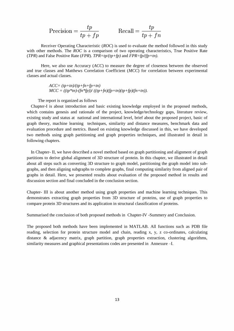
Receiver Operating Characteristic (ROC) is used to evaluate the method followed in this study

with other methods. The ROC is a comparison of two operating characteristics, True Positive Rate

(TPR) and False Positive Rate (FPR). TPR=tp/(tp+fp) and FPR=fp/(fp+tn).

Here, we also use Accuracy (ACC) to measure the degree of closeness between the observed

and true classes and Matthews Correlation Coefficient (MCC) for correlation between experimental

classes and actual classes.

ACC= (tp+tn)/(tp+fn+fp+tn)

MCC = ((tp*tn)-(fn*fp))/ ((tp+fn)(fp+tn)(tp+fp)(fn+tn)).

The report is organized as follows

Chapter-I is about introduction and basic existing knowledge employed in the proposed methods,

which contains genesis and rationale of the project, knowledge/technology gaps, literature review,

existing study and status at national and international level, brief about the proposed project, basic of

graph theory, machine learning techniques, similarity and distance measures, benchmark data and

evaluation procedure and metrics. Based on existing knowledge discussed in this, we have developed

two methods using graph partitioning and graph properties techniques, and illustrated in detail in

following chapters.

In Chapter- II, we have described a novel method based on graph partitioning and alignment of graph

partitions to derive global alignment of 3D structure of protein. In this chapter, we illustrated in detail

about all steps such as converting 3D structure to graph model, partitioning the graph model into sub-

graphs, and then aligning subgraphs to complete graphs, final computing similarity from aligned pair of

graphs in detail. Here, we presented results about evaluation of the proposed method in results and

discussion section and final concluded in the conclusion section.

Chapter- III is about another method using graph properties and machine learning techniques. This

demonstrates extracting graph properties from 3D structure of proteins, use of graph properties to

compare protein 3D structures and its application in structural classification of proteins.

Summarised the conclusion of both proposed methods in Chapter-IV -Summery and Conclusion.

The proposed both methods have been implemented in MATLAB. All functions such as PDB file

reading, selection for protein structure model and chain, reading x, y, z co-ordinates, calculating

distance & adjacency matrix, graph partition, graph properties extraction, clustering algorithms,

similarity measures and graphical presentations codes are presented in Annexure –I.

14

15

CHAPTER- II: GRAPH PARTITIONING/CLUSTERING AND ALIGNMENT

INTRODUCTION

In this chapter, a detail about novel method for comparison of 3D structure using graph

partition and alignment method has been illustrated. A novel methodology has been developed for

comparing protein structure by employing conversion of 3D graph into 2D graph, partitioning of 2D

graph into sub-graphs and then finally aligning sub-graphs to structure. Also, structure similarity has

been calculated by identifying local structural similarities to global structural similarity. The proposed

method has been implemented in MATLAB by writing codes for various functions. The performance

of the developed methodology is tested with two existing best methods such as CE and jFATCAT on

100 proteins benchmark dataset with SCOP (Structural Classification Of Proteins) database. The

proposed method has shown significant improvement over jFATCAT and accuracy has increased up

to 12-15%.

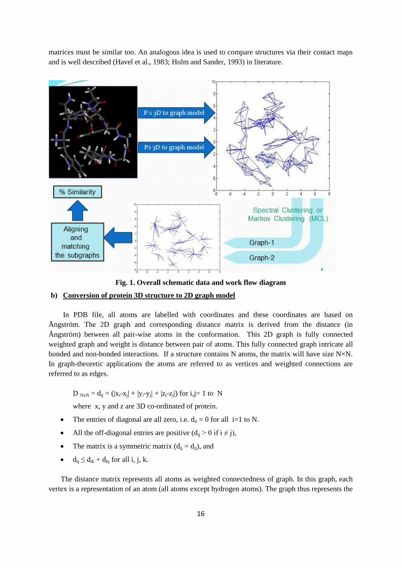
MATERIAL AND METHODS

An algorithm has been developed to calculate the similarity between two protein structure

(Figure 1) based on i) Representing 3D protein structure into 2D graph model, ii) Partitioning the

graph models into sub-graphs and iii) aligning the sub-graphs between pair of proteins. The

information in 2D model is comprehensive and can be perceived to a 3D protein model. It is also

observed that information about geometric and molecular properties in 3D are lost upon

representation of a protein structure from 3D to 2D, but favourable interactions between atoms are

carried (Pietal et al. 2015). The favourable interactions tend to be preserved in physico-chemical and

evolutionary evolution reflections. Also these interactions are covalent bonds, Ionic bonds, Hydrogen

bonds and Hydrophobic interactions, Van der Waals forces that represent transient and weak electrical

attraction of one atom to another and common contact due to chemical interactions. 2D graph model

is an adjacency or distance matrix of all atoms means NXN matrix, where N is number of atoms in the

3D structure. The matrix is an undirected weighted graph model. This graph has been decomposed

into subgraphs using graph partitioning/clustering algorithm. These partitioning on principal of

retaining connection between atoms having strong interaction and discard connections of weak

interaction atoms. Further, it is identified isomorphism of sub-graphs of two proteins and finally

alignment has been done based on similarity between sub-graphs (Figure-1).

a) Basic concepts

A graph G=[V,E] in context of protein 3D structure is defined as an ordered pair consisting of two

sets V and E, where V represents a set of vertices or atoms and E is a set of edges and weighted

distances in set V. The edges of the graph are discriminated from each other by giving different

weights for each of them for calculating Euclidian distance between atoms.

In this, the protein 3D structure is represented as a graph models in terms of 2D distance matrices.

The distance matrix of a protein D= dij is the Euclidean distances between all pairs (i, j) of its atoms.

The matrix provides a 2D representation of a 3D structure, and contains enough information for

retrieving the actual structure, except for overall chirality (Havel et al.1983, Holm and Sander 1993).

The idea underlying DALI (Holm 1993) is that if two structures are similar, then their distance

16

matrices must be similar too. An analogous idea is used to compare structures via their contact maps

and is well described (Havel et al., 1983; Holm and Sander, 1993) in literature.

Fig. 1. Overall schematic data and work flow diagram

b) Conversion of protein 3D structure to 2D graph model

In PDB file, all atoms are labelled with coordinates and these coordinates are based on

Ångström. The 2D graph and corresponding distance matrix is derived from the distance (in

Ångström) between all pair-wise atoms in the conformation. This 2D graph is fully connected

weighted graph and weight is distance between pair of atoms. This fully connected graph intricate all

bonded and non-bonded interactions. If a structure contains N atoms, the matrix will have size N×N.

In graph-theoretic applications the atoms are referred to as vertices and weighted connections are

referred to as edges.

D NxN = dij = (|xi-xj| + |yi-yj| + |zi-zj|) for i,j= 1 to N

where x, y and z are 3D co-ordinated of protein.

The entries of diagonal are all zero, i.e. dii = 0 for all i=1 to N.

All the off-diagonal entries are positive (dij > 0 if i ≠ j),

The matrix is a symmetric matrix (dij = dji), and

dij ≤ dik + dkj for all i, j, k.

The distance matrix represents all atoms as weighted connectedness of graph. In this graph, each

vertex is a representation of an atom (all atoms except hydrogen atoms). The graph thus represents the

17

mathematical relation of spatial proximity for all atoms pairs in 3D space. The proposed distance

function is simple Euclidean distance as real values.

For a typical protein of length 200 amino acids, these 200 amino acids of protein 3D structures are

converted to corresponding distance matrix. This conversion using MATLAB usually takes less than

one second. A visualization of a protein distance matrix is shown in Figure 2.

Figure 2. Example distance matrix

c) Partitioning of the graph model into sub-graphs

Partitioning of graph into subgraphs is done by clustering of nodes /atoms. Subgraph

isomorphism are leads to fold, pattern identification, structural motif recognition. Subgraph is

important for function as binding site, structure, folding and identification of similar folds. This will

finally help to build or generate knowledge between graph topological and physical properties to

protein function.

Identification of clusters is an important operation carried out in the field of unsupervised

classification and it requires several iterative steps to complete clustering. Spectral and MCL (Markov

Clustering) techniques are popular and used as a general techniques for graph partitioning. Graph

spectral method is an important technique and yield unique results by a single numeric computation

(Hagen and Kahng, 1992). Further, it can also be used to get clustering information on weighted

graphs. These concepts are adopted to obtain non-bonded clusters in protein structures (Kannan and

Vishveshwara, 1999; Patra and Vishveshwara, 2000)

The structure of proteins is governed to a large extent by non-covalent, but non-bonded

interactions are conferring unique three-dimensional structures of proteins. Analysis of the topological

details of atoms in proteins using the clustering analysis, specifically non-bonded atoms in a cluster

leads to decipher knowledge of structural confirmation, fold and function.

Detection of clusters/subgraph and isomorphism among them is influential procedure in

protein structure comparison. Since graph partitioning is a hard problem and one of the main research

areas in clustering. As discussed in disadvantages for optimal size of decomposition of protein

structure in aligning SSE approach, we have introduced automatic decomposition of structure into

sub-structures. There are two broad categories of methods namely local and global methods. Local

18

methods are the random initial partitioning of the vertex set and rely on properties of initial partitions,

which can affect the quality of final solution. Global methods rely on properties of the entire graph.

The most common algorithms on global properties are spectral partitioning and Markov Chain

Clustering (MCL) as Algorithm-2 (Stijn van Dongen, 2000).

Two algorithms Spectral (Algorithm-1) and MCL (Algorithm-2) have been used in the

proposed method. In view of time complexity and accuracy, MCL performed well compared to

Spectral as mentioned in the literature. In spectral clustering, number of clusters and size of clusters

are influenced by length of the protein, but MCL produces clusters in small range of variation in

cluster size and this variation indicates class of proteins.

The eigen values and eigen vectors of adjacent or distance matrix associated with a graph are

most important graph spectral parameters, which provide information on the structure and topology of

the graph and analysis. Graph spectra are also extensively used in chemical graph theory to derive

topological indices such as the resonance energy, molecular orbital energy and topology of electron

systems. There is no unique way of identifying graph isomorphism. Graph spectral analysis is one of

prime technique in isomorphism. Graph spectral analysis gives information on isomorphism and

isomorphic graphs have the same spectra (Vishveshwara et al. 2002).

In view of above points, we have employed two graph partitioning or clustering algorithm to

extrication a graph into subgraphs. These clusters exhibit properties of folding, non-bonded

interaction and conserved motifs, which are more frequently observed as properties for 3D structure

confirmation.

Algorithms of Spectral and MCL

Algorithm 1. Automatic spectral clustering (Sanguinetti et. al., 2005)

Given a dataset consisting of n x n symmetric similarity matrix.

1. Form an affinity matrix of the order nxn .

2. Normalize (Laplacian matrix) L=D-½

S D-½.

3. Compute k eigen vectors with the largest eigen values of the matrix L and form a matrix X of

order nxk.

4. Initialize q =2 and two centers from rows of matrix X on maximum value in the 1st and 2

nd

column.

5. Select the first q columns from matrix X and assemble them in n x q as Matrix Y and initialize

(q+1)th center at the origin.

6. Perform automated k-means clustering with q+1 centers on Y (Use Weighted Mahalanobis

Distance procedure).

7. If the (q+1)th

cluster contains any data points, then there must be at least one extra cluster

and (q+1)<given maximum no. of clusters then set q=q+1 and go back to step 5. Otherwise,

end the algorithm.

19

Procedure. Weighted Mahalanobis Distance (Khaled and Younis 1995; Mao and Jain 1996)

1. For each ci, compute the distance of all points x from it as follows:

If ciciT> 0 if the centre is not the origin

e-dist(x,ci)=(x-ci) M (x-ci) T

where M=(I – λ) (ciTci + Iλ)

-1

Here λ is the sharpness parameter that controls the elongation (if greater, the clusters are

more elongated )

If the centre is very near the origin, ciciT<e, the distances are measured using the Euclidean

distance.

2. Using this distance measure, assign each point x to the nearest centre. Update the location

for each centre by taking the mean of all the data assigned to it.

3. Return to step 1 and repeat until there is no change in the location.

Algorithm 2. Markov Chain clustering (Stijn van Dongen 2000; Enright et al 2002)

1. G is a graph and create the adjacent matrix

2. set Γ to some value for granularity

3. set M_1 to be the matrix of random walks on G

4. Normalize the matrix

5. Initialize change=1

6. while (change)

{

M_2 = M_1 * M_1 //expansion

M_1 = Γ(M_2) // inflation

change = difference(M_1, M_2)

}

7. Interpret resulting matrix to discover clusters of M_1

d) Aligning the sub-graphs between pair of proteins and similarity measure

Two protein graphs can be compared by graph isomorphism detection method, which leads

sharing common confirmation. A number of heuristic methods are available for searching a subgraph

in the given graph. Tree searching algorithm compares successive subgraph isomorphism by

superimposing the graph one over another. The superimpose areas are structurally similar, which may

involve structural/functional commonalities.

Two sub-graphs of the same number of nodes (N), they represent two sets of pairwise

interaction matrix of size NxN such as if there a connectivity, the value is set as 1(one) otherwise 0

(zero). The comparison of two graphs by comparing the induced set of 0 or 1 showed the connectivity

of nodes among subgraphs. Let the clusters of protein-1 and protein-2 are represented by graph G1

20

and graph G2 respectively. We construct the graph connectivity/interaction matrix G1, by computing

the connectivity between each pair of elements i, j ∈ Ck. The connectivity between the two elements i,

j, denoted by 1 if these elements are in the same kth cluster (Ck) otherwise 0. It means that, i

th will

interact with jth if i and j are in the same cluster. Similarly, the G2 will be constructed for protein-2.

Once interaction matrix for graph G1 and G2 for all pairs of nodes have been constructed, it can find

the similarity/distance between them by using any distance or similarity measures such as Jaccard

coefficients, Kullback - Leibler distance and Tanimoto similarity measures etc. This is

superimposing of two graphs with best matching by sliding the matrices with window size minimum

(M,N). Here, f-measure calculated as harmonic mean of precision and recall. The f-measure value

shows the percentage similarity between two proteins.

Given two binary matrices, G1 and G2, the Jaccard coefficient is one of the useful measures for

overlapping of G1 and G2 with their attributes. Each attribute of G1 and G2 can either be 0 or 1. The

total number of each combination of attributes for both G1 and G2 are specified as follows:

Algorithm 3: Aligning subgraphs to complete graph and similarity measure

M11 represents the total number of attributes where G1 and G2 both are having value 1.

M01 represents the total number of attributes where the attribute of G1 is 0 and the attribute of

G2 is 1.

M01 represents the total number of attributes where the attribute of G1 is 1 and the attribute of

G2 is 0.

M00 represents the total number of attributes where G1 and G2 both have a value of 0.

The Jaccard similarity coefficient, J = M11/ (M11+ M10 + M01)

The jaccard distance dj = 1-J = ( M10 + M01) / (M11+ M10 + M01)

Precision (p) = M11/ (M11+ M10 )

Recall (r) = M11/ (M11+ M01)

f-measure = 2* p*r /(p+r)

RESULTS AND DISCUSSION

The above algorithms of the proposed method including reading of pdb file and generating

distance matrix for comparing protein structures are implemented in MATLAB. The performance of

the developed methodology has been tested and compared with two existing best methods such as CE

and jFATCAT on 100 proteins benchmark dataset with SCOP (Structural Classification Of Proteins)

(Murzin et al., 1995).

Interaction matrix represents small clusters of atoms that detect local structure similarity. This

reveals bonded and non-bonded interaction of atoms between clusters and within the clusters.

Superpositioning of two binary matrices (interaction matrix) shows the performance with global

similarity. These clusters have intrinsic topological characteristics of the structures. The proposed

method maps cluster to cluster and compares two structures by taking consideration of position of

atom in the clusters over set of residue level structural alignment. Majority of 3D structure

comparison methods are rely on only Cα atoms, but here all atoms are considered except hydrogen

atoms.

The decomposition of SSEs to scaffolds and interfaces rather than single residues could be

observed as basic interaction units in the arrangement of structure elements within a protein structure.

Similarly, the decomposition of structure to sub-structure/clusters than single residues and SSE, could

be favourable interaction of non-bonded residues within a structure as discussed above. Atom

21

positions and associations with other atoms within sub-structure are considered and complete

alignment of the structure was used to identify similar geometry and similarity of the two structures.

The proposed method showed improved performance over the existing techniques based on

classification accuracy. The reason for the improvement in the accuracy is due to inclusion of all

atoms but CE and jFATCAT used only backbone Cα atoms. Non-bonded interaction in a cluster

divulge Van der Waals forces and play important role in inclusion of folding information of protein

while comparing the 3D structures.

Clusters of bonded and non-bonded atoms It is important to note that sub-graphs in a graph would result in cluster of atoms composed

nearest bonded and non-bonded atoms and disconnection of weak bonded atoms. The Non-bonded

interactions are confirming unique three-dimensional structures to proteins. Analysis of the

topological details of atoms in proteins using the clustering analysis specifically non-bonded atoms in

a cluster leads to decipher knowledge of structural confirmation and folding of protein. The specific

interactions between different non-bonded atoms constitute the structural basis for protein stability.

The figure 3(a) sows 3D structure of protein 1tos and 3(b) represents graphical representation of 1tos.

Figure 3(c) and 3(d) depict clusters where some atoms of residues 1, 7, 8 and 10 are belong to same

cluster (5th cluster in figure 3(c) and magenta color in figure 3(d)). This indicates some non-bonded

interaction between them.

Figure 3. 3D structure of 1tos protein, Graph model, clusters of atoms and cluster presentation.

22

Similarly, later part of atoms of residues 2 are identified with atoms of residues 4 and 5.

Atoms of residues 3 and 6 belong to same cluster. Similarly some atoms of 1th and 10

th shares same

clusters. These patterns are converted into binary matrix with locations using algorithm-3. Then

similar patterns searched in another protein binary matrix. Such patterns convey interaction and 3D

confirmation of atoms in structure. Small clusters of atoms detect local structure similarity as well as

get global similarity by aligning all sub-graphs. The method maps sub-graph to sub-graph and

compares two structures by taking into account the position of atom in the clusters over residue-level

(Cα) structural alignment of existing methods. In existing methods, the quality of 3D superposition is

often measured by the number of matched Cα atoms. Automatic decomposition using graph portioning

is unique from existing fragment decomposition methods and is able to identify local structural

similarities and lead to global similarity. Folded polypeptide chain enable to even residues at precisely

different position in amino acid sequences to come into contact one another and vice-versa.

Relation between number of clusters and number of SSEs

We observed that number of amino acid and atoms in clusters range 2.5 to 3.0 and 15 to 30

respectively and significant bifurcating level of alpha-helix and beta-sheet combination in the

structures (Table 1).

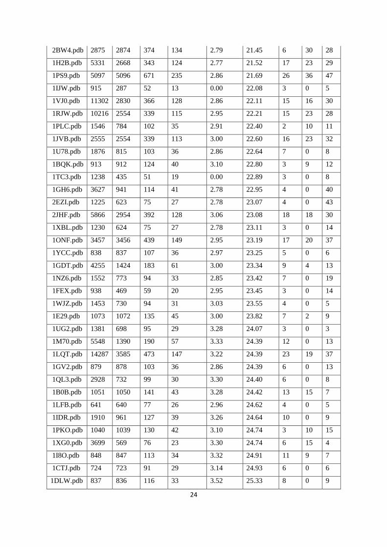
As shown in Table 1, number of atoms and residues per cluster are clearly indicated by main

class of protein structure. Number of atoms per cluster is varying with range from 16 to 20 and this

range indicated structures have influenced by β-sheet (Class B in SCOP). Numbers of atoms per

cluster are in range from 21 to 23 and this range indicated structures have influenced by α-helix and β-

sheet (Class C & D in SCOP). Similarly, α-Helix (Class –A of SCOP) are belongs to a range from 23

to 25 atoms per cluster.

Table 1. Benchmark proteins data with number of atoms and residues and sub-graphs by clustering

PDB pdb

total

atoms

No. of

atoms

in A

chain

No of

C

alpha

in A

Chain

No of

subgraphs

Ration of

no. of C-

alpha in

subgraph

Ration of

no. of

atoms in

subgraph

helix beta coil

1F56.pdb 2070 690 91 41 2.22 16.83 1 7 9

1FP5.pdb 1618 1617 208 92 2.26 17.58 5 17 29

1VCA.pdb 3106 1553 199 88 2.26 17.65 3 17 19

2OZ4.pdb 5245 2022 266 114 2.33 17.74 5 20 46

1DQT.pdb 3624 906 117 51 2.29 17.76 1 11 13

1IAM.pdb 1436 1435 185 79 2.34 18.16 2 19 48

1L6X.pdb 1949 1658 207 91 2.27 18.22 5 18 37

1ZXQ.pdb 1500 1499 192 82 2.34 18.28 3 18 21

1AOZ.pdb 8732 4366 552 237 2.33 18.42 11 32 43

1BDY.pdb 2354 960 123 52 2.37 18.46 2 8 10

1KDJ.pdb 758 757 102 41 2.49 18.46 2 8 11

UGK.pdb 2190 1090 138 59 2.34 18.47 2 8 10

1EAJ.pdb 1962 1010 124 54 2.30 18.70 2 13 23

23

HXM.pdb 13756 1611 206 86 2.40 18.73 4 18 9

1KBV.pdb 13746 2291 302 122 2.48 18.78 6 21 27

1XED.pdb 4988 865 111 46 2.41 18.80 3 8 12

1NEU.pdb 931 930 115 49 2.35 18.98 2 11 15

1JMA.pdb 2783 2053 261 108 2.42 19.01 8 14 12

1QFO.pdb 2702 901 115 47 2.45 19.17 3 11 11

1GMI.pdb 1057 1056 135 55 2.45 19.20 2 8 8

HDM.pdb 2927 1482 184 77 2.39 19.25 2 12 17

1GSK.pdb 4044 4043 502 210 2.39 19.25 10 31 40

1CCZ.pdb 1411 1410 171 73 2.34 19.32 2 16 12

2Q5B.pdb 2432 812 105 42 2.50 19.33 4 9 14

UVQ.pdb 3075 1456 182 75 2.43 19.41 2 13 16

1DN0.pdb 6594 1638 215 84 2.56 19.50 4 19 23

RLW.pdb 1001 1000 126 51 2.47 19.61 2 8 49

2ZKM.pdb 1098 986 986 50 2.47 19.61 2 8 8

1KV7.pdb 3561 3560 463 181 2.56 19.67 10 30 39

1RH8.pdb 2317 1162 142 59 2.41 19.69 4 8 5

1A25.pdb 2174 1087 132 55 2.40 19.76 8 20 26

1IUR.pdb 1511 754 88 38 2.32 19.84 3 0 3

1CID.pdb 1381 1380 177 68 2.60 20.29 1 15 16

UOW.pdb 1248 1247 156 61 2.56 20.44 4 8 22

1M6I.pdb 3525 3524 459 171 2.68 20.61 18 28 41

1DJQ.pdb 11480 5740 729 278 2.62 20.65 29 29 54

1P7I.pdb 1721 434 53 21 2.52 20.67 3 0 4

1RSY.pdb 1066 1065 135 51 2.65 20.88 3 8 22

1FCD.pdb 8724 3018 401 144 2.78 20.96 11 25 35

1FEC.pdb 7453 3743 490 178 2.75 21.03 18 25 41

1TRB.pdb 2394 2393 316 113 2.80 21.18 11 19 30

1K5N.pdb 3362 2404 285 113 2.52 21.27 7 17 24

GVD.pdb 491 490 56 23 2.43 21.30 3 0 13

1QAS.pdb 7969 3990 505 187 2.70 21.34 22 27 39

1GES.pdb 6832 3417 450 160 2.81 21.36 18 27 40

1H6V.pdb 22514 3764 490 176 2.78 21.39 19 29 37

1GTE.pdb 30878 7683 1005 359 2.80 21.40 46 54 77

1PUF.pdb 2082 664 79 31 2.55 21.42 3 0 4

24

2BW4.pdb 2875 2874 374 134 2.79 21.45 6 30 28

1H2B.pdb 5331 2668 343 124 2.77 21.52 17 23 29

1PS9.pdb 5097 5096 671 235 2.86 21.69 26 36 47

1IJW.pdb 915 287 52 13 0.00 22.08 3 0 5

1VJ0.pdb 11302 2830 366 128 2.86 22.11 15 16 30

1RJW.pdb 10216 2554 339 115 2.95 22.21 15 23 28

1PLC.pdb 1546 784 102 35 2.91 22.40 2 10 11

1JVB.pdb 2555 2554 339 113 3.00 22.60 16 23 32

1U78.pdb 1876 815 103 36 2.86 22.64 7 0 8

1BQK.pdb 913 912 124 40 3.10 22.80 3 9 12

1TC3.pdb 1238 435 51 19 0.00 22.89 3 0 8

1GH6.pdb 3627 941 114 41 2.78 22.95 4 0 40

2EZI.pdb 1225 623 75 27 2.78 23.07 4 0 43

2JHF.pdb 5866 2954 392 128 3.06 23.08 18 18 30

1XBL.pdb 1230 624 75 27 2.78 23.11 3 0 14

1ONF.pdb 3457 3456 439 149 2.95 23.19 17 20 37

1YCC.pdb 838 837 107 36 2.97 23.25 5 0 6

1GDT.pdb 4255 1424 183 61 3.00 23.34 9 4 13

1NZ6.pdb 1552 773 94 33 2.85 23.42 7 0 19

1FEX.pdb 938 469 59 20 2.95 23.45 3 0 14

1WJZ.pdb 1453 730 94 31 3.03 23.55 4 0 5

1E29.pdb 1073 1072 135 45 3.00 23.82 7 2 9

1UG2.pdb 1381 698 95 29 3.28 24.07 3 0 3

1M70.pdb 5548 1390 190 57 3.33 24.39 12 0 13

1LQT.pdb 14287 3585 473 147 3.22 24.39 23 19 37

1GV2.pdb 879 878 103 36 2.86 24.39 6 0 13

1QL3.pdb 2928 732 99 30 3.30 24.40 6 0 8

1B0B.pdb 1051 1050 141 43 3.28 24.42 13 15 7

1LFB.pdb 641 640 77 26 2.96 24.62 4 0 5

1IDR.pdb 1910 961 127 39 3.26 24.64 10 0 9

1PKO.pdb 1040 1039 130 42 3.10 24.74 3 10 15

1XG0.pdb 3699 569 76 23 3.30 24.74 6 15 4

1I8O.pdb 848 847 113 34 3.32 24.91 11 9 7

1CTJ.pdb 724 723 91 29 3.14 24.93 6 0 6

1DLW.pdb 837 836 116 33 3.52 25.33 8 0 9

25

1JBO.pdb 2541 1244 162 49 3.31 25.39 9 0 10

2EZL.pdb 1553 789 99 31 3.19 25.45 5 0 42

1H1O.pdb 2618 1318 172 51 3.37 25.84 12 0 13

1LE8.pdb 1807 414 53 16 3.31 25.88 3 0 4

1ALL.pdb 2399 1198 160 46 3.48 26.04 10 0 11

1C75.pdb 985 527 73 20 3.65 26.35 5 0 6

1FAF.pdb 1297 644 79 24 3.29 26.83 4 0 12

1S69.pdb 969 968 123 36 3.42 26.89 8 0 9

1UX8.pdb 971 970 118 36 3.28 26.94 8 0 9

1C52.pdb 1228 997 131 37 3.54 26.95 8 2 11

MBA.pdb 1083 1082 146 40 3.65 27.05 8 0 9

1H97.pdb 2343 1171 147 43 3.42 27.23 10 0 10

1ASH.pdb 1239 1238 147 45 3.27 27.51 9 0 9

1B8D.pdb 6255 1240 164 45 3.64 27.56 8 0 8

1K61.pdb 2749 486 60 17 3.53 28.59 3 0 7

1A6M.pdb 1336 1335 151 46 3.28 29.02 10 0 9

NGK.pdb 12856 1078 131 37 3.54 29.14 8 0 9

Cluster Analysis

The above analysis confirmed that by observation of non-bonded interaction found in clusters

and shows clear indication about association between secondary structures in 3D protein structure and

number clusters. Cluster analysis of benchmark SCOP data set of 100 proteins has been carried out to

compare the proposed method with CE and jFATCAT. The benchmark data has proteins belongs to

all major classes and number of residues are ranging from 51 to 1005. For cluster analysis, a number

of clustering techniques such as Hierarchical clustering, K-Means, C-Means, Spectral K-Means have

been used and various accuracy metrics are calculated. In this analysis, k-means clustering is found

suitable over other clustering techniques. Recall, Precision and f-measure are considered as accuracy

metrics. The percentage of the precise clusters indicates the performance of protein 3D structure

comparison algorithm.

To find out the potential roles of clusters in aligning and comparing two structures with

alignment location, a set of 100 proteins benchmark data has been used. Detailed analysis has been

done and compared with existing tools CE and FATCAT. Under this analysis, similarity matrix of

100x100 using proposed method has been constructed. The example data has shown in table 2.

Similarly, we have calculated similarity matrix of 100x 100 for best existing method CE and

jFATCAT. The K-means cluster technique applied to these three similarity matrices. The clustering

results are evaluated with exact classification obtained from SCOP database of benchmark data. The

cluster analysis results are presented in table 3 with recall, precision, f-measure and random index as

accuracy metrics. Significantly 97% accuracy with CE, 86% similarity with jFATCAT and proposed

method performed at 91% accuracy. The proposed algorithm is computationally expensive since it

involves up to (|M-N|+1)* Min(M,N) comparisons, where M and N are nodes of the two graphs.

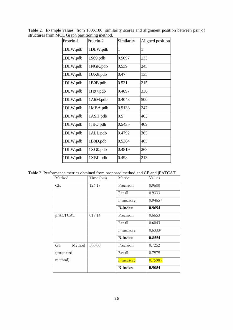
26

Table 2. Example values from 100X100 similarity scores and alignment position between pair of

structures from MCL Graph partitioning method.

Protein-1 Protein-2 Similarity Aligned position

1DLW.pdb 1DLW.pdb 1 1

1DLW.pdb 1S69.pdb 0.5097 133

1DLW.pdb 1NGK.pdb 0.539 243

1DLW.pdb 1UX8.pdb 0.47 135

1DLW.pdb 1B0B.pdb 0.531 215

1DLW.pdb 1H97.pdb 0.4697 336

1DLW.pdb 1A6M.pdb 0.4043 500

1DLW.pdb 1MBA.pdb 0.5133 247

1DLW.pdb 1ASH.pdb 0.5 403

1DLW.pdb 1JBO.pdb 0.5435 409

1DLW.pdb 1ALL.pdb 0.4792 363

1DLW.pdb 1B8D.pdb 0.5364 405

1DLW.pdb 1XG0.pdb 0.4819 268

1DLW.pdb 1XBL.pdb 0.498 213

Table 3. Performance metrics obtained from proposed method and CE and jFATCAT.

Method Time (hrs) Metric Values

CE 126.18 Precision 0.9600

Recall 0.9333

F measure 0.9465 1

R-index 0.9694

jFACTCAT 019.14 Precision 0.6653

Recall 0.6043

F measure 0.63333

R-index 0.8554

GT Method

(proposed

method)

500.00 Precision 0.7252

Recall 0.7979

F measure 0.7598 2

R-index 0.9054

27

CONCLUSIONS

In this study, a novel methodology/algorithm has been developed based on graph partitioning

technique by including 3D co-ordinates of all atoms of protein. The proposed algorithm has been

implemented in MATLAB to assess the performance of the algorithm. The methods encompass

converting 3D structure to 2D graph, partitioning of the graph into sub-graph and alignment of sub-

graphs. Prime notion of the method is the decomposition of structure to clusters than single residues

and SSE. There could be a base interaction of non-bonded residues in the arrangement of structure

elements within a structure. These interaction leads protein fold space and arrangement of SSE

elements in 3D space. The aligned structures are based on atoms positions and association with other

atoms within clusters and between clusters to identify similar geometry and similarity of the two

structures. The proposed method performed better in terms of classification accuracy due to inclusion

of all atoms but CE and jFATCAT uses only backbone C-α atoms and non-bonded atoms. This may

play an important role in inclusion of folding information of protein while comparing the 3D

structures.

28

29

CHAPTER –III: GRAPH PROPERTIES AND MACHINE LEARNING TECHNIQUES.

INTRODUCTION

Construction of graph, database of graph, graph mining, pattern recognition are rich fields of

computational techniques to study structures, topologies and properties of graphs. These techniques

provide a good asset in bioinformatics for transforming biological data into graphs and decipher

biological knowledge hidden in biological structure data. In this chapter, we have demonstrated the way

of converting a protein 3D structure into graphs using various graph properties such as total degree,

maximum degree, no of adjacencies, average number of degree, cluster coefficient, graph energy,

spectrum and number of components etc. Further, we have exploited the graph properties and data mining

technique to perform complex studies on protein 3D structure. The proposed method is fast in terms of

computational time complexity. As far as accuracy is concerned, there is an improved in proposed method

over jFATCAT method. In spite of gaining a small amount of improvement in accuracy, his method has

further scope to improve accuracy by including more graph properties.

MATERIAL AND METHODS

Basic Graph Definition

A graph is a symbolic representation of a network or connected components. It implies an

abstraction of the reality so it can be simplified as a set of linked nodes or components.

Graph theory is a branch of mathematics concerned about how networks can be encoded and their

properties are measured. It has been enriched in the last decades by growing influences of social networks

and other complex networks.

The origins of graph theory can be traced to Leonhard Euler who devised it in 1735 as a problem

that known as the "Seven Bridges of Konigsberg". In this problem, someone had to cross all the bridges

by visiting each bridge only once in a continuous sequence, a problem the Euler proved to have no

solution by representing it as a set of nodes and links. This led the foundation of graph theory and its

subsequent improvements. Initially, graph theory applications on most networks have spatial basic,

namely road, transit and rail networks. This it is not necessarily the case for all transportation networks.

Later, this has been extended to telecommunication system such as Mobile telephone networks or the

Internet. In the current time, this is being extended in bioinformatics to study the hidden phenomenon of

gene regulatory network, gene interaction, protein-protein interactions, and etc.

The transformation of protein 3D structures into graphs 2D model, it is straight forward to consider the

relevant chemical interactions of the proteins. Chemical interactions are the electrostatic forces that hold

atoms and residues together, stabilizing proteins and forming molecules that give them their 3D

confirmation. These interactions are mainly:

Covalent bonds between two atoms sharing a pair of valence electrons.

Ionic bonds between oppositely charged components.

Hydrogen bonds between two partially negative charged atoms sharing partially positive charged

hydrogen.

30

Hydrophobic interactions where hydrophobic amino acids in the protein closely link their side

chains together.

Van der Waals forces that represent transient and weak electrical attraction of one atom for

another when electrons are fluctuating.

The 2D graph model is abstraction of these properties and indeed these properties are transferred

into graph properties (Holm and Sander 1993).

A novel method has been developed to study complexity of 3D structure of protein and calculate

the similarity between two protein structures using graph properties of protein 3D structures. Figure 1

represents the workflow for the proposed method consisting of four steps namely, i) Representing 3D

protein structure into 2D graph model, ii) Calculating graph properties iii) Calculate similarity and iv)

Evaluation by cluster/classification.

Fig. 1: Workflow of proposed method

All functions regarding reading PDB file, selection of module, selection of chain and reading of

X, Y and Z coordinates, converting 3D (X, Y and Z) co-ordinates to 2D graph model, calculating all

above mentioned properties and final calculation of similarity measures are implemented in MATLAB.

For evaluating the proposed 3D structure comparison method, we have taken 100 proteins benchmark

SCOP dataset (as mentioned in Chapter-I).

Construction of Graph models

In PDB file, all atoms are labelled with coordinates and these coordinates are based on Ångström.

The 2D graph and corresponding distance matrix is derived from the distance (in Ångström) between all

31

pair wise atoms in the conformation. This 2D graph is fully connected weighted graph and weight is

denoted as distance between pair of atoms. This fully connected graph intricate all bonded and non-

bonded interactions. If a structure contains N atoms, the matrix will have size N×N. In graph-theoretic

applications, the atoms are referred to as vertices and weighted connections are referred as edges.

D NxN = dij = (|xi-xj| + |yi-yj| + |zi-zj|) for i,j= 1 to N or

DNxN=dij = ‖𝑥𝑖 − 𝑥𝑗‖22

= √(𝑥𝑖 − 𝑥𝑗 )2 + (𝑦𝑖 − 𝑦𝑗 )

2 + (𝑧𝑖 − 𝑧𝑗 )2

The entries of diagonal are all zero, i.e. dii = 0 for all i=1 to N.

All the off-diagonal entries are positive (dij > 0 if i ≠ j),

The matrix is a symmetric matrix (dij = dji), and

dij ≤ dik + dkj for all i, j, k.

Adjacency matrix dij<threshold aij=1 otherwise aij=0

The distance matrix represents all atoms as weighted connectedness of graph. In this graph, each

vertex is a representation of an atom (all atoms except hydrogen atoms). The graph thus represents the

mathematical relation of spatial proximity for all atoms pairs in 3D space. The distance function used in

the study is simple Euclidean distance by considering its real values.

For a typical protein of length 200 amino acids, these 200 amino acids of protein 3D structure is

converted to corresponding distance matrix. This conversion using MATLAB usually takes less than one

second. A visualization of a protein distance matrix is shown in Figure 2. A visualization of adjacency

matrix shown in Figure 3.

Fig. 2: Example distance matrix

32

Figure 3: Example adjacency matrix

Graph properties

We have considered both above graph matrices for calculation of following properties to study

the complexity of 3D structure

1. Average degree deg(G): Minimum and maximum by degrees of all nodes.

deg (𝐺) =1

𝑛∑(deg (𝑢𝑖)

𝑛

𝑖=1

)

deg(ui) is degree of node ui and n is total number of nodes in the graph G. Similarly,

minimum and maximum degree in the graph G can also be calculated

2. Algebraic connectivity of a graph: the second smallest eigenvalue of the Laplacian.

3. Average path length for a network (The average shortest path): Calculate length of the shortest

paths between u and every other node v in G and then calculate average path by summation of all

shortest path and divide by nxn.

4. Clustering coefficient: This is based on triangle motifs count and local clustering.

𝑐(𝑢) =2𝑒𝑢

𝑘𝑢(𝑘𝑢 − 1)

𝐶(𝐺) =1

𝑛∑ 𝑐(𝑢𝑖)

𝑛

𝑖=1

where ku is the number of neighbors of u and eu is the number of connected pairs of neighbors

5. The ith component of the eigenvector corresponding to the greatest eigen value.

6. Graph energy defined as: the sum of the absolute values of the real components of the

eigenvalues.

7. The eigenvalues of the Laplacian of the graph (2nd

to 6th eigenvalues).

8. Closeness centrality: Tracks how close a given node is to any other node. The closeness centrality

measures how fast information spreads from a given node to other reachable nodes in the graph.

For a node u, it represents the reciprocal of the average shortest path length between u and every

other reachable node in the graph.

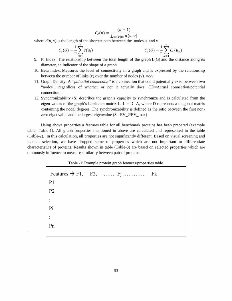
33

𝐶𝑐(𝑢) =(𝑛 − 1)

∑ 𝑑(𝑢, 𝑣)𝑣𝑠(𝑉|𝑢)

where d(u, v) is the length of the shortest path between the nodes u and v.

𝐶𝑐(𝐺) =1

𝑛∑ 𝑐(𝑢𝑖)

𝑛

𝑖=1

𝐶𝑐(𝐺) =1

𝑛∑ 𝐶𝑐(𝑢𝑘)

𝑛

𝑘=1

9. Pi Index: The relationship between the total length of the graph L(G) and the distance along its

diameter, an indicator of the shape of a graph.

10. Beta Index: Measures the level of connectivity in a graph and is expressed by the relationship

between the number of links (e) over the number of nodes (v). =e/v

11. Graph Density: A “potential connection” is a connection that could potentially exist between two

“nodes”, regardless of whether or not it actually does. GD=Actual connection/potential

connection.

12. Synchronizability (S) describes the graph’s capacity to synchronize and is calculated from the

eigen values of the graph’s Laplacian matrix L, L = D -A, where D represents a diagonal matrix

containing the nodal degrees. The synchronizability is defined as the ratio between the first non-

zero eigenvalue and the largest eigenvalue (S= EV_2/EV_max)

Using above properties a features table for all benchmark proteins has been prepared (example

table- Table-1). All graph properties mentioned in above are calculated and represented in the table

(Table-2). In this calculation, all properties are not significantly different. Based on visual screening and

manual selection, we have dropped some of properties which are not important to differentiate

characteristics of proteins. Results shown in table (Table-3) are based on selected properties which are

ominously influence to measure similarity between pair of proteins.

Table -1:Example protein graph features/properties table.

.

Features F1, F2, …… Fj …………. Fk

P1

P2

:

Pi

:

Pn

34

Table 2. All graph properties as described above of all benchmark data

Total

deg

Max

deg

Min

deg

no of

adjanc

es

algebric

connecti

vity

Ave_no

Deg

totaldeg1

Max

deg1

Min

deg1

Ave

path

length

Ave

degree

cluster

coeff1

cluster

coeff

dia

mete

r

max

eigence

ntrality

Graph

energy

Radi

us

spectru

m

no of

conne

ct

comps

1BRF.pdb 1836 8 3 1424 0.0002 1447.411 5.6667 2.3333 56.6069 4.4563 1.2422

0.850

2 161 0.4672 578.9776 81 7.1221 1

1BC9.pdb 23500 14 4 20239 0.0018 20938.04 8.8 3.5 21.3405 7.2064 0.5711 0.763 64 0.2707 5733.5 33 13.2302 1

1DI1.pdb 20886 7 3 16195 0 16460.73 5.5 2.3333 Inf 4.4524 1.2867

0.853

9 Inf 0.4462 6540.889 Inf 6.4555 5

1dly.pdb 4148 7 3 3214 0 3269.469 5.5 2.3333 122.39 4.4411 1.2834

0.854

8 366 0.4462 1301.86 183 6.3701 1

1ecd.pdb 4698 8 3 3651 0 3706.316 5.6667 2.3333

137.424

5 4.4871 1.2611

0.851

3 410 0 1471.192 205 7.1221 1

1EHS.pdb 6360 14 3 5313 0.0001 5524.963 7.875 2.3333 45.8564 6.0745 0.6806

0.816

1 156 0.2386 1648.759 78 13.0974 1

1FQT.pdb 8226 11 3 6469 0 6587.333 8.3333 2.3333 Inf 4.6818 1.1123 0.852 Inf 0.372 2481.342 Inf 10.3512 2

1gvh.pdb 13794 7 3 10698 0 10871.88 5.5 2.3333

399.970

4 4.4554 1.2859

0.853

2

119

1 0.4462 4329.277 596 6.2547 2

1H3E.pdb 23494 8 3 18414 0 18884.76 6 2.3333 Inf 4.6248 1.0919

0.847

1 Inf 0.4265 7295.912 Inf 7.6006 5

1hbi.pdb 23428 9 3 18348 0 18804.33 6.4286 2.3333 Inf 4.6118 1.0863

0.845

9 Inf 0 7301.391 Inf 8.3593 6

1IAA.pdb 23470 8 3 18390 0 18847.25 6.25 2.3333 Inf 4.6201 1.0897

0.845

8 Inf 0.4163 7296.313 Inf 7.7878 5

1IAB.pdb 23462 8 3 18382 0 18837.55 6.25 2.3333 Inf 4.6185 1.0898

0.845

7 Inf 0.4163 7297.86 Inf 7.7878 5

1IAC.pdb 23488 8 3 18408 0 18868.05 6.25 2.3333 Inf 4.6236 1.0867

0.845

7 Inf 0.4163 7302.569 Inf 7.7878 5

1IQW.pdb 23334 8 3 18254 0 18713.54 6 2.3333 Inf 4.5933 1.0737

0.843

6 Inf 0.4265 7318.565 Inf 7.6006 5

1JHK.pdb 23380 8 3 18300 0 18765.76 6 2.3333 Inf 4.6024 1.0746

0.844

2 Inf 0.4265 7315.21 Inf 7.6006 7

1K9O.pdb 22720 8 3 17640 0 17978.15 6 2.3333 Inf 4.4724 1.207

0.851

1 Inf 0.4294 7160.792 Inf 7.5995 5

1KA8.pdb 22632 8 3 17552 0 17863.14 6 2.3333 Inf 4.4551 1.2209

0.847

9 Inf 0 7173.011 Inf 7.5995 3

1mbd.pdb 22776 8 3 17696 0 18017.1 6 2.3333 Inf 4.4835 1.2228

0.849

7 Inf 0 7173.021 Inf 7.5995 3

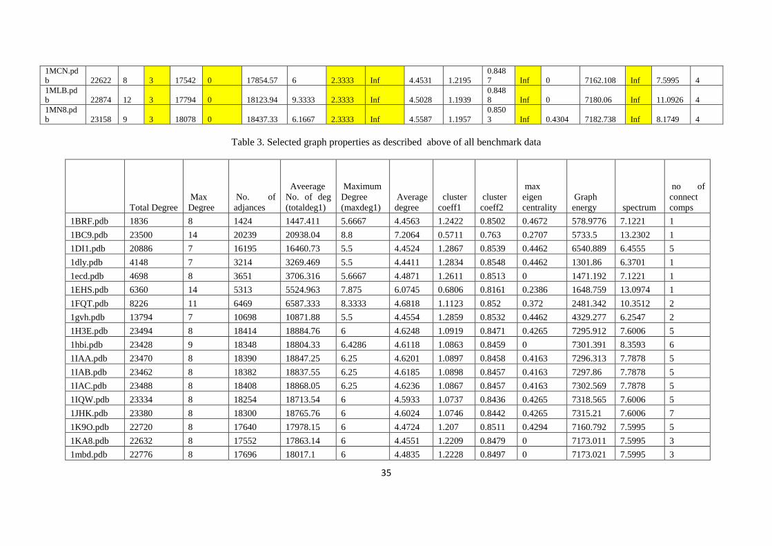
35

1MCN.pd

b 22622 8 3 17542 0 17854.57 6 2.3333 Inf 4.4531 1.2195

0.848

7 Inf 0 7162.108 Inf 7.5995 4

1MLB.pd

b 22874 12 3 17794 0 18123.94 9.3333 2.3333 Inf 4.5028 1.1939

0.848

8 Inf 0 7180.06 Inf 11.0926 4

1MN8.pd

b 23158 9 3 18078 0 18437.33 6.1667 2.3333 Inf 4.5587 1.1957

0.850

3 Inf 0.4304 7182.738 Inf 8.1749 4

Table 3. Selected graph properties as described above of all benchmark data

Total Degree

Max

Degree

No. of

adjances

Aveerage

No. of deg

(totaldeg1)

Maximum

Degree

(maxdeg1)

Average

degree

cluster

coeff1

cluster

coeff2

max

eigen

centrality

Graph

energy spectrum

no of

connect

comps

1BRF.pdb 1836 8 1424 1447.411 5.6667 4.4563 1.2422 0.8502 0.4672 578.9776 7.1221 1

1BC9.pdb 23500 14 20239 20938.04 8.8 7.2064 0.5711 0.763 0.2707 5733.5 13.2302 1

1DI1.pdb 20886 7 16195 16460.73 5.5 4.4524 1.2867 0.8539 0.4462 6540.889 6.4555 5

1dly.pdb 4148 7 3214 3269.469 5.5 4.4411 1.2834 0.8548 0.4462 1301.86 6.3701 1

1ecd.pdb 4698 8 3651 3706.316 5.6667 4.4871 1.2611 0.8513 0 1471.192 7.1221 1

1EHS.pdb 6360 14 5313 5524.963 7.875 6.0745 0.6806 0.8161 0.2386 1648.759 13.0974 1

1FQT.pdb 8226 11 6469 6587.333 8.3333 4.6818 1.1123 0.852 0.372 2481.342 10.3512 2

1gvh.pdb 13794 7 10698 10871.88 5.5 4.4554 1.2859 0.8532 0.4462 4329.277 6.2547 2

1H3E.pdb 23494 8 18414 18884.76 6 4.6248 1.0919 0.8471 0.4265 7295.912 7.6006 5

1hbi.pdb 23428 9 18348 18804.33 6.4286 4.6118 1.0863 0.8459 0 7301.391 8.3593 6

1IAA.pdb 23470 8 18390 18847.25 6.25 4.6201 1.0897 0.8458 0.4163 7296.313 7.7878 5

1IAB.pdb 23462 8 18382 18837.55 6.25 4.6185 1.0898 0.8457 0.4163 7297.86 7.7878 5

1IAC.pdb 23488 8 18408 18868.05 6.25 4.6236 1.0867 0.8457 0.4163 7302.569 7.7878 5

1IQW.pdb 23334 8 18254 18713.54 6 4.5933 1.0737 0.8436 0.4265 7318.565 7.6006 5

1JHK.pdb 23380 8 18300 18765.76 6 4.6024 1.0746 0.8442 0.4265 7315.21 7.6006 7

1K9O.pdb 22720 8 17640 17978.15 6 4.4724 1.207 0.8511 0.4294 7160.792 7.5995 5

1KA8.pdb 22632 8 17552 17863.14 6 4.4551 1.2209 0.8479 0 7173.011 7.5995 3

1mbd.pdb 22776 8 17696 18017.1 6 4.4835 1.2228 0.8497 0 7173.021 7.5995 3

36

1MCN.pdb 22622 8 17542 17854.57 6 4.4531 1.2195 0.8487 0 7162.108 7.5995 4

1MLB.pdb 22874 12 17794 18123.94 9.3333 4.5028 1.1939 0.8488 0 7180.06 11.0926 4

1MN8.pdb 23158 9 18078 18437.33 6.1667 4.5587 1.1957 0.8503 0.4304 7182.738 8.1749 4

1oj6.pdb 22708 8 17628 17944.05 6 4.4701 1.2457 0.8516 0 7131.944 7.5995 3

1P4X.pdb 22644 8 17564 17868.16 6 4.4575 1.2574 0.8522 0 7119.181 7.5995 3

1PSR.pdb 22922 9 17842 18147.06 6.75 4.5122 1.2386 0.8521 0.4215 7132.165 8.5654 3

1PZ8.pdb 24598 8 19114 19446.47 5.8333 4.4854 1.2856 0.8567 0 7638.606 7.3923 8

1PZ9.pdb 24696 8 19212 19549.95 5.8333 4.5033 1.2779 0.857 0 7644.012 7.3923 6

1QGJ.pdb 25724 10 20240 20625.08 7.7778 4.6907 1.0913 0.8532 0.3357 7660.732 10.144 3

1QN2.pdb 25176 10 19692 20051.9 7.7778 4.5908 1.142 0.8527 0.3357 7677.794 10.144 4

1QUU.pdb 25300 10 19816 20165.28 7.7778 4.6134 1.1622 0.8551 0.3357 7643.699 10.144 3

1RIE.pdb 25298 10 19814 20168.53 7.7778 4.6131 1.1525 0.854 0.3357 7658.223 10.144 2

1RQI.pdb 24518 9 19034 19351.2 6.4286 4.4708 1.2866 0.8565 0.4088 7635.934 8.4238 3

1rte.pdb 24916 11 19432 19773.44 7.9 4.5434 1.2082 0.8555 0.3576 7657.405 10.2365 3

1TOS.pdb 25208 12 19724 20093.07 7.9 4.5966 1.1552 0.8544 0.3576 7688.755 11.2812 3

1urv.pdb 25080 12 19596 19939.4 9.7273 4.5733 1.1554 0.8537 0.302 7690.002 12.2145 3

1ux8.pdb 25168 12 19684 20032.65 9.7273 4.5894 1.1512 0.8537 0.302 7692.64 12.2145 3

1VCK.pdb 25102 12 19618 19967.82 9.7273 4.5773 1.1526 0.8538 0.302 7691.909 12.2145 3

1WOV.pdb 24474 8 18990 19308.61 5.8333 4.4628 1.2808 0.855 0 7655.166 7.3923 4

1WOW.pdb 24390 8 18906 19230.68 5.8333 4.4475 1.2902 0.8555 0 7642.503 7.3923 5

1WOX.pdb 24404 8 18920 19244.7 5.8333 4.45 1.2893 0.8555 0 7640.233 7.3923 5

1X3A.pdb 28568 14 23084 23674.4 8.5 5.2093 0.7899 0.8321 0.3108 8163.846 7.3923 5

1XG7.pdb 17234 8 13352 13578.19 5.5 4.4395 1.2667 0.8526 0 5430.895 7.0947 11

1Y2O.pdb 17054 7 13172 13379.18 5.5 4.3931 1.3228 0.8557 0.4462 5392.577 6.3078 16

1YLL.pdb 28898 11 22788 23214.12 8.4 4.7296 1.1276 0.8557 0.3538 8548.02 10.7331 12

1YV0.pdb 28120 10 22010 22388.49 7.7778 4.6023 1.1933 0.8549 0.3844 8541.531 9.6247 8

1Z77.pdb 28012 10 21902 22284.98 7.7778 4.5846 1.1902 0.8542 0.3844 8547.656 9.6247 14

2A1K.pdb 27852 10 21742 22120.06 7.7778 4.5584 1.1969 0.8535 0.3844 8544.077 9.6247 6

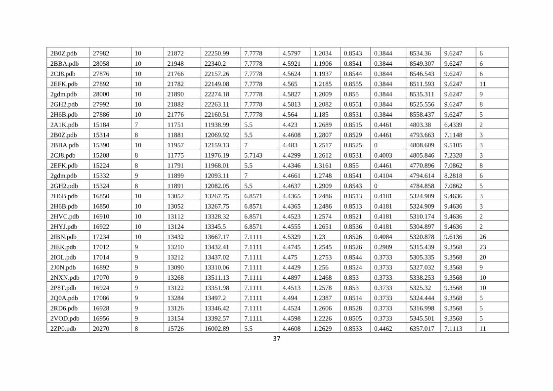
37

2B0Z.pdb 27982 10 21872 22250.99 7.7778 4.5797 1.2034 0.8543 0.3844 8534.36 9.6247 6

2BBA.pdb 28058 10 21948 22340.2 7.7778 4.5921 1.1906 0.8541 0.3844 8549.307 9.6247 6

2CJ8.pdb 27876 10 21766 22157.26 7.7778 4.5624 1.1937 0.8544 0.3844 8546.543 9.6247 6

2EFK.pdb 27892 10 21782 22149.08 7.7778 4.565 1.2185 0.8555 0.3844 8511.593 9.6247 11

2gdm.pdb 28000 10 21890 22274.18 7.7778 4.5827 1.2009 0.855 0.3844 8535.311 9.6247 9

2GH2.pdb 27992 10 21882 22263.11 7.7778 4.5813 1.2082 0.8551 0.3844 8525.556 9.6247 8

2H6B.pdb 27886 10 21776 22160.51 7.7778 4.564 1.185 0.8531 0.3844 8558.437 9.6247 5

2A1K.pdb 15184 7 11751 11938.99 5.5 4.423 1.2689 0.8515 0.4461 4803.38 6.4339 2

2B0Z.pdb 15314 8 11881 12069.92 5.5 4.4608 1.2807 0.8529 0.4461 4793.663 7.1148 3

2BBA.pdb 15390 10 11957 12159.13 7 4.483 1.2517 0.8525 0 4808.609 9.5105 3

2CJ8.pdb 15208 8 11775 11976.19 5.7143 4.4299 1.2612 0.8531 0.4003 4805.846 7.2328 3

2EFK.pdb 15224 8 11791 11968.01 5.5 4.4346 1.3161 0.855 0.4461 4770.896 7.0862 8

2gdm.pdb 15332 9 11899 12093.11 7 4.4661 1.2748 0.8541 0.4104 4794.614 8.2818 6

2GH2.pdb 15324 8 11891 12082.05 5.5 4.4637 1.2909 0.8543 0 4784.858 7.0862 5

2H6B.pdb 16850 10 13052 13267.75 6.8571 4.4365 1.2486 0.8513 0.4181 5324.909 9.4636 3

2H6B.pdb 16850 10 13052 13267.75 6.8571 4.4365 1.2486 0.8513 0.4181 5324.909 9.4636 3

2HVC.pdb 16910 10 13112 13328.32 6.8571 4.4523 1.2574 0.8521 0.4181 5310.174 9.4636 2

2HYJ.pdb 16922 10 13124 13345.5 6.8571 4.4555 1.2651 0.8536 0.4181 5304.897 9.4636 2

2IBN.pdb 17234 10 13432 13667.17 7.1111 4.5329 1.23 0.8526 0.4084 5320.878 9.6136 26

2IEK.pdb 17012 9 13210 13432.41 7.1111 4.4745 1.2545 0.8526 0.2989 5315.439 9.3568 23

2IOL.pdb 17014 9 13212 13437.02 7.1111 4.475 1.2753 0.8544 0.3733 5305.335 9.3568 20

2J0N.pdb 16892 9 13090 13310.06 7.1111 4.4429 1.256 0.8524 0.3733 5327.032 9.3568 9

2NXN.pdb 17070 9 13268 13511.13 7.1111 4.4897 1.2468 0.853 0.3733 5338.253 9.3568 10

2P8T.pdb 16924 9 13122 13351.98 7.1111 4.4513 1.2578 0.853 0.3733 5325.32 9.3568 10

2Q0A.pdb 17086 9 13284 13497.2 7.1111 4.494 1.2387 0.8514 0.3733 5324.444 9.3568 5

2RD6.pdb 16928 9 13126 13346.42 7.1111 4.4524 1.2606 0.8528 0.3733 5316.998 9.3568 5

2VOD.pdb 16956 9 13154 13392.57 7.1111 4.4598 1.2226 0.8505 0.3733 5345.501 9.3568 5

2ZP0.pdb 20270 8 15726 16002.89 5.5 4.4608 1.2629 0.8533 0.4462 6357.017 7.1113 11

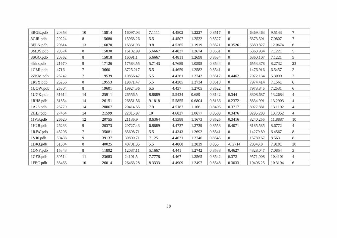
38

3BGE.pdb 20358 10 15814 16097.03 7.1111 4.4802 1.2227 0.8517 0 6369.463 9.5143 7

3CJR.pdb 20224 8 15680 15968.26 5.5 4.4507 1.2522 0.8527 0 6373.501 7.0807 7

3ELN.pdb 20614 13 16070 16361.93 9.8 4.5365 1.1919 0.8521 0.3526 6380.827 12.0674 6

3MDS.pdb 20374 8 15830 16102.99 5.6667 4.4837 1.2674 0.8531 0 6363.934 7.1221 5

3SGO.pdb 20362 8 15818 16091.1 5.6667 4.4811 1.2698 0.8534 0 6360.107 7.1221 5

4hhb.pdb 21670 9 17126 17583.55 5.7143 4.7689 1.0598 0.8544 0 6553.378 8.2732 23

1GMI.pdb 4716 7 3660 3725.217 5.5 4.4659 1.2582 0.8541 0 1476.916 6.5457 2

2ZKM.pdb 25242 7 19539 19856.47 5.5 4.4261 1.2742 0.8517 0.4462 7972.134 6.3099 7

1RSY.pdb 25256 8 19553 19871.47 5.5 4.4285 1.2734 0.8518 0 7974.414 7.1561 6

1UOW.pdb 25304 8 19601 19924.36 5.5 4.437 1.2705 0.8522 0 7973.845 7.2531 6

1UGK.pdb 31614 14 25911 26556.5 8.8889 5.5434 0.689 0.8142 0.344 8808.687 13.2684 4

1RH8.pdb 31854 14 26151 26851.56 9.1818 5.5855 0.6804 0.8136 0.2372 8834.991 13.2903 4

1A25.pdb 25770 14 20067 20414.55 7.9 4.5187 1.166 0.8496 0.3717 8027.881 13.1192 4

2JHF.pdb 27464 14 21599 22015.97 10 4.6827 1.0677 0.8503 0.3476 8295.283 13.7352 4

1JVB.pdb 26620 12 20755 21136.9 8.6364 4.5388 1.1673 0.8525 0.3416 8240.255 11.8887 10

1H2B.pdb 26238 9 20373 20727.43 6.8889 4.4737 1.2739 0.8553 0.4071 8185.585 8.6772 4

1RJW.pdb 45296 7 35081 35698.71 5.5 4.4343 1.2692 0.8541 0 14279.89 6.4567 8

1VJ0.pdb 50438 9 39137 39800.71 7.125 4.4631 1.2746 0.8545 0 15780.67 8.663 8

1DJQ.pdb 51504 8 40025 40701.35 5.5 4.4868 1.2819 0.855 -0.2714 20343.8 7.9181 20

1ONF.pdb 15348 8 11892 12087.11 5.1667 4.441 1.2742 0.8538 0.4627 4828.047 7.0854 3

1GES.pdb 30514 11 23683 24101.5 7.7778 4.467 1.2565 0.8542 0.372 9571.008 10.4101 4

1FEC.pdb 33466 10 26014 26463.28 8.3333 4.4909 1.2497 0.8548 0.3033 10406.25 10.3194 6

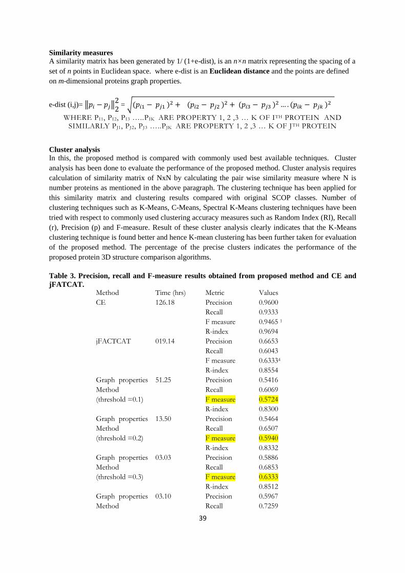
39

Similarity measures

A similarity matrix has been generated by 1/ (1+e-dist), is an n×n matrix representing the spacing of a

set of n points in Euclidean space. where e-dist is an Euclidean distance and the points are defined

on m-dimensional proteins graph properties.

e-dist (i,j)= ‖𝑝𝑖 − 𝑝𝑗‖22

= √(𝑝𝑖1 − 𝑝𝑗1 )2 + (𝑝𝑖2 − 𝑝𝑗2 )

2 + (𝑝𝑖3 − 𝑝𝑗3 )2 … . (𝑝𝑖𝑘 − 𝑝𝑗𝑘 )

2

WHERE PI1, PI2, PI3 …..PIK ARE PROPERTY 1, 2 ,3 … K OF ITH PROTEIN AND SIMILARLY PJ1, PJ2, PJ3 …..PJK ARE PROPERTY 1, 2 ,3 … K OF JTH PROTEIN

Cluster analysis

In this, the proposed method is compared with commonly used best available techniques. Cluster

analysis has been done to evaluate the performance of the proposed method. Cluster analysis requires

calculation of similarity matrix of NxN by calculating the pair wise similarity measure where N is

number proteins as mentioned in the above paragraph. The clustering technique has been applied for

this similarity matrix and clustering results compared with original SCOP classes. Number of

clustering techniques such as K-Means, C-Means, Spectral K-Means clustering techniques have been

tried with respect to commonly used clustering accuracy measures such as Random Index (RI), Recall

(r), Precision (p) and F-measure. Result of these cluster analysis clearly indicates that the K-Means

clustering technique is found better and hence K-mean clustering has been further taken for evaluation

of the proposed method. The percentage of the precise clusters indicates the performance of the

proposed protein 3D structure comparison algorithms.

Table 3. Precision, recall and F-measure results obtained from proposed method and CE and

jFATCAT. Method Time (hrs) Metric Values

CE 126.18 Precision 0.9600

Recall 0.9333

F measure 0.9465 1

R-index 0.9694

jFACTCAT 019.14 Precision 0.6653

Recall 0.6043

F measure 0.63334

R-index 0.8554

Graph properties

Method

(threshold =0.1)

51.25 Precision 0.5416

Recall 0.6069

F measure 0.5724

R-index 0.8300

Graph properties

Method

(threshold =0.2)

13.50 Precision 0.5464

Recall 0.6507

F measure 0.5940

R-index 0.8332

Graph properties

Method

(threshold =0.3)

03.03 Precision 0.5886

Recall 0.6853

F measure 0.6333

R-index 0.8512

Graph properties

Method

03.10 Precision 0.5967

Recall 0.7259

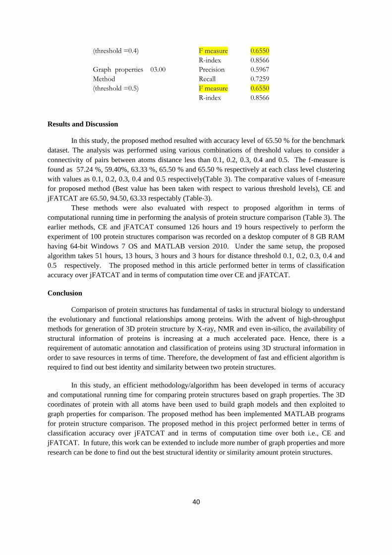
40

(threshold =0.4) F measure 0.6550

R-index 0.8566

Graph properties

Method

(threshold =0.5)

03.00 Precision 0.5967

Recall 0.7259

F measure 0.6550

R-index 0.8566

Results and Discussion

In this study, the proposed method resulted with accuracy level of 65.50 % for the benchmark

dataset. The analysis was performed using various combinations of threshold values to consider a

connectivity of pairs between atoms distance less than 0.1, 0.2, 0.3, 0.4 and 0.5. The f-measure is

found as 57.24 %, 59.40%, 63.33 %, 65.50 % and 65.50 % respectively at each class level clustering

with values as 0.1, 0.2, 0.3, 0.4 and 0.5 respectively(Table 3). The comparative values of f-measure

for proposed method (Best value has been taken with respect to various threshold levels), CE and

jFATCAT are 65.50, 94.50, 63.33 respectably (Table-3).

These methods were also evaluated with respect to proposed algorithm in terms of

computational running time in performing the analysis of protein structure comparison (Table 3). The

earlier methods, CE and jFATCAT consumed 126 hours and 19 hours respectively to perform the

experiment of 100 protein structures comparison was recorded on a desktop computer of 8 GB RAM

having 64-bit Windows 7 OS and MATLAB version 2010. Under the same setup, the proposed

algorithm takes 51 hours, 13 hours, 3 hours and 3 hours for distance threshold 0.1, 0.2, 0.3, 0.4 and

0.5 respectively. The proposed method in this article performed better in terms of classification

accuracy over jFATCAT and in terms of computation time over CE and jFATCAT.

Conclusion

Comparison of protein structures has fundamental of tasks in structural biology to understand

the evolutionary and functional relationships among proteins. With the advent of high-throughput

methods for generation of 3D protein structure by X-ray, NMR and even in-silico, the availability of

structural information of proteins is increasing at a much accelerated pace. Hence, there is a

requirement of automatic annotation and classification of proteins using 3D structural information in

order to save resources in terms of time. Therefore, the development of fast and efficient algorithm is

required to find out best identity and similarity between two protein structures.

In this study, an efficient methodology/algorithm has been developed in terms of accuracy

and computational running time for comparing protein structures based on graph properties. The 3D

coordinates of protein with all atoms have been used to build graph models and then exploited to

graph properties for comparison. The proposed method has been implemented MATLAB programs

for protein structure comparison. The proposed method in this project performed better in terms of

classification accuracy over jFATCAT and in terms of computation time over both i.e., CE and

jFATCAT. In future, this work can be extended to include more number of graph properties and more

research can be done to find out the best structural identity or similarity amount protein structures.

41

CHAPTER- IV: SUMMERY AND CONCLUSION

We have illustrated in detail about two novel methods for comparison of 3D structure using 1) graph

partition and 2) graph properties. The both proposed methods have been implemented in MATLAB

by writing codes for various functions. The performance of the developed methodologies are tested

with two existing best methods such as CE and jFATCAT on 100 proteins benchmark dataset with

SCOP (Structural Classification Of Proteins) database.

First method “graph partitioning” method is comprises conversion of 3D graph into 2D graph,

partitioning of 2D graph into sub-graphs and then aligning sub-graphs. Finally structure similarity

has been calculated by identify local structural similarities between sub-graphs to global similarity of

the whole graph. The proposed method has shown significant improvement over jFATCAT and

accuracy has increased up to 12-15%. Prime notion of the method is the decomposition of structure to

clusters than single residues and SSE, this could be basic interaction of non-bonded residues in the

arrangement of structure elements within a structure. These interaction leads protein fold space and

arrangement of SSE elements in 3D space. Then, aligned the structures based on atoms positions and

association with other atoms within clusters and between clusters to identify similar geometry and

similarity of the two structures. The proposed method performed better in terms of classification

accuracy due to the inclusion of all atoms but CE and jFATCAT uses only backbone C-α atoms and

non-bonded atoms in a cluster may plays important role to inclusion of folding information of protein

while comparing the 3D structures.

In second method, is based on concepts of construction of graph from real world problems,

database for graph and graph mining, pattern recognition are rich fields of computational techniques

to study structures, topologies and properties of graphs. In this method, we have demonstrated that

converting protein 3Dstructures into graphs and into properties such as total degree, maximum degree,

no of adjacencies, average number of degree, cluster coefficient, graph energy, spectrum and number

of components etc. Exploitation of the graph properties and data mining technique to perform

complex studies on protein 3D structure. The proposed method is fast in terms of computation time

complexity. Regarding accuracy is little improved over jFATCAT method. In future, this work can be

extended for including more number of graph properties and more research can be done to find out the

best structural identity or similarity among protein structures.

42

lkjka'k

geus bl ifj;kstuk ds varxZr nks ubZ fof/k;ksa dk fodkl fd;k gS A ;g fof/k;ka 1½ xzkQ foHkktu vkSj 2½

xzkQ xq.kksa dk mi;ksx djds çksVhu ds 3 Mh lajpuk dh rqyuk djus ds fy, cukbZ xbZ gSa A bu fof/k;ksa dks

MATLAB esa dksM fy[kdj ykxw fd;k x;k gS A fodflr rjhdksa dks nks ekStwnk loksZÙke rjhdksa (CE

vkSj jFACTCAT) ds lkFk 100 çksVhu csapekdZ MkVklsV ij SCOP ¼LVªDpjy oxhZdj.k v‚Q çksVhal½

MkVkcsl ds lkFk rqyu Hkh dh x;h gS A bl fjiksVZ esa bu fof/k;ksa dks ,d ljy rjhds ls ifjHkkf"kr dj

mngkj.k ds ek/;e ls le>us dk ç;kl Hkh fd;k x;k gS A

xzkQ foHkktu fof/k esa 3&Mh xzkQ dk 2 &Mh xzkQ esa :ikarj.k] 2 Mh xzkQ dk mi&xzkQksa esa foHkktu vkSj

fQj bu mi&xzkQksa dks lajsf[kr djrk gSA rRi'pkr iwjs xzkQ dks mi&xzkQksa esa oSf'od lekurk vkSj

LFkkuh; lajpukRed lekurkvksa ds vk/kkj ij lekurk dh x.kuk dh xbZ gSA çLrkfor fof/k us jFATCAT

dh rqyuk esa egRoiw.kZ lq/kkj fn[kk;k gS vkSj lVhdrk 12&15% rd c<+h gSA ;g fof/k ç/kku fopkj] ,dy

vo'ks"kksa vkSj ,l,lbZ (SSE) dh rqyuk esa lewgksa ds fy, lajpuk dk ,d vax gS A ;g lajpuk ds rRoksa

dh O;oLFkk esa u‚uc‚.MsM vo'ks"kksa dh cqfu;knh fj'rksa dks [kkstus esa lgk;d fl) gks ldrk gSA ijek.kqvksa

dh fLFkfr;ksa vkSj lewgksa ds chp vU; ijek.kqvksa ds lkFk muds laca/kksa vkSj lewgksa ds chp fLFkfr;ksa vkSj nks

lajpukvksa dh lekurk dh igpku djus ds fy, Hkh fd;k x;k gS A çLrkfor fof/k lHkh ijek.kqvksa dks

'kkfey djus ds dkj.k oxhZdj.k dh lVhdrk ds ekeys esa csgrj çn'kZu djrh gS] ysfdu lhbZ ¼CE½ vkSj

ts,Q,Vh,lh,Vh ¼jFATCAT½ dsoy lh&vYQk ¼Cα½ ijek.kqvksa dk mi;ksx djrh gS vkSj ,d DyLVj esa

xSj&caf/kr ijek.kqvksa dh rqyuk djrs gq, çksVhu dh tkudkjh dks 'kkfey djus dh egRoiw.kZ Hkwfedk fuHkk

ldrh gS A

nwljh fof/k xzkQ ds fofHkUu xq.kksa ij vk/kkfjr gS A xzkQ fuekZ.k vkSj xzkQ [kuu ds fy, MsVkcsl] iSVuZ

ekU;rk lajpukvksa] Vksiksy‚th vkSj vkys[kksa ds xq.kksa dk v/;;u djus ds fy, dEI;wVs'kuy rduhdksa ds

le`) {ks=ksa esa çpfyr gSaA bl i)fr esa geus çksVhu 3 Mh LVªDpj dks xzkQ esa cnyus] xzkQ ds fofHkUu

xq.kksa tSls dqy fMxzh] vf/kdre fMxzh] dksbZ vkSlr la[;k] DyLVj xq.kkad] xzkQ ÅtkZ] LisDVªe vkSj ?kVdksa

dh la[;k vkfn ds xq.kksa esa ifjorZu dk ç;ksx fd;k gS A çksVhu 3 Mh lajpuk ij tfVy v/;;u djus ds

fy, xq.k vkSj MsVk [kuu rduhd dk ç;ksx ls iqjkuh fof/k;ksa ls le; dh rqyuk esa Js"B lkfcr gqbZ gS

tcfd lVhdrk ds ckjs esa ts,Q,Vhlh,Vh ¼jFATCAT½ fof/k ls FkksM+k lq/kkj gqvk gSA Hkfo"; esa ;g dk;Z

vkSj vf/kd xzkQ xq.kksa dks 'kkfey djus ds fy, fd;k tk ldrk gS vkSj çksVhu lajpukvksa esa lcls vPNh

lajpukRed igpku ;k lekurk tkuus ds fy, vf/kd 'kks/k fd;k tk ldrk gSA

43

REFERENCES

Alexandrov NN ( 1996). SARFing the PDB, Protein Engineering, 9(9),727-732.

Artymiuk Peter J, Poirrette Andrew R, Grindley Helen M, Rice David W, Peter Willett A (1994)

Graph-theoretic Approach to the Identification of Three-dimensional Patterns of Amino Acid

Side-chains in Protein Structures, Journal of Molecular Biology, 243( 2),327–344.

Bhattacharya S, Bhattacharyya C and Chandra NR (2007). Comparison of protein structures by

growing neighborhood alignments. BMC Bioinformatics, 8:77.

Carugo1 O and Pongor S (2001) A normalized root-mean-square distance for comparing protein

three-dimensional structures, Protein Science, 10, 1470–1473.

Daniluk P and Lesyng B (2011): A novel method to compare protein structures using local

descriptors, BMC Bioinformatics, 12:344.

Deshmukh S, Dalal A, and Wangikar P(2008). GIPSCo: A method for comparison of protein

structures based on geometric invariants. International Conference on Bioinformatics &

Computational Biology, BIOCOMP 2008, 681-687.

Duda R.O., Hart P.E., and Stork D.G. (2007), “Pattern classification”, Wiley India(p).

Enright AJ, Van Dongen S, Ouzounis CA (2002), An efficient algorithm for large-scale detection of

protein families, Nucleic Acids Research, 30, 1575–1584.

Frömmel Cornelius, Gill1Christoph, Goede Andrean, Gröpl Clemens, Hougard Stefan, Till Nierhoff,

Robert Preißne and Martin Thimm (2003). Accelerating Screening Of 3D Protein Data With A

Graph Theoretical Approach, Bioinformatics, 19(18), 2442–2447, 2003.

Gibrat JF, Madej T, and Bryant SH(1996) Surprising similarities in structure comparison, Current

Opinion Structural Biology, 6(3), 377-385.

Hagen L and Kahng AB (1992). New Spectral Methods for Ratio Cut Partitioning and Clustering,

IEEE Transaction. on Computer Aided Design, 11(9), 1074-1085.

Havel TF, Kuntz ID and Crippen G M (1983). The theory and practice of distance geometry, Bulletin.

Mathematical Biology, 45, 665–720.

Holm L and Sander C (1993) Protein Structure Comparison by Alignment of Distance Matrices,

Journal. Molecular Biology, 233, 123-138.

Kamisetty Hetunandan, Eric P. Xing, and Christopher J. Langmead (2008), Free Energy Estimates

Of All-Atom Protein Structures Using Generalized Belief Propagation, Journal of

Computational Biology, 15(7), 755–766.

Kannan N and Vishveshwara S(1999). Identification of side-chain clusters in protein structures by a

graph spectral method, Journal Molecular Biology, 292(2),441-64, 1999

Kawabata T. (2003) MATRAS: a program for protein 3D structure comparison, Nucleic Acids

Research, 31(13), 3367–3369.

Khaled S, Younis (1996). Weighted Mahalanobis Distance for Hyper-Ellipsoidal Clustering, Thesis -

Faculty of The Graduate School of Engineering of The Air Force Institute of Technology Air

University, December, 1996.

Liu W, Srivastava A, and Zheng J (2010). Protein Structure Alignment Using Elastic Shape Analysis,

ACM Conference on Bioinformatics and Computational Biology, 2010.

44

Lund AW, Bilgin CC, Hasan MA, McKeen LM. Stegemann JP, Yener B, Zaki MJ, and Plopper GE

(2009). Quantification of Spatial Parameters in 3D Cellular Constructs Using Graph Theory,

Journal of Biomedicine and Biotechnology, Article ID 928286, 16 pages,

doi:10.1155/2009/928286.

Mao J and Jain AK (1996). A Self-Organizing Network for Hyperellipsoidal Clustering, IEEE

Transactions on Neural Networks, 7(1), 16-29.

Murzin AG, Brenner SE, Hubbard T and Chothia C( 1995). SCOP: a structural classification of

proteins database for the investigation of sequences and structures. Journal Molecular Biology,

247, 536–540.

Nguyen MN and Madhusudhan MS (2011) Biological insights from topology independent

comparison of protein 3D structures, Nucleic Acids Research, 39(14).

Patra S.M., Vishveshwara S (2000). Backbone cluster identification in proteins by a graph theoretical

method, Biophysical Chemistry, 84 , 13-25.

Perutz MF, Rossmann MG, Cullis AF, Muirhead H, Will G, North ACT (1960). Structure of

myoglobin: a three-dimensional Fourier synthesis at 5.5 Angstrom resolution, obtained by X-

ray analysis, Nature, 185, 416–422.

Pietal Michal J, Bujnicki Janusz M, and Kozlowski Lukasz P (2015). GDFuzz3D: a method for

protein 3D structure reconstruction from contact maps, based on a non-Euclidean distance

function, Bioinformatics, 31(21), 3499-505

Razavian Narges Sharif, Moitra Subhodeep, Kamisetty Hetunandan, Ramanathan Arvind and

Langmead, Christopher J (2010). Time-Varying Gaussian Graphical Models of Molecular

Dynamics Data, Computer Science Department. Paper 1061.

Roland Luthy, James U bowie and David Eisenberg (1992). Assessment of protein models with three-

dimensional profiles, Nature, 356(5), 83-85, 1992.

Sanguinetti G, Laidler J and Lawrence ND. (2005). Automatic determination of the number of

clusters using spectral algorithm, IEEE Workshop on Machine Learning for Signal Processing,

pp. 55-60.

Shindyalov IN and Bourne PE (1998). Protein structure alignment by incremental combinatorial

extension (CE) of the optimal path, Protein Engineering , 11,739–747.

Shindyalov N and Bourne PE (1998). Protein structure alignment by incremental combinatorial

extension (CE) of the optimal path, Protein Engineering, 11(9), 739-747.

Shivashankar S, Srivathsan S, Ravindran B. and Tendulkar Ashish V. (2011). Multi-view methods for

protein structure comparison using latent dirichlet allocation, Bioinformatics, 27, i61–i68

Singh AP and Brutlag DL (1997). Hierarchical Protein Structure Superposition Using Both Secondary

Structure and Atomic Representations, Proceedings of the 5th International Conference on

Intelligent Systems for Molecular Biology, 284-293.

Stijn van Dongen (2000), Graph Clustering by Flow Simulation. PhD thesis, University of Utrecht.

Taylor WR (1999). Protein structure comparison using iterated double dynamic programming, Protein

Science, 8, 654–665.

van Rijsbergen C.J. (1979), “Information Retrieval”, Butterworths London, Edition 2, 112-135,.

45

Wohlers I, Domingues FS and Klau GW (2010) Towards optimal alignment of protein structure

distance matrices, Bioinformatics, 26(18), 2273–2280.

Yan Liu, Eric P Xing and Jaime Carbonell (2005). Predicting Protein Folds with Structural Repeats

Using a Chain Graph Model, Proceedings of the 22nd International Conference on Machine

Learning, Bonn, Germany, 2005.

Yang Y. and Liu X. (1999). A re-examination of text categorization methods, In Proceedings of the

ACM SIGIR Conference on Research and Development in Information Retrieval, pp. 42-49.

Ye Y, Godzik A (2004). FATCAT: a web server for flexible structure comparison and structure

similarity searching, Nucleic Acids Research, 32(Web Server issue):W582-W585.

doi:10.1093/nar/gkh430, 2004.

Zemla (2003) LGA: a method for finding 3D similarities in protein structures, Nucleic Acids

Research, 31(13), 3370–3374.

Zotenko E, Dogan RI, Wilbur WJ, O'Leary DP and Przytycka TM(2007) Structural foot printing in

protein structure comparison: the impact of structural fragments, BMC Structural Biology, 7:53.

i

Annexure – I : MATLAB codes of all functions used in the proposed methods

Converting protein 3D structure to graph model

function [B,t,xy, yx]=pdb_model_to_cord_matrix(pdbmodel, cutoffdist)

[m1,n1]=size(pdbmodel.Model(1,1).Atom); j=1; k=1;

for i=1 : n1-1 if strcmp(pdbmodel.Model(1,1).Atom(1,i).chainID,'A') if strcmp(pdbmodel.Model(1,1).Atom(1,i).AtomName,'CA') k=k+1; % t1(k)=i; end x(j)= pdbmodel.Model(1,1).Atom(1,i).X; y(j)= pdbmodel.Model(1,1).Atom(1,i).Y; z(j)= pdbmodel.Model(1,1).Atom(1,i).Z; xy(j,1)=y(j); xy(j,2)=z(j); yx(k,1)=y(j); yx(k,2)=z(j); j=j+1; t(i)=k; end end n2=j; for i=1:n2-1 for j=1:n2-1 %m(i,j)= abs(x(i)-x(j))+abs(y(i)-y(j))+abs(z(i)-z(j)) ; m(i,j)= sqrt((x(i)-x(j))^2+(y(i)-y(j))^2+(z(i)-z(j))^2) ; if((1/(1+m(i,j))) >cutoffdist) % m(i,j)= (1/(1+m(i,j))); B(i,j)=1; else B(i,j)=0; end

end

end

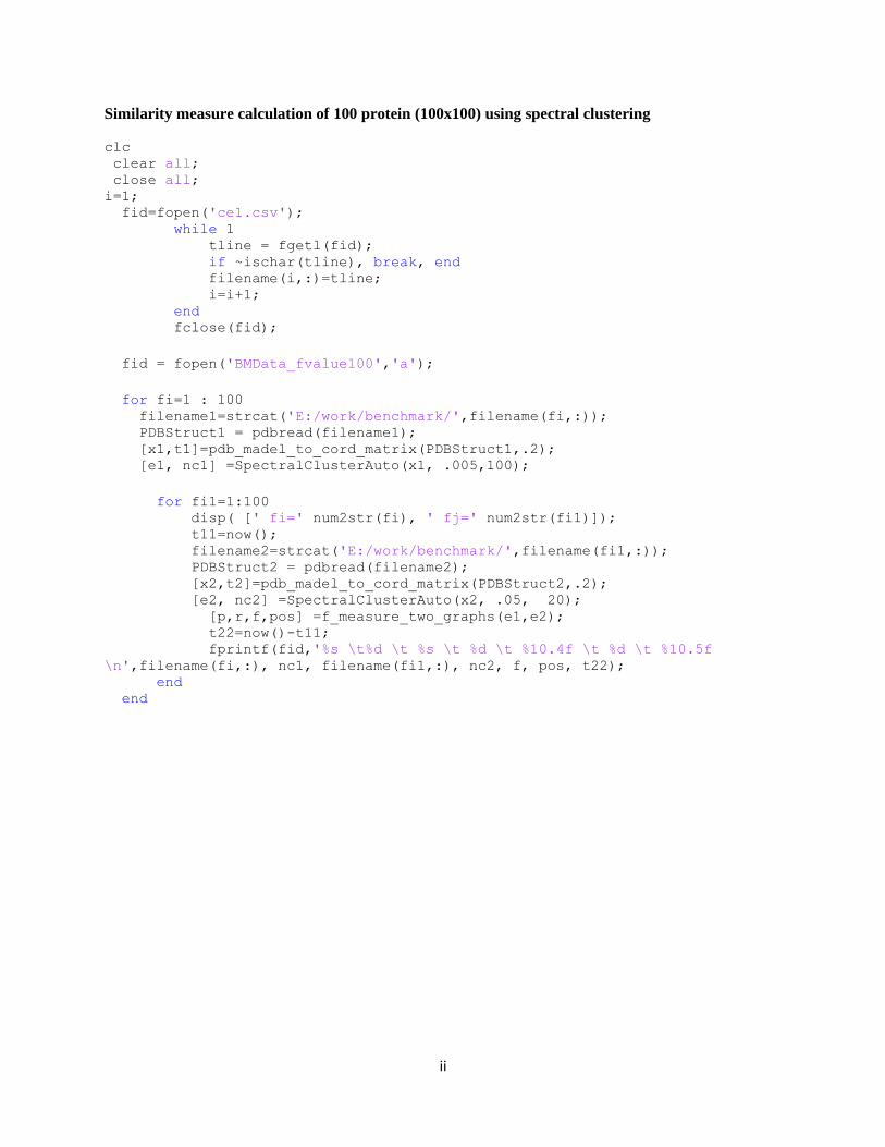
ii

Similarity measure calculation of 100 protein (100x100) using spectral clustering

clc clear all; close all; i=1; fid=fopen('ce1.csv'); while 1 tline = fgetl(fid); if ~ischar(tline), break, end filename(i,:)=tline; i=i+1; end fclose(fid);

fid = fopen('BMData_fvalue100','a');

for fi=1 : 100 filename1=strcat('E:/work/benchmark/',filename(fi,:)); PDBStruct1 = pdbread(filename1); [x1,t1]=pdb_madel_to_cord_matrix(PDBStruct1,.2); [e1, nc1] =SpectralClusterAuto(x1, .005,100);

for fi1=1:100 disp( [' fi=' num2str(fi), ' fj=' num2str(fi1)]); t11=now(); filename2=strcat('E:/work/benchmark/',filename(fi1,:)); PDBStruct2 = pdbread(filename2); [x2,t2]=pdb_madel_to_cord_matrix(PDBStruct2,.2); [e2, nc2] =SpectralClusterAuto(x2, .05, 20); [p,r,f,pos] =f_measure_two_graphs(e1,e2); t22=now()-t11; fprintf(fid,'%s \t%d \t %s \t %d \t %10.4f \t %d \t %10.5f

\n',filename(fi,:), nc1, filename(fi1,:), nc2, f, pos, t22); end end

iii

Cluster analysis code for C-means,K-means, spectral K-means % reading data from file % format %d %d %e clc; clear all; close all; filename1= 'ESA100_ESAO.csv'; filename2='ClassSCP100C3.txt'; i=1; j=1; fid = fopen(filename1,'r'); s = textscan(fid, '%f'); [n,m]=size(s{1}) n=sqrt(n); cnt=1; for i=1: n for j=1:n B(i,j)=1/(1+ s{1}(cnt)); cnt=cnt+1; end end

fclose(fid);

for i=1:n B(i,i)=1; for j=1:m if B(i,j)>B(j,i); B(j,i)=B(i,j); else B(i,j)=B(j,i); end end end

fid = fopen(filename2,'r'); while 1 tline = fgetl(fid); if ~ischar(tline), break, end % disp(tline); ls=size(tline); Qlabel=str2num(tline(1:8)); Slabel=str2num(tline(9:ls(2))); t(Qlabel)=Slabel; end fclose(fid);

ac=[0 45 85 100]; ac=[0 14 20 30 45 65 75 85 90 100]; ac=[0 5 10 14 20 30 35 41 45 52 59 65 70 75 80 85 90 94 100]; maxdim=3; noc=3;

t0=clock;

iv

D = (sum(B,2)); L = inv(diag(sqrt(D)))*(B/diag(sqrt(D)));

OPTS.disp = 0; [u, eigvals] = eig(L); [eigvals, eigvalIndices] = dsort(diag(eigvals)); % eigvalIndices eigvalindex=eigvalIndices(1:maxdim); u = u(:,eigvalindex); ui=sum(u.^2,2);

for i=1:n y(i,:)=u(i,:)/sqrt(ui(i)); end

% for j=1:maxdim % [cv,ci]=max(y(:,j)); % disp(['val=' num2str(cv) ' indx=' int2str(ci)]); % end

[cidx, ctrs] = kmeans(B, noc); PcEig=u; disp(['Time = ' num2str(etime(clock,t0))]);

[n,m]=size(u); x1=1:.0001:1.1; rtold=1; % figure(1); % hold on; % for i=1:21-1 % rt=abs(eigvals(i)/eigvals(i+1)); % uy(i)=rt; % irt=1/100; % jrt=abs(rtold-rt)/100.; % xi=i:irt:i+1; % if rtold<rt % xj=rtold:jrt:rt; % else % xj=rtold:-jrt:rt; % end % % plot(i,rt, 'r+'); % plot(i,x1, 'b-'); % plot(xi, xj, 'g.'); % rtold=rt; % % disp(['i=' num2str(i) ' gap = ' num2str(rt)]); % end % ux=[1:1:20]; % line(ux, uy);

figure(2); for i=1:noc index1 = find(cidx==i);

v

disp(['Cluster-' int2str(i) ' = ' int2str(index1')]); m(index1')=i; [um,un]=size(index1); if(un>0) plot(index1,i, 'r+'); end hold on; end grid; ylabel('Clusters'); xlabel('Sequences'); x1=0:.01:noc;

r=n; nac=size(ac); for i=2:nac(2) plot(ac(i),x1,'g-'); end

mm=zeros(r,r); tt=zeros(r,r); cm=0; ct=0; for i=1:r-1 for j=i+1:r if m(i)==m(j) mm(i,j)=1; cm=cm+1; end if t(i)==t(j) tt(i,j)=1; ct=ct+1; end end end aa=0; bb=0; cc=0; dd=0; for i=1:r for j=1:r if mm(i,j)==1 & tt(i,j)==1 aa=aa+1; end if mm(i,j)==0 & tt(i,j)==1 bb=bb+1; end if mm(i,j)==1 & tt(i,j)==0 cc=cc+1; end if mm(i,j)==0 & tt(i,j)==0 dd=dd+1; % disp( [num2str(i) ',' num2str(j) '= d']); end

end

vi

end disp( ['a=' num2str(aa) ',b=' num2str(bb) 'c=' num2str(cc) 'd='

num2str(dd)]); disp( ['cm=' num2str(cm) ',ct=' num2str(ct)])

pp=aa/(aa+cc); rr=aa/(aa+bb); ff=2*rr*pp/(rr+pp);

disp([' p=' num2str(pp) ' r1=' num2str(rr) ' f=' num2str(ff)]) fid = fopen('pscresult010716-fcm.txt','a'); fprintf(fid,'%s %12.4f %12.4f %12.4f %12.4f %12.8f\n',filename1,pp,rr,ff,

noc); fclose(fid);

color = ['k', 'r', 'g', 'b', 'm']; sym = ['>', 'o', '+', 'x', 's', 'd', 'v', '^', '<']; symbol = zeros(noc, 2); for i = 1:noc; symbol(i, :) = [color(mod(i, length(color))+1) sym(mod(i,

length(sym))+1)]; end

nac=size(ac); for i=2:nac(2) plot(ac(i),x1,'g-'); end

vii

Alignment and comparison of two graph models

function [pp,rr,maxf, maxpos,am] = f_measure_two_graphs(e,t) [r1,q1]=size(e); [r2,q2]=size(t); maxf=0;

rr=0; pp=0; ff=0;

if (r1<r2) r=r1; e1=e; t1=t; else r=r2; e1=t; t1=e; end

mm=zeros(r,r); tt=zeros(r,r);

for i=1:r-1 for j=i+1:r if e1(i)==e1(j) mm(i,j)=1; end

end end

for d=1:abs(r1-r2)+1 maxf=0; maxpos=0; tt=zeros(r,r); i1=1; for i=d:r+d-1 j1=i-d+2; for j=i+1:r+d-1 if t1(i)==t1(j) tt(i1,j1)=1; end j1=j1+1; end i1=i1+1; end

aa=0; bb=0; cc=0; dd=0;

viii

for i=1:r for j=1:r if mm(i,j)==1 & tt(i,j)==1 aa=aa+1; end if mm(i,j)==0 & tt(i,j)==1 bb=bb+1; end if mm(i,j)==1 & tt(i,j)==0 cc=cc+1; end if mm(i,j)==0 & tt(i,j)==0 dd=dd+1; end end

end pp=aa/(aa+cc); rr=aa/(aa+bb); ff=2*rr*pp/(rr+pp); ri=(aa+dd)/(aa+bb+cc+dd); am=(aa+dd)/(aa+bb+cc+dd);

%disp( [' r1=' num2str(r1) ', r2=' num2str(r2) ', d=' num2str(d) ', r='

num2str(r)]); %disp( [' a=' num2str(aa) ', b=' num2str(bb) ', c= ' num2str(cc) ', d='

num2str(dd)]); %disp([' p=' num2str(pp) ' r=' num2str(rr) ', f=' num2str(ff) ', ri='

num2str(ri)])

if (maxf<ff) maxf=ff; maxpos=d; end

end

ix

MCL clustering of a Graph

function [ma]=mcl_cluster(B) % gplot (mm,xy,'r-'); % % figure(2); mm=mcl(B); [n2,m2]=size(B) k1=1; for i=1:m2 index1 = find(mm(i,:)>=1); k=mod(i,6)+1; [um,un]=size(index1); if(un>0) % disp(['Cluster-' int2str(k1) ' = ' int2str(index1)]); ma(index1')=k1; % plot(index1,k1, 'r+'); k1=k1+1; end % hold on; end ma=ma'; end

x

MLC clustering algorithm

function m = mcl(m) % test the explanations in stijn van dongens thesis. % @author gregor :: arbylon . net

if nargin < 1 % m contains T(G3 + I) as stochastic matrix load -ascii m.txt end

p = 2; minval = 0.0000001; e = 1; emax = 0.0000001; i=1; while e > emax fprintf('iteration %i before expansion:\n', i); fprintf('iteration %i after expansion/before inflation:\n', i); m2 = expand(m); fprintf('inflation:\n') [m, e] = inflate(m2, p, minval); fprintf('residual energy: %f\n', e); i=i+1; end % while e end % mcl

% expand by multiplying m * m % this preserves column (or row) normalisation function m2 = expand(m) m2 = m * m; end

% inflate by Hadamard potentiation % and column re-normalisation % prune elements of m that are below minval function [m2, energy] = inflate(m, p, minval) % inflation m2 = m .^ p; % pruning m2(find(m2 < minval)) = 0; % normalisation % if sum(m2)>0 dinv = diag(1./sum(m2)); % else % dinv=1; % end m2 = m2 * dinv; % calculate residual energy maxs = max(m2); sqsums = sum(m2 .^ 2); energy = max(maxs - sqsums); end

xi

Spectral clustering Algorithm

function [elist, noc, PcEig, Centres] = SpectralClusterAuto(x, sigma, numk)

% SPECTRALCLUSTER Clusters a dataset automatically determining the number of

clusters. % % [labels, PcEig, Centres] = SpectralCluster(x, sigma)

% Copyright (c) 2005 Guido Sanguinetti and Jonathan Laidler % SPECTRAL toolbox version 0.1 % % Clusters an arbitrary dataset using the spectral clustering algorithm % outlined in "Automatic Determination of the Number of Clusters using % Spectral Algorithms" by Sanguinetti, Lawrence and Laidler. % % SPECTRALCLUSTER(x, sigma, lambda) % x is the input data. % sigma is the variance measure used when computing the affinity matrix. % lambda is a measure of the elongation of a centre's variance when doing % a Mahalanobis k-means clustering. i.e. Lambda = 1 gives a circular % covariance, Lambda < 1 gives preference to points lying along the vector % normal between the centre and the origin. % % Written by Guido Sanguinetti and Jonathan Laidler, April 2005

% initialisations npts=size(x,1); options=foptions; ExtraCluster=0; Dim=numk; lambda = 0.2;

% compute the similarity matrix A and the matrix L A=x; % A=zeros(npts,npts); % for i=1:npts % for j=1:npts % A(i,j) = exp(-norm(x(i,:)-x(j,:))^2/sigma); % end % end D = (sum(A,2)); L = inv(diag(sqrt(D)))*(A/diag(sqrt(D)));

maxdim=numk; % find the eigenvectors associated with the 10 largest eigenvalues of L OPTS.disp = 0; % [Y, eigvals] = eigs(L, 50, 'LM', OPTS); [Y, eigvals] = eig(L); % [void,Y,eigvals]= ppca(L,10); %ppca gives an alternative eigen-

decomposition % [u, eigvals, v]=svd(L);

[eigvals, eigvalIndices] = dsort(diag(eigvals)); % eigvals

xii

eigvalindex=eigvalIndices(1:maxdim); u = Y(:,eigvalindex);

clear Y; ui=sum(u.^2,2); [n,m]=size(u); for i=1:n Y(i,:)=u(i,:)/sqrt(ui(i)); end

for j=1:maxdim [cv,ci]=max(Y(:,j)); %disp(['val=' num2str(cv) ' indx=' int2str(ci)]); % disp(ci) end

PcEig = Y(:,(1:Dim));

% the first Centre is initialised norms = diag(PcEig*PcEig'); [void, index(1)] = max(PcEig(:,1)); % max(norms); Centres = PcEig(index(1), :);

% the second Centre is initialised S = ((PcEig*Centres(1, :)').^2)./(norms); for ii=1:Dim [void, index(ii)] = max(PcEig(:,ii)); % min(S); end Centres = [PcEig(index, :)];

% [void, index3] = max(PcEig(:,Dim+1));

while ExtraCluster<=3 %& Dim <=maxdim sumdist=0; % introduce a new centre at the origin and do k-means

% Centres = [Centres; PcEig(index3,:)]; [Centres, options, labels] = mahKmeans(Centres, PcEig, lambda, options,

.05); % [W,iter,Sw,Sb,Cova]=kmeansf(PcEig,Centres,.01,100,0) for i = 1:Dim for j = 1:npts CentrDist(i,j) = norm(PcEig(j,:)-Centres(i,:)); sumdist=sumdist+CentrDist(i,j); end end % sumdist % Centres % if anything is assigned to this new centre, there is an extra cluster % if max(labels(:,Dim)) == 1 % ExtraCluster = 0; % Dim = Dim+1; % % take the next eigenvector from Y % PcEig = Y(:,(1:Dim)); % % re-initialise the centres

xiii

Centres=zeros(Dim,Dim); for i=1:Dim [void,point] = min(CentrDist(i,:)); Centres(i,:)=PcEig(point,:); end % else ExtraCluster = ExtraCluster+1; % end end

% erase the last column of labels, as it is empty labels = labels(:,1:Dim);

[r,noc]=size(labels); elist(1)=0; for i=1:noc for j=1:r if labels(j,i)==1 elist(j)=i; end end end elist=elist';

xiv

Mahalanobis distance calculation for spectral K-means algorithm

function [centres, options, post, errlog] = mahKmeans(centres, data, lambda,

options, egv) % MAHKMEANS Trains a k means cluster model, using Mahalanobis distance (based

on Netlab k-means). % % [centres, options, post, errlog] = mahKmeans(centres, data, lambda,

options)

% Copyright (c) 2005 Guido Sanguinetti and Jonathan Laidler % SPECTRAL toolbox version 0.1

% Additional Copyright (c) Ian T Nabney (1996-2001)

[ndata, data_dim] = size(data); [ncentres, dim] = size(centres);

if dim ~= data_dim error('Data dimension does not match dimension of centres') end

if (ncentres > ndata) error('More centres than data') end

% Sort out the options if (options(14)) niters = options(14); else niters = 100; end

store = 0; if (nargout > 3) store = 1; errlog = zeros(1, niters); end

% Check if centres and posteriors need to be initialised from data if (options(5) == 1) % Do the initialisation perm = randperm(ndata); perm = perm(1:ncentres);

% Assign first ncentres (permuted) data points as centres centres = data(perm, :); end % Matrix to make unit vectors easy to construct id = eye(ncentres);

% Main loop of algorithm

xv

for n = 1:niters

% Save old centres to check for termination old_centres = centres;

% Calculate posteriors based on Mahalanobis distance from the existing % centres. (GS) d2 = mahDist2(data, centres, lambda, egv); % Assign each point to nearest centre [minvals, index] = min(d2', [], 1); post = id(index,:);

num_points = sum(post, 1); % Adjust the centres based on new posteriors for j = 1:ncentres if (num_points(j) > 0) centres(j,:) = sum(data(find(post(:,j)),:), 1)/num_points(j); end end

% Error value is total squared distance from cluster centres e = sum(minvals); if store errlog(n) = e; end if options(1) > 0 fprintf(1, 'Cycle %4d Error %11.6f\n', n, e); end

if n > 1 % Test for termination if max(max(abs(centres - old_centres))) < options(2) & ... abs(old_e - e) < options(3) options(8) = e; return; end end old_e = e; end

% If we get here, then we haven't terminated in the given number of % iterations. options(8) = e; if (options(1) >= 0) %disp(maxitmess); end

xvi

Codes for Calculation of graph properties

clc clear all; close all; fi=9; filename=char('1A0F.pdb', '1AR4.pdb', '1AST.pdb', '1AUE.pdb', '1AVX.pdb' ,

'1BC9.pdb', '1BP3.pdb' , '1BRF.pdb' , '1DGP.pdb', '1DI1.pdb' ,

'1dly.pdb', '1ecd.pdb' , '1EHS.pdb' , '1FQT.pdb', '1gvh.pdb',

'1H3E.pdb' , '1hbi.pdb' , '1IAA.pdb' , '1IAB.pdb' , '1IAC.pdb' ,

'1IQW.pdb' , '1JHK.pdb', '1K9O.pdb' , '1KA8.pdb' , '1mbd.pdb',

'1MCN.pdb', '1MLB.pdb', '1MN8.pdb' , '1oj6.pdb', '1P4X.pdb',

'1PSR.pdb', '1PZ8.pdb', '1PZ9.pdb', '1QGJ.pdb', '1QN2.pdb',

'1QUU.pdb' , '1RIE.pdb' , '1RQI.pdb', '1rte.pdb' , '1TOS.pdb',

'1urv.pdb' , '1ux8.pdb', '1VCK.pdb', '1WOV.pdb', '1WOW.pdb',

'1WOX.pdb' , '1X3A.pdb' , '1XG7.pdb' , '1Y2O.pdb' , '1YLL.pdb',

'1YV0.pdb', '1Z77.pdb' , '2A1K.pdb' , '2B0Z.pdb' , '2BBA.pdb',

'2CJ8.pdb' , '2EFK.pdb', '2gdm.pdb' , '2GH2.pdb' , '2H6B.pdb',

'2HVC.pdb', '2HYJ.pdb' , '2IBN.pdb', '2IEK.pdb', '2IOL.pdb' ,

'2J0N.pdb', '2NXN.pdb', '2P8T.pdb', '2Q0A.pdb', '2RD6.pdb',

'2VOD.pdb', '2ZP0.pdb', '3BGE.pdb' , '3CJR.pdb', '3ELN.pdb' ,

'3MDS.pdb' , '3SGO.pdb' , '4hhb.pdb'); % filename1='1EHS.PDB' % '1tos.PDB' %'1h3e.pdb', '1C7M.pdb', '1Q5W.pdb',

'2GTT.pdb' , '2JA7.pdb', '2LFB.pdb', '2MLI.pdb', '2Q4S.pdb' ,; % PDBStruct2 = pdbread(filename1); filename1=strcat('E:/work/pdbs/',filename(fi,:)) PDBStruct2 = pdbread(filename1); PDBStruct2.Model % atoms = fastPDBRead('1TOS.pdb') % plot3(atoms.X, atoms.Y, atoms.Z, '.'); % atoms.atomNum [m1,n1]=size(PDBStruct2.Model(1,1).Atom); %x=zeros(100); j=1; k=0; for i=1 : n1-1 if strcmp(PDBStruct2.Model(1,1).Atom(1,i).AtomName,'CA') k=k+1; t1(k)=i; end x(j)= PDBStruct2.Model(1,1).Atom(1,i).X; y(j)= PDBStruct2.Model(1,1).Atom(1,i).Y; z(j)= PDBStruct2.Model(1,1).Atom(1,i).Z; j=j+1; t(i)=k; % end end n2=j; m=zeros(j-1); for i=1:n2-1 for j=1:n2-1 %m(i,j)= abs(x(i)-x(j))+abs(y(i)-y(j))+abs(z(i)-z(j)) ; m(i,j)= sqrt((x(i)-x(j))^2+(y(i)-y(j))^2+(z(i)-z(j))^2) ; if((1/(1+m(i,j))) >.3) % m(i,j)= (1/(1+m(i,j))); B(i,j)=1;

xvii

else B(i,j)=0; end end

end % B=m; [n,m]=size(B); k=20; % C:\Program Files\MATLAB\R2010a\toolbox\mnr fid = fopen('structparm1-2-16.txt','a'); fid1 = fopen('structparm_header.txt','a'); fprintf(fid,'%s ',filename(fi,:));

%1 calculate degrees of all nodes [deg, ideg,odeg]=degrees(B); totaldeg=sum(deg); maxdeg=max(deg); mindeg=min(deg); fprintf(fid,'%12.4f %12.4f %12.4f ',totaldeg, maxdeg, mindeg); fprintf(fid1,'%s %s %s ','totaldeg,', 'maxdeg,', 'mindeg,');

%2 List out all connected nodes to all nodes % L1 = adj2adjL(B);

%3 Converts an adjacency graph representation to an adjacency list % L = adj2adjL(B);

%4 function to convert adjacency matrix to UCINET dl format % adj2dl(B,'filename.UCINET');

%5 adjacency matrix to edges list; el=adj2edgeL(B); [n1,n2]=size(el);

fprintf(fid,'%12.4f ',n1); fprintf(fid1,'%s ','no of adjances,');

%6 Convert adjacency matrix to an incidence matrix % inc = adj2inc(B);

%7 Converts an adjacency matrix representation to a Pajek .net read format % adj2pajek(B,'filename.txt',x,y,z);

%8 The algebraic connectivity of a graph: the second smallest eigenvalue of

the Laplacian a=algebraic_connectivity(B); fprintf(fid,'%12.4f ',a); fprintf(fid1,'%s ','algebric connectivity,');

%9 Computes the average degree of neighboring nodes for every vertex ave_n_deg=ave_neighbor_deg(B);

totaldeg1=sum( ave_n_deg);

xviii

maxdeg1=max( ave_n_deg); mindeg1=min( ave_n_deg); fprintf(fid,'%12.4f %12.4f %12.4f ',totaldeg1, maxdeg1, mindeg1); fprintf(fid1,'%s %s %s ','ave_n_deg totaldeg1,','maxdeg1,', 'mindeg1,');

%10 Compute average path length for a network - the average shortest path ll = ave_path_length(B);

fprintf(fid,'%12.4f ',ll); fprintf(fid1,'%s ','ave path length,');

%11 Computes the average degree of a node in a graph, defined as 2*num_edges k=average_degree(B);

fprintf(fid,'%12.4f ',k); fprintf(fid1,'%s ','ave degree,');

%12 Implementation of breadth-first-search of a graph %T=BFS(L,1); %T %13 Computes clustering coefficient, based on triangle motifs count and local

clustering [C1,C2,C] = clust_coeff(B); fprintf(fid,'%12.4f %12.4f ',C1, C2); fprintf(fid1,'%s %s ',' cluster coeff1,','cluster coeff,');

% The longest shortest path between any two nodes nodes in the network diam = diameter(B); fprintf(fid,'%12.4f ', diam); fprintf(fid1,'%s ', 'diameter,');

%15 Draws the matrix as a column/row sorted square dot-matrix pattern %dot_matrix_plot(B) % model1=simple_spectral_partitioning(B,k);

%16 Draw a circular graph with links and nodes in order of degree %draw_circ_graph(B)

% 17 The ith component of the eigenvector corresponding to the greatest x=eigencentrality(B); fprintf(fid,'%12.4f ', max(x)); fprintf(fid1,'%s ', 'max eigencentrality,');

% Plot geometry based on extended edgelist % el2geom(el)

%18 Algorithm for finding connected components in a graph but I got no

meaning %comp_mat = find_conn_comp(B);

%19 Graph energy defined as: the sum of the absolute values of the real

components of the eigenvalues G=graph_energy(B); fprintf(fid,'%12.4f ', G);

xix

fprintf(fid1,'%s ', 'Graph energy,');

%20 The minimum vertex eccentricity is the graph radius Rg=graph_radius(B); fprintf(fid,'%12.4f ', Rg); fprintf(fid1,'%s ', 'Radius,');

%21 Computes the similarity matrix between two graphs %S=graph_similarity(B,B);

%22 The eigenvalues of the Laplacian of the graph s=graph_spectrum(B); fprintf(fid,'%12.4f ', max(s)); fprintf(fid1,'%s ', 'spectrum, ');

%23 Test whether a graph is bipartite, if yes, return the two vertex sets L = adj2adjL(B); [isit,A1,B2]=isbipartite(L); fprintf(fid,'%12.4f ', isit); fprintf(fid1,'%s ', 'isbiparate,');

%24 Check if a graph is Eulerian, i.e. it has an Eulerian circuit % "A connected undirected graph is Eulerian if and only if every graph vertex

has an even degree." % "A connected directed graph is Eulerian if and only if every graph vertex

has equal in- and out- degree." S=iseulerian(B); fprintf(fid,'%12.4f ', S); fprintf(fid1,'%s ', 'is eulerian,');

%25 Checks whether a graph is regular, i.e. every node has the same degree. Sr=isregular(B); fprintf(fid,'%12.4f ', Sr); fprintf(fid1,'%s ', 'is regular,');

%26 Find the "optimal" number of communities given a network using an

eigenvector method modules=newman_eigenvector_method(B); [n2,m2]=size(modules); fprintf(fid,'%12.4f ', m2); fprintf(fid1,'%s ', 'no of modules,');

%27 Calculate the number of connected components using the Laplacian % eigenvalues - counting the number of zeros nc=num_conn_comp(B); fprintf(fid,'%12.4f \n', nc); fprintf(fid1,'%s \n', 'no of connect comps,');

%28 Uses the fiedler vector to assign nodes to groups % modules = simple_spectral_partitioning(B,10)

% 29 Weighted clustering coefficient % wc=weighted_clust_coeff(B);

xx

%30 Number of hubs (NHUBS) as hubs when their nodal degree exceeded the

average degree of the graph

%31 Degree centrality: for node i =di(g)/n -1

%32 Closeness centrality: Tracks how close a given node is to any other

node: for node i, one such measure is =n – 1/dij j<>i

%33 Betweenness centrality (or shortest-path between-ness). A measure of

accessibility that is the number of times a node is crossed by shortest paths

in the graph.

%34 Pi Index: The relationship between the total length of the graph L(G) and

the distance along its diameter, an indicator of the shape of a graph.

%35 Alpha Index: A measure of connectivity which evaluates the number of % cycles in a graph in comparison with the maximum number of cycles

%36 Eta Index: Average length per link. Adding new nodes will cause a

decrease of Eta as the average length per link declines.

%37 Beta Index: Measures the level of connectivity in a graph and is

expressed by the relationship between the number of links (e) over the number

of nodes (v). =e/v

%38 Theta Index: Measures the function of a node, which is the average amount

of traffic per intersection. The measure can also be applied to the number of

links (edges).

%39 Graph Density

%40 Synchronizability (S) describes the graph’s capacity to synchronize and

is calculated from the eigen values of the graph’s Laplacian matrix L % L = D -A , where D represents a diagonal matrix containing the nodal

degrees. The synchronizability is defined as the ratio between the first non-

zero eigenvalue and the largest eigenvalue (S= EV_2/EV_max)

fclose(fid); fclose(fid1);