development of algorithm for fusion of hyperspectral and
TRANSCRIPT

Development of Algorithm for Fusion of Hyperspectral and Multispectral Imagery with the Objective of Improving Spatial Resolution While Retaining Spectral Data
Thesis
Christopher J. Bayer Dr. Carl Salvaggio
Digital Imaging and Remote Sensing Laboratory Chester F. Carlson Center for Imaging Science
Rochester Institute of Technology 13 November 2005

2
Copyright „ 2005 Center for Imaging Science
Rochester Institute of Technology Rochester, NY 14623-5604
This work is copyrighted and may not be reproduced in whole or part without permission of the Center for Imaging Science at the Rochester
Institute of Technology.
This thesis is accepted in partial fulfillment of the requirements of the course 1051-503 Senior Research.
Title: Development of Algorithm for Fusion of Hyperspectral and Multispectral Imagery with the
Objective of Improving Spatial Resolution While Retaining Spectral Data Author: Christopher J. Bayer
Project Advisor: Carl Salvaggio 1051-503 Instructor: Joseph P. Hornak

3
Development of Algorithm for Fusion of Hyperspectral and Multispectral Imagery with the Objective of Improving Spatial Resolution While Retaining Spectral Data
Christopher J. Bayer Dr. Carl Salvaggio
Digital Imaging and Remote Sensing Laboratory Chester F. Carlson Center for Imaging Science
Rochester Institute of Technology 13 November 2005
The senior research project that was completed was a study in the field of remote sensing and research area of image fusion technique development. Image fusion is sometimes referenced as image merging in the literature on the subject. The image fusion techniques that were developed for the project were implemented using digital image processing methods. An image fusion algorithm with two main purposes was developed for the project. The first purpose of the algorithm was the fusion of hyperspectral imagery with multispectral imagery. Its second main purpose was the prevention of degradation of the spectral data in the hyperspectral imagery when fusing it with multispectral imagery for improved spatial resolution. The algorithm has the significant capability of producing an imagery product with high spatial resolution and high-quality spectral data. The completion of the project was accomplished with Dr. Carl Salvaggio, an associate professor with the Digital Imaging and Remote Sensing (DIRS) Laboratory, acting as advisor for the project. Dr. Joseph Hornak, professor for the undergraduate course that administered the project, also assisted in the completion of the project.

4
TABLE OF CONTENTS Copyright Release______________________________________________________________2 Abstract______________________________________________________________________3 Table of Contents______________________________________________________________4 Introduction___________________________________________________________________7 Rationale_____________________________________________________________________8 Preliminary Studies_____________________________________________________________9 Background__________________________________________________________________11 Methods_____________________________________________________________________32
Summary of Processing and Degradation of Synthetic Remote Sensing Images and Processing of Image Headers______________________________________________33
Summary of Processing and Degradation of DIRSIG Simulated Remote Sensing Images and Processing of Image Headers___________________________________________35
Summary of Image Fusion Algorithm for Processing of Fused Images______________37 Original WASP and DIRSIG simulated LANDSAT and HYDICE Images__________38
Processing of Synthetic and DIRSIG Simulated Multispectral and Hyperspectral Images________________________________________________________________40
Processed Synthetic and DIRSIG Simulated Remote Sensing Images______________42
Degradation of Synthetic and DIRSIG Simulated Multispectral and Hyperspectral Images________________________________________________________________45
Degraded Synthetic and DIRSIG Simulated Remote Sensing Images_______________47
Processing of Image Headers of Processed and Degraded Synthetic and DIRSIG Simulated Remote Sensing Images__________________________________________49
Image Fusion Algorithm for Processing of Fused Images________________________55
Determination of Spectral Correlation of Multispectral and Hyperspectral Sensor Bands___________________________________________________________55

5
Transformation of Hyperspectral Image Spectral Bands to Hyperspectral Principal Components_____________________________________________________58
Generation of Edge Magnitude Images from Multispectral Image Bands in Spatial Domain_________________________________________________________60 Generation of Edge Magnitude Images from Multispectral Image Bands in Frequency Domain________________________________________________61
Determination of Edge Magnitude Thresholds for Adjustment of Hyperspectral Image First Principal Components____________________________________63
Adjustment of Hyperspectral Image First Principal Components for Fused First Principal Components______________________________________________65
Transformation of Fused Image Principal Components to Fused Spectral Bands___________________________________________________________69
Results______________________________________________________________________71
Original WASP Image Bands______________________________________________71 Processed Multispectral and Hyperspectral Image Bands________________________72 Fused Image Bands for Modified PC Algorithm and Spatial Domain Edge Magnitude Images________________________________________________________________75 Fused Image Bands for Typical PC Algorithm and Spatial Domain Edge Magnitude Images________________________________________________________________78 Fused Image Bands for Modified PC Algorithm and Frequency Domain Edge Magnitude Images________________________________________________________________79
Analysis_____________________________________________________________________81 Qualitative Spatial and Spectral Analysis of Modified PC Algorithm Results________81
Qualitative Spatial and Spectral Comparison of Typical PC Algorithm and Modified PC Algorithm Results_______________________________________________________83
Quantitative Spatial Analysis of Modified PC Algorithm Results and Comparison to Typical PC Algorithm Results_____________________________________________84
Quantitative Spectral Analysis of Modified PC Algorithm Results and Comparison to Typical PC Algorithm Results_____________________________________________91

6
Additional Quantitative Spectral Analysis of Modified PC Algorithm Results and Comparison to Typical PC Algorithm Results_________________________________94
Conclusions__________________________________________________________________97 References___________________________________________________________________98 Appendices__________________________________________________________________99
Additional Quantitative Spectral Analysis of Modified PC Algorithm Results and Comparison to Typical PC Algorithm Results_________________________________99
Acknowledgements___________________________________________________________103

7
INTRODUCTION This senior research project was completed to test the theory that the spatial resolution of hyperspectral imagery can be enhanced significantly with only negligible degradation of its spectral data by fusion with multispectral imagery. The first objective of the project was to fuse hyperspectral imagery with multispectral imagery by implementing the PC component substitution image fusion algorithm that is usually used, modified so that the way in which the PC transformation is used is altered to allow fusion of these imagery types. The second objective was to retain the spectral data of the hyperspectral imagery when fusing it with multispectral imagery for improved spatial resolution by modifying the way that the PC algorithm performs the component substitution. If the project were to prove that spatial resolution enhancement of hyperspectral imagery by fusion with multispectral imagery is feasible, and that the fusion is capable of producing an insignificant amount of degradation of the hyperspectral imagery’s spectral data, then it would be expected that many remote sensing applications would benefit. The applications that would benefit most would be applications that are dependent on both the spectral data contained in hyperspectral imagery and the spatial resolution of multispectral imagery. One of these applications would be land surface or cover classification. The accuracy of any classification method improves with increased spatial resolution or better quality spectral data. Improve spectral data quality improves the accuracy of the classification of materials by their spectral signature, and increased spatial resolution improves the accuracy of the mapping of the borders between different materials. The classification of land surfaces or covers would therefore benefit greatly from fused imagery with both high spatial resolution and high quality spectral data. Many applications in remote sensing are highly dependent on the spectral data in imagery. Such applications benefit from the development of digital image processing methods for hyperspectral imagery. Most methods that are in use are only for the processing of multispectral or trispectral imagery. This is because, until recently, multispectral and trispectral sensors were the only types of spectral sensors that were fully developed. The recent development of hyperspectral sensors has brought about the necessity for the development of methods for hyperspectral imagery processing. Fusion of hyperspectral imagery with multispectral imagery would be expected to benefit these applications if the project were to prove that this could be done without significantly degrading the hyperspectral imagery’s spectral data. The implementation of a fusion technique with the ability to utilize the spectral data contained in hyperspectral imagery would provide a digital image processing method that would be very beneficial to these applications.

8
RATIONALE Previously developed image fusion algorithms generally are for the spatial resolution enhancement of multispectral or trispectral imagery by a fusion process with panchromatic imagery, which has very high spatial resolution. The algorithm developed in this project is for enhancing the spatial resolution of hyperspectral imagery. The spatial resolution of hyperspectral imagery is enhanced by a fusion process with multispectral imagery, multispectral imagery having a higher spatial resolution than hyperspectral imagery. This project’s algorithm was developed with the motivation that it would not be limited to multispectral or trispectral imagery as most of the previously developed algorithms are, but that it could be applied to hyperspectral imagery. The previously developed algorithms for image fusion that are most commonly implemented have some component substitution method as the process for fusion. Component substitution fusion methods include the intensity hue saturation (IHS), principal components (PC), standardized principal components (SPC), regression variable (RV), and Brovey methods. In all of these methods, a high-spatial resolution component is substituted for the low-resolution spatial component of the imagery that is enhanced. Component substitution methods all perform a transformation on the imagery that is enhanced. This transformation can be a color representation, statistical, or rotational transformation. The transformation is performed to attempt to separate the spatial and spectral data of the imagery and generate the spatial component that is enhanced by component substitution. The different types of transformations separate the spatial and spectral data of the imagery by different processes that are successful to varying degrees. The inverse of the transformation that is performed recombines the spatial and spectral data of the imagery after the spatial component has been enhanced as a result of the component substitution. The algorithms having a component substitution fusion method that have been developed prior to this project do not improve the spatial resolution of the imagery that is enhanced without producing degradation of its spectral data. This degradation of the spectral data in the imagery is due to the inability of the transformations performed by these methods to completely separate the spatial and spectral data. The algorithm developed in this project performs a transformation that is unable to completely separate the spatial and spectral data of the imagery that is enhanced, it therefore not better than previous algorithms in this respect. However, it is an improvement over previous algorithms due to its ability to retain the quality of the spectral data of the imagery before enhancement. The spectral data quality of the imagery is retained when it is enhanced as the result of the algorithm having a component substitution method that compensates for the failure of the transformation. Another motivation for the development of this project’s algorithm was the need for an algorithm that preserves the spectral data of the imagery when its spatial resolution is enhanced better than the algorithms developed previously do.

9
PRELIMINARY STUDIES A prior study important to the current project is a research project completed for the Applied Computing professional elective course. The project is relevant because it also was a study in developing image fusion techniques for remote sensing applications. The algorithm for image fusion that was developed for the project is important to this project’s algorithm due to it having the common purpose of preserving the spectral data contained in the enhanced imagery when fusing it with a type of imagery having higher spatial resolution. The capability of the algorithm to produce enhanced imagery with high spatial resolution and spectral data with high quality was one inspiration for the development of this project’s algorithm. The motivation for the development of the prior project’s image fusion algorithm was the need for an algorithm that can be used as a substitute for the IHS component substitution algorithm that is generally implemented, but better preserves the spectral data of the trispectral imagery bands when their spatial resolution is enhanced by fusion with panchromatic imagery. This motivation is similar to one of the motivations for the development of this project’s algorithm: the need for an algorithm that preserves the spectral data of hyperspectral bands when fusion with a multispectral band is performed to enhance the spatial resolution of the hyperspectral bands. This fusion is performed in a similar way to the fusion of multispectral bands and panchromatic imagery that is performed using the PC component substitution algorithm that is typically implemented. The image fusion algorithm in the prior project was developed to preserve the spectral data of the trispectral imagery bands better than the typically implemented IHS algorithm by modifying the simple component substitution process of the algorithm. The algorithm that was developed performs the IHS transformation on the trispectral bands, which is unable to completely separate their spatial and spectral data. It accounts for this failure of the IHS transformation with an improved component substitution process for fusing the trispectral bands with the panchromatic imagery. This project’s image fusion algorithm was developed similarly to take advantage of the improvement in spectral data quality that the prior study’s algorithm produces. It preserves the spectral data of hyperspectral bands better than the usual PC algorithm preserves the spectral data of multispectral bands by implementing a component substitution process that is a modification of the simple process performed by the PC algorithm. The process is modified in the same way that the process of the prior project’s algorithm modifies the IHS algorithm’s process. This modification is what results in the improvement in spectral data quality. The algorithm performs the PC transformation on a number of hyperspectral bands. The transformation is unable to totally separate the spatial and spectral data in the bands, but the improved component substitution process that fuses the hyperspectral bands with a multispectral band compensates for this limitation. Dr. Salvaggio was the professor for the Applied Computing course and acted as advisor for the project. The unpublished technical report “Implementation and Development of Algorithm for Fusion of Three-Band Multispectral and Panchromatic Imagery with the Objective of Improving Spatial Resolution while Retaining Spectral Data” documents the project (Bayer 2004). The

10
project borrowed novel theory from the paper “Merging Multispectral and Panchromatic Images with Respect to Edge Information (Yang, Pei, and Yang 2001).”

11
BACKGROUND Image fusion algorithms that have been developed prior to this project are usually used for the fusion of either trispectral imagery with panchromatic imagery or multispectral imagery with panchromatic imagery. Trispectral imagery is color imagery, which consists of three spectral bands combined to form a color composite. The bands of the imagery are the product of a trispectral sensor. A trispectral sensor has three spectral bands with spectral responsivities maximized for the three red, green, and blue visible wavelengths. Panchromatic imagery is gray-scale imagery, which consists of only a single band. The band is produced by a panchromatic sensor with one band that is responsive across the wavelength range of the red, green, and blue visible maximum spectral responsivity wavelengths of a trispectral sensor. Multispectral imagery is imagery with multiple spectral bands, the bands the product of a multispectral sensor. Multispectral sensors have multiple spectral bands with spectral responsivities maximized for multiple wavelengths. The maximum spectral responsivity wavelengths of a multispectral sensor can be visible, infrared (IR), or ultraviolet (UV) wavelengths, including wavelengths that are near-infrared (NIR) and near-ultraviolet (NUV). Generally, three of the visible maximum spectral responsivity wavelengths of a multispectral sensor correspond to the red, green, and blue wavelengths of a trispectral sensor. These bands can be combined to form a color composite that is color imagery. Any combination of three of the other bands can be combined to form a false color composite. These types of imagery are characterized by different spatial and spectral resolutions, total spectral ranges, total spectral band numbers, and individual band ranges. Spectral resolution is dependent on the number of spectral bands within a discrete spectral range, or the range of an individual band. Spatial resolution is dependent on pixel size, or the number of pixels that are contained in a portion of an image. Panchromatic imagery has the highest spatial resolution of the types of imagery, but the lowest spectral resolution due to it having only a single spectral band within a spectral range equivalent to that of the three bands of trispectral imagery. Trispectral imagery has a higher spectral resolution than panchromatic imagery because it has three bands within the same range as the single band of panchromatic imagery, and the range of one of the bands is smaller than the range of the single panchromatic imagery band. It has a lower spatial resolution, though. Multispectral imagery has the highest spectral resolution of the imagery types because it has more than three bands within the same spectral range as the three bands of trispectral imagery or single band of panchromatic imagery. The range of an individual band is smaller than that of the single panchromatic band or a single trispectral band. It has the lowest spatial resolution of the imagery types, though. Also, multispectral imagery typically has a larger total spectral range than that of panchromatic or trispectral imagery and a greater total number of bands. Imagery also has varying radiometric characteristics that describe the brightness of its pixels in all of its spectral bands. These characteristics include radiometric resolution, brightness range, number of brightness levels, and the range between individual levels. Radiometric resolution depends on the number of brightness levels within a discrete brightness range, or the range between individual levels. These radiometric characteristics typically cannot distinguish different types of imagery as spatial and spectral characteristics can.

12
Having described the imagery types that are exploited when using image fusion algorithms that have been previously developed, these types of imagery will be referred to using the terms “pan,” “tri,” and “multi” when it becomes necessary for parts of these algorithms important to the algorithm developed in this project to be described. These terms will be used for the remainder of the description of algorithms developed prior to this project. The image fusion algorithm that is developed and implemented in this project is for the fusion of hyperspectral imagery with multispectral imagery. Hyperspectral imagery has many spectral bands. It typically has a significantly greater number of bands than multispectral imagery. The number of bands in hyperspectral imagery is generally in the hundreds, while multispectral imagery typically has a number in the tens or less. The bands of hyperspectral imagery are the product of a hyperspectral sensor, the sensor having many spectral bands with maximized spectral responsivities for a large number of wavelengths. Like multispectral imagery, these maximum spectral responsivity wavelengths can be visible, IR, NIR, UV, or NUV. Hyperspectral imagery is characteristically different than the other types of imagery because it has different spatial and spectral resolutions and a different total spectral range, total spectral band number, and individual band range. Compared to multispectral imagery, it has an even higher spectral resolution because it has a greater number of bands within a discrete spectral range, and the range of an individual band is even smaller than that of a single multispectral band. It has an even lower spatial resolution when compared to multispectral imagery. Hyperspectral imagery generally has a larger total spectral range and total number of bands than multispectral imagery, too. When the development and implementation of the algorithm in this project is later described, hyperspectral imagery will be referred to using the term “hyper.” The term “multi” will continue to be used to refer to multispectral imagery. These terms will be used for the entire description of this project’s algorithm in an attempt to make the reading of the description less cumbersome. Before describing the image fusion algorithm developed in this project, it is necessary to describe the important parts of algorithms that have been developed prior to this project and that are especially pertinent to the algorithm’s development. The first algorithm that is described is the typically implemented IHS component substitution algorithm that is used to enhance the spatial resolution of trispectral imagery by fusion with panchromatic imagery. The algorithm is sometimes used for enhancing the spatial resolution of three multispectral imagery bands that are spectrally correlated to the red, green, and blue bands of trispectral imagery. The second algorithm that is described is the algorithm developed by Yang, Pei, and Yang. This algorithm is a modification of the typical IHS algorithm, and it also is for the fusion of trispectral imagery or three multispectral bands with panchromatic imagery. It improves on the typical IHS algorithm by better preserving the spectral data of the trispectral or multispectral bands when their spatial resolution is enhanced. Thirdly, the typically implemented PC component substitution algorithm is described. It is implemented for the fusion of multispectral imagery with panchromatic imagery in order to enhance the spatial resolution of any number of multispectral bands. The following is the description of the most important parts of the typical IHS component substitution algorithm for image fusion. The algorithm attempts to separate the spatial and

13
spectral data contained in the tri imagery or three multi imagery bands by performing the IHS transformation on the red, green, and blue bands for intensity, hue, and saturation components. Before the transformation is performed, the red, green, and blue bands all have both spatial and spectral data content. After the transformation is performed, the intensity component contains only spatial data, and the hue and saturation components both contain only spectral data. The spectral data is represented differently by the hue and saturation components. The red (R), green (G), and blue (B) bands of the tri or multi imagery are transformed to intensity (I), hue (H), and saturation (S) components by
These equations for the IHS transformation represent the most common derivation of the transformation (Gonzalez and Woods 2002). The bands and components in the equations are functions of pixel location as represented by f(x,y). The pixel values of the red, green, and blue bands in Equations 1 through 4 are normalized to the range [0,1] by dividing the values by their maximum. The pixel values of the intensity and saturation components in Equation 1 and 4 are therefore normalized to the range [0,1]. The pixel values of the hue component in Equation 2 must be normalized to the range [0,1] by dividing the values by 360° or 2p rad. This common derivation of the IHS transformation equations is the result of the definition of an IHS geometrical color space with double-pyramid geometry (Gonzalez and Woods 1992). The pyramid geometry is formed from color triangles. This geometrical IHS color space is shown in Figure 1.
†
H =Ï Ì Ó
†
where q = cos-1
12
R - G( ) + R - B( )[ ]
R - G( )2+ R - B( ) G - B( )[ ]
12
Ï
Ì Ô
Ó Ô
¸
˝ Ô
˛ Ô
†
S =1-3
R + G + Bmin R,G,B( )[ ]
†
q if B £ G360° -q if B > G†
I =13
R + G + B( ) Equation 1
Equation 2
Equation 3
Equation 4

14
Figure 1 IHS Geometrical Color Space used in Derivation of IHS Transformation Equations (Gonzalez and Woods 1992)
The complete mathematical derivation of the equations from the geometrical color space can be referenced, as it will not be included for the purposes of this paper (Gonzalez and Woods 1992). The important relationships between the equations and the geometrical color space will be addressed, though. The intensity, hue, and saturation components in Equations 1, 2, and 4 can be related descriptively to the geometrical color space in Figure 1 as follows. The intensity component in Equation 1 is represented by the point on the vertical axis between the black and white points of the geometrical color space. The saturation component in Equation 4 is represented by the length of the vector from the vertical axis at any intensity to a point (P) with the same intensity. The hue (H) component in Equation 2 is represented by the angle from the red axis, or axis between the vertical axis at any intensity point and the red point with the same intensity, and the vector representing the saturation component. The angle (q) in Equation 3, which is calculated in the determination of the hue component using Equation 2, is measured relative to the red axis. The hue component of the IHS transformation is undefined for any pixels that have the same pixel value for the red, green, and blue bands. This can be determined by analysis of Equation 3 and Figure 1. The saturation component is undefined for black pixels (pixels having a pixel value of 0 for the red, green, and blue bands). This can be determined by analysis of Equation 4 and Figure 1. By similar analysis of Equation 1 and Figure 1, it can be determined that the intensity component is defined for pixels with any pixel values for the red, green, and blue bands. After performing the IHS transformation to separate the spatial and spectral data contained in the tri imagery or three multi imagery bands, the typical IHS component substitution image fusion algorithm performs the fusion of the imagery with pan imagery while attempting to only alter the spatial data contained in the imagery. Substituting the pan imagery for the intensity component of the tri imagery or three multi bands does this. The algorithm attempts to perform the fusion without altering the spectral data contained in the imagery by performing the spatial and spectral

15
data separation in the previous step. Successful separation of the spatial and spectral data would result in the intensity component that is replaced having no spectral data content. The substitution of the pan imagery (Ip) for the intensity component (Im) of the tri imagery or three multi imagery bands is performed by , which results in the intensity component of the fused imagery (If). The pan imagery data consists of relative intensity values. Therefore, the intensity component of the pan imagery is equivalent to the pan imagery without the application of any color representation transformation. The histogram of the pan imagery must be matched to the histogram of the tri or multi imagery intensity component for which it is substituted. In the matching of the histograms, the pixels of the pan imagery and the tri or multi imagery intensity component with pixel values that are within some minimum and maximum percentage of the maximum pixel value are excluded. The pan imagery must be normalized to the range [0,1] since the intensity component of the tri imagery or three multi bands is normalized to this range. The hue (Hm) and saturation (Sm) components of the tri imagery or three multi imagery bands are not altered by the substitution of the pan imagery for the tri or multi imagery intensity component. These components are equivalent to the corresponding hue (Hf) and saturation (Sf) components of the fused imagery as and The components in Equations 5 through 7 are functions of pixel location. Following the substitution of the pan imagery for the intensity component of the tri imagery or three multi bands while attempting to not alter the spectral data in the imagery, the typical IHS component substitution image fusion algorithm recombines the separated spatial and spectral data in the imagery. This is done by performing the inverse of the IHS transformation, which transforms the intensity, hue, and saturation components of the fused imagery to red, green, and blue bands. After the inverse of the transformation is performed, the red, green, and blue bands again all contain both spatial and spectral data content. The fused imagery intensity (I), hue (H), and saturation (S) components are transformed to red (R), green (G), and blue (B) bands by
†
I f = Ip Equation 5
†
S f = Sm
†
H f = Hm Equation 6
Equation 7

16
†
G = 3I - R - B
†
R = I 1+S cos H( )
cos 60° - H( )
È
Î Í
˘
˚ ˙
†
B = I 1- S( )When 120° £ H < 240°:
†
R = I 1- S( )
†
G = I 1+Scos H -120°( )cos 180° - H( )
È
Î Í
˘
˚ ˙
†
B = 3I - R - G
When 240° £ H < 360°:
†
R = 3I - G - B
†
B = I 1+S cos H - 240°( )cos 300° - H( )
È
Î Í
˘
˚ ˙
†
G = I 1- S( )
When 0° £ H < 120°:
Equation 8
Equation 9
Equation 10
Equation 11
Equation 12
Equation 13
Equation 14
Equation 15
Equation 16

17
, this resulting in the red, green, and blue bands of the fused imagery. These inverse IHS transformation equations correspond to the representation of the most common IHS transformation derivation by Equations 1 through 4 (Gonzalez and Woods 2002). The components and bands in these equations are functions of pixel location as in Equations 1 through 4. The pixel values of the intensity and saturation components in Equations 1 and 5 are normalized to the range [0,1], and the pixel values of the hue component in Equation 2 are made to be normalized to the same range. In Equations 8, 12, and 16, the pixel values of the hue component must be made to have the range [0°,360°] by multiplying the values by 360° or 2p rad. After this, the pixel values of the intensity and saturation components in Equations 8 through 16 are normalized to the range [0,1], and the hue component pixel values in Equations 8, 12, and 16 have the range [0°,360°]. Therefore, the pixel values of the red, green, and blue bands in Equations 8 through 16 are normalized to the range [0,1]. Multiplication of the pixel values of the red, green, and blue bands by any value gives a different range. The inverse IHS transformation equations are the result of the definition of the IHS geometrical color space that is used in the derivation of Equations 1 through 4. The geometrical color space is shown in Figure 1 (Gonzalez and Woods 1992). The three sectors for the hue component in Equations 8 through 16 can be related to the geometrical color space in Figure 1. They correspond to the 120° hue intervals that separate the three primary colors red, green, and blue on the IHS color triangle in the Figure. Equations 8 through 10 are used if the hue component value is in the range [0°,120°), Equations 11 through 13 are used if it is in the range [120°,240°), and if it is in the range [240°,360°), 360° being equivalent to 0°, then Equations 14 through 16 are used. The typical IHS component substitution image fusion algorithm requires that the pan imagery be spectrally correlated with the intensity component of the tri imagery bands or three multi bands for which it is substituted as in Equation 5. The pan imagery must be spectrally correlated with the tri bands or three multi bands since the intensity component for which it is substituted is generated by the IHS transformation of the bands as in Equations 1 through 4. The pan imagery is spectrally correlated with the tri bands or three multi bands if the spectral responsivity functions of the pan sensor and three bands of the tri or multi sensor that produce the imagery are spectrally correlated. A significant problem with the typical IHS component substitution algorithm for image fusion is its inability to separate the spatial and spectral data contained in the tri imagery or three multi imagery bands as attempted completely. The IHS transformation that is performed to convert the red, green, and blue bands to intensity, hue, and saturation components that separate the spatial and spectral data contained in the bands is unsuccessful at this separation of the data. The intensity component that results from the transformation does not consist only of spatial data, but it also contains some spectral data. The hue and saturation components consist of some spatial data in addition to spectral data. This inability makes the algorithm unable to alter the spatial data contained in the tri imagery or three multi bands as attempted without altering the spectral data contained in the imagery. The replacement of the intensity component of the tri imagery or three multi bands by the pan imagery with the intent to alter only the spatial data contained in the imagery is unsuccessful.

18
The algorithm developed by Yang, Pei, and Yang solves this problem with the IHS component substitution algorithm that is typically implemented for image fusion. It is a modification of the typical IHS algorithm. This modified IHS algorithm solves the problem by not substituting the pan imagery for the intensity component of the tri imagery or three multi imagery bands, but instead replacing the intensity component with a spatial component that is a function of both the pan imagery and the intensity component. By replacing the intensity component with this spatial component instead, the spectral data contained in the intensity component is not altered as much as if replaced by the pan imagery. If the intensity component is replaced by the pan imagery, the spatial data in the component is altered by the spatial data in the pan imagery, but the spectral data in the component is also altered. If it is replaced by a function of both the pan imagery and the intensity component, then its spectral data is altered less. The most important parts of the modified IHS component substitution algorithm for image fusion are described with what follows. The algorithm attempts to separate the spatial and spectral data contained in the tri imagery or three multi imagery bands as the typical IHS algorithm does. It performs the IHS transformation on the red, green, and blue bands of the tri or multi imagery for intensity, hue, and saturation components by Equations 1 through 4. The modified IHS component substitution image fusion algorithm performs the fusion of the tri imagery or three multi imagery bands with pan imagery while attempting to not alter the spectral data contained in the imagery. This follows the IHS transformation to separate the spatial and spectral data contained in the imagery. The fusion is performed differently than in the typical IHS algorithm. A spatial component that is a function of both the pan imagery and the intensity component of the tri imagery or three multi imagery bands is substituted for the intensity component. In doing this, the algorithm attempts to perform the fusion without altering the spectral data in the imagery. It does not have to rely on the unsatisfactory spatial and spectral data separation in the previous step to attempt to not alter the imagery’s spectral data. A spatial component [aIp+(1-a)Im] that is a function of the pan imagery (Ip) and the intensity component (Im) of the tri imagery or three multi imagery bands is substituted for the intensity component (Im) of the imagery by (Yang, Pei, and Yang 2001). This results in the intensity component (If) of the fused imagery. The histogram of the pan imagery must be matched to the histogram of the tri or multi imagery intensity component for which the function of the pan imagery is substituted. This is similar to the histogram matching that must be performed in the case of the typical IHS algorithm. The intensity components in Equation 17 are functions of pixel location as in Equation 5. The fused imagery intensity component (If) calculated by Equation 17 is a function of an adjustment coefficient image (a) in addition to the pan imagery (Ip) and the intensity component (Im) of the tri imagery or three multi imagery bands. This adjustment coefficient image behaves as a weighting factor with the expressions a and (1-a). It is calculated by
†
I f = aIp + 1-a( )ImEquation 17

19
(Yang, Pei, and Yang 2001). The adjustment coefficient image (a) calculated by Equation 18 is a function of an edge magnitude image (E) and an edge magnitude threshold (T). The edge magnitude image is a function of pixel location, and the edge magnitude threshold is a constant. The adjustment coefficient image is therefore a function of pixel location. The weighting of the intensity components Ip and Im in Equation 17 is dependent on the edge magnitude image since the adjustment coefficient image calculated in Equation 18 is a function of this image. The relationships between the adjustment coefficient image (a), edge magnitude image (E), and edge magnitude threshold (T) are shown in Figure 2. The figure shows an edge magnitude threshold equal to 60.
Figure 2 Relationships Between Adjustment Coefficient Image, Edge Magnitude Image, and
Edge Magnitude Threshold (Yang, Pei, and Yang 2001) The edge magnitude image is a measure of the high spatial frequency or edge content in the pan imagery. The process for producing the edge magnitude image (E) in Equation 18 is as follows. Edge detection is applied to the pan imagery by either convolution of edge-detecting filter
†
a =
†
{†
12
sin 2ET
-1Ê
Ë Á
ˆ
¯ ˜
p2
È
Î Í
˘
˚ ˙ +
12
1
†
12
-12
sin 2ET
-1Ê
Ë Á
ˆ
¯ ˜
p2
È
Î Í
˘
˚ ˙
1 If E ≥ T
If T/2 £ E < T
If 0 £ E < T/2
Equation 18

20
kernels in the spatial domain or multiplication of a high-pass filter transfer function by the Fourier transform of the pan imagery in the frequency domain and then the inverse Fourier transform of the result for the spatial domain result. If the edge detection is performed in the spatial domain, the pan imagery is convoluted with edge-detecting kernels such as the Sobel horizontal and vertical kernels, represented by Figures 3 and 4. The convolution in the spatial domain is performed by M x N = dimensions of pan imagery m x n = dimensions of kernel (3 x 3) Equation 19 represents the convolution of an image f(x,y) with a kernel w in the spatial domain for a convoluted image g(x,y). The variables x and y are the spatial variables. The arrangement of the kernel weight coefficients and the subset of the image pixels that correspond to the kernel are represented by Figures 5 and 6.
-1 -2 -1
0 0 0
1 2 1
-1 0 1
-2 0 2
-1 0 1
Figure 4 Sobel vertical kernel
Figure 3 Sobel horizontal kernel
Equation 19 †
g(x, y) = w(s,t) f (x + s, y + t)t=-b
b
Âs=-a
a
Â
†
for x = 0,1,2,...,M -1,y = 0,1,2,...,N -1
where a =m-1
2
b =n -1
2

21
The result of the edge detection by convoluting the pan imagery with two edge-detecting kernels such as the Sobel horizontal and vertical kernels is two edge derivative images. These represent the first derivatives Gx and Gy across the edges of the pan imagery oriented in the directions x and y such as The edge magnitude image is computed from the two edge derivative images by computing the magnitude of the gradient vector —f defined with the two first derivatives as the gradient vector elements such as The magnitude is calculated by summing the absolute values of the two first derivatives by The sum of the two edge derivative images absolute valued is equivalent to the edge magnitude image. Equation 22 is an approximation of the mathematical definition of the magnitude of the gradient vector, which is given by
w(-1,-1) w(-1,0) w(-1,1)
w(0,-1) w(0,0) w(0,1)
w(1,-1) w(1,0) w(1,1)
f(x-1,y-1) f(x-1,y) f(x-1,y+1)
f(x,y-1) f(x,y) f(x,y+1)
f(x+1,y-1) f(x+1,y) f(x+1,y+1)
Figure 5 image pixels corresponding to kernel
Figure 6 arrangement of kernel weight coefficients
Equation 20
†
Gx =∂f∂x
Gy =∂f∂y
Equation 21
†
—f = Gx Gy[ ]
†
—f = mag(—f) ª Gx + Gy Equation 22
†
—f = mag(—f) = Gx2 + Gy
2[ ] Equation 23

22
If the edge detection is performed in the frequency domain, the Fourier transform of the pan imagery is multiplied by a high-pass transfer function such as the Butterworth transfer function, represented by H(u,v) as D0 = cutoff frequency n = filter order The value of the cutoff frequency must be nonnegative. The multiplication in the frequency domain of the high-pass transfer function H(u,v) with the Fourier transform of the pan imagery, represented by F(u,v), is performed by Equation 25 represents the multiplication of the Fourier transform F(u,v) of an image f(x,y) with a transfer function H(u,v) in the frequency domain for a filtered transform image G(u,v). The variables u and v are the frequency variables. The Fourier transform F(u,v) of the pan imagery f(x,y) is defined by the two-dimensional discrete Fourier transform function
†
F u,v( ) = ¡ f x, y( )[ ] =1MN
f x, y( )e- i2p ux M +vy N( )
y =0
N -1
Âx =0
M -1
Â
†
for u = 0,1,2,..., M -1,v = 0,1,2,...,N -1 The inverse Fourier transform g(x,y) of the filtered transform image G(u,v) is the filtered image, which is equivalent to the edge magnitude image. It is defined by the inverse two-dimensional discrete Fourier transform function
†
G(u,v) = H(u,v)F(u,v)
Equation 24
Equation 25
†
H(u,v) =1
1+D(u,v)
D0
Ê
Ë Á
ˆ
¯ ˜
-1È
Î Í Í
˘
˚ ˙ ˙
2n
†
where D(u,v) = u -M2
Ê
Ë Á
ˆ
¯ ˜
2
+ v -N2
Ê
Ë Á
ˆ
¯ ˜
2È
Î Í Í
˘
˚ ˙ ˙
Equation 26

23
†
g x, y( ) = ¡-1 G u,v( )[ ] =1MN
G u,v( )e-i2p ux M +vy N( )
v =0
N -1
Âu=0
M -1
Â
†
for x = 0,1,2,...,M -1,y = 0,1,2,...,N -1 The dc component or zero frequency component F(0,0) of the Fourier transform F(u,v) of the pan imagery f(x,y) computed by Equation 26 is at the origin of (u,v) and is given by
†
F 0,0( ) =1MN
f x,y( )y =0
N -1
Âx =0
M -1
Â
It is equal to the average pixel value of the pan imagery f(x,y). The Fourier transform of the pan imagery computed by Equation 26 must be arranged so that its zero frequency component given by Equation 28 is located at the center of the frequency rectangle where the frequency coordinates are u = M/2 and v = N/2 instead of in its upper-left corner where they are u = 0 and v = 0. The frequency rectangle extends from u = 0 to u = M – 1 and from v = 0 to v = N – 1. This rearrangement of the Fourier transform of the pan imagery is necessary due to the high-pass transfer function represented in Equation 24 being constructed for such an arrangement. The pan imagery Fourier transform’s zero frequency component is centered by multiplication of the pan imagery by the factor (-1)x+y before the Fourier transform of the pan imagery is taken. This is represented by
†
F u - M 2,v - N 2( ) = ¡ f x,y( ) -1( )x +y[ ] Equation 29 requires that the dimensions of the pan imagery both be even numbers for the shifted frequency coordinates to be integers. Since the pan imagery is multiplied by the factor (-1)x+y before taking the pan imagery Fourier transform, the filtered pan imagery after taking the inverse Fourier transform of the filtered transform of the pan imagery is multiplied by the same factor to cancel its initial multiplication with the pan imagery. This makes it so the inverse Fourier transform of the filtered pan imagery transform is properly arranged. The edge magnitude threshold is a threshold value applied to the pixel values in the edge magnitude image to determine the relative amount of edge content in the corresponding pixel locations in the pan imagery. Edge magnitude values greater than or equal to the threshold value correspond to pan imagery pixels that can be classified as pure edge content; values less than the threshold value correspond to pan imagery pixels that can be classified as being mixed with varying amounts of edge content. The following is the process for determining the value of the edge magnitude threshold (T) in Equation 18. It is determined from the histogram of the pixel values in the edge magnitude image, which represents the distribution of edge magnitude image pixel values. The histogram is generated as a discrete one-dimensional function such as
Equation 27
Equation 28
Equation 29

24
where rk is the kth edge magnitude pixel value and nk is the number of pixels in the edge magnitude image having the pixel value rk, L being the number of possible pixel values in the edge magnitude image. The edge magnitude threshold value is determined from the histogram as follows. The pixel value that the most pixels in the edge magnitude image have is determined, and the edge magnitude threshold value is determined to be some pixel value that is greater than this value. The histogram of an edge magnitude image has a maximum at a relatively small pixel value, and it gradually decreases from the maximum to a minimum at a larger pixel value. This is due to the pan imagery from which the edge magnitude image is calculated having only a small number of pixels that are pure edge content relative to the large number of pixels that have varying amounts of edge content or do not have any edge content. The behavior of Equations 17 and 18 together is dependent on the adjustment coefficient image, the edge magnitude image, and the edge magnitude threshold. The behavior for variation in the pixel values of the edge magnitude image is as follows. For pixel locations of the pan imagery where the edge magnitude image pixel values are greater than or equal to the edge magnitude threshold, the intensity component of the tri imagery or three multi imagery bands is replaced by the pan imagery. For pixel locations of the pan imagery where the edge magnitude image pixel values approach 0, the intensity component of the imagery is altered the least by the pan imagery. For pan imagery pixel locations where the pixel values of the edge magnitude image are some value between 0 and the edge magnitude threshold, the intensity component of the imagery is altered more by the pan imagery for pixel locations having higher edge magnitude pixel values and altered less for pixel locations having lower edge magnitude pixel values. If the value of the edge magnitude threshold is varied, the behavior is as follows. A greater edge magnitude threshold results in the intensity component of the tri imagery or three multi bands being altered less by the pan imagery, and a lesser threshold results in it being altered more. The hue (Hm) and saturation components (Sm) of the tri or multi imagery or three multi imagery bands are equivalent to the corresponding hue (Hf) and saturation (Sf) components of the fused imagery, as shown by Equations 6 and 7. The modified IHS component substitution algorithm for image fusion therefore performs the substitution of a spatial component that is a function of both the pan imagery and intensity component of the tri imagery or three multi imagery bands for the intensity component. After doing this while attempting to not alter the spectral data in the imagery, it recombines the separated spatial and spectral data in the imagery as the typical IHS algorithm does. It performs the inverse of the IHS transformation to transform the intensity, hue, and saturation components of the fused imagery to red, green, and blue bands by Equations 8 through 16. The behavior of Equations 17 and 18 is equivalent to the behavior of Equation 5 for the special case of an edge magnitude threshold equal to 0. Equations 17 and 18 are used in the modified IHS component substitution image fusion algorithm for the fusion of the tri imagery or three multi imagery bands with pan imagery by the substitution of a function of the pan imagery and
†
h(rk ) = nk Equation 30
†
for k = 0,1,...,L -1

25
the intensity component of the imagery for the intensity component. Equation 5 is used in the typical IHS algorithm for the fusion by the substitution of the pan imagery. For the case of the edge magnitude threshold in Equation 18 equal to 0, the intensity component of the tri imagery or three multi bands in Equation 17 is replaced by the pan imagery for all pixel locations because all edge magnitude image pixels have values greater than or equal to the threshold. This is equivalent to the substitution of the pan imagery for the intensity component of the imagery in Equation 5. The IHS component substitution algorithm for image fusion that modifies the typical IHS algorithm requires that the spatial component that is a function of the pan imagery and replaced intensity component of the tri imagery or three multi bands be spectrally correlated with the intensity component. This substitution is as shown with Equation 17. The spatial component is spectrally correlated with the intensity component if the pan imagery is since it is a function of the pan imagery and the intensity component. The following is the description of the parts of the typical PC component substitution algorithm for image fusion that are considered to be most important. The algorithm makes the attempt to separate the spatial and spectral data contained in the multi imagery bands as the typical IHS algorithm does. It does this by performing the PC transformation on the spectral bands, which contain data for distinct wavelengths, for principal components. The spectral bands all have both spatial and spectral data before the transformation is performed. After the transformation is performed, the first principal component contains only spatial data. The remaining principal components contain only spectral data that is represented in different ways by the different components. The separation of spatial and spectral data by the IHS and PC transformations can be compared. This separation is the product of the IHS transformation due to the way in which the intensity, hue, and saturation component equations are derived from the IHS geometrical color space. The intensity component contains all of the spatial data in the red, green, and blue bands that are transformed by the IHS transformation, and all of the spectral data in the bands is contained in the hue and saturation components. The separation of spatial and spectral data is one product of the PC transformation, of which the main product is a first principal component containing the majority of the variance in the multi imagery bands and several remaining components containing a negligible amount of variance. Since most of the variance in the multi bands that are transformed by the PC transformation is contained in the spatial data in the bands rather than in the spectral data, the first principal component contains mostly spatial data, and the remaining components contain mostly spectral data. The multi imagery bands are transformed from spectral bands to principal components by the following process involving matrix operations and eigenanalysis. First, the covariance matrix Sx of the multi bands on which the transformation is performed is assembled. The covariance matrix describes the scatter or spread of the pixel vectors in multi vector space, or the vectors defined by the pixels of the multi imagery in the vector space defined by the multi bands. It is assembled by

26
, in which t denotes the transpose of the vector x-m, K is the total number of pixel vectors or the total number of pixels in the multi imagery, xk is the kth pixel vector, and m is the mean pixel vector, or the mean position of the pixel vectors in the vector space defined by the multi bands. The mean pixel vector m for the multi bands is calculated by It defines the average or expected position of the pixel vectors in multi vector space, and therefore is true. The ℘ in the equation is used to represent the expectation operator. Equation 31 is an unbiased estimate of the covariance matrix, which is defined as The covariance matrix Sx of the multi bands on which the transformation is performed is constructed as Each of the off-diagonal matrix elements Si,j
is the covariance between bands i and j, and each of the diagonal matrix elements sj,j
2 is the variance of band j. The off-diagonal matrix elements Si,j
and Sj,i are equivalent. The value of N is the number of spectral bands in the multi imagery. The correlation matrix rx of the multi bands on which the transformation is performed can be calculated from the covariance matrix Sx. The correlation matrix describes to what extent the pixel vectors in multi vector space are independent of one another or dissimilar from one another. Each of its off-diagonal elements ri,j is calculated by
†
=x 1
K -1(x k - m)(x k - m)t
k=1
K
 Equation 31
Equation 35
†
=x ℘{(x - m)(x - m)t} Equation 34
†
=
s1,12 Â1,2 L Â i, j L Â1,N
Â2,1 s 2,22
M O
 j ,i s j , j2
M O
ÂN ,1 s N ,N2
È
Î
Í Í Í Í Í Í Í
˘
˚
˙ ˙ ˙ ˙ ˙ ˙ ˙
xÂ
†
m =1K
x kk=1
K
 Equation 32
Equation 33
†
m =℘{x}

27
, in which each covariance element Si,j
of the covariance matrix Sx is divided by the product of the standard deviations si,i and sj,j of the bands corresponding to the combination of bands of the covariance element. All off-diagonal elements, therefore, must have a value that is in the range [0, 1]. Each diagonal element rj,j of the correlation matrix rx is calculated by dividing each variance element sj,j
2 of the covariance matrix Sx by the square of the standard deviation sj,j of the band corresponding to the band of the variance element. The square of the standard deviation of any band is equal to the band’s variance, and therefore, all diagonal elements must be equal to 1. The construction of the correlation matrix rx of the multi bands on which the transformation is performed is Each of the off-diagonal matrix elements ri,j is the correlation between bands i and j, and each of the diagonal matrix elements rj,j is the correlation of band j. The off-diagonal matrix elements ri,j
and rj,i are equivalent. The value of N is again the number of spectral bands in the multi imagery. Second, the eigenvalues and eigenvectors of the covariance matrix Sx are determined with the next two steps. The eigenvalues l1, l2,…, lN of the covariance matrix Sx are determined first by solving for the solution to the characteristic equation
in which I denotes the identity matrix corresponding to the covariance matrix Sx. The eigenvectors g1, g2,…, gN of the covariance matrix Sx are secondly determined by solving for the vector solution gi corresponding to each eigenvalue li with the equation
Equation 37
†
-lIx = 0
†
-liIxÂ[ ]gi = 0
rx =
r1,1 r1,2 L ri,j L r1,N
r2,1 r2,2
M O
r j,i r j,j
M O
rN,1 rN,N
È
Î
ÍÍÍÍÍÍÍÍ
˘
˚
˙˙˙˙˙˙˙˙
†
ri, j =Â i, j
s i,is j , jEquation 36
Equation 38

28
Each eigenvector gi has the vector elements g1i, g2i,…, gNi. The eigenvectors are normalized to the range [0,1] by Third, the principal components linear transformation matrix G is formed by taking the transpose of the matrix of eigenvectors of the covariance matrix Sx by Finally, the linear transformation matrix G is matrix multiplied by each pixel vector xk to determine each pixel vector yk that results from the transformation by
†
y k = Gxk After performing the transformation on the multi imagery bands, the covariance matrix Sy of the principal components is the diagonal matrix formed with the eigenvalues of the covariance matrix Sx as its diagonal matrix elements, arranged such that l1>l2>…> lN, and its off-diagonal matrix elements all equal to 0. It is formed by where N is the number of principal components after the transformation of the multi bands. This number is equal to the number of spectral bands in the multi imagery. The off-diagonal matrix elements represent the covariances for combinations of principal components, and therefore, all combinations have 0 covariance. The diagonal matrix elements represent the variances of the principal components. Therefore, the variances are equal to the eigenvalues of the covariance matrix Sx, and variance decreases with increasing principal component number. The correlation matrix ry of the principal components after the transformation on the multi imagery bands is performed is the identity matrix
†
for i = 1,2,...,NEquation 39
†
g1i2 + g2i
2 + ...+ gNi2 = 1 Equation 40
†
G = g1g2 ⋅ ⋅ ⋅ gN[ ]tEquation 41
Equation 42
†
for k = 1,2,...,K
Equation 43
†
=
l1 0 0 00 l2 0 00 0 O 00 0 0 lN
È
Î
Í Í Í Í
˘
˚
˙ ˙ ˙ ˙
yÂ

29
formed with its diagonal matrix elements all equal to 1 and its off-diagonal matrix elements all equal to 0. Since the off-diagonal matrix elements represent the correlations for combinations of principal components, all combinations have 0 correlation. The typical PC component substitution image fusion algorithm, after performing the PC transformation to separate the spatial and spectral data contained in the multi imagery bands, performs the fusion of the imagery with pan imagery. The pan imagery is substituted for the first principal component of the multi bands. It does this while attempting to alter only the spatial data contained in the imagery as the typical IHS algorithm does. The algorithm relies on the separation of the spatial and spectral data in the previous step in its attempt to perform the fusion without altering the spectral data contained in the imagery. The pan imagery (Ip) is substituted for the first principal component (PC1,m) of the multi imagery bands by , this resulting in the fused imagery first principal component (PC1,f). The histogram of the pan imagery must be matched to the histogram of the multi imagery first principal component for which it is substituted. This is done in the same way as the histogram matching that must be performed in the case of the typical IHS algorithm. The intensity component and first principal component in Equation 45 are functions of pixel location as the intensity components are in Equation 5. The principal components of the multi imagery bands besides the first principal component (PCn≠1,m) are not altered by the substitution of the pan imagery for the multi imagery first principal component. These components are equivalent to the corresponding components of the fused imagery (PCn≠1,f), as shown by The principal components in Equation 46 are functions of pixel location as the hue and saturation components in Equations 6 and 7 are. After performing the substitution of the pan imagery for the first principal component of the multi imagery bands while attempting to not alter the spectral data in the imagery, the modified IHS component substitution image fusion algorithm performs the inverse of the PC
Equation 45
†
PC1, f = Ip
PCn≠1, f = PCn≠1,m Equation 46
Equation 44
ry =
1 0 0 00 1 0 00 0 O 00 0 0 1
È
Î
ÍÍÍÍ
˘
˚
˙˙˙˙

30
transformation to transform the principal components to the spectral bands of the fused imagery. This is done to recombine the separated spatial and spectral data in the imagery, as is done in the typical IHS algorithm. Following the inverse of the transformation, the spectral bands all contain both spatial and spectral content as they did before the PC transformation was performed. The fused imagery principal components are transformed to spectral bands by matrix multiplication of the transpose of the linear transformation matrix G by each pixel vector yk to determine each pixel vector xk that results from the inverse transformation by This is equivalent to matrix multiplication by the inverse of the linear transformation matrix G such as since the linear transformation matrix is an orthogonal matrix. The inverse of any orthogonal matrix is equal to its transpose. The result of either matrix operation is the spectral bands of the fused multi imagery. In the case of the typical PC component substitution algorithm for image fusion, it is necessary for the pan imagery to be spectrally correlated with the first principal component of the multi imagery bands that is replaced by the pan imagery. This substitution is shown in Equation 45. Since the first principal component that the pan imagery replaces is generated by the PC transformation of the multi bands as shown by Equation 42, the pan imagery needs to be spectrally correlated with the bands. It is spectrally correlated with the multi bands if the spectral responsivity function of the pan sensor and the functions of the bands of the multi sensor that produce the multi bands are spectrally correlated. The typical PC component substitution algorithm for image fusion has the significant problem of not having the capability to separate the spatial and spectral data contained in the multi imagery bands as attempted completely. This problem is related to the inability of the typical IHS algorithm to separate the spatial and spectral data contained in tri imagery or three multi bands as attempted. The problem is due to the failure of the PC transformation that is performed to transform the spectral bands to principal components to separate the spatial and spectral data contained in the bands. It fails because the first principal component resulting from the transformation consists of some spectral data, and the remaining principal components contain some spatial data. This inability causes to algorithm to not be able to alter the spatial data contained in the multi bands as attempted without producing alteration of the spectral data contained in the imagery. It is unsuccessful at substituting the pan imagery for the principal
Equation 47
†
for k = 1,2,...,K
†
x k = G-1y k†
for k = 1,2,...,K
†
x k = G ty k
Equation 48

31
component of the multi bands with the intention to alter only the spatial data contained in the imagery.

32
METHODS The following is a detailed description of the development and implementation of this project’s image fusion algorithm. The description relies on the previous descriptions of parts of previously developed algorithms that are particularly important to the algorithm’s development. The algorithm is a modification of the PC component substitution algorithm that is usually implemented. The typical algorithm is adapted so that it can be used for the fusion of hyperspectral imagery with multispectral imagery to enhance the hyperspectral imagery’s spatial resolution. It also is improved so that it better preserves the spectral data of the hyperspectral imagery when its spatial resolution is enhanced. It is improved in this way by adopting the technique for improving spectral data preservation that is used in the Yang, Pei, and Yang algorithm. The PC component substitution algorithm for image fusion that is typically implemented suffers from the problem of being unable to completely separate the spatial and spectral data contained in the multi imagery bands as attempted. This problem is related to the similar inability of the typical IHS algorithm. The algorithm that is developed and implemented in this project solves the problem with the typical PC algorithm by modifying it significantly. The modification is similar to that made by the modified IHS algorithm developed by Yang, Pei, and Yang to solve the related problem with the typical IHS algorithm. The modified PC component substitution image fusion algorithm does not substitute the high-spatial resolution imagery for the first principal component that results from the PC transformation of the low-spatial resolution imagery bands as the typical PC algorithm does. The typical algorithm does this for pan imagery and multi bands having a lower spatial resolution than pan imagery. It instead replaces the first principal component with a spatial component that is a function of both the high-spatial resolution imagery and the first principal component. It does this for multi bands and hyper bands, multi bands having a higher spatial resolution than hyper bands. Due to this difference, it actually replaces a set of first principal components, each of which results from the PC transformation of a set of hyper imagery bands. The set of first principal components is replaced with a set of spatial components, each of which is a function of both a single multi band and a single first principal component. The replacement of the first principal components with these spatial components rather than multi bands causes the spectral data contained in the first principal components to not be altered as much. The spectral data in the first principal components is altered by the spatial data in the multi bands if replaced by multi bands. If they are replaced by functions of both the multi bands and the first principal components, then their spectral data is altered less.

33
Summary of Processing and Degradation of Synthetic Remote Sensing Images and Processing of Image Headers
downsampling of original WASP red, green, blue image to dimensions of original WASP near-infrared band
registration of original WASP near-infrared band to downsampled red, green, blue image
combination of downsampled red, green, blue image and registered near-infrared band for red, green, blue, near-infrared image
sizing of red, green, blue, near-infrared image
blurring and subsampling of red, green, blue, near-infrared image for synthetic hyperspectral bands
unweighted averaging of red, green, blue bands for panchromatic image that is synthetic multispectral band
removal of blur, blurring, and subsampling of synthetic multispectral and hyperspectral bands for degraded synthetic multispectral and hyperspectral bands

34
modification of synthetic multispectral and hyperspectral band and degraded band headers by inclusion of mean wavelengths and full-width-half-maximums

35
Summary of Processing and Degradation of DIRSIG Simulated Remote Sensing Images and Processing of Image Headers
combination of original simulated LANDSAT bands for simulated LANDSAT image
sizing of simulated LANDSAT image
application of blur to simulated LANDSAT image for simulated multispectral image
upsampling of original simulated HYDICE image to dimensions of original simulated LANDSAT bands
sizing of upsampled simulated HYDICE image
application of blur to sized simulated HYDICE image for simulated hyperspectral image
removal of blur, blurring, and subsampling of simulated multispectral and hyperspectral images for degraded simulated multispectral and hyperspectral images

36
modification of simulated multispectral and hyperspectral image and degraded image headers by inclusion of mean wavelengths and full-width-half-maximums

37
Summary of Image Fusion Algorithm for Processing of Fused Images
determination of spectral correlation of multispectral and hyperspectral sensor bands
transformation of hyperspectral image spectral bands to hyperspectral principal components
generation of edge magnitude images from multispectral image bands
determination of edge magnitude thresholds for adjustment of hyperspectral image first principal components
adjustment of hyperspectral image first principal components for fused first principal components
transformation of fused image principal components to fused spectral bands

38
Original WASP and DIRSIG simulated LANDSAT and HYDICE Images A spatial subset of the original Wildfire Airborne Sensor Program (WASP) red, green, blue image and near-infrared band used in generating a single synthetic multi band and four synthetic hyper bands is shown with Figures 7 and 8. The images were both in the standard Environment for Visualizing Images (ENVI) format. The red, green, blue spectral subset is a true color composite, and the near-infrared band is shown as a gray-scale image. Figure 7 Original WASP Red, Green, Blue Image Figure 8 Original
WASP Near-Infrared Band
Individual spectral bands of the original 6 ENVI-format Land Satellite (LANDSAT) bands and Hyperspectral Digital Imagery Collection Experiment (HYDICE) 210-band image are shown in Figures 9 and 10. The LANDSAT bands and HYDICE image were both simulated using Digital Imaging and Remote Sensing Image Generation (DIRSIG). The bands are shown as gray-scale images.

39
Figure 9 Original DIRSIG Simulated LANDSAT Band 1 Figure 10 Original (l = 0.49 mm) DIRSIG Simulated HYDICE Band 8
(l = 0.4176 mm)

40
Processing of Synthetic and DIRSIG Simulated Multispectral and Hyperspectral Images The processing of the multispectral and hyperspectral images was performed using ENVI. The original WASP imagery and DIRSIG simulated LANDSAT and HYDICE imagery was processed to provide the multi and hyper imagery for the processing of the fused imagery by the image fusion algorithm. Two sets of multi and hyper imagery were produced so as to produce sufficient fused imagery for the types of qualitative and quantitative analysis that would be performed on the fused imagery. The first set that was produced consisted of a synthetic multi image having a single panchromatic band and a synthetic hyper image with four bands that were red, green, blue, and near-infrared bands. The synthetic multi image and the synthetic hyper image were generated from the original WASP tri image with red, green, and blue bands and the original WASP near-infrared band. The second set that was produced consisted of a simulated multi image with 6 bands and a simulated hyper image with 210 bands. These simulated multi and hyper images were generated from the original DIRSIG simulated 6 LANDSAT bands and HYDICE 210-band image. The original WASP red, green, blue image shown in Figure 7 had spatial dimensions that were larger than the spatial dimensions of the original WASP near-infrared band shown in Figure 8 by a factor of 4. The red, green, blue image was downsampled so that its spatial dimensions were equal to the near-infrared band’s spatial dimensions using nearest neighbor resampling. Then, the near-infrared band needed to be registered to the downsampled red, green, blue image using rotation, scale, and translation (RST) corrections and nearest neighbor resampling. After this registration, the downsampled red, green, blue image and near-infrared band could be combined to produce a 4-band image with red, green, blue, and near-infrared bands. The 4-band image was sized by selecting a spatial subset of the image. A single synthetic multi band was generated by computing the unweighted average of the spectral subset of the 4-band image consisting of red, green, and blue bands for a panchromatic image. Four synthetic hyper bands were generated by blurring the 4-band image using a Gaussian blurring 3 x 3 kernel and then subsampling the blurred 4-band image by replacing every 3 x 3 group of pixels with the mean pixel value of the 9 pixels. The image bands were then red, green, blue, and near-infrared bands. The original DIRSIG simulated LANDSAT bands, band 1 shown in Figure 9, were not stored in a multiple-band image as was the case for the original DIRSIG simulated HYDICE image, band 8 shown in Figure 10. The LANDSAT bands were combined into a multiple-band LANDSAT image. The LANDSAT image was then sized by selecting a spatial subset of the image. A simulated multi image with 6 bands was produced with the application of a Gaussian low-pass blurring transfer function with a cut-off spatial frequency of 125. This was done because no sensor modulation transfer function had been applied to the original DIRSIG simulated LANDSAT bands. The original DIRSIG simulated HYDICE image had spatial dimensions that were smaller than the spatial dimensions of the original DIRSIG simulated LANDSAT bands by a factor of 1/3. The HYDICE image was upsampled using nearest neighbor resampling so that it had the spatial dimensions of the LANDSAT bands, this causing it to have a spatial resolution 3 times worse than the spatial resolution of the LANDSAT bands. The HYDICE image was sized by selecting the same spatial subset of the image that was selected for the LANDSAT image. A simulated hyper image with 210 bands was produced with the application of a Gaussian low-pass

41
blurring transfer function with a cut-off spatial frequency of 100, this applying a sensor modulation transfer function to the image.

42
Processed Synthetic and DIRSIG Simulated Remote Sensing Images The single synthetic multi band and four synthetic hyper bands generated from the original WASP red, green, blue image and near-infrared band are shown in Figures 11 and 13. The first three synthetic hyper bands are shown as gray-scale images in Figure 13. Figure 12 shows them combined to produce a color image or true color composite. Figure 11 Synthetic Figure 12 Synthetic Multispectral Band 1 Hyperspectral Bands 1-3 (panchromatic) Combined Figure 13 Synthetic Hyperspectral Bands 1-4 (red, green, blue, near-infrared) Band 1 of the simulated multi image and bands 3 and 8 of the simulated hyper image are shown in Figures 14, 16, and 17. Bands 10, 20, and 30 are also shown in Figure 18 as gray-scale images. These bands are shown combined to produce a false color composite in Figure 15.

43
Figure 14 Simulated Multispectral Figure 15 Simulated Hyperspectral Band 1 (l = 0.49 mm) Bands 10, 20, 30 Combined Figure 16 Simulated Hyperspectral Figure 17 Simulated Hyperspectral Band 3 (l = 0.4008 mm) Band 8 (l = 0.4176 mm)

44
Figure 18 Simulated Hyperspectral Bands 10, 20, 30 (l = 0.4246, 0.4625, 0.5081 mm)

45
Degradation of Synthetic and DIRSIG Simulated Multispectral and Hyperspectral Images The degradation of the multispectral and hyperspectral images was performed using the Interactive Display Language (IDL). The synthetic and DIRSIG simulated multi and hyper imagery was degraded in a way that would allow for a type of quantitative spatial analysis to be performed on the fused imagery produced by the image fusion algorithm. The multi imagery was degraded so that it had a spatial resolution equivalent to that of the hyper imagery. The spatial resolution of the hyper imagery was worse than that of the multi imagery before degradation. The hyper imagery was then degraded so that its spatial resolution maintained the original difference in resolution between the multi and hyper imagery. With the multi and hyper imagery degraded as such, the spatial properties of the fused imagery would be able to be compared quantitatively with those of the hyper imagery before degradation. The fused imagery would be expected to have similar spatial properties as the hyper imagery before degradation since the spatial resolutions of the hyper imagery before degradation and the degraded multi imagery would be equivalent. For the degradation of the multi and hyper imagery, the sensor modulation transfer functions that had been applied to the imagery by the sensors were removed in the frequency domain. This was done by dividing the Fourier transforms of the multi and hyper imagery by the low-pass transfer functions equivalent to the modulation transfer functions of the sensors. These modulation transfer functions were known or assumed to be Gaussian low-pass transfer functions for all of the sensors, represented by H(u,v) as
†
H(u,v) = e- D2 ( u,v )
2D02
D0 = cutoff frequency For both the synthetic imagery and DIRSIG simulated imagery, the cut-off frequency was 125 for the multi imagery and 100 for the hyper imagery. The division in the frequency domain of the Fourier transforms of the multi and hyper imagery, represented by G(u,v), by the Gaussian low-pass transfer function was performed by
†
where D(u,v) = u -M2
Ê
Ë Á
ˆ
¯ ˜
2
+ v -N2
Ê
Ë Á
ˆ
¯ ˜
2È
Î Í Í
˘
˚ ˙ ˙ Equation 49
F(u,v) =G(u,v)H (u,v)
Equation 50

46
Equation 50 represents the division of the Fourier transforms G(u,v) of the low-pass filtered multi and hyper imagery g(x,y) by the Gaussian low-pass transfer function H(u,v) in the frequency domain for transformed multi and hyper imagery F(u,v) with the low-pass filtering removed. The variables u and v are the frequency variables. The Fourier transforms G(u,v) of the low-pass filtered multi and hyper imagery g(x,y) are defined as in Equation 26. The inverse Fourier transforms f(x,y) of the transformed multi and hyper imagery F(u,v) with the low-pass filtering removed are the multi and hyper imagery without the low-pass filtering. They are defined as in Equation 27. The Fourier transforms of the low-pass filtered multi and hyper imagery that are calculated with Equation 26 must be properly arranged using Equation 29 due to the construction of the Gaussian low-pass transfer function represented in Equation 49. This makes it necessary to rearrange the inverse Fourier transforms of the transformed multi and hyper imagery without the low-pass filtering calculated with Equation 27. Then, sensor modulation transfer functions with smaller cut-off frequencies, and therefore low-pass filtering to a larger degree, than the modulation transfer functions that were removed were applied to the multi and hyper imagery in the frequency domain. They were applied by multiplying the Fourier transforms of the multi and hyper imagery by the low-pass transfer functions equivalent to these sensor modulation transfer functions. This caused the modulation transfer functions of the degraded imagery to be known. The modulation transfer functions that were used were Gaussian low-pass transfer functions as represented in Equation 49. For both the synthetic imagery and DIRSIG simulated imagery, the cut-off frequency was 100 for the multi imagery and 75 for the hyper imagery. The Gaussian low-pass transfer functions were applied as in Equation 25. Finally, the imagery was subsampled by where Sxy represents the subset of pixels in the image that the mean is computed for, and m and n are the dimensions of the subset. The image that is subsampled is represented by g(s,t), and the subsampled image is represented by f(x,y). The dimensions of the subset m and n were both 3 for the synthetic and DIRSIG simulated multi imagery and 9 for the synthetic and DIRSIG simulated hyper imagery.
†
f (x, y) =1
mng(s,t)
(s,t )ŒSxy
 Equation 51

47
Degraded Synthetic and DIRSIG Simulated Remote Sensing Images The single synthetic multi band and four synthetic hyper bands after being degraded are shown in Figures 19 and 21. Bands 1 through 3 of the synthetic hyper image after degradation are shown as gray-scale images in Figure 21. They are combined to produce a color image or true color composite in Figure 20. Figure 19 Synthetic Figure 20 Synthetic Multispectral Band 1 Hyperspectral Bands 1-3 (panchromatic) Degraded Combined and Degraded Figure 21 Synthetic Hyperspectral Bands 1-4 (red, green, blue, near-infrared) Degraded Band 1 of the simulated multi image and bands 3 and 8 of the simulated hyper image after being degraded are shown in Figures 22 through 24.

48
Figure 22 Simulated Multispectral Band 1 (l = 0.49 mm) Degraded Figure 23 Simulated Hyperspectral Figure 24 Simulated Hyperspectral Band 3 (l = 0.4008 mm) Degraded Band 8 (l = 0.4176 mm) Degraded

49
Processing of Image Headers of Processed and Degraded Synthetic and DIRSIG Simulated Remote Sensing Images The processing of the processed and degraded remote sensing image headers was performed using ENVI. The image fusion algorithm requires that the mean wavelengths and full-width-half-maximums of the spectral responsivity functions of the multi and hyper sensor bands be used in the determination of the spectral correlation of the bands. It assumes that the spectral responsivity functions are normalized and Gaussian. So that these values would be available to the algorithm, the ENVI header files associated with the ENVI-format synthetic and DIRSIG simulated multi and hyper images were modified to include them. The values were determined so that they could be added to the headers of the multi and hyper image bands as follows. If the bands of the multi or hyper sensor had spectral responsivity functions [f(x)] that are known to be Gaussian and normalized, the known mean wavelength (m) and full-width-half-maximum (fwhm) values for the functions were added to the band headers. If the bands had functions that could be considered to be approximately Gaussian and normalized, then the approximate wavelength ranges of the functions were used to estimate the standard deviations (s) of the functions. Estimated full-width-half-maximums for the functions were calculated from the estimated standard deviations. Approximate mean wavelength values were also estimated from the functions. These approximated values for the mean wavelengths and full-width-half-maximums were then added to the band headers. Figure 25 shows the information that was used in determining the values that were added to the multi and hyper band headers. Figure 25 Determination of Mean Wavelengths and Full-Width-Half-Maximums of Multispectral and Hyperspectral Sensor Bands for Addition to Image Headers A synthetic multi sensor band could be considered for the single synthetic multi image band that was generated from the actual red, green, and blue bands of the WASP multi sensor. This sensor band was considered to have a spectral responsivity function that was approximately Gaussian and normalized. The function was considered to have a wavelength range approximately equal

50
to the total approximate wavelength range of the actual functions of the WASP multi sensor’s red, green, and blue bands. These functions could also be considered to be approximate relative Gaussian functions. Considering the function of the synthetic multi sensor band to be this type of function, the standard deviation of the function was estimated from its approximate wavelength range, and an estimation of the full-width-half-maximum was calculated from its estimated standard deviation. An approximation of the mean wavelength value for the function was estimated from the function, too. After this process of approximations and calculations, the mean wavelength and full-width-half-maximum values for the sensor band could be added to the image band header for the synthetic multi band. These values could also be added to the header for the degraded band. Synthetic hyper sensor bands could also be considered for the four synthetic hyper image bands that were generated from the actual red, green, blue, and near-infrared WASP multi sensor bands. These sensor bands were all considered to have approximately Gaussian and normalized spectral responsivity functions with wavelength ranges equal to the approximate ranges of the actual functions of the bands of the WASP multi sensor. Since the WASP multi band functions could be considered to be normalized and Gaussian, and the wavelength ranges of these functions were equal to the ranges of the synthetic hyper band functions, the ranges of the WASP multi band functions were used in estimating values for the mean wavelengths and full-width-half-maximums of the synthetic hyper band functions. These values were estimated using the same process as was used to estimate the values for the function of the synthetic multi sensor band. After doing this, the mean wavelength and full-width-half-maximum values for the synthetic hyper bands could be added to the image header for the synthetic hyper image. Again, they could also be added to the header for the degraded image. The actual relative spectral responsivity function data for the red, green, blue, and near-infrared bands of the WASP multi sensor are shown in Figures 26 and 27. Figure 26 shows the red, green, and blue band functions, and Figure 27 shows the function of the near-infrared band. These functions were used in the estimation of mean wavelength and full-width-half-maximum values for the functions of the synthetic multi and hyper sensor bands.

51
Figure 26 Actual Relative Spectral Responsivity Functions of WASP Multi Sensor Red, Green, and Blue Bands
Figure 27 Actual Relative Spectral Responsivity Function of WASP Multi Sensor Near-Infrared Band

52
The actual spectral responsivity functions used in the simulation of the 6 bands of the LANDSAT multi sensor using DIRSIG are known. These functions are not perfect Gaussian functions, but they are normalized and can be treated as if they are Gaussian in most instances. They were treated as such, and their mean wavelength and full-width-half-maximum values were estimated using the same process as was used to estimate the values for the functions of the synthetic multi and hyper sensor bands. These values could be added to the image header for the DIRSIG simulated multi image after doing this. They again could also be added to the header for the degraded image. Figure 28 is a series of plots showing the data of the individual actual relative spectral responsivity functions of the 6 bands of the DIRSIG simulated LANDSAT multi sensor. These functions are those that were used to estimate the values of the mean wavelengths and full-width-half-maximums for the functions of the simulated multi bands.

53
Figure 28 Actual Relative Spectral Responsivity Functions of DIRSIG Simulated LANDSAT Sensor Bands 1-6
The values for the mean wavelengths and full-width-half-maximums used in the simulation of the 210 HYDICE hyper sensor bands using DIRSIG are known values, along with values for the minimum wavelength of the smallest wavelength band, maximum wavelength of the largest

54
wavelength band, and wavelength difference. It is also a given that the spectral responsivity functions of the bands are normalized Gaussian functions. The functions can be calculated using the known values for the band mean wavelengths and full-width-half-maximums. Since the mean wavelengths and full-width-half-maximums were known, they simply needed to be added to the image header for the DIRSIG simulated HYDICE hyper image and also to the header for the image that was degraded.

55
Image Fusion Algorithm for Processing of Fused Images The image fusion algorithm was implemented using IDL and ENVI. IDL was used for the processing of the fused images. ENVI was used for the importing of the multispectral and hyperspectral images and the exporting of the fused images. Determination of Spectral Correlation of Multispectral and Hyperspectral Sensor Bands The first important process that is performed by the algorithm is the determination of which hyper sensor band spectral responsivity functions are spectrally correlated to the function of each multi sensor band. This is determined using the mean wavelengths and full-width-half-maximums of the functions of the multi and hyper bands as follows. The spectral correlation of the bands is actually determined from the wavelength ranges of their assumed normalized Gaussian spectral responsivity functions. Whether a multi band and hyper band are spectrally correlated or not is determined by whether or not the wavelength range of the hyper band’s function is within that of the multi band. The wavelength ranges of the functions of the bands are estimated from the mean wavelengths and standard deviations of the functions. The standard deviations are calculated from the full-width-half-maximums of the functions. The information that was used in determining the spectral correlation of the multi and hyper bands from their functions’ mean wavelengths and full-width-half-maximums is the information shown in Figure 25. The relative spectral responsivity functions of the single synthetic multi sensor band and four synthetic hyper bands, normalized and Gaussian as assumed by the image fusion algorithm, are shown in Figures 29 and 30. Figure 29 shows the functions of the multi and hyper bands that are determined by the algorithm to be spectrally correlated. These are the single multi band and first three bands of the hyper sensor. Figure 30 shows that the fourth band of the hyper sensor is determined not to be correlated spectrally with the single multi band by the algorithm.
Figure 29 Spectrally Correlated Relative Spectral Responsivity Functions of Four Synthetic Hyperspectral Sensor Bands and Single Synthetic Multispectral Sensor Band

56
Figure 30 Relative Spectral Responsivity Functions of Four Synthetic Hyperspectral Sensor Bands Spectrally Uncorrelated to Single Synthetic Multispectral Sensor Band
In Figures 31 through 33, the relative spectral responsivity functions of the six DIRSIG simulated multi sensor bands and the first thirty bands of the DIRSIG simulated hyper sensor are shown, again normalized and Gaussian as assumed by the image fusion algorithm. Figure 31 shows the multi and hyper band functions determined to be spectrally correlated by the algorithm. The bands that are spectrally correlated are band 1 of the multi sensor and bands 8 through 30 of the hyper sensor. Figure 31 shows the hyper bands that are determined by the algorithm not to be spectrally correlated with any of the six multi bands. These bands are bands 1 through 7 of the hyper sensor. Figure 32 shows the multi bands that are determined not to be spectrally correlated with any of the thirty hyper sensor bands by the algorithm. These are bands 2 through 6 of the multi sensor.
Figure 31 Spectrally Correlated Relative Spectral Responsivity Functions of Six DIRSIG Simulated Multispectral Sensor Bands and First Thirty DIRSIG Simulated Hyperspectral Sensor Bands

57
Figure 32 Relative Spectral Responsivity Functions of First Thirty DIRSIG Simulated Hyperspectral Sensor Bands Spectrally Uncorrelated to Six DIRSIG Simulated Multispectral Sensor Bands
Figure 33 Relative Spectral Responsivity Functions of Six DIRSIG Simulated Multispectral Sensor Bands Spectrally Uncorrelated to First Thirty DIRSIG Simulated Hyperspectral Sensor Bands

58
Transformation of Hyperspectral Image Spectral Bands to Hyperspectral Principal Components The second process performed by the image fusion algorithm is the application of the PC transformation to each set of hyper imagery bands determined to be spectrally correlated with an individual multi band. This transforms each set of spectral bands into a set of principal components. The PC transformation is performed by the matrix operations and eigenanalysis process described with Equations 31 through 44. The PC transformation of the first three bands of the synthetic hyper imagery into three principal components is shown in Figures 34 and 35, 34 showing the set of spectral bands before the transformation and 35 showing the set of principal components after the transformation. The first three bands are transformed because only these bands are determined to be spectrally correlated to the single synthetic multi band. The fourth band is determined not to be spectrally correlated to the synthetic multi band. Figure 34 Synthetic Hyperspectral Bands 1-3 (red, green, blue)

59
Figure 35 Principal Components 1-3 of Synthetic Hyperspectral Bands 1-3

60
Generation of Edge Magnitude Images from Multispectral Image Bands in Spatial Domain The third process that the image fusion algorithm performs is the generation of an edge magnitude image from each of the individual multi imagery bands with which a set of hyper bands is spectrally correlated. This is done after the histogram of each multi band is matched to the histogram of the first principal component for the hyper bands with which it is spectrally correlated. This needed to be done since these histogram-matched multi bands are used in the step for adjusting the first principal components of the hyper bands, not the multi bands before the application of histogram matching. In this step, a function of each histogram-matched multi band and the first principal component of the hyper bands with which it is spectrally correlated is substituted for the first principal component. If the process for producing the edge magnitude images is performed in the spatial domain, then they are generated using Equations 19 through 23 and the information in Figures 3 through 6. Figures 36 and 37 show the two absolute valued edge derivative images, one for edges of the single synthetic multi imagery band oriented in the horizontal direction and one for edges oriented in the vertical direction, that are summed in Equation 22 for the edge magnitude image. Figure 38 shows this edge magnitude image. Figure 36 Absolute Valued Figure 37 Absolute Valued Figure 38 Edge Magnitude Edge Derivative Image for Edge Derivative Image for Image (Sum of Two Absolute Horizontally Oriented Edges Vertically Oriented Edges Valued Edge Derivative Images)

61
Generation of Edge Magnitude Images from Multispectral Image Bands in Frequency Domain If the edge magnitude image process is performed in the frequency domain instead, then the images are generated using Equations 24 through 29. The Butterworth high-pass transfer function that was multiplied by the Fourier transform of the single synthetic multi imagery band using Equation 25 for a filtered transform image is shown in Figure 39. The equation representation of the function is shown in Equation 24. The value of the cut-off frequency in Equation 24 for the filter that was used is 40, and the value of the order for the filter was 2. Figure 40 shows the Fourier transform of the synthetic multi band that is defined by the two-dimensional discrete Fourier transform function in Equation 26. This definition of the Fourier transform was not used in its calculation. The fast Fourier transform process, which is left undefined in this paper due to its complexity, was used. Figure 41 shows the inverse Fourier transform of the filtered transform image for a filtered image, which is the edge magnitude image result. It is defined by the inverse two-dimensional discrete Fourier transform function in Equation 27, but it was calculated using the inverse fast Fourier transform. Figure 39 Butterworth High-Pass Transfer Function (cut-off frequency = 40, order = 2)

62
Figure 40 Fourier Transform of Figure 41 Edge Magnitude Synthetic Multispectral Band 1 Image (Inverse Fourier Transform of Filtered Transform Image for Filtered Image)

63
Determination of Edge Magnitude Thresholds for Adjustment of Hyperspectral Image First Principal Components The fourth process performed by the image fusion algorithm is the determination of an edge magnitude threshold for the adjustment of the first principal component of each set of hyper imagery bands spectrally correlated with an individual multi band. These thresholds are determined by analysis of the pixel value histograms of the edge magnitude images generated by the process described in the previous section. Each histogram is generated using Equation 30 and analyzed for some edge magnitude pixel value that can be the threshold. A portion of the histogram for the edge magnitude image generated from the single synthetic multi imagery band showing small pixel values is shown in Figures 42 and 43. Figure 42 shows the histogram for the edge magnitude image generated using the spatial domain process described in the previous section. Figure 43 is for the image generated using the frequency domain process. Figure 42 Histogram for Edge Magnitude Image Generated from Synthetic Multispectral Band 1 in Spatial Domain Figure 43 Histogram for Edge Magnitude Image Generated from Synthetic Multispectral Band 1 in Frequency Domain As an example, a threshold determined by the analysis of the histogram shown in Figure 42 could be the edge magnitude pixel value that is 18.8 percent of the maximum value in the image.

64
This would be determined by first determining that the pixel value that is 2.1 percent of the maximum value is the value that the most pixels in the image have. It would then be determined that a value greater than this value approximately equal to the 18.8 percent-value could be the threshold value.

65
Adjustment of Hyperspectral Image First Principal Components for Fused First Principal Components The fifth and most important process performed by the image fusion algorithm is the fusion of the hyper imagery bands with multi bands. This fusion is performed differently than the fusion of multi bands with pan imagery by the typical PC component substitution algorithm. It is performed similarly to the fusion of tri imagery or three multi bands with pan imagery by the modified IHS algorithm. For each individual multi band and spectrally correlated set of hyper bands, a spatial component that is a function of both the multi band and the first principal component of the hyper bands is substituted for the first principal component. Each spatial component [aIm+(1-a)PC1,h] that is a function of both an individual multi imagery band (Im) and the first principal component (PC1,h) of a set of spectrally correlated hyper bands is substituted for the first principal component (PC1,h) by The result of this adjustment of the first principal component of the hyper bands is the first principal component (PC1,f) of a set of fused bands that are spectrally correlated to the multi band. It is necessary for the histogram of the multi band to be matched to the histogram of the first principal component of the hyper bands for which the function of the multi band is substituted. This histogram matching is similar to that performed by the modified IHS algorithm. The intensity and first principal components in Equation 52 are functions of pixel location as in Equation 17. The first principal component (PC1,f) of the fused imagery bands calculated by Equation 52 is a function of the adjustment coefficient image (a) calculated by Equation 18 for the multi band. This image is a function of the edge magnitude image (E) for the multi band and its edge magnitude threshold (T), these generated and determined by the processes described in the previous two sections. As in Equation 18, the adjustment coefficient and edge magnitude images for the multi band are functions of pixel location, and its edge magnitude threshold is a constant. The relationship between the adjustment coefficient, edge magnitude image, and edge magnitude threshold for the multi band is that shown in Figure 2. The behavior of Equations 52 and 18 together is dependent on these in the same way as described for the modified IHS component substitution algorithm for image fusion. The remaining principal components (PCn≠1,h) of the hyper imagery bands are not altered by the replacement of the first principal component by the spatial component that is a function of the multi band and the first principal component. These components are equivalent to the corresponding components of the fused imagery (PCn≠1,f), as shown by The principal components in Equation 53 are functions of pixel location as in Equation 46.
†
PC1, f = aIm + 1- a( )PC1, hEquation 52
PCn≠1, f = PCn≠1,h Equation 53

66
For the special case of an edge magnitude threshold equal to 0 in Equation 18, the behavior of Equations 52 and 18 for the image fusion algorithm is equivalent to the behavior of Equation 45. Equation 45 is used in the typical PC component substitution image fusion algorithm for the fusion of multi imagery bands with pan imagery by the substitution of the pan imagery for the first principal component of the multi bands. For this case, the multi band for all pixel locations replaces the first principal component of the hyper bands in Equation 52. This is due to all of the edge magnitude image pixels having values greater than or equal to the threshold. This behavior is equivalent to the substitution of the pan imagery for the first principal component of the multi bands in Equation 45. The difference between Equations 52 and 45 for this special case is not a difference in behavior. The difference is only that in Equation 52, the two types of imagery are a multi band and hyper bands, and in Equation 45, they are pan imagery and multi bands. The behavior of Equations 52 and 18 for this case becomes equivalent to that of Equation 45 in the same way that the behavior of Equations 17 and 18 used in the modified IHS algorithm becomes equivalent to that of Equation 5 used in the typical IHS algorithm. The image fusion algorithm substitutes a spatial component for the first principal component of each set of hyper imagery bands that is determined to be spectrally correlated to an individual multi band. The spatial component is a function of the multi band and the first principal component that is replaced. The substitution process of the algorithm is performed in this way for sets of hyper bands and spectrally correlated individual multi bands because it requires that each first principal component be spectrally correlated with the spatial component that replaces it. This substitution is as shown with Equation 52. This spectral correlation requirement of the algorithm is similar to that of the modified IHS component substitution algorithm. It requires that the spatial component that is a function of the pan imagery and the intensity component of the tri imagery or three multi bands that it replaces be spectrally correlated with the intensity component. The substitution process of this algorithm is shown in Equation 17. A spatial component is spectrally correlated with a first principal component if the multi imagery band that the component is a function of is spectrally correlated to it. Each multi band needs to be spectrally correlated with the hyper bands that are transformed by the PC transformation shown in Equation 42 into the first principal component that the function of the band replaces. A multi band is spectrally correlated with a group of hyper bands if the spectral responsivity functions of the multi and hyper sensor bands that produce the bands are spectrally correlated. The following figures demonstrate the behavior of Equations 52 and 18, which is dependent on the adjustment coefficient image, the edge magnitude image, and the edge magnitude threshold. Figures 44 through 51 demonstrate Equation 18, which calculates the adjustment coefficient image, and Figures 52 through 54 demonstrate Equation 52, which calculates the first principal component of a group of fused imagery bands. With Figures 44 through 51, the behavior for a constant edge magnitude threshold and varied edge magnitude image pixel values is demonstrated. The behavior for variation in the value of the edge magnitude threshold is not demonstrated, but this would also be beneficial in understanding the behavior of the Equations.

67
Figure 44 Edge Magnitude Figure 45 Edge Magnitude Figure 46 Edge Magnitude Image Where Values ≥ Image Where Values ≥ Image Where Values ≥ 0 and Threshold Threshold/2 and < Threshold < Threshold/2 Figure 47 Adjustment Figure 48 Adjustment Figure 49 Adjustment Coefficient Image for Edge Coefficient Image for Edge Coefficient Image for Edge Magnitude ≥ Threshold Magnitude ≥ Threshold/2 Magnitude ≥ 0 and < (Values = 1) and < Threshold Threshold/2

68
Figure 50 Edge Magnitude Figure 51 Adjustment Image Coefficient Image Figure 52 Synthetic Figure 53 First Principal Figure 54 First Principal Multispectral Band 1 Component of Synthetic Component of Fused Hyperspectral Bands 1-3 Bands 1-3

69
Transformation of Fused Image Principal Components to Fused Spectral Bands The sixth and final process that the image fusion algorithm performs is the inverse PC transformation on each set of fused imagery bands spectrally correlated with an individual multi band due to the set of hyper bands before fusion being spectrally correlated to it. Each set of principal components is transformed into a set of spectral bands. The process described in the previous section has adjusted the first principal component in each set. The inverse PC transformation is performed by the matrix operations of Equations 47 and 48. Figures 55 and 56 show the inverse PC transformation of the first three bands of the fused imagery into three spectral bands. Figure 55 shows the set of principal components before the transformation. Figure 56 shows the set of spectral components after the transformation. There are only three principal components of the fused imagery that are transformed to spectral bands because only the first three bands of the hyper imagery were transformed to principal components. This was due to only these bands being determined to be spectrally correlated to the single synthetic multi band and not the fourth band.
Figure 55 Principal Components 1-3 of Fused Bands 1-3

70
Figure 56 Fused Bands 1-3 (red, green, blue)

71
RESULTS Original WASP Image Bands Figure 57 Original WASP Red, Green, Figure 58 Original WASP Near-Infrared Blue Bands (Downsampled and Sized) Band (Sized)

72
Processed Multispectral and Hyperspectral Image Bands Figure 59 Processed Synthetic Multispectral Figure 60 Processed Synthetic Hyperspectral Band 1 (Unweighted Average of Original Bands 1-3 Combined WASP Red, Green, Blue Bands) Figure 61 Processed Synthetic Figure 62 Processed Synthetic Hyperspectral Band 1 (Original WASP Hyperspectral Band 2 (Original WASP Red Band Blurred and Subsampled) Green Band Blurred and Subsampled)

73
Figure 63 Processed Synthetic Figure 64 Processed Synthetic Hyperspectral Band 3 (Original WASP Hyperspectral Band 4 (Original WASP Blue Band Blurred and Subsampled) Near-Infrared Band Blurred and Subsampled) Figure 65 Processed Simulated Multispectral Figure 66 Processed Simulated Hyperspectral Band 1 Bands 10, 20, 30 Combined

74
Figure 67 Processed Simulated Hyperspectral Figure 68 Processed Simulated Hyperspectral Band 3 Band 8

75
Fused Image Bands for Modified PC Algorithm and Spatial Domain Edge Magnitude Images Figure 69 Fused Synthetic Hyperspectral Figure 70 Fused Synthetic Hyperspectral Bands 1-3 Combined (Edge Magnitude Band 1 Threshold = 12.5 % of Maximum Edge Magnitude) Figure 71 Fused Synthetic Hyperspectral Figure 72 Fused Synthetic Hyperspectral Band 2 Band 3

76
Figure 73 Fused Synthetic Hyperspectral Band 4 (Edge Magnitude Threshold = 12.5 % of Maximum Edge Magnitude) Figure 74 Fused Simulated Hyperspectral Figure 75 Fused Simulated Hyperspectral Bands 10, 20, 30 Combined Band 3

77
Figure 76 Fused Simulated Hyperspectral Band 8

78
Fused Image Bands for Typical PC Algorithm and Spatial Domain Edge Magnitude Images Figure 77 Fused Synthetic Hyperspectral Figure 78 Fused Synthetic Hyperspectral Bands 1-3 Combined (Edge Magnitude Band 4 (Edge Magnitude Threshold = 0) Threshold = 0)

79
Fused Image Bands for Modified PC Algorithm and Frequency Domain Edge Magnitude Images Figure 79 Fused Synthetic Hyperspectral Figure 80 Fused Synthetic Hyperspectral Bands 1-3 Combined Band 1 Figure 81 Fused Synthetic Hyperspectral Figure 82 Fused Synthetic Hyperspectral Band 2 Band 3
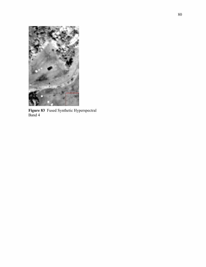
80
Figure 83 Fused Synthetic Hyperspectral Band 4

81
ANALYSIS Qualitative Spatial and Spectral Analysis of Modified PC Algorithm Results The image that combines the first three bands of the fused synthetic hyper image shown in Figure 69 was generated using an edge magnitude threshold value equal to 12.5 percent of the maximum value of the edge magnitude image. The edge magnitude image that was used was generated from the synthetic multi band shown in Figure 59. This band was processed as the unweighted average of the original WASP red, green, and blue bands. The edge magnitude image was generated using the process for spatial domain edge detection. The threshold was chosen as an arbitrary value greater than 0 for this qualitative analysis of the modified PC algorithm’s results. Any value greater than 0 could have been chosen. Several values greater than 0 would have allowed for a more thorough analysis, but this was left for the quantitative analysis described in a later section. The threshold value 0 was not chosen because this value would have only allowed for the assessment of the typical PC algorithm’s results. This assessment is the purpose of the qualitative analysis described in the next section. The spatial resolution of the first three bands of the fused synthetic hyper image shown in Figure 69 has been enhanced. This is due to these bands of the synthetic hyper image, shown in Figures 61 through 63, being spectrally correlated with the synthetic multi band shown in Figure 59. These bands were processed by blurring and subsampling the original WASP red, green, and blue bands. The fourth band of the fused synthetic hyper image shown in Figure 73 is not enhanced spatially. This band of the synthetic hyper image shown in Figure 64 is not spectrally correlated with the synthetic multi band shown in Figure 59. It is due to this that its spatial resolution is not enhanced. Since it is not enhanced spatially, its spectral content is equivalent to that of the fourth synthetic hyper band shown in Figure 64. This band was processed by blurring and subsampling the original WASP near-infrared band. The spatial resolution of the first three bands of the fused synthetic hyper image shown in Figure 69 can be analyzed by comparison with the synthetic multi band shown in Figure 59. The spatial resolution enhancement of these bands is the result of fusion with this high-spatial resolution synthetic multi band. These bands shown separately in Figures 70 through 73 can also be compared with the synthetic multi band to analyze their spatial resolution. It can be determined from this comparison that the spatial resolution of the fused synthetic hyper bands has been made to be equivalent to that of the synthetic multi band in areas of the image with sufficient edge content. The image areas that have not been enhanced to have this spatial resolution do not have sufficient edge content. The edge content in the image that was sufficient to cause areas to be enhanced was determined by the edge magnitude threshold that was used. The spectral content of the first three bands of the fused synthetic hyper image can be compared with that of the first three bands of the synthetic hyper image shown combined in Figure 60. The spatial resolution enhancement of these bands should not cause them to have spectral content that is dissimilar to the spectral content in these high-spectral quality synthetic hyper bands. From this comparison, it can be determined that the spectral content of the fused synthetic hyper bands is equivalent to that of the synthetic hyper bands in most areas of the image. This is due to most of the image areas consisting of insignificant edge content. Only the areas of the image with

82
significant edge content in the fused synthetic hyper bands are not equivalent spectrally to the synthetic hyper bands. The spatial resolution and spectral content of these fused synthetic hyper bands can be further analyzed by comparison with the original WASP red, green, and blue bands shown combined in the image in Figure 57. This image was generated by downsampling the original WASP image to the spatial resolution of the original WASP near-infrared band shown in Figure 58 and sizing it to the dimensions shown. The conclusions that would be made from this comparison would be the same as those made by comparing the fused synthetic hyper bands with the synthetic multi band shown in Figure 59, and with the synthetic hyper bands shown by the combined image in Figure 60.

83
Qualitative Spatial and Spectral Comparison of Typical PC Algorithm and Modified PC Algorithm Results The image that combines the first three bands of the fused synthetic hyper image shown in Figure 77 was generated using the edge magnitude threshold value 0. The threshold value of 0 was chosen for this qualitative analysis to allow for the assessment of the typical PC algorithm’s results and their comparison with the results of the modified PC algorithm. The spatial resolution and spectral content of these fused synthetic hyper bands can be analyzed in the same way as the first three bands of the fused synthetic hyper image generated using the threshold value 12.5. These bands are shown combined in Figure 69. The results of this analysis can be used to compare the spatial resolution and spectral content of these bands produced using the threshold values 0 and 12.5. Some conclusions can be made as a result of this analysis and comparison. In the image shown in Figure 77, these bands are spatially enhanced in a more consistent way throughout all areas of the image than in the image shown in Figure 69. Instead of only the areas in the image with significant edge content being enhanced, the areas with negligible edge content are enhanced too. The enhanced image areas with insignificant edge content are spectrally distorted more in the image shown in Figure 77 than in the image shown in Figure 69.

84
Quantitative Spatial Analysis of Modified PC Algorithm Results and Comparison to Typical PC Algorithm Results This type of quantitative spatial analysis was performed using ENVI and IDL. ENVI was used for the gray level co-occurrence and spatial correlation calculations. IDL was only used for the difference and average calculations. For the quantitative analyses that are described in this section and those that follow, fused synthetic hyper images were generated using the edge magnitude threshold values 0, 4.2, 8.3, and 12.5. The threshold values 0, 3.5, 7, 10.4, and 13.9 were used to generate fused simulated hyper images. The edge magnitude images that were used were generated from the synthetic and simulated multi bands using the frequency domain edge detection process. The threshold value 0 was chosen for the generation of both the synthetic and simulated fused hyper images to allow for the evaluation of the results of the typical PC algorithm, and their comparison with the modified PC algorithm’s results. The threshold values 4.2, 8.3, and 12.5 were chosen for the generation of synthetic fused hyper images because they would allow for a thorough assessment of the modified PC algorithm’s results. The values 3.5, 7, 10.4, and 13.9 were chosen for the generation of simulated fused hyper images for the same reason. The data listed in Table 1 and plotted in Plot 1 is for the purpose of quantitatively analyzing the spatial resolutions of the fused synthetic hyper images produced by the modified PC algorithm when fusing the synthetic multi band and synthetic hyper image. Different edge magnitude thresholds were used to produce fused synthetic hyper images with varying amounts of edge content and degrees of spectral quality. The data is also is for the quantitative comparison of the spatial resolution of the fused synthetic hyper image produced by the typical PC algorithm with the resolutions produced by the modified PC algorithm. The threshold has the value 0 in the case of the typical PC algorithm. To quantitatively analyze and compare the spatial resolutions of the fused synthetic hyper images produced by the modified and typical PC algorithms, a measure was used to evaluate the extent of dissimilarity between each of these images and the synthetic multi band spatially. A significant amount of spatial dissimilarity would indicate that the spatial resolution of the fused synthetic hyper image is much lower than the resolution of the high-spatial resolution synthetic multi band. The specific measure that was used quantified the difference in spatial correlation between the fused synthetic hyper image and synthetic multi band, averaging the differences for all of the pixels in the images and bands in the hyper image. The values in Table 1 and Plot 1 for this measure (SCD) for quantifying the difference in spatial correlation between each fused synthetic hyper image, generated for an edge magnitude threshold (T), and the synthetic multi band were calculated as follows. Each threshold value is in units of percent of the maximum value of the edge magnitude (E) image generated from the synthetic multi band. First, a spatial correlation image was calculated from the synthetic multi band, and spatial correlation images were calculated from the first three bands of each fused synthetic hyper image. Each of these images was generated using one of the four edge magnitude thresholds.

85
Each spatial correlation image was generated from the synthetic multi band or a fused synthetic hyper band by first calculating a gray level co-occurrence matrix for every neighborhood of pixel locations in the band. Each element in these gray level co-occurrence matrices is equivalent to the co-occurrence probability for a sequence of two gray levels in the neighborhood of pixel locations for which the matrix is calculated. The calculation of an element of a gray level co-occurrence matrix using any one of four discrete angular relationships (q) at 45° intervals and any distance relationship (d), for a neighborhood of pixel locations (Lr x Lc) having any dimensions (Nr x Nc), is represented by where Lr = {1, 2, ⋅⋅⋅, Nr} are all row pixel locations in the neighborhood, and Lc = {1, 2, ⋅⋅⋅, Nc} are all column locations. The angle 0°, distance 1 pixel, and dimensions 3 x 3 pixels were used for the calculations. These equations for the calculation of an element of any co-occurrence matrix are the formal representation of the gray level co-occurrence matrix (Haralick 1979). The equations calculate the frequency (P) of a sequence of two gray levels {i,j}. The gray levels (G) have a maximum level (Ng) and can be any level lower than or equal to the maximum value,
Equation 54 P(i, j,d,q = 0°) = #((k,l),(m,n)) Œ(Lr ¥ Lc ) ¥ (Lr ¥ Lc )k - m = 0, l - n = d, I(k,l) = i, I(m,n) = j
È
ÎÍÍ
˘
˚˙˙
P(i, j,d,q = 45°) = #((k,l),(m,n)) Œ(Lr ¥ Lc ) ¥ (Lr ¥ Lc )k - m = d,l - n = -d, I(k,l) = i, I(m,n) = j
È
ÎÍ
˘
˚˙ Equation 55
P(i, j,d,q = 45°) = #((k,l),(m,n)) Œ(Lr ¥ Lc ) ¥ (Lr ¥ Lc )k - m = -d,l - n = d, I(k,l) = i, I(m,n) = j
È
ÎÍ
˘
˚˙ Equation 56
P(i, j,d,q = 90°) = #((k,l),(m,n)) Œ(Lr ¥ Lc ) ¥ (Lr ¥ Lc )k - m = d,l - n = 0, I(k,l) = i, I(m,n) = j
È
ÎÍÍ
˘
˚˙˙
Equation 57
P(i, j,d,q = 135°) = #((k,l),(m,n)) Œ(Lr ¥ Lc ) ¥ (Lr ¥ Lc )k - m = d,l - n = d, I(k,l) = i, I(m,n) = j
È
ÎÍ
˘
˚˙ Equation 58
P(i, j,d,q = 135°) = #((k,l),(m,n)) Œ(Lr ¥ Lc ) ¥ (Lr ¥ Lc )k - m = -d,l - n = -d, I(k,l) = i, I(m,n) = j
È
ÎÍ
˘
˚˙ Equation 59

86
such as G = {1, 2, ⋅⋅⋅, Ng}. The frequency is calculated for all pairs of pixel locations [(k,l),(m,n)] in the band (I) that are an element (Œ) in the set of pairs with a separation distance and an orientation angle. The frequency that is calculated is equal to the number (#) of times a sequence of two gray levels is counted. If the frequencies are normalized, they become equal to the probability of a sequence of two gray levels being counted, or a gray level sequence probability (Pij). After calculating a gray level co-occurrence matrix for every pixel neighborhood in the synthetic multi band or a fused synthetic hyper band, the spatial correlation of every neighborhood in the band could be calculated from the elements of one of the co-occurrence matrices. Each calculated spatial correlation would then generate a pixel value of a spatial correlation image. Each of these pixel values is equivalent to the spatial correlation of a neighborhood of pixel locations in the band from which the image is calculated, or the spatial dependence of the gray tones in that neighborhood. The spatial correlation (r) of a single neighborhood of pixel locations (Lr x Lc) having a set of dimensions (Nr x Nc), for an angular relationship (q) and distance relationship (d), is calculated by It is calculated from the mean gray level (m), gray level variance (s2), and gray level sequence probabilities (Pij). The calculation was performed for the angle of 0°, distance 1 pixel, and dimensions 3 x 3 pixels since these parameters were used in the calculation of the gray level sequence frequencies. This spatial correlation equation is one of several texture feature computations that can be calculated from the results of Equations 54 through 59 (Haralick 1979). The sequence probabilities used in the calculation are the product of normalizing the frequencies (P) of all sequences of two gray levels {i,j}. Then, for each of the first three bands of each fused synthetic hyper image, a spatial correlation difference image was generated. The absolute differences between all pixel values were calculated for each spatial correlation image generated from a fused synthetic hyper band and the image generated from the synthetic multi band. After this, again for each synthetic hyper image, the pixel values of each spatial correlation difference image generated for one band were averaged, and then these averages for all three bands were averaged. These calculations resulted in the spatial correlation difference (SCD) values in Table 1 and Plot 1 for each fused synthetic hyper image, generated for an edge magnitude threshold (T).
r(d,q) =i - m( ) j - m( )Pij (d,q)
s 2i, j Equation 60

87
Table 1 Analysis of Fused Synthetic Hyperspectral Images Produced by Fusion of Synthetic Multispectral Band and Synthetic Hyperspectral Image
Edge Magnitude Threshold T (% of Maximum Edge Magnitude E) 0 4.2 8.3 12.5
Spatial Correlation Difference SCD between Fused Hyperspectral Image
and Multispectral Band 2.613 4068.677 8219.964 12863.336
Plot 1 Analysis of Fused Synthetic Hyperspectral Images Produced by Fusion of Synthetic Multispectral Band and Synthetic Hyperspectral Image
The spatial resolutions of the fused synthetic hyper images produced by the modified PC algorithm can be analyzed by comparing the spatial correlation difference (SCD) values in Table 1 and Plot 1 for the edge magnitude threshold (T) values 4.2, 8.3, and 12.5. Each of these spatial correlation difference values indicates the difference in spatial correlation between the fused synthetic hyper image and the synthetic multi band. From this comparison, it can be determined that the spatial correlation difference between the fused synthetic hyper image and the synthetic multi band increases as the threshold increases. In a general sense, the fused synthetic hyper image becomes less similar spatially to the synthetic multi band. This indicates that the spatial

88
resolution of the fused synthetic hyper image becomes worse with respect to the resolution of the high-spatial resolution synthetic multi band. The spatial resolution of the fused synthetic hyper image produced by the typical PC algorithm can be compared with the resolutions produced by the modified PC algorithm. The spatial correlation difference value for the edge magnitude threshold value 0 is compared with the difference values for the threshold values 4.2, 8.3, and 12.5. This comparison results in it being determined that the spatial correlation difference between the fused synthetic hyper image and the synthetic multi band is much lower in the case of the typical PC algorithm than in the case of the modified PC algorithm for any threshold. This indicates that the spatial resolution of the fused synthetic hyper image is much better with respect to the resolution of the high-spatial resolution synthetic multi band. The data that Table 2 lists, and Plot 2 plots, is for the purpose of quantitatively analyzing the spatial resolutions of the fused simulated hyper images produced by the modified PC algorithm. These images are those produced when fusing the simulated multi band and simulated hyper image using different edge magnitude thresholds. Additionally, the data is for the quantitative comparison of the spatial resolutions of the fused simulated hyper images produced by the modified PC algorithm with the resolution produced by the typical PC algorithm using the threshold value 0. The values in Table 2 and Plot 2 for the measure (SCD) for quantifying the difference in spatial correlation between each fused simulated hyper image, generated for an edge magnitude threshold (T), and the simulated multi band were calculated using Equations 54 through 50. Each threshold value is in units of percent of the maximum value of the edge magnitude (E) image generated from the simulated multi band. Table 2 Analysis of Fused Simulated Hyperspectral Images Produced by Fusion of Simulated Multispectral Band and Simulated Hyperspectral Image
Edge Magnitude Threshold T (% of Maximum Edge Magnitude E) 0 3.5 7 10.4 13.9
Spatial Correlation Difference SCD between Fused Hyperspectral
Image and Multispectral Band 31.044 1220.755 2350.092 5165.818 5515.299

89
Plot 2 Analysis of Fused Simulated Hyperspectral Images Produced by Fusion of Simulated Multispectral Band and Simulated Hyperspectral Image
The spatial resolutions of the fused simulated hyper images produced by the modified PC algorithm can be analyzed by comparison of the spatial correlation difference (SCD) values in Table 2 and Plot 2 for the edge magnitude threshold (T) values 3.5, 7, 10.4, and 13.9. This comparison leads to the conclusion that the spatial correlation difference between the fused simulated hyper image and the simulated multi band increases as the threshold increases. The fused simulated hyper image, in a general sense, becomes less similar spatially to the simulated multi band. This indicates that the spatial resolution of the fused simulated hyper image worsens with respect to the resolution of the high-spatial resolution simulated multi band. This conclusion for the fused simulated hyper images produced by the modified PC algorithm is the same as what was concluded for the fused synthetic hyper images. The spatial resolution of the fused simulated hyper image produced by the typical PC algorithm can be compared with the resolutions produced by the modified PC algorithm. This can be accomplished by comparing the spatial correlation difference value for the edge magnitude threshold value 0 with the difference values for the threshold values 3.5, 7, 10.4, and 13.9. It can be determined from this comparison that the spatial correlation difference between the fused simulated hyper image and the simulated multi band in the case of the typical PC algorithm is much lower than in case of the modified PC algorithm for any threshold. This indicates that the spatial resolution of the fused simulated hyper image is much better with respect to the resolution

90
of the high-spatial resolution simulated multi band. This conclusion for the fused simulated hyper image produced by the typical PC algorithm is, again, the same as the conclusion that was reached for the fused synthetic hyper image.
91
Quantitative Spectral Analysis of Modified PC Algorithm Results and Comparison to Typical PC Algorithm Results This type of quantitative spectral analysis was performed using ENVI. ENVI was used for the covariance and spectral correlation calculations. Table 3 lists, and Plot 3 plots, data that is for the purpose of quantitatively analyzing the spectral content of the bands of the fused synthetic hyper images produced by the modified PC algorithm. These images were produced using different edge magnitude thresholds. They are those produced when fusing the synthetic multi band and synthetic hyper image. The data has the additional purpose of quantitative comparison of the spectral content of the bands of the fused synthetic hyper image produced by the typical PC algorithm using the threshold value 0 with the spectral content of the images produced by the modified PC algorithm. A measure of the extent of spectral similarity between each band of a fused synthetic hyper image and the corresponding band of the synthetic hyper image was used. This measure was used for the quantitative analysis and comparison of the spectral content of the bands of the fused synthetic hyper images produced by the modified and typical PC algorithms. It was used for all of the images produced by the two algorithms. The specific spectral similarity measure that was used was the spectral correlation between the band of a fused synthetic hyper image and the band of the synthetic hyper image. A spectral correlation close to 1 would indicate that the spectral content of the band of a fused synthetic hyper image is comparable to the content of the band of the high-spectral quality synthetic hyper image. The values in Table 3 and Plot 3 for the spectral correlation (r) between each band of a fused synthetic hyper image and the corresponding band of the synthetic hyper image were calculated as follows. The spectral correlations were calculated for all of the fused synthetic hyper images produced using different edge magnitude thresholds (T). Each threshold value is in units of percent of the maximum value of the edge magnitude (E) image generated from the synthetic multi band. An image combining the four bands of each of the fused synthetic hyper images and the four bands of the synthetic hyper image was generated. Each fused synthetic hyper image was produced using one of the four edge magnitude thresholds. After this, a covariance matrix was calculated from the image using the process in Equations 31 through 35. From this covariance matrix, a spectral correlation matrix was calculated using the process in Equations 36 and 37. Taking a subset of the elements of this correlation matrix after its calculation resulted in the spectral correlation (r) values in Table 3 and Plot 3 for each band of each fused synthetic hyper image. Each of these images is for a certain edge magnitude threshold (T).

92
Table 3 Analysis of Fused Synthetic Hyperspectral Images Produced by Fusion of Synthetic Multispectral Band and Synthetic Hyperspectral Image Edge Magnitude Threshold T (% of
Maximum Edge Magnitude E) 0 4.2 8.3 12.5
Spectral Correlation r between Hyperspectral Band 1 and Fused
Band 1 0.867052 0.916479 0.964739 0.991587
Spectral Correlation r between Hyperspectral Band 2 and Fused
Band 2 0.862959 0.903002 0.959319 0.990367
Spectral Correlation r between Hyperspectral Band 3 and Fused
Band 3 0.886058 0.904081 0.959576 0.99049
Spectral Correlation r between Hyperspectral Band 4 and Fused
Band 4 1 1 1 1
Plot 3 Analysis of Fused Synthetic Hyperspectral Images Produced by Fusion of Synthetic Multispectral Band and Synthetic Hyperspectral Image

93
The spectral content of the first three bands of the fused synthetic hyper images produced by the modified PC algorithm can be analyzed by comparing their spectral correlation (r) values in Table 3 and Plot 3 for the edge magnitude threshold (T) values 4.2, 8.3, and 12.5. It can be determined from this comparison that the spectral correlation between each of the first three bands of the fused synthetic hyper image and the corresponding synthetic hyper band becomes nearer to 1 with an increased threshold. This indicates that the spectral content of each of these bands becomes more comparable to the content of the corresponding high-spectral quality synthetic hyper band. More generally, each of these bands becomes more similar spectrally to the corresponding synthetic hyper band. The spectral content of the first three bands of the fused synthetic hyper image produced by the typical PC algorithm can be compared with the spectral content produced by the modified PC algorithm. Their spectral correlation values for the edge magnitude threshold value 0 are compared with their correlation values for the threshold values 4.2, 8.3, and 12.5. This comparison results in the finding that the spectral correlation between each of the first three bands of the fused synthetic hyper image and the corresponding synthetic hyper band is much closer to 1 in the case of the modified PC algorithm for any threshold than in the case of the typical PC algorithm. This indicates that the spectral content of each of these bands is of much higher quality with respect to the spectral quality of the corresponding high-spectral quality synthetic hyper band.

94
Additional Quantitative Spectral Analysis of Modified PC Algorithm Results and Comparison to Typical PC Algorithm Results This type of quantitative spectral analysis was performed using IDL. IDL was used for the spectral RMS error calculations. The data that Table 4 lists, and Plot 4 plots, has the purpose of allowing for further quantitative analysis of the spectral content of the bands of the fused synthetic hyper images produced by the modified PC algorithm. These images are those produced when fusing the synthetic multi band and synthetic hyper image. They were produced using different edge magnitude thresholds. Additionally, the data allows for further quantitative comparison of the spectral content of the bands of the fused hyper image produced by the typical PC algorithm using the threshold value 0 with the spectral content of the images produced by the modified PC algorithm. The extent of spectral dissimilarity between each band of a fused synthetic hyper image and the corresponding band of the synthetic hyper image was measured. This was done to quantitatively analyze and compare the spectral content of the bands of the images produced by the modified and typical PC algorithms. All of the images produced by the two algorithms were measured in this way. Specifically, the spectral dissimilarity was measured by evaluating the spectral RMS (root-mean-square) error between the band of a fused synthetic hyper image and the band of the synthetic hyper image. A spectral RMS error close to 0 would indicate that the spectral content of the band of a fused synthetic hyper image is approximately equivalent to the content of the band of the high-spectral quality synthetic hyper image. The spectral RMS error (erms) values in Table 3 and Plot 3 for the error between each band of a fused synthetic hyper image and the corresponding band of the synthetic hyper image were calculated in the following way. The errors were calculated for all of the edge magnitude thresholds (T) used in producing the fused synthetic hyper images. The units of each threshold value are the percent of the maximum value of the edge magnitude (E) image generated from the synthetic multi band. The spectral RMS error (erms) between each band [ f̂ (x, y)] of each fused synthetic hyper image and the corresponding band [f(x,y)] of the synthetic hyper image was calculated by where M and N are the spatial dimensions of the bands, and x and y are the column and row spatial locations. As denoted by f̂ , the fused synthetic hyper band is an estimate or approximation of the corresponding synthetic hyper band. The results of this calculation were the spectral RMS error (erms) values in Table 4 and Plot 4 for all bands of each fused synthetic hyper image, generated for an edge magnitude threshold (T).
erms =1
MNf̂ (x, y) - f (x, y)ÈÎ ˘̊
y=0
N -1
Â2
x=0
M -1
ÂÈ
ÎÍÍ
˘
˚˙˙
1 2
Equation 61

95
Table 4 Analysis of Fused Synthetic Hyperspectral Images Produced by Fusion of Synthetic Multispectral Band and Synthetic Hyperspectral Image
Edge Magnitude Threshold T (% of
Maximum Edge Magnitude E) 0 4.2 8.3 12.5
Spectral RMS Error erms between Hyperspectral Band 1 and Fused
Band 1 2452.4681 2220.1453 2041.2323 1894.104
Spectral RMS Error erms between Hyperspectral Band 2 and Fused
Band 2 2025.4467 1833.5761 1685.8181 1564.3097
Spectral RMS Error erms between Hyperspectral Band 3 and Fused
Band 3 1685.0429 1525.4183 1402.4911 1301.4035
Spectral RMS Error erms between Hyperspectral Band 4 and Fused
Band 4 0 0 0 0
Plot 4 Analysis of Fused Synthetic Hyperspectral Images Produced by Fusion of Synthetic Multispectral Band and Synthetic Hyperspectral Image

96
The first three bands of the fused synthetic hyper images produced by the modified PC algorithm can be analyzed for spectral quality by comparing their spectral RMS error (erms) values in Table 4 and Plot 4. These error values are compared for the edge magnitude threshold (T) values 4.2, 8.3, and 12.5. The conclusion can be made from this comparison that the spectral RMS error between each of the first three bands of the fused synthetic hyper image and the corresponding synthetic hyper band becomes closer to 0 as the threshold increases. This shows that the spectral content of each of these bands is more comparable to the content of the corresponding high-spectral quality synthetic hyper band for higher thresholds. In a more general sense, the spectral similarity of each of these bands to the corresponding synthetic hyper band is greater. This conclusion is the same as what was concluded in analyzing the modified PC algorithm using the spectral correlation measurement. The spectral content of the first three bands of the fused synthetic hyper image produced by the typical PC algorithm using the edge magnitude threshold value 0 can be compared with the spectral content produced by the modified PC algorithm. Their spectral RMS error values for this threshold are compared with their error values for the threshold values 4.2, 8.3, and 12.5. The results of this comparison is the conclusion that the spectral RMS error between each of the first three bands of the fused synthetic hyper image and the corresponding synthetic hyper band is much nearer to 0 in the case of the modified PC algorithm for any threshold than in the case of the typical PC algorithm. What this shows is that each of these bands has a much higher spectral quality with respect to the spectral quality of the corresponding high-spectral quality synthetic hyper band. Again, this conclusion is the same as the conclusion made in analyzing the typical PC algorithm by measuring spectral correlation. For the purpose of completion, Table 5 in the Appendix section lists the remaining data for this quantitative spectral analysis. The additional data is for the bands of the fused simulated hyper images produced when fusing the simulated multi band and simulated hyper image.

97
CONCLUSIONS The hypothesis of this senior research project was that the spatial resolution of hyperspectral imagery can be enhanced significantly with only negligible degradation of its spectral data by fusion with multispectral imagery. This hypothesis was proven to be true. Two objectives were met by the successful completion of the project. The first was the fusion of hyperspectral imagery with multispectral imagery by implementing the PC component substitution image fusion algorithm that is usually used, modified so that the way in which the PC transformation is used is altered to allow fusion of these imagery types. The second was the preservation of the spectral data of the hyperspectral imagery when fusing it with multispectral imagery for improved spatial resolution. This was achieved by modifying the way that the PC algorithm performs the component substitution. Due to the success of the project in proving spatial resolution enhancement of hyperspectral imagery by fusion with multispectral imagery to be feasible, and its novel ability to prevent significant degradation of the hyperspectral imagery’s spectral data, it can be expected to benefit many remote sensing applications. Applications that depend on both the spectral data contained in hyperspectral imagery and the spatial resolution of multispectral imagery will benefit especially from the results of the project. Any remote sensing application that is dependent on the spectral data in imagery can be expected to be advanced significantly by the project’s results. Since the project proved that the fusion of hyperspectral and multispectral imagery can be accomplished without the unwanted result of degradation of the hyperspectral imagery’s spectral data, these applications will be able to better utilize the spectral information in hyperspectral imagery. The fusion technique developed in this project will help to satisfy the need that these applications have for digital image processing methods for hyperspectral imagery.
98
REFERENCES Bayer, C. J. 2004. Implementation and development of algorithm for fusion of three-band multispectral and panchromatic imagery with the objective of improving spatial resolution while retaining spectral data. Unpublished paper. Available upon request. Contact Carl Salvaggio. E-mail [email protected]. Mail Rochester Institute of Technology; Chester F. Carlson Center for Imaging Science; 54 Lomb Memorial Dr.; Rochester, N.Y. 14623-5604. Gonzalez, R. C. and R. E. Woods. 1992. Digital image processing. Reading, Massachusetts: Addison-Wesley. Gonzalez, R. C. and R. E. Woods. 2002. Digital image processing. Upper Saddle River, New Jersey: Prentice-Hall. Haralick, R. M. 1979. Statistical and structural approaches to texture. Proceedings of IEEE, Volume 67, Issue 5, May, 786-804. Yang, X., J. Pei, and W. Yang. 2001. Merging multispectral and panchromatic images with respect to edge information. Proceedings of SPIE, Multispectral and hyperspectral image acquisition and processing, 252-256. Wuhan, China: International Society of Optical Engineers.

99
APPENDICES Additional Quantitative Spectral Analysis of Modified PC Algorithm Results and Comparison to Typical PC Algorithm Results Table 5 Analysis of Fused Simulated Hyperspectral Images Produced by Fusion of Simulated Multispectral Band and Hyperspectral Image
Edge Magnitude Threshold T (% of
Maximum Edge Magnitude E)
0 3.5 7 10.4 13.9
Spectral RMS Error erms between Hyperspectral Band 1 and Fused Band
1
0 0 0 0 0
Spectral RMS Error erms between Hyperspectral Band 2 and Fused Band
2
0 0 0 0 0
Spectral RMS Error erms between Hyperspectral Band 3 and Fused Band
3
0 0 0 0 0
Spectral RMS Error erms between Hyperspectral Band 4 and Fused Band
4
0 0 0 0 0
Spectral RMS Error erms between Hyperspectral Band 5 and Fused Band
5
0 0 0 0 0
Spectral RMS Error erms between Hyperspectral Band 6 and Fused Band
6
0 0 0 0 0
Spectral RMS Error erms between Hyperspectral Band 7 and Fused Band
7
0 0 0 0 0

100
Spectral RMS Error erms between Hyperspectral Band 8 and Fused Band
8
1599.2254 1507.8783 1418.3028 1330.675 1264.2747
Spectral RMS Error erms between Hyperspectral Band 9 and Fused Band
9
1600.3506 1508.9403 1419.3021 1331.6135 1265.1647
Spectral RMS Error erms between Hyperspectral
Band 10 and Fused Band 10
1546.443 1458.1131 1371.494 1286.7589 1222.5494
Spectral RMS Error erms between Hyperspectral
Band 11 and Fused Band 11
1412.1481 1331.4869 1252.3901 1175.0136 1116.3791
Spectral RMS Error erms between Hyperspectral
Band 12 and Fused Band 12
1447.5927 1364.9076 1283.8274 1204.5091 1144.404
Spectral RMS Error erms between Hyperspectral
Band 13 and Fused Band 13
1694.6246 1597.8292 1502.9103 1410.0549 1339.6921
Spectral RMS Error erms between Hyperspectral
Band 14 and Fused Band 14
1769.2776 1668.2176 1569.1172 1472.1705 1398.7075
Spectral RMS Error erms between Hyperspectral
Band 15 and Fused Band 15
1882.0328 1774.5325 1669.1173 1565.9931 1487.8495
Spectral RMS Error erms between Hyperspectral
Band 16 and Fused Band 16
2000.2476 1885.9936 1773.9555 1664.3541 1581.303

101
Spectral RMS Error erms between Hyperspectral
Band 17 and Fused Band 17
2145.1068 2022.5804 1902.4288 1784.8892 1695.822
Spectral RMS Error erms between Hyperspectral
Band 18 and Fused Band 18
2151.7571 2028.8506 1908.3274 1790.4235 1701.08
Spectral RMS Error erms between Hyperspectral
Band 19 and Fused Band 19
2191.1434 2065.9866 1943.2555 1823.1942 1732.2146
Spectral RMS Error erms between Hyperspectral
Band 20 and Fused Band 20
2222.3939 2095.451 1970.9704 1849.1967 1756.9206
Spectral RMS Error erms between Hyperspectral
Band 21 and Fused Band 21
2247.9299 2119.5308 1993.6186 1870.4455 1777.1096
Spectral RMS Error erms between Hyperspectral
Band 22 and Fused Band 22
2276.2248 2146.209 2018.713 1893.9911 1799.4789
Spectral RMS Error erms between Hyperspectral
Band 23 and Fused Band 23
2321.4273 2188.8265 2058.7988 1931.5989 1835.218
Spectral RMS Error erms between Hyperspectral
Band 24 and Fused Band 24
2342.3437 2208.5514 2077.3513 1949.0052 1851.748
Spectral RMS Error erms between Hyperspectral
Band 25 and Fused Band 25
2249.0311 2120.5668 1994.5946 1871.3612 1777.9791

102
Spectral RMS Error erms between Hyperspectral
Band 26 and Fused Band 26
2206.4867 2080.4531 1956.8636 1835.9631 1744.3463
Spectral RMS Error erms between Hyperspectral
Band 27 and Fused Band 27
2287.1319 2156.4917 2028.3851 1903.0634 1808.1008
Spectral RMS Error erms between Hyperspectral
Band 28 and Fused Band 28
2243.3394 2115.2008 1989.5462 1866.6245 1773.4786
Spectral RMS Error erms between Hyperspectral
Band 29 and Fused Band 29
2189.7459 2064.6695 1942.0178 1822.0323 1731.1131
Spectral RMS Error erms between Hyperspectral
Band 30 and Fused Band 30
2207.2968 2081.2156 1957.5802 1836.6334 1744.9844

103
ACKNOWLEDGEMENTS I would like to thank Dr. Salvaggio for his support and patience throughout the entirety of this project, as well as for his valuable teaching in his courses at the Imaging Science Center. I would also like to thank Dr. Hornak for his organization of the project course. Thanks, as well, to my family and friends for their understanding that I can sometimes be a mad scientist, and to my lovely Mary for waiting for the times that I am not busy with science and helping so much with the poster.