development of analysis tools for certification of flight control laws fa9550-05-1-0266, april...

Development of Analysis Tools for Certification of Flight Control Laws

FA9550-05-1-0266, April 05-November 07

ParticipantsUCB: Ufuk Topcu, Weehong Tan, Tim Wheeler, Andy Packard

Honeywell: Pete Seiler

UMN: Gary Balas

Websitehttp://jagger.me.berkeley.edu/~pack/certify

http://jagger.me.berkeley.edu/~pack/certificates

Copyright 2007, Packard, Topcu, Tan, Wheeler, Seiler and Balas. This work is licensed under the Creative Commons Attribution-ShareAlike License. To view a copy of this license, visit http://creativecommons.org/licenses/by-sa/2.0/ or send a letter to Creative Commons, 559 Nathan Abbott Way, Stanford, California 94305, USA.

http://creativecommons.org/licenses/by-sa/2.0/

Tools for Quantitative, Local Nonlinear AnalysisFocus

– Region-of-attraction estimation

– induced norms

– induced norms

for locally stable, finite-dimensional nonlinear systems, with

– polynomial vector fields

– parameter uncertainty (also polynomial)

Main Tools: Lyapunov, with– Sum-of-squares proofs to ensure

nonnegativity and set containment

– Semidefinite programming (SDP), Bilinear Matrix Inequalities (BMI)

• Interface: YALMIP, SOStools• SDP solvers: Sedumi• BMIs: PENBMI

– Constraints provided by simulation

22 LL LL2

Comparison to Literature–Only method to incorporate both simulation and

certificates of stability

–Superior to other general purpose methods

Doing examples, gaining experience–2, 3, 4, 5 and 6-d examples

–http://jagger.me.berkeley.edu/~pack/certificates

–Simulation: practical, informative, does aid the search for Lyapunov functions to certify an ROA

Pragmatic Goal–A feasible path towards attacking problems with,

eg., 10 states, 5 uncertainties, and cubic (in state) vector fields

Naïve/blind reliance on parameter-dependent Lyapunov functions. New strategy

–Exploit complete understanding in linear case–Employ simulation data

Largely unsuccessful. Recognize inefficiency in our naïve/blind reliance on SOS, etc

–Parameter-Independent Lyapunov functions (“quadratic stability” from late 80’s)

–Branch & Bound in uncertainty space

2005 approach to parameter uncertainty cannot extend

Payoff: quantitative analysis where– Insufficient domain-specific knowledge

• no experience to rely on linear analysis

– performance is being pushed to the limit • approximations associated with linear

analysis are not suitable

Estimating Region of Attraction

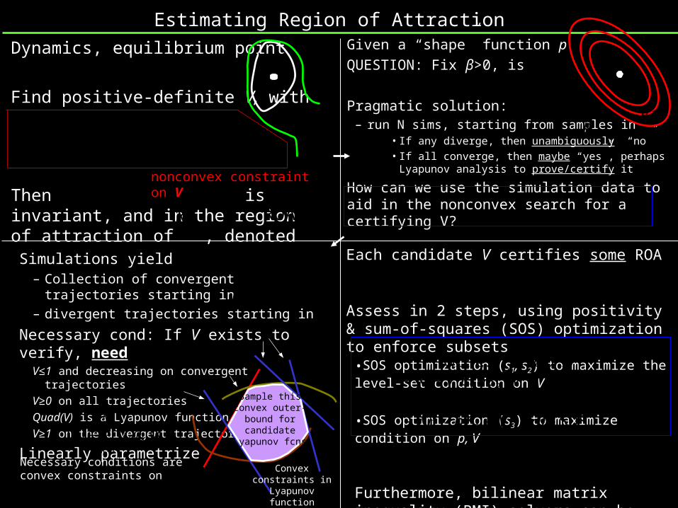
Dynamics, equilibrium point

Find positive-definite V, with

Then is invariant, and in the region of attraction of , denoted

0)(),( xfxfx

01)(,: fVx:xVxxx

bounded is 1,0 x:V(x)xV

1x:V(x)

0fdx

dV

1V

x

x xROA

nonconvex constraint on V

Given a “shape” function p

QUESTION: Fix β>0, is

Pragmatic solution:– run N sims, starting from samples in

• If any diverge, then unambiguously “no”• If all converge, then maybe “yes”, perhaps Lyapunov

analysis to prove/certify it

How can we use the simulation data to aid in the nonconvex search for a certifying V?

xROA )(:: xpxP

P

3p

x

2p

1p

Simulations yield– Collection of convergent trajectories starting in

– divergent trajectories starting in

Necessary cond: If V exists to verify, needV≤1 and decreasing on convergent trajectories

V≥0 on all trajectories

Quad(V) is a Lyapunov function for Linear(f)

V≥1 on the divergent trajectories

Linearly parametrize

PcP

Necessary conditions are convex constraints on

bN

kkk xxV

1

)()(

bNRConvex constraints in

Lyapunov function coefficient-space

Sample this convex outer-

bound for candidate

Lyapunov fcns

Each candidate V certifies some ROA

Assess in 2 steps, using positivity & sum-of-squares (SOS) optimization to enforce subsets

•SOS optimization (s1, s2) to maximize the level-set condition on V

•SOS optimization (s3) to maximize condition on p, V

Furthermore, bilinear matrix inequality (BMI) solvers can be initialized with these, and further optimization (adjusting V too) be performed.

0)(:)(:)(:

max:,

xVxxVxxpxVcert

satisfying that such

SOS 221 lfVssV

SOS Vsp 3

xxl T62 10: e.g., with,

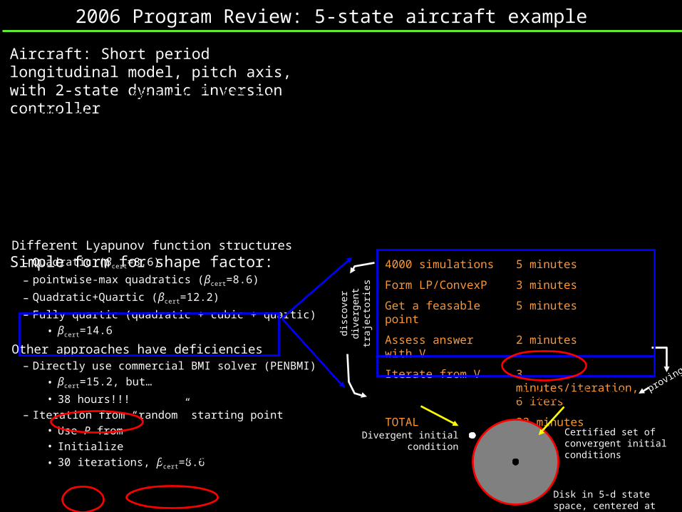
2006 Program Review: 5-state aircraft example

Aircraft: Short period longitudinal model, pitch axis, with 2-state dynamic inversion controller

Simple form for shape factor:

0

054.011.005.0

22.015.44.08.

)( 2332

22

3232

2221

2 zzzz

zzzzzz

uzBAzz

001

02.64.91.

56.3.13

A

q

z

Different Lyapunov function structures– Quadratic (βcert=8.6)

– pointwise-max quadratics (βcert=8.6)

– Quadratic+Quartic (βcert=12.2)

– Fully quartic (quadratic + cubic + quartic)

• βcert=14.6

Other approaches have deficiencies– Directly use commercial BMI solver (PENBMI)

• βcert=15.2, but…

• 38 hours!!!– Iteration from “random” starting point

• Use P from• Initialize

• 30 iterations, βcert=8.6

4000 simulations 5 minutes

Form LP/ConvexP 3 minutes

Get a feasable point 5 minutes

Assess answer with V 2 minutes

Iterate from V 3 minutes/iteration, 6 iters

TOTAL 33 minutes

ROA 6.14)(: xpx9.16)( 0 xp

disc

over

div

erge

nt

traj

ecto

ries

proving

TT zzxp :)(

IPAPAT

5

1

4001.0)(i i

T xPxxxV

Divergent initial condition Certified set of convergent initial conditions

Disk in 5-d state space, centered at equilibrium point

4.0

04.035.1

)(2

2

z

zB

3

1

28.75.

02.06.

00

09.6.z

z 21 2.2 u

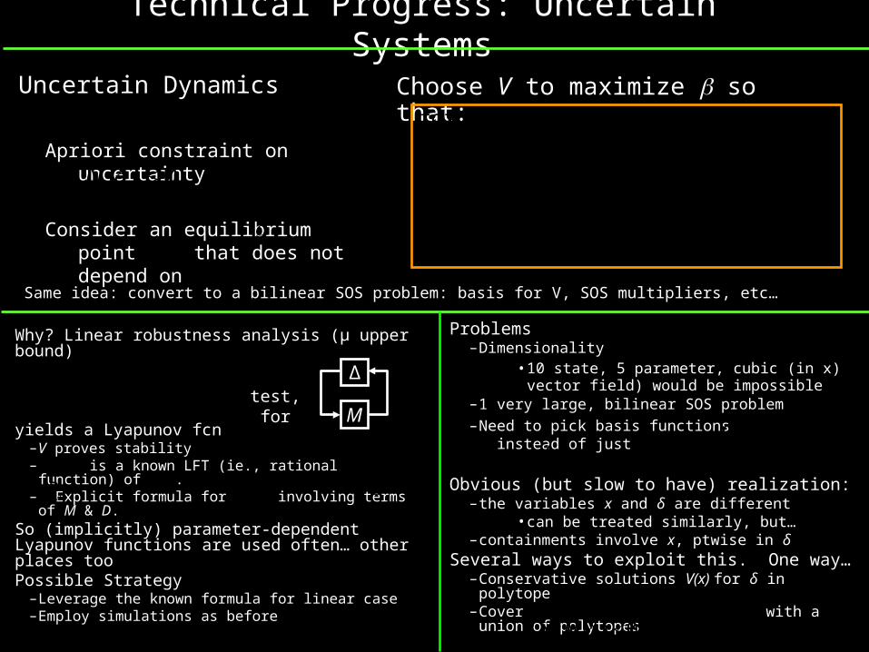
Problems–Dimensionality

• 10 state, 5 parameter, cubic (in x) vector field) would be impossible

–1 very large, bilinear SOS problem–Need to pick basis functions instead of

just

Obvious (but slow to have) realization:–the variables x and δ are different

• can be treated similarly, but…–containments involve x, ptwise in δ

Several ways to exploit this. One way…–Conservative solutions V(x) for δ in polytope–Cover with a union of polytopes

Why? Linear robustness analysis (µ upper bound)

yields a Lyapunov fcn–V proves stability– is a known LFT (ie., rational function) of .– Explicit formula for involving terms of M & D.

So (implicitly) parameter-dependent Lyapunov functions are used often… other places tooPossible Strategy

–Leverage the known formula for linear case–Employ simulations as before

Technical Progress: Uncertain Systems

Uncertain Dynamics

Apriori constraint on uncertainty

Consider an equilibrium point that does not depend on

),( xi

),( xfx

0)( N

Choose V to maximize so that:

0),(1),(,: xfx

Vx:xVxxx

1,)(: )x:V(xxpx

0)( N satisfying each for

definite positive is ),( V

Same idea: convert to a bilinear SOS problem: basis for V, SOS multipliers, etc…

M

Δtest, for

)()()( 1 sDsMsD

xPxxV T),(

P

x

P

)(xi

0)(: N

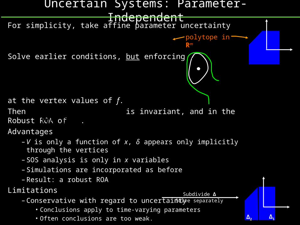
Uncertain Systems: Parameter-IndependentFor simplicity, take affine parameter uncertainty

Solve earlier conditions, but enforcing

at the vertex values of f.

Then is invariant, and in the Robust ROA of .

Advantages– V is only a function of x, δ appears only implicitly through the vertices

– SOS analysis is only in x variables

– Simulations are incorporated as before

– Result: a robust ROA

Limitations– Conservative with regard to uncertainty

• Conclusions apply to time-varying parameters• Often conclusions are too weak.

Δ ,)()(0 txtxftx

1x:V(x)

01)(,:

01)(,:

][

]1[

VnfVx:xVxxx

fVx:xVxxx

0f

dx

dV

1V

x

polytope in Rm

x

Subdivide ΔSolve separately

Δ1Δ2

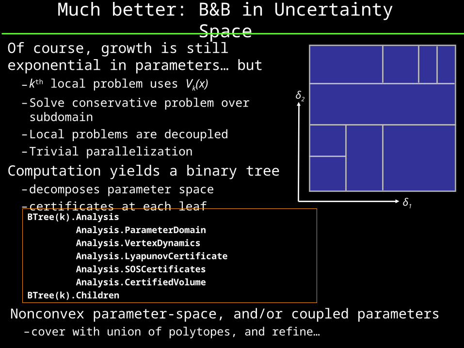
Much better: B&B in Uncertainty Space

Of course, growth is still exponential in parameters… but

–kth local problem uses Vk(x)

–Solve conservative problem over subdomain–Local problems are decoupled–Trivial parallelization

Computation yields a binary tree–decomposes parameter space–certificates at each leafBTree(k).Analysis

Analysis.ParameterDomain

Analysis.VertexDynamics

Analysis.LyapunovCertificate

Analysis.SOSCertificates

Analysis.CertifiedVolume

BTree(k).Children

δ1

δ2

Nonconvex parameter-space, and/or coupled parameters–cover with union of polytopes, and refine…

0 0.1 0.2 0.3 0.4 0.5 0.6 0.7 0.8 0.9 1

0

0.1

0.2

0.3

0.4

0.5

0.6

0.7

0.8

0.9

1

2

0 0.1 0.2 0.3 0.4 0.5 0.6 0.7 0.8 0.9 10

0.1

0.2

0.3

0.4

0.5

0.6

0.7

0.8

0.9

11 subdivisions

0 0.1 0.2 0.3 0.4 0.5 0.6 0.7 0.8 0.9 10

0.1

0.2

0.3

0.4

0.5

0.6

0.7

0.8

0.9

12 subdivisions

0 0.1 0.2 0.3 0.4 0.5 0.6 0.7 0.8 0.9 10

0.1

0.2

0.3

0.4

0.5

0.6

0.7

0.8

0.9

13 subdivisions

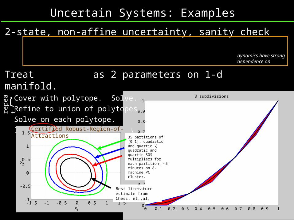
Uncertain Systems: Examples

2-state, non-affine uncertainty, sanity check

Treat as 2 parameters on 1-d manifold.Cover with polytope. Solve.

Refine to union of polytopes.

Solve on each polytope.

Intersect ROAs → Robust ROA

21

22121212

222

231

22211

41261023

46

xxxxxxxxx

xxxxxxx

x1

x2

-1.5 -1 -0.5 0 0.5 1 1.5-1

-0.5

0

0.5

1

1.535 partitions of [0 1], quadratic and quartic V, quadratic and quartic SOS multipliers for each partition, <5 minutes on 8-machine PC cluster.

Best literature estimate from Chesi, et.,al.

Certified Robust-Region-of-Attractions

10dynamics have strong dependence on

2,

repe

at

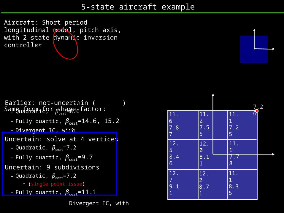
5-state aircraft example


Same form for shape factor:

0

054.011.005.01

22.015.44.08.1

)( 2332

222

3232

22211

2 zzzz

zzzzzz

uzBAzz

before as)(,, 2zBAz

Earlier: not-uncertain ( )– Quadratic, βcert=8.6

– Fully quartic, βcert=14.6, 15.2

– Divergent IC, with

Uncertain: solve at 4 vertices– Quadratic, βcert=7.2

– Fully quartic, βcert=9.7

Uncertain: 9 subdivisions– Quadratic, βcert=7.2

• (single point issue)

– Fully quartic, βcert=11.1

TT zzxp :)(

3

1

28.75.

02.06.

00

09.6.z

z 21 2.2 u

9.16)( 0 xp

1

2

0

0.14)( 0 xp

11.17.25

12.79.11

12.28.71

12.58.46

11.67.87

11.18.35

12.08.11

11.27.55

11.17.78

7.26

Divergent IC, with

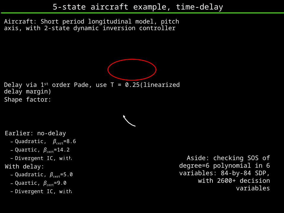
5-state aircraft example, time-delay


Delay via 1st order Pade, use T = 0.25(linearized delay margin)Shape factor:

0

054.011.005.0

22.015.44.08.

)( 2332

22

3232

2221

2 zzzz

zzzzzz

uzBAzz before as)(,, 2zBAz

Earlier: no-delay– Quadratic, βcert=8.6

– Quartic, βcert=14.2


With delay:– Quadratic, βcert=5.0



delayTerm TT zzxp :)(

3

1

28.75.

02.06.

00

09.6.z

z 21 2.2 Tdelayu

9.16)( 0 xp

2.11)( 0 xp

Aside: checking SOS of degree=6 polynomial in 6 variables: 84-by-84 SDP, with 2600+ decision variables

10,)( 2, eqdd xx

5-state aircraft example, time-delay, uncertainty


Set delay as 1st order Pade, 0.25 of linearized delay margin

Shape Factor

0

054.011.005.01

22.015.44.08.1

)( 2332

222

3232

22211

2 zzzz

zzzzzz

uzBAzz

before as)(,, 2zBAz

Nominal: βcert(∂V=2)=8.6, βcert(∂V=4)=14.2


Uncertain: βcert(∂V=2)=7.2, βcert(∂V=4)=11.1


Time-delay: βcert(∂V=2)=5.0, βcert(∂V=4)=9.0


Both (time delay, uncertainty) – Quadratic, βcert=4.25



3

1

28.75.

02.06.

00

09.6.z

z 21 2.2 Tdelayu

1

2

0.14)( 0 xp

delayTerm TT zzxp :)(

2.11)( 0 xp

8.594.25

8.785.21

9.004.93

9.174.95

9.744.69

8.274.67

8.394.70

8.384.45

8.314.47

earlier

7.10)( 0 xp

9.16)( 0 xp

Impact

Linear analysis provides a quick answer to a related, but different question:Q: How much gain and time-delay variation can we accommodate in flight?

A: Here’s a scatter plot of gain margin/time-delay margin at 1000 trim conditions (throughout envelope)

Why does linear analysis have impact in nonlinear problems?–Domain-specific expertise exists to interpret linear analysis & assess relevance

–Speed, scalable• Fast, defensible answers, on high-dimensional systems

Will (these) nonlinear methods ever have such an impact?–Problems where domain knowledge is less well-developed; little/no experience to rely on linear analysis: intuition could break down.

• UAVs with unusual airframe designs• Control laws for high-angle-of-attack maneuvers• Adaptive control laws

–Problems where performance is being pushed to the limit • approximations associated with linear analysis are no longer good enough.

Future Plans induced norms

– Exploiting simulation, along with parametric uncertainty– Incorporating constraint on the disturbance (ACC 06 paper)

Uncertainty modeling and approximation– We presented one class of uncertainty models for which vertex calculations

and Divide & Conquer methods are well suited– Other forms of uncertain models are useful too (CDC 07 paper)

Covering manifolds with polytopes– The affine parameter uncertainty model is limiting, often nonlinear functions of

parameters enter• in 2-state example, the (δ2) term is treated as an additional parameter,• cover low dimensional manifold with polytopes

Develop guidelines for sampling (InitCond & simulations)– Simulation-based approach to generate Lyapunov candidates has been

successful, but…• we have no guidelines on number of simulations and/or number of sample points

to draw from simulation• even theorems for a canonical example would be useful.

Leading to… tools that work on– 12 states, 5+ parameters, cubic (in x) vector field, analyze with ∂(V)=2– 6 states, 3+ parameters, cubic (in x) vector field, analyze with ∂(V)=4

LL2

L 2L

TransitionsRelease it

–SeDuMi (Sturm, McMaster)–SOStools (Anotonis, Prajna, Parrilo, Seiler)–Code (Topcu, Seiler) –PolynomialDynamicalSystem class (Wheeler, Seiler)

Teach it–1-unit course at UCBerkeley, UMinn in Spring 08

• Extend approach, apply to 2 or 3 state system, document, post, submit

• Apply to 6-state, uncertain system, document, post

–Course material online

Promote it–Website/Wiki for nonlinear analysis problems–Conferences, journals, ½ day workshops–Topcu did internship at Honeywell (summer 2007)

Use it–Me, Balas, Seiler, … and …

Final assignment

Publications1. “Stability region analysis using SOS programming,” 2006 ACC

2. “Local gain analysis of nonlinear systems,” 2006 ACC

3. “Stability region analysis using simulations and SOS programming,” 2007 ACC

4. “Stability region analysis via composite Lyapunov functions & SOS programming,” IEEE TAC, 10/07.

5. “Local stability analysis using simulations & SOS programming,” under review, Automatica (12/06, 4/07)

6. “Stability region analysis for uncertain nonlinear systems,” to appear 2007 CDC

7. “Local stability analysis for uncertain nonlinear systems,” submitted IEEE TAC (6/07)

8. “B&B for Local Stability analysis of uncertain nonlinear systems,” in preparation, 2008 ACC, ASME Journal of Dynamical Systems, Measurement and Control.

Project Website

http://jagger.me.berkeley.edu/~pack/certify

All examples, certificates, …

http://jagger.me.berkeley.edu/~pack/certificates

1-unit course: Lecture Schedule1. Intro: polynomial dynamical systems

2. Lyapunov theorem for ROA

3. ROA: simulations constrain V

4. Review, recap LP, SDP optimization problems

5. SOS→PSD, checking SOS ↔ SDP

6. Containments, empty intersections, as SOS, general Psatz

7. Applying 1-6 to ROA problems

8. Code, tools, results for 7

9. Disturbance-to-state problems

10.Uncertain Dynamics, vertex results, Branch and Bound

11.Covering nonpolynomial systems with poly model, error

12.Global & local Control Lyapunov Function (CLF) synthesis

13.Other literature, approaches (Lall, Glavski, Prajna, etc)

14.Other literature (continued)

development of analysis tools for certification of flight control laws fa9550-05-1-0266, april...

Documents